Radio Regulations - ITU-R Recommendations incorporated by ...
532
4 Radio Regulations ITU-R Recommendations incorporated by reference Edition of 2020
-
Upload
khangminh22 -
Category
Documents
-
view
0 -
download
0
Transcript of Radio Regulations - ITU-R Recommendations incorporated by ...

4
4R
adio
Reg
ula
tio
ns
ITU
-R R
eco
mm
end
atio
ns in
corp
ora
ted
by
refe
renc
eE
diti
on
of 2
020
E
Radio RegulationsITU-R Recommendations incorporated by reference
Edition of 2020


4Radio RegulationsITU-R Recommendations incorporated by reference
Edition of 2020

Disclaimer
The designations employed and the presentation of material in this Publication do not imply the expression of any opinion whatsoever on the part of ITU and of the Secretariat of the ITU concerning the legal status of the countries, territories, cities or areas or their authorities, or concerning the delimitation of their frontiers or boundaries.
© ITU 2020 All rights reserved. No part of this publication may be reproduced, by any means whatsoever, without the prior written permission of ITU.

- III -
Note by the Secretariat
This revision of the Radio Regulations, complementing the Constitution and the Convention of the International Telecommunication Union, incorporates the decisions of the World Radio-communication Conferences of 1995 (WRC-95), 1997 (WRC-97), 2000 (WRC-2000), 2003 (WRC-03), 2007 (WRC-07), 2012 (WRC-12), 2015 (WRC-15) and 2019 (WRC-19). The majority of the provisions of these Regulations shall enter into force as from 1 January 2021; the remaining provisions shall apply as from the special dates of application indicated in Article 59 of the revised Radio Regulations.
In preparing the Radio Regulations, Edition of 2020, the Secretariat corrected the typographical errors that were drawn to the attention of WRC-19 and which were approved by WRC-19.
This edition uses the same numbering scheme as the 2001 edition of the Radio Regulations, notably:
With respect to Article numbers, this edition follows the standard sequential numbering. The Article numbers are not followed by any abbreviation (such as “(WRC-97)”, “(WRC-2000)”, “(WRC-03)”, “(WRC-07)”, “(WRC-12)”, “(WRC-15)” or “(WRC-19)”). Consequently, any reference to an Article, in any of the provisions of these Radio Regulations (e.g. in No. 13.1 of Article 13), in the texts of the Appendices as contained in Volume 2 of this edition (e.g. in § 1 of Appendix 2), in the texts of the Resolutions included in Volume 3 of this edition (e.g. in Resolution 1 (Rev.WRC-97)), and in the texts of the Recommendations included in Volume 3 of this edition (e.g. in Recommendation 8), is considered as a reference to the text of the concerned Article which appears in this edition, unless otherwise specified.
With respect to provision numbers in Articles, this edition continues to use composite numbers indicating the number of the Article and the provision number within that Article (e.g. No. 9.2B means provision No. 2B of Article 9). The abbreviation “(WRC-19)”, “(WRC-15)”, “(WRC-12)”, “(WRC-07)”, “(WRC-03)”, “(WRC-2000)” or “(WRC-97)” at the end of such a provision means that the relevant provision was modified or added by WRC-19, by WRC-15, by WRC-12, by WRC-07, by WRC-03, by WRC-2000 or by WRC-97, as applicable. The absence of an abbreviation at the end of the provision means that the provision is identical with the provision of the simplified Radio Regulations as approved by WRC-95, and whose complete text was contained in Document 2 of WRC-97.
With respect to Appendix numbers, this edition follows the standard sequential numbering, with the addition of the appropriate abbreviation after the Appendix number (such as “(WRC-97)”, “(WRC-2000)”, “(WRC-03)”, “(WRC-07)”, “(WRC-12)”, “(WRC-15)” or “WRC-19)”), where applicable. As a rule, any reference to an Appendix, in any of the provisions of these Radio Regulations, in the texts of the Appendices as contained in Volume 2 of this edition, in the texts of the Resolutions and of the Recommendations included in Volume 3 of this edition, is presented in the standard manner (e.g. “Appendix 30 (Rev.WRC-19)”) if not explicitly described in the text (e.g. Appendix 4 as modified by WRC-19). In the texts of Appendices that were partially modified by WRC-19, the provisions that were modified by WRC-19 are indicated with the abbreviation “(WRC-19)” at the end of the concerned text. If an Appendix is referenced without any abbreviation after the Appendix number, in the texts of this edition (e.g. in No. 13.1), or without other description, such reference is considered as a reference to the text of the concerned Appendix which appears in this edition.

- IV -
Within the text of the Radio Regulations, the symbol, , has been used to represent quantities associated with an uplink. Similarly, the symbol, , has been used to represent quantities associated with a downlink.
Abbreviations have generally been used for the names of world administrative radio conferences and world radiocommunication conferences. These abbreviations are shown below.
1 The date of this conference has not been finalized.
Abbreviation Conference
WARC Mar World Administrative Radio Conference to Deal with Matters Relating to the Maritime Mobile Service (Geneva, 1967)
WARC-71 World Administrative Radio Conference for Space Telecommunications (Geneva, 1971)
WMARC-74 World Maritime Administrative Radio Conference (Geneva, 1974)
WARC SAT-77 World Broadcasting-Satellite Administrative Radio Conference (Geneva, 1977)
WARC-Aer2 World Administrative Radio Conference on the Aeronautical Mobile (R) Service (Geneva, 1978)
WARC-79 World Administrative Radio Conference (Geneva, 1979)
WARC Mob-83 World Administrative Radio Conference for the Mobile Services (Geneva, 1983)
WARC HFBC-84 World Administrative Radio Conference for the Planning of the HF Bands Allocated to the Broadcasting Service (Geneva, 1984)
WARC Orb-85 World Administrative Radio Conference on the Use of the Geostationary-Satellite Orbit and the Planning of Space Services Utilising It (First Session – Geneva, 1985)
WARC HFBC-87 World Administrative Radio Conference for the Planning of the HF Bands Allocated to the Broadcasting Service (Geneva, 1987)
WARC Mob-87 World Administrative Radio Conference for the Mobile Services (Geneva, 1987)
WARC Orb-88 World Administrative Radio Conference on the Use of the Geostationary-Satellite Orbit and the Planning of Space Services Utilising It (Second Session – Geneva, 1988)
WARC-92 World Administrative Radio Conference for Dealing with Frequency Allocations in Certain Parts of the Spectrum (Malaga-Torremolinos, 1992)
WRC-95 World Radiocommunication Conference (Geneva, 1995)
WRC-97 World Radiocommunication Conference (Geneva, 1997)
WRC-2000 World Radiocommunication Conference (Istanbul, 2000)
WRC-03 World Radiocommunication Conference (Geneva, 2003)
WRC-07 World Radiocommunication Conference (Geneva, 2007)
WRC-12 World Radiocommunication Conference (Geneva, 2012)
WRC-15 World Radiocommunication Conference (Geneva, 2015)
WRC-19 World Radiocommunication Conference (Sharm El-Sheikh, 2019)
WRC-23 World Radiocommunication Conference, 20231

- V -
VOLUME 4
ITU-R Recommendations incorporated by reference*
TABLE OF CONTENTS
Page
Rec. ITU-R TF.460-6 Standard-frequency and time-signal emissions............................................................. 1
Rec. ITU-R M.476-5 Direct-printing telegraph equipment in the maritime mobile service............................ 7
Rec. ITU-R M.489-2 Technical characteristics of VHF radiotelephone equipment operating in the maritime mobile service in channels spaced by 25 kHz................................................ 19
Rec. ITU-R M.492-6 Operational procedures for the use of direct-printing telegraph equipment in the maritime mobile service................................................................................................ 21
Rec. ITU-R P.525-4 Calculation of free-space attenuation............................................................................ 31
Rec. ITU-R P.526-15 Propagation by diffraction............................................................................................. 35
Rec. ITU-R M.541-10 Operational procedures for the use of digital selective-calling equipment in the maritime mobile service................................................................................................ 77
Rec. ITU-R M.585-8 Assignment and use of identities in the maritime mobile service(Annex 1) ....................................................................................................................... 107
Rec. ITU-R M.625-4 Direct-printing telegraph equipment employing automatic identification in the maritime mobile service................................................................................................ 117
Rec. ITU-R M.633-4 Transmission characteristics of a satellite emergency position-indicating radio beacon (satellite EPIRB) system operating through a satellite system in the 406 MHz band............................................................................................................................... 179
Rec. ITU-R S.672-4 Satellite antenna radiation pattern for use as a design objective in the fixed-satellite service employing geostationary satellites .................................................................... 181
Rec. ITU-R M.690-3 Technical characteristics of emergency position-indicating radio beacons operating on the carrier frequencies of 121.5 MHz and 243 MHz................................................ 207
Rec. ITU-R RA.769-2 Protection criteria used for radio astronomical measurements(parts related to the application of No. 5.372).............................................................. 209
Rec. ITU-R P.838-3 Specific attenuation model for rain for use in prediction methods................................ 221
Rec. ITU-R M.1084-5 Interim solutions for improved efficiency in the use of the band 156-174 MHz by stations in the maritime mobile service......................................................................... 229
Rec. ITU-R SM.1138-3 Determination of necessary bandwidths including examples for their calculation and associated examples for the designation of emissions .................................................. 241
_______________* In some of these Recommendations, which were adopted prior to 1 January 2001, the prefix “S” before the
references to RR is still maintained until the concerned Recommendation is modified according to the standardprocedures.

- VI -
Page
Rec. ITU-R SA.1154-0 Provisions to protect the space research (SR), space operations (SO) and Earth-exploration satellite services (EES) and to facilitate sharing with the mobile service in the 2 025-2 110 MHz and 2 200-2 290 MHz bands.................................................. 249
Rec. ITU-R M.1171-0 Radiotelephony procedures in the maritime mobile service ......................................... 279
Rec. ITU-R M.1172-0 Miscellaneous abbreviations and signals to be used for radiocommunications in the maritime mobile service ............................................................................................... 289
Rec. ITU-R M.1173-1 Technical characteristics of single-sideband transmitters used in the maritime mobile service for radiotelephony in the bands between 1 606.5 kHz (1 605 kHz Region 2) and 4 000 kHz and between 4 000 kHz and 27 500 kHz .............................................. 323
Rec. ITU-R M.1174-4 Technical characteristics of equipment used for on-board vessel communications in the bands between 450 and 470 MHz........................................................................... 325
Rec. ITU-R M.1187-1 A method for the calculation of the potentially affected region for a mobile-satellite service network in the 1-3 GHz range using circular orbits.......................................... 329
Rec. ITU-R S.1256-0 Methodology for determining the maximum aggregate power flux-density at the geostationary-satellite orbit in the band 6 700-7 075 MHz from feeder links of non-geostationary satellite systems in the mobile-satellite service in the space-to-Earth direction ........................................................................................................................ 335
Rec. ITU-R RS.1260-2 Feasibility of sharing between active spaceborne sensors and other services in the range 420-470 MHz...................................................................................................... 343
Rec. ITU-R BO.1293-2 Protection masks and associated calculation methods for interference into broadcast-satellite systems involving digital emissions ................................................................ 357
Rec. ITU-R S.1340-0 Sharing between feeder links for the mobile-satellite service and the aeronautical radionavigation service in the Earth-to-space direction in the band 15.4-15.7 GHz .... 369
Rec. ITU-R S.1428-1 Reference FSS earth-station radiation patterns for use in interference assessment involving non-GSO satellites in frequency bands between 10.7 GHz and 30 GHz...... 385
Rec. ITU-R BO.1443-3 Reference BSS earth station antenna patterns for use in interference assessment involving non-GSO satellites in frequency bands covered by RR Appendix 30 .......... 389
Rec. ITU-R RA.1513-2 Levels of data loss to radio astronomy observations and percentage-of-time criteria resulting from degradation by interference for frequency bands allocated to the radio astronomy service on a primary basis ........................................................................... 397
Rec. ITU-R M.1583-1 Interference calculations between non-geostationary mobile-satellite service or radionavigation-satellite service systems and radio astronomy telescope sites ............ 411
Rec. ITU-R S.1586-1 Calculation of unwanted emission levels produced by a non-geostationary fixed-satellite service system at radio astronomy sites........................................................... 419
Rec. ITU-R F.1613-0 Operational and deployment requirements for fixed wireless access systems in the fixed service in Region 3 to ensure the protection of systems in the Earth exploration-satellite service (active) and the space research service (active) in the band 5 250-5 350 MHz.................................................................................................. 427
Rec. ITU-R RA.1631-0 Reference radio astronomy antenna pattern to be used for compatibility analyses between non-GSO systems and radio astronomy service stations based on the epfd concept.......................................................................................................................... 443

- VII -
Page
Rec. ITU-R M.1642-2 Methodology for assessing the maximum aggregate equivalent power flux-density at an aeronautical radionavigation service station from all radionavigation-satellite service systems operating in the 1 164-1 215 MHz band .............................................. 447
Rec. ITU-R M.1643-0 Technical and operational requirements for aircraft earth stations of aeronautical mobile-satellite service including those using fixed-satellite service network transponders in the band 14-14.5 GHz (Earth-to-space) ............................................... 463
Rec. ITU-R M.1652-1 Dynamic frequency selection in wireless access systems including radio local area networks for the purpose of protecting the radiodetermination service in the 5 GHz band(Annexes 1 and 5).......................................................................................................... 469
Rec. ITU-R M.1827-1 Guideline on technical and operational requirements for stations of the aeronautical mobile (R) service limited to surface application at airports in the frequency band 5 091-5 150 MHz .......................................................................................................... 487
Rec. ITU-R M.2013-0 Technical characteristics of, and protection criteria for non-ICAO aeronautical radionavigation systems, operating around 1 GHz ....................................................... 491
Rec. ITU-R RS.2065-0 Protection of space research service (SRS) space-to-Earth links in the 8 400-8 450 MHz and 8 450-8 500 MHz bands from unwanted emissions of synthetic aperture radars operating in the Earth exploration-satellite service (active) around 9 600 MHz ........................................................................................................ 501
Rec. ITU-R RS.2066-0 Protection of the radio astronomy service in the frequency band 10.6-10.7 GHz from unwanted emissions of synthetic aperture radars operating in the Earth exploration-satellite service (active) around 9 600 MHz.................................................................. 509
Cross-reference list of the regulatory provisions, including footnotes and Resolutions, incorporating ITU-RRecommendations by reference ................................................................................... 517


Rec. ITU-R TF.460-6 1
RECOMMENDATION ITU-R TF.460-6*
Standard-frequency and time-signal emissions
(Question ITU-R 102/7)
(1970-1974-1978-1982-1986-1997-2002)
The ITU Radiocommunication Assembly,
considering
a) that the World Administrative Radio Conference, Geneva, 1979, allocated the frequencies20 kHz 0.05 kHz, 2.5 MHz 5 kHz (2.5 MHz 2 kHz in Region 1), 5 MHz 5 kHz, 10 MHz
5 kHz, 15 MHz 10 kHz, 20 MHz 10 kHz and 25 MHz 10 kHz to the standard-frequency andtime-signal service;
b) that additional standard frequencies and time signals are emitted in other frequency bands;
c) the provisions of Article 26 of the Radio Regulations;
d) the continuing need for close cooperation between Radiocommunication Study Group 7 andthe International Maritime Organization (IMO), the International Civil Aviation Organization(ICAO), the General Conference of Weights and Measures (CGPM), the Bureau International desPoids et Mesures (BIPM), the International Earth Rotation Service (IERS) and the concernedUnions of the International Council of Scientific Unions (ICSU);
e) the desirability of maintaining worldwide coordination of standard-frequency andtime-signal emissions;
f) the need to disseminate standard frequencies and time signals in conformity with the secondas defined by the 13th General Conference of Weights and Measures (1967);
g) the continuing need to make universal time (UT) immediately available to an uncertainty ofone-tenth of a second,
recommends
1 that all standard-frequency and time-signal emissions conform as closely as possible to coordinated universal time (UTC) (see Annex 1); that the time signals should not deviate from UTC by more than 1 ms; that the standard frequencies should not deviate by more than 1 part in 1010, and that the time signals emitted from each transmitting station should bear a known relation to the phase of the carrier;
2 that standard-frequency and time-signal emissions, and other time-signal emissions intended for scientific applications (with the possible exception of those dedicated to special systems) should contain information on UT1 UTC and TAI UTC (see Annex 1).
____________________ * This Recommendation should be brought to the attention of the IMO, the ICAO, the CGPM, the BIPM,
the IERS, the International Union of Geodesy and Geophysics (IUGG), the International Union of RadioScience (URSI) and the International Astronomical Union (IAU).
- 1 -

2 Rec. ITU-R TF.460-6
ANNEX 1
Time scales
A Universal time (UT)
Universal time (UT) is the general designation of time scales based on the rotation of the Earth.
In applications in which an imprecision of a few hundredths of a second cannot be tolerated, it is necessary to specify the form of UT which should be used:
UT0 is the mean solar time of the prime meridian obtained from direct astronomical observation;
UT1 is UT0 corrected for the effects of small movements of the Earth relative to the axis of rotation (polar variation);
UT2 is UT1 corrected for the effects of a small seasonal fluctuation in the rate of rotation of the Earth;
UT1 is used in this Recommendation, since it corresponds directly with the angular position of the Earth around its axis of diurnal rotation.
Concise definitions of the above terms and the concepts involved are available in the publications of the IERS (Paris, France).
B International atomic time (TAI)
The international reference scale of atomic time (TAI), based on the second (SI), as realized on the rotating geoid, is formed by the BIPM on the basis of clock data supplied by cooperating establishments. It is in the form of a continuous scale, e.g. in days, hours, minutes and seconds from the origin 1 January 1958 (adopted by the CGPM 1971).
C Coordinated universal time (UTC)
UTC is the time-scale maintained by the BIPM, with assistance from the IERS, which forms the basis of a coordinated dissemination of standard frequencies and time signals. It corresponds exactly in rate with TAI but differs from it by an integer number of seconds.
The UTC scale is adjusted by the insertion or deletion of seconds (positive or negative leap-seconds) to ensure approximate agreement with UT1.
D DUT1
The value of the predicted difference UT1 – UTC, as disseminated with the time signals is denoted DUT1; thus DUT1 UT1 – UTC. DUT1 may be regarded as a correction to be added to UTC to obtain a better approximation to UT1.
The values of DUT1 are given by the IERS in multiples of 0.1 s.
- 2 -

Rec. ITU-R TF.460-6 3
The following operational rules apply:
1 Tolerances 1.1 The magnitude of DUT1 should not exceed 0.8 s.
1.2 The departure of UTC from UT1 should not exceed 0.9 s (see Note 1).
1.3 The deviation of (UTC plus DUT1) should not exceed 0.1 s. NOTE 1 – The difference between the maximum value of DUT1 and the maximum departure of UTC from UT1 represents the allowable deviation of (UTC DUT1) from UT1 and is a safeguard for the IERS against unpredictable changes in the rate of rotation of the Earth.
2 Leap-seconds 2.1 A positive or negative leap-second should be the last second of a UTC month, but first preference should be given to the end of December and June, and second preference to the end of March and September.
2.2 A positive leap-second begins at 23h 59m 60s and ends at 0h 0m 0s of the first day of the following month. In the case of a negative leap-second, 23h 59m 58s will be followed one second later by 0h 0m 0s of the first day of the following month (see Annex 3).
2.3 The IERS should decide upon and announce the introduction of a leap-second, such an announcement to be made at least eight weeks in advance.
3 Value of DUT1 3.1 The IERS is requested to decide upon the value of DUT1 and its date of introduction and to circulate this information one month in advance. In exceptional cases of sudden change in the rate of rotation of the Earth, the IERS may issue a correction not later than two weeks in advance of the date of its introduction.
3.2 Administrations and organizations should use the IERS value of DUT1 for standard-frequency and time-signal emissions, and are requested to circulate the information as widely as possible in periodicals, bulletins, etc.
3.3 Where DUT1 is disseminated by code, the code should be in accordance with the following principles (except § 3.4 below): – the magnitude of DUT1 is specified by the number of emphasized second markers and the
sign of DUT1 is specified by the position of the emphasized second markers with respect to the minute marker. The absence of emphasized markers indicates DUT1 0;
– the coded information should be emitted after each identified minute if this is compatible with the format of the emission. Alternatively the coded information should be emitted, as an absolute minimum, after each of the first five identified minutes in each hour.
Full details of the code are given in Annex 2.
3.4 DUT1 information primarily designed for, and used with, automatic decoding equipment may follow a different code but should be emitted after each identified minute if this is compatible with the format of the emission. Alternatively, the coded information should be emitted, as an absolute minimum, after each of the first five identified minutes in each hour.
- 3 -

4 Rec. ITU-R TF.460-6
3.5 Other information which may be emitted in that part of the time-signal emission designated in § 3.3 and 3.4 for coded information on DUT1 should be of a sufficiently different format that it will not be confused with DUT1.
3.6 In addition, UT1 – UTC may be given to the same or higher precision by other means, for example, by messages associated with maritime bulletins, weather forecasts, etc.; announcements of forthcoming leap-seconds may also be made by these methods.
3.7 The IERS is requested to continue to publish, in arrears, definitive values of the differences UT1 – UTC and UT2 – UTC.
E DTAI The value of the difference TAI – UTC, as disseminated with time signals, shall be denoted DTAI. DTAI TAI UTC may be regarded as a correction to be added to UTC to obtain TAI.
The TAI UTC values are published in the BIPM Circular T. The IERS should announce the value of DTAI in integer multiples of one second in the same announcement as the introduction of a leap-second (see § D.2).
ANNEX 2
Code for the transmission of DUT1
A positive value of DUT1 will be indicated by emphasizing a number, n, of consecutive second markers following the minute marker from second marker one to second marker, n, inclusive; n being an integer from 1 to 8 inclusive.
DUT1 (n × 0.1) s
A negative value of DUT1 will be indicated by emphasizing a number, m, of consecutive second markers following the minute marker from second marker nine to second marker (8 m) inclusive, m being an integer from 1 to 8 inclusive.
DUT1 – (m × 0.1) s
A zero value of DUT1 will be indicated by the absence of emphasized second markers.
The appropriate second markers may be emphasized, for example, by lengthening, doubling, splitting or tone modulation of the normal second markers.
Examples:
0460-01
0 1 2 3 4 5 6 7 8 9 10 11 12 13 14 15 16 17
Minutemarker
Emphasizedsecond markers
Limit of coded sequence
FIGURE 1DUT1 = + 0.5 s
- 4 -

Rec. ITU-R TF.460-6 5
0460-02
0 1 2 3 4 5 6 7 8 9 10 11 12 13 14 15 16 17
Minutemarker
Emphasizedsecond markers
Limit of coded sequence
FIGURE 2DUT1 = – 0.2 s
ANNEX 3
Dating of events in the vicinity of a leap-second
The dating of events in the vicinity of a leap-second shall be effected in the manner indicated in the following Figures:
0460-03
56 57 58 59 60 0 1 2 3 4
56 57 58 0 1 2 3 4 5 6
event
1 July, 0h 0m30 June, 23h 59m
leap-secondDesignation of the date of the event
30 June, 23h 59m 60.6s UTC
FIGURE 3Positive leap-second
event
1 July, 0h 0m30 June, 23h 59m
Designation of the date of the event
30 June, 23h 59m 58.9s UTC
FIGURE 4Negative leap-second
- 5 -


Rec. ITU-R M.476-5 1
RECOMMENDATION ITU-R M.476-5*
DIRECT-PRINTING TELEGRAPH EQUIPMENT IN THE MARITIME MOBILE SERVICE**
(Question ITU-R 5/8)
(1970-1974-1978-1982-1986-1995)Rec. ITU-R M.476-5
Summary The Recommendation provides in Annex 1 characteristics for error detecting and correcting systems for existing direct-printing telegraph equipment. Annex 1 contains the technical characteristics of the transmission, the code and the modes of operation to be employed in the maritime-mobile service. New equipment should conform to Recommendation ITU-R M.625.
The ITU Radiocommunication Assembly,
considering
a) that there is a requirement to interconnect mobile stations, or mobile stations and coast stations, equipped with start-stop apparatus employing the ITU-T International Telegraph Alphabet No. 2, by means of radiotelegraph circuits;
b) that direct-printing telegraphy communications in the maritime mobile service can be listed in the following categories:
b.a telegraph service between a ship and a coast station;
b.b telegraph service between a ship and an extended station (ship’s owner) via a coast station;
b.c telex service between a ship and a subscriber of the (international) telex network;
b.d broadcast telegraph service from a coast station to one or more ships;
b.e telegraph service between two ships or between one ship and a number of other ships;
c) that those categories are different in nature and that consequently different degrees of transmission quality may be required;
d) that the categories given in b.a, b.b and b.c above may require a higher transmission quality than categories b.d and b.e for the reason that data could be handled through the services in the categories b.a, b.b and b.c, while the messages passed through the service of category b.d, and via the broadcast service of category b.e are normally plain language, allowing a lower transmission quality than that required for coded information;
_______________* This Recommendation should be brought to the attention of the International Maritime Organization (IMO) and the
Telecommunication Standardization Sector (ITU-T).
** This Recommendation is retained in order to provide information concerning existing equipment, but will probably be deleted at a later date. New equipment should conform to Recommendation ITU-R M.625 which provides for the exchange of identification signals, for the use of 9 digit maritime mobile service identification signals and for compatibility with existing equipment built in accordance with this Recommendation.
Note by the Secretariat: The references made to the Radio Regulations (RR) in this Recommendation refer to the RR as revised by the World Radiocommunication Conference 1995. These elements of the RR will come into force on 1 June 1998. Where applicable, the equivalent references in the current RR are also provided in square brackets.
- 7 -

2 Rec. ITU-R M.476-5
e) that the service in category b.d and the broadcast service in category b.e cannot take advantage of an ARQ method, as there is in principle no return path;
f) that for these categories of service which by their nature do not allow the use of ARQ, another mode, i.e. the forward error-correcting (FEC) mode should be used;
g) that the period for synchronization and phasing should be as short as possible and should not exceed 5 s;
h) that most of the ship stations do not readily permit simultaneous use of the radio transmitter and radio receiver;
j) that the equipment on board ships should be neither unduly complex nor expensive,
recommends
1 that when an error-detecting and correcting system is used for direct-printing telegraphy in the maritime mobile service, a 7-unit ARQ system or a 7-unit forward acting, error-correcting and indicating time-diversity system, using the same code, should be employed;
2 that equipment designed in accordance with § 1 should meet the characteristics laid down in Annex 1.
ANNEX 1
1 General (Mode A, ARQ and Mode B, FEC)
1.1 The system in both Mode A (ARQ) and Mode B (FEC) is a single-channel synchronous system using the 7-unit error-detecting code as listed in § 2 of this Annex.
1.2 FSK modulation is used on the radio link at 100 Bd. The equipment clocks controlling the modulation rate should have an accuracy of better than 30 parts in 106.
NOTE 1 – Some existing equipments may not conform to this requirement.
1.3 The terminal input and output must be in accordance with the 5-unit start-stop ITU-T International Telegraph Alphabet No. 2 at a modulation rate of 50 Bd.
1.4 The class of emission is F1B or J2B with a frequency shift on the radio link of 170 Hz. When frequency shift is effected by applying audio signals to the input of a single-sideband transmitter, the centre frequency of the audio spectrum offered to the transmitter should be 1 700 Hz.
NOTE 1 – A number of equipments are presently in service, using a centre frequency of 1 500 Hz. These may require special measures to achieve compatibility.
1.5 The radio frequency tolerance of the transmitter and the receiver should be in accordance with Recommendation ITU-R SM.1137. It is desirable that the receiver employs the minimum practicable bandwidth (see also Report ITU-R M.585).
NOTE 1 – The receiver bandwidth should preferably be between 270 and 340 Hz.
- 8 -

Rec. ITU-R M.476-5 3
2 Table of conversion
2.1 Traffic information signals
TABLE 1
2.2 Service information signals
TABLE 2
Combi-nation
No.Letter case Figure case
International Telegraph
Alphabet No. 2Code
Emitted7-unit
signal(1)
1112131415161718191011121314151617181920212223242526
ABCDEFGHIJKLMNOPQRSTUVWXYZ
–?:(3)
3(2)(2)(2)
8Audible signal
().,9014’57
2/6
ZZAAAZAAZZAZZZAZAAZAZAAAAZAZZAAZAZZAAZAZAZZAAZZAZAZZZZAAZAAZAAZZZAAZZAAAAZZAZZAZZZZAZAZAZAZAZAAAAAAZZZZAAAZZZZZZAAZZAZZZZAZAZZAAAZ
BBBYYYBYBYYBBBBYBBBYYBBYYBYBYBBYBYBBBYBBYYBYBYBBYBYYBYBBBYBBYYBBBBYBYYYBBBBYYBYBYYBBBYYBBBYBYYBBYBBYYYBBBBYBBYBYYBBBYBYBYBYBYBBBYBYYBYYBYBBBYBBBYYBYYBBBBYBBBYYBYYBYBBBYBBYBYBYBBYYYBB
272829303132
(Carriage return)(Line feed)(Letter shift)Figure shift)
SpaceUnperforated tape
AAAZAAZAAAZZZZZZZAZZAAZAAAAAAA
YYYBBBBYYBBYBBYBYBBYBYBBYBBYYYBBBYBYBYBYBB
(1) B represents the higher emitted frequency and Y the lower.(2) At present unassigned (see ITU-T Recommendation F.1 C8). Reception of these signals, however, should not
initiate a request for repetition.(3) The pictorial representation shown is a schematic of which may also be used when equipment allows (ITU-T
Recommendation F.1).
Mode A (ARQ) Emitted signal Mode B (FEC)
Control signal 1 (CS1)Control signal 2 (CS2)Control signal 3 (CS3)Idle signal Idle signal Signal repetition
BYBYYBBYBYBYBBBYYBBYBBBYYBBYBBBBYYYYBBYYBB
Phasing signal 1Phasing signal 2
- 9 -

4 Rec. ITU-R M.476-5
3 Characteristics
3.1 Mode A (ARQ) (see Figs. 1 and 2)
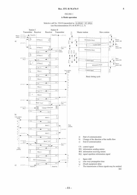
A synchronous system, transmitting blocks of three characters from an information sending station (ISS) towards an information receiving station (IRS), which stations can, controlled by the control signal 3 (see § 2.2), interchange their functions.
3.1.1 Master and slave arrangements
3.1.1.1 The station that initiates the establishment of the circuit (the calling station) becomes the “master” station, and the station that has been called will be the “slave” station;
this situation remains unchanged during the entire time in which the established circuit is maintained, regardless of which station, at any given time, is the information sending station (ISS) or information receiving station (IRS);
3.1.1.2 the clock in the master station controls the entire circuit (see circuit timing diagram, Fig. 1);
3.1.1.3 the basic timing cycle is 450 ms, and for each station consists of a transmission period followed by a transmission pause during which reception is effected;
3.1.1.4 the master station transmitting time distributor is controlled by the clock in the master station;
3.1.1.5 the slave station receiving time distributor is controlled by the received signal;
3.1.1.6 the slave station transmitting time distributor is phase-locked to the slave station receiving time distributor; i.e. the time interval between the end of the received signal and the start of the transmitted signal (tE in Fig. 1) is constant;
3.1.1.7 the master station receiving time distributor is controlled by the received signal.
3.1.2 The information sending station (ISS)
3.1.2.1 Groups the information to be transmitted into blocks of three characters (3 7 signal elements), including, if necessary, “idle signals ” to complete or to fill blocks when no traffic information is available;
3.1.2.2 emits a “block” in 210 ms after which a transmission pause of 240 ms becomes effective, retaining the emitted block in memory until the appropriate control signal confirming correct reception by the information receiving station (IRS) has been received;
3.1.2.3 numbers successive blocks alternately “Block 1” and “Block 2” by means of a local numbering device. The first block should be numbered “Block 1” or “Block 2” dependent on whether the received control signal (see § 3.1.4.5) is a control signal 1 or a control signal 2. The numbering of successive blocks is interrupted at the reception of:
– a request for repetition; or
– a mutilated signal; or
– a control signal 3 (see § 2.2);
3.1.2.4 emits the information of Block 1 on receipt of control signal 1 (see § 2.2);
3.1.2.5 emits the information of Block 2 on receipt of control signal 2 (see § 2.2);
3.1.2.6 emits a block of three “signal repetitions” on receipt of a mutilated signal (see § 2.2).
- 10 -
Rec. ITU-R M.476-5 5
QRQC
QRQ
C
XT
RQ
XT
RQ
KLM
KLM
NOP
NOP
QRS
RQ
QRS
RQ
CS1
CS2
CS1CS1
CS2
CS1
CS1CS1
CS2CS2
CS3CS3
CS2CS2
CS1
CS1
CS1
CS2
CS1
CS3
CS1
CS2
CS1
CS3
CS1CS1
CS1
CS1
no
klm
klm
no
QRQC
QRQ
C
RQRQRQ
RQRQRQ
§ 3.1.6.2ISS
§ 3.1.6.2
§ 3.1.9.2
§ 3.1.9.7
§ 3.1 .6.2
§ 3.1.6.1IRS
§ 3.1.6.1
§ 3.1.6.1
§ 3.1.4.5ISS
§ 3.1.4.3
§ 3.1.4.2
§ 3.1.4.1§ 3.1.3.1
§ 3.1.4.1
§ 3.1.4.4IRS
§ 3.1.6.2
§ 3.1.6.2
§ 3.1.6.2ISS
§ 3.1.6.1
§ 3.1.6.1IRS
§ 3.1.6.1
§ 3.1.9.6
K
L
M
N
O
P
Q
R
S
c)
b)
a)
XT RQ
XT RQ
450
ms
450
ms
450
ms
210
ms
210
ms
140
ms
70 m
s
210
ms
70 m
s
*
*
*
*
k
l
mn
o
?+
t pt E
t p
t E
Information block
Information block
Information block
End of communication
Block “over”
Change of direction
Block “over”
Call block 2
Call block 1
Call block 2
Call block 1
Control signal
Masterstation
Station ITransmitter Receiver
Station II Receiver Transmitter Master station Slave station
Basic timing cycleBlock 2
Block 1
Block 1
Block 1
Block 2
Block 2
Block 1
Slavestation
Line output, 50 Bd
Line output, 50 Bd
Stop polarity
Control signal
Control signal
FIGURE 1
A-Mode operation
Masterstation ISS
Slavestation IRS
Masterstation IRS
Slavestation ISS
Block 1
Stop polarity
Stand-by Stand-by
Stand-by Stand-by
Start of communicationChange of the direction of the traffic flowEnd of communication
control signalinformation sending stationinformation receiving stationsignal repetition information signal
figure shift(one way) propagation time(fixed) equipment delayThe transmission of these signals may be omitted
a)b)c)
CS:ISS:IRS:RQ:
t:t :t :p
E*
Selective call No. 32610 transmitted as Q (RQ)C XT (RQ)(see Recommendation ITU-R M.491 § 2, 3)
D01
FIGURE 1...[D01] = 3 CM
- 11 -

6 Rec. ITU-R M.476-5
CS1
CS2
CS2
CS1
CS1
CS2
CS2
CS2
CS1
*
ABC
DEF
RQRQRQ
GHI
ABC
DEF
DEF
RQRQRQ
GHI
D
F*
A
B
C
D
E
F
G
H
I
§ 3.1.2.4
§ 3.1.2.5
§ 3.1.2.3
§ 3.1.2.6
§ 3.1.3.1
§ 3.1.3.4
§ 3.1.3.4
§ 3.1.3.3
§ 3.1.3.3Block 2 (repeated)
Station IMaster
Transmitter Receiver
Station IISlave
Receiver Transmitter
Block 1
Block 2
Block 1
RQ – Block
Printing
Stop polarity
FIGURE 2Mode A under error receiving conditions
* Detected error symbol
Stop polarity
D02
FIGURE 2..[D02]= 3 CM
3.1.3 The information receiving station (IRS)
3.1.3.1 Numbers the received blocks of three characters alternately “Block 1” and “Block 2” by a local numbering device, the numbering being interrupted at the reception of:
– a block in which one or more characters are mutilated; or
– a block containing at least one “signal repetition”; (§ 3.1.2.6)
3.1.3.2 after the reception of each block, emits one of the control signals of 70 ms duration after which a transmission pause of 380 ms becomes effective;
3.1.3.3 emits the control signal 1 at the reception of:
– an unmutilated “Block 2”, or
– a mutilated “Block 1”, or
– “Block 1” containing at least one “signal repetition”;
- 12 -

Rec. ITU-R M.476-5 7
3.1.3.4 emits the control signal 2 at reception of:
– an unmutilated “Block 1”, or
– a mutilated “Block 2”, or
– a “Block 2” containing at least one “signal repetition”.
3.1.4 Phasing
3.1.4.1 When no circuit is established, both stations are in the “stand-by” position. In this stand-by position no ISS or IRS and no master or slave position is assigned to either of the stations;
3.1.4.2 the station desiring to establish the circuit emits the “call” signal. This “call” signal is formed by two blocks of three signals (see Note 1);
3.1.4.3 the call signal contains:
– in the first block: “signal repetition” in the second character place and any combination of information signals (see Note 2) in the first and third character place,
– in the second block: “signal repetition” in the third character place preceded by any combination of the 32 information signals (see Note 2) in the first and second character place;
3.1.4.4 on receipt of the appropriate call signal the called station changes from stand-by to the IRS position and emits the control signal 1 or the control signal 2;
3.1.4.5 on receipt of two consecutive identical control signals, the calling station changes into ISS and operates in accordance with § 3.1.2.4 and 3.1.2.5.
NOTE 1 – A station using a two block call signal, shall be assigned a number in accordance with RR Nos. S19.37, S19.83 and S19.92 to S19.95 [Nos. 2088, 2134 and 2143 to 2146];
NOTE 2 – The composition of these signals and their assignment to individual ships require international agreement (see Recommendation ITU-R M.491).
3.1.5 Rephasing (Note 1)
3.1.5.1 When reception of information blocks or of control signals is continuously mutilated, the system reverts to the “stand-by” position after a predetermined time (a preferable predetermined time would be the duration of 32 cycles of 450 ms), to be decided by the user, of continuous repetition; the station that is master station at the time of interruption immediately initiates rephasing along the same lines as laid down in § 3.1.4;
3.1.5.2 if, at the time of interruption, the slave station was in the IRS position, the control signal to be returned after phasing should be the same as that last sent before the interruption to avoid the loss of an information block upon resumption of the communication. (Some existing equipments may not conform to this requirement);
3.1.5.3 however, if, at the time of interruption, the slave station was in the ISS position, it emits, after having received the appropriate call blocks, either:
– the control signal 3; or
– the control signal 1 or 2 in conformity with § 3.1.4.4, after which control signal 3 is emitted to initiate changeover to the ISS position;
3.1.5.4 if rephasing has not been accomplished within the time-out interval of § 3.1.9.1, the system reverts to the stand-by position and no further rephasing attempts are made.
NOTE 1 – Some coast stations do not provide rephasing (see also Recommendation ITU-R M.492).
3.1.6 Change-over
3.1.6.1 The information sending station (ISS)
– Emits, to initiate a change in the direction of the traffic flow, the information signal sequence “Figure shift” – “Plus” (“figure case of Z”) – “Question mark” (“figure case of B”) (see Note 1) followed, if necessary, by one or more “idle signals ” to complete a block;
– emits, on receipt of a control signal 3, a block containing the signals “idle signal ” – “idle signal ” – “idle signal ”;
– changes subsequently to IRS after the reception of a “signal repetition”.
- 13 -

8 Rec. ITU-R M.476-5
3.1.6.2 The information receiving station (IRS)
– Emits the control signal 3:
a) when the station wishes to change over to ISS,
b) on receipt of a block in which the signal information sequence “Figure shift” – “Plus” – (figure case of Z) –“Question mark” (figure case of B) terminates (see Note 1) or upon receipt of the following block. In the latter
case, the IRS shall ignore whether or not one or more characters in the last block are mutilated:
– changes subsequently to ISS after reception of a block containing the signal sequence “idle signal ” – “idle signal ” – “idle signal ”;
– emits one “signal repetition” as a master station, or a block of three “signal repetitions” as a slave station, after being changed into ISS.
NOTE 1 – In the Telex network, the signal sequence combination No. 26 – combination No. 2, sent whilst the teleprinters are in the figure case condition, is used to initiate a reversal of the flow of information. The IRS is, therefore, required to keep track of whether the traffic information flow is in the letter case or figure case mode to ensure proper end-to-end operation of the system.
3.1.7 Output to line
3.1.7.1 the signal offered to the line output terminal is a 5-unit start-stop signal at a modulation rate of 50 Bd.
3.1.8 Answerback
3.1.8.1 The WRU (Who are you?) sequence, which consists of combination Nos. 30 and 4 in the ITU-T International Telegraph Alphabet No. 2, is used to request terminal identification.
3.1.8.2 The information receiving station (IRS), on receipt of a block containing the WRU sequence, which will actuate the teleprinter answerback code generator:
– changes the direction of traffic flow in accordance with § 3.1.6.2;
– transmits the signal information characters derived from the teleprinter answerback code generator;
– after transmission of 2 blocks of “idle signals ” (after completion of the answerback code, or in the absence of an answerback code), changes the direction of traffic flow in accordance with § 3.1.6.1.
NOTE 1 – Some existing equipments may not conform to this requirement.
3.1.9 End of communication
3.1.9.1 When reception of information blocks or of control signals is continuously mutilated, the system reverts to the “stand-by” position after a predetermined time of continuous repetition, which causes the termination of the established circuit (a preferable predetermined time would be the duration of 64 cycles of 450 ms);
3.1.9.2 the station that wishes to terminate the established circuit transmits an “end of communication signal”;
3.1.9.3 the “end of communication signal” consists of a block containing three “idle signal ”:
3.1.9.4 the “end of communication signal” is transmitted by the ISS;
3.1.9.5 if an IRS wishes to terminate the established circuit it has to change over to ISS in accordance with § 3.1.6.2;
3.1.9.6 the IRS that receives an “end of communication signal” emits the appropriate control signal and reverts to the “stand-by” position;
3.1.9.7 on receipt of a control signal that confirms the unmutilated reception of the “end of communication signal”, the ISS reverts to the “stand-by” position;
3.1.9.8 when after a predetermined number of transmissions (see Note 1) of the “end of communication signal” no control signal has been received confirming the unmutilated reception of the “end of communication signal”, the ISS reverts to the stand-by position and the IRS times out in accordance with § 3.1.9.1.
NOTE 1 – A preferable predetermined number would be four transmissions of the “end of communication signal”.
- 14 -

Rec. ITU-R M.476-5 9
3.2 Mode B, forward error correction (FEC) (see Figs. 3 and 4)
A synchronous system, transmitting an uninterrupted stream of characters from a station sending in the collective B-mode (CBSS) to a number of stations receiving in the collective B-mode (CBRS), or from a station sending in the selective B-mode (SBSS) to one selected station receiving in the selective B-mode (SBRS).
3.2.1 The station sending in the collective or in the selective B-mode (CBSS or SBSS)
3.2.1.1 Emits each character twice: the first transmission (DX) of a specific character is followed by the transmission of four other characters, after which the retransmission (RX) of the first character takes place, allowing for time-diversity reception at 280 ms time space;
3.2.1.2 emits as a preamble to messages or to the call sign, alternately the phasing signal 1 (see § 2.2) and the phasing signal 2 (see § 2.2) whereby phasing signal 1 is transmitted in the RX, and phasing signal 2 in the DX position. At least four of these signal pairs (phasing signal 1 and phasing signal 2) should be transmitted.
3.2.2 The station sending in the collective B-mode (CBSS)
3.2.2.1 Emits during the breaks between two messages in the same transmission the phasing signals 1 and the phasing signals 2 in the RX and the DX position, respectively.
3.2.3 The station sending in the selective B-mode (SBSS)
3.2.3.1 Emits after the transmission of the required number of phasing signals (see § 3.2.1.2) the call sign of the station to be selected. This call sign is a sequence of four characters that represents the number code of the called station. The composition of this call sign should be in accordance with Recommendation ITU-R M.491. This transmission takes place in the time diversity mode according to § 3.2.1.1;
3.2.3.2 emits the call sign and all further signals in a 3B/4Y ratio, i.e. inverted with respect to the signals in Table 1 in the column “emitted 7-unit signal”. Consequently, all signals, i.e. both traffic information signals and service information signals, following the phasing signals are transmitted in the 3B/4Y ratio;
3.2.3.3 emits the service information signal “idle signal ” during the idle time between the messages consisting of traffic information signals.
3.2.4 The station(s) receiving in the collective or in the selective B-mode (CBRS or SBRS)
3.2.4.1 Checks both characters (DX and RX), printing an unmutilated DX or RX character, or printing an error symbol or space, if both are mutilated.
3.2.5 Phasing
3.2.5.1 When no reception takes place, the system is in the “stand-by” position as laid down in § 3.1.4.1;
3.2.5.2 on receipt of the sequence “phasing signal 1” – “phasing signal 2”, or of the sequence “phasing signal 2” –“phasing signal 1”, in which phasing signal 2 determines the DX and phasing signal 1 determines the RX position, and
at least one further phasing signal in the appropriate position, the system changes from “stand-by” to the CBRS position;
3.2.5.3 when started as CBRS the system changes to the SBRS (selectively called receiving station) position on receipt of the inverted characters representing its selective call number;
3.2.5.4 having been changed into the CBRS or into the SBRS position the system offers continuous stop-polarity to the line output terminal until either the signal “carriage return” or “line feed” is received;
3.2.5.5 when started as SBRS, the decoder re-inverts all the following signals received to the 3Y/4B ratio, so that these signals are offered to the SBRS in the correct ratio, but they remain inverted for all other stations;
3.2.5.6 both the CBRS and the SBRS revert to the stand-by position if, during a predetermined time, the percentage of mutilated signals received has reached a predetermined value.
- 15 -

10 Rec. ITU-R M.476-5
FIGURE 3
B-mode operation
End
of em
ission
sign
al
End
of em
ission
sign
al
6 tim
es ca
ll sig
nal 3
.2.3
.3
4 20
0 m
s
Stand-by Printing
PrintingStand-by
Line
out
put k
ept t
osto
p-po
larity
Errorsymbol
Stop
-pol
arity
Line
out
put k
ept t
o sto
p-po
larity
Stand-by 3.2.5.1
Station II Station IStation I Station IISelective call No. 32610
Stand-by 3.2.5.1
E
S
S
A
G
E
M
E
E
S
S
A
G
M
E
S
S
A
G
E
M
E
S
S
A
G
E
M
E
S
S
A
G
E
M
E
S
S
A
G
E
M
A
G
E
S
S
A
G
M
E
E
S
S
A
G
EE
A
G
E
S
S
A
G
E
M
E
S
S
A
G
E
M
E
E
S
S
A
G
E
A
G
E
S
S
A
G
E
M
E
A
G
E
S
S
A
G
E
M
E
E
S
S
A
G
M
E
S
S
A
G
E
M
Collectively
Overlined symbols (e.g. M) are transmitted in the 3B/4Y ratio
Selectively
QCXT
B-mode - Sending collectivelyB-mode - Receiving collectivelyB-mode - Sending selectivelyB-mode - Receiving selectively
CBSS: CBRS: SBSS: SBRS:
phasing signal 1phasing signal 2carriage return (CR) line feed (LF)Detected error symbol
1:2:
*
1
T
X
C
T
X
Q
C
Q
C
Q
C
X
C
Q
CR
LF
**
*
*
1
1
1
1
1
121*
1
1
1
1
1
1
1
1
1
CR
LF
1
1
1
1
1
T
X
Q
C
3.2.5.4
3.2.
3.1
700
ms
3.2.7.3210
ms
280
ms
3.2.7.1
3.2.7.2
3.2.
2.1
3.2.
4.1
210
ms
3 50
0 m
s
3.2.7.1
3.2.7.2
CBRS
3.2.5.4
3.2.
5.4
SBRS
3.2.5
.43.2.5.3
RXDX 212
3.2.5.2
CBRS
DX RXDX RX
3.2.
1.2
DX RX 3.2.5.23.2.
1.2
3.2.
1.1
*
*
*
*
CR
LF
3.2.7.3
3.2.
4.1
T
Q
T
Q
X
C
X
Q
C
Q
C
C
Q
C
X
T
Q
1
1
X
1
1
1
1
X
T
Q
C
D04
FIGURE 3...[D04] = 3 CM
- 16 -

Rec. ITU-R M.476-5 11
C. RQ. AL.L. RQ
FIGURE 4Flow chart showing processes in B-mode operation
in DXposition
SequencePhasing signal 1-2
orphasing signal 2-1
DX and RX positioning
Phasing signal 1in the RX position
orPhasing signal 2
in the DX position
A-modeIRS
Message
in DXposition
DX and RXfaulty
DX and/or RXsignal correct
Delay210 ms
Printerror-symbol
Printcharacter
Errors
Determine percentageof mutilated signals
Carriage returnor
line feed
De-lock line outputterminal fromstop-polarity
When more thanpredetermined value
CBRS
SBRS
Re-invert all furthersignals to 4B/3Y
MessageMessage
Phasing signals 1 and 2 in the RX and DXposition respectively, minimum 4-pairs
CBSS SBSS
Carriage returnand/or
line feed
Stand-bySendA-mode
B-mode
Emissionrealizedmanually
Emissionrealizedautomatically
Receive
Call
Call six times
Carriage returnand/or
line feed
Overlined symbols (e g ) are transmitted/detectedin the 3B/4Y ratio
in DXposition
D05
FIGURE 4...[D05] = 3 CM
- 17 -
12 Rec. ITU-R M.476-5
3.2.6 Output to line
3.2.6.1 The signal offered to the line output terminal is a 5-unit start-stop ITU-T International Telegraph Alphabet No. 2 signal at a modulation rate of 50 Bd.
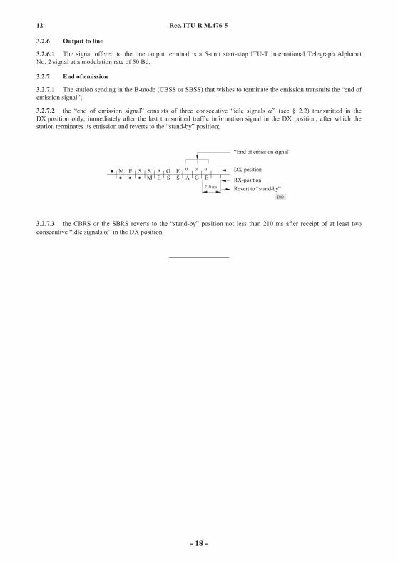
3.2.7 End of emission
3.2.7.1 The station sending in the B-mode (CBSS or SBSS) that wishes to terminate the emission transmits the “end of emission signal”;
3.2.7.2 the “end of emission signal” consists of three consecutive “idle signals ” (see § 2.2) transmitted in the DX position only, immediately after the last transmitted traffic information signal in the DX position, after which the station terminates its emission and reverts to the “stand-by” position;
210 ms
M E S S A G EM E S S A G E
DX-position
RX-positionRevert to “stand-by”
“End of emission signal”
D03
FIGURE ...[D03] = 3 CM
3.2.7.3 the CBRS or the SBRS reverts to the “stand-by” position not less than 210 ms after receipt of at least two consecutive “idle signals ” in the DX position.
- 18 -

Rec. ITU-R M.489-2 1
RECOMMENDATION ITU-R M.489-2*
TECHNICAL CHARACTERISTICS OF VHF RADIOTELEPHONE EQUIPMENT OPERATING IN THE MARITIME MOBILE
SERVICE IN CHANNELS SPACED BY 25 kHz
(1974-1978-1995)Rec. ITU-R M.489-2
Summary The Recommendation describes the technical characteristics of VHF radiotelephone transmitters and receivers (or transceivers) used in the maritime mobile service when operating in 25 kHz channels of Appendix S18 [Appendix 18] of the Radio Regulations (RR). It also contains those additional characteristics of transceivers required to operate digital selective calling.
The ITU Radiocommunication Assembly,
considering
a) that Resolution No. 308 of the World Administrative Radio Conference (Geneva, 1979) stipulated that: – all maritime mobile VHF radiotelephone equipment shall conform to 25 kHz standards by 1 January 1983;
b) that RR Appendix S18 [Appendix 18] gives a table of transmitting frequencies which is based upon the principle of 25 kHz channel separations for the maritime mobile service;
c) that in Opinion 42, the International Electrotechnical Commission (IEC) has been invited to advise the ITU Radiocommunication Sector of any methods of measurement applicable to radio equipment used in land mobile services; and that such methods of measurement may also be suitable for radio equipment used in maritime mobile services;
d) that there is a need to specify the technical characteristics of VHF radiotelephone equipment operating in the maritime mobile service in channels spaced by 25 kHz,
recommends
1 that the following characteristics should be met by VHF (metric) FM radiotelephone equipment used for the maritime mobile services operating on the frequencies specified in RR Appendix S18 [Appendix 18].
1.1 General characteristics
1.1.1 The class of emission should be F3E/G3E.
1.1.2 The necessary bandwidth should be 16 kHz.
1.1.3 Only phase modulation (frequency modulation with a pre-emphasis characteristic of 6 dB/octave) should be used.
_______________* This Recommendation should be brought to the attention of the International Maritime Organization (IMO) and the
Telecommunication Standardization Sector (ITU-T).
Note by the Secretariat: The references made to the Radio Regulations (RR) in this Recommendation refer to the RR as revised by the World Radiocommunication Conference 1995. These elements of the RR will come into force on 1 June 1998. Where applicable, the equivalent references in the current RR are also provided in square brackets.
- 19 -

2 Rec. ITU-R M.489-2
1.1.4 The frequency deviation corresponding to 100% modulation should approach 5 kHz as nearly as practicable. In no event should the frequency deviation exceed 5 kHz. Deviation limiting circuits should be employed such that the maximum frequency deviation attainable should be independent of the input audio frequency.
1.1.5 Where duplex or semi-duplex systems are in use, the performance of the radio equipment should continue to comply with all the requirements of this Recommendation.
1.1.6 The equipment should be designed so that frequency changes between assigned channels can be carried out within 5 s.
1.1.7 Emissions should be vertically polarized at the source.
1.1.8 Stations using digital selective calling shall have the following capabilities:
a) sensing to determine the presence of a signal on 156.525 MHz (channel 70); and
b) automatic prevention of the transmission of a call, except for distress and safety calls, when the channel is occupied by calls.
1.2 Transmitters
1.2.1 The frequency tolerance for coast station transmitters should not exceed 5 parts in 106, and that for ship station transmitters should not exceed 10 parts in 106.
1.2.2 Spurious emissions on discrete frequencies, when measured in a non-reactive load equal to the nominal output impedance of the transmitter, should be in accordance with the provisions of RR Appendix S3 [Appendix 8].
1.2.3 The carrier power for coast stations should not normally exceed 50 W.
1.2.4 The carrier power for ship station transmitters should not exceed 25 W. Means should be provided to readily reduce this power to 1 W or less for use at short ranges, except for digital selective calling equipment operating on 156.525 MHz (channel 70) in which case the power reduction facility is optional (see also Recommen-dation ITU-R M.541 recommends 3.7).
1.2.5 The upper limit of the audio-frequency band should not exceed 3 kHz.
1.2.6 The cabinet radiated power should not exceed 25 W. In some radio environments, lower values may be required.
1.3 Receivers
1.3.1 The reference sensitivity should be equal to or less than 2.0 V, e.m.f., for a given reference signal-to-noise ratio at the output of the receiver.
1.3.2 The adjacent channel selectivity should be at least 70 dB.
1.3.3 The spurious response rejection ratio should be at least 70 dB.
1.3.4 The radio frequency intermodulation rejection ratio should be at least 65 dB.
1.3.5 The power of any conducted spurious emission, measured at the antenna terminals, should not exceed 2.0 nW at any discrete frequency. In some radio environments lower values may be required.
1.3.6 The effective radiated power of any cabinet radiated spurious emission on any frequency up to 70 MHz should not exceed 10 nW. Above 70 MHz, the spurious emissions should not exceed 10 nW by more than 6 dB/octave in frequency up to 1 000 MHz. In some radio environments, lower values may be required;
2 that reference should also be made to Recommendations ITU-R SM.331 and ITU-R SM.332 and to the relevant IEC publications on methods of measurement.
- 20 -

RECOMMENDATION ITU-R M.492-6*
(Question ITU-R 5/8)
(1974-1978-1982-1986-1990-1992-1995)Rec. ITU-R M.492-6
The Recommendation provides in Annex 1 operational procedures for the use of direct-printing telegraph equipment in communication between a ship and a coast station in the selective ARQ-mode on a fully automated or semi-automated basis and to a number of ship stations or a single ship in the broadcast FEC-mode. It also specifies interworking between equipments in accordance with technical characteristics given in Recommendations ITU-R M.476 and ITU-R M.625. Appendix 1 contains procedures for setting up of calls.
The ITU Radiocommunication Assembly,
considering
a) that narrow-band direct-printing telegraph services are in operation using equipment as described in Recommendations ITU-R M.476, ITU-R M.625 and ITU-R M.692;
b) that an improved narrow-band direct-printing telegraph system providing automatic identification and capable of using the 9-digit ship station identity is described in Recommendation ITU-R M.625;
c) that the operational procedures necessary for such services should be agreed upon;
d) that, as far as possible, these procedures should be similar for all services and for all frequency bands (different operational procedures may be required in frequency bands other than the HF and MF bands);
e) that a large number of equipments complying with Recommendation ITU-R M.476 exist;
f) that interworking between equipments in accordance with Recommendations ITU-R M.476 and ITU-R M.625 is required, at least for a transitionary period,
recommends
that the operational procedures given in Annex 1 be observed for the use of narrow-band direct-printing telegraph equipment in accordance with either Recommendation ITU-R M.476 or ITU-R M.625 in the MF and HF bands of the maritime mobile service;
that when using direct-printing telegraphy or similar systems in any of the frequency bands allocated to the maritime mobile service, the call may, by prior arrangement, be made on a working frequency available for such systems.
* This Recommendation should be brought to the attention of the International Maritime Organization (IMO) and the Telecommunication Standardization Sector (ITU-T).
- 21 -
yammouni
Highlight

ANNEX 1
Methods used for setting up narrow-band direct-printing telegraph communications between a ship station and a coast station in the ARQ-mode should be on a fully automatic or semi-automatic basis, insofar that a ship station should have direct access to a coast station on a coast station receiving frequency and a coast station should have direct access to a ship station on a coast station transmitting frequency.
However, where necessary, prior contact by Morse telegraphy, radiotelephony or other means is not precluded.
Through connection to a remote teleprinter station over a dedicated circuit or to a subscriber of the international telex network may be achieved by manual, semi-automatic or automatic means.
NOTE 1 – Before an international automatic service can be introduced, agreement has to be reached on a numbering plan, traffic routing and charging. This should be considered by both the ITU-T and the ITU-R.
NOTE 2 – Recommendations ITU-R M.476 (see § 3.1.5) and ITU-R M.625 (see § 3.8) make provision for automatic re-establishment of radio circuits by rephasing in the event of interruption. However, it has been reported that this procedure has, in some countries, resulted in technical and operational problems when radio circuits are extended into the public switched network or to certain types of automated switching or store-and-forward equipments. For this reason, some coast stations do not accept messages if the rephasing procedure is used.
NOTE 3 – When a connection is set up in the ARQ mode with the international telex network via a coast station, where practicable the general requirements specified in ITU-T Recommendation U.63 should be met.
When, by prior arrangement, unattended operation is required for communication from a coast station to a ship station, or between two ship stations, the receiving ship station should have a receiver tuned to the other station’s transmitting frequency and a transmitter tuned or a transmitter capable of being tuned automatically to the appropriate frequency and ready to transmit on this frequency.
For unattended operation a ship station should be called selectively by the initiating coast or ship station as provided for by Recommendations ITU-R M.476 and ITU-R M.625. The ship station concerned could have available traffic stored ready for automatic transmission on demand of the calling station.
At the “over” signal, initiated by the calling station, any available traffic in the ship’s traffic store could be transmitted.
At the end of the communication, an “end of communication” signal should be transmitted, whereupon the ship’s equipment should automatically revert to the “stand-by” condition.
A “free channel” signal may be transmitted by a coast station where necessary to indicate when a channel is open for traffic. The “free channel” signals should preferably be restricted to only one channel per HF band and their duration should be kept as short as possible. In accordance with Article 18 of the Radio Regulations and recognizing the heavy loading of the frequencies available for narrow-band direct printing in the HF bands, “free channel” signals should not be used in future planned systems.
The format of the “free channel” signal should be composed of signals in the 7-unit error detecting code as listed in § 2 of Annex 1 to Recommendation ITU-R M.476 and § 2 of Annex 1 to Recommendation ITU-R M.625. Three of these signals should be grouped into a block, the middle signal being the “signal repetition” (RQ), the first signal of theblock being any of the signals VXKMCF TBOZA and the third signal of the block being any of the signals VMPCYFS OIRZDA (see Recommendation ITU-R M.491). These signals should be indicated in the ITU List of Coast Stations.
- 22 -

Selections of new signals should preferably be chosen to correspond to the first two digits of that coast station’s 4-digit identification number. If this is not possible because the characters needed are not listed above, or if this is not desired because this combination is already in use by another coast station, it is preferred that a combination of characters be selected from those listed above in the second part of each row, i.e. TBOZA for the first signal and OIRZDA for the third signal of the free channel block. The signals in the block are transmitted at a modulation rate of 100 Bd and the blocks are separated by pauses of 240 ms. For manual systems this “free channel” signal should be interrupted either by a period of no signal or by a signal or signals, that would enable an operator to recognize the “free channel” condition by ear. An aurally recognizable signal, e.g. a Morse signal, may be used alone as the “free channel” signal in manual systems. At least 8 blocks of the 7-unit signal should be transmitted before interruption.
In the case of single frequency operation, as described in Recommendation ITU-R M.692, the free channel signal should be interrupted by listening periods of at least 3 s.
General operational procedures for setting up calls between ship stations and between ship stations and coast stations are given below and specific procedures are given in Appendix 1.
The operator of the ship station establishes communication with the coast station by A1A Morse telegraphy, telephony or by other means using normal calling procedures. The operator then requests direct-printing communication, exchanges information regarding the frequencies to be used and, when applicable, gives the ship station the direct-printing selective call number assigned in accordance with Recommendation ITU-R M.476 or ITU-R M.625 as appropriate, or the ship station identity assigned in accordance with the Preface to List VII A.
The operator of the coast station then establishes direct-printing communication on the frequency agreed, using the appropriate identification of the ship.
Alternatively the operator of the ship station, using the direct-printing equipment, calls the coast station on a predetermined coast station receive frequency using the identification of the coast station assigned in accordance with Recommendation ITU-R M.476 or ITU-R M.625 as appropriate, or the coast station identity assigned in accordance with the Preface to List VII A.
The operator of the coast station then establishes direct-printing communication on the corresponding coast station transmit frequency.
The operator of the coast station calls the ship station by A1A Morse telegraphy, telephony or other means, using normal calling procedures.
The operator of the ship station then applies the procedures of § 1.12.1.1 or § 1.12.1.3.
The operator of the calling ship station establishes communication with the called ship station by A1A Morse telegraphy, telephony, or by other means, using normal calling procedures. The operator then requests direct-printing communication, exchanges information regarding the frequencies to be used and, when applicable, gives the direct-printing selective call number of the calling ship station assigned in accordance with Recommendation ITU-R M.476 or ITU-R M.625 as appropriate, or the ship station identity assigned in accordance with the Preface to List VII A.
The operator of the called ship station then establishes direct-printing communication on the frequency agreed, using the appropriate identification of the calling ship.
- 23 -

The ship station calls the coast station on a predetermined coast station receive frequency, using the direct-printing equipment and the identification signal of the coast station assigned in accordance with Recommen-dation ITU-R M.476 or ITU-R M.625 as appropriate, or the coast station identity assigned in accordance with the Preface to List VII A.
The coast station’s direct-printing equipment detects the call and the coast station responds directly on the corresponding coast station transmit frequency, either automatically or under manual control.
The coast station calls the ship station on a predetermined coast station transmit frequency, using the direct-printing equipment and the ship station direct-printing selective call number assigned in accordance with Recommendation ITU-R M.476 or ITU-R M.625 as appropriate, or the ship station identity assigned in accordance with the Preface to List VII A.
The ship station’s direct-printing equipment tuned to receive the predetermined coast station transmit frequency detects the call, whereupon the reply is given in one of the following ways:
a) the ship station replies either immediately on the corresponding coast station receive frequency or at a later stage, using the procedure of § 1.12.1.3; or
b) the ship station’s transmitter is automatically started on the corresponding coast station receive frequency and the direct-printing equipment responds by sending appropriate signals to indicate readiness to receive traffic automatically.
Where the appropriate facilities are provided by the coast station, traffic may be exchanged with the telex network:
a) in a conversational mode where the stations concerned are connected directly, either automatically or under manual control; or
b) in a store-and-forward mode where traffic is stored at the coast station until the circuit to the called station can be set up, either automatically or under manual control.
In the shore-to-ship direction, the message format should conform to normal telex network practice (see also Appendix 1, § 2).
In the ship-to-shore direction, the message format should conform to the operational procedures specified in Appendix 1, § 1.
Messages may, by prior arrangement, be sent in the B mode from a coast station or a ship station to a number of ships or to a single ship, preceded if desired by the selective call code of the ship(s) concerned where:
a receiving ship station is not permitted or not able to use its transmitter, or
communications are intended for more than one ship, or
unattended reception of the B mode is required and automatic acknowledgement is not necessary.
In such cases, the ship station receivers should be tuned to the appropriate coast or ship station transmitting frequency.
- 24 -

All B mode messages should start with “carriage return” and “line feed” signals.
When the ship station receives phasing signals in the B mode, its teleprinter should start automatically and should stop automatically when reception of the emission ceases.
Ship stations may acknowledge the reception of B mode messages by A1A Morse telegraphy, telephony or by other means.
Recommendation ITU-R M.625 provides for automatic inter-working with equipment which is in accordance with Recommendation ITU-R M.476. The criteria for determining whether one or both stations are of the Recommendation ITU-R M.476 type are the length of the call signal and the composition of the call blocks.
If both stations have equipment in accordance with Recommendation ITU-R M.625, automatic station identification is a part of the automatic call set-up procedures. However, if one or both stations have equipment in accordance with Recommendation ITU-R M.476, no automatic station identification takes place. For this reason, and because Recommendation ITU-R M.625 accommodates the use of the 9-digit ship station identity for the direct-printing equipment call signal, it is desirable that all new equipment be in accordance with Recommendation ITU-R M.625 at the earliest practicable time.
In order to attain full compatibility with the large number of existing equipment, it will be necessary to assign both a 9-digit and a 5- (or 4-) digit identity (i.e. 7- and 4-signal call signals) to such new stations. Ship and coast station lists should contain both signals.
- 25 -

APPENDIX 1
GA
(7)
GA
MSG + ?(5)
QRC + ?
5
6
7
8
9
10
11
12
13
14
? (3)
(2)
TLX xyDIRTLX xy
MSG +
TGMURGRTLOPRWXNAVSTAPOSFREQSVCMANMEDOBSHELPHELP...AMVBRK
MULTLX xy xy xySTS x
VBTLX xyFAX xyTEL xyDATA xyRPT ...TSTTRF
INF
“Message reference charged time, etc.” (8)
Coast station Ship station
Ship initiates the call
Go to step 4 orend of communication
Not
e 2 ap
plie
s
Exchange answer-backs (1)
Step
Exchange answer-backs (1)
Ship transmits itsAAIC, followed by + ? (3) (4)
Message procedure (6)
(2.1) or(2.2) or(2.3) or(2.4) or(2.5) or(2.6) or(2.7) or(2.8) or(2.9) or(2.10) or(2.11) or(2.12) or(2.13) or(2.14) or(2.15) or(2.16) or(2.17) or(2.18) or(2.19) or(2.20) or(2.21) or(2.22) or(2.23) or(2.24) or(2.25) or(2.26) or(2.27) or(2.28) or(2.29) or(2.30)
D01
FIGURE ...[D01] = 20 CM
- 26 -

Operation in the direction coast station to ship may need to be in the store-and-forward mode owing to the fact that radio propagation conditions may not allow the setting up of a call at the intended time.
5
6
7
1
2
3
4
GA
Go to step 3or
Coast station Ship stationStep
Exchange answer-backs (1)
Message procedure
If ship has traffic for coast station go to step 4 of Part 1
orEnd of communication
Coast station initiatescall
Exchange answer-backs (1)
D02
FIGURE 1...[D02] = 9 CM
Notes relative to § 1 and 2:
(1) a) In automatic operation the answer-back exchange is initiated and controlled by the coast station. For calls set up by the ship station the answer-back exchange in manual operation may be initiated by the ship station.
For calls set up by the coast station the answer-back exchange in manual operation is initiated by the coast station, thereby defining the order in which the exchange takes place.
b) Answer-back code as defined in ITU-T Recommendations F.130 for ship stations and F.60 for coast stations.
(2) A coast station need not provide all of the facilities indicated. However, where specific facilities are provided, the facility codes indicated should be used. The facility “HELP” should always be available.
(2.1) MSG indicates that the ship station needs to immediately receive any messages held for it at the coast station.
(2.2) TLX xy indicates that the following message is for immediate connection to a store-and-forward facility located at the coast station.
y indicates the subscriber’s national telex number.
x is used where applicable to indicate the country code (ITU-T Recommendation F.69) preceded by 0 (when applicable). (Where the store-and-forward system is remote from the coast station, TLX alone may be used.)
TLXA may optionally be used instead of TLX which indicates that ship wishes to be advised (using the normal shore-to-ship procedures) when the message has been delivered to the indicated telex number.
(2.3) DIRTLX xy indicates that a direct telex connection is required.
y indicates the subscriber’s national telex number.
x is used where applicable to indicate the country code (ITU-T Recommendation F.69) preceded by 0 (when applicable).
RDL + may optionally be used to indicate that the last DIRTLX xy telex number should be redialled.
(2.4) TGM indicates that the following message is a radio telegram.
- 27 -

(2.5) URG indicates that the ship station needs to be connected immediately to a manual assistance operator and an audible alarm may be activated. This code should only be used in case of emergency.
(2.6) RTL indicates that the following message is a radio telex letter. (2.7) OPR indicates that connection to a manual assistance operator is required. (2.8) WX indicates that the ship station needs to immediately receive weather information. (2.9) NAV indicates that the ship station needs to immediately receive navigational warnings. (2.10) STA indicates that the ship station needs to immediately receive a status report of all store-and-forward messages which have
been sent by that ship station, but which the ship station has not already received on retransmitted or non-delivered information (see also (6)). STA x may also be used where the ship station needs to immediately receive a status report of such a message where x indicates the message reference provided by the coast station.
(2.11) POS indicates that the following message contains the ship’s position. Some administrations use this information to assist inthe subsequent automatic transmission or reception of messages (e.g. for calculating the optimum traffic frequency and/or the appropriate directional antennas to use).
(2.12) FREQ indicates that the following message indicates the frequency on which the ship is keeping watch. (2.13) SVC indicates that the following message is a service message (for subsequent manual attention). (2.14) MAN indicates that the following message is to be stored and manually forwarded to a country which cannot be accessed
automatically. (2.15) MED indicates that an urgent medical message follows. (2.16) OBS indicates that the following message is to be sent to the meteorological organization. (2.17) HELP indicates that the ship station needs to immediately receive a list of available facilities within the system. (2.18) If information is needed on the application of procedures for individual facilities at a coast station, request for further details
concerning the specific procedure can be obtained by the facility code HELP followed by the appropriate facility code for which the information is needed, e.g.: < HELP DIRTLX + indicates that the ship station needs information on the procedures (action by ship operator) for ordering a dialogue-mode connection with a telex network subscriber via the coast station.
(2.19) AMV indicates that the following message is to be sent to the AMVER organization. (2.20) BRK indicates that the use of the radio path is to be immediately discontinued (for use where the ship’s operator can only use
a teleprinter for controlling the ARQ equipment). (2.21) MULTLX xy/xy/xy�+ indicates that the following message is a multiple address message for immediate connection to a
store-and-forward facility located at the coast station.
y indicates the subscriber’s national telex number.
x is used where applicable to indicate the country code (ITU-T Recommendation F.69) preceded by 0 (when applicable).
Each separate xy indicates a different telex number to which the same message should be forwarded. At least two separate telex numbers should be included.
MULTLXA may optionally be used instead of MULTLX which indicates that the ship wishes to be advised (using the normal shore-to-ship procedures) when the messages have been delivered to the indicated telex numbers.
(2.22) STS x + indicates that the following message is for transmission to a ship using a store-and-forward facility located at the coast station. x indicates the addressed ship’s 5- or 9-digit identity number.
(2.23) INF indicates that the ship station needs to immediately receive information from the coast station’s database. Some administrations provide a variety of different database information in which case INF returns a directory listing and a subsequent facility code is used to select the desired information.
(2.24) VBTLX xy indicates that the following message should be dictated, by the coast station, to a voicebank (voice messaging) telephone number for subsequent retrieval by the addressee, and that a copy of the message should be forwarded to telex number xy. The voicebank telephone number should be included in the first line of the message text.
(2.25) FAX xy indicates that the following message should be forwarded, via the PSTN, by facsimile to the telephone number xy. (2.26) TEL xy indicates that the following message should be telephoned, by the coast station, to the telephone number xy. (2.27) DATA xy indicates that the following message should be forwarded by the coast station using data facilities to the
subscriber number xy (via the PSTN). (2.28) RPT xy indicates that the ship needs to receive, using the ARQ mode, a specific identified message (e.g., earlier
transmitted in the FEC mode), if still available for automatic retransmission. x is used as the message identifier. (2.29) TST indicates that the ship needs to receive an automatically transmitted test text (e.g. “the quick brown fox ”).(2.30) TRF indicates that the ship needs to receive information, automatically transmitted, on tariffs currently applicable to the coast
station.
- 28 -

(3) The symbol “?” is not necessary where the coast station is automatic. It is normally required only for manual systems.(4) In cases where the coast station requires information about the relevant Accounting Authority Identification Code (AAIC), this
information should be provided by the ship operator on receipt of the combination < QRC + from the coast station.
Some coast stations may request additional information, e.g. ship’s name, call sign, etc.(5) This sequence may be preceded where necessary by suitable prompts or facility selection information and, if appropriate, any
consequent ship station reply, or may be deleted where not applicable (e.g. where facility codes WX, NAV, STA, MSG or HELP are input at step 4). Where facility code DIRTLX xy was input at step 4, this sequence may be replaced by the distant end answer-back or by any service signal (e.g. NC, OCC, etc.) received from the telex network.
(6) Message procedures depend on which facility is used:
For TLX where the store-and-forward system is remote from the coast station, ITU-T Recommendation F.72 may apply. Where the store-and-forward system is located at the coast station, the complete information content of the message sent at this step will be forwarded to the subscriber whose telex number is given by xy.
For DIRTLX, see ITU-T Recommendation F.60.
For TGM, see ITU-T Recommendations F.1 and F.31.
For SVC and MED, the message will normally be plain text and no specific message procedure is required.
For RTL, the message will be plain text but should include the postal address of the addressee.
For STA, the appropriate status information is returned to the ship in accordance with ITU-T Recommendation F.72, § 11.3 and 11.4.
For POS and FREQ, specific national procedures may apply. (7) This sequence of 4 K’s “KKKK” (4 combination No. 11 signals in the letter case) indicates that any network connection
should be cleared but that the radio path should be maintained and that the procedure should immediately proceed to step 11. This sequence may be used elsewhere in the procedure in which case the procedure reverts to step 3.
(8) This step is optional and may not apply to all facilities.
- 29 -


Rec. ITU-R P.525-4 1
RECOMMENDATION ITU-R P.525-4
Calculation of free-space attenuation(1978-1982-1994-2016-2019)
Scope
Recommendation ITU-R P.525 provides methods to calculate the attenuation in free space.
Keywords
Free space, attenuation, telecommunication links
The ITU Radiocommunication Assembly,
considering
that free-space propagation is a fundamental reference for radio-engineering,
recommends
that the methods in the Annex should be used for the calculation of attenuation in free space.
Annex
1 Introduction
For the purposes of radiocommunication, free space is defined as a perfect vacuum which may be considered of infinite extent in all directions, so that free space propagation is the propagation of a radio wave radiating in free space1.
As free-space propagation is often used as a reference in other texts, this Annex presents relevant formulae.
2 Basic formulae for telecommunication links
Free-space propagation may be calculated in different ways, each of which is adapted to a particular type of service.
1 The International Standards Organisation in its electrotechnical vocabulary (electropedia) has a more general definition:
Free space propagation: propagation of an electromagnetic wave in a homogeneous ideal dielectric medium which may be considered of infinite extent in all directions
NOTE – For propagation in free space, the magnitude of each vector of the electromagnetic field in any given direction from the source is proportional to the reciprocal of the distance from the source beyond a distance determined by the size of the source and the wavelength.
- 31 -

2 Rec. ITU-R P.525-4
2.1 Point-to-area links
If there is a transmitter serving several randomly-distributed receivers (broadcasting, mobile service), the electric field is calculated at a point located at some appropriate distance from the transmitter by the expression:
dp
e30 (1)
where:e : r.m.s. field strength (V/m) (see Note 1)p : equivalent isotropically radiated power (e.i.r.p.) of the transmitter in the
direction of the point in question (W) (see Note 2)d : distance from the transmitter to the point in question (m).
Equation (1) is often replaced by equation (2) which uses practical units:
km
kWmV/m 173
dp
e (2)
where:emV/m : r.m.s field strength (mV/m)
pkW : equivalent isotropically radiated power (e.i.r.p.) of the transmitter in the direction of the point in question (kW)
dkm : distance from the transmitter to the point in question (km).
For antennas operating in free-space conditions the cymomotive force may be obtained by multiplying together e and d in equation (1). Its dimension is volts.NOTE 1 – If the wave is elliptically polarized and not linear, and if the electric field components along two orthogonal axes are expressed by ex and ey, the left-hand term of equation (1) should be replaced by
e ex y2 2 . ex and ey can be deduced only if the axial ratio is known. e should be replaced by e 2 in the case
of circular polarization.NOTE 2 – In the case of antennas located at ground level (typically at relatively low frequencies) with vertical polarization, radiation is generally considered only in the upper half-space. When the ground is assumed to be plane and perfectly conducting, the power flux-density for a given radiated power is doubled, as compared with an antenna in free space. (Alternatively, when considering field strengths, the field strength is similarly increased by 3 dB.) This should be taken into account in determining the radiated power (and is already included in Recommendations ITU-R P.368 and ITU-R P.341, Annex3).
2.2 Point-to-point links
With a point-to-point link it is preferable to calculate the free-space attenuation between isotropic antennas, also known as the free-space basic transmission loss (symbols: Lbf or Abf), as follows (see Recommendation ITU-R P.341):
dLbf4log20 mmmmmmdB (3)
where:Lbf : free-space basic transmission loss (dB)
d : distance: wavelength, and
- 32 -

Rec. ITU-R P.525-4 3
d and are expressed in the same unit.
Equation (3) can also be written using the frequency instead of the wavelength.
Lbf = 32.4 20 log 20 log dmmmmmmdB (4)
where:f : frequency (MHz)d : distance (km).
2.3 Relations between the characteristics of a plane wave
There are also relations between the characteristics of a plane wave (or a wave which can be treated as a plane wave) at a point:
2
2 4120
rpes (5)
where:s : power flux-density (W/m2)e : r.m.s. field strength (V/m)
pr : power (W) available from an isotropic antenna located at this point: wavelength (m).
3 The free-space basic transmission loss for a radar system (symbols: Lbr or Abr)
Radar systems represent a special case because the signal is subjected to a loss while propagating both from the transmitter to the target and from the target to the receiver. For radars using a common antenna for both transmitter and receiver, a radar free-space basic transmission loss, Lbr, can be written as follows:
Lbr 103.4 20 log 40 log d – 10 log mmmmmmdB (6)
where:: radar target cross-section (m2)
d : distance from the radar to the target (km)f : frequency of the system (MHz).
The radar target cross-section of an object is the ratio of the total isotropically equivalent scattered power to the incident power density.
4 Conversion formulae
On the basis of free-space propagation, the following conversion formulae may be used.
Field strength for a given isotropically transmitted power:
E Pt – 20 log d 74.8 (7)
Available power received through a conjugately matched isotropic receiving antenna for a given field strength:
Pr E – 20 log f – 167.2 (8)
- 33 -

4 Rec. ITU-R P.525-4
Free-space basic transmission loss for a given isotropically transmitted power and field strength:
Lbf Pt – E 20 log f 167.2 (9)
Power flux-density for a given field strength:
S E – 145.8 (10)
where:Pt : isotropically transmitted power (dB(W))Pr : available power received through a conjugately matched antenna (dB(W))E : electric field strength (dB( V/m))f : frequency (GHz)d : radio path length (km)
Lbf : free-space basic transmission loss (dB)S : power flux-density (dB(W/m2)).
Note that equations (7) and (9) can be used to derive equation (4).
- 34 -

Rec. ITU-R P.526-15 1
RECOMMENDATION ITU-R P.526-15
Propagation by diffraction(Question ITU-R 202/3)
(1978-1982-1992-1994-1995-1997-1999-2001-2003-2005-2007-2009-2012-2013-2018-2019)
Scope
This Recommendation presents several models to enable the reader to evaluate the effect of diffraction on the received field strength. The models are applicable to different obstacle types and to various path geometries.
Keywords
diffraction, irregular terrain, obstacles, knife-edge, aperture, screen
The ITU Radiocommunication Assembly,
considering
that there is a need to provide engineering information for the calculation of field strengths over diffraction paths,
recommends
that the methods described in Annex 1 be used for the calculation of field strengths over diffraction paths, which may include a spherical earth surface, or irregular terrain with different kinds of obstacles.
TABLE OF CONTENTS
Page Annex 1 .................................................................................................................................... 2
1 Introduction .................................................................................................................... 2
2 Basic concepts ................................................................................................................ 3
2.1 Fresnel ellipsoids and Fresnel zones................................................................... 3
2.2 Penumbra width .................................................................................................. 3
2.3 Diffraction zone .................................................................................................. 4
2.4 Obstacle surface smoothness criterion................................................................ 4
2.5 Isolated obstacle.................................................................................................. 4
2.6 Types of terrain................................................................................................... 4
2.7 Fresnel integrals.................................................................................................. 5
3 Diffraction over a spherical Earth .................................................................................. 6
- 35 -

2 Rec. ITU-R P.526-15
3.1 Diffraction loss for over-the-horizon paths ........................................................ 6
3.2 Diffraction loss for any distance at 10 MHz and above ..................................... 15
4 Diffraction over isolated obstacles or a general terrestrial path ..................................... 16
4.1 Single knife-edge obstacle .................................................................................. 16
4.2 Single rounded obstacle ...................................................................................... 19
4.3 Double isolated edges ......................................................................................... 21
4.4 Multiple isolated cylinders ................................................................................. 23
4.5 Method for a general terrestrial path .................................................................. 26
5 Diffraction by thin screens ............................................................................................. 30
5.1 Finite-width screen ............................................................................................. 30
5.2 Diffraction by rectangular apertures and composite apertures or screens .......... 30
6 Diffraction over a finitely conducting wedge................................................................. 34
7 Guide to propagation by diffraction ............................................................................... 38
Attachment 1 to Annex 1 – Calculation of cylinder parameters............................................. 39
1 Diffraction angle and position of vertex......................................................................... 39
2 Cylinder parameters........................................................................................................ 40
Attachment 2 to Annex 1 – Sub-path diffraction losses ......................................................... 41
1 Introduction .................................................................................................................... 41
2 Method............................................................................................................................ 41
Annex 1
1 Introduction
Although diffraction is produced only by the surface of the ground or other obstacles, account must be taken of the mean atmospheric refraction on the transmission path to evaluate the geometrical parameters situated in the vertical plane of the path (angle of diffraction, radius of curvature, heightof obstacle). For this purpose, the path profile has to be traced with the appropriate equivalent Earth radius (Recommendation ITU-R P.834). If no other information is available, an equivalent Earth radius of 8 500 km may be taken as a basis.
- 36 -

Rec. ITU-R P.526-15 3
2 Basic concepts
Diffraction of radiowaves over the Earth’s surface is affected by terrain irregularities. In this context, before going further into the prediction methods for this propagation mechanism, a few basic concepts are given in this section.
2.1 Fresnel ellipsoids and Fresnel zones
In studying radiowave propagation between two points A and B, the intervening space can be subdivided by a family of ellipsoids, known as Fresnel ellipsoids, all having their focal points at A and B such that any point M on one ellipsoid satisfies the relation:
2ABMBAM n (1)
where n is a whole number characterizing the ellipsoid and n = 1 corresponds to the first Fresnel ellipsoid, etc., and is the wavelength.
As a practical rule, propagation is assumed to occur in line-of-sight (LoS), i.e. with negligible diffraction phenomena if there is no obstacle within the first Fresnel ellipsoid.
The radius of an ellipsoid at a point between the transmitter and the receiver can be approximated in self-consistent units by:
2/1
21
21
ddddnRn (2)
or, in practical units:
2/1
21
21
)(550
fddddnRn (3)
where f is the frequency (MHz) and d1 and d2 are the distances (km) between transmitter and receiver at the point where the ellipsoid radius (m) is calculated.
Some problems require consideration of Fresnel zones which are the zones obtained by taking the intersection of a family of ellipsoids by a plane. The zone of order n is the part between the curves obtained from ellipsoids n and n – 1, respectively.
2.2 Penumbra width
The transition from light to shadow defines the penumbra region. This transition takes place along a narrow strip (penumbra width) in the boundary of geometric shadow. Figure 1 shows the penumbra width (W) in the case of a transmitter located a height, h, above a smooth spherical earth, which is given by:
3/12eaw m (4)
where:: wavelength (m)
ae: effective Earth radius (m)
- 37 -

4 Rec. ITU-R P.526-15
FIGURE 1Definition of penumbra width
2.3 Diffraction zone
The diffraction zone of a transmitter extends from the LoS distance where the path clearance is equal to 60% of the first Fresnel zone radius, (R1), up to a distance well beyond the transmitter horizon where the mechanism of troposcatter becomes predominant.
2.4 Obstacle surface smoothness criterion
If the surface of the obstacle has irregularities not exceeding Δh,
where:3/12λ04.0 Rh m (5)
where:R: obstacle curvature radius (m)
: wavelength (m);
then the obstacle may be considered smooth and the methods described in §§ 3 and 4.2 may be used to calculate the attenuation.
2.5 Isolated obstacle
An obstacle can be considered isolated if there is no interaction between the obstacle itself and the surrounding terrain. In other words, the path attenuation is only due to the obstacle alone without any contribution from the remaining terrain. The following conditions must be satisfied:– no overlapping between penumbra widths associated with each terminal and the obstacle top;– the path clearance on both sides of the obstacles should be, at least, 0.6 of the first Fresnel
zone radius;– no specular reflection on both sides of the obstacle.
2.6 Types of terrain
Depending on the numerical value of the parameter h (see Recommendation ITU-R P.310) used to define the degree of terrain irregularities, three types of terrain can be classified:
a) Smooth terrain
The surface of the Earth can be considered smooth if terrain irregularities are of the order or less than 0.1R, where R is the maximum value of the first Fresnel zone radius in the propagation path. In this case, the prediction model is based on the diffraction over the spherical Earth (see § 3).
- 38 -

Rec. ITU-R P.526-15 5
b) Isolated obstacles
The terrain profile of the propagation path consists of one or more isolated obstacles. In this case, depending on the idealization used to characterize the obstacles encountered in the propagation path, the prediction models described in § 4 should be used.
c) Rolling terrain
The profile consists of several small hills, none of which form a dominant obstruction. Within its frequency range Recommendation ITU-R P.1546 is suitable for predicting field strength but it is not a diffraction method.
2.7 Fresnel integrals
The complex Fresnel integral is given by:
0
2
)()(d2
exp)( jSCssjFc (6)
where j is the complex operator equal to –1, and C( ) and S( ) are the Fresnel cosine and sine integrals defined by:
0
2
d2
cos)( ssC (7a)
0
2
d2
sin)( ssS (7b)
The complex Fresnel integral Fc( ) can be evaluated by numerical integration, or with sufficient accuracy for most purposes for positive using:
40for4
)–(4
)exp()(11
0xxjbaxjxF
n
nnn
c (8a)
4for4)–(4)exp(2
1)(11
0x
xjdc
xjxjF
n
nnn
c (8b)
where:
x = 0.5 2 (9)
and an, bn, cn and dn are the Boersma coefficients given below:a0 = +1.595769140 b0 = -0.000000033 c0 = +0.000000000 d0 = +0.199471140 a1 = -0.000001702 b1 = +4.255387524 c1 = -0.024933975 d1 = +0.000000023 a2 = -6.808568854 b2 = -0.000092810 c2 = +0.000003936 d2 = -0.009351341 a3 = -0.000576361 b3 = -7.780020400 c3 = +0.005770956 d3 = +0.000023006 a4 = +6.920691902 b4 = -0.009520895 c4 = +0.000689892 d4 = +0.004851466 a5 = -0.016898657 b5 = +5.075161298 c5 = -0.009497136 d5 = +0.001903218 a6 = -3.050485660 b6 = -0.138341947 c6 = +0.011948809 d6 = -0.017122914 a7 = -0.075752419 b7 = -1.363729124 c7 = -0.006748873 d7 = +0.029064067 a8 = +0.850663781 b8 = -0.403349276 c8 = +0.000246420 d8 = -0.027928955 a9 = -0.025639041 b9 = +0.702222016 c9 = +0.002102967 d9 = +0.016497308 a10 = -0.150230960 b10 = -0.216195929 c10 = -0.001217930 d10 = -0.005598515 a11 = +0.034404779 b11 = +0.019547031 c11 = +0.000233939 d11 = +0.000838386
- 39 -

6 Rec. ITU-R P.526-15
C( ) and S( ) may be evaluated for negative values of by noting that:
C(– ) = – C( ) (10a)
S(– ) = – S( ) (10b)
3 Diffraction over a spherical Earth
The additional transmission loss due to diffraction over a spherical Earth can be computed by the classical residue series formula. A computer program GRWAVE, available from the ITU, provides the complete method. A subset of the outputs from this program (for antennas close to the ground and at lower frequencies) is presented in Recommendation ITU-R P.368.
The following subsections describe numerical and nomogram methods which may be used for frequencies 10 MHz and above. For frequencies below 10 MHz, GRWAVE should always be used. Section 3.1 gives methods for over-the-horizon paths. Section 3.1.1 is a numerical method. Section 3.1.2 is a nomogram method. Section 3.2 is a method applicable for the smooth earth case for any distance and for frequencies 10 MHz and above. This utilizes the numerical method in § 3.1.1.
3.1 Diffraction loss for over-the-horizon paths
At long distances over the horizon, only the first term of the residue series is important. Even near or at the horizon this approximation can be used with a maximum error around 2 dB in most cases.
This first term can be written as the product of a distance term, F, and two height gain terms, GT and GR. Sections 3.1.1 and 3.1.2 describe how these terms can be obtained from simple formula or from nomograms.
3.1.1 Numerical calculation
3.1.1.1 Influence of the electrical characteristics of the surface of the Earth
The extent to which the electrical characteristics of the surface of the Earth influence the diffraction loss can be determined by calculating a normalized factor for surface admittance, K, given by the formulae:
in self-consistent units:
4/1–22
3/1–
)60()1–(2 eH
aK for horizontal polarization (11)
and2/1
22 )60(HV KK for vertical polarization (12)
or, in practical units:4/1–
223/1– )/00018()1–()(36.0 ffaK eH (11a)
2/122 )/00018( fKK HV (12a)
where:ae : effective radius of the Earth (km)
- 40 -

Rec. ITU-R P.526-15 7
ε : effective relative permittivityσ : effective conductivity (S/m)f : frequency (MHz).
Typical values of K are shown in Fig. 2.
FIGURE 2Calculation of K
If K is less than 0.001, the electrical characteristics of the Earth are not important. For values of Kgreater than 0.001 and less than 1, the appropriate formulae given in § 3.1.1.2 can be used. When Khas a value greater than about 1, the diffraction field strength calculated using the method of § 3.1.1.2differs from the results given by the computer program GRWAVE, and the difference increases rapidly as K increases. GRWAVE should be used for K greater than 1. This only occurs for vertical
- 41 -

8 Rec. ITU-R P.526-15
polarization, at frequencies below 10 MHz over sea, or below 200 kHz over land. In all other cases the method of § 3.1.1.2 is valid.
3.1.1.2 Diffraction field strength formulae
The diffraction field strength, E, relative to the free-space field strength, E0, is given by the formula:
dB)()()(log20 210
YGYGXFEE (13)
where X is the normalized length of the path between the antennas at normalized heights Y1 and Y2
(and where 0
log20EE is generally negative).
In self-consistent units:
da
Xe
3/1
2β (14)
ha
Ye
3/1
2
2
β2 (15)
or, in practical units:
dafX e3/2–3/1β188.2 (14a)
hafY e3/1–3/23– β10575.9 (15a)
where:d : path length (km)
ae : equivalent Earth’s radius (km)h : antenna height (m)f : frequency (MHz).
is a parameter allowing for the type of ground and for polarization. It is related to K by the following semi-empirical formula:
42
42
53.15.4167.06.11β
KKKK (16)
For horizontal polarization at all frequencies, and for vertical polarization above 20 MHz over land or 300 MHz over sea, may be taken as equal to 1.
For vertical polarization below 20 MHz over land or 300 MHz over sea, must be calculated as a function of K. However, it is then possible to disregard ε and write:
3/53/22 89.6
fkK (16a)
- 42 -

Rec. ITU-R P.526-15 9
where is expressed in S/m, f (MHz) and k is the multiplying factor of the Earth’s radius.
The distance term is given by the formula:
F(X) = 11 + 10 log (X) − 17.6 X for X 1.6 (17a)
F(X) = −20 log (X) − 5.6488X1.425 for X < 1.6 (17b)
The height gain term, G(Y ) is given by the following formulae:
8)1.1log(5)1.1(6.17)( 2/1 BBYG for B > 2 (18)
)1.0log(20)( 3BBYG for B 2 (18a)
If KYG log202)( , set )(YG to the value Klog202
In the above:
YB (18b)
The accuracy of the diffracted field strength given by equation (13) is limited by the approximation inherent in only using the first term of the residue series. Equation (13) is accurate to better than 2 dB for values of X, Y1 and Y2 that are constrained by the formula:
limXKYYKYYX ),()β(),()β( 22/1
212/1
1 (19)
where:
β1280.1096.1limX (19a)
)0,(),(β1779.1)0,(),( YYYKY (19b)
Δ(Y,0) and Δ(Y,∞) are given by:
3.0255.0)βlog(5.0tanh15.0)0,( YY (19c)
25.0255.0)βlog(5.0tanh15.0),( YY (19d)
Consequently, the minimum distance dmin for which equation (13) is valid is given by:
),()β(),()β( 22/1
212/1
1 KYYKYYXX limmin (19e)
and dmin is obtained from Xmin using equation (14a).
- 43 -

10 Rec. ITU-R P.526-15
3.1.2 Calculation by nomograms
Under the same approximation condition (the first term of the residue series is dominant), the calculation may also be made using the following formula:
)(H)(H)(Flog20 210
hhdEE
dB (20)
where:E : received field strength
E0 : field strength in free space at the same distanced : distance between the extremities of the path
h1 and h2 : heights of the antennas above the spherical earth.
The function F (influence of the distance) and H (height-gain) are given by the nomograms in Figs 3,4, 5 and 6.
These nomograms (Figs 3 to 6) give directly the received level relative to free space, for k = 1 and k = 4/3, and for frequencies greater than approximately 30 MHz. k is the effective Earth radius factor, defined in Recommendation ITU-R P.310. However, the received level for other values of k may be calculated by using the frequency scale for k = 1, but replacing the frequency in question by a hypothetical frequency equal to f/k2 for Figs 3 and 5, and kf / for Figs 4 and 6.
Very close to the ground the field strength is practically independent of the height. This phenomenon is particularly important for vertical polarization over the sea. For this reason Fig. 6 includes a heavy black vertical line AB. If the straight line should intersect this heavy line AB, the real height should be replaced by a larger value, so that the straight line just touches the top of the limit line at A.NOTE 1 – Attenuation relative to free space is given by the negative of the values given by equation (20). If equation (20) gives a value above the free-space field, the method is invalid.NOTE 2 – The effect of line AB is included in the numerical method given in § 3.1.1.
- 44 -

Rec. ITU-R P.526-15 11
FIGURE 3Diffraction by a spherical Earth – effect of distance
- 45 -

12 Rec. ITU-R P.526-15
FIGURE 4Diffraction by a spherical Earth – height-gain
- 46 -

Rec. ITU-R P.526-15 13
FIGURE 5Diffraction by a spherical Earth – effect of distance
- 47 -

14 Rec. ITU-R P.526-15
FIGURE 6Diffraction by a spherical Earth – height-gain
- 48 -

Rec. ITU-R P.526-15 15
3.2 Diffraction loss for any distance at 10 MHz and above
The following step-by-step procedure should be used for a spherical-earth path of any length at frequencies of 10 MHz and above, for effective Earth radius ae > 0. The method uses the calculation in § 3.1.1 for over-the-horizon cases, and otherwise an interpolation procedure based on a notional effective-earth radius.
The procedure uses self-consistent units and proceeds as follows:
Calculate the marginal LoS distance given by:
212 hhad elos (21)
If d ≥ dlos calculate diffraction loss using the method in § 3.1.1. No further calculation is necessary.
Otherwise continue:
Calculate the smallest clearance height between the curved-earth path and the ray between the antennas, h (see Fig. 7), given by:
d
da
dhda
dhh ee
1
22
22
21
1 22 (22)
)1(21 bdd (22a)
12 ddd (22b)
3)1(3
23arccos
31
3cos
312
mmc
mmb (22c)
21
21
hhhhc (22d)
)(4 21
2
hhadm
e
(22e)
Calculate the required clearance for zero diffraction loss, hreq, given by:
dddhreq
λ552.0 21 (23)
If h > hreq the diffraction loss for the path is zero. No further calculation is required.
Otherwise continue:
Calculate the modified effective earth radius, aem, which gives marginal LoS at distance d given by:
- 49 -

16 Rec. ITU-R P.526-15
2
21
5.0hh
daem (24)
Use the method in § 3.1.1 to calculate the diffraction loss for the path using the modified effective earth radius aem in place of the effective earth radius ae, and designate this loss Ah.
If Ah is negative, the diffraction loss for the path is zero, and no further calculation is necessary.
Otherwise calculate the interpolated diffraction loss, A (dB), given by:
hreq AhhA /1 (25)
4 Diffraction over isolated obstacles or a general terrestrial path
Many propagation paths encounter one obstacle or several separate obstacles and it is useful to estimate the losses caused by such obstacles. To make such calculations, it is necessary to idealize the form of the obstacles, either assuming a knife-edge of negligible thickness or a thick smooth obstacle with a well-defined radius of curvature at the top. Real obstacles have, of course, more complex forms, so that the indications provided in this Recommendation should be regarded only asan approximation. These models do not take into account the profile transverse to the direction of the radio link, which may have a significant effect on diffraction loss.
In those cases where the direct path between the terminals is much shorter than the diffraction path, it is necessary to calculate the additional transmission loss due to the longer path.
The data given below apply when the wavelength is fairly small in relation to the size of the obstacles, i.e. mainly to VHF and shorter waves ( f > 30 MHz).
FIGURE 7Path clearance
4.1 Single knife-edge obstacle
In this extremely idealized case (see Figs 8a) and 8b)), all the geometrical parameters are combined together in a single dimensionless parameter normally denoted by ν which may assume a variety of equivalent forms according to the geometrical parameters selected:
- 50 -

Rec. ITU-R P.526-15 17
21
112dd
h (26)
21
112
dd
(27)
θ)andofsign thehas(2 hh (28)
)andofsignthehas(22121
d (29)
where:h : height of the top of the obstacle above the straight line joining the two ends of
the path. If the height is below this line, h is negatived1 and d2 : distances of the two ends of the path from the top of the obstacle
d : length of the path: angle of diffraction (rad); its sign is the same as that of h. The angle is assumed
to be less than about 0.2 rad, or roughly 12º1 and 2 : angles in radians between the top of the obstacle and one end as seen from the
other end. 1 and 2 are of the sign of h in the above equations.
NOTE 1 – In equations (26) to (29) inclusive h, d, d1, d2 and should be in self-consistent units.
- 51 -

18 Rec. ITU-R P.526-15
FIGURE 8Geometrical elements
- 52 -

Rec. ITU-R P.526-15 19
Figure 9 gives, as a function of , the loss J( ) (dB).
J( ) is given by:
2 21 ( ) ( ) ( ) ( )( ) 20 log
2C S C S
J (30)
where C( ) and S( ) are the real and imaginary parts respectively of the complex Fresnel integral F( ) defined in § 2.7.
For greater than −0.78 an approximate value can be obtained from the expression:
2( ) 6.9 20 log ( – 0.1) 1 – 0.1 dBJ (31)
FIGURE 9Knife-edge diffraction loss
4.2 Single rounded obstacle
The geometry of a rounded obstacle of radius R is illustrated in Fig. 8c). Note that the distances d1and d2, and the height h above the baseline, are all measured to the vertex where the projected rays intersect above the obstacle. The diffraction loss for this geometry may be calculated as:
- 53 -

20 Rec. ITU-R P.526-15
dB),()( nmTvJA (32)
where:a) J(ν) is the Fresnel-Kirchoff loss due to an equivalent knife-edge placed with its peak at the
vertex point. The dimensionless parameter ν may be evaluated from any of equations (26) to (29) inclusive. For example, in practical units equation (26) may be written:
2/1
21
21 )(20316.0dd
ddh (33)
where h and λ are in metres, and d1 and d2 are in kilometres.J(ν) may be obtained from Fig. 9 or from equation (31). Note that for an obstruction to LoS propagation, ν is positive and equation (31) is valid.
b) T(m,n) is the additional attenuation due to the curvature of the obstacle:
22/32/1 8.06.3)5.122(2.7),( mmmnmnmT dB for mn 4 (34a)
22/32/1 8.06.3)172(2.7)(log206),( mmmnmmnnmT dB for mn 4 (34b)
and3/1
21
21 Rdd
ddRm (35)
RRhn3/2
(36)
and R, d1, d2, h and λ are in self-consistent units.
Note that as R tends to zero, T(m,n) also tend to zero. Thus equation (32) reduces to knife-edge diffraction for a cylinder of zero radius.
The obstacle radius of curvature corresponds to the radius of curvature at the apex of a parabola fitted to the obstacle profile in the vicinity of the top. When fitting the parabola, the maximum vertical distance from the apex to be used in this procedure should be of the order of the first Fresnel zone radius where the obstacle is located. An example of this procedure is shown in Fig. 10, where:
i
ii r
xy2
2
(37)
and ri is the radius of curvature corresponding to the sample i of the vertical profile of the ridge. In thecase of N samples, the median radius of curvature of the obstacle is given by:
N
i
i
yx
Nr
1
2
21
(38)
- 54 -

Rec. ITU-R P.526-15 21
FIGURE 10Vertical profile of the obstacle
4.3 Double isolated edges
This method consists of applying single knife-edge diffraction theory successively to the two obstacles, with the top of the first obstacle acting as a source for diffraction over the second obstacle (see Fig. 11). The first diffraction path, defined by the distances a and b and the height ,1h gives a loss L1 (dB). The second diffraction path, defined by the distances b and c and the height ,2h gives a loss L2 (dB). L1 and L2 are calculated using formulae of § 4.1. A correction term Lc (dB) must be added to take into account the separation b between the edges. Lc may be estimated by the following formula:
)()()(log10
cbabcbbaLc (39)
which is valid when each of L1 and L2 exceeds about 15 dB. The total diffraction loss is then given by:
L = L1 + L2 + Lc (40)
The above method is particularly useful when the two edges give similar losses.
FIGURE 11Method for double isolated edges
If one edge is predominant (see Fig. 12), the first diffraction path is defined by the distances a and b + c and the height h1. The second diffraction path is defined by the distances b and c and the height h'2.
- 55 -

22 Rec. ITU-R P.526-15
FIGURE 12Figure showing the main and the second obstacle
The method consists of applying single knife-edge diffraction theory successively to the two obstacles. First, the higher h/r ratio determines the main obstacle, M, where h is the edge height from the direct path TxRx as shown in Fig. 12, and r is the first Fresnel ellipsoid radius given by equation(2). Then h'2, the height of the secondary obstacle from the sub-path MR, is used to calculate the loss caused by this secondary obstacle. A correction term Tc (dB) must be subtracted, in order to take into account the separation between the two edges as well as their height. Tc (dB) may be estimated by the following formula:
p
c pqT
2
10
–1
2log20–12 (41)
with:
1
2/1
)()(2 h
acbcbap (42a)
2
2/1
)()(2 h
cbacbaq (42b)
2/1)(tanac
cbab (42c)
h1 and h2 are the edge heights from the direct path transmitter-receiver.
The total diffraction loss is given by:
cTLLL –21 (43)
The same method may be applied to the case of rounded obstacles using § 4.3.
In cases where the diffracting obstacle may be clearly identified as a flat-roofed building a single knife-edge approximation is not sufficient. It is necessary to calculate the phasor sum of two components: one undergoing a double knife-edge diffraction and the other subject to an additional reflection from the roof surface. It has been shown that, where the reflectivity of the roof surface and
- 56 -

Rec. ITU-R P.526-15 23
any difference in height between the roof surface and the side walls are not accurately known, then a double knife-edge model produces a good prediction of the diffracted field strength, ignoring the reflected component.
4.4 Multiple isolated cylinders
This method is recommended for diffraction over irregular terrain which forms one or more obstacles to LoS propagation where each obstacle can be represented by a cylinder with a radius equal to the radius of curvature at the obstacle top, being advisable when detailed vertical profile through the ridge is available.
The terrain height profile should be available as a set of samples of ground height above sea level, the first and last being the heights of the transmitter and receiver above sea level. Atmospheric refractivity gradient should be taken into account via the concept of effective Earth radius. Distance and height values are described as though stored in arrays indexed from 1 to N, where N equals the number of profile samples.
In the following a systematic use of suffices is made:hi : height above sea level of the i-th pointdi : distance from the transmitter to the i-th pointdij : distance from the i-th to the j-th points.
The first step is to perform a “stretched string” analysis of the profile. This identifies the sample points which would be touched by a string stretched over the profile from transmitter to receiver. This may be done by the following procedure, in which all values of height and distance are in self-consistent units, and all angles are in radians. The method includes approximations which are valid for radio paths making small angles to the horizontal. If a path has ray gradients exceeding about 5º more exact geometry may be justified.
Each string point is identified as the profile point with the highest angular elevation above the local horizontal as viewed from the previous string point, starting at one end of the profile and finishing at the other. Viewed from point s, the elevation of the i-th profile sample (i > s) is given by:
e = [(hi – hs) / dsi ] – [dsi / 2ae ] (44)
where:ae: effective Earth radius, given by:
= k × 6 371 (km)
andk : effective Earth-radius factor.
A test is now applied to determine whether any group of two or more string points should represent the same terrain obstruction. For samples at spacings of 250 m or less any group of string points which are consecutive profile samples, other than the transmitter or receiver, should be treated as one obstruction.
Each obstruction is now modelled as a cylinder, as illustrated in Fig. 13. The geometry of each individual cylinder corresponds with Fig. 8c). Note that in Fig. 13 the distances s1, s2 for each cylinder are shown as measured horizontally between the vertex points, and that for near-horizontal rays these distances approximate to the slope distances d1 and d2 in Fig. 8c). For ray angles to the horizontal greater than about 5º it may be necessary to set s1 and s2 to the inter-vertex slope distances d1 and d2.
- 57 -

24 Rec. ITU-R P.526-15
FIGURE 13The cascaded cylinder model a), overall problem b), details
Similarly in Fig. 13, the height h of each cylinder is shown as measured vertically from its vertex down to the straight line joining the adjacent vertex or terminal points. The value of h for each cylinder corresponds to h in Fig. 8c). Again, for near-horizontal rays the cylinder heights may be computed as though vertical, but for steeper ray angles it may be necessary to compute h at right angles to the baseline of its cylinder.
Figure 14 illustrates the geometry for an obstruction consisting of more than one string point. The following points are indicated by:
w: closest string point or terminal on the transmitter side of the obstruction which is not part of the obstruction
x: string point forming part of the obstruction which is closest to the transmittery: string point forming part of the obstruction which is closest to the receiver
- 58 -

Rec. ITU-R P.526-15 25
z: closest string point or terminal on the receiver side of the obstruction which is not part of the obstruction
v: vertex point made by the intersection of incident rays above the obstruction.
FIGURE 14Geometry of a multipoint obstacle
The letters w, x, y and z will also be indices to the arrays of profile distance and height samples. For an obstruction consisting of an isolated string point, x and y will have the same value, and will refer to a profile point which coincides with the vertex. Note that for cascaded cylinders, points y and z for one cylinder are points w and x for the next, etc.
A step-by-step method for fitting cylinders to a general terrain profile is described in Attachment 1 toAnnex 1. Each obstruction is characterized by w, x, y and z. The method of Attachment 1 to Annex 1 is then used to obtain the cylinder parameters s1, s2, h and R. Having modelled the profile in this way, the diffraction loss for the path is computed as the sum of three terms:– the sum of diffraction losses over the cylinders;– the sum of sub-path diffraction between cylinders (and between cylinders and adjacent
terminals);– a correction term.
The total diffraction loss, in dB relative to free-space loss, may be written:
dBlog20–)()(1
11
Ni
N
ii
N
id CzyLxwLLL (45)
where:L'i : diffraction loss over the i-th cylinder calculated by the method of § 4.2
L"(w x)1 : sub-path diffraction loss for the section of the path between points w and x for the first cylinder
L"(y z)i : sub-path diffraction loss for the section of the path between points y and z for all cylinders
CN : correction factor to account for spreading loss due to diffraction over successive cylinders.
Attachment 2 to Annex 1 gives a method for calculating L" for each LoS section of the path between obstructions.
- 59 -

26 Rec. ITU-R P.526-15
The correction factor, CN, is calculated using:
CN = (Pa / Pb)0.5 (46)
where:
j
N
ji
N
ia ssssP )()( 2
112
11 (47)
ii
N
iNb ssssP )()()()( 21
1211 (48)
and the suffices to round brackets indicate individual cylinders.
4.5 Method for a general terrestrial path
This method is recommended for situations where an automatic process is required to predict diffraction loss for any type of path as defined by a profile, whether LoS or trans-horizon, and whether the terrain is rough or smooth. This model is based on the Bullington construction, but also makes use of the spherical Earth diffraction model as described in § 3.2. These models are combined so that for a completely smooth path, the result will be the same as the spherical Earth model.
The path must be described by a profile consisting of samples of terrain height in metres above sea level for a succession of distances from one terminal to the other. Unlike the profile required in § 4.4, the first and last points of this profile, (d1, h1) and (dn, hn), must give terrain height underneath the two antennas, and the antenna heights above ground must be supplied separately.
In this model, there is no requirement for the profile points to be equally spaced. However, it is important that the maximum point spacing is not large compared to the sample spacing of the topographic data from which it is extracted. It is particularly inadvisable to represent a section of constant height profile, such as water, by a first and last point separated by the length of the flat section of the path. The model performs no interpolation between profile points, and due to Earth curvature a large distance between profile points, however flat the profile between, can lead to significant errors.
Where urbanization or tree cover exists along the profile, it will normally improve accuracy to add a representative clutter height to bare earth terrain heights. This should not be done for the terminal locations (first and last profile points) and care is needed close to the terminals to ensure that the addition of cover heights does not cause an unrealistic increase in the horizon elevation angles as seen by each antenna. If a terminal is in an area with ground cover and below the representative cover height, it may be preferable to raise the terminal to the cover height for the application of this model, and to use a separate height-gain correction for the additional loss actually experienced by the terminal in its actual (lower) position.
This method should be used when there is no a priori information as to the nature of the propagation path or of possible terrain obstructions. This is typical of the case where a computer program is used for profiles selected from a terrain height database on a fully automatic basis, with no individual inspection of path characteristics. The method gives reliable results for all types of path, LoS or trans-horizon, rough or smooth, or over the sea or large bodies of water.
The method contains two sub-models:a) the Bullington diffraction method used with a tapered correction to provide a smooth
transition between LoS and trans-horizon;
- 60 -

Rec. ITU-R P.526-15 27
b) the spherical Earth method given in § 3.2.
The Bullington part of the method is used twice. The following subsection gives a general description of the Bullington calculation.
4.5.1 Bullington model
In the following equations slopes are calculated in m/km relative to the baseline joining sea level at the transmitter to sea level at the receiver. The distance and height of the i-th profile point are di km and hi m above sea level respectively, i takes values from 1 to n where n is the number of profile points, and the complete path length is d km. For convenience the terminals at the start and end of the profile are referred to as transmitter and receiver, with heights in m above sea level hts and hrs,respectively. Effective Earth curvature Ce km−1 is given by 1/re where re is effective Earth radius in km. Wavelength in metres is represented by .
Find the intermediate profile point with the highest slope of the line from the transmitter to the point.
itsiiei
dhdddCh
timS 500max m/km (49)
where the profile index i takes values from 2 to n − 1.
Calculate the slope of the line from transmitter to receiver assuming an LoS path:
dhh
trtsrsS m/km (50)
Two cases must now be considered.
Case 1. Path is LoS
If Stim < Str the path is LoS.
Find the intermediate profile point with the highest diffraction parameter :
iiirsits
dddd
ddhddh
iiei dddCh 002.0max 500max (51)
where the profile index i takes values from 2 to n − 1.
In this case, the knife-edge loss for the Bullington point is given by:
maxJLuc dB (52)
where the function J is given by equation (31) for b greater than −0.78, and is zero otherwise.
Case 2. Path is trans-horizon
If Stim Str the path is trans-horizon.
Find the intermediate profile point with the highest slope of the line from the receiver to the point.
irsiiei
ddhdddCh
rimS 500max m/km (53)
where the profile index i takes values from 2 to n − 1.
Calculate the distance of the Bullington point from the transmitter:
rimtim
rimtsrsSS
dShhbd km (54)
- 61 -

28 Rec. ITU-R P.526-15
Calculate the diffraction parameter, b, for the Bullington point:
bb
brsbtsdddd
ddhddh
btimtsb dSh 002.0 (55)
In this case, the knife-edge loss for the Bullington point is given by:
buc JL dB (56)
For Luc calculated using either equation (52) or (56), Bullington diffraction loss for the path is now given by:
Lb = Luc + [1 − exp(−Luc/6)](10 + 0.02 d) (57)
4.5.2 Complete method
Use the method in § 4.5.1 for the actual terrain profile and antenna heights. Set the resulting Bullington diffraction loss for the actual path, Lba dB, to Lb as given by equation (57).
Find the effective transmitter and receiver heights relative to a smooth surface fitted to the profile.
Calculate initial provisional values for the heights of the smooth surface at the transmitter and receiver ends of the path, as follows:
1 1 12
n
i i i ii
v d d h h (58)
2 1 1 1 12
2 2n
i i i i i i i ii
v d d h d d h d d (59)
2212
dvdvhstip (60a)
212
ddvvhsrip (60b)
Find the highest obstruction height above the straight-line path from transmitter to receiver hobs,and the horizon elevation angles αobt, αobr, all based on flat-Earth geometry, according to:
obiobs hh max m (61a)
iobiobt dh /max mrad (61b)
iobiobr ddh /max mrad (61c)
where:
ddhddhhh irsitsiobi / m (61d)
and the profile index i takes values from 2 to (n – 1).
Calculate provisional values for the heights of the smooth surface at the transmitter and receiver ends of the path:
If hobs is less than or equal to zero, then:
- 62 -

Rec. ITU-R P.526-15 29
stipstp hh masl (62a)
sripsrp hh masl (62b)
otherwise:
tobsstipstp ghhh masl (62c)
robssripsrp ghhh masl (62d)
where:
obrobtobttg / (62e)
obrobtobrrg / (62f)
Calculate final values for the heights of the smooth surface at the transmitter and receiver ends of the path:
If hstp is greater than h1 then:
1hhst masl (63a)
otherwise:
stpst hh masl (63b)
If hsrp is greater than hn then:
nsr hh masl (63c)
otherwise:
srpsr hh masl (63d)
Use the method in § 4.5.1 for a smooth profile by setting all profile heights hi to zero, and with modified antenna heights:
sttsts hhh' masl (64a)
srrsrs hhh' masl (64b)
Set the resulting Bullington diffraction loss for the smooth path, Lbs dB, to Lb as given by equation (57).
Use the method for diffraction over spherical earth given in § 3.2 for the actual path length d km and with:
'1 tshh m (65a)
'2 rshh m (65b)
Set the resulting spherical-earth diffraction loss, Lsph dB, to A as given by equation (25).
The diffraction loss for the general path is now given by:
}0,max{ bssphba LLLL dB (66)
- 63 -

30 Rec. ITU-R P.526-15
5 Diffraction by thin screens
The following methods assume that the obstruction is in the form of a thin screen. They can be applied to propagation around an obstacle or through an aperture.
5.1 Finite-width screen
Interference suppression for a receiving site (e.g. a small earth station) may be obtained by an artificial screen of finite width transverse to the direction of propagation. For this case the field in the shadow of the screen may be calculated by considering three knife-edges, i.e. the top and the two sides of the screen. Constructive and destructive interference of the three independent contributions will result in rapid fluctuations of the field strength over distances of the order of a wavelength. The following simplified model provides estimates for the average and minimum diffraction loss as a function of location. It consists of adding the amplitudes of the individual contributions for an estimate of the minimum diffraction loss and a power addition to obtain an estimate of the average diffraction loss. The model has been tested against accurate calculations using the uniform theory of diffraction (UTD) and high-precision measurements.
Step 1: Calculate the geometrical parameter ν for each of the three knife-edges (top, left side and right side) using any of equations (26) to (29).
Step 2: Calculate the loss factor j(ν) = 10 J(ν)/20 associated with each edge from equation (31).
Step 3: Calculate minimum diffraction loss Jmin from:
)(1
)(1
)(1log20–)(
321 jjjJmin dB (67)
or, alternatively,
Step 4: Calculate average diffraction loss Jav from:
)(1
)(1
)(1log10–)( 2
322
21 jjj
Ja dB (68)
5.2 Diffraction by rectangular apertures and composite apertures or screens
The method described below can be used to predict the diffraction loss due to a rectangular aperture in an otherwise totally absorbing thin screen. The method can be extended to cover several rectangular apertures or finite screens, and is thus an alternative method for the finite-width screen discussed in § 5.1.
5.2.1 Diffraction by a single rectangular aperture
Figure 15 shows the geometry used to represent a rectangular aperture in an infinite totally absorbing thin screen.
- 64 -

Rec. ITU-R P.526-15 31
FIGURE 15Geometry for a single rectangular aperture
The positions of the aperture edges, x1, x2, y1 and y2, are given in a Cartesian coordinate system with origin at the point where the straight line from transmitter T at coordinates xt, yt, zt, to receiver R at coordinates xr, yr, zr, passes through the screen in the X-Y plane, with propagation not necessarilyparallel to the Z axis. The origin is on the plane of the screen.
The angle θp between the direction of propagation and the Z axis is
rad (69)
The field strength, ea, at the receiver in linear units normalized to free space, and in complex form, may be evaluated accurately for small θp by the Fresnel integral method of § 5.2.1.1, or with reasonable accuracy for any θp by the semi-empirical method of § 5.2.1.2.
The corresponding diffraction loss La is given by:
La = −20 log (|ea|) dB (70)
5.2.1.1 Fresnel integral method
ea(x1,x2,y1,y2) = 0.5(CxSy + SxCy) + j 0.5(SxSy – CxCy) (71)
where:
Cx = C( x2) – C( x1) (72a)
Cy = C( y2) – C( y1) (72b)
Sx = S( x2) – S( x1) (72c)
Sy = S( y2) – S( y1) (72d)
C( ) and S( ) are as given in equations (7a) and (7b) and may be evaluated from the complex Fresnel coefficient using equations (8a) and (8b).
- 65 -

32 Rec. ITU-R P.526-15
The four diffraction parameters x1, x2, y1, and y2 are:
82.021
18.018.1
111112)sgn(
trx zz
xx (73a)
82.022
18.018.1
222112)sgn(
trx zz
xx (73b)
82.011
18.018.1
111112)sgn(
try zz
yy (73c)
82.012
18.018.1
222112)sgn(
try zz
yy (73d)
with:
t
t
r
r
zxx
zxx 11
21 arctanarctan rad (73e)
t
t
r
r
zxx
zxx 22
22 arctanarctan rad (73f)
t
t
r
r
zyy
zyy 11
11 arctanarctan rad (73g)
rad (73h)
5.2.1.2 Semi-empirical method
For reasonable accuracy at any θp, the following method does not require the Fresnel integrals C( )and S( ):
2
12
221
11 2
1)sgn(21)sgn(
ii
iii
iia G
PhphG
Phphe (74)
where:
ijij
ijG 4.1arctan121
2cos (75)
with φij from equations (73e) to (73h), and
12ij t proj ij r proj ij proj iD D r (76)
- 66 -

Rec. ITU-R P.526-15 33
221 trtrproj yyzzr (77a)
222 trtrproj xxzzr (77b)
2211 1t proj t tD z y y (78a)
2212 2t proj t tD z y y (78b)
2221 1t proj t tD z x x (78c)
2222 2t proj t tD z x x (78d)
2211 1r proj r rD z y y (78e)
2212 2r proj r rD z y y (78f)
2221 1r proj r rD z x x (78g)
2222 2r proj r rD z x x (78h)
Evaluate D11, D12, D21, D22:2 2 2 22 2
ij r r ij r ij t t ij t ijD z y y x x z y y x x (79)
where, if r-proj 1 t-proj 1j jD D
2 2
r-proj 1 t-proj 1 t-proj 1 r-proj 11 2 2
r-proj 1 t-proj 1
t j r j j j t rj
j j
x D x D D D x xx
D D, (80a)
or if r-proj 1 t-proj 1j jD D
1 2t r
jx x
x , (80b)
and if r-proj 2 t-proj 2j jD D
2 2
r-proj 2 t-proj 2 t-proj 2 r-proj 22 2 2
r-proj 2 t-proj 2
t j r j j j t rj
j j
y D y D D D y yy
D D, (81a)
or if r-proj 2 t-proj 2j jD D
22rt
jyyy (81b)
- 67 -

34 Rec. ITU-R P.526-15
and 1 j jy y , 2 j jx x (82)
using ph11, ph12, ph21, ph22, from
ijij
Djph
2exp (83)
and Ph:
rjPh 2exp (84)
5.2.2 Diffraction by composite apertures or screens
The method for a single rectangular aperture can be extended as follows:
Since in the linear units normalized to free space of equations (71) or (74) the free-space field is given by 1.0 + j 0.0, the normalized complex field es due to a single rectangular screen (isolated from ground) is given by:
es = 1.0 – ea (85)
where ea is calculated using equations (71) or (74) for an aperture of the same size and position as the screen.– The normalized field due to combinations of several rectangular apertures or isolated screens
can be calculated by adding the results of equations (71) or (74).– Arbitrarily shaped apertures or screens can be approximated by suitable combinations of
rectangular apertures or screens.– Since the C( ) and S( ) integrals converge to 0.5 + j 0.5 as approaches infinity,
equation (71) can be applied to rectangles of unlimited extent in one or more directions.
6 Diffraction over a finitely conducting wedge
The method described below can be used to predict the diffraction loss due to a finitely conducting wedge. Suitable applications are for diffraction around the corner of a building or over the ridge of a roof, or where terrain can be characterized by a wedge-shaped hill. The method requires the conductivity and relative dielectric constant of the obstructing wedge, and assumes that no transmission occurs through the wedge material.
The method is based on UTD. It takes account of diffraction in both the shadow and line-of-sight region, and a method is provided for a smooth transition between these regions.
The geometry of a finitely conducting wedge-shaped obstacle is illustrated in Fig. 16.
- 68 -

Rec. ITU-R P.526-15 35
FIGURE 16Geometry for application of UTD wedge diffraction
The UTD formulation for the electric field at the field point, specializing to two dimensions, is:
)jexp()(
)jexp(2
212
1
1
10 ks
ssssD
skseeUTD (86)
where:eUTD: electric field at the field point
e0: relative source amplitudes1: distance from source point to diffracting edges2: distance from diffracting edge to field pointk: wave number 2π/λ
D : diffraction coefficient depending on the polarization (parallel or perpendicular to the plane of incidence) of the incident field on the edge
and s1, s2 and λ are in self-consistent units.
The diffraction coefficient for a finitely conducting wedge is given as:
))((2
)(cot
))((2
)(cot
))((2
)(cot
))((2
)(cot
22/4jexp
1212
1212
1212
1212
0
kLaFn
R
kLaFn
R
kLaFn
kLaFn
knD
n
(87)
where:1 : incidence angle, measured from incidence face (0 face)2 : diffraction angle, measured from incidence face (0 face)
- 69 -

36 Rec. ITU-R P.526-15
n : external wedge angle as a multiple of π radians (actual angle = nπ (rad))j = 1
and where F(x) is a Fresnel integral:
x
ttxxxF d)jexp(–)jexp(j2)( 2 (88)
x
x
tttt0
22 d)jexp(––)j–1(8
d)jexp(– (89)
The integral may be calculated by numerical integration.
Alternatively a useful approximation is given by:
)(2πd)jexp( 2 xAtt
x
(90)
where:
11
0
11
0
otherwise4)j(4)jexp(
4if4
)j(4
)jexp(2
j1
)(
n
n
nn
n
n
nn
xdc
xx
xxbaxx
xA (91)
and the coefficients a, b, c, d are given in § 2.7.
12
12
ssssL (92)
22cos2)( 2 Nna (93)
where:
12β (94)
In equation (45), N are the integers which most nearly satisfy the equation.
π2πβ
nN (95)
nRR ,0 are the reflection coefficients for either perpendicular or parallel polarization given by:
2
2
)cos()(sin
)cos()(sinR (96)
2
2
)cos()(sinη
)cos()(sinη| | R (97)
- 70 -

Rec. ITU-R P.526-15 37
where:
1 for R0 and )π( 2n for Rn
fr /1018j 9
r : relative dielectric constant of the wedge material: conductivity of the wedge material (S/m)
f : frequency (Hz).
Note that if necessary the two faces of the wedge may have different electrical properties.
At shadow and reflection boundaries one of the cotangent functions in equation (87) becomes singular.
However D remains finite, and can be readily evaluated. The term containing the singular cotangent function is given for small as:
)4/jexp()4/jexp(2)ε(signπ2))β((2
βπcot kLkLnkLaFn
(98)
with defined by:
nN2 for 12 (99)
nN2 for 12 (100)
The resulting diffraction coefficient will be continuous at shadow and reflection boundaries, provided that the same reflection coefficient is used when calculating reflected rays.
The field eLD due to the diffracted ray, plus the LoS ray for π,)( 12 is given by:
12
12
for
for)jexp(
UTD
UTDLD
es
ksee (101)
where:s : straight-line distance between the source and field points.
Note that at π)( 12 the 2nd cotangent term in equation (87) will become singular, and that the alternative approximation given by equation (98) must be used.
The field strength at the field point (dB) relative to the field which would exist at the field point in the absence of the wedge-shaped obstruction (i.e. dB relative to free space) is given by setting e0 to unity in equation (86) and calculating:
)jexp(log20
ksesE UTD
UTD (102)
where:s : straight-line distance between the source and field points.
Note that, for n = 2 and zero reflection coefficients, this should give the same results as the knife edge diffraction loss curve shown in Fig. 9.
A MathCAD version of the UTD formulation is available from the Radiocommunication Bureau.
- 71 -

38 Rec. ITU-R P.526-15
7 Guide to propagation by diffraction
A general guide for the evaluation of diffraction loss corresponding to §§ 3 and 4 is shown in Fig. 17.This flow chart summarizes the procedure to be adopted in each case.
FIGURE 17Guide to propagation by diffraction
- 72 -

Rec. ITU-R P.526-15 39
Attachment 1 to Annex 1
Calculation of cylinder parameters
The following procedure can be used to calculate the cylinder parameters illustrated in Figs 8c) and 14 for each of the terrain obstructions. Self-consistent units are used, and all angles are in radians. The approximations used are valid for radio paths which are within about 5º of horizontal.
1 Diffraction angle and position of vertex
Although not used directly as cylinder parameters, both the diffraction angle over the cylinder and the position of the vertex are required.
The diffraction angle over the obstacle is given by:
= w + z + e (103)
where w and z are the angular elevations of points x and y above the local horizontal as viewed from points w and z respectively, given by:
e
wx
wx
wxw a
dd
hh2
)( (104)
e
yz
yz
zyz a
dd
hh2
)((105)
and e is the angle subtended by the great-circle distance between points w and z given by:
e
wze a
d (106)
The distance of the vertex from point w is calculated according to whether the obstruction is represented by a single profile sample or by more than one.
For a single-point obstruction:
dwv = dwx (107)
For a multipoint obstruction it is necessary to protect against very small values of diffraction:
wzwze
z
wv
hhdd 2 for · ae dxy (108a)
2)( wywx
wv
ddd for · ae < dxy (108b)
The distance of point z from the vertex point is given by:
dvz = dwz – dwv (109)
- 73 -

40 Rec. ITU-R P.526-15
The height of the vertex point above sea level is calculated according to whether the obstruction is represented by a single profile sample or by more than one.
For a single point obstruction:
hv = hx (110)
For a multipoint obstruction:
e
wvwwwvv a
dhdh2
2
(111)
2 Cylinder parameters
The cylinder parameters illustrated in Fig. 8c) can now be calculated for each of the terrain obstacles defined by the string analysis:
d1 and d2 are the positive inter-vertex distances to the obstacles (or terminals) on the transmitter and receiver sides of the obstacle respectively,
and:
wz
wvzvzw
e
vzwvv d
dhdhaddhh )(
2(112)
To calculate the cylinder radius use is made of two further profile samples:p: the point adjacent to x on the transmitter side,
and:q: the point adjacent to y on the receiver side.
Thus the profile indices p and q are given by:
p = x – 1 (113)
and:
q = y + 1 (114)
If a point given by p or q is a terminal, then the corresponding value of h should be the terrain height at that point, not the height above sea level of the antenna.
The cylinder radius is calculated as the difference in slope between the profile section p-x and y-q,allowing for Earth curvature, divided by the distance between p and q.The distances between profile samples needed for this calculation are:
dpx = dx – dp (115)
dyq = dq – dy (116)
dpq = dq – dp (117)
The difference in slope between the p-x and y-q profile sections is given in radians by:
- 74 -

Rec. ITU-R P.526-15 41
e
pq
yq
qy
px
px
ad
dhh
dhh
t)()(
(118)
where ae is the effective Earth radius.
The cylinder radius is now given by:
3)4(exp–1/ tdR pq (119)
where ν is the dimensionless knife-edge parameter in equation (32).
In equation (119), the second factor is an empirical smoothing function applied to the cylinder radius to avoid discontinuities for marginally LoS obstructions.
Attachment 2 to Annex 1
Sub-path diffraction losses
1 Introduction
This Attachment provides a method for computing the sub-path diffraction loss for a LoS subsection of a diffraction path. The path has been modelled by cascaded cylinders each characterized by profile points w, x, y and z as illustrated in Figs 13 and 14. The sub-path diffraction is to be calculated for each subsection of the overall path between points represented by w and x, or by y and z. These are the LoS sections of the path between obstructions, or between a terminal and an obstruction.
The method can also be used for a LoS with sub-path diffraction, in which case it is applied to the entire path.
2 Method
For a LoS section of the profile between profile samples indexed by u and v, the first task is to identify the profile sample between but excluding u and v which obstructs the largest fraction of the first Fresnel zone for a ray travelling from u to v.
To avoid selecting a point which is essentially part of one of the terrain obstacles already modelled as a cylinder, the profile between u and v is restricted to a section between two additional indices pand q, which are set as follows:– Set p = u + 1.– If both p < v and hp > hp+1, then increase p by 1 and repeat.– Set q = v – 1.– If both q > u and hq > hq–1, then decrease q by 1 and repeat.
If p = q then the sub-path obstruction loss is set to 0. Otherwise the calculation proceeds as follows.
- 75 -

42 Rec. ITU-R P.526-15
It is now necessary to find the minimum value of normalized clearance, CF, given by hz/F1, where inself-consistent units:
hz: height of ray above profile pointF1: radius of first Fresnel zone.
The minimum normalized clearance may be written:
iiz
q
F Fhpi
C )(/)(min1 (120)
where:
(hz)i = (hr)i – (ht)i (121)
uvivuii dddF /)( 1 (122)
(hr)i, the height of the ray above a straight line joining sea level at u and v at the i-th profile point is given by:
(hr)i = (hu · div+hv · dui) / duv (123)
(ht)i, the height of the terrain above a straight line joining sea level at u and v at the i-th profile point is given by:
(ht)i =hi+dui · div / 2ae (124)
The minimum value of normalized clearance is used to compute the knife-edge diffraction geometrical parameter for the most significant sub-path obstruction:
2– FC (125)
The sub-path diffraction loss L" is now obtained from equation (31) or Fig. 9.
For some applications it may be undesirable to include sub-path diffraction enhancements. In this case a value of L" should be set to zero when it would otherwise be negative.
- 76 -

Rec. ITU-R M.541-10 1
RECOMMENDATION ITU-R M.541-10*
Operational procedures for the use of digital selective-calling equipment in the maritime mobile service
(1978-1982-1986-1990-1992-1994-1995-1996-1997-2004-2015)
Scope
The Recommendation contains the operational procedures for digital selective-calling (DSC) equipment whose technical characteristics are given in Recommendation ITU-R M.493. The Recommendation contains six annexes. In Annexes 1 and 2 the provisions and procedures are described for distress, urgency and safety calls and for routine calls, respectively. In Annexes 3, 4 and 5 the operational procedures for ships, for coast stations and Man overboard devices are described and Annex 6 lists the frequencies to be used for DSC.
Keywords Digital selective-calling, equipment, operational procedures, GMDSS, distress alert
Abbreviations/Glossary BQ End of sequence for an acknowledge message
CS Coast station
DSC Digital selective calling
EOS End of sequence
FEC Forward error correction
kHz Kilohertz
GMDSS Global maritime distress and safety system
HF High frequency
MF Medium frequency
MHz Megahertz
MOB Man overboard
NBDP Narrowband direct-printing
RCC Rescue coordination centre
RQ End of sequence acknowledge required
RR Radio Regulations
SOLAS International convention for the safety of life at sea
UTC Coordinated universal time
VHF Very high frequency
* This Recommendation should be brought to the attention of the International Maritime Organization
(IMO) and the ITU Telecommunication Standardization Sector (ITU-T).
- 77 -

2 Rec. ITU-R M.541-10
The ITU Radiocommunication Assembly,
considering a) that digital selective-calling (DSC) will be used as described in Recommendation ITU-R M.493;
b) that the requirements of Chapter IV of the International Convention for the Safety of Life at Sea (SOLAS), 1974, as amended, for the global maritime distress and safety system (GMDSS) are based on the use of DSC for distress alerting and calling and that operational procedures are necessary for the use of that system;
c) that, as far as is practicable, operational procedures in all frequency bands and for all types of communications should be similar;
d) that DSC provides the primary means of transmitting a distress alert. Provisions of transmitting a distress alert by other methods and procedures are described in the Radio Regulations (RR);
e) that conditions when alarms have to be actuated should be specified,
recommends
1 that the technical characteristics of equipment used for DSC in the maritime mobile service should be in conformity with the relevant ITU-R Recommendations;
2 that the operational procedures to be observed in the MF, HF and VHF bands for DSC should be in accordance with Annex 1 for distress, urgency and safety calls and Annex 2 for other calls;
3 that provisions should be made at stations equipped for DSC for:
3.1 the manual entry of address, type of call, category and various messages into a DSC sequence;
3.2 displaying the information in a user readable format;
3.3 the verification and if necessary the correction of such manually formed sequences;
3.4 automatically set the information when possible;
3.5 a specific aural alarm and visual indication to indicate receipt of a distress or urgency call or a call having distress category. It should not be possible to disable this alarm and indication. Provisions should be made to ensure that they can be reset only manually;
3.6 aural alarm(s) and visual indication for calls other than distress and urgency. The aural alarm(s) may be capable of being disabled;
3.7 such visual indicators to indicate:
3.7.1 type of received call address (to all stations, to a group of stations, geographical, individual);
3.7.2 category;
3.7.3 identity of calling station;
3.7.4 numerical or alpha-numerical type of information, e.g. frequency information and telecommand;
3.7.5 type of “end of sequence” character;
3.7.6 detection of errors, if any;
4 that the equipment should be simple to operate;
- 78 -

Rec. ITU-R M.541-10 3
5 that the operational procedures given in Annexes 3, 4 and 5, which are based on the relevant procedures from RR Chapter VII, Articles 30, 31, 32 and 33, be used as guidance for ships and coast stations;
6 that the frequencies used for distress and safety purposes using DSC are those contained in Annex 6 to this Recommendation (see RR Appendix 15).
NOTE 1 – The following definitions are used throughout this Recommendation: Single frequency: the same frequency is used for transmission and reception. Paired frequencies: frequencies which are associated in pairs; each pair consisting of one transmitting and one receiving frequency. International DSC frequencies: those frequencies designated in the RR for exclusive use for DSC on an international basis. National DSC frequencies: those frequencies assigned to individual coast stations or a group of stations on which DSC is permitted (this may include working frequencies as well as calling frequencies). The use of these frequencies must be in accordance with the RR.Automatic DSC operation at a ship station: a mode of operation employing automatic tuneable transmitters and receivers, suitable for unattended operation, which provide for automatic call acknowledgements upon reception of a DSC and automatic transfer to the appropriate working frequencies. Call attempt: one or a limited number of call sequences directed to the same stations on one or more frequencies and within a relatively short time period (e.g. a few minutes). A call attempt is considered unsuccessful if a calling sequence contains the symbol RQ at the end of the sequence and no acknowledgement is received in this time interval.
Annex 1
Provisions and procedures for distress, urgency and safety calls
1 Introduction The terrestrial elements of the GMDSS adopted by the 1988 Amendments to the International Convention for SOLAS, 1974, are based on the use of DSC for distress and safety communications.
1.1 Method of calling The provisions of RR Chapter VII are applicable to the use of DSC in cases of distress, urgency or safety.
2 Digital selective calling distress alert The DSC distress alert provides for alerting, self-identification, ship’s position including time, and nature of distress as defined in the RR (see RR Chapter VII).
- 79 -

4 Rec. ITU-R M.541-10
3 Procedures for digital selective calling distress alerts
3.1 Transmission by a mobile unit in distress 3.1.1 The DSC equipment should be capable of being pre-set to transmit the distress alert on at least one distress alerting frequency.
3.1.2 The distress alert shall be composed in accordance with Recommendation ITU-R M.493. Although the equipment may be able to automatically include the ship’s position information and the time the position was valid, if this information is not available to the equipment then the operator has to manually enter the ship’s position and time at which it was valid. Enter the nature of distress as appropriate.
3.1.3 Distress alert attempt At MF and HF a distress alert attempt may be transmitted as a single frequency or a multi-frequency call attempt. At VHF only single frequency call attempts are used.
3.1.3.1 Single frequency call attempt A distress alert attempt should be transmitted as 5 consecutive calls on one frequency. To avoid call collision and the loss of acknowledgements, this call attempt may be transmitted on the same frequency again after a random delay of between 3 ½ and 4 ½ min from the beginning of the initial call. This allows acknowledgements arriving randomly to be received without being blocked by retransmission. The random delay should be generated automatically for each repeated transmission, however it should be possible to override the automatic repeat manually.
At MF and HF, single frequency call attempts may be repeated on different frequencies after a random delay of between 3 ½ and 4 ½ min from the beginning of the initial call. However, if a station is capable of receiving acknowledgements continuously on all distress frequencies except for the transmit frequency in use, then single frequency call attempts may be repeated on different frequencies without this delay.
3.1.3.2 Multi-frequency call attempt A distress alert attempt may be transmitted as up to 6 consecutive (see Note 1) calls dispersed over a maximum of 6 distress frequencies (1 at MF and 5 at HF). Stations transmitting multi-frequency distress alert attempts should be able to receive acknowledgements continuously on all frequencies except for the transmit frequency in use, or be able to complete the call attempt within 1 min.
Multi-frequency call attempts may be repeated after a random delay of between 3 ½ and 4 ½ min from the beginning of the previous call attempt. NOTE 1 – A VHF call may be transmitted simultaneously with an MF/HF call.
3.1.4 Distress In the case of distress the operator should transmit a distress alert as described in Annex 3.
3.2 Reception The DSC equipment should be capable of maintaining a reliable watch on a 24-hour basis on appropriate DSC distress alerting frequencies.
3.3 Acknowledgement of distress alerts Acknowledgements of distress alerts should be initiated manually.
Acknowledgements should be transmitted on the same frequency as the distress alert was received.
- 80 -
Rec. ITU-R M.541-10 5
3.3.1 Distress alerts should normally be acknowledged by DSC only by appropriate coast stations. Coast stations should, in addition, set watch on radiotelephony and, if the “mode of subsequent communication” signal in the received distress alert indicates teleprinter, also on narrow-band direct-printing (NBDP) (see Recommendation ITU-R M.493). In both cases, the radiotelephone and NBDP frequencies should be those associated with the frequency on which the distress alert was received.
3.3.2 Acknowledgements by coast stations of DSC distress alerts transmitted on MF or HF should be initiated with a minimum delay of 1 min after receipt of a distress alert, and normally within a maximum delay of 2¾ min. This allows all calls within a single frequency or multi-frequency call attempt to be completed and should allow sufficient time for coast stations to respond to the distress alert. Acknowledgements by coast stations on VHF should be transmitted as soon as practicable.
3.3.3 The acknowledgement of a distress alert consists of a single DSC distress acknowledgement call and includes the identification of the ship whose distress alert is being acknowledged.
3.3.4 Ships receiving a DSC distress alert from another ship should set watch on an associated radiotelephone distress and safety traffic frequency and acknowledge the call by radiotelephony (see RR Nos. 32.28 – 32.35).
3.3.5 The automatic repetition of a distress alert attempt should be terminated automatically on receipt of a DSC distress acknowledgement.
3.3.6 When distress, urgency, and safety traffic cannot be successfully conducted using radiotelephony, an affected station may indicate its intention to conduct subsequent communications on the associated frequency for NBDP telegraphy.
3.4 Distress alert relays Distress alert relays should be initiated manually.
3.4.1 A distress alert relay should use the call format for distress alert relays as specified in Recommendation ITU-R M.493 and the calling attempt should follow the procedures described in § 3.1.3 to 3.1.3.2 for distress alerts, except that the distress relay is sent manually as a single call on a single frequency. Ship stations not provided with the DSC distress alert relay function should relay the alert by radio telephony.
3.4.2 Any ship, receiving a distress alert on an HF channel which is not acknowledged by a coast station within 5 min, should transmit an individual distress alert relay addressed to the appropriate coast station.
3.4.3 Distress alert relays transmitted by coast stations, or by ship stations addressed to more than one vessel, should be acknowledged by ship stations using radiotelephony. Distress alert relays transmitted by ship stations should be acknowledged by a coast station transmitting a “distress alert relay acknowledgement” call in accordance with the procedures for distress acknowledgements given in § 3.3 to 3.3.3.
4 Procedures for digital selective calling urgency and safety calls 4.1 DSC, on the distress and safety calling frequencies, should be used by coast stations to advise shipping, and by ships to advise coast stations and/or ship stations, of the impending transmission of urgency, vital navigational and safety messages, except where the transmissions take place at routine times. The call should indicate the working frequency which will be used for the subsequent transmission of an urgent, vital navigational or safety message.
- 81 -

6 Rec. ITU-R M.541-10
4.2 The announcement and identification of medical transports should be carried out by DSC transmission, using appropriate distress and safety calling frequencies. Such calls should use the call format for an urgency or safety call of the type medical transport and be addressed to all ships at VHF and Geographic Area at MF/HF.
4.3 The operational procedures for urgency and safety calls should be in accordance with the relevant parts of Annex 3, § 2.1 or 2.2 and § 3.1 or 3.2.
5 Testing the equipment used for distress and safety calls Testing on the exclusive DSC distress and safety calling frequencies should be limited as far as possible. VHF, MF and HF test calls should be in accordance with Recommendation ITU-R M.493 and the call may be acknowledged by the called station. Normally there would be no further communication between the two stations involved.
Annex 2
Provisions and procedures for routine calls
1 Frequency/channels 1.1 As a rule, paired frequencies should be used at HF and MF, in which case an acknowledgement is transmitted on the frequency paired with the frequency of the received call. In exceptional cases for national purposes a single frequency may be used. If the same call is received on several calling channels, the most appropriate shall be chosen to transmit the acknowledgement. A single frequency channel should be used at VHF.
1.2 International calling The paired frequencies listed in RR Appendix 17 and in Annex 5 of this Recommendation should be used for international DSC calling at HF.
1.2.1 At HF and MF international DSC frequencies should only be used for shore-to-ship calls and for the associated call acknowledgements from ships fitted for automatic DSC operation where it is known that the ships concerned are not listening to the coast station’s national frequencies.
1.2.2 All ship-to-shore DSC calling at HF and MF should preferably be done on the coast station’s national frequencies.
1.3 National calling Coast stations should avoid using the international DSC frequencies for calls that may be placed using national frequencies.
1.3.1 Ship stations should keep watch on appropriate national and international channels. (Appropriate measures should be taken for an even loading of national and international channels.)
1.3.2 Administrations are urged to find methods and negotiate terms to improve the utilization of the DSC channels available, e.g.: – coordinated and/or joint use of coast station transmitters;
- 82 -

Rec. ITU-R M.541-10 7
– optimizing the probability of successful calls by providing information to ships on suitable frequencies (channels) to be watched and by information from ships to a selected number of coast stations on the channels watched on-board.
1.4 Method of calling 1.4.1 The procedures set out in this section are applicable to the use of DSC techniques, except in cases of distress, urgency or safety, to which the provisions of RR Chapter VII are applicable.
1.4.2 The call shall contain information indicating the station or stations to which the call is directed, and the identification of the calling station.
1.4.3 The call should also contain information indicating the type of communication to be set up and may include supplementary information such as a proposed working frequency or channel; this information shall always be included in calls from coast stations, which shall have priority for that purpose.
1.4.4 An appropriate digital selective calling channel chosen in accordance with the provisions of RR Nos. 52.128 to 52.137 or Nos. 52.145 to 52.153 as appropriate, shall be used for the call.
2 Operating procedures The technical format of the call sequence shall be in conformity with the relevant ITU-R Recommendations.
The reply to a DSC call requesting an acknowledgement shall be made by transmitting an appropriate acknowledgement using DSC.
Acknowledgements may be initiated either manually or automatically. When an acknowledgement can be transmitted automatically, it shall be in conformity with the relevant ITU-RRecommendations.
The technical format of the acknowledgement sequence shall be in conformity with the relevant ITU-R Recommendations.
For communication between a coast station and a ship station, the coast station shall finally decide the working frequency or channel to be used.
The forwarding traffic and the control for working for radiotelephony shall be carried out in accordance with Recommendation ITU-R M.1171.
Prior to a transmission the transmitting device should check as far as possible that no other call is in progress.
2.1 Coast station initiates call to ship station (see Note 1) If a ship station has to be called, the coast station selects the appropriate MMSI or Maritime identity of the terminal, frequency band and transmitter site, if available. NOTE 1 – See Recommendations ITU-R M.689 and ITU-R M.1082 for further details of procedures applicable only to the semi-automatic/automatic services.
2.1.1 Assuming DSC is appropriate, the call is composed by the coast station as follows: – format specifier,– address of the ship, – category, – telecommand information,
- 83 -

8 Rec. ITU-R M.541-10
– working frequency information in the message part of the sequence, if appropriate, – usually “end of sequence” signal “RQ”. However, if the coast station knows that the ship
station cannot respond or the call is to a group of ships the frequency is omitted and the end of sequence signal should be 127, in which case the following procedures (§ 2.2) relating to an acknowledgement are not applicable.
2.1.2 The coast station verifies the calling sequence.
The call shall be transmitted once on a single appropriate calling channel or frequency only. Only in exceptional circumstances may a call be transmitted simultaneously on more than one frequency.
2.1.3 The coast station operator chooses the calling frequencies which are most suitable for the ship’s location.
2.1.3.1 The coast station initiates the transmission of the sequence on one of the frequencies chosen. Transmission on any one frequency should be limited to no more than 2 call sequences separated by intervals of at least 45 s to allow for reception of an acknowledgement from the ship.
2.1.3.2 If appropriate, a “call attempt” may be transmitted, which may include the transmission of the same call sequence on other frequencies (if necessary with a change of working frequency information to correspond to the same band as the calling frequency) made in turn at intervals of not less than 5 min, following the same pattern as in § 2.1.3.1.
2.1.4 If an acknowledgement is received further transmission of the call sequence should not take place.
The coast station shall then prepare to transmit traffic on the working channel or frequency it has proposed.
2.1.5 When a station called does not reply, the call attempt should not normally be repeated until after an interval of at least 15 min. The same call attempt should not be repeated more than five times every 24 h. The aggregate of the times for which frequencies are occupied in one call attempt, should normally not exceed 1 min.
2.2 The following procedures apply at the ship: 2.2.1 Upon receipt of a calling sequence at the ship station, the received message should be displayed.
2.2.2 When a received call sequence contains an end of sequence signal “RQ”, an acknowledgement sequence should be composed and transmitted.
The format specifier and category information should be identical to that in the received calling sequence.
2.2.3 If the ship station is not equipped for automatic DSC operation, the ship’s operator initiates an acknowledgement to the coast station after a delay of at least 5 s but no later than 4 ½ min of receiving the calling sequence, using the ship-to-shore calling procedures detailed in § 2.2. However the transmitted sequence should contain a “BQ” end of sequence signal in place of the “RQ” signal.
If such an acknowledgement cannot be transmitted within 5 min of receiving the calling sequence then the ship station should instead transmit a calling sequence to the coast station using the ship-to-shore calling procedure detailed in § 2.2.
2.2.4 If the ship is equipped for automatic DSC operation, the ship station automatically transmits an acknowledgement with an end of sequence signal “BQ”. The start of the transmission of this acknowledgement sequence should be within 30 s for HF and MF or within 3 s for VHF after the reception of the complete call sequence.
- 84 -

Rec. ITU-R M.541-10 9
2.2.5 If the ship is able to comply immediately the acknowledgement sequence should include a telecommand signal which is identical to that received in the calling sequence indicating that it is able to comply.
If no working frequency was proposed in the call, the ship station should include a proposal for a working frequency in its acknowledgement.
2.2.6 If the ship is not able to comply immediately the acknowledgement sequence should include the telecommand signal 104 (unable to comply), with a second telecommand signal giving additional information (see Recommendation ITU-R M.493).
At some later time when the ship is able to accept the traffic being offered, the ship station initiates a call to the coast station using the ship-to-shore calling procedures detailed in § 2.3.
2.2.7 If a call is acknowledged indicating ability to comply immediately and communication between coast station and ship station on the working channel agreed is established, the DSC call procedure is considered to be completed.
2.2.8 If the ship station transmits an acknowledgement which is not received by the coast station then this will result in the coast station repeating the call (in accordance with § 2.1.5). In this event the ship station should transmit a new acknowledgement.
2.3 Ship station initiates call to coast station (see Note 1) This procedure should also be followed both as a delayed response to a call received earlier from the coast station (see § 2.2.2) and to initiate traffic from the ship station. NOTE 1 – See Recommendations ITU-R M.689 and ITU-R M.1082 for further details of procedures applicable only to the semi-automatic/automatic services.
2.3.1 Assuming a DSC is appropriate the call is transmitted by the ship station as follows: − key in or select on the DSC equipment, – format specifier, – address, – telecommand information, – working frequency, or position (for MF/HF only) information in the message part of the
sequence if appropriate, – telephone number required (semi-automatic/automatic connections only), – the ship station automatically inserts the category, self-identification and “end of sequence”
signal RQ.
2.3.2 The ship station verifies the calling sequence.
2.3.3 The ship station selects the single most appropriate calling frequency preferably using the coast station’s nationally assigned calling channels, for which purpose it shall send a single calling sequence on the selected frequency.
2.3.4 If a called station does not reply, the call sequence from the ship station should not normally be repeated until after an interval of at least 5 min for manual connections, or 5 s or 25 s in the case of semi-automatic/automatic VHF or MF/HF connections respectively. These repetitionsmay be made on alternative frequencies if appropriate. Any subsequent repetitions to the same coast station should not be made until at least 15 min have elapsed.
2.3.5 The coast station should transmit an acknowledgement, after a delay of at least 5 s but not later than 4½ min for manual connections, or, within 3 s for semi-automatic/automatic connections,
- 85 -

10 Rec. ITU-R M.541-10
containing the format specifier, the address of the ship, the category, the coast station self-identification and: – if able to comply immediately on the working frequency suggested, the same telecommand
and frequency information as in the call request; – if no working frequency was suggested by the ship station then the acknowledgement
sequence should include a channel/frequency proposal; – if not able to comply on the working frequency suggested but able to comply immediately
on an alternative frequency, the same telecommand information as in the call request but an alternative working frequency;
– if unable to comply immediately the telecommand signal 104 with a second telecommand signal giving additional information. For manual connections only, this second telecommand signal may include a queue indication.
The end of sequence signal BQ should also be included.
2.3.6 For manual connections, if a working frequency is proposed in accordance with § 2.3.4 but this is not acceptable to the ship station, then the ship station should immediately transmit a new call requesting an alternative frequency.
2.3.7 If an acknowledgement is received further transmission of the same call sequence should not take place. On receipt of an acknowledgement which indicates ability to comply, the DSC procedures are complete and both coast station and ship station should communicate on the working frequencies agreed with no further exchange of DSC calls.
2.3.8 If the coast station transmits an acknowledgement which is not received at the ship station then the ship station should repeat the call in accordance with § 2.3.4.
2.4 Ship station initiates call to ship station The ship-to-ship procedures should be similar to those given in § 2.3, where the receiving ship station complies with the procedures given for coast stations, as appropriate, except that, with respect to § 2.3.1, the calling ship should always insert working frequency information in the message part of the calling sequence.
Annex 3
Operational procedures for ships for digital selective calling communications on MF, HF and VHF
Introduction Procedures for DSC communications on MF and VHF are described in §§ 1 to 5 below.
The procedures for DSC communications on HF are in general the same as for MF and VHF. Special conditions to be taken into account when making DSC communications on HF are described in § 6 below.
- 86 -

Rec. ITU-R M.541-10 11
1 Distress
1.1 Transmission of digital selective calling distress alert A distress alert should be transmitted if, in the opinion of the Master, the ship or a person is in distress and requires immediate assistance.
A DSC distress alert should as far as possible include the ship’s last known position and the time (in UTC) when it was valid. The position and the time should be included automatically by the ship’s navigational equipment if this information is not included it should be inserted manually.
The DSC distress alert attempt is transmitted as follows: – tune the transmitter to the DSC distress channel (2 187.5 kHz on MF, channel 70 on VHF)
if not done automatically by the ship station. – if time permits, key in or select on the DSC equipment
– the nature of distress, – the ship’s last known position (latitude and longitude) if not provided automatically, – the time (in UTC) the position was valid if not provided automatically, – type of subsequent distress communication (telephony),
in accordance with the DSC equipment manufacturer’s instructions;– transmit the DSC distress alert; – prepare for the subsequent distress traffic by tuning the transmitter and the radiotelephony
receiver to the distress traffic channel in the same band, i.e. 2 182 kHz on MF, channel 16on VHF, while waiting for the DSC distress acknowledgement.
1.2 Actions on receipt of a distress alert Ships receiving a DSC distress alert from another ship should normally not acknowledge the distress alert by DSC since acknowledgement of a DSC distress alert by use of DSC is normally made by coast stations only (see Annex 1 § 3.3.4 and Annex 3 § 6.1.4).
If a ship station continues to receive a DSC distress alert on an MF or VHF channel, a DSC acknowledgement should be transmitted to terminate the call only after consulting with a rescue coordination centre (RCC) or a coast station (CS) and being directed to do so.
Ships receiving a DSC distress alert from another ship should also defer the acknowledgement of the distress alert by radiotelephony for a short interval, if the ship is within an area covered by one or more coast stations, in order to give the coast station time to acknowledge the DSC distress alert first.
Ships receiving a DSC distress alert from another ship shall: – watch for the reception of a distress acknowledgement on the distress channel (2 187.5 kHz
on MF and channel 70 on VHF); – prepare for receiving the subsequent distress communication by tuning the radiotelephony
receiver to the distress traffic frequency in the same band in which the DSC distress alert was received, i.e. 2 182 kHz on MF, channel 16 on VHF;
– in accordance with the provisions of RR No. 32.23 acknowledge the receipt of the distress alert by transmitting a message by radiotelephony on the distress traffic frequency in the same band in which the DSC distress alert was received, i.e. 2 182 kHz on MF, channel 16 on VHF.
- 87 -

12 Rec. ITU-R M.541-10
1.3 Distress traffic On receipt of a DSC distress acknowledgement the ship in distress should commence the distress traffic by radiotelephony on the distress traffic frequency (2 182 kHz on MF, channel 16 on VHF) in accordance with the provisions of RR Nos. 32.13C and 32.13D.
1.4 Transmission of a digital selective calling distress alert relay In no case is a ship permitted to transmit an all ships DSC distress alert relay on receipt of a DSC distress alert on either VHF or MF channels. If no aural watch is present on the relative channel (2 182 kHz on MF, channel 16 on VHF), the coast station should be contacted by sending an individual DSC distress alert relay.
1.4.1 Transmission of a DSC distress relay call on behalf of someone else A ship knowing that another ship is in distress shall transmit a DSC distress alert relay if: – the ship in distress is not itself able to transmit the distress alert, – the Master of the ship considers that further help is necessary. In accordance with RR No. 32.19B the DSC distress alert relay on behalf of somebody else should preferably be addressed to an individual CS or RCC.
The DSC distress alert relay is transmitted as follows: – select the distress alert relay format on the DSC equipment, – key in or select on the DSC equipment:
– the 9-digit identity of the appropriate coast station or in special circumstances all ships call (VHF). Geographic area call (MF/HF),
– the 9-digit identity of the ship in distress, if known, – the nature of distress, – the latest position of the ship in distress, if known, – the time (in UTC) the position was valid (if known), – type of subsequent distress communication (telephony);
– transmit the DSC distress alert relay; – prepare for the subsequent distress traffic by tuning the transmitter and the radiotelephony
receiver to the distress traffic channel in the same band, i.e. 2 182 kHz on MF and channel 16 on VHF, while waiting for the DSC distress acknowledgement.
1.5 Acknowledgement of a digital selective calling distress alert relay received from a coast station
Coast stations, after having received and acknowledged a DSC distress alert, may if necessary, retransmit the information received as a DSC distress alert relay, addressed to all ships (VHF only), all ships in a specific geographical area (MF/HF only), or a specific ship.
Ships receiving a distress alert relay transmitted by a coast station shall not use DSC to acknowledge the call, but should acknowledge the receipt of the call by radiotelephony on the distress traffic channel in the same band in which the relay call was received, i.e. 2 182 kHz on MF, channel 16 on VHF.
Acknowledge the receipt of the distress alert relay by transmitting a message, in accordance with the provisions of RR No. 32.23, by radiotelephony on the distress traffic frequency in the same band in which the DSC distress alert relay was received.
- 88 -

Rec. ITU-R M.541-10 13
1.6 Acknowledgement of a digital selective calling distress relay call received from another ship
Ships receiving a distress alert relay from another ship shall follow the same procedure as for acknowledgement of a distress alert, i.e. the procedure given in § 1.2 above.
1.7 Cancellation of an inadvertent digital selective calling distress alert A station transmitting an inadvertent DSC distress alert shall cancel the distress alert using the following procedure:
1.7.1 Immediately cancel the distress alert by transmitting a DSC self-cancel on all the frequencies where the inadvertent DSC distress alert was transmitted, if the ship station is capable hereof. A DSC self-cancel is a distress acknowledgement where the self-id and the distress id is identical as defined in Recommendation ITU-R M.493.
1.7.2 Subsequently cancel the distress alert aurally over the telephony distress traffic channel associated with each DSC channel on which the “distress alert” was transmitted, by transmitting a message in accordance with the provisions of RR No. 32.53E.
1.7.3 Monitor the telephony distress traffic channel associated with the DSC channel on which the distress was transmitted, and respond to any communications concerning that distress alert as appropriate.
2 Urgency
2.1 Transmission of urgency messages Transmission of urgency messages shall be carried out in two steps: – announcement of the urgency message, – transmission of the urgency message. The announcement is carried out by transmission of a DSC urgency call on the DSC distress calling channel (2 187.5 kHz on MF, channel 70 on VHF).
The urgency message is transmitted on the distress traffic channel (2 182 kHz on MF, channel 16 on VHF).
The DSC urgency call may be addressed to all stations at VHF, or a geographic area at MF/HF, or to a specific station. The frequency on which the urgency message will be transmitted shall be included in the DSC urgency call.
The transmission of an urgency message is thus carried out as follows:
Announcement: – select the appropriate calling format on the DSC equipment (all ships (VHF only),
geographical area (MF/HF only) or individual); – key in or select on the DSC equipment:
– specific area or 9-digit identity of the specific station, if appropriate, – the category of the call (urgency), – the frequency or channel on which the urgency message will be transmitted, – the type of communication in which the urgency message will be given
(radiotelephony), in accordance with the DSC equipment manufacturer’s instructions;
- 89 -

14 Rec. ITU-R M.541-10
– transmit the DSC urgency announcement.
Transmission of the urgency call and message: – tune the transmitter to the frequency or channel indicated in the DSC urgency
announcement; – transmit the urgency call and message in accordance with the provisions of RR No. 33.12.
2.2 Reception of an urgency message Ships receiving a DSC urgency call announcing an urgency message addressed to more than one station shall NOT acknowledge the receipt of the DSC call, but should tune the radiotelephony receiver to the frequency indicated in the call and listen to the urgency message.
3 Safety
3.1 Transmission of safety messages Transmission of safety messages shall be carried out in two steps: – announcement of the safety message, – transmission of the safety message.
The announcement is carried out by transmission of a DSC safety call on the DSC distress calling channel (2 187.5 kHz on MF, channel 70 on VHF).
In accordance with RR No. 33.32 safety messages should preferably be transmitted on a working frequency in the same band(s) as those used for the safety call or announcement.
The DSC safety call may be addressed to all ships (VHF only), ships in a specific geographical area (MF/HF only), or to a specific station.
The frequency on which the safety message will be transmitted shall be included in the DSC call.
The transmission of a safety message is thus carried out as follows:
Announcement:– select the appropriate calling format on the DSC equipment (all ships (VHF only),
geographical area (MF/HF only), or individual); – key in or select on the DSC equipment:
– specific area or 9-digit identity of specific station, if appropriate, – the category of the call (safety), – the frequency or channel on which the safety message will be transmitted, – the type of communication in which the safety message will be given (radiotelephony), in accordance with the DSC equipment manufacturer’s instructions;
– transmit the DSC safety announcement. Transmission of the safety call and message: – tune the transmitter to the frequency or channel indicated in the DSC safety call; – transmit the safety call and message in accordance with the provisions of RR No. 33.35.
- 90 -

Rec. ITU-R M.541-10 15
3.2 Reception of a safety message Ships receiving a DSC safety call announcing a safety message addressed to more than one station shall NOT acknowledge the receipt of the DSC safety call, but should tune the radiotelephony receiver to the frequency indicated in the call and listen to the safety message.
4 Public correspondence
4.1 Digital selective calling channels for public correspondence
4.1.1 VHF VHF DSC channel 70 is used for DSC for distress and safety purposes as well as for DSC for public correspondence.
4.1.2 MFInternational and national DSC channels separate from the DSC distress and safety calling channel 2 187.5 kHz are used for digital selective-calling on MF for public correspondence.
Ships calling a coast station by DSC on MF for public correspondence should preferably use the coast station’s national DSC channel.
The international DSC channel for public correspondence may as a general rule be used between ships and coast stations of different nationality. The ships transmitting frequency is 2 189.5 kHz, and the receiving frequency is 2 177 kHz.
The frequency 2 177 kHz is also used for DSC between ships for general communication.
4.2 Transmission of a digital selective calling call for public correspondence to a coast station or another ship
A DSC call for public correspondence to a coast station or another ship is transmitted as follows: – select the format for calling a specific station on the DSC equipment; – key in or select on the DSC equipment:
– the 9-digit identity of the station to be called, – the category of the call (routine), – the type of the subsequent communication (normally radiotelephony), – a proposed working channel if calling another ship. A proposal for a working channel
should NOT be included in calls to a coast station; the coast station will in its DSC acknowledgement indicate a vacant working channel,
in accordance with the DSC equipment manufacturer’s instructions;– transmit the DSC call.
4.3 Repeating a call A DSC call for public correspondence may be repeated on the same or another DSC channel, if no acknowledgement is received within 5 min.
Further call attempts should be delayed at least 15 min, if acknowledgement is still not received.
- 91 -

16 Rec. ITU-R M.541-10
4.4 Acknowledgement of a received call and preparation for reception of the traffic On receipt of a DSC call from a coast station or another ship, a DSC acknowledgement is transmitted as follows: – select the acknowledgement format on the DSC equipment, – transmit an acknowledgement indicating whether the ship is able to communicate as
proposed in the call (type of communication and working frequency), – if able to communicate as indicated, tune the transmitter and the radiotelephony receiver to
the indicated working channel and prepare to receive the traffic.
4.5 Reception of acknowledgement and further actions When receiving an acknowledgement indicating that the called station is able to receive the traffic, prepare to transmit the traffic as follows: – tune the transmitter and receiver to the indicated working channel; – commence the communication on the working channel by:
– the 9-digit identity or call sign or other identification of the called station, – “this is”,– the 9-digit identity or call sign or other identification of own ship.
It will normally rest with the ship to call again a little later in case the acknowledgement from the coast station indicates that the coast station is not able to receive the traffic immediately.
In case the ship, in response to a call to another ship, receives an acknowledgement indicating that the other ship is not able to receive the traffic immediately, it will normally rest with the called ship to transmit a call to the calling ship when ready to receive the traffic.
5 Testing the equipment used for distress and safety Testing on the exclusive DSC distress and safety calling frequency 2 187.5 kHz should be limited as far as possible.
Test calls should be transmitted by the ship station and acknowledged by the called station. Normally there would be no further communication between the two stations involved.
A VHF and MF test call to a station is transmitted as follows: – key in or select the format for the test call on the DSC, – key in the 9-digit identity of the station to be called, – transmit the DSC test call, – wait for acknowledgement.
6 Special conditions and procedures for digital selective calling communication on HF
General The procedures for DSC communication on HF are – with some additions described in §§ 6.1 to 6.3 below – equal to the corresponding procedures for DSC communications on MF/VHF. Due regard to the special conditions described in § 6.1 to 6.3 should be given when making DSC communications on HF.
- 92 -

Rec. ITU-R M.541-10 17
6.1 Distress
6.1.1 Transmission of digital selective calling distress alert and choice of HF bands In sea areas A3 and A4 a DSC distress alert on HF is intended to be received by coast stations and a DSC distress alert on MF/VHF is intended to be received by other ships in the vicinity.
The DSC distress alert should as far as possible include the ship’s last known position and the time (in UTC) it was valid. If the position and time is not inserted automatically from the ship’s navigational equipment, it should be inserted manually.
Propagation characteristics of HF radio waves for the actual season and time of the day should be taken into account when choosing HF bands for transmission of DSC distress alert.
As a general rule the DSC distress channel in the 8 MHz maritime band (8 414.5 kHz) may in many cases be an appropriate first choice.
Transmission of the DSC distress alert in more than one HF band will normally increase the probability of successful reception of the alert by coast stations.
DSC distress alert may be sent on a number of HF bands in two different ways: a) either by transmitting the DSC distress alert on one HF band, and waiting a few minutes for
receiving acknowledgement by a coast station; if no acknowledgement is received within 3 min, the process is repeated by transmitting the
DSC distress alert on another appropriate HF band etc.; b) or by transmitting the DSC distress alert at a number of HF bands with no, or only very
short, pauses between the calls, without waiting for acknowledgement between the calls.
It is recommended to follow procedure a) in all cases, where time permits to do so; this will make it easier to choose the appropriate HF band for commencement of the subsequent communication with the coast station on the corresponding distress traffic channel.
Transmitting the DSC distress alert on HF: – tune the transmitter to the chosen HF DSC distress channel (4 207.5, 6 312, 8 414.5,
12 577, 16 804.5 kHz);– follow the instructions for keying in or selection of relevant information on the DSC
equipment as described in § 1.1; – transmit the DSC distress alert. In special cases, for example in tropical zones, transmission of DSC distress alert on HF may, in addition to ship-to-shore alerting, also be useful for ship-to-ship alerting.
6.1.2 Preparation for the subsequent distress traffic After having transmitted the DSC distress alert on appropriate DSC distress channels (HF, MF and/or VHF), prepare for the subsequent distress traffic by tuning the radiocommunication set(s) (HF, MF and/or VHF as appropriate) to the corresponding distress traffic channel(s).
Where multiple frequency call attempts are transmitted the corresponding distress traffic frequency should be 8 291 kHz.
If method b) described in § 6.1.1 has been used for transmission of DSC distress alert on a number of HF bands: – take into account in which HF band(s) acknowledgement has been successfully received
from a coast station;
- 93 -

18 Rec. ITU-R M.541-10
– if acknowledgements have been received on more than one HF band, commence the transmission of distress traffic on one of these bands, but if no response is received from a coast station then the other bands should be used in turn.
The distress traffic frequencies are (see RR Appendix 15, Table 15-1):HF (kHz): Telephony 4 125 6 215 8 291 12 290 16 420
Telex 4 177.5 6 268 8 376.5 12 520 16 695MF (kHz): Telephony 2 182
Telex 2 174.5VHF: Channel 16 (156.800 MHz).
6.1.3 Distress traffic The procedures described in § 1.3 are used when the distress traffic on MF/HF is carried out by radiotelephony.
The following procedures shall be used in cases where the distress traffic on MF/HF is carried out by radiotelex: – The forward error correcting (FEC) mode shall be used; – all messages shall be preceded by:
– at least one carriage return, – line feed, – one letter shift, – the distress signal MAYDAY;
– The ship in distress should commence the distress telex traffic on the appropriate distress telex traffic channel as follows: – carriage return, line feed, letter shift, – the distress signal “MAYDAY”,– “this is”,– the 9-digit identity and call sign or other identification of the ship, – the ship’s position if not included in the DSC distress alert,– the nature of distress, – any other information which might facilitate the rescue.
6.1.4 Actions on reception of a digital selective calling distress alert on HF from another ship
Ships receiving a DSC distress alert on HF from another ship shall not acknowledge the alert, but should: – watch for reception of a DSC distress acknowledgement from a coast station; – while waiting for reception of a DSC distress acknowledgement from a coast station: prepare for reception of the subsequent distress communication by tuning the HF
radiocommunication set (transmitter and receiver) to the relevant distress traffic channel in the same HF band in which the DSC distress alert was received, observing the following conditions:
- 94 -

Rec. ITU-R M.541-10 19
– if radiotelephony mode was indicated in the DSC distress alert, the HF radiocommunication set should be tuned to the radiotelephony distress traffic channel in the HF band concerned;
– if telex mode was indicated in the DSC distress alert, the HF radiocommunication set should be tuned to the radiotelex distress traffic channel in the HF band concerned. Ships able to do so should additionally watch the corresponding radiotelephony distress channel;
– if the DSC distress alert was received on more than one HF band, the radiocommunication set should be tuned to the relevant distress traffic channel in the HF band considered to be the best one in the actual case. If the DSC distress alert was received successfully on the 8 MHz band, this band may in many cases be an appropriate first choice;
– if no distress traffic is received on the HF channel within 1 to 2 min, tune the HF radiocommunication set to the relevant distress traffic channel in another HF band deemed appropriate in the actual case;
– if no DSC distress acknowledgement is received from a coast station within 5 min, and no distress communication is observed going on between a coast station and the ship in distress: – inform a RCC via appropriate radiocommunications means,
transmit a DSC distress alert relay if instructed to do so by a RCC or a coast station.
6.1.5 Transmission of digital selective calling distress alert relay In case it is considered appropriate to transmit a DSC distress alert relay:
distress alert relays on HF should be initiated manually;– follow the procedures described in § 6.1.1 above (except the call is sent manually as a
single call on a single frequency) and should preferably be addressed to an individual rescue coordination centre or coast station;
– follow the instructions for keying in or selection of call format and relevant information on the DSC equipment as described in § 1.4;
– transmit the DSC distress alert relay.
6.1.6 Acknowledgement of a HF digital selective calling distress alert relay received from a coast station
Ships receiving a DSC distress alert relay from a coast station on HF, addressed to all ships within a specified area, should NOT acknowledge the receipt of the relay alert by DSC, but by radiotelephony on the telephony distress traffic channel in the same band(s) in which the DSC distress relay call was received.
6.2 Urgency Transmission of urgency messages on HF should normally be addressed: – either to all ships within a specified geographical area, – or to a specific coast station.Announcement of the urgency message is carried out by transmission of a DSC call with category urgency on the appropriate DSC distress channel.
- 95 -

20 Rec. ITU-R M.541-10
The transmission of the urgency message itself on HF is carried out by radiotelephony or radiotelex on the appropriate distress traffic channel in the same band in which the DSC announcement was transmitted.
6.2.1 Transmission of DSC announcement of an urgency message on HF – choose the HF band considered to be the most appropriate, taking into account propagation
characteristics for HF radio waves at the actual season and time of the day; the 8 MHz band may in many cases be an appropriate first choice;
– key in or select call format for either geographical area call or individual call on the DSC equipment, as appropriate;
– key in or select relevant information on the DSC equipment keyboard as described in § 2.1; – transmit the DSC call; and – if the DSC call is addressed to a specific coast station, wait for DSC acknowledgement
from the coast station. If acknowledgement is not received within a few minutes, repeat the DSC call on another HF frequency deemed appropriate.
6.2.2 Transmission of the urgency message and subsequent action – tune the HF transmitter to the distress traffic channel (telephony or telex) indicated in the
DSC announcement; – if the urgency message is to be transmitted using radiotelephony, follow the procedure
described in § 2.1; – if the urgency message is to be transmitted by radiotelex, the following procedure shall be
used: – use the forward error correcting (FEC) mode unless the message is addressed to a
single station whose radiotelex identity number is known; – commence the telex message by:
– at least one carriage return, line feed, one letter shift, – the urgency signal “PAN PAN”,– “this is”,– the 9-digit identity of the ship and the call sign or other identification of the ship, – the text of the urgency message.
Announcement and transmission of urgency messages addressed to all HF equipped ships within a specified area may be repeated on a number of HF bands as deemed appropriate in the actual situation.
6.3 Safety The procedures for transmission of DSC safety announcement and for transmission of the safety message are the same as for urgency messages, described in § 6.2, except that: – in the DSC announcement, the category SAFETY shall be used, – in the safety message, the safety signal “SECURITE” shall be used instead of the urgency
signal “PAN PAN”.
- 96 -

Rec. ITU-R M.541-10 21
Annex 4
Operational procedures for coast stations for digital selective calling communications on MF, HF and VHF
Introduction Procedures for DSC communications on MF and VHF are described in §§ 1 to 5 below.
The procedures for DSC communications on HF are in general the same as for MF and VHF. Special conditions to be taken into account when making DSC communications on HF are described in § 6 below.
1 Distress (see Note 1)
1.1 Reception of a digital selective calling distress alert The transmission of a distress alert indicates that a mobile unit (a ship, aircraft or other vehicle) or a person is in distress and requires immediate assistance. The distress alert is a digital selective call using a distress call format.
Coast stations in receipt of a distress alert shall ensure that it is routed as soon as possible to an RCC. The receipt of a distress alert is to be acknowledged as soon as possible by the appropriate coast station. NOTE 1 – These procedures assume that the RCC is sited remotely from the DSC coast station; where this is not the case, appropriate amendments should be made locally.
1.2 Acknowledgement of a digital selective calling distress alert The coast station shall transmit the distress acknowledgement on the distress calling frequency on which the call was received.
The acknowledgement of a DSC distress alert is transmitted as follows: – key in or select on the DSC equipment (see Note 1):
– distress alert acknowledgement, – 9-digit identity of the ship in distress, – nature of distress, – distress coordinates, – the time (in UTC) when the position was valid.
NOTE 1 – Some or all of this information might be included automatically by the equipment; – transmit the acknowledgement; – prepare to handle the subsequent distress traffic by setting watch on radiotelephony and, if
the “mode of subsequent communication” signal in the received distress alert indicates teleprinter, also on NBDP, if the coast station is fitted with NBDP. In both cases, the radiotelephone and NBDP frequencies should be those associated with the frequency on which the distress alert was received (on MF 2 182 kHz for radiotelephony and 2 174.5 kHz for NBDP, on VHF 156.8 MHz/channel 16 for radiotelephony; there is no frequency for NBDP on VHF).
- 97 -

22 Rec. ITU-R M.541-10
1.3 Transmission of a digital selective calling distress alert relay Coast stations shall initiate and transmit a distress alert relay in any of the following cases: – when the distress of the mobile unit has been notified to the coast station by other means
and a broadcast alert to shipping is required by the RCC; and – when the person responsible for the coast station considers that further help is necessary
(close cooperation with the appropriate RCC is recommended under such conditions).
In the cases mentioned above, the coast station shall transmit a shore-to-ship distress alert relay addressed, as appropriate, to all ships (VHF only), to a geographical area (MF/HF only) or to a specific ship.
The distress alert relay shall contain the identification of the mobile unit in distress, its position and other information which might facilitate rescue.
The distress alert relay is transmitted as follows: – key in or select on the DSC equipment (see Note 1 of § 1.2 of this Annex):
– distress alert relay, – the format specifier (all ships (VHF only), geographical area (MF/HF only), or
individual station), – if appropriate, the address of the ship, or geographical area, – 9-digit identity of the ship in distress, if known, – nature of distress, – distress coordinates, – the time (in UTC) when the position was valid;
– transmit the distress alert relay; – prepare for the reception of the acknowledgements by ship stations and for handling the
subsequent distress traffic by switching over to the distress traffic channel in the same band, i.e. 2 182 kHz on MF, 156.8 MHz/channel 16 on VHF.
1.4 Reception of a distress alert relay If the distress alert relay is received from a ship station, coast stations on receipt of the distress alert relay shall ensure that the call is routed as soon as possible to an RCC. The receipt of the distress alert relay is to be acknowledged as soon as possible by the appropriate coast station using a DSC distress alert relay acknowledgement addressed to the ship station. If the distress relay call is received from a coast station, other coast stations will normally not have to take further action.
2 Urgency
2.1 Transmission of a digital selective calling announcement The announcement of the urgency message shall be made on one or more of the distress and safety calling frequencies using DSC and the urgency call format.
The DSC urgency call may be addressed to all ships (VHF only), to a geographical area (MF/HF only), or to a specific ship. The frequency on which the urgency message will be transmitted after the announcement shall be included in the DSC urgency call.
The DSC urgency call is transmitted as follows: – key in or select on the DSC equipment (see Note 1 of § 1.2 of this Annex):
- 98 -

Rec. ITU-R M.541-10 23
– the format specifier (all ships call (VHF), geographical area (MF/HF only), or individual station),
– if appropriate, the address of the ship, or geographical area, – the category of the call (urgency), – the frequency or channel on which the urgency message will be transmitted, – the type of communication in which the urgency message will be transmitted
(radiotelephony); – transmit the DSC urgency call. After the DSC announcement, the urgency message will be transmitted on the frequency indicated in the DSC call.
3 Safety
3.1 Transmission of a digital selective calling announcement The announcement of the safety message shall be made on one or more of the distress and safety calling frequencies using DSC and the safety call format.
The DSC safety call may be addressed to all ships (VHF only), to a geographical area (MF/HF only), or to a specific ship. The frequency on which the safety message will be transmitted after the announcement shall be included in the DSC safety call.
The DSC safety call is transmitted as follows: – key in or select on the DSC equipment (see Note 1 of § 1.2 of this Annex):
– the format specifier (all ships call (VHF only), geographical area (MF/HF only), or individual station),
– if appropriate, the address of the ship, or geographical area, – the category of the call (safety), – the frequency or channel on which the safety message will be transmitted, – the type of communication in which the safety message will be transmitted
(radiotelephony); – transmit the DSC safety call. After the DSC announcement, the safety message will be transmitted on the frequency indicated in the DSC call.
4 Public correspondence
4.1 Digital selective calling frequencies/channels for public correspondence
4.1.1 VHF The frequency 156.525 MHz/channel 70 is used for DSC for distress and safety purposes. It may also be used for calling purposes other than distress and safety, e.g. public correspondence.
4.1.2 MFFor public correspondence national and international frequencies are used which are different from the frequencies used for distress and safety purposes.
- 99 -

24 Rec. ITU-R M.541-10
When calling ship stations by DSC, coast stations should use for the call, in the order of preference: – a national DSC channel on which the coast station is maintaining watch; – the international DSC calling channel, with the coast station transmitting on 2 177 kHz and
receiving on 2 189.5 kHz. In order to reduce interference on this channel, it may be used as a general rule by coast stations to call ships of another nationality, or in cases where it is not known on which DSC frequencies the ship station is maintaining watch.
4.2 Transmission of a digital selective calling call to a ship The DSC call is transmitted as follows: – key in or select on the DSC equipment (see Note 1 of § 1.2 of this Annex):
– the 9-digit identity of the ship to be called, – the category of the call routine, – the type of subsequent communication (radiotelephony), – working frequency information;
– transmit the DSC call.
4.3 Repeating a call Coast stations may transmit the call twice on the same calling frequency with an interval of at least 45 s between the two calls, provided that they receive no acknowledgement within that interval.
If the station called does not acknowledge the call after the second transmission, the call may be transmitted again on the same frequency after a period of at least 30 min or on another calling frequency after a period of at least 5 min.
4.4 Preparation for exchange of traffic On receipt of a DSC acknowledgement with the indication that the called ship station can use the proposed working frequency, the coast station transfers to the working frequency or channel and prepares to receive the traffic.
4.5 Acknowledgement of a received digital selective calling call Acknowledgements shall normally be transmitted on the frequency paired with the frequency of the received call. If the same call is received on several calling channels, the most appropriate channel shall be chosen for transmission of the acknowledgement.
The acknowledgement of a DSC call is transmitted as follows: – key in or select on the DSC equipment (see Note 1 of § 1.2 of this Annex):
– the format specifier (individual station), – 9-digit identity of the calling ship, – the category of the call routine, – if able to comply immediately on the working frequency suggested by the ship station,
the same frequency information as in the received call, – if no working frequency was suggested by the calling ship station, then the
acknowledgement should include a channel/frequency proposal, – if not able to comply on the working frequency suggested, but able to comply
immediately on an alternative frequency, the alternative working frequency,
- 100 -

Rec. ITU-R M.541-10 25
– if unable to comply immediately the appropriate information in that regard; – transmit the acknowledgement after a delay of at least 5 s, but not later than 4½ min. After having transmitted the acknowledgement, the coast station transfers to the working frequency or channel and prepares to receive the traffic.
5 Testing the equipment used for distress and safety calls Perform VHF, MF and HF test calls in accordance with Recommendation ITU-R M.493.
Acknowledgement of a DSC test call The coast station should acknowledge test calls.
6 Special conditions and procedures for digital selective calling communication on HF
General The procedures for DSC communication on HF are – with some additions described in § 6.1 to 6.3 below – equal to the corresponding procedures for DSC communications on MF/VHF.
Due regard to the special conditions described in § 6.1 to 6.3 should be given when making DSC communications on HF.
6.1 Distress
6.1.1 Reception and acknowledgement of a digital selective calling distress alert on HF Ships in distress may in some cases transmit the DSC distress alert on a number of HF bands with only short intervals between the individual calls.
The coast station shall transmit DSC acknowledgement on all HF DSC distress channels on which the DSC distress alert was received in order to ensure as far as possible that the acknowledgement is received by the ship in distress and by all ships which received the DSC distress alert.
6.1.2 Distress traffic The distress traffic should, as a general rule, be initiated on the appropriate distress traffic channel (radiotelephony or NBDP) in the same band in which the DSC distress alert was received.
For distress traffic by NBDP the following rules apply: – all messages shall be preceded by at least one carriage return, line feed, one letter shift and
the distress signal MAYDAY; – FEC broadcast mode should be used.
6.1.3 Transmission of digital selective calling distress alert relay on HF HF propagation characteristics should be taken into account when choosing HF band(s) for transmission of DSC distress alert relay.
IMO Convention ships equipped with HF DSC for distress and safety purposes are required to keep continuous automatic DSC watch on the DSC distress channel in the 8 MHz band and on at least one of the other HF DSC distress channels.
In order to avoid creating on board ships uncertainty regarding on which band the subsequent establishment of contact and distress traffic should be initiated, the HF DSC distress alert relay
- 101 -

26 Rec. ITU-R M.541-10
should be transmitted on one HF band at a time and the subsequent communication with responding ships be established before eventually repeating the DSC distress alert relay on another HF band.
6.2 Urgency
6.2.1 Transmission of urgency announcement and message on HF For urgency messages by NBDP the following apply: – the urgency message shall be preceded by at least one carriage return, line feed, one letter
shift, the urgency signal PAN PAN and the identification of the coast station; – FEC broadcast mode should normally be used. ARQ mode should be used only when considered advantageous to do so in the actual
situation and provided that the radiotelex number of the ship is known.
6.3 Safety
6.3.1 Transmission of safety announcements and messages on HF For safety messages by NBDP the following apply: – the safety message shall be preceded by at least one carriage return, line feed, one letter
shift, the safety signal SECURITE and the identification of the coast station; – FEC broadcast mode should normally be used. ARQ mode should be used only when considered advantageous to do so in the actual
situation and provided that the radiotelex number of the ship is known.
Annex 5
Man overboard devices using VHF DSC Introduction MOB devices using DSC operate on VHF channel 70. The devices are also fitted with an Automatic Identification System (AIS) transmitter. Technical and operational characteristics are described in Recommendations ITU-R M.493 and ITU-R M.1371.
1 DSC alert MOB devices may be activated manually or automatically if a person falls overboard. The device will transmit a DSC distress alert upon activation. The alert message is a distress alert with the nature of distress field set to man overboard and the subsequent communications field set to no information.
There are no voice communications from MOB devices.
MOB devices may operate in either: – open loop mode, with the DSC distress alert addressed to all stations – i.e. a standard
distress alert; or
- 102 -

Rec. ITU-R M.541-10 27
– closed loop mode, with the DSC distress alert relay message addressed to a specific station or group of stations – normally the parent vessel.
In both cases, the AIS transmitter is activated and transmits AIS Man Overboard messages.
2 Identification MOB devices are programmed with a distinctive maritime identifier, coded in accordance with Recommendation ITU-R M.585.
3 Position updating MOB devices are fitted with an integrated electronic position fixing device. However, it should be noted that the initial distress alert from a MOB device will not contain a position and time, as the integrated electronic position fixing device will not have locked onto the satellite constellation.
As soon as the internal electronic position fixing device is able to provide an accurate position and time, the MOB device will transmit a further DSC distress alert and an AIS message with the position and time from the position fixing device automatically inserted.
4 Acknowledgment MOB devices are fitted with a DSC receiver for reception of acknowledgment messages.
An acknowledgment message causes the MOB device to stop transmitting DSC alerts. Accordingly, DSC acknowledgment messages should only be sent when the Master or person in charge of the recovery vessel considers it prudent to do so.
The MOB device will continue transmitting its position via AIS until manually turned off or the battery is exhausted.
As with other VHF DSC distress alerts, DSC acknowledgments to open loop MOB device alerts are normally only sent by coast stations, or under direction of a coast station. However, the recovery vessel may send a DSC acknowledgment message if the person in the water has been recovered.
Once the person in the water is recovered, the MOB device shall be switched off as soon as possible and an announcement cancelling the distress alert made on VHF channel 16.
5 Cancellation of an inadvertent distress alert A station transmitting an inadvertent distress alert from a MOB device shall cancel the distress alert using the following procedure: – immediately turn off the MOB device, which causes a DSC self-cancel message to be sent
automatically; – cancel the distress alert aurally on VHF channel 16; – monitor VHF channel 16, and respond to any communications concerning that distress alert
as appropriate.
- 103 -

28 Rec. ITU-R M.541-10
Annex 6
Frequencies used for digital selective calling 1 The frequencies used for distress, urgency, and safety purposes using DSC are as follows (RR Appendix 15):
2 187.5 kHz4 207.5 kHz6 312 kHz
8 414.5 kHz12 577 kHz
16 804.5 kHz156.525 MHz (Note 1)
NOTE 1 – The frequency 156.525 MHz may also be used for DSC purposes other than distress, urgency, and safety.
2 The frequencies assignable on an international basis to ship and coast stations for DSC, for purposes other than distress, urgency, and safety, are as follows (see Note 2):
2.1 Ship stations (see Note 2) 2 177 (Note 3) 2 189.5 kHz
4 208 4 208.5 4 209 kHz6 312.5 6 313 6 313.5 kHz8 415 8 415.5 8 416 kHz
12 577.5 12 578 12 578.5 kHz16 805 16 805.5 16 806 kHz
18 898.5 18 899 18 899.5 kHz22 374.5 22 375 22 375.5 kHz25 208.5 25 209 25 209.5 kHz
156.525 MHz
2.2 Coast stations (see Note 2) 2 177 kHz
4 219.5 4 220 4 220.5 kHz6 331 6 331.5 6 332 kHz
8 436.5 8 437 8 437.5 kHz12 657 12 657.5 12 658 kHz16 903 16 903.5 16 904 kHz
19 703.5 19 704 19 704.5 kHz22 444 22 444.5 22 445 kHz26 121 26 121.5 26 122 kHz
156.525 MHz
NOTE 2 – The following (kHz) paired frequencies (for ship/coast stations) 4 208/4 219.5, 6 312.5/6 331, 8 45/8 436.5, 12 577.5/12 657, 16 805/16 903, 18 898.5/19 703.5, 22 374.5/22 444 and 25 208.5/26 121 are the first choice international frequencies for DSC (see RR Appendix 17).NOTE 3 – The frequency 2 177 kHz is available to ship stations for intership calling only.
- 104 -
Rec. ITU-R M.541-10 29
3 In addition to the frequencies listed in § 2 above, appropriate working frequencies in the following bands may be used for DSC (see RR Chapter II, Article 5): 1 606.5-3 400 kHz (Regions 1 and 3) 1 605.5-3 400 kHz (Region 2) (For the band 1 605-1 625 kHz, see RR No. 5.89)
4 000-27 500 kHz 156-162.025 MHz
- 105 -


Rec. ITU-R M.585-8 1
RECOMMENDATION ITU-R M.585-8*
Assignment and use of identities in the maritime mobile service(1982-1986-1990-2003-2007-2009-2012-2015-2019)
Scope
This Recommendation provides guidance to administrations for the assignment and conservation of identity resources for the maritime mobile service. The limitations which constrain assignments for ships which utilize the satellite services of the global maritime distress and safety system (GMDSS) are described in this Recommendation.
Annex 1 describes formats for maritime mobile service identities (MMSI) of ship stations, coast stations, aircraft participating in search and rescue operations and other safety-related communications, automatic identification system (AIS) aids to navigation, and craft associated with a parent ship.
Annex 2 describes formats for identification of other maritime devices, such as handheld VHF transceivers with digital selective calling (DSC) and global navigation satellite system (GNSS), AIS-search and rescue transmitter (AIS-SART), man overboard (MOB) and emergency position indicating radio beacon (EPIRB)-AIS.
Annex 3 provides specific guidance to administrations for the assignment, management and conservation of identity resources for the maritime mobile service. This guidance further instructs administrations on methods for the reuse of MMSI assignments, particularly for the reuse of those with three trailing zeroes.
Keywords
MMSI, identities, maritime mobile service
List of Abbreviations/Glossary
AIS Automatic identification systemAtoN: Aids to navigation
DSC Digital selective calling
EPIRB Emergency position indicating radio beacon
GMDSS Global maritime distress and safety system
GNSS: Global navigation satellite system
IALA: International Association of Marine Aids to Navigation and Lighthouse Authorities
MID Maritime indication digit
MMSI Maritime mobile service identity
MOB Man overboard
RCC Rescue coordination centre
SART Search and rescue transmitter
Related ITU Recommendations, Reports and ResolutionsRecommendation ITU-R M.493-15: Digital selective-calling system for use in the maritime mobile service
* This Recommendation should be brought to the attention of International Association of Marine Aids to Navigation and Lighthouse Authorities (IALA), International Civil Aviation Organization, International Hydrographic Organization, International Maritime Organization and Committee International Radio Maritime.
- 107 -

2 Rec. ITU-R M.585-8
Recommendation ITU-R M.1080-0: Digital selective calling system enhancement for multiple equipment installations
Recommendation ITU-R M.1371-5: Technical characteristics for an automatic identification system using time-division multiple access in the VHF maritime mobile band
Recommendation ITU-T E.217(02/19): Maritime communications – Ship station identity
Report ITU-R M.2285-0: Maritime Survivor Locating Systems and Devices (Man Overboard systems) – An overview of systems and their mode of operation
Resolution 344 (Rev.WRC-12): Management of the maritime identity numbering resource
The ITU Radiocommunication Assembly,
considering
a) the need for structured identities for safety and telecommunication purposes in the maritime mobile service;
b) that the maritime identifier in the maritime mobile service is based on a 9-digit structure;
c) that the maritime mobile service identity (MMSI) is one type of 9-digit identifier;
d) that the identities designated for devices for special purposes consist of a second type of 9-digit identifier;
e) that the unique identity assigned to stations indicated in Annex 1 to this Recommendation should be the MMSI;
f) that the identities used for other maritime devices for special purposes indicated in Annex 2to this Recommendation are not necessarily unique and are not MMSI assignments;
g) the need for all maritime identities to be usable with automated radiocommunication systems;
h) that the identities assigned to ship stations, coast stations, aircraft participating in search and rescue operations and other safety-related communications, aids to navigation, craft associated with a parent ship, and used for establishing group calls should be of a similar nature;
i) that it is possible to use the MMSI to establish a telephone call to a ship after routing through the public switched networks to an appropriate coast station;
j) that mobile-satellite systems enable the maritime community to participate in or interwork with international public correspondence telecommunication systems on a fully automatic basis, utilizing the identities, naming and addressing scheme;
k) that the numbering scheme specified for existing generations of mobile-satellite systems participating in the global maritime distress and safety system (GMDSS) is compatible with the international public correspondence service,
recommends
1 that ships complying with the International Convention for the Safety of Life at Sea, 1974, as amended, and other ships equipped with automated radiocommunication systems, including automatic identification system (AIS), digital selective calling (DSC), and/or carrying alerting devices of the GMDSS should be assigned maritime mobile service identities in accordance with Annex 1 to this Recommendation;
2 that maritime identities used for other maritime devices for special purposes should be assigned as specified in Annex 2;
- 108 -

Rec. ITU-R M.585-8 3
3 that ship stations, including handheld VHF transceivers with DSC and global navigation satellite system (GNSS), coast stations, and aircraft participating in search and rescue operations using digital selective calling equipment in accordance with Recommendation ITU-R M.493 should use their 9-digit numerical identities transmitted as a 10-digit address/self-identity, normally with a digit 0 added at the end of the identity (see also Recommendation ITU-R M.1080);
4 that ship stations, coast stations, and non-shipborne stations using AIS equipment in accordance with Recommendation ITU-R M.1371 should use their 9-digit numerical identities;
5 for the purpose of ensuring compatibility with the GMDSS, the numbers, names and addresses of ship earth stations participating in international telecommunication services should be made readily available to all authorized entities by the telecommunication service providers concerned;
6 that the guidance given in Annex 3 to this Recommendation should be consulted for the assignment, management and conservation of identities in the maritime mobile service.
Annex 1
Maritime mobile service identities
Section 1
Assignment of identification to ship station
1 Ships participating in the maritime radio services mentioned in recommends 1 should be assigned a nine digit unique ship station identity in the format M1I2D3X4X5X6X7X8X9 where in the first three digits represent the maritime identification digits (MID) and X is any figure from 0 to 9.The MID denotes the administration having jurisdiction over the ship station so identified.
2 Restrictions may apply with respect to the maximum number of digits, which can be transmitted on some national telex and/or telephone networks for the purpose of ship station identification.
3 The maximum number of digits that could be transmitted over the national networks of many countries for the purpose of determining ship station identity was six. The digits carried on the network to represent the ship station identity are referred to as the «ship station number» in this text and in the relevant ITU-R Recommendations.
4 Group ship station call identities for calling simultaneously more than one ship are formed as follows:
01M2I3D4X5X6X7X8X9
where the first figure is zero and X is any figure from 0 to 9. The MID represents only the territory or geographical area of the administration assigning the group ship station call identity and does not therefore prevent group calls to fleets containing more than one ship nationality.
5 With the evolution of global mobile-satellite systems, ships' earth stations are able to participate in international public correspondence telecommunication services. Ship earth stations having this functionality may be assigned international telecommunication numbers that have no
- 109 -

4 Rec. ITU-R M.585-8
direct correspondence with the ship station MMSI. Those authorized to assign the numbers, names and addresses associated with such ship earth stations should maintain a record of the cross reference relationships with the MMSI, for example in an appropriate database. For the purposes of GMDSS the details of these relationships should be made available to authorized entities such as but not limited to the rescue coordination centres (RCCs)1. Such availability should be on an automatic basis, 24 hours per day 365 days per year.
Section 2
Assignment of identification to coast station
1 Coast stations and other stations on land participating in the maritime radio services mentioned in recommends 3 should be assigned a nine-digit unique coast station identity in the format 0102M3I4D5X6X7X8X9 where the digits 3, 4 and 5 represent the MID and X is any figure from 0 to 9. The MID reflects the administration having jurisdiction over the coast station or coast earth station.
2 As the number of coast stations decreases in many countries, an administration may wish to assign MMSI of the format above to harbour radio stations, pilot stations, system identities and other stations participating in the maritime radio services. The stations concerned should be located on land or on an island in order to use the 00MIDXXXX format.
3 The administration may use the sixth digit to further differentiate between certain specific uses of this class of MMSI, as shown in the example applications below: a) 00MID1XXX Coast radio stationsb) 00MID2XXX Harbour radio stationsc) 00MID3XXX Pilot stations, etc.d) 00MID4XXX AIS repeater stations
4 This format scheme creates blocks of 999 numbers for each category of station, however the method is optional and should be used only as a guidance. Many other possibilities exist if the administration concerned wishes to augment the scheme.
5 Group coast station call identities for calling simultaneously more than one coast station are formed as a subset of coast station identities, as follows:
0102M3I4D5X6X7X8X9
where the first two figures are zeroes and X is any figure from 0 to 9. The MID represents only the territory or geographical area of the administration assigning the group coast station call identity. The identity may be assigned to stations of one administration which are located in only one geographical region as indicated in the relevant ITU-T Recommendations.
6 The combination 0102M3I4D506070809 should be reserved for a Group Coast Station Identity and should address all 00MIDXXXX stations within the administration. The administration may further augment this use with additional group call identities, i.e. 00MID1111, etc.
1 International Maritime Organisation Resolution A.1001(25) requires that distress priority communications in these systems should, as far as possible, be routed automatically to an RCC.
- 110 -

Rec. ITU-R M.585-8 5
7 For the purpose of the GMDSS the details of these MMSI assignments should be made available to authorized entities such as, but not limited to, RCC. Such availability should be on an automatic basis, 24 hours per day 365 days per year.
8 The combination 010293949506070809 is reserved for the all coast stations identity and should address all VHF 00XXXXXXX stations. It is not applicable to MF or HF coast stations.
Section 3
Assignment of identification to aircraft
1 When an aircraft is required to use maritime mobile service identities for the purposes of search and rescue operations and other safety-related communications with stations in the maritime mobile service, the responsible administration should assign a nine-digit unique aircraft identity, in the format 111213M4I5D6X7X8X9 where the digits 4, 5 and 6 represent the MID and X is any figure from 0 to 9. The MID represents the administration having jurisdiction over the aircraft call identity.
2 The format shown above will accommodate 999 aircraft per MID. If the administration concerned has more search and rescue (SAR) aircraft than 999 they may use an additional country code (MID) if it is already assigned by the ITU.
3 The administration may use the seventh digit to differentiate between certain specific uses of this class of MMSI, as shown in the example applications below:
a) 111MID1XX Fixed-wing aircraftb) 111MID5XX Helicopters
4 This format scheme creates blocks of 99 numbers for each of the category of stations, however, the method shown here is optional.
5 The combination 111213M4I5D6070809 should be reserved for a Group Aircraft Identity and should address all 111MIDXXX stations within the administration. The administration may further augment this with additional Group Call identities, i.e. 111MID111, etc.
6 For the purpose of search and rescue the details of these MMSI assignments should be made available to authorized entities such as, but not limited to, RCC. Such availability should be on an automatic basis, 24 hours per day 365 days per year.
7 The MMSI assigned to aircraft should also be available from the ITU MARS database (see RR No. 20.16).
- 111 -

6 Rec. ITU-R M.585-8
Section 4
Assignment of identification to automatic identification systems aids to navigation
1 When a means of automatic identification is required for a station aiding navigation at sea, the responsible administration should assign a nine-digit unique number in the format 9192M3I4D5X6X7X8X9 where the digits 3, 4 and 5 represent the MID and X is any figure from 0 to 9. The MID represents the administration having jurisdiction over the call identity for the navigational aid.
2 The format shown above applies to all types of aid to navigation (AtoN) as listed in the most recent version of Recommendation ITU-R M.1371, see AIS Message 21 parameter “Type of aids to navigation” and the associated table for this parameter. This format is used for all AIS stations for the transmission of messages that relate to AtoN. In the case where an AIS base station is collocated with an AIS AtoN station the messages related to the base station operation should be assigned an identification number in the format given in Annex 2.
3 The format scheme shown above will accommodate 10 000 AtoN per MID. If the administration concerned has more than 10 000 they may use an additional country code (MID) if it is already assigned by the ITU giving a further 10 000 identities.
4 The administration may use the sixth digit to differentiate between certain specific uses of the MMSI, as shown in the example applications below:
a) 99MID1XXX Physical AIS AtoNb) 99MID6XXX Virtual AIS AtoNc) 99MID8XXX Mobile AtoN
5 This format scheme creates blocks of 999 numbers for each category of station, however the method shown here is optional and should be used only as a guidance.
6 In addition to the use of the sixth digit to differentiate between specific navigational aids as explained above, the seventh digit may be used for national purposes, to define areas where the AIS AtoN are located or types of AIS AtoN to the discretion of the administration concerned.
7 The details of these MMSI assignments should be made available but not limited to the International Association of Marine Aids to Navigation and Lighthouse Authorities (IALA) and appropriate national authorities.
8 The assigned MMSI to aids of navigation should also be available from the ITU MARS database (see RR No. 20.16).
Section 5
Assignment of identification to craft associated with a parent ship
1 Craft associated with a parent ship, need unique identification. These crafts which participate in the maritime mobile service should be assigned a nine-digit unique number in the format 9182M3I4D5X6X7X8X9 where the digits 3, 4 and 5 represent the MID and X is any figure from 0 to 9.
- 112 -

Rec. ITU-R M.585-8 7
The MID represents the administration having jurisdiction over the call identity for the craft associated with a parent ship.
2 This numbering format is only valid for devices on board craft associated with a parent ship. A craft may carry multiple devices which would be identified by the MMSI assigned to the craft. These devices may be located in lifeboats, life-rafts, rescue-boats or other craft belonging to a parent ship.
3 A unique MMSI should be assigned for each craft associated with a parent ship and will have to be separately registered and linked to the MMSI of the parent ship.
4 The format scheme shown above will accommodate 10 000 crafts associated with parent ships per MID. If the administration concerned has more than 10 000 they may use an additional country code (MID) if it is already assigned by the ITU giving a further 10 000 identities.
5 The assigned MMSI to these craft associated with a parent ship should also be available from the ITU MARS database (see RR No. 20.16).
Annex 2
Maritime identities used for other maritime devices for special purposes
These identities use MID numbering resources, but have special uses defined in each of the sections below.
Section 1
Assignment of identities for handheld VHF transceivers with digital selective calling and global navigation satellite system
1 A handheld VHF transceiver with DSC and GNSS may require a unique identification showing that this device has restricted battery capacity and restricted coverage area. This may give additional information in an emergency case.
2 The handheld VHF transceiver with DSC and GNSS should be used exclusively in the maritime mobile service.
3 Handheld VHF transceiver with DSC and GNSS participating in the maritime mobile service should be assigned a unique 9-digit number in the format 81M2I3D4X5X6X7X8X9 where digits 2, 3 and 4 represents the MID and X is any figure from 0 to 9. The MID represents the administrationassigning the identity to the handheld transceiver.
81M2I3D4X5X6X7X8X9
4 The procedure and criteria for assignment and registration of these identities should be left to the administration concerned.
5 Some minimum of procedures for registration of this identity should be observed:a) all identities in this category should be registered by the national authority concerned, and
the local RCC or MRCC should be able to access the data on a 24 hour-per-day, 7 days-per-
- 113 -

8 Rec. ITU-R M.585-8
week basis. In systems that have automatic distress priority, this information should be automatically forwarded to an RCC;
b) the reuse of this identity should follow the guidance of Annex 3 of this Recommendation.
6 The administration may use the 5th digit to differentiate between certain specific uses/users of the maritime identity. However, this method is optional and for national use only.
Section 2
Devices using a freeform number identity
These identities, which use the 3-digit prefix (allocated from the table of maritime identification digits), are used to identify maritime radio equipment like the AIS-search and rescue transponder (SART), man overboard (MOB) and emergency positioning indicating radio beacon (EPIRB)-AIS and similar equipment needing identification.
1 Automatic identification system-search and rescue transmitter
The AIS-SART should use an identity:
917203X4X5Y6Y7Y8Y9
(where X4X5 = manufacturer ID 01 to 99; Y6Y7Y8Y9 = the sequence number 0000 to 9999. When reaching 9999 the manufacturer should restart the sequence numbering at 0000.)
2 Man overboard
The MOB device that transmits DSC and/or AIS should use an identity:
917223X4X5Y6Y7Y8Y9
(where X4X5 = manufacturer ID 01 to 99; Y6Y7Y8Y9 = the sequence number 0000 to 9999. When reaching 9999 the manufacturer should restart the sequence numbering at 0000.)
3 Emergency position indicating radio beacon-automatic identification system
The EPIRB-AIS should use an identity:
917243X4X5Y6Y7Y8Y9
(where X4X5 = manufacturer ID 01 to 99; Y6Y7Y8Y9 = the sequence number 0000 to 9999. When reaching 9999 the manufacturer should restart the sequence numbering at 0000).
The user identity of the EPIRB-AIS indicates the identity of the homing device of the EPIRB-AIS, and not the MMSI of the ship.
- 114 -

Rec. ITU-R M.585-8 9
Annex 3
Assignment, management and conservation of maritime identities
Section 1
Maritime mobile service identities
Administrations should employ the following measures to manage the limited identity resource, particularly for the reuse of MMSI with three trailing zeroes, in order to avoid depletion of MID and the corresponding MMSI series:a) implement effective national procedures for identity assignment and registration;b) provide the Radiocommunication Bureau with regular updates of assigned MMSI numbers
in conformity with RR No. 20.16;c) ensure that when ships move from the flag of registration of one administration to that of
another administration, all of the assigned means of ship station identification, including the MMSI, are reassigned as appropriate and that the changes are notified to the Radiocommunication Bureau as soon as possible (see RR No. 20.16);
d) an MMSI assignment could be considered for reuse after being absent from two successive editions of List V of the ITU service publications or after a period of two years, whichever is the greater.
Section 2
Maritime identities used for other maritime devices for special purposes
Administrations, when assigning maritime identities to handheld VHF transceivers with DSC and GNSS, should employ all available measures to effectively manage the limited identity resource. a) The format scheme in Annex 2 Section 1, used for assigning VHF transceiver identities, will
accommodate 100 000 VHF transceivers per MID. When the administration concerned has assigned identities to 100 000 VHF transceivers with DSC and GNSS, it may use an additional country code (MID), if it is already assigned by the ITU, giving a further 100 000identities.
b) When an administration determines it has a need for additional allocation of a MID, because it has exhausted more than 80% of its allocated MID resource, it should communicate a written formal application to the Director, Radiocommunication Bureau to request allocation of an additional MID.
- 115 -


Rec. ITU-R M.625-4 1
RECOMMENDATION ITU-R M.625-4*
Direct-printing telegraph equipment employing automatic identification in the maritime mobile service
(1986-1990-1992-1995-2012)
Scope
The Recommendation provides in Annex 1 characteristics of direct-printing telegraph equipment employing a 7-unit ARQ method for selective communication, a 7-unit FEC method for broadcast mode and automatic identification. Equipment developed in accordance with this Recommendation provides compatibility with equipment without maritime mobile service identity (MMSI) conforming to Recommendation ITU-R M.476.
The ITU Radiocommunication Assembly,
considering
a) that ship stations or ship stations and coast stations, equipped with start-stop apparatus employing the ITU-T International Telegraph Alphabet No. 2, are interconnected by means of radio circuits;
b) that direct-printing telegraph equipment in the maritime mobile service is used for communication: – between a ship station and a subscriber of the (international) telex network; – between a ship station and a coast station or between two ship stations; – between a ship station and an extended station (ship owner) via a coast station; – in a broadcast mode from a coast station, or a ship station, to one or more ship stations;
c) that direct-printing telegraphy are part of the Global Maritime Distress Safety System;
d) that the broadcast mode cannot take advantage of an ARQ method, as a return path is not used;
e) that for the broadcast mode a forward error-correcting (FEC) method should be used;
f) that the period for synchronization and phasing should be as short as possible;
g) that most of the ship stations do not readily permit the simultaneous use of radio transmitter and receiver;
h) that a direct-printing telegraph system employing error-detecting and error-correcting methods in accordance with Recommendation ITU-R M.476, is in actual operation;
* This Recommendation should be brought to the attention of the International Maritime Organization
(IMO) and the Telecommunication Standardization Sector (ITU-T).
- 117 -

2 Rec. ITU-R M.625-4
j) that the use of direct-printing telegraph equipment benefits by an unambiguous identification of both stations when a circuit is established or re-established;
k) that unambiguous identification can be accomplished by the exchange of self-identification signals between the ARQ equipments at the 7-unit level;
l) that Recommendation ITU-R M.585 and ITU-T Recommendations E.210 and F.120 provide information assigning MMSIs;
m) that, in the interest of having a unique identity assigned to each ship station for distress and safety and other telecommunication purposes, the address capability should allow the use of MMSIsin accordance with the provisions of Recommendation ITU-R M.585;
n) that equipment built in accordance with Recommendation ITU-R M.476 cannot provide for the use of MMSIs mentioned in § l);
o) that there is a need to provide for compatibility to the extent possible with equipments built in accordance with Recommendation ITU-R M.476; however, unambiguous identification of both stations cannot be achieved when circuits are established with equipments built in accordance with Recommendation ITU-R M.476,
recommends
1 that for direct-printing telegraph circuits in the maritime mobile service, a 7-unit ARQ method should be employed;
2 that for the direct-printing telegraph service in the broadcast mode, a 7-unit forward acting error-correcting method, using time diversity, should be employed;
3 that equipment designed in accordance with §§ 1 and 2 should employ automatic identification and have the characteristics given in Annex 1.
- 118 -

Rec. ITU-R M.625-4 3
Annex 1
TABLE OF CONTENTS
Page
1 General (mode A (ARQ) and mode B (FEC)) ................................................................ 5
2 Conversion tables ........................................................................................................... 6
2.1 General ............................................................................................................................ 6
2.2 Traffic information signals ................................................................................. 6
2.3 Service information signals ................................................................................ 6
2.4 Identification and check-sum numbers and signals ............................................ 8
2.5 Check-sum signal derivation .............................................................................. 8
3 Characteristics, mode A (ARQ) ...................................................................................... 9
3.1 General ................................................................................................................ 9
3.2 Master and slave arrangements ........................................................................... 9
3.3 The information sending station (ISS) ................................................................ 9
3.4 The information receiving station (IRS) ............................................................. 10
3.5 Phasing procedure ............................................................................................... 10
3.6 Automatic identification ..................................................................................... 11
3.7 Traffic flow ......................................................................................................... 13
3.8 Rephasing procedure .......................................................................................... 15
3.9 Summary of service blocks and service information signals .............................. 17
4 Characteristics, mode B (FEC) ....................................................................................... 17
4.1 General ................................................................................................................ 17
4.2 The sending station (CBSS and SBSS) .............................................................. 18
4.3 The receiving station (CBRS and SBRS) ........................................................... 18
4.4 Phasing procedure ............................................................................................... 18
4.5 Selecting calling procedure (selective B-mode) ................................................. 18
4.6 Traffic flow ......................................................................................................... 19
Appendix 1 – SDL diagrams (mode A) ................................................................................... 29
Appendix 2 – Phasing procedure with automatic identification in the case of a 7-signal call identity (calling station) .......................................................................... 33
- 119 -

4 Rec. ITU-R M.625-4
Page
Appendix 3 – Rephasing procedure with automatic identification in the case of a 7-signal call identity (calling station) .......................................................................... 36
Appendix 4 – Phasing procedure without automatic identification in the case of a 4-signal call identity (calling station)............................................................. 39
Appendix 5 – Rephasing procedure without automatic identification in the case of a 4-signal call identity (calling station)............................................................. 40
Appendix 6 – Phasing procedure with automatic identification in the case of a 7-signal call identity (called station) ............................................................................ 41
Appendix 7 – Rephasing procedure with automatic identification in the case of a 7-signal call identity (called station) ............................................................................ 44
Appendix 8 – Phasing procedure without automatic identification in the case of a 4-signal call identity (called station) .............................................................. 47
Appendix 9 – Rephasing procedure without automatic identification in the case of a 4-signal call identity (called station) .............................................................. 48
Appendix 10 – Traffic flow in the case of a 4-signal call identity and in the case of a 7-signal call identity (station is in the ISS position) ...................................... 49
Appendix 11 – Traffic flow in the case of a 4-signal call identity and in the case of a 7-signal call identity (station is in the IRS position) ...................................... 52
Appendix 12 – State overview diagrams ................................................................................ 54
Sheet 1 – Phasing procedure with automatic identification in the case of a 7-signal call identity (calling station) and traffic flow if the station is in the ISS position ......... 54
Sheet 2 – Rephasing procedure with automatic identification in the case of a 7-signal call identity (calling station) and traffic flow if the station is in the ISS position ......... 55
Sheet 3 – Phasing procedure without automatic identification in the case of a 4-signal call identity (calling station) and traffic flow if the station is in the ISS position ......... 56
Sheet 4 – Rephasing procedure without automatic identification in the case of a 4-signal call identity (calling station) and traffic flow if the station is in the ISS position ... 57
Sheet 5 – Phasing procedure with automatic identification in the case of a 7-signal call identity (called station) and traffic flow if the station is in the IRS position .......... 58
Sheet 6 – Rephasing procedure with automatic identification in the case of a 7-signal call identity (called station) and traffic flow if the station is in the IRS position .......... 59
Sheet 7 – Phasing procedure without automatic identification in the case of a 4-signal call identity (called station) and traffic flow if the station is in the IRS position .......... 60
Sheet 8 – Rephasing procedure without automatic identification in the case of a 4-signal call identity (called station) and traffic flow if the station is in the IRS position .... 61
- 120 -

Rec. ITU-R M.625-4 5
1 General (mode A (ARQ) and mode B (FEC)) 1.1 The system in both Mode A (ARQ) and Mode B (FEC) is a single-channel synchronous system using the 7-unit constant ratio error-detecting code as listed in §§ 2.2 and 2.3.
1.2 FSK modulation is used on the radio link at 100 Bd. The equipment clock controlling the modulation rate should have an accuracy of 30 parts in 106 or better.
1.3 The class of emission is F1B or J2B with a frequency shift on the radio link of 170 Hz. When frequency shift is effected by applying audio signals to the input of a single-sideband transmitter, the centre frequency of the audio spectrum applied to the transmitter should be 1 700 Hz.
1.4 The radio-frequency tolerance of the transmitter and the receiver should be in accordance with Recommendation ITU-R SM.1137. It is desirable that the receiver employs the minimum practicable bandwidth (see also Report ITU-R M.585). NOTE 1 – The receiver 6 dB bandwidth should preferably be between 270 and 340 Hz.
1.5 For direct connection to the international telex network, the line input and output signals should be in accordance with the 5-unit start-stop International Telegraph Alphabet No. 2, at a modulation rate of 50 Bd.
1.6 Equipment designed in accordance with this Recommendation is likely to contain high speed digital circuitry. Special care should be taken to avoid interference to other equipment and to minimize susceptibility to interference from other equipment or electrical lines on board ship (see also Recommendation ITU-R M.218).
1.7 When operating in mode A (ARQ), the called station employs a constant time interval between the end of the received signal and the start of the transmitted signal (tE in Fig. 1). In the case of long propagation distances it is essential to have this tE as short as practicable. However, in the case of short distances it may be desirable to introduce a longer time interval, e.g. 20-40 ms, to accommodate receiver desensitization at the calling station. This time interval can be introduced at the called station either in the ARQ equipment or in the radio equipment.
2 Conversion tables
2.1 General Several kinds of “signals” are used in the system, such as:– traffic information signals, – service information signals (control signals, idle signals, signal repetition), – identification signals, – check-sum signals.
2.2 Traffic information signals These signals are used during communication to convey the message information which is passed from an information sending station to one or more information receiving stations. Table 1 lists the traffic information signals which may be used.
- 121 -

6 Rec. ITU-R M.625-4
2.3 Service information signals These signals are used to control the procedures taking place over the radio circuit and do not form part of the transmitted messages. Service information signals are not normally printed or displayed. Table 2 lists the service information signals which may be used.
TABLE 1
CombinationNo.
Traffic information signals
International Telegraph
Alphabet No. 2Code (1)
Transmitted7-unit
signal (2)
Letter-case
Figurecase
Bit position (3)
1 2 3 4 5 66666Bit position (3)
1 2 3 4 5 6 7 666
1112131415161718191011121314151617181920212223242526
ABCDEFGHIJKLMNOPQRSTUVWXYZ
–?:(4)
3(5)(5)(5)
8(Audible signal)
().,9014’57
2/6+
ZZAAAZAAZZAZZZAZAAZAZAAAAZAZZAAZAZZAAZAZAZZAAZZAZAZZZZAAZAAZAAZZZAAZZAAAAZZAZZAZZZZAZAZAZAZAZAAAAAAZZZZAAAZZZZZZAAZZAZZZZAZAZZAAAZ
BBBYYYBYBYYBBBBYBBBYYBBYYBYBYBBYBYBBBYBBYYBYBYBBYBYYBYBBBYBBYYBBBBYBYYYBBBBYYBYBYYBBBYYBBBYBYYBBYBBYYYBBBBYBBYBYYBBBYBYBYBYBYBBBYBYYBYYBYBBBYBBBYYBYYBBBBYBBBYYBYYBYBBBYBBYBYBYBBYYYBB
272829303132
m m mm (Carriage return)m m mm (Line feed)m m mm (Letter shift)m m mm Figure shift)mm mm (Space)mm No information
AAAZAAZAAAZZZZZZZAZZAAZAAAAAAA
YYYBBBBYYBBYBBYBYBBYBYBBYBBYYYBBBYBYBYBYBB
(1) A represents start polarity, Z represents stop polarity (see also Recommendation ITU-R M.490).(2) B represents the higher emitted frequency and Y the lower (see also Recommendation ITU-R M.490).(3) The bit in bit position 1 is transmitted first; B 0, Y 1. (4) The pictorial representation shown is a schematic of which may also be used when equipment allows
(ITU-T Recommendation F.1, § C9).(5) At present unassigned (see ITU-T Recommendation F.1, § C8). Reception of these signals, however,
should not initiate a request for repetition.
- 122 -

Rec. ITU-R M.625-4 7
TABLE 2
2.4 Identification and check-sum numbers and signals Identification and check-sum numbers and signals are used in the automatic identification procedure in order to provide a means by which, during the establishment or re-establishment of a radio circuit, the stations concerned are clearly and unambiguously identified to each other. The relationship between the transmitted identification signals and their equivalent numbers is shown in Table 3a; Table 3b indicates the conversion from check-sum numbers to the transmitted check-sum signals.
TABLE 3a TABLE 3b
Mode A (ARQ) Transmitted signal Mode B (FEC)
Control signal 1 (CS1)Control signal 2 (CS2)Control signal 3 (CS3)Control signal 4 (CS4)Control signal 5 (CS5)Idle signal Idle signal Signal repetition (RQ)
BYBYYBBYBYBYBBBYYBBYBBYBYBBYBYYBYBBBBYYBBYBBBBYYYYBBYYBB
BYBYYBBBYBYYBBBYBYYBBBYBYYBBBYBYYBBIdle signal Phasing signal 1, Idle signal Phasing signal 2
Identificationsignal(IS)
Equivalentnumber
(N)
Check-sumnumber
(CN)
Check-sumsignal(CK)
ABCDEFIKMOPQRSTUVXYZ
1911161813281523241425221629101220212717
2021222324252627282910111213141516171819
VXQKMPCYFSTBUEOIRZDA
- 123 -

8 Rec. ITU-R M.625-4
2.5 Check-sum signal derivation These identification signals IS1, IS2, IS3, IS4, IS5, IS6 and IS7 are converted into their equivalent numbers N1, N2, N3, N4, N5, N6 and N7 respectively, in accordance with Table 3a. The three numbers N1, N2 and N3 are added and the sum is translated into one check-sum number CN1 using modulo 20-addition. This process is repeated for the numbers N3, N4 and N5 resulting in a check-sum number CN2 and for the numbers N5, N6 and N7 resulting in a check-sum number CN3, as follows:
N1 N2 N3 CN1
N3 N4 N5 CN2
N5 N6 N7 CN3
where denotes modulo 20-addition.
The last conversion is from check-sum numbers CN1, CN2 and CN3 into “check-sum signal 1”, “check-sum signal 2” and “check-sum signal 3” respectively, in accordance with Table 3b.
Example:
The seven identification signals of station 364775427 are: P E A R D B Y (see Recommendation ITU-R M.491).
The check-sum derivation will be as follows:
P E A R D B Y 5 13 19 16 18 11 715 13 19 17 (37-20)19 16 18 13 (53-20-20)18 11 17 16 (36-20)17 13 16 Z E R
where denotes modulo 20-addition.
Result:CK1 becomes “Z” (combination No. 26, see Table 1)CK2 becomes “E” (combination No. 25, see Table 1) CK3 becomes “R” (combination No. 18, see Table 1)
3 Characteristics, mode A (ARQ)
3.1 General The system operates in a synchronous mode transmitting blocks of three signals from an information sending station (ISS) towards an information receiving station (IRS). A control signal is transmitted from the IRS to the ISS after reception of each block indicating correct reception or requesting retransmission of the block. These stations can interchange their functions.
3.2 Master and slave arrangements 3.2.1 The station that initiates the establishment of the radio circuit (the calling station) becomes the “master” station, and the station being called will be the “slave” station. This situation remains unchanged during the entire time that the established radio circuit is maintained, regardless of which station, at any given time, is the information sending station (ISS) or the information receiving station (IRS).
- 124 -

Rec. ITU-R M.625-4 9
3.2.2 The clock in the master station controls the timing of the entire circuit (see circuit timing diagram, Fig. 1). This clock should have an accuracy of 30 parts in 106 or better.
3.2.3 The basic timing cycle is 450 ms and consists for each station of a transmission period followed by a transmission pause during which reception is effected.
3.2.4 The master station transmit timing is controlled by the clock in the master station. 3.2.5 The clock controlling the timing of the slave station is phase-locked to the signal received from the master station, i.e. the time interval between the end of the received signal and the start of the transmitted signal (tE in Fig. 1) is constant (see also § 1.7). 3.2.6 The master station receive timing is phase-locked to the signal received from the slave station.
3.3 The information sending station (ISS) 3.3.1 The ISS groups the information to be transmitted into blocks of three signals (3 × 7 signal elements).
3.3.2 The ISS sends a block in 210 ms (3 × 70 ms) after which a transmission pause of 240 ms becomes effective.
3.4 The information receiving station (IRS) 3.4.1 After the reception of each block the IRS sends one signal of 70 ms duration (7-signal elements), after which a transmission pause of 380 ms becomes effective.
FIGURE 1 Basic timing diagram
M.0625-01
450
ms
450
ms
450
ms
210
ms
210
ms
140
ms
70 m
s
t
t p
t E
t p
Information block
Control signal
Master station ISSSlave station IRS
Slave station ISSMaster station IRS
Master station Slave station
Information block
Control signal
Information block
Control signal
- 125 -

10 Rec. ITU-R M.625-4
3.5 Phasing procedure 3.5.1 When no circuit is established, both stations are in the “stand-by” condition. In this condition neither of the stations is designated master, slave, ISS or IRS.
3.5.2 The “call signal” contains either four or seven identification signals as applicable. The identification signals are listed in Table 3a. The composition of these “call signals” should be in accordance with Recommendation ITU-R M.491.
3.5.2.1 The equipment should be capable of operating with both 4-signal and 7-signal identity procedures and automatically employing the appropriate procedure for either, as indicated by the composition of the “call signal” received from a calling station or by the number of digits (4, 5 or 9) supplied to the equipment of a calling station to identify the station to be called.
3.5.3 The “call signal” (Note 1) contains:– in “call block 1”: in the first, second and third character places respectively: the first
identification signal, the service information signal “signal repetition” and the second identification signal of the called station;
– in “call block 2”: in the first, second and third character places respectively, either:– in the case of a 4-signal call identity: the third and the fourth identification signals of
the called station and “signal repetition”; or– in the case of a 7-signal call identity: “signal repetition”, and the third and fourth
identification signals of the called station; – in the case of a 7-signal call identity in “call block 3”: the last three identification signals of
the called station. NOTE 1 – A station using a two block call signal shall be assigned a number in accordance with RR Nos. 2088, 2134 and 2143 to 2146.
A station capable of using a three block call signal, shall employ the maritime identification digits required in accordance with RR Appendix 43 when communicating with stations also capable of using a three block call signal.
3.5.4 The station required to establish the circuit becomes the master station and sends the “call signal” until it receives an appropriate control signal; however, if the circuit has not been established within 128 cycles (128 × 450 ms), the station changes into the “stand-by” condition and waits for a time of at least 128 cycles before sending the same “call signal” again.
3.5.5 The called station becomes the slave station and changes from the “stand-by” to the IRS condition: – in the case of a 4-signal call identity following the consecutive reception of “call block 1”
and “call block 2”, after which it sends “control signal 1” until the first information block has been received;
– in the case of a 7-signal call identity following the reception of the three call blocks in succession after which it sends “control signal 4” until “identification block 1” has been received.
3.5.6 On receipt of two consecutive identical signals “control signal 1” or “control signal 2” the calling station changes to the ISS condition and proceeds directly with the transmission of traffic information (see § 3.7) without automatic identification. NOTE 1 – Equipment built in accordance with Recommendation ITU-R M.476 sends “control signal 1” or “control signal 2” on receipt of the appropriate “call signal”.
- 126 -

Rec. ITU-R M.625-4 11
3.5.7 On receipt of “control signal 3” during the phasing procedure, the calling station immediately changes to the “stand-by” condition, and waits 128 cycles before sending the same “call signal” again.NOTE 1 – Equipment built in accordance with Recommendation ITU-R M.476 may send “control signal 3” on receipt of the appropriate “call signal”, if the called station is rephasing and was in the ISS condition at the moment of interruption.
3.5.8 On receipt of “control signal 5” during the phasing procedure, the calling station starts the “end-of-communication” procedure in accordance with § 3.7.14, and waits at least 128 cycles before sending the same “call signal” again. During this waiting time the station is in the “stand-by” condition.
3.6 Automatic identification Only applicable in the case of a 7-signal call identity.
3.6.1 On receipt of “control signal 4” the calling station changes to the ISS condition and starts the identification procedure. During the identification cycle, information is exchanged about the identities of both stations; the ISS transmits its identification blocks and the IRS returns the check-sum signals derived from its identity in accordance with § 2.5. On receipt of each check-sum signal, the calling station compares this signal with the appropriate check-sum signal locally derived from the identification signals transmitted in the call blocks. If they are identical, the calling station continues with the following procedure, otherwise the procedure of § 3.6.12 is followed.
3.6.2 The ISS sends “identification block 1” containing its own first identification signal, “idle signal ” and its second identification signal in the first, second and third character places respectively.
3.6.3 On receipt of “identification block 1” the called station sends “check-sum signal 1”, derived from its identity.
3.6.4 On receipt of “check-sum signal 1” the calling station sends “identification block 2” containing the first, second and third character places respectively, “idle signal ”, its third identification signal and its fourth identification signal.
3.6.5 On receipt of “identification block 2” the called station sends “check-sum signal 2”, derived from its identity.
3.6.6 On receipt of “check-sum signal 2” the calling station sends “identification block 3” containing its fifth, sixth and seventh identification signals in the first, second and third character places respectively.
3.6.7 On receipt of “identification block 3” the called station sends “check-sum signal 3”, derived from its identity.
3.6.8 On receipt of the last check-sum signal the calling station sends the “end-of-identification block” containing three “signal repetition” signals.
3.6.9 On receipt of the “end-of-identification block” the called station sends, either:– “control signal 1”, thus starting the traffic flow in accordance with § 3.7; or– “control signal 3”, if the called station is required to start the traffic flow in the ISS
condition (in accordance with § 3.7.11).
3.6.10 On receipt of “control signal 1” the calling station ends the identification cycle and starts the traffic flow by transmitting “information block 1” in accordance with § 3.7.
3.6.11 On receipt of “control signal 3” the calling station ends the identification cycle and starts the traffic flow with the change-over procedure in accordance with § 3.7.11.
- 127 -

12 Rec. ITU-R M.625-4
3.6.12 If any received check-sum signal is not identical to the locally derived check-sum signal, the calling station retransmits the previous identification block. On receipt of this identification block, the called station sends the appropriate check-sum signal once more.
On receipt of this check-sum signal the calling station compares again. If they are still not identical, and the received check-sum signal is the same as the previous one, the calling station initiates the “end of communication” procedure in accordance with § 3.7.14; otherwise the calling station transmits the previous identification block again. Any identification block should not be retransmitted more than four times due to reception of wrong check-sum signals, after which, if the required check-sum signal is still not received, the calling station reverts to the “stand-by” condition.
3.6.13 If, due to mutilated reception, the calling station does not receive: – “control signal 4”, it continues transmitting the “call signal”;– “check-sum signal 1”, it retransmits “identification block 1”;– “check-sum signal 2”, it retransmits “identification block 2”;– “check-sum signal 3”, it retransmits “identification block 3”;– “control signal 1” or “control signal 3”, it retransmits the “end-of-identification block”,taking into account the time limit mentioned in § 3.6.18.
3.6.14 If, due to mutilated reception, the called station does not receive a block during the identification cycle, it transmits a “signal repetition”, taking into account the time limit mentioned in § 3.6.18.
3.6.15 If during the identification cycle the calling station receives a “signal repetition”, it retransmits the previous block.
3.6.16 If, due to retransmission of an identification block by the calling station, the identification signals as received by the called station are not identical, the called station sends “signal repetition” until two identical consecutive identification blocks are received after which the corresponding check-sum signal is transmitted, taking into account the time limit mentioned in § 3.6.18.
3.6.17 If during the identification cycle the called station receives the “end-of-communication block” (containing three “idle signals ”), it sends a “control signal 1” and reverts to the “stand-by” condition.
3.6.18 When reception of signals during the identification cycle is continuously mutilated, both stations revert to the “stand-by” condition after 32 cycles of continuous repetition.
3.6.19 Each station should retain the identity of the other station for the duration of the connection (see § 3.7.1) and this information should be accessible locally, e.g. by means of a display or on a separate output circuit for external use. However, this identity information should not appear on the output line to the network.
3.7 Traffic flow 3.7.1 At all times after the start of the traffic flow and until the station reverts to the “stand-by” condition, the station should retain the following information: – whether it is in the master or slave condition; – the identity of the other station (when applicable); – whether it is in the ISS or IRS condition; – whether the traffic flow is in the letter case or figure case condition.
- 128 -

Rec. ITU-R M.625-4 13
3.7.2 The ISS transmits the traffic information in blocks, each block consisting of three signals. If necessary, “idle signals ” are used to complete or to fill information blocks when no traffic information is available.
3.7.3 The ISS retains the transmitted information block in memory until the appropriate control signal confirming correct reception by the IRS has been received.
3.7.4 For internal use, the IRS numbers the received information blocks alternately “information block 1” and “information block 2” dependent on the first transmitted control signal. The numbering is interrupted at the reception of, either: – an information block in which one or more signals are mutilated; or – an information block containing at least one “signal repetition”.
3.7.5 The IRS sends “control signal 1” at the reception of, either:– an unmutilated “information block 2”; or– a mutilated “information block 1”; or– an “information block 1” containing at least one “signal repetition”.3.7.6 The IRS sends “control signal 2” at the reception of, either:– an unmutilated “information block 1”; or– a mutilated “information block 2”; or– an “information block 2” containing at least one “signal repetition”.3.7.7 For internal use, the ISS numbers successive information blocks alternately “information block 1” and “information block 2”. The first block should be numbered “information block 1” or “information block 2” dependent on whether the received control signal is a “control signal 1” or a “control signal 2”. The numbering is interrupted at the reception of, either:– a request for repetition; or – a mutilated control signal; or – a “control signal 3”.
3.7.8 On receipt of “control signal 1” the ISS sends “information block 1”.
3.7.9 On receipt of “control signal 2” the ISS sends “information block 2”.
3.7.10 On receipt of a mutilated control signal the ISS sends a block containing three “signal repetitions”.
3.7.11 Change-over procedure 3.7.11.1 If the ISS is required to initiate a change in the direction of the traffic flow, the station sends the signal sequence (“ ” combination No. 30), “ ” (combination No. 26), “?” (combination No. 2) followed, if necessary, by one or more “idle signals ” to complete the information block.
3.7.11.2 On receipt of the signal sequence (“ ”, “?” (combination No. 26 and combination No. 2)) with the traffic flow in the figure case condition, the IRS sends “control signal 3” until an information block containing the signals “idle signal ”, “idle signal ”, “idle signal ” has been received.NOTE 1 – The presence of “idle signals ” between the signals “ ” and “?” should not inhibit the response of the IRS.
3.7.11.3 If the IRS is required to initiate a change in the direction of the traffic flow, it sends “control signal 3”.
- 129 -

14 Rec. ITU-R M.625-4
3.7.11.4 On receipt of “control signal 3” the ISS sends an information block containing “idle signal ”, “idle signal ” and “idle signal ” in the first, second and third character places respectively.
3.7.11.5 On receipt of the information block containing the service information signals “idle signal ”, “idle signal ” and “idle signal ”, the IRS changes to ISS and sends, either:
– an information block containing three “signal repetitions”, if it is the slave station; or– one “signal repetition”, if it is the master station,until either “control signal 1” or “control signal 2” is received, taking into account the time limit mentioned in § 3.7.12.1.
3.7.11.6 The ISS changes to IRS after the reception of, either: – an information block containing three “signal repetitions” if it is the master station; or– one “signal repetition” if it is the slave station,and sends either “control signal 1” or “control signal 2” depending on whether the preceding control signal was “control signal 2” or “control signal 1”, respectively, after which the traffic flow starts in the appropriate direction.
3.7.12 Time-out procedure 3.7.12.1 When reception of information blocks or of control signals is continuously mutilated, both stations revert to the “rephase” condition after 32 cycles of continuous repetition, in accordance with § 3.8.
3.7.13. Answer-back procedure
3.7.13.1 If the ISS is required to request terminal identification, the station sends the signals “ ” (combination No. 30) and “ ” (combination No. 4) followed, if necessary, by one or more “idle signals ” to complete the information block.3.7.13.2 On receipt of an information block containing the traffic information signal “ ” (combination No. 4) with the traffic flow in the figure case condition, the IRS: – changes the direction of the traffic flow in accordance with § 3.7.11; – transmits the traffic information signals derived from the teleprinter answer-back code
generator; – transmits, after completion of the answer-back code, or in the absence of an answer-back
code, two information blocks of three “idle signals ”;– changes the direction of the traffic flow in accordance with § 3.7.11, and reverts to IRS.
3.7.14 End-of-communication procedure 3.7.14.1 If the ISS is required to terminate the established circuit, it sends the “end-of-communication block” containing three “idle signals ”, until the appropriate “control signal 1” or “control signal 2” has been received; however, the number of transmissions of the “end-of-communication block” is limited to four, after which the ISS reverts to the “stand-by” condition.
3.7.14.2 On receipt of the “end-of-communication block” the IRS sends the appropriate control signal indicating correct reception of this block, and reverts to the “stand-by” condition.
3.7.14.3 On receipt of the control signal that confirms the unmutilated reception of the “end-of-communication block”, the ISS reverts to the “stand-by” condition.
3.7.14.4 If the IRS is required to terminate the established circuit, it has first to change over to the ISS condition, in accordance with § 3.7.11, before the termination can take place.
- 130 -

Rec. ITU-R M.625-4 15
3.8 Rephasing procedure 3.8.1 If during the traffic flow, reception of information blocks or control signals is continuously mutilated, both stations change to the “rephase” condition after 32 cycles of continuous repetition. Rephasing is the automatic re-establishment of the previous circuit immediately following interruption of that circuit as a result of continuous repetition (see § 3.7.12). NOTE 1 – Some coast stations do not provide for rephasing. Therefore, it should be possible to disable the rephasing procedure.
3.8.2 After changing to the “rephase” condition the master station immediately initiates the rephasing procedure. This procedure is the same as the phasing procedure; however, in the case of a 7-signal call identity, instead of “control signal 4” the rephasing slave station will transmit “control signal 5” after the reception of the appropriate “call signal” transmitted by the rephasing master station.
3.8.3 When “control signal 5” is received by the master station, automatic identification takes place along the same lines as laid down in § 3.6. However, on receipt of the “end-of-identification block”, containing three “signal repetitions”:
3.8.3.1 If, at the time of interruption, the slave station was in the IRS condition, it sends either: – “control signal 1” if the last correctly received block before the interruption occurred as an
“information block 2”; or– “control signal 2” if the last correctly received block before the interruption occurred was
an “information block 1”.
3.8.3.2 If, at the time of interruption, the slave station was in the ISS condition, it sends “control signal 3”, to initiate change-over to the IRS condition. When the change-over is completed, i.e. after correct reception of the block containing three “signal repetitions” by the master station, the master station sends either: – “control signal 1” if the last correctly received block before the interruption occurred was
an “information block 2”; or– “control signal 2” if the last correctly received block before the interruption occurred was
an “information block 1”.
3.8.4 On receipt of “control signal 4”, during the rephasing procedure the master station sends one “end-of-communication block” containing three “idle signals ” after which it continues with the rephasing attempt.
3.8.5 On receipt of each identification block, the slave station compares the received identification signals with the previously stored identity of the master station and: – if the signals are identical, the slave station continues with the procedure by sending the
appropriate check-sum signal; – if the signals are not identical, the slave station initiates the “end-of-communication”
procedure in accordance with § 3.7.14 and remains in the “rephase” condition.
3.8.6 On receipt of a block containing three “idle signals ”, the slave station sends one “control signal 1” and remains in the “rephase” condition.
3.8.7 In the case of a 4-signal call identity, the rephasing master station: – upon receipt of two consecutive signals “control signal 1” or “control signal 2” resumes
directly with the transmission of traffic information if the slave station was in the IRS condition, or initiates the change-over procedure in accordance with § 3.7.11.1 if the slave station was in the ISS condition;
- 131 -
16 Rec. ITU-R M.625-4
– upon receipt of two consecutive signals “control signal 3” proceeds directly with the change-over procedure in accordance with § 3.7.11.4 if the slave station was in the ISS condition.
3.8.8 In the case of a 4-signal call identity, the slave station on receipt of the appropriate “call signal” sends:– if, at the time of interruption, the slave station was in the IRS condition, either:
– “control signal 1” if it had correctly received “information block 2” before the interruption occurred; or
– “control signal 2” if it had correctly received “information block 1” before theinterruption occurred;
– if, at the time of interruption, the slave station was in the ISS condition, “control signal 3” to initiate change-over to the ISS condition.
3.8.9 If rephasing has not been accomplished within the time-out interval of 32 cycles, both stations revert to the “stand-by” condition and no further rephasing attempts are made.
3.9 Summary of service blocks and service information signals
3.9.1 Service blocks X1 – RQ – X2 : “Call block 1” containing the 1st and 2nd identification signals.X3 – X4 – RQ : “Call block 2” for a 4-signal call identity containing the 3rd and 4th
identification signals. RQ – X3 – X4 : “Call block 2” for a 7-signal call identity containing the 3rd and 4th
identification signals. X5 – X6 – X7 : “Call block 3” for a 7-signal call identity containing the 5th, 6th and 7th
identification signals. Y1 – – Y2 : “Identification block 1” containing self-identification signals 1 and 2 and request
for the 1st check-sum signal.– Y3 – Y4 : “Identification block 2” containing self-identification signals 3 and 4 and request
for the 2nd check-sum signal.Y5 – Y6 – Y7 : “Identification block 3” containing self-identification signals 5, 6 and 7 and
request for the 3rd check-sum signal. RQ – RQ – RQ : If occurring within the automatic identification procedure, indicates the end of
that procedure and requests the appropriate control signal. During the traffic flow, indicates request for repetition of the last control signal
or in the change-over procedure response to – – .– – : Block to change the direction of the traffic flow.– – : Block to initiate the end-of-communication procedure.
3.9.2 Service information signals CS1 : Request for “information block 1” or “call signal” has been correctly received during
phasing/rephasing (only in the case of a 4-signal call identity). CS2 : Request for “information block 2”.CS3 : IRS requests change of traffic flow direction. CS4 : “Call signal” has been correctly received during phasing.CS5 : “Call signal” has been correctly received during rephasing.
- 132 -

Rec. ITU-R M.625-4 17
RQ : Request for retransmission of the last identification or information block or in the change-over procedure, response to – – .
4 Characteristics, mode B (FEC)
4.1 General The system operates in a synchronous mode, transmitting an uninterrupted stream of signals from a station sending in the collective B-mode (CBSS) to a number of stations receiving in the collective B-mode (CBRS), or from a station sending in the selective B-mode (SBSS) to one or more selected stations receiving in the selective B-mode (SBRS).
4.2 The sending station (CBSS and SBSS) The sending station, both in collective and in selective B-mode, sends each signal twice: the first transmission (DX) of a specific signal is followed by the transmission of four other signals, after which the retransmission (RX) of the first signal takes place, allowing for time-diversity reception at 280 ms (4 × 70 ms) time space (see Fig. 2).
FIGURE 2 Time-diversity transmission
M.0625-02
280 ms t
M E S S A G E
M E S S A G E
DX position
RX position
4.3 The receiving station (CBRS and SBRS) The receiving station, both in collective and selective B-mode, checks both signals (DX and RX), and uses the unmutilated one. When both signals appear as unmutilated but different, then both signals should be considered as mutilated.
4.4 Phasing procedure 4.4.1 When no circuit is established, both stations are in the “stand-by” condition and no sending or receiving condition is assigned to either of the stations.
4.4.2 The station required to transmit information becomes the sending station and sends alternately “phasing signal 2” and “phasing signal 1”, whereby “phasing signal 2” is transmitted in the DX position and “phasing signal 1” in the RX position. At least sixteen of these signal pairs should be transmitted. 4.4.3 On receipt of the signal sequence “phasing signal 1”-“phasing signal 2”, or of the signal sequence “phasing signal 2”-“phasing signal 1”, in which “phasing signal 2” determines the DX position and “phasing signal 1” determines the RX position, and at least two further phasing signals in the appropriate position, the station changes to the CBRS condition and offers continuous stop-polarity to the line output terminal until either the traffic information signal “ ” (combination No. 27) or “ ” (combination No. 28) is received.
- 133 -

18 Rec. ITU-R M.625-4
4.5 Selecting calling procedure (selective B-mode) 4.5.1 After the transmission of the required number of phasing signals, the SBSS sends the “call signal”, which consists of six transmissions of a sequence, each consisting of the identification signals of the station to be selected followed by an “idle signal ”. This transmission takes place using time-diversity in accordance with § 4.2.
4.5.2 The SBSS sends the “call signal” and all further information signals in a 3B/4Y ratio, i.e. inverted with respect to the information signals in Tables 1 and 2 and the identification signals in Table 3a.
4.5.3 The “call signal” contains either four, or seven identification signals as applicable. The identification signals are listed in Table 3a. The composition of these “call signals” should be in accordance with Recommendation ITU-R M.491.
4.5.4 Following unmutilated reception of one complete signal sequence representing its inverted identification signals, the CBRS changes to the SBRS condition and continues offering stop-polarity to the line output terminal until either the traffic information signal; “ ” (combination No. 27) or “ ” (combination No. 28) is received.4.5.5 The station in the SBRS condition accepts the subsequent information signals received with the 3B/4Y ratio, all other stations reverting to the “stand-by” condition.
4.6 Traffic flow 4.6.1 Immediately prior to the transmission of the first traffic signals the sending station transmits the information signals “ ” (combination No. 27) and “ ” (combination No. 28), and starts transmitting traffic.
4.6.2 A CBSS sends, during breaks in the information flow, “phasing signals 1” and “phasing signals 2” in the RX and DX positions respectively. At least one sequence of four consecutive phasing signal pairs should occur for every 100 signals sent in the DX position during traffic flow.
4.6.3 A SBSS sends, during breaks in the information flow, “idle signals ”.
4.6.4 On receipt of either the traffic combination signal “ ” (combination No. 27) or “ ” (combination No. 28), the receiving station starts printing the received traffic information signals.NOTE 1 – The term “printing” is used in § 4.6.4 and 4.6.5 to denote the transfer of traffic signals to the output device.
4.6.5 The receiving station checks both signals received in the DX and RX position: – printing an unmutilated DX or RX signal; or – printing a “ ” (combination No. 31), or alternatively an “error character” (to be user-
defined) if both DX and RX signals are mutilated or appear unmutilated but are different.
4.6.6 A receiving station reverts to the “stand-by” condition if, during a predetermined time, the percentage of mutilated signals received has reached a predetermined value.
4.6.7 End-of-transmission 4.6.7.1 A station sending in the B-mode (CBSS or SBSS) should terminate the transmission by sending at least 2 s of consecutive “idle signals ”, immediately after the last transmitted traffic information signals after which the station reverts to the “stand-by” condition.
4.6.7.2 The receiving station reverts to the “stand-by” condition not less than 210 ms after receipt of at least two consecutive “idle signals ” in the DX position.
- 134 -

Rec. ITU-R M.625-4 19
FIGURE 3 Phasing procedure with automatic identification
in the case of a 7-signal call identity (mode A)
M.0625-03
P E D
Q R V E D S K K Q V Z R S E P E D
Q R V E D S K
K Q V Z R S E
KRQ
Q
RQVZ
RSE
RSE
Q
RQ
R
VE V
E
DSK
RQRQRQ
ABC
ABC
DEF
DEF
CS4
PP
EE
DD
CS1
CS2
t
CK2
CK3
ISS
IRS
CK1
DSK
KRQQ
RQVZ
RQRQRQ
CS1
CS2
CS1
CS4
A
B
C
D
E
F
CK signalscalled station
Station IMaster
Identity: 179311383
Station IISlave
Identity: 198542593
Transmitter Receiver
TransmitterReceiver
Station check-sum signals
Station identification
signals
Called station identity
198542593
Start ID
End ID
End ID
Start ID
Call block 1
Call block 2
Call block 3
ID block 1
ID block 2
ID block 3
Block 2
Block 1
End-of-ID
Is CKsignal OK?
Transmitthe nextblock
Standby
Yes
Yes
Yes
No No
No
5thretransmission?
Repeatthe last
ID block
Firstreception?
End ofcommunication
procedure
Printing
Identity caller
Standby
Isidentity
OK?Yes
No
- 135 -

20 Rec. ITU-R M.625-4
FIGURE 4 Rephasing procedure with automatic identification in the case
of a 7-signal call identity (station II was ISS)
M.0625-04
ISS
P E D
Q R V E D S K K Q V Z R S E P E D
Q R V E D S K
K Q V Z R S E
KRQ
Q
RQVZ
RSE
RSE
Q
RQ
R
VE V
E
DSK
ABC
ABC
CS5
PP
EE
DD
CS3
CS2t
CK2
CK3
ISS
IRS
CK1
DSK
CS1
RQRQRQ
DEF
DEF
RQRQRQ
KRQQ
RQVZ
RQRQRQ
CS1
CS2
CS1
RQRQRQ
CS3
CS5
A
B
C
D
E
F
Station IMaster
Identity: 179311383
Station IISlave
Identity: 198542593
Transmitter Receiver
TransmitterReceiver
Station check-sum signals
Station identification
signals
Called station identity
198542593
Start ID
End ID
End ID
Start ID
Call block 1
Call block 2
Call block 3
ID block 1
ID block 2
ID block 3
Block 2
End-of ID
Is CK signal
OK?
Transmitthe nextblock
Standby
Yes
Yes
Yes
No No
No
5thretransmission?
Repeatthe last
ID block
Firstreception?
End ofcommunication
procedure
Printing
Identity caller
Standby
Isidentity
OK?Yes
No
IRS (or CS2)
Block 1
Change of direction
Block overYes
No
Transmit theCK signal
AreID-signals
OK?
End ofcommunication
procedure
CK signalscalled station
- 136 -

Rec. ITU-R M.625-4 21
FIGURE 5 Traffic flow with change-over procedure and end-of-communication
M.0625-05
RQRQRQ
ISS
KL
M
QRS
ISS IRSCS1
KLM
NOP
NOP
QRS
RQRQRQ
ABC
ABC
DD
UVW
UVW
CS2
CS1
CS2
CS3
CS1 CS1
CS2CS2
CS1CS1
CS3CS3
CS1 CS1
RQ
CS2 CS2
CS1 CS1
ISS
IRS
IRSRQ
CS3
CS2
CS1
CS2
U
V
W
+
?
O
P
Q
R
S
K
L
M
N
+
?
A
B
C
D
E
Station IMaster
Station IISlave
Transmitter Receiver
Transmitter Receiver
Block 1
Block 2
Block 1
Block 2
Block 2
End-of-communication
Change of direction
Block “over”
Standby Standby
Block 1
Block 1
Block 1
Block “over”
Line output,50 Bd
Line output,50 Bd
Stoppolarity
Stoppolarity
- 137 -

22 Rec. ITU-R M.625-4
FIGURE 6 Phasing procedure with automatic identification in the condition
of mutilated reception in the case of a 7-signal call identity
M.0625-06
CS4
CS4
CS4
RQ
RQ
KRQ
Q
RSE
ISS
IRS
RQ V Z
RSE
Q
R
DSK
CS4
CS1
CS4
*
*
*
Q
RQ
R
CK1PP
VE
VE V
E
CK2
RQ
E
VE V
E
*
EE CK2
CK3
RQ
DSK
RQRQRQ
*
CS1
ABC
ABC
DD
RQRQRQ
RQRQRQ
*KRQQ
RQVZ
KRQQ
CS2
Station IMaster
Station IISlave
Transmitter Receiver
Transmitter Receiver
Call block 1
ID block 1
End-of-ID
Block 1
Call block 2
Call block 3
Call block 1
ID block 1
ID block 2
ID block 2
ID block 2
ID block 3
End-of-ID
Start ID cycle
End ID cycleEnd ID cycle
Start ID cycle
* Detected error
- 138 -

Rec. ITU-R M.625-4 23
FIGURE 7 Traffic flow in the condition of mutilated reception
M.0625-07
ABC
ABC
DEF
CS1
CS2
IRSISS
CS2
CS1
CS1
CS2
CS2
CS1
CS2
*
DEF
DEF
RQRQRQ
RQRQRQ
D
F*
A
B
C
D
E
F
G
H
I
Station IMaster
Station IISlave
Transmitter Receiver
Transmitter Receiver
Block 1
Block 2
Block 2
Block 1
RQ block
Printing
Stoppolarity
StoppolarityG
HI
GHI
* Detected error
- 139 -

24 Rec. ITU-R M.625-4
FIGURE 8 Phasing procedure in the case of a 4-signal call identity
M.0625-08
ZRQF
ZRQ
F
STRQ
ST
RQ
ZRQF
ZRQ
F
ABC
ABC
DEF
DEF
CS1
CS2
IRS
ISSCS1
CS2
CS1
(1)CS1
(1)CS1
Station IMaster
Station IISlave
Transmitter Receiver
Transmitter Receiver
Call block 1
Call block 2
Block 1
Block 2
Call block 1
(1) With some equipment built in accordance with Recommendation ITU-R M.476, this could be CS2.
- 140 -

Rec. ITU-R M.625-4 25
FIGURE 9 Phasing procedure in the condition of mutilated reception
in the case of a 4-signal call identity
M.0625-09
ZRQF
ZRQ
F
STRQ
ST
RQ
ZRQF
ZRQ
F
STRQ
ST
RQ
ZRQF
ABC
ABC
DEF
DEF
*
*
CS1
CS2
IRS
ISS
*
CS2
CS1
CS1
(1)CS1
(1)CS1
(1)CS1
(1)CS1
Station IMaster
Station IISlave
Transmitter Receiver
Transmitter Receiver
Call block 1
Call block 2
Call block 1
Call block 2
Call block 1
Block 1
Block 2
* Detected error (1) With some equipment built in accordance with Recommendation ITU-R M.476, this could be CS2.
- 141 -

26 Rec. ITU-R M.625-4
FIGURE 10 Collective B-mode operation
M.0625-10
t
210
ms
RXDXCBRS
DX RX
*
*
*
2
2
2
2
2
2
2
2 1
1
1
1
1
1
1
1
2
2
2
2
2
2
2
2
*
*
*
*
2
2
2
1
1
1
1
1
1
1
1
1
1
1
1
1
280
ms
2 s
212
1
CBSS
At l
east
16
sign
al p
airs
Line
out
put k
ept t
o st
op-p
olar
ity
Stand-byPrinting
Stand-by
Station I Station II
E
S
S
A
G
EE
E
S
S
A
G
E
S
S
A
G
E
M
E
A
G
A
G
E
E
S
S
A
G
E
M
E
A
G
E
S
S
A
G
E
M
A
G
E
S
S
A
G
M
E
E
S
S
A
G
E
M
Stand-by
Errorsymbol
Stop
-pol
arity
E
S
S
A
G
E
M
E
S
S
A
G
E
M
1: phasing signal 1 2: phasing signal 2 * Detected error
- 142 -

Rec. ITU-R M.625-4 27
FIGURE 11 Selective B-mode operation in the case of a 4-signal call identity
M.0625-11
t 210
ms
RXDXCBRS
DX RX
2 s
212
1
CBSS
1
1
1
1
1
1
1
11
1
1
1
1
1
1
1
SBRS
12
2
2
2
2
2
2
2
Z
F
S
T
Z
F
Z
F
S
T
T
S
F
Z
T
S
F
T
S
F
Z
1
F
S
T
F
S
T
Z
F
S
T
Z
2
2
2
2
2
2
Z
F
S
T
Z
F
Z
F
S
T
SBSS
3 50
0 m
s70
0 m
sA
t lea
st 1
6 si
gnal
pai
rs
Stand-byPrinting
Stand-by
Station I Station II
Lin
e ou
tput
kep
t to
stop
-pol
arity
E
S
S
A
G
E
M
6 ca
ll si
gnal
s
4
200
ms
M
E
S
S
A
G
E
E
G
A
M
E
S
S
E
G
A
M
E
S
SE
G
A
M
E
S
S
Selective call No.: 67890Z F S T
Stand-by
1: phasing signal 1 2: phasing signal 2
Overlined symbols (e.g. M ) are in the 3B/4Y ratio
- 143 -

28 Rec. ITU-R M.625-4
FIGURE 12 Selective B-mode operation in the case of a 7-signal call identity
M.0625-12
t
210
ms
RXDXCBRS
DX RX
2 s
CBSS
11
1
11
1
1
SBRS
122222
22
K
SBSS
5 60
0 m
s1
120
ms
21
QVZR
11
1
11
1
1
1
1
SE
KQVZRSE
KQVZRSE
KQVZRSE
222
222
QVZRSE
K
QVZRSE
K
KQVZRSE
KQVZRSE
212
1
At l
east
16
sign
al p
airs
Stand-byPrinting
Stand-by
Station I Station II
Stand-by
Line
out
put k
ept t
o st
op-p
olar
ity
6 ca
ll si
gnal
s
6 7
20 m
s
Selective call No.: 198542593K Q V Z R S E
MESSAGE
S
M
SAG
E
E
MESSAGE
S
M
SAG
E
E
S
M
SAG
E
E
1: phasing signal 1 2: phasing signal 2
Overlined symbols (e.g. M ) are in the 3B/4Y ratio
- 144 -

Rec. ITU-R M.625-4 29
Appendices to Annex 1
Appendix 1
SDL diagrams (mode A)
1 General The specification and description language (SDL) is described in ITU-T Recommendation Z.100.
The following graphical symbols have been used*:
– A “state” is a condition in which the action of a process is suspended awaiting an input.
– An “input” is an incoming signal which is recognized by a process.
* Note by the Secretariat:
A “connector” is represented by the following graphical symbol:n
x-y (z)
where:
n : connector reference x : number of the sheet y : number of the Appendix (omitted when it occurs in the same Appendix). z : number of occurrences.
State
D13
External input
Internal input
D14
- 145 -

30 Rec. ITU-R M.625-4
– An “output” is an action which generates a signal which in turn acts as an input elsewhere.
– A “decision” is an action which asks a question to which the answer can be obtained at that instant and chooses one of several paths to continue the sequence.
– A “task” is any action which is neither a decision nor an output.
2 Phasing procedure with automatic identification in the case of a 7-signal call identity (calling station)
2.1 The SDL diagrams are given in Appendix 2.
2.2 The following supervisory counters are used in the diagrams:
Counter Time-out State Sheetn0 128 cycles 02, 03, 04 1n1 128 cycles 00 1n2 32 cycles 05, 06, 07, 08 2, 3
3 Rephasing procedure with automatic identification in the case of a 4-signal call identity (calling station)
3.1 The SDL diagrams are given in Appendix 3.
3.2 The following supervisory counters are used in the diagrams:
Counter Time-out State Sheetn5 32 cycles 00, 02, 03, 04 1
05, 06, 07, 08 2, 3n1 128 cycles 1n2 32 cycles 05, 06, 07, 08 2, 3
External output
Internal output
D15
Decision
D16
Task
D17
- 146 -

Rec. ITU-R M.625-4 31
4 Phasing procedure without automatic identification in the case of a 4-signal call identity (calling station)
4.1 The SDL diagrams are given in Appendix 4.
4.2 The following supervisory counters are used in the diagrams:
Counter Time-out State Sheetn0 128 cycles 02, 03 1n1 128 cycles 00 1
5 Rephasing procedure without automatic identification in the case of a 4-signal call identity (calling station)
5.1 The SDL diagrams are given in Appendix 5.
5.2 The following supervisory counters are used in the diagrams:
Counter Time-out State Sheetn5 132 cycles 00, 02, 03 1n1 128 cycles 1
6 Phasing procedure with automatic identification in the case of a 7-signal call identity (called station)
6.1 The SDL diagrams are given in Appendix 6.
6.2 The following supervisory counters are used in the diagrams:
Counter Time-out State Sheetn2 32 cycles 05, 06, 07, 08 2, 3
7 Rephasing procedure with automatic identification in the case of a 7-signal call identity (called station)
7.1 The SDL diagrams are given in Appendix 7.
7.2 The following supervisory counters are used in the diagrams:
Counter Time-out State Sheetn5 32 cycles 00, 01, 02, 03, 04 1
05, 06, 07, 08 2, 3n2 32 cycles 05, 06, 07, 08 2, 3
8 Phasing procedure without automatic identification in the case of a 4-signal call identity (called station)
8.1 The SDL diagrams are given in Appendix 8.
- 147 -

32 Rec. ITU-R M.625-4
9 Rephasing procedure without automatic identification in the case of a 4-signal call identity (called station)
9.1 The SDL diagrams are given in Appendix 9.
9.2 The following supervisory counters are used in the diagrams:
Counter Time-out State Sheetn5 32 cycles 00, 01, 03 1
10 Traffic flow in the case of a 4-signal call identity and in the case of a 7-signal call identity (station is in the ISS position)
10.1 The SDL diagrams are given in Appendix 10.
10.2 The following supervisory counters are used in the diagrams:
Counter Time-out State Sheetn3 32 cycles 09, 10, 13 1, 3n4 4 cycles 11, 12 2n1 128 cycles 12 2n5 32 cycles 11, 12, 13, 14 2, 3
11 Traffic flow in the case of a 4-signal call identity and in the case of a 7-signal call identity (station is in the IRS position)
11.1 The SDL diagrams are given in Appendix 11.
11.2 The following supervisory counters are used in the diagrams:
Counter Time-out State Sheetn3 32 cycles 09, 10, 11 1, 2n5 32 cycles 09, 10, 11, 12 1, 2
- 148 -

Rec. ITU-R M.625-4 33
n0
n0
n0
CB1
2
03
22-10
16
* CS4 CS5
CB2
04
* CS4 CS5
* CS4 CS5
22
2-1016
22
2-1016
11
2, 16
2, 16
1
2, 16
00
t1
CB1
CB2
CB3
11
02
1
APPENDIX 2Phasing procedure with automatic identification inthe case of a 7-signal call identity (calling station)
Sheet 1 (of 3)
n = 128 cycles1
Waitfor CS4
n = 128 cycles1
n = 128 cycles1
No
Stand-by
M7Idle
Datainput
Calculate
Yes
7 identification +3 check-sum signals
9 digit numbertraffic data
n = 128 cycles0
Connectorreference
Startcounter n 0
Stand-by
Stopcounter n 0
Stopcounter n 0
Startcounter n 1
Stand-byWaitfor CS4
Stopcounter n 0
Stopcounter n 0
Startcounter n 1
Stand-byWaitfor CS4
Stopcounter n 0
Stopcounter n 0
Startcounter n 1
t : call identity the same as the one before and n > 0?* Detected error, invalid signal or no signal at all1 1
D18
- 149 -

34 Rec. ITU-R M.625-4
07
06
CK2 * RQ CK2* n2
42
422
t3
t16
42
172-10
ID3
5
2(3)
CK3 * RQ CK3* n2
52
522
t3
t16
52
172-10
63
05
ID2
CK1 * RQ CS4 CK1* n2
3 3 32
t3
t16
32
172-10
3
2(4) ID1
21(3)
2 24
2(3)
2
3
3
3, 17
5, 17
6
5
4, 17
54
4
APPENDIX 2Sheet 2 (of 3)
* Detected error, invalid signal or no signal at all
t16 : fourth reception of a wrong check-sum signal?
CKn*: wrong check-sum signalt3 : same wrong check-sum signal one cycle before?
Waitfor CK3
No
Yes
Connectorreference
n = 32 cycles2
Waitfor CK1
No
Yes
Stand-by
Waitfor CK2
Re-setcounter n 2
Startcounter n 2
2
Stopcounter n
2
Stopcounter n
Stand-by
No
Yes
No
Yes
Stand-by
2
Stopcounter n
2
Stopcounter n
Stand-by
No
Yes
No
Yes
Stand-by
2
Stopcounter n
2
Stopcounter n
Stand-by
Re-setcounter n 2
Re-setcounter n 2
D19
- 150 -

Rec. ITU-R M.625-4 35
CS1 * RQ CS3 n2
63
63
08
EOI
62; 3(2)
6
223-10
71-10
7, 22
6
APPENDIX 2Sheet 3 (of 3)
2
Stopcounter n
Connectorreference
Waitfor CS1
Stand-by2
Stopcounter n
* Detected error, invalid signal or no signal at all D20
- 151 -

36 Rec. ITU-R M.625-4
00
11
1
CB1
CB2
CB3
02
EOC
00
1
22
* CS5 CS4n5
EOC
00
1
22
* CS5 CS4n5
04
CB2
EOC
00
1
22
* CS5 CS4n5
03
CB12
2
1, 21
1
APPENDIX 3Rephasing procedure with automatic identification in
the case of a 7-signal call identity(calling station)
Sheet 1 (of 3)
Waitfor CS5
MR7Idle
Connectorreference
MR7Idle
n = 128 cycles1
Stand-by
Startcounter n 1
MR7Idle
n = 128 cycles1
Stand-byWaitfor CS5
Startcounter n 1
MR7Idle
n = 128 cycles1
Stand-byWaitfor CS5
Startcounter n 1
* Detected error, invalid signal or no signal at all D21
- 152 -

Rec. ITU-R M.625-4 37
00
00
00
223-10
CS3
223-10
CS3
223-10
CS3
07
06
CK2 * RQ CK2* n2
42
422
t3
t16
42
172-10
ID3
5
2(3)
CK3 * RQ CK3* n2
52
522
t3
t16
52
172-10
63
05
ID2
CK1 * RQ CS5 CK1* n 2
3 3 32
t3
t16
32
172-10
3
2(4) ID1
21(3)
2 24
2(3)
2
3
3
3, 17
5, 17
6, 22
5
4, 17
5
4
4
22
22
1
1
1
APPENDIX 3Sheet 2 (of 3)
* Detected error, invalid signal or no signal at all
t16 : fourth reception of a wrong check-sum signal?
CKn*: wrong check-sum signal
t3 : same wrong check-sum signal one cycle before?
No
Yes
MR7Idle
No
Yes
MR7Idle
No
Yes
MR7Idle
2
Stopcounter n
2
Stopcounter n
2
Stopcounter n
Waitfor CK3
No
Yes
Connectorreference
n = 32 cycles2
Waitfor CK1
No
Yes
Stand-by
Waitfor CK2
Re-setcounter n 2
Startcounter n 2
2
Stopcounter n
2
Stopcounter n
Stand-by
No
Yes
No
Yes
Stand-by
2
Stopcounter n
2
Stopcounter n
Stand-by
No
Yes
No
Yes
Stand-by
2
Stopcounter n
2
Stopcounter n
Stand-by
Re-setcounter n 2
Re-setcounter n 2
n = 0?5
n = 0?5
n = 0?5
D22
- 153 -

38 Rec. ITU-R M.625-4
111-10
7, 11
CS1 * RQ CS3 n2
63
63
08
EOI
62; 3(2)
6
223-10
71-10
22
6
CS2
APPENDIX 3Sheet 3 (of 3)
* Detected error, invalid signal or no signal at all
2
Stopcounter n 2
Stopcounter n
Connectorreference
Waitfor CS1
Stand-by2
Stopcounter n
5
Stopcounter n 5
Stopcounter n
D23
- 154 -

Rec. ITU-R M.625-4 39
11
t2
1-107
1-10111, 7, 11
t2 t2
n0CS3
t2
n0CS3* CS1 CS2
CB1
1-1003 7
1-1011
* CS1 CS2
7, 11
00
t1
CB1
CB2
11
02
1
APPENDIX 4Phasing procedure without automatic identification in
the case of a 4-signal call identity (calling station)Sheet 1 (of 1)
Startcounter n 1
Stand-by
n = 128 cycles1
No
Yes
No
Yes
Startcounter n 1
Stand-byStop
counter n 0Stop
counter n 0
Stopcounter n 0
Startcounter n 1
Startcounter n 1
Stand-by
n = 128 cycles1
Yes
No No
Yes
Waitfor CS1
No
Stand-by
M4Idle
Datainput
Calculate
Yes
4 identification signals
5 digit numbertraffic data
n = 128 cycles0
Connectorreference
Startcounter n 0
Stand-by
Waitfor CS1
Stopcounter n 0
Stopcounter n 0
Stopcounter n 0
t : call identity the same as the one before and n > 0?t : same control signal one cycle before? * Detected error, invalid signal or no signal at all
1 12
D24
- 155 -

40 Rec. ITU-R M.625-4
n5
n5
t2
3-1022
t2
3-1022
11
t2
1-107
1-10111, 7, 11, 22
t2 t2
CS3
t2
CS3* CS1 CS2
CB1
1-1003 7
1-1011
* CS1 CS2
7, 11, 22
00
CB1
CB2
11
02
1
APPENDIX 5Rephasing procedure without automatic identification in
the case of a 4-signal call identity(calling station)
Sheet 1 (of 1)
t : same control signal one cycle before? * Detected error, invalid signal or no signal at all2
No
Yes
Stopcounter n 5
Stopcounter n 5
Stopcounter n 5
Stopcounter n 5
Stopcounter n 5
No
Yes
Stopcounter n 5
Startcounter n 1
Stand-by
n = 128 cycles1
No
Yes
No
Yes
Startcounter n 1
Stand-by
n = 128 cycles1Yes
No No
Yes
Waitfor CS1
MR4Idle
Connectorreference
Waitfor CS1
D25
- 156 -

Rec. ITU-R M.625-4 41
01-801 03
02
CB2(4) CB2 *
CB3 *
04
CB3 *
CB1 *
12
91-11
CB1 CB2
12
00
*
0
9
1
APPENDIX 6Phasing procedure with automatic identification in
the case of a 7-signal call identity(called station)
Sheet 1 (of 3)
* Detected error, invalid signal or no signal at all
Waitfor CB2
Waitfor CB3
Waitfor CB3 Stand-by
Stand-by
Waitfor CB1 Stand-by
Stand-by
Connectorreference
S7Idle
Stand-by
D26
- 157 -

42 Rec. ITU-R M.625-4
62
6
CS1
EOC
CS1
RQ
10
09
ID2 ID1 * n2
32
422
CK2
52
ID3
73
08
CK1
ID1 * EOC n2
2
22
CS4
11(2)
23
2
1
2
2
5, 6, 7
5
3, 4
3
42
4
t8
CS1
EOC
RQ
ID2 * n2
52
622
t8
APPENDIX 6Sheet 2 (of 3)
2
Stopcounter n
Stand-by
No
Yes
Stand-by
2
Stopcounter n
Stand-byWaitfor ID3
Connectorreference
n = 32 cycles2
Waitfor ID1
Stand-by
Waitfor ID2
Re-setcounter n 2
Startcounter n 2
2
Stopcounter n
Stand-by
No
Yes
Stand-by
Re-setcounter n 2
Re-setcounter n 2
* Detected error, invalid signal or no signal at allt3: same ID-block one cycle before?
D27
- 158 -

Rec. ITU-R M.625-4 43
CS1
EOC
RQ
EOI ID3 * n2
73
83
91-11
118
3
72; 3
7
8
7, 8, 9
t8
CK3
APPENDIX 6Sheet 3 (of 3)
* Detected error, invalid signal or no signal at allt3: same ID-block one cycle before?
2
Stopcounter n
Stand-by
Connectorreference
Waitfor EOI
No
Yes
Stand-byStop
counter n 2
D28
- 159 -
44 Rec. ITU-R M.625-4
00
CB3 *
00
CB1 *
04 00
CB3 *
03 00
CB2 *
12
CB1
02 00
CB2 *
12
00
1
01
n5
n5 n5
n5
n5
1
1
1
1
1
APPENDIX 7Rephasing procedure with automatic identification in
the case of a 7-signal call identity(called station)
Sheet 1 (of 3)
SRIdle Stand-by SR7
Idle Stand-by
Waitfor CB1
SR7Idle Stand-by
Waitfor CB3
SR7Idle Stand-byWait
for CB2
Waitfor CB3
SR7Idle
Connectorreference
SR7Idle
Stand-by
* Detected error, invalid signal or no signal at all D29
- 160 -

Rec. ITU-R M.625-4 45
00
00
CS1
1
RQ
4
32
2
CS1
ID3 EOC n2
6
132-11
2
1
73
CS1
42
4
62
610
CK2
ID2 * ID1 EOC n2
132-11
52
3
13
5
ID2*
RQ
* ID2
52
5
13
ID3*
00
1
6, 7
09
08
CK1
ID1 * EOC n2
2
132-11
22
CS5
11(2)
23
2
1
2
2
13
3
ID1*
4
APPENDIX 7Sheet 2 (of 3)
Stand-by
Waitfor ID3
Re-setcounter n 2
2
Stopcounter n 2
Stopcounter n
SR7Idle
Stand-by
2
Stopcounter n 2
Stopcounter n
SR7Idle
Connectorreference
n = 32 cycles2
Waitfor ID1
Stand-by
Waitfor ID2
Re-setcounter n 2
Startcounter n 2
2
Stopcounter n 2
Stopcounter n
SR7Idle
Stopcounter n 2
* Detected error, invalid signal or no signal at allIDn* : wrong identification signal(s)
D30
- 161 -

46 Rec. ITU-R M.625-4
171-11
91-11
t11
CK3
00
CS1RQ
83
1
EOI * EOC n2
73
7
9, 17
ID3
11
83
72; 3
7
8
8
APPENDIX 7Sheet 3 (of 3)
No
Yes
Stand-by
2
Stopcounter n
SR7Idle
Connectorreference
Waitfor EOI
Stopcounter n 2
Stopcounter n 5
* Detected error, invalid signal or no signal at all
t11: block 2 was the last received block at the moment the interruption occurred?
D31
- 162 -

Rec. ITU-R M.625-4 47
01 03
CB2(7) CB2 * CB1 *
91-11
01-6
CB1 CB2
91-11
00
*
0, 9
APPENDIX 8Phasing procedure without automatic identification in
the case of a 4-signal call identity(called station)
Sheet 1 (of 1)
* Detected error, invalid signal or no signal at all
Waitfor CB2
Waitfor CB1
Stand-by Stand-by
Connectorreference
S4Idle
Stand-by
D32
- 163 -

48 Rec. ITU-R M.625-4
11
171-11
91-11
t11
00
CB1 *
03 00
CB2 *
11
CB1
00
CB2 *
00
9, 17
01
n5 n5
n5
1 1
1
1
1
APPENDIX 9Rephasing procedure with automatic identification in
the case of a 4-signal call identity(called station)
Sheet 1 (of 1)
No
Yes
SR4Idle Stand-by
Waitfor CB1
SR4Idle Stand-byWait
for CB2
SR4Idle
Connectorreference
SR4Idle
Stand-byStop
counter n 5
* Detected error, invalid signal or no signal at all
t11: block 2 was the last received block at the moment the interruption occurred?
D33
- 164 -

Rec. ITU-R M.625-4 49
1-4(2); 3-31-5(2)
18
3
11
121
131
RQ RQ RQ
217
ISS
* n3
113 23
112
320
CS1 CS2 CS3
10
t5
262-11
71-4(2);1-5(2);3-2; 3-3
81
91
101
RQ RQ RQ
214
ISS
* n3
110
323
19
320
CS2 CS1 CS3
09
t5
7
826
9
10, 14
11
9, 20
10, 23
12
13
17
12, 20
8, 13, 23
APPENDIX 10Traffic flow in the case of a 4-signal call identity and in
the case of a 7-signal call identity (station is in the ISS position)Sheet 1 (of 3)
No
Waitfor CS1
Assemble
Yes
Read next 3 signals fromtraffic data buffer
Block 2
Startcounter n 3
n = 32 cycles3
Stopcounter n 3
Re-setcounter n 3
No
Waitfor CS2
Assemble
Yes
Read next 3 signals fromtraffic data buffer
Connectorreference
Block 1
n = 32 cycles3
Startcounter n 3
Startcounter n 3
n = 32 cycles3
Stopcounter n 3
Re-setcounter n 3
* Detected error, invalid signal or no signal at all
: data block contains message “end-of-communication”?
t5
: notice: station is ISS at the moment the interruption occurred
ISS
D34
- 165 -

50 Rec. ITU-R M.625-4
n4CS2 * CS1
19
25
19
12
19
161-2(3)
EOC
17
19
25
16
19
2
3
2
2(2)
171; 2-2(3);
2-3(3)
n4
15
25
14
15
CS1 * CS2
152
253
152
11
15
2(2)
141
EOC
APPENDIX 10Sheet 2 (of 3)
* Detected error, invalid signal or no signal at all
n = 0?5
n = 0?5
Waitfor CS1
No
Yes
Stand-by
4
Stopcounter n
Startcounter n 4
n = 4 cycles4
Connectorreference
Waitfor CS2
No
Yes
Stand-by
4
Stopcounter n
Startcounter n 4
n = 4 cycles4
Startcounter n 1
n = 128 cycles1
D35
- 166 -

Rec. ITU-R M.625-4 51
RQ RQ RQ ISS
n3
23
1(2)
t6
t7 t7
00
1-5
00
1-3
00
1-9
00
1-7
23
21
25 25
21
2(2)
213
20
18
22
20
CO1 * CS3
213
203
181-11
13
20
1(2); 3
223-2; 1-5(2);2-3(3); 3-3
APPENDIX 10Sheet 3 (of 3)
Change fromISS to IRS
No
SR4Idle
MR4Idle
SR7Idle
No
Yes
Connectorreference
Waitfor CO1
No
Yes
MR7Idle
Startcounter n 3
n = 32 cycles3
Yes
Startcounter n 5
n = 32 cycles5Stop
counter n 3
* Detected error, invalid signal or no signal at all
ISS : notice: station is ISS at the moment the interruption occurred
: station is master station?t6
CO1: if ISS is:– master then “RQ RQ RQ”– slave then “RQ”
: station working in the case of a 4-position call identity?
t7
D36
- 167 -

52 Rec. ITU-R M.625-4
171; 1-9; 3-7
EOC
162
132
132
t13
CS1 IRS1
n3
12
1(2)
* RQ-BL
121
121
142
13
CS2
12
13
12
13, 14
16
101
t15
EOC
162
132
132
183-10
171
t12
t13
t14 CS2 IRS2
n3
11
1(2)
* RQ-BL
111
111
142
12
101
91-8(2); 1-6;1-9; 3-6; 3-7
CS1
18
17
9
10
11
13
11, 17
13, 14
16
10
APPENDIX 11Traffic flow in the case of a 4-signal call identity and in thecase of a 7-signal call identity (station is in the IRS position)
Sheet 1 (of 2)
IRS2: notice: station is IRS at the moment the interruption occurred, last received block 2
IRS1: notice: station is IRS at the moment the interruption occurred, last received block 1
: block 2 with or without the previous block 1 contains the sequence “+?”?
t15
: block 1 with or without the previous block 2 contains the sequence “+?”?
t14
: the emitting control signal is CS3?t13
: block 2 was the last received block?t12
* Detected error, invalid signal or no signal at all
Startcounter n 3
Block 2
n = 0?5
Assemble
No
Stand-by
No
Yes
Waitfor block 2
No
Yes
Yes
Stopcounter n 3
Re-setcounter n 3
Appropriate control signal
Block 1
n = 0?5
No
Yes
Assemble
No
Stand-by
No
Yes
Connectorreference
Waitfor block 1
No
Yes
Startcounter n 3
n = 32 cycles3
Yes
Stopcounter n 3
Re-setcounter n 3
Appropriatecontrol signal
n =32 cycles
3
D37
- 168 -
Rec. ITU-R M.625-4 53
CO2 ISS
n3
14
1(2)
t6
t7 t7
00
1-5
00
1-3
00
1-9
00
1-7
14
16 16
1(2)
13
26
13
* RQ RQ RQ
132
132
261-10
14
131(4); 2(2);2-7(3)
CS3
APPENDIX 11Sheet 2 (of 2)
Change fromISS to IRS
No
SR4Idle
MR4Idle
SR7Idle
No
Yes
Connectorreference
Waitfor
No
Yes
MR7Idle
Yes
Startcounter n 5
n = 32 cycles5
Stopcounter n 3
* Detected error, invalid signal or no signal at all
: station is master station?t6
CO2: if IRS is:– master then “RQ”– slave then “RQ RQ RQ”
: station working in the case of a 4-signal call identity?
t7
D38
- 169 -

54 Rec. ITU-R M.625-4
00
02
03
04
05 12 09 10
1306
08
11
IRS
IRS07
APPENDIX 12
Phasing procedure with automatic identificationin the case of a 7-signal call identity (calling station) and traffic flow if the station
is in the ISS position (state overview diagram)
Sheet 1 (of 8)
Rephasing
Rephasing
Stand-by
State number00020304050607080910111213
Supervisory counters
= 32 cyclesn 3
= 128 cyclesn0= 128 cyclesn1= 32 cyclesn2
= 4 cyclesn4
State descriptionM7 idleWait for CS4
Wait for change-overWait for CS1
Wait for CS4Wait for CS4Wait for CK1Wait for CK2Wait for CK3Wait for CS1Wait for CS2Wait for CS1Wait for CS2
Sheet reference1-2
1-10
1-21-21-22-22-22-23-2
1-102-102-103-10
Counters runningn1n0n0n0n2n2n2n2n3n3n4
,n1 n4n3 D39
- 170 -

Rec. ITU-R M.625-4 55
00
02
03
04
05 12 09 10
1306
08
11
IRS
IRS07
APPENDIX 12
Rephasing procedure with automatic identificationin the case of a 7-signal call identity (calling station) and traffic flow if the station
is in the ISS position (state overview diagram)
Sheet 2 (of 8)
Rephasing
Rephasing
Stand-by Rephasing
State number00020304050607080910111213
Counters runningn5n5n5n5
,n2 n5,n2 n5,n2 n5,n2 n5,n3 n5,n3 n5,n4 n5,n1 ,n4 n5,n3 n5
Supervisory counters= 128 cyclesn1= 32 cyclesn2= 32 cyclesn3= 4 cyclesn 4= 32 cyclesn5
State descriptionMR7 idleWait for CS5
Wait for change-overWait for CS1
Wait for CS5Wait for CS5Wait for CK1Wait for CK2Wait for CK3Wait for CS1Wait for CS2Wait for CS1Wait for CS2
Sheet reference1-3
1-10
1-31-31-32-32-32-33-3
1-102-102-103-10
D40
- 171 -

56 Rec. ITU-R M.625-4
00
02
03
12 09 10
IRS
IRS
13
11
APPENDIX 12
Phasing procedure without automatic identificationin the case of a 4-signal call identity (calling station) and traffic flow if the station
is in the ISS position (state overview diagram)
Sheet 3 (of 8)
Rephasing
Rephasing
Stand-by
State number0002030910111213
Supervisory counters= 128 cyclesn0
= 32 cyclesn3= 4 cyclesn 4
n1 = 128 cycles
State descriptionM4 idleWait for CS1
Wait for change-over
Wait for CS1Wait for CS2Wait for CS1Wait for CS2Wait for CS1
Sheet reference1- 41- 41- 41-101-102-102-103-10
Counters runningn1n0n0
,n1 n4
n3
n4
n3
n3D41
- 172 -

Rec. ITU-R M.625-4 57
IRS
IRS
00
02
03
12 09 10
13
11
APPENDIX 12
Rephasing procedure without automatic identificationin the case of a 4-signal call identity (calling station) and traffic flow if the station
is in the ISS position (state overview diagram)
Sheet 4 (of 8)
Rephasing
Rephasing
Stand-by Rephasing
State number0002030910111213
Counters runningn5n5n5
,n1 n4
n3
n4
n3
n3
Supervisory counters= 128 cyclesn1= 32 cyclesn3= 4 cyclesn 4
n5 = 32 cycles
State descriptionM4 idleWait for CS1
Wait for change-over
Wait for CS1Wait for CS2Wait for CS1Wait for CS2Wait for CS1
Sheet reference1-51-51-51-101-102-102-103-10
D42
- 173 -

58 Rec. ITU-R M.625-4
ISS
0301
00
08
02 04
09 10 11 12 13
14
ISS
APPENDIX 12
Phasing procedure with automatic identificationin the case of a 7-signal call identity (called station) and traffic flow if the station
is in the IRS position (state overview diagram)
Sheet 5 (of 8)
Rephasing
Stand-by
010203
09
111213
10
00
0408
14
State number Counters running
n2n2n2n2n3n3n3
Supervisory counters
n3 = 32 cyclesn2 = 32 cycles
State descriptionS7 idleWait for CB2
Wait for ID1
Wait for EOIWait for block 1
Wait for
Wait for CB3Wait for CB3Wait for CB1
Wait for ID2Wait for ID3
Wait for block 2
Sheet reference1-61-61-6
1-112-11
1-61-62-62-62-63-61-11
D43
- 174 -

Rec. ITU-R M.625-4 59
ISS
ISS08 09 10 12
14
1311
01
02
03
04
00
APPENDIX 12
Rephasing procedure with automatic identificationin the case of a 7-signal call identity (called station) and traffic flow if the station
is in the IRS position (state overview diagram)
Sheet 6 (of 8)
Rephasing
Stand-by Rephasing
010203
09
111213
10
00
0408
14
State number Counters running
n , n2 5
n5
n5
n5n5n5
n , n2 5n , n2 5n , n2 5n , n3 5n , n3 5n , n3 5
Supervisory countersn2 = 32 cycles
n5 = 32 cycles3 = 32 cyclesn
State descriptionSR7 idleWait for CB2
Wait for ID1
Wait for EOIWait for block 1
Wait for
Wait for CB3Wait for CB3Wait for CB1
Wait for ID2Wait for ID3
Wait for block 2
Sheet reference1-7
1-112-11
2-72-72-73-71-11
1-71-71-71-7
D44
- 175 -

60 Rec. ITU-R M.625-4
ISS
ISS
00
01
12 13
14
03
APPENDIX 12
Phasing procedure without automatic identificationin the case of a 4-signal call identity (called station) and traffic flow if the station
is in the IRS position (state overview diagram)
Sheet 7 (of 8)
Rephasing
Stand-by
State number000103121314
Supervisory counters= 32 cyclesn3
Counters running
n3n3n3
State descriptionS4 idleWait for CB2Wait for CB1Wait for block 1
Wait for Wait for block 2
Sheet reference1-8
1-111-112-11
1-81-8
D45
- 176 -

Rec. ITU-R M.625-4 61
ISS
ISS
00
01 03
12 13
14
APPENDIX 12
Rephasing procedure without automatic identificationin the case of a 4-signal call identity (called station) and traffic flow if the station
is in the IRS position (state overview diagram)
Sheet 8 (of 8)
Rephasing
Stand-by Rephasing
Supervisory countersn2 = 32 cycles
n5 = 32 cycles3 = 32 cyclesn
State number
0103
14
00
1213
State descriptionSR4 idleWait for CB2
Wait for block 1
Wait for
Wait for CB1
Wait for block 2
Counters running
n5
n5
n5
n , n3 5
n , n3 5
n , n3 5
Sheet reference1-91-91-91-111-112-11 D46
- 177 -


Rec. ITU-R M.633-4 1
RECOMMENDATION ITU-R M.633-4*
Transmission characteristics of a satellite emergency position-indicating radio beacon (satellite EPIRB) system operating through
a satellite system in the 406 MHz band
(1986-1990-2000-2004-2010)
Scope
This Recommendation provides transmission characteristics of a satellite emergency position-indicating radio beacon system (satellite EPIRBs) operating in the 406 MHz band.
The ITU Radiocommunication Assembly,
considering a) that satellite EPIRBs can be used for distress alerting in the maritime, land and aeronautical environments;
b) that satellite EPIRBs with common characteristics may be employed in diverse operating environments;
c) that satellite EPIRBs are one of the prime alerting means in the Global Maritime Distress and Safety System (GMDSS) of the International Maritime Organization (IMO);
d) that all ships to which Chapter IV of the International Convention for the Safety of Life at Sea (SOLAS), 1974, (as amended in 1988) applies, are required by Regulation IV/7.1.6 to carry a satellite EPIRB from 1 August 1993;
e) that SOLAS Regulation IV/7.1.6 provides for the carriage of a satellite EPIRB operating in the 406 MHz band;
f) that all aeroplanes and helicopters for which Parts I, II and III of Annex 6 of the Convention on International Civil Aviation apply, are required to carry at least one satellite EPIRB operating in the 406 MHz band (referred to as Emergency Locator Transmitter (ELT) in the ICAO documentation),
noting
a) the current and planned availability of operational Cospas-Sarsat satellites in orbit;
b) the current and projected availability of the Cospas-Sarsat ground system,
* This Recommendation should be brought to the attention of the International Maritime Organization
(IMO), the International Civil Aviation Organization (ICAO), the International Mobile Satellite Organization (IMSO) and the Cospas-Sarsat Secretariat.
- 179 -

2 Rec. ITU-R M.633-4
recommends
1 that the transmission characteristics and data formats for a satellite EPIRB operating through a satellite system in the 406 MHz band should be in accordance with Cospas-Sarsat Document C/S T.001 (Issue 3, Revision 10, October 2009 titled Specification for 406 MHz Cospas-Sarsat Distress Beacons).
NOTE 1 – A copy of document C/S T.001 (Issue 3, Revision 10, October 2009) can be obtained free of charge from the Cospas-Sarsat Secretariat ([email protected]) or the Cospas-Sarsat website (http://www.cospas-sarsat.org/).
- 180 -

Rec. ITU-R S.672-4 1
RECOMMENDATION ITU-R S.672-4*
Satellite antenna radiation pattern for use as a design objective in the fixed-satellite service
employing geostationary satellites
(1990-1992-1993-1995-1997)
The ITU Radiocommunication Assembly,
considering
a) that the use of space-station antennas with the best available radiation patterns will lead to the most efficient use of the radio-frequency spectrum and the geostationary orbit;
b) that both single feed elliptical (or circular) and multiple feed shaped beam antennas are used on operational space stations;
c) that although improvements are being made in the design of space-station antennas, further information is still required before a reference radiation pattern can be adopted for coordination purposes;
d) that the adoption of a design objective radiation pattern for space-station antennas will encourage the fabrication and use of orbit-efficient antennas;
e) that it is only necessary to specify space-station antenna radiation characteristics in directions of potential interference for coordination purposes;
f) that for wide applicability the mathematical expressions should be as simple as possible consistent with effective predictions;
g) that nevertheless, the expressions should account for the characteristics of practical antenna systems and be adaptable to emerging technologies;
h) that measurement difficulties lead to inaccuracies in the modelling of spacecraft antennas at large off-axis angles;
j) that the size constraints of launch vehicles lead to limitations in the D/ values of spacecraft antennas, particularly at lower frequencies such as the 6/4 GHz band;
k) that space-station antenna pattern parameters such as reference point, coverage area, equivalent peak gain, that may be used to define a space-station reference antenna pattern, are found in Annex 1;
l) that two computer programs have been developed to generate coverage contours (see Annex 2),
____________________ * Radiocommunication Study Group 4 made editorial amendments to this Recommendation in 2001 in
accordance with Resolution ITU-R 44 (RA-2000).
- 181 -

2 Rec. ITU-R S.672-4
recommends
1 that for single feed circular or elliptical beam spacecraft antennas in the fixed-satellite service (FSS), the following radiation pattern should be used as a design objective, outside the coverage area:
)b4(18090fordBi)(
)a4(90fordBi)(
)3(fordBilog25)(
)b2(5.0fordBi)(
)a2(5.0fordBilog20)(
)1(fordBi)/(3)(
B
F
b
bbNm
bbNm
bbbm
LG
YLG
YbXG
bbLGG
bazLGG
aGG
where:
)–(04.010and)(log25 FNm LLGbbNm bYbLGX
G ( ) : gain at the angle from the main beam direction (dBi)
Gm : maximum gain in the main lobe (dBi)
b : one-half the 3 dB beamwidth in the plane of interest (3 dB below Gm)(degrees)
LN : near-in-side-lobe level in dB relative to the peak gain required by the system design
LF 0 dBi far side-lobe level (dBi)
z : (major axis/minor axis) for the radiated beam
LB : 15 LN 0.25 Gm 5 log z dBi or 0 dBi whichever is higher.
NOTE 1 – Patterns applicable to elliptical beams require experimental verification. The values of a in Table 1 are provisional.
TABLE 1
The numeric values of a, b, and for LN –20 dB and –25 dB side-lobe levels are given in Table 1. The values of a and for LN –30 dB require further study. Administrations are invited to provide data to enable the values of a and for LN –30 dB to be determined;
2 that for multiple-feed, shaped beam, spacecraft antennas in the FSS, the radiation pattern to be used as a design objective shall be selected from the following formulae depending upon the class of antenna and the range of the scan ratio.
LN(dB) a b
–20 2.58 ( log )1 z 6.32 2
–25 2.58 ( . log )1 08 z 6.32 2
–30 – 6.32 –
- 182 -

Rec. ITU-R S.672-4 3
Definition of class of antennas
– Definition of class A antennas:
Class A antennas are those with the boresight location within the coverage area.
– Definition of class B antennas:
Class B antennas are those with the boresight location outside the coverage areas for one or more of the beams.
Definition of scan ratio
There are two definitions of the scan ratio:
The scan ratio in § 2.1 is defined as the angular distance between the centre of coverage (defined as the centre of the minimum area ellipse) and a point on the edge-of-coverage, divided by the beamwidth of the component beam.
Scan ratio S used in § 2.2 and 2.3 is defined as the angular distance between the antenna boresight and a point on the edge-of-coverage, divided by the beamwidth of the component beam.
In the initial determination of which recommends is applicable to a specific class A antenna, the scan ratio definition should be used;
2.1 for class A antennas with scan ratio values 3.5:
00
0
0
0
2
0
dBi
/189244.1
9244.18904.0
8904.00
for
for
for
9244.1log2025–
25
5.0065.13–256.0
)(
Q
Q
QG
G
QG
G
ep
ep
ep
where:
angle (degrees) from the convex coverage contour to a point outside the coverage region in a direction normal to the sides of the contour
Gep : equivalent peak gain (dBi)
Ge 3.0
0 : the half-power beamwidth of component beams (degrees)
72 ( /D)
: wavelength (m)
D : physical diameter of the reflector (m)
22
2
)]02.0)/[()2/1–(000075.0
10 pDFQ
: scan ratio as defined in § 2
F/Dp : ratio of the reflector focal length F to parent parabola diameter Dp
Dp 2(d + h)
- 183 -
4 Rec. ITU-R S.672-4
d : projected aperture diameter of the offset paraboloid h : offset height to the edge of the reflector;
2.2 that for class A antennas with scan ratio values S 5:
18)5.4(
)5.4(
0
for
for
for
)5.4(log2022
22
11–
)(
10
2
dBi
b
bb
b
be
e
be
C
CC
C
CG
G
BG
G
where: : angle (degrees) from the convex coverage contour in a direction normal to the
sides of the contour Ge : gain at the edge-of-coverage (dBi)
B B0 – (S – 1.25) B for S 5 B0 2.05 0.5 (F/D – 1) 0.0025 D/
B 1.65 (D/ – 0.55
b : beamlet radius 36 /D
: wavelength (m) D : physical diameter of the reflector (m)
1–221B
C
S : scan ratio as defined in § 2 F/D : ratio of focal length over the physical diameter of the antenna;
2.3 that for class B antennas, which only use scan ratio S (for S 0):
18)5.4(
)5.4()1(
)1(
0
for
for
for
for
)5.4(log2022
22
coslog7012.1817
11
)(
10
10
2
dBi
b
bb
bb
b
be
e
b
be
be
C
CC
CC
C
CG
G
CG
BG
G
where: : angle (degrees) from the convex coverage contour in a direction normal to the
sides of the contour Ge : gain at the edge-of-coverage (dBi)
B B0 – (S – 1.25) B for S 0 B0 2.05 + 0.5 (F/D – 1) + 0.0025 D/
B 1.65 (D/ )– 0.55
b : beamlet radius
- 184 -

Rec. ITU-R S.672-4 5
36 /D
: wavelength (m)
D : physical diameter of the reflector (m)
1–171B
C
S : scan ratio as defined in § 2
F/D : ratio of focal length over the physical diameter of the antenna;
2.4 that for class A antennas with scan ratio values 3.5 and S 5, the design objective is still under study. In particular, studies are required on the extension of the equations given in § 2.1and 2.2 into this region. One possible method of extending the design objective into this region is described in Annex 1. For the definition of scan ratios and S and their application, see § 2;
2.5 that the following Notes shall be considered part of § 2.1 and 2.2:
NOTE 1 – The coverage area shall be defined as the contour constructed from the polygon points surrounding the service area, using the method given in Annex 2.
NOTE 2 – For the cuts, where the –3 dB gain contour is outside of the constructed coverage contour, the design objective pattern should originate from the –3 dB contour.
NOTE 3 – This Recommendation should be applied only in the direction of an interference sensitive system. That is, it need not be applied in directions where the potential for interference to other networks does not exist (e.g. off the edge of the Earth, unpopulated ocean regions). 10% of the cuts may exceed the design objective pattern.
NOTE 4 – This Recommendation does not apply to dual frequency band antennas. Antennas using the reflector induced phase error for beam broadening belong to this category and require further study.
ANNEX 1
Satellite antenna patterns in the fixed-satellite service
1 Satellite antenna reference radiation patterns
1.1 Single feed circular beams
The radiation pattern of the satellite antenna is important in the region of the main lobe as well as the farther side lobes. Thus, the possible patterns commencing at the –3 dB contour of the main lobe are divided into four regions. These are illustrated in Fig. 1.
Difficulties arise, however, in attempting to apply the postulated pattern to a non-circular beam. Administrations are therefore requested to submit measured radiation patterns for antennas with other than simple circular beams.
- 185 -

6 Rec. ITU-R S.672-4
0672-01
– 20– 25– 30
a bLs
0
– 10
– 20
– 30
12 5
10 1022 5
Ls = – 20 dB
= – 25 dBLs
= – 30 dBLs
dBi
(I)0 a 0
G Gm + Ls
G 0
G Gm + Ls + 20 – 25 log ( / )
G Gm – 3 /
dBi
dBi
dBi
(II)a 0 b 0
(III)b 0 1
(IV)1
G :Gm:
0:
Ls:a, b:
1:
Gai
n re
lativ
e to
Gm
(dB)
Relative off-axis angle, 0
FIGURE 1
Radiation pattern envelope functions
2.582.883.16
6.326.326.32
for
for
for
for
where:
gain at the angle ( ) from the axis (dBi)maximum gain in the main lobe (dBi)
one-half the 3 dB beamwidth in the plane of interest (3 dB below Gm) (degrees)value of ( ) when G( ) in equation (III) is equal to 0 dBithe required near-in-side-lobe level (dB) relative to peak gainthe numeric values are given below:
1.2 Single feed elliptical beams
The functions in Fig. 1 define a maximum envelope for the first side lobes at a level of –20 dB relative to peak gain and this pattern applies to antennas of fairly simple designs. However, in the interest of a better utilization of the orbit capacity, it may be desirable to reduce this level to –30 dB and to use antennas of more sophisticated design. The pattern adopted by the World Administrative Radio Conference for the Planning of the Broadcasting-Satellite Service, Geneva, 1977 (WARC BS-77) for broadcasting satellite antennas meets this requirement and is now being achieved and
- 186 -

Rec. ITU-R S.672-4 7
should therefore apply in that case. Additional studies may be desirable to ascertain the feasibility of achieving these reduced side-lobe levels in common practice, particularly with respect to the 6/4 GHz bands.
1.3 Multiple feed shaped beams
A similar pattern applicable to shaped beams must be based on analysis of several shaped beams and also on theoretical considerations. Additional parameters must be specified, such as the diameter of the elemental beamlet and the level of the first side lobe. In addition the cross-section and means of measuring angles form part of the pattern definition.
The important consideration in producing such a reference is the discrimination to be achieved from the edge of coverage of all types of antenna, including the most complex shaped beam antenna, as a function of angular separation of the coverage areas as seen from the orbit. The radiation pattern of a shaped beam antenna is unique and it is mainly determined by the following operational and technical factors: – shape of the coverage area; – satellite longitude; – maximum antenna aperture; – feed design and illumination taper;
– normalized reflector aperture diameter (D/ );– focal length to aperture diameter ratio (F/D);– number of frequency re-use and independent beam ports; – number of feed elements utilized; – bandwidths; – polarization orthogonality requirements; – total angular coverage region provided; – stability of feed element phase and amplitude excitations; – reconfigurability requirements; – number of orbital positions from which beam coverages must be provided; – reflector surface tolerances achieved; – beam pointing (i.e. derived from satellite or independent beam positioning via earth-based
tracking beacons); – component beam degradations due to scan aberrations that are related to the specific
reflector or antenna configuration (i.e. single reflector, dual reflector, shaped reflector systems without a focal axis, direct radiating array, etc.).
In view of this, there may be some difficulties in developing a single reference radiation pattern for shaped beam antennas.
The reference pattern of Fig. 1 is unsatisfactory for shaped beam antennas, since a key parameter to the reference pattern is 0, the –3 dB half-beamwidth, whereas the beam centre of a shaped beam is ill-defined and largely irrelevant to the out-of-beam response. A simple reference pattern consisting of four segments, as illustrated in Fig. 2 might be more satisfactory for the basis of a reference pattern. The slope of the skirt of this pattern would be a function of the angular distance outside the average contour.
- 187 -

8 Rec. ITU-R S.672-4
0672-02
– 3 dB
– Ls dB
– G0 dB
00º 90º0
L
L
D
D
BL
BL
Edge of coverageR
elat
ive
gain
(dB
)
Main lobe skirt
Limitdiscrimination(typically firstside-lobe level)
Far side lobe
Back lobe
Region a Region b Region c Region d
FIGURE 2
Possible form of reference radiation pattern
off-axis angle relative to edge of coverage(assumed to be equivalent to the –3 dB contour)off-axis angle relative to reference point
The particular direction in which to measure this angular distance is also a parameter which needs definition. One method is to measure this angle orthogonally from the constant gain contour which corresponds most closely to the coverage area. Difficulties arise with this method where portions of the gain contours are concave such as occurs with crescent-shaped patterns. For this type of pattern, the orthogonal direction away from a contour could intersect the coverage area again. From an antenna design standpoint, the difficulty in achieving good discrimination in the concave portion of a pattern increases with the degree of concavity. An alternative method which could circumvent these problems is to circumscribe the coverage area by a contour which has no concavity and then measure the angles orthogonally from this contour; this contour being considered as edge of coverage. Other methods of defining the direction of measurement are possible, e.g. the centre of a circumscribing ellipse could be used as a reference point (see § 2.1 and 2.2), but an unambiguous definition is needed for any reference pattern.
Once the direction is defined, the radiation pattern can be separated into four regions of interest:
Region a: Main lobe skirt (edge of coverage to angle of limit discrimination)
This region is assumed to cover what is considered to be adjacent coverage regions. The required isolation between satellite networks would be obtained from a combination of satellite antenna discrimination and orbital separation.
A simple function which could be applied to this region could be in a form similar to that given in equation (I) of Fig. 1.
- 188 -

Rec. ITU-R S.672-4 9
Region b: Non-adjacent coverage region
This region begins where the radiation pattern yields sufficient discrimination to allow nearly co-located satellites to serve non-adjacent areas ( L in Fig. 2). The limit discrimination (Ls) may be between –20 and –30 dB.
Region c: Far side-lobe region
Region d: Back-lobe region
Each of these regions covers the higher order side lobes and is applicable to very widely spaced service areas and, in those frequency bands used bidirectionally, to parts of the orbit. In the latter case, care must be exercised when considering very large off-axis angles since unpredictable reflections from the spacecraft bus and spill-over from the main reflector might have significant effect. A minimum gain envelope of 0 dBi is suggested pending more information (Region d in Fig. 2).
2 Shaped beam radiation pattern models
For shaped beam modelling purposes, prior to the actual design of an antenna, a simplified reference pattern might be used. Two models which can generate such patterns and their associated parameters are presented below. Both models are suitable for computer-aided interference studies and, in conjunction with satellite centred maps, for manual application. The models form the basis of a recommended pattern or patterns. However, it would be advisable to only apply the resultant pattern “profiles” in the direction of an interference sensitive system. That is, they should not be applied in directions where the potential for interference to other networks does not exist (i.e. off the edge of the Earth, unpopulated ocean regions, etc.).
2.1 Representation of coverage area
Various methods have been proposed in the past for the service area representation of FSS antennas. In one method, the angular distance outside the coverage area is measured in a direction normal to the service area geography (constant gain contour) as seen from the satellite. In practice, the gain contour is designed to fit the service area as closely as possible and therefore the difference between using the service area and the constant gain contour is expected to be very small. However, difficulties will arise with this method in certain cases where portions of gain contours are concave such as with crescent shaped patterns. For such patterns, the orthogonal direction away from the contour could intersect the coverage area again thereby causing ambiguity (see Fig. 3a)). Another difficulty with this representation is that for a given location outside the coverage area, there could be more than one point on the service area at which the line joining the observation location to the point on the service area is normal to the service area contour at that point (see Fig. 3a)).
However, a method has been developed which circumvents the difficulties cited above using angular measurements normal to the coverage area and patterns containing concavities. This method involves a number of graphical constructions and is described in a set of step-by-step procedures in Annex 2.
- 189 -

10 Rec. ITU-R S.672-4
In addition, these step-by-step procedures can be simplified by use of a convex-only coverage contour. To produce a convex-only coverage contour, the same procedure as described in Annex 2is undertaken, except that only convex corners, i.e. those in which the circle lies inside the coverage contour are considered. The resultant coverage contour is illustrated in Fig. 3b).
Another way of representing the shaped beam patterns is by circumscribing the actual coverage area by a minimum area ellipse. The angular distance is measured from the edge of the ellipse in a direction normal to the periphery of the ellipse. This has the advantage that it is relatively easy to write highly efficient computer programs to define such an angular measurement procedure. However, this representation tends to considerably overestimate the area defined by the actual service area.
Another method is a hybrid approach which gives an unambiguous definition for representing the shaped beam coverage area. In this method a minimum area ellipse circumscribing the geographic coverage is used to define the centre of coverage area. The centre of coverage area does not necessarily represent the beam centre and is used only to define the axis of pattern cuts. Once the centre of coverage area is defined, the minimum area ellipse has no further significance.
A convex polygon is then used to define the coverage area boundary. The number of sides forming the polygon are determined based on the criteria that it should circumscribe the coverage area as closely as possible and should be of convex shape. A typical example is shown in Fig. 3c) for the service area representation. The angular directions are radial from the centre of the coverage area.
For an observation location outside the coverage area, the direction of applying the template and the angular distances are unambiguously defined with reference to the centre of coverage area. However, this method tends to underestimate the angular spacing between the gain contours outside the coverage area when the angle of the radial with respect to the coverage contour significantly departs from normal.
In summary, it would appear that the most acceptable method, both in accuracy and ease of construction, is the use of the convex-only coverage contour with the angular distances measured along directions normal to the sides of the contour, as shown in Fig. 3b).
2.2 Equivalent peak gain
In situations where it is not necessary to tailor the beam to compensate for the variation in propagation conditions across the service area, the minimum coverage area gain achieved at the coverage area contour is considered to be 3 dB less than the equivalent peak gain (Gep). In practice the actual peak gain may be higher or lower than the equivalent peak gain and may not necessarily occur on-axis.
In some situations there could be a large variation of propagation conditions over the service area or service requirements may warrant special beam tailoring within the service area. In these cases the minimum required relative gain (relative to the average gain on the coverage area contour) at each polygon vertex is computed and linear interpolation based on the azimuth from the beam axis may then be used to determine the relative gain at intermediate azimuths. Under this scenario the gain at the coverage area contour is direction dependent.
Note that for a shaped beam, the gain variation within the coverage area is not related to the roll-off of gain beyond the edge of coverage. The antenna performance within the coverage area, including the gain, is not related to the interference introduced into adjacent systems. The gain variation within the coverage area, therefore, need not be characterized in shaped beam reference patterns.
- 190 -

Rec. ITU-R S.672-4 11
0672-03
PB1
A1
A2
B3
B2
12
3
4
5
6
7
8
9
AB
B'
C
D EE'
O
c)
a)
Convex polygon circumscribingthe coverage area
b) Measurement of the angle, from the (convex) coverage contour
Coverage areaboundary
Typical cut No. 1
Convex polygon Minimum area ellipse
Coverage area boundary
FIGURE 3
Different representation of coverage area
Typical cut No. 2
Typical cut No. 1
Typical cut No. 2
- 191 -

12 Rec. ITU-R S.672-4
2.3 Elemental beamlet size
The side-lobe levels are determined by the aperture illumination function. Considering an illumination function of the form:
1||2
cos)( xxxf N (5)
which is zero at the aperture edge for N 0. The elemental beamlet radius, as a function of the side-lobe level (dB) and the D/ ratio, is, over the range of interest, approximately given by:
b (16.56 – 0.775 Ls) /D degrees (6)
where Ls is the relative level of the first side lobe (dB).
This expression illustrates the trade-off between antenna diameter, side-lobe level and steepness of the main lobe skirt regions. It is derived by curve fitting the results obtained from calculations for different side-lobe levels. This relationship has been used as a starting point in the models described below.
2.4 Development of co-polar pattern models
Generalized co-polar patterns for future shaped beam antennas based on measurements on several operational shaped beam antennas (Brazilsat, Anik-C, Anik-E, TDRSS, Intelsat-V, G-Star, Intelsat-VI, Intelsat-VII, Cobra) and on theoretical considerations are given in this section.
Previous modelling did not appear to quantify the beam broadening effects. The following models include two separate approaches which deal with these effects, which are essential to predicting shaped beam antenna performance accurately.
2.4.1 First model
The shaped beam pattern given in this section is in terms of the primary as well as the secondary parameters. The primary parameters are the beamlet size, coverage area width in the direction of interest and the peak side-lobe level. Secondary parameters are the blockage parameter, surface deviation and the number of beamwidths scanned. The effect of secondary parameters on the antenna radiation is to broaden the main beam and increase the side-lobe level. Although the dominant parameter in the beam broadening is the number of beamwidths scanned, the effects of the other two parameters are given here for completeness. However, the effect of blockage on side-lobe level should not be overlooked. Though it is true that, due to practical limitations, even for a satellite antenna design which calls for maintaining the blockage free criteria, there is normally a small amount of edge blockage. In particular, edge blockage is quite likely to occur for linear dual-polarization antennas employing a common aperture as is the case of dual gridded reflectors used for Anik-E, G-Star, Anik-C, Brazilsat, etc. This is because of the required separation between the foci of the two overlapped reflectors for the isolation requirements and for the volume needed for accommodating two sets of horns.
In the far side-lobe regions there is very little measured information available on which to base a model. Reflections from the spacecraft structure, feed array spill-over, and direct radiation from the feed cluster can introduce uncertainties at large off-axis angles and may invalidate theoretical
- 192 -

Rec. ITU-R S.672-4 13
projections. Measurement in this region is also extremely difficult and therefore further study is required to gain confidence in the model in this region. In the interim, a minimum gain plateau of 0 dBi is suggested.
It should be noted that the suggested pattern is only intended to apply in directions where side-lobe levels are of concern. In uncritical directions, e.g. towards ocean regions or beyond the limb of the Earth or in any direction in which interference is not of concern, this pattern need not be a representative model.
General co-polar Model 1
The following three-segment model representing the envelope of a satellite shaped beam antenna radiation pattern outside of the coverage area, is proposed:
Main lobe skirt region:
0
2
0dBi 0for5.04–)( QW
QVUGG ep
Near-in side-lobe region:
GdBi ( ) Gep SL for W Q 0 Z Q 0
Far side-lobe region:
GdBi ( ) Gep SL 20 log (Z Q 0 / ) for Z 18
where: : angle from the edge of coverage (degrees)
GdBi ( ) : gain at (dBi) Gep : equivalent peak gain
Gep Ge + 3.0 (dBi)
0 : half-power diameter of the beamlet (degrees)
0 (33.12 – 1.55 SL) /D: wavelength (m)
D : diameter of the reflector (m) SL : side-lobe level relative to the peak (dB)
U 10 log A, V 4.3429 B are the main beam parameters B [ln (0.5/100.1SL)] / [[(16.30 – 3.345 SL) / (16.56 – 0.775 SL)]2 – 1] A 0.5 exp(B)
W (–0.26 – 2.57 SL) / (33.12 – 1.55 SL)Z (77.18 – 2.445 SL) / (33.12 – 1.55 SL)
Q : beam broadening factor due to the secondary effects:
22
2
]02.0)/([)2/1–(000075.0
5.0–22 10)]([])/(8[(exp pDFiQ (7)
The variables in equation (7) are defined as: : r.m.s. surface error : blockage parameter (square root of the ratio between the area blocked and the
aperture area)
- 193 -

14 Rec. ITU-R S.672-4
: number of beamwidths scanned away from the axial direction
0 / 0
0 : angular separation between the centre of coverage, defined as the centre of the minimum area ellipse, to the edge of the coverage area
i ( ) 1 – 2 for central blockage
[1 – [1 – A (1 – )2] 2]2 for edge blockage (8)
A in equation (8) is the pedestal height in the primary illumination function (1 – Ar2) on the reflector and r is the normalized distance from the centre in the aperture plane of the reflector (r 1at the edge). F/Dp in equation (7) is the ratio of the focal length to the parent parabola diameter. For a practical satellite antenna design this ratio varies between 0.35 and 0.45.
The far-out side-lobe gain depends on the feed-array spillover, reflection and diffraction effects from the spacecraft structure. These effects depend on individual designs and are therefore difficult to generalize.
As given in equation (7), the beam broadening factor Q depends on the r.m.s. surface error , the blockage parameter , number of beams scanned , and F/Dp ratio. In practice, however, the effect of and on beam broadening is normally small and can be neglected. Thus, equation (7) can be simplified to:
22
2
]02.0)/[()2/1–(000075.0
10 pDFQ (9)
where:
Dp 2(d h)
d : projected aperture diameter of the offset paraboloid
h : offset height to the edge of the reflector.
Equation (9) clearly demonstrates the dependence of beam broadening on number of beams scanned and the satellite antenna F/Dp ratio. This expression is valid for as high as nine beamwidths, which is more than sufficient for global coverage even at 14/11 GHz band; for service areas as large as Canada, United States or China the value of is generally one to two beams at 6/4 GHz band and about four beams at 14/11 GHz band, in the application of this model. Thus, for most of the systems the value of Q is normally less than 1.1. That is, the beam broadening effect is generally about 10% of the width of the elemental beamlet of the shaped-beam antenna.
Neglecting the main beam broadening due to blockage and reflector surface error, and assuming a worst-case value of 0.35 for F/Dp ratio of the reflector, the beam broadening factor Q can be simplified as:
2)2/1–(0037.010Q
In the 6/4 GHz band, a –25 dB side-lobe level can be achieved with little difficulty using a multi-horn solid reflector antenna of about 2 m in diameter, consistent with a PAM-D type launch. To achieve 30 dB discrimination, a larger antenna diameter could be required if a sizeable angular
- 194 -

Rec. ITU-R S.672-4 15
range is to be protected or controlled. In the 14/11 GHz fixed-satellite bands, 30 dB discrimination can generally be achieved with the 2 m antenna and the use of a more elaborate feed design.
The above equations for the reference pattern are dependent upon the scan angle of the component beam at the edge of coverage in the direction of each individual cut for which the pattern is to be applied. For a reference pattern to be used as a design objective, a simple pattern with minimum parametric dependence is desirable. Hence, a value or values of Q which cover typically satellite coverages should be selected and incorporated in the above equations.
A steeper main beam fall-off rate can be achieved for a typical domestic satellite service area as compared to very large regional coverage areas; and conversely a reference pattern satisfying a regional coverage will be too relaxed for domestic satellite coverages.
Therefore it is proposed to simplify Model 1 into the following two cases for the FSS antennas. For these cases a –25 dB side-lobe plateau level is assumed.
a) Small coverage regions ( 3.5)
Most of the domestic satellite coverage areas fall under this category. The beam broadening factor Q is taken as 1.10 to represent reference patterns of modest scan degradations for small coverage regions as:
181168.2
1168.29794.0
9794.00
for
for
for
)/1168.2(log2025–
25–
)55.0(797.10–256.0
)(
0
00
0
0
202
0
dBi
ep
ep
ep
G
G
G
G
b) Wide coverage regions ( 3.5)
Examples for wide coverage regions are the hemi-beam and global coverages of INTELSAT and INMARSAT. In order to represent the pattern degradation due to large scan, a value of 1.3 is taken for the Q factor. The reference patterns applicable to these coverages ( 3.5) are defined as:
185017.2
5017.21575.1
1575.10
for
for
for
)/5017.2(log2025–
25–
)65.0(73.7–256.0
)(
0
00
0
0
202
0
dBi
ep
ep
ep
G
G
G
G
2.4.2 Second model
There will be many difficulties in providing a relatively simple pattern that could be applied to a range of different satellite antennas without prejudice to any particular design or system. With this thought the template presented here by Model 2 does not intend to describe a single unique envelope, but a general shape. The template may be considered not only for a single antenna application, but as an overall representation of a family of templates describing antennas suitable for many different applications.
In the development of the model, an attempt has been made to take full account of the beam broadening that results from component beams scanned away from boresight of a shaped-beam antenna. A careful attempt has been made to encompass the effects of interference and mutual
- 195 -

16 Rec. ITU-R S.672-4
coupling between adjacent beamlets surrounding the component beamlet under consideration. To avoid complexity in the formulation, two additional adjacent beamlets along the direction of scan of the component beamlets have been considered. The variation in beam broadening with F/D ratio has also been taken into account, the results have been tested over the range 0.70 F/D 1.3 and modelled for an average scan plane between the elevation plane and azimuth plane. If the modelling had been done for the azimuth plane only, sharper characteristics than predicted might be expected. Other assumptions made in the model are as follows:
– the boundary of the component beams corresponding to the individual array elements has been assumed to correspond to the ideal –3 dB contour of the shaped coverage beam;
– the component beamlet radius, b, is given by equation (6) and corresponds to an aperture edge taper of –4 dB;
– the value of B which controls the main beam region, is directly modelled as a function of the scan angle of the component beam, the antenna diameter D and the F/D ratio of the antenna reflector.
The value of F/D used in this model is the ratio of focal length to the physical diameter of the reflector. The model is valid for reflector diameters up to 120 , beam scanning of up to 13 beam widths and has shown good correlation to some 34 pattern cuts taken from four different antennas.
Recognizing that at some future date it may be desirable to impose a tighter control on antenna performance, this model provides two simple improvement factors, K1 and K2, to modify the overall pattern generated at present.
General co-polar Model 2
The equations to the various regions and the corresponding off-axis gain values are described below. Those gain values are measured normal to the coverage area at each point and this technique is allied to the definition of coverage area described in Annex 2.
At present, the values of K1 and K2 should be taken as unity, K1 K2 1.
The equations used in this model are normalized to a first side lobe (Ls) of –20 dB. Ultimately, the particular value of the first side-lobe level chosen for the given application would be substituted.
a) The main lobe skirt region: (0 C b)
In this region the gain function is given by:
G ( Ge – K1B 1–12
b dBi (10)
where:
G ( : reference pattern gain (dBi)
Ge : gain at the edge of coverage (dBi)
: angle (degrees) from the (convex) coverage contour in a direction normal to the sides of the contour
b 32 /D is the beamlet radius (degrees) (corresponding to Ls –20 dB in equation (6))
B B0 – (S – 1.25) B for S 1.25 and
- 196 -

Rec. ITU-R S.672-4 17
B B0 for S 1.25
B0 2.05 0.5 (F/D – 1) 0.0025 D/
B 1.65 (D/ )–0.55.
Equations for both the elevation and azimuth planes are given here in order to maintain generality.
azimuth plane : B0 2.15 T
elevation plane : B0 1.95 T
where T 0.5 (F/D – 1) 0.0025 D/
azimuth plane : B 1.3 (D/ )– 0.55
elevation plane : B 2.0 (D/ )– 0.55
D : physical antenna diameter (m)
: wavelength (m)
S : angular displacement A between the antenna boresight and the point of the edge-of-coverage, in half-power beamwidths of the component beam, as shown in Fig. 4, i.e. S1 A1 / 2 b and S2 A2 / 2 b
1–)3–20(11
2BK
KC
and corresponds to the limit where G ( corresponds to a –20 K2 (dB) level with respect to equivalent peak gain Gep, i.e. G ( Ge 3 – 20 K2.
b) Near side-lobe region: C b (C 0.5) b
This region has been kept deliberately very narrow for the following reasons. High first lobes of the order of –20 dB occur only in some planes and are followed by monotonically decreasing side lobes. In regions where beam broadening occurs, the first side lobe merges with the main lobe which has already been modelled by B for the beam skirt. Hence it is necessary to keep this region very narrow in order not to over-estimate the level of radiation. (For class B antennas this region has been slightly broadened and the gain function modified.) The gain function in this region is constant and is given by:
G ( ) Ge 3 – 20 K2 (11)
c) Intermediate side-lobe region: (C 0.5) b (C 4.5) b
This region is characterized by monotonically decreasing side lobes. Typically, the envelope decreases by about 10 dB over a width of 4 b. Hence this region is given by:
b
e CKGG –)5.0(5.220–3)( 2 dBi (12)
The above expression decreases from Ge 3 – 20 K2 at (C 0.5) b to Ge 3 – 10 – 20 K2at (C 4.5) b.
d) Wide-angle side-lobe region: (C 4.5) b (C 4.5) b D,
where D 10[(Ge – 27) / 20]
- 197 -

18 Rec. ITU-R S.672-4
This corresponds to the region which is dominated by the edge diffraction from the reflector and it decreases by about 6 dB per octave. This region is then described by:
G ( ) Ge 3 – 10 – 20 K2 20 log bC )5.4( dBi (13)
In this region G ( ) decreases from Ge 3 – 10 – 20 K2 at (C 4.5) b to Ge 3 – 16 – 20 K2at 2 (C 4.5) b. The upper limit corresponds to where G ( ) 3 dBi.
0672-04
A2
A1
A1
A2
A1, A2:
Edge of coverage
Antennaboresight
a) Boresight outside the coverage zone
b) Boresight inside the coverage zone
FIGURE 4A schematic of a coverage zone
angular deviation (degrees) of the two points on the edge ofcoverage from the antenna boresight
Antenna boresight
- 198 -

Rec. ITU-R S.672-4 19
e) Far-out side-lobe region: (C 4.5) b D 90,
where D 10[(Ge – 27) / 20]
G ( ) 3 dBi (14)
These regions are depicted in Fig. 5.
0672-05
Ge + 3 = Ls
– 10 dB/4 b
0 dBi
G1
G3
G2
2 3 41
G(
)
6 dB/octave
Ls: first side-lobe level
FIGURE 5
Different regions in the proposed model 2
The model can also be extended to the case of simple circular beams, elliptical beams and to shaped-reflector antennas. These cases are covered by adjustment to the value of B in the above general model: – for simple circular and elliptical beams B is modified to a value, B 3.25– for shaped-reflectors the following parameters are modified to:
75.2
75.275.0
75.05.0
for
for
for
62.0
34.0–56.1
3.1
S
S
S
SB
where: S : (angular displacement from the centre of coverage) / 2 b
- 199 -

20 Rec. ITU-R S.672-4
b 40 /D
K2 1.25
It should be noted that the values proposed for shaped-reflector antennas correspond to available information on simple antenna configurations. This new technology is rapidly developing and therefore these values should be considered tentative. Furthermore, additional study may be needed to verify the achievable side-lobe plateau levels.
Use of improvement factors K1 and K2
The improvement factors K1 and K2 are not intended to express any physical process in the model, but are simple constants to make adjustments to the overall shape of the antenna pattern without changing its substance.
Increasing the value of K1 from its present value of 1, will lead to an increase in the sharpness of the main beam roll-off.
Parameter K2 can be used to adjust the levels of the side-lobe plateau region by increasing K2 from its value of unity.
2.5 Shaped beam pattern roll-off characteristics
The main beam roll-off characteristics of shaped beam antennas depend primarily on the antenna size. The angular distance L from the edge of coverage area to the point where the gain has decreased by 22 dB (relative to edge gain) is a useful parameter for orbit planning purposes: it is related to the antenna size as:
L C ( /D)
For central beams with little or no shaping, the value of C is 64 for –25 dB peak side-lobe level. However, for scanned beams C is typically in the range 64 to 80 depending on the extent of main beam broadening.
2.6 Reference pattern for intermediate scan ratios
recommends 2.1 and 2.2 have two reference patterns for the satellite antennas in the FSS, one for small coverage areas with scan ratios less than 3.5 and the other for wide coverage areas with scan ratios greater than 5.0. However, the radiation patterns for intermediate scan ratios (3.5 5.0) of satellite antennas have not been defined.
In order to fully utilize the Recommendation the radiation pattern for antennas with intermediate scan ratios between 3.5 and 5.0 should be defined. One approach would be to redefine either of the two models to cover the other region. However, as an interim solution it is proposed to connect the two models with a reference pattern defined by parameters similar to those used in recommends 2.1 and 2.2.
Based on this approach a new reference pattern, which is applicable only to Class A antennas, has been developed which satisfies the existing patterns for the small coverage and the wide coverage areas at 3.5 and 5.0 respectively. It is defined as a function of the beam-broadening factor Qi
- 200 -

Rec. ITU-R S.672-4 21
which is the ratio of upper limits of the main beam fall-off regions of the shaped beam ( 1/2) and the pencil beam ( 1/2). For intermediate scan ratios in the range 3.5 5.0, the value of Qi isinterpolated as:
5.1
5.3––7808.1
QCQQi
where:
22
2
]02.0)/[()2/1–(000075.0
10 pDFQ
1–221B
C
B 2.05 0.5 (F/D – 1) 0.0025 D/ – ( – 1.25) 1.65 (D/ )– 0.55
The reference pattern for intermediate scan ratios (3.5 5.0) is defined as:
00
0
0
2
0
dBi
189244.1
9244.18904.0
8904.00
for
for
for
9244.1log2025–
25–
5.0065.13–256.0
)(
i
ii
i
iep
ep
iep
Q
Q
QG
G
QG
G
The variables in the above equations have been defined in recommends 2.1 and 2.2.
Figure 6 shows an example of the new reference pattern for 4.25 and for two different values of D/ .
0672-06
– 5
– 10
– 15
– 20
– 25
– 30
0
0 1 2 3 4 5 6 7 8 9
D/ = 30
D/ = 80Gai
n re
lativ
e to
pea
k (d
B)
FIGURE 6Proposed reference patterns for intermediate scan ratios
(3.5 < < 5.0)
Angle from edge of coverage, (degrees)
D / : parameter of the curves = 1.25
F/D = 1, F/Dp = 0.35
- 201 -

22 Rec. ITU-R S.672-4
Further study is needed to validate this model for the intermediate scan ratio region.
ANNEX 2
1 Defining coverage area contours and gain contours about the coverage area
1.1 Defining coverage area contours
A coverage area can be defined by a series of geographic points as seen from the satellite. The number of points needed to reasonably define the coverage area is a function of the complexity of the area. These points can be displaced to account for antenna pointing tolerances and variations due to service arc considerations. A polygon is formed by connecting the adjacent points. A coverage area contour is constructed about this polygon by observing two criteria:
– the radius of the curvature of the coverage area contour should be b;
– the separation between straight segments of the coverage area contour should be 2 b (see Fig. 7).
If the coverage polygon can be included in a circle of radius b, this circle is the coverage area contour. The centre of this circle is the centre of a minimum radius circle which will just encompass the coverage area contour. If the coverage polygon cannot be included in a circle of radius b, then proceed as follows:
Step 1: For all interior coverage polygon angles 180 , construct a circle of radius b with its centre at a distance ( b) on the internal bisector of the angle. If all angles are less than 180(no concavities) Steps 2 and 4 which follow are eliminated.
Step 2: a) For all interior angles 180 , construct a circle of radius b which is tangent to the lines connected to the coverage point whose centre is on the exterior bisector of the angle.
b) If this circle is not wholly outside the coverage polygon, then construct a circle of radius b which is tangent to the coverage polygon at its two nearest points and wholly outside the coverage polygon.
Step 3: Construct straight line segments which are tangent to the portions of the circles of Steps 1and 2 which are closest to, but outside the coverage polygon.
Step 4: If the interior distance between any two straight line segments from Step 3 is less than 2 b,the controlling points on the coverage polygon should be adjusted such that reapplying Steps 1 through 3 results in an interior distance between the two straight line segments equal to 2 b.
An example of this construction technique is shown in Fig. 7.
- 202 -

Rec. ITU-R S.672-4 23
0672-07
b
b
b
b
b
b
b
Coveragepolygon
Step 2a) fails
Coverage areacontour
FIGURE 7
Construction of a coverage area contour
Step 2a)
Step 2b)
Step 1Step 1
Step 1
Step 1
1.2 Gain contours about the coverage area contours
As also noted in Annex 1, difficulties arise where the coverage area contour exhibits concavities. Using a measured normal to the coverage area contour will result in intersections of the normals and could result in intersections with the coverage area contour.
In order to circumvent this problem, as well as others, a two step process is proposed. If there are no concavities in the coverage contours, the following Step 2 is eliminated.
Step 1: For each , construct a contour such that the angular distance between this contour and the coverage area contour is never less than .
This can be done by constructing arcs of dimension from points on the coverage area contour. The outer envelope of these arcs is the resultant gain contour.
- 203 -

24 Rec. ITU-R S.672-4
Where the coverage area contour is straight or convex, this condition is satisfied by measuring normal to the coverage area contour. No intersections of normals will occur for this case.
Using the process described in Step 1 circumvents these construction problems in areas of concavity. However, from a realistic standpoint some problem areas remain. As noted in Annex 1,side-lobe control in regions of concavity can become more difficult as the degree of concavity increases, the pattern cross-section tends to broaden and using the Step 1 process, discontinuities in the slope of the gain contour can exist.
It would appear reasonable to postulate that gain contours should have radii of curvature which are never less than ( b as viewed from inside and outside the gain contour. This condition is satisfied by the Step 1 process where the coverage area contour is straight or convex, but not in areas of concavity in the coverage area contour. The focal points for radii of curvature where the coverage area contour is straight or convex are within the gain contour. In areas of concavity, the use of Step 1 can result in radii of curvature as viewed from outside the gain contour which are less than ( b +
Figure 8 shows an example of the Step 1 process in an area of concavity. Semi-circular segments are used for the coverage area contour for construction convenience. Note the slope discontinuity.
To account for the problems enumerated above and to eliminate any slope discontinuity, a Step 2 is proposed where the concavities exist.
0672-08
2
3
4
1
2
3
4
Coverage areacontour
Slopediscontinuity
FIGURE 8
Gain contours from Step 1 in a concave coveragearea contour
- 204 -

Rec. ITU-R S.672-4 25
Step 2: In areas of the gain contour determined by Step 1 where the radius of curvature as viewed from outside this contour is less than ( b ) this portion of the gain contour should be replaced by a contour having a radius equal to ( b
Figure 9 shows an example of the Step 2 process applied to concavity of Fig. 8. For purposes of illustration, values of the relative gain contours are shown, assuming b as shown and a value of B 3 dB
This method of construction has no ambiguities and results in contours in areas of concavities which might reasonably be expected. However, difficulties occur in generating software to implement the method, and furthermore it is not entirely appropriate for small coverage areas. Further work will continue to refine the method.
To find the gain values at specific points without developing contours the following process is used.
Gain values at points which are not near an area of concavity can be found by determining the angle measured normal to the coverage area contour and computing the gain from the appropriate
equation: (10), (11), (12), (13) or (14). The gain at a point in concavity can be determined as follows.
First a simple test is applied. Draw a straight line across the coverage concavity so that it touches the coverage edge at two points without crossing it anywhere. Draw normals to the coverage contour at the tangential points. If the point under consideration lies outside the coverage area between the two normals, the antenna discrimination at that point may be affected by the coverage concavity. It is then necessary to proceed as follows:
Determine the smallest angle between the point under consideration and the coverage area contour. Construct a circle with radius ( b , whose circumference contains the point, in such a way that its angular distance from any point on the coverage area contour is maximized when the circle lies entirely outside the coverage area; call this maximum angular distance . The value of
may be any angle between 0 and ; it cannot be greater than but may be equal to . The antenna discrimination for the point under consideration is then obtained from equations (10), (11), (12), (13) or (14) as appropriate using instead of .
Two computer programs for generating the coverage area contours based on the above method have been developed and are available at the Radiocommunication Bureau.
- 205 -

26 Rec. ITU-R S.672-4
0672-09
r rr0
b +
G( dBr = b +
2[ ]( )b
G( ) = – 3 1 + – 1 dB
b
b +
b
0
r = b +
r0:r:
16.011.4
8.45.43.31.5
28.8
Coverage area contour
FIGURE 9Construction of gain contours in a concave coverage area
contour – Step 1 plus Step 2
radius of curvature of coverage contour concavityradius of curvature
r0 = 1.9 b
- 206 -

Rec. ITU-R M.690-3 1
RECOMMENDATION ITU-R M.690-3
Technical characteristics of emergency position-indicating radio beacons operating on the carrier frequencies of 121.5 MHz and 243 MHz
(1990-1995-2012-2015)
Scope
This Recommendation contains technical characteristics to which emergency position-indicating radio beacons (EPIRBs) intended to operate on the carrier frequency of 121.5 MHz and 243 MHz should conform.
Additional characteristics for EPIRBs intended for carriage on aircraft are specified in relevant annexes to the Convention on International Civil Aviation.
Keywords Maritime, EPIRB, 121.5 MHz, 243 MHz, characteristics
Abbreviations/Glossary EPIRB Emergency position-indicating radio beacon ICAO International Civil aviation Organization.
The ITU Radiocommunication Assembly,
considering
a) that the Radio Regulations define the purpose of emergency position-indicating radio beacon (EPIRB) signals;
b) that administrations authorizing the use of EPIRBs operating on carrier frequencies of 121.5 MHz and 243 MHz should ensure that such EPIRBs comply with relevant ITU-RRecommendations and the standards and recommended practices of ICAO,
recommends 1 that the technical characteristics of EPIRBs operating on the carrier frequencies of 121.5 MHz and 243 MHz should be in accordance with Annex 1.
Annex 1
Technical characteristics of emergency position-indicating radio beacons operating on the carrier frequencies of 121.5 MHz and 243 MHz
EPIRBs operating on the carrier frequencies of 121.5 MHz and 243 MHz should fulfil the following conditions (see Note 1): a) emission in normal antenna conditions and positions should be vertically polarized and be
essentially omnidirectional in the horizontal plane; b) carrier frequencies should be amplitude-modulated (minimum duty cycle of 33%), with a
minimum depth of modulation of 0.85;
- 207 -

2 Rec. ITU-R M.690-3
c) the emission should consist of a characteristic audio-frequency signal obtained by amplitude modulation of the carrier frequencies with an upward or a downward audio-frequency sweep within a range of not less than 700 Hz between 300 Hz and 1 600 Hz and with a sweep repetition rate of two to four times per second;
d) the emission should include a clearly defined carrier frequency distinct from the modulation sideband components; in particular, at least 30% of the power should be contained at all times within: ±30 Hz of the carrier frequency on 121.5 MHz; ±60 Hz of the carrier frequency on 243 MHz;
e) the class of emission should be A3X; however, any type of modulation which satisfies the requirements laid down in b), c) and d) above may be used, provided it does not impair the precise locating of the radio beacon.
NOTE 1 – Additional characteristics for EPIRBs aboard aircraft are specified in the relevant annexes to the Convention on International Civil Aviation.
- 208 -

Rec. ITU-R RA.769-2 1
RECOMMENDATION ITU-R RA.769-2
Protection criteria used for radio astronomical measurements
(Question ITU-R 145/7)
(1992-1995-2003)
The ITU Radiocommunication Assembly,
considering
a) that many of the most fundamental astronomical advances made in the past five decades, (e.g. the discovery of radio galaxies, quasars, and pulsars, the direct measurement of neutral hydrogen, the direct measurement of distances of certain external galaxies, and establishment of a positional reference frame accurate to 20 arc s) have been made through radio astronomy, and that radio astronomical observations are expected to continue making fundamental contributions to our understanding of the Universe, and that they provide the only way to investigate some cosmic phenomena;
b) that the development of radio astronomy has also led to major technological advances, particularly in receiving and imaging techniques, and to improved knowledge of fundamental radio-noise limitations of great importance to radiocommunication, and promises further important results;
c) that radio astronomers have made useful astronomical observations from the Earth’s surface in all available atmospheric windows ranging from 2 MHz to 1 000 GHz and above;
d) that the technique of space radio astronomy, which involves the use of radio telescopes on space platforms, provides access to the entire radio spectrum above about 10 kHz, including parts of the spectrum not accessible from the Earth due to absorption in atmosphere;
e) that protection from interference is essential to the advancement of radio astronomy and associated measurements;
f) that radio astronomical observations are mostly performed with high-gain antennas or arrays, to provide the highest possible angular resolution, and consequently main beam interference does not need to be considered in most situations, except when there is the possibility of receiver damage;
g) that most interference that leads to the degradation of astronomical data is received through the far side lobes of the telescope;
h) that the sensitivity of radio astronomical receiving equipment, which is still steadily improving, particularly at millimetre wavelengths, and that it greatly exceeds the sensitivity of communications and radar equipment;
j) that typical radio astronomical observations require integration times of the order of a few minutes to hours, but that sensitive observations, particularly of spectral lines, may require longer periods of recording, sometimes up to several days;
- 209 -

2 Rec. ITU-R RA.769-2
k) that some transmissions from spacecraft can introduce problems of interference to radio astronomy and that these cannot be avoided by choice of site for an observatory or by local protection;
l) that interference to radio astronomy can be caused by terrestrial transmissions reflected by the Moon, by aircraft, and possibly by artificial satellites;
m) that some types of high spatial-resolution interferometric observations require simultaneous reception, at the same radio frequency, by widely separated receiving systems that may be located in different countries, on different continents, or on space platforms;
n) that propagation conditions at frequencies below about 40 MHz are such that a transmitter operating anywhere on the Earth might cause interference detrimental to radio astronomy;
o) that some degree of protection can be achieved by appropriate frequency assignments on a national rather than an international basis;
p) that WRCs have made improved allocations for radio astronomy, particularly above 71 GHz, but that protection in many bands, particularly those shared with other radio services, maystill need careful planning;
q) that technical criteria concerning interference detrimental to the radio astronomy service (RAS) have been developed, which are set out in Tables 1, 2, and 3,
recommends
1 that radio astronomers should be encouraged to choose sites as free as possible from interference;
2 that administrations should afford all practicable protection to the frequencies and sites used by radio astronomers in their own and neighbouring countries and when planning global systems, taking due account of the levels of interference given in Annex 1;
3 that administrations, in seeking to afford protection to particular radio astronomical observations, should take all practical steps to reduce all unwanted emissions falling within the band of the frequencies to be protected for radio astronomy to the absolute minimum. Particularly those emissions from aircraft, high altitude platform stations, spacecraft and balloons;
4 that when proposing frequency allocations, administrations take into account that it is very difficult for the RAS to share frequencies with any other service in which direct line-of-sight paths from the transmitters to the observatories are involved. Above about 40 MHz sharing may be practicable with services in which the transmitters are not in direct line-of-sight of the observatories, but coordination may be necessary, particularly if the transmitters are of high power.
- 210 -

Rec. ITU-R RA.769-2 3
Annex 1
Sensitivity of radio astronomy systems
1 General considerations and assumptions used in the calculation of interference levels
1.1 Detrimental-level interference criterion
The sensitivity of an observation in radio astronomy can be defined in terms of the smallest power level change P in the power level P at the radiometer input that can be detected and measured. The sensitivity equation is:
tfPP
0
1 (1)
where:
P and P: power spectral density of the noise
f0: bandwidth
t: integration time. P and P in equation (1) can be expressed in temperature units through the Boltzmann’s constant, k:
TkPTkP also;
Thus we may express the sensitivity equation as:
tfTΤ
0(3)
where:
T TA + TR
This result applies for one polarization of the radio telescope. T is the sum of TA (the antenna noise temperature contribution from the cosmic background, the Earth’s atmosphere and radiation from the Earth) and TR, the receiver noise temperature. Equations (1) or (3) can be used to estimate the sensitivities and interference levels for radio astronomical observations. The results are listed in Tables 1 and 2. An observing (or integration) time, t, of 2 000 s is assumed, and interference threshold levels, PH, given in Tables 1 and 2 are expressed as the interference power within the bandwidth f that introduces an error of 10% in the measurement of P (or T), i.e.:
fPPH 0.1 (4)
In summary, the appropriate columns in Tables 1 and 2 may be calculated using the following methods:
– T, using equation (3),
– P, using equation (2),
– PH, using equation (4).
- 211 -

4 Rec. ITU-R RA.769-2
The interference can also be expressed in terms of the pfd incident at the antenna, either in the total bandwidth or as a spectral pfd, SH, per 1 Hz of bandwidth. The values given are for an antenna having a gain, in the direction of arrival of the interference, equal to that of an isotropic antenna (which has an effective area of c2/4 f 2, where c is the speed of the light and f the frequency). The gain of an isotropic radiator, 0 dBi, is used as a general representative value for the side-lobe level, as discussed under § 1.3.
Values of SH f (dB(W/m2)), are derived from PH by adding:
20 log f 158.5 dB (5)
where f (Hz). SH is then derived by subtracting 10 log f (Hz) to allow for the bandwidth.
1.2 Integration time
The calculated sensitivities and interference levels presented in Tables 1 and 2 are based on assumed integration times of 2 000 s. Integration times actually used in astronomical observations cover a wide range of values. Continuum observations made with single-antenna telescopes (as distinct from interferometric arrays) are well represented by the integration time of 2 000 s, typical of good quality observations. On the other hand 2 000 s is less representative of spectral line observations. Improvements in receiver stability and the increased use of correlation spectrometers have allowed more frequent use of longer integration times required to observe weak spectral lines, and spectral line observations lasting several hours are quite common. A more representative integration time for these observations would be 10 h. For a 10 h integration, the threshold interference level is 6 dB more stringent than the values given in Table 2. There are also certain observations of time varying phenomena, e.g. observations of pulsars, stellar or solar bursts, and interplanetary scintillations for which much shorter time periods may be adequate.
1.3 Antenna response pattern
Interference to radio astronomy is almost always received through the antenna side lobes, so the main beam response to interference need not be considered.
The side-lobe model for large paraboloid antennas in the frequency range 2 to 30 GHz, given in Recommendation ITU-R SA.509 is a good approximation of the response of many radio astronomy antennas and is adopted throughout this Recommendation as the radio astronomy reference antenna. In this model, the side-lobe level decreases with angular distance (degrees) from the main beam axis and is equal to 32 – 25 log (dBi) for 1° 48°. The effect of an interfering signal clearly depends upon the angle of incidence relative to the main beam axis of the antenna, since the side-lobe gain, as represented by the model, varies from 32 to –10 dBi as a function of this angle. However, it is useful to calculate the threshold levels of interference strength for a particular value of side-lobe gain, that we choose as 0 dBi, and use in Tables 1 to 3. From the model, this side-lobe level occurs at an angle of 19.05 from the main beam axis. Then a signal at the detrimental threshold level defined for 0 dBi side-lobe gain will exceed the criterion for the detrimental level at the receiver input if it is incident at the antenna at an angle of less than 19.05 . The solid angle
- 212 -

Rec. ITU-R RA.769-2 5
within a cone of angular radius 19.05 is 0.344 sr, which is equal to 5.5% of the 2 sr of the skyabove the horizon that a radio telescope is able to observe at any given time. Thus if the probability of the angle of incidence of interference is uniformly distributed over the sky, about 5.5% of interfering signals would be incident within 19.05 of the main beam axis of an antenna pointed towards the sky. Note also that the 5.5% figure is in line with the recommended levels of data loss to radio astronomy observations in percentage of time, specified in Recommen-dation ITU-R RA.1513.
The particular case of non-GSO satellites presents a dynamic situation, that is, the positions of the satellites relative to the beam of the radio astronomy antenna show large changes within the time scale of the 2 000 s integration time. Analysis of interference in this case requires integrating the response over the varying side-lobe levels, for example, using the concept of epfd defined in No. 22.5C of the Radio Regulations (RR). In addition it is usually necessary to combine the responses to a number of satellites within a particular system. In such calculations it is suggested that the antenna response pattern for antennas of diameter greater than 100 in Recommendation ITU-R S.1428 be used to represent the radio astronomy antenna, until a model based specifically on radio astronomy antennas is available; see § 2.2 for further discussion.
1.4 Bandwidth
Equation (1) shows that observations of the highest sensitivity are obtained when radio astronomers make use of the widest possible bandwidth. Consequently, in Table 1 (continuum observations), fis assumed to be the width of the allocated radio astronomy bands for frequencies up to 71 GHz. Above 71 GHz a value of 8 GHz is used, which is a representative bandwidth generally used on radio astronomy receivers in this range. In Table 2 (spectral line observations) a channel bandwidth
f equal to the Doppler shift corresponding to 3 km/s in velocity is used for entries below 71 GHz. This value represents a compromise between the desired high spectral resolution and the sensitivity. There are a very large number of astrophysically important lines above 71 GHz, as shown in Recommendation ITU-R RA.314 and only a few representative values for the detrimental levels are given in Table 2 for the range 71-275 GHz. The channel bandwidth used to compute the detrimental levels above 71 GHz is 1 000 kHz (1 MHz) in all cases. This value was chosen for practical reasons. While it is slightly wider than the spectral channel width customary in radio astronomy receivers at these frequencies, it is used as the standard reference bandwidth for space services above 15 GHz.
1.5 Receiver noise temperature and antenna temperature
The receiver noise temperatures in Tables 1 and 2 are representative of the systems in use in radioastronomy. For frequencies above 1 GHz these are cryogenically cooled amplifiers or mixers. The quantum effect places a theoretical lower limit of hf/k on the noise temperature of such devices, where h and k are Planck’s and Boltzmann’s constants, respectively. This limit becomes important at frequencies above 100 GHz, where it equals 4.8 K. Practical mixers and amplifiers for bands at 100 GHz and higher provide noise temperatures greater than hf/k by a factor of about four. Thus, for frequencies above 100 GHz, noise temperatures equal to 4hf/k are used in Tables 1 and 2.
- 213 -

6 Rec. ITU-R RA.769-2
The antenna temperatures in the Tables are also representative of practical systems in use in radio astronomy. They include the effects of the ionosphere or the neutral atmosphere, ground pickup in side lobes resulting from spillover or scattering, ohmic losses, and the cosmic microwave background. At frequencies above 100 GHz the atmospheric losses due to water vapour in the neutral atmosphere become very important. For these frequencies the values given are typical of the terrestrial sites used for major millimetric-wave radio astronomy facilities, such as Mauna Kea, Hawaii, or the Llano de Chajnantor at an elevation of 5 000 m in Chile, which is the site chosen for a major international radio astronomy array for frequencies in the range 30 GHz to 1 THz.
2 Special cases
The levels given in Tables 1 and 2 are applicable to terrestrial sources of interfering signals. The detrimental pfd and spectral pfd shown in Tables 1 and 2 assume that interference is received through a 0 dBi side lobe, and should be regarded as the general interference criteria for high sensitivity radio astronomy observations, when the interference does not enter the near side lobes.
2.1 Interference from GSO satellites
Interference from GSO satellites is a case of particular importance. Because the power levels in Tables 1 and 2 were calculated based on a 0 dBi antenna gain, interference detrimental to radioastronomy will be encountered when a reference antenna, such as described in Recommen-dation ITU-R SA.509, is pointed within 19.05° of a satellite radiating at levels in accordance with those listed in the Tables. A series of such transmitters located around the GSO would preclude radio astronomy observations with high sensitivity from a band of sky 38.1° wide and centred on the orbit. The loss of such a large area of sky would impose severe restrictions on radio astronomy observations.
In general, it would not be practical to suppress the unwanted emissions from satellites to below the detrimental level when the main beam of a radio telescope is pointed directly towards the satellite. A workable solution is suggested by observing the projection of the GSO in celestial coordinates as viewed from the latitudes of a number of major radio astronomy observations (see Recommendation ITU-R RA.517). If it were possible to point a radio telescope to within 5° of the GSO without encountering detrimental interference, then for that telescope a band of sky 10° wide would be unavailable for high-sensitivity observations. For a given observatory this would be a serious loss. However, for a combination of radio telescopes located at northern and southern latitudes, operating at the same frequencies, the entire sky would be accessible. A value of 5° should therefore be regarded as the requirement for minimum angular spacing between the main beam of a radio astronomy antenna and the GSO.
In the model antenna response of Recommendation ITU-R SA.509, the side-lobe level at an angle of 5° from the main beam is 15 dBi. Thus, to avoid interference detrimental to a radio telescope meeting the antenna side-lobe performance of Recommendation ITU-R SA.509, pointed to within 5° of the transmitter, it is desirable that the satellite emissions be reduced 15 dB below the pfd given in Tables 1 and 2. When satellites are spaced at intervals of only a few degrees along the GSO, the emission levels associated with the individual transmitters must be even lower to meet the requirement that the sum of the powers of all the interfering signals received should be 15 dB below
PH in Tables 1 and 2.
- 214 -

Rec. ITU-R RA.769-2 7
It is recognized that the emission limitations discussed above cannot, in practice, be achieved so as to enable sharing of the same frequency band between radio astronomy and down-link transmissions from satellites to take place. The limitations are, however, applicable to unwanted emission from the satellite transmitters, which fall within the radio astronomy bands listed in Tables 1 and 2. These emission limitations have implications for the space services responsible for the interference, which require careful evaluation. Furthermore, the design of new radio astronomy antennas should strive to minimize the level of side-lobe gain near the main beam as an important means of reducing interference from transmitters in the GSO.
2.2 Interference from non-GSO satellites
In the case of non-GSO satellites, and in particular for low-Earth orbit satellites, the systems usually involve constellations of many individual satellites. Thus determination of interference levels requires analysis of the combined effect of many signals, most of which are received through far side lobes of the radio astronomy antenna. A more detailed side-lobe model than that of Recommendation ITU-R SA.509 is therefore desirable, and it is proposed that the model in Recommendation ITU-R S.1428 be used until such time as a more representative model for radio astronomy antennas is obtained. In using this proposed model the case for antennas with diameter greater than 100 is generally appropriate for radio astronomy applications. It should be noted that Note 1 of Recommendation ITU-R S.1428, which allows cross-polarized components to be ignored, cannot be applied since radio astronomy antennas generally receive signals in two orthogonal polarizations simultaneously. The motion of non-GSO satellites across the sky during a 2 000 sintegration period requires that the interference level be averaged over this period, that is, the response to each satellite must be integrated as the satellite moves through the side-lobe pattern. One system of analysis that includes these requirements is the epfd method described in RR No. 22.5C. Values of epfd represent the pfd of a signal entering the antenna through the centre of the main beam that would produce an equivalent level of interference power. Since the threshold levels of detrimental interference in Tables 1 and 2 correspond to pfd received with an antenna gain of 0 dBi, it is necessary to compare them with values of (epfd Gmb), where Gmb is the main beam gain, to determine whether the interference exceeds the detrimental level. Making use of the epfd method, Recommendation ITU-R S.1586 has recently been developed for interference calculations between radio astronomy telescopes and FSS non-GSO satellite systems. A similar Recommendation, Recommendation ITU-R M.1583 was developed for interference calculations between radio astronomy telescopes and MSS and radionavigation-satellite service non-GSOsatellite systems. The applicability of the protection criteria given in Tables 1 and 2 is described in Recommendation ITU-R RA.1513.
2.3 The response of interferometers and arrays to radio interference
Two effects reduce the response to interference. These are related to the frequency of the fringe oscillations that are observed when the outputs of two antennas are combined, and to the fact that the components of the interfering signal received by different and widely-spaced antennas will suffer different relative time delays before they are recombined. The treatment of these effects is more complicated than that for single antennas in § 1. Broadly speaking, if the strength of the received interfering signal remains constant, the effect is reduced by a factor roughly equal to the
- 215 -

8 Rec. ITU-R RA.769-2
mean time of one natural fringe oscillation divided by the data averaging time. This typically ranges from some seconds for a compact array with the longest projected spacing L' ~ 103 , where is the wavelength, to less than 1 ms for intercontinental arrays with L' 107 . Thus, compared to a single radio telescope, the interferometer has a degree of immunity to interference which, under reasonable assumptions increases with the array size expressed in wavelengths.
The greatest immunity from interference occurs for interferometers and arrays in which the separation of the antennas is sufficiently great that the chance of occurrence of correlated interference is very small (e.g. for very long baseline interferometry (VLBI)). In this case, the above considerations do not apply. The tolerable interference level is determined by the requirement that the power level of the interfering signal should be no more than 1% of the receiver noise power to prevent serious errors in the measurement of the amplitude of the cosmic signals. The interference levels for typical VLBI observations are given in Table 3, based on the values of TA and TR given in Table 1.
It must be emphasized that the use of large interferometers and arrays is generally confined to studies of discrete, high-brightness sources, with angular dimensions no more than a few tenths of a second of arc for VLBI. For more general studies of radio sources, the results in Tables 1 and 2apply and are thus appropriate for the general protection of radio astronomy.
- 216 -

Rec. ITU-R RA.769-2 9
TAB
LE 1
Thr
esho
ld le
vels
of i
nter
fere
nce
detr
imen
tal t
o ra
dio
astr
onom
y co
ntin
uum
obs
erva
tions
Cen
tre
freq
uenc
y(1
)
f c(M
Hz)
Ass
umed
ba
ndw
idth
f(M
Hz)
Min
imum
an
tenn
a no
ise
tem
pera
ture
T A (K)
Rec
eive
r no
ise
tem
pera
ture
T R (K)
Syst
em se
nsiti
vity
(2)
(noi
se fl
uctu
atio
ns)
Thr
esho
ld in
terf
eren
ce le
vels
(2) (
3)
Tem
pera
ture
T(m
K)
Pow
er sp
ectr
alde
nsity P
(dB
(W/H
z))
Inpu
t pow
erP H
(dB
W)
pfd
S Hf
(dB
(W/m
2 ))
Spec
tral
pfd
S H(d
B(W
/(m2
Hz)
))
(1)
(2)
(3)
(4)
(5)
(6)
(7)
(8)
(9)
13.3
8525
.610
73.8
151.
525
325.
340
8.05
611
141
3.5
166
52
695
499
510
650
1537
522
355
2380
031
550
4300
089
000
150
000
224
000
270
000
0.05
0.12 1.6
2.95 6.6
3.9
6.0 27 10 10 10 100
50 290
400
500
100
08
000
800
08
000
800
0
5000
015
000
750
150
40 25 20 12 12 12 12 12 15 35 15 18 25 12 14 20 25
60 60 60 60 60 60 60 10 10 10 10 10 15 30 30 65 65 30 30 43 50
5 00
097
214
.32.
730.
870.
960.
730.
095
0.16
0.16
0.16
0.04
90.
095
0.08
50.
050
0.08
30.
064
0.01
10.
011
0.01
60.
019
–222
–229
–247
–254
–259
–259
–260
–269
–267
–267
–267
–272
–269
–269
–271
–269
–271
–278 27
827
727
6
–185
–188
–195
–199
–201
–203
–202
–205
–207
–207
–207
–202
–202
–195
–195
–192
–191
–189
–189
–188
–187
–201
–199
–196
–194
–189
–189
–185
–180
–181
–177
–171
–160
–156
–146
–147
–141
–137
–129
–124
–119
–117
–248
–249
–258
–259
–258
–255
–253
–255
–251
–247
–241
–240
–233
–231
–233
–228
–227
–228
–223
–218
–216
(1)
Cal
cula
tion
of in
terf
eren
ce le
vels
is b
ased
on
the
cent
re fr
eque
ncy
show
n in
this
col
umn
alth
ough
not
all
regi
ons h
ave
the
sam
e al
loca
tions
.
(2)
An
inte
grat
ion
time
of 2
000
s has
bee
n as
sum
ed; i
f int
egra
tion
times
of 1
5 m
in, 1
h, 2
h, 5
h o
r 10
h ar
e us
ed, t
he re
leva
nt v
alue
s in
the
Tabl
e sh
ould
be
adju
sted
by
+1.7
, 1.
3,
2.8,
4.
8 or
6.
3 dB
re
spec
tivel
y.
(3)
The
inte
rfer
ence
leve
ls g
iven
are
thos
e w
hich
app
ly fo
r mea
sure
men
ts of
the
tota
l pow
er re
ceiv
ed b
y a
singl
e an
tenn
a. L
ess
strin
gent
leve
ls m
ay b
e ap
prop
riate
for o
ther
type
s of
mea
sure
men
ts, a
s di
scus
sed
in §
2.2
. For
tran
smitt
ers i
n th
e G
SO, i
t is d
esira
ble
that
the
leve
ls b
e ad
just
ed b
y 15
dB,
as e
xpla
ined
in§
2.1.
- 217 -

10 Rec. ITU-R RA.769-2
TAB
LE 2
*
Thr
esho
ld le
vels
of i
nter
fere
nce
detr
imen
tal t
o ra
dio
astr
onom
y sp
ectr
al-li
ne o
bser
vatio
ns
Freq
uenc
yf
(MH
z)
Ass
umed
spec
tral
lin
e ch
anne
l ba
ndw
idth
f(k
Hz)
Min
imum
an
tenn
a no
ise
tem
pera
ture
T A (K)
Rec
eive
r no
ise
tem
pera
ture
T R (K)
Syst
em se
nsiti
vity
(2)
(noi
se fl
uctu
atio
ns)
Thr
esho
ld in
terf
eren
ce le
vels
(1) (
2)
Tem
pera
ture
T(m
K)
Pow
er sp
ectr
alde
nsity P S
(dB
(W/H
z))
Inpu
t pow
erP H
(dB
W)
pfd
S Hf
(dB
(W/m
2 ))
Spec
tral
pfd
S H(d
B(W
/(m2
Hz)
))
(1)
(2)
(3)
(4)
(5)
(6)
(7)
(8)
(9)
327
142
0
161
2
166
5
483
0
1448
8
2220
0
2370
0
4300
0
4800
0
8860
0
150
000
220
000
265
000
10 20 20 20 50 150
250
250
500
500
100
0
100
0
100
0
100
0
40 12 12 12 12 15 35 35 25 30 12 14 20 25
60 10 10 10 10 15 30 30 65 65 30 30 43 50
22.3
3.48
3.48
3.48
2.20
1.73
2.91
2.91
2.84
3.00
0.94
0.98
1.41
1.68
–245
–253
–253
–253
–255
–256
–254
–254
–254
–254
–259
–259
–257
–256
–215
–220
–220
–220
–218
–214
–210
–210
–207
–207
–209
–209
–207
–206
–204
–196
–194
–194
–183
–169
–162
–161
–153
–152
–148
–144
–139
–137
–244
–239
–238
–237
–230
–221
–216
–215
–210
–209
–208
–204
–199
–197
*Th
is T
able
is n
ot in
tend
ed to
giv
e a
com
plet
e lis
t of s
pect
ral-l
ine
band
s, bu
t onl
y re
pres
enta
tive
exam
ples
thro
ugho
ut th
e sp
ectru
m.
(1)
An
inte
grat
ion
time
of 2
000
s ha
s be
en a
ssum
ed; i
f int
egra
tion
times
of 1
5 m
in, 1
h, 2
h, 5
h o
r 10
h ar
e us
ed, t
he re
leva
nt v
alue
s in
the
Tabl
e sh
ould
be
adju
sted
by
1.7,
1.
3,
2.8,
4.
8 or
6.
3 dB
re
spec
tivel
y.(2
)Th
e in
terf
eren
ce le
vels
giv
en a
re th
ose
whi
ch a
pply
for
mea
sure
men
ts o
f the
tota
l pow
er r
ecei
ved
by a
sin
gle
ante
nna.
Les
s st
ringe
nt le
vels
may
be
appr
opria
te fo
r oth
er ty
pes
of m
easu
rem
ents
, as
disc
usse
din
§ 2
.2. F
or tr
ansm
itter
s in
the
GSO
, it i
s des
irabl
e th
at th
e le
vels
nee
d to
be
adju
sted
by
15 d
B, a
s exp
lain
ed in
§ 2
.1.
- 218 -

Rec. ITU-R RA.769-2 11
COLUMN DESCRIPTIONS FOR TABLES 1 AND 2
Column(1) Centre frequency of the allocated radio astronomy band (Table 1) or nominal spectral line
frequency (Table 2).(2) Assumed or allocated bandwidth (Table 1) or assumed typical channel widths used for
spectral line observations (Table 2).(3) Minimum antenna noise temperature includes contributions from the ionosphere, the
Earth’s atmosphere and radiation from the Earth.(4) Receiver noise temperature representative of a good radiometer system intended for use in
high sensitivity radio astronomy observations.(5) Total system sensitivity (mK) as calculated from equation (1) using the combined antenna
and receiver noise temperatures, the listed bandwidth and an integration time of 2 000 s.(6) Same as (5) above, but expressed in noise power spectral density using the equation
P k T, where k 1.38 10 23 (J/K) (Boltzmann’s constant). The actual numbers in the Table are the logarithmic expression of P.
(7) Power level at the input of the receiver considered harmful to high sensitivity observations, PH. This is expressed as the interference level which introduces an error of not more than
10% in the measurement of P; PH 0.1 P f: the numbers in the Table are the logarithmic expression of PH.
(8) pfd in a spectral line channel needed to produce a power level of PH in the receiving system with an isotropic receiving antenna. The numbers in the Table are the logarithmic expression of SH f.
(9) Spectral pfd needed to produce a power level PH in the receiving system with an isotropic receiving antenna. The numbers in the Table are the logarithmic expression of SH. To obtain the corresponding power levels in a reference bandwidth of 4 kHz or 1 MHz add 36 dB or 60 dB, respectively.
TABLE 3
Threshold interference levels for VLBI observations
Centre frequency(MHz)
Threshold level (dB(W/m2 Hz)))
325.3 –217611 –212
1 413.5 –2112 695 –2054 995 –200
10 650 –19315 375 –18923 800 –18343 000 –17586 000 –172
- 219 -


Rec. ITU-R P.838-3 1
RECOMMENDATION ITU-R P.838-3
Specific attenuation model for rain for use in prediction methods (Question ITU-R 201/3)
(1992-1999-2003-2005)
The ITU Radiocommunication Assembly,
considering
a) that there is a need to calculate the attenuation due to rain from a knowledge of rain rates,
recommends
1 that the following procedure be used.
The specific attenuation R (dB/km) is obtained from the rain rate R (mm/h) using the power-law relationship:
kRR (1)
Values for the coefficients k and are determined as functions of frequency, f (GHz), in the range from 1 to 1 000 GHz, from the following equations, which have been developed from curve-fitting to power-law coefficients derived from scattering calculations:
4
110
210
10 loglog
explogj
kkj
jj cfm
cbf
ak (2)
5
110
210 log
logexp
j j
jj cfm
cbf
a (3)
where: f : frequency (GHz) k : either kH or kV
: either H or V.
Values for the constants for the coefficient kH for horizontal polarization are given in Table 1 and for the coefficient kV for vertical polarization in Table 2. Table 3 gives the values for the constants for the coefficient H for horizontal polarization, and Table 4 gives the values for the constants for the coefficient V for vertical polarization.
- 221 -

2 Rec. ITU-R P.838-3
TABLE 1
Coefficients for kH
j aj bj cj mk ck
1 –5.33980 –0.10008 1.13098
–0.18961 0.711472 –0.35351 1.26970 0.454003 –0.23789 0.86036 0.153544 –0.94158 0.64552 0.16817
TABLE 2
Coefficients for kV
j aj bj cj mk ck
1 –3.80595 0.56934 0.81061
–0.16398 0.632972 –3.44965 –0.22911 0.510593 –0.39902 0.73042 0.118994 0.50167 1.07319 0.27195
TABLE 3
Coefficients for H
j aj bj cj m c
1 –0.14318 1.82442 –0.55187
0.67849 –1.955372 0.29591 0.77564 0.198223 0.32177 0.63773 0.131644 –5.37610 –0.96230 1.478285 16.1721 –3.29980 3.43990
TABLE 4
Coefficients for V
j aj bj cj m c
1 –0.07771 2.33840 –0.76284
–0.053739 0.834332 0.56727 0.95545 0.540393 –0.20238 1.14520 0.268094 –48.2991 0.791669 0.1162265 48.5833 0.791459 0.116479
- 222 -

Rec. ITU-R P.838-3 3
For linear and circular polarization, and for all path geometries, the coefficients in equation (1) can be calculated from the values given by equations (2) and (3) using the following equations:
2/]2coscos)([ 2VHVH kkkkk (4)
kkkkk VVHHVVHH 2/]2coscos–[ 2 (5)
where is the path elevation angle and is the polarization tilt angle relative to the horizontal( 45 for circular polarization).
For quick reference, the coefficients k and are shown graphically in Figs. 1 to 4, and Table 5 lists numerical values for the coefficients at given frequencies.
- 223 -

4 Rec. ITU-R P.838-3
- 224 -

Rec. ITU-R P.838-3 5
TABLE 5
Frequency-dependent coefficients for estimating specific rain attenuation using equations (4), (5) and (1)
Frequency(GHz) kH H kV V
1 0.0000259 0.9691 0.0000308 0.85921.5 0.0000443 1.0185 0.0000574 0.89572 0.0000847 1.0664 0.0000998 0.9490
2.5 0.0001321 1.1209 0.0001464 1.00853 0.0001390 1.2322 0.0001942 1.0688
3.5 0.0001155 1.4189 0.0002346 1.13874 0.0001071 1.6009 0.0002461 1.2476
4.5 0.0001340 1.6948 0.0002347 1.39875 0.0002162 1.6969 0.0002428 1.5317
5.5 0.0003909 1.6499 0.0003115 1.58826 0.0007056 1.5900 0.0004878 1.57287 0.001915 1.4810 0.001425 1.47458 0.004115 1.3905 0.003450 1.37979 0.007535 1.3155 0.006691 1.289510 0.01217 1.2571 0.01129 1.2156
- 225 -

6 Rec. ITU-R P.838-3
TABLE 5 (continued)
Frequency(GHz) kH H kV V
11 0.01772 1.2140 0.01731 1.161712 0.02386 1.1825 0.02455 1.121613 0.03041 1.1586 0.03266 1.090114 0.03738 1.1396 0.04126 1.064615 0.04481 1.1233 0.05008 1.044016 0.05282 1.1086 0.05899 1.027317 0.06146 1.0949 0.06797 1.013718 0.07078 1.0818 0.07708 1.002519 0.08084 1.0691 0.08642 0.993020 0.09164 1.0568 0.09611 0.984721 0.1032 1.0447 0.1063 0.977122 0.1155 1.0329 0.1170 0.970023 0.1286 1.0214 0.1284 0.963024 0.1425 1.0101 0.1404 0.956125 0.1571 0.9991 0.1533 0.949126 0.1724 0.9884 0.1669 0.942127 0.1884 0.9780 0.1813 0.934928 0.2051 0.9679 0.1964 0.927729 0.2224 0.9580 0.2124 0.920330 0.2403 0.9485 0.2291 0.912931 0.2588 0.9392 0.2465 0.905532 0.2778 0.9302 0.2646 0.898133 0.2972 0.9214 0.2833 0.890734 0.3171 0.9129 0.3026 0.883435 0.3374 0.9047 0.3224 0.876136 0.3580 0.8967 0.3427 0.869037 0.3789 0.8890 0.3633 0.862138 0.4001 0.8816 0.3844 0.855239 0.4215 0.8743 0.4058 0.848640 0.4431 0.8673 0.4274 0.842141 0.4647 0.8605 0.4492 0.835742 0.4865 0.8539 0.4712 0.829643 0.5084 0.8476 0.4932 0.823644 0.5302 0.8414 0.5153 0.817945 0.5521 0.8355 0.5375 0.812346 0.5738 0.8297 0.5596 0.806947 0.5956 0.8241 0.5817 0.801748 0.6172 0.8187 0.6037 0.7967
- 226 -

Rec. ITU-R P.838-3 7
TABLE 5 (continued)
Frequency(GHz) kH H kV V
49 0.6386 0.8134 0.6255 0.791850 0.6600 0.8084 0.6472 0.787151 0.6811 0.8034 0.6687 0.782652 0.7020 0.7987 0.6901 0.778353 0.7228 0.7941 0.7112 0.774154 0.7433 0.7896 0.7321 0.770055 0.7635 0.7853 0.7527 0.766156 0.7835 0.7811 0.7730 0.762357 0.8032 0.7771 0.7931 0.758758 0.8226 0.7731 0.8129 0.755259 0.8418 0.7693 0.8324 0.751860 0.8606 0.7656 0.8515 0.748661 0.8791 0.7621 0.8704 0.745462 0.8974 0.7586 0.8889 0.742463 0.9153 0.7552 0.9071 0.739564 0.9328 0.7520 0.9250 0.736665 0.9501 0.7488 0.9425 0.733966 0.9670 0.7458 0.9598 0.731367 0.9836 0.7428 0.9767 0.728768 0.9999 0.7400 0.9932 0.726269 1.0159 0.7372 1.0094 0.723870 1.0315 0.7345 1.0253 0.721571 1.0468 0.7318 1.0409 0.719372 1.0618 0.7293 1.0561 0.717173 1.0764 0.7268 1.0711 0.715074 1.0908 0.7244 1.0857 0.713075 1.1048 0.7221 1.1000 0.711076 1.1185 0.7199 1.1139 0.709177 1.1320 0.7177 1.1276 0.707378 1.1451 0.7156 1.1410 0.705579 1.1579 0.7135 1.1541 0.703880 1.1704 0.7115 1.1668 0.702181 1.1827 0.7096 1.1793 0.700482 1.1946 0.7077 1.1915 0.698883 1.2063 0.7058 1.2034 0.697384 1.2177 0.7040 1.2151 0.695885 1.2289 0.7023 1.2265 0.694386 1.2398 0.7006 1.2376 0.6929
- 227 -

8 Rec. ITU-R P.838-3
TABLE 5 (end)
Frequency(GHz) kH H kV V
87 1.2504 0.6990 1.2484 0.691588 1.2607 0.6974 1.2590 0.690289 1.2708 0.6959 1.2694 0.688990 1.2807 0.6944 1.2795 0.687691 1.2903 0.6929 1.2893 0.686492 1.2997 0.6915 1.2989 0.685293 1.3089 0.6901 1.3083 0.684094 1.3179 0.6888 1.3175 0.682895 1.3266 0.6875 1.3265 0.681796 1.3351 0.6862 1.3352 0.680697 1.3434 0.6850 1.3437 0.679698 1.3515 0.6838 1.3520 0.678599 1.3594 0.6826 1.3601 0.6775
100 1.3671 0.6815 1.3680 0.6765120 1.4866 0.6640 1.4911 0.6609150 1.5823 0.6494 1.5896 0.6466200 1.6378 0.6382 1.6443 0.6343300 1.6286 0.6296 1.6286 0.6262400 1.5860 0.6262 1.5820 0.6256500 1.5418 0.6253 1.5366 0.6272600 1.5013 0.6262 1.4967 0.6293700 1.4654 0.6284 1.4622 0.6315800 1.4335 0.6315 1.4321 0.6334900 1.4050 0.6353 1.4056 0.6351
1 000 1.3795 0.6396 1.3822 0.6365
- 228 -

Rec. ITU-R M.1084-5 1
RECOMMENDATION ITU-R M.1084-5*, **
Interim solutions for improved efficiency in the use of the band 156-174 MHz by stations in the maritime mobile service
(1994-1995-1997-1998-2001-2012)
Scope
This Recommendation provides ways to improve efficiency in the used of the band 156-174 MHz by stations in the maritime mobile service; specifically describes technical characteristics when using channels spaced by 12.5 kHz, migration to narrow-band channels, an example method for implementing interleaved narrow-band channels at 12.5 kHz offset spacing and assignment of channels numbers to interleaved channels and simplex operation of duplex channels.
The ITU Radiocommunication Assembly,
considering a) that a common international system is essential for maritime communications to ensure the safety of life at sea;
b) that the greatest long-term benefits in spectrum efficiency are gained by using the latest digital or narrow-band transmission techniques;
c) that the introduction of new technology or replanning of frequency bands is a significant exercise involving a long period of transition;
d) that any new equipment needs to be compatible or be able to co-exist with existing equipment conforming to Recommendation ITU-R M.489;
e) that the introduction of new technology should not interrupt the continuous availability of RR Appendix 18 maritime mobile distress and safety communications in the VHF bands for all users;
f) that congestion in the VHF maritime mobile band has become a serious problem in some parts of the world and is continuing to grow;
g) that because of this need administrations may decide to take measures to solve their local congestion problem;
h) that RR Appendix 18 makes provision for administrations to apply 12.5 kHz channel interleaving, subject to coordination with affected administrations;
j) that the implementation of 12.5 kHz channels requires a standard channel numbering plan;
k) that some administrations have implemented single frequency operation of two frequency channels as a means of alleviating current congestion;
* This Recommendation should be brought to the attention of the International Maritime Organization
(IMO). ** Radiocommunication Study Group 5 made editorial amendments to this Recommendation in
November 2010.
- 229 -

2 Rec. ITU-R M.1084-5
l) that these interim solutions are used by the standard automatic identification system developed in accordance with Recommendation ITU-R M.1371 to meet IMO vessel carriage requirements,
recommends 1 that administrations having an urgent need to resolve congestion, should implement single frequency operation of two frequency channels as an interim expedient measure;
2 that, for administrations having an urgent need to resolve congestion, changing to 12.5 kHz analogue frequency modulation (FM) as an interim expedient may be used to improve spectrum utilization but should consider the impact on current operations, especially where it involved international shipping using 25 kHz channel spacing;
3 that administrations, when employing 12.5 kHz analogue FM channels as an interim measure, should take appropriate means to avoid interference to the distress and safety channels and channels affecting the safety of international shipping;
4 that the interim arrangements referred to in recommends 2 and 3 should not prejudice the implementation of the longer term solution resulting from the ongoing studies which may result in the use of advanced technologies and channelling of bandwidth other than 12.5 kHz;
5 that the interim arrangements referred to in recommends 2 and 3 shall not prejudice the implementation of a single international system for distress and safety communications by the international community in the longer term;
6 that administrations intending to resolve current congestion problems through the use of narrow-band channels should consider Annex 2 as a guide to migration from 25 kHz channels to narrower bands;
7 that administrations intending to resolve current congestion problems through the use of narrow-band channels should use equipment conforming to the technical parameters given at Annex 1, whilst taking into account the provisions of RR Appendix 18;
8 that administrations implementing interleaved narrow-band channels at 12.5 kHz offset spacing on an interim basis should consider Annex 3 as an example of a possible implementation method (different example methods are available with other characteristics than those described in Annex 3);
9 that administrations implementing narrow-band channels at 12.5 kHz should consider Annex 4 for numbering the new channels;
10 that administrations implementing single frequency operation of two frequency channels should consider Annex 4, § 3, for numbering the channels;
11 that administrations should, as far as possible, look to the implementation of the latest digital or narrow-band techniques to meet future operational requirements and achieve the efficient use of the band 156-174 MHz.
- 230 -

Rec. ITU-R M.1084-5 3
Annex 1
Technical characteristics for equipment designed to operate in channels spaced by 12.5 kHz
Use of equipment implementing these parameters listed below (see Note 1) should only be in accordance with the provisions of RR Appendix 18: – the frequency tolerance for coast and ship station transmitters should not exceed 5 parts
in 106; – the frequency deviation should not exceed ±2.5 kHz. NOTE 1 – For information, other characteristics are based on European Telecommunications Standard (ETS) 301 925 published by the European Telecommunications Standards Institute (ETSI).
Annex 2
Migration to narrow-band channels in the maritime mobile service
1 Introduction This Annex considers how in future the maritime-mobile service might migrate to narrow-band channels spaced at 5 kHz or 6.25 kHz apart, using linear or digital modulation. Consideration is given to migration from 25 kHz channel spacing as used at present, and from 12.5 kHz if the latter was to be implemented as an interim measure by some administrations.
2 Implications of migration to narrow-band channels
2.1 Migration The most practicable and least disruptive method of migrating from 25 kHz or 12.5 kHz to 5 kHz or 6.25 kHz would be by interleaving the narrow-band channels with the wider ones and a similar technique can be used in all cases. However because the linear and digital modulation techniques using 5 kHz and/or 6.25 kHz are incompatible with current FM equipment, dual mode or additional equipment would be required during the change-over period.
2.2 Interleaving
2.2.1 Interleaving with 25 kHz channels Figures 1 and 2 illustrate how 5 kHz and 6.25 kHz channels could be interleaved with the existing 25 kHz ones. During the change-over period, coast stations and ships would be required to equip with narrow-band equipment and move to the new narrow-band channels as they became available. The numbers of new narrow-band channels would be gradually increased during the transition period with the number of 25 kHz channels available correspondingly decreasing.
On a specified date all remaining 25 kHz channels would be withdrawn to be replaced by new ones.
- 231 -

4 Rec. ITU-R M.1084-5
The migration from 25 kHz channels is fairly straightforward but some realignment of channel or band edges is likely to be required.
FIGURE 1 FIGURE 2 Migration from 25 kHz to 5 kHz channelling Migration from 25 kHz to 6.25 kHz channelling
M.1084-01
25 kHz
a) New channels interleaved between the old
b) All new channels after changeover withreadjustment of channel frequencies
a) New channels interleaved between the old
b) All new channels after changeover
25 kHz
2.2.2 Interleaving with 12.5 kHz channels Figures 3 and 4 show that the principle for interleaving 5 kHz or 6.25 kHz channels with any interim 12.5 kHz channels is exactly the same as for 25 kHz. However, the final transition is made more complicated in the case of 5 kHz as the channel initially interleaved on the centre of the 25 kHz band would have to be moved by 2.5 kHz.
2.2.3 Interleaving with 25 kHz and 12.5 kHz channels If some administrations were to move to 12.5 kHz channel spacing as an interim measure, and if the 12.5 kHz channels were interleaved with the 25 kHz channels, future migration to 5 kHz or 6.25 kHz channels would be significantly more complicated. As shown in Fig. 5, the 5 kHz or 6.25 kHz channel would overlap one or other of the wider bandwidth channels.
- 232 -

Rec. ITU-R M.1084-5 5
FIGURE 3 FIGURE 4 Migration from 12.5 kHz to 5 kHz channelling Migration from 12.5 kHz to 6.25 kHz channelling
M.1084-03
25 kHz25 kHz
a) New channels interleaved between the old
b) All new channels after changeover
a) New channels interleaved between the old
b) All new channels after changeover
FIGURE 5 Inserting a new channel, 5 or 6.25 kHz, on top of 12.5 kHz channels already interleaved
between 25 kHz channels, increases the overlap of transmissions. Two alternative cases are shown
M.1084-05
25 kHz 25 kHz
12.5 kHz
- 233 -

6 Rec. ITU-R M.1084-5
3 Interference The interleaving process has to be done so as to minimize mutual interference. Some measurements of the interference and co-channel performance between interleaved linear modulation and 12.5 kHz FM have been made. No similar published information has been identified for narrow-band digital speech. It is however reasonable to assume that interleaving 5 kHz or 6.25 kHz channels between 25 kHz channels will lead to less interference and better co-channel performance than between 12.5 kHz channels.
4 ConclusionsThe migration path to either 5 kHz or 6.25 kHz channels would be similar. However, a direct transition from 25 kHz rather than via an interim step of 12.5 kHz would be simpler in that: – it would require less channel planning and realignment of centre frequencies; – it would avoid channel overlap if 12.5 kHz channels were interleaved, as an interim
measure, with 25 kHz ones; and – the interference potential is likely to be less.
Clearly interleaving of channels will need to be carefully planned and the use of frequency planning tools will be important. Further field measurements and studies will be needed to provide the necessary information.
Annex 3
An example method for implementing interleaved narrow-band channels at 12.5 kHz offset spacing
This method could be used when 12.5 kHz operation is included along with digital selective-calling (DSC) operation (see Note 1) and 25 kHz in a single equipment. NOTE 1 – DSC operation in this implementation is in full accordance with Recommendations ITU-R M.493, ITU-R M.541, ITU-R M.821 and ITU-R M.825.
1 Receiver performance 1.1 The sensitivity should be equal to or less than 0.3 μV for a 12 dB signal plus noise plus distortion to noise plus distortion (SINAD) ratio at the output of the receiver for a 1 kHz narrow band frequency modulation (NBFM) modulation tone at 2 kHz peak deviation.
1.2 Adjacent channel rejection should be at least 70 dB for a 12.5 kHz spaced adjacent channel.
1.3 The spurious response and out-of-band rejection ratio should be at least 75 dB.
1.4 The radio-frequency intermodulation rejection ratio should be at least 75 dB.
1.5 The power of any conducted spurious emission, measured at the antenna terminals, should not exceed 2.0 nW at any discrete frequency.
- 234 -

Rec. ITU-R M.1084-5 7
1.6 The effective radiated power (e.r.p.) of any cabinet radiated spurious emission on any frequency up to ±70 MHz removed from the carrier should not exceed 10 nW. More than 70 MHz removed from the carrier, the spurious emissions should not exceed 10 nW plus an additional –6 dB/octave in frequency up to 1 000 MHz.
1.7 For receivers with DSC and C4FM capability. C4FM (constant envelope four-level FM) digital modulation in this implementation is compatible with CQPSK (compatible quadrature phase-shift key) modulation for both transmission and reception.
1.7.1 For DSC operation on 25 kHz channels, the receiver must be capable of error-free reception of any DSC data packet at 0.3 μV.
1.7.2 For DSC operation on interleaved (12.5 kHz offset) channels, the receiver must be capable of error-free reception of a DSC data packet at 0.3 μV at a reduced maximum deviation of ±2.5 kHz.
1.7.3 For C4FM operation at 9 600 bit/s, the receiver must be capable of error-free reception of a data packet of 512 characters at 0.5 μV. Forward error correction (FEC) may be applied to accomplish the error-free reception.
2 Transmitter performance
2.1 The frequency tolerance for coast station transmitters should not exceed one part in 106 and that for ship station transmissions should not exceed five parts in 106.
2.2 Spurious emissions on discrete frequencies, when measured in a non-reactive load equal to the nominal output impedance of the transmitter, should be in accordance with the provisions of RR Appendix 3.
2.3 The carrier power for coast station transmitters should normally not exceed 50 W (e.r.p.). 2.4 The carrier power for ship stations transmitters should not exceed 25 W and means should be provided to readily reduce this to 1 W or less for use at short ranges.
2.5 The frequency deviation should not exceed ±2.5 kHz when transmitting on NBFM 12.5 kHz channels. The occupied bandwidth on these channels should not exceed 11 kHz. Deviation limiting circuits should be employed such that the maximum frequency deviation attainable should be independent of the input audio frequency. If a modulation switch is employed, ±5 kHz deviation should be allowed for use on the wideband frequency modulation (WBFM) 25 kHz channels.
2.6 The upper limit of the audio-frequency band should not exceed 3 kHz.
2.7 The cabinet radiated power should not exceed 25 μW.
2.8 Voice transmissions should be by means of standard maritime VHF FM with a 6 dB/octave pre-emphasis. This is necessary to ensure reliable, safe, interoperable communications on the high seas and in the waterways.
2.9 For transmitters with DSC and C4FM capability 2.9.1 Transmitters with DSC capability should comply with the requirements of Recommendations ITU-R M.493, ITU-R M.541, and IMO A.803 (19) with amendments by MSC.68(68) as a minimum. Stations should have provision for monitoring the VHF channel used for DSC purposes to determine the presence of a signal and, except for distress and safety calls, provide facilities for automatically preventing the transmission of a DSC call until the channel is free.
- 235 -

8 Rec. ITU-R M.1084-5
2.9.2 DSC (1 200 bit/s) operation should be used at all times when operating on channel 70. Channel 70 should not be used as a working channel for any purposes. This channel should be kept as an international distress and calling channel. Passing of data for all other purposes such as data messaging, security monitoring, vessel tracking, and automated dependent surveillance (ADS) should be accomplished on another working channel.
2.9.3 General purpose data transmission should be performed on both wideband 25 kHz channels and narrow-band interleaved (12.5 kHz offset) channels and should utilize the DSC protocol to the fullest extent practicable. Enhancements to the DSC protocol should be developed as needed and coordinated in order to maintain regulatory control and thus ensure interoperability between equipments from various manufacturers.
2.9.4 DSC (1 200 bit/s) operation on narrow-band interleaved (12.5 kHz offset) channels should be at a reduced maximum deviation of 2.5 kHz.2.9.5 High speed (9 600 bit/s) data transmissions should be performed using C4FM modulation with baseband filter shaping.
2.9.5.1 C4FM modulation on 12.5 kHz offset frequency channels The C4FM modulator consists of a Nyquist raised cosine filter, cascaded with a shaping filter, cascaded with a frequency modulator.
2.9.5.2 C4FM Nyquist filter The dibits of information (i.e., 4 800 symbols/s) are filtered with a raised cosine filter which satisfies the Nyquist criterion minimizing inter-symbol interference. The group delay of the filter is flat over the passband for | f | < 2 880 Hz. The magnitude response of the filter is:
approximately 1 for | f | < 1 920 Hz
0.5 + 0.5 cos (2 f / 1 920) for 1 920 Hz < | f | < 2 880 Hz
0 for | f | ≥ 2 880 Hz
2.9.5.3 C4FM shaping filter The shaping filter has a flat group delay over the band-pass for | f | < 2 880 Hz. The magnitude response of the filter for | f |< 2 880 Hz is ( f / 4 800)/sin( f / 4 800).
2.9.5.4 C4FM frequency modulator The deviation is +1.8 kHz for dibit 01, +0.6 kHz for dibit 00, –0.6 kHz for dibit 10, and –1.8 kHz for dibit 11.
- 236 -

Rec. ITU-R M.1084-5 9
Annex 4
Assignment of channel numbers to interleaved channels and simplex operation of duplex channels in the VHF maritime band
1 For channel number assignments to interleaved narrow-band channels at 12.5 kHz offsets:
CHANNELNUMBER
SHIP SHIP & COAST COAST
First 25 kHz Channel
Interleaved 12.5 kHzChannel
Second 25 kHz Channel
60 156.025 160.625260 156.0375 160.6375
01 156.050 160.650201 156.0625 160.6625
61 156.075 160.675261 156.0875 160.6875
02 156.100 160.700202 156.1125 160.7125
62 156.125 160.725262 156.1375 160.7375
03 156.150 160.750203 156.1625 160.7625
63 156.175 160.775263 156.1875 160.7875
04 156.200 160.800204 156.2125 160.8125
64 156.225 160.825264 156.2375 160.8375
05 156.250 160.850205 156.2625 160.8625
65 156.275 160.875265 156.2875 160.8875
06 156.300206 156.3125 160.9125
66 156.325 160.925266 156.3375 160.9375
07 156.350 160.950207 156.3625 160.9625
67 156.375267 156.3875
08 156.400208 156.4125
68 156.425268 156.4375
- 237 -

10 Rec. ITU-R M.1084-5
CHANNELNUMBER
SHIP SHIP & COAST COAST
First 25 kHz Channel
Interleaved 12.5 kHzChannel
Second 25 kHzChannel
09 156.450209 156.4625
69 156.475269 156.4875
10 156.500210 156.5125 DSC Guardband
70 156.525 DSC Calling, distress & safety
270 156.5375 DSC Guardband11 156.550
211 156.562571 156.575
271 156.587512 156.600
212 156.612572 156.625
272 156.637513 156.650
213 156.662573 156.675
273 156.687514 156.700
214 156.712574 156.725
274 156.737515 156.750
215 156.762575 156.775 Guardband
275 156.7875 Guardband16 156.800 Calling, distress & safety
216 156.8125 Guardband76 156.825 Guardband
276 156.837517 156.850
217 156.862577 156.875
277 156.887518 156.900 161.500
218 156.9125 161.512578 156.925 161.525
278 156.9375 161.537519 156.950 161.550
219 156.9625 161.5625
- 238 -

Rec. ITU-R M.1084-5 11
2 Extension of channel number assignments for migration to 6.25 kHz channel spacing from the current 25 kHz channel spacing with interleaved 12.5 kHz offset frequencies channels: (This channel numbering sequence is provided as an example.)
CHANNELNUMBER
SHIP SHIP & COAST COAST
First 25 kHz Channel
Interleaved 12.5 kHzChannel
Second25 kHz Channel
79 156.975 161.575279 156.9875 161.5875
20 157.000 161.600220 157.0125 161.6125
80 157.025 161.625280 157.0375 161.6375
21 157.050 161.650221 157.0625 161.6625
81 157.075 161.675281 157.0875 161.6875
22 157.100 161.700222 157.1125 161.7125
82 157.125 161.725282 157.1375 161.7375
23 157.150 161.750223 157.1625 161.7625
83 157.175 161.775283 157.1875 161.7875
24 157.200 161.800224 157.2125 161.8125
84 157.225 161.825284 157.2375 161.8375
25 157.250 161.850225 157.2625 161.8625
85 157.275 161.875285 157.2875 161.8875
26 157.300 161.900226 157.3125 161.9125
86 157.325 161.925286 157.3375 161.9375
27 157.350 161.950227 157.3625 161.9625
87 157.375 161.975287 158.3875 161.9875
28 157.400 162.000228 157.4125 162.0125
88 157.425 162.025
- 239 -

12 Rec. ITU-R M.1084-5
3 For channel number assignments to simplex operation of duplex channels: (This channel numbering sequence is provided as an example.)
NOTE 1 – This method of numbering a duplex channel used for simplex operation is in accordance with Recommendation ITU-R M.493.
4 For channel number assignments to narrow-band operation (12.5 kHz) on 25 kHz channels: (This channel numbering sequence is provided as an example.)
CHANNEL No. SHIP SHIP & COAST COASTFor normal channel operation:
60 156.025 – 160.625For 12.5 kHz operation on 25 kHz channel:
460 156.025 – 160.625
CHANNEL No.(6.25 kHz spacing)
SHIP SHIP & COAST COAST
60 156.025 160.625160 156.03125 160.63125
260 156.0375 160.6375360 156.04375 160.64375
01 156.050 160.650101 156.05625 160.65625
201 156.0625 160.6625301 156.06875 160.66875
61 156.075 160.675
CHANNEL No. SHIP SHIP & COAST COASTFor normal duplex operation:
60 156.025 – 160.625For simplex operation of ship station frequency:
1 060 (see Note 1) – 156.025 –For simplex operation of coast station frequency:
2 060 (see Note 1) – 160.625 –
- 240 -

Rec. ITU-R SM.1138-3 1
RECOMMENDATION ITU-R SM.1138-3
Determination of necessary bandwidths including examples for their calculationand associated examples forthe designation of emissions
(1995-2007-2008-2019)
Scope
This Recommendation serves as a basis for the determination of necessary bandwidths of emissions under amplitude, frequency and pulse modulation by various types of signals. Sample calculations and designation of emissions are also provided.
Keywords
Necessary bandwidth, automated spectrum management system, calculation
The ITU Radiocommunication Assembly,
considering
a) that the assignment of frequencies requires the determination of the necessary bandwidth of emissions;
b) that necessary bandwidth is a key data element of all automated spectrum-management systems,
recommends
that the formulae given in Annex 1 shall be used to calculate the necessary bandwidth when required by the Radio Regulations (RR).
Annex 1
Determination of necessary bandwidths, including examples for their calculation and associated examples for the designation of emissions
1 The necessary bandwidth is not the only characteristic of an emission to be considered in evaluating the interference that may be caused by that emission.
2 In the formulation of the table, the following terms have been employed:Bn: necessary bandwidth (Hz)B: modulation rate (Bd)N: maximum possible number of black plus white elements to be transmitted per second,
in facsimileM: maximum modulation frequency (Hz)C: sub-carrier frequency (Hz)
- 241 -

2 Rec. ITU-R SM.1138-3
D: peak deviation, i.e. half the difference between the maximum and minimum values of the instantaneous frequency. The instantaneous frequency (Hz) is the time rate of change in phase (rad) divided by 2
t: pulse duration (s) at half-amplitude
tr: pulse rise time (s) between 10% and 90% amplitude
K: an overall numerical factor which varies according to the emission and which depends upon the allowable signal distortion. In the case of orthogonal frequency division multiplexed multi-carrier signal, K is the number of active sub-carriers as defined by equation (52) in Recommendation ITU-R SM.328
Nc: number of baseband channels in radio systems employing multichannel multiplexingfp: continuity pilot sub-carrier frequency (Hz) (continuous signal utilized to verify
performance of frequency-division multiplex systems)Ns: frequency separation between two sub-carriers (kHz).
Descriptionof emission
Necessary bandwidth Designationof emissionFormula Sample calculation
I. NO MODULATING SIGNAL
Continuous waveemission
– – NONE
II. AMPLITUDE MODULATION
1. Signal with quantized or digital information
Continuous wave telegraphy, Morse code
Bn = BKK = 5 for fading circuitsK = 3 for non-fading circuits
25 words per minuteB = 20, K = 5Bandwidth: 100 Hz 100HA1AAN
Telegraphy by on-off keying of a tone modulated carrier, Morse code
Bn = BK + 2MK = 5 for fading circuitsK = 3 for non-fading circuits
25 words per minuteB = 20, M = 1 000, K = 5Bandwidth: 2 100 Hz = 2.1 kHz 2K10A2AAN
Selective calling signal using sequential single frequency code, single-sideband full carrier
Bn = M Maximum code frequency is: 2 110 HzM = 2 110Bandwidth: 2 110 Hz = 2.11 kHz 2K11H2BFN
Direct-printing telegraphy using a frequency shifted modulating sub-carrier, with error-correction, single-sideband,suppressed carrier (single channel)
Bn = 2M + 2DK
2BM
B = 50D = 35 Hz (70 Hz shift)K = 1.2Bandwidth: 134 Hz 134HJ2BCN
Telegraphy, multichannel with voice frequency, error-correction, some channels are time-division multiplexed, single-sideband, reduced carrier
Bn = highest central frequency + M + DK
2BM
15 channels;highest central frequency is: 2 805 HzB = 100D = 42.5 Hz (85 Hz shift)K = 0.7Bandwidth: 2 885 Hz = 2.885 kHz 2K89R7BCW
2. Telephony (commercial quality)
Telephony, double-sideband (single channel)
Bn = 2M M = 3 000Bandwidth: 6 000 Hz = 6 kHz 6K00A3EJN
Telephony, single-sideband, full carrier (single channel)
Bn = M M = 3 000Bandwidth: 3 000 Hz = 3 kHz 3K00H3EJN
Telephony, single-sideband,suppressed carrier (single channel)
Bn = M – lowest modulation frequency
M = 3 000lowest modulation frequency = 300 HzBandwidth: 2 700 Hz = 2.7 kHz 2K70J3EJN
- 242 -

Rec. ITU-R SM.1138-3 3
Descriptionof emission
Necessary bandwidth Designationof emissionFormula Sample calculation
2. Telephony (commercial quality) (cont.)
Telephony with separate frequency modulated signal to control the level of demodulated speech signal, single-sideband, reduced carrier (Lincompex) (single channel)
Bn = M Maximum control frequency = 2 990 HzM = 2 990Bandwidth: 2 990 Hz = 2.99 kHz 2K99R3ELN
Telephony with privacy, single-sideband, suppressed carrier (two or more channels)
Bn = Nc M – lowest modulation frequency in the lowest channel
Nc = 2M = 3 000lowest modulation frequency = 250 HzBandwidth: 5 750 Hz = 5.75 kHz 5K75J8EKF
Telephony, independent sideband (two or more channels)
Bn = sum of M for each sideband
2 channelsM = 3 000Bandwidth: 6 000 Hz = 6 kHz 6K00B8EJN
3. Sound broadcasting
Sound broadcasting, double-sideband
Bn = 2MM may vary between 4 000 and 10 000 depending on the quality desired
Speech and musicM = 4 000Bandwidth: 8 000 Hz = 8 kHz 8K00A3EGN
Sound broadcasting, single-sideband, reduced carrier (single channel)
Bn = MM may vary between 4 000 and 10 000 depending on the quality desired
Speech and musicM = 4 000Bandwidth: 4 000 Hz = 4 kHz 4K00R3EGN
Sound broadcasting, single-sideband, suppressed carrier
Bn = M – lowest modulation frequency
Speech and musicM = 4 500lowest modulation frequency = 50 HzBandwidth: 4 450 Hz = 4.45 kHz 4K45J3EGN
4. Television
Television, vision and sound Refer to relevant ITU-Rdocuments for the bandwidths of the commonly used television systems
Number of lines: 625Nominal video bandwidth 5 MHzSound carrier relative tovideo carrier: 5.5 MHzTotal vision Bandwidth: 6.25 MHzFM sound bandwidth includingguardbands: 750 kHzRF channel Bandwidth: 7 MHz
6M25C3F --
750KF3EGN
5. Facsimile
Analogue facsimile by sub-carrier frequency modulation of a single-sideband emission with reduced carrier, monochrome
Bn = C +2N + DK
K = 1.1(typically)
N = 1 100 corresponding to an index of cooperation of 352 and a cycler rotation speed of 60 rpm. Index of cooperation is the product of the drum diameter and number of lines per unit length.C = 1 900D = 400 HzBandwidth: 2 890 Hz = 2.89 kHz 2K89R3CMN
Analogue facsimile; frequency modulation of an audio frequency sub-carrier which modulates the main carrier, single-sideband suppressed carrier
Bn = 2M + 2DK
M =2N
K = 1.1(typically)
N = 1 100D = 400 HzBandwidth: 1 980 Hz = 1.98 kHz 1K98J3C --
- 243 -

4 Rec. ITU-R SM.1138-3
Descriptionof emission
Necessary bandwidth Designationof emissionFormula Sample calculation
6. Composite emissions
Double-sideband, television relay
Bn 2C 2M 2D Video limited to 5 MHz, audio on 6.5 MHz, frequency modulated sub-carrier, sub-carrier deviation 50 kHz:C 6.5 106
D 50 103 HzM 15 000Bandwidth: 13.13 106 Hz
13.13 MHz 13M1A8W --
Double-sideband radio-relay system, frequency division multiplex
Bn 2M 10 voice channels occupying baseband between 1 kHz and 164 kHzM 164 000Bandwidth: 328 000 Hz 328 kHz 328KA8E --
Double-sideband emission of VOR with voice(VOR: VHF omnidirectionalradio range)
Bn 2Cmax 2M 2DKK 1(typically)
The main carrier is modulated by:– a 30 Hz sub-carrier– a carrier resulting from a 9 960 Hz tone – a telephone channel– a 1 020 Hz keyed tone for continual
Morse identificationCmax 9 960M 30D 480 HzBandwidth: 20 940 Hz 20.94 kHz 20K9A9WWF
Independent sidebands; several telegraph channels with error-correction together with several telephone channels with privacy; frequency division multiplex
Bn sum of M for each sideband
Normally composite systems are operated in accordance with standardized channel arrangements(e.g. Rec. ITU-R F.348).3 telephone channels and 15 telegraphy channels require the bandwidth:12 000 Hz 12 kHz 12K0B9WWF
7. Standard frequency and time signals7.1 High frequency (voice)
Voice announcements, double-sideband
Bn 2M SpeechM = 4 000Bandwidth: 8 000 Hz = 8 kHz 8K00A3XGN
7.2. High frequency (time code)
Time code as telegraphy Bn BK 2M B = 1/sM = 1K = 5Bandwidth: 7 Hz 7H00A2XAN
7.3. Low frequency (time code)
Time code as telegraphy Bn BK 2M B = 1/sM = 1K = 3Bandwidth: 5 Hz 5H00A2XAN
- 244 -

Rec. ITU-R SM.1138-3 5
Descriptionof emission
Necessary bandwidth Designationof emissionFormula Sample calculation
III-A. FREQUENCY MODULATION
1. Signal with quantized or digital information
Telegraphy without error-correction (single channel)
Bn = 2M + 2DK
2BM
K 1.2(typically)
B 100D 85 Hz (170 Hz shift)Bandwidth: 304 Hz 304HF1BBN
Telegraphy, narrow-band direct-printing with error-correction (single channel)
Bn = 2M + 2DK
2BM
K 1.2(typically)
B 100D 85 Hz (170 Hz shift)Bandwidth: 304 Hz 304HF1BCN
Selective calling signal Bn = 2M + 2DK
2BM
K 1.2(typically)
B 100D 85 Hz (170 Hz shift)Bandwidth: 304 Hz 304HF1BCN
Four-frequency duplex telegraphy
Bn = 2M + 2DKB: modulation rate (Bd) of the faster channel. If the channels are synchronized:
2BM (otherwise, M 2B)
K 1.1(typically)
Spacing between adjacentfrequencies 400 HzSynchronized channelsB 100M 50D 600 HzBandwidth: 1 420 Hz 1.42 kHz 1K42F7BDX
2. Telephony (commercial quality)
Commercial telephony Bn = 2M + 2DKK 1(typically, but under certain conditions a higher value of K may be necessary)
For an average case of commercial telephony,D 5 000 HzM 3 000Bandwidth: 16 000 Hz 16 kHz 16K0F3EJN
3. Sound broadcasting
Sound broadcasting Bn = 2M + 2DKK 1(typically)
MonauralD 75 000 HzM 15 000Bandwidth: 180 000 Hz 180 kHz 180KF3EGN
4. Facsimile
Facsimile by direct frequency modulation of the carrier; black and white
Bn = 2M + 2DK
2NM
K 1.1(typically)
N 1 100 elements/sD 400 HzBandwidth: 1 980 Hz 1.98 kHz 1K98F1C --
Analogue facsimile Bn = 2M + 2DK
2NM
K 1.1(typically)
N 1 100 elements/sD 400 HzBandwidth: 1 980 Hz 1.98 kHz 1K98F3C --
- 245 -

6 Rec. ITU-R SM.1138-3
Descriptionof emission
Necessary bandwidth Designationof emissionFormula Sample calculation
5. Composite emissions (see Table III-B)
Radio-relay system, frequency division multiplex
Bn 2fp 2DKK 1(typically)
60 telephone channels occupying baseband between 60 kHz and 300 kHz;rms per-channel deviation: 200 kHz; continuity pilot at 331 kHz produces 100 kHz rms deviation of main carrier.D 200 103 3.76 2.02
1.52 106 Hzfp 0.331 106 HzBandwidth: 3.702 106 Hz
3.702 MHz 3M70F8EJF
Radio-relay system, frequency division multiplex
Bn 2M 2DKK 1(typically)
960 telephone channels occupying baseband between 60 kHz and 4 028 kHz; rms per-channel deviation: 200 kHz; continuity pilot at 4 715 kHz produces 140 kHz rms deviation of main carrier.D 200 103 3.76 5.5
4.13 106 HzM 4.028 106
fp 4.715 106
(2M 2DK) 2 fp
Bandwidth: 16.32 106 Hz 16.32 MHz 16M3F8EJF
Radio-relay system, frequency division multiplex
Bn 2fp 600 telephone channels occupying baseband between 60 kHz and 2 540 kHz; rms per-channel deviation: 200 kHz;continuity pilot at 8 500 kHz produces 140 kHz rms deviation of main carrier.D 200 103 3.76 4.36
3.28 106 HzM 2.54 106
K 1fp 8.5 106
(2M 2DK) 2 fp
Bandwidth: 17 106 Hz 17 MHz 17M0F8EJF
Stereophonic sound broadcasting with multiplexed subsidiary telephony sub-carrier
Bn 2M 2DKK 1(typically)
Pilot tone system;M 75 000D 75 000 HzBandwidth: 300 000 Hz 300 kHz 300KF8EHF
- 246 -

Rec. ITU-R SM.1138-3 7
III-B. MULTIPLYING FACTORS FOR USE IN COMPUTING D,PEAK FREQUENCY DEVIATION, IN FM FREQUENCY DIVISION
MULTIPLEX (FM-FDM) MULTI-CHANNEL EMISSSIONS
For FM-FDM systems the necessary bandwidth is:Bn 2M 2DK
The value of D, or peak frequency deviation, in these formulae for Bn is calculated by multiplying the rms value of per-channel deviation by the appropriate “multiplying factor” shown below.In the case where a continuity pilot of frequency fp exists above the maximum modulation frequency M, the general formula becomes:
Bn 2fp 2DKIn the case where the modulation index of the main carrier produced by the pilot is less than 0.25, and the rms frequency deviation of the main carrier produced by the pilot is less than or equal to 70% of the rms value of per-channel deviation, the general formula becomes either:
Bn = 2fp or Bn = 2M 2DKwhichever if greater.
Multiplying factor(1)
Number of telephone channels
Nc20
levelreferencemodulationabovedBinvalueantilog)factorPeak(
3 Nc 12 20 approvaltionadministratosubject
licensee,stationorermanufacturequipmentthebyspecifieddBinvalueaantilog47.4
12 Nc 60 20 log22.6antilog76.3 cN
Multiplying factor(2)
Number oftelephone channels
Nc20
levelreferencemodulationabovedBinvalueantilog)factorPeak(
60 Nc 240 20 log4–1antilog76.3 cN
Nc 240 20 log01–15antilog76.3 cN
(1) In the above chart, the multipliers 3.76 and 4.47 correspond to peak factors of 11.5 and 13.0 dB, respectively.(2) In the above chart, the multipliers 3.76 correspond to peak factors of 11.5 dB.
- 247 -

8 Rec. ITU-R SM.1138-3
Descriptionof emission
Necessary bandwidth Designationof emissionFormula Sample calculation
IV. PULSE MODULATION
1. Radar
Unmodulated pulse emission t
KBn2
K depends upon the ratio of pulse duration to pulse rise time. Its value usually falls between 1 and 10 and in many cases it does not need to exceed 6
Primary radarrange resolution 150 mK 1.5 (triangular pulse where t ~ tr,only components down to 27 dB from the strongest are considered)Then:
lightofvelocity)resolution(range2t
810 3150 2
1 10–6 sBandwidth: 3 106 Hz 3 MHz 3M00P0NAN
2. Composite emissions
Radio-relay systemtKBn
2
K 1.6
Pulse position modulated by 36 voice channel baseband; pulse width at half amplitude 0.4 sBandwidth: 8 106 Hz 8 MHz(Bandwidth independent of the number of voice channels)
8M00M7EJT
3. Standard frequency and time signals3.1 High frequency (tone bursts)
Ticks used for epoch measurement
Bn = 2/tr tr = 1 msBandwidth: 2 000 Hz = 2 kHz 2K00K2XAN
3.2 Low frequency (time code)
Time code leading edge used for epoch measurement
Bn = 2/tr tr = 1 msBandwidth = 2 000 Hz = 2 kHz 2K00K2XAN
V. MISCELLANEOUS
Orthogonal frequency division multiplexing (OFDM) or coded OFDM (COFDM)
Bn = Ns∙K 53 active sub-carriers are used, each spaced 312.5 kHz apart (K = 53 and Ns = 312.5 kHz). Data sub-carriers can be BPSK, QPSK, QAM modulatedBn = 312.5 kHz × 53 = 16.6 MHz
16M6W7D
- 248 -

Rec. ITU-R SA.1154-0 1
RECOMMENDATION ITU-R SA.1154-0*,**
Provisions to protect the space research (SR), space operations (SO) and Earth exploration-satellite services (EES) and to facilitate
sharing with the mobile service in the 2025-2110 MHz and 2200-2290 MHz bands
(1995)
The ITU Radiocommunication Assembly,
considering
a) that the bands 2 025-2 110 MHz and 2 200-2 290 MHz are allocated on a primary basis to three of the space science services (SR, SO, EES), the fixed service (FS) and the mobile service (MS) subject to the provisions of Nos. 5.391 and 5.392 of the Radio Regulations (RR);
b) that the World Administrative Radio Conference for Dealing with Frequency Allocations in Certain Parts of the Spectrum (Malaga-Torremolinos, 1992) (WARC-92), in its Resolution No. 211, invites the ex-CCIR to continue to study appropriate provisions to protect the space science services operating in the bands 2 025-2 110 MHz and 2 200-2 290 MHz from harmful interference from emissions by stations of the mobile service and to report the results of studies to the next competent conference;
c) that there is an increasing use of SR, SO and EES services in these frequency bands by space stations in low-Earth orbit (LEO);
d) that the introduction of future high density or conventional land mobile systems in the 2 025-2 110 MHz and 2 200-2 290 MHz bands would cause unacceptable interference to the SR, SO and EES services; for further information see Annex 1;
e) that studies indicate that specific low density mobile systems, such as those described in Annex 2, could share the 2 025-2 110 MHz and 2 200-2 290 MHz bands with the SR, SO and EES services;
f) that in some countries the space science services have successfully shared for many years with low density mobile electronic news gathering (ENG) systems (see Annex 3) and aeronautical mobile telemetry systems (see Annex 4) without restrictions, however, restrictions may be needed in the future considering the expected growth rate of these systems;
g) that space science service operations in the band 2 200-2 290 MHz are more vulnerable to interference than operations in the band 2 025-2 110 MHz because of high gain antennas of geostationary data relay satellite (DRS) spacecraft pointing towards the Earth when tracking a low-Earth orbiting spacecraft;
h) that the protection criteria required for the SR service are the most stringent of the three space science services and provide adequate protection for the SR, SO and EES services;
* This Recommendation should be brought to the attention of Radiocommunication Study Groups 4, 8
and 9. ** Radiocommunication Study Group 7 made editorial amendments to this Recommendation in 2003 in
accordance with Resolution ITU-R 44.
- 249 -

2 Rec. ITU-R SA.1154-0
j) that Recommendation ITU-R SA.609 (§ 1, 1.1, 1.2 and 2) specifies the protection criteria for the SR service;
k) that the protection criteria of Recommendation ITU-R SA.609 have been used repeatedly in sharing studies and are widely recognized;
l) that SR, SO and EES services use the 2 025-2 110 MHz and 2200-2 290 MHz bands for Earth-to-space, space-to-Earth and space-to-space radiocommunications. The space-to-space links typically include the use of a DRS as described in the hypothetical reference system in Recommendations ITU-R SA.1020 and ITU-R SA.1018. The sharing criteria should consider the protection requirements of DRS radiocommunication links operating in the 2 025-2 110 MHz and 2 200-2 290 MHz bands;
m) that for the protection of SR, SO and EES services, Earth-to-space and space-to-Earth links, a N/I of 6 dB, resulting in a 1 dB degradation is considered sufficient in most cases;
n) that, taking into account the typically low margins on space-to-space links of 2 dB and less, a N/I of 10 dB, resulting in a 0.4 dB degradation is considered necessary for DRS space-to-space links;
o) that the bands under consideration are shared with the FS and the MS. Each service is assumed to contribute half of the total interference to the spacecraft. Due to expected coordination only one of the services is assumed to interfere with an earth station;
p) that DRS spacecraft are typically located on the geostationary orbit (GSO);
q) that the 2 025-2 110 MHz band is used for SR, SO and EES Earth-to-space links to both low-Earth orbiting and GSO spacecraft. This band is also used for SR, SO and ESS space-to-space links, typically for radiocommunications from DRS spacecraft to low-Earth orbiting spacecraft;
r) that the 2 200-2 290 MHz band is used for SR, SO and EES space-to-Earth links from both low-Earth orbiting and GSO spacecraft. This band is also used for SR, SO and EES space-to-space links, typically for radiocommunications from low-Earth orbiting spacecraft to DRS spacecraft;
s) that terms concerning the density mobile systems refer to the number of systems and the population distribution of systems,
recognizing
1 that specifying a maximum number of mobile stations worldwide operating in the 2 025-2 110 MHz and 2 200-2 290 MHz bands such that the aggregate interference level does not exceed the sharing criteria may constitute a valid technical solution. However, the implementation of such a solution may not be practical,
further recognizing
1 that it is a unique combination of technical and operational characteristics of specific mobile systems that facilitate sharing, and sharing between such mobile systems and the SR, SO and EES services can be described in both qualitative and quantitative terms,
- 250 -

Rec. ITU-R SA.1154-0 3
recommends
1 that the following provisions are suitable to protect the SR, SO and EES services from aggregate interference from emissions of mobile systems in the 2 025-2 110 MHz band:
1.1 that the aggregate interference at the input terminals of the spacecraft receiver, except in the case of a space-to-space link, should not exceed –180 dB(W/kHz) for more than 0.1% of the time;
1.2 that in the case of space-to-space links the aggregate interference at the input terminals of the spacecraft receiver should not exceed –184 dB(W/kHz) for more than 0.1% of the time;
2 that the following provisions are suitable to protect the SR, SO and EES services from aggregate interference from emissions of mobile systems in the 2 200-2 290 MHz band:
2.1 that the aggregate interference at the input terminals of the receiver in the earth station should not exceed 216 dB(W/Hz) for more than 0.1% of the time;
2.2 that the aggregate interference at the input terminals of the DRS spacecraft receiver should not exceed 184 dB(W/kHz) for more than 0.1% of the time;
3 that high density or conventional type mobile systems should not be introduced in the 2 025-2 110 MHz and 2 200-2 290 MHz bands, because they will cause unacceptable interference in the SR, SO and EES services as confirmed in Annex 1;
4 that new mobile systems should be introduced in such a way that their long term, worldwide deployment would not cause aggregate interference levels in excess of the values given in § 1 and 2;
5 that technical and operational parameters such as low power spectral densities, low worldwide population densities and intermittent transmissions (see Annex 2) be preferred for the introduction of new mobile systems;
6 that during the consideration of new low density mobile systems for introduction in the 2 025-2 110 MHz band, technical and operational characteristics, similar to those described in Annex 3, should be used for guidance;
7 that during the consideration of new low density mobile systems for introduction in the 2 200-2 290 MHz band, technical and operational characteristics, similar to those described in Annex 4, should be used for guidance.
Annex 1
Compatibility study of space research/space operations and high density land mobile systems
1 Introduction
Sharing between high density and conventional land mobile systems on the one hand and space services on the other hand is not feasible. This Annex is based on contributions which lead to this conclusion and provides the underlying analysis. The mobile system considered in this study is the future public land mobile telecommunication system (FPLMTS). The model used is also applicable to conventional type mobile systems.
- 251 -

4 Rec. ITU-R SA.1154-0
The bands 2 025-2 110 GHz and 2 200-2 290 MHz are intensively used for space operations, Earth exploration by satellite, and space research on a worldwide basis with numerous agreements for international cross-support among space agencies. Due to the long distances between transmitters and receivers, signal levels at the receivers are very low. Consequently these services are very sensitive to interference requiring high protection levels as specified in the RR and ITU-RRecommendations.
Figure 1 shows the various links considered and the resulting interference configurations. Only voice services are considered for the personal and mobile stations. Additional interference from base stations has not been studied yet.
FIGURE 1
Interference configurations between FPLMTS units and space services
Interfering links
Mobilestation
Mobilebasestation
Space-to-Earth
Earth-to-space
Space-to-space links
Personalstationsoutdoors
Basestation
Personalstationsindoors
LEO spacecraft
Data relay satellite
LEO spacecraft
Basestations
D01
- 252 -

Rec. ITU-R SA.1154-0 5
At present it is already a challenge for frequency managers to satisfy new assignment requests for the currently allocated space services in such a way as to minimize interference impacts on existing assignments. Consequently, intra-service sharing with additional users becomes increasingly difficult.
In the case of mobile services antenna patterns are quasi omnidirectional and the envisaged tens of millions of mobile transmitters have a very high cumulative interference level. As FPLMTS units are “mobile” by definition, coordination is not possible for obvious reasons. It can be demonstrated that for practically every configuration considered, sharing with these mobile systems is not feasible.
2 Radio regulatory and band occupation aspects
The 2 025-2 110 MHz and 2 200-2 290 MHz bands are allocated on a co-primary basis to the SR, SO and EES and the mobile service in all ITU regions.
Maximum tolerable interference levels for earth stations are defined in Appendix 7 to the RR, Table 8b and in Recommendations ITU-R SA.363 and ITU-R SA.609. Antenna diagrams for earth stations are based on the radiation patterns specified in Appendix 8 to the RR, Annex III. The minimum elevation angles for earth station antennas are in agreement with RR No. 21.15 and RR No. 21.14. Interference levels for spacecraft receivers are specified in Recommenda-tions ITU-R SA.609 and ITU-R SA.363.
In the band 2 025-2 110 MHz there are currently more than 300 assignments. In the band 2 200-2 290 MHz the number of assignments is above 350. For the space-to-space links there are currently six allocations for the data relay system with a number of additional ones in progress for the international space station programme as well as for the European and the Japanese data relay satellite programmes.
It is apparent that the bands under consideration are heavily used by space services and that a large number of satellites and earth stations would be affected by land mobile services operating in these frequency bands.
3 Land mobile services (FPLMTS) system assumptions
A wide range of services is foreseen for future mobile communication systems. One of the services envisaged for operation in the bands near 2 GHz is the future public land mobile telecommunication system (FPLMTS). The designated bandwidth for these services is 230 MHz.
The FPLMTS is in the planning stage with preliminary figures on subscriber rates, traffic densities, and power levels. Radiocommunication Study Group 8 provided relatively detailed assumptions on power levels, bandwidth requirements, traffic density, etc. A summary of system assumptions provided is listed in Table 1.
- 253 -

6 Rec. ITU-R SA.1154-0
TABLE 1
Summary of system assumptions
In some cases it was found that for an average interference assessment the FPLMTS assumptions were too optimistic, in particular regarding traffic density and subscriber rate. Values quoted between brackets have been used instead. With the original FPLMTS data the interference excess values would be higher. Where no data were available the numbers between brackets have been used for the calculations.
Only the voice services have been taken into account but it is expected that non-voice services will result in very similar values.
The traffic density assumptions for the analyses are based upon figures available for Europe. The population in all common market countries is currently around 323 million living in an area of 2.3 million km2. This leads to an average of 140 people per km2 used as a basis for interference calculation to earth stations.
The traffic density assumptions for the interference scenario for spacecraft receivers can be derived in a similar way. A geostationary spacecraft “sees” an area as indicated in Fig. 3 with approximately 4 billion people living in it by the year 2000. The minimum orbit height of a spacecraft is 250 km.Figure 4 shows the area seen by a spacecraft flying at orbit heights of 250 km and 750 km, respectively. The interference reception area for a 250 km orbit is already 9.6 million m2. The population living in this area is estimated to more than 600 million people. Figure 5 shows interference reception areas for low inclination orbits around 29° which are typical for space shuttle type orbits.
Environmental attenuation for transmission paths through windows, walls, ceilings, buildings and trees have been taken into account for all FPLMTS services. Typical attenuation figures are assumed to be; for windows (6.6 dB), walls and ceilings (27 dB). It was assumed that the signal of most but not all indoor personal units would be attenuated. There will remain a small percentage of
Mobile station outdoor
Personalstation outdoor
Personalstation Indoor
Base station antenna height (m) 50 10 3
Traffic density urban area (E/km2) 500 (0.25) 1 500 (1.2) 20 000 (1.2)
Cell area (km2) 0.94 0.016 0.0006
Duplex bandwidth per channel (kHz) 25 50 50
Traffic per cell (E) 470 24 12
Number of channels per cell 493 34 23
Bandwidth for voice services (MHz) 111 27 24
Station power range (W) 1-5 0.02-0.05 0.003-0.01
Speech coding rate (kbit/s) 8 (16) (16)
Peak-to-mean ratio for traffic (3) 3 (3)
Peak traffic density per station (E) 0.1 (0.04) 0.04 (0.1) 0.2 (0.1)
Subscriber rate (penetration) (%) 50 (10) 80 (20) (20)
- 254 -

Rec. ITU-R SA.1154-0 7
terminals which will radiate through open windows, on balconies, terraces or other “open”locations. For this study it was assumed that the signal from around 5% of the units is hardly attenuated and from 25% of units attenuated by glass. The interference from the remaining 70% of units was considered insignificant. An average attenuation of 10 dB has consequently been taken into account for indoor personal units. The signals from outdoor personal units and mobile units will only be attenuated if the signal is going through buildings and trees. This is often the case for low elevation angles but less significant for higher angles. Considering that the main interference comes from units close to the subsatellite point, which means high elevation angles, an average attenuation of not more than 3 dB is expected.
The interference caused by base stations has not been studied in this paper as sufficient technical information was not available. It is evident that the same order of magnitude must be expected in addition.
4 Protection requirements for space services
4.1 Protection requirements for earth stations
The maximum interference levels at the earth station receivers depend on the service in operation and are in agreement with Appendix 7 to the RR, Table 8b and Recommendation ITU-R SA.363. These values and the corresponding minimum elevation angles r are as follows:
1. Space operation: –184.0 dB(W/kHz), r 3°
2. Space Research: –216.0 dB(W/Hz), r 5°
For typical support of SO and Space Research missions, antennas with a diameter between 5.5 and 15 m are in operation for general support up to and beyond the geostationary orbit. Figure 2 shows antenna gain characteristics for the stations considered. The radiation patterns are based on Appendix 8 to the RR, Annex III.
4.2 Protection requirements for spacecraft receivers
Typical system noise temperatures of spacecraft receivers range around 800 K resulting in a noise spectral density of around –200 dB(W/Hz). Some critical space research missions require noise temperatures down to 600 K.
Recommendation ITU-R SA.609 specifies that interference shall not exceed a value of 177 dB(W/kHz) at the input terminals of the receiver for more than 0.1% of time. With fixed,
mobile and space services in this band, each service is assumed to contribute one third of the total interference. This results in –182 dB(W/kHz) equivalent to –212 dB(W/Hz) acceptable interference contribution from mobile services. This number fits well with the protection criteria in recommends 1.1, 1.2 and 2.2.
The average gain of a quasi omnidirectional antenna is around 0 dBi with gain minima exceeding occasionally –6 dBi. Such an antenna is required to establish a link to the spacecraft in emergency cases or when other antennas cannot be used for technical or operational reasons, for instance during launch and early orbit phases. This applies also to communication satellites. With a 0 dBi antenna the acceptable interference from mobile units at the antenna input is consequently
212 dB(W/Hz).
- 255 -
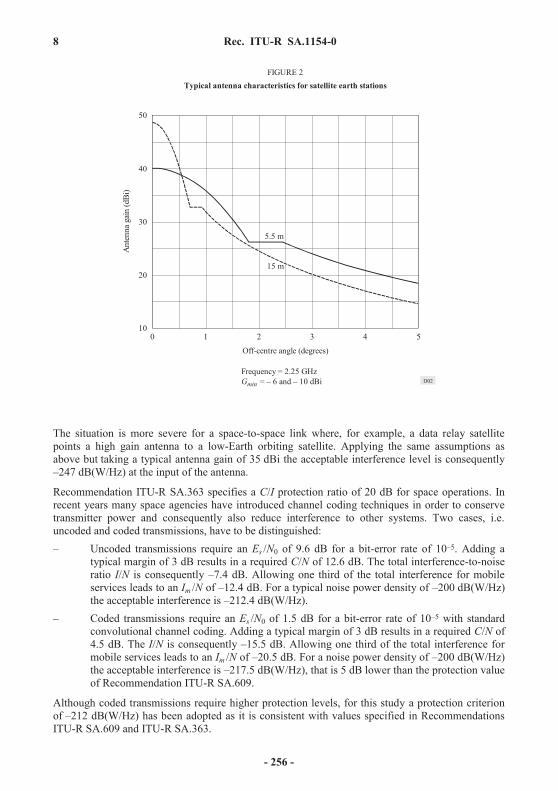
8 Rec. ITU-R SA.1154-0
15 m
10
20
30
40
50
0 1 2 3 4 5
FIGURE 2Typical antenna characteristics for satellite earth stations
5.5 m
Off-centre angle (degrees)
Ante
nna g
ain
(dBi
)
Frequency = 2.25 GHzG = – 6 and – 10 dBimin D02
The situation is more severe for a space-to-space link where, for example, a data relay satellite points a high gain antenna to a low-Earth orbiting satellite. Applying the same assumptions as above but taking a typical antenna gain of 35 dBi the acceptable interference level is consequently _247 dB(W/Hz) at the input of the antenna.
Recommendation ITU-R SA.363 specifies a C/I protection ratio of 20 dB for space operations. In recent years many space agencies have introduced channel coding techniques in order to conserve transmitter power and consequently also reduce interference to other systems. Two cases, i.e. uncoded and coded transmissions, have to be distinguished: – Uncoded transmissions require an Es /N0 of 9.6 dB for a bit-error rate of 10–5. Adding a
typical margin of 3 dB results in a required C/N of 12.6 dB. The total interference-to-noise ratio I/N is consequently –7.4 dB. Allowing one third of the total interference for mobile services leads to an Im /N of –12.4 dB. For a typical noise power density of –200 dB(W/Hz) the acceptable interference is –212.4 dB(W/Hz).
– Coded transmissions require an Es /N0 of 1.5 dB for a bit-error rate of 10–5 with standard convolutional channel coding. Adding a typical margin of 3 dB results in a required C/N of 4.5 dB. The I/N is consequently –15.5 dB. Allowing one third of the total interference for mobile services leads to an Im /N of –20.5 dB. For a noise power density of –200 dB(W/Hz) the acceptable interference is –217.5 dB(W/Hz), that is 5 dB lower than the protection value of Recommendation ITU-R SA.609.
Although coded transmissions require higher protection levels, for this study a protection criterion of –212 dB(W/Hz) has been adopted as it is consistent with values specified in Recommendations ITU-R SA.609 and ITU-R SA.363.
- 256 -

Rec. ITU-R SA.1154-0 9
5 Interference analysis
5.1 Earth-to-space link (2 025-2 110 MHz)
5.1.1 Interference caused to the spacecraft
Earth-to-space links considered in this analysis are based on orbit heights between 250 and 36 000 km as more than 90% of all spacecraft are operated at or below the geostationary orbit.
Figure 3 shows the area from which a geostationary spacecraft will receive signals via a quasi omnidirectional antenna. The arbitrarily selected position of the spacecraft is 10° W. It is estimated that in the worst case the spacecraft can see an area where more than 70% of all mobile terminals on the Earth are located.
10° W
FIGURE 3Interference reception area for geostationary satellites
D03
Figure 4 shows the area from which a low-Earth orbiting satellite at orbit heights between 250 and 750 km will receive signals. The position of the spacecraft has in this case been assumed to be above the middle of Europe. The resulting “window” will move along the ground track given in dotted lines. It is apparent that a very large area with potentially millions of transmitting mobiles can be seen by the spacecraft.
Figure 5 shows the total area from which space shuttle type spacecraft with a typical inclination of 29° will receive interference.
- 257 -

10 Rec. ITU-R SA.1154-0
750 km 250 km
FIGURE 4Interference reception area for low-Earth orbiters (i = 98°)
D04
The area of interference Ai is determined by:
Ai2 R2 hR h
where:
R : Earth radius (6 378 km)
h : orbit height (250 to 36 000 km).
At an altitude of 250 km the spacecraft will receive interference from an area of 9.6 million km2.This number increases to 27 million km2 for an orbit height of 750 km. The maximum area seen by a geostationary satellite is 217 million km2.
The interference spectral density level Pi received by a spacecraft antenna from one single mobile transmitter can be calculated as follows:
PiEi c2
Bi (4 x f )2
- 258 -

Rec. ITU-R SA.1154-0 11
750 km
250 km
FIGURE 5Interference reception area for low-Earth orbiters (i = 29°)
D05
The cumulative interference P i from all mobiles in the interference area is given by:
P ix h
dmna Pi Bi h2 dA(x)
Bm Ai x2 dxna Ei c2
(4 f )2 Bm Aix h
dmdA(x)
x2 dx
A(x)R (x2 – h2)
R h
dA(x)dx
2 RR h x
dm (R h)2 – R2
P ina Ei c2
(4 f )2 Bm R h [ln(dm) – ln(h)]
where: Pi : power density of interferer Ei : e.i.r.p. of interferer x : distance to interferer
- 259 -

12 Rec. ITU-R SA.1154-0
f : transmission frequency
na : number of active mobiles
c : speed of light
Bi : bandwidth of one mobile
Bm : bandwidth of mobile service
dm : maximum distance to interferer.
For the sake of simplicity an equal distribution of active terminals over the available bandwidth and over the interference area has been assumed. Table 2 lists the detailed assumptions made and the resulting interference levels. It must be concluded that sharing for these links is impossible as the interference levels are several orders of magnitude above acceptable levels.
5.1.2 Interference caused to mobile units
Mobile units will receive harmful interference from a transmitting earth station if operated within a certain distance of that station. Maximum e.i.r.p. levels for the support of near-Earth satellites range typically from 66 to 78 dBW.
Taking into account the antenna gains in the horizontal direction as shown in Fig. 2 and the fact that an antenna radiates in principle into all directions with a lowest gain specification of –10 dBi for the back of the antenna (–6 dBi for a 5.5 m antenna) the following e.i.r.p. levels around the antenna must be expected in the horizontal direction. E.i.r.p. density levels depend very much on the transmitted data rate. For the SO service the maximum data rate is typically a few kbit/s whereas for the SR service a range from at least 1 kbit/s to 100 kbit/s must be taken into account.
Protection levels of the FPLMTS units are not known, but the system will be self-interference limited and not noise limited. Assuming that interference levels of around –150 dB(W/4 kHz) are acceptable, and assuming some further loss due to signal diffraction, a protection zone of up to 100 km may be required to allow satisfactory operation of the mobile units.
5.2 Space-to-Earth link (2 200-2 290 MHz)
For these links a distinction between the various space services must be made. The most critical one is space research but results for space operation and Earth exploration are in fact very similar.
Assumptions on the distribution of mobile transmitters around a satellite earth station are difficult to make as they depend to a large extent on the location of the station. An average distribution based on the number of inhabitants in the European common market countries has been assumed. The average population density is 140 people per km2 resulting from 323 million people living in 2.3 million km2. The resulting average traffic density is 2.8 E/km2 for personal stations and 0.56 E/km2 for mobile stations.
Antenna diameter(m)
e.i.r.p. range(dBW)
e.i.r.p. density range(dB(W/4 kHz))
5.5 (3°) 20-50 14-47
15 (3°) 19-50 13-47
- 260 -

Rec. ITU-R SA.1154-0 13
TAB
LE 2
Ear
th-t
o-sp
ace
links
(202
5-2
110
MH
z)
Indo
or p
erso
nal
stat
ion
Out
door
per
sona
l st
atio
nM
obile
stat
ion
Spac
ecra
ft or
bit h
eigh
t (km
)e.
i.r.p
. of s
ingl
e FP
LMTS
uni
t (W
)C
hann
el b
andw
idth
for v
oice
com
mun
icat
ions
(kH
z)e.
i.r.p
. den
sity
of s
ingl
e FP
LMTS
uni
t (dB
(W/H
z))
Spac
e (s
prea
ding
) los
s (dB
)In
terfe
renc
e of
a si
ngle
uni
t (dB
(W/H
z))
Acc
epta
ble
inte
rfere
nce
dens
ity (d
B(W
/Hz)
)In
terfe
renc
e ex
cess
of o
ne u
nit (
dB)
0025
000
000.
003
000
50.0
00–7
2.2
0014
6.7
0–2
18.9
0–2
12.0
000–
6.9
036
000
0000
00.
003
0000
50.0
000
–72.
200
018
9.8
00–2
62.1
00–2
12.0
000
–50.
1
0025
000
000.
020
000
50.0
00–
64.0
0014
6.7
0–2
10.7
0–2
12.0
0000
1.3
036
000
0000
00.
020
0000
50.0
000–
64.0
000
189.
800
–253
.800
–212
.000
0–41
.8
0025
000
001.
0000
025
.000
–44
.000
146.
70
–190
.70
–212
.000
021
.3
036
000
0000
01.
0000
0025
.000
0–44
.000
018
9.8
00–2
33.8
00–2
12.0
000
–21.
8
Are
a of
inte
rfere
nce
seen
by
spac
ecra
ft (m
illio
ns/k
m2 )
Tota
l num
ber o
f pop
ulat
ion
in a
rea
(mill
ions
)Pe
rcen
tage
of s
ubsc
riber
s to
serv
ice
(%)
Ave
rage
uni
ts in
tota
l per
km
2
Perc
enta
ge o
f act
ive
units
in a
rea
(%)
Sim
ulta
neou
sly
activ
e un
its in
are
a (m
illio
ns)
Ave
rage
act
ive
units
per
km
2(E
/km
2 )En
visa
ged
serv
ice
band
wid
th (v
oice
cha
nnel
s) (M
Hz)
Num
ber o
f act
ive
units
per
cha
nnel
Envi
ronm
enta
l atte
nuat
ion
(bui
ldin
gs, t
rees
) (dB
)C
umul
ativ
e in
terfe
renc
e fro
m a
ll ac
tive
units
(dB
(W/H
z))
Av e
rage
exc
ess o
f acc
epta
ble
inte
rfere
nce
(dB
)
0000
9.64
0060
000
020
.000
012
.400
010
.000
012
.000
001.
2400
024
2500
000
010
.00
–196
000
16.0
000
217.
1300
400
000
0020
.000
000
3.7
0000
10.0
0000
80.0
0000
00.
3700
0024
166
667
0000
10.0
00–2
2100
00–8
.5
0000
9.64
0060
000
020
.000
012
.400
010
.000
012
.000
001.
2400
027
2222
200
003.
00
–181
000
30.7
000
217.
1300
400
000
0020
.000
000
3.7
0000
10.0
0000
80.0
0000
00.
3700
0027
148
148
0000
03.
000
–206
0000
06.
2
0000
9.64
0060
000
010
.000
006.
200
004.
000
002.
400
000.
2500
111
0054
100
003.
00
–177
000
34.6
000
217.
1300
400
000
0010
.000
000
1.8
0000
04.
000
0016
.000
000
0.07
000
111
003
604
0000
03.
000
–202
0000
10.1
Incr
ease
d in
terfe
renc
e du
ring
peak
act
iviti
es (d
B)
Incr
ease
d in
terfe
renc
e w
ith h
ighe
r pow
er le
vels
(dB
)In
crea
sed
inte
rfere
nce
over
hig
h de
nsity
are
as (d
B)
Wor
st c
ase
exce
ss o
f acc
epta
ble
inte
rfere
nce
(dB
)
0000
5.0
0000
5.2
0000
5.3
000
31.5
0000
05.
000
000
5.2
0000
00.
000
000
1.7
0000
5.0
0000
4.0
0000
5.3
000
45.0
0000
05.
000
000
4.0
0000
00.
000
0015
.2
0000
5.0
0000
7.0
0000
5.3
000
51.8
0000
05.
000
000
7.0
0000
00.
000
0022
.1
- 261 -

14 Rec. ITU-R SA.1154-0
The interference is integrated over a distance ranging from 1-10 km around the station for which a line-of-sight connection can be assumed. For most station locations it cannot be excluded that mobiles come even closer than 1 km. Additional interference is of course received from further distant mobile terminals but for the sake of simplicity this is not taken into account here. The antenna gain varies with the azimuth angle and has been integrated over 360° in order to come to an average antenna gain value.
The cumulative interference is determined by:
P ix d1
d2mda Pi Bi dA(x)
Bmdx
mda Ei c2
(4 f )2 Bmx d1
d2dA(x)
x2 dx
A(x) x2
dA(x)dx 2 x
P imda Ei c2
8 f 2 Bm[ln(d2) – ln(d1)]
where: mda : average mobile density
d1 : minimum radius around station d2 : maximum radius around station.
Tables 3a and 3b list the detailed results for the space services considered. The worst-case results from a mobile unit transmitting into the direction of the main beam. A single station transmitting at a distance of 10 km was assumed representative although a much shorter distance is possible. The main conclusion to be drawn is that, even when an average gain specification of a few dBi around the antenna is assumed and a simplified interference calculation unfavourable to the space services is performed, interference levels are produced which are several orders of magnitude above the acceptable levels; hence sharing is impossible.
5.3 Space-to-space link (2 025-2 110 MHz)
The most critical case in this category is the link between a geostationary satellite, for example a data relay satellite, and a low-Earth orbiting satellite. The orbit height of the latter one ranges typically between 250 and 1 000 km.
Such a link is for example representative for a manned space shuttle which will orbit around 400 km. It is imperative that this spacecraft has an omnidirectional antenna in order to enable safe commanding and communications during every flight phase and in particular in emergency situations.
Due to power flux-density limitations on the Earth, a limit is also set on the e.i.r.p. which the data relay satellite may radiate towards the Earth, i.e. towards the low orbiting satellite. This results in very tight link margins. Interference, even at low levels, is extremely critical.
The calculated interference levels are so high that any data or communication links to low orbiting spacecraft are totally blanked out. An e.i.r.p. increase on the transmitting geostationary satellite is not feasible due to power flux-density restrictions. Consequently, sharing with land mobiles is impossible.
Table 4 lists the detailed results.
- 262 -

Rec. ITU-R SA.1154-0 15
TAB
LE 3
Spac
e-to
-Ear
th li
nks (
220
0-2
290
MH
z)
Tabl
e 3a
: Spa
ce o
pera
tion
serv
ice
Indo
orpe
rson
al st
atio
nO
utdo
orpe
rson
al st
atio
nM
obile
stat
ion
Ave
rage
hor
izon
tal g
ain
of e
arth
stat
ion
(5.5
m) (
dBi)
Max
imum
hor
izon
tal g
ain
of e
arth
stat
ion
(3°)
(dB
i)A
ctiv
e un
its p
er k
m2
(E/k
m2 )
Act
ive
unit
dens
ity p
er c
hann
el p
er k
m2
e.i.r
.p. o
f sin
gle
FPLM
TS u
nit (
W)
e.i.r
.p. d
ensi
ty o
f sin
gle
FPLM
TS u
nit (
dB(W
/Hz)
)A
ccep
tabl
e in
terfe
renc
e de
nsity
at r
ecei
ver i
nput
(dB
(W/k
Hz)
)A
ccep
tabl
e in
terfe
renc
e de
nsity
at a
nten
na in
put (
dB(W
/kH
z))
Inte
rfere
nce
of u
nits
bet
wee
n 1
and
10 k
m (d
B(W
/kH
z))
Inte
rfere
nce
of 1
uni
t at 1
0 km
dis
tanc
e (L
OS)
(dB
(W/k
Hz)
)Ex
cess
of a
ccep
tabl
e in
terfe
renc
e (d
B)
000
24.0
0000
0.00
300
–72.
20
–184
.00
–208
.0
0–1
61.5
000
46.5
0000
7.5
0000
2.80
000
000.
0058
0000
0.00
300
–72.
20
–184
.00
–191
.50
–152
.4
000
39.1
000
24.0
0000
0.02
000
–64
.00
–184
.00
–208
.0
0–1
53.3
000
54.7
0000
7.5
0000
2.80
000
000.
0052
0000
0.02
000
–64
.00
–184
.00
–191
.50
–144
.7
000
46.8
000
24.0
0000
1.00
000
–44
.00
–184
.00
–208
.0
0–1
33.3
000
74.7
0000
7.5
0000
0.56
000
000.
0001
0000
1.00
000
–44
.00
–184
.00
–191
.50
–140
.9
000
50.6
Tabl
e 3b
: Spa
ce re
sear
chIn
door
pers
onal
stat
ion
Out
door
pers
onal
stat
ion
Mob
ile st
atio
n
Ave
rage
hor
izon
tal g
ain
of e
arth
stat
ion
(15
m) (
dBi)
Max
imum
hor
izon
tal g
ain
of e
arth
stat
ion
(5°)
(dB
i)A
ctiv
e un
its p
er k
m2
( E/k
m2 )
Act
ive
unit
dens
ity p
er c
hann
el p
er k
m2
e.i.r
.p.o
f sin
gle
FPLM
TS u
nit (
W)
e.i.r
.p. d
ensi
ty o
f sin
gle
FPLM
TS u
nit (
dB(W
/Hz)
)A
ccep
tabl
e in
terfe
renc
e de
nsity
at r
ecei
ver i
nput
(dB
(W/H
z))
Acc
epta
ble
inte
rfere
nce
dens
ity a
t ant
enna
inpu
t (dB
(W/H
z))
Inte
rfere
nce
of u
nits
bet
wee
n 1
and
10 k
m (d
B(W
/Hz)
)M
axim
um in
terfe
renc
e of
1 u
nit a
t 10
km d
ista
nce
(dB
(W/H
z))
Exce
ss o
f acc
epta
ble
inte
rfere
nce
(dB
)
000
14.5
0000
0.00
300
–72.
20
–220
.00
–234
.5
0–1
91.5
000
43.0
0000
2.4
0000
2.80
000
000.
0058
0000
0.00
300
–72.
20
–220
.00
–222
.40
–182
.4
000
40.0
000
14.5
0000
0.02
000
–64
.00
–220
.00
–234
.5
0–1
83.3
000
51.2
0000
2.4
0000
2.80
000
000.
0052
0000
0.02
000
–64
.00
–220
.00
–222
.40
–174
.7
000
47.7
000
14.5
0000
1.00
000
–44
.00
–220
.00
–234
.5
0–1
63.3
000
71.2
0000
2.4
0000
0.56
000
000.
0001
0000
1.00
000
–44
.00
–220
.00
–222
.40
–170
.9
000
51.5
- 263 -

16 Rec. ITU-R SA.1154-0
TAB
LE 4
Spac
e-to
-spa
ce li
nks (
202
5-2
110
MH
z)
Indo
or p
erso
nal
stat
ion
Out
door
per
sona
l st
atio
nM
obile
stat
ion
Spac
ecra
ft or
bit h
eigh
t (km
)e.
i.r.p
. of s
ingl
e FP
LMTS
uni
t (W
)C
hann
el b
andw
idth
for v
oice
com
mun
icat
ions
(kH
z)e.
i.r.p
. den
sity
of s
ingl
e FP
LMTS
uni
t (dB
(W/H
z))
Spac
e (s
prea
ding
) los
s (dB
)In
terfe
renc
e of
a si
ngle
uni
t (dB
(W/H
z))
Acc
epta
ble
inte
rfere
nce
dens
ity (d
B(W
/Hz)
)In
terfe
renc
e ex
cess
of o
ne u
nit (
dB)
0025
000
000.
003
000
50.0
00–7
2.2
0014
6.7
0–2
18.9
0–2
12.0
000–
6.9
000
750
0000
00.
003
0000
50.0
000
–72.
200
015
6.2
00–2
28.4
00–2
12.0
000
–16.
4
0025
000
000.
020
000
50.0
00–
64.0
0014
6.7
0–2
10.7
0–2
12.0
0000
1.3
000
750
0000
00.
020
0000
50.0
000–
64.0
000
156.
200
–220
.200
–212
.000
00–8
.2
0025
000
001.
0000
025
.000
–44
.000
146.
70
–190
.70
–212
.000
021
.3
000
750
0000
01.
0000
0025
.000
0–44
.000
015
6.2
00–2
00.2
00–2
12.0
0000
11.8
Are
a of
inte
rfere
nce
seen
by
spac
ecra
ft (m
illio
n/km
2 )To
tal n
umbe
r of p
opul
atio
n in
are
a (m
illio
ns)
Perc
enta
ge o
f sub
scrib
ers t
o se
rvic
e (%
)A
vera
ge u
nits
in to
tal p
er k
m2
Perc
enta
ge o
f act
ive
units
in a
rea
(%)
Sim
ulta
neou
sly
activ
e un
its in
are
a (m
illio
ns)
Ave
rage
act
ive
units
per
km
2(E
/km
2 )En
visa
ged
serv
ice
band
wid
th (v
oice
chan
nels
) (M
Hz)
Num
ber o
f act
ive
units
per
cha
nnel
Envi
ronm
enta
l atte
nuat
ion
(bui
ldin
gs, t
rees
) (dB
)C
umul
ativ
e in
terfe
renc
e fro
m a
ll ac
tive
units
(dB
(W/H
z))
Ave
rage
exc
ess o
f acc
epta
ble
inte
rfere
nce
(dB
)
0000
9.64
0060
000
020
.000
012
.400
010
.000
012
.000
001.
2400
024
2500
000
010
.00
–196
.000
016
.0
0000
26.8
900
080
000
0020
.000
000
5.9
0000
10.0
0000
16.0
0000
00.
5900
0024
033
333
0000
10.0
00–2
00.9
0000
11.1
0000
9.64
0060
000
020
.000
012
.400
010
.000
012
.000
001.
2400
027
2222
200
003.
00
–181
.300
030
.7
0000
26.8
900
080
000
0020
.000
000
5.9
0000
10.0
0000
16.0
0000
00.
5900
0027
029
630
0000
03.
000
–186
.200
0025
.8
0000
9.64
0060
000
010
.000
006.
200
004.
000
002.
400
000.
2500
111
0054
100
003.
00
–177
.400
034
.6
0000
26.8
900
080
000
0010
.000
000
3.0
0000
04.
000
000
3.2
0000
00.
1200
011
100
072
100
000
3.0
00–1
82.3
0000
29.7
Incr
ease
d in
terfe
renc
e du
ring
peak
act
iviti
es (d
B)
Incr
ease
d in
terfe
renc
e w
ith h
ighe
r pow
er le
vels
(dB
)In
crea
sed
inte
rfere
nce
over
hig
h de
nsity
are
as (d
B)
Wor
st c
ase
exce
ss o
f acc
epta
ble
inte
rfere
nce
(dB
)
0000
5.0
0000
5.2
0000
5.3
000
31.5
0000
05.
000
000
5.2
0000
03.
000
0024
.3
0000
5.0
0000
4.0
0000
5.3
000
45.0
0000
05.
000
000
4.0
0000
03.
000
0037
.8
0000
5.0
0000
7.0
0000
5.3
000
51.8
0000
05.
000
000
7.0
0000
03.
000
0044
.6
- 264 -

Rec. ITU-R SA.1154-0 17
5.4 Space-to-space link (2 200-2 290 MHz)
This frequency band is used for data links from low orbiting satellites to geostationary data relay satellites and for short range communications between low orbiting satellites and eventually also between astronauts. Orbit heights between 250 and 36 000 km have consequently to be taken into account.
In principle, the same assumptions as listed above are applicable with the exception that the geostationary satellite uses high gain antennas for the links to the low orbiters. This results in very low acceptable interference levels at the input of the antenna. The beamwidth of the antenna is typically a few degrees so that interference from an area somewhat smaller than for the 250 km orbit can be received. Figure 6 gives a typical example for the area from which interference will be received by a data relay satellite when tracking a low-Earth orbiter.
DRS (59° E)
LEO ( = 0°)
=0°
FIGURE 6Coverage of a data relay satellite antenna and a 250 km LEO
D06
Table 5 lists the detailed results. Also in this case sharing is unfortunately impossible.
5.5 Worst-case scenarios for all links
The assumptions used for the interference studies above are based on an average distribution of mobiles over the interference area, an average activity, minimum power levels for the FPLMTS units and an equal occupation of all available channels. The resulting interference excess values are consequently average numbers on the low end.
- 265 -

18 Rec. ITU-R SA.1154-0
TAB
LE 5
Spac
e-to
-spa
ce li
nks (
220
0-2
290
MH
z)
Indo
or p
erso
nal
stat
ion
Out
door
per
sona
l st
atio
nM
obile
stat
ion
Spac
ecra
ft or
bit h
eigh
t (km
)e.
i.r.p
. of s
ingl
e FP
LMTS
uni
t (W
)C
hann
el b
andw
idth
for v
oice
com
mun
icat
ions
(kH
z)e.
i.r.p
. den
sity
of s
ingl
e FP
LMTS
uni
t (dB
(W/H
z))
Spac
e (s
prea
ding
) los
s (dB
)In
terfe
renc
e of
a si
ngle
uni
t (dB
(W/H
z))
Acc
epta
ble
inte
rfere
nce
dens
ity (d
B(W
/Hz)
)In
terfe
renc
e ex
cess
of o
ne u
nit (
dB)
0025
000
000.
003
000
50.0
00–7
2.2
0014
6.7
0–2
18.9
0–2
12.0
000–
6.9
036
000
0000
00.
003
0000
50.0
000
–72.
200
018
9.8
00–2
62.1
00–2
47.0
000
–15.
1
0025
000
000.
020
000
50.0
00–
64.0
0014
6.7
0–2
10.7
0–2
12.0
0000
1.3
036
000
0000
00.
020
0000
50.0
000–
64.0
000
189.
800
–253
.800
–247
.000
00–
6.8
0025
000
001.
000
000
25.0
00–
44.0
0014
6.7
0–1
90.7
0–2
12.0
000
21.3
036
000
0000
01.
000
0000
25.0
000–
44.0
000
189.
800
–233
.800
–247
.000
0013
.2
Are
a of
inte
rfere
nce
seen
by
spac
ecra
ft (m
illio
ns/k
m2 )
Tota
l num
ber o
f pop
ulat
ion
in a
rea
(mill
ions
)Pe
rcen
tage
of s
ubsc
riber
s to
serv
ice
(%)
Ave
rage
uni
ts in
tota
l per
km
2
Perc
enta
ge o
f act
ive
units
in a
rea
(%)
Sim
ulta
neou
sly
activ
e un
its in
are
a (m
illio
ns)
Ave
rage
act
ive
units
per
km
2(e
rlang
s/km
2 )En
visa
ged
serv
ice
band
wid
th (v
oice
cha
nnel
s) (M
Hz)
Num
ber o
f act
ive
units
per
cha
nnel
Envi
ronm
enta
l atte
nuat
ion
(bui
ldin
gs, t
rees
) (dB
)C
umul
ativ
e in
terfe
renc
e fro
m a
ll ac
tive
units
(dB
(W/H
z))
Ave
rage
exc
ess o
f acc
epta
ble
int e
rfere
nce
(dB
)
0000
9.64
0060
000
020
.000
062
.200
010
.000
012
.000
001.
2400
024
2500
000
010
.00
–196
.000
016
.0
0000
08.
0000
050
000
0020
.000
0062
.500
0010
.000
0010
.000
000
1.25
0000
2402
083
300
0010
.000
–218
.900
0027
.2
0000
9.64
0060
000
020
.000
062
.200
010
.000
012
.000
001.
2400
027
2222
200
003.
00
–181
.300
030
.7
0000
08.
0000
050
000
0020
.000
0062
.500
0010
.000
0010
.000
000
1.25
0000
2701
851
900
000
3.0
00–2
11.1
0000
34.9
0000
9.64
0060
000
010
.000
062
.200
004.
000
002.
400
000.
2500
111
0054
100
003.
00
–177
.400
034
.6
0000
08.
0000
050
000
0010
.000
0062
.500
000
4.0
0000
02.
000
000
0.25
000
111
000
450
0000
03.
000
–207
.300
0038
.8
Incr
ease
d in
terfe
renc
e du
ring
peak
act
iviti
es (d
B)
Incr
ease
d in
terfe
renc
e w
ith h
ighe
r pow
er le
vels
(dB
)In
crea
sed
inte
rfere
nce
over
hig
h de
nsity
are
as (d
B)
Wor
st c
ase
exce
ss o
f acc
epta
ble
inte
rfere
nce
(dB
)
0000
5.0
0000
5.2
0000
5.3
000
31.5
0000
05.
000
000
5.2
0000
00.
000
0037
.4
0000
5.0
0000
4.0
0000
5.3
000
45.0
0000
05.
000
000
4.0
0000
00.
000
0043
.9
0000
5.0
0000
7.0
0000
5.3
000
51.8
0000
05.
000
000
7.0
0000
00.
000
0050
.8
- 266 -

Rec. ITU-R SA.1154-0 19
If the spacecraft flies over large cities or highly populated areas in Europe the cumulative interference will increase significantly due to the shorter distance from a high number of mobiles to the spacecraft. To take into account large urban and suburban areas it was assumed that 20% of all mobile units seen by the spacecraft are close to the subsatellite point. This is easily possible over large cities like Paris and London with traffic densities up to 20 000 E/km2 per building floor. This results in increased interference between 3 dB for a 750 km orbit and 5 dB for a 250 dB orbit. For the geostationary orbits no increase was assumed as it is unlikely that a very high mobile concentration can be found near the equator.
An interference increase will also occur at times with peak activities. A traffic density increase up to a factor of 3 can be assumed. This leads to a potential increase of interference between 4 and 7 dB. Another reason for higher interference can be unequal occupation of channels but as this is difficult to estimate it has not been taken into account in this study.
For the Earth-to-space and the two space-to-space links it can be concluded that the worst-case interference can be between 9 and 16 dB higher than the average value.
The situation for the space-to-Earth link is slightly different. The worst case would be a mobile transmitting in the vicinity of the station near the direction of the main beam. Assuming a distance of 10 km between the mobile and the earth station the corresponding interference level would be 43-75 dB above specified protection levels.
6 Conclusions
A short summary of interference excess is listed in Table 6 for all links analysed. The lower value is based on average interference excess. The higher value takes into account worst cases with respect to increased mobile densities in highly populated areas, upper limits of specified operating power, and times with high communication activity. Unequal channel occupation, yet another source of increased interference, has not been considered.
TABLE 6
Interference summary for all links and all mobile units considered
Interference excess(dB)
Indoorpersonal station
Outdoorpersonal station Mobile station
Earth-to-space (2 025-2 110 MHz) 16-32 31-45 35-52
Space-to-Earth (2 200-2 290 MHz) 39-47 47-55 51-75
Space-to-space (2 025-2 110 MHz) 16-32 31-45 35-52
Space-to-space (2 200-2 290 MHz) 27-37 35-45 39-52
- 267 -

20 Rec. ITU-R SA.1154-0
An interference analysis between FPLMTS type land mobile systems and the space operations, space research and Earth-exploration service has been presented. On all types of links considered in this Recommendation sharing with this and similar high density mobile systems is not feasible. The resulting interference levels are orders of magnitude higher than acceptable levels specified in the RR and in ITU-R Recommendations.
Annex 2
Summary of studies of the characteristics of mobile systems that facilitate radio-frequency compatibility with the space science services
1 Introduction
This Annex summarizes the results of studies concerning the technical and operational characteristics of mobile systems that might be compatible with the SR, SO and EES systems operating in the 2 025-2 110 MHz and 2 200-2 290 MHz bands.
The characteristics of mobile systems that facilitate sharing are:
– emissions of low power spectral density,
– transmissions of an intermittent nature,
– use of directional transmitting antennas,
– number of mobile stations is self-limiting as a result of the nature of the application.
Studies concerning different sets of assumptions and ranges of values for these general characteristics are presented in the following sections. Further studies regarding the compatibility between mobile systems and space science systems in the 2 025-2 110 MHz and 2 200-2290 MHz bands would be required to better define the interference environment.
2 Summary of studies of e.i.r.p. and antenna gain
The introduction of technical requirements for the mobile service in the bands 2 025-2 110 MHz and 2 200-2 290 MHz led to the proposal of an e.i.r.p. limit of 28 dBW together with a minimum antenna gain of 24 dBi in order to facilitate sharing with the space science services. Studies were conducted as to the interference effect of such systems on the space research service.
The model used in the study assumed a global and uniform distribution of directional mobile terminals with antenna gains ranging between 22 and 26.5 dBi and e.i.r.p. ranging between 28 and 37 dBW. Orbital heights for spacecraft between 250 km and 36 000 m were taken into account.
The study results show that space science operations in the 2 200-2 290 MHz band are significantly more susceptible to interference than in the 2 025-2 110 MHz band. An antenna gain sensitivity analysis was performed. For the case of constant e.i.r.p. levels, the probability of interference decreases with increasing antenna gain as shown in Fig. 7. The Figure also shows a non-linear increase in interference probability with linearly increasing e.i.r.p.
- 268 -

Rec. ITU-R SA.1154-0 21
The study finally concluded that the proposed e.i.r.p. limit of 28 dBW, together with an antenna gain in excess of 24 dBi, are adequate provisions to enable sharing with around 1 000 mobile systems of such kind worldwide.
3 A summary of a study of interference from certain mobile systems
A study was conducted that considered four possible scenarios concerning interference to space science services systems as shown in Table 7.
The characteristics of the systems used in the study are discussed in the following.
3.1 System characteristics
3.1.1 Receive characteristics
3.1.1.1 Data relay satellite
Receive antenna (assumed to track the LEO spacecraft when visible):
– boresight gain 34 dBi;
– off-beam characteristics in accordance with the reference radiation pattern for single feed circular beams (near in side-lobe level of –20 dB) as defined in Recommendation ITU-R S.672.
200 300 400 500 600 700 800 900 1 000
4
3
2
1
0
33 dBW / 24 dBi
28 dBW / 22 dBi28 dBW / 24 dBi
FIGURE 7Interference probability for various ENG system characteristics
1 000 ENG systems10 % activity
Inte
rfere
nce
prob
abili
ty (%
)
Spacecraft orbit height (km)
37.3 dBW / 26.5 dBi
28 dBW / 25.6 dBi
D07
- 269 -

22 Rec. ITU-R SA.1154-0
TABLE 7
3.1.1.2 LEO spacecraft (DRS pointing)
Receive antenna (assumed to track the geostationary relay satellite when visible):
– boresight gain 25 dBi;
– off-beam characteristics in accordance with the reference radiation pattern for single feed circular beams (near in side-lobe level of –20 dB) as defined in Recommendation ITU-R S.672;
– orbit altitude 300 km;
– inclination 29°.
3.1.1.3 LEO spacecraft (Earth pointing)
Receive antenna omnidirectional (gain 0 dBi):
– orbit altitude 300 km;
– inclination 29°.
3.1.1.4 Earth station
Receive antenna (assumed to track the LEO spacecraft when visible):
– boresight gain 45 dBi;
– off-beam characteristics in accordance with those defined in RR Appendices 28 and 29.
3.1.2 Transmit characteristics
3.1.2.1 Mobile terminal (directional) – ENG
– antenna boresight gain 25 dBi;
– power spectral density into the antenna –38 dB(W/kHz);
– off-beam characteristics in accordance with those defined in RR Appendices 28 and 29.
2 025-2 110 MHz 2 200-2 290 MHz
Space services Data relay
Space-to-space (Forward)
(1)
Space-to-space(Return)
(3)
Space services Direct-to-ground
Earth-to-space
(2)
Space-to-Earth
(4)
Mobile Directional (ENG) Omnidirectional
- 270 -

Rec. ITU-R SA.1154-0 23
3.1.2.2 Mobile terminal (omnidirectional) – antenna gain 0 dBi;
– power spectral density into the antenna –42 dB(W/kHz).
3.2 Summary and conclusions
Four geometric configurations (A-D) were evaluated for the scenarios shown in Table 7 using the technical characteristics shown above. The results of a probabilistic analysis are summarized in Table 8.
TABLE 8
3.2.1 Interference from directional mobiles to a LEO spacecraft (DRS pointing) in the band 2 025-2 110 MHz
The values in Table 8 suggest that a single ENG terminal in various geometric configurations can exceed the applicable protection criteria. However, considering the majority of configurations, if the ENG transmit power were decreased by 1 dB then the probability that the protection criterion would be exceeded would be decreased to 0.1%. This would not, of course, be true for the more critical geometric configurations and, therefore, some constraints may need to be placed on the siting of terrestrial ENG terminals.
3.2.2 Interference from directional mobiles to a LEO spacecraft (Earth pointing) in the band 2025-2 110 MHz
The results suggest that two or three spatially separated co-channel terminals would be acceptable. This translates into an acceptable community of between 100 and 150 ENG terminals not considering the worst case geometry.
3.2.3 Interference from omnidirectional mobiles to a geostationary data relay satellite (tracking a LEO spacecraft) in the band 2 200-2 290 MHz
The values presented in Table 8 show that the interfering power levels from a single omnidirectional terminal are well within the permissible criteria. However, the probabilities of these
Reference EntryMaximum level of interference
relative to criterion(dB)
Probability criterion exceeded
(%)
1 A1 B1 C1 D
ENG into LEO (DRS pointing)31.007.506.506.5
0.650.200.150.15
2 A2 B2 C2 D
ENG into LEO (Earth pointing)02.502.502.502.5
0.200.040.0450.035
3 A3 B3 C3 D
Omni into DRS– 16.5– 16.5– 15.0– 15.0
2.50(1)
1.50(1)
0.15(1)
0.50(1)
4 A4 B
Omni into ES 48.548.0
1.000.55
(1) Probability of maximum level of interference.
- 271 -

24 Rec. ITU-R SA.1154-0
levels occurring are high and hence multiple terminals could give rise to aggregate levels of interference which whilst just exceeding the permissible power levels would exceed the permissible levels many times in terms of probability of occupance.
3.2.4 Interference from omnidirectional mobiles to an earth station (tracking a LEO spacecraft) in the band 2 200-2 290 MHz
Assuming no line-of-sight paths such that the basic transmission loss follows an inverse third power law, a single omnidirectional terminal may operate within 0.5 km of an earth station (with an elevation greater than 5°).
Annex 3
Description of certain electronic news gathering (ENG) systems operating in the 2025-2110 MHz band
1 Introduction
This Annex presents information about the unique technical and operational characteristics used by specific ENG systems operated by one administration that may facilitate sharing with the SR, SO, and EES services.
2 Characteristics/description of ENG systems
ENG systems include both mobile point-of-view and transportable ENG systems that provide video from a variety of locations and activities. ENG systems are used for on-location coverage of news events or interviews and live-action video during sports or entertainment events. Because of the value of on-location video, most local television stations in urban areas of the United States of America operate ENG systems. The transportable ENG systems, used for on-location coverage, are generally mounted in vans and operate in a stationary mode transmitting video to a fixed receive site. These systems provide mobility for news coverage throughout a geographic region.
3 ENG systems and environments
This section describes two common operational modes.
3.1 Transportable
The transportable ENG systems described in the previous section are used for live or taped on-location video for news, sports, and entertainment broadcasts. The transportable ENG systems are generally mounted in vans and use transmitters operating around 10.8 dBW of power. These systems utilize directional antennas with gains between 20-22 dBi mounted on top of a pneumatic
- 272 -

Rec. ITU-R SA.1154-0 25
mast of up to 15 m in height. ENG systems may employ linear or circular polarization to provide additional interference protection from each other. Many ENG systems (probably 30-50%) transmit with up to 5 dB of transmission line loss.
3.2 Point-of-view
Small light-weight microwave transmitters are used for mobile and close-up video situations since live pictures are desired and because video recorders are impractical due to size and ruggedness requirements. These transmitters usually operate with up to 5 dBW of power. These systems utilize essentially omnidirectional antennas with 0-3 dBi of gain and may also use linear or circular polarization.
A small point-of-view system usually operates instead of, rather than in addition to, a transportable ENG operation on the same channel. Point-of-view systems cannot usually operate simultaneously with transportable systems because the transportable systems cause excessive interference to the point-of-view receiver.
Table 9 presents characteristics of typical ENG systems that operate in the 2 025-2 110 MHz band.
TABLE 9
Typical 2 GHz ENG systems in use in the United States of America
Type of use Transmitterlocation
Transmitpower
Antennagain(dBi)
Receiverlocation
ENG transportable(van)
Van mast 12 W 22 Tower
Temporary fixed link Roof 12 W 25 Roof
Convention Floor of convention hall 100 mW 0-5 Hall rafters
Point-of-view(e.g., skier)
On body/helmet 100 mW 0 Hillside or helicopter
Sports venues
Playing field Field 1 W 12 Pressbox
Golf course (system 1) On golf course 3 W 16 Tethered blimp
Golf course (system 2) On golf course 12 W 12 Crane
Racecam In car 3 W 7 Helicopter
Helicopter Relay helicopter 12 W 7 Ground receive
Marathon
Motorcycle Motorcycle 3 W 7 Helicopter
Relay vehicle Pick-up truck 12 W 12 Helicopter
Helicopter Relay helicopter 12 W 7 Roof
- 273 -

26 Rec. ITU-R SA.1154-0
4 Operational characteristics
All ENG systems, cannot operate simultaneously. Since ENG systems are sensitive to interference, only one transmission per channel per receive site at a time is usually possible. Most television markets in the United States of America contain multiple receive sites that allow for simultaneous transmissions on a channel. In most large markets, however, only six simultaneous transmissions are possible on the busiest channel, and in most markets the number does not exceed two. More than two simultaneous transmissions on a single channel rarely occur. In fact, multiple ENG receive sites and systems exist only in the largest television markets, so most regions have little or no simultaneous ENG activity per channel.
Although used throughout the day, transportable ENG systems operate primarily during weekday local news broadcasts, which usually occur around 1200-1230, 1700-1900, and 2300-2330 local time. In most markets before the afternoon news hours around 1500-1700, ENG use is also significant. The popularity of local morning shows from 0600-0900 is increasing in various markets, and these shows also use ENG systems. Transportable ENG transmitters are operated approximately twice per day. Broadcast engineers estimate that each ENG operation transmits an average of 15 min per operation but can vary from about 5 min to perhaps as long as 5 h.
5 Spectrum use and characteristics
The 1 990-2 110 MHz band is used as the primary ENG band because of favourable propagation characteristics. These include the lower levels of foliage attenuation that apply at higher frequencies and the ability to “building bounce” a signal to achieve a temporary link to a fixed receive site despite unavoidable path blockage.
In the United States of America, the ENG frequency band is divided into 7 channels each with 17 MHz except the first channel which is 18 MHz as shown in Fig. 8. ENG systems are usually operated at the centre of each channel, but the lower offset and upper offset channels are also used. Consequently, 21 carrier frequencies are possible, but all carrier frequencies cannot be used simultaneously. ENG systems may operate at the centre channel, the lower offset channel, the higher offset channel, or the lower and higher offset channels simultaneously, depending on the need and adjacent channel use at any time. Since ENG systems are sensitive to interference, only one transmission per channel per receive site at a time is usually possible.
ENG systems use frequency modulation (FM) for transmitting video. The carrier is virtually never transmitted unmodulated by video raster.
- 274 -

Rec. ITU-R SA.1154-0 27
1 990 2 008 2 025 2 042 2 059 2 076 2 093 2 110
FIGURE 8ENG channel plan in use in the United States of America
Centre carrier frequencies (MHz)
Offset low carrier frequency (MHz)
Offset high carrier frequency (MHz)
Frequency (MHz)
1 994.75Channel 1 –
2 012.25Channel 2 –
2 029.25Channel 3 –
2 046.25Channel 4 –
2 063.25Channel 5 –
2 080.25Channel 6 –
2 097.25Channel 7 –
1 999.00 2 016.50 2 033.50 2 050.50 2 067.50 2 084.50 2 101.50Channel 1 Channel 2 Channel 3 Channel 4 Channel 5 Channel 6 Channel 7
2 003.25Channel 1 +
2 020.75Channel 2 +
2 037.75Channel 3 +
2 054.75Channel 4 +
2 071.75Channel 5 +
2 088.75Channel 6 +
2 105.75Channel 7 +
Channel 1 Channel 2 Channel 3 Channel 4 Channel 5 Channel 6 Channel 7
D08
Annex 4
Description of certain aeronautical mobile telemetry systems operating in the 2200-2290 MHz band
1 Introduction
The aeronautical mobile telemetry systems operated by one administration consist of a small number of controlled, short duration transmitters operating in a few specific areas.
The number of simultaneously operating transmitting systems within any 1 000 km radius will rarely exceed 15. The maximum e.i.r.p. in the direction of a satellite in any 3 MHz bandwidth within any 1 000 km radius will rarely exceed 10 W.
2 Technical characteristics of aeronautical mobile telemetry systems
Aeronautical telemetry has been using the 2 200-2 290 MHz band for testing of missiles, space launch vehicles, air vehicles, and subsystems thereof since the late 1960s. The duration of the majority of these tests is less than 10 min, however some tests last for several hours. Telemetry operations can occur at any hour of the day with the peak usage during daylight hours. The majority of the flight tests occur at one (or more) of the test ranges operated by the United States of America government.
- 275 -

28 Rec. ITU-R SA.1154-0
The characteristics of the telemetry transmitting systems are optimized for the vehicle being tested. Therefore, these characteristics vary considerably from vehicle to vehicle. There is no “typical” transmitting system. The effective radiated power of the telemetry systems is usually between 1 and 5 W. The required power level is determined by the amount of information to be transmitted, the maximum range between transmitting and receiving systems, the required data quality, and the sensitivity of the receiving system. The telemetry transmitting antennas are usually linearly polarized and are typically designed to have nearly isotropic coverage because the orientation of the vehicle under test with respect to the telemetry receiving antenna can change very rapidly. As the receiving antenna tracks a vehicle in flight, large variations occur in the signal levels at the receiver. These “fades” are caused by nulls in the vehicle antenna pattern and propagation anomalies such as multipath and ducting. The decrease in signal level during fades can exceed 30 dB. Therefore, a received signal considerably above threshold is required during optimum flight conditions to avoid data loss during signal fades.
The telemetry data formats and rates vary considerably from vehicle to vehicle. Most telemetry transmitting systems use frequency or phase modulation. The input to the transmitter may be digital, analogue, or a combination of digital and analogue. The 99% power bandwidths of the telemetry transmitting systems vary from less than 1 MHz to more than 10 MHz.
The required pre-detection signal-to-noise ratio (SNR) for acceptable data quality varies from 9 to 15 dB. The maximum distance between the vehicle under test and the telemetry receiving station is usually between 20 and 400 km (the maximum range for some tests is greater than 3 000 km). Typical receiver bandwidths vary from 0.5 to 10 MHz (these values are increasing). Receiving system noise temperatures vary between 200 K and 500 K. Main lobe gains of the receiving antennas vary from 6 dBi for some short-range mobile systems to greater than 50 dBi for large antennas. The larger antennas automatically track the test vehicle while the smaller antennas (gain less than 20 dBi) typically are pointed in the direction of the transmitter. The receiving antenna side lobes depend on the size and design of the receiving antenna. The majority of telemetry receiving antennas have diameters between 2.44 m (8 feet) and 10 m (32.8 feet).
3 Spectrum considerations
Aeronautical mobile telemetry system providers in the United States of America have divided this band into 90 channels each with a 1 MHz bandwidth. Multiple channels are assigned together when a wider bandwidth is needed.
Aeronautical telemetry operations are currently protected by coordination between the various users. The territory of the United States of America is divided into coordination areas. Area frequency coordinators assign and schedule frequency use within these areas.
The potential exists for significant interference between satellite earth stations co-located with aeronautical telemetry transmitting sites in the 2 200-2 290 MHz band. This problem is mitigated by controlling the time, frequency and location of the transmissions by each service in this band. Frequency interference control centres accommodate real-time changes and locate and identify any unauthorized transmissions.
- 276 -

Rec. ITU-R SA.1154-0 29
A sample radiated power spectral density is shown in Fig. 9. This Figure shows the nominal power spectral density for one telemetry system. The data in this Figure is not typical, best case or worst case but is included only as an example of the spectral characteristics of the most common type of system currently used for aeronautical mobile telemetry systems. Some aeronautical mobile telemetry systems may have discrete spectral components during portions of a test flight, therefore the maximum spectral densities (dB(W/kHz)) may be significantly larger than the values shown in Fig. 9.
– 20
– 30
– 40
– 50
– 60
FIGURE 9Sample spectrum
2 248.5 2 256.52 252.52 250.5 2 254.5
Pow
er (d
B(W
/kH
z))
Frequency (MHz) D09
The maximum aggregate radiated power in any direction from all aeronautical mobile telemetry systems within a radius of 1 000 km will be less than 100 W in the band from 2 200-2 290 MHz. The maximum aggregate radiated power in any 3 MHz bandwidth will rarely exceed 10 W in any direction in any 1 000 km radius.
- 277 -


Rec. ITU-R M.1171-0 1
RECOMMENDATION ITU-R M.1171-0*
RADIOTELEPHONY PROCEDURES IN THE MARITIME MOBILE SERVICE
(1995) Rec. ITU-R M.1171
The ITU Radiocommunication Assembly,
considering
a) that there is a need to describe standard procedures for radiotelephony in the maritime mobile service,
recommends
1 that radiotelephony in the maritime mobile service should be performed in accordance with Annex 1.
ANNEX 1
Section I. Introduction
§ 1. Radiotelephone stations should, as far as possible, be equipped with devices for instantaneous switching from transmission to reception and vice versa. This equipment is necessary for all stations participating in communication between ships and subscribers of the land telephone system.
§ 2. (1) Stations equipped for radiotelephony may transmit and receive radiotelegrams by means of radiotelephony. Coast stations providing such service and open for public correspondence shall be indicated in the List of Coast Stations.
(2) To facilitate radiocommunications the service abbreviations given in Recommendation ITU-R M.1172 may be used.
Section II. Calls by Radiotelephony
§ 3. The provisions of this Section relating to the intervals between calls are not applicable to a station operating under conditions involving distress, urgency or safety.
§ 4. (1) As a general rule, it rests with the ship station to establish communication with the coast station. For this purpose the ship station may call the coast station only when it comes within the service area of the latter, that is to say, that area within which, by using an appropriate frequency, the ship station can be heard by the coast station.
(2) However, a coast station having traffic for a ship station may call this station if it has reason to believe that the ship station is keeping watch and is within the service area of the coast station.
_______________* This Recommendation should be brought to the attention of the International Maritime Organization (IMO), and the
Telecommunication Standardization Sector (ITU-T).
Note by the Secretariat: The references made to the Radio Regulations (RR) in this Recommendation refer to the RR as revised by the World Radiocommunication Conference 1995. These elements of the RR will come into force on 1 June 1998. Where applicable, the equivalent references in the current RR are also provided in square brackets.
- 279 -

2 Rec. ITU-R M.1171-0
§ 5. (1) In addition, each coast station shall, so far as practicable, transmit its calls in the form of “traffic lists” consisting of the call signs or other identification in alphabetical order of all ship stations for which it has traffic on hand. These calls shall be made at specified times fixed by agreement between the administrations concerned and at intervals of not less than two hours and not more than four hours during the working hours of the coast station.
(2) Coast stations shall transmit their traffic lists on their normal working frequencies in the appropriate bands. The transmission shall be preceded by a general call to all stations.
(3) The general call to all stations announcing the traffic lists may be sent on a calling frequency in the following form:
– “Hello all ships” or CQ (spoken as CHARLIE QUEBEC) not more than three times;
– the words THIS IS (or DE spoken as DELTA ECHO in case of language difficulties);
– “ . . . Radio” not more than three times;
– “Listen for my traffic list on . . . kHz”.
In no case may this preamble be repeated.
(4) However, in the bands between 156 MHz and 174 MHz when the conditions for establishing contact are good, the call described in § 5.(3) above may be replaced by:
– “Hello all ships” or CQ (spoken as CHARLIE QUEBEC), once;
– the words THIS IS (or DE spoken as DELTA ECHO in case of language difficulties);
– “ . . . Radio”, twice;
– “Listen for my traffic list on channel . . . ”.
In no case may this preamble be repeated.
(5) The provisions of § 5.(3) are obligatory when 2 182 kHz or 156.8 MHz is used.
(6) The hours at which coast stations transmit their traffic lists and the frequencies and classes of emission which they use for this purpose shall be stated in the List of Coast Stations.
(7) Ship stations should as far as possible listen to the traffic lists transmitted by coast stations. On hearing their call sign or other identification in such a list they must reply as soon as they can do so.
(8) When the traffic cannot be sent immediately, the coast station shall inform each ship station concerned of the probable time at which working can begin, and also, if necessary, the frequency and class of emission which will be used.
§ 6. When a coast station receives calls from several ship stations at practically the same time, it decides the order in which these stations may transmit their traffic. Its decision shall be based on the priority (see RR No. S53.1 [No. 4441]) of the radiotelegrams or radiotelephone calls that the ship stations have on hand and on the need for allowing each calling station to clear the greatest possible number of communications.
§ 7. (1) When a station called does not reply to a call sent three times at intervals of two minutes, the calling shall cease.
(2) However, when a station called does not reply, the call may be repeated at three-minute intervals.
(3) In areas where reliable VHF communication with a called coast station is practicable, the calling ship station may repeat the call as soon as it is ascertained that traffic has been terminated at the coast station.
(4) In the case of a communication between a station of the maritime mobile service and an aircraft station, calling may be renewed after an interval of five minutes.
(5) Before renewing the call, the calling station shall ascertain that the station called is not in communication with another station.
- 280 -

Rec. ITU-R M.1171-0 3
(6) If there is no reason to believe that harmful interference will be caused to other communications in progress, the provisions of § 7.(4) above are not applicable. In such cases the call, sent three times at intervals of two minutes, may be repeated after an interval of not less than three minutes.
(7) However, before renewing the call, the calling station shall ascertain that further calling is unlikely to cause interference to other communications in progress and that the station called is not in communication with another station.
(8) Ship stations shall not radiate a carrier wave between calls.
§ 8. When the name and address of the administration or private operating agency controlling a ship station are not given in the appropriate list of stations or are no longer in agreement with the particulars given therein, it is the duty of the ship station to furnish as a matter of regular procedure, to the coast station to which it transmits traffic, all the necessary information in this respect.
§ 9. (1) The coast station may, by means of the abbreviation TR (spoken as TANGO ROMEO), ask the ship station to furnish it with the following information:
a) position and, whenever possible, course and speed;
b) next port of call.
(2) The information referred to in § 9.(1) above, preceded by the abbreviation TR, should be furnished by ship stations, whenever this seems appropriate, without prior request from the coast station. The provision of this information is authorized only by the master or the person responsible for the ship.
Section III. Method of Calling, Reply to Calls and Signals Preparatory to Traffic when Using Calling
Methods Other than Digital Selective Calling
A. Method of Calling
§ 10. (1) The call consists of:
– the call sign or other identification of the station called, not more than three times;
– the words THIS IS (or DE spoken as DELTA ECHO in case of language difficulties);
– the call sign or other identification of the calling station, not more than three times.
(2) However, in the bands between 156 MHz and 174 MHz when the conditions for establishing contact are good, the call described in § 10.(1) above may be replaced by:
– the call sign of the station called, once;
– the words THIS IS (or DE spoken as DELTA ECHO in case of language difficulties);
– the call sign or other identification of the calling station, twice.
(3) When calling a VHF coast station operating on more than one channel, a ship station calling on a working channel should include the number of that channel in the call.
(4) When contact is established, the call sign or other identification may thereafter be transmitted once only.
(5) When the coast station is fitted with equipment for selective calling in accordance with Recommendation ITU-R M.541, and the ship station is fitted with equipment for receiving such selective calls, the coast station shall call the ship by transmitting the appropriate code signals. The ship station shall call the coast station by speech in the manner given in § 10.(1) (see also Annex 2 to Recommendation ITU-R M.257).
§ 11. Calls for internal communications on board ship when in territorial waters shall consist of:
a) From the master station:
– the name of the ship followed by a single letter (ALFA, BRAVO, CHARLIE, etc.) indicating the sub-station not more than three times;
– the words THIS IS;
– the name of the ship followed by the word CONTROL;
- 281 -

4 Rec. ITU-R M.1171-0
b) From the sub-station:
– the name of the ship followed by the word CONTROL not more than three times;
– the words THIS IS;
– the name of the ship followed by a single letter (ALFA, BRAVO, CHARLIE, etc.) indicating the sub-station.
B. Frequency to Be Used for Calling and for Preparatory Signals
B1. Bands Between 1 605 kHz and 4 000 kHz
§ 12. (1) A radiotelephone ship station calling a coast station should use for the call, in order of preference:
a) a working frequency on which the coast station is keeping watch;
b) the carrier frequency 2 182 kHz;
c) in Regions 1 and 3 and in Greenland, the carrier frequency 2 191 kHz (assigned frequency 2 192.4 kHz) when a carrier frequency of 2 182 kHz is being used for distress;
d) in Region 2 except for Greenland, the carrier frequency 2 191 kHz as a supplementary calling frequency in those areas of heavy usage of 2 182 kHz.
(2) A radiotelephone ship station calling another ship station should use for the call:
a) the carrier frequency 2 182 kHz;
b) an intership frequency, whenever and wherever traffic density is high and prior arrangements can be made.
(3) Subject to the provisions of § 12.(6), coast stations shall, in accordance with the requirements of their own country, call ship stations of their own nationality either on a working frequency or, when calls to individual ships are made, on the carrier frequency 2 182 kHz.
(4) However, a ship station which keeps watch simultaneously on the carrier frequency 2 182 kHz and a working frequency should be called on the working frequency.
(5) As a general rule, coast stations should call radiotelephone ship stations of another nationality on the carrier frequency 2 182 kHz.
(6) Coast stations may call ship stations equipped to receive selective calls in accordance with Recommendations ITU-R M.257 and ITU-R M.541.
B2. Bands Between 4 000 kHz and 27 500 kHz
§ 13. (1) A ship station calling a coast station by radiotelephony shall use either one of the calling frequencies mentioned in RR No. S52.221 [No. 4375] or the working frequency associated with that of the coast station, in accordance with RR Appendix S17, Part B Section I, [Appendix 16, Section A]
(2) A coast station calling a ship station by radiotelephony shall use one of the calling frequencies mentioned in RR No. S52.222 [No. 4376], one of its working frequencies shown in the List of Coast Stations, or the carrier frequency 4 125 kHz or 6 215 kHz, in accordance with the provisions of RR Nos. S52.221.2 and S52.221.3 [Nos. 4375.2 and 4375.3].
(3) The preliminary operations for the establishment of radiotelephone communications may also be carried out by radiotelegraphy using the procedure appropriate to radiotelegraphy (see Recommendation ITU-R M.1170 § 17).
(4) The provisions of § 13.(1) and § 13.(2) do not apply to communications between ship stations and coast stations using the simplex frequencies specified in RR Appendix S17, Part B, Section I [Appendix 16, Section B].
- 282 -

Rec. ITU-R M.1171-0 5
B3. Bands Between 156 MHz and 174 MHz
§ 14. (1) In the bands between 156 MHz and 174 MHz, intership and coast station to ship calling should, as a general rule, be made on 156.8 MHz. However, coast station to ship calling may be conducted on a working channel or on a two-frequency calling channel which has been implemented in accordance with RR No. S52.236 [No. 4391]. Except for distress, urgency or safety communications, when 156.8 MHz should be used, ship to coast station calling should, whenever possible, be made on a working channel or on a two-frequency calling channel which has been implemented in accordance with RR No. S52.236 [No. 4391]. Ships wishing to participate in a port operations service or ship movement service should call on a port operations or ship movement working frequency, indicated in heavy type in the List of Coast Stations.
(2) When 156.8 MHz is being used for distress, urgency or safety communications, a ship station desiring to participate in the port operations service may establish contact on 156.6 MHz, or another port operations frequency indicated in heavy type in the List of Coast Stations.
B4. Procedure for Calling a Station Providing Pilot Service
§ 15. A radiotelephone ship station calling a station providing pilot service should use for the call, in order of preference:
a) an appropriate channel in the bands between 156 MHz and 174 MHz;
b) a working frequency in the bands between 1 605 kHz and 4 000 kHz;
c) the carrier frequency 2 182 kHz, and then only to determine the working frequency to be used.
C. Form of Reply to Calls
§ 16. The reply to calls consists of:
– the call sign or other identification of the calling station, not more than three times;
– the words THIS IS (or DE spoken as DELTA ECHO in case of language difficulties);
– the call sign or other identification of the station called, not more than three times.
D. Frequency for Reply
D1. Bands Between 1 605 kHz and 4 000 kHz
§ 17. (1) When a ship station is called on the carrier frequency 2 182 kHz, it should reply on the same carrier frequency unless another frequency is indicated by the calling station.
(2) When a ship station is called by selective calling in accordance with Recommendation ITU-R M.257 it shall reply on a frequency on which the coast station keeps watch.
(3) When a ship station is called on a working frequency by a coast station of the same nationality, it shall reply on the working frequency normally associated with the frequency used by the coast station for the call.
(4) When calling a coast station or another ship station, a ship station shall indicate the frequency on which a reply is required if this frequency is not the normal one associated with the frequency used for the call.
(5) A ship station which frequently exchanges traffic with a coast station of another nationality may use the same procedure for reply as ships of the nationality of the coast station, where this has been agreed by the administrations concerned.
- 283 -

6 Rec. ITU-R M.1171-0
(6) As a general rule a coast station shall reply:
a) on the carrier frequency 2 182 kHz to calls made on the carrier frequency 2 182 kHz, unless another frequency is indicated by the calling station;
b) on a working frequency to calls made on a working frequency;
c) on a working frequency to calls made in Regions 1 and 3 and in Greenland on the carrier frequency 2 191 kHz (assigned frequency 2 192.4 kHz).
D2. Bands Between 4 000 kHz and 27 500 kHz
§ 18. (1) A ship station called by a coast station shall reply either on one of the calling frequencies mentioned in RR No. S52.221 [No. 4375] or on the working frequency associated with that of the coast station, in accordance with RR Appendix S17, Part B, Section I [Appendix 16, Section A].
(2) A coast station called by a ship station shall reply on one of the calling frequencies mentioned in RR No. S52.222 [No. 4376], or on one of its working frequencies shown in the List of Coast Stations.
(3) When a station is called on the carrier frequency 4 125 kHz it should reply on the same frequency unless another frequency is indicated for that purpose by the calling station.
(4) When a station is called on the carrier frequency 6 215 kHz it should reply on the same frequency unless another frequency is indicated for that purpose by the calling station.
(5) The provisions of § 18.(1) and § 18.(2) do not apply to communication between ship stations and coast stations using the simplex frequencies specified in RR Appendix S17, Part B, Section I [Appendix 16, Section B].
D3. Bands Between 156 MHz and 174 MHz
§ 19. (1) When a station is called on 156.8 MHz it should reply on the same frequency unless another frequency is indicated by the calling station.
(2) When a coast station open to public correspondence calls a ship either by speech or by selective calling in accordance with Annex 2 to Recommendation ITU-R M.257, using a two-frequency channel, the ship station shall reply by speech on the frequency associated with that of the coast station; conversely, a coast station shall reply to a call from aship station on the frequency associated with that of the ship station.
E. Indication of the Frequency to Be Used for Traffic
E1. Bands Between 1 605 kHz and 4 000 kHz
§ 20. If contact is established on the carrier frequency 2 182 kHz, coast and ship stations shall transfer to working frequencies for the exchange of traffic.
E2. Bands Between 4 000 kHz and 27 500 kHz
§ 21. After a ship station has established contact with a coast station, or another ship station, on the calling frequency of the band chosen, traffic shall be exchanged on their respective working frequencies.
- 284 -

Rec. ITU-R M.1171-0 7
E3. Bands Between 156 MHz and 174 MHz
§ 22. (1) Whenever contact has been established between a coast station in the public correspondence service and a ship station either on 156.8 MHz or on a two-frequency calling channel (see RR No. S52.237 [No. 4392]), the stations shall transfer to one of their normal pairs of working frequencies for the exchange of traffic. The calling station should indicate the channel to which it is proposed to transfer by reference to the frequency in MHz or, preferably, to its channel designator.
(2) When contact on 156.8 MHz has been established between a coast station in the port operations service and a ship station, the ship station should indicate the particular service required (such as navigational information, docking instructions, etc.) and the coast station shall then indicate the channel to be used for the exchange of traffic by reference to the frequency in MHz, or, preferably, to its channel designator.
(3) When contact on 156.8 MHz has been established between a coast station in the ship movement service and a ship station, the coast station shall then indicate the channel to be used for the exchange of traffic by reference to the frequency in MHz or, preferably, to its channel designator.
(4) A ship station, when it has established contact with another ship station on 156.8 MHz, should indicate the intership channel to which it is proposed to transfer for the exchange of traffic by reference to the frequency in MHz or, preferably, to its channel designator.
(5) However, a brief exchange of traffic not to exceed one minute concerning the safety of navigation need not be transmitted on a working frequency when it is important that all ships within range receive the transmission.
(6) Stations hearing a transmission concerning the safety of navigation shall listen to the message until they are satisfied that the message is of no concern to them. They shall not make any transmission likely to interfere with the message.
F. Agreement on the Frequency to Be Used for Traffic
§ 23. (1) If the station called is in agreement with the calling station, it shall transmit:
a) an indication that from that moment onwards it will listen on the working frequency or channel announced by the calling station;
b) an indication that it is ready to receive the traffic of the calling station.
(2) If the station called is not in agreement with the calling station on the working frequency or channel to be used, it shall transmit an indication of the working frequency or channel proposed.
(3) For communications between a coast station and a ship station, the coast station shall finally decide the frequency or channel to be used.
(4) When agreement is reached regarding the working frequency or channel which the calling station shall use for its traffic, the station called shall indicate that it is ready to receive the traffic.
G. Indication of Traffic
§ 24. When the calling station wishes to exchange more than one radiotelephone call, or to transmit one or more radiotelegrams, it should indicate this when contact is established with the station called.
H. Difficulties in Reception
§ 25. (1) If the station called is unable to accept traffic immediately, it should reply to the call as indicated in § 16followed by “Wait . . . minutes” (or SA spoken as ALFA SIERRA . . . (minutes) in case of language difficulties), indicating the probable duration of waiting time in minutes. If the probable duration exceeds ten minutes the reason for the delay shall be given. Alternatively the station called may indicate, by any appropriate means, that it is not ready to receive traffic immediately.
- 285 -

8 Rec. ITU-R M.1171-0
(2) When a station receives a call without being certain that such a call is intended for it, it shall not reply until the call has been repeated and understood.
(3) When a station receives a call which is intended for it, but is uncertain of the identification of the calling station, it shall reply immediately asking for a repetition of the call sign or other identification of the calling station.
Section IV. Forwarding (Routing) of Traffic
A. Traffic Frequency
§ 26. (1) Every station should transmit its traffic (radiotelephone calls or radiotelegrams) on one of its working frequencies in the band in which the call has been made.
(2) In addition to its normal working frequency, printed in heavy type in the List of Coast Stations, a coast station may use one or more supplementary frequencies in the same band, in accordance with the provisions of RR Article S52 [Article 60].
(3) The use of frequencies reserved for calling shall be forbidden for traffic, except distress traffic (see RR Appendix S13 [Chapter IX]).
(4) After contact has been established on the frequency to be used for traffic, the transmission of a radiotelegram or radiotelephone call shall be preceded by:
– the call sign or other identification of the station called;
– the words THIS IS (or DE spoken as DELTA ECHO in case of language difficulties);
– the call sign or other identification of the calling station.
(5) The call sign or other identification need not be sent more than once.
B. Establishment of Radiotelephone Calls and Transmission of Radiotelegrams
B1. Establishment of Radiotelephone Calls
§ 27. (1) In setting up a radiotelephone call, the coast station should establish connection with the telephone network as quickly as possible. In the meantime, the ship station shall maintain watch on the appropriate working frequency as indicated by the coast station.
(2) However, if the connection cannot be quickly established, the coast station shall inform the ship station accordingly. The latter station shall then either:
a) maintain watch on the appropriate frequency until an effective circuit can be established; or
b) contact the coast station later at a mutually agreed time.
(3) When a radiotelephone call has been completed, the procedure indicated in § 29.(3) shall be applied unless further calls are on hand at either station.
B2. Transmission of Radiotelegrams
§ 28. (1) The transmission of a radiotelegram should be made as follows:
– radiotelegram begins: from . . . (name of ship or aircraft);
– number . . . (serial number of radiotelegram);
– number of words . . . ;
– date . . . ;
– time . . . (time radiotelegram was handed in aboard ship or aircraft);
- 286 -

Rec. ITU-R M.1171-0 9
– service indicators (if any);
– address . . . ;
– text . . . ;
– signature . . . (if any);
– radiotelegram ends, over.
(2) As a general rule, radiotelegrams of all kinds transmitted by ship stations shall be numbered in a daily series; number 1 shall be given to the first radiotelegram sent each day to each separate station.
(3) A series of numbers which has begun in radiotelegraphy should be continued in radiotelephony and vice versa.
(4) Each radiotelegram should be transmitted once only by the sending station. However, it may, when necessary, be repeated in full or in part by the receiving or the sending station.
(5) In transmitting groups of figures, each figure shall be spoken separately and the transmission of each group or series of groups shall be preceded by the words “in figures”.
(6) Numbers written in letters shall be spoken as they are written, their transmission being preceded by the words “in letters”.
B3. Acknowledgement of Receipt
§ 29. (1) The acknowledgement of receipt of a radiotelegram or a series of radiotelegrams shall be given by the receiving station in the following manner:
– the call sign or other identification of the sending station;
– the words THIS IS (or DE spoken as DELTA ECHO in case of language difficulties);
– the call sign or other identification of the receiving station;
– “Your No. . . . received, over” (or R spoken as ROMEO . . . (number), K spoken as KILO in case of language difficulties); or
` – “Your No. . . . to No. . . . received, over” (or R spoken as ROMEO . . . (numbers), K spoken as KILO in case of language difficulties).
(2) The radiotelegram, or series of radiotelegrams, shall not be considered as cleared until this acknowledgement has been received.
(3) The end of work between two stations shall be indicated by each of them by means of the word “Out” (or VA spoken as VICTOR ALFA in case of language difficulties).
Section V. Duration and Control of Working
§ 30. (1) In communications between coast stations and ship stations, the ship station shall comply with the instructions given by the coast station in all questions relating to the order and time of transmission, to the choice of frequency, and to the duration and suspension of work.
(2) In communications between ship stations, the station called controls the working in the manner indicated in § 30.(1) above. However, if a coast station finds it necessary to intervene, the ship stations shall comply with the instructions given by the coast station.
- 287 -


considering
recommends
- 289 -

A. List of Abbreviations in Alphabetical Order
……
… (name and/or callsign)
… (name and/or callsign)
…
…
… …
… or … or
2
- 290 -

… or … or
…
…
…
or or…
…or
or
… or
… …
… or … (place)…
or … (place) …
… (place) … (place)or
place .
3
- 291 -

or …or …
or
…
…
or … (nameand/or call sign)
or … (name and/or callsign ) …
or …(name and/or call sign)
…
…
4
- 292 -

…
…
…
…… or
…… or
…… or
(Relates to communication.)… (or ac-
cording to any other indication)(Relates to communication.)
… …or
or … (name and/or callsign)
or… (name and/or call
sign) …
5
- 293 -

… (figures and units)
… …
… …
…(name and/or call sign)
or… (name and/or
call sign)
… or
……
…
6
- 294 -

or or…
or … (nameand/or call sign) … or
or … (name and/orcall sign) … or
…(name and/or call sign) or
… (nameand/or call sign) or
…
… (name and/orcall sign)
… (name and/or callsign)
or… (name of person)
or …(name of person)
or
…or (in the high
frequency bands normally onlythe last three figures of the fre-quency need be given)
or … or…
or… or
…
or
or … or
oror
… or
7
- 295 -

or… or
…or … or
…
… (name and/orcall sign(s)) … or
……
… (name and/orcall sign(s)) … or
……
or … or
or…
or…
or…
… or… (name and/or call sign)
… (identification) …… (number)
… (number)
or
…(name and/or call sign)
or
……
or
… (nameand/or call sign) …
…
or
8
- 296 -

…(name and/or call sign) …(name and/or call sign)
… (nameand/or call sign) … (nameand/or call sign) …
…
… … (orother indication of position)
… …
oror
… …
or
… (name and/orcall sign)
or(and/or
name) …… or
oror
… …or
or
… (name and/orcall sign)
or(and/or
name) …or
(or according toany other indication)
… …(or according to any
other indication).
…
9
- 297 -

… oror …
(Requests the speed of a ship oraircraft through the water or airrespectively.)
(Indicates the speed of a ship oraircraft through the water or airrespectively.)
…or …
or …
…
…
… (place)… (place) …
oror
oror
or
oror
or
oror
…
and/or …and/or
…
10
- 298 -

… …
… or… …
… or… …
……
or … or …
… (date)
…
… (name and/orcall sign)
… (name and/orcall sign)
… (place of observation)
…(The units used for speed anddistances should be indicated.)
11
- 299 -

(or other indi-cation)
or …(name and/or call sign)
(or other indication)
or … (name and/orcall sign) …
… (name and/orcall sign)
… (name and/or callsign) …
… (language) … (language) …or
… (name and/or callsign)
… (name and/or callsign) …
… (units)
When directed to all stations:
…or
……
or
…
When directed to a singlestation:
…
12
- 300 -

…
…… (or according toany other indication)
…
…… (or according toany other indication)
……
…
…
…
… … (or according to any other
indication)
…
… (specify other marking).
13
- 301 -

… (nameand/or call sign) …
… or… or
… (designator or lati-tude and longitude)
… (designation)
…
… …
… (specify other marking)
14
- 302 -

B. List of Signals According to the Nature of Questions, Answer or Advice
or or…
… …
…or
(or according toany other indication)
… …(or according to any other
indication)
… (place)… (place) …
…
…
15
- 303 -

or … (nameand/or call sign)
or … (name and/or callsign) …
or … (name and/or callsign)
or… (name and/or call
sign) …
…
…
16
- 304 -

…
…
…
or …or
… … or
(and/or name) …(and/or
name) …
17
- 305 -

or … (nameand/or call sign) … or
or … (name and/orcall sign) … or
…or (in the high
frequency bands normally onlythe last three figures of the fre-quency need be given)
or … or…
or… or
…
or
or … or
oror
… or
or… or
…or … or
…
… (name and/orcall sign(s)) … or
……
… (name and/orcall sign(s)) … or
……
or … or
18
- 306 -

……
…
or …(name and/or call sign)
…… or
(Relates to communication )… (or ac-
cording to any other indication)(Relates to communication )
… …or
19
- 307 -

or
… (language) … (language) …or
…
…
……
or
… or
20
- 308 -

……
…
…… or
…… or
…(name and/or call sign) or
… (nameand/or call sign) or
…
… (name and/orcall sign)
… (name and/or callsign)
or… (name of person)
or …(name of person)
… (name and/orcall sign)
… (name and/orcall sign)
(or other indi-cation)
or …(name and/or call sign)
(or other indication)
or … (name and/orcall sign)
…
… …
21
- 309 -

…
… …
or… (name and/or
call sign)
… or
or or…
or…
or…
or…
22
- 310 -

… or… (name and/or call sign)
… or… …
… or… …
or … or …
… or … (place)…
or … (place) …
… (place) … (place)or
… (place)
…(name and/or call sign)
…
… oror …
(Requests the speed of a ship oraircraft through the water or airrespectively )
(Indicates the speed of a ship oraircraft through the water or airrespectively )
23
- 311 -

…or …
or …
…
…
… (place)… (place) …
oror
oror
or
oror
or
oror
When directed to all stations:
…or
……
or…
When directed to a singlestation:
…
24
- 312 -

… (place of observation)
…(The units used for speed anddistances should be indicated )
… (units)
…
or…
(name and/or call sign)
or…
(name and/or call sign) …(name and/or call sign)
……
or… (name
and/or call sign) … …
or… (name
and/or call sign) … (nameand/or call sign) …
…
25
- 313 -

… … (orother indication of position)
… …
oror
… …or
or… (name and/or
call sign)or
and/or…
… or
oror
… …or
or… (name and/or
call sign)or
and/or…
… or
… (name and/or callsign)
… (name and/or callsign)
26
- 314 -

…
… (name and/orcall sign)
… (name and/or callsign) …
… or … or
…or
… or
… (name and/or callsign)
… (name and/or callsign) …
… (figures and units)
27
- 315 -

… …
… (identification) …… (number)
… (number)
……
… … (date)
…
When directed to all stations:
…or
……
or…
When directed to a singlestation:
…
28
- 316 -

…
…… (or according toany other indication)
…
…… (or according toany other indication)
……
… …
…
…
… …(or according to any other
indication)
…
… (specify other marking)
29
- 317 -

… (nameand/or call sign) …
or… or
… (designator or lati-tude and longitude)
… (designation)
… …
… (specify other marking)
30
- 318 -

… (used after a question mark in radiotelegraphy or after RQin radiotelephony (in case of language difficulties) or after RPT, torequest a repetition)
… (used after a question mark in radiotelegraphy or after RQin radiotelephony (in case of language difficulties) or after RPT, torequest a repetition)
(used after a question mark in radiotelegraphy or after RQ inradiotelephony (in case of language difficulties) or after RPT, torequest a repetition)
⎯⎯
… … (used after a question mark in radiotelegraphy orafter RQ in radiotelephony (in case of language difficulties) or afterRPT, to request a repetition)
⎯
or
or
or
or or (usedin radiotelephony, spoken as KOR-REK-SHUN)
(see RecommendationITU-R M.1170)
(used to request a call sign)
Note:
31
- 319 -

… (used to precede the name or other identification of thecalling station)
… ……
or …
(used in radiotelephony,spoken as IN-TER-CO)
⎯
(knots)
or
(negative)
or
or
(used after a question mark in radiotelegraphy or after RQ inradiotelephony (in case of language difficulties) or after RPT, torequest a repetition)
32
- 320 -

… or …
or or …
(used after a question mark in radiotelegra hy or after RQ inradiotelephony (in case of language difficulties) or after RPT, torequest a repetition)
(used after a question mark in radiotelegraphy or after RQ inradiotelephony (in case of language difficulties) or after RPT, torequest a repetition)
⎯
… (used after a question mark in radiotelegraphy or afterRQ in radiotelephony (in case of language difficulties) or after RPT, torequest a repetition)
… (used after a question mark in radiotelegraphy or afterRQ in radiotelephony (in case of language difficulties) or after RPT, torequest a repetition)
or
or
33
- 321 -


Rec. ITU-R M.1173-1 1
RECOMMENDATION ITU-R M.1173-1*
Technical characteristics of single-sideband transmitters used in the maritime mobile service for radiotelephony in the bands
between 1 606.5 kHz (1 605 kHz Region 2) and 4 000 kHz and between 4 000 kHz and 27 500 kHz
(1995-2012)
Scope
This Recommendation provides the technical characteristics for single sideband transmitters used in the MF/HF maritime mobile service bands.
The ITU Radiocommunication Assembly,
considering a) that there is a need to describe the technical characteristics of single-sideband transmitters for the bands 1 606.5 kHz (1 605 kHz Region 2) to 4 000 kHz and 4 000 kHz to 27 500 kHz,
recommends
1 that single-sideband transmitters used in the maritime mobile service for radiotelephony in the bands between 1 606.5 kHz (1 605 kHz Region 2) and 4 000 kHz and between 4 000 kHz and 27 500 kHz should be designed to meet the technical characteristics shown in Annex 1.
Annex 1
Technical characteristics of single-sideband transmitters used in the maritime mobile service for radiotelephony in the bands
between 1606.5 kHz (1605 kHz Region 2) and 4000 kHz and between 4000 kHz and 27500 kHz
1 Power of the carrier: For class J3E emissions the power of the carrier shall be at least 40 dB below the peak
envelope power. 2 Coast and ship stations shall use only the upper sideband. 3 The transmitter audio-frequency band shall be 350 Hz to 2 700 Hz with a permitted
amplitude variation of 6 dB. 4 The carrier frequencies shall be maintained within the tolerances specified in Appendix 2 to
the Radio Regulations.
* This Recommendation should be brought to the attention of the International Maritime Organization
(IMO), the International Electrotechnical Commission (IEC) and the Comité International Radio Maritime (CIRM).
- 323 -

2 Rec. ITU-R M.1173-1
5 The unwanted frequency modulation of the carrier shall be sufficiently low to prevent harmful distortion.
6 When class H3E or J3E emissions are used, the power of any unwanted emission supplied to the antenna transmission line on any discrete frequency shall, when the transmitter is driven to full peak envelope power, be in accordance with the following table:
Separation between the frequencyof the unwanted emission
and the assigned frequency(kHz)
Minimum attenuation belowpeak envelope power
1.5 < 4.5 31 dB
4.5 < 7.5 38 dB7.5 < 43 dB without the unwanted emission power
exceeding the power of 50 mW
Transmitters using suppressed carrier emission may, as far as concerns out-of-band emissions and those spurious emissions which are a result of the modulation process but do not fall in the spectrum of out-of-band emissions, be tested for compliance with this regulation by means of a two-tone-audio input signal with a frequency separation between the tones such that all intermodulation products occur at frequencies at least 1.5 kHz removed from the assigned frequency.
- 324 -

Rec. ITU-R M.1174-4 1
RECOMMENDATION ITU-R M.1174-4*
Technical characteristics of equipment used for on-board vessel communications in the bands between 450 and 470 MHz
(1995-1998-2004-2015-2019)
Scope
This Recommendation describes the technical characteristics for equipment operating in the maritime mobile services in accordance with the provisions of No. 5.287 of the Radio Regulations (RR) for on-board vessel communications. Provision is made for 25 kHz or 12.5 kHz channel spacing for analogue and digital technologies. In addition, 6.25 kHz channel spacing may also be used for digital technology.
Keywords
Maritime, on-board communication, territorial waters, channel spacing, frequency arrangement, UHF
Abbreviations/Glossary
Ch. Channel number
DCS: Digital coded squelch
FSK Frequency-shift keying modulation
The ITU Radiocommunication Assembly,
considering
a) that there is a need to describe the characteristics of equipment for on-board vessel communications in the bands between 450 and 470 MHz;
b) that changes have recently been made to the frequency availability,
recommends
1 that transmitters and receivers used in the maritime mobile service for on-board vessel communications in the bands between 450 and 470 MHz should conform to the technical characteristics shown in Annex 1;
2 that for analogue technology the use of continuous tone coded squelch systems or digital coded squelch (DCS) constitute an effective means of mitigating the impression of congestion to the user;
3 that for digital technology the use of DCS or a similar operational system should be used as a way to mitigate the impression of congestion to user;
4 that during operation, to detect whether there is an available channel for operation, it is advised that a method of listen before talk be employed as a possible mitigation technique;
5 that ship owners when replacing or installing communications equipment upon vessels are encouraged to fit equipment using 12.5 kHz or 6.25 kHz channel spacing.
* This Recommendation should be brought to the attention of the International Maritime Organization and the International Maritime Radio Committee.
- 325 -

2 Rec. ITU-R M.1174-4
Annex 1
Technical characteristics of equipment used for on-board vessel communications in the bands between 450 and 470 MHz
1 The equipment should be fitted with sufficient channels for satisfactory operation in the area of intended use.
2 The effective radiated power should be limited to the maximum required for satisfactory operations, but should in no case exceed 2 W. Wherever practicable the equipment should be fitted with a suitable device to reduce readily the output power by at least 10 dB.
3 In the case of equipment installed at a fixed point on the ship, the height of its antenna should not be more than 3.5 m above the uppermost level of the deck.
25 kHz channelsanalogue technology
12.5 kHz channelsanalogue technology
4 Only frequency modulation with a pre-emphasis of 6 dB/octave (phase modulation) should be used.
Only frequency modulation with a pre-emphasis of 6 dB/octave (phase modulation) should be used.
5 The frequency deviation corresponding to 100% modulation should approach 5 kHz as nearly as practicable. In no event should the frequency deviation exceed 5 kHz.
The frequency deviation corresponding to 100% modulation should approach 2.5 kHz as nearly as practicable. In no event should the frequency deviation exceed 2.5 kHz.
6 The frequency tolerance should be 5 parts in 106.
The frequency tolerance should be 2.5 parts in 106.
7 The audio-frequency band should be limited to 3 000 Hz.
The audio-frequency band should be limited to 2 550 Hz.
12.5 kHz channels digital technology
6.25 kHz channels digital technology
8 Only constant-envelope modulation, entitled 4FSK (Four-level frequency-shift keying modulation) should be used.
Only constant-envelope modulation, entitled 4FSK (Four-level frequency-shift keying modulation) should be used.
9 The frequency deviation is limited to ±3 024 Hz. The frequency deviation is limited to ±1 471 Hz.
10 The maximum transmit frequency error: ±2 ppm.The maximum time base clock drift error: ±2 ppm.
The maximum transmit frequency error: ±1.5 ppm.The maximum time base clock drift error: ±2 ppm.
11 Control, telemetry and other non-voice signals such as paging, should be coded in such a manner as to minimize the possibility of false response to interfering signals. The frequencies specified in § 15 below for on-board communications may be used for single frequency and two-frequency simplex operation.
12 When used in the duplex mode the base transmitter frequency should be selected from the lower range for improved operability.
- 326 -

Rec. ITU-R M.1174-4 3
13 In general, if the use of a repeater station is required on board a ship, the frequency bands described in RR Nos. 5.287 and 5.288 should be used. The detailed duplex frequency arrangement is described in § 15 below.
14 Within territorial waters, these frequencies should be used subject to national regulations.
15 Frequencies
The frequency bands specified in RR No. 5.287 (subject to national regulations) shall be used withthe following arrangement:
Lower channel Upper channel
25 kHz channel
12.5 kHz channel 6.25 kHz channel 25 kHz channel 12.5 kHz channel 6.25 kHz channel
Ch. MHz Ch. MHz Ch. MHz Ch. MHz Ch. MHz Ch. MHz
1 457.525
102 457.515625
4 467.525
202 467.515625
11 457.5250111 457.521875
21 467.5250211 467.521875
112 457.528125 212 467.528125
12 457.5375121 457.534375
22 467.5375221 467.534375
2 457.550
122 457.540625
5 467.550
222 467.540625
13 457.5500131 457.546875
23 467.5500231 467.546875
132 457.553125 232 467.553125
14 457.5625141 457.559375
24 467.5625241 467.559375
3 457.575
142 457.565625
6 467.575
242 467.565625
15 457.5750151 457.571875
25 467.5750251 467.571875
152 457.578125 252 467.578125
161 457.584375 261 467.584375
NOTE – The repeater station should be used as pairs of lower channel and upper channel with frequency separation exactly 10 MHz (e.g. Ch. 2 and Ch. 5, Ch. 11 and Ch. 21).
Interference from digital system to existing analogue system is concerned. Administrations are invited to consider the impact of analogue communication especially those operating lower channel.
- 327 -


Rec. ITU-R M.1187-1 1
RECOMMENDATION ITU-R M.1187-1
A method for the calculation of the potentially affected region for a mobile-satellite service network in the 1-3 GHz
range using circular orbits (Questions ITU-R 83/8 and ITU-R 201/8)
(1995-2006)
Scope
This Recommendation defines the term “active service arc” and provides a method for the calculation of an “affected region” when assigning frequencies to space stations of MSS systems operating between 1 and 3 GHz and for giving assistance in the identification of administrations whose assignments may be included within this “affected region”.
The ITU Radiocommunication Assembly,
considering a) that there is a need to develop Recommendations on coordination methods, the necessary orbital data relating to non-geostationary (non-GSO) satellite systems, and sharing criteria;
b) that non-GSO satellite systems implementing these MSS allocations may have different constellations, with different altitudes, and different inclination angles;
c) that “active service arc” needs to be defined;
d) that there is a need to define the area where other services, including MSS, might be affected and where coordination may be performed for which the relevant criteria and methods are not defined in this Recommendation;
e) that there is a need to further define the concept of an “affected region” (which is not to be confused with the “coordination area”) for MSS operating between 1 and 3 GHz,
recognizing
1 that Chapter III of the Radio Regulations (RR) which includes the procedure for effecting coordination for MSS systems for certain bands within the Table of Frequency Allocations of the Radio Regulations within the frequency range of 1-3 GHz,
recommends
1 that “active service arc” should be defined as: the locus of orbital points in an MSS constellation that describes where the satellites are transmitting or receiving. The MSS operator calculates the arc utilizing those system specific characteristics such as the constellations orbits, spacecraft antenna characteristics, e.i.r.p., which achieves its service objectives for a particular service area;
2 that when a specific active service arc is published, the methodology in Annex 1 could be used to assist in the identification of administrations whose assignments may be included in the “affected region” as defined in Annex 1 (see Note 1).
NOTE 1 – This methodology could be further improved by taking into account more precise technical characteristics of the MSS system.
- 329 -

2 Rec. ITU-R M.1187-1
Annex 1
A method for the calculation of the potentially affected region for an MSS network in the 1-3 GHz range using circular orbits
1 Introduction This Annex defines a methodology for calculating the “affected region”. This affected region should be used to identify co-frequency MSS and other services with equal or higher status in other administrations that might be affected by operation of the MSS network. First, the locus of points of the satellite’s orbital arc are plotted that correspond to points where the satellite would be active in order to cover its service area. Then, the corresponding sub-satellite locations are plotted on the Earth’s surface. The affected region is then defined to be these areas on the Earth within visibility of the spacecraft and referenced to the perimeter of the sub-satellite locus.
This methodology to calculate the affected region identifies the administrations whose co-frequency assignments might be affected.
It is recognized that another methodology of determining affected frequency assignments of other administrations with respect to an MSS space station and its associated service area could be used and that the incorporation of this methodology into an ITU-R Recommendation would not make its use mandatory.
Use of this methodology for calculating an affected region does not change the status (primary or secondary) of the radio services within that region.
2 Calculation of the affected region Let the quadrilateral A depicted in Fig. 1 represent the active sub-satellite area needed to serve an administration for a representative MSS system. Note that the sub-satellite area is not necessarily coincident with the borders of the administration. The distance, D, depicted in Fig. 1 is the distance from the outer perimeter of A to the field of view (FOV) point from the satellite. The FOV is defined as extending to the limits of the visible horizon as seen from the satellite. The total affected region is then the total area calculated from the edges of the sub-satellite area out to the distance D.For circular constellations distance D will be a constant great circle distance which increases with increasing satellite altitudes.
2.1 Calculation of width of affected region envelope This section presents a methodology to calculate the distance that should be used to draw the outer perimeter around the active sub-satellite areas to create the affected region.
Figure 2 illustrates the calculation of the outer perimeter distance D, which is the distance from the edge of the sub-satellite area A to the FOV of the satellite at the active area outer edge. The affected region is defined as follows:
Affected region: an area on the Earth’s surface calculated by defining a distance from the perimeter of the active sub-satellite area A, a distance D from the perimeter of the active sub-satellite sub-area, corresponding to the maximum field of view from the satellites at the perimeter of the active service arc. The region also includes administrations within the active sub-satellite area.
- 330 -

Rec. ITU-R M.1187-1 3
Active service arc and active sub-satellite area are defined as follows:
Active service arc: see the definition in recommends 1.
Active sub-satellite area: the projection down the nadir from the active service arc to points on the Earth’s surface. The perimeter of this area is defined in geocentric coordinates (latitude/longitude).
FIGURE 1 Representation of an active sub-satellite area required to serve
an administration and its corresponding affected region
- 331 -

4 Rec. ITU-R M.1187-1
FIGURE 2 Geometry required to calculate D, envelope distance around sub-satellite area
Definition of variables: Re : Earth radius h : satellite altitude
: nadir angle from satellite at sub-satellite perimeter edge to its field of view distance : geocentric angle from sub-satellite area edge to field of view distance : elevation angle
D : Earth distance from active sub-satellite area perimeter to 0° elevation angle point (maximum field of view limits).
The necessary formulae to calculate the distance D:
cos–1 [Re/(Re h)] (1)
D Re rad (2)
Once D has been calculated, it can be used to determine the affected region in conjunction with the sub-satellite area.
2.2 Example calculation of an affected region This section gives an example of how to calculate the affected region for a mobile-satellite system intending to provide service within the territory of an administration. The example administration is Italy, and Fig. 3 illustrates the sub-satellite area for servicing Italy for the LEO A (see Recommendation ITU-R M.1184) mobile-satellite system.
- 332 -

Rec. ITU-R M.1187-1 5
FIGURE 3 Hypothetical sub-satellite active area for Italy
The necessary parameters to calculate the affected region are: Satellite altitude: 780 km Earth radius: 6 367 km Sub-satellite area width: 1 140 km Sub-satellite area length: 1 625 km Note that the sub-satellite active area was chosen assuming the service area was the Italian administration and is only an example. The actual sub-satellite area for Italy of any mobile-satellite system may be quite different depending on the satellite networks system specific characteristics.
Using equations (1) and (2) for this case, 27 and D 3000 km, so the distance D to add around the sub-satellite area is 3 000 km. Therefore, for the example sub-satellite area in Fig. 3, the affected region would extend into North-Western Sudan, Western Russia (including Moscow), Northern Norway and Mauritania.
- 333 -


Rec. ITU-R S.1256-0 1
RECOMMENDATION ITU-R S.1256-0
METHODOLOGY FOR DETERMINING THE MAXIMUM AGGREGATE POWER FLUX-DENSITY AT THE GEOSTATIONARY-SATELLITE ORBIT IN THE BAND
6 700-7 075 MHz FROM FEEDER LINKS OF NON-GEOSTATIONARY SATELLITE SYSTEMS IN THE MOBILE-SATELLITE SERVICE
IN THE SPACE-TO-EARTH DIRECTION
(Question ITU-R 206/4)
(1997)Rec. ITU-R S.1256
The ITU Radiocommunication Assembly,
considering
a) that the band 6 700-7 075 MHz is allocated to the fixed-satellite service (FSS), in the space-to-Earth direction, on a primary basis, for the use by feeder links of non-geostationary satellite networks in the mobile-satellite service (MSS);
b) that the band 6 700-7 075 MHz is also allocated to the FSS in the Earth-to-space direction, on a primary basis,and the band 6 725-7 025 MHz is subject to the Allotment Plan of Appendix 30B of the Radio Regulations (RR) for geostationary satellite networks;
c) that, under No. S22.5A of the RR, the maximum aggregate power flux-density (pfd) produced within 5 of the geostationary-satellite orbit (GSO) by a non-geostationary satellite system in the FSS shall not exceed _168 dB(W/m2) in any 4 kHz band;
d) that Resolution 115 of the World Radiocommunication Conference (Geneva, 1995) (WRC-95) invites ITU-R to establish a methodology to determine the maximum aggregate power flux-density at the GSO from a non-geostationary satellite network;
e) that non-geostationary satellite networks of the mobile-satellite service have orbital and transmission parameters available as specified in § A.3 vii) of Annex 1 to Resolution 46 (Rev.WRC-95),
recommends
1 that the methodology given in Annex 1 shall be followed to determine the maximum level of aggregate power flux-density (dB(W/m2) in any 4 kHz band), at any location within 5 inclination of the GSO, from the feeder links of a non-geostationary satellite network operating in the band 6 700-7 075 MHz, in the space-to-Earth direction.
ANNEX 1
Methodology
1 Description of methodology
To calculate the aggregate pfd from a non-geostationary orbiting satellite (non-GSO) network to a single test location at the GSO, computer modelling of the full non-GSO constellation and a test location at the GSO is needed.
Basically, noting that in an ordinary situation a GSO satellite will orbit the geostationary orbit with a period of about TGSO 24 h and that the orbital period of a non-GSO satellite (Tnon-GSO) is not necessarily a submultiple of TGSO,extensive time-consuming statistical simulations may be needed to assess the worst-case scenario that would lead to the maximum pfd level at the GSO location.
- 335 -

2 Rec. ITU-R S.1256-0
A simple and very much less time-consuming simulation can be performed to assess the maximum pfd at any GSO location. Instead of a real orbiting GSO satellite, a fixed test location at the GSO is considered whose orbital position is fixed with respect to a 0xyz Cartesian reference system (see Fig. 1) but not with respect to the rotating Earth reference system. With this in mind, since the non-GSO satellites have an orbital period Tnon-GSO, it implies that the position of the non-GSO satellites, as seen from the fixed GSO test location (see Fig. 1), will be repeated at least once every orbital period Tnon-GSO. Moreover, in the case where the non-GSO satellites are uniformly distributed on each orbital plane, the same geometrical disposition of the non-GSO satellites will be repeated with a period equal to Tnon-GSO /Ns (where Ns is the number of non-GSO satellites uniformly distributed on one plane). With these basic considerations, the aggregate pfd level (aggregated over the visible non-GSO satellites) at the GSO test location will have values that will be repeated within this period.
1256-01
z
y
x,
i, j
di, j
i
Line of nodes
Equatorial plane
Aries
non-
GSO pl
ane
GSO
FIGURE 1GSO/non-GSO constellation geometry to calculate pfd: = 0°
non-GSO
FIGURE 1..[1256-01] = 11.5 cm
The aggregate pfd can be calculated for each time step and a maximum aggregate pfd, for the chosen GSO test location, can be derived during the simulation period from T0 to T0 Tnon-GSO /Ns.
The value found for the particular GSO test location in Fig. 1 is not necessarily the maximum pfd level. In order to find the highest possible maximum aggregate pfd level, the same procedure must be repeated to the other GSO test locations by incrementing the angle � (see Fig. 2) between the GSO test location and the non-GSO line of nodes. This second iteration will be done for angles of � between 0 and � max 360 /Np, where Np is the number of non-GSO satellite orbital planes. In cases where Np is even (as per LEO-F and LEO-D) then � max 180 /Np.
The method can also apply to any non-GSO constellation which does not meet the orbital requirements as stated above (e.g. non-uniform satellite distribution, elliptical orbits). In such cases the time simulation will be performed for a period of time equal to the minimum repeatability period of the constellation configuration, which in many cases is equal to the constellation period Tnon-GSO.
The § 2 reports all the basic equations needed to arrive at the aggregate pfd level from a given non-GSO network to a given test location at the GSO and Fig. 3 shows the flow chart for the software implementation of the methodology here described.
- 336 -

Rec. ITU-R S.1256-0 3
1256-02
z
y
x,
i, j
di, j
i
Line ofnodes
Equatorial plane
Aries
non-GSO plane
FIGURE 2GSO/non-GSO constellation geometry to calculate pfd: 0°
non-GSO
GSO
FIGURE 2..[1256-02] = 11.5 cm
- 337 -

4 Rec. ITU-R S.1256-0
1256-03
FIGURE 3Methodology flow chart
Input non-GSO systemand GSO test location
parameters
Initialize simulation parametersand variables: = 0°MAXpfd = – 9999.0 dB
Start simulationt = 0
pfdmax( = – 9999.0 dB
For each non-GSO satellite calculated(t)i, j and (t)i, j as inSteps 1, 2 and 3 of § 2
Calculate the aggregate pfd(t) asin Steps 4 and 5 of § 2
pfd(t) > pfdmax( ) pfdmax( ) = pfd(t)
pfdmax( ) > MAXpfd
MAXpfd = pfdmax( )
Yes
Yes
No
No
Yes
No
No
Yes
= +
= max
OutputMAXpfd
END
Next GSOlocation
t = Tnon-GSO/Ns
t = t + tNexttime step
FIGURE 3..[1256-03] = 24 cm (page pleine)
- 338 -

Rec. ITU-R S.1256-0 5
2 Basic simulation steps
Step 1: Orbital position of the non-GSO satellites
1256-04
R
z
S
j
a
I
yi
x,
p
Satellite
Perigee
Ascending node
Apogee
FIGURE 4
Non-GSO orbit and reference systems
FIGURE 4..[1256-04] = 12.5 cm
Figure 4 indicates the various parameters that are needed to fully assess at any instant the position of any non-GSO satellite on its orbit. These parameters are referenced in § A.3 vii) of Annex 1 to Resolution 46 (Rev.WRC-95):
a : semi-major axis, in case of a circular orbit the semi-major axis is constant and equal to the orbit radius;
I : inclination of the orbit relative to the equatorial plane
j : right ascension of the ascending node for the j-th orbital plane, measured counter-clockwise in the equatorial plane from the direction of the vernal equinox to the point where the satellite makes its south-to-north crossing of the equatorial plane (0 j 360 )
p : argument of perigee, for a circular orbit, the perigee is equal to the apogee and thus p can be put to 0
i : initial phase angle of the i-th satellite in its orbital plane at reference time t 0, measured from the point of ascending node (0 i 360 )
: true anomaly of the satellite.
For a constellation of non- GSO satellites using circular orbits, a and I will be constant and p will be equal to zero, then the variation of the position of each satellite will be defined by and .
- 339 -

6 Rec. ITU-R S.1256-0
For a circular orbit, the angular velocity of a satellite is constant, the angular position of a satellite is then equal to its true anomaly and is given by:
( ) , ,tT
ti j i j360 (1)
for i 1 to Ns and j 1 to Np where Ns is the number of satellites in each orbital plane, Np is the number of orbital planes and T is the orbital period in seconds given by:
T a2 3 (2)
where is the geocentric gravitational constant and is equal to 3.986 E14(m3s–2).
The various values of j will depend on the geometry of the constellation and will be given in the set of elements found in § A.3 vii) of Annex 1 to Resolution 46 (Rev.WRC-95). The same principal applies to the values of i, j.
Knowing for each satellite its true anomaly i, j(t) and the right ascension of its ascending node j, its geocentric coordinates are given by:
x t a t I ti j j i j j i j, , ,cos cos cos sin sin (3)
y t a t I ti j j i j j i j, , ,sin cos cos cos sin (4)
z t a I ti j i j, ,sin sin (5)
The position of the GSO test location with respect to the line of nodes of the non-GSO constellation is determined by �
(see § 1). Hence, in equations (3), (4) and (5) j j, 0 , where ranges from 0 to max (see § 1) and j, 0 j for � 0.
Step 2: Distance between the non-GSO satellite and the test location at the GSO
xGSO, yGSO and zGSO are the geocentric coordinates of the GSO test location given by:
x a IGSO GSO GSOcos (6)
yGSO 0 (7)
z a IGSO GSO GSOsin (8)
where:
aGSO : semi-major axis of the geostationary orbit (42 164 km)
IGSO : inclination of the geostationary orbit (–5 IGSO 5 ).
These equations remain constant during the simulation since it is simpler to vary j in equations (3), (4) and (5) by incrementing the offset �
The distance between a non-GSO satellite and the GSO test location can then be calculated using Pythagora’s theorem:
d t x x t y t z z ti j GSO i j i j GSO i j( ) ( ) ( ) ( ), , , ,2 2 2
(9)
- 340 -

Rec. ITU-R S.1256-0 7
Step 3: Calculation of the non-GSO antenna off-axis angle to the test location at the GSO
Fig. 5 shows the geometry, represented in a two-dimensional diagram, of the non-GSO satellite off-axis angle relative to the test location at the GSO.
1256-05
di, ji, jR
N
a a
LEO
GSO
aGSO
Earth
min
FIGURE 5Calculation of i, j
FIGURE 5..[1256-05] = 8 cm
The non-GSO antenna off-axis angle can be determined using Carnot’s theorem (known also as the “cosine” theorem):
( ) cos( )
( ),,
,t
a d t aa d ti j
i j GSO
i jarc
2 2 2
2(10)
Step 4: Calculation of the non-GSO off-axis antenna gain toward the test location at the GSO
Taken the off-axis angle calculated in equation (10), for each visible satellite it is possible to calculate the off-axis antenna gain G( (t)i, j ). However, as seen in Fig. 5, this is only necessary if (t)i, j is higher than a minimum value of min given by:
min R aarc sin / (11)
Step 5: Calculation of the aggregate pfd level towards the GSO test location
The aggregate pfd level can be expressed as:
pfd tP G t
d ttpeak kHz i j
i ji j N ti j min
v
, ,
,,
42
14
to
for (12)
where:
Ppeak, 4 kHz : peak power in the worst 4 kHz band at the input of the non-GSO satellite antenna, assumed constant and equal for all the non-GSO satellites
N(t)v : number of visible non-GSO satellites from the GSO test location at the time t.
- 341 -
8 Rec. ITU-R S.1256-0
3 Total number of simulation steps and simulation step increments
Two simulation steps are needed to perform the calculation of the maximum aggregate pfd toward the GSO from a non-GSO network, the time step �t and the right ascension step � .
Since there is no direct in-line interference from the non-GSO satellites (either they use isoflux low gain antenna or interference comes from the side lobes of the transmitting antenna), various simulations (for LEO-D and LEO-F) have shown that an angular step of no more than 0.5 is sufficient to get valid results. The calculation steps will then be:
t T ( ) .s 05360
0.5
The total simulation time for each GSO test location and the total number of GSO test locations are given in § 1.
_________________
- 342 -

Rec. ITU-R RS.1260-2 1
RECOMMENDATION ITU-R RS.1260-2
Feasibility of sharing between active spaceborne sensors andother services in the range 420-470 MHz
(Question ITU-R 218/7)
(1997-2003-2017)
Scope
This Recommendation provides the technical and operational characteristics to be respected by EESS (active) sensors operating in the band 432-438 MHz in order to ensure protection of the other primary services operating in the band.
Keywords
EESS, active sensors, Synthetic Aperture Radar (SAR), space object tracking radar, exclusion zone
Related Recommendations and Reports
Recommendations ITU-R F.758, ITU-R F.1108 ITU-R M.1462, ITU-R M.1462.
The ITU Radiocommunication Assembly,
considering
a) that synthetic aperture radars (SARs) can measure soil moisture, forest biomass, can detect buried geologic structures such as faults, fractures, synclines and anticlines, and can map and measure the depth of Antarctic ice, and hydrogeological properties of arid and semiarid regions;
b) that experimental SARs mounted on aircraft have demonstrated the potential for making these measurements;
c) that these spaceborne SARs must operate at frequencies below 500 MHz in order to penetrate dense vegetation and the Earth’s surface on a worldwide repetitive basis;
d) that frequency bands between 420-470 MHz are currently allocated to the radiolocation, fixed, amateur, space operations and mobile services;
e) that within the amateur service weak-signal operations (including Earth-Moon-Earth) are conducted centred around 432 MHz, and amateur-satellite operations (both uplink and downlink) are conducted in the band 435-438 MHz;
f) that other uses are made of portions of these bands including:– wind profilers in the range 440-450 MHz, and in case of incompatibility between wind
profiler radars and other applications, in the bands 420-435 MHz and 438-440 MHz (Resolution 217 (WRC-97));
– launch vehicle range safety command destruct receivers in the band 449.75-450.25 MHz (No. 5.286 of the Radio Regulations (RR)), as well as around 421.0, 425.0, 427.0, 440.0 and 445.0 MHz in the United States of America and Brazil and, in the French Overseas Departments in Region 2 and India, the band 433.75-434.25 MHz (RR No. 5.281);
g) that certain spaceborne SARs could produce pfd’s at the Earth’s surface in excess of the pfd levels that may be required to protect the fixed service and the land mobile service allocated in this frequency range;
- 343 -

2 Rec. ITU-R RS.1260-2
h) that co-frequency sharing with wind profilers is likely to be unfeasible due to interference to the spaceborne active sensor;
i) that SARs and the amateur service (primary in Region 1 and secondary in Regions 2 and 3, except as in RR No. 5.278) can coexist in the band 430-440 MHz, by taking appropriate technical and operational measures defined in Annex 1 to this Recommendation;
j) that in addition, the provisions of RR Nos 5.274, 5.275, 5.276, 5.277, 5.278, 5.281 and 5.283list countries that have defined portions of the band between 430 and 440 MHz as having primary status for the fixed, mobile, space operation and/or the amateur services;
k) that some sharing studies have indicated that co-frequency sharing between the amateur services and some proposed SARs in the Earth exploration-satellite service (EESS) is possible for some amateur modes of transmission such as FM and time division multiple access (TDMA), but would be difficult with continuous wave and single sideband modes of operation;
l) that Recommendation ITU-R M.1462 contains the technical and operational characteristics of, and protection criteria for, radars (airborne, shipborne, and space object tracking) operating in the radiolocation service operating in the band 420-450 MHz;
m) that there is a potential for unacceptable interference from some spaceborne SARs to terrestrial space object tracking radars operating in the band 420-450 MHz if the spaceborne SAR radar is within the view of the terrestrial radars (i.e. above the radars’ visible horizon);
n) that some spaceborne SARs will be tracked by terrestrial space object tracking radars, and that the resultant unwanted received power level at a spaceborne SAR can approach its maximum power-handling capability;
o) that there is a potential for unacceptable interference from some spaceborne SARs to airborne and shipborne radars operating in 420-450 MHz, the probability and severity of which is highly dependent upon the characteristics of the SARs;
p) that any harmful interference, even for very short periods, by SARs into launch vehicle command destruct receivers could impede the safety of life and property;
q) that given the complexity of the EESS (active) instruments implementation in these low frequencies, very few such platforms are expected to be in orbit at the same time,
recommends
1 that active spaceborne sensors operating in the bands used by the amateur service, the amateur satellite service, the fixed, radiolocation, space operation, mobile services and the MSS in the range 420-470 MHz, respect the technical and operational constraints provided in Annex 1 to this Recommendation;
2 that spaceborne active sensors operating in the range 420-450 MHz not be put into operation within view of the terrestrial space object tracking radars listed in Table 2, unless detailed analysis, on a case-by-case basis, to include consideration of the effects of the radars’ receiver processing upon unwanted SAR signals, and possibly field testing have been performed to confirm compatibility with the mutual agreement of the affected administrations;
3 that a spaceborne SAR intended for operation in the 420-450 MHz band be designed to tolerate the unwanted signal power levels that will result from being tracked by terrestrial space object tracking radars;
4 that sufficient frequency and geographical separation between spaceborne SARs and wind profilers operating in the ranges 420-432 MHz and 438-450 MHz may need to be provided;
5 that spaceborne active sensor frequency bands be selected in such a way as not to overlap with launch vehicle range safety command destruct receive frequency bands listed in considering f);
- 344 -

Rec. ITU-R RS.1260-2 3
6 that in cases where recommends 5 becomes difficult to implement, spaceborne active sensors operating in the frequency ranges allocated for launch vehicle range safety command destruct receive frequency bands should not be put into operation within the specific distance of locations where launch vehicle commands are used, in order to avoid interference from spaceborne active sensors into launch vehicle receivers.
Annex 1
Technical and operational constraints for EESS (active)operating in the range 420-470 MHz
For the purposes of protecting stations operating in the existing services, SAR transmissions from stations in the EESS (active) operating in the frequency range 420-470 MHz are subject to the technical and operational constraints specified in this Annex.
The following constraints are based on ITU-R studies. Annex 2 provides information on the feasibility of sharing between active spaceborne sensors and other services in the range of 420-470 MHz.
1 Technical constraints
TABLE 1
Technical constraints for EESS (active) instrumentsin the range 420-470 MHz
2 Operational constraints
EESS (active) operating in the band 420-450 MHz shall not transmit within view of the terrestrial space object tracking radars listed in Table 2, unless detailed analysis, to include consideration of the effects of the radars’ receiver processing upon unwanted SAR signals, and possibly field testing, have been performed to confirm compatibility.
As a consequence of the above constraints, EESS (active) instruments shall be designed in such a way as to allow programmable turning off of all RF emissions over geographical areas or countries where ITU regulations or national regulations do not allow their operations.
The EESS (active) instruments operation profile shall be campaign-oriented, targeted to specific geographical areas and shall limit the instrument active time to the minimum required to achieve the campaign objectives. Thus, the measurements carried out by the instrument do not require continuous operation of the instrument, and intervals of months between successive measurements on the same area can be expected.
Parameter Value
Peak pfd on Earth’s surface from antenna main lobe 140 dB(W/(m2 · Hz))Maximum mean pfd on Earth’s surface from antenna main lobe 150 dB(W/(m2 · Hz))Maximum mean pfd on Earth’s surface from 1st antenna side lobe 170 dB(W/(m2 · Hz))
- 345 -

4 Rec. ITU-R RS.1260-2
The operational duty cycle in campaign-mode will be 15% maximum (typically 10%). While not in campaign-mode, the instrument will be switched off.
FIGURE 1Example of exclusion zone around space object tracking radars for a SAR in a 665 km orbit
(Land masses outside of exclusion zone are shown in “red”)
RS.1260-01
TABLE 2
Space object tracking radars operating in 430-440 MHz
Radar location Latitude Longitude
Massachusetts (United States of America) 41.8º N 70.5º W
Texas (United States of America) 31.0º N 100.6º W
California (United States of America) 39.1º N 121.5º W
Georgia (United States of America) 32.6º N 83.6º W
Florida (United States of America) 30.6º N 86.2º W
North Dakota (United States of America) 48.7º N 97.9º W
Alaska (United States of America) 64.3º N 149.2º W
Thule (Greenland) 76.6º N 68.3º W
Fylingdales Moor (United Kingdom) 54.5º N 0.4º W
3 Protection criteria for existing services in the frequency range 420-470 MHz
Not all protection criteria mentioned in this section are contained in ITU-R Recommendations. Therefore, some of these protection criteria have been derived from information provided in ITU-Rstudies. Table 3 reflects the information available at the time of the development of this Recommendation.
It should be noted that any future Recommendation describing the protection criteria for any given service, has preference above the value listed in the table as derived from ITU-R studies.
- 346 -

Rec. ITU-R RS.1260-2 5
TABLE 3
Protection criteria for services in the range 420-470 MHz
Frequency range (MHz)
RR services
The time percentages and criteria in columns
4 and 5 are to be applied only in the following geographical areas
Maximum percentage of time that the criteria
may beexceeded(1)
Interference criteria at receiving stations Sources
430-440 Amateur Within line-of-sight (LoS) of terrestrial amateur stations located in regions defined in considering i)
1% pfd 204 dB(W/(m2 · Hz))(2)
ITU-R studies
435-438 Amateur satellite
Within LoS of satellite amateur earth stations located in regions defined in considering i)
1% pfd 197 dB(W/(m2 · Hz))
ITU-R studies
435-438 Amateur satellite
Within LoS of receivers of amateur space stations
1% pfd 187 dB(W/(m2 · Hz))
ITU-R studies
420-470(3) Fixed Within LoS of stations of the fixed service including stations located in regions defined in considering j)
Not applicable
(I/N)MEAN –20 dB (equivalent to 1% fractional degradation in performance)
Recs. ITU-R F.758 and
ITU-R F.1108
420-432 and 438-450
Radio-location
Within LoS of wind profiler radars
(4) (I/N)PEAK 6 dB Rec.ITU-R M.1462
420-450 Space operation
Within LoS of launch vehicle command destruct receivers located in regions defined in considering j)
Frequency or geographical separation required
ITU-R studies
420-450 Radio-location
Within LoS of terrestrial space object tracking radars(5)
(4) (I/N)PEAK 6 dB Rec. ITU-R M.1462
420-450 Radio-location
Within LoS of shipborne radars
(4) (I/N)PEAK 6 dB Rec.ITU-R M.1462
420-450 Radio-location
Within LoS of airborne radars
(4) (I/N)PEAK 6 dB Rec.ITU-R M.1462
420-470(3) Mobile Within LoS of mobile stations including stations located in Regions defined in considering j)
0.1% pfd 204 dB(W/(m2 · Hz))(2)
ITU-R studies
- 347 -

6 Rec. ITU-R RS.1260-2
Notes to Table 3:(1) Considering all active SARs in this frequency range.(2) The maximum aggregate pfd specified for the band 430-440 MHz has been based on the maximum
acceptable interference level received by the average side lobe of an amateur receiving antenna.(3) In the frequency range 430-440 MHz, the fixed and mobile services are allocated only in some countries
by footnote. (4) The criterion given in Recommendation ITU-R M.1462 is based on the protection of radiolocation
systems from noise-like interference. Sharing may be possible between radiolocation systems and spaceborne active sensors at interference levels greater than those given in Recommendation ITU-R M.1462 through the use of signal processing techniques to filter out unwanted pulsed emissions. Recommendation ITU-R M.1372 provides a description of some of these interference suppression techniques.
(5) The EESS (active) operating in the band 420-450 MHz shall not transmit within view of the terrestrial space object tracking radars listed in Table 2, unless detailed analysis, on a case-by-case basis, to include consideration of the effects of the radars’ receiver processing upon unwanted SAR signals, and possibly field testing, have been performed to confirm compatibility with the mutual agreement of the affected administrations.
Annex 2
Methodology for interference assessment and mitigation
1 Introduction
A methodology is presented that allows an estimate to be made as to whether or not the unwanted signal received by other services in the band 420-470 MHz from an active spaceborne sensor may cause difficulties if operated in common frequency bands. Much of the content of this Annex has been extracted from Annex 1 of Recommendation ITU-R RS.1280 – Selection of active spaceborne sensor emission characteristics to mitigate the potential for interference to terrestrial radars operating in the frequency bands 1-10 GHz. The calculations highlight a number of parameters of the sensor that can be chosen such that the sharing situation is improved.
2 Calculation of interference to other services
The average interfering signal pfd, Ipfd (dB(W/(m2 · Hz))) and average interfering signal power level, I (dBW), received by the other services from spaceborne active sensors is calculated from the following:
Ipfd 10 log Pt 10 log ( PRF ) Gt – (130.99 20 log R 10 log B) OTR – PG (1a)
and
I 10 log Pt 10 log ( PRF ) Gt Gr – (32.44 20 log ( f R)) OTR – PG (1b)
where:Pt : peak space borne sensor transmitter power (W)
: spaceborne sensor pulse width (s)PRF : spaceborne sensor pulse repetition frequency (Hz)
- 348 -

Rec. ITU-R RS.1260-2 7
Gt : spaceborne sensor antenna gain towards other service (dBi)R : slant range between sensor and radar (km)B : bandwidth of sensor (MHz)
OTR : receiver on-tune rejection (dB)PG : processing gain (dB), rejection of unwanted signals due to receiver signal
processing (assumed to be zero if not known)f : frequency (MHz).
Equation (1a) gives the average interference signal pfd level and equation (1b) gives the average interference signal power level. The average interference power level is used when it can be determined that such use is appropriate. For example, a radar that performs a fast Fourier transform (FFT) on the received signal will “smear” the dissimilar pulsed signal across a number of bins, resulting in an averaged interfering signal level. The on-tune rejection term is calculated from:
OTR 10 log (Br/Bt) for Br Bt (2a)
0 for Br Bt (2b)
where:Br: receiver bandwidthBt: bandwidth of the transmitted interfering signal.
If the peak interfering signal is of interest, then the second term of equation (1) should be left out, and on-tune rejection is calculated from the following:
Input pulse with no frequency modulation:
OTR 20 log (Br ) for Br 1 (3a)
0 for Br 1 (3b)
Input pulse with frequency modulation:
OTR 10 logc
rB
τB2for
c
rB
τB2< 1 (4a)
0 for c
rB
τB2> 1 (4b)
where:Br: other service receiver IF bandwidthBc: chirp bandwidth of spaceborne sensor
: sensor pulse width.
3 Interference criteria for other services
Specific criteria for specific systems in the other services are given in Table 1 in terms of the maximum aggregate pfd limits at the receiving stations (dB(W/(m2 · Hz))) and also the maximum percentage of time that the pfd limits may be exceeded. There are several instances where a different criteria is used as follows.
- 349 -

8 Rec. ITU-R RS.1260-2
3.1 Surveillance radars in radiolocation service
It will be assumed that the received S/N of the surveillance radars may not be degraded by more than 0.5 dB longer than a single scan time, taken to be 10 s. This equates to an I/N power ratio of _9 dB at the receiver IF stage. The average interfering signal power level is considered to be of interest in the case of the surveillance radars.
3.2 Tracking radars in radiolocation service
Tracking radars often use “range gates” to exclude all returns other than those at specific ranges of interest. An important consideration in determining the susceptibility of a tracking radar to an interfering pulse train is the fraction of interfering pulses that are coincident with the range gate. The coincidence of interfering pulses with the range gate will depend upon whether the desired and undesired PRFs are related by integer multiples (Case I) or not (Case II). The fraction of coinciding pulses, fc, is found from:
g
gic PRF
PRFPRFGCFf
),(for Case I (5a)
)( igic ττPRFf for Case II (5b)
where:PRFi :interfering PRFPRFg :gate PRF
GCF (PRFi, PRF)g :greatest common factor of PRFi and PRFg
i :interfering pulse widthg :gate width.
Note that when i g and the desired and undesired PRFs are not related by integer multiples (Case II), fc is approximately the duty cycle of the interfering pulses. This situation is considered to be the typical case, and is used in the following determination of degradation threshold for a tracking radar.
To obtain highly accurate position data on objects of interest, tracking radars use high gain antennas with well-defined, narrow mainbeams. A servo mechanism attempts to keep the boresight of the antenna mainbeam on the target; the servo mechanism is driven by an error signal generated by the angle error between the target and the antenna boresight. Undesired signals entering the radar can increase this bias error.
A degradation threshold for a tracking radar, expressed as an allowed fraction of coincident interfering pulses, fc, as a function of the S/I ratio at the IF output is given as:
1)1/(
9012
ISτB
afr
c when S/I > 1 (6a)
1)1/(
9012
ISτB
afr
c when S/I < 1 (6b)
- 350 -

Rec. ITU-R RS.1260-2 9
where:a : factor associated with total tracking error, with degradation due to interference
included (e.g. a 1.1 allows a 0.1%, or 10% increase due to interference)Br: 3 dB bandwidth of the radar IF filter
: length of the target pulses (note Br 1 for a tracking radar)S/I : S/I power ratio at the radar IF output (not in dB).
Figure 2 is a plot of the fraction of coincident pulses versus S/I at the radar IF output, allowing a 10% increase in the radar tracking error due to interference. The fraction of coincident pulses is approximately the sensor’s duty cycle (6%), so an S/I of 13 dB corresponds to a 10% tracking error. It will be assumed that the S/I must be 13 dB for periods of time longer than 3 s. (Since the interference criterion has been developed based upon an interfering pulse being coincident with the radar’s range gate, the peak interfering signal power should be used.)
FIGURE 2Radar S/I as a function of fraction of coincident interfering pulses (10% increase in tracking error)
RS.1260-02
10–5
Frac
tion
of in
terf
erin
g pu
lses
0 5 10 15
S/I power ratio (dB)
10–4
10–3
10–2
10–1
1
4 Example analysis of the unwanted signal from a spaceborne sensor to other services
4.1 Technical characteristics
4.1.1 Spaceborne sensor
Table 4 gives the technical characteristics of the representative spaceborne sensor used in the following analysis.
- 351 -

10 Rec. ITU-R RS.1260-2
TABLE 4
Spaceborne SAR1 characteristics
Parameter Value
Orbit height (km) 750Orbit inclination (degrees) 98.4Peak radiated RF power (W) 400Average radiated RF power (W) 4.4Pulse width ( s) 50PRF (Hz) 2 200Modulation of pulse Linear FMPulse bandwidth (MHz) 4.8Antenna peak gain (dB) 27.9Antenna orientation (degrees) 37 from nadirAntenna 1st side lobe (dB) –17.6 from peakAntenna 5th side lobe (dB) –34 from peak
4.1.2 Airborne radars
Recommendation ITU-R M.1462 provides the characteristics and protection criteria for radars operating in the frequency band 420-450 MHz. Previous analyses concluded that spaceborne active sensors are not technically compatible with highly sensitive land-based space object tracking radars.
The computer simulation analysis considered the compatibility of spaceborne SARs with airborne radars in this frequency band. Shipboard radar results are similar to those of the airborne radar. The draft revision to the Recommendation lists the airborne receiver bandwidth as 1 MHz, and the radar antenna as a 22 dBi gain planar array. For the purposes of analysis, the antenna was assumed to be scanning in azimuth at a 0º elevation angle. The protection criterion for the radars is an I/N of –6 dB.
4.2 Analysis approach and results
4.2.1 Computer simulations
4.2.1.1 Processing gain
The analysis of the potential interference from spaceborne SARs into the radiolocation service receivers assumed no processing gain (that is, ability to reject the interference due to receiver signal processing). For the radiolocation systems, it may be appropriate to examine the potential response of the receiver to pulsed interfering signals such as from the SARs.
The details of a radar’s resistance to interfering pulsed signals are generally not published. However, many modern radar receivers, particularly those which need to perform a surveillance function in the presence of significant clutter, will do digital Doppler processing in order to resolve targets against the clutter background. The effect of the FFT on the incoming pulsed interference will be to “smear” the peak pulse power over the neighbouring range/Doppler bins, and result in an averaged interfering power effect.
- 352 -

Rec. ITU-R RS.1260-2 11
4.2.1.2 Radar interference criterion
An I/N equal to 6 dB is given as the protection criterion for the airborne radars in Recommendation ITU-R M.1462. No per cent of time or duration of time is given as permissible for interference to exceed this value. It is not appropriate to apply the concept of an allowed per cent of time that interference can exceed this value to radars, and particularly to surveillance radars such as the airborne radars considered in this analysis. The concept of data loss or permitted “outage” can be applied to a communications link or sensor system, but target detection – a basic and critical radar system function – occurs at an instant in time, and thus long-term outages are not relevant.
An approach used in a number of similar analyses in ITU-R, is to examine the simulation results with the assumption that a surveillance radar cannot be degraded for a period of time exceeding a single antenna scan. This means that a target may go undetected during the first scan period that detection may otherwise have successfully been accomplished. The airborne radars in this analysis have antenna rotation times on the order of 10 s. Thus, interference should not exceed I/N 6 dB for longer than 10 s. (Under this assumption, a target with an 800 km/h velocity approaches another ~2 km after detection should have happened in the absence of interference. This may or may not be acceptable, depending upon the situation.) Upon examination of the results of the simulations (using both peak as well as average interfering power into the radars), it is evident that frequency sharing may be difficult between the spaceborne SARs and the radars.
4.2.1.3 Computer simulation results
Simulations were performed using the SAR1 type (see Table 5). Table 6 provides the results of computer simulations of the expected interference environment from spaceborne SAR1 into radiolocation service systems. All simulations were conducted in 2s time increments over a 60-day period. Note that two results with respect to the per cent of time that interference occurs are also given in Table 6.
The first is the per cent of time that the interference criterion is exceeded during periods when one or more SARs are visible (i.e. above the horizon) to the earth station(s); the second is the per cent of time that the interference criterion is exceeded out of the entire period simulated (i.e. including the times when no SAR is visible on some portions of the Earth).
TABLE 5
Peak/average pfd interference from main lobes and side lobes of P-band SAR1 at Earth’s surface
Parameter Value dB
Transmitted power (W) 400.00 26.02Peak main lobe antenna gain (dBi) 27.90 27.90Antenna side-lobes level (dBi) 6.10 6.101/(4 ) 7.96 10–2 10.991/(distance)2 (km) 972.80 119.761/Bandwidth (MHz) 1/4.80 66.81Pulse width ( s) 50PRF (Hz) 2 200Peak power density in main lobe (dBW) 75.86Peak power density in side lobe (dBW) 109.86Peak pfd in main lobe (dB(W/(m2 · Hz))) 143.6
- 353 -

12 Rec. ITU-R RS.1260-2
TABLE 5 (end)
Parameter Value dB
Average pfd in main lobe (dB(W/(m2 · Hz))) 153.2Peak pfd in side lobes (dB(W/(m2 · Hz))) 177.6Average pfd in side lobes (dB(W/(m2 · Hz))) 187.2
TABLE 6
Computer simulation results
Receiver Criterion SAR1
Airborne radar I/N, worst (dB) 36.2I/N, average (dB) 4.4
Per cent of time I/N 6 dB (SAR visible) (%) 12.0
Per cent of time I/N 6 dB (All times) (%) 0.6
Maximum time I/N 6 dB (min) 4.8
Average time I/N 6 dB (s) 7.3
Number of times I/N 6 dB (events) 3 823
5 Procedure to use methodology
The average pfd of an active spaceborne sensor should be examined during the design stages. Equations (1) to (4) can be examined to determine parameters that can potentially be adjusted during the design of the spaceborne sensor, in order to improve sharing with the other services. Transmitter power, antenna gain (particularly side-lobe levels), pulse width and repetition rate, and chirp bandwidth are all likely candidates for adjustment.
When compatibility between a spaceborne sensor and a particular service system is analysed, the processing gain, if any, of the receiving system should be considered since the analysis assumed that there was none. This assumption is valid for the general case since not all receiving stations have processing gain.
For example, consider two radars operating in 420-450 MHz:– a tracking radar with a 0.1 MHz IF bandwidth (radar 1)– an airborne intercept radar with a 1 MHz IF bandwidth (radar 2).
If the spaceborne sensor of Table 4 can be operated with a different pulse width and chirp bandwidth such as in Table 7, then a significant reduction in the unwanted signal power level can be achieved.
- 354 -

Rec. ITU-R RS.1260-2 13
TABLE 7
Example of reduction in received unwanted sensor power,via changes in sensor pulse width and chirp bandwidth
New parameter values for SAR1 OTR
(dB)Pavg
(dB)I
(dB)( s)
Bc(MHz)
Radar 1 25 6 –4.0 Not available(1)
–4.0
Radar 2 25 6 –0.0 –3.0 –3.0(1) It has been deemed appropriate to use average interference signal power for the
airborne radar, and peak interference signal power for the tracking radar.
6 Conclusion
It has been demonstrated that it should be possible to reduce the pfd to improve the emission characteristics of active spaceborne sensor in order to enhance the compatibility with other services. Sensor transmitter power, antenna gain pattern, pulse width, PRF, and chirp bandwidth (if frequency modulation is used) are all possible characteristics that can be adjusted to improve compatibility.
- 355 -


Rec. ITU-R BO.1293-2 1
RECOMMENDATION ITU-R BO.1293-2
Protection masks and associated calculation methods for interference into broadcast-satellite systems
involving digital emissions
(Question ITU-R 223/11)
(1997-2000-2002)
The ITU Radiocommunication Assembly,
considering
a) that protection ratios and associated protection masks are essential characteristics for the television signals in the broadcasting-satellite service (BSS) and associated feeder links;
b) that the Radio Regulations (RR) Appendices 30 and 30A Plans have been developed by using values of protection ratio and interference calculation methods based on fixed frequency offsets and given types of signal;
c) that new systems submitted to the Radiocommunication Bureau (BR) for implementation in these plans propose to use new types of signals for which no protection masks and only limited interference calculation methods are available;
d) that the BR has requested Radiocommunication Study Group 6 to provide additional methodologies and protection criteria to assess interference from and to these new types of signals;
e) that the definition of protection masks and associated calculation methods provides very useful technical information when revising the RR Appendices 30 and 30A Plans for Regions 1 and 3;
f) that several studies have now been carried out by various administrations and organisations that validate the proposed interference calculation method,
recognizing
a) that protection masks extend the usefulness of protection ratios, which are themselves associated with fixed frequency offsets;
b) that appropriate protection masks for interference calculation between digital emissions can be derived by using the methodology provided in Annex 3;
c) that the World Radiocommunication Conference (Istanbul, 2000) (WRC-2000) has established new BSS and associated feeder-link plans for Regions 1 and 3, based on digital modula-tion, and new Regions 1 and 3 Lists, thus updating Appendices 30 and 30A;
d) that Administrations are entitled to implement their Plan assignments at any time without any further restrictions with respect to the characteristics on which the plans are based,
- 357 -

2 Rec. ITU-R BO.1293-2
recommends
1 that for any EPM/OEPM compatibility analysis carried out under Articles 4 and 5 of Appendices 30 and 30A, Annex 1 should be applied;
2 that the associated interference calculation methods of EPM/OEPM provided in Annex 2, should be used for the compatibility analyses referred to in recommends 1.
NOTE 1 – The calculation method to generate protection masks provided in Annex 3 for BSS networks employing all types of digital phase shift keyed emissions may be applied in compatibility analyses for bilateral coordination between administrations.
NOTE 2 – Further studies are needed to develop masks for interference between other types of emission (i.e. for analogue into analogue, digital into analogue and analogue into digital interfe-rence). Until such time as these masks are available, the method described in Annex 1 should be used when calculating interference between emissions when the interference is digital.
ANNEX 1
Calculation of digital interference in the absence of appropriate protection masks
When applying the calculation method of Annex 2, it is desirable to apply the most appropriate protection mask for the digital interference situation under consideration (i.e. the most appropriate value for Di ( foi) in Annex 2). For example, for digital interference into a digital emission, this mask can be derived using the calculation method given in Annex 3.
Further studies are required to derive suitable generic protection masks for the case of digital into analogue interference.
Until such time as these masks are available, the method given below should be used to calculate the interference between two emissions, where the interferer is a digital emission.
The value for D(fo) is calculated as follows:
D( fo) 10 log10 )(/ fobB K
where:
b(fo) : overlapping bandwidth between the interfering carrier and the wanted carrier (MHz)
B : necessary bandwidth of the interfering digital carrier (MHz)
K : positive weighting coefficient.
- 358 -

Rec. ITU-R BO.1293-2 3
In general, a protection mask calculation method such as that given in Annex 3 quantifies the value K which may vary depending upon the wanted and interfering signal parameters and the frequency offset between the two signals (in fact, the method of Annex 3 does not explicitly calculate the factor K but rather calculates directly the value –D( fo)).
In the absence of suitable protection masks which quantify the factor K, either directly or indirectly, it should be assumed that K 0 which corresponds to the worst case.
ANNEX 2
Interference calculation methods associated with Annexes 1 and 3*
1 Introduction The purpose of this Annex is to define a generic method to calculate the interference situation in the BSS Plans, taking into account different categories of interference (e.g. co-channel, adjacent-channel, etc.).
The generic interference calculation method defined below, associated with the appropriate protection mask calculation methods, should be applied to establish the values necessary to assess the interference situation between different emissions of the BSS Plans.
2 Terminology, symbols and operators In order to simplify this Annex and to facilitate its understanding, the following terminology, symbols and operators are defined:
Single entry, se: a single interfering carrier is considered
Aggregate, ag: all interfering carriers are considered
Equivalent, eq: combination of co-frequency and frequency offset interference
Overall, ov: combination of feeder-link (up) and downlink (dn) interference
fo : frequency offset difference between the centre frequencies of two carriers
C/I : carrier-to-interference ratio (dB)
PR : protection ratio (dB)
EPM : equivalent protection margin (dB)
OEPM : overall equivalent protection margin (dB)
____________________ * This method has been developed to carry out the compatibility analysis of assignments, submitted to the
BR under the provision of RR Appendices 30 and 30A, with parameters different from those used in the establishment of the Plans (channel bandwidth, centre frequency, type of emission, etc.).
- 359 -

4 Rec. ITU-R BO.1293-2
X : reduction of the overall C/I due to interference in the feeder link (dB)
Operator : A B –10 log 10/–10/– 1010 BA
Operator : A B –10 log 10/–10/– 10–10 BA
Operator : 10/–10/2–10/1–
110...1010log10– nAAA
N
nnA
3 Interference calculation methods
In order to calculate the interference situation of an assignment, two major elements are needed:
– the equivalent aggregate carrier to interference ratio, C/Ieq, ag, on both up and downlinks, C/Ieq, ag, up, C/Ieq, ag, dn, respectively;
– the overall co-channel (or co-frequency) protection ratios of the wanted carrier, PRov.
In addition, definitions for the EPM (see Note 1) and OEPM are required.
NOTE 1 – EPM is not needed in case of application of this method to the Region 2 BSS Plan.
3.1 The first elements, i.e. the equivalent aggregate carrier to interference ratios, are calculated as follows for both the up and downlinks:
m
iiiupseiupageq foICIC D
1,,,, )(/=/
n
iiidnseidnageq foDICIC
1,,,, )(/=/
where:
m : number of interfering carriers on the feeder link
n : number of interfering carriers on the downlink
fo : frequency offset between the centre frequencies of the wanted carrier and one interfering carrier; a positive or negative value (MHz)
D( fo) : difference (dB) between the appropriate protection mask’s value with no frequency offset (i.e. the centre value at 0 MHz) and the protection mask’s value with a frequency offset of fo MHz.
For the case of a digital wanted carrier and a digital interfering carrier, the value D( fo) –I( fo),where I( fo) ( I( f )) is defined in Annex 3 assuming a linear or non-linear channel.
For other combinations of wanted and interfering carrier types (digital into analogue interference) appropriate masks remain to be defined. Until such time as these masks are available, the model given in Annex 1 should be applied to evaluate D( fo).
- 360 -

Rec. ITU-R BO.1293-2 5
From these first elements the overall equivalent aggregate carrier-to-interference ratio (denoted C/Iov, eq, ag) can be calculated as follows:
C/Iov, eq, ag C/Ieq, ag, up C/Ieq, ag, dn
3.2 The second major element, i.e. the overall protection ratio, PRov, is associated to the type of the wanted carriers.
In addition to this second element, a feeder-link protection ratio and a downlink protection ratio, PRup and PRdn respectively, can be defined. Assuming a given increase, X, in the downlink protection ratio to allow for interference in the feeder link, PRup and PRdn are defined as follows:
XPRPR ovdn
dnovup PRPRPR
3.3 EPMup, EPMdn and OEPM definitions
ovageqov PRICOEPM ,,/
upupagequp PRICEPM ,,/
dndnageqdn PRICEPM ,,/
ANNEX 3
Calculation of protection masks for interference between various types of digital carriers
1 Method
It is assumed that the interfering digital carrier can, for interference calculation purposes, be modelled as a white noise source followed by a square-root, raised cosine pulse shaping filter. The roll-off factor, i, of this filter may be freely specified in the range 0 i 1 (0% to 100% roll-off). The filter’s 3 dB bandwidth is specified by the transmitted symbol rate, Ri, for the interfering digital signal.
The level of digital interference affecting the wanted digital signal is dependent upon:
– the frequency offset between the wanted and interfering signals, f;
– the characteristics of the receiver’s filter;
– the characteristics of the transmission channel that carries the interfering signal.
- 361 -

6 Rec. ITU-R BO.1293-2
The receiver’s filter is also modelled as a square-root, raised cosine filter with a roll-off factor, w,where (0 w 1), and a 3 dB bandwidth specified by the wanted signal symbol rate Rw.
High power amplification of the interfering signal causes spectral side lobe re-growth. The interference contributed by the side lobes is negligible for low values of f, but becomesincreasingly significant as the frequency offset is increased.
Only the first two side lobes need to be considered. The interference contribution from higher order side lobes is negligible in all practical transmission scenarios.
The level of each side lobe is adjusted with respect to the main spectral lobe to reflect the characteristics of the non-linear channel. The relative level of each side lobe comprises two components Ls and X:
– A value Ls that is dependent upon the non-linear characteristics of the high power amplifier (HPA) and upon the amplifier’s drive level (backoff). The value of Ls is different for each side lobe.
– A value X that represents the effect of filtering at the output of the HPA. This attenuation value is assumed to be the same for all spectral side lobes. This approach is conservative, since the gain of the post-HPA filter is not flat, but rolls off with increasing frequency offset from the channel centre frequency.
The parameters Ls and X are expressed in decibels.
The parameters Ri and Rw are expressed in Msymbol/s. The total bandwidths of the wanted and interfering signals are given by Rw(1 w) MHz and Ri(1 i) MHz respectively. The frequency difference parameter f is expressed in MHz. The interference at the output of the receiver filter is assumed to be noise-like.
A common algorithm is used to calculate the wanted signal power at the input to the receiver and the interference power contributions from the main spectral lobe and from each of the spectral side lobes. The procedure for calculating each power contribution is as follows (see § 3 for definitions of the terms used below):
a) set the input parameters (Ri, Rw, i, w, f, Ls and X) to the appropriate values for the power contribution to be calculated (wanted signal, interfering signal main spectral lobe or interfering signal spectral side lobe);
b) calculate the nine pairs of limits (Un, Ln, n 1, , 9);
c) calculate the five power contribution terms (Cm, m 1, , 5);
d) calculate the total received power, P:
5
1
1010m
m
XL
CPs
The level of interference power I( f ), measured at the output of the receiver’s filter and expressed relative to the wanted carrier power for a reference link C/I of 0 dB (i.e. assuming equal wanted and interfering carrier powers), is calculated as follows.
- 362 -

Rec. ITU-R BO.1293-2 7
Step 1: Calculate the wanted signal power, Pw, at the output of the receiver filter using the above algorithm and setting the input parameter values as follows:
Ri Rw, i w, f 0, Ls 0, X 0
Step 2: Calculate the interfering signal power contribution from the main spectral lobe, P0, at the output of the receiver filter using the same algorithm and setting the input parameters as follows:
f f, Ls 0, X = 0
Step 3: Calculate the interfering signal power contribution from the first spectral side lobe, P1, with the input parameters set as follows:
f | f | – Ri, Ls L1 0, X 0
The value for Ls depends upon the non-linear characteristics of the HPA and its drive level. The value of X depends upon the out-of-band attenuation characteristics of the post-HPA filter.
Step 4: Calculate the interfering signal power contribution from the second spectral side lobe, P2,with the input parameters set as follows:
f | f | – 2Ri, Ls L2 L1 0, X 0
The value for Ls again depends upon the non-linear characteristics of the HPA and its drive level. The value of X is the same as in Step 3.
Step 5: Calculate the relative interference power for the given signal parameters and frequency offset:
dBlog10)( 210wP
PPPfI
2 Example calculation of a protection mask As an (arbitrary) example, it is assumed that the wanted and interfering signal parameters are as follows:
Wanted digital signal:
Symbol rate, Rw 27.5 Msymbol/s
Roll-off factor, w 0.35 (35% cosine roll-off).
Interfering digital signal:
Symbol rate, Ri 27.5 Msymbol/s
Roll-off factor, i 0.35 (35% cosine roll-off).
Side lobe levels:
First side lobe level, Ls1 –17.0 dB
Second side lobe level, Ls2 –27.5 dB.
Post-HPA filtering:
Side lobe attenuation, Xf 12.0 dB.
- 363 -

8 Rec. ITU-R BO.1293-2
The frequency offset between the wanted and interfering signals, f, is assumed to be 38.36 MHz. The application of the calculation method described in § 1 of this Annex, and detailed in § 3 of this Annex, gives the following:
Step 1: Calculate the wanted signal power, Pw, at the output of the receiver filter:
Ri Rw, i w, Ls 0, X 0, f 0
L1 U8 U9 –8.937
U1 L2 U2 L3 U3 L4 U4 L5 U5 L6 L7 L8 L9 8.937
U6 U7 18.563
C1 0.825, C2 0, C3 0, C4 0.088, C5 0
Pw 0.913
Step 2: Calculate the interfering signal power, P0, due to the main spectral lobe at the output of the receiver filter:
Ls 0, X 0, f f
L1 L3 L4 29.422, U1 L2 L5 L7 8.937, L6 L9 47.297, L8 –18.563
U9 –8.937, U2 U5 –29.422, U3 U4 U6 18.563, U7 U8 –19.797
C1 0, C2 0, C3 0, C4 0, C5 0
P0 0
Step 3: Calculate the interfering signal power, P1, due to the first spectral side lobe at the output of the receiver filter:
Ls Ls1, X Xf, f | f | – Ri
L1 1.923, U1 L2 L3 L4 L5 L7 8.937, U2 U5 L8 –1.923
U3 U4 U6 18.563, L6 L9 19.797, U7 7.703, U8 U9 –8.937
C1 0.605, C2 0, C3 0, C4 0, C5 0
P1 7.618 10–4
Step 4: Calculate the interfering signal power, P2, due to the second spectral side lobe at the output of the receiver filter:
Ls Ls2, X Xf, f f – 2Ri
L1 U8 U9 –8.937, U1 U3 U4 L9 –7.703, L2 L3 L4 L5 L6 8.937
U2 U5 U7 18.563, L7 L8 25.578, U6 1.922
C1 0.395, C2 0, C3 0, C4 0, C5 0
P2 4.431 10–5
- 364 -

Rec. ITU-R BO.1293-2 9
Step 5: Calculate the total interference power relative to the wanted signal power:
I( f ) –30.5
Following this procedure for a range of frequency offsets results in the example protection mask given in Fig. 1.
1293-01
–30 –20 –10 0 10 20 30–40–50–60–70 40 50 60 70–45
–40
–35
–30
–25
–20
–15
–10
–5
0
FIGURE 1
Frequency offset (MHz)
Rel
ativ
e in
terf
eren
ce le
vel (
dBr)
3 Algorithms: Calculation of the received (wanted or interfering) signal power
3.1 Limits
2)1(
2)1(
2)1(
2)1( i
ii
iw
ww
wR
DR
CR
BR
A
L1 max (–A; f – C) L4 max (A; f – C) L7 = max (A; – f C)
U1 min (A; f C) U4 min (B; f C) U7 min (B; – f D)
L2 max (–A – f ; C) L5 max (A; – f – C) L8 max (–B; – f C)
U2 min (A – f ; D) U5 min (B; – f C) U8 min (–A; – f D)
L3 max (–A f ; C) L6 max (A; f C) L9 max (–B; f C)
U3 min (A f ; D) U6 min (B; f D) U9 min (–A; f D)
NOTE 1: max (a; b): maximum value of a and bmin (a; b): minimum value of a and b
f frequency of interfering signal – frequency of wanted signal.
- 365 -

10 Rec. ITU-R BO.1293-2
3.2 Functions
When 1 n 3:
bababfafbap nnn
for0for)(–)(),(
iRxxf )(1
ii
iiRRx
xf–2
2cos
2)(2
ww
w
i
wwRRx
RR
xf–2
2cos
2)(3
When 4 n 5:
babafbffaffbap nnn
for0for),(–),(),,(
iiwwbiiwwa
RRyxfRRyxfyxf
for),(for),(),(
444
iiwwbiiwwa
RRyxfRRyxfyxf
for),(for),(),(
555
ii
wiii
ii
wi
ia R
RRyxR
RRRy
xR
yxf––2–4
2sin
–22
cos216
1=),(4
iRiiRxy
wRwwRx
wRwiRi
iRxy
wRwwRx
iRiwRwiRi
wRwiyx,f b2–2
2cos
–22
sin2–2
2sin
–22
cos22–224
=)(4
ii
wi
ii
wiii
ia R
RRyx
RRRyx
RR
yxf2
2cos2–
–2–42
sin16
1=),(5
ii
i
ww
www
ii
i
ww
wii
wwii
wwib R
RyxRRx
RR
RyxRRx
RRR
Ryx,f
–2–22
cos2
2sin–
–2–22
sin2
2cos
–4=)(
22225
3.3 Power contributions
9
61
5
211111 ,
41,
21,
nnn
nnn LUpLUpLUpC
fLfUpfLfUpfLfUpfLfUp
LUpLUpC
–,–,,–,–21
,,
992882772662
3322222
9938837736635534433 –,––,–,,21+,, ULpULpLUpLUpLUpLUpC
fLUpfLUpC –,,,, 7746644
,,–,, 9958855 fLUpfLUpC
- 366 -

Rec. ITU-R BO.1293-2 11
3.4 Total received signal power
5
1
1010Powerm=
m
XL
Cs
APPENDIX 1
TO ANNEX 3
Notification of parameters associated to digital emissions
Application of the method described in Annex 3 for calculation of protection masks for interference between digital emissions requires the notification of parameters associated with each digital emission. These parameters are:
– the digital modulation type (this method is applicable only to phase shift keyed signals);
– the transmitted symbol rate (Msymbol/s);
– the roll-off factor of the digital pulse shaping filter (assumed to be a cosine roll-off filter or an approximation thereof), a value in the range 0 to 1;
– the relative levels of the first and second side lobes, Ls1 and Ls2 (dB);
– the side lobe attenuation, X (dB) resulting from post-HPA filtering.
The first three of these items are already required by RR Appendix 4. In addition, the last two items are recommended to be provided to be added to RR Appendix 4 by a future competent conference.
Most downlink digital TV carriers occupy the whole of the transponder bandwidth and the transponder is operated at saturation for maximum downlink power. Studies have shown that, under these conditions, suitable side lobe relative levels are –18 dB and –30 dB respectively. Furthermore, since there is always filtering (an output multiplexer) at the output of the on-board HPA (travelling wave tube amplifier (TWTA), the parameter X is non-zero. The precise value of X will vary from system to system. A value of 12 dB seems to be a conservative minimum value that should be exceeded by all new systems implementing contiguous co-polar channels.
For uplinks there is typically no post-HPA filter but the HPA is operated with a backoff to control the out-of-band side lobe levels. Side lobe levels of –29 dB and –39.5 dB are unlikely to be exceeded in feeder links to BSS systems.
- 367 -


Rec. ITU-R S.1340-0 1
RECOMMENDATION ITU-R S.1340-0*,**
Sharing between feeder links for the mobile-satellite service and the aeronautical radionavigation service in the Earth-to-space direction in the band 15.4-15.7 GHz
(Question ITU-R 243/4)
(1997)
The ITU Radiocommunication Assembly,
considering
a) that Resolution 117 of the World Administrative Radio Conference (Geneva, 1995) (WARC-95) calls for studies by the ITU-R of the sharing situation between feeder links (Earth-to-space) for the mobile-satellite service (MSS) and the aeronautical radionavigation service in the band 15.45-15.65 GHz;
b) that the band 15.4-15.7 GHz is allocated to the aeronautical radionavigation service on a primary basis and that No. S4.10 of the Radio Regulations (RR) applies;
c) that the WRC-95 has added an allocation to the fixed-satellite service (FSS) in the band 15.45-15.65 GHz for feeder links of non-geostationary (non-GSO) satellite networks in the MSS in the Earth-to-space direction;
d) that the requirements for feeder links (Earth-to-space) of non-GSO satellite systems in the MSS need to be accommodated in this band;
e) that emissions from stations in the aeronautical radionavigation service can cause unacceptable interference to satellites;
f) that administrations operating stations in the aeronautical radionavigation service are urged to limit the average e.i.r.p. to 42 dBW in order to limit interference to non-GSO satellites; this value is subject to review and study by the ITU-R (see RR No. S5.511C);
g) that coordination of emissions from aeronautical radionavigation stations with feeder-link space stations is not considered practical;
h) that emissions from feeder-link earth stations propagated along the Earth’s surface can cause harmful interference to aeronautical radionavigation stations;
j) that certain limitations have been placed on the fixed-satellite service for the protection of the aeronautical radionavigation service in accordance with RR No. S5.511C;
k) that there is fairly extensive use of this band by the aeronautical radionavigation service for airborne, land and ocean based stations;
l) that aircraft stations are not permitted to transmit in the band 15.45-16.45 GHz in accordance with RR No. S5.511B;
____________________ * This Recommendation should be brought to the attention of Radiocommunication Study Group 8. ** Radiocommunication Study Group 4 made editorial amendments to this Recommendation in 2001 in
accordance with Resolution ITU-R 44 (RA-2000).
- 369 -

2 Rec. ITU-R S.1340-0
m) that the technical and operational characteristics of the aeronautical radionavigation stations are reasonably well known;
n) that the technical and operational characteristics of feeder links are not well defined;
o) that methods are needed to determine the coordination and separation distances required between feeder-link earth stations and aeronautical radionavigation stations in order to protect the aeronautical radionavigation stations;
p) that studies have been made with respect to the preceding considerings,
recommends
1 that feeder links for the MSS should be limited to the band 15.43-15.63 GHz (see Note 1);
2 that the emissions expressed as effective e.i.r.p. (Eeff ) from aeronautical radionavigation stations should not exceed the following:
2.1 for aircraft landing systems and for feeder-link bandwidths greater than 3 MHz:
904040343432321414880
forforforforforfor
dBWdBWdBWdBWdBWdBW
)40(2.03030
)32(94848
)8(833.05353
effE
2.2 for general purpose aircraft radars and for feeder-link bandwidths greater than 1 MHz:
9068682929252520200
forforforforfor
dBWdBWdBWdBWdBW
8.29)20(log2586.71
48)20(56.062
622
effE
where:
Eeff Ep – 15 log (1 5/PW) dBW
Eeff : e.i.r.p. which causes the same level of interference to a phase modulated signal as a continuous noise like interferer
Ep : peak pulse e.i.r.p. (dBW) of the aeronautical radionavigation station
PW : pulse duration ( s) of the aeronautical radionavigation station
: angle of elevation (degrees) above the local horizontal plane;
3 that feeder links in the Earth-to-space direction should be designed to operate in the interference environment defined in recommends 2;
4 that with recommends 2 and 3 coordination of emissions from aeronautical radionavigation stations with satellite receiving stations is not required;
- 370 -

Rec. ITU-R S.1340-0 3
5 that the e.i.r.p. transmitted toward the local horizontal plane by a feeder-link earth station should not exceed 54 dB(W/MHz) (see Note 2);
6 that surface based radars as described in Annex 1 should not operate in the 15.43-15.63 GHz band;
7 that the coordination distances required to protect the aeronautical radionavigation stations from harmful interference from feeder-link earth station emissions are:
– 515 km from the aircraft landing surface for aircraft landing systems (ALS);
– 600 km from aircraft using general purpose radars (MPR);
– 270 km from the aircraft landing for radar sensing and measurement systems; 8 that additional information is contained in Annexes 1, 2 and 3.
NOTE 1 – The frequency band given in recommends 1 is slightly different to that allocated by the WRC-95. This difference is recommended to facilitate sharing between the non-GSO MSS feeder links and the aeronautical radionavigation service. recommends 1 will be reviewed at a later date in accordance with the outcome of a future WRC.
NOTE 2 – Additional design and operational constraints may be placed on MSS Earth-to-space feeder links in order to take into account the threshold levels for the radio astronomy service given in Recommendation ITU-R RA.769.
ANNEX 1
Aeronautical radionavigation systems in the 15.4-15.7 GHz band
1 Surface based radars (SBR) The land and ship based SBR are used for the detection, location and movement of aircraft and other vehicles on the surface of airports and other aircraft landing areas.
1.1 Antenna patterns
– Nominal 3 dB beamwidth: 3.5 vertical, invertedcosecant to –310.35 horizontal
– Frequency range: 15.65-16.7 GHz – Polarization: circular
– Typical gain: 43 dBi – Maximum side-lobe level: 25 dB below peak gain
– Maximum back-lobe level: 35 dB below peak gain
– Vertical tilt range: 1.5
– Maximum horizontal scan range: 360 .
- 371 -

4 Rec. ITU-R S.1340-0
1.1.1 Antenna elevation envelope pattern
Based on measured data and side-lobe level specifications and with the peak gain directed at 1.5 ,an elevation envelope gain pattern is defined as follows where is the elevation angle (degrees):
904848161699440
forforforforfor
dBidBidBidBidBi
8log212.43
18)4(543
43
)(G
1.1.2 Antenna azimuth envelope pattern
Based on measured data and side-lobe level specifications, the azimuth gain pattern is defined as follows where is the relative azimuth angle (degrees):
180484872.0
72.04.47674767.00
forforforfor
dBidBidBidBi
8log5.607.17
1811043
)(
2
G
1.2 Other characteristics
1.2.1 Transmitting
– Peak e.i.r.p.: 86 dBW
– Pulse repetition frequency: 8 192 Hz
– Pulse duration: 0.04 s
– Pulse 3.5 dB bandwidth: 25 MHz.
1.2.2 Receiving
– Typical antenna gain: 43 dBi
– Typical noise figure: 6.2-6.9 dB.
2 Aircraft landing systems (ALS)
These ALS are general purpose systems and are used on ships, as portable or permanent land based systems and for shuttle landings. The microwave scanning beam landing system (MSBLS) is one such system. Some of the characteristics vary with the particular applications.
2.1 Surface based station antenna patterns
The antenna patterns are similar for all applications including the MSBLS. The scanning ranges vary with application. The scanning ranges given below cover all applications.
- 372 -

Rec. ITU-R S.1340-0 5
The antenna complement of the ALS consists of an elevation antenna and an azimuth antenna.
The elevation antenna portion of the ALS is used to transmit vertical angle data to the aircraft.
– nominal 3 dB beamwidths: 1.3 vertical40 horizontal
– frequency range: 15.4-15.7 GHz
– polarization: horizontal and vertical
– typical gain: 28 dBi
– maximum side-lobe level: 17 dB below peak gain in both planes
– maximum vertical scan range: 0 to 30 .
The azimuth antenna portion of the ALS is used to transmit azimuth information to the aircraft.
– nominal 3 dB beamwidths: 2.0 horizontal6.5 vertical
– the vertical pattern is spoiled to achieve at least a 20 dBi gain at 20 above the horizon
– frequency range: 15.4-15.7 GHz
– polarization: horizontal and vertical
– typical gain: 33 dBi
– maximum side-lobe level: 17 dB below peak gain in both planes
– maximum horizontal scan range: 35 .
2.1.1 Combined antenna elevation envelope pattern
A combined vertical envelope gain pattern based on measured data is defined as follows where isthe elevation angle (degrees):
900440343432321414880
forforforforforfor
dBidBidBidBidBidBi
)40(2.01010
)32(92828
)8(833.03333
)(G
2.1.2 Azimuth antenna patterns
The azimuth envelope pattern of the elevation antenna is defined as follows where is the relative azimuth angle (degrees):
18070700
forfor
dBidBi
37.2–0062.028)(
2G
- 373 -

6 Rec. ITU-R S.1340-0
The azimuth envelope pattern of the azimuth antenna is defined as follows where is the relative azimuth angle (degrees):
180484855330
forforforfor
dBidBidBidBi
53.9–log255.32
15233
)(
2
G
2.2 Other characteristics
2.2.1 Transmitting
– Peak e.i.r.p.: 71 dBW
– Pulse repetition frequency: 3 334 Hz
– Pulse duration: 0.333 s
– Pulse 3.5 dB bandwidth: 3 MHz.
2.2.2 Receiving
– Typical antenna gain: 8 dBi
– Typical noise figure: 8 dB.
3 Aircraft multipurpose radars (MPR) The aircraft MPR is a radionavigation, radiolocation and weather radar.
3.1 Antenna patterns
The antenna is a parabola of approximately 0.3 m diameter which is scanned vertically and horizontally with respect to the heading and attitude of the aircraft:
– nominal 3 dB beamwidth: 4.5
– frequency range: 15.4-15.7 GHz
– polarization: vertical
– typical gain: 30 dBi
– maximum horizontal scan range: 45
– maximum vertical scan range: 20 .
The envelope pattern of the antenna is defined as follows where is the relative azimuth angle (degrees):
18068682929252520200
forforforforfor
dBidBidBidBidBi
17.2–)20(log2586.39
16)20(56.030
30
)(
2
G
- 374 -

Rec. ITU-R S.1340-0 7
3.2 Other characteristics
3.2.1 Transmitting
– Peak e.i.r.p.: 70 dBW
– Pulse repetition frequency: 800 Hz
– Pulse duration: 2 s
– Pulse 3.5 dB bandwidth: 0.5 MHz.
3.2.2 Receiving
– Typical antenna gain: 30 dBi
– Typical noise figure: 8 dB.
4 Radar sensing and measurement system (RSMS)
Measurement techniques using radar technology at 15 GHz are particularly suited to smaller aircraft, including helicopters, offering the benefits of compact, light, equipment with good antenna directivity and more than adequate performance for many operational radionavigation applications which are not practicable at lower frequencies due to propagation or other reasons. For use in a height measurement mode this higher frequency band confers system design benefits, such as lower cross coupling and absence of triangulation effects, which are particularly important for accurate measurement at very low (metric) separations. For some operational applications they present the only viable technical solution.
Systems using these techniques are widely used in certain parts of the world where they make an important contribution to the safety of aircraft operation. Measurement of height and ground clearance is one of the most critical parameters in the operation of aircraft when used to assist the final stages in a landing. High accuracy and interference free operation are vital to success and the enhancement of safety.
RSMS are essentially used in low level operations up to a nominal height of around 1 500 m. An antenna mounting which transmits and receives vertically downwards would be used in the great majority of applications. Power reduction proportional to height above terrain is employed to reduce scatter and other undesirable effects.
4.1 RSMS characteristics
4.1.1 Transmitter
– Frequency range: 15.63-15.65 GHz
– Peak power: 30 dBmW
– Antenna gain: 13 dBi, back lobes 5 dBi
– PRF (pulse repetition frequency): 58 kHz
– Pulse length (max.): 500 ns
– Duty cycle (max.): 3%
– Pulse 3.5 dB bandwidth: 2 MHz.
- 375 -

8 Rec. ITU-R S.1340-0
4.1.2 Receiver
– Antenna gain: 13 dBi, back lobes 5 dBi
– Noise figure: 6 dB.
ANNEX 2
Emission criteria for the aeronautical radionavigation service and sharing feasibility with feed links for the MSS (Earth-to-space)
in the 15.4-15.7 GHz band
1 Introduction
A basic method for protecting non-GSO satellites from unacceptable interference is to establish maximum limits on the e.i.r.p. from aeronautical radionavigation stations and minimum e.i.r.p. limits on the emissions from the feeder-link earth stations.
Alternatively, only maximum e.i.r.p. limits on the aeronautical radionavigation stations can be established which define the interference environment in which the feeder links must be able to operate. This alternative appears more attractive in that it is simpler and allows maximum freedom for the design and operation of feeder links. This approach is addressed in the following sections.
Either of these methods is an effective way to eliminate the need for coordination. Coordination is not practical for this case.
2 Characteristics of aeronautical radionavigation systems
Several systems are identified that operate in this band. These include surface based radars (SBR) used on land and ships for the detection, location and movement of aircraft and other vehicles on aircraft landing areas, ALS, MPR and RSMS. The antenna patterns of these systems is an important element in determining the e.i.r.p. as a function of elevation angle. Antenna envelope gain patterns and other pertinent characteristics are given in Annex 1.
3 Analyses
3.1 Pulsed interference into digital carriers
Task Group 4/4 studied the interference from radars into digital carriers. Measurements were made over a wide range of pulse repetition frequencies (PRF), (1-100 kHz) and duty cycles, d,(0.01%-100%) for radar and data rates from 2 Mbit/s to 45 Mbit/s for 3/4 rate forward error correction (FEC) coded QPSK digital carriers operating at a bit error rate (BER) of 1 10–6. An
- 376 -

Rec. ITU-R S.1340-0 9
empirical equation was developed from the measurement data which can be used to relate the peak pulsed radar e.i.r.p., Ep, to an effective e.i.r.p., Eeff, i.e., an e.i.r.p. which would cause the same level of interference (see Recommendation ITU-R S.1068). The actual average e.i.r.p., Eave, is equal to the peak e.i.r.p. times the duty cycle. Under these conditions the empirical equation is:
Eeff Ep – 15 log (1 0.5(PRF/d )) dBW (1)
where PRF is in kHz and d is in per cent.
Since the pulse width, PW, is equal to (d/PRF ), equation (1) can be expressed as:
Eeff Ep – 15 log (1 5/PW ) dBW (2)
where PW is in microseconds.
With a [(sin x) /x]2 power spectral density function the peak power density is approximately 3.5 dB greater than the power density averaged over a 2/PW bandwidth. The 3.5 dB bandwidth (BW )(MHz) is approximately 1/PW. With this, the effective e.i.r.p. density Eeff /MHz, for feeder-link carrier bandwidths (BW ) (MHz) that are less than 1/PW is:
Eeff /MHz Ep – 10 log (2/PW ) 3.5 – 15 log (1 5/PW ) dBW (3)
and for (BW ) equal to or greater than (1/PW ) the (Eeff /MHz) averaged over (BW ) is:
Eeff /MHz Ep – 10 log (2/PW) 3.5 – 15 log (1 5/PW) – 10 log [(BW) (PW)] dBW (4)
3.2 Emission limits on aeronautical radionavigation stations
The SBRs can be accommodated in the band 15.63-15.7 GHz. By shifting the 15.45-15.65 GHz band to 15.43-15.63 GHz, interference to feeder links in the Earth-to-space direction does not need to be considered.
The dominant area of operation of the MPR is over the ocean which in most cases will be beyond the coordination distance of feeder-link earth stations, and thus would not require coordination with feeder-link earth stations. Therefore, the operation of the MPR in the 15.4-15.7 GHz band would be permitted even though geographical constraints would apply (see Annex 3). The RSMS currently operates in the 15.4-15.7 GHz band and geographical constraints may also apply.
The parameter values for equations (2), (3) and (4) for the ALS, MPR and RSMS aeronautical radionavigation systems are given in Annex 1 along with the antenna envelope gain functions. With this information the values of Eeff can be computed as a function of the elevation angle. The peak e.i.r.p. and PW are limited by equations (2), (3) and (4). The elevation angle, , is in degrees.
- 377 -

10 Rec. ITU-R S.1340-0
3.2.1 ALS Eeff limits
For feeder-link carrier bandwidths greater than 3 MHz:
904040343432321414880
forforforforforfor
dBWdBWdBWdBWdBWdBW
)40(2.03030
)32(94848
)8(833.05353
effE
This function is shown in Fig. 1.
1340-01
60
50
40
30
20
0 8 16 24 32 40 48 56 64 72 80 88
FIGURE 1ALS effective e.i.r.p., Eeff , limits
Elevation angle with respect to the surface of the Earth (degrees)
E eff
(dB
W)
3.2.2 MPR Eeff limits
For feeder-link carrier bandwidths greater than 1 MHz:
9068682929252520200
forforforforfor
dBWdBWdBWdBWdBW
8.29)20(log2586.71
48)20(56.062
622
effE
- 378 -

Rec. ITU-R S.1340-0 11
This function is shown in Fig. 2.
The Eeff for the RSMS for elevation angles above 0 is –13.1 dBW.
1340-02
60
50
40
30
20
0 8 16 24 32 40 48 56 64 72 80 88
Elevation angle with respect to the surface of the Earth (degrees)
FIGURE 2MPR effective e.i.r.p., Eeff , limits
E eff (
dBW
)
3.3 Impact on feeder link up path e.i.r.p.
Protection from up-path interference due to aeronautical radionavigation stations can be achieved by providing adequate up-path e.i.r.p. from the earth station.
For the case of interference to a rate 3/4 FEC QPSK carrier, the carrier-to-interference, C/I, ratio for a 1 10–6 BER was about 9 dB for the measurements described in Section 3.1. This C/I is for the condition where interference from other sources is not significant. Since the percentage of time that a radionavigation station is operating and the –3 dB contour of its antenna is in conjunction with a satellite is very low, it is assumed that a C/I of 9 dB can be tolerated for this small percentage of time. For an uncoded QPSK carrier the C/I is about 12 dB.
The up-path e.i.r.p. required to overcome these interference envelopes as a function of the feeder-link carrier bandwidth can be computed by assuming that only one entry of one type will occur at any one time. In general, e.i.r.p. values in the 60 to 70 dBW range may be required.
- 379 -

12 Rec. ITU-R S.1340-0
4 Summary – The effective e.i.r.p. limits given in § 3.2 are consistent with the operation of currently
existing aeronautical radionavigation systems.
– Specifying the maximum interference environment which must be accepted by MSS feeder links allows the feeder-link designers and operators maximum flexibility to meet their service requirements and eliminates any need to specify orbit altitudes, satellite antenna pattern etc., which may be involved in specifying minimum e.i.r.p.s.
– The minimum feeder-link earth station e.i.r.p.s required to operate in the maximum interference environment given in § 3.3 in the Earth-to-space direction are readily achievable.
ANNEX 3
Coordination distances between feeder-link earth stations in the MSS operating in the Earth-to-space direction and stations in the aeronautical
radionavigation service in the band 15.4-15.7 GHz
1 Aeronautical radionavigation system characteristics
Several systems are identified that operate in this band. These include aircraft landing systems (ALS) and airborne multipurpose radars (MPR). The characteristics and analyses necessary to determine coordination distances are given in the following section.
2 Coordination distances
2.1 Analyses
The coordination distance, Dc, necessary to ensure protection against interference from feeder-link earth stations in the MSS into stations operating in the aeronautical radionavigation service is computed as shown in the following paragraphs.
Dc Dfsl Doth Das km (5)
where:
Dfsl : total radio line-of-sight distance (km)
Doth : over-the-horizon distance corresponding to the necessary over the horizon loss (km)
Das : distance from aircraft to landing surface (km) (applies to ALS and RSMS)
Dfsl (2r h1)0.5 (2r h2)0.5 km (6)
- 380 -

Rec. ITU-R S.1340-0 13
where:
r : radius of the Earth taken as 4/3 geometric to account for atmospheric refraction (8 500 km)
h1 : ARNS station height (km)
h2 : feeder-link earth station height (km)
Loth Eesd 168.6 – Lfsl G/T – I/N dB (7)
where:
Loth : over-the-horizon propagation loss added to Lfsl (dB) (this function is shown in below and in Fig. 1 which is derived from the 5% functions for 15 GHz in Recommendation ITU-R P.528; i.e. loss exceeded 95% of the time)
Eesd : maximum e.i.r.p. density of the feeder-link earth station toward the horizon (this is taken as 54 dB(W/MHz))
Lfsl : free space loss computed for Dfsl (dB)
G/T : gain/noise temperature of the ARNS station (dB)
I/N : acceptable interference/noise of the ARNS station (dB).
The values of Loth as a function of Doth are as indicated in Table 1.
TABLE 1
Values of Doth for values of Loth between those given may be extrapolated by:
Doth Dith 25[(Loth – Lith) / (Ljth – Lith)] km (8)
where:
Lith : next lower value of Loth in Table 1, from Loth determined by equation (7)
Ljth : next higher value of Loth in Table 1, from Loth determined by equation (7).
Doth(km)
Loth(dB)
Doth(km)
Loth(dB)
Doth(km)
Loth(dB)
0 0 175 78 350 104
25 24 200 82 375 107
50 45 225 86 400 110
75 57 250 90 425 113
100 64 275 94 450 116
125 69 300 98 475 118
150 74 325 101 500 120
- 381 -

14 Rec. ITU-R S.1340-0
2.2 Computed coordination distances
Given the equations and computation methods plus some parameter values in § 2.1 and the other necessary parameter values, coordination values are computed as indicated in Table 2:
TABLE 2
A coordination distance of 600 km can be used for the MPR. The dominant mode of operation of the MPR is over ocean areas, which in most cases will be beyond 600 km of feeder-link earth stations and this would not require coordination. If feeder-link earth stations were located inland the areas of operation over the ocean would be enhanced.
2.3 Reduction of earth station limits
Reducing the maximum e.i.r.p. density limit toward the horizon of the feeder-link earth station should reduce the coordination distance. Using the function in Fig. 3, coordination distances versus Eesd are as indicated in Table 3:
TABLE 3
Parameter ALS MPR RSMS
h1 (km) 7.6 15 1.5
h2 (km) 0.01 0.01 0.01
Dfsl (km) 372 518 172.7
Das (km) 100 0 40
Lfsl (dB) 167.7 170.6 160.9
G/T (dB) –22.7 –2.0 –24.4
I/N (dB) –10 –10 –10
Loth (dB) 42.2 60 47.3
Doth (km) 46.7 85.7 54.8
Dc (km) 518.7 603.7 267.5
Eesd(dB(W/MHz))
ALS(km)
MPR(km)
RSMS(km)
54 519 604 268
44 507 573 254
34 495 561 242
24 485 549 231
- 382 -

Rec. ITU-R S.1340-0 15
It is evident that the coordination distance for the ALS, MPR and RSMS where the distance is largely line-of-sight is not very sensitive to the e.i.r.p. density radiated toward the horizon.
1340-03
0
120
100
80
60
40
20
0 250 40050 100 150 300 350200
Distance beyond line-of-sight (km)
Loss
(dB
)
FIGURE 3Loss added to free space loss at line-of-sight
3 Summary
– The maximum emissions from a feeder-link earth station in the local horizontal plane should be limited to 54 dB(W/MHz).
– With this limit a coordination threshold distance of about 515 km is needed to protect ALS stations operating in the aeronautical radionavigation service from unacceptable interference from feeder-link earth station emissions. The distance is about 600 km for the MPR and 270 km for the RSMS.
– The coordination threshold distance for the ALS, MPR and RSMS are not significantly reduced by reducing the maximum allowable emissions from feeder-link earth stations.
The method above can be used in conjunction with other mitigation techniques to minimize the separation distances during coordination.
- 383 -

16 Rec. ITU-R S.1340-0
4 Mitigation factors for reducing the separation distance within the coor-dination distance
The following considerations should be taken into account where it is necessary for a feeder-link earth station operating in the Earth-to-space direction to be located within the coordination distance: – Typically, feeder-link earth stations will have antenna beamwidths of less than and
operate at elevation angles of more than 5 . This will reduce the e.i.r.p. towards the aeronautical radionavigation station and thus reduce the separation distance.
– If the horizontal scan limits of the ALS aircraft landing system do not include the azimuth toward the feeder-link earth station, the air space for the aircraft landing system in not in line with the feeder-link earth station which potentially could reduce the separation distance by up to 100 km.
– Use of an earth mound specifically constructed around the feeder-link earth station antenna(s) to provide additional isolation toward the aeronautical radionavigation station.
– The geographical location of the feeder-link earth station can be considered to take advantage of natural terrain blocking which will increase the propagation path loss.
– Any aircraft antenna discrimination that would exist when the aircraft is in the air space of the aircraft landing system and is using the landing system.
- 384 -
Rec. ITU-R S.1428-1 1
RECOMMENDATION ITU-R S.1428-1
Reference FSS earth-station radiation patterns for use in interference assessment involving non-GSO satellites in
frequency bands between 10.7 GHz and 30 GHz
(Question ITU-R 42/4)
(2000-2001)
The ITU Radiocommunication Assembly,
considering
a) that for earth station antennas in the fixed-satellite service (FSS), Recommendation ITU-R S.465 prescribes a reference antenna radiation pattern which represents an envelope of the side-lobe peaks;
b) that peak envelope antenna reference patterns are necessary for interference calculations involving a non-mobile receiver and a single non-mobile interference source to ensure that the worst case is covered, and that in the FSS such circumstances predominated in the past;
c) that in circumstances where there are multiple interfering sources or receivers whose positions vary substantially with time, the level of interference received inevitably depends on the troughs as well as the peaks in the antenna side lobe gain pattern of the victim or source of interference, respectively, and that the occurrence of such circumstances is rapidly increasing in the FSS;
d) that for FSS earth stations a suitable reference antenna radiation pattern is needed for use in calculations of interference from moving sources or receivers;
e) that to facilitate its use in computer simulations of interference, the reference antenna pattern should cover all off-axis angles from 0° to ±180° in all planes which include the principal axis;
f) that the reference antenna pattern should be consistent both with antenna theory and with the results of measurements on as wide a range of FSS earth station antennas as practicable;
g) that it might be appropriate to establish different reference antenna patterns for different ranges of D/ and for different FSS frequency bands;
h) that for the purpose of specifying antenna performance, the peak envelope reference patterns in Recommendation ITU-R S.580 are appropriate;
j) that the use of the reference antenna pattern should lead to interference levels that would be representative of those received by antennas meeting relevant ITU-R antenna pattern Recommendations,
- 385 -

2 Rec. ITU-R S.1428-1
recommends
1 that for interference calculations involving moving interfering sources and/or victim receivers of FSS interference, the following reference earth station radiation antenna pattern should be employed:
for 20 D 25:
G( ) Gmax – 2.5 × 10⁻³²D dBi for 0 m
G( ) G1 for m D95
G( ) 29 – 25 log dBi for 95D
< 33.1
G ) = –9 dBi for 33.1
G ) = –5 dBi for 80
for 25 < D 100:
G( ) Gmax – 2.5 10–32D dBi for 0 m
G( ) G1 for m D95
G( ) 29 – 25 log dBi for D
95 33.1
G ) –9 dBi for 33.1 80
G ) –4 dBi for 80 120
G ) –9 dBi for 120 180
where: D : antenna
: wavelength expressed in the same unit*
: off-axis angle of the antenna (degrees)
Gmax 20 log D 7.7 dBi
G1 29 – 25 log D
95
m 120 GG
D max degrees
____________________ * D is the equivalent diameter for non-symmetric antennas.
- 386 -

Rec. ITU-R S.1428-1 3
for D > 100:
G( ) Gmax – 2.5 10–32D dBi for 0 m
G( ) G1 for m r
G( ) 29 – 25 log dBi for r 10
G( ) 34 – 30 log dBi for 10 34.1
G( ) –12 dBi for 34.1 80
G( ) –7 dBi for 80 120
G( ) –12 dBi for 120 180
where:
Gmax = 20 log D + 8.4 dBi
G1 –1 15 log D dBi
m 120 GG
D max degrees
r 15.856.0D degrees
NOTE 1 – For the purposes of calculation or computer simulation of the total power at the antenna output due to multiple interfering sources at varied polarizations, it should be assumed that the contribution of the cross-polar components at off-axis angles up to 30 and in the spill-over regions up to 120 is negligible. Outside these angular regions, even though a paraboloid antenna exhibits very little polarization discrimination, for the purpose of non-GSO/GSO interference calculations the contribution of cross-polar components can be ignored.
NOTE 2 – This Recommendation is based on studies of a range of paraboloid antennas. Further study is required of the applicability of the recommended reference patterns to planar array antennas.
NOTE 3 – This Recommendation may require revisions in the future when data on measured performance of antennas in the 20/30 GHz range becomes available.
NOTE 4 - Within this Recommendation, the use of the term moving when applied to an FSS earth station denotes a tracking earth station in the FSS and not a mobile earth station.
- 387 -


Rec. ITU-R BO.1443-3 1
RECOMMENDATION ITU-R BO.1443-3
Reference BSS earth station antenna patterns for use in interference assessment involving non-GSO satellites in frequency bands
covered by RR Appendix 30*
(Question ITU-R 280/4)
(2000-2002-2006-2013)
Scope
This Recommendation intends to provide tri-dimensional reference earth station antenna patterns for the broadcasting-satellite service (BSS) that can be used for the calculation of interference generated by non-GSO FSS satellites into BSS earth station antennas.
Keywords Gain pattern, GSO, BSS.
Abbreviations/Glossary The gain pattern is defined in the form:
Gain = G( , )where:
: off-axis angle of the antenna relative to boresight (degrees) : planar angle of the antenna (degrees) (0° azimuth is the horizontal plane).
Related ITU Recommendations, Reports Recommendation ITU-R S.672-4 Satellite antenna radiation pattern for use as a design
objective in the fixed-satellite service employing geostationary satellites
Recommendation ITU-R S.1428-1 Reference FSS earth-station radiation patterns for use in interference assessment involving non-GSO satellites in frequency bands between 10.7 GHz and 30 GHz
Recommendation ITU-R S.1503-1 Functional description to be used in developing software tools for determining conformity of non-geostationary-satellite orbit fixed-satellite system networks with limits contained in Article 22 of the Radio Regulations
* The basis for the patterns contained in this Recommendation, including the methodology for analysing
and plotting the data which measures the goodness of fit of the data sets to the recommended pattern are contained in Report ITU-R BO.2029 – Broadcasting-satellite service earth station antenna pattern measurements and related analyses. This Report along with the raw data sets and the spread sheets used to perform the graphical analysis are contained on a CD-ROM available from ITU.
- 389 -

2 Rec. ITU-R BO.1443-3
The ITU Radiocommunication Assembly,
considering a) that for earth station antennas in the BSS the reference antenna radiation patterns for GSO BSS receive antennas in Annex 5 to RR Appendix 30 were used to develop the BSS Plans and prescribe a reference radiation pattern which represents an envelope of the side lobes;
b) that such reference radiation patterns are necessary for interference calculations involving fixed or transportable BSS receivers and GSO satellites to ensure adequate protection of the BSS Plans;
c) that in circumstances where there are multiple interfering sources whose positions vary substantially with time, the level of interference received inevitably depends on the troughs as well as the peaks in the gain pattern of the victim BSS earth station antenna;
d) that for BSS earth stations, suitable reference radiation patterns are needed for use in assessing interference from non-GSO FSS systems;
e) that to facilitate computer simulations of interference, the reference patterns should cover all off-axis angles from 0° to 180° in all planes;
f) that the reference patterns should be consistent with the results of measurements on a wide range of consumer BSS earth station antennas;
g) that it is appropriate to establish different reference patterns for different ranges of antenna sizes;
h) that the patterns may exhibit characteristics that may be important when modelling non-GSO interference, for example in the case of small offset-fed antennas,
recommends 1 that for calculations of interference generated by non-GSO FSS satellites into BSS earth station antennas, the reference earth station antenna radiation patterns described in Annex 1 should be employed;
2 that the methodology described in Annex 2 be used to convert the relative azimuth and elevation angle of the non-GSO satellite under investigation into the same coordinate system as employed for the three-dimensional antenna pattern;
3 that the following Notes be considered part of this Recommendation:
NOTE 1 – The cross-polarization radiation pattern may be of importance in non-GSO interference calculations. This issue requires further study.
NOTE 2 – This Recommendation is based on measurements and analysis of paraboloid antennas. If new earth station antennas are developed or are considered for use in the BSS, the reference antenna patterns in this Recommendation should be updated accordingly.
- 390 -

Rec. ITU-R BO.1443-3 3
Annex 1
Reference BSS antenna radiation patterns For 11 D/ 25.5
for 0 < m
for m < 95 /D
for 95 /D < 36.3°
for 36.3 < 50°
For 56.25 123.75 for 50 90
for 90 180
where:
and
where:
and
For 0 56.25 and 123.75 180 for 50° 120°
for 120° 180°
where:
and
where:
and
For 180 360 for 50° 120°
for 120° 180
23105.2 DGG max
1GG
log2529G
10G
11 log· bMG
22 log· bMG
5090log
sin·821M 1050log·11 Mb
90180log
sin·892M 17180log·22 Mb
33 log· bMG
44 log· bMG
50120log
sin·823M 1050log·33 Mb
120180log
sin·894M 17180log·44 Mb
55 log· bMG
66 log· bMG
- 391 -

4 Rec. ITU-R BO.1443-3
where:
and
where:
and
where: D: antenna diameter
: wavelength expressed in the same unit as the diameter G: gain
: off-axis angle of the antenna relative to boresight (degrees) : planar angle of the antenna (degrees) (0° azimuth is the horizontal plane).
For 25.5 < D/ 100
G( ) = Gmax – 2.5 × 10⁻³ (D / )2 dBi for 0 < < m
G( ) = G1 for m < (95 D) G( ) = 29 – 25 log dBi for (95 /D) < 33.1°G( ) = –9 dBi for 33.1 < 80° G( ) = –4 dBi for 80 < 120° G( ) = –9 dBi for 120 < 180°
where: Gmax = 20 log (D/ ) + 8.1 dBi G1 = 29 – 25 log (95 /D) dBi
m = ( /D)
For D/ > 100 G( ) = Gmax – 2.5 10–3 (D / )2 dBi for 0 < < m
G( ) = G1 for m < r
G( ) = 29 – 25 log dBi for r < 10°
G( ) = 34 – 30 log dBi for 10 < 34.1° G( ) = –12 dBi for 34.1° < 80°
50120log
25M 1050log·55 Mb
120180log
96M 17180log·66 Mb
degrees0025.0
dBi95log2529
dBi1.8log20
1
1
GGD
DG
DG
maxm
max
0025.01GGmax
- 392 -

Rec. ITU-R BO.1443-3 5
G( ) = –7 dBi for 80° < 120° G( ) = –12 dBi for 120° < 180°
where:
Annex 2
Geometric conversions for use with the 3-D antenna model
Definition of
is defined as the planar angle of the non-GSO satellite relative to the zero degree plane of the antenna model (corresponding to the standard bottom-mounted offset feed assembly). As seen by the earth station, the = 0 line is to the right, and increases in an anticlockwise direction.
Calculation approach
Figure 1 shows a geometric approach to calculate the planar angle . All calculations are shown using degrees, though typically these must be converted into radians when computing trigonometric values.
Inputs GSO satellite (az, el) Non-GSO satellite (az, el) NOTE 1 – What is required is the difference in azimuth, so if that is available the actual azimuths would not be needed.
The following section shows how to calculate these parameters from the vectors of each station.
degrees)/(85.15
0025.0)/(
dBi)/(log151dBi1.8)/(log20
6.0
1
1
D
GGD
DGDG
r
maxm
max
- 393 -

6 Rec. ITU-R BO.1443-3
FIGURE 1
BO.1443-01
Line to non-GSO
Reference plane
Az
Non-GSOazimuth
GSOAzimuth
b
a
Line to GSO =boresight
Horizon plane
ES
Az
elnon-GSO elGSO
Zenith
From Fig. 1:
Az should be set to be in the range {–180 to +180}
Then the off-axis angle (topocentric separation angle between the satellites) can be calculated by using the spherical geometry formula:
with C = Az and c = . The same formula can be used to define an angle B:
from which the planar angle can be derived: if ( Az > 0 and B < 90) = 90 – B if ( Az > 0 and B > 90) = 450 – B if ( Az < 0) = 90 + B
GSOela 90
GSOnonelb 90
GSOGSOnon AzAzAz
)cos()sin()sin()cos()cos()cos( Cbabac
)sin()sin()cos()cos()cos()cos(
acacbB
- 394 -

Rec. ITU-R BO.1443-3 7
In the case that both satellites have the same azimuth and so Az = 0, then
=
if = 270
else = 90
Example data
For the following positions:
Station Latitude(degrees)
Longitude(degrees)
Height(km)
Earth station 10 20 0GSO sat 0 30 35 786.055Non-GSO sat 0 –5 1 469.200
Then for the earth station, the following az/els can be calculated (with respect to the earth station horizon and north direction):
Station Azimuth(degrees)
Elevation(degrees)
GSO sat 134.5615 73.4200Non-GSO sat –110.4248 10.0300
Hence, the off-axis angles and planar angles are:
Station (off-axis)(degrees)
(planar)(degrees)
Non-GSO sat 87.2425 26.69746
Calculation of azimuth and elevation
The following can be used to calculate azimuth and elevation from the vectors involved. Given: Position vector of earth station:
Position vector of GSO satellite:
Position vector of non-GSO satellite:
Then create: Vector from earth station to GSO
Vector from earth station to non-GSO
Unit vector of earth station position vector
GSOnonGSO elel
GSOnonGSO elel
Gr
Sr
Nr
GSGS rrr
GNGN rrr
Gr̂
- 395 -

8 Rec. ITU-R BO.1443-3
Then the elevation angles are:
To calculate the difference in azimuth, convert vectors from earth station to GSO/non-GSO to be in the horizontal plane that is perpendicular to the zenith vector, i.e.
Then:
The sign of will be the same as the sign of the difference in longitude of the two satellites.
),(90 GGSS rrel
),(90 GGNN rrel
GGSGGSGS rrrrr ˆˆ
GGNGGNGN rrrrr ˆˆ
),( GNGS rrAz
Az
- 396 -

Rec. ITU-R RA.1513-2 1
RECOMMENDATION ITU-R RA.1513-2*
Levels of data loss to radio astronomy observations and percentage-of-time criteria resulting from degradation by interference for frequency bands
allocated to the radio astronomy service on a primary basis(2001-2003-2015)
Scope
This Recommendation addresses the levels of data loss to radio astronomy observations and percentage-of-time criteria resulting from degradation by interference for frequency bands allocated to the radio astronomy service on a primary basis. It includes studies of sharing situations for terrestrial and space-based applications, as well as an extensive section on measurement of data loss from weak, pulsed interference.
The ITU Radiocommunication Assembly,
considering
a) that research in radio astronomy depends critically upon the ability to make observations at the extreme limits of sensitivity and/or precision, and that the growing use of the radio spectrum increases the possibility of interference detrimental to the radio astronomy service (RAS);
b) that for some radio astronomy observations, such as those involving the passage of a comet, an occultation by the moon, or a supernova explosion, a high probability of success is desirable because of the difficulty or impossibility of repeating them;
c) that since interference to radio astronomy can result from unwanted emissions of services in adjacent, nearby, or harmonically related bands, interference from several services or systems may occur in any single radio astronomy band;
d) that burden sharing may be necessary to facilitate the efficient use of the radio spectrum;
e) that mitigation techniques are a part of burden sharing, and more advanced techniques are being developed for future implementation, to allow more efficient use of the radio spectrum;
f) that threshold levels of interference (assuming 0 dBi antenna gain) detrimental to the RAS for 2 000 s integration times are given in Recommendation ITU-R RA.769, but that no acceptable percentage of time has been established for interference from services with transmissions randomly distributed in time and either sharing a frequency band with the RAS, or producing unwanted emissions that fall within a radio astronomy band;
g) that administrations may require criteria for evaluation of interference between the RAS and other services in shared, adjacent, nearby, or harmonically related bands;
h) that methods (e.g. the Monte Carlo method) have been developed to determine the appropriate separation distance between radio astronomy sites and an aggregate of mobile earth stations, and that these methods require the specification of an acceptable percentage of time during which the aggregate interference power exceeds the threshold levels detrimental to the RAS;
i) that studies of sharing scenarios and experience gained from long practice have led to values of tolerable time loss due to degradation of sensitivity, on time scales of a single observation, which are explained in more detail in Annex 1,
* Radiocommunication Study Group 7 made editorial amendments to this Recommendation in the year 2017 in accordance with Resolution ITU-R 1.
- 397 -

2 Rec. ITU-R RA.1513-2
recommends
1 that, for evaluation of interference, a criterion of 5% be used for the aggregate data loss to the RAS due to interference from all networks, in any frequency band allocated to the RAS on a primary basis, noting that further studies of the apportionment between different networks are required;
2 that, for evaluation of interference, a criterion of 2% be used for data loss to the RAS due to interference from any one network, in any frequency band, which is allocated to the RAS on a primary basis;
3 that the percentage of data loss, in frequency bands allocated to the RAS on a primary basis be determined by using one of the following: (1) Recommendation ITU-R S.1586; (2) Recommendation ITU-R M.1583, or (3) the percentage of integration periods of 2 000 s in which the average spectral pfd at the radio telescope exceeds the levels defined (assuming 0 dBi antenna gain) in Recommendation ITU-R RA.769, whichever is appropriate;
4 that the criteria described in § 3.3.2 of Annex 1 be used for evaluation of interference, in any frequency band allocated to the RAS on a primary basis, from unwanted emissions produced by any non-GSO satellite system at radio astronomy sites.
Annex 1
Data loss resulting from interferencePage
1 Introduction .................................................................................................................... 3
2 Data loss and sky blockage............................................................................................. 4
3 Sharing situations ........................................................................................................... 5
3.1 Interference due to variable propagation conditions .......................................... 6
3.1.1 Terrestrial applications......................................................................... 6
3.1.2 Space-based applications ..................................................................... 6
3.2 In-band sharing, where the transmission is variable in time and location.......... 7
3.2.1 Terrestrial applications......................................................................... 7
3.2.2 Space-based applications ..................................................................... 7
3.2.3 Space-based radio astronomy applications .......................................... 7
3.3 Unwanted emissions into a radio astronomy frequency band, where the transmission is variable in time and/or direction of arrival ................................ 7
3.3.1 Terrestrial applications......................................................................... 7
3.3.2 Space-based applications ..................................................................... 7
3.4 Measurement of data loss from weak, pulsed interference................................. 9
- 398 -

Rec. ITU-R RA.1513-2 3
3.4.1 Method ................................................................................................. 10
3.4.2 Effect of regular pulses ........................................................................ 11
3.4.3 Long period pulses ............................................................................... 12
3.4.4 Mitigation methods .............................................................................. 12
3.4.5 Equivalence of rapid pulses and continuous emission......................... 12
3.4.6 Summary .............................................................................................. 13
4 Conclusions .................................................................................................................... 13
1 Introduction
An important parameter for all radiocommunication services is the percentage of time lost to interference. Administrations may need quantitative criteria relative to radio astronomy operations with active services operating in the same, adjacent, nearby, or harmonically related bands. For example, Recommendation ITU-R M.1316 uses this percentage of time lost to interference in the calculation of the separation distance by default between stations operating in the MSS(Earth-to-space) and a radio astronomy observatory, by using the Monte Carlo methodology.
Existing limits to the aggregate time losses tolerated by various other «science» services are given in Table 1, for comparison.
TABLE 1
Example of criteria for aggregate percentage of time of data loss use for other science services
Radio telescopes are designed to operate continuously, following a schedule of observing programs requested by astronomers. As a rule, access to radio telescopes is on a competitive basis, with research proposals often exceeding available telescope time by a factor of 2-3. Virtually all radio astronomy installations are operated out of public funds, and must be used very efficiently. Some loss of observing time resulting from maintenance or upgrading of hardware or software, however, cannot be avoided. Experience over many years of operation with major instruments by one administration
Earth exploration-satellite service (EESS) (passive sensors) (%) (Recommendation ITU-R SA.1029-2):– 3-D atmospheric sounding– All other sensors
0.011.0-5.0
Command and data transmission systems operating in the earth exploration-satellite and meteorological-satellite services (%) (Recommendation ITU-R SA.514-3)
0.1-1.0
EES and MetSat servicesusing spacecraft in geostationary orbit (%) (Recommendation ITU-R SA.1161-1)
0.0025-0.1
Space operations systems S/N 20 dB for 99% of time (%) (Recommendation ITU-R SA.363-5)
1.0
- 399 -

4 Rec. ITU-R RA.1513-2
shows that such losses need not exceed 5% of time, for example one 8 h day per week. Considerations of overall efficiency and cost of operation indicate that the additional aggregate time loss due to interference should be limited to a similar 5% figure.
In order to achieve the figures shown in Table 1, individual services should design their systems and control their operations to an appropriate fraction of these figures. Prudence dictates that individual systems be allowed only a fraction of the interference budget, depending on factors related to the actual allocation situation, such as band sharing and the interference potential due to unwanted emissions from other services.
It should be noted that the concept of aggregate data loss is not fully developed at present. Simulation tools, such as the one described in Recommendation ITU-R M.1316, allow the case of interference resulting from a single system to be considered. Other methodologies for single systems are also being developed. At this time there is no similar tool for the case of aggregate data loss resulting from several systems. A method that takes into account the characteristics of several systems may be difficult to develop. A particular difficulty is the apportionment of the aggregate data loss among the various systems. Further studies of these problems are needed.
The advent of radio services using space stations and high-altitude platform stations requires reassessment of the measures by which the RAS is protected from interference. Frequency sharing with such services is normally impossible, but potentially negative effects upon the RAS by services in nearby bands arise through two factors:a) unwanted emissions falling in bands allocated to the RAS;b) intermodulation and departures from linearity in radio telescope systems due to strong signals
in adjacent bands.
It is assumed that the satellite operators will use all practical means to minimize unwanted emissions, and radio astronomers all practical methods to minimize sensitivity to signals in adjacent or nearby bands. Nevertheless, item b) should be an important consideration when operating systems in bands adjacent or close to bands allocated to the RAS.
2 Data loss and sky blockage
Whenever data loss is mentioned in this Recommendation, it refers to data that have to be discarded because they are contaminated by the aggregate interference, from one or more sources that exceeds the levels of Recommendation ITU-R RA.769, under the assumptions stated therein. The term blockage is used here to indicate antenna directions in which the level of interference received exceed those given for detrimental interference in Recommendation ITU-R RA.769. In the presence of such interference, data useful for research at the frontiers of knowledge is generally not obtainable. Data loss may result from loss of part of the observing band, part of the observing time or from blockage of part of the sky. All of these can be expressed as loss of effective observing time.
It is stated in Recommendation ITU-R RA.1031 that many radio astronomy measurements can tolerate interference from a shared service which exceeds the thresholds given in Recommendation ITU-R RA.769, for 2% of time. It should be noted that such observations, which can tolerate enhanced measurement errors, represent observations such as solar radio flare patrols. Observations of significance in radio astronomy are those which result in new knowledge of astronomical phenomena, which either require making observations of objects not previously studied, or observing known objects with increased precision. Both such cases call for observations at the highest achievable sensitivity. As radio astronomy has matured, the usefulness of data which is limited in accuracy by the presence of interference has declined, and it is the usual practice of astronomers to delete data for which there is any evidence of interference. Thus it is a matter of
- 400 -

Rec. ITU-R RA.1513-2 5
practical reality that interference occurring at any identifiable level results in loss of the contaminated data.
The 0 dBi contour of the pattern for large antennas between 2 GHz and about 30 GHz defined in Recommendation ITU-R SA.509 has a radius of 19°. When a radio telescope points less than 19° from a transmitter, emitting in a radio astronomy band at the detrimental level defined in Recommendation ITU-R RA.769, interference results. This effectively blocks radio astronomy observation within a region of the sky 19° in angular radius. Fractional sky blockage is the ratio of sky blockage (above the horizon), as defined above, to the solid angle of the visible hemisphere.
Figure 1 shows the effect of a hypothetical transmitter on the horizon at the origin of the azimuth scale, which just meets the spectral pfd level of Recommendation ITU-R RA.769 at a radio astronomystation. The contours in the figure show the decibel level by which the received power from the transmitter exceeds the level at which it is detrimental to radio astronomy, as a function of the pointing angle of the radio astronomy antenna. The received transmission causes detrimental interference when it is received in sidelobes of the radio astronomy antenna with gain greater than 0 dBi. Table 2 shows the percentage of sky receiving such detrimental interference, for pointing angles of the antenna at elevations above 5°. Since radio astronomy antennas are rarely pointed below 5°, this is the lowest elevation considered. For a source of interference above an elevation angle of 19° (such as an airborne or space transmitter) for which the spectral pfd at a radio astronomy station just meets the level in Recommendation ITU-R RA.769, a circular area of sky, with a radius of 19° centred on the source of interference, is blocked from radio astronomy observation at useful levels of sensitivity. This area subtends a solid angle of 0.344 sr, which is 5.5% of the 2 sr of sky above the horizon.
The application of the concept of sky blockage in a non-stationary environment (e.g. non-GSO satellite systems or mobiles) requires further study.
3 Sharing situations
In assessing interference it is useful to distinguish between transmissions of terrestrial origin, particularly in cases where there is no line-of-sight (LoS) path, and those coming from aircraft, high-altitude platforms and space-based transmitters in LoS of the affected radio telescope. Concerning the percentage of observing time lost, one should distinguish between interference from distant transmitters due to variable propagation conditions (i.e. beyond human control) and interference from active applications where the emission is effectively random with respect to the power level and the angle of arrival at a radio telescope (see § 3.1).
- 401 -

6 Rec. ITU-R RA.1513-2
FIGURE 1The effect of a source of interference at the detrimental level for the RAS, on the horizon at
zero azimuth
RA.1513-01
19.05
Azimuth (degrees) HorizonHorizon
Ele
vatio
n (d
egre
es)
–20 –16 –12 –8 –4 0 4 8 12 16 20
0 dB3 dB
6 dB9 dB12 dB
5
10
15
The curves show the decibel level by which the interference received by the radio astronomy receiver exceeds the detrimental level for different pointing angles of the radio astronomy antenna. Note that radio astronomy observations are generally made with pointing angles above 5° elevation.
TABLE 2Percentage of sky in which sensitive observations are precluded by interference received above the detrimental level, as a function of pointing elevation of the
radio telescope, for the interfering source in Fig. 1
Minimum elevation (degrees)
Blockage (%)
5 2.010 1.315 0.620 0
3.1 Interference due to variable propagation conditions
3.1.1 Terrestrial applications
In cases where the strength of an interfering signal varies as a result of time-varying propagation conditions, a percentage of time must be specified for propagation calculations. A number of 2% is given in Recommendation ITU-R RA.1031. However, this does not automatically lead to a 2% data loss for radio astronomy observations. Propagation conditions vary episodically, typically over periods of a few days. It should therefore be noted that over periods of weeks at a time, the period for which data are contaminated by interference may be only a few days. These effects occur primarily at longer wavelengths, i.e. below about 1 GHz. Periods of data loss can be reduced by dynamic rescheduling of radio astronomy observations.
3.1.2 Space-based applications
Time variable tropospheric propagation conditions need not be considered under LoS conditions.
- 402 -

Rec. ITU-R RA.1513-2 7
3.2 In-band sharing, where the transmission is variable in time and location
3.2.1 Terrestrial applications
To maximize the efficiency with which radio telescopes are used, loss of observing time due to interference by other users of the spectrum should be avoided. However, some small loss may be inevitable. An example is unwanted emissions from mobile (earth) stations in the MSS. An acceptable practical level of data loss from such a system is 2%. Recommendation ITU-R M.1316 provides an example of coordination between the RAS and the MSS (Earth-to-space). In this Recommendation, the percentage of observing time loss is used in the calculation of the separation distance by default between mobile earth stations in the MSS (Earth-to-space) and the radio astronomy station, using the Monte Carlo methodology.
3.2.2 Space-based applications
Sharing with satellite downlinks is not possible in bands where the RAS has a primary allocation.
3.2.3 Space-based radio astronomy applications
Space-based radio astronomy requires individual analysis appropriate to the application.
3.3 Unwanted emissions into a radio astronomy frequency band, where the transmission is variable in time and/or direction of arrival
3.3.1 Terrestrial applications
Time-sharing between terrestrial applications and radio astronomy is not usually considered operationally feasible. Filtering of transmitters and geographical separation are employed to suppress unwanted emission levels into the radio astronomical band to below the Recommendation ITU-RRA.769 threshold values at the location of a radio telescope. There is a potential for interference when the radio astronomy beam is pointed closer than 19° to a terrestrial source (see Fig. 1). The levels in Recommendation ITU-R RA.769 are based on the assumption that the interference source is at the isotropic contour. As shown in Fig. 1, a terrestrial source on the horizon (elevation = 0°) can cause detrimental interference in up to 2% of the visible hemisphere for a telescope that can point within 5° of the horizon. However, as a rule, radio telescopes are pointed within 5° of the horizon for only a portion of their total observing time. Some sources of interference are known and can be avoided. In practice, a level of up to 2% data loss could be tolerated from one interfering system. It should be noted that as a radio telescope is pointed at very low elevation angles the system noise increases which reduces the sensitivity. This is not taken into account in Recommendation ITU-R RA.769, since the usual elevation limit of 5°-10° results in very little time being spent in the region of degraded sensitivity.
The methodology described in Recommendation ITU-R M.1316 may also be used to evaluate the effect of terrestrial unwanted emissions into a radio astronomy band.
3.3.2 Space-based applications
Protection of radio astronomy in the presence of GSO satellites is covered by Recommendation ITU-R RA.769.
To address the compatibility between non-GSO constellations and RAS sites two Recommendations were developed by the ITU-R:
Recommendation ITU-R S.1586 – Calculation of unwanted emission levels produced by a non-geostationary fixed-satellite service system at radio astronomy sites.
- 403 -

8 Rec. ITU-R RA.1513-2
Recommendation ITU-R M.1583 – Interference calculations between non-geostationary mobile-satellite service or radionavigation-satellite service systems and radio astronomy telescope sites.
These Recommendations provide a methodology to evaluate the levels of unwanted emissions produced by non-GSO constellations and some other systems at radio astronomy sites prior to their bringing into use. In particular, these Recommendations provide methods to determine compatibility between radio astronomy sites and satellite systems, during the construction phase and prior to the launch of the latter, in response to resolves 1 and 2 of Resolution 739 (Rev.WRC-07).
The first step of this approach is to divide the sky into cells. First, a random choice is made for a pointing direction of the RAS antenna, which will lie within a specific cell on the sky. Then, the starting time of the constellation is randomly chosen. The average epfd corresponding to this trial is then calculated for the chosen pointing direction and starting time of the constellation using the following equation to determine epfd corresponding to each time sample:
a i
r
N
iir
i
itP
G Gd
Gepfd1
210
10dBi 0 · 4
· 10log10 (1)
where:Na : number of non-GSO space stations that are visible from the radio telescope;
i : index of the non-GSO space station considered;Pi : RF power of the unwanted emission at the input of the antenna (or RF radiated
power in the case of an active antenna) of the transmitting space station considered in the non-GSO satellite system (dBW) in the reference bandwidth;
i : off-axis angle between the boresight of the transmitting space station considered in the non-GSO satellite system and the direction of the radio telescope;
Gt( i) : transmit antenna gain (as a ratio) of the space station considered in the non-GSO satellite system in the direction of the radio telescope;
di : distance (m) between the transmitting station considered in the non-GSO satellite system and the radio telescope;
i : off-axis angle between the pointing direction of the radio telescope and the direction of the transmitting space station considered in the non-GSO satellite system;
Gr( i) : receive antenna gain (as a ratio) of the radio telescope, in the direction of the transmitting space station considered in the non-GSO satellite system.
For each of these cells, a statistical distribution of the epfd is determined. Then, these epfd distributions may be compared with pfd levels given in Recommendation ITU-R RA.769 (defined assuming a 0 dBi receiving antenna gain in the direction of interference and given a 2 000 sintegration time) so that the percentage of trials during which this criterion is met may be determined for each of the cells which were defined.
- 404 -

Rec. ITU-R RA.1513-2 9
FIGURE 2Comparison between the pfd levels given in Recommendation ITU-R RA.769
and the epfd distribution given for a cell
RA 21513-0
Cum
ulat
ive
prob
abili
ty
%()
40
0
50
60
10
20
30
70
80
9098
100
epfd pfd/ Recommendation ITU-R RA.769 ( )
From the pfd threshold levels of interference detrimental to radio astronomy given in Recommendation ITU-R RA.769, epfd threshold levels can be derived taking into account the maximum radio astronomy antenna gain, Gmax, assumed in the calculations, through the following equation:
epfdthreshold = pfdRA.769 – Gmax
Over the sky, for elevations higher than the minimum operating elevation angle of the radio telescope, the epfd threshold level defined above should not be exceeded for more than 2% of the time.
This methodology was initially developed to cover the case of non-GSO satellite systems, however it may also be used for some airborne systems, e.g. in the aeronautical MSS.
3.4 Measurement of data loss from weak, pulsed interference
This section specifies the measurement of excess data loss from pulsed interference meeting the 2 000 s average detrimental spectral-line threshold level specified by Recommendation ITU-R RA.769. This is the weak interference case. There is a significant difference in the interference behaviour of pulsed and continuous signals. Continuous, time-invariant interference that falls at or below the detrimental level thresholds described in Recommendation ITU-R RA.769 for 2 000 second integrations will not harm shorter observations, as the interference to noise ratio is largest in long integrations. This is not always the case for time variable signals. We define here those situations in which pulsed signals satisfy the threshold level provided by a 2 000 s integration, while still causing some excess data loss for shorter observations.
For periodic interference, the excess data loss measurement depends on two time scales, the interfering pulse period, tp, and the observing interval over which astronomical data are averaged, tobs,making an individual measurement. Technical and scientific reasons determine tobs, which is typically a few seconds in duration. In the case where tobs is greater than 0.8 s, excess data loss > 2% is possible, but only if the interfering pulse period is longer than 40 s, as is shown by the calculations below.
- 405 -

10 Rec. ITU-R RA.1513-2
The data loss measurements are summarized in Fig. 3.
FIGURE 3Excess data loss L% from pulsed interference
RA. 31513-0
10–1
Pulse period s tp ( )
0.1 1 10 100 1 000
0.0 %2
Excess data loss < 0.02%
No excess data loss
1
103
102
10
10–2
10–3
10–4
10–5
Obs
erva
tion
leng
th
st ob
s(
)
0.0%
0. %2
2 %
20 %
Excess Data Loss depends only on the combination of pulse period and observation length, as shown in Fig. 3. An observation is considered to be lost when it contains a signal stronger than 1/10th of the system noise, averaged over the observation length. We find that the maximum excess data loss is less than the duration of one pulse period per 2 000 s. Therefore, radar and other short period pulsed signals do not create significant excess data loss.
3.4.1 Method
Consider the case of periodic pulses that average over time to the detrimental threshold levels for data loss over 2 000 s given in Recommendation ITU-R RA.769. It is apparent that, unlike the case of interference that is constant in time, observations that by their very nature are shorter than 2 000 s(e.g. pulsars, that are periodic emitters on time scales much shorter than 2 000 s) will suffer data loss in some cases, because the interfering pulse energy may be concentrated in one or a few of these shorter observations.
For example, a single interfering pulse every 2 000 s will fall in one out of every two observations in a series lasting 1 000 s each. The interference-to-noise ratio is no longer 1/10, as required in Recommendation ITU-R RA.769, but /10 in one observation and 0 in the other. This is an excess data loss of 50%. (The factor is as the average interference is twice as strong in the affected observation, but the shorter observation’s rms noise is only higher.) This example gives the worst possible case of excess data loss, as will be shown below.
Excess Data Loss is derived as follows:
Let:tobs be the observation length, in seconds,
tp be the pulse period, in seconds,Nobs be the number of observations per 2 000 s, = 2 000/tobs,
Np be the number of pulses per 2 000 s, = 2 000/tp,P be the average pulse power during the observation time interval tobs,
Psys be the undisturbed system noise power averaged over 2 000 s,
- 406 -
Rec. ITU-R RA.1513-2 11
L be the excess data loss, in seconds and,L% be the percentage excess data loss.
The energy supplied by the pulse stream should be ≤ 1/10 of the undisturbed system energy (see Recommendation ITU-R RA.769), so:
Np P tobs ≤ (2000 Psys)/10 (2)
Now parameterize P as:
P = (a Psys/10) √(2000/tobs) (3)
so that the pulse average power is a factor above the detrimental threshold for RFI for the time interval tobs.
From equations (2) and (3), one then derives an upper bound for the number of regular pulses in 2 000 s :
Np,max = (1/a) √(2000/tobs) (4)
and the corresponding shortest allowed pulse period:
tp,min= a√(2000tobs) (5)
This shows that the interfering pulse period must be more than the geometric mean of the observation length and 2 000 s for it to cause excess data loss in shorter observations, while at the same time meeting the a = 1 detrimental limit at 2 000 s set by Recommendation ITU-R RA.769. Thus, for example, there are exactly 100 observations with tobs = 20 s within a 2 000 s interval, whereon (5) guarantees tp,min = 200 s. As tp,min is the longest period that satisfies the a = 1 requirement, fewer than 10 pulses can result in data loss, from at most 9 of the 100 twenty second observations.
The data loss is then:
L = Np tobs in seconds, (6)
and the percentage data loss is:
L% = 100 L/2000 (7)
From equations (5) and (6), one derives:
L(upper limit) = tp,min in seconds, and (8)
L%(upper limit) = 100 (tp,min/2000) (9)
It is clear from this short-period pulsed signals (tp < 40 s) cannot cause significant excess data loss above the 2% limit.
The relationship between tobs, tp and L% is shown in Fig. 3, above, for excess data loss of 0, 0.02, 0.2, 2 and 20%.
3.4.2 Effect of regular pulses
Periodic pulses of interference of constant strength represent the worst case in terms of excess data loss. Pulses that are irregularly spaced in time or varying in strength cause at most the same level of data loss, again on the a = 1 requirement that their average does not exceed the detrimental threshold level after 2 000 s. In some cases, more than one interfering pulse could occur during a singleobservation, which does not, however, increase the total number of lost observations, since just one pulse suffices for that.
Likewise, interfering pulses that vary in strength may decrease the number of lost observations. This occurs when pulses falls far enough below the average as not to exceed the detrimental level. Hence neither case can cause more loss than periodic, constant-strength pulses.
- 407 -

12 Rec. ITU-R RA.1513-2
3.4.3 Long period pulses
The only interfering pulse periods that cause significant excess data loss are those with very long, tens to hundreds of second, periods. Such pulse strings are rare in commercial practice, though ʻpush-to-talkʼ applications may have irregularly spaced transmissions near these rates.
The reason for the limitation to long pulse periods is shown by the following example. From equation (5), to cause excess data loss the pulse period must be greater than the geometric mean of the observation length and 2 000 s. For example, there are one hundred 20-second integrations in 2 000 s. Hence a single pulse averaged over 20 s can be 100 times the 2 000-second detrimental threshold level and still average down to that level, and cause 1% excess data loss. This excess power can be reduced by a factor =10 and distributed over at most 10 pulses before going below the 20-second detrimental level. That gives a minimum pulse period of 200 s.
3.4.4 Mitigation methods
Interference that is easily visible in an isotropic antenna at any integration interval of one second or longer already shows that the average power over 2 000 s will exceed the detrimental threshold level, as shown below.
For signals at or below the detrimental threshold (a ≤ 1), the maximum pulse strength giving 2% data loss is a single pulse every 2 000 s that is 1.5 dB below the average noise in 40 s. That will damage one 40-second integration out of every 50, for 2% loss. The average noise in 40 s is 8.5 dB) above the noise in 2 000 s, while the pulse can be 50 times (17 dB) above that level. The difference is 8.5 dB. This is still fainter than the noise average in 40 s, so it will not be detectable in normal observations. Only very short (millisecond) observations can achieve a significant pulse detection, five sigma or more above the noise.
In all cases, detection of pulsed interference will require an antenna gain in the direction of the interference that is well above isotropic or, in the case of very brief pulses, high time resolution. As acorollary, interference that is visible in an isotropic antenna with a few seconds integration is guaranteed to exceed the detrimental limit when averaged over 2 000 s, even if no further interference occurs.
The discussion in this section assumes that no attempt has been made to synchronize the data acquisition rate with the pulse period. However, regular pulsed signals offer an exceptionally powerful mitigation method if this option is exercised. It is well known from pulsar detection work that an interference to noise enhancement proportional to the square root of the ratio of the pulse width to pulse period, typically 10 to 20 dB for radar, can be achieved.
3.4.5 Equivalence of rapid pulses and continuous emission
Rapid pulses, such as radar, can be treated as continuous interference corresponding in strength to the average pulse strength. In particular, pulsed interference that does exceed the Recommendation ITU-R RA.769 limit for a 2 000-second integration can be below the detrimental limit computed for a shorter integration. For example, consider a pulsed signal with a 20-second period that is 15 dB below the noise in each 20-second integration. The noise after 2 000 s will be 10 times weaker. Hence this signal, which is innocuous in each 20-second integration, will be 5 dB above the detrimental level after 2 000 s.
In other words, the pulsed signal is behaving in just the same way as a continuous signal. It is only pulse periods longer than the geometric mean of the integration time and 2 000 s that can cause excess data loss in the short integrations, while the pulsed interference does not exceed the Recommendation ITU-R RA.769 detrimental interference threshold for a 2 000-second integration. This may be a rare occurrence in practice.
- 408 -

Rec. ITU-R RA.1513-2 13
3.4.6 Summary
These calculations show, on the assumption that the pulsed interference does not exceed the Recommendation ITU-R RA.769 detrimental interference threshold for a 2 000-second observation, the following:1) Radar and other pulsed radiation, with periods less than 40 s, that average down to the
detrimental level at 2 000 s set by Recommendation ITU-R RA.769 will not cause excess data loss > 2%.
2) For measurements with 40-second observing length, the worst-case pulse strength for > 2% excess data loss is 1.5 dB below the system noise, and then only for extremely infrequent pulses (1 in 2 000 s) in the absence of any mitigation effort that synchronizes data taking in anti-correlation to regular pulses.
3) Aperiodic and/or variable strength interference will cause data loss at or below periodic pulses of constant strength.
4 Conclusions
A practical criterion for the aggregate data loss resulting from interference to the RAS is considered to be 5% of time from all sources. The existence of multiple overlapping sources of interference is a practical aspect that should be accounted for. Further study of the apportionment of the aggregate interference between different networks is required.
The data loss from any one system should be significantly less than 5%. To comply with this requirement, 2% per system is a practical limit.
- 409 -


Rec. ITU-R M.1583-1 1
RECOMMENDATION ITU-R M.1583-1*
Interference calculations between non-geostationary mobile-satellite service or radionavigation-satellite service systems
and radio astronomy telescope sites (Question ITU-R 236/8)
(2002-2007)
Scope
This Recommendation describes a methodology to be used to calculate the amount of data loss due to interference produced by a non-GSO mobile-satellite or radionavigation-satellite service system at a radio astronomy site. This methodology is based on the calculation of the epfd produced by the considered active system at the radio astronomy site.
The ITU Radiocommunication Assembly,
considering a) that, in some cases, the radio astronomy service and space services (space-to-Earth) have been allocated to adjacent or nearby frequency bands;
b) that the radio astronomy service is based on the reception of emissions at much lower power levels than are generally used in other radio services;
c) that, due to these low received power levels, the radio astronomy service is generally moresusceptible to interference from unwanted emissions than other services;
d) that due to the characteristics of non-geostationary (non-GSO) satellite systems, and in particular to the time-varying nature of interference, the level of interference from such satellites into radio telescopes cannot be evaluated in the same way as for the case of GSO satellites,
recommends
1 that the determination of unwanted emission levels produced by a non-GSO radionavigation-satellite service (RNSS) or a mobile-satellite service (MSS) systems on radio astronomy sites should be based on the method described in Annex 1;
2 that when performing this determination, the antenna pattern described in Recommendation ITU-R RA.1631 should be used to model radio astronomy antennas;
3 that the percentage of time during which an equivalent power flux-density (epfd) threshold level is exceeded should also be determined in accordance with the method described in Annex 2.
* This Recommendation should be brought to the attention of Radiocommunication Study Group 7.
- 411 -

2 Rec. ITU-R M.1583-1
Annex 1
Calculation of unwanted emission levels produced by a non-GSO RNSS or an MSS system at radio astronomy sites
The methodology described here, based on the “equivalent power flux-density” (epfd) concept, is intended for use in calculating the power flux-density (pfd) levels produced by unwanted emissions of a non-GSO satellite system into radio telescopes, taking into account the characteristics of both the satellite system and the radio telescope antenna. The value of the epfd is the aggregate of the contributions from all satellite emissions expressed as the pfd of a single equivalent source on the boresight (peak of main beam) of the radio telescope.
1 Required parameters Due to the particular characteristics of non-GSO satellite systems, it is clear that the level of the interference from such satellites into a radio telescope cannot be evaluated in the same way as for GSO satellites. A statistical approach is needed which takes into account the dynamic aspect of non-GSO satellites.
The evaluation of interference resulting from the satellites at the radio telescope during the integration time (2 000 s) should be based on statistical calculations and should take into account the parameters of both the satellites and the radio telescope.
Non-GSO satellite system parameters: – the number of satellites visible in the sky at the radio astronomy station; – the detailed orbital characteristics of the satellites; – the pfd radiated by each satellite at the radio telescope within the radio astronomy band
considered, which may be estimated using a model of unwanted emissions mask.
Radio telescope parameters: – the antenna location; – the antenna pattern and antenna gain; – the practical range of pointing directions; – the boresight pointing direction; – the off-axis angles between the boresight of the antenna of the radio astronomy station and
the directions of the transmitting satellites; – the integration time (2 000 s).
2 Calculation of epfd at radio astronomy sites The receiving gain of a radio telescope in the direction of a non-GSO satellite (as opposed to GSO) varies with time chiefly because of the movement of the satellite and the fine angular structure of the radio telescope’s side-lobe pattern. There will be times when the telescope gain in the direction of a satellite is much higher than 0 dBi, and other times when it is less.
In addition, in the case of multiple satellites of a non-GSO system, all their contributions must be included and properly taken into account.
- 412 -

Rec. ITU-R M.1583-1 3
This may be done using the concept of epfd originally defined to assess possible sharing conditions between GSO and non-GSO systems. In the section below the concept is developed for the case of a radio astronomy station subject to interference from non-GSO satellites.
2.1 Definition of epfd When an antenna receives power, within its reference bandwidth, simultaneously from transmitters at various distances, in various directions and at various levels of incident pfd, the epfd is that pfd which, if received from a single transmitter in the far field of the antenna in the direction of maximum gain, would produce the same power at the input of the receiver as is actually received from the aggregate of the various transmitters.
The instantaneous epfd is calculated using the following formula:
maxr
ir
i
itN
i
P
GG
dGepfd
a i
,2
l
1010
)(4
)(10log10 (1)
where: Na : number of non-GSO space stations that are visible from the radio telescope i : index of the non-GSO space station considered
Pi : RF power of the unwanted emission at the input of the antenna (or RF radiated power in the case of an active antenna) of the transmitting space station considered in the non-GSO system (dBW) in the reference bandwidth
i : off-axis angle (degrees) between the boresight of the transmitting space station considered in the non-GSO system and the direction of the radio telescope
Gt( i) : transmit antenna gain (as a ratio) of the space station considered in the non-GSO system in the direction of the radio telescope
di : distance (m) between the transmitting station considered in the non-GSO system and the radio telescope
i : off-axis angle (degrees) between the pointing direction of the radio telescope and the direction of the transmitting space station considered in the non-GSO system
Gr( i) : receive antenna gain (as a ratio) of the radio telescope, in the direction of the transmitting space station considered in the non-GSO system (see Recommendation ITU-R RA.1631)
Gr,max : maximum gain (as a ratio) of the radio telescope epfd : instantaneous equivalent power flux-density (dB(W/m2)) in the reference bandwidth at
the radio telescope.
The epfd calculation in equation (1) assumes that the pfd due to all interfering sources is directed at the boresight of the receiving antenna, where the antenna gain is maximum. However, radio astronomy protection criteria are based on a 0 dBi contour of the radio astronomy antenna. Using the approach in equation (1), the pfd due to all interfering sources directed at the 0 dBi gain of the receiving antenna, can be determined as follows:
)(4
)(10log10 2l
1010dBi0 ir
i
itN
i
P
G Gd
Gepfda i
r(2)
- 413 -

4 Rec. ITU-R M.1583-1
The dBi0rGepfd values resulting from equation (2), averaged (in linear form) over a 2 000 s
integration time, can be compared with pfd levels (defined assuming a 0 dBi receiving antenna gain in the direction of interference and given this integration time). NOTE 1 – It is assumed that each transmitter is located in the far field of the radio telescope (that is, at a distance greater than 2D2/ where D is the effective diameter of the radio telescope and λ is the observing wavelength). Though this may not always be satisfied, it is considered to be an adequate approximation.NOTE 2 – For some telescopes, the direction of maximum gain (boresight direction) may not always coincide with the geometrical axis of the radio telescope. NOTE 3 – In the case of active antennas, Pi should be taken as the radiated RF power rather than the power at the input to the antenna. NOTE 4 – The antenna gain of the transmitting station, Gt ( i) is taken at the frequency of the radio astronomy band considered. This may differ from the gain at the frequencies of the intended transmissions.
Annex 2
Distribution of epfd levels
This Annex describes a way to derive epfd statistics over the whole sky.
1 Division of the sky into cells of approximately equal solid angle The first step of this approach is to divide the sky into M rings parallel to the horizon and equally spaced in terms of elevation angle, from 0° to 90°. The width of each ring is 90/M°. The next step is to divide these rings into cells whose azimuth width is chosen to provide an integer number of cells per ring and is approximately equal to:
)cos(
/90elevation
M degrees
Figure 1 provides an example of division based on a step of 3° width in elevation, this divides the sky into 30 rings of 3° of elevation angle. Then, the azimuth width is approximately equal to:
)cos(
30/90elevation
degrees
Elevation is a mean elevation in a given ring.
- 414 -

Rec. ITU-R M.1583-1 5
1583-01
FIGURE 1
Example of division of the sky in cells of approximately
9 square degrees of solid angle
87° (3 cells)
84° (9 cells)
45° (90 cells)
48° (72 cells)
3° (120 cells)
3°
This leads to a division of the sky into 2 334 cells of approximately 9 square degrees of solid angle each. Table 1 provides the number of cells for each ring corresponding to this example.
TABLE 1
Example of division of the sky into square cells of about 9 square degrees solid angle
Lower elevation of
the ring (degrees)
Ring solid angle
(square degrees)
Cumulativesolid angle
(square degrees)
Azimuthstep
(degrees)
Number of cells in the
ring
Cell solid angle
(square degrees)
Cumulative number of
cells
Percentage of solidangle(%)
Cumulativesolidangle(%)
0 1 079.51 1 079.51 3 120 9.00 120 5.23 5.233 1 076.55 2 156.05 3 120 8.97 240 5.22 10.456 1 070.64 3 226.69 3 120 8.92 360 5.19 15.649 1 061.79 4 288.49 3 120 8.85 480 5.15 20.7912 1 050.04 5 338.53 3 120 8.75 600 5.09 25.8815 1 035.41 6 373.93 3 120 8.63 720 5.02 30.9018 1 017.94 7 391.87 3 120 8.48 840 4.94 35.8421 997.68 8 389.55 3 120 8.31 960 4.84 40.6724 974.68 9 364.23 3 120 8.12 1 080 4.73 45.4027 949.01 10 313.24 3 120 7.91 1 200 4.60 50.0030 920.75 11 233.99 4 90 10.23 1 290 4.46 54.4633 889.95 12 123.94 4 90 9.89 1 380 4.31 58.78
- 415 -

6 Rec. ITU-R M.1583-1
TABLE 1 (end)
Lower elevation of
the ring (degrees)
Ring solid angle
(square degrees)
Cumulativesolid angle
(square degrees)
Azimuthstep
(degrees)
Number of cells in the
ring
Cell solid angle
(square degrees)
Cumulative number of
cells
Percentage of solidangle(%)
Cumulativesolidangle(%)
36 856.72 12 980.66 4 90 9.52 1 470 4.15 62.9339 821.14 13 801.81 4 90 9.12 1 560 3.98 66.9142 783.31 14 585.12 4 90 8.70 1 650 3.80 70.7145 743.34 15 328.46 4 90 8.26 1 740 3.60 74.3148 701.32 16 029.79 5 72 9.74 1 812 3.40 77.7151 657.39 16 687.17 5 72 9.13 1 884 3.19 80.9054 611.65 17 298.82 5 72 8.50 1 956 2.97 83.8757 564.23 17 863.06 6 60 9.40 2 016 2.74 86.6060 515.27 18 378.33 6 60 8.59 2 076 2.50 89.1063 464.90 18 843.23 6 60 7.75 2 136 2.25 91.3566 413.25 19 256.48 8 45 9.18 2 181 2.00 93.3669 360.47 19 616.95 9 40 9.01 2 221 1.75 95.1172 306.70 19 923.65 10 36 8.52 2 257 1.49 96.5975 252.09 20 175.74 12 30 8.40 2 287 1.22 97.8178 196.79 20 372.53 18 20 9.84 2 307 0.95 98.7781 140.95 20 513.49 24 15 9.40 2 322 0.68 99.4584 84.73 20 598.21 40 9 9.41 2 331 0.41 99.8687 28.27 20 626.48 120 3 9.42 2 334 0.14 100.00
2 epfd distribution for a cell First, a random choice is made for a pointing direction of the radio astronomy service antenna which will lie within a specific cell on the sky as defined in § 1. Then, the starting time of the constellation is randomly chosen. The epfd is then evaluated for each time sample over a 2 000 sintegration time. The average epfd corresponding to this trial is then calculated for the chosen pointing direction and starting time of the constellation.
This operation is repeated to obtain a statistical distribution of the epfd in the considered cell. The methodology involves a number of trials, each of which calculates the averaged epfd level over a 2 000 s integration interval. The greater the number of trials, the more accurate this distribution will be. A sufficient number of trials is needed to achieve the required confidence level in the results. In particular, the number of trials multiplied by the 2 000 s integration time should be significantly higher than the period of the constellation. It is also necessary to ensure adequate statistical sampling over the full period of the constellation. Once it is found that no further significant change occurs in the distribution, it can be concluded that a sufficient number of trials has been performed. This check can be done either automatically as an integral part of the simulation, or manually, by stopping the simulation at regular intervals.
- 416 -

Rec. ITU-R M.1583-1 7
3 Output in terms of percentage of data loss The epfd determination described in § 2 provides a distribution of epfd levels for each cell of the sky which can be compared to the threshold levels used for radio astronomical measurements. When these levels are exceeded, some radio astronomy data will be lost. The percentage of this loss is defined as the sum of these losses in all cells over the number of trials. Figure 2 shows an example of the percentage of data loss per cell over the whole sky for a non-GSO RNSS constellation.
FIGURE 2 Distribution of data loss over the sky
- 417 -


Rec. ITU-R S.1586-1 1
RECOMMENDATION ITU-R S.1586-1
Calculation of unwanted emission levels produced by a non-geostationary fixed-satellite service system at radio astronomy sites
(Question ITU-R 236/4)
(2002-2007)
Scope
This Recommendation describes a method that could be used to calculate the unwanted emission levels produced by a non-GSO fixed-satellite service system on radio astronomy sites. It also contains a procedure for the calculation of the percentage of time during which a given equivalent power flux-density (epfd) is exceeded when the receiving antenna gain is assumed to be 0 dBi in the direction of the incoming interference, and a given integration time is considered.
The ITU Radiocommunication Assembly,
considering
a) that, in some cases, the radio astronomy service and space services (space-to-Earth) have been allocated to adjacent or nearby frequency bands;
b) that the radio astronomy service is based on the reception of emissions at much lower power levels than are generally used in other radio services;
c) that, due to these low received power levels, the radio astronomy service is generally more susceptible to interference from unwanted emissions than other services;
d) that several footnotes to the Radio Regulations (RR) (such as RR Nos. 5.149, 5.443B and 5.511A) draw attention to the protection of the radio astronomy service, particularly from space-borne transmitters;
e) that due to the characteristics of non-geostationary (non-GSO) satellite systems, and in particular to the time-varying nature of interference, the level of interference from such satellites into radio telescopes cannot be evaluated in the same way as for GSO satellites,
recommends 1 that the calculation of unwanted emission levels produced by a non-GSO fixed-satellite service (FSS) system on radio astronomy sites could be conducted by administrations using the method described in Annex 1;
2 that when performing these calculations, the antenna pattern described in Recommendation ITU-R RA.1631 could be used to model radio astronomy antennas;
3 that the percentage of time during which an equivalent power flux-density (epfd) level (defined assuming a 0 dBi receiving antenna gain in the direction of interference and given an integration time) is exceeded could be calculated according to the method described in Annex 2.
- 419 -

2 Rec. ITU-R S.1586-1
Annex 1
Calculation of unwanted emission levels produced by a non-GSOFSS system at radio astronomy sites
The methodology described here, based on the epfd concept defined in RR Article 22, No. 22.5C, is intended for use in calculating the power flux-density (pfd) levels produced by unwanted emissions of a non-GSO FSS satellite system into radio telescopes, taking into account the characteristics of both the satellite system and the radio telescope antenna. The value of the epfd is the aggregate of the contributions from all satellite emissions expressed as the pfd of a single equivalent source on the boresight (peak of main beam) of the radio telescope.
1 Required parameters Due to the particular characteristics of non-GSO satellite systems, it is clear that the level of the interference from such satellites into a radio telescope cannot be evaluated in the same way as for GSO satellites. A statistical approach is needed which takes into account the dynamic aspect of non-GSO satellites.
The evaluation of interference resulting from the satellites at the radio telescope during the integration time (2 000 s) should be based on statistical calculations and should take into account the parameters of both the satellites and the radio telescope.
Non-GSO satellite system parameters: – the number of satellites visible in the sky at the radio astronomy station; – the pfd at the radio telescope within the radio astronomy band considered, estimated using a
dBsd or dBc mask; – the distances between the satellites and the radio astronomy station; – the detailed orbital characteristics of the satellites.
Radio telescope parameters: – the antenna location; – the antenna pattern and antenna gain; – the practical range of pointing directions; – the boresight pointing direction; – the off-axis angles between the boresight of the antenna of the radio astronomy station and
the directions of the transmitting satellites; – the integration time (2 000 s).
2 Calculation of epfd levels at radio astronomy sites The receiving gain of a radio telescope in the direction of a non-GSO satellite (as opposed to a GSO satellite) varies with time chiefly because of the movement of the satellite and the fine angular structure of the radio telescope’s side-lobe pattern. There will be times when the telescope gain in the direction of a satellite is much higher than 0 dBi, and other times when it is less. In addition, in the case of multiple satellites of a non-GSO system, all their contributions must be included and properly taken into account.
- 420 -

Rec. ITU-R S.1586-1 3
This may be done using the concept of epfd originally defined to assess possible sharing conditions between GSO and non-GSO systems. In the section below the concept is developed for the case of a radio astronomy station subject to interference from non-GSO satellites. The definition is based upon RR No. 22.5C as adopted at the World Radiocommunication Conference (Istanbul, 2000) (WRC-2000).
2.1 Definition of epfd When an antenna receives power, within its reference bandwidth, simultaneously from transmitters at various distances, in various directions and at various levels of incident pfd, the epfd is that pfd which, if received from a single transmitter in the far field of the antenna in the direction of maximum gain, would produce the same power at the input of the receiver as is actually received from the aggregate of the various transmitters.
The instantaneous epfd, expressed in dB(W/m2), is calculated using the following formula:
a iN
i maxr
ir
i
itP
GG
dGepfd
1 ,2
1010
)(4
)(10log10 (1)
where: Na: number of non-GSO space stations that are visible from the radio telescope
i: index of the non-GSO space station considered Pi: RF power of the unwanted emission at the input of the antenna (or RF radiated
power in the case of an active antenna) of the transmitting space station considered in the non-GSO system in the reference bandwidth (dBW)
i: off-axis angle between the boresight of the transmitting space station considered in the non-GSO system and the direction of the radio telescope
Gt( i): transmit antenna gain (as a ratio) of the space station considered in the non-GSO system in the direction of the radio telescope
di: distance (m) between the transmitting station considered in the non-GSO system and the radio telescope
i: off-axis angle between the pointing direction of the radio telescope and the direction of the transmitting space station considered in the non-GSO system
Gr( i): receive antenna gain (as a ratio) of the radio telescope, in the direction of the transmitting space station considered in the non-GSO system (see Recommendation ITU-R RA.1631)
Gr,max: maximum gain (as a ratio) of the radio telescope epfd: instantaneous epfd in the reference bandwidth at the radio telescope
(dB(W/m2)).
- 421 -
4 Rec. ITU-R S.1586-1
The epfd calculation in equation (1) assumes that the pfd due to all interfering sources is directed at the boresight of the receiving antenna, where the antenna gain is maximum. However, radio astronomy protection criteria are based on a 0 dBi contour of the radio astronomy antenna. The pfd due to all interfering sources directed at the 0 dBi gain of the receiving antenna, can be determined as follows: – From equation (1), the instantaneous epfd directed at the 0 dBi gain of the receiving
antenna, expressed in (W/m2), is given by
a i
r
N
iir
i
itP
G Gd
Gepfd1
210dBi0 )(·
4)(·10 (2)
– The instantaneous epfdGr 0 dBi values resulting from equation (2), averaged over a 2 000 sintegration time, can be compared with pfd levels, also expressed in (W/m2) (defined assuming a 0 dBi receiving antenna gain in the direction of interference and given this integration time).
NOTE 1 – It is assumed that each transmitter is located in the far field of the radio telescope (that is, at a distance greater than 2D2/ , where D is the effective diameter of the radio telescope and is the observing wavelength). Though this may not always be satisfied, it is considered to be an adequate approximation.NOTE 2 – For some telescopes, the direction of maximum gain (boresight direction) may not always coincide with the geometrical axis of the radio telescope. NOTE 3 – In the case of active antennas, Pi should be taken as the radiated RF power rather than the power at the input to the antenna. NOTE 4 – The antenna gain of the transmitting station, Gt( i), is taken at the frequency of the radio astronomy band considered. This may differ from the gain at the frequencies of the intended transmissions.
Annex 2
Distribution of epfd levels
This Annex describes a way to derive epfd statistics over the whole sky.
1 Division of the sky into cells of approximately equal solid angle The first step of this approach is to divide the sky into M rings parallel to the horizon and equally spaced in terms of elevation angle, from 0 to 90 . The width of each ring is 90 /M. The next step is to divide these rings into cells whose azimuth width is chosen to provide an integer number of cells per ring and is approximately equal to:
)elevation(cos
/90 M degrees
- 422 -

Rec. ITU-R S.1586-1 5
Figure 1 provides an example of division based on a step of 3 width in elevation, this divides the sky into 30 rings of 3 of elevation angle. Then, the azimuth width is approximately equal to:
)elevation(cos
30/90 degrees
Elevation is a mean elevation in a given ring.
This leads to a division of the sky into 2 334 cells of approximately 9 square degrees of solid angle each. Table 1 provides the number of cells for each ring corresponding to this example.
- 423 -

6 Rec. ITU-R S.1586-1
TABLE 1
Example of division of the sky into square cells of about 9 square degrees solid angle
Lower elevation
of the ring (degrees)
Ring solid angle
(square degrees)
Cumulativesolid angle
(square degrees)
Azimuthstep
(degrees)
Number of cells in the ring
Cell solid angle
(square degrees)
Cumulative number of
cells
Percentage of solidangle (%)
Cumulative
solidangle (%)
0 1 079.51 1 079.51 3 120 9 120 5.23 5.233 1 076.55 2 156.05 3 120 8.97 240 5.22 10.456 1 070.64 3 226.69 3 120 8.92 360 5.19 15.649 1 061.79 4 288.49 3 120 8.85 480 5.15 20.79
12 1 050.04 5 338.53 3 120 8.75 600 5.09 25.8815 1 035.41 6 373.93 3 120 8.63 720 5.02 30.9018 1 017.94 7 391.87 3 120 8.48 840 4.94 35.8421 997.68 8 389.55 3 120 8.31 960 4.84 40.6724 974.68 9 364.23 3 120 8.12 1 080 4.73 45.4027 949.01 10 313.24 3 120 7.91 1 200 4.60 5030 920.75 11 233.99 4 90 10.23 1 290 4.46 54.4633 889.95 12 123.94 4 90 9.89 1 380 4.31 58.7836 856.72 12 980.66 4 90 9.52 1 470 4.15 62.9339 821.14 13 801.81 4 90 9.12 1 560 3.98 66.9142 783.31 14 585.12 4 90 8.70 1 650 3.80 70.7145 743.34 15 328.46 4 90 8.26 1 740 3.60 74.3148 701.32 16 029.79 5 72 9.74 1 812 3.40 77.7151 657.39 16 687.17 5 72 9.13 1 884 3.19 80.9054 611.65 17 298.82 5 72 8.50 1 956 2.97 83.8757 564.23 17 863.06 6 60 9.40 2 016 2.74 86.6060 515.27 18 378.33 6 60 8.59 2 076 2.50 89.1063 464.90 18 843.23 6 60 7.75 2 136 2.25 91.3566 413.25 19 256.48 8 45 9.18 2 181 2.00 93.3669 360.47 19 616.95 9 40 9.01 2 221 1.75 95.1172 306.70 19 923.65 10 36 8.52 2 257 1.49 96.5975 252.09 20 175.74 12 30 8.40 2 287 1.22 97.8178 196.79 20 372.53 18 20 9.84 2 307 0.95 98.7781 140.95 20 513.49 24 15 9.40 2 322 0.68 99.4584 84.73 20 598.21 40 9 9.41 2 331 0.41 99.8687 28.27 20 626.48 120 3 9.42 2 334 0.14 100
2 epfd distribution for a cell First, a random choice is made for a pointing direction of the radio astronomy service antenna which will lie within a specific cell on the sky as defined in the paragraph above. Then, the starting time of the constellation is randomly chosen. The epfd is then evaluated for each time sample over a 2 000 s integration time. The average epfd corresponding to this trial is then calculated for the chosen pointing direction and starting time of the constellation.
- 424 -

Rec. ITU-R S.1586-1 7
This operation is repeated to obtain a statistical distribution of the epfd in the considered cell. The methodology involves a number of trials, each of which calculates the averaged epfd level over a 2 000 s integration interval. The greater the number of trials, the more accurate this distribution will be. A sufficient number of trials is needed to achieve the required confidence level in the results. In particular, the number of trials multiplied by the 2 000 s integration time should be significantly higher than the period of the constellation. It is also necessary to ensure adequate statistical sampling over the full period of the constellation. Once it is found that no further significant change occurs in the distribution, it can be concluded that a sufficient number of trials has been performed. This check can be done either automatically as an integral part of the simulation, or manually, by stopping the simulation at regular intervals.
3 epfd distribution in worst-case pointing directions (to be applied only if the pfd levels from satellites are constant for a given elevation angle of radio astronomy service antenna)
The evaluation of the epfd distributions in cells on the sky may be simplified by first evaluating the epfd distribution in pointing directions corresponding to worst-case pointing directions. These worst-case pointing directions may be taken as those pointing directions where the probability of visibility of satellites is the highest. These pointing directions may be determined according to Recommendation ITU-R S.1257 – Analytical method to calculate short-term visibility and interference statistics for non-geostationary satellite orbit satellites as seen from a point on the Earth’s surface (equations (28) and (29)). For a given elevation angle and a given constellation of non-GSO satellites, this Recommendation allows the calculation of the worst-case azimuths (there are usually two worst-case azimuths at a given elevation).
For the cells within which these worst-case pointing directions lie, the epfd distribution may be evaluated for a sufficient number of 2 000 s integration times. Then, this epfd distribution may be compared with a pfd threshold level (defined assuming a 0 dBi receiving antenna gain in the direction of interference and given a 2 000 s integration time).
For a cell, the percentage of time during which a pfd threshold level is exceeded can be calculated as the percentage of 2 000 s integration periods in which the average pfd at the radio telescope exceeds this pfd threshold level.
Considering the 2% criterion in recommends 2 of Recommendation ITU-R RA.1513, the comparison of the epfd distribution with the pfd threshold level for cells corresponding to these worst-case pointing directions, can provide the following conclusions:– If, in all M rings, the time-averaged epfd for the worst-case pointing directions is equal to
or less than the threshold of detrimental interference for 98% or more of time (see Fig. 2), then the criteria for avoidance of detrimental interference are met over the whole sky.
– If, in a ring defined for a given elevation angle, the time-averaged epfd for the worst-case pointing directions is equal to or less than the detrimental threshold for 98% or more of time (see Fig. 2), then the criteria for avoidance of detrimental interference are met for the corresponding entire ring.
– If the interference criteria are not met, then further investigation is needed. The consideration of these worst-case pointing directions provides information on the location of worst-case cells.
- 425 -

8 Rec. ITU-R S.1586-1
4 Output in terms of epfd distribution The epfd calculation described in § 2 provides a distribution of epfd levels for each cell of the sky as shown in Fig. 2.
FIGURE 2 Example of a cumulative epfd distribution for a cell
- 426 -

Rec. ITU-R F.1613-0 1
RECOMMENDATION ITU-R F.1613-0*,**
Operational and deployment requirements for fixed wireless access systems in the fixed service in Region 3 to ensure the protection
of systems in the Earth exploration-satellite service (active) and the space research service (active)
in the band 5 250-5 350 MHz
(Questions ITU-R 113/9 and 218/7)
(2003)
The ITU Radiocommunication Assembly,
considering
a) that the frequency band 5 250-5 350 MHz is allocated to the Earth exploration-satellite service (EESS) (active) and space research service (SRS) (active) for spaceborne active sensors and to the radiolocation service on a primary basis;
b) that the allocations in the frequency band 5 250-5 350 MHz will be reviewed by WRC-03 under agenda item 1.5 with a view to allocating this band to the fixed service in Region 3 on a primary basis;
c) that some administrations in Region 3 have proposed using the band 5 250-5 350 MHz for licence-based fixed wireless access (FWA) systems in the fixed service;
d) that these FWA systems operating outdoors may cause unacceptable interference to the EESS/SRS (active) in the above band;
e) that there is a need to specify operational and deployment requirements for FWA systems in Region 3 in order to protect spaceborne active sensor systems,
* This Recommendation was developed jointly by Radiocommunication Study Groups 7 and 9, and any
future revision will also be undertaken jointly. ** This Recommendation should be brought to the attention of Radiocommunication Study Groups 7 and 8.
- 427 -

2 Rec. ITU-R F.1613-0
noting
a) that the interference from EESS/SRS (active) systems into FWA systems with the characteristics described in Annex 1 is considered to be acceptable,
recognizing
a) that it is difficult for FWA and other types of wireless access systems (including radio local area networks (RLANs)) to operate simultaneously on a co-coverage, co-frequency basis,
recommends
1 that the aggregate interference from FWA systems (sum of the directional e.i.r.p. towards the satellite) should be smaller than –7.6 dB(W/20 MHz) at the Earth’s surface within the footprint of the active sensor of the EESS/SRS satellite (see Notes 1, 2 and 3);
2 that the methodology described in Annex 1 should be used to assess the aggregate interference level from FWA systems;
3 that, based on the FWA system characteristics presented in Table 4 for Region 3, amaximum density of 23 FWA base stations per 220 km2 should be allowed within a satellite active sensor footprint. Variation of the maximum e.i.r.p., antenna pattern and frequency planning would imply a variation in the maximum allowed density of FWA base stations;
4 that the maximum e.i.r.p. of each FWA station should be no more than 3 dB(W/20 MHz) (see Notes 4 and 5);
5 that administrations should control these systems to ensure that the deployment requirements for FWA systems specified in the above recommends are satisfied.
NOTE 1 – This aggregate interference level is derived from the interference threshold of 132.35 dB(W/20 MHz) at the satellite receiver specified for the SAR4 in Table 5.
NOTE 2 – The footprint of the active sensor of the EESS/SRS the satellite referred to here has an area of about 220 km2.
NOTE 3 – The aggregate interference from FWA systems toward the spaceborne active sensor satellite depends on such parameters as transmit power of the FWA systems, the antenna directivity and the number of the FWA base stations using the same RF channel within the satellite active sensor footprint.
NOTE 4 – If the main beam direction is above 10° in elevation, a 6 dB lower e.i.r.p. limit should apply, i.e. a maximum e.i.r.p. of 3 dB(W/20 MHz).
NOTE 5 – The direction of FWA station antennas should be controlled in order to avoid accidental direct illumination to the satellite due to misalignment of antenna direction, for example, a remote station not pointing towards the base station.
NOTE 6 – Additional guidance should be developed in order to facilitate the application of this Recommendation. This matter requires further study.
- 428 -

Rec. ITU-R F.1613-0 3
Annex 1
Frequency sharing between FWA systems and spaceborne active sensor systems in the EESS (active) and the SRS (active)
in the band 5 250-5 350 MHz
1 Introduction
The frequency band 5 250-5 350 MHz is considered to be suitable for FWA systems in the fixed service to provide high-speed Internet or other multimedia service applications. Since the frequency band is allocated in the ITU Radio Regulations to the EESS (active) and the SRS (active) on a worldwide basis, sharing feasibilities between FWA systems and systems in the EESS/SRS (active) needs to be determined.
In this frequency band various types of spaceborne synthetic aperture radar (SAR), spaceborne radar altimeter and spaceborne scatterometer systems in the EESS/SRS (active) are operating.
This Annex deals with sharing consideration between FWA systems and these spaceborne active sensors, using typical system parameters that are currently available or being considered in the developmental stage.
2 Technical characteristics of spaceborne active sensors
Technical characteristics of spaceborne active sensors in the 5 250-5 350 MHz are given in Tables 1 to 3.
TABLE 1
5.3 GHz typical spaceborne SAR characteristics
ParameterValue
SAR2 SAR3 SAR4
Orbital altitude (km) 600 (circular) 400 (circular)Orbital inclination (degrees) 57RF centre frequency (MHz) 5 405 5 305 5 300 Peak radiated power (W) 4 800 1 700Polarization Horizontal and vertical (HH, HV, VH, VV)Pulse modulation Linear FM chirpPulse bandwidth (MHz) 310 40Pulse duration ( s) 31 33
- 429 -

4 Rec. ITU-R F.1613-0
TABLE 1 (end)
ParameterValue
SAR2 SAR3 SAR4
Pulse repetition rate (pps) 4 492 1 395 Duty cycle (%) 13.9 5.9Range compression ratio 9 610 10 230 1 320Antenna type (m) Planar phased array
1.8 3.8 Planar phased array 0.7 12.0
Antenna peak gain (dBi) 42.9 42.7/38 (full focus/beamspoiling)Antenna median side-lobe gain (dBi) 5
Antenna orientation (degrees) 20-38 from nadir 20-55 from nadir
Antenna beamwidth 1.7 (El),0.78 (Az)
4.9/18 (El),0.25 (Az)
Antenna polarization Linear horizontal/verticalReceiver noise figure (dB) 4.62Receiver front end 1 dB compression point referred to receiver input
62 dBW input
Receiver input maximum power handling (dBW) 7
Operating time 30% of the orbitMinimum time for imaging (s) 15
Service area Land masses and coastal areasImage swath width (km) 20 16/320Footprint (km2) 159.03 76.5 76.5-220Receiver bandwidth (MHz) 356.5 46.00Interference threshold (dB) I/N 6
- 430 -

Rec. ITU-R F.1613-0 5
TABLE 2
5.3 GHz typical spaceborne altimeter characteristics
TABLE 3
5.3 GHz typical spaceborne scatterometer characteristics
Jason mission characteristics
Lifetime 5 yearsAltitude (km) 1 347 15Inclination (degrees) 66
Poseidon 2 altimeter characteristics
Signal type Pulsed chirp linear frequency modulationC band PRF (Hz) 300Pulse duration ( s) 105.6Carrier frequency (GHz) 5.3Bandwidth (MHz) 320Emission RF peak power (W) 17Emission RF mean power (W) 0.54Antenna gain (dBi) 32.23 dB aperture (degrees) 3.4Side-lobe level/Maximum (dB) 20Back-side-lobe level/Maximum (dB) 40Beam footprint at –3 dB (km) 77Interference threshold (dBW) 118
Parameter Value
System name Scatterometer 1 Scatterometer 2Orbital altitude (km) 780 800Inclination (degrees) 81.5Centre frequency (GHz) 5.3 5.255Pulse width 70 s (mid)
130 s (fore/aft)8 ms (mid)
10.1 ms (fore/aft)Modulation Interrupted CW Linear FM (chirp)Transmitter bandwidth (kHz) 15 500PRF (Hz) 115 (mid)
98 (fore/aft) 29.4
Antenna type Slotted waveguide
- 431 -

6 Rec. ITU-R F.1613-0
TABLE 3 (end)
3 Technical features of FWA systems
Technical parameters of FWA systems should be decided to meet both the high-speed Internet service requirements and the sharing criteria with other services.
When FWA systems are to operate in the band 5 250-5 350 MHz, the following points have to be considered:
– FWA systems are composed of a base station and many remote stations within the service coverage, in other words a cell. It is assumed that all the remote stations communicate to the base station only during the assigned time slot (in case of time division multiple access (TDMA)) or accessible timings (in case of carrier sense multiple access (CSMA)). This means that within a cell only one station is transmitting at any instant in time. Therefore, the deployment density (per km2) of FWA base stations will affect the interference to a spaceborne active sensor satellite station.
– The antenna directivity for high elevation angle is important. If the antenna at the FWA stations has enough upward discrimination, the interference power will be sufficiently suppressed.
– Active ratio of a group of FWA transmitters in a cell may become 100% in the worst case.
– Licence-based measures will be required to control the deployment density of FWA systems.
Parameter Value
Antenna gain (dBi) 31 (mid)32.5 (fore/aft)
28.5 (mid)29.5 (fore/aft)
Antenna main beam orientation (degrees)
Incidence angles:18-47 (mid)
24-57 (fore/aft)
Incidence angles:25.0-54.5 (mid)
33.7-65.3 (fore/aft)
Antenna beamwidth ( 3 dB) elevation (degrees)Azimuth beamwidth (degrees)
24(mid)1.3
26(fore/aft)
0.8
23.6(mid)1.1
23.9(fore/aft)
0.8
Instrument elevation angle (degrees) 29.3 37.6
Antenna polarization VerticalTransmitter peak power 4.8 kW 120 WReceiver noise figure (dB) 3Service area Oceanic and coastal areas, land massesInterferencethreshold (dB(W/Hz)) 207
- 432 -

Rec. ITU-R F.1613-0 7
Considering the aforementioned features, examples of technical parameters for FWA systems are assumed as shown in Table 4 for the purpose of preliminary studies in this Annex.
The characteristics chosen in this analysis are those which would result in the worst-case interference to a narrow-band SAR receiver. For this type of FWA system, if the antenna boresight is pointed approximately along the horizon for a point-to-multipoint connection, the angle from the boresight becomes the elevation angle. At nadir angles of 20° to 55°, FWA station elevation angles directed towards a spaceborne SAR range from 69° to 30°.
TABLE 4
Technical characteristics of FWA system at 5.3 GHz
1613-01
0 10 20 30 40 50 60 70 80 90–20–15–10–5
05
1015
FIGURE 1
Base station antenna pattern
Gai
n (d
Bi)
Elevation angle (degrees)
Base station Remote station
Frequency band (MHz) 5 250-5 350Operational mode Point-to-multipointCell radius (km) 1-2Maximum transmit e.i.r.p./power (W) 2/0.2 2/0.063
Antenna gain/ characteristics
10 dBi/Rec. ITU-R F.1336
Omnidirectional pattern (k = 0)(Fig. 1)
15 dBi/Rec. ITU-R F.1336
Low-cost, low-gain antenna(Fig. 2)
Bandwidth (MHz) 20Receiver noise figure (dB) 8
Interference threshold I/N 6 dB or 128.8 dB(W/20 MHz)Polarization Vertical or horizontalActive ratio (%) 90 10
- 433 -

8 Rec. ITU-R F.1613-0
1613-02
0 20 40 60 80 100 120 140 160 180–10–5
05
101520
FIGURE 2
Remote station antenna pattern
Gai
n (d
Bi)
Off-axis angle (degrees)
4 Frequency sharing between spaceborne active sensors and FWA systems
4.1 Sharing between SAR and FWA
4.1.1 Interference from FWA into SAR
Table 5 presents a calculation result of interference from an FWA system with parameters in Table 4 to SAR4 in Table 1. Although SAR2, SAR3 and SAR4 provide the equivalent interference threshold per MHz, the analysis hereafter refers to SAR4 with the most stringent requirement in absolute value. In calculating the interference, the side-lobe effect of the FWA antenna and the scattering effect at the surface/building are considered. With regard to the side-lobe interference from remote stations, the average e.i.r.p. towards the satellite from all remote stations surrounding the base station is calculated (see Appendix 1 to Annex 1). Note that the frequency reuse factor of 4 is assumed in Table 5.
The surface scattered contribution or eventual scattering from nearby buildings will be possible sources of interference. This is dependent on the area where these systems are deployed and on which altitude they will be placed (top or side of buildings), etc. It can be envisaged that FWA systems are present in high-density urban areas where by definition scattering from a wide range of objects will occur, so besides surface scattering these other cases will have to be taken into account. One could especially envisage modern office buildings, which are constructed out of metal where the possibility of a high reflectivity into the direction of the sensor cannot be excluded. As the worst-case approach, a scattering coefficient is taken as –18 dB. This assumption may need to be reviewed.
The above analysis is based on the hypothesis of having only FWA transmitters not using sector antennas. The presence of sector antennas would deteriorate the sharing scenario related to scattering.
The result indicates that 23 FWA cells can be operated in the SAR4 footprint within an area of 220 km2 while the interference to the SAR satellite receiver is smaller than the acceptable level. If the parameters of FWA systems are different from those listed in Table 4, including the case where sector antennas are employed at the base stations, the number of cells allowed within the satellite footprint would be different. Table 5 should be recalculated with the actual parameters.
- 434 -

Rec. ITU-R F.1613-0 9
TABLE 5
Interference from an FWA system to SAR4
Parameter20 from nadir 55 from nadir
Value dB Value dB
Interfering e.i.r.p. due to FWA antenna side lobe
From base station
Transmitted peak power (W) 0.2 7.00 0.2 7.00Transmit antenna gain (dBi) 14.20 8.80Active ratio 90% 0.46 90% 0.46e.i.r.p. (dBW) 21.66 16.26
From remote station
Transmitted peak power (W) 0.063 12.00 0.063 12.00Average transmit antenna gain (dBi) 4.96 2.34
Active ratio 10% 10.00 10% 10.00e.i.r.p. (dBW) 26.96 24.34
Total e.i.r.p. due to side lobe (dBW) 20.54 15.63
Interfering power due to scattering at the surface
From base station
Transmitted peak power (W) 0.2 7.00 0.2 7.00Active ratio 90% 0.46 90% 0.46Transmitted power (dBW) 7.46 7.46
From remote stations
Transmitted peak power (W) 0.063 12.00 0.063 12.00Active ratio 10% 10.00 10% 10.00Transmitted power (dBW) 22.00 22.00
Total transmitted power (dBW) 7.31 7.31Scattering coefficient (dB) 18.00 18.00Total scattered e.i.r.p. (dBW) 25.31 25.31
Total interfering e.i.r.p. from a cell (dBW) 19.29 15.19
Interference power received at SAR
Receive antenna gain (dBi) 42.70 42.70Polarization loss (dB) 3.00 3.00Free space loss (dB) (427 km) 159.55 (749 km) 164.43Power received (dBW) 139.14 139.92
SAR receiver sensitivity
Noise figure (dB) 4.62 4.62kT 4.0 10–21 203.98 4.0 10–21 203.98Receiver bandwidth (MHz) 20.0 73.01 20.0 73.01Noise power (dBW) 126.35 126.35SAR interference threshold(I/N –6 dB) (dBW) 132.35 132.35
Allowable number of FWA cells
Margin (dB) 6.79 7.57Maximum number of FWA cells using the same RF channel within the SAR footprint 4.78 5.71Maximum number of FWA cells assuming frequency reuse factor of 4 19.1 22.8
- 435 -

10 Rec. ITU-R F.1613-0
4.1.2 Interference from SAR into FWA
The first step in analysing the interference potential from spaceborne SARs into FWA systems is to determine the signal power from spaceborne SARs side lobes onto the Earth’s surface. For this analysis the median side-lobe gain has been used since these side lobes give a substantially larger footprint than the peak gain and will result in a longer duration interference. Table 6 shows the interference levels caused from SAR4 satellite side lobes into FWA. SAR4 was selected torepresent the worst case. This Table shows a positive margin in the order of 20 dB and would result in a positive sharing scenario as far as side lobes are concerned.
TABLE 6
Interference from SAR4 side lobes into FWA
However, the peak antenna gain is 43-47.7 dB higher than the average side-lobe gain of 5 dBi. Therefore, for the duration of the flyover the interference levels at the surface would be above the FWA interference threshold. Although the threshold is exceeded, the frequency and duration of thisexcess interference are estimated once per 8-10 days and 0.5-1 s per event, respectively.
4.1.3 Summary
It is demonstrated that frequency sharing between the SAR system and an FWA system is feasible in the band 5 250-5 350 MHz under certain operational and deployment requirements for the FWA system. FWA systems may experience short periods of high interference from SAR systems during their flyover periods. This interference is considered to be acceptable, given the assumed small joint probability of SAR interference and fading by the FWA systems. However, further studies may be required on the detailed interference effects on FWA systems.
Parameter
20° from nadir 55° from nadir
Interference into base station
Interference into remote
station
Interference into base station
Interference into remote
station
Transmitted power (dBW) 32.3 32.3Transmit antenna gain (dBi) 5.0 5.0Free space loss (dB) 159.5
(427 km)164.4
(749 km)Receive antenna gain (dBi) 14.2 2.2 8.8 2.3FWA feeder loss (dB) 5.0 10.0 5.0 10.0Power received (dBW) 151.4 144.4 150.9 144.8Bandwidth reduction (dB) 3.0 3.0Power received (dB(W/20 MHz)) 154.4 147.4 153.9 147.8FWA interference threshold (dB(W/20 MHz)) 128.8 128.8
Margin (dB) 25.6 18.6 25.1 19.0
- 436 -

Rec. ITU-R F.1613-0 11
4.2 Sharing between spaceborne altimeter and FWA
4.2.1 Interference from FWA into spaceborne altimeter
Table 7 shows the interference calculation from FWA into the spaceborne altimeter. The result shows an ample margin of 42.6 dB with respect to a 118 dBW threshold, and thus it can be concluded that FWA systems will not cause unacceptable interference to the spaceborne altimeter operation.
TABLE 7
Interference from FWA into spaceborne altimeter
ParameterFrom nadir
Value dB
Interfering e.i.r.p. due to FWA antenna side lobe
From base station
Transmitted peak power (W) 0.2 7.00Transmit antenna gain (dBi) 15.84Active ratio 90% 0.46e.i.r.p. (dBW) 23.30
From remote station
Transmitted peak power (W) 0.063 12.00Average transmit antenna gain (dBi) 5.71Active ratio 10% 10.00e.i.r.p. (dBW) 27.71
Total e.i.r.p. due to side lobe (dBW) 21.96
Interfering power due to scattering at the surface
From base station
Transmitted peak power (W) 0.2 7.00Active ratio 90% 0.46Transmitted power (dBW) 7.46
From remote stations
Transmitted peak power (W) 0.063 12.00Active ratio 10% 10.00Transmitted power (dBW) 22.00
Total transmitted power (dBW) 7.31Scattering coefficient (dB) 18.00Total scattered e.i.r.p. (dBW) 25.31
Total interfering e.i.r.p. from a cell (dBW) 20.31
Interference power received at altimeter receiver
Receive antenna gain (dBi) 32.20Polarization loss (dB) 3.00Free space loss (dB) (1 347 km) 169.53Power received (dBW) 160.64
Altimeter interference threshold (dBW) 118.00Margin (dB) 42.64
- 437 -

12 Rec. ITU-R F.1613-0
4.2.2 Interference from spaceborne altimeter into FWA
Table 8 shows interference levels from the spaceborne altimeter main beam into a base station and a remote station. There are sufficient margins in both cases.
TABLE 8
Interference from spaceborne altimeter into FWA
4.2.3 Summary
It has been demonstrated that frequency sharing between spaceborne altimeter system and FWA systems is feasible in the band 5 250-5 350 MHz.
4.3 Sharing between scatterometer and FWA
4.3.1 Interference from FWA into scatterometer
Table 9 shows an interference analysis from FWA into Scatterometer 1. Scatterometer 1 is selected to represent the worst case. Table 9 shows that the interference from FWA does not cause unacceptable interference.
4.3.2 Interference from scatterometer into FWA
Table 10 shows an analysis of interference from the scatterometer into FWA. The negative margins mean that FWA systems may experience short periods of high interference during the flyover of the scatterometer system.
ParameterTo nadir
Interference into base station
Interference into remote station
Transmitted power (dBW) 12.3Transmit antenna gain (dBi) 32.2Free space loss (dB) 169.5
(1 347 km)Receive antenna gain (dBi) 15.8 5.7FWA feeder loss (dB) 5.0 10.0Power received (dBW) 145.8 140.7Bandwidth reduction (20 MHz/320 MHz) (dB) 12.0Power received (dB(W/20 MHz)) 157.8 152.7FWA interference threshold (dB(W/20 MHz)) 128.8Margin (dB) 29.0 23.9
- 438 -

Rec. ITU-R F.1613-0 13
TABLE 9
Interference from FWA into Scatterometer 1
Parameter18 from nadir
(El: 69.7 )57 from nadir
(El: 19.7 )
Value dB Value dB
Interfering e.i.r.p. due to FWA antenna side lobe
From base station
Transmitted peak power (W) 0.2 7.00 0.2 7.00Transmit antenna gain (dBi) 14.20 5.94Active ratio 90% 0.46 90% 0.46e.i.r.p. (dBW) 21.66 13.40
From remote station
Transmitted peak power (W) 0.063 12.00 0.063 12.00Average transmit antenna gain (dBi) 4.93 0.64
Active ratio 10% 10.00 10% 10.00e.i.r.p. (dBW) 26.96 21.36
Total e.i.r.p. due to side lobe (dBW) 20.54 12.76
Interfering power due to scattering at the surface
From base station
Transmitted peak power (W) 0.2 7.00 0.2 7.00Active ratio 90% 0.46 90% 0.46Transmitted power (dBW) 7.46 7.46
From remote stations
Transmitted peak power (W) 0.063 12.00 0.063 12.00Active ratio 10% 10.00 10% 10.00Transmitted power (dBW) 22.00 22.00
Total transmitted power (dBW) 7.31 7.31Scattering coefficient (dB) 18.00 18.00Total scattered e.i.r.p. (dBW) 25.31 25.31
Total interfering e.i.r.p. from a cell (dBW) 19.29 12.53
Interference power received at SAR
Receive antenna gain (dBi) 31.00 32.50Polarization loss (dB) 3.00 3.00Free space loss (dB) (825 km) 165.27 (1 745 km) 171.78Power received (dBW) 156.56 154.81Power received (dB(W/Hz)) 229.57 227.82
Scatterometer interference threshold (dB(W/Hz)) 207.00 207.00Margin (dB) 22.57 20.82
- 439 -
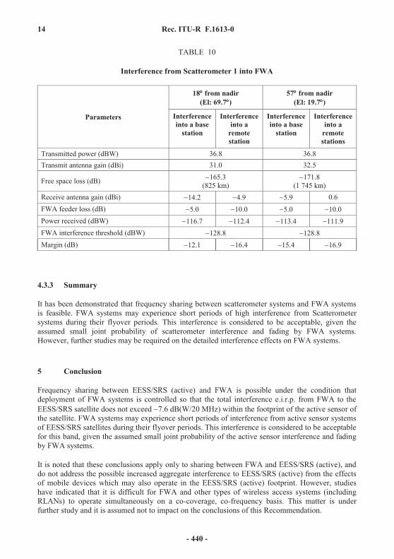
14 Rec. ITU-R F.1613-0
TABLE 10
Interference from Scatterometer 1 into FWA
4.3.3 Summary
It has been demonstrated that frequency sharing between scatterometer systems and FWA systems is feasible. FWA systems may experience short periods of high interference from Scatterometer systems during their flyover periods. This interference is considered to be acceptable, given the assumed small joint probability of scatterometer interference and fading by FWA systems. However, further studies may be required on the detailed interference effects on FWA systems.
5 Conclusion
Frequency sharing between EESS/SRS (active) and FWA is possible under the condition that deployment of FWA systems is controlled so that the total interference e.i.r.p. from FWA to the EESS/SRS satellite does not exceed 7.6 dB(W/20 MHz) within the footprint of the active sensor ofthe satellite. FWA systems may experience short periods of interference from active sensor systems of EESS/SRS satellites during their flyover periods. This interference is considered to be acceptable for this band, given the assumed small joint probability of the active sensor interference and fading by FWA systems.
It is noted that these conclusions apply only to sharing between FWA and EESS/SRS (active), and do not address the possible increased aggregate interference to EESS/SRS (active) from the effects of mobile devices which may also operate in the EESS/SRS (active) footprint. However, studies have indicated that it is difficult for FWA and other types of wireless access systems (including RLANs) to operate simultaneously on a co-coverage, co-frequency basis. This matter is under further study and it is assumed not to impact on the conclusions of this Recommendation.
Parameters
18 from nadir(El: 69.7 )
57 from nadir(El: 19.7 )
Interference into a base
station
Interference into a
remote station
Interference into a base
station
Interference into a
remote stations
Transmitted power (dBW) 36.8 36.8Transmit antenna gain (dBi) 31.0 32.5
Free space loss (dB) 165.3(825 km)
171.8(1 745 km)
Receive antenna gain (dBi) 14.2 4.9 5.9 0.6FWA feeder loss (dB) 5.0 10.0 5.0 10.0Power received (dBW) 116.7 112.4 113.4 111.9FWA interference threshold (dBW) 128.8 128.8Margin (dB) 12.1 16.4 15.4 16.9
- 440 -

Rec. ITU-R F.1613-0 15
Appendix 1 to Annex 1
Interference into the spaceborne active sensor caused by side lobes of FWA remote stations
In an FWA cell, remote stations are scattered around the base station. It is assumed that remote stations surround the base station uniformly in terms of azimuth angles observed from the remote station. Since the main beam of remote stations are directed to the base station, the angle from the main beam of remote station is larger than the elevation angle towards the EESS/SRS satellite due to the azimuth separation as shown in Fig. 3.
1613-03
Remotestation
Direction to the base station(main beam direction)
Direction tothe satellite
FIGURE 3
Off-beam angle: towards the EESS/SRS satellite at the remote station
The off-beam angle: towards the satellite at the remote station is calculated by the following relation, assuming that the elevation of remote station antenna is 0 :
cos cos · cos
where:
: elevation angle towards the satellite
: azimuth separation angle between the satellite and the base station directions.
Assuming to be uniformly distributed over 0° to 360°, the average gain towards the satellite is calculated as shown in Table 11.
- 441 -

16 Rec. ITU-R F.1613-0
TABLE 11
Average antenna gain of remote stations towards the satellite
Appendix 2 to Annex 1
List of abbreviations
Az Azimuth
BW Bandwidth
CSMA Carrier sense multiple access
CW Continuous wave
EESS Earth exploration-satellite service
El Elevation
FM Frequency modulation
FWA Fixed wireless access
PRF Pulse repetition frequency
RF Radio frequency
RLAN Radio local area network
SAR Synthetic aperture radar
SRS Space research service
TDMA Time division multiple access
Satellite elevation (degrees) 70 30Average gain (dBi) 4.96 2.34
- 442 -

Rec. ITU-R RA.1631-0 1
RECOMMENDATION ITU-R RA.1631-0
Reference radio astronomy antenna pattern to be used for compatibility analyses between non-GSO systems and radio astronomy
service stations based on the epfd concept
(Question ITU-R 146/7)
(2003)
The ITU Radiocommunication Assembly,
considering
a) that there is a need to determine the levels of interference which may occur at typical observatory sites, due to various sources of interference;
b) that, to determine these levels of interference, a reference antenna pattern needs to be defined;
c) that Recommendation ITU-R SA.509 gives a reference antenna pattern which represents the side-lobe gain levels that are not expected to be exceeded at most off-axis angles in the majority of antennas used in the service;
d) that the antenna pattern given in Recommendation ITU-R SA.509 is appropriate in some compatibility or sharing analyses;
e) that, if the peak envelope radiation pattern such as given in Recommen-dation ITU-R SA.509 is used in the assessment of the aggregate interference consisting of many interference entries, the predicted interference will result in values that are greater than values that would be experienced in practice;
f) that Recommendation ITU-R S.1586 and Recommendation ITU-R M.1583 provide a methodology based on the epfd concept as defined in No. 22.5C of the Radio Regulations to calculate the level of unwanted emission levels produced by a non-geostationary-satellite system at radio astronomy stations;
g) that it is necessary to use an antenna radiation pattern representing average side-lobe levels to predict interference to a radio astronomy station from one or more fast moving stations seen under continuously variable angle such as non-GSO systems;
h) that, a simple mathematical formula is preferable to the radiation pattern representing average side-lobe levels;
j) that, to derive the epfd resulting from unwanted emission levels produced by a non-geostationary-satellite system at radio astronomy stations, it is necessary to use the typical maximum antenna gain of radio astronomy service (RAS) stations,
- 443 -

2 Rec. ITU-R RA.1631-0
recommends
1 that, in the absence of particular information concerning the radiation pattern of the radio astronomy antenna involved, the mathematical model of the average radiation pattern as stated below should be used for compatibility analyses between non-GSO systems and RAS stations for frequencies above 150 MHz:
G( ) Gmax – 2.5 10–32D dBi for 0 m
G( ) G1 for m r
G( ) 29 – 25 log dBi for r 10
G( ) 34 – 30 log dBi for 10 34.1
G( ) –12 dBi for 34.1 80
G( ) –7 dBi for 80 120
G( ) –12 dBi for 120 180
where:
log20log20 DmaxG dBi
DG log–1 dBi
120 GGmaxDm degrees
6.0–85.15 D
r degrees
D : diameter of the telescope (m)
: wavelength (m);
2 that the following mathematical model of the radiation pattern may be adopted for a more accurate representation of the main beam radiation pattern for frequencies above 150 MHz:
21 )2( J)(x
xGG max (expressed as a ratio not in dB)
where:
J1(x) : first order Bessel function
Gmax 24 effA
: maximum gain (expressed as a ratio not in dB)
Aeff (D/2)2 : area of the aperture of the telescope (m2)
D : diameter of the telescope (m)
: wavelength (m)
- 444 -

Rec. ITU-R RA.1631-0 3
and where:
x360
D with off-boresight angle (degrees) ( 0)
0 : first null in this antenna pattern at 69.88/(D/ ) (degrees) off-boresight
and that the following mathematical model of the radiation pattern may be adopted for a more accurate representation of the radiation pattern of near side lobes up to 1° from the boresight for frequencies above 150 MHz:
2)0953.04/32cos()(x
xBG (expressed as a ratio not in dB)
where:
360Dx with off-boresight angle (degrees) ( 0 1°)
D : diameter of the telescope
: wavelength
and:
B = 103.2 2 (( D/2)/(180 · ))2
This main beam model corresponds to the ideal case of 100 aperture efficiency;
3 that the following typical maximum RAS antenna gain be used in compatibility analysis between non-GSO systems and RAS antenna stations.
RAS allocated band(MHz) Typical maximum antenna gain
150.05-153 44322-328.6 51406.1-410 53608-614 56
1 400-1 427 631 610.6-1 613.8 64
1 660-1 670 652 690-2 700 694 990-5 000 74
- 445 -

4 Rec. ITU-R RA.1631-0
The corresponding antenna diameter may be derived using the following equations (see recommends 2):
Gmax = 24 effA
maximum gain (expressed as a ratio)
where:
Aeff = (D/2)2 : area of the aperture of the telescope (m2)
D : diameter of the telescope (m)
: wavelength (m).
RAS allocated band(GHz) Typical maximum antenna gain
10.6-10.7 8114.47-14.5 8415.35-15.4 8422.21-22.5 8723.6-24 8831.3-31.7 9042.5-43.5 93
- 446 -

Rec. ITU-R M.1642-2 1
RECOMMENDATION ITU-R M.1642-2
Methodology for assessing the maximum aggregate equivalent power flux-density at an aeronautical radionavigation service station
from all radionavigation-satellite service systems operating in the 1164-1215 MHz band
(2003-2005-2007)
Scope
This Recommendation gives a methodology and the reference antenna characteristics for assessing the maximum aggregate equivalent power flux-density (epfd) level produced at the input of a station of the aeronautical radionavigation service (ARNS) by all radionavigation-satellite service (RNSS) systems operating in any portion of the 1 164-1 215 MHz band.
The ITU Radiocommunication Assembly,
considering
a) that in accordance with the Radio Regulations (RR), the band 960-1 215 MHz is allocated on a primary basis to the aeronautical radionavigation service (ARNS) in all the ITU Regions;
b) that analyses show that RNSS signals in the 1 164-1 215 MHz band can be designed not to cause interference to the DME/TACAN ARNS receivers operating in this band;
c) that a protection criterion for the ARNS has been developed and is expressed in terms of equivalent power flux-density (epfd), which is set out in Recommendation ITU-R M.1639,
recognizing a) that WRC-2000 introduced a co-primary allocation for the RNSS in the frequency band 1 164-1 215 MHz, subject to conditions that require the RNSS to protect the ARNS from harmful interference;
b) that WRC-03 determined that protection of the ARNS from RNSS can be achieved if the value of the epfd produced by all the space stations of all RNSS (space-to-Earth) systems in the band 1 164-1 215 MHz does not exceed the level of –121.5 dB(W/m2) in any 1 MHz band, and adopted Resolution 609 (WRC-03) in order to ensure that this level is not exceeded;
c) that the ARNS is a safety service in accordance with RR No. 1.59 and special measures need to be taken by Administrations to protect these services in accordance with provision RR No. 4.10,
recommends
1 that the methodology in Annex 1 and the reference ARNS characteristics in Annex 2 should be used to calculate the maximum aggregate epfd produced by emissions from all RNSS systems at any aeronautical radionavigation station.
- 447 -

2 Rec. ITU-R M.1642-2
Annex 1
Methodology for assessing the maximum aggregate epfd at an ARNS station from all RNSS systems
operating in the 1164-1215 MHz band
Summary of the method With the method described in this Annex it is possible to calculate the maximum aggregate epfd level of all RNSS systems in the band 1 164-1 215 MHz.
This method allows different systems to be combined easily, so that the effect of changes such as including or excluding one or various systems or the effect of changing the characteristics of specific systems can be examined during a consultation meeting.
The method accommodates both non-GSO systems, with constellations of satellites in any orbits of any inclination, and GSO systems.
The method is based on a two-step process:
Step 1: Calculation of the epfd of each individual RNSS system. This step may be performed by each operator independently prior to the consultation meeting, provided that results are submitted in a compatible format (see § 1.3, for non-GSO systems, and § 1.4, for GSO systems).
Step 2: Combination of the maximum epfd of the individual systems, by superposition of the maps, if necessary at different frequencies, to obtain the maximum aggregate epfd (see § 2) in the band 1 164-1 215 MHz.
Description of the method
1 Method for calculating the maximum epfd from satellites of one RNSS system
1.1 Definition of epfd The definition of equivalent power flux-density (epfd) is based upon RR No. 22.5C.1 as adopted at WRC-2000.
When an antenna receives power, within its reference bandwidth, simultaneously from transmitters at various distances, in various directions and at various levels of incident pfd, the epfd is that pfd which, if received from a single transmitter in the far field of the antenna in the direction of maximum gain, would produce the same power at the input of the receiver as is actually received from the aggregate of the various transmitters.
The instantaneous epfd is calculated using the following formula:
a
i
iN
i maxr
iritP
GG
dGepfd
1 ,1010
)(π4
)θ(10log102
where: Na : number of space stations that are visible from the receiver
i : index of the space station considered
- 448 -

Rec. ITU-R M.1642-2 3
Pi : RF power (in the reference bandwidth) at the input of the antenna (or RF radiated power in the case of an active antenna) of the transmitting space station (dB(W/MHz))
i : off-axis angle (degrees) between the boresight of the transmitting space station and the direction of the receiver
Gt( i) : transmit antenna gain (as a ratio) of the space station in the direction of the receiver
di : distance (m) between the transmitting station and the receiver i : off-axis angle (degrees) between the pointing direction of the receiver and the
direction of the transmitting space station Gr( i) : receive antenna gain (as a ratio) of the receiver, in the direction of the
transmitting space station (see Annex 2) Gr, max : maximum gain (as a ratio) of the receiver
epfd : instantaneous equivalent power flux-density (dB(W/(m2 · MHz))) at the receiver.
NOTE 1 – It is assumed that each transmitter is located in the far field of the receiver (that is, at a distance greater than 2D2/ , where D is the effective diameter of the receiver antenna and is the observing wavelength in the same unit). In the case under consideration this will always be satisfied.
1.2 General consideration In the first step of the method, the maximum epfd for each constellation of RNSS satellites is calculated at each latitude and longitude over the whole surface of the Earth for each 1 MHz of spectrum occupied by the system.
As the victim ARNS receiver may be mounted on an aircraft flying at an altitude up to 40 000 ft (12 192 m) (see § 2 of Annex 2), the calculation should include all satellites with elevation angles from 90 down to 3.54 .Calculation of the epfd distribution of each system is only necessary at a single reference frequency, preferably the frequency at which signal power is maximum. The RNSS signal spectral shape should be supplied to a consultation meeting, so that results of the calculation can then be multiplied by the appropriate spectral shaping factors to obtain the results at any other frequency.
1.3 Method for calculating the maximum epfd for a non-GSO RNSS system The simulation methodology given in Appendix 1 to Annex 1, which is based entirely on Recommendation ITU-R S.1325, may be used to accomplish this.
The methodology, given in Appendix 2 to Annex 1, is based entirely on an analytical technique. The method could be used for obtaining prompt estimates but it does not yield an exact upper bound result.
1.4 Method for calculating the maximum epfd for a GSO RNSS system The maximum epfd for each GSO satellite is required to be calculated at each latitude and longitude over the whole surface of the Earth for each 1 MHz of spectrum occupied by the system.
In this case the epfd will not be dependent on time, so a single table of results can be calculated directly.
- 449 -

4 Rec. ITU-R M.1642-2
2 Method for calculating the maximum aggregate epfd from all RNSS systems
2.1 Data required for each system Each non-GSO RNSS system not having a geosynchronous period will, having followed the methodology of § 1.3, provide a consultation meeting with a list of maximum epfd versus latitude (applicable at all longitudes) and a signal spectral shape.
Each non-GSO RNSS system having a geosynchronous period will, having followed the methodology of § 1.3, provide a consultation meeting with a list of maximum epfd versus latitude and longitude, and a signal spectral shape.
Each GSO RNSS system will, having followed the methodology of § 1.4, provide a consultation meeting with a table of maximum epfd versus latitude and longitude and a signal spectral shape.
2.2 Combination of epfds of systems with similar signal characteristics The determination of aggregate epfd of RNSS systems with the same frequency of signal spectral maximum may be achieved using three steps:
Step 1a: point-by-point summation of maximum epfd’s in the 1 MHz of the band where the signal has maximum power at each latitude of all the non-GSO (not having a geosynchronous period) lists to obtain the list of non-GSO (not having a geosynchronous period) aggregate epfd versus latitude;
Step 1b: point-by-point summation of maximum epfds in the 1 MHz of the band where the signal has maximum power at each latitude and longitude of all the non-GSO (having a geosynchronous period) lists to obtain the list of non-GSO (having a geosynchronous period) aggregate epfd versus latitude and longitude;
Step 2: point-by-point summation of maximum epfd’s in the 1 MHz of the band where the signal has maximum power at each point of latitude and longitude of all the GSO tables to obtain the table of GSO aggregate epfd versus latitude and longitude;
Step 3: point-by-point summation of the list of non-GSO (not having a geosynchronous period) aggregate epfd versus latitude, and the list of non-GSO (having a geosynchronous period) aggregate epfd versus latitude and longitude to each longitude column of the table of GSO aggregate epfd versus latitude and longitude to obtain the overall the table of aggregate epfd versus latitude and longitude.
Examination of the highest epfd in this table will reveal whether the protection criterion in Recommendation ITU-R M.1639 in any 1 MHz of the band is respected.
2.3 Combination of epfd’s of systems with different signal characteristicsIt should be noted that the maximum aggregate epfd will be frequency dependent. If the spectra of all the RNSS systems under consideration have their maxima at the same frequency, a single analysis will suffice. However, if different systems have different maxima, either because they use different centre frequencies with overlapping spectra or because they use different modulation techniques, then analysis of the maximum aggregate epfd will require frequency to be taken into account.
The determination of maximum aggregate epfd of RNSS systems with different centre frequencies will require, as a minimum, the above three steps to be performed at each frequency for which any one system has its signal spectral maximum, and may also require analysis at intermediate frequencies.
For each frequency, each list or table will be factored by the appropriate spectral shaping factor before summation with other lists and tables.
- 450 -

Rec. ITU-R M.1642-2 5
Examination of the highest epfd in all of the resultant tables will reveal whether protection criterion in Recommendation ITU-R M.1639 in any 1 MHz of the band is respected.
2.4 Check of results Following determination of the maximum aggregate epfd, a single simultaneous simulation of all RNSS systems at the ARNS station location where the absolute maximum aggregate epfd was determined may be considered to confirm results obtained using Appendix 1 or 2 to Annex 1.
Appendix 1 to Annex 1
A simulation methodology for determining the maximum epfd for a non-GSO RNSS system
1 Method and simulation approach description The framework for this methodology based on Recommendation ITU-R S.1325 is to model all the satellites of one RNSS system at a specific reference frequency (typically the 1 MHz portion of the 1 164-1 215 MHz band with the maximum RNSS signal spectral density). A simulation of the constellation is sampled over a period of time at a relatively fine rate. At each sample the epfd is computed for all latitude and longitude points. The maximum sample should be recorded for each latitude and longitude point. Other samples may be discarded. The result is a table, which can be shown as a map, as illustrated in Figs. 5 and 6. Following this, the maximum epfd, for each latitude should be determined, which will eliminate approximations due to limited simulation time.
2 Simulation assumptions
2.1 Orbit model The orbit models to simulate the space stations in their orbits are for circular and elliptical orbits only accounting for precession of the line of nodes in the equatorial plane due to asphericity of the Earth.
The orbit model represents satellite motion in a geocentric inertial coordinate frame shown in Fig. 1. The origin of this inertial frame is at the centre of the Earth. The x-axis points to the first point in the constellation Aries (i.e. vernal equinox), the z-axis is the mean rotation axis of the Earth, and the y-axis is determined as the cross product of the unit vectors in the z and x direction, i.e. xzy = .
The orbital models are based on Newton’s equation of motion for a satellite orbiting a perfectly spherical Earth in a circle and in an ellipse. For the non-GSO system using circular orbit, the characteristics of this motion that make it easy to model is that the satellite orbital radius and velocity are constant.
- 451 -

6 Rec. ITU-R M.1642-2
2.1.1 Earth-related constants For the Earth, the general constants are:
Re : Earth radius (6 378.137 km) O : Earth centre
: Earth attraction constant (3.986005 105 km3/s2) J2 : second harmonic Earth potential constant (1 082.63 10 6) Te : Earth rotation period (23 h 56' 4.0989" 86 164.0989 s)
e : Earth rotation angular velocity 2 /Te 7.2921151467 10–5 rad/s t : elapsed time since the simulated epoch (s).
2.1.2 Non-GSO satellite system space station related constants For the non-GSO satellite system space stations using circular orbits (see Fig. 1), the constants are as follows:
N : number of space stations of the non-GSO system i : index for each of the non-GSO satellites (0 i N)
hsat : satellite altitude above the Earth (km) r : radius of the satellite orbit (km) hsat Re
I : inclination angle of the orbital plane above the Equator (rad) RAAN : right ascension of the ascending node
i,0 : RAAN of the i-th non-GSO satellite at the time t (rad) ui,0 : argument of latitude of the i-th non-GSO satellite at the time t (rad)
T : satellite orbit period (s) 2 (r3/ )1/2
n : mean motion of a satellite (rad/s) 2 /Tui,t : argument of latitude of the i-th satellite at the time t (rad) ui,0 nt
r : nodal regression of the ascending node (rad/s)
= 42
2 )cos(J23–
rr
RI e
i,t RAAN of the i-th satellite at the time t (rad) i,0 rt
:iON coordinate vector (inertial coordinate system) of a non-GSO satellite in the Earth-centred fixed coordinate frame:
)sin()sin()cos()sin()cos()sin()cos()sin()sin()cos()cos()cos(
,
,,,,
,,,,
IuuIuuIu
rzyx
ON
ti
titititi
titititi
i
i
i
i
- 452 -

Rec. ITU-R M.1642-2 7
For the non-GSO satellite system space stations using elliptical orbits (see Figs. 2 and 3), the constants are as follows:
N : number of space stations of the non-GSO system i : index for each of the non-GSO satellites (0 i < N)
ai: semi-major axis of the i-th satellite (km) ei: eccentricity of the i-th satellite
Mi,0 : mean anomaly of the i-th non-GSO satellite at the initial time (rad)
Ti : satellite orbit period of the i-th satellite (s) 213 )(2 /i /a
ni : mean motion of the i-th satellite (rad/s) iT/2
νi,t: true anomaly of the i-th satellite at time t2
tan11tan2 ,1 ti
i
i Eee
Ei,t: eccentric anomaly of the i-th satellite at time t2
tan11tan2 ,1 ti
i
iee
Mi,t: mean anomaly of the i-th satellite at time tti
EeEtnM itiii ,sin,0,
*
* Once Mi,t is given, Ei,t is determined by iteration. Usually, for short time-steps, the last value of Ei,t can be
used as an initial estimate.
- 453 -

8 Rec. ITU-R M.1642-2
Ii : inclination angle of the orbital plane above the Equator of the i-th satellite (rad) RAAN: right ascension of the ascending node
i,0 : RAAN of each of the i-th non-GSO satellites at the initial time (rad) i,0: argument of perigee of each of the i-th non-GSO satellites at the initial time
(rad) ui,t : argument of latitude of the i-th satellite at the time t (rad) = ωi,0 + νi,t
ri : nodal regression of the ascending node of the i-th satellite (rad/s)
2242
2)1(
μ)cos(J
23
ii
iei
ea
aRI
i,t RAAN of the i-th satellite at the time t (rad) = i,0 rit
:,tiON coordinate vector (inertial coordinate system) of the i-th non-GSO satellite in the Earth-centred fixed coordinate frame at the time t:
tiON , = tiiiti rrotIrotrot ,0,, )(3)(1)(3
rot1( ): rotation about the x-axis
cossin0sincos0
001)(1rot
rot3( ): rotation about the z-axis
1000cossin0sincos
)(3rot
tir , :0
sincos
cos1)1(
0sincos
,
,
,
2,
,
,, ti
ti
tiiti
ti
titi eearr
- 454 -

Rec. ITU-R M.1642-2 9
- 455 -

10 Rec. ITU-R M.1642-2
The non-GSO perturbation can be considered in calculating the non-GSO constellation related constants, as the position of the satellites may vary when taking perturbation into account.
2.1.3 ARNS station related constants Lat : latitude of ARNS station (rad)
Lon : longitude of ARNS station (rad) hARNS : altitude of ARNS station (km)
:OM ARNS station coordinates in the Earth-centred, inertial coordinate system
Lat)(sin)(LonsinLat)(cos)(LoncosLat)(cos)(
ARNSe
eARNSe
eARNSe
hRZthRYthRX
OM
2.2 Antenna parameters
2.2.1 ARNS station antenna parameters The antenna pattern for the ARNS station is an input parameter to the simulation (see Annex 2).
2.2.2 Non-GSO space station antenna parametersIn order to perform interference analysis, non-GSO satellite antennas should be modelled using either of the following patterns, subject to availability: – measured antenna patterns; – proposed reference antenna patterns;
– an analytical function which models the radiation pattern of the non-GSO satellite antenna.
2.3 Calculation of the simulation time
2.3.1 Simulation time increment For obtaining accurate results the simulation time increment, tinc, should be as short as possible, but on the other hand the total simulation time should be reasonable. To attain the accuracy required it is necessary to ensure a sufficient number of epfd measurements (Nhits) when non-GSO RNSS spacecraft falls into the ARNS antenna pattern of maximum gain visible to a space station. Nhits 5 is thought to be sufficient.
The maximum gain visible to a space station occurs at –3.54 to 3 elevation angle (Annex 2) for an aircraft at 40 000 ft (12 192 m). It is important to have 5 Nhits within this range, implying that simulation increments of 1 of constellation movement is sufficient.
- 456 -

Rec. ITU-R M.1642-2 11
2.3.2 Total simulation time A satellite of a non-GSO constellation on any orbit traces out a path on the Earth’s surface. After a time, which is specific to the system, the satellite or another satellite of the constellation returns to the same or practically to the same point. The time between these two cases is the repeat period of the constellation. The repeat periods of different constellations are from a few days to several months. Typical results of the epfd calculation of a RNSS system over one constellation repeat period is illustrated in Fig. 5.
The exact longitude precession rate of the satellites in a non-GSO constellation will be affected by drifts due to longitudinal station keeping errors. This effect can be modelled and integrated in the simulations.
For the non-GSO system not having a geosynchronous period, the aforementioned effect of this will result in the maximum epfd at any longitude becoming, in fact, the maximum epfd at all longitudes. (In other words, if the simulation were to be extended to cover all possible states of the constellation, the “high spots” of maximum epfd on the map in Fig. 5 would spread horizontally to become uniform horizontal stripes.) It is therefore considered more correct to take, for each latitude, the maximum epfd at any longitude and use it for all longitudes. This converts the table of maximum epfd versus latitude and longitude into a simple list of maximum epfd versus latitude.
If this is done, then the simulation time could be reduced to a single orbital period for the non-GSO system not having a geosynchronous period. The “map” produced by such a limited simulation would show only a few “high spots” but, at each latitude, the value of the “high spots”, representing the maximum epfd at any longitude, would be the same.
As a by-product, the amount of information which must be presented to the consultation meeting would be considerably reduced.
- 457 -

12 Rec. ITU-R M.1642-2
On the other hand, non-GSO systems having a geosynchronous period produce ground tracks that are confined to a limited longitude range on the Earth’s surface. This will result in the “high spots” of maximum epfd appearing only within a limited area of the Earth’s surface. (In other words, the “high spots” of maximum epfd on the Earth’s surface would not spread horizontally.) Therefore, the aggregate epfd, caused by the non-GSO systems having a geosynchronous period, shall be computed for the latitude and longitude points within the visible range from the non-GSO.
For this case of a non-GSO system having a geosynchronous period, the computation could be accomplished considering a single orbital period. Typical results of the epfd calculation for a non-GSO system having a geosynchronous period are shown in Fig. 6.
- 458 -
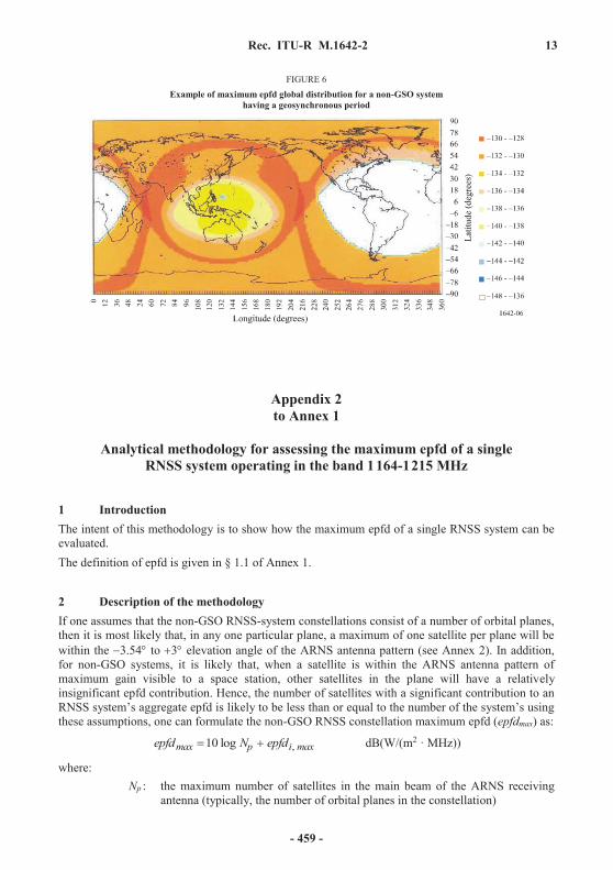
Rec. ITU-R M.1642-2 13
FIGURE 6 Example of maximum epfd global distribution for a non-GSO system
having a geosynchronous period
Appendix 2 to Annex 1
Analytical methodology for assessing the maximum epfd of a single RNSS system operating in the band 1164-1215 MHz
1 Introduction The intent of this methodology is to show how the maximum epfd of a single RNSS system can be evaluated. The definition of epfd is given in § 1.1 of Annex 1.
2 Description of the methodology If one assumes that the non-GSO RNSS-system constellations consist of a number of orbital planes, then it is most likely that, in any one particular plane, a maximum of one satellite per plane will be within the 3.54 to 3 elevation angle of the ARNS antenna pattern (see Annex 2). In addition, for non-GSO systems, it is likely that, when a satellite is within the ARNS antenna pattern of maximum gain visible to a space station, other satellites in the plane will have a relatively insignificant epfd contribution. Hence, the number of satellites with a significant contribution to an RNSS system’s aggregate epfd is likely to be less than or equal to the number of the system’s using these assumptions, one can formulate the non-GSO RNSS constellation maximum epfd (epfdmax) as:
maxipmax epfdNepfd ,log10 dB(W/(m2 · MHz))
where: Np : the maximum number of satellites in the main beam of the ARNS receiving
antenna (typically, the number of orbital planes in the constellation)
- 459 -

14 Rec. ITU-R M.1642-2
epfdi,max : maximum single-satellite epfd contribution (dB(W/(m2 · MHz))).
3 Non-GSO examples For a single-satellite maximum epfd contribution of –136.9 dB(W/(m2 · MHz)) within a non-GSO RNSS constellation of six planes using the equation in § 2 the epfdmax is:
12.1296log10)9.136(maxepfd dB(W/(m2 · MHz))
A similar calculation, with a single-satellite maximum epfd contribution of –130.24 dB(W/(m2 · MHz)), within a non-GSO RNSS constellation of three planes, using the equation in § 2 gives a maximum epfd of –125.47 dB(W/(m2 · MHz)).These values are in very good agreement with the simulation method in Appendix 1 to Annex 1, with only 1.2 dB difference.
Annex 2
ARNS reference station characteristics to be used in epfd calculation
1 ARNS antenna characteristics Table 1 provides the antenna gain for elevation values between 90 and 90 . For elevation values between two values of Table 1 a linear interpolation should be used. The Gr, max value is 3.4 dBi as specified in Recommendation ITU-R M.1639, including 2 dB of circular-to-linear polarization mismatch. It is assumed that the elevation and gain pattern is the same for all azimuth angles.
TABLE 1
Elevation angle
(degrees)
Antenna gain including
circular-to-linear polarization
mismatchGr/Gr, max
(dB)
Elevation angle
(degrees)
Antenna gain including
circular-to-linear polarization
mismatchGr/Gr, max
(dB)
Elevation angle
(degrees)
Antenna gain including
circular-to-linear polarization
mismatchGr/Gr, max
(dB)–90 –17.22 22 –10.72 57 –15.28–80 –14.04 23 –10.81 58 –15.49–70 –10.51 24 –10.90 59 –15.67–60 –8.84 25 –10.98 60 –15.82–50 –5.40 26 –11.06 61 –16.29–40 –3.13 27 –11.14 62 –16.74–30 –0.57 28 –11.22 63 –17.19–20 –1.08 29 –11.29 64 –17.63–10 0.00 30 –11.36 65 –18.06
–5 –1.21 31 –11.45 66 –18.48–3 –1.71 32 –11.53 67 –18.89–2 –1.95 33 –11.60 68 –19.29–1 –2.19 34 –11.66 69 –19.69
- 460 -

Rec. ITU-R M.1642-2 15
TABLE 1 (end)
Elevation angle
(degrees)
Antenna gain including
circular-to-linear polarization
mismatchGr/Gr, max
(dB)
Elevation angle
(degrees)
Antenna gain including
circular-to-linear polarization
mismatchGr/Gr, max
(dB)
Elevation angle
(degrees)
Antenna gain including
circular-to-linear polarization
mismatchGr/Gr, max
(dB)0 –2.43 35 –11.71 70 –20.081 –2.85 36 –11.75 71 –20.552 –3.26 37 –11.78 72 –20.993 –3.66 38 –11.79 73 –21.414 –4.18 39 –11.80 74 –21.805 –4.69 40 –11.79 75 –22.156 –5.20 41 –12.01 76 –22.487 –5.71 42 –12.21 77 –22.788 –6.21 43 –12.39 78 –23.069 –6.72 44 –12.55 79 –23.30
10 –7.22 45 –12.70 80 –23.5311 –7.58 46 –12.83 81 –23.4412 –7.94 47 –12.95 82 –23.3513 –8.29 48 –13.05 83 –23.2414 –8.63 49 –13.14 84 –23.1315 –8.97 50 –13.21 85 –23.0116 –9.29 51 –13.56 86 –22.8817 –9.61 52 –13.90 87 –22.7318 –9.93 53 –14.22 88 –22.5719 –10.23 54 –14.51 89 –22.4020 –10.52 55 –14.79 90 –22.2121 –10.62 56 –15.05
2 ARNS station location
The ARNS station altitude should be taken at worst case (12 192 m)1, which gives maximum visibility of potentially interfering satellites from the ARNS receiving antenna.
1 Equivalent to 40 000 ft.
- 461 -


Rec. ITU-R M.1643-0 1
RECOMMENDATION ITU-R M.1643-0*
Technical and operational requirements for aircraft earth stations of aeronautical mobile-satellite service including those using fixed-satellite service network transponders in
the band 14-14.5 GHz (Earth-to-space)
(2003)
Summary
This Recommendation provides the technical and operational requirements for aircraft earth stations (AES) of aeronautical mobile-satellite service (AMSS), including those using FSS network transponders operating in the band 14-14.5 GHz (Earth-to-space), that should be used by administrations as a technical guideline for establishing conformance requirements for AES and facilitating their licensing, for worldwide use.
The ITU Radiocommunication Assembly,
considering
a) that various technically and operationally different aeronautical mobile-satellite service (AMSS) networks have been designed to commence operation in the near future;
b) that these planned AMSS networks may provide access to a variety of broadband communication applications (Internet, email, internal corporate networks) to and from aircraft on a global basis;
c) that the aircraft earth station (AES) will operate on national and international airlines around the world;
d) that circulation of AES is usually a subject of a number of national and international rules and regulations including satisfactory conformance to a mutually agreed technical standard and operational requirements;
e) that there is a need for identifying the technical and operational requirements for the conformance testing of AES;
* NOTE – The Arab Group represented at RA-03 reserves its position on this Recommendation and is not
ready to accept any repercussions with respect to WRC-03 Agenda item 1.11.
- 463 -

2 Rec. ITU-R M.1643-0
f) that the identification of technical and operational requirements for AES would provide a common technical basis for facilitating conformance testing of AES by various national and international authorities and the development of mutual recognition arrangements for conformance of AES;
g) that the technical and operational requirements need to achieve an acceptable balance between radio equipment complexity and the need for effective use of the radio-frequency spectrum,
considering also
a) that in the frequency band 14-14.5 GHz there are allocations to the FSS (Earth-to-space), radionavigation, fixed and mobile (except aeronautical mobile) services on a primary basis; that secondary services allocated in the band 14-14.5 GHz or in parts of the band include mobile-satellite (except aeronautical mobile-satellite) service (Earth-to-space), space research service (SRS), radio astronomy service (RAS), and radionavigation-satellite service;
b) that there is a requirement to fully protect all primary services and pre-existing systems of secondary services in the band 14-14.5 GHz;
c) that results of the studies conducted in accordance with Resolution 216 (Rev.WRC-2000) showed the feasibility of using the band 14-14.5 GHz by AMSS (Earth-to-space) on a secondary basis under certain conditions and arrangements1;
d) that the identification by ITU-R of technical and operational requirements for AES operating in the band 14-14.5 GHz could assist administrations to prevent harmful and/or unacceptable interference to other services;
e) that technical and operational characteristics should be continuously and accurately measurable and controllable,
recommends
1 that the technical and operational requirements1 for aircraft earth stations of AMSS networks operating in the band 14-14.5 GHz given in Annexes 1 and 2 be used by administrations as a guideline for:– establishing conformance requirements for AES; – facilitating AES operations.
1 The characteristics of the typical aircraft earth stations need to fulfil the requirements described in this
Recommendation and, further, need to be within the envelope of those initially published in the International Frequency Information Circular (BR IFIC) relating to the corresponding FSS network. In the case that the characteristics are outside of the envelope of those in the initial publication, the required coordination of such an aircraft earth station needs to be effected in accordance with the current provisions of the Radio Regulations (RR) and a modified Rule of Procedure as contained in § 2 of the Rules of Procedure relating to RR No. 11.32, as appropriate.
- 464 -

Rec. ITU-R M.1643-0 3
Annex 1
Technical and operational requirements for AES of AMSS networks in the band 14-14.5 GHz (Earth-to-space)
Part A
Essential requirements related to the protection of FSS networks
1 AMSS networks should be coordinated and operated in such a manner that the aggregate off-axis e.i.r.p. levels produced by all co-frequency AES within AMSS networks are no greater than the interference levels that have been published and coordinated for the specific and/or typical earth station(s) pertaining to FSS networks where FSS transponders are used.
2 The design, coordination and operation of an AES should, at least, account for the following factors which could vary the aggregate off-axis e.i.r.p. levels generated by the AES:
2.1 mispointing of AES antennas. Where applicable, this includes, at least, effects caused by bias and latency of their pointing systems, tracking error of closed loop tracking systems, misalignment between transmit and receive apertures for systems that use separate apertures, and misalignment between transmit and receive feeds for systems that use combined apertures;
2.2 variations in the antenna pattern of AES. Where applicable, this includes, at least, effects caused by manufacturing tolerances, ageing of the antenna and environmental effects. AMSS networks using certain types of AES antennas, such as phased arrays, should account for variation in antenna pattern with scan angles (elevation and azimuth). Networks using phased arrays should also account for element phase error, amplitude error and failure rate;
2.3 variations in the transmit e.i.r.p. from AES. Where applicable, this includes, at least, effects caused by measurement error, control error and latency for closed loop power control systems. Network control and monitoring centres (NCMCs) that calculate the e.i.r.p. of AES based on the received signal need to take into account error sources and latency in this calculation. NCMCs that calculate the e.i.r.p. of AES based on input power must account for measurement error and reporting latency.
3 AES that use closed loop tracking of the satellite signal need to employ an algorithm that is resistant to capturing and tracking adjacent satellite signals. AES must immediately inhibit transmission when they detect that unintended satellite tracking has happened or is about to happen.
4 AES should be subject to the monitoring and control by an NCMC or equivalent facility. AES must be able to receive at least “enable transmission” and “disable transmission” commands from the NCMC. AES must automatically cease transmissions immediately on receiving any
- 465 -

4 Rec. ITU-R M.1643-0
“parameter change” command, which may cause harmful interference during the change, until it receives an “enable transmission” command from its NCMC. In addition, it should be possible for the NCMC to monitor the operation of an AES to determine if it is malfunctioning.
5 AES need also to be self-monitoring and, should a fault which can cause harmful interference to FSS networks be detected, the AES must automatically mute its transmissions.
Part B
Essential requirements related to the protection of the fixed service
In the 14-14.5 GHz frequency band as used by fixed service networks, within line-of-sight of the territory of an administration where fixed service networks are operating in this band, the maximum pfd produced at the surface of the Earth by emissions from a single AES, of an AMSS network should not exceed:
–132 + 0.5 · dB(W/(m2 · MHz)) for 40
–112 dB(W/(m2 · MHz)) for 40 90
where is the angle of arrival of the radio-frequency wave (degrees above the horizontal).NOTE 1 – The aforementioned limits relate to the pfd and angles of arrival that would be obtained under free-space propagation conditions.
NOTE 2 – An e.i.r.p. mask can be derived from the aforementioned pfd mask by applying the method given in Annex 2 of this Recommendation. Simplification of the resulting e.i.r.p. mask could also be considered.
Part C
Essential requirements related to sharing with the RAS
In order to protect the radio astronomy in the band 14.47-14.5 GHz, AMSS earth stations should comply with both following measures:
AMSS channels in the 14.47-14.5 GHz band
– AMSS stations do not transmit in the 14.47-14.5 GHz band within line-of-sight of radio astronomy stations operating within this band;
or, – if an AMSS operator intends to operate co-frequency within the visibility of the radio
astronomy station, a specific agreement with the radio astronomy station will be needed to ensure that AMSS AES will meet the requirements of Recommendations ITU-R RA.769 and ITU-R RA.1513 within the 14.47-14.5 GHz band during observations. Where practicable, this may include advance information to AMSS operators regarding observation schedules.
AMSS channels in the 14-14.47 GHz band All AES transmitters on channels in the 14-14.47 GHz band within line-of-sight of radio
astronomy stations during radio astronomy observations have emissions in the band 14.47-14.5 GHz such that they meet the levels and percentage of data loss given in
- 466 -

Rec. ITU-R M.1643-0 5
Recommendations ITU-R RA.769 and ITU-R RA.1513. Results from studies show that the following AES pfd levels (dB(W/(m2 · 150 kHz))) in the band 14.47-14.5 GHz are sufficient, with some margin, to meet the radio astronomy pfd levels in Recommendation ITU-R RA.769 and the percentage of data loss given in Recommendation ITU-R RA.1513, i.e.:
–190 + 0.5 · dB(W/(m2 · 150 kHz)) for 10
–185 dB(W/(m2 · 150 kHz)) for 10 90
where is the angle of arrival of the radio-frequency wave (degrees above the horizontal).
Such AES pfd levels in the band 14.47-14.5 GHz may be achieved by the AMSS operators through a combination of reduced AES signal power, sharp filtering, maintaining adequate frequency separation, or better AES antenna performance.
Part D
Essential requirements related to sharing with the space research service
Coordination agreements should be developed between AMSS and space research systems based on controlling the emissions levels of the AES in the frequency band used by the SRS systems, and, in severe cases, may require cessation of AES emissions on frequencies used by the SRS system when operating in the vicinity of the space research earth station. Specifics of the agreements will vary based on the characteristics of the individual SRS sites and the AMSS networks.
Annex 2
Derivation of a lower hemisphere e.i.r.p. mask from a pfd mask
In testing AMSS equipment to determine if it meets a given pfd mask, such as the one in Annex 1,Part B, it may be useful to determine an equivalent e.i.r.p. mask that can be used for testing purposes.
The pfd mask, pfd( ) where is the angle of arrival (elevation angle) at the Earth’s surface, can be used to mathematically determine an e.i.r.p. mask, e.i.r.p.(γ, H) where γ is the angle below the local horizontal plane and H is the altitude of the aircraft. This conversion proceeds in two steps. First, γis converted to an equivalent angle of arrival, . Then the length of the propagation path for angle of arrival is determined and used to calculate the spreading loss for the path and the resulting e.i.r.p.
Step 1: Calculation of an angle of arrival in degrees, , from γ and H:
)/)cos()arccos(( ee RHR
- 467 -

6 Rec. ITU-R M.1643-0
where:
: angle of arrival Re : earth radius (6 378 km) H : altitude of the aircraft (km)
: angle below horizontal. NOTE 1 – If the argument of the arccos function is greater than 1, the propagation path in the direction of the angle γ does not intersect the Earth. In this case, which occurs for values of γ of about 3.5° or less, a value for does not exist and so there is no defined value for the pfd mask.
Step 2: Calculation of the e.i.r.p. value from the defined pfd( ):
2/122 ))–cos()(2–)(( HRRHRRd eeee
60)4(log10)(pfd),(e.i.r.p. 210 dH
where: d : distance between the AES and the considered point on the Earth’s surface (km)
pfd( ) : (dB(W/(m2 · MHz))) e.i.r.p. : (dB(W/MHz)).
The graph in Fig. 1 shows this function for various aircraft altitudes based on the pfd mask provided in Annex 1, Part B of this Recommendation.
1643-01
0 10 20 30 40 50 60 70 80 90
0
–10
–20
–30
–40
–50
FIGURE 1e.i.r.p. mask derived from pfd mask
Angle below horizontal (degrees)
e.i.r
.p. m
ask
(dB
(W/M
Hz)
)
12.29.17.63.0
Altitude (km)
- 468 -

Rec. ITU-R M.1652-1 1
RECOMMENDATION ITU-R M.1652-1
Dynamic frequency selection* in wireless access systems including radio local area networks for the purpose of protecting the
radiodetermination service in the 5 GHz band (Questions ITU-R 212/5)
(2003-2011)
Scope This Recommendation provides requirements of dynamic frequency selection (DFS) as a mitigation technique to be implemented in wireless access systems (WAS) including radio local area networks (RLANs) for the purpose of facilitating sharing with the radiodetermination service in the 5 GHz band. Annex 1 specifies the detection, operational and response requirements. Other Annexes address the methodologies and provide information which can be used by administrations when conducting sharing studies between radars and WAS including RLANs.
The ITU Radiocommunication Assembly,
considering
a) that harmonized frequencies in the bands 5 150-5 350 MHz and 5 470-5 725 MHz for the mobile service would facilitate the introduction of wireless access systems (WAS) including radio local area networks (RLANs);
b) that there is a need to protect the radars in the radiodetermination service operating in the bands 5 250-5 350 and 5 470-5 725 MHz;
c) that in many administrations, the ground-based meteorological radars are extensively deployed and support critical weather services;
d) that procedures and methodologies to analyse compatibility between radars and systems in other services are provided in Recommendation ITU-R M.1461;
e) that representative technical and operational characteristics of radiolocation, radionavigation and meteorological radars are provided in Recommendation ITU-R M.1638, including maritime radionavigation radars in, inter alia, the band 5 470-5 650 MHz;
f) that WAS including RLANs as described in Recommendation ITU-R M.1450 are capable of operating both indoor and outdoor;
g) Report ITU-R M.2034 which addresses the impact of certain detection requirements of the DFS on the performance of WAS,
* Dynamic frequency selection is a general term used in this Recommendation to describe mitigation
techniques that allow, amongst others, detection and avoidance of co-channel interference with respect to radar systems.
- 469 -

2 Rec. ITU-R M.1652-1
recognizing
a) that the band 5 250-5 350 MHz is allocated to the radiolocation service on a primary basis; that the band 5 250-5 350 MHz is also allocated to the Earth exploration-satellite service (EESS) (active) on a primary basis;
b) that the band 5 470-5 650 MHz is allocated to the maritime radionavigation service on a primary basis;
c) that the band 5 350-5 650 MHz is allocated to the radiolocation service on a secondary basis;
d) that ground-based radars used for meteorological purposes are authorized to operate in the band 5 600-5 650 MHz on a basis of equality with stations in the maritime radionavigation service;
e) that the band 5 650-5 725 MHz is allocated to the radiolocation service on a primary basis;
f) that administrations may take account of detailed information on actual radar deployment when developing guidance for the use of DFS in WAS in consultation with potentially affected administrations,
noting a) that the high RF power level and the receiver sensitivity of radars in the radiodetermination service in conjunction with the expected high density of WAS including RLANs would, in general, not enable compatible operation of WAS including RLANs and radars on a co-channel basis in the absence of mitigation techniques;
b) that WAS including RLANs could be deployed in these bands as licence-exempt devices, consequently making control of their deployment density more difficult;
c) that there are various standards for RLAN specifications;
d) that administrations may consider procedures to confirm the ability of interference avoidance mechanisms to function correctly in the presence of the radar systems deployed in this band,
recommends
1 that, in order to facilitate sharing with radars, mitigation techniques as described in Annex 1 be implemented by WAS, including RLANs in the bands used by radars at 5 GHz;
2 that the mitigation techniques comply with the detection, operational and response requirements as given in § 2 of Annex 1;
3 that the methodologies given in Annexes 4, 5, 6 and 7 can be used by administrations when conducting sharing studies between radars and WAS including RLANs.
NOTE 1 – Further information on the results of studies on the requirements stated in recommends 2is given in Report ITU-R M.2115, which provides information on the procedures in place in various administrations and/or regional groups to test compliance with DFS requirements.
- 470 -

Rec. ITU-R M.1652-1 3
Annex 1
The use of DFS in WAS including RLANs for the purpose of protecting the radiodetermination service in the 5 GHz band
1 Introduction
1.1 DFS
In relation to studies on the feasibility of sharing between the mobile service for WAS1 and the radiodetermination service in the frequency bands 5 250-5 350 and 5 470-5 725 MHz, link budget calculations have shown that interference mitigation techniques are required to enable sharing of WAS with other services such as radar systems. This Annex describes the interference mitigation technique(s) DFS2 as specified in the 5 GHz RLAN standards, with performance calculations based on typical implementations.
WAS and radars operating in the 5 GHz band will interfere when operating at the same frequencies and within range of each other.
DFS has then been envisaged to: – ensure a spread of the loading across the available spectrum of the WAS under the field of
view of a satellite to reduce the aggregate emission levels at the satellites of the FSS (feeder links) and EESS (active) from WAS;
– avoid co-channel operation with other systems, notably radar systems.
Extension of the use of DFS as described herein allows WAS to avoid interfering with the radiodetermination service. The general principle applied is that WAS should detect interference and identify radar interferers and shall not use those frequencies used by the radar.
1.2 Objective of the use of DFS with respect to radars The objective of using DFS in WAS is to provide adequate protection to radars in the 5 GHz band. This is achieved by avoiding the use of, or vacating, a channel identified as being occupied by radar equipment based on detection of radar signals.
For the purpose of this Annex, a discussion of radiodetermination systems in the 5 GHz range utilized in determining DFS characteristics can be found in Annex 3.
The implementation of radar detection mechanisms and procedures used by WAS are outside the scope of this Annex. The main reasons for this are that: – WAS design affects implementation; – practical experience may lead to innovative and more efficient means than can be
formulated today; – different manufacturers may make different implementation choices to achieve the lowest
cost for a given level of performance; therefore only performance criteria rather than specifications for a particular mechanism should be given in regulatory documents.
1 Throughout this Recommendation the term “WAS” denotes “wireless access systems including RLANs”.2 The DFS feature was specified in the 5 GHz RLAN standards initially in order to mitigate interference
among uncoordinated RLAN clusters, and to provide optimized spectral efficiency for high-capacity, high bit-rate data transmission.
- 471 -

4 Rec. ITU-R M.1652-1
2 DFS performance requirements The DFS performance requirement is stated in terms of response to detection of an interference signal.
5 GHz WAS should meet the following detection and response requirements.
Procedures for compliance verification should be incorporated in relevant industry standards for RLANs.
2.1 Detection requirements The DFS mechanism should be able to detect interference signals above a minimum DFS detection threshold of –62 dBm for devices with a maximum e.i.r.p. of < 200 mW and –64 dBm for devices with a maximum e.i.r.p. of 200 mW to 1 W3 averaged over 1 s.
This is defined as the received signal strength (RSS) (dBm), normalized to the output of a 0 dBi receive antenna, that is required to be detected within the WAS channel bandwidth.
2.2 Operational requirements The WAS should be able to perform channel availability check: A check during which the WAS listens on a particular radio channel for 60 s to identify whether there is a radar operating on that radio channel.
The WAS should be able to perform in-service monitoring: Monitoring of the operating channel to check that a co-channel radar has not moved or started operation within range of the WAS. During in-service monitoring the radar detection function continuously searches for radar signals in-between normal WAS transmissions. This requires the use of quiet spaces between successive WAS transmissions (see Annex 4).
If the WAS has not previously been in operation or has not continuously monitored the channel with in-service monitoring, it should not start transmission in any channel before completion of a channel availability check.
2.3 Response requirements A channel that has been flagged as containing a radar signal, either by a channel availability check or in-service monitoring, is subject to a 30 min period (non-occupancy period) where it cannot be used by the WAS device in order to protect scanning radars. The non-occupancy period should start at the time when the radar signal is detected.
Additionally, in the band 5 600-5 650 MHz, if a channel has been flagged as containing a radar, a 10 min continuous monitoring of the flagged channel is required prior to use of that channel. Otherwise, other appropriate methods such as channel exclusion would be required.
Channel move time is defined as the period of 10 s needed by a WAS to cease all transmissions on the operating channel upon detection of an interfering signal above the DFS detection threshold. Transmissions during this period will consist of normal traffic for typically less than 100 ms and a maximum of 200 ms after detection of the radar signal. In addition, intermittent management and control signals can be sent during the remaining time to facilitate vacating the operating channel.
3 In practice, it may not be necessary for each device to implement full DFS functionality, provided that
such devices are only able to transmit under the control of a device that ensures that all DFS requirements are fulfilled.
- 472 -

Rec. ITU-R M.1652-1 5
The aggregate time of the intermittent management and control signals are typically less than 20 ms.
2.4 Summary of the requirements Table 1 provides a summary of the requirements described above. An example of the operating procedures is given in Annex 2.
TABLE 1
Parameter Value
DFS detection threshold –62 dBm for devices with a maximum e.i.r.p. of < 200 mW and–64 dBm for devices with a maximum e.i.r.p. of 200 mW to 1 W averaged over 1 s
Channel availability check time 60 sNon-occupancy period 30 minChannel move time 10 s
Annex 2
Radar detection and example of associated DFS procedures
An example of how a DFS mechanism could be described is given in this Annex.
1 Definitions The following definitions are given for use within this Annex:
Available channel: A radio channel on which a channel availability check has not identified the presence of a radar.
Received radar signal: A signal as characterized below: an RSS equal to or greater than the DFS detection threshold level of TDFS (dBm) within the
WAS channel bandwidth; pulse repetition rates in the range 200-4 000 pulses/s; nominal pulse widths in the range 1-20 s.
Operating channel: Once a WAS starts to operate on an available channel then that channel becomes the operating channel.
- 473 -

6 Rec. ITU-R M.1652-1
2 Procedures
2.1 Finding an initial available channel Before a WAS transmits, and if no available channel has yet been identified, it shall undertake a channel availability check on a radio channel before it is used for transmission. Consequently, when a network is installed and first powered on, channel availability check(s) should be undertaken, so as to identify at least one available channel. Having identified an available channel, the WAS can start operation on that channel; the checking of other radio channels to identify other available channels is optional.
2.2 Starting operation Once a WAS starts to operate on an available channel then that channel becomes the operating channel.
2.3 Monitoring the operating channel In-service monitoring is performed by the WAS to re-check the operating channel for co-channel radar signals that may have come within range of the WAS or started operation on the operating channel.
3 Implementation aspects
3.1 Radar signal detection Radar signals may occur at any time and they may occur in the presence of co-channel WAS signals.
While finding an initial available channel, the WAS will not be operational and this will assure rapid and reliable detection of any radar signal with the possible exception of very slowly rotating radars. However, these will be detected by the in-service monitoring.
During in-service monitoring the radar detection function continuously searches for radar signal patterns – during or in between normal WAS transmissions. For weakly received radar signals, this may increase the time needed for radar signal detection. This is reflected in the requirements contained in Annex 1.
3.1.1 Detection of frequency hopping radars Frequency hopping radars operate over a large frequency range, with a rapid change of the operating frequency.
The time required by a WAS for reliable detection varies with the pulse characteristics of the radar. In the case of frequency hopping radars, the time for which the radar occupies the WAS channel (dwell time) also influences the detection probability.
The results will be one of the following: – if the dwell time is long enough, DFS detects the radar signal (see Annex 4) and WAS
transmissions will cease on the current channel; – if the dwell time is very short, the probability of detection of the radar by a WAS on the
operating channel may be affected, depending on the number of pulses during the dwell time.
- 474 -

Rec. ITU-R M.1652-1 7
3.1.2 Threshold and antenna gain The detection threshold is defined in terms of dBm normalized to the output of a 0 dBi receive antenna. If the WAS uses higher antenna gains, the TDFS level should be increased, by adding the antenna gain.
3.1.3 Spurious emissions Further study is required to determine the impact on the interaction between WAS and radars spurious emissions.
3.2 Channel move time Upon detection of a signal above the detection threshold, the DFS procedures require the broadcasting of commands to cease all operational transmission and to effect a move to (one of) the available channels identified by the channel availability check. This broadcast will be repeated a number of times to assure reception by all member devices. Part of the WAS population may be in so-called “Sleep Mode” in which the devices re-awaken at intervals of typically hundreds of milliseconds but extremes of up to 60 s are possible. Disregarding the latter, the broadcast has to be repeated a number of times during the channel move time to ensure that, for all practical purposes, all of the WAS devices will have left the channel.
Annex 3
Use of characteristics of radiolocation, maritime radionavigation and meteorological radars
The technical characteristics of some meteorological, radiolocation and maritime radionavigation radars operating in the bands between 5 250-5 350 MHz and 5 470-5 725 MHz can be found in Recommendation ITU-R M.1638. This information is used for the determination of the technical requirements of the DFS mechanism to be implemented in the WAS, which is identified as necessary to enable the introduction of WAS in the mobile service in these frequency bands used by radars. Specifically radars A through S provided in Recommendation ITU-R M.1638 are considered in development of DFS characteristics.
Table 1 of Recommendation ITU-R M.1638 shows the allocations within the 5 GHz range to the radiodetermination service.
Annex 4
Parameters and methodology to calculate the probability of detection of radiodetermination systems by WAS including RLAN devices
using DFS in the 5 GHz band during in-service monitoring
The following methodology considers the probability that a WAS device operating in the 5 GHz band using DFS will successfully detect during in-service monitoring a 5 GHz radar operating in the radiodetermination service.
- 475 -

8 Rec. ITU-R M.1652-1
Step 1: Determine the amount of time that an individual device will be in the main beam of the radar antenna (i.e., 3 dB beamwidth/antenna scan rate). Table 2 identifies the radar parameters to be used as a baseline in the study. Analysis time is the period during which the WAS is exposed to the main beam of the radar in one sweep based on the radar antenna pattern and scanned rate.
TABLE 2
Radar C K P S3 dB beamwidth (degrees) 0.95 2.5 2.6 2Scan rate (degrees/s) 36 Not applicable 72 20Analysis time (ms) 26 100 36 100
Step 2: Radars C, K, P and S represent the more stringent cases and can be utilized to define sharing with all the radars shown in the radar characteristics document. Radar K does not utilize a 360º scan type of function.
Step 3: Based on a distribution of WAS devices using data rate and packet length distributions as shown in Table 3, create a waveform to represent WAS transmit time, and listening periods in length (x) · 9 + 50 ms, where x is a random integer between 2 and 32 (i.e., 31 discrete possible durations, uniformly distributed).
TABLE 3
Weighting of RLAN transmit time
Packet size(bytes) Weight Data rate
(Mbit/s) Weight
64 0.6 6 0.1538 0.2 12 0.1
1 500 0.2 18 0.124 0.336 0.354 0.1
The WAS transmit waveform for each instance of a WAS packet transmission is created by randomly choosing a packet transmission, using weights shown in Table 3 for the packet size and transmission data rate, then calculating the transmission time as “Packet size”/(Data rate · 8). Each packet is followed by a quiet period that is required by the WAS network to facilitate sharing of the access medium (i.e., the WAS channel) by the multiple devices using the network. This quiet period is available for in-service monitoring. The quiet period is chosen as defined above. Another random chosen packet is then created in the same manner as the first, with another quiet period following. This is repeated until the waveform has the same duration as that of a WAS device in the main beam of the antenna, as calculated in Step 1.
Step 4: Create a waveform based on the pulse repetition rate (PRR) and pulse width of the radar being analysed. The values to be used for the baseline are shown in Table 4. The waveform should be of the same duration as calculated in Step 1.
- 476 -

Rec. ITU-R M.1652-1 9
TABLE 4
Baseline radar values for determining probability of detection
Radar C K P SPulse width ( s) 0.95 1 20 1PRR (pps) 200 3 000 500 200
Step 5: Determine if a detection event occurs by determining if radar pulses in the simulated radar waveform align with the listen periods in the simulated WAS network waveform.
Step 6: Repeat the simulation multiple times, recording the occurrence, or lack of occurrence of detection events, using this data to calculate the probability of detection (i.e., percentage ofsimulations during which the radar pulse is considered to be detected).
Step 7: Probability of detection in n rotations: p : probability of detection in one rotation
pn : probability of detection in n rotations pn = 1 – (1 – p)n.
Annex 5
Interference assessment using link budget calculations involving a single WAS device and radiodetermination systems in the 5 GHz band
1 Background This Annex addresses the case of interference from a single WAS. The values derived from the calculations in this Annex were used as starting values in the aggregate modelling (see Annex 6) for determination of a detection threshold.
2 Methodology The calculations presented in this Annex are based on link budget analysis. The threshold is determined from a link budget analysis, assuming that this threshold must be reached when the radar can be interfered with by emissions of a single WAS device (i.e., when the WAS signal at the radar receiver exceeds the radar tolerable interference level). This is based on the assumption of a symmetrical propagation path between the path and the radar.
This method based on link budget is considered appropriate to study static cases which involve one WAS and one radar. It is based on Recommendations ITU-R SM.337 and ITU-R M.1461 andapplied in the specific case of DFS.
- 477 -
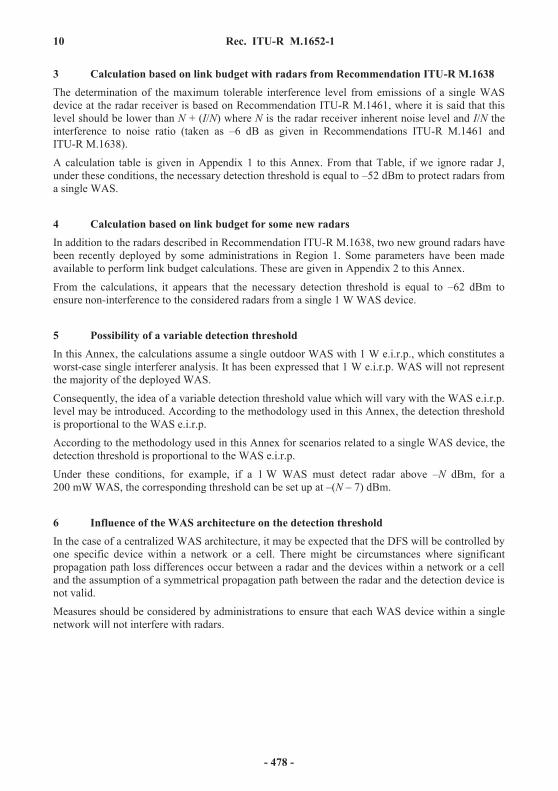
10 Rec. ITU-R M.1652-1
3 Calculation based on link budget with radars from Recommendation ITU-R M.1638 The determination of the maximum tolerable interference level from emissions of a single WAS device at the radar receiver is based on Recommendation ITU-R M.1461, where it is said that this level should be lower than N + (I/N) where N is the radar receiver inherent noise level and I/N the interference to noise ratio (taken as –6 dB as given in Recommendations ITU-R M.1461 and ITU-R M.1638).
A calculation table is given in Appendix 1 to this Annex. From that Table, if we ignore radar J, under these conditions, the necessary detection threshold is equal to –52 dBm to protect radars from a single WAS.
4 Calculation based on link budget for some new radars In addition to the radars described in Recommendation ITU-R M.1638, two new ground radars have been recently deployed by some administrations in Region 1. Some parameters have been made available to perform link budget calculations. These are given in Appendix 2 to this Annex.
From the calculations, it appears that the necessary detection threshold is equal to –62 dBm to ensure non-interference to the considered radars from a single 1 W WAS device.
5 Possibility of a variable detection threshold In this Annex, the calculations assume a single outdoor WAS with 1 W e.i.r.p., which constitutes a worst-case single interferer analysis. It has been expressed that 1 W e.i.r.p. WAS will not represent the majority of the deployed WAS.
Consequently, the idea of a variable detection threshold value which will vary with the WAS e.i.r.p. level may be introduced. According to the methodology used in this Annex, the detection threshold is proportional to the WAS e.i.r.p.
According to the methodology used in this Annex for scenarios related to a single WAS device, the detection threshold is proportional to the WAS e.i.r.p.
Under these conditions, for example, if a 1 W WAS must detect radar above –N dBm, for a 200 mW WAS, the corresponding threshold can be set up at –(N – 7) dBm.
6 Influence of the WAS architecture on the detection threshold In the case of a centralized WAS architecture, it may be expected that the DFS will be controlled by one specific device within a network or a cell. There might be circumstances where significant propagation path loss differences occur between a radar and the devices within a network or a cell and the assumption of a symmetrical propagation path between the radar and the detection device is not valid.
Measures should be considered by administrations to ensure that each WAS device within a single network will not interfere with radars.
- 478 -

Rec. ITU-R M.1652-1 11
App
endi
x 1
to A
nnex
5
Cal
cula
tion
of d
etec
tion
thre
shol
d ba
sed
on li
nk b
udge
t for
the
rada
rs o
f Rec
omm
enda
tion
ITU
-R M
.163
8
Cha
ract
erist
ics
AC
EF
GH
1H
2I1
I1J
KL
MN
OP
Q
RADAR
Func
tion
Met
eoM
eteo
Met
eoM
eteo
Met
eoM
eteo
Met
eoM
eteo
Met
eoM
eteo
Inst
rum
en-
tatio
nIn
stru
men
-ta
tion
Inst
rum
en-
tatio
nIn
stru
men
-ta
tion
Inst
rum
en-
tatio
nSu
rface
an
dai
r se
arch
Surfa
ce
and
air
sear
ch
Plat
form
type
Gro
und/
sh
ipG
roun d
Gro
und
Gro
un dG
roun d
Gro
und
Gro
un dG
roun d
Gro
und
Gro
un dG
roun
dG
roun
dG
roun
dG
roun
dG
roun
dSh
ipSh
ip
Tx p
ower
into
ant
enna
pea
k (k
W)
250
250
250
250
250
250
250
250
250
2.25
250
280
01
200
100
016
536
028
5
Rec
eive
r IF 3
dB
band
wid
th
(MH
z)0.
520
0.91
0.6
0.5
0.7
40.
13
101
4.8
48
81.
510
Ant
enna
pol
ariz
atio
nV
HH
HH
HH
HH
HV
/left-
hand
ci
rcul
arV
/left-
hand
ci
rcul
arV
/left-
hand
ci
rcul
arV
/left-
hand
ci
rcul
arV
/left-
hand
ci
rcul
arH
H
Ant
enna
mai
n be
am g
ain
(dB
i)39
4450
4040
5050
5050
3538
.354
4745
.942
2830
Ant
enna
hei
ght (
m)
3010
3030
3030
3030
3010
e.i.r
.p. r
adar
(dB
m)
123.
012
8.0
134.
012
4.0
124.
013
4.0
134.
013
4.0
134.
098
.512
2.3
148.
513
7.8
135.
912
4.2
113.
611
4.5
Rec
eive
r noi
se fi
gure
(dB)
74
2.3
33
3.5
3.5
1.5
1.5
36
55
115
510
N=
k T
B F
(dB
m)
–110
.0–9
7.0
–112
.1–1
13.2
–114
.0–1
12.0
–104
.5–1
22.5
–107
.7–1
01.0
–108
.0–1
02.2
–103
.0–9
3.9
–99.
9–1
07.2
–94.
0
N–
6 dB
–116
.0–1
03.0
–118
.1–1
19.2
–120
.0–1
18.0
–110
.5–1
28.5
–113
.7–1
07.0
–114
.0–1
08.2
–109
.0–9
9.9
–105
.9–1
13.2
–100
.0
WAS
e.i.r
.p. (
dBm
) out
door
30
TPC
(dB
)0
Band
wid
th (M
Hz)
18
Ant
enna
gai
n (o
mni
) (dB
i)0
10 lo
g (B
rad/
BWA
S)–1
5.6
0.5
–13.
0–1
4.8
–15.
6–1
4.1
–6.5
–22.
6–7
.8–2
.6–1
2.6
–5.7
–6.5
–3.5
–3.5
–10.
8–2
.6
185.
017
7.0
198.
118
9.2
190.
019
8.0
190.
520
8.5
193.
717
2.0
182.
319
2.2
186.
017
5.8
177.
917
1.2
160.
0
Link
bud
get f
or W
AS
sign
al
rece
ived
at r
adar
rece
iver
N–
6 dB
169.
417
7.0
185.
117
4.4
174.
418
3.9
183.
918
5.9
185.
916
9.4
169.
718
6.4
179.
417
2.3
174.
416
0.4
157.
4
Nec
essa
ry d
etec
tion
thre
shol
d–4
6.4
–49.
0–5
1.1
–50.
4–5
0.4
–49.
9–4
9.9
–51.
9–5
1.9
–70.
9–4
7.4
–38.
0–4
1.6
–36.
4–5
0.2
–46.
9–4
2.9
- 479 -

12 Rec. ITU-R M.1652-1
Appendix 2 to Annex 5
Calculation of detection threshold based on link budget for new radar deployed by some administrations in Region 1
RA
DA
R
Function Air search
Platform type Ground/vehicle
Tx power into antenna peak (kW) 15
Receiver IF3 dB bandwidth (MHz) 4
Antenna polarization V
Antenna main beam gain (dBi) 35
Antenna height (m) 10
e.i.r.p. (dBm) 106.8
Receiver noise figure (dB) 5
N = k T B F (dBm) –103
N – 6 dB –109
WA
S
e.i.r.p. (dBm) outdoor 30
TPC (dB) 0
Bandwidth (MHz) 18
Antenna gain (omni) (dBi) 0
10 log (Brad/BWAS) –6.5
Propagation loss for WAS signal received at the radar receiver N – 6 dB (dB) 175.0
168.4
Necessary detection threshold (dBm) –61.7
It is noted that this Table assumes a single 1 W e.i.r.p. WAS, which may be the highest power value in a statistical distribution of the e.i.r.p. in a deployment of WAS (e.g., as described in Table 6 of Annex 6). For example, consideration of a lower e.i.r.p. (< 100 mW) will lead to a corresponding increase by 10 dB of TDFS.
- 480 -

Rec. ITU-R M.1652-1 13
Annex 6
Parameters and methodology for conducting aggregate interference studies involving WAS including RLANs and radiodetermination systems
in the 5 GHz band
The following considerations should be utilized to define the baseline scenario for studies to be conducted in determining DFS parameters: – Recommendation ITU-R M.1461 was utilized in interference calculations. – The radar antenna pattern contained in Appendix 1 to this Annex was utilized. – The WAS antenna pattern contained in Appendix 2 to this Annex was utilized. – The probability of detection (see Annex 4) was utilized in the sharing studies to determine
the aggregate interference into radars. This probability was set for each step interval. – A step interval of 1° was utilized. – Three concentric rings were utilized to define the WAS deployment as shown in Table 5.
Uniform distribution of devices in each zone should be utilized throughout each volumetric zone including height.
TABLE 5
WAS user distribution
Urban zone Suburban zone Rural zone
Radius from the centre (km) 0-4 4-12 12-25WAS user (%) 60 30 10Building height (m) 30 6 6
– A total of 2 753 WAS devices operating on a co-channel basis with a radiodetermination system at a given moment was utilized.
– WAS power distribution in Table 6 was utilized.
TABLE 6
WAS power distribution
Power level 1 W 200 mW 100 mW 50 mWWAS users (%) 5 25 40 30
– Tracking radars were modelled starting with random placement and a random start angle and then moving directly overhead to the opposite horizon.
– Maritime radars were modelled starting at the horizon of the rural area and tracked into the centre of the urban zone.
– Airborne radars were modelled starting at the horizon of the rural area and tracked over the centre of the urban zone.
- 481 -

14 Rec. ITU-R M.1652-1
– The studies focused on the following radars: C, I, K, P and S as defined in Recommendation ITU-R M.1638.
– For ground-based radars a random propagation factor was utilized in determining the propagation path loss to each WAS device. A value from 20 to 35 log D was used. In addition a random building/terrain propagation attenuation was used. A value from 0 to 20 dB was used. A uniform distribution was applied in determining these values.
– For airborne radars, free space loss +17 dB was used. – For maritime radars, free space loss +0 to 20 dB was used. – A smooth Earth line-of-sight calculation was utilized. Any WAS devices beyond the
line-of-sight were discounted.
Appendix 1 to Annex 6
There are no existing radar antenna reference patterns currently in ITU, therefore the following is provided as a baseline. A statistical gain antenna model is used to determine the radar antenna gain in the azimuth and elevation orientations. The model gives the antenna gain as a function of off-axis angle ( ) for a given main beam antenna gain (G). The model includes separate algorithms for very high-gain, high-gain, and medium-gain antennas, corresponding to antennas with gains greater than 48 dBi, gains between 22 and 48 dBi, and gains between 10 and 22 dBi, respectively. Figure 1 illustrates the general form of the antenna gain distribution. The equations for the angles M (first side-lobe shelf), R (near side-lobe region), and B (far side-lobe region) are given in Table 7. The antenna gains as a function of off-axis angle, are given in Table 8 for very high-gain antennas, in Table 9 for high-gain antennas, and in Table 10 for medium-gain antennas. The angle is in degrees and all gain values are given in terms of decibels relative to an isotropic antenna (dBi).
FIGURE 1
M.1652-01
G
G(
)(dB
i)
0° 180°M R B
- 482 -

Rec. ITU-R M.1652-1 15
TABLE 7
Angle definitions
Very high-gain(G > 48 dBi)
High-gain(22 < G < 48 dBi)
Medium-gain(10 < G < 22 dBi)
M = 50 (0.25 G + 7)0.5/10G/20
R = 27.466 10–0.3G/10
B = 48
M = 50 (0.25 G + 7)0.5/10G/20
R = 250/10G/20
B = 48
M = 50 (0.25 G + 7)0.5/10G/20
R = 250/10G/20
B = 131.8257 10–G/50
TABLE 8
Equations for very high-gain antennas (G > 48 dBi)
Angular interval(degrees)
Gain(dBi)
0 to M
M to R
R to B
B to 180
G – 4 × 10⁻⁴ (10G/10) 2
0.75 G – 729 – 25 log ( )
–13
TABLE 9
Equations for high-gain antennas (22 < G < 48 dBi)
Angular interval(degrees)
Gain(dBi)
0 to M
M to R
R to B
B to 180
G – 4 × 10⁻⁴ (10G/10) 2
0.75 G – 753 – (G/2) – 25 log ( )
11 – G/2
TABLE 10
Equations for medium-gain antennas (10 < G < 22 dBi)
Angular interval(degrees)
Gain(dBi)
0 to M
M to R
R to B
B to 180
G – 4 × 10⁻⁴ (10G/10) 2
0.75 G – 753 – (G/2) – 25 log ( )
0
- 483 -
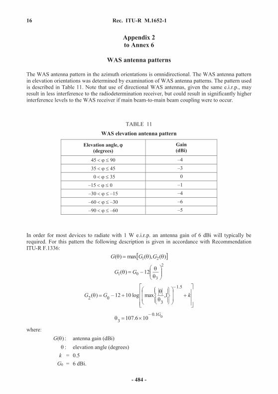
16 Rec. ITU-R M.1652-1
Appendix 2 to Annex 6
WAS antenna patterns
The WAS antenna pattern in the azimuth orientations is omnidirectional. The WAS antenna pattern in elevation orientations was determined by examination of WAS antenna patterns. The pattern used is described in Table 11. Note that use of directional WAS antennas, given the same e.i.r.p., may result in less interference to the radiodetermination receiver, but could result in significantly higher interference levels to the WAS receiver if main beam-to-main beam coupling were to occur.
TABLE 11
WAS elevation antenna pattern
In order for most devices to radiate with 1 W e.i.r.p. an antenna gain of 6 dBi will typically be required. For this pattern the following description is given in accordance with Recommendation ITU-R F.1336: )(),(max)( 21 GGG
2
301 12–)( GG
kGG5.1–
302 1,maxlog1012–)(
01.0–3 106.107
G
where: G( ) : antenna gain (dBi)
: elevation angle (degrees) k = 0.5
G0 = 6 dBi.
Elevation angle, (degrees)
Gain(dBi)
45 90 –4
35 45 –3
0 35 0
–15 0 –1
–30 –15 –4
–60 –30 –6
–90 –60 –5
- 484 -

Rec. ITU-R M.1652-1 17
Annex 7
Interference assessment results analysis and recommendation on DFS threshold values
A summary of the results of simulations using the methodologies detailed in Annexes 5 and 6, for simulating respectively static interference from one WAS device and aggregate interference from a deployment of WAS into a victim radar receiver, is presented for the relevant 5 GHz radars.
Table 12 shows the values derived from the calculations in Annex 5 for the case of interference from a single WAS.
TABLE 12
Values derived from the calculations in Annex 5
Table 13 shows a summary of required protection threshold levels resulting from the aggregate interference modelling calculations.
TABLE 13
Required protection threshold levels
Radar type Simulation scenario DFS threshold for protection (TDFS) (Note 1)
Rotating radars A, C, E, F, G, H, I, JRadars P and Q
Standard per Annex 6 –52 dBm and operational considerations utilized by radar systems
Radar I Annex 6 but radar antenna height between 500 and 1 000 m
–62 dBm
Radar S Standard per Annex 6 See Note 2Radar K Standard per Annex 6 –67 dBm
Annex 6 but half population density
–64 dBm
Annex 6 but all devices 50 mW –62 dBm
NOTE 1 – Assuming a receive antenna gain normalized to 0 dBi for WAS.NOTE 2 – The sharing situation between this radar and WAS is extremely difficult. Initial calculations based on the baseline results show that a required DFS detection threshold of valuesbelow the operating noise floor of WAS devices would be required. Based on discussions, it was found that these systems were limited to military aircraft only. It was agreed to not consider this case when developing a detection threshold requirement.
Radar per Annex 5 Link budget analysis per Annex 5
–62 dBm for 1 W device–55 dBm for 0.2 W device–52 dBm for 0.1 W device
- 485 -

18 Rec. ITU-R M.1652-1
Notes on parameters and methodologies used The impact of the parameters and methodology variations can be summarized as follows: a) A reduction in active device density by half results in a 3 dB increase in TDFS. Similarly,
doubling the active device density results in a 3 dB decrease in TDFS. b) The transmit power of a single interferer in the link budget calculation has a direct dB for
dB impact on the required protection threshold. In the aggregate analysis, the impact depends on the distribution of power levels used in the simulation.
c) In most cases the interaction of variables in the aggregate modelling is not intuitive and therefore simple conclusions cannot be drawn from changes in a single variable.
- 486 -

Rec. ITU-R M.1827-1 1
RECOMMENDATION ITU-R M.1827-1
Guideline on technical and operational requirements for stations of the aeronautical mobile (R) service limited to surface application at airports in the
frequency band 5 091-5 150 MHz (2007-2015)
Scope
This Recommendation provides technical and operational requirements for stations of the aeronautical mobile (route) service (AM(R)S) limited to surface applications at airports in the frequency band 5 091-5 150 MHz that should be used by administrations as a technical guideline for establishing conformance requirements for stations for worldwide use.
Keywords AM(R)S, FSS, airport, conformance.
Abbreviations/Glossary AM(R)S Aeronautical mobile (route) service
ARNS Aeronautical radionavigation service
FSS Fixed satellite service
The ITU Radiocommunication Assembly,
considering
a) that the aeronautical stations will operate on a national, regional and international basis around the world;
b) that circulation of aeronautical stations is usually a subject of a number of national and international rules and regulations including satisfactory conformance to a mutually agreed technical standard and operational requirements of the International Civil Aviation Organisation;
c) that there is a need for identifying the technical and operational requirements for the conformance testing of the aeronautical stations;
d) that the identification of technical and operational requirements for aeronautical stations would provide a common technical basis for facilitating conformance testing of aeronautical stations by various national, regional and international authorities and the development of mutual recognition arrangements for conformance of aeronautical stations;
e) that the technical and operational requirements need to achieve an acceptable balance between radiocommunication equipment complexity and the need for effective use of the radio-frequency spectrum,
considering also a) that there is a requirement to fully protect all primary services in the band 5 091-5 150 MHz;
b) that results of the studies conducted in accordance with Resolution 414 (Rev.WRC-03)showed the feasibility of using the frequency band 5 091-5 150 MHz by the AM(R)S limited to surface application at airports on a primary basis under certain conditions;
- 487 -

2 Rec. ITU-R M.1827-1
c) that the identification by ITU-R of technical and operational requirements for aeronautical stations operating in the frequency band 5 091-5 150 MHz should prevent unacceptable interference to other services;
d) that technical and operational characteristics should be continuously and accurately measurable and controllable,
recognizing a) that the frequency band 5 000-5 250 MHz is allocated to the aeronautical radionavigation service (ARNS) on a primary basis;
b) that the frequency band 5 030-5 150 MHz is to be used for the operation of the international standard microwave landing system for precision approach and landing. The frequency band 5 091-5 150 MHz is also used in the FSS for feeder links for non-geostationary mobile-satellite service systems. The requirements of the international standard microwave landing system shall take precedence over other uses of the band 5 030-5 091 MHz in accordance with No. 5.444 of the Radio Regulations,
recommends
1 that the technical and operational requirements for stations of AM(R)S limited to surface application at airports in the frequency band 5 091-5 150 MHz given in Annex 1 should be used by administrations as a guideline for ensuring compatibility with the fixed satellite service (FSS).
2 the following Note is considered as part of this Recommendation.
NOTE ‒ Due to the fact that other limits may also be acceptable and that all essential requirements are not covered by this Recommendation, further study is required, in particular with respect to the flexible apportionment of Ts/Ts approach used in this Recommendation
Annex 1
Essential requirements related to compatibility with fixed satellite service networks in the frequency band 5 091-5 150 MHz
For the analyses that follow, Table 1 summarizes the assumed FSS receiver characteristics.
TABLE 1
Parameter values used in satellite interference calculations
Parameter Units HIBLEO-4 FL
Satellite receiver noise temperature T K 550Antenna effective area at 5 120 MHz dB(m2) –35.6Polarization discrimination Lp dB 1Feed loss Lfeed dB 2.9Satellite receiver bandwidth B MHz 1.23Satellite receive antenna gain Gr dBi 4
- 488 -

Rec. ITU-R M.1827-1 3
NOTE – The compliance with the pfds defined below would be obtained under free-space propagation conditions.
Requirements on the aeronautical mobile (route) service The requirements that follow represent technical guidelines to be used by administrations for establishing conformance requirements for stations for worldwide use. Other limits may also be acceptable, however further study is required.
The pfd defined in this section is based on ensuring that the increase in noise temperature of the FSS satellite due to operation in the frequency band 5 091-5 150 MHz of the AM(R)S (i.e. ( Ts/Ts)AM(R)S)does not exceed the greater of the following two values:1) 2% 2) 5% – ( Ts/Ts)ARNS
where: ( Ts/Ts)ARNS: is the increase in noise temperature due to the ARNS in the same band.
Three examples of this calculation are provided below. The first assumes that the ( Ts/Ts)ARNS is 3%. The second assumes that no ARNS is present in the band. The third assumes that ( Ts/Ts)ARNS is >3%. The methodology assumes 2502 co-channel AM(R)S transmitters operating concurrently within the field of view of the FSS satellite.
Example 1: ( Ts/Ts)ARNS = 3%
In this case, 5% – ( Ts/Ts)ARNS equals 2%, hence, ( Ts/Ts)AM(R) S = 2%, i.e. –17 dB.Assuming the Table 1 characteristics for the FSS, the maximum aggregate interference level tolerable at the receiver input is IAgg-Rec: MHz)23.1/dB(W3.157dB17KTBI RecAgg
where: K: Boltzmann’s constant (1.38 × 10⁻²³ J/K) T: receiver noise temperature (K) B: receiver bandwidth (Hz).
Therefore at the satellite receiver antenna input the maximum pfd level produced by one AM(R)Stransmitter is:
)MHz23.1m/(dBW77.1456.3597.2319.243.157
4log10)250(log10
2
210PFeedRecAggMax LLGrIpfd
where: Gr: FSS receiver antenna gain
250: maximum number of AM(R)S stations emitting simultaneously in the FSS receiver bandwidth.
Example 2: ( Ts/Ts)ARNS = 0In this case, 5% – ( Ts/Ts)ARNS equals 5%, which is greater than 2%, Hence, ( Ts/Ts)AM(R)S = 5%, i.e. –13 dB.
- 489 -

4 Rec. ITU-R M.1827-1
Hence: MHz)23.1/dB(W3.153dB13KTBI RecAgg
Therefore at the satellite receiver antenna input the maximum pfd level produced by one AMRS transmitter is:
)MHz23.1m/(dBW77.141
6.3597.2319.243.153
4log10)250(log10
2
210PFeedRecAggMax LLGrIpfd
Example 3: ( Ts/Ts)ARNS > 3%
In this case, 5% – ( Ts/Ts)ARNS is smaller than 2%, Hence, ( Ts/Ts)AM(R)S = 2%, i.e. –17 dB, as inExample 1, and the same pfdMax value is obtained as in Example 1.
- 490 -

Rec. ITU-R M.2013-0 1
RECOMMENDATION ITU-R M.2013-0
Technical characteristics of, and protection criteria for non-ICAO aeronautical radionavigation systems, operating around 1 GHz
(2012)
Scope
This Recommendation describes the technical characteristics of, and protection criteria for, non-International Civil Aviation Organisation (ICAO) aeronautical radionavigation service (ARNS) systems operating around 1 GHz for use in compatibility studies. It concerns with non-ICAO ARNS systems operating in countries referred to in RR No. 5.312 and TACAN systems.
The ITU Radiocommunication Assembly,
considering
a) that the tactical air navigation system (TACAN) is an aeronautical radionavigation system used on a national basis and operates in the frequency band 960-1 215 MHz;
b) that the TACAN system is used by both civil and state aircraft;
c) that when used by civil aviation, TACAN functionally is equivalent to the ICAO standardized distance measuring equipment (DME);
d) that the TACAN system provides additional functionality to that of DME, i.e. obtaining bearing information;
e) that this additional functionality results in technical characteristics that differ from those of DME and may require additional consideration in future compatibility studies,
f) that the use of TACAN also includes shipborne and air-to-air applications,
noting
a) that according to Resolution 417 (WRC-07) precedence must be given to the ARNS operating in the frequency band 960-1 164 MHz;
b) that ITU-R studies have shown that following the introduction of aeronautical mobile (route) service (AM(R)S) in the frequency band 960-1 164 MHz, more detailed site-specific compatibility studies between TACAN and AM(R)S systems need to be performed,
recommends
that for compatibility studies the characteristics and protection criteria in the annexes should be used.
- 491 -

2 Rec. ITU-R M.2013-0
Annex 1
Tactical air navigation system
TACAN is an aeronautical radionavigation system used on a national basis operating between 960 and 1 215 MHz. A TACAN system consists of an interrogator on-board an aircraft and abeacon which gives the replies. In most cases the TACAN beacons are fixed ground based installations but there are maritime mobile and aeronautical mobile beacons in use as well. Depending on the generated e.i.r.p. and design of the interrogator slant ranges up to 400 nm(740 km) can be achieved but in practice the range is limited to the maximum radio line-of-sight (RLOS). The aircraft unit transmits regular pulse pairs, so-called interrogation pulses which are received by ground based installations (beacons). The TACAN pulses have a pulse width of 3.5 sat the 50% amplitude points. The spacing between the pulses of an interrogation pulse pair is 12 s(X channel) or 36 s (Y channel). After receiving an interrogator pulse pair a ground station will test the pulse shape and spacing. If these fall within the acceptance limits, it will respond by transmitting a reply after a fixed delay with a ±63 MHz frequency offset from the interrogation frequency depending on selected channel on pulse code. The beacon has a spacing between the reply pulses of 12 s (X channel) and 30 s (Y channel). After receipt of the reply, the interrogator will calculate the momentary slant range distance to the beacon from the time elapsed between transmitting interrogation and receiving reply pulse pairs.
The beacon will receive interrogations from many aircraft and therefore will send out many replies. Each interrogator creates a unique pattern by varying, within certain limits, the time between the pulse pairs to avoid generation of synchronic replies. By this principle each platform is able to recognize among all pulse pairs the replies that are initiated by its own interrogator.
For identification purposes, a TACAN beacon transmits a Morse ID code. The ID tone is used at the airborne interrogators to verify if the range readouts are provided by the correct beacon. Besides the pulse responses, proper reception of the ID tone is also an important condition for TACAN interrogators to properly function.
In addition to the range measurements TACAN also offers azimuth bearing information. The bearing information is provided by applying a modulation in the amplitude of the pulses transmitted by the ground beacon. This pulse amplitude modulation (PAM) is created using either a mechanically or electronically scanning beacon antenna. The variation in the azimuth pattern in the form of 15 Hz and 135 Hz antenna lobes at the maximum allowable modulation index of 55% will reduce the signal level of the reply pulses by up to 10.7 dB below the maximum e.i.r.p. level of pulses without PAM. In order for the interrogator to decode the orientation of the antenna pattern in reference to north from the PAM, an additional 900 pulse pairs, consisting of a north-reference-pulse-group (NRPG) and additional fine reference pulse groups (RPG) are transmitted by the beacon. In order to obtain accurate bearing information and be able to reply to at least 100 aircraft with 70% reply efficiency a constant number of at least 3 600 pulse pairs have to be transmitted.
The TACAN system is used for aeronautical navigation for both state aircraft as well as civil aviation. When used by civil aviation, the TACAN equipment is functionally equivalent to the ICAO standardized DME. TACAN characteristics are given in Table 1.
- 492 -

Rec. ITU-R M.2013-0 3
TAB
LE1
Typ
ical
cha
ract
eris
tics o
f TA
CA
N st
atio
ns
Purp
ose
Uni
tsR
adio
syst
ems f
or a
ir n
avig
atio
n (9
60-1
215
MH
z)
Rad
io tr
ansm
issi
on
dire
ctio
nEa
rth-a
ircra
ftA
ircra
ft-Ea
rthEa
rth-a
ircra
ftm
ariti
me
Airc
raft-
Earth
mar
itim
eA
ircra
ft –a
ircra
ft
Ope
ratin
g fr
eque
ncy
rang
e(M
Hz)
962-
121
31
025-
115
096
2-97
71
025-
108
81
025-
115
1
Ope
ratio
n ra
nge
(lim
ited
to R
LOS)
(k
m)
up to
600
up to
600
up to
600
up to
600
up to
740
Tran
smitt
ed
info
rmat
ion
Ran
ge a
nd b
earin
g re
spon
se si
gnal
s,Id
entif
icat
ion
info
rmat
ion
Ran
ge a
nd b
earin
g re
ques
t sig
nal
Ran
ge a
nd b
earin
g re
spon
se si
gnal
s,Id
entif
icat
ion
Ran
ge a
nd b
earin
g re
ques
t sig
nal
Ran
ge a
nd b
earin
g re
spon
se si
gnal
s,Id
entif
icat
ion
Tra
nsm
itter
cha
ract
eris
tics
Stat
ion
nam
eB
eaco
nIn
terr
ogat
orB
eaco
nIn
terr
ogat
orB
eaco
nH
eigh
t abo
ve th
e gr
ound
(m)
3(1
0ft)
up to
18
288
(60
000
ft)3
(10
ft)up
to 1
8 28
8(6
0 00
0ft)
up to
18
288
(60
000
ft)Si
gnal
type
Puls
edPu
lsed
Puls
edPu
lsed
Puls
edC
hann
el sp
acin
g(M
Hz)
11
11
1Ty
pe o
f mod
ulat
ion
Puls
e fo
rm a
nd p
ulse
pa
ir sp
acin
gPu
lse
form
and
pul
se
pair
spac
ing
Puls
e fo
rm a
nd p
ulse
pa
ir sp
acin
g Pu
lse
form
and
pul
se
pair
spac
ing
Puls
e fo
rm a
nd
puls
e pa
ir sp
acin
gTr
ansm
itter
pow
er
(pul
sed)
(dB
W)
39 (m
ax)
33 (m
ax.)
39 (m
ax)
33 (m
ax)
33 (m
ax)
Puls
e le
ngth
(s)
3.5
±0.
5 (5
0% a
mpl
itude
)3.
5 ±
0.5
(50%
am
plitu
de)
3.5
±0.
5 (5
0% a
mpl
itude
)3.
5 ±
0.5
(50%
am
plitu
de)
3.5
±0.
5 (5
0% a
mpl
itude
)Ty
pica
l dut
y fa
ctor
(%)
2.52
0.10
52.
520.
105
0.73
5A
nten
na ty
peC
ircul
ar a
rray
Om
nidi
rect
iona
lC
ircul
ar a
rray
Om
nidi
rect
iona
lC
ircul
ar a
rray
Typi
cal a
nten
na g
ain
dBi
60
60
6
- 493 -

4 Rec. ITU-R M.2013-0
TAB
LE 1
(end
)
Purp
ose
Uni
tsR
adio
syst
ems f
or a
ir n
avig
atio
n (9
60-1
215
MH
z)
Rec
eive
r ch
arac
teri
stic
sR
ecei
ving
stat
ion
Airc
raft
stat
ion
Airp
ort a
nd e
n-ro
ute
grou
nd st
atio
nA
ircra
ft st
atio
nsM
ariti
me
stat
ion
Airc
raft
stat
ion
Ope
ratin
g fr
eque
ncy
rang
e(M
Hz)
962-
121
31
025-
115
096
2-97
71
025-
108
81
025-
115
1
Hei
ght a
bove
the
grou
nd(m
)up
to 2
088
0(6
0 00
0ft)
3(1
0ft)
up to
20
880
(60
000
ft)3
(10
ft)up
to 2
088
0(6
0 00
0ft)
Rec
eive
r 3dB
ba
ndw
idth
(MH
z)2
2-4.
52
2-4.
52-
4.5
Max
/min
ant
enna
ga
in(d
Bi)
5.4/
09.
1/4.
15.
4/0
9.1/
4.1
5.4/
0
Pola
rizat
ion
Ver
tical
Ver
tical
Ver
tical
Ver
tical
Ver
tical
Rec
eive
r se
nsiti
vity
(dB
W)
−122
−122
−122
−122
−122
Max
imum
ac
cept
able
in
terf
eren
ce le
vel
base
d on
rece
ived
po
wer
(dB
W)
−129
−130
−129
−130
−129
NO
TE –
The
prot
ectio
n ra
tios
show
n in
Tab
le 1
wer
e ob
tain
ed f
or n
on-p
ulse
d si
gnal
s. In
cas
e of
pul
sed
sign
als
it is
req
uire
d to
car
ry o
ut a
dditi
onal
st
udie
s. In
this
resp
ect s
igna
ls w
ith a
pul
se le
ngth
of m
ore
than
50μs
are
con
side
red
non-
puls
ed o
r con
tinuo
us si
gnal
s.N
OTE
–Th
e ai
rbor
ne a
nten
na g
ain
is ta
ken
from
Rec
omm
enda
tion
ITU
-R M
.164
2-1.
NO
TE –
Mea
sure
men
ts o
n so
me
TAC
AN
dev
ices
sho
wed
that
the
TAC
AN
sen
sitiv
ity fo
r the
dis
tanc
e an
d an
gula
r mea
sure
men
ts o
nly
diff
er b
y 3
dB fo
r th
e TA
CA
N in
terr
ogat
or re
ceiv
er (−
90dB
m fo
r dis
tanc
e an
d −8
7dB
m fo
r ang
ular
mea
sure
men
t).
- 494 -

Rec. ITU-R M.2013-0 5
There is a large installed base of TACAN equipment, both ground stations (beacons) as well as aircraft stations (interrogators), in various administrations. The actual technical characteristics of the various types of equipment vary. One important factor, that determines the interference effect, is the receiver selectivity curve. Figure 1 shows the receiver selectivity curves of five types of TACAN interrogator equipment. It can be seen that there is a great spread in the selectivity of the different TACAN type receivers. In the compatibility studies all TACAN type interrogators should be taken into account in order to guarantee sufficient protection of this aeronautical radionavigation service (ARNS) application including both range and azimuth determination functionality.
Figure 2 shows a receiver selectivity curve for a typical TACAN beacon. The TACAN beacon selectivity is worse than those of the TACAN interrogator receivers.
FIGURE 1 Airborne station (interrogator) receiver RF-selectivity curves
F.5-1007-01
–20 –15 –10 –5 0 5 10 15 20
Frequency offset (MHz)
TACA interrogator receiver selectivity (indicative)
TACAN interrogator type 1
TACAN interrogator type 2
TACAN interrogator type 4
TACAN interrogator type 5
TACAN interrogator type 3
–90
–80
–60
–70
–50
–30
–40
–20
0
–10
10
Reje
ctio
n (d
B)
- 495 -

6 Rec. ITU-R M.2013-0
FIGURE 2 Ground station (beacon) receiver RF selectivity curves
F.5-1007-02
TACAN beacon receiver RF-selectivity
–80
–70
–60
–50
–40
–30
–20
–10
0
0 2 4 6 8 10 12
Frequency Offset (MHz)
Annex 2
Non-ICAO aeronautical radionavigation ystems operating in countries referred to in RR No. 5.312
Specifically the countries referred to in RR No. 5.312 of the Radio Regulations operate the aeronautical radionavigation systems of the following three types: – Type 1: the ARNS systems of the first type refer to direction-finding and ranging systems.
The systems are designed for finding an azimuth and a slant range of an aircraft as well as for area surveillance and inter-aircraft navigation. They are composed of airborne and ground-based stations. The airborne stations generate requesting signals transmitted via omnidirectional antennae and received at ARNS ground stations which also operate in an omnidirectional mode. The ground stations generate and transmit response signals containing azimuth/ranging information. Those signals are received and decoded at the ARNS airborne stations. The first type stations transmit the signals requesting the azimuth/ranging data outside the 960-1 164 MHz frequency band. After receiving a requesting signal the ARNS ground stations use the 960-1 164 MHz frequency band only for transmitting the ranging data to be received at the ARNS airborne stations. Thus the ARNS systems of the first type use the 960-1 164 MHz frequency band only for transmitting the signals in the surface-to-air direction. The maximum operation range for
- 496 -

Rec. ITU-R M.2013-0 7
the first type ARNS systems is 400 km. It is expected that in some of the countries mentioned in RR No. 5.312 the usage of Type 1 of ARNS mentioned above may be discontinued.
– Type 2: the ARNS direction-finding and ranging systems of the second type are designed for the same missions as the first type ARNS systems. The primary difference of the second type stations refers to the fact that requesting signals are transmitted by the airborne stations in the same frequency band as responding signals transmitted from the ground stations. Moreover, the ground-based ARNS stations of the second type can operate in both directional and omnidirectional modes. Directional mode provides increased number of operational channels at the ARNS stations. The maximum operation range for the first type ARNS systems is 400 km. It is planned to use the overall frequency band 960-1 164 MHz allocated to the ARNS in order to increase flexibility of operation of the second type ARNS systems. Application of the wideband tuning filter on the ARNS receiver front end is the design peculiarity of the second type ARNS systems which is stipulated by the necessity to receive signals on several channels simultaneously. The 3 dB bandwidth of this filter is 22 MHz and it allows receiving simultaneously up to five channels among 30 overlapping channels of 4.3 MHz each. The simultaneous usage of wideband filter and correlator allows increase in the accuracy of aircraft position data measurement and C/N ratio at the receiver front end as well. Type 2 of the ARNS system can operate in a limited number of countries mentioned in RR No. 5.312.
– Type 3: the ARNS systems of the third type are designed for operating at the approach and landing stages of flight. The system provides control functions of heading, range and glide path at aircraft approach and landing. The ARNS ground stations of the third type operate in both directional and omnidirectional modes. Operation range of the third type ARNS systems does not exceed 60 km. The 960-1 164 MHz frequency band is used for operation of the channels designed for control of the glide path and range between airborne and ground ARNS stations. Type 3 of the ARNS system can operate in a limited number of countries mentioned in RR No. 5.312.
Table 2 provides a brief technical description of the ARNS stations.
Thus the stations of the non-ICAO systems operate using the air-to-surface and surface-to-air links are made up of ground and airborne receivers and transmitters.
- 497 -

8 Rec. ITU-R M.2013-0
TABLE 2
Typical characteristics of the ARNS stations operating in the countries referred to in RR No. 5.312
ARNS system characteristics Type 1 Type 2 Type 3
PurposeRadio systems of
short-range navigation
Radio systems of short-range navigation
Radio systems of approachand landing
Operating frequency range 960-1 000.5 960-1 164
Radioline direction(MHz)
“Earth-aircraft” “Earth-aircraft” “aircraft-Earth” “Earth-aircraft”
“aircraft-Earth”
Operation range up to 400 up to 400 up to 400 up to 45 up to 45
Transmitted information(km)
Transmission of azimuthal signals,
range response signals and request
to indication
Transmission of azimuthal signals, range
response signals and request to indication
Transmission of range request
signal and indication
response signal
Transmission of signals in
glide path and course
channels and range response
signals
Transmission of range request
Transmitter characteristics
Station name Airport anden-route path
ground stations
Airport anden-route path
ground stations
Aircraft station Airport ground station
Aircraft station
Class of emission 700KРХХ 4M30P1N 4M30P1D 700KP0X; 4M30P1N
700KP0X; 4M30P1N
Channel spacing (MHz) 0.7 0.7 0.7 0.7 2Type of modulation pulsed pulsed pulsed pulsed pulsedTransmitter power (pulsed) (dBW) 20-45 29-39 27-33 3-30 5-33
Duty factor (%) 0.018; 0.066 0.064 - 0.3 0.00765 0.04; 0.025 0.009Mean output Power (min/max) (dBW) 7.6/13.2 7.1/13.8 −8.2 −4/−6 −7.5
Pulse length ( s) 1.5; 5.5 1.25; 1.5; 5.5 1.5 1.7 1.7Antenna type Omnidirectional array antenna omnidirectional array antenna omnidirectionalMax/min antenna gain(dBi) 6/0 15.6 3/−10 10/0 1.5/−3
Height above the ground (m) 10 10 up to 12 000 10 up to 12 000
- 498 -

Rec. ITU-R M.2013-0 9
TABLE 2 (end)
ARNS system characteristics Type 1 Type 2 Type 3
PurposeRadio systems of
short-range navigation
Radio systems of short-range navigation
Radio systems of approachand landing
Receiver characteristics
Receiving station Aircraft station Aircraft stationAirport and
en-route path ground stations
Aircraft station Airport ground station
Height above the ground (m) up to 12 000 up to 12 000 10 up to 12 000 10
Receiver 3 dB bandwidth (MHz) 1.5 22 22 7 7
Receiver noise temperature, K (K) 400 1 060 550 400 400
Max/min antenna gain (dBi) 1.5/−3 3/−10 14 1.5/−3 10/0
Polarization horizontal horizontal horizontal horizontal horizontalReceiver sensitivity (dBW) −120 −118 −125 −110…−120 −113Protection ratio C/I (dB) 25 17 20 25 25
NOTE – The protection ratios shown in Table 2 were obtained for non-pulsed signals. In case of pulsed signals it is required to carry out additional studies. In this respect signals with a pulse length of more than 50 μs are considered non-pulsed or continuous signals.
______________
- 499 -


Rec. ITU-R RS.2065-0 1
RECOMMENDATION ITU-R RS.2065-0
Protection of space research service space-to-Earth links in the 8 400-8 450 MHz and 8 450-8 500 MHz bands from unwanted emissions of synthetic aperture radars operating in the Earth exploration-satellite
service (active) around 9 600 MHz (2014)
Scope
This Recommendation provides mitigation techniques that can reduce the unwanted emissions of Earth exploration-satellite service (EESS) (active) systems in the space research service (SRS) band and recommends that EESS (active) systems fully protect the operations of SRS (deep space) missions during their critical events and prevent damages to the SRS earth station receivers at all times.
Keywords Critical events, damages, deep space, earth stations, EESS (active), interference, mitigation, protection, criterion, receiver, SAR, saturation, space-to-Earth, space research service, SRS, synthetic aperture radar, unwanted emissions
Abbreviations/Glossary EESS Earth exploration satellite service
LFM Linear FM (frequency modulation)
SAR Synthetic aperture radar
SRS Space research service
TR Transmit and receive
Related ITU Recommendations, Reports Recommendation ITU-R RS.2043 Characteristics of synthetic aperture radars operating in the
Earth exploration-satellite service (active) around 9 600 MHz
Recommendation ITU-R SA.609 Protection criteria for radiocommunication links for manned and unmanned near-Earth research satellites
Recommendation ITU-R SA.1014 Telecommunication requirements for manned and unmanned deep-space research
Recommendation ITU-R SA.1157 Protection criteria for deep-space research
Recommendation ITU-R SM.1541 Unwanted emissions in the out-of-band domain
Report ITU-R RS.2308 Radio frequency compatibility of unwanted emissions from 9 GHz EESS synthetic aperture radars with the Earth exploration-satellite service (passive), space research service (passive), space research service and radio astronomy service operating in the frequency bands 8 400-8 500 MHz and 10.6-10.7 GHz, respectively
- 501 -

2 Rec. ITU-R RS.2065-0
The ITU Radiocommunication Assembly,
considering a) that the frequency band 9 300-9 800 MHz is allocated to EESS (active) on primary basis;
b) that the frequency band 9 800-9 900 MHz is allocated to EESS (active) on secondary basis;
c) that the frequency band 8 400-8 450 MHz is allocated to SRS (deep space) space-to-Earth links on primary basis;
d) that the frequency band 8 450-8 500 MHz is allocated to SRS on primary basis for space-to-Earth links;
e) that systems operating active radars in the frequency band 9 300-9 900 MHz use high power emissions in the space-to-Earth direction;
f) that SRS (deep space) earth stations operating in the frequency band 8 400-8 450 MHz as described in Recommendation ITU-R SA.1014, use extremely sensitive receivers;
g) that these SRS earth stations also support SRS missions such as Lagrange and lunar missions in the frequency band 8 450-8 500 MHz;
h) that protection criteria of the SRS (deep space) missions in the frequency band 8 400-8 450 MHz is given in Recommendation ITU-R SA.1157 and the protection criteria of the SRS missions in the 8 450-8 500 MHz band is given in Recommendation ITU-R SA.609;
i) that the unwanted emissions of EESS (active) operating in the frequency band 9 300-9 900 MHz may exceed the SRS (deep space) protection criterion in the 8 400-8 450 MHz band;
j) that the frequency band 8 400-8 450 MHz is used by nearly all SRS (deep space) missions for support of their routine and critical events and the frequency band 8 450-8 500 MHz is used by nearly all SRS Lagrange and lunar missions;
k) that SRS (deep space) critical events such as launch, orbit insertion, planetary fly-by, and entry-descend-landing, including sample return, often determine the success of deep space missions;
l) that interference during the SRS (deep space) missions’ critical events can lead to the loss of critical data, or may even jeopardize the health and safety of a spacecraft;
m) that, during routine operations of the SRS (deep space) missions, unwanted emissions of EESS (active) exceeding the protection criterion of SRS (deep space) with a very small probability may be acceptable;
n) that unwanted emissions of EESS (active) may exceed the saturation levels and the damagelevels of SRS earth station receivers described in Annex 1,
recommends
1 that EESS SAR systems should use the methods described in Annex 2 to reduce their unwanted emissions in the frequency band 8 400-8 500 MHz in order to: a) avoid damaging the SRS earth station receivers at all times; b) reduce the probability of saturating SRS earth station receivers; c) avoid causing interference exceeding the protection criteria of the SRS (deep space) earth
stations during critical events;
- 502 -

Rec. ITU-R RS.2065-0 3
2 that, as a last resort, if recommends 1 cannot be satisfied fully by the application of the methods described in Annex 2, operators of EESS SAR systems should predict any remaining potential interference events and mitigate them by coordinating their operations with the operators of SRS missions at least seven days before an event for EESS SAR routine operations and at least 24 hours for EESS SAR acquisition of images in cases of emergency such as disaster management;
3 that in order to facilitate the use of some of the mitigation techniques as well as operational coordination, operators of EESS SAR and SRS systems should share the orbital and telecom characteristics of their respective operations, including the up-to-date trajectory of their missions, antenna pointing, and schedule of critical events;
4 that when applying recommends 1, 2 and 3, the damage and saturation levels of Table 1 of Annex 1 should apply;
5 that recommends 1, 2, 3 and 4 should only apply to the SRS earth stations listed in Recommendation ITU-R SA.1014.
Annex 1
Damage and saturation to front end of the SRS deep-space earth station receivers
The locations and characteristics of SRS deep-space receivers are described in Recommendation ITU-R SA.1014. The United States of America’s civil space agency, the National Aeronautics and Space Administration (NASA), and the European Space Agency (ESA) have provided characteristics of saturation and potential damage levels to their deep-space earth station receivers. These levels are summarized in the Table A1-1 below.
TABLE A1-1
Saturation and damage levels of SRS (deep space) earth station receivers
Parameter Unit NASA ESA
Frequency band MHz 8 200-8 700 8 400-8 500Saturation level dBW –115 –117Damage level dBW –105 –107
These saturation and damage levels are measured directly at the input terminal of the receiver front ends. NASA’s SRS deep-space earth station receivers are designed to also support NASA’s solar system radar operating in the 8 500-8 700 MHz band, which is allocated to the radiolocation service. SRS earth stations as described in Recommendation ITU-R SA.1014 are designed to also support SRS missions such as Lagrange missions and lunar missions in the 8 450-8 500 MHz band. These damage levels should not be exceeded at any time. The unwanted emission from the EESS (active) should be below the saturation level during the critical events of SRS deep-space missions. SRS earth stations that are not described in Recommendation ITU-R SA.1014 typically use different RF front-end technologies. They are typically less susceptible to saturation and damages from the unwanted emissions of EESS (active).
- 503 -

4 Rec. ITU-R RS.2065-0
Annex 2
Mitigation techniques for reducing unwanted emissions in the SRS in the frequency bands 8 400-8 450 MHz and 8 450-8 500 MHz from
the EESS (active) systems operating around 9 600 MHz
This Annex presents the computations of the theoretical unwanted emissions of EESS (active) systems around 9 600 MHz using the parameters for SAR-1, SAR-2 and SAR-3 from Recommendation ITU-R RS.2043. Several mitigation techniques to reduce the unwanted emissions of EESS (active) system in the 8 400-8 450 MHz SRS deep space band and in the 8 450-8 500 MHz SRS band are discussed.
1 Protection of SRS space-to-Earth links Recommendation ITU-R SA.1157 gives the protection criterion of deep-space research earth stations as –221 dB(W/Hz) for the SRS frequency band 8 400-8 450 MHz. The calculation of non-line-of-sight interference due to trans-horizon propagation should be based on weather statistics that apply for 0.001% of the time. Recommendation ITU-R SA.1157 provides the protection criterion for receiver systems in SRS deep-space systems. Compliance to the protection criterion for these assets determines the mission success of SRS deep-space missions. Harmful interference during mission critical events, e.g. orbit insertions, planetary fly-bys, and entry-decent-and-landing (EDL) phases, can cause potential loss of a spacecraft or the loss of irreplaceable data. There are also critical events such as one-time scientific observations where a spacecraft penetrates the atmosphere of a planet or a moon, or it impacts a moon, a planet, an asteroid, or a comet. The spacecraft may be destroyed in the process. The data transmitted during the approach or the moments before and during the impacts define the success of the missions. Therefore, the protection of SRS deep space spacecraft and earth stations during mission critical events, to the extent demanded by Recommendation ITU-R SA.1157, is crucial for the success of SRS deep-space missions.
In addition, spacecraft emergencies for deep space systems should be considered as critical events.
Additionally, Recommendation ITU-R SA.609 gives the protection criterion of space research earth stations as –216 dB (W/Hz) for the SRS frequency band 8 450-8 500 MHz. The calculation of interference that may result from atmospheric and precipitation effects should be based on weather statistics for 0.1% of the time for unmanned missions such as Lagrange and lunar missions.
2 Characteristics of EESS (active) systems around 9 600 MHz The 9 300-9 900 MHz band, typically identified by as the 9 600 MHz EESS (active) band, is used by SAR systems. Recommendation ITU-R RS.2043 provides the characteristics of three SAR systems operating in band.
- 504 -

Rec. ITU-R RS.2065-0 5
TABLE A2-1
Characteristics of SAR-1, SAR-2 and SAR-3 systems
Parameter SAR-1 SAR-2 SAR-3
Orbital altitude (km) 400 619 506Orbital inclination (degrees) 57 98 98RF centre frequency (GHz) 9.6 9.6 9.6Peak radiated power (W) 1 500 5 000 25 000Pulse modulation Linear FM chirp Linear FM chirp Linear FM chirpChirp bandwidth (MHz) 10 400 450Pulse duration ( s) 33.8 10-80 1-10Pulse repetition rate (pps) 1 736 2 000-4 500 410-515Duty cycle (%) 5.9 2.0-28.0 0.04-0.5Range compression ratio 338 < 12 000 450-4 500Antenna type Slotted waveguide Planar array Planar phased
arrayAntenna peak gain (dBi) 44.0 44.0-46.0 39.5-42.5e.i.r.p. (dBW) 75.8 83.0 83.5-88.5Antenna orientation from Nadir 20° to 55° 34° 20° to 44°Antenna beamwidth 5.5° (El)
0.14° (Az)1.6-2.3° (El)
0.3° (Az)1.1-2.3° (El)1.15° (Az)
Antenna polarization Linear vertical Linear HH or VV Linearhorizontal/vertical
System noise temperature (K) 551 500 600
3 Unwanted emission of EESS (active) systems in the frequency range 8 400-8 500 MHz The theoretical unwanted emission levels of the three SAR systems described in Table A2-1 in the frequency band 8 400-8 450 MHz are shown in Table A2-2. The linear FM (LFM) SAR systems are assumed to have 10-ns rise-time and 10-ns fall-time with trapezoidal waveforms. The pulse durations for SAR-2 and SAR-3 systems are 10 s and 1 s, respectively. The SRS deep space earth station antenna gain is 74 dBi.
- 505 -

6 Rec. ITU-R RS.2065-0
TABLE A2-2
Unwanted emissions from SAR-1, SAR-2, and SAR-3 in the 8 400-8 450 MHz band
Parameter SAR-1 SAR-2 SAR-3
e.i.r.p. (dBW) 76 83 86Bandwidth (MHz) 10 400 450Minimum slant range (km) 424 654 536Space loss (dB) –164 –167 –166Rx antenna peak gain (dBi) 74 74 74Polarization loss (dB) –3 –3 –3Spectral roll-off (dB) –109 –86 –78Rx interference PSD (dB(W/Hz)) –196 –185 –174Deep-space protection criterion (dB(W/Hz)) –221 –221 –221Exceedance of protection criterion (dB) 25 36 47
Table A2-2 shows that the unwanted emissions of SAR-1, SAR-2, and SAR-3 systems exceed the deep space protection criterion by 25-47 dB. The unwanted emissions from the SAR systems are computed based on theoretical roll-off of SAR signals. Higher unwanted emissions are possible if EESS (active) systems include components such as high-efficiency power amplifiers operating in saturation modes. Computation of unwanted emissions of the SAR systems using Annex 8 of Recommendation ITU-R SM.1541 results in higher wanted emissions, and hence, higher interference to the deep-space space-to-Earth links in the frequency band 8 400-8 450 MHz. To compute the attenuation levels needed to protect SRS (deep space) operations and to protect the SRS receivers from damages, the unwanted emissions of EESS (active) hardware, rather than theoretical values, should be used.
The level of unwanted emissions falling in the frequency band 8 450-8 500 MHz would even be higher due to the reduced frequency separation. Although studies show that there would not be any harmful interference issue for this band, there may be a risk of saturation and damage of the earth station receivers in case of direct illumination, which requires specific mitigation techniques to also apply in this band.
4 Mitigation techniques Several interference mitigating techniques are described in this section. Potential interference from the unwanted emissions of EESS (active) systems can be reduced using one or a combination of some of the techniques described. Generally, the first three techniques, pulse shaping, antenna pointing, and filtering, can significantly reduce the unwanted emissions of EESS (active) systems.
4.1 Pulse shaping Pulse shaping changes the envelope of the LFM chirp pulses to reduce the unwanted emissions of the radar. Compared to a LFM system with 10-ns rise-time and 10-ns fall-time, pulse shaping with trapezoid waveforms and raised-cosine waveforms with 100-ns rise time and 100-ns fall-time can theoretically reduce the unwanted emissions of LFM radars by about 17 dB to 26 dB. Table A2-3 shows that the 100-ns rise-time and 100-ns fall-time trapezoid waveform can reduce the unwanted emission of SAR-1 system to be below the protection level of SRS deep space, although the unwanted emissions of SAR-2 and SAR-3 still exceed the protection level. With the raised-cosine pulse shaping, the unwanted emissions of all three SAR systems are below the protection criterion.
- 506 -

Rec. ITU-R RS.2065-0 7
It should be noted that imperfections and nonlinearities of various components in the EESS (active) transmit chain will likely increase the unwanted emissions.
TABLE A2-3
Unwanted emissions of EESS (active) with 100-ns rise-time and fall-time trapezoid waveform in the 8 400-8 450 MHz band
Parameter SAR-1 SAR-2 SAR-3e.i.r.p. (dBW) 76 83 86Bandwidth (MHz) 10 400 450Minimum slant range (km) 424 654 536Space loss (dB) –164 –167 –166Rx antenna peak gain (dBi) 74 74 74Polarization loss (dB) –3 –3 –3Spectral roll-off (dB) –135 –106 –95Rx interference PSD (dB(W/Hz)) –222 –205 –191Deep-space protection criterion (dB(W/Hz)) –221 –221 –221Exceedance of protection criterion (dB) –1 16 30
TABLE A2-4
Unwanted emissions of EESS (active) with 100-ns rise-time and fall-time raised-cosine waveform in the 8 400-8 450 MHz band
Parameter SAR-1 SAR-2 SAR-3
e.i.r.p. (dBW) 76 83 86Bandwidth (MHz) 10 400 450Minimum slant range (km) 424 654 536Space loss (dB) –164 –167 –166Rx antenna peak gain (dBi) 74 74 74Polarization loss (dB) -3 –3 –3Spectral roll-off (dB) –168 –147 –137Rx interference PSD (dB(W/Hz)) –255 –246 –233Deep-space protection criterion (dB(W/Hz)) –221 –221 –221Exceedance of protection criterion (dB) –34 –25 –12
4.2 Antenna pointing All three SAR systems in Report ITU-R RS.2094 have highly directional antennas. For example, the antenna peak gain of SAR-2 system is between 43 dBi and 46 dBi. The antenna pattern rolls-off quickly in horizontal (or azimuth) direction to –3 dBi. If SAR-2 can point the antenna away from the SRS earth stations such that the antenna gain is –3 dBi towards the SRS earth stations, the unwanted emission of SAR-2 system can be reduced by 46 to 49 dB. Similar technique will also work for SAR-1 and SAR-3 systems.
- 507 -

8 Rec. ITU-R RS.2065-0
4.3 Filtering Depending on the implementations of EESS (active) systems, transmit filters and waveguides with steep cut-off below the EESS (active) band can be implemented to limit the unwanted emissions of the systems. Filtering techniques have been successfully implemented by EESS space-to-Earth links in the frequency band 8 025-8 400 MHz to reduce the unwanted emissions of EESS space-to-Earth links by 40 dB and more in the frequency band 8 400-8 450 MHz.
SAR systems may use phased array antennas which are composed of several hundreds of transmission and receive (TR) modules including high-power amplifiers. Any output filtering would have to be applied to the high power stages of these modules and, thus, increases the system complexity, costs, and performance losses of the radar.
However, if needed, an appropriate notch filter may be added in the transmission chain in order to attenuate to the best possible extend the unwanted emissions of the SAR, in a limited bandwidth.
4.4 Selection of sweep range and pulse width The spectral roll-off of the unwanted emission for LFM radar is a function of both the frequency sweep range and the pulse width of the LFM chirp signal. The unwanted emission increases as the chirp sweep range increases. It also increases as the pulse width of the chirp signal decreases. It may be possible for an EESS (active) operator to vary the radar sweep range and pulse duration to reduce the unwanted emission, especially when the EESS (active) antenna is pointing near as SRS deep-space earth station. The effectiveness of these techniques is limited. They may reduce the unwanted emission of an EESS (active) system by just a few decibels.
4.5 Geographic separation It is also possible to reduce the interference from EESS (active) systems through geographic separation. EESS (active) systems may keep a minimum slant range from an SRS earth station using the information in Recommendation ITU-R SA.1014 to maintain a minimum free space loss resulting in an exclusion zone. Taken to extreme, EESS (active) systems may refrain from transmission whenever there is line-of-sight between the EESS (active) systems and one of these SRS earth stations.
- 508 -

Rec. ITU-R RS.2066-0 1
RECOMMENDATION ITU-R RS.2066-0
Protection of the radio astronomy service in the frequency band 10.6-10.7 GHz from unwanted emissions of synthetic aperture radars operating in the
Earth exploration-satellite service (active) around 9 600 MHz (2014)
Scope
This Recommendation provides an operational procedure to avoid main-beam to main-beam coupling between Earth exploration-satellite service (EESS) (active) SAR-4 systems when transmitting near 9 600 MHz and radio astronomy service (RAS) stations performing observations in the band 10.6-10.7 GHz in order to avoid damage to the sensitive RAS low noise amplifier.
Keywords EESS (active), RAS, mitigation
Abbreviations/Glossary SAR Synthetic Aperture Radar
Related ITU Recommendations/Reports Recommendation ITU-R RS.2043 Characteristics of synthetic aperture radars operating in the
Earth exploration-satellite service (active) around 9 600 MHz
Report ITU-R RA.2188 Power flux-density and e.i.r.p. levels potentially damaging to radio astronomy receivers
Report ITU-R RS.2274 Spectrum requirements for spaceborne synthetic aperture radar applications planned in an extended allocation to the Earth exploration-satellite service around 9 600 MHz
Report ITU-R RS.2308 Radio frequency compatibility of unwanted emissions from 9 GHz EESS synthetic aperture radars with the Earth exploration-satellite service (passive), space research service (passive), space research service and radio astronomy service operating in the frequency bands 8 400-8 500 MHz and 10.6-10.7 GHz, respectively
The ITU Radiocommunication Assembly,
considering
a) that the frequency band 9 300-9 800 MHz is allocated to EESS (active) on a primary basis;
b) that the frequency band 9 800-9 900 MHz is allocated to EESS (active) on a secondary basis;
c) that the frequency band 10.6-10.7 GHz is allocated to the RAS on a primary basis;
d) that EESS (active) systems operating active radars around 9 600 MHz use high power chirp emissions in the space-to-Earth direction;
e) that radio astronomy stations operating in the frequency band 10.6-10.7 GHz use extremely sensitive low noise amplifiers;
- 509 -

2 Rec. ITU-R RS.2066-0
f) that Report ITU-R RA.2188 provides the power flux-density and e.i.r.p. levels potentially damaging RAS low noise amplifiers/ front-ends;
g) that the level of interference received by RAS stations from the emissions of EESS (active) systems may, under rare conditions of mainbeam to main beam coupling, reach or exceed the critical levels as given by Report ITU-R RA.2188,
recommends 1 that, in order to ensure compatibility of EESS SAR with RAS stations, EESS SAR systems operating around 9 600 MHz should avoid, to the maximum possible extent, to illuminate an area around radio astronomy stations. The size of such an area is defined in Annex 1. Annex 2 provides the list of RAS stations capable to operate in the frequency band 10.6-10.7 GHz and which may perform observations during times of illumination;
2 that, in the event that the conditions referred to in recommends 1 are not met, the operator of the EESS SAR system should contact the operator of the concerned radio astronomy station at least seven calendar days before an event for EESS SAR routine operations and at least 24 hours for EESS SAR acquisition of images in cases of emergency only such as disaster management in order to coordinate and, if necessary, to agree on mitigation or other preventive measures.
Annex 1
Determination of the protection area surrounding RAS stations
The emission beam contour corresponding to the margin determined by applying Recommendation ITU-R RA.2188 defines the damage zone for a potential boresight-to-boresight coupling of both antenna beams. Such a contour has the shape of an ellipse with a major axis h in the horizontal and the minor axis v in the vertical beam direction, thus defining an area where the power level at the RAS station would exceed –18 dBW. The projection onto the Earthʼs surface provides the dimension of an area of size with an extension of ± h in the horizontal direction and ± v in the vertical direction around the radio astronomy station which should be protected. Table 1 provides the parameter range for the avoidance of accidental damage to an RAS receiver1 with an antenna diameter of 100 m with regard to SAR-4 as described in Recommendation ITU-R RS.2043.
TABLE 1
Parameters for the avoidance of accidental damage to RA receivers
Incident angle Horizontal offset angle h
Vertical offset angle v
Horizontal separation (km) h
Vertical separation (km)
v
20° 1.02° 1.8° 9.6 18.255° 0.5° 1.1° 7.4 28.1
1 In the vertical direction, there is an asymmetry of 5.6% for v and v between inner and outer off-set
angles and distances which has been neglected. Only the larger outer value has been listed. The ground projections of the margin contours which are distorted ellipses were approximated by rectangles.
- 510 -

Rec. ITU-R RS.2066-0 3
Figure 1 provides the size of the area around the RAS station to be protected, depending on the RAS antenna diameter and the incidence angle. It can be seen that there is no constraint for RAS stations having an antenna diameter less than 17 m, and that the maximum separation distance from the RAS station is 28 km for most RAS stations.
FIGURE 1 Size of the area around RAS stations to be protected assuming EESS SAR-4 characteristics
RS.2066-01
250
200
150
100
50
01500 10050 200 300250 400350 500450
RAS antenna diameter (m)
Pro
tect
ion
dist
ance
(km
)
X: 100Y: 27.7
Vertical (cross satellite path) incidence 20°
Vertical (cross satellite path) incidence 55°
Horizontal (along satellite path) incidence 55°
Horizontal (along satellite path) incidence 20°
More generally, for a given incident angle i, the distance between the SAR satellite and the acquisition area is given by:
where: r: Earth radius (km) i: incidence angle (°) h: SAR altitude (km).
The corresponding angle between the nadir and the acquisition area in the vertical plane is given by:
where: r: Earth radius (km) i: incidence angle (°) h: SAR altitude (km).
The maximum gain of the RAS antenna can be derived from the antenna diameter and the frequency using the following equation:
where:
D: RAS antenna diameter (m) f: frequency (GHz).
- 511 -

4 Rec. ITU-R RS.2066-0
From these values, the SAR antenna gain limit that allows the received power limit of –18 dBW to be met is given by:
where: Prlimit: received power not to be exceeded (–18 dBW below 20 GHz)
Lp: free space loss (dB) Gr: RAS maximum antenna gain (dBi) Pe: SAR peak power (dBW).
Using the horizontal and vertical SAR antenna patterns, it is possible to determine the corresponding offset angles h and v. From these angles, one can derive the horizontal and vertical separation distances h and v.
where: r: Earth radius (km) d: slant range (km) : horizontal offset angle (°).
The slant range between the satellite and the RAS station that meets the received power limit is given by:
where: r: Earth radius (km) d: slant range between satellite and acquisition area (km) h: SAR satellite altitude (km)θv: angle between nadir and acquisition area in the vertical plane (°)
: vertical offset angle (°). And also, one can derive the vertical separation distance, δv:
where: r: Earth radius (km) d: slant range between satellite and acquisition area (km)
d+ : slant range between satellite and RAS station (km) θv: angle between nadir and acquisition area in the vertical plane (°)
: vertical offset angle (°).
- 512 -

Rec. ITU-R RS.2066-0 5
Annex 2
List of radio astronomy stations operating in the band 10.6-10.7 GHz Region 1
Country Name N Latitude E Longitude Antenna size (m)
Belgium Humain 50° 11' 30" 05° 15' 27" 4Finland Metsahövi 60° 13' 04" 24° 23' 37" 13.7Germany Effelsberg 50° 31' 29" 06° 53' 03" 100
Stockert 50° 34' 10" 06° 43 19 " 10Wettzell 49° 08' 41" 12° 52 40" 20, 13.2
Italy Medicina 44° 31' 14" 11° 38’ 49" 32Noto 36° 52 33'' 14° 59' 20'' 32Sardinia 39o 29' 34" 09o 14' 42" 64
Latvia Ventspils 57o 33' 12" 21o 51' 17" 32Norway Ny Ålesund 78o 55' 45" 11o 52' 15" 20Portugal Flores 38o 31' 12" -31o 07' 48" 13
Santa Maria 36° 58' 12" -25° 10' 12" 13Russia Badari 51o 45' 27" 102o 13' 16" 32
Kaliazyn 57° 13' 29" 37° 54' 01" 64Pushchino 54° 49' 20" 37° 37 53" 22Svetloe 61o 05' 00" 29o 46' 54" 32Zelenchukskaya 43° 49' 34" 41° 35' 12" 32
South Africa Hartebeesthoek –25° 52 48" –27° 40 48" 64MeerKAT –30° 43 16" 21° 24' 40" 64 antennas of 13.5
Spain Robledo 40° 25' 38" –04° 14' 57" 70.34Tenerife 28° 30' 00" -16° 30' 00" 12Yebes 40° 31' 27" –03° 05 22" 40
Sweden Onsala 57o 23' 45" 11o 55' 35" 20Onsala 57o 23' 35" 11o 55' 04" 2 antennas of 12
Switzerland Bleien 47o 20' 26" 08o 06' 44" 5Turkey Kayseri 38o 59' 45" 36o 17' 58" 5UK Merlin Cambridge
(mean)52° 10' 01" 00° 03' 08" 32
Merlin Knockin 52° 47' 25" –02° 59' 50" 25Merlin Darnhall 53° 09 23" –02° 32' 09" 25Merlin Jodrell Bank (mean)
53° 14 07" –02° 18' 23" 64
Merlin Pickmere 53° 17 19" –02° 26' 44" 25
- 513 -

6 Rec. ITU-R RS.2066-0
List of radio astronomy stations operating in the band 10.6-10.7 GHz Region 2
Country Name N Latitude E Longitude Antenna size (m)
Brasil Itapetinga –23° 11' 05" –46° 33' 28" 14Canada Algonquin Radio Obsy 45° 57' 19" –78° 04' 23" 3.7 and 9.1USA Arecibo 18° 20' 39" –66° 45' 10" 305
GGAO Greenbelt 39° 06' 00" –76° 29' 24" 12Green Bank Telescope 38° 25' 59" –79° 50' 23" 100Haystack 42° 36' 36" –71° 28' 12" 18Kokee Park 22° 07' 34" –159° 39' 54" 20Jansky VLA 33° 58' 22"
to34° 14' 56"
–107° 24' 40" to –107° 48' 22"
27 antennas of 25
VLBA Brewster, WA 48° 07' 52" –119° 41' 00" 25VLBA Fort Davis, TX 30° 38' 06" –103° 56' 41" 25VLBA Hancock, NH 42° 56' 01" –71° 59' 12" 25VLBA Kitt Peak, AZ 31° 57' 23" –111° 36' 45" 25VLBA Los Alamos, NM 35° 46' 30" –106° 14' 44" 25VLBA Mauna Kea, HI 19° 48' 05" –155° 27' 20" 25VLBA North Liberty, IA 41° 46' 17" –91° 34' 27" 25VLBA Owens Valley, CA 37° 13' 54" –118° 16' 37" 40VLBA Pie Town, NM 34° 18' 04" –108° 07' 09" 25VLBA St. Croix, VI 17° 45' 24" –64° 35' 01" 25Allen Telescope Array 40° 10' 44" –119° 31' 53" 42 antennas of 6Goldstone 35° 25' 33" –116° 53' 22" 70.3
- 514 -

Rec. ITU-R RS.2066-0 7
List of radio astronomy stations operating in the band 10.6-10.7 GHz Region 3
Country Name N Latitude E Longitude Antenna size (m)
Australia
Parkes –33º 00' 00" 148º 15' 44" 64Katherine –14º 22' 32" 132º 09' 09" 12Mopra –31º 16' 04" 149º 05' 58" 22ATCA (Narrabri) –30º 59' 52" 149º 32' 56" 6 antennas of 22Tidbinbilla –35º 24' 18" 148º 58' 59" 70, 34Hobart (Mt. Pleasant) –42º 48' 18" 147º 26' 21" 26Ceduna –31º 52' 05" 133º 48' 37" 30Yarragadee –29º 02' 47" 115º 20' 48" 12
China
Miyun 40º 33 29" 116º 58 37" 50
Sheshan 31º 05 58" 121º 11 59" 25
Nanshan 43º 28 16" 87º 10 40" 25Tianma 31° 05′ 13" 121° 09′ 48" 65CSRH 42° 12′ 31" 115° 14′ 45" 60 antennas of 2QTT 43° 36' 04" 89° 40' 57" 110
Japan
Nobeyama 35º 56' 40" 138º 28' 21" 45VERA-Mizusawa 39º 08' 01" 141º 07' 57" 20, 10VERA-Iriki 31º 44' 52" 130º 26' 24" 20VERA-Ogasawara 27º 05' 31" 142º 13' 00" 20VERA-Ishigakijima 24º 24' 44" 124º 10' 16" 20Ishioka 36º 12' 31" 140º 13' 36" 13.2Kashima 35º 57' 21" 140º 39' 36" 34Usuda 36º 07' 57" 138º 21' 46" 64Nishi-Waseda 35º 42' 25" 139º 43' 20" 2.4 antennas of 64Tomakomai 42º 40' 25" 141º 35' 48" 11Gifu 35º 28' 03" 136º 44' 14" 11Yamaguchi 34º 12' 58" 131º 33' 26" 32Tsukuba 36º 06' 11" 140º 05' 19" 32
Korea
KSWC (Jeju) 33º 42' 36" 126º 29' 26" 3 SGOC (Sejong) 36º 31' 12" 127º 18' 00" 22 K-SRBL 36° 24' 00" 127° 22' 12" 2 antennas of 2 KVN-Yonsei 37º 33' 55" 126º 56' 27" 21KVN-Ulsan 35º 32' 33" 129º 15' 04" 21KVN-Tamna 33º 17' 21" 126º 27' 37" 21
New Zealand Warkworth –36º 25' 59" 174º 39' 52" 30, 12
- 515 -


Cross-reference list of the regulatory provisions, including footnotes and Resolutions, incorporating ITU-R Recommendations by reference
Recommendation ITU-R Title of the Recommendation
RR provisions and footnotes with ITU-R Recommendations
contained in RR Volume 4
TF.460-6 Standard-frequency and time-signal emissions No. 1.14 (via Resolution 655 (WRC-15))
M.476-5 Direct-printing telegraph equipment in the maritime mobile service
Nos. 19.83, 19.96A, 51.41
M.489-2Technical characteristics of VHF radiotelephone equipment operating in the maritime mobile service in channels spaced by 25 kHz
Nos. 51.77, 52.231, Appendix 18(General notes e))
M.492-6 Operational procedures for the use of direct-printing telegraph equipment in the maritime mobile service
No. 56.2
P.525-4 Calculation of free-space attenuation No. 5.444B (via Resolution 748 (Rev.WRC-19))
P.526-15 Propagation by diffraction No. 5.444B (via Resolution 748 (Rev.WRC-19))
M.541-10 Operational procedures for the use of digital selective-calling equipment in the maritime mobile service
Nos. 51.35, 52.112, 52.149,52.153, 54.2
M.585-8 (Annex 1) Assignment and use of identities in the maritime mobile service
Nos. 19.99, 19.102, 19.111
M.625-4 Direct-printing telegraph equipment employing automatic identification in the maritime mobile service
Nos. 19.83, 51.41
M.633-4
Transmission characteristics of a satellite emergency position-indicating radio beacon (satellite EPIRB) system operating through a satellite system in the 406 MHz band
No. 34.1
S.672-4Satellite antenna radiation pattern for use as a design objective in the fixed-satellite service employing geostationary satellites
TABLE 22-2 (and No. 22.5D.3), TABLE 22-3 (and No. 22.5F.3)
M.690-3Technical characteristics of emergency position-indicating radio beacons operating on the carrier frequencies of 121.5 MHz and 243 MHz
Appendix 15 (Table 15-2)
RA.769-2(parts related to the application of No. 5.372)
Protection criteria used for radio astronomical measurements
No. 5.372
P.838-3 Specific attenuation model for rain for use in prediction methods
Appendix 30A (Annex 3 § 2.2 Step 6)
M.1084-5Interim solutions for improved efficiency in the use of the band 156-174 MHz by stations in the maritime mobile service
Appendix 18 (NOTE B) (prior to the table)
- 517 -

Recommendation ITU-R Title of the Recommendation
RR provisions and footnotes with ITU-R Recommendations
contained in RR Volume 4
SM.1138-3Determination of necessary bandwidths including examples for their calculation and associated examples for the designation of emissions
Appendix 1 (§ 1 and § 2)
SA.1154-0
Provisions to protect the space research (SR), space operations (SO) and Earth-exploration satellite services (EES) and to facilitate sharing with the mobile service in the 2 025-2 110 MHz and 2 200-2 290 MHz bands
No. 5.391
M.1171-0 Radiotelephony procedures in the maritime mobile service
Nos. 52.192, 52.195, 52.213,52.224, 52.234, 52.240, 57.1
M.1172-0 Miscellaneous abbreviations and signals to be used for radiocommunications in the maritime mobile service
No. 19.48
M.1173-1
Technical characteristics of single-sideband transmitters used in the maritime mobile service for radiotelephony in the bands between 1 606.5 kHz (1 605 kHz Region 2) and 4 000 kHz and between 4 000 kHz and 27 500 kHz
Nos. 52.181, 52.229,Appendix 17 (Part B, Section I§ 2 and § 6)
M.1174-4Technical characteristics of equipment used for on-board vessel communications in the bands between 450 and 470 MHz
Nos. 5.287, 5.288
M.1187-1A method for the calculation of the potentially affected region for a mobile-satellite service network in the 1-3 GHz range using circular orbits
Appendix 4 (Annex 2item C.11.b)
S.1256-0
Methodology for determining the maximum aggregate power flux-density at the geostationary-satellite orbit in the band 6 700-7 075 MHz from feeder links of non-geostationary satellite systems in the mobile-satellite service in the space-to-Earth direction
No. 22.5A
RS.1260-2 Feasibility of sharing between active spaceborne sensors and other services in the range 420-470 MHz
No. 5.279A
BO.1293-2Protection masks and associated calculation methods for interference into broadcast-satellite systems involving digital emissions
Appendix 30A (Annex 3 § 3.3), Appendix 30 (Annex 5 § 3.4)
S.1340-0Sharing between feeder links for the mobile-satellite service and the aeronautical radionavigation service in the Earth-to-space direction in the band 15.4-15.7 GHz
No. 5.511C
S.1428-1
Reference FSS earth-station radiation patterns for use in interference assessment involving non-GSOsatellites in frequency bands between 10.7 GHz and 30 GHz
TABLE 22-1A,TABLE 22-1B,TABLE 22-1C (and No. 22.5C.6)
BO.1443-3Reference BSS earth station antenna patterns for use in interference assessment involving non-GSO satellites in frequency bands covered by RR Appendix 30
TABLE 22-1D (and No. 22.5C.11)
- 518 -

Recommendation ITU-R Title of the Recommendation
RR provisions and footnotes with ITU-R Recommendations
contained in RR Volume 4
RA.1513-2
Levels of data loss to radio astronomy observations and percentage-of-time criteria resulting from degradation by interference for frequency bands allocated to the radio astronomy service on a primary basis
No. 5.372
M.1583-1
Interference calculations between non-geostationary mobile-satellite service or radionavigation-satellite service systems and radio astronomy telescope sites
No. 5.372, No. 5.443B (via Resolution 741 (Rev.WRC-15)), Appendix 4 Annex 2(item A.17.b.3) (via Resolution 741 (Rev.WRC-15))
S.1586-1Calculation of unwanted emission levels produced by a non-geostationary fixed-satellite service system at radio astronomy sites
No. 5.551H
F.1613-0
Operational and deployment requirements for fixed wireless access systems in the fixed service in Region 3 to ensure the protection of systems in the Earth exploration-satellite service (active) and the space research service (active) in the band 5 250-5 350 MHz
No. 5.447E
RA.1631-0
Reference radio astronomy antenna pattern to be used for compatibility analyses between non-GSO systems and radio astronomy service stations based on the epfd concept
No. 5.208B (via Resolution 739(Rev.WRC-19), No. 5.372,No. 5.443B (via Resolution 741 (Rev.WRC-15)), No. 5.551H,Appendix 4 Annex 2(item A.17.b.3) (via Resolution 741 (Rev.WRC-15))
M.1642-2
Methodology for assessing the maximum aggregate equivalent power flux-density at an aeronautical radionavigation service station from all radionavigation-satellite service systems operating in the 1 164-1 215 MHz band
Nos. 5.328A (via Resolution 609(Rev. WRC-07))
M.1643-0
Technical and operational requirements for aircraft earth stations of aeronautical mobile-satellite service including those using fixed-satellite service network transponders in the band 14-14.5 GHz (Earth-to-space)
No. 5.504B (refers to Annex 1, Part C of Rec. ITU-R M.1643-0), Nos. 5.504C, 5.508A and 5.509A(refer to Annex 1, Part B of Rec. ITU-R M.1643-0)
M.1652-1 (Annex 1and Annex 5)
Dynamic frequency selection in wireless access systems including radio local area networks for the purpose of protecting the radiodetermination service in the 5 GHz band
No. 5.446A, 5.447F, 5.450A (via Resolution 229 (Rev.WRC-19))
M.1827-1
Guideline on technical and operational requirements for stations of the aeronautical mobile (R) service limited to surface application at airports in the frequency band 5 091-5 150 MHz
No. 5.444B (via Resolution 748 (Rev.WRC-19))
M.2013-0Technical characteristics of, and protection criteria for non-ICAO aeronautical radionavigation systems, operating around 1 GHz
No. 5.327A (via Resolution 417 (Rev.WRC-15))
- 519 -

Recommendation ITU-R Title of the Recommendation
RR provisions and footnotes with ITU-R Recommendations
contained in RR Volume 4
RS.2065-0
Protection of space research service (SRS) space-to-Earth links in the 8 400-8 450 MHz and 8 450-8 500 MHz bands from unwanted emissions of synthetic aperture radars operating in the Earth exploration-satellite service (active) around 9 600 MHz
No. 5.474C
RS.2066-0
Protection of the radio astronomy service in the frequency band 10.6-10.7 GHz from unwanted emissions of synthetic aperture radars operating in the Earth exploration-satellite service (active) around 9 600 MHz
No. 5.474B
- 520 -


Rad
io R
egu
lati
on
sIT
U-R
Rec
om
men
dat
ions
inco
rpo
rate
d b
y re
fere
nce
Ed
itio
n o
f 202
0
Published in SwitzerlandGeneva, 2020
ISBN 978-92-61-30301-3 SAP id
9 789261 303013
4 3 5 1 3