arX

iv:0

805.

0189

v1 [

cond

-mat

.oth

er]

2 M

ay 2

008

Rabi switch of condensate wavefunctions in a multicomponent Bose gas

H.E. Nistazakis1, Z. Rapti2, D.J. Frantzeskakis1, P.G. Kevrekidis3, P. Sodano4 ∗, and A. Trombettoni51 Department of Physics, University of Athens, Panepistimiopolis, Zografos, Athens 15784, Greece

2 Department of Mathematics, University of Illinois at Urbana-Champaign, Urbana, Illinois 61801-29753 Department of Mathematics and Statistics, University of Massachusetts, Amherst MA 01003-4515, USA

4 Max-Planck Institut fur Physik Komplexer Systeme, Nothnitzer Str. 38, 01167, Dresden, Germany5 International School for Advanced Studies and Sezione INFN, Via Beirut 2/4, I-34104, Trieste, Italy

Using a time-dependent linear (Rabi) coupling between the components of a weakly interactingmulticomponent Bose-Einstein condensate (BEC), we propose a protocol for transferring the wave-function of one component to the other. This “Rabi switch” can be generated in a binary BECmixture by an electromagnetic field between the two components, typically two hyperfine states.When the wavefunction to be transfered is - at a given time - a stationary state of the multicom-ponent Hamiltonian, then, after a time delay (depending on the Rabi frequency), it is possible tohave the same wavefunction on the other condensate. The Rabi switch can be used to transferalso moving bright matter-wave solitons, as well as vortices and vortex lattices in two-dimensionalcondensates. The efficiency of the proposed switch is shown to be 100 % when inter-species andintra-species interaction strengths are equal. The deviations from equal interaction strengths areanalyzed within a two-mode model and the dependence of the efficiency on the interaction strengthsand on the presence of external potentials is examined in both 1D and 2D settings.

I. INTRODUCTION

The past decade has witnessed a tremendous explosion of interest in the experimental and theoretical studies ofBose-Einstein condensates (BECs) [1, 2]. Numerous aspects of this novel and experimentally accessible form of matterhave been since then intensely studied; one of them concerns the investigation of the behavior of multicomponentBECs, which have been experimentally studied in either mixtures of different spin states of 23Na [3, 4, 5] or 87Rb[6, 7, 8, 9, 10, 11, 12, 13, 14, 15, 16, 17, 18, 19, 20], or even in mixtures of different atomic species such as 41K-87Rb[21, 22] and 7Li-133Cs [23].

The dynamics of a multicomponent BEC is described, at the mean-field level, by coupled Gross-Pitaevskii (GP)equations, taking into account the self- and cross- interactions between the species. In this framework, a number ofproperties and interesting phenomena have already been extensively analyzed. Among them, one can list ground statesolutions [24, 25, 26] and small-amplitude excitations [27] of the order parameters in multicomponent BECs, as well asthe formation of domain walls [28] and various types of matter-wave soliton complexes [29], spatially periodic states [30]and modulated amplitude waves [31]. Quantum phase transitions in Bose-Bose mixtures have been investigated boththeoretically [32, 33, 34, 35] and experimentally [22]. Moreover, several relevant works analyzed different aspects ofpurely spinor (F = 1) condensates (which have been created in the experiments [3, 12]), including the formation of spintextures [4], spin domains [36], various types of vector matter-wave solitons [37, 38, 39, 40], studies of ferromagneticproperties [41], and so on.

An important resource for the experimental control of multicomponent BECs is the possibility to use a two-photontransition to transfer an arbitrary fraction of atoms from one component to another, e.g., from the |1,−1〉 spin stateof 87Rb to the |2, 1〉 state. The transfer can also occur by using an electromagnetic field inducing a linear coupling,proportional to the Rabi frequency, between the different components. In Ref. [30] it was shown that, in analogywith systems arising in the field of nonlinear fiber optics (such as a twisted fiber with two linear polarizations, or anelliptically deformed fiber with circular polarizations [42]), exact Rabi oscillations between two condensates can beanalytically found when inter-species coupling are equal to unity (in proper dimensionless units).

In this paper, we propose a protocol enabling the transfer of the wavefunction of a condensate to another, evenin presence of interactions. The proposed protocol requires a time-dependent Rabi frequency: this “Rabi switch” isrealized by turning-on the linear coupling for a pertinent period of time, so as to transfer the maximal fraction of thecondensate from the first to the second component. The efficiency of the switch is maximal, if all interaction strengths(nonlinearity coefficients) are equal. If one deviates from the ideal case, the efficiency is modified: to analyze morerealistic situations, we show that it is possible to effectively describe the deviations from equal interaction strengths bya two-mode ansatz, where the impossibility of transferring all the particles from a condensate to the other is identifiedas the self-trapping of the initial condensate wavefunction. Even though in the original experiments (see e.g. [6]) the

∗ Permanent address: Dipartimento di Fisica and Sezione INFN, Universita di Perugia, Via A. Pascoli, I-06123, Perugia, Italy

2

Rabi coupling was used to transfer ground states between two repulsive condensates, our protocol can be efficientlyused for transferring also matter-wave solitons in one-dimensional (1D) attractive condensates, as well as vortices andeven vortex lattices in two-dimensional (2D) repulsive condensates. We study the efficiency of the proposed Rabiswitch in each of these situations and we discuss the generalization of the same idea to a 3-component condensate,where our approach would realize a “Rabi router” of matter into desired components.

The protocol proposed in this paper would allow for to copy a wavefunction from a condensate to the other inthe presence of either attractive or repulsive interactions among atoms, and this could improve the efficiency inthe experimental manipulation of matter solitons and vortices; from this point of view, it provides a matter-wavecounterpart for optical switches realized in nonlinear fiber optics, which are important tools to control optical solitons[43].

Our presentation is structured as follows. In Section II we present the theoretical framework needed to describethe Rabi switch in a two-component Bose gas, which is valid for attractive or repulsive interactions. In Section IIIthe generalization to multicomponent BECs is discussed. In Sections IV and V we provide the results of our analysisin 1D and 2D settings, respectively; there, we also show how the external trapping potentials affect the efficiency ofthe Rabi switch, and compare the findings of the two-mode model with numerical results. Finally, in Section VI wepresent the conclusions and outlook of this work.

II. THE RABI SWITCH

The prototypical system we consider is a two-component Bose gas in an external trapping potential: typically thecondensates are different Zeeman levels of alkali atoms like 87Rb. Experiments with a two-component 87Rb condensateuse atom states customarily denoted by |1〉 and |2〉; in particular, the states can be |F = 2,mF = 1〉 and |2, 2〉, like,e.g., in [10], or |1,−1〉 and |2, 1〉, like, e.g., in [8] (see also the recent work [20]). In general, the condensates |1〉 and|2〉 have different magnetic moments: then in a magnetic trap they can be subjected to different magnetic potentialsV1 and V2, eventually centered at different positions and having the same frequencies (like in the setup described in

[8]) or different frequencies [10]. In [10], the ratio of the frequencies of V2 and V1 is√

2. It is also possible to add aperiodic potential acting on the two-component Bose gas [11, 22].

The two Zeeman states |1〉 and |2〉 can be coupled by an electromagnetic field with frequency ωext and strengthcharacterized by the Rabi frequency ΩR, as schematically shown in Fig. 1. A discussion of (and references on) theexperimental manipulation of multicomponent Bose gases can be found in [44, 45] (for a recent experimental realizationof this coupling, see also [20]). The detuning is defined as ωext−ω0, where ~ω0 is the energy splitting between the twostates (e.g., in [10] ω0 ∼ 2π × 2 MHz). For concreteness we assume that the Rabi coupling can be turned on startingat a given instant, say t0 ≥ 0; at later times, the Rabi coupling coherently transfers particles between |1〉 and |2〉 at aRabi frequency ΩR. When the number of components is larger than two, more coupling electromagnetic fields couldsimilarly be added. The transfer of particles between hyperfine levels may be also regarded as an “internal Josephsoneffect”, since it is similar to the Josephson tunneling of particles between Bose condensates in a double-well potential[46, 47]; the only difference is that in the “internal Josephson effect” the two condensates are spatially overlapping,while the left and right part of a single-species BEC in a double-well are separated by the energy barrier. Thus, theroles of the Rabi frequency and the detuning in the internal Josephson effect are analogous to the ones played by thetunneling rate and the difference between zero-point energies of the two wells, respectively.

In the rotating wave approximation, the dynamics of the two-component Bose-Einstein condensates is described bytwo coupled GP equations [8, 48, 49], which, in a general 3D setup and in dimensionless units, read

i∂ψ1

∂t=

[

−1

2∆ + V1(~r) + g11|ψ1|2 + g12|ψ2|2

]

ψ1 + α(t)ψ2, (1)

i∂ψ2

∂t=

[

−1

2∆ + V2(~r) + g12|ψ1|2 + g22|ψ2|2

]

ψ2 + α(t)ψ1, (2)

where ψj(~r, t) are the wavefunctions of the j-th condensate (j = 1, 2), Vj are the respective trapping potentials(typically, an harmonic potential and/or an optical lattice, plus the eventual detuning, absorbed in them) and thequantities gij , which are proportional to the scattering lengths aij of the interactions between the species i and thespecies j, describe the intra- (j = i) and inter- (j 6= i) species interactions. The system (1)-(2) consists of two linearlyand nonlinearly coupled GP equations: the linear coupling is provided by the Rabi field, while the nonlinear couplingis proportional to g12 and is due to the scattering between particles of the different species. The scattering lengths aijfor experiments with Zeeman levels of 87Rb atoms are normally quite similar: in fact, if |1〉 = |2, 1〉 and |2〉 = |1,−1〉the scattering length ratios are a11 : a12 : a22 = 0.97 : 1.00 : 1.03, while if |1〉 = |2, 1〉 and |2〉 = |2, 2〉 they area11 : a12 : a22 = 1.00 : 1.00 : 0.97. Furthermore, one of the aij ’s can be varied through Feshbach resonances [1].

3

|1>

|2>ΩReiωextt

ω0

FIG. 1: Josephson coupling of the two Zeeman levels |1〉 and |2〉 through an electromagnetic field with frequency ωext andstrength characterized by the Rabi frequency ΩR.

The term α is proportional to the Rabi frequency ΩR [50], and serves the purpose of transferring the condensatewavefunction of |1〉 to condensate |2〉 and of controlling the time modulation of the Rabi frequency.

When the external potentials are the same (V1 = V2 = V ) and the interactions strengths are equal (g11 = g22 =g12 = g), Eqs. (1)-(2) can be rewritten in a more compact form as:

i∂ψ

∂t= −1

2∆ψ + (ψ†Gψ)ψ + V (r)ψ + α(t)Pψ, (3)

where

ψ =

(

ψ1

ψ2

)

, G = g

(

1 00 1

)

, P =

(

0 11 0

)

. (4)

As a result of the fact that G and P commute, one can decompose the solution ψ of the “inhomogeneous” problemdescribed by Eq. (3) as

ψ(~r, t) = U(t)φ(~r, t), (5)

where U(t) is the matrix of the homogeneous problem

U(t) = exp [−iPI(t)] =

(

cosI(t) −i sinI(t)−i sinI(t) cosI(t)

)

, (6)

with I(t) =∫ t

0 α(t′)dt′. Substituting Eq. (6) in Eq. (3), it is readily found that φ(~r, t) satisfies the evolution equation[30]

i∂φ

∂t≡ Hφ = −1

2∆φ+ (φ†Gφ)φ + V (~r)φ, (7)

which is identical to Eq. (3), but without the Rabi term proportional to α(t)P .When the external potentials or the interaction strengths are different, it is formally possible, as discussed in the

Appendix A, to perform a decomposition like the one given in Eq. (5) and remove the Rabi term. However, this isdone at the price of introducing time- and space- dependent effective interaction strengths in the nonlinear terms: inparticular, for different external potentials the effective interaction strengths are both time- and space- dependent,while when the interaction strengths are different, a nonlinear Josephson term also arises in the nonlinear terms (i.e.,

iφ1 is proportional to φ2 through terms proportional to products φ∗i φj). As a result, the removal of the Rabi termis of little practical use and one has to resort to numerical or variational estimates: in the following, we will focuson the situation of different gij ’s, and show that the efficiency of the Rabi switch for small deviations from the equalstrengths situation can be effectively described by a two-mode model.

When the Rabi frequency is fixed, oscillations of atoms between the two components have been studied [8, 10, 30,49, 51, 52, 53] and experimentally observed [8, 10]. In the following, we consider a time-dependent Rabi frequency

4

α(t): through a proper choice of a α(t), we can transfer the wavefunction of |1〉 to |2〉. More precisely, we proposea way to perform the following operation: at a time t0, one has all the particles in |1〉 in the wavefunction ψ1(~r, t0),and no particles in |2〉 (ψ2(~r, t0) = 0). At a time t1 we wish to have all the particles in |2〉 in the same wavefunction:ψ2(~r, t1) = ψ1(~r, t0) (apart a phase factor). The protocol proposed in this paper allows the transfer of the wavefunctionif ψ1(~r, t0) is a stationary state (or a moving soliton, as discussed in Section IV) of the nonlinear Hamiltonian H definedin (7). If it is not, we can however have at the time t1 all the particles in |2〉 in the wavefunction the condensate |1〉would have had without the Rabi coupling [see Eq. (13)].

The proposed protocol works with or without nonlinearity: but with the nonlinearity on, one can transfer alsoa soliton wavefunction; for instance, in 1D one can have a matter-wave soliton of the species |1〉 propagating withvelocity v, and after a time delay, the proposed Rabi switch will generate the same soliton with the same velocityin the species |2〉. Two remarks are due: (i) the transfer mechanism has the highest possible efficiency for equalinteraction strengths, however it is very good and its efficiency is close to 1 in a wider region in the relevant parameterspace [in 1D, deviations from the integrable case of equal interaction strengths are discussed through a two-modeansatz]; (ii) the proposed mechanism is not copying the full many-body wavefunction of the weakly interacting Bosegas, but only the order parameter, which is related to the one-body density matrix.

To be more specific, we assume that α(t) depends on time as

α(t) =

0, 0 ≤ t < t0,γ, t0 ≤ t ≤ t1 = t0 + δ,0, t > t1,

(8)

where t0 is the switch-on time and δ denotes the duration of the Rabi pulse. From Eq. (8) we readily find

I(t) =

0, 0 ≤ t ≤ t0,γ(t− t0), t0 ≤ t ≤ t1,γδ, t ≥ t1.

(9)

Introducing the vector field φ by the decomposition in Eq. (6), it is observed that at the time t0, i.e., before theswitch-on of the Rabi pulse, ψ(~r, t0) = φ(~r, t0), while for t0 ≤ t ≤ t1 we find that

ψ1(~r, t) = cos [γ(t− t0)]φ1(~r, t) − i sin [γ(t− t0)]φ2(~r, t),ψ2(~r, t) = −i sin [γ(t− t0)]φ1(~r, t) + cos [γ(t− t0)]φ2(~r, t).

(10)

When the pulse duration is

δ =π

2γ, (11)

at the end of the pulse we obtain

ψ1(~r, t1) = −iφ2(~r, t1),ψ2(~r, t1) = −iφ1(~r, t1).

(12)

Since, in the interval [t0, t1], φ satisfies the homogeneous coupled GP equations (7), i.e. the same equations satisfiedby the vector field ψ in the interval [0, t0], then

(

ψ2(~r, t1)ψ1(~r, t1)

)

= −ie−iH(t1−t0)

(

ψ1(~r, t0)ψ2(~r, t0)

)

. (13)

Notice that if, instead of Eq. (8), one allows for a different time dependence of α(t), the time t1 at which Eq. (13)holds is given by the condition cosI(t1) = 0. For instance, with α(t) = 0 for t < t0 and t > t0 + δ, and α(t) = f(t)

for t0 ≤ t ≤ t0 + δ, the pulse duration δ such that Eq. (13) is valid is given by∫ δ

0dt′f(t′ − t0) = π/2.

We are interested in the situation in which no particles are in |2〉 at t0 (ψ2(~r, t0)=0); this situation may occur, e.g.,in the case where only a single condensate has been prepared (if, eventually, particles exist in the other component,it is possible to remove them by the suitable application of a Rabi pulse). Notice that this has been experimentallyrealized e.g. in the experiments of [20] (see also references therein). In such a case, Eq. (13) implies that at theend of the pulse one has that (apart from a phase factor) the wavefunction describing the condensate |2〉 is the samewavefunction which the condensate |1〉 would have had in t1 in the absence of the Rabi pulse. We can quantify thesuccess of the described protocol in several ways: one of them will be to define the “efficiency” T as the fraction ofatoms we are able to transfer from |1〉 to |2〉, i.e.,

T =N2(t1)

N1(t0), (14)

5

where Ni(t) =∫

d~r|ψi (~r, t) |2 is the number of particles in the condensate i at time t. Notice that such a definitioncan even be extended in cases where the number of atoms in the second component is not zero initially by replacingin the numerator of Eq. (14) N2(t1) → (N2(t1)−N2(t0)). Another more stringent way is to define a kind of “fidelity”F of the wavefunction transfer, i.e., the quantity

F =

∫

d~r |ψ∗2(~r, t1)| · |ψ1(~r, t0)|. (15)

From Eq. (13) we see that the efficiency of Rabi switch is 1 for equal interaction strengths, but the fidelity is not.However, we can have the fidelity to be equal to 1 if ψ is a stationary state of H corresponding to the eigenvalue µ,i.e.

Hψµ(~r) = µψµ(~r). (16)

If at time t = 0, ψ(~r, 0) = ψµ(~r), then φ(~r, t0) = e−iµt0ψµ(~r) and

ψ1(~r, t1) = e−iµδ [cos (γδ)ψ1(~r, t0) − i sin (γδ)ψ2(~r, t0)] ,ψ2(~r, t1) = e−iµδ [−i sin (γδ)ψ1(~r, t0) + cos (γδ)ψ2(~r, t0)] .

(17)

When no particles are in |2〉 at t0 and the pulse duration is given by Eq. (11), one has

ψ1(~r, t1) = 0,ψ2(~r, t1) = −ie−iµδψ1(~r, t0).

(18)

Equations (18) show that the wavefunctions of the two components have been exchanged up to a phase factor. Thisremarkable feature allows us, again with equal interaction strengths gij , to transfer the condensate wavefunction (with100% efficiency) from a populated hyperfine state to an empty one. In the following section we discuss how to transferfrom a condensate to the other the wavefunction of a moving matter-wave soliton.

We should further note about the latter that the nature of linear operators in the right hand-side of Eq. (3) isirrelevant in the derivation of Eq. (5). Hence, our analysis can be used to deal with:

• repulsively interacting as well as attractively interacting systems;

• continuum, as well as discrete systems;

• homogeneous systems (in the absence of external potentials) or inhomogeneous systems (e.g., in the presence ofexternal harmonic trap and/or optical lattice potentials);

• one-dimensional systems or higher-dimensional ones.

In what follows, we illustrate the versatility of the Rabi switch by examining characteristic examples for each ofthe above settings. We will then illustrate, how the perfect efficiency of the matter wave transfer (discussed abovefor equal inter-particle interactions) is “degraded” in more realistic situations (where such interactions are no longerequal).

III. GENERALIZATION TO MULTICOMPONENT BOSE-EINSTEIN CONDENSATES

The protocol discussed in the previous Section can be generalized for N ≥ 2 components with a suitable choice ofthe time dependence of the Rabi frequencies αij transferring particles from the condensate i to the condensate j. Forinstance, for N = 3 and for equal potentials (V1 = V2 = V3 ≡ V ) and interaction strengths (gij ≡ g), the relevantsystem of the three coupled GP equations can be written in the form of Eq. (3), namely

i∂ψ

∂t= −1

2∆ψ + (ψ†Gψ)ψ + V (r)ψ + P (t)ψ (19)

with

ψ =

ψ1

ψ2

ψ3

, G = g

1 0 00 1 00 0 1

, P =

0 α12(t) α13(t)α12(t) 0 α23(t)α13(t) α23(t) 0

. (20)

6

For general αij , the decomposition ψ = Uφ with

U = e−iR

t

0P (t′)dt′ (21)

fails to recast Eq. (19) in the homogeneous form [54]; however, it still removes the Rabi term when αij(t) = α(t) for

any i, j. With ψ = Uφ and U given by Eq. (21), one finds i∂φ∂t = − 12∆φ+ (φ†Gφ)φ. The matrix Uij(t) (i, j = 1, 2, 3)

has diagonal elements Ujj = (1/3) [2 exp (iI) + exp (−2iI)] and off-diagonal ones Uij = Ujj − exp (iI). Once the Rabiterm has been removed, the “Rabi switch” described in the previous Section can be applied also for general N totransfer a wavefunction from a condensate to any one of the others.

Another choice of αij allowing for the removal of the Rabi term is provided by the generalization of Eq. (8), namely

αij(t) =

0, 0 ≤ t ≤ t0,γij , t0 ≤ t ≤ t1,0, t ≥ t1,

(22)

with all the αij turned on/off at the same time, but with eventually different intensities. As an example, for N = 3,one may consider γ12 = a1, γ13 = a2 and γ23 = 0: the matrix U(t), for t0 ≤ t ≤ t1, then reads

U(t) =

r1(1 + r2) a1r11−r2√a2

1+a2

2

a2r11−r2√a2

1+a2

2

a1r11−r2√a2

1+a2

2

a2

2+a2

1r1(1+r2)

a2

1+a2

2

a1a2r1(r3−1)2

a2

1+a2

2

a2r11−r2√a2

1+a2

2

a1a2r1(r3−1)2

a2

1+a2

2

a2

1+a2

2r1(1+r2)

a2

1+a2

2

, (23)

where

2r1 = r−1/22 = r−1

3 = exp

(

−i√

a21 + a2

2 (t− t0)

)

. (24)

This allows us to determine the transfer of matter from the first to the second and third component. Similar resultsmay be obtained in the more general case of N ≥ 2 components, i.e., “desirable” amounts of matter can be controllablydirected to different hyperfine states according to their Rabi couplings. This general “Rabi router” is quite interestingin its own right, and it could be experimentally implemented in F = 1 spinor condensates [3, 12, 15].

IV. RESULTS FOR 1D SETTINGS

We now consider the 1D version of Eqs. (1)-(2), which is relevant to the analysis of “cigar-shaped” condensatesconfined in highly anisotropic traps [1, 2], and in dimensionless units reads

i∂ψ1

∂t=

[

−1

2

∂2

∂x2+ V1(x) + g11|ψ1|2 + g12|ψ2|2

]

ψ1 + α(t)ψ2, (25)

i∂ψ2

∂t=

[

−1

2

∂2

∂x2+ V2(x) + g12|ψ1|2 + g22|ψ2|2

]

ψ2 + α(t)ψ1. (26)

We use wavefunctions ψi(x, t) normalized to unity, so that N1(t) + N2(t) = 1, with Ni(t) =∫

dx|ψi(x, t)|2. Whenthe effect of the external potentials Vi is negligible (as, e.g., in the case of potentials varying slowly on the solitonscale) and in absence of the Rabi coupling (α = 0), the system (25)-(26) becomes the Manakov system [55], whichis integrable for g11 = g12 = g22. In what follows we examine both attractive and repulsive interatomic interactions,corresponding, respectively, to negative and positive values of the scattering lengths, and we will consider the effectof the presence of the trapping potential on the wavefunction transfer.

A. Stationary bright matter-wave solitons

We consider in this subsection attractive interactions, gij < 0, in absence of external potentials. Putting ℓij = −gij ,we first consider the ideal case where ℓ11 = ℓ12 = ℓ22 ≡ ℓ and assume that, at t = 0, all the particles of |1〉 aredescribed by the 1-soliton solution of the nonlinear Schrodinger equation; thus, ψ2(x, 0) = 0 and

ψ1(x, 0) =

√ℓ/2

cosh (ℓx/2). (27)

7

-10 0 10x0

0.2

ρ

-10 0 10x0

0.2

-10 0 10x0

0.2

-10 0 10x0

0.2

ρ-10 0 10x0

0.2

-10 0 10x0

0.2

(a) (b) (c)

(f)(d) (e)

FIG. 2: Transferring a stationary bright matter-wave soliton: in (a)-(b)-(c) the density ρj = |ψj |2 is plotted for both components

(|1〉 solid line; |2〉 dashed line) at the times t = t0, t0 + 0.4δ, t1. In (d)-(e)-(f) the density is plotted at the same times, but fora velocity v = 1 (δ = π/2, t1 = 5).

In these units the soliton’s chemical potential is µ = −ℓ2/8; turning on the Rabi coupling γ at time t0, and thenturning it off at t1 = t0 + δ, one gets, for t0 ≤ t ≤ t1,

ψ(x, t) =

√ℓ/2

cosh (ℓx/2)e−iµ(t−t0)

(

cos γ(t− t0)−i sinγ(t− t0).

)

(28)

For δ = π/(2γ) no particles are in the condensate |1〉 at t1, and the soliton wavefunction has been transferred in |2〉,i.e., ψ2(x, t1) = −(i/2)e−iµδ

√ℓ/ cosh (ℓx/2). The transfer of the soliton wavefunction is illustrated in Fig. 2(a)-(c).

Notice that if we choose as initial condition

(

ψ1(x, 0)ψ2(x, 0)

)

=

√ℓ/2

cosh (ℓx/2)

( √

N1(0)eiϕ1(0)√

N2(0)eiϕ2(0)

)

, (29)

i.e., two bright solitons with particle numbers N1(0), N2(0) and phase difference ∆ϕ(0) = ϕ2(0) − ϕ1(0), then, att = t1, we obtain

N1(t1) =(

cos (γδ)√

N1(0) + sin (γδ) sin∆ϕ(0)√

N2(0))2

+N2(0) sin2 (γδ) cos2 ∆ϕ(0). (30)

This shows that, by choosing properly the pulse duration and the initial phase difference, one can transfer a “desired”part of the soliton wavefunction from one condensate to the other.

Let us discuss now the interesting situation of different interaction strengths:the aim there is to study the efficiencyof the Rabi switch of the soliton wavefunction and qualitatively understand the effect of the deviation from the idealcase. To that effect, we introduce a variational two-mode ansatz and confine ourselves to the situation in which noparticles are initially in |2〉. For t0 ≤ t ≤ t1, we choose the variational vectorial wavefunction

ψV =

(

ψv1(x, t)ψv2(x, t)

)

= e−iµt( √

N1(t)eiϕ1(t)Φ1(x)

√

N2(t)eiϕ2(t)Φ2(x)

)

, (31)

where

Φi(x) =

√ℓii/2

cosh (ℓiix/2). (32)

The variational parameters are the numbers of particles Ni(t) and their phases ϕi(t). The variational vector wave-function (31) has been used in [56] to study the wavepacket dynamics for two linearly coupled nonlinear Schrodinger

equations with ℓ11 = ℓ22 and ℓ12 = 0. For general ℓij ’s, the Lagrangian L = i2 〈ψ

†V∂ψV

∂t − ∂ψ†

V

∂t ψV 〉 − 〈ψ†V HψV 〉 [where

H is given by Eq. (B1) and 〈〉 denotes spatial integration], is computed in Appendix B, where we show that the

8

variational equations of motion for N1 − N2 and ϕ2 − ϕ1 are the equations of a (non-rigid) pendulum. The massM of the pendulum depends on the ℓij ’s according Eq. (B7) and for ℓ11 = ℓ12 = ℓ22 the pendulum mass is zero,allowing for the transfer of all the particles from a species to the other. When ℓ11 6= ℓ22, a detuning term in thependulum equations is present [see Eq. (B8)]. In the following, we will focus for simplicity on the more illuminatingcase ℓ11 = ℓ22, with a general ℓ12.

Introducing the variables

η = N1 −N2; ϕ = ϕ2 − ϕ1, (33)

one gets the equations of motion

η = 2γ√

1 − η2 sinϕ,ϕ = −2γ η√

1−η2cosϕ+ ℓ11

ℓ12−ℓ116 η, (34)

with initial conditions η(t0) = 1 (i.e., all the particles initially in |1〉) and ϕ(t0) = 0. It is worth noticing that Eqs.(34) are the same equations governing the tunneling of weakly-coupled BECs in a double-well potential [46, 57] (theonly difference being that γ corresponds to −K, where K > 0 is the tunneling rate, which gives the same resultsfor ϕ → ϕ + π). Equations (34) are formally identical to the equations for an electron in a polarizable medium,where a polaron is formed [58]. Analytical solutions have been found for the discrete nonlinear Schrodinger equationsdescribing the motion of the polaron between two sites of a dimer [58, 59].

Eqs. (34) are the equations of a non-rigid pendulum [46, 57], with the effective Hamiltonian being

Heff =M

2η2 + 2γ

√

1 − η2 cosϕ, (35)

where the pendulum mass is given by

M = ℓ11ℓ12 − ℓ11

6. (36)

When ℓ11 = ℓ12, then the mass in Eq. (36) vanishes and η = −4γ2η. The duration δ of the pulse needed to have aperfect switch is such that η(t1 = t0 + δ) = −1, i.e. δ = π/(2γ) in agreement with Eq. (11). If the mass M is positive(i.e., g12 < g11), then it is still possible to transfer all the particles from |1〉 to |2〉, provided that the mass M is smallerthan a critical value Mc. If M < Mc, then the time t1 at which η(t1) = −1 will be different from t0 + π/(2γ) (theanalytical computation of the tunneling period for a mass M 6= 0 is reported in the Appendix of [57]). This meansthat for deviations from the ideal case, one can optimize the transfer by choosing a pulse duration different from Eq.(11). This is illustrated in Fig. 3, where we compare η(t) obtained from the two-mode equations (34) with the resultsof the numerical solution of the GP equations (25)-(26) for ℓ12/ℓ11 = 13: the numerical and variational results are ingood agreement for a wide range of the parameters (see the inset of Fig. 3). The computation of Mc is done accordingto the method discussed in [46]: namely, one has to compute the point at which self-trapping occurs, and the result is

Mc = 4γ. (37)

For ℓ11 = 1, the critical value of ℓ12 is equal to 25. A comparison with the numerical solution of the GP equationsshows that this value is overestimated: e.g., at M = 3γ, the efficiency T at the optimal time is ∼ 0.9, while it shouldbe equal to 1. However, the result (37) gives a reasonable estimate of the point at which is no longer possible totransfer with perfect efficiency all the particles from one condensate to the other, due to the self-trapping of the initialcondensate wavefunction. Finally, we observe that, for M < 0, the agreement between numerical and variationalresults is still good and the critical point is Mc = −4γ. We also notice that similar results can be obtained for theRabi switch of N -soliton solutions.

B. Moving bright solitons and dark solitons

The proposed protocol works also for transferring moving solitons: with ℓ11 = ℓ12 = ℓ22 ≡ ℓ, one can prepare theinitial wavefunction as

ψ(x, 0) =

√ℓ/2

cosh (ℓx/2)eivx

( √

N1(0)eiϕ1(0)√

N2(0)eiϕ2(0)

)

. (38)

9

0 1 2t-1

0

1

η

-15 -10 -5 0 5 10g12

0.75

1.00

T, F

g12

=g11

=g22

g12

=13g11

=13g22

FIG. 3: Comparison of the population imbalance η(t) obtained from the numerical solution of the GP equations (25)-(26) [solidline] with the results of the two-mode equations (34) [dotted line] for g12 = −1,−13 given by Eq. (36) to a mass pendulumM = 0, 2, respectively. Inset: efficiency (solid line) and fidelity (dashed line), respectively defined according to Eqs. (14)and (15), and obtained from the numerical solution of the GP equations. Parameters used in both plots: t0 = 0, γ = 1,g11 = g22 = −1.

For t ≤ t0 one has (with µ = −ℓ2/8)

ψ(x, t) =

√ℓ/2

cosh (ℓ(x− vt)/2)ei(vx−µx−iv

2t/2)

( √

N1(0)eiϕ1(0)√

N2(0)eiϕ2(0)

)

, (39)

so that at t1, i.e., at the end of the pulse, δ = π/(2γ), one has

ψ(x, t1) = −i√ℓ/2

cosh (ℓ(x− vt1)/2)ei(vx−µx−iv

2t1/2)

( √

N2(0)eiϕ2(0)√

N1(0)eiϕ1(0)

)

. (40)

If no particles are initially in |2〉, then one can transfer the moving soliton from a condensate to the other, as depictedin Fig. 2(d)-(f).

When the ℓij ’s are different, one can use the same variational method discussed in the previous subsection. Oneneeds to consider the variational wavefunction (31), but with a time-dependence included in the functions Φ, which now

read Φi(x, t) = (1/2)eivx−iv2t/2

√ℓii/ cosh [ℓii(x− vt)/2]: apart form constant terms, we obtain the same Lagrangian

[c.f. Eq. (B2)] and the analysis is the same as before. In particular, the threshold for the self-trapping transition isstill given by Eq. (37).

On the other hand, when the parameters gij are positive and equal (and Vi = 0), the soliton solution is now a darkmatter-wave soliton, and one can transfer it from one condensate to the other. To examine the situation when the gijare different and estimate the self-trapping threshold, one can also use a variational approach. Omitting the details,when g11 = g22 one gets Mc = 4γ, with M = g11(g12 − g11)n, where n is the (asymptotic) density of the dark solitonfor very large x.

C. Effect of the trapping potential

First, we consider repulsive condensates, in the ideal situation where g11 = g12 = g22 = 1. An example of therealization of the Rabi switch for the ground state of the system is shown in the top panels of Fig. 4: we haveconsidered an harmonic trapping potential of the form V (x) = (1/2)Ω2x2. In the numerical simulations of the GPequations, we use Ω = 0.08, t0 = 10 and γ = π/10; hence, after t ≥ 15, the condensate wavefunctions have completelyswitched between components. Next, we consider the attractive case with g11 = g12 = g22 = −1. In this case, as aninitial condition (for the first component) we have used a bright matter-wave soliton with the well-known sech-profilegiven by Eq. (27). As shown in the middle panels of Fig. 4, the transfer of the wavefunction is complete, just as inthe repulsive case.

To better illustrate the versatility of the Rabi switch, even for N > 2, in Fig. 4 we have also considered the casewith N = 3. In accordance with the results of the analysis carried in Section III, we use a1 = a2 = (π/10)/

√2 between

10

(a) (b)

x

t5 10 15 20

−20

0

20

xt

5 10 15 20

−20

0

20 0 5 10 15 20 250

10

20

N1 ,

N2

t

−20 0 200

1

|ψ1(x

,0)|2

x−20 0 200

1

|ψ2(x

,25

)|2

x

(c) (d)

x

t5 10 15 20

−5

0

5

x

t5 10 15 20

−5

0

5

−10 0 100

1

2

|ψ1(x

,0)|2

x−10 0 100

1

2

|ψ2(x

,25

)|2

x

0 5 10 15 20 250

1

2

3

N1 ,

N2

t

(e) (f)

x

t5 10 15 20

−100

10 0.2

0.4

0.6

0.8

x

t5 10 15 20

−100

10 0.1

0.2

0.3

0.4

x

t5 10 15 20

−100

10 0.1

0.2

0.3

0.4

−20 0 200

1

|ψ1(x,0

)|2

x −20 0 200

1

|ψ2(x,2

5)|2

x −20 0 200

1|ψ

3(x,2

5)|2

x

0 5 10 15 20 250

10

20

t

N1,N

2,N

3

FIG. 4: Panel (a) shows a space-time plot of the density |ψ1(x, t)|2 for the first component (top panel) and |ψ2(x, t)|

2 for thesecond component (bottom panel). Panel (b) shows the spatial profile of |ψ1(x, t = 0)|2 and |ψ2(x, t = 25)|2 in solid and dashedlines respectively. The dash-dotted line shows the magnetic trap potential. They also show the evolution of the particle numberNi =

R

|ψi|2dx for each of the components in the interval of the dynamical evolution. These features are shown in panels (a)

and (b) for g11 = g12 = g22 = 1. In panels (c) and (d), they are shown for a soliton in the case of g11 = g12 = g22 = −1.Analogous features are shown for 3-component condensates in panels (e) and (f) (the third component is shown by dotted linein the right panel), again for the case with gij = 1 for all i, j = 1, 2, 3.

t0 = 10 and t = 15. In line with Eq. (23), at the end of this time interval, r2 = −1 and, as a result (due to thesymmetry in the choice of a1 and a2), half of the matter initially at the first component is transferred to the secondcomponent and half to the third component, in excellent agreement with the results shown in the bottom panel ofFig. 4.

When the gij ’s are different, the transfer will no longer be complete. As a measure of the deviation from the “idealswitch”, we characterize the degradation of the switch in this inhomogeneous case according to the relevant quantitiesintroduced in Eq. (14) and (15). For repulsive condensates, we have considered the case of the ground state of 87Rb,

11

(a) (b)

-10 0 10x0.0

0.2

ρ 1(x,0

)0 5t

-1

0

1

η

(c) (d)

-10 0 10x0.0

0.2

ρ 2(x,t 1)

-10 0 10x0.0

0.2

ρ 2(x,t 1)

(e) (f)

-10 0 10x0.0

0.2

ρ2(x,t

1)

ρ1(x,t

1)

-10 0 10g12

0.75

1.00

T, F

FIG. 5: Panel (a) shows the initial condition: all the particles are in the ground state of the first component. The solid lineshows the harmonic trapping potential. The parameters used in the GP equations are Ω = 0.08, t0 = 0, γ = π/10, g11 = 0.97,g12 = 1.03. In (b) we plot the population imbalance η(t) for g12 = 1 (solid line), −1 (dashed line) and −10 (dotted line). Theoptimal times with the maximum transfer are respectively t1 = 5, 5.02, 6.48. In (c), (d) and (e) we show the spatial profileρ2(x, t1) ≡ |ψ2(x, t1)|

2 at these optimal times. In (e), where the transfer is not optimal, we plot also the the spatial profileρ1(x, t1) ≡ |ψ1(x, t1)|

2. In panel (f) we show the transfer efficiency function T (solid line) and the fidelity F (dashed line) vs.the value of the inter-species interaction coefficient g12.

where the two spin states mentioned above have corresponding scattering lengths such that g11 : g22 = 0.97 : 1.03. Inthis context, we have identified the ground state configuration for the first component alone and have subsequentlyapplied the linear coupling for γ = π/10, for various values of g12. The resulting transfer efficiency as a functionof g12 is shown in Fig. 5 (bottom right panel). The numerical result indicates that in the defocusing regime ofrepulsive inter-species interactions, the transfer efficiency and fidelity remain very high (> 0.9) throughout the interval−10 < g12 < 10. Similar results have been obtained for attractive interactions g11 = g22 = −1 and varying g22, startingform the ground state of the first component in presence of the trap.

We also performed similar computations in the case of attractive intra- and inter- species interactions for thesolitonic initial condition (27) in the first component, which, with the trap confinement, is no longer the ground state.We have set the intra-species interactions at g11 = g22 = −1, varying g12. Our findings are plotted in Fig. 6, showingthe robustness of our protocol in a range of values of g12 between −3 and 3, a range smaller with respect to the case inwhich the initial condition is the ground state of the first component. This is due to the fact that the initial conditionis not the ground state, and to the fact that the Rabi pulse used is homogeneous in space; note that (according tothe analysis of Appendix A) a sort of space-dependent Rabi pulse would be needed to improve further the transfer

12

(a) (b)

-10 0 10x0.0

0.2

ρ 1(x,0

)0 5x

-1

0

1

η

(c) (d)

-10 0 10x0.0

0.2

ρ 2(x,t 1)

-10 0 10x0.0

0.2

ρ 2(x,t 1)

(e) (f)

-3 0 3g12

0.75

1.00

T, F

-2 0 2g12

0.75

1.00

T, F

FIG. 6: Panel (a) shows the initial condition: all the particles are in the soliton (27) of the first component. The parametersused are Ω = 0.08, t0 = 0, γ = π/10, g11 = g12 = −1. In (b) we plot the population imbalance η(t) for g12 = −1 (solid line),1 (dashed line) and 3 (dotted line). The optimal times for maximum transfer are respectively t1 = 5, 5.10, 5.58. In (c) and (d)we show the spatial profile of ρ2(x, t1) ≡ |ψ2(x, t1)|

2 at these optimal times for g12 = 1 and g12 = 3. In panel (e) we show thetransfer efficiency function T (solid line) and the fidelity F (dashed line) vs. the value of the inter-species interaction coefficientg12, and in (f) we plot the same quantities for g11 = −1, g22 = 1 and the same initial condition: the efficiency is reduced withrespect to the case g11 = g22 = −1.

efficiency. Finally, as expected, the Rabi switch is less effective in the case in which g11 and g22 have opposite signs.The qualitative reason is that the wavefunction, being a bright soliton which is supported by a negative couplingconstant, cannot easily be transferred to an environment characterized by a positive coupling constant (which doesnot support bright solitons but rather dark ones). The fidelity and the efficiency are plotted in the panel (f) of Fig.6.

V. RESULTS FOR 2D SETTINGS

Let us now consider the 2D version of Eqs. (1)-(2), pertaining to “pancake”-shaped condensates [2]. We will focuson the realistic case of a binary mixture of two hyperfine states of 87Rb, with g11 : g12 : g22 = 0.97 : 1 : 1.03, andexamine both ground and excited states; the latter, will be characterized by the presence of one vortex or of manyvortices arranged as vortex-lattice configurations. We shall consider only repulsive intra-species interactions, sincefor attractive ones, the system is generally subject to collapse [2]. In order to compare the results with the ones

13

-2 -1 0 1 20.0

0.2

0.4

0.6

0.8

1.0

(a)T

g12

50

0

−50−50 0 50

y

x

(b)

0.2

0.4

0.6

0.8

1 50

0

−50−50 0 50

y

x

(c)

0.2

0.4

0.6

0.8

50

0

−50−50 0 50

y

x

(d)

0.2

0.4

0.6

0.8

1

50

0

−50−50 0 50

y

x

(e)

0.1

0.2

0.3

0.4

0.5

0.6

0.7

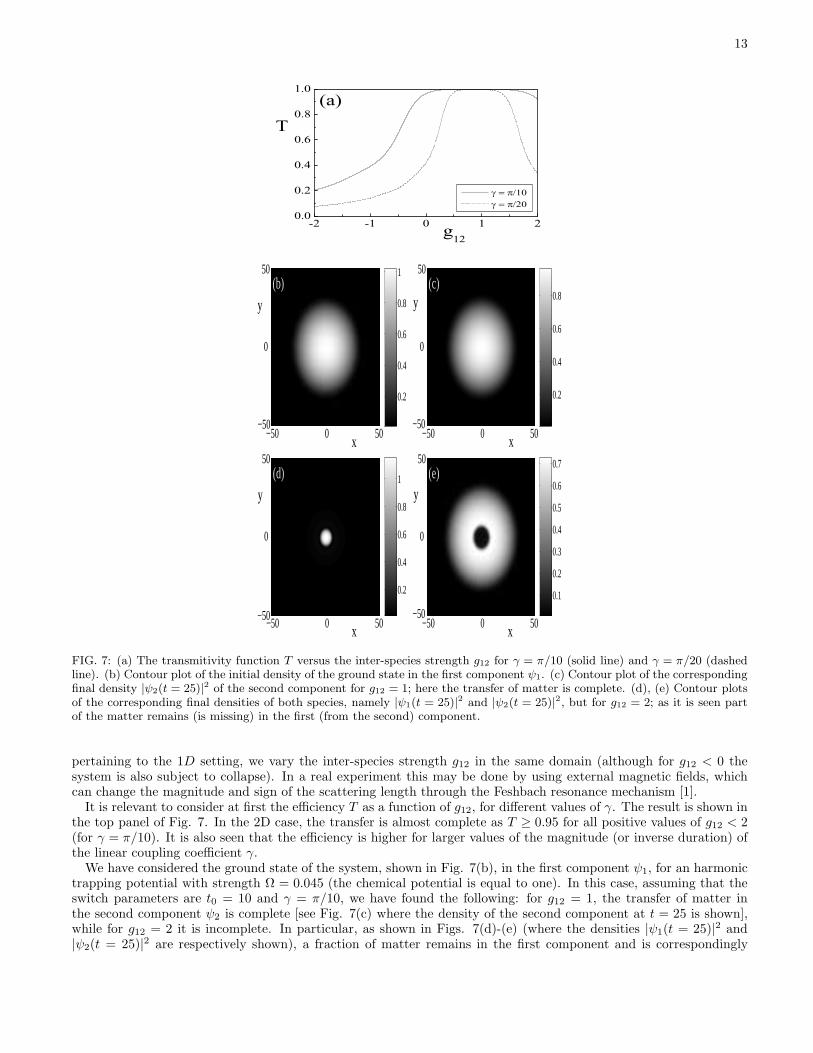
FIG. 7: (a) The transmitivity function T versus the inter-species strength g12 for γ = π/10 (solid line) and γ = π/20 (dashedline). (b) Contour plot of the initial density of the ground state in the first component ψ1. (c) Contour plot of the correspondingfinal density |ψ2(t = 25)|2 of the second component for g12 = 1; here the transfer of matter is complete. (d), (e) Contour plotsof the corresponding final densities of both species, namely |ψ1(t = 25)|2 and |ψ2(t = 25)|2, but for g12 = 2; as it is seen partof the matter remains (is missing) in the first (from the second) component.

pertaining to the 1D setting, we vary the inter-species strength g12 in the same domain (although for g12 < 0 thesystem is also subject to collapse). In a real experiment this may be done by using external magnetic fields, whichcan change the magnitude and sign of the scattering length through the Feshbach resonance mechanism [1].

It is relevant to consider at first the efficiency T as a function of g12, for different values of γ. The result is shown inthe top panel of Fig. 7. In the 2D case, the transfer is almost complete as T ≥ 0.95 for all positive values of g12 < 2(for γ = π/10). It is also seen that the efficiency is higher for larger values of the magnitude (or inverse duration) ofthe linear coupling coefficient γ.

We have considered the ground state of the system, shown in Fig. 7(b), in the first component ψ1, for an harmonictrapping potential with strength Ω = 0.045 (the chemical potential is equal to one). In this case, assuming that theswitch parameters are t0 = 10 and γ = π/10, we have found the following: for g12 = 1, the transfer of matter inthe second component ψ2 is complete [see Fig. 7(c) where the density of the second component at t = 25 is shown],while for g12 = 2 it is incomplete. In particular, as shown in Figs. 7(d)-(e) (where the densities |ψ1(t = 25)|2 and|ψ2(t = 25)|2 are respectively shown), a fraction of matter remains in the first component and is correspondingly

14

-2 -1 0 1 20.0

0.2

0.4

0.6

0.8

1.0

(a)T

g12

50

0

−50−50 0 50

y

x

(b)

0.2

0.4

0.6

0.8

50

0

−50−50 0 50

y

x

(c)

0.2

0.4

0.6

0.8

50

0

−50−50 0 50

y

x

(d)

0.1

0.2

0.3

0.4 50

0

−50−50 0 50

y

x

(e)

0.2

0.4

0.6

0.8

FIG. 8: (a) Same as in Fig. 7(a). (b) The initial density of the first component ψ1, consisting of a cloud with one vortex in thecenter. (c) The corresponding final density |ψ2(t = 25)|2 of the second component for g12 = 1; here the transfer is completeand the final configuration is identical to the initial one. (d), (e) The corresponding final densities of both species, namely|ψ1(t = 25)|2 and |ψ2(t = 25)|2, but for g12 = 2.

missing from the central part of the second component after the switch-off of the Rabi pulse.Next we consider an excited state, in which a vortex is initially placed at the center of the BEC cloud (first

component). Here, it is interesting to investigate whether such a coherent nonlinear state can be transfered in thesecond component. As seen in Fig. 8(a), the efficiency is as high as for the ground state transfer. Also, for g12 = 1, aperfect transfer of this excited state occurs as seen in Figs. 8(b) and (c), where the initial state of the first species andthe final one of the second species are respectively shown. Nevertheless, for g12 = 2, the transfer is not complete, asit can be seen in Figs. 8(d) and (e): starting again from the initial density shown in in Fig. 8(b), after the switch-offof the process, a ring-shaped part of the matter remains in (is missing from) the first (second) component. A carefulobservation of Fig. 8(d) also shows that this “high” density ring surrounds a low density (≈ 0.2) part of matter witha vortex on top of it. Note that even in this case, the vortex is transferred in the second component; on the otherhand, the above mentioned “bright” and “dark” ring structures (respectively in the first and second component) donot carry any topological charge. It is interesting to remark that such methods are similar in spirit to the ones usedto produce ring-like patterns in the recent experimental work of [20].

Finally, we have considered a vortex cluster, namely a triangular vortex lattice, initially placed on top of the BEC of

15

-2 -1 0 1 20.0

0.2

0.4

0.6

0.8

1.0

(a)T

g12

50

0

−50−50 0 50

y

x

(b)

0.1

0.2

0.3

0.4

0.5

0.650

0

−50−50 0 50

y

x

(c)

0.1

0.2

0.3

0.4

0.5

0.6

50

0

−50−50 0 50

y

x

(d)

0.005

0.01

0.015

0.02

0.025 50

0

−50−50 0 50

y

x

(e)

0.1

0.2

0.3

0.4

0.5

0.6

FIG. 9: (a) Same as in Figs. 7(a) and 8(a). (b) The initial density of the first component ψ1, consisting of a TF-cloud witha triangular vortex lattice (≈ 24 vortices). (c) The corresponding final density |ψ2(t = 25)|2 of the second component forg12 = 1; here the TF cloud and the vortex lattice are perfectly transferred to the second species. (d), (e) The correspondingfinal densities of both species, namely |ψ1(t = 25)|2 and |ψ2(t = 25)|2, but for g12 = 2.

the first component. Similarly to what was found for the ground state and the single vortex, we find that the transferefficiency function shown in Fig. 9(a) assumes values very close to 1 for a wide range of values of g12 (especially soin the case of short pulse durations i.e., fast transfer). As shown in the example of Figs. 9(b) and (c) for g12 = 1 thevortex lattice in the first component is perfectly transferred to the second one. An “imperfect transfer”, for g12 = 2,is shown in Figs. 9(d) and (e), corresponding to the final states of the first and second species when the initial stateis as in Figs. 9(b). Here it is observed that small spots of matter (with densities ≈ 0.025), each of which carries avortex on it, remain in the first species, while a robust crystal structure is transferred to the second component. It isworth noting here that the vortex lattice remarkably appears to be even more robust, in its “switching properties”,than the ground state of the 2D system.

16

VI. CONCLUSIONS AND OUTLOOK

In this paper, we have systematically examined the possibility of using the linear Rabi coupling between the two(or more) components of a Bose-Einstein condensate as a means of controllably transferring the wavefunction ofone condensate to the other. In particular, we have focused on the case of different hyperfine states, even thoughsimilar considerations are applicable to multicomponent condensates composed by different atomic species. We haveillustrated that this transfer is exact and can be analytically studied in the limit where all inter- and intra- speciesinteractions are equal. In addition, we have studied departures from this limit both numerically and by means ofa two-mode ansatz, showing that in this two-mode description the impossibility to transfer all the particles from acondensate to the other is seen as the self-trapping of the initial condensate wavefunction. The threshold for the self-trapping has been compared in the homogeneous limit with the findings of the numerical simulations Gross-Pitaevskiiequations.

The two-mode analysis shows that that for deviations from the ideal case one can optimize the transfer by choosingan appropriate pulse duration different from the duration given by Eq. (11) for equal interaction strengths . In thepresence of external trapping potentials, our numerical simulations show that, for repulsive condensates (but, to alesser extent, also for attractive condensates), the Rabi switch is very robust with high efficiency. In general, a changeof sign of the inter-species interactions in 1D has been shown to degrade –although, under appropriate conditions, notsubstantially– the efficiency of the transfer process. The switching was surprisingly found to be even more robust forparticular types of coherent patterns, such as vortex lattices in pancake-shaped condensates. Furthermore, we havealso illustrated that the generalization of the proposed Rabi switch to more than 2 components can offer a possibilityfor systematically routing matter, in a controllable way, between different “atomic channels”.

It would be quite challenging to examine experimental realizations of such atomic switches and routers especiallywithin the context of two hyperfine states, but also in that of spin-1 states recently studied in [15, 17]. Of particularinterest in this setting would be the dynamics and phase separation of vortices and vortex lattices in multicomponentcondensates. We expect that our mechanism may be relevant when transferring a condensate wavefunction also indifferent components of a dipolar BEC [60].

Another relevant issue concerns the analysis of the role of the quantum fluctuations on the Rabi switch of wave-functions: indeed, for two condensates (whose dynamics is described by coupled Gross-Pitaevskii equations) the Rabiswitch is not copying the full many-body wavefunction of a component in the other, but only the (one-body) or-der parameter. Then, we expect that the presence of quantum fluctuations would naturally degrade the efficiencyof our protocol. A study of such degradation is relevant for the implementation of a quantum register through atwo-component Bose gas in an array of double-wells.

The protocol proposed in this paper allows the possibility to copy the wavefunction of a condensate into anotherspecies, providing a matter-wave counterpart for optical switches realized in nonlinear fiber optics [43]. “All-opticalswitches” are very important tools in this context, allowing for to manipulate and eventually store the informationcontained in optical solitons. For this reason, the study of protocols focused on copying of wavefunctions in Bosecondensates is deemed to be an important task towards an efficient manipulation of matter-wave solitons. Furthermore,one can think of a possible application of the present protocol to implement copies for quantum registers: indeed, onecould perform some operations on a component (e.g., with a component in an array of double wells) and arrive at adesired wavefunction. At this point the wavefunction can be copied on the other component, and one can gain access(at a later time) to this information. In this respect, it would be very important to investigate the degradation of thequantum switch due to the quantum fluctuations.

Finally, since the protocol proposed in this paper is not restricted to linearly coupled Gross-Pitaevskii equations,one may safely expect that - once the effects of quantum corrections are accounted for - it can be extended to othersets of coupled equations such as the ones arising in the analysis of the weak pairing phase of p-wave superfluid statesof cold atoms [61] and of quantum wires embedded in p-wave superconductors [62].

Acknoledgements Several stimulating discussions with E. Fersino, A. Michelangeli, and A. Smerzi are gratefullyacknowledged. A.T. also thanks L. De Sarlo, F. Minardi and C. Fort of the Atomic Physics group at LENS for fruitfuldiscussions. In the final stages of the project P.S. benefited from discussions with S. Flach, M. Gulacsi, M. Haqueand S. Komineas. P.S. is grateful to the Particle Theory sector at S.I.S.S.A. for hospitality.

APPENDIX A: DIFFERENT POTENTIALS AND INTERACTION STRENGTHS

When the interaction strengths gij are different (and, for simplicity, V1 = V2), then Eqs. (1)-(2) can be written as

i∂ψ

∂t= −1

2∆ψ + V ψ +

2∑

j=1

(ψ†Gjψ)σjψ + α(t)Pψ, (A1)

17

with

G1 =

(

g11 00 g12

)

, G2 =

(

g12 00 g22

)

. (A2)

Upon removing the Rabi term in Eq. (A1) by setting ψ = Uφ, with U given by Eq. (6), one gets

i∂φ

∂t= −1

2∆ψ + V φ+

4∑

j=1

(φ†Gjφ)σjφ, (A3)

where G1 = L1−S2(L1−L2) and G2 = L2+S2(L1−L2), where the 2×2 matrices L1,2 are defined by L1 = G1−iSδ1Aand L2 = G2+iSδ2A, with A = −iS(σ1−σ2)+C(σ3−σ4), S = sin I(t), C = cosI(t) and δ1 = g11−g12, δ2 = g22−g12.Furthermore G3 = −iCS(L1 − L2) = −G4. For g11 = g12 = g22 = g, then δ1 = δ2 = 0 and G1 = G2 = G andG3 = G4 = 0, so that Eq. (7) is retrieved.

With different external potentials (V1(~r) 6= V2(~r)) and equal interaction strengths (g11 = g22 = g12 = g), Eqs.(1)-(2) can be written in a matrix form as

i∂ψ

∂t=

1

2

(

−i~∇)2

ψ +(

ψ†Gψ)

ψ + V1(r)σ1ψ + V2(r)σ2ψ + α(t)Pψ, (A4)

where

σ1 =

(

1 00 0

)

, σ2 =

(

0 00 1

)

, σ3 =

(

0 10 0

)

σ4 =

(

0 01 0

)

, (A5)

and G given in Eq. (4). It is yet possible to perform a decomposition permitting to formally write Eq. (A4) withoutthe Rabi term α(t)Pψ. We set ψ = Uφ, with

U =

(

u1 u3

u4 u2

)

: (A6)

the Rabi term vanishes, provided that the functions uj(~r, t) (j = 1, · · · , 4) obey the (linear) matrix equation

i∂U

∂t= −1

2∆U + α(t)PU + V(~r) (u3σ3 − u4σ4) , (A7)

where V(~r) = V1(~r) − V2(~r). This matrix equation corresponds to four equations for u1, u2, u3, and u4, which aregrouped in two pairs, one for u1 and u4, namely

i∂u1

∂t= −1

2∆u1 + α(t)u4, (A8)

i∂u4

∂t= −1

2∆u4 − V(~r)u4 + α(t)u1, (A9)

and a similar for u2 and u3 (with V(~r) instead of −V(~r)). Eqs. (A8)-(A9) are two coupled linear Schrodinger equations,and the difference between the potentials V enters as an effective potential in one of the two equations. When V = 0,the result u1 = u2 = cosI(t) and u3 = u4 = −i sinI(t) is readily obtained.

With the functions uj defined by Eq. (A7), then φ satisfies the equation

i∂φ

∂t=

1

2

(

−i~∇)2

φ+(

φ†Gφ)

φ+ V1(r)σ1φ+ V2(r)σ2φ+ ~X · ~∇φ, (A10)

with G = U †GU and ~X = ~X (~r, t) = −U−1~∇U . Eq. (A10) can be written in the form

i∂φ

∂t=

1

2

(

−i~∇ + i ~X)2

φ+(

φ†Gφ)

φ+ V1(r)σ1φ+ V2(r)σ2φ+ Yφ, (A11)

where Y =(

~X 2 − ~∇ · ~X)

/2, showing that, with different external potentials, an effective complex vector potential

acts on the multicomponent gas and the effective interaction strengths are both time- and space- dependent [since

the G depends upon the U(~r, t)].

18

APPENDIX B: TWO-MODE VARIATIONAL EQUATIONS

For the pulse (8) and at times t0 ≤ t ≤ t0+δ, the Lagrangian to be computed is given by L = i2 〈ψ

†V∂ψV

∂t − ∂ψ†V

∂t ψV 〉−〈ψ†V HψV 〉, where

H =

(

K − ℓ112 |ψv1|2 − ℓ12

2 |ψv2|2 γγ K − ℓ12

2 |ψv1|2 − ℓ222 |ψv2|2

)

, (B1)

ψV is defined in Eq. (31) and K = − 12∂2

∂x2 . Then, one gets

L = −N1ϕ1 −N2ϕ2 − γ

√

ℓ22ℓ11

F

(

ℓ22ℓ11

)

√

N1N2 cos (ϕ1 − ϕ2) −ℓ21124N1 −

ℓ22224N2 + µ+

+ℓ21112N2

1 +ℓ22212N2

2 +ℓ228ℓ12L

(

ℓ22ℓ11

)

N1N2, (B2)

where the functions F (θ) and L(θ) are defined as

F (θ) ≡∫ ∞

−∞

dy

cosh (y) cosh (θy); L(θ) ≡

∫ ∞

−∞

dy

cosh2 (y) cosh2 (θy). (B3)

Note that F (0) = π, F (1) = 2, L(0) = 2, and L(1) = 4/3, while both functions → 0 as θ → ∞. For small values of

δθ = θ − 1, one has F (θ) ≈ 2 − δθ + 24−π2

36 δθ2 and L(θ) ≈ 43 − 2

3δθ −2(π2−15)

45 δθ2. For ℓ11 = ℓ22, from Eq. (B2) onegets, apart from constant terms, the Lagrangian

L = −N1ϕ1 −N2ϕ2 − 2γ√

N1N2 cos (ϕ1 − ϕ2) +ℓ21112N2

1 +ℓ22212N2

2 +ℓ11ℓ12

6N1N2. (B4)

Introducing the variables (33), the equations of motions for η and ϕ obtained from the Lagrangian (B2) are

η = 2γ′√

1 − η2 sinϕ,ϕ = −2γ′ η√

1−η2cosϕ+ ∆E +Mη, (B5)

where

γ′ =γ

2

√

ℓ22ℓ11

F

(

ℓ22ℓ11

)

, (B6)

M =1

12

[

3

2ℓ12ℓ22L

(

ℓ22ℓ11

)

− ℓ211 − ℓ222

]

, (B7)

and

∆E =1

24

(

ℓ222 − ℓ211)

. (B8)

The variables η, ϕ are canonically conjugate dynamical ones with respect to the effective Hamiltonian

Heff =M

2η2 + 2γ′

√

1 − η2 cosϕ+ ∆E · η. (B9)

Equation (B9) is the Hamiltonian of a non-rigid pendulum, whose mass and length depend on the parameters ℓij .For ℓ11 = ℓ22, then M = ℓ11(ℓ12 − ℓ11)/6, ∆E = 0 and γ′ = γ, retrieving Eq. (34) and the effective Hamiltonian(35). When ℓ12 = ℓ11 = ℓ22, then the mass of the pendulum is vanishing. When ℓ11 6= ℓ22, then the presence of thedetuning ∆E favours self-trapping and can be studied as in [57].

[1] C. J. Pethick and H. Smith, Bose-Einstein Condensation in Dilute Alkali Gases, Cambridge University Press (Cambridge,2002); L. P. Pitaveskii and S. Stringari, Bose-Einstein Condensation, Clarendon Press (Oxford, 2003).

19

[2] F. Dalfovo, S. Giorgini, L. P. Pitaveskii and S. Stringari, Rev. Mod. Phys. 71, 463 (1999); A. J. Leggett, Rev. Mod. Phys.73, 307 (2001); P. G. Kevrekidis and D. J. Frantzeskakis, Mod. Phys. Lett. B 18, 173 (2004); V. A. Brazhnyi and V. V.Konotop, Mod. Phys. Lett. B 18, 627 (2004).

[3] D. M. Stamper-Kurn, M. R. Andrews, A. P. Chikkatur, S. Inouye, H.-J. Miesner, J. Stenger, and W. Ketterle, Phys. Rev.Lett. 80, 2027 (1998).

[4] A. E. Leanhardt, Y. Shin, D. Kielpinski, D. E. Pritchard, and W. Ketterle, Phys. Rev. Lett. 90, 140403 (2003).[5] R. Dumke, M. Johanning, E Gomez, J. D. Weinstein, K. M. Jones, and P. D. Lett, New. J. Phys. 8, 64 (2006).[6] C. J. Myatt, E. A. Burt, R. W. Ghrist, E. A. Cornell, and C. E. Wieman, Phys. Rev. Lett. 78, 586 (1997).[7] D. S. Hall, M. R. Matthews, J. R. Ensher, C. E. Wieman, and E. A. Cornell, Phys. Rev. Lett. 81, 1539 (1998).[8] J. Williams, R. Walser, J. Cooper, E. A. Cornell, and M. Holland, Phys. Rev. A 61, 033612 (2000).[9] P. Maddaloni, M. Modugno, C. Fort, F. Minardi, and M. Inguscio, Phys. Rev. Lett. 85, 2413 (2000).

[10] A. Smerzi, A. Trombettoni, T. Lopez-Arias, C. Fort, P. Maddaloni, F. Minardi, and M. Inguscio, Eur. Phys. J. B 31, 457(2003).

[11] O. Mandel, M. Greiner, A. Widera, T. Rom, T. W. Hansch, and I. Bloch, Phys. Rev. Lett. 91, 010407 (2003).[12] M.-S. Chang, C. D. Hamley, M. D. Barrett, J. A. Sauer, K. M. Fortier, W. Zhang, L. You, and M. S. Chapman, Phys.

Rev. Lett. 92, 140403 (2004).[13] M. H. Wheeler, K. M. Mertes, J. D. Erwin, and D. S. Hall, Phys. Rev. Lett. 93, 170402 (2004).[14] V. Schweikhard, I. Coddington, P. Engels, S. Tung, and E. A. Cornell, Phys. Rev. Lett. 93, 210403 (2004).[15] J. M. Higbie, L. E. Sadler, S. Inouye, A. P. Chikkatur, S. R. Leslie, K. L. Moore, V. Savalli, and D. M. Stamper-Kurn,

Phys. Rev. Lett. 95, 050401 (2005).[16] J. Kronjager, C. Becker, P. Navez, K. Bongs, and K. Sengstock, Phys. Rev. Lett. 97, 110404 (2006).[17] L. E. Sadler, J. M. Higbie, S. R. Leslie, M. Vengalattore, and D. M. Stamper-Kurn, Nature 443, 312 (2006).[18] N. Lundblad, R. J. Tompson, D. C. Aveline, and L. Maleki, Optics Express 14. 10164 (2006).[19] M. Vengalattore, J. M. Higbie, S. R. Leslie, J. Guzman, L. E. Sadler, and D. M. Stamper-Kurn, Phys. Rev. Lett. 98,

200801 (2007).[20] K. M. Mertes, J. W. Merrill, R. Carretero-Gonzalez, D. J. Frantzeskakis, P. G. Kevrekidis, and D. S. Hall, Phys. Rev.

Lett. 99, 190402 (2007).[21] G. Modugno, G. Ferrari, G. Roati, R.J. Brecha, A. Simoni, M. Inguscio, Science 294, 1320 (2001).[22] J. Catani, L. De Sarlo, G. Barontini, F. Minardi, and M. Inguscio, arXiv:0706.2781.[23] M. Mudrich, S. Kraft, K. Singer, R. Grimm, A. Mosk, and M. Weidemuller, Phys. Rev. Lett. 88, 253001 (2002).[24] T.-L. Ho and V.B. Shenoy, Phys. Rev. Lett. 77, 3276 (1996).[25] H. Pu and N.P. Bigelow, Phys. Rev. Lett. 80, 1130 (1998).[26] B.D. Esry, C.H. Greene, J.P. Burke, Jr, and J.L. Bohn, Phys. Rev. Lett. 78, 3594 (1997).[27] Th. Busch, J. I. Cirac, V. M. Perez-Garcia, and P. Zoller, Phys. Rev. A 56, 2978 (1997); R. Graham and D. Walls, Phys.

Rev. A 57, 484 (1998); H. Pu and N. P. Bigelow, Phys. Rev. Lett. 80, 1134 (1998); B. D. Esry and C. H. Greene, Phys.Rev. A 57, 1265 (1998).

[28] M. Trippenbach, K. Goral, K. Rzazewski, B. A. Malomed, and Y. B. Band, J. Phys. B 33, 4017 (2000); S. Coen andM. Haelterman, Phys. Rev. Lett. 87, 140401 (2001); B. A. Malomed, H. E. Nistazakis, D. J. Frantzeskakis, and P. G.Kevrekidis, Phys. Rev. A 70, 043616 (2004).

[29] Th. Busch and J. R. Anglin, Phys. Rev. Lett. 87, 010401 (2001); P. Ohberg and L. Santos, Phys. Rev. Lett. 86, 2918(2001); P. G. Kevrekidis, H. E. Nistazakis, D. J. Frantzeskakis, B. A. Malomed, and R. Carretero-Gonzalez, Eur. Phys. J.D 28, 181 (2004).

[30] B. Deconinck, P. G. Kevrekidis, H. E. Nistazakis, and D. J. Frantzeskakis, Phys. Rev. A 70, 063605 (2004).[31] M. A. Porter, P. G. Kevrekidis, and B. A. Malomed, Physica D 196, 106 (2004).[32] G.-H. Chen and Y.-S. Wu, Phys. Rev. A 67, 013606 (2003).[33] A. Kuklov, N. Prokofev, and B. Svistunov, Phys. Rev. Lett. 92, 030403 (2004).[34] G.-P. Zheng, J.-Q. Liang, and W. M. Liu, Phys. Rev. A 71, 053608 (2005).

[35] R. V. Pai, K. Sheshadri, and R. Pandit, PhysRev. B 77, 014503 (2008).[36] J. Stenger, S. Inouye, D. M. Stamper-Kurn, H.-J. Miesner, A. P. Chikkatur, and W. Ketterle, Nature (London) 396, 345

(1998).[37] J. Ieda, T. Miyakawa, and M. Wadati, Phys. Rev. Lett. 93, 194102 (2004); J. Phys. Soc. Jpn. 73, 2996 (2004); M. Wadati

and N. Tsuchida, J. Phys. Soc. Jpn. 75, 014301 (2006).[38] L. Li, Z. Li, B. A. Malomed, D. Mihalache, and W. M. Liu, Phys. Rev. A 72, 033611 (2005); L. Salasnich and B. A.

Malomed, Phys. Rev. A 74, 053610 (2006).[39] H. E. Nistazakis, D. J. Frantzeskakis, P. G. Kevrekidis, B. A. Malomed, R. Carretero-Gonzalez, arXiv:0705.1324.[40] B. J. Dabrowska-Wuster, E. A. Ostrovskaya, T. J. Alexander, and Y. S. Kivshar, Phys. Rev. A 75, 023617 (2007).[41] H. Saito, and M. Ueda, Phys. Rev. A 72, 023610 (2005); K. Murata, H. Saito, and M. Ueda, Phys. Rev. A 75, 013607

(2007).[42] B. A. Malomed, Phys. Rev. A 43, 410 (1991); M. J. Potasek, J. Opt. Soc. Am. B 10, 941 (1993).[43] Y. S. Kivshar and G. P. Agrawal, Optical Solitons: from Fibers to Photonic Crystals, CA Academic Press (San Diego,

2003).[44] D. M. Stamper-Kurn and W. Ketterle, Spinor condensates and light scattering from Bose-Einstein condensates, in R.

Kaiser, C. Westbrook, and F. David eds., Coherent Atomic Matter Waves, Les Houches Summer School Session LXXII,

20

Springer (New York, 2001), pp. 137-217 (arXiv:cond-mat/0005001).[45] D. S. Hall, Multi-Component Condensates: Experiment, in P.G. Kevrekidis, D.J. Frantzeskakis, and R. Carretero-Gonzalez

eds., Emergent Nonlinear Phenomena in Bose-Einstein Condensates, Springer Series on Atomic, Optical, and PlasmaPhysics, 2007, pp. 307-327.

[46] A. Smerzi, S. Fantoni, S. Giovanazzi, and S. R. Shenoy, Phys. Rev. Lett. 79, 4950 (1997).[47] M. Albiez, R. Gati, J. Folling, S. Hunsmann, M. Cristiani, and M. K. Oberthaler, Phys. Rev. Lett. 95, 010402 (2005).[48] J. I. Cirac, M. Lewenstein, K. Molmer, and P. Zoller, Phys. Rev. A 57, 1208 (1998).[49] P. Villain and M. Lewenstein, Phys. Rev. A 59, 2250 (1999).[50] Notice that one can pass from α < 0 to α > 0 simply by shifting the phase difference χ = χ2 −χ1 between the condensate

wavefunctions ψj (where ψj =p

Njeiχj ) of π: χ→ χ+ π.

[51] J. Williams, R. Walser, J. Cooper, E. Cornell, and M. Holland, Phys. Rev. A 59, R31 (1999).

[52] P. Ohberg and S. Stenholm, Phys. Rev. A 59, 3890 (1999).[53] I. M. Merhasin, B. A. Malomed, and R. Driben, J. Phys. B 38, 877 (2005); I. M. Merhasin, B. A. Malomed, and R. Driben,

Phys. Scripta T116, 18 (2005).

[54] Using the notation U = eb, with the time-dependent matrix b(t) defined by b = −iR t

0P (t′)dt′, we observe that when the

matrices b and ∂b/∂t commute, then the decomposition ψ = Uφ allows to cast Eq. (19) in the homogeneous form.[55] S. V. Manakov, Zh. Eksp. Teor. Fiz. 65, 505 (1973) [Sov. Phys. JETP 38, 248 (1974)].[56] C. Pare and M. Florjanczyk, Phys. Rev. A 41, 6287 (1990).[57] S. Raghavan, A. Smerzi, S. Fantoni, and S. R. Shenoy, Phys. Rev. A 59, 620 (1999).[58] V. M. Kenkre and D. K. Campbell, Phys. Rev. B 34, 4959 (1986).[59] V. M. Kenkre and G. P. Tsironis, Phys. Rev. B 35, 1473 (1987).[60] T. Lahaye, T. Koch, B. Froehlich, M. Fattori, J. Metz, A. Griesmaier, S. Giovanazzi, and T. Pfau, Nature 448, 672 (2007).[61] S. Tewari, S. Das Sarma, C. Nayak, C. Zhang, and P. Zoller, Phys. Rev. Lett. 98, 010506 (2007).[62] G. W. Semenoff and P. Sodano, J. Phys. B 40, 1479 (2007).