The Cauchy-Schwarz Inequality and Positive

Polynomials

Torkel A. Haufmann

May 27, 2009

Contents

0.1 Introduction . . . . . . . . . . . . . . . . . . . . . . . . . . . . . . 1

1 The Cauchy-Schwarz Inequality 2

1.1 Initial proofs . . . . . . . . . . . . . . . . . . . . . . . . . . . . . 21.2 Some other cases . . . . . . . . . . . . . . . . . . . . . . . . . . . 51.3 Sharpness . . . . . . . . . . . . . . . . . . . . . . . . . . . . . . . 61.4 Related results . . . . . . . . . . . . . . . . . . . . . . . . . . . . 61.5 Lagrange's Identity . . . . . . . . . . . . . . . . . . . . . . . . . . 9

2 Positive polynomials 11

2.1 Sums of squares . . . . . . . . . . . . . . . . . . . . . . . . . . . . 112.1.1 Polynomials in one variable . . . . . . . . . . . . . . . . . 112.1.2 Motzkin's polynomial revisited . . . . . . . . . . . . . . . 13

2.2 Quadratic forms . . . . . . . . . . . . . . . . . . . . . . . . . . . 142.3 Final characterisation of sums of squares . . . . . . . . . . . . . . 15

2.3.1 An illustrating example . . . . . . . . . . . . . . . . . . . 172.4 Hilbert's 17th problem . . . . . . . . . . . . . . . . . . . . . . . . 19

0.1 Introduction

This text consists of two parts. In chapter 1, we discuss the Cauchy-Schwarzinequality and some generalisations of this, in addition to looking at certainresults related to said inequality. In chapter 2, we will instead turn our attentionto positive polynomials, by their nature related to inequalities, and end with acharacterisation of those positive polynomials that are sums of squares.

1

Chapter 1

The Cauchy-Schwarz

Inequality

What is now known as the Cauchy-Schwarz inequality was �rst mentioned in anote by Augustin-Louis Cauchy in 1821, published in connection with his bookCourse d'Analyse Algébrique. His original inequality was formulated in termsof sequences in R, but later Viktor Yakovlevich Bunyakovsky proved the analogversion for integrals in his Mémoire(1859). In the course of his work on minimalsurfaces Karl Hermann Amandus Schwarz in 1885 proved the inequality for two-dimensional integrals, apparently not knowing about Bunyakovsky's work. Dueto Bunyakovsky's relative obscurity in the West at the time, the inequality cameto be known as the Cauchy-Schwarz inequality, as opposed to, for instance, theCauchy-Bunyakovsky-Schwarz inequality.

In keeping with mathematical tradition over historical precedence we willuse the name Cauchy-Schwarz inequality, or CS inequality for short. As we willsee, the inequality is valid in considerably more general cases than the ones thusfar mentioned. We will not distinguish much between the di�erent versions ofthe inequality, for our purposes they are all �the� CS inequality.

1.1 Initial proofs

This is the CS inequality as Cauchy originally discovered it:

Theorem 1.1.1 (CS inequality 1). For two �nite real sequences {ai}ni=1, {bi}ni=1

the following holds:

a1b1 + · · ·+ anbn ≤√a2

1 + · · ·+ a2n

√b21 + · · ·+ b2n. (1.1)

Direct proof. This �rst proof uses nothing but ordinary rules of algebra. Notethat if either of the sequences are zero the CS inequality is trivial, so we assume

2

this is not the case. We know that for all x, y ∈ R,

0 ≤ (x− y)2 = x2 − 2xy + y2 ⇒ xy ≤ 12x2 +

12y2 (1.2)

Next, we introduce new normalised sequences, whose utility will become appar-ent, by de�ning

ai = ai

/ n∑j=1

a2j

12

and bi = bi

/ n∑j=1

b2j

12

.

Applying 1.2 to these two sequences, term by term, it is clear that

n∑i=1

aibi ≤12

n∑i=1

a2i +

12

n∑i=1

b2i =12

+12

= 1.

Reintroducing the original sequences this means that

n∑i=1

ai(∑nj=1 aj

) 12

bi(∑nj=1 bj

) 12≤ 1,

and as an immediate consequence,

n∑i=1

aibi ≤

(n∑i=1

a2i

) 12(

n∑i=1

b2i

) 12

,

thus �nishing the proof.

As a side note, observe that if the sums were in�nite but convergent in theL2-norm we could have performed the exact same proof above, but we have keptthis proof simple so as not to obscure the idea.

The next proof we present will be due to viewing the �nite sequences asvectors a = (a1, . . . , an) and b = (b1, . . . bn) in Rn or Cn. We restate theproperties of the inner product on a vector space V over some �eld K that iseither R or C:

∀v,v′,w ∈ V,∀c ∈ K

1. 〈v + v′,w〉 = 〈v,w〉+ 〈v′,w〉

2. 〈w,v〉 = 〈v,w〉

3. 〈cv,w〉 = c〈v,w〉

4. 〈v,v〉 ≥ 0, 〈v,v〉 = 0⇒ v = 0

Now we will de�ne a norm on this space, which will enable us to prove theCS inequality again. Recall that a norm ‖ · ‖ on some vector space satis�es thefollowing:

∀v,w ∈ V,∀c ∈ K

3

1. ‖cv‖ = |c|‖v‖

2. ‖v‖ ≥ 0 and ‖v‖ ⇒ v = 0

3. ‖v + w‖ ≤ ‖v‖+ ‖w‖

4. |〈v,w〉| ≤ ‖v‖‖w‖

where we recognise property 4 as the CS inequality. Our next theorem essentiallystates that the standard norm de�ned as ‖v‖ = 〈v,v〉1/2 for v ∈ V has thisproperty. That it satis�es the �rst two properties is easy to prove, so only thethird is left. We will return to this later.

Theorem 1.1.2 (CS inequality 2). In a vector space V with an inner product

〈·, ·〉 and the standard norm ‖v‖ = 〈v,v〉1/2 for v ∈ V the following holds for

a,b ∈ V :|〈a,b〉| ≤ ‖a‖‖b‖. (1.3)

We will use the easily checked fact that ‖cv‖ = |c|‖v‖ for c ∈ K, v ∈ V . Wewill also use the notion of projection, and we remind the reader that for w ∈ V ,then the projection of v ∈ V onto the subspace spanned by w is de�ned by

Projw(v) =〈v,w〉〈w,w〉

w.

It is clear that there exists a v′ ∈ V such that v = Projw(v) + v′ and v,v′ areorthogonal. It's easy to verify that

‖v‖2 = ‖Projw(v)‖2 + ‖v − Projw(v)‖2.

From this it is obvious that ‖Projw(v)‖ ≤ ‖v‖, and we can exhibit the proof.

Proof. Assume a 6= 0, otherwise the inequality is the trivial equality 0 = 0. Nowlet W be the subspace spanned by a. Then

‖ProjW b‖ =∥∥∥∥ 〈a,b〉〈a,a〉

a∥∥∥∥ =

|〈a,b〉||〈a,a〉|

‖a‖ =|〈a,b〉|‖a‖2

‖a‖ =|〈a,b〉|‖a‖

,

and since ‖ProjW b‖ ≤ ‖b‖ the theorem immediately follows.

Now, this is all independent of how we have de�ned the inner product onV , thus leaving theorem 1.1.1 as a special case1. The proof is due to [2]. Wecould also have proved this using the method of normalisation from the proofof theorem 1.1.1, adapting notation as necessary, but we will not do that here.

Of particular interest is that Theorem 1.1.2 has Cn as a special case withthe inner product on that space de�ned by

〈z,w〉 = z1w1 + · · ·+ znwn,

1Technically, the theorem is subtly di�erent because of the absolute value on the left. This,

however, presents no di�culty, as obviously, if |x| ≤ |y| then x ≤ |y| for all x, y ∈ R.

4

and thus the CS inequality also holds for sequences in C, provided the secondsequence is complex conjugated as above.

In fact, this inner product form of the CS inequality is the most general formwe will exhibit in this paper, and the fact that the CS inequality holds for anyinner product space surely underlines how general the result truly is.

1.2 Some other cases

The CS inequality for integrals of functions into R is easily obtained for instancethrough taking limits on the discrete case � this is how Bunyakovsky originallyproved it, though we might as well have proven it by de�ning an inner producton the space of integrable functions over some interval, leaving it as a specialcase of Theorem 1.1.2. We merely state it here without proof.

Theorem 1.2.1 (Bunyakovsky's Inequality). Let I ⊂ R be an interval and

assume we have two functions f, g : I → R that are integrable on I. Then∫I

fg ≤(∫

I

f2

) 12(∫

I

g2

) 12

. (1.4)

That said, the twodimensional case, proven by Schwarz as mentioned, ismore interesting. I now state the result and prove it, the proof is after [5].

Theorem 1.2.2 (CS Inequality 3). Let S ⊂ R2, and assume we have two

functions f, g : S → R that are integrable on S. Then the following holds:∣∣∣∣∫∫S

fg

∣∣∣∣ ≤√∫∫

S

f2

√∫∫S

g2. (1.5)

Proof. De�ne the following three quantities:

A =∫∫

S

f2, B =∫∫

S

fg, and C =∫∫

S

g2.

Then consider the following polynomial:

p(t) =∫∫

S

(tf(x, y) + g(x, y))2dxdy = At2 + 2Bt+ C.

p(t) is nonnegative, being the integral of a square, and we know this meansthe discriminant of this polynomial must be less than or equal to 0, that is,4B2 − 4AC ≤ 0, implying B2 ≤ AC, which by taking roots immediately givesus Theorem 1.2.2.

Again, this could have been just as easily proved by de�ning an inner prod-uct, illustrating again that Theorem 1.1.2 is by far the most general case of theCS inequality we discuss here. Note that this particular technique of proof canbe reused, for instance to prove the analoguous discrete version.

5

Theorem 1.2.3 (CS Inequality 4). If ai,j and bi,j are two doubly indexed �nite

sequences such that 1 ≤ i ≤ m and 1 ≤ j ≤ n, the following holds:∑i,j

ai,jbi,j ≤√∑

i,j

a2i,j

√∑i,j

b2i,j . (1.6)

where we implicitly asssume the double sums are over the full ranges of i and j.

Proof. In fact, this proof proceeds exactly analoguously to the proof of Theorem1.2.2. De�ne

A =∑i,j

a2i,j , B =

∑i,j

ai,jbi,j , C =∑i,j

b2i,j .

Now we letp(t) =

∑i,j

(tai,j + bi,j)2 = At2 + 2Bt+ C

and the rest of the proof proceeds exactly as the earlier one.

This could also have been proved by de�ning an appropriate inner producton the space of m× n-matrices, so this too is a special case of Theorem 1.1.2.

1.3 Sharpness

I have not yet discussed sharpness of the inequality, that is, when it is in fact anidentity. As it turns out the answer to this will be that the CS inequality is anequality in the case when the sequences are proportional, or, in the continuouscase, when the functions are. This is, however, much more easily discussed inview of the Lagrange Identity, so I will postpone further discussion of the subjectuntil then for the discrete case.

In the continuous case, however, we can learn this simply by looking at thepolynomial we used in the proof of theorem 1.2.2. If there is some t0 ∈ Rsuch that p(t0) = 0 then the discriminant is obviously zero, so that B2 = AC.This means, however, that the integral is zero, and given that the integrand isnonnegative it, too, must be zero. So

|B| =√A√B =⇒ t0f(x, y) + g(x, y) = 0,

and this last equality simply means the two functions are proportional.

1.4 Related results

As mentioned, the CS inequality is a very general inequality, and various relatedinequalities are found all the time. I've included some of these related resultshere. The �rst is due to [5].

6

Theorem 1.4.1 (Schur's Lemma). Given an m×n-matrix A where ai,j denotesthe element in the i-th row of the j-th column and two sequences {xi}mi=1 and

{yj}nj=1 the following holds:∣∣∣∣∣∣m∑i=1

n∑j=1

ai,jxiyj

∣∣∣∣∣∣ ≤ √RC√√√√ m∑

i=1

|xi|2√√√√ n∑

j=1

|yj |2,

where R = maxi∑nj=1 |ai,j |, C = maxj

∑mi=1 |ai,j |, i.e. R is the largest absolute

row sum, and C is the largest absolute column sum.

Proof. We split the summand into |ai,j |1/2|xi||ai,j |1/2|yj |, considering the �rsttwo terms to be one sequence, and the next two another. Then we use Theorem1.2.3 on this product, obtaining∣∣∣∣∣∣

m∑i=1

n∑j=1

ai,jxiyj

∣∣∣∣∣∣ ≤∑

i,j

|ai,j ||xi|21/2∑

i,j

|ai,j ||yj |

1/2

=

m∑i=1

n∑j=1

|ai,j |

|xi|21/2 n∑

j=1

(m∑i=1

|ai,j |

)|yj |

1/2

≤

(m∑i=1

R|xi|2)1/2

n∑j=1

C|yj |

1/2

=√RC

(m∑i=1

|xi|2)1/2

n∑j=1

|yj |

1/2

.

The next result is given in [1].

Theorem 1.4.2 (An additive inequality). If {ai}ni=1, {bi}ni=1, {ci}ni=1, {di}ni=1

are �nite real sequences, and {pi}ni=1, {qi}ni=1 are nonnegative �nite real se-

quences, the following holds:

2n∑i=1

piaici

n∑i=1

qibidi ≤n∑i=1

pia2i

n∑i=1

qib2i +

n∑i=1

pic2i

n∑i=1

qid2i .

If the pi and qi are positive we have equality if and only if aibj = cidj for all

i, j.

Proof. Recall that if a, b ∈ R then

0 ≤ (a− b)2 ⇒ 2ab ≤ a2 + b2

where equality is attained in the case a = b. Clearly, this means that for any1 ≤ i, j ≤ n we have

2aicibjdj ≤ a2i b

2j + c2i d

2j

7

and equality if and only if aibj = cidj . Since piqj ≥ 0 we can now multiply bothsides of this equation with this, obtaining

2piqjaicibjdj ≤ piqja2i b

2j + piqjc

2i d

2j

We sum over both i and j and collect terms, thus obtaining

2n∑i=1

piaici

n∑i=1

qibidi ≤n∑i=1

pia2i

n∑i=1

qib2i +

n∑i=1

pic2i

n∑i=1

qid2i

which is our desired inequality. If either the pi or qj are ever zero there are nobounds on the corresponding terms in the other four sequences, so if we want tosay something in general about equality, we have to assume pi, qj > 0 for all i, j,in which case it's clear that we have equality only if all the inequalities we sumover have equality, which means that for any i, j we must have aibj = cidj .

It may not be immediately obvious how the last inequality relates to the CSinequality, but consider choosing pi = qi = 1 for all i, ci = bi and di = ai. Thenthe inequality reduces to

2n∑i=1

aibi∑i=1

biai ≤n∑i=1

a2i

n∑i=1

b2i +n∑i=1

b2i

n∑i=1

a2i

which is readily seen to reduce to the standard CS inequality, and so theorem1.4.2 is in fact a generalisation.

Next we tie up a loose end.

Theorem 1.4.3. On an inner product space V with inner product denoted by

〈·, ·〉, the standard norm ‖ · ‖ = 〈·, ·〉1/2 is a norm.

Proof. We have seen that this standard norm possesses three of the four requiredproperties (See the discussion preceding Theorem 1.1.2 � property 1 and 2 aretrivial). We prove that it also possesses property 3, the triangle inequality.

We shall consider ‖a + b‖2 with a,b ∈ V . We can merely take square rootsto obtain the desired result afterwards.

‖a + b‖2 = 〈a + b,a + b〉 = 〈a,a〉+ 2〈a,b〉+ 〈b,b, 〉≤ ‖a‖2 + 2‖a‖‖b‖+ ‖b‖2

= (‖a‖+ ‖b‖)2

where the inequality is due to the CS inequality. The CS inequality thereforeensures the triangle inequality.

A �nal matter worthy of mention is that the CS inequality can be used tode�ne the concept of angle on any real inner product space, by stating that if(V, 〈·, ·〉) is the space in question, ‖ · ‖ is the standard norm on V and x,y ∈ Vthen de�ning

cos θ =〈x,y〉‖x‖‖y‖

8

immediately ensures that cos θ ∈ [−1, 1] and is 1 or −1 only if the vectorsare proportional, as expected, and so this is a workable de�nition of the anglebetween x and y.

1.5 Lagrange's Identity

Lagrange's Identity(LI) is an identity discovered by Joseph Louis Lagrange,which to us is mostly interesting for what it can tell us about the version of theCS inequality stated in theorem 1.1.1.

Theorem 1.5.1 (Lagrange's Identity). For two real sequences {ai}ni=1, {bi}ni=1

we have (n∑i=1

aibi

)2

=n∑i=1

a2i

n∑i=1

b2i −12

n∑i=1

n∑j=1

(aibj − ajbi)2. (1.7)

Proof. The theorem is easily veri�ed simply by expanding sums. I o�er a quickrundown here, as this is more tedious than di�cult:(

n∑i=1

aibi

)2

=n∑i=1

aibi

n∑j=1

ajbj

=n∑i=1

n∑j=1

aibiajbj

Using that (aibj − ajbi)2 = a2i b

2j − 2aibiajbj + a2

jb2j it's clear that(

n∑i=1

aibi

)2

=12

n∑i=1

n∑j=1

(a2i b

2j + a2

jb2i − (aibj − ajbi)2

)=

12

n∑i=1

n∑j=1

(a2i b

2j + a2

jb2i )−

12

n∑i=1

n∑j=1

(aibj − ajbi)2

=n∑i=1

n∑j=1

a2i b

2j −

12

n∑i=1

n∑j=1

(aibj − ajbi)2

=n∑i=1

a2i

n∑i=1

b2i −12

n∑i=1

n∑j=1

(aibj − ajbi)2,

and we're �nished.

Now, the interesting property of Lagrange's Identity, at least for us, is thatit gives us the CS inequality with an error estimate.

Estimating the error in CS. Note that in Lagrange's Identity, the right-handsum

12

n∑i=1

n∑j=1

(aibj − ajbi)2

9

is surely nonnegative, as it is a sum of squares. Therefore, subtracting it mustdecrease the value of the right-hand side(Or leave it as it is, in the case the termis zero), and from this it follows that(

n∑i=1

aibi

)2

≤n∑i=1

a2i

n∑i=1

b2i ,

and taking square roots ∣∣∣∣∣n∑i=1

aibi

∣∣∣∣∣ ≤√√√√ n∑

i=1

a2i

√√√√ n∑i=1

b2i ,

thus proving Theorem 1.1.1 again (This is perhaps the proof we've seen thatbest optimises the trade-o� between speed and using simple concepts).

Further, it is clear that the two sides of the CS inequality are only equal inthe case that the sum is zero, which means that

∀i, j aibj − ajbi = 0⇔ aibj = ajbi ⇔aiaj

=bibj

i.e. the two sequences are proportional.

Thus, the quadratic term 12

∑ni=1

∑nj=1(aibj − ajbi)2 is a measure of the

error in the CS inequality as it is stated in theorem 1.1.1.We take note that Lagrange's identity automatically generates positive poly-

nomials, as it writes them as a sum of squares. We might begin to wonderwhether this is something that can be done in general, i.e. if most or all positivepolynomials may be written as sums of squares. I will discuss this matter in thenext chapter.

10

Chapter 2

Positive polynomials

In the rest of this text, we will concern ourselves with the representation ofpositive polynomials, taking this to mean any polynomial that is never nega-tive (Technically, a non-negative polynomial). Note that we only consider realpolynomials. We shall need the following two de�nitions.

De�nition 2.0.2 (Positivity of a polynomial). If p is a polynomial we shall

take p ≥ 0 to mean that p is never negative. We shall occasionally say that p is

positive if p ≥ 0.

De�nition 2.0.3 (Sum of squares). We shall say that p is a sum of squares

if we can write p = p21 + · · · + p2

n for some n and where pi is a polynomial for

i = 1, . . . , n. We will use sos as shorthand for sum of squares.

Obviously, p is sos ⇒ p ≥ 0. It's not, however, immediately obvious thatp ≥ 0⇒ p is sos, and in fact this is not the case � this is known as Minkowski'sConjecture after Charles Minkowski (The correct implication was proven byArtin in 1928, and we will get back to this later).

An example of a positive polynomial that can't be written as a sum of squareswas originally given by Motzkin in 1967, and we reproduce it as stated in [3].If we de�ne s(x, y) = 1 − 3x2y2 + x2y4 + x4y2 then this polynomial is positive(see Figure 2.1), but it's not a sum of squares, this claim will be proved later.

Now, two questions arise. First, what characterises those polynomials thatare sums of squares? Second, what is the correct characterisation of positivepolynomials? We investigate the �rst question �rst, and then we conclude byshowing the answer to the second.

2.1 Sums of squares

2.1.1 Polynomials in one variable

One thing that is easy to prove is that any second-degree positive polynomial inone variable can be written as a sum of squares. We do as follows, completing

11

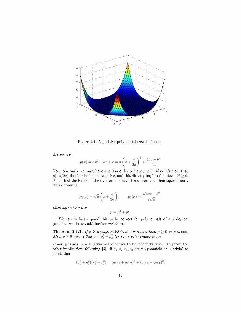
Figure 2.1: A positive polynomial that isn't sos.

the square:

p(x) = ax2 + bx+ c = a

(x+

b

2a

)2

+4ac− b2

4a

Now, obviously we must have a ≥ 0 in order to have p ≥ 0. Also, it's clear thatp(−b/2a) should also be nonnegative, and this directly implies that 4ac−b2 ≥ 0.As both of the terms on the right are nonnegative we can take their square roots,thus obtaining

p1(x) =√a

(x+

b

2a

), p2(x) =

√4ac− b22√a

,

allowing us to writep = p2

1 + p22.

We can in fact expand this to be correct for polynomials of any degree,provided we do not add further variables.

Theorem 2.1.1. If p is a polynomial in one variable, then p ≥ 0 ⇔ p is sos.Also, p ≥ 0 means that p = p2

1 + p22 for some polynomials p1, p2.

Proof. p is sos ⇒ p ≥ 0 was noted earlier to be evidently true. We prove theother implication, following [5]. If q1, q2, r1, r2 are polynomials, it is trivial tocheck that

(q21 + q2

2)(r21 + r2

2) = (q1r1 + q2r2)2 + (q1r2 − q2r1)2.

12

In other words, if q = q21 + q2

2 and r = r21 + r2

2 are both sums of two squaredpolynomials, then p = qr is also a sum of two squares of polynomials.

We assume that p is a polynomial of some degree greater than two that isnever negative. We intend to factor p into positive polynomials of degree two;then the above identity will show us that p is certainly a sum of two squares ofpolynomials.

We split this into two cases. First, we assume p has a real root r of multi-plicity m. Then

p(x) = (x− r)mq(x) where q(r) 6= 0.

Now we need to prove that m is even. We focus our attention on a neighbour-hood of r, setting x = r+ ε. Then p(x+ ε) = εmq(r+ ε). q is a polynomial andthus continuous so there exists a δ > 0 so q(r + ε) doesn't change sign as longas |ε| ≤ δ. Given that p is positive it should be clear that then obviously εm

must have the same sign for all |ε| ≤ δ, in particular even if it is negative, som must be even. Then clearly (x− r)m is a positive polynomial, and so if p isto be positive q must be as well, and we have factored p into a product of twopositive polynomials of lower degree than p.

The other possible situation is that p has no real roots. If so, let r and r betwo conjugate complex roots. Then we can write

p(x) = (x− r)(x− r)q(x),

where obviously (x − r)(x − r) has no real roots, is positive for large x, andas such is always positive on the real line. It follows that in order for p to bepositive q has to be positive as well. Thus we have factored p into a product oftwo positive polynomials of lower degree than p again.

We have proven that if p is a polynomial and p ≥ 0, it can be factoredrepeatedly by the two arguments above until it is a product of positive polyno-mials of degree two (Our arguments hold for any polynomial of degree greaterthan two, so we merely proceed by induction). Technically, we require here thatthe degree of p is even, but if it is not we can't possibly have p ≥ 0, so thispresents no di�culty. As shown initially, each of these second-degree terms is asos of two squares, and using the initial identity and induction again we obtaina representation of their product as a sos of two squares.

2.1.2 Motzkin's polynomial revisited

Expanding the type of polynomials under consideration to those dependent onseveral variables the situation is no longer that simple. We revisit the polynomials(x, y) = x4y2 + x2y4 − 3x2y2 + 1 discussed initially. We prove that this is apositive polynomial. If we take the means of x2, y2 and 1/x2y2 we observe that

13

by the AM-GM inequality

1 =(x2y2

x2y2

) 12

≤ 13

(x2 + y2 +

1x2y2

)3x2y2 ≤ x4y2 + x2y4 + 1

0 ≤ x4y2 + x2y4 − 3x2y2 + 1.

Thus, s ≥ 0, and we need to prove that it cannot be a sum of squares. Weassume, for a contradiction, it is and write it as

s(x, y) = q21(x, y) + q2

2(x, y) + · · ·+ q2n(x, y),

Since s has degree 6 none of the qi can have degree higher than 3. Furthermore,

s(x, 0) = q21(x, 0) + · · ·+ q2

n(x, 0) = 1 and

s(0, y) = q21(0, y) + · · ·+ q2

n(0, y) = 1,

meaning that if either of the variables vanish the qi must be constant. Thus wemay keep only the �cross� terms, giving

qi(x, y) = ai + bixy + cix2y + dixy

2.

It's clear when squaring this that the coe�cient of x2y2 in q2i is b

2i . Then the

coe�cient of the sum of squares must be b21 + b22 + · · ·+ b2n, which is obviouslypositive. However, our coe�cient above was negative! Thus, s can't be sos.

2.2 Quadratic forms

The concept of positive semide�niteness is related to that of positive polynomi-als. We explore this, following [2]. Consider the quadratic form q(x) where x isa column vector of n indeterminates and A ∈Mn×n(R) is a symmetric matrix

q(x) = xTAx. (2.1)

If q ≥ 0 in this case, we say that A is positive semide�nite, or psd.

De�nition 2.2.1 (Change of variable). If x is vector of indeterminates in Rnthen a change of variable is de�ned by an equation of the form x = Py where

P is invertible and y is a new vector of indeterminates in the same space. Note

that this is essentially a coordinate change.

Theorem 2.2.2 (The Principal Axes theorem). Given a quadratic form as in

2.1 we can introduce a change of variable x = Py such that xTAx = yTDywhere D is diagonal, i.e. we have no cross-product terms. Note that the eigen-

values of A will be appearing on the diagonal of D.

14

Proof. It is known from the Spectral Theorem(see [2]), that we do not haveroom to prove here, that a symmetric matrix is orthogonally diagonalizable,and we let P be the matrix that obtains this. Then PT = P−1, P−1AP = Dwhere D is symmetric, and if we let y satisfy x = Py then

xTAx = yTPTAPy = yTDy

thus �nishing the proof.

Now we prove the aforementioned assertion. We know that A has n eigenval-ues, counting multiplicities, by the Spectral Theorem, and the following holds.

Theorem 2.2.3. If A is psd then all eigenvalues of A are nonnegative.

Proof. Using theorem 2.2.2 we obtain a variable change x = Py such that

q(x) = yTDy = λ1y21 + · · ·+ λny

2n.

Now, since A is psd this is nonnegative by de�nition, and so we must haveλi ≥ 0 for all i.

We can now prove the following:

Theorem 2.2.4. If A is psd and q is as before then q is sos.

Proof. By the proof of theorem 2.2.3 we actually obtain just the sum of squaresrepresentation we're looking for (since each yi is a polynomial in some of the xj)by taking roots of the eigenvalues (This can be done since they're not negative)and taking them inside the squares.

We have proven a connection between positive semide�nite matrices andsums of squares. Unfortunately, quadratic forms as de�ned only encapsulatepolynomials of second degree. If we are to prove a more general result aboutsums of squares we need to generalise this notion somewhat. That is what we'regoing to do next.

2.3 Final characterisation of sums of squares

The theorem we will prove in this section was originally proven by Choi, Lamand Reznick, but we will state and prove it as in [4] - though we do not includethe entire discussion from that article, as it's not necessary for our purposes.We must �rst agree on some notation, again due to [4].

We consider polynomials in n variables x1, . . . , xn for some �xed n. Welet N0 denote the set {0, 1, . . .}. If α = (α1, . . . , αn) we de�ne, for notationalconvenience, xα = xα1

1 · . . . · xαnn . We now let m be some nonnegative integer

and de�ne Λm = {(α1, . . . , αn) ∈ Nn0 :∑ni=1 αi ≤ m}, that is, Λm is the set of

all possible vectors α such that xα is a polynomial of degree less than or equal

15

to m. Thus, every polynomial p of degree less than or equal to m can be writtenas a weighted sum of these:

p(x1, . . . , xn) =∑α∈Λm

aαxα

where the aα are weights. Finally, we order the elements of Λm in some way, i.e.we write Λm = {β1, . . . , βk} provided |Λm| = k (It's obvious from the de�nitionthat Λm is �nite, and the nature of the order doesn't really matter as long asthere is an order).

All that said, we can state the theorem we need.

Theorem 2.3.1 (Characterisation of Sums of Squares). If p is some polynomial

in n variables and is of degree 2m, then p is sos if and only if there exists a

real, symmetric, psd matrix B ∈ Rk×k such that

p(x1, . . . , xn) = xTBx

where x is the column vector with k = |Λm| entries whose elements are xβi for

i = 1, . . . , k.

A small note: We won't always actually need the k entries to represent thepolynomial � their weights may be zero. To prove the theorem we need thefollowing lemma(see [2]).

Lemma 2.3.2. If A is a real m× n-matrix, ATA is psd.

Proof. Clearly, ATA is symmetric, since (ATA)T = AT (AT )T = ATA. Nowconsider the quadratic form xTATAx. It's clearly true that

xTATAx = (Ax)T (Ax) = ‖Ax‖2 ≥ 0

under the usual norm on Rn, and this means that A is psd.

We can now prove our main result.

Proof of theorem 2.3.1. First, assume p is sos of degree 2m, and we need, say, tsquares. Then p =

∑ti=1 q

2i where for all i, deg(qi) ≤ m. Let Λm be ordered as

before, and x be as in the statement of the theorem. We let A be the k×t-matrixwith ith column equal to the coe�cients of qi with respect to our ordering ofΛm. Then clearly

p =t∑i=1

q2i ⇒ p = xTATAx.

If we let B = ATA then clearly B is symmetric(and since A is real B is real),and it also has to be psd by lemma 2.3.2. Thus, we have proven one implication.

We next assume that p may be written as

p = xBxT

16

where B is real, symmetric and psd. As B is symmetric it has k eigenvalues,counting multiplicities. Using the Spectral Theorem ([2]) there exists an orthog-onal matrix V such that B = V DV T where D is the diagonal matrix with theeigenvalues λ1, . . . , λk of B on its diagonal. Given that B is psd, then λi ≥ 0for all i. Now

p = xTV TDV x.

De�ne qi to be the i-th element of V x. Now this is a quadratic form in the vector(q1, . . . , qk)T with a diagonal matrix, and we have already seen that this is asum of squares in the previous section � simply write out the product and takethe square roots of the eigenvalues on the diagonal of D to bring them insidethe polynomials (These roots can be taken as the eigenvalues are nonnegative).We have constructed a sum of squares, proving that p is sos. Note also that ifλi is zero, qi is also zero, so the only qi we will use are the ones correspondingto positive eigenvalues of B.

We have found a complete characterisation of positive polynomials that aresums of squares.

2.3.1 An illustrating example

Theorem 2.3.1 may look a little involved, so we include an example to illustratehow it works in a two-variable case. Consider the following polynomial:

f(x, y) = x4 + y4 − 2x2y + 3x2 + 3y2 + 2x+ 1.

This arises by letting f(x, y) = (x2− y)2 + (x+ y)2 + (x− y)2 + (y2)2 + (x+ 1)2,that is, it is a sum of 5 squares. We de�ne

q1(x, y) = x2 − yq2(x, y) = x+ y

q3(x, y) = x− yq4(x, y) = y2

q5(x, y) = x+ 1.

All of these have degree less than or equal to 2, so we consider

Λ2 = {(0, 0), (1, 0), (0, 1), (1, 1), (2, 0), (0, 2)}.

If we de�ne x as above, then

x = (1, x, y, xy, x2, y2)T .

17

We de�ne A to be the matrix with rows equal to the coe�cients of the qi as inthe proof of theorem 2.3.1. Then we get

A =

0 0 −1 0 1 00 1 1 0 0 00 1 −1 0 0 00 0 0 0 0 11 1 0 0 0 0

and ATA =

1 1 0 0 0 01 3 0 0 0 00 0 3 0 −1 00 0 0 0 0 00 0 −1 0 1 00 0 0 0 0 1

.

so de�ning B = ATA it's clear that B is real and symmetric, and it's psdby construction according to Lemma 2.3.2. By calculation, xTBx = 1 + 2x +3x2 + 3y2 − 2x2y + x4 + y4 = f(x, y). Thus f(x, y) = xTBx, illustrating oneimplication in theorem 2.3.1.

Doing this the other way is a little more involved, since diagonalising ma-trices of this size is troublesome by hand (In a practical implementation, somecomputer program would most likely be used). Therefore we will use anotherpolynomial to illustrate this. Assume x = (1, x, y)T and

B =

6 −2 1−2 6 −1−1 −1 5

,and that we are given f(x, y) = xTBx = 6x2 + 5y2− 2xy− 4x− 2y+ 6. ClearlyB is symmetric and real, we want to �nd if it is psd. By calculation, theeigenvalues of B are λ1 = 8, λ2 = 6 and λ3 = 3, so it is in fact positive de�nite� this is more than enough. In order to diagonalise B as done in the proof ofthe theorem, we calculate the eigenvectors and normalize them, getting

v1 =

−1/√

21/√

20

, v2 =

−1/√

6−1/√

62/√

6

and v3 =

1/√

61/√

61/√

6

De�ning V = [v1 v2 v3] and D = diag(8, 6, 3), it's clear that B = V DV T ,

as required. We now de�ne, as in the proof,

q1 =√

8(− 1√

2+

1√2x

)= −2 + 2x,

q2 =√

6(− 1√

6− 1√

6x+

2√6y

)= −1− x+ 2y,

q3 =√

3(

1√3

+1√3x+

1√3y

)= 1 + x+ y,

and it is easy to calculate that q21+q2

2+q23 = 6x2+5y2−2xy−2y−4x+6 = f(x, y),

thus giving us a representation as a sum of three squares. This concludes theillustration of the other implication in the proof.

18

2.4 Hilbert's 17th problem

In 1900 David Hilbert held a speech outlining 23 problems he considered to befruitful questions for mathematicians of that time. The 17th problem is the onethat has been under discussion here, and essentially it's a conjecture by Hilbert� namely that any positive polynomial can be written as a sum of squares ofrational functions. As it turns out, this is the correct de�ning property ofpositive polynomials.

Hilbert's conjecture was resolved a�rmatively in 1928 by Emil Artin, andthe proof is considered one of the greatest triumphs of modern algebra. It usesa number of results beyond what we have room for here, though, and so we shallnot attempt to reproduce it � it's given for instance in [3].

For instance the problematic polynomial s(x, y) = 1− 3x2y2 + x2y4 + x4y2

we considered earlier can indeed be written as a sum of squares of rationalfunctions, as required by Artin's result. It is done in the following way, due to[3]:

1− 3x2y2 + x2y4 + x4y2 =(x2y(x2 + y2 − 2)

x2 + y2

)2

+(xy2(x2 + y2 − 2)

x2 + y2

)2

+(xy(x2 + y2 − 2)

x2 + y2

)2

+(x2 − y2

x2 + y2

)2

.

Note also that in 1967 it was proven by P�ster(see [3]) that if p is a positivepolynomial in n variables then 2n squares will always be enough. It will oftenbe possible, however, to write p as a sum of more squares than that. Note thatthe representation of Motzkin's polynomial above illustrates this, using 22 = 4squares.

19

Bibliography

[1] S. S. Dragomir. A survey on cauchy�bunyakovsky�schwarz type discreteinequalities. Journal of Inequalities in Pure and Applied Mathematics, 4,2003.

[2] David C. Lay. Linear Algebra and its Applications, 3rd ed. Pearson Educa-tion, 2006.

[3] Murray Marshall. Positive Polynomials and Sums of Squares. AmericanMathematical Society, 2008.

[4] Victoria Powers and Thorsten Wörmann. An algorithm for sums of squaresof real polynomials. Journal of pure and applied algebra, 127:99�104, 1998.

[5] J. Michael Steele. The Cauchy-Schwarz Master Class. Cambridge UniversityPress, 2004.

20