arX

iv:h

ep-t

h/04

0404

2v2

10

Apr

200

4

Quantum weights of dyons and of instantons with non-trivial holonomy

Dmitri Diakonova,b, Nikolay Gromovc, Victor Petrovb, and Sergey Slizovskiyc

aNORDITA, Blegdamsvej 17, DK-2100 Copenhagen, DenmarkbSt. Petersburg NPI, Gatchina, 188 300, St. Petersburg, Russia

cSt. Petersburg State University, Faculty of Physics,

Ulianovskaya 1, 198 904, St. Petersburg, Russia.

(Dated: April 9, 2004)

We calculate exactly functional determinants for quantum oscillations about periodic instantonswith non-trivial value of the Polyakov line at spatial infinity. Hence, we find the weight or theprobability with which calorons with non-trivial holonomy occur in the Yang–Mills partition func-tion. The weight depends on the value of the holonomy, the temperature, ΛQCD, and the separationbetween the BPS monopoles (or dyons) which constitute the periodic instanton. At large separa-tion between constituent dyons, the quantum measure factorizes into a product of individual dyonmeasures, times a definite interaction energy. We present an argument that at temperatures belowa critical one related to ΛQCD, trivial holonomy is unstable, and that calorons “ionize” into separatedyons.

PACS numbers: 11.15.-q,11.10.Wx,11.15.Tk

I. MOTIVATION AND THE MAIN RESULT

There are two known generalizations of the standard self-dual instantons to non-zero temperatures. One is theperiodic instanton of Harrington and Shepard [1] studied in detail by Gross, Pisarski and Yaffe [2]. These periodicinstantons, also called calorons, are said to have trivial holonomy at spatial infinity. It means that the Polyakov line

L = P exp

(∫ 1/T

0

dtA4

)∣∣∣∣∣|~x|→∞

(1)

assumes values belonging to the group center Z(N) for the SU(N) gauge group [34]. The vacuum made of thoseinstantons has been investigated, using the variational principle, in ref. [3].

The other generalization has been constructed a few years ago by Kraan and van Baal [4] and Lee and Lu [5]; it hasbeen named caloron with non-trivial holonomy as the Polyakov line for this configuration does not belong to the groupcenter. We shall call it for short the KvBLL caloron. It is also a periodic self-dual solution of the Yang–Mills equationsof motion with an integer topological charge. In the limiting case when the KvBLL caloron is characterized by trivialholonomy, it is reduced to the Harrington–Shepard caloron. The fascinating feature of the KvBLL construction isthat a caloron with a unit topological charge can be viewed as “made of” N Bogomolnyi–Prasad–Sommerfeld (BPS)monopoles or dyons [6, 7].

Dyons are self-dual solutions of the Yang–Mills equations of motion with static (i.e. time-independent) actiondensity, which have both the magnetic and electric field at infinity decaying as 1/r2. Therefore these objects carryboth electric and magnetic charges (prompting their name). In the 3+1-dimensional SU(2) gauge theory there are infact two types of self-dual dyons [8]: M and L with (electric, magnetic) charges (+,+) and (−,−), and two types ofanti-self-dual dyons M and L with charges (+,−) and (−,+), respectively. Their explicit fields can be found e.g. inref. [9]. In the SU(N) theory there are 2N different dyons [8, 10]: M1,M2, ...MN−1 ones with charges counted withrespect to N − 1 Cartan generators and one L dyon with charges compensating those of M1...MN−1 to zero, andtheir anti-self-dual counterparts.

Speaking of dyons one implies that the Euclidean space-time is compactified in the ‘time’ direction whose inversecircumference is temperature T , with the usual periodic boundary conditions for boson fields. However, thetemperature may go to zero, in which case the 4d Euclidean invariance is restored.

Dyons’ essence is that the A4 component of the dyon field tends to a constant value at spatial infinity. Thisconstant A4 can be eliminated by a time-dependent gauge transformation. However then the fields violate theperiodic boundary conditions, unless A4 has quantized values corresponding to trivial holonomy, i.e. unless thePolyakov line belongs to the group center. Therefore, in a general case one implies that dyons have a non-zero value

2

-10

1z -0.5

-0.2500.250.5

t-10

1z

-10

1z -0.5

-0.2500.250.5

t-10

1z

FIG. 1: The action density of the KvBLL caloron as function of z, t at fixed x = y = 0, with the asymptotic value of A4 atspatial infinity v = 0.9πT, v = 1.1πT . It is periodic in t direction. At large dyon separation the density becomes static (left,r12 = 1.5/T ). As the separation decreases the action density becomes more like a 4d lump (right, r12 = 0.6/T ). In both plotsthe L,M dyons are centered at zL = −v r12/2πT, zM = v r12/2πT, xL,M = yL,M = 0. The axes are in units of temperature T.

of A4 at spatial infinity and a non-trivial holonomy.

The KvBLL caloron of the SU(2) gauge group (to which we restrict ourselves in this paper) with a unit topologicalcharge is “made of” one L and one M dyon, with total zero electric and magnetic charges. Although the actiondensity of isolated L and M dyons does not depend on time, their combination in the KvBLL solution is generallynon-static: the L,M “constituents” show up not as 3d but rather as 4d lumps, see Fig. 1. When the temperaturegoes to zero while the separation between dyons remain fixed, these lumps merge, and the KvBLL caloron is reducedto the usual Belavin–Polyakov–Schwarz–Tyutin instanton [11] (as is the standard Harrington–Shepard caloron), plus

corrections of the order of T . However, the holonomy remains fixed and non-trivial at spatial infinity.

There is a strong argument against the presence of either dyons or KvBLL calorons in the Yang–Mills partitionfunction at nonzero temperatures [2]. The point is, the 1-loop effective action obtained from integrating out fastvarying fields where one keeps all powers of A4 but expands in (covariant) derivatives of A4 has the form [12]

S1−loop =

∫d4x

[P (A4) + E2fE(A4) +B2fB(A4) + higher derivative terms

],

P (A4) =1

3T (2π)2v2(2πT − v)2

∣∣∣∣mod 2πT

, v =√Aa

4Aa4 [for the SU(2) group] (2)

where the perturbative potential energy term P (A4) has been known for a long time [2, 14], see Fig. 2. As followsfrom eq.(1) the trace of the Polyakov line is related to v as

1

2TrL = cos

v

2T. (3)

The zeros of the potential energy correspond to 12TrL = ±1, i.e. to the trivial holonomy. If a dyon has v 6= 2πTn

at spatial infinity the potential energy is positive-definite and proportional to the 3d volume. Therefore, dyons andKvBLL calorons with non-trivial holonomy seem to be strictly forbidden: quantum fluctuations about them have anunacceptably large action.

Meanwhile, precisely these objects determine the physics of the supersymmetric YM theory where in addition togluons there are gluinos, i.e. Majorana (or Weyl) fermions in the adjoint representation. Because of supersymmetry,the boson and fermion determinants about L,M dyons cancel exactly, so that the perturbative potential energy (2) isidentically zero for all temperatures, actually in all loops. Therefore, in the supersymmetric theory dyons are openlyallowed. [To be more precise, the cancellation occurs when periodic conditions for gluinos are imposed, so it is thecompactification in one (time) direction that is implied, rather than physical temperature which requires antiperiodicfermions.] Moreover, it turns out [10] that dyons generate a non-perturbative potential having a minimum at v = πT ,i.e. where the perturbative potential would have the maximum. This value of A4 corresponds to the holonomyTrL = 0 at spatial infinity, which is the “most non-trivial”; as a matter of fact <TrL>= 0 is one of the confinement’srequirements. In the supersymmetric YM theory configurations having TrL = 0 at infinity are not only allowed butdynamically preferred as compared to those with 1

2TrL = ±1. In non-supersymmetric theory it looks as if it is theopposite.

3

Nevertheless, it has been argued in ref. [15] that the perturbative potential energy (2) which forbids individualdyons in the pure YM theory might be overruled by non-perturbative contributions of an ensemble of dyons. For fixeddyon density, their number is proportional to the 3d volume and hence the non-perturbative dyon-induced potentialas function of the holonomy (or of A4 at spatial infinity) is also proportional to the volume. It may be that attemperatures below some critical one the non-perturbative potential wins over the perturbative one so that the systemprefers <TrL>= 0. This scenario could then serve as a microscopic mechanism of the confinement-deconfinementphase transition [15]. It should be noted that the KvBLL calorons and dyons seem to be observed in latticesimulations below the phase transition temperature [16–18].

To study this possible scenario quantitatively, one first needs to find out the quantum weight of dyons or theprobability with which they appear in the Yang–Mills partition function. Unfortunately, the single-dyon measure isnot well defined: it is too badly divergent in the infrared region owing to the weak (Coulomb-like) decrease of thefields. What makes sense and is finite, is the quantum determinant for small oscillations about the KvBLL caloronwhich possesses zero net electric and magnetic charges. To find this determinant is the primary objective of thisstudy. The KvBLL measure depends on the asymptotic value of A4 (or on the holonomy through eq.(3)), on thetemperature T , on Λ, the scale parameter obtained through the renormalization of the charge, and on the dyonseparation r12. At large separations between constituent L,M dyons of the caloron, one gets their weights and theirinteraction.

The problem of computing the effect of quantum fluctuations about a caloron with non-trivial holonomy is of thesame kind as that for ordinary instantons (solved by ’t Hooft [19]) and for the standard Harrington–Shepard caloron(solved by Gross, Pisarski and Yaffe [2]) being, however, technically much more difficult. The zero-temperatureinstanton is O(4) symmetric, and the Harrington–Shepard caloron is O(3) symmetric, which helps. The KvBLLcaloron has no such symmetry as obvious from Fig. 1. Nevertheless, we have managed to find the small-oscillationdeterminant exactly. It becomes possible because we are able to construct the exact propagator of spin-0, isospin-1field in the KvBLL background, which by itself is some achievement.

As it is well known [2, 19], the calculation of the quantum weight of a Euclidean pseudoparticle consists of threesteps: i) calculation of the metric of the moduli space or, in other words, computing the Jacobian composed of zeromodes, needed to write down the pseudoparticle measure in terms of its collective coordinates, ii) calculation of thefunctional determinant for non-zero modes of small fluctuations about a pseudoparticle, iii) calculation of the ghostdeterminant resulting from background gauge fixing in the previous step. Problem i) has been actually solved alreadyby Kraan and van Baal [4]. Problem ii) is reduced to iii) in the self-dual background field [20] since for such fieldsDet(Wµν) = Det(−D2)4, where Wµν is the quadratic form for spin-1, isospin-1 quantum fluctuations and D2 is thecovariant Laplace operator for spin-0, isospin-1 ghost fields. Symbolically, one can write

KvBLL measure =

∫d(collective coordinates) · Jacobian ·Det−

12 (Wµν) ·Det(−D2) (4)

where the product of the last two factors is simply Det−1(−D2) in the self-dual background. As usually, thefunctional determinants are normalized to free ones (with zero background fields) and UV regularized (we use thestandard Pauli–Villars method). Thus, to find the quantum weight of the KvBLL caloron only the ghost determinanthas to be computed.

To that end, we follow Zarembo [21] and find the derivative of this determinant with respect to the holonomy or,more precisely, to v ≡

√Aa

4Aa4

∣∣|~x|→∞. The derivative is expressed through the Green function of the ghost field in

the caloron background. If a self-dual field is written in terms of the Atiah–Drinfeld–Hitchin–Manin construction,and in the KvBLL case it basically is [4, 5], the Green function is generally known [23]-[25] and we build it explicitlyfor the KvBLL case. Therefore, we are able to find the derivative ∂Det(−D2)/∂v. Next, we reconstruct the fulldeterminant by integrating over v using the determinant for the trivial holonomy [2] as a boundary condition. Thisdeterminant at v = 0 is still a non-trivial function of r12 and the fact that we match it from the v 6= 0 side is a seriouscheck. Actually we need only one overall constant factor from ref. [2] in order to restore the full determinant atv 6= 0, and we make a minor improvement of the Gross–Pisarski–Yaffe calculation as we have computed the neededconstant analytically.

Although all the above steps can be performed explicitly, at some point the equations become extremely lengthy –typical expressions are several Mbytes long and so far we have not managed to simplify them such that they wouldfit into a paper. However, we are able to obtain compact analytical expressions in the physically interesting case of

4

1 2 3 4 5 6v

0.2

0.4

0.6

0.8

P T3

FIG. 2: Potential energy as function of v/T . Two minima correspond to 1

2TrL = ±1, the maximum corresponds to TrL = 0.

The range of the holonomy where dyons experience repulsion is shown in dashing.

large separation between dyons, r12 ≫ 1/T . We have also used the exact formulae to check numerically some of theintermediate formulae, in particular at v→ 0.

If the separation is large in the temperature scale, r12 ≫ 1/T , the final result for the quantum measure of the KvBLLcaloron can be written down in terms of the 3d positions of the two constituent L,M dyons ~z1,2, their separationr12 = |~z1 − ~z2|, the asymptotic of A4 at spatial infinity denoted by v ∈ [0, 2πT ] and v = 2πT − v ∈ [0, 2πT ], seeeq.(80). We give here a simpler expression obtained in the limit when the separation between dyons is much largerthan their core sizes:

ZKvBLL =

∫d3z1 d

3z2 T6 (2π)

83 C

(8π2

g2

)4(ΛeγE

4πT

) 223 ( v

2πT

) 4v3πT

(v

2πT

) 4v3πT

× exp [−2π r12 P′′(v)] exp

[−V (3)P (v)

], (5)

where the overall factor C is a combination of universal constants; numerically C = 1.031419972084. Λ is the scaleparameter in the Pauli–Villars scheme; the factor g−8 is not renormalized at the one-loop level.

Since the caloron field has a constant A4 component at spatial infinity, it is suppressed by the sameperturbative potential P (v) as given by eq.(2). Its second derivative with respect to v is P ′′(v) =

1π2T

[v−πT

(1− 1√

3

)] [v−πT

(1+ 1√

3

)]. If v is in the ranges between 0 and πT

(1− 1√

3

)or between πT

(1+ 1√

3

)and

2πT (corresponding to the holonomy not too far from the trivial, 0.787597< 12 |TrL|<1) the second derivative P ′′(v)

is positive, and the L and M dyons experience a linear attractive potential. Integration over the separation r12 ofdyons inside a caloron converges. We perform this integration in section VII, estimate the free energy of the calorongas and conclude that trivial holonomy (v = 0, 2πT ) may be unstable, despite the perturbative potential energy P (v).

In the complementary range πT(1− 1√

3

)< v< πT

(1+ 1√

3

)(or 1

2 |TrL|< 0.787597), P ′′(v) is negative (see Fig. 2),

and dyons experience a strong linear-rising repulsion. It means that for these values of v, integration over the dyonseparations diverges: calorons with holonomy far from trivial “ionize” into separate dyons.

II. THE KVBLL CALORON SOLUTION

Although the construction of the self-dual solution with non-trivial holonomy has been fully performed indepen-dently by Kraan and van Baal [4] and Lee and Lu [5] we have found it more convenient for our purposes to use thegauge convention and the formalism of Kraan and van Baal (KvB) whose notations we follow in this paper.

The key quantities characterizing the KvBLL solution for a general SU(N) gauge group are the N−1 gauge-invarianteigenvalues of the Polyakov line (1) at spatial infinity. For the SU(2) gauge group to which we restrict ourselves inthis paper, it is just one quantity, e.g. TrL, eq.(3). In a gauge where A4 is static and diagonal at spatial infinity,i.e. A4|~x→∞ = iv τ3

2 , it is this asymptotic value v which characterizes the caloron solution in the first place. Weshall also use the complementary quantity v ≡ 2πT − v. Their relation to parameters ω, ω introduced by KvB [4] isω = v

4πT , ω = v4πT = 1

2 − ω. Both v and v vary from 0 to 2πT . At v = 0, 2πT the holonomy is said to be ‘trivial’,and the KvBLL caloron reduces to that of Harrington and Shepard [1].

5

There are, of course, many ways to parametrize the caloron solution. Keeping in mind that we shall be mostly inter-ested in the case of widely separated dyon constituents, we shall parametrize the solution in terms of the coordinatesof the dyons’ ‘centers’ (we call constituent dyons L and M according to the classification in ref. [9]):

L dyon : ~z1 = −2ω−→r12T

,

M dyon : ~z2 =2ω−→r12T

,

dyon separation : ~z2 − ~z1 = −→r12, |r12| = πT ρ2,

where ρ is the parameter used by KvB; it becomes the size of the instanton at v → 0. We introduce the distancesfrom the ‘observation point’ ~x to the dyon centers,

~r = ~x− ~z1 = ~x+ 2ω−→r12, r = |~r|,~s = ~x− ~z2 = ~x− 2ω−→r12, s = |~s|. (6)

Henceforth we measure all dimensional quantities in units of temperature for brevity and restore T explicitly only inthe final results.

The KvBLL caloron field in the fundamental representation is [4] (we choose the separation between dyons to bein the third spatial direction, −→r12 = r12~e3):

Aµ = δµ,4 ivτ32

+i

2η3

µντ3∂ν ln Φ +i

2Φ Re

[(η1

µν − iη2µν)(τ1 + iτ2)(∂ν + ivδν,4)χ

], (7)

where τi are Pauli matrices, ηaµν are ’t Hooft’s symbols [19] with ηa

ij = ǫaij and ηa4ν = −ηa

ν4 = iδaν . “Re” means

2Re(W ) ≡W +W † and the functions used are

ψ = − cos(2πx4) + ch ch +~r~s

2rssh sh , ψ = ψ +

r212rs

sh sh +r12s

sh ch +r12r

sh ch ,

χ =r12ψ

(e−2πix4

sh

s+

sh

r

), Φ =

ψ

ψ. (8)

We have introduced short-hand notations for hyperbolic functions:

sh ≡ sinh(sv), ch ≡ cosh(sv), sh ≡ sinh(rv), ch ≡ cosh(rv) . (9)

The first term in (7) corresponds to a constant A4 component at spatial infinity (A4 ≈ iv τ3

2 ) and gives rise to thenon-trivial holonomy. One can see that Aµ is periodic in time with period 1 (since we have chosen the temperatureto be equal to unity). A useful formula for the field strength squared is [4]

TrFµνFµν = ∂2∂2 logψ. (10)

In the situation when the separation between dyons r12 is large compared to both their core sizes 1v (M) and 1

v (L),the caloron field can be approximated by the sum of individual BPS dyons, see Figs. 1,3 (left) and Fig. 4. We givebelow the field inside the cores and far away from both cores.

A. Inside dyon cores

In the vicinity of the L dyon center ~z1 and far away from the M dyon (sv ≫ 1) the field becomes that of the Ldyon. It is instructive to write it in spherical coordinates centered at ~z1. In the ‘stringy’ gauge [9] in which the A4

component is constant and diagonal at spatial infinity, the L dyon field is

AL4 =

iτ32

(1

r+ 2π − v coth(vr)

), AL

r = 0,

ALθ = iv

− sin(2πx4 − φ) τ1 + cos(2πx4 − φ)τ22 sinh(vr)

,

ALφ = iv

cos(2πx4 − φ) τ1 + sin(2πx4 − φ)τ22 sinh(vr)

− iτ3tan(θ/2)

2r. (11)

6

-10

1z -1

-0.5

00.51

x-10

1z

-10

1z -1

-0.5

00.51

x-10

1z

FIG. 3: The action density of the KvBLL caloron as function of z, x at fixed t = y = 0. At large separations r12 the caloronis a superposition of two BPS dyon solutions (left, r12 = 1.5/T ). At small separations they merge (right, r12 = 0.6/T ). Thecaloron parameters are the same as in Fig. 1.

Here Aθ, for example, is the projection of ~A onto the direction ~nθ = (cos θ cosφ, cos θ sinφ,− sin θ). The φ componenthas a string singularity along the z axis going in the positive direction. Notice that inside the core region (vr ≤ 1)the field is time-dependent, although the action density is static. At large distances from the L dyon center, i.e. faroutside the core one neglects exponentially small terms O

(e−vr

)and the surviving components are

AL4

r→∞−→(

v +1

r

)iτ3

2,

ALφ

r→∞−→ − tanθ2

r

iτ3

2

corresponding to the radial electric and magnetic field components

ELr = BL

rr→∞−→ − 1

r2iτ3

2. (12)

This Coulomb-type behavior of both the electric and magnetic fields prompts the name ‘dyon’.Similarly, in the vicinity of the M dyon and far away from the L dyon (rv ≫ 1) the field becomes that of the M

dyon, which we write in spherical coordinates centered at ~z2:

AM4 =

iτ32

(v coth(vs)− 1

s

), AM

θ = vsinφ τ1 − cosφ τ2

2i sinh(vs),

AMr = 0, AM

φ = vcosφ τ1 + sinφ τ2

2i sinh(vs)+ iτ3

tan(θ/2)

2s, (13)

whose asymptotics is

AM4

r→∞−→(

v− 1

s

)iτ3

2,

AMφ

r→∞−→ tan θ2

s

iτ3

2,

EMr = BM

rr→∞−→ 1

s2iτ3

2. (14)

We see that in both cases the L,M fields become Abelian at large distances, corresponding to (electric, magnetic)charges (−,−) and (+,+), respectively. The corrections to the fields (11,13) are hence of the order of 1/r12 arisingfrom the presence of the other dyon.

B. Far away from dyon cores

Far away from both dyon cores (rv ≫ 1, sv ≫ 1; note that it does not necessarily imply large separations – thedyons may even be overlapping) one can neglect both types of exponentially small terms, O

(e−rv

)and O (e−sv).

7

With exponential accuracy the function χ in eq.(8) is zero, and the KvBLL field (7) becomes Abelian [4]:

Aasµ = i

τ32

(δµ4v + η3

µν∂ν ln Φas

), (15)

where Φas is the function Φ of eq.(8) evaluated with the exponential precision:

Φas =r + s+ r12r + s− r12

=s− s3r − r3

if −→r12 = r12~e3. (16)

It is interesting that, despite being Abelian, the asymptotic field (15) retains its self-duality. This is because the 3d

color component of the electric field is

E3i = ∂iA

34 = ∂i∂3 ln Φas

while the magnetic field is

B3i = ǫijk∂jA

3k = ∂i∂3 ln Φas − δi3∂2 ln Φas,

where the last term is zero, except on the line connecting the dyon centers where it is singular; however, this singularityis an artifact of the exponential approximation used. Explicit evaluation of eq.(15) gives the following nonzerocomponents of the Aµ field far away from both dyon centers:

Aas4 =

iτ32

(v +

1

r− 1

s

), (17)

Aasϕ = − iτ3

2

(1

r+

1

s

)√(r12 − r + s)(r12 + r − s)(r12 + r + s)(r + s− r12)

. (18)

In particular, far away from both dyons, A4 is the Coulomb field of two opposite charges.

III. THE SCHEME FOR COMPUTING DET(−D2)

As explained in section I, to find the quantum weight of the KvBLL caloron, one needs to calculate the smalloscillation determinant, Det(−D2), where Dµ = ∂µ + Aµ and Aµ is the caloron field (7). Instead of computing thedeterminant directly, we first evaluate its derivative with respect to the holonomy v, and then integrate the derivativeusing the known determinant at v = 0 [2] as a boundary condition.

If the background field Aµ depends on some parameter P , a general formula for the derivative of the determinantwith respect to such parameter is

∂ log Det(−D2[A])

∂P =−∫d4xTr (∂PAµ Jµ) , (19)

where Jµ is the vacuum current in the external background, determined by the Green function:

Jabµ ≡ (δa

c δbd∂x−δa

c δbd∂y+Aacδb

d+Adbδac )Gcd(x, y)

∣∣y=x

or simply Jµ ≡−→DµG + G←−Dµ. (20)

Here G is the Green function or the propagator of spin-0, isospin-1 particle in the given background Aµ defined by

−D2xG(x, y) = δ(4)(x− y) (21)

and, in the case of nonzero temperatures, being periodic in time, meaning that

G(x, y) =

∞∑

n=−∞G(x4, ~x; y4 + n, ~y). (22)

Eq.(19) can be easily verified by differentiating the identity log Det(−D2) = Tr log(−D2) [35]. The background fieldAµ in eq.(19) is taken in the adjoint representation, as is the trace. Hence, if the periodic propagator G is known,eq.(19) becomes a powerful tool for computing quantum determinants. Specifically, we take P = v as the parameterfor differentiating the determinant, and there is no problem in finding ∂vAµ for the caloron field (7).

8

1/v

R

1/−v

R

r12

r s

L dyon M dyon

z1 z2

x

FIG. 4: Three regions of integration for well separated dyons.

The Green functions in self-dual backgrounds are generally known [25, 26] and are built in terms of the Atiah–Drinfeld–Hitchin–Manin (ADHM) construction [28] for the given self-dual field. A subtlety appearing at nonzerotemperatures is that the Green function is defined by eq.(21) in the Euclidean IR4 space where the topological chargeis infinite because of the infinite number of repeated strips in the compactified time direction, whereas one actuallyneeds an explicitly periodic propagator (22). To overcome this nuisance, Nahm [25] suggested to pass on to theFourier transforms of the infinite-range subscripts in the ADHM construction. We perform this program explicitly inAppendix A, first for the single dyon field and then for the KvBLL caloron. In this way, we get the finite-dimensionalADHM construction both for the dyon and the caloron, with very simple periodicity properties. Using it, we constructexplicitly periodic propagators in Appendix B, also first for the dyon and then for the caloron case. For the KvBLLcaloron it was not known previously. Using the obtained periodic propagators, in Appendix C we calculate the exactvacuum current (20) for the dyon, and in Appendix D we evaluate the vacuum current in the caloron background,with the help of the regularization carried out in Appendix E.

Although there is no principle difficulty in doing all calculations exactly for the whole caloron moduli space, at somepoint we loose the capacity of performing analytical calculations for the simple reason that expressions become toolong, and so far we have not been able to put them into a manageable form in a general case. Therefore, we have toadopt a more subtle attitude. First of all we restrict ourselves to the part of the moduli space corresponding to largeseparations between dyons (r12 ≫ 1). Physically, it seems to be the most interesting case, see section I. Furthermore,at the first stage we take r12v, r12v ≫ 1, meaning that the dyons are well separated and do not overlap since theseparation is then much bigger than the core sizes, see Figs. 1,3 (left). In this case, the vacuum current Jµ (20) becomesthat of single dyons inside the spheres of some radius R surrounding the dyon centers, such that 1

v ,1v ≪ R≪ r12, and

outside these spheres it can be computed analytically with exponential precision, in correspondence with subsectionII.B, see Fig. 4. Adding up the contributions of the regions near two dyons and of the far-away region, we getdDet(−D2)/dv for well-separated dyons. Integrating it over v we obtain the determinant itself up to a constant andpossible 1/r12 terms.

This is already an interesting result by itself, however, we would like to compute the constant, which can bedone by matching our calculation with that for the trivial caloron at v = 0. It means that we have to extend thedomain of applicability to r12v = O(1) (or r12v = O(1)) implying overlapping dyons, presented in Figs. 1,3 (right).To make this extension, we ‘guess’ the analytical expression which would interpolate between r12v ≫ 1 where thedeterminant is already computed and r12v≪ 1 where matching with the Gross–Pisarski–Yaffe (GPY) calculation [2]can be performed. At this point it becomes very helpful that we possess the exact vacuum current for the caloron,which, although too long to be put on paper, is nevertheless affordable for numerical evaluation (and can be providedon request). We check our analytical ‘guess’ to the accuracy better than one millionth. In this way we obtain thedeterminant up to an overall constant factor for any v, v with the only restriction that r12 ≫ 1. This constant factoris then read off from the GPY calculation [2].

Finally, we compute the 1/r12 and log r12/r12 corrections in the Det(−D2), which turn out to be quite non-trivial.

9

IV. DET(−D2) FOR WELL SEPARATED DYONS

The L,M dyon cores have the sizes 1v and 1

v , respectively, and in this section we consider the case of well-separated

dyons, meaning that the distance between the two centers is much greater than the core sizes, r12 ≫ 1v ,

1v . This

situation is depicted in Figs. 1,3 (left). The two dyons are static in time, so that ∂ log Det(−D2)/∂v (19) becomesan integral over 3d space, times 1/T set to unity. We divide the 3d volume into to three regions (Fig. 4): i) a ball ofradius R centered at the center of the M dyon, ii) a ball of radius R centered at the L dyon, iii) the rest of the space,with two balls removed. The radius R is chosen such that it is much larger than the dyon cores but much less thanthe separation: r12 ≫ R ≫ 1

v ,1v . Summing up the contributions from the three regions of space, we are satisfied to

observe that the result does not depend on the intermediate radius R.

A. Det(−D2) for a single dyon

In region i) the KvBLL caloron field can be approximated by the M dyon field (13), and the vacuum current by thatinside a single dyon, both with the O(1/r12) accuracy. We make a more precise calculation, including the O(1/r12)terms, in section V. The single-dyon vacuum current is calculated in Appendix C. Adding up the three parts of thevacuum current denoted there as J s,r,m

µ we obtain the full isospin-1 vacuum current (in the ‘stringy’ gauge)

Jr = 0,

Jφ = − iv(sin(φ)T2 + cos(φ)T1)(1− sv coth(sv))2

24π2s2 sinh(sv),

Jθ = − iv(sin(φ)T1 − cos(φ)T2)(1− sv coth(sv))2

24π2s2 sinh(sv),

J4 = −iT3

[(1− sv coth(sv))3

6π2s3+

1− sv coth(sv)

3s+

coth(sv)(1 − sv coth(sv))2

2πs2

],

where (Tc)ab ≡ iεacb are the isospin-1 generators. We contract Jµ (23) with dAµ/dv from eq.(13) according to eq.(19).

After taking the matrix trace, the integrand in eq.(19) becomes spherically symmetric:

Tr [∂vAµJµ] =2

3s

(coth(sv)− sv +

sv (sv coth(sv)− 2)

sinh2(sv)

)

− (sv coth(sv)− 1)3 (sinh(2sv)− 3sv)

6π2 sinh2(sv)s3+

(sv coth(sv)− 1)2 (sinh(2sv)− 2sv)

2π sinh2(sv) tanh(sv)s2; (23)

It has to be integrated over the spherical box of radius R. Fortunately, we are able to perform the integrationanalytically. The result for the M dyon is

∂ log Det(−D2[M dyon])

∂v= −

∫ R

0

dsTr [∂vAµJµ] 4πs2 = −24(γE − log π) + 53 + 23π

2

18π+

1

v

+4πR3

3P ′(v)− 2πR2 P ′′(v) + 2πRP ′′′(v)− 4

3πlog(Rv). (24)

As we see, it is badly infrared divergent, as it depends on the box radius R. Here P (q) is the potential energy (seeeq.(2))

P (q) =

[π2

12

( qπ− 2)2 ( q

π

)2], P ′(q) =

1

3π2q(π − q)(2π − q),

P ′′(q) =1

3π2(3q2 − 6πq + 2π2), P ′′′(q) =

2

π2(q − π), P IV(q) =

2

π2.

The IR-divergent terms arise from the asymptotics of the integrand. Neglecting exponentially small terms e−sv ineq.(23) we have

−Tr [∂vAµJµ] ≃ −4

[(1 − sv)3

12π2s3+

(1− sv)2

4πs2+

1− sv6s

]

= P ′(

v − 1

s

)= P ′(v)− P ′′(v)

1

s+

1

2P ′′′(v)

1

s2− 1

6P IV(v)

1

s3.

10

Integrating it over the sphere of radius R one gets the IR-divergent terms (the second line in eq.(24)).The fact that the IR-divergent part of dDet(−D2)/dv is directly related to the potential energy P (A4) is not

accidental. At large distances the field of the dyon becomes a slowly varying Coulomb field, see eq.(14). Therefore,the determinant can be generically expanded in the covariant derivatives of the background field [12, 13] with thepotential energy P (A4) being its leading zero-derivative term. The nontrivial fact, however, is that with exponentialprecision the vacuum current is related to the variation of solely the leading term in the covariant derivative expansionof the effective action with no contribution from any of the subleading terms. This is a specific property of self-dualfields, and we observe it also in the following subsection.

B. Contribution from the far-away region

We now compute the contribution to ∂Det(−D2)/∂v from the region of space far away from both dyon centers.With exponential accuracy (meaning neglecting terms of the order of e−rv and e−sv) the KvBLL caloron field is givenby eqs.(17,18), and only the A4 component depends (trivially) on v. The caloron vacuum current with the sameexponential accuracy is calculated in Appendix D. Combining the results given by eqs.(D8,D9) and eqs.(D11,D12) wesee that Jϕ = 0 and for J4 we have

J4 =iT3

2

[1

3π2

(1

r− 1

s

)3

− 1

π

(1

r− 1

s

)2

+2

3

(1

r− 1

s

)]+

[4

π

(1

r− 1

s

)2

− 8

(1

r− 1

s

)+

8π

3

]ω

+

[16

(1

r− 1

s

)− 16π

]ω2 +

64π

3ω3

. (25)

We remind the reader that r, s are distances from M,L dyon centers ~z1,2 and that ω = v/(4π). It is interesting thatthe separation r12 = |z1 − z2| does not appear explicitly in the current. Moreover, it can be again written throughthe potential energy P (A4):

J4 =1

2iT3 P

′(q)|q=v+1/r−1/s . (26)

Therefore, in the far-away region one obtains

−Tr [∂vAµJµ] = P ′(

v +1

r− 1

s

). (27)

We have now to integrate eq.(27) over the whole 3d space with two spheres of radius R surrounding the dyon centersremoved:

−∫d4xTr [∂vAµJµ] =

∫d3xP ′

(v +

1

r− 1

s

)(28)

= P ′(v)

∫d3x+ P ′′(v)

∫d3x

(1

r− 1

s

)+

1

2P ′′′(v)

∫d3x

(1

r− 1

s

)2

+1

6P IV(v)

∫d3x

(1

r− 1

s

)3

.

The first integral in eq.(28) is the 3d volume V , minus the volume of two spheres, V − 2 4π3 R

3. The second integral iszero by symmetry between the two centers, and so is the last one. The only non-trivial integral is

∫d3x

(1

r− 1

s

)2

= 4πr12 − 8πR+O(R2

r12

). (29)

Therefore, the contribution from the region far from both dyon centers is

∂ log Det(−D2)

∂v

∣∣∣∣far

= P ′(v)

(V − 2

4π

3R3

)+

1

2P ′′′(v) (4πr12 − 8πR) . (30)

11

C. Combining all three regions

We now add up the contributions to ∂ log Det(−D2)/∂v from the regions surrounding the two dyons and fromthe far-away region. Since the contribution of the L dyon is the same as that of the M dyon with the replacementv → v and since ∂/∂v = −∂/∂v, when adding up contributions of L,M core regions we have to antisymmetrize inv ↔ v. It should be noted that P (v) and P ′′(v) are symmetric under this interchange, while P ′(v) and P ′′′(v) areantisymmetric. Therefore, the combined contribution of both cores is, from eq.(24),

∂ log Det(−D2)

∂v

∣∣∣∣cores

= 2P ′(v)4π

3R3 +

1

2P ′′′(v) 8πR +

1

v− 1

v− 4

3πln(v

v

). (31)

Adding it up with the contribution from the far-away region, eq.(30), we obtain the final result which is independentof the intermediate radius R used to separate the regions:

∂ log Det(−D2)

∂v= P ′(v)V + P ′′′(v) 2πr12 +

1

v− 1

v− 4

3πln(v

v

). (32)

This equation can be easily integrated over v up to a constant which in fact can be a function of the separation r12:

log Det(−D2) = P (v)V + P ′′(v) 2πr12 +

(1− 4v

3π

)log(v) +

(1− 4v

3π

)log(v) + f(r12) . (33)

Since in the above calculation of the determinant for well-separated dyons we have neglected the Coulomb field of onedyon inside the core region of the other, we expect that the unknown function f(r12) = O(1/r12) + c, where c is thetrue integration constant. Our next aim will be to find it. The O(1/r12) corrections will be found later.

V. MATCHING WITH THE DETERMINANT WITH TRIVIAL HOLONOMY

To find the integration constant, one needs to know the value of the determinant at v = 0 (or v = 0) where theKvBLL caloron with non-trivial holonomy reduces to the Harrington–Shepard caloron with a trivial one and for whichthe determinant has been computed by GPY [2]. Before we match our determinant at v 6=0 with that at v=0 let usrecall the GPY result.

A. Det(−D2) at v = 0

The v = 0 periodic instanton is traditionally parameterized by the instanton size ρ. It is known [2, 24] that theperiodic instanton can be viewed as a mix of two BPS monopoles one of which has an infinite size. It becomesespecially clear in the KvBLL construction [4, 5] where the size of one of the dyons becomes infinite as v → 0, seesection II. Despite one dyon being infinitely large, one can still continue to parametrize a caloron by the distance r12between dyon centers, with ρ =

√r12/π. Since our determinant (33) is given in terms of r12 we have first of all to

rewrite the GPY determinant in terms of r12, too. Actually, GPY have interpolated the determinant in the wholerange of ρ (hence r12) but we shall be interested only in the limit r12 ≫ 1. In this range the GPY result reads:

log Det(−D2)∣∣v=0, T=1

= log Det(−D2)∣∣v=0, T=0

+4

3πr12 −

4

3log r12 + c0 +O

(1

r12

), (34)

c0 =8

9− 8 γE

3− 2 π2

27+

4 log π

3.

We have made here a small improvement as compared to ref. [2], namely i) we have checked that the correction isof the order of 1/r12 basing on an intermediate exact formula, ii) we have also managed to get an exact analyticalexpression for the constant.

The zero-temperature determinant is that for the standard BPST instanton [19, 27]:

log Det(−D2)∣∣v=0, T=0

=2

3logµ+

1

3log(r12π

)+ α(1), (35)

α(1) =2γE

3− 16

9+

log 2

3+

2 log(2π)

3− 4ζ′(2)

π2, (36)

12

where it is implied that the determinant is regularized by the Pauli–Villars method and µ is the Pauli–Villars mass,see section VI.A. Combining eqs.(34,35) one obtains

log Det[−D2]∣∣v=0, T=1

=4

3πr12 − log r12 +

2

3logµ+ c1 +O

(1

r12

), (37)

where

c1 = log 2 +5

3log π − 8

9− 2 γE −

2 π2

27− 4 ζ′(2)

π2= 0.206602292859 . (38)

We notice that P (v) → 0 and P ′′(v)→ 23 at v → 0, therefore the first two terms in eq.(33) become exactly equal to

the first term in eq.(37). At the same time, the last two terms in eq.(33) become log v− 53 log(2π)+c which is formally

singular at v → 0 and does not match the −log r12 in eq.(37). The reason is, eq.(33) has been derived assumingr12 ≫ 1

v ,1v and one cannot take the limit v→ 0 in that expression without taking simultaneously r12 →∞. In order

to match the determinant at v = 0 one needs to extend eq.(33) to arbitrary values of vr12. As we shall see, it will beimportant for the matching that log r12 has the coefficient −1.

B. Extending the result to arbitrary values of vr12

Let us take a fixed but large value of the dyon separation r12 ≫ 1 such that both eq.(33) and eq.(37) are valid.Actually, our aim is to integrate the exact expression for the derivative of the determinant

∂v log Det(−D2) =

∫℘(x)d4x, ℘(x) ≡ −Tr [∂vAµJ

µ(x, x|A)] , (39)

from v = 0 where the determinant is given by eq.(37), to some small value of v ≪ 1 (but such that vr12 ≫ 1) whereeq.(33) becomes valid. We shall parametrize this v as v = k/r12 ≪ 1 with k ≫ 1. The result of the integration overv must be equal to the difference between the right hand sides of eqs.(33,37). We write it as

∫ kr12

0

dv

∫d4x℘(x) = V

[P

(k

r12

)− P (0)

]+2πr12

[P ′′(k

r12

)− P ′′(0)

]+log(k)+c− 5

3log(2π)−c1−

2

3logµ+O

(k

r12

).

(40)Notice that log r12 has cancelled in the difference in the r.h.s. We denote

c2 ≡ c− c1 −2

3logµ− 5

3log(2π) . (41)

We know that the first two terms in eq.(40) come from far asymptotics. Denoting by ℘ our ℘ with subtractedasymptotic terms we have

∫ kr12

0

dv

∫d4x ℘(x) = log k + c2 +O

(1

r12

). (42)

In this integration we are in the domain 1/v ≫ 1 and r12 ≫ 1 and we can simplify the integrand dropping termswhich are small in this domain. At this point it will be convenient to restore temporarily the temperature dependence.With β ≡ 1/T our domain of interest is 1/v ≫ β and r12 ≫ β. Therefore we are in the small-β domain and canexpand ℘ in series with respect to β:

℘ =1

β2℘0 +

1

β℘1 +O(β0) . (43)

As we shall see in a moment, only the first two terms are not small in this domain and we need to know only them tocompute c2. It is a great simplification because ℘0,1 do not contain terms proportional to e−vr since v = 2πT −v→∞at β → 0, and what is left is time independent. Moreover, what is left after we neglect exponentially small terms arehomogeneous functions of r, s, r12, v and we can turn to the dimensionless variables:

℘0(r, s, r12, v) =1

r12℘0

(r

r12,s

r12,

v

r12

),

℘1(r, s, r12, v) =1

r212℘1

(r

r12,s

r12,

v

r12

).

13

We rewrite the l.h.s. of eq.(42) in terms of the new quantities:

∫d4x ℘(x) =

r212β

∫d3x ℘0 + r12

∫d3x ℘1 +O(β) , (44)

where x = x/r12 is dimensionless. We see that it is indeed sufficient to take just the first two terms in the expansion(43) at β → 0. The integration measure can be written in terms of the dimensionless variables r = r/r12, s = s/r12as

d3x = 2π rdr s ds , (45)

where r and s are constrained by the triangle inequalities r+s<1, r+1<s and s+1<r, and we have integrated overthe azimuth angle.

We have now to use the exact vacuum current to compute∫℘0,1. First, it turns out that the first integral in eq.(44)

is zero. This is good news because had it been nonzero, eq.(42) could not be right as its r.h.s. has no dependence onr12 other than possible 1/r12 terms. Second, we have noticed that the second integral in eq.(44) is in fact

∫d3x ℘1 =

1

vr12 + 1. (46)

Unfortunately, we were not able to verify it analytically but we checked numerically that it holds with the precisionof a few units of 10−7 in the range of vr12 between 0 and 15. Combining eqs.(44,46) we obtain for the l.h.s. of eq.(42)

∫ kr12

0

dv

∫d4x ℘(x) = r12

∫ kr12

0

dv

vr12 + 1= log(k + 1) = log k +O

(1

k

).

Therefore, we reproduce the r.h.s. of eq.(42) and in addition find that c2 = 0.Eq.(46) is sufficient to extend the result for the determinant (33) valid at vr12 ≫ 1 to arbitrary values of vr12,

provided r12 ≫ 1 (the extension to arbitrary values of vr12 is obtained by symmetry v↔ v). The final result for thedeterminant to the 1/r12 accuracy is

log Det[−D2] = V P (v) + 2πP ′′(v) r12 +

(1− 4v

3π

)log (vr12 + 1) +

(1− 4v

3π

)log (vr12 + 1)

+2

3log(µr12) + c1 +

5

3log(2π) +O

(1

r12

)(47)

where µ is the UV cutoff and the numerical constant c1 is given by eq.(38). This expression is finite at v→ 0, v → 0and coincides with the GPY result (37) in these limits. At vr12 ≫ 1 we restore the previous result, eq.(33), butnow with the integration constant fixed: c = 2

3 logµ + 53 log(2π) + c1. Eq.(47) is valid for any holonomy, i.e. for

v, v ∈ [0, 2π], and the only restriction on its applicability is the condition that the dyon separation is large, r12 ≫ 1.

C. 1/r12 corrections

Eq.(47) can be expanded in inverse powers of vr12, vr12, which gives 1/(vr12), 1/(vr12) (and higher) corrections;however, there are other 1/r12 corrections which are not accompanied by the 1/v, 1/v factors: the aim of thissubsection is to find them using the exact vacuum current.

To this end, we again consider the case r12 ≫ 1v ,

1v such that one can split the integration over 3d space into three

regions shown in Fig. 4. In the far-away region one can use the same vacuum current (25) as it has an exponentialprecision with respect to the distances to both dyons. In the core regions, however, it is now insufficient to neglectcompletely the field of the other dyon, as we did in section IV looking for the leading order. Since we are now afterthe 1/r12 corrections, we have to use the exact field and the exact vacuum current of the caloron but we can neglectthe exponentially small terms in their separation.

Another modification with respect to section IV is that we find it more useful this time to choose r12 as theparameter P in eq.(19). We shall compute the 1/r212 terms in ∂Det(−D2)/∂r12 and then restore the determinant itselfsince the limit of r12 →∞ is already known. Let us define how the KvBLL field depends on r12. As seen from eq.(7)the KvBLL field is a function of r, s, v, r12 only. We define the change in the separation r12 → r12 + dr12 as thesymmetric displacement of each monopole center by ±dr12/2. It corresponds to

∂r

∂r12=r212 + r2 − s2

4r12r,

∂s

∂r12=r212 + s2 − r2

4r12s. (48)

14

We shall use the definition (48) to compute the derivative of the caloron field (7) with respect to r12.Let us start from the M -monopole core region. To get the 1/r12 correction to the determinant we need to compute

its derivative in the 1/r212 order and expand correspondingly the caloron field and the vacuum current to this order.Wherever the distance r from the far-away L dyon appears in the equations, we replace it by r = (r212 + 2sr12 cos θ+s2)1/2 where s is the distance from the M-dyon and θ is the polar angle seen from the M-dyon center. Expanding ininverse powers of r12 we get coefficients that are functions of s, cos θ. One can easily integrate over θ as the integrationmeasure in spherical coordinates is 2πs2ds d cos θ. We leave out the intermediate equations and give only the endresult for the integrand in eq.(19). After integrating over cos θ we obtain the following contribution from the coreregion of the M monopole:

∂Det(−D2)

∂r12

∣∣∣∣M dyon core

= − 1

r212

∫ R

0

I1/r212

16πs2ds+O(

1

r312

), (49)

where I1/r212

reads

I1/r212

= −coth(sv)

12π2s3− coth(sv)

9s− sv2 coth(sv)csch(sv)

2

36− s2v3 (2 + cosh(2sv)) csch(sv)

4

72

+v (−61 + 3 cosh(2sv) + 4 cosh(4sv)) coth(sv)csch(sv)4

96πs− v2 (37 + 23 cosh(2sv) + 4 cosh(4sv)) coth(sv)csch(sv)4

192π2s

+s2v4 (4 + cosh(2sv)) coth(sv)

2csch(sv)

4

48π− sv3 (54 cosh(sv) + 17 cosh(3sv) + cosh(5sv)) csch(sv)

7

384π

+sv4 (−406 cosh(sv)− 81 cosh(3sv) + 7 cosh(5sv)) csch(sv)7

2304π2− s2v5 (−24− 33 cosh(2sv) + cosh(6sv)) csch(sv)8

1536π2

+v6 + 13csch(sv)

2

72+−10− 5csch(sv)

2+ 9csch(sv)

4

48πs2+ v

40 + 65csch(sv)2

+ 19csch(sv)4

192π2s2

+v2−6− 20csch(sv)2 + 9csch(sv)4 + 27csch(sv)6

48π+ v3 24 + 98csch(sv)2 + 285csch(sv)4 + 234csch(sv)6

576π2. (50)

Fortunately we are able to integrate this function analytically:

∫ R

0

I1/r212

16πs2ds =1

v−π

2 + 36γE + 69

27π+

2v(v2 − 3πv + 2π2)

9πR3+

4(6vπ − 2π2 − 3v2)

9πR2+

10(v− π)

3πR−4 log(Rv/π)

3π.

(51)For the L monopole core contribution one has to replace v by v. Adding together contributions from L,M monopolecores we have

∂Det(−D2)

∂r12

∣∣∣∣cores

= − 1

r212

[1

v+

1

v− 2

π2 + 36γE + 69

27π− 8

9π(3v2 − 6πv + 2π2)R2 − 4 log(R2vv/π2)

3π

]. (52)

Now let us turn to the far-away region. Recalling eq.(26) we realize that the contribution of this region is determinedby the potential energy:

∂Det(−D2)

∂r12

∣∣∣∣far

=

∫d3x∂r12P

(v +

1

r− 1

s

)=

1

2P ′′(v)

∫d3x∂r12

(1

r− 1

s

)2

+1

24P IV(v)

∫d3x∂r12

(1

r− 1

s

)4

.

The integration region is the 3d volume with two balls of radius R removed. We use

∫d3x∂r12

(1

r− 1

s

)2

= 4π − 16πR2

3r212,

∫d3x∂r12

(1

r− 1

s

)4

=2π

3r212

[48 log

(r12R

)− 9π2 + 8

]. (53)

Adding up all three contributions we see that the region separation radius R gets cancelled (as it should), and we get

∂r12 log Det(−D2) = 2πP ′′(v) +1

r212

[4

3πlog

(vv r212π2

)− 1

v− 1

v+

50

9π+

8γE

3π− 23π

54

](54)

which can be easily integrated, with the result

log Det(−D2) = 2πP ′′(v) r12 +1

r12

[1

v+

1

v+

23π

54− 8γE

3π− 74

9π− 4

3πlog

(vv r212π2

)]+ c+O

(1

r212

)(55)

15

where c is the integration constant that does not depend on r12. Comparing eq.(55) with eq.(32) at r12 → ∞ weconclude that

c = V P (v) +2

3logµ+

3π − 4v

3πlog v +

3π − 4v

3πlog v +

5

3log(2π) + c1 (56)

and c1 is given in eq.(38). We note that the leading correction, log r12/r12, arises from the far-away region and is relatedto the potential energy, similar to the leading r12 term. The terms proportional to 1

v and 1v can be extracted from

expanding eq.(47) (which is an additional independent check of eq.(46)). In fact, eqs.(47) and (55) are complementary:

eq.(47) sums up all powers of 1r12v ,

1r12v but misses log r12

r12and 1

r12terms, whereas eq.(55) collects all terms of that

order but misses higher powers of 1r12v ,

1r12v

.

VI. QUANTUM WEIGHT OF THE KVBLL CALORON

A. Quantum weight of a Euclidean pseudoparticle: generalities

If a field configuration Aµ is a solution of the Yang–Mills Euclidean equation of motion, DµFµν = 0, its quantumweight is the contribution of the saddle point to the partition function

Z =

∫DAµ exp(−S[A]), S[A] =

1

4g2

∫d4x F a

µνFaµν . (57)

The general field over which one integrates in eq.(57) can be written as

Aµ = Aµ + aµ (58)

where Aµ is the classical solution corresponding to the local minimum of the action and aµ is the presumably smallquantum oscillation about the solution. One expands the action around the minimum,

S[A] = S[A]− 1

g2

∫d4xaa

νDabµ (A)F b

µν(A) +1

2g2

∫d4xaa

µWabµν(A) ab

ν +O(a3), (59)

where the linear term is in fact absent since A satisfies the equation of motion, and the quadratic form is

W abµν(A) = −D2(A)abδµν + (DµDν)ab(A)− 2facbF c

µν(A), (60)

Dabµ (A) = ∂µδ

ab + facbAcµ. (61)

We have written the covariant derivative in the adjoint representation; the relation with the fundamental representationis given by aµ = −iaa

µta, Tr(tatb) = 1

2δab and similarly for Fµν , etc. The 1-loop approximation to the quantum weight

corresponds to evaluating eq.(57) in the Gaussian approximation in aµ, hence O(a3) terms in eq.(59) have beenneglected.

The quadratic form (60) is highly degenerate since any fluctuation of the type aaµ = Dab

µ (A)Λb(x) corresponding to

an infinitesimal gauge transformation of the saddle-point field A, nullifies it. Therefore, one has to impose a gauge-fixing condition on aµ. The conventional choice is the background Lorenz gauge Dab

µ (A)abµ = 0: with this condition

imposed the operator W simplifies as the second term in eq.(60) can be dropped. Fixing this gauge, however, bringsin the Faddeev–Popov ghost determinant Det(−D2(A)).

To define the path integral, one decomposes the fluctuation field in the complete set of the eigenfunctions of thequadratic form,

aaµ(x) =

∑

n

cnψaµ n(x), W ab

µνψbν n = λnψ

bµ n, Dab

µ ψbµ n = 0, (62)

and implies that the path integral is understood as the integral over Fourier coefficients in the decomposition:

DAµ(x) =∏

n

dcn√2π, (63)

The quadratic form (60) has a finite number of zero modes related to the moduli space of the solution. Let the numberof zero modes be p (for a self-dual solution with topological charge one p = 4N for the SU(N) gauge group [26]). Let

16

ξi, i = 1...p, be the set of collective coordinates characterizing the classical solution, of which the action S[A] is infact independent. The zero modes are

ψaµ i(x) =

∂Aaµ(x, ξ)

∂ξi−Dab

µ (A)Λbi(x) (64)

where the second term is subtracted in order for the zero modes to satisfy the background Lorenz condition, Dabµ ψ

bµ i =

0. The p× p metric tensor

gij =

∫d4xψa

µ iψaµ j (65)

defines the metric of the moduli space. Its determinant is actually the Jacobian for passing from integration overzero-mode Fourier coefficients ci, i = 1...p, in eq.(63) to the integration over the collective coordinates ξi, i = 1...p:

p∏

i=1

dci√2π

= J

p∏

i=1

dξi

(1√2π

)p

, J =√

det gij . (66)

Finally, one has to normalize and regularize the ghost determinant Det(−D2) and the Gaussian integral of thequadratic form. One usually normalizes the contribution of a pseudoparticle to the partition function by dividingit by the free (i.e. zero background field) determinants, and regularizes it by dividing by the determinants of the−D2 and Wµν operators shifted by the Pauli–Villars mass µ [19, 27]. It means that Det(−D2) is replaced by the‘quadrupole’ combination

Det(−D2)n, r =Det(−D2)

Det(−∂2)

Det(−∂2 + µ2)

Det(−D2 + µ2)(67)

and similarly for the determinant of the quadratic form,

Det′(Wµν)n, r =Det′(Wµν)

Det(−∂2δµν)

Det(−∂2δµν + µ2)

Det′(Wµν + µ2), (68)

where the prime indicates that only the product of nonzero eigenvalues is taken. In the integration over Pauli–Villarsfields, the zero eigenvalues are shifted by µ2. Hence the integration over the zero-mode Fourier coefficients in thePauli–Villars fields produces the factor

p∏

i=1

∫dci√2π

exp

[− 1

2g2c2i (0 + µ2)

]=

(g

µ

)p

(69)

which has to be taken in the minus first power. Finally, one obtains the following normalized and regularized expressionfor the 1-loop quantum weight of a Euclidean pseudoparticle:

Z =

∫ p∏

i=1

dξi e−S[A]

(µ

g√

2π

)p

J(Det′(Wµν)n, r

)− 12 Det(−D2)n, r. (70)

If the saddle-point field Aµ is (anti)self-dual there is a remarkable relation between the two determinants [20]:

Det′(Wµν)n, r = Det4(−D2)n, r which is satisfied if the background field is decaying fast enough at infinity and theHilbert space of the eigenfunctions of the two operators is well defined. This is the case of the KvBLL caloron but notthe case of a single BPS dyon having a Coulomb asymptotics. To define the dyon weight properly, one would need toconsider it in a spherical box, which would violate most of the statements in this subsection. For this reason we preferto consider the well-defined quantum weight of the KvBLL caloron in which case the product of two determinants ineq.(70) becomes just Det−1(−D2).

B. KvBLL caloron moduli space

The KvBLL moduli space has been studied in the original papers [4, 5]; in particular in ref. [4] the metric tensorgij (65) has been explicitly computed. We briefly review these results and adjust them to our needs.

17

The KvBLL classical solution has 8 parameters for the SU(2) gauge group. These are the four center-of masspositions zµ and the four quaternionic variables ζ = ρU corresponding to the constituent monopoles relative positionin space and one global gauge transformation, see Appendix A.3. The moduli space of the KvBLL caloron is a productof the base manifold IR3 × S1 parameterized by the ~z ∈ IR3 and z4 ∈ [0, 1], and the non-trivial part of the modulispace parameterized by the quaternion ζ. It should be noted that the change ζ → −ζ, corresponding to the center ofthe SU(2), leaves Aµ(x) invariant, such that one has to mod-out this symmetry.

The 8 zero modes ψaµ i (64) satisfying the background Lorenz condition have been explicitly found in ref. [4]. If one

parametrizes the unitary matrix through Euler angles,

U = e−iΥτ32 ei( π

2 −θ)τ22 e−iϕ

τ12 , 0 ≤ Υ ≤ 4π, 0 ≤ ϕ ≤ 2π, 0 ≤ θ ≤ π, (71)

the metric is [4]

ds2 = (2π)2[2dzµdzµ + (1 + 8π2ωωρ2)(4dρ2 + ρ2d2Ω

)+ ρ2(1 + 8π2ωωρ2)−1dΣ2

3] (72)

where

d2Ω = sin2θ dϕ2 + dθ2, dΣ3 = dΥ + cos θ dϕ. (73)

The first part describes the flat metric of the base manifold IR3 × S1, the remainder forms the non-trivial part ofthe metric. The variables are inside the ranges ρ ∈ [0,∞), θ ∈ [0, π), φ ∈ [0, 2π), Υ ∈ [0, 4π)/Z2 = [0, 2π) for thenon-trivial part, and z4 ∈ [0, 1], zi ∈ IR for translational modes.

The collective coordinate Jacobian is immediately found from eq.(72):

J =√

det(gij) = 8 (2π)8 ρ3 (1 + 8π2ρ2ωω) sin θ . (74)

The factor sin θ is needed to organize the orientation SO(3) Haar measure normalized to unity,

∫d3O =

1

8π2

∫ 2π

0

dΥ

∫ 2π

0

dϕ

∫ π

0

dθ sin θ = 1, (75)

and the KvBLL measure written in terms of the caloron center, size and orientation becomes∫d3z

∫dz4

∫d3O

∫dρ ρ3 (1 + 8π2ωωρ2) 16 (2π)10. (76)

This must be multiplied by the factors(

µ

g√

2π

)8

and exp(−S[A]) = exp(− 8π2

g2

)according to eq.(70). As the result,

the KvBLL measure is

∫d3z

∫dz4

∫d3O

∫dρ

ρ5(1 + 8π2ωωρ2) (µρ)8

1

4π2

(8π2

g2

)4

e− 8π2

g2 . (77)

When the holonomy is trivial (ω=0 or ω=0) it becomes the well-known measure of the BPST instanton [27] or thatof the Harrington–Shepard caloron [2]. The difference between the two is that in the first case one integrates over anyz4 whereas in the second case the z4 integration is restricted to z4 ∈ [0, 1

T ]. Eq.(77) would have been the full result inthe N =1 supersymmetric theory where the determinant over nonzero modes is cancelled by the gluino determinant.In that case one would need to add the integral over Grassmann variables corresponding to the gluino zero modes.

C. Combining the Jacobian and the determinant over nonzero modes

According to the general eq.(70), we have now to multiply eq.(77) by the (regularized and normalized) determinantover nonzero modes, which has been calculated in eq.(47). First of all, we notice that Det−1(−D2) brings in an

additional UV divergent factor µ− 23 . In combination with the classical action and the factor µ8 coming from zero

modes, it produces

µ223 e

− 8π2

g2(µ) = Λ223 (78)

where Λ is the scale parameter obtained here through the ‘transmutation of dimensions’.

18

We notice further that Det−1(−D2) is independent of the SU(2) orientation O and of z4. Therefore, we integrateover these variables, which gives unity. Next, we introduce the centers of the constituent BPS dyons ~z1,2 such that|z1 − z2| = r12 = πρ2 and write

∫d3~z1 d

3~z2 =

∫d3

(~z1 + ~z2

2

)d3(~z1 − ~z2) = 4π

∫d3z r212dr12 = 8π

32

∫d3z dρ r

5212. (79)

Therefore, integration over d3zdρ in eq.(77) can be traded for integrating over the dyon positions in space, ~z1,2. Lastly,we restore the temperature from dimensional considerations and obtain our final result for the 1-loop quantum weightof the KvBLL caloron, written in terms of the coordinates of the dyon centers:

ZKvBLL =

∫d3z1 d

3z2 T6C

(8π2

g2

)4(ΛeγE

4πT

) 223(

1

Tr12

) 53(

2π +vv

Tr12

)(vr12 + 1)

4v3πT

−1(vr12 + 1)

4v3πT

−1

× exp [−V P (v)− 2π r12 P′′(v)] , (80)

where

C =64

π2exp

[8

9− 16 γE

3+

2π2

27+

4 ζ′(2)

π2

]= 1.031419972084 (81)

and P (v) is the potential energy

P (v) =1

12π2Tv2v2, P ′′(v) =

1

π2T

[πT

(1− 1√

3

)− v

] [v− πT

(1− 1√

3

)], v = 2πT − v. (82)

We have collected the factor 4πe−γET/Λ because it is the natural argument of the running coupling constant atnonzero temperatures [12, 30]. Here Λ is the scale parameter in the Pauli–Villars regularization scheme that we have

used. It is related to scale parameters in other schemes: ΛPV = e122 ΛMS = 40.66 · exp

(− 3π2

11N2

)Λlat [31]. The factor

g−8 is not renormalized at the one-loop level: it starts to ‘run’ at the 2-loop level, see below.

The KvBLL caloron weight (80) has been derived assuming the separation between constituent dyons is large intemperature units (r12 ≫ 1

T ) but the holonomy is arbitrary: 12TrL ∈ [−1, 1] corresponding to v, v ∈ [0, 2πT ]. It

means that eq.(80) is valid not only for well-separated but also for overlapping dyons.

D. The limit of large dyon separation

In the limit when the separation of dyons is larger than their core sizes, r12 ≫ 1v ,

1v , the caloron weight simplifies to

ZKvBLL = exp

[−V T 3 4π2

3ν2(1− ν)2

]∫d3z1 d

3z2 T6 (2π)

83 C

(8π2

g2

)4(ΛeγE

4πT

) 223

ν83ν (1 − ν) 8

3 (1−ν)

× exp

[−2π r12 T

(2

3− 4 ν(1 − ν)

)](83)

where we have introduced the dimensionless quantity ν = v2πT ∈ [0, 1]. In subsection V.C we have calculated the 1

r12T

correction to the determinant, see eq.(55). Another correction arises from the Jacobian (74) which cancels the 1v ,

1v

terms in eq.(55). As a result, we get the following correction factor to eq.(83)

exp

[1

r12T

(4

3πlog[ν(1− ν)(2r12T )2

]+ c1/r12

)+O

(1

(r12T )2

)], c1/r12

=74

9π+

8γE

3π− 23π

54= 1.946 . (84)

One can define the interaction potential between L,M dyons as

VLM(r12) = r12 T2 2π

(2

3− 4 ν(1 − ν)

)− 1

r12

(4

3πlog[ν(1− ν)(2r12T )2

]+ c1/r12

)+O

(1

r212T

). (85)

This interaction is a purely quantum effect: classically L,M dyons do not interact at all as the KvBLL caloron ofwhich they are constituents has the same classical action for all L,M separations. Curiously, the interaction potential

19

has the familiar “linear + Coulomb” form. Both terms depend seriously on the holonomy: the Polyakov line atspatial infinity is 1

2TrL = cos(πν). In the range 0.787597< 12 |TrL|< 1 dyons experience asymptotically a constant

attraction force; in the complementary range 12 |TrL|<0.787597 it is repulsive. It should be noted that in its domain

of applicability r12 ≫ 1v ,

1v ≥ 1

2πT , the second term in eq.(85) is a small correction as compared to the linear rising(or linear falling) interaction.

E. 2-loop improvement of the result

The factor g(µ)−8 in eq.(80) is the bare coupling which is renormalized only at the 2-loop level. In the case ofthe zero-temperature instanton one can unambiguously determine the 2-loop instanton weight without explicit 2-loopcalculations from the requirement that it should be invariant under the simultaneous change of the UV cutoff and ofthe bare coupling given at that cutoff, such that the scale parameter

Λ = µ exp

(− 8π2

b1g2(µ)

) (16π2

b1g2(µ)

) b22b2

1 [1 +O

(g2(µ)

)], b1 =

11

3N, b2 =

34

3N2, (86)

remains invariant. The result [32] is that one has to replace the combination of the bare coupling constants

(8π2

g2(µ)

)2N

exp

(− 8π2

g2(µ)

)−→ β(τ)2N exp

[−βII(τ)+

(2N− b2

2b1

)b22b1

lnβ(τ)

β(τ)+O

(1

β(τ)

)](87)

where

β(τ) = b1 lnτ

Λ, βII(τ) = β(τ) +

b22b1

ln2β(τ)

b1, (88)

and τ is the scale of the pseudoparticle, which is 1/ρ in the instanton case. In the case of the KvBLL caloron withwidely separated constituents one has to take the temperature scale, τ = 4πTe−γE . Thus, the 2-loop recipe is toreplace the factor (8π2/g2)4 (ΛeγE/4πT )22/3 in eqs.(80,83) by the r.h.s. of eq.(87).

In contrast to the zero-temperature instanton, in the KvBLL caloron case this replacement is not the only effect oftwo loops. In particular, the potential energy P (v) is modified in 2 loops [33]. Nevertheless, the above modification isa very important effect of two loops, which needs to be taken into account if one wants to make a realistic estimate ofthe density of calorons with non-trivial holonomy at a given temperature. We remark that the additional large factor4πe−γE ≈ 7.05551 makes the running coupling numerically small even at T ≃ Λ (1/β(τ) ≃ 0.07), which may justifythe use of semiclassical methods at temperatures around the phase transition. This numerically large scale is notaccidental but originates from the fact that it is the Matsubara frequency 2πT rather that T itself which serves as ascale in all temperature-related problems. The additional order-of-unity factor 2e−γE is specific for the Pauli–Villarsregularization scheme used.

VII. CALORON DENSITY AND INSTABILITY OF THE TRIVIAL HOLONOMY

Since the caloron field has a constant A4 component at spatial infinity, it is strongly suppressed by the potentialenergy P (v), unless v = 0, 2πT corresponding to trivial holonomy. Nevertheless, one may ask if the free energy of anensemble of calorons can override this perturbative potential. We make below a crude estimate of the free energy of

non-interacting KvBLL calorons. We shall consider only the case of small v < πT(1− 1√

3

). If v exceeds this value

the integral over dyon separations in eq.(80) diverges, meaning that calorons with holonomy far from trivial “ionize”into separate dyons. We shall not consider this case here but restrict ourselves to small values of v where the integralover the separation between dyon constituents converges, such that one can assume that KvBLL calorons are in the“atomic” phase. Integrating over the separation r12 in eq.(80) gives the “fugacity” of calorons:

ζ = T 3 f (T/Λ) I(ν), (89)

f (T/Λ) = 8π2 C β4 exp

[−βII+

(4− 34

11

)34

11

lnβ

β

], β =

22

3ln

4πT

ΛeγE, βII = β +

34

11ln

3β

11, (90)

I(ν) =

∫ ∞

0

dRR13 [1 + 2πν(1−ν)R] (2πνR + 1)

83 ν−1(2π(1−ν)R+ 1)

83 (1−ν)−1 exp

[−2πR

(2

3−4ν+4ν2

)](91)

20

0.02 0.04 0.06 0.08

-0.125

-0.1

-0.075

-0.05

-0.025

0.025

FIG. 5: Free energy of the caloron gas in units of T 3V at T = 1.3Λ (dotted), T = 1.125Λ (solid) and T = 1.05Λ (dashed) asfunction of the asymptotic value of A4 in units of 2πT .

where we have introduced the dimensionless separation, R = r12T , and the dimensionless ν = v2πT . One should be

cautioned that eq.(80) has been derived for R≫ 1, therefore the caloron fugacity is evaluated accurately if the integral(91) is saturated in the large-R region.

Assuming the Yang–Mills partition function is governed by a non-interacting gas of N+ calorons and N− an-ticalorons, one writes their grand canonical partition function as

Zcal = exp

[−V T 3 4π2

3ν2(1− ν)2

] ∑

N+,N−

1

N+!N−!

(∫d3z ζ

)N++N−

= exp[−V T 3F(ν, T )

], (92)

where F(ν, T ) is the free energy of the caloron gas, including the perturbative potential energy:

F(ν, T ) =4π2

3ν2(1 − ν)2 − 2f(T/Λ) I(ν). (93)

We plot the free energy as function of ν in Fig. 5 at several temperatures. The function f(T/Λ) rapidly drops withincreasing temperature. Therefore, at high temperatures the perturbative potential energy prevails, and the minimalfree energy corresponds to trivial holonomy, However, at T ≈ Λ the caloron fugacity becomes sizable, and an oppositetrend is observed. In this model, Tc = 1.125 Λ is the critical temperature where the trivial holonomy becomes anunstable point, and the system rolls towards large values of v where the present approach fails since at large v caloronsanyhow have to “ionize” into separate dyons.

Although several simplifying assumptions have been made in this derivation, it may indicate the instability of thetrivial holonomy at temperatures below some critical one related to Λ.

Acknowledgements

N.G. and S.S. thank the foundation for non-commercial programs ‘Dynasty’ for partial support. N.G. is gratefulto NORDITA where part of the present work has been done, for hospitality.

APPENDIX A: ADHM CONSTRUCTION FOR THE BPS DYON AND THE KVBLL CALORON

1. General ADHM construction

The basic object in the ADHM construction [28] is the k× (k+ 1) quaternionic-valued matrix ∆ which is taken tobe linear in the space-time variable x:

∆(x) = A+ Bx, x ≡ xµσµ, σµ = (i~τ , 12) . (A1)

The ADHM gauge potential is given by

Aµ(x) = v†(x)∂µv(x), (A2)

where v(x) is a (k + 1) dimensional quaternionic vector, the normalized solution to

Ơ(x)v(x) = 0, (A3)

21

and k is the topological charge of the gauge field. An important property of the ADHM construction is that theoperator ∆†(x)∆(x) is a real-valued matrix:

f = (∆(x)†∆(x))−1 ∈ IRk×k . (A4)

In what follows we shall use the equation

∆f∆† = 1− vv† . (A5)

It becomes obvious when one notes that both sides are projectors onto the space orthogonal to the vector v, whichfollows from v†v = 1, ∆†v = 0.

In the case of finite temperatures, because of the infinite number of copies of space in the compact direction, thetopological charge k =∞, and it is convenient to make a discrete Fourier transformation with respect to the infiniterange indices. The Fourier transformed v(x) are 2×2 matrix-valued functions v(xµ, z) of a new variable z ∈ [−1/2, 1/2]and ∆ becomes a differential operator in z.

2. ADHM construction for the BPS dyon

As stated above, at nonzero temperatures the essence of the ADHM construction is the introduction of 2 × 2matrix-valued functions v(xµ, z). The scalar product is defined as

〈v1|v2〉 =

∫ 1/2

−1/2

v+1 (xµ, z)v2(xµ, z)dz . (A6)

For the BPS dyon solution v has been found by Nahm [25]:

v(xµ, z) =

√vr

sinh(vr)exp(izvx†) (A7)

where σ†µ = (12,−i~τ), x† = xµσ

†µ and r = |~x|). The matrix-valued function v is the solution of the equation

∆†(x)v(x, z) = 0, ∆†(x) = i∂z + vx† (A8)

normalized to unity,

〈v|v〉 = 1. (A9)

The gauge field is expressed through v as

Aµ = 〈v|∂µv〉. (A10)

We use anti-hermitian fields such that the covariant derivative is Dµ = ∂µ +Aµ. Comparing eq.(A8) with the generaleq.(A1) we conclude that in this case

A = −i∂z, B = v. (A11)

Eq.(A7) corresponds to the ‘hedgehog’ gauge. However we find it more convenient to work in the ‘stringy’ gaugewhere Aµ has a pure gauge string-like singularity. One proceeds from the ‘hedgehog’ gauge to the ‘stringy’ gaugeusing the singular gauge transformation (see e.g. [9])

v → vs = vS†−, Aµ → As

µ = S−AµS†− + S−∂µS

†− (A12)

with

S− = e−i φ2 τ3

ei π−θ2 τ2e−i φ

2 τ3

(A13)

having the property that it “gauge-combs” A4 at spatial infinity to a fixed (third) direction:

S−naτaS†

− = τ3 . (A14)

In the ‘stringy’ gauge

vs = S†−

√vr

sinh(vr)exp[zv(ix4 + rτ3)] . (A15)

One can check that Aµ = 〈vs|∂µvs〉 gives the M dyon field in the ‘stringy’ gauge as in eq.(13). We note that in the

‘stringy’ gauge vs has a remarkable property

vs(x4 + n, ~x) = einvzvs(x4, ~x) . (A16)

22

3. ADHM construction for the KvBLL caloron

Unfortunately, the original paper [4] does not present an explicit expression for v, the main ingredient of theADHM construction. We could have used ref. [5] but it seems that ref. [4] is more informative in some other respects.Therefore, we have to calculate v ourselves.

From the point of view of the original ADHM construction v is a quaternionic vector of infinite length since finite-temperature field configuration can be viewed as an infinite set of equal strips, the total topological charge in IR4

being infinite. The bracket is formally defined as a contraction along this infinite-dimension side:

〈v|v〉 ≡ v†v . (A17)

The gauge potential results from

Aµ(x) = v†(x)∂µv(x), Dµ = ∂µ +Aµ . (A18)

The vector v(x) is the normalized solution of the equation

∆†(x)v(x) = 0, ∆(x) =

(λ

B − x

), (A19)

where B is a square quaternionic matrix, λ is an (infinite) quaternionic vector, x ≡ xµσµ, σµ = (i~τ , 12). Introducingthe notations

v(x) = Φ− 12 (x)

(−1u(x)

), u(x) = (B† − x†)−1λ† , (A20)

eq.(A19) becomes

(B† − x†)u(x) = λ†. (A21)

The inverse of the matrix (B† − x†) exists almost in all points. The points where it does not exists, are monopolepositions. We are interested in those singular points that lie in the interval 0 < x4 < 1 (we have rescaled the units toset temperature T = 1). The unknown function Φ(x) is determined from the normalization of v:

Φ(x) = 1 + u†u . (A22)

The formalism of infinite-dimensional matrices is not convenient. Following Nahm [25] we pass to the Fouriertransforms in the discrete but infinite-range indices and get instead a continuous variable z ∈ [− 1

2 ,12 ]. In the notations

of ref. [4]:

(B† − x†)nm = −∫ 1/2

−1/2

dz

2πie−2πiznD†

x(z) e2πizm, D†x(z) = −∂z + A†(z) + 2πix† ≡ −∂z + 2πir†(z) ,

where

A(z) = 2πi[ξ +−→r12 · ~σΘω(z)]. (A23)

Here the function Θω(z) = 2ω when z ∈ [−ω, ω] and −2ω otherwise; r†(z) ≡ rµ(z)σ†µ, x

† ≡ xµσ†µ. As it can be seen

from eq.(A23), the quaternion ξ simply represents the center of mass position of the whole system and can be set tozero, ξ = 0. We define rµ(z) = rµ when z ∈ [ω, 1− ω], and rµ(z) = sµ otherwise, where

~s = ~x− 2ω−→r12, ~r = ~x+ 2ω−→r12, s4 = r4 = x4. (A24)

Here ω ≡ 12 − ω, and rµ and sµ have the meaning of the vectors from the dyon centers to the ‘observation’ point,−→r12 = ~r−~s has the meaning of dyon the separation. We choose dyons to be separated in the 3d direction: −→r12 = r12~e3.

As for λ,

λ†n = ρU †e−2πin~ω·~τ , (A25)

where U is a unitary matrix, and ρ > 0. We have an additional constraint [4]

−→r12 · ~σ = πρ2(U †~ω · ~σU)/ω . (A26)

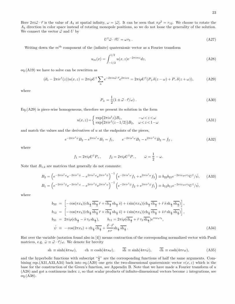
23

Here 2πi~ω · ~τ is the value of A4 at spatial infinity, ω = |~ω|. It can be seen that πρ2 = r12. We choose to rotate theA4 direction in color space instead of rotating monopole positions, so we do not loose the generality of the solution.We connect the vector ~ω and U by

U †~ω · ~τU = ωτ3 . (A27)

Writing down the mth component of the (infinite) quaternionic vector as a Fourier transform

um(x) =

∫ 1/2

−1/2

u(x, z)e−2πimzdz, (A28)

eq.(A19) we have to solve can be rewritten as

(∂z − 2πir†(z))u(x, z) = 2πiρU †∑

n

e−2πin~ω·~τe2πizn = 2πiρU †(P+δ(z − ω) + P−δ(z + ω)), (A29)

where

P± =1

2(1± ~ω · ~τ/ω) . (A30)

Eq.(A29) is piece-wise homogeneous, therefore we present its solution in the form

u(x, z)=

exp(2πis†z

)B1, −ω<z<ω

exp(2πir†(z−1/2)

)B2, ω<z<1−ω (A31)

and match the values and the derivatives of u at the endpoints of the pieces,

e−2πir†ωB2 − e2πis†ωB1 = f1, e−2πis†ωB1 − e2πir†ωB2 = f2 , (A32)

where

f1 = 2πiρU †P+, f2 = 2πiρU †P−, ω =1

2− ω.

Note that B1,2 are matrices that generally do not commute:

B2 =(e−2πis†ωe−2πir†ω − e2πis†ωe2πir†ω

)−1 (e−2πis†ωf1 + e2πis†ωf2

)≡ b22b21e−2πix4ωτ3U †/ψ, (A33)

B1 =(e−2πir†ωe−2πis†ω − e2πir†ωe2πis†ω

)−1 (e−2πir†ωf2 + e2πir†ωf1

)≡ b12b11e−2πix4ωτ3U †/ψ,

where

b22 =[− cos(πx4)(ch 1

2sh 1

2r + ch 1

2sh 1

2s) + i sin(πx4)(ch 1

2ch 1

2+ r s sh 1

2sh 1

2)],

b12 =[− cos(πx4)(ch 1

2sh 1

2r + ch 1

2sh 1

2s) + i sin(πx4)(ch 1

2ch 1

2+ s r sh 1

2sh 1

2)],

b21 = 2πiρ(ch 12− s τ3 sh 1

2), b11 = 2πiρ(ch 1

2+ r τ3 sh 1

2)eπix4τ3 ,

ψ ≡ − cos(2πx4) + ch 12

ch 12

+~s · ~rs r

sh 12

sh 12. (A34)

Hat over the variable (notation found also in [4]) means contraction of the corresponding normalized vector with Paulimatrices, e.g. ω ≡ ~ω · ~τ/ω. We denote for brevity

sh ≡ sinh(4πsω), ch ≡ cosh(4πsω), sh ≡ sinh(4πrω), ch ≡ cosh(4πrω), (A35)

and the hyperbolic functions with subscript “ 12” are the corresponding functions of half the same arguments. Com-

bining eqs.(A31,A33,A34) back into eq.(A20) one gets the two-dimensional quaternionic vector v(x, z) which is thebase for the construction of the Green’s function, see Appendix B. Note that we have made a Fourier transform of u(A28) and got a continuous index z, so that scalar products of infinite-dimensional vectors become z integrations, seeeq.(A38).

24

We note that U is actually a gauge transformation of v. Therefore, the gauge potential AUµ is obtained by a global

gauge transformation of AU=1µ . We conclude that the determinant does not depend on the relative ‘color orientation’

of the Polyakov line or holonomy, and of the vector −→r12 connecting monopole centers. Thus, we set U = 1 and ~ω = ω~e3.We notice further that v(x, z) built above gives Aµ that is not periodic in time direction and zero A4 at spatial

infinity. It is a peculiar feature of the ‘algebraic’ gauge used in [4]. It is more convenient to use the gauge in whichthe fields are periodic. To that end we make a non-periodic gauge transformation g = e2πix4ωτ3 and obtain

v(x, z)per = Φ− 12 (x)

(−g

w(x, z)

), w=ug, (A36)

meaning

w(x, z) = u(x, z) e2πix4ωτ3 . (A37)

In terms of the Fourier-transformed v the bracket takes the form

〈v|v〉 ≡ v†1v1 +

∫ 1/2

−1/2

v†2v2 dz , (A38)

where v1 is an upper element and v2 is a lower one.Now let us determine Φ(x). We use the following identities:

b†12b12 = b†22b22 = ψ/2, b†21b21 = 4π2ρ2(ch 1

2− s3

ssh 1

2

), b†11b11 = 4π2ρ2

(ch 1

2+r3r

sh 12

). (A39)

Note that the right-hand sides of eq.(A39) are proportional to the unity 2 × 2 matrix. Now we can easily calculatethe normalization:

〈v|v〉 = ψ−2b†11b11b†12b12

∫ ω

−ω

dz e−4π~s·~τz + ψ−2b†21b21b†22b22

∫ ω

−ω

dz e−4π~r·~τz

=πρ2

ψ

[(ch 1

2sh 1

2

s+

ch 12

sh 12

r

)+r12s r

sh 12

sh 12

]≡ ψ − ψ

ψ.

We used the identity ~r − ~s = −→r12 = r12~e3. Thus for Φ we get

Φ =ψ

ψ, ψ = ψ + r12

(ch 1

2sh 1

2

s+

ch 12

sh 12

r

)+r212s r

sh 12

sh 12. (A40)

We have checked the Aµ of the KvBLL caloron (7) by calculating 〈vper|∂µvper〉. Note that vper has the following

periodicity property (only for integer n):

vper(z, x4 + n) = e2πinzvper(z, x4) . (A41)

APPENDIX B: SPIN-0 ISOSPIN-1 PROPAGATOR

1. General construction of the Green function

Once the self-dual field is found in terms of the ADHM construction, such that the gauge field is written asAµ = 〈v|∂µv〉 where the scalar product is defined in eq.(A38), it is possible to construct explicitly the Green functionof spin-0 isospin-1 field in the background of the self-dual field [4, 5, 25]. The solution of the equation

−(D2

µ

)ca(x)Gab(x, y) = δcb δ(4)(x− y) (B1)

is given by

Gab(x, y) =12Tr τa〈v(x)|v(y)〉τb〈v(y)|v(x)〉

4π2(x− y)2

+1

4π2

∫ 1/2

−1/2

dz1 dz2 dz3 dz4M(z1, z2, z3, z4)1

2Tr(V†(x, z1)V(x, z2)τ

a)Tr(V†(y, z4)V(y, z3)τ

b), (B2)

25

where V(x, z) ≡ B†v(x, z).We denote the first term by G1 and the second term (the M-part) by G2. The only new object is the function

M(z1, z2, z3, z4) which we determine bellow. As we shall see, we do not need M with arbitrary arguments, but onlyat z3 = z4. For coincident arguments we obtain

M(z1, z2, z, z) = δ(z1 − z2)M(z1, z), (B3)

see below.The propagator (B2) is written for the IR4 space and does not obey the periodicity condition. The periodic

propagator, however, can be easily obtained from it by a standard procedure:

G(x, y) =

+∞∑

n=−∞G(x4, ~x; y4 + n, ~y). (B4)

In what follows it will be convenient to split it into three parts:

G(x, y) = Gr(x, y) + Gs(x, y) + Gm(x, y),

Gs ≡ G1|n=0 , Gr ≡∑

n6=0

G1, Gm ≡∑

n

G2 . (B5)

The vacuum current (20) will be also split into three parts, in accordance to which part of the periodic propagator(B5) is used to calculate it:

Jµ = J rµ + J s

µ + Jmµ . (B6)

2. Propagator in the BPS dyon background

In Appendix A.2 we have found the needed periodic quaternion v(x, z) for the single BPS monopole (see eq.(A15)).The 4-argument function M for the BPS monopole was computed in ref. [25]. The result with the two last argumentstaken equal is

M(z3, z4, z, z) = δ(z3 − z4)M(z3, z),

M(z, z′) = − 1

4v2(2|z − z′| − 1 + 4zz′) . (B7)

Eqs.(A15,B7) completely determine the periodic propagator defined in eqs.(B2,B4) in the BPS dyon background. Theuse of this propagator is demonstrated in Appendix C.

3. Propagator in the KvBLL caloron background

In Appendix A.3 we have found the needed quaternion v(x, z) for the KvBLL caloron. In this Appendix we derivethe M -function for the KvBLL caloron. The propagator (B2) will be then completely determined in the caloronbackground.

In the notations of [25] M is an infinite-dimensional rank-4 tensor, with indices running from 1 to k, the topologicalcharge in IR4. As in the case of v, it is convenient to make the Fourier transformation with respect to the indices:

Mpqnm =

∫ 1/2

−1/2

M(z1, z2, z3, z4) e2πi(−pz1+qz2+nz3−mz4)dz1dz2dz3dz4. (B8)

The tensor Mpqmn is defined by the equation [26]

1

2Tr[(A†A)il(B†B)mj + (B†B)il(A†A)mj − 2(A†B)il(B†A)mj ]Mrsij = δrlδsm , (B9)

All indices here run from 1 to k as rectangular k × (k + 1) matrices A and B are contracted along the longer side.Here A and B are:

∆(x) ≡ A+ Bx, A = ∆(0), B =

(0−1

). (B10)

26

Eq.(B9) can be rewritten as

1

2Tr[(∆†∆(0))ilδmj + (∆†∆(0))mjδil − 2B†

ilBmj ]Mrsij = δrlδsm , (B11)

where ∆†∆(0) = λ†λ+B†B, B and λ are found in eq.(A23) and eq.(A25), respectively. In our case k is infinite andwe rewrite eq.(B11) in the Fourier basis:

1

2Tr

[∆†∆(0, z3) + ∆†∆(0, z4) + 2

(∂z3

2πi+ r†(z3)

)(∂z4

2πi− r(z4)

)]M(z1, z2, z3, z4) = δ(z1 − z3)δ(z2 − z4) ,

where r(z) = riσi when z ∈ [ω, 1 − ω], and r(z) = siσi otherwise; σi = iτi. Zero components of rµ, sµ are absentbecause xµ = 0. We use

∆†∆(0, z) =− ∂2z

4π2+r2(z)+

ρ2

2(δ(z−ω)+δ(z+ω)) . (B12)

Here the first two terms come from the Fourier transformation of B†B (A23) and the last one comes from the Fouriertransformation of λ†λ. We obtain the explicit equation for M :

(− (∂z3 + ∂z4)

2

4π2+ |~r(z3)− ~r(z4)|2

)M(z1, z2, z3, z4) +

+ρ2

2(δ(z3−ω) + δ(z3+ω) + δ(z4−ω) + δ(z4+ω))M(z1, z2, z3, z4) = δ(z1 − z3)δ(z2 − z4) . (B13)

In the case z3 = z4, which is the only one we need as we shall see in a moment, we look for the solution in the form

M(z1, z2, z, z) = δ(z1 − z2)M(z1, z) . (B14)

The equation for the two-argument function simplifies to

(− ∂2

z

4π2+r12πδ(z − ω) +

r12πδ(z + ω)

)M(z′, z) = δ(z − z′) , (B15)

where r12 = πρ2. We see that the solution has to be piece-wise linear in its arguments. The solution is symmetric inits two arguments and for z < z′ is given by

M(z, z′) =

32r212π3ω(z−ω)(1−z′−ω)−8r12π2(ω2+z(z′−1))+π

2d(8r12πωω+1) , z, z′ ∈ [ω, 1− ω]

12π(

4πz(1−2z′)8r12πωω+1 + 1

r12

), z ∈ [−ω, ω], z′ ∈ [ω, 1− ω]

4r12π2[z−z′−2z′z−2(ω−1)ω−8r12π(z′−ω)(z+ω)ω]+π2r12(8r12πωω+1) , z, z′ ∈ [−ω, ω]

. (B16)

Outside this range M is defined by periodicity: M(z + n, z′ +m) = M(z, z′), where n,m are integers.Now let us demonstrate that actually only the two-argument function M(z, z′) is needed to construct the propagator

satisfying the periodicity. It turns out that making the Green function periodic simplifies G2 (section III). One hasfrom the definitions (B2)-(B5):

Gm ≡∑

n

1

8π2

∫ 1/2

−1/2

dz1. . .dz4M(z1. . .z4)Tr(V†(x, z1)V(x, z2)τ

a)Tr(V†(yn, z4)V(yn, z3)τ

b), (B17)

where yn4 = y4 + n, ~yn = ~y. Using eq.(A41) we put

V(yn, z) = e2πiηnzV(y, z) (B18)

Further on, we note that for |η| ≤ 1 one has

∑

n

Tr(V†(yn, z4)V(yn, z3)τ

b)

= Tr(V†(y, z4)V(y, z3)τ

b)δ(z3 − z4)

1

|η| .

27

Now we can see that making the Green’s function periodic results in the substitution

M(z1, z2, z3, z4)→1

|η|M(z1, z2, z3, z3)δ(z3 − z4) =1

|η|M(z1, z3)δ(z1 − z2)δ(z3 − z4) .

It follows from eq.(A16) and eq.(A41) that for the monopole one has to take η = v/(2π) < 1 and for the KvBLLcaloron η = 1. In both cases the M -part of the periodic propagator is given by

Gm =1

8π2|η|

∫ 1/2

−1/2

dzdz′M(z, z′)Tr(V†(x, z)V(x, z)τa

)Tr(V†(y, z′)V(y, z′)τb

), (B19)

where the two-argument M functions are found in eq.(B7) and eq.(B16), respectively.

APPENDIX C: VACUUM CURRENT IN THE BPS MONOPOLE BACKGROUND

We compute the vacuum current (20) in the BPS monopole background in this Appendix. We assume 0 < v < 2πand work in the stringy gauge (13) dropping the index s in vs given by eq.(A15).

1. Singular part of the monopole current Jsµ

This part of the current corresponds to the second term Gs in eq.(B5). At x → y this part of the propagator issingular. The regularization is presented in Appendix E. Eqs.(E2,A11) state:

J sµ

ab = iεadbtr(τdjµ

), jµ =

v2

12π2

⟨v∣∣fσµ∆†f

∣∣ v⟩− h.c., ∆†(x) = i∂z + vx† . (C1)

The function f(z, z′, x) for the BPS monopole is known [25]:

f(x; z, z′) = −eivx4(z−z′)

2vs

(sinh vs|z − z′|+ coth

vs

2sinh vsz sinh vsz′ − tanh

vs

2cosh vsz cosh vsz′

). (C2)

Here we denoted by s the distance to the M-monopole center. It is helpful to calculate the action of the Green functionon v. Since monopole is a static configuration, we can take x4 = 0, moreover f is a scalar function and we can move

S†− matrix to the left:

|ν〉 ≡ S−f |v〉|x4=0 =cosh(svz) tanh(sv/2)− 2z sinh(svz)

4√sv sinh(sv)

12 +sinh(svz) coth(sv/2)− 2z cosh(svz)

4√sv sinh(sv)

τ3 .

We use the following identities

S−~nr~τS†− = τ3 ,

S−~nθ~τS†− = − cos(φ)τ1 − sin(φ)τ2 ,

S−~nφ~τS†− = sin(φ)τ1 − cos(φ)τ2 (C3)

and arrive, after simple algebra, to

j4, jr, jθ, jφ =v3

12π2〈ν|i,−τ3, cosφ τ1+sinφ τ2,−sinφ τ1+cosφ τ2(∂z − vτ3s)|ν〉+ h.c. .

Finally we obtain the singular part of the vacuum current:

J sr = 0,

J sφ = − iv

(s2v2csch2(sv) + sv coth(sv)− 2

)

24π2s2 sinh(sv)(T1 cos(φ) + T2 sin(φ)),

J sθ = − iv

(s2v2csch2(sv) + sv coth(sv)− 2

)

24π2s2 sinh(sv)(T1 sin(φ) − T2 cos(φ)),

J s4 = − i

(1− s3v3 coth(sv)csch2(sv)

)

24π2s3T3 , (C4)

where (Tc)ab ≡ iεacb.

28

2. Regular part of the monopole current Jrµ

We are going to calculate the part of the current that corresponds to

(Gr)ab(x, y) ≡∑

n6=0

1

8π2(x− yn)2Tr[τa〈v(x)|v(yn)〉τb〈v(yn)|v(x)〉

], yn = ~y, yn4 = y4 + n, (C5)

namely

J rµ = J r1

µ + J r2µ , J r1

µ = AµGr + GrAµ, J r2µ = (∂x

µ − ∂yµ)Gr .

At first consider J r1µ . We have to compute Gr with equal arguments. Substituting (A15) into (C5) and calculating

the trace one has

(Gr)ab(x, x) ≡∑

n6=0

∫dzdz′

Tr

8π2n2, (C6)

where

Tr = 2s2v2einv(z−z′)

sinh2(sv)

[cosh(2sv(z − z′))(δab − δa3δb3) + cosh(2sv(z+z′))δa

3δb3+sinh(2sv(z−z′))T ab

3

]

with T c = iεacb. To compute the sum in this expression we use the summation formula (note that v < 2π)

∑

n6=0

eizn

4π2n2=

z2

8π2− |z|

4π+

1

12, −2π < z < 2π . (C7)

It remains now to calculate integrals over z and z′. The result is

Gr(x, x) =

[3 coth(sv)− sv(3csch2(sv) + 2)

8πs+

(sv coth(sv)− 1)2

8π2s2

](δab − δa

3δb3)

+

[sv csch2(sv)− coth(sv)

8πs+

1− s2v2 csch2(sv)

16π2s2+

1

12

]δab .

Now we turn to the J r2µ part of the current where we have to sum over n a derivative of the propagator. First of

all we consider derivatives of the trace in (C5). One finds for x = y:

(∂xθ − ∂y

θ )Tr=2s2v2i

sinh(sv)2(cosh(2svz) + cosh(2svz′))(T1 sinφ− T2 cosφ)eivn(z−z′) ,

(∂xφ − ∂y

φ)Tr=

(sin θ

4s2v2i

sinh(sv)2cosh(sv(z + z′)) cosh(sv(z − z′))(T1 cosφ+ T2 sinφ)

− 4s2v2i

sinh(sv)2cosh(2sv(z − z′))(1 − cos θ)T3

)eivn(z−z′) ,

(∂x4 − ∂y

4 )Tr=− 4s2v3i

sinh2(sv)(z − z′) sinh(2sv(z − z′))T3e

ivn(z−z′) ,

(∂xs − ∂y

s )Tr=0 . (C8)

Here only terms even in z − z′ were left. The last two equations are especially clear as we can drop out the matricesS in eq.(A15).

A derivative of the denominator of (C5) is equal to zero for x = y except for the derivative with respect to x4, butin this case we have the expression of the form (C6) with n3/4 instead of n2 in the denominator. Now we can sumover n. We use the summation formula

∑

n6=0

eizn

iπ2n3=

z3

6π2− z|z|

2π+z

3, −2π < z < 2π . (C9)

29

Next one has to integrate over z, z′. Combining all pieces we obtain:

J rr = 0,

J rφ = i

cos(φ)T1 + sin(φ)T2

48 sinh3(sv)π2s2℘1,

J rθ = i

sin(φ)T1 − cos(φ)T2

48 sinh3(sv)π2s2℘1,

J r4 =

iT3

24π2s3℘2, (C10)

where we denote

℘1 ≡ (s2v3 + 6πs2v2 + 3v + 3s(v + π) sinh(2sv)v − (s2v3 + 3v + 6π) cosh(2sv) + 6π),

℘2 ≡ 8π2s2(−1 + sv coth(sv))− 12πs coth(sv)(−1 + sv coth(sv))2

+ (−3(1 + 4s2v2) + sv(4(3 + s2v2) coth(sv) + 3sv(−4 + sv coth(sv))csch2(sv))).

We have used spherical coordinates. For example, a projection of ~J onto the direction ~nθ =(cos θ cosφ, cos θ sinφ,− sin θ) is denoted by Jθ.

3. M-part of the monopole current Jmµ

Combining together eqs.(B7,B19) we have for the M -part of the periodic Green’s function:

Gm = − v

16π

∫ 1/2

−1/2

dzdz′(2|z−z′|−1+4zz′) Tr(v†(x, z)v(x, z)τa

)Tr(v†(y, z′)v(y, z′)τb

)(C11)

Note that we can drop out S− in (A15). In the stringy gauge one has

v†(xµ, z)v(xµ, z) =vs

sinh(vs)exp[−2vsτ3z] . (C12)

It means that Gm has only the ‘33’ component. Taking the trace we get:

Tr[v†(xµ, z)v(xµ, z)τ

3]

= −2vs

sinh(vs)sinh(2vsz) . (C13)

Therefore the only nonzero component of Gm is

G33m (x, y) = −v3rxry

4π

∫ 1/2

−1/2

dzdz′ (2|z−z′|−1+4zz′)sinh(2vryz

′) sinh(2vrxz)

sinh(vrx) sinh(vry),

(rx = |~x|, ry = |~y|). Performing the integrations we get

G33m (x, y) = − 1

4πv

(1

rxry+

vrx coth vry − vry coth vrxr2y − r2x

). (C14)

Note that (C14) is symmetric in its arguments. For that reason the contribution to the current coming from (ordinary)derivatives of Gm is zero,

∂xGm(x, y)− ∂yGm(x, y)|x=y = 0,

and only the anticommutator Gm(x, x), Aµ remains. Taking the limit x→ y we get for Gm

G33m (x, x) =

1

8πs

[coth(vs)− 2

vs+

vs

sinh2(vs)

](C15)

30

and for the contribution to the current Jmµ = AµGm + GmAµ we obtain in spherical coordinates

Jmr = 0,

Jmφ = − i(sin(φ)T2+cos(φ)T1)(sv coth(sv)+s2v2csch2(sv)−2)

16π sinh(sv)s2 ,

Jmθ = − i(sin(φ)T1−cos(φ)T2)(sv coth(sv)+s2v2csch2(sv)−2)

16π sinh(sv)s2 ,

Jm4 = 0 . (C16)

Adding up (C4,C10) and (C16) we obtain the full vacuum current in the BPS background, see eq.(23) of the maintext.

APPENDIX D: VACUUM CURRENT IN THE KVBLL CALORON BACKGROUND

There are no principal problems to make the calculation of the caloron Green’s function and the ensuing vacuumcurrents exactly. One can consider this Appendix as an instruction how to perform the exact calculation. In fact,we have done it but unfortunately the exact result for the current is about 200 pages long and thus too large to beprinted. However, in certain limits the expressions drastically simplify. In particular, assuming the case when thedyons inside the caloron are widely separated such that their cores do not overlap, it is relatively easy to find theKvBLL caloron current with the exponential precision (i.e. dropping out term of the order e−rv, e−sv). This will besufficient to find the determinant of the KvBLL caloron for large r12 up to some constant.

With the exponential precision, the only nonzero components of the KvBLL caloron’s gauge potential in fundamentalrepresentation are (see section II)

A4 ≃iτ32

(4πω +

1

r− 1

s

), Aϕ ≃ −

iτ32

(1

r+

1

s

)√(r12 − r + s)(r12 + r − s)(r12 + r + s)(r + s− r12)

. (D1)

We are using the coordinates x4, r, s, ϕ, where r, s are defined in (A24) and ϕ is defined by

~x = x(cosϕ ~e2+sinϕ ~e1)+

(r212 + r2 − s2

2r12− 2r12ω

)~e3, x ≡

√(r12+r−s)(r12+s−r)(r+s−r12)(r12+r+s)

2r12. (D2)

One can easily check the consistency of this definition, i.e. that

s = |~s|, r = |~r|, where ~s = ~x− 2ω−→r12, ~r = ~x+ 2ω−→r12, −→r12 = r12~e3 .

Since Ar = 0 and As = 0 we have to calculate only the J4 and Jφ components.We shall use the ADHM construction. The main steps of the calculation are similar to that for the monopole.

Dropping out exponentially small terms in eq.(A36) one has in the periodic gauge

v(x, z) ≃√r + s− r12r + s+ r12

(−e2πix4ωτ3

w(x, z)

), (D3)

w(x, z) ≃

−iπρe2π(is†z−ωs)[

r12+r−sr12

τ3 +2x

r+s−r12(τ1 sinϕ+ τ2 cosϕ)

], −ω<z<ω

iπρe2π(ir†z−ir†/2−rω)[

r12+s−rr12

(i12 sinπx4 + τ3 cosπx4)+

+2x

r+s−r12(sin(πx4−ϕ)τ1−cos(πx4−ϕ)τ2)

] , ω<z<1−ω(D4)

where s† ≡ sµσ†µ, s ≡ |~s|, s4 = x4. We shall use the following formulas to pass to the cylindrical coordinates x3, x, ϕ:

∂r

∂x3=r212 + r2 − s2

2r12r,

∂r

∂x=x

r,

∂r

∂ϕ= 0

∂s

∂x3= −r

212 + s2 − r2

2r12s,

∂s

∂x=x

s,

∂s

∂ϕ= 0 . (D5)

31

1. Singular part of the caloron current Jsµ

Let us calculate the singular part of the vacuum current with exponential precision. It is related to the zeroMatsubara frequency. Similar to the monopole case, we could use eq.(E2), where the Green’s function (A4) for thecase of KvBLL caloron was found in [4]. However it is more convenient to use eq.(E10)) because then we have onlyto take derivatives of the simple expression (D3) and no integrations arise. Eq.(E2) would have been more suitablefor the exact calculation.

It is straightforward to calculate the quantity Γ from eq.(E9). It is sufficient to calculate the second time derivative:

Γ ≃< ∂4∂4v|v > −A24 . (D6)

Bearing in mind that Γ is a vector under gauge transformations, we can perform calculations in any gauge. Up to theexponentially small terms we have

Γab = −(r + s)

((r − s)2 + r12 (r + s)

)δab

4r2s2 (r12 + r + s). (D7)

One can observe from eq.(D1) that all terms with derivatives in the right-hand side of eq.(E10) are zero. Writing theLaplace operator in the cylindrical coordinates we find

js4 ≃1

48π2

[〈∂4

(∂24 +∂2

3 +1

x∂x∂+

1

x2

∂2ϕ

)v|v〉−h.c.

]+

1

24π2

(A3

4+AϕA4Aϕ+6A4Γ),

jsϕ ≃1

48π2

[〈∂ϕ

xϕ

(∂24 +∂2

3 +1

x∂x∂+

1

x2

∂2ϕ

)v|v〉−h.c.

]+

1

24π2

(A3

ϕ+A4AϕA4+6AϕΓ).

Taking the derivatives we obtain simple expressions:

js4 =iτ3

48π2

(1

r3− 1

s3

), (D8)

jsφ = −(

1

r+

1

s

)iτ3xr12

8π2rs(r12 + r + s)2. (D9)

2. Regular part of the caloron current Jrµ

Next we calculate the temperature-dependent part of the KvBLL caloron vacuum current. As in the monopole case(Appendix C.2) we divide the current into two parts,

J rµ = J r2

µ + J r1µ , (D10)

where

J r2µ =

∑

n6=0

1

8π2(∂x

µ − ∂yµ)

Tr[τav†(x)v(y)τbv†(y)v(x)]

(x− y)2 ,

J r1µ =

∑

n6=0

1

8π2

Aµ,

Tr[τav†(x)v(y)τbv†(y)v(x)]

n2

and y4 = x4 + n. The quaternion function v(x, z) has been constructed in Appendix A.3 (actually called vper(x, z)there). It is important that v(x, z) has the remarkable periodicity property (A41).

In evaluating the above currents the tactics is to factor the matrix part out of the integrals over z. We use thefollowing notations for the integrals over z:

In+ ≡

∫ ω

−ω

e2πinz cosh(4πsz)dz, In+ ≡

∫ ω

−ω

e2πin(z+1/2) cosh(4πrz)dz,

In− ≡

∫ ω

−ω

e2πinz sinh(4πsz)dz, In− ≡

∫ ω

−ω

e2πin(z+1/2) sinh(4πrz)dz .

32

We obtain the following relations for the matrix structures:

ψ2w†(x4)w(x4 + n) = (In+β + In

−βs) + (In+β + In

−βr),

ψ2w†(x4 + n)w(x4) = (In+β − In

−βs) + (In+β − In

−βr),

ψ2w†(x4)∂4w(x4 + n) = (In+β0 + In

−β0s + i∂sI

n−β + i∂sI

n+βs) + ...

ψ2w†(x4 + n)∂4w(x4) = (In+β0 − In

−β0s − i∂sI

n−β + i∂sI

n+βs) + ...

where ‘...’ means the same expression but with bar over each quantity and r instead of s. The notation ∂4 means:derivative from the right minus derivative from the left. The definition and the evaluation of the matrix structureswith the exponential precision is

β0s ≡ b†11b

†12s∂4b12b11 ≃ o(e4πsωe8πrω),

β0r ≡ b†21b

†22r∂4b22b21 ≃

iπ2r122

(ϑ+ 1)(s3 − 1)e8πsωe4πrω,

β0 ≡ b†11b†12∂4b12b11 ≃ o(e4πsωe8πrω),

β0 ≡ b†21b†22∂4b22b21 ≃

π2r122i

(ϑ+ 1)(s3 − 1)ωe8πsωe4πrω,

βs ≡ b†11b†12sb12b11 ≃

πr124

(ϑ+ 1)(r3 + 1)ωe4πsωe8πrω,

βr ≡ b†21b†22rb22b21 ≃

πr124

(ϑ+ 1)(s3 − 1)ωe8πsωe4πrω,

β ≡ b†11b†12b12b11 ≃

r12π

4(ϑ+ 1)(r3 + 1)e4πsωe8πrω,

β ≡ b†21b†22b22b21 ≃

r12π

4(ϑ+ 1)(1− s3)e8πsωe4πrω,

where

ψ ≃ 1

4(ϑ+ 1)e4πsωe4πrω, ϑ ≡ ~r ~s

sr=r2+s2−r212

2sr, rr3 = ss3 =

r212+r2−s22r12

.

Substituting this into in the currents Jr1,r2µ we obtain certain sums, which are of the form

∑

n6=0

In+I

n+/(4π

2n2),∑

n6=0

cos(2πnω)gIn+/(4π

2n2),∑

n6=0

sin(4πnω)/(π2n3).

All such sums can be calculated using the summation formulae

∑

n6=0

e2πin(z−1/2)

4π2n2=z2

2− 1

24≡ c2(z), −

1

2≤z≤ 1

2,

∑

n6=0

e2πin(z−1/2)

π2n3= 8πi

(z3

6− z

24

)≡ c3(z), −

1

2≤z≤ 1

2.

For example,

∑

n6=0

In+I

n+/(4π

2n2) =

∫ ω

−ω

∫ ω

−ω

c2(z + z′ − 1/2) cosh(4πsz) cosh(4πsz′) dz dz′

and so on. With some help from Mathematica we come to the final result

J r4 =

[1

4π2 r3− 1

π2 r2 s+

1

π2 r s2− 1

4 π2 s3− 1

π r2+

2

π r s− 1

π s2+

2

3 r− 2

3 s+ (D11)

(4

π r2− 8

π r s+

4

π s2− 8

r+

8

s+

8 π

3

)ω +

(16

r− 16

s− 16 π

)ω2 +

64 π ω3

3

]iT3

2,

J sφ =

(1

r+

1

s

)iT3xr12

4π2rs(r12 + r + s)2. (D12)

33

3. M-part of the caloron current Jmµ

This part of the current is especially simple: with exponential precision it is zero. The main steps are the sameas in the case of a single monopole. The starting formula is our eq.(B19). First of all we note that only the lowercomponents of v are left and only the a = 3 component is nonzero:

Tr[V+(x, z)V(x, z)τa

]=

1

φ(x)Tr[w+(x, z)w(x, z)τa

]∝ δa3 .

Inspecting the definition of the M-part of the propagator (B19) we observe that

Gm ab(x, y) ∝ δa3δb3, Gm ab(x, y) = Gm ab(y, x) . (D13)

The second equation means that the terms with derivatives in the expression for the current (20) cancel each other.It follows from the first one that the product of Gm and Aab

µ ∝ ε3ab is equal to zero, too. Therefore we conclude that

Jmµ ≃ 0 . (D14)

APPENDIX E: REGULARIZATION OF THE CURRENT

Here we consider in more detail J sµ, the contribution to the current from the singular (as x → y) part of the

propagator Gs(x, y) defined by eq.(B5). This part is obviously temperature-independent, so the zero-temperatureresults are applicable. We regularize the current by setting x− y = ǫ and inserting a parallel transporter to supportgauge invariance, see e.g. [20]:

J sµ = J s1

µ + J s2µ ,

J s1µ ≡ [Aµ(z − ǫ/2)Gs(z − ǫ/2, z + ǫ/2) + Gs(z − ǫ/2, z + ǫ/2)Aµ(z + ǫ/2)]Pexp

(−∫ y

x

Aµdzµ

),

J s2µ ≡

[(∂x

µ − ∂yµ)Gs(x, y)

]Pexp

(−∫ y

x

Aµdzµ

), (E1)

where x = z − ǫ/2, y = z + ǫ/2 and we imply averaging over all directions of ǫ in the 4d space. This regularizationmethod was proved to be equivalent to the ζ-function regularization approach [29].

For a background field written in terms of the ADHM construction, a useful expression for the vacuum current wasderived in refs. [20, 29]. In the SU(2) case it acquires the form:

J sµ

ab = iεadbtr(τdjµ

), jµ =

1

12π2

⟨v∣∣Bf

(σµ∆†B − B†∆σ†

µ

)fB†∣∣ v

⟩

(see Appendix A for notations of the ADHM construction elements).We would like to derive another expression for this part of the current – in terms of derivatives. In some cases it is

more useful. We start from writing our result:

jµ =1

48π2

[(DµD

2〈v|)|v〉 − h.c.

]. (E2)

Let us prove it. First of all we consider the action of one derivative

Dµ〈v(x)|=∂µ〈v| − ∂µ〈v|v〉〈v| = ∂µ〈v|(1− |v〉〈v|)=∂µ〈v|∆f∆† = −〈v|∂µ∆f∆† (E3)

=−〈v|Bσµf∆† . (E4)

At the end of the first line we have used eq.(A5). The first equation in the second line comes from differentiating theADHM equation

0 = ∂µ(〈v|∆) = ∂µ〈v|∆ + 〈v|∂µ∆.

The last equation follows from the definition (B10). Therefore we obtain

Dµ〈v(x)|v(y)〉 = −〈v(x)|Bσµfx∆†x|v(y)〉 = −〈v(x)|Bσµfx(x− y)†B†|v(y)〉 ,

34

where in the last line we have used the ADHM equation (A3). We next consider two derivatives. It is important herethat f is proportional to the unity 2× 2 matrix. We have

D2x〈v(x)|v(y)〉=−Dx

µ

(〈v(x)|Bσµfx(x − y)†B†|v(y)〉

)

=〈v(x)|Bσµfx∆†xBσµfx(x− y)†B†|v(y)〉 − 〈v(x)|Bσµ∂µfx(x − y)†B†|v(y)〉 − 〈v(x)|Bσµfxσ

†µB†|v(y)〉

=−4〈v(x)|BfxB†|v(y)〉 .

We have used here

σµ∂µfx = −fx∂µ(σµ∆†∆)fx = −fxσµ(σ†µB†∆ + ∆†Bσµ)fx = −2fxB†∆fx = fxσµ∆†Bσµfx .

We have also used that the derivative of the inverse operator is ∂(O−1) = −O−1(∂O)O−1, as well as the relations

σµσ†µ = 4, σµc σµ = −2c†, (E5)

where c is an arbitrary quaternion.Finally, let us consider three derivatives:

DxµD

2x〈v(x)|v(y)〉 = −4Dx

µ

(〈v(x)|BfxB†|v(y)〉

)= 4〈v(x)|Bfxσµ∆†

xBfxB†|v(y)〉+ 4〈v(x)|B∂µfxB†|v(y)〉 .

Notice that the last term is hermitian at x = y. Thus we have proven that the current written in form of eq.(E2) isequivalent to that of eq.(E2):

1

48π2

[(DµD

2〈v|)|v〉 − h.c.

]=

1

12π2

⟨v∣∣Bf

(σµ∆†B − B†∆σ†

µ

)fB†∣∣ v

⟩.

In fact it is more useful to rewrite everything in terms of ordinary rather than covariant derivatives:

(DµD

2〈v|)|v〉 = 〈∂µ∂

2v|v〉 +AνAµAν − ∂νAνAµ −Aν∂νAµ − ∂µAνAν + ∂µ∂νAν + 6AµΓ , (E6)

where Aµ is in the fundamental representation and

1

2(DµDν +DνDµ〈v|) |v〉 = δµνΓ . (E7)

We have to prove that the left-hand-side of eq.(E7) is a Lorentz scalar as is the right-hand side. Note that eq.(E5) isproportional to x− y. The only way to obtain a nonzero result at x− y → 0 is to differentiate this factor:

1

2(DµDν +DνDµ〈v|) |v〉 = −1

2〈v|B(σµσ

†ν + σνσ

†µ)fB†|v〉 = −δµν〈v|BfB†|v〉 . (E8)

It follows from eq.(E8) that Γ is hermitian. We can write Γ as follows:

Γδµν = 〈∂µ∂νv|v〉 +1

2(∂µAν + ∂νAµ)− 1

2(AµAν +AνAµ) . (E9)

Finally, the regularized singular part of the current can be written as

jµ =1

48π2

(〈∂µ∂

2v|v〉 − h.c.)

+1

24π2(AνAµAν + ∂µ∂νAν + 3AµΓ + 3ΓAµ) . (E10)

Eqs.(E9,E10) are used for the calculation of the singular part of the vacuum current in Appendix D.1.

[1] B.J. Harrington and H.K. Shepard, Phys. Rev. D 17, 2122 (1978); ibid. 18, 2990 (1978).[2] D.J. Gross, R.D. Pisarski and L.G. Yaffe, Rev. Mod. Phys. 53, 43 (1981).[3] D. Diakonov and A. Mirlin, Phys. Lett. B 203, 299 (1988).[4] T.C. Kraan and P. van Baal, Phys. Lett. B 428, 268 (1998) 268, hep-th/9802049; Nucl. Phys. B 533, 627 (1998), hep-

th/9805168.[5] K. Lee and C. Lu, Phys. Rev. D 58, 025011 (1998), hep-th/9802108.[6] E.B. Bogomolnyi, Yad. Fiz. 24, 861 (1976) [Sov. J. Nucl. Phys. 24, 449 (1976)].

35

[7] M.K. Prasad and C.M. Sommerfeld, Phys. Rev. Lett. 35, 760 (1975).[8] K. Lee and P. Yi, Phys. Rev. D 56, 3711 (1997), hep-th/9702107.[9] D. Diakonov and V. Petrov, Phys. Rev. D 67, 105007 (2003), hep-th/0212018.

[10] N. M. Davies, T. J. Hollowood, V. V. Khoze and M. P. Mattis, Nucl. Phys. B 559, 123 (1999), hep-th/9905015; N.M. Davies,T.J. Hollowood and V.V. Khoze, hep-th/0006011.

[11] A. Belavin, A. Polyakov, A. Schwartz and Yu. Tyupkin, Phys. Lett. 59, 85 (1975).[12] D. Diakonov and M. Oswald, Phys. Rev. D 68, 025012 (2003), hep-ph/0303129.[13] E. Megias, E. Ruiz Arriola and L.L. Salcedo, hep-ph/0312126.[14] N. Weiss, Phys. Rev. D 24, 475 (1981); ibid. D25, 2667 (1982).[15] D. Diakonov, Prog. Part. Nucl. Phys. 51, 173 (2003), hep-ph/0212026; D. Diakonov, talks given at BNL, JLab and SLAC,

March 2003.[16] R. C. Brower, D. Chen, J. Negele, K. Orginos and C. I. Tan, Nucl. Phys. Proc. Suppl. 73, 557 (1999), hep-lat/9810009.[17] E.M. Ilgenfritz, B.V. Martemyanov, M. Muller-Preussker, S. Shcheredin and A.I. Veselov, Phys. Rev. D 66, 074503 (2002),

hep-lat/0206004; hep-lat/0209081, hep-lat/0301008, hep-lat/0402010.[18] C. Gattringer, hep-lat/0210001; C. Gattringer and S. Schaefer, hep-lat/0212029; C. Gattringer et al., hep-lat/0309106;

C. Gattringer and R. Pullirsch, hep-lat/0402008.[19] G. ’t Hooft, Phys. Rev. D 14, 3432 (1976).[20] L.S. Brown and D.B. Creamer, Phys. Rev. D 18, 3695 (1978).[21] K. Zarembo, Nucl. Phys. B 463, 73 (1996), hep-th/9510031.[22] N. Dorey, T. J. Hollowood, V. V. Khoze and M. P. Mattis, Phys. Rept. 371, 231 (2002), hep-th/0206063.[23] S. Adler, Phys. Rev. D 18, 411 (1978); ibid. 19, 2997 (1979).[24] P. Rossi, Nucl. Phys. B 149, 170 (1979).[25] W. Nahm, Phys. Lett. B 90, 413 (1980).[26] N.H. Christ, E.J. Weinberg and N.K. Stanton, Phys. Rev. D 18, 2013 (1978);

E. Corrigan, P. Goddard and S. Templeton, Nucl. Phys. B 151, 93 (1979).[27] C. Bernard, Phys. Rev. D 19, 3013 (1979).[28] M.F. Atiyah, V.G. Drinfeld, N.J. Hitchin and Yu.I. Manin, Phys. Lett. A 65, 185 (1978).[29] E. Corrigan, P. Goddard, H. Osborn and S. Templeton, Nucl. Phys. B 159, 469 (1979).[30] S. Huang and M. Lissia, Nucl. Phys. B 438, 54 (1995);

K. Kajantie, M. Laine, K. Rummukainen and M.E. Shaposhnikov, Nucl. Phys. B 503, 357 (1997);S. Chapman, Phys. Rev. D 50, 5308 (1994).

[31] A. Hasenfratz and P. Hasenfratz, Nucl. Phys. B 193, 210 (1981).[32] D. Diakonov and V. Petrov, Nucl. Phys. B 245, 259 (1984).[33] V.M. Belyaev and V.L. Eletsky, Z. Phys. C 45, 355 (1990);

K. Enqvist and K. Kajantie, Z. Phys. C 47, 291 (1990).[34] We use anti-Hermitian fields: Aµ = −itaAa

µ, Tr(tatb) = 1

2δab.

[35] Generally speaking, there is a surface term in eq.(19) arising from integrating by parts [21], which we ignore here since thecaloron field, contrary to the single dyon’s one considered by Zarembo [21], decays fast enough at spatial infinity. We takethis opportunity to say that we have learned much from Zarembo’s paper. However, his consideration of dyons with highcharge k only didn’t allow him to observe the subleading in k infrared divergence of the single dyon determinant, whichis the essence of the problem with individual dyons, as contrasted to charge-neutral calorons. In addition, because dyonshave to be always regularized by putting them in a finite-size box, the theorem on the relation between spin-1 and spin-0determinants (section I) is generally violated. This is one of the reasons we consider well-behaved calorons rather thanindividual dyons, although they are more “elementary”.