Quantum Separation of Variables in Higher Rank and ...
304
Numéro National de Thèse : 2021LYSEN052 THÈSE DE DOCTORAT DE L’UNIVERSITÉ DE LYON opérée par l’École Normale Supérieure de Lyon École Doctorale N° 52 Physique et Astrophysique de Lyon (PHAST) Discipline : Physique Soutenue publiquement le 29/10/2021, par : Louis VIGNOLI Quantum Separation of Variables in Higher Rank and Supersymmetric Integrable Models Séparation de variables quantiques pour les modèles intégrables de plus haut rangs et supersymétriques Devant le jury composé de : Didina SERBAN Ingénieure CEA CEA Saclay Rapporteure Véronique TERRAS Directrice de recherche U. Paris–Saclay Rapporteure Frank GÖHMANN Professeur U. de Wuppertal Examinateur Éric RAGOUCY Directeur de recherche U. de Savoie Examinateur Jean Michel MAILLET Directeur de recherche ENS de Lyon Directeur de thèse Giuliano NICCOLI Directeur de recherche ENS de Lyon Codirecteur de thèse
-
Upload
khangminh22 -
Category
Documents
-
view
0 -
download
0
Transcript of Quantum Separation of Variables in Higher Rank and ...

Numéro National de Thèse : 2021LYSEN052
THÈSE DE DOCTORAT DE L’UNIVERSITÉ DE LYONopérée par
l’École Normale Supérieure de Lyon
École Doctorale N° 52Physique et Astrophysique de Lyon (PHAST)
Discipline : Physique
Soutenue publiquement le 29/10/2021, par :
Louis VIGNOLI
Quantum Separation of Variablesin Higher Rank and Supersymmetric
Integrable ModelsSéparation de variables quantiques pour les modèles intégrables
de plus haut rangs et supersymétriques
Devant le jury composé de :
Didina SERBAN Ingénieure CEA CEA Saclay RapporteureVéronique TERRAS Directrice de recherche U. Paris–Saclay RapporteureFrank GÖHMANN Professeur U. de Wuppertal ExaminateurÉric RAGOUCY Directeur de recherche U. de Savoie ExaminateurJean Michel MAILLET Directeur de recherche ENS de Lyon Directeur de thèseGiuliano NICCOLI Directeur de recherche ENS de Lyon Codirecteur de thèse


Contents1 Introduction 7
2 Classical integrability 212.1 Classical integrability . . . . . . . . . . . . . . . . . . . . . . . . . . . . . . . . . . . . . . . . . . . 212.2 Classical Lax formalism and r-matrix . . . . . . . . . . . . . . . . . . . . . . . . . . . . . . . . . 26
3 Quantum integrability 373.1 Approaching quantum integrability . . . . . . . . . . . . . . . . . . . . . . . . . . . . . . . . . . 373.2 Quantum inverse scattering method . . . . . . . . . . . . . . . . . . . . . . . . . . . . . . . . . . 403.3 Spin chains . . . . . . . . . . . . . . . . . . . . . . . . . . . . . . . . . . . . . . . . . . . . . . . . . 42
4 Algebraic Bethe ansatz techniques 514.1 The gl(2) model: from the spectrum. . . . . . . . . . . . . . . . . . . . . . . . . . . . . . . . . . . 514.2 . . . to the correlations functions . . . . . . . . . . . . . . . . . . . . . . . . . . . . . . . . . . . . . 564.3 Higher rank models . . . . . . . . . . . . . . . . . . . . . . . . . . . . . . . . . . . . . . . . . . . . 604.4 Summary . . . . . . . . . . . . . . . . . . . . . . . . . . . . . . . . . . . . . . . . . . . . . . . . . . 62
5 Fundamentals of separation of variables 655.1 SOV in classical systems . . . . . . . . . . . . . . . . . . . . . . . . . . . . . . . . . . . . . . . . . 655.2 Quantum SOV . . . . . . . . . . . . . . . . . . . . . . . . . . . . . . . . . . . . . . . . . . . . . . . 735.3 Quantum SOV for integrable systems in the QISM framework . . . . . . . . . . . . . . . . . 775.4 Recent developments . . . . . . . . . . . . . . . . . . . . . . . . . . . . . . . . . . . . . . . . . . . 84
6 Separation of variables from transfer matrices 876.1 Foreword: non-derogatory matrices . . . . . . . . . . . . . . . . . . . . . . . . . . . . . . . . . . 876.2 Separate basis from conserved quantities . . . . . . . . . . . . . . . . . . . . . . . . . . . . . . 916.3 Link with Sklyanin SOV in the gl(2) case . . . . . . . . . . . . . . . . . . . . . . . . . . . . . . . 1046.4 Recent results on SOV . . . . . . . . . . . . . . . . . . . . . . . . . . . . . . . . . . . . . . . . . . 105
7 Towards the dynamics in higher rank: scalar products for gl(3) in SOV 1077.1 Generalities on scalar products of separate states and SOV measure . . . . . . . . . . . . . . 1077.2 The gl(2) case: orthogonal SOV bases . . . . . . . . . . . . . . . . . . . . . . . . . . . . . . . . 1107.3 The gl(3) case: pseudo-orthogonal SOV bases . . . . . . . . . . . . . . . . . . . . . . . . . . . 1137.4 Orthogonal bases and the T operator . . . . . . . . . . . . . . . . . . . . . . . . . . . . . . . . . 120
8 Separate bases and spectrum of gl(m|n) models 1258.1 Graded objects . . . . . . . . . . . . . . . . . . . . . . . . . . . . . . . . . . . . . . . . . . . . . . . 1258.2 Separates bases . . . . . . . . . . . . . . . . . . . . . . . . . . . . . . . . . . . . . . . . . . . . . . 1368.3 About the characterization of the spectrum . . . . . . . . . . . . . . . . . . . . . . . . . . . . . 1398.4 Specializing for gl(1|2) model . . . . . . . . . . . . . . . . . . . . . . . . . . . . . . . . . . . . . 1428.5 The Hubbard model case . . . . . . . . . . . . . . . . . . . . . . . . . . . . . . . . . . . . . . . . 145
Conclusion 149
A Yangians and quantum groups 153
Bibliography 161
3


Remerciements
À Jean Michel Maillet et Giuliano Niccoli, mes deux directeurs de thèse. Vous m’avez accordé votre confianceen m’offrant de travailler sous votre supervision sur ces sujets que vous chérissez. Merci pour votre encadrementbienveillant, vos conseils avisés et vos critiques toujours justes. Je vous dois autant scientifiquement quehumainement ; j’espère devenir un aussi bon mentor que vous l’avez été pour moi.
À tous les membres de mon jury de thèse :
À Franck Göhmann, pour avoir amené son expertise sur les modèles supersymétriques et le modèle deHubbard,
À Didina Serban et Véronique Terras pour leur relecture attentive du manuscrit et les commentairespertinents qui ont permis son amélioration,
À Éric Ragoucy pour avoir présidé le jury avec expérience lors de la soutenance.
Au Laboratoire de Physique à l’École Normale Supérieure de Lyon, où que j’ai pu conduire mes travauxde recherche. Je souhaite remercier l’ensemble de ses membres pour le sérieux scientifique et l’enthousiasmegénéral qui y règne. Ses deux directeurs que j’ai connu incarne particulièrement cet état d’esprit :
À Thierry Dauxois pour son accueil chaleureux et notre rivalité complice entre les deux Olympiques—bienqu’il n’y en qu’un seul,
À Jean-Christophe Géminard pour son accessibilité et sa volonté constante d’offrir à tous les meilleuresconditions de travail malgré de difficiles conditions.
À l’École Doctorale PHAST 52 et son directeur Dany Davesne pour l’encadrement de mon diplôme et laformation prodiguée au cours de ce dernier.
À tous les collègues du laboratoire avec qui j’ai partagé le quotidien de la recherche : David, Sylvain, Éric,Antoine, Jérémy, Jérémy, Benjamin G., Benjamin C., Yannick, Louison, Jason, Christophe, Harriet, Salvish,Henning, Denis, François D., François G., Marc M., Marc G., Etera, Karol, Jérémie.
Au personnel du laboratoire qui s’est assuré de la bonne conduite de ma thèse avec une grande bienveillanceet beaucoup de bonne humeur : Laurence, Fatiha, Nadine.
Au Département de Physique, pour m’avoir confié l’enseignement en Licence, Master et Préparation àl’Agrégation de nombreux cours et travaux dirigés. Savoir c’est d’abord apprendre et puis partager. Merci àCendrine, Romain Volk et Christophe Winisdoerffer.
À mes colocataires successifs du 86 avenue Jean Jaurès : Théo, Lou-Alma, Marion, Sow, Salomé, Camilleet Érica. Merci d’avoir contribué au quotidien chaleureux de cet appartement.
À Aleksandra, Gilles, Philip, Andrew, et à tous les participants de l’école d’été des Houches Integrability inAtomic and Condensed Matter Physics, ainsi qu’à tout ceux des différentes éditions du Student Workshop inIntegrability. Qu’il est bon de faire parti d’une communauté de jeunes gens aussi dynamiques et accueillants.
5

6 Contents
À Alain Lhopital, Laurent Barbaza, Jean-Claude Martin, Pierre Grécias et Christian Garing ; vous m’avezforgé un esprit de science que j’exerce chaque jour avec fierté.
À Michel Gonin, Thomas Mueller, Benjamin Quillain et Laura Dominé ; c’est par vous que j’ai véritablementdécouvert la recherche scientifique et en ai fait ma vie.
À mes nombreux amis qui m’ont accompagné durant ces années, et plus particulièrement :
À Camille, pour le partage des nos bureaux qui m’a procuré tant de bonheur. Merci pour ces quatre annéesensemble autour de notre goût pour la science, les origamis, la typographie bien faite et zoomée de près et lesphotos de chats. Il y a un peu de toi dans chacune des équations, chacun des symboles de ce manuscrit.
À Noémie D., sans qui cette heureuse cohabitation n’aurait eu que la saveur—un peu trop aride—descalculs abstraits. Merci pour toutes ces nécessaires pauses cappuccino que nous n’avions pas la présenced’esprit de prendre, le nez dans les équations, et cette joie de vivre qui a ensoleillé notre bureau si mal exposé.
À Augustin, d’être mon compagnon de science depuis nos caserts face à face et de rester sur le front de larecherche pour moi.
À Simon, pour sa curiosité constante et notre intérêt commun aux belles mathématiques.
À Jules ; je te dois les chapitres 3 et 4 de ce manuscrit grâce à notre séjour à Sanary et ton vélo si véloce.
À Lucas ; je te dois les chapitres 6 et 7 par ton séjour à Marseille et ton attachement inexpugnable auxmosaïques urbaines.
Merci pour vos amitiés aussi faciles que précieuses.
Au chat Piana, pour l’animation des laborieuses journées de confinement.
À ma soeur, mon père, ma mère, et toute ma famille ; votre soutien indéfectible est ma plus grande force.
Enfin, à Noémie. Je n’ai rien à écrire que tu ne sais pas déjà, et je te dois tant.

1 Chapter
Introduction
Conserved quantities are quantities that remain constant during the evolution of a physical system.They are central in this thesis. Conserved quantities form the defining feature of the systems studied, theintegrable models, and are precisely used in the techniques we develop here to solve these models, thequantum separation of variables.
It has been a very long and difficult progress to understand there were invariants in the physicalprocesses of Nature, and that these conserved quantities were essential tools in their description. Humanshave proved to have a very developed ability to identify constant and recurring features in their changingsurroundings. This immutable traits and periodic events allow for predictions, giving humans somecontrol over nature, some sense of mastery or a first form of knowledge.
Astronomy was a universal practice among the antique civilizations. They identified that stars appearfixed on a celestial sphere, organized in everlasting constellations, slowly rotating during the year aroundthe fixed Pole Star in Ursa Minor. Periodic astronomical events, from the sunset to solstices, played a keyrole in lives of ancient men, from agricultural planning to religious life. There has been strong motivationto find an explanation for those. At first, scientific and religious arguments mixed up in the proposedexplanations. Gods of ancients Greeks and Romans manifest in the sky as the planets, who move freely inthe cosmos because of their divine status. Yet, some are entitled to constant behaviors, such as Heliosdriving his chariot every day, or Atlas lifting the Earth still in the cosmos for eternity.
Later, the schism between science and religion became more and more inevitable. With the emergenceof physics as the science of the behavior of material reality, the search for constant values and conservationlaws in physical processes guided the experimental and theoretical approaches. We will illustrate thiswith the slow elaboration of the concepts of momentum, angular momentum and energy. That led to thefoundation of modern physics.
There was already some intuition of a conserved quantity when studying the transmission of motion,from one objects to another, which later led to the concept of inertia, and the conservation of momentum.Galileo observed the velocity of a body do not vary in the absence of an exterior force [1, 2], and put anend to centuries of Aristotelian understating of motion, according to which constant velocity requires acontinuous propelling. With some metaphysical justification, Descartes therefore wrote that God, throughthe law of natures he prescribed, “‘conserve maintenant en l’Univers, par son concours ordinaire, autantde mouvement et de repos qu’il y en a mis en le créant. [. . . ] une certaine quantité qui n’augmente nine diminue jamais, encore qu’il y en ait tantôt plus et tantôt moins en quelques-unes de ses parties.’”([3], article 36) While disciples of Galileo formulated many statements on the idea of the conservation ofmovement [4], it is Newton who stated first the modern form of the principle of inertia in its PhilosophiæNaturalis Principia Mathematica: “Every body perseveres in its state, of rest or of uniform motion in a rightline, unless it is compelled to change that state by forces impressed thereon” [5]. The conservation ofthe total vectorial momentum
∑i mi~vi was then recognized by Huygens in isolated systems [6]: despite
internal interactions in the system which reallocate momentum from parts to parts, the whole exhibits aninvariant quantity, a conserved total momentum.
The study of the motion of planets in the solar systems also led very early to the identification offundamental conservation laws of mechanics. Danish astronomer Tycho Brahe gathered a large amount of
7

8 Chapter 1 — Introduction
precise observational data. They allowed his assistant Johannes Kepler to later state in the 1610s his threelaws of planetary motion in the solar system [7, 8]. The second law notably states the steadiness of theareal velocity along the orbit of planets around the sun. This conservation of the areal velocity in planetarymotion is an early understanding of conservation of the angular momentum, the rotational equivalentof (linear) momentum. If Bernoulli already talked of a “moment of rotational motion” [9] in 1744, thework of Poinsot may be considered as a real understanding of this object [10]; he represented rotationsas a line segment perpendicular to the rotation place and introduced the concept of “conservation ofmoments” in his Mémoires sur la composition des moments et des aires [11].
During his experiments on elastic shocks, Huygens observed the conservation of the scalar quantity∑i mi~v
2i [6]. It enabled the concept of the conservation of vis viva (lively force) by Leibniz [12], aside of
the inertia principle, which then led to the concept of energy in mechanics and its conservation. The firstwell-formed idea of energy emerged from the study of mechanical systems as the one of kinetic energy.Indeed, Lagrange proved in his Mécanique analytique [13] the vis viva theorem, which is better known asthe theorem of kinetic energy today: during a non-dissipative process, the work received by each masspoint of mass m and velocity ~v is equal to half the increase in its lively force m~v2. Isolated systems thereforeshow constant energy over time, and energy joined momentum and angular momentum as a first classconcept of mechanics. In its celebrated translation of Newton’s Principia Mathematica, Émilie du Châtelet,with great knowledge of both Newton’s and Leibniz’s scientific works, also postulated the existence ofa law of a conservation of a total energy, of which the kinetic one mv2 is just a possible form [14]. Itremained to understand that conservative forces are derived from potential functions of the positionvariables, and that their work identifies with the decrease of this function along the trajectory of themotion. This function was named potential energy by Rankine [15], and it was then possible to recognizethe sum of the kinetic and potential energies as a conserved quantity called the mechanical energy. Whilemechanics was the first field to grasp the concept, the considerable developments of thermodynamic,started as the field of physics devoted to heat and its propagation, would put energy at the center of thestage.
Conversion of heat into mechanical work was made possible by the heat machines, invented byNewcomen and Savery and perfected by Watt [16]. This propelled humanity in a new paradigm, just likescience. Careful studies by Carnot [17] on the engine cycles of these machines contributed greatly to theearly developments of thermodynamics and most importantly to the discovery of its famous second law.
Thermodynamic highlighted the equivalence between the quantity of heat produced and the amountof work given to the machine. It allowed to consider these quantities as two forms of the same under-lying entity, the energy. The experiments of Joule in the 1840s were decisive [18] in the proof of thiscorrespondence. In these experiments, a falling mass induces the rotation of a paddle wheel immersed inthe water of a calorimeter, whose temperature is observed to increase. It gave a clear demonstration ofthe conversion of potential energy in heat. This idea is also found in the works of von Mayer [19] on thehuman metabolism and photosynthesis, enlarging the circle of possible energy form to food and light.
These observations were encapsulated formally with the full statement of the first principle ofthermodynamic, which came in 1850 from Clausius [20]: “In all cases in which work is produced by theagency of heat, a quantity of heat is consumed which is proportional to the work done; and conversely,by the expenditure of an equal quantity of work an equal quantity of heat is produced.” [20]. He alsointroduces, necessarily, the internal energy function: “In a thermodynamic process involving a closedsystem, the increment in the internal energy is equal to the difference between the heat accumulated bythe system and the work done by it.” [20]
In parallel, the kinetic theory of gases developed and was formalized by Maxwell [21, 22] andBoltzmann [23]. This progress allowed to interpret the macroscopic internal energy of a material as thesum of the mechanical microscopic energies of its constituents, namely the sum of their kinetic energy andthe potential energy of their interactions. It enabled the understanding that non-conservative mechanical

Introduction 9
processes were in fact conservative when one accounts for the possibility of microscopic degrees offreedom to bear mechanical energy, whose macroscopic expression is heat. Energy is therefore not lost innon-conservative mechanical processes, but rather dissipated among the constituent of materials.
As we can see, energy has been a very difficult concept to grasp. Quite early, it has been identified asa universal scalar quantity that is invariant during the conservative evolution of the system at hand. Butbecause it can take many forms, it has been very easy to lose track of some parts when computing thebalance along the evolution of a system. All along the history of modern science, the energy has beenfound conserved, except in some experimental settings showing it was not in non-conservative settings,only to be found conserved again when accounting for hidden degrees of freedom, novel forms of energyand new ways to exchange it.
Feynman has, as always, a clever analogy to introduce energy to students in its Physics Lectures [24];the one of a newborn playing with 28 indestructible blocks. No matter what he does with the blocks,his mother always finds a quantity to be computed that equals to 28: weighting a box, calculating thedisplacement of the level of water, or accounting for the presence of visitors bringing or grabbing someblocks. It is not the concept of blocks that matter here, as it’s rather misleading for the classical meaningof energy (though it is more accurate in the quantum point of view). It is really the idea that a quantityremains equal to the same amount while being distributed in a system in very diverse ways, which apriori are very distinguishable objects, systems, concepts. In other words, a conserved quantity may bescattered in different forms and in different parts of a system, but its collected sum is a constant overtime. This idea of a unified energy quantity was introduced in all generality by von Helmoltz in 1847 inhis book On the conservation of Force1 [25]. He postulated an underlying relationship between mechanics,heat, light, electricity and magnetism by treating them as manifestations of a single energy, unifyingconcepts from very diverse areas of physics.
As of today, modern science has identified energy under numerous forms: kinetic energy, potentialenergy deriving from a force field, electrical energy disposable from a difference of charge density,chemical energy bore by the various types of chemicals bonds, nuclear energy contained inside thenucleus and releasable by the fission and fusion processes, etc. Energy is exchanged between its differentforms by various processes: contact mechanical interactions, thermal exchange, motion of massiveor charged bodies trough space, radiation of light, excitation by electrical and magnetic fields, etc.Thanks to the modern developments on gravity, massive matter was found to also be a form of energy,which is encompassed by the celebrated E = mc2 equation of Einstein’s general relativity [26–28]. Thisequivalence is best illustrated by the disintegration of radioactive elements for example, where part ofthe mass “evaporates” in an electromagnetic radiation [29]. Numerous experiments have verified it, fromthe simple idea of “weighing photons” in a varying gravitational field [30], to modern and accuratemeasurements of atomic-mass difference compared to the wavelength of atoms spectra [31]. Or evenmore strikingly, but tragically, by explosions of atomic bombs. In the end, all these different form of energyand exchange processes have been unified as manifestations in different contexts and space scales of thefour fundamental interactions that are the electromagnetic, weak, strong and gravitational interactions,which are mediated by their own gauge bosons [32, 33]. But depending on the context, some forms ofenergy and energy transfers are more suited to the description of the physical processes.
The conservation of energy for an isolated system is a foundational concept of physics that is shownsatisfied in any experiments, from astrophysics to nuclear physics scale, in relativistic regimes, or quantumprocesses. In fact, one could say most of the research efforts in modern physics were made in the way ofidentifying quantities that can be conserved under certain conditions, the ways they change when theyare not, and how they are exchanged between systems.
Conserved quantities are defining traits of a physical system and therefore are of great usefulness in1Here the word "force" has to be understood as the proto concept of energy.

10 Chapter 1 — Introduction
the study of their evolution. Indeed, conservation of a quantity during the system’s evolution may beviewed as a constraint that has to be satisfied, limiting the size of the available phase space.
This can be illustrated with the Kepler problem. Consider two mass points in interaction by a centralforce deriving from a potential in 1/r . It is well known this can be reduced to the study of an equivalentone-body problem, so that the system really as 6 dynamical variables, the components of the positionand momentum vectors, with unknown dynamics one wants to compute. The conservation of the angularmomentum (vector) enforces the flatness of the motion, reducing this number to 4 and already producinga great simplification in the description of the possible trajectories, and the possibility to use polarcoordinates in place of spherical ones. Using the other conserved quantities, it is a classic exercise tocompute the time evolution of the system in terms of quadrature by computing the first integrals [34].All the parameters defining the orbit are expressed in terms of the conserved quantities of the Keplerproblem, their exact values being determined by the initial conditions.
Note that one can exhibit additional conserved quantities, such as the Laplace–Runge–Lenz vector [34,35], which can be leveraged in other methods of resolution to obtain information on the trajectory,or perform perturbative calculation around the 1/r potential as it is done for the computation of theprecession of Mercure’s perihelion [36].
The central role played by conserved quantities is better understood in the Hamiltonian formalism ofclassical mechanics [34, 37]. There, the configuration of a mechanical system is given by the knowledgeof n generalized coordinates qi , specifying a point on the n-dimensional real manifold configuration space.The additional knowledge of the conjugated momenta pi complete the description of the mechanicalsystem’s state, and specifies a point on the phase space M. The phase space is a 2n-dimensional symplecticmanifold, with canonical Poisson brackets between the canonical variables (qi , pi). The time evolutionof the canonical variables is given by the flow of the Hamiltonian function H : M→ R, which gives theHamilton equations of the motion
∀i ∈ J1, nK ,dqi
dt=∂ H∂ pi
,dpi
d= −∂ H
∂ qi.
In this picture, conserved quantities are functions F j of the dynamical variables (qi , pi) whose imageremains constant along the physical trajectory in the phase space. In general,
dF j
dt=∂ F j
∂ t+
F j , H,
but looking among the functions that do not depend explicitly on time, conserved quantities are functionsin involution with the Hamiltonian
dF j
dt=
F j , H= 0.
The numerical fixed values of conserved quantities—fixed by the initial values of the constants ofthe motion—therefore defines the level submanifold of the phase space, i.e. the subspace fixed by theequations F j(m) = f j = cste ∈ R for m ∈M on which the physical motion is constrained. Each additionalindependent conserved quantity identified thus simplifies further the resolution of the equations of themotion by narrowing down the portion of the phase space reachable during the motion. Great efforts arethus made to identify the conserved quantities systematically, and, if possible, from first principles.
The role of symmetries is central in this search. Any symmetries of the Hamiltonian is indeed associatedto a conserved quantity. The most obvious ones are cyclic coordinates, namely coordinates that do notappear explicitly in the Hamiltonian—which is thus invariant under translations along these coordinates.The conjugated momenta of cyclic coordinates are seen conserved easily by the Hamilton equations, andare therefore conserved quantities. The powerful Noether’s theorem clarify the picture in the case ofcontinuous system: for every differentiable symmetry of a conservative system, there is a corresponding

Introduction 11
conservation law [38]. From this point of view, invariance under space translations corresponds toconservation of momentum, invariance under space rotations corresponds to conservation of angularmomentum, and time invariance is associated with the conservation energy.
Symmetries in physics are best understood using groups and their representations [39–44]. Fordifferential symmetries involving Lie groups, it is often beneficial to consider the corresponding Liealgebra [45, 46]. The study of the underlying symmetry group or algebra, and their representations onthe space of physical states, is a mandatory step to identify conserved quantities in a systematic way.
** *
The possibility to exactly solve analytically and in closed form the equations of motion of mechanicalsystems is very appealing. An obvious reason is that exact formulas of the evolution of a system shouldcontain all the results a physicist is looking for. Moreover, while numerical calculations or computersimulations are more and more common, the computational cost remains prohibitive for many systems,despite their simplicity. Besides, a system may not be exactly solvable in general, but actually is for somespecific values of its parameters. Perturbation theory can then be applied to obtained substantial resultsin the vicinity of these solvable points in the parameter space.
The importance of conserved quantities in exact methods has been acknowledged with the concept ofintegrable system. Integrability is the notion of total and exact solvability made possible by the presence ofenough conserved quantities, and the different methods to obtain the closed form solutions. ConcerningHamiltonian systems, there exists a precise definition of this concept called Liouville integrability [47].For a phase space of dimension 2n, a system is Liouville integrable if there exists a set of n independentPoisson commuting conserved quantities. This property ensures that the system is solvable in closed form,thanks to the Liouville–Arnol’d theorem [48]2. For Liouville integrable systems, it states the existence ofcanonical coordinates whose conjugated momenta are constants of the motion, so that the time evolutionof the system in these canonical coordinates is obtained by trivial independent integrations. Rearrangingthe conserved quantities properly, the canonical action–angle variables are obtained from the canonicalcoordinates aforementioned, and in the compact case proved to be the adapted coordinates for thetopology of the level submanifold of integrable systems: it is diffeomorphic to a n-dimensional torus [37,48, 49]. This produces a foliation of the phase space by n-tori parametrized by the value of the conservedquantities.
The identification and construction of conserved quantities remains a difficult problem in general,as the symmetries of the Hamiltonian may be convoluted or not obvious. As we shall see, the Laxformalism [50] provides a framework to describe mechanical systems such that conserved quantities areeasily obtained.
With great success in the study of mechanical systems with a finite number of degrees of freedom,the search for exact methods and an extension of the notion of integrability continued in close areasof physics. Two categories of system had a particularly lively developments of the integrability ideas:continuous systems, such as hydrodynamics or classical field theory, and statistical models on lattices.
In mechanics of continuous systems, the Korteweg–de Vries (KdV) equation introduced by Boussi-nesq [51, 52], which aims to describe waves in shallow waters, is a prototypical example of an exactlysolvable model. It provided a satisfactory explanation of an intriguing phenomenon observed by ScottRussel [53]: the solitary wave. The KdV equation admits soliton solutions, which are waves with aninvariant shape and constant velocity. The interaction of two solitons is reduced to a temporal shift intheir propagation while shapes remain invariant. Infinitely many conserved quantities are associated tothis conservation of the shape and velocity, and were identified in the works of Gardner, Green, Kruskal
2Some discussion over the topology of the phase space are also necessary.
12 Chapter 1 — Introduction
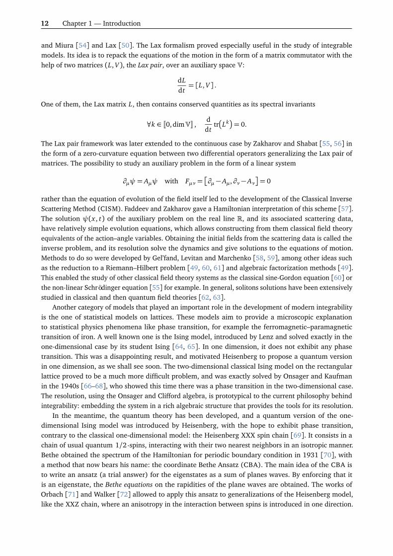
and Miura [54] and Lax [50]. The Lax formalism proved especially useful in the study of integrablemodels. Its idea is to repack the equations of the motion in the form of a matrix commutator with thehelp of two matrices (L, V ), the Lax pair, over an auxiliary space V:
dLdt= [L, V ] .
One of them, the Lax matrix L, then contains conserved quantities as its spectral invariants
∀k ∈ J0, dimVK ,ddt
trLk= 0.
The Lax pair framework was later extended to the continuous case by Zakharov and Shabat [55, 56] inthe form of a zero-curvature equation between two differential operators generalizing the Lax pair ofmatrices. The possibility to study an auxiliary problem in the form of a linear system
∂µψ= Aµψ with Fµν =∂µ − Aµ,∂ν − Aν
= 0
rather than the equation of evolution of the field itself led to the development of the Classical InverseScattering Method (CISM). Faddeev and Zakharov gave a Hamiltonian interpretation of this scheme [57].The solution ψ(x , t) of the auxiliary problem on the real line R, and its associated scattering data,have relatively simple evolution equations, which allows constructing from them classical field theoryequivalents of the action–angle variables. Obtaining the initial fields from the scattering data is called theinverse problem, and its resolution solve the dynamics and give solutions to the equations of motion.Methods to do so were developed by Gel’fand, Levitan and Marchenko [58, 59], among other ideas suchas the reduction to a Riemann–Hilbert problem [49, 60, 61] and algebraic factorization methods [49].This enabled the study of other classical field theory systems as the classical sine-Gordon equation [60] orthe non-linear Schrödinger equation [55] for example. In general, solitons solutions have been extensivelystudied in classical and then quantum field theories [62, 63].
Another category of models that played an important role in the development of modern integrabilityis the one of statistical models on lattices. These models aim to provide a microscopic explanationto statistical physics phenomena like phase transition, for example the ferromagnetic–paramagnetictransition of iron. A well known one is the Ising model, introduced by Lenz and solved exactly in theone-dimensional case by its student Ising [64, 65]. In one dimension, it does not exhibit any phasetransition. This was a disappointing result, and motivated Heisenberg to propose a quantum versionin one dimension, as we shall see soon. The two-dimensional classical Ising model on the rectangularlattice proved to be a much more difficult problem, and was exactly solved by Onsager and Kaufmanin the 1940s [66–68], who showed this time there was a phase transition in the two-dimensional case.The resolution, using the Onsager and Clifford algebra, is prototypical to the current philosophy behindintegrability: embedding the system in a rich algebraic structure that provides the tools for its resolution.
In the meantime, the quantum theory has been developed, and a quantum version of the one-dimensional Ising model was introduced by Heisenberg, with the hope to exhibit phase transition,contrary to the classical one-dimensional model: the Heisenberg XXX spin chain [69]. It consists in achain of usual quantum 1/2-spins, interacting with their two nearest neighbors in an isotropic manner.Bethe obtained the spectrum of the Hamiltonian for periodic boundary condition in 1931 [70], witha method that now bears his name: the coordinate Bethe Ansatz (CBA). The main idea of the CBA isto write an ansatz (a trial answer) for the eigenstates as a sum of planes waves. By enforcing that itis an eigenstate, the Bethe equations on the rapidities of the plane waves are obtained. The works ofOrbach [71] and Walker [72] allowed to apply this ansatz to generalizations of the Heisenberg model,like the XXZ chain, where an anisotropy in the interaction between spins is introduced in one direction.

Introduction 13
The energy of the fundamental state of this model was computed by Yang and Yang [73–75], whichexhibited the link with the vertex models found in statistical physics imagined originally to describe themicroscopic configurations of ice crystals [76–79].
The study of lattice models owes a lot to the works of Baxter. He introduced a new approach relyingon the Q operator and a “Baxter equation” for 6-vertex and 8-vertex models [80]. This proved especiallypowerful for the 8-vertex models, leading to new results [81–83]. The 8-vertex model contains the6-vertex model and the Ising model as particular case, so that this method was thought very general.Baxter also produced key exact results for the eight-vertex model [80, 81, 84], such as the computationof the partition function. He showed that the transfer matrices form a one-parameter commuting family,thanks to the existence of relations for the Boltzmann weights [80, 85]. These results were derived fromthe star-triangle relations obtained for the 8-vertex weights and their matrix rewriting. The same type ofequations were obtained by Yang in the context of factorizable scattering processes [86]. These equationsnow goes under the celebrated name of the Yang–Baxter equation, as named by Faddeev and collaborators,and write
R12(u, v)R13(u, w)R23(v, w) = R23(v, w)R13(u, w)R12(u, v).
The R-matrix R(u, v) is interpreted as the matrix gathering the Boltzmann weights of a 2D lattice vertexmodel, or, as found by C. N. Yang, are related to the two-body S-matrix for a factorizable scattering ofquantum particles moving on the real line, with rapidities u and v [87, 88]. The associated Yang–Baxteralgebra is generated by the elements Mi j(u) of a monodromy matrix M(u), with relations
R12(u, v)M1(u)M2(v) = M2(v)M1(u)R12(u, v),
where M1(u) = M(u)⊗ 1, M2(u) = 1⊗M(u). The quantum R-matrix intertwines two copies of the samemonodromy operators. The trace of the monodromy matrix gives the transfer matrix
T (u) = tr M(u).
The commutativity of the family of transfer matrices (T (u))u is given by the Yang–Baxter algebra relations,provided R(u) is invertible. If the Hamiltonian is found to be a function of these matrices, then one gets awhole family of conserved quantities of the system at hand.
The knowledge of conserved charges is not sufficient to claim integrability. For a classical system, aswe said above, it is also necessary to prove there are in sufficient number, independent and in involutionto claim that the system is Liouville integrable. To do so, one need to compute systematically the Poissonbrackets between the entries of the Lax matrix. Just like the R-matrix gave the commutators betweenthe entries of the monodromy, is it possible to pack the Poisson brackets of the Lax matrix entries in acompact, similar form? Remarkably, these Poisson brackets can be written in a commutator with the helpof a classical r-matrix [49, 89–91], for example
L1(u), L2(v)= [r12(u, v), L1(u) + L2(v)].
Historically, this object was identified after its quantum counterpart, the R-matrix introduced above, andthe classical limit of the quantum R-matrix indeed gives a classical r-matrix.
Using techniques derived from the CBA, Lieb and Liniger computed the energies of a one-dimensionalgas of bosons in delta interaction, corresponding to a non-linear quantum Schrödinger equation [92, 93].On the other hand, solutions of the non-linear (classical) Schrödinger equation were obtained, thanks theCISM [54]. This raised the question of the existence of a quantum version of the CISM method, whichwas elucidated with the developments of the Quantum Inverse Scattering Method (QISM) [90, 94–97].The main idea is the construction of a monodromy matrix for the problem from quantum local Lax

14 Chapter 1 — Introduction
operators, whose elements are auxiliary operators and quantum counterparts to the scattering data in theCISM. As described above, a R-matrix solution to the Yang–Baxter equation prescribes the commutatorsbetween the entries of the monodromy matrix, forming a Yang–Baxter algebra. Conserved quantitiesare then obtained from the family of the transfer matrices. Besides, the Yang–Baxter algebra can alsobe leverage to reconstruct the eigenstates of the conserved quantities. Indeed, the QISM serves as theprivileged framework for the definition of an algebraic version of the CBA, the Algebraic Bethe Ansatz(ABA) [95, 98, 99]. For a review, see [100]. The core idea of the ABA is that the off-diagonal elementsof the monodromy matrix somehow contain creation and annihilation operators for the eigenstates ofthe trace. The idea stem from the CISM, where these off-diagonal elements contain the action–anglevariables. Hence, the repeated action of an operator B(u) constructed from the off-diagonal elementsover a well-chosen reference state |0⟩ should therefore produce an eigenstate of the form
B(u1) . . . B(um) |0⟩ ,
under conditions on the values of the spectral parameters u1, . . . , um, which are eventually written as theBethe equations. The joint development of QISM and the ABA allowed numerous results in quantumintegrable models, such as the quantum sine-Gordon model [95], the massive Thirring model [101] andthe quantum Heisenberg chains [102, 103]. We shall focus heavily on the history of the later models,usually referred to as “spin chains”. The monograph [99] by Bogoliubov, Izergin and Korepin describe theformalism of QISM and ABA, as well as many results obtained by these techniques.
The computation of the monodromy and transfer matrices from local Lax matrices amounts to the“direct” problem of quantum integrability. The actual inverse problem is the computation of the dynamicalvariables, say the local spin operators for a spin chain, in terms of the monodromy matrix elements,namely the diffusion data. The effective resolution of the inverse problem was achieved only aroundthe year 2000, when Kitanine, Maillet and Terras [104–106] obtained explicit expression of the localoperators in terms of the monodromy matrix elements. Their results were extended by Göhmann andKorepin to the supersymmetric case [107].
These developments on the quantum side had great repercussions on the theory of classical integrablemodels. Sklyanin realized that the R-matrix, the Yang–Baxter equation and the Yang–Baxter algebras hadclassical counterparts, which could be obtained as a classical limits of the quantum objects [89]. This ledto a program of classification of the classical integrable models by their Yang–Baxter algebra, using Liealgebra theory [108–110]. The monograph of Bernard, Babelon and Talon [49] is a modern account ofthe progress in this field during the last decades of the 20th century.
Similarly, great efforts were made to construct and classify the solutions of the quantum Yang–Baxterequation. The works of the Kulish and Reshetikhin [111–113], Jimbo [114] and Drinfel’d [115] led tothe discovery of quantum groups, which may be introduced as deformed universal enveloping algebras ofLie algebras and Lie groups, replacing the role played by Lie algebras in the classical case. The R-matricesalready identified were found to be representations of a universal object, the universal R-matrix, andquantum integrable models were shown to be representations of these quantum groups. This opened anew field of research in mathematics, the study of quantum algebras [116–118]. The tools of integrabilityalso proved useful for the computation of invariants in knot theory and invariants of 3-dimensionalmanifolds [119–121]. This makes integrable models a nice example of the deep interleaving betweenmathematics and physics, one being inspired by the other and conversely.
The underlying symmetries of quantum one-dimensional spin chains have been identified, dependingon the anisotropy of the coupling, to be prescribed by Yangians Y (gl(n)), quantum affine algebrasUq(gl(n)), and related algebras [117]. As the classification of quantum integrable models developed, thestudy of higher rank models gained weight. The Heisenberg XXX chain is associated to the fundamentalrepresentation of the Yangian Y (gl(2)) of the gl(2) Lie algebra, in link with the simple Lie algebra

Introduction 15
A1 = sl(2), of rank 1. Keeping the Lie algebra in the same series, higher rank models are associatedto the Yangian Y (gl(n)), with n ≥ 3. The ABA proved to be useful for these models, leading to thedevelopment of a Nested version of the Algebraic Bethe Ansatz (NABA) [122, 123], where creationoperators acting over a reference state have a non-trivial expression in terms of the off-diagonal elementsof the monodromy matrix, and involve several levels of Bethe roots. The ABA techniques have also beenextended to the supersymmetric case of Y (gl(m|n)) models [124–129].
For quantum integrable model on the lattice, a longstanding goal—solved for some models by now—isthe computation of the correlation functions between operators, which are quantities of the form
trH (Oe−H/kB T )trH (e−H/kB T )
,
where O is an observable over the Hilbert spaceH of the system, H is the Hamiltonian, T the temperatureand kB the Boltzmann constant. In the limit of zero temperature, and assuming there exists only onefundamental state | f ⟩ of the lowest energy, correlation functions are reduced to a single matrix element,the normalized expectation value of O in the fundamental state
⟨ f |O| f ⟩⟨ f | f ⟩ .
Usually, in lattice models, one would like to compute the above quantity for local operators, or productsof local operators. A quantum integrable model on the lattice may be considered “solved” when it ispossible to compute such correlation functions exactly.
This first requires to compute the fundamental state | f ⟩. In the QISM and ABA framework, it iswritten in the form of a Bethe state. If O is some monodromy matrix elements, its action on an on-shellBethe state may be computed in the form of a linear combination of off-shell Bethe states, thanks to theYang–Baxter relations and the choice of the reference state. This leaves the correlation functions as sumsof on-shell/off-shell scalar products, which for some models have been computed as determinants in theworks of Gaudin [130], Korepin [131] and Slavnov [132]. The action of a local operator on these statesis a priori not known, but the resolution of the quantum inverse problem allows writing local operatorsin terms of the matrix elements of the monodromy. This enables the computation of correlation functionsby ABA procedure and the repacking of the final formulas into determinants [105]. In collaborationwith Slavnov, Kozlowski and Niccoli, many results stemmed from the first ones obtained on the XXZchain by Kitanine, Maillet and Terras, up to the computation of the thermodynamic limit of multipleintegral representations of correlation functions [105, 133–139]. The computation of the dynamicalstructure factor with the help of Caux [140, 141] allowed to successfully compare the results fromintegrability with the neutron scattering experiments [142, 143]. Important results were obtained in thetemperature dependent case by Göhmann, Klümper and Suzuki [144–147], and also by Kozlowski, Mailletand Slavnov [148, 149]. For the higher rank case, many results have been obtained by Ragoucy, Slavnov,Beillard, Pakuliak and Lyashyk, allowing to express scalar products as determinants and computingsome form factors [129, 150–156]. Some of these results were obtained in great generality, holding forsupersymmetric models as well [127, 129, 157–162].
At this point it worths pointing out that the tools of integrability have been extensively used by theAdS/CFT correspondence and super Yang–Mills communities to derive exact results in quantum fieldtheories using the lattice as a regularization [163–171]. This makes integrability a topic of formidableinteraction between various branches of physics and mathematics.
However, and despite its considerable successes, the algebraic Bethe Ansatz suffers from somelimitations. The first and most obvious one is that it is an ansatz; it is necessary to verify that all theeigenstate of the model are obtained by the ABA procedure. This counting is called the problem of the

16 Chapter 1 — Introduction
completeness of the Bethe Ansatz, and is a non-trivial task. Various techniques have been employed [172–174], and the recent work of Chernyak, Leurent and Volin [175] seems to give a new understanding ofthe Bethe equations completeness problem.
Furthermore, the ABA needs a reference state to be performed. For some not-so-intricate systems,such as the antiperiodic XXZ chain [176] or the Toda chain [177], such a state simply does not exist,which makes the ABA fails from the very start.
Finally, the nesting procedure of the NABA in the higher rank case is quite heavy [129]. In particular,it would be desirable to have a representation of the eigenstates simpler than the nested one. Thelook for more compact representations found some success with the conjectures of Gromov, Levkovich–Maslyuk and Sizov on the expression of a single B(u) operator in higher rank models that led to compactrepresentations of the eigenstates [178, 179].
Several variants of the ABA method were proposed to overcome these difficulties, such as the off-diagonal Bethe Ansatz [180] or the modified Bethe Ansatz [181]. But ultimately, there is room foranother approach of integrable models, partly because of the aforementioned limitations of the Betheansatz techniques, but also because the definition of quantum integrability remains unsatisfactory. Thesubject of this thesis is the development of new techniques of separation of variables for higher rank andsupersymmetric quantum integrable models, with the goal of finding more simple representations of thebasic objects, like the transfer matrix spectrum characterization, representations of the eigenstates, scalarproducts, and ultimately make the first steps towards correlation functions.
** *
The first occurrence of separation of variables (SOV) may be attributed to d’Alembert in its Traitéde dynamique in 1758 [182, 183], and is found in the part dedicated to the study of the wave equationthat bears its name. It has been used extensively by Fourier during the 19th century to solve variousdifferential equation, especially the heat equation [184], so that it also referred to as the “Fourier method”in english literature. Consider the d’Alembert wave equation
∂ 2u∂ x2
− 1c2
∂ 2u∂ t2
= 0.
With the coordinates change¨
p = x − c t
q = x + c t⇔
x =p+ q
2
t =q− p
2c,
the wave equation is rewritten∂ 2u∂ q∂ p
= 0.
Clearly the coordinates (p, q) are more adapted to describe the motion: solutions to the above equationsare easily computed to be of the form
u(x , t) = fp(x , t)
+ g
q(x , t)
= f (x − c t) + g(x + c t),
where f and g are C2 functions of their arguments. They have a separate form, in two variables p = x− c tand q = x + c t, with f depending only on p and g only on q. Initial conditions and conditions at theboundary of the space-time domain considered fix the solution. This example illustrate how separatevariables can drastically simplify the resolution of the dynamic. Henceforth, it is very desirable to separatethe variables whenever it is possible. This procedure decouples the equations of the motion of the systemat hand in independent and separate problems of lower complexity.

Introduction 17
Separation of variables was found very useful in classical mechanics in the resolution of the Hamilton–Jacobi equation for Hamiltonian systems [34]. In practice, Hamilton–Jacobi equations of separate formsare among the only cases where the resolution is tractable and the action–angle variables can be computedin closed form. In all generalities, the 2n canonical variables (x i , zi) of a 2n-dimensional Hamiltoniansystem are separate if there exist n independent separate relations of the form
Fi(qi , pi , F1, . . . , Fn) = 0.
Note that Fi depends only on the corresponding qi and pi , and a priori also on all the conserved quantitiesFi . Realizing pi as ∂ /∂ qi , one sees clearly that the above equations gives independent ordinary differentialequations for each coordinate qi .
It is Sklyanin who laid the foundations of SOV in the inverse scattering framework for classical andquantum integrable models, with its seminal paper on the Toda chain [177] in which he acknowledgesinspiration from Gutzwiller’s results [185] and the help of Komarov. Sklyanin introduced SOV techniquesin the CISM context [186–188], and contributions for the generic gl(n) case were made by Scott [189]and Gekhtman [190]. The idea relies on the existence of a pair of two functions (A(u),B(u)), such thatthe roots x i of B and their image zi =A(x i) by A form conjugated canonical variables. The (x i , zi) arethen shown to be separate variables for the dynamical problem, because of the form of the A(u) andB(u) functions.
Having developed SOV for classical spin chains models, Sklyanin was able to extend his constructionto gl(2) quantum spin chains [191–193], under the name of functional Bethe Ansatz3. The principlesremain the same, with the A(u) and B(u) functions promoted to operators. This makes the definitions ofthe operatorial roots x i of B(u) more subtle. The separate basis is the eigenbasis of the B(u) operator,which should be diagonalizable with simple spectrum. The conjugate momenta zi to the x i give shifts onthe spectrum of the x i operators, and therefore on the spectrum of B(u). In the separate basis, the wavefunctions of the eigenstates of the transfer matrix factorizes as a product of one-variable wave functions,each of them satisfying an independent finite-difference equation. Hence, separation of variables inthe quantum case indeed reduces drastically the complexity of the multi-variable problem to severalone-variable ones.
Since these seminal models, SOV has been developed for a wide range of other important models.SOV has been implemented for the rational Gaudin model by Sklyanin [191], and extended to thequantum elliptic case with the help of Takebe [194]. He also considered the infinite volume case for thenon-linear Schrödinger model [195] and the sinh-Gordon model [196]. Furthermore, he studied the3-particles quantum Calogero–Sutherland model with Kuznetsov [197], the A2 Ruijsenaars model withNijhoff [198, 199]. The non-compact XXX chain case was studied in the works of Derkachov, Korchemskyand Manashov [200–202], while the lattice sinh-Gordon model was tackled by Bytsko and Teschner [203].Additional contributions to the XXX spin 1/2 chain SOV were made by Frahm and collaborators [204,205].
The SOV method for higher rank quantum integrable model was initiated by Sklyanin himself, byquantizing his classical construction. In [206], he constructed separate variables for the gl(3) quantumspin chain by constructing corresponding A(u) and B(u) operators. He already acknowledged en passantthat for the scheme to be well-defined, one needs to verify a non-intersection condition between thespectrum of the roots of B(u) and possible poles of A(u). This construction was discussed in the genericn≥ 2 case by Smirnov [207].
Later, Gromov, Levkovich-Maslyuk and Sizov used exact computer-aided computations to conjectureand verify for small length chain the form of the spectrum of B(u) operators that would yield separate
3In the considered models, the A(u) and B(u) functions were polynomials in u or euη for some η ∈ C, making all themanipulations rather explicit.

18 Chapter 1 — Introduction
variables from its operatorial roots for higher rank (and supersymmetric) models [178, 179]. They havenot considered the question of the operator A(u), though.
In the 2010s, Maillet and Niccoli, in collaboration with Grosjean and Teschner used the SklyaninSOV method to get great results over various quantum integrable models [176, 208–216]. For the gl(2)models in particular, the complete SOV characterization of the transfer matrix spectrum allowed to provethe completeness of the Bethe Ansatz characterization, and to compute the form factors of local operatorsthanks to the separate representation of the eigenstates of the transfer matrix. This work has been pursuedin collaboration with Terras and Kitanine towards the computation of correlation functions [217–220],with some very recent results in this domain [221, 222]. The open case boundary case was recentlystudied with Pezelier [223, 224].
A new idea emerged recently from this line of research: the construction of separate bases fromconserved quantities [225]. A most general form of such bases is
⟨L|N∏
j=1
h j∏k j=1
T
y(k j)j
,
where the y(k j)j are complex numbers and T (u) is the transfer matrix generating the conserved quantities
of the model at hand [see 225, Definition 2.2]. For example, for the Y (gl(n)) fundamental models, thebasis constructed from the powers of the transfer matrix evaluated in the inhomogeneity parameters ξ j
of the models
⟨S|N∏
j=1
Tξ j
h j ,
where the h j are integers between 0 and n− 1, is shown to be separate provided weak restrictions on theinhomogeneities of the model, and that the boundary conditions are given by a twist matrix with simplespectrum. The possibility to construct such bases originates from the existence of cyclic vectors for simplespectrum matrices, or non-derogatory matrices [226]. There are in general many possible choices for thecovector ⟨S|; a useful one for quantum integrable lattice models is a tensor product form made up fromthe cyclic covectors of the twist matrix at each lattice site.
This construction of separate bases from the transfer matrix itself has some advantages to Sklyanin’sapproach of SOV. First, it bypasses the need for the identification and construction of the A(u) and B(u)operators4, and in place relies on a fundamental object of quantum integrability, the transfer matrix. Thisis desirable, for it minimizes the number of different objects and the complexity of the SOV procedure,but also because the construction of proper A(u) and B(u) operators has been identified as a blockingpoint for the proper generalization of Sklyanin’s SOV to higher rank model. Furthermore, with thisconstruction, the knowledge of an eigenvalue fixes completely its unique associated eigenvector by itswave functions in the separate basis—one proves the transfer matrix has simple spectrum, thanks to thetwist matrix having this property.
In this new take on quantum separation of variables, the fusion relations verified by the fused transfermatrices play a key role [111, 112, 128, 227–231]. They originate from the decomposition in irreduciblecomponents of the tensor products representations. First, they allow to compute the action of the transfermatrix in the separate bases. But ultimately they also provide a characterization of the complete spectrumof the transfer matrix, which can be put in the form of a quantum spectral curve by exhibiting thenecessary Baxter Q-functions.
This novel SOV procedure has been shown to be applicable in a wide range of cases. It was shown tobe applicable for higher spin representations [232], where Q operators are used to construct the separate
4We still need to identify their spectrum, which are the separate variables.

Introduction 19
basis. The open boundary case of gl(2) models was considered in [233]. Separate bases of this formwere also constructed in the general Y (gl(n)) [234] and Uq(Õgl(n)) [235] cases, and used to provide acharacterization of the complete spectrum of the transfer matrix.
Article [225] triggered general progress on a SOV procedure based on conserved quantities. Ryanand Volin [236] proved that the B(u) operator—conjectured by Gromov, Levkovich-Maslyuk, and Sizovin [178] to be the generalization of Sklyanin’s B(u) operator in the general gl(n) case—produces in itsroots the same separated variables obtained in [225], and moreover can serve as the correct creationoperator for a Bethe Ansatz description of the eigenstates. However, construction of the A(u) operatorrealizing the proper shifts in the B(u) spectrum remained unaddressed, as well as the completeness of thespectrum. These results were obtained for a general class of representations, and rely on the constructionof the eigenbasis of the B(u) operators by deformation of the Gelfand–Tsetlin basis of Y (gl(n)). Thisconstruction was later extended in [237] where the connection with Bäcklund flow was made, and aconstruction of the conjugate momentum variables of the separate (coordinate) variables was proposed,in the form of Wronksian of Q-functions. In collaboration with Cavaglià, Gromov and Levkovich-Maslyuk,some progress was also made in the direction of correlation functions, with results on the SOV measurefor higher rank models [238–240].
** *
The work introduced in this thesis is two folds:i) The characterization of the SOV measure in the Y (gl(3)) fundamental models, making a first step
towards the computation of correlation functions by SOV in higher rank models. This is the subjectof chapter 7.
ii) The extension of this SOV procedure to the supersymmetric integrable models, and how to tacklethe spectral problem of the transfer matrix in this framework. This is the subject of chapter 8.
We need to introduce several topics in details before discussing the original works of the thesis presentedin chapters 7 and 8. This is the role of chapters 2 to 6, which are devoted to the exposition of the necessarytechniques and ideas for the manuscript to be essentially self-contained.
We introduce classical and quantum integrable models and their description in the classical andquantum inverse scattering formalisms in chapters 2 and 3. The Algebraic Bethe Ansatz techniques andits nested versions are detailed in chapter 4, as well as the results towards correlation function obtainedin the gl(2) and higher rank case. Next, we describe the separation of variables procedure in generalin chapter 5. The classical and quantum SOV principles are introduced, and we discuss the Sklyanin’sSOV construction for classical and quantum integrable models. In chapter 5, the idea of separate basesfrom conserved quantities is given in details for Y (gl(n)) models, laying the necessary concepts andnotations for the discussion of results of the last two chapters.
Two articles are attached to the main manuscript:
[LV1] J. M. Maillet, G. Niccoli, and L. Vignoli, “Separation of variables bases for integrable glM|N andHubbard models,” SciPost Phys., vol. 9, p. 60, 4 2020. DOI: 10.21468/SciPostPhys.9.4.060
[LV2] J. M. Maillet, G. Niccoli, and L. Vignoli, “On Scalar Products in Higher Rank Quantum Separationof Variables,” SciPost Phys., vol. 9, p. 86, 6 2020. DOI: 10.21468/SciPostPhys.9.6.086
They are the author’s peer-reviewed contributions to the field, and contain additional lengthy proofs anddetails of the results featured in chapters 7 and 8.


2 Chapter
Classical integrability
There are several frameworks in which we can describe the configurations of a mechanical systemand study its dynamics. The Hamiltonian formulation [34, 37, 48] is proved most useful in the context ofintegrability, as integrable models and the role of conserved quantities are best described in it, but alsobecause quantization of Hamiltonian systems is a customary procedure.
The role of conserved quantities in the resolution of Hamiltonian systems is emphasized, with theintroduction of Liouville integrability [47] and the Liouville–Arnol’d theorem [48]. We also discussed theprivileged role of action–angle variables in this setting [34, 49].
We introduce the Lax formalism [49, 50, 63, 241] in details for mechanical systems and classical fieldtheory. The benefit of the Lax formulation is to possibility to produce conserved quantities systematicallyform the spectral invariants of the Lax matrix. Then, we introduce the (classical) inverse scatteringmethod (CISM) [49, 54, 96], whose goal is to produce action–angle variables analogs for integrablemodels on continuous space or on the lattice. The direct problem is the construction of such variablesfrom the diffusion data, while the inverse problem consists in expressing the original dynamical variablesin terms of the diffusion data. The notion of classical r-matrix [89–91] and the associated integrablestructures are then discussed, setting the course to the quantized version of these objects.
2.1 Classical integrability
Hamiltonian formulation of classical mechanics Consider a mechanical system with N degrees offreedom. A state of the system is described by N coordinates defining a point in the N -dimensional config-uration space C. These are the generalized coordinates q1, . . . , qN . The phase space of the system is the 2N -dimensional cotangent manifold M= T ∗C with canonical conjugate coordinates (q1, . . . , qN , p1, . . . , pN ),that is with the following Poisson brackets
qi , q j
= 0=
pi , p j
and
qi , p j
= δi j . (2.1)
More precisely, to describe globally the phase space, a canonical atlas of local canonical charts is re-quired [48]. In the following, it is implied that qi , pi are local coordinates.
M has a symplectic structure fixed by a closed and non-degenerate symplectic 2-form
ω= −dα=N∑
i=1
dqi ∧ dpi , (2.2)
where α =∑N
i=1 pi dqi is the canonical 1-form. The Poisson brackets are defined over M by ω: forf , g ∈ C1(M) and X f , X g the vector fields associated to f and g by d f =ω(X f , ·) and dg =ω(X g , ·), wehave
f , g :=ω(X f , X g) = X f (g) = −X g( f ). (2.3)
21

22 Chapter 2 — Classical integrability
In local coordinates, they write
f , g=N∑
i=1
∂ f∂ qi
∂ g∂ pi− ∂ g∂ qi
∂ f∂ pi
, (2.4)
and
X f =N∑
i=1
∂ f∂ qi
∂
∂ pi− ∂ f∂ pi
∂
∂ qi, (2.5)
and the same holds for X g . The fact that the qi , p j are canonical conjugated coordinates is seen in theirPoisson brackets: qi , p j = δi j and qi , q j = 0= pi , p j , ∀i, j ∈ J1, NK.
The dynamics of the system is prescribed by a Hamiltonian function H(q, p, t) ∈ C1(M) such that theequations of the motion read
qi = qi , H= ∂ H∂ pi
,
pi = pi , H= −∂ H∂ qi
.(2.6)
This is the Hamiltonian formulation of classical mechanics [34, 37]. From now on, we restrict to time-independent Hamiltonian for simplicity.
Solving (2.6) is the main goal in the study of mechanical systems; it can be a challenging task. Itis a system of 2N first-order coupled differential equations. A reformulation of the problem in a new,appropriate set of canonical coordinates proves useful in most of the cases.
Change of coordinates Other sets of canonical variables
Q i(q, p, t), Pi(q, p, t), (2.7)
have the property that if the equations of the motion for (q, p) are Hamilton’s canonical equations (2.6)with some Hamiltonian H(q, p), then there exists a new Hamiltonian H ′(Q, P) ∈ C1(M) such that
Q i =Q i , H ′
=∂ H ′
∂ Pi,
Pi =
Pi , H ′= −∂ H ′
∂Q i,
(2.8)
so that H ′ serves as the Hamiltonian function in the new coordinates. Canonical coordinate transformationsare characterized by a generating function which makes the bridge between the two sets of canonicalcoordinates (q, p) and (Q, P) [34, 37]. For a “type 2” generating function of the form F(q, P, t) that mightdepend explicitly on time, we have
pi =∂ F∂ qi
, Q i =∂ F∂ Pi
, (2.9)
H ′ = H +∂ F∂ t
. (2.10)
Under such transformation (q, p)→ (Q, P), the 1-form α is transform in α′, that differs from α by anexact differential, so that the 2-form ω is actually invariant.
Constants of the motion and integrability The knowledge of constants of the motion is crucial in theconstruction of canonical coordinates adapted to the dynamics of the system at hand. It is the key featureof Liouville integrable systems to ensure their solvability from the knowledge of their conserved quantities.
2.1. Classical integrability 23
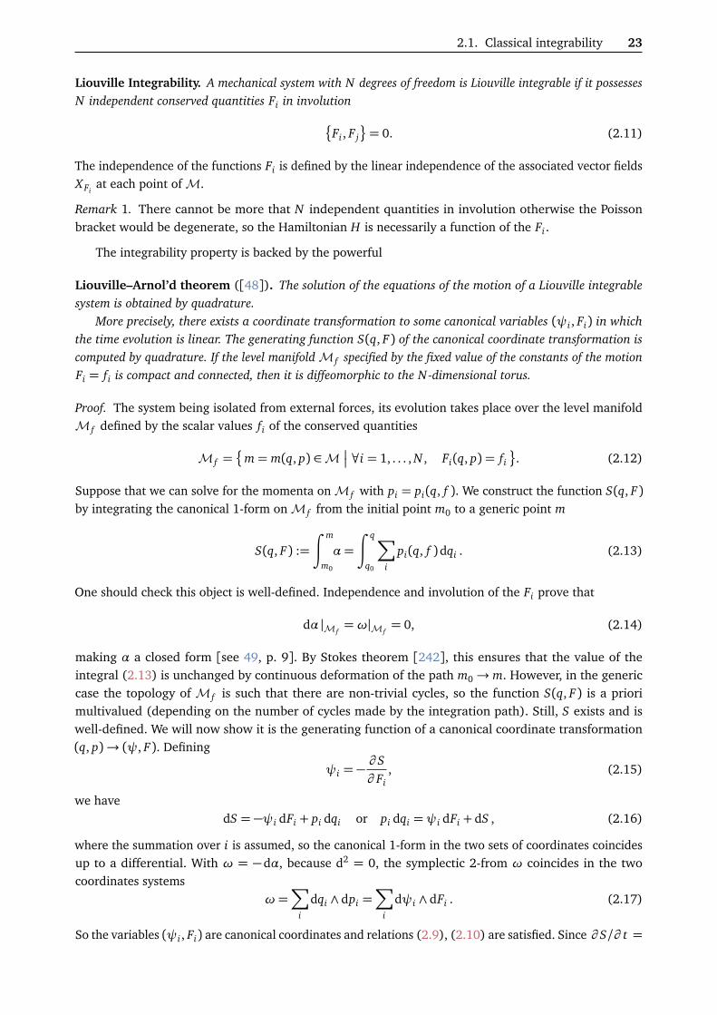
Liouville Integrability. A mechanical system with N degrees of freedom is Liouville integrable if it possessesN independent conserved quantities Fi in involution
Fi , F j
= 0. (2.11)
The independence of the functions Fi is defined by the linear independence of the associated vector fieldsXFi
at each point of M.
Remark 1. There cannot be more that N independent quantities in involution otherwise the Poissonbracket would be degenerate, so the Hamiltonian H is necessarily a function of the Fi .
The integrability property is backed by the powerful
Liouville–Arnol’d theorem ([48]). The solution of the equations of the motion of a Liouville integrablesystem is obtained by quadrature.
More precisely, there exists a coordinate transformation to some canonical variables (ψi , Fi) in whichthe time evolution is linear. The generating function S(q, F) of the canonical coordinate transformation iscomputed by quadrature. If the level manifold M f specified by the fixed value of the constants of the motionFi = fi is compact and connected, then it is diffeomorphic to the N-dimensional torus.
Proof. The system being isolated from external forces, its evolution takes place over the level manifoldM f defined by the scalar values fi of the conserved quantities
M f =
m= m(q, p) ∈M ∀i = 1, . . . , N , Fi(q, p) = fi
. (2.12)
Suppose that we can solve for the momenta on M f with pi = pi(q, f ). We construct the function S(q, F)by integrating the canonical 1-form on M f from the initial point m0 to a generic point m
S(q, F) :=
∫ m
m0
α=
∫ q
q0
∑i
pi(q, f )dqi . (2.13)
One should check this object is well-defined. Independence and involution of the Fi prove that
dα |M f=ω|M f
= 0, (2.14)
making α a closed form [see 49, p. 9]. By Stokes theorem [242], this ensures that the value of theintegral (2.13) is unchanged by continuous deformation of the path m0→ m. However, in the genericcase the topology of M f is such that there are non-trivial cycles, so the function S(q, F) is a priorimultivalued (depending on the number of cycles made by the integration path). Still, S exists and iswell-defined. We will now show it is the generating function of a canonical coordinate transformation(q, p)→ (ψ, F). Defining
ψi = −∂ S∂ Fi
, (2.15)
we havedS = −ψi dFi + pi dqi or pi dqi =ψi dFi + dS , (2.16)
where the summation over i is assumed, so the canonical 1-form in the two sets of coordinates coincidesup to a differential. With ω = −dα, because d2 = 0, the symplectic 2-from ω coincides in the twocoordinates systems
ω=∑
i
dqi ∧ dpi =∑
i
dψi ∧ dFi . (2.17)
So the variables (ψi , Fi) are canonical coordinates and relations (2.9), (2.10) are satisfied. Since ∂ S/∂ t =

24 Chapter 2 — Classical integrability
0 the new Hamiltonian is simply the old one written in terms of the new coordinates
H ′(ψ, F) = Hq(ψ, F), p(ψ, F)
. (2.18)
By (2.8) it is clear that H ′ depends only on the constants of the motion Fi. The constant value of theHamiltonian H(q, p) = H ′(F) over the level manifold M f is the energy E of the system
H(q, p)q0→q⊂M f
= H ′( f1, . . . , fn) = E. (2.19)
H ′ has no explicit dependence in the ψi; they are tagged as ignorable coordinates1. Noting
νi(F) := ψi =ψi , H ′
=∂ H∂ Fi
= const, (2.20)
we have the following linear time evolution for the system at hand when written in the (ψ, F) canonicalcoordinates
Fi(t) = fi ,
ψi(t) =ψi(0) + νi t.(2.21)
To obtain this solution, we had to perform a single—but curvilinear over a N -dimensional submani-fold—integration to compute S, and invert the coordinate transformation to get the νi from the explicitexpression (2.18) of the Hamiltonian H in terms of the ψi and Fi. Hence, we solved it by quadrature,and some additional algebraic manipulations.
For the proof of the topology of M f under the suitable conditions, see [48].
Action–Angle variables Since under suitable conditions M f is a torus, we can choose an even moreappropriate set of coordinates than (ψ, F) to describe the motion: the action–angle variables (θ , I).
Choosing the values fi of the Fi fixes the level-manifold M f and thus fixes a particular torus in thefoliation in tori of M. We may choose any N independent functions I j = I j(F1, . . . , FN ) such that once thevalues I j of the I j are known, then M f is determined. But since the N -dimensional torus Tn is isomorphicto the product of N circles C j, we define the action variables I j as the integrals of the canonical 1-formover the closed cycles C j
I j =1
2π
∮
C j
α= I j(Fi). (2.22)
Using the same generating function as before, but expressed in terms of the I j
S(q, I) =
∫ m
m0
α, (2.23)
the new canonical variables in the coordinate transformation characterized by S are the
I j and θk =∂ S∂ Ik
, 1≤ j, k ≤ N . (2.24)
1It remains useful to characterizes their dynamic to get the ones of the original coordinates (q, p).
2.1. Classical integrability 25
By definition of θk, ∮
C j
dθk =∂
∂ Ik
∮
C j
dS =∂
∂ Ik
∮
C j
∑i
∂ S∂ qi
dqi +∂ S∂ Ii
dIi
=∂
∂ Ik
∮
C j
∑i
pi dqi + 0=∂
∂ Ik
∮
C j
α
= 2π∂ I j
∂ Ik= 2πδ jk,
(2.25)
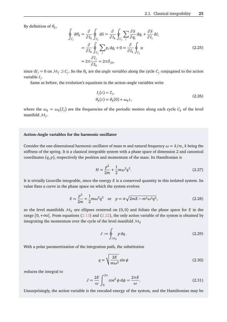
since dI j = 0 on M f ⊃ C j. So the θk are the angle variables along the cycle C j conjugated to the actionvariable I j .
Same as before, the evolution’s equations in the action–angle variables write
I j(t) = I j ,
θk(t) = θk(0) +ωk t,(2.26)
where the ωk = ωk(I j) are the frequencies of the periodic motion along each cycle Ck of the levelmanifold M f .
Action–Angle variables for the harmonic oscillator
Consider the one-dimensional harmonic oscillator of mass m and natural frequencyω = k/m , k being thestiffness of the spring. It is a classical integrable system with a phase space of dimension 2 and canonicalcoordinates (q, p), respectively the position and momentum of the mass. Its Hamiltonian is
H =p2
2m+
12
mω2q2. (2.27)
It is trivially Liouville integrable, since the energy E is a conserved quantity in this isolated system. Itsvalue fixes a curve in the phase space on which the system evolves
E =p2
2m+
12
mω2q2 or p = ±Æ
2mE −m2ω2q2, (2.28)
so the level manifolds ME are ellipses centered on (0,0) and foliate the phase space for E in therange [0,+∞[. From equations (2.13) and (2.22), the only action variable of the system is obtained byintegrating the momentum over the cycle of the level manifold ME
J :=
∮
ME
p dq . (2.29)
With a polar parametrization of the integration path, the substitution
q =
√√ 2Emω2
sinφ (2.30)
reduces the integral to
J =2Eω
∫ 2π
0
cos2φ dφ =2πEω
. (2.31)
Unsurprisingly, the action variable is the rescaled energy of the system, and the Hamiltonian may be

26 Chapter 2 — Classical integrability
rewritten H = ωJ/2π . Eventually, the original coordinates take the form
q =
√√ Jπmω
sinθ , (2.32)
p =
√√mJωπ
cosθ , (2.33)
which effectively solves the dynamics of the system by providing the explicit time evolutions of theoriginal coordinates. Also,
J =π
mω
p2 +m2ω2q2
, (2.34)
θ = arctan
mωqp
, (2.35)
and one verifies J ,θ= 2π, so the action–angle (canonical) variables are ( J/2π ,θ ) (a 1/2π normal-ization in the contour integral (2.29) would give the correct action straight away). The angle θ evolveslinearly in times
θ (t) = θ0 + νt given ν=∂ H
∂ J2π
=ω=
√√ km
. (2.36)
One recovers the well-known formula for the pulsation of the oscillation. Here, the θ variable findsa direct physical interpretation as being the phase of the position, so it comes as no surprise that itsfrequency matches the physical one.
Computing the coordinate transformation to canonical coordinates made from constants of the motion,which are pre-action–angle variables, requires to compute a curvilinear integral over a curve lying on thelevel manifold. This is in general a non-trivial calculation. In practice, the integral (2.13) is tractableonly when the variables are separate: it can then be reduced to a sum of one-variable independentintegrals. This substantially alleviates the computational difficulty of the problem. Hence, developpingtools to effectively separate the variables in integrable systems has been of extreme interest, and QuantumSeparation of Variables (SOV) is the core subject of this thesis. We will describe such tools in chapters 5and 6. It requires first to develop a more algebraic understanding of classical and quantum integrablemodels, that we will detail in the following sections. For now, we pursue the description of classicalintegrable models and the algebraic tools developed to study them systematically.
2.2 Classical Lax formalism and r-matrix
As we saw with the Liouville–Arnol’d theorem, conserved quantities are at the center of the description ofintegrable models. Any studies of integrable models should therefore be committed to identify clearly theconstants of the motion at the earliest stage. Modern studies of integrable mechanical systems goes alongwith the Lax formalism, first developed for solving differential equations of continuous systems [50, 55,56] and then extended to the general Hamiltonian description of classical mechanics [57, 63].
The seminal idea is to recast the equations of the motion into a commutator of two matrices, theLax pair (L, V ). By doing so, conserved quantities of the system are found in the spectral invariants of L,called the Lax matrix.
Lax pair. Let M be the 2N-dimensional phase space of a mechanical system whose dynamics is given bythe Hamiltonian H independent of the time. Two n × n square matrices L(m, u, t) and V (m, u, t), with

2.2. Classical Lax formalism and r-matrix 27
(m, u) ∈M×C, form a Lax pair if they rewrite the equations of the motion as
dLdt= L, H= [V, L]. (2.37)
L(m, u, t) is the Lax matrix. The variable u is called the spectral parameter. The space V0 := Cn, n ∈ Z≤2,on which the matrix L and V are constructed is called the auxiliary space. We often omit the time and phasespace dependency and simply write L(u), V (u).
Note that for a given system, the Lax pair—if it exists—may not be unique. The dimension of the Land V matrices may even be different for different pairs associated to the same system. The addition of aspectral parameter is necessary to ensure the spectral invariants contains all the conserved quantities of themodel, see the examples of tops in chapter 2 of [49]. In many integrable systems, the spectral parameteru is a complex number. However, it could be a more sophisticated object depending on the space-timesymmetries of the system at hand. For example, it is a twistor in self-dual Yang–Mills theories [243, 244].
Set of commuting conserved quantities The interest of the Lax construction is the easy access to theconserved quantities of the system.
Indeed, the spectral invariants of the Lax matrix
∀ j ∈ J1,dimV0K , F j(u) := trV0
L0(u)
j, (2.38)
are integrals of the motion. The proof is done by direct computation of the flow of the F j under theHamiltonian. Omitting the spectral dependence in u, one has
dF j
dt=
F j , H= trV0
¦L j
0, H©
= trV0
j−1∑k=0
L j−1−k0 L0, HL j
0
!= j trV0
L j−1
0 L0, H
= j trV0
L j−1
0 [V0, L0]= 0,
(2.39)
where we used the trace identify tr(AB) = tr(BA) over the auxiliary space.Also, note that matrices of the form
L(u, t) = g(t)L(u, 0)g(t)−1, (2.40)
where the invertible g(t) matrix evolves by the equation
dgdt= V (u, t)g(u, t) with g(u, 0) = id, (2.41)
are solution to equation (2.37) Therefore, any function F(L(u)) invariant under the conjugation by g(t)is a constant of the motion. Such functions are the eigenvalues of the Lax matrix L(u), so the spectrumof L is preserved over time and L time evolution is said isospectral. The conserved charges F j obtainedabove are symmetric functions of the eigenvalues of L(u), so it is no surprise that they are conserved.
r-matrix The Lax pair is a convenient way to construct constants of the motion without referring tothe Poisson structure of the phase space. But for Liouville integrability of the system, we need to havethem independent and in involution. The discussion of the involution of the integrals of the motion F j istied to the existence of an r-matrix, which encodes a general form of Poisson bracket between the matrixelements of L that ensures the involution property of the conserved quantities [49, 62, 63, 89, 90, 241].

28 Chapter 2 — Classical integrability
Theorem 1 (Babelon & Viallet, see [49, 241]). The involution property of the spectral invariants of L isequivalent to the existence of a matrix r12(u, v|m) acting on V0 ×V0 whose matrix elements are function onM, such that
L1(m, u), L2(m, v)= [r12(m|u, v), L1(m, u)]− [r21(m|v, u), L2(m, v)]. (2.42)
The indices 1 and 2 in L and r label two distinct copies of the auxiliary space V0.
The Poisson braket between the two Lax matrices has to be understood as the matrix whose coefficientsare the Poisson brackets between the matrix elements of L1 and L2:
L1(m, u), L2(m, v)=∑
i, j,k,`
Li j(m, u), Lk`(m, v)
ei j ⊗ ek`. (2.43)
Most of the time, the dependence in m ∈M is suppressed from the notation. The proof that the involutionimplies the existence of the r-matrix is done by direct construction of it, while for the converse waythe Poisson brackets of the invariants of the Lax matrices write as trace over commutators, whichvanish [49]. Integrability is then ensured once the independence of N spectral invariants of L is proven,N ≤ n= dimV0, which is now a model-dependent problem.
Lax pair and r-matrix of the harmonic oscillator
The Lax pair of the harmonic oscillator (2.27) with m= 1 are the 2× 2 matrices
L =
p mωq
mωq −p
, V =
0 − ω/2ω/2 0
. (2.44)
It is not necessary to introduce a spectral parameter here. One checks easily that the Lax equationdL/dt = [V, L] is equivalent to the equations of the motion q = p/m , p = −mω2q. We also observe thatthe Hamiltonian can be written 1
4m trL2. The matrix
r = − ω4E
0 1−1 0
⊗ L, (2.45)
with E = p22m + mω2q2
2, is such that the relation (2.42) holds with the above L. For example, the
equality of the (1, 2) matrix elements in equation (2.42) specialized to the above matrices computes fromits left-hand side the Poisson bracket p, q , and the right-hand side is
− ω4E
2m2ω2q2 + 2p2
= −1, (2.46)
which is the expected value of p, q from the equations (2.1), (2.4). Note that the r-matrix is dynamical(it depends on the q and p variables).
Classical Yang–Baxter equation What are the solutions (L, r) of (2.42) such that the induced Pois-son bracket indeed defines a symplectic structure on M? This mainly amounts to the verification ofthe skew-symmetry property and the Jacobi identity for the Poisson bracket [49]. Skew-symmetry isobvious from (2.42), while the Jacobi identity may hold only after imposing some conditions on L and r.Constraints on L and r are decoupled when restricting to r-matrices that are constant on M, i.e. which

2.2. Classical Lax formalism and r-matrix 29
have scalar entries. In particular, the Jacobi identity is satisfied if a constant r-matrix satisfies
[r12(u, v), r13(u, w)] + [r12(u, v), r23(v, w)] + [r32(w, v), r13(u, w)] = 0, (2.47)
When r is antisymmetric as r12(u, v) = −r21(v, u), this is called the classical Yang–Baxter equation.Unitary antisymmetric solutions of difference type to the classical YBE are constant r-matrices
verifyingr12(u, v) = −r21(v, u),
r12(u, v) = r12(u− v).(2.48)
They are associated to the Poisson algebra with a linear in L right-hand side
L1(u), L2(v)= [r12(u− v), L1(u) + L2(v)], (2.49)
but also to another symplectic structure called the Skylanin’s quadratic Poisson algebra
L1(u), L2(v)= [r12(u− v), L1(u)L2(v)], (2.50)
which is quadratic in L right-hand side, leading to a different class of Lax matrices and integrable models2.
The classical numeric r-matrices satisfying (2.47) have been extensively studied and classified infamilies labelled by Lie algebras representation theory [112, 245]. A notable solution is the one associatedto the gl(n) algebra, n≥ 2, with its fundamental vector representation taken for the spaces V1,2
r12(u) =cuP12, c ∈ C, (2.51)
where P is the permutation operator on V⊗V; with ei j the n× n coordinate matrices, it writes
P =n∑
i, j=1
ei j ⊗ e ji . (2.52)
Classical Inverse Scattering This discussion extends to classical field theory with a space-dependentLax pair (L(u, x , t), V (u, x , t)), where x is the space coordinate. It rationalizes the Classical InverseScattering Method (CISM) originally designed by Gardner, Greene, Kruksal and Miura [54] under an Land r-matrix construction.
Considering a non-linear partial differential equation for a classical field ψ(x , t) on the real line ofthe form
Kψ,∂ψ
∂ t,∂ψ
∂ x
= 0, (2.53)
we suppose there exists a Lax pair such that it can be recast in
[∂x − L,∂t − V ] = 0, (2.54)
which is the continuous equivalent of (2.37). This allows to interpret the equations of the motion writtenin the form (2.54) as the compatibility condition—or zero-curvature equation—of the linear auxiliarysystem (
∂xχ = Lχ,
∂tχ = Vχ.(2.55)
2It is possible to rewrite this quadratic algebra in a linear form and recover Poisson bracket of the form (2.42), but ther-matrix is then, obviously, a different one. In particular, it is non-constant.

30 Chapter 2 — Classical integrability
The study of the partial differential equation (2.53) then reduces [90, 95] to the study of the spectralcharacteristics of the spatial part of the Lax pair, the linear differential operator ∂x − L(x , u).
Let us show in more details how this is done. Consider two points A and B of the two-dimensionalspace-time (x , t). Let Ax = L and At = V . The Wilson line element between points A and B is the orderedexponential
WBA =←−exp
∫ B
AAµ dxµ , (2.56)
with Aµ = Aµ(x , t, u). For a spacetime with trivial topology, this Wilson line is independent of theintegration path chosen between A and B, so that (2.54) is a zero-curvature equation for the Aµ. Considernow A= (xA, t) and B = (xB, t) two points on the same surface t = cste of the space-time. Wilson lineelements are multiplicative along the integration path so for two other points A′ = (xA′ , t ′), B′ = (xB′ , t ′)on another constant time surface, t ′ 6= t, one has
WBA(t, u) =WBB′WB′A′(t′, u)WA′A. (2.57)
For a system periodic in the box [0, y], i.e. Aµ(y, t, u) =Aµ(0, t, u) for µ= x , t, the space-time has thegeometry of a cylinder and the closed Wilson line between points A= (0, t) and B = (y, t)≡ A is calledthe monodromy matrix3
M(u, t) :=WAA =←−exp
∮ A
AL(x , t, u)dx . (2.58)
Then WA′A =W−1BB′ due to spatial periodic boundary conditions and
WBA(t, u) =WBB′WB′A′(t′, u)W−1
BB′ . (2.59)
With the partial differentials
∂
∂ xBWBA = L(xB, tB, u)WBA,
∂
∂ xAWBA = −WBAL(xA, tA, u), (2.60)
∂
∂ tBWBA = V (xB, tB, u)WBA,
∂
∂ tAWBA = −WBAV (xA, tA, u), (2.61)
and t ′ = t + ε, ε→ 0, from (2.59) one computes
dMBA
dt= [VA(0, t, u), MBA(t, u)], (2.62)
which is the Lax equation (2.37) for the monodromy matrix. Then, by a computation similar to (2.39)
∀k ∈ N,ddt
trM(t, u)k
= 0, (2.63)
that is the spectral invariants of the monodromy matrix are constants of the motion. In the case of twistedboundary conditions
Aµ(y, t, u) = K(u)−1Aµ(0, t, u)K(u), (2.64)
it is the twisted monodromy M (K)(u) = K(u)M(u) which gets a derivative in the form of a commutator
ddt(K(u)M(t, u)) = [V (0, t, u), K(u)M(t, u)], (2.65)
3A monodromy studies how objects behave as they run around a singularity.

2.2. Classical Lax formalism and r-matrix 31
and
∀k ∈ N,ddt
tr(K(u)M(t, u))k
= 0. (2.66)
Just as for point-like mechanical systems, it is possible to introduce a r-matrix to pack efficiently thePoisson brackets of the monodromy entries in a commutator form. Linear Poisson brackets for L reads
L1(u, x , t), L2(y, v, t)= δ(x − y)r12(u, v), L1(u, x , t) + L2(y, t ′, v)
, (2.67)
and leads [90] to quadratic Poisson brackets for M
M1(t, u), M2(t, v)= [r12(u, v), M1(t, u)M2(t, v)], (2.68)
with r(u, v) antisymmetric and satisfying the Yang–Baxter equation (2.47).Then the transfer matrix
T (u) := tr M(u) (2.69)
defines a family of conserved quantities. Indeed, thanks to (2.68), it is trivial to show that the transfermatrix commutes with itself and generates a family of conserved quantities in involution as the coefficientsin its expansion in u. One has,
T (u), T (v)= tr12 M1(u), M2(v)= tr12 [r12(u, v), M1(u)M2(v)] = 0. (2.70)
This computation extends to the trace of higher powers of M they are all in involution. If this generatesenough conserved quantities, the system is integrable.
Consider now the 2× 2 case and suppose V is diagonal. Noting
M =
a bc d
, V =
α 00 β
, (2.71)
then (2.62) givesddt
a = 0,ddt
d = 0
ddt
b = (α− β)b,ddt
c = (β −α)c.(2.72)
Hence, a and d are constants of the motion, while ln(b) and ln(c) have linear time evolution: they open theway to obtain action–angle variables. More generally, if V is a constant matrix, the equations (2.72) givea linear time evolution for the monodromy matrix M , which are easily solved. For example, for systemsover the real line R with specific boundary conditions at ±∞ such that V → cste, the computationof the scattering data by the monodromy matrix M is a direct transformation towards action–anglevariables. Now, the main question is to obtain the inverse transformation, that is to solve explicitly theinverse problem by computing the dynamical variables in terms of the scattering data (the monodromymatrix entries) to obtain the solution of the original PDE (2.53). This is a non-trivial computation. Itcan be obtained by solving the Gelfand–Levitan–Marchenko linear integral equation, which requiresthe knowledge of the scattering data [58, 59]. The inverse scattering problem is also reducible to aRiemann–Hilbert factorization problem [49, 60, 246, 247].
Systems on the lattice The CISM works similarly for discrete theories on the 1-dimensional latticewith N sites. The discrete analogue of the Lax matrix now depends on the site index n ∈ J1, NK ratherthan the continuous space coordinate x . We note Lab(u) the Lax matrix of auxiliary space Va with itsentries acting over Vb. It is instructive to see the Lax matrix L0n(u, t) as analogous to a monodromymatrix (2.58) calculated over a segment [xn, xn +∆] where ∆ is the lattice site spacing. Consequently,

32 Chapter 2 — Classical integrability
the Poisson brackets for L at site n are quadratic [90, 248]
L1n(n, u, t), L2n(m, v, t ′)
= δnm [r12(u− v), L1n(n, u, t)L2n(m, u, t)]. (2.73)
Note that more general quadratic brackets can be introduced [248, 249]. The monodromy is now theordered product along the lattice sites
M0(u, t) = L0N (u, t) . . . L01(u, t), (2.74)
and has quadratic Poisson brackets as well
M1(u, t), M2(v, t ′)
= [r12(u− v), M1(u, t)M2(u, t)]. (2.75)
Similarly, the transfer matrix construct a family of quantities in involution, which are constants of themotion provided the Hamiltonian writes as a function of them. Should the Lax construction provides“enough” independent conserved quantities in involution, the system will be integrable.
As we will see soon with quantum spins chains, the structure for quantum integrable lattice models isvery similar.
The classical sl(2) spin-s chain [63, 187, 250, 251]
Consider classical sl(2)-spins at each site of a one-dimensional periodic lattice with N sites. Their angularmomenta are represented by the vectors
~Sn =
S xn
S yn
Szn
∈ R3,
~Sn
= (S xn )
2 + (S yn )
2 + (Szn)
2 = s2. (2.76)
The Poisson brackets between the components are
Sαn , Sβm
= δn,mεαβγS
γ, (2.77)
where εαβγ is the Levi–Civita symbol. For the Hamiltonian
H = −2N∑
n=1
ln
s2 + ~Sn · ~Sn+1
2s2
, (2.78)
the equations of the motion are
ddt~Sn =
~Sn, H
=
2 ~Sn ∧ ~Sn+1
s2 + ~Sn · ~Sn+1+
2 ~Sn ∧ ~Sn−1
s2 + ~Sn · ~Sn−1. (2.79)
They rewrite as the compatibility condition of the site n Lax pair
L0n(u) = u+ cS0n, (2.80)
V0n(u) =v+0n
s+ uc− v−0n
s− uc
, (2.81)
where the S0n matrix packs the spins components at site n in a sl(2)matrix on the auxiliary space V0 = C2

2.2. Classical Lax formalism and r-matrix 33
of the fundamental representation of sl(2)
S0n = ~Sn · ~σ0 =∑
α=x ,y,z
Sαnσα0 =
Sz
n S xn − iS y
n
S xn + iS y
n −Szn
0
=
Sz
n S−nS+n −Sz
n
0
, (2.82)
and the coefficients appearing in the V -matrix
v±0n =is2
s2 + ~Sn · ~Sn
1± S0n
s
1± S0n−1
s
, (2.83)
are such that the residues at the poles ±c/s cancel. Let us carry the derivation explicitly: from thecompatibility condition
dL0n
dt= V0n+1(u)L0n(u)− L0n(u)V0n(u), (2.84)
which is the discrete analog of (2.62), the differential equation for the time evolution of S0n is obtainedat u= 0
cdS0n
dt=
cs
v+0n+1 − v−0n+1
S0n −
csS0n
v+0n − v−0n
. (2.85)
Since the product of S0k matrices along the auxiliary space is given by
S0kS0` = ~Sk · ~S` + i~Sk ∧ ~S`
· ~σ0 (2.86)
it gives
dS0n
dt=
2i
s2 + ~Sn · ~Sn+1
s2 + ~Sn · ~Sn+1 + i
~Sn+1 ∧ ~Sn
· ~σ0
− 2i
s2 + ~Sn · ~Sn−1
s2 + ~Sn · ~Sn−1 + i
~Sn ∧ ~Sn−1
· ~σ0
, (2.87)
ord~Sn
dt· ~σ0 =
2 ~Sn ∧ ~Sn+1
s2 + ~Sn · ~Sn+1+
2 ~Sn ∧ ~Sn−1
s2 + ~Sn · ~Sn−1
· ~σ0, (2.88)
which are exactly the equations of the motion (2.79), once one identifies the coefficients of the auxiliaryspace sl(2) generators σx ,y,z
0 .Having a Lax pair, we now describe how to derive the constants of the motion from it. The Poisson
brackets between the S0n real coefficients S(n)i j , S0n = S(n)i j e(0)i j , are computed to be
¦S(n)i j ,S(m)k`
©= iδn,m
S(n)i` δ jk − S(n)jk δi`
, (2.89)
so that the Poisson brackets between the Lax pairs coefficients (of the same site Lax matrix, the othervanish) admits the quadratic form
Li j(u), Lk`(v)
=
icu− v
Lk j(u)Li`(v)− Lk j(v)Li`(u)
. (2.90)
One can put this formula into the compact form
Lan(u), Lbn(v)= [rab(u− v), Lan(u)Lbn(v)], (2.91)

34 Chapter 2 — Classical integrability
with the r-matrixrab(u− v) =
icu− v
Pab. (2.92)
Constructing the monodromyM0(u) = L0N (u) . . . L01(u), (2.93)
the Poisson brackets (2.90) replicates themselves for M0(u) and one has
Ma(u), Mb(u)= [rab(u− v), Ma(u)Mb(v)]. (2.94)
The transfer matrixT (u) = tr0 (M0(u)), (2.95)
is in involution with itselfT (u), T (v)= 0, (2.96)
which is seen easily from the r-matrix form of the brackets (2.94). Thus its N subdominant coefficientsin its u polynomial expansion forms a family in involution. The Hamiltonian H is some function of the Jk.Because
dM(u)dt
= [V01(u), M(u)], (2.97)
it is easy to check that theJk := tr0
M0(u)
k
, 1≤ k ≤ N (2.98)
are N constants of the motion—in particular, T (u) is.
Generating integrable systems In the above discussion, we started from an integrable mechanicalsystem and formalized the description of its integrable features thanks to the idea of the Lax pair. Weconstructed a Lax matrix that embed the conserved quantities and a r-matrix specifying the Poissonbrackets of its entries. The natural question is now: can we walk the converse path? More precisely, havingclassified the r-matrices, can we generate integrable models upon request?
The answer is yes. Somehow, the r matrix contains the structure constants of the Poisson bracketalgebra for the monodromy matrix elements, with the Yang–Baxter equation for r ensuring the Jacobiidentify. Then finding a solution M (or L) of (2.75) is a problem of representation theory of the algebradefined by (2.75). See [248, 252] for additional discussion about this.
In short, from the knowledge of a r-matrix and an associated monodromy matrix M , it is sufficientto pick the Hamiltonian as some function of the spectral invariants, which have been shown to forma commuting family in involution. Besides, the equations of the motion have a Lax form, where the Vmatrix is constructed from r and M .
Let us be more specific. Consider r(u) be an antisymmetric solution of difference form of the classicalYang–Baxter equation, and M(u) a n×n monodromy matrix solution to (2.68) on a given 2n-dimensionalphase space M and n-dimension auxiliary space V0. We can define the Hamiltonians Fk(u) defined formthe spectral invariants of the monodromy matrix
Fk(u) := trM(u)k
for all k ∈ J1, nK . (2.99)
They are all in involution∀k,` ∈ J1, nK , Fk(u), F`(v)= 0. (2.100)
The associated equations of the motion of the monodromy under the flow of these Hamiltonians admit a

2.2. Classical Lax formalism and r-matrix 35
Lax formdM(u)
dtk= M(u), Fk(v)=
V (k)(u, v), M(u)
, (2.101)
whereV (k)(u, v) = −k trV0
M0(u)
k−1r01(u− v). (2.102)
Any C1 function of its arguments F then defines the Hamiltonian
H(u) = FF1(u), . . . , Fn(u)
(2.103)
of an integrable system with n conserved quantities Fk, k ∈ J1, nK, in involution, whose equations of themotion have a Lax form
dM(u)dt
= M(u), H(v)= [V (u, v), M(u)], (2.104)
where
V (u, v) =n∑
k=1
∂F∂ Fk
(F1(v),...,Fn(v))
V (k)(u, v). (2.105)
Starting from a r-matrix, we can solve for L defined over M in (2.49) or (2.50). The couple (r, L) isthen sufficient to construct an integrable mechanical system. Let H =
∑j c j F j be the Hamiltonian of our
choice on M, with the F j of (2.38). Then the V -matrix of the Lax pair is given by the linear combination
V0(u) =∑
j
c j
− j tr0
L j−1
0r00(u)
, (2.106)
and the equations of the motion are given by (2.37). The integrals of the motion are the spectral invariantsof L, and their independence should be checked regarding the model at hand.
In summary, the privileged objects in the theory of the classical integrable models are the r-matrix,the Lax matrix and the Yang–Baxter algebra. Together they pack the conserved quantities and the Poissonbrackets of the system by the Yang–Baxter equation, paving the way for a systematic resolution of Liouvilleintegrable models. For continuous or lattice systems, the explicit resolution is achieved by the CISM. Inthe following section 3.2, we will investigate the quantum counterparts of the Lax formalism, as well as aquantum version of the Inverse Scattering Method for lattice quantum systems.


3 Chapter
Quantum integrability
We begin this chapter with a broad discussion on the nature of quantum integrability, which, contraryto its classical counterpart, is not a definitive and established concept [see 253, 254, for example].
After that, we present the quantum version of the inverse scattering method (QISM), with the notionof quantum R-matrix, and Lax, monodromy and transfer matrices [90, 97, 99, 100, 103, 193].
We then introduce in details the model that are studied in this thesis: quantum spin chains, which areone-dimensional integrable models on the lattice first introduce by Heisenberg and heavily studied andgeneralized along the 20th century and until today [62, 69, 97, 99, 143, 193, 255, 256]. The resolutionof the quantum inverse problem for Y (gl(n)) spin chains [104–107, 257] is discussed at the end of thechapter.
3.1 Approaching quantum integrability
In a moment we will describe the quantization of the Lax formalism and how the Quantum InverseScattering Method (QISM) is a preferred framework to describe 1+1 quantum integrable models. Butfirst, let us linger on what quantum integrability should be.
Like in the classical case, we expect to exhibit enough independent conserved charges Q i containingor generating the Hamiltonian that are in involution. They would play the role the Fi had in the classicalcase. This should be sufficient to ensure the solvability of the model by a generic method that would be aquantum version of the Liouville–Arnol’d theorem, specific to integrable systems. The following wordsstrike in the these sentences
1. enough: how many conserved quantities will ensure integrability?2. independent: what is independence for observables?3. in involution: what does it mean in the quantum context?4. solvability: what are we solving for exactly?
The third observation is the easiest to answer to: quantization of Poisson brackets between functions givescommutators between observables [258]. We are thus looking for a commutative family of observables Q i
∀i, j ∈ I ⊂ N ∗,Q i ,Q j
= 0, i, j = 1, 2, . . . . (3.1)
Questions 1 and 2 are imbricated: adding additional observables that are not independent of the formershould not add any information to the integrability—though “independent” is yet to be properly defined.So the answer to question 1 depends mainly on how we define independence between observables. Atleast, we ask for the set Q i to be simultaneously diagonalizable with simple spectrum, so that the Q i
label their common eigenstates uniquely, such that for two different eigenstates |λ⟩ and |µ⟩ we have
∀i, Q i |λ⟩= qλi |λ⟩ , Q i |µ⟩= qµi |µ⟩ with qλj 6= qµj for a least one index j. (3.2)
But the answer turns out to be more subtle than expected. Indeed, the notion of independence of theconserved quantities fails to find a direct quantum equivalent. Weigert discuss in details in [253] howadditional conserved quantities may be constructed and joined to an existing set of commuting operators
37

38 Chapter 3 — Quantum integrability
with simple spectrum, such that the notion of functional independence of the constants of motion hasto be dropped when transitioning to the quantum. This is due to a fundamental theorem worked byvon Neumann [259]. This is a great annoyance in our search for a consistent definition of quantumintegrability.
Lastly, we have to define when a quantum model is said to be solved. In the classical case, this isclaimed when the whole dynamics is characterized as function in time depending on the constants ofthe motion and the initial conditions. For integrable models, this is obtained by finding the coordinatetransformation to the action–angle variables, and it should require the computation of a sole integral,as the Liouville–Arnol’d theorem specifies by “in quadrature”. From there we get x i(t) = . . ., pi(t) = . . .and the configuration of the system is known at any time. This change of coordinate was achieved inthe direct way (q, p)→ M(u) by the construction of the monodromy operator, and in the inverse wayM(u)→ (q, p) by the reconstruction of the initial dynamical variables in terms of the action–angles ones,the diffusion data contained in the monodromy matrix elements. In the quantum case, we solve thedynamics by diagonalizing the Hamiltonian: eigenstates |ϕn⟩ of H evolve over time only by a phase fixedby their energy
|ϕn(t)⟩= e−iħhEn t |ϕn(0)⟩ , (3.3)
so the evolution of generic states is obtained by decomposing them on the eigenbasis of the Hamiltonianand let each vector of the latter evolve
|Ψ(t)⟩=∑
n
cn |ϕn(t)⟩=∑
n
cne−iħhEn t |ϕn(0)⟩ . (3.4)
A mandatory step to call the system solved is therefore the diagonalization of the Hamiltonian. But it isnot sufficient. Contrary to the configurations of a classical system, quantum states are difficult to accessdirectly. Most likely, we would like to access to macroscopic quantities from the microscopic, quantumdescription of a material, such as critical exponents, magnetic susceptibilities, scattering cross-sectionsand angles, dynamical structure factors. . . . These quantities are way more accessible experimentally,and computing them allows to confront the theoretical predictions coming from a theory of quantumintegrability to experimental results.
Hence, we have to add many more objects to the collection of the desirable quantities, rather thanlimiting us to the spectrum of H. In summary, we would like to compute
• the spectrum of the Hamiltonian• its eigenstates• the norm of the constructed eigenstates• scalar products of generic state with eigenstates• action of “physical” operators on the left and right eigenbasis• their matrix elements in the basis, i.e. the form factors• correlation functions• and higher-level quantities depending on the previous quantities
The first points are directly related to (3.4). Correlation functions for an observable O ∈ EndH arequantities of the form
trHOe−H/kBT
trHe−H/kBT
, (3.5)
where T is the temperature and kB the Boltzmann constant. The operator O is usually a product of localone-site operators, but may be a more intricate object. In the limit of null temperature, the contributionof the ground state |ψg⟩ of the Hamiltonian is the only one to survive — because it has the smallesteigenvalue under the action of H1. So correlation functions are reduced to the expectation value of O in
1If ground state is not unique, i.e. if they are several state with the lowest energy, there are multiple contributions of the

3.1. Approaching quantum integrability 39
the ground state ψg
Oψg
ψg
ψg
. (3.6)
From all the above discussion, let us throw a tentative definition of the quantum version of Liouvilleintegrability
Tentative quantum LI. A quantum system with Hilbert spaceH and Hamiltonian H is said integrable ifthere exist a family of mutually commuting observables Q ii∈I ∈ End(H ), I ⊂ N, that are diagonalizablewith simple spectrum and generate the Hamiltonian H = f (Q i).
Similarly to the classical case, a quantum version of the inverse scattering method has been developed:the quantum inverse scattering method (QISM). In the classical case, the Lax matrix L(u) gathered theconstants of the motion in its spectral invariants; we may find a similar situation in the quantum case.The monodromy M(u) is then construct from the local Lax matrices, and its spectral invariants, suchas its trace, the transfer matrix T(u), generate conserved quantities. Anticipating on the notation, weincorporate the spectral parameter by a rephrasing of the above definition around the transfer matrix.
Tentative quantum LI (one-parameter family version). A quantum system with Hilbert space H andHamiltonian H is said integrable if there is a one-parameter family of operators T(u) ∈ End(H ), u ∈ C,such that
1. [T (u), T (v)] = 02. for some complex number u0, H = F(T (u))|u=u0
3. T (u) is diagonalizable and has simple spectrum: ∀λ(u),µ(u) ∈ Sp(T (u)), λ(u) 6= µ(u).As anticipated, these definitions cannot be seen as completely satisfactory. The crucial notion of
independence is lacking and does not constrain enough the choice of the conserved charges that wouldclaim the integrability of the model. Moreover, the definition of classical Liouville integrability is backedby the Liouville–Arnol’d theorem. It ensures that the conserved quantities can be recast in action variables,and that the coordinate transformation to the action–angle variables is obtained by quadrature. Theabove definitions are orphan of such a theorem, making these definitions of quantum integrability apurely descriptive feature.
Somehow, what is missing is a property leading to solvability, i.e. a property, an object or a tool thatallows the computation of the spectrum by means of quadratures or some analogous procedure. As wewill see, the Yang–Baxter algebra provides at least for a class of models a framework in which a suchprocedure can be performed.
It is puzzling that no definitive definition of what a quantum integrable model is exists to this day.Still, the study of quantum integrable models is vivid and plethoric, and in fact not really embarrassed bythe absence of a precise definition. For recent reviews of what quantum integrability should be, see forexample [79], and [254] with citations 1–4 therein.
However, there is a clearer picture of quantum integrability in the context of separation of variables.We will describe in great details the classical and quantum SOV method in chapter 5 and 6.
Being fair with History
As stated in the introduction of this thesis, the quantum Yang–Baxter structures have been found andstudied before their classical counterparts.The classical construction has been linked naturally to the
form (3.5).

40 Chapter 3 — Quantum integrability
existing framework of classical integrable models, while the quantum one has not found at the time analready existing extensive groundwork to rely on.
That is why introductions to quantum integrable systems often start from the R matrix and the YBE,and go down the algebraic ladder until reaching an actual physical system. In the next section, we describethis process and the algebraic framework in which quantum integrable systems are best understood: thequantum inverse scattering method.
3.2 Quantum inverse scattering method
Quantum Yang–Baxter equation Since there are no quantum version available of the Liouvilleintegrability property and its Liouville–Arnol’d sidekick, a most common way to define quantum integrablemodels is to construct systems with a quantum version of the Lax formalism and Yang–Baxter structures.
Hcl ←− Lcl ←− r↑ classical limit
Hq ←− Lq ←− R
Starting from R matrices satisfying a quantum version of the YBE, it is easy to produce non-trivialquantum systems, with “enough” conserved charges, for which we can solve in closed form numerousquantities. The Quantum Inverse Scattering Method framework gives a generic way to produce suchquantities. It all start with a quantum equivalent of the classical Yang–Baxter equation for a quantumR matrix, and a quantum Lax matrix. Let us introduce for the quantum case the “R→ L → M → T →H and conserved quantities” chain that we have already described for the classical case.
Being simplistic, quantization mainly amounts to the transformation of functions over the phasespace M in linear operators over a Hilbert spaceH , mapping the Poisson brackets to the commutator , → iħh [ , ].
The (quantum) Yang–Baxter equation [100, 260] writes
R12(u, v)R13(u, w)R23(v, w) = R23(v, w)R13(u, w)R12(u, v), (3.7)
where Rab(u, v) is an n× n square matrix acting non trivially over Va ⊗Vb only, with V1,2,3 ' V ' Cn.For a R matrix of difference form, one simplifies the notation by writing R(u) := R(u, 0) and the YBEbecomes
R12(u− v)R23(v)R23(v) = R23(v)R23(v)R12(u− v). (3.8)
From the semi-classical expansion
R(u) = 1+ iħhr(u) +O(ħh2), (3.9)
the classical Yang–Baxter equation (2.47) for r is recovered from (3.7). Note that the Yang–Baxterequation is homogeneous, so that it still holds after R(u) → f (u)R(u) where f is any function of thespectral parameter.
In the gl(n)-invariant case (2.51), the quantum R-matrix is
R(u) = 1+η
uP, η= iħhc, (3.10)
where P is the permutation operator. One indeed verifies that [R(u), A⊗ 1+ 1⊗ A] = 0 for any A∈ gl(n).

3.2. Quantum inverse scattering method 41
It is common to multiply it by u and use the non-singular solution
R(u) = u+ηP. (3.11)
The classical r matrix encoded the behavior under the Poisson bracket of the Lax matrix. Similarly, thequantum R matrix characterized the commutator between the coefficient of the Lax matrix.
Quantum Lax matrix and the monodromy matrix [90, 100] For a fixed R-matrix and a given HilbertspaceH , one can look for solutions L of the quantum counterpart of the quadratic algebra (2.50)
R12(u, v)L1Q(u)L2Q(v) = L2Q(v)L1Q(u)R12(u, v). (3.12)
L0Q(u) is the quantum Lax matrix, it is a n × n square matrix in the auxiliary space V0 ' Cn whoseentries are operators on the Hilbert space H , symbolized here by the index Q. The indices 1 and 2label two copies of the auxiliary matrix spaces V0 ' Cn. Identifying the matrix entries from the left andright-hand sides of (3.12), one gets n2 algebraic relations between the Lax matrix entries often referredto as the Fundamental Commutation Relations (FCR). This forms a Yang–Baxter algebra associated tothe R-matrix. The generators are the Lax matrix entries, which are represented as operators over thespace H , and the structure constants are given in terms of the R-matrix coefficients. We describe ingreater details the mathematical structure of these algebras, and especially the Yangians of classical Liealgebras, in appendix A. It is worth noting that the classical limit of (3.12) gives the quadratic Sklyaninbracket (2.50).
Quantum inverse scattering method (QISM) Let us now consider a quantum system on a one-dimensional lattice of length N with Hilbert spaceH = ⊗N
k=1Vk. A quantum counterpart to the classicalinverse scattering method exists and is unsurprisingly called the quantum inverse scattering method. LetHk and L0k(u) be respectively the Hilbert space and the Lax matrix at sites k ∈ J1, NK, where the Laxmatrices share the same auxiliary space V0 ' Cn and verify (3.7) with the same fixed numeric R-matrixR(u). A nice feature of (3.7) is that it behaves well under tensorization of multiples copies of L. It is similarto the property of composition satisfied by Wilson lines in the continuous case. Indeed, as operatorsacting on V0 ⊗V0 ⊗Vk ⊗V`
R00(u, v)L0k(u)L0`(u)L0k(v)L0`(v) = R00(u, v)L0k(u)L0k(v)L0`(u)L0`(v)
= L0k(v)L0k(u)R00(u, v)L0`(u)L0`(v) = L0k(v)L0k(u)L0`(v)L0`(u)R00(u, v)
= L0k(v)L0`(v)L0k(u)L0`(u)R00(u, v).
(3.13)
This can be shown as a consequence of the Hopf algebra structure of the Yang–Baxter algebra. So from asolution L0 j(u) ∈ End (V0 ⊗V j) of (3.12), one can construct the monodromy operator
M0(u) = L0N (u) . . . L01(u) ∈ End (V0 ⊗H ), (3.14)
in a way similar to the classical construction (2.74), which verifies
R12(u− v)M1(u)M2(v) = M2(v)M1(u)R12(u− v). (3.15)
The n2 relations defining the algebra between the monodromy entries Mi j(u) are obtained by identify-ing the left and right-hand sides of (3.15). For the usual gl(n)-invariant R-matrix, these fundamentalcommutation relations write
∀i, j, k,` ∈ J1,nK ,Mi j(u), Mk`(v)
=
η
u− v
Mk j(v)Mi`(u)−Mk j(u)Mi`(v)
. (3.16)

42 Chapter 3 — Quantum integrability
Conserved quantities are constructed from the quantum Lax matrix through the transfer matrix, whichis the trace of (3.14) on the auxiliary space
T (u) = tr0 M0(u) ∈ EndH , (3.17)
withH = ⊗Nk=1Hk. Thanks to the Yang–Baxter equation, with R invertible, the one-parameter family of
transfer matrices T (u)|u∈C is commutative [80, 85, 100, 102, 103]
[T (u), T (v)] = 0, (3.18)
so that transfer matrix coefficients in its u expansion are a set of mutually commuting operators. Whenthe Hamiltonian is a function of them, this defines a family of conserved charges, which can be leveragedto diagonalize the Hamiltonian: they are all diagonalizable in the same basis.
The interest of this construction truly reveals in chapter 4, where the monodromy entries and theirsalgebraic relations are used to generate the eigenvectors of the T (u) family. This constitutes the directproblem part of the QISM, namely the construction of commuting integrals of motion and generatorsof the Yang–Baxter algebra that surround them. To solve the dynamics, one also has to deal with theresolution of the quantum inverse problem, namely the reconstruction of local quantum operators interms of the monodromy matrix entries Mi j(u), i.e. the scattering data. The explicit resolution for gl(n)models will be given in section 3.3.3 below. Before this, we consider fundamental models that can bedescribed in the QISM framework and are at the center of this thesis.
3.3 Spin chains
Spin chains are 1+1 discrete quantum models on the lattice. Their studies have thrived in the integrableworld, and they are at the center of this thesis. Note that we already presented a chain of classical spinsin 2.2. The quantum XXX 1/2 spin chain is a simple yet non-trivial 2N -dimensional quantum model that isfundamental in the study of integrable models.
3.3.1 The XXX Heisenberg 1/2 spin chain
Most simple examples of non-trivial spin chains are the sl(2)-invariant ones, with usual 1/2 spins at eachsite that are linear combination of up |↑⟩ and down |↓⟩ states. They have been introduced by Heisenbergin [69], and are nowadays called after his name.
The model and its Hamiltonian Consider a one dimensional lattice with N sites equipped with 1/2spins. We represent them over C2 with |↑⟩ = 1
0
and |↓⟩ = 0
1
, and note Sαk = 1/2σαk , with α ∈ x , y, z,
the spin operators at site k. The operators σαk ∈ End(C2) are the usual Pauli matrices
σx =
0 11 0
, σ y =
0 −ii 0
, σz =
1 00 −1
. (3.19)
The Hilbert space Vk at each site is the sl(2) fundamental representation space Vk = C2, so that the totalHilbert space isH = ⊗N
k=1Vk = (C2)⊗N of complex dimension 2N .Each spin interacts with its two nearest neighbors by a spin–spin interaction, and the chain closed on
itself with periodic boundary conditions by identifying site N + 1 with site 1 such that SαN+m = Sαm. TheHamiltonian has therefore the following form
H = C + JN∑
k=1
~Sk · ~Sk+1 = C + JN∑
k=1
∑α=x ,y,z
Sαk Sαk+1. (3.20)

3.3. Spin chains 43
The constant C shifts the overall spectrum and may be chosen at convenience. The constant J quantifiesthe spin–spin interaction. Whether it is positive or negative, it favors anti-aligned or aligned adjacent spins,changing the energy ordering of the eigenstates of H and its fundamental statement. All the coefficientsin front of the Sαk Sαk+1 are equal (to J), hence the name XXX for this model. The total spin operator isdefined in component as
∀α= x , y, z, Sα =N∑
k=1
Sαk . (3.21)
The components Sα are representations of the Pauli generators of the sl(2) Lie algebra over the HilbertspaceH = (C2)⊗N , up to a 1/2 coefficient. The model is sl(2)-invariant since
∀α= x , y, z, [H, Sα] = 0. (3.22)
QISM description Let V0 = C2 be the auxiliary space, the same as the one on each site. The Laxmatrix at site k is
L0k(u) = u+ηP0k, (3.23)
where P0k =∑2
i, j=1 e(0)i j ⊗ e(k)ji is the permutation operator on V0 ⊗Vk. Note that since
P = 12
1+
∑α=x ,y,z
σα ⊗σα
, (3.24)
one has
L0k(u) =
u+η
2
+η
∑α=x ,y,z
Sαkσα0 =
u+ η
2 + Szk ηS−k
ηS+k u+ η2 + Sz
k
0
, (3.25)
where S±k = S xk ± iS y
k =12
σx
k ±σyk
≡ σ±k . This is the basic building block of the integrable structure ofthe XXX chain.
WritingL0k = L(k)i j e(0)i j , (3.26)
with e(0)i j the elementary matrices of V0, the commutators between the Lax matrix entries L(k)i j are
L(k)i j (u),L
(k)kl (v)
=
η
u− v
L(k)k j (v)L
(k)il (u)−L(k)k j (u)L
(k)il (v)
, (3.27)
whileL(n)i j ,L(m)k`
= 0 for n 6= m. They are written in the compact Yang–Baxter form
Rab(u− v)Lan(u)Lbn(v) = Lbn(v)Lan(u)Rab(u− v), (3.28)
using the gl(2)-invariant quantum R-matrix
R(u) = u+ηP. (3.29)
The matrix representation of R in V⊗V' C4 is
R(u) =
u+η 0 0 00 u η 00 η u 00 0 0 u+η
. (3.30)
Immediately, one remarks that L0n(u) = R0n(u), so that (3.28) is nothing but a rewriting of the Yang–

44 Chapter 3 — Quantum integrability
Baxter equation (3.8) verified by the R-matrix.The monodromy of the periodic N -site XXX chain is constructed by taking the ordered product along
the auxiliary space of the Lax matrices
M(u) = L0N (u) . . . L01(u). (3.31)
The Yang–Baxter equation (3.28) replicates to the monodromy, and one has
Rab(u− v)Ma(u)Mb(v) = Mb(v)Ma(u)Rab(u− v), (3.32)
with Ma(u) = M(u)⊗ 1 and Mb(u) = 1⊗M(u) in Va ⊗Vb ' V0 ⊗V0 ' C4, or in components
Mi j(u), Mk`(v)
=
η
u− v
Mk j(v)Mi`(u)−Mk j(u)Mi`(v)
, (3.33)
with the decomposition on the auxiliary space
M(u) = Mi j(u) e(0)i j . (3.34)
Since the monodromy is a 2-by-2 matrix in the auxiliary space, it is customary and useful to write it asthe following matrix in the auxiliary space
M(u) =
A(u) B(u)C(u) D(u)
0
. (3.35)
The transfer matrixT (u) = tr0 M(u) = A(u) + D(u) (3.36)
commutes with itself[T (u), T (v)] = 0, (3.37)
by virtue of (3.32). Expanding T in u by
T (u) = F1 + F2u+ · · ·+ FN uN−1 + uN , (3.38)
the Fi forms a commutative family of N operators.Eventually, we should find the XXX Hamiltonian as a function of the Fi to justify this whole construction.
It appears to be constructed by F2, but let us first compute F1 = T (0). One has
T (0) = ηNP12 . . .PN−1N =: ηN U with USαk = Sαk+1U , (3.39)
so η−NQ1 = U ∈ End(H ) is the right-shift operator in the number of sites. By definition, the momentumoperator P produces an infinitesimal shift along the chain, therefore
U = eiP , (3.40)
andP = −i ln
η−N T (0)
. (3.41)
Now,
F2 =ddu
T (u) = ηN−1N∑
k=1
P12 . . .Pk−1k+1 . . .PN−1N = η−1T (0)
N∑k=1
Pkk+1, (3.42)

3.3. Spin chains 45
where by the use of (3.24), we identify the Hamiltonian and write
F2 =T (0)2η
N + 4J−1(H − C)
. (3.43)
One finally expresses the Hamiltonian (3.20) in terms of the transfer matrix with
J−1(H − C) =η
2ddu
ln T (u)u=0 −
N4
. (3.44)
Using the QISM formalism, one has constructed N commutative conserved charges of the XXX model,collected in one operator, the transfer matrix (3.36), which profit of a rich surrounding Yang–Baxteralgebraic structure given by (3.32)–(3.33) that can be leveraged to solve the system. In chapter 4, wewill diagonalize the T(u) family (3.36) using the Algebraic Bethe Ansatz, obtaining the spectrum andeigenstates of the XXX model.
Physical realization of the Heisenberg spin chain
The KCuF3 crystal has a fully three-dimensional structure, but displays magnetic properties characteristicto one-dimensional antiferromagnetic magnets. It appears that the Cu2+ octahedral orbitals are deformedby the Jahn–Teller effect, resulting in strong magnetic interactions along one axis of the crystal, whilemagnetic interactions in the perpendicular directions are very weak due to a poor overlap of the orbitals.The magnetic behavior of the KCuF3 crystal is therefore effectively one-dimensional: the ratio betweenthe longitudinal and orthogonal interaction constants is close to 0.027 [261]. Moreover, the Cu2+ ionsare effective 1/2 spins, in interaction mostly with their nearest neighbors along the chain axis.
Hence, the description of the magnetic property of the KCuF3 compound is well achieved by a longHeisenberg XXZ chain embedded in a uniform external magnetic field ~h= h~ez with Hamiltonian
HKCuF3effective = −hSz +
N∑k=1
σx
kσxk+1 +σ
ykσ
yk+1 +∆
σz
kσzk+1 − 1
, (3.45)
where ∆ quantifies the anisotropy of the spin coupling in the z direction. It is very close from 1, so theXXX Hamiltonian (3.20) is a very good approximation of (3.45).
Ideally, studying the finite chain and then taking the large chain limit N → +∞ should extract thephysical magnetic properties of KCuF3 from a microscopic model [143]. It is sufficient to take a verylong but finite chain—for example N ∼ 500—to get a good approximation converging in 1/N of thedynamical structure factor.
The Y (gl(2)) As we see from the above construction, the QISM promotes the use of the monodromyentries over the local spin operators for the study of the XXX chain, so it is worth describing their algebrain greater details.
Here we deal with a representation of this algebra overH , described by the 4 generators Mi j(u) ∈End(H ) and the 16 relations (3.33) obtained by identifying matrix elements by matrix elements thetwo sides of the Yang–Baxter equation (3.32). We identified this to be a representation of a Yangianalgebra [117], and more precisely the Yangian subalgebra Y (sl(2)) ⊂ Y (gl(2)) associated to the gl(2)Lie algebra. Appendix A provides a summary of Yangians and their properties.
Note that the one-site Lax matrix L0 j(u) already defines a representation of Y (gl(2))—over V j 'C2—thanks to equation (3.28). In fact, it is only because the Lax operator (3.23) verifies the YBE thatthe monodromy satisfies it as well. This is well explained by the Hopf algebra structure of Y (gl(2)): the
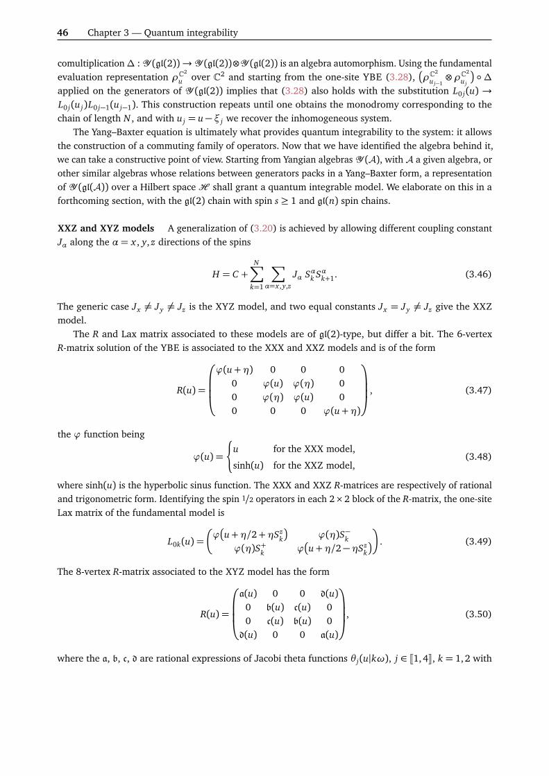
46 Chapter 3 — Quantum integrability
comultiplication∆ : Y (gl(2))→Y (gl(2))⊗Y (gl(2)) is an algebra automorphism. Using the fundamentalevaluation representation ρC
2
u over C2 and starting from the one-site YBE (3.28),ρC
2
u j−1⊗ρC2
u j
∆applied on the generators of Y (gl(2)) implies that (3.28) also holds with the substitution L0 j(u) →L0 j(u j)L0 j−1(u j−1). This construction repeats until one obtains the monodromy corresponding to thechain of length N , and with u j = u− ξ j we recover the inhomogeneous system.
The Yang–Baxter equation is ultimately what provides quantum integrability to the system: it allowsthe construction of a commuting family of operators. Now that we have identified the algebra behind it,we can take a constructive point of view. Starting from Yangian algebras Y (A), with A a given algebra, orother similar algebras whose relations between generators packs in a Yang–Baxter form, a representationof Y (gl(A)) over a Hilbert spaceH shall grant a quantum integrable model. We elaborate on this in aforthcoming section, with the gl(2) chain with spin s ≥ 1 and gl(n) spin chains.
XXZ and XYZ models A generalization of (3.20) is achieved by allowing different coupling constantJα along the α= x , y, z directions of the spins
H = C +N∑
k=1
∑α=x ,y,z
Jα Sαk Sαk+1. (3.46)
The generic case Jx 6= Jy 6= Jz is the XYZ model, and two equal constants Jx = Jy 6= Jz give the XXZmodel.
The R and Lax matrix associated to these models are of gl(2)-type, but differ a bit. The 6-vertexR-matrix solution of the YBE is associated to the XXX and XXZ models and is of the form
R(u) =
ϕ(u+η) 0 0 00 ϕ(u) ϕ(η) 00 ϕ(η) ϕ(u) 00 0 0 ϕ(u+η)
, (3.47)
the ϕ function being
ϕ(u) =
(u for the XXX model,
sinh(u) for the XXZ model,(3.48)
where sinh(u) is the hyperbolic sinus function. The XXX and XXZ R-matrices are respectively of rationaland trigonometric form. Identifying the spin 1/2 operators in each 2×2 block of the R-matrix, the one-siteLax matrix of the fundamental model is
L0k(u) =
ϕu+η/2+ηSz
k
ϕ(η)S−k
ϕ(η)S+k ϕu+η/2−ηSz
k
. (3.49)
The 8-vertex R-matrix associated to the XYZ model has the form
R(u) =
a(u) 0 0 d(u)0 b(u) c(u) 00 c(u) b(u) 0
d(u) 0 0 a(u)
, (3.50)
where the a, b, c, d are rational expressions of Jacobi theta functions θ j(u|kω), j ∈ J1,4K, k = 1,2 with

3.3. Spin chains 47
quasi-periods π and kπω [262]
a(u) =2θ4(η|2ω)θ1(u+η|2ω)θ4(u|2ω)
θ2(0|ω)θ4(0|2ω), b(u) =
2θ4(η|2ω)θ1(u|2ω)θ4(u+η|2ω)θ2(0|ω)θ4(0|2ω)
,
c(u) =2θ1(η|2ω)θ4(u|2ω)θ4(u+η|2ω)
θ2(0|ω)θ4(0|2ω), d(u) =
2θ1(η|2ω)θ1(u+η|2ω)θ1(u|2ω)θ2(0|ω)θ4(0|2ω)
.(3.51)
It is called an elliptic model.From a quantum group point of view, the XXX model is associated to the Yangian algebra Y (gl(2)),
the XXZ model is associated to the quantum affine algebra Uq(Õgl(2)), and the XYZ model to the elliptic
quantum algebra Uq,p(Õgl(2)) [263, 264].
3.3.2 Inhomogeneous twisted gl(n) spin chains
As we see from the QISM illustrated on the common XXX spin chain, the fundamental objects of quantumintegrable models are the R-matrix and the monodromy matrix who verify the Yang–Baxter equation,and the underlying algebra structure is a Yangian one.
The construction can be extended to a wide class of R-matrix and monodromy matrix, while keepingthe Yang–Baxter equation verified, ensuring the integrability of the one-dimensional quantum systemdefined by the transfer matrix.
Starting from the XXX model, this is done in several ways, such as i) adding inhomogeneities at thesites of the chain ii) imposing other boundary conditions at the edges of the chain iii) having differentquantum objects at each site along the chain iv) allowing other symmetry algebras than Y (gl(2)).
i) Inhomogeneities The Yang–Baxter equation (3.8) with site-dependent inhomogeneities along thechain. Indeed, the following equation holds
R12(u, v)R1 j(u,ξ j)R2 j(v,ξ j) = R2 j(v,ξ j)R1 j(u,ξ j)R12(u, v), (3.52)
at any site j ∈ J1, NK. Therefore, one can choose a different ξ j in the Lax matrix at each site,
L0k(u) = R0k(u,ξk), ξk ∈ C, (3.53)
(which manifest as a shift in the spectral parameter for R-matrix of difference form) while keeping (3.28)verified, so the inhomogenous monodromy
M(u) = L0N (u) . . . L01(u) (3.54)
still verifies (3.15), and the transfer matrix still defines an integrable model.The ξ j are called the inhomogeneities parameters; they may be kept in generic position. In the
η→ 0 limit, the inhomogeneous XXX spin chain gives the Gaudin model [130, 265, 266], where theinhomogeneities ξk are interpreted as the particles’ positions [191]. The possibility to add an extra degreeof freedom at each site may prove useful in some calculation, where the analytic dependence in the ξ j
provides insights in the mathematical structure of the quantity at hand. This comes at the price of anadditional step to recover a meaningful physical model in the end: performing the homogeneous limitξ1, . . . ,ξN → ξ, with ξ= 0 for example, in the final formulas.
ii) Boundary conditions For the above XXX chain, periodic boundary conditions have been imposedby identifying the quantum space at site N + 1 with the one at site 1, but other boundary conditions thatkeep the integrability may be specified. Rather that making the plain identification, one may identify the

48 Chapter 3 — Quantum integrability
spaces VN+1 and V1 up to an isomorphism V1 ' VN+1 making the chain quasi-periodic. This is encodedby a twist matrix K ∈ End(V), det K 6= 0, and the Hamiltonian then becomes
H = C + JN−1∑k=1
~Sk · ~Sk+1 + J~SN · ~SN+1 = C + JN−1∑k=1
~Sk · ~Sk+1 + J~SN ·K1~S1K−1
1
. (3.55)
The monodromy is twisted as well by
M K(u) = K0 L0N (u) . . . L01(u), (3.56)
so that the transfer matrix T K(u) = tr0 M K(u) gives the proper Hamiltonian (3.55) by (3.44). Note thatsince K ∈ GL(2),
[R(u), K ⊗ K] = 0 or written differently R12(u)K1K2 = K2K1R12(u), (3.57)
so the Yang–Baxter equation (3.32) indeed holds for M K(u) as well, and the whole scheme is preservedfor the twisted XXX chain. K is interpreted as a Lax matrix with a trivial quantum representation, orsimply as an element of the group under which the R-matrix is invariant, here GL(2).
In this thesis, the discussion focuses solely on quasi-periodic models, but other boundary conditionsmay be imposed while keeping the system integrable. The reflection algebra [267] allows for instancethe construction of open spin chains—spin chains that are not closed on themselves and have non-trivialmagnetic fields applied on the boundary sites. See for example the thesis [268] as a resource for SOVtechniques in quantum integrable models with open boundary conditions.
iii) Representations on the quantum sites Let the representations (ρ,Vk) at each site be the sl(2)spin sk ones, with sk ∈ Z>0/2, and Vk a space of dimension 2sk + 1. The sk may be different from eachothers. The sl(2) generators
h, x±= ±x±,
x+, x−
= 2h, (3.58)
are represented over V= C2sk+1 explicitly as
ρk(h) =
sk
sk − 1...
−sk
, ρk(x
+) = ρk(x−)t =
0 jn(1). . . . . .
. . . jn(2sn)0
, (3.59)
where jn(a) =p
a(2sn + 1− a). Keeping the auxiliary space V0 to C2, the Lax operators is then written
L0k(u) = u+η2∑
i, j=1
e(0)i j ⊗ρk(e ji) =
u+ η
2 +ρk(h) ηρk(x−)ηρk(x+) u+ η
2 −ρk(h)
0
, (3.60)
and verifies (3.28) with the 4-by-4 R-matrix (3.30). The construction of the monodromy and transfermatrix is the same as above, exhibiting form T(u) a commuting family of N operators acting onH =⊗N
k=1Vk ' ⊗Nk=1C
2sk+1. Any Hamiltonian chosen as a function of these N quantities makes the modelintegrable.
Remark that the auxiliary space has been hold to the fundamental representation C2 here. It is possibleto make this construction with a different representation (ρ0,V0) of sl(2) for the auxiliary space, because

3.3. Spin chains 49
the Yang–Baxter equation R12R13R23 = R23R13R12 holds at the virtual algebra level for
R(u) = u1⊗ 1+η2∑
i, j=1
ei j ⊗ e ji , (3.61)
where the ei j are the unrepresented elementary generators of the gl(2) algebra.When all the quantum spaces are equipped with the same representation (ρ,V) with dimV = 2s+ 1,
one gets the spin s chain. Taking the same representation on the auxiliary space is then beneficial, sincewe recover the desirable feature that Lax matrices degenerate to the permutation operator on V⊗V
Lab(ξ j) = Rab(0) = ηdimV∑i, j=1
ρ(ei j)⊗ρ(e ji) = ηPV⊗V. (3.62)
It is also possible to put representations of different spin values at each site while keeping the modelintegrable.
iv) Other symmetry algebra Two equations are at the core of the description of quantum integrablesystem by the quantum inverse scattering method
R12M1M2 = M2M1R12, (3.63)
R12R13R23 = R23R13R12. (3.64)
On page 45, we identified that the XXX spin chain of length N is obtained as the N -fold tensor productof fundamental evaluation representations of the Yangian Y (gl(2)). The two RRR and RM M equationsoriginated naturally from this underlying algebraic structure.
Starting from similar algebras, different integrable models are constructed. In appendix A, we reviewthe mathematical structure of Yangian algebras Y (gl(n)), and show how spin chain models are obtainedas representations of these algebras.
3.3.3 Reconstruction of local spin operators
The QISM formalism puts the monodromy entries at the center of the stage with their rich algebraicstructure. But they are highly non-local quantities, being a sum of products of the local spin operatorsalong all the sites of the chain. A quick induction shows that they are a sum of 2N−1 terms, where eachterm is a product of N local one-site operators.
Can one express the local one-site spin operators S±j , Szj , in terms of the monodromy entries A, B, C ,
D? This is actual the inverse problem. In the classical case, this solves the dynamics by expressing theinitial dynamical variables in terms of the action–angle variables of the system.
The solution was obtained by Maillet, Kitanine and Terras, first using the Drindfel’d twist and theF -basis [104] for the XXX and XXZ chains. This was extended to a large class of chains in [106], whereformulas are obtained in a more direct way which bypass the use of the F -basis. These results have beengeneralized to the supersymmetric case in [107].
The reconstruction of local operators of fundamental gl(n) chains is surprinsigly simple: local spinoperators at site n are equal to a corresponding monodromy entry dressed by a product of transfermatrices. Specializing in the gl(2) case, the proof is rather short. Let us consider the operator S−1 = σ
−1 .
Then, by (3.31),tr0
e(0)21 M(0)
= e(1)21 η
N U = σ−1 T (0), (3.65)
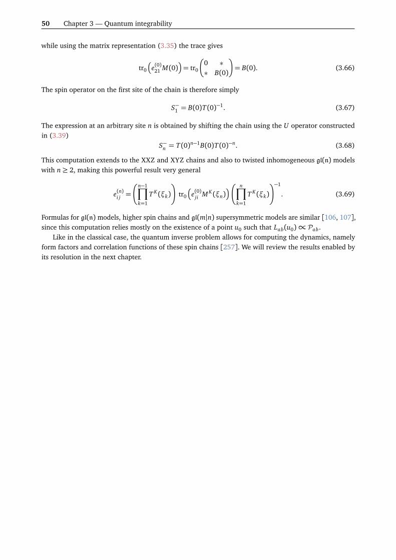
50 Chapter 3 — Quantum integrability
while using the matrix representation (3.35) the trace gives
tr0
e(0)21 M(0)
= tr0
0 ∗∗ B(0)
= B(0). (3.66)
The spin operator on the first site of the chain is therefore simply
S−1 = B(0)T (0)−1. (3.67)
The expression at an arbitrary site n is obtained by shifting the chain using the U operator constructedin (3.39)
S−n = T (0)n−1B(0)T (0)−n. (3.68)
This computation extends to the XXZ and XYZ chains and also to twisted inhomogeneous gl(n) modelswith n≥ 2, making this powerful result very general
e(n)i j =
n−1∏k=1
T K(ξk)
tr0
e(0)ji M K(ξn)
n∏k=1
T K(ξk)
−1
. (3.69)
Formulas for gl(n) models, higher spin chains and gl(m|n) supersymmetric models are similar [106, 107],since this computation relies mostly on the existence of a point u0 such that Lab(u0)∝ Pab.
Like in the classical case, the quantum inverse problem allows for computing the dynamics, namelyform factors and correlation functions of these spin chains [257]. We will review the results enabled byits resolution in the next chapter.

4Chapter
Algebraic Bethe ansatz tech-niques
In this chapter, we describe the techniques of the Algebraic Bethe Ansatz (ABA) for the gl(2) mod-els [100], as well as its Nested version (NABA) for higher rank models [129]. The ABA idea is to extractcreation and annihilation operators from the off-diagonal elements of the monodromy matrix, and createthe eigenstates of the transfer matrix by action of these creation operators on a pseudo-vacuum referencestate. This gives an ansatz form for the eigenstates, namely we search for eigenstates of the form of Bethevectors. The action of the transfer matrix on Bethe vectors can be computed by using the Yang–Baxteralgebra of the monodromy entries [99]. Unwanted terms arise, and are cancelled by requiring the spectralparameters in which the operators are evaluated satisfy a set of tightly coupled equations, the Betheequations. This line of research has proven extremely successful and rich of results in the past decades.We close the chapter with a review of the ABA results towards the computation of correlation functions,but also highlight the limitations of this framework justifying the developments of other techniques forthe study of quantum integrable models.
4.1 The gl(2) model: from the spectrum. . .
We make use of the notations introduced in Section 3.3.1.
Fundamental commutation relations First, let us explicit the FCR (3.33) of the gl(2) Yang–Baxteralgebra in terms of the monodromy matrix elements A, B, C , D introduced in (3.35).
[A(u), A(v)] = 0, (Y.1)
[B(u), B(v)] = 0, (Y.2)
[C(u), C(v)] = 0, (Y.3)
[D(u), D(v)] = 0, (Y.4)
A(u)B(v) = f (v, u)B(v)A(u) + g(u, v)B(u)A(v), (Y.5)
A(u)C(v) = f (u, v)C(v)A(u) + g(v, u)C(u)A(v), (Y.6)
B(u)A(v) = f (v, u)A(v)B(u) + g(u, v)A(u)B(v), (Y.7)
B(u)D(v) = f (u, v)D(v)B(u) + g(v, u)D(u)B(v), (Y.8)
C(u)A(v) = f (u, v)A(v)C(u) + g(v, u)A(u)C(v), (Y.9)
C(u)D(v) = f (v, u)D(v)C(u) + g(u, v)D(u)C(v), (Y.10)
D(u)B(v) = f (u, v)B(v)D(u) + g(v, u)B(u)D(v), (Y.11)
D(u)C(v) = f (v, u)C(v)D(u) + g(u, v)C(u)D(v), (Y.12)
51

52 Chapter 4 — Algebraic Bethe ansatz techniques
[A(u), D(v)] = g(u, v)C(v)B(u)− C(u)B(v)
, (Y.13)
[B(u), C(v)] = g(u, v)D(v)A(u)− D(u)A(v)
, (Y.14)
[C(u), B(v)] = g(u, v)A(v)D(u)− A(u)D(v)
, (Y.15)
[D(u), A(v)] = g(u, v)B(v)C(u)− B(u)C(v)
. (Y.16)
with
f (u, v) =ϕ(u− v +η)ϕ(u− v)
, g(u, v) =ϕ(η)ϕ(u− v)
. (4.1)
The ϕ function depends on the model at hand as in (3.48).The main idea of the Bethe Ansatz in its algebraic form is to generate the eigenstates of T as the
descendants of a reference state |0⟩ by the successive action of some creation operators, yet to be defined,but available somewhere in the Yang–Baxter algebra. In a way, this is a generalization of the harmonicoscillator treatment where the eigenstates a† . . . a† |0⟩ of the particle number operator N = a†a arecreated by the successive action of creation operators on a pseudo-vacuum state |0⟩, with the algebra
a, a†
= 1, [N , a] = −a,
N , a†
= a†, (4.2)
anda |0⟩= 0, a† |0⟩ 6= 0. (4.3)
Since the underlying Yang–Baxter algebra of the model has a richer structure, the setting is more involved,and the actual computation of the eigenstates require more work.
A toy example
Let (Ji ,θk) be the action–angle variables of a classical integrable mechanical system. We have Ji ,θk = δik.Under quantization, the Poisson bracket becomes a commutator
[Ji ,θk] = iħhδik. (4.4)
Let us note Ak := Jk and Bk := ei bkθk , bk ∈ C, for a fixed k. Since [Jk,θ ak ] = aiħhθ a−1
k , we have
[Ak, Bk] =+∞∑a=0
ia
a!
Jk,θ a
k
= −bkħh+∞∑a=1
ia−1
(a− 1)!θ a−1
k
= −bkħhBk.
(4.5)
Let |ϕ⟩ be an eigenstate of Ak of eigenvalue λ. The action of Bk on |ϕ⟩ generates a new eigenstate of Ak
AkBk |ϕ⟩= BkAk |ϕ⟩ −ħhbkBk |ϕ⟩= (λ− bkħh) Bk |ϕ⟩ , (4.6)
of shifted eigenvalue λ − bkħh, provided that Bk |ϕ⟩ 6= 0. Bk thus realizes a shift operation on the Ak
spectrum, meaning that the choice of the parameter bk defining Bk is a rather subtle issue.Consider now two operators A(u) and B(u) satisfying an exchange algebra
A(u)B(v) = β(u, v)B(v)A(u), (4.7)

4.1. The gl(2) model: from the spectrum. . . 53
for some u, v. Then for |ϕ⟩ an eigenstate of A of eigenvalue λ(u), the action of B generates a neweigenstate
A(u)B(v) |ϕ⟩= β(u, v)λ(u)B(v) |ϕ⟩ , (4.8)
whose eigenvalue is obtained from the original λ(u) one by a multiplicative coefficient β(u, v). Oneshould check that (4.8) is a non-zero vector, though.
This motivates the use of the off-diagonal elements of the monodromy matrix to generate the eigen-vectors of the transfer matrix from a first known eigenstate |0⟩. Indeed, we know from the quantizationprocedure that they should contain in some form the quantum counterparts to the angle variables, whichin classical gl(n) models are generated by off-diagonal elements of the monodromy matrix, see page 31.
Bethe states and ABA calculation Let us go back to the gl(2)model with periodic boundary conditions.Let |0⟩ ∈ H be a reference state verifying
A(u) |0⟩= a(u) |0⟩ , D(u) |0⟩= d(u) |0⟩ ,B(u) |0⟩ 6= 0, C(u) |0⟩= 0,
(4.9)
and consider a Bethe state of level mB(u1) . . . B(um) |0⟩ , (4.10)
where u1, . . . , um are m complex numbers. The state |0⟩ is therefore an eigenstate of T (u) = A(u) + D(u)and shall play the role of the highest weight state, such that its descendants (4.10) by the creation operatorsB(uk) are eigenstates.
The action of A(u) over this state is easily computed thanks to the above FCR’s. Shifting A(u) to theright by making it pass through all the B’s to finally act on its eigenvector |0⟩ produces 2m terms, thatre-sum in only m+ 1 different contribution thanks to the commutation of the B’s
A(u)B(u1) . . . B(um) |0⟩= Λ0 B(u1) . . . B(um) |0⟩+m∑
k=1
Λk B(u)B(u1) . . .×B(uk) . . . B(um) |0⟩ , (4.11)
where the hat Õ means the concerned term is omitted. The Λ0 coefficients is given by following only
the direct term in the FCR (Y.5) until A(u) acts on |0⟩, and therefore is
Λ0 = a(u)m∏`=1
f (u`, u). (4.12)
Λ1 is obtained by using the first indirect term once and then only the direct terms to push A(u1) to theright and make it act on |0⟩, so
Λ1 = a(u1)g(u, u1)m∏`=2
f (u`, u1). (4.13)
Because the B’s commute, the Λk coefficients are obtained simply by substituting u1→ uk, and eventually
A(u)B(u1) . . . B(um) |0⟩= a(u)m∏`=1
f (u`, u)B(u1) . . . B(um) |0⟩
+m∑
k=1
a(uk)g(u, uk)m∏`=16=k
f (u`, uk)B(u)B(u1) . . .×B(uk) . . . B(um) |0⟩ .(4.14)

54 Chapter 4 — Algebraic Bethe ansatz techniques
The action of D(u) is computed similarly
D(u)B(u1) . . . B(um) |0⟩= d(u)m∏`=1
f (u, u`)B(u1) . . . B(um) |0⟩
+m∑
k=1
d(uk)g(uk, u)m∏`=16=k
f (uk, u`)B(u)B(u1) . . .×B(uk) . . . B(um) |0⟩ ,(4.15)
and the action of T (u) on (4.10) is therefore
T (u)B(u1) . . . B(um) |0⟩=
a(u)m∏`=1
f (u, u`) + d(u)m∏`=1
f (u, u`)
B(u1) . . . B(um) |0⟩
+m∑
k=1
a(uk)g(u, uk)
m∏`=16=k
f (u`, uk) + d(uk)g(uk, u)m∏`=16=k
f (uk, u`)
× B(u)B(u1) . . .×B(uk) . . . B(um) |0⟩ .
(4.16)
It is clear that if (4.10) is a non-zero vector, it is an eigenstate of T (u) of eigenvalue
t(u) = a(u)m∏`=1
f (u`, u) + d(u)m∏`=1
f (u, u`), (4.17)
as soon as the m unwanted contributions in (4.16) vanish, which is the case if the u1, . . . , um verify the mBethe equations
a(uk)d(uk)
=m∏`=16=k
f (u`, uk)f (uk, u`)
. (4.18)
Note that these condition for (4.10) to be an eigenstate of T (u), u ∈ C, are independent of u (wheneverg(u, v) = −g(v, u)). This is good agreement with the fact that the (T (u))u∈C family is commutative, andthus diagonalizable in the same basis. Bethe vectors (4.10) whose parameters satisfy the Bethe equationsare called on-shell, in opposition with off-shell Bethe vectors if the u’s are arbitrary complex numbers.Specializing to the inhomogeneous model, the Bethe equations and the eigenvalue associated to theBethe state (4.10) write explicitly
N∏j=1
ϕ(uk − ξ j +η)
ϕ(uk − ξ j)=
m∏`=16=k
ϕ(uk − u` +η)ϕ(uk − u` −η)
, (4.19)
t(u) =N∏
j=1
ϕ(u− ξ j +η)m∏`=1
ϕ(u− u` −η)ϕ(u− u`)
+N∏
j=1
ϕ(u− ξ j)m∏`=1
ϕ(u− u` +η)ϕ(u− u`)
. (4.20)
Note that (4.17) is then an analytic function in u, since the m apparent poles at the u` are cancelled outby the Bethe equations. An analytic way to recover the Bethe equations is thus to require the analiticityof the eigenvalue of generic Bethe states on the complex plane.
For Bethe state of level 1, there is only one Bethe root u1 constrained only by a unique Betheequation (4.19). For Bethe state of level 2, the two Bethe roots u1 and u2 have to satisfy the coupledsystem of two equations (4.19), and already the resolution is more intricate. One may try the naivesolution u1 = ξ j −η for some j between 1 and N , cancelling the LHS of the first Bethe equation, but thisimposes that ϕ(u2 − u1 +η) = 0 or u2 = ξ j . The corresponding Bethe state B(ξ j)B(ξ j −η) |0⟩ vanishes,

4.1. The gl(2) model: from the spectrum. . . 55
since B(ξ j)B(ξ j −η) = 0 in the gl(2) case1, so this solution of the Bethe equations is not admissible, inthe sense that it does not correspond to an eigenvector.
Choice of the reference state The reference state |0⟩may be constructed in a tensor product form one-site similar states. At site k, the action of the Lax matrix on the vector |0⟩k =
10
becomes upper-triangular
in the auxiliary space
L0k(u) |0⟩k =ϕ(u+η) ∗
0 ϕ(u)
0
|0⟩k . (4.21)
Hence, the action of the monodromy matrix on
|0⟩= ⊗Nk=1 |0⟩n =
10
⊗ · · · ⊗
10
, (4.22)
is easily computed by multiplication of scalar upper-triangular matrices
M(u) |0⟩=∏N
k=1ϕ(u− ξk +η) ∗0
∏Nk=1ϕ(u− ξk)
0
|0⟩ ≡
A(u) |0⟩ B(u) |0⟩C(u) |0⟩ D(u) |0⟩
0
. (4.23)
The state |0⟩ indeed verifies (4.9) by identification.
Left Bethe covectors Performing the same calculation with Bethe covectors
⟨0|C(v1) . . . C(vm), (4.24)
with ⟨0| such that⟨0|C(u) 6= 0 and ⟨0|B(u) = 0, (4.25)
one proves they are eigenvectors of T (u) if the v j verify the same Bethe equations (4.19). The computationof the scalar products between Bethe co-vectors and vectors
⟨0|m∏
j=1
C(v j)m′∏
k=1
B(uk) |0⟩ , (4.26)
is of prime interest for the computation of correlation functions. We elaborate on this in the next section.
Energy and momentum of the eigenstates The physical characteristics of the eigenstates are deducedfrom equations (3.41) and (3.44) in the homogeneous limit ξi → 0. Noting
B(u) := B(u1) . . . B(um) |0⟩ , (4.27)
we have
PB(u) =m∑
k=1
p0(uk)B(u), p0(u) = −i lnϕ(u+η)ϕ(u)
, (4.28)
J−1(H − C)B(u) = −Nϕ′(η)
2B(u) +
m∑k=1
ε0(uk)B(u), ε0(u) =ϕ(η)2
2ϕ(u)ϕ(u+η). (4.29)
1This can be proved by using the fact that (σ−j )2 = 0, and using the reconstruction of σ−j by the quantum inverse problem
which can be done in two ways: from B(ξ j) and from B(ξ j −η) [104].
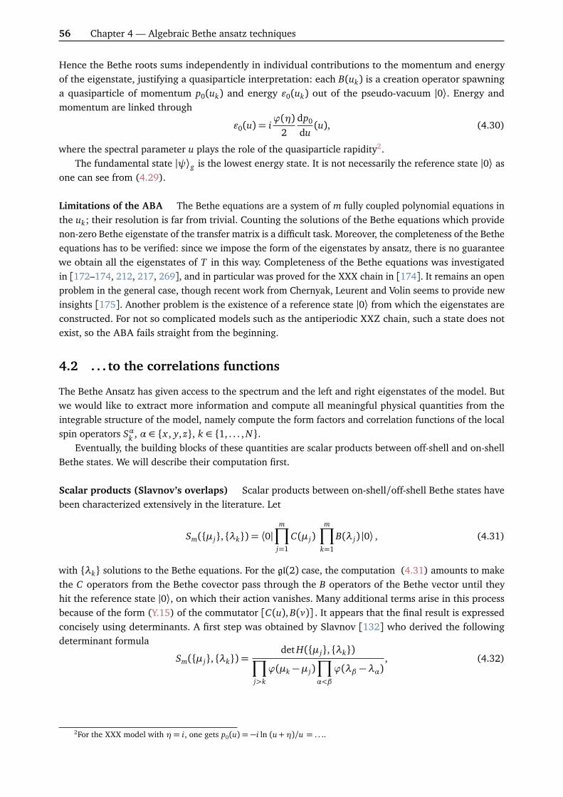
56 Chapter 4 — Algebraic Bethe ansatz techniques
Hence the Bethe roots sums independently in individual contributions to the momentum and energyof the eigenstate, justifying a quasiparticle interpretation: each B(uk) is a creation operator spawninga quasiparticle of momentum p0(uk) and energy ε0(uk) out of the pseudo-vacuum |0⟩. Energy andmomentum are linked through
ε0(u) = iϕ(η)
2dp0
du(u), (4.30)
where the spectral parameter u plays the role of the quasiparticle rapidity2.The fundamental state |ψ⟩g is the lowest energy state. It is not necessarily the reference state |0⟩ as
one can see from (4.29).
Limitations of the ABA The Bethe equations are a system of m fully coupled polynomial equations inthe uk; their resolution is far from trivial. Counting the solutions of the Bethe equations which providenon-zero Bethe eigenstate of the transfer matrix is a difficult task. Moreover, the completeness of the Betheequations has to be verified: since we impose the form of the eigenstates by ansatz, there is no guaranteewe obtain all the eigenstates of T in this way. Completeness of the Bethe equations was investigatedin [172–174, 212, 217, 269], and in particular was proved for the XXX chain in [174]. It remains an openproblem in the general case, though recent work from Chernyak, Leurent and Volin seems to provide newinsights [175]. Another problem is the existence of a reference state |0⟩ from which the eigenstates areconstructed. For not so complicated models such as the antiperiodic XXZ chain, such a state does notexist, so the ABA fails straight from the beginning.
4.2 . . . to the correlations functions
The Bethe Ansatz has given access to the spectrum and the left and right eigenstates of the model. Butwe would like to extract more information and compute all meaningful physical quantities from theintegrable structure of the model, namely compute the form factors and correlation functions of the localspin operators Sαk , α ∈ x , y, z, k ∈ 1, . . . , N.
Eventually, the building blocks of these quantities are scalar products between off-shell and on-shellBethe states. We will describe their computation first.
Scalar products (Slavnov’s overlaps) Scalar products between on-shell/off-shell Bethe states havebeen characterized extensively in the literature. Let
Sm(µ j, λk) = ⟨0|m∏
j=1
C(µ j)m∏
k=1
B(λ j) |0⟩ , (4.31)
with λk solutions to the Bethe equations. For the gl(2) case, the computation (4.31) amounts to makethe C operators from the Bethe covector pass through the B operators of the Bethe vector until theyhit the reference state |0⟩, on which their action vanishes. Many additional terms arise in this processbecause of the form (Y.15) of the commutator [C(u), B(v)] . It appears that the final result is expressedconcisely using determinants. A first step was obtained by Slavnov [132] who derived the followingdeterminant formula
Sm(µ j, λk) =det H(µ j, λk)∏
j>k
ϕ(µk −µ j)∏α<β
ϕ(λβ −λα), (4.32)
2For the XXX model with η= i, one gets p0(u) = −i ln (u+η)/u = . . ..

4.2. . . . to the correlations functions 57
where H is the m×m matrix of elements
Hab =ϕ(η)
ϕ(λa −µb)
a(µb)
∏k 6=a
ϕ(λk −µb +η)− d(µb)∏k 6=a
ϕ(λk −µb −η)!
. (4.33)
His demonstration also proved the symmetry in the Bethe roots of the scalar products: we have Sm(µ j, λk) =Sm(λk, µ j), where the λk verifies the Bethe equations.
This result had been refined ten years later by Maillet, Kitanine and Terras [104, 105], when theyobtained (4.32) in another manner, and identified that it could be rewritten in a ratio of two determinants
Sm(µ j, λk) =detT (µ j, λk)det V (µ j, λk)
, (4.34)
where T and V are the m×m matrices
Tab =∂
∂ λat(µb, λk) and Vab =
1ϕ(µb −λa)
. (4.35)
The function t(u, λk) is the eigenvalue of the transfer matrix T (u) on the on-shell Bethe state∏m
k=1 B(λ j) |0⟩.Remark that on-shell Bethe states with a different number of excitations, i.e. a different number of Betheroots, are orthogonal (for periodic boundary conditions).
A key ingredient in their derivation was the use of the F -basis [270]. In the F -basis, the monodromyentries B(u) and C(u) write as a sum of only N local, one-site terms, dressed by a tensor product ofdiagonal operators acting on the other sites [104]. This is a huge combinatorial simplification to the2N -term expression of B(u) and C(u) in the original spin basis |↑↑ ... ↑⟩ , . . . , |↓↓ . . . ↓⟩, where each term isa product of N spin operators along the chain.
Note that the formula (4.34) is nothing but the product of a Jacobian of the transfer matrix eigenvalueand a normalization factor. The recent article [271] gives some understanding of why scalar products havethis determinant form. It shows that the scalar products satisfy a homogeneous system of linear equations,hence the determinant form, while the Jacobian arises from a particular property of the eigenvalue t(u)— namely its linear and symmetric dependence in the Bethe roots, up to a symmetric normalization factor.Still, it would be of great interest to understand why it is a Jacobian.
Norm of on-shell Bethe vectors — the Gaudin formula When the λk verify the Bethe equations,Sm(λk) := Sm(λk, λk) is simply the squared norm of the Bethe vector (4.27). The formula (4.34) isthen reducible and can be written as a unique determinant, already conjectured by Gaudin [272] andlater argued by Korepin [131]
Sm(λk) = ϕ(η)m m∏
k=1
a(λk)d(λk)
∏p 6=q
1f (λp,λq)
!det G(λk), (4.36)
where G is the m×m Gaudin matrix of elements
Gab = −∂
∂ λbln
a(λa)
d(λa)
m∏k=1k 6=a
f (λa,λk)f (λk,λa)
. (4.37)
Equation (4.34) gives a direct proof of this result by taking the limits µ j → λ j for j = 1, . . . , m.
Form factors The gl(2) Yang–Baxter algebra (Y.1)–(Y.16) allows to determine the actions of theA, B, C , D operators on the left and right Bethe states. On the other hand, the action of the local operators

58 Chapter 4 — Algebraic Bethe ansatz techniques
Sαk on the Bethe state is not immediate. Thankfully, they are reconstructed rather easily from the A, B, C , D,see page 49.
A tedious but straightforward induction computation give the actions of A, B and D on generic Bethecovectors [99, 257]
⟨0|m∏
j=1
C(u j) A(um+1) =m+1∑k=1
a(uk)
m∏l=1
ϕ(ul − uk +η)
m+1∏l=1l 6=k
ϕ(ul − uk)
⟨0|m+1∏j=1j 6=k
C(u j), (4.38)
⟨0|m∏
j=1
C(u j) D(um+1) =m+1∑k=1
d(uk)
m∏l=1
ϕ(uk − ul +η)
m+1∏l=1l 6=k
ϕ(uk − ul)
⟨0|m+1∏j=1j 6=k
C(u j), (4.39)
⟨0|m∏
j=1
C(u j) B(um+1) =m+1∑k=1
d(uk)
m∏l=1
ϕ(uk − ul +η)
m+1∏l=1l 6=k
ϕ(uk − ul)
(4.40)
×m+1∑
k′=1k′ 6=k
a(uk)um+1 − uk +η
m+1∏p=1p 6=k′
ϕup − uk +η
m+1∏p=1
p 6=k,k′
ϕup − uk
⟨0|m+1∏j=1
j 6=k,k′
C(u j). (4.41)
The action of C(um+1) is simply absorbed in the Bethe vector and increase its rank by one. Similar relationsare obtained for the action of A, C and D on the Bethe vectors, so the computation of form factors may bedone by keeping on-shell states at the left or the right of the scalar products and using the scalar productformula (4.32).
The action of the monodromy entries over on-shell Bethe states gives a sum of off-shell Bethe states.Therefore, the computation of form factors reduces to a sum of scalar products between on-shell andoff-shell Bethe states. While the formula (4.32) for scalar products have been obtained decades ago, itwas the resolution of the quantum inverse problem, namely reconstruction of local operators in terms ofthe monodromy matrix elements obtained in [104] and [106], that enabled the systematic computationof the form factors. For periodic boundary conditions, since scalar products of states with a differentnumber of Bethe roots vanish, only the following form factors are non-zero
⟨0|m∏
j=1
C(µ j) S+n
m+1∏k=1
B(λk) |0⟩ , ⟨0|m+1∏j=1
C(µ j) S−nm∏
k=1
B(λk) |0⟩ ,
⟨0|m∏
j=1
C(µ j) Szn
m∏k=1
B(λk) |0⟩ .(4.42)

4.2. . . . to the correlations functions 59
For example, explicitly,
⟨0|m+1∏j=1
C(µ j) S−nm∏
k=1
B(λk) |0⟩= ⟨0|m+1∏j=1
C(µ j)n−1∏a=1
T (ξa) B(ξn)n∏
a=1
T (ξa)−1
m∏k=1
B(λk) |0⟩
=φn−1(λk)φn−1(µ j)
∏mk=1ϕ(λk − ξn +η)∏mk=1ϕ(µ j − ξn +η)
× det H−(n, µ j, λk)∏j>kϕ(µk −µ j)
∏β>αϕ(λβ −λα)
,
(4.43)
with φn(λk) =∏n
j=1
∏mk=1 f (λk,ξ j) and H− is the modified m×m matrix H from (4.35)
H−ab(n, µ j, λk) = Hab(µ j, λk) for b < m, (4.44)
H−am(n, µ j, λk) =ϕ(η)
ϕ(λa − ξn +η)ϕ(λa − ξn)otherwise. (4.45)
For the detail computations and the exact expressions of the form factors, see Proposition 5.1 and 5.2of [104].
Correlation functions Let e(k)αk ,βk
be the elementary quantum operators acting at the quantum sitek, with αk,βk = 1,2. Recalling from Section 3.1, we are interested in the computation of correlationfunction at zero temperature of the form, the elementary blocks
Fn
αk,βk;ψg
=
ψg
∏mk=1 e(k)
αk ,βk
ψg
ψg
ψg
. (4.46)
Thanks to (3.69), the local operators are reconstructed as
e(k)αk ,βk
=
k−1∏a=1
T (ξa)
Mβk ,αk
(ξk)
k∏a=1
T (ξa)
−1
, (4.47)
while the fundamental state writes as an on-shell Bethe vector
ψg
=
m∏j=1
B(u j) |0⟩ andψg
= ⟨0|m∏
j=1
C(u j), (4.48)
where the u j are solutions to the Bethe equations (4.19). So the following n-point correlation function ofn adjacent local operators
Fn
αk,βk; u j=⟨0|∏m
j=1 C(u j)∏n
k=1 e(k)αk ,βk
∏mj=1 B(u j) |0⟩
⟨0|∏mj=1 C(u j)
∏mj=1 B(u j) |0⟩
, (4.49)
is the expectation value of a product of monodromy entries in the ground state∏m
j=1 B(u j) |0⟩
Fn
αk,βk; u j=ψn(u j)
⟨0|∏mj=1 C(u j)
∏nk=1 Mβk ,αk
(ξk)∏m
j=1 B(u j) |0⟩⟨0|∏m
j=1 C(u j)∏m
j=1 B(u j) |0⟩, (4.50)
where
ψn(u j) =n∏α=1
1
a(ξα)
m∏j=1
1f (u j ,ξa)
!(4.51)

60 Chapter 4 — Algebraic Bethe ansatz techniques
is a scalar coefficient given by the action of the dressing product of transfer matrices in (4.47), namelythe eigenvalue of the product
∏nα=1 T (ξα)
−1corresponding to the Bethe eigenstate
∏mj=1 B(u j) |0⟩.
From there, formula (4.50) may be computed explicitly in terms of the Bethe roots [105]: one makesthe monodromy entries act on the left Bethe state and produce a sum of off-shell/on-shell scalar productsof the form (4.31). This produces n sums over the Bethe parameters of the left Bethe state. In thethermodynamic limit N → +∞, these n sums become n integrals over Bethe roots that are continuousparameters, over fixed ranges and with certain densities for the Bethe roots. The reader can refer to [105]for explicit formula of the emptiness formation probability and more general correlation functions. Furtherimportant objects are the physical 2-point functions
σz
1σzm+1
and their arguments for m→ +∞ with
m/N → 0, see [105, 133, 134, 273–276].
This closes the study of the gl(2) model from the algebraic Bethe ansatz view-point. We will nowdescribe how it extends to higher rank models
4.3 Higher rank models
The Algebraic Bethe Ansatz method generalizes to higher rank gl(n) models where n≥ 3. As usual thefirst step is the most difficult: most of the results have been obtained first by adapting the proofs to thegl(3) model, before being extended to the general case.
As we will see, with the ABA for higher rank spin chains, the eigenstates are given by cumbersomeformulas. This makes without surprises the results on scalar products and correlation functions just asintricate, despite considerable recent progress [129, 271].
The nested ABA The above Bethe Ansatz scheme generalizes to the higher rank model: a reference state|0⟩ serves as a starter to create other eigenstates using creation operators derived from the monodromyM(u).
While in the gl(2)model there was only one raising operator B(u)≡ M12(u) for the Bethe states, thereare now n(n− 1)/2 operators Mi j(u), 1≤ i < j ≤ n, that can create excitations from a pseudo-vacuum
state |0⟩, and n− 1 sets of Bethe roots u( j)1 , . . . , u( j)a j where j = 1, 2, . . .n− 1 and a j ∈ Z≥0.
The bar notations introduced in [158] are useful to write formulas of the NABA concisely (seealso [129]). They are as follows:
• the overhead bar denotes a set of elements: u := u1, . . . , um• individual elements of a set have a latin subscript• cardinality is noted by a hash: #u= m• subsets of elements are denoted by roman indices: uI, uII
• a overhead bar with a single latin subscript denotes a subset of cardinality #u− 1, for exampleuk := u \ uk
• therefore the set of level j Bethe roots is u( j) = u( j)1 , . . . , u( j)m j, and the set of all Bethe roots is
u= u(1), . . . , u(n−1)• when a quantity takes a set as an argument, the product over the elements of the set is implied:
f (z, u( j)) :=m j∏
k=1
f (z, u( j)k ), f (z, u) :=n−1∏j=1
m j∏k=1
f (z, u( j)k ),
f (uI, uII) :=∏w∈uI
∏w′∈uII
f (w, w′).(4.52)
Generic Bethe vectors and covectors, associated to the Bethe roots u, are also denoted with the barnotation as B(u) and C(u) respectively3. Their form is now non-trivial, since the monodromy entries
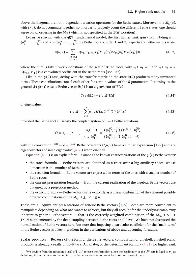
4.3. Higher rank models 61
above the diagonal are not independent creation operators for the Bethe states. Moreover, the Mi j(u),with i < j, do not commute together, so in order to properly count the different Bethe states, one shouldagree on an ordering in the Mi j (which is not specified in the B(u) notation).
Let us be specific with the gl(3) fundamental model, the first higher rank spin chain. Noting u :=u(1)1 , . . . , u(1)a1
and v := u(2)1 , . . . , u(2)a2 the Bethe roots of order 1 and 2, respectively, Bethe vectors write
B(u, v) =∑uI ,uIIvI ,vII
C(uI, uII, vI, vII)M12(uII)M13(uI)M23(vII) |0⟩ , (4.53)
where the sum is taken over 2-partitions of the sets of Bethe roots, with uI t uII = u and vI t vII = v.C(uI,II, vI,II) is a convoluted coefficient in the Bethe roots [see 129].
Like in the gl(2) case, acting with the transfer matrix on the state B(u) produces many unwantedterms. These contributions cancel each other for certain values of the u parameters. Returning to thegeneral Y (gl(n)) case, a Bethe vector B(u) is an eigenvector of T (z)
T (z)B(u) = t(z; u)B(u) (4.54)
of eigenvalue
t(z; u) =n∑
i=1
αi(z) f (z, u(i−1)) f (u(i), z) (4.55)
provided the Bethe roots u satisfy the coupled system of n− 1 Bethe equations
∀i = 1, . . . ,n− 1,αi(u
(i)I )
αi+1(u(i)I )=
f (u(i)I , u(i)II )
f (u(i)II , u(i)I )
f (u(i+1), u(i)I )
(u(i)I , u(i−1)), (4.56)
with the convention u(0) = ; = u(n). Bethe covectors C(u, v) have a similar expression [129] and areeigencovectors of same eigenvalue (4.55) when on-shell.
Equation (4.53) is an explicit formula among the known characterizations of the gl(n) Bethe vectors:
• the trace formula — Bethe vectors are obtained as a trace over a big auxiliary space, whosedimension is the number of Bethe roots
• the recursion formula — Bethe vectors are expressed in terms of the ones with a smaller number ofBethe roots
• the current presentation formula — from the current realization of the algebra, Bethe vectors areobtained by a projection method
• the explicit formula — Bethe vectors write explicitly as a linear combination of the different possibleordered combinations of the Mi j , 1≤ i < j ≤ n.
These are all equivalent presentations of generic Bethe vectors [129]. Some are more convenient tomanipulate depending on what one wants to achieve, but they all account for the underlying complexityinherent to generic Bethe vectors — that is the correctly weighted combination of the Mi j, 1 ≤ i <j ≤ N supplemented by the deep coupling between Bethe roots at all level. We have not discussed thenormalization of Bethe vectors here, but note that imposing a particular coefficient for the “main term”in the Bethe vectors is a key ingredient in the derivations of above and upcoming formulas.
Scalar products Because of the form of the Bethe vectors, computation of off-shell/on-shell scalarproducts is already a really difficult task. An analog of the determinant formula (4.31) for higher rank
3We deviate from the notation Bm(u) of [129] to ease the formulas. Since the cardinality of the u( j) sets is fixed to m j atdefinition, it is not crucial to remind it in the Bethe vector notation — at least for our usage of them.

62 Chapter 4 — Algebraic Bethe ansatz techniques
algebras is not known as today, though it has been obtained in some particular cases [129, 150, 151,277].
However, there exists a sum formula, first found for gl(2) in [131] and then generalized to the higherrank case in [160–162]. The scalar product of two Bethe vectors is written
C(s)B( t) =∑I,II
c(sI, tII)Wpart(sI, sII| tI, tII), (4.57)
where c(sI, tII) is a scalar coefficient depending on the representation, and Wpart is computed from thehighest coefficients of the Bethe vectors.
The squared norm of on-shell Bethe vectors enjoys a Gaudin formula similar to (4.36), where theGaudin matrix is a block matrix consisting of n− 1 square blocks, each of them being of size m j ×m j thenumber of Bethe roots at level j [129].
Form factors and correlation functions Form factors
C(u)Mi j(z)B(v) (4.58)
and correlation functions
C(u)n∏
k=1
e(k)αk ,βkB(v) (4.59)
may be computed in the same fashion as in the gl(2) model. Because of the form of Bethe vectors andscalar products, this turns out to be a tremendous task which requires the use of tricks and subtlerapproaches than plain, brute force calculations. We will not linger on these and refer to article [129]which presents a detailed summary of these techniques.
However, let us note that it could be sufficient to compute just one form factors, as the other ones canbe obtained from the form factor of a diagonal matrix element in special limits of the Bethe parametersby the zero mode method [278].
4.4 Summary
The Algebraic Bethe Ansatz technique is a powerful method to generate eigenstates of a quantum integrablemodel as Bethe vectors, using creation operators on a pseudo-vacuum state called the reference state.While the family of conserved quantities is constructed from the diagonal elements of the monodromy,equivalent of creation/annihilation operators are constructed from the off-diagonal ones at special points.These points, the Bethe roots, are tightly constrained all together by the Bethe equations, which arisefrom the cancellation of the unwanted terms in the action of the transfer matrix over Bethe vectors, asin (4.16). From the Bethe vector description of the eigenstate, important results for scalar products, formfactors and correlation functions of gl(n) models have been obtained.
However, the above review pointed out the fundamental requirements necessary to implement theABA procedure. The first one is the necessity of a reference state, whose existence is not guaranteedas we already highlighted. This is a great restriction that can make the ABA fail from the very start.Moreover, being an ansatz, one should ensure that all the eigenvectors of the transfer matrix are indeedobtained by this procedure. In particular, this requires to check that the constructed vector are non-zero.Finally, one can mention the intricacy of the nested procedure for higher rank models, which impact thecalculations that rely on them this description of the eigenstates. Scalar products and form factors aretherefore difficult to handle in their NABA form, and this as early as the first higher rank case of thegl(3) models. This motivates alternative approaches, such as the quantum separation of variables whichis at the center of this thesis.
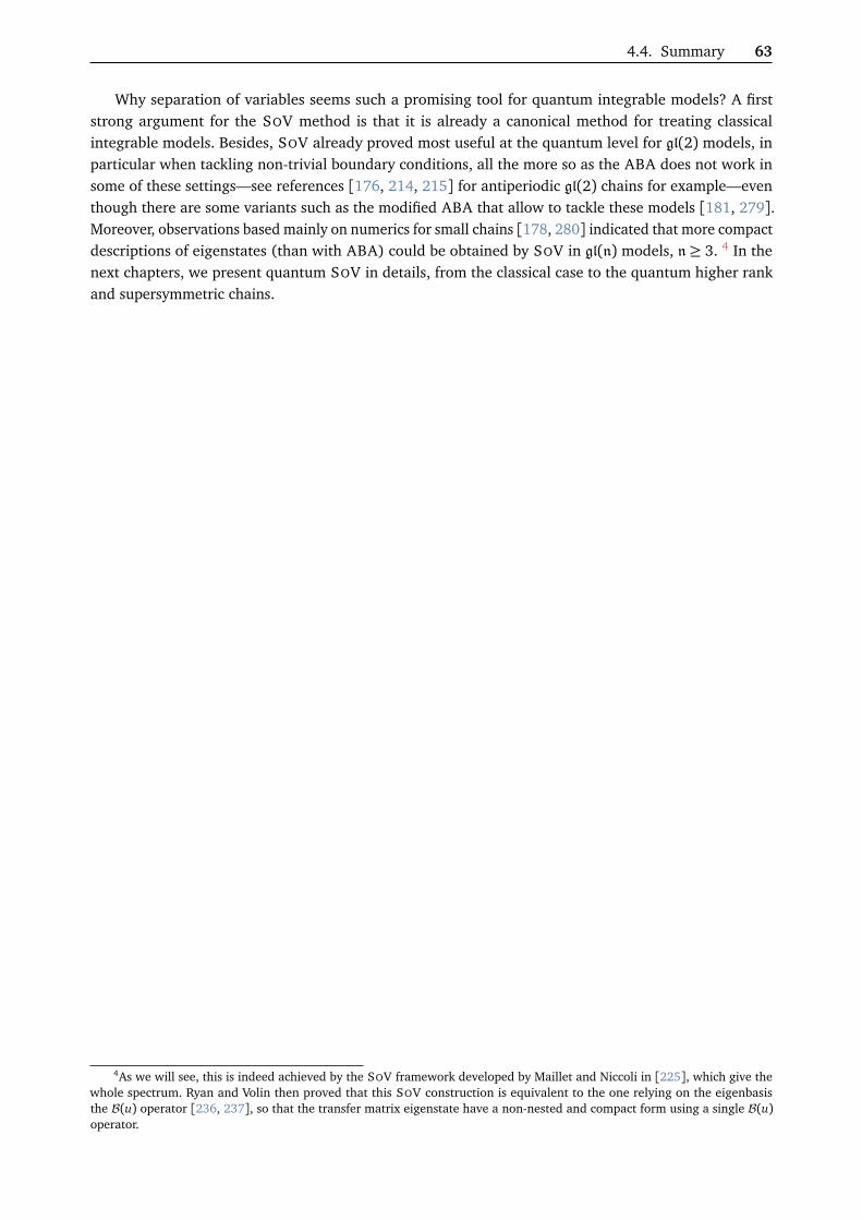
4.4. Summary 63
Why separation of variables seems such a promising tool for quantum integrable models? A firststrong argument for the SOV method is that it is already a canonical method for treating classicalintegrable models. Besides, SOV already proved most useful at the quantum level for gl(2) models, inparticular when tackling non-trivial boundary conditions, all the more so as the ABA does not work insome of these settings—see references [176, 214, 215] for antiperiodic gl(2) chains for example—eventhough there are some variants such as the modified ABA that allow to tackle these models [181, 279].Moreover, observations based mainly on numerics for small chains [178, 280] indicated that more compactdescriptions of eigenstates (than with ABA) could be obtained by SOV in gl(n) models, n≥ 3. 4 In thenext chapters, we present quantum SOV in details, from the classical case to the quantum higher rankand supersymmetric chains.
4As we will see, this is indeed achieved by the SOV framework developed by Maillet and Niccoli in [225], which give thewhole spectrum. Ryan and Volin then proved that this SOV construction is equivalent to the one relying on the eigenbasisthe B(u) operator [236, 237], so that the transfer matrix eigenstate have a non-nested and compact form using a single B(u)operator.


5Chapter
Fundamentals of separation ofvariables
In this chapter, we introduce the separation of variables procedure in generality for classical [34]and quantum Hamiltonian systems [281]. We begin by a description of separation of variables as a toolto solve the differential equations that characterize the motion in classical and quantum Hamiltoniansystems. Then, we focus on Sklyanin construction of separate variables in classical integrable models indetails [186–190], and show how to quantize this construction to produce a quantum SOV procedure [177,188, 192, 193, 206]. Some limitations of the quantization procedure for higher rank Y (gl(n)) quantumintegrable models are discussed [206], and a review of SOV results of the last decades closes the chapter.
5.1 SOV in classical systems
5.1.1 Classical SOV
For a classical Liouville integrable system, we outlined in Chapter 2 that the Liouville–Arnol’d theoremensures the existence of desirable canonical coordinate transformation1(q, p)→ (ψ, F) computable byquadrature. “By quadrature” simply means there is a sole integral to perform to compute the generatingfunction S(q, F) of the canonical coordinate transformation, which is the curvilinear integral (2.13)
S(q, F) =
∫ m
m0
α=
∫ q
q0
∑i
pi(q, f )dqi (5.1)
on the curve m0(q0, p0)→ m(q, p) laying on the level submanifold M f specified by the values fi of theconstants of the motion Fi . To compute S, one should first get the actual parametrization pi(q, f ) of thecanonical momenta by the qi ’s over M f . Since S defines a canonical transformation, these are simply thepartial differential of S with respect to the qi ’s we already stated in (2.9)
pi(q, f ) =∂ S∂ qi
. (5.2)
Plugging these in (2.19) it gives
H
q1, . . . , qn,∂ S∂ q1
, . . . ,∂ S∂ qn
= E. (5.3)
This is known as the Hamilton–Jacobi equation — and more precisely as the restricted Hamilton–Jacobiequation, for systems where the Hamiltonian does not involve time explicitly. It is a partial differentialequation of order 1 in n variables q1, . . . , qn for the generating function S(q1, . . . , qn, F1, . . . , Fn). Solvingit for S provides the desired coordinate transformation and solves the mechanical system, but it is a prioria hard task. In practice, this equation is tractable only when the variables are separable.
Separable coordinate in the H–J equation
1That is to canonical variables where the time evolution is linear.
65

66 Chapter 5 — Fundamentals of separation of variables
Definition. A coordinate q1 is said to be separable in the H–J equation if the generating function S(q, F) canbe split in two additive terms S1(q1, F) and S•(q2, . . . , qn, F)—one depending only on q1 and one independentof q1—and the H–J equation can be split in two independent H–J equations: one for S1 and one for S•.
Motivation. Say q1 is a separable variable as explained above. Then
S = S1(q1, F1, . . . , Fn) + S•(q2, . . . , qn, F1, . . . , Fn), (5.4)
so (5.3) becomes
H
q1,dS1
dq1, q2, . . . , qn,
∂ S•
∂ q2, . . . ,
∂ S•
∂ qn
= E. (5.5)
In practice the H–J equation is separable in two when the contribution of q1 and p1 ≡ ∂ S/∂ q1 can be“segregated” in the Hamiltonian2, such that the above equation can be rewritten
H
q1,dS1
dq1, f
q2, . . . , qn,∂ S•
∂ q2, . . . ,
∂ S•
∂ qn
= E. (5.6)
The function f is some helper function that repacks the dependence of H in the 2n variables qi , pi in adependence in three variables q1, p1 and the function f of the remaining canonical variables qi≥2, pi≥2.Note that f (q2, . . . , qn, p2, . . . , pn) is then necessarily a constant of the motion:
H, f =n∑
i=1
∂ H∂ pi
∂ f∂ qi− ∂ f∂ pi
∂ H∂ qi
=∂ H∂ p1
∂ f∂ q1− ∂ f∂ p1
∂ H∂ q1
+n∑
i=2
∂ H∂ pi
∂ f∂ qi− ∂ f∂ pi
∂ H∂ qi= 0
= 0+∂ H∂ f f , f = 0.
(5.7)
In principle (5.6) can be inverted by the implicit function theorem: there exists a function g such that
f
q2, . . . , qn,∂ S•
∂ q2, . . . ,
∂ S•
∂ qn
= g
q1,
dS1
dq1, E
. (5.8)
The two sides of this formula are equal but depends on independent variables, respectively qi≥2 and q1.They have to be equal to the same constant, the separation constant α1, which is the value of the constantfunction f and is some function of the fi . With the notation H• := f and H1 := g, we have
H1
q1,
dS1
dq1, E= α1, (5.9)
H•
q2, . . . , qn,∂ S•
∂ q1, . . . ,
∂ S•
∂ qn
= α1, (5.10)
and it is clear that the H–J equation has been separate in two independent H–J equations.
If all the coordinates qi are separable, the system is said completely separable. By iterating the aboveprocedure on the residual term H•, the generating function is fully separate as a sum of n terms with amutually exclusive dependence in one qi, while the Hamilton–Jacobi equation is split in n differential
2Quote from [34].

5.1. SOV in classical systems 67
equations of order one in one variable for the function S
S(q1, . . . , qn, F) = S1(q1, F) + · · ·+ Sn(qn, F), (5.11)
Hi
qi ,∂ Si
∂ qi, F= αi for i = 1, . . . , n. (5.12)
Note that the separation constants αi are some function of the values fi of the conserved quantities Fi onthe level manifold M f , so we can write
Hi
qi ,∂ Si
∂ qi, F1, . . . , Fn
= 0 (5.13)
in place of (5.12), where Hi = Hi −αi .The generating function S(q, F) is now constrained by its n independent partial derivatives, for which
we do have closed equations. Solving these n differential equations in one variable gives (by (2.9)) theparametrization pi(qi , F) over M f of the original canonical momenta — which in fact depend solelyon their associated coordinate qi, a feature of the separate variables. The generating function S ofthe coordinate transformation (q, p) → (ψ, F) that linearizes the dynamics is then constructed by nindependent quadratures in an additive separate form (5.11) which explicitly is
S(q1, . . . , qn, F1, . . . , Fn) =n∑
i=1
∫ qi(m)
qi(m0)pi(qi , F1, . . . , Fn)dqi . (5.14)
Remark 1 (Ignorable coordinates). Coordinates that do not appear explicitly in the Hamiltonian arecalled ignorable or cyclic. They are easily separable. The conjugate momentum p1 of a cyclic variable q1 isconstant since p1 = p1, H = − ∂ H/∂ q1 = 0. Coordinate q1 is also immediately separable: with S inthe form (5.4), equation (5.5) involves only S• and S1 is solution of the equation
p1 = α1 =∂ S1
∂ q1, (5.15)
where α1 is some (separation) constant.
Separate variables in Liouville integrable systems Essentially, what is done on the H–J equation ismerely the extraction of a conserved quantity from the expression of the Hamiltonian. When workingwith a Liouville integrable system, we already have some knowledge of conserved quantities. Therefore,we can define separate canonical variables in the following way.
Definition (Classical separate variables). Consider a Liouville integrable system with a phase space M andHamiltonian H, and N independent constants of the motion F1, . . . , FN in involution
∀i, j = 1, . . . , N ,
Fi , F j
= 0 and
H, F j
= 0. (5.16)
Let (x i , zi) be 2N canonical variables
x i , x j
=zi , z j
= 0,
x i , z j
= δi j . (5.17)
The x i are separate coordinates if there exists independent separate relations
Fi
x i , zi , F1, . . . , Fn
= 0, (5.18)
where the Fi are C1 functions and ∂ Fi/∂ zi 6= 0. The system is thus fully separate.

68 Chapter 5 — Fundamentals of separation of variables
Change of variables Usually the original canonical coordinates (qi , pi) do not enable the separationof the system, and it is necessary to perform a first coordinate transformation to new canonical variables,say (x i , zi), that are separable
(q, p)1st CT to−−−−−−−−−−→
separate variables(x , z)
2nd CT to−−−−−−−−−−−−−−−→pre-action–angle variables
(ψ, F). (5.19)
It is now the generating function S(x , F) that we solve for. Usually, the coordinate transformation tothe separate variables is hinted by the symmetries and invariances of the system and other physicallymeaningful statement made on it.
Central force problem by separation of variables
Let ~r be the position of a particle of mass m, with Cartesian coordinates ~r= (x , y, z) in its configurationspace R3. The phase space of the system is the 6-dimensional Poisson manifold with original canonicalvariables (x , y, z, px , py , pz), where the pi ’s are the conjugated canonical momenta to the x , y, z coordi-nates. The particle evolves in the potential V (r) of some central force ~F(~r) parallel to the position vector~r from the origin, r =
px2 + y2 + z2; the dynamics is thus prescribed by a Hamiltonian of the form
H =‖~p‖22m
+ V (r) using ~p=
px
py
pz
. (5.20)
It is well-known that the motion of this isolated system is planar and has constant areal velocity, reducingthe number of effective degrees of freedom of the particle. Precisely,
• because the force derives from a potential, it is conservative and the energy E is conserved,• d~L
dt = ~r× ~F = ~0 given that ~F ‖ ~r, so the norm and direction of the angular momentum ~L are
conserved, hence ~L and the projection L↑ of the angular momentum on some axis O↑ orthogonal
to the plane of the motion (usually set to be Oz) are constants of the motion.
This gives three constants of the motion F1 = E, F2 = ~L and F3 = L↑. One can prove they are
independent and in involution with additional calculations, making this system Liouville integrable.This knowledge acquired from the conserved quantities can be leveraged to simplify the descriptionof problem (like using polar coordinates in the plane of motion), but let us look for separate variablesstraight away. Because of the spherical symmetry of V (r), the spherical coordinates (r,θ ,ϕ) are theadapted way to describe this system. With ~∇ = ∂ /∂ r , r−1 ∂ /∂ θ , (r sinθ )−1 ∂ /∂ ϕ
the gradient in
spherical coordinates, the Hamiltonian becomes
H =1
2m
p2
r +p2θ
r2+
p2ϕ
r2 sin2 θ
+ V (r). (5.21)
This system is completely separable in these canonical variables as we shall see. Let us pick the generatingfunction S(~r, ~F) of the coordinate transformation (~r, ~p) → ( ~ψ, ~F) in a separate form in the sphericalcoordinates
S(~r, ~F) = Sr(r, ~F) + Sθ (θ , ~F) + Sϕ(ϕ, ~F). (5.22)
The coordinate ϕ is ignorable, so we can introduce the constant αϕ with ∂ Sϕ∂ ϕ = αϕ. The H–J

5.1. SOV in classical systems 69
equation (5.3) is written
∂ Sr
∂ r
2
+1r2
∂ Sθ∂ θ
2
+ αϕ
sinθ
2+ 2mV (r) = 2mE. (5.23)
The θ -dependent part is “segregated”, so following (5.6) this is separate in two equations with theintroduction of the constant αθ
∂ Sθ∂ θ
2
+α2ϕ
sin2 θ= α2
θ , (5.24)
∂ Sr
∂ r
2
+α2θ
r2+ 2mV (r) = 2mE. (5.25)
Together with∂ Sϕ∂ ϕ
= αϕ, (5.26)
this makes the system entirely separate, and integrating these three equations provide a formal solution tothe H–J equations of the system, solving its dynamics. Obviously the resolution is a bit intricate, becausewe have not accounted for the planar motion in the description of the system, so both the angle θ and ϕparametrize the trajectory3. Nevertheless, the separation constants have a clear physical interpretation:
• α0 ≡ E is the energy of the system,• αϕ = pϕ is the constant value of the projection of the angular momentum ~L = ~r× ~p along the polar
axis Oϕ4,
• αθ =r
p2θ+
p2ϕ
sin2 θis the constant norm
~L of the angular momentum.
We identify easily F1 = E ≡ α0 and F3 = ~L ≡ αθ , while αϕ is a projection of the ~L vector, also constant
since ∂ ~L∂ t = ~0, but a priori Oϕ is not the axis orthogonal to the plane of the motion. Nonetheless, it is
uniquely defined by the constants Fi by some function αϕ(F1, F2, F3).
In summary, separation of variables (SOV) in a Liouville integrable classical system is a procedurethat identifies or constructs canonical variables in which the Hamilton–Jacobi equation becomes tractable,thanks to the newly obtained separate form. In essence, it performs a reduction from a coupled n variableproblems to n independent problems in one variable. It is a primer to the full resolution of the system:solving the Hamilton–Jacobi equation characterizes a coordinate transformation to momenta that areconstants of the motions, effectively solving the dynamics.
In the context of the inverse scattering method, Sklyanin has introduced an approach to defineseparation of variables for integrable models. We expose the classical and quantum cases in the nextsections.
5.1.2 Classical SOV for integrable systems in the CISM framework
The classical spin 1/2 chain of length N is a Liouville integrable system: thanks to the CISM, one canconstruct N independent constants of the motion in involution. Characterizing the coordinate transform
3The description of the system in polar coordinates is recovered by taking the initial condition θ(t = 0) = π/2 andϕ(t = 0) = 0, fixing θ = π/2 so that the motion is described only with the (polar) coordinates (r,ϕ).
4pθ is the canonical momentum conjugated to the coordinate θ , and hence the component of ~L along the Oϕ axis. It is notthe component of the momentum vector ~p= m~r along the eϕ unit vector of the local spherical frame.

70 Chapter 5 — Fundamentals of separation of variables
to the constants of the motion solves the system. Can we use separation of variables to do so? Is thesystem fully separable? What are the separate variables? In the framework of the CISM, these questionsabout SOV were pioneered by Sklyanin see [186, 187] and the review [188]. We need to introduce someobjects in order to describe the SOV method.
Spectral curve & Baker–Akhiezer function Consider the classical gl(n) spin chains introduced inChapter 2. Let χM (u, z) be the characteristic polynomial of the n× n monodromy matrix M(u)
χM (u, z) := detz1−M(u)
, (5.27)
where the determinant is taken on the auxiliary space V0. The spectral curve is the locus of the eigenvaluesz(u) of the monodromy matrix at point u for the spectral parameter. It is an algebraic curve in C2 definedby the equation
χM (u, z) = 0. (5.28)
It implicitly defines the eigenvalue z(u) of M(u) as a n-multivalued function on C. The eigenfunctionΩ(u) associated to an eigenvalue z(u)
M(u)Ω(u) = z(u)Ω(u) (5.29)
is called the Baker–Akhiezer function [188, 282, 283]. The normalization of the Ω(u) vector will play aspecific role, so we fix it by the use of some coefficients αi(u) and the linear constraint on the componentsof Ω(u)
n∑i=1
αi(u)Ωi(u) = 1. (5.30)
Relation between the spectral invariants The determinant in (5.27) may be expanded as
χM (u, z) =n∑
k=0
(−1)kzn−kTk(u), (5.31)
where the spectral invariants Tk(u) are defined as
Tk(u) = trk∧
M(u). (5.32)
In particular, T0(u) = 1 and Tn(u) = det M(u). For a point (a, b) ∈ C2 on the spectral curve, (5.31) givesa non-trivial relation between the spectral invariants of M(u).
Sklyanin “magic recipe” From the B–A function, Sklyanin gives a way to construct separate variables
“Take the poles of the properly normalized Baker–Akhiezer function and the corresponding eigenvalues of themonodromy [Lax] operator and you obtain a SOV.” — Sklyanin in [188, p. 41].
The exact statement is the following
Theorem 2 (SOV in the CISM framework). Consider the classical gl(n) spin chain of length N. There existtwo functions A(u) and B(u) such that
• A(u) is a rational function of the monodromy entries Mi j(u)• B(u) is a polynomial of degree N n(n− 1)/2 in the Mi j(u)
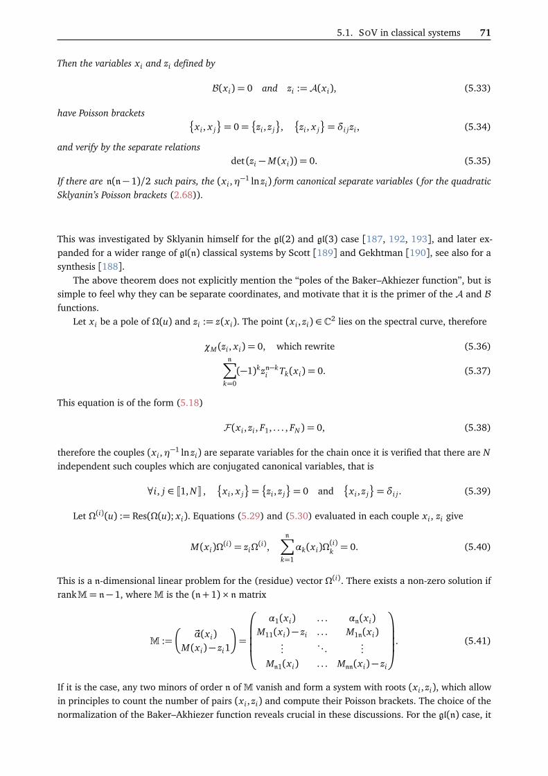
5.1. SOV in classical systems 71
Then the variables x i and zi defined by
B(x i) = 0 and zi :=A(x i), (5.33)
have Poisson brackets x i , x j
= 0=
zi , z j
,zi , x j
= δi jzi , (5.34)
and verify by the separate relationsdet (zi −M(x i)) = 0. (5.35)
If there are n(n− 1)/2 such pairs, the (x i ,η−1 ln zi) form canonical separate variables ( for the quadratic
Sklyanin’s Poisson brackets (2.68)).
This was investigated by Sklyanin himself for the gl(2) and gl(3) case [187, 192, 193], and later ex-panded for a wider range of gl(n) classical systems by Scott [189] and Gekhtman [190], see also for asynthesis [188].
The above theorem does not explicitly mention the “poles of the Baker–Akhiezer function”, but issimple to feel why they can be separate coordinates, and motivate that it is the primer of the A and Bfunctions.
Let x i be a pole of Ω(u) and zi := z(x i). The point (x i , zi) ∈ C2 lies on the spectral curve, therefore
χM (zi , x i) = 0, which rewrite (5.36)n∑
k=0
(−1)kzn−ki Tk(x i) = 0. (5.37)
This equation is of the form (5.18)
F(x i , zi , F1, . . . , FN ) = 0, (5.38)
therefore the couples (x i ,η−1 ln zi) are separate variables for the chain once it is verified that there are N
independent such couples which are conjugated canonical variables, that is
∀i, j ∈ J1, NK ,
x i , x j
=zi , z j
= 0 and
x i , z j
= δi j . (5.39)
Let Ω(i)(u) := Res(Ω(u); x i). Equations (5.29) and (5.30) evaluated in each couple x i , zi give
M(x i)Ω(i) = ziΩ
(i),n∑
k=1
αk(x i)Ω(i)k = 0. (5.40)
This is a n-dimensional linear problem for the (residue) vector Ω(i). There exists a non-zero solution ifrankM= n− 1, whereM is the (n+ 1)× n matrix
M :=
~α(x i)
M(x i)− zi1
=
α1(x i) . . . αn(x i)M11(x i)− zi . . . M1n(x i)
.... . .
...Mn1(x i) . . . Mnn(x i)− zi
. (5.41)
If it is the case, any two minors of order n ofM vanish and form a system with roots (x i , zi), which allowin principles to count the number of pairs (x i , zi) and compute their Poisson brackets. The choice of thenormalization of the Baker–Akhiezer function reveals crucial in these discussions. For the gl(n) case, it

72 Chapter 5 — Fundamentals of separation of variables
turns out that any constant numeric normalization vector ~α(u) ∈ Cn produces SOV. A simplest choice5is
α1(u) = 1 and α2(u) = · · ·= αn(u) = 0. (5.42)
gl(2) case Specializing to the gl(2) case, we can take the vanishing minors of order n= 2 to be
1 0
M11(x i)− zi M12(x i)
= 0,
1 0
M21(x i) M22(x i)− zi
= 0. (5.43)
Using the A, B, C , D notation, this gives immediately
B(x i) = 0, (5.44)
D(x i) = zi . (5.45)
In the end, the separate variables are simply the zeroes of the B(u) polynomial, and the zi ’s are definedequally simply as the images by D of the x i ’s
6. We identify immediately A(u) = D(u) and B(u) = B(u).In u= x i the monodromy becomes triangular
M(x i) =
A(x i) 0C(x i) zi
, (5.46)
so it is no surprise its eigenvalue zi = z(x i) is given by the diagonal element D(x i). The explicit separaterelations for the (x i , zi) are
det M(x i)− zi T (x i) + z2i = 0. (5.47)
It remains to compute the Poisson brackets between the x i ’s and zi ’s. This can be achieved by theknowledge of the quadratic Poisson brackets between the monodromy matrix elements (2.75). The r-matrix that gives the Poisson bracket is r(u) = c
uP, where P is the permutation operator. Taking particularindices in (2.75), one obtains
B(u), B(v)= 0, (5.48)
D(u), D(v)= 0, (5.49)
D(u), B(v)= cu− v
(B(u)D(v)− B(v)D(u)). (5.50)
The involution of the B’s entrain immediately that x i , x j = 0, for all i, j. Now, for any function F overthe phase space,
0= F, B(x i)= F, B(u)u=x i+
dBdu
u=x iF, x i. (5.51)
5Note that historic literature [188, for example] usually takes α1 = · · · = αn−1 = 0 and αn = 1, which produces an equivalentdiscussion.
6Sklyanin’s is used to take A(u) = A(u) [187], which is essentially the same thing.
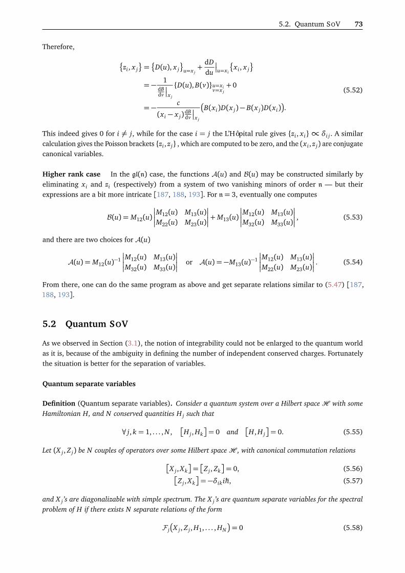
5.2. Quantum SOV 73
Therefore,
zi , x j
=
D(u), x j
u=x j
+dDdu
u=x i
x i , x j
= − 1dBdv
x j
D(u), B(v)u=x iv=x j+ 0
= − c
(x i − x j)dBdv
x j
B(x i)D(x j)− B(x j)D(x i)
.
(5.52)
This indeed gives 0 for i 6= j, while for the case i = j the L’Hôpital rule gives zi , x i ∝ δi j. A similarcalculation gives the Poisson brackets zi , z j , which are computed to be zero, and the (x i , z j) are conjugatecanonical variables.
Higher rank case In the gl(n) case, the functions A(u) and B(u) may be constructed similarly byeliminating x i and zi (respectively) from a system of two vanishing minors of order n — but theirexpressions are a bit more intricate [187, 188, 193]. For n= 3, eventually one computes
B(u) = M12(u)
M12(u) M13(u)M22(u) M23(u)
+M13(u)
M12(u) M13(u)M32(u) M33(u)
, (5.53)
and there are two choices for A(u)
A(u) = M12(u)−1
M12(u) M13(u)M32(u) M33(u)
or A(u) = −M13(u)−1
M12(u) M13(u)M22(u) M23(u)
. (5.54)
From there, one can do the same program as above and get separate relations similar to (5.47) [187,188, 193].
5.2 Quantum SOV
As we observed in Section (3.1), the notion of integrability could not be enlarged to the quantum worldas it is, because of the ambiguity in defining the number of independent conserved charges. Fortunatelythe situation is better for the separation of variables.
Quantum separate variables
Definition (Quantum separate variables). Consider a quantum system over a Hilbert spaceH with someHamiltonian H, and N conserved quantities H j such that
∀ j, k = 1, . . . , N ,H j , Hk
= 0 and
H, H j
= 0. (5.55)
Let (X j , Z j) be N couples of operators over some Hilbert spaceH , with canonical commutation relations
X j , Xk
=Z j , Zk
= 0, (5.56)
Z j , Xk
= −δik iħh, (5.57)
and X j ’s are diagonalizable with simple spectrum. The X j ’s are quantum separate variables for the spectralproblem of H if there exists N separate relations of the form
F j
X j , Z j , H1, . . . , HN
= 0 (5.58)

74 Chapter 5 — Fundamentals of separation of variables
for j = 1, . . . , N, where some order between the non-commutative operators X i, Z j and the commutativeH j family has to be prescribed. The basis of common eigenvectors of the X j ’s is the separate basis. Eachvector is labelled uniquely by its eigenvalues x j under the action of the X j
|~x⟩= |x1, . . . , xN ⟩ and X j |~x⟩= x j |~x⟩ . (5.59)
Letψ(x1, . . . , xN ) := ⟨x1, . . . , xN |ψ⟩ (5.60)
be the wavefunction of a stationary state |ψ⟩ of the system, where ⟨~x| = ⟨x1, . . . , xN | is the (separate)Hilbert basis of eigencovectors associated to the separate coordinates X j. Then the relations (5.58)suggests a factorized form of the wave function
ψ(x1, . . . , xN ) =N∏
j=1
ψ j(x j). (5.61)
For a continuous system with an infinite-dimensional Hilbert space, it is handy to realize quantumstates as functions and work in the x-representation of the operators to picture the implications of theabove definition. Operators X j are the multiplication operators by the j-th coordinate x j , and Z j = ∂
∂ X j .
Then, acting on ψ(~x) with the j-th relation (5.58), one can restrict the equation to the ψ j(x j) term
F j
x j ,
∂
∂ x j, h1, . . . , hN
ψ j(x j) = 0, (5.62)
where the hi are the scalar value of the conserved quantities operators on the ψ(~x) eigenstate. Theseare separate differential equations in one variable; the original spectral problem has been decoupled inindependent simpler ones.
For a finite-dimensional Hilbert space, the “wavefunctions” (5.60) we consider are simply the co-efficients of the linear decomposition of an eigenstate in the separate basis. The Z j dependence in theseparate relations (5.58) should be realized as a shift in the spectrum of X j . Noting
S j := x(h j)j | h j = 1, . . . , d j (5.63)
the d j eigenvalues of X j , this yields independent separate finite difference equations for the ψ j(x j) factorof the form
F j
x(h j)j , D±j , h1, . . . , hN
ψ j
x(h j)j
= 0, (5.64)
where D±j are the shift operators in the spectrum of X j
D±j ψ j
x(h j)j
=ψ j
x(h j±1)j
. (5.65)
This shows how the original spectral problem separates in N independent ones of smaller dimension di
on the Hilbert spaceH j , with
H =N⊗
j=1
H j andN∏
j=1
d j = dimH . (5.66)

5.2. Quantum SOV 75
Link with classical SOV We can illustrate the classical limit with the simple case of the particle in Ndimensions in some potential V (~x). The Hamiltonian of this continuous system is of the form
H = − ħh2
2m∆+ V (~x). (5.67)
Writing the spatial wavefunction of the state |ψ⟩ in the form of a stationary phase
ψ(~x) =ψ0 e iS(~x)/ħh and ψ(~x, t) =ψ(~x)e− iE t/ħh , (5.68)
and taking the classical limit in the (time independent) Schrödinger equation, we obtain
E =(∇S(~x))2
2m− iħh
2m∆S(~x) + V (~x) −−→
ħh→0
(∇S(~x))2
2m+ V (~x), (5.69)
which is the classical reduced Hamilton–Jacobi equation with a given energy E and Hamilton characteristicfunction S(x) for the corresponding classical system — see equations (5.1) and (5.3) with H = ~p2
2m +
V (~x). Now for a separate problem with a factorized wavefunction
ψ(~x) =ψ0
N∏j=1
e−iħhS j(x j), (5.70)
one recovers the equations (5.11) and (5.12).In the classical case, the separate relations are used to solve the equations of the motion, constructing
by additive separate quadratures the generating function of the coordinate change to the constants of themotion which linearize the time evolution. In the quantum case, the separate relations are used to solvethe spectral problem for the Hamiltonian, constructing the wavefunction of eigenstates by multiplicativeseparate wavefunctions responding to their own spectral problems of smaller dimension.
The hydrogen atom
Consider the Hamiltonian describing the motion of an electron in the potential of proton at the origin,
H =~p2
2m+ V (~r) with V (~r) = − e2
4πε0r, (5.71)
where ~r is the position vector, r = ‖~r‖, and ~p the momentum. The electron state is described by vectors|Ψ⟩ of the Hilbert spaceH ' L2(R3). The time-independent Schrödinger equation for the wave functionΨ(~r) = ⟨~r|Ψ⟩ is, with ~p= −iħh ~∇,
− ħh2
2m∆Ψ + V (~r)Ψ = E, with V (~r) = − e2
4πε0r, (5.72)
for some energy E ∈ R. Because of the central nature of the force—namely the potential V (r) dependsonly on the radial distance r—the three components Lx , L y and Lz of the orbital angular momentum~L = −iħh~r× ~∇ are operators that commute with the Hamiltonian. This can be shown using the fundamentalcommutation relations [ri , p j] = iħhδi j . Therefore,
H, ~L2
= [H, Lz] =
~L2, Lz
= 0. (5.73)
Any eigenstate of the Hamiltonian is thus also a shared eigenstate of the ~L2 and Lz operators, so one can

76 Chapter 5 — Fundamentals of separation of variables
search for the eigenstate of H in the set of common eigenstates of the commuting family (H, ~L2, Lz).Because of the rotational invariance of the system, the spherical coordinates (r,θ ,ϕ) are well suited
to describe it. The wavefunction of the state |Ψ⟩
Ψ(r,θ ,ϕ) = ⟨r,θ ,ϕ|Ψ⟩ (5.74)
are function of L2(R+× [0,π[×[0, 2π[, r2 sinϕ dr dθ dϕ), and the H, ~L2, Lz operators are represented as
∆=1r2
∂
∂ r
r2 ∂
∂ r
+
1r2 sinθ
∂
∂ θ
sinθ
∂
∂ θ
+
1
r2 sin2 θ
∂ 2
∂ ϕ2, (5.75)
~L2 = −ħh2
1
sinθ∂
∂ θ
sinθ
∂
∂ θ
+
1
sin2 θ
∂ 2
∂ ϕ2
, (5.76)
Lz = −iħh ∂∂ ϕ
. (5.77)
Defining the three operators
F1
r,∂
∂ r, H, ~L2
:= − ħh
2
2mr2
∂
∂ r
r2 ∂
∂ r
+
12mr2
~L2 − e2
4πε0r−H, (5.78)
F2
θ ,∂
∂ θ, ~L2, Lz
:= − 1
sinθ∂
∂ θ
sinθ
∂
∂ θ
− L2
z
ħh2 sin2(θ )+ħh−2~L2, (5.79)
F3
ϕ,∂
∂ ϕ, Lz
:= −iħh ∂
∂ ϕ− Lz , (5.80)
one can verify that their action vanishes on wavefunctions Ψ() of eigenstate of the commuting family(H, ~L2, Lz)
∀a ∈ J1, 3K , FaΨ(r,θ ,ϕ) = 0. (5.81)
This gives relations of the form (5.58), so the spherical coordinates (r,θ ,ϕ) are thus separate coordinatesfor this system.
Consider Ψ(r,θ ,ϕ) an eigenfunction of the commuting family (H, ~L, Lz), i.e.
HΨ = EΨ, (5.82)
~L2Ψ = h2Ψ, (5.83)
LzΨ = h3Ψ, (5.84)
with E, h2, h3 ∈ R. The vanishing action of F3 of Ψ gives the simple enough differential equation
∂
∂ ϕ+
h3
iħhΨ(r,θ ,ϕ) = 0, (5.85)
with only derivatives in ϕ, so that we can solve it, giving
Ψ(r,θ ,ϕ) = A(r,θ )eiħh−1h3ϕ, (5.86)
with A(r,θ ) some function of the r and θ variables. Acting further with F2 on Ψ, one gets a differentialequation for A(r,θ) with only derivatives in θ , so that it further separates the resolution in r and θ .

5.3. Quantum SOV for integrable systems in the QISM framework 77
Eventually, the wavefunction can can be written in a factorized form
Ψ(r,θ ,ϕ) = R(r)Θ(θ )Φ(ϕ), (5.87)
where each factor verifies independent and separate differential equations.The definitive form of the solution (5.87) is obtained by multiplying solutions of the three differential
equationsF1R= 0, F2Θ = 0, F3Φ= 0, (5.88)
and selecting the Ψ = RΘΦ that indeed verify the Schrödinger equation (5.72) on the whole space R andhave a finite norm. The result is well-known: the discrete spectrum of the Hamiltonian is enumerated bythe quantum numbers (n,`, m)
E = En = −En2
with n ∈ N∗ and E = me2
2(4πε0)2ħh2 ≈ 13.6eV, (5.89)
h2 = `(`+ 1)ħh with ` ∈ J0, n− 1K , (5.90)
h3 = mħh with m ∈ J−`,`K , (5.91)
and the wavefunctions are of the form
Ψn,`,m(r,θ ,ϕ) = Rn,`(r)F`,m(θ )eimϕ, (5.92)
where the angular part are the so-called spherical harmonics [284]
Y`,m(θ ,ϕ), (5.93)
and the radial part are generalized Laguerre polynomials [see 281, appendix B]
Rn,`(r) = L2`+1n−`−1(r). (5.94)
Note that solutions with infinite norm are obtained for E > 0 and describe non-bound states correspondingto the continuous spectrum of the Hydrogen atom.
5.3 Quantum SOV for integrable systems in the QISM framework
5.3.1 SOV in the QISM description of quantum integrable models
For a quantum integrable model generated by some transfer matrix T (u), the above definition of separatevariables holds similarly, except that it is more convenient to express the separate relations (5.18) usingthe transfer matrix which packs the conserved quantities
FX j , Z j , T (X j)
= 0 (5.95)
In the QISM context, the core idea of Sklyanin’s “magic recipe” is still the same: there should exist anoperator B(u) whose properly defined operatorial roots are separate variables. Here, the roots X j areoperators over the Hilbert space, and they should commute together in order to write unambiguously
B(u) = B0
N∏j=1
u− X j
. (5.96)

78 Chapter 5 — Fundamentals of separation of variables
Like in the classical case, conjugated variables Z j are obtained by evaluating an operator A(u) in theoperatorial roots X j , see (5.33). It is necessary to define how one substitutes an operator in place of thescalar parameter in A(u). We can choose the left ordering of the argument in the polynomial expansionof A
A(X j) =∑
k
X kj Ak given A(u) =
∑k
ukAk for all u ∈ C. (5.97)
In fact, a former name of the quantum separation of variables was the Functional Bethe Ansatz (FBA) [192,193, 204, 205], whose name is a syncretism of the known way to solve quantum integrable systemsand the necessity to introduce spaces of functions to rigorously describe the zeroes of operator-valuedpolynomials. One should also ensure that the spectrum of the X j and the poles of A(u) do not intersect.
The separate relations shall be provided by some quantized version of (5.28), the quantum spectralcurve, that we do not explicit for the moment. The common eigenbasis |~x⟩ = |x1, . . . , xn⟩ of the X j
operators, labelled by their eigenvalues, is also the eigenbasis of the B(u) operator. Hence, the separatebasis may be constructed by the direct diagonalization of the B(u) operator.
5.3.2 The gl(2) case
Let us show how to obtain separate variables à la Sklyanin for gl(2) models associated to the 6-vertexalgebra. The classical case hints us to look at B(u) = M12(u) and D(u) = M22(u) for the B(u) and A(u)operators, respectively. Let us consider a twisted monodromy M(u) = M K(u), and suppose the twistmatrix K is such that M12(u) is diagonalizable with simple spectrum (note that for K = Id, this is not thecase). Having
[B(u), B(v)] = 0 (5.98)
is already good news: we can define the commuting root operators X j and write (5.96) as
B(u) = B0
N∏j=1
ϕu− X j
. (5.99)
Since B(u) = B(u) is diagonalizable with simple spectrum, then its operatorial roots X j are simultane-ously diagonalizable with simple spectrum: following (5.63) we note
x(h j)j ∈ C for 1≤ h j ≤ d j , (5.100)
the d j eigenvalues of the X j operator. We have
N∏j=1
d j ≡ dimH , (5.101)
and the eigenvectors of B(u) consists in the d1 . . . dN vectors~x(~h)
¶:=x (h1)
1 , . . . , x (hN )N
¶(5.102)
of eigenvalue
b~h(u) = B0
N∏j=1
ϕ
u− x(h j)j
. (5.103)
To ease the heavy notation (5.102), we will make use of the shorthand notation |~x⟩ = |x1, . . . , xN ⟩ in thefollowing to denote a generic vector of the separate basis.
What is the action of the conjugated D(x j) operators on the separate basis? By equation (Y.8) one

5.3. Quantum SOV for integrable systems in the QISM framework 79
computes
B(u)D(x j) |~x⟩=ϕu− x j +η
ϕu− x j
b~h(u)D(x j) |~x⟩ . (5.104)
Hence, unless D(x j) |~x⟩ is zero, D(x j) |~x⟩ is an eigenvector of eigenvalue
B0ϕu− (x j −η)
N∏k 6= j
ϕu− x (hk)
k
. (5.105)
Therefore, D(x j) is the shift operator by −η in the spectrum S j of X j , and the eigenvalues can be labelledand ordered by successive shifts of the η parameter
S j =
x (1)j , . . . , x(d j)j
=
x (0)j , x (0)j −η, . . . , x (0)j −d j − 1
η, (5.106)
for some x (0)j ∈ C, such that
x(h j)j = x (0)j + (h j − 1)η. (5.107)
Similarly, the action of A(x j) = M11(x j) performs the opposite shift x j → x j +η on the eigenvectors ofthe separate basis, so we have
A(x j) |~x⟩ ∝x1, . . . , x j +η, . . . , xN
, (5.108)
D(x j) |~x⟩ ∝x1, . . . , x j −η, . . . , xN
. (5.109)
Using the notation ~x+ ae j := (x1, . . . , x j + a, . . . , xN ), this gives
A(x j) |~x⟩ ∝~x+ηe j
,
D(x j) |~x⟩ ∝~x−ηe j
.
(5.110)
On covectors of the left separate basis, A(x j) and D(x j) shift the spectrum in the opposite way:
⟨~x|A(x j)∝~x−ηe j
,⟨~x|D(x j)∝
~x+ηe j
. (5.111)
Using the quantum determinant (A.17), whose explicit expression in this case is
q-det M(u) = det Ka(u)d(u−η) = det KN∏
j=1
(u− ξ j +η)(u− ξ j −η), (5.112)
where d(u) =∏N
j=1(u− ξ j) = a(u−η) are the eigenvalue of the untwisted diagonal matrix elements ofthe untwisted monodromy on the highest weight state, we compute
⟨~x|A(x j)D(x j −η) = q-det M(x j) ⟨~x| . (5.113)
Hence, with a proper choice in the normalization, we may put
⟨~x|A(x j) = a(x j)~x−ηe j
,⟨~x|D(x j) = d(x j)
~x+ηe j
. (5.114)
Spectral problem We can now describe the spectral problem of the model using the separate basisconstructed above. Let |t⟩ be an eigenvector of eigenvalue t(u) for the transfer matrix T (u) = A(u)+D(u).

80 Chapter 5 — Fundamentals of separation of variables
Ultimately we want to solve the spectral equation T (u) |t⟩ = t(u) |t⟩. To do so, we can make good use ofthe above left separate basis by computing
⟨~x| T (x j) |t⟩ (5.115)
in two different ways: i) by making T acts to the right on its eigenvector and ii) by making T = A+ Dacts to the left on the separate basis. It yields the following equation
∀~x ∈ S1 × · · · × SN , t(x j) ⟨~x|t⟩= a(x j)~x−ηe j
t+ d(x j)~x+ηe j
t . (5.116)
Reintroducing the exact notation for the spectrum, the wavefunctions of eigenstate |t⟩
ψt
x (h1)
1 , . . . , x (hN )N
=¬
x (h1)1 , . . . , x (hN )
N
t¶
for (xh11 , . . . , x (hN )
N ) ∈ S1 × · · · × SN , (5.117)
which are the 2N components of the eigenstate in the separate basis, obey the following second orderfinite difference equation
tx(h j)j
ψt
x (h1)
1 , . . . , x (hN )N
= a
x(h j)j
ψt
x (h1)
1 , . . . , x(h j+1)j , . . . , x (hN )
N
+ dx(h j)j
ψt
x (h1)
1 , . . . , x(h j−1)j , . . . , x (hN )
N
. (5.118)
Using a factorized form (5.61) of the wavefunctionψt , these form N separate equations of the form (5.58).They manifest as finite difference equations, because we deal with a Hilbert space of finite dimension. Itis enough to solve this system of finite-difference equation to solve the spectral problem of the twistedXXX chain, offering an alternate picture from the one of the ABA.
How does the quantum spectral curve arise in this discussion? In the classical case, it was the objectwhich provides the separate relations from the help of an eigenvector of the monodromy matrix, theBaker–Akhiezer function. In the above discussion, we obtained the separate relations straight from thead-hoc constructed separate basis without referring to the spectral curve once. But there is a way torecover it from the quantum determinant: from the expression q-det M(u) = A(u)D(u−η)−B(u)C(u−η),the following equation holds
A(u)A(u−η)− A(u)T (u−η) + q-det M(u) + B(u)C(u−η) = 0. (5.119)
Sandwiching this equation by a covector of the separate basis at the left and an eigenvector of the transfer
matrix at the right and putting u← x(h j)j , it produces the quantum analog of the spectral curve (5.31)
ax(h j)j
ax(h j+1)j
ψt
x (h1)
1 , . . . , x(h j+2)j , . . . , x (hN )
N
− ax(h j)j
tx(h j+1)j
ψt
x (h1)
1 , . . . , x(h j+1)j , . . . , x (hN )
N
− q-det M(x j)ψt
x (h1)
1 , . . . , x(h j)j , . . . , x (hN )
N
= 0, (5.120)
which is exactly (5.118) after one factors out the common ax(h j)j
factor, and rescale h j in h j − 1.
Necessity of the twist The attentive reader should have notice that for an untwisted gl(2) model, saythe XXX gl(2) fundamental models with periodic boundary conditions, the B(u) = M12(u) operator isnilpotent, which is incompatible with the above construction. However, it is possible circumvent to this

5.3. Quantum SOV for integrable systems in the QISM framework 81
issue by adding a non-trivial twist to the chain. For the XXX chain, taking K =
1 α0 1
, we have
BK(u) = B(u) +αD(u), (5.121)
in terms of the elements of the untwisted monodromy, which is now a diagonalizable operator, being asum of a nilpotent and a diagonalizable one. The simplicity of the BK spectrum is then ensured by takingan inhomogeneous chain up to some constraints. For the XXZ chain, non-trivial linear combinationsK = α
0 11 0
+ β
0 −ii 0
of the σx and σ y Pauli matrices give a diagonalizable BK(u) operator. We can
therefore state the following theorem for the 6-vertex Yang–Baxter algebra:
Theorem 3. Consider the twisted inhomogeneous XXX chain of length N, with a twist matrix K that is notproportional to the identity, so that it can always be brought to the form
K =
k1 α
0 k2
with α 6= 0 (5.122)
by an isomorphism7, and monodromy
M K(u) = K0R0N (u− ξN ) . . . R01(u− ξ), (5.123)
with the inhomogeneities ξ j satisfying
∀a, b ∈ J1, NK, a 6= b, ∀r = −1, 0,1, ξa 6= ξb + rη. (5.124)
The left separate basis is the basis of eigenvectors of the 2N covectors BK(u) = BK0
∏Nj=1ϕ
u− X j
operators,
which are the
⟨~h| := ⟨0|N∏
j=1
AK(ξ j)
h j for h j ∈ 0,1, (5.125)
of eigenvalue
b~h(u) = αN∏
j=1
ϕu− (ξ j − h jη)
. (5.126)
The spectrum of the operatorial roots X j is therefore
S j = ξ j ,ξ j −η (5.127)
which is indeed of the form (5.106) and is simple thanks to conditions (5.124). The above separate basisallows to re-express the spectral problem for the transfer matrix T K(u) = tr M K(u) as a system of discreteequations (5.120) with
q-det M(u) = det(K)N∏
j=1
ϕu− ξ j +η
ϕu− ξ j +η
(5.128)
and a(u) being replaced by
aK(u) = k1a(u) = k1d(u+η) = k1
N∏j=1
(u− ξ j +η). (5.129)
Proof. These results are obtained by specializing the above discussions on the eigenstate of B(u) = BK(u)and the spectral problem of the transfer matrix to the fundamental representation of gl(2), and not
7See [225], section 3.2.

82 Chapter 5 — Fundamentals of separation of variables
forgetting to take the twist into account.The operator BK(u) = k1B(u) +αD(u) is diagonalizable since D(u) is and α 6= 0. The family (5.125)
is proved to be the eigenbasis of BK(u) by induction.Any eigenstate |t⟩ of T K(u) has its eigenvalue t(u) and wavefunctions in the separate basis ψt(~x)
satisfy the system of equations (5.120), with the correct replacement for a(u) and q-det M(u).
The above computations generalize to many gl(2) models. A most interesting case is the one of theantiperiodic XXZ chain, because the ABA cannot be applied in this case for the lack of a reference state.
Example: SOV for the XXZ antiperiodic chain [176]
Consider the inhomogeneous XXZ spin 1/2 model of length N with the antiperiodic twist K = σx =
0 11 0
.
The explicitly twisted monodromy of this system is
M K(u) = KR0N (u− ξN ) . . . R01(u− ξ1) =
C(u) D(u)A(u) B(u)
. (5.130)
From the above analysis, we define
A(u) := M K22(u) = B(u), (5.131)
B(u) := M K12(u) = D(u). (5.132)
The B(u) = D(u) operator is diagonalizable with simple spectrum, as desired. For generic inhomogeneitiessatisfying the condition (5.124), the left and right eigenbasis of D(u) are the covectors and vectors
~h := ⟨0|
N∏j=1
C(ξ j)
d(ξ j −η)
h j
, (5.133)
~h :=N∏
j=1
B(ξ j)
a(ξ j)
h j
|0⟩ , (5.134)
labelled by vectors ~h= (h1, . . . , hN ) ∈ 0, 1N , with |0⟩= ⊗Nj=1
10
and ⟨0|= ⊗N
j=1
1,0
8. The eigenvalue
associated to~h and
~h under the left and right action of D(u), respectively, is
d~h(u) =N∏
j=1
sinhu− ξ j − h jη
. (5.135)
These are clearly of the form (5.125) and (5.126). Proof is made by direct calculation using the FCRof the trigonometric 6-vertex algebra. Similar calculations show that the action of the B(u) and C(u)operators over (5.133) and (5.133) is a non-local shift in the hi—but the action of the B(ξ j) and C(ξ j)are. The SOV measure is diagonal with
~h~k∝ δ~h,~k. (5.136)
From there, one may prove that the spectrum of the transfer matrix T K(u) = tr M K(u) = B(u) + C(u)are the functions t(u) solutions of the N discrete equations
t(ξ j)t(ξ j −η) = q-det M k(ξ j) = −a(ξ j)d(ξ j −η), (5.137)
within a certain set of Laurent polynomials of degree N −1 constrained by the length of the chain. This is

5.3. Quantum SOV for integrable systems in the QISM framework 83
good agreement with (5.128). The eigenstates have a separate form
|t⟩=∑~h
N∏j=1
Q t(ξ j − h jη)~h , (5.138)
and similarly for the left eigenstates, so the wavefunctions~ht are indeed factorized. Details can be
found in [176], where the analysis is pursued until form factors of local operators.
5.3.3 SOV for the gl(3) model
The SOV description for the quantum gl(3) chain was first made by Sklyanin himself [206], based on hiswork for the classical gl(3) case [187]9. Recall that the quantum-determinant is a central element of theYangian algebra, which here for Y (gl(3)) is explicitly written as
q-det M(u) = tr123
P−123M1(u)M2(u+η)M3(u+ 2η)
, (5.139)
where P−123 = 1/6∑σ∈Σ3
sign(σ) Pσ is the antisymmetrizer over three copies of the auxiliary space. Thematrix
U(u) :=3 tr23 P−123M2(u)M3(u+η)
ᵀ1 , (5.140)
is a quasi-inverse of the monodromy matrix, as by direct computation one proves
q-det(M(u)) = (M(u)ᵀ)U(u+η), (5.141)
where ᵀ denotes the matrix transposition. Note that T2(u) = tr U(u). Let
B(u) := M23(u)U31(u−η)−M13(u)U32(u−η), (5.142)
which mirrors the expression (5.53) of the classical case, up to the η shifts. Direct calculation shows that[B(u),B(v)] = 0, so it is meaningful to write
B(u) = B0
3N∏k=1
(u− Xk), (5.143)
and [X j , Xk] = 0. Similarly, the operator A(u) is defined as a deformation of the classical case as
A(u) := −M23(u−η)−1U32(u−η) = −U32(u−η)M23(u−η)−1, (5.144)
with [A(u),A(v)] = 0. Sklyanin proved [206] that
(u− v)A(u)B(v) = (u− v −η)B(v)A(u) +B(u)E(u, v), (5.145)
whereE(u, v) =A(u)
M23(u−η)M23(u)
−1M23(v −η)M32(v). (5.146)
It is then tempting to define Z j :=A(u)|u=XJas the conjugated variable, as it seems to produce the desired
shift in the spectrum of X j . However,
8The notation in [176] is multiplicative, but it is easy to make the connection with λ = exp(u), q = exp(η) and η j = expξ j
,
and a factor 2 in the R-matrix.9Extension to the generic gl(n) case was also discussed in [207].

84 Chapter 5 — Fundamentals of separation of variables
“the condition that ∪3N
j=1 Sp(X j)∩ poles(A(u)) = ; (5.147)
should be checked for any specific representation of the [gl(3) Yang-Baxter] algebra,”
as Sklyanin points out very appropriately in [206], before saying that “here[for the unspecified repre-sentation at hand] we assume it to be satisfied”. Indeed, in case the intersection (5.147) is non-empty,the right-hand side of (5.145) do not vanish for all u= x j ∈ Sp(X j). However, it can be checked that forfundamental gl(3) chains with generic twist of length N ≤ 3, the condition (5.147) do not hold: somezeros of B(u) ares poles of A(u) and thus E(u, v) is indeterminate of the form 0/0 when the left-handside vanishes. This jeopardizes the SOV program as described above, since the Z j :=A(X j) operator failsto deliver the desired shift
Z jXk =Xk −ηδ jk
Z j , (5.148)
in the spectrum of X j . Details and proofs of such an argument are found in appendix A of [225]. It is anatural conjecture to expect the issue does not solve by itself for longer chains. While other representationsmight not have this issue, the case of the fundamental one is already bothering. This forms a strongobstacle for Sklyanin quantum SOV method in higher rank algebra.
This objection has been made only fairly recently by Maillet and Niccoli—publication [225] appearedin 2018—together with a new SOV approach bypassing this problem. Let us add that for specific boundaryconditions of the gl(2) model, the B(u) operator already fails to provide a separation of variables. Theseare enough argument to look for other method to produce separate variables in quantum integrablemodels. Chapter 6 is entirely devoted to the description of the novel SOV method introduced in [225]which do not rely on Sklyanin’s B(u) and A(u) operators.
5.4 Recent developments
Still, there has been many developments of Sklyanin’s SOV in the last decades, mostly in the gl(2) casethough. The next section is devoted to a brief review of the recent literature and its results.
5.4.1 SOV for gl(2) models
Sklyanin’s SOV allows to tackle the spectral problem associated to the 6-vertex Yang–Baxter algebra in adifferent way from the one of the ABA. It is natural to either i) compute scalar products, form factorsand correlation functions using SOV and try to reproduce some known results of the ABA, which wasdone fairly quickly [188, 193, 206], or ii) use SOV to compute the spectrum in gl(2) models known forthe failure of the ABA. We showed an example of the latter with the antiperiodic XXZ chain on page 82.
The models associated to the 6-vertex algebra with non-trivial periodic boundary conditions arenatural candidates for SOV. In the case of the inhomogeneous antiperiodic XXX and XXZ chains, for whichno reference vector is available for the ABA, the spectrum, eigenstates and form factors were computedfor spin 1/2 representations [176, 215, 285]. The results were extended to higher spin representationsby [215, 222]. A rewriting of the formulas for the XXX spin 1/2 chain was achieved in [218] and madethem suitable for the homogeneous and thermodynamic limits. Correlation functions at zero temperaturewere later obtained in [221]. The spectrum, eigenvectors and the SOV measure of the antiperiodicdynamical 6-vertex Yang–Baxter algebra were characterized in [214], and form factors were studiedin [286]. Similar results have been obtained in the open case for XXX and XXZ spin 1/2 chain [211, 217,219, 220, 287] and for the cyclic representations of the 6-vertex algebra [223, 224].

5.4. Recent developments 85
5.4.2 SOV for gl(n) models
Relying on the pioneer work of Sklyanin, the form of the B(u) operators for the SOV of gl(n), n ≥ 3,models was proposed by Gromov, Levkovich-Maslyuk, and Sizov in [178]—and [288] for supersymmetricchains. The B(u) diagonalizability and its spectrum were conjectured and verified numerically for smalllength chain, and it was conjectured that the B(u) operator was able to produce eigenstate in an ABA-likeform B(u1) . . .B(um) |0⟩. This was proved by Slavnov and Liashyk for the gl(3) symmetric representationscase [289]—see also [290].
From there, progresses on the gl(n) case benefited from the novel SOV construction from conservedquantities developed by Maillet and Niccoli in [225] that we will describe in the next chapters. Thanks toit, Ryan and Volin proved the diagonalizability and compute the spectrum of the B(u) [236]. Once it isshown that the new SOV basis [225] coincides with the eigenbasis of the B(u) operator, the ABA form inB(u) of the transfer matrix eigenvectors follows. We address the recent bibliography on this subject inmore details in the next chapter.


6Chapter
Separation of variables fromtransfer matrices
The seminal ideas of SOV are found in Sklyanin’s methods, but we already discussed how the extensionto the gl(3) case does not work out of the box: the identification and construction of the proper A(u) andB(u) operators is not easy, i.e. the quantization of the classical counterparts is not immediate.
The central idea of this chapter, which originates from the seminal publication [225] from J. M. Mailletand G. Niccoli, is to construct a separate basis from conserved charges themselves, by acting on somereference vector. Conserved quantities are the core features of integrable models, and it is natural toleverage them to solve their own spectral problem. Besides, the very form of the basis presented hereallows a separation of variables straightforwardly. The key computation relies on algebraic propertyspecific to non-derogatory matrices, thus we begin by some linear algebra results on this family of matricesthat will serve the following discussion. Then, we show forY (gl(n)) rational fundamental models how therepeated action of transfer matrices evaluated in the inhomogeneities on certain seed states ⟨S| generatesa separate basis as soon as the twist matrix K is non-derogatory. This SOV basis is exploited to solve thespectral problem for the gl(2) case in details, while elements of the proofs for higher representations,higher rank, other boundary conditions or different quantum groups are summarized from the relatedreferences [225, 232–235]. We will also show the precise link with Sklyanin’s original SOV for the gl(2)case.
The ideas behind this new construction of a separate basis unlatched recent progress on quantumSOV, allowing the construction of the eigenbasis of the B(u) operators in higher rank models [236],which effectively factorizes the wavefunctions of eigenstates. The results were refined in [237], wherethe authors propose an explicit realization as Wronskians of the conjugate momenta that realize the shiftin the separate basis.
6.1 Foreword: non-derogatory matrices
Definition. A square matrix is non-derogatory if its characteristic polynomial and minimal polynomialcoincide.
This is equivalent to say the matrix has simple spectrum, i.e. each distinct eigenvalue has only oneeigenvector: for a non-derogatory matrix X ∈Mat(Cd),
∀λ ∈ Sp(X ), ∃!vλ ∈ Cd , X vλ = λvλ. (6.1)
It means that each eigenvalue has geometric multiplicity one, despite possibly being a multiple root inthe characteristic polynomial. In terms of Jordan block, every Jordan block has an eigenvalue differentfrom the other ones, see proposition 2. Such matrices are also called cyclic, see next paragraph.
Non-derogatory matrices have the property to be similar to the companion matrix of their characteristicpolynomial. Let X be such a matrix and
χX (u) = det(u id− X ) = ud +d−1∑k=0
akuk (6.2)
87
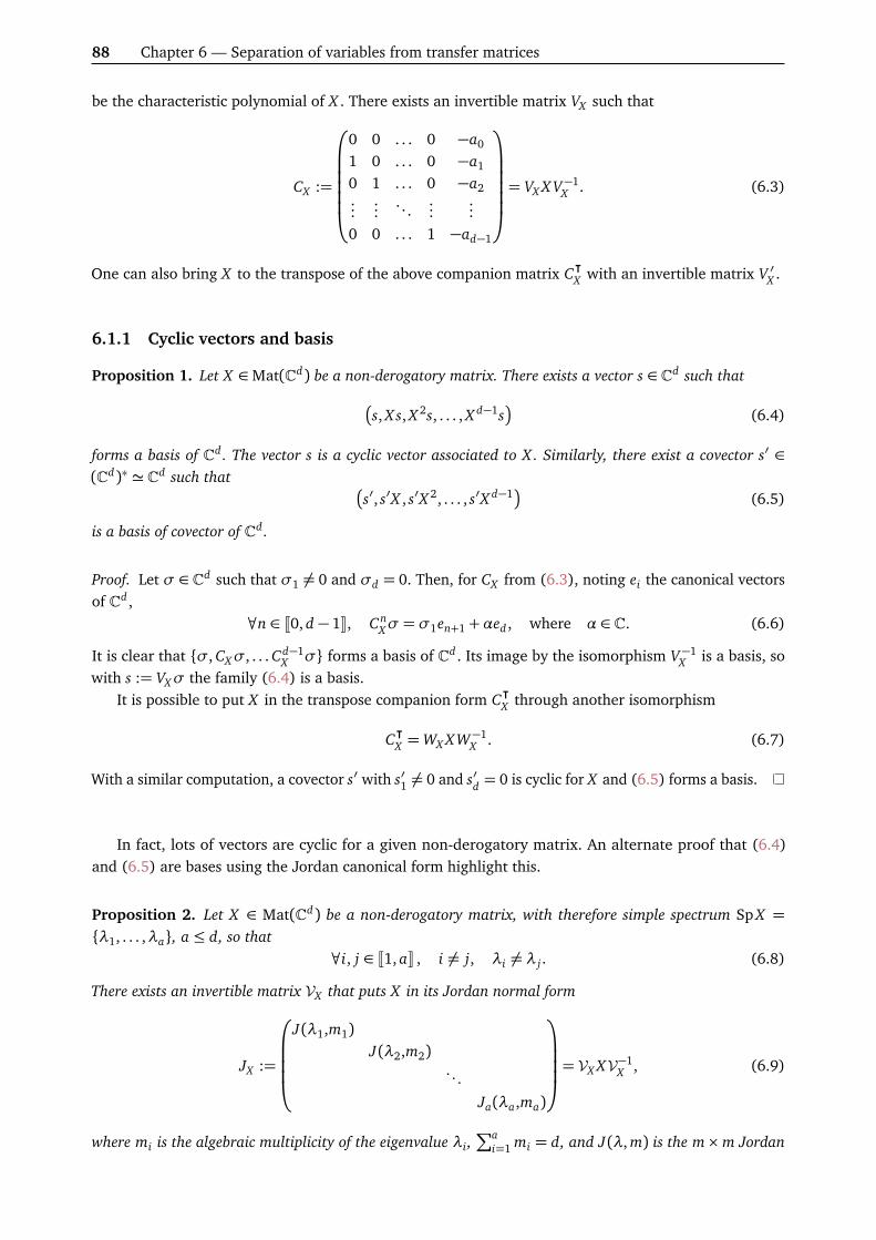
88 Chapter 6 — Separation of variables from transfer matrices
be the characteristic polynomial of X . There exists an invertible matrix VX such that
CX :=
0 0 . . . 0 −a0
1 0 . . . 0 −a1
0 1 . . . 0 −a2...
.... . .
......
0 0 . . . 1 −ad−1
= VX X V−1
X . (6.3)
One can also bring X to the transpose of the above companion matrix CᵀX with an invertible matrix V ′X .
6.1.1 Cyclic vectors and basis
Proposition 1. Let X ∈Mat(Cd) be a non-derogatory matrix. There exists a vector s ∈ Cd such that
s, Xs, X 2s, . . . , X d−1s
(6.4)
forms a basis of Cd . The vector s is a cyclic vector associated to X . Similarly, there exist a covector s′ ∈(Cd)∗ ' Cd such that
s′, s′X , s′X 2, . . . , s′X d−1
(6.5)
is a basis of covector of Cd .
Proof. Let σ ∈ Cd such that σ1 6= 0 and σd = 0. Then, for CX from (6.3), noting ei the canonical vectorsof Cd ,
∀n ∈ J0, d − 1K, CnXσ = σ1en+1 +αed , where α ∈ C. (6.6)
It is clear that σ, CXσ, . . . Cd−1X σ forms a basis of Cd . Its image by the isomorphism V−1
X is a basis, sowith s := VXσ the family (6.4) is a basis.
It is possible to put X in the transpose companion form CᵀX through another isomorphism
CᵀX =WX XW−1X . (6.7)
With a similar computation, a covector s′ with s′1 6= 0 and s′d = 0 is cyclic for X and (6.5) forms a basis.
In fact, lots of vectors are cyclic for a given non-derogatory matrix. An alternate proof that (6.4)and (6.5) are bases using the Jordan canonical form highlight this.
Proposition 2. Let X ∈ Mat(Cd) be a non-derogatory matrix, with therefore simple spectrum Sp X =λ1, . . . ,λa, a ≤ d, so that
∀i, j ∈ J1, aK , i 6= j, λi 6= λ j . (6.8)
There exists an invertible matrix VX that puts X in its Jordan normal form
JX :=
J(λ1,m1)J(λ2,m2)
. . .Ja(λa,ma)
= VX XV−1
X , (6.9)
where mi is the algebraic multiplicity of the eigenvalue λi ,∑a
i=1 mi = d, and J(λ, m) is the m×m Jordan

6.1. Foreword: non-derogatory matrices 89
block
J(λ, m) =
λ 1 0 · · · 00 λ 1 · · · 0...
......
. . ....
0 0 0 λ 10 0 0 0 λ
. (6.10)
Let S be a covector in (Cd)∗ and note
SVX =s(1)1 , . . . , s(1)m1
, . . . , s(a)1 , . . . , s(a)ma
. (6.11)
Ifa∏
i=1
s(i)1 6= 0, (6.12)
then the familyS, SX , . . . , SX d−1
is a basis of covectors.
Proof. Noting Ei := V−1X ei the image of the canonical basis by V−1
X , the familyS, SX , . . . , SX d−1
is a
basis if there exists an invertible bijective maping with another basis, for example the canonical one. Thisis the case if the determinant of the d × d matrix M, defined by its coefficients
Mi j = SX i−1E j , (6.13)
is non-zero. Thanks to the block diagonal form, this determinant is the product of the determinant ineach Jordan block J(λi , mi). Using standard linear algebra techniques [see 225, proposition 2.2], oneeventually computes
detM=a∏
i=1
s(i)1
mi∏
1≤i< j≤a
(λ j −λi)mi m j , (6.14)
proving the desired result.
The above proposition also holds for cyclic bases of vectors, but we anticipate on the integrable modelcase, where we will mainly use a basis of covectors similar to this one.
Remark 1 (Centralizer of X ). Let
CX = M ∈Mat(Cd) | [M , X ] = 0 (6.15)
be the centralizer of a non-derogatory matrix X . Because the minimal polynomial of X coincides with itscharacteristic polynomial, CX has dimension d and consists in the set of matrices which are polynomialsin X with coefficients in C [226]. Hence, the family (1, X , . . . , X d−1) is a basis of the vector space CX .Products of two powers of X re-decompose as a linear combination of powers smaller than d − 1. ForX · X d−1 = X d , this is computed explicitly from the minimal/characteristic polynomial, see (6.21).
6.1.2 Spectrum and eigenvectors
The cyclic basis is useful in the study of the eigenvectors of X : for a given eigenvalue, the unique associatedeigenvector is fully determined by its coefficients in the cyclic basis, which are easily computed to bepowers of the eigenvalue. From now on we will use braket notation.
Proposition 3. Let X ∈Mat(Cd) be a non-derogatory matrix. Let ⟨S| := s′ and ⟨ fn| := ⟨S|X n−1. A vector|λ⟩ ∈ Cn is an eigenvector of X of eigenvalue λ if and only if
∀n ∈ J1, dK , ⟨ fn|λ⟩= λn−1 ⟨S|λ⟩ . (6.16)

90 Chapter 6 — Separation of variables from transfer matrices
Proof. Suppose |λ⟩ 6= 0 is an eigenvector of X with eigenvalue λ. Then (6.16) is verified immediately,but one should check that ⟨S|λ⟩ 6= 0. Because the ⟨ fn| form a basis of Cn, the dual vectors
| fn⟩ := ⟨ fn|∗ =X ᵀn−1(s′)ᵀ (6.17)
form a basis of Cn. Since |λ⟩ 6= 0 and
|λ⟩=d∑
n=1
⟨ fn|λ⟩⟨ fn| fn⟩
| fn⟩= ⟨S|λ⟩d∑
n=1
λn−1
⟨ fn| fn⟩| fn⟩ , (6.18)
necessarily ⟨S|λ⟩ 6= 0 and (6.16) indeed holds.Consider now a vector |v⟩ ∈ Cd such that ⟨S|v⟩ 6= 0 and for an eigenvalue λ ∈ Sp(X ), it holds
∀n ∈ J1, dK , ⟨ fn|v⟩= λn−1 ⟨S|v⟩ . (6.19)
Is |v⟩ the eigenvector of X of eigenvalue λ? For n< d,
⟨ fn|X |v⟩= ⟨S|X n |v⟩= ⟨ fn+1|v⟩= λ ⟨ fn|v⟩ , (6.20)
which puts us on good track. For n = d, the vector ⟨ fd |X = ⟨S|X d is no longer a vector of the ⟨ fn|basis. However, the power X d can be rewritten thanks to the characteristic polynomial of X : by theCayley–Hamilton theorem, X satisfies its characteristic equation
χX (X ) = 0= X d + ad−1X d−1 + · · ·+ a1X + a0. (6.21)
This effectively decomposes the right action of X on ⟨ fd | over the ⟨ fn| basis
⟨ fd |X |v⟩= −d−1∑n=0
an ⟨S|X n|v⟩= −d−1∑n=0
an ⟨ fn+1|v⟩= −⟨S|v⟩d−1∑n=0
anλn. (6.22)
Because λ ∈ Sp(X ), χX (λ) = 0 so we reconstruct λd in the above equation. Therefore,
⟨ fd |X |v⟩= λd ⟨S|v⟩= λ ⟨ fd |v⟩ . (6.23)
Eventually, this proves that |v⟩ is the eigenvector of X of eigenvalue λ— and may be noted |λ⟩ := |v⟩.
This discussion on non-derogatory matrices shows that a basis may be constructed by repeated actionon a cyclic vector. This basis is especially useful for their spectral problem, because the eigenvectors’decomposition in the | fn⟩= ⟨ fn|∗ basis is entirely determined by powers of corresponding eigenvalue, upto an overall normalization fixed by ⟨S|λ⟩. Hence, in such a basis, we can construct explicitly the uniqueeigenvector (up to a non-zero normalization) as soon as we know the eigenvalue. This is a very handyresult, as it is often possible, and easier, to compute only the eigenvalues.
“Constructing a basis that facilitates the spectral problem” is clearly of prime interest for quantumintegrable models. In the context of quantum integrability, can one construct a separate basis with similarproperties as the ones of non-derogatory matrices? We investigate this in the next section.

6.2. Separate basis from conserved quantities 91
6.2 Separate basis from conserved quantities
6.2.1 Basis from conserved quantities
While Sklyanin’s SOV sounds a promising tool which could supersede ABA techniques, the identificationof the A(u) and B(u) operators are in general not trivial. All the more so as it is also required to provenon-immediate properties, such as the diagonalizability of B(u), then characterize its spectrum and proveits simplicity, and ensure the A(u) operator evaluated in the spectrum of B(u) indeed perform shifts onthe B(u) spectrum.
Even for the rank one gl(2) case, there are models for which such a program cannot be completed,for example the XXZ chain with a diagonal twist. Working with a greater algebra make the picture moreinvolved. In the gl(3) case, we already investigated how the expression of A(u) given by Sklyanin cannotperform the desired shift over the full spectrum of B(u). This is essentially because it is not anymore apolynomial in the monodromy matrix entries.
These observations provide strong motivation to look for a more universal construction of SOV inquantum integrable models. Integrability leverages the conserved quantities to ensure solvability. Couldthey be used to developing a separation of variables as well?
It appears they can: repeated action of the transfer matrix evaluated in the inhomogeneities on acertain covector produce a basis, which is immediately separate for the spectral problem of the transfermatrix itself. The key point in this construction is that it relies on the very object we ought to diagonalize.This overcomes entirely the identification of the A(u) and B(u) operator families and the proofs of theirrequired properties. Besides, this SOV construction applies for a larger class of models. It generalizes tohigher rank rather trivially, though the details of the use of the basis to solve the spectral problem aremuch more tedious than in the gl(2). We discuss them in section 6.2.5.
Consider the Y (gl(n)) chain of length N with the commuting family of transfer matrices (T (u))u∈C,∀u, v ∈ C, [T (u), T (v)] = 0, and Hilbert spaceH . Suppose one can construct dimH matrices from T (u)gathered in N sets
T (a)0 , . . . , T (a)da−1, (6.24)
with a ∈ J1, NK, and∏N
a=1 da = dimH . Some functional f (a)haof the (T (u))u∈C family are such that these
matrices are obtained from the transfer matrix T : C→ End(H )
T (a)ha= f (a)ha
T. (6.25)
For any N -tuple in I = J0, d1 − 1K× · · · × J0, dN − 1K, we note
T~h :=N∏
a=1
T (a)ha(6.26)
the dimH possible products made by picking one operator in each set. Because the T (a)haare functions of
the (T (u))u∈C family, they commute together and with T (u) for any u ∈ C, and so do the T~h. We note
CT := X ∈ End(H ) | ∀u ∈ C, [X , T (u)] = 0 . (6.27)
Suppose there exists ⟨S| ∈ H ∗ such that the dimH covectors
⟨~h| := ⟨S| T~h (6.28)

92 Chapter 6 — Separation of variables from transfer matrices
form a basis ofH ∗. LetG(⟨S|) :=
⟨S| T~h | ~h ∈ I
(6.29)
Proposition 4. If G(⟨S|) is a basis ofH ∗, then the family T (u) has simple spectrum. Moreover, the family(T~h)~h∈I is a complete set of commuting matrices, i.e. it has simple common spectrum.
Proof. Let |t⟩ , |t ′⟩ ∈ H be two non-zero eigenvectors of the T(u), u ∈ C, associated to the sameeigenvalue t(u) ∈ Fun(C,C). Because T~h ∈ CT , |t⟩ and |t ′⟩ are also eigenvectors of T~h. We note t~hthe associated eigenvalue, which is the same for |t⟩ and |t ′⟩ and is determined from the eigenvaluet : u 7→ t(u) by the knowledge of the functionals (6.25):
t~h =N∏
a=1
t(a)ha=
N∏a=1
f (a)~ha[t] for all ~h ∈ I. (6.30)
We abuse the notation t(a)~ha
to also refer to the functionals from Fun(C,C) to C derived from (6.25). The
wavefunctions of |t⟩ in the basis G(⟨S|) are
⟨~h|t⟩= ⟨S|t⟩ t~h and ⟨~h|t ′⟩= ⟨S|t ′⟩ t~h (6.31)
Because |t⟩ 6= 0, ⟨S|t⟩ 6= 0, and the same holds for |t ′⟩. With a renormalization of |t ′⟩, one can put⟨S|t ′⟩= ⟨S|t⟩ in all generality. Then,
∀~h ∈ I, ⟨~h| |t⟩ − |t ′⟩= ⟨~h|t⟩ − ⟨~h|t ′⟩= ⟨S|t⟩ t~h − t~h= 0. (6.32)
The image of |t⟩ − |t ′⟩ under the basis of linear forms ⟨~h| is zero, so this vector is zero. Henceforth, thecommon spectrum of (T (u))u∈C family is simple
Moreover, the T~h commute together, as functions of T(u), and share the same eigenvectors withT (u). For |t⟩ , |t ′⟩ ∈ H two eigenvectors of the family (T~h)~h∈I with the same eigenvalues t~h, the abovediscussion holds starting from (6.31), so that |t⟩= |t ′⟩, and |t⟩ is defined by its wavefunctions in G(⟨S|).Therefore, the family (T~h)~h∈I is a complete set of commuting matrices, namely it has simple commonspectrum.
Proposition 5. If G(⟨S|) is a basis ofH ∗, then the T~h form a basis of the centralizer CT of (T (u))u∈C.
Proof. Suppose there exist a linear relation between the T~h, i.e. there exist coefficients λ~h ∈ C, not allzero, such that ∑
~h∈Iλ~hT~h = 0. (6.33)
Then, acting on ⟨S| by the right, ∑~h∈Iλ~h ⟨~h|= 0, (6.34)
so this would imply that G(⟨S|) is not a basis. By contraposition, if G(⟨S|) is a basis of H ∗, the T~h arenecessarily a free family. Besides, the family (T(u))u∈C has simple spectrum by proposition 4, so itsminimal polynomial coincide with its characteristic polynomial and its centralizer CT has dimensiondimH . The family (T~h)~h∈I is a free family in CT of cardinal dimH , and therefore is a basis of thematrices that commute with the (T (u))u∈C family.
By proposition 5, for T (u) ∈ CT at generic value u ∈ C, it can be decomposed as a linear combinationon the T~h family, which is a basis of CT . Therefore, there exists functions C~h(u) such that
T (u) =∑~h∈I
C~h(u)T~h for all u ∈ C. (6.35)

6.2. Separate basis from conserved quantities 93
The product of two matrices T~h, T~k is in CT as well, so the T~h are dim(H ) generators of an associativeabelian algebra with relations
T~h · T~k =∑~∈I
C~
~h,~kT~. (6.36)
The C ~~h,~k
are numerical coefficients that satisfy the associativity and commutativity constraints, namely
C~
~h,~k= C
~
~k,~h, (6.37)
∑~p∈I
C ~p~h,~k
C ~q~p,~=∑~p∈I
C ~p~k,~
C ~q~h,~p
. (6.38)
Relations (6.36) also holds at the eigenvalue level
t~h · t~k =∑~∈I
C~
~h,~kt~. (6.39)
The functions C~h(u) and the constant numbers C ~~h,~k
are fixed by the model at hand and the choice of the
T (a)haoperators. With the decomposition of the transfer matrix over the T~h, one also has
T (u) · T~k =∑~h∈I
C~h(u) T~h · T~k =∑~h,~∈I
C~h(u)C~
~h,~kT~. (6.40)
The relations (6.39) can serve as a characterization of the transfer matrix spectrum. Let
Σ :=
(x~h~h∈I
∀~h, ~k ∈ I, x~h · x~k =∑~∈I
C~
~h,~kx~ and ∃~h ∈ I, x~h 6= 0
)(6.41)
be the set of dimH -tuples of complex numbers solutions to the (dimH )(dimH + 1)/2 quadraticequations (6.39).
Theorem 4. If G(⟨S|) is a basis of H ∗, then every eigenvalue in Sp(T(u)) is characterized uniquely by atuple of Σ. Namely, there is a bijection between Sp(T (u)) and Σ.
Proof. Suppose G(⟨S|) is a basis. Then the transfer matrix has simple spectrum, and the unique eigenvector|t⟩ associated to t(u) ∈ Sp(T (u)) is an eigenvector of the T~h as well, with eigenvalues t~h defined in (6.30).Obviously the tuple
t~h~h∈I is in Σ—this is seen easily by computing the action of the T~h · T~k over |t⟩.
Consider nowx~h~h∈I ∈ Σ different from the zero tuple. We construct the non-zero vector |x⟩ by
fixing its images under the basis of linear forms ⟨~h|
∀~h ∈ I, ⟨~h|x⟩= x~h. (6.42)
One has
⟨~h|T (u)|x⟩= ⟨S|T~h · T (u)|x⟩= ⟨S|T~h∑~k∈I
C~k(u)T~k|x⟩
=∑~k,~∈I
C~k(u)C~
~h,~k⟨S|T~|x⟩=
∑~k,~∈I
C~k(u)C~
~h,~kx~ (identifying ⟨~|x⟩)
= x~h ·∑~k∈I
C~k(u)x~k (using relations (6.41)).
(6.43)

94 Chapter 6 — Separation of variables from transfer matrices
Hence, defining the functionτx(u) :=
∑~k∈I
C~k(u)x~k, (6.44)
one has that∀~h ∈ I, ⟨~h|T (u)|x⟩= ⟨~h|x⟩τx(u). (6.45)
Therefore, |x⟩ is an eigenvector of T (u) with eigenvalue τx(u). Two different tuples of Σ cannot yield thesame eigenvalue: let (x~h)~h, (y~h)~h ∈ Σ, (x~h)~h 6= (y~h)~h such that τx(u) = τy(u). Then the two states |x⟩and |y⟩, having different images under the basis of linear form ⟨~h|, are different eigenvectors of T(u),yet with the same eigenvalue. This is not possible, since T (u) has simple spectrum.
Hence, every eigenvalue t(u) of T (u) is associated to a unique tuplet~h~h∈I in Σ, and any tuple of Σ
defines an eigenvalue of T (u). Therefore, #Σ= # Sp(T (u)), and the two sets are in bijection. One wayis realized by the f (a)ha
functions, and the other by the linear combination (6.44) with the coefficientsC~h(u).
Hence, whenever a basis of the form G(⟨S|) can be constructed, the spectrum of the transfer matrixhas a characterization in terms of solutions of a system of quadratic equations given by the relationsbetween the generators of the centralizer of T (u) that constructs the basis.
However, the number of relations (6.39) is a priori dimH (dimH + 1)/2, which in case of quantumlattice models is exponential in the number of sites, since dimH =∏N
j=1 m j , where m j is the dimension ofthe representation of gl(n) at site j ∈ J1, NK. For quantum models constructed from a Yang–Baxter algebra,one observes a drastic reduction of the number of relations necessary to characterize the spectrum. Thisis the hallmark of integrability. Thanks to the fusion relations holding between the transfer matrices ofthese models, the number of relations implying the full relations (6.39) becomes in such case polynomialin the number of sites. Such a reduction from an exponential to a polynomial dependency in the numberof sites N happens due to the possible careful choice of the set of the T~h in integrable models. We willgive several examples of such reduction in the remaining of this thesis. For now, let us give here a toyexample of this phenomenon.
A toy situation is the one where the relations remain local in the indices of the N -tuples ~h. Within ournotation, the wavefunctions of eigenstates are already factorized
⟨~h|t⟩= ⟨S|t⟩N∏
a=1
t(a)ha. (6.46)
Suppose the actions are moreover local in the indices ha of the N -tuples of I, that is
T (a)i · T (a)j =da∑
k=1
c(a),ki j T (a)k , (6.47)
with some fixed numerical coefficients cki j. The knowledge of the ck
i j coefficients completely fixes therelations (6.36), by
T~h · T~k =N∏
a=1
T (a)ha· T (a)ka
=N∏
a=1
da∑`a=1
c(a),`ahaka
T (a)`a≡∑~∈I
C~
~h,~kT~. (6.48)
Rather than the system of equations given in (6.41), it is now simpler to consider N systems. For all

6.2. Separate basis from conserved quantities 95
a ∈ J1, NK, let
Σa :=
(x (a)1 , . . . , x (a)da
∀i, j ∈ J1, daK , x (a)i x (a)j =da∑
k=1
c(a),ki j x (a)k and ∃ j ∈ J1, daK , x (a)j 6= 0
)
(6.49)be the set of da-tuples of complex numbers solutions to the da(da + 1)/2 quadratic equations (6.47).
Proposition 6. If G(⟨S|) is a basis ofH ∗, and if the T (a)i multiply locally as in (6.47), then every eigenvaluein Sp(T(u)) is characterized uniquely by N tuples picked from Σ1, . . . ,ΣN . Namely, there is a bijectionbetween Sp(T (u)) and Σ1 × · · · ×ΣN .
Proof. Let |t⟩ be an eigenvector of T(u) of eigenvalue t(u). It is also an eigenvector of the T (a)ha, with
eigenvalues t(a)ha. It is clear that the (t(a)1 , . . . , t(a)da
) are da-tuples of complex numbers in Σ∗a, and this forevery a ∈ J1, NK.
Consider now (x (a)1 , . . . , x (a)d1) ∈ Σa, for every a ∈ J1, NK. We construct the vector |x⟩ ∈ H from its
image by the linear form ⟨~h|:∀~h ∈ I, ⟨~h|x⟩=
N∏a=1
x (a)ha. (6.50)
Then, by a proof similar to the one of Theorem 4, one proves that |x⟩ is an eigenvector of T(u) ofeigenvalue
τx(u) =∑~k∈I
C~k(u)N∏
a=1
x (a)ha. (6.51)
With such local actions for the T (a)ha, the discrete characterization of the spectrum by the set of solutions
Σ is separate in a product of N sets Σ1, . . . ,ΣN . The system of equations (6.41) has been decoupledin the N independent systems (6.49), each of rank da(da + 1)/2. This is a great simplification of thespectrum characterization. Moreover, eigenvectors are obtained from their corresponding eigenvaluewith the knowledge of their image under the basis of linear forms ⟨~h|, which now has a factorized form.
In the following, we will give several example of quantum integrable models where a similar simplifi-cation can be made, although they are more intricate than the above toy model. In particular, in the nextsection where we take
T (a)ha= T (ξa)
ha , with ha ∈ J0,n− 1K , (6.52)
we will see that we observe a drastic simplification of most of the above relations (6.47) and (6.48). Thedifferent cases have been treated in a series of articles, covering the gl(2) case with fundamental [225]and higher spin representations [232], gl(3) and gl(n) models [234, 235], and supersymmetric gl(n|m)models [LV1].
6.2.2 Bases from the powers of the transfer matrix
Following the case of non-derogatory matrices, we can define a family of vectors of the form (6.28) withpowers of the transfer matrix evaluated in the inhomogeneities, and they will form a basis under someweak conditions on the twist and the inhomogeneities.
Theorem 5 ([225]). Consider the Yangian Y gl(n) R-matrix R(u) = ϕ(u)id+ϕ(η)P ∈ End(Cn ⊗Cn).The fundamental inhomogeneous twisted chain of length N, with Hilbert spaceH = ⊗N
j=1Cn, corresponds tothe monodromy matrix
M(u) = K0R0N (u− ξN ) . . . R01(u− ξ1), (6.53)

96 Chapter 6 — Separation of variables from transfer matrices
and its transfer matrix T (u) = tr0 M(u). If the twist matrix K is non-derogatory, the nN covectors
⟨~h| := ⟨S|N∏
j=1
T (ξ j)h j , (6.54)
labelled by the N-tuples ~h ∈ J1,nKN , form a basis ofH ∗ for generic inhomogeneities ξ j when ⟨S| is of theform
⟨S|= ⟨s| ⊗ · · · ⊗ ⟨s| , (6.55)
where ⟨s| is a cyclic vector of the twist matrix K.
Proof. Lete j
, j ∈ J1,nN K, be the canonical basis ofH , constructed by tensorization of vectors the local
canonical bases at each site. We define the square matrix M of size nN by its elements
Mi j =~h(i)
e j
, (6.56)
where ~h(i) is uniquely defined by
i = 1+N∑
a=1
ha(i)ai−1. (6.57)
The ⟨~h| form a basis ofH ∗ ifdet(M) 6= 0. (6.58)
The above determinant is a polynomial in the twist matrix entries, the inhomogeneities ξ j and thecoefficients
Se j
. It is sufficient to prove (6.58) in some limit in this parameter to prove it for almost all
values of them. Let us impose inhomogeneities that are scaled from a single value relatively to the sitethey are attached
∃ξ ∈ C, ∀ j ∈ J1, NK , ξ j = jξ. (6.59)
Because
T (ξa) = Raa−1(ξa − ξa−1) . . . Ra1(ξa − ξ1)KaRaN (ξa − ξN ) . . . Raa+1(ξa − ξa+1), (6.60)
T (ξa) is a polynomial in ξ of degree N − 1 and is of the form
T (ξa) = caξN−1Ka +O
ξN−2
given ca = (−1)N−a(a− 1)!(N − a)!. (6.61)
Therefore,~h= ξ(N−1)
∑Nj=1 h j ×
N∏
j=1
ch ja
!× ⟨S|
N∏j=1
Kh j
j +Oξ−1+(N−1)
∑Nj=1 h j
. (6.62)
The determinant of M is now a polynomial in ξ as well, of degree (N − 1)∑nN
i=1
∑Nj=1 h j(i) and dominant
coefficientnN∏i=1
N∏j=1
ch j(i)j det
M, (6.63)
where M is the matrix with coefficients
Mi j =S
N∏a=1
Kha(i)a
e j
. (6.64)

6.2. Separate basis from conserved quantities 97
Taking the covector ⟨S| in a tensor form of covector local in the site
⟨S|= ⊗Nj=1 ⟨S, j| where ⟨S, j| ∈ V∗j , (6.65)
the above determinant is factorized as a product of N determinants over square matrices of size n
detM=
N∏a=1
det(ma), (6.66)
where, using |e j⟩= ⊗Na=1 |e j(a)⟩,
(ma)i j =S, a
K i−1a
e j(a)
. (6.67)
Because K is a non-derogatory matrix, there exists a covector ⟨S, a| ∈ Va such that det(ma) 6= 0, thanksto proposition 1. Even better, proposition 2 gives explicit form of cyclic covector ⟨S, a| such that (6.54)forms a basis. Hence, there exists ⟨S| ∈ H ∗ such that det(M) 6= 0 for almost all values of the parametersit depends on.
The above theorem is a specialization of the discussion of the previous section, with
T~h =N∏
j=1
T (ξ j)hi with ~h ∈ J0, N − 1KN . (6.68)
These operators are now proven to form a basis of the Bethe algebra of the model. Thanks to the powerform of the basis, the relations (6.36) are not too complicated for many generators. If
∀ j ∈ J1, NK , h j + k j ≤ N − 1, (6.69)
then we simply haveT~h · T~k = T~h+~k. (6.70)
If there is only one j ∈ J1, NK such that h j+k j ≥ N , then it is necessary to compute the linear decompositionof a higher power on the ones smaller than N − 1. The characteristic polynomial is here of no help, sinceit is a polynomial of degree nN . However, the fusion relations can be used to compute this decomposition.Indeed, evaluated in the inhomogeneities, the fusion relations links products of transfer matrices tofused transfer matrix. The interesting point is that the one corresponding to the totally antisymmetricrepresentation, namely T (1)n (u), coincide with the quantum determinant which is a central element. Thisis seen easily in the gl(2) case: the relevant fusion relation is written in the inhomogeneities as
T (ξ j)T (ξ j −η) = q-det M(ξ j). (6.71)
While we do not have directly T (ξ j)2 = q-det M(ξ j), it is clear that this relation provides a reduction inthe power of the transfer matrix, which is 2 in the left-hand side and 0 in the right-hand side. To resolvethe inconvenience of having one transfer matrix shifted by η, it is possible to interpolate T(u) in thecorrect points to make use of the fusion relation to compute the decomposition of T~h · T (u) over the T~h.This is done in the proof of proposition 7.
The gl(n) case is more involved, because the successive use of the tower of n− 1 fusion relations torequires to interpolate once again between each step. We explain the procedure to compute T~h · T (u) inthis manner in section 6.2.5, where we give elements of the proof of the spectral problem of gl(n).
Note that the possibility to construct the basis (6.54) ensures that the transfer matrix T (u) itself isnon-derogatory. In fact, we have the following stronger result.

98 Chapter 6 — Separation of variables from transfer matrices
Lemma 1. If the matrix K has simple spectrum, then the transfer matrix has simple spectrum. Moreover, ifK is diagonalizable with simple spectrum, then T (u) itself is diagonalizable with simple spectrum.
Proof. Suppose K has simple spectrum, and let t(u) be an eigenvalue of T(u) and |t⟩ an eigenvectorassociated to t(u). Then,
⟨~h|t⟩=N∏
j=1
t(ξ j)h j ⟨S|t⟩ (6.72)
so |t⟩ is uniquely defined, up to an overall normalization, by the eigenvalue t(u). All eigenvalues havegeometric multiplicity of one, so T (u) is non-derogatory.
Let us now restrict to the case of K diagonalizable with simple spectrum. Noting
Sp(K) = k1, . . . , kn, (6.73)
we label the eigenvectors by their corresponding eigenvalue
⟨k j| and |k j⟩ , j ∈ J1,nK . (6.74)
The left and right eigenvectors of K form a basis of (Cn)∗ and Cn respectively. Tensoring N -times, weconstruct bases forH ∗ andH
⟨K , ~h| := ⊗Nj=1 ⟨kh j
| , |K , ~h⟩ := ⊗Nj=1 |kh j
⟩ . (6.75)
Taking the inhomogeneities as in (6.59), the above bases are eigenbases of the leading coefficient of thetransfer matrix polynomial expansion in ξ (6.61) of the T(ξ j). Thus, for some left eigenvector ⟨t| ofT (u), there exists a unique N -tuple ~h ∈ J1,nKN such that
lim|ξ|→+∞
1N←t (ξ)ξN−1
⟨t| T (ξ j ,ξ) = c jkh j⟨K , ~h| , (6.76)
for some proper normalization N←t (ξ). Reconstructing T (u) by Lagrange interpolation in the ξ j = jξ andsubtracting the dominant term, one can find that
lim|ξ|→+∞
1ξN−1
⟨t| T (u)− ξN (−1)N N ! tr K= (−1)N−1
N∑a=1
cakha
∏
b 6=ab=1
N
ba− b
⟨K , ~h| . (6.77)
The left-hand side of the above limit, once rewritten using Lagrange interpolation, has the same form asthe right-hand side. By the above limits, it has to hold
lim|ξ|→+∞
1N←t (ξ)
⟨t|= ⟨K , ~h| , lim|ξ|→+∞
1N→t (ξ)
|t⟩= |K , ~h⟩ (6.78)
with the proper normalizations N←t (ξ) and N→t (ξ) are fixed. Eventually, this implies that
lim|ξ|→+∞
=⟨t|t⟩
N←t (ξ)N→t (ξ)= ⟨K , ~h|K , ~h⟩= 1. (6.79)
In a non-trivial Jordan block, left and right eigenvectors are orthogonal. Here, ⟨t|t⟩ 6= 0, so the Jordanblock associated to the eigenvalue t(u) must be trivial, i.e. of size 1. Eventually, this makes the transfermatrix diagonalizable with simple spectrum.

6.2. Separate basis from conserved quantities 99
6.2.3 Separate property
The basis (6.54) is immediately seen to have the first features of a separate basis. Let |t⟩ be an eigenvectorof T (u) of eigenvalue t(u). Then, the wavefunction in the basis (6.54)
Ψ(~h) = ⟨~h|t⟩=N∏
j=1
t(ξ j)h j ⟨S|t⟩ , (6.80)
is factorized, with each factor depending on only one coordinate h j .Can we find some separate relations of the form (5.58)? The fusion relation (A.61) for gl(2), specialized
in the inhomogeneities, areT (ξ j)T (ξ j −η) = q-det M(ξ j). (6.81)
This clearly has the desired form; in the next section we show how it is used in the resolution of thespectral problem for the gl(2) case. For higher rank cases, the fusion relations shall provide separaterelations as well, but in a more intricate way, see section 6.2.5.
6.2.4 Spectral problem for gl(2) models
Consider the inhomogeneous XXX spin 1/2 chain with twisted boundary conditions. As anticipated, theseparate relations constraining the spectrum in this case are the fusion relations particularized in theinhomogeneities. These N relations form a system which select eigenvalues among a certain family offunctions determined by the analytic properties of the transfer matrix.
Proposition 7. The eigenvalues of T (u) are the polynomials t(u) in u of degree N and dominant coefficienttr K, verifying the N relations
∀ j ∈ J1, NK , t(ξ j)t(ξ j −η) = q-det M(ξ j), (6.82)
where the quantum determinant is the scalar
q-det M(u) = det KN∏
j=1
(u− ξ j +η)(u− ξ j − eta), (6.83)
which fix the N remaining coefficients. Explicitly, they are the polynomials
t(u) = tr KN∏
j=1
(u− ξ j) +N∑
a=1
N∏b=1b 6=a
u− ξb
ξa − ξbxa, (6.84)
where the N-tuple x1, . . . , xN is a solution to the linear system of N quadratic equations
xn
tr K
N∏j=1
(xn −η− ξ j) +N∑
a=1
N∏b=1b 6=a
xn −η− ξb
ξa − ξbxa
= q-det M(ξn) for n ∈ J1, NK . (6.85)
The unique eigenvector associated to the above eigenvalue is characterized by the factorized wavefunction inthe left SOV Basis
⟨~h|t⟩=N∏
j=1
t(ξ j)h j , (6.86)
with the normalization ⟨S|t⟩= 1.

100 Chapter 6 — Separation of variables from transfer matrices
Proof. It is immediate that any eigenvalue t(u) and associated unique eigenvector are of the above form,so one just needs to check the converse way. Consider the polynomial f (u) of degree N defined by itsvalues in the inhomogeneities xa := f (ξa), such that
∀a ∈ J1, NK , f (ξa) f (ξa −η) = q-det M(ξa). (6.87)
By Lagrange interpolation, f (u) can be written
f (u) = tr(K)uN +N∑
a=1
N∏b=1b 6=a
u− ξb
ξa − ξbxa, (6.88)
and then (6.87) is explicitly a system of N equations in the xa. We define the vector |v⟩ by imposing itscoordinates in the left SOV basis
⟨~h|v⟩=N∏
j=1
xh j
j . (6.89)
Consider ⟨~h| such that ha = 0 for some a ∈ J1, NK. Then,
⟨~h|T (ξa)|v⟩= ⟨h1, . . . , 1, . . . , hN |t⟩= f (ξa)N∏
j=1j 6=a
f (ξ j)h j = f (ξa) ⟨~h|v⟩ . (6.90)
Now, if ha = 1,
⟨~h|T (ξa −η)|v⟩= q-det M(ξa) ⟨h1, . . . , 0, . . . , hN |t⟩= f (ξa) f (ξa −η)N∏
j=1j 6=a
f (ξa)h j
= f (ξa −η)N∏
j=1
f (x j)h j = f (ξa −η) ⟨~h|v⟩ ,
(6.91)
thanks to (6.87). Given a fixed N -tuple ~h, and noting ξ(hi) = ξ−hiη, the transfer matrix and the functionf (u) are written by Lagrange interpolation similarly
T (u) = tr(K)uN +N∑
a=1
N∏b=1b 6=a
u− ξ(hb)b
ξ(ha)a − ξ(hb)
b
T (ξ(ha)a ) (6.92)
f (u) = tr(K)uN +N∑
a=1
N∏b=1b 6=a
u− ξ(hb)b
ξ(ha)a − ξ(hb)
b
f (ξhaa ), (6.93)
therefore∀u ∈ C, ⟨~h|T (u)|v⟩= f (u) ⟨~h|v⟩ . (6.94)
This holds for any ⟨~h| of (6.54). Because it is a basis,
∀u ∈ C, T (u) |v⟩= f (u) |v⟩ , (6.95)
so |v⟩ is an eigenvector with eigenvalue f (u) of the transfer matrix. It is unique since T(u) is non-derogatory.
Note that for any eigenstates |t⟩ one has ⟨S|t⟩ 6= 0 since |t⟩ 6= 0, otherwise the right-hand side

6.2. Separate basis from conserved quantities 101
in (6.89) always vanishes, which would contradict the fact that the ⟨~h| are a basis.
While the above proposition 7 gives a characterization of the spectrum through a quadratic system, itis possible to give a functional characterization as well by what is called the quantum spectral curve.
Proposition 8. Under the same assumptions as above, a polynomial t(u) is an eigenvalue of T(u) if andonly if there exists a unique polynomial Q t(u) of degree M ≤ N with no ξ j for its roots such that the couple(t(u),Q t(u)) lies on the quantum spectral curve
k21a(u)d(u)Q t(u− 2η)− k1a(u)t(u−η)Q t(u−η) + q-det M(u)Q t(u) = 0. (6.96)
Furthermore, the unique eigenvector |t⟩ associated to t(u) has the following wavefunctions in the SOV basis
⟨~h|t⟩= k∑N
j=1 h j
1
N∏j=1
Q t(ξ j). (6.97)
Proof. Let (t(u),Q t(u)) be a couple lying on the spectral curve. We note k2 the second eigenvalue of K —which might be equal to k1. Because ∀ j ∈ J1, NK , q-det M(u)(ξ j +η) = 0, equation (6.96) evaluated inpoints u= ξ j and u= ξ j +η produces the 2N equations for 1≤ j ≤ N
t(ξ j −η)Q t(ξ j −η)− k2d(ξ j −η)Q t(ξ j) = 0,
k1a(ξ j)Q t(ξ j −η)− t(ξ j)Q t(ξ j) = 0.(6.98)
Since Q t(ξ j) 6= 0 by hypothesis, multiplying the two equations gives
∀ j ∈ J1, NK , t(ξ j)t(ξ j −η) = det(K) a(ξ j)d(ξ j −η)≡ q-det M(ξ j), (6.99)
where one identify the quantum determinant in the right-hand side. This is exactly the spectrum charac-terization obtained in proposition 7, so t(u) is an eigenvalue of the transfer matrix. The wavefunctionsare recovered from (6.86) after an overall normalization.
Conversely, let t(u) be an eigenvalue of T(u). Let Q t(u) be a polynomial of degree M ≤ N , andconsider
P(u) = k21a(u)d(u)Q t(u− 2η)− k1a(u)t(u−η)Q t(u−η) + q-det M(u)Q t(u). (6.100)
The polynomial P(u) is easily proved to be of maximum degree 3N − 1, as the leading contribution inu2N+M vanishes. It is zero for all ξ j − η, because the scalar coefficients of the three terms are zero inthese points. The condition P(ξ j) = 0= P(ξ j +η) is equivalent to the systems (6.98) which reduces tothe N following equations thanks to the fusion relations (6.82)
∀ j ∈ J1, NK , t(ξ j)Q t(ξ j) = k1a(ξ j)Q t(ξ j −η). (6.101)
On can prove such a polynomial Q t(u) satisfying these conditions exists and is unique, as it is donein [218]1. The form of the unique eigenvector associated to t(u) then follows from (6.86) and the aboveequation.
6.2.5 Spectral problem for fundamental gl(n) models
Like in the gl(2) case, the characterization of the spectrum using the SOV basis (6.54) requires a subsetof the fusion equations. Noting Ta(u) the fused transfer matrices obtained from the antisymmetric repre-
1The form of the transfer matrix eigenvalues in terms of Q-functions is already accessible from the ABA.

102 Chapter 6 — Separation of variables from transfer matrices
sentations with a ∈ J1,nK, we recall that the relevant fusion relations are written in the inhomogeneitiesas
∀a ∈ J1,n− 1K , T (ξ j)Ta(ξ j −η) = Ta+1(ξ j), (6.102)
with the identifications T1(u)≡ T (u) and Tn(u) = q-det M(u).Let us defined a handler quantity which will be useful to write interpolation formula concisely. For all
integers a ∈ J1,nK and p ∈ J1, NK, we define
g(a)p (u) =N∏
q=1q 6=p
u− ξq
ξp − ξq
N∏j=1
a−1∏k=1
1
ξp − ξ(−k)j
, (6.103)
with ξ(k)j = ξ j − kη. Then the fused transfer matrix Ta(u) can be written by Lagrange interpolation in theinhomogeneities as
Ta(u) =N∏
j=1
a−1∏k=1
u− ξ j − kη
σa(K)
n∏j=1
(u− ξ j) +N∑
p=1
g(a)p (u)T (ξp)Ta−1(ξp −η), (6.104)
where σa(K) = tr1,...,a(P−1,...,aK1 . . . Ka) is the a-th elementary symmetric polynomial in the eigenvalues ofthe twist K .
The following results was obtained in [234].
Theorem 6. Suppose the family (6.54) is a basis of covectors ofH ∗ under some conditions we suppose verified,as stated by Theorem 5. Let x1, . . . , xN ∈ CN define the following polynomial by Lagrange interpolation inthe inhomogeneities
t(u) = tr KN∏
j=1
(u− ξ j) +N∑
a=1
g(1)a (u)xa. (6.105)
We can further define the n− 2 polynomials of degree aN for 2≤ a ≤ n− 1
ta(u) =N∏
j=1
a−1∏k=1
u− ξ j − kη
σa(K)
n∏j=1
(u− ξ j) +N∑
p=1
g(a)p (u)t(ξp)ta−1(ξp −η). (6.106)
If x1, . . . , xN is a solution of the system of N equations of order n in the x j
x j tn−1(ξ j −η) = q-det M(ξ j) for j ∈ J1, NK , (6.107)
then the polynomial t(u) defined above is an eigenvalue of the transfer matrix T(u)— and the ta(u) areeigenvalues of the Ta(u), respectively. Furthermore, the spectrum of T(u) is simple: the eigenvector |t⟩associated to a given eigenvalue t(u) is unique and is defined by its wavefunctions in the separate basis up toan overall normalization as
∀~h ∈ J0,n− 1KN , ⟨~h|t⟩=N∏
j=1
t(ξ j)h j . (6.108)
Proof. The proof follows the same line as the one for the gl(2) case. Since the successive functions ta(u)are constructed by the interpolation formulas originated from the fusion relations between the transfermatrices, it is immediate that any eigenvalue of T(u) has its values in the inhomogeneities x j = t(ξ j)verify the system (6.107).
Conversely, let x1, . . . , xN be a solution of (6.107) and f (u), f2(u), . . . , fn(u) be the polynomialsdefined recursively by Lagrange interpolations as in the statement of the theorem. Let |v⟩ ∈ H be the

6.2. Separate basis from conserved quantities 103
vector with wavefunctions
∀~h ∈ J0,n− 1KN , ⟨~h|v⟩=∏j=1
N f (u)h j . (6.109)
Then one can show after lengthy calculation leveraging the fusion relations for the transfer matrices andthe one verified by the f polynomials that
∀~h ∈ J0,n− 1KN , ,~hT (u)
v= f (u) ⟨~h|v⟩ . (6.110)
Hence, |v⟩ is an eigenstate of eigenvalue f (u), and we may note |t⟩ := |v⟩ and t(u) := f (u). The exactcomputations of (6.110) in the case of a N -tuple ~h with at least one entry equal to n− 1 follows thelines given in (6.43), where the coefficients C~k
~hare obtained indirectly by the successive use of the fusion
relations. Subtleties of the calculations are found in appendix A of reference [234].
A functional characterization is also known for gl(n) thanks to the spectral curve.
Proposition 9. Let t(u) be a polynomial of degree N. We construct the polynomials ta(u), 2 ≤ a ≤ n− 1from t(u) as in (6.106). Under the same assumptions as above, t(u) is an eigenvalue of T(u) if and onlyif there exists a unique polynomial Q t(u) of degree M ≤ N with no ξ j for its roots such that the couple(t(u),Q t(u)) lies on the quantum spectral curve of equation
n∑a=0
αa(u)Q t(u− aη)tn−a(u− aη) = 0. (6.111)
We make the identifications
t0(u)≡ 1, t1(u)≡ t(u), tn(u)≡ q-det M(u), (6.112)
and the coefficients αa(u) are defined as
∀a ∈ J0,nK , αa(u) = (−1)a+1ka1
a−1∏b=0
d(u− bη), (6.113)
where k1 is an eigenvalue of the twist matrix K. Moreover, the unique eigenvector |t⟩ associated to t(u) isdefined by its wavefunctions in the SOV basis up to an overall normalization as
∀~h ∈ J0,n− 1KN , ⟨~h|t⟩=N∏
j=1
α1(ξ j)Q t(ξ j −η)
haQ t(ξ j)n−1−h j (6.114)
Proof. The proof is very similar to the gl(2) case.For a couple (t(u),Q t(u)), evaluating (6.111) in the (n− 1)N points ξ j + kη, k ∈ J1,n− 1K, one can
prove that it holds
∀ j ∈ J1, NK , ∀a ∈ J1,n− 1K , t(ξ j)ta(ξ j −η) = ta+1(ξ j), (6.115)
such that by Theorem 6 t(u) is an eigenvalue of T (u), and the form of the wavefunction of |t⟩ follows.Conversely, if t(u) is an eigenvalue of T(u) and Q t(u) is some polynomial of degree M ≤ N . Con-
straining Q t(u) by imposing
∀ j ∈ J1, NK , ,α1(ξ j)Q t(ξ j −η) = t(ξ j)Q t(ξ j), (6.116)

104 Chapter 6 — Separation of variables from transfer matrices
which is equivalent to place (t(u),Q t(u)) on the quantum spectral curve, one can prove Q t(u) exists andis unique. Details can be found in the appendix B of reference [234]. The form of the wavefunctions ofthe eigenvector |t⟩ follows easily.
6.3 Link with Sklyanin SOV in the gl(2) case
In the gl(2) case, for a certain choice of the covector ⟨S|, the basis (5.59) made from the power of thetransfer matrix coincide with the Sklyanin’s original SOV basis, namely the eigenbasis of the B(u) = M12(u)entry of the monodromy.
Proposition 10. Let
⟨~h|Skl := ⟨0|N∏
j=1
AK(ξ j)
a(ξ j)
h j
, with ~h ∈ 0, 1N , (6.117)
which are the vectors defined in (5.125) up to a scalar factor. For ⟨S|= ⟨0|= ⊗Nj=1
1, 0
,
⟨~h|= ⟨~h|Skl . (6.118)
Proof. The proof is made by induction. For ~h= (0, . . . , 0), then obviously
⟨~0|= ⟨S|= ⟨0|= ⟨~0|Skl , (6.119)
and (6.118) is verified.Take ` ∈ J1, NK and suppose that for any ~h ∈ 0,1N such that
∑Nj=1 h j = `, equality (6.118) is
verified. Let ~h ∈ 0,1N be the specific N -tuple with
h j =
(1 for 1≤ j ≤ `,0 otherwise.
(6.120)
We have
⟨~h|D(ξ`+1) = ⟨~h|Skl D(ξ
`+1) = ⟨0| ∏
j=1
A(ξ j)
a(ξ j)
!D(ξ
`+1), (6.121)
and using (Y.16) one time, it gives
⟨~h|D(ξ`+1) = ⟨0|
`−1∏j=1
A(ξ j)
a(ξ j)
!D(ξ`+1)A(ξ`)− g(ξ`+1,ξ`)
B(ξ`)C(ξ`+1)− B(ξ`+1)C(ξ`)
. (6.122)
The covector ⟨0|∏`−1
j=1 A(ξ j)a(ξ j)
is an eigencovector of B(u), whose eigenvalue vanishes in the ξ j,
j ≤ ` (see (5.126)). Therefore, the two contributions in B are zeros, and everything happens as the Aand D have commuted together. Iterating on this, one can bring D(ξ`+1) all to the left of the product ofA(ξ j) operators. Since ⟨0|D(ξ j) = ⟨0| d(ξ j) = 0, it means that the action (6.121) is zero. Hence, notinge j the N -tuple with 1 at the j-th position and 0 everywhere else,
⟨~h+ e`+1|= ⟨~h| T (ξ`+1) = ⟨~h|Skl A(ξ`+1) = ⟨~h+ e`+1|Skl . (6.123)
From every N -tuple of sum `, we can rearrange the indices by a permutation and perform the abovecomputation. Hence, we have just proven equality (6.118) for N -tuples of sum `+ 1.
Eventually, this proves (6.118) by induction over `.
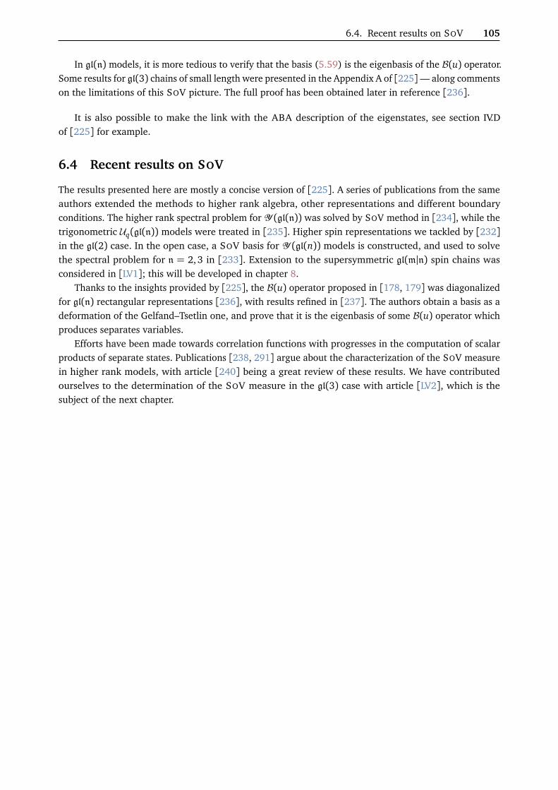
6.4. Recent results on SOV 105
In gl(n) models, it is more tedious to verify that the basis (5.59) is the eigenbasis of the B(u) operator.Some results for gl(3) chains of small length were presented in the Appendix A of [225]— along commentson the limitations of this SOV picture. The full proof has been obtained later in reference [236].
It is also possible to make the link with the ABA description of the eigenstates, see section IV.Dof [225] for example.
6.4 Recent results on SOV
The results presented here are mostly a concise version of [225]. A series of publications from the sameauthors extended the methods to higher rank algebra, other representations and different boundaryconditions. The higher rank spectral problem for Y (gl(n)) was solved by SOV method in [234], while thetrigonometric Uq(gl(n)) models were treated in [235]. Higher spin representations we tackled by [232]in the gl(2) case. In the open case, a SOV basis for Y (gl(n)) models is constructed, and used to solvethe spectral problem for n = 2,3 in [233]. Extension to the supersymmetric gl(m|n) spin chains wasconsidered in [LV1]; this will be developed in chapter 8.
Thanks to the insights provided by [225], the B(u) operator proposed in [178, 179] was diagonalizedfor gl(n) rectangular representations [236], with results refined in [237]. The authors obtain a basis as adeformation of the Gelfand–Tsetlin one, and prove that it is the eigenbasis of some B(u) operator whichproduces separates variables.
Efforts have been made towards correlation functions with progresses in the computation of scalarproducts of separate states. Publications [238, 291] argue about the characterization of the SOV measurein higher rank models, with article [240] being a great review of these results. We have contributedourselves to the determination of the SOV measure in the gl(3) case with article [LV2], which is thesubject of the next chapter.


7Chapter
Towards the dynamics inhigher rank: scalar productsfor gl(3) in SOV
This chapter is devoted to the results obtained in the article [LV2]. As we have shown in the previouschapter, one can construct left and right separate bases ⟨~h|, |~h⟩ for the fundamental Y (gl(n)) model inparticular, using powers of the transfer matrix in the inhomogeneities for example. Eigenstates are thencharacterized by their factorized wavefunctions in the left separate basis. One would like to computescalar products of these eigenstates, paving the way towards form factors and correlation functions.
In the first section of this chapter, we introduce the bases p⟨~h| and |~h⟩p orthogonal to the left andright separate bases, and the SOV measure M that computes scalar product of separate states.
We then consider the gl(2) fundamental chain case, and show that the left and right separate basesobtained earlier for these models are orthogonal with respect to the canonical scalar product of theHilbert space. More precisely, |~h⟩p =
~h and p⟨~h| = ⟨~h|. This makes the computation of the SOV measurerelatively easy, and we compute it exactly.
The higher rank case of the gl(3) fundamental chain is more intricate. Using bases of the form (6.28),we have been are able to construct only pseudo-orthogonal left and right SOV bases at best. That is,though one has equality for a certain amount of tuples ~h, one has |~h⟩p 6= |~h⟩ in general. In the thirdsection, we give pseudo-orthogonal separate bases for the gl(3) fundamental model, and characterizecompletely their pseudo-orthogonality in terms of the diagonal coupling ⟨~h|~h⟩ of the separate bases; Thisallows us to give the form of SOV measure, once again in terms of the diagonal couplings, by computingthe decomposition of a generic |~h⟩p vector as a linear decomposition over the separate basis of the |~h⟩.
Comparing with the gl(2) case, the picture for non-orthogonal separate bases gets so more complexthat it is desirable to construct orthogonal left and right separate bases for the gl(3) case as well. In thefourth and last section of this chapter, we remark that orthogonality of the separate bases is achieved inthe limit of non-invertible twist (with simple spectrum), and compute scalar product of separate states inthis case. We then proceed to describe the existence and properties of an operator T(u), defined by itseigenvalues and eigenvectors and commuting with the transfer matrices, that can be substituted to thetransfer matrix to construct left and right separate bases that are indeed orthogonal.
7.1 Generalities on scalar products of separate states and SOV measure
7.1.1 Dual states of SOV left and right bases
Consider the Y (gl(n)) twisted inhomogeneous fundamental model. We note (·, ·)H the scalar product ofthe Hilbert spaceH = CnN of the model. We may take it to be the dot product for the canonical basis:noting ei the vectors of the canonical basis ofH , it simply gives
∀i, j ∈ J1,nNK , (ei , e j)H = δi j . (7.1)
The induced norm is ‖a‖H := (a, a)H . A similar notation is used for the scalar product on the dual spacewith (·, ·)H ∗ and ‖·‖H ∗ .
107

108 Chapter 7 — Towards the dynamics in higher rank: scalar products for gl(3) in SOV
Consider now the left and right SOV bases made from the powers of the transfer matrices
⟨~h| := ⟨L|N∏
j=1
T (ξ j)h j , (7.2)
|~h⟩ :=N∏
j=1
T (ξ j)h j |R⟩ . (7.3)
A very important point is that a priori ⟨~h| is not the dual of |~h⟩ by the canonical conjugation H 'H ∗.Indeed, the adjoint of a vector of the right SOV basis decomposes as a non-trivial linear combination onthe left SOV basis yet to characterize
|~h⟩† =∑~p
c~p ⟨~p| , (7.4)
and similarly for ⟨~h|†. The notation could therefore be misleading, so we will clarify it. It is misleadingin the sense that for |ψ⟩ ∈ H , the corresponding bra is usually by definition the unique linear form onH obtained by taking the adjoint, as in ⟨ψ| := |ψ⟩†, and then the braket is used to denote the scalarproduct involving the corresponding ket: ⟨ψ|ϕ⟩= (|ψ⟩ , |ϕ⟩)H . Here, for the notations (7.2) and (7.3),this is not the case. The left and right states ⟨~h| and |~h⟩ are just notations attached to the covectors andvectors defined in (7.2) and (7.3). In this sense, the braket
⟨~h|~k⟩ (7.5)
is the action of the linear form ⟨~h| in H ∗ on a vector |~k⟩ of H , with no relation a priori induced bythe natural isomorphism H ∗ ' H . The only common point is that they are both labelled by N -tuplein I := J0,n− 1KN . We can thus refer to the above brakets as a mere coupling between covectors andvectors. Let us stress again that in this notation,
∀~h, ~k ∈ I, ⟨~h|~k⟩ 6= |~h⟩† , |~k⟩ H . (7.6)
Orthogonal states We introduce the 2× nN orthogonal states
|~h⟩p ∈H and p⟨~h| ∈ H ∗ (7.7)
defined as the unique states such that1
∀~ ∈ I, p⟨~h|~k⟩= δ~h,~k ⟨~h|~h⟩= ⟨~k|~h⟩p. (7.8)
We noteN~h := ⟨~h|~h⟩ . (7.9)
Since |~h⟩ and
|~h⟩p
are Hilbert space bases, we have the closure relations
IdH =∑~h∈I
~h p
~h
N~h=∑~h∈I
~hp
~h
N~h. (7.10)
The closure relation gives the linear decomposition of the orthogonal states on the left and right SOVbases
~hp =∑~k∈I
p⟨~k|~h⟩pN~k
~k and p
~h=
∑~k∈I
p⟨~h|~k⟩pN~k
~k , (7.11)
1This is the notation introduced in article [LV2] at section 3.3. The index p is a shorthand for perpendicular.

7.1. Generalities on scalar products of separate states and SOV measure 109
which are a more explicit rewriting of (7.4), and the SOV left and right states decompose similarly onthe states (7.7)
~h=∑~k∈I
~k~h
N~k
~kp and~h=
∑~k∈I
~h~k
N~kp
~k. (7.12)
7.1.2 Scalar products of separate states
Solving the spectral problem of these models in the previous chapter, we saw that the eigenstates |t⟩ ofT (u) had factorized wavefunctions of the form
⟨~h|t⟩=N∏
j=1
t(ξ j)h j . (7.13)
The same computation can be done for eigencovector ⟨t| at the left of the transfer matrix T (u) using theright SOV basis, so that
⟨t|~h⟩=N∏
j=1
t(ξ j)h j (7.14)
as well. Therefore, the left and right eigenstate are rewritten as
|t⟩=∑~h∈I
N∏
j=1
t(ξ j)h j
!|~h⟩pN~h
, (7.15)
⟨t|=∑~h∈I
N∏
j=1
t(ξ j)h j
!p⟨~h|N~h
. (7.16)
This gives a natural definition of separate states as
|α⟩=∑~h∈Iα~h
~hp
N~h, α~h =
N∏j=1
α j(h j) (7.17)
⟨β |=∑~h∈Iβ~h
p
~h
N~h, β~h =
N∏j=1
β j(h j), (7.18)
which have factorized coordinates α~h and β~h. Scalar products of separate states simply reads as
⟨β |α⟩=∑~h,~k
β~h M~h,~kα~k, (7.19)
where the SOV measure M is defined by its matrix elements
M~h,~k =p⟨~h|~k⟩pN~hN~k
. (7.20)
We have the closure relationId=
∑~h,~k∈I
M~h,~k |~h⟩⟨~k| . (7.21)
Consider now the matrix N whose elements are defined by the coupling between the left and right SOVbases
N~h,~k = ⟨~h|~k⟩ . (7.22)

110 Chapter 7 — Towards the dynamics in higher rank: scalar products for gl(3) in SOV
We have N~h =N~h,~h. Then, for all ~h, ~p ∈ I,
∑~k∈I
M~h,~k N~k,~p =∑~k∈I
p⟨~h|~k⟩pN~hN~k
~k~p= p⟨~h|~p⟩
N~h= δ~h,~p, (7.23)
thanks to the closure relation (7.10) and the definition of p⟨~h|, and similarly
∑~k∈I
N~h,~k M~k,~p = δ~h,~p. (7.24)
Hence, the matrices M and N are mutual inverse, so the SOV measure is obtained by inverting thematrix of the coupling between left and right SOV bases. They are also the matrices of the change ofbasis from the SOV basis to the adjoint of the opposite side basis (up to some normalization), namely
⟨~h|=∑~k∈I
N~h,~kp⟨~k|N~k
, (7.25)
p⟨~h|N~k=∑~k∈I
M~h,~k ⟨~k| , (7.26)
and similar relations hold for vectors |~h⟩ and |~h⟩p ofH .
7.2 The gl(2) case: orthogonal SOV bases
Let us show how SOV bases constructed from conserved charges can be shown to be orthogonal in thegl(2) case.
7.2.1 Left and right separate bases
Let I = 0,1N . We already know from Theorem 5 that the family of covectors
⟨~h| := ⟨L|N∏
j=1
Tξ j
h j for ~h ∈ I (7.27)
is a separate left basis for almost any choice of ⟨L|.Let us note
V (x1, . . . , xN ) :=∏
1≤a<b≤N
(xb − xa) (7.28)
the Vandermonde determinant. We define a slightly different family of vectors inH
|~h⟩ :=N∏
j=1
Tξ j −η
1−h j |R⟩ for ~h ∈ I, (7.29)
where |R⟩ ∈ H is chosen to be the unique vector satisfying
∀~h ∈ I, ⟨~h|R⟩=δ~h,~1
V (ξ1, . . . ,ξN )=
∏Nj=1δh j ,1
V (ξ1, . . . ,ξN ). (7.30)
In fact, the basis (7.29) is also a separate basis, as it is a rewriting of the basis constructed from the

7.2. The gl(2) case: orthogonal SOV bases 111
power of the transfer matrix acting on the state
|~0⟩=N∏
j=1
Tξ j −η
|R⟩ , (7.31)
which actually is proportional to ⟨L|†. Using the fusion relations, for all ~h ∈ I, one has
N∏j=1
Tξ j
q-det M(ξ j)
h j
|~0⟩=N∏
j=1
Tξ j
q-det M(ξ j)
h j
Tξ j −η
|R⟩
=N∏
j=1
q-det M
ξ j
q-det Mξ j
h j
Tξ j −η
1−h j |R⟩
≡ |~h⟩ .
(7.32)
This holds for q-det M(ξ j) 6= 0, i.e. det K 6= 0. If det K 6= 0, it is still possible to prove by direct computationthat (7.29) is a separate basis, as it has been done earlier for (7.27). The use of the form (7.29) in theabove is just a matter of convenience for the practical computations of the couplings ⟨~h|~k⟩.
7.2.2 Orthogonality of the separate bases
We claim the following proposition.
Proposition 11. The family of vectors (7.29) is dual to the left separate basis (7.27), for it holds
∀~h, ~k ∈ I, ⟨~h|~k⟩=δ~h,~k
Vξ(h1)1 , . . . ,ξ(hN )
N
. (7.33)
Proof. Let us first prove that all non-diagonal terms of (7.33) are zero. The proof is done by inductionover the (decreasing) number of coefficients equal to 1 in the right vector |~k⟩ of formula (7.33).
Let ~k= ~1, so that |~k⟩= |~1⟩= |R⟩. By definition,
∀~h ∈ I, ~h 6= ~k, ⟨~h|~k⟩= ⟨~h|R⟩= 0. (7.34)
This proves the base case.Now for the induction step. Fix m ∈ J1, NK. Suppose that for all tuples ~k ∈ I such that
∑Nj=1 k j ≥ m,
formula (7.33) holds for ~h 6= ~k, namely that
∀~k ∈ I,N∑
j=1
k j ≥ m, ∀~h ∈ I, ~h 6= ~k, ⟨~h|~k⟩= 0. (7.35)
This is our induction hypothesis. Considering a fixed ~h ∈ I, we now pick ~p ∈ I such that ~p 6= ~h and∑Nj=1 p j = m−1. We will prove that ⟨~h|~p⟩ = 0. There exists at least one index a ∈ J1, NK such that pa = 0.
Let ~p+ ea be the N -tuple of I defined in coefficients by
(~p+ ea) j = p j +δ ja. (7.36)
We have⟨~h|~p⟩=
~hT (ξa −η)
~p+ ea
. (7.37)
We now distinguish two cases depending on the value of ha.If ha = 1, then we can extract a T(ξa) from ⟨~h|, and by the virtue of the fusion relation (6.82) we

112 Chapter 7 — Towards the dynamics in higher rank: scalar products for gl(3) in SOV
have⟨~h|~p⟩=
~h− ea
T (ξa)T (ξa −η)~p+ ea
= q-det M(ξa)
~h− ea
~p+ ea
. (7.38)
Because ~p 6= ~h, it implies ~p+ ea 6= ~h− ea. Since∑N
j=1(~p+ ea) j = m,~h− ea
~p+ ea
= 0 by the induction
hypothesis, so that ⟨~h|~p⟩= 0.If ha = 0, we cannot extract T (ξa) to absorb the T (ξa −η) in a quantum determinant, so we have to
make T (ξa −η) act on ⟨~h|. Using Lagrange interpolation in the points ξ(h j)j , this gives
⟨~h| T (ξa −η) = tr KN∏
j=1
ξa −η− ξ(h j)
j
~h+
N∑r=1
N∏s=1s 6=r
ξa −η− ξ(hs)s
ξ(hr )r − ξ(hs)
s
~h+ (−1)δhr ,1 er
. (7.39)
For r = a, ha = 0 so the corresponding N -tuple in the right-hand side is ~h+ ea, which cannot be equalto ~p+ ea since ~p 6= ~h. For r 6= a, the a-th coordinate of ~h of the corresponding term is left untouchedi.e. (~h+ (−1)δhr ,1er )a = 1. Because (~p+ ea)a = 1, we have ~h+ (−1)δhr ,1er 6= ~p+ ea. Therefore, putting|~p+ ea⟩ at the right of the above equation, all the terms cancel by the induction hypothesis.
This proves (7.37) for all ~p ∈ I different from ~h and such that∑N
j=1 p j = m− 1. By induction, this
proves (7.33) for all, ~h, ~k ∈ I, ~h 6= ~k, so that the left and right separate bases are indeed orthogonal.Let us now compute ⟨~h|~h⟩. Any ~h ∈ I can be constructed from ~1 by flipping the required coefficients
from 1 to 0, so it is sufficient to characterize the ratios
⟨~p|~p⟩⟨~p− ea|~p− ea⟩
, (7.40)
for ~p ∈ I with pa = 1. We have
⟨~p|~p⟩⟨~p− ea|~p− ea⟩
=⟨~p|~p⟩
⟨~p− ea|T (ξa −η)|~p⟩, (7.41)
and interpolating T (ξa −η) in the ξ(q j)j , ~q= ~p− ea, gives
⟨~p|~p⟩⟨~p− ea|~p− ea⟩
=N∏
b=1b 6=a
ξa − ξ(pb)b
ξa −η− ξ(pb)b
. (7.42)
A quick induction starting from ⟨~1|~1⟩= V (ξ1, . . . ,ξN )−1 proves that
∀~h ∈ I, ⟨~h|~h⟩= Vξ(h1)1 , . . . ,ξ(hN )
N
−1. (7.43)
This complete the proof of (7.33).
A very similar proof can be found in the appendix B of [292], with some minor differences in thenotations and the induction reasoning.
7.2.3 SOV measure
The above result states that the dual vector of the left separate basis (7.27) are, up to a normalization,the vectors of the right separate basis (7.29), where the clever choice of indexation in the latter allowsfor a satisfying δ~h,~k. Indeed, from (7.12) we have
|~h⟩p = |~h⟩ , (7.44)
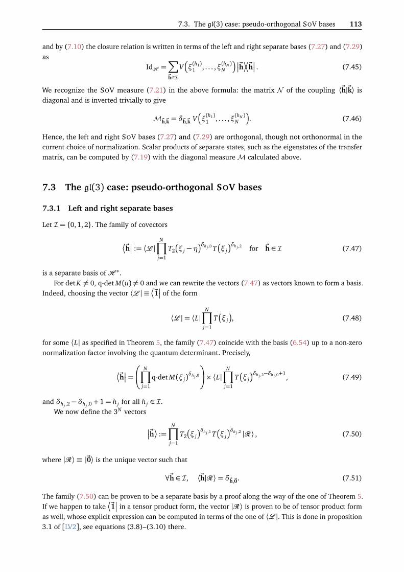
7.3. The gl(3) case: pseudo-orthogonal SOV bases 113
and by (7.10) the closure relation is written in terms of the left and right separate bases (7.27) and (7.29)as
IdH =∑~h∈I
Vξ(h1)1 , . . . ,ξ(hN )
N
~h~h . (7.45)
We recognize the SOV measure (7.21) in the above formula: the matrix N of the coupling ⟨~h|~k⟩ isdiagonal and is inverted trivially to give
M~h,~k = δ~h,~k Vξ(h1)1 , . . . ,ξ(hN )
N
. (7.46)
Hence, the left and right SOV bases (7.27) and (7.29) are orthogonal, though not orthonormal in thecurrent choice of normalization. Scalar products of separate states, such as the eigenstates of the transfermatrix, can be computed by (7.19) with the diagonal measure M calculated above.
7.3 The gl(3) case: pseudo-orthogonal SOV bases
7.3.1 Left and right separate bases
Let I = 0,1, 2. The family of covectors
~h := ⟨L |
N∏j=1
T2
ξ j −η
δh j ,0 Tξ j
δh j ,2 for ~h ∈ I (7.47)
is a separate basis ofH ∗.For det K 6= 0, q-det M(u) 6= 0 and we can rewrite the vectors (7.47) as vectors known to form a basis.
Indeed, choosing the vector ⟨L | ≡ ~1 of the form
⟨L |= ⟨L|N∏
j=1
Tξ j
, (7.48)
for some ⟨L| as specified in Theorem 5, the family (7.47) coincide with the basis (6.54) up to a non-zeronormalization factor involving the quantum determinant. Precisely,
~h=
N∏
j=1
q-det M(ξ j)δh j ,0
!× ⟨L|
N∏j=1
Tξ j
δh j ,2−δh j ,0
+1, (7.49)
and δh j ,2 −δh j ,0 + 1= h j for all h j ∈ I.We now define the 3N vectors
~h :=N∏
j=1
T2
ξ j
δh j ,1 Tξ j
δh j ,2 |R⟩ , (7.50)
where |R⟩ ≡ |~0⟩ is the unique vector such that
∀~h ∈ I, ⟨~h|R⟩= δ~h,~0. (7.51)
The family (7.50) can be proven to be a separate basis by a proof along the way of the one of Theorem 5.If we happen to take
~1 in a tensor product form, the vector |R⟩ is proven to be of tensor product form
as well, whose explicit expression can be computed in terms of the one of ⟨L |. This is done in proposition3.1 of [LV2], see equations (3.8)–(3.10) there.

114 Chapter 7 — Towards the dynamics in higher rank: scalar products for gl(3) in SOV
All of this holds for det K 6= 0. Still, even if det K = 0, it is possible to prove by direct computationthat (7.47) is a separate basis, following the usual proof given earlier.
7.3.2 Pseudo-orthogonality
In this higher rank case, the left and right separate bases defined above are not orthogonal, but theyare pseudo-orthogonal. By “pseudo” we mean that the coupling matrix N~h,~k = ⟨~h|~k⟩ is mainly diagonal,
meaning that ⟨~h|~k⟩ is zero for “many” indexes ~h 6= ~k ∈ I, but has a few non-zero off-diagonal entries.More precisely, the coupling is characterized by the following theorem
Theorem 7 (Theorem 3.1 of [LV2]). For any ~k = (k1, . . . , kN ) ∈ I, and α, β , two disjoint subsets of J1, NK,we define the corresponding modified N-tuple
~k(~0,~2)α,β = (k1(α,β), . . . , kN (α,β)) where (7.52)
∀ j ∈ J1, NK , k j(α,β) =
0 for j ∈ α,
2 for j ∈ β ,
k j for j /∈ α∪ β.(7.53)
Let ~1~k := j ∈ J1, NK | k j = 1 be the indexes of the ones of ~k, and
Γ2(~1~k; r) :=(α,β) | α,β ⊂ ~1~k, α∩ β = ; and #α= r = #β
, (7.54)
the set of couples of non-intersecting subsets of cardinal r of ~1~k. With the above notations, the couplingmatrix N between the left and right SOV basis (7.47)–(7.50) has coefficients
N~h,~k =~h~k= ~k
~kδ~h,~k + C
~k~h
n~k∑r=1
(det K)r∑
(α,β)∈Γ2(~1~k;r)
δ~h,~k(~0,~2)α,β
, (7.55)
where the coefficients C~k~h
are non-zero coefficients independent of det K, and
n~k =
$12
N∑j=1
δk j ,1
%, (7.56)
where bxc denotes the integer part of a real number x. The diagonal coefficients explicitly read as quotient ofVandermonde determinants
~h~h=
N∏j=1
dξ j −η
d
ξ
1+δh j ,1
+δh j ,2
j
V (ξ1, . . . ,ξN )2
V
ξ
δh1,1+δh1,2
1 , . . . ,ξδhN ,1+δhN ,2
N
V
ξ
δh1,1
1 , . . . ,ξδhN ,1
N
. (7.57)
The proof of this theorem is rather convoluted. It is given explicitly in great details in appendix Cof [LV2]. We first prove the pseudo-orthogonality and obtain the Kronecker deltas involved in (7.55). Thenwe characterize the form of the non-diagonal elements in terms of the diagonal ones. The coefficientsC~k~h
are characterized completely though implicitly by a heavy recursion. Finally, we derive the explicitexpression (7.57) of the diagonal elements.
Let us stress here that all the off-diagonal elements are proportional to a strictly positive power ofdet K. There is even a grading showing that the power (det K)r increases as one goes away from thediagonal. Anticipating on the next section, this indicates that we should get a diagonal SOV measure for

7.3. The gl(3) case: pseudo-orthogonal SOV bases 115
non-invertible simple spectrum twist matrix K .In the following, we outline the proof and recall the notations necessary to understand it. The general
idea to prove (7.55) is to distinguish between cases for both ~k and ~h, and proceed by induction overthe number of indexes in ~k equal to a certain value. The usual procedure in the induction is to extract atransfer matrix from the vector
~k and make it act on the other side over~h, lowering the number of
indexes equal to a certain value in ~k, allowing us to apply the induction hypothesis. Usually this requiresto rewrite the extracted transfer matrix as a sum of transfer matrices in points where the action over~h is known, and this is done by Lagrange interpolation. While this proof is in the same way as the one
of proposition 11 for the gl(2) case, the overall procedure is now much heavier; first because there aremany cases to distinguish, and secondly because the coupling (7.55) is only pseudo-orthogonal.
We use several notations to make formulas more compact throughout appendix C of [LV2].
• Many Lagrange interpolations are required in the proof. To ease the notation, appendix C makeheavy usage of the symbol
=UpC
(7.58)
which is interpreted as equality of two objects up to the non-zero numerical coefficients beforeeach term. Hence, we have the handy notation
T (u) =UpC
tr K +N∑
j=1
Tξ(h j)j
, (7.59)
where we use the symbol T to put emphasis on missing coefficients. In particular the dependence inu is not explicit in the right-hand side of the above equations.
• We perform lots of manipulations which shift from one vector~k to another |~q⟩, where ~q is a N -tuple
constructed primarily from ~k. We thus make great benefit of the compact notations similar to (7.52)–(7.53). In general, for a vector ~k= (k1, . . . , kN ) ∈ I, a subset of indices α= (α1, . . . ,αm) ⊂ J1, NKwith #α= m and a vector of values ~p= (p1, . . . , pm) ∈ 0, 1,2m, we note
~k(~p)α =k1(α, ~p), . . . , kN (α, ~p)
(7.60)
the N -tuple whose coefficients marked by α are replaced by those specified by ~p, which moreprecisely are
k j(α, ~p) =
(p` for j ∈ α with ` ∈ J1, mK such that α` = j,
k j for j /∈ α.(7.61)
Sometimes the notation is used to recall explicitly the value of some coefficients in the N -tuple athand, as in (C.67) of [LV2].
• Equation (C.45) defines the notation~h 6=(C.45)
~k. (7.62)
It means that ~k cannot be brought into ~h by substitutions of the form (1,1)→ (0,2), i.e. for anycouples of disjoint subsets (α,β) of ~1~k with the same cardinality #α= r = #β ≤ n~k, it must hold
~h 6= ~k(~0,~2)α,β . (7.63)
This defines the non-zero coefficients in (7.55): N~h,~k is zero if and only if ~h 6=(C.45)~k. This is the
condition of pseudo-orthogonality for the left and right separate bases.

116 Chapter 7 — Towards the dynamics in higher rank: scalar products for gl(3) in SOV
Another way to state this is to define an equivalence class over I as follows
∀~k ∈ I,~k
:=¦~k(~0,~2)α,β
α,β ∈ Γ2(~1~k; r) for 1≤ r ≤ n~k©
. (7.64)
Then ~h being different from ~k in the sense of (C.45) simply means it does not belong to theequivalence class of ~k
~h 6=(C.45)
~k ⇔ ~h /∈ ~k. (7.65)
As an example, if ~k= (1,1, ~p) ∈ I with ~p ∈ 0, 2N−2, the three N -tuples
(1, 1, ~p), (0,2, ~p), (2, 0, ~p), (7.66)
are in the equivalence class of ~k and are not different from ~k in the (C.45) sense: the corresponding⟨~h| bras have non-zero coupling with |~k⟩, i.e. ⟨~h|~k⟩ 6= 0 as we will demonstrate. The six otherN -tuples of the form (a, b, ~p) are different from ~k in the (C.45) sense, and have a vanishing coupling.For ~k= (1,1, 1, ~q) ∈ I with ~q ∈ 0, 2N−3, the 7 bras ⟨~h| corresponding to the N -tuples
(1, 1,1, ~q), (0, 2,1, ~q), (2,0, 1, ~q), (0,1, 2, ~q), (2, 1,0, ~q),
(1,0, 2, ~q), (1,2, 0, ~q),(7.67)
have non-zero coupling, while the 20 others N -tuples of the form (a, b, c, ~q) have a vanishingcoupling with |~k⟩.
Let us prove the orthogonality. This is done in details in section C.1 of [LV2], and amounts to provethat
∀~k ∈ I, ∀~h 6=(C.45)
~k, ⟨~h|~k⟩= 0, (7.68)
which is obtained by retaining only the Kronecker deltas dependence of (7.55). First, note that (7.68) isverified with |~k⟩= |~0⟩ for all ⟨~h| by the definition of |~0⟩ ≡ |R⟩. Next, we want to prove that
∀~k ∈ 0,2N , ∀~h ∈ I, ~h 6= ~k, ⟨~h|~k⟩= 0. (7.69)
This is done by induction over the number of 2’s in ~k in section C.1.1. The base case with one 2 is treatedin paragraph i), and the induction step is carried in paragraph ii). Suppose (7.69) holds for all ~k havingat most m 2’s. Let ~k have its first m coefficients equal to 2, the others being 0 (up to a reordering of theindices). We note ~k(2)m+1 the modified vector where km+1 = 2, according to notation (7.60)–(7.61). We
have¬~h~k(2)m+1
¶=~hT (ξm+1)
~k. The ~k at the right has m 2’s so is within the scope of the recursionhypothesis, and we can use the matrix element to show that the scalar product is zero. Depending on the~h at the right, some cases are immediate, see equations (C.32)–(C.36). The only non-trivial one is the
one for a ~h with its m+ 1 first coefficients equal to 2 as well. The lemma C.1 computes~hT (ξm+1)
~k interms of similar matrix elements with a modified ~h(1,1)
r,s , where a couple of coefficients at indexes r and s
equal to (0,2) has been set to (1,1) (this is done up to some condition on ~h regarding ~k stated in thelemma). By using this recursive formula several times until there are no couples of coefficients (0, 2) inthe covector at the left, we show in corollary C.1 the matrix element is zero. It allows to perform theinduction over the number of 2’s and prove (7.69).
Next step is to incorporate some 1’s in ~k. We want to prove that for a fixed ~h, for any ~k different from~h up to substitutions of couples (1, 1) in couples (0, 2), ⟨~h|~k⟩= 0.
In section C.1.2, we first consider a ~k with only one coefficient ka = 1, the others being 0 or 2. Nosubstitution (1, 1)→ (0, 2) can be done here, so we only have to consider the ~k at hand. Direct action (byLagrange interpolation) of the transfer matrix extracted from such a |~k⟩ on any ⟨~h|, ~h 6= ~k, gives 0, see

7.3. The gl(3) case: pseudo-orthogonal SOV bases 117
equations (C.38)–(C.43).The induction step over the increasing number of 1’s in ~k is carried in section C.1.3, and aims to fully
prove (7.68) by induction. Multiple substitutions (1,1)→ (0,2) are now possible in ~k. Suppose (7.68)holds for any ~k with m coefficients equal to 1. We now fix ~k such that its m+ 1 first coefficients areequal to 1 as in (C.44) (up to a reordering of the indexes), and let ~h ∈ I be outside
~k. Depending
on the values of the coefficients of ~h, some cases are simpler than others such as h1 = 0, see (C.62).For h1 6= 0, we can rearrange the scalar product ⟨~h|~k⟩ in a matrix element with a |~k(0)1 ⟩ at the right asstated in (C.64), which has m 1’s now and is within the scope of the recursion hypothesis. Lemma C.2takes a matrix element of this form and computes it as a sum of similar matrix elements, but with atransformation (0,2)→ (1,1) in the ⟨~h| at the left. Applying this recursive formula several times untilthere are no remaining (0, 2) couples allows proving matrix elements of this form vanish. This is done incorollary C.2. Finally, performing the induction over the number of 1’s completes the proof of (7.68).This gives the dependence in the Kronecker deltas of formula (7.55), and completes the proof of theorthogonality.
Now we can compute the actual form (7.55) of the coupling, as well as the explicit form (7.57) ofthe diagonal elements. This is done in sections C.2.1 and C.2.2 of [LV2] respectively.
Let ~k ∈ I have, up to a reordering of the indices, its m first coefficients equal to 1 and the N −mlast ones be in 0,2. We want to prove equation (C.67) of [LV2], namely that for any ~h ∈ I withr ∈ q
0, n~k − 1y
such that
∀a ∈ J1, r + 1K , (h2a−1, h2a) = (0, 2) and ∀s ∈ J2r + 3, mK , hs = 1
and ∀ j ∈ Jm+ 1, NK , h j = k j ,(7.70)
it holds ~h~k= cr+1C
~k~h
~k~k , (7.71)
with the notation c := det K for the non-zero determinant of the twist matrix.Alternatively, ~k can be written in terms of ~h as
~k= ~h(1,1,~q)1,2,3,...,2r+2 with ~q= (q1, . . . , q2r) = (1, . . . , 1). (7.72)
The m first coefficients of ~h are explicitly recalled with the notation ~h(0,2,~p)1,2,3,...,2r+2 where ~p is a 2r-tuple of
alternating 0 and 2 as defined in equation (C.69) of [LV2]. Therefore,
C~h(1,1,~q)
1,2,3,...,2r+2
~h=
¬~h~h(1,1,~q)
1,2,3,...,2r+2
¶
cr+1¬~h(1,1,~q)
1,2,3,...,2r+2
~h(1,1,~q)1,2,3,...,2r+2
¶ , (7.73)
by its definition in (7.71), which is equation (C.74) of [LV2]. The numerator can be rewritten as
¬~h~h(1,1,~q)
1,2,3,...,2r+2
¶= c1
¬~h(1,1,~q)
1,2
T1(x(1)1 )T1(ξ2)
~h(0,1,~q)1,2,3,...,2r+2
¶, (7.74)
with c1 = q-det M(ξ1). Lemma C.3 of [LV2] performs the explicit computation of the above quantity as alinear combination of matrix elements of the form
~h(1,1,~p(2)2 j )1,2,3,...,2r+2
T2(ξ2 j+2)
~h(0,1,~q)1,2,3,...,2r+2
. (7.75)
These matrix elements are in turn computed in lemma C.4 of [LV2] as linear combinations of matrixelements of the same form, but with a substitution (0,2)→ (1,1) in the covector at the left, effectively

118 Chapter 7 — Towards the dynamics in higher rank: scalar products for gl(3) in SOV
decreasing the number of (0, 2) couples in the ~h-like tuples at the left. The formula (C.88) obtained thereis recursive and acts only on (0,2) couples to transform it in (1,1) couples. In principles, it allows theexact computation of the C~k
~hcoefficients by the repeated use of it on (7.75), though the results is very
involved.The base case of the recursion, corresponding to r = 0, is tractable. Indeed, it corresponds to only one
matrix elements of the form (7.75), which is computable by direct calculations. From equation (C.73) oflemma C.3 in [LV2],
C~k(1,1)
1,2
~h(0,2)1,2
=d(ξ2 −η)d(ξ1 −η)
q-det M(ξ1)cη−2(ξ1 − ξ2 +η)
N∏a≥3
ξ(1)1 − ξ
δha ,2a
ξ2 − ξ(1−δha ,0)
a
ξ(1)2 − ξ
δha ,2a
ξ1 − ξ(1−δha ,0)
a
. (7.76)
This ends the proof of form (7.71) of off-diagonal couplings. The coefficients there are determinedimplicitly through explicit recursive formulas summed up in lemmas C.3 and C.4. It remains to computethe diagonal coupling
~h~h to completely determined the SOV measure of the fundamental gl(3) model.
This calculation is usual and follows the lines of the one done for the proof of proposition 11 for thegl(2) case. It is detailed in section C.2.2 of [LV2]. Any N -tuple of I can be constructed from ~0 by flippingthe desired coefficients with a 0→ 1 transformation, and then a 1→ 2 one if needed. One only needs tocompute the ratios
~h(0)a
~h(0)a
¬~h(1)a
~h(1)a
¶ and
~h(1)a
~h(1)a
¬~h(2)a
~h(2)a
¶ (7.77)
for a generic ~h ∈ I and a ∈ J1, NK, and one gets the relative normalization of~h~h with respect to
~0~0= 1 as a successive product of the above ratios. One has
~h(0)a
~h(0)a
=~h(1)a
T2(ξ(1)a )~h(0)a
, (7.78)
and the action of T2(ξ(1)a ) on~ha
(0)can be computed by Lagrange interpolation in the right points. The
same goes for the other ratios, as
~h(2)a
~h(2)a
=~h(1)a
T (ξa)~h(2)a
. (7.79)
All calculations done, we recall equations (C.121) and (C.131) to make the proof of eq. (7.57) self-contained
~h(1)a
~h(1)a
¬~h(0)a
~h(0)a
¶ =dξ(1)a
dξ(2)a
N∏
j=1j 6=a
ξa − ξδh j ,1
+δh j ,2
j
ξ(1)a − ξ
δh j ,1
+δh j ,2
j
, (7.80)
~h(2)a
~h(2)a
¬~h(1)a
~h(1)a
¶ =N∏
j=1j 6=a
ξa − ξδh j ,2
j
ξ(1)a − ξ
δh j ,2
j
. (7.81)

7.3. The gl(3) case: pseudo-orthogonal SOV bases 119
7.3.3 SOV measure
We can now compute the SOV measure associated to the left and right separate bases (7.47)–(7.50).Recall that for separate states of the form
|α⟩=∑~k
α~k|~k⟩pN~k
, α~k :=N∏
j=1
α(h j)j , (7.82)
⟨β |=∑~h
β~kp⟨~h|N~h
, β~k :=N∏
j=1
β(h j)j , (7.83)
their scalar products is⟨β |α⟩=
∑~h,~k∈I
⟨β~h|M~h,~k|α~k⟩ (7.84)
where the SOV measure M is defined by coefficients as
M~h,~k =p⟨~h|~k⟩pN~hN~k
. (7.85)
To get the SOV measure, it is sufficient to compute p⟨~h|~h⟩p. Somehow, this amounts to invert N .Could one have |~h⟩p = |~h⟩ here? For the diagonal term, this indeed gives p⟨~h|~k⟩p = p⟨~h|~h⟩ = ⟨~h|~h⟩,
by definition of p⟨~h|. But then, ⟨~k|~h⟩p = ⟨~k|~h⟩, which cannot be equal to δ~k,~h ⟨~h|~h⟩ as required by the
definition (7.8) of |~h⟩p, since we know from Theorem 7 that there are in general several non-zero
off-diagonal couplings ⟨~k|~h⟩—namely the ones of the form ~k= ~h(~0,~2)α,β .
|~h⟩p is therefore decomposed as sum over multiple |~k⟩ vectors. The idea to construct it is to start
from the corresponding |~h⟩ vector and add a “correction” as a linear combination of the |~h(~0,~2)α,β ⟩. The
constraints ⟨~k|~h⟩p = 0 for ~k 6= ~h would fix the values of the coefficients in the linear combination. This isdone explicitly in lemma 3.1 of [LV2]. There, we obtained the linear decomposition of |~h⟩p in the rightseparate basis as
|~h⟩p = |~h⟩+n~h∑
r=1
cr∑
α,β∈Γ2(~1~h;r)
Bα,β ,~h
~h(~0,~2)α,β
¶, (7.86)
where the Bα,β ,~h coefficients are defined recursively by
Bα,β ,~h = −C~h~h(~0,~2)α,β
−∑
α′⊂α,β ′⊂β1≤#α′=#β ′<α
Bα′,β ′,~h C~h(~0,~2)α′ ,β′~h(~0,~2)α,β
, (7.87)
where the C coefficients are proportional to the C coefficients found in (7.55), with
C~r~s =⟨~r|~r⟩⟨~s|~s⟩C
~r~s . (7.88)
Finally, the SOV measure is written as
p⟨~h|~k⟩p = ⟨~h|~h⟩δ~h,~k +
n~k∑r=1
cr∑
α,β∈Γ2(~1~h;r)
Bα,β ,~h δ~h,~k(~0,~2)α,β
(7.89)
This is corollary 3.1 of [LV2].

120 Chapter 7 — Towards the dynamics in higher rank: scalar products for gl(3) in SOV
As we can see, the complexity of the SOV measure increases strongly from the gl(2) to the higher-rankgl(3) case. Remember that while all the formulas derived here are exact and give the general form of thecouplings and the measure, the coefficients C~k
~hand Bα,β ,~h are all defined implicitly by recursive formulas.
This makes the upcoming calculations of form factors and correlations functions more complicated. Maybethere are local operators for which the computations turn out easy enough in a certain limit, for examplec→ 0. Still, it would be much more convenient to have orthogonal separate bases for the gl(3) case aswell. The next section is devoted to the construction of a such bases.
7.4 Orthogonal bases and the T operator
7.4.1 The non-invertible twist matrix case
Comparing of the gl(2) and gl(3) cases, most of the complexity in the computations is already accountedby the fusion relations. Having one more level in the fusion relations greatly increases the number ofnecessary Lagrange interpolations to compute, say, the action of the transfer matrix over the left andright separate bases.
It is thus tempting to study gl(3) models for which the hierarchy of fusion relations simplifies. This isdone easily by choosing a non-invertible twist, which forces the quantum determinant to be zero. For atwist matrix K with simple spectrum but with one zero eigenvalue, the fusion relations for the associated
transfer matrices T (K)1 (u) and T (K)2 (u) are
T (K)1 (ξ j)T(K)1 (ξ j −η) = T (K)2 (ξ j), (7.90)
T (K)1 (ξ j)T(K)2 (ξ j −η) = 0, (7.91)
T (K)2 (ξ j)T(K)2 (ξ j −η) = 0. (7.92)
The last relations is a consequence of the first two ones. The covectors and vectors families definedin (7.47), (7.50) still form a left and right separate bases, respectively, since it is only required for thetwist matrix to be with simple spectrum. The statement of theorem 4.1 of [LV2] elaborates a bit on this.
The picture is strikingly simpler now: the SOV coupling between the left and right separate bases (7.47),(7.50) is now diagonal. This follows immediately from Theorem 7, since c = det K = 0 in the presentcase.
It is still useful to obtain this results independently of the calculation done in the general case: sincethe fusion relations are much simpler now, the computations should be less intricate, and it should bepossible to derive the orthogonality and the diagonal coupling (7.57) formula directly from the simplifiedfusion relations.
This is done by theorem 4.1 of [LV2]—whose proof lies from page 23 to 26. Before that, the action of
T (K)1 (u) and T (K)2 (u) over the left and right separate bases are explicitly computed as linear combinationsover the separate bases by proposition 4.1. The actual computations are as usual Lagrange interpolationin the points where the fusion relations (7.90)–(7.92) can be applied. Because they are now simpler, it isquicker and easier to compute the actions exactly.
The description of the eigenstates as separates states is now very direct, since the two bases are dualto each other, up to some N -tuple-dependent normalization. This is the content of theorem 4.2, whichstates that the vectors and covectors
|ta⟩=∑~h∈I
N∏j=1
t2,a(ξ(1)j )
δh j ,0 t1,a(ξ j)δh j ,2|~h⟩N~h
, ⟨ta|=∑~h∈I
N∏j=1
t2,a(ξ j)δh j ,1 t1,a(ξ j)
δh j ,2⟨~h|N~h
, (7.93)
are eigenstates if and only if the functions t1,a(u), t2,a(u) are eigenvalues of the corresponding transfer

7.4. Orthogonal bases and the T operator 121
matrices, i.e.
T (K)1 (u) |ta⟩= t1,a(u) |ta⟩ , T (K)2 (u) |ta⟩= t2,a(u) |ta⟩ , (7.94)
T (K)1 (u) ⟨ta|= t1,a(u) ⟨ta| , T (K)2 (u) ⟨ta|= t2,a(u) ⟨ta| . (7.95)
The eigenvalues and eigenvectors in this det K = 0 case can be characterized by SOV as describedin chapter 6. This is done explicitly in [LV2]. It also ensures the simplicity of the transfer matrix family(T (u))u∈C when K has simple spectrum.
7.4.2 SOV measure and scalar products of separate states
The SOV measure is the inverse of the left and right separate bases coupling matrix. The latter is diagonal,so it is especially simple to invert. Therefore, the scalar product of left and right separate states of theform
⟨α|=∑~h∈Iα~h⟨~h|N~h
, α~h =N∏
j=1
α(h j)j , (7.96)
|γ⟩=∑~h∈Iγ~h|~h⟩N~h
, γ~h =N∏
j=1
γ(h j)j , (7.97)
is written as the following sum of products of ratios of Vandermonde determinants
⟨α|γ⟩=∑~h∈I
N∏j=1
dξ
1+δh j ,1
+δh j ,2
j
dξ j −η
α(h j)j γ
(h j)j
×Vξ
δh1,1+δh1,2
1 , . . . ,ξδhN ,1+δhN ,2
N
Vξ
δh1,1
1 , . . . ,ξδhN ,1
N
V (ξ1, . . . ,ξN )2 . (7.98)
For mixed scalar product of separate states, where the vector at the right is an eigenstate of the transfermatrix, it is possible to repack efficiently this big sum into products of determinants. This is achieved bytheorem 4.3 of [LV2], and more precisely in equation (4.77).
For K a simple spectrum twist matrix with one zero eigenvalue and |γ⟩ = |tn⟩ for some n ∈ q1, 3N
yan
eigenstate of the transfer matrix, the right-hand side of formula (7.98) can be simplified by accountingfor the known root pattern of the eigenvalues functions, which we recall is
∀(a, b) ∈ πn(A)×πn(B), t1,n(ξb) = 0= t2,n(ξa −η),t1,n(ξa) 6= 0, t2,n(ξb −η) 6= 0,
(7.99)
where πn is some permutation of the set J1, NK and
A= J1,MnK , B = J1, NK \ A= JMn + 1, NK (7.100)
for some integer Mn specific to |tn⟩. Keeping only the non-zero terms in the right-hand side of (7.98),one can rearrange it as a product of two independent sums, specified in equations (4.85)–(4.88) of [LV2].These sums are identified to coincide with known determinants, similar to the ones encountered inreferences [211, 213], for example. Eventually, the mixed scalar product is written as the following

122 Chapter 7 — Towards the dynamics in higher rank: scalar products for gl(3) in SOV
product of determinants
⟨α|tn⟩=N∏
a=1
d(ξ(2)a )
d(ξ(1)a )
Vξ(1)πn(1)
, . . . ,ξ(1)πn(Mn)
Vξπn(1), . . . ,ξπn(Mn)
×detN−Mn
M(α|xAt2,n)+,N−Mn
Vξπn(Mn+1), . . . ,ξπn(Mn)
detMn
M(α|xB t1,n)−,Mn
V (ξπn(1), . . . ,ξπn(Mn)), (7.101)
where xA and xB are scalar coefficients defined in equation (4.80) of [LV2],
xA(u) =∏
a∈πn(A)
u− ξa +ηu− ξa
, xB(u) =∏
b∈πn(B)
u− ξb −ηu− ξb
, (7.102)
and the explicit forms of the matrices M± are
Mα|xAt2,n+,N−Mn
i j=
1∑h=0
α(h)πn(Mn+i) x1−h
A
ξπn(Mn+i)
th
2,n
ξ(1)πn(Mn+i)
ξπn(Mn+i)
j−1, (7.103)
Mα|xB t1,n−,Mn
i j=
1∑h=0
α(h+1)πn(i)
xhB
ξπn(i)
th1,n
ξπ(i)
ξ(h)πn(i)
j−1, (7.104)
with
t2,n(u) = t2,n(u)N∏
j=1
u− ξ j
u− ξ j −η. (7.105)
They happen to be of the form of determinants similar to the gl(2) case; the fusion relation in thisdegenerate case are indeed close to the ones of gl(2). The norm of an eigenstate |tn⟩ is then obtained bysimplification from (7.101), and is written
⟨tn|tn⟩=N∏
a=1
Vξ(1)πn(1)
, . . . ,ξ(1)πn(Mn)
Vξ(1)πn(1)
, . . . ,ξ(1)πn(Mn)
·∏
b∈πn(B)
t2,n(ξ(1)b )xA(ξb) ·
∏a∈πn(A)
t1,n(ξa) · detTMn, (7.106)
where TMnis the Mn ×Mn square matrix with coefficients
TMn
(i, j)∈πn(A)×A =
1∑h=0
t1,n(ξi)(1−h) xB(ξi)
hξ(h)i
j−1. (7.107)
Despite working on a gl(3) model, these scalar products are similar to product of gl(2) type scalarproducts.
7.4.3 Extension to the invertible twist matrix case
As we see in the above paragraph, it would be very desirable to construct the separate bases for the gl(3)chain with a general twist K from conserved quantities that obey a set of simpler fusion relations. Luckily,such an operator exists.
Assume K is a diagonalizable and invertible twist matrix with simple spectrum. From the results ofthe previous chapter, we know that the associated transfer matrix T (K)(u) is diagonalizable with simplespectrum for almost all values of the inhomogeneities, and have a complete characterization of thespectrum by SOV. Let
|t(K)a ⟩ and ⟨t(K)a | (7.108)
be respectively the 3N eigenvectors and 3N eigencovectors of T (K)(u). Now let K denote the matrixobtained from K by putting one of its eigenvalues to zero, while preserving its diagonalizability. It alsohas simple spectrum. Using K as a twist matrix, we can construct the T (K)(u) transfer matrix, which is

7.4. Orthogonal bases and the T operator 123
associated to a gl(3) spin chain of same length but different boundary conditions than the one associatedto T (K)(u). The transfer matrix T (K)(u) is diagonalizable with simple spectrum. We note
|t(K)a ⟩ and ⟨t(K)a | (7.109)
its 3N eigenvectors and 3N eigencovectors, respectively, and t(K)1,a (u), t(K)2,a (u) the corresponding eigenvaluesdefined by
T (K)1 (u) |t(K)a ⟩= t(K)1,a (u) |t(K)a ⟩ , T (K)2 (u) |t(K)a ⟩= t(K)2,a (u) |t(K)a ⟩ , (7.110)
T (K)1 (u) ⟨t(K)a |= t(K)1,a (u) ⟨t(K)a | , T (K)2 (u) ⟨t(K)a |= t(K)2,a (u) ⟨t(K)a | . (7.111)
We define the new two operators
T(K)j (u) :=3N∑a=1
t(K)j,a (u)|t(K)a ⟩⟨t(K)a |⟨t(K)a |t(K)a ⟩
, with j ∈ 1,2. (7.112)
It is immediate that these operators have been defined specifically to have the eigen(co)vectors of T (K)(u),but with the corresponding eigenvalue of the T (K)(u) matrix. Because they are diagonalizable in the samebasis, the T(K)j (u) and the T (K)k (u) commute
∀ j, k ∈ 1, 2,T(K)j (u),T
(K)k (u)
= 0=
T(K)j (u), T (K)k (u)
. (7.113)
But the T(K)j (u) shares the same spectrum as the T (K)j (u)matrices, so they satisfy the same fusion relations:
T(K)1 (ξ j)T(K)1 (ξ j −η) = T(K)2 (ξ j), (7.114)
T(K)1 (ξ j)T(K)2 (ξ j −η) = 0, (7.115)
T(K)2 (ξ j)T(K)2 (ξ j −η) = 0. (7.116)
The above equations can be checked on the eigenvalues. This makes the T(K)(u) transfer matrix a veryinteresting operator: it is a conserved quantity of the gl(3)model with the boundary conditions associatedto the K matrix, but has a much simpler structure in terms of fusion relations than the usual transfermatrix T (K)(u). Following the general philosophy introduced in [225], we can construct separate basesstarting from T(K)(u) instead of T (K)(u). Let
⟨b~h| := ~1
N∏j=1
T(K)2 (ξ(1)j )
δh j ,0T(K)1 (ξ j)δh j ,2 , (7.117)
|b~h⟩ :=N∏
j=1
T(K)2 (ξ j)δh j ,1T(K)1 (ξ j)
δh j ,2~0 , (7.118)
be the family of 3N vectors and 3N covectors indexed by ~h ∈ I. By the proposition 3.1 of [LV2], theyare respectively left and right separate bases. But besides, the matrix of the couplings is diagonal, i.e.these two bases are orthogonal. This is ensured by theorem 4.1 of [LV2], since it relies only on the fusion
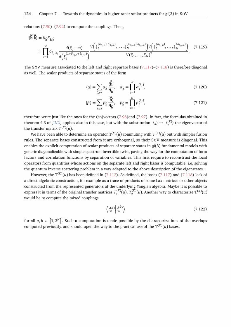
124 Chapter 7 — Towards the dynamics in higher rank: scalar products for gl(3) in SOV
relations (7.90)–(7.92) to compute the couplings. Then,
⟨b~h|b~k⟩= N~hδ~h,~k
=N∏
j=1
δh j ,k j
d(ξ j −η)dξ(1+δh j ,1
+δh j ,2)
j
Vξ(δh1,1+δh1,2)1 , . . . ,ξ
(δhN ,1+δhN ,2)N
Vξ(δh1,2)1 , . . . ,ξ
(δhN ,2)N
V (ξ1, . . . ,ξN )2 .
(7.119)
The SOV measure associated to the left and right separate bases (7.117)–(7.118) is therefore diagonalas well. The scalar products of separate states of the form
⟨α|=∑~h∈Iα~h⟨b~h|N~h
, α~h =N∏
j=1
α(h j)j , (7.120)
|β⟩=∑~h∈Iβ~h|b~h⟩N~h
, β~h =N∏
j=1
β(h j)j , (7.121)
therefore write just like the ones for the (co)vectors (7.96)and (7.97). In fact, the formulas obtained intheorem 4.3 of [LV2] applies also in this case, but with the substitution |tn⟩ → |t(K)n ⟩ the eigenvector ofthe transfer matrix T (K)(u).
We have been able to determine an operator T(K)(u) commuting with T (K)(u) but with simpler fusionrules. The separate bases constructed from it are orthogonal, so their SOV measure is diagonal. Thisenables the explicit computation of scalar products of separate states in gl(3) fundamental models withgeneric diagonalizable with simple spectrum invertible twist, paving the way for the computation of formfactors and correlation functions by separation of variables. This first require to reconstruct the localoperators from quantities whose actions on the separate left and right bases is computable, i.e. solvingthe quantum inverse scattering problem in a way adapted to the above description of the eigenstates.
However, the T(K)(u) has been defined in (7.112). As defined, the bases (7.117) and (7.118) lack ofa direct algebraic construction, for example as a trace of products of some Lax matrices or other objectsconstructed from the represented generators of the underlying Yangian algebra. Maybe it is possible toexpress it in terms of the original transfer matrices T (K)1 (u), T (K)2 (u). Another way to characterize T(K)(u)would be to compute the mixed couplings
¬t(K)a
t(K)b
¶(7.122)
for all a, b ∈ q1, 3N
y. Such a computation is made possible by the characterizations of the overlaps
computed previously, and should open the way to the practical use of the T(K)(u) bases.

8Chapter
Separate bases and spectrumof gl(m|n) models
Some quantum integrable models are associated with a Z2-graded algebra, or superalgebra [107,125, 128, 229, 293, 294]. This is usually the mark of the presence of fermionic objects in the physicalsystems. Most notable are the t-J model [295] and the Hubbard model [126, 255, 296].
The structure of the Lie superalgebras gl(m|n) differs a bit from the classical Lie algebra gl(n), asthe defining relations has to take the grading into account. In particular, the representation theory ofLie superalgebras contains additional subtleties [297–299], and so do the one of the correspondingYangian algebras Y (gl(m|n)) [117, 300]. The description of quantum integrable models associated withsuperalgebras can still be done in the QISM language of R-matrix, monodromy and transfer matrices.An important point of divergence is the structure of the fusion relations, as we will highlight in theforthcoming material. The ABA program towards the computation of correlation functions has beendeveloped for the Y (gl(m|n)) models with great success [124, 125, 127, 128, 157, 158, 160–162, 229,255, 294, 295, 301].
In this chapter, we extend the construction of separate bases from transfer matrices to the supersym-metric case by recalling the results of article [LV1]. The construction is very similar to the non-gradedcase, though some extra care is required in the definition of the objects at hand to properly account oftheir grading. We begin with a clear introduction of the graded objects of quantum integrability. Then,we prove the existence of separate bases made out from conserved quantities by showing bases of theform (6.54) are candidate separate bases for Y (gl(m|n)) models. The use of such a basis in the resolutionof the spectral problem of the transfer matrix is then discussed, in light of the particular fusion hierarchyof the Y (gl(m|n)) transfer matrices. An inner-boundary condition (IBC) is then identified to serve asthe necessary functional constraint on eigenvalue, and closure relation for the action of the transfermatrix on the basis. It is used explicitly to solve the spectral problem of the Y (gl(1|2)) model with somenon-invertible quasi-periodic boundary conditions. We close this chapter with the construction of separatebases for the Hubbard model.
8.1 Graded objects
8.1.1 Super vectors spaces
We introduce the notion of Z2-grading on vector spaces [44].
Definition. A Z2-graded vector space, or super vector space, is a complex vector space with V0, V1 ⊂ V suchthat
V = V0 ⊕ V1, (8.1)
and V0 and V1 are stable under the addition:
∀a ∈ 0,1, ∀v, w ∈ Va, v +w ∈ Va. (8.2)
Vectors that are elements of either one of the two subspaces V0 or V1 are said homogeneous: they havea well-defined grading, or, because it is a Z2-grading, a well-defined parity. Vectors of V0 are even and
125

126 Chapter 8 — Separate bases and spectrum of gl(m|n) models
vectors of V1 are odd. The grading map, or parity map, is an application that associate 0 or one regardingthe parity of homogeneous vectors
p : V0 ∪ V1 −→ 0, 1
v 7−→ p(v) =
(0 if v ∈ V0,
1 if v ∈ V1.
(8.3)
Suppose V is of finite dimension m+ n, with
dim V0 = m, dim V1 = n. (8.4)
It is handy to define the adapted basis (e1, . . . , em+n) with
e1, . . . , em ∈ V0, em+1, . . . , em+n ∈ V1. (8.5)
A common shorthand notation for these vectors is to define
∀i ∈ J1,m+ nK , i := p(ei). (8.6)
One also finds the similar notations [i] or |i| in the literature.Consider the dual space V ∗ of linear form over V . It is graded as well. Using the braket notation, the
grading of the covector ⟨i|= |i⟩† ≡ (ei)† is the same as the one of |i⟩, namely p(⟨i|) = i.
8.1.2 Superalgebras
Useful references on superalgebras and Lie superalgebras are [44, 298, 299, 302]
Definition. A complex Z2-graded algebra, or superalgebra, is a complex algebra A over the complex fieldadmitting the direct sum decomposition
A= A0 ⊕ A1 (8.7)
such that its multiplication operation A× A→ A verifies
∀i, j ∈ 0, 1, AiA j ⊆ Ai+ j mod 2. (8.8)
Note that the set of even elements form the subalgebra A0, while A1 is not a subalgebra. The gradingmap p : A0 ∪ A1→ 0, 1 is equivalently defined here, and we note x := p(x).
Definition. A Lie superalgebra g is a superalgebra whose product [·, ·], called the Lie superbracket, super-commutator or graded commutator, is skew-symmetric and satisfies the graded Jacobi identity:
∀x , y ∈ g, [x , y] = −(−1) x y[y, x], (8.9)
and∀x , y, z ∈ g, (−1) x z[x , [y, z]] + (−1) y x[y, [z, x]] + (−1)z y[z, [x , y]] = 0. (8.10)
Any associative superalgebra A may be turned into a Lie superalgebra by equipping it with the gradedcommutator
∀x , y ∈ A0 ∪ A1, [x , y] = x y − (−1) x y y x , (8.11)
and extend this definition linearly to the whole superalgebra.The space End(V ) of endomorphisms over a super vector space V is a super vector space as well. It is
also a superalgebra with the multiplication given by the composition, and is a Lie superalgebra with the

8.1. Graded objects 127
graded commutator (8.11); it is noted gl(V ) as a Lie superalgebra.We will focus a bit more on the superalgebra gl
Cm|n
, where Cm|n is the complex super vector space of
dimension m+n whose canonical basis (e1, . . . , em+n) splits in two to generate the even and odd subspace:
(Cm|n)0 = Vect(e1, . . . , em), (Cm|n)1 = Vect(em+1,...,em+n). (8.12)
It is the Lie superalgebra of endomorphisms over Cm|n. We note e ji , i, j ∈ J1,m+ nK the elementary
operators (or matrices) defined bye j
i ek = δjkei . (8.13)
Their grading isp(e j
i ) = i + j mod 2. (8.14)
Because they multiply as e ji e`k = δ
jke`i , the graded commutator is
e j
i , e`k= δk
j e`i − (−1)(i+ j)(k+¯)δ`i e jk. (8.15)
Any element is decomposed as a linear combination on the elementary operators
a =m+n∑i, j=1
aije
ji . (8.16)
From now on we will often omit sums over repeated indices. It is useful to represent these endomorphismsas block matrices of the form
a =
a(m,m) a(m,n)
a(n,m) a(n,n)
, (8.17)
where the definition of the matrices a(m,m), a(m,n),. . . should be self-explanatory. The above matrices formthe matrix associative superalgebra M(m|n,C). The even and odd elements are respectively of the form
A 00 D
,
0 BC 0
. (8.18)
From the above block form, it is clear that even elements are maps that preserve the parity of the vector,while odd elements flips it. The supertrace is defined on the elementary operators by str e j
i = (−1)iδ ji .
Using the block form, this givesstr a = tr a(m,m) − tr a(n,n). (8.19)
Similarly, the superdeterminant, or Berezinian, is defined to be
Ber
A BC D
:= det
A− BD−1C
detD−1
. (8.20)
It has properties similar to the ones of the determinant in the non-graded case, see [44]
8.1.3 Tensor products of graded objects
The tensor product V ⊗W of two super vector spaces V and W is itself a super vector space. Indeed, wehave the following decomposition in direct sum
V ⊗W =⊕
i, j∈0,1Vi ⊗Wj , (8.21)

128 Chapter 8 — Separate bases and spectrum of gl(m|n) models
and we can group terms in an even and an odd subspace
(V ⊗W )k :=⊕
i+ j=k mod 2
Vi ⊗Wj for k = 0 or 1. (8.22)
The tensor product A⊗ B of two associative superalgebras A, B is defined the same way.The basic rule of signs in supersymmetric space is that a factor (−1) x y appears whenever two elements
x , y are flipped. We can already see this from (8.9) and (8.11) for instance. The multiplication in A⊗ Bof homogeneous elements also benefit from this additional sign factor
∀a, c ∈ A0 ∪ A1, ∀b, d ∈ B0 ∪ B1, (a⊗ b)(c ⊗ d) = (−1)bcac ⊗ bd, (8.23)
and the above definition is extended linearly to A⊗ B in its whole. The rule extends naturally to N -foldtensor product with N ≥ 2. For example,
(a⊗ b⊗ c)(d ⊗ e⊗ f ) = (−1)(b+c)d+c ead ⊗ bd ⊗ c f . (8.24)
Similarly, the action of matrices of glCm|n
⊗ glCm|n
over Cm|n ⊗Cm|n has signs
∀a, b ∈ glCm|n
, ∀v, w ∈ Cm|n, (a⊗ b)(v ⊗w) = (−1)b vav ⊗ bw. (8.25)
A consequence of this is that the matrix representation of an operator a⊗ b ∈ End(V )⊗End(V ) is not thetensor product of the matrix representations of operator a and operator b. There are additional gradingsigns, more on this in the following paragraph.
Let A∈ glCm|n
⊗N. It can be decomposed on the canonical basis constructed by tensorization from
the local ones asA= Ai1,...,iN
j1,..., jNe j1
i1⊗ · · · ⊗ eiN
iN. (8.26)
It is important to not confuse the coefficients Ai1,...,iNj1,..., jN
in the above linear combination with the components
of the image of the vector e j1⊗ · · · ⊗ e jN ∈ Cm|n, which are
A(e j1⊗ · · · ⊗ e jN ) = (−1)∑N
k=1 ik(ik+1+···+iN )Ai1,...,iNj1,..., jN
ei1⊗ · · · ⊗ eiN . (8.27)
In the non-graded case, these two coefficients would be identical. The coefficients of the matrix represen-tation of operators A are the ones found in (8.27).
Some authors feel necessary to stress the grading dependent behavior of the tensor product anddenote it explicitly by referring to the “super tensor product” or “graded tensor product”, accompaniedby a notation ⊗s or ⊗g . We will not make use of this notation.
Signs also appear in the definition of dual states in tensor product spaces. Let V ' Cm|n. We use thebraket notation for the canonical basis defined in (8.5):
∀i, j ∈ J1,m+ nK , ⟨i| j⟩= δi j , (8.28)
and p(⟨i|) = p(|i⟩) = i. Let |i1⟩ ⊗ · · · ⊗ |iN ⟩, i1, . . . , iN ∈ J1,m+ nKN , be a vector of the basis of V⊗N
obtained by the simple tensorization of the one-site basis. What is its dual state. We would like to recoverthe usual behavior
∀ j1, . . . , jN ∈ J1,m+ nKN ,|i1⟩ ⊗ · · · ⊗ |iN ⟩
† | j1⟩ ⊗ · · · ⊗ | jN ⟩= δi1 j1 . . .δiN jN . (8.29)
It cannot be ⟨i1| ⊗ · · · ⊗ ⟨iN |, since many additional signs emerge from covectors and vectors passing

8.1. Graded objects 129
through each others. Adding this precise sign factor in the definition of the adjoint does the trick. With
|i1⟩ ⊗ · · · ⊗ |iN ⟩†
:= ⟨i1| ⊗ · · · ⊗ ⟨iN | (−1)σ(i1,...,iN ) with σ(i1, . . . , iN ) =N∑
k=2
iki1 + · · ·+ ik−1
, (8.30)
the sign compensate for the ones arising from the covectors and vectors passing through each others
|i1⟩ ⊗ · · · ⊗ |iN ⟩† | j1⟩ ⊗ · · · ⊗ | jN ⟩= (−1)σ(i1,...,iN )(−1)
∑Nk=2 ik( j1+···+ jk−1) ⟨i1| j1⟩ . . . ⟨iN | jN ⟩
= δi1 j1 . . .δiN jN .(8.31)
Similarly, for N even operators A1, . . . , AN ∈ glCm|n
, where A j acts non-trivially only on the jth space of
V N , the matrix elements have a factorized form over the spaces
|i1⟩ ⊗ · · · ⊗ |iN ⟩†
A1 ⊗ · · · ⊗ AN | j1⟩ ⊗ · · · ⊗ | jN ⟩= ⟨i1|A1| j1⟩ . . . ⟨iN |AN | jN ⟩ . (8.32)
Indeed, the Ak are even i.e. p(Ak) = 0 and produce no sign when passing through, say, the covectors, andthen their evenness forces ik = jk, so that the signs compensate.
Consider the permutation operator over the tensor product V ⊗ V of two copies of the same supervector space V . It accounts for the grading when flipping the vectors, and is defined by
P(v ⊗w) = (−1)vww⊗w. (8.33)
Thus, it writesP = (−1) je j
i ⊗ eij . (8.34)
For two homogeneous operators A and B in End(V ),
P(A⊗ B)P = (−1)p(A)p(B)B ⊗ A. (8.35)
The permutation operator is globally even, as an operator of the superalgebra End(V ⊗ V ).
8.1.4 Yangian of gl(m|n)
Yangians of classical Lie superalgebras are introduced in details [300]. See also [256, 303] and Molev’smonograph [117].
Consider the operator of End(Cm|n ⊗Cm|n)
R(u) = u+ηP. (8.36)
It is the R-matrix of the Yangian of the superalgebra gl(m|n). It is decomposed on the canonical basis ofelementary operators as
R(u) = Rikj`(u) e j
i ⊗ e`k with Rikj`(u) = uδi
jδk` +η(−1) jδi
`δkj . (8.37)
As in the non-graded case, we write
Rab(u) := Rikj`(u) id⊗ · · · ⊗ id⊗ e j
i︸︷︷︸space a
⊗id⊗ · · · ⊗ id⊗ e`k︸︷︷︸space b
⊗id⊗ · · · ⊗ id, (8.38)
the R-matrix Rab(u) = uid+ ηPab acting non-trivially the ath and bth spaces. The R-matrix is globally

130 Chapter 8 — Separate bases and spectrum of gl(m|n) models
even. It satisfies the Yang–Baxter equation
R12(u− v)R13(u)R23(v) = R23(v)R13(u)R12(u− v). (8.39)
This equation can be written in coordinates using the matrix representations R(u) of the operator R(u)
R(u) e j ⊗ e` = R(u)ikj`(u) ei ⊗ ek with R(u)ikj`(u) = uδijδ
k` +η(−1)i kδi
`δkj . (8.40)
Then (8.39) implies
Rαβαβ ′(u− v)Rα
′γα′′γ′(u)R
β ′γ′β ′′γ′′(v) (−1)β
′(α′+α′′) = Rβγβ ′γ′(v)R
αγ′α′γ′′(u)R
α′β ′α′′β ′′(u− v) (−1)β
′(α+α′). (8.41)
This is referred to as the graded Yang–Baxter equation, since there is an explicit modification by gradingsigns. The R-matrix (8.36) is invariant by the gl
Cm|n
algebra
∀x ∈ glCm|n
, [R(u), x ⊗ id+ id⊗ x] = 0. (8.42)
Also, if K is an even matrix of M(m|n,C)' glCm|n
, we have
R(u)(K ⊗ id)(id⊗ K) = (id⊗ K)(K ⊗ id)R(u), (8.43)
which is the scalar version of the Yang–Baxter equation, where there is a trivial representation of thegl(m|n) algebra on the third space. One sees that any even matrix K can serve as a twist for gl(m|n)integrable model.
8.1.5 The Y (gl(m|n)) fundamental chain
Let V0,V1, . . . ,VN be N copies of the super vector space Cm|n. The space V0 will serve as the auxiliaryspace, while the others will be the quantum, physical ones. We note H := V1 ⊗ · · · ⊗VN . Let K be aneven matrix of gl
Cm|n
. The Y (gl(m|n)) twisted inhomogeneous fundamental model is defined by the
monodromyM(u) = K0R0N (u− ξN ) . . . R01(u− ξ1). (8.44)
It is a globally even, as an operator of the superalgebras End(V0 ⊗H ). In coordinates, it is written
M(u) = M iα1...αNjβ1...βN
(u)e ji ⊗ eβ1
α1⊗ · · · ⊗ eβN
αN
= K ijN
R jNαNjN−1βN
(u− ξN ) . . . R j1α1jβ1(u− ξ1) e j
i ⊗ eβ1α1⊗ · · · ⊗ eβN
αN.
(8.45)
There are no additional sign because of the evenness of the R-matrices. Noting
M(u) = e ji ⊗M i
j (u), (8.46)
the above expression shows that the monodromy elements M ij (u) are homogeneous elements of the
superalgebra End(H ), with their grading depending solely on the coordinates i, j
pM i
j (u)= i + j mod 2. (8.47)
The monodromy matrix verifies the Yang–Baxter equation
Rab(u− v)Ma(u)Mb(v) = Mb(v)Ma(u)Rab(u− v). (8.48)

8.1. Graded objects 131
a
b •
•
•
•
•
•
•
•
•
•
•
•
•
•
•
•
•
•
•
•
•
•
N
M
Fig. 8.1 The Hm|n domain for Y (gl(m|n)) fusion
This expands in the (m+ n)2 relations
M j
i (u), M`k(v)
= (−1)i k+i¯+k¯
M i
k(v)M`i (u)−M j
k(u)M`i (v)
, (8.49)
where [·, ·] is the graded commutator (8.9). The transfer matrix is obtained by taking the supertrace
T (u) := str0 M(u). (8.50)
As a sum (and difference) of diagonal elements of the monodromy, the transfer matrix is an even operatorof End(H ). Because the super trace vanishes on the graded commutator, the family of the transfermatrices forms is a commuting family
∀u, v ∈ C, [T (u), T (v)] = 0. (8.51)
8.1.6 The fused transfer matrices
Like in the non-graded case, the family of transfer matrices can be enlarged with the higher order transfermatrices, which are obtained by taking arbitrary representations of the superalgebra gl(m|n) on theauxiliary space. And as in the non-graded case, they can be constructed via fusion.
Tensor product of fundamental representations of gl(m|n) are decomposable in direct sum of irre-ducible subrepresentations. Young diagrams can be used to carry out calculations, with mechanics properto superalgebra though very similar to the non-graded case [128, 297, 298, 304]. Finite dimensionalirreducible representations are labelled uniquely by Kac–Dynkin labels, but the correspondence betweenKac–Dynkin labels and Young diagrams is not one-to-one [304]1.
Admissible Young diagrams lie inside a fat hook domain pictured in fig. 8.1, defined over the bidimen-sional lattice
Hm|n := Z≥1 ×Z≥1 \Z>m ×Z>n, (8.52)
with coordinates (a, b). Young diagrams expand infinitely in both directions a and b, but the pointsa > n, b > m are forbidden, leading to the hook shape.
Let λ be some representation of gl(m|n). The degeneracy points of the fundamental R-matrix allow toconstruct the projectors Pλ : (Cm|n)⊗n→ Vλ which extracts the wanted subrepresentation λ as a productof R-matrices. Fusing on the auxiliary space from the fundamental monodromy M(u), we obtain newmonodromy operators associated to λ, and then new transfer matrices one the supertrace is taken. All ofthese transfer matrices commute together, since an analog Yang–Baxter equation is verified by the fusedmonodromies, for the projectors are constructed from R-matrices at specific points.
1Highest weight irreducible representations are characterized uniquely by their highest weight, which can be noted on aKac–Dynkin diagram. When using Young diagrams, the corresponding highest weight is obtained from the length of the m firstrows and height the n first columns, see [304] for details. In the case of a Young diagram with at least m+ 1 rows of length n
and n columns of height m, one can delete a length n row and add a height m row, add compute the same highest weight.

132 Chapter 8 — Separate bases and spectrum of gl(m|n) models
0 −η −2η−3η−4η
η 0 −η −2η−3η
2η η 0
3η 2η η
Fig. 8.2 The domain Hm|n domain is filled with multiples of the deformation parameter η. Startingfrom 0 in box (1,1), one adds η when moving down and −η when going right.
For rectangular Young diagram corresponding to the point (a, b) ∈ Hm|n with b rows and a columns,the corresponding monodromy matrix reads
M (a)b (u) := P(a)b
←⊗1≤s≤a1≤r≤b
M(u+η(r − s))
P(a)b (8.53)
The shifts in (8.53) are obtained by filling the fat hook Hm|n as in fig. 8.2. Then, reading the rectangulardomain corresponding to the Young diagram associated to λ column by column, top to bottom from leftto right, and tensoring a fundamental shifted monodromy corresponding to the current box at the left ofthe previous ones, one obtain (8.53). The projectors are obtained as a product of R-matrices [227, 229].For rectangular diagrams (a, b), they are of the form
P(a)b ∝∏i< j
Ri j(s j − si), (8.54)
where i, j run over the boxes of the diagram of fig. 8.2 in the same way as described earlier, and thesi, s j are the shifts in the boxes. The projectors associated to row and columns Young diagrams are thesymmetrizer and antisymmetrizer, respectively, over the V⊗a space:
P(1)a = P+1...a =∑σ∈Sa
Pσ, (8.55)
P(a)1 = P−1...a =∑σ∈Sa
sign(σ) Pσ, (8.56)
where Sa is the symmetric group of rank a. We have the following recursion relations for the symmetrizersand antisymmetrizers making explicit use of the R-matrix
P+1...a =1
aηP+1...a−1R((a− 1)η)P+2...a, (8.57)
P−1...a = −1
aηP−1...a−1R(−(a− 1)η)P−2...a, (8.58)
in agreement with (8.54).The fused transfer matrix is obtained by taking the super trace on the representation λ on the auxiliary
space. For the rectangular representation, one has
T (a)b (u) := strVab
M (a)b (u), (8.59)
where V ab ' V⊗ab. All these transfer matrices commute together, as a consequence of generalized form of
the Yang–Baxter equation (8.48) being true for any irreps taken on the auxiliary spaces a and b. Hence,
∀(a, b), (c, d) ∈ Hm|n, ∀u, v ∈ C,T (a)b (u), T (c)d (v)
= 0. (8.60)

8.1. Graded objects 133
There are other ways to construct the fused transfer matrices (8.59). The nice coderivative formalismobtain these matrices and all their characteristics and relations from the characters of the super algebragl(m|n) [229, 231].
Let us recall the most relevant properties of the transfer matrices T (a)b (u) for our purposes.
Polynomial structure The transfer matrix T (a)b (u) is a polynomial in u of degree abN , with (ab− 1)Ncentral zeroes given by
Z (a)b (u) =N∏
j=1
(u− ξ j)
−1b∏`=1
a∏m=1
u− ξ j +η(`−m)
, (8.61)
which therefore factorizes asT (a)b (u) = eT (a)b (u) Z (a)b (u), (8.62)
where eT (a)b (u) is a polynomial of degree ab.
Fusion equations There are bilinear relations between transfer matrices associated to adjacent rectan-gular diagrams, often called the Hirota relations
T (a)b (u−η)T (a)b (u) = T (a)b+1(u−η)T (a)b−1(u) + T (a−1)b (u−η)T (a+1)
b (u), (8.63)
where in our normalization, the following boundary conditions are imposed
T (0)b≥1(u) = 1= T (a≥1)0 (u). (8.64)
All the transfer matrices outside the extended fat hook Hm|n := (Z≥0 ×Z≥0) \ (Z>m ×Z>n) are identicallyzero, i.e.
∀(a, b) /∈ Hm|n, T (a)b (u) = 0. (8.65)
Inner-boundary condition Because the correspondence between Young diagram and the irreduciblerepresentation of the superalgebra gl(m|n) is not bijective, there exists non-trivial relations linking transfermatrices associated to distinct Young diagrams. This concerns rectangular Young diagrams saturating onearm of the fat hook Hm|n [128, 304, 305]. The first relation is called the inner-boundary condition (IBC)and is written
(−1)n q-Ber(u)T (m+1)n (u+η) = T (m)n+1(u), (8.66)
where
q-Ber M(u) = sdet(K)a(u)
∏m−1k=1 d(u− kη)∏n−m
`=1 d(u+ `η)idH , (8.67)
with
a(u−η) = d(u) =N∏
j=1
(u− ξ j). (8.68)
The operator q-Ber(u) is called the quantum Berezinian, for m 6= n, and plays a role similar to the quantumdeterminant in the non-graded case [127, 306]. This relation is explicitly verified in appendix C of [LV1]by the use of the coderivative formalism.

134 Chapter 8 — Separate bases and spectrum of gl(m|n) models
Reconstruction of fused matrices from the fundamental one The Bazhanov–Reshetikhin determinantformulas allow to write all the transfer matrices T (a)b (u) in terms of the row and column type ones
T (a)b (u) = det1≤i, j≤a
T (1)b+i− j
u− (i − 1)η
(8.69)
= det1≤i, j≤b
T (a+i− j)1
u+ (i − 1)η
. (8.70)
We will use the simpler notations
Ta(u) := T (1)a (u) and T(a)(u) := T (a)1 (u),
eTa(u) := eT (1)a (u) and eT(a)(u) := eT (a)1 (u).(8.71)
The asymptotics of these matrices are given solely by the corresponding symmetrization of the twistmatrix:
T∞,a := limu→∞u−aN Ta(u) = str1...a P+1...aK1 . . . KaP+1...a, (8.72)
T∞,(a) := limu→∞u−aN T(a)(u) = str1...a P−1...aK1 . . . KaP−1...a. (8.73)
One recognizes that T∞,a and T∞,(a) are the characters of the completely symmetric and antisymmetricrepresentations, respectively, applied to the twist matrix. It is seen explicitly with a diagonalizable twistmatrix with spectrum Sp(K) = k1, . . . km+n, for example.
In the inhomogeneities, the matrices enjoys simpler fusion relations thanks to the structure of theircentral roots. We have, for all j ∈ J1, NK and for all positive integer n,
T1(ξ j)Tn(ξ j +η) = Tn+1(ξ j), (8.74)
T1(ξ j)T(n)(ξ j −η) = T(n+1)(ξ j). (8.75)
The proof is done easily by induction, using the general bilinear Hirota fusion relations (8.63), and thecentral zeroes (8.61). This is done in lemma 2.1 of [LV1]. These row and columns transfer matrices arereconstructed from the fundamental one by successive Lagrange interpolation in the inhomogeneities.
Remark 1 (Comparaison with other conventions). In a great part of literature, such as articles [128, 305],the conventions used for the fused transfer matrices differ from ours. We make the link explicit in thefollowing.
1. Rectangular representations and orientation of the fat-hookRectangular diagrams sa with a rows and s columns in [128, 305] correspond to diagrams (a, s) inour convention. This is because the conventions chosen for the fat-hook differ: figure 1 of [128]matches with fig. 8.1 when rotated by − π/2.
2. R-matrixThe value of theη parameter, free in our discussion, is fixed at 2 in [128, 305]. This is inconsequential,as it amounts to a rescaling of the spectral parameter, but change the definition of all the relatedobjects.
3. Definition of transfer matricesTransfer matrices associated to rectangular representations in [128, 305] are defined up to non-constant shifts compared to definition (8.59). We note them U(a, s, u), and they are defined as [see305, equation (6)]
U(a, s, u) := strVab
πa
s (g)T (u− s+ a), (8.76)
where T (u) is the untwisted monodromy constructed from the R-matrices with η = 2, g ∈ GL(()m|n)a twist and πa
s the representation associated to the rectangular Young diagram sa. In our notation,

8.1. Graded objects 135
reintroducing the η parameter, the link is done by
T (a)b (u)η=2= U(a, b, u+ b− a). (8.77)
4. Hirota equationTogether with the specific choice η = 2, the latter convention leads to a different form of the Hirotaequation. In [128, 305], it is written
U(a, s, u+ 1)U(a, s, u− 1) = U(a, s+ 1, u)U(a, s− 1, u) + U(a+ 1, s, u)U(a− 1, s, u). (8.78)
Compared to (8.63), each of the three terms is shifted in only one of its variables, by ±1, makingit easy to remember. Introducing the constant shift u→ u+ s− a− 1, one obtains with η= 2 thefollowing form
T (a)s (u−η)T (a)s (u) = T (a)s+1(u−η)T (a)s−1(u) + T (a+1)s (u)T (a−1)
s (u−η), (8.79)
which is exactly equation (8.63) for s→ b.5. Boundary conditions
The boundary conditions chosen here (see equations (8.64) and (8.65)) also differs from the onesin [128, 305]. There, it is imposed that
T (0, s, u) = φ(u− s), T (a, 0, u) = φ(u+ a), (8.80)
where φ(u) is some function fixing the input data of the problem—in this precise case it would beφ(u) =
∏Nj=1(u− ξ j) for the inhomogeneous chain of length N . In our setting, the input data are
fixed by the giving of the transfer matrix T (u)≡ T (1)1 (u). Both choices are valid, but produce slightlydifferent hierarchies of fused transfer matrix: the U(a, s, u) matrices are polynomial in u of degreeN for all values of a and s, while in our case the degree in u of the T (a)b (u) transfer matrices growsas abN , with (ab(N − 1)) central zeroes (see equation (8.61)). Consequently, the inner-boundaryconditions also differ, up to a scalar factor that happen to be the total quantum Berezinian, andby shifts in the spectral parameter because of the different definitions of the transfer matrices(compare equation (8.66) with equation (28) of [305]).
We have the following lemma, which is corollary 2.1 of [LV1]
Lemma 2. Under the condition
∀ j, k ∈ J1, NK , j 6= k, ξa 6= ξb mod η (8.81)
on the inhomogeneities, the transfer matrices Tn+1(u) and T(n+1)(u) are constructed in terms of T1(u) by thefollowing recursive Lagrange interpolation formulas
Tn+1(u) =n∏
r=1
d(u+ rη)
T∞,n+1(u) +
N∑a=1
f (n+1)(u)a T1(ξa)Tn(ξa +η)
, (8.82)
T(n+1)(u) =n∏
r=1
d(u− rη)
T∞,(n+1)(u) +
N∑a=1
g(n+1)(u)a T1(ξa)T(n)(ξa −η)
, (8.83)
where the asymptotics coefficients are
T∞,a(u) := T∞,a
N∏j=1
(u− ξ j) and T∞,(a)(u) := T∞,(a)
N∏j=1
(u− ξ j), (8.84)

136 Chapter 8 — Separate bases and spectrum of gl(m|n) models
and the interpolation coefficients are
f (m)a (u) :=
N∏b=1b 6=a
u− ξb
ξa − ξb
N∏b=1
m−1∏r=1
1
ξa − ξ(r)b
, (8.85)
g(m)a (u) :=
N∏b=1b 6=a
u− ξb
ξa − ξb
N∏b=1
m−1∏r=1
1
ξa − ξ(−r)b
, (8.86)
with the usual shorthand notation ξ(r)j := ξ j − rη.
Proof. The proof of this lemma is very direct. The Ta(u) and T(a)(u) are polynomials of degree aN . Wealready know (a−1)N central roots of them, so they can be reconstructed by Lagrange interpolation fromtheir asymptotic behavior and their values at N different points. The asymptotics are computable andwritten above, and the fusion relations provide values in the inhomogeneities in terms of the previoustransfer matrices in the fusion hierarchy.
One see easily that the general form of T (a)b (u) in terms of the fundamental transfer matrix T (1)1 (u)≡T (u) is a linear combination of the form
T (a)b (u) =∑
s1,...,sab
c(u) T (u+ s1η) . . . T (u+ skη), (8.87)
where the s1, . . . , sk are some shifts governed by the Lagrange interpolations and the shifts in the Bazhanov–Reshetikhin formulas, with 1≤ k ≤ ab. Hence, the degree in T (u) of T (a)b (u) is ab.
8.2 Separates bases
As in the non-graded case, it is possible to construct bases from conserved quantity that are separatefor the spectral problem of the transfer matrix. The basis made from powers of the transfer matrixin Theorem 5 is constructed very similarly for the Y (gl(m|n)) fundamental model. The proof relies mainlyon the reduction of the R-matrix to the permutation in a particular point. We reproduce here the theoremand its full proof.
Consider a (m+ n)× (m+ n) square twist matrix K of glCm|n
which is even and non-derogatory. It is
block diagonal of the form
K =
Km 00 Kn
. (8.88)
For X = m,n, we notek1,X , . . . , kmX ,X = Sp(KX ) (8.89)
the mX eigenvalues of KX of algebraic multiplicity d1,X , . . . , dmX ,X , with∑mX
a=1 = X . The spectrum of thetwist matrix is (geometrically) simple
∀i, j ∈ J1, mX K , ki,X 6= k j,X . (8.90)
There exists a change of basis invertible matrix WK ∈ glCm|n
WK =
WK ,m 0
0 WK ,n
, (8.91)

8.2. Separates bases 137
even as well, that puts K in its Jordan normal form
KJ =
KJ ,m 0
0 KJ ,n
=W−1
K KWK , (8.92)
where for X = m or n, the KJ ,X matrices write in Jordan normal form with mX Jordan blocks of theform (6.10)
KJ ,X =
J(k1,X ,d1,X ). . .
J(kmX ,X ,dmX ,X )
. (8.93)
Let I := J0,m+ n− 1K, and consider the twisted inhomogeneous fundamental model of length N ofthe Y (gl(m|n)) algebra. We note T (u) its transfer matrix as defined in (8.50).
Theorem 8. Let the twist matrix K be an even non-derogatory matrix of glCm|n
as above. For almost
any choice of a covector ⟨S| ∈ H ∗ and of the inhomogeneities ξ j under the condition (8.81), the family ofcovectors
∀~h ∈ I, ⟨~h| := ⟨S|N∏
j=1
T (ξ j)h j (8.94)
forms a covector basis ofH ∗.In particular, the state ⟨S| can be taken as follows. For a one-site |S, a⟩ := S(a)i |i⟩ in the a-th space Va.
Its dual covector in V∗a is ⟨S, a|= |S, a⟩† = S(a)∗i ⟨i|. For the vector
|S⟩ := |S, 1⟩ ⊗ · · · ⊗ |S, N⟩ , (8.95)
constructed by tensoring N copies of the one site state |S, a⟩, the dual state ⟨S|= |S⟩† is
⟨S|=m+n∑
p1,...,pN
S(1)∗p1. . . S(N)∗pN
(|p1⟩ ⊗ · · · ⊗ |pN ⟩)†, (8.96)
where (|p1⟩ ⊗ · · · ⊗ |pN ⟩)† has signs in its definition as in (8.30). Noting
⟨S, a|W−1K ,a =
x (1)1,m, . . . , x (1)d1,m, . . . , x (mn)
1,n , . . . , x (mn)dmn
,n
, (8.97)
it is sufficient to take |S, a⟩ such that
mm∏k=1
x (k)1,m
mn∏k=1
x (k)1,n
6= 0 (8.98)
for the family of covectors (8.94) to form a basis.
Proof. As in the non-graded case, we have
R(0) = ηP and stra Pab = idb, (8.99)
so the transfer matrix in the inhomogeneities is
T(ξ j) = R j j−1(ξ j − ξ j−1) . . . R j1(ξ j − ξ1)K jR jN (ξ j − ξN ) . . . R j j+1(ξ j − ξ j+1). (8.100)
It is now very similar to the proof of Theorem 5: it is sufficient to prove that the determinant of the matrix

138 Chapter 8 — Separate bases and spectrum of gl(m|n) models
M of size (m+ n)N , of elements
Mi j =~h(i)
e j
for i, j ∈ q
1, (m+ n)Ny
, (8.101)
is non-zero. Here ~h(i) is the unique N -tuple labeled by i defined by
i = 1+N∑
a=1
ha(i)ai−1, (8.102)
while the e j are the vectors of the canonical basis H —constructed by tensoring the local canonicalbases—enumerated by j. For j ∈ q
1, (m+ n)Ny, one has
|e j⟩=e1+h1( j)(1)
⊗ · · · ⊗e1+hN ( j)(N)
(8.103)
from (8.102), where the |ea( j)⟩, a ∈ J1,m+ nK are the vectors of the canonical basis at site j. Thedeterminant detM has polynomial dependence in the inhomogeneities and the twist matrix coefficients,so it is sufficient to prove that detM 6= 0 in some particular points of these parameters to have it almosteverywhere. As in the non-graded case, a sufficient criterion for detM 6= 0 is therefore obtained in thelarge inhomogeneities limit and reads
det M 6= 0, (8.104)
with M the (m+ n)N square matrix of coefficients
∀i, j ∈ q1, (m+ n)N
y, Mi j =
S
N∏a=1
Kha(i)a
e j
. (8.105)
Let us compute this last matrix element precisely. From (8.96), it writes the sum
S
N∏a=1
Kha(i)a
e j
=
m+n∑p1,...,pN
S(1)∗p1. . . S(N)∗pN
(|p1⟩ ⊗ · · · ⊗ |pN ⟩)†
× N∏
a=1
Kha(i)a
e1+h1( j)(1)⊗ · · · ⊗
ehN ( j)(N)
. (8.106)
Because the Kha(i)a are even, the matrix elements factorizes by (8.32) as a product over N one-site matrix
elements:
∀i, j ∈ q1, (m+ n)N
y, (|p1⟩ ⊗ · · · ⊗ |pN ⟩)†
N∏a=1
Kha(i)a
e1+h1( j)(1)⊗ · · · ⊗
ehN ( j)(N)
=N∏
a=1
pa
Kha(i)a
e1+ha( j)(a)
. (8.107)
The sum over the p1, . . . , pN is therefore decoupled as a product of N independent sums
Mi j =N∏
a=1
S, a
Kha(i)a
e1+ha( j)(a)
, (8.108)
and the same goes for the determinant:
det M=N∏
a=1
det ma, (8.109)

8.3. About the characterization of the spectrum 139
where ma the m+ n square matrix of coefficients
(m)i j =Sa
K i−1a
e j(a)
. (8.110)
Consequently, the family (8.94) is a basis if
∀a ∈ J1, NK , det ma 6= 0. (8.111)
These determinants are explicitly computed in terms of the eigenvalues of K and the coefficients of thecovector (8.97) to be
det m=mm∏a=1
x (a)1,m
da,mmn∏a=1
x (a)1,n
da,nmm∏a=1
mn∏b=1
ka,m − kb,n
da,mdb,n
×∏
1≤a<b≤mm
ka,m − kb,m
da,mdb,m∏
1≤a<b≤mn
ka,n − kb,n
da,ndb,n . (8.112)
Since K has simple spectrum, all the coefficients depending on its eigenvalues in the above formula arenon-zero. Therefore, det m is non-zero under the condition (8.98). This proves the desired result.
Proposition 12. If the twist matrix K has simple spectrum, then the transfer matrix T(u) has simplespectrum. If moreover it is diagonalizable, then T (u) is diagonalizable as well.
Proof. Let the twist K has simple spectrum, then (8.94) is a basis by the above theorem. For an eigenvaluet(u) of T (u), and |t⟩ an associated eigenvector, it is immediate that
∀~h ∈ I,~ht= ⟨S|t⟩
N∏j=1
t(ξ j)h j . (8.113)
This determines completely the unique eigenvector associated to t(u)— up to a normalization. If moreoverK is diagonalizable, then one can prove that T (u) is diagonalizable as well with computations similar tothe proof of lemma 1, that we do not repeat here. The main idea is to show that there are no non-trivialJordan block, i.e. of size greater than one, by using the asymptotic form of the eigenvectors.
8.3 About the characterization of the spectrum
Just like in the non-graded case, we would like to use this SOV basis to solve the spectral problem ofthe transfer matrix. We will heavily rely on what we did on the non-graded case. As we already know,the unique eigenvector of an eigenvalue of the transfer matrix is fully fixed by the knowledge of theeigenvalue, thanks to the immediate computations of its coefficients in the basis (8.94):
∀~h ∈ I, ⟨~h|t⟩=N∏
j=1
t(ξ j)h j . (8.114)
We thus restrict to the characterization of the eigenvalues, and already have some constraints on themfrom the characteristics of the transfer matrix itself. Namely, they are polynomials of degree N , withdominant coefficient str(K) and have to satisfy the fusion relations.
For a polynomial P ∈ CN [X ] of degree N , a diagonalizable matrix with simple spectrum K suchthat the dominant coefficient of P is str K, and inhomogeneities ξ1, . . . ,ξN verifying (8.81), one canconstruct successively the polynomials P(1)n and P(n)1 by the interpolation formulas (8.69)–(8.70), and

140 Chapter 8 — Separate bases and spectrum of gl(m|n) models
the polynomial P(a)b from the determinant formulas (8.82)–(8.83). We also add the additional constraintthat all the functions for points outside the extended fat hook are identically zero.
For any vectors of (x1, . . . , xN ) ∈ CN , we define the following polynomial
t1(u|x j) := T∞,1(u) +N∑
a=1
f (1)a (u) xa. (8.115)
We can then define recursively the infinite family of higher polynomials
tn+1(u|x j) :=
n∏r=1
d(u+ rη)
T∞,n+1(u) +
N∑a=1
f (n+1)a (u) tn(ξa +η|x j) xa
, (8.116)
t(n+1)(u|x j) :=
n∏r=1
d(u−η)
T∞,(n+1)(u) +N∑
a=1
g(n+1)a (u) t(n)(ξa −η|x j) xa
, (8.117)
and∀(a, b) ∈ Hm|n, t(a)b (u|x j) := det
1≤i, j≤atb+i− j
u− (i − 1)η|x j
= det1≤i, j≤b
t(a+i− j)u+ (i − 1)η|x j
.
(8.118)
We set ta≥10 (u|x j) = 1= t(0)b≥1(u|x j) for full consistency with the fusion relations (8.63). Let us note
FH(x j, ξ j, K) :=
f (a)b (u) ∈ C[u]
f (a)b (u) =
(t(a)b (u|x j) for (a, b) ∈ Hm|n,
0 for (a, b) /∈ Hm|n,
(8.119)
the infinite family of polynomials obtained from a vector (x1, . . . , xN ) ∈ CN by the fusion hierarchyformulas (8.115)–(8.118), where the asymptotics are prescribed by the matrix K ∈ End(Cm|n) and theLagrange interpolations are done in the inhomogeneities ξ j.
For f , g and h functions of one variable u ∈ C, we note
IBCm|n,η( f , g, h)[u] := (−1)nh(u) f (u+η)− g(u). (8.120)
For h(u) = q-Ber M(u), and |t⟩ such that
T (m+1)n (u) |t⟩= t(m+1)
n (u) |t⟩ , T (m)n+1(u) |t⟩= t(m)n+1(u) |t⟩ , (8.121)
we have the inner-boundary condition at the function level
IBCm|n,η
t(m+1)n , t(m)n+1, q-Ber M
= 0. (8.122)
We now define the following family of polynomials
FamNm|nK , ξ j
:=§
f (u) ∈ CN [u] ∃(x1, . . . , xN ) ∈ CN , x j 6= 0, f (u)≡ t1(u|x j),
IBCm|n,η
t(m+1)n (u|x j), t(m)n+1(u|x j), q-Ber M
= 0,
for t(m+1)n (u|x j), t(m)n+1(u|x j) ∈ FH
x j, ξ j, Kª
.
(8.123)
In words, this is the set of all the polynomials of degree N that can be written in the form (8.115) fromsome non-zero vectors (x1, . . . , xN ) ∈ CN and twist matrix K , whose fused higher polynomials obtainedby the fusion hierarchy (8.119) satisfy the inner-boundary condition at the function level.

8.3. About the characterization of the spectrum 141
From all we said above, it is clear that
Sp(T (u)) ⊆ FamNm|nK , ξ j
. (8.124)
This is another wording for the statement made by lemma 2.2 of [LV1], that we recall here
Lemma 3. Any eigenvalue t(u) of the transfer matrix T(u) admits the representation t1(u|x j), where
the (x1, . . . , XN ) 6= (0, . . . , 0) are N complex numbers such that the fused polynomials t(a)b (u|x j) verify theinner-boundary condition
(−1)n q-Ber M(u)t(m+1)n (u+η|x j) = t(m)n+1(u|x j), (8.125)
and the out-boundary conditions
∀n, m≥ 1, ∀u ∈ C, t(m+m)n+n (u) = 0. (8.126)
Are these two set equal? If no, what are the additional requirements for a polynomial of Fam(K , ξ j)to be an eigenvalue of T (u)? This is where the basis (8.94) enters the stage.
Let t(u) ∈ Fam(K , ξ j), and |t⟩ the associated vector ofH defined by
∀~h ∈ I, ⟨~h|t⟩=N∏
j=1
t(ξ j)h j . (8.127)
We want to prove that upon some possible additional constraints on t(u),
∀~h ∈ I, ∀u ∈ C, ⟨~h|T (u)|t⟩= t(u) ⟨~h|t⟩ . (8.128)
To do so, one has to compute ⟨~h|T (u)|t⟩ and rearrange it in the left-hand side of (8.128), requiringsome assumptions on t(u) along the way if necessary. The immediate concerns is therefore, as in thenon-graded case, to know how to act on the basis of ⟨~h| with T (u). As we know from section 6.2.1 for thenon-graded case, this is given by some Lagrange interpolation and the use of the algebra of the conservedquantities, whose relations, in practice, are derived from the fusion relations. This is no different here.
Action of T (u) on ⟨~h| Action of T (ξ j) over ⟨~h| is merely a shift if there is some room to increase thepower of the corresponding factor in ⟨~h|
∀ j ∈ J1, NK , ∀~h= (h1, . . . , hN ) ∈ I, h j < m+ n− 1, ⟨~h| T (ξ j) = ⟨~h+ e j| . (8.129)
The non-trivial case is when h j is at its maximal value m+ n− 1. In the non-graded gl(n) case, we were
able to characterize the linear decomposition of ⟨~h| T (ξ(r)j ) over the basis of the ⟨~h| by the repeated useof the fusion relations. Indeed, the last fusion relation eventually gives a central element, the quantumdeterminant, so that any product of n transfer matrices can be recast after many Lagrange interpolationsin a linear combination of products with at most n− 1 transfer matrices.
In the graded gl(m|n) case, the picture is not as simple. Indeed, there are no representation ofdimension 1 that would yield a central fused transfer matrix, unlike in the non-graded case where thecentral quantum determinant can be obtained by fusion. The closest we have from such a tool is theinner-boundary condition (8.66). The degree in T (u) of the left-hand side of (8.66) is (m+ 1)n, and thedegree of the right-hand side is m(n+1). With n 6= m, the degree in T (u) is lower on one side or the other.This was somewhat expected with the presence of the quantum Berezinian, that gather fundamentalmatrices T (u) in a rational function to produce a central element. Nonetheless, supposing m< n, it means

142 Chapter 8 — Separate bases and spectrum of gl(m|n) models
2
1
Fig. 8.3 The Hm|n domain for the Y (gl(1|2)) model
that a non-trivial linear combination of terms of degree mn+n in T (u) is actually recombinable in a linearcombination of terms of degree mn+m< mn+ n. This gives a very indirect way to possibly rewrite termsof degree m+ n− 1 in T (u) into terms of smaller degree, effectively computing the missing relations inthe abelian algebra of conserved quantities that gives the linear decomposition
⟨~h| T (u) =∑~k∈I
C~k~h(u) ⟨~k| (8.130)
for ~h ∈ I with at least one h j = m+ n− 1 for some j ∈ J1, NK.
8.4 Specializing for gl(1|2) model
We now specialize the discussion to the gl(1|2) model. From now on, I = 0, 1, 2. The fat-hook domainis for m= 1, n= 2 is pictured in fig. 8.3.
Let K ∈ glC1|2 be diagonalizable. We note k1, k2 and k3 its eigenvalues, and have det K1 = k1,
det K2 = k2k3. The associated asymptotics of the column transfer matrices are explicitly
∀n≥ 2, T∞,n = kn−21 (k1 − k2)(k1 − k3). (8.131)
The inner-boundary condition (8.66) reads
k1T (1)2 (u+η) = k2k3d(u)T3(u), (8.132)
for the fused transfer matrices, and
k1 t(1)2 (u+η) = k2k3d(u)t3(u) (8.133)
at the level of the corresponding eigenvalues. The out-boundary condition (8.126) reads out
∀m, n≥ 0, ∀u ∈ C, t2+n3+m(u) = 0. (8.134)
We make the following conjecture
Conjecture 1. For the general gl(1|2)-graded Yang–Baxter twisted inhomogeneous fundamental model oftransfer matrix T (u),
Sp(T (u)) = FamNm|n(K , ξ j). (8.135)
In others words, polynomials t1(u|x j) defined in (8.115) are eigenvalues of T (u) if and only if the higherfused polynomials associated to it satisfy the inner-boundary condition (8.125) and the null out boundarycondition (8.126).
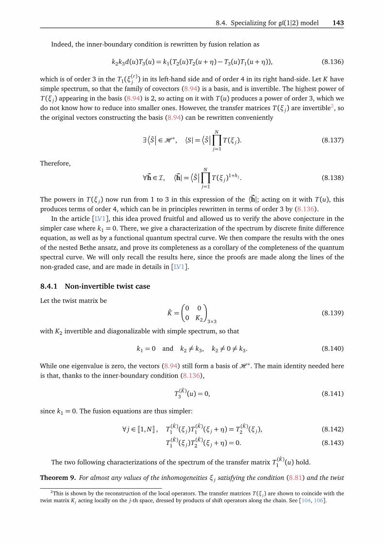
8.4. Specializing for gl(1|2) model 143
Indeed, the inner-boundary condition is rewritten by fusion relation as
k2k3d(u)T3(u) = k1(T2(u)T2(u+η)− T3(u)T1(u+η)), (8.136)
which is of order 3 in the T1(ξ(r)j ) in its left-hand side and of order 4 in its right hand-side. Let K have
simple spectrum, so that the family of covectors (8.94) is a basis, and is invertible. The highest power ofT (ξ j) appearing in the basis (8.94) is 2, so acting on it with T (u) produces a power of order 3, which wedo not know how to reduce into smaller ones. However, the transfer matrices T (ξ j) are invertible2, sothe original vectors constructing the basis (8.94) can be rewritten conveniently
∃ S ∈H ∗, ⟨S|= S
N∏
j=1
T (ξ j). (8.137)
Therefore,
∀~h ∈ I, ⟨~h|= S
N∏j=1
T (ξ j)1+h j . (8.138)
The powers in T(ξ j) now run from 1 to 3 in this expression of the ⟨~h|; acting on it with T(u), thisproduces terms of order 4, which can be in principles rewritten in terms of order 3 by (8.136).
In the article [LV1], this idea proved fruitful and allowed us to verify the above conjecture in thesimpler case where k1 = 0. There, we give a characterization of the spectrum by discrete finite differenceequation, as well as by a functional quantum spectral curve. We then compare the results with the onesof the nested Bethe ansatz, and prove its completeness as a corollary of the completeness of the quantumspectral curve. We will only recall the results here, since the proofs are made along the lines of thenon-graded case, and are made in details in [LV1].
8.4.1 Non-invertible twist case
Let the twist matrix be
K =
0 00 K2
3×3
(8.139)
with K2 invertible and diagonalizable with simple spectrum, so that
k1 = 0 and k2 6= k3, k2 6= 0 6= k3. (8.140)
While one eigenvalue is zero, the vectors (8.94) still form a basis ofH ∗. The main identity needed hereis that, thanks to the inner-boundary condition (8.136),
T (K)3 (u) = 0, (8.141)
since k1 = 0. The fusion equations are thus simpler:
∀ j ∈ J1, NK , T (K)1 (ξ j)T(K)1 (ξ j +η) = T (K)2 (ξ j), (8.142)
T (K)1 (ξ j)T(K)2 (ξ j +η) = 0. (8.143)
The two following characterizations of the spectrum of the transfer matrix T (K)1 (u) hold.
Theorem 9. For almost any values of the inhomogeneities ξ j satisfying the condition (8.81) and the twist
2This is shown by the reconstruction of the local operators. The transfer matrices T(ξ j) are shown to coincide with thetwist matrix K j acting locally on the j-th space, dressed by products of shift operators along the chain. See [104, 106].

144 Chapter 8 — Separate bases and spectrum of gl(m|n) models
matrix K of the form (8.140), the spectrum of T (K)1 (u) coincides with the set of polynomials FamN1|2(K , ξ j),
namely
(t1(u) ∈ C[u]
∃(x1, . . . , xN ) ∈ ST (K) , t1(u) = −(k2 + k3)N∏
j=1
(u− ξ j) +N∑
a=1
f (1)a (u) xa
), (8.144)
with ST (K) the set of solutions of the system of N cubic equations in the N unknowns (x1, . . . , xN )
∀a ∈ J1, NK , xa
k2k3 d(ξa +η) +
N∑r=1
f (2)r (ξa +η) t1(ξr +η) xr
= 0. (8.145)
Moreover, T (K)1 (u) is diagonalizable with simple spectrum, and for any eigenvalue t1(u) of T (K)1 (u), theassociated unique eigenvector |t⟩ is defined by its wavefunctions in a separate form as
∀~h ∈ I, ⟨~h|t⟩=N∏
j=1
t1(ξ j)h j . (8.146)
Theorem 10. Under the same conditions as the previous theorem, a polynomial t1(u) is an eigenvalue of
T (K)1 (u) if and only if there exist a unique polynomial of degree M≤ N
ϕt(u) =N∏
j=1
(u− ν j), (8.147)
withνa 6= ξ j for all (a, j) ∈ J1,MK× J1, NK , (8.148)
such that the triplett1(u), t2(u|t1(ξ j)), ϕt(u)
lies on the quantum spectral curve of equation
ϕt(u−η)t2(u−η) +α(u)ϕt(u)t1(u) + β(u)ϕt(u+η) = 0. (8.149)
We have defined
α(u) = αN∏
j=1
u− 2η− ξ j
and β(u) = α(u)α(u+η), (8.150)
with α= k2 or k3, a non-zero eigenvalue of the twist matrix K.Moreover, the unique associated eigenvector |t⟩ is defined by its wavefunctions in a separate form as
∀~h ∈ I, ⟨~h|t⟩=N∏
j=1
α(ξ j +η)h jϕt(ξ j +η)
h jϕt(ξ j)2−h j . (8.151)
8.4.2 Comparaison with the NABA results
The spectrum of the gl(1|2) fundamental twisted model has already been characterized by NABAtechniques [124, 125, 293, 295]. Let
Q1(u) =L∏`=1
(u−λ`) and Q2(u) =M∏
m=1
(u−µm) (8.152)

8.5. The Hubbard model case 145
be two polynomials of degree L, M ≤ N , respectively. Eigenvalues of the transfer matrix were shown tobe of the form
t1
u|λ1≤`≤L, µ1≤m≤M
:= Λ1(u)−Λ2(u)−Λ3(u), (8.153)
with
Λ1(u) = a1(u)Q1(u−η)
Q1(u), (8.154)
Λ2(u) = a2(u)Q1(u−η)Q2(u+η)
Q1(u)Q2(u), (8.155)
Λ3(u) = a3(u)Q2(u−η)
Q2(u), (8.156)
and
a1(u) = k1a(u) = k1
N∏j=1
(u− ξ j +η) anda2(u)
k2=
a3(u)k3
= d(u) =N∏
j=1
(u− ξ j), (8.157)
if the Bethe roots λ` and µm satisfy the L +M Bethe equations
a1(λ`)a2(λ`)
=Q2(λ` +η)
Q2(λ`), (8.158)
−k2
k3=
Q1(µm)Q2(µm −η)Q1(µm −η)Q2(µm +η)
. (8.159)
When this is the case, the apparent pole in the expression (8.153) are regularized, retrieving a polynomialform for the eigenvalue of T1(u).
The spectral curve characterization stated in Theorem 10 allows to prove the following corollary onthe completeness of the NABA description.
Corollary 1. For inhomogeneities satisfying the condition (8.81), a polynomial t1(u) is an eigenvalue of T1(u)if and only if there are Bethe roots λ`, µm solutions to the system of Bethe equations (8.158)–(8.159)such that
t1(u)≡ t1
u|λ`, µm
. (8.160)
Moreover, the associated solution is unique, and satisfy the following conditions:
λ` ⊆ ξ j and µm ∩ξ j ∪ ξ j +η
= ;. (8.161)
8.5 The Hubbard model case
The Hubbard model is a one-dimensional lattice model where fermionic particle of spin 1/2 hops from siteto site. One can think of it as a chain of hydrogen nuclei, which can accommodate up to two electronsof opposite spin per site. It is of tremendous importance in condensed matter physics, as the simplestgeneralization beyond the band theory description of solids which still contains enough complexity tocapture non-trivial physical behaviors, such as Mott insulators of high temperature superconductivity forexample [126, 255, 296].

146 Chapter 8 — Separate bases and spectrum of gl(m|n) models
8.5.1 Preliminary notations
With periodic boundary conditions, its Hamiltonian is written
H = −N∑
j=1
∑σ=↑,↓
c†
j,σc j+1,σ + c†j+1,σc j,σ
+ U
N∑j=1
ni,↑ni,↓, (8.162)
where c(†)j,σ are the Fermi operators of spin σ at site j, and n j,σ = c†j,σc j,σ are the number operators.
The constant U is some coupling constant. The two terms are seen to correspond to a kinetic terms,allowing the hopping of particles along the chain, and a potential term of an on-site interaction favoringor disfavoring the presence of opposite spin particles regarding the sign of U .
It has been shown to be linked with the Yangian extension of the centrally extended superalgebrapsu(2|2) [255, 307, 308].
Its description by the quantum inverse scattering method relies on the Shastry R-matrix [see chapter12 and 13 in 255, for details on its construction]. With η= −2iU , let
Rab(u) :=
cos u 0 0 00 sin u 1 00 1 sin u 00 0 0 cos u
∈ End(Va ⊗ Vb), (8.163)
where Va ' C2 ' Vb, and
R12,34(u|v) := R13(u− v)R24(u− v)
− sin(u− v)sin(u+ v)
tanhh(u) + h(v)
R13(u+ v)σ y
1 R24(u+ v)σ y2 , (8.164)
where σ y are the usual Pauli matrices, and
h(u) :=12
arcsinh
iη2
sin2u
. (8.165)
Then the Shastry R-matrix reads
R12,34(u|v) := I12(h(u)) I34(h(v)) R12,34(u|v) I12(−h(u))I34(−h(v)), (8.166)
whereI12(h) := cosh(h/2) +σ y
1σy2 sinh(h/2) = eσ
y1σ
y2 h/2 . (8.167)
The Shastry R-matrix (8.166) satisfy the Yang–Baxter relation in End (VA⊗ VB ⊗ VC)
RA,B(u|v)RA,C(u|ξ)RB,C(v|ξ) = RB,C(v|ξ)RA,C(u|ξ)RA,B(u|v), (8.168)
where the uppercase roman letters A, B, C represent couples of integers. For example, A= (1, 2), B = (3, 4)and C = (5, 6), and then
VA = V1 ⊗ V2 ' C4, etc. (8.169)
Properties of the Shastry matrix are summed up in section 4.1 of [LV1]. Let us recall specifically the

8.5. The Hubbard model case 147
following invariance: for any matrix K ∈ EndC4 of the form
K(a,α,β ,γ) = δa,1
α 0 0 00 β 0 00 0 γ 00 0 0 βγ/α
+δa,2
α 0 0 00 0 β 00 γ 0 00 0 0 βγ/α
+δa,3
0 0 0 α
0 β 0 00 0 γ 0
βγ/α 0 0 0
+δa,4
0 0 0 α
0 0 β 00 γ 0 0
βγ/α 0 0 0
, (8.170)
where α, β , γ are generic complex number, then
RA,B(u|v)KA KB = KB KA RA,B(u|v). (8.171)
This is the scalar version of the Yang–Baxter equation for the R-matrix (8.166), and matrices of this formcan be used to twist the model and change is boundary conditions. Some comments about the simplicityof (8.170) regarding the value of a are made in [LV1].
The monodromy matrix of the twisted Hubbard model of length N of Hilbert spaceH =⊗Nj=1 VA j
is
M (K)A (u) := KA RAAN(u|ξN ) . . . RAA1
(u|ξ1) ∈ End(VA⊗H ). (8.172)
The transfer matrix is the trace over the auxiliary space VA ' C4
T (K)(u) := trA M (K)A (u), (8.173)
and defines a family of commuting operators thanks to (8.168).
8.5.2 Separate basis
The family of covectors (8.94) can be constructed and proved to be a basis for the Hubbard model aswell.
Theorem 11. Suppose K is diagonalizable with simple spectrum. We note WK the invertible matrix diago-nalizing K by
K =WK Diag(k1, k2, k3, k4)W−1K . (8.174)
For almost any choice of the twist matrix K(a,α,β ,γ), the transfer matrix T (K)(u) is diagonalizable withsimple spectrum, and the family of covectors
∀~h ∈ J0, 3KN , ⟨~h| := ⟨S|N∏
j=1
T (K)(ξ j)h j (8.175)
forms a basis of H ∗ for almost any choice of ⟨S| ∈ H ∗. In particular, ⟨S| can have the following tensorproduct form
⟨S|=N⊗
j=1
(x , y, z, w)a Γ−1W with ΓW :=
N⊗j=1
WK , j , (8.176)
simply asking that x yzw 6= 0.

148 Chapter 8 — Separate bases and spectrum of gl(m|n) models
Proof. As always, the proof relies on the identity
T (K)(ξ j) = RA jA j−1(ξ j|ξ j−1) . . . RA jA1
(ξ j|ξ1) KA jRA jAN
(ξ j|ξN ) . . . RA jA j+1(ξ j|ξ j+1). (8.177)
The other key points is algebraic dependency of the determinant of the matrix whose rows are elementsof the family (8.175) expressed in the canonical basis of H ∗ in the parameters η and eξ j . Hence, itis sufficient to show it is non-zero in some limits of these parameters to show it is non-zero almosteverywhere. Here, it is possible to do so in the η= 0 point. Then,
h(u, 0) = 0 oriπ2
mod iπ. (8.178)
This impliestanh(h(u, 0) + h(v, 0)) = 0, (8.179)
so that the Shastry R-matrix (8.166) reduces to the product of two XX R-matrices:
RA,B(u− v) = R1,3(u− v)R2,4(u− v), (8.180)
where A= (1,2) and B = (2,4). Having said all of this, it is possible to make the same reasoning as inthe proof of Theorem 8 to factorize the determinant of the aforementioned matrix into product of Ndeterminant of 4× 4 matrices, which are all non-zero due to K having simple spectrum.
Then, in the case η= 0 as well, one can prove that ⟨t|t⟩ 6= 0 for any eigenvector |t⟩ of the transfermatrix, using the same argument as in the proof of lemma 1. This implies the diagonalizability andsimplicity of the transfer matrix for almost all values of the parameters.
Currently, we have not yet tried to use this basis to tackle the spectral problem of the Hubbard model.Because the underlying symmetry algebra is bigger and has more structure than, say, the gl(1|2) one,there are some subtleties in the fusion procedure, and in particular have an intricate dependency on thespectral parameters [309]. Henceforth, we do not have the full knowledge of the action of the transfermatrix over the vectors (8.175)—a necessity for the full characterization of the spectral problem.
Still, with such a basis, one can construct the unique eigenvector associated to an eigenvalue obtainedby other means, say the coordinate Bethe Ansatz for example. Indeed, the construction of the eigenvectorsof the Hubbard model from the NABA procedure is intricate. First, the monodromy is a 4× 4 matrix,meaning the Yang–Baxter algebra of the model is generated by 16 generators, linked by 256 commutationrelations, which is not convenient. Besides, the parametrization of the R-matrix by the spectral parametersu and v is inconvenient; in particular (8.166) is not of difference type. Moreover, hints of hidden 6-vertexstructures or link with the t-J model suggests (8.166) is not the most adapted object to perform analgebraic description of the Hubbard model. An ABA for the Hubbard model has still been obtained byRamos and Martin [307, 310–312], with “an unusual recursive construction of the eigenvectors” [255].See section 12.6 of the monograph [255] for a detailed account of the reasons for the difficulty to performABA for the Hubbard model.
This SOV method provides an alternative way to construct them, which could be of great help inselecting the solution of the NABA equations which are indeed in the spectrum of the transfer matrix.Besides, this could already be useful for numerical methods dealing with finite chains with quite a fewsites, where direct diagonalization is out of reach.

Conclusion
The work of this thesis belongs to the studies of quantum integrable models on the one-dimensionallattice. It focuses on the development of a new quantum separation of variables method for these particularmodels.
Chapters 2 and 3 have been devoted to a detailed introduction to classical and quantum integrablemodels, and the common techniques used in their studies. The Bethe Ansatz was then described in itsalgebraic formulation, and the results obtained from ABA techniques, ranging from the spectrum to thecorrelation functions, were reviewed in chapter 4. With chapter 5, the SOV techniques were introduced inthe classical and quantum cases, from first principles to Sklyanin contributions in the context of integrablemodels. The recent take on SOV proposed in [225] was described in details in chapter 6, being the basetechniques of the contributions of the manuscript. Chapters 7 and 8 form the core of the thesis andgather my personal contributions to quantum SOV techniques applied to respectively higher-rank gl(3)fundamental chains and supersymmetric gl(m|n) fundamental chains.
** *
Chapter 7 sums up results of [LV2]. It introduces the gl(3) fundamental spin chains, and details howcanonical left and right SOV bases obtained following methods of chapter 6 are not orthogonal fromeach others, but rather pseudo-orthogonal. More precisely, while many ket states of the right SOV basisfind their orthogonal state among the bras of the left SOV basis, many others states see their orthogonalstates being constructed as a linear combination over a well-defined subset of the left SOV basis. Thiscreates an additional complexity in the computation of scalar products and form factors. The main resultof this chapter is two-fold. First, non-diagonal elements of the pseudo-orthogonal SOV measure arecharacterized exactly in terms of the diagonal ones through recursive formulas. The diagonal elementsare computable, and we computed them exactly. Secondly, a novel operator T(u) is introduced, definedby the giving of its eigenvalues and eigenvectors. By construction, it is shown that the left and right SOVbases constructed from it are orthogonal, greatly reducing the computational cost of scalar products andform factors in the SOV context.
An obvious improvement would be the algebraic construction of the T(u) operator from the basicblocks of the model, for example from the R matrix or the monodromy. Besides, one can hope for anexact derivation of the non-diagonal elements of the SOV measure by solving for them their definingrecursive formulas.
As already stated in the main text, a parallel line of research has been conducted by Cavaglia, Gromov,Levkovich–Maslyuk, Ryan and Volin since 2018 in a series of publications [236–238, 240, 291]. The mostrecent one [240] is a pedagogical and almost self-contained exposition of their approach on left and rightseparate bases and their SOV measure towards scalar products, form factors and correlation functionsfor gl(n) models. They explicit the block diagonal form of the SOV measure and exhibit a lexicographicordering that makes it triangular.
Relying on an orthogonality relation in the form of an integral, they propose an interesting indirectapproach to get integral representations of scalar products of on-shell/off-shell Bethe states, as well assome matrix elements, bypassing the explicit computation of the SOV measure from the overlaps of theseparate bases vectors.
Still, these publications do not develop the idea of separate bases whose measure is diagonal. One
149

150 Chapter 8 — Separate bases and spectrum of gl(m|n) models
could argue that most of the complexity of these methods may be drastically reduced with the algebraicconstruction of an adapted T(u) operator.
** *
Chapter 8 focuses on the gl(m|n) fundamental chains and sums up results of [LV1]. Having introducedthe graded formalism and models, it demonstrates how separate bases can be constructed following thesame ideas as in the non-graded cases, so that separation of variables can be envisioned in the same wayfor gl(m|n) models. In this SOV setting, a closure relation is necessary to enforce constraints on a familyof polynomials so that it forms the spectrum of the transfer matrix. In the non-graded case, this relationis identified as one of the fusion relations linking altogether the hierarchy of fused transfer matrices.The transfer matrix obtained by total antisymmetrization over the auxiliary space is actually a centralelement of the operator algebra, namely the quantum determinant of the monodromy. These fusionrelations thus play the role of a functional characterization of the eigenvalues of the transfer matrix, justas the characteristic polynomial does for a numerical matrix. In the graded case however, there is notruncation of fusion hierarchy in either direction of fusion. However, there exists non-trivial relationsbetween different transfer matrices, constructed by different symmetrization procedures. The first ofthese relations, the Inner Boundary Condition (IBC), is conjectured to play the role of a closure relationfor the transfer matrices in fundamental gl(m|n) models, namely it allows a functional characterization ofthe spectrum of the transfer matrix. It is shown explicitly how the IBC succeeds to do so for the gl(1|2)fundamental chain with specific quasi-periodic boundary conditions, and the results of the SOV approachare compared with the known NABA ones.
The natural direction of research here is to pursue the likely development of a proof of conjecture 1,and the extension of such a result to general gl(m|n) spin chains. This requires either very heavy algebraiccomputations involving multiple Lagrange interpolation in the spirit of [234], or a better comprehensionof the structure of Bethe algebra so that privileged objects for a simple closure relation may be identified.The latter is very reminiscent of the T(u) idea for the gl(3) case. Indeed, the integrability property is,after all, all about conserved quantities. It is expected some choices of conserved quantities are muchmore adapted to certain computation, like the T(u) for a diagonal SOV measure in the gl(3) case, or acertain choice of operator for the closure relation of gl(m|n) models.
Another interesting direction of research would be to extend results from Ryan and Volin [236, 237]to the supersymmetric gl(m|n) case. The authors have developed the construction of SOV bases, in thevein of Maillet and Niccoli method [225], for gl(n) spin chains with different representations at eachsite. The vectors of the separate basis are constructed by a recursive embedding of gl(k) to gl(k+ 1) spinchains, controlled by Gelfan’d–Tsetlin patterns, which reveals itself to have the form (6.29). They alsopropose a construction of the momenta conjugated to the separate variables—namely the operator ofshift in the spectrum of SOV coordinates—in Wronksian forms. It would be nice to investigate theseoperators, say for the fundamental gl(3) model, and compare them to the ones found by Sklyanin [206]to find whether they do perform the shift on the whole spectrum [225]. More generally, the extension ofresults of [236, 237] to gl(m|n) models, as well as the developments of the algebraic machinery necessaryto prove them, would be beneficial.
** *
These developments pave the way towards the computation of correlation function in the new SOVsetting for higher rank and supersymmetric spin chains. With the growing interests in quantum separationof variables and its surroundings [175, 221, 222, 313–315], we hope the theory of quantum integrablemodels will benefit from the rise of more sophisticated SOV techniques. A possible and very desirable

8.5. The Hubbard model case 151
outcome may be a precise definition of quantum integrability founded on the existence and structure ofquantum separate variables.


A Appendix
Yangians and quantum groups
The Y (gl(n)) Yangian; its RT T presentation The Yangian Y (gl(n)) of the Lie algebra gl(n) is anassociative algebra over C of infinite dimension [117, 256], generated by the countable generators
t(r)i j for i, j ∈ J1,nK and r ∈ N, (A.1)
and relations[t(r+1)
i j , t(r)kl ] − [t(r)i j , t(s+1)kl ] = t(s)k j t(r)il − t(r)k j t(s)il , (A.2)
with t(0)i j = δi j . Using the formal series
t i j(u) := δi j + t(1)i j u−1 + t(2)i j u−2 + · · ·=+∞∑r=1
t(r)i j u−r ∈ Y (gl(n))[[u−1]], (A.3)
the above relations are rewritten as the n2 equalities
(u− v)t i j(u), tkl(v)
= tk j(v)t il(u)− tk j(u)t il(v). (A.4)
Defining the n× n matrix Γ (u) ∈ End(Cn)⊗Y (gl(n))[[u−1]]1, whose i j-entry is t i j(u), i.e.
Γ (u) :=n∑
i, j=1
ei j ⊗ t i j(u) (A.5)
the relations (A.4) are packed nicely in the Yang-Baxter equation
R(u− v)Γ1(u)Γ2(v) = Γ2(v)Γ1(u)R(u− v), (A.6)
whereR(u) = 1+Pu−1, (A.7)
P the permutation operator, and Γ1(u) = Γ (u)⊗ 1, Γ2(u) = 1⊗ Γ (u). This is the so-called RT T realizationof the Y (gl(n)) Yangian algebra (T (u) being the usual notation in place of Γ (u)). Note that there existtwo other realizations [117, 256], both introduced by Drinfel’d: the Drinfel’d or first realization [316]and the Chevalley–Serre or second realization [317].
Hopf algebra structure The Yangian Y (gl(n)) is a Hopf algebra [318] with comultiplication
∆ : t i j(u) 7→n∑
k=1
t ik(u)⊗ tk j(u), (A.8)
antipodeS : Γ (u) 7→ Γ−1(u) (A.9)
1We choose the unconventional notation Γ (u), because T (u) is already used for the transfer matrix throughout the wholemanuscript.
153

154 Chapter A — Yangians and quantum groups
and counit ε : Γ (u) 7→ 1. The coproduct ∆ is also given by the relation
∆ : Γ (u) 7→ Γ (u)1[1](u)Γ1[2](u), (A.10)
where the left-hand side is in End(Cn)⊗Y (gl(n))[[u−1]]⊗Y (gl(n))[[u−1]], and the indexed label thecopies of End(Cn) andY (gl(n))[[u−1]]. More precisely, when working in End(Cn)⊗m⊗Y (gl(n))[[u−1]]⊗n,we note
Γa[b](u) :=n∑
i, j=1
1⊗(a−1) ⊗ ei j ⊗ 1⊗(m−a) ⊗ 1⊗(b−1) ⊗ t i j(u)⊗ 1⊗(n−b), (A.11)
for a ∈ J1, mK, b ∈ J1, nK and m, n ≥ 1. The Yangian Y (gl(n)) is also a Hopf algebra for the oppositecoproduct
∆′ : Γ (u) 7→ Γ (u)1[2](u)Γ (u)1[1](u), (A.12)
for the same antipode and counit as above.Because Y (gl(n)) is a Hopf algebra, the RT T relation also holds for ∆Γ (u), namely
R(u− v) Γ1[1](u)Γ1[2](u) Γ2[1](v)Γ2[2](v) = Γ2[1](v)Γ2[2](v) Γ1[1](u)Γ1[2](u) R(u− v). (A.13)
Relationship with U(gl(n)) The mapping
π : Y (gl(n)) −→ U(gl(n))
t i j(u) 7−→ δi j + ei ju−1,
(A.14)
defines a surjective algebra homomorphism, while the assignment ei j 7→ t i j(1) defines an embeddingU(gl(n)) ,→Y (gl(n)). The assignment π is called the evaluation homomorphism. Thanks to it, any repre-sentation of the Lie algebra gl(n) can be regarded as a representation of Y (gl(n)), and the irreducibilityproperty is preserved.
Center of Y (gl(n)) Viewing Γ (u) as a n× n matrix in the auxiliary space Cn, one defines quantumminors as deformation of the matrix minor, with some shifts integer shifts. The quantum minor of maximalrank is called unsurprisingly the quantum determinant. Taking any permutation q ∈ Sn, the quantumdeterminant as the expressions
q-det Γ (u) = sgn q∑
p∈Sn
sgn p · tp(1),q(1)(u) . . . tp(n),q(n)(u− n+ 1) (A.15)
= sgn q∑
p∈Sn
sgn p · tq(1),p(1)(u− n− 1) . . . tq(n),p(n)(u). (A.16)
In particular these simplify for q = id. The quantum determinant can also be written as
q-det Γ (u) = tr1...n AnΓ1(u) . . . Γn(u− n+ 1)
= tr1...n Γn(u− n+ 1) . . . Γ1(u)An,(A.17)
whereAn ≡ P−1...n =
1n!
∑σ∈Sn
sgnσ · Pσ (A.18)
is the antisymmetrizer on the n copies 1, . . . ,n of the auxiliary space Cn.
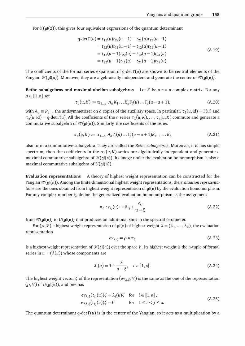
Yangians and quantum groups 155
For Y (gl(2)), this gives four equivalent expressions of the quantum determinant
q-det Γ (u) = t11(u)t22(u− 1)− t21(u)t12(u− 1)
= t22(u)t11(u− 1)− t12(u)t21(u− 1)
= t11(u− 1)t22(u)− t12(u− 1)t21(u)
= t22(u− 1)t11(u)− t21(u− 1)t12(u).
(A.19)
The coefficients of the formal series expansion of q-det Γ (u) are shown to be central elements of theYangian Y (gl(n)). Moreover, they are algebraically independent and generate the center of Y (gl(n)).
Bethe subalgebras and maximal abelian subalgebras Let K be a n × n complex matrix. For anya ∈ J1,nK set
τa(u, K) := tr1...a Aa K1 . . . KaΓ1(u) . . . Γa(u− a+ 1), (A.20)
with Aa ≡ P−1...a the antisymmetrizer on a copies of the auxiliary space. In particular, τ1(u, id) = Γ (u) andτn(u, id) = q-det Γ (u). All the coefficients of the n series τ1(u, K), . . . ,τn(u, K) commute and generate acommutative subalgebra of Y (gl(n)). Similarly, the coefficients of the series
σa(u, K) := tr1...a AaΓ1(u) . . . Γa(u− a+ 1)Ka+1 . . . Kn (A.21)
also form a commutative subalgebra. They are called the Bethe subalgebras. Moreover, if K has simplespectrum, then the coefficients in the σa(u, K) series are algebraically independent and generate amaximal commutative subalgebra of Y (gl(n)). Its image under the evaluation homomorphism is also amaximal commutative subalgebra of U(gl(n)).
Evaluation representations A theory of highest weight representation can be constructed for theYangian Y (gl(n)). Among the finite-dimensional highest weight representations, the evaluation representa-tions are the ones obtained from highest weight representation of gl(n) by the evaluation homomorphism.For any complex number ξ, define the generalized evaluation homomorphism as the assignment
πξ : t i j(u) 7→ δi j +ei j
u− ξ (A.22)
from Y (gl(n)) to U(gl(n)) that produces an additional shift in the spectral parameter.For (ρ, V ) a highest weight representation of gl(n) of highest weight λ = (λ1, . . . ,λn), the evaluation
representationevλ,ξ = ρ πξ (A.23)
is a highest weight representation of Y (gl(n)) over the space V . Its highest weight is the n-tuple of formalseries in u−1 (λ(u)) whose components are
λi(u) = 1+λ
u− ξ , i ∈ J1,nK . (A.24)
The highest weight vector ζ of the representation (evλ,ξ, V ) is the same as the one of the representation(ρ, V ) of U(gl(n)), and one has
evλ,ξ(t ii(u))ζ= λi(u)ζ for i ∈ J1,nK ,
evλ,ξ(t i j(u))ζ= 0 for 1≤ i < j ≤ n.(A.25)
The quantum determinant q-det Γ (u) is in the center of the Yangian, so it acts as a multiplication by a

156 Chapter A — Yangians and quantum groups
scalar on V , determined byq-det Γ (u)|V = λ1(u) . . .λn(u− n+ 1). (A.26)
It is customary to abuse of the notation q-det Γ (u) to denote this scalar quantity as well.Consider N highest weight evaluation representations
evλ(k),ξk
, Vk
, k ∈ J1, NK . (A.27)
We note
evλ,ξ :=N⊗
k=1
evλ(k),ξk(A.28)
andζ := ζ1 ⊗ · · · ⊗ ζn (A.29)
the vector of V1⊗· · ·⊗VN constructed by tensorization of the highest weight vector of each representation.The submodule evλ,ξ(Y (gl(n)))ζ of V1⊗· · ·⊗VN formed by the descendant states of ζ is a highest weightrepresentation of Y (gl(n)) as well, with highest weight vector ζ and highest weight (λ1(u), . . .λN (u)),with
λi(u) =N∏
k=1
1+
λ(k)i
u− ξk
!. (A.30)
Spin chains as representations of Yangian algebras Highest weight evaluation representations ofYangian Y (gl(n)) over a Hilbert space define integrable models. Consider N spaces V1, . . . , VN , N ≥ 2,each equipped with a finite irreducible highest weight representation (ρλ(k) , Vk), k ∈ J1, NK, of gl(2),where λ(k) is some Young diagram λ(k) = (λ(k)1 , . . . ,λ(k)n ) labelling the representation.
The evaluation representation at each site gives the local Lax matrix L0k(u) which is in End(Cn)⊗ Vk
L0k(u) := evλ(k),ξk[Γ (u)] =
n∑i, j=1
ei j ⊗ρλ(k) πξk
[t i j(u)]. (A.31)
The representation of the defining RT T relation impose the Yang–Baxter equation for the Lax matrix atsite k with the R-matrix (A.7)
R12(u− v)L1k(u)L2k(v) = L2k(v)L1k(u)R12(u− v). (A.32)
Tensoring these representations, one gets a highest weight evaluation representation of Y (gl(n)) onthe whole Hilbert spaceH = V1 ⊗ · · · ⊗ VN with the monodromy matrix M(u) in End(Cn)⊗H
M(u) := evλ,ξ (∆′)⊗(N−1)Γ (u)
=N∑
i, j=1
ei j ⊗n∑
p1,...,pN−1=1
ρλ(1) πξ1
[tp1 j(u)]
. . .ρλ(N) πξN
[t ipN−1(u)]
,
(A.33)
which identifies to the matrix product of Lax matrices in the auxiliary space
M(u) = L0N (u) . . . L01(u). (A.34)
M(u) verifies the Yang–Baxter equation with the R-matrix (A.7)
R12(u− v)M1k(u)M2k(v) = M2k(v)M1k(u)R12(u− v) (A.35)
as a direct consequence of the defining RT T relation (A.6) by the representation onH .

Yangians and quantum groups 157
The conventions between this mathematical presentation and the spin chains literature differ a bit.First we introduce the deformation parameter η explicitly by a rescaling of the spectral parameter (andinhomogeneities)
u→ uη
and ξk→ξk
η. (A.36)
Then we multiply the monodromy matrix by the scalar factor
N∏k=1
(u− ξk). (A.37)
Equivalently, this amounts to a redefinition of the evaluation homomorphism πξ. Now the monodromy ispolynomial of End(H )[u], and is written
M(u) = (u− ξ1 +ηΠ01) . . . (u− ξN +ηΠ0N ), (A.38)
where
Π0k =n∑
i, j=1
ei j ⊗ρλ(k)[e ji]. (A.39)
It still satisfies the Yang–Baxter equation, the YBE is homogeneous. It is customary to use the R-matrix
R(u) = u+ηP. (A.40)
The scalar value of the quantum determinant is now
q-det M(u) =n∏
i=1
N∏k=1
u− ξk +η(λ
(k)i − i + 1)
. (A.41)
The highest weight of the representation is now given by the polynomials
∀i ∈ J1,nK , Mii(u)ζ= λi(u)ζ with (A.42)
λi(u) =N∏
k=1
u− ξk +λ
(k)i η
. (A.43)
Taking the trace of the monodromy over the auxiliary space, this gives the transfer matrix
T (u) := tr M(u) (A.44)
which is a commuting family of operators of End(H ) thanks to the YBE (A.35)
∀u, v ∈ C, [T (u), T (v)] = 0. (A.45)
Note that the highest weight vector ζ is an eigenstate of the transfer matrix
T (u)ζ=n∑
i=1
λi(u) ζ. (A.46)
gl(n) and GL(n) invariances The one-site Lax matrices are gl(n)-invariant: for all k ∈ J1, NK
∀i, j ∈ J1,nK ,L0k(u), ei j ⊗ 1+ 1⊗ρλ(k)(ei j)
H = 0. (A.47)

158 Chapter A — Yangians and quantum groups
This also implies a GL(n) group symmetry
∀K ∈ GL(n), [L0k(u), K ⊗ ˜ρλ(k)(K)]H = 0, (A.48)
where ρλ(k) is the induced representation of GL(n) by the representation ρλ(k) of gl(n). This invarianceextends straightforwardly to the monodromy matrix. Applying a GL(n) isomorphism to each site of thechain is equivalent to performing the inverse transformation on the auxiliary space Cn.
Fusion procedure It is possible to construct gl(n)-invariant R-matrices corresponding to higher rep-resentations of gl(n) by the fusion procedure. It was introduced by Kulish, Reshetikhin and Sklyaninin [227], and explained in details for the gl(3) case in [111]. See also [225, 229–231, 319, 320] amongthe modern literature for their used in the context of integrable system. The general idea is to construct aproduct of R-matrices along the same auxiliary spaces while fusing along the other, quantum spaces. Letλ = (λ1, . . . ,λn) be a Young diagram corresponding to an irreducible representation (ρλ, Vλ) of gl(n). Wewrite
Pλ : ⊗di=1Vi −→ Vλ (A.49)
the corresponding projector on the irreducible component Vλ. We note
Rλ0Vλ(u) := PλR0d(u+ sdη) . . . R01(u+ s1η)PΛ, (A.50)
where shifts s1, . . . , sd are determined by filling each boxes (i, j) of the Young diagram by −i+ j, and readit from left to right, top to bottom. The R-matrix degenerate in two points
R(±η) = η(1±P) = ±2ηP±, (A.51)
where P+ and P− are respectively the symmetrizer and antisymmetrizer over V ⊗ V . From them, it ispossible to obtain explicit expression of the projector Pλ as a product of shifted R-matrices [319, 321].For instance, the symmetrizer over n copies of the V space is the ordered product
P+1...d =
d−1∏`=1
1(d + 1)!
yd−1∏`=1
yd∏
k=`+1
R`k((k− l)η). (A.52)
From the choice of the shifts si and the R-matrices product form of the projectors Pλ, one proves
R12(u− v)Rλ1Vλ(u)Rλ2Vλ
(v) = Rλ2Vλ(v)Rλ1Vλ
(u)R12(u− v) (A.53)
by repeated use of the YBE for the fundamental R-matrix (A.40).Fusing along the auxiliary space, the fusion procedure allows to construct a wide family of monodromy
matrices MλVλ(u) indexed by Young diagrams λ of gl(n). They are intertwined by Yang–Baxter equations
of the formRλ,µ
VλVµ(u− v)Mλ
Vλ(u)Mµ
Vµ(v) = Mµ
Vµ(v)Mλ
Vλ(u)Rλ,µ
VλVµ(u− v), (A.54)
where λ, µ are two Young diagrams and Rλ,µVλVµ(u) is the R-matrix constructing by fusing on its two space
to the corresponding Vλ, Vµ representations.The fusion procedure thus generates new transfer matrices
Tλ(u) := trVλ Mλ(u), (A.55)

Yangians and quantum groups 159
which are shown to form a commuting family by taking the trace of (A.54) over Vλ ⊗ Vµ:
∀λ,µ ∈ YD, ∀u, v ∈ C,Tλ(u), Tµ(v)
= 0, (A.56)
where YD is the set of admissible Young diagrams indexing gl(n) highest weight irreducible representations
YD= λ= (λ1, . . . ,λn) | λ1 ≥ · · · ≥ λn ≥ 0 \ (0, . . . , 0). (A.57)
Hierarchy of fused transfer matrices The transfer matrices Tλ(u) are not all independent, but tiedtogether by the fusion relations. They arise from the decomposition in irreducible components of tensorproducts of highest weight representations of gl(n).
As we already know, the elements τa(u, K) defined in (A.20) generates the Bethe algebra. Theirrepresentations overH
Ta(u) = evλ,ξ[τa(u, K)] (A.58)
are the fused transfer matrices corresponding to the pure column Young diagram with a boxes (1, . . . , 1, 0, . . . , 0).All transfer matrices Tλ(u) can be expressed in terms of the Ta(u) by means or the Bazhanov–
Reshetikhin formulaTλ(u) = det
1≤i, j≤λ1
T(λᵀ) j+i− j(u−η(i − 1)) (A.59)
Also, the bilinear Hirota relations holds between transfer matrices associated to rectangular Youngdiagrams. Noting (a, b) the rectangular Young diagrams with a ≤ n rows of length b2, the other beingzeros, it holds
T(a,b)(u)T(a,b)(u−η) = T(a,b−1)(u)T(a,b+1)(u−η) + T(a+1,b)(u)T(a−1,b)(u−η). (A.60)
The fusion hierarchy for the T (K)a (u) transfer matrices is given by the relations
T (K)a−1(ξ j −η)T (K)(ξ j) = T (K)a (ξ j), (A.61)
for j ∈ J1, NK and a ∈ J1,nK, with T (K)n (u) ≡ q-det M (K)(u). From (A.20) and (A.58), one can see theTa(u) are polynomials in End(H )[u] of degree aN . Their leading coefficients is easily identified as theantisymmetric characters of the twist matrix K . Moreover, one can exhibit the (a− 1)N central zeroes
∀ j ∈ J1, NK , ∀r ∈ J1, a− 1K , Ta(ξ j + rη) = 0. (A.62)
This can be shown by bringing two projectors whose product is zero in the expression (A.20) [128, 227].Therefore, the knowledge of N fusion relations is sufficient to reconstruct the transfer matrix Ta(u) formTa−1(u) by Lagrange interpolation in the inhomogeneities.
Ta(u) =N∏
j=1
a−1∏r=1
(u− ξ j − rη)
T∞a
N∏j=1
(u− ξ j) +N∑
k=1
g(a)k (u)Ta−1(ξk −η)T1(ξk)
, (A.63)
whereT∞a = tr1...a(P
−1...aK1 . . . Ka) (A.64)
2In chapter 8, we use similar but different notations when dealing with transfer matrices associated to rectangular Youngdiagrams, because the convention chosen there for the orientation of the Young diagrams is different.
160 Chapter A — Yangians and quantum groups
and
g(a)k (u) =N∏`=16=k
u− ξ`ξk − ξ`
·N∏
j=1
a−1∏r=1
1ξk − ξ j − rη
. (A.65)
The above discussion still holds for other algebras A, such as A = Uq(Õgl(n)) which gives generalization
of the XXZ model, or Z2-graded algebras A= Y (gl(m|n)), Uq(Úgl(m|n)) giving supersymmetric quantumintegrable models. The latter are described in more details in chapter 8.

Bibliography
Publications of Louis Vignoli
[LV1] J. M. Maillet, G. Niccoli, and L. Vignoli, “Separation of variables bases for integrable glM|N andHubbard models,” SciPost Phys., vol. 9, p. 60, 4 2020. DOI: 10.21468/SciPostPhys.9.4.060(pages 19, 95, 105, 125, 133–135, 141, 143, 146, 147, 150, 181).
[LV2] J. M. Maillet, G. Niccoli, and L. Vignoli, “On Scalar Products in Higher Rank Quantum Separationof Variables,” SciPost Phys., vol. 9, p. 86, 6 2020. DOI: 10.21468/SciPostPhys.9.6.086(pages 19, 105, 107, 108, 113–124, 149, 239).
References
[1] G. Galilei, Dialogo sopra i due massimi sistemi del mondo. Edizioni Studio Tesi, 1992, vol. 36(page 7).
[2] G. Galilei, Discorsi e dimostrazioni matematiche. Elsevier, 2013 (page 7).
[3] R. Descartes, Les principes de la philosophie. par la Compagnie des libraires, 1723 (page 7).
[4] S. Roux, “Découvrir le principe d’inertie,” Recherches sur la philosophie et le langage, vol. 24,pp. 453–515, 2006 (page 7).
[5] I. Newton, Philosophiæ naturalis principia mathematica. 1687 (page 7).
[6] R. J. Blackwell and C. Huygens, “Christiaan Huygens’ The Motion of Colliding Bodies,” Isis, vol. 68,no. 4, pp. 574–597, 1977 (pages 7, 8).
[7] J. Kepler, Astronomia nova ..., seu physica coelestis, tradita commentariis de motibus stellae martis.Heidelberg: Voegelin, 1609. DOI: https://doi.org/10.3931/e-rara-558 (page 8).
[8] J. Kepler, The harmony of the world. American Philosophical Society, 1997, vol. 209 (page 8).
[9] D. Bernoulli, Euler’s correspondence with daniel bernoulli, 1744 (page 8).
[10] A. Borrelli, “Angular momentum between physics and mathematics,” in Mathematics meets physics,V. H. Deutsch, Ed., 2011 (page 8).
[11] L. Poinsot, Éléments de statique: suivis de quatre mémoires sur la composition des moments et desaires. Hachette Livre, 2018 (page 8).
[12] G. W. Leibniz and K. Gerhardt, Leibnizens mathematische schriften, A. A. Berlin, Ed. 1849 (page 8).
[13] J. L. Lagrange, Mécanique analytique. Mallet-Bachelier, 1853, vol. 1 (page 8).
[14] É. du Châtelet, Principes Mathématiques de la Philosophie Naturelle, D. et Saillant, Ed. Lambert,1859 (page 8).
[15] W. J. M. Rankine, “Xviii. on the general law of the transformation of energy,” The London,Edinburgh, and Dublin Philosophical Magazine and Journal of Science, vol. 5, no. 30, pp. 106–117, 1853. DOI: 10.1080/14786445308647205. eprint: https://doi.org/10.1080/14786445308647205 (page 8).
161

162 Bibliography
[16] H. W. Dickinson, A short history of the steam engine. Cambridge University Press, 2011 (page 8).
[17] S. Carnot, “Réflexions sur la puissance motrice du feu et sur les machines propres à développercette puissance,” Annales scientifiques de l’École normale supérieure, vol. 1, pp. 393–457, 1872.DOI: 10.24033/asens.88 (page 8).
[18] J. P. Joule and M. Faraday, “III. on the mechanical equivalent of heat,” Philosophical Transactionsof the Royal Society of London, vol. 140, pp. 61–82, 1850. DOI: 10.1098/rstl.1850.0004.eprint: https://royalsocietypublishing.org/doi/pdf/10.1098/rstl.1850.0004(page 8).
[19] J. R. von Mayer, Remarks on the forces of nature, 1841. as quoted in: Lehninger, a. bioenergetics-themolecular basis of biological energy transformations, 1971 (page 8).
[20] R. Clausius, “I. on the moving force of heat, and the laws regarding the nature of heat itselfwhich are deducible therefrom,” The London, Edinburgh, and Dublin Philosophical Magazine andJournal of Science, vol. 2, no. 8, pp. 1–21, 1851. DOI: 10.1080/14786445108646819. eprint:https://doi.org/10.1080/14786445108646819 (page 8).
[21] J. C. Maxwell, “Illustrations of the dynamical theory of gases.—Part I. On the motions andcollisions of perfectly elastic spheres,” The London, Edinburgh, and Dublin Philosophical Magazineand Journal of Science, vol. 19, no. 124, pp. 19–32, 1860. DOI: 10.1080/14786446008642818.eprint: https://doi.org/10.1080/14786446008642818 (page 8).
[22] J. C. Maxwell, “Illustrations of the dynamical theory of gases.—Part II. On the process of diffusionof two or more kinds of moving particles among one another,” The London, Edinburgh, and DublinPhilosophical Magazine and Journal of Science, vol. 20, no. 130, pp. 21–37, 1860. DOI: 10.1080/14786446008642902. eprint: https://doi.org/10.1080/14786446008642902 (page 8).
[23] L. Boltzmann, “Weitere studien über das wärmegleichgewicht unter gasmolekülen,” in KinetischeTheorie II, Springer, 1970, pp. 115–225. DOI: https://doi.org/10.1007/978-3-322-84986-1_3 (page 8).
[24] R. Feynman, R. Leighton, and M. Sands, The Feynman Lectures on Physics, Vol. I: The NewMillennium Edition: Mainly Mechanics, Radiation, and Heat. Basic Books, 2015 (page 9).
[25] J. Tyndall and W. Francis, Scientific Memoirs, Selected from the Transactions of Foreign Academiesof Science, and from Foreign Journals. Natural Philosophy, v. 1. 1853 (page 9).
[26] A. Einstein, “Does the inertia of a body depend upon its energy-content,” Ann Phys, vol. 18,pp. 639–641, 1905 (page 9).
[27] A. Einstein, “Elementary derivation of the equivalence of mass and energy,” Bulletin of theAmerican mathematical society, vol. 41, no. 4, pp. 223–230, 1935 (page 9).
[28] R. Wald, General Relativity. University of Chicago Press, 2010 (page 9).
[29] M. L’Annunziata, Radioactivity: Introduction and History, From the Quantum to Quarks. ElsevierScience, 2016 (page 9).
[30] R. V. Pound and G. A. Rebka, “Apparent weight of photons,” Phys. Rev. Lett., vol. 4, pp. 337–341,7 Apr. 1960. DOI: 10.1103/PhysRevLett.4.337 (page 9).
[31] S. Rainville, J. K. Thompson, E. G. Myers, J. M. Brown, et al., “A direct test of e=mc2,” Nature,vol. 438, no. 7071, pp. 1096–1097, Dec. 2005. DOI: 10.1038/4381096a (page 9).
[32] M. Peskin and D. Schroeder, An introduction to quantum field theory. CRC press, 2018 (page 9).
[33] M. D. Schwartz, Quantum field theory and the standard model. Cambridge University Press, 2014(page 9).
References 163
[34] H. Goldstein, C. Poole, and J. Safko, Classical Mechanics (3rd Edition). Jun. 2001 (pages 10, 17,21, 22, 65, 66).
[35] J. Hermann, “Extrait d’une lettre de M. Herman à M. Bernoulli datée de Padoüe le 12 juillet1710,” Histoire de l’académie royale des sciences (Paris), vol. 1732, p. 519, 1710 (page 10).
[36] U. Le Verrier, “Lettre de M. Le Verrier à M. Faye sur la théorie de Mercure et sur le mouvementdu périhélie de cette planète,” Comptes Rendus de l’Academie de Sciences (Paris), pp. 379–383,1859 (page 10).
[37] J. V. José and E. J. Saletan, Classical Dynamics: A Contemporary Approach. Cambridge UniversityPress, 1998. DOI: 10.1017/CBO9780511803772 (pages 10, 11, 21, 22).
[38] E. Noether, “Invariante variationsprobleme,” in Springer Collected Works in Mathematics, SpringerBerlin Heidelberg, 1983, pp. 231–239. DOI: 10.1007/978-3-642-39990-9_13 (page 11).
[39] M. Nakahara, Geometry, topology and physics. CRC press, 2003 (page 11).
[40] F. Gieres, “About symmetries in physics,” Dec. 1997. arXiv: hep-th/9712154 (page 11).
[41] M.-L. Ge, “Quantum Groups and Quantum Integrable Systems,” in Quantum Group and QuantumIntegrable Systems, World Scientific, Jul. 1992. DOI: 10.1142/9789814538534 (page 11).
[42] J. F. Cornwell, Group Theory in Physics: Volume 1, ser. Techniques of Physics. Elsevier Science,1986 (page 11).
[43] J. Cornwell, Group Theory in Physics: Volume 2, ser. Techniques of Physics. Elsevier Science, 1986(page 11).
[44] J. F. Cornwell, Group Theory in Physics. Volume III: Supersymmetries and Infinite-DimensionalAlgebras. Academic Press, 1989, vol. 10, pp. 1–628 (pages 11, 125–127).
[45] J. E. Humphreys, Introduction to Lie algebras and representation theory. Springer Science &Business Media, 2012, vol. 9 (page 11).
[46] R. Gilmore, Lie groups, Lie algebras, and some of their applications. Courier Corporation, 2012(page 11).
[47] J. Liouville, “Note sur l’intégration des équations différentielles de la dynamique, présentée aubureau des longitudes le 29 juin 1853.,” Journal de Mathématiques Pures et Appliquées, pp. 137–138, 1855 (pages 11, 21).
[48] V. I. Arnol’d, Mathematical methods of classical mechanics. Springer Science & Business Media,2013, vol. 60. DOI: 10.1007/978-1-4757-1693-1 (pages 11, 21, 23, 24).
[49] O. Babelon, D. Bernard, and M. Talon, Introduction to Classical Integrable Systems, ser. Cam-bridge Monographs on Mathematical Physics. Cambridge University Press, 2003. DOI: 10.1017/CBO9780511535024 (pages 11–14, 21, 23, 27, 28, 31).
[50] P. D. Lax, “Integrals of nonlinear equations of evolution and solitary waves,” Communicationson Pure and Applied Mathematics, vol. 21, no. 5, pp. 467–490, 1968. DOI: https://doi.org/10.1002/cpa.3160210503. eprint: https://onlinelibrary.wiley.com/doi/pdf/10.1002/cpa.3160210503 (pages 11, 12, 21, 26).
[51] J. Boussinesq, “Théorie de l’intumescence liquide appelée onde solitaire ou de translation sepropageant dans un canal rectangulaire,” CR Acad. Sci. Paris, vol. 72, no. 755-759, p. 1871, 1871(page 11).
[52] J. Boussinesq, Éssai sur la théorie des eaux courantes, ser. Mémoires présentés par divers savants àl’Académie des sciences de l’Institut National de France. Imprimerie nationale, 1877 (page 11).

164 Bibliography
[53] J. S. Russell, Report on Waves: Made to the Meetings of the British Association in 1842-43. 1845(page 11).
[54] C. S. Gardner, J. M. Greene, M. D. Kruskal, and R. M. Miura, “Method for solving the korteweg-devries equation,” Phys. Rev. Lett., vol. 19, pp. 1095–1097, 19 Nov. 1967. DOI: 10.1103/PhysRevLett.19.1095 (pages 12, 13, 21, 29).
[55] A. Shabat and V. Zakharov, “Exact theory of two-dimensional self-focusing and one-dimensionalself-modulation of waves in nonlinear media,” Soviet physics JETP, vol. 34, no. 1, p. 62, 1972(pages 12, 26).
[56] V. E. Zakharov and A. B. Shabat, “Interaction between solitons in a stable medium,” Sov. Phys.JETP, vol. 37, no. 5, pp. 823–828, 1973 (pages 12, 26).
[57] V. E. Zakharov and L. D. Faddeev, “Korteweg–de vries equation: A completely integrable hamilto-nian system,” Funktsional’nyi Analiz i ego Prilozheniya, vol. 5, no. 4, pp. 18–27, 1971 (pages 12,26).
[58] I. M. Gel’fand and B. M. Levitan, “On the determination of a differential equation from its spectralfunction,” pp. 253–304, 1955. DOI: 10.1090/trans2/001/11 (pages 12, 31).
[59] V. A. Marchenko, “On reconstruction of the potential energy from phases of the scattered waves,”in Dokl. Akad. Nauk SSSR, vol. 104, 1955, pp. 695–698 (pages 12, 31).
[60] M. J. Ablowitz, D. J. Kaup, A. C. Newell, and H. Segur, “Method for solving the sine-gordonequation,” Physical Review Letters, vol. 30, no. 25, p. 1262, 1973 (pages 12, 31).
[61] V. A. Marchenko, Sturm-Liouville operators and applications. American Mathematical Soc., 2011,vol. 373 (page 12).
[62] L. Faddeev, “Integrable models in 1+ 1 dimensional quantum field theory,” CEA Centre d’EtudesNucleaires de Saclay, Tech. Rep., 1982 (pages 12, 27, 37).
[63] L. Faddeev and L. Takhtajan, Hamiltonian methods in the theory of solitons. Springer Science &Business Media, 1987 (pages 12, 21, 26, 27, 32).
[64] W. Lenz, “Beitrag zum verständnis der magnetischen erscheinungen in festen körpern,” Z. Phys.,vol. 21, pp. 613–615, 1920 (page 12).
[65] E. Ising, “Contribution to the Theory of Ferromagnetism,” Z. Phys., vol. 31, pp. 253–258, 1925.DOI: 10.1007/BF02980577 (page 12).
[66] L. Onsager, “Crystal statistics. I. A two-dimensional model with an order-disorder transition,”Phys. Rev., vol. 65, pp. 117–149, 3-4 Feb. 1944. DOI: 10.1103/PhysRev.65.117 (page 12).
[67] B. Kaufman, “Crystal statistics. II. Partition function evaluated by spinor analysis,” Phys. Rev.,vol. 76, pp. 1232–1243, 8 Oct. 1949. DOI: 10.1103/PhysRev.76.1232 (page 12).
[68] B. Kaufman and L. Onsager, “Crystal statistics. III. Short-range order in a binary Ising lattice,”Phys. Rev., vol. 76, pp. 1244–1252, 8 Oct. 1949. DOI: 10.1103/PhysRev.76.1244 (page 12).
[69] W. Heisenberg, “Zur Theorie des Ferromagnetismus,” Zeitschrift für Physik, vol. 49, no. 9-10,pp. 619–636, Sep. 1928. DOI: 10.1007/bf01328601 (pages 12, 37, 42).
[70] H. Bethe, “Zur Theorie der Metalle,” Zeitschrift für Physik, vol. 71, no. 3-4, pp. 205–226, Mar.1931. DOI: 10.1007/bf01341708 (page 12).
[71] R. Orbach, “Linear antiferromagnetic chain with anisotropic coupling,” Physical Review, vol. 112,no. 2, pp. 309–316, Oct. 1958. DOI: 10.1103/physrev.112.309 (page 12).
[72] L. R. Walker, “Antiferromagnetic linear chain,” Physical Review, vol. 116, no. 5, pp. 1089–1090,Dec. 1959. DOI: 10.1103/physrev.116.1089 (page 12).

References 165
[73] C. N. Yang and C. P. Yang, “One-dimensional chain of anisotropic spin-spin interactions. i. proofof bethe’s hypothesis for ground state in a finite system,” Phys. Rev., vol. 150, pp. 321–327, 1 Oct.1966. DOI: 10.1103/PhysRev.150.321 (page 13).
[74] C. N. Yang and C. P. Yang, “One-dimensional chain of anisotropic spin-spin interactions. ii.properties of the ground-state energy per lattice site for an infinite system,” Phys. Rev., vol. 150,pp. 327–339, 1 Oct. 1966. DOI: 10.1103/PhysRev.150.327 (page 13).
[75] C. N. Yang and C. P. Yang, “One-dimensional chain of anisotropic spin-spin interactions. iii.applications,” Phys. Rev., vol. 151, pp. 258–264, 1 Nov. 1966. DOI: 10.1103/PhysRev.151.258(page 13).
[76] L. Pauling, “The structure and entropy of ice and of other crystals with some randomness ofatomic arrangement,” Journal of the American Chemical Society, vol. 57, no. 12, pp. 2680–2684,Dec. 1935. DOI: 10.1021/ja01315a102 (page 13).
[77] E. H. Lieb, “Residual entropy of square ice,” Phys. Rev., vol. 162, pp. 162–172, 1 Oct. 1967. DOI:10.1103/PhysRev.162.162 (page 13).
[78] B. Sutherland, “Two-dimensional hydrogen bonded crystals without the ice rule,” Journal ofMathematical Physics, vol. 11, no. 11, pp. 3183–3186, 1970. DOI: 10.1063/1.1665111. eprint:https://doi.org/10.1063/1.1665111 (page 13).
[79] B. Sutherland, Beautiful Models. WORLD SCIENTIFIC, Jun. 2004. DOI: 10.1142/5552 (pages 13,39).
[80] R. J. Baxter, “Exactly Solved Models in Statistical Mechanics,” in Series on Advances in Statis-tical Mechanics, World Scientific, May 1985, pp. 5–63. DOI: 10.1142/9789814415255_0002(pages 13, 42).
[81] R. Baxter, “Eight-vertex model in lattice statistics and one-dimensional anisotropic Heisenbergchain. i, II, III,” Annals of Physics, vol. 76, no. 1, pp. 1–24, 25–47, 48–71, Mar. 1973. DOI:10.1016/0003-4916(73)90440-5 (page 13).
[82] R. J. Baxter, “Corner transfer matrices of the eight-vertex model. I. low-temperature expansionsand conjectured properties,” Journal of Statistical Physics, vol. 15, no. 6, pp. 485–503, Dec. 1976.DOI: 10.1007/bf01020802 (page 13).
[83] R. J. Baxter, “Corner transfer matrices of the eight-vertex model. II. The Ising model case,” Journalof Statistical Physics, vol. 17, no. 1, pp. 1–14, Jul. 1977. DOI: 10.1007/bf01089373 (page 13).
[84] R. J. Baxter, “Eight-vertex model in lattice statistics,” Physical Review Letters, vol. 26, no. 14,pp. 832–833, Apr. 1971. DOI: 10.1103/physrevlett.26.832 (page 13).
[85] R. J. Baxter, “One-dimensional anisotropic Heisenberg chain,” Annals of Physics, vol. 70, no. 2,pp. 323–337, Apr. 1972. DOI: 10.1016/0003-4916(72)90270-9 (pages 13, 42).
[86] C. N. Yang, “Some exact results for the many-body problem in one dimension with repulsivedelta-function interaction,” Phys. Rev. Lett., vol. 19, pp. 1312–1315, 23 Dec. 1967. DOI: 10.1103/PhysRevLett.19.1312 (page 13).
[87] J. B. McGuire, “Study of exactly soluble one-dimensional n-body problems,” Journal of Mathe-matical Physics, vol. 5, no. 5, pp. 622–636, 1964 (page 13).
[88] C. N. Yang, “S matrix for the one-dimensional n-body problem with repulsive or attractiveδ-function interaction,” Physical Review, vol. 168, no. 5, p. 1920, 1968 (page 13).
[89] E. Sklyanin, “On complete integrability of the Landau-Lifshitz equation,” LOMI, Tech. Rep., 1979(pages 13, 14, 21, 27).

166 Bibliography
[90] E. K. Sklyanin, “Quantum version of the method of inverse scattering problem,” Journal of SovietMathematics, vol. 19, no. 5, pp. 1546–1596, 1982. DOI: 10.1007/bf01091462 (pages 13, 21,27, 30–32, 37, 41).
[91] M. A. Semenov-Tyan-Shanskii, “What is a classical r-matrix?” Functional Analysis and Its Ap-plications, vol. 17, no. 4, pp. 259–272, Oct. 1983. DOI: 10.1007/BF01076717 (pages 13,21).
[92] E. H. Lieb and W. Liniger, “Exact analysis of an interacting bose gas. i. the general solution andthe ground state,” Phys. Rev., vol. 130, pp. 1605–1616, 4 May 1963. DOI: 10.1103/PhysRev.130.1605 (page 13).
[93] E. H. Lieb, “Exact analysis of an interacting bose gas. ii. the excitation spectrum,” Phys. Rev.,vol. 130, pp. 1616–1624, 4 May 1963. DOI: 10.1103/PhysRev.130.1616 (page 13).
[94] E. K. Sklyanin and L. D. Faddeev, “Quantum-mechanical approach to completely integrablefield theory models,” in Fifty Years of Mathematical Physics, WORLD SCIENTIFIC, Feb. 2016,pp. 290–292. DOI: 10.1142/9789814340960_0025 (page 13).
[95] E. K. Sklyanin, L. A. Takhtadzhyan, and L. D. Faddeev, “Quantum inverse problem method. i,”Theoretical and Mathematical Physics, vol. 40, no. 2, pp. 688–706, Aug. 1979. DOI: 10.1007/bf01018718 (pages 13, 14, 30).
[96] E. Sklyanin, “Method of the inverse scattering problem and the nonlinear quantum Schroedingerequation,” Sov. Phys. Dokl., vol. 24, pp. 107–109, 1979 (pages 13, 21).
[97] L. Faddeev, “Instructive history of the quantum inverse scattering method,” in KdV ’95: Proceed-ings of the International Symposium held in Amsterdam, The Netherlands, April 23–26, 1995, tocommemorate the centennial of the publication of the equation by and named after Korteweg and deVries, M. Hazewinkel, H. W. Capel, and E. M. de Jager, Eds. Dordrecht: Springer Netherlands,1995, pp. 69–84. DOI: 10.1007/978-94-011-0017-5_3 (pages 13, 37).
[98] H. B. Thacker, “Exact integrability in quantum field theory and statistical systems,” Rev. Mod.Phys., vol. 53, pp. 253–285, 2 Apr. 1981. DOI: 10.1103/RevModPhys.53.253 (page 14).
[99] V. E. Korepin, N. M. Bogoliubov, and A. G. Izergin, Quantum Inverse Scattering Method andCorrelation Functions, ser. Cambridge Monographs on Mathematical Physics. Cambridge UniversityPress, 1993. DOI: 10.1017/CBO9780511628832 (pages 14, 37, 51, 58).
[100] L. Faddeev, “How Algebraic Bethe Ansatz works for integrable models,” arXiv preprint hep-th/9605187, 1996 (pages 14, 37, 40–42, 51).
[101] H. Bergknoff and H. B. Thacker, “Method for solving the massive thirring model,” Phys. Rev. Lett.,vol. 42, pp. 135–138, 3 Jan. 1979. DOI: 10.1103/PhysRevLett.42.135 (page 14).
[102] L. A. Takhtadzhan and L. D. Faddeev, “The quantum method of the inverse problem and theHeisenberg XYZ model,” Russian Mathematical Surveys, vol. 34, no. 5, pp. 11–68, Oct. 1979. DOI:10.1070/rm1979v034n05abeh003909 (pages 14, 42).
[103] L. D. Faddeev and L. A. Takhtajan, “Quantum inverse scattering method,” Sov. Sci. Rev. Math,1981 (pages 14, 37, 42).
[104] N. Kitanine, J. Maillet, and V. Terras, “Form factors of the XXZ Heisenberg finite chain,” NuclearPhysics B, vol. 554, no. 3, pp. 647–678, Aug. 1999. DOI: 10.1016/s0550-3213(99)00295-3(pages 14, 37, 49, 55, 57–59, 143).
[105] N. Kitanine, J. Maillet, and V. Terras, “Correlation functions of the XXZ Heisenberg spin- chain in amagnetic field,” Nuclear Physics B, vol. 567, no. 3, pp. 554–582, Feb. 2000. DOI: 10.1016/s0550-3213(99)00619-7 (pages 14, 15, 37, 57, 60).

References 167
[106] J. Maillet and V. Terras, “On the quantum inverse scattering problem,” Nuclear Physics B, vol. 575,no. 3, pp. 627–644, Jun. 2000. DOI: 10.1016/s0550-3213(00)00097-3 (pages 14, 37, 49,50, 58, 143).
[107] F. Gohmann and V. E. Korepin, “Solution of the quantum inverse problem,” J. Phys. A, vol. 33,pp. 1199–1220, 2000. DOI: 10.1088/0305-4470/33/6/308. arXiv: hep-th/9910253(pages 14, 37, 49, 50, 125).
[108] A. A. Belavin and V. G. Drinfel’d, “Solutions of the classical yang–baxter equation for simple liealgebras,” Functional Analysis and Its Applications, vol. 16, no. 3, pp. 159–180, Jul. 1982. DOI:10.1007/BF01081585 (page 14).
[109] A. A. Belavin and V. G. Drinfel’d, “Classical young–baxter equation for simple lie algebras,”Functional Analysis and Its Applications, vol. 17, no. 3, pp. 220–221, 1984. DOI: 10.1007/bf01078107 (page 14).
[110] A. Belavin and V. Drinfeld, Triangle Equations and Simple Lie Algebras, ser. Soviet scientific reviews:Mathematical physics reviews. Harwood Academic Publishers, 1984 (page 14).
[111] P. P. Kulish and N. Y. Reshetikhin, “GL3-invariant solutions of the Yang-Baxter equation andassociated quantum systems,” Journal of Soviet Mathematics, vol. 34, no. 5, pp. 1948–1971, Sep.1986. DOI: 10.1007/bf01095104 (pages 14, 18, 158).
[112] P. P. Kulish and E. K. Sklyanin, “Solutions of the Yang-Baxter equation,” Journal of Soviet Mathe-matics, vol. 19, no. 5, pp. 1596–1620, 1982. DOI: 10.1007/bf01091463 (pages 14, 18, 29).
[113] P. P. Kulish and N. Y. Reshetikhin, “Quantum linear problem for the sine-Gordon equation andhigher representations,” Journal of Soviet Mathematics, vol. 23, no. 4, pp. 2435–2441, 1983. DOI:10.1007/bf01084171 (page 14).
[114] M. Jimbo, “A q-difference analogue of U(g) and the Yang-Baxter equation,” Letters in MathematicalPhysics, vol. 10, no. 1, pp. 63–69, Jul. 1985. DOI: 10.1007/bf00704588 (page 14).
[115] V. G. Drinfel’d, “Quantum groups,” Journal of Soviet mathematics, vol. 41, no. 2, pp. 898–915,1988. DOI: 10.1007/BF01247086 (page 14).
[116] V. Chari and A. Pressley, A Guide to Quantum Groups. Cambridge University Press, 1995 (page 14).
[117] A. Molev, Yangians and classical Lie algebras, 143. American Mathematical Soc., 2007 (pages 14,45, 125, 129, 153).
[118] C. Kassel, Quantum Groups, ser. Graduate Texts in Mathematics. Springer New York, 2012(page 14).
[119] N. Reshetikhin and V. G. Turaev, “Invariants of 3-manifolds via link polynomials and quantumgroups,” Inventiones mathematicae, vol. 103, no. 1, pp. 547–597, Dec. 1991. DOI: 10.1007/BF01239527 (page 14).
[120] V. Turaev and O. Viro, “State sum invariants of 3-manifolds and quantum 6j-symbols,” Topology,vol. 31, no. 4, pp. 865–902, 1992. DOI: https://doi.org/10.1016/0040-9383(92)90015-A (page 14).
[121] V. G. Turaev, Quantum Invariants of Knots and 3-Manifolds. De Gruyter, 2016. DOI: doi:10.1515/9783110435221 (page 14).
[122] P. P. Kulish and N. Y. Reshetikhin, “Diagonalisation of GL(N) invariant transfer matrices andquantum N-wave system (Lee model),” Journal of Physics A: Mathematical and General, vol. 16,no. 16, pp. L591–L596, Nov. 1983. DOI: 10.1088/0305-4470/16/16/001 (page 15).
[123] N. A. Slavnov, “Introduction to the nested algebraic Bethe ansatz,” SciPost Phys. Lect. Notes, p. 19,2020. DOI: 10.21468/SciPostPhysLectNotes.19 (page 15).

168 Bibliography
[124] M. P. Pfannmüller and H. Frahm, “Algebraic Bethe ansatz for gl(2, 1) invariant 36-vertex models,”Nuclear Physics B, vol. 479, no. 3, pp. 575–593, 1996. DOI: https://doi.org/10.1016/0550-3213(96)00425-7 (pages 15, 125, 144).
[125] F. Göhmann, “Algebraic Bethe ansatz for the gl(1|2) generalized model and Lieb–Wu equations,”Nuclear Physics B, vol. 620, no. 3, pp. 501–518, 2002. DOI: https://doi.org/10.1016/S0550-3213(01)00497-7 (pages 15, 125, 144).
[126] D. Baeriswyl, D. Campbell, J. M. P. Carmelo, F. Guinea, and E. Louis, The Hubbard Model: ItsPhysics and Mathematical Physics. Springer, Boston, MA, Jan. 1995. DOI: 10.1007/978-1-4899-1042-4 (pages 15, 125, 145).
[127] E. Ragoucy and G. Satta, “Analytical Bethe Ansatz for closed and open gl(M |N) super-spinchains in arbitrary representations and for any Dynkin diagram,” Journal of High Energy Physics,vol. 2007, no. 9, pp. 001–001, 2007. DOI: 10.1088/1126-6708/2007/09/001 (pages 15, 125,133).
[128] V. Kazakov, A. Sorin, and A. Zabrodin, “Supersymmetric Bethe ansatz and Baxter equationsfrom discrete Hirota dynamics,” Nuclear Physics B, vol. 790, no. 3, pp. 345–413, Feb. 2008. DOI:10.1016/j.nuclphysb.2007.06.025 (pages 15, 18, 125, 131, 133–135, 159).
[129] S. Pakuliak, E. Ragoucy, and N. Slavnov, “Nested Algebraic Bethe Ansatz in integrable models:recent results,” SciPost Phys. Lect. Notes, p. 6, 2018. DOI: 10.21468/SciPostPhysLectNotes.6(pages 15, 16, 51, 60–62).
[130] M. Gaudin, The Bethe Wavefunction, J.-S. Caux, Ed. Cambridge University Press, 2014. DOI:10.1017/CBO9781107053885 (pages 15, 47).
[131] V. E. Korepin, “Calculation of norms of Bethe wave functions,” Communications in MathematicalPhysics, vol. 86, no. 3, pp. 391–418, 1982. DOI: 10.1007/bf01212176 (pages 15, 57, 62).
[132] N. Slavnov, “Calculation of scalar products of wave functions and form factors in the frameworkof the algebraic bethe ansatz,” Theoretical and Mathematical Physics - THEOR MATH PHYS-ENGLTR, vol. 79, pp. 502–508, May 1989. DOI: 10.1007/BF01016531 (pages 15, 56).
[133] N. Kitanine, J. Maillet, N. Slavnov, and V. Terras, “Spin-spin correlation functions of the XXZ-Heisenberg chain in a magnetic field,” Nuclear Physics B, vol. 641, no. 3, pp. 487–518, Oct. 2002.DOI: 10.1016/s0550-3213(02)00583-7 (pages 15, 60).
[134] N. Kitanine, J. Maillet, N. Slavnov, and V. Terras, “Master equation for spin–spin correlationfunctions of the XXZ chain,” Nuclear Physics B, vol. 712, no. 3, pp. 600–622, Apr. 2005. DOI:10.1016/j.nuclphysb.2005.01.050 (pages 15, 60).
[135] N. Kitanine, K. Kozlowski, J. M. Maillet, N. A. Slavnov, and V. Terras, “On correlation functionsof integrable models associated with the six-vertex R-matrix,” Journal of Statistical Mechanics:Theory and Experiment, vol. 2007, no. 01, P01022–P01022, Jan. 2007. DOI: 10.1088/1742-5468/2007/01/p01022 (page 15).
[136] N. Kitanine, K. K. Kozlowski, J. M. Maillet, N. A. Slavnov, and V. Terras, “Algebraic Bethe ansatzapproach to the asymptotic behavior of correlation functions,” Journal of Statistical Mechanics:Theory and Experiment, vol. 2009, no. 04, P04003, Apr. 2009. DOI: 10.1088/1742-5468/2009/04/p04003 (page 15).
[137] N. Kitanine, K. K. Kozlowski, J. M. Maillet, N. A. Slavnov, and V. Terras, “On the thermodynamiclimit of form factors in the massless XXZ Heisenberg chain,” Journal of Mathematical Physics,vol. 50, no. 9, p. 095 209, Sep. 2009. DOI: 10.1063/1.3136683 (page 15).

References 169
[138] N. Kitanine, K. K. Kozlowski, J. M. Maillet, G. Niccoli, et al., “Correlation functions of the openXXZ chain: I,” Journal of Statistical Mechanics: Theory and Experiment, vol. 2007, no. 10, P10009–P10009, Oct. 2007. DOI: 10.1088/1742-5468/2007/10/p10009 (page 15).
[139] N. Kitanine, K. K. Kozlowski, J. M. Maillet, G. Niccoli, et al., “Correlation functions of the openXXZ chain: II,” Journal of Statistical Mechanics: Theory and Experiment, vol. 2008, no. 07, P07010,Jul. 2008. DOI: 10.1088/1742-5468/2008/07/p07010 (page 15).
[140] J.-S. Caux and J. M. Maillet, “Computation of dynamical correlation functions of Heisenbergchains in a magnetic field,” Physical Review Letters, vol. 95, no. 7, Aug. 2005. DOI: 10.1103/physrevlett.95.077201 (page 15).
[141] J.-S. Caux, R. Hagemans, and J. M. Maillet, “Computation of dynamical correlation functions ofHeisenberg chains: The gapless anisotropic regime,” Journal of Statistical Mechanics: Theory andExperiment, vol. 2005, no. 09, P09003–P09003, Sep. 2005. DOI: 10.1088/1742-5468/2005/09/p09003 (page 15).
[142] M. Kenzelmann, R. Coldea, D. A. Tennant, D. Visser, et al., “Order-to-disorder transition in thexy-like quantum magnet Cs2CoCl4 induced by noncommuting applied fields,” Phys. Rev. B, vol. 65,p. 144 432, 14 Apr. 2002. DOI: 10.1103/PhysRevB.65.144432 (page 15).
[143] J.-M. Maillet, “Heisenberg spin chains: From quantum groups to neutron scattering experiments,”in Quantum Spaces: Poincaré Seminar 2007, B. Duplantier, Ed. Basel: Birkhäuser Basel, 2007,pp. 161–201. DOI: 10.1007/978-3-7643-8522-4_4 (pages 15, 37, 45).
[144] F. Göhmann, A. Klümper, and A. Seel, “Integral representations for correlation functions of theXXZ chain at finite temperature,” Journal of Physics A: Mathematical and General, vol. 37, no. 31,pp. 7625–7651, Jul. 2004. DOI: 10.1088/0305-4470/37/31/001 (page 15).
[145] F. Göhmann, A. Klümper, and A. Seel, “Integral representation of the density matrix of the xxzchain at finite temperatures,” Journal of Physics A: Mathematical and General, vol. 38, no. 9,pp. 1833–1841, Feb. 2005. DOI: 10.1088/0305-4470/38/9/001 (page 15).
[146] F. Göhmann, A. Klümper, and A. Seel, “Emptiness formation probability at finite temperature forthe isotropic heisenberg chain,” Physica B: Condensed Matter, vol. 359-361, pp. 807–809, Apr.2005. DOI: 10.1016/j.physb.2005.01.234 (page 15).
[147] F. Göhmann and J. Suzuki, “Quantum spin chains at finite temperatures,” New Trends in QuantumIntegrable Systems, Oct. 2010. DOI: 10.1142/9789814324373_0005 (page 15).
[148] K. K. Kozlowski, J. M. Maillet, and N. A. Slavnov, “Long-distance behavior of temperaturecorrelation functions in the one-dimensional Bose gas,” Journal of Statistical Mechanics: Theoryand Experiment, vol. 2011, no. 03, P03018, Mar. 2011. DOI: 10.1088/1742-5468/2011/03/p03018 (page 15).
[149] K. K. Kozlowski, J. M. Maillet, and N. A. Slavnov, “Correlation functions for one-dimensionalbosons at low temperature,” Journal of Statistical Mechanics: Theory and Experiment, vol. 2011,no. 03, P03019, Mar. 2011. DOI: 10.1088/1742-5468/2011/03/p03019 (page 15).
[150] S. Belliard, S. Pakuliak, E. Ragoucy, and N. A. Slavnov, “Highest coefficient of scalar productsin SU(3)-invariant integrable models,” Journal of Statistical Mechanics: Theory and Experiment,vol. 2012, no. 09, P09003, Sep. 2012. DOI: 10.1088/1742-5468/2012/09/p09003 (pages 15,62).
[151] S. Belliard, S. Pakuliak, E. Ragoucy, and N. A. Slavnov, “The algebraic Bethe ansatz for scalarproducts in SU(3)-invariant integrable models,” Journal of Statistical Mechanics: Theory andExperiment, vol. 2012, no. 10, P10017, Oct. 2012. DOI: 10.1088/1742-5468/2012/10/p10017 (pages 15, 62).

170 Bibliography
[152] S. Pakuliak, E. Ragoucy, and N. Slavnov, “Form factors in quantum integrable models withGL(3)-invariant R-matrix,” Nuclear Physics B, vol. 881, pp. 343–368, 2014. DOI: https://doi.org/10.1016/j.nuclphysb.2014.02.014 (page 15).
[153] S. Z. Pakuliak, E. Ragoucy, and N. A. Slavnov, “Determinant representations for form factors inquantum integrable models with the GL(3)-invariant R-matrix,” Theoretical and MathematicalPhysics, vol. 181, no. 3, pp. 1566–1584, Dec. 2014. DOI: 10.1007/s11232-014-0236-0(page 15).
[154] S. Pakuliak, E. Ragoucy, and N. A. Slavnov, “GL(3)-based quantum integrable composite models.I. Bethe vectors,” Symmetry, Integrability and Geometry: Methods and Applications, Jul. 2015. DOI:10.3842/sigma.2015.063 (page 15).
[155] S. Pakuliak, E. Ragoucy, and N. A. Slavnov, “GL(3) -based quantum integrable composite models.II. form factors of local operators,” Symmetry, Integrability and Geometry: Methods and Applications,Jul. 2015. DOI: 10.3842/sigma.2015.064 (page 15).
[156] A. Liashyk and N. A. Slavnov, “On Bethe vectors in gl(3)-invariant integrable models,” Journal ofHigh Energy Physics, vol. 2018, no. 6, Jun. 2018. DOI: 10.1007/jhep06(2018)018 (page 15).
[157] A. Hutsalyuk, A. Liashyk, S. Z. Pakuliak, E. Ragoucy, and N. A. Slavnov, “Multiple actions of themonodromy matrix in gl(2|1)-invariant integrable models,” Symmetry, Integrability and Geometry:Methods and Applications, Oct. 2016. DOI: 10.3842/sigma.2016.099 (pages 15, 125).
[158] S. Z. Pakuliak, E. Ragoucy, and N. A. Slavnov, “Bethe vectors for models based on the super-Yangian Y (gl(m|n)),” Journal of Integrable Systems, vol. 2, no. 1, Jan. 2017. DOI: 10.1093/integr/xyx001 (pages 15, 60, 125).
[159] A. A. Hutsalyuk, A. N. Liashyk, S. Z. Pakuliak, E. Ragoucy, and N. A. Slavnov, “Current presentationfor the super-Yangian double DY gl(m|n) and Bethe vectors,” Russian Mathematical Surveys, vol. 72,no. 1, pp. 33–99, Feb. 2017. DOI: 10.1070/rm9754 (page 15).
[160] A. Hutsalyuk, A. Liashyk, S. Z. Pakuliak, E. Ragoucy, and N. A. Slavnov, “Scalar products ofBethe vectors in models with gl(2|1) symmetry 2. determinant representation,” Journal of PhysicsA: Mathematical and Theoretical, vol. 50, no. 3, p. 034 004, Dec. 2016. DOI: 10.1088/1751-8121/50/3/034004 (pages 15, 62, 125).
[161] A. Hutsalyuk, A. Liashyk, S. Pakuliak, E. Ragoucy, and N. Slavnov, “Scalar products of bethevectors in the models with gl(m|n)symmetry,” Nuclear Physics B, vol. 923, pp. 277–311, Oct.2017. DOI: 10.1016/j.nuclphysb.2017.07.020 (pages 15, 62, 125).
[162] A. Hutsalyuk, A. Liashyk, S. Pakuliak, E. Ragoucy, and N. Slavnov, “Norm of bethe vectorsin models with gl(m|n) symmetry,” Nuclear Physics B, vol. 926, pp. 256–278, Jan. 2018. DOI:10.1016/j.nuclphysb.2017.11.006 (pages 15, 62, 125).
[163] N. Beisert, C. Ahn, L. F. Alday, Z. Bajnok, et al., “Review of ads/cft integrability: An overview,”Letters in Mathematical Physics, vol. 99, no. 1, pp. 3–32, Jan. 2012. DOI: 10.1007/s11005-011-0529-2 (page 15).
[164] N. Beisert, “The S-matrix of AdS/CFT and Yangian symmetry,” in Proceedings of Bethe Ansatz: 75years later — PoS(Solvay), Sissa Medialab, Aug. 2007. DOI: 10.22323/1.038.0002 (page 15).
[165] N. Beisert, “The analytic Bethe ansatz for a chain with centrally extended su(2|2) symmetry,”Journal of Statistical Mechanics: Theory and Experiment, vol. 2007, no. 01, P01017–P01017, Jan.2007. DOI: 10.1088/1742-5468/2007/01/p01017 (page 15).
[166] I. Kostov, D. Serban, and D. Volin, “Strong coupling limit of bethe ansatz equations,” NuclearPhysics B, vol. 789, no. 3, pp. 413–451, 2008. DOI: https://doi.org/10.1016/j.nuclphysb.2007.06.017 (page 15).

References 171
[167] H. Saleur, “Superspin chains and supersigma models: A short introduction,” Exact Methods inLow-dimensional Statistical Physics and Quantum Computing: Lecture Notes of the Les HouchesSummer School: Volume 89, July 2008, vol. 89, p. 455, 2010 (page 15).
[168] D. Serban, “A note on the eigenvectors of long-range spin chains and their scalar products,”Journal of High Energy Physics, vol. 2013, no. 1, Jan. 2013. DOI: 10.1007/jhep01(2013)012(page 15).
[169] D. Serban, “Eigenvectors and scalar products for long range interacting spin chains II: Thefinite size effects,” Journal of High Energy Physics, vol. 2013, no. 8, Aug. 2013. DOI: 10.1007/jhep08(2013)128 (page 15).
[170] Y. Jiang, S. Komatsu, I. Kostov, and D. Serban, “The hexagon in the mirror: The three-pointfunction in the SoV representation,” Journal of Physics A: Mathematical and Theoretical, vol. 49,no. 17, p. 174 007, Mar. 2016. DOI: 10.1088/1751-8113/49/17/174007 (page 15).
[171] F. Levkovich-Maslyuk, “A review of the AdS/CFT Quantum Spectral Curve,” J. Phys. A, vol. 53,no. 28, p. 283 004, 2020. DOI: 10.1088/1751-8121/ab7137. arXiv: 1911.13065 [hep-th](page 15).
[172] V. Tarasov and A. Varchenko, “Completeness of Bethe vectors and difference equations withregular singular points,” International Mathematics Research Notices, vol. 1995, no. 13, p. 637,1995. DOI: 10.1155/s1073792895000377 (pages 16, 56).
[173] E. Mukhin, V. Tarasov, and A. Varchenko, “On separation of variables and completeness of theBethe ansatz for quantum glN Gaudin model,” Glasgow Mathematical Journal, vol. 51, no. A,p. 137, Feb. 2009. DOI: 10.1017/s0017089508004850 (pages 16, 56).
[174] W. Hao, R. I. Nepomechie, and A. J. Sommese, “Completeness of solutions of bethe’s equations,”Physical Review E, vol. 88, no. 5, Nov. 2013. DOI: 10.1103/physreve.88.052113 (pages 16,56).
[175] D. Chernyak, S. Leurent, and D. Volin, Completeness of Wronskian Bethe equations for rationalgl(m|n) spin chain, 2020. arXiv: 2004.02865 [math-ph] (pages 16, 56, 150).
[176] G. Niccoli, “Antiperiodic spin-1/2 XXZ quantum chains by separation of variables: Completespectrum and form factors,” Nuclear Physics B, vol. 870, no. 2, pp. 397–420, May 2013. DOI:10.1016/j.nuclphysb.2013.01.017 (pages 16, 18, 63, 82–84).
[177] E. K. Sklyanin, “The quantum Toda chain,” in Non-Linear Equations in Classical and Quantum FieldTheory, Springer Berlin Heidelberg, 1985, pp. 196–233. DOI: 10.1007/3-540-15213-x_80(pages 16, 17, 65).
[178] N. Gromov, F. Levkovich-Maslyuk, and G. Sizov, “New construction of eigenstates and separationof variables for SU(N) quantum spin chains,” Journal of High Energy Physics, vol. 2017, no. 9,Sep. 2017. DOI: 10.1007/jhep09(2017)111 (pages 16, 18, 19, 63, 85, 105).
[179] N. Gromov and F. Levkovich-Maslyuk, “New compact construction of eigenstates for supersym-metric spin chains,” Journal of High Energy Physics, vol. 2018, no. 9, Sep. 2018. DOI: 10.1007/jhep09(2018)085 (pages 16, 18, 105).
[180] Y. Wang, W.-L. Yang, J. Cao, and K. Shi, Off-Diagonal Bethe Ansatz for Exactly Solvable Models.Springer Berlin Heidelberg, 2015. DOI: 10.1007/978-3-662-46756-5 (page 16).
[181] S. Belliard, “Heisenberg XXX model with general boundaries: Eigenvectors from algebraic BetheAnsatz,” Symmetry, Integrability and Geometry: Methods and Applications, Nov. 2013. DOI: 10.3842/sigma.2013.072 (pages 16, 63).
[182] J. L. R. d’Alembert, Traité de dynamique. David, 1758 (page 16).

172 Bibliography
[183] S. Engelsman, “D’Alembert et les équations aux dérivées partielles,” 1984. DOI: 10.3406/dhs.1984.1480 (page 16).
[184] J. B. J. Fourier, Théorie analytique de la chaleur. Firmin Didot, 1822 (page 16).
[185] M. C. Gutzwiller, “The quantum mechanical Toda lattice, II,” Annals of Physics, vol. 133, no. 2,pp. 304–331, 1981. DOI: https://doi.org/10.1016/0003-4916(81)90253-0 (page 17).
[186] E. K. Sklyanin, “Goryachev-chaplygin top and the inverse scattering method,” Journal of SovietMathematics, vol. 31, no. 6, pp. 3417–3431, Dec. 1985. DOI: 10.1007/bf02107243 (pages 17,65, 70).
[187] E. K. Sklyanin, “Separation of variables in the classical integrable SL(3) magnetic chain,” Com-munications in Mathematical Physics, vol. 150, no. 1, pp. 181–191, Nov. 1992. DOI: 10.1007/bf02096572 (pages 17, 32, 65, 70–73, 83).
[188] E. K. Sklyanin, “Separation of variables : New trends,” Progress of Theoretical Physics Supplement,vol. 118, pp. 35–60, 1995. DOI: 10.1143/ptps.118.35 (pages 17, 65, 70–73, 84).
[189] D. R. D. Scott, “Classical functional bethe ansatz for SL(n): Separation of variables for themagnetic chain,” Journal of Mathematical Physics, vol. 35, no. 11, pp. 5831–5843, Nov. 1994.DOI: 10.1063/1.530712 (pages 17, 65, 71).
[190] M. I. Gekhtman, “Separation of variables in the classicalSL(n) magnetic chain,” Communicationsin Mathematical Physics, vol. 167, no. 3, pp. 593–605, Feb. 1995. DOI: 10.1007/bf02101537(pages 17, 65, 71).
[191] E. K. Sklyanin, “Separation of variables in the gaudin model,” Journal of Soviet Mathematics,vol. 47, no. 2, pp. 2473–2488, Oct. 1989. DOI: 10.1007/bf01840429 (pages 17, 47).
[192] E. Sklyanin, “Functional Bethe Ansatz,” in Integrable and Superintegrable Systems, World Scientific,Oct. 1990, pp. 8–33. DOI: 10.1142/9789812797179_0002 (pages 17, 65, 71, 78).
[193] E. K. Sklyanin, “Quantum inverse scattering method. Selected topics,” Oct. 1992. arXiv: hep-th/9211111 (pages 17, 37, 65, 71, 73, 78, 84).
[194] E. K. Sklyanin and T. Takebe, “Separation of variables in the elliptic gaudin model,” Com-munications in Mathematical Physics, vol. 204, no. 1, pp. 17–38, Jul. 1999. DOI: 10.1007/s002200050635 (page 17).
[195] E. K. Sklyanin, “New approach to the quantum nonlinear schrödinger equation,” Journal of PhysicsA: Mathematical and General, vol. 22, no. 17, pp. 3551–3560, Sep. 1989. DOI: 10.1088/0305-4470/22/17/020 (page 17).
[196] E. Sklyanin, “Exact quantization of the sinh-gordon model,” Nuclear Physics B, vol. 326, no. 3,pp. 719–736, 1989. DOI: https://doi.org/10.1016/0550-3213(89)90552-X (page 17).
[197] V. B. Kuznetsov and E. K. Sklyanin, “Separation of variables in the A_2 type jack polynomials,”arXiv preprint solv-int/9508002, 1995 (page 17).
[198] V. B. Kuznetsov and E. K. Sklyanin, “Separation of variables for the ruijsenaars model and a newintegral representation for the macdonald polynomials,” Journal of Physics A: Mathematical andGeneral, vol. 29, no. 11, pp. 2779–2804, Jun. 1996. DOI: 10.1088/0305-4470/29/11/014(page 17).
[199] V. B. Kuznetsov, F. W. Nijhoff, and E. K. Sklyanin, “Separation of variables for the ruijsenaarssystem,” Communications in Mathematical Physics, vol. 189, no. 3, pp. 855–877, Nov. 1997. DOI:10.1007/s002200050231 (page 17).

References 173
[200] S. Derkachov, G. Korchemsky, and A. Manashov, “Non-compact Heisenberg spin magnets fromhigh-energy QCD,” Nuclear Physics B, vol. 617, no. 1-3, pp. 375–440, Dec. 2001. DOI: 10.1016/s0550-3213(01)00457-6 (page 17).
[201] S. Derkachov, G. P. Korchemsky, and A. N. Manashov, “Separation of variables for the quantumSL(2,R) spin chain,” Journal of High Energy Physics, vol. 2003, no. 07, pp. 047–047, Jul. 2003.DOI: 10.1088/1126-6708/2003/07/047 (page 17).
[202] S. Derkachov, G. P. Korchemsky, and A. N. Manashov, “Baxter Q-operator and separation ofvariables for the open SL(2,R) spin chain,” Journal of High Energy Physics, vol. 2003, no. 10,pp. 053–053, Oct. 2003. DOI: 10.1088/1126-6708/2003/10/053 (page 17).
[203] A. G. Bytsko and J. Teschner, “Quantization of models with non-compact quantum group symme-try: Modular XXZ magnet and lattice sinh-Gordon model,” Journal of Physics A: Mathematical andGeneral, vol. 39, no. 41, pp. 12 927–12 981, Sep. 2006. DOI: 10.1088/0305-4470/39/41/s11(page 17).
[204] H. Frahm, A. Seel, and T. Wirth, “Separation of variables in the open XXX chain,” Nuclear PhysicsB, vol. 802, no. 3, pp. 351–367, Oct. 2008. DOI: 10.1016/j.nuclphysb.2008.04.008(pages 17, 78).
[205] H. Frahm, J. H. Grelik, A. Seel, and T. Wirth, “Functional Bethe ansatz methods for the open XXXchain,” Journal of Physics A: Mathematical and Theoretical, vol. 44, no. 1, p. 015 001, Nov. 2010.DOI: 10.1088/1751-8113/44/1/015001 (pages 17, 78).
[206] E. K. Sklyanin, “Separation of variables in the quantum integrable models related to the YangianY [sl(3)],” Journal of Mathematical Sciences, vol. 80, no. 3, pp. 1861–1871, Jun. 1996. DOI:10.1007/bf02362784 (pages 17, 65, 83, 84, 150).
[207] F. A. Smirnov, “Separation of variables for quantum integrable models related to Uq(bslN ),” inMathPhys Odyssey 2001, Birkhäuser Boston, 2002, pp. 455–465. DOI: 10.1007/978-1-4612-0087-1_17 (pages 17, 83).
[208] G. Niccoli and J. Teschner, “The sine-Gordon model revisited: I,” Journal of Statistical Mechanics:Theory and Experiment, vol. 2010, no. 09, P09014, Sep. 2010. DOI: 10.1088/1742-5468/2010/09/p09014 (page 18).
[209] G. Niccoli, “Reconstruction of Baxter-operator from Sklyanin SOV for cyclic representations ofintegrable quantum models,” Nuclear Physics B, vol. 835, no. 3, pp. 263–283, Aug. 2010. DOI:10.1016/j.nuclphysb.2010.03.009 (page 18).
[210] G. Niccoli, “Completeness of Bethe ansatz by Sklyanin SOV for cyclic representations of integrablequantum models,” Journal of High Energy Physics, vol. 2011, no. 3, Mar. 2011. DOI: 10.1007/jhep03(2011)123 (page 18).
[211] G. Niccoli, “Non-diagonal open spin-1/2 XXZ quantum chains by separation of variables: Completespectrum and matrix elements of some quasi-local operators,” Journal of Statistical Mechanics:Theory and Experiment, vol. 2012, no. 10, P10025, Oct. 2012. DOI: 10.1088/1742-5468/2012/10/p10025 (pages 18, 84, 121).
[212] N. Grosjean and G. Niccoli, “The τ2-model and the chiral Potts model revisited: Completenessof Bethe equations from Sklyanin’s SoV method,” Journal of Statistical Mechanics: Theory andExperiment, vol. 2012, no. 11, P11005, Nov. 2012. DOI: 10.1088/1742-5468/2012/11/p11005 (pages 18, 56).
[213] N. Grosjean, J. M. Maillet, and G. Niccoli, “On the form factors of local operators in the latticesine–Gordon model,” Journal of Statistical Mechanics: Theory and Experiment, vol. 2012, no. 10,P10006, Oct. 2012. DOI: 10.1088/1742-5468/2012/10/p10006 (pages 18, 121).
174 Bibliography
[214] G. Niccoli, “An antiperiodic dynamical six-vertex model: I. complete spectrum by SOV, matrixelements of the identity on separate states and connections to the periodic eight-vertex model,”Journal of Physics A: Mathematical and Theoretical, vol. 46, no. 7, p. 075 003, Feb. 2013. DOI:10.1088/1751-8113/46/7/075003 (pages 18, 63, 84).
[215] G. Niccoli, “Form factors and complete spectrum of XXX anti-periodic higher spin chains byquantum separation of variables,” Journal of Mathematical Physics, vol. 54, no. 5, p. 053 516,May 2013. DOI: 10.1063/1.4807078 (pages 18, 63, 84).
[216] N. Grosjean, J.-M. Maillet, and G. Niccoli, “On the form factors of local operators in the Bazhanov-Stroganov and chiral Potts models,” Annales Henri Poincaré, vol. 16, no. 5, pp. 1103–1153, Oct.2014. DOI: 10.1007/s00023-014-0358-9 (page 18).
[217] N. Kitanine, J. M. Maillet, and G. Niccoli, “Open spin chains with generic integrable boundaries:Baxter equation and Bethe ansatz completeness from separation of variables,” Journal of StatisticalMechanics: Theory and Experiment, vol. 2014, no. 5, P05015, May 2014. DOI: 10.1088/1742-5468/2014/05/p05015 (pages 18, 56, 84).
[218] N. Kitanine, J. M. Maillet, G. Niccoli, and V. Terras, “On determinant representations of scalarproducts and form factors in the SoV approach: The XXX case,” Journal of Physics A: Mathematicaland Theoretical, vol. 49, no. 10, p. 104 002, Jan. 2016. DOI: 10.1088/1751-8113/49/10/104002 (pages 18, 84, 101).
[219] N. Kitanine, J. M. Maillet, G. Niccoli, and V. Terras, “The open XXX spin chain in the SoV framework:Scalar product of separate states,” Journal of Physics A: Mathematical and Theoretical, vol. 50,no. 22, p. 224 001, May 2017. DOI: 10.1088/1751-8121/aa6cc9 (pages 18, 84).
[220] N. Kitanine, J. M. Maillet, G. Niccoli, and V. Terras, “The open XXZ spin chain in the SoV framework:Scalar product of separate states,” Journal of Physics A: Mathematical and Theoretical, vol. 51,no. 48, p. 485 201, Oct. 2018. DOI: 10.1088/1751-8121/aae76f (pages 18, 84).
[221] G. Niccoli, H. Pei, and V. Terras, “Correlation functions by separation of variables: The xxx spinchain,” SciPost Physics, vol. 10, no. 1, Jan. 2021. DOI: 10.21468/scipostphys.10.1.006(pages 18, 84, 150).
[222] H. Pei and V. Terras, On scalar products and form factors by separation of variables: The antiperiodicxxz model, 2021. arXiv: 2011.06109 [math-ph] (pages 18, 84, 150).
[223] J. M. Maillet, G. Niccoli, and B. Pezelier, “Transfer matrix spectrum for cyclic representationsof the 6-vertex reflection algebra I,” SciPost Physics, vol. 2, no. 1, Feb. 2017. DOI: 10.21468/scipostphys.2.1.009 (pages 18, 84).
[224] J. M. Maillet, G. Niccoli, and B. Pezelier, “Transfer matrix spectrum for cyclic representations of the6-vertex reflection algebra II,” SciPost Phys., vol. 5, p. 26, 3 2018. DOI: 10.21468/SciPostPhys.5.3.026 (pages 18, 84).
[225] J. M. Maillet and G. Niccoli, “On quantum separation of variables,” Journal of MathematicalPhysics, vol. 59, no. 9, p. 091 417, Sep. 2018. DOI: 10.1063/1.5050989 (pages 18, 19, 63, 81,84, 85, 87, 89, 95, 105, 123, 149, 150, 158).
[226] R. A. Horn and C. R. Johnson, Topics in Matrix Analysis. Cambridge University Press, Apr. 1991.DOI: 10.1017/cbo9780511840371 (pages 18, 89).
[227] P. P. Kulish, N. Y. Reshetikhin, and E. K. Sklyanin, “Yang-Baxter equation and representationtheory: I,” Letters in Mathematical Physics, vol. 5, no. 5, pp. 393–403, Sep. 1981. DOI: 10.1007/bf02285311 (pages 18, 132, 158, 159).

References 175
[228] A. Kuniba, T. Nakanishi, and J. Suzuki, “Functional relations in solvable lattice models I: Functionalrelations and representation theory,” International Journal of Modern Physics A, vol. 09, no. 30,pp. 5215–5266, Dec. 1994. DOI: 10.1142/s0217751x94002119 (page 18).
[229] V. Kazakov and P. Vieira, “From characters to quantum (super)spin chains via fusion,” Journalof High Energy Physics, vol. 2008, no. 10, pp. 050–050, Oct. 2008. DOI: 10.1088/1126-6708/2008/10/050 (pages 18, 125, 132, 133, 158).
[230] A. Kuniba, T. Nakanishi, and J. Suzuki, “T-systems and Y-systems in integrable systems,” Journalof Physics A: Mathematical and Theoretical, vol. 44, no. 10, p. 103 001, Feb. 2011. DOI: 10.1088/1751-8113/44/10/103001 (pages 18, 158).
[231] V. Kazakov, S. Leurent, and Z. Tsuboi, “Baxter’s Q-operators and operatorial Bäcklund flow forquantum (super)-spin chains,” Communications in Mathematical Physics, vol. 311, no. 3, pp. 787–814, May 2012. DOI: 10.1007/s00220-012-1428-9 (pages 18, 133, 158).
[232] J. M. Maillet and G. Niccoli, “On quantum separation of variables beyond fundamental represen-tations,” SciPost Physics, vol. 10, no. 2, Feb. 2021. DOI: 10.21468/scipostphys.10.2.026(pages 18, 87, 95, 105).
[233] J. M. Maillet and G. Niccoli, “On separation of variables for reflection algebras,” Journal ofStatistical Mechanics: Theory and Experiment, vol. 2019, no. 9, p. 094 020, Sep. 2019. DOI:10.1088/1742-5468/ab357a (pages 19, 87, 105).
[234] J. M. Maillet and G. Niccoli, “Complete spectrum of quantum integrable lattice models associatedto Y (gl(n)) by separation of variables,” SciPost Phys., vol. 6, p. 71, 6 2019. DOI: 10.21468/SciPostPhys.6.6.071 (pages 19, 87, 95, 102–105, 150).
[235] J. M. Maillet and G. Niccoli, “Complete spectrum of quantum integrable lattice models associatedto Uq(Ógln) by separation of variables,” Journal of Physics A: Mathematical and Theoretical, vol. 52,no. 31, p. 315 203, Jul. 2019. DOI: 10.1088/1751-8121/ab2930 (pages 19, 87, 95, 105).
[236] P. Ryan and D. Volin, “Separated variables and wave functions for rational gl(N) spin chains inthe companion twist frame,” Journal of Mathematical Physics, vol. 60, no. 3, p. 032 701, Mar.2019. DOI: 10.1063/1.5085387 (pages 19, 63, 85, 87, 105, 149, 150).
[237] P. Ryan and D. Volin, Separation of variables for rational gl(n) spin chains in any compact represen-tation, via fusion, embedding morphism and Bäcklund flow, 2020. arXiv: 2002.12341 [math-ph](pages 19, 63, 87, 105, 149, 150).
[238] A. Cavaglià, N. Gromov, and F. Levkovich-Maslyuk, “Separation of variables and scalar productsat any rank,” Journal of High Energy Physics, vol. 2019, no. 9, Sep. 2019. DOI: 10.1007/jhep09(2019)052 (pages 19, 105, 149).
[239] N. Gromov, F. Levkovich-Maslyuk, P. Ryan, and D. Volin, “Dual separated variables and scalarproducts,” Physics Letters B, vol. 806, p. 135 494, Jul. 2020. DOI: 10.1016/j.physletb.2020.135494 (page 19).
[240] N. Gromov, F. Levkovich-Maslyuk, and P. Ryan, Determinant form of correlators in high rankintegrable spin chains via separation of variables, 2020. arXiv: 2011.08229 [hep-th] (pages 19,105, 149).
[241] O. Babelon and C.-M. Viallet, “Hamiltonian structures and lax equations,” Physics Letters B,vol. 237, no. 3-4, pp. 411–416, Mar. 1990. DOI: 10.1016/0370-2693(90)91198-k (pages 21,27, 28).
[242] W. Appel and E. Kowalski, Mathematics for Physics and Physicists. Princeton University Press, 2007(page 23).

176 Bibliography
[243] J. Avan, H. De Vega, and J. Maillet, “Conformally covariant linear system for the four-dimensionalself-dual Yang–Mills theory,” Physics Letters B, vol. 171, no. 2, pp. 255–260, 1986. DOI: https://doi.org/10.1016/0370-2693(86)91544-3 (page 27).
[244] J. Avan, F. Nijhoff, and J. Maillet, “Spinorial linear system for self-dual Yang–Mills equations,”Physics Letters B, vol. 211, no. 3, pp. 329–334, 1988. DOI: https://doi.org/10.1016/0370-2693(88)90911-2 (page 27).
[245] N. Reshetikhin and P. Weigmann, “Towards the classification of completely integrable quantumfield theories (the Bethe-ansatz associated with Dynkin diagrams and their automorphisms),”Physics Letters B, vol. 189, no. 1-2, pp. 125–131, Apr. 1987. DOI: 10.1016/0370-2693(87)91282-2 (page 29).
[246] M. J. Ablowitz, M. Ablowitz, P. Clarkson, and P. A. Clarkson, Solitons, nonlinear evolution equationsand inverse scattering. Cambridge university press, 1991, vol. 149 (page 31).
[247] V. A. Marchenko, Sturm–Liouville operators and applications. American Mathematical Soc., 2011,vol. 373 (page 31).
[248] J.-M. Maillet, “New integrable canonical structures in two-dimensional models,” Nuclear PhysicsB, vol. 269, no. 1, pp. 54–76, May 1986. DOI: 10.1016/0550-3213(86)90365-2 (pages 32,34).
[249] L. Freidel and J. Maillet, “Quadratic algebras and integrable systems,” Physics Letters B, vol. 262,no. 2, pp. 278–284, 1991. DOI: https://doi.org/10.1016/0370-2693(91)91566-E(page 32).
[250] Y. Ishimori, “An integrable classical spin chain,” Journal of the Physical Society of Japan, vol. 51,no. 11, pp. 3417–3418, 1982. DOI: 10.1143/JPSJ.51.3417. eprint: https://doi.org/10.1143/JPSJ.51.3417 (page 32).
[251] N. Papanicolaou, “Complete integrability for a discrete heisenberg chain,” Journal of Physics A:Mathematical and General, vol. 20, no. 12, pp. 3637–3652, Aug. 1987. DOI: 10.1088/0305-4470/20/12/018 (page 32).
[252] J. M. Maillet, “New algebraic canonical structures of integrability in 2-d field theories,” in SuperField Theories, H. C. Lee, V. Elias, G. Kunstatter, R. B. Mann, and K. S. Viswanathan, Eds. Boston,MA: Springer US, 1987, pp. 527–532. DOI: 10.1007/978-1-4613-0913-0_30 (page 34).
[253] S. Weigert, “The problem of quantum integrability,” Physica D: Nonlinear Phenomena, vol. 56,no. 1, pp. 107–119, 1992. DOI: https://doi.org/10.1016/0167-2789(92)90053-P(page 37).
[254] J.-S. Caux and J. Mossel, “Remarks on the notion of quantum integrability,” Journal of StatisticalMechanics: Theory and Experiment, vol. 2011, no. 02, P02023, Feb. 2011. DOI: 10.1088/1742-5468/2011/02/p02023 (pages 37, 39).
[255] F. H. Essler, H. Frahm, F. Göhmann, A. Klümper, and V. E. Korepin, The one-dimensional Hubbardmodel. Cambridge University Press, 2005. DOI: 10.1017/CBO9780511534843 (pages 37, 125,145, 146, 148).
[256] F. Loebbert, “Lectures on yangian symmetry,” Journal of Physics A: Mathematical and Theoretical,vol. 49, no. 32, p. 323 002, Jul. 2016. DOI: 10.1088/1751-8113/49/32/323002 (pages 37,129, 153).
[257] V. Terras, “Méthode du problème inverse, groupes quantiques et fonctions de corrélation desmodèles intégrables quantiques,” Ph.D. dissertation, ED 52 PHAST, 2000 (pages 37, 50, 58).
[258] P. A. M. Dirac, The principles of quantum mechanics, 27. Oxford university press, 1981 (page 37).

References 177
[259] J. v. Neumann, “Uber funktionen von funktionaloperatoren,” Annals of Mathematics, vol. 32,no. 2, pp. 191–226, 1931. DOI: https://doi.org/10.2307/1968185 (page 38).
[260] M. Jimbo, “Introduction to the yang–baxter equation,” International Journal of Modern PhysicsA, vol. 04, no. 15, pp. 3759–3777, 1989. DOI: 10.1142/S0217751X89001503. eprint: https://doi.org/10.1142/S0217751X89001503 (page 40).
[261] S. K. Satija, J. D. Axe, G. Shirane, H. Yoshizawa, and K. Hirakawa, “Neutron scattering study ofspin waves in one-dimensional antiferromagnet kcuF3,” Phys. Rev. B, vol. 21, pp. 2001–2007, 5Mar. 1980. DOI: 10.1103/PhysRevB.21.2001 (page 45).
[262] M. Abramowitz and I. A. Stegun, Handbook of mathematical functions with formulas, graphs, andmathematical tables. US Government printing office, 1964, vol. 55 (page 47).
[263] O. Foda, K. Iohara, M. Jimbo, R. Kedem, et al., “An elliptic quantum algebra for csl2,” Letters inMathematical Physics, vol. 32, no. 3, pp. 259–268, 1994 (page 47).
[264] G. Felder, “Elliptic quantum groups,” in 11th International Conference on Mathematical Physics(ICMP-11) (Satellite colloquia: New Problems in the General Theory of Fields and Particles, Paris,France, 25-28 Jul 1994), Jul. 1994. arXiv: hep-th/9412207 (page 47).
[265] M. Gaudin, “Modeles exacts en mécanique statistique: La méthode de Bethe et ses généralizations,”Note CEA, vol. 1559, no. 1, p. 1973, 1972 (page 47).
[266] M. Gaudin, “Diagonalisation d’une classe d’hamiltoniens de spin,” Journal de Physique, vol. 37,no. 10, pp. 1087–1098, 1976 (page 47).
[267] E. K. Sklyanin, “Boundary conditions for integrable quantum systems,” Journal of Physics A:Mathematical and General, vol. 21, no. 10, pp. 2375–2389, May 1988. DOI: 10.1088/0305-4470/21/10/015 (page 48).
[268] B. Pezelier, “Separation of variables and new quantum integrable systems with boundaries,”Theses, Université de Lyon, Jun. 2018 (page 48).
[269] E. Mukhin, V. Tarasov, and A. Varchenko, “The B. and M. Shapiro conjecture in real algebraicgeometry and the Bethe ansatz,” Annals of Mathematics, vol. 170, no. 2, pp. 863–881, Sep. 2009.DOI: 10.4007/annals.2009.170.863 (page 56).
[270] J. M. Maillet and J. Sanchez de Santos, “Drinfel’d twists and algebraic Bethe ansatz,” Dec. 1996.arXiv: q-alg/9612012 (page 57).
[271] S. Belliard and N. Slavnov, “Why scalar products in the algebraic Bethe ansatz have determinantrepresentation,” Journal of High Energy Physics, vol. 2019, no. 10, pp. 1–17, 2019. DOI: 10.1007/JHEP10(2019)103 (pages 57, 60).
[272] M. Gaudin, B. M. McCoy, and T. T. Wu, “Normalization sum for the Bethe’s hypothesis wavefunctions of the Heisenberg–Ising chain,” Phys. Rev. D, vol. 23, no. 2, p. 417, 1981. DOI: 10.1103/PhysRevD.23.417 (page 57).
[273] S. Lukyanov and V. Terras, “Long-distance asymptotics of spin-spin correlation functions for thexxz spin chain,” Nuclear Physics B, vol. 654, no. 3, pp. 323–356, Mar. 2003. DOI: 10.1016/s0550-3213(02)01141-0 (page 60).
[274] N. Kitanine, J. Maillet, N. Slavnov, and V. Terras, “Dynamical correlation functions of the spin-1/2chain,” Nuclear Physics B, vol. 729, no. 3, pp. 558–580, Nov. 2005. DOI: 10.1016/j.nuclphysb.2005.08.046 (page 60).
[275] N. Kitanine, J. M. Maillet, N. A. Slavnov, and V. Terras, “On the spin–spin correlation functions ofthe XXZ spin-1/2 infinite chain,” Journal of Physics A: Mathematical and General, vol. 38, no. 34,pp. 7441–7460, Aug. 2005. DOI: 10.1088/0305-4470/38/34/001 (page 60).
178 Bibliography
[276] N. Kitanine, J. M. Maillet, N. A. Slavnov, and V. Terras, “Exact results for the σz two-point functionof the XXZ chain at ∆ = 1/2,” Journal of Statistical Mechanics: Theory and Experiment, vol. 2005,no. 09, Sep. 2005. DOI: 10.1088/1742-5468/2005/09/l09002 (page 60).
[277] N. A. Slavnov, “Scalar products in GL(3)-based models with trigonometric r-matrix. determinantrepresentation,” Journal of Statistical Mechanics: Theory and Experiment, vol. 2015, no. 3, P03019,Mar. 2015. DOI: 10.1088/1742-5468/2015/03/p03019 (page 62).
[278] S. Pakuliak, E. Ragoucy, and N. A. Slavnov, “Form factors of local operators in a one-dimensionaltwo-component Bose gas,” Journal of Physics A: Mathematical and Theoretical, vol. 48, no. 43,p. 435 001, Oct. 2015. DOI: 10.1088/1751-8113/48/43/435001 (page 62).
[279] S. Belliard, N. A. Slavnov, and B. Vallet, “Modified algebraic bethe ansatz: Twisted xxx case,”Symmetry, Integrability and Geometry: Methods and Applications, Jun. 2018. DOI: 10.3842/sigma.2018.054 (page 63).
[280] N. Gromov and F. Levkovich-Maslyuk, “New compact construction of eigenstates for supersym-metric spin chains,” Journal of High Energy Physics, vol. 2018, no. 9, p. 85, Sep. 2018. DOI:10.1007/JHEP09(2018)085 (page 63).
[281] A. Messiah, Mécanique quantique. Tome 1. Dunod, 2003 (pages 65, 77).
[282] I. M. Krichever, “Integration of nonlinear equations by the methods of algebraic geometry,”Functional Analysis and Its Applications, vol. 11, no. 1, pp. 12–26, Jan. 1977. DOI: 10.1007/BF01135528 (page 70).
[283] I. M. Krichever and S. P. Novikov, “Holomorphic bundles over algebraic curves and non-linearequations,” Russian Mathematical Surveys, vol. 35, no. 6, pp. 53–79, Dec. 1980. DOI: 10.1070/rm1980v035n06abeh001974 (page 70).
[284] A. Messiah, Mécanique quantique. Tome 2. Dunod, 2003 (page 77).
[285] G. Niccoli and V. Terras, “Antiperiodic XXZ chains with arbitrary spins: Complete eigenstateconstruction by functional equations in separation of variables,” Letters in Mathematical Physics,vol. 105, no. 7, pp. 989–1031, May 2015. DOI: 10.1007/s11005-015-0759-9 (page 84).
[286] D. Levy-Bencheton, G. Niccoli, and V. Terras, “Antiperiodic dynamical 6-vertex model by separationof variables II: Functional equations and form factors,” Journal of Statistical Mechanics: Theoryand Experiment, vol. 2016, no. 3, p. 033 110, Mar. 2016. DOI: 10.1088/1742-5468/2016/03/033110 (page 84).
[287] S. Faldella, N. Kitanine, and G. Niccoli, “The complete spectrum and scalar products for theopen spin-1/2 XXZ quantum chains with non-diagonal boundary terms,” Journal of StatisticalMechanics: Theory and Experiment, vol. 2014, no. 1, P01011, Jan. 2014. DOI: 10.1088/1742-5468/2014/01/p01011 (page 84).
[288] N. Gromov and F. Levkovich-Maslyuk, “New compact construction of eigenstates for supersym-metric spin chains,” Journal of High Energy Physics, vol. 2018, no. 9, Sep. 2018. DOI: 10.1007/jhep09(2018)085 (page 85).
[289] A. Liashyk and N. A. Slavnov, “On bethe vectors in gl3 -invariant integrable models,” Journal ofHigh Energy Physics, vol. 2018, no. 6, Jun. 2018. DOI: 10.1007/jhep06(2018)018 (page 85).
[290] S. Derkachov and P. Valinevich, “Separation of variables for the quantum SL(3,C) spin magnet:Eigenfunctions of Sklyanin B-operator,” arXiv preprint arXiv:1807.00302, 2018 (page 85).
[291] N. Gromov, F. Levkovich-Maslyuk, P. Ryan, and D. Volin, Dual separated variables and scalarproducts, 2019. arXiv: 1910.13442 [hep-th] (pages 105, 149).

References 179
[292] J. M. Maillet, G. Niccoli, and L. Vignoli, “On Scalar Products in Higher Rank Quantum Separationof Variables,” SciPost Phys., vol. 9, p. 86, 6 2020. DOI: 10.21468/SciPostPhys.9.6.086(page 112).
[293] P. P. Kulish, “Integrable graded magnets,” Journal of Soviet Mathematics, vol. 35, no. 4, pp. 2648–2662, Nov. 1986. DOI: 10.1007/bf01083770 (pages 125, 144).
[294] J. Gruneberg, “On the construction and solution of Uq(gl(2, 1;C))-symmetric models,” NuclearPhysics. B, vol. 568, Mar. 2000. DOI: 10.1016/S0550-3213(99)00675-6 (page 125).
[295] F. H. L. Essler and V. E. Korepin, “Higher conservation laws and algebraic Bethe ansätze for thesupersymmetric t-J model,” Phys. Rev. B, vol. 46, pp. 9147–9162, 14 Oct. 1992. DOI: 10.1103/PhysRevB.46.9147 (pages 125, 144).
[296] “The Hubbard model at half a century,” Nature Physics, vol. 9, 523 EP, Sep. 2013. DOI: 10.1038/nphys2759 (pages 125, 145).
[297] I. Bars, “Supergroups and their representations,” in Introduction to Supersymmetry in Particleand Nuclear Physics. Springer US, 1984, pp. 107–184. DOI: 10.1007/978-1-4757-0917-9_5(pages 125, 131).
[298] I. Bars, “Supergroups and superalgebras in physics,” Physica D: Nonlinear Phenomena, vol. 15,no. 1-2, pp. 42–64, 1985. DOI: 10.1016/0167-2789(85)90147-2 (pages 125, 126, 131).
[299] L. Frappat, P. Sorba, and A. Sciarrino, Dictionary on Lie algebras and superalgebras. AcademicPress (London), 2000, p. 410 (pages 125, 126).
[300] L. Gow, “Yangians of Lie superalgebras,” Ph.D. dissertation, University of Sydney, 2007 (pages 125,129).
[301] A. M. Grabinski and H. Frahm, “Non-diagonal boundary conditions for gl(1|1) super spin chains,”Journal of Physics A: Mathematical and Theoretical, vol. 43, no. 4, p. 045 207, Jan. 2010. DOI:10.1088/1751-8113/43/4/045207 (page 125).
[302] V. Kac, “Lie superalgebras,” Advances in Mathematics, vol. 26, no. 1, pp. 8–96, 1977. DOI: https://doi.org/10.1016/0001-8708(77)90017-2 (page 126).
[303] R. Zhang, “The gl(M |N) super Yangian and its finite-dimensional representations,” Letters inMathematical Physics, vol. 37, no. 4, pp. 419–434, 1996 (page 129).
[304] I. Bars, B. Morel, and H. Ruegg, “Kac–Dynkin diagrams and supertableaux,” Journal of math-ematical physics, vol. 24, no. 9, pp. 2253–2262, 1983. DOI: 10.1063/1.525970 (pages 131,133).
[305] A. V. Zabrodin, “Bäcklund transformations for the difference Hirota equation and the supersym-metric Bethe ansatz,” Theoretical and Mathematical Physics, vol. 155, no. 1, pp. 567–584, Apr.2008. DOI: 10.1007/s11232-008-0047-2 (pages 133–135).
[306] M. Nazarov, “Quantum Berezinian and the classical Capelli identity,” Letters in MathematicalPhysics, vol. 21, no. 2, pp. 123–131, 1991. DOI: 10.1007/bf00401646 (page 133).
[307] P. B. Ramos and M. J. Martins, “Algebraic Bethe ansatz approach for the one-dimensional Hubbardmodel,” Journal of Physics A: Mathematical and General, vol. 30, no. 7, pp. L195–L202, Apr. 1997.DOI: 10.1088/0305-4470/30/7/009 (pages 146, 148).
[308] F. Göhmann and V. Inozemtsev, “The Yangian symmetry of the Hubbard models with variablerange hopping,” Physics Letters A, vol. 214, no. 3-4, pp. 161–166, May 1996. DOI: 10.1016/0375-9601(96)00174-0 (page 146).

180 Bibliography
[309] N. Beisert, M. de Leeuw, and P. Nag, “Fusion for the one-dimensional Hubbard model,” Journal ofPhysics A: Mathematical and Theoretical, vol. 48, no. 32, p. 324 002, 2015. DOI: 10.1088/1751-8113/48/32/324002 (page 148).
[310] M. Martins and P. Ramos, “The quantum inverse scattering method for Hubbard-like models,”Nuclear Physics B, vol. 522, no. 3, pp. 413–470, Jul. 1998. DOI: 10.1016/s0550-3213(98)00199-0 (page 148).
[311] P. B. Ramos and M. J. Martins, “One parameter family of an integrable spl(2|1) vertex model:Algebraic Bethe ansatz and ground state structure,” Nucl. Phys. B, vol. 474, pp. 678–714, 1996.DOI: 10.1016/0550-3213(96)00342-2. arXiv: hep-th/9604072 (page 148).
[312] M. J. Martins and P. B. Ramos, “The Algebraic Bethe ansatz for rational braid-monoid latticemodels,” Nucl. Phys. B, vol. 500, pp. 579–620, 1997. DOI: 10.1016/S0550-3213(97)00342-8.arXiv: hep-th/9703023 (page 148).
[313] P. Ryan, “Integrable systems, separation of variables and the yang-baxter equation,” Ph.D. disser-tation, Trinity College Dublin, 2021 (page 150).
[314] S. Ekhammar, H. Shu, and D. Volin, “Extended systems of Baxter Q-functions and fused flags I:simply-laced case,” Aug. 2020. arXiv: 2008.10597 [math-ph] (page 150).
[315] S. Ekhammar and D. Volin, “Bethe Algebra using Pure Spinors,” Apr. 2021. arXiv: 2104.04539[math-ph] (page 150).
[316] V. G. Drinfeld, “Hopf algebras and the quantum Yang–Baxter equation,” Sov. Math. Dokl., vol. 32,pp. 254–258, 1985 (page 153).
[317] V. G. Drinfeld, “A New realization of Yangians and quantized affine algebras,” Sov. Math. Dokl.,vol. 36, pp. 212–216, 1988 (page 153).
[318] P. Cartier, “A primer of hopf algebras,” in Frontiers in Number Theory, Physics, and Geometry II:On Conformal Field Theories, Discrete Groups and Renormalization, P. Cartier, P. Moussa, B. Julia,and P. Vanhove, Eds. Berlin, Heidelberg: Springer Berlin Heidelberg, 2007, pp. 537–615. DOI:10.1007/978-3-540-30308-4_12 (page 153).
[319] A. V. Zabrodin, “Hirota equation and Bethe ansatz,” Theoretical and Mathematical Physics, vol. 116,no. 1, pp. 782–819, Jul. 1998. DOI: 10.1007/bf02557123 (page 158).
[320] V. Kazakov, S. Leurent, and D. Volin, “T-system on T-hook: Grassmannian solution and twistedQuantum Spectral Curve,” Journal of High Energy Physics, vol. 2016, no. 12, Dec. 2016. DOI:10.1007/jhep12(2016)044 (page 158).
[321] A. Zabrodin, “Discrete Hirota’s equation in quantum integrable models,” International Journal ofModern Physics B, vol. 11, no. 26n27, pp. 3125–3158, 1997. DOI: 10.1142/S0217979297001520(page 158).
Article [LV1]
J. M. Maillet, G. Niccoli, and L. Vignoli, “Separation of variables bases for integrable glM|N and Hubbardmodels,” SciPost Phys., vol. 9, p. 60, 4 2020. DOI: 10.21468/SciPostPhys.9.4.060


SciPost Phys. 9, 060 (2020)
Separation of variables bases for integrableglM|N and Hubbard models
Jean Michel Maillet?, Giuliano Niccoli† and Louis Vignoli‡
Univ Lyon, ENS de Lyon, Univ Claude Bernard, CNRS,Laboratoire de Physique, UMR 5672, F-69342 Lyon, France
? [email protected], † [email protected], ‡ [email protected]
Abstract
We construct quantum Separation of Variables (SoV) bases for both the fundamentalinhomogeneous glM|N supersymmetric integrable models and for the inhomogeneousHubbard model both defined with quasi-periodic twisted boundary conditions given bytwist matrices having simple spectrum. The SoV bases are obtained by using the inte-grable structure of these quantum models, i.e. the associated commuting transfer ma-trices, following the general scheme introduced in [1]; namely, they are given by set ofstates generated by the multiple actions of the transfer matrices on a generic co-vector.The existence of such SoV bases implies that the corresponding transfer matrices havenon-degenerate spectrum and that they are diagonalizable with simple spectrum if thetwist matrices defining the quasi-periodic boundary conditions have that property. More-over, in these SoV bases the resolution of the transfer matrix eigenvalue problem leadsto the resolution of the full spectral problem, i.e. both eigenvalues and eigenvectors.Indeed, to any eigenvalue is associated the unique (up to a trivial overall normalization)eigenvector whose wave-function in the SoV bases is factorized into products of the cor-responding transfer matrix eigenvalue computed on the spectrum of the separated vari-ables. As an application, we characterize completely the transfer matrix spectrum in ourSoV framework for the fundamental gl1|2 supersymmetric integrable model associatedto a special class of twist matrices. From these results we also prove the completenessof the Bethe Ansatz for that case. The complete solution of the spectral problem forfundamental inhomogeneous glM|N supersymmetric integrable models and for the in-homogeneous Hubbard model under the general twisted boundary conditions will beaddressed in a future publication.
Copyright J. M. Maillet et al.This work is licensed under the Creative CommonsAttribution 4.0 International License.Published by the SciPost Foundation.
Received 28-04-2020Accepted 26-08-2020Published 27-10-2020
Check forupdates
doi:10.21468/SciPostPhys.9.4.060
Contents
1 Introduction 2
2 Separation of variables for integrable glM|N fundamental models 62.1 Graded formalism and integrable glM|N fundamental models 62.2 The tower of fused transfer matrices 11
1

SciPost Phys. 9, 060 (2020)
2.3 Reconstruction of fused transfer matrix in terms of the fundamental one 142.4 SoV covector basis for glM|N Yang-Baxter superalgebra 162.5 On closure relations and SoV spectrum characterization 19
3 On SoV spectrum description of gl1|2 Yang-Baxter superalgebra 203.1 General statements and conjectured closure relation for general integrable twist 203.2 SoV spectrum characterization for non-invertible and simple spectrum twist
matrix 223.2.1 The quantum spectral curve equation for non-invertible twist 253.2.2 Completeness of Bethe Ansatz solutions by SoV for non-invertible twist 26
4 Separation of variables basis for inhomogeneous Hubbard model 294.1 The inhomogeneous Hubbard model 294.2 Our SoV covector basis 31
A Compatibility of SoV and Bethe Ansatz framework 32A.1 Compatibility conditions for higher transfer matrix eigenvalues 32A.2 On the relation between SoV and Nested Algebraic Bethe Ansatz 35
B Verification of the Conjecture for the general twists up to 3 sites 36
C Derivation of the inner-boundary condition 38
References 39
1 Introduction
In this paper, we generalize the construction introduced in [1] to generate quantum separa-tion of variables (SoV) bases for the class of integrable quantum lattice models associated tothe glM|N Yang-Baxter superalgebras [2–4] and to the Hubbard model [5–10] with quasi-periodic twisted boundary conditions given by twist matrices having simple spectrum. Thequantum version of the separation of variables and its development in the integrable frame-work of the quantum inverse scattering method [11–19] originate in the pioneering worksof Sklyanin [20–25]. Since then, the SoV method has been successfully applied to severalquantum integrable models [26–60] .
Integrable quantum models define the natural background to look for exact non-pertur-bative results toward the complete solution of some 1+1 dimensional quantum field theoriesor some equivalent two-dimensional systems in statistical mechanics. They have found natu-ral applications in the exact description of several important phenomena in condensed matterand have provided exact results to be compared with experiments. A prominent example is thequantum Heisenberg spin chain [61] introduced as a model to study phase transitions and crit-ical points of magnetic systems. First exact results for the Hamiltonian’s spectrum (eigenvaluesand eigenvectors) have been obtained by Bethe for the spin 1/2 XXX chain, thanks to his fa-mous coordinate ansatz [62]. Then it has been extended to the anisotropic spin 1/2 XXZ chainin [63,64], while Baxter [65,66] has obtained first exact results for the Hamiltonian’s spectrumof the fully anisotropic spin 1/2 XYZ chain. In statistical mechanics, these quantum modelscorrespond to the six-vertex and eight-vertex models. The ice-type (six-vertex) models [67],accounting for the residual entropy of water ice for crystal lattices with hydrogen bonds, has
2

SciPost Phys. 9, 060 (2020)
first been described in the Bethe Ansatz framework in [68]. For the eight-vertex model [69,70]first exact results in the two-dimensional square lattice are due to Baxter [66,71,72]. The in-tegrable structure1 of these spin chains and statistical mechanics models has been revealedin the Baxter’s papers [65, 72, 78]. There, the one-parameter family of eight-vertex transfermatrices have been shown to be commutative and the XYZ Hamiltonian to be proportional toits logarithmic derivative, when computed at a particular value of its spectral parameter. Thesubsequent development of a systematic description of quantum integrable models has beenachieved through the development of the quantum inverse scattering framework [11–19]. Inparticular, the work of Faddeev, Sklyanin and Takhtajan [12] has set the basis for the classifica-tion of the Yang-Baxter algebra representations and the natural framework for the discoveringof quantum groups [79–82]. The paper [12] has also introduced the Algebraic Bethe Ansatz(ABA), an algebraic version of the original coordinate Bethe Ansatz.
Exact results are also available for the quantum dynamics, i.e. form factors and correlationsfunctions, of some integrable quantum models. This is for example the case for XXZ quantumspin 1/2 chain under special boundary conditions whose correlation functions admit multipleintegral representations [83–95].
In this context, the form factor expansion has proven to be a very powerful tool: on the onehand, to compute dynamical structure factors [96, 97], quantities directly accessible experi-mentally through neutron scattering [98]; on the other hand, to have access to the asymptoticbehaviour of correlation functions of these XXZ chains in the thermodynamic limit and explicitcontact with conformal field theory [90–92,99–105].
Integrable quantum models also led to non-perturbative results in the out-of-equilibriumphysics context, ranging from the relaxation behaviour of some classical stochastic processesto quantum transport. The XXZ quantum spin chains, under general integrable boundaryconditions, appear for example both in the description of the asymmetric simple exclusionprocesses [106–112] and the description of transport properties of quantum spin systems[113,114].
The new experiments allowing ultra-cold atoms to be trapped in optical lattices have pro-duced concrete realizations of quantum integrable lattices, like the Heisenberg spin chains butalso more sophisticated models like the Hubbard model [115, 116]. They provide a furthernatural context for direct comparison of exact theoretical predictions with experiments.
The Hubbard model is of fundamental importance in physics. It is a celebrated quantummodel in condensed matter theory, defining a first generalization beyond the band approachfor modelling the solid state physics. It manages to describe interacting electrons in narrowenergy bands and allows to account for important physical phenomena of different physicalsystems. Relevant examples are the high temperature superconductivity, band magnetism andthe metal-insulator transitions. We refer to the book [10] for a more detailed description of itsphysical applications and of the known exact results and relevant literature. Here, let us recallthat the Hubbard chain is integrable in the quantum inverse scattering framework and it hasbeen first analysed by Bethe Ansatz techniques in a famous paper by Lieb and Wu [117,118].Coordinate Bethe Ansatz wave-functions for the Hubbard Hamiltonian eigenvectors have beenobtained in [119] and subsequent papers. The quantum inverse scattering formulation hasbeen achieved thanks to the Shastry’s derivation of the R-matrix [120–122]. From this, theone-parameter family of commuting transfer matrices, generating the Hubbard Hamiltonianby standard logarithmic derivative, can be introduced. The proof that this R-matrix satisfies theYang-Baxter equation has been given in [123]. In [124–126] a Nested Algebraic Bethe Ansatzfor the Hubbard model has been introduced while the quantum transfer matrix approach tostudy the thermodynamics of the Hubbard model has been considered in [127]. Interestingly,the Hubbard Hamiltonian is invariant under the direct sum of two Y (sl2) Yangians, as derived
1See also [68,69,73–77] for some previous partial understating.
3
SciPost Phys. 9, 060 (2020)
in [128–131], while the structure of the fusion relations for the Hubbard model have beenstudied in [132], see also [133] for the finite temperature case. It is also relevant to remarkthat under a strong coupling limit and some special choice of the remaining parameters [10],the Hubbard Hamiltonian leads to the Hamiltonian of the t-J gl1|2-supersymmetric model,another well known model for the description of the high-temperature superconductivity, see[134–136] and references therein.
While integrable quantum models naturally emerge in the description of 1+1 quantumor 2-dimensional statistical mechanics phenomena, they are not really confined to this realm.For example, they play a fundamental role in deriving exact results also for four-dimensionalquantum field theory like the planar N = 4 Supersymmetric Yang-Mills (SYM) gauge theory,see the review paper [137] and references therein. In this context, integrability tools havebeen used to derive exact results, like characterizations of the scaling dimensions of local op-erators for general values of the coupling constant. Notably, such results can be used also as atest of the AdS/CFT correspondence in this planar limit. Indeed, holding for arbitrary valuesof the coupling, they allow for a verification of the agreement both at weak and strong cou-plings with the perturbative results obtained respectively in gauge and string theory contexts.Integrability is also becoming relevant in the exact computation of observables. Interestingly,quantum integrable higher rank spin and super-spin chains have found applications in thecomputation of correlation functions in N = 4 SYM, see e.g. [138–143]. The same integrableHubbard model enters in the description of the planar N = 4 SYM gauge theory [137,144] inthe large volume asymptotic regime. Indeed, relevant examples are the connection betweenits dilatation generator at weak coupling and the Hubbard Hamiltonian derived in [145] andthe equivalence shown2 in [146,147] between the bound state S-matrix for AdS5 × S5 super-string [152–154] and two copies of the Shastry’s R-matrix of the Hubbard model multipliedby a nontrivial dressing phase. Moreover, this S-matrix enjoys the Yangian symmetry associ-ated to the centrally extended su(2|2) superalgebra [152–155] and an Analytic Bethe Ansatzdescription of the spectrum has been introduced on this basis in [146,147,156].
The large spectrum of applications of these higher rank quantum integrable models andof the Hubbard model, clearly motivate our interest in their analysis by quantum separationof variables. Let us mention that the first interesting analysis toward the SoV description ofhigher rank models have been presented in [25,28], see also [57]. More recently, in [157], bythe exact analysis of quantum chains of small sizes, the spectrum of the Sklyanin’s B-operatorhas been conjectured together with its diagonalizability for fundamental representations of gl3Yang-Baxter algebra associated to some classes of twisted boundary conditions. While in [158]the SoV basis has been constructed for non-compact representations. In [1,159–161] we havesolved the transfer matrix spectral problem3 for a large class of higher rank quantum integrablemodels. That is for integrable quantum models associated to the fundamental representationsof the Y (gln) and Uq(Ógln) Yang-Baxter algebra and of the Y (gln) reflection algebra. This hasbeen done by introducing and developing a new SoV approach relying only on the integrablestructure of the model, i.e. the commutative algebra of conserved charges. In [163, 164] ourconstruction of SoV bases has been extended to general finite dimensional representations ofgln Yang-Baxter algebra with twisted boundary conditions. In [1], we have proven for thegl2 representations and for small size gl3 representations that our SoV bases can be madecoinciding with the Sklyanin’s ones, if Sklyanin’s construction can be applied. In [163, 164]this statement has been extended to the higher rank cases, in this way providing an SoV proof4
2One should remark that the spin chain approaches, as those in [146,147], miss the so-called wrapping correc-tions of the AdS/CFT spectrum while a full description for this spectral problem has been proposed in [148] andthereafter extensively tested, see e.g. [149] and the reviews [150] and [151] for further developments.
3While in [162], we have described in detail how our approach works beyond fundamental representations forY (gl2).
4Indeed, the first proof of this conjecture has been given in [165] in the nested Bethe Ansatz framework.
4

SciPost Phys. 9, 060 (2020)
of the non-nested Bethe Ansatz representation conjectured in [157] of the transfer matrixeigenstates as Sklyanin’s B-operator multiple action in the zeros of a polynomial Q-functionon a given reference state.
Here, we construct the quantum Separation of Variables (SoV) bases in the representationspaces of both the fundamental inhomogeneous glM|N Yang-Baxter superalgebras and theinhomogeneous Hubbard model under general quasi-periodic twisted boundary conditionsdefined by twist matrices having simple spectrum. Let us mention here an interesting proposalfor a representation of the eigenvectors using a single B operator in [166] for glM|N modelsinspired by the SoV related methods [157]. In our approach, the SoV bases are constructed byusing the known integrable structure of these quantum models, i.e. the associated commutingtransfer matrices, following our general ideas introduced in [1]. The SoV bases are generatedby the multiple actions of the transfer matrices on a generic co-vector of the Hilbert space.The fact that we are able to prove that such sets of co-vectors indeed form bases of the spaceof states implies important consequences on the spectrum of the transfer matrices. In fact,it follows that the transfer matrices have non degenerate (simple) spectrum or that they arediagonalizable with simple spectrum if the twist matrix respectively has simple spectrum or isdiagonalizable with simple spectrum. Moreover, in our SoV bases the resolution of the transfermatrix eigenvalue problem is equivalent to the resolution of the full transfer matrix spectrum(eigenvalues and eigenvectors). Indeed, our SoV bases allow us to associate uniquely to anyeigenvalue an eigenvector whose wave-function has the factorized form in terms of productof the transfer matrix eigenvalues on the spectrum of the separated variables.
It is worth pointing out that for these classes of higher rank quantum integrable models,fewer exact results are available when compared to those described for the best known ex-amples of the XXZ spin 1/2 quantum integrable chains. Exact results are mainly confined tothe spectral problem and only recently some breakthrough has been achieved toward the dy-namics in the framework of the Nested Algebraic Bethe Ansatz (NABA) [167–170], for somehigher rank spin and super-spin chains [165,171–180].
More in detail, in the supersymmetric case, the associated spectral problem has been anal-ysed by using the transfer matrix functional relations, generated by fusion [181–183] of ir-reducible representations in the auxiliary space of the representation. The Analytic BetheAnsatz [183–185] developed in this functional framework has been applied to the spectralproblem of these supersymmetric models. An important step in the systematic descriptionand analysis of these functional equations has been done by rewriting them in Bazhanov andReshetikhin’s determinant form in [186], and in a Hirota bilinear difference equation formin [187–189]. These so-called T -systems appear both in classical and quantum integrabil-ity. An interesting account for their relevance and different application areas can be foundin [190]. The validity of these fusion rules and of Analytic Bethe Ansatz description in thesupersymmetric case have been derived in [191–194]. In [195,196] a method has been devel-oped and applied to the supersymmetric case based on the use of Bäcklund transformations onthe Hirota-type functional equations [197–199]. It allows a systematic classification of the dif-ferent Nested Algebraic Bethe Ansatz equations and TQ-functional equations, which emergenaturally in the supersymmetric case, due to different possible choices of the systems of simpleroots. It also allows the identification of QQ-functional equations of Hirota type for the Bax-ter’s Q-functions, see for example [200–202]. Nested Algebraic Bethe Ansatz [136, 170, 203]has been successfully used to get Bethe vectors representations for fundamental representa-tions of Y (glM|N ) and Uq(ÙglM|N ), see also the recent result [204], while determinant for-mulae for Bethe eigenvector norms, scalar products and some computations of form factorshave been made accessible in [205–208] for the Y (gl1|2) and Y (gl2|1) case. The completenessof the Nested Algebraic Bethe Ansatz approach for supersymmetric Yangian representations
5

SciPost Phys. 9, 060 (2020)
has been shown in the following papers5 [209, 210], respectively for the representations ofY (gl1|1) and of the general Y (glM|N ), in the setup of the so-called QQ-Wronskian equationsintroduced in [211] for the non-supersymmetric case Y (glM ) and more recently in [204] forthe Y (glM|N ) models.
In this paper we start to develop the quantum separation of variables method for thesesupersymmetric integrable quantum models. The natural advantage of the SoV method is thatit is not an Ansatz method and then the completeness of the spectrum description is mainly abuilt-in feature of it, as proven for a large class of quantum integrable models [39–41,43–59].More in detail, no Ansatz is done on the SoV representation of transfer matrix eigenvectors.6
Indeed, their factorized wave-functions in terms of the eigenvalues of the transfer matrix, orof the Baxter’s Q-operator [66,212–233] are just a direct consequence of the form of the SoVbasis. Moreover, these SoV representations are extremely simple and universal and shouldlead to determinant formulae for scalar products.7 The SoV representation of transfer matrixeigenvectors also brings to Algebraic Bethe Ansatz rewriting of non-nested type for the eigen-vectors,8 i.e. as the action on a SoV induced "reference vector" of a single monomial of SoVinduced "B-operators" over the zeros of an associated Q-operator eigenvalue [1]. It is worthto point out that this represents a strong simplification w.r.t. the eigenvector representation inNABA approach, where the holding different representations [170] are equivalent to an "ex-plicit representation" which is written in the form of a sum over partitions. This type of resultsin the SoV framework is even more important in the case of the Hubbard model. Indeed, there,algebraic approaches like NABA are mainly limited to the two particle case [124] and otherexact results are accessible only via coordinate Bethe Ansatz.9
The paper is organized as follows. In section 2, we first shortly present the graded formal-ism for the superalgebras glM|N and their fundamental representations, we sum up the mainproperties of the hierarchy of the fused transfer matrices and their reconstruction in terms ofthe fundamental10 one. The SoV basis is then constructed in subsection 2.4 by using the inte-grable structure of these models. In subsection 2.5, we make some general statement aboutthe closure and admissibility conditions to fix the transfer matrix spectrum for these quantumintegrable models. In section 3, we specialize the discussion on the gl1|2 model. We state ourconjecture on the corresponding closure conditions and we present some first arguments infavour of it in subsection 3.1. Then, we treat in detail a special twisted case in subsection 3.2,for which we prove that the entire spectrum of the transfer matrix is characterized by our con-jecture. Then, we give a reformulation of the spectrum in terms of the solutions to a quantumspectral curve equation. Moreover, for these representations, we show the completeness of
5Both the papers [209, 210] appeared after the present paper and they are not directly related to our SoVapproach.
6In the Bethe Ansatz framework, the fact that the form of the eigenvectors is fixed by the Ansatz implies that toprove the completeness of the spectrum description one has to define first admissibility conditions which generatenonzero vectors and then one has to count the number of these solutions and show that it coincides with thedimension of the representation space, in absence of Jordan blocks. This first step is for example done in thepapers [204,210,211] through the introduction of the isomorphism to the QQ-Wronskian equations.
7Indeed, our recent results on higher rank scalar products [234] show the appearance of simple determinantformulae once the SoV basis are appropriately chosen, see also [235,236] for some interesting SoV analysis of thehigher rank scalar products.
8Note that this SoV versus ABA rewriting of transfer matrix eigenvectors was first observed in a rank 1 casein [30,31] and it can be extended in general for polynomial Q-operators, as e.g. argued in [1]. One has to mentionthat these non-nested forms were first proposed in [157, 166] together with the form of the B-operator for rankhigher than 2.
9In fact, to our knowledge, the generic N-particle transfer matrix eigenvalues are well verified guesses [10], noBethe vectors representation is achieved for the corresponding eigenvectors and the conjectured norm formula [10]has to be proven yet.
10That is the transfer matrix associated to Lax operators on isomorphic auxiliary and quantum spaces, i.e. in ourfundamental representations the transfer matrices with Lax operators coinciding with the R-matrix.
6

SciPost Phys. 9, 060 (2020)
the Nested Algebraic Bethe Ansatz, by proving that any eigenvalue can be rewritten in a NABAform using our Q-functions. In section 4, we derive an SoV basis for the Hubbard model withgeneral integrable twist matrix having simple spectrum. Finally, in appendix A for the gl1|2model with general integrable twist matrices, we verify that the NABA form of eigenvaluessatisfies the closure and admissibility conditions, implying its compatibility with our conjec-ture in the SoV framework. In appendix B, we present the proof that our conjecture indeedcompletely characterizes the transfer matrix spectrum for any integrable twist matrix havingsimple spectrum for the model defined on two sites while we verify this property by numericalcomputations for three sites. In appendix C, we give a derivation of the closure relation forthe glM|N case.
2 Separation of variables for integrable glM|N fundamentalmodels
Graded structures and Lie superalgebras are treated in great details in [237,238]. The quan-tum inverse scattering construction for graded models was introduced in [2–4], and summa-rized in many articles, see e.g. [10, 156, 239]. Details on Yangians structures for Lie superal-gebras can be found in [240,241].
For the article to be self contained, we introduce the graded algebra glM|N and its funda-mental Yangian model in the following, and make explicit the notations and rules for gradedcomputations.
2.1 Graded formalism and integrable glM|N fundamental models
A super vector space V is a Z2-graded vector space, ie. we have
V = V0 ⊕ V1. (2.1)
Vectors of V0 are even, while vectors of V1 are odd. Objects that have a well-defined parity,either even or odd, are called homogeneous. The parity map, defined on homogeneous objects,writes
p : A∈ V 7−→ p(A) = A=
¨0 if A∈ V0
1 if A∈ V1. (2.2)
Maps between Z2-graded objects are called even if they preserve the parity of objects, orodd if they flip it. An associative superalgebra is a super vector space with an even multipli-cation map that is associative and the algebra has a unit element for the multiplication. For asuperalgebra V we have ViVj ⊆ Vi+ j(mod 2). A Lie superalgebra is a super vector space g= g0⊕g1equipped with an even linear map [ , ] : g⊗ g→ g that is graded antisymmetric and satisfiesthe graded Jacobi identity.
The set of linear maps from V to itself is noted End V , and it is a Z2-graded vector spaceas well. It is an associative superalgebra with multiplication given by the composition. It isalso a Lie superalgebra with the Lie super-bracket defined as the graded commutator betweenhomogeneous objects for the multiplication
[A, B] = AB − (−1)ABBA, (2.3)
which extends linearly to the whole space. As a Lie superalgebra, it is denoted gl(V ).
7

SciPost Phys. 9, 060 (2020)
Tensor products The tensor product of two super vector spaces V and W is the tensor prod-uct of the underlying vectors spaces, with the Z2-grading structure given by
for k = 0 or 1, (V ⊗W )k =⊕
i+ j=k(mod2)
Vi ⊗Wj . (2.4)
This also defines the tensor product of associative superalgebras, being defined on theunderlying vector space structure, but then we have to define an associative multiplicationcompatible with the grading. For A, B two associative superalgebras, the multiplication ruleon A⊗ B is given by
(a1 ⊗ b1)(a2 ⊗ b2) = (−1)b1 a2 a1a2 ⊗ b1 b2, (2.5)
for a1, a2 ∈ A and b1, b2 ∈ B homogeneous, and extends linearly to A⊗ B.This rule of sign also appears in the action of A⊗B on V ⊗W , where V is an A-module and
W is a B-module. We have
(a⊗ b) · (v ⊗w) = (−1)b va · v ⊗ b ·w , (2.6)
for a ∈ A, b ∈ B, v ∈ V and w ∈W .This rule extends naturally to N -fold tensor product, N > 2. For example,
(a1 ⊗ b1 ⊗ c1)(a2 ⊗ b2 ⊗ c2) = (−1)a2(b1+c1)+b2 c1 a1a2 ⊗ b1 b2 ⊗ c1c2. (2.7)
For some authors, the above construction goes explicitly by the name of super or gradedtensor product. We will stick to the name tensor product.11
Lie superalgebra glM|N Let V = CM|N be the complex vector superspace with evenpart of dimension M and odd part of dimension N . The general linear Lie algebraglM|N = gl(CM|N ) is the Z2-graded vector space EndCM|N with the Lie super-bracket de-fined by the graded commutator (2.3).
We fix a homogeneous basis v1, . . . , vM , vM+1, . . . , vM+N of CM|N , where vi is even fori ≤M and odd for i ≥M +1 and we assign a parity to the index themselves for convenience:i = 0 for i ≤M and i = 1 for i ≥M + 1.
The elementary operators e ji of glM|N have parity p(e j
i ) = i + j(mod 2). They are definedby their action on the basis of V by
e ji · vk = δ
jk vi . (2.8)
Since they multiply ase j
i elk = δ
jk el
i , (2.9)
it follows that the graded commutator is
e j
i , elk
= e j
i elk − (−1)p(e
ji )p(e
lk)el
ke ji = δ
jk el
i − (−1)(i+ j)(k+l)δli e j
k. (2.10)
Elements of glM|N decompose on the elementary operators as
a =M+N∑i, j=1
aije
ji ≡ ai
jeji , (2.11)
11Note also that some authors prefer to use a matrix formalism and by “super tensor product” denote a morphismbetween graded and non-graded structure, see [4], appendix A of [136] or appendix A [195]. We will not makeany extensive use of it in the following.
8

SciPost Phys. 9, 060 (2020)
where in the last term the sum over repeated indexes is omitted, as we will do in the following.
Elements ofglM|N
⊗Nwrites
A= Ai1...iNj1... jN
e j1i1⊗ . . .⊗ e jN
iN. (2.12)
Note that due to the sign rule (2.5), the coordinates Ai1...iNj1... jN
do not coincide with the components
of the image of v j1 ⊗ . . .⊗ v jN in the tensored basis of V⊗N:
A · v j1 ⊗ . . .⊗ v jN = (−1)∑N−1
k=1 ik(ik+1+...+iN)Ai1...iNj1... jN
vi1 ⊗ . . .⊗ viN . (2.13)
In the non-graded case, these two tensors would be identical.One may use the coordinates expression to check the parity of a given operator of
glM|N⊗N
. An operator A is homogeneous of parity p(A) if
∀ i1, . . . , iN, j1, . . . , jN, (−1)i1+ j1+...+iN+ jN Ai1...iNj1... jN
= (−1)p(A) Ai1...iNj1... jN
. (2.14)
The supertrace is defined on the elementary operators as str e ji = (−1) jδ j
i . Elements ofglM|N may write as a block matrix
A=
A(M ,M ) A(M ,N )A(N ,M ) A(N ,N )
∈ glM|N , (2.15)
where A(M ,M ) is anM byM square matrix, A(M ,N ) anM by N square matrix, etc. Hencewe have str A= tr A(M ,M ) − tr A(N ,N ). Note that the supertrace vanishes on the graded com-mutator
str([A, B]) = 0. (2.16)
Dual space Let us denote |i⟩ ≡ vi . The dual basis ⟨ j| j=1,...,M+N is defined by
∀ i, ⟨ j|i⟩= δ ji . (2.17)
The covectors are graded by p(⟨ j|) = j. The dual of a vector |ψ⟩=ψi |i⟩ is
⟨ψ|= (ψi |i⟩)† =ψ∗i ⟨i| , (2.18)
where the star ∗ stands for the complex conjugation. For V⊗N, the dual basis covectors havean additional sign in their definition
(|i1⟩ ⊗ . . .⊗ |iN ⟩)† ≡ ⟨i1| ⊗ . . .⊗ ⟨iN | (−1)∑N
k=2 ik(i1+...+ik−1), (2.19)
such that it compensates for the permutation of vectors and covectors:
(|i1⟩ ⊗ . . .⊗ |iN ⟩)†(| j1⟩ ⊗ . . .⊗ | jN⟩) = (−1)∑N
k=2 ik(i1+...+ik+1)+∑N
k=2 ik( j1+...+ jk−1) ⟨i1| j1⟩ . . . ⟨iN | jN ⟩= δi1 j1 . . .δiN jN .
(2.20)Similarly, for N even operators A1, . . . , AN where each A j acts non-trivially only in the jth spaceof the tensor product V⊗N, the following matrix element factorizes over the tensorands
(|i1⟩ ⊗ . . .⊗ |iN⟩)† A1 . . . AN (| j1⟩ ⊗ . . .⊗ | jN⟩) = ⟨i1|A1 | j1⟩ . . . ⟨iN|AN | jN⟩ . (2.21)
Indeed, through the matrix elements ⟨ia|Ka | ja⟩ that arise from the calculation, the evennessof K forces the grading ia and ja at site a to be equal, so the signs compensate.
9

SciPost Phys. 9, 060 (2020)
Permutation operator The permutation operator has to take account of the grading whenflipping vectors P · (v ⊗w) = (−1)vww⊗ v. Thus we have
P= (−1)β eβα ⊗ eαβ , (2.22)
P · (vi ⊗ v j) = (−1)i j v j ⊗ vi . (2.23)
Remark the additional signs in the action as discussed in (2.13). For two homogeneous oper-ators A and B,
P (A⊗ B)P= (−1)p(A)p(B)B ⊗ A. (2.24)
On an N-fold tensor product V1 ⊗ . . . ⊗ VN, with Vi ' CM|N , the permutation operator Pabbetween spaces Va and Vb writes
Pab = (−1)β I⊗ . . .⊗ I⊗ eβα︸︷︷︸site a
⊗I . . .⊗ I⊗ eαβ︸︷︷︸site b
⊗I . . .⊗ I, (2.25)
where the number of identity operators is obvious by the context. The permutation operatoris globally even. We have P2
ab = I⊗N , and the usual identities are verified
P12 = P21, (2.26)
P12P13 = P13P23 = P23P12, (2.27)
P13P24 = P24P13, P12P34 = P34P12, (2.28)
which extend naturally to a N-fold tensor product.
TheY (glM|N ) fundamental model The R matrix for the fundamental model of the YangianY (glM|N ) writes
R(λ,µ) = (λ−µ) I⊗ I+ηP ∈ End(CM|N ⊗CM|N ). (2.29)
It is of difference type and decomposes on elementary operators as R(λ) = Rikjl (λ) e
ji ⊗ el
k with
Rikjl (λ)≡ λδi
jδkl +η (−1) jδi
lδkj . (2.30)
It generalizes to a N-fold tensor product : the matrix Rab(λ) = λ I⊗(N+1) + ηPab ofEnd(V1 ⊗ . . .⊗ VN) who acts non trivially only on Va and Vb writes
Rab(λ) = Rikjl (λ) I⊗ . . .⊗ I⊗ e j
i︸︷︷︸site a
⊗I . . .⊗ I⊗ elk︸︷︷︸
site b
⊗I . . .⊗ I, (2.31)
using the generic notation (2.30). The R matrix is globally even and satisfies the Yang-Baxterequation
R12(λ−µ)R13(λ)R23(µ) = R23(µ)R13(λ)R12(λ−µ). (2.32)
Sometimes the Yang-Baxter equation is written in coordinates and is explicitly referred toas a “graded” version [2,3]. By equation (2.13),
R(λ)v j ⊗ vl = Rikjl (λ)vi ⊗ vk, (2.33)
with Rikjl (λ) = λδ
ijδ
kl +η(−1)i kδi
lδkj . Then we have
Rαβα′β ′(λ,µ)Rα
′γα′′γ′(λ)R
β ′γ′β ′′γ′′(µ)(−1)β
′(α′+α′′) = Rβγβ ′γ′(µ)R
αγ′α′γ′′(λ)R
α′β ′α′′β ′′(λ−µ)(−1)β
′(α+α′).(2.34)
10

SciPost Phys. 9, 060 (2020)
One may check the glM|N invariance of the R matrix (2.29)
∀x ∈ glM|N , [R(λ), x ⊗ I+ I⊗ x] = 0. (2.35)
If K is an homogeneous even matrix of glM|N of the form
K =
KM 00 KN
, (2.36)
we haveR(λ)(K ⊗ I)(I⊗ K) = (I⊗ K)(K ⊗ I)R(λ). (2.37)
This is a scalar version of the Yang-Baxter equation (2.32), where we put a trivial representa-tion on the third space.
For a spin chain of length N, we denote the Hilbert space by H = V1 ⊗ . . .⊗ VN and theauxiliary space by V0, all the Vj superspaces being isomorphic to CM|N . Taking an even twist(2.36), the monodromy is an element of End(V0 ⊗ V1 ⊗ . . .⊗ VN) and writes
M (K)0 (λ) = K0R0N(λ− ξN) . . . R01(λ− ξ1), (2.38)
where ξ1, . . . ,ξN are the inhomogeneities of the chain. The monodromy is globally even as aproduct and tensor product of even operators. In coordinates, using the notation Rik
jl of (2.30),it writes
M (K)(λ) = M iα1...αNj β1...βN
(λ) e ji ⊗ eβ1
α1⊗ . . .⊗ eβNαN (2.39)
= K ijN
R jNαNjN−1βN
(λ− ξN) . . . R j1α1jβ1(λ− ξ1) e
ji ⊗ eβ1
α1⊗ . . .⊗ eβNαN , (2.40)
where all the signs from the multiplication of the operators actually vanish because of theevenness of R. We are dropping the superscript (K) from the coordinates to make the notationless cluttered. Writing M (K)(λ) = e j
i ⊗M ij (λ), the above expression shows that the monodromy
elements M ij (λ) ∈ End(H ) are homogeneous of parity p(M i
j (λ)) = i + j.The Yang-Baxter scheme generalizes to the monodromy thanks to the global evenness of
the R matrix and the form (2.36) of the twist, and we have
Rab(λ−µ)M (K)a (λ)M(K)b (µ) = M (K)b (µ)M
(K)a (λ)Rab(λ−µ). (2.41)
One can prove the Y (glM|N ) Yang-Baxter relations between the monodromy elements writeas
M ji (λ), M l
k(µ)= (−1)i k+i l+kl
M j
k(µ)Mli (λ)−M j
k(λ)Mli (µ)
, (2.42)
whereM j
i (λ), M lk(µ)
is the graded commutator (2.3).
The transfer matrix is obtained by taking the supertrace over the auxiliary space V0
T (K)(λ) = str0 M (K)0 (λ). (2.43)
It is an even operator of End(H ) as a sum of diagonal elements of the monodromy. Becausethe supertrace vanishes on the graded commutator, one proves the commutation of the transfermatrices
∀λ,µ ∈ C,T (K)(λ), T (K)(µ)
= 0. (2.44)
11

SciPost Phys. 9, 060 (2020)
2.2 The tower of fused transfer matrices
Tensor products of fundamental representations of glM|N decompose in direct sum of irre-ducible subrepresentations (irreps). Young diagrams are used to carry out calculations with amechanic proper to superalgebras, though very similar to the non graded case [195,242–244].Finite dimensional irreducible representations are labelled in a unique way by Kac-Dynkin la-bels, but the correspondence between Kac-Dynkin labels and Young diagrams is not one-to-one [245].
Admissible Young diagrams lie inside a fat hook domain pictured in figure 1, defined inthe (a, b) bidimensional lattice as HM|N ≡ (Z≥1×Z≥1) \ (Z>M ×Z>N ). Young diagrams canexpand infinitely in both a and b directions, but the box (a ≥N +1, b ≥M +1) is forbidden,leading to the hook shape.
a
b •
•
•
•
•
•
•
•
•
•
•
•
•
•
•
•
•
•
•
•
•
•
N
M
Figure 1: The fat hook domain HM|N of admissible Young diagrams for the super-algebra glM|N . Bullet points correspond to admissible coordinates (a, b) definingrectangular Young diagrams.
Remark 2.1. For N = 0, the fat hook degenerates to a vertical strip, forcing a ≤ M . Werecover the usual Young diagram indexation of gl(M ) irreducible representations, though thediagrams are here displayed vertically, corresponding to the transposition of the usual gl(M )ones. This is consistent, for example, with the convention of [195], if one rotate the diagramsfound there by −π/2.
The tensoring procedure is called fusion in the context of the quantum inverse scatteringmethod [181,182]. It is used to generate higher dimensional glM|N -invariant R-matrices. TheYang-Baxter scheme is preserved, as degeneracy points of the fundamental R-matrix allow toconstruct the projectors Pλ : (CM|N )⊗n→ Vλ, that extract the wanted subrepresentation λ, asa product of R-matrices. Fusing on the auxiliary space from M (K)0 , we obtain new monodromyoperators and thus new transfer matrices of End(H ).
For a rectangular Young tableau corresponding to the point (a, b) ∈ HM|N , with b rowsand a columns, the monodromy matrix reads
M (a),(K)b (λ)≡ P(a)b
←−⊗1≤s≤a1≤r≤b
M (K)(λ+η(r − s))
P(a)b , (2.45)
and the transfer matrixT (a),(K)b (u)≡ strV (a)b
M (a),(K)b (u) (2.46)
is obtained by taking the supertrace over the a × b auxiliary spaces V ' CM+N , withV (a)b ≡ V ⊗ . . .⊗ V , ab times.
The shifts in (2.45) are given by filling the fat hook as in figure 2. We then read therectangular Young diagram column by column, top to bottom from left to right, and tensor theshifted monodromy (2.38) corresponding to the current box to the left of the previous ones.
12

SciPost Phys. 9, 060 (2020)
0 −η −2η−3η−4η
η 0 −η −2η−3η
2η η 0
3η 2η η
Figure 2: The domain HM|N is filled with multiples of the deformation parameterη. Starting from 0 in box (1,1), we add η when moving down and −η when goingright.
As said earlier, the projectors Pλ can be constructed as a product of R-matrices, like in thenon graded case [181,195,199]. For rectangular diagrams (a, b), we have12
P(a)b ∝∏i< j
Ri j(s j − si), (2.47)
where i, j run on the boxes of the diagram of figure 2 column by column, top to bottom fromleft to right, and si , s j are the shift contained in the boxes.
All these transfer matrices commute with each other, as consequence of the Yang-Baxterequation (2.32) being true for any irreps taken in the spaces 1, 2, and 3
∀ (a, b), (c, d) ∈ HM|N , ∀λ,µ ∈ C,
T (a),(K)b (λ), T (c),(K)d (µ)= 0. (2.48)
Let us comment that through the nice coderivative formalism [246, 247], in a different butequivalent manner, these fused transfer matrices and the following fusion properties can bealso derived. In particular, we make use of this formalism in appendix C to verify (2.54).
Among many others, the fused transfer matrices satisfy the following important properties[191–195]:
Polynomial structure The generic fused transfer matrix T (a),(K)b (λ) is polynomial in λ ofdegree abN, with (ab− 1)N central zeros given by
Z (a)b (λ)≡N∏
n=1
(λ− ξn)
−1b∏
l=1
a∏m=1
(λ− ξn +η(l −m))
, (2.49)
and therefore factorizes as
T (a),(K)b (λ) = eT (a),(K)b (λ)Z (a)b (λ), (2.50)
where eT (a),(K)b (λ) is polynomial in λ of degree N.
Fusion equations There is a bilinear relation between transfer matrices associated to adja-cent rectangular diagrams
T (a),(K)b (λ−η)T (a),(K)b (λ) = T (a),(K)b+1 (λ−η)T (a),(K)b−1 (λ) + T (a−1),(K)b (λ−η)T (a+1),(K)
b (λ), (2.51)
where in our normalization, the following boundary conditions are imposed for consistency
T (0),(K)b≥1 (λ) = T (a≥1),(K)0 (λ) = 1. (2.52)
12Note that in fact one has to use Cherednik regularization to extract the wanted projectors when the diagramsare not purely of row or column type [199].
13

SciPost Phys. 9, 060 (2020)
All the fused transfer matrices outside the extended fat hook HM|N ≡Z≥0 ×Z≥0
/ (Z>M ×Z>N )
are identically zero, i.e.∀(a, b) /∈ HM|N , T (a),(K)b (λ) = 0. (2.53)
These relations come from the Jacobi identity applied on the determinant form of the trans-fer matrices given by the Bazhanov-Reshetikhin formula (2.57), (2.58). We exclude the case(a, b) = (0,0) from the system of the T (a)b (λ), as it cannot be defined uniquely from the bound-ary conditions.
Inner-boundary condition As the correspondence between Young diagrams and irreps is notbijective, there exist non-trivial relations linking transfer matrices coming from distinct Youngdiagrams. This is especially the case for rectangular diagrams saturating one of the branch ofthe fat hook HM|N [195,196,245]. We shall call the first of these relation the inner-boundarycondition, which writes
(−1)N Ber(λ)T (M+1),(K)N (λ+η) = T (M ),(K)N +1 (λ), (2.54)
where
Ber(λ) =det KMdet KN
a(λ)∏M−1
k=1 d(λ− kη)∏N −M
l=1−M d(λ+ lη)IH , (2.55)
and
a(λ−η) = d(λ)≡N∏
n=1
(λ− ξn). (2.56)
Ber(λ) coincides with the central element called the quantum Berezinian, for N 6=M , andit plays a role similar to the quantum determinant in the non graded case [156, 240]. Asanticipated, we verify this relation in appendix C.
2.3 Reconstruction of fused transfer matrix in terms of the fundamental one
Here we want to recall that all these fused transfer matrices are completely determined in termsof the transfer matrix T (K)1 (λ) obtained in (2.43). Indeed, the Bazhanov and Reshetikhin’s
determinant formulae [186] allows us to write all the T (a),(K)b (λ) in terms of those of column
type T (1),(K)r (λ) and row type T (r),(K)1 (λ) by:
T (a),(K)b (λ) = det1≤i, j≤a
T (1),(K)b+i− j (λ− (i − 1)η) (2.57)
= det1≤i, j≤b
T (a+i− j),(K)1 (λ+ (i − 1)η), (2.58)
then our statement is proven once we prove it for the transfer matrix of type T (1),(K)r (λ) and
T (r),(K)1 (λ). Let us use in the following the simpler notations
T (K)a (λ)≡ T (1),(K)a (λ), T (K)(a) (λ)≡ T (a),(K)1 (λ), (2.59)
and similarlyeT (K)a (λ)≡ eT (1),(K)a (λ), eT (K)(a) (λ)≡ eT (a),(K)1 (λ). (2.60)
The fused transfer matrices T (K)a (λ) and T (K)(a) (λ) are polynomials of degree aN in λ, while
eT (K)a (λ) and eT (K)(a) (λ) are of degree N. We have the following properties for these matrices:
14
SciPost Phys. 9, 060 (2020)
Lemma 2.1. The following asymptotics hold:
T (K)∞,a ≡ limλ→∞
λ−aNT (K)a (λ) = str1...aP+1...aK1....KaP+1...a, (2.61)
T (K)∞,(a) ≡ limλ→∞
λ−aNT (K)(a) (λ) = str1...aP−1...aK1....KaP−1...a, (2.62)
where, in agreement with (2.47), the projectors admit the following iterative representations interms of the R-matrix:
P(1)a ≡ P+1...a =1
aηP+1...a−1R((a− 1)η)P+2...a, (2.63)
P(a)1 ≡ P−1...a = −1
aηP−1...a−1R(−(a− 1)η)P−2...a. (2.64)
In the inhomogeneities the following fusion relations hold:
T (K)n+1(ξa) = T (K)1 (ξa)T(K)n (ξa +η), (2.65)
T (K)(n+1)(ξa) = T (K)1 (ξa)T(K)(n) (ξa −η), (2.66)
for any positive integer n.
Proof. The asymptotics are an easy corollary of the definition of the fused transfer matrices oftype T (K)r (λ) and T (K)(r) (λ). Let us now prove the fusion relations in the inhomogeneities, forn= 1 the identity:
T (K)2 (ξa) = T (K)1 (ξa)T(K)1 (ξa +η), (2.67)
T (K)(2) (ξa) = T (K)1 (ξa)T(K)1 (ξa −η), (2.68)
are obtained by the fusion equations (2.51) just remarking that being:
Z (2)1 (λ) = d(λ−η), Z (1)2 (λ) = d(λ+η), (2.69)
it holdsT (K)(2) (ξa +η) = 0, T (K)2 (ξa −η) = 0. (2.70)
Then we can proceed by induction to prove the identity, let us assume that it holds for n ≥ 1and let us prove it for n+ 1, the relevant fusion identities reads:
T (K)n (ξa +η)T(K)n (ξa) = T (K)n+1(ξa)T
(K)n−1(ξa +η)
+ T (0),(K)n (ξa)T(2),(K)n (ξa +η), (2.71)
and
T (K)(n) (ξa −η)T (K)(n) (ξa) = T (n),(K)2 (ξa −η)T (n),(K)0 (ξa)
+ T (K)(n−1)(ξa −η)T (K)(n+1)(ξa), (2.72)
which being:Z (2)n (λ)∝ d(λ−η), Z (n)2 (λ)∝ d(λ+η), (2.73)
read:T (K)n (ξa +η)T
(K)n (ξa) = T (K)n+1(ξa)T
(K)n−1(ξa +η), (2.74)
15

SciPost Phys. 9, 060 (2020)
andT (K)(n) (ξa −η)T (K)(n) (ξa) = T (K)(n−1)(ξa −η)T (K)(n+1)(ξa), (2.75)
which lead to our identities for n+ 1 once we use the induction hypothesis for n
T (K)n (ξa) = T (K)1 (ξa)T(K)n−1(ξa +η), (2.76)
T (K)(n) (ξa) = T (K)1 (ξa)T(K)(n−1)(ξa −η). (2.77)
The known central zeros and asymptotic imply that the interpolation formula in the N
special points defined by the fusion equations to write T (K)n (ξa) and T (K)(n) (ξa) completely char-acterize these transfer matrices. Let us introduce the functions
f (m)a (λ) =N∏
b 6=a,b=1
λ− ξb
ξa − ξb
N∏b=1
m−1∏r=1
1
ξa − ξ(r)b
, ξ(r)b = ξb − rη, (2.78)
g(m)a (λ) =N∏
b 6=a,b=1
λ− ξb
ξa − ξb
N∏b=1
m−1∏r=1
1
ξa − ξ(−r)b
, (2.79)
and
T (K)∞,a(λ) = T (K)∞,a
N∏b=1
(λ− ξb), T (K)∞,(a)(λ) = T (K)∞,(a)
N∏b=1
(λ− ξb), (2.80)
then the following corollary holds:
Corollary 2.1. Under the following conditions on the inhomogeneity parameters ξi
∀a, b ∈ 1, . . .N, a 6= b, ξa 6= ξb mod η, (2.81)
the transfer matrix T (K)n+1(λ) and T (K)(n+1)(λ) are completely characterized in terms of T (K)1 (λ) bythe fusion equations and the following interpolation formulae:
T (K)n+1(λ) =n∏
r=1
d(λ+ rη)
T (K)∞,n+1(λ) +
N∑a=1
f (n+1)a (λ)T (K)n (ξa +η)T
(K)1 (ξa)
, (2.82)
T (K)(n+1)(λ) =n∏
r=1
d(λ− rη)
T (K)∞,(n+1)(λ) +
N∑a=1
g(n+1)a (λ)T (K)(n) (ξa −η)T (K)1 (ξa)
. (2.83)
2.4 SoV covector basis for glM|N Yang-Baxter superalgebra
In the next section, we construct a separation of variables basis for the integrable quantummodel associated to the fundamental representations of the glM|N -graded Yang-Baxter alge-bra. The construction follows the general ideas presented in the Proposition 2.4 of [1].
As in the non-graded case, the proof relies mainly on the reduction of the R matrix tothe permutation at a particular point, and on the centrality of the asymptotics of the transfermatrix.
Let K be a (M +N )× (M +N ) square matrix solution of the glM|N -graded Yang-Baxterequation of the block form (2.36), then we use the following notation
K =WK KJW−1K , (2.84)
16

SciPost Phys. 9, 060 (2020)
where KJ is the Jordan form of the matrix K
KJ =
KJ ,M 0
0 KJ ,N
, (2.85)
where for X =M or N
KJ ,X =
K(1)J ,X 0 · · · 0
0 K(2)J ,X. . . 0
0.. . . . . 0
0 0 · · · K(mX )J ,X
, (2.86)
and K(i)J ,X is a di,X ×di,X upper triangular Jordan block for any i in 1, ..., mX with eigenvalueki,X , where
∑mXa=1 da,X =X . Moreover, it is interesting to point out that the invertible matrix
WK defining the change of basis for the twist matrix is itself a (M +N )× (M +N ) squarematrix solution of the glM|N -graded Yang-Baxter equation. Indeed, it is of the same blockform (2.36):
WK =
WK ,M 0
0 WK ,N
. (2.87)
Then, the following similarity relation holds for the fundamental transfer matrices:
T (K)1 (λ) =WK T (KJ )1 (λ)W −1
K , with WK =WK ,N ⊗ · · · ⊗WK ,1, (2.88)
i.e. they are isospectral. We can now state our main result on the form of the SoV basis:
Theorem 2.1. Let K be a (M +N )× (M +N ) square matrix with simple spectrum of blockform (2.36), i.e. we assume that:
ki,X 6= k j,X ′ for (i,X ) 6= ( j,X ′) ∀(i, j) ∈ 1, ..., mX ×1, ..., mX ′,X ,X ′ ∈ M ,N , (2.89)
then for almost any choice of the covector ⟨S| and of the inhomogeneities under the condition(2.81), the following set of covectors:
⟨h1, ...,hN| ≡ ⟨S|N∏
n=1
T (K)1 (ξn)
hnfor any h1, ...,hN ∈ 0, ...,M +N − 1×N, (2.90)
forms a covector basis of H . In particular, let us take a one-site state |S, a⟩ = S(a)i |i⟩, S(a)i ∈ C.
Its dual covector in the single space Va is ⟨S, a|= |S, a⟩† = S(a)∗i ⟨i|. When acting on it by the W−1K
isomorphism, it is noted in coordinates
⟨S, a|W−1K ,a =
S(a)∗1 , . . . , S(a)∗M+N
W−1
K ,a =
x (1)1,M , ..., x (1)d1,M , ..., x (mN )1,N , ..., x (mN )dmN ,N∈ V ∗a . (2.91)
Following (2.19), we have ⟨S|= (|S, 1⟩ . . . |S,N⟩)† as
⟨S|=M+N∑
p1,...,pN=1
S(1)∗p1. . . S(N)∗pN
(|p1⟩ . . . |pN⟩)† . (2.92)
Then, it is sufficient thatmM∏k=1
x (k)1,M
mN∏k=1
x (k)1,N 6= 0 , (2.93)
for the family of covectors (2.90) to form a basis. Furthermore, the T (K)1 (λ) transfer matrixspectrum is simple.
17

SciPost Phys. 9, 060 (2020)
Proof. As in the non graded case, the identity:
T (K)1 (ξn) = Rn,n−1(ξn − ξn−1) · · ·Rn,1(ξn − ξ1)KnRn,N(ξn − ξN) · · ·Rn,n+1(ξn − ξn+1), (2.94)
holds true as a direct consequence of the definition of the transfer matrix T (K)1 (λ) and theproperties
R0,n(0) = ηP0,n, strV0P0,n = 1. (2.95)
From this point we can essentially follow the proof of Proposition 2.4 of [1]. Indeed, thecondition that the set (2.90) form a covector basis ofH is equivalent to
det(M+N )N ||R (⟨S|, K , ξ) || 6= 0, (2.96)
where we have defined:
R (⟨S|, K , ξ)i, j ≡ ⟨h1(i), ...,hN (i)|e j⟩, ∀i, j ∈ 1, ..., (M +N )N. (2.97)
We are uniquely enumerating the N -tuple (h1(i), ...,hN(i)) ∈ 0, ...,M +N − 1×N by:
1+N∑
a=1
ha(i)(M +N )a−1 = i ∈ 1, ..., (M +N )N, (2.98)
and for any j ∈ 1, ..., (M + N )N, |e j⟩ = |e1+h1( j)(1)⟩ ⊗ . . . ⊗ |e1+hN( j)(N)⟩ ∈ H is thecorresponding element of the canonical basis in H , where |er(a)⟩ stands for the elementr ∈ 1, ...,M +N of the canonical basis in the local quantum space Va. Now, being thetransfer matrix T (K)1 (λ) a polynomial in the inhomogeneities ξi and in the parameters ofthe twist matrix K , the same statement holds true for the determinant on the l.h.s. of (2.96),which is moreover a polynomial in the coefficients ⟨S|e j⟩ of the covector ⟨S|.
Then it follows that the condition (2.96) holds true for almost any value of these parametersif one can show it under the special limit of large inhomogeneities. Using this argument,the form of the transfer matrix in the inhomogeneities (2.94) and the central asymptoticsof the glM|N -graded R-matrix one can show that a sufficient criterion is that the followingdeterminant is non-zero:
det(M+N )N ||⟨S|Kh1(i)
1 · · ·KhN(i)N|e j⟩
i, j∈1,...,(M+N )N || 6= 0. (2.99)
Let us compute this matrix element precisely: from (2.92), it decomposes as the following sum
⟨S|Kh1(i)1 . . . KhN(i)
N
e j
= (2.100)
M+N∑p1,...,pN=1
S(1)∗p1. . . S(N)∗pN
|p1 . . . pN⟩† Kh1(i)1 . . . KhN(i)
N|e1+h1( j)(1)⟩ . . . |e1+hN( j)(N)⟩ .
Now, the Kha(i)a being even, the matrix element factorizes by (2.21) as a product over the one
site matrix elements
|p1 . . . pN⟩† Kh1(i)1 . . . KhN(i)
N|e1+h1( j)(1)⟩ . . . |e1+hN( j)(N)⟩= ⟨p1|Kh1(i)
1 |e1+h1( j)(1)⟩ . . . ⟨pN|KhN(i)N|e1+hN( j)(N)⟩ . (2.101)
Therefore the sum over p1, . . . , pN decouples as a product of N sums, and identifying⟨S, a|= S(a)∗pa
⟨pa| in the expression leaves us with
⟨S|Kh1(i)1 . . . KhN(i)
N
e j
= ⟨S, 1|Kh1(i) |e1+h1( j)(1)⟩ . . . ⟨S,N|KhN(i) |e1+hN( j)(N)⟩ . (2.102)
18
SciPost Phys. 9, 060 (2020)
Hence, the determinant factorizes and the criterion amounts to
N∏a=1
detM+N ||⟨S, a|K i−1
a |e j(a)⟩
i, j∈1,...,M+N || 6= 0. (2.103)
Finally, by Proposition 2.2 of [1], it holds for the factor corresponding to site n in the aboveproduct
detM+N ||⟨S, n|K i−1n |e j(n)⟩i, j∈1,...,M+N ||=
mM∏a=1
x (a)1,M
da,MmN∏a=1
x (a)1,N
da,NmM∏a=1
mN∏b=1
ka,M − kb,N
da,M db,N
×∏
1≤a<b≤mM
ka,M − kb,M
da,M db,M∏
1≤a<b≤mN
ka,N − kb,N
da,N db,N , (2.104)
which is clearly nonzero under the condition that the twist K has simple spectrum and that(2.93) holds. The simplicity of the transfer matrix spectrum is then a trivial consequenceof the fact that the set of covectors (2.90) is proven to be a basis. Indeed, it implies thatgiven a generic eigenvalue t(λ) of T (K)1 (λ), the associated eigenvector |t⟩ is unique, beingcharacterized uniquely (up to normalization) by the eigenvalue as
⟨h1, ..., hN|t⟩=N∏
a=1
tha(ξa), ∀(h1, ..., hN) ∈ 0, ...,M +N − 1×N. (2.105)
Remark 2.2. Note that ⟨S| 6= ⟨S, 1| . . . ⟨S,N|.The norm of |S⟩ is ⟨S|S⟩=∏N
a=1
∑M+Ni=1 |Si|2 and can be set to convenience. In particular,
it may be taken to one.Let us observe that some stronger statement can be done about the transfer matrix diago-
nalizability and spectrum simplicity according to the following
Proposition 2.1. Let the twist matrix K be diagonalizable and with simple spectrum on CM|N ,then T (K)1 (λ) is diagonalizable and with simple spectrum, for almost any values of the inhomo-
geneities satisfying the condition (2.81). Indeed, taken the generic eigenvalue t(λ) of T (K)1 (λ) itholds:
⟨t|t⟩ 6= 0, (2.106)
where |t⟩ and ⟨t| are the unique eigenvector and eigencovector associated to it.
Proof. Following the proof of Proposition 2.5 of [1] the non-orthogonality condition (2.106)can be derived. Such condition together with the simplicity of the spectrum implies that wecannot have non-trivial Jordan blocks in the transfer matrix spectrum so that it must be diag-onalizable and with simple spectrum.
2.5 On closure relations and SoV spectrum characterization
In the previous two subsections, we have shown how the transfer matrix T (K)1 (λ) associated togeneral inhomogeneous representations of the glM|N -graded Yang-Baxter algebra allows toreconstruct all the fused transfer matrices (mainly by using the known fusion relations (2.65)and (2.66)). Moreover, we have shown that T (K)1 (λ) allows to characterize an SoV basis,which also implies its spectrum simplicity or diagonalizability and spectrum simplicity if thetwist matrix K is, respectively, with simple spectrum or diagonalizable with simple spectrum.
19

SciPost Phys. 9, 060 (2020)
This analysis shows that the full integrable structure of the glM|N -graded Yang-Baxteralgebra can be recast in its fundamental transfer matrix as well as the construction of quantumseparation of variables. However, there is still one missing information, which is a functionalequation, or a discrete system of equations, allowing the complete characterization of thetransfer matrix spectrum. As already mentioned, the fusion relations (2.51) alone only givethe characterization of higher transfer matrices in terms of the first one. Some further algebraand representation dependent rules are required in order to complete them and extract aclosure relation on the transfer matrix.
In the case of the quantum integrable models associated to the fundamental representa-tions of the glM and Uq(ÕglM ) Yang-Baxter and reflection algebras, such a closure relationcomes from the quantum determinant [1,45, 46, 159–161]. Indeed, P−1...M is a rank 1 projec-
tor in these cases, implying that the corresponding transfer matrix T (K)(M )(λ) becomes a com-putable central element of the Yang-Baxter algebra, namely the quantum determinant. Then,substituting the quantum determinant in the fusion equation (2.65) for n=M − 1 and usingthe same interpolation formulae for the higher fused transfer matrix eigenvalues, we pro-duce a discrete system of polynomial equations with N equations in N unknowns which wasproven [1, 45, 46, 159–161] to completely characterize the transfer matrix spectrum in quan-tum separation of variables. In the case of non-fundamental representations13 of the samealgebras the closure relation comes instead with the appearing of the first central zeros in thefused transfer matrices of type T (K)n (λ). In [162], this analysis has been developed in detailin the case ofM = 2. There, it has been shown that imposing the central zeros of the fusedtransfer matrix T (K)2s+1(λ), for a spin s ≥ 1 representation, a discrete system of polynomial equa-tions with N equations in N unknowns is derived for the transfer matrix eigenvalues. The setof its solutions completely characterizes the transfer matrix spectrum in quantum separationof variables. In the nonfundamental and cyclic representations of the Uq(ÕglM ) Yang-Baxteralgebra for q a root of unity such closure relation comes from the so-called truncation identi-ties. ForM = 2, it has been shown in [40] how these identities emerge and are proven in theframework of the quantum separation of variables and how they are used to completely char-acterize the transfer matrix spectrum. In [44] and [59,60] these results have been extended,respectively, to the most general cyclic representations of the Uq(Ógl2) Yang-Baxter algebra andreflection algebra.
In the case of integrable quantum lattice models associated to the fundamental repre-sentations of the glM|N -graded Yang-Baxter algebra, the natural candidate for the closurerelation is the inner-boundary condition (2.54). Indeed, once we impose it on the eigenvaluest(M+1),(K)N (λ) and t(M ),(K)N +1 (λ) of the transfer matrices T (M+1),(K)
N (λ) and T (M ),(K)N +1 (λ), we areleft with one nontrivial functional equation containing as unknowns the eigenvalues of the firsttransfer matrix computed in the inhomogeneities t(K)1 (ξi≤N). This is the case as the eigenvalues
t(M+1),(K)N (λ) and t(M ),(K)N +1 (λ) admit the same expansion in terms of the transfer matrix eigen-
value t(K)1 (λ) as those derived in subsection 2.3 for the transfer matrices T (M+1),(K)N (λ) and
T (M ),(K)N +1 (λ) in terms of the transfer matrix T (K)1 (λ). Moreover, the inner-boundary condition(2.54) involved the quantum Berezinian as a central element hence playing a role similar tothe quantum determinant in the bosonic case. More precisely, we can introduce the followingpolynomials:
t1(λ|xa) = T (K)∞,1(λ) +N∑
a=1
f (1)a (λ)xa, (2.107)
13Here q is not a root of unity for the quantum group case.
20

SciPost Phys. 9, 060 (2020)
and from them recursively the following higher polynomials
tn+1(λ|xa) =n∏
r=1
d(λ+ rη)
T (K)∞,n+1(λ) +
N∑a=1
f (n+1)a (λ)tn(ξa +η|xa)xa
, (2.108)
t(n+1)(λ|xa) =n∏
r=1
d(λ− rη)
T (K)∞,(n+1)(λ) +
N∑a=1
g(n+1)a (λ)t(n)(ξa −η|xa)xa
, (2.109)
and
t(a)b (λ|xa) = det1≤i, j≤a
tb+i− j(λ− (i − 1)η|xa) (2.110)
= det1≤i, j≤b
t(a+i− j)(λ+ (i − 1)η|xa). (2.111)
Then the following lemma holds
Lemma 2.2. Any transfer matrix T (K)1 (λ) eigenvalue14 admits the representation t1(λ|xa),where the xa are solutions of the inner-boundary condition (2.54):
(−1)N Ber(λ)t(M+1)N (λ+η|xa) = t(M )N +1(λ|xa), ∀λ ∈ C, (2.112)
and of the null out-boundary conditions (2.53):
t(M+n)N +m (λ|xa) = 0, ∀λ ∈ C and n, m≥ 1. (2.113)
In the next section, we conjecture that the above system of functional equations completelycharacterizes the transfer matrix spectrum in the case of the gl1|2-graded Yang-Baxter algebra.We prove this characterization for some special class of twist matrices while we only give somefirst motivations of it for general representations. In appendix B we verify it for quantum chainswith two and three sites. Let us also mention that this conjecture can be checked explicitly forthe simple gl1|1 case. It would be interesting in this respect to elucidate the relation of ourmethod with the one developed recently in [204].
3 On SoV spectrum description of gl1|2 Yang-Baxter superalgebra
Specialising to the gl1|2 case, some results have already been obtained in the context of theNABA, see [136,205] for instance.
3.1 General statements and conjectured closure relation for general integrabletwist
We use this subsection to clarify and justify the following conjecture
Conjecture 3.1. Taken the general gl1|2-graded Yang-Baxter algebra with twisted boundary con-
ditions, the polynomial t1(λ|xa) defined above is an eigenvalue of the transfer matrix T (K)1 (λ)(excluding the trivial solution x1 = . . . = xN = 0) iff. the higher polynomials associated to itsatisfy, in addition to the fusion relations, the inner-boundary condition (2.112) and the nullout-boundary conditions (2.113) forM = 1 and N = 2.
The fat hook domain for gl1|2 is pictured in figure 3. In the gl1|2-graded case under con-
14The trivial solution x1, ..., xN= 0, ..., 0 has to be excluded for invertible twist matrix.
21

SciPost Phys. 9, 060 (2020)
2
1
Figure 3: Admissible domain for Young Diagrams of gl1|2.
sideration the inner-boundary condition (2.54) reads:
T (2),(K)2 (λ+η)k1 = k2k3d(λ) T (K)3 (λ), (3.1)
where:det KM=1 = KM=1 = k1 and det KN =2 = k2k3. (3.2)
Moreover, we have the following expressions15 for the asymptotics of the fused transfer ma-trices
T (K)∞,n = kn−21 (k1 − k3)(k1 − k2), ∀n≥ 2. (3.3)
Then imposing it for the corresponding eigenvalues we get
k3k2d(λ)t3(λ) = k1 t(2)2 (λ+η), (3.4)
which, once we express the eigenvalues t(2)2 (λ+η) by the use of the fusion relation (2.51):
t(2)2 (λ+η) = t2(λ)t2(λ+η)− t1(λ+η)t3(λ), (3.5)
takes the following closure relation form:
k3k2d(λ)t3(λ) = k1(t2(λ)t2(λ+η)− t3(λ)t1(λ+η)). (3.6)
Now, using the interpolation formulae (2.107) and (2.108) for the transfer matrix eigenvalues,we get that the closure relation is indeed a functional equation whose unknowns coincide withthe x i≤N ≡ t(K)1 (ξi≤N). The transfer matrix eigenvalues have to satisfy furthermore the nullout-boundary conditions (2.53), which reads:
t(2+n)3+m (λ) = 0, ∀λ ∈ C and n, m≥ 0, (3.7)
in the gl1|2-graded case under consideration.According to our Conjecture the transfer matrix spectrum coincides with the set of solu-
tions to the functional equations (3.6) and (3.7) in the unknowns t(K)1 (ξi≤N). This spectrumcharacterization for general twist matrix will be proven by direct action of the transfer matri-ces on our SoV basis in our next publication. Here we present some arguments in favour of itwhile in the next subsections 3.2 we prove it for a special choice of the twist matrix.
Let us consider the case of a twist matrix K invertible with simple spectrum16, then ourSoV basis can be written as follows:
⟨h1, ...,hN| ≡ ⟨S|N∏
n=1
(T (K)1 (ξn))hn for any h1, ..., hN ∈ 1,2, 3×N, (3.8)
15They can be computed for example by induction starting from the explicit formulae for T (K)∞,1 and T (K)∞,2, byusing the fusion equations and the null out-boundary conditions.
16Indeed, the case of K non-invertible but having simple spectrum of the form (3.12) will be described in detailin the next subsection.
22

SciPost Phys. 9, 060 (2020)
indeed in this case the transfer matrices T (K)1 (ξn) are invertible17 and so we can write ouroriginal vector ⟨S| as it follows:
⟨S|= ⟨S|N∏
n=1
T (K)1 (ξn). (3.9)
If the t1(ξi≤N) solve the closure relation (3.6) and the null out-boundary conditions (3.7),to prove that a vector |t⟩ characterized by
⟨h1, ...,hN|t⟩ ≡N∏
n=1
thn1 (ξn) ∀h1, ..., hN ∈ 1, 2, 3×N, (3.10)
is indeed a transfer matrix eigenvector, the main point is to be able to reduce the covectorscontaining a fourth order power of T (K)1 (ξn) in those of the SoV basis, of maximal order three.Moreover, this reduction must come from relations which are satisfied identically by both thefused transfer matrices and the functions tr(λ|xa) defined in (2.108), in terms of the givensolution t1(ξi≤N). Indeed, this is exactly what it is done by the closure relation for the transfermatrix:
k3k2d(λ)T (K)3 (λ) = k1(T(K)2 (λ)T (K)2 (λ+η)− T (K)3 (λ)T (K)1 (λ+η)), (3.11)
and by the corresponding one (3.6) for the eigenvalues. As one can easily remark that (3.11)and (3.6) are both of fourth order, respectively, in the T (K)1 (ξn) and t1(ξn) on the right handside while they are both of third order on the left hand side.
In appendix A, we will verify that Nested Algebraic and Analytic Bethe Ansatz are indeedcompatible with these requirements, i.e. the functional ansatz for the eigenvalues t1(λ) in-deed satisfies the closure relation (3.6) and the null out-boundary conditions (3.7). There, wemoreover argue the completeness of the Bethe Ansatz which is compatible with our Conjecture.
It is also worth to mention that we have verified our Conjecture on small lattices, up to threesites. More in detail, we have solved the discrete system of N equations in the N unknownst(K)1 (ξi≤N) obtained particularizing (3.6) in N distinct values of λ. Among these solutions wehave selected the solutions verifying the null out-boundary conditions (3.7) for n = m = 0.This has produced exactly 3N distinct solutions which are proven to coincide with T (K)1 (λ)transfer matrix eigenvalues computed by direct diagonalization, see appendix B.
3.2 SoV spectrum characterization for non-invertible and simple spectrum twistmatrix
Let us study here the spectral problem for the transfer matrices associated to the fundamentalrepresentations of the gl1|2-graded Yang-Baxter algebra in the following class of non-invertiblebut having simple spectrum K twist matrices:
K =
k1 = 0 0
0 K2
3×3
, (3.12)
with K2 any invertible, diagonalizable and simple 2× 2 matrix, i.e. it holds:
k2 6= k3, ki 6= 0, i = 2, 3. (3.13)
Despite K having a zero eigenvalue, the results of subsection 2.4 imply that the set of cov-ectors (2.90) still forms a covector basis of H . Moreover, these are non-trivial fundamental
17The reconstruction of local operators, pioneered in [87,88], implies that the twisted transfer matrix computedin the inhomogeneities coincides with the local matrix K at the site n dressed by the product of shift operatorsalong the chain. So, they are invertible as all these operators are invertible.
23
SciPost Phys. 9, 060 (2020)
representations of the gl1|2-graded Yang-Baxter algebra for which our Conjecture is verified,as shown in the following:
Theorem 3.1. For almost any values of the inhomogeneities ξa≤N satisfying the condition
(2.81) and the twist matrix eigenvalues satisfying (3.13), the eigenvalue spectrum of T (K)1 (λ)coincides with the following set of polynomials
ΣT (K) =
¨t1(λ) : t1(λ) = −(k2 + k3)
N∏a=1
(λ− ξa) +N∑
a=1
f (1)a (λ)xa, ∀x1, ..., xN ∈ ST (K)
«,
(3.14)where ST (K) is the set of solutions to the following system of N cubic equations:
xa
k2k3d(ξa +η) +
N∑r=1
f (2)r (ξa +η)t1(ξr +η)xr
= 0, ∀a ∈ 1, ...,N, (3.15)
in N unknown x1, ..., xN. Moreover, T (K)1 (λ) is diagonalizable and with simple spectrum. Forany t1(λ) ∈ ΣT (K) , the associated and unique eigenvector |t⟩ (up-to normalization) has the fol-lowing wave-functions in our SoV covector basis:
⟨h1, ...,hN|t⟩=N∏
n=1
thn1 (ξn). (3.16)
Proof. The main identity to be pointed out here is the following one:
T (K)3 (λ)≡ 0, (3.17)
due to the closure relation (3.11) being k1 = 0. So that the fusion equations (2.66) for n = 1and n= 2 read:
T (K)2 (ξa) = T (K)1 (ξa)T(K)1 (ξa +η), (3.18)
0 = T (K)1 (ξa)T(K)2 (ξa +η). (3.19)
Now it is easy to verify that the system of equations (3.15) just coincides with the above fusionconditions once imposed to functions which have the analytic properties (polynomial form andasymptotics) of eigenvalues. So that it is clear that any eigenvalue has to satisfy them and oneis left with the proof of the reverse statement. This proof can be done just showing that thestate |t⟩ of the form (3.16) is indeed an eigenvector of the transfer matrix, i.e. that it holds:
⟨h1, ...,hN|T (K)1 (λ)|t⟩= t1(λ)⟨h1, ...,hN|t⟩, (3.20)
by direct action of the transfer matrix T (K)1 (λ) on the SoV basis. The steps of the proof areindeed completely similar to those described in the proof of Theorem 5.1 of [1].
Finally, let us point out that Proposition 2.1 implies also that the transfer matrix T (K)1 (λ)is diagonalizable and with simple spectrum for general values of the inhomogeneities param-eters.
Remark 3.1. It is important to point out that the above theorem proves the validity of our Con-jecture for the representations considered here, as the system of equations (3.15) is equivalentto the conjectured characterization given by the functional equations (3.6) and (3.7) in the un-knowns t(K)1 (ξi≤N). Indeed, the system of equations (3.15) is just equivalent to the functionalequation
t3(λ|t(K)1 (ξi≤N)) = 0, (3.21)
24

SciPost Phys. 9, 060 (2020)
which coincides with the closure relation (3.6) for the k1 = 0 case under consideration. Then itis easy to verify that the null out-boundary conditions (3.7) are also verified. Note for examplethat the condition (3.21) together with the interpolation formula (2.108) for k1 = 0 implies:
tn(λ|t(K)1 (ξi≤N)) = 0, ∀n≥ 3, (3.22)
so that the interpolation formula (2.110) implies:
t(2)3 (λ|t(K)1 (ξi≤N)) = t3(λ−η|t(K)1 (ξi≤N))t3(λ|t(K)1 (ξi≤N))− t4(λ−η|t(K)1 (ξi≤N))× t2(λ|t(K)1 (ξi≤N)) (3.23)
= 0, (3.24)
i.e. the null out-boundary conditions (3.7) for n= m= 0 and similarly for the others.
Remark 3.2. Let us comment that a different proof of the above theorem can be given by
using the fact that the transfer matrix T (K)1 (λ) is diagonalizable with simple spectrum. Thisin particular means that this transfer matrix admits 3N distinct eigenvalues anyone being asolution of the system (3.15) of N polynomial equations of order three in N unknowns. TheTheorem of Bézout18 states that the above system of polynomial equations admits 3N solutionsif the N polynomials, defining the system, have no common components.19 So, under thecondition of no common components, there are indeed exactly 3N distinct solutions to theabove system and each one is uniquely associated to a transfer matrix eigenvalue. The proofof the condition of no common components can be done following exactly the same stepspresented in appendix B of [160].
Remark 3.3. The fact that T (K)3 (λ) is identically zero in these representations associated to non-invertible simple spectrum twist matrix K means, in particular, that it is central so that the alge-bra shows some strong resemblance to the twisted representations of the gl3 Yang-Baxter alge-bra. In fact, taking the gl3-representation associated to the twist matrix K ′ = −K and η′ = −η,
then the SoV characterization of the spectrum implies that the transfer matrix T (K)1 (λ|η), asso-
ciated to the gl1|2-representation, is isospectral to the transfer matrix T (−K)1 (λ|−η), associated
to the gl3-representation. In the same way, we have that T (K)2 (λ|η), associated to the gl1|2-
representation, is isospectral to T (−K)(2) (λ| −η), associated to the gl3-representation.
It is worth remarking that the same type of duality indeed holds between the gl1|N -gradedand the glN +1 non-graded Yang-Baxter algebra when associated to the non-invertible but sim-ple (N + 1) × (N + 1) twist matrix K with first eigenvalue zero. More in detail, we havethe isospectrality of the transfer matrices T (K)m (λ|η), associated to the gl1|N -representation,
with the transfer matrices T (−K)(m) (λ| − η), associated to the glN +1-representation, for any
1 ≤ m ≤ N . This in particular implies that we can characterize completely as well the spec-trum of the transfer matrices of the gl1|N -graded Yang-Baxter algebra for this special class oftwist matrices just using the results of [159]. Then the results of the next two subsections canbe as well generalized to these special classes of gl1|N -graded Yang-Baxter algebras.
3.2.1 The quantum spectral curve equation for non-invertible twist
The transfer matrix spectrum in our SoV basis is equivalent to the quantum spectral curve20
functional reformulation as stated in the next theorem.18See for example William Fulton (1974). Algebraic Curves. Mathematics Lecture Note Series. W.A. Benjamin.19Indeed, if there are common components the system admits instead an infinite number of solutions.20To our knowledge, the quantum spectral curve terminology has been introduced by Sklyanin, see for example
[25]. It comes natural as the transfer matrices can be seen as the quantum counterpart of the spectral invariants of
25

SciPost Phys. 9, 060 (2020)
Theorem 3.2. Under the same conditions of the previous theorem, then an entire function t1(λ)is a T (K)1 (λ) transfer matrix eigenvalue iff. there exists a unique polynomial:
ϕt(λ) =M∏
a=1
(λ− νa) with M≤ N and νa 6= ξn ∀(a, n) ∈ 1, ...,M × 1, ...,N, (3.25)
such that t1(λ), t2(λ|t1(ξa≤N)) and ϕt(λ) are solutions of the following quantum spectralcurve functional equation:
ϕt(λ−η)t2(λ−η) +α(λ)ϕt(λ)t1(λ) + β(λ)ϕt(λ+η) = 0 , (3.26)
where we have defined
α(λ) = −αN∏
a=1
(λ− 2η− ξa), β(λ) = α(λ)α(λ+η), (3.27)
and α is a nonzero solution of the characteristic equation:
α T (K)∞,2 − α2 T (K)∞,1 + α3IH = 0, (3.28)
i.e. α = −k2 or α = −k3 is a nonzero eigenvalue of the twist matrix −K. Moreover, up to anormalization, the common transfer matrix eigenvector |t⟩ admits the following separate repre-sentation:21
⟨h1, ..., hN |t⟩=N∏
a=1
αha(ξa +η)ϕhat (ξa +η)ϕ
2−hat (ξa). (3.29)
Proof. From the above Remark 3.3, we have that this theorem is a direct consequence of theTheorem 5.2 of [1]. To make the comparison easier, one has just to take the quantum spectralcurve characterization of Theorem 4.1 of [159] and use it in the case n= 3, K →−K , η→−ηto get the quantum spectral curve associated to the non-invertible simple spectrum twist K .
Here, t1(λ) is the eigenvalue associated to the gl1|2-transfer matrix T (K)1 (λ|η), isospectral to
the gl3-transfer matrix T (−K)1 (λ| − η), and t2(λ|t1(ξa≤N)) is the eigenvalue of the gl1|2-
transfer matrix T (K)2 (λ|η), isospectral to the gl3-transfer matrix T (−K)(2) (λ| − η). Then, just
removing the common zeros, in the three nonzero terms of the equation and making the com-mon shift λ→ λ− 2η, we get our quantum spectral curve equation (3.26). Let us recall thatthe main elements in the proof of the theorem rely on the fact that the quantum spectral curve
the monodromy matrix. In fact, in [25], these are operatorial functional equations involving just one Q-operator,the canonical operators (i.e. the separate variable operators) and the exponential of their canonical conjugatedoperators (i.e. the shift operators) and the quantum spectral invariants of the monodromy matrix. In general, wewrite the quantum spectral curve in its coordinate form, i.e. our quantum spectral curve can be seen as the matrixelement of the Sklyanin’s one between a transfer matrix eigenstate and an SoV basis element, when Sklyanin’s SoVapplies, otherwise our results generalize Sklyanin’s ones. However, in general, the fact that we can prove that thetransfer matrix has simple spectrum and it is diagonalizable allows us to rewrite these quantum spectral curves atthe operator level.
21Note that (3.29) can be seen as a rewriting of the transfer matrix eigen-wavefunctions in terms of the eigenval-ues of a Q-operator. In fact, for k1 = 0, the equation (3.54) and (3.58) imply that the functions ϕt(λ) are strictlyrelated to the eigenvalues of the operator Q2(λ). Similarly for k1 6= 0, by using the NABA expression (3.45) and theoriginal SoV representation of the transfer matrix eigen-wavefunctions (3.16), one can argue that (3.29) shouldbe true with α= k1 and ϕt(λ) coinciding with the eigenvalues of the operator Q1(λ).
26

SciPost Phys. 9, 060 (2020)
is equivalent to the following 3N conditions:
α(ξa +η)ϕt(ξa +η)ϕt(ξa)
= t1(ξa), for λ= ξa, ∀a ∈ 1, ...,N, (3.30)
α(ξa +η)ϕt(ξa +η)ϕt(ξa)
=t2(ξa)
t1(ξa +η), for λ= ξa +η, ∀a ∈ 1, ...,N, (3.31)
ϕt(ξa +η)t2(ξa +η) = 0, for λ= ξa + 2η, ∀a ∈ 1, ...,N, (3.32)
once the asymptotics are fixed as stated above in this theorem. It is then easy to observethat the compatibility of this system of equations is equivalent to impose that t1(λ) andt2(λ|t1(ξa≤N)) satisfy the fusion equations:
t1(ξa)t1(ξa +η) = t2(ξa), ∀a ∈ 1, ...,N, (3.33)
t1(ξa)t2(ξa +η) = 0, ∀a ∈ 1, ...,N. (3.34)
Here, the equation (3.33) is derived as compatibility conditions of (3.30) and (3.31). While,being
α(ξa +η) 6= 0, ϕt(ξa) 6= 0 ∀a ∈ 1, ...,N, (3.35)
the equation (3.34) is derived from (3.32) multiplying both sides of it for the finite nonzeroratio α(ξa +η)/ϕt(ξa) and by using (3.30).
3.2.2 Completeness of Bethe Ansatz solutions by SoV for non-invertible twist
As detailed in the introduction, Nested Algebraic and Analytic Bethe Ansatz have been used tostudy the spectrum of the model associated to the fundamental representation of the glM|NYang-Baxter superalgebra. For the fundamental representation of the gl1|2 Yang-Baxter super-algebra associated to a simple and diagonalizable twist matrix K , let us recall here the form ofthe Bethe Ansatz equations [3,134–136]:
k1Q2(λ j)a(λ j) = k2d(λ j)Q2(λ j +η), (3.36)
k2Q2(µ j +η)Q1(µ j −η) = −k3Q2(µ j −η)Q1(µ j), (3.37)
where
Q1(λ) =L∏
l=1
(λ−λl), Q2(λ) =M∏
m=1
(λ−µm), (3.38)
and the Bethe Ansatz form of the transfer matrix eigenvalue
t1(λ|λ j≤L, µh≤M) = Λ1(λ)−Λ2(λ)−Λ3(λ), (3.39)
defined by
Λ1(λ) = a1(λ)Q1(λ−η)
Q1(λ), (3.40)
Λ2(λ) = a2(λ)Q1(λ−η)Q2(λ+η)
Q1(λ)Q2(λ), (3.41)
Λ3(λ) = a3(λ)Q2(λ−η)
Q2(λ), (3.42)
where
a1(λ) = k1a(λ), (3.43)
a2(λ)k2
=a3(λ)k3
= d(λ). (3.44)
27

SciPost Phys. 9, 060 (2020)
It is worth to observe that being
t1(λ|λ j≤L, µh≤M) = k1a(λ)Q1(λ−η)
Q1(λ)− d(λ)
k2
Q1(λ−η)Q2(λ+η)Q1(λ)Q2(λ)
+ k3Q2(λ−η)
Q2(λ)
,
(3.45)under the following pair-wise distinct conditions
λl 6= λm, µp 6= µq, µq 6= λm, ∀l 6= m ∈ 1, ..., L, p 6= q ∈ 1, ..., M, (3.46)
it follows that the function t1(λ|λ j≤L, µh≤M) has only apparent simple poles in the λ j≤Land µh≤M . The regularity of t1(λ|λ j≤L, µh≤M) for λ= λ j≤L is implied by the Bethe equa-tion (3.36) while the regularity of t1(λ|λ j≤L, µh≤M) for λ= µ j≤M is implied by the Betheequation (3.37). Hence22 t1(λ|λ j≤L, µh≤M) is a polynomial of degree N with the correctasymptotic for a transfer matrix eigenvalue, i.e. it holds:
limλ→∞
λ−N t1(λ|λ j≤L, µh≤M) = k1 − (k2 + k3). (3.47)
So that the above ansatz is indeed consistent with the analytic properties enjoyed by the trans-fer matrix eigenvalues. Now, we show that the Bethe ansatz solutions are complete as a corol-lary of the completeness of the derived quantum spectral curve in the SoV framework, for theclass of representations considered in this section. More precisely it holds the next
Corollary 3.1. Let us consider the class of fundamental representations of the gl1|2-graded Yang-Baxter algebra associated to non-invertible but simple spectrum K twist matrices, with eigenvaluessatisfying (3.13). Then, for almost any values of the inhomogeneities, t1(λ) is an eigenvalue of
the transfer matrix T (K)1 (λ|η) iff. there exists a solution λ j≤L, µh≤M to the Bethe Ansatzequations (3.36) and (3.37) such that t1(λ) ≡ t1(λ|λ j≤L, µh≤M), i.e. t1(λ) has the BetheAnsatz form (3.45) associated to the solutions λ j≤L, µh≤M. Moreover, for any t1(λ) ∈ ΣT (K)
the associated Bethe Ansatz solution λ j≤L, µh≤M is unique and satisfies the admissibilityconditions:
λ j≤L ⊂ ξ j≤N, µh≤M ∩ ξ j≤N ∪ ξ j≤N +η= ;. (3.48)
Proof. This corollary directly follows from our previous theorem. The proof is done pointingout the consequences of the special form of the fusion equations for these representationsassociated to these non-invertible twists. In particular, from the fusion equations (3.33) and(3.34), which have to be satisfied by all the transfer matrix eigenvalues, we derive the followingequation on the second transfer matrix eigenvalues only:
t(K)2 (ξa)t(K)2 (ξa +η) = 0. (3.49)
Being by definition t(K)2 (λ) a degree 2N polynomial in λ, zero in the points ξa − η for anya ∈ 1, ...,N, it follows that a solution to (3.49) can be obtained iff for any a ∈ 1, ...,N thereexists a unique ha ∈ −1,0 such that:
t(K)2,h (λ) = k2k3
N∏a=1
(λ− ξa +η)(λ− ξ(ha)a ). (3.50)
So we have that the system (3.49) has exactly 2N distinct solutions associated to the 2N dis-tinct N-uplet h = h1≤n≤N in −1, 0N. Now for any fixed h ∈ −1, 0N we can define apermutation πh ∈ SN and a non-negative integer mh ≤ N such that:
hπh(a) = 0, ∀a ∈ 1, ..., mh and hπh(a) = −1, ∀a ∈ mh + 1, ...,N. (3.51)
22One should also ask for some condition like µh≤M∩ξ j≤N= ; from which the Bethe equation (3.36) impliesλh≤L ∩ ξ j≤N= ; unless k1 = 0.
28

SciPost Phys. 9, 060 (2020)
It is easy to remark now that fixed h ∈ −1, 0N then (3.33), for a ∈ 1, ..., mh, and (3.34) aresatisfied iff it holds:
t(K)1,h (ξπh(a)) = 0, ∀a ∈ 1, ..., mh. (3.52)
Indeed, if this is not the case for a given b ∈ 1, ..., mh, then (3.34) implies t(K)2,h (ξhπh(b)+η) = 0
which is not compatible with our choice of t(K)2,h (λ). So, for any fixed h ∈ 0,−1N, we havethat the eigenvalues of the transfer matrix have the following form:
t(K)1,h (λ) = t(K)1,h (λ)mh∏
a=1
(λ− ξπh(a)), (3.53)
where t(K)1,h (λ) is a degree N−mh polynomial in λ, and the function ϕt,h(λ) associated by the
quantum spectral curve to the eigenvalue t(K)1,h (λ) has the form:
ϕt,h(λ) = ϕt,h(λ)mh∏
a=1
(λ− ξπh(a) −η), (3.54)
where ϕt,h(λ) is of degree M−mh ≤ M polynomial in λ. Then, simplifying common prefactors,the quantum spectral curve rewrite as it follows:
t(K)1,h (λ)ϕt,h(λ) = α dh(λ−η)ϕt,h(λ+η) +k2k3
αdh(λ)ϕt,h(λ−η), (3.55)
where we have defined:
dh(λ) =N∏
a=mh+1
(λ− ξπh(a)). (3.56)
So, once we chose α = −k2, we get the following representation of the transfer matrix eigen-value:
t(K)1,h (λ) = −mh∏
a=1
(λ− ξπh(a))k2 dh(λ−η)ϕt,h(λ+η) + k3dh(λ)ϕt,h(λ−η)
ϕt,h(λ). (3.57)
It is now trivial to verify that this coincides with the Bethe ansatz form (3.45) for k1 = 0, oncewe fix:
Q
t(K)1,h
1 (λ)≡ dh(λ), Q
t(K)1,h
2 (λ)≡ ϕt,h(λ). (3.58)
Clearly by definition Q
t(K)1,h
1 (λ) and Q
t(K)1,h
2 (λ) are solutions of the Bethe Ansatz equations(3.36) and (3.37) and their roots satisfy the conditions (3.48).
Remark 3.4. It is worth to point out that the above set of Bethe Ansatz solutions indeed satisfiesalso the pair-wise distinct conditions (3.46). Indeed, from the proof of the previous corollary,we know that for any fixed h ∈ −1, 0N, there are 2N−mh eigenvalues of the transfer matrixof the form (3.57) associated to as many polynomials ϕt,h(λ) of degree M ≤ N−mh in λ. Forany fixed h ∈ −1, 0N, these are solutions to (3.37) which coincide with the system of BetheAnsatz equations associated to an inhomogeneous XXX spin 1/2 quantum chain with N−mhquantum sites, with inhomogeneities ξπh(a) for a ∈ mh+1, ...,N and parameter −η. Then, tothese Bethe Ansatz solutions apply the results of the paper [248] which implies the pair-wisedistinct conditions
µp 6= µq, ∀ p 6= q ∈ 1, ..., M, (3.59)
which together with the already proven (3.48) imply in particular (3.46).
29

SciPost Phys. 9, 060 (2020)
4 Separation of variables basis for inhomogeneous Hubbardmodel
4.1 The inhomogeneous Hubbard model
The 1+1 dimensional Hubbard model is integrable in the quantum inverse scattering approachwith respect to the Shastry’s R-matrix, which contains as a special case the Lax operator of theHubbard model [120–122]. In order to introduce them let us start defining the followingfunctions:
h(λ,η) : sinh 2h(λ,η) =iη2
sin 2λ, Λ(λ) = −i cotg(2λ) cosh(2h(λ,η)), (4.1)
here, we use the notation η= −2iU with the parameter U , the coupling of the Hubbard model,as it plays a similar role as the parameter η in the XXX model from the point of view of theBethe equations. In the following we omit the η dependence in h(λ,η) if not required. Thenthe Shastry’s R-matrix reads:
R12,34(λ|µ) = I12(h(λ))I34(h(µ))R12,34(λ|µ)I12(−h(λ))I34(−h(µ)), (4.2)
where
R12,34(λ|µ) = R1,3(λ−µ)R2,4(λ−µ)−sin(λ−µ)sin(λ+µ)
tanh(h(λ) + h(µ))R1,3(λ+µ)σy1 R2,4(λ+µ)σ
y2 ,
(4.3)and
Ra,b(λ) =
cosλ 0 0 00 sinλ 1 00 1 sinλ 00 0 0 cosλ
∈ End(Va ⊗ Vb), (4.4)
where Va∼= Vb
∼= C2 and we have defined:
I1,2(h) = cosh h/2+σ y1 ⊗σ y
2 sinh h/2= expσ
y1σ
y2 h/2
, (4.5)
which satisfies the Yang-Baxter equation:
RA,B(λ|µ)RA,C(λ|ξ)RB,C(µ|ξ) = RB,C(µ|ξ)RA,C(λ|ξ)RA,B(λ|µ) ∈ End(VA⊗ VB ⊗ VC), (4.6)
where we have used the capital Latin letters to represent a couple of integers, for exampleA= (1,2), B = (3, 4), C = (5,6), meaning that:
VA = V1 ⊗ V2∼= C4, VB = V3 ⊗ V4
∼= C4, VC = V5 ⊗ V6∼= C4. (4.7)
This R-matrix satisfies the following properties:
RA,B(λ|λ) = P1,3P2,4 , (4.8)
where Pi, j are the permutation operators on the two-dimensional spaces Vi∼= Vj
∼= C2, more-over, it holds:
RA,B(λ|0) =LA,B(λ)
cosh h(λ), RA,B(0|λ) =
LA,B(−λ)cosh h(λ)
, (4.9)
where LA,B(λ) is the Lax operator for the homogeneous Hubbard model:
LA,B(λ) = I12(h(λ))R1,3(λ)R2,4(λ)I12(h(λ)). (4.10)
30

SciPost Phys. 9, 060 (2020)
We have the following unitarity property:
RA,B(λ|µ)RB,A(µ|λ) = cos2(λ−µ)(cos2(λ−µ)− cos2(λ+µ) tanh(h(λ)− h(µ))), (4.11)
and crossing unitarity relations:
R−1A,B(λ|µ)∝ σ
y1 ⊗σ y
2 RtAA,B(λ−η|µ)σ y
1 ⊗σ y2 , (4.12)
R−1A,B(λ|µ)∝ σ
y3 ⊗σ y
4 RtBA,B(λ|µ+η)σ y
3 ⊗σ y4 . (4.13)
This R-matrix satisfies the following symmetry properties, i.e. scalar Yang-Baxter equation:
RA,B(λ|µ)KAKB = KBKARA,B(λ|µ) ∈ End(VA⊗ VB), (4.14)
where K ∈ EndV ∼= C4
is any 4× 4 matrix of the form:
K(a,α,β ,γ) = δa,1
α 0 0 00 β 0 00 0 γ 00 0 0 βγ/α
+δa,2
α 0 0 00 0 β 00 γ 0 00 0 0 βγ/α
+δa,3
0 0 0 α
0 β 0 00 0 γ 0
βγ/α 0 0 0
+δa,4
0 0 0 α
0 0 β 00 γ 0 0
βγ/α 0 0 0
,
(4.15)
where α,β and γ are generic complex values. Note that K(1,α,β ,γ) is simple for genericdifferent values of α,β ,γ satisfying βγ/α 6= α,β ,γ. Being
α,βγ/α,
pβγ,−pβγ the eigen-
values of K(2,α,β ,γ), then K(2,α,β ,γ) is simple for generic nonzero values of α,β ,γ satis-fying βγ 6= α2. Being
β ,γ,
pβγ,−pβγ the eigenvalues of K(3,α,β ,γ), then K(3,α,β ,γ)
is simple for generic different and nonzero values of β ,γ. The matrix K(4,α,β ,γ) is insteaddegenerate being
pβγ,−pβγ its eigenvalues.
We can define the following monodromy matrix:
M (K)A (λ)≡ KARA,AN(λ|ξN) · · ·RA,A1
(λ|ξ1) ∈ End(VA⊗H ), (4.16)
whereH =⊗Nn=1 VAn
, VAn∼= C4. Then the transfer matrix:
T (K)(λ)≡ t rAM (K)A (λ), (4.17)
defines a one-parameter family of commuting operators.
4.2 Our SoV covector basis
The general Proposition 2.4 and 2.5 of [1] for the construction of the SoV covector basis andthe diagonalizability and simplicity of the transfer matrix spectrum can be adapted to theinhomogeneous Hubbard model. Let us denote with KJ (a,α,β ,γ) the diagonal form of thematrix K(a,α,β ,γ) and WK the invertible matrix defining the change of basis to it:
K =WK KJW−1K , (4.18)
clearly WK is the identity for a = 1, then the following theorem holds:
31

SciPost Phys. 9, 060 (2020)
Theorem 4.1. For almost any choice of the inhomogeneities under the condition (2.81) and of thetwist matrix K(a,α,β ,γ), for a = 1, 2,3, the Hubbard transfer matrix T (K)(λ) is diagonalizableand with simple spectrum and the following set of covectors:
⟨h1, ..., hN| ≡ ⟨S|N∏
n=1
(T (K)(ξn))hn for any h1, ..., hN ∈ 0, 1,2, 3⊗N, (4.19)
forms a covector basis ofH , for almost any choice of ⟨S|. In particular, we can take the state ⟨S|of the following tensor product form:
⟨S|=N⊗
a=1
(x , y, z, w)aΓ−1W , ΓW =
N⊗a=1
WK ,a, (4.20)
simply asking x y z w 6= 0.
Proof. We have just to remark that also in this case the following identity holds:
T (K)(ξn) = RAn,An−1(ξn|ξn−1) · · ·RAn,A1
(ξn|ξ1)KAnRAn,AN
(ξn|ξN) · · ·RAn,An+1(ξn|ξn+1). (4.21)
Let us now point out that eh(λ,η) is an algebraic function of order two in η and eλ. Then thedeterminant of the matrix whose rows are the elements of these covectors in the elementarybasis is also an algebraic function of eξmm∈1,...,N and η. So that showing that this determi-nant is nonzero for a specific value of η one can prove that it is nonzero for almost any value ofη and of the others parameters, i.e. the inhomogeneities satisfying (2.81) and the parametersα,β ,γ of the twist matrix, for a = 1, 2, 3. We can study for example the case η = 0. In thiscase h(λ,η) has the following two different determinations:
h(λ,η= 0) = 0, iπ/2 modiπ. (4.22)
Note that in both the cases, we have that it holds:
tanh(h(λ, 0) + h(µ, 0)) = 0, (4.23)
so that the Shastry’s R-matrix reduces to the tensor product of two XX R-matrix, i.e. it holds:
RA≡(1,2),B≡(3,4)(λ|µ)η=0 = R1,3(λ−µ)R2,4(λ−µ). (4.24)
In turn this implies that:
limλ→−i∞
e−iλRA≡(1,2),B≡(3,4)(λ|µ)η=0 = (e−iµ/4) IVA⊗VB
, (4.25)
so that we can repeat the same type of proof of the general Proposition 2.4 of [1] to showthat for a covector ⟨S|, of the above tensor product form, the determinant of the full matrixfactorizes in the product of the determinants of 4× 4 matrices which are nonzero due to thesimplicity of the spectrum of the matrix K . This already implies the w-simplicity of the transfermatrix T (K)(λ) then in the case η= 0 we can prove the non-orthogonality condition:
⟨t|t⟩ 6= 0, (4.26)
for any transfer matrix eigenvector by the same argument developed in general Proposition 2.5of [1], which implies the diagonalizability and simplicity of the transfer matrix spectrum forη= 0 and so for almost any value of η and of the others parameters of the representation.
32

SciPost Phys. 9, 060 (2020)
Let us briefly comment about the consequences of the existence of such a basis. The firstimportant point to stress is that whenever we have an eigenvalue for the transfer matrix, wecan write the corresponding eigenvector in the above basis. It means that if we compute a setof solutions to the Nested Bethe Ansatz equations we can immediately write the transfer matrixeigenvalue and hence the corresponding eigenvector; in particular it will be a true eigenvectoras soon as it is non zero. This could be of great use in practice when dealing with finite chainswith a number of sites greater than the values accessible by direct diagonalization. In partic-ular, scalar products and form factors could become accessible, at least numerically, from thisprocedure. For using the above basis on a more fundamental, analytical level, one needs toobtain the complete set of fusion relations that lead to the full closure relations enabling tocompute the action of the transfer matrix in the SoV basis (see the discussion on this pointgiven in [1, 159]). This should lead to the full characterization of the spectrum. These fu-sion relations being rather involved for the Hubbard model, due in particular to the intricatedependence on spectral parameters [132], we will come back to this question in a future pub-lication. Let us nevertheless anticipate that the results obtained for the glM|N case will be ofdirect importance when dealing with the Hubbard model.
Acknowledgements
J.M.M. and G.N. are supported by CNRS and ENS de Lyon. L.V. is supported by École Poly-technique and ENS de Lyon. The authors would like to thank F. Delduc, M. Magro and H.Samtleben for their availability and for interesting discussions.
A Compatibility of SoV and Bethe Ansatz framework
In this appendix, we verify how the results obtained in the Nested Algebraic and Analytic BetheAnsatz framework for the gl1|2 Yang-Baxter superalgebra are compatible with the conjecturedspectrum characterization in the SoV basis. This analysis is done in the fundamental represen-tations of the gl1|2 Yang-Baxter superalgebra associated to generic diagonalizable and simplespectrum twist matrices.
A.1 Compatibility conditions for higher transfer matrix eigenvalues
Here we use the Bethe Ansatz form (3.39) of the transfer matrix eigenvalues together with theBethe ansatz equations (3.36) and (3.37) to describe the eigenvalues of the higher transfermatrices in order to verify that they satisfy both the null out-boundary (3.7) and the inner-boundary (3.4) conditions. Under these hypothesis, we get the following lemma:
Lemma A.1. The eigenvalues of the higher transfer matrices admit the following representationin terms of the Λi(λ) functions:
t2(λ) = Λ1(λ)(k1 t1(λ+η) + k3k2d(λ))/k1 (A.1)
= Λ1(λ) (Λ1(λ+η)−Λ2(λ+η)−Λ3(λ+η) + k3k2d(λ)/k1) , (A.2)
andtn+1(λ) = Λ1(λ)tn(λ+η) ∀n≥ 2. (A.3)
Proof. We have already observed that due to the Corollary 2.1 the eigenvalues of the highertransfer matrices admit the interpolation formulae (2.108) in terms of the transfer matrix
33
SciPost Phys. 9, 060 (2020)
eigenvalue t1(λ). Equivalently, given t1(λ) an eigenvalue of the transfer matrix then those ofthe higher transfer matrices are of the form
tn(λ) =n−1∏r=1
d(λ+ rη) tn(λ) ∀n≥ 2, (A.4)
where tn(λ) are degree N polynomials in λ, fixed uniquely by the recursive equations:
t2(ξa) = t1(ξa)t1(ξa +η), (A.5)
tn+1(ξa) = t1(ξa)tn(ξa +η), (A.6)
and the known asymptotics:
limλ→∞
λ−N tn(λ) = T (K)∞,n = kn−21 (k1 − k3)(k1 − k2), ∀n≥ 2. (A.7)
So to prove the above Bethe Ansatz form for the higher transfer matrix eigenvalues we havejust to verify these conditions. Concerning the asymptotic behaviour, from the r.h.s. of formula(A.1) and (A.3) we get:
k1(k1 − k3 − k2) + k3k2 = (k1 − k3)(k1 − k2) (A.8)
=(strK)2 +
strK2
/2= T (K)∞,2, (A.9)
andlimλ→∞
λ−N tn(λ) = kn−21 T (K)∞,2 = T (K)∞,n, (A.10)
so they are satisfied. So we are left with the proof of the fusion properties. It is easy to remarkthat by the definition of the Λi(λ) it follows that the tn(λ) indeed factorize the coefficients∏n−1
r=1 d(λ+ rη), for n≥ 2. Let us now show that
et2(λ) =Q1(λ−η)
Q1(λ)(k1 t1(λ+η) + k3k2d(λ)), (A.11)
is indeed a degree N polynomial in λ. This is the case iff the residues of this expression in thezeroes of Q1(λ) are vanishing, namely iff the following identities hold:
t1(λ j +η) = −k3k2
k1d(λ j) for any j ∈ 1, ..., L, (A.12)
and this is the case thanks to the Bethe equation (3.36) in λ j being:
t1(λ j +η) = −Λ3(λ j +η) = −k3a(λ j)Q2(λ j)
Q2(λ j +η). (A.13)
Similarly, we have that
etn(λ) = k1Q1(λ−η)
Q1(λ)etn−1(λ+η) (A.14)
= kn−21
Q1(λ−η)Q1(λ+ (n− 3)η)
et2(λ+ (n− 2)η) (A.15)
= kn−21
Q1(λ−η)Q1(λ+ (n− 2)η)
(k1 t1(λ+λ+ (n− 1)η) + k3k2d(λ+ (n− 2)η)), (A.16)
which is a degree N polynomial in λ due to the identity (3.36).
34

SciPost Phys. 9, 060 (2020)
So to show that the tn(λ) satisfy the characterization of the higher eigenvalues, we havejust to verify that their values in the inhomogeneities agree with (A.5) and (A.6). Indeed, itholds:
t2(ξa) = Λ1(ξa)(k1 t1(ξa +η) + k3k2d(ξa))/k1
= Λ1(ξa)t1(ξa +η)
= t1(ξa)t1(ξa +η),(A.17)
where in the last line we have used the Bethe Ansatz form of t1(λ) and similarly:
tn+1(ξa) = Λ1(ξa)tn(ξa +η) = t1(ξa)tn(ξa +η). (A.18)
Here we have explicitly rewritten the eigenvalues form in Bethe Ansatz approach for the
higher transfer matrix T (K)
n (λ), by using the fusion we can easily derive those of the others.Now we are interested in showing that these expressions for the higher eigenvalues indeedimply the null out-boundary (3.7) and the inner-boundary (3.4) conditions. Indeed, we havethe following lemma:
Lemma A.2. Let us take a Bethe equation solution and associate to it the t1(λ) of the form(3.45), then the higher functions t(m)n (λ) generated from t1(λ) by the fusion equations, i.e. byusing (2.57) , (2.58) , (2.82) and (2.83), satisfy the null out-boundary condition (3.7) and theinner-boundary (3.4).
Proof. By using the result of the previous lemma it is easy to show the following null conditionsare satisfied:
t(2)3+n(λ) = 0, ∀n≥ 0, (A.19)
indeed, the condition (A.3) implies:
Λ1(λ) = t3+n(λ)/t2+n(λ+η), ∀n≥ 0, (A.20)
so that, in particular, it holds:
t3+n(λ) = (t2+n(λ)/t1+n(λ+η))(t2+n(λ+η)), ∀n≥ 1, (A.21)
or equivalently:t2+n(λ)t2+n(λ+η) = t3+n(λ)t1+n(λ+η), ∀n≥ 1, (A.22)
which by the fusion equations implies the above null conditions. Similarly, we can derive allthe other null out-boundary conditions (3.7).
Let us now show the inner-boundary condition, from the formula (A.1) we can write:
Λ1(λ) =t2(λ)
t1(λ+η) + k3k2d(λ)/k1, (A.23)
and so
t3(λ) =k1 t2(λ)t2(λ+η)
k1 t1(λ+η) + k3k2d(λ), (A.24)
which is equivalent to our closure relation:
(k1 t1(λ+η) + k3k2d(λ))t3(λ) = k1 t2(λ)t2(λ+η), (A.25)
and taking into account the fusion equation:
t(2)2 (λ+η) = t(1)2 (λ)t(1)2 (λ+η)− t1(λ+η)t
(1)3 (λ), (A.26)
35

SciPost Phys. 9, 060 (2020)
we are led to the required identity:
k3k2d(λ)t(1)3 (λ) = k1 t(2)2 (λ+η). (A.27)
It should be noted that all these relations can be proven in a pure algebraic way usingthe general constructions of T and Q operators and the various relations they satisfy, as givenin [246, 247, 249, 250]. Hence the computations presented here, although quite instructivecould be considered merely as consistency checks.
A.2 On the relation between SoV and Nested Algebraic Bethe Ansatz
Let us consider the fundamental representation of the gl1|2 Yang-Baxter superalgebra associ-ated to generic values of the inhomogeneities ξa≤N, satisfying the condition (2.81), and ofthe eigenvalues k1, k2 and k3 of a simple and diagonalizable twist matrix K . Note that in thiscase the transfer matrix is similar to the transfer matrix associated to a diagonal twist withentries the eigenvalues k1, k2 and k3 of K to which Nested Algebraic Bethe Ansatz (NABA)directly applies. Therefore, the following discussion on the connection between the SoV de-scription and the NABA can be directly addressed in this diagonal case.
Let us recall that in the NABA framework, given a solution λ j≤L, µh≤M of the BetheAnsatz equations (3.36) and (3.37) satisfying the pair-wise distinct conditions (3.46), then theassociated Bethe Ansatz vector |tλ j≤L,µh≤M ⟩ is proven to satisfy the identity
T (K)1 (λ)|t(NABA)λ j≤L,µh≤M ⟩= |t
(NABA)λ j≤L,µh≤M ⟩t1(λ|λ j≤L, µh≤M), (A.28)
with t1(λ|λ j≤L, µh≤M) defined in (3.39), so that it is a transfer matrix eigenvector as soonas it is proven to be nonzero. Then, such a Bethe Ansatz vector has in our SoV basis thefollowing characterization:
⟨h1, ..., hN|t(NABA)λ j≤L,µh≤M ⟩=
N∏n=1
thn1 (ξn|λ j≤L, µh≤M)⟨S|t(NABA)
λ j≤L,µh≤M ⟩, (A.29)
for any hn ∈ 0, 1,2 and n ∈ 0, ...,N. Note that also in the SoV basis the condition thatthis Bethe vector is nonzero still remains to be verified. This is the case even for the specialrepresentations considered in subsection 3.2. Indeed, we have shown that the specific set ofsolutions to the Bethe Ansatz equations (3.36) and (3.37) introduced in subsection 3.2.2 iscomplete and the associated eigenvalues t1(λ|λ j≤L, µh≤M) and eigenvectors |t(SoV )
λ j≤L,µh≤M ⟩have the form (3.45) and (3.29), i.e.
⟨h1, ..., hN|t(SoV )λ j≤L,µh≤M ⟩=
N∏n=1
thn1 (ξn|λ j≤L, µh≤M), (A.30)
eigenvectors known to be nonzero by the characterization of the transfer matrix eigenvaluesfor which there exists at least one N-uplet h1, ..., hN leading to a nonzero value of the aboveSoV wave-function. Nevertheless, this a priori does not allow us to rule out the possibility that:
|t(NABA)λ j≤L,µh≤M ⟩= 0, (A.31)
as we have still to verify that ⟨S|t(NABA)λ j≤L,µh≤M ⟩ is nonzero.
Relying on some already existing results in the literature, we want to present a reasoningthat allows to argue that the completeness of the Bethe Ansatz in the SoV framework, for the
36

SciPost Phys. 9, 060 (2020)
special representations of subsection 3.2, indeed implies the completeness for the NABA spec-trum description. The reasoning goes as follows. In [1,159]we have shown in general that theSoV characterization of the transfer matrix eigenvectors allows for an Algebraic Bethe Ansatzrewriting on a well defined reference state, see for example section 5 of [159]. Adapting to thecurrent fundamental gl3-representation associated the twist matrix K ′ = −K and η′ = −η theanalysis of [163], it can be argued23 that the B-operator defined in our SoV basis indeed coin-cides with the one defined by Sklyanin [25]. Then by adapting the results presented in [165],one can deduce that these SoV eigenvectors rewritten in an Algebraic Bethe Ansatz form, interms of the Sklyanin B-operator, in turn coincide (up to nonzero normalization) with NestedAlgebraic Bethe Ansatz vectors, associated to the same Bethe Ansatz solutions. If implementedwith all details this reasoning shows the completeness of the Nested Algebraic Bethe Ansatzas a consequence of the completeness of the SoV characterization derived in subsection 3.2.2for the fundamental representations associated to non-invertible but simple spectrum K twistmatrices, with eigenvalues satisfying (3.13).
It is also worth to comment that once the NABA completeness is derived for these specialrepresentations, it can be derived for general gl1|2-representations by adapting to them theproof given in [248] for the gl2 fundamental representations associated to general diagonaliz-able twist. Indeed, one of the main ideas of the proof in [248] is that for a special value of thetwist parameter, one can characterize the set of isolated Bethe Ansatz solutions that producenonzero Bethe vectors, and which is proven to be complete. Then, the results on the com-pleteness of Bethe Ansatz solutions by the SoV approach, derived in subsection 3.2.2, and theabove argument on the NABA completeness for these gl1|2-representations associated to thetwist matrices K can be as well the starting point for the proof of completeness by deformationw.r.t. the twist parameters like in [248]. Finally, let us add that relations with [204] would beinteresting to explore.
B Verification of the Conjecture for the general twists up to 3 sites
Here, we make a verification of our conjecture on the form of the closure relations for the gen-eral twisted representation of the glM|N Yang-Baxter superalgebra, in the case M = 1 andN = 2 for small chain representations, i.e. for a chain having up to N = 3 sites. The verifica-tion is done in the following way, we impose the closure relation (3.6) in N pairwise differentvalues24 of λ to the polynomials (2.107) and (2.108) for n= 1,2. This determines a system ofN polynomial equations of order 4 in the N unknowns which are the values of the polynomial(2.107) in the inhomogeneities. We solve this system of equations by Mathematica and weselect the solutions which generate polynomials (2.108) which satisfy the null out-boundaryconditions 3.7. Our analysis shows that it is enough to impose 3.7 for n = m = 0 to selectthe correct solutions which generate exactly the N3 different eigenvalues of the diagonalizableand simple spectrum transfer matrix T (K)(λ), obtained by diagonalizing it exactly with Mathe-matica. For N= 1, 2 the results of both the approaches are analytic and we present them herefor the interesting N = 2 case. While for N = 3 we have verified our statements for differentvalues of the parameters, i.e. the inhomogeneity parameters and the three eigenvalues of thetwist matrix.
We put ξ1 = 0 without loss of generality to shorten the expressions while leaving freeall the others parameters ξ2, k1, k2, k3 and η. Then the solution of the system of equationsobtained by (3.6) plus the null out-boundary conditions (3.7) for n = m = 0 leads to thefollowing 23 distinct solutions for the values of the polynomial (2.107) respectively in λ= ξ2
23Note that we have proven this statement for a chain with a small number of quantum sites in [1].24Note that any value can be taken if different from the transfer matrix common zeros.
37

SciPost Phys. 9, 060 (2020)
and λ= ξ1 = 0:
k1η(η+ ξ2), k1η(η− ξ2) , (B.1)
k2η(η− ξ2), −k2η(η+ ξ2) , (B.2)
k3η(η− ξ2), −k3η(η+ ξ2) , (B.3)η
2
(k1 + k2)ξ2 −
q4k1k2η2 + (k1 − k2)2ξ2
2
,−η2
(k1 + k2)ξ2 +
q4k1k2η2 + (k1 − k2)2ξ2
2
,
(B.4)η
2
(k1 + k2)ξ2 +
q4k1k2η2 + (k1 − k2)2ξ2
2
,−η2
(k1 + k2)ξ2 −
q4k1k2η2 + (k1 − k2)2ξ2
2
,
(B.5)η
2
(k1 + k3)ξ2 −
q4k1k3η2 + (k1 − k3)2ξ2
2
,−η2
(k1 + k3)ξ2 +
q4k1k3η2 + (k1 − k3)2ξ2
2
,
(B.6)η
2
(k1 + k3)ξ2 +
q4k1k3η2 + (k1 − k3)2ξ2
2
,−η2
(k1 + k3)ξ2 −
q4k1k3η2 + (k1 − k3)2ξ2
2
,
(B.7)η
2
(k2 + k3)ξ2 −
q4k2k3η2 + (k2 − k3)2ξ2
2
,−η2
(k2 + k3)ξ2 +
q4k2k3η2 + (k2 − k3)2ξ2
2
,
(B.8)η
2
(k2 + k3)ξ2 −
q4k2k3η2 + (k2 − k3)2ξ2
2
,−η2
(k2 + k3)ξ2 −
q4k2k3η2 + (k2 − k3)2ξ2
2
.
(B.9)
The values at the points ξ2 and ξ1 = 0 and the asymptotic limit allows to reconstructthe polynomials (2.107). The polynomials constructed in this way can be directly verified tocoincide with the eigenvalues of T (K)(λ), whose expressions are obtained by diagonalizingT (λ) exactly with Mathematica:
(strK)λ2 +2ηk1 − (strK)ξ2
λ+ k1η(η− ξ2), (B.10)
(strK)λ2 +2ηk2 − (strK)ξ2
λ− k2η(η+ ξ2), (B.11)
(strK)λ2 +2ηk3 − (strK)ξ2
λ− k3η(η+ ξ2), (B.12)
(strK)λ2 +(k1 + k2)η− (strK)ξ2
λ+
η
2
−(k1 + k2)ξ2 −
q4k1k2η2 + (k1 − k2)2ξ2
2
, (B.13)
(strK)λ2 +(k1 + k2)η− (strK)ξ2
λ+
η
2
−(k1 + k2)ξ2 +
q4k1k2η2 + (k1 − k2)2ξ2
2
, (B.14)
(strK)λ2 +(k1 + k3)η− (strK)ξ2
λ+
η
2
−(k1 + k3)ξ2 −
q4k1k3η2 + (k1 − k3)2ξ2
2
, (B.15)
(strK)λ2 +(k1 + k3)η− (strK)ξ2
λ+
η
2
−(k1 + k3)ξ2 +
q4k1k3η2 + (k1 − k3)2ξ2
2
, (B.16)
(strK)λ2 +(k2 + k3)η− (strK)ξ2
λ+
η
2
−(k2 + k3)ξ2 −
q4k2k3η2 + (k2 − k3)2ξ2
2
, (B.17)
(strK)λ2 +(k2 + k3)η− (strK)ξ2
λ+
η
2
−(k2 + k3)ξ2 +
q4k2k3η2 + (k2 − k3)2ξ2
2
. (B.18)
C Derivation of the inner-boundary condition
One may use the coderivative formalism introduced in [246] and developed in [247] to derivethe inner-boundary condition. The coderivative formalism allows to construct the transfer
38

SciPost Phys. 9, 060 (2020)
matrices associated to a given irreducible representation on the auxiliary space by acting onthe associated character evaluated at the twist matrix. For a rectangular Young tableau (a, b),we have in our notation
eT (a),Kb (λ) =λ− ξ1 +ηD
⊗ . . .⊗ λ− ξN +ηDχ(a)b (K). (C.1)
Let us take g = diag(x1, . . . , xM , y1, . . . , yN ) a diagonal twist. For k ≥ 1, the characters ofthe rectangular representations (a, b) which saturate an arm of the fat hook write [196]
χ(M )N +k(g) =
M∏i=1
xki
M∏i=1
N∏j=1
(x i − y j), (C.2)
χ(M+k)N (g) =
N∏j=1
(−y j)k
! M∏i=1
N∏j=1
(x i − y j), (C.3)
thus the following relation holds for all k ≥ 1
χ(M )N +k(g) = (−1)kN sdet(g)kχ(M+k)
N (g), (C.4)
where sdet(g) is the superdeterminant of g defined by
sdet(g) =
∏Mi=1 x i∏Nj=1 y j
. (C.5)
Acting on it with the coderivative D, we have
Dχ(M )N +k(g) = (−1)kN ei j∂
∂ φji
⊗sdet(eφ·e g)k χ(M+k)
N (eφ·e g)φ=0
(C.6)
= (−1)kN sdet(g)kei j∂
∂ φji
⊗(1+ k str(φ · e))χ(M+k)
N (eφ·e g)φ=0
(C.7)
= (−1)kN sdet(g)k
Dχ(M+k)N + k ei j
∂
∂ φji
⊗str(φ · e)χ(M+k)
N (g)φ=0
(C.8)
= (−1)kN sdet(g)k(k+ D)χ(M+k)N (g). (C.9)
Now, acting withλ− ξ1 +ηD
⊗ . . .⊗ λ− ξN +ηD
on (C.4), and putting g = K , we thushave
eT (M),(K)N +k (λ) = (−1)kN sdet(K)k eT (M+k),(K)N (λ+ kη). (C.10)
Putting k = 1, and reintroducing the trivial zeros to recover the T (a),(K)b (λ)matrices, we obtain(2.54).
References
[1] J. M. Maillet and G. Niccoli, On quantum separation of variables, J. Math. Phys. 59,091417 (2018), doi:10.1063/1.5050989.
[2] P. P. Kulish and E. K. Sklyanin, Solutions of the Yang-Baxter equation, J. Math. Sci. 19,1596 (1982), doi:10.1007/bf01091463.
[3] P. P. Kulish, Integrable graded magnets, J. Math. Sci. 35, 2648 (1986),doi:10.1007/bf01083770.
39

SciPost Phys. 9, 060 (2020)
[4] P. P. Kulish, Yang-Baxter equation and reflection equations in integrable models, in Low-dimensional models in statistical physics and quantum field theory, Springer (1996).
[5] J. Hubbard, Electron correlations in narrow energy bands, Proc. R. Soc. Lond. A 276, 238(1963), doi:10.1098/rspa.1963.0204.
[6] J. Hubbard, Electron correlations in narrow energy bands III. An improved solution, Proc.R. Soc. Lond. A 281, 401 (1964), doi:10.1098/rspa.1964.0190.
[7] M. C. Gutzwiller, Effect of correlation on the ferromagnetism of transition metals, Phys.Rev. Lett. 10, 159 (1963), doi:10.1103/physrevlett.10.159.
[8] J. Kanamori, Electron correlation and ferromagnetism of transition metals, Prog. Theor.Phys. 30, 275 (1963), doi:10.1143/ptp.30.275.
[9] D. Baeriswyl, D. K. Campbell, J. M. P. Carmelo, F. Guinea and E. Louis, The Hubbardmodel: Its physics and mathematical physics, Springer, ISBN 9781489910448 (1995),doi:10.1007/978-1-4899-1042-4.
[10] F. H. L. Essler, H. Frahm, F. Göhmann, A. Klümper and V. E. Korepin, The one-dimensional Hubbard model, Cambridge University Press, ISBN 9780521802628(2005), doi:10.1017/CBO9780511534843.
[11] E. K. Sklyanin and L. D. Faddeev, Quantum-mechanical approach to completely inte-grable field theory models, in Fifty years of mathematical physics, World Scientific, ISBN9789814340953 (2016), doi:10.1142/9789814340960_0025.
[12] E. K. Sklyanin, L. A. Takhtadzhyan and L. D. Faddeev, Quantum inverse problem method.I, Theor. Math. Phys. 40, 688 (1979), doi:10.1007/bf01018718.
[13] L. A. Takhtadzhan and L. D. Faddeev, The quantum method of the inverseproblem and the Heisenberg XYZ model, Russ. Math. Surv. 34, 11 (1979),doi:10.1070/rm1979v034n05abeh003909.
[14] E. K. Sklyanin, Method of the inverse scattering problem and the nonlinear quantumSchrödinger equation, Sov. Phys. Dokl. 24, 107 (1979).
[15] E. K. Sklyanin, On complete integrability of the Landau-Lifshitz equation, LOMI-79-3,LOMI-E-79-3 (1979).
[16] L. D. Faddeev and L. A. Takhtajan, Quantum inverse scattering method, Sov. Sci. Rev.Math. (1981).
[17] E. K. Sklyanin, Quantum version of the method of inverse scattering problem, J. Math.Sci. 19, 1546 (1982), doi:10.1007/bf01091462.
[18] L. D. Faddeev, Integrable models in 1+ 1 dimensional quantum field theory, CEA-CONF–6565, Centre d’Études Nucleaires de Saclay (1982).
[19] L. D. Faddeev, How Algebraic Bethe Ansatz works for integrable models (1996), arXiv:hep-th/9605187.
[20] E. K. Sklyanin, The quantum Toda chain, in Non-linear equations in classical and quan-tum field theory, Springer (1985), ISBN 9783540152132, doi:10.1007/3-540-15213-x_80.
40

SciPost Phys. 9, 060 (2020)
[21] E. K. Sklyanin, Functional Bethe Ansatz, in Integrable and superintegrable systems,World Scientific (1990), doi:10.1142/9789812797179_0002.
[22] M.-L. Ge, Quantum group and quantum integrable systems, World Scientific (1992),doi:10.1142/9789814538534.
[23] E. K. Sklyanin, Separation of variables in the classical integrable SL(3) magnetic chain,Commun. Math. Phys. 150, 181 (1992), doi:10.1007/bf02096572.
[24] E. K. Sklyanin, Separation of variables: New trends, Prog. Theor. Phys. Suppl. 118, 35(1995), doi:10.1143/ptps.118.35.
[25] E. K. Sklyanin, Separation of variables in the quantum integrable models related to theYangiany Y [sl(3)], J. Math. Sci. 80, 1861 (1996), doi:10.1007/bf02362784.
[26] O. Babelon, D. Bernard and F. A. Smirnov, Quantization of solitons and the restrictedsine-Gordon model, Commun. Math. Phys. 182, 319 (1996), doi:10.1007/bf02517893.
[27] F. A. Smirnov, Structure of matrix elements in the quantum Toda chain, J. Phys. A: Math.Gen. 31, 8953 (1998), doi:10.1088/0305-4470/31/44/019.
[28] F. A. Smirnov, Separation of variables for quantum integrable models related to Uq(bslN ), inMathPhys Odyssey 2001, Birkhäuser (2002), ISBN 9781461266051, doi:10.1007/978-1-4612-0087-1_17.
[29] S. É. Derkachov, G. P. Korchemsky and A. N. Manashov, Noncompact Heisenberg spinmagnets from high-energy QCD: I. Baxter Q-operator and separation of variables, Nucl.Phys. B 617, 375 (2001), doi:10.1016/s0550-3213(01)00457-6.
[30] S. É. Derkachov, G. P. Korchemsky and A. N. Manashov, Separation of variables for thequantum SL(2,R) spin chain, J. High Energy Phys. 07, 047 (2003), doi:10.1088/1126-6708/2003/07/047.
[31] S. É. Derkachov, G. P. Korchemsky and A. N. Manashov, BaxterQ-operator and separationof variables for the open SL(2,R) spin chain, J. High Energy Phys. 10, 053 (2003),doi:10.1088/1126-6708/2003/10/053.
[32] A. G. Bytsko and J. Teschner, Quantization of models with non-compact quantum groupsymmetry: modular XXZ magnet and lattice sinh-Gordon model, J. Phys. A: Math. Gen.39, 12927 (2006), doi:10.1088/0305-4470/39/41/s11.
[33] G. von Gehlen, N. Iorgov, S. Pakuliak and V. Shadura, The Baxter–Bazhanov–Stroganovmodel: separation of variables and the Baxter equation, J. Phys. A: Math. Gen. 39, 7257(2006), doi:10.1088/0305-4470/39/23/006.
[34] H. Frahm, A. Seel and T. Wirth, Separation of variables in the open XXX chain, Nucl.Phys. B 802, 351 (2008), doi:10.1016/j.nuclphysb.2008.04.008.
[35] E. Mukhin, V. Tarasov and A. Varchenko, On separation of variables and completenessof the Bethe ansatz for quantum glN Gaudin model, Glasg. Math. J. 51, 137 (2009),doi:10.1017/s0017089508004850.
[36] E. Mukhin, V. Tarasov and A. Varchenko, Schubert calculus and representations of thegeneral linear group, J. Amer. Math. Soc. 22, 909 (2009), doi:10.1090/s0894-0347-09-00640-7.
41

SciPost Phys. 9, 060 (2020)
[37] E. Mukhin, V. Tarasov and A. Varchenko, The B. and M. Shapiro conjecturein real algebraic geometry and the Bethe ansatz, Ann. Math. 170, 863 (2009),doi:10.4007/annals.2009.170.863.
[38] L. Amico, H. Frahm, A. Osterloh and T. Wirth, Separation of vari-ables for integrable spin–boson models, Nucl. Phys. B 839, 604 (2010),doi:10.1016/j.nuclphysb.2010.07.005.
[39] G. Niccoli and J. Teschner, The sine–Gordon model revisited: I, J. Stat. Mech. P09014(2010), doi:10.1088/1742-5468/2010/09/p09014.
[40] G. Niccoli, Reconstruction of Baxter-operator from Sklyanin SOV for cyclic rep-resentations of integrable quantum models, Nucl. Phys. B 835, 263 (2010),doi:10.1016/j.nuclphysb.2010.03.009.
[41] G. Niccoli, Completeness of Bethe ansatz by Sklyanin SOV for cyclic represen-tations of integrable quantum models, J. High Energy Phys. 03, 123 (2011),doi:10.1007/jhep03(2011)123.
[42] H. Frahm, J. H. Grelik, A. Seel and T. Wirth, Functional Bethe ansatz methods forthe open XXX chain, J. Phys. A: Math. Theor. 44, 015001 (2010), doi:10.1088/1751-8113/44/1/015001.
[43] N. Grosjean, J. M. Maillet and G. Niccoli, On the form factors of local operatorsin the lattice sine–Gordon model, J. Stat. Mech. P10006 (2012), doi:10.1088/1742-5468/2012/10/p10006.
[44] N. Grosjean and G. Niccoli, The τ2-model and the chiral Potts model revisited: com-pleteness of Bethe equations from Sklyanin’s SOV method, J. Stat. Mech. P11005 (2012),doi:10.1088/1742-5468/2012/11/p11005.
[45] G. Niccoli, Non-diagonal open spin-1/2 XXZ quantum chains by separation of variables:complete spectrum and matrix elements of some quasi-local operators, J. Stat. Mech.P10025 (2012), doi:10.1088/1742-5468/2012/10/p10025.
[46] G. Niccoli, Antiperiodic spin-1/2 XXZ quantum chains by separation of vari-ables: Complete spectrum and form factors, Nucl. Phys. B 870, 397 (2013),doi:10.1016/j.nuclphysb.2013.01.017.
[47] G. Niccoli, An antiperiodic dynamical six-vertex model: I. Complete spectrum by SOV,matrix elements of the identity on separate states and connections to the periodiceight-vertex model, J. Phys. A: Math. Theor. 46, 075003 (2013), doi:10.1088/1751-8113/46/7/075003.
[48] G. Niccoli, Form factors and complete spectrum of XXX antiperiodic higher spinchains by quantum separation of variables, J. Math. Phys. 54, 053516 (2013),doi:10.1063/1.4807078.
[49] N. Grosjean, J.-M. Maillet and G. Niccoli, On the form factors of local operators in theBazhanov–Stroganov and chiral Potts models, Ann. Henri Poincaré 16, 1103 (2015),doi:10.1007/s00023-014-0358-9.
[50] S. Faldella and G. Niccoli, SOV approach for integrable quantum models associated withgeneral representations on spin-1/2 chains of the 8-vertex reflection algebra, J. Phys. A:Math. Theor. 47, 115202 (2014), doi:10.1088/1751-8113/47/11/115202.
42

SciPost Phys. 9, 060 (2020)
[51] S. Faldella, N. Kitanine and G. Niccoli, The complete spectrum and scalar products forthe open spin-1/2 XXZ quantum chains with non-diagonal boundary terms, J. Stat. Mech.P01011 (2014), doi:10.1088/1742-5468/2014/01/p01011.
[52] N. Kitanine, J. M. Maillet and G. Niccoli, Open spin chains with generic integrable bound-aries: Baxter equation and Bethe ansatz completeness from separation of variables, J. Stat.Mech. P05015 (2014), doi:10.1088/1742-5468/2014/05/p05015.
[53] G. Niccoli and V. Terras, Antiperiodic XXZ chains with arbitrary spins: complete eigenstateconstruction by functional equations in separation of variables, Lett. Math. Phys. 105, 989(2015), doi:10.1007/s11005-015-0759-9.
[54] D. Levy-Bencheton, G. Niccoli and V. Terras, Antiperiodic dynamical 6-vertex model byseparation of variables II: functional equations and form factors, J. Stat. Mech. 033110(2016), doi:10.1088/1742-5468/2016/03/033110.
[55] G. Niccoli and V. Terras, The eight-vertex model with quasi-periodic boundary conditions,J. Phys. A: Math. Theor. 49, 044001 (2015), doi:10.1088/1751-8113/49/4/044001.
[56] N. Kitanine, J. M. Maillet, G. Niccoli and V. Terras, On determinant representations ofscalar products and form factors in the SoV approach: the XXX case, J. Phys. A: Math.Theor. 49, 104002 (2016), doi:10.1088/1751-8113/49/10/104002.
[57] D. Martin and F. Smirnov, Problems with using separated variables for computing expec-tation values for higher ranks, Lett. Math. Phys. 106, 469 (2016), doi:10.1007/s11005-016-0823-0.
[58] N. Kitanine, J. M. Maillet, G. Niccoli and V. Terras, The open XXX spin chain in the SoVframework: scalar product of separate states, J. Phys. A: Math. Theor. 50, 224001 (2017),doi:10.1088/1751-8121/aa6cc9.
[59] J. M. Maillet, G. Niccoli and B. Pezelier, Transfer matrix spectrum for cyclicrepresentations of the 6-vertex reflection algebra I, SciPost Phys. 2, 009 (2017),doi:10.21468/scipostphys.2.1.009.
[60] J. M. Maillet, G. Niccoli and B. Pezelier, Transfer matrix spectrum for cyclic rep-resentations of the 6-vertex reflection algebra II, SciPost Phys. 5, 026 (2018),doi:10.21468/SciPostPhys.5.3.026.
[61] W. Heisenberg, Zur Theorie des Ferromagnetismus, Z. Physik 49, 619 (1928),doi:10.1007/bf01328601.
[62] H. Bethe, Zur Theorie der Metalle, Z. Physik 71, 205 (1931), doi:10.1007/bf01341708.
[63] R. Orbach, Linear antiferromagnetic chain with anisotropic coupling, Phys. Rev. 112, 309(1958), doi:10.1103/physrev.112.309.
[64] L. R. Walker, Antiferromagnetic linear chain, Phys. Rev. 116, 1089 (1959),doi:10.1103/physrev.116.1089.
[65] R. J. Baxter, Partition function of the eight-vertex lattice model, Ann. Phys. 70, 193(1972), doi:10.1016/0003-4916(72)90335-1.
[66] R. Baxter, Eight-vertex model in lattice statistics and one-dimensional anisotropic heisen-berg chain. II. Equivalence to a generalized ice-type lattice model, Ann. Phys. 76, 25(1973), doi:10.1016/0003-4916(73)90440-5.
43
SciPost Phys. 9, 060 (2020)
[67] L. Pauling, The structure and entropy of ice and of other crystals with some randomness ofatomic arrangement, J. Am. Chem. Soc. 57, 2680 (1935), doi:10.1021/ja01315a102.
[68] E. H. Lieb, Residual entropy of square ice, Phys. Rev. 162, 162 (1967),doi:10.1103/physrev.162.162.
[69] B. Sutherland, Two-dimensional hydrogen bonded crystals without the ice rule, J. Math.Phys. 11, 3183 (1970), doi:10.1063/1.1665111.
[70] C. Fan and F. Y. Wu, General lattice model of phase transitions, Phys. Rev. B 2, 723 (1970),doi:10.1103/physrevb.2.723.
[71] R. J. Baxter, Eight-vertex model in lattice statistics, Phys. Rev. Lett. 26, 832 (1971),doi:10.1103/physrevlett.26.832.
[72] R. J. Baxter, Exactly solved models in statistical mechanics, in Series on ad-vances in Statistical Mechanics, World Scientific (1985), ISBN 9789971978112,doi:10.1142/9789814415255_0002.
[73] E. H. Lieb, Exact solution of the problem of the entropy of two-dimensional ice, Phys. Rev.Lett. 18, 692 (1967), doi:10.1103/physrevlett.18.692.
[74] E. H. Lieb, Exact solution of the F model of an antiferroelectric, Phys. Rev. Lett. 18, 1046(1967), doi:10.1103/physrevlett.18.1046.
[75] E. H. Lieb, Exact solution of the two-dimensional Slater KDP model of a ferroelectric, Phys.Rev. Lett. 19, 108 (1967), doi:10.1103/physrevlett.19.108.
[76] B. Sutherland, Exact solution of a two-dimensional model for hydrogen-bonded crystals,Phys. Rev. Lett. 19, 103 (1967), doi:10.1103/physrevlett.19.103.
[77] B. M. McCoy and T. Tsun Wu, Hydrogen-bonded crystals and the anisotropic Heisenbergchain, Nuov. Cim. B 56, 311 (1968), doi:10.1007/bf02710156.
[78] R. J. Baxter, One-dimensional anisotropic Heisenberg chain, Ann. Phys. 70, 323 (1972),doi:10.1016/0003-4916(72)90270-9.
[79] P. P. Kulish and N. Yu. Reshetikhin, Quantum linear problem for the sine-Gordon equationand higher representations, J. Math. Sci. 23, 2435 (1983), doi:10.1007/bf01084171.
[80] P. P. Kulish and N. Yu. Reshetikhin, GL3-invariant solutions of the Yang-Baxterequation and associated quantum systems, J. Math. Sci. 34, 1948 (1986),doi:10.1007/bf01095104.
[81] M. Jimbo, A q-difference analogue of U(g) and the Yang-Baxter equation, Lett. Math.Phys. 10, 63 (1985), doi:10.1007/bf00704588.
[82] V. G. Drinfel’d, Quantum groups, J. Math. Sci. 41, 898 (1988),doi:10.1007/BF01247086.
[83] M. Jimbo, K. Miki, T. Miwa and A. Nakayashiki, Correlation functions of the XXZ modelfor ∆< −1, Phys. Lett. A 168, 256 (1992), doi:10.1016/0375-9601(92)91128-e.
[84] M. Jimbo and T. Miwa, Algebraic analysis of solvable lattice models, American Mathe-matical Society (1994), ISBN 9780821803202, doi:10.1090/cbms/085.
44

SciPost Phys. 9, 060 (2020)
[85] M. Jimbo, R. Kedem, T. Kojima, H. Konno and T. Miwa, XXZ chain with a boundary,Nucl. Phys. B 441, 437 (1995), doi:10.1016/0550-3213(95)00062-w.
[86] M. Jimbo, R. Kedem, H. Konno, T. Miwa and R. Weston, Difference equations inspin chains with a boundary, Nucl. Phys. B 448, 429 (1995), doi:10.1016/0550-3213(95)00218-h.
[87] N. Kitanine, J. M. Maillet and V. Terras, Form factors of the XXZ Heisenberg spin-12 finitechain, Nucl. Phys. B 554, 647 (1999), doi:10.1016/s0550-3213(99)00295-3.
[88] J. M. Maillet and V. Terras, On the quantum inverse scattering problem, Nucl. Phys. B575, 627 (2000), doi:10.1016/s0550-3213(00)00097-3.
[89] N. Kitanine, J. M. Maillet and V. Terras, Correlation functions of the XXZ Heisenbergspin-chain in a magnetic field, Nucl. Phys. B 567, 554 (2000), doi:10.1016/s0550-3213(99)00619-7.
[90] N. Kitanine, J. M. Maillet, N. A. Slavnov and V. Terras, Spin–spin correlation functionsof the XXZ-12 Heisenberg chain in a magnetic field, Nucl. Phys. B 641, 487 (2002),doi:10.1016/s0550-3213(02)00583-7.
[91] N. Kitanine, J. M. Maillet, N. A. Slavnov and V. Terras, Dynamical corre-lation functions of the XXZ spin-1/2 chain, Nucl. Phys. B 729, 558 (2005),doi:10.1016/j.nuclphysb.2005.08.046.
[92] N. Kitanine, J. M. Maillet, N. A. Slavnov and V. Terras, Master equation forspin–spin correlation functions of the XXZ chain, Nucl. Phys. B 712, 600 (2005),doi:10.1016/j.nuclphysb.2005.01.050.
[93] N. Kitanine, K. K. Kozlowski, J. M. Maillet, G. Niccoli, N. A. Slavnov and V. Ter-ras, Correlation functions of the open XXZ chain: I, J. Stat. Mech. P10009 (2007),doi:10.1088/1742-5468/2007/10/p10009.
[94] N. Kitanine, K. K. Kozlowski, J. M. Maillet, G. Niccoli, N. A. Slavnov and V. Ter-ras, Correlation functions of the open XXZ chain: II, J. Stat. Mech. P07010 (2008),doi:10.1088/1742-5468/2008/07/p07010.
[95] P. Baseilhac and T. Kojima, Correlation functions of the half-infinite XXZspin chain with a triangular boundary, Nucl. Phys. B 880, 378 (2014),doi:10.1016/j.nuclphysb.2014.01.011.
[96] J.-S. Caux, R. Hagemans and J. M. Maillet, Computation of dynamical correlation func-tions of Heisenberg chains: the gapless anisotropic regime, J. Stat. Mech. P09003 (2005),doi:10.1088/1742-5468/2005/09/p09003.
[97] J.-S. Caux and J. M. Maillet, Computation of dynamical correlation functionsof Heisenberg chains in a magnetic field, Phys. Rev. Lett. 95, 077201 (2005),doi:10.1103/physrevlett.95.077201.
[98] M. Kenzelmann, R. Coldea, D. A. Tennant, D. Visser, M. Hofmann, P. Smeibidland Z. Tylczynski, Order-to-disorder transition in the XY-like quantum magnetCs2CoCl4 induced by noncommuting applied fields, Phys. Rev. B 65, 144432 (2002),doi:10.1103/physrevb.65.144432.
45
SciPost Phys. 9, 060 (2020)
[99] N. Kitanine, J. M. Maillet, N. A. Slavnov and V. Terras, Large distance asymptotic be-haviour of the emptiness formation probability of the XXZ spin-1/2 Heisenberg chain, J.Phys. A: Math. Gen. 35, L753 (2002), doi:10.1088/0305-4470/35/49/102.
[100] N. Kitanine, K. K. Kozlowski, J. M. Maillet, N. A. Slavnov and V. Terras, Algebraic Betheansatz approach to the asymptotic behavior of correlation functions, J. Stat. Mech. P04003(2009), doi:10.1088/1742-5468/2009/04/p04003.
[101] N. Kitanine, K. K. Kozlowski, J. M. Maillet, N. A. Slavnov and V. Terras, On the thermo-dynamic limit of form factors in the massless XXZ Heisenberg chain, J. Math. Phys. 50,095209 (2009), doi:10.1063/1.3136683.
[102] N. Kitanine, K. K. Kozlowski, J. M. Maillet, N. A. Slavnov and V. Terras, A form factorapproach to the asymptotic behavior of correlation functions in critical models, J. Stat.Mech. P12010 (2011), doi:10.1088/1742-5468/2011/12/p12010.
[103] K. K. Kozlowski, J. M. Maillet and N. A. Slavnov, Long-distance behavior of temperaturecorrelation functions in the one-dimensional Bose gas, J. Stat. Mech. P03018 (2011),doi:10.1088/1742-5468/2011/03/p03018.
[104] N. Kitanine, K. K. Kozlowski, J. M. Maillet, N. A. Slavnov and V. Terras, Form factorapproach to dynamical correlation functions in critical models, J. Stat. Mech. P09001(2012), doi:10.1088/1742-5468/2012/09/p09001.
[105] K. K. Kozlowski and J. M. Maillet, Microscopic approach to a class of 1D quantumcritical models, J. Phys. A: Math. Theor. 48, 484004 (2015), doi:10.1088/1751-8113/48/48/484004.
[106] B. Derrida, An exactly soluble non-equilibrium system: The asymmetric simple exclusionprocess, Phys. Rep. 301, 65 (1998), doi:10.1016/s0370-1573(98)00006-4.
[107] G. M. Schütz, Exactly solvable models for many-body systems far from equilibrium, inPhase transitions and critical phenomena, Elsevier (2001), ISBN 9780122203190,doi:10.1016/s1062-7901(01)80015-x.
[108] M. Shiroishi and M. Wadati, Integrable boundary conditions for the one-dimensional Hub-bard model, J. Phys. Soc. Jpn. 66, 2288 (1997), doi:10.1143/jpsj.66.2288.
[109] F. C. Alcaraz, M. Droz, M. Henkel and V. Rittenberg, Reaction-diffusion pro-cesses, critical dynamics, and quantum chains, Ann. Phys. 230, 250 (1994),doi:10.1006/aphy.1994.1026.
[110] Z. Bajnok, Equivalences between spin models induced by defects, J. Stat. Mech. P06010(2006), doi:10.1088/1742-5468/2006/06/p06010.
[111] J. de Gier and F. H. L. Essler, Bethe Ansatz solution of the asymmetric ex-clusion process with open boundaries, Phys. Rev. Lett. 95, 240601 (2005),doi:10.1103/physrevlett.95.240601.
[112] J. de Gier and F. H. L. Essler, Exact spectral gaps of the asymmetric exclusionprocess with open boundaries, J. Stat. Mech. P12011 (2006), doi:10.1088/1742-5468/2006/12/p12011.
[113] J. Sirker, R. G. Pereira and I. Affleck, Diffusion and ballistic transport inone-dimensional quantum systems, Phys. Rev. Lett. 103, 216602 (2009),doi:10.1103/physrevlett.103.216602.
46

SciPost Phys. 9, 060 (2020)
[114] T. Prosen, Open XXZ spin chain: Nonequilibrium steady state and a strict bound on ballistictransport, Phys. Rev. Lett. 106, 217206 (2011), doi:10.1103/physrevlett.106.217206.
[115] R. Jördens, N. Strohmaier, K. Günter, H. Moritz and T. Esslinger, A Mottinsulator of fermionic atoms in an optical lattice, Nature 455, 204 (2008),doi:10.1038/nature07244.
[116] The Hubbard model at half a century, Nat. Phys. 9, 523 (2013), doi:10.1038/nphys2759.
[117] E. H. Lieb and F. Y. Wu, Absence of Mott transition in an exact solution of theshort-range, one-band model in one dimension, Phys. Rev. Lett. 20, 1445 (1968),doi:10.1103/physrevlett.20.1445.
[118] E. H. Lieb and F. Y. Wu, The one-dimensional Hubbard model: a reminiscence, Phys. A:Stat. Mech. Appl. 321, 1 (2003), doi:10.1016/S0378-4371(02)01785-5.
[119] F. Woynarovich, Excitations with complex wavenumbers in a Hubbard chain. I. Stateswith one pair of complex wavenumbers, J. Phys. C: Solid State Phys. 15, 85 (1982),doi:10.1088/0022-3719/15/1/007.
[120] B. S. Shastry, Exact integrability of the one-dimensional Hubbard model, Phys. Rev. Lett.56, 2453 (1986), doi:10.1103/physrevlett.56.2453.
[121] B. S. Shastry, Infinite conservation laws in the one-dimensional Hubbard model, Phys. Rev.Lett. 56, 1529 (1986), doi:10.1103/physrevlett.56.1529.
[122] B. S. Shastry, Decorated star-triangle relations and exact integrability of the one-dimensional Hubbard model, J. Stat. Phys. 50, 57 (1988), doi:10.1007/bf01022987.
[123] M. Shiroishi and M. Wadati, Yang-Baxter equation for the R-matrix of the one-dimensionalHubbard model, J. Phys. Soc. Jpn. 64, 57 (1995), doi:10.1143/jpsj.64.57.
[124] P. B. Ramos and M. J. Martins, Algebraic Bethe ansatz approach for the one-dimensionalHubbard model, J. Phys. A: Math. Gen. 30, L195 (1997), doi:10.1088/0305-4470/30/7/009.
[125] M. J. Martins and P. B. Ramos, The quantum inverse scattering method for Hubbard-likemodels, Nucl. Phys. B 522, 413 (1998), doi:10.1016/s0550-3213(98)00199-0.
[126] R. Yue and T. Deguchi, Analytic Bethe ansatz for 1D Hubbard model and twisted coupledXY model, J. Phys. A: Math. Gen. 30, 849 (1997), doi:10.1088/0305-4470/30/3/011.
[127] G. Jüttner, A. Klümper and J. Suzuki, The Hubbard chain at finite temperatures: ab initiocalculations of Tomonaga-Luttinger liquid properties, Nucl. Phys. B 522, 471 (1998),doi:10.1016/s0550-3213(98)00256-9.
[128] D. B. Uglov and V. E. Korepin, The Yangian symmetry of the Hubbard model, Phys. Lett.A 190, 238 (1994), doi:10.1016/0375-9601(94)90748-x.
[129] F. Göhmann and V. Inozemtsev, The Yangian symmetry of the Hubbard models with vari-able range hopping, Phys. Lett. A 214, 161 (1996), doi:10.1016/0375-9601(96)00174-0.
[130] S. Murakami and F. Göhmann, Yangian symmetry and quantum inverse scatteringmethod for the one-dimensional Hubbard model, Phys. Lett. A 227, 216 (1997),doi:10.1016/s0375-9601(96)00953-x.
47

SciPost Phys. 9, 060 (2020)
[131] S. Murakami and F. Göhmann, Algebraic solution of the Hubbard model on the infiniteinterval, Nucl. Phys. B 512, 637 (1998), doi:10.1016/s0550-3213(97)00793-1.
[132] N. Beisert, M. de Leeuw and P. Nag, Fusion for the one-dimensional Hubbard model, J.Phys. A: Math. Theor. 48, 324002 (2015), doi:10.1088/1751-8113/48/32/324002.
[133] A. Cavaglià, M. Cornagliotto, M. Mattelliano and R. Tateo, A Riemann-Hilbert formu-lation for the finite temperature Hubbard model, J. High Energy Phys. 015 (2015),doi:10.1007/jhep06(2015)015.
[134] F. H. L. Essler and V. E. Korepin, Higher conservation laws and algebraicBethe Ansätze for the supersymmetric t-J model, Phys. Rev. B 46, 9147 (1992),doi:10.1103/PhysRevB.46.9147.
[135] M. P. Pfannmüller and H. Frahm, Algebraic Bethe ansatz for gl(2,1) invariant 36-vertexmodels, Nucl. Phys. B 479, 575 (1996), doi:10.1016/0550-3213(96)00425-7.
[136] F. Göhmann, Algebraic Bethe ansatz for the gl(1|2) generalized model and Lieb–Wu equa-tions, Nucl. Phys. B 620, 501 (2002), doi:10.1016/S0550-3213(01)00497-7.
[137] N. Beisert et al., Review of AdS/CFT integrability: An overview, Lett. Math. Phys. 99, 3(2012), doi:10.1007/s11005-011-0529-2.
[138] J. Escobedo, N. Gromov, A. Sever and P. Vieira, Tailoring three-point functions and inte-grability, J. High Energy Phys. 09, 028 (2011), doi:10.1007/jhep09(2011)028.
[139] N. Gromov and P. Vieira, Quantum integrability for three-point functions of max-imally supersymmetric Yang-Mills theory, Phys. Rev. Lett. 111, 211601 (2013),doi:10.1103/physrevlett.111.211601.
[140] P. Vieira and T. Wang, Tailoring non-compact spin chains, J. High Energy Phys. 10, 035(2014), doi:10.1007/jhep10(2014)035.
[141] J. Caetano and T. Fleury, Three-point functions and su(1|1) spin chains, J. High EnergyPhys. 09, 173 (2014), doi:10.1007/jhep09(2014)173.
[142] B. Basso, S. Komatsu and P. Vieira, Structure constants and integrable bootstrap in planarN = 4 SYM theory (2015), arXiv:1505.06745.
[143] Y. Jiang, S. Komatsu, I. Kostov and D. Serban, The hexagon in the mirror: the three-point function in the SoV representation, J. Phys. A: Math. Theor. 49, 174007 (2016),doi:10.1088/1751-8113/49/17/174007.
[144] A. Rej, Review of AdS/CFT integrability, Chapter I.3: Long-range spin chains, Lett. Math.Phys. 99, 85 (2012), doi:10.1007/s11005-011-0509-6.
[145] A. Rej, D. Serban and M. Staudacher, Planar scriptN = 4 gauge theory and the Hubbardmodel, J. High Energy Phys. 03, 018 (2006), doi:10.1088/1126-6708/2006/03/018.
[146] N. Beisert, The analytic Bethe ansatz for a chain with centrally extended su(2|2) symmetry,J. Stat. Mech. P01017 (2007), doi:10.1088/1742-5468/2007/01/p01017.
[147] M. J. Martins and C. S. Melo, The Bethe ansatz approach for factoriz-able centrally extended su(2|2) S-matrices, Nucl. Phys. B 785, 246 (2007),doi:10.1016/j.nuclphysb.2007.05.021.
48

SciPost Phys. 9, 060 (2020)
[148] N. Gromov, V. Kazakov, S. Leurent and D. Volin, Quantum spectral curve forplanar N = 4 super-Yang-Mills theory, Phys. Rev. Lett. 112, 011602 (2014),doi:10.1103/physrevlett.112.011602.
[149] N. Gromov, V. Kazakov, S. Leurent and D. Volin, Quantum spectral curve forarbitrary state/operator in AdS5/C F T4, J. High Energy Phys. 09, 187 (2015),doi:10.1007/jhep09(2015)187.
[150] N. Gromov, Introduction to the spectrum ofN = 4 SYM and the Quantum Spectral Curve(2017), arXiv:1708.03648.
[151] F. Levkovich-Maslyuk, A review of the AdS/CFT Quantum Spectral Curve, J. Phys. A:Math. Theor. 53, 283004 (2020), doi:10.1088/1751-8121/ab7137.
[152] N. Beisert, The su(2|2) dynamic S-matrix, Adv. Theor. Math. Phys. 12, 948 (2008),doi:10.4310/atmp.2008.v12.n5.a1.
[153] G. Arutyunov, S. Frolov, J. Plefka and M. Zamaklar, The off-shell symmetry algebraof the light-cone AdS5 × S5 superstring, J. Phys. A: Math. Theor. 40, 3583 (2007),doi:10.1088/1751-8113/40/13/018.
[154] N. Beisert, The S-matrix of AdS/CFT and Yangian symmetry, Proc. Sci. 038, 0002 (2007),doi:10.22323/1.038.0002.
[155] N. Beisert and M. de Leeuw, The RTT realization for the deformed gl(2|2) Yangian, J.Phys. A: Math. Theor. 47, 305201 (2014), doi:10.1088/1751-8113/47/30/305201.
[156] E. Ragoucy and G. Satta, Analytical Bethe ansatz for closed and open gl(M|N ) super-spin chains in arbitrary representations and for any Dynkin diagram, J. High Energy Phys.09, 001 (2007), doi:10.1088/1126-6708/2007/09/001.
[157] N. Gromov, F. Levkovich-Maslyuk and G. Sizov, New construction of eigenstates and sepa-ration of variables for SU(N) quantum spin chains, J. High Energy Phys. 09, 111 (2017),doi:10.1007/jhep09(2017)111.
[158] S. Derkachov and P. Valinevich, Separation of variables for the quantum SL(3,C) spinmagnet: eigenfunctions of Sklyanin B-operator (2018), arXiv:1807.00302.
[159] J. M. Maillet and G. Niccoli, Complete spectrum of quantum integrable lattice mod-els associated to Y(gl(n)) by separation of variables, SciPost Phys. 6, 071 (2019),doi:10.21468/SciPostPhys.6.6.071.
[160] J. M. Maillet and G. Niccoli, Complete spectrum of quantum integrable lattice modelsassociated to Uq(Ógln) by separation of variables, J. Phys. A: Math. Theor. 52, 315203(2019), doi:10.1088/1751-8121/ab2930.
[161] J. M. Maillet and G. Niccoli, On quantum separation of variables: beyond fundamentalrepresentations (2019), arXiv:1903.06618.
[162] J. M. Maillet and G. Niccoli, On separation of variables for reflection algebras, J. Stat.Mech. 094020 (2019), doi:10.1088/1742-5468/ab357a.
[163] P. Ryan and D. Volin, Separated variables and wave functions for rational gl(N)spin chains in the companion twist frame, J. Math. Phys. 60, 032701 (2019),doi:10.1063/1.5085387.
49

SciPost Phys. 9, 060 (2020)
[164] P. Ryan and D. Volin, Separation of variables for rational gl(n) spin chains in anycompact representation, via fusion, embedding morphism and Bäcklund flow (2020),arXiv:2002.12341.
[165] A. Liashyk and N. A. Slavnov, On Bethe vectors in gl(3)-invariant integrable models, J.High Energy Phys. 06, 018 (2018), doi:10.1007/jhep06(2018)018.
[166] N. Gromov and F. Levkovich-Maslyuk, New compact construction of eigen-states for supersymmetric spin chains, J. High Energy Phys. 09, 085 (2018),doi:10.1007/JHEP09(2018)085.
[167] P. Kulish and N. Y. Reshetikhin, Generalized Heisenberg ferromagnet and the Gross-Neveumodel, Sov. Phys. JETP 53, 108 (1981).
[168] P. P. Kulish and N. Y. Reshetikhin, Diagonalisation of GL(N) invariant transfer matri-ces and quantum N-wave system (Lee model), J. Phys. A: Math. Gen. 16, L591 (1983),doi:10.1088/0305-4470/16/16/001.
[169] S. Belliard and E. Ragoucy, The nested Bethe ansatz for ‘all’ closed spin chains, J. Phys.A: Math. Theor. 41, 295202 (2008), doi:10.1088/1751-8113/41/29/295202.
[170] S. Pakuliak, E. Ragoucy and N. Slavnov, Nested Algebraic Bethe Ansatzin integrable models: recent results, SciPost Phys. Lect. Notes 6 (2018),doi:10.21468/scipostphyslectnotes.6.
[171] G. P. Pronko and Y. G. Stroganov, Families of solutions of the nested Bethe ansatzfor the A2 spin chain, J. Phys. A: Math. Gen. 33, 8267 (2000), doi:10.1088/0305-4470/33/46/309.
[172] S. Belliard, S. Pakuliak, E. Ragoucy and N. A. Slavnov, Highest coefficient ofscalar products in SU(3)-invariant integrable models, J. Stat. Mech. P09003 (2012),doi:10.1088/1742-5468/2012/09/p09003.
[173] S. Belliard, S. Pakuliak, E. Ragoucy and N. A. Slavnov, The algebraic Bethe ansatz forscalar products in SU(3)-invariant integrable models, J. Stat. Mech. P10017 (2012),doi:10.1088/1742-5468/2012/10/p10017.
[174] S. Belliard, S. Pakuliak, E. Ragoucy and N. A. Slavnov, Bethe vectors of GL(3)-invariant integrable models, J. Stat. Mech. P02020 (2013), doi:10.1088/1742-5468/2013/02/p02020.
[175] S. Belliard, S. Pakuliak, E. Ragoucy and N. A. Slavnov, Form factors in SU(3)-invariant integrable models, J. Stat. Mech. P04033 (2013), doi:10.1088/1742-5468/2013/04/p04033.
[176] S. Pakuliak, E. Ragoucy and N. Slavnov, Form factors in quantum inte-grable models with GL(3)-invariant R-matrix, Nucl. Phys. B 881, 343 (2014),doi:https://doi.org/10.1016/j.nuclphysb.2014.02.014.
[177] S. Z. Pakuliak, E. Ragoucy and N. A. Slavnov, Determinant representations for form fac-tors in quantum integrable models with the GL(3)-invariant R-matrix, Theor. Math. Phys.181, 1566 (2014), doi:10.1007/s11232-014-0236-0.
[178] S. Pakuliak, E. Ragoucy and N. A. Slavnov, GL(3)-based quantum integrable compositemodels. I. Bethe vectors, SIGMA 11, 063 (2015), doi:10.3842/sigma.2015.063.
50

SciPost Phys. 9, 060 (2020)
[179] S. Pakuliak, E. Ragoucy and N. A. Slavnov, GL(3)-based quantum integrablecomposite models. II. Form factors of local operators, SIGMA 11, 064 (2015),doi:10.3842/sigma.2015.064.
[180] S. Pakuliak, E. Ragoucy and N. A. Slavnov, Form factors of local operators in a one-dimensional two-component Bose gas, J. Phys. A: Math. Theor. 48, 435001 (2015),doi:10.1088/1751-8113/48/43/435001.
[181] P. P. Kulish, N. Y. Reshetikhin and E. K. Sklyanin, Yang-Baxter equation and representationtheory: I, Lett. Math. Phys. 5, 393 (1981), doi:10.1007/bf02285311.
[182] P. P. Kulish and N. Y. Reshetikhin, GL3-invariant solutions of the Yang-Baxter equation andassociated quantum systems, J. Math. Sci. 34, 1948 (1986), doi:10.1007/bf01095104.
[183] N. Y. Reshetikhin, A method of functional equations in the theory of exactly solvable quan-tum systems, Lett. in Math. Phy. 7, 205 (1983), doi:10.1007/bf00400435.
[184] E. Ogievetsky and P. Wiegmann, Factorized S-matrix and the Bethe ansatz for simple Liegroups, Phys. Lett. B 168, 360 (1986), doi:10.1016/0370-2693(86)91644-8.
[185] N. Yu. Reshetikhin and P. B. Weigmann, Towards the classification of completely integrablequantum field theories (the Bethe-Ansatz associated with Dynkin diagrams and their au-tomorphisms), Phys. Lett. B 189, 125 (1987), doi:10.1016/0370-2693(87)91282-2.
[186] V. V. Bazhanov and N. Reshetikhin, Restricted solid-on-solid models connected with sim-ply laced algebras and conformal field theory, J. Phys. A: Math. Gen. 23, 1477 (1990),doi:10.1088/0305-4470/23/9/012.
[187] A. Klümper and P. A. Pearce, Conformal weights of RSOS lattice models and their fu-sion hierarchies, Phys. A: Stat. Mech. Appl. 183, 304 (1992), doi:10.1016/0378-4371(92)90149-k.
[188] A. Kuniba and T. Nakanishi, Rogers dilogarithm in integrable systems, in Differential geo-metric methods in theoretical physics-Proceedings of the XXI international conference,World Scientific (1993), doi:10.1142/9789814536448.
[189] A. Kuniba, T. Nakanishi and J. Suzuki, Functional relations in solvable lattice models I:Functional relations and representation theory, Int. J. Mod. Phys. A 09, 5215 (1994),doi:10.1142/s0217751x94002119.
[190] A. Kuniba, T. Nakanishi and J. Suzuki, T-systems and Y-systems in integrable systems, J.Phys. A: Math. Theor. 44, 103001 (2011), doi:10.1088/1751-8113/44/10/103001.
[191] Z. Tsuboi, Analytic Bethe ansatz and functional equations for Lie superalgebrasl(r + 1|s + 1), J. Phys. A: Math. Gen. 30, 7975 (1997), doi:10.1088/0305-4470/30/22/031.
[192] Z. Tsuboi, Analytic Bethe ansatz related to a one-parameter family of finite-dimensionalrepresentations of the Lie superalgebra sl(r + 1|s + 1), J. Phys. A: Math. Gen. 31, 5485(1998), doi:10.1088/0305-4470/31/24/010.
[193] Z. Tsuboi, Analytic Bethe ansatz and functional equations associated with any simple rootsystems of the Lie superalgebra sl(r+1|s+1), Phys. A: Stat. Mech. Appl. 252, 565 (1998),doi:10.1016/s0378-4371(97)00625-0.
51
SciPost Phys. 9, 060 (2020)
[194] Z. Tsuboi, Nonlinear integral equations and high temperature expansion forthe Uq
bsl(r + 1|s+ 1)
Perk–Schultz model, Nucl. Phys. B 737, 261 (2006),doi:10.1016/j.nuclphysb.2005.12.017.
[195] V. Kazakov, A. Sorin and A. Zabrodin, Supersymmetric Bethe ansatz and Bax-ter equations from discrete Hirota dynamics, Nucl. Phys. B 790, 345 (2008),doi:10.1016/j.nuclphysb.2007.06.025.
[196] A. V. Zabrodin, Bäcklund transformations for the difference Hirota equation and the su-persymmetric Bethe ansatz, Theor. Math. Phys. 155, 567 (2008), doi:10.1007/s11232-008-0047-2.
[197] I. Krichever, O. Lipan, P. Wiegmann and A. Zabrodin, Quantum integrable systems andelliptic solutions of classical discrete nonlinear equations, in Low-dimensional applicationsof quantum field theory, Springer (1997), ISBN 9781489919212, doi:10.1007/978-1-4899-1919-9_16.
[198] A. Zabrodin, Discrete Hirota’s equation in quantum integrable models, Int. J. Mod. Phys.B 11, 3125 (1997), doi:10.1142/S0217979297001520.
[199] A. V. Zabrodin, Hirota equation and Bethe ansatz, Theor. Math. Phys. 116, 782 (1998),doi:10.1007/bf02557123.
[200] V. Kazakov, S. Leurent and D. Volin, T-system on T-hook: Grassmannian solu-tion and twisted Quantum Spectral Curve, J. High Energy Phys. 044 (2016),doi:10.1007/jhep12(2016)044.
[201] C. Marboe and D. Volin, Fast analytic solver of rational Bethe equations, J. Phys. A: Math.Theor. 50, 204002 (2017), doi:10.1088/1751-8121/aa6b88.
[202] C. Marboe and D. Volin, The full spectrum of AdS5/CFT4 I: representation theory andone-loop Q-system, J. Phys. A: Math. Theor. 51, 165401 (2018), doi:10.1088/1751-8121/aab34a.
[203] A. M. Grabinski and H. Frahm, Non-diagonal boundary conditions for gl(1|1) su-per spin chains, J. Phys. A: Math. Theor. 43, 045207 (2010), doi:10.1088/1751-8113/43/4/045207.
[204] C. Huang, K. Lu and E. Mukhin, Solutions of glm|n XXX Bethe ansatz equation and rationaldifference operators, J. Phys. A: Math. Theor. 52, 375204 (2019), doi:10.1088/1751-8121/ab1960.
[205] A. Hutsalyuk, A. Liashyk, S. Z. Pakuliak, E. Ragoucy and N. A. Slavnov, Multiple actionsof the monodromy matrix in gl(2|1)-invariant integrable models, SIGMA 12, 099 (2016),doi:10.3842/sigma.2016.099.
[206] A. A. Hutsalyuk, A. N. Liashyk, S. Z. Pakuliak, E. Ragoucy and N. A. Slavnov, Currentpresentation for the super-Yangian double DY (gl(m|n)) and Bethe vectors, Russ. Math.Surv. 72, 33 (2017), doi:10.1070/rm9754.
[207] S. Z. Pakuliak, E. Ragoucy and N. A. Slavnov, Bethe vectors for models based on the super-Yangian Y(gl(m|n)), J. Integrable Sys. 2, xyx001 (2017), doi:10.1093/integr/xyx001.
[208] A. Hutsalyuk, A. Liashyk, S. Z. Pakuliak, E. Ragoucy and N. A. Slavnov, Scalar productsof Bethe vectors in models with gl(2|1) symmetry 2. Determinant representation, J. Phys.A: Math. Theor. 50, 034004 (2016), doi:10.1088/1751-8121/50/3/034004.
52
SciPost Phys. 9, 060 (2020)
[209] K. Lu and E. Mukhin, On the supersymmetric XXX spin chains associated to gl1|1 (2019),arXiv:1910.13360.
[210] D. Chernyak, S. Leurent and D. Volin, Completeness of Wronskian Bethe equations forrational glm|n spin chain (2020), arXiv:2004.02865.
[211] E. Mukhin, V. Tarasov and A. Varchenko, Spaces of quasi-exponentials and representationsof the Yangian Y (glN ), Transform. Groups 19, 861 (2014), doi:10.1007/s00031-014-9275-8.
[212] R. J. Baxter, Spontaneous staggered polarization of the F-model, J. Stat. Phys. 9, 145(1973), doi:10.1007/bf01016845.
[213] R. J. Baxter, Corner transfer matrices of the eight-vertex model. I. Low-temperature expansions and conjectured properties, J. Stat. Phys. 15, 485 (1976),doi:10.1007/bf01020802.
[214] R. J. Baxter, Corner transfer matrices of the eight-vertex model. II. The Ising model case,J. Stat. Phys. 17, 1 (1977), doi:10.1007/bf01089373.
[215] R. J. Baxter, Solvable eight-vertex model on an arbitrary planar lattice, Philos. Trans. R.Soc. A: Math. Phys. Eng. Sci. 289, 315 (1978), doi:10.1098/rsta.1978.0062.
[216] V. Pasquier and H. Saleur, Common structures between finite systems and conformal fieldtheories through quantum groups, Nucl. Phys. B 330, 523 (1990), doi:10.1016/0550-3213(90)90122-t.
[217] M. T. Batchelor, R. J. Baxter, M. J. O’Rourke and C. M. Yung, Exact solution and interfacialtension of the six-vertex model with anti-periodic boundary conditions, J. Phys. A: Math.Gen. 28, 2759 (1995), doi:10.1088/0305-4470/28/10/009.
[218] C. M. Yung and M. T. Batchelor, Exact solution for the spin-s XXZ quantum chain with non-diagonal twists, Nucl. Phys. B 446, 461 (1995), doi:10.1016/0550-3213(95)00168-r.
[219] V. V. Bazhanov, S. L. Lukyanov and A. B. Zamolodchikov, Integrable structure of conformalfield theory II. Q-operator and DDV equation, Commun. Math. Phys. 190, 247 (1997),doi:10.1007/s002200050240.
[220] A. Antonov and B. Feigin, Quantum group representations and the Baxter equation, Phys.Lett. B 392, 115 (1997), doi:10.1016/s0370-2693(96)01526-2.
[221] V. V. Bazhanov, S. L. Lukyanov and A. B. Zamolodchikov, Integrable structure of confor-mal field theory III. The Yang-Baxter relation, Commun. Math. Phys. 200, 297 (1999),doi:10.1007/s002200050531.
[222] S. É. Derkachov, Baxter’s Q-operator for the homogeneous XXX spin chain, J. Phys. A:Math. Gen. 32, 5299 (1999), doi:10.1088/0305-4470/32/28/309.
[223] G. P. Pronko, On Baxter’s Q-operator for the XXX spin chain, Commun. Math. Phys. 212,687 (2000), doi:10.1007/s002200000235.
[224] C. Korff, A Q-operator for the twisted XXX model, J. Phys. A: Math. Gen. 39, 3203 (2006),doi:10.1088/0305-4470/39/13/002.
[225] S. E. Derkachov, Factorization of the R-matrix and Baxter’s Q-operator, J. Math. Sci. 151,2880 (2008), doi:10.1007/s10958-008-9010-x.
53

SciPost Phys. 9, 060 (2020)
[226] V. V. Bazhanov, T. Łukowski, C. Meneghelli and M. Staudacher, A shortcut to the Q-operator, J. Stat. Mech. P11002 (2010), doi:10.1088/1742-5468/2010/11/p11002.
[227] V. V. Mangazeev, Q-operators in the six-vertex model, Nucl. Phys. B 886, 166 (2014),doi:10.1016/j.nuclphysb.2014.06.024.
[228] H. Boos, F. Göhmann, A. Klümper, K. S. Nirov and A. V. Razumov, Exercises with theuniversalR-matrix, J. Phys. A: Math. Theor. 43, 415208 (2010), doi:10.1088/1751-8113/43/41/415208.
[229] H. Boos, F. Göhmann, A. Klümper, K. S. Nirov and A. V. Razumov, Quantum groupsand functional relations for higher rank, J. Phys. A: Math. Theor. 47, 275201 (2014),doi:10.1088/1751-8113/47/27/275201.
[230] H. Boos, F. Göhmann, A. Klümper, K. S. Nirov and A. V. Razumov, Oscillator versus prefun-damental representations, J. Math. Phys. 57, 111702 (2016), doi:10.1063/1.4966925.
[231] H. Boos, F. Göhmann, A. Klümper, K. S. Nirov and A. V. Razumov, Oscillator versusprefundamental representations. II. Arbitrary higher ranks, J. Math. Phys. 58, 093504(2017), doi:10.1063/1.5001336.
[232] C. Meneghelli and J. Teschner, Integrable light-cone lattice discretizationsfrom the universal R-matrix, Adv. Theoret. Math. Phys. 21, 1189 (2017),doi:10.4310/atmp.2017.v21.n5.a3.
[233] R. Frassek, T. Łukowski, C. Meneghelli and M. Staudacher, Oscillator construction ofQ-operators, Nucl. Phys. B 850, 175 (2011), doi:10.1016/j.nuclphysb.2011.04.008.
[234] J. M. Maillet, G. Niccoli and L. Vignoli, On scalar products in higher rank quantum sep-aration of variables (2020), arXiv:2003.04281.
[235] A. Cavaglià, N. Gromov and F. Levkovich-Maslyuk, Separation of variablesand scalar products at any rank, J. High Energy Phys. 09, 052 (2019),doi:10.1007/jhep09(2019)052.
[236] N. Gromov, F. Levkovich-Maslyuk, P. Ryan and D. Volin, Dual sepa-rated variables and scalar products, Phys. Lett. B 806, 135494 (2020),doi:10.1016/j.physletb.2020.135494.
[237] V. G. Kac, Lie superalgebras, Adv. Math. 26, 8 (1977), doi:10.1016/0001-8708(77)90017-2.
[238] I. Musson, Lie superalgebras and enveloping algebras, American Mathematical Society,Providence, Rhode Island, ISBN 9780821868676 (2012), doi:10.1090/gsm/131.
[239] J. Gruneberg, On the construction and solution of Uq(gl(2, 1;C))-symmetric models,Nucl. Phys. B 568, 594 (2000), doi:10.1016/S0550-3213(99)00675-6.
[240] M. L. Nazarov, Quantum Berezinian and the classical capelli identity, Lett. Math. Phys.21, 123 (1991), doi:10.1007/bf00401646.
[241] L. Gow, Yangians of Lie superalgebras, Ph.D. thesis, University of Sydney (2007).
[242] I. Bars, Supergroups and their representations, in Introduction to Supersymmetry in Par-ticle and Nuclear Physics, Springer US, Boston, MA, ISBN 9781475709193 (1984),doi:10.1007/978-1-4757-0917-9_5.
54

SciPost Phys. 9, 060 (2020)
[243] I. Bars, Supergroups and superalgebras in physics, Phys. D: Nonlinear Phenom. 15, 42(1985), doi:10.1016/0167-2789(85)90147-2.
[244] J. Alfaro, R. Medina and L. F. Urrutia, Orthogonality relations and supercharacter formu-las of U(m|n) representations, J. Math. Phys. 38, 5319 (1997), doi:10.1063/1.531945.
[245] I. Bars, B. Morel and H. Ruegg, Kac–Dynkin diagrams and supertableaux, J. Math. Phys.24, 2253 (1983), doi:10.1063/1.525970.
[246] V. Kazakov and P. Vieira, From characters to quantum (super)spin chains via fusion, J.High Energy Phys. 10, 050 (2008), doi:10.1088/1126-6708/2008/10/050.
[247] V. Kazakov, S. Leurent and Z. Tsuboi, Baxter’s Q-operators and operatorial Bäck-lund flow for quantum (super)-spin chains, Commun. Math. Phys. 311, 787 (2012),doi:10.1007/s00220-012-1428-9.
[248] V. Tarasov and A. Varchenko, Completeness of Bethe vectors and difference equa-tions with regular singular points, Internat. Math. Res. Notices 637 (1995),doi:10.1155/s1073792895000377.
[249] V. V. Bazhanov and Z. Tsuboi, Baxter’s Q-operators for supersymmetric spin chains, Nucl.Phys. B 805, 451 (2008), doi:10.1016/j.nuclphysb.2008.06.025.
[250] Z. Tsuboi, Solutions of the T-system and Baxter equations for supersymmetric spin chains,Nucl. Phys. B 826, 399 (2010), doi:10.1016/j.nuclphysb.2009.08.009.
55


Article [LV2]
J. M. Maillet, G. Niccoli, and L. Vignoli, “On Scalar Products in Higher Rank Quantum Separation ofVariables,” SciPost Phys., vol. 9, p. 86, 6 2020. DOI: 10.21468/SciPostPhys.9.6.086


SciPost Phys. 9, 086 (2020)
On scalar products in higher rankquantum separation of variables
Jean Michel Maillet?, Giuliano Niccoli† and Louis Vignoli‡
Univ Lyon, Ens de Lyon, Univ Claude Bernard, CNRS,Laboratoire de Physique, UMR 5672, F-69342 Lyon, France
? [email protected] † [email protected] ‡ [email protected]
Abstract
Using the framework of the quantum separation of variables (SoV) for higher rankquantum integrable lattice models [1], we introduce some foundations to go beyondthe obtained complete transfer matrix spectrum description, and open the way to thecomputation of matrix elements of local operators. This first amounts to obtain simpleexpressions for scalar products of the so-called separate states, that are transfer matrixeigenstates or some simple generalization of them. In the higher rank case, left andright SoV bases are expected to be pseudo-orthogonal, that is for a given SoV co-vectorh, there could be more than one non-vanishing overlap
hk with the vectors
k ofthe chosen right SoV basis. For simplicity, we describe our method to get these pseudo-orthogonality overlaps in the fundamental representations of the Y(gl3) lattice modelwith N sites, a case of rank 2. The non-zero couplings between the co-vector and vectorSoV bases are exactly characterized. While the corresponding SoV-measure stays rea-sonably simple and of possible practical use, we address the problem of constructingleft and right SoV bases which do satisfy standard orthogonality (by standard we meanhk∝ δh,k). In our approach, the SoV bases are constructed by using families of con-
served charges. This gives us a large freedom in the SoV bases construction, and allowsus to look for the choice of a family of conserved charges which leads to orthogonalco-vector/vector SoV bases. We first define such a choice in the case of twist matri-ces having simple spectrum and zero determinant. Then, we generalize the associatedfamily of conserved charges and orthogonal SoV bases to generic simple spectrum andinvertible twist matrices. Under this choice of conserved charges, and of the associatedorthogonal SoV bases, the scalar products of separate states simplify considerably andtake a form similar to the Y(gl2) rank one case.
Copyright J. M. Maillet et al.This work is licensed under the Creative CommonsAttribution 4.0 International License.Published by the SciPost Foundation.
Received 28-08-2020Accepted 24-11-2020Published 11-12-2020
Check forupdates
doi:10.21468/SciPostPhys.9.6.086
Contents
1 Introduction 2
2 SoV bases for the fundamental representation of the gl3 Yang-Baxter algebra 92.1 Fundamental representation of the gl3 Yang-Baxter algebra 9
1

SciPost Phys. 9, 086 (2020)
2.2 On SoV bases construction in our approach 11
3 Scalar products for co-vector/vector SoV bases 123.1 Another construction of co-vector/vector SoV bases 123.2 Pseudo-orthogonality conditions of these co-vector/vector SoV bases 133.3 On higher rank SoV measure 16
4 On the construction of orthogonal co-vector/vector SoV bases 204.1 The case of non-invertible K-matrices with simple spectrum 204.2 Scalar products of separate states in orthogonal SoV basis 284.3 On the extension to the case of simple spectrum and invertible K-matrices 30
5 Conclusions and perspectives 32
A Explicit tensor product form of SoV starting co-vector/vector 33
B Orthogonal co-vector/vector SoV basis for gl2 representations 36
C Proof of Theorem 3.1 41C.1 Orthogonality proof 41
C.1.1 First step: the casek with k ∈ 0, 2N 42
C.1.2 Second step: the case |k⟩ with ka = 1, kb 6=a ∈ 0, 2 46C.1.3 Third step: orthogonality by induction on the number of ki = 1 in |k⟩ 47
C.2 Non-zero SoV co-vector/vector couplings 50C.2.1 Nondiagonal elements from diagonal ones 50C.2.2 Computation of diagonal elements 56
References 58
1 Introduction
The quantum separation of variables (SoV) has been introduced by Sklyanin [2–6] in theframework of the quantum inverse scattering method [7–15]. It enables to analyze the transfermatrix (and Hamiltonian) spectrum using the Yang-Baxter commutation relations. It does notrely on any ansatz, which makes explicit its advantage w.r.t. Bethe Ansatz methods [8,16–22].This method has been first systematically developed in the class of the rank one integrablequantum models [23–54] proving its wide range of application. The completeness of thetransfer matrix spectrum characterization in the SoV approach for compact representations hasbeen clearly addressed and proven in [33–35,37–55]. In this rank one case, the SoV approachhas also been shown to lead to simple determinant formulae for scalar products of the so-calledseparate states [37,39–45,48,53,54]. Those include the transfer matrix eigenstates and theirgeneralizations with factorized but otherwise arbitrary wave functions in the SoV basis. Inseveral important cases, the form factors of local or quasi-local operators have been computedin terms of determinants, while in [50,52,56] a rewriting of the determinants giving the scalarproduct formulae has been obtained paving the way for the direct analysis of form factors andcorrelation functions in the homogeneous and thermodynamic limits.
Our aim is to extend these achievements to the higher rank cases. Let us comment thatscalar product formulae and matrix elements of local operators have been already computed
2

SciPost Phys. 9, 086 (2020)
in the literature [57–70] for the higher rank case in the nested algebraic Bethe ansatz (NABA)framework [71–74] and that more recently have appeared interesting works analyzing theseproblems in SoV related frameworks [75,76].
Sklyanin has also pioneered the SoV approach in the higher rank case1, in the particu-lar example of rank two [6]. Sklyanin’s beautiful SoV construction involves the identificationof a B-operator, whose eigenco-vector basis is meant to separate the spectral problem of thetransfer matrix. The other fundamental elements of the Sklyanin’s construction [6] are theidentification of an A-operator, whose role is that of generating the shift operator on the B-spectrum, together with the identification of an operator quantum spectral curve equationinvolving the transfer matrices, the B-operator and the A-operator. These operator equationsshould separate the transfer matrix spectrum when computed in the zeroes of the B-operator.However, in [6] the SoV construction has been developed just using the gl3 Yang-Baxter com-mutation relations without introducing any specific representations of the algebra. Only morerecently, the SoV analysis for higher rank has been revived. For the fundamental representa-tions of gl3 Yang-Baxter algebra, in [77] the spectrum of the Sklyanin’s B-operator has beenconjectured together with its diagonalizability for some classes of twisted boundary condi-tions on the basis of an exact analysis of quantum chains of small sizes. Moreover in [77], theSklyanin’s B-operator has been used to conjecture a formula for the transfer matrix eigenvec-tors bypassing the traditional nested Bethe Ansatz procedure and consistent with small chainsverification2. Then, in [79] the separation of variables approach has been initiated for non-compact representations of the gl3 Yang-Baxter algebra determining the eigenfunctions of theSklyanin’s B-operator. While these findings are quite interesting, the complete implementationof the Sklyanin’s SoV program for higher rank seems more involved as, at least for fundamen-tal representations, the proposed A-operator acts as shift only on part of the B-spectrum whichleaves unproven the separate relations in this SoV framework. This phenomenon has been al-ready anticipated by Sklyanin in [6] and it occurs when the spectrum of the B-operator zeroespartially coincides with that of the poles of operators appearing in the commutation relationsbetween A-operator and B-operator and/or in the operator quantum spectral curve equation,see [1] for further discussions.
In [1] we have overcome these difficulties by developing a new SoV approach which reliesonly on the abelian algebra of conserved charges of the given quantum integrable model. Inour SoV approach the SoV co-vectors/vectors bases are generated by the action of appropriatesets of conserved charges on some reference co-vector/vector, hence bypassing the construc-tion of the Sklyanin’s A and B operators.
In its most general form, our construction uses a family of commuting conserved chargessay T (λ), λ ∈ C (typically the transfer matrix, its fused versions or the Baxter Q-operator inmost of the cases considered, but in principle more general situations could occur) acting onsome Hilbert space H (H∗ being its dual) of the considered model. Such a family is said tobe SoV bases generating if there exist a co-vector ⟨L| ∈ H∗ (resp. a vector |R⟩ ∈ H) and setsof commuting conserved charges constructed from T (λ), T (a)ha
(resp. T (a)ka) where a = 1, . . . , N
and ha, ka = 0, . . . , da − 1 with d =∏N
a=1 da the dimension of the Hilbert spaces H and H∗,such that the set of co-vectors,
⟨h1, . . . , hN |= ⟨L|N∏
a=1
T (a)ha, (1.1)
1See also [25,51] for some interesting analysis toward the SoV description of higher rank cases.2This conjecture has been then proven in the ABA framework in [70]. These observations and conjectures have
also been extended to the super-symmetric case in [78].
3
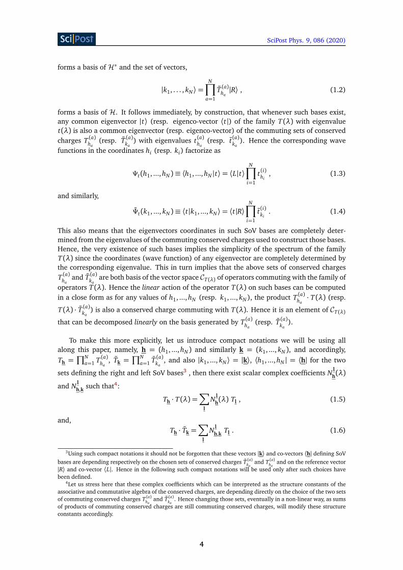
SciPost Phys. 9, 086 (2020)
forms a basis of H∗ and the set of vectors,
|k1, . . . , kN ⟩=N∏
a=1
T (a)ha|R⟩ , (1.2)
forms a basis of H. It follows immediately, by construction, that whenever such bases exist,any common eigenvector |t⟩ (resp. eigenco-vector ⟨t|) of the family T (λ) with eigenvaluet(λ) is also a common eigenvector (resp. eigenco-vector) of the commuting sets of conservedcharges T (a)ha
(resp. T (a)ka) with eigenvalues t(a)ha
(resp. t(a)ka). Hence the corresponding wave
functions in the coordinates hi (resp. ki) factorize as
Ψt(h1, ..., hN )≡ ⟨h1, ..., hN |t⟩= ⟨L|t⟩N∏
i=1
t(i)hi, (1.3)
and similarly,
Ψt(k1, ..., kN )≡ ⟨t|k1, ..., kN ⟩= ⟨t|R⟩N∏
i=1
t(i)ki. (1.4)
This also means that the eigenvectors coordinates in such SoV bases are completely deter-mined from the eigenvalues of the commuting conserved charges used to construct those bases.Hence, the very existence of such bases implies the simplicity of the spectrum of the familyT (λ) since the coordinates (wave function) of any eigenvector are completely determined bythe corresponding eigenvalue. This in turn implies that the above sets of conserved chargesT (a)ha
and T (a)kaare both basis of the vector space CT (λ) of operators commuting with the family of
operators T (λ). Hence the linear action of the operator T (λ) on such bases can be computedin a close form as for any values of h1, ..., hN (resp. k1, ..., kN ), the product T (a)ha
· T (λ) (resp.
T (λ) · T (a)ka) is also a conserved charge commuting with T (λ). Hence it is an element of CT (λ)
that can be decomposed linearly on the basis generated by T (a)ha(resp. T (a)ka
).
To make this more explicitly, let us introduce compact notations we will be using allalong this paper, namely, h = (h1, ...,hN ) and similarly k = (k1, ..., kN ), and accordingly,Th =
∏Na=1 T (a)ha
, Tk =∏N
a=1 T (a)ka, and also |k1, ..., kN ⟩ = |k⟩, ⟨h1, ..., hN | = ⟨h| for the two
sets defining the right and left SoV bases3 , then there exist scalar complex coefficients N lh(λ)
and N lh,k such that4:
Th · T (λ) =∑
l
N lh(λ) Tl , (1.5)
and,Th · Tk =
∑l
N lh,k Tl . (1.6)
3Using such compact notations it should not be forgotten that these vectors |k⟩ and co-vectors ⟨h| defining SoVbases are depending respectively on the chosen sets of conserved charges T (a)ka
and T (a)haand on the reference vector
|R⟩ and co-vector ⟨L|. Hence in the following such compact notations will be used only after such choices havebeen defined.
4Let us stress here that these complex coefficients which can be interpreted as the structure constants of theassociative and commutative algebra of the conserved charges, are depending directly on the choice of the two setsof commuting conserved charges T (a)ha
and T (a)ka. Hence changing those sets, eventually in a non-linear way, as sums
of products of commuting conserved charges are still commuting conserved charges, will modify these structureconstants accordingly.
4

SciPost Phys. 9, 086 (2020)
Similarly one can define two other sets of complex coefficients, namely C lh,k and C l
h,k such that:
Th · Tk =∑
l
C lh,k Tl , (1.7)
and,Th · Tk =
∑l
C lh,k Tl . (1.8)
The knowledge of these relations together with the action of the complete family of conservedcharges T (λ) on our SoV bases has been shown to completely characterize the common spec-trum of all the above commuting conserved charges. Particular realizations of this situationinclude the case where the T (a)ha
are powers of the transfer matrix evaluated in the inhomogene-
ity parameters as T (ξa)ha , or are given as the fused transfer matrices Tha(ξ(ha)
a ) in some shifted
points ξ(ha)a , where ha is the level of fusion. In the higher spin gl2 case, they are simply ob-
tained from the Q-operator evaluated in shifted inhomogeneities as Q(ξ(ha)a ). In all these cases,
the coefficients N lh(λ), N l
h,k, C lh,k and C l
h,kare completely determined by the fusion relations orthe T -Q relations satisfied by the transfer matrices and the Baxter Q-operator.
The conditions on the above sets of conserved charges to indeed generate SoV bases wereidentified and proven5 in [1], together with the factorization of the wave functions in termsof conserved charge eigenvalues and the proof of the completeness of the description of thetransfer matrix spectrum. The discrete separate relations were proven to be equivalent to thequantum spectral curve equations, involving the transfer matrices and the Q-operator holdingboth at the eigenvalue and operator level, due to the proven simplicity of the transfer matrixspectrum [1]. In our approach, the separate variables relations are themselves proven to beoriginated by the structure constants of the abelian algebra of conserved charges, in particularby the transfer matrix fusion equations for the charges considered in [1]. From this perspectiveour SoV approach has the potential to be universal in the realm of quantum integrable model.Indeed, we have proven its applicability for a large class of quantum integrable models from thefundamental representations of gln, gln,m and the Uq(gln) Yang-Baxter algebras with simplespectrum twist matrices up to the higher rank reflection algebra cases with general boundaryconditions, deriving new and complete descriptions of the transfer matrix spectrum [1,80–84]6. Moreover, in [85, 86] our construction of SoV bases using conserved charges has beenextended to arbitrary finite dimensional rectangular representations of the gln Yang-Baxteralgebra.
The relation of our SoV approach with the Sklyanin’s one has been first analyzed in [1].There we have observed the coincidence of our SoV co-vector basis with the Sklyanin’s B-operator co-vector eigenbasis for chains of arbitrary length in the gl2 case. This correspon-dence has been obtained for special choices of the reference co-vector and of the set of con-served charges used to generate the SoV basis. The same result has been derived in [1] forthe gl3 case for chains of small sizes. In [85] this observation has been proven for arbitraryfinite dimensional rectangular representations of the gln Yang-Baxter algebra and for chainsof any size. Moreover the simple spectrum of the Sklyanin’s B-operator, and its gln exten-sions proposed in [77], has been obtained in [85]. This result together with the completenessof the description of the spectrum by factorized wave functions in terms of polynomial Q-functions [1] implies the ABA type formula of [77] for all the transfer matrix eigenvectors7.
5They mainly reduce to properties satisfied by the twist matrix and the inhomogeneities parameters.6Note that our reference [83] describe our approach for higher spin representations for the rank one case.
While [84] also contains the SoV basis construction for the quasi-periodic Hubbard model.7Note that it was first remarked in [26] for non-compact rank one models that the factorization of the wave-
functions in terms of polynomial Q-functions imply the ABA form of transfer matrix eigenvectors in the SoV basis
5

SciPost Phys. 9, 086 (2020)
An important feature of our new approach to the SoV bases is that it relies only on finding asuitable set of commuting conserved charges and a corresponding reference co-vector/vector⟨L| ∈ H∗ and |R⟩ ∈ H, (the number of choices for those being in fact very large as shown inour first paper [1]). However, any other sets build from sums of products of given commutingconserved charges being again sets of commuting conserved charges, it results in a huge free-dom in constructing SoV bases which was not available if one would have stick to SoV basesidentified as eigenbasis of the Sklyanin’s B-operator or its higher rank extensions.
Clearly, this is a very interesting built in aspect of our new approach to SoV that enables usto ask a new key question in this context: what would be optimal choices of the sets of conservedcharges determining the SoV bases for the quantum integrable model at hand?
A first answer to this question, from the point of view of the determination of the spectrum,is that an optimal SoV basis is such that the action of the transfer matrix (and hence of theHamiltonian of the model) on the chosen basis is as simple as possible. This could mean forexample that the action of the family of T (λ) on any element of the set Th decomposes backon that set with only a very few non-zero coefficients, and moreover that it is given only bylocal shifts of finite and lowest possible order on the coordinates ha. This amounts to havechosen the basis Th of the space CT (λ) in such a way that the structure constants N l
h(λ) havesuch a simple property; namely that the only non zero coefficients are those where h and ldiffer only by localized shifts in the coordinates. This is exactly what happens for SoV basesin the gl2 case that are generated directly from the Baxter Q-operator. Indeed, the BaxterT -Q relation determines an action of the transfer matrix T (λ) on the basis generated by Q(λ)which involves only two terms with a local shift ±1 for each coordinate ha, to be compared tothe dimension of the Hilbert space H and of the Bethe algebra CT (λ) which is 2N for a spin-1/2chain of length N . This is in some sense the hallmark of integrability that generate a charac-teristic equation of degree two, hence much smaller than the dimension of the Hilbert space.
Another meaning of simplicity in the choice of our SoV bases could also be related to thecoupling between the two chosen left (1.1) and right (1.2) SoV bases. Namely, a criterion ofsimplicity could be to take such two SoV covector/vector bases such that their scalar productsare calculable in terms of manageable expressions. This is certainly an important question andcriterion as it determines to what extend the chosen left (1.1) and right (1.2) SoV bases areeasy to use when computing scalar products of separate states, form factors and correlationfunctions, that are our main goals.
The main purpose of the present paper is to study the important question of scalar productsfrom this perspective.
In the class of rank one quantum integrable models, the SoV analysis so far developed [2–6,23–54] leads to the expectation that the transfer matrix construction of the co-vector/vectorSoV bases can be defined in such a way that these are orthogonal bases. Similarly, in theSklyanin’s approach, this leads to the expectation that the co-vector/vector Sklyanin’s B-operatoreigenbases (orthogonal as soon as B is diagonalizable with simple spectrum) both implementthe separation of variables for the transfer matrix spectrum. This feature has been proven to bevery useful in computing scalar products of the so-called separate states and also in obtaining
once the Sklyanin’s B-operator is proven to be diagonalizable. As we have explained in [1], this proof extends alsoto the higher rank case under the same assumption as it only uses the SoV representation of the transfer matrixeigenvectors.
6

SciPost Phys. 9, 086 (2020)
determinant formulae for the form factors of local operators. As we will see in the next, inthe higher rank quantum integrable models, this is not directly the case if the charges used toconstruct the co-vector/vector SoV basis are simply the transfer matrices or their fused higherversions, for a generic twist K .
On the one hand, the SoV vector basis is univocally fixed in terms of the co-vector one de-fined in [1] if one requires that it is of SoV type, i.e. that it is generated by a factorized actionof conserved charges, and that it satisfies the orthogonality conditions with the co-vector basison one quantum site (this is obviously a necessary requirement for general orthogonality!). Itturns out that in general such SoV vector basis stays only pseudo-orthogonal to the co-vectorone for quantum chains of arbitrary length N . More precisely, the matrix of scalar productsNh,k = ⟨h|k⟩ for the natural SoV bases introduced in [1] is in general not a diagonal matrix.
The aim of the present paper is twofold:
• Characterize the matrix of scalar products Nh,k = ⟨h|k⟩ and the associated SoV measure(related to the inverse of Nh,k) for the natural SoV bases introduced in [1] in the exampleof the rank two gl3 case in the fundamental representations.
• Determine, in the same gl3 representations, two sets of commuting conserved charges,Th and Tk generating a left and right SoV bases that are orthogonal to each other andcompute the corresponding SoV measure.
Given our left SoV co-vector basis, we first prove that the defined set of SoV vectors indeeddefine a basis and we exactly characterize the pseudo-orthogonality conditions writing all thenon-zero non-diagonal couplings in terms of the diagonal ones, which we explicitly compute.This set of SoV vectors has been introduced recently in [76] as the set of eigenvectors of aC-operator which plays a similar role to the Sklyanin’s B-operator and some integral form hasbeen given for the coupling of the SoV co-vectors/vectors in [76]. Due to the quite differentrepresentations, a direct comparison of the results of [76] with those that we obtained stays acomplicate task which however deserves further analysis.
Let us comment that this pseudo-orthogonality is intrinsically related to the form of fusionrelations of the transfer matrices for higher rank case when computed in the special inhomo-geneous points. In fact the matrix of scalar products can be directly related to the structureconstants of the algebra of commuting conserved charges (1.6) that are in fact determinedcompletely by the fusion relations as shown in [1]. To be more precise let us illustrate this inthe following situation. Suppose we have chosen a left SoV basis of the type (1.1). Then let usconsider a right SoV basis (1.2) where we have chosen the right reference vector |R⟩ in sucha way that it satisfies ⟨h|R⟩= δh,h0
for some h0. Then the corresponding matrix Nh,k of scalar
products can be computed in terms of the structure constant Nh0h,k to be:
Nh,k = Nh0h,k . (1.9)
A very interesting question is thus if there exists an optimal choice of the left (1.1) and right
(1.2) SoV bases such that for some h0 we have Nh0h,k = δh,k n(h) with a calculable non-zero
coefficient n(h) whose inverse determines the SoV measure.This naturally leads to the observation that if we want to obtain co-vector/vector SoV bases
mutually orthogonal we have to chose in general a different family of commuting conservedcharges than the simple choice taken in [1] to generate both of them (or at least look for dif-ferent points where the transfer matrices are computed). These observations in the Sklyanin’sSoV framework for rank two mean that while the Sklyanin’s B-operator define the co-vector
7

SciPost Phys. 9, 086 (2020)
SoV basis, its vector eigenbasis is actually only a pseudo-SoV basis, i.e. not all the wave func-tions of transfer matrix eigenco-vectors have factorized form in terms of the transfer matrixeigenvalues.
Despite the absence of direct orthogonality the SoV-measure that we derive in section 3stays reasonably simple and can be used as the starting point to compute matrix elements oflocal operators in this SoV framework. While, this seems a sensible line of research and wewill further analyze it in the future, we would like to further investigate the potentiality of ournew SoV approach.
In the present paper, for the rank two gl3 case in the fundamental representation, wedefine some new family of commuting conserved charges whose spectral problem is separatedfor both a co-vector and a vector bases, which are moreover orthogonal to each other. Further,we show that the corresponding SoV measure takes a form very similar to the rank one case.The consequence is that w.r.t. this family of commuting conserved charges scalar productssimplify considerably and take a form very similar to the rank one case for the separate states.Of course, in order to be able to compute matrix elements of local operators we will need toaddress the problem of the representation of the local operators in these new SoV bases.
The paper is organized as follows:
Section 2 is dedicated to recall some fundamental properties satisfied by the transfer ma-trices in the fundamental representations of the gl3 Yang-Baxter algebra. In subsection 2.2,we moreover recall the results of [1] for the construction of the SoV bases for the consideredrepresentations, that is equations (2.23) and (2.24).
In section 3, we introduce a standard construction of co-vector/vector SoV bases (3.6)-(3.7) using the choice of the generating charges made in [1], i.e. given by the transfer matricesevaluated in the inhomogeneity parameters. The Theorem 3.1 characterizes completely the co-vector/vector coupling of these two systems of SoV states. The main results of this section arei) that the given system of SoV vectors form a basis, ii) the computation in (3.10) of the knowntensor product form (3.9) of the reference vector associated to a fixed reference co-vector inthe SoV basis, iii) the exact characterization in Theorem 3.1 of the pseudo-orthogonality re-lations (3.14), with the description of the non-diagonal couplings in terms of the diagonalones, and iv) the explicit computation of the diagonal couplings in (3.20). Finally, the sub-section 3.3 characterizes with Corollary 3.1 the SoV measure in terms of the non-zero SoVco-vector/vector couplings.
In section 4, we use the freedom in the choice of the generating family of conserved chargesto construct orthogonal co-vector/vector SoV bases. The subsection 4.1 is dedicated to thisconstruction in the class of quasi-periodic boundary conditions associated to simple spectrumbut non-invertible twist matrices. The main theorem there, Theorem 4.1, states the orthog-onality properties and the form of the diagonal SoV co-vector/vector couplings. These aresimilar to the SoV co-vector/vector couplings of the rank one integrable quantum models. Insubsection 4.2, these results are used to compute scalar product formulae of separate states(4.77) and (4.81), showing that they take a form similar to the rank one case. Finally, in sec-tion 4.3, we introduce a new set of charges (4.93) that extends the results of subsections 4.1and 4.2 to the general quasi-periodic boundary conditions, associated to simple spectrum andinvertible twist matrices.
We give several technical and important proofs in the three appendices. The appendix Adetails the proof of the tensor product form of SoV starting co-vector/vector in our SoV con-
8
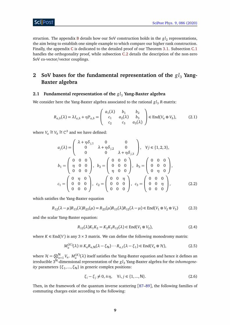
SciPost Phys. 9, 086 (2020)
struction. The appendix B details how our SoV construction holds in the gl2 representations,the aim being to establish one simple example to which compare our higher rank construction.Finally, the appendix C is dedicated to the detailed proof of our Theorem 3.1. Subsection C.1handles the orthogonality proof, while subsection C.2 details the description of the non-zeroSoV co-vector/vector couplings.
2 SoV bases for the fundamental representation of the gl3 Yang-Baxter algebra
2.1 Fundamental representation of the gl3 Yang-Baxter algebra
We consider here the Yang-Baxter algebra associated to the rational gl3 R-matrix:
Ra,b(λ) = λIa,b +ηPa,b =
a1(λ) b1 b2c1 a2(λ) b3c2 c3 a3(λ)
∈ End(Va ⊗ Vb), (2.1)
where Va∼= Vb
∼= C3 and we have defined:
a j(λ) =
λ+ηδ j,1 0 0
0 λ+ηδ j,2 00 0 λ+ηδ j,3
, ∀ j ∈ 1, 2,3,
b1 =
0 0 0η 0 00 0 0
, b2 =
0 0 00 0 0η 0 0
, b3 =
0 0 00 0 00 η 0
,
c1 =
0 η 00 0 00 0 0
, c2 =
0 0 η
0 0 00 0 0
, c3 =
0 0 00 0 η
0 0 0
, (2.2)
which satisfies the Yang-Baxter equation
R12(λ−µ)R13(λ)R23(µ) = R23(µ)R13(λ)R12(λ−µ) ∈ End(V1 ⊗ V2 ⊗ V3) (2.3)
and the scalar Yang-Baxter equation:
R12(λ)K1K2 = K2K1R12(λ) ∈ End(V1 ⊗ V2), (2.4)
where K ∈ End(V ) is any 3× 3 matrix. We can define the following monodromy matrix:
M (K)a (λ)≡ KaRa,N(λ− ξN) · · ·Ra,1(λ− ξ1) ∈ End(Va ⊗H), (2.5)
where H =⊗Nn=1 Vn. M (K)a (λ) itself satisfies the Yang-Baxter equation and hence it defines an
irreducible 3N-dimensional representation of the gl3 Yang-Baxter algebra for the inhomogene-ity parameters ξ1, ...,ξN in generic complex positions:
ξi − ξ j 6= 0,±η, ∀i, j ∈ 1, ...,N. (2.6)
Then, in the framework of the quantum inverse scattering [87–89], the following families ofcommuting charges exist according to the following:
9

SciPost Phys. 9, 086 (2020)
Proposition 2.1 ([87–89]). Defined the antisymmetric projectors:
P−1,...,m =1
m!
∑π∈Sm
(−1)σπ Pπ, (2.7)
where Sm is the symmetric group of rank m, σπ the signature of the permutation π and
Pπ(v1 ⊗ · · · ⊗ vm) = vπ(1) ⊗ · · · ⊗ vπ(m), (2.8)
then the following quantum spectral invariants (the fused transfer matrices):
T (K)m (λ)≡ tr1,...,m
P−1,...,mM (K)1 (λ)M (K)2 (λ−η) · · ·M (K)m (λ− (m− 1)η)
, ∀m ∈ 1, 2, 3,
(2.9)are one parameter families of mutual commuting operators. Furthermore, the quantum determi-nant q-det M (K)(λ)≡ T (K)3 (λ) is central, i.e.
q-det M (K)(λ), M (K)a (µ)
= 0. (2.10)
Moreover, the general fusion identities [87–89] imply the following
Proposition 2.2 ([87–89]). The quantum determinant has the following explicit form:
q-det M (K)(λ) = det KN∏
b=1
(λ− ξb +η)
2∏m=1
(λ− ξb −mη)
, (2.11)
and T (K)1 (λ) and T (K)2 (λ) are degree N and 2N in λ. Their asymptotics are central and coincideswith the corresponding two spectral invariants of the matrix K:
T (K ,∞)1 ≡ lim
λ→∞λ−NT (K)1 (λ) = tr K , T (K ,∞)
2 ≡ limλ→∞
λ−2NT (K)2 (λ) =(tr K)2 − tr K2
2. (2.12)
The fusion identities hold:
T (K)1 (ξa)T(K)m (ξa −η) = T (K)m+1(ξa), ∀m ∈ 1,2, (2.13)
and T (K)2 (λ) has the following N central zeroes
T (K)2 (ξa +η) = 0. (2.14)
Let us introduce the functions
g(m)a,h (λ) =N∏
b 6=a,b=1
λ− ξ(hb)b
ξ(ha)a − ξ(hb)
b
(m−1)N∏b=1
1
ξ(ha)a − ξ(−1)
b
, (2.15)
a(λ−η) = d(λ) =N∏
a=1
(λ− ξa), ξ(h)b = ξb − hη, h= h1, ..., hN, (2.16)
and
T (K ,∞)m,h (λ) = T (K ,∞)
m
N∏b=1
(λ− ξ(hn)b ). (2.17)
The known central zeroes and asymptotic behavior imply that the transfer matrix T (K)2 (λ) is
completely characterized in terms of T (K)1 (λ), e.g. by the following interpolation formula
T (K)2 (λ) = d(λ−η)
T (K ,∞)2,h=0 (λ) +
N∑a=1
g(2)a,h=0(λ)T(K)1 (ξa −η)T (K)1 (ξa)
, (2.18)
where h= 0 means that for all k ∈ 1, ...,N we have hk = 0.From now on when we have an h with all the elements equal to the integer 0, 1 or 2 we
use directly the bold underlined notation 0, 1 and 2.
10

SciPost Phys. 9, 086 (2020)
2.2 On SoV bases construction in our approach
The general Proposition 2.4 of [1] for the construction of the SoV co-vector basis applies inparticular to the fundamental representation of the gl3 rational Yang-Baxter algebra. Notethat we have presented the construction for the co-vector SoV basis just to get a factorizedform of the wave-functions of the transfer matrix eigenvectors in terms of the transfer matrixeigenvalues. Evidently, the same construction applies as well to define a vector SoV basisin which the wave-functions of the transfer matrix eigenco-vectors have the same factorizedform. In order to clarify this, we present in the following a proposition for this gl3 case. LetK be a 3× 3 simple spectrum matrix and let us denote with KJ the Jordan form of the matrixK and WK the invertible matrix defining the change of basis:
K =WK KJW−1K with KJ =
k0 y1 00 k1 y20 0 k2
. (2.19)
The requirement K simple spectrum implies that we can reduce ourselves to the followingthree possible cases:
i) ki 6= k j , ∀i, j ∈ 0,1, 2 and y1 = y2 = 0, (2.20)
ii) k0 = k1 6= k2, y1 = 1, y2 = 0, (2.21)
ii) k0 = k1 = k2, y1 = 1, y2 = 1. (2.22)
Then,
Proposition 2.3. Let K be a 3×3 simple spectrum matrix, then for almost any choice of ⟨L|, |R⟩and of the inhomogeneities under the condition (2.6), the following set of co-vectors and vectors:
⟨L|N∏
n=1
T (K)1 (ξn)
hnfor any h1, ...,hN ∈ 0,1, 2N, (2.23)
N∏n=1
T (K)1 (ξn)
hn |R⟩ for any h1, ...,hN ∈ 0,1, 2N, (2.24)
forms a co-vector and vector basis of H, respectively. In particular, we can take the followingtensor product forms:
⟨L|=N⊗
a=1
(x , y, z)aΓ−1W , |R⟩ =
N⊗a=1
ΓW (r, s, t)taa , ΓW =
N⊗a=1
WK ,a (2.25)
simply asking in the case i) x y z 6= 0 for the co-vector and r s t 6= 0 for the vector, in the case ii)x z 6= 0 for the co-vector and s t 6= 0 for the vector, in the case iii) x 6= 0 for the co-vector andt 6= 0 for the vector.
Proof. As shown in the general Proposition 2.4 of [1], the fact that the transfer matrix inthe inhomogeneity ξn reduces to the twist matrix in the local space n dressed by invertibleproducts of R-matrices implies that the set of co-vectors and vectors above defined form basesof H∗ and H, once the following co-vectors and vectors (obtained by taking the asymptoticlimit over the ξa)
(x , y, z)W−1K , (x , y, z)W−1
K K , (x , y, z)W−1K K2, (2.26)
WK(r, s, t)t , KWK(r, s, t)t , K2WK(r, s, t)t , (2.27)
11

SciPost Phys. 9, 086 (2020)
or equivalently:
(x , y, z), (x , y, z)KJ , (x , y, z)K2J , (2.28)
(r, s, t)t , KJ (r, s, t)t , K2J (r, s, t)t , (2.29)
form bases in C3, that is the next determinants are non-zero8:
det(x , y, z)K i−1
J e j
i, j∈1,2,3 =
−x yzV (k0,k1,k2) in the case i)x2zV 2(k0,k2) in the case ii)x3 in the case iii)
, (2.30)
detet
j Ki−1J (r, s, t)
i, j∈1,2,3 =
rstV (k0,k1,k2) in the case i)s2 tV 2(k0,k2) in the case ii)t3 in the case iii)
, (2.31)
which leads to the given requirements on the components x , y, z, r, s, t ∈ C of the three dimen-sional co-vector and vectors.
Note that both these choices of co-vector and vector SoV bases are perfectly fine to fix thetransfer matrix spectrum, by factorized wave functions in terms of transfer matrix eigenvaluesfor both eigenvectors and eigenco-vectors. However, if we wish to go beyond the spectrum,and compute matrix elements of local operators starting with scalar products of the so-calledseparate states, we need an appropriate choice of the co-vector and vector SoV bases. In therank one quantum integrable models, the SoV analysis so far developed [2–6,23–54] leads tothe expectation that the transfer matrix construction of the co-vector and vector SoV bases canbe defined in such a way that these are orthogonal bases or similarly that the co-vector andvector Sklyanin’s B-operator eigenbases both implement the separation of variables for thetransfer matrix spectrum. As we will see in the next, in the higher rank quantum integrablemodels, this is not directly the case if the charges used to construct the co-vector and vectorSoV basis are simple powers, or even fusion, of the transfer matrices for general twist K .
3 Scalar products for co-vector/vector SoV bases
3.1 Another construction of co-vector/vector SoV bases
Let us first introduce a slight modification of the co-vector SoV basis w.r.t. the standard oneintroduced in the previous section by changing the set of conserved charges used to constructthem. It reads9:
⟨h| ≡ ⟨h1, ...,hN|= ⟨1|N∏
n=1
T(K)δhn ,0
2 (ξ(1)n )T(K)δhn ,2
1 (ξn), ∀ hn ∈ 0,1, 2, (3.1)
where ⟨1| is some generic co-vector of H. Let us remark that for an invertible twist matrix Kusing the identification:
⟨1|= ⟨L|N∏
n=1
T (K)1 (ξn) , (3.2)
the two sets of co-vectors defined in (2.23) and (3.1) are identical up to a non-zero normal-ization of each co-vector; hence the two sets are related by the action of a diagonal matrix. To
8Here and in the following, we denote by V (x1, . . . , xn) the standard Vandermonde determinant∏
i< j(x j − x i).9Throughout this section we use compact notations for the left and right SoV bases defined as in (3.1) and
(3.7).
12

SciPost Phys. 9, 086 (2020)
be more precise, with such an identification and using the fact that for an invertible K-matrixthe operator T (K)2 (ξ(1)n ) is proportional to the inverse of T (K)1 (ξn) due to the fusion relations,we get:
⟨h|= αh⟨L|N∏
n=1
T(K)δhn ,2−δhn ,0+11 (ξn), ∀hn ∈ 0, 1,2, (3.3)
whereαh =∏N
n=1(q-det M (K)(ξn))δhn ,0 is a non-zero coefficient. Then, beingδhn,2−δhn,0+1= hn
for any hn ∈ 0, 1,2, we get:
⟨h|= αh⟨L|N∏
n=1
T (K)hn1 (ξn) ,∀ hn ∈ 0,1, 2, (3.4)
thus proving that the two sets defined in (2.23) and in (3.1) are equivalent bases up to aninvertible diagonal matrix made of the non-zero coefficients αh. Moreover, even if K has zerodeterminant, it can be proven that the two sets (3.1) and (2.23) are both SoV bases (see nextsection), the linear transformation relating them being in that case more involved.
3.2 Pseudo-orthogonality conditions of these co-vector/vector SoV bases
Here, we show that for the SoV co-vector basis chosen as in (3.1), we can define a pseudo-orthogonal vector SoV basis which is orthogonal to the left one for a large set of co-vector/vectorcouples. We exactly characterize these pseudo-orthogonality conditions and the non-zero cou-plings of these co-vector and vector SoV basis. The corresponding SoV-measure, related to theinverse of the scalar products matrix, is completely characterized in the next subsection. Itis the starting ingredient to compute matrix elements of local operators in this SoV frame-work. This will be further employed in forthcoming analysis in this gl3 case as, despite theabsence of direct orthogonality, the SoV-measure stays reasonably simple to be used in practicalcomputations.
Let us now introduced the vector |0⟩ uniquely characterized by
⟨k|0⟩=N∏
a=1
δ0,ka. (3.5)
Then we have the following
Proposition 3.1. Let K be a 3 × 3 simple spectrum matrix, then for almost any choice of theco-vector ⟨1|, of the vector |0⟩ and of the inhomogeneities under the condition (2.6), the set ofco-vectors (3.1)
⟨h|= ⟨1|N∏
n=1
T(K)δhn ,0
2 (ξ(1)n )T(K)δhn ,2
1 (ξn), (3.6)
and the set of vectors:
|h⟩ ≡N∏
n=1
T(K)δhn ,1
2 (ξn)T(K)δhn ,2
1 (ξn)|0⟩, (3.7)
form co-vector and vector basis of H∗ and H, respectively. In particular, we can take ⟨1| of thefollowing tensor product form:
⟨1|=N⊗
a=1
(x , y, z)aΓ−1W , ΓW =
N⊗a=1
WK ,a, (3.8)
13

SciPost Phys. 9, 086 (2020)
simply asking x y z 6= 0 in the case i), x z 6= 0 in the case ii), x 6= 0 in the case iii). Then theassociated vector |0⟩ having the property (3.5) also has tensor product form:
|0⟩= ΓWN⊗
a=1
|0, a⟩, (3.9)
where we have defined
|0, a⟩= 1∆
k2(yk0 − xy1)(zk2 + yy2)− (yk1 + xy1)(xy1y2 + k0(zk1 − yy2))x(xk0y1y2 + k2
0(zk1 − yy2)− k1k2(zk2 + yy2))x(k0 + k1)k2(yk1 + xy1 − yk0)
a
, (3.10)
with
∆= x
yk0− yk1−xy1
z(k0−k2)(k1−k2)+y2
y(k2−k1)+xy1
q-det M (I)(ξa−2η). (3.11)
Proof. The proof that these two sets are indeed bases of the Hilbert space and its dual canbe performed along the same lines as the one presented already in [1] and in the previoussection. Namely, using the polynomial character of all the expressions involved in the inho-mogeneity parameters ξn it is enough to prove the proposition in some point in the param-eter space. This is achieved by scaling the inhomogeneity parameters from a single scalar,as ξn = nξ, and sending the parameter ξ to infinity. In turn, this amounts to obtain theasymptotic behavior of the transfer matrices in that limit. The leading term for the operatorT (K)1 (ξn) is given by ξN−1Kn times some constant, while for the operator T (K)2 (ξ(1)n ) it is givenby ξ2(N−1)(2K2
n − 2Kn tr(K) + tr(K)2 − tr(K2)) times some other constant. Hence, it is enoughto exhibit a co-vector ⟨u| such that the set ⟨u|, ⟨u|K , ⟨u|K2 is a basis of C3, which is the case assoon as K has simple spectrum. Similarly, the asymptotic of the operator T (K)2 (ξ(0)n ) is foundproportional to the matrix ξ2(N−1)(K2
n − Kn tr(K)), leading to the same conclusion. By thesearguments, all we need to prove is that the co-vectors
(x , y, z)KJ , (x , y, z), (x , y, z)KJ , (3.12)
where KJ is the adjoint matrix of KJ , form a tridimensional basis. If we denote by Mx ,y,z,KJthe
3× 3 matrix which lines are given by these three co-vectors, it holds:
det Mx ,y,z,KJ=
−x yzV (k0,k1,k2) in the case i)
x2zV 2(k0,k2) in the case ii)
x3 in the case iii),
(3.13)
so that in the case i) we take x y z 6= 0, in the case ii) we take x z 6= 0 and finally in the case iii)the condition is x 6= 0. The construction of the orthogonal vector is a standard computationin C3 and the fact that it defines a vector basis by action of K and K2 follows from a directcomputation. Another proof uses the characteristic equation of K . Finally, the fact that thereference vector for the right SoV basis can be then chosen of tensor product form is provenin the appendix A.
Let us now compute the scalar products of these two SoV bases as follows:
Theorem 3.1. Let all the notations be the same as in Proposition 3.1, then the following pseudo-orthogonality relations hold:
Nh,k = ⟨h|k⟩= ⟨k|k⟩
δh,k + Ck
h
nk∑r=1
(det K)r∑
α∪β∪γ=1k,α,β ,γ disjoint,#α=#β=r
δh,k(
0,2)α,β
, (3.14)
14

SciPost Phys. 9, 086 (2020)
where the Ckh are non-zero and independent w.r.t. det K, nk is the integer part of (
∑Na=1δka ,1)/2.
We have used the further notations
k(0,2)α,β ≡ (k1(α,β), ..., kN(α,β)) ∈ 0,1, 2N, (3.15)
1k ≡ a ∈ 1, ...,N : ka = 1, (3.16)
with
ka(α,β) = 0, kb(α,β) = 2, ∀a ∈ α, b ∈ β (3.17)
kc(α,β) = kc , ∀c ∈ 1, ...,N\α∪ β. (3.18)
Moreover, we prove that it holds:
Nh = ⟨h|h⟩ (3.19)
=
N∏
a=1
dξ(1)a
dξ(1+δha ,1+δha ,2)a
!
V 2(ξ1, ...,ξN)
Vξ(δh1,2+δh1,1)1 , ...,ξ
(δhN ,1+δhN ,2)
N
Vξ(δh1,2)1 , ...,ξ
(δhN ,2)
N
. (3.20)
Proof. The heavy proofs of the pseudo-orthogonality and of the expressions of non-zero SoVco-vector/vector couplings are given in Appendix C. There, the coefficients Ck
h are character-ized completely, but implicitly, by an unwieldy recursion that we do not solve for the genericcase. We compute them in the simplest case, see (C.73).
It is worth to make some remarks on the above theorem. Let us first comment that the sumin (3.14), for any fixed k and h , always reduces to at most one single non-zero term. Indeed,fixing k 6= h, we can have a non-zero coupling between the vector and co-vector associated ifand only if there exists a couple of sets (α,β) ⊂ 1k with the same cardinality r ≤ nk such that
h = k(0,2)α,β , and of course if the couple (α,β) exists it is unique. The above condition means
that if∑N
a=1δka ,1 is smaller or equal to one, then the standard orthogonality works, i.e. only
h= k produces a non-zero co-vector/vector coupling. While if∑N
a=1δka ,1 is bigger or equal to
two, we have non-zero couplings also for all the co-vectors of (3.1) with10 h = k(0,2)α,β . Let us
remark that if one looks to this pseudo-orthogonality condition in one quantum site, then thebasis (3.7) naturally emerges as the candidate to get the orthogonal basis to (3.1). Indeed, forone site, orthogonality is satisfied by them while the fact that the orthogonality is not satisfiedfor higher number of quantum sites is intrinsically related to the form of fusion relations ofthe transfer matrices for higher rank. From these considerations follows our statement that ifwe want to obtain mutually orthogonal co-vector/vector SoV bases, we have to use different11
families of commuting conserved charges to generate the co-vector and the vector SoV bases.It is also useful to make some link with the preexisting work [76] in the SoV framework. In
fact, the set of vectors (3.7) has been introduced recently in [76] as the set of eigenvectors of aC-operator, which plays a similar role to the Sklyanin’s B-operator. There, the starting vector,analogous to our |0⟩, is taken as some not better defined eigenvector of this C-operator, andthe proofs that C is diagonalizable and that so (3.7) form a basis are not addressed, while theco-vector/vector coupling of these SoV bases is represented with some integral form.
In our paper, we prove that (3.7) is a basis, we fix the tensor product form of the startingvector |0⟩in terms of the starting co-vector ⟨1| and the general twist matrix K , we characterize
10That is for the h obtained from k removing one or more couples of (ka = 1, kb = 1) and substituting them with(ka(α,β) = 0, kb(α,β) = 2).
11w.r.t. those used above.
15

SciPost Phys. 9, 086 (2020)
completely the form of the co-vector/vector couplings of the two SoV bases and from them theSoV -measure.
Let us also remark that in [76] is given a selection rule which selects sectors of the quantumspace which are orthogonal, which translates in our setting as
⟨h|k⟩= 0 ifN∑
a=1
δha ,1 6=N∑
a=1
δka ,1. (3.21)
This is compatible with our result (3.14), but much less restrictive as one can easily understandby looking, for example, to our formula for r = 1. In this case, the h fixing the co-vector in(3.7) and k fixing the vector in (3.1) differ only on one couple of index (ha, hb) 6= (ka, kb).The above selection rule only imposes that ⟨h|k⟩ = 0 if ha + hb 6= ka + kb, while our formulainstead specifies that ⟨h|k⟩= 0 unless ka = kb = 1 and ha + hb = 2.
3.3 On higher rank SoV measure
In the Theorem 3.1, we have shown that the original higher rank SoV co-vector and vectorbases as defined in (3.7) and (3.1) are not mutual orthogonal basis if the twist matrix isinvertible. Here, we want to show that from the Theorem 3.1, we can also characterize theSoV measure associated to these bases, i.e. the measure to be used in the computation ofscalar products of separate states in these co-vector and vector bases.
Let us start introducing the following sets of co-vectors and vectors that are bases of theHilbert space orthogonal to our left and right SoV bases:
p⟨h| and |h⟩p, ∀h ∈ 0, 1, 2N, (3.22)
uniquely characterized by the following orthogonality conditions12:
p⟨k|h⟩= δk,h⟨h|h⟩, ⟨k|h⟩p = δk,h⟨h|h⟩, ∀h,k ∈ 0,1, 2N, (3.23)
where |h⟩ and ⟨h| are the vectors and co-vectors of the SoV basis (3.7) and (3.1), respectively.Clearly, the set generated by the p⟨h| and |h⟩p are bases of the Hilbert space, and moreoverwe have the following decompositions of the identity:
I=∑
h
|h⟩p ⟨h|Nh
=∑
h
|h⟩ p⟨h|Nh
, (3.24)
where the sums run over all the possible values of the multiple index (h). As a consequence,the transfer matrix eigenco-vectors and eigenvectors admit the following SoV representationsin terms of their eigenvalues:
|ta⟩=∑
h
N∏n=1
tδhn ,0
2,a (ξ(1)n )t
δhn ,2
1,a (ξn)|h⟩pNh
, (3.25)
⟨ta|=∑
h
N∏n=1
tδhn ,1
2,a (ξn)tδhn ,2
1,a (ξn)p⟨h|Nh
. (3.26)
Thus, we can naturally give the following definitions of separate vectors :
|α⟩=∑
k
αk
|k⟩pNk
, αh ≡N∏
a=1
α(ha)a (3.27)
12Note here that we have included, for convenience, in the orthogonality relations the normalisation factor⟨h|h⟩ as it leads to more natural identifications in the particular case where the right and left SoV bases are directlyorthogonal to each other.
16

SciPost Phys. 9, 086 (2020)
with factorized coordinates αh and separate co-vectors,
⟨β |=∑
h
βhp⟨h|Nh
, βh ≡N∏
a=1
β (ha)a (3.28)
with factorized coordinates βh on the respective bases. The scalar product of such two separatevector and co-vector reads:
⟨β |α⟩=∑h,k
βhMh,kαk (3.29)
with the SoV measure Mh,k defined as:
Mh,k =p⟨h|k⟩pNh.Nk
. (3.30)
It can be obtained from the knowledge of the scalar products between the vectors and co-vectors of the two bases orthogonal to our chosen SoV bases:
p⟨h|k⟩p, ∀h,k ∈ 0, 1, 2N. (3.31)
Let us note here that these two matrices Nh,k and Mh,k, modulo some normalisation, havedirect interpretation as change of bases matrices between the bases ⟨h| and p⟨k|, namely wehave:
⟨h|=∑
k
Nh,kp⟨k|Nk
, (3.32)
and conversely,p⟨k|Nk=∑
h
Mk,h⟨h|. (3.33)
We also have similar relations (with transposition) for the bases |k⟩ and |h⟩p. Moreover, it easyto verify that these two matrices are inverse to each other:
∑h
Mk,h ·Nh,l = δk,l . (3.34)
Hence to compute the SoV measure Mk,h, we just need to get the inverse of the matrix ofscalar products Nk,h; in the following we show how to characterize it in terms of Nk,h, provingin particular that it has in fact the same form as Nk,h
13.
Let us start proving the following:
Lemma 3.1. The vectors |h⟩p of the basis orthogonal to the SoV co-vector basis (3.1) admit thefollowing decompositions in the SoV vector basis (3.7):
|h⟩p = |h⟩+nh∑
r=1
cr∑
α∪β∪γ=1h,α,β ,γ disjoint,
#α=#β=r
Bα,β ,h|h(0,2)α,β ⟩, (3.35)
13Somehow this is not surprising as in the appropriate labelling of the SoV bases, the matrix Nk,h is lower-triangular with finite depth out of the diagonal and hence its inverse should have a similar form.
17

SciPost Phys. 9, 086 (2020)
where the coefficients Bα,β ,h are completely characterized by the following recursion formula:
Bα,β ,h = −
Ch
h(0,2)α,β
+∑
α′⊂α, β ′⊂β ,1≤#α′=#β ′≤#α−1
Bα′,β ′,h Ch(
0,2)α′ ,β′
h(0,2)α,β
, (3.36)
and
C rs =⟨r|r⟩⟨s|s⟩C
rs , (3.37)
where C rs are the coefficients of the measure (3.14).
Proof. The fact that we can write each vector |h⟩p, satisfying (3.23), in terms of the SoV vectors|k⟩ follows from the fact that these last ones form a basis. Here we have to prove that the aboveexpression for |h⟩p and for its coefficients indeed imply the orthogonality condition (3.23).
Let us start observing that this is the case for the diagonal term. Indeed, the followingidentity follows:
⟨h|h⟩p = ⟨h|h⟩, (3.38)
by the measure (3.14) being
h 6=(C.45)
h(0,,2)α,β , ∀α,β ⊂ 1h, disjoint with 1≤ #α= #β ≤ nh. (3.39)
So we are left with the proof of the orthogonality of
⟨k|h⟩p = 0, ∀k 6= h,k ∈ 0, 1, 2N. (3.40)
Let us start observing that for any k such that
k 6=(C.45)
h, (3.41)
then it also follows
k 6=(C.45)
h(0,2)α,β , ∀α,β ⊂ 1h, disjoint with 1≤ #α= #β ≤ nh, (3.42)
and so by the measure (3.14) the orthogonality holds.
So, we are left with the proof of the orthogonality for the case k = h(0,2)µ,δ for any fixed
disjoint sets µ ⊂ 1h and δ ⊂ 1h such that 1≤ #µ= #δ ≤ nh. Let us observe that the followinginequalities holds:
h(0,2)α,β 6=
(C.45)h(
0,2)µ,δ , (3.43)
for any disjoint sets α and β contained in 1h with #α= #β such that
α * µ and β * δ. (3.44)
Then, by the measure (3.14), we get the following co-vector/vector coupling:
⟨h(0,2)µ,δ |h⟩p = ⟨h
(0,2)µ,δ |h⟩+
nh∑r=1
cr∑
α∪β∪γ=1h,α,β ,γ disjoint,#α=#β=r
Bα,β ,h⟨h(0,2)µ,δ |h
(0,2)α,β ⟩ (3.45)
= ⟨h(0,2)µ,δ |h⟩+ c#δBµ,δ,h⟨h(0,2)
µ,δ |h(0,2)µ,δ ⟩+
#δ−1∑r=1
cr∑
α⊂µ,β⊂δ,#α=#β=r
Bα,β ,h⟨h(0,2)µ,δ |h
(0,2)α,β ⟩,
(3.46)
18

SciPost Phys. 9, 086 (2020)
that we impose to be zero to satisfy the orthogonality condition:
⟨h(0,2)µ,δ |h⟩p = 0, ∀µ ⊂ 1h,δ ⊂ 1h disjoint with 1≤ #µ= #δ ≤ nh. (3.47)
Here, the main observation is that this can be seen as one equation in one unknown Bµ,δ,h,and solved as it follows:
Bµ,δ,h = −⟨h(0,2)µ,δ |h⟩c−#δ
⟨h(0,2)µ,δ |h
(0,2)µ,δ ⟩
−#δ−1∑r=1
cr−#δ∑
α⊂µ,β⊂δ,#α=#β=r
Bα,β ,h
⟨h(0,2)µ,δ |h
(0,2)α,β ⟩
⟨h(0,2)µ,δ |h
(0,2)µ,δ ⟩
, (3.48)
in terms of the known SoV co-vector/vector couplings and of the coefficients Bα,β ,h for anyα ⊂ µ,β ⊂ δ, with 1≤ #α= #β ≤ #δ− 1. Then, by using the formulae (3.14) we get:
⟨h(0,2)µ,δ |h⟩c−#δ
⟨h(0,2)µ,δ |h
(0,2)µ,δ ⟩
= Ch
h(0,2)µ,δ
,⟨h(0,2)µ,δ |h
(0,2)α,β ⟩cr−#δ
⟨h(0,2)µ,δ |h
(0,2)µ,δ ⟩
α⊂µ,β⊂δ,#α=#β=r
= Ch(
0,2)α,β
h(0,2)µ,δ
, (3.49)
from which our formula (3.36) easily follows.Now, it is simple to argue that (3.36) gives us recursively all the coefficient Bµ,δ,h for any
µ ⊂ 1h,δ ⊂ 1h disjoint, with 1≤ #µ= #δ ≤ nh.In the case #µ= #δ = 1, the formula (3.36) reads:
Ba,b,h = −Ch
h(0,2)a,b
, ∀a 6= b ∈ 1h, (3.50)
which fixes completely these coefficients. Then, we can consider the case of the generic coupleof disjoint sets µ ⊂ 1h,δ ⊂ 1h, with #µ = #δ = 2. In these cases, we have that the formula(3.36) reads:
Bµ,δ,h = −Ch
h(0,2)µ,δ
−∑
a∈µ,b∈δBa,b,hC
h(0,2)a,b
h(0,2)µ,δ
, (3.51)
which fixes completely these coefficients in terms of those computed in the first step of therecursion.
In this way the formula (3.36) fixes the coefficients Bµ′,δ′,h for any fixed couple of disjointsets µ′ ⊂ 1h,δ′ ⊂ 1h, with #µ′ = #δ′ = m+ 1 ≤ nh, in terms of those already computed, i.e.the Bµ,δ,h for any fixed couple of disjoint sets µ ⊂ µ′ ⊂ 1h,δ ⊂ δ′ ⊂ 1h, with #µ= #δ ≤ m.
Let us note that the coefficients Bα,β ,h are, as previously with the coefficients Ckh , also
characterized in a recursive manner, and their generic expression is missing from this Lemma.The previous lemma implies the following corollary, which completely characterizes the
SoV measure.
Corollary 3.1. Under the same condition of Theorem 3.1, the SoV measure is defined by thefollowing pseudo-orthogonality relations:
p⟨h|k⟩p = ⟨h|h⟩
δh,k +
nk∑r=1
cr∑
α∪β∪γ=1k,α,β ,γ disjoint, #α=#β=r
Bα,β ,kδh,k(0,2)α,β
. (3.52)
19

SciPost Phys. 9, 086 (2020)
Proof. We have to use just the expression derived in the previous lemma for the generic vector
|k⟩p = |k⟩+nk∑
r=1
cr∑
α∪β∪γ=1k,α,β ,γ disjoint, #α=#β=r
Bα,β ,k|k(0,2)α,β ⟩, (3.53)
and the definition of the co-vectors p⟨h| for which it holds:
p⟨h|k⟩p = p⟨h|k⟩+nk∑
r=1
cr∑
α∪β∪γ=1k,α,β ,γ disjoint, #α=#β=r
Bα,β ,k p⟨h|k(0,2)α,β ⟩ (3.54)
= p⟨h|h⟩
δh,k +
nk∑r=1
cr∑
α∪β∪γ=1k,α,β ,γ disjoint, #α=#β=r
Bα,β ,k δh,k(0,2)α,β
, (3.55)
and being p⟨h|h⟩= ⟨h|h⟩, our result follows.
4 On the construction of orthogonal co-vector/vector SoV bases
We would like now to introduce a new family of commuting conserved charges in order toconstruct from them orthogonal co-vector/vector SoV bases. We first describe our constructionfor the class of simple spectrum and non-invertible K-matrices. Then, from this class, we willdefine a new family of commuting conserved charges T(λ)which allows for the construction ofthe co-vector/vector orthogonal SoV bases for a generic simple spectrum K-matrix. The scalarproduct of separate states w.r.t. the charges T(λ), a class of co-vector/vector which containsthe transfer matrix eigenstates, are computed and shown to have a form similar to those ofthe gl2 case once one of the two states is a T(λ) eigenvector.
4.1 The case of non-invertible K-matrices with simple spectrum
In the gl3 case, the construction of a vector SoV basis orthogonal to the left one is not auto-matic, as it was in the gl2 case. Here, it seems that the choice of the appropriate family ofcommuting conserved charges to construct the basis plays a fundamental role. In this sub-section, we consider the special case of a simple spectrum K-matrix with one zero eigenvalue.The orthogonal co-vector and vector SoV bases will be constructed using the transfer matricesas in the previous section.
Theorem 4.1. Let K be a 3 × 3 simple spectrum matrix with one zero eigenvalue. For almostany choice of the co-vector ⟨1| and of the inhomogeneities under the condition (2.6), the set of co-vectors (3.1) and vectors (3.7) form SoV co-vector and SoV vector bases of H∗ and H, respectively.In particular, we can take ⟨1| of the tensor product form (3.8), then the associated vector |0⟩ hasthe tensor product form defined in (3.9)-(3.10) and (3.1) and (3.7) are basis of H simply askingx y z 6= 0 in the case i), x z 6= 0 in the case ii), x 6= 0 in the case iii).
Furthermore, (3.1) and (3.7) are mutually orthogonal SoV bases, i.e. they define the followingdecomposition of the identity:
I≡∑
h
|h⟩⟨h|Nh
, (4.1)
20

SciPost Phys. 9, 086 (2020)
with
Nh =N∏
a=1
d(ξ(1)a )
dξ(1+δha ,1+δha ,2)a
V 2(ξ1, ...,ξN)
Vξ(δh1,2+δh1,1)1 , ...,ξ
(δhN ,1+δhN ,2)
N
Vξ(δh1,2)1 , ...,ξ
(δhN ,2)
N
. (4.2)
Proof. This theorem follows immediately from the results of Theorem 3.1 putting to zero thedeterminant of the matrix K .
However, the proof of our Theorem 3.1 is rather involved and takes quite numerous stepsthat we give in the appendices. It is therefore of interest to have a more elementary proof inthe case at hand, namely whenever the simple spectrum twist matrix K has zero determinantor better to say as soon as the fusion relations for the transfer matrices simplify due to thevanishing of its associated quantum determinant. In fact, this case will provide the genericidea to get orthogonal left and right SoV bases in the general situation. So let us explain fromnow on a direct proof of this theorem.
Idea of the direct proof. The statement that (3.1) is a co-vector basis of H is proven as in theprevious proposition. Indeed the main condition:
det Mx ,y,z,KJ6= 0 (4.3)
can be satisfied as well in the case det K = 0. In fact, if the matrix K satisfies the case i), wetake k2 = 0 and the condition is still x y z 6= 0; if the matrix K satisfies the case ii), we takek0 = 0 or k2 = 0 and the condition is still x z 6= 0. Finally in the case iii) with k0 = k1 = k2 = 0the condition is still x 6= 0. So that we are left with the proof of the orthogonality conditions.which can be proven by using the next results.
The first step in the direct proof of the above theorem is to obtain the SoV representationsfor the action of the transfer matrices in the case where the fusion relations simplify due tothe vanishing of its associated quantum determinant. It is given in the following Proposition.
Proposition 4.1. Under the same conditions of the above theorem, the following interpolationformulae hold for the transfer matrices:
i) On the SoV co-vector basis:
⟨h|T (K)2 (λ) = d (λ−η)
N∑a=1
δha ,1 g(2)a,z(h)(λ)⟨h|T−a + T (K ,∞)2,z(h) (λ)⟨h|
, (4.4)
and
⟨h|T (K)1 (λ) = T (K ,∞)1,y(h) (λ)⟨h|+
N∑a=1
δha ,1 g(1)a,y(h)(λ)⟨h|T+a +N∑
a=1
δha ,2 g(1)a,y(h)(λ)d(ξ(1)a )
×
N∑b=1
δhb(a),1 g(2)b,z(h(1)a )
(ξa)⟨h(1)a |T−b + T (K ,∞)2,z(h(1)a )
(ξa)⟨h(1)a |
, (4.5)
where
z(h) = δh1,1 +δh1,2, ...,δhN,1 +δhN,2, y(h) = δh1,2, ...,δhN,2, (4.6)
h(1)a = h− (ha − 1)ea with ea = δ1,a, ...,δN,a , (4.7)
and⟨h1, ..., ha, ..., hN|T±a = ⟨h1, ..., ha ± 1, ..., hN|. (4.8)
21

SciPost Phys. 9, 086 (2020)
ii) On the SoV vector basis:
T (K)2 (λ)|h⟩= d (λ−η)
N∑a=1
δha ,0 g(2)a,z(h)(λ)T+a |h⟩+ |h⟩T (K ,∞)
2,z(h) (λ)
, (4.9)
and
T (K)1 (λ)|h⟩= |h⟩T (K ,∞)1,y(h) (λ) +
N∑a=1
δha ,0 g(1)a,y(h)(λ)T+a2 |h⟩+
N∑a=1
δha ,2 g(1)a,y(h)(λ)T−a |h⟩
+N∑
a=1
δha ,1 g(1)a,y(h)(λ)d(ξ(1)a )
N∑
b=1
δhb(a),0 g(2)b,z(h(2)a )
(ξa)T+b |h(2)a ⟩+ |h(2)a ⟩T (K ,∞)
2,z(h(2)a )(ξa)
,
(4.10)
whereh(2)a = h− (ha − 2)ea , (4.11)
andT±a |h1, ..., ha, ..., hN⟩ = |h1, ..., ha ± 1, ..., hN⟩. (4.12)
Proof. The fusion identities take the following form in the case det K = 0:
T (K)2 (ξ(1)a )T(K)1 (ξa) = q-det M (K)(ξa) = 0, (4.13)
T (K)1 (ξ(1)a )T(K)1 (ξa) = T (K)2 (ξa), (4.14)
T (K)2 (ξ(1)a )T(K)2 (ξa) = T (K)1 (ξ(1)a )q-det M (K)a (ξa) = 0. (4.15)
Let us take the generic co-vector14 ⟨h1, ...,hN| and then use the interpolation formula:
T (K)2 (λ) = d(λ−η)
T (K ,∞)2,z(h) (λ) +
N∑a=1
g(2)a,z(h)(λ)T(K)2
ξ(δha ,1+δha ,2)a
, (4.16)
to compute the action of T (K)2 (λ) on ⟨h1, ...,hN|:
⟨h|T2(λ) = d(λ−η)
T (K ,∞)2,z(h) (λ)⟨h|+
N∑a=1
g(2)a,z(h)(λ)⟨h|T(K)2
ξ(δha ,1+δha ,2)a
, (4.17)
where it holds:
⟨h1, ...,ha, ..., hN|T (K)2
ξ(δha ,2+δha ,1)a
= δha ,1⟨h1, ...,h′a = 0, ..., hN| , (4.18)
being by the fusion identities:
⟨h1, ..., ha = 2, ..., hN|T (K)2 (ξ(1)a ) = 0, (4.19)
⟨h1, ...,ha = 0, ..., hN|T (K)2 (ξa) = 0. (4.20)
This proves our interpolation formula for the action of T (K)2 (λ) on the generic element of theco-vector basis ⟨h1, ...,hN|. Let us now use the following interpolation formula:
T (K)1 (λ) = T (K ,∞)1,y(h) (λ) +
N∑a=1
g(1)a,y(h)(λ)T(K)1 (ξ
(δha ,2)a ), (4.21)
14For convenience, in this section, we do not use uniformly compact notations for the SoV basis co-vectors astheir explicit form is sometimes more convenient to write the action of the transfer matrices on them.
22
SciPost Phys. 9, 086 (2020)
to compute the action of T (K)1 (λ) on ⟨h1, ...,hN|:
⟨h|T (K)1 (λ) = T (K ,∞)1,y(h) (λ)⟨h|+
N∑a=1
g(1)a,y(h)(λ)δha ,1⟨h|T (K)1 (ξa) +δha ,2⟨h|T (K)1 (ξ(1)a )
, (4.22)
where we have used that by the fusion identity it holds:
⟨h1, ...,ha = 0, ..., hN|T (K)1 (ξa) = 0, (4.23)
so that the above formula reduces to:
⟨h|T (K)1 (λ) = T (K ,∞)1,y(h) (λ)⟨h|+
N∑a=1
g(1)a,y(h)(λ)δha ,1⟨h|T (K)1 (ξa) +N∑
a=1
g(1)a,y(h)(λ)δha ,2⟨h(1)a |T (K)2 (ξa).
(4.24)This leads to our result for the action of T (K)1 (λ) on ⟨h| once we use the proven formula for
the action of T (K)2 (λ) on ⟨h|.Let us now prove the interpolation formulae for the action on SoV vectors. The fusion
identities for the case det K = 0 imply15:
T (K)2 (ξ(1)a )|h1, ..., ha 6= 0, ..., hN⟩ = 0, (4.25)
and so the only contributions to the action of T (K)2 (λ) on a vector |h⟩ come from the central
asymptotic term and the terms for ha = 0, from which the action of T (K)2 (λ) easily follows.Let us now remark that the fusion identities together with the commutativity of the transfermatrices also imply the following actions:
T (K)1 (ξa)|h1, ...,ha = 1, ..., hN⟩= T (K)2 (ξa)|h1, ..., ha = 2, ..., hN⟩, (4.26)
T (K)1 (ξ(1)a )|h1, ..., ha = 2, ..., hN⟩= |h1, ...,ha = 1, ..., hN⟩, (4.27)
T (K)1 (ξa)|h1, ..., ha = 0, ..., hN⟩= |h1, ...,ha = 2, ..., hN⟩, (4.28)
from which we get the following action by interpolation formula
T (K)1 (λ)|h⟩= |h⟩T (K ,∞)1,y(h) (λ) +
N∑a=1
δha ,0 g(1)a,y(h)(λ)T+a2 |h⟩
+N∑
a=1
δha ,2 g(1)a,y(h)(λ)T−a |h⟩+
N∑a=1
δha ,1 g(1)a,y(h)(λ)T(K)2 (ξa)T
+a |h⟩, (4.29)
from which our formula for T (K)1 (λ) on |h⟩ follows by using the one proven for T (K)2 (λ) on|h⟩.
We can complete now the proof of the Theorem 4.1:
Proof of Theorem 4.1. Let us start proving the orthogonality condition:
⟨h1, ..., hN|k1, ..., kN⟩= 0, ∀k1, ..., kN 6= h1, ...,hN ∈ 0, 1, 2⊗N. (4.30)
The proof is done by induction, assuming that it is true for any vector |k1, ..., kN⟩ such that∑Nn=1(δkn,1+ δkn,2) = l, l ≤ N − 1, and proving it for vectors |k′1, ..., k′N⟩ with∑Nn=1(δk′n,1+δk′n,2) = l+1. To this aim we fix a vector |k1, ..., kN⟩with
∑Nn=1
δkn,1 +δkn,2
= l
and we denote by π a permutation on the set 1, ...,N such that:
δkπ(a),1 +δkπ(a),2 = 1 for a ≤ l and kπ(a) = 0 for l < a. (4.31)15It is important to remark that the only ingredient of the proof for this theorem involve only the simplified
fusion relations.
23

SciPost Phys. 9, 086 (2020)
a) Let us first compute:
⟨h1, ..., hN|T (K)2 (ξπ(l+1))|k1, ..., kN⟩= ⟨h1, ..., hN|k′1, ..., k′N⟩ , (4.32)
where we have defined:
k′π(a) = kπ(a), ∀a ∈ 1, ...,N\l + 1 and k′
π(l+1) = 1, (4.33)
for any h1, ..., hN 6= k′1, ..., k′N ∈ 0,1⊗N. There are three cases. The first case is hπ(l+1) = 0,then the fusion identity implies:
⟨h1, ..., hN|T (K)2 (ξπ(l+1))|k1, ..., kN⟩= 0. (4.34)
In the remaining two cases hπ(l+1) = 1 or hπ(l+1) = 2, we can use the interpolation formula to
compute the action of T (K)2 (ξπ(l+1)) on the co-vector ⟨h1, ..., hN|:
⟨h1, ...,hN|T (K)2 (ξπ(l+1))|k1, ..., kN⟩= d(ξ(1)π(l+1))T
(K ,∞)2,z(h) (ξπ(l+1))⟨h1, ..., hN|k1, ..., kN⟩ (4.35)
+d(ξ(1)π(l+1))
N∑a=1
δha ,1 g(2)a,z(h)(ξπ(l+1))⟨h1, ...,h′a = 0, ..., hN|k1, ..., kN⟩.(4.36)
Let us remark now that from h1, ...,hN 6= k′1, ..., k′N and hπ(l+1) = 1 or hπ(l+1) = 2, it followsalso that h1, ..., hN 6= k1, ..., kN, being kπ(l+1) = 0, so that:
⟨h1, ...,hN|k1, ..., kN⟩= 0. (4.37)
Moreover, it holds:
δha ,1⟨h1, ..., h′a = 0, ..., hN|k1, ..., kN⟩= 0, ∀a ∈ 1, ...,N. (4.38)
Indeed, if a ∈ 1, ...,N\π(l + 1) and ha = 1, we have h1, ...,h′a = 0, ..., hN 6= k1, ..., kN,being kπ(l+1) = 0 6= hπ(l+1) ∈ 1, 2. While in the case a = π(l + 1) either hπ(l+1) = 2,so that δhπ(l+1),1 = 0, or hπ(l+1) = 1 and the condition h1, ..., hN 6= k′1, ..., k′N implies thatthere exists at least a j 6= π(l + 1) such that h j 6= k j , so that we have stillh1, ..., h′
π(l+1) = 0, ..., hN 6= k1, ..., kN.
b) Let us compute now:
⟨h1, ...,hN|T (K)1 (ξπ(l+1))|k1, ..., kN⟩= ⟨h1, ...,hN|k′1, ..., k′N⟩, (4.39)
where we have defined:
k′π(a) = kπ(a), ∀a ∈ 1, ...,N\l + 1 and k′
π(l+1) = 2, (4.40)
for any h1, ...,hN 6= k′1, ..., k′N ∈ 0,1⊗N. There are three cases as well. The first case ishπ(l+1) = 0, then the fusion identity implies:
⟨h1, ...,hN|T (K)1 (ξπ(l+1))|k1, ..., kN⟩= 0 . (4.41)
For the second case for hπ(l+1) = 1, it holds:
⟨h1, ..., hN|T (K)1 (ξπ(l+1))|k1, ..., kN⟩= ⟨h1, ...,hπ(l+1) = 2, ..., hN|k1, ..., kπ(l+1) = 0, ..., kN⟩= 0. (4.42)
24

SciPost Phys. 9, 086 (2020)
So we are left with the case hπ(l+1) = 2. Note that in this case the conditionh1, ..., hN 6= k′1, ..., k′N implies that there exists a j 6= π(l + 1) such that h j 6= k j , being bydefinition hπ(l+1) = k′
π(l+1) = 2. We can use the following interpolation formula to compute
the action of T (K)1 (ξπ(l+1)) on the co-vector ⟨h1, ..., hN|:
⟨h1, ..., hN|T (K)1 (ξπ(l+1))|k⟩= T (K ,∞)1,y(h) (ξπ(l+1))⟨h1, ...,hN|k⟩
+N∑
a=1
g(1)a,y(h)(ξπ(l+1))δha ,1⟨h1, ..., hN|T (K)1 (ξa)|k⟩
+N∑
a=1
g(1)a,y(h)(ξπ(l+1))δha ,2⟨h1, ..., hN|T (K)1 (ξ(1)a )|k⟩. (4.43)
From h1, ..., hN 6= k1, ..., kN it follows:
⟨h1, ..., hN|k⟩= 0, (4.44)
and, moreover, it holds:
δha ,1⟨h1, ..., hN|T (K)1 (ξa)|k⟩= δha ,1⟨h1, ..., h′a = 2, ..., hN|k⟩= 0, (4.45)
as for a = π(l + 1) it holds δha ,1 = 0, because hπ(l+1) = 2, while for a 6= π(l + 1) we have stillhπ(l+1) = 2 6= kπ(l+1) = 0 so that:
⟨h1, ..., h′a = 2, ..., hN|k⟩= 0. (4.46)
So, we are left with the last sum in (4.43), for which it holds:
δha ,2⟨h1, ...,hN|T (K)1 (ξ(1)a )|k⟩= δha ,2⟨h1, ..., h′a = 1, ..., hN|T (K)2 (ξa)|k⟩. (4.47)
i) For a = π(r) for r ≥ l + 1 it holds:
δha ,2⟨hπ(1), ...,h′π(r) = 1, ..., hπ(N)|T (K)2 (ξπ(r))|k⟩= δha ,2⟨hπ(1), ..., h′
π(r) = 1, ..., hπ(N)|kπ(1), ..., k′′π(r) = 1, ..., kπ(N)⟩, (4.48)
with hπ(1), ...,h′π(r) = 1, ..., hπ(N) 6= kπ(1), ..., k′′
π(r) = 1, ..., kπ(N). Indeed, if r = l + 1 wehave shown that there is a j 6= π(l + 1) such that h j 6= k j , while if r ≥ l + 2 we have stillhπ(l+1) = 2 6= kπ(l+1) = 0.
So that for a = π(r) for r ≥ l + 1, we can use the step a) of the proof to get:
⟨hπ(1), ...,h′π(r) = 1, ..., hπ(N)|kπ(1), ..., k′′
π(r) = 1, ..., kπ(N)⟩= 0. (4.49)
ii) For a = π(r) for r ≤ l. If kπ(r) = 2, then we can write the l.h.s. of (4.47) as it follows:
δhπ(r),2⟨h1, ..., hN|T (K)1 (ξ(1)π(r))|k⟩= δhπ(r),2⟨h1, ...,hN|kπ(1), ..., k′′
π(r) = 1, ..., kπ(N)⟩, (4.50)
which is zero being hπ(r) = 2 6= k′′π(r) = 1.
If kπ(r) = 1, then we use the interpolation formula:
T (K)2 (ξπ(r))|k⟩= d(ξ(1)π(r))
|k⟩T (K ,∞)
2,z(h) (ξπ(r)) +N∑
n=l+1
g(2)n,z(h)(ξπ(r))T(K)2 (ξπ(n))|k⟩
, (4.51)
25

SciPost Phys. 9, 086 (2020)
where we have used that, by the fusion identity:
T (K)2 (ξ(1)π(n))|k⟩= 0 for n≤ l as T (K)2 (ξ(1)
π(n))T(K)2−δkπ(n) ,2
(ξπ(n)) = 0. (4.52)
Then, for a = π(r) for r ≤ l and if kπ(r) = 1, (4.47) reads:
δhπ(r),2⟨hπ(1), ...,h′π(r) = 1, ..., hπ(N)|T (K)2 (ξa)|k⟩= δhπ(r),2d(ξ(1)
π(r))(T(K ,∞)2,z(h) (ξπ(r))⟨hπ(1), ...,h′
π(r) = 1, ..., hπ(N)|k⟩
+N∑
n=l+1
g(2)n,z(h)(ξπ(r))⟨hπ(1), ..., h′π(r) = 1, ..., hπ(N)|kπ(1), ..., k′′
π(n) = 1, ..., kπ(N)⟩).
(4.53)
Here we have:⟨hπ(1), ..., h′
π(r) = 1, ..., hπ(N)|k⟩= 0, (4.54)
being hπ(l+1) = 2 6= kπ(l+1) = 0. Moreover, the remaining matrix elements
⟨hπ(1), ...,h′π(r) = 1, ...,hπ(N)|kπ(1), ..., k′′
π(n) = 1, ..., kπ(N)⟩, (4.55)
for r ≤ l and l + 1 ≤ n are such that hπ(1), ..., h′π(r) = 1, ..., hπ(N) 6=
kπ(1), ..., k′′π(n) = 1, ..., kπ(N). Indeed, for n= l +1 it holds hπ(l+1) = 2 6= k′′
π(l+1) = 1 while forl + 2≤ n it still holds hπ(l+1) = 2 6= kπ(l+1) = 0.
Finally, we can apply the step a) of our proof to show that (4.55) is zero for any fixedl + 1≤ n, just exchanging the permutation π with the following one
πn(a) = π(a)(1−δa,l+1)(1−δa,n) +π(n)δa,l+1 +π(l + 1)δa,n. (4.56)
The computation of the SoV measure is standard [37,39] once one uses the interpolationformulae of the transfer matrices given above. Let us write the elements of the proof. Let usfirst define:
h( j)a = h− (ha − j)ea, ∀a, j ∈ 1, ...,N × 0, 1,2,and compute the matrix elements:
⟨h(1)a |T (K)2 (ξ(1)a )|h(0)a ⟩ = ⟨h(0)a |h(0)a ⟩. (4.57)
We compute the action of T (K)2 (ξ(1)a ) on the right by using the corresponding interpolationformula, and from the orthogonality conditions we get that there is only one term with non-zero contribution, which reads:
⟨h(1)a |T (K)2 (ξ(1)a )|h(0)a ⟩= ⟨h(1)a |h(1)a ⟩d(ξ(2)a )
d(ξ(1)a )
N∏n6=a,n=1
ξ(1)a − ξ(δhn ,1+δhn ,2)n
ξa − ξ(δhn ,1+δhn ,2)n
. (4.58)
Similarly, we want to compute:
⟨h(1)a |T (K)1 (ξa)|h(2)a ⟩ = ⟨h(2)a |h(2)a ⟩, (4.59)
by using the interpolation formula for the right action of T (K)1 (ξa), we obtain that once againthere is just one term that give a non-zero contribution due to the orthogonality and it reads:
⟨h(1)a |T (K)1 (ξa)|h(2)a ⟩= ⟨h(1)a |h(1)a ⟩N∏
n6=a,n=1
ξa − ξ(δhn ,2)n
ξ(1)a − ξ(δhn ,2)
n
, (4.60)
from which our formula for the normalization holds.
26

SciPost Phys. 9, 086 (2020)
The following corollary holds:
Corollary 4.1. Let K be a 3×3 simple spectrum matrix with one zero eigenvalue. Then for almostany choice of the co-vector ⟨1| and of the inhomogeneities under the condition (2.6) the states
⟨0|= ⟨h1 = 0, ..., hN = 0|, ⟨2|= ⟨h1 = 2, ..., hN = 2| (4.61)
are T (K)2 (λ) eigenstates:
⟨0|T (K)2 (λ) = t2,0d(λ−η)d(λ)⟨0|, (4.62)
⟨2|T (K)2 (λ) = t2,0d(λ−η)d(λ+η)⟨2|, (4.63)
T (K)2 (λ)|h⟩= |h⟩t2,0d(λ−η)d(λ+η), ∀h ∈ 1, 2N (4.64)
while ⟨0| is also T (K)1 (λ) eigenstate:
⟨0|T (K)1 (λ) = t1,0d(λ)⟨0|. (4.65)
Proof. It is enough to take the interpolation formulae for the transfer matrices and apply themover these states.
Theorem 4.2. Let K be a 3× 3 simple spectrum matrix with one zero eigenvalue and with theinhomogeneities under the condition (2.6). Then the transfer matrix spectrum is simple and, foralmost any choice of the co-vector ⟨1|, the vector |ta⟩ and the co-vector ⟨ta| are transfer matrixeigenstates if and only if they admit (up to an overall normalization) the following separate formin the co-vector and vector SoV eigenbasis:
|ta⟩=∑
h
N∏n=1
tδhn ,0
2,a (ξ(1)n )t
δhn ,2
1,a (ξn)|h⟩Nh
, (4.66)
⟨ta|=∑
h
N∏n=1
tδhn ,1
2,a (ξn)tδhn ,2
1,a (ξn)⟨h|Nh
, (4.67)
where the index a run in the set of the transfer matrix eigenvalues of T (K)1 (λ) and the coefficientsof the states are written in terms of the corresponding eigenvalues:
T (K)1 (λ)|ta⟩= |ta⟩t1,a(λ), T (K)2 (λ)|ta⟩= |ta⟩t2,a(λ), (4.68)
⟨ta|T (K)1 (λ) = t1,a(λ)⟨ta|, ⟨ta|T (K)2 (λ) = t2,a(λ)⟨ta|. (4.69)
Finally, if the matrix K has simple spectrum and is diagonalizable, the same is true for the transfer
matrix T (K)1 (λ), which therefore admits 3N distinct eigenvalues t1,a(λ) with a ∈ 1, ..., 3N.Proof. Let us compute the matrix element:
⟨h|t⟩= ⟨1|N∏
a=1
T(K)δha ,0
2 (ξ(1)a )T(K)δha ,2
1 (ξa)|t⟩= ⟨1|t⟩N∏
a=1
tδha ,0
2 (ξ(1)a )tδha ,2
1 (ξa). (4.70)
From our SoV decomposition of the identity, it holds:
|t⟩=∑
h
⟨h|t⟩ |h⟩Nh
, (4.71)
and then fixing the normalization of the state |t⟩ by imposing ⟨1|t⟩ = 1, our statement isproven.
The functional equation characterization of the transfer matrix eigenvalues and ABA likerepresentations of the states hold also in the case where the 3× 3 simple spectrum matrix Khas one zero eigenvalue.
27

SciPost Phys. 9, 086 (2020)
4.2 Scalar products of separate states in orthogonal SoV basis
Let us introduce the following class of "separate" co-vectors and vectors:
|α⟩=∑
h
N∏a=1
α(ha)a
|h⟩Nh
, ⟨α|=∑
h
N∏a=1
α(ha)a
⟨h|Nh
. (4.72)
The eigenvectors and co-vectors of the transfer matrix are of this form, with coefficients αhaa
constrained by their eigenvalue. We have the following scalar product formulae:
Theorem 4.3. Let K be a 3 × 3 simple spectrum matrix with one zero eigenvalue and let theinhomogeneity condition (2.6) be satisfied. Then, taken the generic transfer matrix eigenvector:
|tn⟩=∑
h
N∏a=1
tδha ,0
2,n (ξ(1)a )t
δha ,2
1,n (ξa)|h⟩Nh
, (4.73)
there exists a permutation πn of the set 1, ...,N such that:
t1,n(ξπn(b)) = t2,n(ξπn(a) −η) = 0, ∀(a, b) ∈ A× B, (4.74)
t1,n(ξπn(a)) 6= 0, t2,n(ξπn(b) −η) 6= 0, ∀(a, b) ∈ A× B, (4.75)
where we have defined:A≡ 1, ...,Mn, B ≡ Mn + 1, ...,N. (4.76)
Moreover, the action of the generic separate co-vector ⟨α| on it reads:
⟨α|tn⟩=N∏
a=1
d(ξ(2)a )
d(ξ(1)a )
Vξ(1)πn(1)
, ...,ξ(1)πn(Mn)
Vξπn(1), ...,ξπn(Mn)
×detN−Mn
M(α|xAt2,n)+,N−Mn
Vξπn(Mn+1), ...,ξπn(N)
detMn
M(α|xB t1,n)−,Mn
Vξπn(1), ...,ξπn(Mn)
,
(4.77)
where we have defined:
M(α|xAt2,n)+,N−Mn
(i, j)∈1,...,N−Mn2
=1∑
h=0
α(h)πn(Mn+i)x
1−hA (ξπn(Mn+i))t
h2,n(ξ
(1)πn(Mn+i))(ξ
(h)πn(Mn+i))
j−1,
(4.78)M(α|xB t1,n)−,Mn
(i, j)∈1,...,Mn2
=1∑
h=0
α(h+1)πn(i)
xhB(ξπn(i))t
h1,n(ξπn(i))(ξ
(h)πn(i)) j−1, (4.79)
with
xA(λ) =Mn∏a=1
λ− ξπn(a) +η
λ− ξπn(a), xB(λ) =
N∏a=1+Mn
λ− ξπn(b) −ηλ− ξπn(b)
,
t2,n(λ) = d(λ)t2,n(λ)/d(λ−η).(4.80)
We have the following identity for the action of the eigenco-vector ⟨tn| on the eigenvector |tn⟩:
⟨tn|tn⟩=N∏
a=1
Vξ(1)πn(1)
, ...,ξ(1)πn(Mn)
Vξπn(1), ...,ξπn(Mn)
N∏
b=1+Mn
t2,n(ξ(1)πn(b)
)xA(ξπn(b))Mn∏a=1
t1,n(ξπn(a))detMnTMn
,
(4.81)where we have defined:
TMn
(i, j)∈A2 =
1∑h=0
t1,n(ξ(1−h)πn(i)
)xhB(ξπn(i))(ξ
(h)πn(i)) j−1. (4.82)
28

SciPost Phys. 9, 086 (2020)
Proof. It is worth recalling that the zero and non-zero pattern of (4.74) and(4.75) has beenderived in [81]. There, we have moreover observed that the eigenvalue of the transfer matrix
T (K)2 (λ) is completely fixed by them, i.e. it holds
t2,n(λ) = T (K ,∞)2 d(λ−η)
Mn∏a=1
(λ− ξ(1)πn(a)
)N∏
b=1+Mn
(λ− ξπn(b)). (4.83)
The proof of this theorem is a direct consequence of the new found SoV measure (4.2) andof the form of the separate states, from which we get
⟨α|tn⟩=2∑
h1,...,hN=0
N∏a=1
d(ξ(1+δha ,1+δha ,2)
a )
d(ξ(1)a )tδha ,0
2,n (ξ(1)a )t
δha ,2
1,n (ξa) α(ha)a
×Vξ(δh1,2+δh1,1)1 , ...,ξ
(δhN ,1+δhN ,2)
N
Vξ(δh1,2)1 , ...,ξ
(δhN ,2)
N
V 2(ξ1, ...,ξN). (4.84)
We now use the existence of the permutation πn and the characterization of the zero andnon-zero pattern for the transfer matrix eigenvalues (4.74) and (4.75) to factorize the abovesum into two sum and get our result. Indeed, by using them the r.h.s. of (4.84) reads(M+n =Mn + 1):
2∑hπn(1),...,hπn(Mn)=1
1∑hπn(Mn+1),...,hπn(N)=0
Mn∏a=1
d(ξ(2)πn(a)
)
d(ξ(1)πn(a)
)tδhπn(a) ,2
1,n (ξπn(a)) α(hπn(a))πn(a)
N∏b=M+n
dξ(1+δhπn(b) ,1
)
πn(b)
d(ξ(1)πn(b)
)tδhπn(b) ,0
2,n (ξ(1)πn(b)
)α(hπn(b))πn(b)
Vξ(1)πn(1)
, ...,ξ(1)πn(Mn)
Vξ(δhπn(1) ,2
)
πn(1), ...,ξ
(δhπn(Mn) ,2)
πn(Mn)
V (ξπn(1), ...,ξπn(Mn))V (ξπn(1), ...,ξπn(Mn))
Mn∏a=1
N∏b=M+n
ξ(δhπn(b) ,1
)
πn(b)− ξ(1)
πn(a)
ξπn(b) − ξπn(a)
Mn∏a=1
N∏b=M+n
ξ(δhπn(a) ,2
)
πn(a)− ξπn(b)
ξπn(a) − ξπn(b)
Vξ(δhπn(Mn+1) ,1
)
πn(Mn+1) , ...,ξ(δhπn(N) ,1
)
πn(N)
V (ξπn(Mn+1), ...,ξπn(N)).
(4.85)
We can then factorize out of the above sum the factors:
N∏a=1
d(ξ(2)a )
d(ξ(1)a )
V (ξ(1)πn(1)
, ...,ξ(1)πn(Mn)
)
V (ξπn(1), ...,ξπn(Mn)), (4.86)
being left with the product of the following two independent sum, i.e.
2∑hπn(1),...,hπn(Mn)=1
Mn∏a=1
tδhπn(a) ,2
1,n (ξπn(a)) α(hπn(a))πn(a)
x(hπn(a)−1)
B (ξπn(a))Vξ(δhπn(1) ,2
)
πn(1), ...,ξ
(δhπn(Mn) ,2)
πn(Mn)
V (ξπn(1), ...,ξπn(Mn))
(4.87)times
1∑hπn(M
+n )
,...,hπn(N)=0
N∏b=M+n
tδhπn(b) ,0
2,n (ξ(1)πn(b)
)α(hπn(b))πn(b)
x1−hπn(b)
A (ξπn(b))Vξ(δhπn(Mn+1) ,1
)
πn(M+n ), ...,ξ
(δhπn(N) ,1)
πn(N)
V (ξπn(M+n ), ...,ξπn(N))
.
(4.88)
29
SciPost Phys. 9, 086 (2020)
As previously remarked in [37, 39], these sums admit a representation in terms of one deter-minant formulae, thanks to the multi-linearity of the Vandermonde determinant. From this,our result (4.77) follows.
To derive the formula for the "norm" of the transfer matrix eigenvectors, we just have toobserve that by the definition of the vector SoV basis, it holds:
⟨tn|h⟩=N∏
a=1
tδha ,1
2,n (ξa)tδha ,2
1,n (ξa) =N∏
a=1
tδha ,1
1,n (ξ(1)a )t
(δha ,1+δha ,2)1,n (ξa), (4.89)
and so we have that
⟨tn|h⟩= 0, ∀(hπn(Mn+1), ..., hπn(N)) 6= (0, ..., 0). (4.90)
Then the sum (4.88) reduces to
N∏b=1+Mn
t2,n(ξ(1)πn(b)
) xA(ξπn(b)), (4.91)
while the first one reads:
Mn∏a=1
t1,n(ξπn(a))2∑
hπn(1),...,hπn(Mn)=1
Mn∏a=1
t1,n(ξ(2−hπn(a))πn(a)
)x(hπn(a)−1)
B (ξπn(a))
×Vξ(δhπn(1) ,2
)
πn(1), ...,ξ
(δhπn(Mn) ,2)
πn(Mn)
V (ξπn(1), ...,ξπn(Mn)). (4.92)
It is now quite direct to verify the formula (4.81).
4.3 On the extension to the case of simple spectrum and invertible K-matrices
The results of the previous subsections give us the possibility to define a new family of con-served charges, from which we can introduce the orthogonal left and right SoV bases also inthe case of a general simple spectrum K-matrix with non-zero eigenvalues.
Let us assume that K is 3 × 3 simple spectrum and diagonalizable matrix with non-zeroeigenvalues. Then, by our previous results in the SoV approach [1], we know that the associ-ated transfer matrix T (K)1 (λ) is diagonalizable with simple spectrum almost for any value of theinhomogeneities under the condition (2.6), and we have the SoV complete characterization ofits spectrum.
Let |t(K)a ⟩, a ∈ 1, .., 3N be the eigenvector basis and let ⟨t(K)a |, a ∈ 1, .., 3N be the
eigenco-vector basis associated to the transfer matrix T (K)1 (λ). We define the two new familiesof conserved charges:
T(K)j (λ) =3N∑
a=1
t(K)j,a (λ)|t(K)a ⟩⟨t(K)a |⟨t(K)a |t(K)a ⟩
, with j ∈ 1, 2. (4.93)
Here, we have denoted with t(K)j,a (λ) the spectrum of the transfer matrices T (K)j (λ) associated
to the matrix K , obtained from K by putting one of its eigenvalue to zero while keeping itsspectrum simplicity and its diagonalizable character, i.e.:
T (K)1 (λ)|t(K)a ⟩= |t(K)a ⟩t(K)1,a (λ), T (K)2 (λ)|t(K)a ⟩= |t(K)a ⟩t(K)2,a (λ), (4.94)
⟨t(K)a |T (K)1 (λ) = t(K)1,a (λ)⟨t(K)a |, ⟨t(K)a |T (K)2 (λ) = t(K)2,a (λ)⟨t(K)a |. (4.95)
30

SciPost Phys. 9, 086 (2020)
Note that, by construction, the families T(K)j (λ) are mutually commuting and they commutewith the original transfer matrices as they have diagonal form in the eigenbasis of the originaltransfer matrix T (K)1 (λ):
T(K)l (λ),T
(K)m (λ)
=T (K)l (λ),T(K)m (λ)
= 0, l, m ∈ 1, 2, (4.96)
and they share the same spectrum as the transfer matrices T (K)j (λ). Hence, they satisfy thefollowing fusion equations:
T(K)2 (ξ(1)a )T
(K)1 (ξa) = T(K)2 (ξ
(1)a )T
(K)2 (ξa) = 0, (4.97)
T(K)1 (ξ(1)a )T
(K)1 (ξa) = T(K)2 (ξa). (4.98)
We can now use these new family of conserved charges to construct SoV basis accordingto (3.1) and (3.7) since the twist matrix K has simple spectrum:
⟨bh| ≡ ⟨1|N∏
n=1
T(K)δhn ,0
2 (ξ(1)n )T(K)δhn ,2
1 (ξn), ∀ hn ∈ 0, 1,2, (4.99)
|bh⟩ ≡N∏
n=1
T(K)δhn ,1
2 (ξn)T(K)δhn ,2
1 (ξn)|0⟩, ∀ hn ∈ 0,1, 2. (4.100)
They are mutually orthogonal as the direct proof of Theorem 4.1 uses only the fusion relationswhich are just identical to the above ones (4.97) and (4.98):
⟨bk|bh⟩= Nh
N∏a=1
δha ,ka(4.101)
=N∏
a=1
δha ,ka
d(ξ(1)a )
dξ(1+δha ,1+δha ,2)a
Vξ(δh1,2+δh1,1)1 , ..., ,ξ
(δhN ,1+δhN ,2)
N
Vξ(δh1,2)1 , ..., ,ξ
(δhN ,2)
N
V 2(ξ1, ..., ,ξN).
(4.102)
They are also SoV bases as the spectrum of the T(K)j (λ) is separate in these bases. We have the
following representation of the vector and co-vector of the original transfer matrix T (K)1 (λ):
|t(K)a ⟩=∑
h
N∏n=1
t(K)δhn ,0
2,a (ξ(1)n )t(K)δhn ,2
1,a (ξn)|bh⟩Nh
, (4.103)
⟨t(K)a |=∑
h
N∏n=1
t(K)δhn ,1
2,a (ξn)t(K)δhn ,2
1,a (ξn)⟨bh|Nh
. (4.104)
Moreover, let us comment that separate states of the form
|α⟩=∑
h
N∏a=1
α(ha)a
|bh⟩Nh
, ⟨α|=∑
h
N∏a=1
α(ha)a
⟨bh|Nh
, (4.105)
satisfy the same Theorem 4.3 with the transfer matrix T (K)1 (λ) eigenvectors. This is easilyderived by using the representation of the transfer matrix eigenvector in the SoV bases con-structed by the conserved charges T(K)1 (λ), since from them one gets scalar product formulaesimilar to those of the gl2 case, even for the simple spectrum invertible K matrix.
31

SciPost Phys. 9, 086 (2020)
5 Conclusions and perspectives
In the present paper we have addressed the problem of computing the scalar products betweenthe left and right SoV bases introduced earlier in [1] (see also [75]) for the fundamental rep-resentations of the Y(gl3) lattice model with N sites. These SoV bases are determined fromchosen sets of conserved charges generated by the transfer matrix. In the model at hand theleft and right SoV bases following the construction given in [1] can be written in terms of thetransfer matrix T (K)1 (λ) and its fused transfer matrix T (K)2 (λ). An important feature of theseSoV bases is that they are not orthogonal to each other for generic twist matrix K having simplespectrum. The first key result of the present paper is the computation of the matrix of scalarproducts between these right and left SoV bases as stated in Theorem 3.1.
Theorem 3.1 also shows that whenever the twist matrix K has simple spectrum and zerodeterminant, the chosen left and right SoV bases are orthogonal to each others since the off-diagonal elements of the matrix of scalar products are all proportional to some strictly positivepower of the determinant of K . Moreover, in that case, we have been able to give a direct proofof this result simply using the simplified fusion relations resulting from the vanishing of thecorresponding quantum determinant. As a consequence, it leads to very simple formulae forthe scalar products of the so-called separate states. In that case they are just given by productsof determinants which are similar to the ones of Y(gl2) type.
This observation leads us to consider the generalization of these features for the case ofa generic twist matrix K having simple spectrum and non zero determinant. This amountsto define new SoV bases constructed from different sets of conserved charges with respect tothe one’s so far considered. We have shown that such sets of conserved charges indeed existsand we have characterized them using their generating functional T(K)j (λ) for j = 1, 2 definedin (4.93). By using them, we have determined new left and right SoV bases that are indeedorthogonal to each other, leading to simple scalar products formula for their separate states,and in particular for the scalar products of separate states with transfer matrix eigenstates.They are given as products of Y(gl2) type determinants. This paves the way for their use incomputing form factors and possibly even correlation functions of local operators. For this wewill need to be able to write the resolution of the quantum inverse scattering problem in aform suitable to act in a simple manner on separate states. This question is now under study.
Another important question, with regards to the key results obtained in the present paper ishow to determine in general sets of charges having properties similar to the one determined in(4.93). One possible route to this could be to construct explicitly the similarity transformation
between the operator families T(K)j (λ) and T (K)j (λ). In a future publication, we plan to showfor example how to compute
⟨t(K)a |t(K)b ⟩, ∀a, b ∈ 1, .., 3N, (5.1)
which just define the matrix elements of the similarity transformation from T(K)1 (λ) to T (K)1 (λ).This seems accessible thanks to the scalar products analyzed in Theorem 3.1. Another impor-tant open problem, deserving further analysis, is the possibility to find a direct construction ofthe new family of conserved charges T(K)j (λ) in terms of the original transfer matrix T (K)1 (λ)
or the associated known family of commuting operators like the T (K)2 (λ) and the Baxter Q-operators for the general invertible twist K . More generally, the purely algebraic constructionof a family satisfying the same simplified form of the fusion equations, like those written in(4.97)-(4.98), is one of our future goals.
32

SciPost Phys. 9, 086 (2020)
Acknowledgements
J.M.M. and G.N. are supported by CNRS and ENS de Lyon. L.V. is supported by Ecole Poly-technique and ENS de Lyon.
A Explicit tensor product form of SoV starting co-vector/vector
Here, we want to prove the statements of the Proposition 3.1 about the fact that given theco-vector ⟨1| of tensor product type then we can write explicitly the vector |0⟩ and it has atensor product form too according to (3.9) and (3.10).
Let us start proving the following general property, that we state for the gl3 case but thatindeed can be extended to the gln cases as well for rational R-matrices:
Proposition A.1. Let K be a 3 × 3 matrix, then we have the following explicit formula for theproduct of transfer matrices:
M∏j=1
T (K)1 (ξa j) = na1,...,aMRa1;1,...,a1−1 R(a1)
a2;1,...,a2−1 · · · R(a1,...,a j)a j+1,1,...,a j+1−1 · · · R(a1,...,aM−1)
aM;1,...,aM−1
×M⊗j=1
Ka jR(a2,...,aM)
a1;a1+1,...,N · · · R(a j+1,...,aM)a j ;a j+1,...,N · · · R
(aM)aM−1;aM−1+1,...,NRaM;aM+1,...,N, (A.1)
where we have taken a1 < a2 < · · ·< aM−1 < aM and M≤ N and we have used the notation:
Ra;b1,...,bM= RabM
(ξa − ξbM) · · ·Rab1
(ξa − ξb1), (A.2)
while R(ba1
,...,bak)
a;b1,...,bMdenotes the same product of R-matrices however with the factors Raba1
up to
Rabakomitted and na1,...,aM =
∏i< j nai ,a j
, with nai ,a j= η2− (ξai
−ξa j)2. Then, for any choice of
1≤ ha j≤ 2 we have:
⟨0|M∏j=1
T (K)1 (ξa j)ha j =
∑r1∈A1,...,rM∈AM
∑s1∈B1,...,sM∈BM
Cr1,...,rM,s1,...,sM
× V (r1, ..., rM)V (s1, ..., sM)⟨0|M⊗j=1
Kr j
M⊗j=1
Kh j−1s j
, (A.3)
where we take the following tensor product form for the co-vector:
⟨0|=N⊗
a=1
⟨0, a|. (A.4)
V (x1, ..., xM) is the Vandermonde determinant, and Cr1,...,rM,s1,...,sM are some finite non-zero coef-ficients. We have defined:
A j = a j , ...,N ∪¨1, ..., a j − 1 if ha j
= 2,
; if ha j= 1,
(A.5)
B j = a j ∪¨a j + 1, ...,N if ha j
= 2,
; if ha j= 1.
(A.6)
33

SciPost Phys. 9, 086 (2020)
Proof. Let us consider the following product:
Ra;a+1,...,NRa+l;1,...,a+l−1 = Ra;a+2,...,NRa+l;a+2,...,a+l−1Ra,a+1Ra+l,a+1Ra+l,aRa+l;1,...,a−1 (A.7)
= Ra;a+2,...,NRa+l;a+2,...,a+l−1Ra+l,aRa+l,a+1Ra,a+1Ra+l;1,...,a−1 (A.8)
= Ra;a+3,...,NRa+l;a+3,...,a+l−1Ra,a+2Ra+l,a+2Ra+l,a
× Ra+l,a+1Ra+l;1,...,a−1Ra,a+1 (A.9)
= Ra;a+3,...,NRa+l;a+3,...,a+l−1Ra+l,aRa+l,a+2Ra+l,a+1
× Ra+l;1,...,a−1Ra,a+2Ra,a+1, (A.10)
where we have used the commutativity of R-matrices on different spaces and the Yang-Baxterequation. So, by iterating it, we get:
Ra;a+1,...,NRa+l;1,...,a+l−1 = na,a+l R(a)a+l;1,...,a+l−1R(a+l)
a;a+1,...,N, (A.11)
once we use that:Ra,a+lRa+l,a = na,a+l . (A.12)
From this identity we get:
T (K)1 (ξa)T(K)1 (ξa+l) = na,a+lRa;1,...,a−1R(a)a+l;1,...,a+l−1Ka
⊗Ka+l R
(a+l)a;a+1,...,NRa+l;a+l+1,...,N,
(A.13)from which we easily obtain our statement (A.1) in the case M= 2. The general case is provenby induction on M. To get the M+ 1 case knowing that the formula (A.1) is satisfied for M,we need to prove the following equality for al−1 < al < · · ·< ak < ak+1:
R(al ,...,ak)al−1;al−1+1,...,N R(al ,...,ak)
ak+1;1,...,ak+1−1 = nak+1,al−1R(al−1,...,ak)
ak+1;1,...,ak+1−1 R(al ,...,ak+1)al−1;al−1+1,...,N. (A.14)
We have the following chain of equalities using the Yang-Baxter commutation relations, thenthe unitarity relation for the R-matrix and in the last step the fact that two R-matrices actingon different spaces commute:
R(al ,...,ak)al−1;al−1+1,...,N R(al ,...,ak)
ak+1;1,...,ak+1−1 =
= R(al ,...,ak)al−1;ak+1+1,...,N Ral−1ak+1
R(al ,...,ak)al−1;al−1+1,...,ak+1−1R(al ,...,ak)
ak+1;al−1+1,...,ak+1−1 Rak+1al−1R(al ,...,ak)
ak+1;1,...,al−1−1
= R(al ,...,ak)al−1;ak+1+1,...,N R(al ,...,ak)
ak+1;al−1+1,...,ak+1−1 R(al ,...,ak)al−1;al−1+1,...,ak+1−1 Ral−1ak+1
Rak+1al−1R(al ,...,ak)
ak+1;1,...,al−1−1
= nak+1,al−1R(al ,...,ak)
ak+1;al−1+1,...,ak+1−1 R(al ,...,ak)ak+1;1,...,al−1−1 R(al ,...,ak)
al−1;ak+1+1,...,N R(al ,...,ak)al−1;al−1+1,...,ak+1−1
= nak+1,al−1R(al−1,...,ak)
ak+1;1,...,ak+1−1 R(al ,...,ak+1)al−1;al−1+1,...,N.
(A.15)et us prove the induction going from M to M+ 1. We have:
M+1∏j=1
T (K)1 (ξa j) =
M∏j=1
T (K)1 (ξa j) T (K)1 (ξaM+1
)
= na1,...,aMRa1;1,...,a1−1 R(a1)a2;1,...,a2−1 · · · R
(a1,...,a j)a j+1;1,...,a j+1−1 · · · R(a1,...,aM−1)
aM;1,...,aM−1
×M⊗j=1
Ka jR(a2,...,aM)
a1;a1+1,...,N · · · R(a j+1,...,aM)a j ;a j+1,...,N · · · R
(aM)aM−1;aM−1+1,...,NRaM;aM+1,...,N
× RaM+1;1,...,aM+1−1KaM+1RaM+1;aM+1+1,...,N.
(A.16)
Then, keeping the last factor as it is and moving the term RaM+1;1,...,aM+1−1 to the left using theabove proven exchange relation (A.14) successively, and then moving KaM+1
freely (there is no
34

SciPost Phys. 9, 086 (2020)
object acting in the same space) to the left until it will join the products of other matrices K ,we get the desired result.
We have to use now that ⟨0| is an eigenco-vector for a generic product of rational R-matricesacting on the local quantum spaces, hence:
⟨0|Ra1;1,...,a1−1R(a1)a2;1,...,a2−1 · · · R
(a1,...,a j)a j+1;1,...,a j+1−1 · · · R(a1,...,aM−1)
aM;1,...,aM−1 = ma1,...,aM⟨0|, (A.17)
with ma1,...,aM some calculable non-zero coefficient. Using the explicit formula for the R-matrix,this implies the following identity:
⟨0|M∏j=1
T (K)1 (ξa j) = na1,...,aMma1,...,aM⟨0|
M⊗j=1
Ka jR(a2,...,aM)
a1;a1+1,...,N · · · R(a j+1,...,aM)a j ;a j+1,...,N · · ·
· · · R(aM)aM−1;aM−1+1,...,NRaM;aM+1,...,N,
(A.18)
and so:
⟨0|M∏j=1
T (K)1 (ξa j) =
∑r1∈a1+1,...,N,...,rM∈aM+1,...,N
Cr1,...,rMV (r1, ..., rM)⟨0|M⊗j=1
Kr j. (A.19)
Applying once again this formula, we get our second statement.
The following lemma holds for a general simple K matrix.
Lemma A.1. Let K be a 3× 3 w-simple matrix, then if we chose the tensor product form:
⟨1|=
N⊗a=1
⟨1, a|Γ−1
W , ΓW =N⊗
a=1
WK ,a, (A.20)
we have that the vector |0⟩ defined in (3.5) has the tensor product form:
|0⟩= ΓWN⊗
a=1
|0, a⟩, (A.21)
where |0, a⟩ has the form (3.10) and it satisfies the following local properties
⟨1, a|K(a)J |0, a⟩= 1/q-det M (I)(ξa), (A.22)
⟨1, a|(K(a)J )h|0, a⟩= 0, for h= 0, 1, (A.23)
where KJ is the adjoint matrix of KJ :
KJ KJ = KJ KJ = det K . (A.24)
Proof. Let us take the following normalization for the SoV co-vector basis:
⟨h1, ...,hN|= ⟨0|N∏
n=1
T (K)1 (ξn)hn
q-detM (K)(ξn)(1−δhn ,0)
, (A.25)
where we have defined:
⟨0|= ⟨1|N∏
a=1
q-detM (I)(ξa)N⊗
a=1
K(a). (A.26)
35

SciPost Phys. 9, 086 (2020)
Now we can use the previous lemma to get the following statement:
⟨h1, ...,hN|=∑
k1,...,kN=0,1,2
ck1,...,kNh1,...,hN
⟨0|N⊗
a=1
K(a)ka , (A.27)
withck1=0,...,kN=0h1,...,hN
= 0 if ∃ j ∈ 1, ...,N : h j 6= 0. (A.28)
By definition:
⟨0|N⊗
a=1
K(a)ka |0⟩=N∏
a=1
⟨0, a|K(a)kaJ |0, a⟩= 0 if ∃a ∈ 1, ...,N : ka 6= 0, (A.29)
so we get:⟨h1, ...,hN|0⟩= 0 if ∃ j ∈ 1, ...,N : h j 6= 0. (A.30)
The fact that:
⟨0|0⟩=N∏
a=1
⟨0, a|0, a⟩= 1 (A.31)
is proven by direct computations.Finally, let us observe that the following identities:
⟨0|N∏
n=1
T (K)1 (ξn)
hn
q-detM (K)(ξn)
1−δhn ,0= ⟨1|
N∏n=1
T(K)δhn ,0
2 (ξn −η)T (K)δhn ,2
1 (ξn), (A.32)
holds for any hn ∈ 0, 1,2. Now, in the limit det K → 0, keeping K a 3×3 w-simple matrix16,we have that the r.h.s. of the equation (A.32) is well defined and it defines the limit of the l.h.s.,so that our co-vector SoV basis goes back to the one defined in the case det K = 0. Moreover,the |0, a⟩ are well defined and so the |0⟩ above defined in this limit still satisfies (3.5).
B Orthogonal co-vector/vector SoV basis for gl2 representations
Here, we consider the fundamental representations of the gl2 Yang-Baxter algebra associatedto generic quasi-periodic boundary conditions, with transfer matrix:
T (K)(λ)≡ trVaKaRa,N(λ− ξN) · · ·Ra,1(λ− ξ1) ∈ End(H), (B.1)
where H is the quantum space of the representation, Ra,b(λ) ∈ End(Va⊗Vb), Va ' C2, Vb ' C2
is the rational 6-vertex R-matrix solution of the Yang-Baxter equation and the twist matrixreads
K =
a bc d
∈ End(C2). (B.2)
The construction of the orthogonal co-vector and vector SoV bases for these gl2 repre-sentations is here implemented to define a reference to compare with for the more involvedconstructions that we have considered in this paper for gl3 representations. One should men-tion that up similarity transformations17 the SoV bases in these gl2 cases are already availablein the literature using the framework of the traditional Sklyanin’s SoV construction, see for
16That is according to the three cases considered in the Theorem 3.1.17As discussed in section 3.4 of [1]
36
SciPost Phys. 9, 086 (2020)
example [40] for the antiperiodic case and [55] for more general twists. However, here weare interested in implementing these constructions entirely inside our new approach [1].
The following proposition allows to produce the orthogonal basis to the left SoV basis
⟨h1, ...,hN| ≡ ⟨0|N∏
a=1
T (K)(ξa)
a(ξa)
ha
for any h1, ..., hN ∈ 0,1N, (B.3)
and to show that itself is of SoV type just using the polynomial form of the transfer matrix andthe fusion equations.
Let us denote with |0⟩ the non-zero vector orthogonal to all the SoV co-vectors with theexception of ⟨0|, i.e.
⟨h1, ...,hN|0⟩=∏N
n=1δhn,0
V 2(ξ1, ...,ξN), ∀h1, ..., hN ∈ 0, 1N, (B.4)
with ⟨h1, . . . , hN| the set of SoV co-vectors a basis. |0⟩ is uniquely defined with the abovenormalization. Similarly, we can introduce the non-zero vector |1⟩ orthogonal to all the SoVco-vectors with the exception of ⟨1, ..., 1|, i.e.
⟨h1, ..., hN|1⟩=∏N
n=1δhn,1
V (ξ1, ...,ξN)V (ξ(1)1 , ...,ξ(1)
N), ∀h1, ..., hN ∈ 0, 1N, (B.5)
which also fixes the normalization of |1⟩.Proposition B.1. Under the same conditions assuring that the set of SoV co-vectors is a basis (i.e.almost any choice of ⟨0|, K 6= x I, for any x ∈ C, and the condition (2.6)), then the following setof vectors:
|h1, ..., hN⟩=N∏
a=1
T (K)(ξa −η)
a(ξa)
1−ha
|1⟩, ∀h1, ..., hN ∈ 0, 1N (B.6)
forms an orthogonal basis to the left SoV basis:
⟨h1, ..., hN|k1, ..., kN⟩=∏N
n=1δhn,kn
V (ξ1, ...,ξN)V (ξ(h1)1 , ...,ξ(hN)
N). (B.7)
Let t(λ) be an element of the spectrum of T (K)(λ), then the uniquely defined eigenvector |t⟩ andeigenco-vector ⟨t| admit the following SoV representations:
|t⟩=1∑
h1,...,hN=0
N∏a=1
(t(ξa)a(ξa)
)ha V (ξ(h1)1 , ...,ξ(hN)
N)|h1, ...,hN⟩, (B.8)
⟨t|=1∑
h1,...,hN=0
N∏a=1
(t(ξa −η)
a(ξa))1−ha V (ξ(h1)
1 , ...,ξ(hN)N)⟨h1, ...,hN|, (B.9)
where we have fixed their normalization by imposing:
⟨0|t⟩= ⟨t|1⟩= 1/V (ξ1, ...,ξN). (B.10)
Proof. Let us start proving the orthogonality condition:
⟨h1, ..., hN|k1, ..., kN⟩= 0, ∀k1, ..., kN 6= h1, ...,hN ∈ 0, 1N. (B.11)
37

SciPost Phys. 9, 086 (2020)
The proof is done by induction, assuming that it is true for any vector |k1, ..., kN⟩ with∑Nn=1 kn = N− l for l ≤ N−1 and proving it for vectors |k′1, ..., k′N⟩ with
∑Nn=1 k′n = N− (l+1).
To this aim we fix a vector |k1, ..., kN⟩with∑N
n=1 kn = N−l and we denote withπ a permutationon the set 1, ...,N such that:
kπ(a) = 0 for a ≤ l and kπ(a) = 1 for l < a, (B.12)
then we compute:
⟨h1, ..., hN|T (K)(ξ(1)π(l+1))|k1, ..., kN⟩= a(ξπ(l+1))⟨h1, ...,hN|k′1, ..., k′N⟩ , (B.13)
where we have defined:
k′π(a) = kπ(a), ∀a ∈ 1, ...,N\l + 1 and k′
π(l+1) = 0, (B.14)
for any h1, ..., hN 6= k′1, ..., k′N ∈ 0,1N. There are two cases. The first case is hπ(l+1) = 1,then it holds:
⟨h1, ..., hN|T (K)(ξ(1)π(l+1))|k1, ..., kN⟩=q-detM (K)(ξπ(l+1))
a(ξπ(l+1))⟨h′1, ...,h′N|k1, ..., kN⟩, (B.15)
where we have defined:
h′π(a) = hπ(a), ∀a ∈ 1, ...,N\l + 1 and h′
π(l+1) = 0. (B.16)
Then from h1, ...,hN 6= k′1, ..., k′N ∈ 0, 1N it follows also thath′1, ..., h′N 6= k1, ..., kN ∈ 0,1N and so the induction implies that the r.h.s. of (B.15) iszero and so we get:
⟨h1, ..., hN|k′1, ..., k′N⟩= 0. (B.17)
The second case is hπ(l+1) = 0. We can use the following interpolation formula:
T (K)(ξ(1)π(l+1)) = (tr K)
N∏a=1
(ξ(1)π(l+1) − ξ
(hπ(a))π(a) ) +
N∑a=1
N∏b 6=a,b=1
ξ(1)π(l+1) − ξ
(hπ(b))π(b)
ξ(hπ(a))π(a) − ξ
(hπ(b))π(b)
T (K)ξ(hπ(a))π(a)
,
(B.18)from which ⟨h1, ..., hN|T (K)(ξ(1)π(l+1), ξ)|k1, ..., kN⟩ reduces to the following sum:
(tr K)N∏
a=1
(ξ(1)π(l+1) − ξ
(hπ(a))π(a) ) ⟨h1, ...,hN|k1, ..., kN⟩+
N∑a=1
N∏b 6=a,b=1
ξ(1)π(l+1) − ξ
(hπ(b))π(b)
ξ(hπ(a))π(a) − ξ
(hπ(b))π(b)
× (q-det M (K)(ξπ(a)))hπ(a)a(ξπ(a))
2hπ(a)−1⟨h(a)1 , ..., h(a)
N|k1, ..., kN⟩, (B.19)
where we have defined:
h(a)π( j) = hπ( j), ∀ j ∈ 1, ...,N\a and h(a)
π(a) = 1− hπ(a). (B.20)
Let us now note that from hπ(l+1) = 0 it follows that h1, ..., hN 6= k1, ..., kN, as kπ(l+1) = 1
by definition and similarly h(a)1 , ...,h(a)N 6= k1, ..., kN being by definition h(a)
π(l+1) = hπ(l+1) = 0for any a ∈ 1, ...,N\l+1. Finally, from h1, ...,hN 6= k′1, ..., k′Nwith hπ(l+1) = k′
π(l+1) = 0,
clearly it follows that h(l+1)1 , ...,h(l+1)
N 6= k1, ..., kN. So, by using the induction argument,
38

SciPost Phys. 9, 086 (2020)
we get that any term in the above sum is zero. So that also in the case hπ(l+1) = 0, we getthat (B.17) is satisfied, and so it is satisfied for any h1, ...,hN 6= k′1, ..., k′N which proves theinduction of the orthogonality to l + 1. Indeed, by changing the permutation π we can bothtake for π(1), ...,π(l) any subset of cardinality l in 1, ...,N and with π(l + 1) any elementin its complement 1, ...,N\π(1), ...,π(l).
We can compute now the left/right normalization, and to do this we just need to computethe following type of ratio:
⟨h(a)1 , ..., h(a)N|h(a)1 , ..., h(a)
N⟩
⟨h(a)1 , ..., h(a)N|h(a)1 , ..., h(a)
N⟩= a(ξa)
⟨h(a)1 , ...,h(a)N|h(a)1 , ...,h(a)
N⟩
⟨h(a)1 , ..., h(a)N|T (K)(ξ(1)a )|h(a)1 , ...,h(a)
N⟩
, (B.21)
with h(a)j = h(a)j for any j ∈ 1, ...,N\a while h(a)j = 0 and h(a)j = 1. We can use now onceagain the interpolation formula (B.18) which by the orthogonality condition produces onlyone non-zero term, the one associate to T (K)(ξa, ξ). It holds:
⟨h(a)1 , ..., h(a)N|h(a)1 , ..., h(a)
N⟩
⟨h(a)1 , ..., h(a)N|h(a)1 , ..., h(a)
N⟩=
N∏b 6=a,b=1
ξa − ξ(hb)b
ξ(1)a − ξ(hb)
b
. (B.22)
Using the above result, it is now standard to get the proof of the Vandermonde determinantform for the normalization.
Let us note that being the set of SoV co-vectors and vectors basis in H, it follows that forany transfer matrix eigenstates |t⟩ and ⟨t| there exists at least a r1, ..., rN ∈ 0, 1N and as1, ..., sN ∈ 0, 1N such that:
⟨r1, ..., rN|t⟩ 6= 0, ⟨t|s1, ..., sN⟩ 6= 0, (B.23)
which together with the identities:
⟨h1, ...,hN|t⟩ ∝ ⟨0|t⟩, ⟨t|h1, ...,hN⟩ ∝ ⟨t|1⟩, ∀h1, ..., hN ∈ 0,1N, (B.24)
imply that:⟨0|t⟩ 6= 0, ⟨t|1⟩ 6= 0. (B.25)
So we are free to fix the normalization of |t⟩ and ⟨t| by (B.10). Finally, the representations forthese eigenco-vectors and eigenvectors follow from the use of the SoV decomposition of theidentity:
I= V (ξ)1∑
h1,...,hN=0
V (ξ(h1)1 , ...,ξ(hN)
N)|h1, ..., hN⟩⟨h1, ...,hN|. (B.26)
Corollary B.1. Let us assume that the condition (2.6) is satisfied and that K 6= x I, for anyx ∈ C, and furthermore det K 6= 0, then the vectors of the right SoV basis admit also the followingrepresentations:
|h1, ..., hN⟩=N∏
a=1
T (K)(ξa)
det K d(ξ(1)a )
ha
|0⟩, ∀h1, ..., hN ∈ 0, 1N, (B.27)
as well as for any element of the spectrum of T (K)(λ) the unique associated eigenco-vector ⟨t|admit the following SoV representations:
⟨t|= Nt
1∑h1,...,hN=0
N∏a=1
t(ξa)
det K d(ξ(1)a )
ha
V (ξ(h1)1 , ...,ξ(hN)
N)⟨h1, ..., hN|, (B.28)
39

SciPost Phys. 9, 086 (2020)
once we fix the normalization by (B.10), where we have defined:
Nt = ⟨t|0⟩=N∏
a=1
t(ξ(1)a )
a(ξa)6= 0. (B.29)
Proof. Taking into account the chosen normalizations clearly it holds:
|0⟩= |h1 = 0, ..., hN = 0⟩=N∏
a=1
T (K)(ξ(1)a )
a(ξa)|1⟩, (B.30)
so that:
N∏a=1
T (K)(ξa)
det Kd(ξ(1)a )
ha
|0⟩=N∏
a=1
T (K)(ξa)
det Kd(ξ(1)a )
ha T (K)(ξ(1)a )
a(ξa)|1⟩
=N∏
a=1
T (K)(ξa)T (K)(ξ(1)a )
det Kd(ξ(1)a )a(ξa)
ha
T (K)(ξ(1)a )
a(ξa)
1−ha
|1⟩
= |h1, ...,hN⟩,
(B.31)
by the quantum determinant identity. From this representation of the right SoV vectors itfollows also that for any fixed left transfer matrix eigenstate ⟨t| it holds:
⟨t|h1, ..., hN⟩ ∝ ⟨t|0⟩, ∀h1, ..., hN ∈ 0, 1N, (B.32)
so that it must holds ⟨t|0⟩ 6= 0.
As we have already shown in the previous appendix for gl3 representations, also in gl2representations the tensor product forms hold.
Corollary B.2. Let the inhomogeneity condition (2.6) be satisfied and K 6= r I , for any r ∈ C,and let (x , y) ∈ C2 be such that:
nK(x , y) = bx2 + (d − a)x y − c y2 6= 0. (B.33)
Then, once we define:
⟨0|=N⊗
a=1
(x , y)a, (B.34)
it holds:
|1⟩= 1n1
N⊗n=1
−yx
n, |0⟩= 1
n0
N⊗n=1
bx + d y−(ax + c y)
n, (B.35)
where:
n1 = n1,...,N nNK (x , y)V (ξ1, ...,ξN)V (ξ(1)1 , ...,ξ(1)
N)
N∏
n=1
a(ξn)
−1
, (B.36)
n0 = nNK (x , y)V 2(ξ1, ...,ξN), n1,...,N =∏
1≤i< j≤N(η2 − (ξi − ξ j)
2). (B.37)
40

SciPost Phys. 9, 086 (2020)
C Proof of Theorem 3.1
This appendix is dedicated to the completion of the proof of the Theorem 3.1: here we provethe orthogonality properties and the non-zero coupling of the SoV co-vectors/vectors. It isworth remarking that the proof of the "pseudo-orthogonality" is quite intricate and we havedivided it in several steps to make it more intelligible. The orthogonality conditions are estab-lished in section C.1, while section C.2 is dedicated to the proof of the form of the non-zerocouplings of co-vectors/vectors.
The form of the orthogonality condition naturally leads to consider in the first instancevectors with k ∈ 0,2N, this is achieved in subsection C.1.1. In this case, the co-vector/vectorcoupling is diagonal, i.e. standard orthogonality holds with non-zero coupling only for co-vector/vector associated to the same N-tuple h = k ∈ 0, 2N. This proof requires alreadydifferent steps. We prove it first for the case with only one ka = 2 while all the others beingzero, and then by induction for the generic N-tuple k ∈ 0, 2N. In subsection C.1.2, we thenconsider the case with just one ka = 1 while all the others kb 6=a being in 0, 2. Here, weprove that the standard orthogonality still works. In subsection C.1.3, we finally considerthe proof for the case with non-diagonal and diagonal couplings, which correspond to SoVvectors associated to k with at least one couple (ka = 1, kb = 1). First, the case with just onecouple (ka = 1, kb = 1) is developed, and then the case of vectors associated to a generalk ∈ 0, 1,2N.
In subsection C.2.1, we write the non-diagonal couplings in terms of the diagonal ones. Inparticular, we prove the formula (3.14) and its power dependence w.r.t. det K . The coefficientsCk
h in (3.14) are shown to be independent w.r.t. det K and completely characterized by theLemma C.3 and by the solutions to the recursion equations derived in Lemma C.4. We donot resolve these recursions in general. Rather we argue the dependence of the coefficientsin terms of the involved transfer matrix interpolation formulae and explicitly present themin the case of co-vectors having one couple of (ha = 0, hb = 2) associated to vectors witha couple (ka = 1, kb = 1). Finally, in subsection C.2.2, we prove the explicit form of theco-vector/vector diagonal coupling. The proof derived there does not use the fact that fordet K = 0 we have an independent derivation of the same SoV measure.
C.1 Orthogonality proof
We use the following incomplete18 notation for the interpolation formulae in the shifted inho-mogeneities ξ(hn)
n of the transfer matrix:
T (K)a (λ) =UpC
ta +N∑
n=1
Ta(ξ(hn)n ), (C.1)
with
ta = aδa,1b d(λ−η)δa,2
N∏a=1
(λ− ξ(ha)a ), Ta(ξ
(hn)n ) = T (K)a (ξ(hn)
n )dδa,2(λ−η)g(a)n,h(λ) (C.2)
for a ∈ 1,2, where
a= tr K , b=(tr K)2 − tr(K2)
2, c= det K ,
are the spectral invariants of the matrix K and
cn = q-det M (K)(ξn) = c q-det M (I)(ξn). (C.3)
18We need only to keep partial information on the interpolation formulae for our current aims.
41

SciPost Phys. 9, 086 (2020)
Note that this shorted notation hides the original value in which the transfer matrix was com-puted before the interpolation, which is λ in (C.1). It also loses the coefficients of the sameinterpolation formulae. In the following of this appendix, all the equalities written down withsymbol =
UpChave to be interpreted up to these implicit, missing coefficients. This does not rep-
resent a problem, as here we are only interested in proofs that some matrix elements are zeroor proportional to each other, which is something that remains true independently of the exactcoefficients (as long as they do not vanish).
C.1.1 First step: the casek with k ∈ 0, 2N
In the following, we introduce needed notations to implement operations onN-tuple of indices.Let us denote with x = x1, ..., xN ∈ 0, 1, 2N a generic N-tuple from 0, 1, 2, and with( j1, ..., jm) ∈ 0,1, 2m a generic m-tuple from 0,1, 2. We introduce the following notations:
x( j1,..., jm)a1,...,am
= x−m∑
i=1i 6=r1,...,rl ,0≤l≤m−1
(xai− ji)eai
∀ai ∈ 1, ...,N, i ≤ m≤ N, (C.4)
where ea = δ1,a, ...,δN,a and the r1, ..., rl are defined as follows for any fixed choice ofa1, ..., am:
∀h≤ l, rh ∈ 1, ..., m : ∃s ∈ 1, ..., m\r1, ..., rl, rh < s with arh= as, (C.5)
while it holds:ap 6= aq, ∀p 6= q ∈ 1, ..., m\r1, ..., rl. (C.6)
In simple words, for any fixed a1, ..., am, the r1, ..., rl are defined as the minimal set of thesmallest integers in 1, ..., m such that removing them from 1, ..., m make the condition(C.6) satisfied. Clearly, we have l = 0 if the a1, ..., am are all distinct.
i) Only one kn = 2 Let us first prove:
⟨h|0(2)n ⟩= ⟨h|T1(ξn)|0⟩= 0, for h 6= 0(2)n . (C.7)
If hn = 0, 1 this statement is evident, since
⟨h|T1(ξn)|0⟩= cδhn ,0n ⟨h(hn+1)
n |0⟩= 0. (C.8)
Now, let us fix hn = 2. Here we proceed by induction, first assuming that all the othersh j 6=n = 0, 1:
⟨h|T1(ξn)|0⟩ =UpC
t1⟨h|0⟩+ ⟨h(1)n |T2(ξn)|0⟩+ ⟨h|N∑
l 6=n,l=1
T1(ξl)|0⟩
=UpC
t1⟨h|0⟩+ ⟨h(1)n |T2(ξn)|0⟩+N∑
l 6=n,l=1
cδhl ,0
l ⟨h(hl+1)l |0⟩
=UpC⟨h(1)n |T2(ξn)|0⟩.
(C.9)
42
SciPost Phys. 9, 086 (2020)
Now, we have to use the interpolation formula for T2(ξn)
⟨h|T1(ξn)|0⟩= ⟨h(1)n |T2(ξn)|0⟩
=UpC
t2⟨h(1)n |0⟩+ ⟨h(1)n |N∑
l=1
(δh′l ,0T2(ξl) +δh′l ,1
T2(ξ(1)l ))|0⟩
=UpC
t2⟨h(1)n |0⟩+N∑
l=1
δh′l ,1⟨h(1,0)
n,l |0⟩+N∑
l=1
δh′l ,0cl⟨h(1,1)
n,l |T1(ξ(1)l )|0⟩
= 0,
(C.10)
where we have defined h′ = h′1, ..., h′N = h(1)n and used that h(1,0)n,l 6= 0 holds even for l = n,
as the condition h(2)n 6= 0(2)n implies h(1,0)n,n = h(0)n 6= 0. Moreover, it holds
⟨h(1,1)n,l |T1(ξ
(1)l )|0⟩ =UpC
t1⟨h(1,1)n,l |0⟩+
N∑m=1
⟨h(1,1)n,l |T1(ξm)|0⟩, (C.11)
and defining h′′ = h′′1 , ...,h′′N= h(1,1)n,l , we get
⟨h(1,1)n,l |T1(ξ
(1)l )|0⟩ =UpC
N∑m=1
⟨h(1,1,h′′m+1)n,l,m |0⟩= 0. (C.12)
Let us now consider the induction, i.e. we assume that the orthogonality works when thereare m≥ 1 values of ha = 2 in ⟨h| and we want to prove it for the case of m+1 values of ha = 2in ⟨h|. Up to a reordering of the index of the ξa, this is equivalent to prove that
⟨h1 = 2, ..., hm+1 = 2, hl≥m+2 ∈ 0, 1|T1(ξm+1)|0⟩= 0. (C.13)
Settingh= h1 = 2, ...,hm+1 = 2, hl≥m+2 ∈ 0, 1, (C.14)
and once again using the development by interpolation formula, we get
⟨h|T1(ξm+1)|0⟩ =UpC
t1⟨h|0⟩+ ⟨h|N∑
l=m+2
T1(ξl)|0⟩+m+1∑l=1
⟨h|T1(ξ(1)l )|0⟩ (C.15)
=UpC
m+1∑l=1
⟨h(1)l |T2(ξl)|0⟩, (C.16)
so expanding T2(ξl):
⟨h(1)l |T2(ξl)|0⟩ =UpC
t2⟨h(1)l |0⟩+ ⟨h(1)l |N∑
r=1
T2(ξ(δh′r ,1+δh′r ,2)r )|0⟩ , (C.17)
where h′r are the elements of h′ = h′1, ...,h′N ≡ h(1)l . Then, we can use the rewriting
δh′r ,1 +δh′r ,2
⟨h′|T2(ξ
(1)r )|0⟩=
δh′r ,1 +δh′r ,2
cδh′r ,2r ⟨h(1,h′r−1)
l,r |0⟩= 0. (C.18)
Indeed, h(1,h′r−1)
l,r 6= 0 holds even for r = l, as h(1,h′l−1)
l,l = h(0)l has at least one element equal to2 being by assumption m≥ 1. Then, we get
⟨h(1)l |T2(ξl)|0⟩ =UpC⟨h(1)l |
N∑r=m+2
δh′r ,0T2(ξr)|0⟩=N∑
r=m+2
δh′r ,0cr⟨h(1,1)l,r |T1(ξ
(1)r )|0⟩, (C.19)
43

SciPost Phys. 9, 086 (2020)
and finally:
⟨h(1,1)l,r |T1(ξ
(1)r )|0⟩ =UpC
t1⟨h(1,1)l,r |0⟩+ ⟨h(1,1)
l,r |N∑
s=1
T1(ξs)|0⟩, (C.20)
which is zero by the induction. So we have proven the orthogonality:
⟨h|0(2)j ⟩= 0, for any h 6= 0(2)j . (C.21)
ii) The general k ∈ 0,2N We now perform the induction over the number of ka = 2 ink ∈ 0, 2N. The orthogonality is assumed to work when there are m values of ka = 2 in k,while the others being all 0, and we want to prove it for the case of m+ 1 values of ka = 2 ink.
Let us start proving the following
Lemma C.1. Let k ∈ 0,2N withN∑
a=1
δka ,2 = m, (C.22)
andabh a N-tuple in 0,1, 2 such that ha 6= ka and hb 6= kb if a 6= b, while ha = 1 6= ka = 0 if
a = b. The following recursive formula holds for any fixed c ∈ 1, ...,N :
⟨abh |T1
ξ(δhc ,0+δhc ,1)c
|k⟩ =
UpC
N∑r=1
δhr ,2
N∑s=1,s 6=r
δhs ,0cs⟨abh (1,1)
r,s |T1(ξ(1)s )|k⟩. (C.23)
Proof. Let us use this first interpolation formula:
⟨abh |T1
ξ(δhc ,0+δhc ,1)c
|k⟩ =
UpCt1⟨
abh |k⟩+ ⟨
abh |
N∑r=1
T1
ξ(δhr ,2)r
|k⟩
=UpC
N∑r=1
δhr ,2⟨abh(1)
r |T2(ξr)|k⟩, (C.24)
as by the orthogonality assumption it holds:
⟨abh |k⟩ = 0, (C.25)
as well as
δhr ,0 +δhr ,1
⟨abh |T1(ξr)|k⟩ =
δhr ,0cr +δhr ,1
⟨abh(hr+1)
r |k⟩ = 0, ∀r ∈ 1, ...,N, (C.26)
beingabh(hr+1)
r 6= k under the conditionδhr ,0 +δhr ,1
= 1. This is easily the case for b 6= a
asabh(hr+1)
r keeps at least one h j 6= k j , for j = a or j = b, independently from the choice of r.
In the case a = b it holdsabh(hr+1)
r = h(1,hr+1)a,r so that for r 6= a it still holds ha = 1 6= ka = 0.
Finally, in the case r = b = a it holdsabh(hr+1)
r = h(2)a 6= k.Now, let us use the following second interpolation formula to develop the terms on the
r.h.s. of (C.24) :
⟨abh(1)
r |T2(ξr)|k⟩ =UpC
t2⟨abh(1)
r |k⟩+ ⟨abh(1)
r |N∑
s=1
T2
ξ(δh′s ,1+δh′s ,2)s
|k⟩
=UpC
N∑s=1,s 6=r
δhs ,0cs⟨abh(1,1)
r,s |T1(ξ(1)s )|k⟩,
(C.27)
44

SciPost Phys. 9, 086 (2020)
where we have defined h′1, ..., h′N ≡abh(1)
r . Indeed, by the orthogonality condition it holds:
⟨abh(1)
r |k⟩= 0, (C.28)
and
δh′s ,1 +δh′s ,2
⟨
abh(1)
r |T2(ξ(1)s )|k⟩ =
δh′s ,1 +δh′s ,2
cδh′s ,2s ⟨
abh(1,h′s−1)
r,s |k⟩= 0, ∀s ∈ 1, ...,N,(C.29)
beingabh(1,h′s−1)
r,s 6= k under the conditionδh′s ,1 +δh′s ,2
= 1. Indeed, this is easily the case for
s 6= r asabh(1,h′s−1)
r,s keeps h′r = 1 6= kr∈ 0, 2, independently from the choice of s. In the case
s = r, it holdsabh(1,h′s−1)
r,s =abh(0)
r so that for b 6= aabh(0)
r keeps at least one h j 6= k j , for j = a or
j = b. Finally, in the case s = r and a = b it holds r 6= a and soabh(0)
r 6= k as by our hypothesis
onaah we have ha = 1 while by (C.24) it must hold hr = 2.Putting together the results of these interpolation developments, we get our recursion
formula as a consequence of the orthogonality assumed for m values of k j = 2 in k.
Note that the above lemma gives a recursive formula. The terms on the r.h.s. of equa-tion (C.23) are of the same type as the starting one on the l.h.s. , and for any r, s such
δhr ,2 = δhs ,0 = 1, theabh (1,1)
r,s surely satisfies the condition to have at least two different ele-
ments w.r.t. the given k ∈ 0,2N. Indeed,abh (1,1)
r,s contains a couple of elements equal to 1.Hence it is possible to apply the same recursion formula to the terms on the r.h.s. of equation(C.23).
The previous lemma implies the following:
Corollary C.1. Let k ∈ 0, 2N with
N∑a=1
δka ,2 = m, (C.30)
andabh such that ha 6= ka and hb 6= kb if a 6= b, while ha = 1 6= ka = 0 if a = b. The following
orthogonality conditions hold for any fixed c ∈ 1, ...,N :
⟨abh |T1
ξ(δhc ,0+δhc ,1)c
|k⟩= 0 . (C.31)
Proof. Note that ifabh does not contain h= 2 or h= 0, the orthogonality is proven just by apply-
ing once the recursion formula. Otherwise, the recursion generate theabh (1,1)
r,s where we havereduced by one the number of h = 2, reduced by one the number of h = 0 and increased bytwo the number of h= 1. This amounts to change h in h′, with h′a 6=r,s = ha but hr = 2→ h′r = 1
and hs = 0 → h′s = 1. Then, ifabh (1,1)
r,s does not contain h = 2 or h = 0, the orthogonality isproven just by applying the recursion formula one more time. Otherwise, we continue to apply(C.23) until we arrive to the condition that there are no h= 2 or h= 0 in the index of the SoVco-vectors involved. This proves the above corollary.
45

SciPost Phys. 9, 086 (2020)
We are now in position to perform the induction over the number m of ka = 2 for theorthogonality.
Up to a reordering in the indices of the ξa, this is equivalent to prove:
⟨h|T1(ξm+1)|k⟩= 0, for any h 6= k(2)m+1, (C.32)
where we have defined:k= k1 = 2, ..., km = 2, kl≥m+1 = 0. (C.33)
The only case that we have to consider is
h 6= k(2)m+1 with h1 = 2, ..., hm+1 = 2. (C.34)
Indeed, if this is not the case we can write:
⟨h|T1(ξm+1)|k⟩= ⟨h|T1(ξl<m+1)|k(0,2)l,m+1⟩, (C.35)
and we can directly apply the corresponding T1(ξl≤m+1) on the left vector ⟨h|, increasing byone the associated hl≤m+1 ≤ 1. Then, using the orthogonality assumed for m values of k j = 2in k, we get zero, i.e. for hl≤m+1 ≤ 1 it holds19:
⟨h|T1(ξm+1)|k⟩= ⟨h(hl+1)l |k(0,2)
l,m+1⟩= 0. (C.36)
So it is sufficient to consider the tuples h of the form (C.34). But then h has at least twoelements different from the given k ∈ 0, 2N. Indeed, from h 6= k(2)m+1 it follows that thereexists at least one j ∈ m+ 2, ...,N such that h j 6= k j = 0, and by the definitions (C.34) and(C.33) of h and k, it holds hm+1 = 2 6= km+1 = 0. So we get our proof of the orthogonalityinduction being:
⟨h|T1(ξm+1)|k⟩= 0, (C.37)
as consequence of (C.31). Note that the proven orthogonality also implies that the abovelemma and corollary indeed hold for any m≤ N.
C.1.2 Second step: the case |k⟩ with ka = 1, kb 6=a ∈ 0, 2Let us make the orthogonality proof in the case where k contains only one a ∈ 1, ...,N, suchthat ka = 1 while kb ∈ 0, 2 for any b 6= a ∈ 1, ...,N, i.e. let us show that it holds:
⟨h|T2(ξa)|k(0)a ⟩= 0, ∀h 6= k with h ∈ 0,1, 2N. (C.38)
In the case ha = 0, it rewrites
⟨h|T2(ξa)|k(0)a ⟩= ca⟨h(1)a |T1(ξ(1)a )|k(0)a ⟩= 0, (C.39)
and this follows by (C.31), observing that k(0)a ∈ 0, 2N.In the case ha = 1 or ha = 2, we first implement the interpolation development of T2(ξa):
⟨h|T2(ξa)|k(0)a ⟩ =UpCt2⟨h|k(0)a ⟩+ ⟨h|
N∑s=1
T2(ξ(δhs ,1+δhs ,2)s )|k(0)a ⟩
=UpC
N∑s=1,s 6=a
δhs ,0cs⟨h(1)s |T1(ξ(1)s )|k(0)a ⟩.
(C.40)
19Note that the above discussion also implies the orthogonality ⟨h|2⟩= 0 for any h 6= 2.
46

SciPost Phys. 9, 086 (2020)
Indeed, we have:⟨h|k(0)a ⟩ = 0, (C.41)
andδhs ,1 +δhs ,2
⟨h|T2(ξ(1)s )|k(0)a ⟩ = (δhs ,1 +δhs ,2c
δhs ,2s )⟨h(hs−1)
s |k(0)a ⟩ = 0, (C.42)
as it holds h(hs−1)s 6= k(0)a for s 6= a being ha ∈ 1, 2, while for s = a it still holds h(ha−1)
a 6= k(0)aevidently for ha = 2 but also for ha = 1. Indeed, in this last case, the condition h 6= k isexplicitly written as h(1)a 6= k(1)a , which is equivalent to h(0)a 6= k(0)a . Now our orthogonalitycondition follows just remarking that h(1)s and k(0)a have different a and s(6= a) elements, sothat it holds
⟨h(1)s |T1(ξ(1)s )|k(0)a ⟩= 0, (C.43)
by applying (C.31).
C.1.3 Third step: orthogonality by induction on the number of ki = 1 in |k⟩Let us now prove our final orthogonality statement for the general case of m+1 indices ka = 1in k by induction. Up to a reordering of the indices, this is equivalent to ask that given theN-tuple
k : k1 = k2 = · · ·= km = km+1 = 1, kl≥m+2 ∈ 0, 2, (C.44)
(we are fixing 1k = 1, ..., m+ 1 and so nk is the integer part of (m+ 1)/2) then the covectorh is orthogonal to
k, i.e. ⟨h|k⟩ = 0, if and only if:
h ∈ 0,1, 2N such that
nk∑r=0
∑α∪β∪γ=1k,
α,β ,γ disjoint, #α=#β=r
δh,k(
0,2)α,β
= 0. (C.45)
The above condition on h is denoted by
h 6=(C.45)
k. (C.46)
It simply says that for any choice of the disjoint subsets α, β ⊂ 1k with the same cardinality0≤ #α= #β = r ≤ nk, it must holds:
h 6= k(0,2)α,β . (C.47)
In the following, we assume that this orthogonality holds in the case where there are only mvalues of ka = 1, and prove it for m+ 1.
Let us start proving the following Lemma.
Lemma C.2. Let h be the generic element of 0, 1,2N with h1 6= 0 and hr 6= 0, satisfying (C.46)with k of the form (C.44). The following recursive formula
⟨h(h1 6=0,hr 6=0)1,r |T2(ξr)|k(0)1 ⟩ =UpC
N∑p=1
δhp ,0cp
N∑q=1
δhq ,2⟨h(h1 6=0,hr 6=0,1,1)1,r,p,q |T2(ξq)|k(0)a ⟩, (C.48)
holds for any fixed r ∈ 1, ...,N, indifferently equal or different from 1.
47

SciPost Phys. 9, 086 (2020)
Proof. Let us make a first interpolation
⟨h(h1 6=0,hr 6=0)1,r |T2(ξr)|k(0)1 ⟩ =UpC
t2⟨h(h1 6=0,hr 6=0)1,r |k(0)1 ⟩+ ⟨h(h1 6=0,hr 6=0)
1,r |N∑
s=1
T2
ξ(δhs ,1+δhs ,2)s
|k(0)1 ⟩
=UpC
t2⟨h(h1 6=0,hr 6=0)1,r |k(0)1 ⟩+
N∑s=1
cδhs ,2s
δhs ,1 +δhs ,2
⟨h(h1 6=0,hr 6=0,hs−1)1,r,s |
+δhs ,0cs⟨hh1 6=0,hr 6=0,1)1,r,s |
T1(ξ
(1)s )|k(0)1 ⟩.
(C.49)Now we have that it holds:
h(h1 6=0,hr 6=0)1,r 6=
(C.45)k(0)1 , (C.50)
h(h1 6=0,hr 6=0,hs−1)1,r,s 6=
(C.45)k(0)1 for any s such that δhs ,1 +δhs ,2 = 1. (C.51)
Let us show the validity of (C.50) first. Clearly, we have h(h1 6=0,hr 6=0)1,r 6= k(0)1 as h1 ∈ 1,2 6= k1 = 0.
Moreover, taking k(0,0,2)1,a,b for any a 6= b ∈ 2, ..., m+ 1, it holds h(h1 6=0,hr 6=0)
1,r 6= k(0,0,2)1,a,b , because
h1 ∈ 1,2 6= k1 = 0. Similarly, if we take the generic α, β ⊂ 2, ..., m+ 1 with α∩ β = ; and0≤ #α= #β = r ≤ nk, it must holds:
h(h1 6=0,h1 6=0)1,r 6= k(0,2,...,2,0,...,0)
1,α,β , (C.52)
which is (C.50). Note that our proof of (C.50) holds independently from the value of r : it isvalid both for r 6= 1 and for r = 1 where h(h1 6=0,hr 6=0)
1,r = h(h1 6=0)1 .
Let us now show (C.51). We have to distinguish the two cases s = 1 and s 6= 1. If s = 1and h1 = 2, we have h(h1 6=0,hr 6=0,hs−1)
1,r,s = h(hr 6=0,1)r,1 , so the proof of (C.51) follows the same
steps as the one for (C.50), independently from the value of r. If s = 1 and h1 = 1, we haveh(h1 6=0,hr 6=0,hs−1)
1,r,s = h(hr 6=0,0)r,1 , and the following implication holds:
h(hr 6=0,1)r,1 6=
(C.45)k(1)1 =⇒ h(hr 6=0,0)
r,1 6=(C.45)
k(0)1 , (C.53)
where the l.h.s. is our starting point assumption once we fix h1 = 1, holds independently fromthe value of r. Note that we have used the notations h(hr 6=0,1)
r,1 and h(hr 6=0,0)r,1 , as these correctly
reduce to h(1)1 and h(0)1 for r = 1, respectively.
Now, if s 6= 1, we have by definition h1 6= k1 = 0 in h(h1 6=0,hr 6=0,hs−1)1,r,s so the proof of (C.51)
follows once again the same lines as those of (C.50). This proves equation (C.51).Returning to (C.49) and using the fact that in k(0)1 there are exactly m entries with k = 1,
equations (C.50), (C.51) and the assumed orthogonality give
⟨h(h1 6=0,hr 6=0)1,r |k(0)1 ⟩= 0 and
δhs ,1 +δhs ,2
⟨h(h1 6=0,hr 6=0,hs−1)1,r,s |k(0)1 ⟩= 0, (C.54)
and we are left with
⟨h|T2(ξ1)|k(0)1 ⟩ =UpC
N∑p=1
δhp ,0cp⟨h(h1 6=0,hr 6=0,1)1,r,p |T1(ξ
(1)p )|k(0)1 ⟩. (C.55)
Note that it similarly holds:h(h1 6=0,hr 6=0,1)
1,r,p 6=(C.45)
k(0)1 , (C.56)
48

SciPost Phys. 9, 086 (2020)
as h1 = 1 or 2 does not coincide with k1 = 0 and p 6= 1 and r, being associated to the conditionδhp ,0 = 1.
Defining h′1, ...,h′N ≡ h(h1 6=0,hr 6=0,1)1,r,p , we can now perform a second interpolation:
⟨h(h1 6=0,hr 6=0,1)1,r,p |T1(ξ
(1)p )|k(0)1 ⟩
=UpC
t1⟨h(h1 6=0,hr 6=0,1)1,r,p |k(0)1 ⟩+ ⟨h(h1 6=0,hr 6=0,1)
1,r,p |N∑
q=1
T1(ξ(δh′q ,2)
q )|k(0)1 ⟩ (C.57)
=UpC
N∑q=1
δh′q ,0 +δh′q ,1
cδh′q ,0
q ⟨h(h1 6=0,hr 6=0,1,h′q+1)1,r,p,q |k(0)1 ⟩+
N∑q=1
δh′q ,2⟨h(h1 6=0,hr 6=0,1,1)1,r,p,q |T2(ξq)|k(0)1 ⟩
(C.58)
=UpC
N∑r=1
δhq ,2⟨h(h1 6=0,hr 6=0,1,1)1,r,p,q |T2(ξq)|k(0)1 ⟩, (C.59)
where (C.59) follows as it holds:
h(h1 6=0,hr 6=0,1,h′q+1)1,r,p,q 6=
(C.45)k(0)1 , for any q such that
δh′q ,0 +δh′q ,1
= 1, (C.60)
while we have suppressed the prime notation in the last line of (C.59), as h′q = 2 iff. hq = 2.
Indeed, q = 1 is possible iff. h1 = 1 and then h(h1 6=0,hr 6=0,1,h′q+1)1,r,p,q = h(hr 6=0,1,2)
r,p,1 . Then the compo-
nent 1 of h(hr 6=0,1,2)r,p,1 is 2 6= k1 = 0, as p 6= 1, r, so we can argue the proof of (C.60) as done
for the proof of (C.50). Instead, if q 6= 1, h1 is not modified in h(h1 6=0,hr 6=0,1,h′q+1)1,r,p,q so it stays
h1 6= k1 = 0, and once again we can argue the proof of (C.60) as done for the proof of (C.50).Collecting the results of the two interpolation expansions, we get the wanted formula (C.48)of the Lemma.
Let us now remark that from the fact that h(h1 6=0,hr 6=0)1,r satisfies (C.46) with k of the form
(C.44), then h(h1 6=0,hr 6=0,1,1)1,r,p,q satisfies (C.46) with the same k. Moreover, we have that h(h1 6=0,hr 6=0,1,1)
1,r,p,q
satisfies (C.46) with k(0)1 , as it stays true that the component one of h(h1 6=0,hr 6=0,1,1)1,r,p,q is non-zero,
independently from the value of p ∈ 2, ...,N\r and of q ∈ 1, ...,N\p. Then, all theterms ⟨h(h1 6=0,hr 6=0,1,1)
1,r,p,q |T2(ξq)|k(0)1 ⟩ on the r.h.s. of (C.48) can be expanded once again accord-
ing to the same formula (C.48), as h(h1 6=0,hr 6=0,1,1)1,r,p,q behaves exactly like a h(h1 6=0,1)
1,r ′ with r ′ = qand hr ′ = 1 6= 0. This ensure that this is a recursive formula.
The previous lemma implies the following:
Corollary C.2. Under the same assumptions on h(h1 6=0,hr 6=0)1,r and k as in the previous lemma, the
following orthogonality condition holds
⟨h(h1 6=0,hr 6=0)1,r |T2(ξr)|k(0)1 ⟩= 0, (C.61)
for any fixed r ∈ 1, ...,N.Proof. If h(h1 6=0,hr 6=0)
1,r does not contain h = 2 or h = 0, this is proven by applying once the
recursion formula. Otherwise, a first application of the recursion generates the h(h1 6=0,hr 6=0,1,1)1,r,p,q
where we have reduced by one unit the number of h = 2 and the number of h = 0, while wehave increased by two unit the number of h = 1, transforming h like hp = 0 → h′p = 1 and
hq = 2→ h′q = 1. Then, if h(h1 6=0,hr 6=0,1,1)1,r,p,q does not contain h = 2 or h = 0, the orthogonality
49

SciPost Phys. 9, 086 (2020)
is proven just by applying once again the recursion formula. Otherwise, we can continue toapply it over and over until there are no h = 2 or h = 0 in the index of the SoV co-vectorsinvolved. This proves the above Corollary.
Let us now perform the induction step over the number m of ka = 1 in the vectork. Let
h be the generic element of 0,1, 2N satisfying (C.46) with a fixed k of the form (C.44). Ifh1 6= 0, then the orthogonality condition reads
0= ⟨h|k⟩=⟨h(h1 6=0)1 |T2(ξ1)|k(0)1 ⟩, (C.62)
which follows by a direct application of the above corollary. If h1 = 0, it holds
⟨h(0)1 |k⟩=⟨h(0)1 |T2(ξ1)|k(0)1 ⟩ = c1⟨h(1)1 |T1(ξ(1)1 )|k(0)1 ⟩,
and so we use the following interpolation
⟨h(1)1 |T1(ξ(1)1 )|k(0)1 ⟩ =UpC
t1⟨h(1)1 |k(0)1 ⟩+ ⟨h(1)1 |N∑
s=1
T1(ξ(δh′s ,2)s )|k(0)1 ⟩
=UpC
N∑s=1
(δh′s ,0 +δh′s ,1)cδh′s ,0s ⟨h(1,h′s+1)
1,s |k(0)1 ⟩+N∑
s=2
δh′s ,2⟨h(1,1)1,s |T2(ξs)|k(0)1 ⟩,
(C.63)where we have defined h′1, ...,h′N= h(1)1 . From the assumed orthogonality (i.e. the inductionhypothesis) we get
⟨h(0)1 |k⟩=⟨h(0)1 |T2(ξ1)|k(0)1 ⟩ =UpCc1
N∑s=1
δhs ,2⟨h(1,1)1,s |T2(ξs)|k(0)1 ⟩, (C.64)
being
h(1,h′s+1)1,s 6=
(C.45)k(0)1 , for any s such that δh′s ,0 +δh′s ,1 = 1. (C.65)
Indeed, for s = 1 it holds h′1 = 1 and so h′1 + 1 = 2 6= k1 = 0, so we can argue the proof of(C.65) as done for the proof of (C.50). While for s 6= 1 it stays h′1 = 1 so we have h′1 6= k1 = 0,and once again the proof of (C.65) is done as that of (C.50).
It remains to observe that the terms at the r.h.s. of (C.64) satisfy the requirements of theprevious corollary. This completes the proof by the induction of the pseudo-orthogonality(3.14).
Note that the proven orthogonality also implies that the above lemma and corollary indeedhold for any m≤ N− 1.
C.2 Non-zero SoV co-vector/vector couplings
C.2.1 Nondiagonal elements from diagonal ones
The orthogonality conditions implied in the formula (3.14) of the Theorem 3.1 have beenproven in the previous subsection. Here, we complete the proof of this formula for the non-zero matrix elements ⟨h|k⟩ with their expressions in terms of the diagonal ones ⟨k|k⟩ and thepower dependence w.r.t. c= detK .
More precisely, let us assume that there are m k = 1 in |k⟩, let us say
kπ1= kπ2
= · · ·= kπm= 1, (C.66)
50

SciPost Phys. 9, 086 (2020)
then we want to show that it holds
⟨h|k(1,...,1)π1,...,πm
⟩= cr+1Ckh⟨k|k⟩, (C.67)
with Ckh non-zero and independent w.r.t. c for20 hπ1,...,πm
=kπ1,...,πm∈ 0, 2N−m and
(hπ2a−1, hπ2a
) = (0,2), ∀a ∈ 1, ..., r + 1 and hπs= 1, ∀s ∈ 2r + 3, ..., m. (C.68)
Moreover, the next lemmas completely characterize the coefficients Ckh in terms of solutions to
a derived recursion relations.Up to a reordering in the indices of the ξi , the generic case of r + 1 (0,2) couples in ⟨h|,
corresponding to r + 1 (1,1) in |k⟩, is equivalent to compute ⟨h(0,2,p)1,2,3,...,2r |h
(1,1,q)1,2,3,...,2r+2⟩ in terms
of ⟨h(1,1,q)1,2,3,...,2r |h
(1,1,q)1,2,3,...,2r+2⟩, where:
p= p1, ..., p2r with p2a−i = 2(1− i), ∀a ∈ 1, ..., r, i ∈ 0, 1, (C.69)
q= q1, ...,q2r with q2a−i = 1, ∀a ∈ 1, ..., r, i ∈ 0, 1, (C.70)
while h1,2,3,...,2r+2 ∈ 0,1, 2N−2(r+1). Then the following lemma holds:
Lemma C.3. Under the previous definition of the p and q, the following expansion holds:
Ch(1,1,q)1,2,3,...,2r+2
h(0,2,p)1,2,3,...,2r+2
=
=c−r q− detM (I)(ξ1)
⟨h(1,1,q)1,2,3,...,2r+2|h
(1,1,q)1,2,3,...,2r+2⟩
N∏a 6=2,a=1
(ξ(1)1 − ξ(δh′a ,2)a )
(ξ(1)2 − ξ(δh′a ,2)a )
⟨h(1,1,p)1,2,3,...,2r+2|T2(ξ2)|h
(0,1,q)1,2,3,...,2r+2⟩
+r∑
j=1
N∏a 6=2 j+2,a=1
(ξ(1)1 − ξ(δh′a ,2)a )
(ξ(1)2 j+2 − ξ(δh′a ,2)a )
⟨h(1,2,p(1)2 j)
1,2,3,...,2r+2|T2(ξ2 j+2)|h(0,1,q)1,2,3,...,2r+2⟩
, (C.71)
where we have denotedh′ ≡ h′1, ...,h′N= h
(1,1,p)1,2,3,...,2r+2, (C.72)
and for r = 0 we get:
Ch(1,1)
1,2
h(0,2)1,2
=d(ξ2 −η)d(ξ1 −η)
q− detM (I)(ξ1)η−2(ξ1 − ξ2 +η)2
N∏a≥3
(ξ(1)1 − ξ(δha ,2)a )(ξ2 − ξ(1−δha ,0)
a )
(ξ(1)2 − ξ(δha ,2)a )(ξ1 − ξ(1−δha ,0)
a ). (C.73)
Proof. By the definition of the coefficients Ckh we have:
Ch(1,1,q)1,2,3,...,2r+2
h(0,2,p)1,2,3,...,2r+2
=⟨h(0,2,p)
1,2,3,...,2r |h(1,1,q)1,2,3,...,2r+2⟩
cr+1⟨h(1,1,q)1,2,3,...,2r+2|h
(1,1,q)1,2,3,...,2r+2⟩
, (C.74)
then formula (C.71) follows by the following identity
⟨h(0,2,p)1,2,3,...,2r |h
(1,1,q)1,2,3,...,2r+2⟩= c1⟨h
(1,1,p)1,2,3,...,2r+2|T1(ξ
(1)1 )T1(ξ2)|h
(0,1,q)1,2,3,...,2r+2⟩, (C.75)
20Where we have introduced the notation xr1 ,...,rmwithout the upper index values to indicate the N − m-tuple
obtained from the generic N-tuple x removing the entries r1, . . . , rm ⊂ 1, ...,N.
51

SciPost Phys. 9, 086 (2020)
once we make an interpolation expansion of T1(ξ(1)1 ). More in detail, up to the coefficients,
we use the interpolation identity
T1(ξ(1)1 ) =UpC
t1 +T1(ξ1) +N∑
s≥2
T1(ξ(δhs ,2)s ), (C.76)
from which it follows
⟨h(1,1,p)1,2,...,2r+2|T1(ξ
(1)1 )T1(ξ2)|h
(0,1,q)1,2,...,2r+2⟩=
=UpC
t1⟨h(1,2,p)1,2,...,2r+2|h
(0,1,q)1,2,...,2r+2⟩+ ⟨h
(2,2,p)1,2,...,2r+2|h
(0,1,q)1,2,...,2r+2⟩+ ⟨h
(1,1,p)1,2,...,2r+2|T2(ξ2)|h
(0,1,q)1,2,...,2r+2⟩
+r∑
a=1
1∑i=0
⟨h(1,2,p)1,2,...,2r+2|T1(ξ
(1−i)2a+2−i)|h
(0,1,q)1,2,...,2r+2⟩+
N∑s=1+2(r+1)
⟨h(1,2,p)1,2,...,2r+2|T1(ξ
(δhs ,2)s )|h(0,1,q)
1,2,...,2r+2⟩
(C.77)
=UpC⟨h(1,1,p)
1,2,...,2r+2|T2(ξ2)|h(0,1,q)1,2,...,2r+2⟩+
r∑j=1
⟨h(1,2,p(1)2 j)
1,2,...,2r+2|T2(ξ2 j+2)|h(0,1,q)1,2,...,2r+2⟩ . (C.78)
Indeed, from the previous orthogonality conditions, we have:
⟨h(1,2,p)1,2,3,...,2r+2|h
(0,1,q)1,2,3,...,2r+2⟩= 0, ⟨h(2,2,p)
1,2,3,...,2r+2|h(0,1,q)1,2,3,...,2r+2⟩= 0, (C.79)
and
⟨h(1,2,p)1,2,3,...,2r+2|T1(ξ2a+1)|h
(0,1,q)1,2,3,...,2r+2⟩ = c2a+1⟨h
(1,2,p(1)2a−1)
1,2,3,...,2r+2|h(0,1,q)1,2,3,...,2r+2⟩ = 0, (C.80)
for any 1≤ a ≤ r. Also, for s ≥ 2r + 3 and hs = 0,1, we have:
⟨h(1,2,p)1,2,3,...,2r+2|T1(ξs)|h
(0,1,q)1,2,3,...,2r+2⟩ = c
δhs ,0s ⟨h(1,2,p,hs+1)
1,2,3,...,2r+2,s|h(0,1,q,hs)1,2,3,...,2r+2,s⟩= 0, (C.81)
as well as for s ≥ 2r + 3 and hs = 2 we have:
⟨h(1,2,p)1,2,3,...,2r+2|T1(ξ
(1)s )|h
(0,1,q)1,2,3,...,2r+2⟩= ⟨h
(1,2,p,2)1,2,3,...,2r+2,s|h
(0,1,q,1)1,2,3,...,2r+2,s⟩= 0. (C.82)
So we are left only with the terms written in (C.78) and our formula (C.71) follows once wereintroduce the missing interpolation coefficients of the formula (C.76).
Let us now compute explicitly the case with only one couple of (0,2), i.e. the case r = 0.Formula (C.71) reads:
Ch(1,1)
1,2
h(0,2)1,2
= q− detM (I)(ξ1)N∏
a 6=2,a=1
(ξ(1)1 − ξ(δha ,2)a )
(ξ(1)2 − ξ(δha ,2)a )
⟨h(1,1)1,2 |T2(ξ2)|h(0,1)
1,2 ⟩⟨h(1,1)
1,2 |h(1,1)1,2 ⟩
, (C.83)
then by using the following, up to the coefficients, interpolation identity:
T2(ξ2) =UpC
t2 +T2(ξ1) +N∑
s≥2
T2(ξ(1−δhs ,0)s ), (C.84)
we get:⟨h(1,1)
1,2 |T2(ξ2)|h(0,1)1,2 ⟩ =UpC
⟨h(1,1)1,2 |h(1,1)
1,2 ⟩, (C.85)
as by the orthogonality conditions, proven in the previous subsection, it holds:
⟨h(1,1)1,2 |T2(ξ
(1−δhs ,0)s )|h(0,1)
1,2 ⟩= 0, for any s ≥ 2. (C.86)
52
SciPost Phys. 9, 086 (2020)
Indeed, we have:
⟨h(1,1)1,2 |T2(ξ
(1−δhs ,0)s )|h(0,1)
1,2 ⟩=¨ ⟨h(1,1)
1,2 |h(0,1,1)1,2,s ⟩= 0 if hs = 0 ,
cδhs ,2s ⟨h(1,1,hs−1)
1,2,s |h(0,1)1,2 ⟩= 0 if hs = 1, 2 .
(C.87)
Then, reintroducing the missing interpolation coefficients in front to T (K)2 (ξ1) in (C.84) weget our result (C.73).
Note that any term in the sum in (C.78), associated to a fixed j ∈ 1, ..., r, is formallyidentical to the first term of (C.78) up to the exchange of indices 2 and 2 j + 2 in ξh.
The following lemma gives a recursive formula to compute the matrix elements on the righthand side of (C.71). To simplify the notations, the lemma is formulated explicitly for the firstmatrix element but it can be used similarly for the others matrix elements
⟨h(1,2,p(1)2 j)
1,2,3,...,2r+2|T2(ξ2 j+2) |h(0,1,q)1,2,3,...,2r+2⟩,by exchanging the indices 2 ↔ 2 j + 2 in the ξh, for
every term involving the j index.
Lemma C.4. Under the previous definition of the p and q, then for r ≥ 1 the following recursionformulae hold
⟨h(1,1,p)1,2,3,...,2r+2|T2(ξ2)|h
(0,1,q)1,2,3,...,2r+2⟩= c3r1,2
r∑s=1
s1,2,3,2s⟨h(1,1,p(1,1)
1,2s)
1,2,3,...,2r+2|T2(ξ2s+2)|h(1,1,q(0)
1)
1,2,3,...,2r+2⟩
+r∑
a=1
c2a+1r2a+1,2
r∑b=1
s1,2,2a+1,2b⟨h(1,1,p(1,1)
2a−1,2b)
1,2,3,...,2r+2|T2(ξ2b+2)|h(0,1,q)1,2,3,...,2r+2⟩
,
(C.88)
where:
r2a+1,2 =d(ξ(1)2 )
d(ξ(1)2a+1)
r∏n=0
ξ2 − ξ(1)2n+2
ξ2a+1 − ξ(1)2n+2
r∏n=0n6=a
ξ2 − ξ2n+1
ξ2a+1 − ξ2n+1
∏2r+3≤ j≤N
ξ2 − ξ(1−δh j ,0
)
j
ξ2a+1 − ξ(1−δh j ,0
)
j
, (C.89)
and
s1,2,2a+1,2b =2∏
i=1
ξ(1)2a+1 − ξi
ξ(1)2b+2 − ξi
r∏n=1n6=b
ξ2a+1 − ξ2n+2
ξ2b+2 − ξ2n+2
r∏n=1
ξ(1)2a+1 − ξ2n+1
ξ(1)2b+2 − ξ2n+1
∏2r+3≤ j≤N
ξ(1)2a+1 − ξ
(δh j ,2)
j
ξ(1)2b+2 − ξ
(δh j ,2)
j
,
(C.90)with the following initial condition for r = 0:
⟨h(1,1)1,2 |T2(ξ2)|h(0,1)
1,2 ⟩= ⟨h(1,1)1,2 |h(1,1)
1,2 ⟩d(ξ2 −η)d(ξ1 −η)
η
(ξ1 − ξ2 +η)2
N∏a≥3
ξ2 − ξ(1−δha ,0)a
ξ1 − ξ(1−δha ,0)a
. (C.91)
53

SciPost Phys. 9, 086 (2020)
Proof. Using the interpolation formula (C.84), we get
⟨h(1,1,p)1,2,3,...,2r+2|T2(ξ2)|h
(0,1,q)1,2,3,...,2r+2⟩
=UpC
t2⟨h(1,1,p)1,2,3,...,2r+2|h
(0,1,q)1,2,3,...,2r+2⟩
+ ⟨h(1,1,p)1,2,3,...,2r+2|h
(1,1,q)1,2,3,...,2r+2⟩+ ⟨h
(1,0,p)1,2,3,...,2r+2|h
(0,1,q)1,2,3,...,2r+2⟩
+r∑
a=1
1∑i=0
⟨h(1,1,p)1,2,3,...,2r+2|T2(ξ
(1−i)2a+2−i)|h
(0,1,q)1,2,3,...,2r+2⟩
+N∑
s=1+2(r+1)
⟨h(1,1,p)1,2,3,...,2r+2|T2(ξ
(δhs ,1+δhs ,2)s )|h(0,1,q)
1,2,3,...,2r+2⟩ (C.92)
=UpC⟨h(1,1,p)
1,2,3,...,2r+2|h(1,1,q)1,2,3,...,2r+2⟩+
r∑a=1
c2a+1⟨h(1,1,p(1)
2a−1)
1,2,3,...,2r+2|T1(ξ(1)2a+1)|h
(0,1,q)1,2,3,...,2r+2⟩.
(C.93)
Indeed,
⟨h(1,1,p)1,2,3,...,2r+2|h
(0,1,q)1,2,3,...,2r+2⟩= 0, ⟨h(1,0,p)
1,2,3,...,2r+2|h(0,1,q)1,2,3,...,2r+2⟩ = 0, (C.94)
and
⟨h(1,1,p)1,2,3,...,2r+2|T2(ξ
(1)2a+2)|h
(0,1,q)1,2,3,...,2r+2⟩ = c2a+2⟨h
(1,1,p(1)2a)
1,2,3,...,2r+2|h(0,1,q)1,2,3,...,2r+2⟩= 0, (C.95)
for any 1≤ a ≤ r. Also, for s ≥ 2r + 3 and hs = 1, 2, we have:
⟨h(1,1,p)1,2,3,...,2r+2|T2(ξ
(1)s )|h
(0,1,q)1,2,3,...,2r+2⟩ = c
δhs ,2s ⟨h(1,1,p,hs−1)
1,2,3,...,2r+2,s|h(0,1,q,hs)1,2,3,...,2r+2,s⟩ = 0, (C.96)
while for s ≥ 2r + 3 and hs = 0, we have:
⟨h(1,1,p)1,2,3,...,2r+2|T2(ξs)|h
(0,1,q)1,2,3,...,2r+2⟩ = ⟨h
(1,1,p,0)1,2,3,...,2r+2,s|h
(0,1,q,1)1,2,3,...,2r+2,s⟩ = 0. (C.97)
So we are left only with the following terms for a ∈ 1, ..., r which read:
⟨h(1,1,p)1,2,3,...,2r+2|T2(ξ2a+1)|h
(0,1,q)1,2,3,...,2r+2⟩= c2a+1⟨h
(1,1,p(1)2a−1)
1,2,3,...,2r+2|T1(ξ(1)2a+1)|h
(0,1,q)1,2,3,...,2r+2⟩. (C.98)
Now we can use the interpolation formula (C.76) and we get
⟨h(1,1,p(1)2a−1)
1,2,3,...,2r+2|T1(ξ(1)2a+1)|h
(0,1,q)1,2,3,...,2r+2⟩ =UpC
t1⟨h(1,1,p(1)
2a−1)
1,2,3,...,2r+2|h(0,1,q)1,2,3,...,2r+2⟩
+⟨h(2,1,p(1)2a−1)
1,2,3,...,2r+2|h(0,1,q)1,2,3,...,2r+2⟩+ ⟨h
(1,2,p(1)2a−1)
1,2,3,...,2r+2|h(0,1,q)1,2,3,...,2r+2⟩
+r∑
b=1
c1−δb,a
2b+1 ⟨h(1,1,p(1)
2a−1)
1,2,3,...,2r+2 + e2b+1|h(0,1,q)1,2,3,...,2r+2⟩
+r∑
b=1
⟨h(1,1,p(1,0)2a−1,2b
)
1,2,3,...,2r+2|T1(ξ(1)2b+2)|h
(0,1,q)1,2,3,...,2r+2⟩
+N∑
s=1+2(r+1)
⟨h(1,1,p(1)2a−1)
1,2,3,...,2r+2|T1(ξ(δhs ,2)s )|h(0,1,q)
1,2,3,...,2r+2⟩ (C.99)
=UpC
r∑b=1
⟨h(1,1,p(1,1)2a−1,2b
)
1,2,3,...,2r+2|T2(ξ2b+2)|h(0,1,q)1,2,3,...,2r+2⟩. (C.100)
54

SciPost Phys. 9, 086 (2020)
Indeed, by the orthogonality it holds:
⟨h(1,1,p(1)2a−1)
1,2,3,...,2r+2|h(0,1,q)1,2,3,...,2r+2⟩ = 0, ⟨h(2,1,p(1)
2a−1)
1,2,3,...,2r+2|h(0,1,q)1,2,3,...,2r+2⟩ = 0 (C.101)
⟨h(1,2,p(1)2a−1)
1,2,3,...,2r+2|h(0,1,q)1,2,3,...,2r+2⟩ = 0, ⟨h(1,1,p(1)
2a−1)
1,2,3,...,2r+2 + e2b+1|h(0,1,q)1,2,3,...,2r+2⟩ = 0, (C.102)
while for hs = 2 it holds:
⟨h(1,1,p(1)2a−1
,2)
1,2,3,...,2r+2,s|T1(ξ(1)s )|h
(0,1,q)1,2,3,...,2r+2⟩= ⟨h
(1,1,p(1)2a−1
,2)
1,2,3,...,2r+2,s|h(0,1,q,1)1,2,3,...,2r+2,s⟩= 0, (C.103)
as well as for hs = 0,1 it holds:
⟨h(1,1,p(1)2a−1)
1,2,3,...,2r+2|T1(ξs)|h(0,1,q)1,2,3,...,2r+2⟩= ⟨h
(1,1,p(1)2a−1
,hs+1)
1,2,3,...,2r+2,s |h(0,1,q,hs)1,2,3,...,2r+2,s⟩= 0. (C.104)
Therefore we obtain the following mixed recursion formula
⟨h(1,1,p)1,2,3,...,2r+2|T2(ξ2)|h
(0,1,q)1,2,3,...,2r+2⟩ =UpC
⟨h(1,1,p)1,2,3,...,2r+2|h
(1,1,q)1,2,3,...,2r+2⟩
+r∑
a=1
r∑b=1
c2a+1⟨h(1,1,p(1,1)
2a−1,2b)
1,2,3,...,2r+2|T2(ξ2b+2)|h(0,1,q)1,2,3,...,2r+2⟩.
(C.105)
Indeed, all the matrix elements ⟨h(1,1,p(1,1)2a−1,2b
)
1,2,3,...,2r+2|T2(ξ2b+2)|h(0,1,q)1,2,3,...,2r+2⟩ on the r.h.s. of (C.105)
have (r −1)-couples of (0, 2), i.e. one less w.r.t. the first matrix element on the r.h.s. of (C.78)
⟨h(1,1,p)1,2,3,...,2r+2|T2(ξ2) |h
(0,1,q)1,2,3,...,2r+2⟩ . Moreover, the matrix element ⟨h(1,1,p)
1,2,3,...,2r+2|h(1,1,q)1,2,3,...,2r+2⟩
contains one couple less of (0,2) that the starting matrix element ⟨h(0,2,p)1,2,3,...,2r+2|h
(1,1,q)1,2,3,...,2r+2⟩,
i.e. r-couples of (0,2). Up to a reordering in the indices, ⟨h(1,1,q)1,2,3,...,2r+2|h
(1,1,q)1,2,3,...,2r+2⟩ can be
developed just as done in (C.71), generating matrix elements with (r−1)-couples of (0, 2). Intotal, we have that
⟨h(1,1,p)1,2,3,...,2r+2|h
(1,1,q)1,2,3,...,2r+2⟩ =UpC
c3
r+1∑j=2
⟨h(1,1,p(1,1)1,2 j)
1,2,3,...,2r+2|T2(ξ2 j)|h(1,1,q(0)
1)
1,2,3,...,2r+2⟩, (C.106)
and by substituting it in (C.105) we get the recursion formula (C.88), up to the coefficients.Now that we have identified the non-zero contributions in the used interpolation formulae,
we can easily compute the missing coefficients presented in (C.88). From (C.92), the non-zerocontributions of T2(ξ2) read:
r∑a=0
d(ξ(1)2 )
d(ξ(1)2a+1)
∏b 6=2a+1
ξ2 − ξ(1−δhb ,0)
b
ξ2a+1 − ξ(1−δhb ,0)
b
T2(ξ2a+1), (C.107)
where h0 = 1 and hb is the b element of h(1,1,p)1,2,3,...,2r+2 for any b ≥ 2. Similarly, from (C.99), the
non-zero contributions of T1(ξ(1)2a+1) read:
r∑b=1
∏c 6=2b+2
ξ(1)2a+1 − ξ
(δhc ,2)c
ξ(1)2b+2 − ξ
(δhc ,2)c
T1(ξ(1)2b+2) , (C.108)
55

SciPost Phys. 9, 086 (2020)
where hb is the b element of h(1,1,p)1,2,3,...,2r+2 for any b ≥ 1. Finally, from (C.106), the non-zero
contributions of T1(ξ(1)2 ) read:
r∑b=1
∏c 6=2b+2
ξ(1)3 − ξ
(δhc ,2)c
ξ(1)2b+2 − ξ
(δhc ,2)c
T1(ξ(1)2b+2) , (C.109)
where hb is the b element of h(1,1,p)1,2,3,...,2r+2 for any b ≥ 1. From these expansions, it is simple to
verify that the recursion holds as written in the lemma.Finally, the initial condition (C.91) for the recursion just coincides with the identity (C.85),
proven in the previous lemma, by reintroducing the missing interpolation coefficients in frontto T (K)2 (ξ1) in (C.84).
It is worth remarking that in the recursion formula (C.88) the common part h1,2,3,...,2r+2of the SoV co-vectors and vectors are left unchanged by the recursion, i.e. the recursion actsonly on the (0,2) couples.
Moreover, thanks to Lemma C.3 the solution of these recursions formulae lead to the de-termination of the coefficient Ck
h , as defined in (C.67). Here, we do not solve these recursionsbut we use the previous lemmas to complete the proof of the Theorem 3.1 by proving the in-dependence of the Ck
h w.r.t. c. We have just to remark that at the right hand side of (C.88) wehave matrix elements of T2(ξ2h) with (r − 1)-couples of (0,2) in the co-vector correspondingto (r − 1)-couples of (1, 1) in the vector. The same statement holds true adapting (C.88) for
the development of the others matrix elements ⟨h(1,2,p(1)2 j)
1,2,3,...,2r+2|T2(ξ2 j+2) |h(0,1,q)1,2,3,...,2r+2⟩. Hence,
applying (r−1)-times the same recursion formulae to all the non-zero matrix elements gener-ated in this first step of the recursion, we end up exactly in the same diagonal matrix element
⟨h(1,1,q)1,2,3,...,2r+2|h
(1,1,q)1,2,3,...,2r+2⟩, proving the following proportionality:
⟨h(0,2,p)1,2,3,...,2r+2|h
(1,1,q)1,2,3,...,2r+2⟩ ∝ cr+1⟨h(1,1,q)
1,2,3,...,2r+2|h(1,1,q)1,2,3,...,2r+2⟩, (C.110)
as any time that we make a recursion we generate exactly a power one of c. The proportionalitycoefficient Ck
h must then be independent with respect to c as the full dependence in c is alreadymade explicit in the previous formula.
C.2.2 Computation of diagonal elements
Here we give a proof of the form of the diagonal coupling between SoV co-vectors and vectors.It is independent from the proof of the same result, but in the special case det K = 0, that isgiven in the main body of the paper, see Theorem 4.1.
We follow the standard procedure used to prove the “Sklyanin measure” [37,39], by usingthe usual interpolation formulae of the transfer matrices.
i) We have that⟨h(1)a |T (K)2 (ξ(1)a )|h(0)a ⟩ = ⟨h(0)a |h(0)a ⟩. (C.111)
Computing the action of T (K)2 (ξ(1)a ) by interpolating in the right points
T (K)2 (ξ(1)a ) = d(ξ(2)a )
T (K ,∞)
2,z(h) (ξ(1)a ) +
N∑b=1
g(2)b,z(h)(ξ(1)a )T
(K)2 (ξ
(δhb ,1+δhb ,2)b )
, (C.112)
56

SciPost Phys. 9, 086 (2020)
where we recall the definitions
z(h) = δh1,1 +δh1,2, ...,δhN,1 +δhN,2, (C.113)
g(m)a,h (λ) =N∏
b 6=a,b=1
λ− ξ(hb)b
ξ(ha)a − ξ(hb)
b
(m−1)N∏b=1
1
ξ(ha)a − ξ(−1)
b
, (C.114)
we get
⟨h(0)a |h(0)a ⟩= d(ξ(2)a )(T(K ,∞)2,z(h) (ξ
(1)a )⟨h(1)a |h(0)a ⟩+ g(2)a,z(h)(ξ
(1)a )⟨h(1)a |h(1)a ⟩ (C.115)
+N∑
b=1,b 6=a
g(2)b,z(h)(ξ(1)a )⟨h(1)a |T (K)2 (ξ
(δhb ,1+δhb ,2)b )|h(0)a ⟩). (C.116)
Now, we can use the following identities:
⟨h(1)a |T (K)2 (ξ(δhb ,1+δhb ,2)b )|h(0)a ⟩=
¨⟨h(1,hb−1)
a,b |h(0,hb)a,b ⟩ if hb ∈ 1, 2,
⟨h(1,0)a,b |h(0,1)
a,b ⟩ if hb = 0,(C.117)
and then being
h(1)a 6=(C.45)
h(0)a , h(1,0)a,b 6=
(C.45)h(0,1)
a,b , (C.118)
h(1,hb−1)a,b 6=
(C.45)h(0,hb)
a,b if hb ∈ 1, 2, (C.119)
the orthogonality conditions implies the identity:
⟨h(0)a |h(0)a ⟩= d(ξ(2)a )g(2)a,z(h)(ξ
(1)a )⟨h(1)a |h(1)a ⟩, (C.120)
or equivalently:
⟨h(0)a |h(0)a ⟩⟨h(1)a |h(1)a ⟩
=d(ξ(2)a )
d(ξ(1)a )
N∏n6=a,n=1
ξ(1)a − ξ(δhn ,1+δhn ,2)n
ξa − ξ(δhn ,1+δhn ,2)n
. (C.121)
ii) Similarly, we have⟨h(1)a |T (K)1 (ξa)|h(2)a ⟩ = ⟨h(2)a |h(2)a ⟩. (C.122)
Computing the action of T (K)1 (ξa) by interpolating in the right points
T (K)1 (λ) = T (K ,∞)1,y(h) (ξa) +
N∑a=1
g(1)a,y(h)(ξa)T(K)1 (ξ
(δha ,2)a ), (C.123)
where we recall the definitions
y(h) = δh1,2, ...,δhN,2, (C.124)
we get
⟨h(2)a |h(2)a ⟩= T (K ,∞)1,y(h) (ξa)⟨h(1)a |h(2)a ⟩+ g(1)a,y(h)(ξa)⟨h(1)a |h(1)a ⟩ (C.125)
+N∑
b=1,b 6=a
g(1)b,y(h)(ξa)⟨h(1)a |T (K)1 (ξ(δhb ,2)b )|h(2)a ⟩. (C.126)
57

SciPost Phys. 9, 086 (2020)
Now, using the following identities:
⟨h(1)a |T (K)1 (ξ(δhb ,2)b )|h(2)a ⟩=
¨⟨h(1,hb+1)
a,b |h(2,hb)a,b ⟩ if hb ∈ 0, 1,
⟨h(1,2)a,b |h(2,1)
a,b ⟩ if hb = 2,(C.127)
and then being
h(1)a 6=(C.45)
h(2)a , h(1,2)a,b 6=
(C.45)h(2,1)
a,b , (C.128)
h(1,hb+1)a,b 6=
(C.45)h(2,hb)
a,b if hb ∈ 1, 2, (C.129)
the orthogonality conditions implies the identity:
⟨h(2)a |h(2)a ⟩= g(2)a,y(h)(ξa)⟨h(1)a |h(1)a ⟩, (C.130)
or equivalently:
⟨h(2)a |h(2)a ⟩⟨h(1)a |h(1)a ⟩
=N∏
n 6=a,n=1
ξa − ξ(δhn ,2)n
ξ(1)a − ξ(δhn ,2)
n
. (C.131)
References
[1] J. M. Maillet and G. Niccoli, On quantum separation of variables, J. Math. Phys. 59,091417 (2018), doi:10.1063/1.5050989.
[2] E. K. Sklyanin, The quantum Toda chain, In Non-Linear Equations in Classical and Quan-tum Field Theory, pp. 196, Springer Berlin Heidelberg (1985), doi:10.1007/3-540-15213-x_80.
[3] E. Sklyanin, Functional Bethe ansatz, In Integrable and Superintegrable Systems, pp. 8,World Scientific (1990), doi:10.1142/9789812797179_0002.
[4] E. K. Sklyanin, Separation of variables in the classical integrable SL(3) magnetic chain,Commun. Math. Phys. 150, 181 (1992), doi:10.1007/bf02096572.
[5] E. K. Sklyanin, Separation of variables: New trends, Prog. Theor. Phys. Suppl. 118, 35(1995), doi:10.1143/ptps.118.35.
[6] E. K. Sklyanin, Separation of variables in the quantum integrable models related to theYangian Y [sl(3)], J. Math. Sci. 80, 1861 (1996), doi:10.1007/bf02362784.
[7] E. K. Sklyanin and L. D. Faddeev, Quantum-mechanical approach to completely integrablefield theory models, In Fifty Years of Mathematical Physics, pp. 290, World Scientific,(2016) doi:10.1142/9789814340960_0025.
[8] E. K. Sklyanin, L. A. Takhtadzhyan and L. D. Faddeev, Quantum inverse problem method.i, Theor. Math. Phys. 40, 688 (1979), doi:10.1007/bf01018718.
[9] L. A. Takhtadzhan and L. D. Faddeev, The quantum method of the inverseproblem and the Heisenberg XYZ model, Russ. Math. Surv. 34, 11 (1979),doi:10.1070/rm1979v034n05abeh003909.
[10] E. Sklyanin, Method of the inverse scattering problem and the nonlinear quantumSchroedinger equation, Sov. Phys. Dokl. 24, 107 (1979).
58

SciPost Phys. 9, 086 (2020)
[11] E. Sklyanin, On complete integrability of the Landau-Lifshitz equation, Tech. rep., LOMI(1979).
[12] L. D. Faddeev and L. A. Takhtajan, Quantum inverse scattering method, Sov. Sci. Rev. Math(1981).
[13] E. K. Sklyanin, Quantum version of the method of inverse scattering problem, J. Math. Sci.19, 1546 (1982), doi:10.1007/bf01091462.
[14] L. Faddeev, Integrable models in 1+1 dimensional quantum field theory, Tech. rep., CEACentre d’Etudes Nucleaires de Saclay (1982).
[15] L. Faddeev, How Algebraic Bethe Ansatz works for integrable models (1996), arXiv:hep-th/9605187.
[16] H. Bethe, Zur Theorie der Metalle, Zeitschrift für Physik 71, 205 (1931),doi:10.1007/bf01341708.
[17] L. R. Walker, Antiferromagnetic linear chain, Phys. Rev. 116, 1089 (1959),doi:10.1103/physrev.116.1089.
[18] E. H. Lieb, Residual entropy of square ice, Phys. Rev. 162, 162 (1967),doi:10.1103/physrev.162.162.
[19] R. J. Baxter, Partition function of the Eight-Vertex lattice model, Ann. Phys. 70, 193 (1972),doi:10.1016/0003-4916(72)90335-1.
[20] R. J. Baxter, Eight-vertex model in lattice statistics, Phys. Rev. Lett. 26, 832 (1971),doi:10.1103/physrevlett.26.832.
[21] R. Baxter, Eight-vertex model in lattice statistics and one-dimensional anisotropic Heisen-berg chain. i, II, III, Ann. Phys. 76, 1 (1973), doi:10.1016/0003-4916(73)90440-5.
[22] R. J. Baxter, Exactly solved models in statistical mechanics, In Series on Advances in Sta-tistical Mechanics, pp. 5, World Scientific, doi:10.1142/9789814415255_0002 (1985).
[23] O. Babelon, D. Bernard and F. A. Smirnov, Quantization of solitons and the restricted sine-Gordon model, Commun. Math. Phys. 182, 319 (1996), doi:10.1007/bf02517893.
[24] F. A. Smirnov, Structure of matrix elements in the quantum Toda chain, J. Phys. A 31, 8953(1998), doi:10.1088/0305-4470/31/44/019.
[25] F. A. Smirnov, Separation of variables for quantum integrable models related to Uq(bsln), InMathPhys Odyssey 2001, pp. 455, Birkhäuser Boston (2002), doi:10.1007/978-1-4612-0087-1_17.
[26] S. Derkachov, G. Korchemsky and A. Manashov, Non-compact Heisenberg spin mag-nets from high-energy QCD, Nucl. Phys. B 617, 375 (2001), doi:10.1016/s0550-3213(01)00457-6.
[27] S. Derkachov, G. P. Korchemsky and A. N. Manashov, Separation of variables for thequantum sl(2,R) spin chain, J. High Energy Phys. 07, 047 (2003), doi:10.1088/1126-6708/2003/07/047.
[28] S. Derkachov, G. P. Korchemsky and A. N. Manashov, Baxter Q-operator and separa-tion of variables for the open sl(2,R) spin chain, J. High Energy Phys. 10, 053 (2003),doi:10.1088/1126-6708/2003/10/053.
59

SciPost Phys. 9, 086 (2020)
[29] A. G. Bytsko and J. Teschner, Quantization of models with non-compact quantum groupsymmetry: modular XXZ magnet and lattice sinh-Gordon model, J. Phys. A 39, 12927(2006), doi:10.1088/0305-4470/39/41/s11.
[30] G. von Gehlen, N. Iorgov, S. Pakuliak and V. Shadura, The Baxter-Bazhanov-Stroganovmodel: separation of variables and the Baxter equation, J. Phys. A 39, 7257 (2006),doi:10.1088/0305-4470/39/23/006.
[31] H. Frahm, A. Seel and T. Wirth, Separation of variables in the open XXX chain, Nucl. Phys.B 802, 351 (2008), doi:10.1016/j.nuclphysb.2008.04.008.
[32] L. Amico, H. Frahm, A. Osterloh and T. Wirth, Separation of variables for integrable spin-boson models, Nucl. Phys. B 839, 604 (2010), doi:10.1016/j.nuclphysb.2010.07.005.
[33] G. Niccoli and J. Teschner, The sine-Gordon model revisited: I, J. Stat. Mech. P09014(2010), doi:10.1088/1742-5468/2010/09/p09014.
[34] G. Niccoli, Reconstruction of Baxter Q-operator from Sklyanin SOV for cyclic rep-resentations of integrable quantum models, Nucl. Phys. B 835, 263 (2010),doi:10.1016/j.nuclphysb.2010.03.009.
[35] G. Niccoli, Completeness of Bethe ansatz by Sklyanin SOV for cyclic represen-tations of integrable quantum models, J. High Energy Phys. 03, 123 (2011),doi:10.1007/jhep03(2011)123.
[36] H. Frahm, J. H. Grelik, A. Seel and T. Wirth, Functional Bethe ansatz methods for the openXXX chain, J. Phys. A 44, 015001 (2010), doi:10.1088/1751-8113/44/1/015001.
[37] N. Grosjean, J. M. Maillet and G. Niccoli, On the form factors of local operatorsin the lattice sine–Gordon model, J. Stat. Mech. P10006 (2012), doi:10.1088/1742-5468/2012/10/p10006.
[38] N. Grosjean and G. Niccoli, The τ2-model and the chiral Potts model revisited: com-pleteness of Bethe equations from Sklyanin’s SoV method, J. Stat. Mech. P11005 (2012),doi:10.1088/1742-5468/2012/11/p11005.
[39] G. Niccoli, Non-diagonal open spin-1/2 XXZ quantum chains by separation of variables:complete spectrum and matrix elements of some quasi-local operators, J. Stat. Mech.P10025 (2012), doi:10.1088/1742-5468/2012/10/p10025.
[40] G. Niccoli, Antiperiodic spin-1/2 XXZ quantum chains by separation of vari-ables: Complete spectrum and form factors, Nucl. Phys. B 870, 397 (2013),doi:10.1016/j.nuclphysb.2013.01.017.
[41] G. Niccoli, An antiperiodic dynamical six-vertex model: I. complete spectrum by SOV, matrixelements of the identity on separate states and connections to the periodic eight-vertex model,J. Phys. A 46, 075003 (2013), doi:10.1088/1751-8113/46/7/075003.
[42] G. Niccoli, Form factors and complete spectrum of XXX anti-periodic higher spinchains by quantum separation of variables, J. Math. Phys. 54, 053516 (2013),doi:10.1063/1.4807078.
[43] N. Grosjean, J.-M. Maillet and G. Niccoli, On the form factors of local operators in theBazhanov-Stroganov and chiral Potts models, Annales Henri Poincaré 16, 1103 (2015),doi:10.1007/s00023-014-0358-9.
60

SciPost Phys. 9, 086 (2020)
[44] S. Faldella and G. Niccoli, SoV approach for integrable quantum models associated withgeneral representations on spin-1/2 chains of the 8-vertex reflection algebra, J. Phys. A 47,115202 (2014), doi:10.1088/1751-8113/47/11/115202.
[45] S. Faldella, N. Kitanine and G. Niccoli, The complete spectrum and scalar products forthe open spin-1/2 XXZ quantum chains with non-diagonal boundary terms, J. Stat. Mech.P01011 (2014), doi:10.1088/1742-5468/2014/01/p01011.
[46] N. Kitanine, J. M. Maillet and G. Niccoli, Open spin chains with generic integrable bound-aries: Baxter equation and Bethe ansatz completeness from separation of variables, J. Stat.Mech. P05015 (2014), doi:10.1088/1742-5468/2014/05/p05015.
[47] G. Niccoli and V. Terras, Antiperiodic XXZ chains with arbitrary spins: Complete eigenstateconstruction by functional equations in separation of variables, Lett. Math. Phys. 105, 989(2015), doi:10.1007/s11005-015-0759-9.
[48] D. Levy-Bencheton, G. Niccoli and V. Terras, Antiperiodic dynamical 6-vertex model byseparation of variables II: functional equations and form factors, J. Stat. Mech., 033110(2016), doi:10.1088/1742-5468/2016/03/033110.
[49] G. Niccoli and V. Terras, The eight-vertex model with quasi-periodic boundary conditions,J. Phys. A 49, 044001 (2015), doi:10.1088/1751-8113/49/4/044001.
[50] N. Kitanine, J. M. Maillet, G. Niccoli and V. Terras, On determinant representations ofscalar products and form factors in the SoV approach: the XXX case, J. Phys. A 49, 104002(2016), doi:10.1088/1751-8113/49/10/104002.
[51] D. Martin and F. Smirnov, Problems with using separated variables for computing expec-tation values for higher ranks, Lett. Math. Phys. 106, 469 (2016), doi:10.1007/s11005-016-0823-0.
[52] N. Kitanine, J. M. Maillet, G. Niccoli and V. Terras, The open XXX spin chain in theSoV framework: scalar product of separate states, J. Phys. A 50, 224001 (2017),doi:10.1088/1751-8121/aa6cc9.
[53] J. M. Maillet, G. Niccoli and B. Pezelier, Transfer matrix spectrum for cyclic rep-resentations of the 6-vertex reflection algebra I, SciPost Physics 2, 009 (2017),doi:10.21468/scipostphys.2.1.009.
[54] J. M. Maillet, G. Niccoli and B. Pezelier, Transfer matrix spectrum for cyclic rep-resentations of the 6-vertex reflection algebra II, SciPost Phys. 5, 026 (2018),doi:10.21468/SciPostPhys.5.3.026.
[55] Y. Jiang, S. Komatsu, I. Kostov and D. Serban, The hexagon in the mirror: the three-pointfunction in the SoV representation, J. Phys. A 49, 174007 (2016), doi:10.1088/1751-8113/49/17/174007.
[56] N. Kitanine, J. M. Maillet, G. Niccoli and V. Terras, The open XXZ spin chain in theSoV framework: scalar product of separate states, J. Phys. A 51, 485201 (2018),doi:10.1088/1751-8121/aae76f.
[57] S. Belliard, S. Pakuliak, E. Ragoucy and N. A. Slavnov, Highest coefficient of scalar productsin SU(3)-invariant integrable models, J. Stat. Mech. P09003 (2012), doi:10.1088/1742-5468/2012/09/p09003.
61

SciPost Phys. 9, 086 (2020)
[58] S. Belliard, S. Pakuliak, E. Ragoucy and N. A. Slavnov, The algebraic Bethe ansatz forscalar products in SU(3)-invariant integrable models, J. Stat. Mech. P10017 (2012),doi:10.1088/1742-5468/2012/10/p10017.
[59] S. Belliard, S. Pakuliak, E. Ragoucy and N. A. Slavnov, Bethe vectors of GL(3)-invariant integrable models, J. Stat. Mech. P02020 (2013), doi:10.1088/1742-5468/2013/02/p02020.
[60] S. Belliard, S. Pakuliak, E. Ragoucy and N. A. Slavnov, Form factors in SU(3)-invariant integrable models, J. Stat. Mech. P04033 (2013), doi:10.1088/1742-5468/2013/04/p04033.
[61] S. Pakuliak, E. Ragoucy and N. Slavnov, Form factors in quantum inte-grable models with GL(3)-invariant R-matrix, Nucl. Phys. B 881, 343 (2014),doi:https://doi.org/10.1016/j.nuclphysb.2014.02.014.
[62] S. Z. Pakuliak, E. Ragoucy and N. A. Slavnov, Determinant representations for form factorsin quantum integrable models with the GL(3)-invariant R-matrix, Theor. Math. Phys. 181,1566 (2014), doi:10.1007/s11232-014-0236-0.
[63] S. Pakuliak, E. Ragoucy and N. A. Slavnov, GL(3)-based quantum integrable compos-ite models. I. Bethe vectors, Symmetry Integr. Geom.: Methods Appl. 063 (2015),doi:10.3842/sigma.2015.063.
[64] S. Pakuliak, , E. Ragoucy, N. A. Slavnov and and, GL(3) -based quantum integrable com-posite models. II. form factors of local operators, Symmetry Integr. Geom.: Methods Appl.064 (2015), doi:10.3842/sigma.2015.064.
[65] S. Pakuliak, E. Ragoucy and N. A. Slavnov, Form factors of local operators in a one-dimensional two-component Bose gas, J. Phys. A 48, 435001 (2015), doi:10.1088/1751-8113/48/43/435001.
[66] A. Hutsalyuk, A. Liashyk, S. Z. Pakuliak, E. Ragoucy and N. A. Slavnov, Multiple actionsof the monodromy matrix in gl(2|1)-invariant integrable models, Symmetry Integr. Geom.:Methods Appl. 099 (2016), doi:10.3842/sigma.2016.099.
[67] A. A. Hutsalyuk, A. N. Liashyk, S. Z. Pakuliak, E. Ragoucy and N. A. Slavnov, Currentpresentation for the super-Yangian double DY gl(m|n) and Bethe vectors, Russ. Math. Surv.72, 33 (2017), doi:10.1070/rm9754.
[68] S. Z. Pakuliak, E. Ragoucy and N. A. Slavnov, Bethe vectors for models based on the super-Yangian Y (gl(m|n)), J. Integr. Syst. 2, xyx001 (2017), doi:10.1093/integr/xyx001.
[69] A. Hutsalyuk, A. Liashyk, S. Z. Pakuliak, E. Ragoucy and N. A. Slavnov, Scalar productsof Bethe vectors in models with gl(2|1) symmetry 2. Determinant representation, J. Phys.A: Math. Theor. 50, 034004 (2016), doi:10.1088/1751-8121/50/3/034004.
[70] A. Liashyk and N. A. Slavnov, On Bethe vectors in gl(3)-invariant integrable models, J.High Energy Phys. 06, 018 (2018), doi:10.1007/jhep06(2018)018.
[71] P. Kulish and N. Y. Reshetikhin, Generalized Heisenberg ferromagnet and the Gross-Neveumodel, Sov. Phys. JETP 53, 108 (1981).
[72] P. P. Kulish and N. Yu Reshetikhin, Diagonalisation of GL(N) invariant transfer matri-ces and quantum N-wave system (Lee model), J. Phys. A: Math. Gen. 16, L591 (1983),doi:10.1088/0305-4470/16/16/001.
62

SciPost Phys. 9, 086 (2020)
[73] S. Belliard and E. Ragoucy, The nested Bethe ansatz for ‘all’ closed spin chains, J. Phys. A41, 295202 (2008), doi:10.1088/1751-8113/41/29/295202.
[74] S. Pakuliak, E. Ragoucy and N. Slavnov, Nested Algebraic Bethe Ansatzin integrable models: recent results, SciPost Phys. Lect. Notes 06 (2018),doi:10.21468/scipostphyslectnotes.6.
[75] A. Cavaglià, N. Gromov and F. Levkovich-Maslyuk, Separation of variables and scalar prod-ucts at any rank, J. High Energy Phys. 09, 052 (2019), doi:10.1007/jhep09(2019)052.
[76] N. Gromov, F. Levkovich-Maslyuk, P. Ryan and D. Volin, Dual separated variables and scalarproducts, Phys. Lett. B, 806, 135494 (2020), doi:10.1016/j.physletb.2020.135494.
[77] N. Gromov, F. Levkovich-Maslyuk and G. Sizov, New construction of eigenstates and sepa-ration of variables for SU(N) quantum spin chains, J. High Energy Phys. 09, 111 (2017),doi:10.1007/jhep09(2017)111.
[78] N. Gromov and F. Levkovich-Maslyuk, New compact construction of eigen-states for supersymmetric spin chains, J. High Energy Phys. 09, 085 (2018),doi:10.1007/JHEP09(2018)085.
[79] S. E. Derkachov and P. A. Valinevich, Separation of variables for the quantum SL(3,C) spinmagnet: eigenfunctions of Sklyanin B-operator (2018), arXiv:1807.00302.
[80] J. M. Maillet and G. Niccoli, Complete spectrum of quantum integrable lattice mod-els associated to Y (gl(n)) by separation of variables, SciPost Phys. 6, 071 (2019),doi:10.21468/SciPostPhys.6.6.071.
[81] J. M. Maillet and G. Niccoli, Complete spectrum of quantum integrable lattice models asso-ciated to Uq(dg ln) by separation of variables, J. Phys. A: Math. Theor. 52, 315203 (2019),doi:10.1088/1751-8121/ab2930.
[82] J. M. Maillet and G. Niccoli, On separation of variables for reflection algebras, J. Stat.Mech. 094020 (2019), doi:10.1088/1742-5468/ab357a.
[83] J. M. Maillet and G. Niccoli, On quantum separation of variables beyond fundamentalrepresentations (2019), arXiv:1903.06618.
[84] J. Michel Maillet, G. Niccoli and L. Vignoli, Separation of variables basesfor integrable glM|N and Hubbard models, SciPost Phys. 9, 060 (2020),doi:10.21468/SciPostPhys.9.4.060.
[85] P. Ryan and D. Volin, Separated variables and wave functions for rational gl(N)spin chains in the companion twist frame, J. Math. Phys. 60, 032701 (2019),doi:10.1063/1.5085387.
[86] P. Ryan and D. Volin, Separation of variables for rational gl(n) spin chains in anycompact representation, via fusion, embedding morphism and Backlund flow (2020),arXiv:2002.12341.
[87] P. P. Kulish, N. Y. Reshetikhin and E. K. Sklyanin, Yang-Baxter equation and representationtheory: I, Lett. Math. Phys. 5, 393 (1981), doi:10.1007/bf02285311.
[88] P. P. Kulish and N. Y. Reshetikhin, GL3-invariant solutions of the Yang-Baxter equation andassociated quantum systems, J. Sov. Math. 34, 1948 (1986), doi:10.1007/bf01095104.
63

SciPost Phys. 9, 086 (2020)
[89] A. Kuniba, T. Nakanishi and J. Suzuki, Functional relations in solvable lattice models I:Functional relations and representation theory, Int. J. Mod. Phys. A 09, 5215 (1994),doi:10.1142/s0217751x94002119.
64