DOCUBIT RESUME

ED 164 895 CE 019 141

AUTHO Barnacle William G., Ed.; And OthesTITLE The Iipact of rternaAjtonal Trade and Investment on

. Employment. A Conferenee on the Department of Laborresearch Resultslashington, D.C., December 2-3,976)1,,

IN TUTION Burear-of kpternational Labor Affairs (DOL),Washington, P.c.78PUB DIE

NOTE 35f7p.; Notational and some tabular information willIlibt reproduce well due to small print

AVAILABLE FROM Su rintendent of :Documents, U.S. Government PrintingOf/4ice, Washington, D.C. 20402 "(Stock Number0 9-000-00335-1, $5.50)

ERRS PRICE ._IMF- $0,.83 HC..$19.41 Plus Postage..DESCRIPTORS Comparative Analysis; *Employment Projections;

Eq0loyment Trends; Federal Legislation; ForeignCountries; *Foreign PolibRelations; Investment; L or Eclonomics; *Labor

Industry; *International

Market; Labor Turnoyer; Models;," Prediction;Productivity; Research Projects; Unemployment N

IDENTIFIERS Japan (Tokyo); Trade Adjustment Assistance Program;'. Trade Expansion Act 1962 ,-

,

.,'

ABSTRACTTaken from a December 1976K conference sponsored by

the Bureau bf International Labor Aft/tics, these proceedings.' presentresearch reports on the impact of international.tFade an,d investmenton. U.S. employment. The research, produced or in some instandescontracted and monitored by the Department of'Labor, is intended tobe of use to economists and policymakers. Generally, introductory

rremarks precede each session part and comments and replies follow thepaper's pregentation. In the first of seven parts, a sample ofindustry studies is concerned with the steel and auto industr.es.Proceedings in part 2 involve labor market adjustments and the issueof displacement. Part 3 introduces a paper evaluating direct labormarket effects of the old trade adjustment assistance program before.4ts reformulation under -the 1974 Trade Act. The fourth part examinesforeign' investment and employment. In part 5,a paper is presented oninternational productivity comparisons. Part 6 is concerned with 'theeffect of the U.S. tariff policy on trade and employment.' The finalpart examines issues for research and policy and the value ofresearch on policy making. (CSS)

44g************************************************4444,44**************** Reproductions supplied by. EDRS are the best thmt can be made *

e* from th originalodocument. . , *****************11******************************************************,,

1 7:

IP

a.

The Impa t ofInternati nal Tradeand Inv = stment on

ploymentA Con1/4ference on the Departmentof Labor Ffesearch Results

-U.S. Department of LaborRay Marshall, Secretary

Bureau of)nternational Labor Affairs.1978

O

1

4

:6-

(..

U.S. DEPARTMENT OF HEALTH,EDUCATION IL WELFARENATIONAL INSTITUTE OF

EDUCATION

THIS DOCUMENT HAS BEEN REPRO.'DUCED EXACTLY AS RECEIVED FROMTHE PERSON OR ORGANIZATION ORIGIN-ATING IT POINTS OF VIEW OR OPINIONSSTATED DO NOT NECESSARILY REPRESENT OFFICIAL NATIONAL INSTITUTE OFEDUCATION POSITION OR POLICY

6

.0

O

t

.

Editor: y . William G[ Dewald

Co- editors: Harry GilmanHarry-GsubertCarry Wirif

O

..0

r

I ,

Contributors

donald R. AllenGeneral Director, Economic Analysis Division,Canadian Department-of Industry, Trade, andCommerce.

Clopper AlmonProfessor of Economics, the University ofMaryland

Edmund Ayoubsistant Research Director, lc United SteelWorkers

men ca, AFL-CIO.

'1:34bert E: BaldwinThe Frank W. Taussig Research Professor of Eco-nomics, the LrniversitY 61 Wisconsin-Madison.

Haryey E. BeleChief Economist, U:S. belegation to the MultilateralTrade

-Jack Baranson

I-

President; Developing World Indust, Technology,Inc.

Herbert N. BlackmanAssociate Deputy .Undersecretary for InternationalAffairs, Lt S. Department of"Labor:

Frank BrechlingProfessor of Economics, Northwestern University, andResearch Analyst, Public Research Institute, Center forNaval Analyses.

N. Scott CardellRegearch AssoCiate, Charles River Associates.

ChristensenProfessor_of Economics, the University of Wisconsin -Madison.

William. R. ClineSenior' Fellow, the Brookings Institution.

,

J

HI

Dianne CummingsResearch Associate.in Economics, the University ofWisconsin-Madison.

Donald J. DalyProfessor of Administrativ'e Studies, York UniN,sity,Canada. /

William G. DewaldProfessor of Economics, the CAio Slate University, .

and editor of the Journal of Money, Credit, andBanking, and was formerly. Director of Research,Office of Foreign Economic Research, U.S, Depart:ment of Labor.-

Murray H. Finley .

General President!theAmalgamate0 Clothing and'..Textile Workers, .

Marvin FooksDirector, Office gfTrade Adjustment Assistance, U.S.Department L r. 'e

Robert FrankAssistant/Professoc of Economics, CornellUniversity.

Richard FreernanAssociate Professor of Economics, HarvardUniversity.

Richard T. FreemanAssistant Professor of Economics, Co;nellUniversity. -

Harry GilmanAssociate Professor of Economics, RochesterUniversity, and International Economist, Office ofForeign Economic Researdh, U.S. Departmetnt ofLabor.

.

Donald F. GordonProfessor of Economics and Con-rnerce, Simon Fraser

University, and was the first director of the Depart--ment of Labor researdh program on. internationaltrade and employment.

Harry GrubertHead, Othde of Foreign Economic Research, U.S.Department of Labor.

Arnold C. HarbergerGustavus F. and Ann M.Swift Distinguished Service Professor of Economics,the University of Chicago .

, Joseph A. HassonPr ()lessor of Econornicso'Howard University.

Joseph E. Hight -

Labor Economist, Office of the Assistant Secretaryfor Po lib valuation and Research, U.S. Department

, .

of Labor.

..

Thorna's Horst ..,,

DeputyDirector, Dificeof-ii---liernational Tax Affairs,,._ .

peparrrrient of the Taceisury,

.Hendrik S: Houthakker_ Renry Lee Professor of EcOnomics, Harvard University.

Gary C. HUfbaUer . ,Depu5nAssistant Secretary" for Trade id InveStment,

-Policy, U.$: Department owe Treasury.-6ik Louis 5:, ;Jacobson 1,

Research Arfklyst, Public-Research Institute, Center-far.Naval Analydes.

. I

Elizabeth R. Jager .

Economist., Department of Research, AFL-CIO.

T Harry G. JohnsonDied in Geneva in May, was Charles F. Grey Dis:tinguiShed Service professor of Economics, the

'Univertity of Chicago; and .Professor of Economics,the Graduatenstitute of International Studies,Gehwa. Ls '-'

Jimes JondrowResearch Analyst, Public Research Institute, Center forNaval Analyses.

Dale W. Jorgenson ,0

Professor of Economics, Harvard University.

Contributori

Noboru Kawahabe,Assistant Professor of Economics. Kobe University of'Commerce,- Japan.

LaWrence R. KleinBenjarhiri Franklin Professor of Economics, the Uni-'versity of Pennsylvania:

Helen M. Kramer .

Assistant International Affairs' Represenlative,International Association of Machinists and AerospacersWorkers (IAM), was at'the time of the conferenceResearch Economist for the International Union,.United Automobile, Aerospace .arld"AgriculturalImplement Workers of America-UAW.

T.-0.M Kronsjo.PrOfessor of Economic,Planning: the University ofBirmingham, Great Britain.

Anne 0. KrueProfessor of Econ ics, the University of Minnesota.

Harold T: LamarA Professional Staff Member, Subcommittee on Trade,Ways and Means Committee, U.S. House of Repre-sentatives.

Wayne E. LewisEconomist, International Monetary Rind,

l'' .(Michael H. MOskow .

Director of CorPbrate Development and Planning,.E.smark, Inc.,and in 1976 was the Undersecretary, U.S.Departmerit of Labor.

George R. NeumannAssistant Profebsor, Graduate Sc,hool of Business, theUniversity of Chicago:

Donald RousslangInternational Economist, Office of Foreign EconomicResearch, U.S. Department of Labor, -

,Joel Segall,President,- Bernard Baruch College, and from 1974 to1976 was Dep Undersecretary for InternationalAffairs, U.S. O,epatftment of Labor,

a

Guy V.G. Ste' -Chief, Quantitative Studies, Division of International

Finance, Board of Go(iernors of the Federal Reserve /System.

5

_

Contributors4,"

..

/ le*

. , Eric J. Toder . Thcimas W. Williams ,

: Financial Economist, Office of Tax Analysis, Assistant Professor of Economics, Brandeis Univeriity.0Department, of Treasury.

, .. ,.

. . Larry J. Wipf . *'Jack E. Triplett I , International, economist, Office of Foreign EconothicAssistant:Commissioner, U.S. bureau of Labor Sta- Research, 0.S. Department of Labor. .

, JtrStiCS. . ,

-Clayton Yeutter...4

Attorpey -in Lincoln, Nebraska. He was DeputySpecial Representative for Trade NegotiaticinsFord administration.'

9. Norman Van CottAssociate Professor of Economicd, Ball -StateUnivers i . - ,

e

y

.4-

io

r.

*

vl

Preface

Times and circumstances change; a new Administra-tion takes office; new principles and goals emerge. Thepapers in this volume were designed about two to fouryears ago, and delivered more than a year ago. Theyhave been brought togepther and published in this vol-ume to fulfill comniitments.made at that time.

Howard D. SamuelDeputy Under Secretary for

International Affairs

O o Nits

.

Contents

v11

, .Page

-3Editors' Introduction William G. Dewald 1

'Harry GilmanHarry GrubertLfrry J. Wipf

Introfluction to the Conference 'Joel Segall 5

Part One: Industry Studies

Introduction Harry Grubert 10

Effects of Trade RstrIcdons James M. Jondrow 1,1

on Imports of Steil

Comment 4 Edmund Ayoub , . 26

Corriment Hendrik SA-louthakker , 28- ,.

Reply .46 James .M. Jondrow '31

Effects of Trade Barrierson the U.S. Automobile Market

Comment I

Comment

Reply

,Rejoinder

.

Eric J, foder .33with N. Scott Cardell

Helen M. Kramer 5.Jack E. Triplett . 56

Eric J. Toder 60with N. Scott Cardell

nkJack E. Triplett 62

Part Two: Labor Market Adjustments

Introduction Harry J. Gilman 66

1,1tA Time Settles Analysis of Labor Turnover. Frank Brechling 67

Earnings Losses of Workers Displaced tuie S. Jacobson 87from Manufacturing industries

Comment

Comment

Rich?rd Freeman' ). 99

Harry J. Gilman .100

8

viii Contents '

4

Page

Reply

Part Three: Trade Adjustment Atsistance

Introduction

The Direct Labor Market Effects of theTrade Adjustment Assistance Program:The Evidence from the TM Survey

Comment

Foreign Trade and U.S. Employment

Part Four: Foreign Investment and TechnologyTransfer

Introduction

The Impact of American Investments'Abroadon U.S. Exports, imported and Employment

The Distributional9onsequences ofDirect Foreign 411restment

Corwit

Comment

Technology er: Effects on U.S.Competitiveness andEmployment

Cpmment

Comment

Reply

Part Five: International Productivity Comparisons

Introduction

Productivity Growth, 1947-73R An intercomparison

Comment

Reply

Louis S. Jacobson 102

1r I

arvin M. Fooks 1 10,

George R. Neumann 107

Joseph Hight 127.

Murray H. Finley 129

Gary C. Hufbauer 136

Horst 139

Robert H. Frankand Richard T. Freeman

153

Guy V. G. Stevens 171

Donald J. Rousslang 175

Jack 136\ranson 177

\re

T. Norman Van Cott 203

Arnold C. Harberger 204

Jack Baranson 206

Donald F. Gordon 210

Laurits R. Christensen 211Dianne Cummings'and Dale W. Jorgenson

Donald J. Daly / -234

Laurits R. Christensen 237Dianne Cummingsand Dale W. Jorgenstin

9)

,ConientsIx

Page

Pare U S Tariff Policy

Introduction . William G Dewald 240

U.S. Tariff Effects on Trade andEmploynient In Detailed SIC Industries

Robert E. Baldwinand Wayne E. Lewis

241

Comment Harry G. Johnson 260

Reply %bed E. Baldwinand Wayne E. Lewis

262

Multilateral Effects of Tariff NegotiationsIn the Tokyo Round

. William R. Cline,Noboru Kawanabe

265

T.O.M. Kronsjoand Thomas Williams

Comment Anne 0, Krueger 285

Comment Donald J. Daly 288

Reply William R. Cline 289

Trade Impact Studlps Using the Wharton Lawrence R. Klein 293Annual and Industry Forecasting Model

Comment Clopper Almon 306

Reply' Lawrence R. Klein 3.09

Comment Larry J. Wipf . '310

Cbmment Harvey E. Bale . . 311

mments from the Floor.

313

Pan Seven: The Value in Policy Making of the FDepartment of Labor Research on the Impactof International. Trade and Investment on U.S.Employment '

,

International Trade and Employment:Issues for /tessera and Policy

Panel

Michael H. Moskow

4Herbert N. Blackman, Chairman 321Robert E. BaldwinHarold T. LamarClayton Yeutter

318

Index 3,30

0-

.

Editors' introductionWilliam G Dewald, Harry Gilman. Harry Grubert, and Larry Wipl

Do imports cost the U.S. economy jobs and contributeto unemployment?Do foreign investment and the export of U.S. tech-nology take tools from U.S. workers and reduce theircomparative ability to produce?Do workers who lose their jobs because of internationaltrade have a harder time getting other jobs or get worseones than other displaced workers?.

Yes and no answers to such questions have beeneasy to come by over the years. Yet what is neededto implement U.S. international economic policy is notjust a yes or no answer. What is needed is an answerthat estimates how large effects are and how long ittakes them to occur as a consequence of a change ininternational economic policy. What would happen totrade flows, prices, output, and employment in theindustry directly affected? What would be the indirecteffects in the rest of the economy? How long wouldit take for the adjustments to occur? AV by howmuch would the various interests involved be ~eel?

It is surprising, considering how politically importantthese issues have become, that little systematic investi-gation of such questions existed until the inaugurationof _the Department of Labor research program on Em-ployment Effects of International Trade and Invest-ment. Though the Department of Labor research pro-gram is comparatively new, having been started asrecently as 1973, it has already. had considerableinfluence in directing the attention of research econo-mists to the serious issues' that are involved. Theprogram as it was conceived and as it has beenmanaged intends not to advocate particular positionswith respect to free ,trade or for that matter particulailabor or business interests. The intent was for dis-passionate, scientific analysis ot.the important issuesthat were involved. Information, not opinion, was the"objective. It is not clear that the program has beenuniformly successful in this regard. But it is . clearthat an enormous quantity of information has been

. accumulated, only part of which is presented irtshisconference volume. Such information has been useibl

"`td policy makers with regard.jo issues as divierse asmultilateral trade negotiations, quotas on imports of

particular commodities, and the administration of thetrade adjustment assistance program. Thus the pro-gram has gained the attention not only of professionaleconomists, but also of policy makers.

The major pail of thiresearch program was designedto assist in the continuing,interagency review of in-ternational trade policy. One area of active policy re-.view that is highlighted in the conference is the,U.S.position in the current round of multilateral tradenegotiations. Issues of major concern include the selec-tion of a teriffeutting formula, the development of a listof-products that will be excepted from tariff cuts,negotiation of reductions in nontariff barriers to trade,safeguard mechanisms to smooth adjustments, andgeneral reform ci the General Agreement on Tariffs andTrade (GATT) itself:

The Department of Labor research program naturallyis focused particularly on labor dislocation. costs thatmight be expected to follow cutbacks of employmentin an industry. These costs include both the durationof unemployment after layoff and any reduction ofwages in the subsequent job. Knowledge about thesecosts is important not only for decisions about changesin trade policy but also in the area of direct foreigninvestment and technology transfer. Aspects of thelabor adjustment process that are of interest include:

How dislocation costs -differ from one industry toCher.

t())w dislocation costs depend on such characteristicsEt c

.

/ of workers as age, job tenure. skill kvel. and location.l Whether reductions in employment occur through rust-

ural attrition cm:actual 4isplacement. '

Another area of research involves tiating the.impact of dirift foreign investmenrbyb. . compaNeson U.S. trade, the distribution of wage and employ-ment, the e of investment, and so on. A related

ti:le lbng-t pattern of U.S. trade and the status ofar s the ffect of transfers of-U.S. technology. on

I.J.S. workers. One aspect of this problem involvesthe analysis of the principal channels for technologytransfer whether by sale or licensing.

11

s

In addition to providing essential information fortrade negotiations and analysis of legislative proposalsaffecting trade and investment. the Ikpartment ofLabor's International Trade and Employment ResearchProgram deals directly with problems associated withthe trade adjustment assistance program. which is ad.

. ministered by the Bureau of International Labor Affairs.The objective of this research is to identify workerswho are genuinely impacted by international trade. todetermine 'how much TAA payments compensateworkers for their pecuniary losses us well as to explorealternatives to trade adjustment assistance.

As noted, the Bureau of International Labor Affairshas been conducting research on these iiiiZ'rifitedissues for several years. It operates with a smallstaff of economists in the Department of Labor. Thestaff isjny'olveij direoly in rcuarck_111.4_ton ng a contract research program._ On Decemberand 3: 1976. the Department of Labor sponsored a1151ifereric-FTJ present a sample, of read; of_thisresearch profiram'on the impact of international tradeand investment on U.S. employment. Papers in theconference were all bated on research contracts atleast partly funded by the Bureau of International

_Labor Affairs. The studies had. necessarily been re-cently completed or in a few cases were close tocompletion at the time of the conference.

The main objective of the cunfcience was to examinecritically these research studies and to make the re-sults available- to a wide audience of economistsand policymakers in and out of government. This volumepresents the main prociedingi oT the conference. Itis organized into sections that more or less follow- theorganization of the conference. First is the brief presen-lation by Joel Segall who, at the time of the conference. was the Deputy Undersecretary for InternationalAffairs in the Departmena of Labor. The remainder ofthe volume is organized in 7 parts corresponding tosessions at the conference. Following the researchpapers in each section are comment on particular pa-perk by formal discussants. Authors'of the papers insome instances have prepared replies to these criticcisms.

In Part I. a sample of industry studies is pre-sented covering the steel and auto industries. Thesestudies were prepared by research teams at the PublicResearch Institute of the Center for Naval Analyses andCharles Riyer Associates respectively. The studies in-volsie very detailed edronometric estimates of supply anddemand conditions in the industries and the output andemployment effects of changes in import competition.Other industries that have been studied under the au-spices of the Office of Foreign Economic Research

t

editors' Introduction

includr oil, shoes, sugar: electronics. chemicals, andtrucks, among others. , e

Port 2 of the volume involves labor markets directly.Two Public Research Institute studies are presented.One is concerned wit ht he dynamics of the labor marketadjustment process. the other is concerned with estima-tion of the earn'ngs losses incurred by individuals dis-

'placed front see cted manufacturing industries.In Part 3 the is a paper based on a research report

evaluating the old trade acbustinent assistance programbefore its reformulation under the 1974 trade act. Alsoincluded is a speech by Murray Finley. Though hispresentation was made at a'luncheo9 session at .theconference. Murray Finley's remarks are publishedunder the trade adjustment assistance heading. As pres-ident of the Amalgamated Clothing and Textile Work-ers. he provided numerous illustrations of problemsthat the trade adjustment assistance program has had inmeeting its objectives.

Part 4 involves foreign investment and employment.The papers by Thomas Horst and by Richard Freemanand Robert Frank utilized widely different researchmethodologies that yielded largely contradictory re-sults. Horst found limited employment effects 9fforeign investment whereas, though Freeman andFrank found little total job effect, they identified thepossibility of substantial wage losses to U.S. workers asa consequence of foreign investment. This possibilitywas developed in another way by Jack Baranson whodescribed ip,detail recent cases of technology transferfrom the United States.

-Pan 5 presents a paper by Laurits Christensen, DaleJorgenson, and Dianne Cummings on international pro-duc ,3ivity comparisons. It was based on their well-known factor productivity methodology. They iden-tified saving as an important source of high productivitygains in Japan and Germany which in this reApect haveoutperformed many of the other countries studied in-cluding 'the 'United States.

Part 6 is concerned with U.S. tariff policy. The pa-pers in the session reported quite detailed industry esti-mates of the international trade d employment effectsof changes in tariffs. The study Robert Baldwin andWayne Lewis examined the em yment effects in over350 industries including the indirect effects on thesuppliers to those industries. William Cline's studyconsidered interactions of trade ows with the rest ofthe world, as well as emplciyment ffects that might beexpected to result, depending which tariff cuttingformulas were applied. The Wharton EconometricForecasting Associates research, which was sum-marized by Lawrence Klein, presented results of theWharton Industry Model as modified to, incorporate

12

RJr

Idttors' Introditeilon .

; a 71

6."7, - -, ..,,''',- international trade. The papers generally' frxind fairy rip isejn- valuating the conferencervapers candidl9

?n* ..evaluating

.

'small aggiegatiVe eMployment effects as a consequence, - and ,professio . Among these. very diktinguished.1. . economists, it, e apdropriate to single out HarrfC.,'of loivering ,tariffs but in many cases- ickntifie4 large - Johnson, Uni, ty of Chicago and the"Grit-duate Insti-.

tbte of International Studies,,Geneva; 4efio participated in

y It-1\

- -

effects partitular industries.: .

-"Part inelUdes comments by Michael MoskoW, whoi the confgrence de' ire his not. having fully recoveredffom an' eaclier.stroke Harry Johnson's presence made -1-at time of the coifetence..was the Uridersecretary.of.

-tre Repartment al-abort an4a panel discussion on The .the conference offiqial in ascertain sense. He was one or

:Thtiughihis bent wa ighly theoretidal, he continuallythe mist published i ernatiSnal economists in history..i sue of what is the value ot.the Depa.rtment of Labor :

.research results for-pcIlicy making. Tlit panel consisted ' strived )o bring econ mi9 analysis 'to the attention oforRobert SaldWin, representing the economic researchcommunitI, and g'overainent makers ClaytonYeutter, who vas then Deputy. Special Tradwitepreseft:-tative, and HarolabLamar, an economist-from the Stall'of the House Ways and Means Comttee. The panel -also ineludces,a brief comment by Elifabeth Jager of theAFL-cIO, who is 9ne of the strongest critics not only ofinternational ecoriomiopi?licy making as it relates tolabor movement, but also of the kind of economi

4,-, search that .was presented at the con fArence:... As organizersId the conference and editmos of

conference volume we wish to thank the manyviduals who made it all possible.

Joel Segall, whose idea it was to develop this ine ofresearch on international trade and employmen

N.---n . The professional staff in the.Department of La r, theEmployment and Training Administration, (formed eManpower AdministrAtion) and other agencies of v-

: ernment who have cooperated so splendidly not onfinancially, but also in the evaluatiOn of research propos.als.and monitoring research in progresS. 1

The economic re rchers who took whit oftenamounted to.tn. - gth ,research reports and-rewrotethem as conferen papers, sometimes wit the heavyapplicatinn the editors' blue pencils.

practical policy makers. Ile was an inveterate conference,tid organizerand participant Protestor Johnson died in`, Geneya on May p, I977at ale 53. . .0

'... Earnestine Barnes and Kaye Sykes who provided eiccel-leptasecretarial services at the Office of Foreign Eco-'no ligt Research in Washjngton. ..

ii Ronald H. Sinith who took major responsibility in or-. ganizing the pPysical a ments for the cOnterence at

the !via ower Hotel in W hi on December:2 an' 3,i

Ric a..s Mathews who designed the volume from coverto cover and William Kusterbeck who organized its print-ing.The editor's c.plipagues.A Ohio State University,Jeanette White, who coordinated the complex corres- ,pondence and, manuscript preparation that was entailed,and Lynne Wakefield who copyedited the manuscriptsand prepared the index.

Finaft, our gratitude goes to the hundreds of confer-me participants, not only thOse from various govern-

ent and research offices in Washington, but manyfrom aroundffie country. Their presence at the confer-&ice madeAt a lively and interesting affair befitting theenormous importance of the issues that were underconsideration. All in all it was a most successful confer-mice. We hope that the conference proceedings give

The formal iscussants MK) offered their considerable some sens of this to an even wider audjence.

941

As:

N

VP.

,Introdtctioin tolthe Confetrencq.et Segall

About four years ado the'Departinerlt of Labor begana program of research on the relationship between theeconomic conditions of U.S. workers and internationaleconomic force At that time, the Hartke-Burke billwas under consideration by the Congress, the admini-.

. stration had starte*t9 draft its own versioti of tradelegislation, there had been an importagt change in thestructure of international exchange systems, ancrthepatterns of trade and foreign investment were shiftingrapidly. In all these matters, the Department of Laborwas becOming increasingly involved. The impact onU:S. employment and employment conditions was acentral issue and debates on employment effects werefrequeni, intense, and unconstrainectby reference \to A

rrfco mon base of empirical knowledge and understand-ing. .

1. Issues

The questions that lacked -;- and probably stilllack persuasive answers are embarrassing in their

4significance for policy.. A phial list would include thefollowing:

Trade Negotiations/ -

It seems clear that the United States will gain, onbalance, from freer trade.. But the gains from trade arenet gains, the difference between the ,gains to somegroups in the economy and the losses to others. Sensi-ble policy formulation requires knowledge, in quantita-tive terms and in disaggregated' form, about,

5

4

* Ia

Adjustment to Changing-Trade Patterns,

When the patt2rns . of trade change, for whateverreason, the cods of adjusting tend to fall on smcificsgroups of Workers in the import-competitive iiidustries..The process and cost of such adjuslinent have neverbeen well studied and, as a consequence, we know toolittle about workers unemployed as a result of impoiti..'For these workers, we must know sucti things as:

How long does it take to find another job? What will the'new wages be?To what extent do the adjustment costs depend on thespecific industries involved and local labor market 'con-ditions?Are workers displaced because of ithports different fromworkers displaced for other reasons?

Foreign investment

An area ,of almost unrelieved ignorance has involvedthe relationship between U.S. investment abroad andU.S. employment. A central issue is whether U.S. in-vestment abroad replaces U.S. domestic investment ofother countries' investments. If U.S. foreign invest-ment replaces domestic investment, U.S. jobs and realwages may be adversely affected. The problem is dif-ficult because it poses the counterfactual question:what would .have happened if the U.S. invesimentabroad had nit taken place? Would a firm from a dif-

nt countryhave made the investment? If so, the im-pact on U.S. employment is small. It is probably noaccident that in the past, estimates of the employ-ment impact of U.S. foreign investment have rangedfrom a job loss of over a million to a job gain ofover half emillion, and sonietimes in the same study.Policy makers ought to know:

What woul ngiv, been the effect on domestic employ-ment, productivity, and terms. of trade if U.S. invest-ments abroad hadnot been made?

s.Who gains, from expandegtZte, who loses, and how",much ?.

-.Where do the U.S. interests lie in the current multilateraltrade negotiations? What.tariff formula would serve usbest? What industries should be excepted from thenegotiations?

1

) cv:t Introductionto the Conference-

e

.Should we be concerned about the transfers of technol-ogy that frecjuently accompany U.S. investment abroad?What rpletidcs the transfer of technology play' in raisingforeign pkductivity and what implidations are there for-U.S. production and employment?

-TIT inventory of unanswered questi6ns could be ex-tended, of course, and many of the questions, as stated,conceal deeper, more complex questions. But in viewof the little that is known about the effect of _trade yinvestment on U.S.' employment, it isknot surprisingthat discuSsions in this area commonly take on an air ofacademic unreality. The Department of Labor researchprogram was initiated to induce competent, profes-\ The very broad papers just described are supple-

mented, by two intensive indiistry..studies on steeland motor vehicles: ,The steel Vwly suggests that thgcomplete removal of trade banAersyuring the period1969-73 would !Ave had'a signifkant but gradual im-pact on the U.S. steel industry rid that. some, but notmany,, layoffs would have reiulted. The auto studyestimates the sensitivity of the U.S. share. of the au-'

The program is now old enough to make the results tomobile market to changes in import price arid tariffs.public and to beginarriving at some judgment on the 'Mite two studies are the first in a library .of industryprogram's value. That is why the conference was held studies contemplated by the Department of Labor:and why this volume is being published. The papers in , It is obvious that these findings have value for policy

Itthis volume are summaries, of course, since most of the formulation. Indeed, the work on tariff formulas hisoriginal commissioned works ran ib several hundred already been used extensively by several governmentpages each. A serious effort was made to insure that the agencies. The qbantitative estimates of employmentpapers could be readily understood by, noneconomists. impact promise to be of special importance when, theThat effort was not always successful and extra study trade negotiations become more detailed.may be required for some items. The Papers do not?constitute the, entire research prograiri. Rather, theywere selected to provide coverage of the topics likely to Adjustment to Changing Trade. Patternsbe of general interest at a large conference.

The primary, and perhaps the only, justification for t When employment in a particular industry falls' be-government funded research is that it helps policy mak- cause of increasing imports, it is customary to treat theers make poliCy. Accordingly, it/may be useful to touch reduction in employment as equivalent to the numberOf ;:r

'-One of the papers (Bald n and Lewis) offers unusu-ally, detailed estimatesof ade and employment effectsin the U.S.: by indus ; region; and occupationalgroppi. T esc disaggi: gated findings, are not particu-larly etrikin in that thtThiport-sensitive industries arealready well known and that one would,expect multilat-eral tariff cots to increase the demand in the UnitedStates for farmers While/decreasing the demand forsemiskilled wqrkers. Yet, the Modest magnitude ofthese impactti in tttel is striking and, especially so itiview oIthe assumptions that tend to bias results in thedirection of exaggerating the adverse impacts.

sional researchers to study these important policy-related problems that they had, in the main, ignored-forso long. The more specific goajs were to assist theDepartment of Labor in arrivingfat policy positions onforeign trade and investment issues'and to make a startinsaccumulating a body of empiricaLevidence that couldserve to inform public discussion.

I

,i.,ton what these papers offer policy makers in the areas jobs lost or the number of layoffs required. Yet, thec'lx,., 'q'specified /':'specified above. 1 number of layoffs is not necessarily equal to the %'$_' -13,'N ,i,,/ employment reduction. In the normal course of events, ,IN4".4),''/ , \ :

some workers in the industry will quit voluntarily, some2. Papers retire,,die, etc. The number of required layoffs is less as 1a consequence. One study in this section attempts toTrade Negotiations establish the relatioe4ip between a fall, in demand foran industry's output lind the number of layoffs required,taking iuto 4(ccount normal attrition of the industry'sworkforce. The subject is also,a-eated in the steel inaus-

The papers in this area generally csubstantial reductions in trade barriers cwith significant gains to consumers and wiadverse impact on aggregate employment.applies( to nontariff as well as to tariff barnCanada, Japan, the European Economic Coand some other countries, as ell as to theStates. Alternative fariff-cutting ( ormulas are ev

ests of theStates and its major trading partners.

elude that verybe achieved

little or nois findings and to

unity,niteduatednitedfor their coincidence with the in

try paper noted above. -Another paper in this subject area provides estimates

of theit:Mg-term earnings losses of workers displaced ineWien industries. The estimates range from about 25percent earnings loss in some industries to zero loss inothers. In general earnings, losses are higher among theprimeage males' studied in industries where.wages are

.high and attrition rates low.6 15

Introduction t the Conference .

Issuesin.trade policy ' I ently turn t5;r4 matter ofadjusiment' costs. Bs.. pe clause cases, for example,fret:Wendy involve nsidoration of the expectednumber of layoffs. The selection of industries for tradelibe ization should take into account the costs im-pose on workers in the industries under considexation,espe ially since the Worker adiustment costs appeatovary greatly aniongindustries. These studies can help insdctrigsves: .

It is worth, noting that the findings do not relate onlyto trade matters. If the papers have value, they shouldapply to labor adjustment costs, whatever the cause odisplacement.

Foreign investment

Thed one element characteristic of all the papers in thissection is the, diffidence with which the empirical resultsare presented. In view of the difficulties in studying thesubject, noted previously, the diffidence is probablywarranted.

On the matter of whether U.S. multinationals couldserve export markets by domestic production ratherthan foreign production, one paperietibrts no statisticalevidence of association between U.S.. exports or im-ports and U.S. investments abroad: This suggests thatU.S. Production abroad does 'nokeduce U.S. exports(or increaseimports) and, therefore, has little impact onU.S. unemployment. But another paper concludes thatprohibitions of foreign investment would increasedomestic employment demand, substantially. Otherfindings on the impact of foreigninvestment include anestirrifite of duration of unemployment for disOlacedworkers (a matter of months) and a moderate redistribu-tion of income favoring capital.

7

A third paper treats thei transfer technology on thebasis of twenty-five case studies. The piper .suggeststhat I urrent trends continue, the industrial composi;tion a id competitive position of the United States could '

be altered in important ways and significant adjustmentcosts imposed. I

It is hard -to argue that the papers in this' sectionpresent clear, or even fuzzy, guides topoli4 making.Perhaps the most that can be said isethat the impact offoreign investment cogtinues to be a research areahigh priority.

ConclusionThe' papers I have been summarizing so calialierly

need not be thought of as definitive; nor should anythingelse in empirical economics. But they do constitute agood measure of current research directed to complexand important policy. matters. And in any event', thealternatives to policy making withont serious researchare unappealing. The volume 'is worth reading. Goiahead!

It is customary in an intrOduction of this sot to thank/"the people who made- it possible." Yet, I am notinclined to-do so. The authors were paid for their work,Department of Labor Officials should not be thanked orstarting a pro in that should have been started..ye rsbefore it wa and the taxpayers who, in fact, rn de itpossible we e not even consulted. But if the.`Orogramhas merit, . e people most responsible are the. direc-tors: Donald G rdon now at SiMon Fraser Iversity,William De now at the Ohio State Univer, y, andHarry Grub rt, the current director. For the selectionof these o standing "and highly professional people, Iunblushingly take full credit.

3

; Part One

Industry Studies,

10 7 Part One: Induitry Studies

1 o

Introductionkarry Grubert.The papers in this session are two examples of a seriesof industrystudies by th Bureau of International LaborAffairs. In addition to ese two, studies have beencompletedon oil, footw and sugar, and are under-way on chemicals an ctronics. Each of these studiestakes a close 16ok atlhe special features of a particularindiisiry in contrast to .some orthe more broad rangingprojects reported iij other sessions.

The itetrproject reported by Mr. , Jondrow for thePublic Research Institute was the first major indust17._study undertaken by the, Bureau of International LaborAffairs (ILAB). It wasintended as a prototype for the'series in the sense ttat its components would tend to befound in the other indUstry studies. These industrystudy elements arel) an analysis of the responsiVenessof import demand to relative prices;, (2)' the determi;nant of domestic and foreigq prices; (3) the relationshipbetween changes in domestic output and employment;and (4) the estimation of losses in lifetime earning&incurred by displaced walkers in. he industry. This 1 tarea, earnings losses, is one, in which ILAB' researhas pioneered. It is reported an more fully in the paiferby Louis Jacobson in the session on'labor adjust ent.

Although each of the industry studies tends to havesimilar components, the paper by Eric Toder on ad-tomobiles demonstratthat every industry his specialfeatures which necessi &differences in the analysis:In automobiles, the differences chaincteriVicsamong makes of cars and the differing tastes of con-sumers for these characteristics create special Prob-

. lems. A time series analysis 'relating imports to therelative prices of imported and domestic cars is notentirely adequate. It is not enough` to adjust price indi-,ces for the changing characteristics Of cars using so-called hedonic methods 'which make adjustmetnts fordifferenceg in characteristics. For not only,will demandfor imports depend on relative prices, holding qpalityconstant, but also on how many makes of particulartypes of cars are available. For example, there may be aswitch to domestics if U.S. producers start to make carsthat are closer to foreign automobiles in terms of sizeand performance. Because of the need to enrich thedemand analysis, the autoMobile project developed theKedonic share model described by Mr: Toder.

In part because of the variety of consumer tastes,economies of scale seem to 1,4e significant in the au-'tomobile industry. the stusly, therefore, found it neces-sary to Take a close examination of the minimum effi-cient scale for automobile plants. This information, inturn, becomes important in predicting what kinds -of

/V 4

cars will be troduced in various locations. For exam-ple, Mr. Toder suggests that as the market for Germanand Japanese small cars expands in the United States,Japanese and German. producers may well find it effi-cient to establish plants In this country, a developmentthat, of course, has already started.

Returning Ito dewand for a moment, I do not wish to .

imply that the analysis of delnand for steel is particu-lady straightforyiard. Indeed the apparent uniformity inquality between foreign and domestic steel raises aquestion gifts own. Why do foreign and domestic steelsell at different prices at any time, and farther, whydoes the price,differential change sybstantially, as itdoes, over time2,111r. Jondrow tias examined this prob-lem in a follow-up study that is just being completed andfound that foreign and domestiC steel' are not reallyidentical products from the Purchhser's point of view.Foreign steel takes much longer to get delivered afterbeing order d, and the delivery lag is more variable.Moreover, buYer who depends on foreign. steel will ,eexperience gr ter variability in price. These factohincrease inve ory and other costs whiCh means thatmany, custo rs, will be willing to pay a, substartialpremium for omestic steel.

It may be seful for me to point to a few similaritiesand contrast in the auto and steel study results. Bothfind-that tlie rice elasticity of the demand for imports isrelatively low in the shod run, but seems to be verylarge in the long run: On the other hand, doinestic price'setting behavibr in.the auto and steel industries seemsto differ. It is estimated that domestic steel prices areunaffected by changes in import prices, but that domes-tic automobile prices respond to import competitionsignificantly. Theautomobile study did not investigatethe formation of foreign prices, but the steel results areof interest. -Mr. Jondrow finds that import prices arehighly responsive to capacity utilization abroad, in con-trast to ,domestic steel prices- whictiappear unaffecte&by, demand conditions, a contrak which ProfessorHouthakker specially notes in his comment.

In conclusion, I would like to emphasize the fact thatthe objective of these studies is to improve the evalua-tion of trade policy. When changes in trade barriersare considered, it is critically important to know howdomestic demand' responds to import costs, how em-ployment will be affected, and what will be the impactof the labor market experience of workers in the in-dustry: The' two industry studies presented here arean attempt to expand the amount of availiple infor-mation on these questions.

18

.11

r.

Effects of Tiade RestrictionsOn Imports /of SteelJames M. Jond rows

\-5t

r,

11

IntroduCtion and Sunlmary of Results, would have approximately eliminated net income inthat year.

val of import barriers would have generatedgains td purchasers of imported steel. These gains, inthe form of loWer prices, would have accrued both toindustries using steel and to consumers of steel-usingproducts. We estimate that these gains would havemore than offset the total losses to steel workers and thedomestic industry.

-5In analyzing the relative merits of free and restrictedtrade, economists have te ded to concentrate on the netlong-run effects: wheth r the long-rap gains. to onegroup exceed the losses to others. This'paper uses aneconometricModel to estimate the short-term gains andlosses to particular groups &cal free trade in the steelindustry. Because there has not been free trade, westudied what would have happened had there been free,trade in the period 1969-73.

During 1969-73, Were were two trade barrie One/a tariff of about 7 percent, has exjsted for a lot time,but was declining because._ ka_vvie Kennedy Roundagreemenfs. The other, a volul y 'quota starting in1969, had been accepted by Japan and the EuropeanCcimmon Market, the major steel exporting countries.

One central finding of the study is that removal ofimport barriers would not have led to a sudden shrink-ago of the domestic'industry. Import penetration wouldhave built gradually. In the first year of our period ofstudy, imports would have displaced less than 2 percentof domestic shipments. This percentage displacethentwould have increased gradually to about 8 percent fouryears later.-

Employment would have been reduced-more thanproportionately to output .because ithe oldest, mostlabor-intensive equipment would halve been most af-fecteCtpthe employment reduction would have beengradual, and would ha* come about, in part, by attri-tion.- Still, there would 'have been some layoffs. Weestimate that removal of trade barriers would have in-duced annual layoffs in the first years, averaging toroughly 3 perientof the labor`force. On the average,each displaCed worker would have lost in lifetime earn-ings an estimated $6 thousand (in 196b dollars).

There would have been losses to the steel industry. Inthe 'of greatest effect, losses to industry wouldhave amounted to about 3 percent of gross revenue and

This paper is based on "Removing Rations on Imporg.of;Steel," ILAB 73-8 by James Jondro, Eugene Devino, LonisJacobson. Arnold Katz, and David O'Neill, Public Research Insti-tute, Center for Naval Analyses. 1975.

The Historical Context c 4.

Before 1958, imports were not much of a challenge.Then in the late 1950s, the import price d sharplyfrom w 1 above the domestic price to about 15 percentbelow. e import price remaispit 10.1erceni to 20percent low the domestic price during most of thenext ten ygars, whereas the import share-grew from lessthan 2 percent to almost 17 percent in 1968.

Several reasons have been offered for the weakeningof the domestic ,steel industry's competitive position.The "over-valuation" of the dollar has been suggestedby Floyd [8] as a cause for the U.S. trade deficit ingeneral and by Thompson [ 15, p. 87] as a cause ofgrowth in steel imports.

In addition, American comparative advantage mayhave been shifting away from steel. The steel industryiq the United States, relying on relatively old plants,had lost some of its technical superiority over foreignproducers. Evidence for this position offered by Dir-

, lam and Adams [2] is the slower U.S. adoption of thebasic oxygen furnace. In addition, foreign steel indus--tries had begyn to recover from World War H. Thorn[14] suggests that the U.S. industry also faced muchhigher wage costs than their foreign competitors.

A source of import penetration not related to com-parative advantage is the existence of "excess" capac-ity in foreign countries[ 15 pp. 17 27] . Another is thepolicy of the domestic steel industry to hold pricesconstant in the face or import competition [1 , pp..627-29]. Indeed, when imports precipitated a tempo-rary price war in 1968, the press commented that price

14

12, .

. r b

cutting was a tactic domestic firms had long avoided[16].

Finalry, American labor disputes enfouraged im-ports. The first major inflow of imports coincided withthe record -116-day steel strike in 1959. To replace Icistt.domestic shipments, purchasers turned to imports.more than doubling import tonnage. After the strike,the inif)ort spare did no return to its pre-strike level,perhaps beciuse American` purchasers had gainedfamiliarity wihimports.

-- ,Throiighotrthe sixites, the perslitent.iinport price

advantage led to a steady increase in the iTport sharebut, in additi6n; impdrt penetration alWay?MciZeasedwhen a strike was threatened. o .4'By 1968, the import-share had reached a -peak of

almost 17 percent. Though part of this.was due to liedg-ing before a possible strike, it still generatectepncern inCongre;,s. To head off a possible mandatory-quota, the

L____major_earporting countries agreed to =the Obluntaryquota." ..

The quota covered the five years 1969-73`. Sinceimport penetration was still increasing when the quotawas ins9Sted, a stable equilibrium hart.' not been

' . reached. The-effect- of the quota was go limit further, - %import penetration.

. The quota was not the only factor limiting. importg in. this period. Higher world demand (especially in #969

an4 1973),' increasing foreign labolicoitA, and dollardealuation all would have playe, a part if the quota.had not been in effect. In the final year of the quota,1973, these factors created such a high import price thatthe quota was not binding.

There have been violent cyclical swings. During late.1973 and 1974, there was an extreme worldwide short-age in ste , resulting in import prices far above thedomestic p e. Then, in 1975, world demand fell sharp-ly and the import price fell below the domestic. Thefall in U.S. demand was accentuated by consurner in-ventory rundown and the resulting drop in domesticmill shipments was unprecedented in the postwaperiod. As world markets recovered in early o p, t e

j import price approached the domestic price, buT sin ethen, the import price has again fallen below the domes-tic. .

One of the most staking facts about the steel indus-try's long period of vulnerabili 's that import penetra-tion was so slow. Although the pe tration was unre-lenting, imports never threatened to lake over the mar-ket.- .

An Overview of Methods Used to EstimateThe Effect of Free Trade

Our estimate of the effect .of removing the tariff and

'Part One.: Industry 61_19,11

quota beginsand

an analysis of competition between .

impotted. and domestic steel. Statistical relations areestimated .which represent the behavior of participantsin the steel market, domestic steel purchasers, dom s-tic suppliers, and foreign suppliers. These relationsused to estimate the hypothetical effect of removing

...restrictions on steel imports in 1969 and leaving themoff through 1973. The effects are summarized as differ-ences due to free tridein domestic shipments, prices,import shipments, and import prices.

The estimated effect on domestic shipments thenused to estimate empliWment and earnings, and t sti-mate-the effect on the welfare of pacticulatiroups.

The_next section describes some of the data used forestimatn. This is folldwed by a more detailed descrip-tion of the .nrethodolOgy and results.

The ata ysed for the Study'Much of the data used in this study was taken' from

?.standard sources. For example, tonnage figures for im-ports and domestic shipments were available 'from theAmerican Iron and Steel Institute Annual StatisticalReport. These series are reprinted in the CommerceDepartment's Survey of Current Busii;essome im-portant data were not available from governmint statis-tical series; as a result, we found it useful to go to basicsources. .

For example, there is no U.S. government priceindex fstr imported steel. Perhaps the clos4t4heasure isthe unit value of imported steel, the cirs4rins valuedivided by import tonnage. This is not very accurate,

'however, since a,shift from lower to higher valued steelwill increase the unit value, even if the actual price isunchange4. In addition, the valuation for a given itemcan be detErmined in a number of ways and "frequentlydoes not reflect the actual transaction,value" [ II, p. 1].

To construct an import price index, we used tradePress quotations of export prices for Japan, and theCommon Market. These prices-are published for par-ticular types of steel in,the British trade journal, TheMetal Bulletin. The individual prices were weightedand aggregated into a single index of the foreign dollarexport price.

To this export price, we added transport and tariffcosts to approximate the U.S. landed price. The trans-port cost index was constructed from data in CharteringAnnual [5]. The percentage tariff was constructed as afixed weighted average of numerous individual tariffs.

We also needed basic data to form an index of foreignmaterials cost. Suc i an index was readily available forJapan, since the Japanes vernment publishes a set ofinput-output price indices f various industries, bin for

20

iffects o rade Restrictions on imports of Steel

. , - 7

, EurOpe, it was necessary to create an index' of Steelinput costs from price indices for ;separate factors.(Germanfac tor priceswere used to re pre sent,European'costs.) -,

A More Detailed Description of MethodsUse to Estimate the Effect otFree Tradeon Paces and Output

The economic model of the steel marxetiose,d to esti-mate the impact of free trade has four behivioralequa-tions. The first two describe demabd:,the sribstitiitionbetween imported and domestic steel and-the substitu-tion between steel and other products. The remainingtwo behavioral equations describe supply: price settingbehavior by producers of mestic and imported steel.The model is completed ith several identities.-

The'following sectib s give.a general descrititionofthe equations and tesults. The equations themselves arepresenied in Appendix A. ,

Sub4titution between imported ant domestic steel.The first etluationdescribes the choice between domes-tic and imported steel. The variable'to be explained isthe ratio of import to domestic shipments.

An important determinant is the import- domesticprice ratio, an index of landed import price divided by'an index of the domestic steel price (represented by the

- BL price index for steel mill products). ri is estimatedtha if trade restrictions increase the relative irimortpriceby 1 percent, the dependent.variable will fall by 1percent during the first year. This effect.is' statisticallysignificant; its level is almost eight times its gtandarderror.

The relative price variable measures only the short-run effect of prices. To represent the 'lagged effett ofprices and other variables, we include several laggedvaluei of the dependent variable, which allows the ef-fect of ajpersisting price cbange to cumulate.

Tabl#11 illustrates the cumulative effect of a 1 percentdrop in import price.

Table 1Cumulative Effect of a 1 Percent Fall In the Priceof imported Steel on the Ratio of imports to,DoMestic Shipments

Percent Changein the patio

First year 1.0Second year 1.5Third year 1.9Fourth year 2.3Long-run effect 5.9,

. 13-

Another important determinant of the immix,mestic_ quantity ratio is the expectation of a. strike.

when a strike is expected, consumers often tarn toimported steel because of limitations on domestic fcapacity and because deliveries during'a strike can beguaranteed only by impOt4 suppliers. The, eptimated.equatiori indicated Oar a period of hedging 4gainst a .

strike, such as the one in 1968, woupendent variable by about rce

Substitution between steel andaddition to encouraging substitutidamestir steel, free trade also einto steel from other products. Thdescribes the degree of substitutiing how consumpt n of steel chsteel falls:

d increase the de-.

titer products.n into imports fromourages substitution

second equationinto 'steel, estimat-

ges when the price of

The dependent Varlible in this equation is a measureof the total amount of steel, domestic and imported. Themeasure is not the sum of the twa types of steel, but aslightly more complex magnitude b sed on the assump-tion that the two 'ate imperfect su titutes with a con-stant elasticity of substjfution.

This dephdent variable turns out to have only alimited sensitivity to the price. of steel as a'whole, A 1percent drop in the prite of steel, relative to the osteel-using output, leads to a, 0.4 percent rise n steelshipments. Even if free trade lowers the price i if steel, ,steel consumption willnot increase much. . .

Other-determinants of steel demand are output insteel-using industries and lagged steel ship ents. Out-put has a powerful effect, indicating that Stec a highlycyclicalindustry. Lagged steel shipments ha e a nega-tive effect. This probably indicates inventory adjust-ments. ,A, high value of last year's shipments, holdingconstant this year's desirecd consumption; means thatinventories will need to be reduced t year, reducingthis year's shipments. .

Inventory adjustment seems to have been partiallyreiponsible-for the precipitous drop in steel shipmentsin early 1975. IriventOries built by purchasers trying toprotect themselves against the shortage in late 1973 and.1974 and the expected 1974 coalltrike were liquidatedin early 1971 as demand dropped.

.. .The remaining determinant of steel deinand is a sim-

ple time trend we a negative effect of about 1.8 percenta year. The trend may represent the discovery of newapplications for competing materials sach'as plastics,cement, and aluminunl. ,

The supply price of domestic steel. The variable to beexplained is the.BLS Wholesale Price Index for steelmill products. Import could affect the domestic priCeby creating slack i the demand for domestic steel.However,, we did no find that capacity uti *zation was ..

,man important etermant of price, which s gests that

4

14

domestic pric I sharply to limit import penetration. This esult s not seem to stem froth inaccu-racies in the surf. The one major stiglic di-.rected towa:fd measuring Os extent of discountingfounalt unimptirtanf for steel [ 13, ml; 72- 741. Vari-ables that did secauacraffect price were input costs andithe price inithe previous, year.. '

. - The suppily price of foreign exports. This equation'explains an index of the foreigtiexport price. The majorissue is whether this export price' is affected by U.S.import demand. If so, then trade restrictions will tend tolower the foreign export price.

U.S. demand can affikt the export price either as partof world demand or through some independent

r mechanism. The empirical analysis 'suggests -that ourdemand1s important only as part of world demand, notindependently. Entering our demand as a determinantof foreign expo', price did not yield successfu' results.Since our import demand is only a small part of worlddemand, the export price does not depend importantlyon U.S. import demand.ence, foreigners are unlikelyto bearsa large fraction of any burden imposed by traderestrictions.

Though our import demand does not influence theforeign export price, world, demand does. We estimatedthat a 10 percent increase in world capa,city utilization .

raised . foreign export prices by almost 20 percent.Foreign materials prices and technical change also in-

.fluriced the foreign export ,price.The effect -of the quota was measured within the

import price equation. The presence of the quota wasmeasured by dummy variables for the quota years 1969to 1972. A quota variable was not included for 1973,since the quota was nonbinding in That year.

The coefficients on the quota variables are estimatesof the tariff equivalent of the quota, i.e., the tariff thatwould restrict imports the same amount. This tariffequivalent ranges from 19 to 28 percent depending on'the year; the same order of magnitude as those reportedby Floyd [ 7, p. 1331. -1-iis estimate is based on compari-sons of prices of Japanese steel in Canada and theUnited States. .

'In interpreting the estimated tariff equivalent, wenote that the dependent variable is a posted world ex-port pike, not necessarily specific to U.S. puichasers:Foreign producers with rights to sell under the U.S.quota receive a moriopoly rent, creating a differencebetween the world export price and the price to theUnited States. The question is, Which price is mea-sured by posted prices during the quota period?

We answered this question empirically. We enteredthe quota variables in both the -export price relation (asdiscusted in this section) and in the import-domesticsubstitution relation. If the quota rent is included in

Part One: Irilustry Studies -

( (

poked prices, the quota variables should ignificantin the export price equatiok If the quota ent is not'included, the quota variables should be significant insstead in the import demand equation. That is, actualimnort prices to the United States will be underesti-mated by posted prices during the quota period and thequota variables will pick up this underestimation:Thus,they will be significant detrminants of the ratio ofimports to domestic tonnage in the import demandcu e.

Thresults indicat'e'd that the rent Imitable to theU.S. quota was included in the poSt90 price during the

'Table 2The Estimated_ Effect of Import Restrictions'1969-73

(1) (2) (3)

Year

19691970197119721973

19691970197119721973

Predictedwith Trade

Actual Restrictions

PredictedwithoutTrade

Restrictions

Imports of Steel Mill Prodbcts(in thousands of net tons)

14.03413,364 ,18,30417,6811511'52

13,60012,00016,80017,30014,600

16,90016,10926,00027,50021,800

(4)/Effect of

TradeRestrictions

as aPercent ofColumn (2)

-.25-34-54-58-48

Domestic Shipments of Steel Mill Products(in- thousands of net tons)

`"93,877 98,600 97,10090,798 90,770 . 87,90087,038 87,800 81,80091,805 95,400 87,700

111,430 111,000 103,163

Import Price(index base 1967)

1969 1.271970 1.361971 1.151972 1.291973' 2.09

1.331.381.151.271.98

1.041.100.861.031.87

Import Share1969 0.14 0.13 0.161970 0.14 P.13 0.171971 0.18 0.17 0.251972 0.17 0.16 0.251973 0.12 0.12 0.18

Capacity Utilization1969 0.93 0.97 0.9*

'1970 0.86 0.86 0.831971 0.78 0.79 0.741972 0.87 0.90 0.8?1973 0.98 0,97 0.90

1.53.16.8

V8.16.8

212026195

-23=33-50-55-49

1.53.1 'c6.88.1 -/6.8

EffeC'ts of Trade Restrictions on Imports of SteelA

quota period and ether purchasers received discountsk from this. lthis result is consistent with the fact that

quoted prices usually refer to the mkximum price whererent purchasers pay different prices.' Note that it is

also c sistent with the foreign exporters receiving,thequota ren

Identities. The behavioral relations discussed aboveare supplemented with several identities. One showsthe exchange rate converetween the export pricein foreign currency and ifie export pricd in dollars. ),

(Another-adds transport costs and the tariff to theforeign dollar export price toform the landed importprice, the price used to estimate substitution betweenimported and domestic steel. .

) ..

i-The Impact of Free Trade

The model outlined above was used to estimate howfree trade would affect the U.S. steel market between19p9 ane1973. As shown in Table 2 we estimate thatimports would have been much higher had tradeb4r-trs not existed. Import tonnage would have grown toan estimated peak of 27.5 million tons in 1972 comparedwith the 17 illion tons actually imported.

.

f

..-,

e effect of trade restrictions was to limit the importsha e to about thurequota level (see Figure 1). Therests ve effects of the tariff and quota increased overtime; they are estimated tp have reduced imports by 25percent in the first year and by almost 60 percent in1972, the year of the peak effect.Trade restrictions had a major impact on import ice,

as much as 25 percent in some years; yet imports are asmall fraction of U.S. consumption, so a substantialrestrickon of imports still does not translate into a largepercentage increase in do estic shipments. In fact, weestimate that the largest i crease in domestic shipmentsdue to the tariff and quo a was rcent. Had therebeen no trade restrictions, the m effeci,of importpenetration would have been to acre tuate the cyclicaldoWntuntin domestic steel shipments 1970772: 1970would have remained a mediocre year; 1 1 would have,become a very weak year; and 1972 would have been amediocre rather than a good year.

The effect on employment. $till to be determined isJpew the output changes described above would affectemploymeUt, and the welfare of specific groups. Toconvert output changes to employment changes, weused the work of Arnold Katz -of the University ofPittsburgh. Katz's research describes the way in which

15

Importshare

5

.15

.10,

0'1952 55 60

Year

t, -I If I Predicted import shareI with free trade

Predicted import sharewith trade restrictions

Actual import share

Figure 1The Share of imports in Apparent Consumption Actual,Predicted with Free Trade, and Predicted with tradeRestrictions.

70 73

got

st

wk.

1.

16

labor rgiuiremptits depend on the age of the- capitalstock [11J. Old plants tend to"be more labor intensivethan the industry's average plant. and hence have

- higher variable costs. These are the plaPts Rost likelyaffected by the trade, hence employmett losses aremore than proportional to output chan es. IndeedKatz has estimated that the older, marginal plants areabout titce as labor intensive as the industry aerage,so that a permanent 1 peiCent drop in output leads\to a 2

7) percent drop in permanent employment.The permanent employment eff ct of output hanges

is delayed by labor hoarding, hich explain whyemployment varies less thap ou put over the cyPle. Abusiness will generally not kn w ether an observeddrop in demand is permanent. 1 it is judged to betemporary, laying off workers m be costly; some willfind other work. Increasing ou ut back to "normal"requires wiring new workers with attendant search costsand training costs. Because of these costs, management\tends to delay some layoffs until it becomes sure thatthe fall in demand is permanent. Katz estimates that, in.

the steel industry, only 50 percent of any long-term-employment drop is made in the first year of decliningdemand. Thrremaining half is delayed until the secondyear.

We applied Katz's model to translate output changesto employment changes. First. actual employment wasassumed to be desired employment 'in the presence oftrade restrictions. (Note, this implicitly ignores laborhoarding in the actual employment figures). Experi-ments with relaxing this assumption tended to lower thecosts of free trade (leaving the gains unchanged). Toderive desired free trade employment, we adjusted ac-tual employment by the estimated percentage effect offree.trade on employment, twice the percentage blitputeffect.

ki,..LTable 3.

Employment Estimates With andFree Trade

(1) (2)'

PredictedEmploymentwith Trade

Year Restrictions

Without

(3)Effect of

Predicted TradeEmployment Restrictions

with Free as a PercentTrade of Column (1)

Employment in SIC 331(Adjusted for manhours)

thousands or workers1969 659.8 , 643.6 2.51970 628.4 ( 589.4 6.21971 578.1 544.5 5.81972 584.4 494.6 15.41973 628.4 518.8 17.4

,'

Part One: Industry Studies

The desired e ployment under free trade was thenadjusted to allow Tabor hoarding. Using Katz's result,we assumed that n the first year the firm retains one.-half of the workers it intends finally to layoff. If, in thenext year, demand does not return to "normal," work-ers hoarded from the previous year ar6 laid off, and

e-half of thejiew employment adjustment is made.We ised the employment figures, after labor hoarding,to estimate layoffs with and without free trade. In doingthis, we subtracied an assumed 1.5 percent naturalattrition. . - /

As can be seen from Table 3, the effect on employ-ment cumulates because of gradual adjustment in

'domestic output and because of labor hoarding. Theeffect on layoffs (Table 4) was much smaller. Only in

two of the five years in which the quota aisted wouldfree trade have 4creased estamatec) layoffs. In 1970 anadditional 3.5 percent of the. industry's labor forcewould have been laid off. In 1971 the estimated differ-ence is 8.4 percent Of the labor force.

The effect on welfare of specific groups. Gains andlosses to specific groups include:A'

gain to steel purchasersloss to steel manufacturers.loss to steel workersloss of tariff revenue.

6

(- The gain to consumers is estimated using a standardtechnique, consumer's surplus (see Appendix B).

_Table 4Layoff Estimates With and Without,FreeTrade

Predicted Predict "' Effect ofLayoffs Layoffs Free Trade

with Trade with F as a PercentYear Restrictions Trade of Employment

(Layoffs in thousands of workers)1969 0 0 , 01970 21.5 44.6 3.51971 40.9 36.1 0.01*1972 0 41.6 8.4

.1973 0 0 0.

*Though estimated layoffs are generally higher under freetrade, there is one exception. Free trade layoffs in 1971 areslightly below layoffs with trade restrictions. This results fromthe fact that labor hoarding is taken into account in the freetradekase, but not in the actual employment figures used torepresent the situation with trade restrictions. Labor hoardingunder free trade spreads the desired employment drop overtwo years, making the 1971 free trade layoffs smaller than withno trade restrictions The delayed layoffs under free tradeshow up in 1972.

24

Effect* of Trade Restrictions on Imports of Steel

The lossto steel manufacturers. is of two types. Firstthere is the cost of labor hoarded. We assume that thislabor is not used, so that-the loss to industky i4 the salary,of the hoarded labor, which undoubtedly overstates thecost to indusity since the extra labor probably has someproductivity.

There is also a further loss of profits. This iS the areaabove a competitive supply curve, or marginal costcurve, ustfilly termed producer's surplus. We did notobserve an upward sloping supply curve for steel in ourempirical work; instead we found that the price is'unre-sponsive to market conditions. However, Kates workoncosts for equipment of different ages suggests. ashape for the marginal cost curve, which can be used toestimate profit losses.

Losses to labor. 'were estimated by comparing thelong-term earnings of displaced steel Workers with theearnings of similar workers who remain. Jacobsonestimates that the lifetime earnings losses per steelworker laid off are $6,300 in 1960 dollars. To get totalcosts,-we adjusted this figure to 1969 dollars using thewholesale pric index (as used throughout the paper)and multiplied t by th' number of layoffs induced by-free _trade. L sses of tariff revenue are estimated asimport val s (at the foreign port) multiplied by thepercentage tariff. The estimated gains and losses tospecific groups are shown in Table 5.

The discounted sums shown in Table 5 are presentvalues in 1969 dollars. Gains and losses for individualyears are first deflated to 1969 dollars using thewholesale price index, then discounted back- to 1969,using a real interest rate of 5 peitent.

AS can be seen from the table, gains to steel consum-ers are sizeable, about $2.8 billion. Much of this is, atransfer from other groups. Thetargest losses are not tolabor, but to shareholders in the steel industry. theylose about $1.1 billion, in profits, which includes about$0.85 billion due to labor hoarding. Lossts to taxpayersin tariff revenue are another $0.7 billion, and losses to -labor are a somewhat more nosiest $0.4billion.

Adding the gains and losses yields a net gain of about$0.62 billion. 1f-redistribution is thought to hAve somecost, this net gain is not costless. The net gain necessi-tates a transfer of about $2.2 billion, or over three timesthe net effect 'Part of this transfer is from taxpayers, nota concentrated group. The transfer from labor and in-dustry is about $1.5 billion, more than twice the neteffect.

Though thedstment for free trade requires lossesthat are large in relation to the gains, the losses arenot sudden, nor are they large in relation to industryrevenue or payroll.

In the worst year for layoffs, the expected lifetimeearnings lois was less than 5 percept of payroll. The

17

My.

Table 5Gains and k,ores Due to Free Trade/

Year

19691970 -197119721973.

discounted sum

196919701971

1973

Discdunted Sum

. 19691970197119721973

Discounted Sum

Gains to SteejPurchasers(millions)

$539 117610

1048903267

2839

Losses to Workers(millions)

S 017036329

0

379

Losses th Industryfrom 'Lab* Hoarding

rions)

$ 43300578730

864

Losses to IndustryProducer's Surplug

(millions)

1969 $1970 . 381971 141

1972 95-1973 30

Discounted Sum 249 .

Losses of TariffRevenue(millions)

1969 $1411970 151.

1971 195

1972 2051973 189

Discounted Som 726

Total Gains MinusTotal Losses

(inillions) .

$621

18Part One: Industry Studios

largest single ik.a; loss to igilustry was modest irkrela-don to revenue, about 3 rcent; howevr, it wouldhave elhausted net income that year.

Some of the losses described abbve do not usuallyappear in calculations of the net gains from trade. Theloss to industry in the form of payments for hoardedlabor is usually not included, on the assumption that the,industry moves immediately to its new -equilibriumlevel-of employ ant. One argumentfor this is that laborhoarding is a puNili cyclical phenomenon. On the otherhand, it seems unlikely that the effects of permeentoutput changes can be distingtfishcol easily from cycli-cal changes. Hence, the uneertainty and reaction to itmight be similar. .

Also omitted from the usual gains add losses calcula-tion is the loss of industry profits and labor earnings.The rationale is that a competitive supply curve repre-sents the opportunity costs for both labor and capital.Hence, any losses they would suffer are completelyincluded in the steel price drop they are willing to ac-cept. But, it turns out, this loss is exactlyoffset by againto consumers of the domestic product. The gains toconsumers or the domestic product and the losses tocapital and labor cancel, leaving a net gain only toconsumers of the imported product.

We 4o not assume this cancellation for the steel in-dustry because neither the steel price nor wage seems'sensitive tcrshort-run demand conditions. Yet,lhe exis-tence of marginal plants alongside much more modernones suggests that the industry has an upward slopifigmarginal cost curve, as discussed earlier.

We limited our study to specific'years and to gainsto pecific groups. A word should be said,

ut the welfare effects that lie outside thisimport penetration causes an adjustmente rate, or a downward adjustment in the

omestic price level, our exports will become

and 1howefocuin thgentmore competitive: If the United States has monopolypowervin export markets, import trade restrictions.willhelp us exploit this and shift the terms of trade in 'ourfavor. Removing import restrictions prevents us from.iercising.our monopoly power as effectively. We havenot taken account of this.

On the other hand, thegains to import consumers willextend indefinitely into the future. The adjustmentcosts to industry and labor, all the costs but the lost-tariff revenue, will die out as adjustment becomes,com-plete. Hence, limiting the study to the first few years offree trade could lead to massive underestimates Of thenet gains.

Appendix A

Equations Used to Describe the Steel MarketThe results in tl text are based on at econometricmodel. The model has fOur behavioral equations (dis-cussed beld'w) and a number of identities.

Background on"the demand curves. There are twodemand equations, one representing the substitutionbetween imported 10 domestic steel, the other repre-senting the demand for kteel as a whole. These equa-tions are derived from a E5 production function forsteel-using commodities y. The pruction function isassumed to be of the followingnested type, as describedin [41.

, = + b3X-(11-14

= + C2 MA-1/0

The first production function is homogeneous anddepends on an index of steel input s, constructed as aCES function ofr (import-tonnage) and q (domesticshipments to domestic purchasers). Vie, coefficient ameasures substitutability between stet' and other in-puts, the elasticity of substitution being 8 = (1 + a)-1.Similarly, the coefficient /3 represents subttitutabil-ity between imported and domestic steel.

Profit maximization by firms, taking as Oven theprice of output, results in the following factor demandequations:

where

PmPqPy.

rn Pqq pm

(q m) = °In

or

Gin(Pq) ,Pm

b

S kH r orPs

In(s) = Ink + SIn + in(v),

= price of imported steel= price of domestic steel= price of output

(2)

Effacts of Traci, Restrivetons on imports of Steel

k = constantcr = (I + (3)-18 ..;(1+a)-'Ps = composite price for steel, which can be de-

fined by the relation dln ps = vmd In pm +(1v,n) d In Ai, where 'm is the import valueAare

y = output of steel-using commoditiej.

For estimation. both (1) and (2) are assumed to hold inlong-rtin equilibrium. Actual estimation employs laggedvalubs of left-and-right-hand variables to allow forgradual, adjustment. These short-run forms approach(1) and (2). as adjustment becomes complete.

Before,proceeding to estimates of individual equa-tions,. It is necessary to discuss a genenti econometricissue. Aeopirtbnodel includes almost as many predeter-mined observations. Hence, two-stageleast-squares is virtually the sameas ordinary least-squares. Obvious alternatives are to use a subset of thepredetermined variables or a set of principal nip°-

. vents. However, the first seems, arbitrary and Ivesthrowing away information. The latter is subj ct t thescale problem. Moreover, .the endoge fight -handvariables turn out to be not vemendOgenous. Hence,the low variance of least-squares ma well outweigh itsasymptotic bias. For these- reasons, ordinary least-squares is uspEl for estimation. To correct' for first -order correlation, generalized lar-Squaros isemplaged.

The substitution equatiotie The substitution equation(equation (3)) is estimated using a Jorgenson rational lag(hence the lagged values of m /q) and an added variableIf to measure hedging before a possible strike. Beforeeach major negotiation, steel users build inventories,domestic shipments become large, domestic capacityoften proves inadequate, and- users often turn to.im-ports. After the agreement is reached, domestic ship-rents fall off suddenly. A measure of the hedge's inten-Pi, is the ratio of maximum monthly shipments duringthe year t6 average monthly shipments. Our variable His this ratio multiplied by the estimated length of thehedge. The length measure is provided in the 1968 SteelImport study[ 15, pp..149 56] with our own extensionsfbr more recent years. .

7

Equation (3) Substitution Equation Annual Data1956-73 (t values. in parantfbses)

In ) = L0.394 0.994 In (0.84 --m)( -3.)0) (-3493) Pq

P

s.

where

Pm

.1.

19

0.454 In CI) +. 0.265 In C/)(6.74) -1 (3;21) q -2

+ -0,113 In C2-1) +0.037 H.(1.56) q -3- (7.61)

R2 (on transformed datai--0.98N= 18d.f. y 1.2DW = 1.79p = 0.542,

1-= tonnage imports, of steel mill products= domestic tonnage shipments of steel mill

products to dorr)tstic users= index (base.1967) of the dollar price .of im-

ports including tariff and transport. It is con;structed from export quotations for the com-mon market and Japan. These export quota-.tidns were used to form. a fixed' weightmeasure of the dollar export price. To thiswe added a measure of tariff and transportcosts. The former was , based on a fixedweight average of U.S steel tariffs. The lat-ter was based on an index of tramp steamerrates published' in [5]. The dollar import,price, thus formedi was, then expressed asan index, bilge 1067. in estimation, the indexis multiplied by 0.84, since in 1967he mediaeimport price was about 16 percent belowthe domestic IF5, pp.,409, ft)]

= domestic price as measured by the BLSwholesale price index for steel mill products

= measure of temporary hedge deman.

Py

This regression suggests that imported and domesticsteel are fairly substitutable, even in the short run. Theelasticity of substitution after one year is about unity.The long -run elasticity of. substitution is much higher,about 6, since only 17 percent of the adjustment takesplace in the first year.

The demand for steel as a whole. The demand forsteel as a whole expresses tie steel input index s as afunction of the steel price index ps, the price of (Inputpy, and output in steel-using comModities y. The vari-ables s and ps are derived using the assumed CESproduction function for steel-using commodities.

The composite price index is formed from the relationcomposite

d In ps -= vmd In pm + (1v ni)d In ,

20

where po, is the import value share. The resulting-sure of is-expressedosas an index, baSe 1967. Thevariable s is formed by the relation "

s = + c2ni-411-"Illi

Estimate's of et, 2, and are akenrom the steady-state form of equation ( I ),.

The aggregation formulas forps and s are both basedon long-run equilibrium conditions. Hence, they arejustified only asymptotically, as the system approacheslong-run equilibrium.

The estimates are based on aionger series than usedearlier to provide needed variation in the.prip ratio.Because of the maintained hypothesis of constant re-turns to stale; the coefficients on output in steel-usingindustries and the coefficient on lagged steel shipmentswere constrained to sum to unity.

Equation The Demand for Steel as aWhole --Annual Data 1948-73 (1 values'inparentheses)

Part One: Industry Studies

The supply price of domestic steel. The estimateddomestic supply curve is prFsented below as equation(5). A capacity, utilization term was tried, but had linkeffect on the predictive power of the equation. To rep-resent a maintained hypothesis of complete pass-through of cost in the long ru , the coefficients on thelagged, price and on the cost va able were constrainedto sum to unity. Unconstrained sults were similar.

Equation 5: The SupplyPrIce of Domestic Steel0 Sia Annual Data 1948,73.(t Values inpkvntheses)

In (s) = 14.44 0.446 Ine- f )+ 1.294 In (y)(14.44) (-3.63) PY (14.50)

0.2414 In (s...!) 0.018t.(--6.00)

(on transformed crata) = 0.955N = 26d.f. = 2/

= 1.92p = 0.045,,

where

s = composite steel indexp, = composite price of steelpy. = price of steel using output, measured here by

the overall BLS wholesale price indexy =index-of output in steel-using commodities.

This is.onstructed as a weighted average ofFederaMeserve Board indices of productionin the auto, business equipment, and inter-mediate construction materials industries.Weights are based on relative stefl ship-ments to these sources

= time trend.

In (pq) = 0.0653 + 0.374 In(w) + 0.626 In (pq)_,(0.738) (13.0)

R2 (on transformed data) = 0-.49N = 26d.f. = 24D-W = 1.61p = 0.440.

The supply price of import The supply price ofports like the domestic suctl .ce, was originally

xpressed as a function of mar et conditions andcosts.In addition, a measure of technical change, the perc'en-tage of foreign- production using the advanced basicoxygen process, turned out to be important. To repre-.sent the effect of the quota, separate diimmy variableswere entered for tke years 196 -72. A 1973 dummy wasinsignificant, indicating that the import quota was notbinding in the tight 1973 market. °

The cost measure employed was a weighted averageof 'prices for individual steel-making materials in Ger-many and Japan. steel wage index did not add sig-nificantly to the xplanatory power of the equation,suggesting that fo gn steeepriced according to mar-,ginal cost and that there is a disinclination to varyemployment.

. Market conditions were represented in two alterna-tive ways, by the level of imports to the United Atates,and by world capacity utilization. The former wasdropped because of low explanatory power. This meansthat the United States does not seem to possess impor-tant monopsony power in the market fOr imported steel.

The regtession results are presented in equation (6).

28

1LX.

Effects of Trade ReairIctionsi on imports of Steel 21

Equation 8: The Supply Price of Exported ForeignSteel_ Annual Data 1958-73 (f values inparentheses)

In(pf) F, 0.135 + 1.84 In(uw) + 1.10 In(wf)(0.409) (3.63) (2.19)

1.09 bf + 0.089 t + 0.213 d69(1.48) (1.22) (3.05)

+ 0.205 d7c, + 0.276 d71 + 0.194 d72.(2.67) . (2446) (1.52)

R2 (on transformed data) = 0.908N = 18d.f. = 9 . .D-W = 1.66p

where

Pf = index of the foreign export pricein foreign currency units deflated bythe foreign wholesale price index

14w = world capacity utilizationwf = index of deflated-Japanese and German

materials pricesbf = fraction- of 'European and Japanese

steel made using the, basic- oxygenprocess

. --;.time trendd69 d72 = dtrmmy variables indicating separate

years in the period 1969 to '1972.

The positive coefficients on the dummies indicatethat the quota had a sharp effect on supply priqc in these

, years. Its tariff equivalent seems to.be about 20 percent.This helPs explain the recent propensity to use quotas,since a tariff of this size would certainly be difficult to/obtain.

Appendix B

Techniques Used to Estimate Gains end Lo* Particular Gioups:

This appendix discusses the conversion of output, pand employment changes into measurOof,gains anlosses. The traditional method of calculatin the netgain or Toss makes use of consumer surplus, which tilts,always been'the source of controversy among econo-mists. The original definition of consumer surplus was

the area under the demand curve. This particular mea-sure is often replaced by one based on an inbarne corn--pensated dema d curve. The original uncompensatedmeasure is use in this study for several reasons.

First, the inc e compensated measure requires in-formation not a ailable froM our model, *timely thedemand for each final product using steel. Second, part.of the gain from a fall in steel prices is to producers ofsteel-using goods. It is not clear what type of compensa-tion, if any, is appropriate for these rents: Third, 4thecompensated and uncompensated measures are likelyto be close to one anothet when the level of expenditureon the-gockl is small or 4hr-di price changes are small.Imported steel, where a significant, price Change is pre-dicted, is less than one-fifth of 1 percent of GNP.

The Traditiqnal Analysis of Gains and Losses Dueto Free TradeThe traditional analysis of consumer gains an ossesis from gorden [6]. The analysis assulgaies that im edand domestic goods are perfect substitutes (an as mp-tion that seems roughly consistent with our results fcrrthe long run but not for the short run).

The Corden method treats the demand for importi asthe excess demand for the commodity. The supplycurve for the domestic product is used to measure themarginal cost of domestic production. Forjt good de-scription, see [12].

The Modified Version of the Cordon AnalysisFor use in describing the steel market, we modifleOheCorden an 9a to take into account the following fea-tures of the steel market:

Imported and domestic steel seem to be imperfect substi-tutes, especii4ilyin the short run.The price of dothestic steel does not seem to fall when de-mand is slack. This takes place despite an upward-slop-ing marginal cost curve based on different vintages ofcapital. Hence, the supply and marginal cost curves seemto differ.Because of uncertainty about the i)ermanence'of any de-mand change, steel producing firms do not adjust theirwork force completely to a drop in demand. There is acost to them of hoarding the labor when adjusting to freetrade..

es to The modified analysis treats impOrts and domestic,,, production as imperfect substitutes. Hence, two dia-

grams are needed; One for imports and one for domesticproduction.,

Figure B-1 represents the import parket. When .atariff,of T and a,tOnnage quota of m, m's in effect, tariffrevenues are equal to area X and the quota rent receivedby foreign producers is XI-./ When import restitctions are

4

a

Part One:. Industry Studies

6

Importprice

ApXI

XII

ID n3

Figure B-1The Cialne to Trade In the Import Market

a Or"

Imports

removed, imports rise from m, to rn-'0, and import pricefalls from p! top.. The gain to import users is area +XI + XII. Of this, there is a loss of area X in tariffrevenue. , .

The domestic steel market is described in Figure B-2.The gemand for domestic steel is represented by DIwhen trade restrictions are in effect. Domesticprice isp3, which we assume is just equal to full capacity long-run marginal cost LRMC . (This assumption is equiva-lent to defining capacity as including all vintages of

eief,

equipment that would be profitable to use at this price.)For expoSitional convenience, we alio assume that, inthe presence of trade restrictions, domestic productionis at full _capacity. This assumption4 relaxed in *Mal _.'

Ie

fculations. . - -Short -run marginal cost is representedas SRMC. Theettence between this and long-run marginal cost is.

e cost of temporarily hoarding labor.While assessingpermanence of a drop in demand.

We now turn to the Welfare effects Offree trade on thedomestic steel market. When e, restrictions are re-Moved and the import price s, the demand fordomestic steel shifts inward. ecause. of the lack of'historical responsiveness of th domestic price to mar-ket conditions, we assume that mport penetration does

not lower the domestic steel price. 'Domestic outputfalls from q. to q..

Since the,domotic steel price does nqfall, consum-ers of domestic steel do not receive a gain. On the'otherhand, there is some loss to producers. The loss of long-run profits isr shown by the area above the long-runmarginal cost curve, areas X/// and XIV. In addition,there. is a further short-run loss in profits due to the costof hoarded labor. This is represented IA, area XV +XV/.

_There is also another cost, not shown. This is the loss"of earnings to displaced workers. It should . be em-phasized that these adjustment costs, losses of profitsand earnings, are a net loss only because the domesticprice does not fallIf the price always equaled the.marginal opportunity cost of labor. capital (as itwould under competitive assumption's), then thedomestic price would,fall when demand was slack. Anylosses to capital and lair would be offset kin a cdrres-ponding gain to consumers of domestic steel.

6

Algebraic. Formulae for Estimating Galna and .

Loomis it..,"_The areai that represent gains and losses froill'*eetrade need' to be expressed in algebraic form torldert

Effects of Trade Restrictions on Imports of Steel-' 23

Domesticprice

FigureThe Effect of Free Trade on the Domestic Market

90 qa

a

numerical estimates of gains and losses to particulargroups.

Gains to consumers, shown as areas f' + XI + XII inFigure B-1, are approximately equal to the following:

consumer gain =

where

AP

Dm =%tip

Yorn

FRM

+1-4L-ni.

absolute value of the change in the landedimport price due to. free tradechange in the import quantitychange in the landed price of imports, as .apercentage of the price with trade restric-tionsincrease in import quantity as a percentageof the import quantity with trade restric-tionsimport revenue including tariff and trans-port. This is estimated from publishedimport revenue in the foreign port adjustedby our estimates of tariff and transpor6

The loss of tariff revenue that would accompany freetrade is'estimnted as the product of the value of importsin the foreign port multiplied by the percentage equiva-lent of the tariff...

The loss of industry profits is based on,the long-runmarginal cost. This is shown as areas XIII + XIV inFigure B-Z, This area is approximately equal to

LITRAIG[Aq]profit loss,-

2 '

where LRMC is the drop in marginal cost from loweroutput due to free trade and A q is the drop in domesticshipments: s. *

In practice, a modified version of this formula wasused to reflect the fact that the industry would not havebeen operating at full capacity, even when trade restric-tions are in effect. Hence, par[ of the profit loss, mew-sured from fill capacity, would occur in any case, Thenew area representing profit loss is shown as the shaded .

area in Figure B-3.In Figure B.-3, qe is full cal:malty shipments, q2 is

shipments with trade restrictions, and qo shipmentswith free trade. The shaded area can be evaluated as

24

a

a Part One: Industry Studlis

-' loss'to*producers = iiLRA/C

where SLRMC is marginal cost evaluate at full capa-city minus marginal cost evaluated at their 'average ofoutput with and without free trade id A4 is the absd-lute value of the change in shipments due to free trade,

In percentage change form, the loss to producers isevahlated as

losi to producers = %;&L,RMV %Aq LRMC;.= %,TiLRMC %Aq R,

where

Voe; R

964

q2

LRMCC

. R

ALRMC as a percentage of full capa-city marginal cost

= (absolute value of the) reduction indomestic shipments expressed At apercentage of shipments with traderestrictions

= domestic shipments in the presenceof trade restrictions

= long-run marginal cost evaluated atfull capacityvalue of domestic shipments. in thepresence of trade restrictions.

. 1

41.

We.have used the assiiinption that. full cal5pcity long-run marginal cost is equal to the prevailing price. Thig.allows us to substitute price for marginal cost and tiit-ftsubStilute revenue foi price times shipments.

Deviations in shi nts from capaCity are calculatedby coni,eiting.rated c parity, measured in tons o re-duction, to tonsots ipments. Since production sgoei above 97 percent of rated capacity, even. Itdemand is heavy, we took 97 percent of rated capacityas actual-capacity.

, . . .

The calculation. of the change in marginal cost wasbased on Katz's rdsearch on vintage capital [11]. Hefound that kp é elasticity of labor requirements With-reipect to output was approximately 2. We assumedthat other inputs (which we term materials) for marginalplants varied proportionally witkoutput and that bothlabor and materials had fixed prices. The elasticity ofindustry cost with respect to output is a weighted aver-age of the elasticity for individuakinputs with weightsequal to (industry average) factor shares. Using a laborshare -of 038, an elasticity of labor costs of 2,' and anelasticity of other costs of 1, the elasticity of total costswith respect to output is 1.38.. (The labor share for theyear 1971 is taken from [3, p. 13]). If this elasticity is

32

Moto of Trade Rootr lotions on Imports of Stool . 25

tqken as roughly constant when output contracts, theelasticity of marginal cost with respect-to output is 0.38.Hence, the percentage change in marginal cost is

To3L.RAIC = %-liq 0.3$,

where %lig is shipments at fLll capacity minus the aver-.

age of, shipments with: and without trade restrictions.The difference is expreised as a percentage' of ship-merits at full capacity.

The preceding discussion describes a loss of rent tothe industry based on the long-run vintage marginal costcurve. In addition, there is a loss due to labor hoarding.

We estimate the quantity df labor hoarded in severalsteps. The. first is to derive desired employment. Wetake observed annual employment in 1969-73 as ameal re of desired employment in the presence of traderes ctions. To derive desired employment without.

e restrictions, we adjust these employment figuresby the percentage effect of free trade 'on employment.We use Katz's estimate that the percentage effect ondesired employment is twice the output change.

Once the free trade employment figures are derived,they are used to estimate.free trade labor hoarding. Weassume that, if employmtnt idrops between year.° andyear 1, ode -half the desired employment reduction ismade, the rest being hoarded. If demand drops fartherin year 2, the year 1 hogrclees are laid off and one-half ofthe remaining employment decline is made, the remain-der being hoarded. (If desired employment had risensufficiently in year 2, none of the year 1 hoardees wouldhaie been laid off. j

These 'assumptions are used to estimate hoarding inthe free trade situation, The. cost of hoarding to the .industry is the number of workers hoarded multipliedby employment costs per worker, the latter from [ 3 ].

The remaining loss from free trade is the earnings lossto worker§: The calculation of earnings losses beginswith the estimation of layoffs) with and without freetrade. Layoffs are the change in employment. (afteraccounting for labor hoarding) Minus the amount thatcan be haridled by attrition. We assume that attrition is-equal to 1:5 percent of 'die previous year' sAabor force. .

From layoffs with and without free trade, we estimatethe change/in layoffs due to free trade. This change ismultiplied by. Jacobson's estimate of loss in lifbtime

a

earnings per laid,off worker to obtain total 'earningslosses.

In this appendix we have described the calculation ofgains and losses to specific groups. The losses are calcu-lated for each group and for each year between 1969 and,1973. These annual figurers are then converted to pre-sent values as descitibed in the text.

Literature lilted

1. Adams, Walter, and Joel Dirlim, "Steel Imports andVertical Oligopoly Power, "AmericanEconamic Review,54 ep e , 626 -55.

2. "Big St , Invention and Innovation." TheQuarterly Jourhal o Economics, 80 (May 1966), 167-89.

3. 'Annual Statistical R ort, American Iron and Steel Insti-tute, 1973. Washington, D.q., 1974.

4. Armington, Paul S. "A Theory of Demand for ProductsDistinguished by Place of Production." IMF Staff Papers(March 969), 159-76.

5. CharterinLAnnual. New York: Maritime Research, Inc.Various ales.

-6. Corden, W. M. "The Calculation 5f the Cost of Protec-, don." Economic Record. 33 (April 1957) 29-51.

7. Floyd, John E. "The Effects of United States TradeRestrictions on Economic Effidiency." Manuscript pre-pared for the Department of Labor (ILAB), 1974.

8. "The Overvaluation of the Dollar: A Note onthe International Price Mechanism." AmericanEconomic Review, 55 (March 1965), 95-106. '

9. Jacobson, Louis. Earnings Loss of Workers Diiplacedfrom the Steel Industry by Imports of Steel (PM 197-75).Arlington, Va.: Public Research Institute;1975.

10. Highlights of U.S: Export and 'Import Trade, 'August1974, U,$. Department of CoMmerce (FT 990)(

11. Katz, Arnold. "Estimates of 1,,abor Displacement: AStructural Approach." Removing Restrictions on Im-ports of Steel. edited-by James Jondrow et al., pp. 4-1 to4-50. PR175 -2. Arlington: Va.: Piblic Research Institute.

12. Magee, Stephen. "The Welfare Effects of Restrictions onU.S. Trade." Brookings Papers on Economic Activity,

.No. 3 (1972), 645-701.13. -Stigler, George, and James Kindahl. The Behavior of

Industrial Prices. New York City: National Bureau ofEconomic Research, 1970.

14. Thorn, Richard S. '!SteeI Imports, Labor Productivityancl Cost Competitiveness." Western EconomkJournal(December.: W68); 375-84.

15. U.S.eSenate,, Committee on Finance,, Staff Study, 90thCongress, 2d session, Steel Imports, 1968.

16. "U.S. Steel Cuts Prices to Fight Import Boom, Dismay-. ing Other Mills." Wall Street Journal, May 19, 1968, p. 1.

CommentEdmund Ayoub

-

I find mil h to agree and to disagree with Mr.Jondrow's study. His time-frame (1969- 73) allows.hima little complacency about steel import penetration dour ability to adjust to its "gradualness." The sshow a decline in import penetration from 1 9 t 1 73.However, the peak penetration rate in 1971 as nearlyquadruple what it was in 1960. Under s me Or- ,

cumstances one might consider import netrationgrowth from 4.7 percent to 17.9 percent in eleven yearsas reasonably easily ,adjusted to. But the adverse jobimpact of steel import penetration compounded theprob1C of the secular decline in employment causedby such factors as technological developments and. theU.S. industry's significantly declining share of theworld market. All told, the job impact takes on a mag-

'nitude that justifies our concern about the steel imsortproblem.

Though neither appears to be on the horizon, twodevelopments could mitigate our cbncern: the achieve-,ft-lent and maintenance of a full employment economy,and a strengthening Of "fair" trade in world steel. .

The author of this paper seeks to determine what theeffect of free trade would have been during the 1969=73period, had we not had the restraints Oltariffs and theVoluntary Restrpint Agreement (VITA).' Briefly, be-lie le that the, pf nod of the investigation. is too narrowDtoallow Officielit perspective on the Problem of steel.intpoits: This &sults in a distortion of the impact of free-'trade on the U.S. steel industry.

The structure of world steel trade has changedin thepost-World War.II period. In most countries, steel was

, an indUstry2,that -.produeed mainly' for domestic con-'stnnption. The postwar rebuilding of new, efficient in-dustries abroad soon resulted in the surfeit of domelticsupply in other. countries, part of which was exported tothe U.S. market. The U.S. share of the -world marketcontinued to, decline long after the rehabilitation periodabroad, when decline was expected and iiievitabte. Re-strictive practices of U.S. trading partners that wereestablished during this rebuilding period awe hung on,and now constitute an unfair advantage in trade to theU.S. industry. In Other wordi, the United States mighty:,well have a natural comparative advantage in producing

34

I-

Part Om Industry Studios

steel.'but foreign subsidies and tradesestrictiona haveprevented it from being exploited in world trade. Insuch a situation it is not at all clear that "free trade" insteel is in the U.S. national interest, let alone that °ficheindustry.

Jondrow identifies his time-frame (1969273) as theperiod between import penetration lithe 1960s) and theperiod of "reduced threat &dm imports" (after '1973).Perhaps he is right for the former-period, but it is notclear that he is right for the latter period. For one thing,the decline of import penetration since 1973 resultedlargely from an "institutional" factor in collectivebargainingthe Experimental, Negotiating Agreement(ENA). The ENA preVented an industry-wide Strikeover economic issues, thus communicating to steel-consuming industries that stockpiling was .unnecis-sary. ENA effectively altered the buying behaviorof consuming industries. Without ENA, we wouldsurely have had another surge of imports accompanying'the 1974 steel negotiations. However, importsrose onlymoderattly, reflecting domestic shortages of eartiCularproduct& and some apprehension over a possible coalstrike in, late 1974. Thus, by Uniting the period of studythe author has denied himself a sufficient length of timefor an appropriate perspective on the import problem;and he h omitted an important causal factor in thequestion f import penetration_ that a broader timi-frame w uld' have provided.

There are two cyCles in steel that affect output andemploymentthe "economic cycle", and. the"negotiating cycle." They overlap, but their separateeffects can be identified, particularly with respect to the'initial phases of each. The initial phase of the "negotiat-.ing cycle" is particularly pertinent to imports. Jondrowacknowledges the effect of contract negOtiations onimport penetration. However; it is not treated syStemat--ically as a substantive factor in the Causal.reititionship....The data .suggest' otherwise. They show ithatrimportPenetration peaked in negotiating years:And the peakswere higher in each successive negotiating'year of.the1960s and in 1971the last negotiating year precedingENA. The,surge of steel buying abroad was most pro-nounced in the eight to tine_months preceding contracttermination: This was followed by a sharp drop inout-put and employment after the contract termination dateas inventories were worked off. During, the interimyears between negotiations, steel imports were sus-tained at relatively high levels because of consumingkndustries",:, familiarity with import purchasing. andlong-term contract requirements with foreign suppliersto pipteCt steel buyers from short supplies during thenext presettlement cycle. This cyclical pattern did notbear in the' 1974 negotiations under ENA.

I. do not mean to suggest that import/Oniestic price

effects of Trade Restrictions on Imports of Still

differential is nat a factor; but it is not a suftifiently,complete explanation. It may suggest that' steel import.purchasing, under certain conditions ,-*is' not as pricesensitive as one might think a priori: Steel-consumingindustries that chose to stockpile in the early !italics ofthe negotiating cycle prior to the 1974 negotiation wouldprobably have puechased imports even without a p-propriate price differential. That is a hypothes s thatwould warrant investigation, by studying price differen-tials during the high import periods preceding 1%5,1968, and 1971 steel negotptions.

I wish to take exception to another one of the author'sassumptions. The Voluntary Restraint' Agreement(VRA) is assumed by Jondrow to have restrained tradeduring most of the period 1969-73. (VRA was,in effectfor the period 1969-74.) I think that the reverse wastrue, Without the "restraint" of the quota, less steelprobably would have entered our market. VRA pro-vided for an annual quota increase of 5 percent, which i,double the average long-run rate of increase in steeldemand it the United States. Foreign steel producerssought tagarner their quota shares despite shortages ofsteel in theieown counties during part of this period.The long-run benefits of eitablishinga larpr base in theworld's largest market are obvious. Without' the en-couragement of the VRA, the foreign producers mightwell have su lied their own domestic' needs, more%)fully, and th .S. market might have been spared thealleged benefits of VRA "protection." Voluntary re-straint agreements can be useful on a, temporary basisfor circumventing market 'disruption; but without abuilt-in penetrationflactor. .'

Is the U.S. industry's period of vulnerability to im-port penetration over? Jondbow seems to suggest that itis. The time-frame for this stu coincided with what he

-4

1,101. obt

1 - ' -successful,. we cato eitpect a rise in European impoets ofsteel to'the 'United St ,Jei, probably by means of dump-ing.' F`-.; IT' ,. .

The rising level and proportion of imports into theUntied Statestwer the st decade and a half have cost'the steel industry d y in jobs. A methodology basedupon' untertai ssumptions and qkiestionable datawhich leads to conclusions about job loss and the abilityto absorb such losses ii one I find difficultto accept. We\have lost tens of thousands of steel jobs to imports. The-loss of incothe to individual_ employees is great. In anarticle publishediti this volume, Louis Jacobson esti-mates an earnings loss for displaced st5e1wOrkers over asix-year period of about'24 percent, with an average

.

loss for the first two year of over-46. percent. Manycities in this.country are largely dependent upon steelfor employment. Therefore, entire communities are ad-versely affected when steel 'jobs .are lost. The tax base'deteriorates; retail establishrtfents suffer, and the entireinfrastructure of the community is threatened. Adjust -ments to job losses, of such pervasive influence take along time and are very costly.

The author'makes a case for trade, liberalization. Theeffort i?i these comments is not to argue against tradeliberalization. It is to suggest that trade must be a two-way street tb be effective; and it must assure reasonablestability in world markets. That foreign imports did not"take over" the U.S. market during to industry's"long period of vulnerability" is no assurance thatjgrowing import penetration could not resume an 'dofurther damage to U.S. markets and jobs. The 1 a weshould be able to expect is a safeguard against marketdisruption, Ad some 0i-responding, effort 'by foreignproducers to eliminate trade restrictions in their own

. .markets.

27

believed to be the peak pert f import penetration, at We are faced with a problem of growing nationalleast for several years ahea,.. Alternatively I have t concern. It is inadvisable to allow excessive deteriora-suggested that the ENA played a decisive role in limiting t tion of our steel base in this country through, furtherfurther penetration in the period after 1973. import penetration. We will, at some point, jeopardize

Market penetration is an important goal of foreign national security interests in excessive import dis-steel.producafs; once they achieve it, they tend to hank placement of domestic steel production. Steel shor-on. Pricepifferentials are a mechanism for penetration.Thus, even if rapidly rising cost factors are workingagainst the comparative advantage of foreign steel pro-ducers, I am not fully satisfied that penetration wouldstabilize or decline. The recent agreement between theEEC and Japan to reduce the latter's exports to theEuropean market has shifted those exports to the U.S.market. Japanese imports rose two million tons in 1976representing nearly 56 percent of total imports.Moreover, European producers have expressed a 41- was written in January 1977. The annual rate of EECsire to restrict steel shipments with one another, while on the first seven months Of 1977, amounted to 4.8maintaining output leveli in thp individual countries. If million tons, or 49.2 percent above MI-year 1976 imports.

tages are expected in the 1980s. If high.import penetra-lion discourages sufficdnt capital investment in newcapacity, we could well find ourselves unable to supplyOfir awn domestic needs fully. The skilled labor supplythat is now being lost because of high imports could wellbecome another bottleneck to expansion later an.These are matters that must also be addressed inevaluating the impact of,steel trade in the U.S. market.

a

3

2$

Mr. ,Idrow has made an effective contribution tothe stud yTof trade liberaliiation in steel; but we must becautious about drawing premature conolusions aboutpolicy implications. A much broader perspectiveon theissues is essential at.this stage.

4

Part One: Industry Stlidles

CormiientHendrik SHouthakker

i 1 ".The following comments on the paper by Jondrow etal. deal mostly with chapter 3 on the econometricmodel. This chapter is of particular interest not onlybecause of its central position in the study and its gener-ally high quality, but also because of the analytical andpolicy issues it raises. Since many of my comments willinevitably be critical, let me preface them by expressingbroad agreement with the approach taken in the studyand with the methods by which they were derived.More specifically I endorse the principal finding thatremoval of steel import rwtrictions would not lead to asignificant decline in domEstic employment end that thebenefits to the public at large from such removal wouldoutWeighthe losses. Indeed I shall argue that.the sludydid not go far enough in identifying the benefits of freetrade in steel to the U.S. economy.

The basic model formulated in the beginning ofceap-ter 3 presents no great problems, though disaggregationwith respect to jprci4uct classes or steel-consuming in-dustriel, might ha -1.0dded to its usefulness (and, to besure, to the difficulty of estimating it). The first majorquestions arise on pages 3-9, where, it is stated withoutfurther explanation that "The estimates are con-structed using annual data (1956-73). Equations werealso estimated based on quarterly data (1964-1973. II),but they Were mdehless satisfactory and hence are notreported."

.

Why didllot the annual data cover a longer period?Some of the graphs indicate that earlier data were avaril-able; since no list of data sources is included, it is

,difficult to check further into this question. It is impor-tant because an adequate number of observations isessential to confidence in any econometric exercise.Considering the large number of variables that have to

, be considered, eighteen or nineteen observations aredecidedly skimpy. /

It viould also have been illuminating to know moreabout the problems with quarterly

reata (and why they

were aviailable for less than ten years . Did the quarterlyresults contradict the underlying e onomic theory, orwere too many estimates statistically insignificant? The'author may well have been correct in concentrating on

3 6

Effects of Trade Restrictions on Imports of Steel 29

the annual results, but if quarterly data gave a differentpicture the reader should be. told.

Although the analysis of substitutiim betweenhome-produced and imported steel is competentlydone, further insight could have been provided by look-ing at the composition of imports by product classes,which was rather different from the.Aomposition ofdomestic output. Import penetration was greatest insimple products such as reinforcing Ars, while, the.domestic industry, at least until the imposition ofquotas, was not Seriously threatened in such bread-and-butter prodpcts as cold-rolled sheet. The estimatedelasticity of slibstitution between imPorts, and homeproducts may in large part reflect substitution amongdifferent product classes, whether on thosupply side or.on the demand side.

The overall demand equation for steel is much lessconvincing than the substitution equation. It is not clearthat Q as defined by Jondrow is a sufficiently coin-prehensive measure of activity in steel-consuming in-dustries:, where do cans and electric appliances comein, for instance? Moreover one wonders whether Q isreally exogenous, considering that it is affected by im-ports of steel-intensive products such as automobiles. Itis also difficult to believe that nonferrous metals are themajor'substitute for steel, to the extent (assu flied in the.equation on p. 3-28) that a change in iWerrous.pricewould have as much impact on steel coaumption as anequal percentage change in steel prices. In this equationthe elasticity estimate is not very significant and a trendterm with a surprisingly large negative coefficient' doesnearly all the work, casting doubt on the assumptionthat the coefficient of In Q is unity.

With the short-term supply equation (More precisely,the price equation) we come to the crux of the steelindustry's problems. Steel executives have long beenemphatic in theirrejection of price competition as inap-propriate for industrial materials. Except for the regu-lated sector, there is probably no major industry whereprices are less respoMive to demand fluctuations thanin steel, though some discounting from list prices oc-curs intermittently. This inflexibility of steel pritis, towhich I shall return below, is confirmed by Jondrow's'analysis where the coefficient of capacity utilization isWWI and barely in excess of its standard error.

In other respects, however, the 1Nscussion of short-term price determination leaves something to be de-sired. The observed leveling-off of steel pricei in the1960s may. indeed have been due to imports, but couldalso have reflected President Kennedy's 1962 interven-tion and later jawboning by the Couneil of EconomicAdvisers, for which steel was the 'principal target.Furthermore the early and middle 1960s were a periodof relinive price stability generally. No reference is

a

made to the extensive literature on industrial price equa-tions with its stress o_ n labor productivity (output permanhour); this factor is not adequately caritured by thebasic-oxygen penetration ratio used by Jondrow as aproxy for technological change. As is true in the otherequations, a more precise_definition of the variables andtheir relations to the data would have been in order.

The author makes only modest claims for the remain-ing two equations of his moOlel, those for domesticcapacity and foreign supply, and his modesty is jus-tified. Both the published equations are the result of a_long process of trial and error that is not described inany detail. Apparently the capacity problem was ap-proached through the accelerator rather than through

J2rofitsiegain the literatare on investment functions isnot referred to. It is unfortunate that amore satisfactorycapacity equation could not be obtained, for the de-velopment of steel capacity is a major puzzle. Since the1950s only one major new mill has been. built in theUnited States, and none are under construction at pres-ent. Many of the existing mills are now obsolete byinternational standards (and often also by environmen-tal standards), and thjs mhy well be the main reason forour steel indUstry's vulnerability to imports. As far asone can tell, capacity has actually been declining de-spite some inyestmenrin the modernization and exPan-sion of existing plants.

The foreign supply (or export price) equation featuresa large number of parameters (nine, with only eighteenobservations) but even so does not fit the data very

'closely. Some of. these variables could advantageouslyhave been omitted or combined. The most interestingconcluslbn from this equation is "the' strong effect ofworld demand on the export price," illustrating theradical differeike in price flexibility between the worldmarket and the U.S! Market. It is also estimated that in1969-72 the export quotas held imports info the UnitedStates down by about 20 percent, a plausible. figure thatmakes one wonder why the quota scheme was pursuedwith such vigor;Surely our market could have absorbeda few million additional tons without seriously affectingthe domestic industry. . .

Notwithstanding the defects of particular equations,the, model of chapter 3 is acceptable as a first approxi-mation: the. table-Whetter than the parts. r AO notcomment on the projections for 1974-78, since theassumptions on which they are based appear to havebeen unrealistic; apparently the macroeconomic fore-casts used for this purpoie did not anticipate the sever-ity of the 1974-75 recession. In 1975, for instance,domestic shipments were only 80 million, tons com-pared to the projected 102 million tons, and importswere also tvell below the projections. An updati9g ofthese projections would clearly be desirable.

7.

A

Space does not permit detailed comment on the otherchapters. In chapter 4 of the underlying research reportthat was summarized in Iondrow's paper, Arnold Katzgrapples imaginatively, but in the end inconclusively,with the well-known conundrum of increasing returnsto labor in the short run. Some of his work on theproduction function could be integrated into the overallmodel of chapter 3. The analysis of displacement lossesin chapter 5 is extremely detailed and apparently com-plete.; whether it will convince the unions is anothermatter. Chapter 6, a sophisticated discussion of surplusmeasurement, is somewhat oqt of place in this generallydown-to-earth study.

Chapter 7 deals mostly with the suitability of basic-oxygen penetration as an indicator of cost differences;not surprisingly it does not come to a definite conclu-sion. The fact is that there have been importanttechnological cluinges unrelated to BOF, but these arenever mentioned. Examples are continuous casting,which dispenses with the labor-intensive blooming mill.and computerization of rolling the ever-increasing size of blast furnaces and the pretreatment ofores can also have a significant effect on cost. Thetendency throughout the report to identify technologi-cal change with the basic-oxygen furnace detracts fromits usefulness as a contribution to 'steel industryeconomics.

conclusion I return to the question of price flexibil-ity as it, is affected by imports. The industry's abhor-rence price.competition goes back many years, atleast to Judge Elbert Gary X1846-1927) who, frustratedin.his plans to turn.U.S. Ste into a monopoly, enjoinedthe successor firms to "fiv and let live." In effect, thesteel industry behaves like cartel; though th' oes notnecessarily mean that its p tires are illegal. e his-torical argument for this industry's adherence to full-cost pricing. namely large fixed cost, is incidentallycontradicted by the report, which puts variable cost at87 percent of total cost.) .

This harmony among potential rivals was sbreatenedwhen imports became competitive in the 1950s. Theexporters did not belong to the U.S. informal cartel andthey were not used to inflexible prices. Although theEuropean and Japanese steel inclustilles are hardlyexamples of perfect competition, substantial price fluc-tuations in response to changes in demand do occur.The American industry was concerned not only be-cause of the loss of business, but also,because its pricingpractices became vulneiable. This is one of the reasonswhy imports were ultimately controlled by quotasrather than tariffs; import quotas reinforce a domestic

Vi

Part Om Industry Studios

cartel, while tariffs (unless prohibitive) encourage priceflexibility. ,

The federal government under Presidents Johnsonand Nixon was only too willing to negotiate "volun-tary" export quotas, following a pattern already laiddown in textiles and meat. Foreign steel industries wereprepared to cooperate because export quotas permittedthem to charge higher prices in the United Stated As faras revenue is concerned, an export quota is equivalentto a duty collected by the exporting industry (not, be itnoted, by the exporting country). By making the quota"voluntary," compensation under the General Agree-ment on Trade and Tariffs rules was avoided.

Were these arrangements in the public interest? Al-though the voluntary quotas have lapsed, the questionis not merely of academic interest, for any future pro-tection given to our steel industry may well be on simi-lar lines. In my opinion the answer is clearly no. Inflexi-ble prices are contrary to economic efficiency both in amicroeconomic and a macroecOnomic sense. Micro-economically, becausevartel-like pricing practicestend to keep inefficient firms in operation; there havebeen very few bankruptcies in this stagnant industrywhere the efficient firms have apparently refrainedfrom expansion (especially through new plants) for fearof upsetting the eotablished market pattern. As a resultboth the profitability and the productivity performanceof the steel industry hive been below average.

Even more serious is the macroeconomic effect ofinflexible prices (more precisely, of prices that are de=terrnined primarily by cost and bear little relation to

. demand conditions). When 'prices are in xible.changes in demand are immediately trans) d intdchanges in output, and ultimately in employment. Thusif demand in an important industry (such as steel)weakens, its customers are not given any incentive tobuy more, especially for inventory. The fall in outputand employment brings stimulative fiscal and monetarypolicies into action, with their attendant inflationarypressures. Inadequate price flexibility in majorindustries steel is not an exception, just an extremecase therefore contributes powerftilly to the corn- --..bined inflation and unemployment that has increasinglyplagued us in recent years. Fui-thermore, the low level'sof investment implicit in cadel-like,pricing deprive theeconomy of needed stimulus from the private sector.

The remoyal of import restrictions on steel, there--fore, has an importance well beyond the industry im-mediately affected. As the report shows, the disruptiveeffects of such liberalization would be minor in anycase. Among its benefiti, considerable weight should

38

I

ffooto of Trade Ploofrfoliono on Into.,Is of Stool-'

be givery to the invigorating fole of price competition.which Mould give our steel industry the dynamic role in . "our economy it had many years ago.' James M. Jondrow

4

'Ma

'in this coanection it is unfornmate that the report has little ornothing to say about steel exports, which have been significant even

- in some roPent Years On 1970 and 1973 exports were about half thesize of hr.orts). A leas hidebound pricingad investment policymight well mike our Indust**. a gable exporter of certain ,products;

,

40

4.

31

Though agrzeing broadly with the general approachand findings of the study, Professor Houthakker makesa number of specit comments on_the estimation of themodel.

- One is on tip limited number of annual observations.This commenTis applied specifically to.the import-sup-ply equation. Though more observations are clearlybetter than fewer, a large number of observations is notnecessary for precision of estimation. Most of theparameters of interest in the model have.-significantaefficients, even when degrees of freedwn are takeninto account. A necessity for reliable estirMtion is vari-ation in the independent variables, and this variationwas available for most of our time series. Furthermore,by using a short sample period one avoids some of thedifficulties associated with structural change that mayaffect long-term estimates.

One possibility for increasing the sample size, asProfessor Houthakker mentions, is quarterly data. Our.sources for quarterly data did not extend baekThas far asfor the annual data. Furthermore, though quarterly dataincreased the number of observations, there was actu-ally less variation in die independent variables over theshorter. number of years and there was apparentlyrandom variation in the dependent variables. In thequarterly model, these problems led to imprecise esti-mates of substitution between domestic and' mportedsteel. Estimates of the elasticity of substitution hadhigh standard errors and were not robust to even minorchanges in the specification of the equation. In con-trast, results based on annual data over a longer span ofyears were more precise and robust.

Profelsor Houthakker finds the demand for steel.- equation less convincing than the substitution equation,

The latter is much more important in evaluating theeffect of imports. He questions the use of the .non-ferrous price as the price of substitute materials in thedemand for steel equation. Yet results using thewholesale price index for all commodities as reported inthe paper were much the same. This robustness is de-sirable since there is no obvious best measure oftheprice of substitutes.

His main' comment on the short term price equationis thatthert are other explimationabesides imports forthe leveling off of steel prices in the 1960s. We agree.Indeed our empirical work found that the leveling of the ,

steel price during the 1960s could be explained by aleveling of input prices. But other factors might also beinvolved.

An estimated Rapacity equation was.repdtted in theresearch report on /which our conference paper wasbased. The equation turned out to be unimportant, andwas dropped. Still, as Professor Houthakker corn-Tents, an equation explaining capacity formationwould be very useftil. We agree. In fact, our findings onthe subject seem plausible. Output is a strong determin-ant of capacity when corrected for cyclical o/ariationand substitution between capacity and other inputs islimited.

.

O

4.

40

1

)tPart One: Ind Wry Stud140,

I

$14.

Effects of Traderiaarriers_on4The U.S. Automobile MaiketEric J. Toder with N. Scott Cardell'

1. Introduction

This paper summarizes some of the principal findings ofa study performed at Charles River ,Associates [6],which assessed the benefits and costs of potential tradepolicy changes affecting the U.S. automobile industry.We focus here: on the determinants of Changes in U.S.automobile iinports, with particular eniplwsis on theeffects of trade policies that alter the price' bf importedautomobiles on import new car shares and on domesticautomobile industry output.

The fraction of new car sales in the U.S. marketaccounted for by imPorts, which was less than 1 percentuntil the late 1950s, reached a peak of 29 percent in early1975.: The growth of theimport share in 1974 and 1975coincided with a decline in the total U.S. automobilenew car market accompanying the 1974 oil embargo andsubsequent fuel price increases and the 1974-75 reces -.sion. In 1976, the' import share of new car sales fellsignificantly as the U.S. auto industry experienced astrongzecovery.

Tile growth in imports that accompanied the 1974-75decline in U.S., automobile induStry output andemployment led to sothe discussion of the use Of tariffsand/or quotas to increase domestic automoliile industry

'The research' for thii paper was performed while the principalauthor was employed at CRA for a report prepared under contract tothe U.S. Department of Labor, Bureau of International Labor Af-fairs. James C. Burrows provided overall supervision for the prepara-tion of the original report. The authors are indebted to both Dr.Burrows and to Zvi Griliches for valuable guidance and advicethroughout the preparation of the study and for comments on Prelimi-

Von drafts. Harry Grubert of the U.S. Department of Laborand Liickey. of the U.S. Motor Vehicle Manufacturers Associa-tion reviewed earlier drafts of the report and Contributed manyuseful suggestions...The hedonic market share model of automobiledemand referred to iil. the paper watdeveloped by N. Scott Cardell.Many other members of the CRA ham' contributed to the originalreport. This' piper is based on Charles River Associates %Impact ofTrade Policies on' the U.S. Automobile ILAB 74-19 whichwas released as an ILAB/OFER Discussion Paper on' InternationalTrade. Foreign Investment, and Employmentin 1976.

l

33

employment by reducing imports.' The current U.S.importlariff on finished automobiles is only 3 percent,2much lower than the tariffs imposed by other majorproducing nations. An increase in the tariff would re-duce imports both by etitouraging U.S. consumers tosubstitute; U.S.-manufactured automobiles for au-toMobiles currently imported and by encouragingforeign manufacturers' to shift production facilities tothe Uriited States.

In the past twenty years automobile imports haveoccupied a' special niche in the U.S. market; they havegenerially been lighter, less powerful, and more fuel-efficknt than automobiles manufactured in the UnitedStates. The analysis ih this paper views imported au- ,tomobiles at a separate product that is a clOse, but not aperfect, substittile for U.S.-made automobiles. Dif-ferentiation in consumer tastes and the existence ofimportant scale economies in automobile productiontogether explain how it is possible for the United Statesto import large numbers of autOmobileS even if theUnited States has a comparative advantage in produc-tion at minimum efficient scale. Manufacturers produc-ing automobiles at or above minimum efficient scale inEbroPe (Japan), which are designed to be optimal for"majority European (Japanese) consumer tastes andhighwa conditions, can potentiall undersell US.,

'For example, the United Automobile Wo rs (UAW) in 1975suggested "harmonization of U.S. duties with duties imposed by theCommoir Market: The UAW position in effect amounted to advocacyof a U.S. tariff increase, at4least until the Europeans agree to lowertheir rates. UAW also believes that U.S. jobs in the automobileindustry are being lost because of imports of autcs at less than fairmarket value. A recent. U.S. Treasury Department investigation todetermine whethefforeign auto companies are in fact violating anti-dumping regulations has been terminated with a decision to take noaction, possibly because Volkswagen has just announced plans tobuild an assembly plant in the United States.

*The base to which the tariff is applibd is based onan estimate of thesum of foreign production cost plus an assumed profit markup, whichis lower than the sales price of imports, net of tariff. Thus, theeffective tariff rate as a fraction of the price of an imported automobileis somewhat lower than 3 percent.

P

34

companies in segmerkts of the market whey U.S. de---mand-is-too-snialkto-supportoptimal.wale-o treven

if the United States has a production cost antage atoptimal scale.

The empirical findings presented in this paper ad-dress two separate questions: (9,the effect of relativeprice changes on the, market she in the. United Statesof automobiles currently produced in Europe and Ja-pan; and (2) the effect of tariffs and future market trendson the location of production of automobiles that arecurrently imported to the United States. The formerquestion is examined using several techniques of de-._maid analysis, and the latter is examined by piecingtogether available statistical evidence on relative factor

. prices, material input prices, and motor vehicle indus-try labor productivity in the United States, Japan, andWest Germany, costs of shipping automobiles to theUnited .States from Europe and Japan, and percentagecost penalties for producing automobiles at levels ofannual output below minimum efficient scale.

The principal findirig from the demand research isthat dbmestic and currently imported autorrrobiles aregood, but not perfect, substittites. Application of bOthconventional time series analysis anda new method ofestimating demand for differentiated durable goodsprovides econometric Lestimates which imply that a 1

' percent increase in tha ratio of imported to domesticnewcar prices would Mad to about a 2 percent reduction-in the ratio of imported to domestic new Car sales. Thelong-run; elaSticity of substitution between domesticand it iported. new cars is shown to' be higher in some .

specifications, of the demand equations. "-

COmParison of relative costs of inputs to the au-tomobile industry. in different countries, using weightsfrom an inPut-outpUt table, reveals that in 1974 produc-tion of automotive industry products at efficient scaleWas abdUt 17 percent less expensive in Japan, and about9 percent more expensive in West Germany than in the'United States. Adding transport cost estimates to'esti-mated foreign production costs makes the supply costto the United' States 3 percent higher for automobiyproduced in Japan and 15 percent higher for auto-mObiles produced in West Germany than ,for auto-mobiles produced in the United States.

The best available evidence shows that economies ofscale are very important in the production of au-tomobiles. Production below optimal scale leads tosubstantial per-unit cost penalties, especially for small-er cars. It appears that an annual' output rate of 400,000units is sufficient to attain most economies in small carproduction.

At current levels of U.S. sales of major Japaneseimports, the supply cost to the United States is lowerfor production in Japan than for production in the,

ar

Part Qne: Industry Studies

United States.3 However, the data indicate that the-.---'-supply-toSt.of -Volkswagens-to-the .S:IriarkeTWOTtld---

be lo,wer if VolkSwagens were produced in the UnitedStates. Volkswagen's recent decision to establish Pro-duction facilitie0 in the United States is consistentwiththe implicationg of the analysis.

The findings from the comparative proiluct costanalysiS suggest that there may be a large' pbtentialmarket in Europe for U.S.-manufactured automobiles if 4411_

- E.E.C. auto import tariffs are lowered,. This finding isconsistent with the results of research on comparativetruck prices, which suggest that U.S. heavy truckscould also conipete favorably in the. West German mar-ket if E.E.C. tariffs were lowered (see [4]).

The remaining sections of this paper detail the ie-rsearch Methodology, and principal findings. 'Seetion 2provides estimates of the effects of import Prite

. changes on the import share demanded,' using timeseries analysis, cross-section analysis, and a new mar- .

ke't share demand model developed for thiS study. Themarket share demand model is discussed in more detail .

in an appendix. Estimates are provided of the likelyeffect of tariffincreases on domestic and imported newCar saleS in the absence of a shift in productioniOcationof individual automobile models. Section 3 reviews theavailable evidence on the shape of autOrnobile produc-tion 'cost curves and outlines the Methodology used tocompare automobile production, costs in different coun-tries. Sample simulations are presented showing fib*tariff changes may affect productiOn location. In sec-tion'4, we review the principal findings and examine theImplications for the U.S. automobile market in the nextfew years.

2. Effects of Auto Import Price Changeson Import Shates and Domestic Prices #

One major effect of higher import tariffs is to-increasethe price, of imported automobiles by increasingthe cost Of selling in the4United States automobiles thatare produced abroad.4' An increase in the price of irn-mr,.ported autos means that both the price ratio of importedto domestic new cars and the average price of all new

'As the.same vehicles are being produced in Japan foi the localmarket, minimum. efficient scale can be attained even for low levelsof U.S. sales. If sales of Japaneie.imports continue. to grow alongpast trend lines; it may be more economical to produce Toyota andDatsun in the United States in a few years.

*If other tariff'. and/or fiscal/monetary policies keep exchange ratesand relative rates of inflation .con§tant, and if.foreign and domesticmanufacturers are both on horizontal leng7rtin supply curves, .thenthe percent increase in foreign car prices will be equal to the absoluteincrement .in the .ad 'valorem tariff rate. .

Effeits of Trade Barrie% orthe U.S. Automobile Market

Iis ,

cars sold in the market will rise. An increase 1 therelative price of imports will lead consumers to substi-tute imported new cars for domestic new cars; a rise inthe average price of all new cars will lead to a decline innew car.sales, ,as: consumers keep their old cars forlonger periods of time. A rise in the pride of importedautomobiles may lead to an increase inslomestic pricesin response to a Ilessening of competitive pressures.

In this section, we provide econometric estimates ofthe effect of changes in the ratio of imported to domestieautomobile prices on the ratio of imported to domesticnew car sales. We combine these estimates with theresults of pfevifus econometric research on the de-

- mand for:automobiles to obtain rough estimates of the;effect of import price increases on domestic sales.

Most preAous research an automobile demand hasfocused on estimating equations for total sales which donot distinguish aniong types of car purchased. The liter-ature on total demand for automobiles is extensive, butmud.? resework has been done on modeling changes in,market shares by type of car sold. Much of the researchon automobile market share has been unsuccessful in-obtaining estimates' of price effects that are consistentwith econOmic'theory.5 -

The relative price:elasticity of import share demand is'.estimated here using three different methods: (1) timeseries analysis, (2) cross - section analysis, and (i) a newtechnique refiarred, to as the "hedonie market shareModel." The principal findings from each approach,together with the data and, methodology used and someof the problems of interpretation are discussed below.

. ,_ . .. . .

Time Series Analysis of Import Share DemitndliFor the time series analysis, we defined tw compos-

tomobiles (D). Using data for the years 1 74, terite.goods, imported automobiles IF) and do estic au7

estimated equations of the form

°Cowlini and Cubbin (10] estimated a negative relationship be-tween market shares and quality-adjusted prices (where the "quality -adjusted" price is the residual from .11 hedonic price equation),ulingtime Aeries data from the United Kingdom for 1956-68. The COWlingand Ctibilin model estimated firm sales asti function of Iaggbd'iales,the, '',City-adjusted" and advertising. expenditures: theirfindings implied a short-run price elasticity of individual manuflietur- .

ert' deniand of - 1.9497, and a long-run price elasticity of 7.06.However, Triplett and Cowling [23], using a similar model with UnitedStates data, were unable to detect a negative relationship be-tween changes in individual manufactureri'.market shares over timeand changes in the residuals of hedonic price regressions. c,

Recent interest in designing policy instruments to increase the fueleconomy of the automobile st(Scichas motivated research to estimate'demand for different size. classy& Of automobiles. Research inthis direction have been. handicapped by-,:the difficulty of findingsignificant differences:acroii- time or across geographic areas in thequality- adjusted price of automobiles of different site classes.. Forexamples, see [3,12,7).

Mir

+'c log (TPF) + d log Xt, (1)D

where (F/D)t is the ratio of import to domestic new carsales in year's, (PF/PD)t is the ratio of price index ofimport to domestic automobiles in year f, and XI is avector of exogenous variables, which included, in dif-ferent specifications, per capita" disposable income, percapita disposable income diVided by per capita dispos-able income of the previous year, the price of gasoline,anct a time trend Variable.' L

The price indices for imported and 'domestic au-. tomobiles were created from regressions for adjacent

years of prices of individual models, both imported anddomestic; on physical characteristics and.. a timedummy. Estimates of one-year-old transactions, pricesreported in-past issues' of the automobile ,Red. Book,published byNational Market Reports, Ine., *ere used

' as a proxy fOr new car transactions prices. The alterna-tive of using new carlist prices was rejected becauseprevious researchershave shown that the relationshipbetWeen transactions prices and list prices of new carshave varied widely over time.° One-year-olfl frantic-dons prices, are'41ot an ideal prOXy for new car priceseither;' the ratio between new car- transactions pricesand one-year-old transactions prides will change if themarket is in disequilibrium. Despite these problemsour ,estimated price index for domestic cars mirrorsclosely the BLS index of new car prices since. 1960.7

Equation (1) was also estimated using a 'compositeindex for relative first-year ownership cost of importedto domestic automobiles in place of the relative priceindex. Thee compositecost indices for imported anddomestic automobiles were computed by combining theprice indices with indices of nal gasoline costs fordomestic and foreign automobi s, using werghts of 0.65for selling price and (r.35 for nual gasoline costs. Inderiving the weights, via assumed a 20 percent dePre-elation rate in the first year, a 5 percent interest rate, agasoline price of $0.55 per gallon, and. 10,000' averageannual miles driven. The gasoline cost index,was com-puted by'dkiding a gasoline ncpe index (supplied by .

.'in addition, relative discounts on foreign and domestic modelshave not been ccinstant over time. Fora /history of list prices andtransactions prices of U.S:autos in the early post- war years, see [24].

*The BLS index is constructed from'surveys of transactions pricesof selected models in a number of cities and is heavily weightedtowards domestic automobiles, though VolksWagen is included" asozsif the niodeli. BLS does.nbt publish separate indices for domes-tic and iniported automobiles.

a.a.

J

(

BLS) by a mileage index. Mileage indices for domesticand imported automobiles were compute J 11 from his-torical estimates of mileage for automobiles of differentweight classei.9

Table 1 shows that the relative price index and therelative composite cost index both showed significantfluctuations in the sample period. The two indices prac-tically. mirror each other, with the relative,compositecost index lower because of the superior fuel efficiencyOf imported cars.. The relative price index of foreigncars rose faster than the relative composite cost indexof foreign cars between 1973 and 1974, The year of thebig gasoline price. increases

The Major problem with estimating a relative priceelasticity of import share demand from the time seriesppproach is that fluctuationS in the quality-adjustedratio .of domestic to imported ar prices; althoughclearly detecta,ble, have been .s all relative to otherchanges that have influenced im ort shares.50me.ofthese changel are not easily qua* finable; th1611 includechanges in th availability of close omeslic substitutes :for import ?, the groWth in importe car dealer netvPorkSWith its conseqiient spread of infortnatiOn and reductionOf servicing costs, Chang 46 available variety andquality of f9teign trod , especially since the introduc-i'yLion oljapanese cars in the late 1960s, and changesnenvironmental and safety regulations, "which have, im-pacted new car purchase priCes ajid fuel costs.

Despite problenis of model specification and difficul-4

ties in data eonstrtictiQn, we foun0 strong eVidenc.f of asignificant mice effect on import tliares. Sample resultsfrom time-series equation, estimates for. the 'years,199 -74 are shown.in Table 2.10"The equations are estimated by 'gerieralized least-

squares; the "value of p, the serial correlation coeffi-E-cient, was selected by trial. and error to Minimize the

standard error -of estimate.The coefficient ofFDPRICE, the ratio of imported. to

domestic quality-adjusted auto_pricits, is: the short-runelasticity of relative import denviid with respect torelative import price. The long-RA elastiCity is equal tothe short-run elasticity divided by (1-M), where m is thecoefficient of lagged sales. The long-run elasticity is

pnye

details of the constration of the hedonic price indi andrd composite cost index, respectively, see [6. Appendi 3 -.Aand 3-13].

Part One: Industry Studies

Comparison of Imported to Domestic CarRelative Price and Total cost Indices,1960-74

Year

'Import to Import toDomestic Domestic

Price Ratio Gas Cost Ratio

)960 1.099 0.6081961 0.971 0.4731962. 1.011 0:535

1963 1.001 0.5171964, 0.930 0.566.1965 1.098 0.5171966 0.953 0.5891967 0.902 0.5351968 0.963 0.6221969 1.013 0.5361p70 1.018 0.513

'1971- 1.119 0.5181972 1.054 0.4831973' 1.000 0.4541974 -1.217 0.542

.soofrce. [6, Table. 3:78].

Import toDomestic

Composite Ratio

0.98e

0.907.0.881,0.8510.9490.8600.8070.874.0.8'850.865 ,

0.9470.8900.832

. 0.981

high relative to the firm year's response when the coef-ficient oflagged sales is lair

. .

The 'implied long-run and s run relative priaeelasticitiei from equations. (2-1) hrough (2 -6) arerepOrted in Table 3.

From Table 3, it can be seen that the short -run rela-tive price elasticity fairly stable. witie respect tochanges in specifications; it varies between, -0.945 and ..._

-.1./54. However, the tong -run elasticity is very sensi-tive to specification changes because of the instabilityof the coefficient on lagged relative sales; it ranges froma low of r-1.4364o a high of 718.253; The lower long-run elasticity estimates are for equations including theVariable AN. JAPAN is A. trend Variable that picksup the shfirp owth in import shares after 1965; this 7

growth cold ided With the Introduction 'of poplarJapanese orts beginning in 1966. The coefficient ofJapan in equations: (2 -2) and a75) shows an annualgrOv;th rate of approximaiely. 10 percent in the importsales ratio after 1965, which is independent Of all pthe,explanatory factors.'

('Although the fuel efficiency of imported autos relative to domestic _

aut s worsened between 1973 and 1974, the fuel-pride increase stillhil the'relatiVe competitiveness of iMportS, since their fuel effi-ciency, ough.worsening.Lniained superior to the fuel efficiency ofdomesti

"The same equation1961-73 to correct for adby the 1973-74 0 9( embargEstimation for both sasuits. See [6: Tabl

were also estimated for the sAmple periodspecial effect that might haVe been causedand subsequent gasoline price increase.

le periods yielded 'qualitatively similar re--10].

"JAPAN. measures a growth trend in the import shar#between1966 and 1974 which is not adequately explained by other variables. Ifthe equation is' to be used for .forecasting purpoies, it is clearlyinappropriAte .to eitrapolate equations including JAPAN in futureperiods.

Efforts to find a more satisfactory qu "liable variable to explainthe 1966 -74growth trend tb the import were insuccessful. Fora full discussion see [6, chap. 3 and Appendix 3 -C].

44

r- Ti

Effects of Trade Barriers on the U. . Automobileylarket 37

,-:-Table-2.-Import Share Demand Estimates: Time, Series Equations (1961-74)

Equation (2-i)e

Log (FDSALE) = 0.00140 + 0.917 Log (FDSALE 1) 1.515 Log (FDPRICE) +qi882 Log' (INCOME)(0.012) (10.078) (3.405) L (3.450)

Rs = 0.9509 - -0.131

Equation (2-2) .

_ Log (EDSALE) = 0.202 +I 0.347 Log (FDSALE_ 1) - 1.166 L.Og (FDPRICE) -0.423 Log (//s/COME). . (1.518) (1.349) (2t968).. (1.539).

+ 0.107 JAPAN '1

(2.383), R2 = 0.9615

Equation (2-,3)

./sa 0.030

Log (FDSALE) = 0.0282 + Leg (FDSALE ) - 1,754 Log (FriP...RkE) +1.017 1...:og(IeomE)(3.252) (3.282)(0.227) (8.055)

- 2.404 Log (RELJNC)1(1.149)

R2 40.9468 p = 0.016.Equation (2-4).

Log (FDSALE) = 0.0638 + 0.814 Log (FDSALE ) - 1.895 Cog (FDCOST) + 1.036 Log (INCOME)(0:604), (8.506), (3.967) (4.010)

'Rs = 0.9576 p = 0.100Equation . eLog (FDSALE) '= 0.223 + 0.342 Log(FDSALE ) -1.454 Log (FDCOST) + 0.572 Log (INCOME)

(1'.799.) (1.417) 1 (3:262)- 0 (1.947)+ 0.0939 JAPAN(2.175)

R2 = 0.9646 0.068Equation (V-6)

_Log (FDSALE) = 0.1118 0.742 Log (FDSALE ) - 2.279 Log (FDCOST) + 1.242 bog (INCOME)-'` (0.977). (6.773) (4.177) (4.205) t

\.... - 2.894 Log (RELINC)t

(1.620)

= 0.9592

...

. Variable Definitions (and Sources) ,

FDSALE ratio of foreign to domestic new car sales (Automotive News Almanac, successive issues)FDSALE = ratio of foieign to domestic new car sales in previous year

'FDCOSTrfio of imported car price index to domestic car price index [6, Table 3-7; derived from hedonic regressions]

FDCOST = ratio of imported car composite cost index to domestic composite cost index [6. Table 3-8]u

, . INCOME = -real-per capita disposable personalithcothe (Economic RePokt of the President, 1975)JAPAN = Dumniy variable for number of years since mass entry of Japanese imports; before 1965 =1 1, after 1966 =

year - 1965 + 1RELINC = ratio of per capita disposable income to per capita disposable income of previous year

p =- 0.047

(t- statistics are in parentheses in all equations)

eto

Part One: industry, Studies

Table 3Implied Short-Run and ion Run Relative. Price Elasticities from Time Serlea Equations for importShare Demand

-EquationShortRunElasticity*

Long-RunElasticity*

. PriceVariable

Other IndependentVariables

'2 I 18.253 FDPRICE INCOS .

2-2 1.166 1.786 FDPRICE .INCOME, JAPAN2-3 1.754 -14.051 FDPRICE INCOME, RELINC2 4 1.232 6.624 FDCOSTt INCOME2 5 0.945 1.436 FDCOSTt INCOME, JAPAN2-6 1.481 5.740 FDCOSTt INCOME, RELINC

Short -run elasticityLong-run elasticity1 (8log[FDSAVE]lelog[FDS A LE ID

*Elasticity of foreign to domestic sales 'rati with respect to foreign to domestic price ratio.t Where FDCOST was used as the price ariable in an equation, the formula'

ALE) dlog(EDSALE) dlog'FDCOST)RICE) dlogFDCOST) 711dlogFliPRICE)ti

ellog(FD4I-E)dlogFDCOST)

was used to. translate the elasticity .of iiliport stare with respect to relative inclusive cost into an estimated elasticity with respect torelative sales price. 1

The very high income elasticities reported in:equa-tions without the variable JAPAN suggest that incomemay be acting in part as a proxy fof time trend in thoseequations. Where the post-1965 time trend variable isinchided, the ;income elasticity is lower, though, stillpositive.. The positive income coeffieient indicates thatimports may be viewed as a luxury good,'2 a findingconfirmed by cross-section evidence reported below.On the other` hand, the,negative coefficierit on RE-LINC, the ratio of income to income of lorevious. year,

equatiorts..(2-3) and (2 -6), shows that import,shares tend to rise during recessiOns..thiS result doesot necessarily colaradict the view -ofitnports as `.`lux-

Try" cars; ricessias appear ilkaffect,the sales of low-priced domestic autoinobiles much more than luxurydomestic automobiles because the auto buying of thevery wealthy is less affected by ten,orary economicdeclines..' 3

"Even though imported autos are less expensive than domesticautos, on the average, they maybe a luxury good if imported cars arepurchased disproportionately by families owning more than one car.For evidence from consumer survey data that, in the.recent past,buyers of new imported cars hav been higher income consumersthan btiyers of new American cars, ee [171

"For example, in the 1974-75 rec sion sales of Buick and Cadil-tually increised along with sales fmmQQst imports, while sales of

d stic coMpacts and subcompacts dech ed by over 30 percent.See .

In conclusion, the time series equations Show sig-nificant price substitutability between domestic andimported cars, despite problems in defining an approp-,riate price variable and jskplaining with quantifiable

mic variables the trend growth in import shares.between 1966 and 1974. Differences in estimates of thelag coefficient cause the estimates of the long-run effectof a relative price, change to be somewhat imprecise;Where a trend variable is included in the equatilatts, thelong-run relative price elasticity the import4o-

sales ratio is slightly under

Cross-Section Analysis of import Sh -DemandThe 'cross-Section equations estimated _use observa-tions of the ratio of imported to domestic new car sales-in individual states in 1974: Data Ort.differences in

/transactions prices of new cars in different states werenot available. Estimates of the relative price of im-ported _to domestic automobiles inindividual stateswere constructed by adding freight charges in differentstates" to list priees of "representative" domestic andimported models. Freight on imported automobiles is

4Freight.was computed from port of entry for imports and fromtroit for domestic autos. The freight "included" in the sticker pric

, of imports is computed from the nearest port of entry regardless of theorigin of the automobile; thus, freight on a Japanese car sold in NewJersey. is computed from New York, not from California.

46

I

Effects of Trade Barriers on the U.S. Automobile Market

lowest on the east and west coasts and highest in themiddle of the Country, and freight charges on domesticautos are lowest near Detroit and highest on the twocoasts. Thus, the estimated relative impo l. price ishighest in the Middle West and lowest on the East Coastand the West Coast. The import share of new car says ishighest in states along the two coasts and lowest in theMiddle West states. '5

The, relationship between the import-to-domesticsales ratio and the import-to-domestic price ratio, withother determinants of the sales ratio taken into account,

' is shown in equation (2)

log (FDSALE) 63.424 18.188 log (FDPRICE)(6.156) (8.6434+ 1.845 log (PC26129)-.

(2.992)+ 0.271. og (PCAPI)

(0.91+ 1.490 og (PGAS)r

(0971)

(t-statistics are in parenthesis)

.R2 = 0.7102 F(4,42) = /5.745, . (2)

where FDSALE is the ratio of imported to domesticnew car registrations, FDPRICE is the ratio of esti-mated average delivered list prices of new importedcars 'to 'average delivered list prices of new domesticcars, PC2029 is the Rercent of population between agestwenty and twenty4ine, PCAPIAs 1973 per capita in-come, and PGAS is the price of gasoline.1,6

Ck_ The relative price elasticity of the import-to-doniesticrsales raga estimated in equation (2) is - 18.188, a valueapproximately equal to the highest value of the long-runelasticity estimated in the time series equations in Table2. The import-to-dbmestic sales.ratio is also positivelyCorrelated with the pecentage of the population. agedtwenty to twenty-nine, per capita income, and the priceof gasoline. In other specifications of the equation, wefound no significant statistical relationship between theimport-to-domestic sales ratio and the percentage of

. -

'"For a fuller description Of how the price data were constructedand for tables showing import shares and estimated domestic andimported auto freight charges in different states,4see [6, chap. '3,sec.

"FDSALE was constructed from data in Automotive Newsmanac. 1975, and FDPRICE was constructed from data on averagelist prices from Automotive 'News Almanac, 1975; data on importfreight charges were supplied by Volkswagen of America. The datasources for the other variables were: PC2029, Census of Populdtion,1970, General Population Characteristics-United States Summaty,

API, Survey of Current Business, April 1974; PGAS, Platt's Oilce Handbook and Oilmanac, 1974.

we

39

population in urban.areas..The percentage of_populationresiding in U.S. census-defined Standard Metropolitan'Statistical Areas (S.M.S.A.$), and the median educa-tion level of the population. We also estimated equa-tions omitting Michigan aid other auto- producingareas; these omissions had little effect on the results. '7 'P

Both theoretical considerations and comparison withthe time series results suggest the possibility that theabsolute value of the ptice elasticity estimated in equa-tion

:

(2) is biased upwards. Low foreign car sales instates with higher relative foreign car pricei may in part.reflect the reluc ce of some consumers to purchaseautomobiles tha are not locally popular and for whichadequate service facilities are not available. In otherwords, -the relevant price variable for buyer decisionson imported car purchases, which inclUdes both selling-

price and money -and time costs of repair and mainte-nance, may be systematically higher in states withlower iiin. ported car sales: Thus, small differences indesired purchases caused by price differentials may bemagnified by availability problernt in the states withsomewhat higher prices. If so, the differences in foreignshares acrois states associated with differences in rela-tive prices may- provide too high air estimate of, the

, nationwide change iiisales. that Would occur in responseto a small cynge in the foreign4o-domestic price ratio.

It is als Ppssible that' other factors, possibly pa-triotisin, coulOe causing the relatively higher domesticsales in the Midwest.' However, the data do not revealany obvious correlation between political attitudes'and/or related socioeconomic variables (such as therural/urban population mix) and ImpOrted auto shares.

In conclusion; the cross-section estimates shoW avery high pdace elasticity of substitution betweendomestic an fOreign-Made automobiles. For the rea-sons noted above, the cross-section resultt are viewedas Upper-bound estimates of the price -elasticity.

Hedonic Market Share Model of Import ShareDemand /The hedonic irw4cet 'share model is a new technique'of demand anal/ysis that is 'used here to provide analternative set Of estimates of the impact of changes inimported car 'Prices. on the import share of new car'sales. The technique yields general predictions of theeffects of changes in prices and characteristics' of anyset of automobile mddels on the market shares of indi-vidual models. The predictions of the share changes for

the subsequent increase in the pembargo/and rice Of gasoline. How-"It m be argued that 1974 was an unusual year because of the oil

ever, estimates of the price elasticity from an analogous set of cross-sectioaequations using 1,73 data yielded almost identical results. See[6, chip. 3, sec. 19.a

individual models are thol. SAIMMed..to..ObtaitlAIX..P.rg-dieted change in the share of a clasi Of models resultingfrom any price changes."

The hedonit market share model was developed forthis study primarily because use of conventional de-

, ,mand methods cannot fully record the main elernentsaetermining market share demand for broad classes ofautomobiles, even if,totally accurate price data are avail-,able. The principal problem in applying time series,and cross-section approaches is the necessity to view

each group of automobiles as a single, composite good\ -With an identifiable price. Both changes in the range of\automobiles available within each group and changes inthe extent to which a typical automobile within eachgroup has characteristics that appeal to a large fractionof buyers cannot be. modeled nrdily within the conven-tional framework.

= ;

The hedonic market share model is designed specifi:cally to account for changes in the substitutabilityamong automobiles in the two groups. It does this by

- viewing each automobile as a bundle of eharacteristics,and estimating the distribution of buyers' tastes for theseparate characteristics. The Model represents both anapplicritiorf of recent theoretical work On consumer de-mand theory, and an extension of models used inanalogous empirical research on mode c nice in urbantransportation."

The main idea behind the hedonic market share-.model is simple, though its, details are complex. De-mand for automobile characteristics, including price; isassumed to vary among individual consumers becauseof diffpredces M income, use patterns, and personaltastes. A consumer, in purchasing an automobile, isrejecting alternatiYe models with slightly differentcharacteristica and priCe; by examining the characteris-tics and price of the model choien and the modelsrejected, it is possible to place bounds on the marginalrates of substitution among characteristics and price inthe consumer's utility function. If market coverage isreasonably complete, data on market shares andcharacteristics (including price) of all models can be

"The hedoliic market share model was originally developed atCharlei River Associates try N. Scott Cardell for the purpose ofestimating the effects of tariff changes on imported auto sales. Themodel was substantially improved and extended through subsequentwork funded by acjige!! River Associates, the Electric Power Re-search Institute, e Bureau of International Labor Affairs, U.S.Department of Labor: A complete statement of the model ii pre-sented in [5]. A full discussion of the application of this model toestimation of import share demand is presented in [6, Chap. 3, sec. Uand chap. 3, app. DI, A shorter discussion, based on the same mate-rials, is included in the appendix to this paper.,

"For a theoretical discussion that views consumer goods as bun-dles of attributes, see [16]. For an exam of a Istatiatical model thatestimates the probability of choosing betwe n alternative goods as afunction of their. attributes, see [IS].

Part One: Industry Studies

__usAcl- to ...estiru.ate_:a.....diatiibution. of consumer" taste_parameters, where the taste parameters reflect the mar-ginal utility to consumers in dollar terms of additionalamounts of the different characteristics. For anyjiven

-set of available models, with known prices and charac-teristics, the market shares can be predicted if the dis-tribution of the consumer taste parameters is' known.

The input data used in the .model are the price,selected characteristics, and new car ales in a giventime perio4bta set of automobile mpd s.2° The charac-teristics, include available attributes t t either contrib-ute to, or are correlated with, the quality of a 'car.Available characteristics data for recent years includeboth physical dimensions reported inAutdmotive NewsAlmanac and performance data colleCted by the U.S..DepailmeM of Transportation and the U. Environ-mental ProtectionrAgency. The physical chrikac ten sticsdata include number of cylinders, headroom, height,horsepower, legroom, length, gas tank capacity, trans-' T .

mission type (automatic or manual), turning circle,weight, arid width; the: performance variables usedwere acceleration and fuel economy (miles per gallon).The simple period was the five-month period betweenApril 1974 and Aug* 1974: '

The actual technique used to estimate the distributionconsumer tastes for characteristics in the hedonic

m share model is complex. In short, the techniqueSelects statistics describing a distribution of consumers'utility functions which reproduces the market shares ofindividual models actually observed: The selectionprocess is performed using numerical rfrethoda."

The imposition. of a tariff on irriported automobileswill, in the short run, change the prices of importedmodels. Thus, after a tariff we have a new set of avail-able models that is known, if we assume the effect of thetariff is, to raise the price of all imports by a givenpercent. The'market shares with the initial set of modelscan be used to estimate the distribution of consumertaste parameters; then the estimated taste distributioncan be used to predict market shares of the new set ofavailable models,22 Changes -in the individual market

"For the share estimates to be reasonable, market coverage of theset of 'automobile-models included should be almost complete. Thiscondition was met in the sample used, which excluded only a fewspecialty cars which accounted for less than 1 percent of all sales inthe sample period.

'!The algorithm used to generate the estimates of the distribution ofthe parameters of consumers' utility functions is described in [5].

"The new set of automobile models is the same as the original set,except that import prices are higher. In principle, the hedonic marketshare model can be used to estimate the effect on market shares ofmany other changes including, for example, taxes on weight, horse-power,power, or fuel consumption or improvement in fuel economy of agiven class of models. It can also be used to predict the market share -

of a new automobile model, if the model's, price and characteristicsare known.

Effects of Trade Barriers on the U.S. Automo Ile Market. .

---shareg-oraltinitiortedinodel§ can then be aggre tee tocompute the new share of imports at the highe importprices."

The advantage of the hedonic market Shar model isthat it enables us to us nsiderable detaile infotina-non on the product differe iation charact stics thatmake imports attractive to ome newcar irers. Thetechnique provides actual stimates of the distributionacross consumers of sub ective tradeoff among dif-ferint characteristics and p 'ce, and thus it 'elds insightsinto the number of buyers o are just at the marginbetween purchasing a domestic car and purchasing animport, as well as how many are willi to pay a muchhigher price for an import. Further, e technique inprinCiple will predict which individu i I import modelswill lose sales because of a tariff, as ell as the aggre-gate import sales decline. Tables 4 an 5 summarize theresults of the firit run of the hedOnic market sharemodel. 24

Table 4 compares the predicted .shares consistentwith the utility function with actual market shares ofdifferent automobile types. The:model was estimatedusing two different price variablis - the one-year-oldprice in August 1974 of 11974 Models reported in Na-tional Market Reports, Inc., Refl Book and the esti-mated new-transactions price/6f 1974-models. The newtransactions price variable Was corrected by applying"typical" discount factors for different types of cars

:Vetorted in thelannual automobile buying issue of Con-sumer Reports (April 1974) to list:prices reported ih the1974 issue of Autotnotive 'News Almcinac.

The data reported in Table 4 show that the model fitsthe data well, though., predicted imPort shares aresl. tly higher thin actual shares. One possible eXpla-

tion fOr the "import bias" of the model may be thatutomatic transmission was not included as an, argu-

"The hedonic market share model) io its present form, assumkithat the market size is fixed. This assumption is clearly incorrect

, because buyers can,keep their used car an adOiticinal year if new carprices rise (or reduc automobile ownership), but the model can yielduseful forecasts of the effects of import price changes on import anddomestic new cars bles if combined with estimates derived from othersources of the totO market price elasticity of new car demand.

"The automo e characteristics used in estimating the distributionof consumerls u ity functions. in; addition to price, were volume,passenger area, eight, turning circle, and miles per gallon.expense in esti sting the model precluded repeated tests of altern -.tive specifications using different combinations of variables. Themean. median, and variance of the distribution of estimated marginalvalues (price per characteristic), which deicribe the distribution ofconsumer tastes for automobile characteristics. are reported in [61.The fitted distribution fUnction was log-normal.' .

vdobilobliiMmai

41

Table 4Comparison of _Pregicted Shareito ActualShares by Automobile Type, April-August1974

Domestic AutosSubcompact,Compact-'Luxury small .

IntermediateStandardLuxury standardSpecialty

All domesticsImported Autos

SubcoinpectCompactSports carLuxury

All importsDefinition of Automobiles by Type

Domestic AutosSubcompact: Gremlin, Pinto, Vega'Compact: Hornet, Javelin, Valiant, Dart, May.trick,

Comet, Apollo, Nova, Camaro, Omega, Fire7bird, Ventura

Luxury small: Muitang IIIntermediate: Matadat, Satellite, Coronet,. Torino,

Montego, Cougar, Century. Chevelle, MonteCarlo, CutlassLeMans, Grand. Prix

Standard: Ambassador, Fury, Chrysler New Yorker,.Dodge; Ford, Mercury, Thunderbird, Buick,

'Riviera, Chevrolet, Oldsmobile, Pontiac, To&

ActualShare

PredictedPredicted, .Share: Esti-

Share: mated NewOne-Year-Old 'Transactions

Price Price

0.0879? 0.07900 0.077670.21413 0.23299 0.237010.03397 0.01825 0.018220.26943 0.24582 0.256330.20846 0.21383 0.209820.05108 0.05598 0.060750.00299' 0.00215 0.002230.86795 0.84802 0.86183

0.08013' 0.09624 0.090800.05340 . 0.04449 . 0.037440.01200 0.00815. 0.006920.00444 0.00321 0.003360.13197. 0.15209. 0:13852

ronado-Luxury standard: Imperial, Lincoln, Mark IV:Cadil-

lac, EldoradoSpecialty: Corvette

Imported AutosSubcompact: Audi Fox, Marina, Colt, Datiun B210,

Fiat 128, Fiat 124,'Fiat XI/9; Honda, Mazda 808,Opel Manta, Renault, Subaru, Toyota Corolla,Toyota Corona, VW Beetle, VW 412; .VWDasher, Datsun PL 610

Compact: Audi 100 LS, Capri, Mazda RX-4, MazdaRX-2, Mazda RX-3, Peugeot 504, Saab 99 LE,Toyota Celica, Toyota MarkII; Volvo 140 Series,Volvo 164, Datsun PL

Sports car: MG, Jaguar, 'humph, Patsun. 260 Z.Paniera. Porsche .

Luxury: BMW-Bavaria, Mercedes-Benz

42* Part One; Industry Studies

Table 5Effect of Proportionate Chang-es In Impoit Prices on Market Sharesfrom tledonlc Market Share Model

(1)

Domestic AutosSubcompactCompactLuxur9 smallIntermediateStandardLuxury standardSpecialty

AU domesticsImported Autos

SubcompactCompactSports carLuxury

All imports

(3)(2) Predicted Share: 'Import Prices

Predicted Share: Up 10 PercentBase Cate (Percetit Change)

0.079000.232990.018250.245820.213830.055980.002150.84802

0.096240.044490.008150.00321'0.15209

Fodefutition of automobiles by type, see Table 4.

(4)Predicted Share: Import Prices,

Down 10 Percent(Percent Change)

0.08281 (+4.8)0.24023, (+3.1)

0.07777 (-1.6)0.23409 (J 1.1)

0.01895 (+3.8) 0.01802 (-1.3)0.25287 (+2.9) 0.24347 (- 40)0.21943 (+2.6) 0.21188 (-0.9)0.05716 (+2.1) 0.05560 (-0.7)9.00221 (+2.8) 0.00214 (-0.5)0.87366 (+0) 0.83937 (-1.0)

0.08124(-15.6) 0.10083. (+4.8)0.03560(- 20.0) 0.04725 (+6.2)0.00647(-20.6) 0.00873 (+7.1)0.00235(-2618) 0.00353(+ 10,0)0.12566(-17.8) 0.16034 (+5.4)

Ment in the utility function;" a much larger fraction ofdoniestic thin imported autos have automatic transmis-.sion and American buyers probably place a positivebias on that."

Table 5 summarizes the effects of fixed pe entageChanges in dtoprices of 'all imported autom des Onmarket shares of.. different major su ategories ofdomestic and foreign autos. Column (3) f Table 5 provides estimates of the impact of a 11) percent increase inall import prices on market shares, and column '(4)estimates the effectf a percent reduction of importprices. .

. The results in Table ;5 are consistent with a prioriexpectations. The pententa,ge changes an , shares ofdomestic car tyi5es comas' ponding to a given percentagechange in the import price are greatest for the closestsubstitutes for imports -7- the subcompact, luxurysmall, and compact cars"- and the percentageckange

'in import shares is greater for compact imports than 'for

-...

"The price variable, however, was appropriately adjusted for thepresence of automatic transinission.

"The exclusion of automatic transmission, in particulF, may ex-plain the fact that the share of domestic subcompacts is about 10percent higher than the predicted share in Table 4, as domesticsubcompacts are closest to iMports in all other characteristics.. Alter-nativity, it is possible that many people simply prefer domestic autosto importea autos of equal characteristics because of "patriotism** orsuspicion of foreign products, or that the preference for domestic

. autos reflects some unmeasured advantage such as better availabilityof service facilities.

subcompact imports. Compact imports are probably onthe whole closer substitutes for typical domestic au-'tonaibiles than subcoMpact imports. However, thepercentage figures partially mask the fact that largeabsolute changes in the share of subcompact importsand intermediate and standard llomestics occur in re,sponse 40-:the relative price change because these au.;tomobiles account for a significant fraction of domesticand import sales, respectively. For example, the 'pre-dicted absolute increase in sales of domestic inter-mediates in response to an increase in the import priceis greater than the predicted absolute increase in salesof domestic subcompacts. This result can be explainedlpartially by shifts from imported compacts to domesticintermediates; for buyers of imported "`compacts-'such as Volvo and Audi a medium-sized Buick or Olds-mobile may. be perceived as a better substitute than aPinto or a Vega. In other words, it"appears that au-tomobiles in the. same price range are better substitutesthan automobiles irk the same size range. Importedcompacts such as Volvo and .Audi, although they areSmaller than domestic compacts, are More expensivethan host domestic intermediates and some full-sizedcars.

The relatively high percentage Fhinges in importedsports car and luxury car sales in Table 5 reflect verysmall absolute sales changes because these twocategories account 'fdr a minor fradtion of the totalmarket.

50

Effects of Trade Barriers on the U.$. Automoillle Market

The data in Table -5 can be aggregated to obtain anestimate of the relative price elasticity of the import-to- domestic sales ratio. Simulations were performedwitV'the estimated Utility function distribution for a

. number of different changes in the price of importedautos. The relative price elasticity was estimated to 13e1.9381. for an import price increase of 10, percent,1.8702 for an import price increase of I percent,,1.8377 for an import price reductiqn of 3 percent,and 1.7739 for an import prfee reduction of 10 percent.The estimated relative price elasticity increases in-abso-lute terms with increases in the import price, suggestingthat import shares would decline relatively morerapidly for successive increases in tariff rates.

Table 6 compares ,the findings from estimating thehedonic market share model with the findings from asurvey questionnaire conducted by Market Facts, Inc.[20] under contract to the U.S. Department of Labor inthe past year. The Market Facts survey asked buyers ofimported cars how their automobile purchase decisionswould have been affected by increases of $500 to$1,000, respectively, in the price of all imports. Count-ing only buyers who would have purchased a new ear,and dividing the "don't know': responses in the same

Table 6bomparison of Hedonic Market Share (HMS)`Estimate's to Market Facts (MF) Estimates ofEffect of Mice increases for ImportedAutomobiles

(I)Percent of Elityers

Purchai**

Same carOther's

$500 Increase

(2) (3)MF HMS

66-34 -

$1,000 Incrense

(4) (5)MF HMS

2476

Others, DOmtstic 26 26 59 44Subcompact 9 4 20 7Compact 6- .7 , 12 . 13Luxury small 4 e 1 9 1'

Intermediate 2 7 5 12Standard 4 '5 8 9Luxury 0 1 1. 2SpecialtY and other 0 0. 1 0

Qthets, Imported 8 17Subcompact 5 7 9LUxury small 2 5Luxury 0Specialty 0 1,

Total Imported 74' 74 41 56Source: (20)*Numbers do not always add up to 100 because of rounding

errois.

.

proportion among categories as the definite responses,we combined two tables from -the Market Facts reportinto percentage estimates of .the .effects of $500 and$1,000 import price increases on new car shares.

Columns (2) and (4) of Table 6 give the resultingpredictiOns froMthe Market Facts survey of the break,down of new car purchases per 100 initial buyers offoreign cars who are still purchasing a new car. Col-umns (3) and (5)''shOw...the corresponding estimates ofthe switch to domestic cars and the breakdown by cartype of increaged domestic sales from the hedonic mar-ket share model with increases in import prices of $500and $1,000, respectively. In the hedonic market share 'model as currently prograrnmed,.it is not p6ssible topredict how many people would have bought the samecar.

Table 6 shows a close correspondence between theprecfictions from the Market Facts survey and the VC-dictions from the hedonic market alike model. For a$500 import price increase; the predicted total shift todomestic' autos is exactly these e. The hedoziic marketshare model prediCts relativelry bigger Sluit to domes-tic intermediates and a relatiyely smaller shift to domes-tic subcompacts and luxury cars than the MarketFScts survey. For a $1,000 price increase, theitotal shift-

, to doreestic autos predicted by Market Facts is greaterthan .the shift predicted by the hedonic market share

.

model, as is the relative shift to subcompact anlluxurysmall domestic autos."

In all, the first-run estimates from the hedonic marketshare model seem quite plausible and are broadly con-sistent with the results of other research. The relativeprice elasticity is close to the lower bound estimatesfrom the time series analysis-and the predicted effect ofa moderate ($500) increase in import prices on importshares is exactly the same. as the implied forecast froman actual market survey using a totally different ap-proach.28

Import Share Demand Estimates: ConclusionsThe preceding pages have reviewed our findings on theeffect of changes in the ratio of imported auto prices todomestic auto prices on the ratio of imported to domes-tic new car sales.

Both the time series and cross-section equations ex-plain a large proportion of the variance in import shares.

"The hedonic market share model shows a relatively greater sub-,stitutability between autos of similar price classes, and'the MarketFacts predictions show a relatively greater subititutability betweenautos of similar size clisses.,

"Future research aimed at experimenting with different forms ofmodel specification and validating the predictions against historicalexperience would be useful.

. -

44 Part One: Industri Studies

Both yield coefficients indicating strong and statisti-cally significant effects of relative price changes on

. import shares; the elasticities from the cross-sectionequations, however, were much higher..The impliedlong-run elasticities froin the time series equations aresensitive to changes in specification because of theinstability of the coefficient of lagged import share; theshort-run elasticities,'hoWever; are relatively insensi-

. tive.to changes in specification. The statistical findingsfrom the hedonic market share model, which suggestthat the relative price elasticity '''of the import-to-domestic sales ratio is almost 2.0, are very close to theresults of t -wer-bound estimates of the time seriesequation are also close to a set of piedictions de-rived inde ndently by a Survey questionnaire. TheloWer715oun price ejakticitY estimates from the timeseries equations are probably the more plausible onbecause they are -from equatiopimith a better, thougna

.still far tiom.ideal,, adjustment for ttie upward trend ininiport shares. The relative price elasticity' of 18 esti-mated in the cross - section equation is close to some ofthe high long-run elasticity estimates in the time seriesequations. Thecross!Section equations probably over -estimate the relative price elasticity by understating therehalveCost of ownership differences between 'dome s-.tic and imported automobiles, in different states.

.Effect of Imported-Auto Pride Changes on 1, .

Domestic Salesthe effect of a Milt-induced increase in imported at-tomobile priCes on domestic sales, assuming no changein location of production of any models, cd be com-puted by combining the relative price. elasticity egti-mates from the import share demand equations with anestimate of the, rice elasticity for new car sales in theentire automobile market. Previous research on totalautomobile demand in the U.S' market has been exten-

,

sive (e.g. [8, 11, 13, 14, 21, 22]); most past. econometricwork has explained new car sales as a function of a priceindex series, income, a variable for credit conditions,and a lodged sales or lagged stock variable. Esfimatedprice astiCities from these studies..have centeredaround 1.0.

For the 'calculagions made, the p;rameters of a pair oflinear demand eVations for domestic and importednew car salerwere derived as functions of the relativeprice. elastidity of the import -to- domestic sales ratio,using 1974 sales levels and average prices of domesticand imported automobiles to convert elasticities intoslopes. The equations derived were of the form ,

F= aci-arPF ± alPD:

"D= b- + PF+ 62PD, (3)

where F is import new car sales, D is domestic new carsales, PF is import new car price, and PD is domesticnew car price. The values of the parameters of thedemand equation were estimated to be

='-62.64 + 412.7A ,

= 335.6 339.2A: ,

b1 = 335.6 339.241,b2 = .-1797 105.5A.1, (4)

where A, is the relative price elasticity of the import -.

to- domestic sales ratio As A , <0 and IA I >1 for allestimated import share dethand equations, a; <0, 02>0,b,>0,andb2 <0 for the entire range of estimates OM.

In deriving the.values ofa 1,a 2, 6, and 02, we assumedthat the total market elasticity of new car demand withrespect to average new car price is 1.0 and that a2 =b,; i.e., the cross 'derivatives are equal.29

Applying equations (4), we find that a 10 percentincreaseie imported automobile prices leach to a 1.344percent increase in dome$tic sales .when the r lativeprice elasticity of the import sales ratio is 2.decline in impost sales of 100 units brought 'about by animport price increase, 'we calculate that domestic newcar sales will' increase by slightly under forty units."

The percentage increase in domestic sales is rela-tively small in relationship-to the percentage increase inthe iirnported automobile price. As doMestic auto-mobiles account for about 85 percent of the new carmarket, even a one-for-one 'Aubstitution of domesticautos for redirect imports Ik6u till me a smallerpercentage increase in domestic s s`than

J'iv decline in imported auto sales. Ikdditionn the risimported car prices means that,on tie average ;new carprices are higher. Some potential import buyers willswitch to domestic new cars, but others will substituteeither imported or. domestic .used cars.

A higher value of the relative priceelasticity in (4)would imply both a greater elasticity.of domestic saleswith respect to import prices and a bigger increase indomestic sales corresponding to any given decline inimported auto sales.

"The derivation of the parameters.reported in (4) 15 prfsented in [6.chili). 8].

"The actual increase in doinestic new car sales in response to4nexogenous increase in imported auto prices will.be smallcr than theincreass implied by applying (4) if domestic auto prices rise in re-

-sponse to an increase in imported auto prices. Some econometricevidence that import competition does indeed keep domestic au-tomobile prices lower is shown in [6, chap. 43.

52.

Effects of Trade Barriers on the U.S. Automobile Market

3. Potential Effects' of Trade.Policy onProduction Location

In th?s idetion, we examine evidence on the minimumcost location, among several alternatives, of producingautomobiles for the U.S. markTt. The cost comparisonspresented here explain in part recent trends, in produc,'tion location, and give some indication both of what toexpect in the future and-how locational deoisions mightbe affected by trade barriers.

The minimum cost location of automobile produc-tion, is,not the only determinant of where automobiles'will be produced. Domestic political pressures maydelay or 'prevent some firms'from establishing produc-tion plants outside their home countries that would bewarranted by economic considerations. Further, theremay be lags in adjustment to changes in exchange ratesand relative labor costs, partly resulting from the Cagi,that such changes may not be viewed as permanent.

In the absence of trade barriers, international differ-ences in production costs and intercountry transportCosts of automObiles?will determine the minimum costlocation of automobile production. International pr-O-duction cost differences, depend both on (1) interim-tional production cost differences when.producing at orabove minimum efficient scale, and on (2) the Mercer-tage cost disadvantage from producing below minimum

Mficient. /scale. The relative cost disadvantage from) below minimum scale production, in' Win, depends on

both the shape of the'production cost curvelor differenttypes of vehicles and on the demand for automobiles indifferent markets.

In the first part of this section; we present compara-tive estimates of production,cOsts at minimum efficientscale of motor vehicle sector products in the Unitedptates, West Germany, and Japan, using data on com-Parative wages, materials prices, and productivity inthe thressoutries. We then examine the implicationsfor theiWott comparisons of scale economies in aWtomobile. produclion. Finally, we combine the two setsof data on sales of leading imports to simulate the poten-tial effects of trade policies on the location oilVtnall carproduction for the U.S. market.

International Comparison of Production CostsCost comparisons presented,below are developed fromdata on comparative wages, productivity, and materialsprices of inputs used in the production of automobiles.Therinput Cost information is aggregated using weightsfro .S. input-output table. The results can be inter-preted as rough estimates of the comparative costs of

45

Producing automobile, industry 'product's When eachcountry is producing at minimum efficient seale.31

Our computations for 1974 show Japanese unit costsat about 83.2 percent of U.S. unit costs, and Germanunit costs about 9.3 percent higher than U.S. unit costs.-Wien transport costs are added to the computation,Japanese delivered unit, costs in the United' States are .s-

estimated to be- 3.6 percent greater than domestic unitcosts of production of the Smile automobiles, and Ger-man unit costs are estimated to be 15.1 percent greaterthan U.S. unit costs: Product differentiation enablesimports tO have large -salehlri the United States evenwith a unit cost disadvantage. Auto production inEurope and Japan is feasible because most foreignmanufacturers' annual output for the U.S. market:isstill below minimum efficient scale."

The estimates shown here give a snapshot at onepoint in time. International comparative advantagechanges with changes in exchange 'rates, relativedomestic price levels, relative labor costs, and. relativeproductivities :among countries, gowever, a big 'dis-equilibrium resulting from the pegging of other curren-cies to the U. S. dollar prior Co 1971 has been eliminated.If future' changes in relative costs of production aremort gradual than in the recent past, our estimates for ,

1974 may be reasonably indicative of international costdifferences in automobile production through the mid-1970s.

The relative-input prices were aggregated into a rela-:tive cost of production index using an Input-out Ut tableand assuming value shares of all factor aterialinputs were the same in every country. lativescosts of production,. with value share_ s constant:, can be kexpressed as "

n iFIKLP ) fg,

i

i= 2 pi 1 fan(5)

"An alternative approach to cost compel/soli would be to compareprices of equivalent products in home Markets using hedohic regres-sion techniques. Such h comparison would yield a composite of theeffects of cost differences it optimal scale, differences in domesticmarket structure (if any), effects of tariff protection, and cost differ-ences due to differendes in degree of realization of scale economies.The method used here, which compares hypothetical costs at.efficientscale productionfievels by comparing unit input costs, although arough approximation, yields an answer more in line with the purposeof this study than would straight output price comparison.

Same comparisons of quality- adjusted prices of automobiles' indifferent countries in 1969oiiing hedonic regression techniques arepresented in [e]. For a recent study of comparative prices of trucksof different w ght classes between the United States and West Ger-many, which also used hedonic regressions, see [4].

"Volkswagen was a notable excepticM.in 1974.

)

In equation (5), Cris foreign average cost of produc-tion, fps the automobile industry's value share of in-puts Omni:immobile production in_the U.S. input-outputtable, oil is the unit price in the United States of the ithinput, pet is *eV nit price in the foreign country of the ithinput, and f ' is the input's value share in the inputoutput table from all sectors other than the automobileindustry. Equation (5)',expresses relative costs of pro-duction as a weighted product of relative input prices,with the weights being each input's share of total value,net of value of motor vehicle industry sector productsUsed up in .pgishicing motor vehicles."

In deriving (5). it was assumed that all factors and.Material supply curves are horizontal to the automobile.indnitry and that production functions in all countrieshave the same parameters. Differences in unit costs ofproducing automobiles are thus assumed to be causedonly by differences in factor and material prices anddifferences in the efficiency of labor. Labor efficiencydifferences enter the model through the labor inputprice, which is computed as the ratio of relative hourlycompensation and relativ labor productivity. In effect;the.production function is efined in"'efficiencY units''of labor.

Unit costs of automobileJatan'were-compared to tinby' applying equatiow(5) tty." Both West Genfiany

roduction in Germany andt costs in the United State;fate on relative productivi-d Japan were found to have

lower unit labor costs and higher materials prices thanthe United States. Hourly compensation for workers inboth Japan and West Germany is lower in comparison,to the United States than is labor productivity. Bothhourly compensation and productivity are higher' inWest Gennany than in Japan; unit labor costs are al-most twice as high in West Germany as in Japan in themotor vehicle sector.

Transport costs between Japan and the United Statesand betWeen West Germany and the United States werecomputed using freight rate data between East Coastports, Tokyo, and Bremerhaven. Shipping costs were

Part One: Industry Studies

Table 7Estimated Relative Supply Cost-index 'toUnited States of "Typical Imports" atMinimum Efficient Scale-1973

TransportForeign/U.S. Cost/ Foreiipi/U.S.Production Markup Supply

Country Cost (Percent\ - Cost

West Germany 1.093 5.57 ' 1.154Japan 0.832 24.5> 1.03,6

The Ships of Production7Coat Curves JEselnittes of the percentage cost .Perialties from sub-efficient production volumes for different tpes'of au-

.

tothobiles were developedin consultation with Profes-sor Merrill Ebner of Boston University, of theauthors of the Consultant Report to the Coniittee onMotor Vehicle Emissions (CMVE) (1974), on the costs -Of meeting automobile pollution standards. Data On 'production costs developed for that repoq weresupplemented with-information collected separately onthe mix of fictois used in automobile production and onthecdiiiiiion 'of individual cost components into fixedand variable costs; these revised datewere used tocompute cost aurves for automobile production:"

Autoniobiles are a highly differentiate() good, offeredWith many different features and options, as well as indifferent sizes, degrees of luxury; and -body styles.Major components of different autotntile models, aswell as the final product, can lie prodii It on the sameassembly line if the models are sufficiently siinilar." Inestimating production scale economies, we divii*I au'tomobiles into four categories: mini, compact, inter-mediate, and stihdard-Itixury. As a reasonable approx-imation to reality, we assumed autos w e perfect sub-

' stittttes in production within eaclecate ory. and as-6

sumed no joint economies of prodution r autos indifferent categories.

then expressed as a fraction of U.S. price net of ship- For compact, intermediate, and Standping costs of the most popular German' and Japanese cats, the U.S. market size is more than adimports. The estimated percent increase in supply,costto the United States from shipping was estimated to be

-luxury

approximately 24.5 percent for automobiles made in"A _number of preiious studies by economists supply estimates of

Japan ond approximately 5.5 percent for .atitoniobilesmade in West Germany (see [6, cbap...6]).

Table 7 summarizes the computatiOrorthe relativesupply cost to the United States of automobile sector.products manufactured in West Germany and Japan.

"The derivation of equation (5) is shown in (6, chap. 6, AppendixAl.

"Data sources and problems of data defined for differ-ent sectors hi different sources are described in 16. chap. 61.

-

minimum efficient scale output of automobiles but do not quantify thepercentage cost penalty from suboptimal scale output. See 124,2,191.'The authors disagree on the annual rate of output required to attain allscale economies.

"For example, a Cheirnlet Vega and a Pontiac Astre might beproduced together. bedause the main difference between the two carsis in Abe pasneplate and in a small amount of external trim. Forpurposes bf assesfing scale economy, it is not sensible to view theAstre as a separate car with a suboptimal level Oroutput; on the otherhand-Vegas and Cadillac& cannot be produced on the same line. For

'less extreme cases, there sire joint economies of production but notperfect jointness.

Effects of Tariffs. on Production LocationIn. the long run, we expect firths to locate production.fa,Cilities for the U.S. market where supply costs arelbwest: The analysis above suggests that supply:costs ofsmall car models for the U.§. market wilt becorile lower

Effects of Trade Barriers on the U.S. AutomoblikMarket

enable the three major° domestic firms to realize mostscale economies. For small cars, the market, althoughgrowing rapidly in recent years, is still relatively smalland is divided among a large number of firms, bothdomestic and foreigit As foreign firms can realize scaleeconomies from supplying home markets, they canproduce for the U.S. market without incurring scalediseconomies even though U.S.,,sales are too low tosupport, an opt' al produAon facility by themselves.The shape of tl* production cost curve influences howmany U.S. manufactured prodUce subcompacts, thepoint at which U.S. companies begin to manufacture"minis" (the only current example is GM's Chevette,introduced in 1975) and the point at which foreign man-ufactureei view output as sufficiently large to warrantestablishment of automobile production facilities in theUnited States.

Estimates of minimum efficient scale output for dif-ferent stages of production of different size autos weresupplied in the CMVE report. These data were com-bined with data on the breakdowo of costs betweenlabor, capital, and materials in different parts of theproduction proCess, the breakdown of labor costs intofixed and variable costs (materialS were treated as vari-able and capital as fixed), 'and the percentage ;break;down of costs among the separate stages of the-produc-tion process to estimate the percentage cost penalty foroutput below the given optimal scale; using a lirlpar totaL-cost function for output below the optimal scale with apositive intercept equal to total fixed cost.*

Table 8-summarizes the set of estimates of relativeunit production costs for below optimal scale output.38The table shows that unit cost eventually rises sharplyat lower levels of otitput. Optimal icale'is higher forMinis and compacts than for standards and inter-Mediates." The percentage cost penalty for large cars isinsignificant as tong as the annual output is at least200,000 units; however, for minis the percentage cost,penalty for 200,00 units.is on, the order of 15 percent.

"Derivation of the cgst'curves and a discussion of the raw data.sources ark, provided in [6, chap. 5].

, "Other computations were slightly different because of differentrassumptiolis about the breakdown of the markup perfentage betweencapital costs and ecotioniic

e findiDg that the relat e cos penalty for low volumes is highercarloroduetion-f .s i great part from other estimates

hiclf show that ininirny tci 'tale in major production pro-cesses is higherfor small; than' for big cars. For an explanation ofthe difference in minim efficient scale among different types ofars, see Pg.

go

Table 8Manufacturing Cost at below Optimal Scalefor Four Types of Automobiles

&umberof Units

Production Cost as Percent of Minimum CostMini Compact Intermediate Standard

400,000 100.00 100.00 100.00 100.00350,000 _ 102_02 _ 100.39 _ _ 100.00 100.00--300,000 104.74 _100.89 100.55 100.04250,000 108.54 '103.97 101.37 100.18200,000 114.31 108.53 105.69 100.87150,000 124.02 116.34 113.08 105.80100,000 143.43 131.93 127.82 115.6350,000 201.78 178.74 172.13 145.14

for production in the United States than for productionin either Japan or West Germany as annual outputlevels approabh 400,000' nits. Tariff; may in somecases lower the output le a! at which unit cost becomes.lower for U.S. production; in effect, tariffs can shelterfirms producing at less than efficient scale.

Table 9 compares hypothetical foreign and domesticunit production costs at varying output levels. tolumils(2) and (3) give the unit costs of supply (production plus

Table 9Estimates of Relative Supply Costs to the U.S.Market from U.S. and Foreign Production ofPopular Imports at Different AnnualAalesLevels in the United States

Minimum Cost LocationAnnual Cost Cost in CostU.S. in West in the U.S. vs U.S. vs

'Sales Japan Germany U.S. Japan West Germani

Case 1: No Tariff on Imported Automobiles(Index: U.S. at 400,000-units = 1.000)

4%

400,000.350.000300,000250,000'200,000150,000

1.0361,0361.0361.0361.0361.036

1.1541.154.1.1541.154

. 1.1541.134.

1.0001.0221.0471.0851.1431.240

U.S.,' U.S.TJ. S. . U.S.Japan U,9,Japan U.S.Japan. U.S. 'Japan Germany

Case 2: 10"Percenf Supply Price Increapefor Imported Autoinobiles

,(hidex: U.S. 'at 400,000'tnits. = 1.000)400,000 1.140 1.269 31.000 U.

1:140 1.2W 1.022 U.S. U.10.300,000 1:140 1.269 1p47 -U.S. - U.S.250,000 1.140. 1.20 1.0113 . U.S.

,200,000 1.140 1.269 1,141.: Japan U.S.,150,000 1.140 1.269 .1.240' Japan . U.S..

- ). At lower outputs, Japatrand West Germany have aadvantage over the United'States.

cost

0 ,

48.

transport) to the U.S. market for autos produced ,inJapan and West Gerntany, respectively, relative to unitcosts of minimum efficient scale production in theUnited States. Column (4) gives the unit cost in theUnited States .for selected outputs relative to unit costin the United States at minimum efficient scale, usingthe data on costcurves in mini production reported inTable 8.

lir Table 9, case 1 compa supply cost to the U.S.market in the absence of a tariff. At 1973 sales levels,Volkswagen costs would have been lower if producedin the ,United States, but Toyota and Datsun costswould have been higher if produced in the UnitedStates." If Datsun and Toyota,sales continue to growalong past trends, it might become less expensive, ig-noring start-up costs, to produce most Datsuns andToyotas in the United States by the late 1970s.

Case 2 of Table 9 presents a similar cost comparisonassuming a tariff on imported cars causes a 10 percentincrease in the foreign supply price. The 1416ff redulresthe level Of output for which production h the UnitedStates remains the least-Cost solution. However, siniu-lation of the marginal effect of the tariff on the produc-tion location decision is more complicated~tbati Table 9reveals because the increase in the supPlir price offoreign cars reduces the volume of sales, making theappropriate sales volume for comptiring unit costslower than the 1973 sales volume.

For Volkswagen, with 469,000 sales, production inthe lkited States remains the least-cost solution, as itwas IN the example with no tariffs.

For.Toyota, sales, in 1973 were 273,000 cars. Apply-ing linear interpolation to the unit cost estimate of U,S.prodnction between 250,000 and 300,000 units, we findunit cost to be approximately 6.75 percent greater thanunit cost in the. United States. at minimum efficientscale. As production in 1974 actually Occurred in Japan,-where cost was about 3.6 percent greater than U.S. costat minimum efficient scale, the price increase forToyota brought about' by the tariff is estimated to beabout 4 percent if TOyota were produced in the UnitedStates.if the demand elasticityfor Toyotwere equal to2, Toyota sales would decline by. 8 percent to about251,000 unit;- Tile reduction in sales would raise unitcost still flitther, leading to another rise in price. Thesolution converges to equilibrium at 244,000 units, anoutput at which U.S.'suPply price, though 9.2 percenthigher.than the supply price at minimum efficient sCale,is still lower than the sum of Japanese supply price and

- .

1,160iSwagen, TojrCia, and pat* were The three hugest-sellingi its

c compulsion because/he-4974 iegeseiCii and .energy, crisis made

in9973; .sii/ei of 469;000; 211.000, and /28,000 unitsre tvely. 1971-'rappertheri 1974 "sales volumes are dyed here for 1

inks volun& 41ineiticanditported."-caili abnormally low. . .

Part One: Industry Studios

thertariff. As Japanese costs are 3.6 percent higher thanU.S. costs at minimum efficient scale, the tariff, by thisestimate, switches Toyota production to the UnitedStates and increases the cost of a Toyota to U.S. con -.sumers by 5.4 percent (1.092/1.036).

Use of a higher demand elasticity in the simulationcould reverse the above conclusion because, if thetariff -induced price increase leads to too great a reduc-tion in annual sales, unit costs of domestic productionwould become higher than the foreign supply price.

A similar computation finds that the same tariff in-crease would not have made Datsun production costslower in the tinned States thatilljapan at 1973 levels ofdemand (see [6, chap. 6]).

The rough illustrative.calculations Shown above indi-cate that tariffs may change the minimum cost level ofproduction location, depending on sales levels, demandelasticities, and comparative production costs at scale.

Actual location decisions depend on more complexfactors, including domestic political pressures andcosts o4felocating existing production facilities. Iklso,the industrial market dAarnics that determine the sizedistribution of firms help to determine future locationdecisions. The current market structure, in turn,' de-pends in part on comparative costs in recent yeart, aswell as on random factors such as the relativ lit), ofmanufacturers to design. and to market m whosefeatures appeal to U.S. buyers. It is difficult o developa formal, quantitative model, to predict future marketshares of U.S. minicar sates among, domestic andforeign manufacturers. However, it is clear that con-tinuedtinned growth in the minicar market increases the pro -ability that a larger fraction of minicars will be made ithe United States both by enabling more firms to pro-duce at output levelsclbse to minimum efficient scale inthe United States and by increasing the relative com-petitive disadvantage to foreign producers.

The data in Table 7 suggest that it may be moreeconomical teo produce automobiles for the Europeanmarket (thoughnot for Japan) in the United States. Theestimated relative cost advantage for production atscale in the United Itates instead, of West Germanyexceeds the estimate transport Gosh as a fraction ofprice. The cut E.E C. impbrt tariff of 11 .pereent on

.

automobiles ap&ars from these data to be an tffectiyebarrier' 'blocking U.S. exports -fbr most cit.,cumstance.s." In addition, related research suggests___i_., . -

.. .

"However, thereare cases where the E. E.C. tariff might nor be aneffective barrier. For example; suppose a European manufacturerestimated a total marlxt size of 400,000. for its closely relatedminicars, 200,000 in the United States and 200,000 impirope. The.scale economy da 'Fable 8 suggests that it would be most eponom-icel to produce 000 in the same place. As the relatiye cost'IldVuetage of,produ in the United Slates for the U.S. markm, of 15 : :

percent exceeds the aiisce cost disadvantage of OrOdiicifien the-1, . .

r . ..SR

Sie

Effects 4Trade Barriers on the U.S. Automobile Market

tharthe 22 pmay also be ai 1 ctive barrier impeding the growth ofa large potential export market (see [4]).

The analysis presented above, though based on roughdata, gives reason to believe that imports may decline inthe future because of a shift in production of types ofautos previously imported to the United States fromJapan and West Germany. N similar analysis could beperformed to determine whether or not other locations,such as Brazil and Span, are likely to be significantexporters to the U.S. market in the future. Highertariffs are found in some cases to lower the market sizeat which a shift to production in .thetUnited States islikely, although it is very difficult to compute the exacteffect of any change in the tariff.

49

cent import tariff on heavy trucks Further rises in domestic fuel prices caused by ac-tions of the oil cartel or byktel conservation policies of

.4. Conclusions

. ,

This paper has examined thuole of imports in the U.S.automobile market and.thelwa)1 in _which changes inthe imp thi tariff may affect import shares and domes-tic output. Using 'several alternative methods. of de-mand analysis, we shoWed that -market ihar s of iin-

Forted models are sensitive to changes in impo ed autoprices YThe best estimates imply that a 1 p rcent in-crease in average prices ofTnportedautos would tead toabout a 2 percent reduction in the katio of imported todomestic' new car side's. The international cOmparisonsf production hosts suggests that automobiles are lessixperisiver6 produce in the United States than in WestGerffiany when annual output is at or above °the levelrequired to achieve most production kale economies.Production costs are lower in Japan than in the UnitedStates, bin inclusion of transport costs eliminates Jarpan's advantage. It.was still cost-effective, as of early1976,-to produce small cars in Japan for the U.S. marketbecause U.S. sales of individual Japanese makeu,zerestill too low to allow production at minimum efficientscale. -

The findings of this paper suggest that, if economicwti and sales of passenger cars in Europe, Japan,.

an the United States continue to increase along recentpa t trends, we may obserya tendency for the amount.of trade in finished automobiles to decline in futureyears, The rAtons for European and Japanese speciali-zationin small car productio6for.the entire world maltItert will diminish; as it will be possible to achieve scaleecoUMMes of small car prodUction in the United Statesfor gev'eral firms supplying the U.S. market..Some ofthese firms, thbugh, may be foreign owned.

the U.S. government, by /reducing differences amongmajor markets in the ty0es of autos consumed, willaccelerate the growth of a domestic "minicar" indus-try. In that-case, the extraordinarily high jnport sharein the U.S. market in early 1975 may be viewed inretrospect as a temporary disequilibrium before U.S.manufacturers adjusted by produ'cing a mix of autosmore attuned to changes in demand, especially in termsof improved fuel economy.

On the other hand, if fuel price increases level off andU.S. demand shifts away frOm small cars the trendtoward U.S.' small car production will slow down.However, imports will also decline because a shift to-wards big cars means a shift away from autos currentlyimported towards autos in which the United Statesspecializes and for which markets are 'small in othercountries._ In this case, also, the import share is ex-pected to remain below the 1975 peak, though ,importswill remain important in the U.S. auto market.

,

nti

-.Appendix: The Redonic Market ShareDemand Model

This appendix briefly expands upon the dikussion Ofthe he4onic market share demand model summarized ilkthe texl, providing a more formal outline of the modeland supplying details Of the estimation of demand forautomobile characteristics from 1974 data.

As noted in the text, the estithating technique as-sumes that individual consumers have varying demandfor automobile characteristics, including price, becauseof differences in income, use patterns, and persontastes. In the absence of differences in consumer perences, we would not expect the product differentiadoh in the automobile market that is in fact observed.

The utility Of an individual consumer i from-purchaseof model jean be denoted as

'

where is a vector of characteristics of model j, Pi isthe price of model j, and fa/ is a set of parametersmapping Ci and Pi into 1/1 . If the utility function is lined'we can write U. = EN a' Cjr P. where d representsco risumer i's marginal rates of substitUtion between theN characteristics;(/ = 1, . . . , N) and price. The al'sare different because of differences in tastes .acrossindividual consumers. Consumer I will choose, a model

United States foftie Europeanimairket with ap II percent tariff. it k if .Id be least costly, even including the impdrt tariff as a cost, to

liMle.e all ve6iclei in the United States. UA (Ck,Pk, al) U(Ci,Pi, al) for all f (A -2)

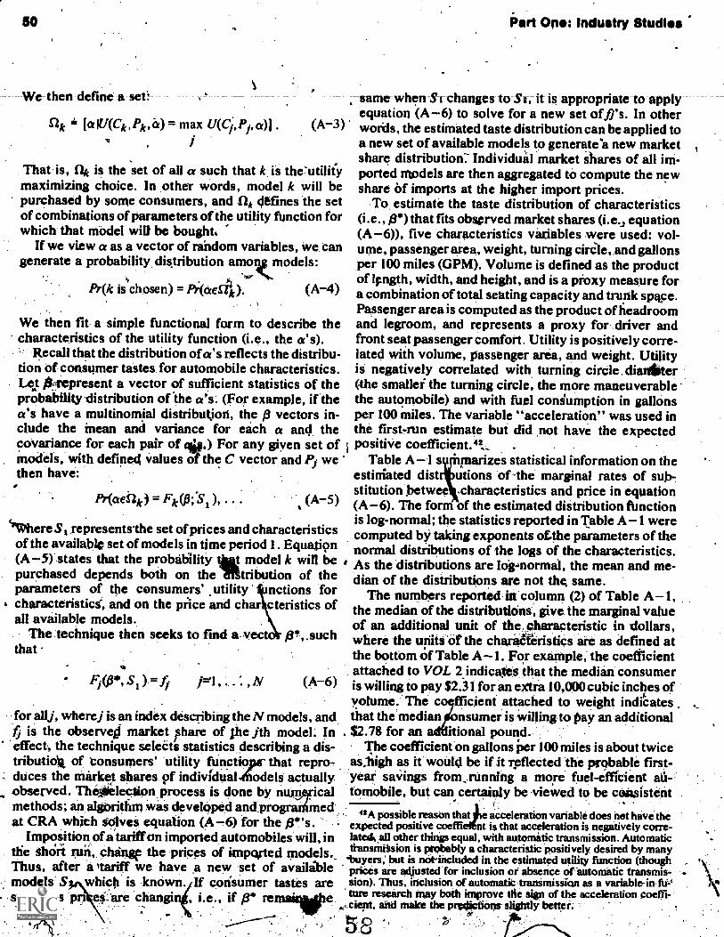
We then define a set:

S/k [a IU(Ck,Pk, )."-* max U(0, Pi, a)] . (A-3) '

That is, fik is the set of all a such that k is the'utilifymaximizing choice. In other words, model k will bepurchased by some consumers, and A, defines the setof combinations of parameters of the utility function forwhich that model will be bought,

If we view a as a vector of random variables, we cangenerate a probability, distribution amorig models:

&(k is chosen) = Pi(aefek). (A-4)

We then fit a simple functional form to describe thecharacteristics of the utility function (i.e., the a's).

Recall that the distribution ofa's reflects the distribu-tion of consumer tastes for automobile characteristics.Let li,irepresent a vector of sufficient statistics of theprobability distribution of the a's. (For example, if thea's have a multinomial distributiori, the p vectors in-clude the mean and variance for each a and thecovariance for each pair of cia.) For any giyen set ofmodels, with defined values of the C vector and Pi wethen have:

Pr(aenk) = Fk(fit.,Si ), . . . (A-5)

*here S1 representsthe set of prices and characteristicsof the available set of models in time period 1. Equation(A-5) states that the probability t model k will bepurchased depends both on the attribution of theparameters of the consumers' utility nctions forcharacteristics, and on the price and ch cteristics ofall available models.

The technique then seeks to find a vector jrsuchthat

Fio*, s = p=1, . ,N (A-6)

for allj, where j is an index describing the N models, andf is the observej market ?hare of ihejth model. In'effect; the technique selects statistics describing a dis-tributio of Consumers' utility ftinctiopc that repro--duces the market shares of individialAodels" actuallyobserved. Thitielection,procesi is done by ritiwicalmethods; an algbrithm was develOped andprowirimedat CRA which soivei equation (A -6) for the pi,- s . .

Imposition of a tariff On imported automobiles will, inthe Short xttri,. Chingf the prices of impqrted models._Thus, after a tariff we have .a new .set of availiblemodels- S which is known. If consumer tastes arestable as pri es...are changi i.e., if ps

Part Ono: Industry Studios

same when Si changes to SI, it is appropriate to applyequation (A-6) to solve for a new set off)'s. In otherwords, the estimated taste distribution can be applied toa new set of available models to generate a new marketshare distribution:" Individuid market shares of all im-ported models are then aggregated to compute the newshare of imports at the higher import prices.

To, estimate the taste distribution of characteristics(i.e., p*) that fits observed market shares (i.e, equation(A-6)), five characteristics variables were used: vol-ume, passenger area, weight, turning cirCie, and gallonsper 100 miles (GPM). Volume is defined as the productof length, width, and height, and is a proxy measure fora combination of total seating capacity and trunk space.Passenger area is computed as the product of fieadroomand legroom, and represents a proxy for driver andfront seatpassenger comfort. Utility is positively corre-lated with volume, passenger area, and weight. Utilityis negatively correlated with turning circle , diantiter(the smallei the turning circle, the more maneuverablethe automobile) and with fuel consumption in gallonsper 100 miles. The variable "acceleration" was used inthe first-run estimate but did not have the expectedpositiVe coefficient.*?_ ..

Table A-1 s ntarizes statistical information on theestimated dist utions of -the marginal rates of sub-.stitution .betwee .characteristics and price in equation(A-6). The form of the estimated distribution fbnctionis log-normal; the statistics reported in Table A-1 werecomputed by taking exponents athe parameters of thenormal distributions of the logs of the characteristics.As the distributions are Idg-normal, the mean and me-dian of the distributions are not thrS same.

The numbers reported. in.column (2) of Table A-1,the median of the distributions, give the marginal valueof an additional unit of the: characteristic in dollars,where the units of the chara6teristics are as defined atthe bottom of Table A-1. For example; the coefficientattached to VOL 2indicatis that the median consumeris willing to pay $2.31 for an extra 10,000 cubic inches ofvolume. The c fficient attached to weight indicates ,

that themedian nsumer is willing to 'Say an additional.$2.78 for an Iional pound. . .

The coefficient on gallons per 100 miles is about twiceasitigh as it would be if it reflected'reflected the probable first-year savings fromjunning a more fuel- efficient aer-.tomobile, but can certainly be viewed to be caitsisterit

42A possible reason that e acceleration variable does net hive theexpected positive coeffi nt is that acceleration is negatively corre-lated% all other things equal, with automatic transmission. Automatictransmission is rotobably a characteristic positively desired by manybuyers, but is not-included in the estimated utility function (thoughprices are adjusted for inclusion or absence of 'automatic transmis-sion). Thus, inclusion of automatic transmission as a variable-in fti-4tare research may both improve the Sign of the acceleration coeffi-

.,,cient, arid make the pre4icti ons slightly better..4,

5 8 141f.

Visas of Trade'Darriers on the-U.S. Automobile Market 51

Tabla'A-1Distribution of estimated Marginal Values of Automobile Characteristics(Dollars per Unit)

(1)Chiracteristic

VOL 2AREAGWEIGHTTURNGPM

(2)Median

2.3053'

5.17952.7782

7.4435565.42

(3)Mean

711495.83833.1316

303.29637.33

(4)Variance in

Consumer Tastes

431.579.22192.6532

152,630,000109,990

95 Percent Consumer Taste Range

(5)Absolute +

Lower Bound '

Vatiable DefinitionsVOL 2 (0.0001) x (length) x (width) x (height) (in cubic inches)AREAG =. (headroom) x (legroom) (in square inches)WEIGHT = weight (in pounds)

I TURN = turning circle diameter (in feet)GPM = gallons per 100 miles

'Range of valuet of marginal rates of substitution including 95 percent of consumers.12.5th 'percentile of consumer taste distribution.*97,5th slercentik of consumer taste distribution.

0.121561.98551.0648

0.03581216.70

as

(6)Absolute +

Upper Bound*

43.71713.5157.2492

1,547.41,475.30

with rational behavior. A simple example servesillustrate this point. Suppose the typical domestic cmileage is 15 miles per gallon, and the typical importmileage is 25 miles per gallon. Then, mileage falls byabout.2.7 gallons per 100 miles with a switch from thedomestic to the imported automobile. If a typical newcar is driven 12000 miles and the price of gasoline is$.60 per gallon, then the annual savings for the morefuel-efficient auto is about 1194 (the product of milesdriven, gasoline price per gallon, and the improvementin gallons per mile). The coefficient of GPM in TableA-1 indicates that the median consumer it,-..willing topay $565.42 for.ran idditional gallon per 100 miles,or $1,527 for an additional 0.027 gallon per mile. If the/ depreciation rate on a new car is 20 percent in the firstyear and the interest gte is 5 percent, then the annualfixed alp of spendingil ,527 extra for a new car is (0.25)x ($1,527), or proximately$382 in the first year. In,

'that case, the nual-smuunrirebligiiiiitifirivilling topity for owning' new car with improved mileage isabout, double the annual savings in gataline cost.

Two factors could account for this difference betweenthe estimated utility of better mileage and the estimateofgasoline ccistsavirigs. First, the combined, interestand depreeiltion as a fraction<of new car price 'is muchlove Ati subsequent years than in the initial year ofOwnership; if the buyer is not planning to sell the car inthe first year and has a longer time horizon, the annual_cost of a Price_ increase of $1;527 may be considerably

<6.

lower than $382. Second, ih 1974 buyers may have beenexpecting gasoline Rrices fo rise or may have fearedfuture shortages and/6r rationing because of the experi-encein the previous winter. For this reason, additiona)fuel economy in an automobile may have been valued atmore than its current dollar sirilings in lower 'fuel con-suniption. For these reasons, the coeffigient of gallonsper mile reported in Table A-1 certain4k seems to bewell within the range of asonable values.

The upper and abwer ands of the 95 percent rangeindicate the degree o dispersion in tastes for eachcharacteristic..aeng co sumers. The mOsit widely dis-persed values are for the. characteristic "turning cir-cle"; this result appears to make some sense becausesow, buyers place a, very high ,value on a car thathafidles well 'and can get into small parking places,while other buyers have practically no use for thatcharacteristic. The dispersion of the coefficient at-tached 'to gallons' per mile reflects differences amongbuyers in annual miles driven, subjective discount rates,relating current to future Cost saving , expected lengthof ownership of an omo an xpectations.aboutfinuce trends in gasoline prices and availability.

The co timated distribution of consumer tastesautomobile characteristics shown in Table A-1 is usedto generate the predicted shares for alternative sets ofavailable domestic and imported models (dined .by-characteristic's ind' price) 'reported in Tables 4 and 5 ofthe text.

"

52

E.

Literature Cited

I. Austin, Thomas C. , and Karl H. Hellman. Passenger Car*Fuel Economy - Trends and Influencing Factors. Paperpresented to National Combined Farm', CqnstructiondIndustrial Machinery and Fuels and LUbricants Meeiant-ings, Milwaukee, WiscOnsin, September 10-13, 1973.

2. Bain, Joe S: Barriers to New Competition; Their Charae-ter-and Consequences in Mankfacturing Industries.Cambridge, Mass.: Harvard University Press, 1956.

3. Chambetiain, Charlotte. 4A Preliminary Model of Au-tomobile Choice by Class of Car." Transportation SyS-tems Center Discussion Paper, January 31, 1974.

4. Charles River Associates. Analysis of the Effects ofTrade Policy Changes on the ,U.S. Truck Industry. Finalreport submitted to U.S"Motor Vehicle ManufacturersAssociation, ApHI 1976.

5. . "The Development of a Methodology for Predict-ing Demand for New Goods with Illustrative Applica-tions to Residential Heat Pumps." Drafteport kubmittedto Electric Power Research Institute, July 1976,

6. , . Impact of tr-Tai e-Policies on the U.S. Automobile -

Market. Final report submitted to .U.S. Department ofLabor, Bureau of International Labor Affairs, October

.' 1976: ,

7.. Chase Econometric Associates Inc. The Effect of Taxnd Regulatory Alternatives on Car Sale* and Grithline

nsumption. Submitted.to Council on Environmental

uality, May 1974, ..

8.` Chow, Gregory C. "Statiftical Demand. Functions forAutomobiIesnd Their Use in Forecasting." In Me De-:and forDurable Goods, edited by Arnold C. Harberger.

, Chicagoll hi.: University of Chicago Press, 1960.9. Consultant Report to* Committee on. Motor Vehicle

Emissions, Commission on Sociotechnical Systems. "Manufacturability and Costs of Pro sed Low-Emissions Automotive Engine Systems. ashington,DC.: National Research Council, Sept tier 1974.

10. Cowling, K., and J. Cubbin. "Price,. Quality and:Advertising CIM11113Ctiti011: An Econometric Investigation of theUnited Kingdom Car Market." Economica, 38(November 1971), 378-94. -

11.' Cragg, John C., and Russell S. Uhler. "The oimand forAutoniobiles." Can'adian Journal of Economics, 3, (Au-

. 7- gust 1970), 386-406. ° - .-

Part Ons: Indust Stud's*

12. Difiglio, Carmen, Damian Kulash, and Anthony Morton.Marketing and Mobility PaneInteragency Task Force f1980, March I, 197

13. Dyckman, T

eport. Prepared for thedtor Vehicle Goals Beyond

as R. "An AggregateiDenfInd Model forAutom es:" Journal of Business', 38 (July 1965),252-66.

14. Farrell, M. J. "The Demand for Motor Cars in theUnited States." Journal of the Royal Statistical Societyin the United States, 117 (Part 2, 1954), 171-93.

15. Kravis, Irving, Zolten Ken'essey, Alan Heston, andRobert Summers. A System of International Compari-sons of Gross Product and Purchasing Power. UnitedNations International Comparison Project: Phase One.Washington, D.C.: International Bank for Reconstruc-tion and Development, 1975.

16. Lancaster, }Cr.!. "A New Approach to ConsumerTheory." Journal of Political Economy, 74 (April 1966),132-57.

17. Linden, Fabian. "The Market. for Foreign Cars." TheConference Board Recorth10 (June 1973), 62-64.

18. McFadden, Daniel. "Conditional Legit Analysis of Qual-itative Choice Behavior." In Frontiers in Econometrics,edited by Paul Zarenibka, pp. 105-39. New York: Aca-demic Press, 1974.

19. McGee, John S. "Economies of Size in Automotive BodyManufactbre." Journal of Law and Economics, 16 (Oc-

gober 1973), 239-74.20. Market Facts Inc. A Foreign Automobile Impact Study.

Report submitted:to U.S. Department of Labor, 13treauof.International Labor Affairs, March 1976. -

21. Nerlove, Marc: ''A Note on Long-Run Automobile De-,mand." Journal of Marketing, 22 (July 1957), 57-64.

22. Suits, Daniel. "Exploring Alternative Formulations ofAutomobile Demand." Review of Economics and Statis-tics, 43 (February 1961), 66-69.

23. Triplett, Jack E., and Keith Cowling. "A Quality-Adjusted Model for Determining Market Shares inOligppoly:" U,S. Department of Labor, Bureau of LaborStattitics, Working Paper 4, December 1971.

24. Whitt, Lawrence J. The U.S. Automobile Incliistry1945.. Cambridge, Mass,./flatyard University Press,1971. '

t

liffects of Trade Barriers on the U.S. Automobila Market

CommentHelen M. Kramer

OP

AP

My comments will deal with the policy implications ofthe Charles River Associates' s(CRA) study of the au-tomobile industry [ l]:

Since my credentials include a doctorate ineconomics from a reputable university, I hope this au-dience will not interpret my remarks about the biases ofthe economics profession as merely an expression ofdistemper.

Robert Lekachman titled his most 'recent book:Economists at BayWhy the Experts Will Never SolveYour Problems . To quote: "The touble with economicsis the profession's diction to techniques diminish-.ingly relevant to the t stitutions and interests whichdetermine prices, empl yment, growth, and prosperityand' depression. The w rld will continue to astonisheconomists to, long as the concentrate upon the smallincremental changes in pure economic magnitudestowhich their. training has habituated them" [3, p. 7].

My criticism will focus on several aspects of CRA's. ..estimates of the social welfare impact of a tariff increaseon automobiles. First, the social cost ofunemploymentis seriously understated. CRA relies on the reSjlts of astud by the Cerger for Naval Analyses of auto work-

o e /earningsarnings losses from unemployment. The accep-tariCe of such a measure is an illustration of the kind oftunnel. vision characteristic of the economics profes-

ssion.

The report states, "On balance, 'we believe that theearnings lois measure overstates the cost of un-,employment, especially the private cost ause of thelarge, unemployment compensation paymen s receive4by displaced auto workers."

However, . the system of Supplementa Unemploy=ment Benefits (SUB) won by the United Auto Workerssilt contracts with the Big Four companies was designedto cushion workers. against the sh -term layoffscharacteristic of the industry's op onfor exam-ple, the layoffs occurring as a res It of shift cancella-tions or plant shutdowns to reduce inventories of cer-

,

taio models, or as a result of shutdowns for the purposeof retooling. During the massive layoffs in- the periodfolio:4%ring the Organization,', of Petroleum ExportingCountries' embargo, which for many workers,. lasted

53

over a year, laid-off auto workers exhausted. their enti-tlement to benefits, and the SUB funds at GeneralMotors and Chrysler were completely exhaustediEventhese workers were fortunate compared withrfhoseworking for independent suppliers, who do not haveSUB funds.

Furthesmore, it is itnportant to note that extendedunemployment results in ,more than loss of earnings:

once ,SUB entitlements are exhausted, the worker losescompany paid medical insuraugg coverage for himselfand his family;workers unable to keep up with mortgage and installmentpayments would lose equity accumulated in homes andconsumer durable goods purchased on credit;workers with seniority rights who are not recalled loseservice credits accumulated to and pension benefits aswell as seniority in their place of employment, where_it is available, which subjects them to greater vulnerabil-ity to future layoffs and permanent reduction of earningsand benefits in alternative, employment.

Certain costs of extended unemployment are notmeasurable by conventional means. It is noteworthy '41111

that. the authors completely, ignored recent researchfindings on the impact of unetriployntelit on physicaland mental illnest; mortality rates ,and.deterioration offamily relations manifested in.higher divorce rates andchild abuse. In contrast, they., assert: "earnings lossoverstates the social cost of unemploynient by not1,41ti-ing the gain to employees in increased leisure time.' Itis obvious the authors have never stood in an un=employment line. ,, ,

The. authors''.narrow foot also left out of view theintarelatedness of the auto industry and Other indus-tries.. Diming 1964-74, average direct employment inmotor vehicle manufacturing (StandardIndustrialsification 371) was 860,000 ,while related indirectemployment was 497,000 a total of about 2:4 millionjobs. The Bureau of Labor Statistics estimates, thatunemployment of 100,000 auto workers leids to un-employment of about 175,000 workers in other indus-tries, but CRA did not take this into account:

Second, the study does not eve% begin to do justice to .the probleMs of stagnating or declining employment inthe autilindustry and the implications Kw the nationalunemplSyMent problem. In fact, the latter aspect isdismissed in a fOotnote. If the experience of the 1960 ,taught economists anything, it should have driven homethe lesson that reliance on 'macroeconomic fiscal andmonetary policies to regulate aggregate demand is notan effective instrument for ensuring adequate employie

. ment opportunities .I' shall outline ..the for expecting. future

employment in the auto industry to stagnate orat bestgrow slowly.

6

54 Port Ow Industry Stud)*

Productivity ofTabor is expected to continue to increasein the auto industry. During 1957-72 the increase av,er-aged 3.8 percent a year.,

. Legislation mandating gradual increases in ',sales-weighted average fuel economy of U.S. autos will reqiiirea continuing Shift in the industry's:product Mix towardsmallercars, which require less labor input. In 1974 itrequired 24 worker-hours to assemble a standard-size carand 16 t9 assemble a subcompact car.The U.S. auto companies are prodacias an increasingnumbitr of cars and automotive components abroad forimport into the United States.Substantial tariff and nontariff barriers exist to the exportof 11..S.-made motor vehicles to the rest of the world.Included among these isthe fact, totally ignored by thereport, that the Big Three companies have plants inEurope and have no motivation to compete with theirEuropean facilities by exporting from the United States.The number of autos per capita is approaching amaximum. Currently there is one car for every 21/4people. Net new car demand has come mainly from thegrowth in multicar faibities. 'The percent of real disposable income,spent on aut9s,hasbeen declining.

.7..

The Carter.adthiriistratiOn is coming into office at atime of high and rising unemployment During the cam-paign, President Carter promised to take VigoroUS'ac-tio0o reduce unimployirient. There are two ways oflooking at. the role of public policy toward the, autoinduitry in relation tithe unemployment problem., Oneli".to define the problem narrowly in terms of un7,etnployment of auto workers in local labor Marketssuch as Detroit; where altermativejobs are unavailable.This is the approach taken by. the present study. -Thesecond way is to ask whether employmeht Oppor-tupities for other kindi of workers can also be expandedby pNcies affecting the auto industry. This approa chisreject Ed by the authors in a footnote: (p. 349) "Whilethere is ,undoubtedly a net social gain in providing au-tomobile industry employment for any otherwise un-employed worker, there is no logial reason why itwould be easier to employ nonaut'o industry workers inthe auto industry than anywhere elk; thus; there is noargument for an auto import tariff as a weapon againstgeneral unemployment."

Part of the-problem lies in the narrow way the authorshaKe phiased the questicin. They have riot exploredwhether tariff poliCy can be used'in a way, that *ouldincrease domestiC 'employment and social welfare. In-stead their have adopted the absurd assumptions ofoithodox welfare economics about perfectly competi-tive markets, consumer rationality, and a fixed patternof income slistribution whose justification cannot bequ within the framework of the theory. On, this

ured the alleged social losses and gainstariff on autos and made the customary

ts-about the allocation of resources. The

fact that welfare economics is based on the static as-sumptions of neoclassical economics, in which relit,tively minor adjustments take place in an economy offull employment of all resources and pure competitionin product and factor markets, does not cause the au-thors any qualms in making policy prescriptions for thereal, very imperfect world. The authors state:'(p. 43)"While the simple consumer surplus analysis used herehas some theoretical and empirical shod, asmings andqualifications, it still provides a reasonabir approxima-tion of the net social gains, or losses, from changes, intrade restrictions." The fact is that most quantitativelyoriented. economists will adopt whatever absurd as-sumptions arc necessary to enable them to write equa-tions that can be processed on a computer.

Not surprisingly, the authvrs conclude that the sociallosses of a tariftlincrease would outweigh the gains,measured by tfa fieduction in lotto 'workers'. un-,einployment I have already dicussed the serious un-derestimation of the cost of unemployment, which re---sults in the underestimatiOn or the gains from its reduc-tion. For those who might actually read the report, I

',should also point to'other reasons why the calculationsshould not be taken seriously. For one thing, although,the text repeatedly refers to a 10 percent tariff, in factthe. calculations were based on an increase in retailforeign car prices of 10 percent, which, given the exist-ing.methods of CHsjoine-valuation, would imply ,atariff considerably higher than 10 percent.

Another area where reality interferes with the Stith-.tical requirements of the analysis and is therefore dis-tmissed -is in the specification. of.pricing behavior. Theprice forMation equationS for .domestid autos assumethat prices of imported autos are independently deter-mined, exogenous variables. The evidence in the autodumping case, however, indicated that foreign 'Man-ufacturers establish prices according to conditions, inthe export market [2]. Admissions of this practice are. occasionally quoted in the :-akbusiness press. The interdependence of the, supposedly independent variablesraises serious doubts about the validity of the results.

I would like to suggest an alternative way of viewingthe tariff A a policy instrument. For reasons aboutwhich I shall, refrain from speculating, the authors ofthis study acknowledged in passing that an increase inthe ftariff could speed up the opening of assembly plantsin the United States by foreign proliceri, but thendismissed the idea. j,...et us explore tffil idea further.

CRA's estimates of comparative production costs asof 1973 indicate that when shipping costs are taken intoaccount, production of Toyotas and Datsuns would beslightly cheaper in the United States than in Japan._suice_thatthan int the United States and the yen has risen in value

I : .1

' ifflots of Trade Barrier* on the U.S. Automobile Market 55

At

com pared with the dollar. Both factoritend to raise thecost of producing 'autos in Japan for the American mar-ket relative to costs 'in the United States at minimumefficient scale, which CRA estimates as'400,000 cars ayear.

Automotive trade with Japan is notoriously lacking inreolVocity. Imports From all sources account for lessthan 2 "-percent of the Japanese market, largely _as aresult ofJapinese nontariffbarriers. In 1975, the UnitedStates impolied 695,573 autos and 138,875 compactpickup trucks from Japan, valued at almost $2.1 billion,while U.S. exports to Japan were only 14,842 autos and

A

no trucks whatsoever. ).

There are a number of reasons for expecting that the'U.S. market will be able to support a Japanese-ownedassembly plant at 'efficient scale. First, any bPEC-imposed increase in petroleum prices will raise the costof shipping autos from Japan. This will chaw thebreakeven point between production in Japan affd pro-duction in the United States in favor of the latter. At thesame time; any further increase in domestic gasolineprices would widen the market for fuel-efficient cars.

SecOnd, adults twenty to thirty years old, who nor-mally account for a high proportion of auto purchases,appear to prefer smaller cars. Further increases ingasoline prices would intensify this preference. Recov-ery from the recession would increastdeMand amongthis population group, which his experienced above-average unemployment rates and losses in real income.

Third, resumption Of the trend of rising real dispos-able incorilwould increase the number of multicarhouseholds, with additions to the car stock most likelyto be subcompacts for short-distance city driving.

Between the date of a decision to open an assemblyplant and actual 'production, there is a lapse of at least

..,,two years, as the recent experiences of Volvo andVolkswagen demonstrate. The Japanese auto compan-ies have given contradidtory indications of their inten-tions. On several occasions they stated t they wilt,postpone a decision until sales in the Unite tes havereached 400,000 units and on other occasions they have

denied that they are seriously considering production inthe United States. An announcement by the U.S. gov-ernment that, in view of the high ri tes of domesticunemployment, the tariff On autos will be increased on adate three years hence would have a 'salutary effect onthe production location decision.

There are special reasons for fostering the growth ofauto-industry employment through import substitutionas part. of an economic recovery program. Numerousanalyses of the characteristics of unemployed workersand new entrants to the labor force have stressed thatthe most urgent need is forireatly, expanded job oppor-tunities in unskilled occupations. Auto assembly workis unskilled labor and totally inexperienced persons canbe trained,on the job to perform any task. At the sametime, v, s and benefits are substantially above theaverage f r manufacturing industries. Thus, expandedJob oppo unities ikthis industry are a potential vehiclefor the ab orption 'or Chronically unemployed minori-ties into the labor force and an aid to correction of theimbalance cif income distribution between whites andnonwhites.

I challenge the authors of ;his report and its sponsor,the Bureau of International Labor Affairs, U.S. De-partment of Labor, to offer an alternative program ofjob creation that would provide equal social benefits atlower social cost.

Literature Cited,

1. Charles River Associates. "Impact of Trade Policies onthe U.S. pifomobile Market," Prepared for the Bureau ofInternational Labor Affairs, U.S. Department of Labor,October 1976.

2. Kahn, Helen. "Treasury to Drop Import Dumping Probe."Automotive News (May 10, 1976) 1, 31-32.

3. ekachrnan, Robert. Economists at Bay: Why the ExpertsWill Never Solve Your Problems. New York: McGraw-Hill, 1976.

4. U.S. Bureau of Labor Statistics. 1975 Manpower Reportof the President and The Structure of the U.S. Etonomy in1980 and 1985. BLS Bulletin 1831 (1975).

a

ti

CommentJack E. Triplett*

ft-

This comment will be concerned solely with ritethodsfotestimating the demand for iMports. Most studies Oflinport demand, and import:substitution for domesti-cally produced goods, employ what I' characterizebelow as the "Conventional method." Eric Toder [10]follows "this tradition, but also intrdduces a newmethod, the "CRA hedonic market share model"(hereafter, the "HMS model").

In this note, I with to make but two points: (1) Thegeneral approach to demand analysis embodied in theHMS model has considerable potential for studyingimport demand, and for all similar problems where it is

4necessary to model the demand for particular varietiesof goods . 12) The particular. model developed by Toderand his ,associates has teriota -defieiencied, for in de-veloping a new.emPirical approach to' demand analysis,they have neglected what the theory of demand tells usabout the subject.

The General Approach

The HMS model derives the demand for *particularvariety of car from underlying consumer preferencesfor automotive characteristicsIcarrying apacities, Neieconomy, performance, and so forth). The value of thecharacteristics approach to in demand analysis canbest be demonstrated by co ring the informationone gets from conventional mods.

When conventional methods cif demand analysis areapplied to estimating the c'emand tor imported cars,imports and domestically produced automobiles aretreated as if they were different goods. The only infor-mation necessary is prices and quantities sold fordomestic and imported cars. Standard techniques willproduce various elasticities ("own" price, cross-price,substitution) that will measure how demands for thetwo types of autos *ill vary as their prices changerelative to each other.

Such elasticities would appear to be exactly what we

..w Part Ono: Industry Studios

require. The difficulty is that the elasticity estimateswill vary with the composition of imported and domes-tically produced cars. Thus, if imports are Volkswagens 1'

and other small cars, and domestics are ftill-size Fordsand Chevrolets, the conventional technique will 'pro-duce a measure of substitutability between impcitts anddomestics that will _probably_ be _Quite_ different_ Fromwhat we would get if Small cars 'such as Vegas andPintos were added to the list of domestics. Using con-ventional techniques, if a new type of domestic or im-ported car appears (or if one of.them changes specifica-tions in order to fifi a "gap" in the market) we simply getnew elasticitiesafter

willfact. There no way to

predict how shares will change in response to suctproduct-line shifts, or to tell how they may affect thelasticities. Clearly, this is a serious liability, for thehistory of imported car sales in the United Statessuggests that These factors have frequently been as-sociated with changes in market shares.

A characteristics demand model, the HMS Modelbeirig one example, has the potential to do exactly Whatconventional techniques cannot' dopredict li`Owshares 'will change when a new car, or a change inspecifications, appears. Though economists interestedits estimating import elasticities have so far paid littleattention to the characteristics approach, Toder's paperis evidence suggesting. that Ofchmethods will' eventu-ally prove practicable, given development and the in-centive to collect or generate the kind of data that thecharacteristics approach to demand analysis requires.

Problems with the HMS Model

Though I applaud the approach taken in the HMSmodel, I have reservations about its execution. .

The HMS model can be viewed as an empirical im-plementation of ideas from a large body of economicliterature', in which the analysis of collections of charac-teristics provides the common feature. One may in-clude under this heading such diverse examples as Lan-caster's well-known work on the theory of consumerdemand for characteristics [6], Thomas King's analysisof the demand for housing characteristics [5], an exten-sive (and rather confused) literature on air quality andproperty values, the literature on "human capital" (onone interpretationsee [13]); and the analysis of wagesand working condition's using "hedonic Wage equa-tions," along the lines of Antos and Rosen DI Centralto all of these various areas of research is the "hedonicfunction," a construction that has a rather long history,and which first emerged i the economic literature as a

ofviews of propos or Improving methods for handling quality

staff members. . .change in price indexes.

64

Effects of Trade Barriers on the U.S. 01()utoinebile Marketr

I have pointed out elsewheie [I 2],1hat the role playedby the hedonic function (which is wfilation between themarket prices of the goods themselves and the quan-tities of characteristics embodied in them) with respectto the demand for characteristics is directly analogousto that of the budget constraint in the conventionaltheory of consumer demand. One chooses a particularcar, in this way of looking at'thines, by fin clibg.the carthat provides the optimal set of characteristics for eachconsumer's particular preference function, given thatthere is a set of prices for the various characteristics toWhich the consumer responds. For any consumption

--/problem there must be a budget constraint, in recogni-lion of the fact that a coniirmer's chOfces rare con-strained by his resources. In the analysis of chaiaCteris-tics demand, the consult takes the form of. an oppor:'tunity locus that shows iternative quantities of charac-tenistics thai can be purchased for the same total expen-d'iture. The opportunity locus is derived .from prices forgoOds (via the hedonic function), although it is definedon charicteristics. It embodies "implicit" prices forcharacteristics, which prices are estimated from thehedonic. functip (for more details, see [In.

Though Toder estimates some hedonic functions inone part of his study, the HMS model makes no directuse of hedonic prices for characteristics. In fact, the.HMS model lacks any explicit budget constraint orreference to characteristics prices, which leads to someGonfusing problems in interpretation, and some empiri-cal results that suggest that something is wrong. Con-sider, as an illustration of the latter point, a comparisonof prices and valuations from different parts of thestudy.

The variikble chosen to represent automobilecheacteristics and the HMS model results are arrayedin oder's appendix Table A-1. Toder interprets thenumbers reported in this table as the "marginal value ofan additional unit of the characteristic in dollars." Thatis, the model isinterpreted as indicating what consum-ers would be willing to pay to get an additional unit of aparticular characteristic on the cars they buy. Forweight,' to take one example, that valuation is $2.78 per

P°411d*A hedonic equation on automotive characteristics,

on the other hand, provides an estimate of the pricesactually charged in the market for additional units of

'Weight has along history of use io studies as a characteristic ofautomobiles, even though it is quite clear that weight in and of itselfmakes no contribution to the usefulness of an automobile. It is notentirely unreasonable, however. because it stands as a proxy for awhole host of thinp which are desirable. Unfortunately, the proxyrelationship frequengy introduces problems that can be serious,-especially when -it comes to intetpeting the results: See (11].

57

characteristics, Toder's own hedonic, equations' indi-cate the price of weight varies for different size classesof cars. Because of the functional form used in the'estimation, the characteristic. price is expressed as apercentage: For subcompacts, each additional pound ofweight costs 0.026 percent. For compact care, a 2.0percent increase is charged for every extra pound ofweight. Assuming that the average subcompact carcosts'$3,000 and the average compact car costs $4,000,the hedonic prices suggest that an incremental pound ofweight in a subcompact sells for around 78 centst in acompact, however, the price is much higher, in the'vicinity* of 80 dollars per pound, But in

thatmarket..

sharesvart of the study we: were told that people arewilling to pay, $2.78 per pound. If this were really true,then we would have to conclude that consumers wantmore weight in subcompact cars (because they valueweight at $2.78 per pound, whereas it costs only 78cents per pound for these cars); at the same time, how-ever, they want smaller, lighter compact cars (becausetheir $2.78 valuation of a"pound of weight on these carsis far under its rather high $80 cost). In other words,people want to buy larger small cars and smaller bigcars! Such results seem inconsistent, to put it mildly.

.',The paper does, of course, reference all kinds ofqualifications: the HMS model is only very preliminary,it is by no means certain that the variables arethe appropriate ones, somewhat different variables ap-pear in the hedonic function than in the market sharesmodel, and so forth. I would add another to the list:theory suggests that in the hedonic world, consumerswill typically be at cornet solutions, so exact equalitybetween characteristics price ratios and marginal ratesof substitution will not in general be attained. Althoughdue allOnce should be made for all theie'points, thediscrepMy between hedonic prices and HMS modelevaluations is too large to be explained by any aspect ofthe automobile market.

What seems to be wrong is that the. HMS modelershave tried to model consumer choice toward automo-tive characteristics without incorporating the prices ofcharacteristits Into the model in any explicit way. Instead, they have entered of the car in what th4refer to as the utility functi d performed an uncon-strained maximization. There can be no theoreticaljus-,tification for writing price as an argument of the utilityfunction. The best that catche -laid for this way of

'The hedonic price functions were used to construct the priceindexes for the "time series" demand estimates (that is, Toder'sequation 2.1 and the consequent Tables 2.1 and 2.2), and were notreproduced in the paper prepared for this volume. The numbers citedin the present note were taken from (3, Table 3.5, p.8].

watt of a demand Meld is to argue thatit-caivbe given arationalization as some sort of "reduced-form estima-tion. Because such a rationalization provides insightinto what is really going on in the HMS model, andsuggests follow-up research strategies, it is worth de-veloping briefly in the remaining space.

We first assume what has come to be known as a"two-stage budgeting procedure" (2] or "utility tree"(M. This permits forming a utility function on automo-tive characteristics and negleitingafter the overallallocation to automotive expendkures has beenestablishedprices of other consumption goodsanalyzing choice of a particular m9etaTokar, Next; wispecify a ftinctional form for the resulting. "branch"utility function on automotive characteristics* (froMwhich one derives estimating equations for 'a set ofdemand functions on automotive characteristics). Sucha procedure is not so very unusual in demand analysis.Christensen and Manser (4), for example, use similarassumptions and methods to estimate demand equa-tions for a "meat branch," with beef, pork, and soforth, as the goods. To perform an equivalent study onautomobile characteristics, the catewry "automo-biles" replaces "meat," with (e.g.) the characteristic"fuel economy" treated equivalently to Christensen'and Manser's "beef' or "pork." Toder uses a linearutility function, Christensen and Manser the translogutility ftinetion; other forms are available. --

A budget constraint is needed for the maximizationprocess, and this can in principle be, derived from thehedonic function. Again, there is a precedent in thework of King, who employed a Rotterdam demandmodel, the "branch" utilityfunction idea, and hedonicprices for characteristics.' Finally, one specifies tastedistribution parameters along the lines suggested in To-der's appendix (or in ( 6, chap. 7] where a very similarprocedure for predicting market shares is proposed,though Lancaster suggested a Cobb-Douglas utilityflinction). The remainder of the investigation could fol-low the outline in ,Toder's appendix (equations A 4through A-6)..:The HMS model simply short-circuits the first few

strips of the above process, by inserting the-price of thecar 'in an equation containing the quantities of au-tomobile characteristics (equation A 1). In thehedonic world, however, the price of the car is inter-preted as total expenditure on characteristicsthat is,for the functional form employed by Toder,

'The reader is warned that there are tnany difficulties involved inthis step, and King's solutions are not the only ones possible.

tie

Part Onci Industry Stales

(.4r in " e LPPII),

.whe yi are price and quantity of the ith charac-teristic ntroduction of this quantity' into what islabeled ity flinction" (equation A thus servesto proxy or the *Met of characteristics prices onchoice of characteristics and for the "first stage"budgeting level, where expenditures on automobilesand nonautomotive goods are'deterthined. EquationA I is, therefore, not a utility flinction ,,properly speak- 4ing, but Some sort of amalgarh ofa utility llinction and afunction that specifies consumption opportunities. ,

Writing the pl; in this, way does not evade thedifficulty. of d in characteristics prices (which,because they must be 'estimated from a hedonic func-tion, are in some .sense data not as "hard" as moreconventional pride data), or setting up a budget con-straint from hedonic prices. Rather, the hedonic func-tion is tangled.up a the resulting estimates in a way thatis very hard to disentangle, and nearly impossible toevaluate.

Thus; the traditional consumer demand lit in-volving sets or systems of demand equatio vedfrom explicitly modeled utility functions pr' des a,framework that meshes theory and econometricspecification, and qould be adapted to the task of es-timating demand tot automobile characteristics, if ontorecognizes the propermie and interpretation of hedonicprices. The tradidosid approach simply treats importsand dornestically produced cars as different goods; itthen relies on consumer theory to Construct demandcurves for these two goods. 4n the process, it ignorestwo fundamental aspects of the problemthe charac-teristics of the cars that,are being analyzed, and .thenature of a discrete choice problem (which arises in thepurchase of any large durable good because peopleusually phtchase only one at a time rather than a little ofthis 'arid a little of that). The HMS model explicitlyincorporates the discrete choice problem and theanalysis of characteristics, and, this is its strength. Itsweakness, however, is that it ignores the traditionaltheory of consumer demandthat is, a world_in whichconsumers maximize utility in a setting in which pricesare parameters forming constraints on their behavior.

I think Toder (and Scott Cardell, who is credited withdevelopment of the HMS model) deserve credit forjumping off into uncharted and treacherous terrain.These comments-ire intended to point out some of thequicksand encountered in the first step.

One final remark is directed. toward anyone whowishes to extend the approach. So much data are avail-able on cars that it should not be difficult to choose

Effects of Trade Barriers on the U.S. Automobile Market

variables that correspond with what consumers reallywant, and to "avoid the use of rough proxies such asweight, which causes iota many problems in interpretingand using the results. Ohta-Griliches (7), for example,experimented with Consumer Reports data, and there isnow EPA data fbr all cars on such characteristics at fUeleconomy and standardized acceleration times. Thehedonic tradition of using whatever convenient proxyvariables that seem to work in the equations should,,beabandoned without regrets.'

a

Literature Cited

1. Antos, Joseph R.. and Sherwin Rosen. "Discriminationin the Market for Public School Teachers." Journal of.Econometrics. 3 (1975), 123-50.

2. Blackorby. D., D. Primcint.-and R. R. Russell. "Budget-ing Decentralization, and Aggregation." Annals ofEcono ,jk and Social Measurement. 4 (Winter 1975).23-44.

3. Charles Ritter Associates. "Impact of Trade Policies onthe U.S. Automobile Market." Report prepared for theBur!au of International Labor Affairs, U.S. Departmentof Labor. October 1976.

'In an ideal research setting, one would ask that the investigation beconducted on characteristics of automotive services (rather than justPars), that the demand for services be derived from the underlyingdemands for service characteristics, and all of this be used to predictthe demand for new cars. This is clearly beyond the realm of thepossible with currently-developed techniques. and for some caseswill result in the same model.

"t.

4. Christensen, l.autrifs R.. and Marilyn'E..Manser.-vCostof Living IndexeS and Price indexes for U.S,. Mutt andProduce. 1947-1971." In Household Production andConsumptlosr, edited by Nestor E. Terleckyj. Studies inIncome and Wealth. vol. 40. New York: National Bureauof. Economic Research, 1976.

5. King, Thomas A. "the Dimond for Housing: Integratingthe Roles of Journey-to-Work, Neighborhood Quality.and Prices." In Household Production and Consump-tion. edited-by Nestor P.. Terleckyj. Studies in Incomeand Wealth. vol. 40. 'New York: National Bureau ofEconomic Research, 1976.

6. Lancaster, Kelvin. Consumer beiiiand: A New Ap-proach. New York and Londo;i: Columbia UniversityPress. 1971.

7. Ohm. Makoto. and Zvi Griliches. "Automobile PricesRevisited: Extensions of the Hedonic .Hypothesis." InHousehold Production and Consumption, edited by Nes-tor E. Terleckyj. Studies in Income and Wealth. vol. 40.New York: National Bureau of Economic Research.1976.

8. Strotz. Robert H. "The Empirical Implications of a Util-ity Tree." Ecortemetrica. 23 (April 1957), 269-80.

9. Theil, kenri. Theory and Measurement of Consiimer. Demand, Vol. I . Studies in Mathematical and Managerial

Economics. University of Chicago. North-Holland Pub-lishing Company, 1,75.

10. toder, Eric. "Effects of Trade Barriers on the U.S. Au-tomobile Market." Oresented at a confeitence sponsoredby the Bureau of International Labor Affairs, U.S. De-partment of Labor. December, 1976.Triplett. Jack E. "Automobiles and Hedonic QualityMeasurement. "Awned ot Political Economy 77 (May/June 1969), 408-17.

12. "Consumer Demand and Characteristics of Con-sumption Goods." In Household Production and Con-sumption. edited by Nestor E. Terleckyj. Studies in In-come and Wealth, vol. 40. New York: National Bureau ofEconomic Research, 1976.

13. "Measuring Prices-and Wages." AmericanEconomic Review. 617 (Febritary 1977). 135-40.

I

GO

c Toder with N. Scott Carden.

Part One: Industry Iltudlies

fir,. TripIetrs comments are of a more technical na-lure, focusing .mainly on the hoglonic market share(HMS) model developed at CRA to analyse the impact .of changes in relative prices of different automobiles onmarket share demand.

The Authors have four major points of disagreement fwith Triplett:

1. Triplett's assertion that the HMS model ignore',/,'the theory of consumer demand is incorrect. The choice'equation posited in the Hkft mod5l can be derived',

-----..directly from the standard constrained maximizationl ,

approach of consutner theory. .Dr. Kramer's comments focus on the analysls thebenefits and costs of changes in tariffs on importedautomobiles that are presented in the Charles RiverAssoziates report (I) but arenot discussed in the con-ference .paper included it (his volume.

Because Knuner's comments do not relate directly tdthe aiiithair iti this piper, they will.not Wevaluated indetait' here. ° Howeftr; we disagree with- much ofKramer's economic analysis and also with her policyconclusions. A few clarifying points about the CRAreport-merit brief mention:

a The C A report used conventional tools of micro-econo c analysis, as Kramer Nests. The measure-ment he net welfare effects other tariffs was per-formest 'thin the context of Axed segregate demand (notnecess y full employment). The. issue examined iswhether t ere are net social gains frontstimulating labordemand auto import tariffs rather than by some moreneutral method. The findings do not-imply that there arenet sociall losses from reduc ing aggregate u n e mplo ymelit.The conclusions of the CRA report do not depend on anassumption that the automobile industry is competitive.Both competitive and noncompetitive cases were simu-lated, with both showing . net social costs from highertariffs. (For the case of imperfect competition, see (1, pp:337 -481.)

. The use of a 10 pereent price increase of impqrtedtomobiles in the simulations does not affect the qualitvfive conclusions. Assumption of a smaller priceincreasewould have reduced both the auto industry employmentgain and the resource allocation kiss froth a tariff, leavingtheir relative magnitudes similar.The price formatgll equations referred to by Dr. Kramerused import pricei as the exogenous variables in somespecifications arittiMport *ores in others. (See (1, pp.1,4'199).) The' Battings from these equationv-that

14.herinitioff fates may lead to higher domestic autos..,,-ftelicen the tune for tariffs. HoWeVer, the wel-coMptaationi4n. the Competitive 'Case were. per-.

.;fortncti .fir the aVinaPtion Wit domeitic auto pricesare utinOcted by exopenotei.increases in the prittS 'ofauto imports

I Selected excerpts front CRA report quoted by. Dr.t Kramer do idol accurately represent the tone of there-- pOrt. Readers interested it! evaluating -the methodology

and ConclusiOnstof the '-benefitkost eniiilysis in. the CRAreport should consult the Nil study.

, Using the standard approach, a- consumer's utilitymay be written V 'y (up F(z)). where V is tota.tility %from both the discrete good fi.e., the automobiletriOde1 chosenfand the collection of all other soOds z.The. Consigner maximizes V subject to the budget Zoti-atraJnt /. Pzz, where! Is income, Pi is trie price ofthe automobile model f, and PE is the price index for all .other goods.

Assuming either separability of utility betWeen theautomobile and other goods or constant relative ..ptices-within the set of all other goods, wecan derive from thismaximization problem the expression reported thetext, where the consumer chooses the automobilemodel./ to maximize utility, which is a Ibnction of theprice off and the characteristics of j

TMs point c be illustrated easily for the case of aHoar utility fit don. The problem is to maximize

Subject to

+ Fitz)

1=P/ +Pzz

Solving (2) for z, and substituting in (1), we.

V .. ui + F((1Pd/P:).

(1)

(2) ,

obtainY.

1r3)

If the composite food is the numeraire, so that Pi, = 1, -and F(z) is a linrear function, the prolplem reduces to Oneof maximizing

V=u P +II 1 (4)

where uj is a function. of the characteristics of the auto-mobile model chosen, In thii linear version, the choiceainong disCrete yarieties does not depend on the con-kumer'syincome I. since income enters the utility func-tion in the same way foe each consumer.

f

drrft°

Effects Trade orders on ihe. Ms. Atitomobile Markey,. ,%0 , '

Equation (4) is trialogous to the utility function dis-cussfed in the. text.

A similar, but slightly more complicated; derivationof the sante general result can be perkrmed for quad-ratie and logarithmic utility functions:1n these formu-lations, the _interpretation- cif the price coefficient igdifferent (see [2, pp. 6 -7]). 4

1 The alternative apprOach to k& problem sketchedby-Triplett would not havehelped to answer ques-tions raismf:by the.study with ,the available data, andmay noteven be useful with a 'richer data set available.It is not clear from Triplett's comments hOW such a

would face the same implicit pricefunctimPforchatac-teristics. How then would one estimate the effect 42L.variations in price on the demarid-for characteristic

Triplett's approach could not have. used in thestudy, even if it were a better gendral methrtd,becausedata on auto purchasts by individual consumers werenot available to the authors: Eveti with disaggregatedata on individual behavior, it might be much preferableto use a logit model approach, folloiving the' work al-ready successfully applied in mode choice studies in thefield of transportation demand. (For example, see [3].)

3., .TripletCs long dismission about alleged contradic-model can 'be applied to the problent at hand. . ' tions in the results is largely irrelevant. The hedonic

, Triplett is 'disturbed that implicit prices derivedfrom '6410th:ins to which he refers are drawn from a section of .

a hedonic pride equation never appear in the HMS the CRA report that attempted to make a. rough com7'model. i'lledOnic" prices are absent Troth the.HMS parison' of "quality-adjusted" prices of imported andmodel liecause the probleM is poied as a choke among , domestic automobiles in 1975. (See [ 1, pp. 81 82]).discrete alternatives, rather than as a series of demand These are not the equations used to construct the price

'ethiationS for "characteristics." In the latter approach, index in the time series regressions. Because thosesuggested by Triplett; linters are xiewed as-buying equations were not carefully specified, no implicationtairsbundles of charac ics, with thOir choice con- was made in the CRA report that the coefficients should

.. strained by the price of adding more units of `a charac- be interpreted as the marginal ptiCe of weight and horse-'...teristic (for example, the, price per pound of adding pOwer. It-is well known that. when multicollinearity

more weight ,to a car, other things fixed). exists and proxy variables are used one should be care-Triplett's apprOach has a number, of theoretical and ful about 'interpreting the meaning .of coefficients. It is

practical shortcomings. First, consumers cannot vary not clear why Triplett wants to make such an inference-

their coMbinations of characteristics continuously as when the authors do not. In addition, the implied co-, the approach asSumes; in the 'real world, they are lira- efficient of weight in ate. HMS model represents-theited to Amite number of modeli7With given'bundles of "mean"..Itste of all consumers. Contrary to Triplett's

..ve

,

characteristics.. Thus, characteristics are not exact assertionv. the use of that coefficient does not mean thatanalogous to sets of uniform commodities, among marginal value of consumer's of, an additional unit ofwhich infinite combinations, within any budget con- weight4thsisame for both subcompacts and compacts,soint, can b(shosen by the consumer. Incorporating ,: becaus4bRiers of subcompacti are different peoplethe finite, choice aspect Of a problem explicitly make- who haVE different mean tastes than buyers of corn-the 'model ore. general and more difficult, as well as pacts. Imore re tic: The solution of this finite choice problem ' 4,. Triplett's sugge ons about the use of data in .is the Methodological adVance inthe HMS yikocielSeC- ftti-ther research 'contain some factual inaccuracies..oftd, the implicit plices discussecrt Triplett .can 'be °Contrary to Triplett's implication, the UPS. Enviroii-meaningfulty defined only under ecial conditions. mental Protedtion Agency data on fuel economy were ":*These prices are derived by ta, g a regression of the used in the HMS model, as were U.S. Department of.total price of an automobile on it characteristics, usu- ransportation data on acceleration. Weight is used inally using a cross-section of auto obile models or a Ilith S model as a proxy for several utility-producing

. given: year. If the form of the regresOon is ProOerly attributes; these include such dimensions asuxiirious7.linear, then the coefficient of each characteristiC repre-.

--Sents an estimate of its implicit price. However, if thehest:ionic function is nonlinear, as is likely to .be the case,and has nonzero cross - product terms, the meaninf of an.imptic it.price becomes unccharacteristic then depen on thelevel of the ciitirac-

ar. The marginal price of a

ness, quietness and smoothneSs of ride, as,:well as,possibly, safety. Subjective measures of some-of thesedimensions are available in Consumer Reports for alimited number of models,.but cannot be readily used inthe HMS model, which requires data on a relativelycomplete set of the available choices. .

teristic being consiniiedi it i not longer jest an external The authors share Triplett's view that the right ap-parameter confronting the buyer. Thir4, even jtf' icit proach to studying market share demand for durableprices. could be sensibly define,cle°ar what ;Triplett would hatPresumably, in the U.S. automo

in any year, it is not goods should incorporate an explicit guano tiveauthors estimate. analysis describing the factors behind consumer cl ice

ile market,' all buyer Thamong competing models. The HMS model developed

62

for this'study, in its present form, represents a prelimi- Rejoinder F-nary step in this direction. The authors agree that Muchfurther work remains to be done and hope that research

crack E_Tri p lettalong these tines will. e,encouraged...

Literature Cited

. Charles River Associates. Impact of Trade Policies on theU.S. Auiomohile Market. Final report submitted to Bureao

1110_ of International Labor Affairs, U.S. Department of Labor,October 1976 (CRA re ort)P

P.:" Me t ho do tog y for Predicting the Demand for

- New:lectricity-Using Goods:.! Draft report submitted toElectnc Power Research InstituteNovember 1976.

ir 3. Domencich, T.A. and D. McFadden. Urban Travel, Re-mand: A Behavioral Analysis. Amsterdam: North-Holland Publishing Company, 1975.

Part One: IndusTry Studies

Their reply indicates that Toder and Cardell (hereafter,T-C) did not understand. nir commelas Perhaps I was

_unclear.1. I pointed out that there is an $conoinictielationshipbetween some of the parameter estimates of- T-0:sHMS market 'share model and the coefficients of theirhedonic price study, and also that their MS-demandmodel could be thought ofas a kind of "reduced form"of the general characteristics demand 'model

- popularized by Kelvin Lancaster [1]. ,These relation-ships were not discussed by -the authors, and indeedhave generally, been ignored in the qualitative choiCeliterature on which the HM demand model is based. Iwas calling attention, in, her: words, to the fact thattwo sets of literature were r deeding somewhat inde-pendently on the s. e pr lem. The campariions ofparameters from th r,heilonic'price function and theirHMS model, which T-C feel were irreleVant (numberedpOi9t 3 in their reply), were .siinply a .graphic way ofdemonstrating the interrelationships between iech-niques ,USed in different parts of the study, and. thereason for raising these issues was 'preCisely that-, theauthors did not.

I feel strongly that carrying out a direct analysis ofbehavior toward .chatacteristics is an important step in

,establishing the economic. 011imiwork which underliesthe HMS model. However, the economics of the rela-ticinship between qualitative choice demand models; ofWhich the HMS is an exaniple, and Lancasteriaiicharacteristics demand models have not beenthoroughly worked out.. A. reeent paper by AnthonyLawrence [2]; may beihelpful to readers who want top?:into the matter.2. T-C feet them t`a number. eoretical andpractical shortcomings" to-alterp vea roaches. It

_ happens that a number of the specifi points they list(intheir point # 2) are already coVer4d lsex(here (see mypaper on characteristics dem nd ' odels [5] and myreview of Lancaster [4]), and are not nearly the intract-able problems they, make them out to be.

T-C's one valid point is the paucity of data for'carry-ing out nontraditional dernancanalysiS; but this is aproblem in implementing any alternative to the cOriven-

Effects of Trade Barriers on the U.S. Automobile Market

*nal approach to ,consuther demand, including theHMS model itself (see their listing of variables 'theywould like to have, but couldn't get, in their point # 4);With respect to my original comment on the data ques-tion, I diditot mean, in the paragraph in question (whichwas directed to ".anyone who wishes to extend theapproach") to imply that Toder had used none of theEPA-DOT data. Rather, I was urging that greater ef-forts be made to obtain data which measure characteris-tics directly, rather than variables which merelytkvesome relation to what is desired, The serious problems rwhich plague estimates basedtn proxy variables such

----as-weight-have-been'ywell IcnoWn in the hedonic Mem--ture for years (see my 1969. paper. [3]), and the HMSmodel did, as T-C theniselves note in their "Reply,"use precisely this troUbtesome proxy variable.3. One should keep all this in the proper context. Icertainly intended to convey in my comment dn the T-Cstudy my harmony .with their general approach to theproblem of estintating demand for heterogeneousgoods. For the heterogeneous goods case: dne must payattention to the ways that varieties of goods differ andSihy consumers want thetarieties they do in fac t select;this the traditional approafh to demand analysis doesnot, and cannot do. To say that I would like to seeiMprovements along -certain lines in any subsequenattempt's to follow the pitmeering route T-C have setdown was not intended to denk them credit tor what 1call "jumping. off into uncharted and treacherous ter-

,

Oft

Literature Cited

1. Lancaster, Kelvin. Consumer Demand: A New ApproaCh.New York and London: Columbia UniversitY Press, 1971.

2. Lawrence, Anthony G. "The Role of Prices in QualitativeChoice Models:: Unpiublished paper; jtigy Analysisand Environment Division, Electric Pow, gsearch Insti-tute, Palo Alto, California, (revised) November 1976!"'

3: Triplett, Jack E. "Automobiles and Hedonic Quality Mea- ,

rement." Journal of Political Economy, 77 (May /June1969), 408-17.

A Review:Of Consumer Demand: A NewApproaq by KelVin :Lancaster." Journal of aonomicLiterattirc, 11. (March' 1973), 71=81.

5: ' "Consumer Demand Characteristics ofConsurnption Goods." In House Production andConsumption, edited byNestor E, Terleckyj. Studies inIncome and Wealth, Vol. . 40. New York: National Bureauof Economic Resegch, 1976.

Part Two

a Part Two: Labpi Market AdJuitibente

Introdjuction.Harry J. Gilinarf r

Po(icies designed to .reduce restriction's\ on' interna-tional trade have historically been supported on thegroudds that the resultant increases in exports and im-portswould raise real inComes.'The focus generally hasbeen on the net income changes in trading countries andnot op the distribution of income and on the costs of.adjustment in reallocating resources to production inwhich they have a comparative advantage: Nevertheless, it is precidely these two aspects of the problem thatare likely to influence the politics of trade liberalization.

Increases In impqrtifrom Whatever source.are likelyto impose both in9. and nomtiotriary costs onworkers enployedi,, port competing industries. Fordisplaced who atereemployed in lines wheretheir experience anApecific skilli are less-valuable, thelosses can be 'permanent. In fact, even workers luckyenough to be reemployed at comparable- earningsexperience the permanent loss of foregone earningsother costs involved in trying_io.futd-newpositions.

The Brechling and Jacobson-studies that appear inthisaection were motivated by the realization that pre-vious studies in the trade area have largely ignored thelabor market adjustment process. These new studiesare complementary in the sense that each concentrateson a particular dimension of what is 'essentially amany-sided prcOem. Brechling examines the way towhich reductions in-employme t occur in response todeclines in output; Jacobson c ates the earnings lossincurred by workers displacr fromi. particular man-ufacturing industries, eleven told. Though their gild-ings are far from definitive, both provide new and sig-nficTt insights' into the-labor market adjustment pro-

, Brechling's major finding is that the primary method)f reducing employment in a particular industry:in re-Onse to a fall in demand for its output is throughliiplacements ratter- thanithrough natural attrition,hough this importantivfinding holtsply if relativesages in expanding industries -do simultaneouslyise. Brechling is aware that his particular model does

not apply well to the case of trade liberalization asone woul ike. Nevertheless, his work provides impor-tant ne insights into complex labor market dynamicsthat necessarily accompany any restructuring of labordemand among firms and industries. IJacobson 'esennates monetary losses incurred byWorkers displaced from particular industries whichheretofore have simply not been estimated systemati-cally. Economists addressing the issue Of displacementcosts sometimes, equated these costs With earningsforegone during he periodOof unemploYnient*lied the possibility of lower reeinploY nt Wages:But even if they considered reemployment ages, theyassociated the wage loss with the differen tweenthe wageirearned priin to the job loss with th earnedimmediately after reemployment.: As Jacobson ints.out, these economists have generally ignored the s ularpatterns of earnings of teemployed workers; which maybe very different from those of continuotusly employedworkers. Jacobson's estimates took their secular wagepattern into account: Jacobson was also able to improvethe -quality of the estimatei by using social security \data for individuals classified by the employer's indus-try, the so-called LEED file.

Jacobson's major findings:

Displaced workers often, bear substantial casts beyondthese imposed during 'the initial period of unemploy-ment.

ff These added costs are likely tovary substantially amongindustries, depending among other things on the differ-'ences in the skill levels of workers in those industries:

Asa always trueof empirical work,rk, there is a lotmore.

that could be done to improve these, tudies. Indeed inthe . comments by .Richard Freeman d those by me .'that appear after. the hling and J obson papers,there are a variety of 'led suggesti s that providean agenda for future -work on the- very in resting andimportant topic of labor adjustment to, ta, in thedeiriand for labor by firms and industries.

A Tim Series Analysis .ofLabot urnover Rf

.. Frank. Brechling* ..1'

;1:- Introduction' 'well as for the evaluation of the trade adjustment assis-e 4

. Several data basis have been used for th combuta-tion of-displacements and unreplaceiiattii ns. 3 In theresearch underlying 'tile present paper, d time series

.dala 'on -labor turnover by Industry' published by theBureau of Labor Statistics have been used. In part 2 ofthis paper g conceptual framework and a desdriptionof these statistics are presented. The conc.eptualization ofthe labor turnover relationships also yields formal, op-"trationallii meaningful expressions for displacementsand unreplaced.: attritions.

For thg estimation of displacements and unreplacedattritions a model, is required within which these labor-flows or their comptments arc linked to their determi-nants, in partic4lar, to net chaliges in employment. Part3 of thilfaper devoted to the description, derivation,pstimatie and simulation of labor turnover models.This part is subdivided into four sections. In section 3Aa turnover model with exogenous quits, which wasdeveloped and fitted by a previous investigator, is pre-sented and its implidations for displacements and unre-placed attritions are described. This model and-the ap-propriate parameter estimates suggest that 79 percentof any net reduction in employment is accomplished byutikeplaced attritions and only 21 percent by displacemelts.

e est s .of unreplaced attritions and dis-plac nts, however, depend crucially on the assump--tion o xogenous quits. By contrast, model, whichhas been used in the major

ratesof the re ch un rly-

.thin endo enous

Import penetrations of eta' necesiitate,ireduCtions in the empl ment levels of the affected

domestic. suppliers. T se ..de teductions' in , employ-ment can be subdiv d co 'ently_ into displace

.ments and unreplaced attritions. Displacements arepermanent separations initiated by employers 'an2k atto /e to the import penetration. AttritiOns are allothe nnarient separations that may be due to valutik-

iting; retirement, death, disability, incOmpe,tence r 'dishonesty. When emPloyers refrain. fromreplacing 'attritions they are termed unreplaced attritions: The essential difference between displacenientsand attritions arises from the nature.of their costs. Dis-placements involve unexpected' costs that, in the ab-,seVe of compensation for them,. must be borne in,

HVoluntarily by the displaced workers. The wits of ittri=tions, on the other hand, ate anticipated and bornevoluntarily by workers as part of the normal costs ofObtaining and leaving jobs.' For this reason it is oftensuggested that displaced workers be compensated fOrtheir displacement costs, especially if the import pane-tration is attributable to a change in governmental pol-icy. In the United States some compensation for dis-placement cosisiiS provided for under the trage adjust-ment assistance program of the 1974 Track Act.

The aim of the research underlying this paper hasbeen to _Obtain estimates of displacements and unre-placed attritions in industries that experience perma-nent net reductions. in employment. Such informationmay be helpful in the formulation of trade -policies as

.

'I am deeply indebted to my colleagu t the Public ResearchInstitute for many he di sions of the seemingly insuperableproblems encoktntered i research underlying this paper. KathyClassen, Waliarn Dewald, Paul Feldman, Harry Gilman, and BruceVavrichek read a previous draft of this paper and made many valtiablecomments. Theirhelp is acknowledged gratefully. This paper is basedon Frank P. Brechlint k'A Time Series Analysis of Labor Turnover,"'LAB 75-19 which Wad completed in 1976. _

'Costs of displacements and attritions have been estimated by BMf I] and Jacobson (10].

Ma.

ing this paper, incorporat quits as

'Although the research has here been motivated in' terms of the.consequences of trade liberalization measures, estimates .of`-displacements and unreplaced attritions may be useful/or many otherpurposes. Suppose, forimstance; that a net reduction in :employment

-is brought about by a regulation designed to prOteet the environment.The costs incurred by displaced' workers would be a legitimate cost of

'the implementation of the regulation and hence, it would ,be itart to knoW the le .e_cfsi displacements and unreplaced ttriti

. ;See,. for instanw, COI WhO used Social Secuestimate chiplacements -and attritions in the steel indus

y'-variable. This model, which is described in section 3B, turnovconsists -of several dynamicallypinterdependent equa- used i

mss, designed to describeithe b4haviorover time ofall atmthe relevant (abor turnover categories. over

The labor turnover model with endogenous quits has 'don'sbeen fitted to the data for twenty -four manufacturing containdustries, but section 3C :contains the empirical resultsfor only two groUps; .nathely total durable and totalnondurable goods industries. The results lend consid-

Part Two; Labor Marks trnentsyuffus

.--- , .. -_

as well as the main characteristics of the data "e analysis are described, Such a description is

e introduction to the discussion' of labor-turn-odds in, part 3. The main labor turnover rela-s are discussed' in section A, andksection Ba description df the time series data:,P.-

'erable siirlportiCy the model with endogenous.

quits. The equations explairring new hires 'and layoffs:by; firths conf to *le data' especially -well.

Sinee it is difficult to ascertain the fullimplicationspfa model that consists of several dynamically interde-pendentiquations by analytical methods, its,main implications for displacement and unreplaced attritionshave Ueen obtained by a simulation exercise. yleindus-try in question is assumed to be initially in equilibriumand then it is disturbed, a permanent 10. percentreduction in 'output. The ensuing Paths of employment .

- and the labor-turnover categories are then traced andestimates of disPlacements and .unreplieed attritions

are made. The results for total durable and total hon-durable goods industries are reported in section 3D.They suggestthat unreplaced attritions play only a sec°Nig role, in effecting net reductions in employment.10'r different estimates of unrepladed attritions, thehighest one is 43 percent of the net reduction in

- employment, which is substantially below the 79 per-cent implied by, the model with exogenous quits. Thefailure of unreplaced attritions to bring about much ofthe net reduction in employment occurs in spite of largereductions in new hires and is due to the sharp decline involuntary quits. In other words, a decline in the demandfor an industry's output and, hence,.for labor discour-ages attritions so strongly that, despite large reductions-in replacements, the level of unreplaced attritions can-not rise much. '-

In part 4 of this paperthemain conclusions and majordesirable extensions, of the research are highlighted.

-The empirical results suggest That the extent to whichcostless unreplaced attritions can bring about net re-.ductions in employment maybe:quite limited and this

= ASI; +)31-11 +-Artful:

whore ESL stands for the/ net increase in the stock oflaid-off wbrkers in period t.

TWo cOncepts of displacements can be derived frOMequation (2). First, displacements can be measured byDIS,, the burriber of laid-off workers who leave the

conclusion may well be at Variance With-the views heldc0,71 only bylabor economiStS. To be sure, many prob-lem' of conceptualization, and interpreta-ti ...remainto be solved. In particular, it seems desir-able to distggregate the data.and to estimate and simu-late model for many 'industries.

A. The Basic Labor Turnover RelationshipsFigures 1 illustrates the relationships among an. intry's various gross and net flows of labor. e AddisA are. all permanent and tediporary additions to thepayrolls of establi'shments in a specified 'time period.Separa/ionS'S are all terminations of ernpldrent ates hrnents during the period. Thus accessions andse tions measure,:the groserriflows and outflows oflabor Consequently the net 'change in employmentequ s the difference between accessions -and setara-tions

tciN = At (1)'

.

where N. measures the net change in eMP -y4ment in`period t.

It is helpful to distinvish between two main flows offlbor in Figure 1. First, is the upper. counter-Clockwise flow; which cptains workers.who.have beenlaid off. Layoffs are terminations df employment,initiated by the employer because of economic dondi-dens, siilack 'of orders, and without prejudice tothe Laid:-off" workers initially join and,hence4sise the stock of laid-off emplOyees SL whoquil*fTer and are awaiting recall, by their previOusemployers. Workers who leave the stock of laid-off

. employees may (1) be rehired by their previous em-Oloyers and included in RH, a component of A, (2) benewly hired by other emplOYers in the same industryand included in Nat, a component of A, or (3) leavethe industry altogether(and be included ,in DISi., Thisbasic identity' arnong the variablestari be Statedforrnal-

2. Conceptiraid Definitions.

In part 2 thelasid-concepts and definitions of labor

t' (2)

industry:

DISu = ESL RH, NH,t, (3)75

A Time Series 'Analysis of Labor Turnover

REHIRES (RH)

[ACCESSIONS (A)

[NEW HIRES (NH)

STOCK'Or LAID OFFEMPLOYEES (SL).

INDUSTRY'S114 NET STOCK-OF EMPLOYMENT 4(N)

111MFFSIL)

t °

SEPARATIONS (S)

(WITS (1) ---

NH0,401,

4

NREST.Of THEECONOMY

ATT1 4

ODIS

Figure 1Gross Flotvs of Labor Into and out of an Industry

OTHERSEPS..(D)

Second, displacements can be measured by DIS, thenumb& of workers. who leave the industry plus theincrease-in the stock of laid-off workers:

bDIS, = DIS1, + LiSL = L, RH, (4)

The second basic flow, of labor in Figure 1 is thelower clockwise one, which contains quits.Q and otherseparations D. Quits are terminations of employment

- i_ itiated by employees for-the purpose of changing tonother job; searching for another job, or leaving. the

labor force. Other separations include _discharges fcirreasons such as incompetence or dishoiesty, as wellas terminations due to retirement, death,.and. physicaldisability. Workers who are classified as.quits or otherseparationS may (1) find jobs in the same industry andappear in NH3, a- component. of A, or. (2) leavedtheindustry and .appear in ATT,. Thisjdentity can be

.written as:

Qt + D, = NH21, Ana, (5)

As shown in Figure 1, total new hires consist ofitree components: laid-off workers who are. hired byn% employers in the same industry NH workers

vin -quits, and other, separations who find, a job' in the

same industry NH2, and workers who are hired fromoutside the industry NH3:

-6 NH1= NH,i. .4, NH21+ NI131.

The concept of unreplaced attritions can now be de-fined in terms of die. labor turnover categories. Foran industry, unreplaced attritions ATT measure Vlenumber of workers, classified as ;quits and other separa-tions. who leave the industry and atenot replaced bynew hires from outside the industry:

An' T7 AT T N1131,

or, because of equations (5) and (6)-

+ DI -;,Nlit NH11.-.

By adding equations (4) and (8)- it can easily beestablished' that the sum of DM' dnd ATrinust equalthe net reduction in employment.

DISI + A 77't = (I, 1÷Qt+D t)

= S A =

(7)

(8)

70Pad Two: Labor Market Adjustments

r.

Similarly, by adding equations (3) and (8) it can beshown easily that the sum of DIS1 and ATT must beequal to -A (N+SL). . .

. ,..B. The Time Series Data - ..st-

*the Bilreau of-Labor 'Statistics, 'in'eollaboration with, the state .employment isecurity7 agencies, collects andpublish fiV inontlAi labor turnover series for 191ma tun industries. These five series are acces-sions, n res, separations, quits, and layoffs:4 The;definitions used for these concepts by the BLS arevirtually identiCal to thoSe presented in the previous.Section. : -if!

-i-Absolitte numbers for the five turnover Categories,, , are obtained by the BLS each Month for a sample, of

establishments In eachindusto. These figureiare thenconverted into-percentages by dividing them. by-- thetotal numh of kmployeeS who are on the sampledestablishments' payrolls during the week containing thetwelfth day of the month. The monthly percentageturnover series are ed in Employment and Earn-

. ings. ' _ . .For the purpo f the empirical research under--

lying the present 'pap r, the published BLS turnoverrates were Converted i o absolute numbers and then

-.hires. But unfortunately there is no published informa-tion on the other part of the gross outflow which inFigure I is measured by NH, D/S1. Hence, theother Part of the gross outflow was assumed to be ,aconstant. Koixirtiort .8 of the stock of laid-off* workers.

. Let Si.; stand for the stock oflaid-off employeeS at4he-end of period t. The followi4 equation then describeshow SL, is'determined by 6, L,, and

SL, = 4- (L, -RH,), (l0))w ere Li-RH, measures the net layoffs in period ( anda 0 (r--8)S41_, the: number of employees in the stock

_both at the beginning.and at the end of periOd t.,o 00) implies that NI I 1+DIS 1 =84.1_,. In order to

compute SL, -assumptions have been wide about theSize of tht initial stock SL and the papcirtion .8. Theinitial stock was assumed to be approximately equal tothe mean laYoff.'s for a period of one to three monthsand the proportion -6.Was chosen between.0 and 0.3.These two .atSuMptionS- permit the compUtation Of atime series for SL,. In the actual calculations SL, wasexpressed as a Proportion of the labor force, SLASL, +

' N,). The assumptions abott SL, and 8 were changedcumulated over three Months, so that the basic data until plausible time series for this proportion were gen-set consists of quarterly absolute turnover levels. Three '" crated. The occurrence of negative SL,'s proved to beother turnover series were &instructed front the basic , a particular problem. In some industries 'rehires are sodata set: rehirei, other separations, ,and: the stock of i large in relation to layoffs that negative SLe,'s could be

-ieid-off y,eqrkers. Let us disciiss these-series in turn. itvOeed, only by very ,large 'SLo's and small S's.5(1) Rehires were computed as ifhe difference between '7 :144:#44a are available or could be generated for-som.

Of the labor turnover categories mentioned in the de-scription of Figure 1. In particular, no infOrrnaltion existson NH1, NH2, NI13;.DIS and A 7T, . The lack of dataon NH, is especially 'unfortunfe because it plays a OM -pclentially,important rOlein ii*"definition'ofdisplace:7.

accessions and new hires, or RH = A -NH. Becauseof the BLS'cleflnitions,, this concept olrehires includesnot,c(nly 'recalls of laid-off workers but, also transfersfrom 'other egtablishments_of the same gpmpany andemployees returning from military service or unpaidleaves of absence. : 'r_ ments and unreplaced attritions in equations (3), (4).(2) Qthe separations were comptited as' he differ-. and (g). ,In _the actual- coniputations of DS51; DIS , and

ATP, it wks necessary, therefore, to aSsuniethat NH1 =,0. Moreover; since' if Is often'approPriate" to measure

ccertrthe labor turnov ows at tievi:atiO;fis from, some . ,

ence between total separations acid the sum of layoffsadd D = :S Thus, other separations in-clude distitissals initiated by the employer for reasonssitcb,.as incornpetence-"r dishonesty, as .swell as lermi-nlions Otis, to milftark service, retirement, death,phYsical" disability, and transferS to Other establish-nents of the same corn , . .

(3) The stock of laid ff emplowes SL is somewhatmore complicated to c than that of rehires andother separations. Tit rocs inflow into SL consists oflayoffS and part of the gross outflow consists of re-

libriurn stea y-state level, Ni! i need not necessarilybe poSitive and hence, noOling.can- be said about the-direction of the bras-in DYSI, DDS, and ATT, which iscaused by the omission-,of N/W.

In order to give the reader an impressibn of the roughorder of magnitude of the time series data on labor.turnover, Table 1 has been prepared. It shows the,stknpie means ofthe net change Memployment and all the

sln a recent paper, Parsons and Fleisher [161 have argued that 8should be allowed-to fluctuate over the business cycle. Moe'eover,sAcc mg tolhe questionnaire. whiCh is Sent to the plc of their preliminary, calculations seem to suggest that'8,4s.significantlyfirms, form DL1219. the' LS requests and rece'ves information also higher in prosperous than in derfresi.td. times. The abOveassumptionop a 'bah turnover category, namely. discharges. is series, bow- of a cOstant 8 is thus undesirable but unfortunately apparently un-ever, is not Published separately: avoidable until better data become available.7 .1

4

A Time Series Analysis of Labor Turnover

Table 1Mean-Quarterly. Turnover and EmploymentVariables for Total Durable and

''Nondurable.Goods Industries 9.

Durables Nondurables

Vet .change in employ-'.meat, AN /N. inpercent . .0:16

Accessions, A/N in.. percent- 0.1':' :11.85New hires, NHI in

percent. 8.11Rehires, RH/N in

percent . 3.74.Separations, SIN in

percent 12.35.Quits, Q/N in percent 5.25Layoffs, LIN in '''

percent t47Other separations, P/N

in percent . 2.62Accessions7separations,

(A -5)/N in perCent 0.50Error in. data, Z IN: =

(AN A +S)IN in'percent 0.66. 0.38

Mean:employment stock,N in thousands' 10,705 7,750

Mean stocI('0,1aid-offSemployees, L in

thousands 518 258

0.15

13.92

4.816

09

/14.156.88

5:11

2.16

0.23

Sample Periods: 1960.11 ta 1975,1V for durable goods iri- Tdustries: 1958.11 to 1974:1V for nondnrable goods industries.

la/kir turnover flows as percentages, of the sample meanof the employment stock:6 Th'e latter and the mean stockOf laid-off employees are also presented. The followingcharacteristics of the data are worth nbting.

First, the turnover florws are all quite large in-tion to the net changes in employment. In particulaw,the,sums ofkitiits and other separations,- which amoiit

, to 7:9 :90 pertent for The- two industry groups,.seem 4uffi 'ebtly large to suggest that unreplaced attri-tions are ca e of playing an important role in effectingnet reductions nImployment levels.

ond, Cher nerns to be ankititernal inconsistenin the data, which may cause Problems,in both theempirical estimation and the inteipretatibn of the env-

-,

1

, .

pirical results. According toequation (1), the net changein employment is equal.to the difference between aCces-:sions and separations. However; the figfires in Table 1show that on average A-4 is negative and AN is posi-tive. The percentage errors ZIN in the data amount to0,46 and 0.18. for the durable and nondurable goodsincluitries..resneetively.,fn absolute'numbers these ciif- ,

ferenCes amount to just tinder 70,000 and,30,000 work-ers for. the two; industry groups. AlthoultAthis incon-sistency between the labor turnover and employmentstack ,datathas been recognized before. relatively littleis known about its causes and sources.tin the empiri-cal analysis 'Underlying the preSent paper, the ineim-sislency in the data has been treated la two ways: Inoneott,has been allowed to-exidt, ,so- at4lhe identityAN =.A -S iS,not imposed i he 'empirical iitirnation.In the other the difference betwe and A-S hasbeen attributed alternatively to displa eats or to up--replaced attritions so that -the aidentity bas been maleto hold in the empirical estimation.

Third, rehires tend to be quite large in.relation to14bffr--Thqs, for boith industry groups rehires average .

more than 80:percent of layoffs. This evidence suggeitsthat, at least for the sample period under consideration,a large proportion of layoffs are temporary in the sensethat they, do not involve the severance of long-run em-ployer-employee relationships.

odels of Labor Turnover

Reiativetime sera

little research has been undertaken on thes behaVior of labor 'turnover in LT,S. manu-

facturing dustries.8 Further, three previous investiga-tors confined their analyses to only one labor turnovercategory: Barth [21:studied only layoffs; Mattila [11]

sons [15] only quits. For present purpoSe's theus work by errnesh (8] is the most relevant. z-

Fcir this son his a rciach has been studied in detail',as part o the reSearc Underlying' the paper and the

'For the computation of the net change iiremployment; it is neces-sary to obtain an estimate of the level(employment at the and of thequarter., These estimates were obtained by computing the means of

-the employment levels in the last month of the quarter in question andthe first month o4,the following quarter. Thus employment at the endof, for instance, the first quarter was set equal to the mean of theMal,ch and April employment. levels.

407.71.

'The difference between tiAkand (A S) infrequently attributed tothe under-reporting of rehires, but this explanation does not seem tobe wholly satisflictory because in many industries rehires are alreadyvery large in relation to layoffs.

'There are, however, quite a number of excellent cross-sectionanalyses'of labor turnover, of.which the ones by. Burton and Parker[6], Hall [7], Parsons [14], Pencavel [17, 18], and Stoikov and Raimon(19] seem to be the most noteworthy. One other interesting recentcontribution is that by Toikka [20]. He uses time series data to studythe probabilities of movements between employment, unemploymentand nonparticipation. Toikka's main focus is his labor force participti-tion,ovhich is different from, put related to, the focus of the presentstud?, namely tht determinants of displacements and. unreplacedattritions. .

l'6)kp.,

72 I Part Two: Labor Market Adjustments

findings are summarized in section A..41 sectionB analtenative model is presented, which is similar in spiritto Hameimesh's but differS from it in crucial respects.It is estimated in section C And simulated in sectionD.

A. A Labor Turnover Model with ExogenoUs QuitsThis section contains a condensed version of a work-ing 'paper 14] in which Hamermesies approach isanalyzed and its implications for unreplaced attritionsand'displacements ascertathed by means. of simulationexperiments. t0

Hamermesh's model consists. of the following, fiVeequations:

log n = ao a; log n_ ct2 X + cr3S), (11)

log 1 =13o + al log1-1 4- R2X 03.1), (12)

oa 7o +11 oa-i +721-2, (13)

os = rlo + n1 n_2, (14)

'120 + (1WO) + A2 a, (15)

where n; I, oa, os, and q stand for new hires, layoffs,other accessions, other separations, and quits;_all mea-sured as percentages of the employment stock. Further,

is the. percentage change - in output, u is the national,unemployment rate, and X = q oa The timeperiod to which the subscripts refer is one: Month.

For present purposes, two aspects of Hamermesh'smodel should be emphasized.. First; crucial relation-ships have been specified.entirely.in terms of the pro-portionate growth- rates .ofemployment and output. (in- employment.' 2

.Hence, the Model' ddet not yield any nontrivial _corn- Thus' the present analysis of the implications ofPartitive static predictions about the' level of ernpfoy4- Hamermesh's model for unreplaced attritions and dig-ment. Moreoverrthee actual level of current employment placements has led to the" conclusion that unreplacedis not allowed' to have an influence. on labor turnover, attritions may play a major role .in bringing aboutso that, for example, neWptutes milk rise with outputgrowth, no matter whether the firm'S current level .oremployment is excessive or deficient.

Second, quits are postulated to depend:only on.thenational unemployment rate and its change,"*Oleh areindependent of the activities of the small industry themodel describes. Thus quits are really assumed to beexogenous. 'This assumption is impOrtarit for the com-putation of unreplaced attritions for the following rea-.

I

son: If quits are independent of the industry's activities,then a reduction irl'employ,ment can be brought aboutrelatively easily -fly reductionS byin new hireS. if, bcontrast, quits should decline in response to reductidnsin demand, then firms would have to offset these de-alines by further reductions in) ew hires in order tobring about a given cut in employment. through unre-placed attritions, and firms may find it difficult ac- _

corn/Misty. thiS.. T.:- 1Hamermesh' model, with his orn parameter' esti-

mates, was simulated for Several industries. For brevity,the results for only one industry, iron and steel found7ries (SIC 332),. are sketched here.'Initially the iirclustry 'assumed to be in the- Steady state, which is gen'erated by an output growth. of 0.6.percent and a: quitrate of 1.27 percent per glOnth. These numbers are ap-proximately equal to the average output growth ,andquit rate for Hamermesh's sample:-period. In the simu-lation the output growth then declines to -1.0 Percentfor a period of twelve months, after which it returns toits former level. The cumulative permanent reductionin output below its initial growth path is thus about20 percent. The simulation -has shown that,, as a con-sequence, of this assumed disturbance, employmentmust also fall below its initial growth path until thetotal reduction is about 8 percent. HowAs.this reduc-Aion in employment brought about? The simulation pro-vides the following answers: Forevery Dpercerit recinctiOriln employment (1) new hires fall by 0.93 points(2) loyOffS rise by 0.51 points, (3) rehires rise by 0.30points .and (4) other separations fall by 0.14 points."Since quits not allowed to vary, these numbers im-ply that displacements account for 21 percent and un-replaced attritions for 79 percent of the net reduction

' i'The detailed results of this study of Hamermesh's, model are

contained in a working paper [41. which is availableon request."Hamermesh did not construct his model with the aim ofsimulat-

ing it or of obtaininglts implications for displacements and unreplacedattritionr. Hence. he should not be held responsible for the methodsor results of this part of the analysis. t7

'ductions in employment. But this result depends cru-cially on the invariance of quits. What would happdnif quits - -should fall with reductions'in the demand forlabor? In the next three sections an attempt is; made, toanswer this, question.

7

B. A. Mbdel with Endogenous' QuitsIn this secticirr a labor .turnover -model is presented;which is similar in spirit to Hamermesh's ,but differs

... , v- .

.

These figures are cumulated percentage. deviations of the labdrturnover,flows from their initial steady:siate levels. *'" -

"Didplacements and' unreplaced attritions are defined as. D/S =4.-RH and ATT = '(2.71-D -NH , where all variables are measuredappropriately as cumulated deviations from their initial steady-statelevels. But the estimates of DIS and ATT may contain biases becauseNH, has been omitted from both.

y

Analyals'of Labor Turnover

S..from it in crucial respects; In partiCular, the level of'employment is now alloVied to influence labor turnoveraid qUits ao longer independent of conditions with-In the ind'ust. _ 4

In the present framework; labor turnovpr actions areinitiated by either employers or emplciyees Or caused by

-"tie,,liontirelyautoliornous'factors such .as military conscrip-bon; the compultory.retirement age, Or ill health. LetuSexarnine in tt.IN-n the. derision problems faced by em-,ployers and-by ernplOyees.

(1) Em'ployers' are assumed to treat, their voluntaryquits and other separations as exogenous acid to con-.

accessions (new hires phis rihirs) and lay--offs so as to bring about a net change in employmentthat is also endogenous and determined by the deMatidfor tht- outos.-anci similar co.. ihtewiTh usassume, for-the present argument, that the erripkzyingunit is so small that all its employees are-homoge nous.The quantity AN; +0;)-1-4. theti.ineasuiroOkith.employer7s deficiency of employees ifx; > Surplusif xi < For sucli(inittil.ainPoyers, it would not beoptimal. to bo0 hire.and--lay' off. emplciyees.COnse-.quently when Xi 0, then 41 7 xi. add 0; and

.:when xi gQ 0, then 1,1 = and 0. The defini-tion Of'xi also implies that both Ai and Li are relatedlinearly to Qi and Di, the 'former positiyely andthe latternegatiyiely. In-contrast to this miCrotheoreticprediction that there should be either accessions orlaYOffs but not -both, virtually all the available dataon labor turnover show that both accessions and lay-offs are quite large rin all phases of the businegs cycle.This. PikenOitienon is likely to: be 510 to the:fact that thedata refer to Ti1S11',e than on&emplayinginiit as definedabove, so, that employing Units with both,positive andnegatiYe xi are aggregated. Let us; therefore, cqnsider

jibriefly how aggregation might meet the relationships.among. 4;0 L, ..N, Q, and D.' ".

= Let the lie distributed according to the discrete fre-quency function. r). Total industry layoffs, defined asa positive number, are then simply the sum of all negt-tive x's, and similarly accessions are the ;sum of allpositive x's: 4o t

X =x

x f (x)x=0

(17)

.where xo and xi are the lower upper fimits., of the,observed x'-s. The 'sum of all x s ifl the .industry is de=noted by X and can be?ressed as

J F,41r

73

x.,x.E x f (x) (18),x=x0

it fol vs thittX =A-L. MOreover,.sincex- = ANi +Qi +Di is a linear relationship, it'can' be aggregated so'that X.4. AN+4-/) anci-,-hence, AN Awhich is the basic identity expresied in equation (1).

Let us now consider the relationshipS between theaggregate-variables X, A, and.L. Suppose, for ingiarice,that the 'x's for all micro units rise by an .identicalamount, so that the entiref(x) distribution shifts to theright. Two effects of this shift can be 'distinguished;First, there are now fewer, negative and more positivex's and, second, all the remaining negative and posi-tive x's are higher than before. Both effects operate inthe same direction.,10 aggregate, L must fall and.bothA and X must risi.hough the identity AN A -L-

..a':=1) must hold Oath befoie -rd after the- rise in the.'x'S; there is no'reason to believe that the relationshipsbetween X and A or X and L. are simple, linear ones.:Xpltimentation with even simplef(x) functionstendsto result ill complex nonlinearAroregatiyerelation-ships.

AccOrdingqo the above' analysisi.-aggregate acces-sions and layoffs should both depend on agdegateQ. and D, the; former positively and the latter, nega7.tively. These predictions have been derived froth' thebasic identity xi.= AN; +Q; +D; and, -as long as thisidentity holds 'exactly, all determinants of A and Lmust be reflected by Q, and D, so that no adtional factOri can exert ah influence oil 4 and-r.has been mentonedin part 2t. the dine SerieS.data, V:thhave been used in the empiriCal analysis; do,not satis

. the identity exactly. In order to formalize.this pecarity.of the data, let us introduce an.errOr term4kw ch:.brings.about the identity in the data. other.: wOrds,:kZ is defined by AN .--=. A +.Z. 'The e*idesie-".of Table 1"suggests that Z is; (in average, positive.lVithgiven AN, Q, and D if is now passible that A and Lbetin-fluencedby additional ctqrs that,operate throt§th Z -.-

For instance', somede rinfinuit may raise iOth Z andand leave WI; Q, and D titiaffic (11 &nee not'mpch-

Ks about thenatuire of k ; it i not easy ititheOrizeabout its determinants; At this s it is only recog-nizedthat there may be deterthinots of A, and L thatare not reflected by' AN,V, and D But Operate through.Z. rt -

So far, only total accessions and layoffs-have- beenexamined and nothing-has beck said about the determi,nation of the components of .accessions, nainelyf new Ala

hires and rehires. Let us turn td. this iiroblem. Giventhat accessions Ai at the microeconomic level arepositive, it seerria plausible that 'employers first of all

74

rehire: their previously laid-off but still availabie'em-ployees until their own stocks of laid-off employeesSL, are exhausted and only tben, f indeed Ai > SL;,do they hire new employees. The reason for this be-

' havior is quite, SL may be viewed as a sec-,ondary work force from which employers can add totheir employment ks rapidly and at a relativelylow cost of hirin 'ninkand phasing in. If, at themicroeconomiC el, employers are distributed overvarious SL; (fo 0), 'th 'en an aggregation argu,ment similar that used in the previous two para.graphs can used to obtain the following aggregate-prediction; Al a given level of ;aggregate accessionsA, a. rise 'in: aggregate SL should lead/to a rise inaggregate rehires RH -.and *ill 'in aggregate new hiresNH. MoreOver, in aggregate, at a given Aemiel of SLarise in A should ins/I:age both NH and RH. The -effecton 'Rif shOuldbecOme weaker as A rises and more andMore gmtiloyers exhaust their own stocks of -litid-offworkers SL;;

By way of summary, let us express the determina-tion of aggregate new hires, rehires, and layoffs infornial ;terms:

+ +NH = (AN, Q, D. SL), (19)

+ + _+Rh! = !I (AN, Q, D. SL),

3 b. *

(20)

421)

where the signsabOve the Variablesindicate the direc-'flan of their theoretically expected influence upon NH,RH, and L. For the sake of generality, SL has'beenincluded, also in the layoff equation. This can bejnsti-lied 'only on the grounds thai SL is a determinant ofthe errOr, terifiZ, but no sign prediction.can be made.

-Equations (19).-Co (21) can also be rearranged-.to yieldexpressions for the two variables that are of primaryinterest, displacements and utireplaced attritions: 13.

DIS = =f4 (AN, Q, D, SL), (22)- +.A.t 4 ,A77 Q+D.-q711 = f, (ON, Q. Di4SL). (2)-

As mentioned, emPloyers are envisaged, within thepresent _framework, to regard their quits and otherseparatiops as exogenclus and to take oinrdecision

.. .

*I

- isilis has been pointed out in part 2 of this pap er, theseexpresfor DU and A TT are only approximately correct: DIS includesshould dlbcludeNH and A IT'excludes but should include it. Typi-cally DM must be expected toe 'high and A7T too low. 11-cilattempt has been made to esti to empirically the other displacementconcept, namely DIS, .. L L RH and, hence, it is not dealt withexplicitly in this- part of the paper. "

Part Two; Labor Market Adjustments

.new hires, rehires, layoffs, and the net change.inployment. Having discussed the determination of newhires, retires, and laYpffs, let 66* turn to a descrip-tion of the net.'dema0 for labor. There exists an eit-tensive literature an net. employment functions -'The,particular version of employment function proposedhere is similar to- the' one derived, by. ,Brechling andMortensen [5], Brechling (3], vc1 Nediii and Rosen[13].0 is part of a multivariate s ck adiustnient Model ..in which emplommenil,,t; realinventoiies .aiid unfilledorders U.,are The comparative static ,levels

14`, and .U* are determined,. -threUgli a costmininiization procedute, by rear olden pot.:ilie realwage rate, w, technological, change repreininted by a-time trend-. 1,* quits Q, Other seParations D, -find thestock of laid -off Workers$L. The net emPloyment furczt ion can be written:formally as:

AN = m 1 (Nt*--Nt_,)+ m2

+ m3 (Utc-14_1),+ -

gi (OR, w, t,Q,D,SL),+

= g2 (OR, w, t , Q, SL),-

= 13 (OR, D.SL11*.:+ + -

(24)

- (25)

(2)

.427)

.

Asbefore, the ,ifits over coefficients or variables.indicate the.plausible directions of Ste- influences ofthe exogenous variables. Most, but not all., of thesesigns, are implied unambiguously bY_the theqry, as is,,shown in the studies cited:The influenbe of f; D,,andSL upon NC requires Special. 4-tannic/it:. As Q. and .

rise, with c-imistant real orders, wAployeeS have!to be ."@

teplaCed more frequently; this implies.a, rise in the costof labor and hence, a-tendeticylor/V* to fall. But therise in Q and D. also implies an in the, pro-Portion of erfiployees who are being traiited.and phasedin at any /ime and. thus' a reduction'in the average -level of training of the employees and this effect tendsto.:raise N*. In equation (25). the -second effect isassumed to dotriinate. The nega*e influenee,of'SLupon' N* is baAed cm a proPosition: put forward 'byBarth [2]: If firins r6gird SL as a kind of secondary

bor force that is used as a buffer in cyclical adjust-tnenti, then a rise in SL reduces the probability thatthis buffer 'Will Awe exhausted, and consequently firmseduce their con parative static employment levels NC.It should perhaps be emphasized that eqUation (24) is

only one' of three dynamically interdependent equa-tions. The Other two relate A/ and AU to the sameindependent variables throu,gh related parameters. The

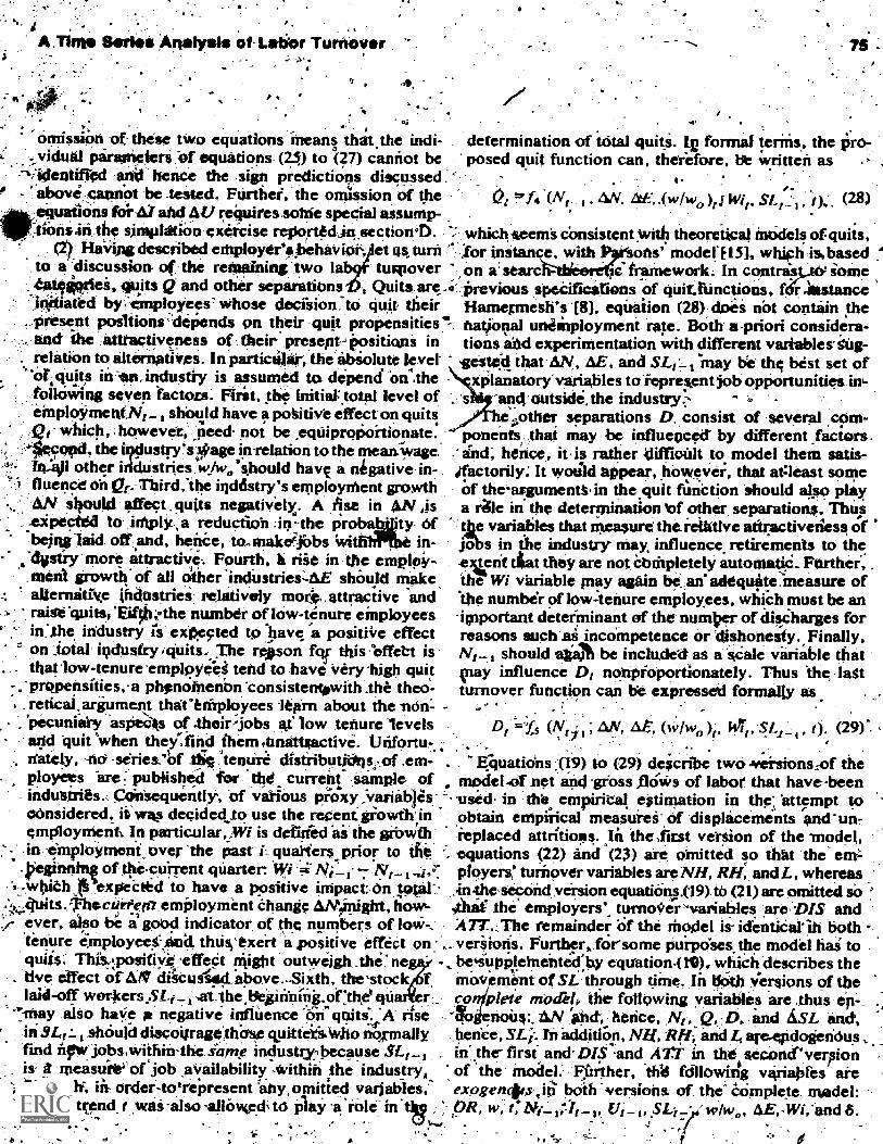
A .TInte Serie' Analysis of Labor Turnover

rOmission of' these two equations means that.the indi- determination of total quiti. 11.2 formal terms, the pro-

. ,victual pirarnekrs -of equations (25) to (27) cannot be posed quit function can, therefore, Be written as _

--tlidentiaod and hence the sign predictiOns discussed: :

0 - above, cannot be _tested. Ftirther, the omission of theequations foi a and All requires some special assump-;tiOni in the simphitiOn exercise reportedin.sectionto.

(2) HaVing described employersaffiehavior, et as, turnto a 'discussion or-the remaining two 1 tumover

tcgiotiei, quits Q and other separations , Quits are:initiated by;employees' whose dm-Colon, to quit their

...present posItions'kkpands on their quit propensities. ..,. and the attractiveness of their present, positicuii in

relation to alternatiVes. In partict4ar, the abiolute level-of.quito in 'an.industry is assumed to depend On .thefollowing seven 'factors. First, the Initiattotal level ofeinploYmetit,Nz_ , should have a potitive effect on quitsQ, which, -however, ,peed not be _eqiiiproPortionate:.

lecopel, the iodustry!a4age in-relation to the mean-Wage.`., In-illl other indUstries wfw s.hould have a negative in-'.°) tluence on at. Third:the iqddstry's employment growth-.; AN should affect . quits negatiVelx. A Ilse in AN is

expected to iniply, a reduction in -the prob *ty of. .being 'laid off and, hence, to makelobs wit in-

.Y.1107.le.' more attractivie. Fourth, k rise in the employ-ment growth' of all other 'indUstries:-AE should make,

.- allenuitrY.e ihdastriel relatively more,. attractive and.. : raise 'quits, 'Elf$6,,.,the number of tow-tenure employees

in:the industry 4 expected to :have a positiim effect' on _total industry iquits.-:.The re son fqf this 'effebt is

. _ that low-tenure -employi tend to have Very 'high quit-. propensities,.a phenotnenbn 'consistentowith _the theo-., . reticai.ariument that's niployees learn about the non-

'pecuniary asPedss of .thoir'jobs at' low tenure levels- arid -quit 'when they; find ihemitmatractive. Crifortu,_

!lately, -lid -series.'of 'tenure distributOrisf.of _em-ployees are published for the current. :sample- of

. industries., Consequently, -a variousproxy variable's.cOnsidered, its wale derided to use the recent giowth inemploynierit. In particular,"Wi is deflried as the grOWthin employment over the past I.qu4fers., prior to AC

.4;ft-sinning of thecuirrent quarter. Wi Ni NI__,whith yexpected to have a positive inipact- on, total:.

...",,,,4Auits.Thecultern employment Chang; AMin'ig,ht, how-ever, also be a good indicator of the numbers of lowTtenure imployee*.anit thu; exert a positive effect onqukts: This. positive effeCt Might outweigh _the nethe effect of AM illicusted_above.-Sixth, the'stocklaid-off wor4cers.SI.i_, .art-the tlikirining.of:the

-7-May also haVe a negative inilUence oa gaits: 'A. thein 34; .shOuld discoi;rage'th'ose q.uitteriAvitio normallyfind firVijobs,Withiirthe lain" industixbecause St_iit measuito'or job ,aVailabilityitvithin the industryiSeventlf, iii. orciertotripresent "any, omitted variables,'a time trend, t was also allowed to play a role in .t18 ,

A

. .

AN. At,.(w/wo )1,1 Wi,, al :1, t),'. (28)

whicheeeMs consistent with theoretical models of-quits,';for instance, with .11sotts' model F151, whichis,basedon a' searcthlre:c: framework: In contrasptF some

speCiflcations of qUir.rtinctions, ficr.itastanceliamegmesh's18), equation (28): doei not contain thenational unionployment rate. Both a-priori considera-tions and experimentation with different variables' ing-tested that.AN, AE, and may be the best set of

xPlanatorY variables to represent job opportunities in,-ant*. outside,the industry: A

egpther separations D. consist of several ,cOm-ponents. that may be influenced' by different factors.and; hence, it, is rather difficult to model them tatis-

ifactorily: It would appear, however, that at:least someof the argumentt. in the quit fiinction should also playa reee in the determination 'of other. separations. Thu,tee variables that measure' the relative attractiveness ofAs in the industry may, influence, retirements to the-e,4erit t at they are not CbdipletelY automatic_ Ftirther,the Wi variable may again be,adadeqtiteineasure of'the number of low:tenure employees, which must be an'important deterMinant of the number of disCharges forreasons sUch .ai incompetence or dishonesty. Finally,Np., should alia,111 be included as a Cale variable thatmay influence DI nonpioportionately. Thus the lastturnover function can be expressed formally as

.

1.

Di =15 (N 14. AN, A4-, (:,/wo fir. t).. 7'

Equaticins:-(19) to (29) descnbe two -visions.,:of the, model.of net and 'gross Mows of labor that have-been

used in the empirital estimation in the attempt toobtain empiiical measures- of displacements and'un,ieplaced attritions. lit the ,first version. of the model,equations (22) and (23) area Omitted so that the em=',foyers,' turnover variables are NH, RH, and .L, whereasinthesecond.version equation:1.('19) to (21) are omitted sosthai..the employers', turnover'- "variables are DIS andATT.:. The remainder of the Model is- identiCal'iti both

.., versions. Furthers fosome PurpOks. the model hal tobe4uppletnented:by equationM), which describes theMoir ment of SL through time In 110th versions of theco plete models the following variables are .thus

dons:: AN ild; :hence, Q, D, and SS L and,he rice , SL;.. hi addition, NH, RIC and L., are4dogienOusin' the first and- DIS -and Ari in the seconcrverpionof the model. .-Fiiither they falowitig variables areexpgencto,i6 both versions of. the' Ccimple,te. model:PR; w, _ _ .S1.47 wiwo, 4E,-Wi,'.and 8.

Let uskaw turn to a -description of the estimAttion ofthis,mo111111.

t--C.--Tho- Empirical IltteultsThe model that is summarized by eqUations (19) to(29rhas been fitted to quarterly data .for twenty-fourmanufacturing industries. Most of the data requiredfoi this Purpose are readily available in Empl6ymentand. Earnings, Manufacture1,s' Sales, InVentories andOrdert, andthe Monthly Labor Review. SoMe data hadto be processed prior to fitting the model. The raw datahave, however, n.ot been seasonally adjusted and,hence, intercept dummies for the second, third, andfourth quarters have been imjuded as-independent Vari;-ables. Typically these, dunNies take on the value 1 intheir own quarter- and 0 in others. In the equationsfor quits and other separations, ho.weyer, the seasonalpattern was found to be slightly different ancrthe dum-mies take an the value of Nt in their own quarter and0 in all others.

In initial trials the net labor demand, and labor turn -over .functions were approximated by both linear and'log4itiear fort By and large, the linear versions ofthemspecifigiven

tended to give better result,s; The linearalso has the advantage that the Constraint= A -S can be checked-or incorporated _

it* e model quite easily. . .' -- ..ffr' y

Various alternative est' atori "methods have been14fk.used, but the ,difference the results do seengee

to` be substantial. For the results presented here,. thenet deniand for labor, Ihe quit, aild the other Separationsfunctions have been estimated by ordinary least-squaresand all the other labor turnover functions by 'two,stage least-squares for which AA( is the jointly de

eqt variable. Y.some equations the Durbin-Watson statistics are

sd owhat low. These eqtiations were adjusted for auto-correlation ad reestimated. 'Since, however,t,the re-

"Edon Coefficieettlid not Change very much, onlyultrof the =adjusted eqtrilauns are reported.

DUrbin-Watson statistics sOould thus be regarded. s sigtials.pointing turpassible nustrifications.

For breyity the results for only o industrial cafe-gories, total durable, and-total nondurable goods indus-

" tries 'are prOenteinat some of- the .olif6presults are4

meth5P briefly. 11te evidence of Table.? suggests:-that e net,flOv4gmanci for labor is determined 'pre-dominant' 4 orders, the time tragl; quits, andlagged e t. 1p dufable goods industfies unfilled

: orders ar to exert a positive inffuence uponNsi.. The re agttuidihe stock cif laid-off workers donot pct the nettalirge in emplOstient significantly.;Table 3 'cgs the :empirical estimates of the

paraiyeter&f6T jhe navfahh-eorehire, layoff, and

Part Two: Labor Market Adjustments'

Ta6le 2The Net Emplojment Demand Equations

iealependeofVariables

OR

D

. R2D-W

Durables

. _

Nondurablec

0.0262 0.0330(1.08) . (4.26)

114.-- (-2.28)

ve (-0.07)10.043

29.085

0.6996 0.2480(2.39) (1.84)

1.3649' 0.7459,.7. (1.28) (1.54)

(1:0871 0.2021(-9.41) (0.76)

0.0193(1.11)

0..0124(1.890.79

0.2181(-2.02)0.0244

0.0074(-0.21)

Q.93

1.21 2.23

,Note: res in parentheses are t-ratiosperi , see T& e e 1. The column' headedDu R-Watson d-,statistic's.

Or samplecontains the

.

pla ment equations. In all these equations, AN istrea ed as the jointly depend nt variable, so that thevalues for A./0 'are those predicted by the instrutnen-tal variables that arcthe independent variables listed ine.Table 2, Let us lliScuss the parameters:in Table 3 insome detail. Ne hires are affected positively and sig-.nificantly,by the net change in employinent and qaitsAnd negatively by the stock4ollaid-off employees. Re-hires are related po vely to the stoek of laid-offworkers but not very ougly,or consistently-to any ofthe other variableS, Layoffs respoqd negatively JninetemplciymenIchanges, quits, and other separations and -

positively. to the. stockof laid-off employees. As hasalready been pointed o,u_t, this positive association be-(tween L and SL must be attributed' to a positiveassociation-between the error Z and S4. In other Words,'as die stock Of laid-off employees rises, the .error 4

4efined by AN = A -L-Q4+Z, tends torise and ,this rise is offset by t' ase in L . Thisis aninterestmkaSsociation,- whir la deserves further.analysis and me-y Thyield a clue' to The reason why Zoccurs.. Next let us considerdisplacernentsTwO seriesfor displacement. have been fitte*Series A is definedas and series B asDISB = L -RH-Z.

A Time Series Analysis of Labor T nover rt

Table 3.

ao

The New Hire, Rehire, Layoff, and Displacement Equationis

V independentVariables'

Q

D

SL -z.

, New Hires

0.3984(8.95)

0.9210(8.93)

- 0:1192(-0.42)-0.2589

(-5.52)

Rehires

-0.1101(-3.47)

0.0780(1.07) ll0.1885

(0.95).

0.3085{9.23)

R2 ; 0:97 0.87-.

D-W- - 2.06 1.22 =-

AN 0.4037 0.0405(4.87.) (0.24)

Q 0.8254 -0.0125tl 1.13) (-0.32')

0.2952 -0.1893(1.20) (-1.45)

SL -0.1900 0.1855.1.69). (3.10)

R 2 0; 98 - 0.94

D-W . 1.11 1.09

For notes, see Table 2.'

Itt

Layoffs

Durables

\ 4, -07310(.-13.94)

. 0.0985(0.81)

.

.. , 0.75794- 2.27)

Displacements %

-0.6210(-13,22)

0.0200(0.1'8)

- 0.9463.(-3.17)

'0.1739(3.15)

Ar882.19

Nondurables "'It-0.5929

(- 10.49)-0.1576( 3.12)AP0.4352( -2.59)

0.1721."I (2.24)

0.9

l''

Displacements B

-0.6016(71305J)

-6.0790 ,

(-0.77)192

(-73.96)

-0.1346 -0.2589(-:2.72).; (-5.5E)

0.89 0.91

2.27 2.06

(-0.6634 -0,5963

(-9.38) ''.. (-7.19)- 0,1450 . . -0.17-46

(-2.52) (- 2.35)0.24 9 -0.40484,

,(-1.2 t (-2.86),0-, ' -0.1900

''7,;(79:.1,51 .. (421.69)

-.,..- ,. .- .0.95 * .. 0.95

1-.82 , NI , 1.11 °

.Corresponding t4,theSe rwo series there are two series the :. and DISB' equations are gititelinlilar, but.

., for.unreplaced atititions; series A includes and series ,13 '.c; B ibliecifiCation;which assigns the error 2 to dis-.excludes Z, or ATTA = Q +D -NH -7 and ATIB = tjalacements,, seems 'slightly superior to the A .sPecifica-

,Q +D -NH ,' As a result of these dgfinitionstthe' errAK dpn, By and large; the results for the other tiVenty-two .Z is attributed to either DIS (4_A TT,.so.that the clef , induStlies are sithilario those' presented in Table 3: In..

.

-tidnal identitY,betWbenthe net and grdfs flows of la ,r , particular, new hires tend to be related positively andhas: been made to hOld exactly in the '.data.14.olittile.; layoffs: negatively. to AA.- Q, and R. FUrther7 inwords,. AMA + D1SA = -6N and A R.-:i-- Al,/ and eitherthe A or the 13: speciflcatioused. ThAcoefficientsqhat relate ATTA ansi.A

.03 = creasss in -4,/, tend to raise new hires and reduce. re-art. be hireseBpt other; aspects of the rehire equations are not.

entirely-satisfactory.41.1t), Q, D, ,And SL can be obtained easily from the Table 4 cokains the ft gel of results, nanielythdsecoefficients 6f thebdisplacemerit equaiions in Table 3. for quits and Other separations. Both quits-and otherThe 4610 coeff Tents of the displacement and attrition separations are related ppsttively to, the leVel. of gm-

.

equations du sum to -1 and the coefficiSL have same it;sOlute value but opdisplace nt and attrition equations." A

.

ofa ployment and the current,and.reeent Qhanges -invs in_ the empioyment'Orand W4. Further the impact of rela-.

happens, tine wage i.v/wo is negative but notsignifcant. The timetrend-tends to have positive influence on quits StIji a

"Thus the eoefficientsof the A tTA eciton- for total durables are-negative one on other separations. The stock.of laid off

"#-0.3790; -0.0100. 0.9463 and 0.1346 for , Q. D, and SL, respec.- 'Workers raises quits y)-clurables and reduces them inIts hould be noted lhat piss can alsfi be expressed as DISB

;citations are r ed. side.the industry reduces qu ts irdutablet and raises

uve y. durables whereas-the gAange'iltemOloyinent out-.--aN+mf-ii-estand. hqnce, the coefficients of the Nil and DISB

!

.

. .

. ,

TS Part Two: Labor Market-Adjust Monts1

Table 4The. Quit and Other Separations Equations

IndependentVariables Quits ''

Durablis-

Other Separations 'Quits

Nondurubles

Other Separations

AN 0.2941 0.0486 0:0188 0,0287(6.63) (3.29) 41 (0.12) "" co.rn r

' 0.2642 0.0578 -1 0:36i7 0.0688(10.75) (7.06) (5.56) (3.19)

-3.5610 0.1607 -0.3312 0.7831(-5.30)' (0.72) (- 0.44), (313)

.SL Or ri37 0.0043 0.0133(2.29) (0.19) 1.16) (0.24)

-506.09 -334.18 -922:fel -508.03'( -0.68) (-1.34) (-04) (-1.15)

W4 0.0848 0.0044 0.1071 0.0152.(3.75) (0.59) (2.09) 0.91)

*AE -0.1965 -0.0240 0.1092 -0.0029(-2.26) ' (-0.83) (3.06) (-0.25)

R* 0.97 0.96 0.97 . 0.91

1.76 1.35 1.48 ` 1.76

Fir' notes, see able .2.

'them in, durables. The results from ter twenty-, Iwo in striei-seem to contain very -Si messages:

, /-;:andW4 influence quits and other separations4"/ predominantly positively. But the strongest result is/ that far the relative wages w/wi,: In twenty of the re-

/ maining industries the coefficient of w/ivo is negativeand in thirteen it is significantly so. This is an encourag-ingly strong ;result,; 'especially in' view of difficultiesthat are often encountered in attempts to discover theeffects of relatiVe prices in time series analyseS..

It is not cleaned that the "empiricalgstiMates pre-sented in Tablet to 4 are entirely satisfactOry: SeVeralof the parameters hai,e imillausible signs and others' arenot significant. But this e*idence doeis contain somesubstanth5e information on the interrelationships be--tweerinet and gross flows of labor. These interrelations.-will be analyzed further next section.

d

D: Thte Simulation

(I) For a discussion of the steady-State properties of ..

the model, equations (19) to (29) have to- be. supple-mented by equation (10), which describes the 'Move-

. ment thrpugh time of the, stock Of laid -off eMployees.The steady state of the model isihen said to exist whenAN = NI-Ni_,=0,W1 0, and All,

= 0. In other words, with given exogenoliswatiatts, All endogenous variables are at their steady-state levels when both the stock Of employrneniand thestock of laid-off employees are constant' over time.

en these steady-state conditions are assumed, theodd, with the estimated. parameters, can be solved

for its, endogenous variables on the basis of any arbi-trary set of exogenous variables. For the initial compu-tations, the exogenoils variables OR, w, /1_1,

-110/Hitu it, and 8 were assumed to be at their samplemeans. The resulting steady-state values 'of the 'ea-dogenous*ariables are presented-in Table 5, togetherwith their-sample mean,. For version'2 of the model'the error Z. has been attributed to displaceMents Indtherefore DOB ± A147713 = -AN.

Inspectiontidf the figure's in Table 5 suggests-that thesleady-ttate values of the endogenous variables are not

different from their samMe'rucans. This similar-,ity. is not necessarily implied by the structure of tip= `+model or the estimation techniques and, hence, it maybe viewed as a -Satisfactory voect of the model.'.

in'order to be able to study he respOnse of the modelto an txogenciiis reduction in demand, the SysteM was

."-The model summarizea, in eluAtions (191' to (29) has

stveral complex dynainic interdependencies -mild, .

hence, it ts difficult to- ascertain al its properties: byanalytic's) knethods. An attempt h s,stherefore, been

mildew obtain the most importAn implicAtions of.the/model by means of a simulation, xercise. Let us de-' scribe this simulation in some d by dealing, ,first,

With the steady-state properties of the model and,.

secdnd, with its .abort -run responses to exogenous. 4

A Time. Series Analysis of Labor ;turnover+! 79

Table 5..The Steady; State Values of the Enchigenouti Variables

Durables NondurablesSteady-State Values Steady-Stati Values

Sample Means Version I.

AN 16105 '0fiI 107057281 10719.087Si Nvir.518.142 555.540NH 7'868.019 848.157

C RH 400.792 413.798

.II" 47.8.545 497.129Q 562.095, 558.222D 281.003,: *-: 280:663DISB 8:226,

A 27.8, , 24.921. .NH+RH-L '-'52.832 -74,059.L -RHQ.+D-NH -24.921 -9.272

83.331

69.527 74.059

Version II Sample -14Acans-7-.7ersion I Verion. Pi

0'10709.419

583.676

.. ,

11.642:749.953

257.607

C .

07861.774255.530

( 761.760 .316.676

787,815313.976

396.342 , 393.191529.1.40 533.014 567.951 *

. 279.340 167.287 173.88657.551 49.818

-57.551 -61.460 It .

- 18.207 -33.23779.666 . . 79.215

.- 61.459. -45.9780Q. 29.849 33.237- .0

07757.818

211.,250

536.617165.90765.488

- 65.488

.0.. . _,

Nose: All. numbers in thousands. For sample periods, see Tablet. Version 1 consists of equations (10), (19) to (21) and (24) to 9).Version!! consists of equations (10), (22), (23) and (24) to (9). Z is defined as Z = AN -NH-RII+1,.+0+D :,-- AN + A TT + a.W'....

started in the initial steady state: and then subjected, to an ,exogenous shock that ,took the form,of a 10 per-

. cent reduction in real orders OR, real inventories I,;and real unfilled orders U. But the other exogenous

variables were all held at their sample means. 'ThisprocedUre may 'require so further explanation.; Ashas been mentioned in n B of this part of t epaper, the model expressed jn equations (19) to ( )

I should be supplemented by two additional dynamic lyinterdepe ent functions; they'determine the ch ein real in ntories M and in real unfilled orderi QU. Ina' complete specification of the dynamic effects ofchanges in demand, firms should be allOWed to respondto a ceteris paribus reduction in real orders OR byreducing gradually the stocks of eqpment, real inven-tories, anreal unfilled,ers to their new steady-stateleVels. In the present.: ration, by contrast; real.inventories and unfilled ers are reduced to their newsteady-state levels- instantaneintsly.., and, moreover,

.. these reductiOns are supposed to be ,proportionate tothat in real. orders.' Thus, the simulation traces theshort-run and long-run effects of a 10 percent reductiOnin real orderi, real. inventories, and reall.iinfilled Order§.upon net employment and all the !abbr. turnover cater

gories. ThL on for this implified s 'hatthe primary P, lase of th research un erlying thispaper has been to tain e relationshipsbetweeh netchanges in employment and the labor-turnover-flows.The estimates of these relationships may, not be af-fected 'much by the aboVe 'simplification, which seemsto influence primarily the estimate Of the net change inemployment. : , . ).. . , ..11 ---,k

The-long-run effects of a 10 percent reduction in OR,I, and U are presented in Table 6. Tills table' con-

the ew steady-state. levels of the eridogfnous

1(.:ariables or the two vetsions of the model and the twoindUstry groups as well at the percentage differencesbetween the initial and to new steady-state levels.Thus, the reductions in 00,1, and U cause reductionsin the steady-state values of emploYnient, new hires,

. quits; *other seParations, and unreplaCed attritionS andincreases in those of the stocf laid-off emplbyees,.

:-rehires; layoffs and displacements. The signs of the '.0changes in the steady-state levels are the Samefor bothindustiy groups though their magnitudes differ substan-tiallyin SOine instances. A particularly striking feature,of thele 'numbers is the large decline in quit ,which.r:

isis much larger proportionately than that i ni lo y -`

,---11111r=ar

P Yrnent. Consequently, the quit rate, that th ratio of

"Iifthe reduction in an industry's.output is due to a trade liberalize-lion policy that involves inte done! reciprOcjty, then the simulationexercise should be based .on t assumptioti tlae some induitriescontract and others expand their plciyment levels. In the abovesimulation alternative -industries rtm unaffec and henti, thepresent results may bey toes gloomy.

Q to N, is much lower in the depressed than in theprosperous steady state.

A comparison of the steady-state levels in Tables 5 ,

and 6 suggests that, in relatively prosperous times,quits, other separatiOns; and new hires tend to be high. /

ra

IN)

''TibleThe Second Steady-State Values

:7 DtirabIes

SLNH.RHL

DDISBATTBNH +RH -L -Q -DL -RH

For es, see Table 5.*The. differences in the steady-stat

Version I' 'Version 11

Percent Percentew. Level Diffrencti. New Level .Difference

Part Two: Labor Market Adjultments

10004.447683.323'657.045431.364531-863381.189

.238.496

-65.139102.499

-37.360

4. N

'and to take care of a relatively large °portion of the.._realleelition of workers among . ablishments and.industries: In relatively depressed times, on the other.-hand,.quits, other separations, and new hires tend to below and the. function, of . the reallocation, of workersseems to.be shifted to layoffs, rehires, and the stock oflaid -off employees, all of which are larger than in pros-perous 'dines. . . .

(2) Although the long-run consequences' of reduc-

1 .tons in, real orders, inventories, and unfilled ordersay be 'of -Considerable interest, the priMark focus of

the: research underlYing the present paper is on the.short-run adj.Wient paths of ernp mem. and thelabor turnoveWws. Figures 2 to 4., e the paths ofemployment, the vock of laidkff employees, and theturnover. .variables that. occur as a consequence of the10 percent exogenous 'reduction. in real orderS, inven-tories* And .unfill41 orders..'=The 'figures .refer to ibothversions of hie model and both industry groups.' The'

er shoUld.note thatsthe.stales of Figures 2 to 5 are.,all identical and that-the origin of the stock of em -

ploYmenthat beerisadjusted so as to make itfitintO thediagrams with the .other variables. The maftrimplicaT_dons of -Figures. ;.to S are as follow,: all:four versions

.

of the model are, stable 'in the settiesthat the variablesapproach thsir, new steadystatel levels antk.do not

:diverge frOmibein..Furtherin theciurnble gOodSoindut- -

*tries, adjUgfinent tends to be qUite ,fai: --all variables.*quite elOse to their npw steady- states, within .one ...

after ti0.4iStUrbance. In the nondurable goodstlustries theldjustmept is somewhEkt slower. Furtheri'

1 rioincitirahles the variable": approach their' neW

-/ No:Wu-fables' ...Version 1 , . Version II

Percent PercentNew Level Difference New Level' Difference

-6.67 9995.944 -6.66 6721.53$ -14.50 6.618.925 -14.68Y 23.00 532.159 38,70 537.127 110.20 493.418 133.57-22.53 301.41,6 -61.74

4.25- 387.062 23.287.39 553.571 40.79

-31.71 355.610 r*, -32.79 71.139 -87.47 40.210 -92.51-15.02 237.332 -15,04 96.575 -44.46 88.699 -46.54

79.824 38.70. 152.96p 133.57-79.824 -38.70 -152.960 -133.57

12.04 -32.807 1.2923.00 166.509 110.20

-302.93 -133.702 -190.80

levels in Tables 5 and 6.

I

steady-state levels monotonically, whereas in durablesthey overshoot theipsteady-state levels and then return:to them.

In order to obtain an impression of the roles playedby the various labor turnover categories in a downwardadjustment of employment; Table 7 has been prepared.It contains the cumulated deviations from the initial "IS

steady states of the various net and gross flows of labor.The period over which the observations have beencumulated is, one caleriaar year, namely the four,qtiarters that follow the 'exogenous deniand reduction.Thus, the nuMber, in the first row and column in Table 7indicates that, during the four quarters after t C. distur,bance, employnient has fallen by a total of 709;f6Obelowits initial-steady-state level and the other numbers in thefirst column should be interpreted similarly. To obtainan impressiOn of the relative iniPortgpce the variouslabor turnover categosies, the numbers are' presentedalso as percentages of-i-Ak. ThelfolloWing ch ter-istics of the 'evidence in "r4nble 7 should noted: Inversion I of the model new hires decline by more tfianthe net reduction in employment in both industrygroups. But this decline is offset by substantial reduc-dons in quits and other separations, so that the esti-mated unreplated attritions are only 15.6 percent of-4/"/ in durables and -13.5 percent in nondurables.Layoffs rise substantially and are offset only partiallyby increases in rehires so that the estimated displace-mentsare 57.2 and 69.5 perceni of. N. for durablesand ,nondurahles, respectively. The error, that is thedifference, between AN and :('N +RI-174.:-Q-D) is

2 percent for durables and 44 pertent for nondura-lr.

A Time liar lea Analysis Of Labor Turnover

900

81

40NH

4

200 -7-

100

. 0 -

- _ - . .

Q

. .mmimi

N - 10000. nos ..... +

Figure 2Durable Goods industries, Version 1

16

Quakers

20 24

r)

Part Two: Labor Markst, 'Adjustments

800

700aL

11. s wow

600

500L

400

- .,..;:`" 1al4..1=

N

.11.....QI1

\DISB........

.. 1141.i.

11- 10000

.07.--/X ATTE;

Figure 3Durable Goods Industries, Version =2

0/ Labor Turnover

. :

13

1,200

1,000

- =0 71.

\ilo

800 '1

VI

3 \ -Z .-0. \ \ !.._.

1 .-.0 \\ L

E

). \ \tr a ....\

SLa

.'w X-4.

°°°°°°° ......... . II*.\.......ft....... NH

400 \ ...., ....... ,-.6 . ° \

111

,. .mi ..

1.4am . ei =N. . am min . 4= ow don ems me, OD mr .05

a

12

QuartersFigure 4 /NondUrable Goods Industries, Version 1

'C)

Part Tad Labor Market Adjustments

Figure 5Nondurable Goode industries, Version 2.

A- Time- 8..41 Analyile of Labor- Turnover ,

Table 7 av

dimulated, Deviations from Initial !Reedi Ste_

# k

AN.NHRHE.

DL-RH,Q+D-NHNH+RH-L-,Q-DISHATTB

Durables

Version I Version 1E .111r

Patient PercentThousands or -AN Thousands of -AN

,,,Nondu-rablcsVersion I " Version lk

PercehtThousands of -AN Thousands.

Percentof -AN

-709.8 100.0 -708.3 r 100,0 100,0 -372.2 100.0-873:1 -123.0' -392.1 -104.7

273.8 38.6 63.8 17.0679.7 95.8 324.2 86.6

-633,6. -8'9.3 -628.3 -88.7 -381.7 -101.9 -383.6 -103.1-128.7 -18.1 -128.5 -18.2 -16.3 -60.6 -16.1

405.9 57.2 . 260.4 . 69.5110.8 15.6 -50.7 -13.5

-516.7 -72.8 -209,7 -56.0404.4 57.1 268.7 72.2303.9 42.9 103.5 17.8

I,

. bles. In versibn2 of the model this error must disap-peat. The differences between the estimate; of -4N,Q, and,DIS fOr the two versions of the model arenegligiblyilmall. The only strikihg differences. oc9g inthe. estimates of unrephiced attritions, which are sub-stantially higher in version 2 than in version I . Indeed,the entire error of version 1 seems to be attributed toA7TB in version 2i. .

Forpilesent purpOses, the most interesting implication.4.'of Table 7 is that, despite the very large decline in nevkthires, 'unreplaced attritions seem to'play only a' sec-

! . ondary role in btinging about net reductions in employment. The reason for this phenomenOn is that new hiresrespond to a sharp fall in quit; so that new hires andquits fall in a mutually offsetting manlier., I ectionit has been pointed rout that Ilamermesh.s. approacimplies that unreplaced attritions account for 79 percent14' any net reduction in employMent. AsAoted thisfinding is,baied on the assumption that theindustry'squit rate is-independent of economic conditions withinthe industry. The finding/the present research is thatsuelvanassunintion can substantially bias the resti17.The numbers in Table 7 suggest, by contrast to Ham-ermeth's, that the fall' in quits may prevent unre-placed attritions from bringing about,41 large proportionof any net reductiop iii.einployinen*cCording to theSe .estimates unreplaced attritions amount to, at most, 42.9percent,of v.-AN:Although no finality is claimedketheprelent results, they do suggestlat quits ouglMo beallowed to 'respond to changes in gnomic canditions,within "the industry in future investigations of laborturnover, especially if they are aimed at obi aiall esti-mates Of unreplaced ;atriums and displacefneM.

4. Conclusiont

In the research underying this,paper an attempt has.been ,made to- estimate the displacements and unre-placed attritions that must be expected to occur as aresult of exogenous reductions in the demand for anindustry's output. Such reductions tray_ be caused bymany factors, including trade liberalization Measuresand the ensuing increase in import- penetration, theeffects of which are of particular'interest in the presentcontext.

Rini 2 and 3 of this paper contain the general concep-tual framewbrICof the analysis, rt description of the time

. series data,., and the result of the construction, estima-don, simulation of the model. The' main conclusionoft analysis is that unreplaced attritions may not be.as important' in bringi about net- ,reductions in

loyment as is sometimes suggested. Although firmscut eir new hires drastically when demadfalls4 this is

ly caused and offset by substantial reductions inv ntary quits. In other words, since attritions falrwithdemand conditions, attempts by firms to effect net re-ductions in employment through uniepleied attritionstend to have only limited success and the priMarymethod of reducing employment Wces the form of dis-placements.

4 seems that the. time series data on labor turnoverhave not been analyzed previAtly with a view to ob-taining estimates of displacements aglCl.unreplaged attri-

. tions. The estimates. presented ill this piper should,therefore, be regarded as. a first attempt at generating.

. quantitative information that has potentially importantimplications for economic policy: A number of obvious

4.

4110 r tiirther research suggespthemselves. The cort- . 15. Brechling, Frank, and Dale MOrtensen/ -"Interrelatedceptual rienework Might be changed. Following Mor- Factor DemIspd Functions." MimlOgraphed.tensen (ri) And Pencave112), it Might be assumed that 6... Burton, John F., and John F:. Parker. "InteAndultry

Robert-E. "Turnover in the Labor Force." firaoL7As Papers on Economic f4ctivity, (3: 1972), 709-53.

the tYpi I fi

Part Two: Labor Market Adjustments

rnkcontrols its quits through its relative Variaticios in. Voluntary.Labor Mobility." Industrial nd

. -Wages:- The rehire equatioh,- whichvurrently.yields.uT -11-61-16141 Role"2. 22 0011401-19fM,- 199 -216

satisfactory empirical restilts, sh cruld..pertiaps. alsospecified differently. For the empirical estimation, dif-ferent functional .fornis and :,different econometricmethods could be .tried- in an effort, to improve theresults.. Finally, estimates' of diiplacemetitt and Unre-plated attritions'shopld be obtainer] for industries thatare, smaller; than total durable and total nondurablegoods industries. Disagiregatioh seems to tre tspeCiall yde2irable, becauratit highly aggregated industry clas-siftations'much'Iaborturnover is intra-rnduitrp turn-over and, asrhas been pointed out in pact 2 of thi;'per, such intra-industry turnover, to the extent that

H1 >.0, tends to bias the estimates of displacementsand unreplaced attritions. As discussed in part 3, themodel has been fitted to twenty-two additional man-ufacturing industries and the results are being analyzed-currently. Al has been found by Nadiri and Rosen [13],'however, the same model of factor demand does notperform equally well at all levels of aggregation and,hence, some industrytspecific modeling may be netes-'miry. It is hoped that futufe research will provide infor-mation on the reliability of the currently available esti-mates of displacements and unreplaced at ions aswell as onthe source.of any intra-industry cl. erences inthe relative itnportance of displacemen and unre-

'attritions as a means of reducing e loyment.

Literature Cited

I. Bale, Malcolm D. "Estimates of Trade:Displacement,Costs "for U.S. _Workers." Journal of InternationalEconomics. 6 (AugUst 1976). 245-50. .

2. Barth, Peter S. "A Time es Analysis/ of LayoffKr . ates. The Journal of II min Resource's, 6. (Fall

1971), 4487

3. 'Brechling, rank. "Harnermeshs Labor TurnoverModel a Its Implications for Displacements and Attri-tions.",Mimeographed. PRI

4Working pivot 76-306. 20.

-4. InVestment and Employment Decisions. Man-chester: Manchester University Press, 1975.

14. Parsons, Donald 0. "Quit Rates over Time: A Searchand Information ApproaCh." American Economfc Re-view. 63 (June 1973), 390-401.

15. _. "Specific Human Capital: An Application to Quitand Layoff Rates." Journal of Political Economy, 80(November/December 1972), 1120-43.

t6. Parsons, Donald O.. and Belton Fleisher.," Layoffs and'Experienced Worker Unemployment Behavior."Mimeographed. . . .

.17. Pencavbli Jotirn'IVAtt Analysis a the Quit Rate in Ameri-.can Manufaciurimanduitry. Piinceton: Industrial Rela-tions Section, Princeton University, 1970.

18. ___.;_. "Wages, Spscitic Training and Labor Turnoverin U,S. ,Manufacturing' Industries." InternatiOncilEcoijgmic Review. 13 (February 1972). 53A-64.

19. Stoikov, Vladimir, and Robert R. Raimon."'Deternitn-ant0;it.the Differences. in the Quit Ratejamoandus,

'trigs, :"AinerIcan Economic Review, 58 (Decem 1968),1283,984,,

a.1,(-:- .,_>Toiitita, Richard S. t" A Markovian Mows En Labor Mar-ket Decisions by WorkerS," American EConomic Re-view.;66 {December. 1976), 821-34.

8. Hamennesh, Daniel $, Disaggregative,EconometricModel of gross Changes in Employment." ,tale. Eco-nomic.Essays, 9'( Fall 1969), 107-45,

9. Jacobson, Louis S. "Earntabg Losses of Wtirkers Dis-placed from Manufacturing Industries." This volume. -,

10, .,"Estimating the Loss in-Earnings for DisplacedWorkers in the Steel Industry." In Removing Restric-'tions.On-Imports of Steel. PRI 75-2, Center for NavalAnalyses.

I h Mattila. J. Peter. "Quit Behavior in the Labor Mmket."Proceedings of the Business and Eco knomSection.- American, Statistical Association, 1969,697-701.

12. Mortensen, Dale T. "A Theory of Wage and EmploymentDynamics," In Miroeconomi Foundations of Employ-ment and Inflation, edited by Edmuqd S. Phelps et. al.New York: W. W. Norton, 1.970.

9r3. Nadiri, M. !shag:ard Sherwin Rosen. A Disequilihrium'Model of Deinandfor Factors of Production. New York:National Bureauof Economic **search, 1974. .

9

0,

a

1

:fr

Earnings Losses. of WorkersDisplaced from ManufactUring linduOdoisLouie-S. Jacobson'

r

;-)introduction

'A particularly sensitive current policy Issue is theeffect of Changes, in tariffs and quotas on employment

,and earnings. This study examines enthirically some ofthe effects of a permanent labor 'displacement thatmight result from changes in international trade policy;Specifically, this paper presents estimates of how jobdisplacement. would change the long-term earnings ofworkers in eleven indhstries, and relates the findings toindustry characteristics se that they can be projected toindustries not threCtly studied. The study describedhere was designed to assist iRdeterthining industries in.which trade liberalization would impose largelosse) onworkers,

The results show that average prime age male work-ers suffer substantial losses of earnings in industriesWhete the normal rate of .labor turnover is low and,prime age malesinake up a high percentage of the totallabor force. These industries also tend to be high-wageindustries.

DisPlaceM01. from. the auto and steel industries is, estimated to reduce earnings 0* a six-year period byabout 24 percent,' and by almM as much in severslotherhigh-wage industries. The estimated loss in low-.

wage industries wits very much smaller, averagingabourCpercent: I nsome cases, such as cotton Weaving,no appreciable losi could be detected.

The methodology and data used in the study wereaPpliediarlier in Meastiring how the earnings of steel

port competiti n [31- That study used data drawnworkers Would angel: if they -lost their jobs due to

seaportfrom dins- Social Security system's Longitudinal Em-ployee-Employer Data (LEED) file to examine bothearnings ldsses per worker and the number and Charac-teristics of workers displaced under a 'range of Cir-cumstances, for groups of workers who'differ by race, .age, and prior work history: We founthattheearningslosses for most groups of steel workers*Quld be. quite

rs

$7

" 4 i .4.(

....

large, Walingas much as $17,000 oiler. itgiven worker'slifeti . We found that, although 'any worker losing histnjob W pay a high price, comparatively feW workers

, ,would placed in this position as a result of tradeliberalization. ., .

This study extends our earlier work 41sithet. indus-tries, providing estimates of how much the eatnings of ,

displaced workers would be reduced./She basic prpce-dure used was to measure the earnings of workeit:afterthey permanently left an industry during,an employ-ment reduction. These earnings were then Comparethethe earnings of similar.Workers who were not displaced,:

,51uring the employment cutback.Although we are interested in losses resulting frOth an

employment reduction induced by trade liberalization,the employment reductieryi we examined were due, inmost cases, to other causes. The size of the !psi de-pends on the value' of human capital lost and "bn thecosts of searching for a new job, but not on the reasonan employment reduction is made. The findings are thusrelevant for considtiing how reduced labor demandaffeets a, worker's earnings, whether the reduced de-mand is due to import penetration or to other factorisuch as chapgei iii technology. or government'igula-tions stip as pollution control.

Definitions.rt

In the following discussion a number of term s withprecise meanings tare tried repeatedly. The objectiviortAthe study is o measure-the effects of reductions in labordemand on he earnings of workers in,industries likely 411

'Chat'The steel study. wairmorii complete in inipg earnings losses.

study measured how loises were affexam

workers' age andtehure, and by economic conditions in the .workers' local labormarket. It also handled the bask data somewhat differently. Work-ail were grouped based on changes in steel employment by plant*her than by. Standard Metropolitan Statistical Area (SMSA) and

'cins.in different years were examin'ed..bleVertheless, the 're-ts from the steel industry,when redone using the methodology de-

imbed -in this Mei were IsrikinfilY sirlitlar; thus, enhancing ourconfidence in the resit resented here. .

*This paper is based on Louis S. Jacobson "Earnings Losses '.or

in. 1976.splaced from Manufacturing Industries,:' 1LAfi -74 23

which,w

9I

to be affected by increasing import penetration. Earn-ings loss is the difference tietween what a worker actu-ally earns toner demand, has fallen and what he wouldhays earned had demand not fallen at that time.,

Topeasure earnirialosies, we corn-pare the earningsof woikers who are adliersely affected to the earnings ofworkers who are not affected., We make a basic dist inc-don between workers who permanently leave an indus-try in a year when labor demand is falling and those whodo not leave in that year. Workers who leave are calledleavers; those who do not leave are called stayers

Some (dyers would have left because of illness, '8-charge for cause, or to searchifot a better job, even ifthere had been no employment reductions. Such, leav-era are called attritions. Workers who leave an industrypermanently and not have done so in the absenceof reductions 'nor demand will be called displacedWorkers.' These displaced worker* are the principalfocus of the study. -

To measure the earnings losses of displaced wakers.vile should compare their postdisplacement earnings tothe earnings of similar workers who were not distilaCed.'The data did not allow us to diatinguish which wereattritions, however: Instead, losses of displaced work-ers were estimate4 by measuring how earning thing,etdiffered in groups ofliavers, that contained 'differentproportions of displacements and attriti ns.

We were able to identify two groups f workers whopermanently left each industry-On group includedmost of those displaced but also inc did. some attri-tions. The other comprised mostly attrition's but in-cluded some displaced workers as Well.

By assuming that otherwise similar attritions In bothgroups had the same earnings, and that otherwise simi-.lar displaced workers in both groups had the same earn-ings, and. by estimating. the probability that a workerwould be classified asp attrition, we could then sub-tract tie effect of attritionon the earnings of the group.contaang. most of thealisplaced workers; the remain-der would then be a mesure of the &riling* loss due todisplacement alone.

The two groups way id,entified by dividing workersin each indUstry oitihd basis. of whether employment inthe industry in the worker's SMSA was rising, orffillitig,in the year of seriaration. An SMSAwith.rising industryemployment. be called a rising SMSA. An SMSA.

, .

'The displacement and attrition cOncepti used in this paper arenot analosoui to ,the More 'Usual BLS turnover concept of layoffsand quits. As measured by BLS, all but abdut IS percent of lay-offs do not lead to a permanent . We cannot even con-.eider ;eminent layoffs as rents, dance some of theseworkers would have left luryway should be considered awl-dons. Similarly, quits measured by BLS exclude workers who leavedue to accident, Deis, or dischage. This probably, accounts fbrat least oae-third of attritions. .

Part Two: Labor Market Adjustment*

with falling industrremployment will be culled afullingSMSA. 'Thus, tf a gr'oup of leavers in SMSAs whereemployment was increasing (rise-arc tkers) were lesslikely to be displaced workers than the group ofieevers

--In SMSAs where in the aggregate Berns are reducingemployment (fall - leavers ).

The measured loss in earnings for fall-leavers provedto be a reasonably accurate estimate of the loss due todisplacement alone. Losses estimated by subtractingthe effect of attrition from the weighted average oflosses did not add much- useful information bfcausethey were subject to a very large measurement error.They did, however. suggest that using the loss esti-mates for the group with comparitiyely.mare displace-ments, without cprrecting for the inclusion of attritions,tended to underestimate slightly 'the loss due to dis-pliaementsbilone in high'wage industries, to overesti-mate the loss in lower wage industries, and-to estimateaccurately the loss in industries in the middle of theearnings distributi4. ' :

The following disteuision Will describe in greater de-jtaif how these results 'were obtained, This will be fol-lowed by a discussion of possible underlying deterrai-.tants of these results.

I..

Measuring Earnings Losses, .4

In order to measure'what the eadnings.of.*orkos Who'recently separated .from "it given' industry ould havebeen had they not left, cotnparisongicifdIsfayersinthe 'same industry is statistically Matched to the leaversso that earnings potential is dittributed.identically:b e,tWeen the two gro'ups. Then the earnings of thesetwo .grOups are compared over tithe. \

Although many previous studies have eXamitted theearnings losses of workers, few, if any, use atompari-son grouP 12]. Mostly, the measures of earning" lossesare based on before - and - after comgarisons among

,these losing their jobs. This procedure may be aCcept-able in iculustriea where Fige-earniitgs profges:are flat',and specific human capital is not important, but it canlead.to very misleading resulfsjii:tifthe industries studiedhere, a before-and-after comparitOn among leaversWoad undegisimate:the total loss, since earnings. ofvery few oft workers are reduced below presepara,tion earnings for more than a year or two.

Also, because a before-and-afte comparison gener-'ally shows only a sfiort-lived effect, it is not possible toestimate the permanence of the loss and the natureofthe iitcovery process.

The methodoligy for measuring the lois econometri-.cidly was derived from our previous work on the steelindustry and recent attempts to measure ttte impact of

,

S

:Earnings Loss*, of VforitOrsikiplassd from Manufacturing IndUstrits-

manpower training on earnings. The anlYsis,,is based ona simple autoregressive model of earnings determina-tion, sdmetimespilled an earnings generating function.Equation (I) shows one specification for this Ilinction-designed to- heapplied-einarktelv-for different rec-e-sex.

.rlitOilPs

4.gli cfp,

.1t(). I , 5, (

where -VI is earnings in year, r, and 1) is a dummy var'i-'able equal to one if an individual we's diriPlaugd in year O.

If equal to zero otherwise.Figure I illustrates the coMparison being made using

the autoregressive earnings function. The Solid line rep-. resents the actual earnings of workers displaced in year

zero. The dashed line represents the earnings of work-ers whose prior earnings patterns were identical butwho were,not displaced in year zero. The vertical dif-ference between the two lines represents the earningsloss due to Displacement..

The two curves also illustrate how a loss measurebased, on a before-and-after comparison can lead tosystematic ,underestiniates of the actual loss. Theaggregate foss, measured telative to a comparisongroup, is equal to the arektietween the two carves. Theearpingt loss based on a before-and-after comparison isonly the area bounded by a hofiiontal line drawnthrough the earning level just before the st of year.zerp'and the line describing the actual earni s of dis-

;placed workers.

Proinfed ownpnes of closolookl *rodeo,.In di* abloom of flosplacompflt

..-Artual 0flontro.of

ddelfeed workers

1

. ,

Tom fywors)

.3

Figure 1..--Comparison of Earnings of Displ

. Workers and Workiniticit Dispi<

4

.1;

Although studies of. manpower training frequentlyrecognize the importance musing an appropriate corn..paragon group in measuring earnings differenees,.thisparticular formulation has only bear .developed re,centlyforusewith Sociat,Sedoritrearaings data similarto the Social Security data used-here. It Is more COT-.MOk to use variables such age, education, occupa-tion, and Marital status ,to conaolsfer differences inearnings potential.. Sherwin Rosen and others havegued, however, that "previous earnings patterns mustbe among the most gx)werftil controls for reckoningcallings capacity, being the end result.of The (humancapital) accumulation,process. p. 37). OrleyAshenfelter has shlwn, in a 'recent paper (1), that thefunctional form is hilly consistent with what is knownabout the shape of the age-income profile and that,underreasonable assumptions, the formulation is also consis-tent with a Becker-Mincer type model of optimal !Inmancapital accumulation.

Most importantly, this approach produce* vvha aregenerally regarded as the most accurate estimates o heimpact of manpower training available to dates In par- _

tkular, by comparing earnings trajectOries prior to en-teting a manpower training program, Ashenfelter dem-onstrates that this eethodology is accurate in statisti-

tching a trainee and comparison groups-in the "-pretriiiiing period, even though tpleissoles are drawn'from very different populations. mparison groupincluded a random 'sample of all workers covered bySocial, Security.d In this work, the comparison group for workers dis-placed from a given inditstry, is cted from etherworkers In the same industry. ditional informationabout' the age' and job ten -of workers is used tocontrol for difference's ketween thegroups of separa-tees and comparison groups of stayers. The estimatedearnings diDiences should, therefore, be consider-ably more accurate.. -

Modificaticin of the basic autoregressive earningsfunction (equation ( I )) is requ Wed because, as discussedearlier; there is no simple way of deterMining whether a .

worker who separates from an industry is displaced orleaves duel° nornill attrition. wen if it was knownwhich workers were laidoff, it would not be correct toassume that, all, such Workers were displaced: Manyworkers with:a high'prohabilitof beinglaid off wouldhave left anyway in thrbgenee of layoff.,

For instance, recent hired'event,

workers are verylikely to change jobs in any event, The* workers,however, are precisely those mostlikely.tdcbe laid offwhen eMployment mbst be reduced. '

Because subsequent earning trends of displacedworkers may be conOderably different from the earning.trends.of workers leavingdue Wattrition, it is-essential .

I-t

t

Zt

F fto deterMine how our results are affected by this poten-

' iially complicating fa4Or.To identify losses dile to dielacement from a! en

induitry, the sample of workers emploXed in the indus-try tt. year zero was divided -on thg basis .of whetheremabyment in the worker's industry was, rising or fall-ing in the worker's SMSA in the year of separation.This Produced four groups:

Fall-Leavers: those who ieparated from the industry,in it year when industry employment in the SMSAwas fallingRise- vers: thcoe- who separated in a year whenndustry employment in the SMSA was rising or un- -changedFall-Stayers: those who remained in the indtistrywhen industry employment in. the SMSA was fall-ingRise-Stayers: those who remained in the industrywhen industry employment in the SMSA was risingorlinchanged.The earnings of fell-leavers and rise-leavers follow-

ing separation represent different combinations of thenearnings of workers who left due to both attrition anddisplacement, as shown in Figure 2. Equations (2a) and(2b) show the distinction more explicitly:

YFL = 0Y A + (1a)Y

L = r&r.A +(1-0)YD,

whereYEL = average annual earning of fall-leavers in

any year following separationYRL, = average. annual earnings of rise-leavers in

any year following separationkA = average annual earnings of workers leaving

due to attrition in any year following sep-aration

YD = average annual earnings of workers dis-placed in any year following separation

= proportion of fall-leavers leaving due, toattrition

= proportion of rtse:leavers leaving due toattrition.

(2a)

(2b)

We now make two Crucial assumptions. First, weassume that, holding personal characteristics andworkers' histories constant, a worker leaving a par-ticular industry due to attrition will have the same

earnings, irrespective of whether industry ernproymentis rising or falling in) the SMSA. Second, we assumethe same condition holds for all displacement:. Thus,as shown in equation 9), equations (2a) and (2b) can shies.

Part Twd: Labor Market Adjustments

.EMPLOYEE

STAYS

INDUSTRY EMPLOYMENT IN SMSAFALLING . 'RISING

FALL-STAYER RISE-STAYER

LEAVES

COMPARATIVELYMORE DISPLACEMENTS

Figure 2

FALL-LEAVER RISE- LEAVER

f

COMPARATIVELY MORE .

_ATTRITIONS

Classification of Workers in an Industry

be solvld simultaneously for I'D in terms of a, p, YFL,and Y.

IICYD = [11/03a)i. YFL ja/03-a )1 YRL. (3)

Since YFL, and Yid, are observable, we need to esti-mate only a. and f3 to determine the earnings of, dis-placed workers: To do this, we make the assurnptionthat, controlling for worker Eharacteristics, the prob-ability of leaving due to attrition is independent ofwhether employment in a particular industry is rising orfalling in an SMSA.3 The observed number of workersleaving an industry in rising SIJkS.As divided by thetotal number employed in the indtistry in rising SMSAs(NRL/NR) is a good measure. of the probability ofleaving. This fraction times is an estimate of theprobability of leaving due to attrition in both rising andfalling SMSAs. a is the proportion of fall-leavers sepa--rating due to attrition. It equals by definition the prob-ability of leaving due to attrition tiTes the number ofrisers divided by ,the number of fallleavers. This rela-tion is shown in equation (4).

a = P-y, (4)

where

NRL .NFNR

3This"assumptio probablY an oversimplification. To some ex-. tent, the age and ten specific attrition probabilities will be affected

by changes in the probability of finding a better job which will, in turn,be associated *lib cyclical swings. The effect jnay not be irdporiant I .

here because the observations are cross-sectional and the relative /returns jobob change may not vary much aoi3mS SMSAs. In addi-tion, there may be a systematic relation between4hanges in employ -tment in an individual industry in an SMSA and changes in generalbusiness activity in the SMSA. This would tend io eqOalize relat,i4retuiSs of leaving a specific industry in falling anI rising SMThere it little empirical evidence bearing .on the accuracy of theassumption. In particular; the cyclical sensitivity of the BLS quit rate.niay be due to changerin the agc and tenure distribution of thdse em-ployed rather than changes in the age and tenure specific quit Propen-

9 '.1m

Earnings Loss s of Workers Displaced from- Manufacturing Industries

Substituting equation (4) into equation (3) produces. an expression for the earnings of displaced workers.

YD, in terms of Y-nu, and y, all of whih can beF-1_,

estimated erripirically. This expression is shoWn in, equation (5).

YD- 1_7 hL 1_7 YRL% (5)

Finally, we can transform equation (5), expressingYD as a function of Yn alone plus an adjustment factor.

his is done by subtracting [y/(1--y.).JYFL-from the firstright-hand term and adding it to the second right-handterm of equation (5). The transformed equation isshown in equation (6).

71y (Y YD Y1)1' FL RL)- (6)

Thelearnings of fall-leavers would provide an .ade-quate point estimate of the earnings of displaced ork-ers if either y were very small or the difference in theearnings of fall-leavers and rise-leavers were small. Inboth instancVs the adjustment factor shown in equation(6) wquld be extremely small.

Measuring the earnings of displaced workers is anintermediate step. What we want to measure ultimatelyis the earningi loss ofdisplaced workers. To do thiswe must subtract the earnings of a mparisoin groupof workers not displaced from the arnings of displaced workers.

Either fall-stayers or rise-stayers could have beenused as a comparison group. It turned out that the.earnings of workers in both groups were verythe earnings of fall-stayers were slightly below thq.serise - stayers in the year separation occurred. Probablythis is, because fall-stayers are more likely to be onshort hours ortemporarily laid off in that year. Fall -stayers were as the comparison group based onthe supposition that displacements due to trade liberali-zation are likely to be large only when an industry is

ressed anyway. The stayers in a trade impactedstry would therefore probably be more like thetayers than the rise-stayers.

To calculate the losses LD of displaced workers, theearnings of fall-stayers were subtracted from both sidesof eqyation (6). This produceckequation (7):

deindfall-

where

Lp FLL (LFL L R ) (7)

Li = 'Y Fs), I = D: FL, RL.

91

Equation (8) was used in the econometric estimation of,earnings losses,'

Earnings-f

where

ao + a 1 Eart3ings-Mt +412 Earnings -M2+ a sEarnings-M3 + a4 Age ,+ as Tenure+ a6 Race + bi,Y63 + b2 Y64 + b3 Y65+ c1 Fall-Leave + c3 Rise -Leave + c3Fall-Slay + (d1 Qsep2 + d2 Qsep3 .

d3-Qsep4)t=0, 1, . , 5,

Earnings-i

AgeTenure

ace

tFall-Stay.Rise-Leave,Fall-Leave

Qsepj4%

Average quarterly earnings in year i(year i =0 is year some workers left;year i =M1 is one year before dis- 1placement)Age in years as of year = 0Tenure since '1957 in quarters as ofyear = 0

-,-_-,Race dummy: 0 = white; 1 = non-whiteDummy 'variables for vtual yearsome workers left (Samplesforfouryears are pooled. Y62 is omitted.)

-

I:hOmies for four subsamplestworkers either leave in year = 0 orstay in year = 0, and are either em-ployed in SMSAs where industryemployment fell or did not fall inyear = '0 (Rise-Stay. is bmittecl).Quarter of separation in year = 0,dummies. (Qsepl is omitted.) (Thesevariables. are enclosed in/ paren-theses because regressions wererun both With and Without thesevariables.)

The first four terms in the equation incorporatethe autoregressiwe earnings-generating function shownin equation (1). These variables, together- with a8e andtenure, con trol for differences in human capital. The racevariable is included to take into account the possibility .

4A slightly different estimating equation was also used. Thisequa-

t:Lblinuwerec:o:IldwPs:.ashowandbyevierndtenure,ulmujide. urnmiThacInisemailstewillgainPti:kfaliMeSiZe-nritlielffiC,

tr:tuail;rvee

dummies in order to measure how earnirms losses differed by age and

Pinar), vain, of these regressions was that they showed that differ-.ernes in thefterage losseSacmoss industries were not due to differencesin the age and tenure distribution of the industries' work forces.

9 2

7,(12

92 art Two: Labor Market Adjustments

that the earnings-generating function is different for' Industry and Worker Selectionblacks and whites. In part, this difference may be a resultof st ination. .. ''- .Themethodology.desdribed in the previous s ction was

,,

The ye dummies are required because leavers and used to estimate the earnings losses of disP ed work-- Istayers in four separate years, 1962-65, were pooled ers shoWn in-Figure 1. The industries are lis ed in orderin the regression to increase the sample size and there- by average-earnings of workers befotk leaving. Theyby improve the statistical accuracy of the results. ere were chosen to represent a diverse group of manu-vas considerable variation over time in industry em- facturing induktries. The wide range for each industryploymentwithin each SMSA. That is, a falling SMSA characteristic included in Table 1 indicates that thisinone year had .an equal probability of being a rising effort was reasonably successful. Selection also quirea.%SMSA the next. This limited the possibility that SMSA- . that the industries have: (a) a wilde'geographi istri/71;,:,f,

specific characteristics rather than differences due to bution to improve the dispersion of mployment ch ges ekattrition and displacement were responsible for differ- across local labor markets and, us increase the aCcu.-ences in earnings of fall-leavers and rise leavers. racy of the fall-rise breakdo ; (b) large declines in

The 1962-65 period was chosen because a substan- employment, to produce as large a sample of fall-leaverstial period was needed n order to trace the earnings as possible; and (c) substantial import competition.pattern following displacement. The yeardummies thus The size of the average loss was estimated for each'Control for systematic differences ,in- earnings &ding of six years following displacement usin'g equation (8)1962-65 due ta changes either in productivity or the for all workeiltIroneeting the criteria shown in Table 2.-inflation ratrLover time. The quarter-of-separation The first crite n limits the sample to workers lv{rloduramiessadjust the losses to reflect separation at the were permanently attached to the industry before the}beginning of a calendar year. This is paiticularly were displaced. The second criterion insures-that each .important in the year of separation. worker can be classified as a riser or faller. The third

The c1. c2, and c3 coefficients measure the earningi criterion, including work histories of,prime-age malesdifference between fall-leavers, rise-leavers', and fall- only, is designed to limit the study to workers leaststayers, respectively, and rise-stayers (Yi - YRS). Equa- likely to withdraw from the labor force. Labor force,lion (7) can be expressed in terms of these coefficients as withdrawal' creates the very difficjlt problem of e I-

uating the monetary value of nonmarket time. The fou. ! criteriqn is related to the third: Once the group studied

(9) is limited to wakers unlikely to withdraw/from the labor! force, a year or more of no reported earnings most

shOwn in equation (91.

Vii.{-1c, 01..4, (C C2 )l.

if-71

Table 1Worker Characterlstioe by Industry

Industries Studied'

1. Petroleum refining2. Aerospace3. Electronic compotos-4. Television receivers5. Steel6.,,Automobiles7. Meat packing8. Toys

. 9. Women's clothing10. Shoes11. Cotton weaving

. .Average Earnings. of

Prime-Age Male Leavers.(in 1964 dollars)

$7,6777,1326,3385,8745,712

,62070

4,6703,8243,705

.1

Prime Age (23-53)Mal ej as a Percent ofTop] Employment--

Priin-Age MaleAltrition

66 1.868 4.2

lt,43 4.536 10.672 . 1.97164

1.61.5

34, 11.9 %10 5.826 9.438 8.0

-4

Earnings ',omit of Workers pisplaced from Manufacturing Industries 93

Table 2Strection Criteria -I. Employed at least three consecutilic quarters in the

, designated industry and empioyeci atIlbast one quar-ter during the period 1962-65.

2. 'Employed in one of 229.SMSAs defined in 1967. ,

.3. 'Males age 23-53, in above year1-.

4. Reported earnings each year 1960.-70.

probably is associated with work in uncovered employ-ment, which is primarily self-employment, agricultural,and government work, incapacitation due to accidentor illness, or a 'reporting error of some type. If work-ers in these categories were included in the sample, it,would lead to serious overestimation of the earningsloss. The fact that some displaced workers who wereincludet in the sample may work part -time in coveredmployment but full-time in uncovered employment

ans the losses may still bAlightly overestimated.. i, v able 3 shows the size of the samples foreach of tile' llnur subgroup's in each industry, based* the criteria

discussed in Table 2, and the estimated value of ybased on equation (6): We will call_y_ the probabilityof leaVing the industry, in a falling MSA, due to anti-

. tion. This is strictly true only if /3 = 1.In all cases, the sample size of the stayer groups is

large e ough to ensure an, accurate' measure of theirearnin , which is assumed:to represent what leaverswould ave earned had they stayed. Among' leavers,however, there are several cases w re the samples arefairly small and estimation of losses obably is, lessprecise. It is somewhat surprising that the number offall-leavers is not greater, particularly because a majorcriterion for including an industry in the study was thatit had experienced.substantial employment reductions.. .

Even in she manufacturing, which is generally re-garded as a ,,prime example of a, declining industry,only slightly more than 50 percegt of the workers werein SMSAs-with employment declines..

It also appears that in some cases, such as toy manu-facturing and cotton weaving, the reductions themselvesare not severe in a single labor market but are. widelydispersed. For these industries, the sepitration rate isonly about 15 percent higher in SMSAs where industryelployment fell. than where it rose.. , -

The results for the steel industry appear atypical. Theproportion of workers in SMSAs with falling employ-ment is higher than for other, industries and the.rate ofleaving falling SMSAs tower. On close inspection it was

discovered that the unusually heavy concentration, of- steel workers in Pittsburgh SMSA (one-third of all steel

ytworkers), cou led with the Lact that employment in Pitts::burgh fell b very small amounts in three of the fouryears, was respOsible for these results. For instance,the employment ?eduction in 1962 was only about 1/2 ofaperce_atage point,. 'Thislaised the total numb of workersin falling SMSAs and made the separation rate for fall-leavers appear unusually low..

. The small observed employment reduction resultedfrom aggregating across the steel plants in Pittsburgh,some of which were increasing employment while others .

-- were deoreasing employment. Fortunately, our previouswork on the Steel industr perrhitted us to disaggre- .

gate employment within SMSAs. The disaggregateddata was, used to estimate the value of y for the steelindUstry /shown in Table 3.

Eitimated Earnings Losikas

Tale 4 shows the annual earnings loss, averaged overthe .first six years following displacement, for fall-leavers compared to fall-stayers and rise- leavers com-pared to fall-stayers./The -cases" where the loss is an.earnings reduCtion is indicated by an unsigned num-ber. Negatives denote the few cases where the "loss" isactually an earnings increase. The standard error of theestimates over the six years is shown in parentheses.

The lassel of the fall - leavers are substvdial and sig-nificant& diffe from zero in five of the eleven in-dustries oil, erospace, steel, auto, and meat.' Asshown in Table 1, t ese industries are among the higher-wage,indatries and employ the highest percentages ofprime-age males.

In industries where rise-leavers suffer large losses,fall-leavers also tend to have large losses,' and viceversa. The losses are substantial and, statistically sig-nificant in four industries. They only industry wherefall-leavers show a statistically significant loss, but rise- ,-leavers do not, is oil. This is probably due to thevery small sample of rise-leavers in the oil industrx.

The fact that' rise-leavers show losses in all but oheindu'stiy is w6rth commeno is likely that these work:ers are almost all attritions: Although attritions inselude some worker* whoquit to take a better job, theevidence 'suggests that this type of attrition is rela-1.tively rare and the predothinant reason for leaving inthe absence of a firm's desire to tower employmentis a mismatch between a worker's.tastes add abilitiesand what employees require to perform a job. ThisexplanatiOn is also suppo ed by the finding that rise-

'94 Part Two: Labor Market-Adjustments"

Tab4 3Simple Size for the Four Subgroups In Each Industry and Estimated Probability of Leaving Due toAftrItIon

OilAero-space tronics

TVReceivers Steel Auto Meat Toys

Women'sClothing Shoes Cotton

1. Rise - Stayers (RS) 553 10,204 1094 573 5280 4068 2628 275 .376 359 428

2. Fall-Stayeri (FS) 1693 5,306 ., 632 13'1 5673 678 1104 229 568 387 338

3: Rise-Leavers (RL).a. number 10 .451 51 68 105, 66 41 38 23 38 37b. % RL=RII(RL+RS) 14:13 4.2 1..5 10.6, 1.9 1.6 1.5 11.9 5.8 9.6 8.0

4.' Fall-Leavers (FL)a. number 77 394 49 28 103 68 I11 37k. !45 56 46 .b. % FL=FLI(FL+FS) I 4.4 6.9 7.2 , 17.6 1.8 9.1 9.1 13.9' 1.3 12.6 9.4

5. Estimated probabilityof leaving a falling 0.41 0.61 0.63 0.60- , 0.45' 0.18 0.16 0.86 b.79 , 0.76 0.85SMSA due to attrition (y) fr

*The estimate of y for the styel industry was derivpd from more highly disaggreSMSAs. .

ed data than used to designate falling an4 rising

leavers 'show larger lo s than fall-leavers in eight'ofthe eleven industav: Thus`, workers whe leave due to

.`attrition are estimated to have larger losses than dis-placed workers.'

This evidence is consistent with the hypothesis thatthe quality (amount of human capital) of displaced'workers is higher than the quality of those leayingdwsto attrition. if this-is true, potential employersmay usefully screen job applicants on the basis of a

4.... isk

vibe fact at theseresults are for 1962-65. a period of, relativelyhigh utiempidyment, when comparatively few opportuniitiestor jobadvancement were available. possibly accentuated the differencebetwepn rise and fall-leavers. It would be possible to test this findingby examining the difference over the business-cycle. '

previouS history of str ng. job atthchment anti 'mayreasonably prefer to hire workers who had been laid offrather than those who quit. This appears to be par-ticularly true in low-wage industries .where minimalskills are required.

Losses Dais to DisplacementWe are fina.py in a position to calculate the loss due todisplacemei*. As shown in equation (5), the loss is thesum of twOlerms. The first terkp is the estimated lossof fall-leavers,' and the second term, which we called an .

adjustment factor, is the prodbCt of two elements. Thefirst is the differences between the'loss of fall-leaversand rise-leavers, which for simplicity we yin repre-

Table 4q.

Loss of Fat eavers and .111se-4eavers

I. Average earnings lossfol Fall- Leaver .relative.'to Falf-StayerLFL=YFL-YFs=c, -CS.

2. Average earnings loss -for Rfse-Leaverrelative to..fall-StoyeiLRL=YRi.A.,Y,Fs=c,-c

cte: Negative iiims,ind*l dollars. -;,

(300)

Aero-space

1284(151)

Elec- TVtronics Receivers

351 7,2691(472) <111,4)

Steel

1366(26)

Auto

1380(300)

Meat

464(299)

Toys

167/(467)

Women'sClothing

274(631)

Shoes

180:(359)

Cotton

-191(228?) .

tr \

413 896 39Y 372 152? 1504 1300 -366 554 476 127(713) (144) (474) (383) (219) .(314) (323) (471) 747) (393 (274)

a

e,earninis gains (negative losses). Standard errors are showri in parentheses. Doilar.figures.are in1

1

101

Earnings Losses of Workers Displaced from Manufacturinig Industries 95

sent as L. The second is an expression that stion only of y. The value of the expressionby %OleAL will be multiplied is shown for pad industry inthe first line of Table 5. The value of.the expressionhas a very broad range, from 0.191* the meat miltingindustry to 6.14 in toy marnufacturin4:

The difference between the losses of fall-leavers andrise-leavers (AL) is shown on line 2 of Table 5. A posi-tive number indicates that {all- leaver losSes -exceedthose of -rise- leavers, a negative number indicates thereverse. These figures are generally smatl and are notstatistically significant:

Only in aerospace 'We reject the hpothesis thatfall-leavers and rise- eayers suffer the same losses.This finding is a reflection' of theAtrong correlationbetwpen the lossesof fall-leavers awl rise-leavers in thesame industry hilted in discussing Table 4.

On the other-hand, differences fromindustry to in-dustry exist and, exhibit a distitft pattern. With onlytwo major exceptions, TV and toys, the losses of rise-leavers become pAressively larger relative to the fall-leaver lossests the average earnings of the industry'sleavers falls. ,r

The adjustment factors, which equal thkprod7lcts ofthe figures on lines I and 2, are presented- on line 3.An estimate of the standard error of the adjustment

factor, assuming that the value of y is khown withcertainty, is shown in parentheses. In several instancesthe standard error is extremely . In fact these large'standard errors may consi rably underestimatedsince the Nall of y is of certain and relatively small.

.

. 'changes 'in.), can vreate extremely large changes in thevalue of the figures in row I.

'Finally the loss of fall-leavers from line .1 of Table 4 isadded to the.djustment factor to complete the calcu-flation of the .loss due to 'displacement. These resultsand the standard error are shown on line 4 of Table 5.

Siz,able losses are shown for six industries. Theielosses are statistically significant in five cases. In,aerospace, steel, autos, and meat, the, standard errorsof the estimates are relatively small, indicatilig fiat wecan be reasonably confident of the point estimates.

Sorriewhat surprisingly, displacement is estimated tolead'to an earnings gain in five of the eleven ihdus-,tries. In none of these cases, however, do the resultsappcoach acceptable levels of statistical significance by

I whic h wecould reasonably reject the hypothesis thatthere as neither gains nor losses. It is disappointing'that the methodology that was expected to produce un-biased results does not lead to the most reliable esti-mates. In fact, the unadjusted estimate of the losses offall-leavers seems to be far more reasonable as poehtestimates. This can be seen in Table 6, where the lossestimates biased on assuming the unadjusted losses offall-leavers adequately reflect the losses due to dis-placement, and the loss estimates using the indirectprocedure, e.shown in percentage terms. '

Por the five Industries that show losses greater than10 percent, the results using either procedure are rela-tively close. The correction. for attrition, therefore,makes little difference. For the.ottiefindustries, exceptelectronics, the correction for attritiohs is so large as

Table 5.Data Elements Used to Calculate Loss Due to Displacements

P.

L y/(1 -y)

Difference in the lossFall-Leavers rela:

to Rise-Leavers. (AL) .

Aero- _Elec. r- ' T1.1

Oil space tronics Receivers

,assl0.69 1.5 1.70

of 542(744 (203)

-46(669)

3. Adju'itt to the toss of, 377 607 -78Fall-Lea-Vers to reflectdisplacement

(5341 (317) (1137)

My/IA/AL]

4.1 Displacemem loss 1352 i 891 -273[Ln + NA' -y)1(4L)1 (613) 5f) (1223)

1 ,t

Women'sSteel Auto Meat 'Toys Clothing Shoes Cotton

1.50 0.82 0.22 0.19 6.144

3.76 3.17 5.67

-641 -155 -126 -218 $33 -280 -296 -37$(641). (315) (481) (396)' (663) (978) (522) (398)

37 -12W -27 -45 3274 -1053 -937 -1802(9 (258) (1.06) (4071)' (3177) (1655) (2257)

-1006 1239 1353 1019 3441 -779 -757 -1993(1090) (343) (318) (241) (4098) (3731) (1693) (2275)'

Note: Negatives denote-earnings gains Parentheses denote a measure of the standard error of estimates. Dollar figures arein 1964 dollars.

1

sr

to be implausible. It is not difficult to see that theapparent overcorrection could easily be a result of evensmall measurement errors et high ys and the largevariances surrounding the estimate of AL. The fourfigures in Table 6 marked by asterisks are' all caseswhere y > 0.75 and standardterror of AL is);reatertharl.1,600or 43 percent of the average.earnings figure.

-s'Earningi Losses. over Time

The estimates of thefollowing job loss is a ctive displatement costs

a

rnings loss over the six years ..nvenient summary of the rela-to workers in different indus-

tries. It is, however, an imperfect measure becauseyear-to-year differences are concealed. As can be, seenin Table 7, the losses of fall-leavers in the first twoyears following displacement is substantial in almost allindustries. The information in Table 7 alSo shows thattheloss falls substantially in the subsequent four years.For the five industries where the loss remains sub-stantial', there are important differences in the patternin the latter

In autosralloteel, the lossei`were,.extremely large,initially, but continually narrowed and apparently wereeliminated by the end of the sixth year. In the threeother industries where initial losses were large - meat,acrospace,and oil the loss remained constant in yearsthree through six. Losses in electronics were also con-stain througlf thoss3 years, but the initial loss was

Table 6Percentage saes of Fall-Leavers andoDisplaced ricers,

I,

Unadjusted% Loss of

Fall-Leavers

Adjusted % Lossof Fall- Leaver toReflect Displace-

ment

1. Auto 24.3 23.82. Steel 23.9. 21.73. Meat 20.0 19.1

.4. Aerospace j.8.0. 26.55. Oil 12.4 .17.36. Women's clothing 5.97. Electronics 4.38. Shoes a 4.7 -20.0'9. Toys 73.7'

10. TV receivers -4.6 -17.1I I. Cott n -5.5, -54.0'

sAhidustsies where y > 0.75 and the standanerrorOf AL is greater than 1,600.

Part Two: Labor Market Adjustments

r

.

Table 7 _

Earnings Lbsses of Fall-Leavers over Time

'Industries Studied

I. Automobiles2. Steel3. Meat packing4. Aerospace5: Petroleum refining-6. Women's clothing7. Electronic

componeats8.- Shoes9. Toys

10. Television receivers1 1. Cotton weaving .-

AveragePercentpieLoss First

2 Years

41.4"46.6"23.9*23.6*12,4*13.3

8.311.316.1*0.77.4

AveragePercentage

Loss Subse-quent 4 years

15.8*12.6*18.1*14.8"12.3"2.1

4.11.5

-2.7'-7.2

-11.5

*Denotes loss,estimate is statistically significant at the 5percent level. Negative indicates gainsi

small.° Apparently there is a rmanent earnings re-duction for,wOrkers in these ind tries. This meals thatthe total discounted value of e losi is larger in theseindustries and smaller in the steel and auto industrythan the undiscounted average loss figures suggest.

Generalizing the Loss Patterns AcrossIndOstrles

0 .A key objective of this study was to uncover systematicrelationships between, industry characteristics and thesize of the earnings losses. Successfully identifyingthese relationships is important for two reasons:.

I. It will enhance our confidence that the lossesare accurately, measured for the industries

. studied, . - .

2. It will provide a means for projecting the lossesin other industries.

- ,sSystematic relationships' between industry charac-

teristics and. the measured losses of fall- leavers. were. analyzed. This was done rather than examining the dis=

placement loss measured using the ., more complexmethod because, as just discu sed, the adjustment-maybe a good indicator of direct n birt it probably over-states the magnitude of the br .

.Since it is possible that the losses .lire simply pro-portional to the earnings of displaced workers, the, ,,

The'earnings Otterns for workers in all other\-industries becameindistinguishable from the earnings path of workers who did not leavetheir jobs in year 0. ..

1. .

-0

.06

Earnings Losses of Worker* Displaced from Manufacturing Industries 97

fall-leaver losses are examined in percentage terms todistinguish more sharply the reasons why losses differacross industries.

Patterns in the Losses of Fall-LeaversThe' relationship between industry characteristics andlosses for each of the eleven industries studied wasexamined using simple correlations and in a series Ofregressions. Losses of fall-leavers were calculated as apercent of the earnings of leavers prior to separation(% Loss).

Industry characteristics incltded:

1. The industry's attrition rate (Attrition), whichwas measured as the separation rate of priNe-age workers in risitig SMSAs.

2. The ratio of prime-age males to total industryemployment (Primate), derived from tabulationsof LEBO data.

3. The average earnings of all leavers prior to'sepitratiOn (Earnings), which is a proiy-for theaverage skill level of the industry. `k

.leadlo large earnings losses. The egplanation for thestrong correlation between the % Loss and Primate

concerning the degree of spec' 'c lc training in differentvariables possibly can be based n the same argument

industries. The prime-age male .variable could be aproxy' for the proportion of production workers. Thesupposition is that a far higher percentage of totalhuman capital is industry-specific for production work-ers than for' workers in other occupations.'

Additional evidence that a loss of specific humancapital is responsible for Ihe size of the 'earnings losscomes from the finding that the Earnings variable isnot significant and contributes very little to the explana,tory power of theijegression when either the Attritionor Primate variabres are included. One could argue thatit is not specific human capital, but simply that workerswith high e gs experience larger losses. These

.' workers hav fewer "better" job opportunities andthus will ha more trouble regaining their previousearnings lev . This alternative hypothesis is not stip-ported by the regression results.

The "best" regressions are shown in Table 9. Be-cause only eleven observations are included in the data,and there' is a high degree of intercorrelation_amongthe explanatory variables, the highest adjusted R' oc-curred with both Attrition and Primate entered to-gether, although. neitherecoefficient was statistically

The simple eorrelaiion'arnong the percent loss andother variables is shown-in Table 8. A positive corre-lation means that, a .,,rloss,." which is always repre-sented here as a positive number, becomes larger (Morepositive) as the other variable increases. For instance,the negative correlation between % Loss and Attrition(-6.821) indicates that the loss becomes smaller asthe industry's attrition rate rises. The positive corre-lation between- % Loss and Primate (0.774) indicatesthat the loss becomes larger as the percent of primeage males rises. .

Both these relationS are in.-the expected direction,based on human capital theory. Industries.with highnormal turnover (attrition) are likely to offer jobswhere specific training is not important. Thus, WorkerswhO leave those industries should not experience largepermanent earnings losses. Industries where attrition islow probably offer jobs where specific human capital isvery important.and leaving these industries should ,

Table 8porrelations among Percentage Loss ofFall-Leavers, Attrition Rate, Prime AgeMales Percentage'and Average Earnings

% Loss

% Loss 1.000Attrition 0.821Primale 0.774Earnings OA

Attrition Primale Earnings

0.60 1.000 ,

.550 0,598 .1.000 .

?Note that all workers studied are prime-age males. This argumentis that in manufacturing jndustrics most workers are productionworkers; thus in industries primarily employing prime-age maleworkers a high proportion would be production workers. In industrieswith Comparatively few prime-age males, however, most of the pro-

eduction workers must be women or young men; thus the prime-agemales are more likely to be in supervisory, managerial, technical-scientific, or similar occupations.

Table 9'Regressions with Percent Loss of_Fall-Leavers-es Dependent Variable

ed-

I' 1. %Los; = 4.03 0.13 x Attrition + 0.27 x Primale(0.3) (1.4) (1.7)

adj R2 = 0:86 F(2/8) = 30.52. % Loss =- 12.00 + 0.46 x Frimale

(2.1'0 (4.7)adj R2 = 0.84 F(1/9) = 54.2

3. '% Loss 251, A nrition(8.5) (4,1)

=0.83 F(1/9) = 48.4Varjable description

% Loss...-= Percent loss- of fall-leavers relative, to fall-% stayerii .

Attrition .= Attrition rate of prime-age males,lorimak = Percent of total industry employment that is

. prime -age males-

9.

significant at the 95 percent confidence level.Almostas good A fit was obtained with Prima le alone.Attrition alone did Slightly worse, with respect' to boththe standard error and R', than Prima le alone.

In all cases, the regressions were weighted by theinverse of the standard error of the measure of thefall-leaver losses. This was requiredto correct for thefact. that the measurement error's on the independentvariables, which were the results of separate regres-sions, were not equal as required for the minimumvariance ordinary least-squares.regression. The correc-tion procedure is similar pa that used in correctingfor heteroscedasticity.

The regressions with Priinale as an independentvariable are particularly useful Tor projecting th'e lossesof fall-leavers in industries other than those directlystudied because the variable can be easily derived from _

tabulations already compiled from The LEED file orfrom standard sources. The Attrition regressions areless useful, because the Variable-was based on turnoverof prime-age males in areas without heavy overall em-,ployment declines, a statistic not currently tabulatedfrom the LEED file and not readily available from othersources. The quit rate in manufacturing in these indus-tries is likely to be of some use in projecting lossesbut not nearly- good a measure as Attrition be-cause the quit rate refers to worker in all sex-agecattiocits. In industrt,with few p e-age Males, thequit rate, will, of course, reflect t over of these othergroups.

Summary and Conclusions

The major finding of this study is that earnings lossesare likely to be substantial for prime-age workers hoare displaced from industries where the rate of at "onis very low and a high 'percentage of all employee e

. prime-age men. Earnings- over a six-year period afterdiiitlacement could be reduced as much as 25 percent.For a worker displaced in 1970, such a loss could totalover $10.,000. The losses are likely to be far less forworkeri displaced from industries where attrition ishigh and few prime -age males are in the ipdus 's laborforce. Although our measurements for oss indus-tries are not nearly as accurate as for' du stries,showinglarge losses, th losses probably ould not average'Much more that5 percent over a s -year period andcould be considetably less. 1. ; -

Despite some measurement probldifas affecting esti-mates for individual industries, the results are intliir

Part Two: Labor Market Adjustments

tively appealing and make good economic sense. Inparticular, it is reasonable that workers forced to leaveIndustries that normally offer relatively high wages andstable employment have difficulty finding an equallygood job. The fact that low-attrition industries also tendto offer high wages suggests that workers employed inthese industries have special skills specific to the induf-try.. This also suggests that these workers would haveinordinate difficulty finding other employment wheretheir skills can be used effectively.

A few caveats should be attached to these conclu-sions. First, this study was limited to measuring theearnings losses of prime-age males who returned towork following displacement. Workers of this type maynot be in the majority in an actual displacement. Sec-ond, this study did not consider the impact on the lossesof tranWer payments other than severance pair. On the,one hand, the loss of nonvested pepsfbng might addconsiderably to the loss. On the other hand, if we hadincluded unemployment compensation, the estimatedloss would have been less. We estimate alb* half theloss is due to unemployment (rather than reducedwages).' Finally the study did not consider non-

. pecuniary costs such as the psychic cost of adjusting tounemployment, losing friends and familiar workingconditions and adjusting to a new working environ-ment..

Altlimigh it is theoretically possible that these factorswould cancel each other, leaving our overall estimates 4

unchanged, this is by no means certain. There is noreason to expect, however, that these factors wouldchtuitche relative ranking of induitries, in terms of thecost to 'workers displaced, which is probably the mostuseful information that we have uncovered for polidypurposes.

Literature Cited

1. Ashenfelter, Orley. "Estimating the Effect of TrainingPrograms on Earnings with Longitudinal Data." Paperpresented at the Conference on Evaluating ManpowerTraining Programs; 7 May 1976, Industrial Relation Sec-tion."Princeton University..Nolen. Arlene. "Losses to Workeri Displaced by PlantClosure or Layoff: .A Survey of the Literature." PublicResearch Institute (21 July 1976), 257-76.

3. Jacobson, Louis. "Earning Losses of WS&ers Displacedfrom the Steel Industry by Imports of Steel." Public Re-search Institute (August 1975), 197-75. ,

4. Rosen, Sherwin. "Human Capitil: A Survey of Empirical

1976.De-

partment of Economics, discussion paper, January .(._Research." Mimeographed. University of Rochester,

?.

.sK4.

Barn Loam of Work's* Dim Mood from ManufakturIng Induatrioi

mmentRichard Freeman

Under what conditions are adjustments in the workforce due to changes in trade patterns. technologicalchange, or other factors costly to specific groups ofworkers? How can we estimate these costs?

The Brepling and Jacobsoh papers deal, in quitedifferent ways, with these important questions. Viewedbroadly, the question of the extent or distribution ofadjustment costs in a world in which, without specificprograms, HiCks-Kaldor compensation is not paid, de-pends on the level of labor turnover. Consider twopossible worlds: one in which workers are permanentlyattached to enterprises and in which economic benefitsare strongly dependent on gears of tenure with allowemployer; and one in which, on average, gross turnoverrates are quite high, say 15 percent per year, withnumerous workers quitting, being permanently laid off.being newly hired, and so forth. In the former world,changes in demand for labor due to some exogenousshock, such as the reduction of a tariff, will be quitepainful to Workers: those affected will Suffer.siwtificantcapital losses. In the !star world, losses are small, for

. job changes are a normal way of life. The extent towhich dislocation due to trade (or other factors) is likelyo be a major problem depends on which of these worldsw live in or more properly, on how many of us- arepermanently attached to enterprises, with considerablefirm specific capital, versus how many are normallymore mobile.

Brechling's analysis of turnover provides some evi-dence on this key issue. He deals withIBLS time seriesdata on turnover which, on the face of it, suggest thatours, is a world of significant mobility and hence rela-:lively little joss. (on average) from new dislocations.Average turnover rates in the BLS statistics are high:-Separations in manufacturing average 12+ percent aquarter, 'although temporary layoffs are included in thetotal. Excluding layoffs entirely, quits average 6 per-cent a lig an annual change of about 25quarter if/percent-. W: normal "voluntary" changes of' thistype, there tn't be much "general" problem withdislocations, though obviously certain groups, such asolder men with accumulated specific human capital andseniority could be extremely adversely affected by pit

99

tieular changes. If declines in demand for labor can bemet by normal quilling and attrition, by reductions innew hires, and so forth, with relatively few permanentlaSoffi and losses of accumulated specific capital, shiftsin the market (ignoring cyclic patterns) would be only ofmodest concern.

But sate of Brechling's evidehce suggests- that the"high gross turnover" story may be less applicable toour world than at first appears to be the case. In particu-lar, the regression of quits in the durable goods sectoryields apositive coefficient on Dv, Brechling's instru-mental variable for shifts in demand for labor, whichsuggests that when demand declines, gaits also declinein a sector, thereby increasing the need for larliffs andother involuntary adjustments. This is an odd finding,for it suggests that when demaild for an industry falls,people prefer to stay with the sector. despite lower ratesof promotion and potentially lower fhture earnings,rather than to leave. One possible explanatkon is thatthe calculations fail to differentiate adequately.betweenbroad cyclic changes in demand (which would reducequits by reducing opirtunities to get jobs elsewhere)

. and industry-specific shifts. Another is that the calcula-tions hive. failed to allow adequately 'for the relationbetween new hires and a large proportion of quitstend to be recent hires and the model controls for thisonly wieldy (with the W4 change in employmentterms). I have the suspicion that if more work is done onthe effect of demand shifti on quits, the perverse resultsfound in the table, which imply that dislocations requiremany more layoffs than would otherwise be the case,will be overturned. In terms &the costs of adjustment, Ihope that would be the case, The particular relationBrechling uncovers enters, it should be stressed, signif-icantly into hii final simulations, making attritions les.kimportant and thslocations more impo than inHamermesh's earlier work and than one ld like.

Jacobson provifies explicit estimates of the lossisaccruing to workert separated from an industry bycomparing their earnings with thou of persons whostay in the industry. He makes one major and, I believe,correct point about 'the relation between losses andindustry chiracteristicsnamely, that losses or primeage adult men are largest in industries where thb normalrate of turnover is low. By providing6a link betweenturnover at the industry level and earnings losses,'Jacobson ties together,:the Brechling type of Analysiswith ihore traditional studies of earnings losses due todisplacement.

The major difficulty with the analysis is that the cal-culations exclude nonprime age men and womentheprime job losers in many sectors and the vast majorityof the work force in six of Jacobson's eleven industries

.4006 1). Fofthis group, ft is clearly not legitimate to

exclude labor market withdrawals from the estimates(as can be done for prime age men). Prime age menconstitute but 10 percent of the workers in women'sclothing, but they are used to estimate the. losses 'ofworkers from the industry. To get a valid industry rank-ing, I would suggest a more complex methodology,involving: (a) estimates of the Josses by demographicgroups, and (b) estimates of extent of displacementof those groups. The resultant ordering, mat berql.titesimilar to that found by Jacobson. but it wOsurelyyield different magnitudes. Losses would ably beraised for workers in the industries with fewer primeage men, as at least some persons might be forced offthe job market.

An additional problem in this study is that some of theanalysis is based on comparisons of industries that growin an SMSA with those that are declining. But theevidence given (p. 94) shows little persistence in/pat-terns, raising some probltm about the potential iitfer-ence toward more permanent and extensive disloca-tions. The likelihood is that losses are understated as aresult.

One final point about the economic losses due tochange. This concerns the institutional rules by whichdisplaced workers may be able to obtain.jObs in thesame company. Many collective bargaining agreementscontain such provisions and many companies have suchpblicies. Private as well as public "insurance" or redis-tribution schemes are needed to make sure that thoseinjured by economic changes (which benefit society as awhole) do not bear an enormous cost.

Part Two: Labor Market Adlustment

CommentHarry J

Although the Brechling and Jacobson studies providenew insights into the dynamics of labor markets, theirflndings,are far from definitive. Iris worth noting thatboth studies examine adjustments in the context ofgeneral declines in output or general separations ratherthan in the context of declines in domestic productioninduced by changes in international trade.

The approach has merit insofar as effects of trade on!domestic employment and earnings would be largelydetermined by the speed and the extent of the ruljut-.ments that occur in the domestic labor markets. Theseadjustments, the authors argue, will be largely deter-mined by the characteristics of the affected industriesand by the characteristics of the workers employed inthese industries. not by the forces that trigger the de-cline in production. On the other hand. the duration ofunemployment of workers displaced from a particularindustry and their reemployment wages are both likelyto be influenced by the level of output in other indus-tries. Consequently the force that triggers the cutbackmay 'generate an independent effect on the adjustmentprocess.

A second problem is that both studies equate disloca-tions with-displacements from an industry, ignoring thedisplacements that occur within an industry. In myjudgment, this is incorrect; for adjustment costs arelikely to be a function of the specific skills of displacedworkers. And. if such skills are acquired through on-the-job training or investment, they kre more likely tobe wecific io a single firm than to an industry. For

;:disidlacements caused by import competition, the ap-proach of the authors may not have biased the results

-very much. This' conjecture follows since i rt com-petition is likely to have a simultaneously d pressingeffect on many arms within an industry. Th fore,t4displacements ould mainly take the fo specified inthe models. N ertheiess, to the extent, that even de-,clininalndust es may have some expanding firms, theo sioh of effects of the intraindustry shifts inI r would bias the estimates of displacemEnt costsdownward.

'The opinions expressed reOresent the views of the author. notnecessarily the views of the Labor Department.

Earnings Losses of Wetrtiers Displaced from Manufacturing Industries 101

Brechling's findings are sensitive to the level ofaggregation. In his model, a decline in output in is singlefirm will require proportionately more displacementsthan will a comparable decline in an entire indifstry . The'difference would be smaller the more narrowly the in-dustry is defined. In addition, it is important to note thatBrechling's findings are directly applicable only to thescenario highlighted in his modela reduction inemployment in specific industries with employmentand wages in other industries remaining unchanged.Brechling is aware that his particular model may notapply well to the case of trade liberalization, since re-ductions in output in import competing industns-aresooner or later likely to be offset by increases in outputelsewhere in the economy. The increase in output inother industries would be expected to increase quits inthe declining industries, both because of the employ -ment effect in his model and because of the probableconcomitant changes in relative wages.

Aside from the applicability of his, findings to thetrade situation, ,Brechling's study addresses only asingle dimension of a multidimensional problem. Forsome.purposes, it may be sufficient to know whetherrequired reductions in employment can be accommo-dated by regular attrition% or whether they requite dis-"placements. In the context of the estimation of thelosses imposed on' workers that have to . shift fromimport-competing to other industries. the distinctionbetween regular' attrition and displacements is impor-tant only to the eVent that adritions involve signifl-candy lower costs`than displacements. Since regularattrition% are by and large voluntary. their costs are bydefinition lower, than those associated with displace-ments. However, the differences in the costs associatedwith these two types of separations may be small in thecase of &dining industries. Although Jacobson's evi-dence on this point may be unreliable, his estimates ofth, differences in losses between fall-leavers' and rise-leaverksuggest that this is in fact the case.

My many reservations notwithstanding, Jacobson'sestimates of the monetary losses of displaced workersare superior to those available heretofore. His majorinnovation was to include in displacement costs lossesin future earnings and not just the losses incurred duringthe initial period of unemployment. For a variety ofreasons, the absolute magnitudes of his estimates areless reliable than his ordinal ranking of these costsacross industry groups. As I mentioned, his exclusionof intraindustry shifts in employment is likely to under-state the magnitude of the loss incurred by the averagedisplaced worker. A further downward bias in his esti-mates is introduced by comparing the earnings of thosewho have left an industry with those who did not duringthe so-called impact year. This second bias arises from

1u

the fact that many of those in his contl'ol group arelikely ,..,to he separated from the industry in subsequent yeiirs..If that were the case. Jacobson in effect would be com-paring the earnings of those who left an industry in yearI with those who remained in that year but left in sub-sequent ye rs. Ansl to the extent that separations from

earn-ings of thus in Jacobson's control group are likely tube,an indust result in lower future earnings, the earn-

iinderstatedAlhe extent Of the downward bias beinggreatest for those in sharply declining industries. suchas thole in the shoe or electronics industries.

In fact, even the earnings of those whoreinain in a'continuously declinink ihdiistry are unlikely to rise asmuch or as riipidly as in a stable or expanding industry.Jacobson's contra' evidence derived from his obser-vations on fall-leavers and rise-leavers is presumably _

based on too few observations, even these observationsare not generated from industries that are generally .

expanding or generally declining.Among the biases operating in the opposite direction

is one that is introduced by the difference inproductiv-ity between those who are laid off and thus who remain .

employed. Jacobson assumes that durinftutbacks Sn ,' .

employment employers will lay off individual% in a ran-dom manner from among those with comparable priorwages, comparable tenure, and comparable age. Thisassumption is questionabIe. If, as is much more likely tobe the case. employers tend to lay off the less produc-tive workers of any given cohort; then Jacobson's esti- :Mites of the losses are biased up_ward. ,

The data used by Jacobson-are deficient in severalother ijssipects whose combined influence on his esti-

' mates is daily* to assess. To begin with, these data donot actually identify those who have lost their jobs andthose who remained employed. Instead, they identifythose who have and those who have not covered earn-ings in any given quarter. Jacobson's study is limited toprime-kge.males4males between the ages of 23 and 53).And undoubtedly, most prime-age males without cov-ered earnings are unemployed. Some of them have nocovered earnings either use they have become dis-abled. have found emplo nt in the uncovered sec-tors, or have voluntarily -ithdrawn 'from the laborforce. It should be noted that even the prime-age malesinclude a substantial number of individuals (about 6percent to 8 percent) who voluntarily out of the 'labor force at any giveniime Since Jacobson is unableto. isolate these various ps, his estimates ofthe losses are, far from definitive.

In this connection it is also -worth noting that Jacob-son eliminated from his sample all individuals who hadzero covered earnings for all four quarters in a singlecaiendir year. The reason for this exclusion, I Istlieve,was- his assumption that these individuals had proba-

,

on7!` .

-.bly withdrawn* frOm the lab is force or 'were' in Uncov-

,

.-ered einployrnent. To the extent ;hat some of these in-diiidilars weft long-teringhemploied, their exclusionwill bias the estinlatedioskes db.wnWard. The excof even those WhC) had actually withdrawn from the413ot-force-is equivalent to ifrlacing: a value: oh house-hoja act iyit31 of-leisure:time equal to the 'earnings oftith`o wt rentained.erhplOjfed. This procedure is likelyto o+erestimate the value &time forthos,e no longer inthe labor force and unadrestimate the losses .due todispracenie ts,s,As Jacobso recognizes; the costs of displacements

to absolute terms aii.14celyto be a function,of the regionand size of the market in-which the displacement oc7urred, the number of empl6yees displaced, and theeneral level. Of. /economjc, activity at the time of dis-lacement. Yet these -yariables by and large have been

ored in Jacobson's Wdrli. To the extent that hisyen industries had different regional Or size of mar-

k distributions dr to the extent tlfatAbeRdiStocationsoc urred under different economic conditions, his in-to ndustry-differences in costs may not be primarilythe result of differences in the amount of specific humanca tal across these industries. In any event, the impactof ese factors could be estimated.directly. A similar

,co ment applies to Jacobson's exclusion of fringe ben-efits. Since the magnitude- of these. benefits is posi-tively related to the wage levels, Jacobson probablyassumes correctly that the inclusion of these benefitswill not change the ranking of costs across his elevo-industry group. However, the exclusion of these ben-efits does affect the leiteCT, these costs.

Future work in t is acmay be able to inco*oratean estimate of onetary value of at least some of thenonmonetary costs associated with dislocation that theBrechling and Jacobson studies ignored. Suiphmates can perhapsl,e derived with a methodology suchas that employed by Sherwinitosen and Richard Thaler[l] whith estimates compensatory wage differentialsfor diffetenceOn risk that are associated with differentmarket activities. .;

All in allthe studies by. IBiechlino and Jacobson haveimportantly cOntribUted' to our understanding' of thelabor market adjustmeJtt process. gut there remains alot to be done.

Literature Cited'

14. Rosen, Sherwin, and Richard er. "The Value of Sav-ing a Life." In Household Productionedited by Nestor Terleckyj. Nati al Bureau ofEconomic Research, Columbia University Press, 1975.

. -

1O)

Part Two:, Caber Market Adjustments,

ROPIY.s.s $. Jacd,bsop

a

O

. -

..

\SCProfessor Freeman's major point is, that because+women and nonprinietage men are excluded in esti-mates of.tke average loss in different industries, theaverage Mes, which were .meatrred" for priMe-age,'males alone, 06 not reflect the erage losses for theworkers in thee inildstries.

As Professor Freeman points out, the most generalconclusicin of my work is that there is a strong positive

sociation between normal turnover. (attrition) in an*ndustry and the *size of the per person loss. This associ=ation makes Sense becaffse having-to accept large earn-ings.. reductions should be a major factor in inhibitingworkers from leaving. What's more, attrition affects thenumber of workers displaced, as well as the averageloss for workers. Low attrition industries must adjust todecreases in laborAdemand4w,displacing workers to amuch greater exte t than high4ttrition industries.

Although it woul probablY'be valuable to study thelosses of groups no included in my sample directly, wealready know that omen and young workers tend tohave:high attrition r tes and we might therefore expectthe losses to be lo for these groups.

Further, they is -.a strong positive correlation be-.tween theisiZe 6f theiass I estimated for prime-age males

"and the proportion of prime-age males in the inchistry. Iwould therefore be purprised if the industry ranking ormagnitude of the loskfOr all groups combined was very'different from those measured, for prime-age males.

Professor Freeman also suggests that the loss, forthose groups excluded from the sample would be largerthan for prime-age' males because labor market with-,draWal would. s' 'ficantly lower the earnings of theexcluded grou . e magnitude and direction of thepotential bias cannot be analyzed in a few sentences. Ibelieve, however, that the 'exclusion of labor fOrcewithdrawal would not significantly bias the measure-ment, even for those groups that are very likely towithdraw. Workers who have a higher preference forleisure might withdraw even if they receive job offers*deistical to those accepted by other v4orlters Thus, the

bs obtained- by those remaining in the- labor forceId adequately describe available opportunities.

Jco

Earnings Losses of Workers Displaced from Manufacturing industries\\ ..- -

. 1A

ft

4

orkers who withdraw Woultl simply value leisure, -- more than the earnings front available jobs. _ r :

sicerestimated. because I me ut A b-s Professor freeman suggests

red the loss for work-at the los may alsot

eis Avho sepatated due to both temporaWand perina-nexnt 'employment Jedaction, whereas in alt industryad4tersely affected by trade liberalization, the decline inlabor demaxid will- be large and permanent. ,.

Since all WorkerS in the sample permanently.left eachindustry, the pemanence of the .decline should_ notaffect the estimated loss for a worker with given per-sonal characteristics. Rather, the npt loss (which I didnot intend.to measure) would be affected because it

.. depends upon the characteristics of workers displaced.The total number of workers displaced in .a single labormarket, however, could have an impctitant effect. In thesteel industry, workers leaving a plant thattclosed lost

.about $420 more on average thamthenvise similar-workers who left operating plants. TigS;c'oiild be due toincreased competition for jobs among th6large numberof workedisplaced in a plant closing.

There tadditional evidence in the steel study thatjob competition within local labor markets influencedthe site of the loss. Labor market conditions, such asthe relative unemployment and sizerof the labor market,

w s-t importantw re shown to have an impoant influence on .steel-

rker losses, and could be important in other indutries.There is little evidence, however, that either

major or permanent declines are distributed very differ-ently frpm temporary declines. Therefore, the Impactof differential labor market conditions on losses in dif-Serent industries is probably reflected in my estimates..One possibly important influence that wal not takeninto consideration is the effect' of the business cycle on -labor mirket conditions. It is reasogable that losses willbe smaller if the decline occurs in a generally prosper-ous period.

0

ti

e.

I.

0

,

TradeAdjustment

,Assistance(.?

S

IntroductionMarvin M. Fooks

r

._

George NeuMann's paper represents the most intensivereview of individual woker response to adjustmentassistance benefits and the impact of such benefits onindividual recipients that has been attempted by thehandful of economists who have studied the program.

:His findings 'lend to validate the rationale for theprogram presented in 1962 when the Congress was con-sidering the program for the first time: Neumann finds,that trade displaced workers are different from workeriodisplaced from employment for other reasons. He notes.a :significant and beneficialprOgrnm impact do jobitarch efforts at least for males; the results are ambigu-ous as far as females are concerned. Differences inlabor market behavior between men and women areattributed to the compensation effect of trade readjust-ment allowances. Since job loss costs to women are lessthan for men, it is conceivable that the program over-.compensates some individuals. The basis for thif Cori-

' elusion surely should generate some warm responseand discussion.

. It isimfortunate that studies such as this one were notavailable.Aduring congressional consideration of theTrade Act of 1974 and its adjustment assistance pro-gram. A useful public policy debate on the .coMpensa-don and adjustment aspects of the program might haveresulted in modifications of the progratn different fromthose that were enacted.

The new adjustment assistance program enacted aspart of the Trade Act of 1974 has been in operation sinceApril 1975. It differs substantially from the Trade_Ex-pension ACt program that pro ided benefits to theworkers studied in Neumann's aper.Petitioning andqiialifYing 'criteria for groups o workers, have been

14

Part Three: Trade Adjinstment Assistance

.

simplified'under the Trade Act. Imports need only con-tribute importantly to worker displacement. A link be-tween a tariff concession and imports does not nset tobe established. "Contribute importantly'. in.lhe TadeAct defined as referring to a cause that is important,but not necessarily more important than any othercause. With reference to Neurriann's findingS, this eas-

;king of qualifying criteria may differ-ences in characteristics.

result in lesseningof trade impacted workers

compared with workers displaced from employmentbecause of other factors.

The criteria for individual eligibility hake" beensimplified to conform closely to individual require-ments for unemployment insurance eligibility. Thiichange was made to facilitate delivery of benefits, but itmay also result iivka caseload of workers eligible forprogram benefits Whose characteristics differ little fromthose who are not eligible.

Finally; the ienefit package Sas been altered ,signifi-cantly under the Trade Act to provide more generouscash allowances, easier acCess, to training and reloca-tion assistance, acid for the first time a cah 'grant tofacilitate job'se'arch.

Obviously the new program will haveoto be studiedand evaluatedThi Government Accounting Office hasa statutory misdate to evaluate the program and reportto the Congress by Jung 1980. The Labor Departmentwill also be allocating some of its research funds forpro studies. Thus, ape would, expect that futurestufrofworker adjustment assistance would considerthe Trade Adjustment Assistance program in the con-text of trade policy alternatives and their respectiVelabor market costs.

:°

A

The Direct Labor Market EffectsOf the Trade Adjustment Assistance Program:The EVIdencbArom the TAA SurveyGeorge R. Neumann

Iii the debate over U.S. foreign trade policy, concern'has been. raised over, the costs of .job displacement.Expression orthis concern by. President John F. Ken-nedy anti by various segments of organized labor was inpart responsible for the inclusion of the Ttade Adjust-ment Assistance frAA) program in the Trade Expan-sion Act of 19622The intent of this legislation was toreduce the costs of job loss for workers and to encour-age their meal-transferral to new employment. Fifteenyears later, comparatively little is known tit theeffect of the Act on individuals, and to co ate mat-ters, the 1962 Act has been supplanted by e Trade Act.of 1974.1 In it there is" a new and more liberal TAAprogram, particularly insofar as workers on temporary_layoffs, in addition to workers who are .permanentlyseparated from their jobs, are eligible for benefits.Nevertheless, the new program is similar in some re-.spects to the previous one. For example, eligible work-ers can receive higher unemployment benefits that areavailable under regular unemplOyment insurance. It istherefore still timely to examine the effects of the old

'TAA program-on the reemployment experience oftrade-impacted workers.

The results from a' recently completed survey oftrade-impacted workers are repoited in this paper.These results provide information about who receivedassikance under the okl program and what its effectswere. In section 1 Eidiscussion of the nature of the oldTAA prOgram is given.'In section 2 'the, data are de-

; I 41

'This paper has benefitted from discussions at,the labor workshopsof Chicago and Cornell. Helpful suggestions have been made by

G. Dewald, Arlene floelen, Harry Grubert, Harry Gilman,o and* the official discuisant, "Joseph Hight. Research assistance by

Steve Sheingold IS grateftilly acknowledged. None of theselsidividu-als is responsible fcs. any remaining errors. The paper is based onGeorge R. Neumann, Mown V. Lewis,,and Gerald P. Glyde "AnEvaluation of the Trade Adjustment Assistance Program," ILAB74-23 which was cimpleted in 1976.

Asidefrom a fel,/ in-house case studies conducted by the Bureau of'International Labor Affairs, there have been,..onvb significantstudies of workers displaced by imports [6,1].-'

107

41/

scribed and problems of interpretation are noted. Threefindings are of particular note:

Approximately 40 percent of the samplelinid not foundemplownent by the date of interview, Which in somecases was years after they had lost their jobs.The length of time between jobs was unusually high forTAA recipients-61 weeks for females and 39 weeks formales compared with an average. of 33 weelFs for workerswho lost jobs for other reasons.Female TAA recipients tended to hai substantiallylonger pelifids of unemployment than fe es who didnot receiVI TAA benefits.

In sections 3 and 4 estimates of the impact of TAA onthe dth-ation of unemployment and reemploymentwages are presented. These estimates indicate that theold TAA-program had fan impdct on malestheirweekly earnings were estimated to be 5.42 percenthigher .than without the program, unemployment dura-tion increased by about 2 weeks. The TAA program had.a limited effect on tile reemployment of females, provid-ing some evidence that the reported unemployment offemales' who received TAA. benefits was not signifi-cantly spent in job search activity.

Worker Adjustment Assistance underthe Trade Expansion Act: An Overview

The provisions for,a)djustmeirt assistance to individuals,which are 9ontained in Title III, chapter 3 of the Trade.Expansion Act, s pulate four separate services avail-able to certified

VIe-impacted workers:

....)

Trade Readj stment Allowances (TRA) for unemploy-ment or underemployment caused by, importsjob training programstesting, counseling, and placement seryices40,relocation expenses. .

TRA payments are basically unemployment compensa-tion. These allowances provided for payment of thelesser of 65 percet of the *orker's wage or 65 percent

I

..g

108 'Part Three: Trade Adjustment Assistance

of the weekly wage in manufacturing for up to 52weeks.2 Most state unemployment compensation pay-ments averaged less than 50 percent of the weekly wagefor a shorter period, usu y 26 weeks.s In effect thefederal 'government comp sated the state programsfor any regular unemploy nt insurance payments totrade-i pacted worke , in addition, paid eligibleindividuals at the higher rate to which theyAvere enti-tled. This created incentives for both state govern-menrpriligrams and the individuals to participate in theTAA program.

The provision ofjob.training and job placement ser-'vices depended to a great extent on the existing' systemwithin each state.. No special funding was'allocated forthe creation of training centers or of job placemptservices, "adversely-affected workers [were to] be af-forded where appropriate-, the testing, counseling,training, and placement services prAded under anyFederal Law."4 As a consequence, the availability ofthese services depended upon the existing dist/it:intimof services intended for other programs, and tkpdb thelevel of activity,of the different-state employment ser-vices. ti

The provision of relocation expenses provided anadditip job search incentive,,but it was limited in animpo -rt way. The program would pay thei="reason-able and necessary expenses" of moving, plus a .lumpsum equivalent to two and bile-half times the averageweekly manufadturing wage, Provided tliat the indi-vidual found employment in another labor market area.Not only was payment made conditional on finding ajob, but it was also necessary to convince the programofficials that there were no jobs availably without mov-ing.

In 1962 these benefits appeaLed quite liberal but werecounterbalanced by stringent eligibility requirements.These requirements took two forms: a particular groupof workers had to be certified as eligiblethai is, de-termination had to be made that their unemplo§menlwas used- 12,y increased importsand Conditionalupon th certification, each individual had to meet the'following rsonal standards:

In the ree-year period prior to the impact date, the

:

'Under sae circumstances a longer benefit period was possible.An individual could have up to 26 weeks additional in order-to corn-,piete a training program. If the worker was sixty years old by the date.,of impact e was eligible for 13 additional weeks. By exercising the'program its maximum, a sixty -year could have obtained 91weeks of benefits.

'When the Act was written 'MA benefits were clearly superior to .alternatives under state prograths:. Subsequent liberalization ofpay-ments and dritration by many states' have reduced the advantage, andOresently in some states benefits are More liberal in theshort run-under the state program.

41Public Law 87 -794, sec. 326.

/trade-impacted worker had to have beed employed atleast 7f weeks at wages of at least $15 a week.in the gear receding the impact date, the worke?' had tohave work at least 26 weeks in the *verse! y affecardfain at w es of at least $15 a week. , ,

To be eligible for relocation assistance. a worker has to' head a household.

ele

. The-effects 6f these personal eligibility requirementswere twofold: benefits were narrowly focused on thegroup that Congress felt required assistance, but theadministration of thoprOgram,yas made more complex.Ii particular, since the information required to certify'an individual diftered from that- which was routinelycollected for regPlar Unemployment Insurance pur-poses by the various state agencies, TAA benefits werelikely to be received long after layoff.

A far greater obstacle to the speedy receipt of ben-efits was the initial-certification process. In order forworkers to We determined eligible for TAA benefits theU.S. Tariff Commission had to find that the workers'uneffiploYment *as caused by increased imports due taiconcessions granted under trade agreements.s Therewere two options available toT isplaced workers:

If an industry had filed for relief with the Tariff Commis-sion and an affirmativefinding had been mlle-rworllerscould directly petition-be Secretary of Labor for cehifi-cation.If no industry petition was under consideration,, workersin a given firm could petition the Tariff Commission.

Petition to the Tariff Commission was lengthier, sincea full investigation of the import situation was required.Nevertheless this procedure was, the one most fre-quently followed. A certification and personal eligibil-ity process that could take many months meant that

'benefits were received, if at all, long after the onset of aspell of unemployment,In fact, in several-cases benefitswere not paid until-after the trade- imptctedworker hadfound a job.

In spite of-the obstacles, there were five petitions forcertification the year after the Actwas passed. All weredenied because of a very strict interpretation of the Act, "and the program remained in limbo until PresidentRichard M. Nixon's trade speech in November 1969,which signaled a new birth of the program. Three peti-tions from the steel industry were quickly approved.6

'There was, and probably always will be, disagreement over whatis the "cadge" of workers' uhemployment. A discussion of the mean-

; ingsgivetiat various times to sections of the TEA is Contained in [7,chap. 11.

qn the intervening years the Automotive Products Trade Act (Oc-tober 1965June 1968) was in Operation during the rationalization ofthe automotive industry between the United States and Canada. ThisAct had provisions similar to the TAA program, and fourteen oftwenty-one were approved. This indicated that this type of programcould be successfully implemented.

. , : . .

The Direct iabor arket*Effects of. the Trade AdjustmentAdsistence PrOgram: The.Evidence.from the TAA Survey

fF.) t

,.

Theie hal been 113 successful petitions covering tgiestimated 51,140 workers and TRA paymentsamounted to $65.6 million through February 1974. Forthe entire period 1969-75 the estimated cost was $/1.5'million.'

Although the incidence of certified unemployment-due to tariff reducp ns v as widespread, "there Ttrse-_-_,,iheavy concentrations in ceitain.states and industriTables .1 and 2 indicate that the' incidence h beenparticularly heavy in the shoe industry (SIC 31 I er

it

and 30 rubber) and becaus of this, states such as MaSaehus Ts and Ne * Hampshire have-had a relativelylarge number of cases.

The evidence from the e tables indicates that the TAAprogram as operated u er the 1962 Act was relativelysmall, covering about ,000 who wpkceriffled by May1974 (and only about 52,0Q0 through 1975), with evenfewer workers actually receiwing benefits. To a large

- extent the size of the program was limited by the strict-ness of the eligibility criteria -- only 40 percent of thepetitions filed were eventu y certified. Since thecriteria for eligibility and the i of the Tart Commis-sion (now the Inteqational Trade Commissi n) haivebeen changed in the new T 'Act of 1974, size ofthe new program is sfantially larger..

109

2. Wh6 Are the Trade Impacted Workers?,

In Octo41975 the Institute for Research on iluman4Resources of the Pennsylvania State University con-ducted a survey of trade impacted workers in fourteenStates. The individuals covered were all displaced

*thin the four years 1970-73. A total of,916 interviewswere completed from, three categories:,

71narmitiOn for 1969-73 comes from an internal Bureau of Inter-national !..abor Affairs memorandum dated May 31, 1974. Informa-tion ferthe subsequent period comes from Table 41 of UnemploymentInsurance Statistics. ti

TeA: individuals who received TAA benefits; . tiQNR: qualified nonrecipients who were separited fromplants that received certifications, but who personally didnot receive TAA benefits; and t

UI: individuals in the same labor market who were re-ceiving only regular Unemployment Insuratice benefits atthe same times as those who were eligible for TAA ben-'-efits.°

Because under the old TAA program, workers gener-ally had to .be permanently displaced from their jobs tobe consideltd eligible for TAA _benefits, to obtain acomparable UI group the sample includes no individulars on temporary layoffs.

Several feakines of the popplationitreing sampled de-serve mention. First, the characteristics andexperienceof either the TAA or the QNR groups may not be -representative of the average worker who loses a jobbecau e of increased imports. In several cases the plantclosin date was knovo montV advance, and this

'The full details for the sampling plan are contained in [7, chap. 3]. .

Table. 1Distribution of Trade Adjustment Assistance Petitions, by industry,October 1962May 1974

IndustryMetal miningFoodland kindrelt products

t TextilesApparelChemicalsRubberLeatherStone, clay, and glassPrimary metalsFabricated metalsNonelectrical machinerElectrical-equipment

riinsportation equipmentMiscellaneous manufacturingTOTALS

(

_StandardIndustrial

ClassificationCertifi

PetitionsonsWorkers

DenialsPetitions Workers

lo 2 0 r 650r 20 0 0 1 163

22 6 2,900 18 10,87623 0 0 3 1,12628 2 1,30030 6 4,970 6 3,07331 37 11,173 67 13,61732 8 T 2,320 8 1,92033 -1/ 400 1,98234 3 450 1 20035 2 676 6 3,925

,36 -' 16 15,025 22 10,2 537 2 L 2,150 3 739 14 4,785 4 5,

05 44,849 149 55,697

Source: Bureau of Internationalplar Affairs, U.S.' bePartment of Labor.

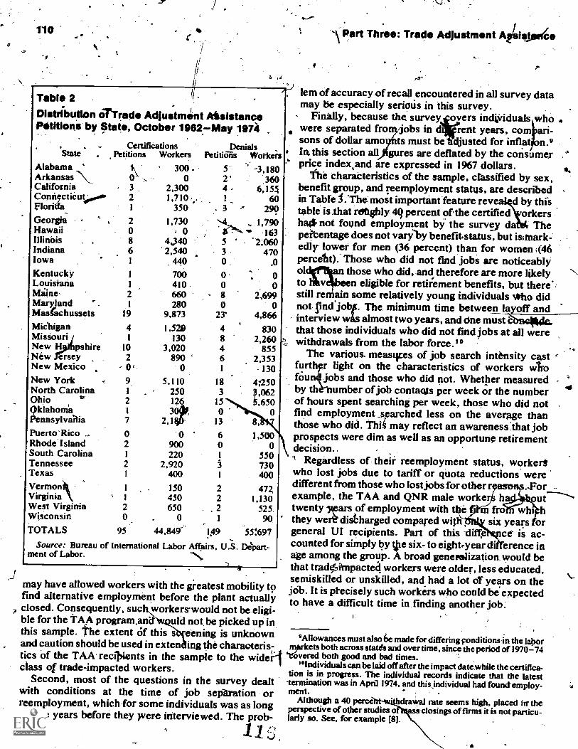
J

110

Table 2

b

Distribution SrTrade Adjustment AisistancePetition.s by State, October 1962 May 19721

State

AlabamaArkansasCaliforniaConnecticutFlorida_GeorgiaHawaiiIllinbisIndianaIowaKentuckyLouisianaMilne,MarylandMasfachussetsMiChigan

New H pshireNew erseyNew Mexico .New York ..

North CarolinaOhio t'

Oklahoma

nnsylvaiaOk

Puerto' Rico' Rhode IslandSouth CarolinaTennesseeTexasVermonVirginia\West VirginiaWisconsinTOTALS

ource: Bureau of International Labor Affairs, U.S. Depart-ment of Labor.

1. 300 .0

3 2,3002 1,7101 3502 1,7300 08 4,3406 2,5401 ,440

Certifications DenialsPetitions Workers Petitions Workers

150 2450 2650 2

0 1

5 -3,1802' 3604 6,15A1 60

. 3 290

1,790163

5 2,0603 4700. .0

0 00 08 2,6990 0

23° 4,866

1 7001 4102 660I 280

19 9,873

4 1,529I 130

10 3,0202 8900 , 0

9 5,1101 2502 126

7 2.30,1

0 02 9001 2202 2,9201 400

1

1

20

95 44,849- 1149 55;697S

4 8308 2,2604 8556 2,3531 -130

183

150

13 8,

6 1,5000 0

5503 7301 400

4;250,062

5,6500

4721,130

525.90

may have allowed workers with the greatest mobility tofind alternative employment before the plant actuallyclosed. Consequently, sue workers would not be eligi-ble for the TAA program.an- uld not be picked up inthis sample. The extent of this s eening is unknownand caution should be used in exten ing the characteris-tics of the TAA recipients in the sample to the wide'class of trade-impacted workers.

Second, most of the questions in the survey dealtwith conditions at the time of job sea' ration orreemployment, which'for some individuals was as longas five years before they were interviewed. The prob-

, 1

° Part Three: Trade Adjustment Athis ce

lem of accuracy of recall encountered in all survey datamay be especially serious in this survey.

Filially, because the survey overs indiViduals who .o were separated fro 'obs in d rent years, com ari-

sons of dollar amo is must be djusted for inflat n.In, this section all gures are deflated by the consumer .1"

price indexiand are expressed in 1967 dollars.II.

the charatteristics of the sample, classified by sex,benefit group, and reemployment status, are describedin Table #.'The most important feature reve d by thistable is.that reighly 49 percent of the certified orkershad, not found employment by the survey da Thepercentage does not vary'by benefit.status, but isimark-edly lower for men (36 percent) than for women; (46

percept).. Those who did not find jobi are noticeablyol those who did, and therefore are more likelyto v n eligible for retirement benefits, but there'.still remain some relatively young individuals Who didnot Eind'jobf. The minimum time between layoff andinterview was almost two years, and dne must cthat those individuals who did not find jobs at all were

.-1. withdrawals from the labor force.' °_

The various. meastFes of job search intensity castfurth r light on the characteristics of workers Anfaun .jobsobs and those who did not. Whether measuredby th umber of job contaqts per week or the numberof hours spent searching per week, those who did notfind employment _searched less on the average thanthose who did. Thi4 may reflect an awareness that jobprospects were dim as well as an opportune retirementdecision..1 Regardless of their reemployment status, worker*who lost jobs due to tariff or quota reductions weredifferent from those who lost jobs for otherr For -

ha out -----f m fro will hsix years or

ce is ac-erence in

example, the TAA and QNR male workertwenty wars of employment withthey were distharged compared withgeneral UI recipients. Part of this -diffecounted for simply by 4te six- to eight-yeard'age among the group. A broadgeneralization, would bethat trade,ii'mpacted workers were older, less educated,semiskilled or unskilled, and had a lot of years on thejab. It is ptecisely such workers who could beexpectedto have a difficult time in finding another job.

°Allowances must also 6e made for differing conditions in the laborkets both across states and over time, since the period of 1970-74

vered both good and bad times."Individuals can be laid off after the impact date while the certifica-

tion is in progress. The individual records indicate that the latest-termination was in April 1974, and this individual had found employ-ment.

Although a 40 price Wal rate seems high, placed in theperspective of other studies o ass closings of firms it is not particu-larly so. See, for example [8].

V

.

T1114 3

;Sample Characteristics; by Sex, Benefit Status, and Reemployment Experience

I

I .

.

Reemployed Indiviclu f . Never Found Job

Characteristics" TAA Qb111 4 U1 .TAA QNR 1)1

%.

to Total Males Females Total I Males Females Total Males Feinales Total Males . Females Total Males Females Total Males Females

309: 178 131 112 72 40 115 74 41 . 208 95 113 .86 51 , 35 86 47 39

Years of education 10.3'.. 10:4 ' 9.7 9.2

Dependent! 0.9' 1.0 ' . 0.8 0.8t

Years of job tenure 17,7 19.2 14.5'. 16.8

Weeps '

ndtice Of yoff 7,3 7.7 ' 5.0 8.8

,

Weeks ofjo search

before layoff 2,2 2,1 0.3 1.1

Job contacts

,per week ' 3,0 3.2 1.9 3.0

Percent white '86.9 87,1 :185.5 90.2

Percent married 84.8 '87.1 '71.8 83.9

Percent union

;arst received

X78.5 5 82.6 55.0 59.0

Pe

training 15.2 15.7 12.2 1.8

Percent received)

counseling

.

19.1 20,2 13.0 . 3.5

Age .' '46.0 46,645,8 _46.6---anr---7---- 5,5153..4 63.9 37.2

Ell/Wt 48.7 47.2 51.5 371

Percent skilled 20,6 23.0 lis 21.4

'Real hourly earnings

at layofr (S1967). i 3,4 3,6 2.3 2.9

Real weekly earnings .1..

at layoff ($1967) '140.9 149.2 93.2 121.9

DURI . number of

weeks between

layoff and

reemployment 48.7 39.4 01,4 32.7

DUR2 . DURI minus

out of thewe

labo force 44,3 35.7 /56.0 31.2

s

)

DUR3 DUR2 minus

weeks.of job training 39.5 30.3 51.9 31.0

Percent change in real .i

hourly earnings -26.9 -27.01,21.7 -2,4.1

Percent change in rear

weekly earnings -29.5 -30.1 -25.9 -25.2

.2 9.3 12.6 12.8 12,1 9.2 9,3 9.1 1.7

,0,9 0.8 1,2 1 '1,'! 1,2 0,4 0,4 0.4 ' ,P.3.'

20.4 10.4 5.6 5.9 5,d, 22.9 25.9 19.4 22.1

4

15.3

'

12.0i 3.0 3.2' 3.5 2.6 ,5.6 /.2

. ,

4.3

1,2 0.4 0.7 1.0 0.2 0,5 0.7 '0:9 0.4

.0.53.7 1.8 2.9' 3.0 2.8 IF 0.9 1.3,

97.2 : 77.5 781 78.4 78.0 82.4 72.0 94.8 89.6

88.9 75.0 67.8 71.0 61.0 75.0 88.0 59.7 66.8

69.5 40.0 43.5 54.1 \ 24.5 68,9 81,0 54.5 63.7

1.4 2.5, I,t7 2.7 4. 11,1 5.21 18:2 2.0

4.1 2.5 ' 4,3 2.7 7.3 104, 10.3 10.4 2.0

48.1 44.0 38.4 38.2 38.9 55.7 56.8 54.3 56,1

34.1 42.9 43.5 39.0 51.6 58.6 55.0 62.9 33.3

34,1 42.9 43.5 39.0 51.6 513 47.0 57.2 33.3

)1,9 2.5 35.6 48.6 12.2 12.4 20.7 2.6 11.8

3,3 2.2 3.3 3.9 2.2 3.0 3.5' '2.3 2.9

139.6 90.0 132.8 09.6 84.4 123.5 147.9 94,4 124,3

30.8 36\2 33.3 32.6 34.7

29.6 34.1 ', 28,6 26.2 32.9

29.6 33.4 28,5 26.0 32.9

-27.9 -17.5 -13.2 -15:4 -9.1

-26.4 -53.0 -17.6 -19.0 -15.2'rirP

'Ratio of weekly unemployment benefits and TRA payments to prelayoff weekly earninp

tRatio of expected weekly benefits to playoff weekly tunings. Expected benefits are defined in the teat.

9.1 8.2 10.2 10.0 10. 1

0.3 0,2" 0, 0,6 k 0:r33.9 19.5 7.8 10.4 5.3

5.9 , 1.9 2.5 1.5 3.3

v0,6 -0- " 111.. 0.4' I..

,

0.6 0.3 )2.1 2.4 1.9' i

88.9 90.5 67,1 67.7 66.7

83.3 42.8 68.4 74.2 63.7

P' ,

77.9 42.9 49.9 58.1 43.3I

-0- 4,8 12 3.2 3.3

20- 4.8 9,9 9.7 10.0

57.0 54,54' 48, 51,0 46,1

34.9 30.9 ) 43.3 37.7 47.8

34.9 30.9/ 43.3 37.7 47.8

16.7 4,7 22,2 29.0 16.7

3.5 2.9 3.5 2.4

'147.7 .90,2 117.4 140.1 59.1

a

112

For thoseworkers who did find jobs, the average time. bettveen layoff and reemptoyinent was 48.7 weeks forTAA recipients 2:7 for QNRs and 33.3 for UI recip-ients. TAA recipients tended to have spells of un-employment between jobs that were 46 percent longerthan for UIs and 48 percent longer than for QNRs. If thetime that workers were not in the labor force is sub-tmcted,'the adjusted duration of.unemployment figures

----..111the following: TAA, 44:3eeks; QNR, 34:2 weeks;ap UI, 28.6 weeks. If time spent in training programs issebtracteeas well, the average duration figures areTAA, 39.5; QNR; 31.0; and UI, 28.4. These figuresindicate that 'there were substantial differences in theunemployment experience of the various groups. How-ever, Table 3 indicat that the difference is 'mainlyaccounted for by very large difference in the un-employmenteployment be vior of female TAA recipients.iv Table 4 shows the fraction employed within a given

, period by benefit status and sex. These results are con-, sisteril All previous studies, i.e., women in all

categories have longer spells of unemployment than do--men. At the end-of a year, this difference is reduced to2.1 percentage points for the UI group due to successfuljob search or to labor force withdrawal. However, forthe TAA group, the difference remains large-13.6per-

- centage points. Since the male behavior does not differvery much between the TAA and the UI or QNII group,almost all of the difference in the aggregate is due toTAA females being unemployed tonger, than TAAmales.

Turning to the-changes in hourly wages and weeklyearnings as reported in Table 3, a similar observation

Table 4

Cumulative Employment Percentage ofReemployed Workers

Group1 2-13

Weeks14-26 26-52 52+

TAAMales 19.9 46.4 60.6 81.5 100Females 10.9 23.7 40.7 67.9 100

Difference 9.0 22.7 19.9 13.6 -0-QNR

Males i4.2 59.8 69.0 84.0 100Females 14.9 37.1 57.5 79.7 100

Difference 9.3 22.7 11.5 4.3 -0-UI

Males 12.4 43.8 65.1 89.8 100Females 2.2 25.2 g. 46.0 87.7 100

Difference 10.2 18.6 19.1 2.1 -Q-Note:. Calculations are based on duration of unem'ployment with

time spent in training and out of the labor force subtracted.

Part Three: Adjustment Assistance

can lie ade. Sincejhe individuals in this sample be-came un ployed at different times during the period1170-73, and since thii period was one of acceleratinginflation, all dollar figures are expressed in constant)967- dollars. Thus real earnings at layoff,,iscpoininalearnings 'divided by the consumer price index for themonth that the individual was laid off, and real weekly,earnings at reemployment is nominal earnings atreemployment divided by the consumer price index forthe month in which the indidual became reemployed.For the TAA group, t olu n 1 shows that real hourlyearnings decreased by almost 26 pe ent, whereas realWeekly earnings declined by 28.8 rcent. Thesereemployment wage losses were con Clerably largerthan the losses experienced by, worke n either theQNR or the ,UI groups.

.

Another interesting observation is that over 14 per-cent of the TAA group received job training comparedwith only 1.8 percent of the QNR group and 1.7percentof:0e %LI group. Comparably, 11.1 percent Of the TAAgroup received job counseling, whereas only 3.5 per-cent of the QNR and 4.3 percent of the UI group re-ceived counseling. These services, although important;were not major aspects of the old TAA progrim, a factthat is reflected in the small percentage of individualsreceiving them.

The major part of the program, the provision df TRApayments, can be seen in the ratios of benefits to pre-layoff wages, B/W, and expected benefits to prelayoffwage, EB/W. The former is the ratio of the sum ofweekly unemployment b'ellefits and TRA payments toprelayoff weekly earnings-commonly called the re-placement rate. Since many benefit payments were de-layed, an expected replacement rate was calculated asthe ratio of expected benefits to prelayoff earnings.

xpected benefits.are defined as the sum of unemploy-ent benefits plus the amount of extra TRA paymentsultiplied by the individual's subjective probability of

receiving TRA benefits-i.e., EB = UI payments +a (TRA payments), where a is the probability of re-ceiving TRA benefits. The survey elicited responsesabout individual's perceived probabilities, as of thedate of layoff, of receiving TRA payments. These re-sponses were used to weight the actual benefits re-ceived. Benefits should be further discounted to reflectthe delay in payment, but, as a practical matter, sincethe delays were less than a year for the individualsstudied, this was not done. Theratio of actual benefitsto prelayoff earnings was 6.3 percentage points higherthan the:ratio of expetted kenefits to prelayoff earn-ings.

the amount of benefits received was com-puted using the unemployment insurance benefit al-

The Direct Labor Markettects o the Trade AdjustmentAssistance Program: The Evidence irom the FAA Survey

. \

gorithm for ach state, the forniipa for TRA benefits,and the individual's normal weekly earnings beforelayoff. Although the survey elicite esponses about theamount eceived from UI and TR , thlk informationwas sufficiently unreliable to nece sirate the use of

. calculations from actual benefit formu ae. For exam,in Visne cases, TAA benefits were paid in one checalong with UI benef s. In other cases a\sep rate check

;. was paid for each, or only a TAA ch Ck 'as paid.Coifseqtrently, individuals had difficulty i entifying thetwo sources of compensatio . and for co sistency theappropriate benefit formula. as used. Bakd on thesecalculations, TAA recipie h a higher replacement

. rate than workers in either of t other two groups. Thisdifference averaged over $1 per week in 1967 dollarsnot subject to income tax. his amount is not inconse-quential. .

In summary, the sample indicates that they weresignificant differendes in labor market characteristicsbetween TAA recipients and UI recipients. The effectsof the TAA program on, the labor market experience ofthese workers is discussed in the next section.

3. The Effects of the TAA Program on theJob Search Process

The purpose of the TAA program under the 1962 ctwas to. promote .the reemployment of workers and tominimize the loss in earnings. Consequently an evalua-tion of the effects of the program on individuals mustincorporate its effects both on the duration of un-employment and on changes in earningsAs indicatedin section 1, changes in the outcome of thjob searchprocess due to the TAA. program mustbe attributed to(1) higher yeplacement rate of earnings under the TAApiogram. (2) greater access to job training programs,and (3) greater access to job counseling services. Toincorporate these possibilities into a simple model wedraw on the theoryOf job search.'.' According to thistheory, individuals who become unemployed will con-tinue to participate in the labor market, that is they Willsearch for a job, so long as their anticipated earningsfrom reemployment exceed the value of their time spentin nonmarket activities. In this interpretation the effectof a decline in anticipated .market earnings would beexpected to differ across groups to the extent that thevalue of time in nonmarket activity differs. For exam-ple, the presence of children is likely to increase thevalue of time spent at home, as would the availability of

pension incowomen withwould be les

- .113

e. One wo_pld expect then that married:hildren and older workers in generallikely to become reemployed.

. Given that an individual does search for,work and isaware of The distribution of wages in the market, anoptimal strategy would be to formilate a reservationwage and silly. accept an offer that exceeded it. Thereservation wage may be affected by the TAA program.Stith an effect would he expected becaijse higher un--employment compensation levels under this prograMlower the cost of search, and hence would be expectedto increase both the duration of unemployment andreemployment earnings. Unfortunately the data are notideal to test these propositions fully, since unerdploy-ment payments are per period of time and not per unit ofsearch, and there may be a substitution of time forintensity of search. In addition. job training, to theextent that it is effective, would increase an individual'sskill level and earnings, although its effect on durationof unemployment is' ambiguous.'2

%An empirical representation of the outcome of the jobsearch process is embodied in the following model:

DUR = (11R +cf2T +a3C+ a4X1 ci (1)

tiv = IR +432T+ B3C'+ B X2 + 62 (2)

D U R -7- number of weekskunemploYment= percentage change in Weekly earnings

(hourly wages) from layoff date to re-,employment= replacement rate, i.e., unemployment

payments divided by previous earnings= 1 if an individual received job train-

ing, 0 otherwiseC = 1 if an individual received counseling,

0 if otherwi eXI, X2 = vectors of e ogenous variablesEP 62 = random err r terms.

R

In essence this model was used by Ehrenberg and Oax-raca [31. and by Classen [2] except that effects of trainingand counseling are added in our specification.

Two issues arise in estimating this model. First, animplication of the theory of search is that the error,terms are jointly distributed and that their covariance isnegative. That is, individuals who haVe overestimatedtheir prospects will have longer than average 'un-employment, and would tend to have lower reemploy-ment earnings if their reservation wage declines overtime.'' Oil the other h4, as argued above, if expecta-

"A detailed description of the theoretical work on the job search '21n effect\ob training should offer the individual a different wageprocess as well as a summary of the previous empirical work pertain- offer di striburon.ing to search duration and subsequent wage change is contained in [7. "This argu ent suggests that an efficient estimator such as Zell-chap. 2). ,miner's seeming) unrelated regressions estimator be used [9).

1

114

a

/ t are realistic, those with higher reservation wageswill on average experience longe durkions of un-employment, but will be com nsatect by higher

, reernployniatlearnings. This is the productive invest-ment nature of the search 'process.

The second issue is the possible endogeneity of thedecision to participate in training or counseling ses-'sions. Since these services are potentially available.toTAA, QNR, and UI groups, perhaps at different prices,the decision to participi(te in these programs may bebased on characteristics of the individual that are re-lated to both wage change and duration of unemploy-ment. For example, it could be that only those individu-als who have an expected duration of unemploymentgreater than some critical value enroll in training pro-grams. If this 'were the case, the coefficient on training(T) in equation (1) would show that training was as-sociated with a longer duration of unemployment.However, thi; would be a biased estimate of the trueeffect of training if the training decision is correlatedwith the expected outcome of the job search process.Only when the urren e of training or counseling isbeyond a,n i avid al's co trole.g. , givell to everyonein one area', to no one in another areacan anunbiaied est ate of these effects be obtained fromequations (1) and (2'). The use of appropriate instrumen-tal variable -will eliminate this problem when training (T)and counseling (C) are continuous variables. Ananalogous result has been shown by Heckman [5] whenthe variable is dichotomous. In essence this requiresthat the values of T and C, which are either 0 or 1, bereplaced by their predicted values from a probit regres-sion. These predicted values have the interpretation ofprobabilities -of receiving training or counseling. Themodel in (1) and (2) then becomes

DUR = + o2P(T ta3P(C 1) + ct4X 4- el . (1')

vi"," =i3IR +02P(T= 1) + 03P(C= 1) + l34X2 E2 t2')

The probabilities of receiving training and counsel-. ing, P(T = Al) and P(C = 1), are the fitted values-from theprobit regressions. Variations in the determinants ot'-these probabilities due to the TAA program are denotedas

aP(T = 1) aP(C = 1-)/7 = and 8

aTA A

The effects of the TAA program on the job searchprocess can be- calculalpd then as

aDURa TAA

aR= 01- 0(27 + Q341aTAA +

1t3)

)P in Three: Trade Adjustment Assistance

al, aR .4., x, aTAA' . PI aTAA -. P27 #131.

8 ,.... /where y'is the mar inil effect of TAA participation on ,the probability of receiving training, and 8as similarlydefined for counseling. As (3) and (4) indicate, the totaleffect of the TAA program has two components.'effect' is.due to the higher level of unemployment ben-efits, whichl,alters the cost of-unemployment, andhence has a diject effect- upon the search process. Theother effect is composed of the direct effect that training ,...-and counseling have On the search process, multipliedby the increased probability of an individual's receivingthem. For these latter effects it is possible that the-TAAprogram had no substantive effect on the job' searchprocess, either because the program had .no effect onproviding 'these services, or because these servicesthemselves as .provided were of no value in the labormarket."

Evidence on the likelihood of an individual's receiv'ing job training or counseling is presented in Table 5,and larger set of results are contained in Tables Al andA2 If the appendix (a description of the ariables is

--given on p. 115). Examination of colu ns (1) (3)reveals that the TAA recipients were sign scantly morelikely to receive training or counseling than were QNRor UI recipients. The coefficient on the variable TAA ispositive and signifiCant, regardless of the specificationof the equation. (See Tables Al and A2 of the appen-dix.) The size of the. coefficient refers to the effect ofTAA participation n the index variable of the 'cumbla-dye normal proba 'ty function. Translating these ef-

1 fects into probabilit , the coefficient on TAA in col-umn 12) of Tabl mplies that TAA recipients had aprobability receiving training that' was 6.72 percent-age points higher than without _the' program. In thenotation of equation (3), y = 0.0672.For counseling, theestimate of 0.6502 in column (3) implies that 8, the effectof the TAA.,program on the probability of receivingcounseling, was 0.0872. This evidence indicates' that theTAA program, as operated under the old Act, providedgreater to job training and job counseling 'thanotherwise would have existed. To be sure, not all indi-viduals received training or counseling; in fact only asmall percentage did. Nevertheless, the TAA programappears to have made it easier for recipients to obtainthese services.

(4)

"At first thought it may seem unlikely that any individual wouldparticipate in a program that is worthless in terms of future employ-ment. However, since many training programs pay a subsidy, or, inthe case of-TAA, enable an individual to receive unemploymentbenefits for a longer time, there is an incentive to enroll in the programto lower the cost of current job search.

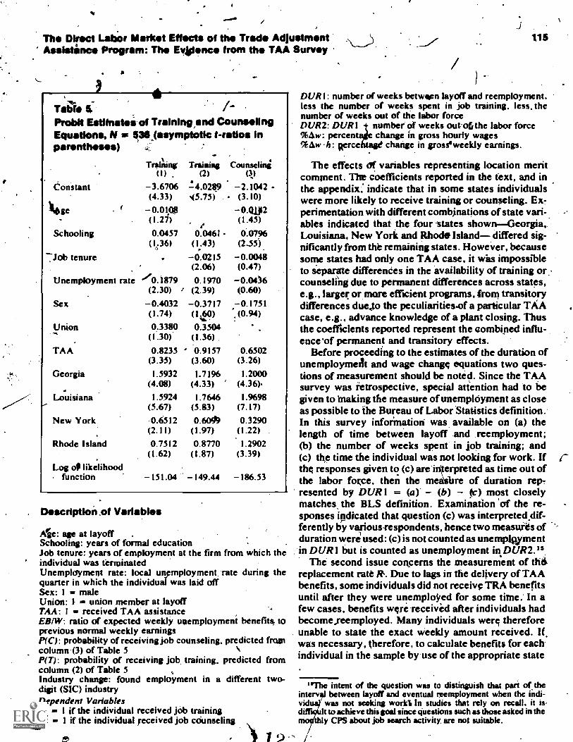
The Direct Labor Market Effects of the Trade AdjustmentAssistince Program: The El/fence from the TAA Survey

3

TableI

Probit Estilnates of Training and CounselingEquations, N 535 jasymptotic Natio* inparentheses)

Trai/ing Training Counseling(1) . (2) (3)

Constant -3.6706 14.0289 -2.1042 -(4.33) (5.75) (3.10)

koge -0.01g8 -0.Q1j12(1.21) (1.45)

Schooling 0.0457 0.0461 0.0796(1.36) (1.43) (2.55)

7Job tenure -0.0215 -0.0048(2.06) (0.47)

tl ne mplo y m e nt rate /0.I879 0.1970 -0.0436(2.30) (2.39) (0.60)

Sex -0.4032 -0.3717 -0.1751(1.74) (le) (0.94)

Union 0.3380 0.3504(1.30) (1.36) .

TAA 0.8235 0.9157 0.6502(3.35) (3.60) (3.26)

Georgia 1.5932 1.7196 1.2000(4.08) (4.33) (4.36).

Louisiana 1.5924 1.7646 1.9698(5.67) (5.83) (7.17)

New York 0.6512 0.6049 0.3290(2.11) (1.97) (1.22)

Rhode Island 0.7512 0.8770 1.2902(1.62) (1.87) (3.39)

Log a likelihoodfunction -151.04 -149.44 -186.53

Description of Variables

Ale: age at layoffSchooling: years of formal educationJob tenure: years of employment at the firm from which theindividual was terminatedUnemployment rate: local unemployment rate during thequarter in which the individual was laid offSex: 1 = maleUnion: 1 = union member at layoffTAA: I = received TAA assistanceEBIW: ratio of expected weekly unemployment benefits. toprevious normal weekly earningsP(C): probability of receiving job counseling. predicted fromcolumn (3) of Table 5P(T): probability of receiving job, training, predicted fromcolumn (2) of Table 5Industry change: found employment in a different two-digit (SIC) industryDependent VariablesT. = I if the individual received job training

.4V = 1 if the individual received job counseling

tt.

115

DUR I: number of weeks betwrien layoff and reemployment,less the number of weeks spent in job training, less, thenumber of weeks out of the labor forceDUR2: DURI number of weeks ouofithe labor force%Aw: percentaje change in gross hourly wages%Aw-h: Rerce change in groseweekly earnings.

The effects of variables representing location meritcomment. The coefficients reported in the text, and inthe appendix; indicate that in some states individualswere more likely to receive training or counseling. Ex-perimentation with different combinations of state vari-ables indicated that the four-states shown - Georgia,.Louisiana, New York and Rhode Island- differed sig-nificantly from the remaining states. However, becausesome states had only one TAA case, it was impossibleto separate differenes in the availability of training orcounseling due to permanent differences across states,e.g., larger or more efficient programs, from transitorydifferences due.cto the peculiarities-of a particular TAAcase, e.g., advance knowledge of a plant closing. Thusthe coefficients reported represent the combined influ-ence 'of permanent and transitory effects.

Before proceeding to the estimates of the duration ofunemployment and wage change equations two ques-tions of measurement should be noted. Since the TAAsurvey was retrospective, special attention had to begiven to making the measure of unemployment as closeas possible to the Bureau of Labor Statistics definition.In this survey information was available on (a) thelength of time between layoff and reemployment;(b) the number of weeks spent in job training; and(c) the time the individual was not looking for work. If rthe responses given to (c) are interpreted as time out ofthe labor force, then the measure of duration rep,resented by DUR 1 = (a) (b) - (c.) most closelymatches the BLS definition. Examination of the responses indicated that question (c) was interpreted,dif-ferently by various-respondents, hence two measures ofduration were used: (c) is not counted as unemplAymentin DUR I but is counted as unemployment in.DUR2. 13

The second issue concerns the measurement of the-replacement rate R. Due to lags in the delivery of TAAbenefits, some individuals did not receive TRA benefitsuntil after they were unemployed for some time. In afew cases, benefits were received after individuals hadbecomexeemployed. Many individuals were thereforeunable to state the exact weekly amount received. If,was necessary, therefore, to calculate benefits for eachindividual in the sample by use of the appropriate state

'The intent of the question was to distinguish that part of. theinterval between layoff and eventual reemployment when the indi-vid was not seeking world In studies that rely on recall. it isditl'a9lalt to achieve this goal since questions such as those asked in the

tidy CPS about job search activity. are not suitable.

ee4116 Pert Three:irade Adjustment Assistance

formula, or in the case of TAA recipients, by thena-tional formula. '6

In additicin, since TRA payments were often delayed;a questiOn arises as to how they should be inclu$1ed in R.If perfect foresight is a'Ssumed,, then actual benefitsreceived, suitably discounted, is the conect measure ofTRA payments. Since thtre was uncertainty as to eligi-bility, it is appropriate to use expected benefits, againwith discounting for the delay in receipt of benefits. Forthis sample, the adjustment for time discounting is neg-

"TRA payments were 8 percent of the individuals' previous aver-age weekly earnings or 65 percent of the averagetweekly earnings inmanufacturing, whichever is less. Thus the algorithriVed to com-pute TRA,payments does not change, over time, although the upper

. limit does.

g4.

ligible, and was:ignored. In the estimates that follow theexpectecllenefit ratio is4adopted

The estimates of the duration and wage change equa-.tions are contained in Table 6 for the sample of 536individuals who found employment. The first two col-umns contain the estimates of equation (1) for the twomeasures of unemployment, and the-last two columnscontain the estimates of (2) for weekly and hourly earn-

'Expected benefits were calculated as the sum of regu'ar UI ben-efits plus o'times the TAA differential. The probability of receivingTAA benefits, a, is taken from question 50 of the survey. (How surewere you of receiving TAA benefits at the time you were laid off?)which was coded 1-5 (very sure, sure, etc.). These answers wereranked as probability assessments ranging from 0.2 (no knowledge) to1.0 (very sure). The average replacement rate of expected benefitocalculated in this manner was 6.3 percent lower than the actual.

Duration of Unemployment nd *age Change(f-statistics in parentheses)

, Dependent ariable DUB('

Constant 13.06)1_(1.30)

EB/W "f--2195, (1.80)

P(C) -0.6424(1.98)

P(T) 0.6530(1.67)

.Unemployment rate 1.1700(0.81)

Union 5.5435

Industry change

Sex

, Strhooling

Job, tenure

Rhode Island

Georgia

New York

R2

F

(1.39)

17.4807(4.25)

-15.7956(3.70)

40.5557(3.21)

- 536

DUR2(2)

%Aw(3)

to h(4)

14:6097 -37.5100 -55.6215'(1.34), (3.80) (4.19)

0.3116 0.4392 0.5944(2.31) (4.15) (4.18)

--0.5021(1.40)

0.7726(1.78)

0.2464(0.15) '1.2992 -8.4620 -7.3792

(0.29) (2.14) (1.39)19.5888 -8.0164 -11.9749(4.29) (2.25) (2.50)

-13.9107 -1.7344 7.2949(2.94) (0.48). (1.50)

0.6333 1.350(1.1l) (1.77)

-0.5152 ,-0.9553(3.47) (4.78)

33.5838(2.40)

"'2 16.4889 `, 21.7907(2.76) (2.72) /

-4.8897 -12.4871(1.03) (.1.97)

0.1002 0.1164 0.11047.3419 8.6823 8.1750

The Direct Labor Market Effects of the Trade laijustmentAssistance Program: The. Evidence from the TAA Survey

',iris change. The molt important result is that the effectof higher unemployThent benefits on both duration andwage change is positive as expected. The coefficient onthe expected replacement rate-0.2195 in column (1)and 0.3116 in column (2) imply that an increase in thereplacement rate by 10 percentage points would in-crease DUS1 by 2.2 weeks, and DUR2 by 3.1 weeks.For recipients of TRA payments, the expected re-placement rate was 6. rcentage points higher; there-fore, the effect of hi erTRA payments was to increaseduration of unempl ment by 1.4 weeks (= 0.2195 x6.3) for DUR1 and by 2.0 weeks for DUR2. A similarcalculation using the coefficients on the expected re-placement rate from columns (3) and (4) ields the effectof higher TRA payments on earnings: h urly earningswere 2.7 percent (--= 0.4392 X 6.3) and we kly earnings3.7 per nit higher than without the program. Onecaveat this is that all of the effects of TRA paymentsmay not have beeh captured: In particular; the longerpotential benefit period for TAA recipients may have aseparate, independent effect on both durlition and earn-ings. Preliminary tests of this, proposition7using thestate maximum UI durations and the -TAA maximumduration, aid not indicate that this factor was important,

Sbut the test was not conclusive because in several statesextended unemployment benefits were available; hencepotential dUration was measured incorrectly. ThusEB/W may be only a rough measure of the true ex-pected replacement rate 7

The remaining effects of the TAA program are relatedto the availability .counseling and training. As reportedin Tables A4 and AS of the appendix, no significanteffects Of framing or counseling on earnings could befound; and the effects on duration are hard to interpret.C6Unseling has the expected sign, but it is insignificantwhen time out of the labor force is counted as un-employment. (See columns (1) and (2) of Table 6.) Thissuggests the possibility that time spent between layoffand the provision of job counseling was not spent in jobsearch." The estimates indicate that job training in-Creased unemployment duration-although not, sig-

. nificantly. Since the availability of training services wasseverely limited at the time of layoff for most .TAArecipients ,3tie majority of (hose receiving training didnot start until after a considerable period had elapsed.Furthermore,' thereewasan incentive to take training to

"Evidence of this behavior is partially revealed in the correlationcoefficient between various measures of duration and counseling ortraining:

X PT.X PC.X

I. Time between jobs 0.2734 0.12172. Leis time in training 0.2020 0.07083. Less time "out of labor force" 0.0110 -0.0313

increase the length of time for which TRA benefitswould be paid. Thus the evidence that training had noeffects on earnings, c upled with a lengthened durationof unemployment, s pport he interpretalion that thetraining programs m y have s ved to provide, a type ofextended unemployment bene s for those who par-ticipated.

The effects of the remaining explanatory variablesare of the anticipated sign but are, with a few excepttions, insignificant. For example, there was no signifi-cant effect' of the local unemployment rate at time oflayoff. Union members were estimated to have aslightly longer duration of unemployment, but again thedifference was insignificant. All else equal, union mem-bers were estimated to experience an 8.5 percent de-cline in hourly earnings, after a job loss a figure that islarge and significant. This effect is compensated some-what by an estimated increase in their hours worked sothat the loss in weekly earnings' was 7.4 percent,.

The impact of job termination had considerably dif-ferent effects for men than-for women. The coefficientson sex (male = 1) reported in columns (1) and (2) ofTable 6 indicate that on the average spells of, un-employment for males were 13.9 to 15.8 weeks less thanfor females. The apparent source of difference is thebehavior of female TAA recipients: whereas UI andQNR females had. durati 14 that were only 1.7 and 0.9months longei than for al TAA females were un-employed for 4.9 months onger. NO ready explanationfor this ,difference seems obvious. The estimatedchange in reemployment earnings is not so different,however. .

The effects of human capital accumulation can beseen in the coefficients of schooling and years of jobtenure. Years of schooling is a measure of generalhuman capital, and years of job,tenure, since it mea-sures the number of years employed at the firm theindividual was laid off from, is a proxy for job specificcapital. Although neither has an appreciable effect onduration of unemployment, they did have the expectedeffects on wage chaltge.:7he effect of education wasconsistently positive in all specification that controlledfor interstate differences. The potsitive coefficients canbe interpreted to mean that job termination does notreduce the value of general human capital. In contrast itwas estimated that the reduction of firm specific humancapiial due to a jab loss had a large negative effect;indeed, this variable and the replacement rate are by farthe most powerful explanatory variables. Other thingsequal, the regression coefficients in columns (3) and (4)of Table 6 imply that each additional year 'of job tenureis, associated with a 0.5152 percent ,decrease in realhourly earnings and a 0.9553 percent-decrease in realweieldy earnings when an individual lose§ ajob. Thus an

1 2 _

118

individual-with-twenty 'years with Tie employer wouldbe estimated to' have a 10 percent decrease in hourlyearnings and an 18 percent loss in weekly earnings.

The inclusion of controls for place of residence at timeof layoff was intended to capture any systematic differ-ences across states that were not captured by othervariables. ' ° For the same reasons-as discussed above itis not possible to separate permanent state effects fromtransitory effects due to individual TAA cases, an

Island

of the coefficients is therefore more,diftficult. In particular, the estimated impact of RhdileIsland on duration is eon large to believe. However, thedirection of the effect is consistent with the view ofsev,1 obsAers that in Rhode Island, moreAo than inotfitates, there was wide notice ,in advance of theTAA programNrithat.many individuals took advan-tage of the program.

1 9In addition to the local unemployment rate we also included theaverage manufacturing wage in the SMSA, manufacturing employ-ment as a percent of nonfarm employment, and the ratio of tradeimpacted workers to manufacturing.employment. When the statevariables were luded, none of these-had an effect.

Part Three: Trade Adjustment Assistance

Afinal factor of interest is the role of industry changeoh duration and wage change. This variable 'was in-cluded to measur the effect of the'departure of anindustry from an ea, and hence the lois of whateverindustry specific uman capital an individual 'pos-sessed. It appears t at the variable is picking up' more,than this. In partial , since the decision to accept ajob in a different industry is voluntary, it may be pickingup the effects.of unmet expectationeqo test this hypo-thesis we estimated (1) and (2) using Zellner's seem-ingly unrelated, estimator kut obt4ined no substantialdifference 'n estimates. Vereason for no differencebetween equitiens (1) and (2) was the low correlation ofthe disturbances.2° When industry change is deletedfrom both equations and the Zellner estimatos is used,the correlation of the error terms is significant, but theremaining coefficients are not altered significantly.

"The variance-covariance matrix of one equIn of a two-equation system can be writtenor Zellner's estimator as Vi = (1 --Ps){cr - P' a,"' XVCi(x;x2)-tvelx ,y.. If P, the correlationcoefficient of the residuals, equals zero, this reduces to the OLSestimator.

Tab 7

Du ion of UnemploymentM es, N = 324 (t statistics

Dc ndent.Variable

Constant

EBIW

P(C)

P(T)

Unempldthiont ..rater.

Union

Industry change

Schooling

st Tenure

Georgia

New. York

R2

F

I.

d Wage Changen parentheses)

DURI ,

-16.037(1.24)0.2409

(1.57)

0.4108(1.14)

-0.7595(1.72)

3.2976(1.71)

9.4243(1.68)16.4459(2.97)

0.0636

2.3135

DUR2

-13.616(0.94)

o 0.3506(2.04)

0.3259(0.80)

-0.4243(0.85)

2.6607(1.22)

4.0804(0.64)

18.7866(3.01)

f;441

0.0542

3.0323

%tov

-40.532(2.99)

0.5178

Voil(w 11)

-44.780,(2.49)

0.6608(3.57) (3.44)

-11.4703. -10.9044(L88) (1.35)

-3.6296 -2.8392(0.68) (0.40)

0.5203 0.7678(0.66) '(0.74)

-0.6640 -1.25300.3 (4.72)

'17.8231 21.5046(1.71) y1.62)

--2.0596 -0.545'6(0.27) (0.97)

0.1032 0.1232."u

5.1957 6..3449

4

The Direct Labor Market Effects of the Trade Adjustment" 119Assistance Program: The Evidence from the TAA Survey

o'

The pattern ofresults thus far suggests.that a separateinvestigation of male and female behavior would revealgreater insight into the workings Of the TAA program.The resume of reestimating th odel on the samples of24 male and 212 females were reemployed are

contained in Tables 7 and 8. 'though the explanatorypower of each IS not very i h, pronounced differencesin response to unemployment compensation are re-vealed. Higher unemployment benefits Were estimatedto increase duration and to lead to pigherreemploymentwages for men. Reemployment earnings of womenwere estimated to increase as a result of higher un-employment compensation but no effect can be foundOn duration. This is rather difficult to understand-Con-)theivably there were two different types of responses.To analyze this possibility fisirth,the duration equa-tion was estimated with various subsimples of females.The results appear in Table 9. When females are splitinto married-spouse present and all others, a markedimprovement in the explanatory power of the model is

observed, Unmarried women, although their numbersare small, behave somewhat more like men as measuredby their response to higher unemployment benefits.Married women, on the other hand, seem to, have nosignificant response to higher benefits. Also, it is mar-ried women whO account for the perverselfaining ef-fect. Males were estimated,to experience Oorter spellsof unemployment as a result of although thesignificance level is not very high. T *ning does notappear to have any significant effect on unemploymentFor unmarried women. For married women, however,training prolonged unemployment by about two weeks(exclusive of thelime spent in, training), and the effect ishighly significant.

4. Summary and Can)cluslons

The empirical findings of the previous section implythat the TAA program under the 1962 Trade Expansion

Table 8Duration,of Unemployment and 'Wage CHange,Females, N,,= 212 (f statistics in parentheses)

Dependent VariableConstant

EB/W

P(C)

P(T)

Unemployment rate

Union

Industry change

Schooling

Tenure

Rhode Island

Georgia

New York

R'F

DUR I .

9.1321(0.65)

iio46o(0.21)

-0.6822(2.18)

1.3471(3.95)

2.1849(.1.16)

8.5420(1.36).

20.3349(3.28)

D(.42 %Aw %4(w .h)13.466 -32.1122 -58.7951(0.92) ,J (2.51) s (3.31)

0.1007 0.2611 0.3902(0.44) (1.73) (1.86)

-.0.4504 I ,,,(1.35)

i15795(4.33)

0.6630(0.33)

7.5177(1.12)20.6742'.

/ (3.13)

26.3951 . 14.0497(1.56) (0.77)

0.1880 0.1953

,6.7475 7.0761

-4.9504(1.03)

12.5833(2.79)

0,8313(1.06)

-0.1334(0.60)

13.3665(2.01)

- 6.2855(1.13)

0.1021

3.3169

, -2.4647t:(0.37)-22.222d,

(3.55) .`2.4975

(2.29)

-Q.3039(0.99)

20.2965(2.20)

,13.0331`.111.69)

it`' 0.1;68,,r ,44t346

120

Table 9, .

Duilltion of Unemplo rledMeiWomenSpouse Present, and All OtherWomen

, A .

P(T)

Unemploynient

Union

Industry change

'Rhode Island

R'FN

All OtherMarried Women

Spouse Present

27.6838 7.5112(1.50) (0.39)0.3274 0.0342

(1.11) (0:11)0.4614 1.0878(1.16) (2.47)

0.1674 1.9212', (0.34) - (4.05)

2. 48 2.7626(0.70) (1.19)

15.5488 15.1612(1.52) (1.93)

18.6615 1T:0112(2.12) (2.08)

6419507 19.7375 .

(2.29) (0:90)

0.2044 0.2237

2.0190 5.8075

63 149

4

Act had a small but significant effect on at least part ofthe recipient population. As.described in equations (3)and (4), the net effect of the TAA-program is the sum ofthe separate effects of: (a)' higher. benefits while un-employed (the difference between TRA payments andwhat would have been received under regular Uti-employment Insurance); (b) a greater probability ofreceiving job training; and (c) a greater probability ofreceiving job counseling. For male TAA recipie.nti thenet effect on,Onemployment (DE1R2) and-weekly earn-'inv. is computed from (3) and (4) using the regressioncoefficients from columns (2) and (4) of Table 7 as:

aDuR2 = 03506(8.1) 0.4243(0.06725aTAA

+ 0.3259(0.0812)

= .2.84 weeks..

a(i Cv.h) z=-- 0.6608(8,1)7aaA-) 5.4%.

Part Three: trade Adjustment Assistance;

This increase in duration appears to have been used inproductive job search, since weekly earnings were 5.4percent higher than would otherwise have occurred.

For women the tesults are less clear. Estimates of thenet effect of the program on duration of unemploymentrange from zero to a one -week increase; but these esti-mafes are not sighificant for the entire sample of wom-en. There is) some indication (see columns 3 and 4 ofTable 4 that higher unemploymegt benefits lead toincreased reemployment earnings-2.3 percent forweekly earnings gnd 1.5 percent for hourly earningsbut the evidence is not strong. The pronounced differ-ence in the behavior of males and females is perhaps themajor finding of this study in regard to the, operation ofthe program. these results Indicate thy "for the mostpart women TAA recipient p/who were married did notsearch for ajob while unemployed. It seems likely thattheir average of 61 weeks between jobs was due in partto the higher benefits available under the TAA program.This interpretation is reinforced by the finding that,un-

, married women respond to higher unemployment ben-efits in essentially the same way as men do. One maytentatively conclude that the provision of ben-

.

efits to families wit more than one w earner canmake receiving th benefits an attrac ive alternativeto employment.. .

4' Further insight into the differential labor market be-havior pf men, and women is revealed by observing theIncome maintenance role of the TAA program. Al-though the -1962 Act was not specifically intended tocompensate indAviduals forjoblosses, higher TAA ben-efits -while u4mployed certainly has this 4effec InTable 10 estimates of the net present value of the privatEcosts of job loss are presented under three differentnssunigiiiiis.

I. The value of time while unemployed is zero and all wageloss it permanent.

(5)!

(6)

For the Average male TAA recipient duration of un-emploYntent increased by 2.8 weeks (1.9 for DUR1).

Table 10PrIvate.Costs of Job Loss for Workers WhoReceived Trade Adjustment Assistance byReemployment Status and Sex, 1975 Dollars

. Assumptions:,Group 1. 2 3

A. Never Found Jobs .Males 47,273 7,644 7,644 'Females 18,934 1,452 1,452

B. Reemployed.Males 29,895 25,690 4,704Females 11,002 6,543 481'

C. Average TkA Recipient 26,322 11,860 3,293

- 121

The Direct Labor Market Effects of the Trade AdjustmentAssistance Program: T Evidence from the TAA Survey

-2, The value of time while unernployed is 50 percent ofprevious earnings for males, and 65 percent of previousearnings for females; all 'wage loss is permanent."

n t ears.3. The value ehZn 2 and all wage loss is transitory,

disappearing

1. These calculations should be interereted as upper-bound estimates' of the private cost ofjob displacementfor this particular group of individualts)and not for allindividuals who change jobs due to import competition:These estimates are biased upwards,...since they do notallow for differential Unemployment* rates, for job lossdue to health reasons, for the value of any pensionsreceived, and for differing marginal tax rates amongindividuals." Two points are of primary importance.First, the costs of a job loss, tend to be smalleil- forwomen for three reasons: their lower market earnings,relatively higher nonmarket opportunities, and higherreplacement rates of earnings while unemployed. Eachfactor should make married females less sysitive tolabor market programs designed to foster job searchactivity:' Second, and perhaps most important, the pri-vate costs that individuals bear depends critically uponthe extent to which a loss in earnings potential is per-manent. If the loss is transitory, as is assumed in, col-umn 3 of Table 10, then it is possible that the TAAprogram can overcompensate some individuals. Thispossibility is enhanced for individuals facing high mar-Opal tax rote.

The eVidence presentedin thit paper coneetninithelabor market effects of the TAA program pertains onlyto the program as operated under the Trade Act of 1962,and thus the findings are not necessarily indicative offuture behavior under the new Trtrde Act of 1974. AMir.tfrom changes such as an increase in the replacementrate to 70 percent frOm 65 percent, and that workersmay be eligible for benefits even though they are notpermanently displaced frm their jobs, the Ow workeradjustment assistance provisions are not very different,

1'

and thus there are some grounds for extrapolating the

alThe estimates for women are baied on [4] with rough adjustment,made for the older nature, and fewer dependents, of this sample:Comparable values for males are available (except for the inappro-priate measure of commuting time value), and the 50 percent figure islittle more than an edUcated guess. *

"In performing these calculations a tax rate of 28.4 percent wasused.

. I

121

resitIts of the survey reporte,I in this paper to the new. ,

TAA program. Some, but it is hoped- not all, of thedifficulties noted may continue to occur. The two majorproblems that have significant labor market consequ-Ances are the delivery of benefits and the level of be-nffits. The cumbersome nature of the certification pro-cess, which existed in the old program in order to focusbenefits narrowly, resulted in lengthy delays betweenthe date -of job loss' and the date when benefits werereceived. This had the effect of reduCing the impact ofREA payments on the job search activity of individualsbyXmost one-half of the extra benefits. The dilemma is

(ea familiar one; mo. intensive eligibility criteria directresources where Congress intended th.rn, but alsodelay their receipt, making them less useful.

The leirl of benefits provides a comparable dilemma.Higher beittefits can lead to better job matches forsomeworkers,' but for others, particularly married womenwith spouse present, there is no obvious gain other than 'an income transfer.. The dilemma 'in this ca sF is thatequal TAA benefits for primary and seconder' incomeearners in a household, may, due to the higher marginal,'tax rate facing the secondary worker, result in withdrawal from the labor force during the period that ben-

. efits 'are available. This is an effect opposite to thatintended if the TAA program was designed to stimulatejob search and reemployment." In any event the pro-gram can serve as a vehicle for compensating workerslaid off because of increased foreign traile especially ifthe connection between benefits received and un-employment were severed. One may speculate that this

"'`'sw could beCome More generally applicable if theadministration of the new TAA program turns increas-inillowards compensating workbrs who are only tem-porarily laidoffitue to imports and ,fo do not ct tosuffer any wage loss upon reemployment. - .

"Akant..ximpleof the potential size of the benefits consider thecase ,of an iitiaividual who lost his job in. manufacturing during June of1976. Eh lite for TRA payments and earning the.average for man-ufacturing this timeS298.06 per weekif 'he stayed unemployedfor the full 2 weeks he:Avould receive $7,57,3. If he were fullyemr4pyed iond facedim avWaw tax rateincome, social seciirity;'of 28:4 percent, then he would have netted $7,746a difference ofonly A173. This ignores the effect of fringe benefits and non-pecuniaryrewards, but italso ignores work related expense. The point is thattheprogram can subsidize a large part of lost earnings and may reduce theincentive to work.,

122 . Part Throe: Trade Adjustment AssistanceV

Table .A1Probit Estimates of the Probability of teceiving Job Training N d36(Asymptotic f-values in parentheses)

(I) (i)Regressions.

(3)

Constant -3.8367 -3.8424 -3.6706(3.85) (4.19) (4.33)

Number of dependents -0,0463 -0.0398. (0.69) (0.61)

Age -0.0022 -0.0023 -0.0108(0.18) (0.20) (1.27)

Schooling 0.0443 0.0434 0.0457

.(1.32) (1.30) 2(1.36)

. Job tenute -0.0211 , -0.0217-. (1.73) (1.80)

Unemployment rate 0.1899 0.1941 0,1879(2.28) (2.34) is (2.30),

Seit -0.3546' -0.3626 -0.4032(1.51) (145) (1.74)

Race -0.1027(0.39) /

0

Urban/Rural (1 in urban),

I 0.0977(0.22) '

Union 0.3317 0.3449 .0.3380(1.26) (1.33) (130)

TAA (1 MP recipient) 0.9312 0.9179 0.8235.,(3.62) (3.60) (3.35)

State dummies:

Georgia 1.6566

- ,

1.7076. IV

1.5932(4.02) (4.30) (4.08)

Louisiana 1.7495 1.7722 1.5924(5.26) (5.82) . (5.67)

NewoYork 0.6032 0.6108 0.6512(1.88) (1.27) (2.11)

Rhode Island 0.8674 0.8706 0.7512(1.79) (1.86) (1.62)

Log of likehhood function -149.14 -149.25 - 151.04 .

1

(4)

-4.0289(5.75)

I

(5)

-3.4388(7.77)

0.0461'(1.43)

-0.0215(2.06)

0.1970(2.39)

-0.3717(1.60)

-0.002.4(0.23)

0.0074(0.24)

0.0091(0.92)

0.2499(433) -

- 0.1113(0.61)

0.3504(1.36)

0.9157 ,Q.9748(3,60) .. (4.18)

,

1.7196(4.33)

1.7646(5.83)

0.6099(1.97)

Ot8770(1.87)

-149.44 -176.91

"'

The Direct Labor Market Mots of the Trade AdjustmentAssistance Program: The Evidence.from the TAA Survey

Table A2

123

*obit Estimates of the Probability of Receiving JOb Counseling and Testing N(Asymptotic l-values In parentheses)

Variable .. (I) (2) (3) 'Regressions

(4) (5) .

Constant .-1.7882 -2.1042 -2.001 -2.7447 -2.6978(2.20) (3.10) (5.40) (5.10) (5.00)

IgUmber of dependents -0.0786 -0.0402,.. (1.14) (0.67)

Age -0.020 -0.0142 '.(1.97) (1.45)

Schooling 0.0682 0.0796 0.0919 0.085 .0.0849(2.21) (2.55) (3.20) (2.90) (2.92)

Job tepure -0.0077 )-0.0048 -0.0127(0.74) (0.47) (1.491

Unemployment rate -0.0640 0.0436 -0.0321 -0.4769 : 0.3943(0.84) 0.60) .(0.44) (0.66) (0.54)

Sex -0.1627 -0.1751 -0.2189 -0.1764(0.83) (0.94) (1.19) (0.95)

Race 0.3463(1.25)

Union -0.1065(0.49) ...

TAA 0.6731 0.6502 '0.5663 0.6649. 0.6397.(3.33) (3.26) (2.96) .t.(3.39) (3.23)

,State durnrniei..: . 81`;

Georgia 1.1653. 1.2000 1.1045. 1.2207 1.1852(3.56) (4.36) (4.10) (4.52)

.. .

(4.35)

Louisiana- 2.0712 1.9698 '' 4.8324 1.9275. 1.9688(7.15) (7.17) (7.05) (7.13) (7.15).'

New York 0.3076 0.3290 0.3084 0.3164 0.2840(1.12) (1.22) (1.16) (1.20) (1.06)

jii Rhode Island 6 1.2979 c 1.2902 1.2907 1.3533 1.3308(3.35) (3.39) (3.41) (3.58) (3.51)

Lag of likelihood . .unction -184.18 -186.53. -188.50 ,-188.05 -187.60

(6) (7)

-2.8782 -2.4158(6.72) (4.33)

-0.0147(1.62)

0.0847 0.04080.92) (1.50)

-0.0123. 0.0210(1.45) (2.40)

0.1281

(2.61)

-0.1888 -0.0514(1.03) (0.32)

0.6396 0.7167(3.23) (4.01) /

1.2243- (4.64) '

1.8897-(8.15)

0.2474(0.96)

1.3022(3.47)

.

-187.75 -119.75

124

-Table A3

Duration of nemploymentN 536

Variable

Constant

B/W

DURI

(1) , (2)

14.1244 13.0617(1.48) (1.30)

' 0. 1t39 ,

(1.52) t0.2195

.80)0-0.6475 -0.6424(1.99) (1.98)

, 0.6527 0.6530(I.66) (1.67)

1.1758 1.1700(0.81) (0.81)

5.5763 5.5435(1.38) (1.39)

170395 V17.4807,' (4.23) (425)

-16.1919 -15.79116(3.78) (3.70)

41.4941 40.5557(3.21)(3.29)

0.1096 0.1113

1, nos 8.2493

(3(9.0322

(0.89)

0.2075(1.78)

q

'P -T0.2477

(0.81)

0.2239. (0.60)

2.0328(1.41)

7.4447

Ee/W

(C)

P(7)

Unemploy -.ment rate

Union.

Industry... change

Sep!

RodeIsland

R'

F

roe: grade Adjustment Assistance

44} 10

'

4 4.

DL R2

14) (5) (6)

6.9087 16.7560 1 14.6097(0.69) (1.49) (1.34)

r 0.2530 '.

- ( I .97)' , .r0.2643

/ (2.16)0,3116

(1.3 lj

-0.2517 -0.5074 -0.5021 ..

(0.83) (1.41) (1.40)

0.2349 0.7695 0.7726(0.63) . (1177) (1.18)

2.0048 0.2614 0.2464(1.39) k (0.16) 40.15)

, 7.3344 1.3000, 1.2992(1.8$), (1.83) (0.29) (0.29)

17.1439 17.1954, 19.4868 19.58881 (4.11) (4.14) (4.27) (4.29).

-17.8212 -17.2629 - 14.3951 -13.9107: (4.15) .(4.03) (3.04) (2.94)

. 34.8563 33.5838(2.49) . (2.40)

. 0.0914 0.0939 0.0978 0.1002

: 7.5853 7.8209 7.1431 7.3419

I .4ra t

I

(7) (8)

11.8905 9.05144)

(1.06) (0.86)

0.2813(2.19)

4- , 0.%87' (2.59),...=0.1715 0.51786(0.51) (0.53)

0.4092 0.4264, (0.99) (1.04)

0.9812 0.9377(0.61) (0.59)

2.8746 2.7823(0.65) (0.63)

,19.2384 0.232) 2 6(4.19) (4.22)

-15.7638 -15.957(3.33) --.. (3.31)

0.0871 0.0904

7,2020 V7. 989

I4

The DIrpot Labor Market Effects of the Trade AdjOstment 125Assistance Program: The Evidence from the TAA Survey

6

Tab 14444

Percent Change In Real Hourly 'EarningsN =634

Variable

Constant(1)

-33.46664%'13.35)

B/W 0.3393(3.37)

EBIW

.P(C)

P(T)

.Schooling 0.6408

(1.12)

Tenure ' -0.5406(3.62)

Sex' -2.5580(0.70)

Union -8.2154(2.06)

industry -8.0428change (2.26)

Oborgia 16.3379(2.72)

New York -4.13)38(0.87)

0.1067

F 7.8744

Dependent Variable Percent Change In Real Hourly.EAumings

(2) (3) .. (4) (5) \

-37.5100 :-31.7926 -39.8347 -21.3939(3.80) (3.52) (3.95) (2.39)

0.3486 0.3086(3.41) (3.06)

0.4392 0.4461(4.15) (4.22)

-0.1325 -0.1609(0.48) (0.59) ,

-0.0523 -0.0167(0.17) (0.05)

0.6333 0.8442 0.8556 -0.0521(1.11) (1.36) (1.39) (0.09)

.10.5152 --0.4843 -0.4573 -0.4614(3.47) (3.15), (2.99) (3.12)

-1.7344 -72.4639 -1.6774 -3.1365.(0.48) (0.67) (0.46) (0.85)

-8.4620 -7.6942 -7.W*4 -12.4845(2.14) (1.92) (2.00 (3.59)

-8.0164 -7.4438 -7.3691 -8.0899(2.25) (21)7) 1(2.06) (2.24)

16.4889(2.76)

17.9680(2.93)

18.1861(,2.9,8)

-44897 44123 .3480

f4t

(1.03)

0.1164

8.6823

(0.88)

0.1120

- 6.6240

11.07)

0.1215

7.2674

(6)

-25.2520(2.85)

0.4028(3.81)

-0.0749(0.14)

0,434)(2.95)

-2.3197(0.43)

-12.912(3.69)

-8.0315(2.214)

6906 0.0992-

9.7115

IL

4

12S Part Three: Trade Adjustment Moistens"

Table A.Percent Change in.Real Weekly EarningsN 530

Variable

Constant

B/W

BBIW

P(C)

P(T) ,

Schooling

Tenure

Sex .

Union

(I)- 50.7468

(3:79)

0.4694(3.47),

1.3702(t78)

-0-.9897(4.93)

6.3201(1.29)

-7.1130

44.

Industty

itaecorgia

New York

R'

(1.33)

-12.1023(2.52)

21.6301(2.68)

-11.5000(1.80)

0.1014

7.4359

Dependent Variable Percent Change in-Real

(2)

-55.6215. .

(4.19)

0.5944(4.18)

1.3549(1.77)

-0.9553(4.78)

7.294911.50)

;7.3792'(1.39)

1-11.9749C12.50)

21.7907(2.72)

-12.4871(1.97)

0.1104

8.1750

(3) (4)

-49.8486 - 54.7568(3.63) (4.03)

0.4/S2(3.48)

0.5950(4.17)

0.1996 0.1614(0.53) (0.43)

-0.2626 -0.2142(0,64) (0.52)

1.2301 1.2411. (1.47) (1.49)

-0.9954 -b.9595(4.81) (4.65)'

6.3377 7.2739(1.28) - (1.49)

- 6.7116 -7.0304(1.24) (1.31)

-11.9837 -11.8662(2.47) -(2.46)

21.1409 21.3947(2.55) (2.60)

-10.1823 -11.4101(1.50).. (1.69)

0.1021 0.1108

5.9745 6.5483

Weekly Earnings

(5)

-35.0236(2.90)

0.4187(3.08)

(6)

-39.5097(3.30)

0.3486(0.48)

-0.8553(4.29)

5.6618

0.3151(0.44) .

-0.8196(4.12)

65889(1.14) (1.34)

-11.9743 -12.1634'(2.55) (2.62)

- 12.1 i90 -12.0154(2.49) (2.41)

0.0794 03)868

7:6042 8.3891

.13C

The Wool Labor Market Effects of the Trade AdjustmentAssistance Program: The Iv Idiome from the TAA Survey

Litoratuweited

I. Bale, Malcolm D. "Adjustment to Freer Trade: AnAnalysii of the Adjustment Assistance Provisions of theTrade Expansion Act of 1962." Ph,D. dissertation, Uni-versity of Wisconsin, 1973.

2. Classen. Kathy. "The Effect of Unemployment Insuranceon the Durittion of Unemployment and Subsequent Earn-ings." Industrial and Labor Relations Review. in press.

3. Ehrenberg, Ron. and Ron Oaxaca. "Unemployment In-surance. Duration Of Unemployment, and SubsequentWage Gain," American EconomkReview. 66 (December1976). 754-66.

4. Gronau. Reuben. The Interfamily Allocation of Time:The Value of Housewives' Time." American EconomicReview. 63 (September 1973), 634-51.

5. Heckman, James. "Simultaneous Equations Models withBoth Continuous and Discrete Endogenous VariablerWith and Without Structural Shift in the Equations."Mimeographed. Chicago: University of Chicago,November 1975.

6. McCarthy, James E. Trade Aklustment Assistance: ACase. Study of the Shoe Industry in Massachusetts. Bos-ton: Federal Reserve Bank of Boston. June 1975.

7. Neumann, George et al. An Evaluation of the TradeAdjustment Assistance Program." Report submitted tothe Bureau of International Leber Affairs, U.S. Depart-meat of Labor,, under eontract.

8. Wikocke. Richard, and Walter Franke. Unwanted Work-frs: Permanens Layoffs and Long-Term Unemployment.Glencoe. III.: The Free. Press of Glencoe, 1963.

(9. tellner. Arnold: "Au Efficient Method for EstimatingSeemingly Unrelated Regr sions and Tests for Aggrega-

- tion Bias." Journal oft American Statistical Association. 57 (June 1962), 34 68.

13

CommentJoseph Hight

127

The study by George Neumann is similar to some recentempirical studies on the effect of unemployment insur-ance benefits% the duration of unemployment and onreemployment earpings I, 2, 3, 4). The most notabledifference in this study is the inclusion of training andcounseling variables inthe regression analysis. Since anapparent objective of the Trade Adjustment Assistance(TAA) Program is tot urease trade-impacted workers'access to training and dIttliseling services, this is impor-tant.

The data Neumann used are from a sample of un-employed workers, of whom some received TAA andsome received only regular unemployment conipensa-tion. However,4although Neumann's model usertheinfonnation, regarding receipt of TAA to predict prob-abilities of receiving training and counseling, it does notuse this information to estimate either the duration cifunemployment , or wage changes. In Neumann'sanalysis, the only purpose served by the use of data thatincludes TAA as well as non-TAA recipients is that itincreases the variance of the benefit-wage replacement.ratio.

One aspect of TAA that the Neumann analysis fails toconsider is the certification process for groups of work-ers. Crucial to an evaluation of TAA is an assessment ofhow accurately trade impacted workers are beini iden-tified, for if the wrong workers are being certified thenevaluation of the effects of treatment of these workersmay be pointless.

When designing a study of the effect of a program thatprovides special services to those who become un-employed becauie of trade policy i'mpacts, it is .impor-tant to ask what it is about trade-impacted unemploy-ment that justifies 'separate treatment from unemploy-ment in general. Two answers-occur to me. -

The first is that losses resulting from unemploymentdue to trade impacts are, on average, greater than lossesincurred from unemployment generally, because of (1)Capital losses resulting from decreased demand for theindustry specific human capital of the trade-impactedworkers and perhaps due to loss of seniority rights and(2) higher adjustment costs involved when taking a job

.1 in a different industry. 'MIS suggests that we compare.A

411111)

the tosiist -ifteUrf-Cti by the TAA recipients with thoseincurred by the nob -TAA group2Neumann has notdone this in his paper. but I believe his 'data', and hisresults should allow him to do so.

The second difference between trade-impactedworkers and the unemployed generally is that thesearch invironments of the two groups differ. I wouldsuggest that trade-impacted workers know less aboutthe wage offer distribution which confronts their*, thando the unemployed in general. In addition, trade -impacted, workers may face a wage offer distributionwith a wider variance. For both of these reasons. other

. things being equal, the expected duration of unem-ployment for trade-inipacted workers is likely to belonger. 1

Neumann's failu to recognize explicitly this struc-tural difference in th job search relationships for thetwo groups of worker has probably biased his parame:ter estimates. In part' War, the estimate of the effect ofthe wage replacement ratio on the average duration ofunemployment is likely to be biased upwards, since thetrade-impacted workers received a hither .wage re-placement and were unemployed longet..Some part of

VI this longerjamemployment results from being trade im-patted and not from the higher, replacement ratio.Neumann's methodology fails to control for this.

There is sonic evidence that Neumann's estimate is infact upward biased.,In a study of the effect of U Iefits on job search behavior using data similar toNeuntan&cin-Many respects, Ehrenberg and,Oaxaca[2] found that Id males aged 45 to 59, an increase in thereplacement ratio from 0.4 to 0.5 led to an increase inUnemployment duration of 1.5 weeks. Neumann's es'-timate is that the unemplo ent of an average maleTAA recipient increased in d tween 1.89 and2.84 weeks. Since the average replacement ratios fornon-TAA recipients and TAA recipients in his sampleare 0.37 and 0.47, respectively, this implies that a 0.1increase in the replacement ratio.leads to a 1.89 to 2.84week increas in dui-at n, i.e., a larger effect thanindicated 139._ renberk axaca's estimate.

It is possible that wit the proper control variablesNeumann's estimates nee not be biased,. but I havedifficulty colesiving of control variables that wouldmeasure differences in wage distribution informationand variance. ckne possibility is a change in the industryof employment from the pre-unemployment to post-,unimployment job. Neumann does use a dummy vari-able indicating whether. a change in industry, at the

- 2-digit SIC level occurred. But I qyiestion whether this-: OM

Peri Three: Trade Adjustment Assistance

post-tint atplo merit job variable could eliminate. all the'bias. Another possible control variable would be yearsof job tenure prior to unemployment. Neumann usedsucha variable in his wage change equation but not inhis duration equations.

Given the lack of adequate control variables, I wouldsuggest a .dummy variable -indicating receipt or non-receipt of TAA. If such a variable were statisticallysignificant, would be evidence that ( 1) trade - impactedworkers face a different job search environment' ashypothesized above and (2) that genuinely trade -impacted worker) have been the ones certified andgranted TAA.

The same considerations that would lead Neumann'sduration effecjipstimates to be upward biased uldbias his, wagehange estimates downward.

The Ehrenberg-Oaxaca estimate of the wage c gereplacement ratio relationship for 45-59-year-old malesimplies that an increase of 0.1 in the replacement ratioleads.to a 7 percent increase in the post-unemploymentwage [2]. Neumann's estimate iMplies that an equiva-lent rise in the replacement ratio leads to a625 percentincrease in the post-unemployment wage. Again, itwould be a simple matter for Neumann to include in hisregression equationsia dummy variable indicating re-ceipt of TAA.

Professor Neumann has provided us with an analysisof an important aspect of international trade policy, forif we are to achieve the expected benefits of more trade--'we must devise an effective program of compensatingthose workers who will be hurt and who will be forcedto make adjustments. :With some revisions. I believethis study could provide useful information about im-portant aspects of the TAA program.

Literature Cited

I. Classen, Kathy. "The Effect of Unemployment Insitranceon the Duration of Unerriployment and Subsequent Earn-ings." Industrial and Labor Relations Review, in press.

2. Ehrenberg. Ron. And-Ron Oaxaca. Unemployment Insurance. Duration of Unemployment. and Subsequent WageGrin . Technical Analysis Paper No. 37. Washington.D.C.: Office of the,Assistant Secretary for Policy Evalua-tion and Reseafch; U.S Department of. Labor. I975

3. . "Unemployment Insurance, Duration of Unem-ployment, and Subsequent Wage Gain.' AmericanEconomic Review. 66 (December 1976), 754-66.

4. Holen. Arlene. "Effects of Unemployment. Insurance En-titlement on Duration and Job Sear0 Outcome. Indus-trial and Labor Relations Review.- in press.

Foreign Trade and U.S EmploymentMurray H Finley'

My invitation to this conference suggested that I givemy "unvarnished" view of the relationship betweenforeign trade and investment and employment. I was

1/2 del*hted to accept the invitation for two reasons. Pint.I will.pleased to know that at least there were some ingovernment who rec k ized and acknowledged thatthere Is a relationship weep foreign trade, invest-ment, and Employment. en it seems to us in the labormoxement that man/ people. both in and out of gov-emMent. do not accept the relationship and if they do,would prefer to simply sweep this fact under the rug.Most seem to consider it a 10%0-priority problem that canbe dealt with at some time in the tioureif it has to bedealt with at all.

Secondly. I was pleased to come because I believethat the relationshipbetween foreign trade. investment.and employment is extremely important; that the labormovement has something significant to say that no oneelse is saying. and that should be

The. "unvarnished" messageffiat the labor move-ment 'is working hard to get across is

it That jobs. are the ftindamental base on which oureconomic and social well-being rest;That not sting social or economic progress can be made.or political stability maintained, either within the UnitedStates or elsewhere in the free world, unless the U.S.economy remains strong. The increasing internationalinterdependence not only means that the United Statescannot act in isolation from the rest of the world, but alsothat our own economic health is essential tp the economicandliccJid welfare of the entire internationalcommunity.That there are things happening as aresult of our foreigntrade policies that are undermini$ U.S. economicstrengthand these things should not go uncorrected.These things include the loss of jobs to imports. thecontinuing flow of investment capital overseas, and the

)accelerating transfer of technology without planning orrecognition of the impact of such transfers. All of thesefactors are contributing to the steady shift in this countrytoward a service-oriented economy rather than a produc-tion economya shift we believe has serious implica-tions for the ftrture growth of this country.

*Mr. Finley. who isfresident of the Analgamated Clothing andTextile Workers Union. delivered this speech at the U.S. Departmentof tabor Conference imam Impact rt international Trade and Invest-anent on Employment. December 2, IWO.

12

It sounds glamorous to say we will be engaged intransportation, in communication, in banking, in ser,vices. We will be a kind of technological and managerialelite who wUl send our production offshore, but con- / 'sume in abundance at home. We supply the computeand the brains; the rest of the world supplies the re-sources and the brawn. That is, in my judgment.0 totalmisconception about what would happen. If such aservice-oriented economy ever did come to its Own,there would be a separation between those who don'thave the skills to participate in the good life and thosewho do. two-class society would develop: 19 underclass and those in the elite who manage the resat of theworld.

C.7

There are political dangers besides the domesticeconomic dangersJ've mentioned. The high consump-tion, nonproduction service oriented economy soundsvery good it least if you're an elite. but this assurfies apeaceful political world. Can we imagine what could '/happen if we produced no steel, or plastic, or elec-tronics etc., but only managed their production in therest of the world. Suppose there are expropriations ofour investments around the world, .We'd be left with an-elite with no ope to manage around the world.

n

cannot but lead to seriousri

ry rious political con-our judgment, undermining the industrial base of

thi countsequencei. We need a strong production orientedeconomy to maintainour military and political strength.But we also need a strong production oriented economyto provide basic industrial employment.

Now, probably, most of you had already decidedwhat I was going to say today before I started,. Youprobably expect me to say that importsare flooding thecountry, that American workers are losing their jobs;that something has to be done. I won't disappoint you.

. Imports in many industries, including my own,are flooding the country. Let me cjte a few examples. ro,

In my own industrytextiles and apparelimports haveincreased dramatically since 1970. in 1975, the quanXitYof foreign-made suits entering the domestic market wasmore than double the I970 level. Jacket imports were upabout 75 percent and trouser's imports were-higher by 35

"'refit. The import penetration rate of thC domesticitr

130 Part Three: Trade Adjustment Assistance

o

market fef suits increased from 6.3 percent in 1970 to°944:apProxitnately 35,000: And in filing for these ,

percent in 1975. For coats and jacketi, the penetrationrate for the same period increased from 16.3 percent to22.0 percent. For trouserC the rate increased from 7.5percent to 13:4 percent. The 1976 figures, are even moreelevated.In the specialty steel industry, the story is similar. lin-.ports this year have already increased 12.5 percenyover.last yeir. The quotas apparently are'alreddy filled. Obvi-,ouslyglimports would go higher withOut the qu,otas.

41- The shoe induktry has been all but destroyed by imports.In the ten -yeah period 1965-75 imports of shoes andfootwear increased' 1,000 percentwith a ces4lting de-cline in .the U.S. domestic industry 'of more than 30percentand it is still going down. Ten years ago, im-ports accounted for less than 2120 percent of domesticconsumPtiontoday they make up about half of the total.Black and white TVsthe indtistri has been-wiped outby imports-70 percent are imported: This last year, thepenetration rate for color TVs has shot up to 35 percent.It is not just the labor intensive, consumer goods' indus-tries which are affected by imports. Between 1971 and1975, imports of capital goods increased 132 percent, oralmost twice-the rate for all 'manufactured goods.

Workers Are Losing Jobs

The debate over how many jobs have been 16st both to,imports and foreign investment is not going to be solvedhere today. But there is no question that jobs have beenlostand that the number stretches into the hundredsof thousands, even millionsdepending on when you.,want to start counting and on what kind of assumptionsyou makeesPecially as to what might have happenedif there had been no foreign investment, and no increasein imports.

. But 6/en if we cannot provideirrefutable macro data,there are plenty of /flier° data to tell the stork. It is notonly sufficiently convincing to provide a basis for publicpolicy determination, but also represents such seriousdisruptions in individuals' lives-that attention must bepaid to it. To the' hundreds of thousands of individualswho have lost their jobs because of imports, to talkabout the broad picture is most unpersuasive. -

The caseload data from the International TradeCommission and the Department of Labor provide onein ation of the extent Of job displacement resultingfro Our foreign trade policies. tinder the 1974 TradeAcr; adjuitment assistance petitionslaVe been filed forabout 435,00f workers. Labor Department- figuresshow that through the firsilsix months of this year morethan 160,000 work rs had been certified as,eligible forassistance. In own industrymen's and boys'apparel=we that at least 45,000 workers havealready lost their jobs, and the remaining thousands aredistinctly uneasy. We filed TAA petitions for close to50,000 workers and have had eligibility certified for

"

used certain arbitrary yar4sticks that left out a lot ofaffected workers. First, a cutoff dat of 1974. Second,only,cases where unemployment re, hed 15 percent ormore. This is only in our industry alon , and not eventhe 'total industry, but basically only tailored clothing,shirts, and some of the outerwear industry.

In the footwear industry, about 80,000 have lost jobs.Just through the first six months of this year, more than '160,000 wort whose jobs were lost to imports havebeen certifie eligible for TAA. However, none ofthese figures count those who lost their jobs because ofincreased foreign investmentwhen U.S companiesestablish new plants overseas rather than here; andserve foreign or even U.S. markets from overseasplants instead of from U.S. plants.

As I mentioned, it is not just the economic problemsthat concern usbut the very human ones that lie be-

. hind all these figures. Let me quote from a letter I.received a couple of weeks ago. The letter is from one ofour members in New Albany, Indiana. The plant 'inwhich she was employed closed a short time ago.

( Mr. President Murray H. Finley, I would like someinformation on whether and if there is anything that canbe done about the imports and the illegal aliens in thiscountry. We at the H.A. Seinsheimers Mens Clothinghave been closed doWn because of imports. Is it fair forus to be out of jobs and isn't there a way to deal with thisbusiness through legislation. I hope . . . unemploy-ment pay is nice. But it isn't enough the way prices areand this small town doesn't,have many jobs if you areover 40 and besides you can't be paying in on yourSocial Security. Thank you very much, Mrs.'Mary Har-ris.

'I haven't answered this member of ours. ram hopingsomeone at this conference will provide an answer. But.I can't bring myself to answer o the broad, overall

cture of trade and a promise that s ewhere downth road, adjustments. will be made. he is plcing,

at can be done ?" And she is tal ng about herselfand the 450 other people who have just lost their jobsin New Albany, Indiana.

.

Something Has toBe Done

All of us here no doubt agree that something has to bedone. But many-7-maybe mostbelieve that the"liberalized" Trade Adjustment Assistance programfills that bill. It does not. Of course, we intend to makefull use of itbecause it there. We have an obligationto do the best we can for members who lose their jobsbecauie of imports. If as a' result of the federal

they are able to get $l,200 'additional dollars as a

1371.

Foreign Trade and U.S. Employment

kin of employment-bunalpay, we have an obligation tos ek it out for them. But it is a band-aid approach whena tourniquet is called for. I am often asked, why isn'tTAA enough? Why isn't it a good answer?

There are two reasons why not:V.

.0.It doesn't get to the root oflhe problem, andTAA doesn't workit is not effective in helping the in-diyiduals who need help.. ,

Let me talk about the second pointthe kind of helpactually received by workers displaced by, imports.,(.There are at least 435,000 workers on whose behalfpetitions for assistance have been filed since enactmentof the Trade Act. Of these, only 160,000 workers have

. been certified 'as eligible. Of these, only 106,000 havemanaged to make their way through the maze of regula-tion and procedure and have actually applied for assis-tance: Of. these, only 58,000 had received any paymentsby last lune, 1975. So only about one in eight has'actually been helped. And what help they get is 'mini-

, 'Mal.Through JuneT176,,they had received an averageof aboUt $1,200 apiece..Only 24 workers had receivedfinancial job search assistance and only 23 workersreceived relocation assistance. This is out of at least435,000 workers on .Whpse behalf petitions have 'beenfiled. It is in fact a band-aid program, and a small one atthat! ) ,

We made a study to'see wliat happens once the peti-tions are approved and eligibility certified. And I willtell you,,it is a maze. We had a situa,tron in Illinois where,a lark plant closed with about50b ivorkers..They werecertified as eligible, but far frOM automatically. It wasimposSible simply to go to the various employmentservice field offices, most of which didn't even knowhow to handle petitions for trade adjustment assistance.

ju Were not trained to do it. We ended up almostdesper ely writing.to the governor, the secretary oflabor, I think, to President Ford and possiblyPresident-elect Carter. And this was not, by the way, anunusual case;. We generally have to fight for the work-ers' certification.

We know some 35,000 have been certified in ourindustry. But we can't even tell you how many got tradeadjustment assistance nor how much. We know somedid. But we don't know how to find outlhe full story.There is no meChanism to notify workers- potentiallyeligible for TAA to get them to the employment office togetlhe money. This, by the way, may be a year afterthey were laid off as a result-of the impact of imports.While money, when,it comes, is always welcome to anunemployed .worice,, it obviously does not handle theproblem that it was meant to handle, that is to get theminto new jobs.

131

4

A study of adjustment assistance in the shoe industryas reported in the Monthly Labor Review bears this out[I]. The study fdund that only one of the Sample of 185workers who were laid off had participated in a: gov-ernment training program, only one had received a re-location allowance, and only five had been placed injobs through the efforts of the local state employmentservice agency in this case the Massachusettsemployment service. One-fciurth of those laid off neverfound another job. Half were not employed full time,and teal wages for those who were employed had de-clined almost 18 percent from prelayoff levels.

The report also found that wlirs waited an average19.4 months between the date layoff and the receipt,of their first TRA cheek. That this long delay is typical issubstantiated by numerous reports from my Own Union:Our field people report ``horrendous red-tape *In-volved in getting' help to our members frOnn, the stateemployment service agencies. In Illinois for exantple,,the state employment ervice simply faile to do the job,it was supposed to do and this des ite repeatedmeetingi with state personnel, and re ate' reassur-ances that the problems with local Offices had beencorrected. In our view, the time lags between'applica-tion and receipt of benefits are inexcusable.,

One "safeguard" sUpposedly built into the TradeReform Act was the advisPury tormigtees through ,

which the labor movement and other affected grOupscould participate in all asPects of fOreign. trade Policy':development, The idea was that through the advisorycommittees, constituent probleins .could either bequickly solved or avoided in- iheifirst place. I andother fficers dour union are members of the Advisory .Com tee for Trade NegotiationS, the Labor Policy .

Adyiso Committee, and the labor sector of the Ad-YisorY ommittee for Textile Apparel and LeatherProducts. Meeting have certainly been held and wehave participated;even preSentted detailed positions onspecific Problems facing-workers in our industry. Butthese meetings have been designed more to brief us onthe issues that will arise in the multilateral negOtiations-to take place in Genela, not to get our advice or to re4-4Xsolve problems, What I sense is happening is that themeetings are being carefully orchestrated so that mostof the time is spent on being briefed. Wbatlittle time isspent on advising is to no avail because the negotiatorsignore the advice and, in fact, had already developedpredetermined positions before the, advice was given.Thus, instead of a safeguard, to assure that trade policyis consistent with national interests and goals, I andmany of my colleagues feel that we are engaged in acharade designed merely to meet the literal require-ments of the Trade' Act. But the Labor policy Advisory

Committee is not in any real sense advisory.J.2

132

Now to go biick to the first point that TAAlimplydoes not get to the roots of the problem. 'Adjustmentassistance is based on the premise that so-called freetrade provides benefits Wall of us, and that the cost ofthese benefits should not be borne unequally by the fewwho suffer immediate (but supposedly temporary) in-jury, but should be spread among all taxPayers. We inthe labor movement havelearned to our sorrow that this'premise, and the presumptions underlying the program,are wrong.

FimtWe don't have a free trade situation or anythingapproaching it in the world today if indeed we everdid. The United States may or may not on a,free trade basis, depending on how loose you want todefine it. But welare alohe among the tradingnations inacting as if the free trade foncept were 'fact and norfancy. Suck common phettpniena as administeredprices, nontariff baniers, local content laws, preferen-tial tradiqgagreements; and subsidized exports make amockery of "free trade." The labor movement expectsU.S policy to start from a recognition of things as theyare not frotnan imaginary world; as we might like itto be = 1

. Second, and most important U.S. policy, particu-arly foreign trade policy ..= must become the natural

. outgrowth Of national economic policy. Foreign trade'questions, foreign investment issues cannot be resolvedor even considered apart from domestic economic concerns. Our foreign trade and investment poliCy must bean adjunct of national economic policy they mustserve national needs not the other way around. Letme briefly sketch the picture as, we, see it.

p.

On the Home Front *There can be no question that the United States is thestrongest nation in the free world. I am speaking here ineconomic terms. There is nothing chauvinistic in rec-.ognition of the fact theft we have more resources, anduse them .better,- than any other nation.. Our. re-sourcs skilled labor, capital, technology, Manage-

.

ment capability, natural wealth, climate, and social.or-ganizatien 7 all combine to make us the .strongesteconomic unit. Yet at the present time our economy isin trouble teetering on the brink of recovery and Isay that,a6visedly. .

There are almost 8. million .'American . worltrs un-employed consisting a festering Sore on the economy, asevere drain on the-federal-budget (about $17 billion thisyear), and a drag en'ONIP growth. This is not to mentionthe individual hardship that the unemployed incur. -

Psirt Three: Trade Adjustment Assistance,

We are told that an insufficient amount of capital invest-ment is being.snade to create the new jobs that must becreated in order to reduce unemployment. - .

We read of potential shortages both of:essential rawmaterials and of produCtion capacity to convert thesebasic material& for our industries. Shortages are forecastin such basic industries as iluminum, copper; lead, andzinc.

.

The wholesale price index has been rising steadily overthe year and in the past feW months, fairly sharply, signal-.ing an increase in the rate of inflation in the very near'future.

. .,

There has been a long -term decline in the average rateOf productivity 'growthwhich not only affects theU.S.. ability to compete in World markets but also meansa slower of iniprovement in the average worker'sstandard of thing. Between 1948 and 1966, productivityin' the United. States increased each year at an averagerate of ,2.4 percent. But between 1966 and 1973, 'theaverage rate of productivity increase dropped, to only1.7 percent. This decline in productivity, growth oc-curred at the same time that there has been a gradual

- *lift of the economy from the goods producing sector tothe service sector;, and this, really 'worries us: .°

TWeniy-five years ago, only 30 percent of the GNP-was attributable to the service sector of the economyand almost 60 Percent to the pick's producing sector

.

Since that time there has been a steady increase in the ------.-.service sector and a steady decline the goods produc-ing sector. Last year, the two sectors were abouteven but clearly the service sector has the forward'momentum. -4-I"- ' I -

In our view there is a Connection between these tw,11developments -- th&declinejlproductivitY growth andthe trend toward a service. oriented economy. Sincetechnology is more readily applied to manufacturingto the production of goods =than it is to the previsionof services, it is in this area that the greatest imProve-ments in productivity can be ade. And ,without pro -,ductivity growth, there can no improvement in thegeneral standard of living. We all here today maybesurfeited with material goods, and maybe our collegeeducated, middle class children are ready to spurnmaterialistic things, and return to the "simple like." Butlet me regaind you that the 2¢_million citizens whoseincome isbelow the poverty level are not ready to giveup on improving their material and physical well being.Nor, I venture to say , 'are the tens of millions moreWhose income currently falls somewhere between the$5,500 poverty ei/el and the $114,000 median familyincome. They are already savoring the simple life. Andthey don't like it. Improvements in the general standardof living. and therefere in productivity are not only -.........-viable goals, they are still, very fundamental goals.

133

s4 Foreign Trade. and U.S. Employment 133

(

So here we have the U.S. economy the keystoneof the world economy the rock on which the freeworld economy must depend and there are ominoussigns that the rock is turning to sand.

The Picture Outside the U.S.

What is happening in the rest of th world? In' thedeveloped-cotntries, the pace of,recove is no betterthan in the United States, and in many it is even worse.Great Britain's situation is almost desperate. I can onlysay as an aside, if we looked at the history of what weare .doing with direct foreign investment, and whatBritain did in the 1800s and 1890s, in terms of portfolioinvestment, becominge Rentier economy, we, are goingon the same road and unless turn d, 'in myjudgment, We will end up wit the same dire results.Italy is also in-a bad way. F ce, with tilg inflationand in serious trouble. Even J an has'an inflation rate

'cnnsiderabfy higher than our o n, and its recOvery isfaltering, if not actually stopped. Only West Germany isdoing well The situati orse when w.o look at the

countrie ;except the OPEC which;,pfcotirse,:ire doing very nicely. 'Many of-the developingcountries, dependent as they are; on exports of rawmaterials to buy the goods they,need for deVeloPthent,and sometimes simply to maintain a subsistence stan-

L, Bard of for their .peoplt,,.are 'seeking ways toparlay their control: over cawL:maerial resources intogreater l'enefits and returns for themselves.. . The nevt'ly established cartels of which the .bauXite.producers' asSOciatiop .is probably the most success-ful the -demands for a new International ,EconOmicOrder for debt repaymentdeferments, for special tradepreferences, and for U.S. financing of price stabilizingbuffer stocks of these efforts are indicative of thebasic economic insecurity oftheseinations. The successof these nations in improving heir economic and socialwell-being is completely dependent on a healthy worldeconomy and the world economy cannot prorperwithout a strong, growing .U.S.: econOW If .the U.S.economy fain; if our PeCovery falters and we slide intoaapther recession, which is the way the signs are point-

at the moment, t1Ye free'WoOd economy y comedown like a.hOuse of cards:

andis .why it is 'mpor-

t to pay attention first and foremost to what is /tap-ing:in the' United States. end that is. wily sit is so

ration to what is: happening to U.S.jo that are the base on which the

moment ta what is 'happening ininvestment.

U.S. Foreign Trade and investment Trends

Perhaps the most signiflcantinternational developmentin the past ten. to fifteenyears is the rise of the multina-,tional corporation and the spread of U.S. capital andtechnology throughout the world. In 1975, the value of -

U.S. direct investment abroad was two and half timesas much as it was ten years before,. increasing from $52billion to more than $133 billion. Annual expendOuresfor plant and equipment by majority owned fates ofU.S. companies abroad trebled in 10 years, in rearingfrom $8.6 billion in 1966 to an expected $27.1 bi 'on thisyear And there is noend in sight. At the same e thatthis capital is going out of the country, we are told thatwe are facing a capital shortage in the United States.

We are also told, don't worry; foreign investment isgood for, the U.S. economy. Foreign investment; it issaid, creates jobs. It brings in more money. than flowsbut. And,,besides, we are ,told; even if some workerslbse, their jobs, other jobs will .quickly become avail-able. I don't believe it!

' 'If mat were really so, then how can You account for thefact that the Commerce Department survey of 298 multi-national corporations showed that overall employment in

da .. their foreign affiliates grew by 26.5 percent between 1966and 1970, , whereas einployment in these companies'domestic .plants grew by iils144 5.quarter of the fate of increase oWhere is the job creation here.,fact that production worker em

percent, less than aernploymenroverseas?r What accounts for theloyment increased 14.5

percent faster for the MNCs overseas than for the U.S.domestic plants? =

If it were true, how can you account for the fact that. 'balance.ef-payments income from direct investment de-

clined by 47 percent in 1975? Last year income was only$9.5 billion, considerably less than the $13.4 billion thatwas added to-the book valete.of direct investment that;year. .

If it were trim that other jobs are going to become aviiila-,ow can you account for the stubbornly high .tin

employ 'eat rate almost 8 percent which at the.moment eems to be going up, not down?

We have been told that one of ogations is to recognize the need offlto industrialize and to obtain a largtrade. We don't disagree. But thhere ist that this, will not be. one -unle

*onomy is strong. There will be no proble-d `terms of trade for developing coup

g their share of the world's economiis bigger. We are also told that we s

t mechanism; that left ,alone everyt

im rtant .to payempl e teconomy standi.

Let us look forforeign trade an

international obli-veloping countries

hare of worldint' * t to ake

s the .S.in impr y-es, oriin-pie , if theuld trust

ng willcome o'bt I right. All I-can say on that is, w cannotafford to simply let things happ on the theo that themarket is the best arbiter and effickent allocatbr of

creaspie itsthe m

1 t ,

"Mt

134

..resources. The fact is that the matket doesn't work verywell. For example, there was. no sensel ssiangrain deal which eliminated the U.S. grain. ifrpl ledto tight supplies and-set-of fa furith round -ofinfla 'on.There is no sense in closing down Wilts here,* we arein the case of aluminum, simply, to open.Up new onesoverseas, and at the same time paying higher prices for

could develop substitute sources of aluminum in thealuminum we need, when for the same price

United Statei, and keep the jobs in the United States. Itmikes no sense to continue to keep millions:of Muni,can workers on an unproductive income maintenanceprogram, and at the same time, through discriminatorytax incentiiis, encourage U.S. companies not only togo overseas but to increase their capital expendituresoversee .

What we have' to decide is where we want to -go,where, we want to be, and then do the thingi that are:necessary to get there. The first step obviously is a full

ry

Part Three: Tra Assistance

employment policy, a domestic program that through a. carefully planned, integrated program brings us to full

employment within the next four years.The-second step is to stop doing the Things that inter -

fere with the goal Of full employment. High on the list*the development Or a foreig trade policy that is firmlybased on Land completely consistent with. nationaleconomic %d social policy. Not the kind of backwardnod in the direction of national goals that is epitomizedby the trade adjustment assistance program. But aforward-looking program where such ineffectuA ar-.tifices are not necessary and are not even considered.

Literature Cited

1. McCarthy., James E. "Contrasting Experiences withTrade A stment Assistancet: Monthly Labor Review, 6(June 75), 25-30. °.

F

w

Jejsueal ABOTOugbel-Put? ivatuisemq uBleioA

r\

a

inod fed

13$

IntroductionGary C. Hufbauors

Part Four: Foreign Investment and Technology Transfer

The paperi by Horst, Frank and Freeman, and Baran-son make a contribution to the economic analysis ofdirect foreign inVestment. These studies might wellserve as references bOth in the conceptualization ofissues and in the application of techniques. At the sametime, the .apers usefully illuminate points of- agree-ment and ement. The studiesare rich in findingsand anal is; but my introductory comments willneeessan be confined to a few themes.

Hors

In his paper, '`The Impact of American InvestmentAbroad on U.S. Exports, IMporis and Employment,Horst is concerned with measuring the net effect ofwhatever relationships exist between U.S investmentabroad and U.S. trade. Reviewing the microeconomicsdebate, Horst ia a persuaded agnostic. Foreign invest-ment may either complement or substitute foillomesticinvestment. Investment abroad by American firmsmay either flow passively in response to the compelling

cies of foreign governments, Or it may result froman 'active *arch by U.S. firms for new opportunities.,Once located in foreign Markets, American companiesmay either pull large amounts Of U.S exports withthem:or on balance they may substitute foreign pro;ductiOn for U.S. eN3orts'.

Horst's contribution 'to' assess the net result ofthese Opposing forces. Using a model that controls foreOther influenCes, he 'measures the impact of foreigninvestment on U.S. exports and imports, industry by'industry. On the whole, Horst finds no stronestitislicalrelationship, positive or negative, between U.S. directinvestment. and U.S. trade performance.

Commentators at polar ends, of the foreign investment debate have argued that production by U.S. subsidiaries abroad either materially assists or badlyerodes U.S. exports. The absence of astrong statistical..'relationship is thus highly significant. -It implies that,

revenuesion U.S. investment abroad, abet shift of that

e opinions expressed represent the views of the author, not the investment back to te United States would increaseof the Treasury Department.. U.S real national income.

*3-

contrary to accept belief, the complementary and)substitute forces are about equally balanced. A. lowthreshold of foreign investment may promote exports;beyond that threshold level, Horst finds that the con-nection varies from industry to industry. Consequently,if a U.S policy towards -- foreign investment were de-signed to promote export's, that policy would necessar-ily be "selective?' in order to be efficient, The policywould have to discriminate between' industries, andpossibly between countries. This prekents a dilemma,for not only would it strain the capability of governmentbureaucracy to favor the right industry in the right place;at the right time, but also such an approach would

/contradict eitablished precepts of neutrality, reflectedboth in international trade agreernetts. and in nationaltax jaws. A I

Frank and Freeman

Prank and Freeman examine "The Distribnforl Con-.sequences-of Direct Foreign Investment. r Their anal-ysis contemplates a significant degree of sUbstitutionbetween investment abroad by U.S. enterprises andinvestment at home. Based on this premise, Frank andFreeman carry out a step -by -step analysis of the cone:sequences of U.S. foreign investment for: (a) U.S.employment, by skill/Category; (b) implied adjustments)in U.S. relative wage ratec necessary to restore f9.11'

) the level of real national income.k and Freeman, the initial impact

ent fall's most heavily on lower skill ,

oupi traditionally experience the high-est rates of unemployment; and thus Frank andFreeman see freign dire& investment as worsening thebottlenecks that already exist in the labor market.Further, as$e adjustment mechanisms come into play,he initiaternployMent impact' would be-translated intolower relative wages for blue collar groups. Finally,because fSreign governments collect nearly all the tax

employment; andAccording to F

of foreign investgroups. These

JIntroduction

The estimated employment impacts are very sensi-tive felothe substitution parameters. Frank and Freemanreport thaftheir best estimate of the initial employmentloss attributable to plant and equipment expendituresby foreign subsidiaries of U.S. firms, in the year 1970was 160,000 jobs. This estimate drops to 20,000 jobs ifthe substitution parameters are half as large as the pre-

-' (erred estimates, and rises to 440,000 ,jobs if the sub-stitution parameters are twice as large.

The Frank and Freeman results depend on ti.vo as-sumptions concerning world capital markets: first,, thatsufficient friction either exists in the world economicsystem, or can be created by government action, toensure that rates of return on capital differ between theUnited States and other countries; and second, thatforeign governments would not retaliate against apolicy-inspired reduction in the investment expendi-tures of U.& subsidiaries abroad.

Baranson

In "Te0i nology Transfer: Effects on U.S. Competi-tiveneSs and Employnient,. Baranson summarizessome twenty-five case examples drawn from the air-

_

Craft, automotive, computer, consurner.electronics;and chemical engineering industriesof technologytransfer by U.S. firms to independent foreign: CoTh-panics.

Baranson finds a variety of motives underlying therelease- of proprietary technology. In one case, theacute' capital needs of a :small U.S. computer firmexplaine r! the transfer. .In other eases, .the technologywas no !ginger central to the American company's busi-ness. The atmosphere of detente was part_of the bargain

\.. lb 'Eastern Europe. In other situations, the risks as-sociated with tangible investment were too. great, andcompanies saw the license. of technology as the only

olfeasible meth .of participation in foreign markets. .

,. In twenty o Baranson's twenty-five cases, alternative Western firms. had competitive technology, andthis contributed-to a bandwagon m ntality on the part of

U.S. firinl,. In addition, foreign governments, often.

/ 137

k

made coordinated use of policy instruments to improvetheir bargaining power. In Baranson's view, the inevit-able result was a reduced financial return for-Americantechnology and increased competition in the produc-tion of goods for American firmi. Again, Atte> implica-tion for U.S. policy is that countervailing restrictionswould have to be selective to be effective. Those famil-iar with the work of the North Atlantic Treaty °Nan-ization's Intanational . ExporfoContrgl CoordinatingCOmmittee (CoCom) realize the difficulty of imple-menting selective restrictions on the internationaltwister of technology.

I"a

Agreement and M\a ieement

From these three papers, it is possible to diitill certainmajor points of agreement and disagreement. To &ginwith, direct investment and technology transfer policiesmust begrounded on microeconomic considerations;such policies are likely not an effective vehicle forreaching macroeconomic goals.

A major point of disagreement is the extent of sub-stitution between investment at home and investmentblvd. In the past, the debate has focused on physical

ital, but, as Baranson points out, the same questionsarise in the context of new production technology. Theextent of substitution is a critical issue; virtually every-thing in the foreign investment deblte-hinges-on thishighly sensitive parameter.

Finally, U.S. involvement in world markets, both y4

through trade and investment, enhances the demand for .

skilled American labor, and possibly increases the re-turns to U.S. capital while reducing the demand forunskilled American labor, Building on this observation,one sChool of thought views 'an open econ y asdevice for stimulating the acquisition of hum n skillsand the accumulation of physical capital in' the UnitedStates.' By contrast, another school views an openeconomy as attacking the economic interests of theweakest segment of American society. The formulationof international economic policy in the years ahead willin part depend on which school prevails.

The Impact of AmericaOn U.S. Exports, ImpoThomas Horst*

Introduction

Investments. Abroads and. Employment

IWhen American manufacturers invest abroad, do theydisplace American exports and wit them Americanjobs? When they establish plants irk' Mexico or SmithKorea and export back to the United'States, do theyadd to the flood of American, impOrts and leave moreAmericans unemployed? Or are they merely riding atide of ecoriomic change that they/have neither initiatednor controlled'? Jndeed, could it be that American mul-tinationals through their foreign operations -promoteU.S. expOrts and/or minimize V.S. imports? Of all thequestions raised by U.S. investments abroad, few havetprovoked as extended.and as acrimonious a public de-bate as these. i .

Although many international economists have em-:vtoyed generakequilibrium,analysis to the relationshipbetween international trade and investment, the publicpolicy debateand our own analysis has focused largelyon the microeconomics of foreign investment behavior.In a general-eqUilibrium model of perfect competition,

, the atomistic firth can invest as 'much of its. capitalabroad as it Wants without worrying about the impactof its own exports or imports; any relationship between

iinternational trade; ,investment, and employment de-,rives from the aggregate conditions for a generalecon-Comic equilibrium.

By contrast, the/labor unions have largely ignored thegeneral equilibri,rin issues and focused instead on the

, impactof a firm's foreign investment on its own exportsand imports: Liikeviise, the multinationals in counteringlabOr's charg s have accepted the microeconomicframework, t argued that the effects on U.S.

. employment e positive, :rather than negative. , Al-, though economists are hardly obligated to respond to

'This paper summarizes the analysis and findings of C. FredBergsten, Thomas Horst. and Theodore Moran, American Multi-nationals and American Interests. Brookings Institution, forth-coining, Chapter 3. 1* Phase of the broader study was supported byresearch contract !LAB 74-20 from the Office of Foreign EconomicReSearch of the U.S:. Department of Labor. The views txpressed in..this pa are those of the, author. They do not necessarily reflect ,

those oie U.S. Department of Labor.

139

impdOant pplit policy issties on the narrow terms theyare often posed, the very nature of the debate suggeststhat there may be important microeconomic issues thathave been overlooked by general-equilibrium analysts.

1. The Microeconomics of Foreign. Inieitment behavior

Most microeconomic models of fireign investment be-.

havior suggest that foreign investment SubstituteS fordomestic U.S. production and employment: This sub-stitutional relationship may arise in two ways, the firstbeing that the multinational may haVesilimited fundsavailable for ddmestic or foreign investment. Mosteconomists- are uncomfortable with this supposition,since it implies that the firm cannot raise new capital atthe going rate.of interest: A second ,possibility is thatProduct Markets, rather thancapital markets, constrainthe manufacturer's new investment. The typical inves-tor manufactures a product different from that of itscompetitors. Maybe the firm has a secret.flormula, apatent protecting a superior prrodUct or process, or abetter reputation with its customers than its com-petitors do. When IBM decides to build its.computers inEurope, or RCA, to build ifs television sets in the 'FarEast, U.S. employment falls because no other Ameri-can producer has the rights to use these companies'patents, trademarkS, distribution and Service facilities,and so forth. This is latter supposition, that the multina-tionals' products are less than perfect substitutes forone another, has been amply documented by analysts offoreign investment behavi9r.

But although most microeconomic theory emphasizes factors affectiaithe hication of production, amodern, American corporation is much more, -than amanufacturer in the narrow sense of ;the term. 'Thecorporation recruits and trains workers and managers,researches and develops new producti% seeks out newcustomers through . advertising and direct sellingmethods, finances and distributes its product,'providestechnical assistance, to users, and maintains repair, ser-vice; and spare-parts facilities for old customers. The

1 4 tz,

140 Part Four: Foreign Investment and Technology Transfer

literature on foreign investment behavior is replete withtestimonials to the importance of thqse activities inmaintain ingNand expanding markets at home andabroad. Recognition of these ''ancillary" activities iscritical becatise the foreign investment statistics wecompare to U.S. ,exports and imports often includethese nonmanufacturing endeavors, and because publicpolicy towards foreign investment rarely discriminatesbeaten manufacturing and nonmanufacturing activ-ities. For instance, the balance of payments guidelin*sof 1965 -74 or various aspects of U:S. tax policy makeno distinction amongthese different types of foreign in-vestment activity.' inicroeconomic theory is to 'bereal assistance in interpreting foreign trade and invement statistics or in formulating new policy towardsforeign investment behavior, the theory must be broenough to encompass manufacturing and nOnmanufac-Wring activities.

To show the importance of this distinction and toWing out other points, let us briefly analyze a multina-tional's decision to establish a foreign manufacturingplant to supply ap erstwhile export _market and thencontrast that type of investment with other activities.For the time being, we will make the conventional- as-sumption that Ate foreign market for the firM's productis fixed and given (in the sense that there is ado n ard-sloping demand curve), so that the deCisionto p uce abroad is also a decision not to port.

e foreign marker for American goo s is thuslimited \what determines the choice bet exportingand overseas production? Some Amen an firms may bevery conservative about investing abroad; especially ifthey have had little experience operating overse4?andthey will Continue to.export as long as they can nantaina reasonable market 'share from an American base.Since Anierican, wtige rates until recently have beenhigher than those in Canada or Western Europe, to saynothing of Latin Am#ica, and othetdeveloping areas,the American firm wthild have to face low tariffs, trans-port spsts, and other barriers to exporting and haveeithif`a distinctive product_ or enjoy some significantcost advantage for exporting to be feasible. Such costeconomies might 'come from the 'economies of large-

- scale operation or the experience embodied in a highlyskilled and experienced labor force. We have consider-able empirical, evidence that "U.S. manufacturing ex-ports are highly concentrated in industries 'employingmore scientists, engineers, and other highly skilledlabor than is typical in U.S. manufacturing as a vJhole.

Foreign, production saves on tariffs and transportcosts and allows the. American firms to tap cheaperforeign labor, but it has its drawbacks as well. In par-ticular, investors often encounter substantial start-upand overhead costin establishing fooreign plants. Al-

,1

though the American firm may be able to export usingexisting U.S. plant capacity, especi4fly in periods ofslack domestic demand, foreign production may com-,pel additional property, plant, and equipment expendi-turesthat exporting does not. More importantly, if lesstangibly, foreign production may bring a host of hiddenlearningcosts as the investor learns the ropes of laborrelations and trains a foreign work force. If these start-up costs are too imposing, foreign production may sim-ply pot be worth the effort. We have cpnsiderable evi-dence froM various case studies that IL S. investors ar,4nore, willing to consider foreign produttion should,elt-porting becOme difficult when it has already spent muchtime, effort, and money establishing its name withforeign customers, when the foreign market is large orlooks like it will grow quickly, or when the Americaninvestor has had experience in other countries in settingup foreign operations. . .

4 An American firm's decision to replace its own ex-ports may be precipitated by -several factors: .(1) ahincrease in the tariff on its exports, (2) a wide variety cifother pressures and incentives by host countries toUndertake local prodUction, (3) inflation itt U.S. labqr :

and matOal costs relative to those overseas, 0) a de-valuation of the foreign currency against the dollar, (5growing competition in the foreign iicarket forcing it toutilize cheaper foreign production, (6) growtb of theforeign market to a point where foreign itari-up andoverhead costs no longer loom so large, or (7) the firm's ,

,own seemingly gratuitous reaisessnient of the pros and ,cons' of investing overseas. In each of these case ,foreign production will expand and U.S. exports con-4tract:" Given a, limit on hots( much the firm can sellabrbad, more foreign produc'ibn is bound to mean lessexporting, whatever the reason for the substitution.

But it is important to note that even when the rela-tionship between American and foreign production isPurely substitutional, we have no simple' answer to thecritical issue of what, would have happened if theAmerican firm did not or could not invest abroad. Theanswer depends in large part on what factor or factorsprecipitated the foreign investment. In some cases,such as' higher tariffs or other new barriers to exporting,inflation of U.S. wage rates, devaluation of the foreign_currency, or an increase in lcical competition, the alter-nat*e to foreign productibn may be either a reductionin U.S. exports or; total withdrawal from the foreignmarket. In othercases, however, Vieh as the growth ofthe foreign market (unaccompahiEd by an increase inforeign competition) or the seemingly tuitous reas-sessment of the benefits of investing a road, U.S.. ex-rports might be maintained or even ex anded. Much ofthe controversy over what would have happened ifAmerican firms had not invested abroad (theU

The Impact of American faestinents Abroad on U.S.Exports, Imports, and Employment

continued-exporting, hypothesis versus the other-firms-would-have hypothesis) *ould seem to be a de-pate over what sorts of factors typically precipitate theBecision to invest overseas.

The case of a foreign SUbsidiary exporting back to theUnited States the runaway shop 7- can easily beintegrated into the. type of_ analyiis outlined. above.American production and emPloYment benefits notonly from the economic and psychological inertia Of thestatus quo why close an American plant as.long as itis competitive -- but also from tariffs, transport costs,shipping dslays and all the other barriers to trade thathurt U.S. exports. For an American firm to shut-downdomestic operations and produce overseas, these tradebarriers would have to be low and/or the differential inlabor costs high. Highly standardized products requir-

' ing a large, input of low-skilled labor, such as shoes,electronic componentS, small appliances, or textiles,are primary candidates for this type of foreign invest-ment. And since American: firms are more likely toundertake these investments when threatened with out-right losses rather than foregone profits, competitionfrom foreign_ producers is often a' spur to this type ofinvestment. But, in theory it least; this: type of invest-ment could be precipitated by a variety of initiatingforces: (1) U.S. tariff reductions, (2) explicit or implicitsubsidies offered by foreign countries, (3) inflation ofU.S. labor'and material costs relative to those overseas,(4) a reyaluation of the U.S. dollar against foreign cur-rencies, (5) increasing competitive pressure fromforeign or other Amerkan producers, or (6) a seeminglygratUitous reassessment of the advantages of produCingoverseas. And here, as before, we must know which ofthese factory initiated a.,iiivestment before we calhope to' determine what would have happened if theinvestment could not or had not been undertaken.

One final note beforeturnitig to other types of foreigninvestment. In looking at foreign versus domestic pro-ducion, there is a natural tendency to,etriphasize thosecases where the two are or recently were-both viablealternatives. In actual practice, ofcourse, Americanproduction is often a remote and distant alternative toforeign investment. Only a drastic change intariffs andtransport costs, wage rate differentials, and so forth,would induce a multinational firm,to relocate its pro-duction. The potential, 'substitution of foreign fordomestic employment often is more a theoretical possi-bility than an economic reality.

As noted above, &foreign investment activity is notmanufacturing, in the narrow sense of the term. Ourforeign investment statistics, including those measuringthe activities of "manufacturing" -affiliates, typicallyinclude a wide variety of nonnunufacturing efforts. Byany standard other than, the composition of value-added

141

or total expenditures, the manufacturing may be theancillary phase. Comparing U.S. exports or imports tototal production or sales by manufacturing subsidiariesis like comparing a basket of apples to a basket ofaPpIeS, oranges, Mangoes, and bananas. The abience ofMore precise statistics may force us to make such corn-pariscins, but we should at-least be aware of the pitfallsof relying On such heterogeneous data. . .

Rather than discuss the full spectrum of nonmanufac- N, -turing activities, let us focus on he particularly con -,crete ekatnplewholesale distributionand-then try tcr'generalize our conclusions. The distribution of prod- .ucts from a manufacturer to retailers or final users isusually subjedt to substantial overhead and,low variablecosts. The economies of size come 'from various indi- - '-visibilities in the construction and operation ofWarehouses, automation in the ban ling of inventory,the scheduling and routing of de , and the train-ing of the sales force. An indePend t wholesaler ordistributor keepS his costs and charges down by hay-'Wing the prodUCts of sever manufattirers simultane-,ously. Although a manufacturer will often insist that adistributor not handle any directly Competing productlines,' the independent wholesaler is rarely dependentotkany one manufacturer for his livelihood: The seem-ingly inevitable consequence is that the independentdistributor is less anxious about the succes of a prod-uct line than its manufacturer is. AltitouA the man-ufacturer can try to negotiate a contract with the dis- ,

tributor requiring satisfactory performance, deficienteffort is difficult to anticipate, difficult to detect, andoften difficult to remedy-. A distribution contract, likeall'others, is essentially'a license to sue. 4

The obvious alternative to relying on uncertain inde-pendent distributors is to own and /hereby control thedistribution network. With one's own sales and de-liverymen' in the field, quick delivery of undamagedgoods can be better 'assured. ImpOrtant informationabout new customers, or new markets can be' morefaithfully and accurately communicated back to the,manufacturer; buyer reactions to new products can bequickly assessed.' The drawback to owning the distribu-tion network, of course, is that all those overhead coststhat were implicitly shared by several manufacturersnow fall on the one firm. alone. Within the UnitedStates, we see how American corporations with fragileor rrerishable products -are more ready to undertaketheir own distribution than others are and that largerfirms are more likely to do so than' smaller firms are.Likewise, we have Considerable evidence that export-ers, U.S. andoreign, will undertake more and moreresponsibility for foreign distribution the larger the po-tential foreign market for their product is.

Much the same could be said of an American man-fr",...r.

142 Part ROUT: Foreign Investment and Technology Transfer

ufacturer's willingness to einigoy and train its ownsalesmen, to provide maintenance, repair, and spare-parts facilities, to adapt its prodndt to local specifica-tions, or to provide technical assistance to its custom-ers. These requirements obvious& vary substantially.from one. industry to another (e.g., durables versusnondumbles, new pindlicts versus old ones, producergoods versus consumer goods,- so forth). The criti-cal difference between all these ket-oriented ac-tivities and the manufacturing o rations Considered

.. above is that the former expand the foreign, market forAmeri

.ProdtictioU.S. ex

acts and the latter affect the location ofatid employment.. The one may promotes (because.,of the economies of scale and

other 'co pkmentarities between manufactuiing andnonmanufacturing activities,, increased nuirketintopfort may encourage local production), and the lad*

- surely-does not .

. Falling between the two extremes 5f simple manufac-turing and the market- expanding activities are assem-bly operations. When an American investor establishesa subsidiary `to assemble U.S. components for localsales, U.S. exports of finished goods may be displaced,blif U:S. exports of componeliparts or machinery eh-handed. In theory; and perhlips in practice, the netimpact on total U.S. exports could bepositive. If U.S.parts and components are being assembled abload for'export back to the United States the factorie `110rOSSthe Rio Grande hi Mexico are the most obvious exaM-pie -- the impact on U.S. production and employmentis once again ambiguous a priori. Thus, assembly opera-tions provide a Mixture of the export displacement weassociate with puremanufacturing and the comple en-

The heterogeneity of Atnerican investments ab adtarities we have identified in market-oriented active ies.

is critical both for understanding, why statisticalanalyses usually come to ambiguous conclusions aboutthe net impact of foreign investment on U.S. trade andemployment, as ours does below, and to formulatingpublicipolicy towards foreign investment behavior.With both substitutional, and coMplementary forces atwork, foreign investment in the pggregate may simul-taneouily promote and displace. U.S:-' productionandemployment; LMewilie, a policy that discourages alltypes of foreign investment --; as the balance-of-

: payments 'guidelines might have done had they beenmore stringent, or fundamental changes- in U.S. taxpolicy would, if implemented 7- is apt to have an am-biguous outcome. The impact depends on the type, ofinvestment (manufacturing, distribution, assembly,and so forth) and the reason that the investment isundertaken (higher tariffs,firowing foreign competi-tion, expansion of foreign markets, and so forth). Some-times the impact would be positive, sometimes negative,

.1

and often it would be nil. So, although microeconornictheory can shed some welcome light on the relationshipbetween international trade and investment, it cannotand should not lead to simplistic conclusions about thenature of that relationship.

- 2 Croas-Sectional Empirical Results...

Both the inieroeconomit theory outlined above and thecase-study literature on foreign investment behavior

`preclude our drawineany strong inferences about theimpact of foreign inyestment on U.S. exports, imOrts,or employment. FOr public policYpurposesne.wouldlike to estimateemPirically the structural parameters ofa tally specified niodel of multinational firm behaviOr inorder to determine what would happen if U.S. policy.were changed ina variety otpassible ways. Frank andFreeman [11 have shown how one can pfilizz infonna-

---tion about tariffs and transport costs, wage rate differ-entials, and so forth. We believe that thisuseful as far as it goes, but its primary limitation isdoes not go far enough. Their procedure is toforeign markets for U.S. products asiven and f sonly on the location of productiopl Unfortunatel t isvirtually impossible to Supplemt their analysis 'bydeveloping comparable estimates of the importantPalameteri of investors' -market-oriented activities.HoW does one quantify the cost of gain informationabOut foreimmarket oppo lies, of d = eloping salesand service facilities, of adaptin roduct local mar-ket cOnditionS, or of establishin& brand nam ughadvertising? The dilemma is cleilk -;.-7- a partially spec-ified-miidel.focusing only on the lOc-ation.of productionoversimplifies and pyejudges the relationship betweenforeign. and domestic investment, but a fully specifiedModel does not lend itself to empirical verification.

Faded with this dilemma, we have been reduced tolooking at the, de facto relationship.betiveen American ,

industries' foreign investment on the Ofie handarid theirexports and imports on the other. Do industries trimhave invested more:abroad tend to export more or im-port less than those that have not? This exercise is anal-oitous to tracing the statistical relationihip between thepnce of a commodity and the quantity bought and sold.

.

One cannot interpret a positive relationship as a supplycurve or a negative relationship as a demand curve, norcould one infer from abet analysis what /would have ,

happened if, for example, atal were imposed on out-put.. One may be able to infer, however, whether themarket was fluctuating because of disturbances in sup-ply or demand. A consistent tendency of the price torise as the quantity fell would indicate that supply wasless stable than demand. In looking, at the statistical

The Impact of American Investments Abroad on U.S.Exports, Imports, sad Employment

relationship between foreign investment and U.S. ex-ports: 'a consistent tendency for the one to rise as theottierfell would indicate that substitutional factors --such as tariffs, transport costs, and eAchange rateswere 'more volatile than the compleritary factorssuch as market growth and the development of foreignmarketing facilities. Such results cannot be used todetermine what would happen if U.S. policy were

'changed, but they may at least indicate the historicalsignificance of various economic factors. Of course, ifboth substitutional-'and complementary factors Kayebeen equally significant or insignificant, the statisticalrelationship will be largely random.

Our empirical analysis is based on a cross section ofseventy-five manufacturing industries over the seven-year interval 1965-1-71. This was, of course, a periodofstagnating U.S. exports and surging U.S. imports dur-ing which U.S. labor turned away from its liberal at-titude towards foreign trade and investment and beganpushing the Burke-Haftke Bill. Our primary statisticalsource is the U.S. Internal Revenue Service, Source-book of .Statistics on Inconie Corporations , whichpresents data drawn from corporations' income tax re-turns. We have relied on this source rather than themore familiar Department of Commerce statistics bi-cause'the former are collected annually and offer far

(\_. more. industry detail..-) The real and inunediate liability of the I.R.S. statis-

tics is that the foreign investment activities' of U.S.-corporations must be inferred from the levels of foreigndividends anax credits. Although data on the sales orassets of foreign affiliates of U.S. corporations wouldhave been preferable, they are unavailable. Our proxyfor firms' foreign investment levels is their foreign sub-sidiaries' dividends plus their foreign tax credits de-flated by the total assets of the U.S. parents (whichincludegjhe book value of the parents' investment,. jnovers/as subsidiaries). Conceptually, our foreign' in-vestment proxy is so riddled with distortions and errorsas to be almost unworthy of further consideration. Inactual practice, howeyer, it does not appearliFbe so bada proxy.

In Table 1, we have ranked our seventy-five indus-tries according to the average value of our foreign in-vestment proxy over the seven years 1965-71. As onecan see, the top industries (toiletries, drugs, soft drinks,computers and office machinery, and photographicecititipinerit and supplies) are indeed those led by thearierlAmerican multinationals (Procter and Gamble,Eli Lilly, Coca-Cola, IBM,' and Eastman Kodak).Likewise, the clothing, furniture, and wood industriesat the b9ttom of the table consist of many small firms,few of which have national, much less multinational,operations. Although our proxy is probably biased to-

443

ward the highly profitable, highly advertised productsand against the less profitable, more mature pro ts.(e.g.., rubber products, farm machinery, and metalcans), it seems -to work surprisingly well despite itsunavbidable deficiencies.'

If the AFL-CIO-and others emphasizing the substitu-tion of foreign for'domestic investment were substarit-tially correct in their characterization of foreign in-vestment, then induswies investing more abroad shouldexhibit lower exports agdZstr higher imports than !indus-tries investing less. In fairness to their hypotheas, weshould take account of spurious differences amongmanoficturing industries. American investors who forone reason or another enjoy suatantial technology

*advantages over their foreign caikpetitors may si 1-

taneously export more and jnvest more than firms ing- more traditional technology,-but to credit their superiorairport performance to theirflpfeign investment wouldbe inlippropriate. Accordingly, we need to match ourforeign investment statistics not only with export andimport statistics, but also With information about indus-tries' technological levels and other factors facilitatingforeign 'expansion.

-Jove have rine to Department of Commerce, publica-tions to gather etport, import, and domestic shipmentsstatisticsby the detailed Standard Industrial Classifica-tion and matched those statistics as best we could withthe standard Enterprise Classification used by theln- .

ternal ReVenue Service. Our measure of dustry'sexport or import performance is the ratio expoits

rtor impos to comparable domestic shi ts.- The\ ,value of exports and imports as a percentage: of domes- 'tic shipments averaged over the seven years 1965-71are shown in the fpurth and fifth columns of Table 1.One can 'see, for instance, that over this seven-yeperiod toiletry exports averaged 1.9 percent of dome -tic shipments, and toiletry imports (perhaps, but notnecessarily, from overseas affiliket of U.S. corpora-tions) averaged 0.3 percent of domestic shipments. Weare also interested in the growth of exports and importsover this period, which we have measured by the in-crease in the average ratio between 1965-67 and1969-71. Referring to the sixth andNeventh columns ofTable 1, we see thai toiletry exports as a percentage ofdomestic shipments declined by 0:1 percentage:pointsbetween 1965-67 and 1969 -71, and toiletry importsincreased by 0.1 percentage point's. Finally, the eighthand ninth ckluninshow industries' employment of sci-entists and engineers as a percentage of total employ-ment in 1970 (a conventional masure of technologicalsophistication) and the industries' advertising expendi- ', ,,,tures as a percentage of total assets (a, conventionalmeasure of advertising intensity). As one can see, thehigh technology and high advertising industries have a

144

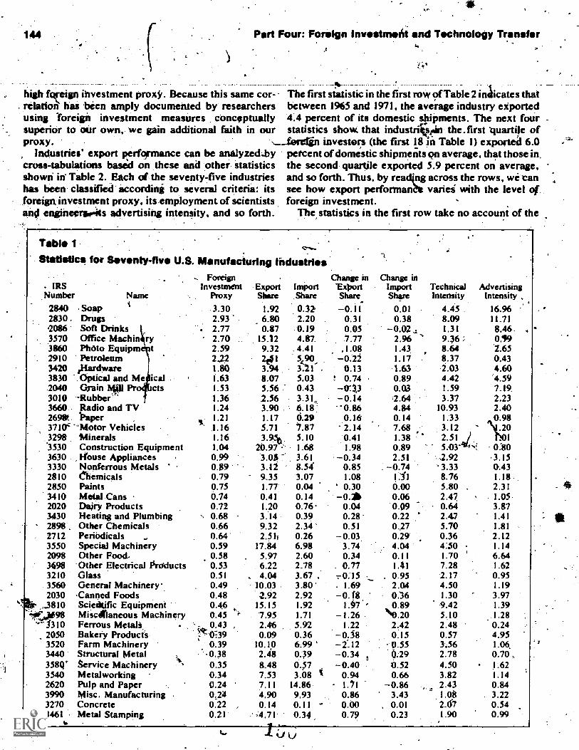
144 Part Four: Foreign investment and Technology Transfer

.. . . '. . . _ _ ,high kreign investment proxy. Because this same cor- The first statistic in the first row of Table 2 indicates that

. relation has been amply documented by researchers between 1965 and 1971, the average industry exportedusing -foreign investment measures conceptually 4.4 percent of its domestic shipments. The next four -

superior to our own, we gain additional faith in our statistics show that industrir the.first quartile ofproxy. investors (the first 1.8 in Table 1) exported 6.0

Industries' export Rerformance can be analyzed .by percent of domestic shipments on average, that those in,cross-tabulations based on these and other statistics the second quartile exported 5.9 percent on average,shown in Table 2. Each of the seventy-five industries and so forth. Thus, by reading across the rows, we can .4

has been classified according to several criteria: its see how export performanbt varies with the level offoreign: investment proxy, its employment of scientists foreign investment.and engineereeits advertising intensity, and so forth. The statistics in the first row take no account of the

Table 1

Statistics for Seventy-five U.S. Manufacturing Industries

- IRSNumber Name

ForeignInvestment

ProxyExport ImportShare ,Share

change inExportShare

Change inImportShare

2840 SoaP 3.30 1.92 0.32' -0.1f 0.012830 . Drugs 2.93 6.80 2.20 0.31 0.382086 Soft Drinks . 2.77 0.87 0.19 0.05 -0.02,3570 Office Machin ry 2.70 15.12 4.87. 7.77 2.963860 Photo Equipm t 2.59 9.32 .4.41 1.08 1.432910 Petroleum 2.22 201 5(90 -0.21 1.173420 tHardware 1.80 3.94 3:21" . 0.13 1.633830 Optical and Me ical 1.63 8.07 5.03 .! 0.74 0.892040 Gjain 11 Pr cts 1.53 5.56 0.43 -0:1,3 0.033010 -Rubber'' 1.36 2.56 3.31,, -0.14 2.643660 Radio and TV 1.24 3.90 6.18 -0.86 4.84269W Paper 1.21 1.17 6.29 0.1.6 0.143710'; 'Motor Vehicles ,1.16 5.71 41.87 2.14 7.68329 Minerals 1.16 3.950 5.10 0.41 1.38'3530 Construction Equipment 1.04 20.97 .-- 1.68 1.98 0.893630 House Appliances 0.99 '3.0B 3.61 -0.34 2.513330 Nonferrous Metals 0.89 3.12 8.54 0.85 -0.742810 Chemicals 0.79 9.35 3.07 1.08 1:312850 Paints 0.75 1.77 0.04 ' 0.30 0.003410 Metal Cans 0.74 0.41 0.14 -O.* 0.062020 Dairy Products 0.72 1.20 0.76. 0.04 0.093430 Heating and Plumbing 0.68 3.14 0.39 0.28` 0.222898 . Other Chemicals 0.66 9.32 2.34 0.51 0.272712 Periodicals 0.64 2.51e 0.26 -0.03 0.2935502098

Special MachineryOther Food..

0.590.58

17.84 6.98. 5.97 2.60

3.740.34

_. 4.04

0.113698 Other Electrical Products 0.53 6.22 2.78 . 0.77 1,413210 Glass 0.51 , 4.04 3.67 . 0.15 ._ . 0.953560 General Machinery- 0.49 10.03 3.80' - 1.69 2.042030 .Canned Foods 0.48 2.92 2.92 -0. fil 0.'36

,..3810 Sciatific Equipment 0.46 15.15 1.92 1.97 0.89,698 Miscellaneous Machinery 0.45 a- 7.95 1.71 -1.26 NO.20'' 3310 Ferrous Metalt. ,.._ 0.43 2.46 5.92 1.22 2.42

2050 Bakery Product's 7'0:39 0.09 0.36 -0.38 0.153520 Farm Machinery 0.39 10.10 6.99' -2112 0.553440 Structural Metal .0.38 2.48 0.39 -0.34 6.29358Q' Service Machinery 0.35 8.48 0.57 -0.40 0.523540 Metalworking 0.34 7.53 3.08 1 0.94 0.662620 Pulp and Paper 0.24 7.11 14.86 - 1.71 -0.863990 Misc. Manufacturing 0.24 4.90 9.93 0.86 3.433270 Concrete 0.22 , 0.14 0.11 - 0.00 , 0.013461 Metal Stamping 0.21 4.71 0.34 0.79 0.23

Technical AdvertisingIntensity Intensity

4.45 16.968.09 11.711.31 8.46- .9.36 0.198.64 2.658.37 0.432.03 4.604.42 '4.591.59 7.19,3.37 2.23

10.93 2.401.33 0.983.12 "'

2.511/ 1

5.03' 4.4. 0:80.2.92 '3.15

`3.33 0.438.76 1.185.80 2.312.47 1.050.64 3.872.47 1.415.70 1.810.36 2.124:50 1.141.70 6.647.28 1.622.17 0.954.50 1.191.30 3.979.42 1.395.10 1.282.48 0.240.57 4.953.56 1.06.2.78 0.704.50 1.623.82 1.142.43 0.841.08 3.222.67 0.541.90 0.99

cJIV

'

,St

I .

v The Impact of American Investments Abroad on U.S.Exports, Imports, and Employment

145

Table 1 Continued

IRSNumber Name

ForeignInvestment

ProxyExport.Share

ImportShare

Change inExportShare

Change inImportShare

TechnicalIntensity

AdvertisingIntensity

2711 Newspapers 0.19 0.05 0.08 r 0.00 0.04 0.08 0.453870 Watches 0.19 1.55 17.44 '0.22 2.09 2.38 6.892998 Other Petroleum 0.19 14.85 ,, 0.08 -0.05 0.07 3.89 1.333240 Cement 0.18 0,32 1.72 -0.08 1.13 2.07 0.16

100 Tobacco 0.18 3.16 0.21 0.84 0.15 1.41 .. 6.92.2715 Books 0.17 3.63 2.06 0.46 0.28 0.36 3.683662 -4Electronics. : 0.17 7.41 .2.99 5.38 1.86 7.28 1.003798 Other Transportation

Equipment0.16 3.26 7.06 -1.04 3.96 1.95 \ 0.68

2410 Logging 0.15 7.06 9.73; 2.63 1.88 0.38 0.292310 Men's Clothing 0.14 0.80 3.29 0.28 2.25 0.21 1.923930 Ordnance 0.13 12.29 1.84 -4.64 Q.38 14.72 1.673720 Planes 0.13 10.67 1.31 6.18 0.26 14.63 0.283498. Miscellaneous Fabricated 0.12 4.65 3.65 0.39 1.33 2.47 1.00

Metals'2084 Liquors ' 0.12 0.88 27.31 -0.08 2.66 1.31 3.722228 Weaving 0.11 2.86 4.65 0.11 0.92 0.92 ,.0.712798 Printing 0.10 0.66 0.27 -0.25 1.12 0.36 0.882060 Sugar 0.09 0.34 26.89 0.09 .72 2.13 0.532430 Plywood 0.09 0.81 6.03 0.28 0.77 0.46 . 0,683450 Screws 0.09 2.18 3.19 0.59 1.64 2.05 0.72,2010 Meat 0.08 1.55 3.75 -0.07 0.94 0.58 2.183140 Footwear 0.08 0.28 9.24 -0.02 9.16 0.28 2.55.1:2398 MiscellaneouS Textiles 0.07 2.35 1.08 -0.97 0.13 0.46 1.092298 Other Textiles 0.07 2.02, 7.45 -0.17' -1.74 0.96 0.832250 ?Knitting Mills 0.06 '0.74 4.15 -0.04 2.60 0.33 1.6821182 Beer 0.06 0.18 0.9,7 -0.07 -0.02 1.31 9.682330 Women's Clothing . 0.05 0.51 3.45 0.03 2.25 0.21 1.972590 Other Furniture 0.14 -0.81 1.83 0.05 1.24 0.65 1.493098 Plastic Products 0.04 2.25 2.21 1.14 0.93 2.35 1.222510 House Furniture 0.04 0.43 1.83 -0.11 1.24 0.65 2.34 *2498 Other Wood 0.02 1.41 4.99 0.09 ' 0.82 0.67. 0.953198 Other Leather 0.01 2.65 10.06 0.12 3.72 0.69 l'ar 2.252380 Other Apparel 0.01 0.83 7.96 -0.06, 3.43 0.21 1.733730 Ships and Boats

.0:01 2.30 0.90 -1.26 0.71 441 .. 0.85,

Sources of data are described in the Statistical Appendix to chapter 3 of C. Fred. Bergston, Thomas Horst, and Theodore Moran,American Multinationals and American interests, Brookings Institution, forthcoming.

The foreign investment proxy is an industry's foreign dividends and tax credits as a percentage of its firms' total assets, the percentagebeing averaged over the years 1965-71.

The export share is the industry's exports as a percentage of domestic shipments averaged over the years 1965-71.The import share is U.S. imports as a percintage of comparable domestic shipments averaged over the years 1965-71.The growth of exports is measured by the difference between the ratio of exports to domestic shipments averaged:over the years

1969-71, and the comparable ratio averaged over, the years'1963 -67. , . ,.

The growl!) of imports is the difference between the ratio of U.S. imports to cornagrable domestic shipments averagedover the years1 969'-71 and the comparable ratio averaged over the years 1965-67. . ,

Technical-intensity is measured by the employment ofseientists antl engineers as a percentage of total industry. employment in 1970.Advertising intensity is measured by advertising expenditures asa percentage of total industry assets averaged over the seven yfars

1965-71. .

technological intensity or other Charaoteristics of the the second quartile; and so forth. Thus, by reading:tipindustries. Accordingly, the second and third rows con- and down the colunins, we can see roughly how exporttrast the export. performance of high- and low- ,..rformance varies ,with the characarisciis of the intechnology industries. Across °the hoard, the high- ustries, holding.the foreign_ lZvel inoretechnologyindus s exported 8.1 peecent of domestic less constant. 'G.:.

iPmspts, and lo -tecpnology industries averaged Several features of TaErle 2 are striking. U.S. eik)artIy 2 percent; se Ifigh-technology induStries that performanee was clearly stronger in the high -

-quartile-of-foreign-investora-ex :-.- technologyPorted 7.6 perce compared to 9.7 percent for those in t/1 former averaged exports equal to 8.1 pernt of

"1Co

.4

146 Part Four:, Foreign Investment and Technology Transfer

Table 2Crops-Tabulation of Industries' Average Export Performance, 1965-71, Accords to ForeignInvestment Level and Other Industry CharactOrlatics

All 1st QuartileForeign Investment

2nd Quartile 3rd QuartileAll 4.4 6.0 5.9 4.3,High technology 7.6 9.7 7.8Low technology

.133.5 2.5 3.0

High advertising '3.1 4.6 2.4 2.8Low advertising 5.0 7.7 7.5 4.8Machinery 10.6 18.0 11.0 8.4Non mac hi n ery 3.0 4.5 3.6 4.1High education 6.5 6.6 7.9 6.2Low education 2.2 3.1 2.5 2.9High earnings 5.7 6.9 6.4 5.0Low earnings 2.4 4.3 3.0 3.0High,experience 4.5 4.1 5.2 5.1Low experience 4.2 8.9 6.7 3.3High skill group 1 7.5 8.7 8.8 6.1Low skill group. I 2.6 3.3 3.3 3.2High skill group 2 4.6 5.8 2.3Low skill group 2 4.2 6.1 47,13

High skill group .3 6.9 7.4 8.94i., skill group 3 2.6 4.3 2.5 3.6High' skill group 4 3.1 5.6 3.5 1.7'

Low skill group 4 5.0 6.2 7.0 6.1High skill group 5 4.9 7.6 6.Q 4.0Low skill, group*5High skill group 6

3.93.0

5.23.4

5.8- 4.3

4.74.3

Low skill group.6 5.7 7,7 7.1 4.2 .igh skill group 7 2.9 3.4 4. 2.8Mow skill group 7 5.0. 6.7 6. 5.1White 6.0 6.9 6.7 5.7Nonwhite 2.1 3.7 2.9 2.3Male 6.8 5.8 5.0Female 3.4 6.1 3.1Unionized 4.4 3.8 4.4 5.5Non-unionized 4.3 7.8 7.0 3.2

A

4t1; Quartile

1.3

2.31.3

1.01.4

?.31.2

1.01.4

1.3. 1.3

1.4'1.31.51.3

1.81.51.4

'1.3

1.5.3

1.31.41.1-

0.91.5

1.31.3

1.111

domestic shipments and the latter 10.6 percent. These°industries employ proportionately higher numbers of

well- educated;, highly skilled, and highly experiencedWorkers.

. Although these charicteristics of U.S. industrieswith.strong exhort records have been noted by metier-

. -ousauthors, Table 2 alio reveals the sepatate contribu-tion of foreign iiivetting to eiporting. As we read acrossthe rows of Table 2, we can see the marked difference-between industries.iii the top three quartiles of foreigninvestors and those its ,the bottom ,quartile. Industriesyitti little or.,nO foreign investment export only 1.3

rceill Of domestic shipments; and that poor perfor-..

duCation.or among Ihe /ago,- force, or'any other, .

hc).

industry attribute we have measured. It apilears that amodest amount of foreign investment, perhaps in the'form of overseas sOes and service affiliates, may be aprerequisite to exporting. But dace we move into thetop athree quartile§ of-industries, further _incleases inforeign inviitmeat are 'not matched by coMparable in!creases in U.S. exports.

The relationship between foreign investment andU.S1 imports, which"' s analyzed in Tible 3, is somewhltthe opposite of that with .S. exports. Imports arehigher in industries marked by lois; foreign investment,low technology, low education, low annual earnings; a

deers, a percentage of bperatives,*na.highlow

dof professional, technical 'and kindrid

percentage of nonwhite workers. This pattern kproba-..,,

-0

The Impact of American invastmants Abroad on.U.S.Exports,- imports, and Employment

147

Table 3Cross - Tabulation of industries' Average import Performance, 1965-71, recording to ForeignInvestment Level and Other Industry Characteristics

AllHi technologfhLo technologyHigh dvertisingLow advertisingMachineryNonmachineryHigh educationLow education}Ash' earningsLow earningsHigh eiperience.Low experienceHigh skill group ILow skill group.'High skill group 2Low skill group 2 .

Hig l? skill gronp.3Lo skill group 3High skill group 4Low skill group 4High skill mob Se"-Low skillgtoup 5High skiff group 6Low group 6High skill group 7Low skill group 7WhiteNonwhiteMaleFemaleUnionizedNon-unionized

All 1st QuartileForeign Investment

2nd Quartile 3rd Quartile4.3 3.7 2.3 5.6.3.2 4.1 3.0 1.94.8 3.0 1.7 7.04.6 2.9 1.2 11.44.1 4.7 2.9 3.63.0 3.3 .3.0 3.34.5 3.7 '2.1 6.33.8 3.8 2.7 6.7

.4.7 2.9 1.8 4.93.5 4.0 2.4 5.05.4 2.9 2.0

9 4.2 2.72.9 2.1 8.9

2.5 3.7 2.3 1.6'5.3 3.6 2.4 8.03.9 - 2.7 .2.0 5.64.5 4.3 ) .2.8 5.73'.4 3.41 . , 2..7 4.549 4.0 1.9 6.53.7 1.9 1.1 $.24.5 4.8 2.9 6.03.6 5.0 2.5 4.74.8 . 3.0 2.1 6:94.7 4.6 2.5 6.6.3.8 3.1 2.2 4.95.9 3.6 3.0 7.73.6 3.7. 2.0 4.43.5 3.8 2.25.2 3.4 3.0

.5.06.6

4.4 4.1 2.3 5.94.1 2.9. 2.4( 5.14.3 5.1 2.9 4:74.2 "-2.5 2.0 6.5

,4th Quartile

5.30.95.65.25.4.0.9566.76.21.36.4

11.34.20.6-5.97.14.7 .

.7

8.04.61.66.64.96.48.54.23.7

5.75.65:1

3.55.5

reflects more the cheap-labor or natural-reSourcecharacteristics of certain ndustriei (e.g., pulp andpaper,4watches and clocks, liquors, sugar, furniture,pnd leatOerd3ods) than the 3bsence of foreign invest-ment per se, the evidence will not support any coficla-sion that foreign investment has led to highgr than aver-

.. age tiworts.Looting only at the levels of U.S. exports and

ports and their relationship to foreign investment; onemight wonder why the AFL-CIOhas been so upset. The,reasons become more appgent when we turn to Tables

d 5, which show how U.S.. exporti and imports as antage of domestic shipments increased between

1965-67 and 1969-71. According to our way of.

(ST,*

measuring export or import growth, if one or the otnerincreased from say, 5 percent to 6,percent of domesticshienents, we would show an increase of one percen-tage point. According to Table 4, the average industryincreased its exports by only One half of a percentagepoint between 1965-67 and_1969-71. As for variationsaround this low average, weSee that thtraditionallystrong export industries --- the high-technology indfis-trieS and the machinery manufacturers showed thelargest increases. The low-technology industries barelymaintained their low export ratios over this seven -yearinterval. Finally, we might note that here, as before,industries in the lowett quartile of foreign investors hadslower-growing experts than di those in top three.'

r,

146 Part Four: Foreign Investment and Techriplogy. Transfer

Table 4Cross- tabulation of Industries' Export Growth, 1965 -67 to 1969-71, According to ForeignInvestment Level and Other Industry Characteristics

All

All. 0.50High technology 103Low technology 0.22High advertising 0.19Low advertising 0.67

''-Machinery 1.46Nonmachinery 0.30High education Q.79 .Low education 0.21High earnings 0.74

.Low earnings 0.17

.kligh experienceexperience

0.500.50

High .skill group ILow skill group 1

1.(20.16

High skill group 2 0.64Low skill group 2 4141High group 3, 0.89Low skill group 3 0.25High skill group 4 Q.45towikill group 4 0.53High skill group 5 0.54Low skill group 5 0.47High skill,group 6 0.30Low skill group 6 0.70High skill group 7 0.29 11111Low skill group 7 0.59White 0.68Nonwhite 0.26Male 0.54Female 0:44Unionized 0.44Non-unionized 0.34

.1st Quartile

0.82,I.140.320.231.564,880.310.940.241.160.130.331.601.500.141.170.601.270.251.230.56,0.710.870.221.200.12.1.11

0:970.43

.05.35

0.191.32

Foreijrr Invfitment2nd Quartile

0.320.58 .

0.090.070.441.09

- 0.030.420.150.380.040.230.430.84

- 0.120,78

-0.190.520.110.19.0.380.230.450.160.67

-0.020.330.320.340.260.45

-0.030.58

3rd Quartile 4th Quartile

8 0.111.56 1.27.50 .. 6.04

0.46 -0.030.89 0.16.

0.36 1.270.89 0.041.25 0.310.44 0.070.92 0.380.54 .031.05 0.200.48 0.091.18 0.510.55 0.060.26 0.201.16 0.071.05 0.170.58 0.100,24 -0.081.17 0.150.87 0.310.65 . 0.031.31 0.030.39, 0.330.36 0.140.82 0.120.95 0.360.55'

010.56 0.1.15 -0.011.11 0.260.48 0.09

quartiles. But, generally speaking; the relationship be-Omen foreign ,investmer4 levels and export growth wasvrandom.

Ttible 5 examines the growth in U.4ermports between1965 -67 and,1969-75. Imports wire growing muchfaster thanittpotts: the average increase foriinportswas 1.30 percentitge points, or two and a half times thecomparable increase in exports. :As Table 5 makesabundantly clear; thli growth. in U.S. imports was notfOcused in a few %isolated industries. .Virtually .every,type of industry witnessed an increase in the importshare.° e to two percen e points. Perhaps the mostInteres att.= of yari 'on around this

for eighteen ind triei1,1

foreign inve ors (see the secOnd'iolunm of Table 5).Within this group of investors, imports were growingespecially quickly in industries whose workers hadmore edUcation, higher earnings, and more experienceand were operativei, not laborers, nonwhite and: co-vered by a union cOittract. ;

Of course, our statistics do not indicate, whetherforeign investme was the cause of this rapid growth ofimports. Looking back to Table 1, we can see that theindustries in question were Motor vehicles, radio;. tele-,Vision and communications equipment, Office machin.ery, and rubber produCtsi Although one would have toundertake' detailed 'industry Studies to deterniine thero fforeiga;invi,tstnentkin promoting imports in these

4.1'

The impaci of American. Investments Abroad on'U.S. 149Exports, Imports, and Employment

Table 5Cross-Tabulation of industries' Import Growth, 1965-67 to 1969-71, According to ForeignInvestment Level and Other Industry Characteristics

AllAll' 1.30High technology 1.14Lowtechnology 1.39High advertising .50Low adVertising .20Mac hi ne ty -1 .46Nonmachinery .27High education .14Low eduCation .47High earningsLow earnings .62High experience .10Low experience .47High skill group I .04Low skill group I .45High skill group 2 0.90Low skill group 2 .57High skill group 3 1.16Low skill group 3 1.40High skill group 4, 0.68Low skill'group 4 .62High skill group 5 1.12Low skilrtroup 5 1.45High skill group 6 .51Low skill group 6 1,10High skill group 7 0.69Low skill group 7 1.56White 1.20Nonwhite 1.44Male 1.17Female 1.51Unionized 1.25Non-unionized 1.33

1st Quartile.62.44.91.44.85

.58

.74

.05

.88'

.10

.85

.26.55.70

0.782.161.441.850.632.251.991.442.181.27

.7

. 5

.0434

.122.440.97

Notes to Tables 2 throughk5Sources of statistics are given in the statistical appendix to

Chapter 3 of C. Fred Bergsten, Thomas Horst, find Theodore H.Moran, op. cit.

The cross-tabulatiog are based on industries classified accord-ing to the following criteria:

The first quartile of foreign investors are those ranked fromone to eighteen4 Table I; the second quartile are thoseranked from nineteen to.thirty-seven, and so forth.

a "High technology'; were those with scientists and engineers(a subs of skill group I) in excess' of 3.2 percent oftotal emp oyment in 1970."High ad ertising" were.thoso industries with aciv singexpenditures equal to 2 percent or more of total assets a r-aged over the years 1%5-71."Machinery" industries were those judged by the author t ,

be manufacturing durable capital' equipment for sale to otherproducers::.,"Hi education" were diode series in which the medianyear( of education of employees was greater than twelve in1970."High .dxperience" were those industries in which morethan 55 percent of the employees were between 30 and 54years old in 1970."High earnings" were those induitries whose employeeeS'median yearly earnings, excered $7,000 in 1970.

tiP

Foreign Investment2nd Quartile 3rd Quartil 4th Quartile

0.79 1.15 1.671.14 0.65 0.710.50 1.33' 1:720.17 1.73 3.011.07 0.95 1.181.52 1.32 0.71 '0.45 1.11 1.72

'0.94 0.66 0.270.52 1.51 1.930.89 0.670.22 1.980.71 0.46 1.770.88 1.92 1.651.08 0.51 0.420.5.3 1.53 1.810.86 1.04 .00.920.71 1.24 1.931.03 1.06 0.880.52 1.22 1.760.16 0.98 0.941.08 1.28 1.860.98 0.83 0.990.52 1.59 1.900.47. 1.31 1.89-1.01 1.04 1.040.71 0.72 1.050.82 ,1.40 1.890.79 0.93 2.960.77 1.45 1.320.84 0.98 1.120.67 1.45 2.150.7 '160 1.290.81. 1.71

"High skill group 1" re those industries in which morethan 8.8 pergigke...f all e ployees.Wereprofessional, techni-cal, and kin rs in 1970."High skill 2" were those in Which ..more than 5.8percent of all employees were managers and kindred workersin 1970. .

st,"High skill group 3" were those in wifich more than 12.5 per-cent of employees were clericaland kindred workers is 1970.'.'High skill group 4" Were those in which more than 3.0percent of employees were; sales workers in 1970..

,",High skill group 5" were thoie in which more than 19:2percent of employees were craftsmet foremen, and kindredworkers in 1970.,"High skill group 6" were Otiose in which more than 43.2 per-,cent of employes. wese-ependlts 0.' "-.

ch"High skill group7" were those n 5:0 per-cent of employees werelaborers in 1970."Nowhite" industries were' thorie in which more than 9.5percelit of employees were - nonwhite in 1970."Female" indukries were those in which more than 28.1 per-cent of all employees were female in 1970."Unionized'; inthistries were those in which more than 70percent of all-employees. work in plants, in which'at leasthalf of all in .ncluction workers were covered by union con-tracts.

Pkrt Four: Foreign Investment and Technology Transfer

industties, casual evidence suggests that the relation-ship between foreign investment and importing variesfrom industry to industry. A substantial portion of theincreased importof motor vehicles did come front theCanadian subsidiaries oft -OkThree U.S. automobileproducers and were induced b he tariff recItctions ofthe Canadian - American Automotive Pact of/ 965. Thiswould seem to be a classic case of the fidestitution offoreign for domestic investment and employment in-duced by a Aariff reduCtion. One should not ignore, ofcourse, the growing automotive exports of Japaneseand German companies to the Unitgd States. In radio,teleVision, and communications equipment, the growthof imports was probably due to the growing competi-tiveness- of Japairse . producers (such :as Sony andPanasonic) and the induced export of production andjob& by- U.S. companies to the -Far East. In this in-stance, U.S. investments abroad appeik to be more"defensive" than they were in the case of automotivemiiports. Finally, the growth of U.S. imports of rubber

,tOroducts probably consisted largely of radial tires fromEuropean producers, and the correlation kith U.S. in-vestments abroad may well be spitrious. We must bewary of drtwing any simplistic conclusions from thesesorts of statistics.

Summary and Conclusion

Our analySi's has focused on the microe it rela-tionship between U.S .iiyestMents a U.S.exports, imports, and employment. Although foreigninvestment niaY have important effects on the generalequilibrium of the world economy, the public policydebate in the United States has focused largely,on mic-roeconoinic issues. The labor unions have charged thatU.S. Multinational firms displace U.S. exports, aug-ment U.S. imports, and in either instance export U.S.jobs. The multinationals have emphasized the positiveeffects di foreign investment on U.S. exports andemployment and aimed that when foreign investmentsubstitutes for domestic, the substitution is induced by

I, higher foreign tariffs, the growing competitiveness offoreign producers, and other econfornic &dors that'leave them little choice but to invest oversea.

Microeconomic theory inTcates that these views arenot nelliessarily contradictory. -Even if one regardsforeign demand for U.S. produets as fixed, a variety,ofeconomic factors tariffs, wage rate differentials, theSize of the foreign market, and the firm's own subjective

sment of the costs and benefits of investing over-seas influence, the choice between domestic andforeign production. In some cases exporting may be a

0

"0viable alternative (though, presumably, a less profitableone in the long run) to overseas production, and in otherinstances it is not.

But one should not base policy analysis on the as-sumption that foreign demand for ,U.S. products isfixed. A multinational's foreign activities include a widerange of activities gathering market information,sales, servicing and distribution, adapting products tolocal market specifications aimed at expanding thesize of the foreign market rather than merely relocatingproduction. This point is criticaljn two respects: under-standing why there is no clear statistical tendency forU.S. exports to fall or imports to rise as foreign invest-ment expantand why 'broad restrictions on foreigninvestment such as the balance-of-paymentsguidelines or proposed changes in U.S. taxation offoreign investment income .-- might havean ambiguouseffect on U.S. production and employment.

To predict the impact of a change in U.S. policyrequires a fully specified Model of foreign trade andinvestment behavior. Although many of the factors af-fecting the location of production can be quantified,those influencing,the size of the foreign market cannot.Our statistical analysis focused on the de facto relation-ship between U.S. investments abroad and U.S. ex-ports and imports. While one cannot infer from this'analysis what would have happened if U.S. policy weredifferent from what it was, one might be able to identifythe relative importance of substitutional and com-plementary factois encouraging American firms to in -'vest overseas. A consistent tendency of exports to fallor imports to rise as foreign investment expands mightbe evidence of the historical importance of substitu-tional effects, and the opposite statistical felationshipwould underscore the importance of complementaryforces. If both effects are -weak or of roughly equalhistorical significance, the statistical relationship will.

, 41 ..+,.: ..be haphkard. i..,'

We have exathined differences,

among seventy-fivemanufacturing industries' average export and importlevels from 1965 to 1971 and the growth ijt these levelsover the same period. On the wpole we have failed -touncover any consistently strong statistical relationship,positive or negative, between U.S. investments aband any of our measures of trade performance.though our data and our methodology have obvioflaws, one cannot escape the impression that the mic-roeconomic relationship between international tradeand investment i's complex and/or weak. We do havesome tentative evidence that a modest amount of ovseas rivestment, perhaps in'the form of sales, and er-vice facilities, is a prerequisite to U.S. exporting: WealSo covered some evidence that certain indus es

15S-

The Impact of American Investments Abroscren U.B.Exports, Imports, and Employment

marked by high foreign investment motor vehicles,radio, television and communications equipment, of-fice machinery, and rubber products did experiencefaster than average import growth between 1965 and1971. Without more detailed industry studies, however.,it is impossible to determine the extent to which foreigninvestment was the cause, the effect, or merely a spuri-ous correlate of the growth of imports.. If U.S. foreigninvestment policto be geared more towards protect-ing U.S. employment than it was in the past, then itwould also have to be more selective and discriminatingthan it has traditionally been. Broad and undiscriminat-ing changes in U.S. policy could do more harm thangood.

Literatuiiielted7

1. Frank, Robert H., and Richard T. Freeman. "The pis-,tributional Consequences of Direct Fiveign Investment."Presented at the Conference on the Infact ounternationalTrade and Investment on Employment. Washington,D.C.. December 2 and 3, 1976.

r,

.151 ..

15';'

d.

II

The Distributional ConsequencesOf Direct Foreign InvestmentRobert H. Frank and Richard T. Freeman*

Introduction and Summary

When countries can make adjustments through offset-ting stabiliiation policies, the most important long-runeffect of direct foreign investment (DFI) will be a redis-tribution of income. This report examines the effect ofoverseas investment by U.S. firms on both the short7run level of employment demand and the long-run dis-tribution of incomes within the United States. .

Section l begins with a summary of the findings of ourearlier study [6] of the short- em loyniertt..dernifind

effects of foqign investment. This sec on considers thequestion.of what fraction of'the ove eas markets 'thatare presently served by foreign subsidiaries could havebeen served byexPorting from the United States. Weconclude that, even though sales in these foreign- mar-.kets would shrink by more thanhalf in the event ofa banon 'foreign investment; such a ban would neverthelessbe likely to produce an increase in domestic employ--ment demand. EitiMates of the short-WO employmentdeniand reductions that result from DFI e presentedor the economy's manufacturin ndii. rigs..,

Section 2 presents an extension ese findings, inwhich we have broken down the employment demandeffects of DFI by ,occupation. The' question of whateffect' foreign investments hive on problem- ofbottlenecks in the demand forlabor is then considered.We conclude 'that DFI exacerbates 'such bottlenecksslightly by causing muchlarger redUctions in blue. collarthan in white collar employment demands.'

Section 3 examines the question of hoW long labor .77markets take to adjust to the employment. demand re-

: ductions associated with the overseas activities Of mul-linational subsOiaries. A dynamic simulation model isUsed in thstudy of this question and we conclude that

v1101 paperis based on Robert H. Frank and Richard T. F.pf U.S. Direct Foreign Investment on Domes nem-

," State 1722-4200-30 which was jointly funded by the U.S.t of Labor and the State Department and completed in"Estimating the Distributional Consequences Of-Directvestment,' ILAR J91(60018 which was expected *to bein 1977.t study that makes this point is fin

-1.5

, 15$ ",

almost the entire membership of a cohort of workerswho lose their jobs as a result of these employmentdemand reductions can expect to have been placed innew jobi within a.matter of months.

Taking %cognition of the fact that short -run disloca7tions are PRY6a small -part of theoVerall effect of DFI,section 4 (radettakes an analysis of the long-rim effect ofcapital (Attflows on both the size and se:Imposition ofnationarincome in the' [Anted States. We conclude thatwhen account is taken of the leakage of tax revenuesinto the treasuries of host countries, foreign investmentresults in .a slightly lower, level of equilibrium U.national income. As far the distribution of income' isconcerned, the Principal long-run consequence of DFIappears .to be a moderate shift favoring capital.

1. Home-Foreign Substitution and-theShort -Run Domestic Employment

. Demand Effects of Foreign investment. ,

Estimates of the effect of. DFI on' short-run domesticemployment demands are usually constructed by ag-gregating various positive and negative effects attrib.;uted to the overseas .activities of subsidiaries. Theprincipal negative effect is usually calculated as thefraction of foreign stkbsidtary employment that couldhave been retained 'in the United. States had MNCsattempted,to servefforeign markets by exporting fromdoMestic productiongsites. The main. offset to this ex-pOrt:tlisplacement is an.e,,,xport stimulus effect, which'represents the domestic.employment required to meetforeign sub'sidiaries' 'demands for U.S. exports of in-termediate products.' .

Subsidiary imports from U.S. parents and other U.S.firms account for only a small fraction of subsidiary net

'Other employment stimulating effects that have been mentionedinclude increased employment in domestic MNC headquarters,increased employment associated with export of complementaryMNC,products, and additional domestic employment stimulated in-directly by increased incomes and export demand abroad all ofwhich are likely to be minor in relation to the direct, productionrelated effects on Which we focus. For more detail, on these and re-;ated issues, See [10, 8, 91.' . ,

1134 Part Four: Foreign Investment and Technology Transfer

sales-(4 percent for all industries in 1970), and the pro-cedures used for calculating the magnitude of the exportstimulus effect have according! generated little

researchers. M t of the controversydis-

agreement among reseaover whether th net domestic employment effect ofDFI is positive (negative has focused instead on thecalculation of the export displacement effect. The cen-tral issue in this discussion haS been the question ofwhat MNCs would or could have done had they not un-dertaken foreign investment projects.

-,,

Studies that have produced conclusions of domestic.

job stimulus have usually found that, largely because of.cost advantages in overseas sites, markets now beingserved by foreign subsidiaries of MNCs could not havebeen served by expbrt from the.United States. Thesemarkets would thui have 'been lost entirely to foreigncompetitors had MNCs been prevented from pro6cingoverseas. Studies that identify a major negatife netemployment effect of DFI have fotind that a large frac-tion of overseas markets could have been served byU.S. export s.

.-.

Debate has continued on this issueOargely becausethere has been virtually no hard evidence on the criticalquestion of what the alternatives to subsidiary

areopera-

tions really a for U.S. MNCs. The mostevidence_ concerning alternatives to overs produc-tion currently exists in the form of statistical studies.

. . that associate various forms of domestic and foreignactivity measures. In out recent study [6], we argue thatevidence frit* this sOurce.has been misinterpreted andprovides no real indication of what MNCs -Would haVedone in the absence of a foreign in-vestment alternative.

As a simple illustration, consider the case of an over-seas subsidiary that requires $50 of intermediate inputsfrom its U.S. parent-for each $100 in foreign sales. In thcontext of a growing foreign market, one would obsea positive association between a subsidiary's sales anU.S. exports to the subsidiary. This posi assOcition clearly does not imply, however, that U. xpoto the subsidiary host country would decline ids opertions were prohibited. If U.S. production costs are tmuch higher thin foreign costs and if foreign demand snot highly elastic, U.S. exports could increase substi ally in the event of such a restriction. .

The principal contribution of ouf,. study [ is thedevelopment of a specific analysis .that is c able ofgenerating evidence on the critical counterfa al ques-tion, What would have happened if DFI h: d been pro-hibited. This analysis involves the comparison of theMNC operating under widely different policy regimes.The first places no restrictions on the MNC's overseasactivities, whereas the second denies the MNC theoption of operating foreign subsidiaries. The first re-gime corresponds approxitvately to the present envi-

ronment in which MNCs operate, whereas the second isan essentially hypothetical construct. MNCs operatingunder the first policy regime will, in general, elect toserve foreign markets from foreign production siteS.Under.the second regime MNCs are assumed to sepveforeign markets by exports.

The ratio of MNC employment in the seco egimeto employment in 'the first defines our measu of theextent to which MNC overseas subsidiary emplOymentsubstitutes for or displaces, domestic employment. Atone extreme, if MNC employment is the same underboth cases, the substitution ratio takes the value unity,indicating that employment in overseas subsidiariesdisplaces domestic employment on a one-for-one basis,Alternativ ly, if export from the United States is noteconomic ly viable, the substitution ratio is zero, indi-eating no job displacement. Between these two ex-'tremes th is a full range of-intermediate .cases.

The principal factors that affect thetubstitution ratioare inferred from an economic model of firm behavior.One key factor is the degree of monopoly power evr-cised by the MNC in foreign markets. When thesells a highly standardized product in nearly perfect,competition with many foreign .producers of nearlyidentical, products, market power is low. In this com-petitive situation the higher price -forced tbe,highercosts of producing in the United States will cause the,MNC to lose most or all of its foreign 'market if it is .

constrained to produce at home. Most MNCs are in factfar from perfect competitors. Instead, they tend to belarge, technplogy-intensive organizations which sellhighly- differentiated products; and which, in conse-

. quence, possess substantial market power.In many" instances this may enable the MNC to ab-

sorb higher U.S. production dbas without losing all itsforeign sales. In [6] we describe a procedure wherebythe degree of MNC market Power (specifically the elas-ticity of the demand curve facing the firm) can be esti-mated with information taken from the income State-ments of U.S. multinationals surveyed by the Depart-ment of Commerce.

Another major factor affecting home-foreign sub-stitution is the extent to which the cost of supplyingforeign markets by U.S. exports exceeds the.costs offoreign production. Such cost differences are duelargely to differences in unit labor costs, transport andhandling costs, tariffs, and other similar trade restric-tions.. Using a variety of' data sources, we have con-structed estimates of .tiome to foreign production costratios for major manufacturing industry groups. Thesecost ratio estimates are then combined with demandsensitivity estimatet in a procedure that yields esti-mates of the substitution ratios 'bed above.

Once estimates of these ho ign substitution

The Distributional Contequen2es of Direct Foreign investment

parameters were obtained,',we were able to calculiatethe net employment gain or loss associated with agivenyear' foreign investment. Here we attempted im-provron existing work by explicitly taking into accountnot only DFI- related employment, 'effects in the man-ufacturing sectors of first impact, but also employment

effects'related to changes in the demand for inter-mediate products ,reqUired in industries that investoverseas. Their exclusion would result in.an under-estimation of the ifirect effect on U.S. employment. InPrimary metals, for example, shifting SI Million worthof activity overseas has a relatively small direct impacton domestic employment in that .in try, beciuse oflabor's relatively small share in indditry value added.Yet thaotal impact on U.S. emploYnient is really muchlarger because a reduction of domestic activity in themetals industry? .means that sectors providing inter-mediate inputs (many of which are highly labor-intensive) wit experience corresponding declines.There are analogous secondary effects augment'domestic employment, which need to be taken intoaccount in estimating the export stimulus effects of

4 DFI. - .Tar trace out both priruiary and secondary effects we

used', awaggregated version of the Bureau of Laboi-Statiitics 1963 input-output table for the U.S. economy,updated to 1970, together with corresponding capital-output and employment-output ratios. The employ-

Me specific expression employed for estimating the substitutionparameter is a (MCFIMCH) , where MCF is marginal productioncosts in the foreign market. MCH is the cost of landing an additionalunit of domestically produced output in the foreign market. and 71 isthe price elasticity of demand in the foreign "pt.

i

155

ment gain or loss associated with a given year's realforeign investment as measured by Department of,.Commerte estimates of property, plant, and equipment,,expenditures of U.S. wholly owned subsidiaries wasfound by-first computing the full (i.e., the primary andsecondary) "export displacement" effect associatedwith these activities, modified by the appropriate sub-stitution factor for each industrial sector. This job lossfigure was then offset by a similar calculation of theexport stimulus effect from the addition of y.s. exportrequirements of U.S forelgisubsidiaries.4

Our estimates.of the substitution parameters and netemployment demand reductions attributable to the 1970flow of DF1 are reported for several large manufactur-ing,iodustries in Table 1. Column 1 of Table 1 reportsourbest estimates of the industry substitution param-eter!' al . Column 2 lists DFI flows (property, plant,and equipment expenditures) by industry for the year.1970. Column 3 reports .the net employment demandeffects by industry basedon the substitution paf.ameterentries of column 1.

Because many of the essential inputs to the calcula-tions were inferred from somewhat incomplete data,i,and the estimation procedure itself is founded oft anumber of strong assumptions, we emphasize that thefigures in column 3 of TIsble I are, at best, only indica-tive of the scale it'd distrib,ution of DFI-related job loss.In particular, the results above are quite sensitive to thevalues of the home-foreign substitution factors; fur,.t.,

'Estimates (idle U.S. export share in total subsidiary intermediate 1input requirements were based on the 1970 Department of Commercespecial survey or U.S. multinationals.

rTable1Substitution Ratio, and Net Emploiment Demand Effects for 1970 DFI Vector

1

Industry Name Substitutionst. parameter a*

2DFI

(S1000)

3 4 5Net Employment Demand Change'

cr') (0 cer2) (o. 201Food 0.368 266,879 2.644 15.173Chemicals 0.441 882;445 14,944 5,833 33,056Primary and fabricated metals 0.245 336,535 8.854 5.063 36,711Electrical machinery 0.345 359,044 17,620 . 5.017 42.806

,, Nonelectrical machinery 0.358 1,242,846 446,905 16,636 98.283Transportation equipment 0.191 782.366 310 22.271Rubber . 0.463 123,594 5,062 1,197 12,790aPaper 0.463 320,929.. 7,321 2.549 16,564Other manufaZturing (. 0.402 365,534 4,439 2,865 19,041Nonmanufacturing

(indirect only)5.311.557 44.278 6.072 134,937

TOTAL 9,991,729 160,377 19,574 441";706'Change in -number of jobs; minus indicates jOb

tee Part Fa*: Foreign iniastinanf and,Tachnology.Transfarz.

t.

thermore, the estimation of these &Oars was based ondata that stands out lathe least reliable in the study: Forthese reasons we have calculated two additional sets ofnet employment effects, one based on substitutionparameters set at half the values of our best estimates,

. another based on substitution parameters Set at twicec those, values, These alternative employment .demand

estimaps are reported in columns 4 and 5 of Table I .

Even for the estimates based oh the low values of thesubstitution parameters (column 4), the export dis-placement effect was seen to dominate the exportstimulus effect, resulting' in a net employment demandreduction for each industry,

We have also computed break-even values for thesubstitution factors; i.e., values at which the exportdisplacement effect is Alpaca)/ offset by job gains as-sociated with new exports, and at which the net job lossis zero. We found the average break-even value to beapprdximately equal to 0,10. This means that for thereto be do bet' loss of production jobs, for eVery 100 jobscreated 'overseas by U.S. subsidiaries, on average nomore than ten U.S. jobs must be displaced in the sameindustry. Since all of the substitution factors that wecalculated Were well above this figure (the averagevalue was, in fact, approximately 0.35), there is clearly'a strong presumption that, even allowing for consider-able deficiencies in the data, the net impact offoreigninvestment by U.S. multinationals is a substantialdomestic employment demand reduction.

2. The Effect of DFI on the OccupationalComposition of Domestic EmploymentSemand

In order to determine whether foreign investmentproves or worsens the problem of bottlenecks in thelabor market, it is necessary first toestablish a criterionby which to measure imbalances in the composition of

_demand kir labor. The theoretical concept that under-,lies this criterion is the model of unemployment disper-.

sion and wage inflation introduced by Lipsey [101. Lip-sey's model considers a group df identical labor sub-markets and concludes that wage inflationary pressuresare :minimized for a given-aggregate unemployment ratewhen the unemployment 'rates in all the submarkets areequal. Lipsey's model has been generalized for thecaseof submarkets that have different wage levels (see [5)), amore realistic description of submarkets defined byskill category. Here the conclusion is that the leastinflationary distribution of demands calls for relativelyhigh unemployment rates at least temporarily in thosestibmaskets with relatively high wage rates and vice-versa. ° In terms of skill categories, a balanced composi-tion of demand is one in which more skilled,' high wage,groups have high unemployment rates and less skilled,low wage, groups have low unemployment rates.° Sincethe present distribution of unemployment across skillcategories is precisely the reverse of the optimal dis-tribution more skilled groups now have the lowestunemployment rates the, generalized dispersionmodel reinforces a basic conclusion of the Lipseymodel: any shift in the composition of demand in thedirection of greater equality across skill categoriescon-stitutes a clear improvement over the composition ofdemand presently observed in the United States,

Employing this criterion, we have attempted to an-swer the question of whether 13F1 improves or worsensthe problem of structural imbalances in the occupa-tional distribution of employment 'demand. To do this

'With two submarket's the inflation minimizing distribution ofem-ployment rates must satisfy

e w 2 g (e2)

2 /4'1 g1'

where .wilrlhe wage rate, ei the employment rate, and gi' (et). theslope of the Phillips curve for the ith market. See (5. p. 244).

The submirkets with the higher wage rate must have a higher un-employment rate if wage inflation is to be minimized because of thelarger than proportional contribution of the high wage submarket tothe overall wage index. A given increase in unemployment is worthjust as much in the low wage submarket as it would be in the highwage submarkeLhut produces a smaller boost in the aggregateof wage irdlatiM when taken in the low wage submarket.

Table 2

Employment Domand Reductions from 1970 DFI Vector, by Occupational Category (four-order)

.11 2 3 4Occupationalr Employment Demand Employment Demand Reduction 1970 UnemploymentCategory . Reduction (1000s) (10000 Ratio (1 +2)x100 Rate (percent)White collar 62.2 37,997 0.164 2.8Blue collar 185.4 27,791 0.307 6.2Service 8:6 9,712 0.088 5.3Farm workers 4.2 3,124 0.134 2.6

^

1The Distributional Consequent'', of Direct Foreign investment

we have employed data from the 1970 National Industry. Occupational Employment Matrix [161 in conjunction

with our estimates of .industry substitution ratios incarrying out an input-output calculation of the typedescribed in the previous section.' The results of thiicalculation for the:1970 flow of DFI are reproduced inTable 2 for a four.order breakdown of OcFuPationalcategories. , '

Column 1 of Table 2 lists thiggitimated employmentdemand reductions by occupeonal category. Cplumn2 lists total 1970 employment' in these. categofies. Incolumn 3 we have shown emplilyment demand reduc-tion ratios'by occupational category, calculated as 100times the ratio of occupational employment demandreduction to total occupational employment. Columnshows the 1970 occupational unemployment rates.

Most of the employment demand reductions are con-centrated on white and blue collar workers, with ser-vice and farm workers experiencing only comparativelyminor effects. Among the former groups, blue collarworkers are far and away the hardfst hit. In terms of ourcriterion for a balanced composition of demand, theentries of Table 2 suggest strongly that the foreign in-vestment flows of 1970 have exacerbated the problemof structural bottlenecks in the labor market.'

'The short-run impact study produced a vector of loss effectsby industry, WI]. To find the effect of this job loss by skill categor-ies, this vector was pre-multiplied by a matrix (SO, where each entrymeasured the percentage of 1970 employment in industry I in skillclass J.

'A very similar pattern of results emerged when the same calcWadens were carried out for the remaining years in the 1966-73 period-for which we have data.

S157

`,.e collar" and "white collar" are extremely ag-e occupational categories and our conclusions

modified if employment demand reductionswere concentrated' on high wage groups within eachcategory. In order to investigate this possibility, wehave repeated the original calculations in the context ofa nine-order occupational breakdown. These resultsappear in Table 3.' Within the blue collar category,"operatives" experience tubstantially larger employ-ment demand re uctions than do workers in the moreskilled "craftsm n, forernen and Kindred" category.Within the white collar category, employment demandreductions are not highly concentrated within any of thefour subgroups shown in Table 3. Accordingly, we con-

de that the entries in Table 3 are generally consistentwith the hypothesis that foreign investment outflowstend to create additional imbalances in the compositionof demand for labor.

At this point we should stress that, number ofreasons, the estimates reported in Tab d S shouldbe regarded* tentative. Because w d specificinformation on the types of activities t are Arens-ferred abroad, we constructed Tables 2 and 3 under theassumption that the labor requirements associated witheach unit of export stimulus and export displacementare the SWIM 1111 the overall labor requirements veatorfor the partitehir industry in which they occur. Someoffer researchers who have addressed the issue of theeffect of DFI on the composition of demand for labor

'In the interest of space, we have not feported the results of similarcomputations we Snadador a thirty-order occupational breakdown.

Table 3

Employment Demand ReduCtions from 1970 DFI Vector, by Occupational Category (nine-order).

1

Employment Demand2

Employment3

Demand Reduction4

1970 UnemploymentOccupational Category Reduction (1000s) (1000s) Ration (1+2) x 100 Rate (%)

WHITE COLLARProfessional, technical, and kindred 21.7 11,140 .195 2.0

Managers, officials, and proprietors 11.9 8,289 .141 1.3

Clerical and kindred 23.5 13,714 .171 4.0

Sales workers 5.2 4,854 .1061 3.9

BLUE COLLARCraftsmen, foremen, and kindred 29.4 10,158 .289 3.8

Operatives 49.7 13,909 .357' 7.1

Laborers: except farm and mines 6.3 3,724 .169 9.5

SERVICE WORKERS .7 8.6 9,712 .088 '5.3FARMERS AND

FARM WORKERS

TOTALS .

4.2

160.3 78,627

:133 ,

.203 4.9

Iii Pad Pour: RoraiOn Inseattnnt and T.oh y Transfer

have Argued that multinationals tend to export produc-tion activities to overseas sites while concentratingmanagementand other front office support activities indomestic sites. (See. e.g. [8, 18J.) Ifso, our estimates inTables 2,and 3 will tend to understate the increase instructural imbalances in the labor mauitit that resultfrom capital outflows. On the other hand,there is someindication that the firmi most heavily insolved, inforeign investment activities may employ productionprocesses that,- more technology intensive thanthose employed by other firms. If so, and if suchtechnologies are relatively intensive in their require-ments for skilled labor categories, our estimates willtend to (We/state the occupational labor demand im-balance associated with DFI.

Finally, all of the occupational employment demandredaction estimates are based on Aar earlier estimatesof thchcime-foreign substitutiontatios and accordinglyare subject to the same qualifications that apply tothese.

With these qualifications in mind, our estimates ofthe occupational employment demand. effects of DFIprovide no support for the hypothesis Mitt the desire 'toescape domestic labor market bottlenecks is the pri-mary motive for the establishment of foreign subsidiar-ies by MNCs. On the contrary, our estimates seem to,suggest that foreign investment is if anything ectauserather than an effeet of domestic labor marketbottlenecks. l To be sazarDPII is notothe.only cause ofsuch bottlenecks and the magnitudes of the effects weestimate are small enough to suggest that the problem ofpoorly distributed demands in the labOr market wouldbe with us for quite some time event new foreigninvestments were prohibited altogether.

3. Short-Ryp Labor Market Adjustmentsto Uneffifiloymeht Resulting fromOverseas Production Transfers

In this section we employ a simple probabilistic modelof the labor market in an attempt to simulate the timeprofile of industry unemployment as it responds to aninitial DFI-related displacement of workers.,

Previous discussions -of the effect of DFI on un-employment have produded estimates of the totalnumber of jobs lost by cumulating the equivalent ofour

Demployment demand reduction estimates for a ratherlengthy historical period. The U.S. Tariff Commission,for example, has .estimated [181 that as many as 1.3

-

"This interpretation is consistent with the Addyii heldbelief dialmultinationals go abroad primarily because of the multiple costadvantages of locating production facilities in close proximity withthe markets they serve.

.

million jobs maychave been lost. becatnie of the cumula-tive effects of foreign investment through 1970. Esti-mates such **these shed very little light on the questionof how much of our current domestic unemployment isthe result of DPI. Most workers who lost their jobswhen plants moved abroad during the mid-sixties havepresumably either retired, died, or found new jobs inthe meantime. Accordingly, explicit account of labortnarket adjustment processes must be taken in order togenerate even a crude picture of the actual unemploy-ment that results from overseas investment.

Contemporary discussions of. the problem of un-employment have stressed its dynamic character. Theflouts in and out of unemployment are very substantiarin relation to the stock of unemployed individuals and .

spellkof unemployment are of short average duration.A certain degree &job turnover is inherent in the nor-mal fUnctioning of any labor market. Even in equilib-

. unemployed job seekers and a c of unfilled jobrium we usually ',observe simulAeously a group off/

vacancies. Under given institutional conditions, thelikelihood that ajob seeker will be placed in ajob duringa certain time period will depend onthe overall balancebetween those vancancies and 'searchers. In an expand-ifig sectorin which vacancies greatly outnumber search-ers, the likelihood of a rapid placement is high, andvice-versa. .

In our exercise, we consider a situates in which eachindustry labor market is in an initial state of equilibriumsuch that vacancies and searchers arc approximately inbalance. The first impact ofOversell& produCtion trans-fers for a given industry is taken to be the addition to theunemployed pool of a grouP of workers. Their numberis detennined by the-size of the export displacementeffect for that industry, as deseribed in.section 1. Simul-taneously, the industry adds vacancies due to the ex-port slimulys effect, also described in section 1. Be-causethe export displacement effect outweighs the ex-port stimulus effect for every industry in our study, theoutcome of these additions is to increase the ratio ofunemployed.job seekers to unfilled vacancies. This, inturn, reduces an individual searcher's probability perperiod, of successibl job placement. We employ thisreduced placement probability to estimate the numberof searchers who will find jobs during the next periCid.'.

The normal turnover.process is preaturied all thewhile to generate flows of new searchers and vacancieseach period. These fldws are used in conjunction withthe estimated placement outcomes from the pre"period to determines new placement probability ft:)gnext period. The sametalculations are then perforl edfor successive periods until moasf of the;originally dis-placed wittiteri have secured w jobs. Once most ofthese placements halie occurred, the labor market Will

The I istrIbutional Consequences of Direct Foreign Investment , 169

have moved to a state in which the fl: Ws into and out ofunemployment are again equal. Even though the llowbalance is restored, the, stock stf job seekers will con-tinue to be Jager than the 'stock of vacanci,s untilaggregate polio i6 can restore demand or met a fall inwages Fan restore labor market equilib um. As a result.the probability per period(eof success' I job placementwill be less than it.was originally, eve after all. of theworkers displaced by the production transfer havefound new jobs.

The most striking feature of tilt estimhtes reported inTables 4 and 3 is that, for each industry, a majority .ofthe displaced workers will-have found new jobs withinseven weeks,of the date of the onset (g. their unemploy-

.ment. The nonelectrical machinery industry. which ex-periences the largest initial job displacement. alsoexhibits the most seriously persistent unemploymentproblems. but even in this case more than 80 percent ,

the initially displaced workers will have found dew jobswithin fourteen weeks of their layoff dates. Thai, the

'Our model thus points to two types of u ritployment unemployment profiles in 'Pettit% 4-and $ suggest thatthat are attributable to overseas ptoduction transfers. protracted periods of joblessness are notigne of theThe Mit and most visible of these is the initial spells of nukjoro'sts aokOciated witp,,thc transfer ofIrosiuctioti

'Iotilessness-experienaed bythose workers directly twerscai. . .

placed by the production transfers. The secon,

d and,

In Table 6 we summarize our estirnatasofthe indirectits!ltewhat more subtle type result; romthi fadt that oyment that results from DF1. edolumns 1 74 of.

Table &report weekly job placement probabilities byindustry and the corresponding average unemploymentdurations both before the 1970 DF1 displacementcurs and again after the initially displaced workers havefound new jobs. Column 5 reports residual unemploy-meht by industry. which is the increase in the stock ofunemployed workers associated with the higher aver-age durations of unemployment resulting from Dip re-lated reductions in labor demand.

0:the employ MiLdemand redaCtioni reduce placementprobabilities for all job seekers, so that even those notdisplaced directly by the production transfers will takelonger on average to secure new jobs. . .

On the basis of a model of this type, we have esti-mated adjustment profiles for the initially di6placedworkers in eight large manufacturing industries."These estimates are reportedin Tables 4 and 5. Row I ofTable 4 records the number of layoffs (in thousands)associated with the 1970 export displacement effect for . As it was in the case of direct unemployment'effects,each industry. Successive rows affable 4 list our esii- the nonelectrical machinery industry is hardest hit with

. mates of the number of these initially displaced workers ,respect to indirect effects. Its average duration of un-whO temain unemployed on Successive weeksitom thelayoff date. Table 5 translates the entries of Table 4 intoproportional terms: its fth row entries are interpretedas the fractions of the originally displaced cohorts thatremain unemployed i weeks from the layoff date.

"For details of the proCedures and data Sources used. see Appen-dix 1..

employment rises by more than 40 percent because ofthe employment demand reductions stenamin# ftom1970 DF1. Even after tliose workers directly displacedby DFI have found new jobs, this higher duration ofunemployment results in an increase of mote than40.000 in the nonelectrical machinery industry's stockof unemployed job seekers. The indirect effects aremarkedly smaller in all the other industries but are

Table 4Direct Unemployment Resulting from 1970 yectOr Initially Displaced Workers WInkflemainUnemployed (Thousands)

Weeks fromlayoff date Food Paper Chem Rubber

tIndustry

Metal MachElec

s -

MachTransEquip

1 8.3000 9.3000 18.0000 7.6000 27.4000 53.9000 24.9000 14r.4000

2, 6.3160 7.5529 15.6094 6.2345 22.2453 47.4677 21.5880 12.2774

3 4.8079 6.1430 13.5481 5.1180 18.0667 4111344 18.7230 10.46894 3.6609 5.001 11.7677 4.2039 14.6775 36.8936 16.2431 8.9277.

5 2.7881 4.0771 10.2277 3.4547 -.\ 11.9270'7.8802

32.548 14.0953 7.61407 1.6178 2.7144 7.7375 2.3351 25.3836 10.6211 5.5393

10 0.7156 1.4796 5.1055 1.3011 4.2362 17.5240 , 6.9560 3.438615 0.1839 0.5409 2.5650 0.4921 1.5076 9.4956 3.4431 . 1.5543

20 0.0473 0.1984 1.2931 0.1865 0.5370 ' 5.1657 1.7070 0.7028

25 0.0122 0.0730 . 0.6534 0.0708 ' 0.1913 2.8182' 0.8472 0.3179

sr 1

ParkFourForeign 'Investment and Techho ogy Transfer

Dltect Unemployment,ResultIng from 1970 Vector Percentage of Initially DliplacedWorkers Who Remain UnempIeyed, 1970

Weeks fronilayoff date

345-'

'7101520

Industry. TransFOod *japer Rubber Metal Mich

1.0000 V1.0000 1.0000 1.0000 1.0000 ". 1.00000.761( 0.8121 0.8672 -0.8203 0.8119 0.88070.5793. 0.6605 0.7527 0.6734 0.6594 0.77610.4411 0.5379 0.6538 0.5531. 0.5357 0.68.450:-`3359

-N0.4384. , 0.5682 0.4546 0.4353 0.6040 .0.1949 0.2919 -0.4299 0.3013 0.2876 0.47090.0862 0.1591 0.2836 0:17/2 0.1546 0.3 10.0222 0.0582 0.144. 0.0647. 0.0550- 0.17 T0.0057. 0:0213 0.0718 0.0245 0.0196 0.' 8

10.0015 0.0078' 0.0363 0.0093 0.0070 0.0523

, K.Iec. Mach Equip1.0000 1.00000.8670 '0.85260.7519 0.72700.6523 ' 0.6200 f0.5661 0.5288 10.4266 0.38470.2794 0.2388 .0.1383 . 0.10790.0686 , 0.04880.0340 0.0221

_./

:nonetheless substantial in Several, especially. electricalmachinery and chemic ,- s;

Atthe micro-leve residual unemployment in-creases constitute a Smaller social bunted than might atfirst appear, inasinuchas.these are the-result of a sing!-increase .in the average duration of a spell of un-.employrnent of roughly one week. On the other hand, .

when viewed in terms of their implied costs in output, forgone, .the residual unemployment figures appear

much more significant.Like direct unemplOymenreffects, the residual411

effects ar a transitory phenomenon; they will tend todecay as real wages adjust and as the employment de-mand reductions from which they. stem are offset byaggregate clangPd policy. How long these effects will./aktiremains an open question. - 414

In interpreting the findings reported in Tables 4, 5,and 6, one should bear in mind that the estimates-of thesize of the initial displacerbents are. rather more unaer-.tarn than ate, those orthe indirect effects 'as noted. in

Appendix 1. We also stress, that any -conclusions thatmay be drawn from the analysis above will be appli-cable only to labor markets whose degree of tightness isroughly the same as in 1970. Particular care should beWien to avoid any inference that Our estimates are ,indicative. of what the time profiles of DFI-relatedemployment would be like in the arket withits nearly 8 percent unemployment rate.

1 .

4. TheL.Ong-Run Distributional.Consequences of Omerseas- investment

Up to thiapoint our study has been primarily 'micro- --

economic in its approach. The analysis of the labor-market dislOcations due to DFI has been based on firmsincliistrY, and labor market behavitir. Althouih, this.focus is appropriate for shorter run issuessit is leis

Table 6!indirect Unemployment Resulting from 1970 DFI Vector

IndustryFood .Paper,ChemicalsRutilier ,

: MetalsNonelectrical MachineryElectrical machineryTransportation equipment

Weekly Placement ProbabilityPre-1970 DFI

0.2530/360.182`0.20.1980.1640.1510.153

Avertige Duration ofUnemployment (Weeks)

Post-1970 DFI Pre-1970DFI 'Post-1970 DFI0.239 .3.95 4.190.1,85 4.24 5.420.1' 5.49 7.720.118 4.93 5.q0.187

10.105.045.9.1

5.358.65,

0.132 6.62 7.580.147- 6.54 6.80

lestozinatUnemployment

6;4036,967

8,38841,70816,5576,449

164

The Distributtonal Consequences Direct Fo Ign investment

pertinent when the relevant time horizonis extended,since the aggregate-economy, can eventually, adjust todislocations caused by DFI through' either marketforces or direct policy intervention.q,Thus, when'con--sidering'the long =itinconsequenCeS of foreign invest-!tent, emphasis should be giyen to its effects on thegeneral wage level, national income shares, and aggre-gate output, rather_than on the details of temporary joblosses. The change to a broader, long-run frame of

-.reference simplifies the analysis in some respecti,; but italso introduces' some neW.S..iSsues that could safely beignored in the more niicroeconomic approach. Forexample, a. long-run ,.study must deal with a moregeneralized notion of factor substitution. In this regardthere are two types. ofvubstitution possibilities thatneed to be distinguished substitution between foreignand doMestic investment (i.e., the aggregate counter-part of the micro economic, home-foreign substitutionissue 'disCussed earlier) and substitution betweendomestic factors of production. Both have a bearing onsuch questions as the effect of foreign investment ondomestic wages. To the ,extent that overseas iiivest;

,inent substitutes for domestic investment the equilib-rium U.S. capital stock will be smaller arid, therefore,home wages lower \then foreign investment is allowedtha would be the case if it were prohibited. Similarly,whe capital-and labor Can be substituted freely for'onesnot er in domesticproduction processes, a large de-Creas ip the home capital stock from foreign invest='inent will have a relatively small:impact on_Wages.,;'

In addition, in both cases.the concept of substitutionapplies to a very highly aggregated view of the econ-oiny. Thus', theineasure of domestic factor substitutionmust implicitly e into account all the underlyingcompositional c Ages' and, adjustmeits that bring,

is to equilibrium.-ubsfitution 'con-ution within The

doineslic factorAnproduct.LikevAie,.*.eiggregate home-cept ,should not Only for 41

multirtafirinal firm but alikfor. general inducedeffects in domestic and international marketS.

ALnurnber of estimates of aggregate domestic factor..substitution in ET. S, producticin have been made,but, aswas the case in the microeconomic studies discusseearlieroalrnost trio, evidence exists on the long-ruaggregat'e substitution between ..home and foreign in-vestment. Although thiS issue is obviously of central

12 Moye specifically, these adjustment mechanism's include (I) drect adjUStment through wage changes in the affected industries(2) indirect accommodation through exchange rate changes. differetialrates of inflation:and induced changes in income, (3) general anspecific dofnestic stabilization policies, and (4) offsetting intern

. tional!conunercial policy measures, including tariffs. iquot4i_sx,'sidles and special taxes:""and regulations on DF1. Of course.. thisvariety of possible adjustment 'mechanisms greatly complicates anyanalysis of the long-run adjustment process and its outcome.

importance, most past analyses have bypassed, thequestion somftimes without -explicit, indicationand instead usee assumed values for key 'substitutionparameters. In the analysis that we report here, we haveattempted to provide' indirect estimates Ogle size ofthiS substitution effect by inference from Observeddata. '

The basis for these estimates is a highly aggregatedmodel of the world economy, in which we haveiried to' _

preServe the most relevant macroeconomic features. ofan ongoing overseas investment program.9 In partiCu-lar,.we have foUnd it convenient conceptually to divideglobal Production into three main sectors, each with itsown distinct prodUction functkrtjhese sectors are (1)a home sector (in which home lahorand homecapitalare the main inputs to production), t2)a-fordige;SeCt(in which.foreign labor and foreign capital.are,ttiputs), and (3) a foreign investment 'sector (in whhome capital and foreign labor 'are. the inputs).. Tosimplify matters, production relationships in each sec-tor are taken to be of the same general formThey differfrom one another, however, by scale factors that arechosenIto reflect differences in productivity, systematicdifferences in c sts (not fully offset'by other.fac.tors), or the irnpac of local commercial policy.speCtiVe of the tin flying causes of these differences,they are similar in theikeffect on thelplocation Ofproduc='Lion. If we atituneIlfat investors seek 'the highest aftertax, real ret 'en their investment, it is obvious thatforeign investment; will be encouraged, by a largetechnology 'or cost gap that favors use of home versusforeign capital and fOreign versus tiorne labor.

In this regard, the influence of capital7specific factorson 'foreign investnie,nC should be emphasized, since ithas largely. been 'ignored' fortnal treatments of the I.topic. In the conyentional approach it is generally as::Slimed that nternatijinal,technology gapsderive fromlocal conditions and We' associated witli intethationallynonmobile .factors %of production (which collectivelycorrespond ,to "labor" in this context). Accordingly,nonlocal investors can take advainageofthesegaps by an,inward flow of capital. Investment for raw materials

.

extraction, provides :a convenient- illustration of thistype..:If all foreign investment were, motivated by similar loCal,factors, simply distinguishing bp.tvireri home`and foreign-pioiluction .would-prObably be sufficient inan aggregate Model; However, tecent analysis hasphasized the importance of caPit9.1 flows based on fac-tors specific tolhe investor pat are also transferable tothe overseas site (seep ete, [12])".The advantaqs may

13The*detaiLS of the Model are spelled out moretfullY in our "TheDistributional Coniequences of Direct 'Foreign 'Investment." re-search report submitted to VS. Department of Labor-, 1977 and inAppendix 2. :

166

162 Part Four:. Foreign Investment and. Technology transfer

reside in access to a superior technology in the narrow,technical sense or they may depend on better dtaiage-ment, successful product identification, or skillful mar-keting. Regardless of. the underlying cause, the result-ing DFI serves as a vehicle for extending this specialadvantage to ,a foreign site in order to capture its fullvalue. To model this capital-specific aspect of foreigninvestment wehave, therefore, added the foreign in-vestment sector as a separate4ntity.in which relativelyhigh-powered U.S. owned capital is combined Withlocal labor:

It is important to stress the point that when dealingwith long-run issues foreign investment should be re-garded as part of an ongoing, dynamic process. Thereason that this needs emphasis is that it is quite,com-mon in some popular views to treat foreign investmentas if it amounted to 'a physical transfer of units of capitalacross international boarders.' In these yiews, theforeign 6hpital stock is augmented by DFI and thedomestic ,capital stock is reduCed in a simple one-for-one fashion just as if the corresponding physicalmachinery were unbolted and reinstalled across. theborder. In making such aAimpliiTcalion, however, thisapproach predetermines the answerto an important andcontroversial qiiestion narrcely, the degree to whichforeign investment substitutes for home investment.

More plausibly, real foreign investment takes& placeA's new ,capital goods are pUrChased by foreign sub-.sidiarieS from the output streams of both the host andh economies TheSe investment goods provide new

petal inputs fof production in subsequent periods.ence, a fullanalysis of long-run equilibrium must take

intcraccotint:notonlythe current period's internationalallocation ofCapital but also; its effect on the' continuousprOcesS of savings, investment, and output growth;Only: after the true long-Tun equilibrium is determinedcan we measure the complete.effect of-foreign investment on concepts of particplar interest thedegree of home-foreign substitution in the egitatStockAs we shall see, when these dynamic effects are intrO;'diked, the degree of home-foreign substitution can varyover a rather wide range and is by no means confined toa value of unity.

It may be( h At this Point to summarize brieflythe mechanic r the model we have in mind. Whendirect foreign investment is first alkowed, U.S. firmsrespOnd to the opportunity for greateiWits by invest-ing in foreign-'operationS The initial transactions arefinancial, but we assume that the real counterpart even:tually takes, place as well. When this shift has beenaccomplished, ordinarily more capital will be itistaliedoverseas, and, to a degree, less at home. The effectivetransfer areal capital implies that foreign wages will bedriven up in both the foreign sector and the foreign

investment Sector.. and hbme wages Will be reduced.DomestiC tax collections will also-decline. In addition,domestic income ley and aggregate saving will beaffected. AsSeimi that saving is positiVely, related toincome, if DF raises total national income, then-therate of net capital formation will be increased accOrd-ingly.:HoweVer, since these-new contributions to thecapital stock will alter rates ofreturn, further rounds ofadjustment are needed to reach equilibrium.

This- dynamic process of adjustment Will terminateonly after several conditions are met.- First, U.S._firmswill continue to shift toward .foreign investment ac-tivities until, foreign and domestic (after-tax) rates 44.-.return to U.S. capital are brought into, alignment.Likewise, wage levels in the DFI.and foreign sectorsmust be equaliketf, since- those two sectors share acommon labor market. Finally, the rate of net capitalftirmation (as determined by savings and, henee, byincome) must eventually be in balance with the growth

or force, adjusted for productivitypid a. growth in the capital stock willto marginal Produtt of capital dOwn,cing a slower grovith of outplit apd of

itself. An, initial rate of growth of

rate ofchan Toodrive the aggreeventually prthe capital stbcapital that is toolovv will have: they reverse effect,"

Our experiment is the opposite of the one describedL.ab.ove that is, we currently observe A wdrld in whichDFI is already permitted, and we seek to reconstructwhat would have happened had, DFI been restricted 'by. .inferring the long-run equilibrium to ,WhiCh: the ecoh-,.omy would tend..

Before turning to our estimations, seve omMentsshould be added regardini the role of govern nt pcil-icy and the ture of the foreign sector in the model.-Govern tivhy influepCis ibtiign investment-in ,

several way : First, tax Poliey with'respect to, profitsfrom domestic and oversea'inivestritent directly affectsthe global alloation of capital' and alters the flow dfincome and savings. Takes levied on foreign investment r

... earnings are also part of the government:s total taxrevenues. In addition, by its domestic fiscal activitiesthe government can contribute to aggregate savings tothe extent Thal net tax revenues exceed goyerihnentcontsu ption , expenditure..: In our estimations thespeCifi ation of foreign investme t taxes was based on

( t 67

' 'These arguments arg based on a Slightly extended versicin of the.siinplisingle-sector Solow growth model for a closed economy. Atthe. point of dynamic equilibnum the eccinorriy's gross savings andinvestrrientlineludin&foreign investment) v7ill offset depreciation ofthe current capital sOck (again, inCluding foreign invested capital)and match (in percentage terms) any growth of the' labor force andincrease productivity, This equilibriuin is stable in the sense that.if the aggre&te economy is dislodged from this point, it will automati-capy tend' backpward this configuration. For more details ontype of growth kodel,,,see [24

.

pal Conseque4s of Direct Fore gn investment

current U.S tax policy in which a cr dit is all wed forforeign taxes paid uPto the full amoinit of the U.S. tax.The size of the government surplus or deficit was irn-

hsliaggbedded in the choice of an aggregate- i propen-. Sity, which in this case was based on istoncal values.This procedure, of course, ignored some possibly im-portant compositional aspects of the savings and in-

be captured in a more-.vestment process that codetailed version Of the m 41eI . .

To reach any determine yttcome in the model it isalso necessary to speeify-the economic behavior of thehost dountry. In this area we have tried to strike aprac tic nce between realisticassumptions and the'need to the Model a:incise. Foreign investmentearnings assumed t9 be taxed. abroad at a fixedproportional rate; In addition, saints policies are pur-sued in the foreign country thatsesult inra stable long-run foreign capital-labor ratio (i.e., the ratio of 9aPitalowned by foreigners to the foreign labor Supp19). WerecOgnize that other, assumptions L such as a fixedforeign sayings propensity are legitimate altdna:fives. to this specificatarinbUt an assumption of the'latter type leads to the unnecessary complexities of afull-fledgeld1W,c4'0.untry model

Easie model we have followed the.ft classical` view that in the- lOng; run the current ac:

count i;e:, net eiportS plus net earnings on overseasinveitritent must be in balance. However, it is po

le to allovJvfor an Unbalance -nritimby an appropriate changsity to.save. This situationvtoulthe United States were assigned tdollar transactions balanCes to the rest of the-World, aswas the case in the late fifties and sixties. Any persistentcurrent account deficit, of course, acts as an additionalsou re of savings to the aggregate economy.

Estimates of Long.:Run EffectsOne.of the attractive features of a highly, aggregatedmodel is that it requires relatively few pieces of outside

Informatioil. The other side of this "advantage " how-

l-e steady-state eqmlib-he aggregate Propen-

'se, for example, ifrole.of supplying

ever, is that results tend to depend closely on thespecification of relationships and parameters. In thisregard it is sufficient to point out here that relativelyreliable, values for many of the basic parameters areavailable in p(iblished sources. For. several ;others,however, we have had to supply our own estimates; inthislitse we have also experimented with variationsaround these values to check the sensitivity of conclu-,

,..,...,' ,

. i"Some experiments with a fixed savings rate hi, a two - country

model indicate-that approximately the same results can be Obtained.Also. "sensitivity jests on the choice of foreign capital-labor ratioshow that our results ,are fairly stable ()Vera reasonable range 'ofvalues.

sioiis to their Assumed values-Perhaps the p lost uncer-tain are the parameters that measure thy- size of thetechnology and cost gaps across the three sectors- of the - .

global Model. These parameters are important, iAas-much as they provide the basic motive for DFI', andempirical evidence on their'values is partitularlY lim-

Ited.and of dubious quality.We have proceeded by choosing jarameter values for

the technology and cost gaps that result' in an equilib-rium level of overseas investment that is 1n accord withobserved historical- levels. In doing so we have takennote of the fact that in the early 1970s the Averagereported net return-from foreign investment was mime-what higher than that from domestic investMent.1 6 Ai:though reported foreign Profits may have 6een somewhat inflated foi: tax .purposes, we-have)ssumed thatforeign inVestorslin our baSe year 970 required ap-proximately a 251percent premium .on "the return to".,foreign invested capital. Then, relying on the fact that in1970 the stock of f6reign investedcapital was approxi-mately 6 pef:sent of the total,V.S. owned capital stock,we fOund the teehnology patameteri.that produCed this

; capital stock ratio-in the steady 'I%

ki-Ta6le 7 we present the results from three alterna-'live experiments that measure the effect of bF.IOn thesize and composition of national income.. The estimatesin row 1 ire calc,ulatedon the basis of the 25-percent rateof return difference described abo e. us, the entriesindicate in percentage terms the change i quilibriumincome levels and shares- that:would have oc un-ed hadforeign investment been prohibited in 1970, ese val-ues are also-used as our base values ill nsitivitYtests reported in- Appendix 2, Table' A-1. It may beargued; however, that in 1970 the adjustment processmight not iet comffererNtitrthat-ers-441!,...--passed the requirefl, premium on foreign investmentearnings wotildhavedeclined.: These results thus con-stitute an unduly conservative view. Accordingly, forcomparison we also show in rows 2 and .3 the outcome

"Estimates. of rate of return on domestic and foreign invest-ment vary and. are somewhat uncertain due to both conceptua4diftferences and reporting errors. We have used the figures appearing,in[13, chap. 10],as a best approximation..

"The Capital stock concept inthis calculation is ir4ended to includethe entire privately owned cap*1 stock of theUnited' States i.e.,property, plant, equipment, and inventories of the corporate; unin-corporated, and household sectors (excluding conirner durables):The 6 percent, figure was derived. by first ustgeligutes for allindustries in [13. Table 2 4, Cols (2) and (4)) for. do Me sticaiiitfpreignfixed aisets, Foreign Assets werefexit'andecl by allowinglpercentfor foreigii inventories, and dcime-stic assets were expanded so thebroadit definition of,capital stock by applying:the' proportiOns.givenin [3, p.:3011..Ii*a narrower definition of the capita1StOckwere used(on the 'assumption, for example, thatthat; thereJs.relatively little factOrsubstitutiOn between the corporate 'sectorancrthe rest olthe' ecOn:omyithe.6 percent stockcratie Shatild be increasedand the effect Of:PF1 on domestic incomes in the corporate sector would. be larger:

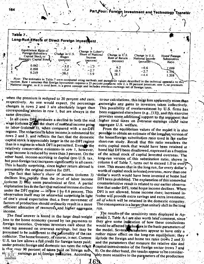
,k ...

PartsFour: Poreiglyestment and Technology Tkanater..-"--r

Table 7,Long-RodEffecrs of DiraCt Foreign

Equilibrium Ratio ofForeign Subsidiary Caitge in U.S.

Wages(percent)

.23.2

Capital Stock toDomes is Capital Stric

0.062 .

,0.0980.219

inyeatlkint ,

A' 3Change in Labor'sShare of National

Income(percent)fr-

: 4:7. 2.7-5.9

4

Change in U.S. Change in U.S.Rate of Return National Inconie

(percent) (percen

6.2 0.610.5 2.728.1 4.4

Nute: The-estimates in Table 7 were comlnited using methods and pasection. Row I assume,s that foreign investment requires a 25 percent preNational inc re, as it is used here, is a gross concept and includes ove

Home Foreign'Substitution

Ratio

:099

1.208

eter values described in the technical appendix to thisurn: row 2. a 20 percent premium: row 3..no premium.

eas earnings net of foreign taxes..

when the premium is itedgeed to 20 percent and zero,respectively. As on_ e, would expect, the percentagechanges in .rows, 2 and 3 are absolutely larger thancorresponding*tries in row I, but are always in thesame direetion:'. . ,

in all cases DF roduce s a declinP In both the real..

wage (colutnn the share of nattanal income goingto labor (colu ), when- compared with a no-DPIregime. The rechtetionlnabor incomeas substantial forrows 2 and 3 and reflects the fact. that the domesticcapital stock is appreciably larger in the no-DFI regimethan in a regime in which DFI is permitted. Even* -dierelatively conservative estimates in row 1, hoWever,wage income is reduced by more than 3 percent. On theother hand, income accruing to dapital (pre-U.S. tax,but post-foreign tax) increases significantly in all cases:This is hardly surprising, since higher return abroad ispresumably the original motive for DFI. .

The fact that labor's, share of income. (column 3)neClines lessAapidly than the .level of labor income

p,.(colunin 2) Miry seem paradoxical at first. A partialeiplanation lies in the fact th4t national income declinesunder the DFr regime in ow I py 0.6 percent. Thisobservation itself may be sdmewhat surpriiiiigln lightof, tine's usual expectation that a freer movement offactors .of production should ordinarily result in a moreefficient alloCation of resources and higlier aggregate.income.

The final answer is found in the large 'dead-Weightloss to the home economy caused by tax payments toforeign treasuries. Overseas inVestors care about thetotal: tax assessed on:Overseas earnings, but may bepresumed to be indifferent to th ionality of the,taxcollector. The home reasury, of course; is not. CurrentU.S. tax law allows a fUll,credit for foteign taxes paid;under present foreign and. tax rates the re Itis that over 90 percent of taxes is 'A on' foreign su

c\sidiaries' earnings gd t foreign Sinies. According

to our calCulations, this large loss apparently Cliote;than.outweighs any gains to investors taken collectively.This posSibility of overinveStment by U.S. firms,. hasbeen suggested elsewhere (e.g., t131),and this exercise.provides SoMe:addition4 support to the argtOent that'higher total taxes on 5verseas.earniigs could` raiseaggregate U.S. welfare.

From the equilibrium values of the mo it is alsopossil* to obtain an estimate of the version ofthe home/foreign substittition ratio used in t e earliershort-run study. Recall that this ratio meas res theextra capital stock.. that would have hen retained athome had DFI been disallowed, expressed as a fractionof the actual stock of capital invested overseas: Thelong-run version of.' this sUbstinition ratiO,.., shown incolintin 6 of Table 7, turns out to exceed 1.0;ineverCase. This means that in the long run, for every dollar'sworth of capital stock iniested,overseas, more than one

. !dollar's worth would have been invested at 'home hadDFI been iirohibited. The explanationof this-somewhatcounterintuitive result is related to our earlier observa-tion that under DFI, tOtal home income declines. WhenDFI is not allowed, home income rises; increased in-coine will provide extra savings and extra investment,all of which will be retained in thedomestic economy.The consequence is a larger than unitar3, shift in the lOngrun.

. .

The results.:ofthe sensitivity tests displayed in Ap-pendii 2, TableA.7l are also worth briefccirnMelit, since'they give soine in4Fation of how these concluiionswould be affected *hatesin the basic parameters ofthe model., Severra eters appear to have only arather minor effect on the long-run eiluilitiuni; theyinclude the foreign an& hoine tax rates 0.6 s 2 and 3)and the parameters, that' measure the relative size and

capitalLintensiveness of the foreign sector (roWs 7 wig!8). On the Other hand, the results appear to'be consider-bly more sensitive to the parameters of the production

;.%

. The DistrItutIonal Consequences of Direct Foreign. Investment5

4.

function Now 9 and 10), and especially to the technol- Appendix 1ogy parameters (row 5), suggeSting the need for further

.-refinemen of the production -data. The Industry Labdr"Market. Model'The rather strong influence of thtax rate-riled to For a single industry labor market we employ

foreign eainings is alp worth pointing out, sin e the taxtreatment of foreign investment ha been the focus of.much recent debate.In one experiment we reduced thetotal tax on foreign investment earnings &equal theforeign. tax level (holding 9413.S. tax ,rate at constant);this is equivalent to .a regime in .which b.s. 'foreigti.

.

iidefinite deferralprvestment earning?are subject-to-on payment of. U.S. taxes. In case the percentagedifferenoe in wages rises alnibst percentt, and the,net loss of national into exceeds 1 percent when DFIis allowed.

Finally, as might expe in long -run grOWthmodel, the, results are rat er sensitive to the Assumedgrowth rate. By implication:they jam, also sensitillethe to of depreciaticin and rate of growth of the labor." .

fore ince these parameters play a similarrOle in tkee has been suggested that t e domestia savings

prop ity; rather than being constant, might be re-sponsive to changes in the domestic interest rate, and

. that foreign investment Might thereby' contribute toeconomic grotyth by indirectly stimulating savings.Some preliminary experiments that allow for a positivea.4115ciation between savings and the interest rate indi-:cate that, even under extremely high interest 'elaszticities, the qualitative results obtained earlier are un-changed. However, it still may be the Casrttrat a suffi-ciently strong association between foreign' investmentand savings for example, if foreign earnings werealmost entirely retained and reinvested could reduce

. the income asses cited above. Further investigation ina more disiggregated model is needed in order toevaltiate this possibility.

In general, the results in this section are ronsistentwith and support the findings in the earlier part of thisstudy. It appears that foreign investment has broughtabout a moderate decline in both wage rates and labor'sshare of total national income. At the same time thereappears to have been a slight overall loss in total incomeaccruing to the U.S. economy, primarily becausoflarge tax payments on foreign ings that are. col-lected by foreign treasu s under e current tax sys-tem. It is impo o point' out that, although thenumbers that we have generated in ihis section areindicative of-the scale and direction of these effects,they Stiouid be-regarded at this point as tentative esti-mates only. As Ike haVe already emphasized, the results-depend to a considerable extent on the yalnes assignedto several key parameters: This sensitivity sogests thatfuture research should be directed partiCidarly at pp-grading the quality of these inputs to the estimation.

lowing notation:

t separations rate, exogenousIrietermined.a = accessions ratep = probability .a job.seeker secures emploYment

in a given period .

d -= expected duration of a spell of unemployment .-e indus-=

VE'_L=

number a unernployed workers intrynumber of job vacancies in, the inumber of-employed worktotal demand for laborlabor force = E + U

W. the-moneywage rat.

/W e rate of Wage inflation = g (V /U),0:

The prO ability that a job seeker secures employ-ment in,d given period is assumed proportional to thenumber 'of vacancies per job seeker in the industry

dustry

with

ViU, %len V/U.< I/k;1, when V/U> 1Ik;

where 0 < k r. 9

The probability that a given job seeker secures em-ployment only after T periods of search is equal top(1-p)T-1. Thus; the expected duration of a spell ofUnemployment is given by

ET p(1-p)p

T=I .

the accessions We, i.e., the number of job seekers, .

who cure "lkniach period as a fraction of total em-ph) ri t, is given by

a = 5V IE.

Ile, following conditions define comjpletf equili-britnn in the industry 'labor. market:

,

(Alternatively, the number of vacancies created eachperiod tE must be the same,as vacancies filled kV).

We shall alsd-cnsider. the possibility of leisconiplete equifibnum.configurations, a :4semi-eqbrium," in which

,

Eventually, in this situation,, the Phillips relation1W = g (VIU) will produce fig fling wages, bringing V

back into balance with I, As a practical matter, how-ever, wages may be very slow to fall in response to an-excess of searchers ove vacancies and, moreover, in-dustry labor detuand Ma be highly wage inelastic, mak-ing possible a protracte etcess ofU over V. The exis-tence of such reason ly stable disequilibrium config-urations; first rationa ed by Keynes interms of wagerates being "sticky downts.i.ardi.," has received consid-erablp empirioal,dosumentation in recent yeals,andcreasing] y haq.comPto'be interpreted in terms.of wan-.tity rates of adjustment strongly dominating price eatesof adjuginent when markets are. displaced from equilib-rium. .

Part Four: Foreign Investment and Techogy,Transter''--

Olir simulation exercise considers the indinstrylabormarket to be in an initial equilibriums conf*uration ofthe complete type. This initial equilibrium is disturbedby industry 'direct foreign investment .activities thatiiinnitanepnily.disPlace AUexih and d Create AVnew jobs, the immediate effect of 'which is to. increase'

*--/.the stock of unemployed Workei.s trout U to U .+ AUand the stock of vacancies from V to V + AV.

These changes in the vacancy and unemploymentstocks. produce an immediate change in the probabilayJilliacement and, hence, in the duration of an unem- .t. sployment spell from d to c/1, where and

W assume that wage$ in this case are slow to re-spOn and/or that industry labor demand is insensitiveto w ge rates; the industry labor market then proceedsto tablish a semiequlibrium of the type discusseda e; M. which the flow of accessions etiltal js, the flowof se ations, but in which the stock-of searchers per-sists at a. 'gher level than the stock of vacancies. Thissemiequilibriumtlosition is formally defined by

tE* =IV*

.where the starred variables rgpresent values:taken in'thesemiequilibrium position. V* and E* are also related

E* + V* = .1*, r (3)

by

wherer - '

Solving (2) and (3), .we obtain

Ay =I+ AI.-

di = 14V+ AV)(U+ AO) I'4111111°'

Sintce the abor force has remained unchanged we also..Expression (1)' illustrates the importance of keeping Itays:4; '-

separate accounts for. both job gains and job losseswhen assessing the dislocative effects of a shift in labordemand. Most studies of the effects of DFron-dnmesticemployment have instead placed primary emphasis on or'.the net job displacennint figure, i.e., (AUAV) in ournotation. Using expression (1), it.is a simple matter todenionstrate that ajob displacement of (AUAV) jobsproduce$ a smaller increase in the, duration of unem-ployment than does ajob 1O$s of AU accompanied bynot fully offsetting job stiMiilti§4V.:Ivioreci:,er, empha- is thensi on 'the net job displacement figure tends to obscure

, ,

di fact that 'AU, nOt41/:--AV,:individuals are initiallyded to the stock of job searchers as a result of the,

labor de and shift.If the FI=related labor demand shifts result in more

workers ing displaced than there are new job vacanr ".

cies created, as we have estimated they do for each of --which yields a corresponding'unempldyment durationthe indutries in -out' ithdy, the duration of a spell of ofunemployment, ii.sgen from expreSsion (I) to rise ini-tially.

= E ++k t+k*

V* = r = V+t+k r+k

U* + E* = U + E

Us TEs)= tkhe probability of job plaCemen the seiniequilihrium

kV* ....k[V + A.101(r+k))]P*

U* [UL1.01-101

The Distributional Consequenchs of Direct Foreign' inveslent

We compare the values of the original eiluilibruimduration of unemployment d, -its initial diiturbanceyalde d1, and the semiequilibrium duration d* when

= V and. tit/ > AV and find

d <d d*:

Or, in placement probabil y terms

p > Pi> p*. A

As long as the duration of unemployment remains-higher than its initial value following a DVI:rilatetf.. disturbance, all Workers 'Who enter the pootoljobeeek-ers, whether becausd Of a DFI displacement or not,can expect to experienCe a longerspell of unemploy-ment than they would have in the absence of the dis-turbanc-e. Put another way, there will continue to bemore men unemployed, on the average, than there wereoriginally, even well after most of the initially displaced.workers have secured new jobs. In terms of the semi-

; equilibrium position &Scribed above, there Will be U*Men unemployed each period as compared with the ini-tial equilibrium value U. The difference,

*u*-u=-61( (4)

we will label the residual contribution to industry unem-ployment oithe DFI-related disturbance. This residual

tribution will persist as long as-the semiequilibriumc ndition..persiSts; that is, 'until:falling wages, a sec-

ral product demand shift, aggregate' policies, or ioniether phenomenon occurs so as to reestablish the in-

dustry balance between vacancies and unemployment.

Data ,So4urcet for the Simulation ExerciseThe year '1970 was chosen fOr our simulation exercisebecause the overall Unemployment rate of 4.9 PerCent:

'during that year approximates pig- ,:`full employment"level characteristic of contemporary macroeconomicpolicy discussions:.

Employment and Earnings. publishes data for eni-.ployment, unemployment, and separations rates. formost important manufacturing industries at the leveloLaggregation,corresponding. to our emploYment de-ri.,i0rd estimates reported in section 1. For a year inwhich industry labor markets are in equilibrium' as de-.fined in our model, initial industry. unemployment ditr-atons can becalculated by exploiting the equilibri&n.relation, .

14i = lj X

167

whereli; is the ith iredustry unemploy ent rate, ti is the, --.<

separations rate (separations per nth, per 100 em-ployeeS) and di is the average durati n per spell of Lin=employmerk measured in months. :

For the year 1970, a year of increasing. unemployrienL such a cedure woulchipt be entirely appro-priate,.sirice th ecorded separations rates for mostindustries exc d those required to generate equili- ,brium unemployment stOcks tat IWO-Values: We. makean adjustment for this:problem .by adopting as our esti.-mates of industry equilibrium separations rates the'-arithmetic means of- tile published values for separa--.4ions rates and accession rates. Pie latter figures, incontrast to the ,separations rates, areflower than those .corresponding to equilibrium Vabancy - u employ -ment stocks in a year of rising unemploym nt. Iliaadjustment is somewhat crude, and inexact but the .

general pattern of results produced by our pro edure isfortunately not very sensitive to 'rain& inaccuracies inthe measurement of industry separations rates.

Finding di enables us to calculate the correspondingplacement probability pi, and. again exploiting: theequilibrium assumption, the proportionality factor kiin the place_ment probability expression.

Our first calculations in the simulation exercise tracethe placement probability movements from p, to j inweekly intervals and employs these/values to computetime profiles of the number of DFI-displaced workehwho remain unemployed in each industry: these arethe -!`direct unemployment effects" summarized inTables 4 and 5. The properties of the serniequilibriii\inare summarized as 'indirect unemployment effects 'in Table 6,

When interpreting the results reported in Tables 4 6,several qualifications should be borne in inhid.

As the exercise was set up, all of the dislocations re-sultant from both the direct and indirect effects of the1970 DFI vector were presumed to haYe occurrecliall atonce: One might easily argue Pig, at the level of indus-try aggregation of our study, DTI effects would be bet-ter' characterized as occurring Art a smooth flowthroughout the year. The effect of such a characteiiza-tion is to replace the large 'groups-of unemployed work-ers whose experience we,trace in Tables 4 and 5 withmany smaller groups. The unemployment profiles ofthese smaller groups will be very much like tflose ofthe larger: groups and, as the DFI accumulates -to its.yearly . total, the' residual Unemployment cOntribumwtion under the smooth flow view becomes. identical`With its lump sum approach Counterpart.

Actual implementation of our model required first.that certain assumptions be made cbncerning the natureof the expart 'displacement and export stimulus effects"discussed in section 1. If the foreign investment project1 7 9 ,,- . . , , .

d..,. ,

.Part Four: Foreign Investment and Technology Transfer.

is preceded by a complete shutdown of the domestitproduction facility, whereupon a domestic operation isreorganized to serve the export requirements of theforeign production site, , the number' bf initially _dis-plaid workers° iscleterminecl by size of the export dis-placementeffect,aand the number of new vacancies willbe d byffie size of the export stimulus effect..

a hand. if the U.S. export requirements of-the o pas production site are satisfied by sirriOlyretaining some portion of the domestic productionOperation intact, the number of initially displaced workr-\.ers is determined by the differencOitween the exriortstimulus and export displacement effects, whereas the (.number of new vacancies .would be zero. The actualmix of. theselvv,o assum.ptif.ms that best characterize theindustriesiii our study would_ be quitedifficult.topsti-

.mate prediselt FOC filkiiitirOoses of our calculations inthis,section welave assumed the maximally dislocativealternative, namely that U.S. export requireinents of.foreign produnized domestictherefore itsthe number Of init.'this particular acco

es are 'served from newly Orga-perations. In interpreting our findings,d be. kept in mind that oar estimates of where

y displaced workers are, at least ont, upward biased. Since the ex-

port.stimulUs is usually_ only a small fraction of the ex-port displacement, howeVer, this bias is probably vdrysmall. . (

A very similar qualificadonppplies 4n the case when:.:-Ir the overseas production transfer.occuri in the context,

Of a firin whose domeiiic emplOyment is growing-rapid- ,

ly. For such firms, the export displacement effect maytake the form of fewer new workOs being hired ratherMan existing employees being discharged.. If So, our

:estimates % the ininallyslisplaCed workers will again be .oupward biat .

As far as the residual unemployjnent estilhates- areconcerned;- however, .these depen.d only 'on the size ofthe -net employent demand reduction 0.e., the; differ-ence between the export displacement and export-stim-ulus-effects) and will thus be affected neither by theortitular assuniptims made4bout whether the export

5'Istimuliweffect requires the reorganization oir,dOinestic -° prodtictiOn facilities r by the rate Of growth of domes-

tic employment,de anc , :

In our model it w also. assumed that industry labormarkets were' esse 'tally independent of. one another.In practice,.hoWev r,, we may witness substantial inter- -

industry' Migration on the part of job seekers, the effectof which would be to eliminateMuch of what limitedheterogeneity is displayed in. the 'qollection of adjust-insitliatIA in Tables 4 and 5'.. ; r------

Appendix 2

The Long-Run Model.The following equations. Summarize the basic 'Modelused to deternine equilibrium values:

OR -;e1 -e'11 = 8[1+4i]1 [1 Opc*= O, (1)

EisR-__)f-+

j(2)

J*; (e*).=-4(eF )"-eFfOeF), (3)

f '(e) = f IF(eF)nic 0 = 1(E)1: Ei F'(eF) [k (5)

k = capital-AM/Or ratio for factors owned by -,the home country

ks = capital/labor ratio for 'factors owned bythe foreign country .(assumed constant)

e = capital/labor ratio for factors emplOyed iirhome production .

capital/labor ratio for_factors employed inthe foreign investment sector

= capital/labor ratio forfactorS employed inforeign production ..

:f(e) =. output per unit of labor in home produs;tion . ,

a t.fF(ei) = output per unit of labor in the foreign in-.

vestment sector(e*) = otitputter unit Of labor rn foreign produc-

8- = ratio of home labor to jotal world labor ,

(constant) . ;.= ratio of foreign labor employed in the

foreign investment sector to labor enit-ployed at- honA

.

= growth rate Of the home labor force plusthe rate of capital stock depreciation(constant)home average savings propensity (con-stant) .

= home tax rate on domestic returns to.- capital (constant)

The Distributional Consequences of Direct Fi; n Investment

.foreign tax rate on foreign returns to capi-tal .(consiant)

= total tax rate (including bith-foreign and

c.i vested Capital.domestic takes) on return to foreign in-

As may be seen, `production is carried out in three'locations: at home, abrOaci by home entrepreneurs(foreign investment), or abroad by forei entre,prenevrs. Each sectof,hasits own production lation-ship and torrespondirifae tor employment ratio: Equa-.tions (1) and (2) are full employment cOnd#ions, whichrequire that the total world stocks of capital and labor,

thi (3) indicates that, in equil. foreigifin-respectively, ke. fully utilized in the threefsectors.Equativestors and local foreign producers, who9hare a com-mon marker for labor services, pay the same wage rate.Similarly, according to' &libation (4), in equilibriumhome producers will equalize the post-tax returns fromdomestic and foreign investment.

Equation (5) expresses the key steady-state condi-;tion that, in long-run equilibrium, the investment re-quired to offset depreciation and growth, inlhe laborfor-0 must exactly equal dAnestic savings: We. haveassumed here that domestic savings constitutes a fixedpercentage of-total national income:including the re-

. turns from foreign investment.We also have selected as our basic"production _rela-

tionship a CES. (constant elasticity of substitution)function of' the form 1-

.14.1 (e*)= A Ewe* + -tts41 I# (6)

Itvhere /3 is related to p, the Constant elasticity of sub-stitution, by /3 = (1/p) 1, A is an appropriate scaleparameter, and co is a weighting factor for the input ofcapital?'

The function in (6) applies to production in the 'for-eign sector, According to our assumptions regardingtgchittloty differeucz0hOtome and DM sector func-tions"c be written as

fF (eF) = iz.f* (eF), (7)

ft!) = X h. (e),

where 1.1, and measure the size of thtse gaps./These eight etivations are sufficient' to determine

equilibrium levels of the model's variables.The dynairiks 'of this system can be understood by

.referring to Figure 1, which is a modified version of thefamiliar phase diagram for a simple, single-sectorclosed economy. The function

a(k4) ---=f(e) + (1 -7*..) (ep)

Table A-1SenlitiviV Tests

.A

tip

. e

Change Change Change inin in Rate National

Wages of Return. Income(percent) (percent) (percent)

I . Base values -3.2 6:16_ 70.62. "1";° = 0.35 73.0 . 6.1 -0.4

(down 12 percent).3. r' 0.48 -3.2

t 48(1). t up 12 percent]

fr 4. r = 0.43 . -4.8 -

t = 0.40ft. d'Own 7 percent)

5. A. = 85= 1.18

(change .-= 6 percent) 4%

6. k* = 5.5 -5.2. (down 8 percent)

7. 8 0.5 -2.7(up '25 percent)

8. o- = 0.16(up 7 percent)

9. = 0.43 1.2 -1.0(down '16 percent)

. ,

6;2 -0.6.

9.6. -1.1

7.7 5.7 -1.2

10.3 "' -0.9

5_1 -0.5

-1.06.2 .12.4

10. p = 0.6 -1.6 3.5 -1.1(down 20 percent)

Notes: Under a CES specification the wages and the horheurn to capital can be expressed as

Ilp= p .r *= X p (c,)(14--=!-')

.eNati nal income (pet capita), defined to include the returns tocapi invested abroad, is

y = w r e (k-e) r ).The share of labor in national income is, therefore, wly, andcapital's share is

The parameter values, used in results reported in Tables 7and - I are (unl s.ottierwise indicated): - - . f

A .0 . n = 0.05p 0.15 (13 1.43 .r = 0.43w

. .

= 0.50 ,r* 0.40'a = 0.15 t = '0.43k. = 6.0. = 0.900 = 0.40 p = 1.10

Production parameters (A, p, and ii) and tax levels (7,..r*,and t) are based on [13, chap. 9]. Derivation of the technologyparameters (A and it) is described in the text. The aggregatepropensity to save, cr, is based on annual data in various issues,of the Survey ofCurrentPusiness , and includes alloWance for a2 perceRt (of GNP) government budget deficit. The 5 percentfigure forn is based on a 4 percent annual depreciation rate andI percent annual growth rate of the labor force. The .capital:labor ratio estimate for the foreign sector, k*, is assugied to be10 percent lower than the corresponding steady-state figure for

It'the parametei'O is intended tobe a rough Measure 'Ofthe relative-size of the foreign corporate-sector(s);ie DFI hostcountries.

`,-(9) j...7

J.

170 Part Four: Foreibn Investment and Technology Transfer

ORA

0

Figure 1Phasi Diagram for Determining Steady-StateValues

NOTE: PB hap slope PC is perpendicular toOBC;OB measuressteady-stateexpenditure per capita; BC measures steady4tate saw;int; Per capita.

where e =.e(k.; t)eF=eF(lc; I)

r

P.Literature Cited

measures per capita nation income, including thepost-foreign-tix returns from foreign investment whenequations (1) - (4) are satisfieCl." :the appropriatestability conditions are met,' the economy willmove tothe intersection of G0c,t) and the ray from the-originwith slope At this point, labeled P in Figure 14equation (5) will abiobe satisfied. The intersection (withthe vertical 1)04). of the _ perpendiculir and 110 with-glial5e equal tg drawn from point P mark out the leVelsof per capita expenditure and per capita saVings.

.

1. Adler, Michael, and Guy 'V. G. Steens.. "The Trade1 Effects of Direct Investment." Journal oVinanee, 29

(May 1974), 655-76.2. Christensen, Lauriti, Dale Jorgenson, and Dianne Cum-

mings. "Productivity GroWth, 1947 -1973: An Inter-national Comparison." Paper presented to the Confer-ence on the Impact of Inlernational Trade and Invest-ment on Employment. Vshington: Department of La-bor, December 1976. .

p

,'In this case the stability condition isk 0 iffoik -.(-akto) 0 forall kWh off in the acceptIble range, which is directly analogous tothe stability conditions of the simple, closed-economy version ofthismodel. In the range' ofparameter,values,wcha ve selected, this condi-tion is met. /

3. Christensen, I..aurits, and. Dale Jorgensen.: "The Mee-.surement of-U.S. Real Capital Input, 1929 - 1067." The

Review .ref IncoMe and Wealth, 15- (December 1969),-293- 320.

. .

4. "U.S. Real and Real factor Input,1929-1967." The Review Income and W Ith, 16(March 1970); 19-50:

5. Cook, Phiplip J.., and Robert Hi. Frank. "The, ffect.of,Unemplo*nent Diipersibrion ihe Rate of 'W ,tiOn."JoUrnal-ofMonetary EconoMics 1 (1975), 241-49. ;,

6.. Frank.. Robert H., and Richard 14; , Freeman. Maltina-tiona1Corporations'and Domestic Ernpkiyme,nt. CornellUniversity, 1976 (prOcessed). -

7. Freenian, Richard T. "The-Optimal Foreign InvestmentTax." Cornell University, Department of EconomicsWorking Paper, Jul 4976.

8. -Hawkins, Robert G.-lob Displacement and the Multi-national Firm: A Methodologkal Review. OccasionalPaper #3. New York: Center for Multinational Studiep,New York University, June 1972.

9. Horst, Thomas. "American Exports and Foreign DirectInvestment. "' Harvard Institute of Economic Research,Discussion Paper No. 362, May 1974.

10. Lipsey, Richard G. "The Relatimi Between Unemploy-ment and the Rate of Change in Money Wages in theUnited Kingdom, 1862-1957-A Further Analysis."Economica. 2.7 (February 1960), 1-31.

11. Lipsey., Robert E., and Merle Yahr Weiss. "The Relationof U.S. Manufacturing. Abroad to, 1.1,.S, Exports: A.!Framework for Analysis." Proceedings of the AmericanStatistical Association, Business -and Ecofibmic Statis-tics-1969, 497-509..

12." Kindleberger, Charles. American Business Abroad. NewHaven: Yale University Press, 1969.

13. Musgrave, Peggy B. Direct Investment Abroad and theMultinational CorporationsfEffects on the United StatesEconomy. Report prepared for the use of the Subcom-.

, miner on Foreign Relations, United States Senate, U.S. ..Government Printing Office, 1975;

14. Sato, Kazuo. Product Functions and Aggregation.York: North Hollan merican 8Isevier-1975.

15..,-Stobaugh, Robert B. and Associates.: "U.S. Multine.tional 4nterprists and the Economy: A Research .

Study of the Major Industries that Account for 90 Pekent.- of us. Foreign Direct investment in Manufacturing.". Benton, Mais., 1972.

16. United States Bureau of Labor StatiStics. 'ITomorrow'sManpower Needs." 'Washington: U.S, GoVernMerit.:,..Pi;intihg OffiCe; 1971.-

17.- United States DepariMnt;of CommtiCe.Spetial SO'vey.of U.S. Multinational Companies. 1970.

,

. .

18. United States Tariff Commission: ImplicOtions of MUlti-national .Firmsfor World Trade and investment and forU.S. Tra.dend Labor. Report to the U.S. Senate Corn-

-.mince on Finance, February 1973.19. Vernon, Raymoild. "International Investment and In-

ternational Trade the Product Cycle.". QuarterlyJournal of Economics. 80 (May 1966), 190=207.

20. Wan, Henry. Economic Growth. New York: Harcourt, .

Brace,' iovanovich% 1971.ri

r-

.?"*.

4444.

)11,Plitribudonal Consoquoncoo of DIrict FOroign Investment

CommentGuy V.. G. Stevens* I

My, comments will be' on Thomas Horst's paper and,,inA less cOmprehensive way, on the paper by ProfessorsPrank and Freeman..They will be 'ignited to what 1 thinkis the central issue in both of these papers, the substitu-.tion effect hetweekexports and foreign investment.

'Let Me startA;gy congrakilatingthl auriati of Intepna-tional Labor- AMTirs for -suppoitingi thesestudiei. Ithink the bureau and the publiC, -got, their,.moneyworth. Both studies did :what. .they shin-fhat-thcy:('introduced something' new and

otilas far.. as

research resultra07cOsicelnesl;Getting .to, parAiettlais; .Horst's development of the ;

idea that the nonpit3duction aspects of direct investmentInay be of crucial importanCe for the size and signof the substitutionffect is an-important contribution. Itis an important and plausible hypothesis that directinvestment ih foreign facilities may actually push outthe demand curve for the subsidiary's .pi-odtict.

As far as the Frank and Freeman paper is concerned,the cdntribution that impresses me the most is theirimaginative use' of economic. theory and the availablechga _ to make a breakthrough in the estiination of ttle '.

f elasticitY c4the foreign ibbsidiaryl,adernand curve. Itiawell known that this is a crucial parameter for the mea-surement of the substitution - effect. As a-person whoas tried to do this inthe Past incl;1 think4 failed, can

t, - .,-. s that this.is a very,*4t,t4o ;ra*Ault.: ' I will try,b low

to More specific coiikerOng'the importance o itesti e s the implication of their work ,fc.9 f tureresearch. . , " A

The Horst Paper..4.

,

.

The Horst' paper starts with an excellent summary ofthe major considerations that affect the decision to

. 'The. views expressed here ate .solely those of tht author and do notnecessarily represent those 9f the Fed Reserve Sk,stem:

'In p1, we were fticed td assume alternative valued forthe elasticities of the deinand cu ittbsidiatiefand,theircPmPetitorS; odr attempts to estiinnta these elititieities, using aggre-gate time-series data, led t inconclusive results.

.,

locate abroad --; the choke between exporting anddirect investment. The most important and original

'nt -that Horst emphasizes in the paper is that theyio prodUction 'aspects of 'direct investment, namely

drtiSing and setting up distributional and servicefacilities, can add new elements to the firm's product,market: there= actually shift out the demand curve forthe firm's product over whatii would be if the firm justexported from the -United States.

If'that idea can be verified and actualli/measured,then. as Horst has said, it puts the analysis of the impactof direct investment on U.S. employment in a com-pletely different light. In fact, we may find that directinvestment and eitporting are complementary, anckthat,employment May be. increased l'iy!,:lireV investment....

The only problem with' the paper is that Hdriteschew's tryingiOkniasure this impact,,and even vergeson saying thaf*Ild so, is 'impossible. I am glad to seethat in' hisnrallSomments hOre he 'maintained only that itis, very difficult a position with which I agree. It isdifficUlt now, especially, given kind of data that wellitVe. But we should be able to point the data that arenecessary and sufficient tdmeaSure,ttie,effect Horsthypothesizes. Then, if thity_.are -not .aVailabie, one canpush to have these data collected.

Concerning the empirical results' actually pfb-duces-in the paper, I-frankly don't see'hoW the rankingsthat he has to his Table I conFlissively show anything; Iam not sure,. but I think he inightagree. These results.seem to glye one simple correlations.or, at 'best:condi-tinal:coirelations,-. holding bne factor constasuch they are subject to the -Cr-Welkin :that h 'been,leveled pisi regression` results . where teigntinvestment was just enteredas -an'independen vari-able. The foreign investment variable'and the ex rting.variable may be determined by third factorath causeboth to move to 'the same- directick. Therefore,,yoiican't conclusively say :that these' simple tips- ofcorrelations or tven regreision results area real test ofhypotheses abotit the substitution effect. .

the statistical 'tes s have tried to' measure. theDespite these it seems thatfausF about

irripact. -of foreign. investment on zexpOrts have, shoWn .1

either rid effect of direct investment onteapckts Or somekind of thinplementarity bet en the tIvo.2

These regressioni have liatiqy just added some kind'of foreign investment -variable to an export equation in

'Adler thoroughly analyzed, the aggregilte data by country and are ,

' in most cases (except for Japan) he found eitherefo effect of?'complementarity. Lipsey and Weiss- (mind .cdmplementarity in theirstui of the directinvestment in manufacturing [SI. Finally, in earliercross-section work. Horst found a positive effect of foreign sub-:

. sidiary sales on\L1.S. exports (reported. in DI).

176

172 Part Four: Foreign Investment and Technology Transfer ,

Which case there certainly, is a sin ultaneous lequationproblem. .But nevertheless, we do have this tantalizing

. evidence that foreign investrKent actually helPsports. Although it ,may. be a misinterpretation ofcausality 1 do not thihk it has yet been conclusivelyShown to be incorrect.

The Frank-FreenftfhiPaper.

Getting the Frank and.,Freeman paper, ',agree withtheir Cri 'ism, on theoretical grounds, of the correla-,..

_ tion ancl egression results mentioned above. Given the,simultaneous equation' probfems present, one can cOn-

.

Struct 'models where' sports and foreign subsidiarysales are substitutes and yet, because of third faettirs,the regression'oefficient of subsidiary saleS 'in anexport awake may be positive. However; Showingthe - ssibility of a fallacy is not proof of the fallacy:Rather, to show this latter, the researcher' mustdemonstrate that a properly run test op the same (orvery similaridata leads to-the ofJpOsite result.'

Concerning the many positive contributions- in this, and earlier papers, Ijklqiild lIfe to concentrate on their

method of estimatinTlhe substitution effect betweenexports and foreign subsidiary sales. I commend

.Messrs. Frank and Freemarilfor their imaginative use ofthe marginal conditions of profit maximization and their

. use of revenue and 'Cost data to get estimates of thetie demand 'curve.for 'exports an* diforeign

subsidiary sales. I think anoVe-prOCedure, and it'led to very interesting and reasonable results. As I try-toshow, below, their work. should stimulate 'research inthis field. -

As their Table I ShoWs, their results- are verysensitive to the estimate of their substitution paraineter:(T...They

-bavein athis table couple alternatives, to

their estimated ratio. Their best guessis that U.Sdirect''foreign investment in 1979 led to a total losa of 160,000jobs; but when you halve a, the loss drops to'19,000jobs; when you double it, it increases to 441,000 jobs.Thus their bottom. line. the effect of direct investmenton 'jobs -- is very sensitive to the :estimate of the

5 6stitutiOn ratio." 4

First, I fail to see -in their apprOach one of the most.important elements that I thought was wrapped Up inthe analysis of -the substitution effect: assumptionsabout the behavibr of competing foreign firms. Hereto-fore all estimates of the substitution effect havedepended on assumptioni or estimates of what foreigncompetitors would do if U.S. firms were prevented orrestrained from investing Abroad (see- [5, 2]).- In the

case, du d by Hauer and Adler [51 as the"reverse allassical we might expect foreigncompetitors to-jump into the market that U.S. firmsWere restrained from serving by, diuect investment; inthis case, exforfs would not be helped by restrainingdirect investment. . It is, my opinion that ;Frank andFreeman have not adequately accounted for this facto`in fadt, it seems to me that intlicit irrtheir -analysis is theassumption that foreign .competitors will-do nothing ifdirect investmenCis restrained. Since the authorsdisputed this conclusion at the cgpference, as anappendix to this comment prov.ide short Counter-example; this shoWs, I think, how their frameworkcannot, generally,. be accounting for the eitestior for-.eigri competition. If I am correct, most would agree thatsomething-should be done to incorporate tkis neglectedeffect .into their framework. .

The final comment I have Oar procedure isthpir use of & to calculate the al de cts. for 1970,in their Table F. Pain not Sure that t is:Wfroper way to..cakulate a mai:ginal effect. Their question. is:. "What,happens to lops. if we ban ,the direct investment thathappened iq 1970?" And they iise their average '07. of0:33 as an important parametef to calculate this em-ployment effect..

Now;just as a counter- example, suppose. that in 1970the total production from direct investment abroad was

_.well above the level: that would be exported if all U.SJfirms were forced to produce only at hame..That wouldmean that even if you held incremental direct invest-

in 1970 to zero, there' probably wouldn't be anyeffect chi exports; for we would already have proijuc-,tion al3road that would be above the optimal level of ex-ports. Yet their calciilation gives a different result. ThisIs so, I think, because their substitution parameter is a

pite their innovative use of available data; policy-makers. shotild be 'warned as the authors correctlydo that the estimates of (rthat are presented ispaperre the-first fruits of -re searc hand. May

_

iup to scrutiny, For one.thing each estimate s ba d ors'ode observation, and. derived by ..a, co tic tedcalculation that cannot allowfor errors in the dattheory, or for the normal grror term in econotik °-equations.. Second, Oeir procedure may have substan-tive -flaws; concerning .the possibility of these;' I havetwo critical ointments perhaps better put as queries.

I

global eititriate:,what would hapPen.ifyou,iOrp/et4 7banned foreign4n vestment and made U.S.' business sell -all its foreign facilities. It should not be used withoutmodification to calkulate the incremental effect of put-

ting a pajtiaL ban, or some kind of partial constraint, On 'foreign investment activity.

Implications for Future Research

I would like to close -by_reiterating .what I see 'as the

177

r.

The Distributional Consequences of Foreign Investment 173 tr-

...,

implications of these two udie r future research.Firit, both 'studies indicate the need for more work onthe careful estimation of the substitution effect betweenproduction abroad through foreign subsidiaries apd ex-porting from the United States,( Frank and Freemangive us hope that we can make- progress in measuringthe key parameters that determine the substitution ef-Rio. Horst point's to a new set of considerationsLhat,miiist be taken into account and Measured, factors deal-ing with OW production abroad affects the foreign de-Mand for products produced by V.S. firms.

SeconcL'it is clear that the theories underlying thesetwo studies are not consistent: Horses implies thatdirect investment may shift out the demand curve for

Frank and Freeman specify their demand (pnce)curve as Cobb-Douglas: Q = NP-4; constant marginalcosts are assumed: thus Ci(Q) = MC, + K, whereMC, is the constant marginal cost for the particular pro-duction location and K is some'(irrefeVant)Ievel oCtixedcosts. very irri rtant point is that the inlefcept Of thefirm's deman curve is a constant/1/;'in particular it isnot a function of what competitors do. Under these cir-cumstances. the authors show that their ratio .a is afunttion of marginal costs and the (constant) demandelasticity (n) alone.

QH /QF =AMC? MCH]n.

the product previously exported, whereas Frank and The following simple example shows that this sort ofFreeman's makes the usual, assumption that the foreign procedure does not generally act ount for the actions of. demand curye is unaffected by the location of produc- competing firms. We will consider a case with constant

lion. Both papers have done a goodjaib in describing thi marginal costs identical to Frank and Freeman;. to' sim-factors that underlie these theories and the differences plify'thingswe will assume that the market price (de-in Vieir implications. What remains to be done see nand) curve is linear; P where Q is total mar-if these conflicting theoretical strands panbiiiiitegratedis ket supply. In our example we, will specify precisely theinto a more general model vile that is Iiiired to em-, behavior pattern of cdmpeting firms: for simplicity as-. opirical data, existing or potentially collectable: and, *muffle that there is one other firm supplying an identicalthat, therefore, can be used to test the alternative hypo_ produCt to the foreign market; in this duOpoly situation,

We will assume that each competitor adopts Cornot-.type behavior: maximizing his profit function on theassumption that the competitor does not reect. We willshow that estimates made of a = QUIQF on the basis of

t any, given equilibrium position as done by Freeman'Frank ffrid Freeman define their cr Alothe tatio cif (1) the and Frank will be incorr t. The reason is that suchoptini tallevelpfoutPut (QH) if the firm is constrained to estimates will not account for the reaction of the cori-petitor as the equilibrium changes.

The market price curve (inverse of the market de-mand curve) is P = ad' bQ ; since total output Q is pro-duced by firm I and 2, Q = + 02. The U.S. multi -,national maximizes profits, assuming as given the cur-rent level of the competitor's output (Q2).

max Ir = la b (Q Q2 Qi MCi Qias the result of a simple profit maximization problein:the, following profit (7r) function is maxiized,JD ;.hhe- As discussed above, the optimal level of home and

foreign production is found by inserting, respectively.,the marginal cost at home (MCii) and abroad (MCF).

Maximizing with respect to Q1: the firm sets the fol-.

iving marginal.equation to zero:

. 'theses.

APpendix

Supply the rnairket from exports from the United Statesand (2) the optimal level of outPilt (QF) if the firm' isallowed to produce outside, the United States, where itis, presumably' cheaper- The rates of- thes two-levelJH /QF equali a; for their 'calculations they make fur-' ther assumption that each added that. Of productionabroad will replace a units, of exports from the UnitedStates-.

ri)r both cases the optimal output level is determined

choice of an optimal,,. 1

!VV.- ci(Q),.

where Q is quantity; P(Q) isihe price fuhetion for thee .

market, i.e., the reverse of the downward sloping de- ) bQ2) 2bQ MCi =41, .:mad curve- for, the foreign ;market; and C, (Q) is the

cost function for production in Iodation i. i can equal H This leads to optimal leveWofthomeand foreign produc(home productioq) or P' (production abroad). tion of .

(1)

'This model is developed in detail-in their earlier paper [N._(d-bQ2)- MCl/ .

34" 2b (2)

174,

Pah Four: ForeIgneltivestment and Tedlinology Transfer

. (3)

We might estiniate these levelh; or their rattfa a- in wayssimilar to those suggested by Frank and.Ffteman. To

AietQH (abQ MCll,

' =QF (a -bQ2)

we need measures of the marginal cost of production` afhome and abroad and a measure of (a -6Q2), this: latteris a measure of the intercept of the firm's deMandcurve: Frank and Free needed,needed, exactly the ,gamecost data. Analogous to rank .and Preeman we canmanipulate die dap at, any point of equilibrium to getestimates "Sfa bQ2 and apy other parameters of the.system. Thus:

In amax' on states:

. ,P =- (a bQ2) bQi and

=1) + b(4)

n, the first - order. cOridition (1) for a profit

.-bQ2 -1111?

Hence from (4) and (5)::

a bQ2 =,P + b`Q, ..=12 + P,- MC .-;213t MC..

of Q2 for the two polar-cases behind the calculation ofQll and QF will both be different, and different fro" any

_ intermediate_ point.of .eqUilib ii. For . this _re on, _ _ _

given this model, no data can bruSed in the :Wa sug-..,. deated above to calCulate an unbiased cr. The variation

in Qs must be takeninto account to obtain unbiased . --.,

estimate of a. . . ''' -. - , . rIn fact we know the estimate cofoo will usually be bi-

ased upward . If home costs are higher ;--the actual level ---,,of Q2 for the calg of all production *home willbe high-e eQkletually observed when some productionis undertaken abroad; thus the numerator-of o- w'. I belover than estimated. Similarly the level of Q2 e-''sponding to all production abroad tvill be greater t an

--or equalito the-observed Q2t; thus leaving the denomi-nator unchanged or higler. 4,',

in this particular caw, one might note. that One cani fake account' of the effect of foreign competitors just

by knowing the marginal cast faced by these c6nipeti-.tors (MCC). --

. .

PrOfit.maximization by the competitor adds one moremaeginal,.condition to the model'.

ar'P= bQi is) ok El4. ly

an 'estimate of a constructed in a way similar tothat used by Frank and.Freemarl (using,data from any

roved point of equilibrium) would be

rip Aki _

=MCi = MCF

-

Within the framework of thfM model, the aboye mea-sure of cr is ,wrong Ail the data t are used to con-struct O-Presuppole that the produttiob level Of Com-petttors vilrbe Qp°, theparticuiar level of supply bytiatopeti.totsCat th tithe the data;Were gathered for thecalcula o owe*, this level 02 will almostcertainl the .ievel of competitors'. pfoduction iii

circumstances: in..pantcular'thd caseOction is foreed to be don Ott home (theQi), or the aftective, where all pria-

artg othwhere 01case le

ttInetion-is done ad (OF). Be se of the duopolisticAnarfat situation. the multinational adjusts its supply

foreirnarket; it do its competitois. The revels:-

.

bQI-:.-2bQ2 -MCc =Q.

.

ations ( I-) and (6) can be user Q, and Q2. It can be v

re' ced-form solution for

(6)

iitriliandous-t the,netv, true

3a,'+.11,1Cc Mt. iQ1 3"p

Or"

This an be Ampared to (2) and (3) by substitutingUCH or li1CFfoyM9.The values for QH and QNcalcu-

.4ated from (7) arethe correct onescfo use in calculatingthe a sought by Freeman and Frank.

-Literittii*Cited'

1. Adler, Michael. "Direct Interactiops.between U.S. Ex-ports and. Sales by U.S. Direct 4nvestment VenturesAbroad." 'Unpublished paper prepared under contractwith U.S. Department of State, Graddate School -of Busi-

----41edS, Columbia University; NovernAt 1971.2. Adler; Michael,' and Guy *OAP ens. -"The Trade

:Effects qf'Diktt Investrrient.'? jle Journal of FinanCe,(May '1974), 655-776. -

3. Bergsteh, IC. Fred, Thomas -Hoist, aildlT. H. Moran.American Multinationals and, American Interests. Wash-ington: Brpokings Iustitution,-foithcoming.

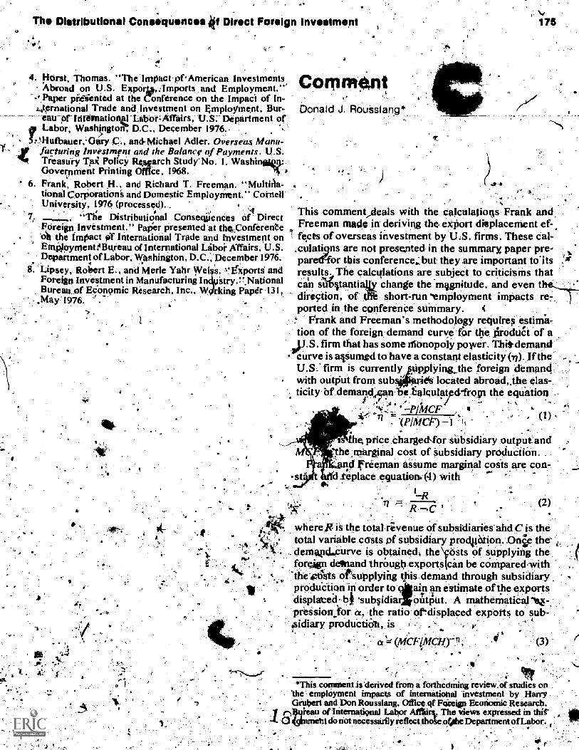
The Distributional Consequences f Direct Foreign investment

ra

01.,-.

4. IiOrst, Thomas. "The Impel pf.AmeriCan InvestmentsAbroad on U.S. Expartv,:lmports and Employment."'

' Paper pf.eliented at the Conference on the Impaci of In-a,trnational Trade and Investment on Employment, Bur-eau-printeitnatiorietabot;Affairs; U.S; Department of

it Labor, Washington: D.C., December 1976..5:!Hufbauer,' Gary .C.., and Michael Adler. Overseas Matta-

Y ir factoring Investment and the Balance of Payments. U.S.We( Tieasuiy Tai Policy Rwarch Study' No. I. Washinfilq.:

Government Printing Office, 1968.,.-

6. Frank, Robert H., and Richard T. Freeman. "Multhla-tionsil Corporation and Domestic Employment." Coi-nellUniversity, 1976 (processed)..

, ,; -.i.,........ "The Distributional ConsequenCes ofd Direct

Foreign Investment." Paper presented at th,Conferente'oft the Impact of International Trade and Investment onEmPtlerymentfBuLeeau of International Liboi Affairs, U.S.

, Department of Labor, Washington, D.C.,December 1976.8. Lipsey, Rotten E., and Merle Yahr Wei s..rgsports. and

Foreign investment in Manufacturing In Stry.:!.NationalBureau..of Economic Research, Inc., W. rking Paper 131, .

May'19'76. " - .

a

Comment, 1 1

Donald J. Rousslang*

J

175

This commentAeals with the Calculations Frank andFreeman made in deriving the etPort displacement ef-fects of overseas investment by U.S. firms. These Cal-

cculati9ns are not presented in the summary paper pre-pareTfor this conference.:but they are important to-itsresults. The calculations are subject to criticisms thatcan iiigitantially change the mtignitude, and even tdirection, of short-run ftemPloyment impacts re:-ported in the conferenCe summary.

Frank and Freeman's methodology requireS estima-tion of the foreign demand curve' for itroduCt of aV.S. firm that has some monopoly power. Thitdemandcurve is alsumgd to have a constant elasticity (vi). If the

output from sub "' : ,ri.e(s located abroad,.the elas-U.S.' firm is foreign demandwith outticity bf demand:A.1n be.ialculayd"frogi the equation

...a

-P/SicF , -) (1)(P /MC' ,

. -

t he, price charged,for siibsidiary output:and'the marginal cost of subsidiary producliOn. .

d freeman assume marginal costs are con-._replace equation. (4) with

RR

(2)

where .R is the totalevenue of subsidiaries'and C is thetotal variable casts of subsidiary prodpektion. Janie the 1,

.. demapcLcurve is obtained, the \vo,sts of supplying theforeign demand through exportsican be compared-with

"the.ot`Sis orsupplying this demand through subsidiaryproduCtion ip order to ain an estimate of the exportsdisplaced- 14 sulnidia

*output, A mathernatical114-.

pression:for a, the ratio otdisplaced exports to sub-. . ., .Aidiary productidh, is , - .. , E .

a !--` (itiCF/MC'HyTl,

*This comment is 'derived from a fOrtiirOMing review.of studies onShe employment impacts of international investment by HarryGrubert and Don Rousslang, Office qf Fokeign Be-06°6de Research,

Ivan of International Labor . The views expressed in thirt do not necessarily reflect tho .ofothe Department of Labor.

ifs Part Four: Foreign investment and TechnOlogy Transfer

tom:

price

et ---

.o

MOH

qh. It

%**. Merginol Revenue

MCPDone tld

Ott OF

Figure 1

.quontita--6

ariabfe cost. The estima demand elasticityfurtherAcreased if The average t dist is made to

include the opportunity cost, of-T-he-following-exarripte-shows Avh

portunity costs is inappropriate. Suppose .a firm oper-ates undercoaditions of perfeOtoompetition and faces a

_perrectlrelesticAemand curve: Even' f the system is in:.long-Fun equilibrium, accounting cogs need not,equal

'tont revenues so long as there is an opportunity cost ofcapital. But if accounting costs were used in eqaation(2), ,the estimated elasticity of demand would 'be lessthan infinite

Using tota cost instead of total variable,cost. inequation (2) and iricluding a 10 percent rate of return tocapital as itsOpporninity cost great1V-increases the es-timated demand tiilasticities. This reducei the estimatedexport displacement effeCts to such aii.extent that theyare more than offset by the export Stimulus effects thatrekult from subsidiary imports of parts and, equipmentfrom the United Statesj . ,

chiding' transp Atari/and tariff costs, assumed -to be mates of the short-run employment impacts of overseaswhere /l/C1-/ marginal costs of U.g%.exPorts,. in- .,. The 'arbitrary nature of Frank and 'Freeman's esti-.

constant. t. . investment has been demonstrated above by showing

A grap example, of Frank a Freeman's the variability of 'these estimates with respect tomethod gy is. iven in Figure 1..1-ler export dis- reasonable changes in the assumptions. Other assump4-pllee ent effect iigkien by the ratio /QF), where tions used by-Frank and Freeman are also subject toQ s :the qtiMitity the firm would 'export from the question. For example, in another recent attempt toUnited States in, he absence of subsidiary production estimate the effect of direct foreign, investment on U.S.and ar is the quantity the firm'would choOse to supply export& Adler and Stevens [11 used the assumption thatwith subsidiary prodUction. . subsidiary output was a perfect Substitute for Oulputiof

From Figure 1 and from-equation .(3) we see tkat as native firms in the host country but not for U.S. ex-(bng as MCF is less thankfCH, the offset coefficienta is ' ports, Frank and Freeman's methodology is inappro-greater when demand is less elastic: From equation: 2) priaitr where, this assumption' holds. They use the as-we see that the smaller the cost figure used, the smaller \iss.umption that subsidiary output is a perfect substituteis the estimated elasticitx. of demand. There are two: U.S. exports; but not for output of native Arms.iMportant reititps why thj cost figurh used by Frank Another possibility is that other foreilin producers 'mayand Freelinan may resulOn Underestimating theelastic- be induced to ;enter the Market at price levels betweenity of deaand. (1) They assume that Marginal costs,are PF and PH in Figure 1. lin this case, the demand curveconstantand therefore eqUal to aver* variable costs. . may become much more elastic in the range betweenThip,, -probably understateS trite- marginal costs, (2r4itlese'priCes, which would reduce the export displace-Prank and Freeman used accounting costs to calcull melt effect from that ealculated by. Frank and Freenian.

AP `i77 fitful eiquation (2), a procedure that does not atcounfor the opportunity cost of capital._

Since overseas investment' has been growing, it isNtinlikely that ,sUbsidiaries. have been operating widerconditions of constant short-run marginal costs, and' tis alSolualikely that they.haVObeen Operating at-outputlevels less than those necessary to.lt hieye minimumAverage total costs. _Therefore it,is Unlikely that short-run marginal- pOSts have been less than average totalcastt, And it viould probat* be a better prOcedure to ,

Use average total inplaeeofshort-run variable costequation (2 TillOwillincrease the estimated elasticof demand, since average, total cost alwaits eiceeds

Literature Cited,.. .

1.. Adler, MiChael, a11d GuySteVens. "Direct Investment andTrade: Ailknalysis of the Export Displacement Etfeet."Journal of Fivince (May 1974), 65576.

, .

'These calculations are available in a"forthcoming review of illvestment Ntudievby Harry Grub-ert and otissiang.

r.

r

Technology Transf Effects on U.S.,Competitiveness and Employmentjack'Bataristn*

ProjectOvervieW

Project Foeuefor some tiMenow, it havbeen the prevailing view,that

- U.S. induStry has a self-interest in restricting there-lease of proprietary technology and that thistitude has'safeguarded U.S. economic interests. Co ventkonalwisdom has argued that, on balance, U.S.-based rim*national firms have minimized losses in U.S. 'income,trade, and employment through judicious- investmentand licensing in foreign facilities, withotit which re-sidual earningS for the U.S. economy would have beengreittly diminiShed or entirely, lost. It is further arguedthat manufacturing investments made 'to serye localmarkets that are otherwise closed to imports also, gen-erate exports of components and equipMeht 'for over-seas production,- which 'would otherwise go to, foreignsuppliers. This view reinforced by corollar as-.sumptions' thit (a) Aine firms .enjoy subst tial)com ercial leads in high tethn,ology. fields, (6) the warcontin to invest in R&D to maintain these I s asmajof s urees of design and manufacturing technology,

. and (c) there is little danger oVompetitive threats from'enterprises in newly industrialiiing nations (including*the socialiit economies and resource-rich developingcountries) in the foreseeable future.

More recently, cogiOrn has been expressed over thedissemination. of U. N. tuitnology to other economiesand the adverSe consegtiaces these transfers may havefor our economy. Some analysts haye egun to arguethat U.S. firms are contributing to botd, thedeteriora-tion of U.S. trade balance and to the loss of technicalleadership by establishing foreign manufacturing af-filiates. and by licensing their technology to- foreignmanufacturers (see i2,

A . new generation of technology transfer arrange-ments with non"controlled foreign enterprises has given

The views expressed in th paper are thoullatthe author. They donot necessarily reflectsthose e U.S. DepiffiEnent of Labor. Thepaper is based on 'Jack BarAns ,'s !InterillItional Transfers ofIndustrial Technology by U.S. Firms eir Implications for theU.S. Economy". under contract ILAB 75-1

.

177

N.

further cause for concern: The following scenarios illus-trate these new arrangements:

General Motors Corpolation is negotiating a new ag-reement with a Polish stateowned automotive man-ufacturing enterprise (POLMOT) that represents a land-mark or change in U.S. business involvement in over-seas markets. U)ader the:proposal, General Motors willdesign and engineer fdr volume production 100,000,units/year) in Poland a new line of vehicles ran fromlight pick-tip vans to Medium trucks in the 5-m -tonrange. General Motors will market.under itstradeni&tlinea per entage ofthe Polish plant's outputis the likely.number, initially. GM wiagers and technicians in their facilitie

Wilts

h. IllIan-..ated' in Eng-

land and other parts of Europe, and Polish technicianswill participate in the design and engineering of the neW-truck line. The proposed' GM agruement takes a sig-nificant step beyond the coproductiOn' and comarketing

. agreements that have been.negotiated by American andother foreign enterprises in Eastern Europe in that itincludes the st4ring of design and engineering of anewproduct line for the highly sophisticated and comPeti-five Western European market. .

. Cummins Engine Company, a billionliollar corpora-

.. its west generation ofAesel iniOne esign with its

corpora-tion, committed to sharing the productir function on

licen g affiliate in Japan; Komatsu, .a leading tractorand construction equiptikni Manufacturer. Based upOita comparative analysis of-capital requirements.for fu-ture expansion Of R&D, marketing, and :productioncapacities, the latter was found to be least 'efficient interms of relative rates of return. Ctimniins' long-rangeplanning seems to -point %ward a shifting center of.gravity in the direction of a-Technology, and marketingcompany, rather than a manufacturing company.

. In March of 1975, a leading U.S. auto parts.manufac.1tirer completed four years of negotiations with a'Socialist country fora sizeable contract under which the.firM will supply manufacturing equipment andi&chniCal*know-hdiv for an auto parts manufacturing. Mitt-The-.technology and equipment .including.. luirgical,MechaniCal,-electroPlating, and casting line .',.,.will bethe most sophisticated available andprOkises to pro-duCe an internationally competitive produat; The-Con-.tract was.the first one this firm had negotiated with the ,

,particularcoUntry,officialsnd its officials quickly realized thatthey faced an astute and well- informed bargainingagent. They felt alack in both th'e backstop coMMercial-and economic intelligence ,andnn understanding of their

R9 0

17$

1.

.

Part Four: Foreign Investment and Technology TransferI.

, . adversary's behavior in negotiating for and acquiringforeign industrial technology. A lor asset" that theU.S., firm h4 vas a "cadillac-Iine" technology, whichtheir client ed to ryfer. and thisis what ultimatelyled Wan agreement on their. terms.

Between' 1972 afid:1975. Fujitsu,Ltd.. a leading com-' uter manufacturer in Japan, acquired progressive ac-.

cess to highli, ed computer technology de-. veloped by t Amdahl rporation, founded in 1970

by a former HIM design engineer. Amdahl equipmentenables users of 04 equipment to double the cost:Wee-INen-ass of-their data proesiing.-In return forSuccessive rounds of venture capital, Fujitio4, backedby Japanesejovernment financing. acquired ll patentand manufacturing rights for Japan and has since movedthe tecthhology to Spain and is negotiating with Siemensin Germany for sharing Amdahl technolciiyi. Eightypercent of Amdahl computer manufacturing require-ments, have been shifted to Fujitsu in Japan. Fujitsu isnow planning ko use Amdahl coniponent technology todesign and mapufacture small to medium computers forsale in the market.

In 1971. General Electric entered into a joint venturewith SNECMA; the French government- controlledmanufacturer of military aircraft engines, to design andmanufacture 10 -to-IS-ton, ckyilian prototypes. Underthe agreement, GE was to provide tec ology for the"tiewcore" (compressor portion) of jet engine, °rig,-inally developed, for the U.S. Ion -range B-1 bomber.R&D expense (estimated at nearly a half billion dol-lars twice GE's annual R&D budget) and ownershipof the new engine was to be shared by GE andSNECMA. GE entered into the agreement to maintainits long-tenit position in the civilian aircraft engine mar -ket globally. The agreement represented a marked shift

(.

in G.E'spilfingness to share front-end technology withanothertommerclal group,' " - .

General Telephone and Electranics in 1972 signed, .a$22i million contract with SCANS C/Algelia,to builda completely/ integrated corisum electronics plant.

. from raw materials through compo nt manufacture (in-cluding cathode-ray tubes and semiconductors) to endproducts (TVs, radios, tape recorders, and cassettes).Under the agreement, over three hundred Algeriantechnicians and managers, ranging from shop foremant . lant director, are to be trained in the United States at

f $23 m iffron.-SONEL EC is planning to managee facility entirely with Algerian-nationals within two

years.In 1975, Honeywell entered into &joint venture with

CII, the dominant French computer firm, stronglybacked by the French government ($280million in.R&Dfunding and over $400 million in government pur-chases). The strong inflow of U.S. technology was acondition of Honeywell's entry into the French publicsector market. ' -

''19.

The foregoing scenarios are excerpts from twenty-five case studies Developing World Industry &Technology prepared in five industries aircraft, au-tomotive, computers, consumer electronics and chemical engineering. (See Table I for complete listing of casestudies.)The sceilitrios cited represent the forefront ofa

atrend revealed he case material in which U.S.corpo-rations have redefined their "self-interest" such thatunder some circumstances, they now find attractive thesale of industrial technology to nonconttolled foreignenterprises.* The technology sold, in such cases, is in-

.10

Table IIndustries and Case Studies

AIL_ General Electric

SNECMA (France)

General Dynainics:40 European

ConsortiumSikorsky Helicopters

' VFW Fokker (WestGermany)

Lockheed.Kawasaki (Japan)

Piper AircraftEMEIRA$R

(Broil)

A utaleGeneral Motors

. PciL MOT (Poland)

Cumrhini 'EngiKomatsu (Japan)

-Gamma Auto*Socialist Country

Swindell-DresslerU.S.S.R.

BendixtBosch (West

(Germany)

Computers

Amdahl--Fijutsu (Japan)

HOneywellCII-HB. (France)

Control DataROM-SRL

(Roumania)

SingerICL (U.K.)Dataproduets-7Videotonungary)i and Tokyo-Juki

ConsumerElectronics

General Telephone & ,Electronics -

SONE,LEC (Algeria)Sigmaliistruments*-7,Nippon Eleotric(,,

Instriaments "japan)MotorolaMatsushita (Japan)

RCA/Corning--UNITRA (Poland)Fairchild CameraKyoto Ceramies,

(Japan),

ChemicalEnineering

LIOP ,Foreign Auto

SohioPRC

FluorSaudi Arabia .&

Iran

Alpha*.--Worldwide TransferBeta*DeVeloping. Countries

t (Japan)Vat

'The U4 firms marked with an asterisk were assigned pseudonyms. due to the sensitive nature of the information provided by theirofficials.

Technology Transfer: Effects on U.S. Comp With/emir and Etnployment

creasingly the most sophisticated and recent generation. available, and its release is, Often under terms that as-

r:sure.,,O rapid and efficient implantation of .aninterna,tionally cOmpititive productiye capability. This trendrepresents a adical depallUte from the traditionaltransfer Mode of direct foreign investment and licens-ing, in which the technologN released was generallybaied on "mature" product lines and generally avail-able production techniqueS..

A basic lbrustorour reseal-di effort has been toexplOre often conflicting viewpoints and to developsome n insights and-understanding on the economicimpact ertain technology transfers. A central objec-tiyi was identify the determining factds and condi-tions that uenced the U.S corporation's decision toenter into e agreement, including the extent and tim-

,r ing of the tr nsfer: We have 'attempted to trace through,.

-where feasi le, the-effects of such transfers on theproductive c pabilitio of recipient enterprises, and the

, consequence for the U.S. , competitive position inworld markets (and their implicit impact upon levelsLand distributions of U.S. e ployinent and national in-come):

The study also aims at s mg more light on what itmeant by the term "technologytransfer" and which

. modes of transfer (and related conditions and practices)lead to the most rapid, pre'tnatiire, or otherwise disad-vantageous erosion of the firm's proprietary'technol-

. ogy. A purposeful effort has been --&de to isolatetechnological factors from other operating considera-dons: and to ditinguish between relatively innocuous

f transfers of standardized technology easily availablefrom alternative sources and the more advanced or

. sophisticated technology that cannot readily hatamed from other U.S. companies or elsewhere. in the'world. Important distinctions are &awn between tsale of turnkey plants or process elements and the iiplanting,,abroad in the eign enterprise of technicaknow-how to duplicate t e hnology or to design aidengineer new generations of technology from the baseacquited 'uncle': the licensing arrangement.

Technology, as used in this study, lifers to the pack-age `of product designs, production and processingtechniques, and Managerial systems that are. used tornanitfac* particular industrial produ A moderntruck.diesel engine consists otapproximat y 750 indiLvidual parts and requires over 30,000:separate steps to .

alikonVert industrial materials (over 350 different kinds)l'into. finished.. compOnents. , The tichdolOgy paCkage

consItits of detailed process sheets, material's specifica-

transplant.' These tens of thousands of elements for asingle industrial procjuct, suckas a high-Speedlhetel,

. are Meticulou.Stly :accumulated over- ..time throngii re-searc d development, and through trial and error inequip t, factOry methods, and the detailed specifiell:tions and procedures developed through prolonged ex-perience'. This is even more true of the chemical proces-sing and other high-technology fields such as computersand jet aircraft. Technology transfer is best effected: .

through sirstained enterprise,to-enterprise relation-shipS, during which time, elements Of the techn

;package are conveyed to the recipient through thvision of the afbrementioned technical data, trai gand demonstration, and through an interactive processof adjusting implanted procedures and equipment oper-ation until the desired etid products. including produc-tion efficiencies and quality standards, arethieved:

The continuum of technology packages ay rangefrom mere patent and trademark rights to a complete"turnkey-plus" plant that includes all of the foregoing.

' Management service contracts 'stand in the forefront ofhighly effective technology transfer modes to implantoperative-technology. including the trailing of mana -1

and technical supervisors in a rapiff and efficientwa,y. i

An important set of distinctions needs to be drawnamong specific," "system-specific," ane"gen-eral" technology.' The first refers to" the tried-and-tested, practical knowledge that a-firm has developedover time to produce a particular product with all thebits and pieces fitting together and funetioning at a 'cost-con itetitive leYel. "System-specific" refers tospecialized capabilities that a firm may have developedover time in such areas as welding techniqUes (for.example, to attach the fins of a turbo jet engine to thedrive shaft) or caring techniques for a special alloy (ofhigh quality without porosity for the same turbo-jetengine). "General" knowledge is the easily obtained;nondetailed, information` about. design and manufacturfing principles for, say, fractionoEhOrsePower electricalmotors.

Another critical aspect lies in the distinction betweeniMplanting "operational" (turnkey) technology andimparting teChnical, capabilities to duplicate that ,

technology which, in some cases, may lead to anindi-gennus.capabilitY to design and engineer inchtstrialtems. The Japanese have been particularly successful inUsing, licensing arrangements, as steppi stones to

alself-sufficient tecnnological capabilities, 'filch were

tions; .processing and testing equipment designations,For further details on measuring:Auld quantifying this "qaantumand quality control procedures. Together they are a and complexity," see [1, pp. 18,r-13? . .measure of ''quanturnipd complexity.' af a technology , 'This is a basic distincti dntwn in [51.

184.

v

Part Four: fs.

eventuallytited to develop new generations of interna-'tionally competitive groducts, processes, and production systems. Achieving worthwhile resutts in the latterarea depends -in part upon the atage4f, dev alopilleht ofthe recipient enterprise ,and stippOrtinnindfstrial sec-

' ''tors.Research ApproachSelection of the twenty-five case studies was based onsegeral criteria. First, each case study must have iden-tified'aparticular agreement between atI.S. firm and anoncontrolled foreign enterprise; resulting in the trans-fer of proprietary, industrial technology to the foreignenterprise. Secondly? our analytical model called for adiversity of CorpOrate- considerations, purchaser envi-ronments and technology packages. We attempted toselect cases that, collectively,- would provide a rep-resentative sample of this universe. Our search for 'suit-able case materials was also based on 'the experienceand knowledge of DEWIT associates and Consultationswith other individuals in government and industry whpare, knowledgeable in the sectors researched. In someinstances; we were able to capitalize on a unique accessto company information enjoyed by a case writer. Ac-cess to and availability' of information on a particularagreement were not unimportant considerations in casestudy selection: Of approximately fifty, possibilities forcase write -ups, 35 percent were discarded for lack 'ofinformation and an additional 15 percent rejected on theground that they contained a theme similar to one al-ready selected.

The subject of international licensing and the transferof techtiovis, in most technblogy-based companies,-highly, proprietary. Although general policies andhypothetical .scenarios are acceptable topics of discus-sion, most firms are loathe to disclose details of indus-triallicensing arrangements: This is true foriivarieNif-

A reasons. First; there is a villistasive feelingNithIn theU.S. business Community that recent attention focusedby various governmental agencies and gingressiOnalcommittees on their overseas activitiesharbeen exces-sive and that the, new disclOsure'requitements reduce.their flexibility in Overseas operations. Secondly, #07eral of the cases of technology transfer selected forstudy have been highly controversial and have gener--ated considerable discussion in government and laborcircles and the press on Corporate responsibility beyondtheir immediate responsibility, to earn returns for theshareholder. Thirdly, in some of the Cases; the U.S.firm had entered into an agreement witlythe:p*chasingenterprise that prohibited the release of any idorinationrelated to the.transfer agreemeet, with the exception ofinformation required by their resPective governments.And, finallY; technolog transfer that, takes the f of

5

elan Investiree and TeChnciloty Transfer, 4

Ot

Ijoint Venturesor acquisition can be construed, at times,as having, rada restricting overtones and U.S. firmsarixious/to avoid any suggestion of antitrust Violation,will be rehiCtarif to discaSSIi-partictilar-tranSter.

The experiences of the case writers varied widely intheir efforts to obtain from corporate officials informa-tion that related tothellAsnario in question-. Some in-/vestigatars encoinitered cOrporate officials who wereextremely cooperative ande'kensitive to the issues andquestions we raised in interviews. In a few instances, theofficial articulated a concern that his corporate interestin selling a particular technology to a noncontrolledforeign enterprise may not be in ,the best infrereik of

U.S. econorri& Some officials even indicakdlatn-cern fol- the comfititive position of their own ftriii overthe long term as a result of the sale. Four of the firmsinterviewed were granted anonymity in the case write-ups in exchange for their providing sensitive material ona particulatechnology transfer agreement. In thogecases, a pseudonym is used-instead of the real nameOfthe firm in the case study. In those cases where relevantinformation was denied by the U.S. party to the agree-ment, the case writer had to rely on information ob-tained from trade journals, officials in. trade associa-tions, U.S. government officials with knowledge of theagreement, and academicians: Most of the case studiesare based on a combination, of interviews with corpo -:rate executives and informed noncorporate individuals,and readings irlsdiverse publications ranging from con-gressi9r1 testimony and trade ass9Oiation literature toannual reports arid business magazines and newspap-'ers. In developing scenarios, the case writer was onoccasion cenfronted with the "Rashamon" phenome-non, with different sourcestf information on the same,set of events each 'telling a' different story. Where dis-crepancies did appear among the various sources ofinformation, it was left to the case writer's discretionand judgement to resolve Or explain the differences inviewpoint.

A draft coy of each case study was sent to therelevant cornIgrate official (generally the vice presidentfor interilational operations or international licensingandatents) with the request that it be reviewed forfactual Or- interpretive inaccuracies: We also solicitedfroin the officials anyidditional material or informationthey felt bore on the Ictise. Significant differences inviewpoint or interpretation are Ned accordingly'

The Analytical ModelOur analytical model has-been designed to d ayv fromthe case Materials policy implications as thy relate toimpact on the U.S. economy. The technology transfersdttipnd Upon an interrelated set of factors consisting of(a) the motivations, sic t es an of

IlleCiinolog re411111111P'iffects on U.S. CompethlvVi ss and Employ

r

technology 'suppliers.(cohditioned, in part, by govern.meat policies and economic situations); (b) the astute-nose, bargaining power and absorptive, capabilities ofrecipient enterprises (as ,rel forced or tonditioned ygineirturielit.actioicirid edOn polielei); and (6) thnature, quantim, and comp xity of the techno gy'transferred. Each of these elerhents is described i atfollows.

A summary view of the analytical model appears inTable 2.,What is actually transferred 'and the tirhakofthese transfers is a function of the supplier enterprisestrategies, supplier government policies, purchaser en-terPrise objectives, and bargaining position as .rein.forced or conditioned by purtaser governmentpolicies and activities. ;

It was not feasible, nor withifithe scope of this study,to trace through the net effect of technology released inindividual cases. The case material does, however.provide insights into the problem and indicate how

181

."

quantitative research in this area might be pursued. Theemployment consequences of exporting Americantechnology have multiple effects, as follows:

increase in U.S. technical emPloyment in research,*design, and engineering seoilces (unless wook is done by

the U.S. firm's foreign subsidiary).An increase in employment in the capital odds industry.supplying ,equipment associated With e transferredtechnology.A decrease in ernploymenrfor America competitors offoreign firms who have acquired advan d technologyand salriable to diAlace U.S. firms' marke hares.A stimulus of foretn competition that coul forcefirms to upgrade production facilities and thereby createnew jobs in capital goods and maintain or expand produc-tion jobs.An increase in employment, to the degree that technologyexports to foreign economies false per capit come(particularly in developing countries) and genettle in-creased demand for U.S. exports.

Table 2Analytical Model: Technology Transfers by U.S. Corporations

SupplierEnterprise,

Government

Government policiesEconomicPoliticalStritegic

Bargaining powerGovernment controls over

enterprise actionTechnological lead of

'enterpriseEnterprise strategies

Shift from equity invest-'Tient and managementcontrol to sale of tech-nolOgy and management'services

Measured release of roretechnoloa,1

Release &Technology, nolonger central to companyliusiness

Necessity to accept foreignlL affiliate-due to enormity

of R&D. or capital invest-mint costs, offset require-ments, scale of operatic"requires consortium

e

TeChnology

m and complexityLicens to manufacture or

turnk. -plusOperativ -duplicative-

innotat eGeneral-firm-system

specificStage in product/process

cycle

N.-.

Source: De4ekoing World Industry and Technology, Inc.

PurchaserEnterprise,

Government.

Government policiesEconomicPoliticalStrategic

Bargaining powerAbsorptive capabilitiesAlternative sources of

technologyAstutenessFinandial resources

Enterprise,strategies..` Internationally com-

petitive technologyOuplicative and/or in-nova-

tive design engineering.capabilities

Market entry to exportexports

Training of technicalmanagerial nianpoiver

Fast, efficient .technologytransplants

Cl

PO Four: Foreign Investment and Technology Transfer

4' Ai

.

!The illit,effect of the'above depends uptin the relative

levelsofjoh-eroding versus job-generating effeqts, and 'the response of U:'S. industry to .meetingi newtiehriafOgical-challenge-s in the form of foreign-competi.tion. It also .clear that different occupations in the'U.4 la force Will be affected by different impactsincreased technical and related high-skill employmentin technology exporting firins and decline of blue-collarproduction jobs among firms competing with..foreign production facilities based upon newly acquiredtec logy;

°

pose formidable competition in world markets (as intGeneral Motors-POLMOT,andytmdahl-Fujitsu caSes);;,

. In Cases involvtg the "mtasiired 'release of care$141."-technology; ", mu 1/sends-Upon the-aiiititeness- and-bargaining positioni'a the foreign purchaser r%laikietothe U.S. firm..technologicalthat Icadioeffecticorporate and chic

other deterrninIrtnot central' to ,c

cant backlash_effpand foreign markets. A. techri ally strl nd commer-dally aggressive foreign purch ser mtVpreempt third-coupiry markets, or second-generation R&D by theforeign enterprise group(s) may result in a new aggres.aiiisive outward ,thrust, e.g., Japanesescolor televisionAirpocket computers, and solid-state tape recorders. U.S..,firths are particttlar. ly vulnerable' where they face thenecessity to accept a foreign affiliate due to the enor-mity of R&D outlay or production tooling requirement(GE-SNECMA and/Amdahl- Fujitsu). Nontitriff bar-dors to entry or offset purchase reqUirements = typicalof the aircraft industry are two other conditions thatundermine the U.S. firrh's bargaining position, particu-larly where the foreign enterprise is strongly supportedby government policies and financial resources(aircraftinFrance and Germany' and computers in Iapan'andFrance). . -

The nature of what. a particular firm is Willing to`release itridThe timing of the technology release dependin ai on whether the firm'considera itself essentially apr Wilc;sion:.and .Marketing 'group; as 'distinct froni. a,

s' design or construction engineering firm. 'NSion is :especially evident in the chemical indtis-reXample,. a:cOnglornerate enterprise such as

2. Summary of Findings 'The :following is a summary of case material findingsaccording to the analytical model categories: corporatestrategies, technology purchasers, and the technologypackage.

Corporate Strategies ..The willingness. to release proprietary technology torivcOntrolled enterprises has stemmed from a varietyOf Motivations and conditions. The motivations rangefrom acute 'capital shortages (as in the Amdahl-Fujitsucase) to the sale of technology that is no-longer centralto company business. The shift froin equity positionand managerial control of overseas production facilitiesto management service contracts (GM.POLMOT andGTE-SONELEC) is in paredue to the shift in the natureof demands for industrial technology by .purchasers .

(particularly in EaStent European countries) and in the :

relative bargaining position of resoUrce-rich developingcountries. The shifts are also de tq a 'Major change incorporate at hides towards overseas capital invest.'rnents in el .and equiPment.1 The new trend ha.4Contrjbuted to acceleration of implanted ca liabilityto nOncontrolle4 foreign 'enterprises, which may then

,

oatt gr4ine nuMber of 14.S. firMs have noW decided that the riaksassociated with capital investments in overseas p ts Pave becometoo high for realized rates of return, For Genel Motors' in 1075foreign operations represented 28 percent of total' sales but only 1,5percent of.earnings. virtually all of whibh came from Canada. Asidefrom the political uncertainties in a widening area of the world. thereare the econainie. vicissitudes brought an by Worldexchange-rate revaluations and recessionary cycles. all of whichhave adder) to, the risks of locking into fixed inVestmentOn a world ofchanging-circuinstances. These uncertainties have been compqunded'by .the fragmentation of world markets resulting froM impart,substiltution behind tariff barriers and regional trading blocs as a partialoffset to the inefficiencies of protected national economies: Addi-tional financial burdens haVe resulted from expanded researCk anddevelopment costs in response to emerging demands for fuel ;con-Orriy, emission controls, and.more Stringent Safety standards, coupledwith more exacting demands for model changes and variations underintensified competition on a worldwide basis.

e ability of the U.S'.firn to maintain itsd, and to continue to commersigkzeely ,in Ifirid markets from Kith the

.'s viewpoint' late dhriolp t is

n domestic

actors. The smoth 's bu es

r U.S.

stintries. FUbfris ly threefirms in one. The product firm that

maricets tomobile catalytic converters is particula4wary Of leasing productton technology to potentialcompetit s that can "run" with the acquired technicalknow-how. Their. process design company is interestedin selling newly develppedteChnology as extensively. asRim, and:reinvesting aportion-of its profits in develop-in new generations of technology. There is little con-cern for, The competitive optential of technology pur-chasers. The:construction engineering group expertise

s

--4Thie new Manage trservice,contracts also represe nsider-able drain of tech cid, 4flatifigerial Manpower tp"offshoreliites.TheBusiness Council international Understanding is discussing con- -tracts with fotirtee U.S, multinational firms to provide orientationCourses for apprOxiMately 7;200 technicians whc are "ta be placedabroad in connection. itt!" nt s2itice contracts for twenty -three projects in line cou tries. ..:.. iii

4,0

'"1 4 .,

Technology TrinSfer: Effects on U.S .: CompetIthieneso

Ilies irintsteMs manageMent and the logistics of fast andefficient installation and run-in,of turnkey plantiprocess technologies embodied in distilled equifare black box elements of an overall plant constriktproject, and as such are of no proprietary.Conoern..ft (4 categorical listing of cases aCcording to corporatestrategies for release of technology appears in Table 3.

. The end column lists possible implications tbr other

a

183

. .

tiEularly in the fields of ,corilistifers, jet aircraft, incertain automotive and elettronic components, in ordero develop internatAnally cOnipetitive industries. An.

-Boni rte in these-cases is.forniation of a joint venture'- between the U.t. firm andthe foreign firm or consortium of.firms in which theformer provides the technology and the latter, withgovernment financing,. provides venture capital andR&D and production-tooling fundi Or the means bywhich nontarilkbarriers to market entry are circum-.vented or, offset' requirements met. To the U.S. firm-suffering .severe capital constraints and firgling itselfexcluded from important markets, these an be ,ex.-tremely attractive terms on which tb negoWategh joint -venture. Amdahl-Fujitsu in the computer field and litGE-SNECMA in jet aircraft are two cases indpoint: Thefirms in this groupinhave demonstrate on numerous-occasions a high absorptive capacity anhe ability notonly to duplicate and innovate U.S. industrial technol-ogy, but to tOnimercialize and market the improvedTechnology successfully.

. The teChnoldgy transfer agreements with tile sociali4tcountries have been state- negotiated and are aimed attechnological self- sufficiency. This grouping, ?Windand Romania in particulio, have spearheaded the drivato negotiatettie new generation of technology transferage eats, which involVe the implanting of interna-.tional competitive technology and prdductionsys-

- terns gh'-volume, cost efficient, and quility con-'. trolled p cts). This was the case in the General

MotioniPOLMOT case and in several other transac-tionsvflth,Eastern European economies involVing Con-trol Data (computer peripherals), clerk Equipment CO.(heavy equipment a3jes); and International Harveste(specially designenieavy-duty trailers and chassisThese agreements- generally inclu*:- (a) fait and 1-

cient enterprise-to-enterprise implantation. of produc-,.tion capabilities; (b) patent and trademark rights; (e),marketing of end-products outside socialist 'countrymarkets to earn the foreign exchange peeded to pay forthe acquired technologY.;.and (d) SOlhetimes. (as in theGeneral fvfeftors-POLMOT case), the design and engi-neering of a new or imProvectisioduet line to compete inworld markets. Some U.S. firms have argued, spe-ciously ornaively, that this type of invOlveinent obviatesthe purchaser's need 'to. develop his owe produCtionsysteni designs and thereby *cid assotiated enter-prises into a .continuing teehnologicatdePendence..

The bargaining' position of Eastern European andother socialist countries is. considerably enhanced bythe fact that in _most cases they are' dealing in-technologies for which there are usually several alterna-tive sources of similar, if not as; ttractive, technology...Iirt theGeneralMotors case, if om had turneddOwnlhe

. .,

U.S. firms or the U.S. economy.

'Technology Purchsieri ,

This recent phenonienon, however, cannot befullyexplained by examining alone the factor* and condi-tions that motcant; if not mo

.S. corporations; equally impdr-mportant, is the shift in the nature of

.foreign deman :for technology and in the bargainingpower of the purchasers.

At the enterprise level, a basic purpose in purchasing,technbldgi (ranging from patent rights to turnkey

. plants) is to gain time and ultimately to save resources.Neva acqtiired technology may be .used to modernizeor ervise upgrade existing plant :arid /industrial

ilities or to moveinto new or improved product linesd to acquire new or improved production or materials

p cessing techniques. lo?nnt the governmentalpersPective,.fndustrial development goals may range, .

from the narrowly economic (to improve productivity?-"" or to enhance competitiveness:in world markets) to

broader developmental and political goals (to developdecreased. dependence or absolute self-reliance in"basic" or defense-oriented industries). In both in-

. stances, there are important: distinctions betweenturnkey (operational) technology iinen-depthand technicalinfonhation that would permit aleclinok

purchaSer duplicate acquired technology and toinnovate beyond that point. Ai

From an analytical vie point it is useful toguish among three distinct recipient environnients;411-

strially'advanceeeccinomies (Japan and *esternpe); Socialist conntrietr(the Soviet .Union, the

tOple's Republic of China, and Eastern Europe), and .

Oil-rich developing countries (Algeria and Venezuela)and/or those with a relatively:advanced industrial base(Brazil. and Iran). There -allite!...,..tantial differencesamong and within these jiroupings ,,in terms of gOv.;ernment policies;-0) bargaining power (igiatms of fi-nancial resources, ashiteness.* orchestratrng contractnegotiations, and access to alternative technologysources); and (c) technical absorptive capfliiities at theenterprise level and. anriong supportingAhstrial see-tors. (See Table 4.) .

It is Official policy in sev Western tiropearf goy..enunents and the ane government. that nationale n a n p r i s c e should ac vaned technologies, par-

18

Title I

luOvoloy of Cools Corporto itrologlos

44\ Consumer

*Woo ' Engineering Electronics

Nice:1111Mo accept

Coproduction ttman./ J

---,agementiervicoart

ningement for market

entry.

Meisured release of Alpha

core lichnilogy, Bela

Fluor

GTESONELEC

-4-1Algetio). /-

Re4orning-

UNITRA'

(Poland)

Sigma

Nipponilectric

(Japan)

routers Aerospace

GESNECMA

(Fratite)

Dataprotincts Siaorsa.y

Videoton VFW 'FoOer

(Hungary) a (West "

Tokyo.Juki Germany)

4.1apin),

the of technology UOP- Fairchild Control Data Lockheed ,

that is not central to Japanese Kyoto (Japan) ROMSRL Nippon

company business. auto. (RoRiania) (Japan)

firms Motorola

Matsushita 'Singer,

, (Japan)' ignited

Kildbm)

Necessity' to accept for

eign affiliate due to:

capital,shanage,,

inormity of lop out-

lay or production

tooling requirertent,

nontariff barrier, to

mtrketentry, or oft

set requirements.

Sohip'-

PRC

Amdahl .Geheral

Fujitsu (Japan) Dynamics

EuropeanEuropean

Coniortium

CIIHB (France)

Implications for U,S.

Automotive Firm/Economy

GMPOLMOT Danger of a Winer spinning off a

(Poland) a competing against the technology

lupplitr? ,

Swindell. Erosion of U,S, technological ad-

Dressler ,Vantage?

,USSR, Failure of U.S. 'firms to develop',

Qama

otialist cotmtry

Bendix

Bosch (West

Germany)

Cummins

Komatsu

(Japan)'

Source: Developing World Industry and Technology, Inc., 1916,

more appropriate technologies to

meet U.S. ,high wage conditions?

Brain drain?

Astuteness iii managinglagigile

pendence?

Resources and capabi I it y, to maintain

technological lead?

Should certain fir s specialip in

,4'rTt4 technology tray er'?,

Side effects on of r U,S, firms in

both domestic d foreign Markets?

Strong affil' es to third cop.

tries and pros markets there

orpushes tecltnology forward and

preempts markets?l:

Are second stage effects of R&D ac.

tivitiel detrimental when the foreign

,firm takes the technology abroad?

Does the position of the foreign AOlead torapidintemational coromd '

cialization of the acquired teat

nology?

Defense,considerations overshadcrw

economic consequences?

Particular vulnerability when° there

is stro ign government back-

ing of R& (Japan/Frace)?

a

I

3

30

TWA

Cali Stimuli':

lecipiont

Group

Industrially 11()P.,

advanced Japanese

auto,firms

AlphaWorldwide,

\ A 1

Purchaser EnvIronmants

Chemitlit

'Engineering.

, Eastern Europe, Sohio

USSR, and PRC

theIRC

Resfurcerich Fluordeveloping bast

countries BetaL

Chile I,

A

Consumer ,

Electronics Computers

Sigma

Nippon

Electrie

(Japan)

Motorola

Matsushita .

(Japan)

Fairchild

Camera

Kyoto

Ceramics

(Japan) ,,

Amdahl GE e'Fujitsu (Japan) SNECMA (France)

ittineywdl

Mal (France) DyndicsSinger , Suropean'

(CL (United Consortium

Kingdom) Sikorsk y

Dataproducts VFW Fokker

TokyoJuki (West Germany)

(Japan) Lockheed

Kuwisaki

(Japan)

RCA/Corning Control Data

UNITRA ROMSRL

(Poland) (Roumania)

DataprodUcts

Videoton

(Hungary)

GTE

SONELEC

(Algeria)

Souk.: Develiming World Industry and Technol y, Inc:

V

Piper

EMBRAER (Brazil),

Automotive

Cummins

Komatsu

(Japan)

BendixBosh (West

Germany)

Environment

Highest absorptive capability

Public and private finking,

ArtiCulited national policies for

ikey sectors 4

Bargaining power: geielally high

(OM.; ' Medium level absorptive capabi0 ,

Coproduction and barter agreements

4Polaki) StatecontroliEt transfer aimed at

Garama technological self.;development

,Socialist country Bargpining power: state monopoly

Swindell., purchaser

Dressler

USSR),

Low absorptive capability

Stietsplial financial resources,

Policy bi rapid industrialization

based on foreign technology

toBargainirli power: reak leash

r

186 . Part Four: Foreign Investment and Technology Transfer

ds-r

deal, Mercedes-Benz (Ger any) or V (Sweden)rpundoubtedly would have bee equally potent andwilling to consummate a simil_ arrangement. Anotherstrong bargaining factor is that the socialist govern-ments are prepared to provide investment. capital andpay design and engineering costs, thus obviating theneed for. capital expenditures by the .U. S. firm, whichcan still earn highly attractive returns on their manage-ment and technology assets.

Thithiretgrouping of purchasers the resource-richdeveloping countries is characterized by articinatedgovernment policies of rapid industrialization onforeign technology and rapid' growth of industrialfacilities to process ant3 fabricate their raw materials forworld markets. The Fluor Corporation, .a leading U.S.chemical engineering company, has $4 billion in mewcontracts in Saudi AraBia alone. In other oil-rich coun-tries, the demands are for progressive management andcontrol of lead sector industrial facilities. In Algeria, theagreement between SONELEC and General Telephoneand Electronics is a case in point. Implicit in the agree-ment are motivations,on the part of the Algerians to laythe base for an internationally competitive industry andan expanding self-reliance to design and engineer futuregenerations of production systems adapted to Algeria'semerging needs. and industrial capabilities. Two otherconsiderations in contract relations involving the de-sign and construction of industrial facilities are: (a) thetraining of techniciaps and engineers-to duplicate and

' innovate, and (b) the-progressive involvement and de-velopment of domestic capital, goods industries and re-lated supplier plants as contributions to overall indus-trial growth and development. The resource -riche de-,veloping countries, although they are loin technolog-ical absorptive $apabilities, do have theifinancial re-sources to purchase in comprehensive packages thebest technology available'.`

See Tables 5A and 5B through 9A and 9B for a synop-sis of each of the twenty-five case studies.

Industry TrendsPolicies governing the transfer of .technology to nop-'controlled foreign enterprises vary widely among thelive industries of this study. Corporate decision-makersin their respeCtive industries are motivated by a differ-ent sot of considerations and confronted with a differ-ent set of puhasing environithents. From these differ-ent sets of corporate considerations ,-and purchaserswithin each industry have emerged different technology,packages and, modes 'of transfer and the tinting of re-lease of unique and proprietary technology. See Table10 for a synopsis of the industry characteristics andtrends.

19:4

U.S. firms, in the aircraft industry have been faced inrecent years. with prohibitively high R&D costs for de-sign of new generation technology. The development ofa new airframe or jet engine is perhaps one of the mostexpensive undertakings in modern industrial activity.lit addition, even if the U.S. firm were capable ofindependently financing the R&D, it finds its access tomarkets in the industrially Advanced countries slowlybur surely narrowing through' the erection of nontariffbarriers. PurChasers of advanced U.S. aircraft technol-.ogy can be characterized by an eagerness to developtheir industries to internationally competitive ,levelshigh absorptive capabilities, and a position of strongfinancial government backing and financial support:

Joint ventures and coproduction arrangements be-.. tween foreign firms and U.S. firms in the aircraft indu4-try meet the needs and aspirations of both parties. Theforeign firm.provides the U.S. firm with funds to al-leviate the financial burden of R&D and productiontooling as well as the Means to circumvent nontarifgbarriers (as the foreign' status of the U.S. firm is re-moved by virtue of the joint Venture in the targetedmarket). The U.S. firm Ofovides the foreign partnerwith 'advanced technology and management ifstems

.

that are the indispensabligingredients for competing in',international markets. TA likelihood that U.S. aircraftfirms will'in the near future enter into overseas turnkey,arrangements, as have firms in other industries we'vestudied; is slim. Advanced 0/craft know-how does notlend. itself as well to packaging as does, say; color TVtube teamalogy. But, more. important, it appears thatU.S. firms in the industry still perceive themselves asproduction firms and feel that their compafative advan-tage lies in production, whether independently or.Anpartnership with a foreign firm.

Cctproductikin in the industry will be the trend for'thefuture:In the short term, such agreements will be highlyadvantageous for the U.S. firms, as they will benefitfrom the earnings needed to develop new generations oftechnology and will provide access -to markets from c.which they might otherwite be excluded; In addition,the U.S. aircraft industry can expect to gain technologi-cal im from its foreign partners. But, over-the lon 'term, the likely narrowing of the technology-gap between the U.S. industry and foreign enterprisescan lead to a buildup bf pote9tial competition iptworld `---markets.

' 4Firms in the U.S. computer industry. sugerounder .

constraints similar to those present in the aircraft indus-try:' shortage ,of capital for expensive RiD and pro- .

tected foreign markets. In addition, alrlirms 'in theindustry, both U.S. and foreign, must contend with thegiant Corporation IBM. Due to its conpetitive strength,some U.S. computer manilfacturErs'_have chosen to

Tiblo 6

Altus Industry

Case

yiltudy

General Electric,

SNEt MA (France)

\General Dynamics

European Consortium

I

Sikorsky Helicopters

VFW Fokker (West

Germany)

Lockheed

Kawasaki (Japan)

Piper Aircraft

EMBRAER (Brazil)

Nature of Sophistication

Agreement of Technology

vJoint venture to Advance design, inter- Yes

manufacture jet natinally competitive

engines for civilian

aircraft

Coproduction

military aircraft

Coproduction for

helicopter trans-

pop

License to manu-

facture military

patrol' aircraft

License to manu-

facture civilian

passenger aircraft

Advance design and

sophisticated manu-,

factoring knowhow

Sophisticated design

and manufacturing

kno*how

Sophisticated naviga

tion systems and

manufacturing know -

how

Moderately sophisticated

deign and production

techniques.

ra

Alternative Sources

of Competitive Tech.

U.S Foreign

Total

RemunentionProjected Impact on

Other U.S.to U.S Finn

Producers

,Possible Unknown

Eurppeon

consortium'

to develop

"ten-ton"

engine

Yes Yes Unknown

Yes, Bell,

others

'Yes, bur

-second

choice

Yes, Cessna

,or Beech

Pre-empt sales in European

and other world markets

Displaces sales from U.S.

production sources `

Probably not Unknown Displaces sales from U.S.

production sources,

Probably Unknown

similar

lines in

United

Kingdom

Yes, other,

European

sources

Probably no diiplacement

Unknown (Increased competition in third

country markets, especially '

African, once Brazilian

industry becbmes more de-

veloped

Sow: Developing World Industry and Technologs, Inc.

194

Al

2

a

C ,

a

a

3o,

3

3

,

.195

MalinAircraft Industry

Companies

General Electric

SNECMA (France)

V

General Dynamics-7

European Cosottium

Technology Corporate

Transferred Considerations4

Fear of b ng excluded,

even o partial bas4i,

from lucrative Euro-

pean market

U.S. government insists on

j"measured release" of

core techhology

Need to helplay for high

R&D expenditures

Design and preduction of

high technology; ad.'

vanced design jet engine

for civilian aircraft

Production technology for'

advanced fighter aircraft,

under coproduction

arrangement

)

Sikorsky Helicopters Production technology for

VW Fokker (West mediurn transport hell-.

many) copter

Lockheed

Kawasaki (Japan)4

Piper, Aircraft. 4

MBRAER (Brazil)

1 PJ

Production techndlogy.tor,

military patrol aircraft

Production technology for

light civil aircraft; assist-

' ance in export ides

,Source: Developing World liklusny and Teohnology, Inc.

Sale of technology helps

amortize huge R&D costs

Need to maintain technologi-

cal lead to remain.interni-

tionally, competitive

U.S. government defer&

considerations

Development of future ,sup-

ply of low-cost com-

ponents

Sharing R&D expenditures

Technology sale helped sup-

port R&D expenditure by

U.S. firm

Need to maintain technologi-

cal lead, and production

Ibmpetitiv ess against

future B zdian export

capabiliti

Purchaser

, Environment

Necessity to accept strong

,foreign pirtner to obtain

internationally competi-

tive technology

Strong backing of French

governqtent to acquire

designihd engineering

. Insistence by purchaser

government on coproduc-

lion and offset purchase,

arrangements

Government interest in de-

veloping national induitry

and offset sales earnings,

."4

1

. Government insistence

implanting manufacturing

technology with spread

effects on' supplier indus-

tries ,

Piper pre-empted from ex-

portport by import

restn ns,

Brazilian government inteq.

est in developing national

desigd and production

capabilities

(.)

Policy

Impkationi

Possible erosion of U.S.

techologIcal lead over

French firms as a result

of involveinent of French

design and production

engineers

question ofpether SNECMA

can become mkjoi innovator

an4 significant competitive

threat to segments Or.

industry

Substantial net contribW

tiOn to U.S. balance of

payments, but techhology

transfer may considerably

enhance competitive posi-

tion of European industry

visavis U.S. firms

Indication purchaser im-

proving on acquired

technology and may liecome

source of future competition

No demonstrable loss of

jobs or U,S. technologi-

cal lead at time (late

1950s)

Prospect of Brazil becom- ,

ing significant exporter

of aircraft components

(following trend in auto-

motiveexprts) '

Table IA'

Automotive Industry

.Case

' Study

General MOtora'.

POLMOT (Poland)

Cummins Engine

Komatsu (Japan)

Gamma Auto

Socialist country

SwindellDressler.

USSR .

BendixBosch (West

Germany)

Nature of L'

. Agreement

Coproduction of

commercial

trucks

License to inanu-

facture and co-

marketing

, .

SOphistication

f Technology U.S.,

competitive Yes

&tint-end

Altemath Soirees

of Competitive Tech.

Foreign

Yes, Europe

,or Japan

Highly competitive Probably no

front-end technology

License to menu Most sophisticated

facture auto parts technology available

for particular products.

Turnkey construc-

tion of truck

parts foundry

Crbsslicensing of Advance design

.electroniC fuel in product

jection system

Yes, two

U.S. firms

International competi Yes, but not

tive facility "Cadillac"

line

Source: 'Developing World Industry and TeChnology, Inc, 1976.

, a

Probably no

Total ,,

Remuneration

to U.S. Firpi

$50 million in potential

earnings

Sales of vehicle com

ponents and replace-

ment parts

Sharing in MAE

costs of new model

Savings in capital in

vestments of up to

1200 million for new

line

Royalty earnings

Cummins would have

had difficulties pro-

ducing the K engine

without Komatsu

Yes, two $47 million

former Anticipate future sales

European of equipment, tools,

licensees of and training not

Gamma called for in ongi

nal contract

Approximately $50

million

Sale of parts ankom-

ponents

Yes \ , Yes Licensing fees and ,

continuing sharing

of technology and

components

Yes, Europe

or Japan1.

Projected

pact on Other

U.S. Producers

Competition in

Western European

truck market and

possibly imports

into U.S.

Engine parts

manufacturers

lose out to

Japanese pro-

' ducers

Competition in

Western European.

and U.S. markets

Competition to

auto parts

manufacturers

in Western Europe

Competition to

. U.S. engine sales

in Western Europe'

and possibly

U.S.

198

Table 0

AutomotivtIndustry

Companies

General M'Ptort

POLMOT (Poland)

;

Cummins Engine

Komatsu (Japan) '

Gamma Auto,-

Socialist country

SwindellDressler ; Designiand engineering of

USSR advanced iron foundry

facility to supply truck

manufacturing complex

Technology

(J\ Traniferred

Design and induction for

nel line of commercial

trucks to be marketed in-

ternationally

Manufacturidg technology

for advancedesign diesel4

engine

-Manufacturing technology

for latest g!neration

automotive bearings

4

S5

2

Coprate

Conkrationi

Opportunity to earn corpo-

rate return on Eastern

European and segment of

Western European mar-

kets that would otherwise

respectively be inacces-

sible or require prohib-

itively high capital

investment

Severe capital constraints

prompted company to

assign major manufac-

turing responsjbilities to

former lipaOse licensee

Corporal! plan is to develop

next generation of manu-

facturing technology that

will cut costs by 40%, be-

fore purchaser is ready to

enterand compete in inter-

national market

SD is a process engineering

arm of the Pullman Cor-

porationandAnlike "prod-

uct" company is not con-

cerned about future com-

petition from facility'iout-

put

1

Environment,aernhmelnt.

Pdlish government wanted

training of technicians and

managers in production de

sign operations as well as

in engineering

POLMOT wanted rapid place.

me nt of internationally com-

petitive facility to earn

foreign exchange

Komatsu anxious to take on

major manufacturing roles

for world market

Purchaser government anxious

'to obtain most modern and

up-to-date faeilit to manu-

facture auto com nentx to

internationally co peti-

five standards

Evidence Soviets interested in

acquiring both operative

(turnkey) and duplicative

(designengineering) cepa-

bilihes

Policy

Implications,

GM putting a potential

competitor into busi-

ness that may displace

U.S. truck exports to

Western Europe and even-

tually even compete in

US. market with vehicle

or truck parts

J

Erosion of U,S, produc-

lion jobs yielded to

Japanese production

facilities

U.S, firm shifting invest

ment emphasis away from

production and toward

marketing and reseirch

Possible erosion of U.S.

jobs if purchaser enterprise

is able.te successfully

operate facility and

export at competitive

prices before Gamma is

able to commercialize new

auto mt

Increased competition for

4 U.S. flirt's in LDC markets

Contribution to indus-

,trial complex (auto

motive),that 'may In

short time compete in

international sales of

original equipment and

automotive replacement

parts

UI

"Ps

TOW 1I (continued)

Campania

BendixBosch (Germany)

Technology.

Transferred

Licensing of electronic

,finl injection syetim

Sarre: Developing World Industry and Technology, Inc.. 1476,

CmateConsiderations

Necessary to license hot

en i technology to strong

technical partner with

dominant market position

in order tp earn return, to

avoid patent infringement

claims, and to benefit from

technoloiy exchange

Purchaser

Environment

German firm able to maintain

its technological parity with

U,S, firm through cross.

licensing arringement.

European into market de

mind ahead of U.S. for

this technical innovation

Polky

Implicatlans

Such interchanges edvantag

eous to relative market

positions of involved U.S.

and German firms, but en

hence competitive politioji

of foreign manufacturers

vit.avit other US, firms

S

1

202 4

Tsbls ,r'

COns,inor Elch Industryilc Indust

Case Nature of.10

%b

4 1

sAlternative Sources ' , ,

f Compel rtil TechnofogyTotal Projected ['Impact

Sop histicatio 4 Ilemuneration °Odle). U.S.

' StudY Agreement .1 oftTechno T,S. , Foreign ;/,,, to U.& Finn . -- Producers

t'ackajp includes

)' ,standard technology,

as well as sophists'

cated manufacturing'

GeneraLlelephope Turi# cone

and pl6s

SONELEC (Algeria) marrafactuiing

liitow-hoW and. ,

,; managerial

4training '

Slima InstruntootsL ,Ctosslicensing Fairly sophistjcated ,Yes '

Nippon Electric

Ihstrtirqnts '

. Om); s'

Yes, .French, 4213 nullton

Brit!skand, (including $2,5

West Oeri million for

man firms anagement

knot -how, training in .U.S.). 7,,!'"? "If

r q'

fot electronic

control and

instrumentatiod

Motoro Acquisition-

"lstsushita, (Japan) license to

manufacture

patented

products

RCA/Corning7 Lice* and

UNITRA (Polaid). .1.: know-how lo

manufacture

cathode ray

tubes

Fairchild Camera License and

Kyoto, ceramics knoik-how to

011111)) , manufacture

ceramicIsemi-

conductors

4 containers ,

o

'1, Yes; Over $1. Million

technology, Othich is ., ',' .), approxi 4eryeax

prod$ed by only, . matO 1; '

;few firms . world-wide . :.

-*\\* competitors

Sec d generation . Yes

'technology, Moderate

sophistication

, - Yes, but

Japimese

more price'.

competitive

eurFhase price

unknown

Moderatelysophisii- yes ,.....-1 Yes, espe- Over $124

cated manufacturing cially , 'million

techniques , Japan, but

. U.S. firma'

, preferred

Fair) sophisticated Yes Yes $104,000

ma ufacturing tech-, (For nlar, "(For near

nique alternatives) alternatives) 'l

Source: Developing World industry and Technology, inc.,1976.

'11 7

204

.lossible loss of

' oyerseas market,

' if SONELEC begin's

to export

%.

Loss olmarkets be- (-

cause dNEI:s suc-

cess; agreement be-

,came co,mpetitive

liability to,Sigma

Reduction,of U.S. ,

parts content

Displaced by Jap-

anese imports

No immediate effect

on U.S. markets ,

iytoto may have,'

proved to U.S. pro -

ducers that market

for containers

existed, thereby

spurring R&D effort

I

C

3

P.

N2a

A

ss,

Table TB

Consumer Electronlcilndusiry.

Gent

SO

Companies,

lTelephone

tronicsE

Tunikey-ptus arrange-

ment providing plant,

LEC (Algeria) co1itructipn, manu-

facturing technology

(filly integrated

from raw material to

radio and TV) and

training of full

range of man &

Itnicians

Technology

' xTransferred

1

Sigma Instruments

Nippon Electric

Instruments ,

(Japan)

Motorola

Matsushita (Japan)

RCACorning

UNITRA (Poland)

Fairchild Camera:t

Kyoto Coqmics

(Japan) V

Complete access to

product design and

manufacturing know-

how for electronic

control & instrumen-

tation devices

TV manufacturing

plants and patents

sold out to

Matsushita,

Prdduct design, plant

engineering, manufac.

luring know-how, and

technical training for

/cathode ray tubes

/ Manufacturing know-

' how for ceramic semi-/

// conductor packages

Source: Developing W rid Industry and Technology,

COnlideratitec:

Opporttniii to

:andel rn

n technology assets

oat Capital

resource commitment

/Maintaincontrolled

release of technology,

but Japanese firm

began td compete with

U.S. firms in third-

world country, markets

U.S. firm decided to

phase out its involve-

ment in consume! elec-)

tropics field in face

of mounting R&D costs

& intensified competi-

tion from foreign

(Japanese) imports

Acquisition came at

time when consumer

demand had fallen off

in U.S. market

Financially remunera-

tive opportunity to

earn return on tech

nology asset in oth r-

wise inaccessible

market

Fairchild sold off

technology it con

siderOperiphe to

its core busin s

Purchaser.

Environment linplications

Oil re' venues permitted, 'Future competition of

government to finance

: industri facility

Want selftsufficient

- operational & even-

tually design engineer-

ing to compete in world

Market

High absorptive cepa-

Ability 'of foreign

r. partner and supporting

.,industrial environment

1kPidly expanding

Japanese market

r (j-Aatsushila gained some

manufacturing know-how

(less in product design)

Company able td expand

product lineworldwide

and rapidly penetrate,

U.S. market

A1gerian source as sup.

plier of components to,

Western European market'

On the rfosit,ve side, 4,

this is new, generation

of technical assistance de-

veloping countries want from

U.S. firms & this way affords

sa political leverage

to M. foreign policy

High technical absorptive

capability of foreign

partner led to rapid'de-

velopment of international

competitor

U.S. firms lose vigor in

responding tb import,

challenge

Impact on U.S. loyment

minimum beca Japanese

firm took over S. plant

Polish enterprise inter -'°d

ested in internationally

competitive Production,

capability to supply

domestic & Eastern

' European market

a Japanese firm acquired

technologi for manu-

facture and export to

. world markets, including

U.S.

Long-term (10-year) po-

tential for expori of

cathode tubes (& TV sets)

to Westefn European and

.'° LDC markets. 4

US. Produtn employ.

technolo been 'Ora.

t tn,ment less t Vial hwould hp eiriebad the

mercialized by iliOrm)

2(46

I

II 720F

S0

2#

1 ()

L.0

a'

3

3

z4,

0w.

207

.00

Tattle 8A

Computer Industry

Case

satNatu of

wentAmdahl ', License to

Fujitsu apart) facture

advanced

generation of

peripheral

tquipment

,

Honeywell

CflHB (France)

Licerise to

manufacture

advance.

design com-

putet

Control Data Joint venture

ROM-SRL (Roumania) to, manufac-

ture computer

peripherals

Alternative Sources

Sophisticationof Competitive Tech. ,

of Technoligy \i U.S. Foreign

Highly sophisticated, No No

internationally corn-

Petilive

Highly sophisticated,

idternationally com-

petitive

Yes

Moderately'sophistica- Yes

ted, second generation

design

Singer Acquisition by Moderately sophistica Yes

ICL (U.K.) ICL of Singer's ted, second generation

International design

Business Machines

Division `cManufacturing.;

rights

Dataproducts LiCense to Moderately sophisti Yis

Videoton (Hungary) manufacture rated, second orthird

Tokyo-Juki (Japan) computer generation'design

peripherals

e.Source: oDeveloping World Industry and Technology, Inc., 1916.

Yes, but

second

Total Projeclai Impact

Remuneration

to U.S. Firm

Becathe of agree-

ment,. Amdahl was

able to employ

large-scale into-

grated circuitry

in the logic of

its computers,

thereby surpass-

ingIBM

Venture capital ,

Almoit 000 mil Possible disphice":

. lion Avenue 4 ment of U.S. corn-

chojce .. from operatio puter sales in

Accesslo French

public sector

market

Yes, 6ut .Access to, to

cost !abort

choice Guaranteed pre-

tax profit of 10

percent on ROM'

Control Data's

operations 'Increased entry.

\ into Roumanian

ticket

Yes Singer relieved

itself of un-

profitable

operation

\ on Other U.S.' Producers

Probable displace;

ment of co utor

sales IBlnd,others in European

and other world

mar4ts. Also loss

of parts manufacture

for U.S. market

Yes Export of

components

Fees and royal-

, ties paid

. Europe and else-

,where

Possible displace- 'ment of U.S. (

subsidiary sales

in European markets

Loss of component

exports to Europeah

markets .

Some displacement

of previous U.S.

exports tsi these

countries

406

e

k

la,b11111

Compthr Indystry

.cloopoes

Amdahl

Fujitsu (Japan)

Honeywell

CII-HB (Frana),

Control Data

ROM-SRL (Roumania

SingerICL (U.K,)

dataproducts--'

Videoton (Hungary)f

Tokyo-Jukit (Japan)

Technology

Transferred

Manufacturing tech,

nology Or advance

generation peri-

pheral equipment

used in conjunction i

with IBM computers

Manufacturing tec

nology and compu

design inherited from

acquisjtion of GE

computer division

Manufacturing tech-

nology for computer

peripherals

Mantifacturing

nology for

business computers

/danufactuiing tech .

nolOgyfor computer

peripherals (line

printers)

L

soZe: Developing World Industry and Tecluudogy, Inc., 1976

ecaidCcrations

Inabil y obtain

venthfe capital in U.S.,

market led to associ-

ation with Japanese,

firm

Soie means of obWn-

ntaccess to French

market

Guaranteed, iales'to

French government and

:heavy R &D support

for technical develop-

ment

Access to Eastern

European market

Low-cost procurement

source for components

exported to Western

Europe

U.S. firm.unable to

compete in this pro-

duct line; decided

to divest marginal

ng product groups

e,d cote tech-

gy on patented

"hammers" for line

printer and maintain

lagged dependence

position

Purchaser

Environment

Japanese firm 811XiOUS

to obtain inter-

nationally competi-

live technology to

compete in Japanese

and other world

markels.

Strong backing of

Japanese government

Finnntial backing of

French government to

develop French com-

puterindustry to

challenge dominant

IBM position

Anxious to obtain ad-

.Vanced generation of

U.S. technology

Roumanian government

interested in copro-

duction agreements

that upgrade tethno- ,

logical, capabilittes

and earn foreign ex-

chabge for economy

UK firm ankious to up-

grade its competitive

position through ac-

quisition of comple-

Mentary product line

gak foreign fims

"I4r satisfied with lagged

dependence arrangemen

Policy

Implicadons

'Acquisition of,U.i. tech-

, nology enhances Japanese

competitive positions;in

Japan and Europe and pro-

vided technology for

future penetration of

market 1

( '

Technology agreement.

,permits displacement of

certain U.S. computer

product exports

Components procured in

Roumania obviates pro-

duction requirement in

Competitive position of

foreign firms enhanced

. over other U.S. firms

remaining in industry

None ite

210

:I

I

S

3

I

2

ce.

3

If,

. la

)113

1

211

Tab A

Englitorhir Industry

1 Case Nature of

Study 4greement

UOP License to

Foreign auto install'

,firms catalytic

converters

on autos for

Alternative Sources

Sophisticationof Competitive Tech.

o Technology $ U.S. Foreign

Apilication know-how Yes Yes

for fitting converters

Total

Remuniation

to U.'S. Fum

Unknown

Projected Impact

on Other U.S.

Produces,

Soie possibility

of future import

competition

4

R

Fluor.Saudi Arabia

and Iran' 1,

AlphaWorldwide Trans.

fer

BetaDeveloping

countries

export /

Licenseiand

process know.

how for

production of ,

acrylonitrile

l!oesign and

construction

of turnkey

plants; process

kcensing .

and manage-

ment,training

Turnkey-plus

Turnkey-plus

Soihisticated process

15gic and catalytic

equipment

'Yes 4 Y'es

Varying degree of so- Yes

phistication in pro-,

cess logic and

equipment

Varying degree of

sophisticationhigh

in design logic and

"core" equipment

Sophistication Yes

in management

of construction

projects

Source: Developing World Industry and Technology, Inc., 1916.

Yes

S8 million pay-.

[tient '

U nknown

Yes es, Unknown

especially

the Japanese

Yes Unknown

Little immediate

impact; however,

( Chinese IV beco

compelitivNn

world markets for

synthetic fiber

Aiture production

of chemical products

could compete wi

U.S. chemical'ex-

ports

Foreign production

could compete with

U.S. chemical

exports

c,Little prospect

of competition

2

G.a

t 3

tD

Tab4 9B

Choofic#,Eogl000rIng I6Ostry0

CcpPanica

UOP L , Catalysts and catalyst

Foreign alio firms containers for cilia-,

with U.S export lytic converters

markets

Technology

Transferred

SohioPeople's Republic

of China

FluorIran and Saudi )

Arabia

4

Process technology

fqr synthetic fiber'

feedstock (acrylo-

nitiile). Through

Japanese engineer-

ing intermediary

includes plant en-

gineering and

training of

engineering per-

sonnel

Engineering and con- .

struction.af chemical

and petroleum pro-

cessing facilities,

with a strong emphasis

on efficient and rapid

installation. (Saudi

Arabia: a natural gas

collection and pro-

cessing plant; Iran:

a series of refin-

eries)

I

1.

CorPorge

Considerations . ,

Process company fbcikses

on the development and

sale of successive gen-

,erations of innovative

technology; product

firm, the Automotive

Division, retains colt-

trol over technology &

mamifacture & returns

profit factor to com-

pany for each unit

sold

Acting here as a pro.;

cess enginaeringfirm

(as distinct from

product firm with con-

cern over world future

market shafts), prime

consideration is maxi-

mizing revenues from

technical innovation

Process and plant en-

gineering firin's basic

interest in maximizing

returns from sale of

design and engineering

services anywhere in

the world (Over half

of $10 billion in'con-

tracts now overseas).

In order ,to maintain

commercial & techno-

logical lead in world,

firm must improve its

cost competitiveness by

con,stantly upgrading its

efficiency in project

management

Purchaser

Environnsent

Foreign auto makers with.

U.S. export markets com-

pelled by law o install

emission contr I de-

yices to maintain mar-

ket share

PR anxious to acquire

u to-date operative

tec ology with export

pole al and at the

same me lay base foi

adaptive engineering

of related families of

chemical facilities

Saudi Able anxious to

expand its domestic,

processing,of oil and

natural gas resources

Strong drive in Iran

to develop [pal ex,,

pertise in project

,management

Policy

Implications

Production jobs and

income retained in e

U.S. as result of

UOP's automotive

division's manage-

mast of technology

assets

Proliferation of ad-

vanced process

design in synthetic

fiber field, when

linked to textile &

clothing fabricating

industries in Far

East, pose further

threat to U.S. exports

in this area

U.S. employment gen-

erated among design and

engineering firms and

among related capital

goods industries, but,

long-tertn employment

effect on prodUction

workers in petrochem-

icals likely to be

undermined

,mmilminmnoommnrmilk

73

;I

Si

its

;o,3

C

30

3

3

215

Table N (continued)

intaCommies - oUstured

Alpha Corporation Complete turnkey

(W4Iwide Transfer) plants, including

training of operation

al personnel in ethyl.

ene processing.

Particularly active in

selling advanced pro

cm designs for

ethyknerduction

COPOrikConsiderations

Retains core techn

0(der

equip that it sup-

plies, rather than re

kuing manufacturing

specifications. The

same applies to certain

sllitrflogic that it

does not share with

clients

Perchner

Eminent

Japanese laws prohib-

ited US, finnifrom

puticingin Japan.

Japanese purchuen,'Prepared to piffilib

price for full sets

of technical

bodied in eq p

drawing, goo lbw

sheets, plant layouts,

and operating instruc °

, lions

Beta Corporition- General contractor in Unique and proprietary LX (Chi e) interested

1Developing petrochemicals, non. ciptbility in project in deve

countnes ferrous metals and management systems; engineer technical

minerals, mining, and utilizes process tech. personnelwhich Betapharmaceuticals, nology supplied by

others, Relies on

foreign subsidiary's

engineers obtainable at

acconlidstes

degree possible

to fullest

, much lower costs

Source: Developing World Industry and Technology, Inc., 1976,

y.

st

4

Policy

implications,

The transfer of en

gineering and design

carbilties to Japan

haslielped-develop a

competitor Pn the

lineering,s, and end product

industries serving World

markets -- partly offset ,

by improved technology

, resulting frofn R&D efforts

U.S. firm provides phased

in engineenntcapabili.

ties for newly indus-

trializing nations,,with

little probability of

imparting capabilities

that will compete with

U.S. industries

(

T,echnology Transfer: Effects on U.S. Competitiveness and Ediployment

-")

199

Table 10Overview: industry Trends and Economic implicitions

Industry Characteristicsand Trends

AircrqftHigh R&D and production-tooling costs GESNECMA (France)and nontarlff barriers forcing U.S.firms to share new aircraft-design' General Dynamics!Unctions and to enter into coprO- European Consortium,duction agreements to reduce burden- Sikorsky Helicon-some capita_l outlays for component 4 tersVFW (Westproduction and obtain means to Germany)market entry.

AutomotiveEmergence of management ser ice con-tracts in lieu of equity investmentas a result of diminishing access toworld markets coupled with heightened

elt/114kriligitilt foreign capital investmentAnd reinforced by theArthanced bar-gaining power of socialist and otherdeveloping countries.

ComputersMounting R&D costs to develop newgenerations of products, e. dearth fventure capital (particularly torsmaller U.S. firms), and intensified

.foreign competition,liVe-forced somefirms to withdraw from market and sell "

r dual technology to foreign firmsoiliFelease advanced technology toforeign enterprises in return forcapital funding.

Consumer EkctronifsIncreased foreietompetition coupledwith relative narrowing returns forcemultiproduct companies to phase outcertain product lines and sell' offtechnology, and foreign firms withaggressive commercial expansion caps-bilities to take over competitivetechnology.

Management service contracts to oil-,rich developing countries and social-

.4 ist (state capitalism) countries alucrative source of income to U.S.corporaticins without capital invest-ment.

Chemical EngineeringIndustry furthest advanced in firmsthat specialize in process design andplaid engineering and constructionfOr foreign' (and U.S.) enterprisesThese "design engineering" companieshaye distinctive "product" companieswith interests in maintaining mar- -ket shares; (See also Swindell-Dressler-USSR)

Leitmotif Cu's

General MotorsPOLMOT (Poland)

Cummins EngineKomatsu (Japan)

Gamma AutoSocialist country

AmdahlFujitsu' (Japan)

HoneywellCII/HB(France)"

Motorola -- Matsushita(Japan)

Sigma instrumentsNipporiEleetronic.InvestMents (Japan)

General Telephoneand ElectronicsSONELEC (Algeria)

RCA/CorningUNITRA(Poland)

AlphaWorldwide

FluorSaudi Arabiaand Iran

U.O.P.Japan

Sohio--PRC

ounce :_ Developing World 'Industry and Technology, .4c., 1976.

Economic Implications

(I) Narrowing of technologygap Can-lead to buildupof potential competitionin world markets.

See (I)

(2) Shifting emphasis from in=vestments in production, .

facilities to marketing andR&D companies.

See (I)

.(3) Inability to obtain riskcapital in U.S. givesforeign enterprise accessto U.S. technology.

See (I)

(4) Highly effective managementservice contracts aimed atinternationally competitiveenterprises help developfuture competitors in tradi-tional product lines.

See (1)

(5)"U.S. firms benefitfromsale of engineering skills/and capital eqiiipnaggt, butforce competition !Tompetrochemical plants nowprOliferating in oil-richcountries including followonindustries (from syntheticfibers to textiles).

.

218

200 Part Four: Foreign Investment and Technology Twister

withdraw from the businessilltogether --1'General Elec-tric in 1970,RCA in 1971, and Xerox in 1975. Otherfirms have opted to compete with IBM solely in theproduction of special-purpose computers or computer'peripheral devices.

To overcome thesiobilicles, firms in the U.S. com-puter industry have taken measures similar to thosetaken by U.S. aircraft firms. In exchange for access toforeign markets and an infusion of foreign governmentfunds for developing new geneiations of technology,the U.S. computer firm is ptepared .to share its know-how. Small, new computer firms, such as the AmdahlCorporation, find such arrangements papicularly com-pelling during recurring periods of ventufe capital short-

. ages in the United Sfates. U.S. firms that have earneddiminishing returns. on their computer assets, and optedto sell out altogether, have found a scarcity of interestedU.S. firms and have been forced to sell their operationsto foreign enterprises,thereby enhancing their (the lat-ter's) competitive position vis-a-vis the U.S. industry.Most of the purchasers of U.S computer technology,whether they have acquired it throughAjoint venture oracquisition, are both highly absorptive and intent onbecoming internationally.competitive.5

The trend of the future in the American automotiveindustry seems to be toward an increased incidence ofmanagement service contracts'in lieu of equity invest-

r ment. This phenomenon is the result of diminishingaccess to world warkets combined with heightened

^ risks of foreign_capital investment. In many countries,roduct take=off as payment for technology and man-

agement services is becoming one of the few ways toremit earnings. These considerations are reinforced byan enhanced bargaining position of socialist and otherdeveloping countries. Expanding capital requirementsto Maintain growth and market shares forced some U.S.automotive firms to rethink where their comparativeadvantageliesa Cummins Engine Co., for example, longa leading manufacturer of high-speed diesel engines,has elected to share a significant portion of the produc-tion function for its newest generation diesel engine

. sAn analogous set of conditions and consequences have occurredin the.puclear reactor industry. Faced with high R&D costs to de-velop nuclear reaclor technology for commercial use and with domei-tic demaird Tallinifshort of anticipations, U.S. firms have sought toamortize investments through licensing arrangements abroad, which,in'-turn, has led to a proliferation of nuclear reactor technology.Germany, France, and Japan now compete with the U.S. industry astechnology suppliers. The worldwide energy crisis, triggered by therise in petroleum prices, has intensified the demand for nuclear tech-nology by developing countries -T- Argeritina, Brazil, India, Pakistan,and Iran in particular and countries like Germany are prepared to'trade technology on processing nuclear materials and the design andeenstruetion of nuclear plants for'access to uranium and other fission-able ores and the vast amount of hydroelectric- power needed toprocess :nuclear power plant feeder stocks. .(See (31.)

re

21.9

with its former Japanese licensee, rather than to pro-duce the entire engine in its U.S. facilities. Other U.S.firms, as well, are shifting emphasis frompvestment inproduction facilitie ' to marketing and 'R&D. Thenever-ending struggle y the U.S. automotive industryto design production s stems for a high-wage laborforce in competition wit low-wage economies withhigh productivity potential is Unothermi0:yrtant factorcontributing to this new phentimenon.,While tl#s trendcan be expected to be remunerative in the shah. run toboth the U.S. firm inliolved and the U.S. capital goodsindustry employed to equip the new facilities overseas,Willey result in the long run in an erosion of U.S.-basedautomotive production, increased foreign competitionin world markets, and a consequent loss in blue-collarjobs and intome.

The U.S. consumer electronics industry has experi-enced a severe erosion of, its world market share overthe past decade -- in large part due to aggressive andinnovative Japanese competition coupled with a rel-ative narrowing of returns. Many multiproduct firms inthe industry have, as a result, been forced to phase outcertain prbduet lines and sell off their technology.Foreign purchasers with the combination df high tech-nical absorptive, and aggressive commercial .expansioncapabilities have beed able to adapt acquired technol-ogy and in some cas to shift segments of production tolower wage-areas, thy posing strong competition,toother U.S. firms that remain. in the industry.

Other active purchasing groups of U.S. electronicstechnology have been socialist economies and oil-richdeveloping countries. These two groups have been suc:cessful in negottating highly effective Management ser-vice contracts aimed at developing internationallycompetitive enterprises. U.S. firths in the consuarrelectronics industry may face competition in traditionalproduct lines in their export markets for componentt'once these turnkey operations come on-stream.

The chemical engineering industry, for some decadesnow, has been in the business of commercializingtechnology, whether it is embodied in a special proceisfor deriving ethylene from petroleum or embodied in acomputerized schedule for engineering and construct-ing the ethylene facility.' Chemical engineering firms._have rarely gone through the evolutionary, phases intheir overseas operations that prodUct-otiented indus-tries have followed: beginning with export and thendirect investment to serve protected local markets, fol-lowed by licensing to foreign affiliates, and finally, es-tablishing pi-oduction facilities overseas for export tothird-country markets or backto the U.S. market. All ofthese stages had in common a need, on the part Of theproduct firm to retain its technology under parent cor-potation control, because a return was earned only

TeChnology Transfer: Effects on U.S. Competitiveness and Employment

when the product, based on that technology, wascom-.mercialized in the marketplace. The chemical engineer-ing firm, howeVer, earns a return on its technologicalassets only when it commercializes its technology, arid;therefore, seeks to sell newly developed technology asrapidly and extensively as it can and to reinvest a por-tion of its profits in further R&D. There is tittle concernfor the conthetitive potential of technology purchasers.

The U.S. chemical engineering isdastry has alwayshad a broad international oudoef. In recent years,howevei, its share of business conductiti overseas hasincreased significantly. This has been due, in large part,to a slack in new construction, and expansion of tdomestic petroleum and petrochemical industry and thenew purchasing.power and desire for sophisticated in-&Lena] projects in.resource-rich developing Countriesand the socialist economies. Firms in the industry ag-gressively compete for and cultivate new marketsabroad. Many engineering firms have established over-seas affiliates in order to be able to bid more effectively-on construction contracts. Despite the employment andincome gains to be made from this vast market in theprocess of setting up these plants, the end result will bethe proliferation of internationally competitive produc-tion capabilities in what have been U.S. export marketsfor commodities such as synthetic rubber and textiles,plastics, and petrochemical feedstocks.

201

provide foreign enterprises a variety of other forms ofsuppbrt, ranging from the subsidization of bidding costsfor ojobsforeigsector.

2., T e new enterprise -to- enterprise arrangenientsfor transferring late generation technology and produc-tion techniques are designed to contribute to rapid andextensive implanting of operative technology to enter-prises and economies with even modest absorptivecapabilities. e release of proprietary technology is

irrparticularly die lug in a world of intensified competi-tion from astute and aggressive enterprises of indus-trially advanced countries. In addition, enterprises inindustrially advanced countries have become alterna-tive suptffial% of first-class, operative technology aresult, in part, of the proliferation of design and man-ufacturing capabilities by U.S. firms. We found that inat least twenty of the twenty-five case studies, anequally competitive 'technology was available fromforeign enterprises. This has had a bandwagon effect onU.S. firms that now argue if they do not-provide thetechnology, someone else will.

The impetus to release design and manufacturingtechnology to socialist Countries is further reinfoicedby the U.S. policy 'of detente. Ia the case of EasternEuropean econaInies, it is contended that technologicalsupport leading to internationally competitive industryhelps to weaken the political dependence on theVSSR. An even stronger argument is 'put forth re-garding the People's Republic of China, where the ab-sorption of advanced technology is viewed as a coun-tervailing force to Soviet power.

3. The foregoing obseivations provide new and re-vealing insights on product cycle theory. It is no longermerely mature products and standardized technologiesthat are moving abroad. Certain U.S. firms, for thevarious reasons outlined, now feel compelled to release .to foreign enterprises their most recently:developedtechnology (in terms of product designs, process en-gineering, and production systems). In some instances,the "producethas become-the implanting of design anengineering capabilities that are the spawning groundof future industriaLcompetitors.

erseas contracts, and cost overruns of overseasthe collection-of commercial intelligence in

countries and its dissemination to the private

Major FindingsThe following three dimensions of international trans-fers of industrial technology are among our most salientfindings based on case materials. They firmly challengethe viewpoint that decisions made by U.S. corporationsin their own self-interest regarding the sale of industrialtechnology coincide with and protect the interests ofthe U.SAeconomy.

. 1. The role played by the governmena,of the foreignpurchasers of U.S. technology has greatly expanded,thereby lending, increased bargaining leverage to thepurchasing enterprise in negotiations with Americancorporations. This role assumes several forms: theerection of nontariff barrAers (Honeywell's majority-owned French 'subsidiary was denied sales to theFrench government until it merged in a minority posi-tion with krench computer firm CII) dWiff barriers(the Brazilian government raised on imports ofaircraft products already under producti -in the cowl-try from 7 to 50 percent in 1974); acting as purchaserthrough state trading companies (the .practice incommercial negotiations in socialist economies); andthe provision of generous R&D subsides to nationalenterprises (in 1971 SNECMA, the French aircraft en-gine manufacturer, received $200 million in public

funds for civilian engine development). Governments

4

implications for the U.S. EconomyBased on our analysis of the, case- studieis, we haveidentified the following six Aets of implications for the -U.S. economy. 4

1. The new genetation of management service con-tracts, coupled with evolving corporateperceptions formaximizing returns on technologyassets, may result ina further erosion ofU.S. production. jobs in key indus-

Z02

a

Part Four: Foreign Investment and Technology Transfer

-;;--tries such) as automotive, aircraft, consumer elec.tronics, and chemicals. Design engineering and capitalequipment industriei will benefit, from the first -roundeffects of foreign plant construction; but where thetransfers result in intebnationally competitive facilitiesand as.the plant capacitiei proliferate, U.S. productionand employment could be threatened.

2. These, technological displacements could proveparticularly troublesome: (a) under adverse domesticeconomic conditions (low gro*th. rate, high un-employment, inflation, declining productivity, -and_balance-of-payment difficulties); (b) in the absence ofsubstantial improvement in labor market adjustmentmechanisms (to relocate and retrain displaced produc-tion workers); and (c) in an economy where technolog-ically dynamic industries (or iervices).are not expand-ing at a rate 'sufficient to absorb labor displacementfrom declining industrial sectors. The shift from the lowskill range, of production jobs to higher skill technicalsupport requirenients poses additional manpower ad-justment problems. .

3. A perinbsive, posture in the release of front-endtechnology to commercially astute an4 aggressiveforeign enterprises can prove to have especially damag-ing consequencetfor,other U.S. producers in that in-dustry. Not only can there be anticipated an erosiotishrthe U. ymarket share in newly developing regions, butalso in the most industrially advanced export markets.The Amdahl - Fujitsu joint venture is an excellent case inpoint.. It has been estimated that the infusion of Am-

, dahl's technology his. allowed Fujitsu to close approx-initel9 a three-to-five year technological gap betweenit and the U.S. industry. By 1970, the Amdahl-Fujitsujoint venture can Sell a sufficiently large number of 150systems in North America, Western Europe and Japanto displace more than $500 million in revenue to IBM.

_Furthermore, Fujitsu is now negotiating with severalGerman compu r firms to establish joint ventures toenter European e ..ts. %

4. There .is some 'dente that IJ-tS., firms are en-countering increasing difficulties in adjusting to techni-cal change and are considering the marketing of theirtechnology as an &et:native to aggressively enginieer-ing for competitive production in the high-wage U.S.economy. In the- Cummins Engine-Komatsu case, thecorporatedecision was to allocate major manufacturing

a.responsibtury for its most advanced engine line to-41strong, successful Japanese firm (formerly, a licensee),because of the falte proficiency of production in theUnite" States and cycliCal difficulty Ofraising ex-pansiOn capital in e United State's. The dearthiofventure-capital was determinant factor in the substan-tial-release of fro -end technology in the Amdahl -.

Fujitsu edit. ,

5. The proliferation of internationally 'competitive,industrial technology to Japan, Western Europe, andsocialist economies may be weakening the bargainingposition of . U.S. firms as suppliers of technology tonewly industrializing countries and. trade negotiations with these countries. Jap has become atechnological intermediary for m y countries of thedeveloping world, having absorbed and adabted seg-;tents of U.S. technologY. The socialist countries mayfollow suit in time, depending on the volume of transfersand the efficienci, of implantation. These trends in theworld economy add:to the continuing necessity for U.S.industry to maintain technological leads through in-vestments in R&D and the commeriializing of technicalinnovation within the U.S. produaion'system (as dis-tinct from the tendenCy to move abroad as it becomesdifficult it maintain production competitiveness in theU.S. economy). .

6. Techtfological partnerships with industrial enter-prises in developing countries (such as Algeria' andBrazil) could be mutually beneficial. Until such time asthe technology and managerial gaps are' considerablynarrowed, U.S. enterprises c continue to exportU.S.-manufactured goods, en ering services, andcapital equipment. In a c gin world economy. inwhich developing countrie take expanding share inthe international division of la for mantifit4tUred=goods, the Unified States will continue to shift to Olecapital-intensiv range of manufacturing, relinquishingthe more labor-intensive segments of productkon tolovIer-wage countries. These shifts, however, place anadded burden on U.S. labor market adjustmentmechanisms.

. A final note of caution may be in order. The evidencepresented in the case material is an early warning, ofwhat may prove to be emerging trends in the interna-,tional economy -- an enlarged Mobility of technologyin international tlide, the importance' of technologiCaldiffusion in changing patterns of contparatiye !advan-tage, and theintensified competition among suppliers oftechnology. If these trends materialize-and they proveto be of significant proportions, it may mean an inten-sified set of problems for the U.S. economy in adjustingto these international shifts in comparative advantage.,The emphasis in the analysis his been upon the identifi-cation of fattrirs' and trends thatWoutd prove harmful tothe U.S. economy. Whether-or not these factors andtrends do prove harmful, on balance.; depends upon

'offsetting factors' and Tesbonse meehanisms within in=dividual firms and other impacted* fIrknoalkewhere inthe economy. For example, the earni&s g,snerated bytechnology sales could result in new asiElim*e competi-tive industry, and the newly industrialized nations that

Technology Transfer: Effects on U.S. Competitiveness and Employhmo

f.

benefit from' the purchase. of our technology could ex- . Co.mmentpand ,demand for U. ports.

To assess the n effect of the economic forces at play T. Norman Van Cottwould require sector and general equilibrium analysis,which is well beyond the scope of this study. We have,therefore, stopped short of definitive policy recom-

endations. Even if the individual events cited in theases proved to be significant trends within the econ-my, there is basic disagreement aihong economists on

intervention mechanisms, and indeed-whether on bal-ance any intervention in the long run can prove benefi-cial (see, for example [6]).

Literature Cited

I. Baranson, Jack. Manufacturing Problems in India: TheCummins Diesel Experience. Syracuse: Syracuse Univer-sity Press, 1967.

2. Defense Science Board Task Force on Export 'of U.S.Technology. An 'Analysis of Export awn)! of U.S.Technology--A DOD PerspOctive. Washington: U.S. De-partment of Defense, February ..1976

3. Gall, Norman. "Atoms for Brazil, Dangers for All."Foreign Policy, 23 (Summer 1976), 155 -201.

4. General Acco.unting Office. The Government's Role inEast-West TradeProblems and Issues. Sumniftry State-ment of Report to the Congress, February 4, 1976.

5. Hall, George A., and Robert E. Johnson. "Transfers ofUnited States Aerospace Technology to. Japan." In TheTechnology factor, in International Trade, edited byRaymond Vernon. A Conference of,the UniversitiesNational Bureau Committee for Economic Research. NewYork: Colurabia'University Press, '1990.

6. Johnson, Harry G. "Technological Change and Compara-tive Advantage: An Advanced Country's Viewpoint."Journal of World TradeLaw, 9 (January-February 1975),1-14.

Ji

In Jack Baranson's view, technology transfers by

203,

firms may (1) cause an erosion of job opportunities inkey industries in the United States, and (2) weaken thecompetitive poisition of UPS. suppliers. of technology.Baranson admits the paper is one-sided. The emphasisin his twenty-five case .studies is almost entirely onaspects oftechnology transfers that areharmibl to U.S.economic interests, to the neglect of beneficial effects.

But one - sidedness aside, my major criticism is that hemisinterprets his evidence. He concludes that there is acausal relation between the harmful effects he describesand the transfers themselves. pot-the-evidence does notsupport this conclusion. pi at least twenty of thetwenty-five case studies, Sorenson observes that U.S.firms food foreign competition. For these cages, evenif the American firms had been prohibited from engag-ing in 'technology transfers; the actions : of foreigntechnology sources in marketing their technology andrecipients selling the resulting products for home con-siimption or e port would have led to harmful effectssimilar tb tho Baranson describes. By directing atten-tion to the nterfictual implications of Baranson'sevidence; it is exposed as incapable of confirming theproposition Chat the technology transfers he considersharmed U.S. interests. Curbing technology export ac-tivity in the face of competitive pressures will not avoidthe harmful effects, and with no gains realized from thetechnology exports, the f rfeited export revenue wouldimpoie a net burden on e United States. There wouldnot be any "goOd news' to offset the "bad news."Baranson's failure to fcici us on the implications of theforeign competition issue is a critical oversight on hisPart, since it risks reversing the thrust of his argunientabout the desirability of technology Venders.

In those technology markets where a number of U.S.firms possess world monopoly power, specific restric-tions to prevent these firms from cbmpeting this na-tional advantage away may prove profitable. In suchcases Baranson's conclusion is at least plausible. AsBaranson suggests, hOWever, the trend of the last sev-eral decades is toward increasing world competition in

n technology, with a concomitant decrease in U.S. mar-423et power. Consequently we should be cautious about

( Part Pour: Proridgn Invostmnt and Toohnolooy Transfor

the current prospects for such pins, whatever' pastopportunities mighthave been. Withdrawing from theworld market after competitive conditions emerge isanalagous to paying a toll for shutting the gate after thehorse is out. Professor Harberger has argued that (ealworld competitive forces are soostrong that we could ofbuild a very effective gate to 'keep our technologicaladvantages at home in any event.

In addition to the foreign competition issue, I findBaranson's analysis marred by other defects. Forexample, in seventeen of the-twenty-five case studies,the royalty or payment received by the U.S. firm ifbest only vaguely described. In what is basicallya pageabout firm behavior with respect to technology, it iscurious that the price of technology does not enter as aconsideration fbr the supplier enterprise in Baranson'sanalytical model as illustrated by Table 2 in his paper.Yet if the technology transfers Baranson discusses ac-tually cause adverse employment effects or a logs ofcompetitive edge, is it not Conceivable that the royaltycould more than compensate for the damage? Surelythere is some royalty that would! Baianson does noteven consider the possibility. Although the "What'sgood for General Motors is good for the pountrY"criteria for social policy has been discredited, one ,

should not totally disregard the firm's interests. It is anappropriate part of the cost-benefit calculations, dif-ficult as that exercise may,appear judging from Baran-sort's concluding comments. . u

41.

ConimentArnold C. Harberger

Le,t me begin by congratulating both the organizers fortheir wiseloices and the authors.themselves for thehigh level professionalism and IF hnical competencethat the papers demonstrate. This1takes it a pleasure tobe a discussant, and at the same time tempts the discus-sant to take a wide-ranging strategical approach, ratherthin carp at tactical or technical details. As yoli will see,I have found it easy to succumb to that temptation.

I was lucky, I think, in my choice of the order in=which I read the papers:, First, Frank and Freeman,then Horst, and finally, Baranson; for as it worked out,each subsequent paper helped me move further alongthe line of thought on which I had left the previous one.

On the Frank-Freeman paper, I was pleased by the'sophistication with which they dealt with the labormarket, and in a way, gratified to learn how felativelywell our economy seemed to work in absorbing theunemployment induced by shocks in theforeign tradeand .investment sectois. The atititors state that "pro-tracted perioAs ofjoblessne?s are hot oqs of the majorwelfare costs associated with the overseas' transfer ofproduction uactivities." This statemept is amply con-firmed their Table 6, which shows the ayerage dura-Aon of indirect unemployment ass ed with theseshodks to range between four and e" eks, and byTable 5, whicliistimates that more y all of those.initially displaced are reabsorbed within six weeks.

The long-run picture emerging out of their section 4,however, is much more disturbing. There; it appearsthat of direct foreign investments couldlgad to a rise of 3 to 10 percent in U.S. labor income, andof up to 4percent in U.S. national income. These are bignumbers; even if it is recognized that such differences inmeasured income are likely to overestimate, signifi-cantly the differences in economic welfare involved.You should recall that I have been engaged in welfarecost "estimation for many years, .working withmonopoly, the U.S. tax system in general, the corpora-

. tion income tax in particular, measures of the'costs ofec "c distortions in other countries; etc. I never gotnumbe as large as those obtained by Frank andFreeman. of am impressed.

223

4.itoohnolegy Transfer: Effects on U.$; Competitiveness and Employment

Frank and Freeman's results have powerftil policyimplications that go in a direction antithetical to theconventional wisdom of economics: Are we to takethem seriously? If so, how can we avoid following themto their apparent .policy implication of prohibitingforeign investment? And if we are not going to tpkethem seriously, on what basis?

I, for one, do not believe that serious empirical andtheoretical work, ,competentlY carried out, should bedismitsed merely on the basis that the results do notaccord with our precOnceptioni. My own' reaction tothe results was to try to relate them to my own thoughtsand observations on the international flow of capital.This' (the international capital market) is the place

'where the experience of other countries touches mostdirectly ottothe subject matter of today's session.

To mike a long story short, the evidence points to theexistence of a single grand. capital market, covering atleast the great bulk of the nonCommunist world.Within this capital market the rates of return on invest-ments have a tendency to be held within a relativelynarrow band. I have estimated national aggregate ratesof return to Capital for some twenty countries, and theyshow an amazing degree of similarity. Moreover, thereis no stron6 tendency for the rate of.return to behigherin poor than in rich. countries. Thailand's rate of 7.3percent .is close to Germany's (7.1 percent), and Co-lombia's (7.8 percent) is close to Belgium's (7.9 per-cent). The average rate for eleven less-developed coun-tries (8.7 percent) is close to those of the U.S.; (8.5percent) and Canada. (8.4 percent).

The most plausible explanation for these observa-tions is that capital flows with relative' ease among thecountries concerned. In many cases it is free to move; inothers there are legal obstacles. But it seems that evenwhere the legal obstacle§ are numerous and strong, theingenuity of economic agents overcomes the assiduityof the bureaucrat and capital nonetheless flows quitefreelytOn the basis of a rather systematic though in-formal poll of knowledgeable pedple in the Indian fi-nancial community; for example; capital flowsfreelyover the black market between Bombay and Europe,and Indian investors in the'Eurocurrency market earnessentially the Eurodollar rate. In Latfn America thereis widespread evidence of capital flight (mainly throughunderinvoicing of exports and overinvoicing of im-ports) when the local situation becomes precarious (ornonremunerative), and of a reflux of funds when local_Conditions return to "normal."

Taking the above evidence at face value, I believethat international capital flows can be likened to move-ments of subsurface water. Though there are some dif-ferences in the level of water, due to theodifferentcharacteristiesof sbil and rock formations, etc., there is

ktill a strong and dominant tendency for the water in anyplace to find its natural level.

I think it is the same with the rates of capital indifferent places. Some rates of return may be higherthan othemowing to conditions of risk, location, etc.But dramatic differences are hard to find and the bestavailable evidence suggests that attractive new invest-ments.will create a sort of suction, drawing Hinds fromother parts of the market, or diverting funds that wouldotherwise have gone elsewhere. In, the end, the newinvestment opportunities wilt be financed in large mea-sure from the world capit*market. fit were iiot so, wewould observe far more dramatic and persistent differ-ence in rates of return than we normally do.

Where does all this lead us? lichv is it relevant to thistopic of foreign investment? As I see it, the key is thatthe policy implication of the Frank-Freeman paper, of'cutting off direct private investment abroad, becomes

ether- worldly. If one tried to 'prohibit foreign invest-ment the flows in question would simply find new chan-nels. My guess is not that the location of productionWould be totally unaffected. Barriers cannot be gotaround costlessly. But strong real economic forceswould continue to influence the location of productionin a baiically unaltered, way.

The other papers have some bearing on this issue.HOrst points out, on p. 141, that in actualpractice; U.S.production is often a remote, and distant alternative toforeign' investment; and Bat anson. shows how manydifferent kinds of relationships the multinational firmshave entered into as alternatives to the more traditionaldirect investment.

As I was reading the Frank-Freeman paper, my imag-ination immediately went to possibilities such as theAmerican firms providing licensing and the Americancapital market providing debt capital, with this combi-nation supplanting the more traditional kind of directinvestment. But Baranson shows that the actual tela-tionships haye been far more complicated and incredi-bly more ingenious than I had known.

draw very different conclusions from thoseI3aranson, however. seems ,to suggest that thevarious types Of relatiOnshitstaight appropriatelyregulated. My own reaction is that it would be absurd totry to do so. If direct investment is regulated, licensingiscgoing to_do much the same thing. If some disadvan-tages appear to licensing, management service con-tracts will accomplish much,the sane ob" ive. And ifthe government tries to cl n on managementservice contracts, there is still nothing to prevent thesame or similar individuals from being contractedldi-rectly, and personally, by the foreign firms tSldo muchthe same work.

And after all is said and done, one caa simply recon-

305

20$ Part Pour: Foreign Investment and Technology Transfer

stitute multinationals, or pieces of them, as Panama orthefts corporations totally outside U.S. jurisdictionexcept as far-as their U.S. operationare concerned. Solet's not kid ourselves.

In any event, I am'troirbied by the attitude that con-siders such regulation as a plausiblelline of policy. As Ican see it, international movements of capital andtechnology are a lot harder to prohibit than the con-sumption of alcoholic beverages was in the UnitedStates during the Prohibition years. And in a deepsense, I am worried by it. venAf foreign investmentcould be effectively prohibited and even if this raisedU.S. income, the policy would violate some ftindamen-tal goals that I think are widelY.shared in the free world.

If there is any single thin that will help lift the poorertwetthirds of humanity out of its p sent poverty andMisery, it is the application of modern echnology, I justdo not want to see it accepted as a te. et of our publ'cand social values ,that the U.S. woul , as a matter' fnational policy, limit the spread of technology arou dthe world, trying, as it were, to explpit our nationalmonopoly position even beyond what individual firmsdo in the_purSuit of their own self-interest. I reallyWould feet a, sense otshame if we ended up institMtingthe very kind of international trade and investmentpolicies that, as carried on by-Great Britain, promptedthe American Revolution two centuries agl,

\

1

ReplyJack Baranson

e's

o.

C.T. Norman Van Cott's cotiunents allow me an excellentopportunity, On the one hand, to acknowledge somedeficiencies in the study, and on the other, to correctsome misconceptions that have arisen concerning myanalysis. What I have reported is that the, transfer oflatest generation technology by U.S. firms to noncon-trolled foreign enterplises may, in Mr. Van Cott'swords: (I) cause an erosion of job opportunities in keyindustries in the United States, and (2) weaken thecompetitive position of United Statei Suppliers oftechnology, over the long term. That final qualifier issignificant and, in fact, carries several other importantqualifiers: . 44-

(a)under adverse doniestic -economic conditiojes (lowgrowth rate, high unemployment, inflation, declining

. productivity, the balance-of-payment difficulties); (b)in the absence of substantial improvement in labor mar-ket adjustment mechanisms,(to rekicate and retrain die-Placed production workersWand (C) in an economywhere tlichnblogically dynamic industries (orseryiies)are not expanding at it race sufficient to-absorb labor

. displacement from declining .industrial sectors.

e case studies may be faulted for not sufficientlyrecognizing the first and-second round of beneficialeffects that accrue to the V.S. economy, as a result oftechnology transfers.' Most of the calk analyses do,however, point to the employment and national incomegenerated among U.S. capital goods and engineeringfirms in constructing and equipping new manufacturingfacilities overseas and among the suppliers of technol-

. ogy that are callesi upon to export; before Start-tip oper-ations begin, finished products and later, parts andcomponents not produced by the technology pur-chaser. Also, if not explicit, implicit, in the case write-ups is the recognition that a willing and quilified alter-native foreign source of comparable technology existed.And, ilarthennore, if the U.S. firm refrained from sellingthe technology, these first and second rounds of benefitswould be denied the economy and any long-termrad-

4, verse consequences would be stifkred 'in any event.I tuIIX appreciate,both Mr. Van Cott's and Professor

Harberger's clever analogies on ,the: ftitility and court-

225

Tohnoloei Tronsfon BMWs on U.S. Co pnont

r. 304:06 g.

-11. , &

terprOductivitx_of U.S. gavernment attenipts to 4antrot.the flow of technology across niaonal bouridaries. It 7'has not beentny intent to suggest that I advocate such A

measures. What I have called for are Improi4t / ,earlywarning systems of adverse impaetrao that timely ad.:justments can be implemented in thefi indicated Indus-tales and in the economy at large;

Finally,' I agree with Mr. Van Colt that a greaterknowledge Ig royalty payments would have been ex- ,tremely vaharble to our analysis; however, the expecta-tion that U.S. firms would reveej precise figures 1,,onparticular royalty revenues for a public document isslightly naive. Such itiforrnation, inmost cases, is con.-sidered highly proprietary by thefirm. In the absence ofspecific data, we can safely assume' that most suppliersof internationally competitive technology ,are gener- Iousiy compensated for its release. And, if U.S. flrnisemploy those revenues to generate more competitive

4 technology or to employ more worker's productively:most adverse consequences would be offset. -

."i I do believe.Frofessor Harberger is mistaken in his. jucigthents on,the geoid and, pyblic interest in controlling

the activities of MN(s andin the potential for effectiveaction in this, area /-- .bath. from the US. and LDC

4 viewpoint. Govenient intervention in foreign enter-involvements inIapan was a maicir contribution to

the growth and dynamics of JaPariese enterprise. I be-lieve similar effortain Brazil, Mexico, and other newlyindustrializing nations ,-.when judiciously conceivedand applied ,.- have contributed to the dynaniic growth

, and developmept cif their national indusuief. .

U.S., i

From the ., viewpoint, I believe that the new rgeneration of awe transfers of operational technol-ogy

to Controlled foreign enterprise shouldogy by U.S. c rations based upon commercial con-

now be viewed in the-larger context of impacts on theU.S. economy. I,ha* gone a bit further ii spelling outU.S. economic polick implications of the DOL study in

/11 -r. s

Lltorature ,CIted

1. Biranion; Jack. "Technology Ear*, Hurt Us."Foreign Polley: nn 2.5 (Winter 1976-77); 180-95.

.

67

i.

,1

2?6

6

r

Part 7vet

Internation4ProductivityComparidons

110 Part Five: Intsr dgpal Productivity Comparisons

IntroductionI Donald F. Gordon

t/

44

The largest part of the research initiated by the Bureauof International Labor Affairs, which has been reportedat this conference, has concerned the short-run dislocaitions and employment effects of rather sudden changesiri trade flows. I think this is as it should be. The costs ofsuch changes are very real to the individuals who suffer,and are properly of concern to legislators. Moreoversuch questions have teen woeftilly neglected in thetextbook and other standard literature, where- onesmoothly slides, up or down oh supply and demandcurves.

Hdovever, as a result of this pro emphasis a casualobsenier of these proceedings mi pg get the imp

, that we regard exports as O 'and imports, bad.This, of course, is not so. It

J

'll true thatin t longrun imports raise our standard of living and that exportssire ultimately, only worthwhile because they enable usto buy these imports. It is perhaps easier today than itwas four years ago to see this. In the interim we had onesharp crisis over a lack of oil imports, and another overa surge in grain exports.

. The international trade of the United Stites has ex-\panded rather spectacularly over the past few years,

. and the benefits to the American worker of this expan-sion would not have been possible without the impresssive increases in productivity in many foreign, econ-omies.Some of the sources of this productivity, relativeto the United Statei, for several countries, is the subjectof the study to be presented and discussed this morning.

There are at least the reasons why labor -- that isnearly all of vs should be interested in comparativeinternational productivity. First; as already alluded to*,increased fOreign productivity makes other countriesbetter suppliers of goods for us and, what is the otherside of the same coin, better customers for our goods. Itis only, in minoirespects that we should envisage twolarge trading nations as competing as, say, two neigh-boring hamburger stands the type of notion behind

.0

much popular thinking. A more correct analogy wouldbe the agricultural and manufacturing industries of the

.United.States, providing each other with goods and mar-kets for goods. Both thrive individually when the otheris more productive.

Second, the more we understand about growth pro-cesses the more we can explain our own rather =Owrate of growth: To some extent we may be able to-karnsomething that will improve our performance. Thiscannot, of course, be guaranteed. But it is important tor tuber that even a minor change in productivity

- int, ovement compound interest being what it iswill result in a much greater gain in real, wages andwelfare than short-run disturbancet will cost.

Finally, comparative productivity studies show upthis latter fact They,free us from the tyranny of thejournalist's conception of economic problems, whichemphasizes price changes, monetary crises, exchangerate crises, and other superficial or ephemeralphenomena. These must concern political leaders, andthey do make headlines, but they are basically of sec-ondary importance compared to productivity. Let mecite bireonk exampk.Everyone "knows" from seveyears of panic headlines that the Italian economy is"Sick man of Europe." Who would guess that in fact,reported in my latest e lion (1976) of the Statistic'lionAbstract of the United fates, real hourly wageri in .

Italian manufacturing to 3. percent from 1967 to1974? This was much the highest increase among west-ern European industrialized countries, and compareswith a'5.5 percent increase in the United States for thesame period.

For these, kinds of rei4.ns I believe we should beinterested in the results of the recent and relativelysophisticated research on the determinants of produc- ,.

tivitY change by Professors Christensen and Jorgen-son.

Productivity Growth, 1947-73:An. International Comparison

eo

Laurits. R. Christensen. Dianne Cumming, and Dale W. Jorge"Rhon*

1. Introduction

The purpose of this piper is to provide an internationalcomparison of postwar patterns of productivity growthfor the United States and eight of its major tradingpartners Canada, France, Germany. Italy, Japan,Korea, the Netherlands, and the United Kingdom. Ourstudy covers the periodlp47 73 for the United .Statesand as much of this period as is feasible for each of theeight remaining countries. We compare growth in out-put and growth in output per hour worked for all ninecountries for the Period 1960-73. For all countrieiex-cept Korea we comparel*ductivity growth during thisperiod with productivity growth beginning earlier andextending through 1960. .

A complete' analysis of productivity growth includesthe growth of real product and its sources: growth inreal factor in t and in total factor productivity.

factor input must be further dividedin real capital input and in real labor

in labor input in yes growth in hoursworked and growth M real labor in t per hour worked,which We'denote the quality of worked. Growthin capital input inyolves growth in capital stock as acomponent of wealth through saving andcapital forma=tion and growth in real capital input per unit ofcapitalstock, which we denote the quality of capnal stock.

In section 2 we present our methodology for measur-ing real product, real factor WPC and total factor pro!ductivity. This methodoleay; based on the economictheory of procluakm,htfins with a production functiongiving output as a fimctiOn of capital input, labor input,and time. We derive index numbers for real product,real capital input, real labor input, and total factorpro-ductivity. We express, the rate of growth areal productas the sum of the growth rateof total factor productiVityand a weighted avenge of growth rates of real capitalinput and real labor input. We provide descriptive mea-sures of hours worked, espial stock, capital quality,

This 914, is' based on Laurin R. Christensen and Me' W.Jormsesson. "Maw* Economic 'Performance: 1947-1973"undercontract !LAB 734 !Ana was compleled in 1973.

Growth inbetween groinput. Grove

NO.

211

and labor quality. Using these descriptive measures, weexpress the growth rate of output per hoUr worked as aweighted sum of the growth rates of the quality of hoursworked, the quality of capital stock, capital stock perhour worked, and total factor productivity.

In Section 3 we outline the empirical implementationof our indegintimbers for real product. real factor input,and total Mar productivity for the nine countries in -'eluded in our study. In section 4 we present andonel comparison of patterns of productivity growth forall nine countries. Our first finding isthat, for .1960-73,differences in growth rates of real produkare as-sociated-with differences in growth rates of re factorinput, and that, for a given country during this period,growth rates of real product different from those ofearlier periods are associated with differences in growthrates of real factor input. Our second finding is that'growth rates of output per hour worked are associatedwith growth rates Of real factor input per hour workedamong countries for a given time period -and betweentime periods for a given country. We present a moredetailed summary of our conclusions in section 5.

2. Methodology

IntroductionOur first objective is to Separate growth in real factor in-put from growth in total factor productivity in account-ing for growth in real product for each of the nine coun-tries included in our study. For this purpose we requirea 'methodology for measuring real product, real factorinput, and total factor koductivity. Our methodologyis based on the 'economic theory of production andtechnical change. The point oOcleparture for this theoryis a production function giving output as a function ofcapital and labor inputs and time. We consider produc-tion under constant returns to scale, so that a propor!dotal change in all inputs results in a proportionalchange in outputs

In analyzing changes in production patterns, we com-bine the prOduCtian function-with necessary conditions

229

$11

I for producer equilibrium. We express these conditionsaaequalitlimbetw of each input 1st the valueof output and the elasti ity of output.with respect to thatinput. The elaiticities depend bn inputs and time, thevariables that enter the production Aniction. To analyzechanges in the pattern of production with time we con-sider the rate of technical change, defined as the rate ofgrowth of output, holding all inputs constant. The rateof technical change, like the elasticities of output withrespect to input, depends on inputs and time..

Index NumbersOur methodology for productivity measurement isbased on a specific form of the production (Unction F:

Y = exp aK In K + at I n + ourT

+ ;ip K(InK)2 + aia InK 1111, + InK T

+ L(In 1)2 +OLT I n T + YiarTr2)

For this production (Unction, output is a transcendentalor. more specifically, an exponential fbnction of thelogarithms of inputs. We refer to this form as the trans-cendental logarithmic production ffinction or. more.simply, the translog production fiinction.'

The translog production function is characterized by"Constant returns to scale if and only if the parameterssatisfy the conditions

+ at.

he PiaOW SU. = 0.

The value shares capital and labor input can be ex-pressed as

.. .

ve aK +IIKK In K+OKL 1 n /. + PKTT

pi. eti, + SK L, In K + OLL In L + OLTT.

Finally the vote of technical change can be expressedas

WT. = orhr InK LT In L OTTTa,

If we consider data at any two discrete points of time,say T and T-1, the average rate of technical change canbe expressed as the difference between successivelogarithms of output less a weighted average of the dif-ferences between successive logarithms of capital andlabor input weights given by average value shares

elesios production inection was introduced by wan,Imogene, and Lour, The treatment of technical chew outlinedbelow is from Jorgenson and 1.1m (151

I )part Flies: International ProduatIviti Comparisons

In Y(7' I YIP 11°

where

C

p i'r

yid In K IT) In IT-144.,y1.11n 1. (T) In I. (T-

10 To

,1/2IPK(n+PK(T--1)1.

impt(7:)+1,t(7.--01,

qlvrm+PT(T-01.We refer to this expression for the average rate of tech-nic. change i,yT as the translog index of technicalchange.4 can also Ionsider specific forms for the ffinctionsdefining aggreglite output Y, capital, input K, and laborinput L. For ehtample, the translog form for aggregateotitput as a hiliction,of its compatents is

Y a eXplat In YIi.a2 In Y2 + + am In Ym

+ i(In Yi )2 + f3L2 In Yi In Y2 +

+ ( n Ym

)2

The translog output aggregate is characteriied by con-sten returns tcf scale if and only if

rn "-al + a2 + + am. u 1,

pet +012 + Palm °I),

-

P1 + 02 ni + + Si?!=0.

The value shares of individual outputs {yn} can beexpressed as

= pii I n yi + + pon I n Yi,

(i 21 I ,2, . . , m).

Considering data at discrete points of time. the dif-ference between successive logarithms of aggregateoutput can be expressed as a weighted average of differ-ences between successive logarithms Of individual out-puts with Weights give31) average value shares

In Y(T) -In Y(T-1) ag T17,yi [In Y i(T) - In Yi(T-1)] ,

w Yi

where

WY1 = [Nei (T) + Wyt(T-1)),*

2301,2, . .. ,m).

Productivity Growth, 194743: An International Comparison 213

Similarly, if aggregate capital and labor input are trans-

log AinNions of their components, we can express the

difference between successive logarithms in the form

In X(71 In AU' I) sit Iln Aft 71 In Kit r 1)1 .

4111.( In 1.(T I) A Pfl LA (1) In 1.A IT Ali

where

lop

/Pi A al

%Iv t 110 IT . 01.2. .?I).

V2Ivik171'+ PI A (T 1)I, (A-i.:, p).

We refer to these expressitkns for aggregate output,capital input, and labor input as translog indexes of out-put, capital input, and labor input.*

To den rice indexes correspondinc to translog in-dexes of gate output. capital input, and labor in-

r put, we em y the fact that the product of price andquantity fnde ties for each aggregate must be equal to thesum of the values of the components of the aggregate.For exahtple, the price index for aggregate qutput is de-fined as the ratib of the sum of the values of the indi-dividual outputs to the translog output index. Price in-dexes for capital and labor input can be defined in astrictly analogous way. Although the resulting aggre-gate price indexes do not have the form of translog in-dex numbers, these price indexes are nonetheless welldefined. Each aggregate price index can be determinedsolely from data on p s and quantities of the compo-nents of the te. By definition the product ofprice and quantity indexes for at aggregate is equal tothe sum of thi values of its components: However,these indexes do not have the reproductive propertythat a translog index of' translog indexes remains a

.translog index. The translog index for an aggregate de-pends on the structure of the subaggregates on hich it

is defined.'

Productivity ChangeOur methodology for separating growth in real factorinput from growth in total factor productivity is basedon translog index numbers of aggregate output, capitalinput, labor input, and 'technical change. These indexnumbers provide a direct connection between the

'The quantity indexes were introduced by Fisher [ I 1] and dis-cussed by Tornquist (18), Theil [17), and Klock [ 16]. These indexes ofoutput and input were _first derived from the trans)°, productionfunction by Diewert (91. The caresporlding index of technical changewan introduced by Christensen and Jorgenson [6]. The translog indexof technical change was first derived fmm the font) of the translogproduction function given above by Diewert (10] and by Jorgensonand Lau [15]. Earlier Dieweit had interpreted. the ratio of translogindexes or output and input as an index of technical change underthe hssumption of Hicks neutrality.

'This corrects an error in [5, p. 261).

economic theory of production and technical changeand data on prices and quantities of output and input atdiscre4 points of tithe. We find it usehtto developfurther implications of our methodology for data oncapital and labor input. The measurement of capital In-put begins with data on the stock of capital for eachcomponent of capital input. Similarly, the measure-ment of labor input begins with data on hours workedfor each component of labor input. It is important to beexplicit about the relationship between these data andthe aggregates for capital and labor input defined bytranslog index numbers.

For a single type of capital input we first characterizethe relative efficiency of capital goods of different agesby means of a sequence of nonnegative barsd(0), d( I). . . . We/normalize the efficie y of a newcapital good at unity, MO) I so that th emaining ele-ments in the sequence represent the efficiency of capi-tal goods of every age relative to the efficiency of a newcapital good. We assume that relative efficiency is non-increasing with age, say T. so that

d(r) d(r--1 ) G 0, (t1,2, . ),

and that every capital good is eventually retired orscrapped, so that relative efficiency eventually drops tozero.

lam d(r) 0.

The stock of capital. say A(T), is the sum of past in-vestments, say /(T-r).each weighted by relative effi-ciency.

A(T) E d, /(7'--r).

SimillirlY, the price of acquisition of new capital goods,say pi(T), is the discounted value of the future prices ofcapital input, say px(T+1). weighted by relative effi-ciency.

pi(7) = I1+1(T+s.)

p(T+T+ Io S =r

where r(T) is,the rate of return on capital iaperiod t and

J

r(T S)]

is the discount factor in period T for future prices inperiod T +S.

23

"4,

214

Using data on decline in efficiency, estimates of capital stock can be compiled &or/140a on prices and qUan-tities of investmentin new.capital 'goods at every pointin time. by means of the perpetual inventory method.'We assume that:relatiVe efficiency of capital goods de-clines geothetriCally with Age:.

Part Five: international Productivity Comparisons

A'dr = (1 6)7, 0=0;1, ;

Under this assumption capital stock is a weighted sumtf past investments with geometAcally decliningweights.

A(T).E _.5yr /0--T= I)

Similarly, the price oT investment goods is a weightedSum of future prices of capital input with the sameweights.

PAT) .= E (1 -5 )rilr=o S=1

1

11-r(T+S) P K(747+1).

Capital stock at the end of each period is equal to in-vestment during the period less a constant proportion8 of capital, stock at the beginning of the period.

A(T) = 1(T) - 8A(T- ,

Siinilarly, the price of capital input is equal to the sum ofthe nominal return to capitalpi (T-1),r(T) and deprecia-.'tion 8 pj (Tt less revaluation p (7) p (T- 1).

PK(T) = 'PA71-1)?(T) ± 61,1(7).- [PAT); PAT-01.

We canal's° express the price of capital inputas dip sumof the price of investment pi,(T -1) multiplied by theown rate of return on capital r(T) (pi(T)* pi(T-1)J1[MT 1)] and depreciation

pi(T) pi(T-1)1?

1+.0) = pi(T-1) [r(T) . 6 P1(71pi(T-1)

Second, for eacit<ef the components of capital input{Ki (T)} thj flow of capital service's is proportional to

, 'Thep al inventory method has been employed by Goldsmith[121 and in fie BEA capital stock study [1]. The dual to the perpetualinventory Method, involving investment goods prices and capitalinput prices, was introduced by Christeien andJorgenson [3, 5]. For'further discussion of the underlying model of durable, capital goods,see [13].

-0

the stock of capital at the end of the preceding period,say {A; (T

K1(T) = (21,,Ai(T-1);" 1/41.-(j= 1,2 ..... ti),

where the constants of proportionality {(2KA trans-form capital stock into a flow of capital services perperiod of time. For example, the flow of capital servicesfrom aWoup of Machines is measured as the services of,thekmaOines per period of time, and the stock of capitalis measured as the number of machines. The flow ofcapital services reflects the own rate of return to capitaland the rate of depreciation, both expressed per periodof time, as well as the quantity of capital stock. The-flowof Services per unit of stock varies from one type of cap-ital to another, so that the constants {QK} can be takenas measures of the quality of capital stock in produc-ing capital services. .

The translog index of aggregate capital input can beexpressed in terTs of its components or in terms of cap-ital stocks. <

In K(T)- In K(T-I) = 17/[1n (T)

1 n Kt (T-1)].,

E vi[lnAi (T-1)

I n (T-2)] .

If we define the stock of capital at the beginning or thepreceding time period, say A (T -1); as a translog indexof its components,

In A (T-1)-1n A(T-2):= IITAi[Irt A i.(T-1)- In Ai (T-:2)1,....

with weighti given by the value sharei of the individual ;capital stocks {vy} and

Ai 7- Ih[vAi (T-1) + vAi (T-2 I, 2, ... , n),

we can define an index of the ,quality of capital stock,say QK(T), thit transforms the translog index of capitalstock into th6 tranSlog index of capital input

If (7) = Q (7) A (T-1).

Our index 'of the quality of capital stock can be ex-ptessed in the form

QK (T) In QK (T-I) = [ln Ai (T-1)

In Ai (T-2)1

[In A (T-1)

In A -(T-2)) ,2 3

Productivity' Growth, 1947-73: An International Comparison 215

so that this index reflects ch ges in the composition ofcapital. If all components capital stock are grOwingat the same rate, qu i mains unchanged. If compo-nents with higherflows of capital, input per unit of stockare growing more rapidly, quality will increase:If com-ponents with lower flows per unit of stock are growingMore rapidly, qua* will decline. .

Second, for each of the co'mponents of labor input{LK(T)} the flow of labor serviced is proportional tohours worked, say, {HK(T)}.

,Lk (T)=. QLkHk (T), (k = 1, 2, . , p),

where the constants of proportionality ntx.z,k} trans-.form hours worked into a flow of labor services perperiod of time. The flow of services varies from onetype of labor to another, so that the constants {(2/Ji} canbe taken as measures of the quality of hours worked inproducing labor services.

The translog index of aggregate labor input can beexpressed in terms of its components or` in terms ofhours worked

1n (T) 1 n31., (T-1) = 17k On (T).- 1 n Lk (T-01,

= E Tk [ln (T)fnHk(T-1)].

If we define hours worked, say H(T), as the unweighted .sum of its components,

11 (T) = E H k (7),

we can define ail index of the quality of hours worksay Qi (T), that transforms hours worked into the tranlog index of labor input.

L = QI (7) H (r).

. Our index of the quality of hours worked can be ex-.pressed in the form

n Q1, In QL (T-11

=E vk [in Hk (T) in Hk (T-1)]

[ln H (T) H (T-1)],

so that this index reflects changes in the composition ofhours worked. Quality remains unchanged if all compo-

, nents of hours, worked are, growing at the same rate.Quality rises if components with higlielllows of laborinput per hour worked are growing more rapidly andfalls if components with lower flows of input per hourworked are growing more rapidly.

We have decomposed the growth rate of the translogindex of aggregate output into the sum of a weightedaverage of the gr9wth rates of tran slog indexes of aggre-gate capital and labor input and .the rate of technicalchange. Using the indexes of capital and labor quality,we-Can decompose the output growth. rate as follows:

7__ 1

In y(n- In,Y(T-1) = vk [In K(T) lnK (T-01+ FL [1 n'L: (T) 1 n (T-1)1 .

= K [In QK (7)

(T-1)j

+ [ 144 (77-71- 1 n A,

.(T-2)J-

171, [In QL fn(T-01+ vL [1nH(T) lnH(T-1)1

.QL

The output growth rate is the of aweighted averageof the growth-rated of capital st k and,hburs worked, aweighted average of the growth rates of quality of capi-tal stock and hours worked, and the rate of :technicalchange.

Finally, we can define an index of real product perhour worked, say M(T), that transforms' hours workedinto the index of real product

Y(T) = M(T) H(T).

Our index of real product per hour worked can be ex-pressed in the form

M (T) ln M (T-1)

.1 = Tic [1.

+i)-1 [1

Q lc (7)- 1 n Q;4T-'-1)]

QL (7)7-- In QL (T-1)]

1

)12'-2

The

111 (7') H (T1)1' T..

The growth rate of real product per hour ivorked is thesum of a weighted average of the growth rthes of qualityof capital stock and hours worked with weights givenby the value shares of capital and labor input, thegrowth rate of capital stock per hour worked weightedby the value sh are'ofof capital input, and the growth rateof total factor productivity.

12-

211

3. Production Account

introductionOur next objective is to identify output, capital input,labor input, and technical change with accounts for realproduct, real capital. input, real labor input, and totalfactor productivity for each of the nine countries in-cluded in our study. It is important to emphasize thatonly the translog indexes of output, capital input, laborinput,' and technical change can be derived. from the

w . theoretical model of production we have presented-in- section 2. The stock of capital, the number of hours

worked, the indexes of quality of capital stock andhours yorked, and the index of output per, hour workedare purely descriptive measures.. In this section weoutlinelhe Principles we havef011owed in constructingproduction accounts for the nine: countries in our study.A deicribtibn of the complete accounting system and

.details of its empirical implementation for the United.States can be found in [5].5

Product: and Factor OutlayThe starting point for constructing translog irulexes ofoutput and technical change is the measurement of thevalues in current prices of total produet and total factoroutlay. The fundamental accounting identity fortheproducticin account is that the value of total productequals the value of total factor outlay. We exclude

. indiiect business taxes unrelated to-factor outlay, suchas retail sales taxes and excise taxes, fromthe value oftotal product; however, indirect business taxes that arepart of the outlay on factor services, such as property)

total product. Our concept of ou put is intermediatetaxes; are retained in the value of trifactor outlay and

between output at market prices and ouliptit at factorcost.

The production account in a complete system of na-tional economic accounts includes the activities of theprivate sector, the government sector, and the rest Ofthe world. In analyzing productive activity and its dis-tribution between consumption and investment on the

\ 'output side and between capital and tabor on the inputside, we have limited the scope of our production ac-count to the private domestic sector of each country.Rest of the world production is excluded on the groundsthat it can reflect a different phySical and social envi-ronment for. productive activity than the environmentprovided for the domestic sector.

Part Five: international Productivity Comparisons

Ths boundary between private and government ac-tifiPrVaries from cekntry to country within our study, ,

due to variations in the role of government enferprises.Although gdvernment administration must be. excludedfrom Our privaSe domestic production account, essen-tially similar economic activities .= telecommuhiCa-tions, transportation, and public utilities are con-ducted by government enterprises and by private en-terPrises. Foi some of the countries inCluded in ourstudy it is impossible to obtain 'separate accounts forgovernment and private enterprises. For the United.States, on the other hand, government enterprises are-treated in a manner that is more closely analogous to thetreatment of government adthinistration than to thetreatment of private enterprises. No, sepagate capitalaccounts are maintained for government enterprisesand government administration. Of course, govern-ment enterprises produce an, ahnoit negligible propor-tion of the gross national product of the United States.To provide international comparability in the scope ofour kroduct measure we have.. included governmentente#rise product for all countries. .

The ifielusion of government enterprises in gross pvate domestic product- should not result in confusion,Since .`:private" grosS" national PrOducv incl des goy-. ..

e andeirlinent enterprises in the OfficiarnatiOnal inproduct accounts of all nine countries. One uncon

:tional aspect of our measure of total output.is an impution for the .services of consumer dUrables.. OuisObj c-,tive is to attain consistency, in the 'treatment of ow ``t-occupied residential structuresand owner-utilized consumer durable equipAnt. It is standard procedqe fornational income accounts to include an imputatiAn for.owner-occupied housing in national product but not to ,

include an analogous imputationgross

dUra-bles. 'Our measure of total input is gross private domes-tie factor outlay, whiCh is equal tofross privatedomes-tic product.

The, product and ictor, outlay accounts are 140:through capitul. forMation and the 'compensation. ofproperty. To make this link explicit we divide totaloutput between consumption and investment goods andtoed factor outlay between labor and property compen-sation. We include anervices and-nondurable goods innconsuMption goods; we include all structures and pro-.&leer and consumer durable equipment in investmentgoods. Data for the United States are available. for a:complete .separation of iron' private domestic product,"between. Consumption. goods and investment goods.

e countries it has been possible to separate.`gross prl ate domestic product between ConsuMptiongoods an stment goods, except for inventory in:ve ent and ne xports. The .value shareS. of invest-

5A detailed descriptiOn of sources and methods for each country isavailable in our report to the Office of International Competitiveness,U.S. Department of COmmerce and the. Bureau of Internns!

,.,Labor Affairi; U.B. Department of .f.fabOr; see [4].

Productivity Growth 1947-73: An InternationalComparison

ment goods 'product for each country are presented inTable 1. \

To divide totalfactor outlay between labor ato prop-erty compensatioit is necessary to allocate the factoroutlay for splfi-employed persons between labor andproperty compe'nsation. We have used Christensen'smethod (21 to impute\ labor compensation to. self-employed workers; we have assigned the estimatedwage rate for employees to_Oe hris-tensen has shows that for the United States this.methocrresults in an allocation consistent with the assuniptionthataafterctaxtrates of return are equal in .the corporateand noncorporate sectors. The value shares of propertycompeniation for each country are presented in Table2.

Real Capital inputThe starting point or the co 'nation of a 'translog,quantior index of c ital input aperpetual inventor*estimate of the stoc of each type of capital; based onpUst inVestments in. constant prices. At each point 'in,.time the st k each type of capital is the sum of pastinvestment eighted-by relative efficiency: Under the

217

a

assumption that the efficiency of capital goods declinesgeometrically, the rate of replacement for thejth cal)italgood, say 8), constant. Capital stock at the end ofeach period be estimated from investment duringthe period d capital stock at the beginning Of theperiod

(T) = rl (7) + (1-61) Al (Tc--1),

n).

We have compiled time series of capital stock esti-mates for seven asset classes: consu er durables,. non-residential structures, producer du le equipment, res-idential structures, nonfarni inventories, farm inven,st,tories, and land. For each of the seven asset classes wederive perpetuid inventory estimates of the stock asfollows: First, we obtairka benchmark estimate a,Capital stock froth data on national wealth in constantprices. Second, we deflate the investment series fromthe national n9orne and product accounts to obtain-ihi,estment. in constant !vices. Third, we choose inestimate of the rate of reikeemefit from data on ,

lifetimes of capital goods. 'Finally, we estimate capital

Table 1yelue Share of investment Goods Product, 1947-73 ;

Year Canada`: France Germany Italy

194719481949

,275.294.300

1950 ' .307 .243 .3041951 .294 .255: .3241952 .297 .249 .336

- 1953 .299. .242 .3211954 .296 .249 .3391955 .302 .262 .3681956 .327 .264 .3621957 .332. .272 .3651958 , .313 .274 .3591959. .306 .272 .3631960 .297 .276 .3861961 .292 .287 .3911962 .300 , .292 .3961963 .0 .309 f .294 .3901964. .313 .309 .414965 .326 ; .311 .4221966 .336 .317 .3981967 329 ,.317 . .3581968 .330' .119 .389196 .324 326 .41219 .324 .327 - .424197 ,321 .331 .4201972 ..323 .333 .40919 .323 .333 .405

Japan ' Korea

.247 .298

.252 .271/258 .274

.295 :`.

.267 .334

.277 .372 .

.272 .322

.278 .351.289 .389. .125.

'.300 .450 A32.305 .414 .152.309 '.421 .160.290 .429. .139.269 °- .408 gr .169.263 .414 .227.269 .443 .232.276 .458 .270.281 .463 .281.284, .482 .264.284 .469 .250.280 .460 .224 kA.281. .486 .256 Cor

Nether-lands

United 'Kingdom

UnitedStates .

gie .279t .306

.287

.337.251 .336.243 A .318.272 -.314.279 .303.297 .213 .334.310 .216 .331..322 .223 .323.300 .2/47 .295.316. .235 .315.325 .238 ..297.326 .238 .291.326 .233 4 .302.3)9 *.234 .306.342 .253 .306.341 .251 .314.340 .246 .313.343 x.253 .301348 57 .303

4 0 .300.14 .254 .288.347 .258 .2933,337 .255 .300.329 .264 .302

235

218 Pert Five: International Productivity Compari ns

Table 2

)8Value hare of Capital Input, 1947-73

Year

194719481949195019511952195319541955

. 95619571958'

19591960196119621903196419651966

'1967196819691970

23

Canadtt France

.346.376.397.413.406.430.426.418.449

i .443.423:441.444.444

..447.448.460.470.467.462.440.442.436:434'.441.430.470

-.439.387.376.396.386.381.372.377

-360.366.389.385.384.387.394398.431:436.432.441.443.435.439.439

Germany Italy;

...340

..348..419' .382'

.361 .420 .334

.358 .394 .335.371. .403 . .336.369 .399 .351 -.373 .400-.369 .402386 , .407.396 ,409 .

.3$9 .418.379 .415.385 .389.395 .379A00 385.400.405 r .390.423 .391.421 .404.413 .374.405 .332.409 .311.404 329 ..

Japan

. 362

.346

. 3621

.433.40139$.422.402

.396 .415.431.442.441.

..436.409.405

.., . Nether- United (United

I Korea lands Kingdom States

.474

.480

.467

.469.483*.482.468.454

, .459, 132, .465

* .394 D. .448.385 .443.405 .437.423 .432.394 .432.384 .416.3.75 .424.341 .433.334 , .422.355 .413.342 ' .415:355 .421 -.378 '.4I0

.370

.379375.395.402.393.377.396

.385 .399,..370. .384'.379 .381.381 .399.386 394 ,.385 .3%.381" .402.378 .406.389 .409.387 .411.384, .422*.303 424.389 .416.394 .410.386 .407.371. .391.387 .400.405. .410.404 .415

stock in every period by.applying the perpetual inven;tory' method as olptlined in section 2.,,,

Each type of c ital stock can be valued in currentprices by usipg an index of the acquisition prices fornew capital gds. We employ the investment goodsPrice indexes 'to convert stocks of assets in constantpricOlo stocks of assets in current prices. TheSe valuescan be employed in estimating value shares by class ofassets. The value shares and stocks can be combined,to obtain a translog quantity index of aggregate capitalstock. The price index of capital stock is obtained: bydividing the value of all'assets by the translogquantity

Value shares of thoseven assets in each countryfor 1970 are presented in Table 3.

TO construct trranslog price and quantity indexes ofcapital input e require value shares Of individual capital inputNi total property coMpensation and stocks ofindividual sets. In the absence of taxation the value ofthe jthown retrevalua

I

pKi (T) (7) = [pp (T-1) r (7) + pi/ (7)

-P211 (n -1,1; (r--0)] Al (T-1),'= 1, 2: , n).

Given propertrcompensation, the stocik of assets, theprice of. acquisition of capital stock, and the rate ofdepreciation, we can determine the nbminal..rge ofreturn. The n6minai rate of return is equal to the ratio ofproperty compensation less depreciation plus revalua-tion of assets to the value of capital stock at the begin-ning of the period.

In measuring the rate of return, differences in taxtreatment of property compensation must be takeninto account. For tax purposes the private do esticsector can be divided into corporate business, noncoer-

Illorate business, and households and nopiroft institn-ital input is .the sum of depreciation and the Lions. Households anto capital, defined as the nominal return less direct taxes on the fib

on. Noncorporate business

236.

institutions are not subject toof capital services they utilize.'s 'subject to personal income

Lt.

Productivity Growth, 1947-73: An international Comparison iiipkwb 219

7.

Table 3Value Shares of Capital Stock by Asset Class, 1970

Canada France Germany Italy Paw Korea

Consumer .196 .067 .076 .081 .055 .038durables

tNonresidentitil .233 .150 .193 .180. .239

structures- .376

Producerdurables

.156 .198 .222 .173 .176

Residentialstructures

.200 .276 , .294 .371 .188 .177

Nonfarm .110inventories .111 .078. .077 .139

Farminventories

.017 .043

Land .222 .198 .136 .117 .243 .217.'

a

Nether-t United Unitedlands ifingdom States

.094

.192

.206

.2511

.163

.086 .137

.205 .157

.316 .136

.168 .216

.105 .077is

.019 .012

.101 .263

taxes on income generated from capital services, andcorporate ,business is subject to both corporate andpersonal income taxes. Households and corpopte hndnoncorporate businesi are subject to indirect taxes onproperty income through taxes levied on the value ofproperty. In order to take these differences intoiitccountwe allocate each class of assets among the four Sectors.For all countries, households and institutions have beentreated separately from the business secto ,...t.Wome ofthe countries it was not possible to separa*thorpo-rate and noncorporate sectors:' ' A

I 14Property compensation associated with assets m thehousehold sector is not taxed directly; however, part ofthe income is taxed indirectly through property taxes.

To incorporate property taxes into our Odexes of the'price and quantity of capital services we add propertytaxes to the return to capittd and depreciatiOn in thedefinilion of thetwalue of.thejth capital input.

. PK;(7)1C1(7)= 11211(T-1)r (7) P111(T)45/

p ),t (7)1 Aj (P71),

1; 2, . . . , n),V.

ti is the rate of property taxation. The nominalrate of return "s the ratio of property compeni lessdepreciation us revaluation of capital sets lesi-property taxes t the value of capital stock 'a pm begin-ning of the peri .

Given the nominal rate of return for households andinstitutions, we can construct estimates of capital input

prices for each class of assets held by households andinstitutions land held by houtehohnThd institutions,-residential structures, nonresidential strticttn-es, pro-ducerdurables, and consumer :durables, These. esti-mateslrequire acquisition prices for each capital goad,rates .of replacement, rates of property taxation forassets held by households, and the nominal rate ofreturn for thesector as a whole: We employ separateeffective tax rates for owner. occupied residential prop-erty, bolh land and structures, and for consumerbles: Finally, we combine the pricelnd 'quantity ofcapital input for each asset class into a translog index ofcapital input for Households andjpstitutions.

To ..pbtain an estimate of the doncorporitte rate ofretu 'we deduct p y taxes. from noncorporateproperty compensatiOn, revaluation of assets, sub-tract depreciation, and-di e he result by the value.itnoncorporate assets at the ginning 'of the period. Thenoncorporate rate of return is gross of personal incometaxes on noncorporate property compensation. Propeity compensition of households and institutions is notsubject to the personal income tax. The value of prop-erty compensation in the noncorporate sector, is equalto the value of the flow of capital services from residen-tial and nonresidential structures, producer duriibleequip ent, farm, and nonfarin inventories, and landherd he sector. All farm inventories are assigned tothe onCOrporate sector. Given the noncorporate rateof return, estimated from noncorporate pro COM-peniation by the method outlined a Oven

data on prices of acquisition; stocks,' rates, dreplacement rates for each asset class, we can estimatecapital input firices for each asset class: Price .and

2, 3 ';Z,

............

quantity data are combined into a translog indei of thequantity of capital input foi- the noncorporate sector.

We next consider the measurement of prices andqutunitiesof capital input for corporate business. TOobtsen an estimate of the corporate rate of return wemust take into account the corporate income tax. Forthe United States, the value of capital input for thecorporate sector, modified to incorporate the corporateincome tax and indirect business taxes, becomes

1 i-u (r) zi (T) -19 (T) + Y 1 (T)]1-u (T)

r (71+ pi/ (T) 6/ (pli (T)

1pi/ (T-1))] p11(7) t, (T) Al (T-1),

.014

(1= 1, 2, . . . , n),

where u(T) is the corporate tax rate, zi(T) is the presentvalue of depreciation 'allowances on one dollar's in-vestment, ki(T) is the investment tax credit, and yi (T) =

.11

-

Part Five: international Productivity Comparisons

. -.

ki(T)u(T)zi(7) for 1962 and 1963 and zero for all -otheryears. The tax credit is different from zero only forproilticers' durables, Depreciation allowances are dif-ferent from zero only for producers' durables and struc-tures. For other countries this formula has . beenadapted in order to reflectthe corporate tax structure in

,,,,

each country.Oifr method for estimating the corpOrate nominal rate

of return 's the Same as for the noncorporate nominalrate of re rnth. Property compensation in the corporatesector is e sum of the value of services from residen-tial and nonresidential structures, producer durableequipment, nonfarm inventories,/and land held by thatsector. To estimate the nominal rate of return in thecorporate sector, we require estimates of the varitiblesthat describe the corporate tax structure - the effec-tive corporate tax rate, the present Value of deprecia-tion allowances, and the inVestment tax credit. Weobtain estimates of all the variables - acquisitionprices and stocks of assets; rates of replacement, andVariables describing the tai structure - that enter thevalue of capital input except of course, for the nominalrate of return. We ;then determine the nominal rate of

Table 4 AOwn Rate of Return to Capita in the Business Sector, 1947-73

Year Canada

1947 .0571948 .0681949. .0721950 .0701951 .0581952 .0731953 .0661954 .0531955 .0661956 Ars,

1957. . e.0591958 .0611959 .0601960 .0551961 .0501962 .0551963 .0601964 ANS4

'1965 .0671966 .0661967 .0531968 .0541969 :0461970 .049197 .0471972 .045

1973 .065'

.093 ..053

.069 .065

.058 .07.1.066 .065.063 .067

..062 .082.059 .079.059 .079.050 .073.049 - .079.064 .087

.062 :0691 .067

..066 .072.066 .074

-.081 .069:081 .061.081 .075.088 .075.

.085. .079

.080 .070

.083 .067

.083 .064

- Italy Japan Korea i

.049.057.050

.044

.030.037

.063 .048

.063 .057

.063 .056 (' .068 .042 .

.073 .052

.078 .072 i .066.088 .102 ,1 .109.086 .079; .095.075 .085 .173.062 AO .217.067 IN .157.077 . 07 . .136.080 .103..080

.092

jeeii

/ .138.113.124

.074 .137 .131

.046 / .109 .124e .042 .105 .141

.035 .101 / .185

-

Nether - United Unitedlands Kingdom States

40 .0774 .079

.063

.065.057 .071.045, .059.053 .052.

.066 , .052

.072 .071, .061

.067 .072 .049

.065 .07.1 .048

.056 .067 .049061 .072 .051

.067 .081 .046- .057 .081 :049

.055 .073 .059

.050. .081. .061

.057 .089 .:063

.054 .085 .071

.046 .078 .076.051 .079 .068.

.053 .081 .062..053 .069 .053

t.S61 :065 .048.057 .045

.047- .066 .054

.044 .058 .058

221Ploductivity Growth, 1947-73: An International Comparison

return fiora these variables and total corporate prepertycompensation.

To estimate the nominal rate of return in the corpo-rate sector, We first subtract property taxes from totalproperty compensation before taxes, then subtract cor-porate profits tax liability. We then add revaluation ofassets, subtract depreCiation, and divide thp result bythe value of corporate assets at the beginning of theperiod. The corporate rate of return is gross of personalincome taxes, but net of the corporate income tax. Weestimate the price of capital input for each asseteinplOyed,in the corporate sector by substituting thecorporate tate of return into the corresponding formulafor the price of capital input. Theie forniulai also de-pend on acquisition prices of capital assets, rates ofreplace merit,' anCtvariablesslescigibing the tax structure.Data on the stock of each asset class are constructed bythe perpetual inventory method. Orice and quantitydata of capital input by asset class are combined into atranslog index of the quantity of Capital input for thecorporate sector:

It is interesting to compare the rate of return oncapital over time and across countries. In Table 4 wePresent own rates of return for the

1These rates of return are computed as a weighted aver-age of own rates of return on corporate and noncorporpte assets, using the value of assets atthe beginning ofthe period in each sector.as Weights. Own rates of returnare adjusted for differences in rates of inflation overtime and across countries. Capital input prices dependsonly on own rates of return. The price and quantityindex numbers for capital input in the various sectorscan be combined into price and quantity index forrtheprivate .domestic sector. The quantity index is a traits-log index number.and the price index is defined as the -

ratio of propert compensation to tb,p_quantity index.Growth rates of. al capital input are presented for eachcountry in Table

Real Product and Factor liutTo construct a quantity index f labor input it would bedesirable. to use the formula for a translog labor index`for a large number of skill classifications.. Classifica-dons could be defined by level of education, sex,,age,occupation, and so -on. Following Jorgenson- andGriliches (14], we have limited our consideration to asingle skill measure - educational attainment. This re-sults in a quality of labor index, whichwe apply to total

Table 5 seAnnual Rages of Growth of Real Private Domestic Capital Inpue947-73

Year

19481949195019511952195319541955195619571958195961960

,D196119621963

51966196719681969 ,

1970197119721973 ,

Canada

.092,072.071

France Germany Italy

.083 .054 .043

.073 .042 ; .052

.066 .039 .070 .019

.074 .044 .068 .027

.049 .048, . .075 7

.064 .051 .088 .03

.080 .055 .080 :038

.065 .052 .077 .040

.049 .045 .073 .037

.048 .042 '.069 .042.043, .054 .082 .055.036 .059 .079 .066.041 .064 .079 .070.045 .066 ..067." .078.054 .077 .049.065

.i.070.061 .084 .036

.068 .064 .066 .039 6

.054 .060 .041 .052..049 .059 .055 .049

.051 .967 .071 .053

.037'.\ .064 . .076 . .060

.044 .062 .073 .049

.052 .064 .062 ,'.046

Nether- ° UnitedJapan Korea lands Kingdom

UnitedStates

.067

.063

.042

.067.026 .054

- .014 .004 .037-.003 .021 .039:.016 .052 .032'.017 .055 .053 .052.078 .064 .035 .042.119 .062 .040 .034.054 .035 .044 .018.069 .041 .051 .034,109 .056 .031.157 .012 .049 .023.113 .037 .073 .039 .034.089 2059 .063 .046 .019.117 .050 .073 .060 .043.089. .038 .074 1051 .053.083 .096 .062 .041 .057.117 .111 ..057 .043 .044.140 .124 .059 .046.138 .133 .060 .034 .046.148 .107 .076 .035 .031.123 .101 .067 .047 .035.116 .069 .062 .059 , .045

.239

-0'

manhoUrs in the private domestic sect r. Growth ratesof real labor input are presented for east, country, inTable 6. The quantity indexes of priv to domestic capi-tal and labor ut can be combin into a triknslogquantity index of rivate dottiest factor inpaINTheprice index is the computed as the tio of the value ofprivate dotnesti input to the Tr tity index. GroWthrates of real fac i input are prese ted for each countryin Table 7. ,,r....

Given measures o total produ t incurrent prices; theremaining task is to separate se data into price anquantity components. Total pr uct is first.divided intinvestment goods and consum tion goods. These com-ponents of total product are parated into price andquantity components using flatorS from the nationalincome and product accoun The quantity indexes forconsumption and investme t goods are then combinedusing translog index num rs. Price indexes are con-strticted, so 'that the prod t of price and quantity in-dexes equals the current ollar magnittide. Since inven-tory investment and net,exports can be negative, quan-tity indexes aremIded tOthe quantity index of consump-tion and investmierligods to obtain the quantity indexbf gross private do tic product. Growth rates of realProduct area presen d for' each country in Table 8.

41e.

, Part Fivq: International Productivity Compadsons

Growth rates of total factor productivity, where totalfactor productivity is defined as the ratio of real.productto real factor input, are present d for each counkry inTab* ' 9. Finally, growth rate of ,output per hourworked, where output per hour wo ked is defined as theratio of real.product to hours worked, are presented inTable 10. 0

4 IntestatiOnal CoMpailsons

IntioductlonOur international comparisons are based on growth ofoutput, input, total factor productivity; and output perhour worked for the nine countries included in our:study. In section 3 we have presented annual growthrates of real gross private domestic produC4 real grossprivate domestic factor input, total factor productivity,and output per holt; worked for all nine countries. Wehave also. presenteli growth rates Of real capital input

;#..- and real labor input for these countries. In this sectionwe first exami, growth in real factor input and in total

All annual growth rates presentedin this paper are computed asfirst differepces of maural logarithms.

Tlible 6Annual Rates of Growth of Real' Private Domestic Labor InpuL.1947-73

,

Year

1948 it"194919501951195219531954195519561957,19581951

1

1

19631964196519661967.

1968

113`191119721973

1

2

&nada.013...017

-.019.620.011.014

-.005.017.043.014.

.031

.010

-.021

.029

.017

.031'

.032

.027

.019

.002

.019

--.001

".019.027.054

Nether,-Japin Korea lands ,

.016' .030-.006 .Q22-

-.007 .029 .031. 049\.010 '.035 .033 .027.003. .044 .004 .040.005 .015 -.001 .077.010 -.014 .031 .649

-.007 -.009 .005 .035-.006 -.006 .023 .046

. 015 .012 -.051 .059

.004 -.000 .026 , .013

. 007 -.016 ..003 .022

. 008' -.016 .028 .026

. 013 . ..012 -.036 .030

.006 -.008 -.075, .043

.012 -.019 . _'.027, .0277.002 -.058 .039 .038-.007 .018 .021 .034

.016 -.006 .014.008. .006 .026 .018

-.002 -.022 -.019 ''.012-.003 -.016 ...016 .014

. 007 -.003 .007 .033

2

.UnitedKingdom,

.024

.024

.023 1.

.020 .005

.006 -.020-.006 -.012

.020 .024

.025 .014.061 -.029 ,02261,2, .026 .002.041 .021 ..014

-.002 41' .013 .018.106. -014 -.002.030 .011 - -.013.057 . x.018 ' -.015.079 .014 -.000.063 '.016 .005.002 -.004 -.027..066 -.001 -.053.064 -.018 .010.066. -.004 .038.

United.States

.016-.039

.038

.044, .010

.017-.034

.035.021

-.008

.041

.013-.005

.028,

.016'. .021

.037

.1338'

. 015

. 024.032

-.011:006.038.050

Productivity Growth, 1947-73: An International Comparlsno

.7

I

ri 223

f.

Table 7Annual Rates of Growth of Real Private Domestic Factor Input, 1947-73 46,

Nether- UnitedYee Qua& ranee German Italy Japan Koiea lands Kingdom1948 .042 J > v

61949 .038 .0001950 .017 .0391951 .046 .032 .034 --. .0541952 .037 .012 .033 .009 .028195pc1954

.036

.028.0111023

.044

.047.026.030

.036

.017.015.023 i

C.. 4 .025-.005

1955 .031 .020 ..055 .013 .032 .037 .0341956 .052 .022 .042 .013 .056 --. .037 .023 .0331957 .043 .027 .021 .034 .059 .034 .001 .0111958 .020 .014 .023 .019 4 .064 .025 .007 -.0021959 .039 .013 . .024 .029'. .048 .027 .032 .0321960 .027 .025 .034 .047 .063 .032 .028 .0221961 .007 .023 .032 .038 .052 .042 .012 .035 .0101962 .032 .027 .021 .029 .078 .016 .046 .020 .0261963 .01.8 .029 - .020 .045 .061 .039 .044 .024 .0231964 .038 .034 ,1034 .007 .054 .023' .035 .029 .028'.1965. .042 .024 .026 - .027. .073 .083 .039 .022 .0401966 .044 .03 .022 .030 .052 .033 .038 .01.1 .0451967 .041 .027 .008 -039 .057 .071 .015. . .007 .. .0331968 \025 .022 .028 -.033 .071 .090 .032 .017 ,. .0331969 .. .032 .036 .033 .016 , :070 .084 , .034 .020 .0381970 :022 .034 .033 .030 .071 .047 .023 -.004 .0121971 .027 .019 .009 .069 .080 .031 -.020 .0161972 .035' .026 .020 .006 .059 .077 '.017 .025 .0371973 .053 .032 '.024 .020 .066 .067/ .024 .046 .048

factor productivity as source of growth in real prCidnct:We then look at growth in e quality of capital stock,the quality of hours worked, capital stock pet hourworked, and total factor. produCtivity as sources ofgrowth in.realproducl per. hour 'worked.'

Since anntial growth rates ofreal product, reakapitalinput, real faCtor input, total factor productivity, andreal produCt Oer hour workickareavailable for all ninecountries inclided in our study for the period 1960-73,

we can \ompare patterns of productivity growth acrosscountries for this period. For all countries exceptKorea, annual growth rates are available for periodsendingln .1960 and beginning at various Points plumefrom 1947 to 1955; so that vie can 'compare patterns ofprOductivity growth between time Periods for everycountry except Korea: Since the earlier periods vary inlength from country to country, we do not attempt tomake systematic compaiiions of productivity groWthpatterns across countries for periods before 1940-731

Aggregate 'Economic GrOv;thWe present 'average annual growth rates for realproduct, real factor input, total factor productivity, realcapital input, and real labor input in Table 11. ThiS table

provides average anaal growth rates for all' ninecountries included in our study for the period 1960.-73.

Our first international comparisons of 'aggregate eco-noinic growth are based on growth in real product, realfactor input, and total factor productivity for all ninecountries for this period. Table 11 also includes averageannual growth rates for all, countries except Korea for pearlier periods beginning from 1947 to 1955 and endingin .1960. Our intertemporgl comparisons of growthpatterns are based on data for the period 1960-73 andfor the earlier periods, ,. .

During the 1960-73 period, average growth rates ofreal product fell within the relatively narrow range 'of4.1 cent to 5.9 percent for six of the nine countriesinclu si in our 'study. For Canada and the- LiniteilStates", average growth rates Or. real product were. 5.1percent and 4.1 percent, reipectivety. For Prance,Germany, Italy; and the Netherlands, average owthrates were 5.9"percent, 5.4 percent, 4.8 percent, d 5.6percent. Growth of real pr duct for. the itedKingdom fell below this rang with an average rate of3.8 Percent: For Japan an Korea, growth of realproduct greatly exceeded this range with average ratesof 10.9 percent and 9.8 percent, respectively.

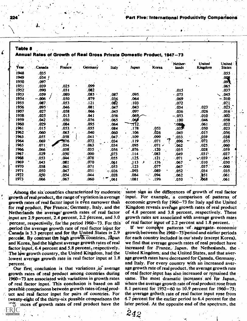
224' Part Five: international Productivity Comparisons;

Table 8Annual Rates of Growth of Real Gross Private Domestic Product, 1947-73.

.A.

Ilear194819491950

.Canada

.035.654.097

France Germany Italy

1951 .039 .025 .0991952' .090 .031 .0821953 .059 / .080 .085 L .0871934 -.006 .050 .079 .0361955 .087. .053 .121 .0821956 .095 .046 .081 .0471957 .027 .058 -066 .0451958. .025 i .015 .041 .0561959 .042 .050 .076 .0651960 .029 .084 .095 .0641961 .015 .053. .055 .0841962 .060' .063 .040 .0601963 .055 .058 .041.- .0471964 ..069 101.1076 .072, , .0341965 .071 .054 .063 .0341966 .066 .058 .035 :0561967 .029 .050 .000 ,9731968 :053 .044 .078 .0551969 .043 .081 .070 .0011970 .038 .061 .071 .0531971 .050 .047 .031' 7.0261972 .050 .054 .044 .0281973. .066 .067 .060 ,061

'Nether-. UnitedJapan Korea lands Kingdom

.095.

.064

.103

.043

.097

.069

2.

.015

.075

.069+072.054.036

-.053.100

..78:314#5-

.033.

.096:062:035.049..071.067.067.052.062.050

.178 .053

.106 126

.109 .099

.119 ,071

.095 .071.076 .120.114 '.083.12S .121J13 l .176.123 .077

-.093 ..089.084 .094:081 .199

.023'

.026

.010

.046.061.050.015X039.072.025..028.031/

a-.039..O10.037.034

1113

UnitedStates

.055

.065

.037

.045-.010.

.071

.013 .-

.016--

.002-

.058

.022

.023

.056

.038

.053

.060

.059 *

.027

.045

.030-.000

.035.

.061'

.061

Among the six 'countries characterized by moderate'grOyith of real products the range of variation inaveragegrowth rates of real factor input is den narrower thanfor reit product: FOr France; Germany, Italy, and theNetherlands the 'average' growth rates of real factorinput are 2.9 percent, 2A percent, 2.2 jercent, and 3.0percent, respectively, for 'the period 1960-73. For this'

,period the average growth rate of real factor input forCanada is 3.3 percent and for the United .States is 2.9percent. By contrast the high groWIFTemintries, JIpanand Korea, had the highest average growth rates of realfactor input, 6.4 percent and 5.8 percent, respectively.The 13w growth country, the United Kingdom, had thelowest averse growth rate in real factor input at 1.8percent.

Our first, conclusion is that variations ;inn averagegrowth rates of real product among Countries during1960--,73:are associated withvariations in growth ratesof real factor input. This conclusion is based on allpossible comparisons between growth rates Ofre4prod-uct and real factor input for pairs of countries. Fortwenty-eight of the thirty-six ifossiblie comparisons thedifferences ofgrowth rates of real product have the

same sign as the differences of growth 'of real factorinput. For example, a comparison of patterns, ofeconomic growth for 1960-73 for Italy apci the UnitedKingdom reveals avePage growth rates of real productof 4.8 percent and 3.8 percent, respectively. Thesegrowth rates are associated with average growth ratesof real factor i ut of 2.2 percent and 1.8 percent_

If we com e patterns of aggregate.. economicgrowth betireen t e 1960-73'Period and earlier periodsfor each country included in ourstudy (except Korea),we find that average growth rates of real product have

for France,, Japan, the Nethenlands, theUnited Kingdom; and the United States, and that average growth rates have decreased for Canada, Germany,and Italy. For every country with an 'increased aver-age growth rate of real product, the average growth rateof real factor.,input has also increased or retained thesame. The most dramatic increases' are for Japan,,Where the average growth rate of real product rose from8.1 percent for 1952-60 to 10.9 percent for 1960 -73;the average grdwth rate of real factor input rose from4.7 percent for the earlier period to 6.4 percent for thelater period. At the opposite end of the spectrum, the

42

Prod- uotivIty Growth, 1947-73: An international Cdmparison-

Table 9 .

Annual Rata of Growth of Total Factor Productivity

Year Citiatht Rance GermanyL948 -.6071949 .0161950 .0801951.. -.0071952 .0531953 .023

.1954 -.034;,1955 -.056

1956 .043'1957 -.0161958 .0051959. .003'19601961

49621963Y19641965196619671968 .

19691970197119721973.

.003.L -008

.028.027'.032.029.022

-.012.029.010.016.023

_.016.013

-.006.019.069.027.033.024:031.001.037.059'

'.036.029.043.030.025.023..021..045.027.619.029.035

.064.050.041.032.066.038.0450

.061.023.020.021-038.037.013.008.051..038.038.013

.037

1t4ly

.062.006.069.034.012

.13367

.017

.046

.031,002.026.061.025.634

.022.045.016

).622-.035

(041

Nether- .Jaien Korea. landi.

i :058

.047

.071

.038

.004

.020

.049

.125.028.048.065.022.024.957

.054.043.053.024.025

.

.005

.061

.046

.034.017.002

.073

.047.011' .022.009 -.002,060 -.011.048 .061

.. -.012' .022.087 -.003.012 .034.031 .038.092 .033.030 '4044/.009 1.021-.017 .045.132 .027

UnitedKingdom

-.001.025.002.014.033.015

-.005.015

f

UnitedStates

.019..008.054,011.009.021

-.004.037 1

. 004.004. 026.000..014.030.015.025.ALa.020

.013-.008-.012

.019

.024..013 ,

.016

.025.

.023-.010

.041.055.026.022

growth rate of real product for the Uriitel KingdomitiseModestly from 3.3 percent1for 1955 -60 'to 3.8 percentfor 1960-73, and the groWth" rate of real factor input.remained virtually unchanged. at 1.8 percent for bothperiods.

Among countries with decreases in .the averagegrowth rate of real product, the greatest change'was forGermany with a decline from 8.2 percent for, 1950-60 to5.4 percent during 1960-73. The average growth rate ofreal factor input dropped from 3.6 percent to 2.4 percentbetween the two periods. Hot. Canada the grovith rate ofreal, product dropped from 5.2 percent for 1947-60 to,5.1,perCent for-.1960-b, and the growth rate of realfactor inpitIO dropped from1.3.5 percent to 3.3 percentbetween the two periods: For Italy the average growth '-rate of real product declined from 6.0 percent for'1952 -60-to 4.8 percent fsir 1960=73, and the growthrate of real factor input declined (tom 2.6 percent for theearlier period to 2.2 percent for the later period. Our

. second conclusion iS that -increases and decreases inaverage growth rates of real factor input between1960-73 and various earlier periods beginning from1947 to 1955 and ending in 1960 are strongly associated

with-increases and d reases ireal product for all t countneavailable.

The most striking iflustTation'of the association ofgrowth in real factor input and growth in real product isprovided by, a comparison of patterns of aggregateeconomic growth for Germany and Japan. During1950-60 Germany had an average growth tate of real. -product of 8.2 percent, and foy 1952-60 Japan had anaverage growth rate of real broduct of 8.1 percent. For1960-73 Japan's average growth rate of real productrose to 10.9 percent, andGermany's average growthrate fell to 5.4 percent. Japan's average growth rate pfreal .factor input rose- from -4,7 percent for the earlier

?period to 6.4 percent for the 1960-73 period, and Ger-many's average growth rate fell from 3.6 percent to 2.4perCent.

.

GrOwth in Capital and Labor inputin analyzing the growth of real factor input among coun-tries or between time periods for a given country, wefirst recall that the growth rate of real factor input is aweighted average of growth rates of real capital input

Part Five: International Productivity Comparisons

Table 10Annual Rates of Growth of Output per Hour Worked

Year194819491950

Canada

.025

.042

.121

' France

...I

Germany Italy

..

Japan KoreaNether-

lands.

.

UnitedKingdom

UnitedStates

.046

.052

.062..1951.

1952.024:085

..014.042

.070'.061 ... '.026

.026

.0331953 .051 .092 .057 .059 ' .045 .057 ,034

-' 1954 .'005 .046 .045 .006 .045 gr.e. .050 .0291955 .076 '.055 .078 .081 .031 .053 .0421956 .059 .046 .066 .051 -.030 .038 .023. .0081957 .019 -.053 .081 .017 .Q50 .035 .051 .0291958 .046. .028 ..050 '.054 .033 -.042 .028.. . .0401959 .018 1 .061 .083 __., .044 .030 .085 .028 .0291960 .026 .075 -.084. .016 .058 .060 .053 .0161061 .042 .055 '056 .069 .166 .004 .068 .034 :0351962 .036 .061

t..057 1)69 .084 .019 024. .019 ..036

1963 :042 .055 . .05$ .031 .08/ .071 Ill/ :031. .0291964 .043 .068 .061 .083 .095 .085 .088

..0(31.039

1965 .044 .064 .072 .122 .057 , -.023 .053 -' .0301966 .044 .049 .055 .042. .051 .102' .029 .047 .0291967 .015 .056 .060 .047 :083 .038 073 .052 .0211968 .05, .055 :061 .046 .098 .054 1.061 .045 .0301969 .028 :068. .055 .080 .111 .125 '.056 .011 .006,1970 .041- .058 ° .066 .040 .114 .086 .076 .,, .070 .019-1971 ..036 .053 .054 .006 .088 .035 .058 .094 ..0381972 .028 .062 , :061 .057 .076 .042 .086 .047 .0321973 .017 .064, .065 .067 .056 .144 .059 '.036 .020

)

Table 11 -,

'Average Annual Growth Rates of Real Product, Real Factor Input, Total Factor Productivity,Real Capital Input, and Real Labor Input

Canada Frknce Germany Italy Japan

1960-73

Korea'Nether- United United

lands Kingdom States

Real prquct .051 '.059 .054 .048 .109 .098 .056- .038 .041

Real factor input .01 .029 .024 .022 .064 .058 :030 .018 .029.

dotal factor pro-ductivity

.018. .030 .030 .026 .045 .040 '.026 .021 .ori

Real capital input .049 .063 .0701 .054 .115 .073 .066 .046 .040

Real labOr input ..020 .004 -.007 .002 .027 .050 .003 .000 .022

1947-60 1950-60 1950-60 1952-60 1952760 1951-613 1955-60 1947-60

Real product .0524 .049 .082 1:060 .081 .050 .033 .036

Real factor input 4 .035 .020 .036 .026 .047 .027 .018 .025

Total factor pro-.ductivity

.017, to .029 .047 '. .034 .034 .023 .015 ;Olt-

Real capital input .068 .047 .069 .033 : .045 .040 .045 .046

Real labor input .011 .003 .016 .022 .048 .014 .002 .012

244

CProductivity Iovith, 1947-73: An International Comparison,

,

and real labor input with weights given by the valueshares of each input. We give value shares for capital

lapin together with ratios of the average weightedgrowth rates of capital input, labor input, and t taifactor productivity to the average growth of realproduct in :Table 12. The growth rate of each input isweighted by the! value. share of that input. Table 12provides data for all nine countries for 1960-73 and forall countries except Korea for earlier periods ending in1960.

Value sharel for capital input vary within a narrowrange *from 0.369 for Korea to 0.44rfor Canada for1960-73, so that variations in weights assigned to capi-.tal and labor input account for little variation in. avalitegroWth rates of real factor input across countries. How-ever, average growth rates of real capital and laborinput vary substantially among countries, as indicatedin Table 11. For the European countries the growth rateOf labor input ranges from a negative 0.7 percent forGermany to a sitive 0.4 percent for France. Averagegrowth rates o labor input for Canada and the United.States are 2.0 ent and 2.2 percent, respectively, andfor Japan and rea are 2.7 percent and 5.0 percent,respectively.

Comparing a rage growth rates of real capital inputamong cou'ittri for 1960-73, we find that Japan andKorea havOthe ighest average growth rates, with 11:5percent-1'nd .7.3 percent, fespectively. Canada,. -04United Kingdom, and the United States have relativelyv. f

227

1

low average groWth rates of 4.9 perfent, 4.6 percent,and 4.0 percent. For the remaining European countriesthe average growth rates of capital input are higher thanfor the United Kingdom and the two North Americancountries and lower than for the two Asian countries.Average rates of growth for France, Germany, Italy,and the Netherlands are 6.3.percent, 7.0 percent, 5.4percent, and 6.kpercent.

Our third conclusion is that for 1960-73 very highaverage growth rates in real prOdtict are associated withhigh average growth rates of. both capital and laborinput and that low average rates of growth in real prod-

ruct are associated with low average growth rates pfboth inputs. Averagegrowth rates of real product in themoderate range froin-4.5'to 6 percent, which includesfive of the nine countries in our study, can be associatedeither with low average growth rates for labor and highgrowth rates for capital, as in Germany, or with highaverage growth rates for labor and low growth rates forcapital, as in the United States. Since thereare substan-tial variations among countries in average growth ratesof both capital and labor input, further analysis reqUiresa study of the sources of growth of capital input throughthe supply of saving and capital formation and the'sources .of-growth of labor input through the supply of4/ork effort.

We find it useful to illustrate our third conclusion by.comparing the economic perfoeTsance of the UnitedKingdoni and the United 'State for 1960-73. The

Table 12'Value Share of Capital Input and Contributions of. Growth in Real Capital input, Real Labor Input

-4rriss

and Total Factor Productivity to Growth In Real Prqditct

Canada - Frame Germany Italy Japan

1960-73

KoreaNether-

landsUnited Uti.

Kingdom

Capital value share .449 .417 .401 .383 .415. .369 .429 .387 .408Contributions of

Real capital input .430 .444 .520 .435. .437 .264 .509 .468 .401Real labor input .209 ..043 -.074 .020 .147 .324 .031 -.006 .317Total factor pro-

ductivity.361 .513 .556 .545. .414 .412 .460 .538 .282

1947-6&1950260 1950-60 1952-60 1952-60 . 1951-60 1955-60'1947-60Capital value share .4t ,420 .382 .367 .405' .352 .470 .380 .387Contributions of I

Real capital input -.549 .365* .340 .220 a 197; .381 .513 .497Real labor input .127 .039 .120 .21.5 Sti .155 .042: .204Total factor pro-

ductivity.3125 , .595 .568 ;565- .421 -.465 .445 .303

United States' average gr th rate of real product ishigher at 4.1 percent than e United Kingdom'st 3.8percent. Average growt ates of real factor input are2.9 perddit-for the Unit d States and 1.8 percent for theUnited Kingdom. The difference in growth rates of realfactor input can be accounted for by the difference inaverage rates of growth of real laborinput, 0 for theUnited Kingdorn and 2.2 percent for the United States.Thi United Kingdom's average growth rate of capitalinput of 4.6 per*it exceeded that for the United Statesof 4.0 percent. The Vnited Kingdom's average growthrate of total 'factor productivity of 2.1 percent also ex-

. ceeded that for the United States of '1.1 percent. Thedifference in average growth rates of real labor input in,the two countries Accounts almost entirely for the dif-ference in average growth rates of real product.

If we 'compare the growth of real factor input during1960-73 with that of earlier periods, we first observethat the greatest change in value shares of capital inputis Japan's increase to 0.415 for the period 1960-73 from0.352 for the earlier period. Changes in value shares ofcapital input between time periods do not.account formuch variation in average growth rates of real factorinput between time periods. For five of the eight coun-tries included in our intertemporal comparisons, thevalue share of capital input increases between the ear -lier periods and the period 1960-7,?. If technicil changewere Hicks-neutral, this would iniply an average elas-ticity of substitution in excespof unity for these five

;' Countries, since the growth rate of capital input exceedsthe growth 'rate of labor input for all countries and allperiods except Japan for the period 1952-60.

Comparing the average growth rates of real capitalinput and real labor. input between time periods forJapan, weind that its average growth rate of real laborinput for the period 1952-60 was 4.8 percent, and itsaverage growth rate of real capital input was only 4.5percent for this period. For the period 1960-73 Japan'saverage groivth bate of labor input declined to 2.7 per-cent, still high by international standards, and its aver-age growth rate of capital input jumped to 11.5 percent.The improvenaent in Japan's economic performance-was due almost,entirelyto the increased average growthrate of real capital input.

Germany's decline itithe average growth rate of reallabor input from 1.6 percent during the period 1950-60

e. to -0.7 percent from (960 -73 was as large as_Japan'sdecline from the period 1912-60 to the later"ftliod.

's average growth 'rate of capital input rosefor 1950-60 tb 7.0 percent for 1966-73

growth rate of real product fell from 8.2the earlier period to 5A percent irk: the later

The decline. in. Germany's economic .perfor-mance :was due 'primarily to the deCreased average

Germanfrom 6.9and itsPercent

Seri.

Pert Five: internationit Productivity Cornparlein

growth rate of real labor input; the contrast to changesin Japan's economic performance between 1960-73and the earlier period is due to differences in the in-crease of the average growth rate of capital input.

Our fourth conclusion is that a rise or fall in theaverage growth rate of real labor input is associatedwith a fall or rise in the growth rate of real capital,input.This pattern reflects the process oft substitution be-tween capital and labor input in production. Germanyand Japan provide the most striking illustrations of thispattern with substantial changes in aggregate economicgrowth between 1960-73 and the earlier periods. How-ever, the same pattern can be seen for two countrieswith moderate changes in aggregate economicgrowth - Canada and the United States. Canada's av-erage growth rate of real capital input fell from 6.8percent to 4.9 percent, and that for the United States fellfrom 4.6 persnt to 4.0 percent, betkyeen therperiods1947-60 anir 1960-73. For the' same two periods,Canada's average growth rates of labor input rose from1.1 percent to 2.0 percent, and theUriited States' rosefrom 1.2 percent to 2.2 percent. France is, the onlyexception to the general pattern; its aikrage growthrates of real labor input and real capital input rose from0.3 percent to 0.4 percent and from4.7 percent to 6.3percent between the periods 1950-60 and 1960-73.

As a second illustration of our fourth conclusion wecompare Korean growth for the period 1960-73 withJapanese growth for.the period 1952r,-6(elapan's aver-age growth rate of real labors was'4.8 percent andKorea's was 5.0 percent. Kor average growth rateof capital input was 7.3 percent, and Japan's was only43'percent. KOrea's average growth rate, of real prod-uct for the later period was 9.8 percent, compared withJapan's rate of 8.1 percent for the earlier period.Korea's average growth rate of total factor productivityfor the later period was 4.0 percent, and Japan's aver-age in the earlier period was 3.4 percent;The differencein average growth rate's of capital input accounts for thedfference in economic performanck

4:00k

_

ProductivityProwthUp to this, point we have Compared patterns of aagre-gate economic growth among 'the nine couniriet6 in-cluded in-our study for the period 1960-13. We havealso coMpared patterns of groWN betWeen various timeperiodkbegimnng'from 100. toq955-and extending to ,.1960 andthettme period 1,60-73 for all countries ex-cept Korea; W can provide additionalp,spectiveon. 'these results.by comparing patterns of growth in outputper hour i.V,tirked. aknorkg Countries' and betweoghtinieperiods. In Table 13 we present average annual groW*h

r4ates

of real product per hoer worked, real factor input

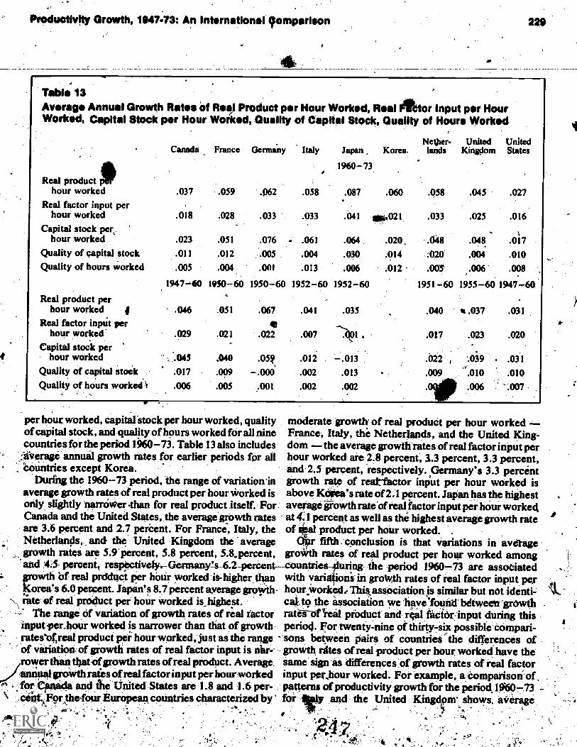
Productivity Growth, 1947.73: An International omparleon 229

.ep

Table 13011Average Annual Growth Rates of Rea) Product per Hour Worked, Real :tor Input per Hour

Worked, Capital Stock per Hour Worked, Quality of Capital Stock, Quality of Hours Worked

Canada France Germany Italy Japan

1960-73

Korea.Nether-lands

Real producthour worked .037 .059 .062 .058 .087 .060 .058

Real factor input perhour worked .018 .028 .033 .033 .041 000021 .033

Capital stock per,hour worked .023 .051 .076 .061 .064. .020. .048

Quality of capital stock .011 .012 :.005 .004 .030 .014 :020Quality of hours worked .005 .004 .001 .013 .006 .012 .005

1947-60 1950-60 1950-60 1952-60 1952-60 1951-60

Real product perhour worked 4 .046 .051 .067

Real factor inpUt perhour worked .029 .021 .022

Capital stock perhour worked ,, ..045 .040 .059

Quality of capital stock .017 .099 -.000Quality of hours worked .006 .005 :001..

UnitedKingdom

UnitedStates

.045 .027

.025 .016

.048 .017

.004 .010

/006 .008

1955-60 1947-60.

.041 .035 .040 .037 .031

. 007 -41 .017 .023 .020

. 012 -.013

.002 .013

.002 .002

.022 , '.039 .031

.009 .010 .010

.0(1111 .006 -.007

per hour worked, capital stock per hour worked, qualityof capital stock, and quality of hours worked for all ninecountries for the period 1960-73. Table 13 also includes.1-Verage annual groWth rates for earlier periods for allcountries except Korea.

Durihg the 1960-73 period, the range of variation.inaverage growth rates of real product per hour worked isonly slightly narrower than for real product itself. ForCanada and the United States, the average growth ratesare 3.6 percent and 2.7 pereent. For France, Italy, theNetherlands, and the United Kingdom the averagegrowth rates are 5.9'percent, 5.8 percent, 5.8.percent,and percent, respectively.- Germany!s-62-percent:-growth bf real prdduct per hinir worked is- higher. thanKorea's 6.0 percent. Japan's 8.7 percent average groyith-

N, rate of real product per hour worked is highest.The range of variation of growth rates of real factor

inputper.hourworked is narrower than that of growthrates'ofireal product per hour worked, Just as the rangeof variation Of growth rates of real factor input is nisr-.rower than tbatof growth rates of real product. Average.annuidgroWth rates of real factor input per hour worked

. for Cfuticla and tie United States are 1.8 and 1.6 per-.ceht., For theibur EUropean countries characterized by

moderate growth of real product per hour workedFrance; Italy, the Netherlands, and the United King-dom - the average growth rates of real factor inPut perhour worked are 2.8 percent, 3.3 percent, 3.3 percent,and 2.5 percent, respectively. Germany's 3.3 percentgrowth rate of reatfactor input per hour worked, isabove Ktirea's rate of 2.1 percent. Japan has the highest .average growth rate real factor input per hour workedat 41 percent as well as the highest average growth rate

alai product per hour worked: .

r fifth - conclusion is that variations in averagegroWth rates of real product per hour worked among_countries,-uring- -the period 1960-73 are associatedwith varin tons in growth rates of real factor input perhourWorked Thil.assOciation js similar but not identi-c4, to the association we have'fOunit bitweelt -growthrataWm-id product and real factor input during thisperiod. For twenty-nine of thirty7ii,x possible Compari-sons between pairs of countries the differences ofgrowth rdtes of real product per hour worked have theSame sign as differences :of growth rates of real factorinput per hour worked. For example, a Comparison ofpatterns of productivity growth for the period 19607713 --

for illy and the United Kingdr shows. av'erage

II

growth rates of real product per hour worked of 5.8percent and 4.5 percent, respectively. These growthrates are associated with growth rates of real factorinput pet' hour worked of 3.3 percent and 2.5 percent.

If we compare patterns of productivity growth be-tween the period 1960-73 and earlier periods for eachcountry included in our study, except Korea, we find

Lthat average growth rates of real product per hourworked havelncreased for France, Italy, Japan, theNetherlands, and the United Kingdom, and have de-creased for Canada, Germany, and the United States.Every country with an increased average growth rate ofreal product per hour worked also has an increasedaverage growth rate of real factor input per hourworked. The most dramatic increases are for Japan,Where the average growth rate of real product per hour_Worked rose "from 3.5 percent for the period 1952-60,the lowest for aff country included in our study forperiods before. MO, , to -8.7 'percent :for the period1960-73, the highestfor anSf country included in ourstudy for this period. Similarly, the groWth rate,of realfactor input per hour Worked. rose M 0:1 percent forthe earlier period to 4.1 percent f r the later period,again the lowelyand highest average growth dates' forthe two periodii. .

Amo un -es with decreaies in the averagegrowth vale of re product per hour worked, Canada'wdplined from 4.6 percent Mir the period 1947-60 topercent for the periOd 1960-73. For the United States

..-the decline was from 3.1 percent to 2.7 percent fdi thesetwo periods. The corresponding declines in ,averagegrowth rates of real factor input per hour worked werefrom 2.9 percent to 1.8 percent for Canada and from 2.0.percent to 1.6 percent for the United States. Germany'saverage growth rate of rell-product.per hour werkedfellfrom 6.7 percent for the period 1950611to 6:2 percent

Ifor the period 1960-73; its average growth rate of realfactor input per hour worked rose from 2.2 percent to3.3 percent for the same periods.- Our siXth conclusionis that changes in "rowth rates of real-product per hourworked and real factor input per hour,worked betweenvarious earlier ptiriods ending in 1960 and the periOd

%1X3 are almost as closely associated as changes in

rates of reajproduct and real factor input for thetwo periods. 1 . -,4

..,..ik._ A useful illultration of the association of growth inreal factor input per hour worked and growth ititealproduct per hour worked is prOvided by .a comparison

'' Of patterns of productyiti growth for the United King-dont ant the United --es. During.the perioir195760thetenited ICingikim's 3:7 percent average growth rateof rea)Aproduct pek"hour worked Was higher than theUnitedStates' 3.1 Percent for the period 1947-60. Forthe period

&1960___ 73.the United Kingdom's growth rate-

Pad Fiva) Internetepnal Productivity CO orisons

°9of real product per hour worke s se to 4.5 percent, athat for the United States fell .7 percent. For tperiod 1955-60 the United Kingdo 's growth ra ofreal factor input per hour worked was 2. s nt, andthat for the United States for the period 1947-60 was2.0 percent. For the period 196073 the growth rate ofreal factor input per hour worked for the United King-dom rose to 2:5 percent, and that for the United Statesfell to 1.6 percent.

Real.Factor Input Per Flour Worked ,

The growth rate in real factor input per hour worked isthe sum of the growth rate of capital stock per hourworked, weighted by the value share of capital input,and ii weighted average of growth rates of quality ofcapital stock and quality of hours worked, weighted bythe valueshares of capital and labor input, respectiVely.We give the ratios of the weighted growth rates ofcapital stock per hour worked, quality of capital stock,

,quality of hours worked, and the unweightedh rate of total factor productivity to the growth

rate of realyroduct per ho worked in Tables 14. Thistable provides data for all e countries included in ourstudy for the period 1960- and for all.countries ex,-cept Korea for earlier periods ding in 1960.

Average growth rates of quality chan r both capi-tal and labor input are positive for all °unities-and forall time' periods included in our study, except growth ofcapital quality for Germany for the period 1950-60.The average growth rate of capital stock per hour'worked is positive for every country and every timeperiod, except for Japan for-the period 102-60. Ja-pan's growth rate of. hours -worked actually exceededthe growth rate of capital stock for the period 1952 -60.-For the period 1960- 73 the contribution of pieal stock&per hour worked exceeds that of either qu of capitastock or quality of hours worked for all coup es exceptKorea. For earlier periods, the contribution of capital ,

41M,ock per hour worked is greater for every countryexcept Japan. * -

-In accounting. -for growth in real product per hourworked for Canada, France, and Korea for the period1960-11, growth in total factor productivity is moreimportant than growth in quality of capital stock, hoursworked, or capital stock per hour worked. Since thesethree countries areassociated with low, moderate, andhigh growth rates of; utpin per hour worked, respec-tively, there is no association between average growthrates of outpdt per hour worked and a large contribu-tion of total factor productivity for this 'period. 'Forearlier periodg the contribution of total factor produt-tivity is more -important than the contribution of other_sources of growth in real product per hour worked forall count ices exceptjte United Kingdom and the

6.

P A - .

Productivity Growth, 1947-73: An international Comparison 231

Table 14 ,

Contributions of Growth In Capital Stock per Hour Worked, Quality of Capital Stock,Quality of Hours Worked, and Total Factor Productivity

Canada France GermNether- United United

Japan Korea lands Kingdom States

1960-73Contributions of

Capital stock perhour worked .287 .360 .476 s .397 .301 .125 .358 .417 .251

Quality of capital!stock .134 .084 .029 .027 .141 .086 .148 .039 .147

Quality of hours worked .074 .042 .010 .135 .038 .126 .050 -.082 .180Total factor

productivity .506 .513 .487 .444 .516 .673. .445 .463 .423

1947-60 1930-60 1950-60 1952 -60 1952-60 1951-60 1955-60 1947-60Contributions of

Capital stock perhour worked .415 .298 ..299 .114 -.129 .254 .401 .391

Quality of capitalstock .155 .067 -.002 .019 .124 .105 \i"..0199 .123

Quality oillinurs worked .071 .062 .007 .030 .066 . 1 .143Total factor

productivity .366 .573 .693 .833 .968 .575 .400 .348

United States. Japan's 'average growth rate of totalfactor productivity for the period J952-60 is almost.equal to the averaowth rate bf real product perhour worked; the cartbution of growth in total factorproductivity, as we have efined it, is equal to 0.968.

Our seventh conclusio is that the contribution ofgrowth in real factor inpu r hour worked is moreimportant than the contribu n of total factor prOduc7tivity ih accounting for growth in real product per hourworked for the periOd 1960-73 and less important forearlier periods beginning from 1947 to. 1955 and endingin 1960. The most dramatic illustration of this conclu-sion is. for Italy: During the period 1952 --60 the con-tribution of iletilfactor input per hour worke0 was 0.169,the lowest for any country and any time period included

, in our study (except JapanJor the pericid 1952,z-60). Forthe period 1960-73 thesi6ntribution of real factor input4r hour worked was 0.559, whi exceeded the cor-l'espOndinglevel for every other ountry except theUnited States. the United States' contribution of realfactor input per hour worked fell from 0:652. for the .

period 1942-60 to 0.578 for the period 1960-73.We find that the cont'ribUliOns Of groWth of the quality

of capital stock and growth of the quality of hoursinorked are cl ly tomparable for period 1960.-73.The contribu n of growth in exceedi

/*

that of labor quality fol.' Canada, France, Gernimy,Japan, and the Netherlands, but the contribution ofgrowth_ in labor quality is larger for. Italy, Korea, theUnited Kingdom, and the United States. For earlierperiods the Contribution of growth in capital quality islarger for Canada, France, Japan, and the Nether-lands, but that of labor quality is larger for Germany,Italy, the Unit Kingdom and the United States. Oureighth and final conclusion is that the most importantcontributionto growth in real product per hour workedis provided bY grOwth in capital stock per hour worked.Less significant contributions to growth in real product .

i t. hour worked are accountable to growth in capital,tind labor quality. Though of comparable magnitudeformer is soniewliat more important.

-A useful illustration of our final conclusion pro-vided by comparing contributions to fooWth i ealproduct per hour worked for thqpnited Kingdom andthe United States. For the period 1960 -73 the UnitedKingOin's average growth rate of real product per hourworked is 4.5 percent and the United States' ispercent. GroWth rates of capital and labor quality are0.4 and 0.6 percent, respectively, for the Lid King-dom and 1.0 it'd 0.8 ;percent, respeOtiv-ely, r theUnited State&. The differences in groWth rates f real

pet- hpor worked are largely attributable to the

241q

232 Part Five: War:national Productivity Comparisons

.difference in growth rates of capital stock per hourworked, which was 4.8 percent for the United Kingdomand 1.7 percent for the United States. If we extend ourcomparison -to, earlier periods, we find that the UnitedStates' growth rate of capital stock per hour workedropped from 3.1 percent for the period 1947-60 to 1.7percent for the period 1960 -73, and the United King-dom's growth rate rose from 3.9 percent for the period1955 -60 to 4.8 percent for the period 1960-73. Growthrates of .capital and labor quality are roughly similarbetween the two periods for each country. We concludethat theadifferences in growth of real product per hourworked between the United States and the UnitedKingdom and between the period 1960-73 and earlierperiods for each country cairbe explained by differ-cues. in growth of capital stock per hour worked.

economic growth for the period 1960-73 are associatedwith variations in the growth of real factor input. Thisconclusion is strongly reinforced by a comparison of

)"N patterns of aggregate economic growth for this perioda with growth during earlier periods ending in 1960 for

each country except Korea.Our second objective was to assess the relative im-

portance of growth in real factor input per hour workedand in total factor productivity in accounting for thegrowth of output per hour woriced. We find thai varia-tions in average growth rates of real product per hourworked for the period 1960-73' are associated, withvariations in growth rates of real factor input pet. hour 'worked. Changes in growth rates ofAeal product perhour worked and real factor input p& hour workedbetween earlier periods ending in 1960 and the period1960-73 are also closely associated,

The third objective of our analysis was to assess therole of growth in real capital input and in real labor inputin accounting for aggregate economic growth. For theperiod 1960-73%we find that very rapid growth of realproduct is associated with rapid growth of both realcapital input and real labor input and that slow growthof real product is associated with Slow growth of bothinputs: 'Moderate growth of real product can be as-sociated wiitth rapid growth of real capital input;rapidgrowth of real labor input, or mode to growth rates ofboth inputs. Our intertemporal co arisoneshow thatincreases and decreases in the a rage growth rate ofreal capital input:are associated with decreases andincreases, respectivelL in the average growth rate ofreal labor input. This fading provides evidence of sub-stituttotabetw 'capital' and labor inputs in produc-tion. ,

Our fourt bjective was to assess the role of growthin qtr.* capital stock, quality of hours worked, andcapitlk per hour worked in accounting for growthin real product per hour worked.. The sum of the con-tributionsOf these three sources of growth in real prod-uct per hour worked is equal to the contribution, of realfactor input per hoar Worked. We conclude that growth.In real factor inpbt per hour w rked is more importantthan growth in total citor p oductivity in accountingfor the growth in real p t per hiiur worked for thePeriod 1960- -less portant for earlier periodsending in 1960: The st important Contribution to

.grOwth in rear product per hour worked is prOvidecl byvgrowtji in capital stock per hour worked.4Growth incapital quality is somewhat more important thangrowth in labor qaality, but the: contributions of thesetwo'sourCes of growth are compatible in magnitude:

We analysis of international. and intertbmporaldifferencei in thesroWth of capital input and the growthof labor input requires a detailed charaCterization of

5. Summary

In section,2 we outlined a methodology for separatinggrOwth in.real factor input from growth in total factorproductivity, based on the transcendental logarithmicproduction function. Beginning with a production func-tion that gives output as a function of capital input,labor input, and time, we defined translo indexes ofoutput, capital input, labor input, and to nical changein terms of data on prices and quantities o outpdt andinputs at discrete points of time. We also troduceddescriptive measures of the quality of capital tock andhours worked that transform indexes of capital stockand hours 'worked into translog indexes of capital andlabor input. These descriptive measures are useful incomparing the results of our analysis of growth in totalfactor productivity with an analysisof groWth in outputper hour worked as a measure of prod-activity change.

In sectio3 we identified translog indexes of output,capital input, labor input; and technical change withaccounts forieal product, real capital input, real 1i forinput, and taw factor productivity for each of the ninecountries included-la-our study. For all countries wecons cted annual production accounts in current and .-cons t prices for the period 1960-73. Por all coun-' tries e ept Korea-we constructed annual oductionaccounts for various earlier periods, beginni g from1947 to. 1955 and ending in 1960.

Our Arstobjeative Was to assess the relative impoitanie of growth in renritbtor input and in total factorproductivity in accounting for patterns of productiVitygrowth for all nine countries for the period 1960 -73 andfor Chaties in 'productivity growth between earlierPeriods ending in 1960 and-the period 1960-73 for allcountriesexcept Korea. We conclude that, for the ninecountries included in dur study, variations in aggre

I.

Productivity GrOwth, 1947-73: An Attornotional Comportion 233

a sources of grOwth of these inputs. Growth in capitalinput involves growth in capital stock as a component ofwealth through saving and capital formation. A com-plete system of accounts, like that developed by Chris-tensen and Jorgenson [5), is essential to the analysis ofsources of growth of capital input through saving, capi-tal formation, and accumulation of wealth. An analysisof the sources of growth in labor input through thesupply of work effort is also required. The analysis ofsources of growth in capital and labor input remains animportant objective for further research on patterns ofaggregate economic growth.

'as

Literature Cited

I. Bureau of Economic Analysis. Fixed NonresidentialBusiness and Residential Capital in the United States,1925 -75. Washington, D.C., U.S. Department of Com-merce, June 1976.

2. Christensen, Laurits R. "Entrepreneurial Income: 'How'Does It Measure Up?" American Economic Review, 61(September 1971), 575-85.

3. Christensen, Laurits R., and Dale W. Jorgenson, "Mea-sUreMent of U.S. Real eispital.biput, 1929-1967." Re -,view of IncoMe and Wealth, Series 15, No. 4, December1969, 293-320.

4. "Measuring Economic Performance,1947-1973." Report to the Offi&of International Com-petitiveness, U.S. Department of ;Commerce, and thgBureau of International Labor Affairs, U.S. Departmentof Lair., 1975.

5. "Measuring the Performance of the Private Sec-', tor of the U.S. Economy, 1929-1969." In Measuring

Economic and Social Performance, edited by M. Moss.New York: National Bureau of 'Economic Research,1973.

alw

6. "U.S, Real Product and Real Fadbr *Tut,1929-1967." Review of Income and Wealth, Series 16,No. 1, March 1970, 19-50.

7. Christensen, Laurits R., Dale W. Jorgenson, and Law-rence J. Lau. "Conjugate Duality and the Transcenden-tal Logarithmic Production Function." 'Econometrica39 (July 1971), 235756.

8. "Transcendental Logarithmic Production Fron-tiers." Review of Economics and Statistics, 55 (February1973), 28-45.

9. Diewert,- W. Erwin. "Exact and Superlative Index Num-bers." Journal of Econometrics, 4 (May 1976), 115 -46.

10. "Aggregation Problems in the Measurement ofCapital." Discussion paper 77-09, Department ofEconomics, University of British Columbia, 1977.

11. Fisher, Irving. The Making of Index Numbers. Boston:Houghton Mifflin, 1922.

12. Goldsmith, Raymond. W. A Study of Saving in the UnitedStates. Princeton, N.J.: Princeton University Press,1955. ,

13. Jorgenson, Dale W. "The Econoinic Theory of Replace-ment and Depreciation." In Econometrics and EconomicTheory, cdited by W. Sellekaerts, 189-221. New York:Macmillan, 1973.

14. Jorgenson, Dale W., and Zvi Griliches. "The Explana-tion of Prdiluctivity Change." Review of EconomicStudies, 34, No. 99 (1967), 249-83.

15. Jorgenson, Dale W., and Lawrence J. Lau. Duality andTechnology. Amsterdam: North-Holland, 1977.

16. Klock, Teun. lndexcIffers: enige methodologisch aspec-Jen The Hague: Pasmans,''1966,

17. Theall. Henri. "The Information Approach to DemandAnalysis." Ecrinometrica, 33 (January 1965), 67-$7.

18. Tornquist; Leo. "The Bank of Finland's ConsumptionPrice, Index . " Bank of Finland Monthly Bulletin, No. ID(1936), 1-8.

Q

t

r

234 Part Five: InternatIonal PrOduCtIvIty*COmparlsons

is

CommentDonald J. Daly

This paper summarizes the results of a larger study ofthe United States and eight of its major trading partneriiirfor the period 1 73 (where poisible). The full studyfor the indiv. countries is about four inches thickand.a numb of interim reports have been presented.The major emphasis is on the measurement and con-tribution of the factors of production of labor and capittal to the growth of total real product and Output perman hour. Total factor procibctivity is derived as aresidual, but has not been further broken down for anyof the individual countries as part of the current project.

When I was asked to discuss this paper I. was encour-aged to be relatively nontechnical and to emphasize thepolity implications of the study. My task has been madedifficult by the inelusion offOurteen tables in the rePort,and the relative technicality*Of. sections 2 and 3. Themain theoretical, portion of this paper has been pub-lished in essentially its present form in1a number of:previous articles and volumes. of conference papers.The conference paper contains a narrative description ofthe $69- major conclusions, but is deyoid of policyimplications for eithergovernment or bUsiness) for theUnited States or the eight other countries.

T)ie two most important themelilmphasized by theauthors of the study are (1) the importande of the con-tribution of total factor inputs, rather than output inrelation to total factor inputs, to total growth in the ninecountries studied; and (2) the importance of capital as aproductive factor- Almost all seven conclitsions in seC-tion 4 relate to these two themes=themes that havereappeared in their work since the initial 1967 study byJorgenson and Griliches argued that the increases in.real output could be almost completely explained byincreases in total factor inputs the factor inputs weremeasured properly. The de results for the UnitedStates as part of the curre study have modified this toa significant degree as the increase in Outputin relationto total factor inputs is currently-tatimated as 1.05 from1945'to 1965, compared to 0.10 in the 1967 article; This .

substantially alters the earlier conclusion that growth intotal factor productivity plays a very. small role ingrOvth- ''

1

252

It should be noted that other recent studies for someof the same countries show quite a differing relativecontribution of labor and capital inputs compared tototal factor productivity over a roughly comparabletime period. This is illustrated in Table 1 for the UnitedStates and Japan.

The differences in the share contributions of capitaland total factor productivity to growth are large for both'countries, especially for the United States. Two pointsseem particularly implikutt to mention as reasons forthat result: Por one thing, the weights for the contribu-tion of capital are much lager in this study than emergein the studies initiated. by Denison. This picks up adebate that has been going on for a decade. This arisesbecause the current Wilier uses' weights for share ofcapital in national income, which includes depreciation,restiential structures and consumer durable= -,all. ofwhiCh are excluded from the income share to capital inthe Denison resultsompariions kw eight countriesare shown in Tablet 2. When the 'stock, capialik.groWing more 'rapidly than employment for almillPlircountries and time periods covered, the point contribu-tion of capital input to growth is increased and the'sizeAif output in relation to total factor inputs is reduced bythis larger weight forIthe contribution of capital. Thecurrent study also incorporates quality ,Chafige in thecapital stock, which worIcS in the same' direction. The"quality" adjustment for capital basically reflects thedifferences in weights between the flows of the services

Table 1Share Contribution -to Sources of Girth ofNational Incoms

United 'States Japan .

1947-73 1948-69'. 1952-73 1953 -71

C.C.! D. CC.J. D.C.

Capital input 0.462 0.151 . 0.317 0,238Labor input 0.242' -0.256 "0.264 0.'210Total factor

productivity 0.296 0.594 0.41-e 0.557'

Sources: Christensen, Cummings and Jorgenson., Table(average of two subperiods for the United States and Japan)for columns 1 and 3; Edward F. DenisOn Accounting forUnited. States. Growth, 1929-1969 (Washington: The Brook-ings Institution, 1974) Table 8-2,: p. III, for eolith-HO; andEdward F. Denison and William K. Chudg, How; Japan'sEconomy Grew So Fast:The Sources of Postwar Growth(Washington: The Brookings Institution, 1976) Table 4-8, pp.42-43, fakcoliunn4.There are some diffirencel, in periodscovered andolefinitions_of national income, but-- these -wouldnot be too important in the differences shown. .

Productivity Growth, 1947-73: An international Comparison

Table 2

Weights for Capital Inputs 19610-02

PresentPaper

NetNationalIncome . Difference

Canada .446 .219 +.227France .386 .223 +.163Germany .388 .258 +.130ItalyJapan

AL .414.408

.180

.279+ .234+:129

Netherlands .452 .252 +.200United Kingdom .381 .214 +.167United States .439 .201 - +.238

Mean .368 .203 +.165

Sources.. Column 1 from Christensen, Cuminings, Jorien-son, Table 2; Column 2 from Edward F. Denison assisted byJean- Pierre Poullier,' Why Growth Rates Differ (Washington:The Brookings Institution, 1967) Table 4-I, p. 38, DorothyWalters, Canadian Income bevels and Growth: An Interna-tional Perspective (Ottawa: Queen's Winter, 1968) p. 28, andEdward F: Denison and William K.' Chung, Now Japan'sEconomy Grew So Fast (Washington: The BrOokings Insti-tution, 1976) p. 28. There. are slight.differefices in the defi-nition of national income, as column'2 includes governmentand housing (except for the.U. S. and JaPaii) but excludes carii-tai consumptionAand column "I excludes both governmentand housing and includes depreciation. The largest differenceswise in the income to capital as column I includes an impu-tatn for the services of consumer durables and Is gross ofdepreciation. The revised national accounts for Canada wouldlower the share to capital slightly from that shown in the table.

. ,ofcapital, as they measure them, and the weights for thestock of capital. I merely want to note these differenceswithout -trying to debate or resolve the issues. (For. .afurther dismission of technical issues, s -ft42, 4, 5, 3,lb) )

It might be noted that the industry studies and others- presented at She conference concentrate on manufic-,

wring and the commodity-producing industries. When!one considers these industries, it seems preferable toexclude housing and consumer 'durables from the in-come weights for capital. .'

In this papa/. the authors have not, made any policyrecommendations based on the series of studies .too.,either government or business in the Countries con-cerned. I am neither able to $ilevelep anypolicy implica-tiOns from, the study nor to see much policy relevance inthe study as it stands without much further 'analysis.

. The last two sentences 'in the study suggest furtheranalysis of "the supply of work effort" and the"sources of growth in capital and labor input." Orallyat the conference, Professor Jorgenson emphasized the..

scope for encouraging capital to a greater degree than inthe paper. How could such a `study throwIght on lower

prices tq cmpurners, larger reaLprodtict in_relatinn.tofactor inputs, or improve the balance of paymenti orsome economic goal? Is capital stock the really centraldeterminant of growth? Why is the study so,disappoint-ing in its relevance to the policy issues that are being,considered in other papers at the conference? Let meanalyze this by considering the research strategy op-tions in international growth comparisons, using thefollowing two-by-four simple conceptual table. Thesecomments go beyond theiprrint.papir and deal withthe broader queitions ofTesearch strategy. ProfessorJorgenson has under way additional studies that willexplore some of these additional topics and .cinestions.

Research Strategy Option"

Cilnlfarisons over time.Factor inputsOutput in relation to inputs

Level 'ComparisOnsFaCtor inputsOutput in relation to inputs

Macro '' Micro

Present study

The present study was limited to the contribution offactor inputs over time and did not attempt the interest-ing task of quantifying the contribution Of economies ofscale, interindustry shifts, and the scope for technolog-ical change. Furthermore, other studies provide addi-tional illumination from making level comparisons bet-ween countries at a point in time in addition to making,comparisons over, time with the same conceptualframework; in this they are helped by the Kravii\dati on-levels,' but needed data on differences in eddcation,capital, and capital quality are not in the public domain.An analysis covering both is mutt more interestingthan either alone, and the cost of doing them simultane-ously is less than doing them both independently. ,

Another, diction that can be fruitful is to do moreindustrial desaggregation. This is the direction that Pro-fesscoriorgenson has begun to take both for the UnitedStates over time and Japanese-United Stites compari-sons at a point in time. The current study is limited tothe private dothestic sector, excluding government butincluding housing. However, a major part of the cov-ered sector involves "nontraded goods," to use thecurrently popular phrase in international trade litera-ture. Much of doe output of the service industries isproduced and purchased in local markets. The interest-ing issues of growth, prodogivity, and trade relate toproductiOn and marketing in the comniodity-producingindustries of manufacturing, agriculture, mining, andpetroleum. It is interesting that all the papers presented

#

231 Part Five: international Productivity Comparisons

previouily at thii conference have emphasiied themicro aspects, with important, policy applications.

It might be of interest that some of the initial work oninternational growth comparisons in Canada Started'at.the wtgative level, using the Denison framework, butquickly shitted to manufacturing. The role of tariffs,science policy, monetary policy, and business man-

, agement in the price, productivity, and cost position ofCanadian manufacturing in relation to the United Stateshas been looked at in this general perspective. Canada'scomparative advantages and disadvantages in factorsupplies and productiVity diffenacceS have beenanklyzed in relation to both the United States and la-ypan. Output per person in Canadian mining is 65 percent,higher, and in manufacturing, 25 percent lower than inthe United States. Capital stock per person in Canada ishigher than in the United States, but oitput per personis lower. The studies have also had Implications foreconomic theory and such tow`cs as the economies ofscale, the influence of tariffs of the distribution of na-tional income, and intraindustry specialization in inter-national trade. Research, costs haVe been relatiVelysmall;:but policy implications have been both importantand controversial,

Let me rnentiolli an interesting area in the Japan-Vnited States comparisons.. Yukizawa's [6] compari-sonsy idtial manufacturing industrie one for*years. over a

of output per person in t two hundred, indi-

Itiyear period) suggest the levels in manufacturing out,-parper man are much closer to North-American levelsthan suggested by the aggregative results for GDP ob-tained by Kravis and associates.. The aggregate 'forJapan elative to North America has been held do*n bymuch

relativeer leVels Of outputiper person in agriculture

and the se Ce industries. After a sharp drop during therecession, manufacturing output per man and per manhour has been increasing.sharply since early .1965 andnow approaches North Amerievell, even thoughthe stock of capital per worker iqpbstantiafly lower.Are product-specific and plant- specific scale econ-omies fir individual manufacturing products in Japansimilar to those in other indastrialized countries, ordifferent? Will the more rapid diffusion, of new tech-nology slow down as the Japanese begin. to attain thelevels of the most industrialized countries, or couldthey surpass the United States, as France and Germanyhave surpassed the United Kingdom in the period sincethe Second World War? What are the costs and benefitsOf a science policy that emphasizes new research and'development (as Canadian policy has), or of one thatemphasizes the diffusion of technology .(as Japanese.policy has)? What are the implications' for steel and.autos in the United States if theincreases in output perperson and in relation to total factor inputs in Japan

054

become substantially greater than in the Unit d Statesonce again? These research questions can be importantfor the direction of trade and domestic adjustments onthe employment side in ,the United. Statei and otherindustrialized countries. ..

I would encourage the United States Dtpartment ofLabor to, emphasize additional research on these impor-tant questions in future research plahs.

Addendum . ,

In the oral- presentation at the conference, ProfessorJorgenson added further comments on the policy impli-cations of the study, recommending encouragement toadd to the capital stock in the United States, presuin-bly the business portion, in the form of reproducibleDied assets. ,

The reader is reminded that Table 3 in the- paperows the share of nonresidential structures and pro-

ducer durables as about 30 percent of the total capitalstock. The hilance relates to consumer durables, resi-dential structures, inventories and land. Should all, oronly some, of these categories be encouraged?' In connection with business capital stocks, the avail-

able evidence indicates that the existing capacity wasbeing utilized at quite low rates, even before the addi-tional underutilization since '1974 ;merged. (See ,[6].)Can one really defend incentives to' add to businew,capital facilities if the existing'facilities are being aber-ated at such low rates of utilization?

I am sure that union economists and union memberswould like to raise these and other questions about the

.policy implications, of the study suggested orally at theconference by Professor Jorgenson.

Literature Cited

1. Daly, tionald J. "Combining Inputs to Secure a Measureof Total Factor Input." Review of Income and Wealth(March 1972), 27-53.

2. Discuss'on of "Economic Growth, 1947-1973:An Internatio Comparison," by Christensen, Cum-mings, and Jo son. InRecent Developments in Produc-tivity Meas ent, edited by John Kendrick and BeatriceVaccara. New York: Columbia University Press for theNBER, forthcoming.

3. Denison, Edward F. "Classification, of Sources ofGrowth." Review of Income and Wealth, Series, 18, no. 1(March 1972), 1.-25.

4. "Some Major Issues in Productivity Analysis: AnExamination of Estimates. by Jorgenson and Griliches."Survey of Current Businesi (May 1972), 37 -63..t

5 Jorgenson, Dale, and Zvi Griliches. "Issues in GrowthAccounting: A Reply to Edward F. Denison." Survey ofCurrent Business (May 1972), 65-94.

.rProductivity Growth, 1247-73: An international Comison

6. Winston, Gordon C. ''The Theory of Capacity Utilizationand Idleness." humid of Economic Literature, 12 (1974),1301-20.

7. Yukizasma. Kenzo. "Japanese and American Productivity:An Intetnational Comparison of Physical Output perHead." Mimeographed. Kyoto: K oto Institute ofEconoMic Research, 1975..

kgr.

Reply

'231

Laurits R. Christensen, Dianne Cummings, and Dale W.Jdrgenson

*

Productivity growth is a serious candidMe for any list ofleading policy concerns of the next decade. The resultsof our study reveal that it is difficult to exaggerate theneed for policies to stimulate U.S. productivity growth.Between the periods 1947-60 and 1960-73 U.S. pro-..ductivity growth dropped from 3.1 percent per year to2.7 percent. During the period 1960-73 the UnitedStates trailed every major industralizedicountry, in-cluding the United ,Kingdoiri, in prodecivity growth:a

Our gtudy also suggests some useful directions for the .

additional, mork required to develop an strialyfis of. -policies to stimulate productivity growth: ;`;

1. Growth of capital ,stock per hour worked is the'most significant ot the three sources of productivitygrowth we'have .analyZed. Capital is not limited to busi-ness fixed capital, as suggested by Daly in his com-ments, and measures to stimulate capital formationshould not be limited to industrial plants or to producers'durable equipment.

2. Growth in capital and labor quality are roughlyequal in importance as sources of Oroductivity growth.Policies to stimulate growth in the quality of factorinputs will enhance the effectiveness of utilizatimi ofboth labor and capital in the process of production.

3. Growth in work effort through increased laborforce participation and increased employment is an im-portain source of economic growth. For the next two to -

five years policies to provide, productive employmentopportunities should have top priority.

Previous international comparisons of productivitygrowth have sOpported the conclusion that grokth ofreal factor input is a much less significant determinantof productivity growth than growth in total factor pro-.ductivity. This conclusion has very important policyimplications. It implies that policies to stimulate growthin productivity should emphasize measures to augmentthe growth of total factor productivity rather than mea-sures to increase the supply of labor and Fapital input.

By contrast our results show that the emphasis hasbeen misplaced. Growth in real factor input and growth

. .: 110 111

accounting for productivity growth. Differences be-255 tween time periods for a given country and differences

art . International Producitivity Comparisons

. ,

among countries show that variations in productivitygrowth rates are mainly due to variations in rates ofgrowth of factor input. This conclusion implies thatpolicies to stimulate the supply of labor and capitalinput can have substantial impact on the rate of produc-tivity growth. t

Daly correctly emphasizeetheventral importance ofour methodology for measuring cipital input in' ouranalysis of productivity growth. It is equally importantto emphasize that our studies cover a much broaderrange of historical experience than the studies by Deni-son and his associates cited y Daly. Unfortunately,Denison's studies are' based' a defective methodol- (.

ogy that fails, to treat lair an capital input symmetri-cally. - -'9,

Labor instils .should be weighted by wage rates, re-flecting the cost of using labor in the production pro-cess. Capithl inputs should be weighted by annualizedcosts, including all components of the cost of usingcapital the rate of return, taxes, and depreciation.The marginal productivity of lilbor is understated if anycomponent of labor costs is 'omitted. Similarly, themarginal productivity of capital is understated if anycomponent of capital costs is omitted. ,

Denison and his associates have pioneered in themeasurement of labor input. However, Denison hasfailed to incorporate a symmetrical approach to capital,so that his measures of capital input are not consistentwith his measures of labor input. His results completelydistort the analysis of sources of economic growth andresult in misleading recommendations for policies tostimulate productivity growth. Daly has provided use-ful documentation of sources. of differences betweenour results and Denison's, ..

Daly has pointed out that much' additional work ierequired to support detailed policy analysis of measures..to stimulate productivity growth; we endorse all of hisvery, useful suggestions: Finally, it is a pleasure to thankDaly for providing a careful and thoughtful set of com-ments on our paper. His suggestions have given us a .,,

great deal to think about and we hope that readers of his ---*-.

comments will share his enthusiasm for support of addi-donal research on the questions he has raised.

(

-t

1

art Six

4

U.S. /TariffPolicy.

A

240 Pa Iu U.S. Tariff Polley

IntroductionWilliam a Dewald

In the years from the Smoot-Hawley Tariff Act in 1930to the Trade Expansion Act in 1962 the majority of U.S.businessmen switched from supporting trade restric-tions generally to supporting them only for their owninduVry. 'During this interval the Anieriean unionmovnt may have switched from neutrality on inter-national trade liberalization to suitport of the TradeExpansion Act. But since 1962 the union movement hascome to represent perhaps the most forinidable opposi-

ption to further trade liberalization. The opposition ap-pears to be quite general arid to be opposition in princi-pie. There 'certainly have been numerous cases ofworkers who lost their jobs in induitries injured byforeign competition. But it is common sense. at leastamong us academic economists, to expect.that, if onelooks at i employment in enough detail, thereMust be and workers that would be bene-fited by nal foreign trade. Last night a dis-tinguished labor leader asked me which industries wouldbe benefited by trade liberalization. In my mdstpleasantand evasive way I said "lots." He wasn't satisfied withmy answer. Nor should he have been. The papers in thissection are far more specific than I was in terms ofparticular industries that would probably beeaffectedfavorably, unfavorably, or not atoll by expanded trade,aliglhey alsd have a contribution to make in terms ofestimating the aggregative disruptions that tradeliberalization might impose on U.S.- production,employment, and international trade patterns.

The studies reported in this session on tariff negotia-tions are industry studies in the broad sense of lookingat a wide spectrum of industries unlike the one-industrystudies discussed earlier. But in contrast, and very im-portantly, thpers attempt to account for a variety ofindirect effects in assessing the likely net benefits orcosts of tariff changes fn terms.pf real incomes as well asthe distribution of such benefits and costs to consumersand to, particular workers in particular industries. The.

, authors. ideritify a .variety of very detailed results,. infact, more detailed results than have ever before beenprepared in studies of this kind. ,

. .

fi

Perhaps the most striking result that is general to eachof the three papers is that the employment effectt oftariff changes in the aggregate are comparatively small,at least in comparison with employment variationthat isthe result of the busintss cycle. if true,, it may bereasonable to conclude hat monetary and fiscal policycould:encompass any aggregative employme effectsof tariff changes within the domain of Yonder:cyclicalpolicieit. Nevertheless one can't be altogether sanguineabout this conclution for several reasons. First, themore detailed results in the Robert. Baldwin-WayneLewis and Williant Cline-Noboru Kawanabe-T.0.14.Kronsjo-Thomas Williams papers really don't take intoaccount the possibility that simultaneous tariff changesmight add up to a different total effect than the sum ofthe changes introduced separately. To some extent thispossibility is explored in the general equilibriumframework of the Wharton industry model in workof Ross Preston as reported by Lawrence Klein. But agnawing doubt remains. Second, the detailed studiesfound that there are significant effects on the demandfor labor in particulalplaces and in particular industriesthat would requige in some instances quite a massiveredistribution of workers to new jobs. Such a munitionCould be very painful and costly to individuals; andpresumably to the society they compose. The transitioninvolves a period of job search, sometimes with so littleprospect of finding another job that the worker givesarp..Even the successful job seekers often experience a spellof unemployment before finding a new job. And it, atleast initially, may well pay. a lower wage than the jobthat was 'lost. Such costs, age real costs and must. beassessed along with benefits to the nation as a wholein appraising the appropriate stance of the govern-ment. in trade negotiationi. ; \

As in any empirical work, the studies reported in this.section do not ereal with theoretical certainties but Wiih _

real world probabilities. The results areomplete as isall empiriesai work. Nevertheless; they represent what Ibelieve to be amoccg the best available informationabout the effect a_Aangel in tariffs on U.S.. income..einployment, and trade-pattenis.i

2p;f0

U.S. Tariff Effects on. Trade and. EmployinentIn Detailed. SIC IndustriesR060 Baldwin arid*Wayne E Uite

Introduction, yq

This paper summarizes the trade and empfoinient ef-faits in the linked States of a -significant multilateralreduction in trade- distorting measu'es by the Worlifs

.' majoaikatling natione: ,BY-estimatina not only' the heti,trade and employment effects of a significant tariff re-duction in over 350 industries but also in the fifty statesand on Some fourteen occupational groups, it is hopedthat the results will be usefid fbr tho ho are nowembarked on the Tokyo round of e negotiatidns

de framework of the Gene Agreement onwithinTariffs and Trade (GATT). A novel feitturaof the studyis the estimation of the net employment eMcts of mul-tilateral tariff cuts undei the assumption of flexible ex-change rates.

The analytical framework for estimaiinglithe.tradeand employment effects of tariff reductions is presentedin pert I. A key assumption of the model is that imports

. are imperfect substitutes for domestic production. Al-though trade models often employ an assumption ofperfect substitutability, a more appropriate Model formost U.S. commodity trade is one in which imports anddomestic production areimperfect substitutes and sup-ply curves for each of these types(of infinitely,elastic, Also, in order to eliminate any mac

eeffects, it

is assumed that total government expenditures and taxrevenues remain unchanged. It is assumed that whenimport duties are changed, income taxes are modified insuch a way as to hold total tax revenue constant.

Part 2 deseribes the data sources employed in thestudy. The requisite trade and tariffdata were collected

' for 1971 on a tariff -line basis by the GATT secretariatfrom die major trading countries. The industry break-down employed corresponds tothe 367-sectOr delinea-tion of the 1%7 U.S. input-output table. Five additionalsets of data were utilized in estimating .the trade-balanceimpact of .muftilaterals tariff reductions and the as-sociated employment changes. They are import and

*This paper istesegi on Robert E. Baldwin, "U.S. Tariff Policy:Pagination and Effects" which' was completed in 1976 under 1LAB

.. COntnict 74-H.

241

'export demandelastioities for the410 trading industriesin the 367-sector input-output table; employment coef-ficients &waled on the same industry basis; a break-down of employment in each induitry by skillgrditpt;breakdown of employment in each industir 1,n+ state;and finally a set of price deflators to put the 1971 tradefigures on a comparable basis with the 1967 input-Output and labor7outpukcoefficientS used in the study.

Estimates of the trade and employment effects in theUnited States of a 50 percent multilateral tariff reduc-'''Lion are pretented in part 3. The larger study from wh)cllthe present paper is drawn also considers "harmonize- '-tion" formulas for reducing tariffs, which. specify that .the higher is the initial tariff rate, the greater will be thepercentage cut in the tariff. The economic argumentsfor harmonization are examined and estimates of thetrade and employMent effects under various harmonj- 'zation formulas are presented in the ftJI1 report to theDepartment,of Labor.

Certain U.S. commodity exports and imports (mainlytextile and agricultural products) have been excludedfrom the tariff-cutting process because they are subjectto nontariff barriers that operate independently oftariffs, Cutting duties on these items will not increasetrade. Five aft* nailVe sets of trade elasticities are usedin the calculations. Based on the preferred set of exportand import demand elasticities (set 1), a 50 pewent dutyreduction leads to changes in exports and implirts thateach exceed $1.5 billion in 1971 prices. However, thenet trade change is a negligible S4-4 million for tariffcuts

Manufactures

all industries and 126 milliorklf tariffs are cut onManufactures alone.. The net employMent impact is alsosmall: 15,200 man-years for all industries and 31.700man-years for manufacturing.

Some indication of the distribution effect of tariffreductions can be obtained by breaking down aggr to .

employment changesinto various skill groups. Di iding.net employrrient changes into fourteen oocu tionalclasses yields percentage changes in I irementsranging from +0.47 percent for farmers and farm mana-gers to 7.0.14 percent for operatives.. Similarly, theregional distribution of employment effects may be

259

Part Six: U.S. Tariff Po lici

interest- to trade negotiators, and therefore the stater. foreign exporters redUce their pitcei by the fullAMOunt.0by -.' employment impact of 50 percent duty reduc-: of the duty cut; to theextent that they do, t, imports

motion is estimated (Table 6). * e into the United Stateswill rigerleis ihatiindntedhy theAlthAigh overall trade and eMplOyment effects of a estimates reported here: This means that less dainestic

50 perCeithariff cur are smait under the most likely sets. employment will be displaced:_ Utilizing. 1971 t dataof trade elasticities, thidoes not mean that no industry for the estimates further exaggerate§ any adverse ef-.ii significantly. harmed or benefited fro he duty re.- fectS. The dollar was still overvalued in that year andductions. If one-halfr one percent Alr an indutrys's thus the trade balance was less favorable than under._ ,itabor force is arbitrarily chosen to divide industries that current conditions (ignoring oil imports, of Course).

' are or are not significantly affected, there would be 54 . : a

iMport-sinsitive in41stries aid .19 export-oriented in-.

dustries. If tariff cuts in iMport-Sensitive industries 1; The Model (were phased over the full ten years peribitted by theTrade Act of 1974, normal industry growth may offset. A key assumption of the -model is that imports are im-the tariff -related employment declines-in 33 of the 54 perfect substitutes for domestic production. Thus, theimport-sensitive industries.. 7 : import demand for a particular good qm can be written

All the results mentionedthis far are impact effects; as follows Ithey do not include the effects -of the exchange-rate °change rewired on ale part of the United States to qm ---- fm (Pr 7 (1/E) - (1 + t + b)/Py, , Pd /Py, Y/py ), (1)eliminate any efickor surplus pressures on the trade J .

N balance as ult of tariff cuts. For three plausible where Pf is the foreign curl importtncy price of the impo.e sets ..

of trade. sticities (1-3), the required percentage good, E is the exchange rate (the number of units ofexchange -rate changes needed for a 50 percent tariff cut -foreign currency per unit of domestic currency), t is theon all industries are within a range of +0.003 to -0.688. tariff rate on imports, b is the rate on imports of inter-The extretne elasticity' assumptions used in sets 4 and_5 national transport and insurance costs,2Pd is the-price,-

' - yield +2.43 and -2.46,`respectively. There are still of the domestic substitute, PY

is the price of all prod-;.labor demand effects even though there is no trade- ucts consumeil domestically other than the import good

balance impact, but these changes are small for all and its domestic substitute, and Yis domestic money in-elasticity setS. c--. , . ,....k- CoMe. Similarly, the demand for the domestic substi-

e' 1 A final exercise in part 3 is to convert the nontariff jute qd depends upon its own pricePd, the price of thetrade distortions in a,griculture and the textile-industry fOreign sithstifute el, the price of all other goods Py,into their ad valorem equivalents and then to estimate.,iisidfmoney income /"...--theAtrAde and employmsnteffects of reducing their pro,:. y,'' :

.

tea've levels fq 50 percent. Net expqrts Of asticultura qd = fd (PdIPy,PmiPy, YlPy) - (2products would increase by $320 million aid net im I .,.-ports.Of textile products would rise $965.inillion..,.The Finally, the dethand for exports qx depends upon thenet employment changes in agriculturea0 the textile price .of the doMestic productlring expcirted Pd, the

Industry are 4-1,135 and:,%.--88,0004nakt-years,..nespe.c- exchange rate E, the foreign tariff-rate rf,- the rate on :tiVely. exports of international transport and insurance costs:%The main conclusion emerging from :this e pineal,. b', the foreign currency price of the foreign substitute -

analysis is that ,a substrantial multilateral tan timing , pf, the foreign currency price of other products con-exercise can be Undertaken without causing sign t sumed -abroad Pyf other than therexport.good,and its-adverse aggregate trade and ,employment effects in the foreign`substitu7 te, and, foreign money income. Yf:

.

U.S. economy. Even without taking into account -

exchange-rate changes, any adverse Arade and qx 'Ix 'Wet (1E I + thl + bq)1P,-,,pflPuf, YflPf): ,(3).,employment effects are ver7.-small, except under one , ) " ' 'i ' "extreme set of. elasticity conditioneifflowever, when The perfect subStitution giodel is reas(pnable for deal-exchange-rate v 'ations are take mto account, net ing with agricultural products acrd' raw materials but is

. ment shifts beco e mininfal)eve under the--most ad- --,L---trade changes. eliminated an aggrigate emPloy- \.

verse -elasticity assumptions. 'An appendix io this paper covering in detail the effects in theSome of the key assumptions of the ,Moddl tend to model of .a change in import prices on expenditures for domestic

goods and imports is available from the authors request.exaperate the adverse effects of the tariff-reductions of 2111e price of an imported good in domestic culency (117, .}equalsemployment. Specifically, it has +fen assumed that Pf(x) (1 + t 4.: M.

2 G 0

U.S. Tariff Effects on Trade and Employment in Detailed SIC Industries

not appropriate for ths large voluthe of U.S. trade inmanufactures. It is clear' &Orli direct observation thatimports of most manufacturedgoods are onlysubstitutes :for domestic goods with which they com-pete, Moreover, empirical estimates for manufacturedgoods of domestic and import demand elasticities andof domestic simpl elasticities giveinconsistent results,if a perfect subs ution model is assumed. The lattermodel,implies ,th following relationship:

.where em and

and'are the import and domestic demand

elasticities an es is the domestic supply elasticity.The levels of domestic output and imports are Os andOm, respectively. Suppose one assumes that the importdemand elasticity for a product is 3, the domestic de-mand elasticity is 0.3, and the ratio Os/OM is 10. Solvingfor es yields a figure of only 0.267. Raising the estitnatefor em and lowering thosefored and Os /Om willincrease -

the implied figure for the supply elasticity but evennumbers at t/he extremes of eMpiriCal estimates forthese variables still tend to yield low supply. elasticities.For agricultural and mineral products; direct estimatesof supply elasticities are in fact quite low. However, the

-. actiiring industries indicate that sh-run and long-runresults of numerous empirical studies of U.S. manu-

atr

supply functions tend tote highly. elaStic.3 Thus, eitherthe methods of estimating these quiouSelastieities havebeen faulty &the perfect substitution model is inappro-priate: ,Though there are bias prOblem7 in estimating

-elasticitie they-do not appear to be significant enoughto account kir the differences in, supply elasticities ob-Mined fromptual esti , and those implied in the

.perffeet 'trbstitntion in

,, . , - . 1

1, i I a knowledge of em andef.. '' ':

1.

(4)

- The mOstappropiiate oach would seem to be toemplOy aperfect substitution model for agricidturalandMineral products that introduces less -than- completelyelastic 'supply curved 'and an imperfect substitutionmodel with infinitely elastic supply curves for manu-factiired.nrOduets. This approach' will be followed insirbsequeril%vork,, but the part reported here utilizes theimperfect'substitution 'model for all commodities andassumes infinitely elastic domestic- .supply curves.Since exports, 'of agricultural and mineral products to

.2the eighteen GAIT countries which cut duties amounttb..-only10 percent, of but total exports to these coun-tries and agriC'ditural barriers are not likely to be re-

4duced significantly, the distorting effects of this as7.

3[14J. For a recent study that supports the infinitely elastic sup-Ply assumption, see [8].

243

sumptir are re4ced. In any event,, the results ofcutting duties on manufactures alone will always bereported separately.

Another assumption made in the model, namelythat all import supply curves are infinitely elastic,has been frequently psed in estimating the effects oftariff reductions. In fact, however, recent-experienceswith devaluation seem to suggest that foreign supplierswill reduce -their prices somewhat in response to a re-duction in U.S. impoit dernand.s The failure to intro-duce a finite import supply elasticity tends, tonse-

- quently, to overstate he actual increase in imports anddecrease in employma-that tends to resultfrom tariffreductions. 31, _ r . .

The,use of infinitely elastii domestic importsupply curves .within the framework of effectsubstitution model obviously. greatly simplifies theanalysis. However, it also raises the necessity of-com-ing up with estimates of cross elasticities of demandbetween imports and domestic production. Unfortun-ately there are-very:few studies of such elasticities forindividual industries. 6 Until reliable estimates of cross-price effects e available on a detailed industry basis, -

it is there! e necessary to make some Simple but rea-sonableni uniptioniconcring theeffect of price cutsin i rt gqptls on the quantit3f demanded of the do-meSt c,Subsfitute. The one-that hivill be used here thatex ndilureS on the domestic substitute are reduced bya sum equallq the foreign costs, i.e.,..costS exclusive ofremaining duties, of the additional imports pinchased inresponse to the price reduction.

Figure l can, be Used toillustrate,this assumption. Letthe slopes of AE and AF reflect the post-tariff dope sticprice and free trade price, respectively; of imports. Theequilibrium position for the consumer when the govern-ment tedistrikutes the tariff prc(ceeds,i&C, whei4as thefree trade equilibiium consumption Point is D.A.Vith ttariff, the Money income of consumers idcluglingsidY equal to the tariff.proceeds . is .OK . -Under thecircumstances they spend KG of money income for GC

rtof the import good. However, .KA of money incomegoes too thefgoverntrient as tariff prOceeds so that for- .eigners, receive only AG of Money income for the goodsthey sell. When the tariff is rernovetrconsumerNiend

Afrof their Money income. of OA on the in)port goodand receive in return fir) Of this good. TheinCrease in/

'See Magee [5, 1565n1]. As Magee notes, estimated values bf,thisfunCtion for the Milted-States are high enough to'make this tidahly,

°For examPle, Clark found that a' I percent change in U.S. de-mand for finished manufactures caused foreign producers to Change

,their price by 0.32 percent [3].

'innocuous. a,ssumptiOn.

"Two studies diat estimate cross elastibities of deMand betwnimports and domestic paduction are [9; 7, chap. 2].

261

Part Six t.U.S arlft Policy

imports resulting from freetrade is LD and the sum paidfor these additional imports is CL . 'It is assumed thatthis sum is withdrawn -entirely from purchases of the

Aomestic' substitute. In the tariff case, the additionalsum spent on imports is Wso edual to the change in th9total sum paid foreigners forimports. Thus, the value etimports plus ditairiount spent on the substitute homeproduct remains constant.

Figure 2 also shows, these relationships. Let Si. andSfift be the foreign..supply curve and tariff-inclusive

. 'foreign supply, respectively; Sd is the doniestictupplyturire;_and'Dm and Dd are the import and doMestic demand curves.- When the duty is eliminated, pUrchases,

-->s< of unions by the country 'increase by the area ACDB.The demand curve for the domestic sithstitute shifts tothe left and doMestic consUmption of thisproduct failsfrom 0GtO OF The decline in spendingon the domeslic'good FHJG is made equal to/the cost of the additionalimports. Figure .2 appears on page 249:

Thus far, no mention has beedmade of the indirecteffects on output

increase it*, fo example, demand for auto-mobiles will not only increase output and erploymentin the automobile industry but also in the industriesthat supply the automobile industry with intermediateinputs, i.e., steel, paint, rubber, etc. When final de-man changes take place in many industries at the sametthese indirect output and employment effectscanbe considerable and must be-taken into account. TO do`thiS a matrix of the dime and indirect input-outputcoefficients is,' needed for. illrl industries. The industryvector of netchanges in final demand is pre- multipliedby this matriI to obtain the change in output by industryresulting frOffithe 'change in final deMand. These outputchanges by industry are then multipliedIby the appro.,priate marginal labor/output c'oefficients for the indtis',tries to obtain changes in employment.

;

.

Income Effect rand Exchange Rate'Changes.The increa value of imports (4/iii.of a 'particularptoduc which also equals the decrease In value, ofexp ditures on its domestic substitute),with a giVen.Y,Pd., Py, and E can be written:`

AM=M-e t+1.' (5)

where M equals the initial import value, e,,, is, the elas-ticity of import demand, t is the tariff rate on the importgood, and it is assumed that income fixes rise by theamount of the decrease in tariffreceipts in order to holdgovernment revenue constant.' When other duties arecut simultaneously P, and Pd do not, in filet, remainconstait since the cast of imported inputs used to pro-duce domestic goods declines. The supply price of theimport good P1 also declines as the costs oimported

. inputs for -foreign suppliers decrease. Conceptually,tution effects betWeen imports and, domestic

good (and exports and, their foreign substitutes) astheir rices 'decline differently in' tesponse,"to lower-cost of imported inputs should betaken into accountin th analysis. However, because a knowledge of foreign input- output relationships\ would be required tomike these calculations and-the differential price and

, ,... ,thus substitution . effects,are., occeedingly small em-pirically, the simulation rosolt's.reporteci-inthe paper donot, include these, effects. . . . ..'

Another income effect of tariffTreduaiOns that mustbe considered in a fixed exchange'. rate model is the

, . ..

impact of shifts in the trade b Ce. It-iia, usually as-sumed in sufchk",modeis that the: in etary authoritiesv the money.Supply so;as-to main ;-il investment at

stant level and that less thap dill emplOyment withfi ed Wages ancit.excess. capital capatity exist in theeconomy.. The?ofore,' the income consequences of 'tradftalance changes can be handled by the standardmultiplier analy.Sis ..(see, e.g. [1]). litirther. changes intrade and employment can th_ en 36' determined fromthese income changes. These various assumption's aremade the Model, but rather than proceed with a mul-tiplier analysis, the model followed Are assumes thatthe exchange rate is flexible and adjusts to eliminatesurplus or .deficit pressures in the' trade balance andthus any net changeftn money income.s The various

262

,IStrictlY-speaking,,e, in equation 5) is:the income-Compensatedelasticity of import demand. 'Actual estimates. of these elaiticities areUncompensated import.demand elasticities. Since all dutiable importsin the United States are 5 percent of GNP, the differenceln- thatelasticities for any one item will be negligible.

'As will be seen later in the paper, the trade impact of a 50.percentlatiffent is so small that aggregate feedback effects on tradeof a multiplier process would be very small.

,16

U.S1pritt Effecta on ade and.E-mplo ment in Detailed SIC Industries 245

assumptions made thus far together, with the fact thatthe impofts are a small fraction'of ON? in the UnitedStates enable one to move from the impact effects ofchanges in tariff rates on many individual items to suchmacro variables -as exchange rates. This equilibriumcondition for the balance of' trade' can be written

E (6)4x)9d EAqmPf 's 0-

One can think Of the effects of a multilateral tariff re-duction as taking place in two steps. Impact changes in,

value of exports and imports caused by ttie duty re-ions are first'determined under the assumption thatxchange rate is. fixed. Then, since with completely

stic import and export .supply curves an exchangerate depreciation [appreciation] of x percept raises[lowers] all import prices to domestic residents by

100Y

!Do

po + x , 100%1

-and, lowers [raises] all export prices to foreigitgs. laxperceX, the exchange rate change, i.e., the uniform

',pride change, necessary to eliminate the trade deficit orsuiplus resulting from the tariff cut is then determined.9Although the final 'position is one in wrch no net

...chmge in, trade balance' has 'Occurred, net employment_

use of composition changeschanges are possiblin domestic production

2.- Data Sources), .

.Trade DataPrObably the most serious data problem faced by priorinvestigatOrS attempting . to analize the detailedeconomic effects on the U.S. economy of reducing,duties his been the lack of suitable information on

: foreign trade and tariffs-. To obtain a complete picture oftrade and employment effects, it is necessary to knowthe exports of each domestic industry to each fdreigncountry participating in the negotiations as well as thetariff rates facing each industry in the different coup-tries. Otherwise, the effect on U.S. exports of duty cuts'by other countries cannot be deterMined. Calculating

itad valorem tariff equivalents on a detailedrhasit for the.major trading nations is an enormous job that is beyond,.the financial capability of any single investigator. Even,goverrimentt haVe found this task to be very difficult,

*An ,appendix to this paper dealing, with the exchange rate re-quired to achieve a desired change in' the bal nce of trade is avail-able from the' authors upon request:,

although some efforts along the; lines were made dur-..

. ing the Kennedy Round.Fortunately, in the late sixties the Off10 of the Spe-

cial Trade Representative reaognized the importance of .

these data for future negotiatiqps and through theOATT.perauided- other major trading, nations.. to pro-vide the secretariat with their relevant trade and tariffdata The secretariat then put tilts' infOrination on acOmparable basis:: and :provided it to all members in i.printed form and on magnetic tape. Trade flows for 1and .1971 -are listed along, with post4(ennedy Roundtariff data on'the GATT tape onthe basis ofthe BrusselsTariff Nomenclature (BTN) for nineteen countries:..United States, Japan, 'Canada, Au.stiia,.Ndw Zealand,Finland, SWitzerland, Sweden, Australia, NorWay, andthe nine European,Community (EC) countries; namely,France, Germany, . Italy!' Netherlands, Belgium,`Luxemb urg, Denmark, Uhited KingdoM, and Ireland 'The data lie presented on a 4-digit BTN basis for thesecountries and cover fill- ninety-nine chapters of the13,T.N. The trade andtariff information is also listed on ,

the basiS of each country's Own tariff schedule, e.g., the.TSUS Schedulefor the United Stateiorthe ET-bditit BMschedule for the-EC countries.

Unfortunately, ad valorem, equivalentS of the vari-able levies of the European Cpmmunity on'agricipiiiiral-items are not available on tape. HoWever, throughthe efforts of Larry Wipf of e Foreign EconomicResearch Office of the Bureau. of ternational LaborAffairs in the Department of Labo these rates werecalculated for. 1971-72. Wipf also ... culated ad oval

equivalents for V.S. imports agricultural com-modities subject to quantitative restrictions.

Since this study deals with.the trade of the UnitedStates on =which confessions will be made orreceived, itutilizes only, that part of the GATT tape listing bothU.S. iMports froM all countries and imports from theUnited States (U. S. exports) by the eighteen othercountries covered in the tape. Of all the **ries in-cluded, only the United States, Canada, New Zealand,and Australia preSent their trade data on an f, o.b. b is(all others express import figures in c.i.f. teitns). The e-fore, U.S. exportS, as measured by imports of the oth rcountries from the United State S, are on a c.i.f., ba isexcept for Canada, New Zealand and Australia. on theother hand, U.S. import -data aueported:on the tape .

are in, f.o.b. terms. In order ,'1.1it all:data.On a coin-parable c.i.f. basis, a:i.f.-f.o.b, corrective factors forimports taken from the 1967 U.S. 367-seCtor input-output table were utilized. These were applied not only -,to-U.S. import figures in'order to express them in c.i.f.terms but also to imports by Agstralia from the ,UnitedStatesSbexportS to AUstralia). However, ihey werenot applied to Canadian and New Zealand imports from

, ,

26.3

Table 1 iskr tTrade, Average Doty leis, end DisperslOn Measures by Cou

e

r. Imports fron*Unital ,Stie

New Swity- 18 GAITU.S. Imports Australia Austria Canada EC Finland Japan Zealand No* Sweden erland Countries

Ditiable Imports (inmilliops' of Ss)* 34,758,9 421,3. 48.1 .4,048.7 7,993.4

Trade:weighted liv,,dtitP(T-w ay.) 7.4 ' 23.2 15,0 12.7 9,1

Unweighted velutf (U ay.) 9.9 271 15.0' , 10.4

Trade-wiiihted)tindard deviation fli4 sty- 6.8 ' 17.4 9.4 5.9 5.8

Uriweighted standard deviation,(U sa.Y 877 17.2" 8.9 5.3 7.6

Total Imports (in millions Of?1,4*

ay.

U ay.

'11-w ed.

U sd,

50,090.4, 1,0 6

5.1 7

8.7 ,8

6.6 6.0

8.8 18.7

Dutiable Imports excl. Textiles, Oil, etc:t 27,748.2 401.1

T-w ay. , 6.4 22.8.

' U ay. 9.0 26.7

T-w sd.' 4.7 17.1

8.3 16.9

Total Impgrts, excl: Textiles, Oil, etc.t

T-w

U ay.

U sd,'

cDutiable Imports of Mfred. Goods

T-w ay,

U ay.

T-w sd. ,

U sd,

Dutiable Imports of Mfred: Goods excl.

Textiles, etc.

T-w ay.

U ay.

1-w sd,

U sd.

42,360.7

4.2

7.7

4.9

8.3

30,300.5

7.8

, 10.1

6.9

8.7

23,289.8

6.7

9.1

4.6

8.2

564 3,0179 , 96.7 104.8 346] 434,4 16,648.2

m 11.1 26.2 9.8 16,3 ;2.2 10.6

12.3 11.7 .32.6 10.8 7.2 4.6 14.4'

8.Q ').7. 19.5 7..4 .3.3 3.94 : 7,3

4,1 6.6 29.9 9.2 , 3.7 5.2 14.6

133.5 10,400.5 10,320,9 124,9 4,883.4 142.6. 240.5 542.5 484.3 28,285;7

5,4 ;, 4.9 7,1 3.5 1.1 17.8 ,4,3 4,0 2.0 .6.2'

12.4 9.6 8.4. 10.9 26,0 8.7 p 4,5 . 11.0

7,2, 6;4' 6.6' 7.1 20.2 '6.9 41,0 1 ;.6

9.9 7.8' 7.0 29.8. 9.3 4.4 14,1

46.9 3,875.8 7,826.9 55.9 3,071.5 926 1023 4 ,235.0

143 12.2 , 9.,0 7.5 11.1 .26.5 6.1 2.1 10.4

14.4, 14.3, 10.3 11.0 11.7 32.4N 10,1 6.7 4.2 14:0

8.6 5.4 5.9 7.8 5.8 20.0 ` 7.3 ' 3.2 3.7 7.1

8.5 4,8 7.7 9.8 6.6 303 . '9.0 3.5 5.0 , 14.5

989.3 132.0, 10,214.6 10,150.1 1123.6 4,856.6

9,2 . '5.1 t4,6 7.0 3.4 .7.0

15.1 11.7 '8.4 '9.6:' 7.3 10.8

15.6 8.7 6.9 6.4 6.4 7.1

27.8 11.8 7.9 8.5 12 7,9

05,8 45:6 3,879,5

21.4 14.8 13.0

27.3 15.1 14.6

,15.8 9.3.' 5.7

17.2' . 8.9 5.2,

44.3 3,706,l

20.8

26.9

12.3 8.4'. 5.3

16.9 . 8.4 1 5.0

138,4 237.7 532.2 475.8 '27,85013

17.7 4.1 3.8 1..9 6.1

252, , 8.0; 5.4 4.1 10.7

20.3 6.7 3.9' .3.6 : 7,4

36.5 10.9. 5.3 5.0 14.0

7,288.4 2,390.3 89.0 '100.9

8.8 7.8 11.4 25.8 10.1

10.3 12.1 11.7 32.7 10.8

5.2 6.9 5.5 19.8 6.6,

7.6 4103 6.6 29.7 9.0

t-

7,121.9 48.8 2,363.9 84.9 98.4

8.7 7.5 , 11.4 26.1 9.8

10.3 10.8' 11.7 32,5 10,1

5.2 6.5' 5.6 19.9 7.2

7.7 9.0 9.0 30.1 8.8

344.2. 422.3

6.2' 2.2

7.1 ; 4.7

'3.2 3.9

3.6 5.2

334.2 413.7

6.0 '2.1

6.6 4.

3.2 2.8

34 5.0

15,0053

10.5

14.4

7.0

14.6

1'4)5914

10.3

14.0

6.9

14.5

Table 1 (continued)

,Sonora: GATT Tape

... Nutt The table covers the trade on which the United Slatt6 iiiii matte and rattive concessions. This includes 'all imports and exports to the other eighteen countries in the GAIT t Tariff

weightedaveros and dispersion meaSurglor .1he' United States; thereforean we

by thiir Unions from the UniteiStates. All tariff rates or ad valorem equi

lariabk kvy items of the EC are 'excluded. 'nodes covered by the new flanational textile agreement are exclud

goods subject to gRs as he. variable levy items of thc EC are exc,

titre definition d makfactured goods followed here differs somewhat

cultural alsd'ntineral goods anghapters 20-0 is .consirting dmanu

,goods by sectors 13-64,The main difference incased food prod

irtau iisteipoitsil ides covered by the new international

imports frOm.all countries, whereas the duty averages and standard deviations for other countries

nts are basedon statutory tariff rates in effect onlanuari I, 1973.

from U.S. imports andimpons of the otherItountries from the U.S, U.S. oil impixtsa nd imports of agricUtiral. ,. .

the convention followed under the IN. Under the BTK Chapters I i-25 are usually regarded as &of agriproducts. In this study, agriculture and mining are covered by sectors I 12 uf the U.S, inputnutput table and factureii,

is (sector 14 in the inPuit.nutprt table) are as manufactures in this,study ho agricultural. under FIN:nt as well as U.S. irnpcida of refined gietro as deluded..

rr

266

It

AV

287

the United States (U.S. exports to Canada). ,It wasfelt that using corrections based on imports from coun-tries generally much farther sway than Canada wouldcreate greatei dfstortion than leaving the Cinadian

' (lets; on an f.o.b.-basis. No- correction of. New Zealasad-'-import "from United .States was made- because of

rt Six: U.S. Tariff 1241111cy

The 367-seCtoriransaction table as well as.its matrixof total inpiit-outpiit coefficients are, unfortunately, noton a domestic base. An input-output table construsildon a total baserather than a. domestic base includes arow (80.02) liking What* "termed' "transferred im-ports." These are simply iniports of goods that compete

he rela ively small volume of trade involved. Table Ipresents information from the GATT tape (with theabove-mentioned f.o.b./CA-1: corrections) on trade,average duty levels, -and measures of, tariff dispersionfor U.S: imports front allsountries an-cV ports ofthe eighteen other coy:tunes (U.S. exports)United States.

. .

tilterinifuntrieRniatIonefflpsA second intpertant data base for-the study is the-1967.

367sectdr input- output table for. the United States. As.

roqi 'the

mentioned in part 1, a ma x of direct and indirect. input-outPut coefficients is n eded in order to measure

the , utput effects of'a change in exports orpo ,.Until 1969 the most detailed table constructed by

Vernnient contained only 85 sectors or industries.0, .1

This akdoWn is too broad to be of much use for.,negoti tors in,niaking decisions about such matters asexceptiOns -or possible sector negotiations. The 367 -sector classification, however, is not so detailed as to beunManageable'in terms...of common notions of whatconstitutes an indbstry hof kibroad as to be of littleu sein dealing with distingUishable pressure grOupt$.

Reclassifying the GATT data on impdrts firotn.the.:United States (U.S. exports) for-eighteen Countries intothe 367-sector system di the input-output table involvedthe following steps. The UN concordance [11] betweenfrm and SITCwas first Utilized to put the GATT dataon an SITC basis. Then a concordance between SIT,Cand SIC obtained from the C,ominerce.Departinent andbased on _1970 U.S.. exports was Used to eipreS4 SITCeXports,of U.S. manufactured goods in SIC tehns.1° ASimilar concordance for agricultural and_ mineral goodswas deVeloped and employed to switch U.S. exportsofthese-Jots:ids to basis. Finally, these SIC exPOrt,data ,Were rearranged into the _367 sectors used foirlhe..-input.ou ut table." U.S. iMport data'were taken from

. the GA taPokin their TSUS form and then expressed'in SIC t rtns---With the aid'Of a concordance developed

. by_ I Ozzello of the U.S. State Department."These mport figures were then shifted to the:classifica-.tion syStem of the input-outputlable by using the con-cordance in [13].

4 1°The Commerce Deptirtinent concordarthased on_theAKIU.S. export trade and the.concordances given in [12].

concordance-is given in [.13]."The SIC input-output sycotioadance also was on ii21,, .

2 6

with domestic production and that are not distinguishedfrOm-donteiric output in the rest of the table. For exam-ple; the row fo'r, say, copper ore mining includes" thedistribution by industry.of both domestically produbeaand imported copper ore.'In order to ensure that the lastcoltrinn and 'last row (total inputs ,and total outputs,respeCtIvely) of the table 'Sum up to the same figure, it isnecessary; therefore either to put in a separate row'showing transferred imports or a final demand columnof negative slumbers tistiagothese tran Sferi-ed 'imports.Under the first arrangent one views each inQustry aspurchasing imports of the final product produced by theindustryand then distributing them to other industriesand 10 final-demand uses along ,with the output prO-

,ddced domestically. The 367-sector table used in thestudy follows this proceddre. However, the 85-Sectdrtable for 1967 is available on a domestic base, and thistable will betsed in sortie subseqUent parts of the study.The drawback of a total-base table is that impOrts ap-pear twice in the table and thus bias analyses directedonly at the domestic consequences of chalfges in fmaldemand. However, it is too costly to shift the 367-sectortable to a domestic base and invert the matrix of directcoefficients to obtain new direct plus indirect cdeffi-cients.,

Although a domestiebase table corrects for the dou-ble counting of iniportSythe coefficients still includeimports. Therefore, the direct and indirect supplychanges fOr various:industries as determined by pre-multiplying the change in a vector of final demand bythe direct and indirect- input- output coefficients willinclude both .domeitic and 'imported goods...If isinterested in. only the change in domestic supply, thecoefficientsinust be decreased to eliminate their importComponents. ThiS I's .accomplished by, multiplying thetotal coefficients of each row by the ratio: total inter-mediate die' of tike industry7s produc (Which is com-posed of clomegitic and import goOds)-less transferred .

importS of the tridustry'S products diVided by total in-termediate use of the industry's products."' Althoughthe 367 - sector table was not Shiftedioa domettic base,the direct and ,indirect coefficients from this table weremodified along the above lines in order to remdf,e theirimport content.

"The method assumes,that the share of imported inputs used byeach industry is the same as the total import share for the input.

...\

U.S, Tariff-Effects_on Trade and Emplent In Detailed SIC industries

..

,,-)"- -' Elasticity Estimates .

_

After classifying U.S. trade and tariffs by input-outputindustry the next 'stip in estimating trade effects is to .

obtain elasticities. of import and export demand forThese industries.' &Vera] sources were utilizedlin thisendeavor. One set of elasticities is composed, -esti-,

-mates by Margaret Buckler' and' ClopPer Almon for.'some 45 manufactured goods and by Stephen Magee forcrude foodstuffs, chide materials, Anil Manufactured.food [2, 4]. ThesA are listed in the fn. report as elastwines set 14 second set of elasticities is the same asset 1 except that import demand{,'-elasticities estimatedby the International Trade COmmission for 20 sensitiveindustries (15 industries in th input-output tablelre-place the import deMand el ticitierlisad for theseindustries in set 1.'.4 .

In addition to. these two lists of ,elasticities, Threeother sets are utilized. These are based upon a survey ofthe literature of elasticities by Robert Stern [10]. Table 2lists these elasticities by 1-0 industry and SITC group.The three ,elasticity sets are obtained by using StQ"best" estimates (which are equal to the approximatemean when several estimated valueS'iVere aiailable) for

- imports and exports, his high iinpOrt and lOw. export

e .

249

elasticities, and finally his Jow im rt and high exportfigures..

. Thus far, the analytical framework has implicitly as- ,

sumed that there are only two goods and tiro

.being

coon 'es.

iMports depict a particular commodity that i 'bIn Figure 2, for example, the deMand and supply ryesofexported'fr . . then country (Often described as therest. of .world) . the co mitry: whose demand andiuprilk lationship are indijited on the right-hand

-P- portion of the figure. oweyer, the data base used in the, study covers U.S. mports 'and exports in iiime 300 'i.-product sectors (each of which is; in turn, usually madeup of a number of taiff-line items) from and to theenlarged Europein CoMmunity,,,each of 9 other indust-rial nations and an "all ,othey". ntry group. Thus,-itis aesirable to obtaitrelliccity esitmates fOr disaggre-gated product groups.

The Buckler-Almon import and export klemand elas-ticities, which are regarded as the preferred set for this

are: Veneer and Plywoody1.4The. Internatior

input-output industryl Trade Commission elasticities (expressed as

positive npmbers)420.06) .58; rubber footwear (32.02) 5.49; leather tanning (33.00)2.42: footwear cut stock (34.01) 2.42: other leather-Products, (34.03)2.42: footsVeat, except rubber (34.02) 4:31.:. foOd .uteriaili; pottery(36.07) 1.03: cutlery (42.41..47; typewriters (51.02) .92; inOto ve-hicles and trucks: (59:03) 2.34:. watches, clocks, and parts (62..09; jewelry (64.01) 2.70; gam-es, toys, etc! (64.03) 2.55; sporting andathlekic goods.(({..04) 1.45: And btittolii, pins, needles; and fasteners

_ %COT) 2.68. ,

Ft GDoitutit le Output 4qd)

.

Table 2Elasticity Estimates Based on Stern Survey

input- Output Industry4.-

1.01-2.03, 2.03;2.106, 3.00,14.01:14.23

14.24-14.27, 2.04,2.06,.07, 4.00, 5.04-6.02,

10.00

7. 8.00All Others

Source:' [10].*Stern does notgive export elasticities for SITC group 3. Consequently, his values for SITC groups 2 and 4 are used.tNiern's high figure for SITC '5-9"ii 10.55'and is based upon a study by J. David Richardson, "Some Issues in the

Structural Determination of International Price Responsiveness," presented at International Collocjuium on Quantitative Studies ofInternational Economic Relations, Namur, Belgium, January 31 - February I, 1974. In view ofRichardson's owp skepticism aboutthe figures and the fact that no other estimate 9f a broad aggregate of manufactiors exceeds 4.72, the Richardson figure was not

'SITC Cbta

0.1

2,4

3

5-9

HighIMPORTS"Best' ft 'Low High

EXPORTS"Best" Low

3.45 0.10 -2.09 0.85 0.38'0.90 0.43 0.02 3.10, 0.86 0.31

1'

; 1.30 0.96 0.63 3.10* 0:86* 0.31*

5.00t 1.80 0.48 2.62 1.24 0:56 -

used for the high estimate.

A

study, were estimated by regressing imports and ex-.ports by industry on the ratio of an ihdustry's domestic.to foreign price. For 'domestic prices, they used thedeflators for the output of an industry. AS they pointOut, there is no atiSfactOrY index of foreign prices.They used either German or Japanese export price in-dexes or a weighted combination of the two as repre;senting foreign prices. 'Soinetisnes it was even neces-sary to emplqy broad export unit values calculated' bythe U.S. Department of Commerce for this purpose.

In 'estimating U.S. Import effects ofa tariff negotia--Lion; one wishes to ialbw the impact of a uniform pricedecline M all foreign export priCes relative to the pricesof U.S. "domestic substitute*. Employing German 'andJapanese prices either singularly or in combination, isnot very satitfactory for this purpOie if there are rela-tive price changes among the various foreign exportingcountries. A given average change in foreign pricescanbe achieyed with many different combinations of pricechanges among individual foreign exporters. However,for the lack of better information the import demandelasticities of Buckler and Almon are used.

The inadequacy of the export demand elasticities thatare employed,in the absence of better data is even rhore-apparent, The desired relationship- sought is how U.S.exports to each country change when each countrif:loWers' its tariffs not only on Li: S. goods but on theexports of every other country: If a particular change inthe average of the foreignPrice index used in estithating ,export demand. elastiCities ,Occurs by a declinecountry's export prices '-(which equals its domesticprices) and no change at all in export prices for the restof the foreign exporters included in the ind .c,.itsing thechange.M.foreign export prices relative top.S.--domes-t iO prices as the bases of the elistiCities needed forestimating the effects of a.Multilaterid trade negotiationwit6Verstate the increase in U.S. exports to thecoun=try. This will be the apse because a multijateral.tariffnegotiation lowers the prices of all expbrters to each,country. However, there are some types of U.S. trade.in which export prices ofcertain foreign exporters do infact remain unchanged in a multateral- trade negotia-tion. For example, when the Mropean Community'(EC). lowers its external duties on U.S. goods, exilort%prices for the members of the European Free Trade.Area (EFTA) will not decline since there is already freetrade between tlfese two .groups. The same holds truefor the EC when EFTA members lower their externalduties. Thus, the existence of important free trade areasgreatly reduces the potential estimation bias asSodiatedWtihnsing the Buckler-Almon export elasticities. At the'same time we retain .the advantage of employing a de-tailed set of commodity elasticities.

Part Six: U.S. Tariff Polley

Another instance in which the expOrt prices of certainforeign exporters remain unchanged, by 'multilateraliatiff cuts relates to the tariff preferences. (duty -free

already granted' for certain products by theUnited States, Ja n, and the EC to he developing na-dons: This also r uces. the pote ial estimation biasassociated with using the Buckler- hoop export elas-,tkities:

Alternative approaches could have been. followed. indealing with the exportside ',of U.S. trade. One is tobtain import elasticidei for each foreign country anthen allocate on the basis of histOrial shares the importIncrease in a ,Partieular sector between 'the UnitStates and all other suppliers. 1Flowever, detailed Com-modity elasticitieSi.were not readily available for all ofthe countries included7 in this study. ,COnsequently,uylizing the detailed Buckler-Almon export elasticitiesseemed preferable to alternative' ways Of estimatingU.S. export effects in a multilateral trade negotiation.

Price DeflatorsGiven a'set of import and export demand elasticities andthe 1971 trade and tariff data from the GATT tape, it ispossible to estimate changes in U.S. exports .and im-ports as a result of a particular tariff-cutting rule. Thesechanges are, however, expressed in, terms Of 1971prices. Since the inpui-oUtput table is baSed on 1967data, -the export and import changes must first be ex-'pressed in 1967 prices before total resultant changes in'domestic output can e be calculated. This is ac-complished by deflating the trade changes classified ona 4-digit SIC 'basis by 1971 4-digit SIC unit vahies .

(Where 1967 = 100) and then reclassifying the tradechanges on the basis. of input-Output istry defini-tions. The 4-digit SIC 'unit values Jor manufacturesWere obtained from the Bureau of Economic Analysis,Department of Commerce. 'For noninanufacturing in=dustries, they were obtained partly. froM PublishedBureau of Labor Statistics sources and partly fromWork sheets at OLS.-

Employment CoefficientsThe next step ih the analysis is to. obtainemploymenteffects of the changes in imports and eiports/This isScoinplishied by first subtiacling,the appropriate inter- wnational margins from exports to olitain exPorton an

basis and then deduCiing dOmestic trade andtransportation. margins ft-Om .both f.o.b. exports andc.i:f. imports,inOrder.to obtain-anal demand shifts foreach sector on a producer value basis. In assigning themargins to the aPpropriate trade and transportation sec-tors, it is assumed that exports aye transported abroadby -U.S; firMs and imports to the United States by('

U.S. Tariff Effects on Trade and Employment in Detailed SIC Industries

I

)foreigners. The changes in final demand are next pre-multiplied by the inverse matrix of the input-output

.. table to obtain the direct and indirect shiftsiin don*sticoutput. These output shifts are the ,n7fnultipliell hy4etof labor coefficients fer the 367-sector table that Were

4 kindly supplied by ProfesSor Clark Bullard of the Uni-versity of Illinois. Some small modifications in his fig-iii-es vere made after consulting with BLS. These fig-'ores: are average coefficients rather than marginal caefficients, which would be the appropriate ones to use.However, there ii- little information available on mar-ginatcoefficients and it is necessary to employ averagefigures, If short-run siiriply curves are, in fact, hori-zoptal, there will be no difference between the twoineatu .re ,, ; .-

. v , ; i "'....

Skill GrOUps ,;,,Besides being interested 07 e.lOtal numbei of

.. .. .

.cuts,displaced or absOr , by tariff .CUtS, ptIllCy-makexsige.novolalso concerned with the skilicomposi.tion oEttie affected'workers. 'To provide this We-ma-fion'a BLS tape was obtained' that contained dOtaileddata on otC4upaticins for .120 industries. (The BLS iiataare based on the 1970 Sample Census of Population).Thede data were-then classified according to the 367industries of the input-output table." For the purpose.

,of this study; 14 skill groups are divinguiihed:.researChand, development workers; professional and technicalworkers (production related); professional and techni-

. . . . ...cal workers (other); managers and admmioratorsi(pro-duction related); Managerd and; admittitratora (cither;craftsmen; sales vvciikerv, .c le ri6a1 Workers; operatives;l'aboreri, except farm; service workers; farmers andfarm managers; private hoUsehold -workers; and fahnlaborers and foremen.

.. .. .

Regional Distributions 4..

The regional distribution of employment changes.caused by a policy decision by the government isanother matter of interest: For this'purptse 'the distribu-tionty state of the igdustries:distinfiished in 85-Sector input-output -table. was obtairied from tber.1 p:Sample Census of Population..Thus, it is pOssibie tonly to determine the total c in employment by. ..

state that is associated with a part ulartard-cuttingrule, but also the distribution of each. employ-ment change by the 14 skill'groups. :

"This, of.course, involved assigning data fora given industry onthe BLS tape to more than,p,n industry it!, the 3674ndustry classifica-.tiOn-system.

,

-

251

Effects of. Tariff Reduction op 'Trade andEmployment

The first question investigated with the modeland data:described in. parts' 1 and 2 is: -What are-the trade anderaPloyinent effects in the United States of a significantreduction in tariffs by this country and the other eigh-teen nations-listed on the GATT tape? A unifollIk' 50percent cut in tariff rates by thesecountries is selectedas an example of a significant tariff cut.

Aggregative Effects .

.

.table "indicates the aggregate trade and employinediimpiat of a multilateral 50'percent linear cut under thadsuniPtioitthat exchange rates remain fixed: get I im-port and export demand elasticities were used in hecalenhillIons. In our judgement, these are the "best"

. elasi/cities to emplom. Certain products have, however,'been excluded from the tariff-cutting process. They are:U.S: exports to the EUropean Community of agricul-tural items subject to. variable levies by the EC, U.S.imports of agricultutal.Products subject to quantit4liveimport. restrictions, U.S: "imports and expo s of is

j:-textile items "Coliered* the flaw international textileagree n, and :U.S. oil 'imitiOrts. MI oE these com-modities are subject to noiftartff trade barriers (NTBs)that operate independently of tariffs.' 6 tutting-dutiedon these items wilt not increase imports. Furthermore,

is unlikely that the nontarifl' bartierS protectifig,them"wilt be reduced appreciably during the nt nego,tia=tionsf'ConsequentlY., if the objective to estimate -the

-edon)smic effects Ota substantial nttini exerciseunder the current negotiations, 'these ems should be

.A

eadi tO'changesalmost $2 billion

$4 million. As

. excluded.Although the tariff-cuttingeZereis

in exports and iMpOrts ontthe order ofcacti,- the net trade shift is'a, negligibthe figures in Table 4 shOW;the surphis is compoSed of a 1.$425 million surplus with the eighteen industrial noun-

1 million deficit'Oatfepreseriti the 'freeride"' b efifs to .the rest-of-The world." The overall

1 4'

igAlthough quOttLs_on reinovecl-, they (Or equivalent. . .

restrictions) are likelylhavehe reim . The actual textile items

covered ateonly those on ,which QR's under the new agatementare effective. The specific input-output sectors affected by` the ex- , .

elusions armlor textileS, 16.01-16.04, 17.01, 17.10,"18.01-18.04,0.7....19.01-19,03; for oil, 8.00, 31.01: .feir agriculture, part of 2:06 (Peg-nuts), part of 14.01 (frozen )feet). 14.02, part of 14.03 (most cheese);14.05,- 14.06.

'rThe same bilateral breakd Table 4 for the other four . .elasticity sets is giver in Ap e'dt-l-of theft!' report ofwhich this paper is a co,ndengation. .

252

Tab lel- ,Effects on U.S. Trade and Employment of a50 Percent Linear- Tariff Reduction

44.Tariff Reduction All Industrie,s ManufacturingChanges (millions 6f. 1971 dollatyff:.

, Exports 4 1,750Imports

. Net trade 'shift1,746 ,

+4Employment change

; (man-years)Export-related 4 136,000Import -reltod -.-151,200Net bmplentchange ; -:--15,200

116,400148,100c

. 31,700*11111mufacturing -0'ects refer.to the effects in all'sectori of

tariff cuts on manufactures rather that? to the effects.only inmanufacturing sectors.

employment effect '( 15,000 jobs) is also very small,especially in vi of the fact that the tuts can be stagedover a ten- period. Estimates of the trade andemployment effects of a 50 percent linear cut that isrestricted to manufactures alone are sonsswhat larger (a$126 pillion trade deficit and loss of 32,000. jobs), butstill very sink* in relation to aggregate exports andimports and to the total labor force in manufacturing.?:06,4interestifill aspect of the-rfsalts ii :that Os ewer-a

age labor coefficient for -the 'reduced domestic outputcaused by the tariff cuts is higher than the average laborcoefficient for the increase in exportproduction. Con-sequently. employment declines evert though ,e tariffreductioni in all industries prOducelt sliglit surplus inthe trade balance. 'However, the labor content of as

-< representative bundle Of all --exports 44:: stilt slightly- higher than the labor content of a representative bundleof import-comPeting production.'° In other words, al-though the -,PVertige labor content of all exports isslightly higherthan ofplf import-competing production,the partitular set of domestic commodities protected byU.S. tariffs is more labor intentiive than the set afiU.S.. .goOds t ha a ac e foreig n d duties'...

' '-'

-

Denand Changes,..:',

.

for Various Skill GroupsWithin recent years there has been an in in con-

'cern Or the income- distribution impact' go rmentpolicis. Mull income-diStribution niodel 1 beydnd thescope of this study, but the initial impct o different

U.S) Tariff Policy

Tablas

Net Tiade Changes by Country troy a 50Percent Linear Tariff Cut (In mIllicolls of1971 dollars)

CotintrY All Industries ManufacturingAustralia . 62 54Avstria 3 ' 4Marla 289 284EC 221 149

°Vinland 4 0.2 . 0.3Japan .141 -206New Zealand 16 14Norway 4 .

Sweden.Switzerland . 21 -

0.421

18 Countries above 425 273Rest of world 421 399

Net 4 126

-labor groups can be estimated .brbrealtitil Oovitathe.total trade-related changes 'in emplOymetti intoemplpyment changes by labor-skill categories. Table 5.lists these Changes by 14 bolls- for all indus-;tries and manufacturing elasticity set 1. I 9

The -50 percent cut allikimb° the all-industry re-,quirements for it & D eft 01.9.13,pereent of theirlabor force, production-related technical workers by0.08 percent, farriers 15y 0.47 percent, and farm labor-

7 ers 0.45 percent. The demand for all other types oflabor declines. The large fit of the declines both abso-lutely and relatively is for operatives,' i.e., semiskilledworkers. The periehtage drop for this category is 0.14percent, whereas the decreases for nonfarm laborersand craftsmen are 0.0g percent 0.0Kpercent, re-spectively. 'The percentage. decline' for all workerscombined is 0.02 .percept. 'Tariff reductions for man-ufactures: alone produde essentially the' same resultsexcept that.,the demand for. farm employees.does-notincrease.' Thus, tariff reductions in all indu'striei raise

/the demand for the services of- highly educated techni-cal workers and farmers; and lower the demand forskilled, semiskilled; and unskilled labor': This holult e-another inditation: that high levels' of 'education endrekitivel abundant supplies of agricultural land serveas the basis for the comparative-advantage position 'ofthe United States. ,

Employment Changes by stateAnother di%trihution question of interest to policy mak-ers is the regional impact of any negotiation. Table 6

310n the basil of 41 trade (deflated to 1967 Price 1967 labortabcoefficients, and 1967 input-output le, the aveiage labor co-

efficient of a tative export bundle is .119 5 man- ears. y permillion dollars, the same coefficient for a representativeimport-coinpeting bundle is 88.0 Man-years per million dollars of ' "The same skill-group changes for elasticity sets 3, 4, and 5 areoutput. - given in Appendix Table A-2 of the MI report.

27 r)

U.S. Tariff Effects on Trade

'

Employment In Detailed sic Industries 253

Table 5Change in Employment brOccupatlon Group for 50 Percent Linear Tariff Cut under Set 1 Elaittleltlies

All Industries ManufactMinget as Net asPercerit,=. oral Export- Import- of Total

Occupation Re Net Work Force Related Nct Work Force,(man-years) (man-years)

1. R & D 6318 4682 1636 0.14 6211 4652 . 1559 0.122. Professional & tech.

(prod, related). 7399 5848 1551 0.08 7206 5807 1399 0.073. Professional & tech'.

(other) 3044 3197 -153 2883 3161 -2784. Management &

admin. (prod.related) -40291 12245 -1954 -0.03 9720 1 12135 2415 0.04.

5. Management & _Jo

.admig. (other) 255 227 28 .- 224 223 1

6. Craftsmen 19622 2424.4 -4622 -0.05 18821. 24026 -52057. Sales workers 5236 6659 -1423 -0.03 482V 6596 -L.1769 -0.048. Clerical worked '20095 , 22904 -2809 -0.02 19033 22707 -3674 -0.039.- Operatives 36776 '53092 -16316 -0.14 35589 , .52766 -17477 -0. 1

10. Laborers, except mfarm 5717 8393 -2676 -0:08 , 5181 8259 -3078 ,- -0.09

11. Service workel's12.. Farmers.. farm

4404 4841' -4374a

-0.01 4096 471)5 -689 . -0.01

9206 24757 6731. 0.47 1289 1467 -178 -0.01; 13. Private household

workers 0 0 , 0 0 0 0 . 014. Farm laborers, -

foremen 7376 2011 5365 0.45 1050 1203 -1531

-gives these results, again for elasticity set 1.20 The tariffreductions bring about a net loss Wi employment in 34 ofthe 1$0 states. The n ittjob loss is more -than 1,000 inIllinois, Massa*usetts, Michigan, New York, and-Peditsylvania. The major garners are California, Min-nesota, and Texas. In relative terms, four New Englandstatea:Massachusetts, Maine New, Hampshire, andIthod*Island-suffer the most, whereas Kansas, Min-

: nesota, Noith Dakota, and South Dakola gain the most.The changes are all veiy small, however.

a'.. -Trade and Entployment Effects Ily,:h(dustryNot only must. policy makers be .0Ticerned with therilacroeconotioc pressures resulting from ateral

'-.Eradc negotiatica, but they must bèawaof its possibleeffects ort, individual industriei. Negli 'ble oi ralt ef-fects-are no guarantee that indiyidual induscwill .notsuffer front, sharp declines in employment anä output.Table 7 indicates all those industries In which employ.-ment would either decrease or increase by at least ofI, percent under a 50 percent cut if elasticity sets 1,2, or

."Employment changes by state and skill grout are reported. inAppendix. Table Az3 of the fill! report.

4

.3.are utilized.2'0n the basis of this arbitrary criterion ofof 1 percent or more employment cha4ge, there are

54 import-sensitive and 19 export-sensitive industfies.that.appear at least once when these three elasticity setsare emploYed: The employment change for the import-sensitive industries is;1.048,429 and for the expos,-oriented industries, 33,052.

rn considering whether to phase cuts in import-sensitive industries over the full'ten-years permitted bythe Trade Act of 1974, an initial consideration might bewhether the annual growth gate for labor in ah, industrymore than offsets the labor 'force decline --asiociatedwith a ten-year phasing arrangement. If it ,did, there.would Seem to be no reason for not reducing duties inthe industry by the full 50 percent. If average growthrates-for _labor_ that prevailed from 1958 to. 197L arerepresentative of the next ten years, the growth factorelirninateiunemployment-problems caused by the tariff' reductions in 33 of the 54 import-sensitive industries..

. .

.1 4

"EmploymeolChanges for each of the 367 industries and for thefive elasticity sets are listed in Appendix Table A-4, and the ratios

the net employment changes to total industry emploxinent ategiven in Table AS of the full report.

2°'?

.

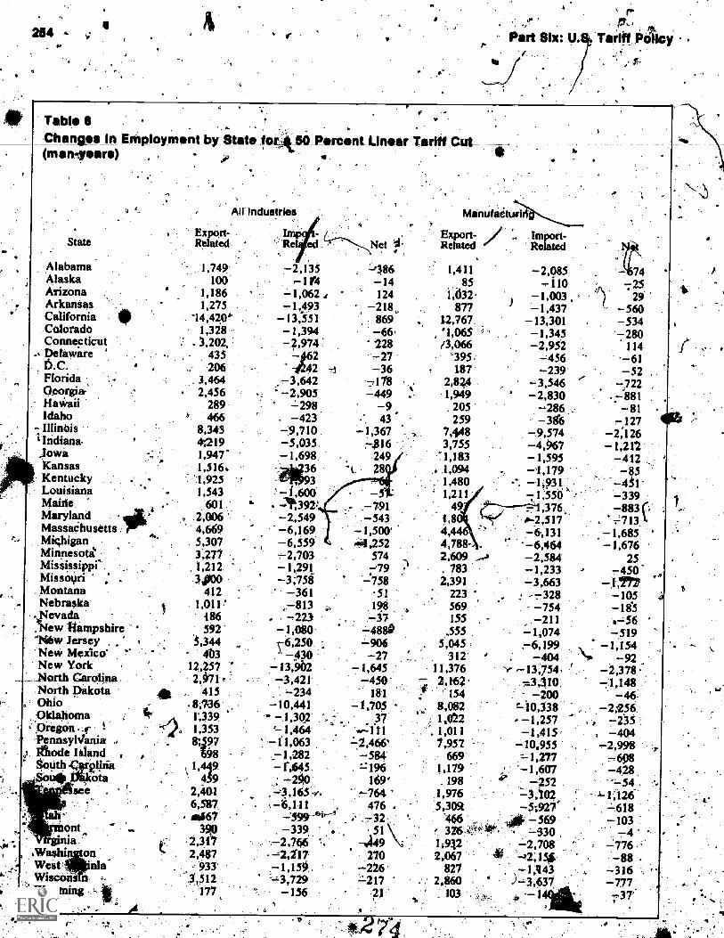
I.

1

2541"'

Part 51x: U.r. Tariff Policy

, /It

TableChanges In Employment by State Ikt(mettles

State

AlabamaAlaskaArizona.ArkansasCaliforniaColoradoConnecticut

. Delaware15:C.Florida(korai arHaWaiiIdahoIllinbis

;Indiana_IowaKansasKentuckyLouisianaMaineMarylandMassachusettsMishiganMinnesotaMississippi

. MissouriMontanaNebraska

NevadaNew liampshire

-'14 w' Jersey .New Mexico-New York_North CarolinaNorth Dakota

. OhioOklahoma

. Oregon .Fennsyl4anialatode Island ,South Car2liziaoislit Mots

sic .

101/

onta

Washi oqWest 'FaitWiscons

_50_.Percent_LInear T.aritt Cut-

All Industries

Expqrt-Relate4 ed

:.1,749100

1,1861,275

- 14,420'1,328

. 3,202,435206

- 3,4642,456

289466

8,3434t2191,9471,516,1,9251,543

6012,0064,6695,3073.2771,212

-

3p00412

486592

5,344463

12,2572,971

4158;7361;339

. 1,3538197

t 981,449

4392,4116,587m667

39,02,3172,487

933'3,512

177

2,135r1 V4

-1,062- 1,493

-13:551- 1,394-2,974

46422

-3,642-2,905

-L 298-4239,7105,035.1,698

:261;36

- ,600141,392:- 2,549-6,169

6,559-2,703

1,291-3;758

-361-813

. -2231,080

76,250' -430

Net 4'.

-'386-14124218869-66.228-27-36

-118449-943

-1,36774116

24928

-791-543 -

-1,500'A4,252

574-49

-758

198

-4880-906-27

-1,645-3,421 -450

-234 181-10,441 -1,705- 1,3Q,2

1,464-11,063 - 2,466'_7-1,282 -584

:196-290 1693,165 ?.. -764

. -6,111 . .4767-32

-3392,766 -. -449\.51

-.2,117 270- 1,159., -226`-;,3,729 -217

-156 2)

%'

Manufaiturl

Export- /0 '.. Import-Related Related

1,41185

i ,i132877

12,767'1,065 3

/3,066395:187

2,841,949. 205259

7,4483,7551,183

..1,0941,4801,211

49!,84,44,788-2,609

7832,391

223569155

.555. 5,045

31211,3762,162'0154

8,0821,022

. 1,0117,957

6691,179_198

1,9765,3051

466376-4!t''

1:9122,067

827. 2,860

. 103

- 2,085-1101,003,,

-1,437-13,301-1,345

2,952- 456-239'

- 3,5462,830-286- 38-69,5744,967

- 1,595-1,179

-. -1;931-;- 1,550

,3760-2,517

6,131-6,464-2,584- 1,233.

3,663-7328-754

,. -211- 1,074.-6,199

-404,-- 13,754,

7.3 41-200

10,338-1,257

1,415-10,955

4-1,277-1,607

252=3,102-5;927-

- 569. -330-2,708-)2;15,S

1,t143)-3,637

-1

4

74725

29-560-5347 280

114-61- 52

- 722,--.1181

81127

-2:126-1,212

-412- 85

-431'- 339

883 (., 7713-1,685 '-1,676

25- 4501197

105 411f5

g 56- 519

-1,154- 92

-2,37871,148

46- 2,256.-235-404

- 2,998698

-4285-54

1;126-618-103

-776- 88 .

-316- 777

37'

U.S. Tariff Effects on'Tradi( and Employment In Detailed SIC industries

H.4

255

.0*,' Table 7 %v

, I. ..,

Changes ip Employment in lielected Industries for a 50 Perg4ent L Cut

> A. InduStries Losing 0,5 Percent or More of Thei4ebor Force )Loss in rcentage Annual Average Labor

- Employment . ,6f Industry's Growth Rate1-0 No. Industry (man- years)' 1967 Labor. Forcet 1958,71t b,

e ' r-5.00 Iron, ferroalloy mining6.02' Other nonferrous mining

13:05 Small arms .14,19 Sugar

,14.26. Vegetable oil mills16pf Thread mills17.03 Lace goo&'17.07 . lire cord, fabric-mos Scour, combing-p1ants

Cordage and twine.- - 20.06, Veneer and plywood

26.09 Wood producti33.07 F,urniture, fixtures,28:02 Synthetic rubber32.01. Tires and innertubes32.02 Rubber f twear32.04 Miscella eous plastic. products33.00 Indint Heather tanning34.01 Footwe r cut stock34.02 Footwear, nonrtibber34.03 4 Other leather products

5.01 Glass products, no containers.03 Ceramic wall, floortile.

' 36.07 Food utensils, pottery36.31k. PoreeJainelectrical supply36., Pottery products5840 Nonmetal mineral prbduCts37.01 Ftintaces, steel products,311.0t ''"-_PriMary lead38.0 Primary zinc38.04 Primary aluininuni38.05 ',Primary nonferrous.inetals,42.01 -.Cutlery t42:1f- Fabricated metal products46.014 Elevator, moving stairs . 10348.02. ,Text ire Machiritry '741

!.54.06 Sew* machines .171 .

5447 Household appliances 7255.02. Lighting-fixturel .4p_x 521.56.01 Radio, TV sets Af... :23;979

'57.01 Electfonic tube's 85858.05 Electrical'equipment R 20661:06.. Motorcycle, bicycle parts s 1,417

":.62.07 Watches, clocks, , st163.01. Optical in lenses

f63.02 Ophthalmic goo.64:01, Jewelry

Musical instruments, parts64.03' tz.,: Games, toys.. i

. 64.04 . -$pOrt, athletic goods64.06.:' Artificial flowers

Buttons, ;medics, pins and fastened364,081" Brooms and brushei

64.12 . Mistellaneous.manufactures:1.Total

173281

71 0.5,4;1- 1.23

19 CT -.1.06.80 0.67

111 2.0954 0.51

242 4.5756 0.52

1,330 1,70`463 0.61

1,663 14.59*79 0.53.

489 0.5.3.

Q.63

3,838 13.141,469 0.581,021 -3.09

78 0.43 4,

6,104' 2:673,046 3.95-

8544-7,- 0.82.°3401 : A 21/470

'20.5923 0.84(1

832 9.67'.36 0.62

11.080' 0.65= -40 1.33

41Z '102 .1.15. .104 0.5452 0.66'

297-

14°

"s\:.

-0.8-2.8-0.8-3:9-17. 4-3.2-2.6

1.0

714.92.32.1'1.2' 2.82.3

-5.2-3.7-L9-.0.5-0.4'-3.8-

v22.1

.1.70.6

. . 2.3636 0.79

0.721.862.59

0.62, 2.51

1.361.42

11.991,018 2.45 .

'434 1.9023134 0.85

12,72444 - 1.01

3.,1 *2.51..

. 11.272:23Ce53

44:

1,598.1,063

.552-.501

861,468

0.3-0.2

2.68.6

6.2 .4.3

0.12.82.3

-&22.821.6

5.93.42.01.81.5

;01.6- -5.2

6.'60.11.9"

256

Table 7 (Conti n Ad)

Indunries.Gathing 0.5 Percent or More of Their Labor Force

Gain-in ;

employment(man-years)",

1-0 NO. Industry

2.03 Tobacco:r , . : °14.10 Pehydratedlood products24.01' Pulp mills4.03 : Paperboard niills28.01 ' Plattfc material, :resins45.03. Oil field machinery51.01 Computing machines5t.02 Typewriters51.04 Office machines53.01 Electrical measuring instrument953.05 Industrial controls53.08 Electrical industrial apparatus57.02 , SemicOntluctors57.03 Electronic components58.03 - X-ray apparatus, tubes'60.01 . Aircraft60.04 ; Aircraft' equipm t ,6211 .., i 'Engineering, science instruments62V- t Mechanical measuring device

.4

U.S. TOM' Polley ,

Percentage ofIndustry's 1967Labor Force"

10,229 3.0365 0.53

161 0.94750 0.98789 0.941g6 0.57

5,826 3.22224 0.79526 2:34582 0.87337 Q.61989 0.50

5,138 6.303,242 1.35

92 1.102,903'- 0.721,223 0.53

305 0.56 .

1,276 1.48Total 53052

4The.,largest absolute loss under three elasticity sets is reported. ,

.tThe largest percentage loss under the three elasticity Sets islreported. .tSotirce:U.S: bepartmetit ofCommerce, Annual Survey of Manufactures, 1971: ,Industry Profitei U.S. Government Printing,Office, 1975. .

_

'ithe classificatiiins of U.S. imports of furaiturn.do.not adequitely distinguish furniture by type of material or by use hence inconcordini TSI.IS numbers, to SIC and 1.0 industries, all furniture, arbitrarily is assigned to 1-0 23.07, Furniture and fixtures, n.e.c.It follows that in ,,calculating the percentage domestic outisi or employment changes that result from tariff cuts, it would bebetter to consider all furniture sectors of the 1-0 table as a single industry. -When this is done, the percentage less is 0.51."The largest absolute gain under the three elasticity sets is reported.

, .41k**The largestIrcentagegaii..under.the three elasticity sets is reported.-ma

,

Titg remaining 21.indusztries thatcannot coperwith *oh'unemployment ptOblem through growth eliticatedin the table by boldface .numbers.

Even in these latter industries, voluntary its canrelieve much of thee pressure to lay off: workers on aninvoluntary basis. Reducing duties less than the generalrule ortperhapii in a fevL cases excepting tEe item coin-'Pletely from- duty cuts can prevent most remaining-Pressures for invOlOntary uneinploYmerit. Ili 'other.words; even if one adopts tife very pro-labor position

. that tariff, cuts should not cause any involuntarytinemPloYment-:a position that ignores the consumer

6 and gzowth benefftsoftariff reductione-it appears that

Sensitivity of Aggregative Changes to ElaStiel- .

AssumptionsThe next stepi,in the analysis as to instigate the sen-itivity of the precediniresults to variations in importa

and export demarid elasticities. To do this, four sets of'elaftticities in addition to set 1 are employed. As noted inpart 2, s& 2 is the same as set 1 eiceprthat importelifticities estimated by.the International Trade Com-mission for 15 input-output sectors are substituted for --the import elasticities eUfployed. in set few these 15sectors". Set; 3. :utilizes rntilizes Ste's summary of "beselelasticities its enumerated in Table 2. Selet combines the ,

t h e ittnbel- of indUitries in.vvhich tariffs should be Cut:,less thfutAllb general average is quite small. 2r The values for these elasticities are given in rtnote 14.

U.S. Tariff on Tiede end Employment in betelleti.SIC Industries.

"high" export demand elasti les and "low" importdemand. elasticities and set 5 combines the "low" ex;port demand and "high" import demand elasticities .listed in Table 2. ,

Table 8 gives the resuleof the 50 percent cut underthese various'elaSticities assumptions. As the table in-

- dicates, sets 2 and 4 give hitter figures _for the tradesurplus ihan,set,1 does also yield net incteases,inemployment. Sets 3:and 5,16n the other hand, yield_neydeficits and net decreasei in employment. (7heemployment decline under set 3 (Stern's "best" elas-ticities) is still small, but the 266,000 job loss that occurs,if import .demands are highly elastit and export ,de-mands are charaCter4ed bYlo*elasticities ,must be

' regarded as significant. Generally, similar conclusionshold for manufacturing alone as for all industries. Thus,there is an outside possibility tha port demand etas-tickies are so high- relative to egpo dernand elasticitiesthat considerable unemployment Ould' igult from a.one-step 50 percent multilateral tariff cut, If exchangerates were fixed. HoweVer; the most probable range for

.,, these elasticity values yields overall trade and employ- t.,ment changes small enough that a significant tariff- Icutting exercise cannot reasonably be opposed On

. balance-of-trade or aggregate employ ment grounds,especially when it is remembered thitt the cuts can be-staged-over a ten-year period....,

Exchange §gp ChangesIf-exchangefilbs are flexible, the t deficits andsurpluses reported in previous tables will riot in fact

257

emerge. Instead, as these bressuresfiegin to opera 'nresponse to the tariff cuts, exchange rates will change torestore., equilibrium:23 Table .9 indicates the exchangerate shifts need-e-d-to re sioTe equilibrium as-wen--as-the-,net changes in employment after the deficit or sbrpluspressures, have 1?een eliminated. The requiredexchange- rate changes are very small except under'elasticity sets 4 and 5.. As would be expeCted, the netemploythent effect when both tariffs and exchangerates are changed is small even in those instances wherethe trade effect large in the absence of exchange -rateshifts. The existence of exchange rate flexibility thinacts.as a powerful adjustment assistance program thatprevents any significant adverse impact on labor as, awhole.

tt. Cutting Dirties on NTB ItemsA final exercise at the aggregative level involved con-verting the various notitariff trade distortions on theexcludediteintinto their ad valorem tariff equivalentsand then estimating trade and entyment effects bycutting these tariff equivalents by 5 went: As notedin part 2, Larry Wipf Of the Offi of roreign EconomicitesearCh, Department of cuinted ad valorem'equiValenti for the Euro Cominunity's variable

"In determining required exchan$ rate changes. it is assumedthat the dollar appreciates or depreciates the same percentage againstall foreign currencies. With a multiliferal negotiation and hexiblerates fir all participants, one would:'need to know all the pairwisetrade balances to determine the change inthe value of the dollar visa vis every other currency. a

Table 8

/

Aggregate U.S. Trade and Employment Effeci,ot a 50 Percent Tariff Cut under Various TideElasticities without Exchange-Rate Changes ./

All IndustriaChangemillions of 1971(dollars)

Export (AX)Import (AM)AX AM

Employmegt change (man-years)From &11From AM

Net employmtnt changeManufacturingS XAM 'AX AMEmployment change fr. A XEmployment change froNet employment change

Set 1

1,7501,746

4

)36,000-151,206

-115,200

El sticitiesSet 2 / Set 3. Set 4 5

6.000135,100

900

1,591 1,591'1,71 1,560

6 31116 00 116,4001 ,I00 -132,000

1,700 - 1.5,600

877, ,187

-310

1,900407

1,493

-' 644,000 140,109--101,300 -26.800-37,300 113,300

809 121''1,153 .393

-343 1,32855,8(10 '118,800

-96,700 -75,700-40;900' 93,100

394.0327-2,932

28,700-295.100-266,400

3653,189

-2,83425,200

-276,400-251.70

I

2U

Tal:ile 9

Part 81x7, U.S. Tariff Policy

Aggregate' U.S. Trade and Employment Effects of. a §0 'Percent .Tetiff_ ut undeVarlousTrade ElleticItitiCvilth Exchange,Reti. Changes

ElasticitiesSet I Set 2 Seta Set 4. 4e15

All IndustriesChangc(millions of 197,1 dollars)

Expdrf(AX)Import (QM)

t AX - AM - ..1

Employment change (man-years)From AXFrom AM .,

Net employment changeExchange rate change (percent)Manufacturing'AOAX - AMEmployment changi from AXEmployment .change from AMNet employment change

'Exchange rate cRange (per nt)

m

.1,747 1,612 1;179 -465 8771,747 1,612 1;179 -465 877

0 0 0 o

135,800 123,300 90,200 -66,400 70,700-151,200 -137,000 -101,500 +48,600 -98,800-15,400 -13,700 -11,300 -17,800 -28,100+0.003 +0.166 . -0.688 i4-2.43 -2.46

1,695 1,564 1,0443 -386 8321,695 1,564 1,143 -386 832

0 A 0 0 0126,600 l 14,000. 84,8004 -65,200 65,700

-146,200 -132,400 -96,900 +41,100 -85,900-20,200 -18,400 -12,100 -24,100 -20,200-646 +0.032 -0.761 +2.17 -2.38

levy items as well as for those U.S. imports of agricul-tural products that are subject to quantitative restric-tions. Using Mintz's study on the effects of quotas,duties on textiles and apparel were adjusted so thatthe quantitative, controls have the effect of raisingprices by 5 percent over existing levels [6, p. 62]. Noadjustment was made in the duty on iMportal oil.

Table 10 indicates the trade and employment effectsfrom a 50 percent linear cut on the N'tR iteatts, assuminga f d- exchange rate. Ctittio protective le vels'on agri-c nil items tmproves4hUI.S. tradebalailte Signifi-.c y under ail-elasticity sets.- However, except Under,set 4 eihsticities, the increase -in textile kmports, whenquantitative' "restrictions on these items are reduced,inorelhttn offsets- the,surplas-creating impact of cuttinglevels of foreign, protection on agricultural. items. Ex- '.cept when set &elasticities are utilized; there also is,,a fairly large net decline in employment when the pro-tective levels of nontanff, bamer's ard reduced by 0

. .

.percenf...

Literature Cited

(7., Baldwin, Robert E.; and Gerald M. Lege. "A-MultilateralModel of Trade-Balancingariff Concessions." Reviewof Economics and Statistics, 52 (August 1971), 237 -45:

2. Buckler, Margatet, and Cloppqr Almon. "ImportsExports in an Input- Output Model." Proceedings o iheBusiness awl Eccilkmics Secti m of the Arnerkpn .Sta-ast,Issociatior(1972), 175-.84..

d

rj

3. Clark, Peter. "The Effects of Recent Exchange RateChanges on U.S. Trade Balance." In The.Effeets of Ex- Atchange Rate Adjustments, edited by I. Clark, D. Logueand R. Sweeney, Washington, D:C.:Government Print-ing Office, 1977. "Ssi

4: Magee, Stephen P. "Prices, Incomes. and ForeignTrade." In International Trade and Finance: Frontiersfor Research, edited by P. B. Kenen. Cambridge: Cam-

. bridge University Press, 1975.,5. -..'"The Welfare Effects of Ristrictiods on U.S.

Trade." Brookings Papers on' Econpmic. ActiOity, 3(1972), 645-97.

6.

7.

8:

Mintz, Ilse. U:S. Import Quotas,; 'Costs and Conse--quences. Washingtoa, D.C.: AMerican Enterprise Institute,- 1972.. . .

Mtitti; John. H. "The Etaployment and Welfare Effects ofForeiKp'radePoliCy." Ph:D. thesis,#iversity of Wis-cousi 74

Richardson,iI. David. "Estimating Demand and SupplyParameters ,without Import Prices: Methodology dEmpirical Results :" Proceedings of the BusinessEconoMics Section of the American Statistiql Assoctlion (1973), 132-41.

9. . "The Response of Impopts, and Domestic De-mand to Price, Tariff and Exchange Rate Changes: AStructural EstimatiOn Stud yfor Selected Man ufactures.Mimeographed. Waihington, D.C. Department of State,Bireau of Economic Alfairs, 1972.

10.: Stern, Robert M. Price ElaSticities rin InternationalTrade: An Annotated Bibliography. London: Trade.:

d

Policy,Research Centre, 1976: .

UnitedNations. Standard International Trade Classifi-cation. Revised: NeW York: United Nations, .1961.

#U.S. Tariff Effects on Trade and Employmept in Detailed SIC Indu r

' . r

12. U.S. Departnient of Comme ice, Bureau of the Censusq 1967. Washington,. D.C.: Government, Printing Office,O.S. FooreiPi Trade Stan *kw: Classifications and ''' 1974:.

, .. Crass-Classifications,. 1970. Washington, D:C.: Gov--------ernment Printing OffiCe, 1971,

. .

13. US: Department of Cornmerce,. Bureau of Econo' Analysis. Input-Outinst.Stracture.a4the U.S. Econom

. .

\14: Walters; Alan A, ?'Production and Cost Functions: An.Econometric Survey." Econornetrica , 31 (.1anuary-Aril'1963), 1-66. j

Table 10Effects on U.S. Trade and Employment, by Commodity, Group, of Reducing Tariff Equivalents ofNTBs by 50 Percent

'Textiles, V

: Agricultural Including Crude, Oil.,

41:: Goods Apparel & Refined All Other?' Total

Set 1 (and Set 2)* Elasticities.Change (millions of 1971 dollars)

Exports (AX) ' 385.2 48,5 'Imports (AM) 65.2 1,012.3AX - AM , ' +320.0 -963.8

Empl4ment change (man-years)Fri* AX 12,679 3,143From AM _,' -11,545 -91,636Net employment change +1,134 -88,493

Set 3 ElasticitiesChange (mi s of 1971 dollars)

Exports ( 152.8, 40.0Imports ( 44.8 604.5Ax AM +108.0 -564.5

Employment change (man-years) 'Y

From AX '4, 5,207 2,480From LtM -1012 -52,290Net employment c rigs.le -3,105 -49,810

Set 4 ElasticitiesChange (millions of 1971 dollars)

Exports (AX) 384.2 84.4 ,Imports (AM) 111 161.5

AX AM . +367.1 -77.1Employment change (man-years)

From AX ' Obik 13,054 5,257From AM - 2,209. - 1,3,946Net employment change +10,845 i43,689

Set 5 Elasticities .

Change (millions of 1971 dollars)Exports (AX)' . 67.8 . 18.0 .Imports (AM) 191.2 1,678.8

AX AM . ,=123.4 -1660.8Employment change (mtn-years)

From AX ' 2,301 - 1,120-'From 4M .1 -27,298 -145-,697Net employment change -24,997 -144,577

0 . 0 433.779.6 -12.7 1,144.4

-79.6 -02.7 -710.7

320.0 16,805 32,947-1,653 -36,609 -141,443-1,333 -19,804 -108,496

0' 70.3.-70.3

....

1341,3691,23,5

A 0..1 -9.8

+9.8

7,2634-23,550-16,287

1102.8.,

709.8-517.0

15,084-85,521-70,437

0 0 468.635.9 3.3 . 217.8

-35.9' -3.3 +250.8

329 17,690 36,330-680 -7,021 -23,474-351. 10,669 +.12,856

0 0 , 8.7132.7 -34.0 ' °' 1,..4:6.7-

-132 7..,+34.0 -1,882.0

,

60 3,236 6,717-2,682 -66,676 --242,347-2,622 :-63,434 -.235,631

I

Note; The input-outPut sectors covered by the NTBs are 1-4, 8, 14, 16-19, and 31.01. Within sectors 16-19 NTBs are reduced only

on sectors 16.01-.16.04, 17.01;-20, il8.01-18.44, 19:01-A9.03_. -

,.

For the sectors covered by- NTBs, set 1 and elasticities are the same.tlndicates the intermediate inputslother than of agricultural goods, textiles, and oil) associated with impart and export changes

in the other three, sectors and thus the import change can be positive or negative.

CommentHarry G. Johnson .

,et Pan' tilgr 4.9: Tariff Policy

from what 'essentially reduce to micrOeContrnic etas-,

his brings Me to a. third point: the results of theinmirical'estitnationtrthat are given fl OSt emphasii inthe paper, the effects of trade liberalization on tradevolumes and employment, are "impact effects" Only,

th nvolve a change to the balanee be-, tween exports ana'impOrts, that is, a change in therelation between ad/aorption and output or aggregateproduction and aggregate consumption, which cannotbe taken to bean equilibrium position except on a veryBaldwin and Lewis are to be congratulated on a very

thorptigh and carefully thought out study probably themost professionally satisfactory study yet outon the subject: My comments are therefore directed,not in criticism of this particular study, but at certaincharacteristics'and assumptions of the tradition of workin this field. Before entering into them, howeve*, IshOuld state expliciily that I support their choice of theperfectly' substitutable supply, imperfectly substituta-ble demand, assumption (especially if, as they intend,they modify it in later work by 'making a different as-sumption for agriculture and mineral deposits). In fact,,there is an additional justification for this assumption,in my view, in that perfect substitutability in demandWould probably give rise tp seriousiflifficulties of esti-mation .in a situation in which foreign demanders im;pose different tariffs on imports and these are altered bydifferent amounts following negotiation of a standardpercentage of tariff rate reduction. (In particular, ern-

-, s phasis would have to shift- from, demand to supplyelasticitiesto whose estimation 'much less profes-sional effort has been directed.)

*first, not major, criticism relates to the assunipdon explained in detail in their paper, that an increase inexpenditure on imports, net of tariffs Js matched by an:eqUal decrease in expenditure on domestic ThiShas the advantage 4, simplifying 411pe talMationsgreatly, and Can bejuitiked as applied to a general tariffInduction' in Whiciternis-effects COme -out in thewash "; but it does impoierestiicti011is on cross- effectson import acid export demand that.might be important ingetting from the impact effect to the muter orexchange-rate adjustment. Second, the analyi seemsto use one term only to represent real income as a--constraint on total d_i Macroeconomically, how-

"- ever, a Country'* penditure or absorptict need notequal its output 0 ions the 'different& beingconstituted by cap' movements including reservemovements. TheoretiCallY, the savingki#dissavingsplied liould:enter into thedefinind andaupply func-: thins poSited, rather than being left to be determinedresidually by the effectsafrelative price changes resulting from trade liberalilatiOnotit trade vOlurnet,-CledUced7

peculiar set 'of assumptions about aggregate 1/4ilemand,saving, and reserve or cash accumulation or ecUrnula-tion, whiekcannot be accepted as teaks 1.

To corn te the calculation and arrive at results con-sistent with full equilibrium, there are two possibilitiesopen. The first, obvious, and necessarily consistent oneis to calculate the exchange rate change necessary torestore equilibrium a change that would occur au-tomatiOally under the present system of floating ex-change rates, particularly given the relatively small de-preciation of the dollar indicated: as required by theestimates produced by the study. It may be noted inpassing that such an equilibrating depreciation of thedollar should not be interpreted as necessarily entailinga welfife loss for the United States. (A calculation of thewelfare effects of trade liberalization is not provided inthe paper, though I understand the largerostudy envis-ages sow detailed calculations along these lines.) Thereason why a terms-of-tradeloss implicit in ,a deprecia-dOn is not necessarily a welfar e loss is that the liberali-zation of trade itself involves a welfare gain. Neverthe-less,previons studiek, notably that of Basevi [1],confirm the general expectation that, with the low, elas-ticities SuggeAted by empirical estimates, the, UnitedStates is likely to lose more on the terms of trade than itgains from trade liberalization.

The second alternative is suggested by foreign trademultipliertheory, the initialexcess supply in the UnitedStates evoking a multiplier redUetion in U.S. incomeand emPloyment (and converse expansion elsewhere)lead* to a new equilibriuM with r9ower U,S. tradedeficit than the impact defielk but still a deficit as-Iodated With a reduction in U S. and an increase inforeign net international saving (or, more accurately,"hoarding;''ofaccumulation of international reserves).The authors suggest that the tecessary, calculations an

vasilybe made` onlhe usual assumption th lie mone-tary authorities main!ain afixed level of rest rates.On the contrary, in principle the maint ce of fixedinterest rates.in face of a balance-of-flayMents deficitinvolves. a continuing process of replacing an outflow ofinternational reserve. by open-market purchases ofdomestic seciteities, and this is virOCeis that cannot be

,3/4y U.111#

v. 'wownowt. on Trachor Emplo mentin pitfall

assumed for most countries to be. able to go on forever[3, 41. In'the case of the United States in relation to therest of.the wot boWeiver, given.the ery small tradekiss emergitig mthe calculations, an he still smaller i,

\- -10mi at,would ppear after the mul lie ionshad been madi, ogether with the int ationtirrole ofthe-dollar as a reserve currency, th ssumption wouldprobably be tolerable as an approximation.

The foregoing relates to the efficson trade. Theaultioysare, however,, particulaM oncerned withemfiroyment, which, ondtheir input-output calculations,they find will decrease evenif trade is kept balanced byan appropriate (small) depreciation'oPthe dollar. Thisfinding, however, leaves a loose end, which is the sub-ject of my fourth comicnent: Presumably, less labor perUnit of value added is accompanied or balanced by morecapital per unit of value adiled, on the tautological prin-ciple that all value added has to be added by-Something(either libor or nonlabor inputs), and the question is*here in.the economrelke nonlabor 'sources of value.

-1fidded, needed to keep value added in exporting. qual tovalue added in importing, are to come from. In otherwords,. in addition to the exchange rate adjustmentnecessary to keep value added conVant,he calculationshould include An adjustment of the price of labor re*tive, to capital necessary to keep employment of lab&and "capital" (nonlabor value added) constant. To bestrictly accurate, the calcula n should includechanges in' two relative J3. es o three nutheraireprices, to maintain full employment o he two factors ofproduction and therefore, implicitly, ull-employmentproduction and balanced international, rade.

My fifth comment concerns the-use of a (modified) 50'percent reciprocal tariff cut as the standard case ofreciprocal trade liberalization for analysis. Most of theargument relating to the computation.effect is devotedto discussion of the elasticities selected; nd on thisscore 'one can only accept the authors' judi Ous di cus7sion of arid selection amon alternatives, Its clear omthe nature of the calculati ns, however, that apart Cal-the' elasticities- employe the outcome will depend;

rhaps significantly and substantially, on two "struc-'" magnitudes, ,the tariff tes now in force, to

which thelinear 50 percent cuts will apply, and therelative volumes of exports d imports of the trade-

. liberalizing countries., It is also apparent from the itatis-.tics presented that the United States has a lovier aver-age tariff rate on manufactured goods than have itsmajor tradingjartners, and that the United States ex-ports in larger volume. to than it imports from othercountries. On both grounds, a 50 percent tariff tec-IMOapplied by all major: countries might well be assumed a.priori automatically to favor the United States as com-pared with the odors,' leading ..them (especially the

. .

ittt;strhiS

Comrlon Marketcountries) to argue, "as they did i0.theearly stages of the Kennedy Round, for some differentprinciple of reciprocal tariff reduction. In this connec-

.tionrit would:seem-that; rather thatjallept the (mod-ified) 50 percent.tariff,cutting rule as obviously fair andthen calculating, its actual :efflects, the study's 're 'tiltsshould be used explicitly to s w that, despite sup -

cial arguments to the contga , The 50 perc nt principleleaves the United Strnes or reasons re ted to theinteraction of differences i elasticities wi dispersion J.of tariff rates about their erages) at- sig

d th a r-ifiCa if /

mula producing exactly equal xpani n of it trade in ,i'.i'relatively small disadvantage s coin

both directions. Alternative principles of negotiationare, of course, discussed in William Cline's paper forthis conference.

.My sixth and final comment relates to the discussion

of adverse effects of trade libffalization oMJ.S.employment in the aggregate and by state and indu try.It seems to me completellobitrary to set 0.50 percentas a standard 'defining negligible effects on employ-inent, especially over a ten-year adjustment periodstarting in 1980, or to study whether thetirdverse effectwill be absorbed by employment growth in the indus-

',try concerne&over the adjustment period. It wouldseem more ec nomically relevant to relate employmentdisplacement/by irtOtepsed import competition to thenatural wastage ofexisting ern oyees through retire-ments and voluntary quits. a reasonably fullyemployed economy, which o 'hopes will be the nor-mal situation by 1980, the earliest date at,which tradeliberalization is likely to start, adjustments Of employ-ment to trade liberalization are likely to be negligible inrelation to everyday labor market adjustment, as ex-pressed in new entries, retirente ts, and voluntaryjhb

per se is likely to be, typically, th prOtiltrn of a seniorchanges, The real' problem of a Ployinent adjUstment

group .of relatively' unskilled but -well-paid Workers,whose traditional employment is threatened by rapidincreased from the lower-paidand frequently

, .

''more skilled workers in other developed countries or1 developing countries. Such a problem would be in-ktrequent, enough, . and manageable enough by policy

(including temporqary slowing Of import growth), not toneed toipose a serious obstacleto tradegiberalizatiO.Unfortunately, this problem tends to be Compounded

.and confounded with the much more serious problemof abnormally low aggregate dethand resulting fromrestrictive fiscalpionetary-polick and antidepreclitionexchange rate policy, the effect of whiCh ire creatingune yment is most easily blamecynaCcurately, onu foreign competition and used support, demandsItii increased barriers against imports.

tihilretUri Clt lidti

rlf,Part Sht: U.S. Ta Palley. ,

. . .

44,

Tariff and Value." The American tioionitc 010bert Wayner,I. Basevi, Giorgio. "The RestricfiVe .Effett 'of the' U.S.

Review; 58 (Septomber 1968), 840-52. . .,,ii VIDornbnich, Rudiger. "Devaluation, Money, and Non-

Traded Goods." The American'Economic Review (De-c.ember 1973), 871"-80, # .

3. Frenket, Jacob A.:' and Harry G Johnson: eds. The

.,don; George Allen, a win; Toronto:, UnlyeAity ofMonetary Approach of PayMenrs. Lok

oroilto Pre's, 1976. .

4. Johnson, Harry G. "Elasticity, Absorption, Keynesian HarrylOnson rightMultiplier, Keynesian Policyjhand Monetary Approaches . tions of an analysis sto the DevaluationTheory: A Simple Geometrical Exposi- . example, that our fition ' The American Economic Review 66 (June 1976)448'52.

empha some of the finite-h as flbsisk He points out, fort estimates of the trade and

employment :effects of general tariff cuts arcjalial"impact effects." To determine the total. effec thecuts, the secondary trade and employment conse-quences of these 'Impact-effects" must be calculated.,Ina worllof flexible exchange rates this involves esti-mating the exchange rate movement needed to eliminatethe aisequili llipting impact of the tariff reductions andthe determUng the net employment change as-sociated with the tariff and eXchanie rate changes. Thisis the approach we have follOwed. With fixed exchangerates it is necessary to calculate the multiplier effecteofthe initial shifts in foreign trade and that the net tradeand employment changes due to the tariff cuts and thesemultiplier effects. As Johnion points out, even .thesecalculations do not give a long-run eqUiligium, since..trstdii balance will generally not beCompletely restored'by the multiplierprocesi and there wotdd.be an indefi--'nite inflow or outflow. of international reserves., We ,

clOse, not to calculate either the multiplier.isfects orexpIale the longer run implications of , continuingChanges. in international reserves. The.$4 milliqn "im-pac;t effect" of the 50 .percent cuts seemed too insig-

. nificant to 'Warrant such calculations, and., moreover,we were primarily concerned with the prettent sysfem:Of

Johnson's point witkresOct to the change. in valuadded.by capital in theadjUstment process is wentaken,When the exchange rate changes in response :to the;tariff cuts and trade-balance ata higher level is restoredwith a net.decrease itemployment, changes:in capitalutililation are occurredg .in the background. In a fill:employment world a.change in the price ,of labor reliFtive to capital would take plate and ill' affect-laborand capitalittilfzation. Instead of folio this interest-ing line of filialysis we have implicitly assumed lessthatfull emploYment of labor and capital and fixedrelativeprices.of these factors. In a continuing study of

. tariff-c effects .J. Dav101- tichardsal and I are be-..-eitploreethe welfare and distributional con

sequences of.tariff Cuts on capital,

'flexible rates.

A

.11, Tariff athlete.

rad* and EMployMeint Dtirld OIC

0 .

")The model is' being used to test. he "i ct effe4ts"

on trade and employment o4dittereni ta infor-mulas being proposed in .the current Tok d of

trade- negotiations-in-Getteva. -The-10 1511 i$0 1/4 used in the paper only for illustrative puipOses, and the

effects of varioui harmonization rules are presented inmy. largerstudy. n appendix to this hoter ptudy givesthe trade and em oyment chinges in a industries andenables one to ecide .for himself what a reasonablecutoff figure Laid be for presenting summary tables.More 'impo t, in our continuing study we haveutilized a 'r Department stody of the 'length ofunemploy t of workers displaced by imports, de-pendi their economic characteristics, to calcu-late t real income change associated with theemployment shifti due to tariff cuts. These welfareeffects together with those affecting other factors will

15e.combined with the consumerbenefits of tariff reduc-tions to derive the total 'welfare .change.

8 tY

o

Multilateral liffeots of Tariff Negotiations in/ Tokyo Nanda

4'

\ ai Multlia" era! Effects of Tariff Negotiations

In the ,okyo Round''William R. R. Cline,Wo,boru Kawanabe, K nsjo, and Thomas Williams"

Introdtiction rr

Tins' stddy presents e model .of.the tariff negotiations-developed in a broader study (the Brookings TradeStudy referred to in this paper) of multilateral tradenegotiations in the:Tokyo Round [8). Section:Q setsforth the model itself; section 3 reports the estimates,oftrade, welfare, and exchange rate effeatrnfalterhativetariff-cutting forrnulas; section 4 discusses cogispond-ing estimates of employment effects. The c ncludingsection draWS.Policy implications and in addition sum ---:2.mariaes,our. findings on nontariff barriers in the broaderstudy:

Tariffs remain 'significant barrier to trade despitethe success of earlier negotiations specially the Ken-nedy Round in the mid-1960s. F r themaior industrialcountries tariffs on manufact s stand at an average

. of 11 percent, and tariffs on non cultural raw mate-'rial average 5..7 percent forAftiable items [1 1]. Muchhigher-tariffi. 'exist on individual products; moreover,the escalation of tariffs as the' tage of processing risescauses the effective rate of protection-on Vaiiiadded to

. be.; substantially higher than nominal proteCtion formanufactured goods. .

:The redirction of tariffs and nontariff barriers should' pmake.possibk incirefsedefficienc yin wiarld prOduction--'Pact rns, Yet little progress was. made "toward fiberfill--;

. zat ti in the:first-two years of active negotiations'folL1 ng the passage'of the U.S. Trade. Act in January1975. American pegotiators, jioposed tariff - cuttingformulas :that would cut most' tariffs by close to 60 .

percent; the EEC proposed a harmonization approach(in- whidhlower tariffs are cut by lower proportions)yielding . much- more, modest liberalization;- and the

This paper. is based on William R. Cline, Noboru Kawanabe,TAM. 'icrantiorand Thomas Williams' "Tnide; Welfare, and

. ployMent Efects of Multilateral Trade Negotiations in the TRound" which was completed in 106 under BAB. contractAtte Brookings lnktitution.. The study will be published as 71Negotiations.in the Tokyo &son& ,Quantitative AssessmeWashington, D.C.: Brookings Institution, 1978.,

4'

285

'Japanese subsequently prOposed another relatively tostrictive formula (as discussed below), The possibilitof agreement on tariff liberalizatlotli this period suf-fered from opposing views between'the United Statesand the EEC in the area of agricultural products, anthe atmosphere of impasse in this field spread tareas of the negotiations.

This study seeks to quantify the economic stakesthe Tokyo, Round, by estimating. effects tha( could beexpected:under-alternative outcomes of the. negotia-tions. The empirical results should facilitate policy as-sessments by governments 'and by legislatures and thepublic concerned about the implications of the agree-ments eventually achieved.

2. A Model of Tariff Negotiations.1k

The basic calculations of-the model examinelhe effectsof reducing tariffs; With computations at the "tariff,line" that 80 then ad 4d up to sector Or global levels.Theharrnoliiiation tariff-cutting approaches can onlybe evaluat :accurately. at' the tariff line level (eventhough tens'of thoutands of categories,.and millions ofuiece of data on trade,flows are required)b4cause these of average tariffs over aggregated dateg ries will

seriously bias estimates when the percent cut in tariffdiffers by .height of tariff. .

Increased imports in rePons$ to lowered tariffs arecalculated -by applying empirically estimated "impOrtelaalicities" (percent change in imports per`unit percentchange in impOrt price),to the base level of imports andthe percentage change in consumer price caused.by artaairticulartaiiff cut. Increased exports are calculated bysumming- up over other count's' their increased im-ports from,the supplier in iqueifion.

For both world 'supply of import''; and home countryexports we assume a horizontal. supply curve. Como;pletely elastic, supply is the, reasonable assumption invieilitof the extremely small trait changes relatiye tooutput, especially considering the fact the even_ these

I

1111b.s.

.'small changes would be phased in over a Period of fiveor, more years.' ' ,

. Given estimates of trade and tariffNchanges, staticWelfategainif from iberalfzitionire clIcillated Usingthe tradltipnal "Ariatille" method (which, measures Say.

,, ingsio Consu;:s and savings front reducing inefficientdomestic pr. tion). WY attempt to examine the mag-nitude of, total welfare bffects (including economies of

*. scale, induced investment and growth effects, stimulusto technical change from' increased Outside. Competl- . Fo

. .

Y 'I

.

Part Slx: U.S. Tartrolloi

ITi/+ ti ("force of tarn 4; +

quptity elasticity of substitution among'alternative suppliers . .

M1 '....,vatue of imports of buxerj frail* supplying,a country I =.

TC,S superscr'ipt's to "trade creation ".*and " substitution" respectively

ci change in variableN,

all importing .Cou es f mot belonging to thetio_04.,aacl macroeconomic output gains facilitated by thd' free t -bloc of the EEC a EFTA (for mr(nufac-MUCtion in Inflationary pressure) by Considering diet. .lures; EEC alone for agricultural products);relationship Of total welfare gains to static gains alone arr,measured in other 'studies of the experience 'of the 6mTC = tAke

(1)European 'Common Market. cii .4.4

Exchange. rate effects are culated by considering , For importing countries belongirs to' the bloc theaggregate export and iihport demand ,elasticities and corresponding equations areacomputing the implied change in exchange rate requiredto eliminateany trade balance change initially induced'by tariff cuts at home and abroad. Employment effectsare calculated by applying "job cciefficients" (loth di-rect and "indirect" to account for intermediate goodsrequirements) to the changes in iruports'(joblo,.$) andexports (Ipb gain). I

For Europe, e model has special treatment of the"substitution off t". through which outsiders (such as,the United Stet , Japan, and Canada) increase theirshare Wine market as the tarikwalls around the EECand EFTA decline. The model also includes the addi-tional exports industrial countries may expect as devel-oping countries "respend" their extra earnings offoreign eltthange, gained from increased exports to the -

industrial areas redillOng tariffs.In the remainder of this section we state the form

'structure of the model. The reader unconcerned withthe algebraic formulation of the model is invited to.prOceed directly to section 3.

Define, the following variables for a sin "co!modity" at the tariff line level:

import valtte for country) (in dollars)o superscript for base period

= price elasticity of import demand,couotrYjt/ MFN tariff rate for country

,A,*1

'Note diet the Avid equilibrinertioodel of the trade negotia-tions prepared by Deardorff, Daum [9) the audoonsintro-duce an upward sloping 'supply curve under the asetunistionnf fixedcapital and nutPut-adlustment through labor change alone (itieed onconstant elasticity Or substitutkin estimitee). This penceduri wouldappear to bils nikward the priceisffects of liberalization and, cape-

' ciallY, the ernployinent effects. Note also that the model Cotestrade effects at levels of am rogation 441 abOOe the tariff line, rtdingOM examination. key set ofharmonization tariff-cutting for-.mules under in the negotiations.

+

al111;C =

The substitution term, for bloc imports is (see [8] ?orderivations of,equations (4) and (5))

0NBri

o CBI tivrti1Ai(?, (4)°Nei

' TNBj;

for i e NB,

where

07/01'Nni..,. le iir (5) ,

1+ fpNliaTNBi

for. I' e B,

bloc, nonbloc suppliers *original share of nonbloc Suppliers in coun-try j's imports'original share drbloc suppliers in countryj.'( importsoriginal share of-tupplier of theritliablOcgroup Within total nonbloc supply to coun-try./original share of suppliers of the bloc groupwithin total bloc supply to country)

'In 'ecluation...Z3) the trade creation effect is the same as before,except that the force of tariff term has an additional..subscript Ibet:sane the tariff is specific to supplier: it equals. zem for blocpartners: lie) and the MFN tariff for nonbloc :suppliers B).

Multilateral Effects of Tariff Negotiations In the Tokyo sound

Nil

0

e

proportional change in fOrcpdf tariff facingnonbloc suppliers (and hafice facing MFNtariff)elasticity of subslitutimiln importdemandamong suppliers.

. Note that 04+ 017/ F I.

The above equations' complete the trade measure-ments of the model. These calculations exclude trade

'?,effects caused by input-output feedb k. Those in-duced intermediate trade changes shout be lean (es-pecially in, the larger ecopomies where ost interme-diate supply is provideadOisesticallffand in any eventshould nd to cancel out each other (increased importsof in ediate supply needed to produce extra directex s will offset reduced imports of intermediategoods associated with the reduction in domestic outputas direct imports rise).

.

The measure of static welfare gain is the standard cal-culation (specified to include the case with a tnonzerofinal tariff): ' `

, AMr5(0.5) (to .+ ti ); , , J. (6)

ratt° and ti are tariff rat befOre and after liberali-zation. imprirters inside t e free trade bloc, have anadditional, corresponding elfare lain from trade sub-stitution. For these coun 'es static welfare gain is [8]

w= o.5 (to + ti )4 Mg(' + MA1%* ) (7)

where KB is the base level of imports from' nonblocsuppliers and

Ao TNBi

1 =+ WNBjv TNBi

To considefOthe "respeilding effect," let AMukbe the

free rideri in industrial country). Summing up all freeridecountries, industrial country) can anticipate theextra total exports shown in equation (8). Note that,unlike the calculations for direct trade effects of talent-ization, the induced exports due to the respending ef-fect cannot be broken down by commodity, becauseour coefficients forjjnport propensities (4v) are basedon total import data rather than oh data by commodity.

Given the estimates of trade balance changes result-ing from a particular tariff-cutting formula, it is possibleto calculate the implied offsetting change in exchangerates that would be necessary to restore the initial tradebalance. Assuming infinitely elasticsuPply for impoitsand exports, an appreciation in the trade-weightgdexchange rate of a cowl-try by the fraction dR will cause ,

an increase inmport value by (dR) (%) (W?) and.*duction in export value by (dR, ) (N°).,where%,,.%are overall price elasticities a demand for imports andexporta,toespectively, and ti°, X° are the base valuesof imports and exports, respectively. With a trade bal-ance effect of B' caused by tariff liberatizathin, thetradeweighted exchange rate should move 'by justenough ,to cause an offsetting change in the trade bal-ance of -B.- Therefore, the required 'change in 'thetrade-weighted exchange rate for a giyen country willbe that shown in equation (9).

dR1.

, (9)76 ;

This method Yields an estiipate of the change in the:trade-weighted exchange rate: in order to'translate thischange into a set of changes in nominal'exchkige ratesfrom their original Rarities with respect to an unchang-ing outside standard, the calculation of equation (10) isapplied.

increase of imports into industrial country j from a"free Oder': country Vim practical application, all cOun-

`tries Mier than the alever industrial.' importing areasexamined directlY in our study). Let subscript k refer toproduct category. k. Let,c1libe the fraction of.cotery i'stotal imports purchased in industrial country). Then forin4ustrill country), the extra exports to "free rider"cointries caused by tariff liberalization is calculated as

AXI 2 Z Oki Ei I k

'That is, fdreachito. ng country ithere will bedirect 'e4ort gains 'totaling ;144/Wilk Of- these exportearnings, the fraction be respect on importsfrom cr4.intryi or, chi respent by

mx! mxm mX1

where R* is a vectoi of nominal exchange rate ChaitgeSfor 'all m Countries; Oils a vector of required trade-

:, weighted exchange rate changes bind on equation (9);/ e identity matrix; (pis a matrix of trade wieghts( the eiemente in row i being the share's of eachcolumn country] in the total trade turnover exportsplus imports of country i); and the expreSsion[I 4.1 refers to the inverse of the/-thmatrix.

Finally, our estimates of employmentVfects apply'"job, coefficients" 'to the estimates of increased inilports and exports (by product sector). Thil calcubr.don provides an'upper bound estimate of job changes,because it assumes that the entire change translates in-to output change; in practice, part of the trade change

286 .

, (10)

1

would be absorbed by change in domestic consump-tion. The calculations apply both direct labor coeffi-cients and total coeffichints, including labor required(or interniediataftput s..Resuitsondirev t changedmay be computed by product sector; total ehiploymentChange by producing sector is unkndwn because thd,in-direct labor component applicable to a given tra deproduct is not allocated across producing sectors. (Inaddition our employment estimates omit extra jobsfrom induced exports under the respending effect\because this export effect is not calculated. on a prod-1uct sector basis.. is '

.3. Estimates of Trade, Welfare, andExchange'Ret Effects

We haVe apslied the model of tariff negotiations to thetrade and tariff data base provided by GATT for thenegotiations (with i01 trade data and 1973 tariffs).Because 1971 was a year of major disequillbrium as wellas one now seriously outdated, we have updated allresults by. applying more than 8,000 trade base caper',sicn factors based on detailed O.E.C.D. trade value

. data for 1971 and 1974 (see (8, _Appendix 13)).. For imps'elasticities wile have applied the best detailed empiricalestimates available from'existing studies (see AppendixA). The resulting aggregate import elaiticities are com-parable for the major importing areas (UnitekStates,.1.85; Canadec, t.94; Japan,, 1.39; EEC -tiMbr im-.

_ports from nonbloc suppliers 2.17).We have applied the model of tariff liberalization to'

twelve separate tariff cutting formulas, summarized inTable 1. The, -most basic fOrindas are the first three andthe sixth all actively under consideration in the peso- .nation's, during .1975 and 1976. The' first formula 'is a The contrast between formulas I and 2 reflects the6perCent linear tariff cut. the hypothesis subMitted by issue of linear-versus haamonizationduts inherited fromthe United States early in.the.rkegotiations.The formal ', the Kennedy Rouhd. With:relatively uniform tariffsProposal subsequently tabled-4%y. the Vnited States in alreidy harmonized by the process of integration, theMarch 1976 deParts little Train the 60 percent cut al- EEC has favored harmonization as the principle of tariff

'thiSugh it cuts tariffs below 7 percent by' slightly less.3- sytting., The United States traditionally has preferredThe second formula wharmonization tiOprolich sug- linear Cues, although if the textiles sector is excluded

appears' that there is little advantage to the UnitedStates in linear as opposedlo harmonization formulas

(on the .previous -rou '[i]. Indeed, more important difference between the. f6rmally Proposed the. same formula with four item= . two forrnui is-the faet,that thesecond formula would

lions a very m_in?t change [221.4 cut tariffs by only -about,half as the 60 per-./ 'cent cut, because when aispiied the average tariff of

Part Six: U.S. Tariff Policy.

Table ITariff Cutting Formulas Examined

FormulaNumber

z

Iiiliff Cut Equationt

41. 0.60

tr t(I --to) 3 times

If t -::: 5%, 4, .4 0to 40% - 20%(7therwfse-11 0.5toy 1,0

y 0.3 + to

ti 4, 0.03 -+ 0.4 tt,

7 - 0.434y 0.Wif to < 0.05 t 0

9 y 0.60 except:if to < 0.05 1 - 0if to < 0.05

10#

I

12$

ty proportio tariff cut: to is original tariff: ti.

r, t*to

y 0.2 + 3 to

Verbal DescriOtion

60 percent linear cutThree-iterationharmonization (ECvariant)Canadian -type formula

100 percent linear cutHarmonization. 10 per-cent plus tariff60 percent cut plusabsolute, 3 percenttariff43;4 peefent linedrcutFull Ug. authority

60 percent cut with5 percent floor

Sector harmonization(t* four-area BTNminimum tariff 6

Harmonization. 20 .percent plus 3 timestariff

(I t) l!) times Six iterationhar onization

tariff after cut. .

tStibject tg maximurrycukof 60 percent.

is

gested by the EEC-atIons of a percOntag

in the negotiations: three Oer-t in the tariff equal to the tariffitself. In July 1976 the EEC

"The 1.1. formuletabted in March 1976 is: y 44 I.Sx + 50, where approximitely:I0 perent, the three-iterati n.approachis percentage cut and x is original tariff. The formula is subjectio a yields madepuutimum cut ot 60 percent. (Cakulatedlrom 1141.)

. 11C'Note that in the iteritivtrforniula originally higher than 50. percent atf a.# to the new level appl for a 50 percent tariff (a 'it 41iniinatesffnal tariffof 15.2.3 percent). . ', set. of Can

. .

cuts. .1,

formula resembles suggestillns.by Canariffs under. 5 percent (crucial to abrotan exports t6 the United States), cuts

. . .V

Multilateral Effects of Tdrlff Negotiations in Hie Tokyo Round

others in half, and sets a maximum resulting tariff 0percent.

Formula 6 is also closely related to an actual pro alin the negotiations. It involves a tariff cut of 60 percent,but with a subsequent tariff shelf of 3 percent added.back in (though in no case is the original tariff in-creased). Thusft strongly resembles the Japanese for-mula tabled in October 1976:9 .

The remaining nine formulas are exploratory; none ofthem has been as actively considered in the negotiationsas the first three. Formula 4 is the complete eliminationof tariffs, to provide a benchmark for fully liberalizedtrade (with respect to tariffs alone). Formula 5 is aharmonization variant; seven, an intermediate linear cut.Formula 8 is full U.S. tariff-cutting authority (60 per-cent cut with tariffs of 5 percent and less eliminated).Formula .9 sets a 5 percent floor and cuts tariffs by 60percent otherwise. Formula 10 reduces tariffs in eachfour -digit BTN category to the minimum sectoral aver-age tariff among the United States, Canada, Japan, andthe EEC. Formula 11 is a particular harmonizationvariant (percent cut equals 20 percent plus three timestariff); formula 12 is six iterations of tariff cut equalto tariff. The final three formulas all constrain the cutsto a maximum of 60 percent (in accordance with theU.S. authority).

The basic estimates applying these formulas excludepetroleum products (as outside the domain of tariffpolicy) and textiles (as politically sensitive, controlledby quotas, and highly unlikely fo be liberalized in theTokyo Round).9 The resulting aggregate trade and wel-

t fare calculations for each formula are shown in Table 2,along with the average depth of tariff cut associatedwith each formula.'

The first and most impo rtant policy question to beexamined is: What are the potential economic benefitsfrom tariff liberalization in the negotiations? Under fullU.S. tariff-cutting authority (formula 8), the annualstream of static welfare benefits from liberalizationwould be $1.7 billion: On the basis of recent estimatesby Balassa for the case otthe formition of the European

'The Japanese proposal.was z = 0.3 x + 3.5, where z is the finaltariff expressed as a percentage, and x is the original tariff.. TheJapanese proposal differs from formula 6 here only by using a 70 per-cent instead of a 60 percent linear element (in the direction of greaterliberality) and an add-on of 3.5 percent instead of 3 percent (in thedirection of greater restriction) [7].

'In addition, U.S.'iMports from Canada under preferential agree-ment are excluded from the calculations.

'Calculated as total tariff collections foregone (base value of im-ports times change in tariff) as a fraction of hypothetical base-leveltariff collections.

269

Common Market, we might conservatively estimatetotal welfare gains (including nontraditional static anddynamic effects mentioned above) to be five times aslarge as the static effects alone, giving an annual flow of$8.5 billion in aggregate welfare.9 Under the assump-tion that this stream would grow at the. same real rate asthe trade base, say 5 percent annually, and discountingat a 10 percent per annum ratei the present discountedvalue of the stream of future total welfare benefitswould approximate $170 billion(in 1974 values). There-fore, the economic stakes of tariff liberalization in theToyko Round are large.

With respect to the magnitude of trade effects, Table2 indicates that. the 'complete elimination of tariffsWould increase imports into.the eleven industrial areas(the United States, Canada, Japan, EEC, five EFTAcountries, Australia, and New Zealand) by approxi-

' mately $17 billion, or about 3 percent of total imports in1974 and 11 percent of the relevant trade base, whichexcludes petroleum, textiles, duty-free goods, intra-EECEFTA, and imports under agricultural variablelevies.9

The aggregate results shown in Table 2 indicate es-sentially three clusters of trade creation effects. Thefirst, benchmark level is the amount gf trade created bycomplete elimination of tariffs,. A second level repre-sents a dater of formulas that go only about two-thirdsof the way toward the free trade result: the full U.S.authority formula (8), a 60percent tariff cut (formula 1),and the formula similar to suggestions.by Canada (for-mula 3).

The third and lowest tier of formulas goes only aboutone-third of the way to the trade effect of complete tariffelimination. This lowest cluster of formulas createsonly about $51/2 billion in new trade. This grouping offormulas includes the three-iteration harmonization cut(formula 2), the sector harmonization approach (for-mula 10), and the 60 percent cut with a 3 percent tariffshelf added to all resulting tariffs.

Other formulas lie in between these three tiers. How-ever, the two most important alternatives in view of theactual negotiations are in two clusters. The early U.S.suggestion of a aor thEercent tariff cut is in the inter-mediate tier and EC-type cut (three-iteration har7-

ifialassa's estimates indicate that when ad¢ing gains fromeconomies of scale and from increased growth duel° induced invest-Meat, welfare gains from EEC integration rise to a$proximately six /times the static welfare gains from trade creation alone (excludinglosses from trade diversion) [1, pp. 113-15]. ,

'Trade for 1974 [12]. Approximate estimates of subcategories_based on [18] and on the GATT trade and tariff data base.

. 28

270 Part Six: U.S. Tariff Policy

Table 2Total Import and Welfare Effects of Alternative Tariff-Cutting Formulas for

t Eleven Industrial Importing Areas19111111ons, 1974)(Nontextlle, nonoll trade)

Il!miens' (Rank) Welfare (Rank)

(StaticEffects)

C DWelfare/ Average DepthImports f Cut

4 &east

(Rank)'

1 10,158 (3) ' 1,681 (3)(.. 0.165 60% (3)2 5,738 (11) 1.347 (9) 0.243 33.3 (.10)3 9,780 (4) 1,601 (6) 0.164 59.1 (4)4 '16,930 (I) 1,991 (I) 0.118 100.0 (1)5 7,989 (6) 1,603 (5) 0.201 46.4 (6)6 5,411 (12) -11,330 (11), 0.246 29.9 (1147 7,449 (8) 1,374 (10) 0.184 43.4 (7)

10,976 (2) 1,686 (2). 0.154 65.2 (2)9 7,566 (7) 1,564 (7) 0.207 42.0 (8)

10 5,769 (10) 1,098 .( I 2) 0.190 23.2 (12)1I 8,670 (5) 1,622 (4) . 0.187 49.9 (5)12 7,403 (9) . 1,530 (8) 0.207 42.0 (9)

Noses: See 'able 1 for description of formulas. The eleven areas are States, Canada, Apan, EEC, Atistria, Finland,Norway, Sweden, Switzerland, Australia, and New Zealand.

'Net of reduted imports by EEC memlor countries from each other.tSee (8).

monization) is in the lower tier. Thus, the .S. tariff cutformula would cream approximately t as muchtrade as the EEC formula ($10.2 billion and S.7 billion,respectively). ..

Table ; shows the average depth of tariff cut for theUnited,States, Canada, Japan, and the EEC. As wouldbe expected, the 'ordering of formulas by amount oftrade created closely parallels_ their ordering on thebasis of average depth of cut. .

Finally, as shown in the table, the level of staticWelfare gain associated with each formulit has a rankingalmost identical to that for the level of trade creation.Howe er, the amount of welfare gain relative to tradecreatio is the highest for the harmonization formulas(2, 5, 11, 12): This pattern reflects the fact that thewelfare gain rises geometrically with the level of tariff,so that harmonization formulas which cut highertariffs by greater proportions tharklower tariffs pro-duce greater welfare gains per unit of trade change thando linear formulas. .

The results jn 'table 2 refefto liberalization excludingtextiles. However; it is important to recognize that in-creased textile kmports could be extreniely large, ifliberalization extended to thii politically sensitive sec-tor.. This study assumes that textiles will not 'be11ralized, but the calculation's consider 'the .impact. - .

that liberalization in the sector wou have. Theinclu-sion of the sector in liberalimition would rai e totalimport creatibn by approximately percent.'

In order to consider the negotiating positions of indi-vidual areas, it is necessary to tutr from Aggregateestimates td CalCulations by country. Table 3 presentsour estimates al changes in imports and exports (includ-ing those induced by the respending effect) for each ofthe four major negotiating partners." A broad patternof the results immediately evident' in Table 3is that theUnited States and Japan tend to experience trade bal-ance' increases while Canada and the EEC experiencetrade balance declines from liberalizationsegardless ofthe formula chosen, although the magnitudes of thechanges depend on the formula.

These overall country patterns may be explained asfollowl: for Japan, a strong competitive position andpositive trade balance in the 1974 base year (at least foritems included in the analysis, which petroleum)

"Calculations including tektites (presented in [19) assume thatquotas are at levels that allow domestic price to exceed the importprice by precisely the amount of the tariff. ffAuotai are more strin-gent, then increased imports from the joint reduction of tariff andquota protectioliwould be still greater.

"The trade effects for the fiVbEFTA countries considered (Aus-tria, Finland, Norway, Sweden, and Switzerland) are much smaller;and it is whether Australia and NeWZealand will adopt ageneral a llaattees ula in any event.

PA!ftliateral Effects of Tariff Negotiations in the Tokyo Round \ 271 ff>s

Table 3Trade Effects of Alternadve Tariff -Cutting Formulas: Four Major Negotiating Areas($ Millions of 1974; Results Exclude Textiles and Petroleum)

. .,E

Formula Imports Exports Trade Balance (Res endingorts

rt Total "4 Trade Balance(Direct) (Direct) , ect) Exports (Total)

(1) (2) (3) (4) (5) (6) (7)

A. United States1 3,611 3,821 211 421 4,2422 1,924 1,875 - - 49' 224 2,0993 3,773 3,460 - 313 387 3,847 744 6.018 6,321 303 708 7,02 1,0115 2.820 2,756 - 63 322 3, 2596 1,639 1,966 327 216 _ 2,1 5437 2,648 2.811 163 315, 3,126 4788 4,130' 4,019 - 112 460 4,479 3489 2,225 2,941 716 307 3,248 e' ''1,023

10 ,41,736 2,514. 778 119 2,633 897

12 2,391 2,7324 3404:15ir 9

033,653

64379611 '7,858 3,294 437

B. Canada3,035

1 1,680 565 -1,116 00 ..,. 51 616 .-- 1,0652 922 249 -' 673 34 283 - 6393 -1.43,1 ... 603 - 828 51 654 - 7774 2,801 , 936 -1,864 85 1,0215 1,255 400 855 45 445 --1'8771096 1,023 221 - 802 29 250 773

... 7 1,232. . 415 817 38 453 2 - 7798 114705 664 -1,041 761 56 720 it - 9859 1,5 - 326 1 -1,174 , , 38 , 364 ' -1,136

10 1, f -313 -1,00Z 12 325 - 99011 1 436 . . -1,123 .

4. .444. 48012 1,3

....i

' 349 - 993 , i . 38 387-1,081- 955

3 ' C; 'Japan'k Y

1 1,736 2,237 .. 501 326 2;563 8272 1 57 90 193 1,350 *2833

4

. ,176 493 287 2,463 780

5 .1,4 1,687 '263815 . -'

260 14.532543

2,8 ,709 539...4 4,248

6 '994 ; '1.406 . ' 112 1116

1,9471,292 298

7 1,273 1,644 371 240 1,884 6118 1,834 -2,458 624 340 2,798 9649 1,385 '` 1,586 .. 201 t 259 1,845 . 460

10 92'7 . 1,318 . 392 #4' 105 .1,423 49711 1,521 1,866 ' f, 346 287 2,153 63312 . 14;312 556.. 243 . 250 1.806 ' 493.

\ . D. EEC* C.,'".-1 4,495 2,293 -2,202 .1 882 ,175 -1,3202 2,130

X.

1,575; . , - 555 470 '4045 - 853 4,105 2,244 I.

813 -1,048Anao-1861 3,057' F.ill 7,376 3,827 ,

v,0 5,280 ' -2,096,, 1,453

5 3,201 2,046 6; 6732

4410.6 2,219" . 1,370

1,681- 845 460 1,119) - 385

7 3,318 -1,637. 650 2; 31

\--)9878 -4,746 2,466 -2,280 952 '3,418 1,328

10 2,214 1,5401,761 -1,571 627

621' 2,32',395

- 944- 674 '`.

269 1A09 4059 3,339

12 4

-1,808 73696 -

2,7217292 3,125 1,775 -1,350

- 1,072.11 3,793 1,985

Refers to trade of EEC with nonmember countries, and therefore excludes changes in, trade among countries within the EEC.

dominate the results and yield positive trade balancesgenerally from liberalization. For the United Statel, the'driving. forces'behind the results appear to be the sig-nificant opening of Canadian and EEC markets throughliberalization the first because of high Canadiantariffs, and the second because of the opportunity loreplace privileged EEC suppliers as the tariff wall de-clines. '

An importani .feature of the Canadian, case whichhelps explain her trade balance reductions underliberalization" is that Canada has high tariff; on those.products that are subject to duly (14.2 percent on duti-able goods, compared with 10.7 percent for the elevenindustrial areas altogether) [11]. In addition, Canadaprimarily exports [raw already facing lowtariffs abroad (or else subject to agricultural nontariff.barriers).

In.tive cape of the EEC, o,ne reason for the pattern ofnegative trite balance effects is the substitution effectthre. gh which partner supptits are replaced by; imports

!,... f outside areas. However, thiAffect is probably ofr ly limited ,importance, in view of the fact that6tt& taking, the substitution into account life iruportelasticity ofthe EEC for purchases from outside areas is

,_,1 . not dmmaticallrhigher than the import elasticity ofI-, other major countriei.'3 Another impOrtant factor ap-

, ''Pears to be that in the estimated trade,effects the com-munity experiences a relatively high increase in importsfrom the " est of the world," making the free rider'problem so ewhat greater for the EEC than for other

areas."Despite these patterns, the salient feaque of the trade

balance effects is that they are all extierMly Small,Under the 60 percent tariff cut, for example, the tradebalanCe increase for the United States would amount toonly 0.6 percent of 1974 exports; that for Japan, 1.5percent. Similarly, the trade balance decline for Canadawould represent 3.1 percent of 1974 exports; that for the

. EEC would. be 1.0 percent-of 1974 exports to non-member countries (see Table 6 for 1974 export data).

NoKeeping in mind the fact that even these small thanges.would be phased in over a period of five or more'years,

. "Note that the reduction may be overstated because the model'does not capture industrial transformation from raw materials export-ing to the production and expoft of processed goods, an effect particutlady important for Canada (and for the developing countries).

n of the su¢stitution effect gives the EEC an aggre-gate p elasticity for imports from outsiders of 247, only slightly

1 larger in absolute value than the elasticities.for the United States(-1.85) and .eanada (-1.94). The aggregate elasticity for Japan issomewhat lower. 1.39.

"Rest of world suppliers (free riders not reducing their own tariffs)account for 43 percent of increased EEC imports from non-EECcountries. whireas the corresponding share of rest of world supply is33 percent for increased imports by Japan, 4.6 percent for Canada,anc119 percent for tht United States:

Part,SIE U.S. Tariff Policy

e

the principal conclusion must be that under whatevertariff formula any/trade balance declines would be tooinconsequential *constitute I.-significant, problem foreconomic policy.' 3

Before turning to the issue of preferred rankings oftariff forijulas, it is important to emphasize lhat thetrade effect_ estimates should not be considered to behighly precise despite the fact that the estimates applythe beit empirical information available."

The estimates for expiirt, import, and welfare effectsof alternative tariff- cutting formulas providethe basisfor examining each negotiating country's presumedranking of the various formulas. Those rankings in turnconstitute the grounds for determining which formulaswould be the most desirable for all negotiating countries,considered jointly. The following discussion of thesequestions concentrates on the resits of the four majornegotiEtting areas: the United States, Canada, Japan;and the EEC.

There are two broad criteria for ranking the tariffformulas for each country: welfare effects and tradeeffects. ;rabic 4 presents the static welfare effects byformula for the four major negotiating 'parties. Assum-ing that total welfare gains have Ine same rank orderingas static welfare gains, we assume that each area ranksthe formulas as shown in the table. .

"Note furthermore that even the moderaterdeficits iden 'fled forCanada and the EEC would be still smaller if our metbodol y forcedthe eliminatiortf any "1 ge" in the respendina effe estimates.Because free rider coup b do not putchaseall of their extra imports.from the eleven liberaliz areas, only a portion of the export earn-ings ,of the "rest of world" (57 percent of the $3.3 billion earned byfree rider countries, in the 60 percent tariff cnt case) returns to theliberalizing areas in our respending effect estimates of inciuced. ex-ports. If a full 100 percent were forced to return, allocating the extra rrespending exports proportionately to the estimates above (for thecomparable but smaller respending effect), the specific trade balanceestimates would cliange but the-qualitative patterns by country andformula would not, (For the 60 percent tariff cut, the trade balance.would change_as follows: United States, from +$632 million to +$951million,: Canada, from $1,065 million to $1,026 million; Japan,from +$827 million to +$ 1 ;074 million; EEC, from $1,320 million to$652 million: tr

"In order to examine the sensitivity of the results to the particularelasticities used, we have conducted experiments milting all elasticityvalues by 50 percent and lowering them all by 50 percent for theUnited States, Canadit", Japan;and the EEC (giving 81 podsible com-binations when the original elasticities are included as a third'option). tIn statistical terms, a band of 50 percent around a statistically signifi-cant pitrameter (pith ratio of standard deviation to parameter esti-mate of one-half or less) should include the true parameter value witha proba):61ity of at least 68 percent, for a normally distributed randomvariable aiparameter estimate.

The results of this sensitivity analysis indicate that there cquld be aconsiderable range of uncertainty in the trade balance estimates. Forexample, under a 60 percent tariff cut, in one-third of the cases.thetrade balance effect for the EEC is positive rather than negative;.similarly, in 47 percent of the cases the trade balance effect could benegative for the United States rather than positive (as in our centralestimate jboth statements refer to effects including respending ex-

J'5"1le"

Multilateral Effects of Tariff Negotiations in the Tokyo Round

Tabiee 4

Static Welfare Gains from Alternative Tariff-Cutting Formulas: Four Major NegotiatingParties ($ millions of 1974; nontextile)

USA CAN JPN EECFormula

1 490.3(4) 178.2(3) 289.3(5) 451,2(3)2 437.8(9) 124.5(12) 268.5(9) 304:4(11)3 470.3(6) 159.4(7) 296.2(Z) 415.5(5)4 583.7(1) 212.10) '344.4(i) 527.7(1)5 491.0(3) 151.5(8) 293.7(3) 38,4.6(7)-

.6 395.2(12) 114.4(1 I) 244.4(10) 317.8(10)7 400,6(10) 145.6(10) 23644(11) 374.3(9)8 491.1(2) 178.4(2) 289.9(4) 453.0(2)9 448,9(8) t71.5(5) 276.8(7) 409.4(6)

10 395.4(11) 150.2(9) 83.7(12) 235.1(12)11 470.8(5) 174.0(4) 281.7(6) 426.9(4)12 451.1(7 160.4(6) 270.5(8) 384.5(8)

273

, cept for reserve currency centers) may involve- reces-sionary measures reducing dorlieMic output. Underflexible exchange rates, the adjustment cost will in-volve exchange rate depreciation and therefore, underthe ,normal assumption of 4high .supply elasticities forimports and exports, a decline in the country's terms oftrade (17). For 'countries usually iAt paymentesurpluconditions, this cost will be negligible (because the_would otherwise appreciate); countries facing chronicpayments deficits would have a higher cost associatedwith additional depreciation induced byshanges in pro-tective structure domestically and abroad..In the current internatippal _economic situation, ongoing tradedeficits associated with higher prices for petroleum im-ports constitute one reason for at least some attention topotential trade balance reductions from other sources.

We have specified the trade effects criterion as theaverage of ra kings under two alternative measures:the trade balanc effect, and the per&ntage increase in

e percentage increase in imports.ures the extent to which a for-

cFor all area's the highest welfare ranking is for for- exports relative toThe latter measure camula 4, the elimination of t s. F r the United States,

Canada, and the EE.g,---t e- highest ranked practical'formula is full U.S4uthority (formula 8). For Japan,

.Because of the existence of high tariffs in some sectors,welfare gains are higher under harmonization formulas3 and 5 than under the full U.S. authority cut.

The second criterion for judging liberalization alter-natives is that of the degree of reciprocity of tradeeffects. Under this criterion, ceteris paribus, a countryprefers those formulas ,that_inCrease its exports rela-

ft tively more than its imports. Econoinists have faultetnegotiators its irrational for pursuing reciprocity ortrade balancre objectives in view of the welfare gainsfrom import liberalization by itself; or, as a minimum,negotiiitors have been viewed as seeking objectivessuch as a preference Tor industrial output and employ-ment, outside the realm of triditiOnal welfare gains [131.However, for two reasons it is 'reasonable fornegotiators toconsider export effects relative to importeffects. FirSt, negoliations represent a bargaining situa-tion. The bargaining objective, as distinct from a ob-

,jectiv that could be pursued by eash country in isola-tion, is to obtain the maximum possible liberalization ofexport mekkets in exchange for the liberalization of thehome country's own import marlet. If import liberali-zation alone were the objective, each country couldreduce tariffs unilaterally; it would be unnecessary tohold negotiations in the first place.

A seconCrea.son for attention to trade effects is tlrt if''coup 's impofts will increase farmore than its

ports m'a particular proposal, the country will facedju ent.costs n ssary to offset the trade balanceduction. tinder fixed exckange rate's' ,these costs (ex-

' )> .

mula achieVes"th&-negotiating objective of a countrylikely to experience, because of its protective and trad-ing structure ,a reduction in trade balance as such, butnevertheless 'illing to partiCipate in the negotiations asa means of obtaining the maximum liberalization bypartners. Similarity, the relative rathir than absollitespecification helps abstract from the particular year of.the trade data base, considering that liberalization willmild to show'keduced trade balance when the Oase yearis one of deficits and increased trade balandeyvhen thebase is a SttrpluIlial.

Table 5_Presents formula rankings by major negotiat-ing party tinder the trade and welfare criteria. Under the'trade effeskicriterion the highest ranked formula for theEEC is its own proposal (formula2); the same is true forCanada (formula 3). However, in neither case is thecountry's proposal the formula ranking highest underthe country's own Welfare' ranking. For the IlititedStates, the 60 percetit proposal ranks intermediatelyunder trade effect criteria but high under the welfarecriterion, suggesting that' U.S. objectives give substan-tial weight to welfare gains.' 7 For Japan, trade,effectscriteria indicate that most liberal formulas (full U.S.authority, formula 8, and the 60 percent cut) are themost desirable. The welfare criterion shows a high rank-ing for these fognulas astweU, although the ranks of theharmonizatiodionnulas 3 and 5 are still higher.Paradoxically, the formula closest to Japan's own

. "Formula 9, a 60percent,cut with a,5 percent tarirf floor. is tied forthe highest U.S. ranking under trade effe ends result emphasizesthe key role of the broad set of imports al eady entering the UnitedStates at tariffs of 5 perowt or,lower.

292 6

274

Table 5 _

Part Six:' U.S.7arlff Policy

.Consolidated Rankings of Alternative Tariff Cutting Formulas (1274, Nontextli Basis)

FORMULA'U ,S.

I. Trade Effect RankingstCAN JPN EEC 4-areas* U, S. CAN

Welfare Rankings.V1 ,

JPN EEC 4-areas*

III. Sum (I + II)

I 6' 7 2 i1 7.307(9) 3 2 4 2 2.684(2) 9.991(3)2 9 2.5 11 1 5.927(5) 8 11 8 10 8.959(9) 14.886(10)3 II I 4 6.5 7.722(11) 5 6 1 4 4.3031(5) 12.025(7)5

b 9 5 7 3 6.378(7) 2 7 2 6 3.821(4) 10.199(4)6 4.5 6 10 2 4.443(2) 11 10 9 9 , 10.005(10) 14.448(9)7 , 7 2.5 4 9 6.886(8) 9 9. 10 8 8.781(8) or, 15.667(11)8 9 4 I 9 7.595(10) I 1 3 1 1.230(1) 8.825(1)9 1.5 11 9 6.5 4.954(3) 7 4 6 5 5.926(6) 10.880(5)

10 % 1.5 9.5 4 4 3.399(1) 10 8 1.1 11 10.255(11) 13.654(8)11 3 9.5 6 9 5.980(6) 4 3 5 3 3.684(3) 9.664(2)12 4.5

08 8 5 3.409(4) 6 5 ' 7 7 6.352(7) 11.761(6)*

' Original formula 4 (100 percent tariff Cut) omitted. Ranks are adjusted accordingly.(Trade effect rankings based on case including exports due to rest of world respending. Average of rankings for (I) trade balance

and (2) ratio of percentage increase in exports to percentage increase in imports.*Applies the, following weights to country rankings: U.S., 0.454; Canada, 0.097; Jipan, 0.115; EEC, 0.334. See text.

o f proposal, number 6, ranks very low for Japan on bothtrade and welfare criteria.

Before turning to an assessment ad" best overalltariff cutting formula judged jointly for the majornegotiating countries, we consider,,the implications ofTables 4 and 5. for the issue of linear4ersus harmoniza-tion tariff cuts. In the Kennedy Round this issue washighly controversial, with the EEC fa ring harmoniza-don and the United States favoilitillinear tuts [20, pp.3 -4]: Without entering into detail on the case for har-monization or linear cuts,! ..4 note that in practice the

"Note t thkrelative theoretical merits of linear versus harmoni-zation cuts ambiguous. Advocacy d( linear cuts implies that"bygonei are ygones"; high tariffs exist because of political consid-erations in the past, and a liberalizing country has an obligation to cue)Fall iariffs, low or high. The case for harmonization is usually made interms of the proposition that high tariffs are "more protective,"

that Neff

N'

issue appears to have been inflated out of proportion. Iftextiles are excluded, linear cuts do not have a morepositive effect on the U.S. trade balance than harmoni-''zation cuts. Trade results depend on the depth, and theparticular specification, of the cut. In fact the largesttrade balance increase for the United States .occursunder a particular type of harmonization fonnila: a 60percent cut with a 5 percent floor on tariffs. Anotherresult concerning harmonization is that the EEC-typeharmonization cut creates little trade. Alternative har.

'motion' ftion approaches create much more trade, arid ifsthe EEC commitment is to the concept of hannonita- '.,/tion pet se rather than to restrictive tariff cuts, then itshould be possible to identify harmonization formulasthat are much more favorable to overall 'trade creationAnd welfare gains than.the three- (or four-)Tteration cutsuggested by the EEC. '9

Viewing the negotiations as a whole, the most in-teresting question is: Which tariff-cutting formulashould be adopted in order to maximize the joint prefer-ence rankings of thenegotiating partners? To examinethis question it is necessary to make two decisions onweighting' procedure. The first concerns the relative

eight assigned to trade effect as opposed to Ile are

"Moreover, there is little substance in the notion that e EECcould maintain the "cement in the tariff well" more ectively,through restrictive rather than generous liberalization i e Tokyo .Round. With the common external tariff already as low 10 percenton the average, remaining tariffs after farther liberalization will playprimarily & symbolic role it supporting unity of the EEC. This sym-bolic role can be as easily performed by a 4 percent external tariff asby a 7 percent tariff (the resulting levels after a 60 percent cut and a30 ! 6.

percerit cut - implied by the three-iteration formula - respec-tively).

proportionately, than low tariffs. (The implication hereof 21 on good Arepresents more than twice the amount f protectionafforded by tariff of r on pod /I having equiem value net oftariff.) This viewpoint would wrong from the point of thepebportionate price effect of tariff reduction' cause of the existenceof the tariff in the denominator, with a h tarp causing a lower

high tariffs hal4 lower import value eqtries than categories with low

proportionate price reduction for a given fractional tariff reduction).The position might have some merit insofar as tariff categories with

enlightened argument',(or harmonization would be the that atariffs (the familiar tariff weighting prpblem). However, more

harmonization cut will generate higher static welfare gains per unit ofJetport increase?crease than a linear .cut with equal average 'depth of cut

the harmneization cuf will focus .61. higher tariffs, and thgstatic welfare gain rises as the square of the tariff). If adjustment color

- are to the change in import value, then this considewould make a harnioniz' ation cut more "efficient" (a Mohler be I-

f boat ratio) than linear approach., However, all of these coisidera-. dens are valid only if the particular linear and harmonization options

are equally liberalizing on average, creating comparable amounts ofnew trade.

293

. Multilateral Effects of Tariff Negotiations In the Tokyo Round

I

effect rankings. We assign a weight of one-half to each,in the absence of fiirther information on the social ob-jectives of countries in the negotiations." The secondweighting question is the appropriate weight to assign to

. each'tountry in arriving at an overall weighted averagerepresenting .the joint interests of participants in thenegotiations. For these weights we use the share of eacharea in the value of ytal dutiable imports. It is thiseconomic good -7- the magnitude of the market pro-tected by duties --- that. ach partner is offering to theothers as its own contribution in the liberalization eflfort. Therefore; this base is a reasonable gauge of thevoice each area should\ have in liberalization decisions.

:As shoWn in the final; colpmn of Table 5, the consoli,. dated rankings- indicated- that the most preferred for-mula under the joint criteria of trade effects and welfareeffects, considering the weighted perferences of thefour major 'negotiating areas, is the mosr liberalizingpractical formula: full U.S. tariff-cutting authority (60.percent cut, and`the elimination'of tariffs under 5 per-cent): The second overall,ranking is for formula 11, a

11

armonization fbrinula of the form: percent cut equals0 percent plus three times the tariff, subject toaximuniNpf 60 percent. For practical reasons this

ormula is of great interest, because in the strategic- range of tariffs from 5 percent to 13 percent it represents

a cut that is intermediate between the initial U.S. pro-posal (60 percent cut) and the initial EEC formula (three-iteration harmonization, formula 2).2' In terms of wel-fare gain, this compromise formula would sacrifice verylittle of 'the welfare gains possible under the full U.S..authority formula (see Table 2; column B).

A 60 percent tariff cut ranks third under the jointranking, indicating that this formula (the one most simi-lar to the U.S. posal) is fairly close to the best solu-tion for all pharmonizationEEC, proposal)suggesting that a considerable sacrifice in the overall"

jointly.ointly. By c ntrast, the iterativermula 2 (the rmula Closest to theks next to I under the joint ranking,

objectives of all parties considered jointly wduld occurif this approach were adopted. The reason for the for-mula's low rank is its poor performance under the wel-

"Economists traditionally would assign a higherweight to welfareeffects: most negotiators traditionally wadi probably assign some-what more weight to trade effects although some negotiatorswould probably seek to "satisfice" rather thattataximize trade bal-ance-objectives, pursuing a rougheequivalence of export and importeffects. See [10).

" compromise featureiolds true even when considering theformal proposals of the two parties: respectively 60percent qpt

th slightly smaller cuts for tariffs below 7 percent, and four itaV-of the harmonization formula.

275

fare criterion, attributable to its relatively restrictivenature."

These results complete our analysis of possible tradeand welfare effects of tariff liberalization in the TokyoRound. Before turning to employment effects, we mayconsider the exchange rate effects that might followliberalization. Table 6 presents estimates of these ef-fects for the case of a 60 percent tariff cut. These esti-mates are based on the;method described in section 2,using the aggregate import elasticities'reported in Ap-pendix" A and assuming a price elasticity of foreigndemand for exports of 2.0 for each country or area.As may be seen in the table, all exchange rate changeswould be trivial in size with the possible exception ofthe case of New Zealand, so that further examination ofexchange rate effects by tariff-cuttin formula is un-necessary.

4. Employment Effects

A potential source of polin opposition tradeliberalization isr&ganized lab . Fears of job 31%.place-ment from imports have co tributed to such protec-tionist efforts in the recent past as the Burke-Hartke billintroduced in 1971. Therefore it is important to examinethe likely consequences of liberalization in the TokyoRourid for employment in-the' United States and othermajor negotiating countries.

We have applied the method described in section 2 toestimate employment changes from tariff liberalizationin the United States, Canada, Japan, and the EEC.Labor and input - output, data were directly available forthe United States and Japan; for Canada, we have as-sined that U.S. direct and indirect tabor coefficientsapply; for the EEC, we have applied direct labor coeffi--cients drawn from United Nations estimates; but wehave made no estimates of indirect employment effectsin the case of the EEC."

"Finally, although of limited use for the overall evaluation_pf theformulas. the weighted ave rankings based on trade effet%alonedeserve comment. Under 's measure (part I, table 5) restrictiveformulas rank high. partly use they limit the size of any tradebalance reduction that an area can experience. The highest rankingunder this measure is for formula 10, sector harmonization al-though this result requires the unrealistieassurtiption that countriesother than the fouc major areas woul accept the formula even thoughit is based on minimum sectors! among these four areas alone.Note also that the final joint ranking heavily influenced by the wel-fare rankings, because these tend to be unanimous among the fourareas. .. . ,

"Fora discussion of data sources, including procedures for adjust-ing data to comparable years, see [8. chap. 3j

*2941.

'276 Part Six: U.S. Tariff Policy

Table 6

Changes In Exchange Rates Required to Offset Trade Balance Effects of a 60 PerebntTariff Cut (Nontextiles, Nonoll)

(1) (2) (3) (4) .(5) (6) (7) (8)

Exchange Rate ChangeTrade 4.

Country Effect / Ineorts , Ex rtsrod*

ElasticityImport

ElasticityExport Trade-

NominalBalance 1971

IS million) (S billion) ($ billion) W(peeirted0 (percent). %

United States 632 108.0 98.5 -1.82 -2.0 0.16 -0.28

Japan 827 62.1 55.6 -1.39 -2.0-0.7

0.4-1.13

0.16Canada -1,065 34.6 34.2 -1.94 -2.0

EtC -1.320 . 151.0 .133.9 -2.17 -2.0, -6.2 -0.79Atritria 16 9.0 7.2 -0.65 -2,0 0.08 -0.64Finland -49 6.8 5,5 -0.61 -2.0 -0 -.32 -1.08Storway -41 8.4 6.3, -1.72 -2.0 -0.15 -0.89Sweden , -75 15;8 15.9 -1.50 ' -2.0 -0?14 -0.90Switzerland- 93 14.4 11.9, , -0.69 -2.0 N.

0.28 -0.44Australia -275 . 12.4 ' 11.0 -1.24 -2.0 -0.73 -1.17New Zealand -175 3.7 ;.4 -1.23 -2.0 -1.87 -2.48

Sources: Columns (2), (5): [8). Columns (3), (1): (12, February 1976, pp. 38 -39J; and [8, Appendix In Column (6): assumed values.'Columns (7). (8): calculated from coluMns (I) through (: trade shares used in the calculation of column (8) are based on (19).

'EEC entries refer to trade external to the EEC.

Table 7 reports the estimates of employment effects perceiu for the EEC [181. The results are similarly min-for each arecuunder the ttitelve alternative tariff-cutting imal, all well under I percent of labor force, even ifformulas examined. It must be recalled that these esti- attention 'is limited only to the reduction in jobs at-mates tend to exaggerate job changes because they tributable to increased imports, giving no credit to in-assume all trade changes translate into production icreaSed export jobs: Moreover, even these smallchanges, while in fact a part of the change in trade lempliCyment effects would be spread over five years orwould represent change in consumption. In additimi, more due to the phasing -in of tariff reductions.

,

the estimates are biased downward for the creation of The analysis of employment effects might be ex-new export jobs, because they%omit increased jobs at- tended by considering the present discounted value oftributable to exports induced by the respending effect. adjustment costs for workers losing jobs to increasedDespite these facts; the resulting estimates It ow ex- imports (see [51). These welfare costs could in principip-tremely small employment effects resulting from i be dompared with the total welfare gains from liberali-liberalization even under the complete elimination of nation. However, in view of the small- size of thetariffs, formula 4. For the United States and Japan, the employment effects .estim@ted here, it appears unwar-gain in export jobs generally would eiceed losses of ranted to go into greater detail on the present, value ofjobs in import competing sectors; for Canada and the 'adjustment costs. Our qualitative conclusion getEEC there would tend to be net job lossei, but these employment effects would be extreme) skill is sup-would be small, especially considering the bias due to ported by similar results from a model o liberalizationexclusion' of export jobs induced by the respending fleets on the United States, prepared b B dwin [3],effect. The net job effects by formula tend for each d from a multilateral liberalization mod prepared bycountry to parallel the results examined above for trade ardorff, Stern, and Haim [9].24effects. . It is possible that cona4oyment problems could .rise---4-4'

By far the most important implication of the results from liberalization isiondiwidual producj sectors evenpresented in Table 7 is that undo all formulas the though aggregate employ-40ot effects would be negligi-emplpyment effects are very smal Considering the ble. Table 8 reports our employment estimates for themost liberalizing practical form la, 011 U.S. authority ,United States by .BTN section; similar tables for(formula 8), the net, job balan e between export and Canada, Japan, and the. EEC appear in Appendix B.

. importjob changes would be o ly +0.02 percent for the e ,

United' States, -0.53 percen tot Canada, +0.08 per- "Despite the fact that this model gives an upward bias to estimatedcent for law, and co ideri direct.jobsonly; -0.11 employment effects as noted above.

MuNNeteral Mots of Tariff Negotiations In the Tokyo Round 277

Table 7Changes In Employment from Tariff Liberalisation: pour Major Importing Areas, 1974 ease(excluding petroleum and textiles), 1,000 Jobs (excludes employment from responding effect)

' Job Lo*i ' Job Gainss 1

, Tariff Formula. from' Increased Imports Net Balancefrom Increased Exports

1.23456789

1011

12

1

2345678

109

11

-

DirectA

65.229.866.6

108.746.827.247.874.4

1 39.3N 26.5

51.141.7

37.420.731.6

/ 62.328.022.827.437.833.229.534.6-'

12.1%(

30.1.

( \....) .

1 98.42 53 -' .64 163.9S 76.96 59.17 72.08 101.19 . 1 82.8

10 29.611 88.8 i,12 79.0

1.

3456789

10

1.0712

C

91.844.283.4

153.165.4

(46.571.8

102.575.835.884.570.8

Total Direct Total Direct .. , ' TotalB i C D C - A D - B

I, United States ,

18.8 28.910.5 14.19.8 8.0

30.3 46.213.3 17.7

140.767.5

146.2234.4103.859.6

84.040.376.4

% 139.0,,- 60.1

41.8

169.681.6

154.2280.6121.585.1

103.1 61.8 124.8161.7 t" 88.7 179.0 \84.1 .62.6 127.4

158.6 52.9 108.4I 109.9 - 71.5 144.8

90.2 59.1 119.8II. Canada

76.2 11.7 25.642.2' 4.8 10.864.7 12.2 26.9

127.0 19.4 42.457.2 -8.0 . 17.746.6 4.4 9.855.9 8.6 18.877.1 13.6 29.967.8 6.7 . 14.7

.. 59.4 5.6 12.670.7 9.0 19.761.1 7.1 15.7

III. Japan239.9 101.0 263.8223.9 - 57.7 142.8222.0 95.1 < 254.4399.9 167.5 437.7200.2 , 7941 202.6147.4174.8

...., 56.174.2

138.0193.9

246.1 108.3 287.9200.4 78.5 193.787.9 , 61:8 J .152.1

218.7 88.2 224.5224.3 75.8 , 190.1

IV. EEC*-20,4 -112.2- 4,4 -39.8

-11.5 -94.9- 27.8 ' , -180.8-2.2 -67.6-4.8' -51.3--4

-13.5 -85.3 ,-13.6 -116.1

, -15.2 -91.015.0 -20.8

- 16.0 -100.5-9.0 -79.8

14.6 25.514.0' 1 21.714.3 17.323.3 .> 43.326.4 49.820.4 ilk 34.917.4 W /9.6

..

-25.7 -50.6-15.9 2'31.4-19.4 437.8-42.9 -84.6-20.0 -39.5-18.4 -36.8-18.8 -37.1-24.2 -47.2

-23.9 -46.8.'-26.5 -53.1

-25.6 -51.0-23.0 -45.4

2.7 23 :91-.1, 81.28.5 32.43.6 42, A7.82.5

-3.0 n-9712.2 19.17.2 41.8

-4.3 -6.732.2 64.7-.6 5.8

-3.2 -34.2

'Note that results for the EEC refer to employment effects of, export jobs for increased exports to outsiders (excluding exportsall trade changes including reduced imports from, and exports to. lithrough the spendingeffect).EEC partner countries. Negadve entries in column C indicate that For the EEC. estimates of total job effects (including indirectreduced export jobs for exports to partners outweigh increased jobs) are unavailable. ,

g? 6

1

all Part Six: U.S. Tariff Policy

United States: Trade and Employment Effects by Product Groups: 60 percent Tariff Cut Case(1971 Mau; $millions and 1,000 jobs)

BIN Section

Imports

Trade

Exports Balance Imports

Direct Jobs

Exports Balance

Net Jobs asPercent of Sectors!

Emplpyment

1 Animal pr ts 18.3 8.6 -9.7 0.5 0.2 -0.3 n.a.2 Vegetahle products 21.3 33.5 12.2 1.1 1.7 0.6 n.a.3 Fats. oils 2.8 8.1 5.1 0.1 0.2 0.1 n.a.4 Food, beverages, tobacco 152.5 50.0 -102.5 3.8 2.1 -1.7 -0:105 Mineral products' 2.1 19.0 17.0 0.1 0.6 0.5 0.146 Chemicals 45.1 215.6 170.5 0.9 4.2 3.3 0.317 Plastic!, rubber 324.5 147.1 -177.4 3.9 3.3. -0.5 -0.098 Hides, leather 54.9 5.8 -49.2 3.9 0.4 -3.5 nat.9 Wood. corkproducts 25.6 10.0 -15.6 '1.1 0.5 -0.7 -0.15

10 Paper products 7.8 78.9 71.1 0.3 2.5 2.2 0.35II Textiles 831.4 113.0 -718.4 41.6 4.6 -37.0 -1.6512 Shoes, Nets 73.0 2.6 -70.4 4.1 0.2 -3.9 n.a.13 Non-metallic minerals 37.8 27.4 -10.4 1.5 1.1 -0.4 -0.0714 Jewelry 45.5 3.2 -42.3 1.8 0,1 -1.7 n.a.15 Base metals 319.6 143.8 -175.8 8.9 4.5 -4.4 -0.1816 Machinery, electrical

equipment 160.8 657.6 496.8 5.8 22.7 16.9 0.4917 Transportation equipment 251.2 190.4 -60,8 1.9 5.9 0.0 0.0018 Precision instruments 99.9 146.6 46.7 3.8 5.4 1.6 n.a.19 Arms 7.8 2.2 0.2 0.1 -0.2 n.a.20 Miscellaneous including

fttrniture 76.9 37.4 -139.5 8.0 1.6 -6.4 n.a.21 Art . 0.1 0.0 -0.1 0.0 0.0 0.0 n.a.

Total excluding oil 2658.8 1900.8 -758.0 97.3 61.8, -35.6Total excluding oil & textiles 1827.4 1787.8 -39.6 55.7 57.2 1.4

Manufacturing excludingtextikst 1630.4 1668.6 38.2 50.1 52.4 2.3

'Excludes oil.t Excludes sections I -5. II.

These sectoral estimates refer to results computedu the 1971 data base without subsequent updating to1974." These results, for a 60 percent tariff cut, refer todirect jobs only - because our coefficients for indirectjob changes caused by trade change in a given sector donot distribute the changes across product sectors.

Table 8 indicates that if textiles (STN section 1 1)were iniluded in liberalization there would be a sub-stantial concentration of jobs lost to imports in thatsector, approximately 42,000 jobs out of a total of97,000. However, textiles trade is unlikely to beliberalized; e n if it were, the estimated reductionfjobs due to i imports would be only about 2

-percent of U.S. employment in the textile sector. Arelatively less c ly adjustment would seem ferible if

*The- labor for 1974 in Table 7 apply single overallexpansion ham to indented labor effects for 1971; our only avail-able smnibvnicet eiltilnlibli at the 'pectoral level are for 1971.

23

liberalization were p)ased in over a period of years." Inother sectors, employment effects would be =eh morelimited. The most important sectoral effeelliktside oftextiles appears to Be the potential for sizable export jobgains in the machinety sector (BTN section 16).

The final column in Table 8 presents estimates ofdirect job changes as a percentage of sectoral employ-ment." For the sectors in which estimates are possible,our conclusion of limited cmptoyment effects is borneout at the sectoral level-as well as at the aggregate level.As shown in Appendix Tables B-1 through B-3, thesame conclusion holds for Canada, Japan, and theEEC.

"In 1971 the United States had approximately 2.2 million workersin the textile and wearing appeal actors (SIC 321 and 322) 1211 P.5753.

"For detain Oil data and sectors! corre4poodences.. see [II.

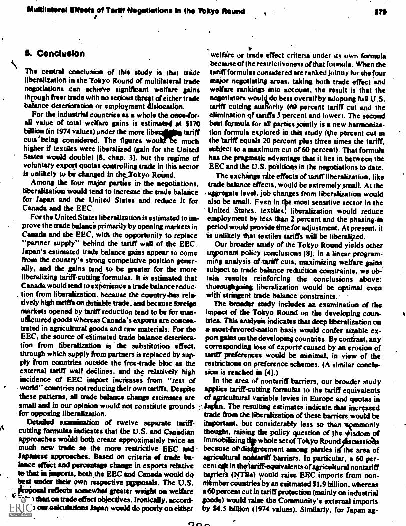
,Multilateral Mete of Tariff Negotiations In the Tokyo Round

5. Conclusion

The central conclusion of this study is that tradeliberalization in the Tokyo Round of multilateral tradenegotiations can achieve significant welfare gainsthEough freer trade with no serious thre4t of either tradebalance deterioration or employment dislocation.

For the industrial countries as a whole the once -for-all value of total welfare gains is estimated at $170billion (in 1974 values) under the more liberal.' tariffcuts' being considered. The figures woulrbe muchhigher if textiles were liberalized (gain for the UnitedStates would double) (8, chap. 3). but the mem ofvoluntary export quotas controlling trade in this sectoris unlikely to be changed in the..Tokyo Roimd.

Among the four major parties in the negotiations,liberalization would tend to increase the trade balancefor Japan and the United States and reduce it forCanada and the EEC.

For the United States liberalization is estimated to im-prove the trade balance primarily by Opening markets inCanada and the EEC, with the opportunity to replace"partner supply" behind the tariff wall of the EEC.Japan's estimated trade balance gains appear to comefrom the country's strong competitive position gener-ally, and the gains tend to be greater for the moreliberalizing taiiff-cutting. formulas. It is estimated thatCanada would tend to experience a trade balance reduc-tion from liberalization, because the country has rela-tively high tariffs on dutiable trade, and because fore*markets opened by tariff reduction tend to be for man-ufictured goods whereas Canada's exports are concen-trated in agricultural goods and raw materials. For theEEC, the source of eitimated trade balance deteriora-tion from liberalization is the substitution effect,through which supply Prom partners is replaced by sup-ply from countries outside the free-trade bloc as theexternal tariff wall declines, and the relatively highincidence of EEC import increases from "rest ofworld" countries not reducing their own tariffs. Despitethese patterns, all trade balance, change estimates aresmall and in our opinion would not constitute groundsfor opposing liberalization.

Detailed examination of twelve separate tariff-cutting formulas indicates that the' U.S. and Canadianapproaches would both create approximately twice asmuch new trade as the more restrictive EEC andJapanese approaches. Based on criteria of trade ba-lance effect and percentage change in exports relativeto that in imports, both the EEC and Canada would dobest under their cnen respective pepposals. The U.S.Stroirosal reflects somewhat greater weight on welfarespins than on trade effect objectives. Ironically, accord-ing to ourcalculations Japan would do poorly on either

279

welfire or trade effect criteria under its own formulabecause of the restrictiveness of that formula. When thetariff formulas considered are ranked jointly fur the fourmajor negotiating areas, taking both trade effect andwelfare rankings into account, the result is that thenegotiators woultdo best everall' by adopting MI U.S.tariff cutting authority (00 percent tariff cut and theelimination of tariffs 5 percent and lower). The secondbest formula for all parties jointly is a new harmoniza-tion formula explored in this study (the percent cut inthe 'tariff equals 20 percent plus three times the tariff,subject to a maximum cut of 60 percent). That formulahas the pragmatic advantage that it lies in between theEEC and the U.S. poittions in the negotiations to date.

The exchange rite effects of tariff liberalization, liketrade balance effects, would be extremely small. At theaggregate level, job changes from liberalization wouldalso be small. Fven in toe most sensitive sector in theUnited States. textiles, liberalization would reduceemployment by less then 2 percent and the phasing-inperiod would provide time for adjustment. At present. it`is unlikely that textiles tariffs will be liberalized.

Our broader study of the Tokyo Round yields otherimportant policy conclusions [8]. In a linear program-ming analysis of tariff cuts, maximizing welfare gainssubject to trade balance reduCtion constraints, we ob-4tain mutts reinforcing the conclusions above:thoroughiping liberalization would be optimal evenwith stringent trade balance constraints.

The broader study includes an examination of theimpact of the Tokyo Round on the developing coun-tries. This analysis indicates that deep liberalization ona most-favored-nation basis would confer sizable ex-port pins on the developing countries. By contrast, anycorresponding loss of exports' caused by an erosion oftariff preferences would be minimal, in view of therestrictions on preference schemes. (A similar conclu-sion is reached in [4].)

In the area of nontariff barriers, our broader studyapplies tariff-cutting formulas to the tariff equivalentsof ultural variable levies in Europe and quotas in

L.,J The resulting estimates indicate. that increasedtrade film the liberalization of these barriers, would beimportant, but considerably less so than mmonlythought, raising the policy question of jthe isdom ofimmobilizing whole set of Tokyo Round cussiasbecause oftdi ment among parties i the area ofagricultural tariff barriers. In particular. a 60 per-cent cgt in -equivalents of agricultural nontariff

) would raise EEC imports from non-Irr?bercountries by an esitmated $1.9 billion. whereasa 60 percent cut in tariff protection (mainly on industrialgoods) would raise the Community's external importsby $4.5 billion (1974 values). Similarly, for Japan ag-

ricultural NTBs are less significant than tariffs; thecorresponding import effects would be 52110 million and51.7 billion respectively. Measured by static welfareeffects, agricultural nontariff barriers are more impor-tant because of their very high tariff-equivalents. Oftotal welfare gains from a 60 percent cut in tariffs and intariff equivalents of agricultural NTBs. the agriculturalbarriers would provide one-third of the gains for Japanand SO percent of gains for F.urope.' Finally, for ex-ports of the United States and Canada, agriculturalNTBs would be of less importance than tariff liberali-zation on industrial and agricultural products. Agricul-tural exports due to a 60 percent cut in tariff equiva-lents of NTBs would represent only 13 percent of totalU.S. export increases from tariff and agricultural NTBsliberalization together; for Canada, the correspondingfigure is 37 percent.

Another NTB examjned in the broader study is dis-crimination in government procurement. Based onstudies by other authors (2, 161, we estimate that theremoval of government discrimination would raise U.S.imports by approximately SI billion and those of theEEC by 5150 million in 1974 values. Although signifi-cant. these effects are considerably smaller than those

-resulting fro tariff liberalization.In sign, theatates of this study indicate that it

tively deep cuts in tariffs and 'ff barriers (sucthe full U.S. authority 60 perce na-tion of protection below 5 percent) could provide im-portant welfare gains to consumers in industrial coun-tries as well as important export gains to developingcountries. cThese potential gains would be approxi-mately cut in half if, instead, negqtiators adopted themore restrictive tariff-cutting formulas under activeconsideration in tbe negotiations, and would be stilltbrther reduced if major areal such as biiiiculturalNTSs were omitted from liberalization. The impact of.liberalization on "labor displacement" would be incon-sequential. Any prospective trade balance losses forindividual countries from even the most liberal tariff-cutting formulas would be extremely modest and wouldnot constitute the basis for limiting the extent ofliberalization.

For these reasons it would appear incumbtnt uponnegotiators in the Tokyo Round to move quickly to-wards agreements very substantially reducing the re-maining structure of tariff and nontariff barriers totrade. Their failure to do so would not only sacrificeimportant potential pins for consumers and for produc-tive efficiency and progress in limiting inflation in in-

,dustrial countries, as well as the export hopes of de-veloping countries; but would also run the risk of aneventual retrogression towards increased rather than

29!)

Part Six: U.S. Tariff Policy

reduced protection. as the continuing Irritations inhe-rent in areas of potential dispute (especially in NTBs)threatened to spread to other areas of trade policy.

Appendix A A.\

ElasticitiesTable A-1 lists se empirical sources used for the importelasticities applied in the model of tariff negotiations.The EEC elasticities are averages of member-countryelasticities with weights proportional to member coun-try imports from nonbloc sources. Table A-2 reports theresulting price flasticitiel of imports for each area, byBIN section, and overall. For the elasticity of substitu-tion, a. we used the value -2.5, based on varioussources (especially (15J).

Table A-2 shows in the final column EECX the priceelasticity of EEC imports from nonbloc supPliers. Thiselasticity reflects the combined influence of the importelasticity regardless of source and the sobstitution elas-ticity for shifts.froibloc to nonbloc suppliers.

e

able A:1Sources for Estimates of Import Elasticities

Country

United AgatesCanadaJapanEEC:

United KingdomFrance eGermanOthers

Austria

FinlandNorwaySwedenSwitzerlandAustraliaNew Zealand

Squrce (by order of

Kreinin; Almon-Bu TaplinTaplin(8, Appendix CI; Taplin

Barker; TaphnKreinin; TaplinGlismanrr, TaplinTaplinTaplin (nonzero); Germany/Glis-

mann ; Germany/replanTaplin: SwedenfraplinKreinin; TaplinKreinin; TaplinTaplinNew alandfraplinTaplin

Soarces: Clapper Almon, Jr., Buckler. LawrenceHanvitz, Thomas Reimbold, 1965: Interindustry Forecasts ofthe American Economy. (Lexington. Mass.: D.C. Heads,1974). Terence Barker, The DeffITAIGNINS of &babe VisibkImports: !On 1966. (Cambridge: University al Cambridge.

Gesamiwirtschafilchen Kart det./Protektion. KielDepartment o( Applied Economics. 970). Hans H. Glisemna.pieDiscussion Papers No. 35. (Kid Waltwirtaebeft.1974). Mordeckei E. Kreinin. "Diseogrepted Import DeemedPuncdoes-Purtber Resuks," Southern Economic Journal,Vol. 40, No. 1 (July 1972),19 -25. Taplin estiammr.=in R. J. BM, The International Lbtkao qf NationalModels. (Amsterdam: North-Holland Publishing Co.. 1973).

a

"

"

4

I' I

Ti1t1S-04:2;

slitillidAidrogo,PricellootIc,fty of ImPorti by Product indiriporting Arai1. I

/ t °,

i,

'

.1

^

, FM sectioa , 1 ilW, , CAN , , i P N .. 'ATA NOR, SWO, ' .. 'SWZ AlA ,1 ,.myz. ,, En 'Hinifid product; -03 -0.84 11.13

' 2 Vegetable .,... . ,

4; prOductr, , .4,90 -0,85' 1 -0.47

1 fits, oils:' 40A3 '''' -2,30 '-0.62Epodi;beverage's .4 ' ',

-0.50

i(-0,55,

-,0.51 -0.58

' A.57.yr

L0,41

. .

'- 0,$ 6 -0A7 -0.15 -1.12' 1 I .6 -1.09,a, ',,s , ,

-0.20 ,030 -04 . -016 -11b' ,,i'. -1.13 70.89..r'-0.95 . '-if Oo 76.70 " 70.69 , 71.65 ' 1.51 ,'-1.26

e * ' ,

ci,

.14' tobacco , -1,13 ' -0.76 -0,58 -0.50 4-11:60 -0,09.' -0.82 -0.41 -0.17' ., $-1..12 L1-12 -11.025 Mineral 4 ''' '

1 , 4.--' .1, \ .. ,,

iteducte' . 422 -1.81 -1.59 O.% -0.56 , -0.99 1'27 ;0.26 -I.4r -1.44 -1.68 -2.07

I Plastics, ru r 7.3.5t, -2.13. -1,96* . , -1.32 \ -0;74 , -4.99 2 -1,11 -.0.90 -1.24 -113 -3.25

6 ChemicalNo'e ' ,-1197 -2.07 -1.37 -D.96 -0.72 .-0.98 '50 -0.90 -1.05 . -1.22 41.23 -2.50

8: gides, leather 1,_ -2,46 -2.07 '-1.32 -14.09 -0.74 -0.§9 -2.61 - -4138 -0.97 -1.23 -4.23 -2331 9 Wood, cork ' ,

1

p ucts f\ -0.96 -2.14 ' 133 70,83 -07 -0.99 , -2.47 ''''1,53 -0.61 -1.62 -1.64, -2.090.10. r products -14.44 =2.07 1.74 -0.79 1 0,70 . -0.99 -2.80 A -1,29 -0.85 ' -1.27 -1.23' -2.60

11 T tiles I ' -2.43 -2.09 -1.56 -1.07 -0.74 -0.9p. ;1..99r -2.09 -0.95 -1.24 -1.23 -2.6112 S as, hats , . - -1.23, -2.07 -1.42 -1.27 -0.74 4,99 -2.53 -5,73 ,-1',05 -1,23 71.23 -2,77If onmetallic II

" ) t iminerals 71,37 -2;07 -1.42 -1.20 -0,74 i-0.99 -0.89 ' -1,60 -1.05 -1.23 -1.23 -3.1714 JeWelry.l., -337 -2.07 -111' -0,74 -0.99 -210. 1131 -0.57 -114, -1.48 -2.6415' Base metis':`,., -1.99 -2.07 kP* L- 2196 -0,74 -0.99 -1.85 71.31 -1.05 -1.23 -1.23 -3,2516 Machinery, elec.

,Arica! equipment. -0.87 -2.07 -138 -0.92 -0.74 -0.99$ -331- -L27 -1.05 -1.23 -1.23 -2.63

17 Traniportaga

equipment. -2.53 -2.07 -1.87 -1.15 , -0,74 . -0.99 -1.03 -1.27 -L05- -1.23 -1.23 -2.4318 Precision

instruments -1.70 -2.07.,e19 Arms -2.07

20 Miscellaneous

including

, -2.220 -1.26 -0,74 - 0.99., -1.89 -4.72 -1.05 -1.23 -1.23 -2.79-1.42 -0.74 -0.99 -2.80; -4,50 -1.05 -1.23 -1.23 -3.56

furniture -4.44 -2.07 -1.42 1.138 -0.74 -0.99 -2.80 -5.80 -1.05 -1.23 -1.23 -3.0021 Art -3.02 -2.07 -1.42 445 , 0.74 -0.99 -0.50 -5.80 -1.05 -1.23 -1.23 -437

TOTAL -1.85 -St. -1.39 492 -0.65 -0.61 -1.72 -1.50 -0.69 -1.24 -1.23 2.17'

Source: see Table

NO1E: Weighted by v e of imports (from suppliers tside bloc, fot EEC and EFIby 4-digit BTN sector. Column EECX imports from outside bloc'after includingsubstitution effect. .

'Excludes ail.

4

it.

(

p.

3-ro

ar

I`

4 t

0

0

, 2

, 0

0

0.

301

7

)

Ap\rilbndix B

Sect Oral EMployment Effects: Canada, Jarm, EEC

Part x: U.S. Tariff Policy

Immo 8-i ) cCanada: Trade and Employment Effects by Product Groups IldPercepfel'oriff Cut Case (1971 Base)

BTN Section Tradenullions),

birecja?bs (thousands) Net Jobs as' Percent of Sectoral 4

.." Imports Exports Balance Imports Exports Eahtnce Employment

1 Animal products ,3t6 2.6 0.1 0.2 9.12 Vegetable products 7.7 13.4 5.7 0.4 0.7 03 k

.n.a.n.a.

3 Fats, oils 4.4 1.7 '1,2.7 0..1 0.0 ,r.O. 1 n.a.4 Food, beverages, tobacco 25.7 29.0 ' 3.3 0.8 0.09

5 Mineral products' 1.2 1.5 0.3 0031.: 0.0 `,4,0 0.00

6 Chemicals 60.0 12.7 -47.3 1.2 0.3 -1.157 Plastics, rubber 57.9 33.7 -24.2 1.2 0.5 "--745.'? -1.568 Hides, leather 11.5 3.8' -7.8 0.8 0.3 -0.6 n.a.9 Wood, cork products 10.6 13.6 3.0 0.5 0.7 fr 0.2 . 0.22

10 Paper products 28.8 32.7 3.9 1.1 1.0 -0.1 , -0.08.11 Textiles ' 163.2 24.7 -138.5 7.0. 1.2 -5.8 .-2.9312 'Shoes, hats 22.9 -21.2 1.5 0.1 -1.4 it.a.13 -Nonmetallic minerals 26.2 3.49 -22.5 1.1 0.2 -0.9 -1.7314 Jewelry 0.5 -2.6 0.1 0.0 :.-0.1 n.a.15 Base metals 106.5 72.3 -34.2 3.5 1.5 -2.1 -0.8816 Machinery, electrical equiptnent 271.94-40 -40.9 -231.0 9.7 1.5 -8.2 -3.9017 Transportation equipment 117.5 '33.3 -84.2 3. 1.1 -1.9 -1.2718 Precision instruments 40.3 9.9 -30.3 1.5 '0.4 -1.1 n.a.19 Arms 1`.8 .1.3 -0.5 6.1 0.0 -0.0 n.a.

-20 Miscellaneous including furniture 28.0 13.5 -14.5 1.3 0.7 -0.6 n.a:21 Art 0.0 0.0 -0,0 0.0 0.0 -0.0 n.a.

Total excluding oil 992:7 349.9 -642.8 34.7 11.0 -23.6Total excluding oil & textiles // 829.4 325.2 -504.2 27.7 9.8 -17.9

Manufacturing excluding textiles t 876.9 273.5 -513.4 26.5 8.1 -18.4

'Excludes oil.t Excludes sections 1-5, II.

p

yvMuMinters Effacts of TariffNegot dons In the Tokyo Round

,Table B-2Japan: Trade and

I Animal products2 Vegetable products3 Fats, oils

'4 Food, beveer(s, tobacco5 Mineral pr ucte6 Chemicals7 Pla.itics, rubber8 Hides, leather9 Wood, cork proAucts

10 Paper products.r_11 Textiles12 Shoeshats13 Nonrn tallic minerals14 Jewel15 Base metals16 Machinery, electrical equipment17 Transportation equipment18 Precision instruments19 Arms

283

Employmbit Effects by Product Gr4s 60 Percent Tariff Cut Case (1971 Base)

BTN Sectiqn

20 Miscellaneous including furniture21 Art

Total excluding oilTotal excluding oil & textilesManufacturing excluding textilesf

'Excludes oil.tExcludes sections 1-5, 11.

"Trade ($millions)

Imports Exports

Direct Ls (thousands) ; Net Jobs asRercent,of Sr/dorsi

Balance Imports EZports &dant* Employment36.6:54.5

2.5,_.0.8

-34.1-53.7

1.7 0.4 -1.392.8 , 10.6 -82113.7 0.0

. - -13.761.6 28.4 -33.218.0 95.5 ._ 77.53.3 17.4 14.04.0 10.0 6.09.7 7.8 -1.9

45.8 249.7 203.94.4 22.2 17.82.8 28.6 25.85.6 5.1 -0.4

70.2 191:7 121.5170.4 -1725 1.946.5 201.1 154.638.8 93.0 54.34.5 1.5 . 1.9

18.9 77.4 58.40.0) 0.0 0.0

699/1( 1215.8 516.0654.0 966.3 312.2

45e 951.8 497.,1

3.8 0.5 -3.3 .,.n.a.

33.9 ( 0.14 -33.8 'v. n :a .-0.0 0.0! -0.0 - n.a.2:3 1.3 -1.0 -0.09'0.0 0.0 -0.0 0,002.81.5

.4"_/ -IA8.3 ,

-0.281.924k

0.5 4.2 3.7 / n.a.0.4 0.8 0.130.4 0.6 0.2 0.066.8 47.5 40.7 2.440.6 4.4 t 3.8 ,n.a. -.0.3 5.5 5.2 0.930.5 0.6 0.1. n.a.3.4 7.9 4.5 0.28

10.5 12.0 1.5 0.062.3 9.5 7.2 0-.834.0 8.8 4.8 nit.0.1 0.2 0.1 n.a.

3 2.1 8.7 6.,6 n.a.0.0 0.0 0.0 n.a.

76.4 124.4 48.069.6 76,9 7.3

29.6 75/.0 45.414.

err

°

11

,41

Part Six: U.S. Tariff Policy

Table 8-3EEC: Trade

frX

and EMploydrt Effects by Product GrO4Os 60 PerCent Tariff Cut Case 971 Base)

.1

BIN Section Trade (Smillions) DireCt Jobs; (thousands) Net Jobs as

N Imports, Exports Balance Imports

1 Animal$roducts 32.8 -2ft 1 -58.9 3,52, Vegetable products 114.5 -71.1 -185.6 20.93 Fats, oils 16.8 -19.0 -35.8 0.54 Food, beverages, tobacco 115.9 -31,4 r147.3 3.25 Mineral products' 13.5 -14.5 -28.0 1.46 Chemicals 99.6 -60.2 -159.8 4.07 Plastics, rublieF 63,9 123.9 60.08 Hides, leather. 13.3 2.6 -z 10.7 1.1

9 WoOd, cork products 20.4 a. -9.1 -29.5 1.410 Paper products 31'.8 -16.4 -48.e 1.911 Textiles 171.0 -5.8 -176.9 15.812 Shoes, hats 20.5 7.6 -12.9 2.113 Nonmetallic minerals 16.5 5.0 -11.5 - 1.1

14 Jewelry '- "2.6 20.5 17.9 0.215 Base metals 107.3 4.2 -73.1 5.716 Machinery, electrical equipment 180.5 92.7 -'273.2. 11.917 Transportation equipment 9.9 87.1 7.1 4.t.18 Precision instruments 77. -23.0 -100.8 6.619 Arms' 1.2 3.5 . 2.3 0.120 Miscellaneous including furniture 1).9 12.9 ; -18.0 2.121 Art 0.0 0.1 0.1 0.0-

Total excluding oil 1210.8 -72.2 -1283.1 91.1

excIuding.dil & textiles 1039.7 -66.4 - 1.106.1 75.3

Manufactu4frring excluding textilest 746.2 125'.7 Lis020.5. 45.8

'Excludes oil.tExcludes sections 1-5, 11.

(

Exports Balance

-4.6 -8.1-17.7 -38.6-0.6 -1.1-0.7 -3.3-1.5 -2.9-2.4 -6.410.6. 7.5-0.2 -0.9

-0.6 -2.0-0.9 -2.8-1.2 -17.1

0.9 -1.20.3 -0.81.4 ;1.32.0 -3.7

-6.2 -18.05.1 0.4

-1.9 -8.50.2 -0.20.9 -1.20.0 0.0

-16.6 -107.8-15.4 -90.7

9.7 -36.1

Percent of SectoralEmployment

q.a.n.a.

- 0.16-0.31- 0.34

0.781n.a.>

0.38- 0.49n.a.

06ma.

-0.- 0.28

0.01n.a.ma.n.a.n.a.

Literature Cited

1. Balassa, Bela, ed. European Economic Integration.Amsterdam: North-Holland/American Elsevier, 1975. '

2. Baldwin, Robeit. Nontariff Distortions of InternationalTraass Washington, D.C.: Ellookings Institution, 1970.

3. . "Trace .arid Employment Effects in the UnitedStates of -eNtiltilateral Tariff Restrictions." Mimeo -graphed. V shington, D.C., 1975.

4. Baldwin,, Robert, and Tracy Murray, "MFN Tariff Re-ductions and 'beveloping Countries' Trade Benefitsunder the GSP." Economic Journal, 87 (March 1977), 10.30-46.

5. BaldwIC, Robert, andiack ainti.2yolicy Issues in Ad-justment Assistance: The 'United States." In ProspeCts 11.for Partnership: Industrialization and Trade Policies inthe 1970s, edited by Helen Hughes, pp. 149-77. Balti-more: Johns Hopkins University Press, 1973. 12.

6. Chamber of Commerce of the United States, Interna-tional Group. Trade Negotiations Information-Service 13.Bulletin No).2. Washington, D.C., 1976.

7.. Traile NegotiatioksInformation Service BulletinNo. 5. Washington; D.C:, 1976. '

8. Cline, William R., Noboru Kawanabe, T.O.M. Krons,and Thomas Williams. "Trade, Welfare, and Employ-ment Effects of Multilateral Trade Negotiations in theTokyo Round." Mimeographed. Washington, .D.Cf:

9.

304

Brookings Institution, 1976.Deardorff, Alan7Robert Stern, and christoplr Baum."A Multi-Country Ai rhulation\of themployment andExchange Rai'.' of Post - Kennedy Round. TariffReductions."pniversity of Michigan, Research Seminar

'in International Econ ics, Discussion Paper No. 68,1976.

Evans, John W. The ennedy Round in American TradePolicy: The Twilight of the GA77? Cambridge. Mass.:Harvard University Press, 1971.GATT. Basic Documentation for the Tariff Study: Sum-mary by Industrial Product Categories. Geneva, 1411rch)974.International Monetary und. International FinanilalStatistics. Monthly. Washington, D.C.: IMF, 1976.Johnson, Harry a "An Economic Theory of Protec-tionisin, Tariff Bargaining, and the Formation of CustomsUnions." Journal of Political Economy, 73 (June 1965),256-83.

C.

JI/

.41

-r'

Multilateral Effects of Torii Negotiations in the Tokyo Round

O 1.

14. Journal of Commerce. "Quest for Worldwide Formula toCut TariffscResumes Soon." July /, 1976.

15. KravispIrving, and Robert Lipsey. Price Competitive-ness in. Wortd Trade. New York: Columbia UniversityPress, 1971.

16. Lowitiger, Thomas. Discrimination in GovernmentProcurement of Frei Goods in the United States andWestern Europe. meographed. Pullman: Washingto#State. University, 1973.

17. Meade, James. the Theory of International EconomicPplicy. Vol. I: The,Balance 21 Payments. London: Ox-ford finirrsity Press, 1951.

18. O.E.C.D. Labour Force Statistics: 4962-1973. Paris:O.E.C.D., 1975.

19. Trade by Commodities: Schedule B, 1974.20. Preeg, Ernest H. Traders and Diplomats. Washington,

D.C.: Brookings Institution, 1970.21. United Nations. The Growth of World Industry: 1973'

Edition, Vol. I. New York: United Nations, 1975.22. Wall Street Journal. "Comrrion Market Proposes Tariff

Cuts but U:S. Delegates Call Formula 'Puny."' July 8,'1976.

A

4

3

4/Comment.Anne 0. Klueger

r.

a

285

The Cline-liawanabe-Kronsjo-Williams (CKKW)papdi presedis the results of An investigation of theimplications of alternative tari4cutting formUlas. Toaccomplish this, the authors use detailed, line -itemtariff data in the context of a multicountry model. Theyestimate the tariff cuts that would take place underalternative formulas and combine those estimates with"best available" estimates of demand elasticities foreach of the eleven 'geographic .regibns (ten countries'plus the EEC group) to generate estimates of orders ofmagnitude of changes in trade flows and other variablesin response to each of the formulas.

There is little doubt as to the importance of the re-search. It representss distinct improvement in 9ur toolkit and provides information on a complicated subjectin which the plethora of detail has heretofore discour-aged analysis.

There are two mlin.,uses to which the CKKW moteland its risults' can belga On one hand, the model yieldsestimates of change ade flows for indjidual com-modity groups and countries. I 'will ref& to thesecommodity -spec ific results, and the accompariyingemployment estimates, as the microeconomic featuresof the model. These uses can be contrasted with theapplication of the model to estimating aggregatechanges in trade balances, exchange rates, andemployment levels. These are the macroeconomic as-pects of the model. In a nutshell, I fin4the value andsignificance of the CKKW model in its iiicroeconornieaspects, and am dubious as to thervalue of the model formore macroeconomic purposes i I therefore intend to-divide my comments into two parts. I wish first todiscuss the microeconomic aspects of the model thatraise interesting and important questions and point theway for fUrther research. Thereafter, I will explain Afiebasis for my misgivings with regard to the mac-roeconomic appliations of the model.

Turning, therefore, tolhe microeconomic aspects ofthe Plaper, let me first repeat that the CKKW results areof great significance. I have no quarrel with their find-ings with respect to alternative tariff cutting. rules. Mycomments in this regard, therefore, are directed towardfurther uses to which the model could be put..

286

A first Point is that the model devised by CKKW ishighly complex; entailing data on about five thousandline-item tariffs for each of eleven regions, and employ-ing sepirate demand elasticity estiniates in each. case.In view of the-expense-of running such a large model, Iwould have hod that CKKW ould hive shed somelight on two questions. Pirst, what extent are" theestimates of trade and crrnployment effects, taking alleleven together, significantly different from the es

. mates obtained when considering a single country attime? That is, to what extent is the additional complex-ity of the model resulting from cits simultiheous treat-ment of all elevenjountries warranted in terms of in-creasing information about the properties of alternativetariff cuts? Here, I have in tifind Baldwin's model dis-

Wssed in his confererice pear with Lewis -4 anoltorna-tive. Baldwin was able to concentrate iri g&ater detailon various aspects of U.S. markit's.,In so doing, there isbotlittgain and a lops in inlormation. I would hope thatCKKW could shectsome light on the sorts of questions .

for which a in 'country model is better suited.The second q stion applies to the extent to

, disaggregation of the tariff rates alters the results.problem is rather more- -comp ate1d than the ne"bias" discussed by CKKW. The nt out, correctly,

"that use of tariff averages may well re the implica-tions of alternative formulas for tariff cuts. If, for exam-ple, one tariff-cutting formula tends to decrease very.high, tariffs by more, and intermediate tariffs by less,than another formula, application Of the twoformulas toaverage tariff rates within commodity groups will con-ceal some of thdifferences in results. That much is so.However, CKKW had to use fairly aggregated eiti-mates of demand elasticities (only four different valuesfor Finland, eight for Australia, and sd on) and thenapplied those -aggregate elasticities to all the detailedtariff changes. Depending on a variety of factots, onecan imagine the bias in the estimated u*e change re-sulting from this procedure as being eMer larger orsmaller than the bias resujting from applying average'tariff changes to the aggro to elasticities. Suppose, forexample, that high tariff rates within categories occurwhen the price elasticity of demand is low. The "bias"from using detailed tariff rates could be significant, andworse yet, it might alter the ranking of the estimates of,different formulas for cutting tariffs. It wotild hake beenuseful had the authors attempted some ar&lysis Of thenat t::the bias implicitin using detailed tariff data ,-with fairy aggregative demand estimates. Perhaps asimulation rUn,,within their model, in which they corn-

', ',,pate the average tariff change under each formula to the,same level of aggregation as theirslemapeelasticities,and contrast the resulting estimates of changes in tradeflows with those in which detailed tariff-rate changes

:2) *

Part Slx: U.S e Tarlit,Policy

4f

are applied, wuld yield.the relev ant information, Eventhat, however? would not' get at the problem that the -elasticities ofkathand for different commodities mightbe significantlY-different.

finally, I would have hoped that CKKW would pro-vide more detail on individual commodity results and,in p icular, would report on the quantitatiye signifi-

of indirect trade effects for particular' industrygroups. Questions of some _importance are the extent towhich alternative formulas Might have smaller "ad-

se" efficts, as measured by the number of industry.gr s that would experience importincrealies in ex-'ce s o articular cut-off numbers.

The sorts of questions pertain to ways in which theusefulness of the model has not yet been fully exploited.They point to additional areas in which the model canyield insights into important questions.,By contrast, Iam very skeptical as to the value of some of the mac-roeconoinie results obtained from the model. r.

First, some strenuous objections. it Seems totallyimplausible that demand elasticities siippqied to bepartial in nature% with real income held cogstant canbe applied to price changeg, andtlfat the resaulting esti-mates can be summed to yield any insight into the netchange in the trade balance. Worse yet is the effort toestimate the necessary change in the exchange raterequired to ompensate for the presumed trade balanceeffects. De bleats of both the tfatt,,ltalance and theexchange ra e basically macroeconomic in nature,and summa n of results from microeconoinic demandrelations i a fundamentally fallacious procedure.

The difficulty with it is illustrated in only one'oJmany possible ways by recognizing that CKKW ob-tained their estimates of trade balance shifts by assum-ing that the Marginal propensity to spend of the indus-trialized countries is zero and that of the rest of the'world is one. However, when one sums their net tradebalance effects, only for one tariff cut 60 percent(Table 6) do they give the net tree.balance effect forall eleven regions, and it is a 'leg tive $1.4 billion. Butby thir assumptions, the rest of the world has an unal-tered net trade accOunt: since trade must balance for theworld as a whole, something is surely wrong! Inciden-tally, if one sums tie net trade thanes for the fourregions listed iii le 3, the net change in trade balancetor the four regions is implausibly, large for all possibletariff-cutting formulas except the tentVndeed, underthe full liberalization (alternative 4), the net change forthe four is minus $1.5 billion = again implausibly largerelative to the economic sizeof the'countries not listed.

Given the meaninglessnas of the net change in tradebalance estimates, the estimates of changes in exchange%rates .must anyway be discarded: if One assumed thatmarginal propensities to spend among the eleven re-

hich

.1

/Mutt eferel Effects of Tariff thlthtlatIons In the Tokyo Round

I, a.gions were proportional to their expenditure-income relationship in tha base year, surplus countries' surpluseswould increase and deficit countrie# deficitl wouldincrease in response to tariff cuts: all that comes out ofthe model is what goes in, and CKKW have implicitlygiven -the eleven regions a marginal propensity to spin4of less than one and have thereby generated a deficit inthe worlIpAde !Agleam.' .

'

The same sort of reservation applies to the aggregateemploymeterstimates. As already stated, it is useful toattempt to identify the individual industries that willexperience increased and decreased deltaktfor theiloutputs, and consequently shift their demand for laborupward and downward, as a result of tariff cuts. Thoseestimates can'serve to assist. policy makers in identify-ing the regions and sectors of the economy in whichproblems of adjustment are likely to arise. When, how-ever; the estimated change in'employment in individuialsectors is4ummed over the entire economy, iris doubt-ful whether any' significance can be attached to theresul number. First, there.' the reservations al-ready pressed about the means used for estimatingtrad_ _alance-effects yep those effects dominate the.

- aggregate employment estimates. Second, there areqvo major classes of macroeconomic models, and in

neither can a chan e in employment be determined in...

the manner sugges by the KW model.' In oneiclass of models., the is a "n rate of unemploy-ment," in which case tariff cuts will leave that rateunaffected. In the other class of models, aggregate de-mand affects the level of employment. If the "naturalrate" hypothesis is correct, estimating an aggregateemployment effect is wrong; if aggregate demand af-fects tIV leverof employment, then monetary and fiscalpolicy *e presumably able to attain the desiredemployment level. -

My misgivings about the aggregate employment fig-ures should'not be interpreted to mean that .I regard theemployment effects of tariff cuts as unimportant;rather, my concern is with the fact that the useful infor-mation that can begle.aned from an admittedly partial

'Their statement that devaluation necessarily implies a deteriom-t in any event. Although James Literature Cited

itions in international trade, it-of-trade change, if any,

tion in the terms of trade is inMeade is the authority on mot prohas long since teen recognized that thefollowing a transfer payment (of which evaluation is one form) is afunction of the marginal propensities to consume exportables andimportablei, and not of price elasticitieS. See, for example. [I].

____14137

equilibrium model lies in the insights it provides with .

respect to the initial impact on particular industries' -

denuinii for labor,.and hot-on the aggregate emplo menteffect.

Finally, I find the ranking of benefits arising ou of thealternative tariff-cutting formulas useful, and wouldhave been interested to see how .those estimates com- t.pare with ones derived from more aggregated tariffdata, single-country estimation proceduresnand so on.However, ite.is not evident that one can tech any

. significance to the absolute value of the emated"areas under the triangle." An attempt to blo.. p thestatic 'estimates by Balassa's ratio for the ClimmonMarket mentioned in Cline's paper is suspect on severalgro ds. First, there are questions as to the reliability of

oB a's estimate itself. Second, there is dmajorques-ti o whether even free trade between, e.g.; Japanand Australia could yield benefits as large as int%grationof the Eur Economic Community_simp becausedistance pl es natural barriers to greater tra ,

the EEC provided individuals within its boundconsiderable certainty that there would not be artificibarriers to continued trade between themb Insofar sthagort of certainty is important in terms of whatever"4 amic" benefits there are, those benefits are Muchless likely to arise from tariff cuts than theyrare fromcustoms unions, simply because "escape clauses" andother instrumentspf national policy are less likely to beinvoked under the latter. Finally, the EEC arrangementgreatly increased the mobility of factors of productionamong countries, a source of gain that will not be avail-able under the tariff cuts. A

I copld elaborate other reasons why the mac-roecondmic estimates arising out of the CKKW modelare suspect. However, it is enough ,to say that the mis--ioecoknic strengths of the model are appreciatedalong with the macroeconomic weaknesses. There aremany interesting questions remaining on _Which theCKKW model Can shed light: it is to be hoped thatfuture research by the authors will continue to yielddividends as large as those repoited from their initialApplication of the mbdel.

A

1. Pearce, Ivor F. "The Problem of the Balance of Pay-ments." International Economic, Review, 2 (January1961), 1-28.

7

CommentDonald J. Daly

4

-4

The study by Cline and others is interestg and impor-tant with significant policy implications f&r the tradenegotiations currently usder way. Two areas a recentresearch in Cariada are relevant to thr stut and may beof

Simulations of a nuner of tariff changes for Canadawere made by theEconomic Council of Canada usingthiCANDIDE model [2, pp. 166-71]; the employmenteffects were small; even without co nation, andcould be further reduced by offsettiWexpenditureselsewhere. These results are consistent with the resultsfor this study and the others referred to on the top ofpage 276 in (line's paper.

Most studies of tariffs and the costs of tariffs andeffects of removing them usually assume constant re-turns to scale, similar production conditions with andwitho t .tariffs, and unchanged input-output coeffi-cients fore and after tariffs.. A series of studies indicate that all ese assump-tions are inappropriate and mislead' ig for Canada. Akey conclusion is that tariffs havt a significant effect onproduction conditions in addition to the usual staticcosts to the consumer. The presence of tariffs (andnontariff barriers) leads to greater product divemity in asignificantly large part of manufacturing. These productspecific scale economies are quantitiyely large, andmuch larger than the scale economies associated vAthvariations imilant size (the only scale economy usuallyconsidered). Under these conditions, differencesoutput per person can be significantly [pwer in Cana-dian than in U.S. manufacturing (even *ith similar or.higher levels of capital stock per person employed inCanadian than in U.S. manufacturing). The levels ofoutput per person in Canadian manufacturing are esti-mated to be between one fourth and one fifth below theUnited States levels during the 1970s and labor costsper unit and total costs are normally higher thin in theUnited. States. (See [4, esp. parts 4,arid3 ;, 2, chaps..3, 6;3; Postscript' 1975, pp. 473-87; 1].)

These analyses predict that under free trade (or re-duced tariff and nontariXbarriers), the productivity aridcost differences would narrow appreciably thro ghlonger 'runs-, of individual commodities and re

06)

...-----

Pa SIX: U.S. Tariff Policy

t lb.,.....

speialization with lcreased intraindustry trade. Tradein manufactured products would increase bath wayswith other countries as part of any multilateral reduc-tion, and the ease of adjustment would be heavily influ-enced by the willingness of Canadian managginent tochange in response to the new trading enviroAment.Changes would occur as the input-output coefficientswould change, cost and productivity differences wouldnarrow, and the composition of trade in manufactured,products would change significantly. Product specificscale economies would be significant, and productionconditions would change in Canada. Changes alongthese lines have taken place since the initiation of theKennedy Round rekuctions and the Canada-UnitedStates automotive agrement. Exports of primary prod-ucts would be less affected as tariff rates are alreadylower than on manufactured products.

The results of these studies do not seem to have beenadequately incorporated into the curr 't study by Clineand others. The study notes that " ese calculationsexclude effects caused by input-outp t feedback" (p.267). Page 276 seems to imply that the same direct andindirect labor coefficients would apply before and aftertariff changes. The welfare effects include the s cwelfare gains (p. 266), but exclude the scale effect thatlire so significant for Canada. Tlit results for Csuggest latger trade and employment losses fr m in-creased imports.

These results are more in line with the views f thosewho support the status quo on Canadian tariffs elud-ing some businessmen and union officials) but do notadequately incorporate recent empirical work done ontariffs and their effects on productivity, prices, costs,and international trade. Trade with Canadi,is suffi-ciently important that this type of analysisTould affectthe aggregative results for the United Sta esas well.

Let me illustrate my point with some magnitudes ofthe real income gains to Canada from a Canada-UnitedStates free trade area (a narrower option than formula 4in this study). Ron Wonnacott estimates the benefits toCanada of a Canada-United States free trade area as 8.2percent of GNP [3, p. 117]. ,His estimate would includethe effects of increased specialization, higher prices todomestic factors of production on sales to U.S. mar-kets, and increased productivity based on economies ofscale. At 1974 levels of GNP, this would amount toAbout $11.5 billion as a real income gain to Canada, or,more than 50 times the size shown for Canada for for-mula 4 in Table 4 and almost six times as large as shownfor formula 4 in Table 2 f all eleven industrial import- %,

ing areas! Furthermore the gains to Canada would uesomewhat larger if the percentlinear cutwere ex-tended on a multilateral is to the other nine indus-in ed countries, or if other. .dynamic effects were

Multllat Effects of Tariff Negotiations In the Tokyo Round

allowed fothe consuincreased s

7su mation of static welfare effects`'to

t allowance for welfare gains fromon And economies of scale !fads to

a drastic unders ementoNvelfare gains, on the basisof careful emptiA work for' Canada.

The Economic Council of Canada h.6 also estimatedthe initifi employment effects of a Canada-UnitedStates free trade area, without allowing for reorganiza-tion of production or depreciation of the Canadian dol-lar. They estimated the difference in employment asless than 25,000 persons [2, pp. 168, 169], or substan-.

daily less than the %wetly 85,000 shown for tariff for-mula 4.in yable 7 fortanada..The effects would be evensmaller if the reorganization effects and the associatedhigher real incomes and declines in prices of manufac-tured products relative to other prices were allowed forin the form gif a longer-term increased demand within

. Canada for manufactured products. The simulationsusing the CANDIDE model thus ,suggest even'smallertransitional employment effects without allowing for

' thedonger-term_ employment effects on demand andsupily for manufactured products. The speed and easeof that adjustment will depend critically on the willing-ness and skills of management in adapting to that new,more competitive envir ent for manufacturing.

It is hoped that later wok in the Brookings project0can incorporate these resu is for Canada more com-

. pletely.

Literature Cited

1. Daly, Donald J., and Steven GlobenlIan. Tariff and Sci-ence Policies: A Model of Nationalism. Toronto: Univer-sity of Toronto Press. 1976.

2. Economic Council of Canada. Looking Outward: A NewTrade Strategy for Canada. Ottawa: Information Canada,1975. .

3. Wonnacott. Ronald J. Cahada's Trade Options. Ottawa:Information Canada, 1975.

4. Wonnacott, Ronald J., and Paul Wonnacott. Free Tradebetween the United States and Canada, The PotentialEconomic Effects. Cambridge, Mass.: Harvard UniversityPress, 1967.

309

ReplyWilliam R. Cline

4

289\ -`

Although I am delighted that Anne Krdeger considersour study to be of "great significance," her misgivints.abbut the macroeconomic estimates puzzle me. Nowould disagree that "determinants of both the tradebalance and the ,exchange rate are basically mac -roec nomic in nature. . . ."_But I disagree that for thisreasdrrone should ignore the trade balance 6rAxchangerate "impact effects," viewed as deviations fiein themain 'paths determined by macroeconomic t ces,when examining the use of a policy instrument suctrade liberalization. Kreuger implies that even themacro impact effect cannot be estkmated by "summa-tion of results from macroeconomic demand rela-tions. . . . " Apparently Harry Johnson disagrees withthis critique. He accepts as legitimate the correspond-ing macro impact effects estimated by Baldwin andLewis (using similar methods), although he suggeststhey could go further and add multiplier and other in-duced effects.' Krueger's "hands off' approach tomacro estimates would leave policy makers adrift;rigorous adherence to her approach would precludesaying whether liberalization in the Tokyo Roundwould have a 'eater or lesser effect upon trade bal-ances than, for instance, the OPEC oil price increase.Yet an important conclusion that emerges from ourstudy as well as from the study by Baldwin and Lewis isthat trade balance impacts from liberalization wouldbeminor and should not stand in the way of thoroughgoingliberalization. Some might be prepared to throw out thiscrucial policy conclusion because TO supposed but un-measured macroeconomic influences; we are not.

Krueger's acceptance of our micro results is gratify-ing, although it raises other questions. If the microeco-nomic estimates are acceptable, why isn't their sum?Presumably Krueger means that the micro results areaccurate in relative terms the machinery sectofstrade balance would rise and the textile sector's trade

11 would argue that the initial impact effects arc more meaningfulfor purposes of policy formulation than estimates that take account ofinduced multiplier and other secondary effects, since the latter isti-matescan include a whole variety of odtcomes depending on golicyresponses.

fi

\1

(2

balance would decline but not in absolute terms be-cause 'Qf Offsetting influences of *macro policy.Moreover, if Kruegr is concerned about biases causedby applying broader aggregate elaiticities Ip more.de-

ei;Nommodity classes, it is not clew why she con-siders the micro estimates to be useful.

As for disaggregation and elasticities, experimentswith individual commodity groups suggest that dis-

gation is important in prime as well as in princi-ple. kven when going from the tariff line level to thefour'digit Bmisels Tariff Nomenclature level, which isstill quite disaggregated, the preaggregation of tradeand tariff data causes an understatement of approxi-mately' LO percent in the e timated import tncreasesunder the EEC harmoni on tariff cutting formula (forselectacrSettors a ed in the cae of the UnitedStates). As f o r Krue r s comment that at the level ofindividual commodities there may be biases that arecaused by the use of more aggregative elasticities, wecan say only-that we agree with Krueger's statementthat there is no a priori reason to expect such biases.be in any one direction, so that we could expect $eresultsigter correction for any such biases (if correctionwere possible) to be, on the average, the same as ourestimates.

Krueger is correct in observing that the aggregatetrade balance effect for liberalizing countries is nega-tive. This result reflect the fact that part of the in-creased export .

of nonliberalizing "free rider"countries would not return immediately in the form ofextra importvgrom the liberalizing countries. The leak-age in our estimated "respending effect" exports oc-curs because outsider-countries spend some of theirextra foreign exchange outside of the eleven liberalizingareas. Most analyses of tariff negotiations do not evencapture a part of the respending effect; in contrast,Krueger's comments imply that we should have forcedthe respending effect to exclude any leakage what-

this change were introduced, the resultswould show a rise in the trade balance increases esti-mated for Japan and the United States and a reductionin the trade balance declines comptited for Canada andthe EEC, but no change in the qualitative results bycountry or by tariff formula (as indicated in the note tothe text). In any event, whether the trade balance im-pact estimate is more accurate with or without leakagein the respending effect is a moot point. We consider themethod in the main text to be more realistic than thealternative of completely eliminating leakage ;since thatelimination would require a long period- of successiverespending rounds (i.e., eventually the foreign ex-change spent in outsider countries would be respent,

lx: U.S. Tariff Policy

after succ sive rounds, on imports from the liberaliz-ing countrie

Fiinally,.14rueger criticizes our )iimate of total wel-fare gains based on Balassa's results for European. in-tegration, although she proposes no alternativemethod. Once again the question is whether the analystmore faithfully discharges the responsibilities inherentin policy analysis by disclaiming the possibility of mak-ing any estimate whatsoever, or by arriving at the bestpoisible estimate given the s to of the art. We opt formaking the best possible esti ate, elpecially since, inthis case, to do otherwise lea es the f se impressionthat trade liberalization simply may no be worth theeffort an impression protectionists wo seize uponwith alacrity.

Daly's comdiepts are helpful in qualitative rms'butmisleading with respect to magnitudes. Wonn: ti's es-timate of 8.2 percent of Canadian GNP as the welfaregain from a free trade area with theaUnited States ap-pears, be seriouslyexaggerated [3, pp. 177-78]. Theestimate is based on the assumption that the removal oftrade barriers would raise output pet worker through-out the entire Canadian manufacturing sector to thehigher levels (by app(mately one- fourth) found inthe United States. Gains 'from economies of scalethrough longer production runs are cited as the primesource of the productivity increase. However, the kapin productivity is assigned to the entire existing indust-rial park rather than to increased production associatedwith increased exports; and instead of applying sectoralestimates of returns to scale parameters to sectoralspecific estimates of increased output volume, thestudy assumes productivity in all sectors would rise toU.S. levels. Mpreover, except for a modest reduction inestimated liberalization gains from earlier estimates re-lative to 1963 (because automobile trade has since beenli ralized), the method fails to specify a relationship ofpr uctivity gain to tariff levels. It is difficult on theface of it to see how the elimination of industrial tariffsaveraging 14 percent (7 percent if nondutiable items areincluded ) [2] can raise productivity in the manufactur-ing sector by one-fourth (or by 7 percent, for that mat-ter). Indeed, the one available study relating Canadiansectoral productivity relative to that in the UnitedStates to sectoral protection levels finds no significantrelationship, casting &doubt on the entire approach.(Study by West, cited in [1, p. 25].)

Our own estimates of total welfare gain (which doinclude scale economies, despite Daly's reference onlyto our more restricted static estimates) follow the morerealistic assumption that gains from economies of scaleand new investment would be strictly linked to,, the

31

MultIlateral Effrts1 of Tann Plot;oadonii In the Tokyo Round

-.. . \magnitudes tencriased trade.* Agforjob chapges, I donot consider discrepancy beta our figure andthat cited by Daly to be particular' important, espe-cially considering that the results a thS.-Canadianfree trade area should be expect to ve smaller im-port increases for Canada than the elimination of

.

facbitall suppliers (iin particular, the U. . share is o61 percent of increirteedCanadian in our tariffelimination case). , I interpret ''istintates/I cited by Daly as confirming the general er of mag-nitude of our own ernplayme estimates. withthe direction of Daly's co ts: ,gains Canadawould probably be greater esti by the

tier of achievi economics of Scale instandard f ulations, of (a) the Stetter rehi-

Canada than in the larger eta of the United Statesand Europe, and (b) the stimulus to exports of pro-cessed manufactured goods (instead of raw materials)resulting from reduction in effective protection, a Oe-npmenon not captured in our early analysis using nom-inal tariffs.

Literature Cited

1. Daly, Donald J., and S. Globernum Tariff and SciencePolicies: Applications of a Model of Nationalism. To-ronto: University of Toronto Press, 1976.

2. General Agreement on Tariffs and Trade. Basic Docurtstationfor the Tariff Study: Summary by Industrial ProiluctCategories. Geneva: GATT, 1974.

3. Wonnacott, Ronald 3. Canada's Trade Options. Ottawa:Economic Council of Canada, 1975.

460

ar.

'Our application of the five-toone relationship of total- to staticweffare pins would in fact tenkto overstate Canadian pins from thestandpoint that increased economies of scale and increased invest-ment would be related to additional exports, and Canada's exportsrise by considerably less than imports in our results (and, therefore.by relatively small amounts compared to static welfare gains, whichare based on import increases).

311

`Trade Impact Studies Using the WhartonAnnui0 and Industry Forecasting Mgc!el

.Lawrence R. Klein* '

The Wharton Annual and Industry Model is a large-scale equation system that attempts to analyze both thesupply and demand sides of the economy simulta-neously. It differs from much ofinput-output analysis inthat final demand and value added cannot be deter-mined separately and used to generate interindustryflows in the economy. Interniediati flows are endoge:nnus from the point of view of the standard version of amacromodel of entries in the National Income andProduct accounts. At tge same time, the final demandand value addpoint of view osystem. Bo

accounts are endogenoils from thee standard version of an input-output

interdependent with market equationsfor the formation of prices, wage rates, and interestrates.

A further, important Characteristic of the WhartonModel is that input-output coefficients are not regardedas parameters in this system;'they are variables. Theinput-output matrix is not treated as constant, nor evenas parameters that may undergo occasional change,exogenously imposed on the basis of a priori engineer-ing, inAtutional, or general social information. The1-6 coefficients are endogenously generated within themodel, principally as functions of relative pricechange.'

A graphical layout of the accounting scheme is givenin Figure 1, where the intermediate flows among sec-tor's are juxtaposed to final demand (the expenditureside of the National Income and Product Accounts sys-tem) and to value added (the income side of the NIPAsystem).

The standard equation, in matrix form, for input-out-put systems is written as

(I A)X = F.

The matrix A is4ntsid principally on the cell entries inthe intermediate" transactions portipn of Figure 1.

This paper is based on !'Trade Impact Studies Using the WhartonAnnual and Industry Fort:Casting Model":by Ross S. Preston andYuen-Yun C. O'Brien which was completed under 1LAB contract74-12 in 1976 at The Wharton Econometric Forwasting Associates.

'For a description of crirlier generations of dltis Wharton model.see [2.31.

A = Rau II

=

. 293

/it being recognized that X../ and xj. are identical forevery sector. X in the basic equation is a whole vectorof total output elements across sectors. The column F isthe total of final transactions in Figure 1. To show thetie to a macromodel of the economy as a whole, let ussplit F into two parts, a matrix of ratio, coefficients andcopponents of the GNP. We write this

F = CG,

where the typical element of C can be expressed as

C I Ciik ./ .

Delivery of the ith type of output pa thejth type of finaltransaction is denoted by cii , and c.1 is the total expen-diture type of final transaction. Each cti is amajor component NP, denoted as G.

The typical macromodel is designed to provide esti-mators of GNP and its components; therefore, onemight think of a one-way linkage process by 'which

. macromodel estimates of G can be transformed intoestimates of X by the relation'

X al (/A r I Ca

One-way linkage in complete model solutions is notgenerally possible, though, because equations for somecomponents of G will depend on specific componentsof X, particularly the investment equations, which areusually some generalization of the accelerator prin-ciple. Sector price equations in a macromodel will depend on sector productivity, and this requires the esti-mation of output and employment by sect- in order tosolve the macromodel. It is because of these and other

coefficients in C are not assumed to be constant. Theyare eat implicitly. by an adjustment process that is analog6usto that used for the elements of A.

312

Part Slx: U.S. Tariff Policy

9

INTERMEDIATE TRANSACTIONS

j

FINAL TRANSACTIONS .

k

.

,

t .

SALES or witirrity 1 To mamma i/ ...

.

I rI IMPORTS OF THEI i X+ PRODUCINGAI mime

.

.

.

.

Nif( J 'T11101

TOTAL/OUTPUT

FINALSPENDING

Xi,

.

.

,

MOWRYVALUEADDED

.

-4 '.-1.-.1

.

INTERMEDIATE OUTPUT

4 .

. . ..

9..

I

I

.

q1I 4rIlwFINAL' DELIVERIES

1 (DISTRIBUTION Orimams BY PRO-OWING CATEGORY)

I',. -

...

I1

,..

IINTERMEDIATE INPUT

. .

.

tei . ,,.Alt 1.

GNP 4,..-.....--X l+J.I. TOTAL INPUT PUT

Figure 1

The Input/Output Tableau

structural characteristiCs that the inputiaptput systemcannot be solved without simultaneously solving themacromodel and the macromodel cannot be solved with -out'solving the input-output system. This feedback ar-rangement has always been a feature of the WhartonAnnual and Industry Model. .

The other main' part of macromodel constructionconcerns the development of the components of nation-al income. Their total when adjusted by well-knownreconciling items (indirect taxes, subsidies, capital con-sumption) equals GNP in a basic accounting identity foralmost any macromodel. The con6ponents of nationalincome are modeled through production functions forvalue added output, giving employment required, capi-tal accumulation functions, wage rate equations, inter-est rate equations, and so on. Factor prices multipliedinto factor requirements gives factor income. Thesetotals, together with some equations for miscellaneousfactor payment flows (rents, royalties, self-employed

mes, and so forth) giye total value added, an se13

are estimated by sectors. Because of data limitations,the sectors used for estimating value added are fewer innumber than those treated separately in the input-out-put system. Some sectors are aggregated for estimationof national income.

The treatment of imports and exports within'this sys-tem is central to the analysis of this study. On the sideof final demand aggregates in the NIPA totals, thereare six equations for imports' of goods and serviceg,covering the following categories: crude foods, manu-factured foods, nonfoodtrude materials, semimanufac-tured materials, manufactured materials, and Services.The all-important category of oil/gas imports is thedominant part for 'nonfood rnalerials. There is; is addi-tion, a single, overall equation for exports of goods andservices. Exports depend mainly on external variables,namely world trade and world prices, but they alsodepend on domestic (export) prices.

The import column of the final demand part of theaccounting layout gives the total for the entry for goods

40

Trade Impact Studies Using the Wharton Annual and Industry Forecastin

and services in the GNP. This total is then disaggre-gated into.the six categories listed above, but there isanother important way of looking at imports, namely,by producing sectors. These are the cell entries in thefinal demand column for imports.

A special disaggregation of these for the purposes ofthis study is listed in Table 1. This disaggregation isused in order to trace the impact of changes in importson domestic producing sectors of the economy. Theimport 'equations developed for this study are all of aspecial form.

In + Ew, In +Iri In SMTM PM iDP

=.a

whereA4%,

TM = real importsDP -1 domestic productionPM = import price index (unit values

aggregate import categories)PGPO = price index of gross output origin ing by

output sector -

S = shipmentsSA/ stocks.

All the lag distraition'S are of finite length. The coeffi-cients of relativlprice may be regarded as estimatespf"elasticities of substitution." As the occasion requires,special dummy variable's art introduced for quotas,strikes, embargoes, and so oP, in particular markets.

. The variables in all these import equations are sectorpeCific. A summary listing of principal coefficients is

given in Tables 2 4, followed by a definition of vari-ables used in these equations in Tables 5 and 6.

An-understanditig"of the treatment of the input-out-put sector of this Wharton mddel is also important forappreciating the way in whiCh the import impact analy-

issi carried out. Intermediate inputs for a given sectorm asured ad the cell entries in a column of the usualinpUt-output accounting tat& are not estimated in fixedproportions. The ratio of any two intermediate inputswithin a column are assumed to be proportional to apower of relative prices of those two inputs the'power being the elasticity of substitution within thesector. The technique for moving the estimated input-output coefficients through time as a fun6tion of rela-tive price Movegtents is a mathematical analog of thetechnique used to move coefficients of the internationaltrade matrix through time, deVeloped originally in re-search for Project LINK.'

la The use of the Hickman-Lau method for input-output analy- '''

sis is desaibed in (3), but has been modified for explicit adjustmentof the strict input - output coeffrajeltkmatiix in the present study.

Model 295

&

Disaggregatlon Level for Import Functions

Industry. C.

FarmAgricultural services, forestry and fisheriesMetal mining /Crude petroleum and natural gasMining and quarrying of nonmetallic

ritinerals TMO8. .

Contract 'Construction TMO9,

Food and kindred products TM012 itobacco manufactures TM013Textile mill products TM014Apparel and related _products T14015Paper and allied products TM016Printing and publishing. TM017ghemicals and allied products TM018Petroleum and related industries TM019

,Rubber and miscellaneous products TM020Leather and leather products TM021-Lumber and wood products, excluding,

furniture TM023Furnittie and fixtures TM024Stone, clay and glass products TM025Primary iron and steel TM027Primary nonferrous metals' TM028Fabricated metal products TM029Machinery, except electrical TM030Electrical machinery TMO31Nonauto transportation equipment

including ordnance TM032Motor vehicles and equipment TM033Instruments TM034Miscellaneous manufacturing industries TM035Railroad transportation TM037Local and highway passenger

transportation , TM038Motor freight and warehouse transportation TM039Water transportation TM040Air trkrsportation TM041Telephone and telegraph TM045Utilities . TM047

. .

Services, except transportation,communications utilities TMOS

VariableName

TMO2TMO3

,TM 05TM 07

This feature of the Wharton model, namely, /thatinput-output coefficients be variable through time andestimated on the basis of relative price movements, isimplemented through the following equations

3.14

Xi ar (eiXk 5k Pk

Tile 2

Nabs Price Ruponii.

'Wintry

Farm

Agricultural services forestry

and fisheries

Metal mining

Mining and quarrying of nonmetallic minerals-

Contract construction

Food and kindred products

Tobacco manufactures

Textile mill prodita

Apparel and related products

Paper and allied products

Printing and publishing

Chemicals.and allied products

PetroleuM and related industries

Rubber and miscellaneoui

plastic products

Leather and leather products

:Lumber and wood products

'Furniture and fixtures

Stone, clay and glass

Primary iron and steel

Primary nonferrous metals

Fabricated metal products

Machinery except electrical

Electrical machinery

Nonauto transportation

equipment.

Motor vehicles and equipment

InItrumenta

Miicellaneobs manufacturing

Rail transportatimi

Local and highway passenger

transportation

Motofteight and warehousing

transportation

Water transportation

Air transportation

Telephone and telegraph

Utilities

Other services '

aro

\ftice Concept

In(PWF581POP03)

In (PMCM581P0PO4) '

In (PMCM5810PO4)

A In (PMMF581P0P012)

In(PMFM581P0P013)

A In(PMSM581P0P014)

In (PMFNE8/POP015)

A In (PMSM58/P0P016)

iln(PMSM581PGP018)

41 In (PN\SM58IPOP019)

In (PMSM58IPGP020)

In (PMSM581POP023)

In (PMFM58/POP024)

In (PMSM581P0P026)

In(PMSM58/POP026)

In(PMSM58/POP029)

1) In (PMFM58/PGP030)

ITOMFM58/POP031)

illn(PMFM58/POP038)

In (PMFM581PGP03235)

(PMSI01P0P036)

In (1)}0{011V036)

In (PMS101PGP036)

In(PMS101PGP044)

Lag (negative sign on coefficients has been omitted)

1; 2 3 . 4 , 5 6

0,5628

0,05 0,711a 1,4931 1.9429' 1.5992

0.7043 1.1824 1.4292 1,4395 1.2082 0.7301

0.46% 0,6139 0, 69 0,3407 0.1216

0,7541' 1,2010 1.2708 0,8938

0,5130,7660 0.8108 0.7024 0.4950 0.;428

0.1272 0.2279 0.2925 0.31151 0,/754 .1748

0,73 2 0.7278 0.35%

0.2777 0.3294

03460 0.082 1.2574 1.0844

0.6315

0.6240 0.5538 0.2067

0.9101

1.3456 1.2830 0.5788

1.2703

0.1691

0.9579

0./294

1.2851

0.9571

0.4192, O. 3 0.S018 , 0.2922

0.6825

3.7401

*MN

0.85%,

Sum

.0.5628

5.8065

6,6937

2.0881

4,11%

3.5306

1,4093

1.8196

0.6071

3,5760

0.6315

1,3845

0,9101

"3,2075

1.2703

0,1697

0.9579

0.7294

1.2851

0.9571

1.7785

0,6825

3,7401

01590

I.

1

SI

3/6

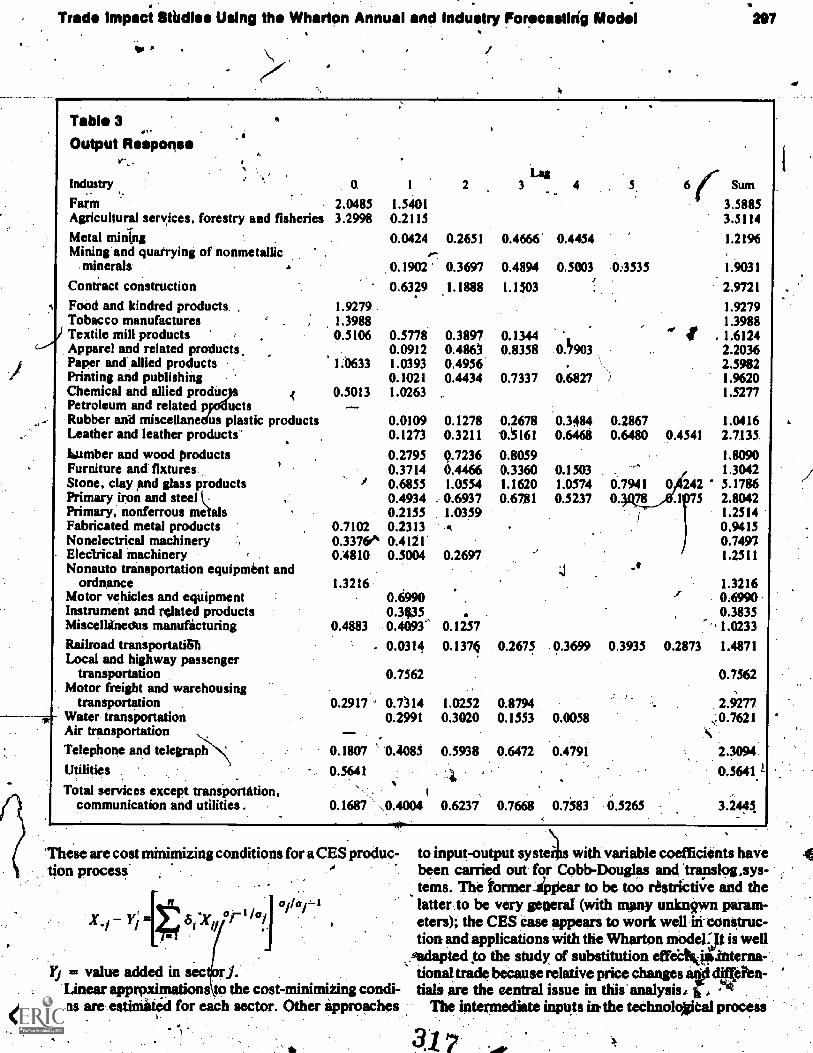
Trade Impact Stbdles Using the Wharton Annual and Industry Forecasthig Model 297

ti

Table 3 1,Output Response

1,

Industry 0. 2 4

Farm 2.0485 1.5401Agricultural services, forestry and fisheries 3.2998 0.2115

Metal mining 0.0424 0.2651 0.4666' 0.4454Mining'and quarrying of nonmetallic

.minerals 0.1902 0.3697 0.4894 0.5003

Contract construction 0.6329 .1.1888 1.1503

Food and kindred products. 1.9279Tobacco manufactures 1.3988Textile mill products 0.5106 0.5778 0.3897 0.1344Apparel and related products. 0.0912 0.4863 0.8358 03903Paper and allied products 1;0633 1.0393 0.4956Printing and publishing 0.1021 0.4434 0.7337 0.6827Chemical and allied produc 0.5013 1.0263Petroleum and related p uctsRubber and miscellane us plastic products 0.0109 0.1278 0.2678 0.3484Leather and leather products' 0.1273 0.3211 0.5161 0.6468

Lumber and wood products 0.2795 0.7236 0.8059Furniture and fixtures 0.3714 0.4466 0.3360 0.1503Stone, clay and glass Products 0.6855 1.0554 1.1620 1.0574Primary iron and steel 0.4934 0.6937 0.6781 0.5237Primary, nonferrous metals 0.2155 1.0359Fabricated metal products 0.7102 0.2313Nonelectrical machinery 0.3376,A 0.4121Electrical machinery 0.4810 0.5004 0.2697Nonauto transportation equipment and

ordnance 1.3216Motor vehicles and equipment 0.6990Instrument and related products 0.3035Miscellinedus manufacturing 0.4883 0.4093 0.1257Railroad transportatiSb - 0.0314 0.137k 0.2675 0.3699Local and highway passenger

transportation 0.7562Motor freight and warehousing

transportation 0.2917 0.7314 1.0252 0.8794Water transportation 0.2991 0.3020 0.1553 0.0058Air transportationTelephone and telegraph 0.1807 0.4085 0.5938 0.6472 0.4791

Utilities-

0.5641 '4Total services except traniportition,

communication and utilities 0.1687 \ 0.4004 0.6237 0.7668 0.7583

5 6f Sum

3.58853.5114

1.2196

0:3535 1.9031

2.9721

1.92791.3988

, 1.61242.20362.59821.96201.5277

0.2867 1.04160.6480 0.4541 2.7135,

1.80901.3042

0.7941 0 242 5.17860. '78 x.1075 2.8042

1.25140.94150.74971.2511

.1

1.32160.69900.38351.0233

0.3935 0.2873 1.4871

0.7562

0.5265

2.9277.0.7621

2.3094.

0.5641 L

3.2441

These are cost minimizing conditions for a CES produc-tion process

X y1 atI /al I

CVO/ -I

to input-output systes with variable coefficients havebeen carried out for Cobb-Douglas and .trunslog,sys-tems. The tormerippear to be too restrictive and thelatter to be very general' (with numy unknown param-eters); the CES case appears to work well ui- construc-tion and applications with the Wharton model: ft is well

.sudapted to the study of substitution efficteiiilinterna-tional trade because relative price changes an dif(ehn-tials are the central issue in this' analysis, r,

The intermediate inputs in the technologital process

31 7

25S

ft

Table 4Inventory Stook Rospor

Part Six: U.S Tariff Policy

Industry 0 1 2 5

FarmAgricultur cervices, forestry and

fisher's -0.4t204Metal nil insMining quarrying of nonmetallic

minerals

Contract constructionFood and kindred products -0.0530 -0.1022 -0.1003Tobacco manufactures -0.3866 -6.4413 -0.2754Textile mill prOductsApparel and related productsPaper and allied products -0.7322 -0.7278 -70.3596Printing and publishing -0.0061 -0.0899 -0.1913 -0.2502 -0.2065Chemical and allies products -0.2680 -0.2118Petroleum and related products. -0.9840 -0.8501' -0.2911Rubber and miscellaneous plastic, productsLeather and leather products -0.2601 -0.2052 -0.0476Lumber and wood productsFurniture ant fixtures -0.3347 -0.4966 -0.5225 -0.4491 -0.3131 -0.1511Stone, clay and glass products -0,0725 -0.1433 -0.1990 -0.2259 -0.2108 -0.1400Primary iron and steel -0.0117 -0.2311 -0.5312 -0.7856 -0.8657 -0.6463Primary, nonferrous metal -0.7528 -1.0418 -0.9947 -0.7392 -0.4031 7.0.1141Fabricated inetal products ' -0.1907 -0.2949 -0.3265 -0.2990 -0.2263 -0.1221Nonelectrical machinery -0.4077 -0.6562 -0.7595 -0.7315 -0.5863 -0.3378Electrical machinery' -Nonauto transportation equipment and

ordnance -0.7394 20.9530 -0.7968 -0.4271Motor vehicles and equipment -0.3036 -0.4207 -0.4024 -0.3000 -0.1647Instrument and related products 0.3379 0.4764 0.4635 0.3477 0.1771Miscellaneous manufacturing

6 'Sum

- 0.2204

-0.2555- 1.1033

- 1:8196- 0.7440- 0.4797- 2.1252

0.5129

- 2.2672- 0.9914-3.0710

--4.94591.4595

-3.4789

-2.9163.-0.0476 -1.6389

4.8026

are thus modeled according to a CES production func-tion specification. Value added can be obtained fromgross output by subtracting intermediate input, and forthis part of the production process, this Wharton modeluses a Cobb-Douglas specification, with appropriateallowance for technical progress and short-run dynamicadaptation.

The production function for gross output, theretire,consists of two additive parts - one covering inter-mediate inputs and one covering r inputs. The totalequation is

..' I

X, a 61 xatjt.

cri1I I

+ ?it Liel Kt/ e7it.

. -

. Productiimis is,' in ,general, assumed to be carried outaccording to a YES process, which is tip sum of a CZS

( d11/43

and Cobb-Douglas function. These' are purely simplify-ing empiridal assumptions, that are very convenient toestimate and apply.

Tice model has been put through the usual validatiohtests. It has beensimulated in one-period solutions from1960 through 1971. Sample data for intial conditions(lags) and exogenous variables are used for these simu-lationmetroestatistics for complete model performance,measured as mean absolUte percentage error (MAPE)are given in separate tables by model composition. -Table 7 gives MAPE statistic& for major aggregates.These are all under 3 percent and often under .1 or 2 per-Cent. The corresponding statistics for imports by indus-trial sector are given in Table 8. These highly disaggre-gated import flows are not as closely estimated as themain aggregates. Although total imports are estimated,with an error of about 2 percent, most of the sectorimports have MAPE statistics between 2 and 4 percent.Some are between 5 and /I percent.

4.

Trade Impact illtudimi Using the Wharton Annual ind Industry Forecasting Model .299

a

. Error statistics for sector output and labor require-ments aro/liven in Tables 9 and 10. Most of the indi-vidual output errors are under 4 percent or even 3glercent, and the employmenyman hours statistics are'equally small., Generally leaking,: the pparate errorstatistics for imports are a bit larger, but this study istrying to break new grapnd in'the detailed treatment ofimports, and .it is not surprising, therefore, that the

-initial attempt contain. more error than is likely to bethe case with repeated application of the methods setout here.

The central aim of the study is to analyze the impactof changes in imports on the economy as a whole, and

on output/employment vitriablis by sector. To d_ o this,once the model has been confitructed, we haveic estab-lish a baseline or control simulation for a pet iod ofinxestigation (1975 -81)) and comparative simulations inwhkh specified changes are introduced in the tradesectors.

The control solution is enitialized 'from December1974, and extrapolated for the solution period 1975 80.The economy was in recession at the initializationperiod. The control solution projected a slow 'recoveryof th economy, reaching an unemelloyment rate of 5perceif by 1980. The main assumptions for the controlsolution concerned input values for gover4ment pur-

Table 5

Glossary

Industry

Agriculture, forestry and fisheriesImpoits

TMO-1.

DomesticProduction

ShipmentExcluding OwnConsumption

OutputOriginating

Farm TMO2 DP2 GP02'Agricultural services, forestry Ind fisheries TMO3 DP3 S3 GP03

Mining TMO4Metal mining TMO5 DP5 S5 GP05

'Coal mining IMO& DP6 S6 GP06Chide petroleum and natural gas TMO7 DP7 S7 GP07

v. ,.Mining and quarrying of nonmetallic minerals TMO8 S8"e G12084

,DP8

Contract construction DP9 54 GP09'Nondurable manufacturing TM011

Food and kindred products TM012 DP12. S12 GP012Tobacco manufactures TM013 -11P13 S13 GP013Textile mill products TMQ14 DP 14

1.

$14 GPO I4Apparel and related products TM015 DPI5 $15 , . GP01.5Paper And allied products TM016 DP16 .S16 GP016Printing and publishing TM017 DP17 S17 GP017Chemical and allied products TM018 DP18 518 GP018Petroleum and related industries TM019 DP19 S19 GPO19Rubber and miscellaneous plastic products TM020 ppai S20 GP020Leather and leather products TM021 tin! S21 GP021

Durable maufacturing TM022 41

Lumber and wood products, except furniture TM023 DP23 0 S23 GP023Furniture and fixtures TM024 DP24 S24 GP024

,Stone, clay and SUSS products TkI025 DP25 S25 GP025Primary =pals

Primary iron and steel TM027 DP27 S27 G?027Primary nonferrous_ metals TM028 DP28 S28 GP028

Fabricated metal products TM029 DP29 S29 GP029Nonelectrical machinery TM030 DP30 S30 GP030Electrical machinery . t TM031 DP31 S31 GP031Nonauto transportation equipment and ordnance TM032 DP32 S32 GP032Motor vehicles and equipment TM033 DP33 S33 GP033Instruments and related products . TM034 DP34 S34 GP034Miscellaneous durable manufacturing TM015 DP35 S35 GP033Nonauto tiansportation equipment and ordnance

plus miscellaneous durable Manufacturing

SectorPrice 4

PGPO3

PGP04

PGP012PGP013POPOIPGP01.5PGrP016

41.

PGP018PGP019PGP020

PGPO23PGP024

PGPO26

,PGP029POP030PGP031

PGp033

PGP03235

.319

1

C

Par Slat U.S. T riff Polley

Tsibl 5 (continued) k

Industry . 1mportiDOmestic

Production

ShipmentExcluding Own OutputConsumption,. Originating

SectorPrice

Total transportation services TM036 P036Rail transportation services TM037 DP37 S37 OP037

Local and highway passenger transportationservices TM038 DP38 S38 GP038

Motor ffeight and warehousing transportationservices TM039 DP39 S39 O1'039

Water transportation services TM040 DP40 S40. GP040Air transportation.',services TMO4I DP41 S4 1 GP041Pipeline transportation services TM042 DP42 S42 OP042Other transportation services TM043 DP43 S43 GP043

Total ccurmunication TM044 PGP044Telephrine and telegrilph TM045 DP45 S45 GP045Radio and tele'ision TM046 DP4d S46 GP046

Electric, gas and Sanitary services TM047 DP47 S47 GP047

Total servic'es, except transportation,Communications and utilities TMOS' DPS SS

Wholesale trade TM049 DP49 S49 GP049Retail trade TM050 DP50 S50 GP050Banliting TM052 DP52 S52 GP052Credit agencies, holding and investment

company ,TM053 PP53 S53 GP053Security and commodity brokers TM054 DP54 S54 GP054Insurance carriers TM055 DP55 S55 GP055Insurance agents, brokers and services TM056 DP56 S56 GP056Real estate and combination offices TM057 DP57 S57 GP057Hotels and lodging places TM059 DP39 S59 GP059Personal and miscellaneous repair services TM080 ,DP80 S80 GP080,Miscellaneous business services TM061 DP61 S61 GP06 1Auto repair, auto services and garages TM062 DP62 S62 GP062Motion pictures TM064 DP64 S64 GP064Amusement and recreation, except motion

pictures TM065 DP65 S65 GP065Medical and other health services TM066 DP66 S66 32 GP066Legal and miscellaneous professional services TMO8 1 DP81 S81 GP081Educational services . TM058 DP68 S68 GP068Nonprofit membership organizations TM069' DP69 S69 G P069Government industry TM082 DP82 S82 GP082

---, Government, federal enterprises TM075 DP75 S75 GP075Governtnent, state and local enterprises TM078 DP78 S78 GP078Reit of the world 1 . . TM079 DP79 S79 GP079Private households - - TM071 bin S7 I GP071

chases, some particular prices, government employ-ment, monetary policy, fiscal policy, and world trade.

Modest increments in real nondefense spending andvery small increments in real defense spending wereassumed. Higher than average inflation accounted for

07,1 more Subilantiai current dollar increments in bothtypes of validity. State and local spending was 'pro.jected to rise- mere rapidly in real terms and also as-sumed relitively high price rises. Agricultural priceswere made to move up sharply during 1975-76, todecline in 1977, and to rise byabout 5.percent annually ,

after that point. Defense manpower was leveled off attwo million. Small growth we; projected for federalcivilian jobs and one million were added for state andlocal jobs over the whole simulation period.

Credit policy was assumed, to be easy in 1976 and banother step in 1977. It was not changed markEerthat date. Import prices were variously set on growthpaths of 4 to 6 percent and world trade volume at 5 to 6percent; followed by 7.5 percent after 1977. Statutorychanges in social security payments were introduced,but tax cuts during 1975-76 were not assumed (con-

32n

Jrade Impaotetudles Using the Wharton Anhual and Industry PoreciastIng Model 301

A

Table

Other Variables

CMIBQ Dummy, percentage change in meat im-port adjusted base quota for those yearsthat the quota was in effect

DCU,BA Dummy, 1.0 for years/tuba stopped ex-porting cigars to the United States

DCUSTK Dummy, for strikes in the domestic cop-per industry

DD Dummy, 1.0 for 1965-67; 0 elsewhere forU.S. government disposals of copper

DX Dummy, 1.0 for 1959-64; 0 eldtwhere forspecial conditions in domestic primary re-fined copper production

IM Imports, total goods and servicesPMCFS8 Unit value indeX for the imports of rude

foods, 1958 - 100,0PMMFS8 Unit value index for the imports of manu-

factured foods, 1958 100.0

PMCM58 Unit value index for the imports of non-food crude materials, 1958 = 100.0

PMSM58 Unit value indei-for the imports of semi-manufactures, 1958 - 100.0

-7 I3MFM58 Unit value index for the imports of fin-ished manufactures, 1958 - 100.0

PMSIO Unit value index for the imports of ser-S('vices, derived from input/output table topreserve the NIA current dollar identity,1958 = 100.0

SFAI Farm inventory stockSMI Manufactures inventory stockTIME Trend, 32.0 for 1952

TMO7RD Percentage ratio of imports to dOmesticproduction for crude petroleum and nat-

,

9't ural gas #TMOIFU. Percentage ratio of imports of producing

sector i to TMOS.

\

tram to what actually happened). A tax cut of $10 billionwas Programmed for 1977. The investment tax credit'rate *as set it 8 Perc4nt during 1975-76.

Th resulting control solution shows a steady returnto full mployment along a path that is lesi pessimisticthan OMB outlook presented in the Budget of theUnited \ States Government, 1976 (p. 41): As theeconom \ appioaches full employMent in Su i'olution,the fede deficit fills and the inflation rate, comesdOwn. A mMarytabulation of the main aggregates inthe contro solution is given in Table 11.

In to of today's economy and what is beingplanned kw it in contemporary policy, this appears tohave been a\ perceptive extrapolation. It serves as a

realistic baseline case against which to judge varioustrade alternatives. It must be remembered, however,that Table 11 is presented, in 1958 prices. These formedthe base system of U.S. accounts prior to January 1916,and were the data available at the time the present studywas made. The version of the Wharton model used herehas since been retired and replaced by one that is esti-m ted froni the nee, revised data.,

e first alternadte simulation is for an across-the-ard increase in import prices by 10 percent above the

Table 7

Mean Absolute Percentage Erior (MAPE)

Major AggregatesIndicator

Gross national product(current $) GNP*(58 $) GNP

(MAPE)

.96

.76

Personal consumption expendi-ture (current S) PCE .88

(58 S) PCE .74

Fixed investment (current $) 2.07Fl 2.15

Nonresidential investment NRI 2.29Imports (current $) 2.07'

(58 $) IM'` .2.05Output "

Agriculture, forestry, andfisheries . GPO! 2.35

Agricultural services,forestry and fisheries GP03 1.10'

Mining GP04 2.32Contract construction '0P09 2.98Durable manufacturing GP022 2.86Nondurable mam1facturing GP011 1.31Transporta.tion services GP036 1.67Communicatiorts GP044

112'Utilities GP047Commercial and others GPORES .65

Money supply. MSPL 1.21

Personal income PI .96Disposal personal income DPI .90Employee compeniation; all

industries EMCOT 1.23

Wage rate, total WT -8:)Deflator 0

Gross national product GNPD .34Personal consumption

expenditure PCED .32Fixed investment FID .78

Sector. priceManufacturing PGPO 10 .39Durable manufacturing PGP022 .61Nondurable manufacturing PGP011

r`, .21

. -, ,

' 321

302

A'

!art .Ix: U.8. Tariff Polley

Tobli 8Moon 4booluto Poroontogo Error (MAPE),

ImportsAOIndustry

Agriculture, forestry andfisheriesFarmAgricultural services,

forestry and fisheries TMO3

TMO1TMO2

Mining TMO4Metal mining TMO5Crude petroleum and

natural gas TMO7Mining and quarrying of

, nonmetallic minerals TMO8Contract construction TMO9Manufacturing TM010Nondurable manufacturing TM011

Food ;and kindred products TMOI2TobaccO manufattures TM0131

TextiTextile still products TM0114leand related productsTM015

Paper and allied products TM016,Printing and publishing TM017

Chemical and allied productsTM018Petroleum and related

industries TM019Rubber and miscellaneous

.,.plastic.products , TM020Leather andleather pioductsTM021

Dunible manufacturing TM022Lumbetand wood products,

except furniture TM023Furniture and fixture TM024Stone, clay and glass

products TM025

a..

!Moor&(NAPE)

5.454.32

t 8.702.684.81

.2.18

4.08

6.22

2.27

3:385.768.423.62'1.462172.582.89

3.56

3.063.42

-1.76

2.453.80

2.71

11

.

Industry

Primary iron} and steel . TMO27. Primary nonferrous -metals TM028

. Fabricated metalprodUcts TM029'..H,Nonelectrical machinery .T144030Electrical machinery . T.M031Nonauto transportation

equipment and ordnance .1M032Motor vehicl and

equipment TM033Instruments and lated

pirtducts TM034Mi ellaneous du ble

manufacturing TM035Total transportation services TM036

Rail trartiportation services TM037Local and highway

passenger transportationservices TM038

Motor freight and ware-housing transportationservices TM039

. Water transportationservices TM.40

Air transportation services TM041Totalcommunications TM044

Telephone and telegraph TMO4S

Electric, gas and sanitaryrseivices - TMQ47

rTotal services, except

transportation, cornInunica-tions and utilities TMOS

..1

(MAPE)

3.763.482.613.152.42

3.77

3.71

1.94

2:70

3.393.12

4.14

2.29

4.523.05'

.61 '

.61

3.50

6

2.06

control solution path. The initial impact of the higher441ort prites is a redUction of imports, by heady $2.0billion. This decline gradually gets larger and reaches afigure of $3.35 billion by 1980, according to the mintiplierSimulation, The major impact occurs _within the man-ufacturing sector. Of the initial impatt, $1.81' billion istraceable directly to manufacturing imports, sp 't fairlyevenly between durable'and nondurable lines. ut thegradual decline in manufacturing imports is rriuc lessthan for imports as a whole. By 1980, the cutback inmanufacturing imports is only $2'.28 billion comparedwith estimates of $3.35 billion for total importsimpkct declines overtime in nondurable manufaZtur-ins, but increases in durablps.

As, for the ipilationary consequences of increasingimport Prices, it would appear that there is undid

. .

decline in the GNP deflator. This is because importsenter the GNP calculation explicitly with a negativesign in computing net exgorts). After years, how-ever, the inflationarrforces show through, even in theGNP deflator, and the overall price index is greater inthe changed solution than in the control solutiwt. ThedeflaLor of consumer expenditures is less ambotts; itshows an inflationary impact effect of 0.53 index pointsat the beginning and gradually rises to an impact effectof 4.58 index points.

The higher import prices, followed by reduced int-ports, tends to create additional domeatic jobs. In thefirst year, there are an estimated 38,000 new jobscreated, 29,000 of those in manufacturing. After a fewyears, however, the price increases brought about bythe higher import cosis loWer aggregate activity apd

Trade Impaet,Studlee Using the Wharton Annual and Induatcy Forec,istIng Model

Table II \\\

Mean Absolute Percentage Error (MAIM)

OutputIndustry .

Farm qc, S2

Agricultural services, forestry andfisheries S3

Metal mining 55

Mining and quarrying of non-. etallic Minerals 58

-.Contract cosugruction 59Nondurable manufttpurcriordig

Food and kindre ucts S12Tobacco manufactures S13Tixtile mill products S14 ,Apparel and related products S15 .

Paper and allied products S16Printing-and publishing S17.Chemical and allied products S18Petroleum and related industries S19Rubber and miscellaneous

plastic products S20Leather and leather products S21

Durable numufacturinaLumber and wood products,

except furniture S23Furniture and fixtures S24Stone, clay and glass products S25

. Primary iron and steel S17Primary nonferrous metals S28 .Fabricated metal products S29Nonpleciri4al machinery S30Electrical machinery b. "S31Nonasto transportation equip-

ment and ordnance S32Motor vehicles and equipment S33Instruments and.related products 534Miscellaneous durable

manufacturing S35

Total transportation servicesRail trans on services S37Local and ighway passenger

trans ation services S38Motor t an warehousing

transportation s S39

(MAPS)

1.40

2.21

3.56

2.23

2.69

1.612.401.771.671.681.921.991.69

3.063.96

1.125.391.883.84

, 2.33,3.633.32

. 2.85

2.185.993.66

1.94

2.29

3.04

1.47

OutputIndustry *

Water transportation services S40Air transportation services S41

Telephone and telegraph. S45

Electric, gas and sanitaryservices S47

Total services, except transpor-tation, communications andutilities SSWholesale trade S49Retail trade S50Banking S52Credit agencies, holding and

investment company S53Security and commodity brokers 554Insurance carriers S55Insurance agents, brokers and

services S56Real estate and combination

offices S57Hotels and lodging places S59Personal and miscellaneous

repair services 580Miscellaneous business services S61Auto repair, auto services and

ilarallei ') S62Motioq plc WM S64Amusement Ind recreation,

except motion pictures S65Medical.and other health services S66Legal and miscellaneous repair

services S81Educational services S68Nonprofit meniberthip organ-

izatidns S69Government industry S82Government, fedetal enterprises S75Government, state and local

enterprises S78Rest ¢if world S79Pri mhouseholds S71

(MAPS)

1.99(.4.13

1:75

1.90

' .591.321.403.57

9(.676.852.36

2.10

1.193.17

1.701.10

1.922.51

2.03 /1.75

1.891.41

1.031.736.71,-).

1.59'6.708..98

consequently', job opportunities. The moral is, thus,'quite clear. Short-rUn gains . are not sustainable. Thehigher import prices. lead to more inflation which, inturn, depresses spending together with overall activityand ultimately results in fewer job opportunities.

The second set otelternative simulations increases. imports"' in each of thirty -sift impOrt demand categoriat

by"$l billion. These are one- at -a-time changes; i.e. one

category of Imports is increased while others are un-changed. There is a regular pattern to most of theseindusby-import simulations, namely that the industrywhose imports are being increased has the major andMost easily discernible decrease in employment. It alsohappens in most cases that the model tends to have amajor part of the adjustment taken up by movements (inthe same direction as in the industry direcfly affected) in

323

A

Part ;Ix: UAL Tariff Policy

Table 10Mean Absolute Percentage Error (MAPS)

Employment and ManlounEmployment

(MAPE)

AU industries

FarmMininj

Manufacturing'Nondurable manufacturing

Food and kindred products'Tobacco manufacturesTeitik mill productsApparel and related productsPaper and allied productsPrinting and publishingChemical and allied products.Petroleum and related industriesRubber add miscellaneous plastic productsLeather atd leather products

Duralile manufacturingLumber and wood products, except

furnitureFurniture and fixturesStone, clay and glass productsPrimary metalsFabricated metal productsNonelectrical ;machinery.Electrical tnachineryMotor vehicles and equipmentInstruments and related productsNonauto transportation equipment and

ordnance plus miscellaneous durablemanufacturing

Total regulated sectorsTotal transPortadon services

:Total communicationsElectric, gas and sanitary servicesCOMM0Cilll and other

41/

1

. 'Mahouts(NAPE)

', NT 0.50'1.71

N2 2.93 MH2 3.69

N33 1.32 MH33 1.07

N34 0.97 MH34 1.37N19 1 0.48 MH19 0.63N25 2.14 MH25 2.28N20 1.65 MH2O 2.06N26 1.55 MH26 2.01N21 s 1.66 MH21 1.95N28 1.15 MH28 1.40N22 2.59 MH22 2.54N23 2.17 MH23 1.94N24 3.17 MH24 3.96N27 2.15 MH27 2.62

N35 1.84 MH35 2.19

N14 .1.28 Mt MH14 1.33N15 -3.54 MHIS 3.92

'N 1.42 MH112 1.56N3 2.49 MH3 3.11N13 2.39 MH43 2.97N7 2.32 MH7 3.11N6 3.17 MH6 3.30N9 5.12 MH9 5.56N16 2.02 MH16 2.29

N44 1.29 MH44 2.46N29 1.02

N39 0.87

N31 2.62

N30 0.58

N32 0.41

the commercial sector. This may or may not be a plans-, ible result.

some examples show the relative magnitudes or ef-fects. If farm imports are ibcreased by $1 billion, therewould be, according to the model, about 30,000 fewerjobs incfarming initially. In the economy as a whole, thejob loss would be about 43,000. After seven years, weestimate that the farm loss would be. 77,000 jobs, andtotal employment would, fall by 109,000.

Consider the automobile industry. If motor vehicleimports are raised by SI billion, the model estimatesthat 9,060jobs would be lost in the antomObile,sectorcompatid with 60,000 in the economy as a whole. The

ratio of these two figures is somewhat more than six toone.' After seven years, the estimate is that 17,000 jobswould be lost in the motor vehiCle sector against 94,000in the economy at large. The ratio falls to about five toone.

- Industries that are closely tied to motor vehicle pro-duction also suffer parallel job losses. Primary metalsand fabricated metals are two cases in point. Theircombined job loss exceeds that of motor vehicles. Thisis indicative of part of the multiplier effect. Such aneffect is indicative of the great economic importance ofthe motor vehicle industry for the United States.

-In a third set of simulations, the ratio of side oil

324

JTAN 11

Control Solution

New Wharlef Annual and Industry Forecasting Model Dependence on Foreign Oft After 11/1February 1111

Model Newt WsSelected Indiction Label Vet 1973 1974 1975 1976 1977 1971 1979 1*Gross Nationatoduct (cur $) GNP 6181 1294,9 1396.1 1413,7 1638.0 1866,0 2117,1 , 3I.4 2543.7Percent chanV11.8 7.8 6.3 10.4 13,9 13.5 ` 10,1 9.1Gross national product (58 S) GNP 1651 83$.2 821.3 798.0 820,6 890.1 963.3 999,9 1018,3Percent change5.9 -2.1 -2.8 2.8 8,5 L2 3.8 1.8Orori MIL prod. deft (1958.100.0) ONPD 6411 154,3 170.0 185.9 1996 209.6 219.8 2i3.2 249.8Percent change5.6 10.2 9.4 7.4 5.0 4,8 6,1 7.1Labor force (millions) CIFT 2881 88.7 91.0 92.4 93,2 93.1 97.0 98,5 100.2Percent change2.5 '2.6 1,5 0.8 2.0 2,0 1.5 1.7Participation rate

59.9 604 60.2 59,7 60,0 60.3 60,3 60,4Percent change0,7 0,8 -0.2 -0.8 0,4 0,5 0.0 0.2Manufacturing average weekly hours H33 2101 40.8 0 40.3 40.0 40,3 40.7 40.8 40.7 40.6Percent change 0,2 -1,0 -0,7 0.7 0.8 0.4 -0,4 -0.3Productivity (manufacturing) 648.5 639.7 651.8 677,0 706,9 734.5 753.1 7712Percent change5.8 -1.3 1.9 9 4.4 3.9 2,5 i 2.5Money supply (demend + time deposits) MSPL 6921 634,9 698.6 764.6 112i1 881.0 974,4 1096.4 1229.7Percent change

11,6 10.0 9,4 8,0 6.7 10.6 . 12.5 12.2Bond rate (96) TR 3238 1.8 9,1 p. 9.5 9,7 9,4 8.8 8.5 8,6Prime commercial paper rate (96) PCP 6918 8.1 9.9 6,4 7,3 6,8 6.7 7.1 7,3Corporate profits (cur S) PDT 7371 122.7 143.2 122.1 152.0 187,8 232,2 260,8 292.6Percent change'23.7 . 16,7 -14.7 24.5 23.6 23.7 12.3 12.2Manufacturing output (58 SI GP010 059! ; 272.4 263.2 254.3 266.1 293.9 .319.8 329.8 336.1Percent change11.0 -3,4 -3,4 4,6 10.5 8.8 II 1.9Nondurable goods (58 S) 0P011 0601 112.7 110.6 108.9 '1118 120." 129.7 133.0 . 134.3Percent change'8.5 -1.9 -1.5 2,7 71 7.8 2.5. 1,0Durable goods (58 3) )3P022 0711 159.7' 152,6 145.4. 154.2 173,6 190.0 196.8 201.8Percent change

12.8 -4.4 -4.7 6.0 11,6 9.5 3.6 2.5Unemployment rate (96) UNR 2861 4.9 5.1 8.3 8.4 7.8 6,4 . 5.4 5.2Spiny rate (% SR 7711 8,2 7.4 9.5 8,9 7.8 1.3 6.5 6.3tSurplus or deficit, federal (cur S) . spF 7771 -5,6 -6,2 -53.4 -56,2 -33.3 -15.6 -11.4 -10.7'Surplus or def., state & lac (cur S) SD$ 7801 9.2 1.9 -1.7 -3.2 1.9 ' 6.4 6.5 40.1Consumption to disposable me

89.1 90.0 88.0 88.7 89.5 90.1 90.9 91.0Fixed investment to gross tut prod.15.0 14.0 13.0 136 14,7 15.5 15.5 15.9'Compen. to 'employees to nat. income73.8 74.9 75,2 14.4 13.1 13.6 14,5 75.0Profile to national income11.5 12.6 10.1 11.4) 12.3 13.4 13,6 14.0Farm income to national incomeLi 2.8 2.6 2,5 2.2 2.0 1.9 1.8'Other income to national income,

13.0 13,4 13.8 13.0 12,6 11.8 11.0 103'

riiEmr..mamemw

a

326

impoWi 10 domestic -prodwrion it held iTati. ilitit. Theinitial impact is small, but by the sixth year, imports arereduced by $1.7 billion. Activity is stimulated in dometic oil/gas production and there are increases in realGNP by S2.76 billion above the control solution value.Imports are hieluced in other sectors, and, as a result,total imports decline by only $1.2 billion. This brings

1 out an interesting point. Increased domestic activityassociated with strict import-domestic productionratios has secondary effect( that induce importselsewhere, thus reducing any initial gains.

The import price increase across the board was intro-duced without any direct change in export cqnditions. If

.., the change occurred as a result of dollaOvaluation.there would be a quantity response on the 'side of de-ports. The long-run elasticity of imports was increasedfrom 0.36 to 0.664 (by ma e services price sensitive)together with the introdu on of an elasticity for ex-ports at 0.S. Without she adjustment to exports, theincrease in import prices now gives rise to 117,000 morejobs in Otufacturing: but these are offset by losses inthe seriector. Real ON P"loes not change. Burl( weinclude the 0.5 elasticity for exports, there is an overallincrease of 507,000 jobs. The trade balance improves by.44.2. billion. Personal income and the federal budgetbalance improve. These are elasticity-optimist resultsin contrast with elasticity-pessimist results for the casein which export elasticity is s

...- Finally, there is a duty50 percent in tariffs.twined increase jn net exports. Consumer prices are-shaved, together with slight increases in GNP andemployment. The net gain totals 75,000 jobs by 1980. Ifduty reduction and devaluation are, combined. 581.000

. jobs are created by 1980, with somewhat fewer thanunder the pure devaluation case in manufacturing butwith many more in commercial employment. Duty re-duction appears to have a relatively strong effect in thecommercial sector and devaluation on manufacturing(especially in durables).

zero.tion scenario a cut of

e is anal mediate and sus-

Literature Cited

I,. Hickman. Bert G.. and L. Lau. "Elasticities of Substitu-tion and Export Demands in a World Trade Model." Euro-ran Economic Review. 4 (1973), 347-80.

2 Preston. Ross S. The Wharton Annual and Industry Fore-casting Model. Philadelphia: University of Pennsylvania,Economic Research Unit, 1972.

3. . "The Wharton Long-Term Model: Input/Output.within the Context of a Macro Forecasting Model." Inter-national Economic Review. 16 (February '1975), 3-19.

Part Six: U.S. Tariff Policy

CommentClopper Almon

Lawrence Klein's succinct paper is a summary of a556-page volume by Ross Preston and Yuen!YunO'Brien, Trade Impart Studie,s( Using the WhartonAnnual and industry Forecustittg Model. 'This treatise,to which all page numbers in this comment refer, pvides a valuable overview of the Wharton aenual model'plus special chapters on the sixty-industry input - outputblock of the model, on the production functions, on theimport equations, as well as on theiimalations of the

:effectsof changes in foreign trade. This work repre-

sents a very substantial achievement in the integrationinput-otttput industrial detail into a macromodel. My

comments, however, in keeping with the interests ofthis conference, will be limited to the parts dealing withinternational trade. Unfortunately, this part of themodel appears to be its weakest link, and I find myselfpointing out the weal points of a model which has manystrong points which it would be more pleasant to em-phasize. These weak points can be readily remedied,and 'I am sure they will be. The dprincipal and mostparadoxial result of the trade impact studies will then, Isuspect, vanish.

That striking and paradoxical result comes from theulation of an increase of all import prices by 10

pe ent. Relative prices for exports are unchanged. Ineff t, we are looking at the impact of a 10 percentacross-the-board duty. One would expect such a mea-sure to have a shdrt-run stimulative effect on theeconomy, but after a few years the employment level

,should return to what it would have been without thestimulus, and real GNP should be smaller. The equilib-rium level of employment should certainly not dependon the terms of trade, but the level of real GNP should.

In the model, the initial stimulus proves, rather weak;only 38,000 jobs are created in the first year. In thesecond year, 6,000 of these are lost; in the third, another50,000 are lost; in the fourth, another 99,000; in the fifth,126,000; in the sixth, 95,000, in the seventh 132000, fora total loss of 459,000 relative to the control solution.Real GNP is off 8.4 billion 1958 dollars. The economyhas beeh put into an accelerating tailspin by this"stimulus." Contrary to expectations, changes in.

327sf

Trade Impact Studies Using the Wit& Annual and IndUstry Forecasting Model 307

terms atrade seem to hav e long-run 'effects on the level' -levels after seven year's: Food and beverages empTO-17------of employment: merit is. also still above the control level, as is that in

If this result is correct: 'if it describes what would mining, cheniicals, rubber, and petroleum refining.happen in response-to an across-the-board duty; then it Where then is the recession?-0f the 459,000 jobs lostis certainly a potent argument against protection. But is relative . to the control solution, fully 409 are in theit correct? What causes the accelerating recessio ? "commercial" sector, which covers trade, finance,and

Preston sees the cause in inflation.,He states:,' n theinitial year of impatt, increasing import price by tenportent has, the effect of reducing prices-,by approxi-mately one index number point. . . This result is di-reedy related to the fact that import -prices enter thegross national product identity with a negative weight. equations. Those equations are of the following form:.If import prices are increased, . .0 the, increase has a

services. Another 11,000 come in stone, clay, and glass;another 15,000 in apparel, and 14,000 in printing andpublishing. Su h a recession is clearly unusual andprompts a os look at the mechanism causing it.

In the mode , that mechanism begins with the import

tendency to reduce domestic price levels, other thingsbeing equal. The long run impact . hoviever, ap-pears fo be inflationary. The inflationary tendencies ofincreased import prices eventually depress the real de-mand categories of the disturbed solution below ourcontrol solution." (p. 405)

This is a revealing, though contestable passage. Inthe first place, import prices -should enter the GNPdeflator with a zero, not a negative weight. An increasein the price of an imported caletcreases personal con-sumption expenditures in current dollars and then thisincrease is canceled out of GNP by the increase inimport prices. Similarly, an increase in the price' ofimported crude oil should increase the price of refinedproducts and, gradually, of everything made with them.All thesprice rises increase the current dollar value ofconsumption and investment, but the increase is againcanceled out of GNP by the increase in the, currentdollar value of imports: Apparently, only the second,the canceling-out part of this protess is modeled atpresent. That is, surely just a technical defect that can beremedied. But until-it is fixed, the analysis Of the in-'flationary effects ofincreasing import priCes is mislead-ing.

In the second place, I cannot agree that it is the"inflationary tendencies" which in the preknt model"eventually depress the real demand categories." Thewage rate and the consumption deffator rise part passu,(p. 4161. Something else must be holding down demand.Also, if the stimulus' of the duty set off the rise inpri ,why does not the slack demand halt the infla-,tion . What then does cause this recession? I have beenunable to put my finger on the cause, bufmy search hasturned up sorife features of the model that make mehesitate to accept the resultlibet me share what I found.

Ode duet° the ,c use of the recessionmay lie in thefact that it is very oncentrated.in a few sectors, whichare, moreover, he ones usually affected by bustnesi cycles. Such'cyclically sensitive sectors as motorvehicles, electrical machinery, and prikary metals arestill showing increased or unchanged employment

328___--,--------------

6 In (PMIPGP0)1.4

1=0

{- or .

A In (PM/PGPO)t_i

6

+E q In St_i tsi A St_,o i=o

tri A In SMI.Ji.i=o

TM is total imPorts of the products of the sector; DP istheir domestic production; PM is their import price;PGPO is the price of the corresponding domestic prod-uct; S, "sales" is DP + TM less the sales on the di-agonal of the input-output matrix; and SM is the inven-tory of the product ;the w,,q,s, and r are distributed lagweights.

The long-run price elasticities are the sum of the wswhen they apply to the logarithms of relative price. Inseven cases, however, they. apply, to the first differ-ences of these logarithms, so the lolero. Bearing that fact in mind, we finlong-run elasticities: metal mining, 5.8ferrous metals, 1.3; nonelectrical m

-run elasticity. isthe following

teel, 3.2; non -inery, 1.0; elec-

trical machinery, 0.7; fabricated metal products, 0.2;automobiles, 0.0; other transportation equipment, 0.0;instruments, 0.0. These results rtin directly counter tothose of other researchers who found the highest elas-ticities for the finished goods and the lowest for the rawmaterials. A 'number of other zero long-run elasticitiesare found, such as those for food, textiles, paper, chem-icals, and petroleum refining. Together 'with au-tomobiles, these 'sectors accounted for half of the initialdrop in imports. Naturally, the effect fades out after a Ifew years. Since change s.in terms of trade should have apermanent effect on the ratio of imports to domesticproduction, that permanence should be insisted uponby the form, of the fUnction.-

308 Part Six: U.S. Tariff Policy

---The-opposite-problem.a.rises_with_the_sum_ofIho,qs.....the weights on the logarithms of the levels of output. AllbUt two products have positive sums ofqs, whiCh implythat an increase in sales permanently increases the ratioof importt to domestic production. Generally, largeeconomies have smaller import/prOduction ratios thando small economies, so one wmddexpect that the sumof the qs shotild be slightly negative. None:are negative;twenty-five out of thirty-five are over 1.0; eleven areover 2.0; and four, including those for commercial andstone, claY, and glass, are over 3.0. Such a high elastic-ity implies that enough growth in "sales" Will eventu-ally wipe opt the domestic industry. If, for example,, theelasticity 3 and imports are initially 20 percent ofdomestic production, a doubling of "sales" will push upimports so much that domestic production is reduced 4percent. A second doubling will reduce it , to only 3/percent of its initial yalue. There is, moreover, a strongcorrespondeice between the sectors with high saleselasticities and those with large employment losS intfieimpact study. Perhapsibese equations have attributedto "sales" effects that should be attributed to reductionin trade barriers, to improving quality of products man-ufactured abroad, or price differentials not pickedup bythe rather crude price series. Clearly such equations are

,unacceptable for long-term forecasting and even inmedium-term impact studies they may produce spuri,7ous effects.

_...,The_first difference of the logarithms -of sales appearsin only eleven of the thirty-five eq&ations, and in all Mittwo of these the Oeights are all negative. That againruns contrary to expectations that a domestic boomwould produce a; temporary increase in the ratio ofimport's to domestic production. Are these negativeterms perhaps used by the least-squares fitting processto offset 'the short-term effects of the spurious coeffi-cients on the level of sales?

Finally, I must confess that I find the reported resultsfor the commercial sector arithmetically inconsistentwith the import equation given for the sector. In the frityear, output of this sectordecreased $.30 billion (p. 415)while imports increased $.10 billion (p. 412),, so "sales" rmust have decreased $.20 billion. According to theim-port equations for this sector (p. 90), imports lathe firstperiod could differ from the control solution 'only byttieeffects of sales and output. and they are an increasingfUtiction of both. How then can imports go up whjleboth output and sales go down? If it were my model,.Iwould strongly suspect an error in the program. Is theresome peculiarity in the treatment of trade margins opimports?

Let me conclude by repeating that, thinigh I am ,

doubtful about the results of this foreign trade analysis,I greatly admire Preston's achievementin Struttinga model so thoroUghly integrated.; hapesthat y com-ments can be helpful to the model's masters in thecontinuing task, of refining and improving it.

Trade Impact Studies Using-the Wharton Annual and Industry Forecasting Model

Lawrence -R. Klein

w.

I

Clopper _Almon finds the results of the 10 percent(acioss-the-board) increase in import priees to be coun-terintuitive, btit,I will stick by the Wharton model fe-sults for this case and argue that the depressing effect ofexternal price rises is quite realistic as well as beingvery signifidant.

He says, ."Onivould expect such a measure to havea short-nin stimulative effect on the economy, but aftera few years, the employment level should return to whatit would have been without the stiinulus, and real GNPshould. be smaller." *

With regard to the ultimate movements, we are inagreement, after) experimentation, That real GNPshonld be smaller as a result . of the external priceincrease. i do riot, however, find reasorrto believe that

- the employment level should return' to what it wouldhave been in the absence of employment-creatingpolicies.. ." .

The Wharton Model used for this study and otherWharton Econometric Forecasting Associates modelshave the proi)erty that if the economy underg9es exter-

- nal price disturbance, there will be a deflairdary reac-

t (

the-UnitedStates-.--lf--priees-are-outside the economy, we should look for-an inversecorrelation between production Or employment and

-price change. In the case of domestically imposed ex-pansion, we should find a positive correlation betiveenproduction or employment and the price change. Theseare, to some extent, the expected results under normalcircvmstances. *

An externally imposed price increase (the case oftariffs) causes price indexes for final purchase's to rise.The normal reaction is for physkil demand to contract,the degree depending on the variolis price elasticities ofdemand.' Falling real demand manifests itself in thedeflator's rising faster than the value of nominal output;so the deflated (or real) value declines. On a large wale,this is what has happened in the. U.S. economy during1974 -75 under'the burden of the embargo, followed byhigh cartel controls on oil prices. Similar results werefound when proposed value added tax isystems wereseriously being discussed,

Because of the way the .GNP.deflator is computed;we may find: an .initial lowering of the overall° deflatorWhen invert prices are rising. Other price indexes showmore familiar results"7- higher tariffs; higher domesticprices. Eventually, the results -for the. GNP ;dtflatpr.change sign;

What seems puzzling to Clopper Almon strikes me asbeing quite plausible. would 'stand by, our results,apart from the biased tendency of the commercialsector to capture most of the shift of employMent. Thatsector's response equation has, to be reestimated, butthat does not invalidate: the general size of the findingsfor the economy as a whore.

. rf

310 6 Part Six: U.S. Tariff Policy J

----ConunenLarry J. Wipf

izatiOn. The level of industry detail and the emphasis on_ .

emplOyinentiriipaciiiieldriiiirpasiit-tharbreirlitrinvestigations. In previous r negotiations economic(analysis the decision-making process in a fairlyaggregative form. Most studies covered only broad in- I.

dustryaggregates or a few selected industries. The sec-tor studies were supplemented with detailed institu-tional information and advice of industry experts.While the advice of these experts is very useful in any

4 ''.\ negotiation, the Baldwin-Lewis and Cline tudiesgreatly add to this information by directly esti sting

Progress in the current 'round of Multilateral TmdeC..,.. the Consequences of multilateral tariff cuts on tit the

Negotiations (MTN) will require resolution of a nuniber4. '' exportand import-competing industries and by ng

of key policy issues: Difficult economic and political. into account interindustry effects and interactions with

decisions 'need to be made concerning the type of tariff the rest of the economy. ..

formula which best serves U.S. i terests, the particular .. Thejesults of these studies are directly relevant to aindustries .which should be' ex mpt froth tariff Cuts, number of policy decisiona in the KIN. For examplemethods of achieving reductious, in nontarinaiiiers to the exaMination of alternative types .pf tariff-cuttingtrade,. safeguard mechanisms t smooth ajustments form as. is of aid in deteimining whether the Unitedindaced. by trade, and approp ate compensation of i States should strive for uniform :tariff reductioni Of.thOse whp experience losses due to trade liberaliiatiOn2 , some torn) of a harmonizatton formula as proposed by

Sensible policy formulation in the MTN requires some of ourmajor trading partners .sit is also:taluable inknowledge of the costs.... . . nefits of Specific changes determining whether a tariff flOor should be adoptedininterraitiOnal trad ;',.licy. To be useful this inforina- - below whiCh existing duties, would not be 'cut. Thenon must be available at a fairly disaggregated level. Of ,r,estirnatekof who gains and loses from reductions incourse, policy furmulatium.involve's much More"than trade barriers and by how much is useful in determining

just economic analysis. Yet without basic economic which industries, may. reqt4e,loi ger staging of Miffresearch, economic factors cannot be appropriately cuts, less 'than fug formula cuts, or' complete exemption

4' weighted and it is difficult to iPehtifyU.S. interests. from tariff pits. The studies areitso important in assessWith this recognition; the Depirtment Of Labor spon= ing the values of specific trade concessions on the part

sored two major" studisL-rone by. Baldwin and Lewis of our traili0 partners and in appraisinip the potentialand the other by Cla, Kawanabe, Kronsjo and , acceptability of Various proposals to onr,major tradingWilliamsof the effects of multilateial reductions in partners. -trade barriers on the U.S. economy. ... : These studies do not provide all of the analysis

These studies provide detailed industry estimates of needed in the negotiations. Moreover the resultspf thixthe effects of-alternatiVe types of tariff-cutting formulas . research are not, nor should they be, the iole:determi-on U.S. imports, exports, exchange rates, consumer , pants of the U.S. position in the MTN. As stated earlier,.prices, domestic output and.employment. They also though icy formulation involves = much. more thancontain estimates of the consequences of redUcing cer- just econo c analysis, these studies provide detailedtaro nontariff barriers to trade. Baldwin and Lewis pro -kinformatid which should be useful in fdrmulating%U.S.vide particularly detailed estimates of the employment policy. 'This information is supplemented by otherimpacts.'These are available tor some 350 industries' studies initiated by the Bulreau. These include detailedand are also broken down by skill group and geographic, industry studies involving steel, motor vehicles, foot-Wion. The studyj,y Cline ajmd others adds to this wear, chemicals, electronics and sugar as. Irvell. as

Mrmation by providing detailed estimates t 'trade specific studies of labor adjustment costs. Examples ofand employment Uimpacts on. the United States and ;mss research have already been presented in previousther major participants in the trade.negotiations. sessions of this conference. Together these studies pro-

eSe studies . mark an imliartant step forward in vide pOlidy makers with important u uts for appraisingasse in a gat d losses entailed'in trade liberal- specific policy issues in the MTN.

tise and Relevance of Trade and Employment Studios 311

CommentHarvey E. Bate

e

.

OiVen the problems associated With the slow economicgroWth of the United States and other industrial coun-tries in recent years, it has becothe difficult for theUnited "States- and other governments to press aheadwith the Mfiltiliteral Trade Negotiations' (MTN), Anumber of governments have been under pressure totake import-restrainirtg meaSurea. to . stimulate laggingproduction- and reduce high unemployment in :pan-Catty and economically important sectors. In the United

: States,although the Trade Act of 1974 sets, as a 'pritriepurpose of the MTN "to foster the economic; growth of

d full eMployniept in the United States," many lead=era of the Americah labor movement today believe thattrade lberalizatiOn would have the opposite result.

Th efore, those of us in trade negotiations have agreat i terest in the studies commissioned by the LaborDepartment to examine the trade and emploYment ef-41. fects of gene tariff reductions in the MTN. These canprovide s ,objective indication of whether theremight be significant adverse effects (*labor markets orexchange rates of our efforts to negotiate significant'reductions in tariff barriers. ,;

Value of 'die Studies VegotlatorsBoth the Baldwin-Lewis d Cline et al: papers arrive atsimilar results, viz. aSross-theboard tariff reductionsdo-th4 appear to result in severe adjustment problems inthe labor and freign exchange markets (with qualifica-tions regardchg product coverage of the tariff formula).'These results are quite useful from the viewpoint ofindicating that labor-adjustment problems appear to besmall relatiVe to the resource reallocation benefits ofMajor tariff reductions. Further, the studies appear topresent the extreme case for adverse effects of the tariffreductions since actual reductions Will be staged over aperiod of Aye to ten years. The models haVs a furtherusefulness in that during the process of negotiations andafter the 'MTN, actual tariff reductions (alcitig with ex-ceptions) resulting-from the negotiations can be pluggedinto the models to obtain an assessment of the seotoraland overall effects' of the negotiated packages:

Baldwin and Lewis provide additional useful infor-

'Stern [3] also finds small overall net job changes relative to totalemployment as a iy,sult of formula-based tariff reductions in theindustrial countries.

3.12

manon for negotiators by identifying detailed productareab. orthe-367-industry inputzotitputable -thgthowmarked negative, as wellas positive, employment ef-.fects in the United States.: This, information is helpfs1

. in conjunction with-analysis by government and private'commodity expert'sr in identifying areas, of concern thatmay requirp, special treatment in the MTN.

' Cline et W. arrive at the interesting conclusion thatnone of the alternative tariff-cutting formulae that maybe' considered appear to require great-adjustments in thelabor markets of the various countries applying thetariff formula, even though they have different resultson the depth of tariff reductions and increase in trade.This Conclusion could have a beneficial effect on thenegotiations by indicating that a reasonable bails forcompromise exists between 'the current' strongly heldPositions of majortrading partners regarding the choiceof a tariff-Catting formula. For its part, the UnitedStates )17,Qd like to see significant reductions at all.tariff levels. Another major country sees its interestsserved by 'elimination. of Tow duties and lesser reduc-tions_in high duties; while yet another bloc of countriesthinks that.high duties should be reduced substantiallyleaving low duties baSically Unchanged. The Clinestudy adds a subStantive element to.the discussiOn thatshould lead to a compromise tariff-cutting approach

Of course, these studies cannot. be used as the prin-cipal inputs to policy decisions: They will be supple-mentary to the information the government' receivesfrom, private sector advisers and government corn-.modity' experts. In the United States we have a veryelabdtate system for obtaining information on the sec-total effects of policy changes from almost ethousandpriyate sector advisers drawn from industry, labor, andagriculture.

Weaknesses of the 'ModelsThere are tseveral technical difficulties in the:data lin-k

o y measures and -4derlying the models'

in the 'elasticitthoCiated with the insufficient de

gree of disaggregatifaults in _the tariff and trade aata.3 Some of these proba-

'Stern [3] also shows detailed (3-digit ISIC) sectoral enipleymentresults of all of the GATT Tariff Study countries assuming flexibleexchange rates.

'First, the elasticities used are too aggregative and are frequentlytoo dated for use in detailed tariff negotiations. Second, the datagenerally used in the, studies are for 1971, which was an abnormalyear for trade relatidns (the U.S. dollar being revalued relative tosome other major currencies). While it would be preferable to usethe 197411ATT Tariff Study data tapes now available, the tariffs con-tained in These tapes are higher than many, rates actitally In fixtsbsince 1972 for Japan, Canada, and Australia.. These countries havemade many tariff reductions that they are hot legally .bound tomaintain and that, therefore, are not shown. Firiall, U.S. importswere artificially allocated to fit the'BTN product categories.in 1971.These allocations were frequently erroneous and are being corrected.The same problem exists for Canada, which, too, does not have aBTN classification scheme for its tariffs.

I.

312 Part Six: U.S. Tariff Policy/

bly can be solved. However, there are 'several otherweaknesses thit seriouslyimpair the utility of the mod-els as guides for the negotiatOrs.

One of the more important weaknesses in bothstudies is that nontariff barriers (NTBs) are ignored,except for thosetquantitative restrictions in developedcountry textiles and variable levies on imports of ag-ricultural products most European countries (mostnotably the EEC and Sweden)." However, types ofNTBs such as product standards requirements, sub-sidies, government procurement, and quotas abound tosuch an extent that the elimination of these trade bar-riers is as important as tariff reductions in the MTN.The trade and employment results of negotiations inNTBs could swamp the effects of tariff changes. Also,failure to liberalize NTBs would make tariff changes inmany areas meaningless. The omission of most NTBs intheBaldwin-Lewis add Cline studies provides a sourceof upWard bias in the estimates of the trade changeslikely to occur as a result of tariff changes,* Should beadded that much:more work is needed to evaluate theeffect of NTBs on trade flows.5

.A second weakness in any trade aria employmentanalyses such as these is that there has been a reorienta-tion in the goals of governments in tiaele negotiations.The trade and consumer welfare changes that Cline,uses to define the preference functions of the industrialcountries are inadequate. In fact, representatives of themajor countries in the MTh deny that trade balancechanges are now a major consideration in fixing, their

(`negotiating positions."' Today goyernments de not seeksimply a balance of concessions (or, more specifically,

'Errors are committed in the studies irthe handlinOf the textilerestrictions. For instance, Baldwin and Lewis exclude textileProducts from their calculations because, they claim; the presentMulti-Fiber Arrangement (MFA) 'would prevent imports from'responding to tariff changes. Yet MFA quantittitive limits only applyto imports of developed countries' from someLOCs. They do not

d-.-4apply to intradevelopf country. e. There is much current andpotentially greater here affect Ed 6

iby tariffs only:

There is only one analysis that I knoW of on the trade effectsof government procurement programs that increasingly affect tradeas governments increase their purchases in relation to GNP [2].

°See [I, pp. 33-34]. Johnson attributes is attitude to the curerent system of flexible exchange rates.

a balance of changes in trade flows), but a final set ofarrangements at the end of the gm-under which ac-cess for sales of their products in foreign markets is"equal" to the access granted to foreign products intheir home' Markets. Practically, this means that somecountries may ask other countries to make greater con-cessions than would be called for according to the "ben-efits" received by the latter. The rationale for this isthe view that a few developed countries and many rela-tively' prosperous less developed countries have ob-tained a free ride in past negotiations (via the MostFavored Nation principle) by pleading the existence ofspecial circumstances (underdeVelopment, foreign ex-change needs, and so forth). Accordingly, they are ex-pected to try to catch up in the liberalizAtion processunder the threat to deny their exports major conces-sions in this round of negotiations. The measurement ofequivalent competitive opportunities will have to takeinto account several Conditions e.g., roughly equiva-lent tariff leVels, similar rules for product standardssetting, and similar rules for foreign bidding on govern-ment contracts.

Despite the drawbacks that I have suggeSted above,,the two models discussed here provide useful', albeitincomplete, frameWorks for evaluating results . of theMTN. There are in fact other policy options to whichthese'models could be applied. They might be used, forexample, to study the probable effects on trade andemployment of a f. e trade area between the UnitedStates; and Can a an agreement the president is,encouraged to negOtiate under the Trade Act of 1974.

aLiterature Cited

1. Johnson, Harry G. rade Negotiationnational Monetary System. Geneva: GInternational Studies, 1976.

2. Lowinger, Thomas C. "Government ocurement ofPoreign Goods in the United States and Europe.' Mimeo-graphed. 1973.

3. Stern, Robert. "Evaluating the Consequences of Alterna-tive Policies for Trade Liberalization in the MTN."Mimeographed. 1977.

nd the, New Inter-uate Institute of

33:;

v

Use and Relevance of Trade and Employment Studies 313

from the -floor

MR. DEWALD: There will be an opportunity for a fewbrief questions from members of the audience. Who willthrow the first stone?

MS, .KRAMER: Helen Kramer, United Auto .Work-ers. My question is addressed to Professor Baldwin. Iwould like to know whether any tests have been doneOn the 1967 input and output table for its validity today,in light of the changing technology that has a relativeprice effect.

_MA. BALDWIN: Isn't it right, Wayne, that there aresome estimates of changes in those over time? This is

co- author..

MR. LEWIS: Yes. There have'been studies made ofchanges over time in input-output coefficients; and theydo change over time. The input-butput tables haVebeen updated to atjeast 1970 to my knowledge; but 1967

) is the most recent yearfor which the detailed 367-sectortable is available. So input-output coefficients may wellhave changed since then, but they are the most recent

rlata available to us.( .

MS. KRAMER: So then I wonder how valid the resultsare.

MR. ALMON: May I comment that a group at theUniversity of.Maryland, working at a 200-sector level,has just completed an update to 1974. This would beavailable at a 200-sector level, if Mr". Baldwin wanted touse it. I

-

MR. BALDWIN: That is very good. The point to bemade is that you don't know which way the bias wouldgo. It may show a better or a worse picture; I don't thi kthere is any a priori knowledge that it will go oneway ranother.

MS. KRAMER:. That is the problem, though. You aregoing to show conclusions on which, presumably, our

e repreientatives are going to take positions. If you

don't even know the direction of the change, what-kind*of a guide is that to policy makers?

MR. LEWIS: Well, the 'comment has already beenmade that the use of the 1971 trade data for the U.S,does bias the results of our study in the direction of'.showing an unfayorable effect on the U.S. ,trade bal-ance. Whilf we don't know the direction of the bias in :using outdated mput-output coefficients, we do knowthat we would ha -estimated a much more favorabletrade balance as a onsequence of cutting tariffs, if, infact, we had use the updated trade date.

,No

MR. DEWALD:. Next, please? /MS. JAGER: My name is ElizabethJager. I work forthe AFL-CIO. My principal comment is that for twodays now, the more indecisive and /incomplete and in-sufficient the data, the firmer and/more dogmatic thepolicy conclusion. I find this rather shocking. I wouldthink that people would be very hesitant to advise pub-lic policy makers on the basis of the theoretical andrather unrealistic_ models that I/have been listening to.The re sophisticated the mathematics, it seems tomeoihe

%oless data seem availableto ,be plugged in. -

My second Omment is' related very much to whatHelen Krameetwas asking: it seems to me that most ofwhat Professor Baldwin haS been talking about is doneaway with by the facts of life in the. world in which wenow live. In the years since these economists started toplay this very interesting, and, I think, highly sophisti-cated game, nations like Brazil, for exampleg have put100 percent import depOsit rules on imports of sophisti-cated equipment. The deposits must be left there forone year, bearing no interest. The result ofthis systemhas very little to do,with any of these models. But theresult is a loss ofjohs in sophisticated industries acrossthe board in the Uailtid States. This occurs With theagreement,-I might add (tf U.S. negotiators, who havebeen advised by people using the type of informationthe models pro ide.

In the same riod of time I think it is fair to mention,the fact that there has been a-change in the value" ofcurrencies. Algreat deal of trouble has developed. Swe-den has putdlobal quotas on shoes outside &the GATTagreement. /Japan and the EEC have trade restraints,and on anf on and on. All this piling on of barriers hasociurrecikin top of barriers that were in effect at thebeginning of the exercise that is known'as the "TokyoRound. /'

Given ..thest conditions, I find it very hard to bepatient, not with the fact that these very skilled andintelligent people. are pursuing their academic plea-

*

334

314

4.Sures;1 think thatiagreat I dcatave, hoWever,a yerydifferent concern. Somebody asked me yesterday why Ikept bringing reality into the discussion: The reason isthat very real people are affected.

With that introduction, I would like to ask two ques-tions. My first question: Has any member of this groupexamined, not the one-volume !`telephone kook"; thatProfessor Klein's Wharton group, has produced, but thefour-volume International Trade commission book onnon-tariff barriers to trade? I don't think that book is anexhaustive study. It includes only the barriers Ameri-can business was interested in removing not whatthink the policy makers would be interested in seeing.My second question is and it is an hooest one, be,cause I think the Wharton model 'may haVe predictedit Has any member, of lite panel used, even in ashort-term forecast, any model that predicted that wewould have, at this moment, an 8.1 percent unemploy-ment rate?

- MR. DEWALD: I wonder whether I could ask each ofthe authors to respond to those questions. Let's start

. , with Professor Klein.

MR. KLEIN: No comment.

MR. BALDWIN: In response to your two questions,respectively, yes and no. We know the non-tariff bat-rier study by the National Trade Commission; I havewritten ..a book myself. on the subject at Brookings,trying to' estimate the impact of.NTBs. These are veryhard' to quantify. But it is true that there are a lot ofnontariff, barriera being erected-which, unless we canget on with negotiations in Geneva, may threaten manyof the benefits of liberalilation that we esently have.

Let me,comment also onthe unemploy nt problem.I think you want to take a much different ture ofhaving a trade negotiatioh when you are in ape_ d ofconsiderable unemployinent than when you are t.You may well want to decide that this is not the apprprate time to start cutting duties; or if you do, you say,"We will stage tam in or begin them when unemploy-ment falls to some particular level." We find out, forexample, wren workers, are thrown out of jobs; if the

. general unem ment rate is high, or it is particularlyhigh in their hat it takes longer for them taget jobsthan otherwise; and we hOpe to take that into account inour estimates, where the local uneMployment rate isone of the variables.

Part Six: U.S. Tariff 'Icy

to Liz-Jagees--questions, thatan-theone-hand,there is 'obvious disagreement among economists asthey are trying to find techniques that are more...satisfac-tory; and in this regard, some of us have to be critical.

Eithe other hand, it seems to me that 'somehow orotheii. there are all kinds of interests. involVed in thingslike tariff negotiatiions. There are some things that aregoing to ome out positive and some are gOing to comeout nega for particular intere#ts. It is important toemphasize tha all of these papers come up verystrongly with a message which I think is fairly robust.These models:all come outthe same way, as does any-thing else: namely, if you t to worry about the levelof unemployment, you d t look at "the trade instru-ment.

The models don't really have that much to do withaggregate employment but rather with employment inparticular industries or industry groups. This is pre-cisely where their value lies; namely, in trying, to esti-mate that there are going to be some people who arebetter off, some who are worse off, and there can bepolicy problems in:the short run as a consequence ofthese shifts in labor demand. [would say that the valueof Bob Baldwin's or Bill Cline's work is in trying to

cpinpoint industries where there will be some peoplevilso might be .worse off. The question is identifyingthose cases, limiting the adverse effects, and getting themaximum gains froth trade negotiations. Simply be-cause no model captures every aspect of reality, it, isunfair to say we shouldn't use models at all, and besat1sfied with any seat-of-the-pants estimate. Quite thecontrary, the models give us some guidance as to wheretolook for the kinds of policies that can offset negativeeffects and can accentuate the positiemployment impacts,) such as they

ones, so thatcan be reason-

ably anticipated and ' handled- at the acroeconomiclevel.

(APPLAUt E.) '4

MS. JAGER: Why are- your clapping? May I make aomment in response, to that last comment?

R. DEWALD: Yes. dould you speak into the rincro-phone, please?

MS. JAGER: Now, I know that thiS is your belief, and Iknow that it is the dogma, anctl_know that it is yourtheory. I have spent 25 years looking at this situation.What yoU are talking about simply has not appert ried.Over a period-of time, imports have had ve much todo with American employment.'So have exports. Sohave operations of firms outside the United States. TheVery simplistic, theoretical models assume that policy

MR. DEWALD: Anne Krueger like to respond.

MS. KRUEGER: Yes. As one of the critics of thesemodels, I feel called upon to say a word or two in regard

1335

t Use and Relevance of Trade artdmploy nt Studies

1 7,.

7.7----ac-fions nViliTUorafaiiionomous charac er fife-TA-in, interrelated.with what is happening in the w' Id: That is

.', really what you are prescribing. The only di ction yourprescription suggests to increase trade, if trade initself were of benefit, wit t regard to s s me very realcosts that are involved.

That is not way world works. I am sureyouare sincere in y r co ents about the scape clause. Ihave been study' a roblems for long time. Thatis simply not what haPpen the real Odd. ProtestorBaldwin told us that the jobs in New,E gland are only inshoes, leather and textiles. That is n t what happened

.tliOre, either.We work for people 'Who have 'li ed with this situa-

tion. 'They are out of vork. They d 't believe that all iswell. I 'used to believe the theory, aild go along with a ,

simplistic freer trade policy prescription. But I had toleave it, particularly in the year 1970, when it wasdemonstrable-that the results that were predicted had.

.

not oCcurrect: /What,I am saying is that you model's iriteresting,

but they are not sufficiently predictive to , used as a ..

basis for policy makini.\An I think that in many instances, they have caused, r accelerated; some of theworst economic distortie that the world has everseen.

.)%4APPLAUSR.)

MR. DEWALD: Additional points be made at thepanel this afternOcin.

315

a

,/ -Pan tSeven

The Value in Policy4

Making Of theDepartMent of LaborResearch on theImpact Ofinternational Tradeand Inyestment on

Emploiltient

337

.

, .

318 Peri Seven: The Value of Research in Policy Making

International Trade and Employment:Issues for'Research and PolityMichael* H.--MoskOw A

Although we are already a day and a half into this.Conference on trade policy research, it may be goOd toreview the reasons for the Department of Labor's in-terest in trade and foreign investment issues, what our

'Present involvement is at the policy level, and what wesee as continuing issues for policy makers.

Why is the, Department of Labor concerned abouttrade and foreign investment? The antwdx is simply thattrade and foreign investment are of larie and growingSignificance in the lives of U.S workers. Let me justrepeat some facts with-which you are no doubt familiar.From 1960 to 1975, total U.S. exports rote from 5.5percent of GNP to 9.8 percent' f GNP. Similarly, totalirnpOrts over the same period grew from 4.6 percent ofGNP to. 8.4 percent of GNP. Looking only at merChan-disc trade arid relating it ,to total final goods output'Mining, manufacturing, and agriculture -- we find thatmerchandise e its grew from 7.8 percent of total.goods output in 1960 to 15.8 percent in 1975. importsgrew at an eve faster rate.

A similar Pic re can be seen in the area of foreigndirect investme although here the data do not go backvery far. In 1 , capital expenditures of foreign if-filiatesamount to $26.7 billion or 18 percent of grossfixed U.S. no residential Investinent. This is arise from11 percent in 1966.

What is the significance of these changes? I do notWish to give the impression that all these changes arenecessarily bad, or_ necessarily good for that matter.But the growing size of trade and foreign investment hasthe potentialfor a significant impact on the jobs and realearnings of U.S. workers subjects of natural concernto the pepartment of Labor.

How can trade and foreign investment affect employ-ment and real earnings? Changes in 'internationaleconomic policy, can affect ,the level of aggregate em--ploymene, at least in the short run. Real earnings canalso change because of changes in consumer prices andbecatise of the change in the industrial and occupationalmix of jobs. We have, for example, estimated that Eitore

than 4 million people work in jobs different from theones they would have had in the absence of interna-tional trade.

In addition to these changes in real earnings of a morelong-term mature, there are Short-run earnings lossesand gains due to changes in employment in partielAarindustries. Workers displaced because of imports maylose incOme because of their time out of,wodc and alsobeeause they may not be able 18 find jobs as good as theones-they lost.. Similarly, exports may shorten the un-employment spells bf others as they are absorbed byexpanding industries. I do not mean to.downlay theseearnings losses and gains by referring.to-them as shortrun,- for they can be significant in relation to lifetimeearnings. For example, the effect of displacement maybe felt for a long time, such min the case of la or forcewithdrawal or a change in demandfor particUlar skills.

It is, therefore, not difficult to understand, why we inthe. Departnient of Labor. have a serious interest ininternational economic developments. It is also notsurprising that we have a significant and increasinginvolvement in the forthation of international economicpolicy. The Department of Labor participates activelyin the wide range of interagency committees and sub-committees that have responsibility for making recom-mendations to the president, on trade policy. Theseinclude the Multilateral Trade Negotiations, escapeclause cases, unfair trade practices, the GeneralizedSystem of Preferences, East-West trade, the MultifiberTextile Arrangement and negotiation of steel agree-ments, to mention a feW. Related to these are the ac-tivities-of the General Agreement on Tariffs and Trade,Organization of Economic Cooperation and Develop-ment, United. Nations Committee on Trade and De-velopment, the Intel-national Labor Organization andother United Nations bodies concerned with trade, in-vestment and transfer of technology, and other mattersrelated to the North -South dialogue. The secretary oflabor is a member of the Economic Policy Board, theEast-Wett Foreign Trade Board, and the Council on

338

1'

c

International Trade and Employment: Issues for Research and Pcillby

Policy, all of which deal, at thehig,hdbt levels, with -major issues affecting trade andforeign investment.

A particularly- important aspect of our current responsibilities is the program to fircilitate the use 'ofadvice and information from the labor sector on issuesbeing negotiated in the MultilateralTrade Negotiations:

'The labor advisory committees,- with a roster of about160 union Officials, are active and:vocal and provide theDepartment' of Labor and the special representathie fortrade negotiations with the views of organized labor onthe enti range of issues covered in the trade negotia-

: tions. -

One mportant area In which the Department ofLabor hasrecentlyteen given expanded responsi ity.is trade adjustment assistance for workers. TheAct .of 1974 -.gave. the Department of Labor prin palreigioniihility for detenniningmligitiility of workers forassistance, and liberalized the criteria for assistance aswell. The program is now running at the rate of 150,000certified workers a year, and is currently budgeted at,$240 million annually, over and above the unemploy-Inept insurance that workers wouldbe entitled to. Thisprogram has important policy implications. If trade ad-.justment assistance can 'truly ease the transition for

climate for a lit oral trade.Many displaced workers, and if theteis colence ttiatit is administered fairly; the clipolicy will be improved.

. The Department of Labor is then very interested andinvolved in trade and investment Perhaps be-cause of this, we are aware of the oblems that con-tiaue to make policy formation is area very dif-ficult.

One problem, which we in the Department of Laborfeel particularly keenly, irhow to weight the respectivebenefits or losses to consumers, to workers, and toother producers wheeration. For examplewilling to pay to presfeasible to compensat

e barriers are under consid-how ch should. society be

e a particular job If it is notfully a worker whOls.displaced

or to' place him in a comparable job. Economists havenot offered us much guidanceron this score.

Now I don't thiniirm revealing any secrets by sayingthat questions of trade policy are usually not decided atthis rather abstract level. But the fact that we-econo-mists doh't completelTunderstand the issue may limitthe value of the advice we give. It may even be that theso-called political factcirs that economists tend tOlookat with disdain-capture dimensions of costs that areusually left out. '

Beyond this basic question of how to balance offgains and losses, there are other kinds of informationinvolving somewhat less cosmic issues that would bevery useful in forming trade policy. For example, we

319

don't really know at this point what is the best way ofhelping trade impacted workers. Will higter trade bar-riers in the industry help the right people, for example?If a tariff is raised six months or a year after layoff, willthe workers stiltbe available for rehire or will they have/drifted'away to other areas? In other words, we don'tknow how prompt policy changes must be to be effec-tive. We also don't know whether higher trade barriersswill.canse the rehiring of displaced workers or simplynew hires by firms in the industry that are still prosper-ing.

Trade adjustment assistance is frequently Offerid asthe alterna&e to higher trade barriers, **hard evi-dence on the effectiveness of trade adjustment assis-tance is not yet available, particularly under the pro-gramai liberalized by the 1974 Trade Reform Act. Doestrade adjustment assistance compensate workers for asignificant part of their hisses? Do the payments andservices ease the transition process? I know that ourBureau .of International Labor Affairs has-started re-search on theseissues;as can be seen from'the tonforce, and they should. be encouraged toceed further along these lines.

In most of ttieSe questions inforniation on the extentof losses incurred by workers rW1.)% is Parartiorit..What

"are earning-losses in a partictillir in(lustry and howtheY compare with losses in other industries? It is t*that the financial losses alone may miss importantpsychic aspects of displacement, NI knOwing the fi-nancial los4s, will be a crit.cten in icy.evaluation:For one thing, psychic costs dray-Well i er, whenincome losses are higher. In al% case, I an plethe Department of Labor is pioneering in the area, and I__look forWard to.future rts.sults of there§earch program.

Since we have been discussing areas in which-muchmore information is needed, I should touch on foreigndirect investment andU.S. multinational corporations.The conference papers'on the subjeCt indicate that therange of uncertainty is now narrowing very quickly withregard to the impact of foreign direct investment onemployment and real wages. This is: subject of muchpublic concern and I can only hope that further studywill, reduce the controversy: that the, issue evokes. .

I have been dismissing the kinds of information that-itwould be nice to have But can I leave you with anyencouraging words . that research really affects

' economic policy? Not frequently enough. This is some-times the fault of researchers, because their work is notpolicy relevant, or because they are not effective incommunicating their results to policy makers. In fact,we probably need people with different skills, let us callthem- "translators," to summarize key research studiesand present them in noneconomist language to policy.makers. Policy makers' may also be at fault because

Part Sovori: Tho Value of R000arch,In PolicliAoking

they don't realize that researchers may have somethingusefulto say on an issue. Sometimes they haven't reallycommaicated the questions that need to be answered,

: the real policy alternatives, and the interests that are inconflict. We can all probably do much better. I hope thisconference and the research behind it has given us astart.

2

d.

ro"

tt. Intornadonsl Trade nd. Employment for Research and Polk,/

The Value of Research in Policy. Making.Herbert' N. Blackman, ChairmanRobert E. BaldwinHarold T. LamarCalytort Yeutter

a.

.1

,

MR. BLACKMAN: We are ready to start the post-luncheon session. We ale now reaching the real meatand potatoes of the day. We want to find outiiow all thework that has been discussed in the past two days willhelp arrive at the important policy decisions. The sub-ject is "What value does economic research have forpolicy making?"\c, We are singularly fortunate in the selection of ourpanelists. First, we ve Professor Robert Baldwin ofthe University of Wi nsin. He his a special. role here,because, in a sense, he 's at least partly responsible forwhere we are today in th field of trade, having beep oneof the chief economists r the Kennedy Round of tradenegotiations.

Harry Leman' of Ways and Means Committeestaff; also has some res risibility for where we are, asone` of the framers of the Trade Act 41974, which set allthese tasks before the trade negotiators.

. Finally, we have Ambassador Clayton Yeutter, towhom all of this has been addressed, since he is oneofthe principal, negotiators for the United States in themultilateral trade negotiations. I should note that he hashad a distinguished career in law, a Ph.D. from the

. University of Nebraska, he has been Assistant Secre-tary of Agriculture, and is now the Deputy Special

-Trade Representative for the trade negotiations.We start with Professor Baldwin.

A

MR. BALDWIN: After some of the comments thismorning, I have a feeling I am offering myself as, asacrificial lamb for the Foreign Economic Researchgroup in the Labor Department, but I shalllo so. Now,obviously, since I undertook a study atteepting to es-timate trade and employment effects of the tradenegotiations, I believe that they are useful studies. Attheir present stage of development, I would by nomeans rely exclusively on theni, if I were a tradenegotiator. There is still a very important, perhapsdominant, role for the so-called industry experts,people knowledgeable either on the labor side or themanagement side, who have spent their Hies in theseindustries and have the feel for some of the interrela-

tions that you just can't get out of the numbers that wework with.'" Of course, there is sometimes a danger that an indus-try specialist becomes a bit too identified with an indus-try, and too sympathetic to its, pro6iems, but certainlythe experts are highly valuable. I am sure the variousadvisory groups that we hal" in the negotiations arevery valuable to the negotiaters, and they win. wait'toconsider their advice.

The type of economic studies that we nowt have will, I.think, become more and more valuable as we gain more

4..detailed knbwledge about probable trade and empjoy-Ment effects. The studies are simply war& of organizing '

a large set of relationships, bringing them together, andexploring the' implications of these relationships for aparticular problem; in this case, cutting tariffs. We inthe social sciences are trying to appl scientific

organize facts and relationships s e.mitically in tryingmethod to the problems we hav 'to with and

. to explore or simulate the effects of possible changes inthe various policies in which we are interested. Weknow that we are in a world of imperfect knowledge.But we don't have the option of not-doing anything. Wehave to mate decisions in life; one just can't sit and say,"Well, we will do nothing." It is a question of choosinsitamong imperfect alternatives.

These models are certainly imperfect. The advice of .

various industry representatives is also imperfeet.Negotiators should use both at this stage in formulating

. decisidns that must be made. We have a trade negotia-doh going on. We have agreed to decide upon sometariff - cutting formula, and we must also decide whatexceptions to make. How do we do this? Certainly onestep is to utilize

makevarious sources of information-

available. rl think models such as mine are helpful in. providing one such information input for thenegotiators.

Now, how do we deal with the fact that we don'tknov economic relationships exactly? We don't knowthe exact value of the coefficients needed for such ananalysis: input-output coefficients change over time;labor coefficient& change over time. How do we handlethis?

341

322 Part Seven: The Value of Research in Policy Making'

First we do have some experience as to how thesechanged in the past. For example, it is my view thatinput-output coefficients haven't changed too signifi-c,antly over time. When we put the same kinds of broadpolicies into one input-output table and use anothertable later on, the results tend to cone out about thesame.

But more importantly, 1,,ve undertake various experi-ments to see haw sensitive the results are to changes inSome of these relationships. For example, we don'tpretend that we know exactly what the import and ex-port demand elasticities are. But we have lots of empiri-cal measures that build up confidence limits on therange oltheir possible values. In our study, we try totake into account this range that has been estimated byvarious investigators. We take the highest import elas-ticities that have been estimated; these implS, that lots ofimports are going to come in, if our tariffs are cut. Onthe other side, we take the lowest export demand elas-ticities that have been estimated. Combined, these im-port and export demand elasticities tend to maximizethe adverse effect on trade and employment in this.country. In addition to performing this kind of experi-ment, we take valties for the elasticities that are mostfavorable to us in trade and employment terms. Wheiiyou don't haverperfect knowledge, you say, "Well, letme put in values for key coefficients that are about as farout as could possibly be plausible," and see v!that hap"-pens. This so-called sensitivity analysis gives an idea ofthe range of possible outcomes.,

To be sure we did not minimize the labor adjustmentproblem, we triedin our study always to bias the resultsin the direction of showing the largest, ernOloymentlosses. For example, we used. 1967 labor coefficients.Those coefficients decrease over time,.as productivityincreases; so the adverse effects would even be smallernow We took one of the worst years we could take interms of our trade picture, 1971. Theseason was mainlybecause the tariff and trade dataollected by the GATT.was for that year. But as Bill Cline mentioned thismorning, one can try to correct for this bias.*

*Now, some Of our results may seem implausible toscinie..If they are implausible, we must try to obtainbetter empirical estimates 'of the key relationships. Inthis regard, .I think it is important tOtry to obtriin better .

direct estiMates of the effects of cutting dutiei. So of-ten, we in international trade, or almost any branch.of,economics, have to use imperfect data, data that oftenwere collected for

e always thought t

iWam R. Cline et Ad.dons in ,theTokyaImpact of Intel-natio rade and Investment on EmployMent,%ppon, D.C., December 2 and 1, 1976.

tiler purpose. For example, Itit was too bad that we did not

ultateral Effects of Tariff Negotia-, ' presented at the Conference on the

monitor the tariff cuts in the Kennedy Round. Thosewere significant cuts: 50 percent in many areas, over afive-year period. I used to say, "Let's try to pick outsome of the sensitive industries, on both sides, exportand import cthnpetirig, and try to follow these through;collect the data directly for the purpose we want, andseelf we can't pick out just what the effects of the tariffcuts have been."

There are many other events occurring all the time,and you have to try ,to account for them. But if youfocused on some particular industry, I think you wouldhave a better chance of picking up what really is hap-pening. Trace the effects on a particular firm, or on aparticular industry. 'We certainly should do that nexttime. I hope in this negotiation we make sure the De-partment of Labor or somebody will try to followthrough what! happens after we .cut tariffs we canbetter understand what iwy happen irr th titre if wedo the same thing again4F

A very distUrbing development in the trade area isthat we now have a wide difference in views held byeconomists in universities or in nonprofit private re-search institutions and the staff and the rank and filar'the labor Movement. These latter people feel that mostof what we are doing is esoteric game-playing and reallyhas very little applicability to the real problems theymust face.

As Liz Jaeger was saying this morning, in the. Ken-,nedy Round, the labor movement did support thetailif :

negotiations, but they now believe that, beittipe ofverystiff import competition and extensive oVerseaS in-vestment by U.S. firms, they have significantly lost interms of employment. Of course, one'big culprit wasour overvalued exchange rate. We pay an awfully highprice when we do something like that. When ouf ex-change rate was changed, pressure for trade restrictionsfrom some of our import-sensitive industries did,weaken. That is one of the reasons we'were able to gettbe Trade AC't Of 1974 pasied. It is a remarkable bill that'gives inoreiff-cutting authority than we had in theKennedy R

;d.But the gulf is so -wide, it is hard it, talk 'withdut

becbming very emotional; If only we could get togetherwith some of the labor people, away from public meet=ings, and over a period &time,. try to resolve issues orfind out just what are our differenees. Sometimes yousay to those against.trade liberalizatibn, whatkopt--....ionsUmer benefits?" But sorikone4will im-mediately say, "Thitis all-wfong: Importers don't re-duce their prices. You reduce duties and the mew_ .

chandising people will imPOrt loWer-cost items. .The/will buy them instead ofithe dontestic gOOds, 'but theywill price them the same, and sell them and make thereprofit. Therg are no consumer benefits then."

0*.

International Trade and Employment: Issues for Research and Policy 323

That is an empirical question. Why cah't we setupstudies to find out if that is true. Using a methodologyon which all agree initially, we could look at partial/tarfirms, particular sectors, and try to settle these differ-ences in views.

Does it finally just come down to a matter of valuejudgments? If you are representing certain people, andyou don't want to hay m hurt, you naturally pushtheir particular point of. I am convinced this is notthe case in the labor movement. In my opinion they be-lieve that for the good of the country, significant tariffcuts should not be made, and much of our foreign in-vestment should not be made. How can we bridge thetremendous gulf in views? One way may be to have aseries of thorough, low-keyed discussions betweentrade experts in the labor movement and trade special-ists from the academic community and npnprofit re-search organizations that are based on carefully writtenpapers by some of the participants. These papers wouldbe' directed at specific questions ag011$ veil by theparticipants prior the 'discussions. The general waythe authors would proceed in answering the questionswould alsobe agreed upon beforehand. In such discbs-siAns, which could perhaps be sponskoOd by the LaborDepartment, we would develop a basis for better under-standing whether trade liberalization really does servethe national interest.

MR. BLACKMAN: Thank you, Bob. Now, we willityrn to Harry Lamar of the House Ways and MeansCommittee staff.

MR. LAMAR: Thank you. I am very pleased to be herethis afternoon. I noticed that in most Papers presentedto the conference, there was a general disclaimer thatthe authors were not speaking for the Department of

_Labor. I would like to add that I am not speaking for theDepartment of Labor or even the Ways and MeansCommittee this afternoon.

he question of whether economic -research has,a, value to the trade negotiations; I suppose,: could beanswered in tivo ways. 'One is "none," in that the

- `negotiators have theingninds made up as to the ends ofthe 'negotiations and, they don't' really, ward . to be'bothered by the ansWers.-that research might yield. Adthe other answer is, "It ;depends on what type of re-search can be done." ,

I recall that in. the .preparation for the KennedyRound, a study was being Made in the Department ofCommerce of the utilizalion of the 50 percent authorityforreductions in tariffs.The study was not done in the

t usual way' in ITT's of economic analysis and model-/ building .b_ttt_mthier_was_bwrklon:,the_o_pidcms of cord-

moatranaly* aa_to Wh4t would happen, if the full-50

a

percent basic authority of the Trade Expansion ect wereused. The analysis engaged theammodity analysts inguessing what would be the increase in imports and theincrease in exports if most of the industrialized coun-tries reduced tariffs by 50 percent. The study made thebasic assumptions that there would be,no major infla-tion, no wars, and all of the other assumptions thatnormally would be made; and. the results were aggre-gated. The study, being made in the mid-65 period,indicated that there would be a trade deficit in the early1970s if the full Kennedy Round tariff reductions weremade. That study was miry shortly shelved on thegrounds that it was not very scientific, because theestimated trade flows were not expressed in terms ofthe appropriate elasticities. Secondly, it was shelvedbecause it came up with the wrong answer.

Events proved the study to be correct; probably forthe wrong reasons but nevertheless, we did experiencea deficit in the ear y 1970s. And I have, as an erstwhileeconomist, been nable ever to understand thy, whena commodity an st looks at market conditions andchanges therein, ar makes estimates of trade flows,his estimates aren't just as valid as an eeohomist'sestimates, which utilize a rather sophisticated set- ofassumptions about elasticities.

I would suggest that if economic r ch for thetrade negotiations is to be meaningful, OWould have alittle wedding of what commodity analysts can tell usabout what is going to happen in world markets andwhat economists can tell us about what is going tohappen by using the analytical tools that are available.

I have attended the conference yesterday and today.I have listened to most of the papers. I have tried to readthem. I must confess, it -has been a few years since Ihave been in themniversity, and the meaning of some ofthe analyses escapes me somewhat. Being,confronted.wjth immediate trade impact problems at times, I amnot alway's able to follow all of the complicated fortmulae that economists these days use Mn arriving.atconclusions.

But I have so e rather practical conclusions abouteconomic researt hand how tt applies to the formulationof trade policy, at least as it is seen in term spf develop-

.

ing tradOesislatton. . ,

It is, r-s-ofeose, a. cliché to' say that 'the value ofeconomic analysis is directly prOportional to thetionship of the assumptions to the real World. I findMany of the pipers at this conference lacking in thisrespect. Secondly, the analysis Must be understandableto the official who. is to apply the results in forming .

policy. Thirdly, and most important, it must answer theright guest .

- otiationi.afe based..on conventional icononiic theory that there are coin-

-324 Part Seven: The ValuOof Research in Policy Making

parative advantages in producing and exchanging goodsin world tradeand that the correct allocation of re-. .

sources is a good thing. Therefore, it is not surprisingthat most economic research papers result in a findingthat redgction in trade barriers does result in a higherincome lid output based on an improved allocation ofresourC' . There will be an increase in the actual wel-fare ste ming from the economic operations affectedby such ductions in trade barriers.

But after eading most of the papers, two things occurto me. I am not so sure about all of these measurementsof job impact. I am not sure that we, can measure whatjobs are due to exports; I am not sure we can measurewhat jobs are lost by importing competitive com-;modifies. I. am not even sure that this is the right cties:tion td ask.

I was interested to learn, in the steel paper, for exam-ple, that if we had had free tyde in 1968 to 1973 therewouldn't be all that much:of ajob loss. Byt I think whatorganized labor is concerned with is not the immediateimpact of job loss, but what is happeniifg over the longrun to job opportunities. And this has to do vii41 morethanjust*he current trade negotiations.think 0/ere isreal quest*, and I think it das posed yesterday ig theluncheon talk by Murray Fitly, that labor is concernedwith --the health of tte- productive '`industries in theUnited 'States..II- been said.in congressional hear-ilia, and I think it, is a very real concern, that we mayend up selling other people insurance, and other ser-vices. The question is, "How much of a productivegoods industry are we going to maintain in the. UnitedStates?" And I believf that this is one of the questionsthat economic esearch should address.

I can think of one example in the trade negotiationsthat involves such a question; and that is the request bythe developing countries for special' ankdifferehtialtreatment in all aspects of the trade negotiations. Wehave a generalized tariff preference scheme. It is work-ih welly or not, depending on' youePoint of View; butno y has ever really developed economic proof that aspec tariff preference system is of long-run economicbene t to developing countries; Just the Opposite, asBob Baldwin korws. But more than that, the request ofthe' deVeloping countries for *dal and differentialtreatment in all aspects of the trade negotiations inGdnevgiloises the very fundamental question of

- whether oe negotiations in' Geneva are going to resultin a trading world based on the principle ,of nondis-criminatory most -favored-natigps treatment, orwhether it is going to arrive ata inultitude.of arrange-,

based on special econdillaic but also political in-of developing and deVeloped countries, And

make no mistake &join 4_041 of the efforts of the di-veloping countries apkaimed at the transfer:of-re-

sources.They have made that clear over the period offifteen to twenty years. What are the resources that aretalked about iri terms of transfer? It is the productive

. resources: who prixluces the goods that are exchangedin international trade? Their answer is that they wouldlike to produce a lot more. The question that remains is,"What are they going to produce?"-Goods, both raw materials and manufactures, can be

produced in all countries, if the negotiations can resultin a trading system which treats each economy fairly interms of its, own economic advantage. I think it is abouttittle that we returned to the principle of:comparativeadvantage in economic relations world-wide. I wouldsuggest that many or the actors in these negotia-tions see the ends a little tit differently, in that theUnited States should.be willing to transfer many of itsproductive resources abroad in order to "readjUst the

..balance" between the developing countries. However,the other industrialized' countries are not willing to doso, but are *fling, for appearance's sake, to reachanangementi On the basis Of bilateral Considerationswith the developing- countries, impell d as much bynarrow political interest unrelated to b ilding a viableWading system.

think some of the questions that sho d be ad{dressed in economic research might highlight such de-veloPmects and lead to different conclusions as to ap-propriate U.S. policy. Thank you.

MR. BLACKMAN:Thank you; Harry. Now, we turnto Ambassador Clayton Yeutter, Deputy Special Rep-resentative for Trade 'Negotiations.

MR_ . YEUTTER: Thanks very much, Herb. It is niceto beliere. I am sorry that haven't had a chance tattend some of the sessions, particularly the one thismorning, which., I tmderstand, provided, somefireworks. I have had an opportunity to read some of thepapers and Bill try to give you the flavor of the issuesas I see them from the standpoint of those of us on thenegotiating scene, even though I do so as a lame ducknegotiator with an .anticlpated departure daie,,of Jan-uary 20. Because of that, what I have to say may notbe all that relevant in terms of the forthcoming multilat-eral trade negotiations. You can qualify my commentsappr,?nriately.

It is easy to be a critic of economic research. I havespent a good many hours of my lifetime being a critic ofigy fellow economists and agricultural economists. Thissummer I addressed the annual meeting of the WesternAgricultural Economics ASsociatiOn,aild posed somehard questions in this very area of international trade. Itried_ to indicate the 6.volutios that,we.,Might4htiiipatein.tite next few year's, Particularlyrii an 'agricultural

Interhational Trade and Employment: Issues for Research and Policy 325

.

standpoint, and how agricultural economists mightmore effectively fit into that picture.

I won't Cover that area today. But I will say that,d notwithstanding the critical comments that I have made

of my fellow economists through the years,,1 don% wantthem to stop doing research. I don't want to see theBaldwins or the. Kleins or anyone else stop working.

The 'challenge for those of us who are using research,whether it comes from the .prvate or public sector,universities or the government itself, is to interpret itand telate it to the. real world. No one will -make theargument that apiece of economist research'of the broadscaleillustrated by the .papers discussed at this Confer-

: ence is the real world in every respect. I don't think you/ will find Professor BaldWin,or anyone else arguing thatit is. The question is whether thosle of u who use their.work can understand the assuniptio s that are in-volved, and therilinterpret it in the real-world setting inWhich we operate. If we can't, then maybe we hadbetter go back and have some more economics training.If we can, then we will achieve benefits from the re-search that they are undertaking.

Of course, we have an iikligation to them just as theyhave an obligation to us. we feel they have departedtoo far from the real-world seiting, or if we feel theirassumptions are inappropriate, or that they are ignoringimportant aspects of the problem, we bright to say so,arid ask them to go back and start over, if need be, oralter their research activities. If we haven% made our

. own contributions as critics, then we are not very effec-tive in helping them to provide lkseful product for us.So there is an obligation for those of us who use the

. material, and who are'critical of it, to hclirmake it moreuseful.

. There have been Par too many occasi s through theyears in Which academicians have Spent o much timetalking to each-other: Thathas been oile of my criti-cisma of the academic community 'even when I was apart of it. In the almost ten yeari since I have left theacademic, community' it is, still one of my criticisms.:Academicians continue to Spend a great part of theirtime talking toor writingfor each Other, and not enoUgltime communicating with people in decision-makingrol4 in the government Or the private sector. That ishard to correct. All I can say is thatke need to. work at,it, That melts academiciani: should make a donseffort to spend More ...time. with .those wh are, indecisionmildrig roles and vice-versa., We in government tend to get heavily wrapped up in

day - today activitlesnand lose sight,of 'what others mightdo for us at a particular point in time. We get caught up

: ;ln hi rioritY shOrt-te issued, in trouble-shootingdealt with Crites, d forget.that res bag-

Lterm encleav

plan ahead as tO what we might need in two or threeYears, but we often fail to do so. Therefore, one canreadily criticize government decision makers for notgetting organized to use research results effectively.

With this general background, let us focus on thenegotiations themselves. One cannot simply lake astudy by Bob Baldwin or anybody else and plug it into,the negotiations. Even though the writers of suchstudies would like to feel that that is. the way it is dcine, itnever happens quite that way. Certainly those researchefforts can be influential and, hopefully, will be influen-tial, but there are a lot of other things that get pluggedinto the negotiating matrix as well.

First of all, anyone with economic training knowsthat there are numerous variables ire this field that can-not be quantified. Someckne has to bring the nonquanti-,fiable .variables into the kcinfe. This can't always bedone in the studies, but must be done at the ikvel ofapplication. Befand that there are a lot of inputs fromother sources that cannot be ignored. Trade negotia-tions are a political-economic process, not a purelyeconomic process, and somebody has to plug

rmdo stic political.element. This means input from heprivate sector. We get this through 43 advisory commit-tees with r )300 members, through congressmen andsenators, an through direct contact with many organi-zations, age les, and private individuals.

Bob, you are getting some of the input this morning,that we get every day of the,week. So don't feel badabout that kind, of input. That is what makes the worldgo around, and we. warit it to continue If people in theacademic' WorldWisconsin, Ohio State, whereVerare not feeling. that kind of input, then they may beoperating outside the ganiut of the Al world in terms oftheir. research. Even if it is critical, this input is impor-tant and the an obligation to considercriticism at an appropriate time in the research; process.

We in trade negotiations don't alwaysabide by theWishes of the critics. Sometitnes we ignore them. Some-times we try to convince them they are wrong. Some-._times we araonvinced that they are right. That is whatjudgment ia'all about, and that is why we are sitting inthese roles. We are suppbsed to take inputi from vari-ous sources, incl uding academia, plug 'them _into a ma-trix, and go from there. That is what the policy - makingprocess is all about Beyond that, there is tte matter ofnegotiating, itsel pure and siniple horse-tradingwhere indiVidual skills that have nothing whatioever to

with economic research are involved.;Before closing, I would like to comment briefly on

two issues that have surfaced in the discussion, that isthe area of nontariff barrfers andithe interests Of.'de-velnping countries,. I Would particularly like to-ern-

328 Part Seven: The Value of Research In Policy Making'

North-South dialogue, because in my judgment there is,going to be a lot of activity in that area in the comingyears. 1

What has been going on in tariffs may really turn outto be irather limited or parochial element of the totalproblem. Nontariff barriers, such as quotas, are a muchmore important part of the international economic;scene today. For example, when one speaks of theprinciple 'of comparative advantage, quotas can workagainst it quickly. We need to know a lot more about theimplicalions of quota programs that are in existencetoday, Ond particularly those that may continue aftel-the multilateral trade negotiations conclude.

Beyond that; the implications of prQyiding specialand differential treatment for developing countries invarious areas of the multilateral trade negotiationi is,agigaittic area for economic research that must attract alot more attention in the future than in the past.

I spoice a great deal today about criticism. My onlyother comment' is to note that criticism is often basedupon one's own self-interest. I can remember from mynays in_ the tiepartMent of Agriculture that ,I often re-ceiied coincrients from farmers that the USDA ought tostop publishing reports of production conditions in theagricultural. sector. Now, 'what tliose farmers 'reallymeant was that if estimates at' a given time were for gcrop, they didn't want that published because it wo Idhave an adverse impact on prices. But if the estimatwere for a small crop they wanted that in six-inch head-lines, so that the price would go up. Therefore, "itdepends" as to whe!her farmers criticize governmentor praise itand to whether they want goVernment totake a high profile or a low profile.-Perhaps the sameanalogy applies to the research'discussed in this confer;ence. Thank you.

, \(MR. BLACKMAN: Bob, do you want to speak toHarry's point about wlither research 'can help us dealwith the question of wher the productive base of theUnited States is being eroded:and whether you couldprove& research n the issue of special and differential

_treatment,

Mk. BALDWIN: My own feeling is that there is noreason that we can't have some of -these negotiationsWithout causing any significant ad see effects on labor:if anyone Cart show there are <ome adverse effects,signifillhit ones, then I am for not cutting a tariff in that:area. in thistoutary,,it is inexcusable to run somethinglike this and cause real hardship. We don't have to. Thatis not good fOr the welfare of those people, nor for thecommunity at large: 0

MR. YEUTTER: Well, beyond that, Bob, I don't seewhy we want always to talk about avoiding reductionsin employment. Why don't we talk about trade negotia-tions from a positive standpoint, about doing somethings that will lead to greater employment? And I don'tthink we should assume that that is an impossibility.

We have a lot 9f sectors which have export potential.You mentioned the matter of having an overvaluedexchange rate. You know, I don't think it is out ofstupidity that everybody around the world is investingirrthe United States today. They recognize the potentialof this country; and the great unrest and uneasiness ofinvestment elsewhere in the world. I think there is greatpotential, Bob, for actually expanding employmakas aresult of trade negotiations.

MR. BALDWIN: I think that is a good point. As to theLDC "point, I think I fully agree with, that. I don't thinkpreferences are in their long-run interests. I think it isgoing to turn out that theww are going to expand theirmanufacturing and exports less in the long run Withthese very preferences, which are always associatedwith all kinds of controls. Look at the Japanese schemeor the Economic .Community ,scheme, both of,orkielihave all kinds of quotas. After a while the managementof these schemes will 17e put on such a technical levelthat it will be impossible for most people to know what,is going on, particularly_with all theselittle quotas.. Butthe end result, I think' will be harmfirl to the LDCs.Tracy Murray of the Graduate. School of Business atNYU and I argue in a paper** dist tbe LDCs will gainmuch more by participat. more actively in the mul-tilateral general neigotiati n. That will bring them moregains than the small er sion in "the preference marginthat they will smpr. . .

Ito4eMR. YEUTTE . e have been telling' them that in'Genova, Bob, as you.know; but not with great persua-simito date. The LriCs have had such a head of steamon this preference issue for the last ten years or so that itis difficult -tO view the issue in a siraightforward, un-emotional way. That was a big'enfleavor in UNCTADfor a long time.

MR. BALDWIN: it f fE1th in UNCTAD.

MR. YEVTTER: You are right. In terms of basit,economics, I think it is unlikely that tariff preferencesforl..D,Cs will lead to any major benefits for them.,"Robert E. Baldwin and Tracy Murray, "MEN Tariff Reduction

and Developing Country Trade Benefits Under the pSP.''EcononsicJou I (March 19Th. 30-46. -

k,

international Trade andEmployment: lesus for Research and Policy 327

1'

MR. BLACKMAN: Harry, would the Congress like toget in the last word?

MR. 'LAMAR: Yes; I wo,uld like to. say that there is alittle more involved than just tariff preferences. Thereare the requests by the dvieloping countries for specialand differential treatment in all aspects otthe rules ofthe game; that i5,. in the agreement on subsidies andcountervailing duties; in the 'agreement on governmentprocurement, or the code on government procurement;in all aspects of the negotiations.- And it is how wechange the rules of the game to accommodate the de-velOping countries that is really the real question in thenegotiations right now. .,- _.

-Sure, there'is an issuejon how the U.S. and the EECare going to reach ,accommodation on the agriculturalissue. But aside from that, both in the tariff formulae,and in negotiations on the codes on NTBs, the basicquestion facing the industrial countries is how, they aregoing to accommodate the request by. the developing,. countries for special and differential-, treatment in allaspects of the trading. rules.

As I tried to suggest in my-comments, I: think thisraises a batic question of whether thinie negotiations are

?going to develop a framework for a trading world whichmore or less runs on 'the basis of nimascriminatory,most-favored-nations' treatment% whether it is goingto evolve 'into a whole plethora of special trading ar-rangeithents, and bilateral , deals, subject to politicalforces both domein and international.

MR. BL' ACKMAN: Thank you.. CoMments or ques-tions from the floor?

MR. AL -LEN: I am Don Allen from Indusiry Trade andCommerce, Canada. I 'haYe a questiorr which I wouldlike to put to any of the panel -You mentioned the gulfbetween the economists and labor, the gulf betweeneconomists and negotiators, negotiators and labor, andother groups. nd yet, in anticipating some of the ad-verse commentsfrom people from the labor movement,

4. you have indicated that the labor unions are concernedabout the long-run health of the economy and unionpeople yesterday said, "We want jobs, not trade ad-justment assistance," het the research often is showing*this conference pretty .;goffid . news: long-run jobscreated roughly eqdal to jobs lost; and so on. Is this aquestion of poor public relations by the researchers? Or .

is it a question of risk discounting; that workers can seethe job losses as fairly automritidi the job-gains are there'on paper, but something has to be done to create jobs-either by the private sector or maybe by the govern-ent, that is, governMent policy to ensure that jobs willexist, or to speed up the creation of jobs whiCh simula

tion models or research show are there to be had. I haveto ask, what is the link between the trade policy or thetrade negotiations and the domestic job programs thatare going to have to be in place as the tariff or nontariffbarriers come down?

MR. BLACKMAN: May I have a volunteer/'''

MR. BALDWIN: I am afraid that the people in thelabor movement just ddn't believe those studies areaccurate. The studies show aggregative job effects to besmall. They do show there are some losses in particularindustries, mid they do show some industries gain; but Ithink labor feels that, based on their experience of thelast several years, that those studies are much toooptimistic. They believe there would be severe 'hard-ship with tariff cuts. That is the way I read them.

MR. LAMAR: Well, I would like to comment. I couldbe wrong, but in reading most of these studies, I see thatthe job impact estimates are discounted in terms of thenormal job losses that take place through retirements orquits, and so forth; so that the net impact is estimated inthose terms. This approach ignores the continuingstream of job opportunities that a particular industryshould be able to offer in maintaining its place in theeconomy. I think that the labor unions naturally look atthese problems in terms of the job opportunities theycan offer their members over a period of time, Everfthere is a gradual decline in the size of the industry a%people are retiring or just leaving the industry, that isnot a very satisfactory result from their viewpoint'and'therefore, there is s2me dissatis ction with these typesof analyses of trad? flows and jobs.

MIt'YEUTTER: Well, I think it allgoeka littlitTeeper,too, .though far be, it for me to speak for the labormovement! I hope they don't all faint, now!

But it seems to me that adjustment assistance, orjustsimple adjustment, is not very haply alternative foranybody anytime. Labor union leadership is bound tohear froth its members if and whn their jobs go downthe drain. People don't like to be out of work, and theydon't like to adjust to something else. They don't reallywant to partake in adjustment assistance programs andfigure out a way to retrain and 'go elsewhere. Theywould much prefer to stay right where they are,whether their industry is competitive or, not. So thepeople whO represent labor are inevitably going to feel-those pressures; and they are going to enunciate those

Lreiujiressures. That is their ob. Adjuoment is a painful and'made process, and one that doesn't come happily to fa-

ople in the business. .

347.

1 /

Pert Seven: The Value of Research In Polley Maim'

On the export side, which is the counterpOint to that,one never knows for sure whether increased jobs arereally going to materialize, or ifthey do whether theywill last. Obviously there are jobs associa ed with ex-ports, just as there are jobs involved with ports; butthere is a fear, often legitimate, that if e begin topenetrate other markets around the wort ith exports,somebody is going to shut them off; that you will see aresponse by the impoiellg countries. If, for example,the country is an LDC, and gets into balance of pay-ments problems, it may slap on quotas, like Brazil hasdone in recent months, and cut out our exports. Or, if itis a developed country, it may figure out some way touse administrative mechanisms to hold down imports.If so, eventually those gains that we have on the exportside Will be dissipated. We will then be left with theworst of all worlds where imports have increased, andwe have gone through the adjustrt4nt of trying to livewith those, and exportshave increased temporarily, butthat .hasn't lasted. So why go through tite exercise,some would argue if you are going to enli up losing.Now, it may not always work out that way .Hopefully, itwould not work out that way; but one can certainlyunderstand the trepidation that is involved in the unionmovement.

MR. BLACKMA

. MR. HASSON: My name is Joseph Hasson, HowardUniveriity. It seems to me that in the research that has!leen reported, import elasticities and other estimatedcoefficients have heel extensively used in estimatingwhat the effect of tElff reduction would be. ThosecoeffloieniS are derived largely on the basis of historicalinformation. And the title of this panel is, What ValueEtofi Economic Research Have for Trade Piegotia-dons?" wonder if it is pertinent to ask: isn't it quitelikely that the value of those coefficients; say after atariff cut, will be different than th6se used in the re-search that has been reported? And if so, how do wedeal with -the problem?

MR. ALDWIN: Well, I. don't know why they shoulddiffer. They are baSed on price series,, historical infOr-inati4n which you can take at different ti es over thepast, You can test to see ifthe coefficients changing.There' may, be some trends in certain- c You mea-sure something over five or ten years, d then another

t five or ten years; if you see that it is.changing, and youhave some reason to believe :it will Continue to change,

project the trend. I would think demand elasticitiesover the relevant range would not change simply be-

, cause' tariffs changed,.

Otheit questions ?.

38

MR. YEUITER:' Bob, I would disagree to at leastsome degree. I don't think they will change a whole lotin what I would call "basic products," wheat, c rn,steel, or something of this nature. But when awe gdsbeyond that, the product mix and the products them-selves chinge so much as the world changes.Technology is adjusting so rapidly; and what we areselling today is not going to be the same thing that wesold five years ago. The whole structure of internationaltrade is changing so rapidly that Many elasticity esti-mates are out of date.

In addition to this, a lot of them will change due toincreased knowledge around the world of purchase op-portunities. More and more we are communicating bet-ter than we have in the past, we are-selling more aggres-sively, and so is everybody else in the world. All ofthose efforts are going to have an impact on expOrt andimpoitt elasticity; so I really think many of them will

,change over. time. CMS. R: I think it would be better if we had-some-body represent the labor viewpoint front '-the laborunions rather than having the panelists tell us aboutwhat we are'about.

MR. YEUTTER: Sorry about that, Liz.

MS. JAGER: 'I think the question from'the young manWas an interesting one: Why aren't the labor unionsconcerned-about jobs in exports? believe that

that union members and the unionswho represent them. are concerned about jobs in ex-ports. But .k was clear from the answers that jobs inexports do not make up for job losses in imports andthat jobs in exports exist oily so long as other countriesdon't decide to take action to protect themselves. Othercountries start with= many protections and, as 'Ambas-sador Yeutter pointed out, may add more, .so that jobsin exports do not necessarily result from the reductionin negotiated tariffs., Harry Lamar's response was quiteaccurate.

;However, all three spOkesmen, almost Without think-ing, fell into -the mythical concept of labor's interest iir.trade -- they sound as if it were a "special" interestnot a general one. Partly that is built into basic interne-tional trade theOry, where labor is a sector with a fewharmed by trade in the short run but all helped in theJoni run. Most. textbooks implant that Viety,...83kthelabor unions, in the United States have, shown a muchbroader interest, 'When the AFL -CIO goes before theCongress bf the United States; it does not ask just forjobt. for its:membersIt supports the growth andstrength of the U.S. economy and jobs for American

$

InternatIonel Trade and Employment: Issues for Research and Polley

workers generally. We want jobs not just for steelwork-ers and irachinists, our members; but for workersgenerally.. We want jobs not just for our members, but,we want our members to have jobs. In some instanceswhere we have spoken the loudest and,the longest, theunemployed have very often been people who are notmembers of labor unions. Most, of the people. Who losttheir jobs through the Mexican border problem werenot labor union members -. at the beginning. Therewere no other spokesmen for them. The unions speakfor American labor and 'seek a strong economy/0 thenation as a whole. The implication that they hateworked exclusively as a special interest, while all thetrade theorists and others who oppose our vievo "areworking for the general interest, is not bnly unrealistic,it is prejudicial to a fair hearing for our experience andour viewpoint. ,

MR. BLACKMAN: Thank you, Liz. Thank you,panel.

r.

349

32

330

Index

Accessionslabor, defined, 68related to layoffs, aggregated data and. 73

Advertisingdirect foreign investment and, 171related to foreign investment, 143-44

Advisory Committee for Textile Apparel andLeather Products, 131

Advisory. Committee for Trade Negotiations,!` 131

Aerospace industrydisplacement earnings loss in; 95earnings losses in, 93, 96

'AFL-C10, 143, 147.M3, 328Aircraft industry

technology purchasers, 183, technology transfer, 178 (table), 186,

185-88 (table)Algeria'

consumer electronics industry, 178as. technology recipient, 183technologynsfer agreements, 186

Amdahl Cor1ticâ, 178, 183,-200, 202Assembly operations, foreign investment in,

142 .

Attrition': See also Quits. .

' costs Of, 67cost 6f, relatiSe to displacements, 101, 102defined, 67, 88and demand conditions, 85,99and earnings loss, 94, 102and human capital, 94and industry employment, 90

thuds for estimating, 68percent of net employment reduction,

67, 72. 85probability of, estimating, 90,93rate of, and percent loss, 98rise-leavers as, 93-94

, ' Autonsobile industry, U.S.Canadian subsidiaries, 150displacements, 87., 95 .

earnings losses in, 93, 96impost increase, effects,-304management service contracts, 200enlIndon standards, coot, 46pies elasticity, 307

. production, relative-cost of foneignandchimes*, 47 (tabie)

teclusology purchasers. 183

Automobile market, U.S.consumer taste parameters, 40consumers' utility functions, 40domestic auto percent share o(,effect of import price increase on. 41

(table), 44effect of *canons, 38effect of Siff. 40.41-elasticity of new car demand, 44import and domestic prices compared, 36

import share of, 33import substitutability in.-56import-to-domestic sales ratio, 43import-to-domestic share of, 4 14&ble tminimum cost location of production,

45-49price elasticity in, 36-37 .

scale economies of imported minis, 46-47survey of price Increase effects, 43

Automobile prodrictioncost curves for, 46-47 , .

economies Of scale, 34effects- afterlife on location of, 47-49"minimum cost location, 45minimum efficient scale, 45Poland, 177.political pressures and, 45unit costs of, 46value shares of, 45-46West Germany, 45 ,

Automobiles ,

value of, 1 (table)._dap rate, first yWjlfirst-year ownership cost estimates, 35-36import-to-domestic sales ratio, 39'manufacturing costs by type, 47 (table)price indices of, 35quality-adjusted price, defined, 35n.total demand for, studies, 35

. transactions prices, estimating, 35Automobiles, domestic

definition of, by type, 41 (table)T.:demand increase, effects, 244

Automobiles, domestic (dondnind)sales, related to patriotism, 39 ",as substitutes for imports, 42unit cost of, 45

Automobiles; importedcharacteristics of,.33-34characteristics of buyers, 38n,.close dc °Meade substitutes for, 36, 42 'cost; of surl'pIy to U.S.' market, 47748definition of, by type, 41 (table)elasticity of substitution between, and

domestic, 34freight dunes of 34, 38-39fuel efficiency of, 36growth in dealer networks, 36increase in price ratio of, effect, 34 .

relative price of, to domestic, 36 (table),38-39" ' *"."'

predicted market share by typb, 41 (table):price elasticity of, 35, 38.(trible),*39price increase effect on domestic sales,

34-35, 42-43price increase effect on market share, 42

(table)relative supply cost index, 46 (table)as substitutes for U.S.-produced, 334.34time sçnes share demand equatioill7.

(table)transport cost estimates, 34, 46unit cost diiadveritage of, 45U.S. Orciduction plants. 47-48, 54-55

Aiitomobiles. Japaneseeconomy of scale of, 34n.exports t9 U.S., 150introduction of, effect on import share, 36Production, 45production at efficient scale, 34supply cost to U.S., 34unit cost of, 45 "''U.S. 'Production of, 55

Automobiles, West Germanexports to U.S., 150production at efficient scale, 34supply cost to U.S., 34

EuroPsess market for, 34 unit cost of, 45freight dherges of, 38.39 Automotive Products Trade Act, 108n.import price increase, effect on sales,

42.-43, 44iniprawyl Nal economy. 49; 50-51Model similarity and Stale economies, 46a.

Brazil-- import deposit rule, 313 \

tariffs on aircraft products, 201

(tabie), 200

. . .

.

r-rr,

recession sales of, 38n.340

as lent, 183Brussels Tariff Nomenclature, 245

Melon

Bureau of International Labor Affairs, U.S.Department of Labor, 40n., 1090.;210, 245, 319

Bureau of Labor Statistics, 53, 67, 70, 99,115, 155

Burke-Hartke Bill, 143,4275Business Council on International Under-. standing, 182

Canadacapitol stock per person, 236income gains from VS.-Canada trade

. liberalization, 288-89, 290output per person, 236trade and employment effects of tan ff cut,

262 (table)Canadian-American Automotive Pact of

1965, ISO 4'.CANDIPE model, 288, 289Capital

importance, as productive factor, 234international flow of, 205

Capital inputgrowth in, defined, 211measurement of, methodology, 213-15real. growth in, 225-28real private domestic, annual growth rates,

by country, 22i .(table)value share of, by. country, 218 ttable)weights for, 4,Cortn. 233 (table)

Capital itockby asset class,and coOntry,119 (table)

dec ase from foreign investment, 161. Contributions to growth, 231 (table)

rereal, 213

and direct foreign investment, 162, 164(table)

foreign investment capital as percent of,163

rate of return by country, 220 (table)real grciwth by country, 221 (table).,underutilization, 236valmme share of, by asset,class and country,

219 (table) .

Center for Naval Analyses, 53Charles-River Associates, 40n., 53Chemical engineering industry 'MP

technology transfer, 178, 200-201, 196-98(tables)

Children, effect of, on job search, 113Clark Equipment Company, 183Committee on Motor Vehicle Emissions

(CMVE), 46Competition, international, and technology

transfer, 202Computer industry

foreign investment, 143France, 178Japan, 178technology purchasers,. 183technology transfer, 178 (table), 186-200,

194-95 (table)'Consumer electronics industry

Algeria. 178Japanese competition, 200

Consumer electronics industry (continued)technology transfer, 178 (table), 192-93

(table)Control Data, 183Cotton weaving industry

earnings loss from displacements, 87separation, rate in, 93

Council o318.19

CumminsCurrency

tion, 140

International Economic Policy,

ngine Company, 177, 200, 202evaluation, and foreign nroduc-

_

Datsuneconomies of scale of production, 34n..ppOly costs to U.S. market, 48

Dinsand elasticities, tariff reduction and, 286Detroit, unemployment 54DiVeloping World Industry & Technology,

178

Direct foreign investmentduration of unemployment resulting from,

159-60 (tables) ,

effect on capital stock. 162effect on domestic emp yrnent demand,

156-58

effect on national income, 163, 164 (table)effect of, on U.S. employment and in.

come, 153emplOymeht demand redudtions by occu-

pation, lei (table)export displacement effect, 154, 155, 156.

175-76export stimulus effect, 156job loss resulting from, 172long-run consequences of, 160-65net domestic employment effect, 154and occupational distribution of employ-

ment demand, 156-57prillipidng, effect of, 172. 204-5substitution between, and domestic, 161taxes on earnings from, 164-65and technology gaps, 161.62U.S. production as alternative, to, 205and U.S. tax policy, 162-63

Discrimination, and displaced workers.91-92

Displaced workers. See also Layoffs.collective bargaining agreements and, 100defined, 88earnings of, estimating, 90, 91earnings losses of, 91earnings loss of, compared to attn ns, 94as human capital, 94men's and boys' apparel industry, 130shoe industry, 130trade adjustment assistance program and,

67

Displacements. See also Trade impactedworkers; Layoffs; Unemploymentaverage earning losses by industry, 94

(table), 93 (table)costs of, 67, 101cumulative losses by industry, 96 (tibia),

107 (table), 98 (table)

331 .

Displacements. (continued)defined, 67duration of unemployment, 100earnings gain due to, 95'earnings loss due to, 88-92, 94-96 'effects of, 318equations for, 77 (table)and losses over time, 101method; for estimating, 68nonmonetary costs of 102as percent of net employment reduction,

67, 72percentage losses by industry, 96 (table)related to attritions, 94 (table), 102related to industry employment, 90related to tariff changes, by skill groups,

251 (table)resulting from foreign investment, 158-60resulting from technology transfer, 202,

203tariff reduction and, 280Trade Adjustment Assistance as solution

to, 130.3)U.S. autnanct steel industries, 87

Dollar, revkluition of, 'and foreign' inimest-meat, 141;

Drug' industry, foreign investment, 143Durable goods industries

adjustment paths, 80, 81-82employment equations, 77 (table)quit andnther separations equations, 78

Agression of 'quits in, 99steady-state-values of endogenous vari-

ables, 79, 80turnover and employment variables, 71

Earnings. See also Wages.average, by industry, 92 (table)effect of Trade Adjustment Assistance, oil,

113

percent change in, 125 (table), 126Earnings losses. See also Education; Job

Tenure; Union membersdefined, 88displaced workers, econometric estima-

tion of, 91-92due to displacements, industry differ-

ences, 95 (table)East-West Foreign Trade Board, 318Ebner, Merrill, 46Economic Council of Canada, 288, 289Economic Policy Board, 318Education, effect of, on wage change, 117Elastkrities

of export demand, by input-output indus-try, 249 (table)

of import demand, various industries, 249(table), 249n., 281 (table), 307

source of estimates, 249, 280 (table)Electric Power Research Institute. 40n. ,Electronics industry .

displacement earnings losses in, 95earnings losses over time, 96foreign investment in, 141sharply declining, 101

Electronic) industry (continued)technology transfer, 192 stable), 193

Electronic components industry, technologypurchasera, 183

Employees, low-tenure, as quits, 75Employment

change by industry, from tariff reduction.235-56 (table)

change by occupation fro(n tariff 'reduc-tion, 253 (labia)

change by state 11'0111 tariff reduction, 254(table)

and decline in putput demand, 67, 68affect of import price increase on, 307effect of tariff increase, 306-7 -

equations, durables and nondura6lea, 77foreign, substitution of, for domestic, 141increases from exports, permanence of,

0328 4rp a"

initial total leveiof., ifirainclustry, shifts in, 101'eyel of, computations, 72

.". MAP4 by industry, 304 (table)net change in, 76, 78-85net, demand equations. 76 (table)net. industry demand changes and.'79net reduction in, 69variables, table, 71

Employment demandnet reduction from direct foreign invest-

ment. 156occupational distribution of, 156-57

Employment and Earnings. 70, 76, 167Employment reduction

percent of, as attrition, 67percent of, as, displacements, 67quits and, 72

European Economic Communityauto import tariffs and,tariffs blocking U.S. exports, 48-49

employment effectsfif tariff cut,lircalble)

ExChange rate, floatingand market equilibrium, 260

Experimental Negotiating Agreement(ENA). 26

Export demand elasticities,- estimating, 250Export displacement effect,' 140, 141, 158,

175-76Export, stimulus effect, defined, 153Exports, U.S.

level of, 318toiletry industry. 143trade, average duties. and dispersion mea-

sures by country, 247-48 (table)Exports

,

cost of supplying-foreign markets by, 154domestic demand nand. 140elasticity estimates, 249-50festithility of, criteria, 140 cof intermediate eroding, 153 I

level of foreign investment and,.144net, computing. 302

Exports (continued)permanence of-job increases, 328statistical relationship between, and

foreign investment, 142-43as substitute for direct foreign investment,

154

value of, to U.S., 210versus; foreign'production. 140

Factor inputs, total, contributions to totalproductivity growth, 234

Fannie SMSA, defined, 88Fall-leavers

defined. 88-90earnings of, 91earning, losses of, 93, 96patterns in tosses of, 97-98

Fali-stayers, .

defined. 90earnings of, 91

Fluor Corporation, 186Foreign investment: See also Direct foreign

investment.ad;:ertising 'and, 143-44in assembly Operations. 142-direct unemployment resulting from, 164

(table)effect, on U.S. trade.performance, 136employment loss estimates, 137factors precipitating, 141and import growth. 148, 149 (table)indirect unemployment resulting from, 164

(table)labor unions and; 150level of technology and, 143-44long-run effects, 168 (table)microeconomic theory of, 139-42net employment effects by industry, 159

(table)netemployment effects by occupation, 160

(table), 161net return from, 165prohibiting, 206relation to expoks and imports by indus-

try, 144-45 (table)relation to exports by industry and worker

characteristics. 146 (table). 148 (table)relation to imports by industry and worker

characteristics, 147 (table), 149 (taMe) -relation to technical and advertising inten-

sity by industry, 144-45 (table)relation to unemployment by industry, 163

(table)statistical relationship between, and U.S.

exports, 142-43U.S. imports and, 146-47.U.S. labor and, 143U.S. tax policy and, 140, 142U.S. taxation of income from. ISO

Foreign trade multiplier theory, 260-61Free trade

consumer gains and losses, 21demand for steel, 19-20, 224 so

Ind* x

Free trade,(continued) -

layoffs and, 17-L8losses from, 17.18loss of industry profits, 23-24

2osJosses 40 labor, 17inssecto shareholders, 17loss to steel producers, 17loss of tariff revenue, 23peak import penetration, 15steel consumption and, 13

1

U.S. labor movement and, 132Fujitsu Lid., 178; 183, 262

Gary, Judge Elbert, 30General Agreement on Tariffs and-Trade

(QATT), 241, 245, 268, 318General Electric Company, 178, 183, 200General Motors Corporation. 177, 182, 183General Telephone and Electronics, 178,186Government Accounting Office, 106Gross national product, U.S., government

enterprises and, 216Gross domestic product

contributions of capital, labor, and totalfactors to'growth by country, 227 (table)

contributions to growth per hour workedby country, 229 (table) Nh.

real growth by country, 224 (table)

Hedonic market share demand model k

development of, 49-51potentialities of, 56defined, 39-40

Honeywell, 178, 201. ,

Import competition, depressing effect of, onindustry, 100

Import fkinctions, disaureption level by in-dustry, 295 (table)

Import price increaseeffect on employment, 301inflation as response to, 307trade and employment impacts, 301-)

Importsauto industry, effect of increase, 304effects of alternative tariff cutting formulas

by negotiating areas, 271 (table)elasticity of demand by industry class. 249

(table)elasticity of demand by product and imi

porting - 281 (table)elastitity mend, sources, 290 (table) -elasticity es mates, 249-50and eligibility for Trade Adjustment Assis-

tance, IX' 'farm, effect of intrease, 304foreign investment and, 146-47growth in, by industry type, 148, 149

(table) ,imperfect substitutes for domestic produc-

tion, 242input-output matrix including imports, 294 ,

(figure)

-147-48 gains to steel consunceal 17

Q. 35

'. -1110,1 1 Ai.' Indus-try' Model, 302 (table)

Index

Import (continued)oil. 303 (table)percent of domestic shipnients, 141.48price elasticities, defined, 265responses to output in Whenon Industry

Model. 297 (table) - .

response to relative prices in WhanonIndustry Model, 296 (table)

shoe industry, 13dsteel industry. 130 -

television receivers;` 130textiles and apparel industry, 129-30toiletry industry. 143 ,'total effects of alternative tariff coating

formulas. 270 (table)trade, average duties, and dispersion mea-

sures by connUy. 247-48 (table)transferred, defined, 246U.S.. from foreign subsidiary of U.S. firm.

141

value of dutiable and total by country, 247(table)

value of, to U.S., 210Wharton Industry Model, 298 (table)

Import substitution, free trade and. 13Imports, supply prices, calculation of, 20-21Income, national

components of, 294share contribution to sources of:growth.

U.S. and Japan. 234 (table)Industry Trade and Commerce. Canada. 327Inflatibn

' foreign investment and. 141and foreign production, 140as response to import price increase. 307

Input-output matrixfigure. 294output effects of changes in exports or im-

ports. 246Institute for Research on Human Resources:

109

Internal Revenue Service. Sourcebook ofStatistics on !noire- Corporations, 143

International Business Machines Corpora-. don. 139. 143..178. 186, 200. 202.

International Harvester. 183International Labor Organisation. 318International Trade Commission. 109, 130.

249. 256. 314. See also U.S. Tariff Corn-mission

Investment goods product, value shares of,by country. 217 (table)

Iran. as technology recipient 183Iron and steel foundries,. labor turnover.

model. 72

Japan (continued)trade reciprocity with,

Job counselingdecision to participate, Ieffect on duration of uneeffect on earnings, 117likelihood of receiving, 114Probability of receiving, 123 (table)

Job &eartheffect -beventian benefits on. 113 1

,TAA vs, non -TAA, 128Jab trairang:decision to pirticipate. 114effect of. off duration of unemployment.

113, 117 'reffect on earnings, I Y7probability of receiving 114. 122 (table)TAA incentives for participation. 114n,technology transfer and, 186

nt. 117

Kennedy Round Trade Negotiations. 261.265, 268. 274. 322. 323

Komatsu, 202

Laboraccessions, defined, 68cost of. and foreign production, 140effect of tariff cut on demand. 251-53monthly labor turnover reports. PLS. 70net demand for. 74-76net flow demand for, 76quits, defined. 69rehires'related to layoffs. 71separations, defined. 68stock of laid-off employees. 74-76, 158-60

Labor demanddirect foreign investment and. 156-58effect of tariff reduction on. 261

Labor disputessteel imports and. 12

Labor flows, gross and net. 69 (figure)Labor hoarding

cost of. 22cyclical phenomenon, 18defined, 16estimates of quantity. 25free trade and, 17

Labor inputgrowth in, defined, 211 .-growth rates, by country, 222 (table).measurement of, methodology, 215real, growth in, 225-28

Labor market. U.S.. bottlenecks in. 157, 158Labor Policy Advisory Committee, 131Labor turnover

actions, initiation of 73basic relationships. 68-70computation of rehires. 70computation of other separations. 70 ,

deviations from steady states, 83 (table)equations. 77-78 (tables)industry demand changes and. 79iron and steel foundries; 72.and et

t and,'72j7mark

level employmen

Japanautomobile production in. 34. 45competition in electronics industry. 200computer industry, 'inhourly worker wages. 46as technology recipient. 183 47technology transfer to, 177

_____ trade and employmenteffects of tariff cut;283 (table)

Labor turnover (continued)mean qoerterly variables. 71 (table)

. models of, 71.85'related to net employment change. 71"steady-state values, 79-80 (tables)stock of laid-off employees, computation

of. 70 .

time series computation of. 70.71'Labor unions

earnings losses of, 117foreign investment,. 150 4unemployment duration of. 1,17yoffs. Seesaw Displaced workers,irsae and. titOrre effects on. 89

in auto industry. 33- defined. 68 .

and demand decline, 99emplbyers' criteria for. 107equations for. 77 (table)and export displacement effect. 159free trade and; 17-18related to accessions. aggregated data and,

73

related to net employme s. 76related to rehires, 71stock of laid- offemploy ..111'.

,r . unions.70

Trade Adjustment Assistance and. 1017Leavers. defined. 88Longitudinal Employee-Employer Data

(LEED) file. 66. 87, 97, 98

Management service contractsand erosion of production jobs, 201-2as technology transfer. 179U.S. auto industry. 200

Manpovieer training, effect of, on earnings,88-89

Mawfacturers' Sales. inventories and Cfr-ders, 76

Market Facts, Inc., 43Massachusetts. trade-impacted workers in.

109

Meat packing industry, displacement earn-ings loss in, 93, 95, 96

Men's and boys' apparel industry. TradeAdjustment Assistance petitions for dis-placed workers, 130

Mercedes-Benz, 186Meitico. U.S. components assembly in. 142Monthly Labor Review, 76, 131Motor vehicles industry, import growth in.

148-50. 151Motor vehicles and trucks industry. import

- 'demand elasticity. 240n.MuIti -Fiber Textile Arrangement. 312n.:

318

Multinational, corporationscharacteristics of, 154 ,export displacement. 153export of production activities. 158growth of, 113monopoly Power in foreign_ markets.

1,

New Hampshire trade-Impacted workers In,109

New hires, equations for. 77 (table)Nondurable gooda industries

adjustment paths, 80, 83-84employment equations, 77 (table)quit and other separations equations, 78steady-state values of endogenous van -

>v ' lions, 79, 80turnover and employment vallables. 71

Nontariff barriersericultural ptoducts, effect of reducing,

242agricultural and textile products,.244effects of liberalization, 279410effect on U.S. trade' and employment of

reduction, by commodity group. 259(table)

government discrimination in procure-plant. 280

importance of, in trade negotiations, 312and technology transfer, 182, 201threat to trade liberalization, 314

North Atlantic Treaty Organization Interne-dorm, Export Control Coordinating Corn-

_ mittee (Cocom), 137

Office machinery industry, import growth in,148-50, 151

Oildependence on foreign. 305 (table)embargo effect on automobile Imports, 33trade deficits associated with iMport, 273

Oil industrydisplacement earnings losses in, 93. 96price elasticities. 307

Organization for Economic Cooperation andDevelopment (OECD). 318

Organization of Petroleum Exporting Coun-tries (OPEC). 53, MD

Output demand, decline in, and employment.

67,6$Output growth rate, defined, 215 *Ou tput, MAPEAk industry, 303 (table)Output per worked, growth rates in.

211, 226 (table) .

Output per manhour. Canadian vs. U.S.. 288Output per person. United States, 236

Panasonic. 150Pennsylvania State University, 109People's Republic of Chine

as technology recipient. 183technology transfer and. 201

Photographic equipment inchistry, foreigninvestment, 143

Pittsburgh, 93Poland '

automobile production in, 177tachnolopy transfer, 18)

POI.MOT. 177, 183Price elasticities, long -rue, by industry, 3071Price raWirtspoirt-dnitieftle,13

- - - --

Primary and fabricated metals industry, 155

Production patterns, analyzing changes in,211.12

Produetiiityeconomic growth, aggregate. 223-23measurement of. methodology. 212.13

Productivity growthcomparieon of patterns of. 22110.el4Wens of. 223

Productivity growth comparisonannual, by factor, by country. 229 (table)by factor, by countra, annual. 226 (table)

Productivity growth. U.S., declines in, 132.237

Project LINK. 295Public Law 87-794, 108n.

Quitsabsolute level of, 75cyclical sensitivity of, 90n.defined, 69durable goods industries, 99effect of. on new hires, 76exogenous, 67independent of industry economic condi.f

tions. 85low-tenure employees aa. 75as pe;cent of turnover statistics. 99reduced by cyclic demand changes. 99and reduction in employment, 72trade liberalization and. 101

Radio, television., and communicationsequipment industry' , import growth in,148-50, 151

Rate of return to capital, by country, 220 '(table)

Raw materials extraction, direct foreign in-vestment:In62

RCA, 139, 200Real capital input, measurement of, 217-20Real factor input

growth rates in, 211measurement of 221-22private domestic, annual growth rates, by

country, 223 (table)Real factor input per hour Arked, measur-

ing growth rate, 230-32Real product

gross private domestic, annual growth `rates, by country, 224 (table)

growth contrilxitions, by factor, by coun-try. 231 (table) .

-growth in. value shares and contributionsto. 227 (table)

growth rates in. 211, 223-25growth rates, and real factor input, 224-25measurement of. 221-22

Real product per-hour worked, index of. 215Reemployed workers. secular wage patiems

of, 66Rehires

equations for, 77 (table)related to layoffs, 71

-lasing-Standard MetropolitariAJtatistical

54Area (SMSA), defined,'88

9iP

1Rise-leaversas attrition'', 93.94defined, 88, 4o

. earnings losses of, 93Rise-stayers, defined, 90 .

Romania, technology transfer, 183Rubber products industry, import growth

in, 148-50, 1,51Runaway shop. defined. 141

Saudi Arabia, technology transfer. 186Sepanstions, labor; defined, 68Shoe manufacturing

fall-leavers in. 93foreign investment in, 141imports as percent of domestic consump-

tion, 130reemployment of trade-impecjed workers.

131

sharply declining. 01Trade Adjustment ssistance petitions for

' displaced workers, 130trade-impacted workers in, 109

' Siemens, 118. Small appliances industry, foreign

ment in, 141Smoot-Hawley Tariff Act, 240SMSA, falling, attrition probability. 93SMSA, ripinpattrition probability in, 90SNECM A. f78. 183, 201 'Soft drink industry, foreign investment, 143SONELEC, 178. 186Sony, 150Spain. computer industry. 178Stayers. &fined, 88Steel, demand equation, 20Steel, domestic. supply price of, 20-21Steel industry, foreign, market penetration.

27Steel, foreign producers' monopoly rent, 14Steel imports

cumulative effect of the import price. 13,( )--

free trade gains and losses, .17 (table)quota. 14-15restrictions effect of, 14 (table)substitution equation. 19voluntary quota; 12

Steel industry, C.S.displacements. 87domestic price, 13-14earnings losses in, 93, 95, 96. 103

'Tree trade and consumption. 13import penetration, 29import percentages. 130inflexible prices, #0taped shipmepts. i3

, peak import penetration. 12:26Post-Wirld War U, 26price elasticity, 307pricing Policies of. 11-12 -"

'separation rate. 93TAA petiti4is of. 108trade -*fla and. I If

invest-

IntliAlry. U.S. NontInuethtrade restrictions, effect on employment.

16 (table)voluntary export quotas. 30

' Steel prices, demand fluctuation: and*..29.30

Steel workers. 1..eamings kiss due toimports. 87

Stockpiling, labor negotiations and; 27alike. steel import quantity antIS\11

Tariffon automobiles. 33automobile production location and, 45,

47-49average. duty levels and dispersion mea-

sures by country. 247 (table)Sffects of,. on U.S. automobile 'market,

14-44pioduct diversity and. 288ene,taihnology-tmeitfer. 201

Write' chaises, effIkt. of on employment,.2.511251

Tariff increaseeffect on real demand. 309tend foreign production. 140U.S. unemployment and 53-54

Tariff negotiation. multilateral. effect. of.250 .

Tariff ratemi,nofacturevelk5nonagricultural raw materials. 265

Tariff reductionalternative formulas. 268 (table)aggregate U.S. trade and employment

effects. 757 (table). 258 (t!bk)amount necessary for equilibrium. 261chgnges in labor demand. by skill group,

252. 253 (table)consumer benefits. 322and displacements. 280distribution effect of, 241-42duties on non-tariff-Warder (NTB) items.

257-58effects. 306effect, on Canada. 272. 382 (table) /effect, on European Econorrub Commun-

ity. 272. 284 (table)effect, on Japan, 270-72. 283 (table)effect on U.S. trade and employment.

252 (table)employment adjustment to. 261-empkiyment changes by occupation. 253

(table)employment changes, by country. 276.277

(table)employment changes by industry. 253-56;

255=56 (table)employment effects. .266, 267 '

employment effects by product group.278 (table)

employment effects by state, 252-53: 254(table)

exchange rite changes and. 257; 276(table)

rarer reduction (continued)exchange rate effects. 266. 267, 279, 2/14s,

N7

export effects by country. 271 (table)foreign inVestrttent and, 141formulitsfilr, 268 (table). 269formula/ ranked by country, trade effects,

welfare effects.271.74; 274 (table)harmonization approach. 241. 265, 274import supply curves, 24)net trade changes by country. 232

alms in deterrn inn). effects, 250-specific scale economies. 211$

price deprodre ding effect. 290static welfare benefits. U.S.. 269. 270 ,

(table)static welfare gains sly country, table. 27)total import and incoiripeffects.by cOubtry.

270 qablettotal welfare-gain, 279*trade balance effects. 244-45v, 271. 779. 286trade deficitand. 323trade effects of, 269.70. 270 (table)trade effects of. by country. 271 (table)trsde.effects. reciprocity of. 273trade and welfare effects by country. 274

(table) 'U.S. employment effects by product group.

276-78, Z78 (table)welfare effects of. 266; 267, 273 (table)

Tax policy. U.S., and foreign investment,140. 142, 162-65

Technical change. of. defined. 212Technology'

defined. 179and export!. 144-46level of. find foreign investment.

158

turnkey, defined. 179types of,. 179 -

Technology gapcomputer industry, 202endrdirect foreign investment, 161-62

Technology purchasers, characteristics. 183Techdology transfer

agreeMents, nature of. 183-86. 201aircraft industry. 178. 187-88 (tablei)and antitrust violation, 180automobile industry. 189.91 (tables). 200backlash effects of, 182blue-collar unemployment ancl, 18Zchemical engineering industry. 196-98

(tables), 200-1computer industry, tables. 194-95consumer electronics industry. 192-93

(tables)corporate strategies toward. 182-83. 184

(table)counterfactual evidence. 23.,effects of, 181factors involves in. 180-81and future trade negotiations. 202implications of. for U.S. economy. 201-2Lad indultiy grusbnents. 207industry trendt. 186200

143-44,

technoloay transfer Icontinimilland international campe. tition, 202, 204,

206 .

and johdisplatement, 201.management service contracts as. 179motivation for, byintluOry. 1116..199

(table)overview by industry, 16+9 (table),and People's Republic of Chine. 201and product cycle theory. 201prohibiting effect of, 203purchaser environment, table. 183raises income of poor countries, 206regulating, desirability of 2119regulating. difficulties.'205-6jiyrole cif Yoreign governments. Iand tiSMC201

Television receivers industrydisplacement earnings loksein. 95import penetration rate, 130

Tenure, effect of. on we change. 117-18Textiles and apparel industry import pene-

trritiart 129-30 "Textile industry

effect of reducing notitariff barriers. 242.foreign investment in. 141 ".**price elasticity. 307trade liberalization, 279

Toiletries industryforeign investment. 143 -

Tokyo Round Tariff Negotiations. 241. 263.265, 269. 275. 279, 289. 313

Total factor outlay, measurement of, 216-17Total factor productivity

annual growth rates, by country. 225

o(ttablue)ttpj growth per hour worked, bycountry, 226 (table)

real product growth components by coWtry, 226 (table)

Totid product. measurement -of. 2,16-17Toy manufacturing industry

distacement earnings loss in. 95sepaMfiOn rite in, 93

Toyotaeconomies of scale oPproducti 34n.supply costs to U.S. market. 48

Trade Act of 1982. 121Trade Act of 1974, 106, 107, 1Q9. 12 130,

242. 253. 311. 319, 322Trade Adjust n sten (T ) be

fitsas al ye to tariff increase. 319impact , on individual recipients. 106related regular nnemploymeneinsur-

ance, 1Trade Adjustment Assistance (TAM program

adrninistration,of. 319availability of services. 108and displaced workers, 67dissatisfaction with, 3.27effect of. on job search, 113-19Vfect of. o OVIcotliages1.10'Leffect of wages, s. 116, 125, 126eligibility requireme is for, 108

355V.

Tradt Adjustment,Apistance (TAA) pro-gam (continued)emplovient burial pay, j31incentives to particiflate, 108intuit of,' 107job search incentives.of, 108objectiye of 127 ".

petition's, distribution by industry, 109. (table) V.-

pc titionytistribution by statel 1,10 (tilbie).purpolieof, 113services of; to trade-impacted workers,

107-8,as solution to displacements, 130-31and unemployment, length of, 107, 113,

. ,116 (tables), 124,Trade Adjustriient Assistance recipients .

characteristics, .109-,13chiratiOn of unemployment and wage'

'change, 116 (table)private posts of job loss, 120 (table) 121

reemployment wage losses or 112. . replacement rate of, 113 -

training and counseli , 114, 115(iable): 122 (table), table) .

Trade Adjustment Assistance 'recipients,f emale - .

- darationof unemployment, 117, 119 (table),. 120 (table)effect bn reemployment earnings, 120unemployment behavior of, 112

Trade Adjustment Assistance recipients, maleduration of unemploy'rnent, 117, 118 (table)net effect on weekly earnings, 120net e on unemployment, 120

Trade defi it, U.S. .

over-val lion of dollar arid, 1 1steel industly and, 11. .tariff cut and, 3 n

Tide Expansion , 106, 107, 119-20 240,323

Trade-impacted workerscertification of, '128characteristics of,' 106,.109 -13

-classified by characteMtics, I 1 1 (table) ;,b-dutation,of unemployment, 128

w identifiCatitan of, 127job search intensity, 110 1

length of unemployment, 110,- 112"percent eligible for TAA, 131reemployment percentage, 112 (table)shoe industry, 109steel induitry, \ 108TAA services to, 107-8

Trade liberalizationdeclinein labor demand, 103and eniployment reduction, 87related t6 quits, 101U.S.-labot movement and, 2

Trade Readjustment Allowaecementsamount of; 107-8, 116n. U.S. Department of Agriculture, 326delays in receipt, 131 U.S. Department of CoMmerce, 155, 250,

o effect on duration of unemployment, 117 323 .

Trade Readjustment Allowance (TRA) pay-ments (continued)ratio of, to prelayzif millings, 112

Trade Reform Act, 131,319grade restrictions

effect on employment, 15716layoffs and, IIsteel inddsq,K5steel, fore* export price and, 14U.S. exports and, I I, 18

Treasury Department, U.S., anti-dumpinjregulations, 33n.

Trucks, U.S. made; European market for, 34)

Undhployed, long-term, exclusion from dis-placements-estimates, 101-2

Unemployment. See also fob, counseling;. Job training; TAA recipients; Linton mem-

hersand direct' foreign investment, 158-60distributiOn of, across skill categblies,duration of, 116 (table), 124duration of, and direct foreign investmen

159, 139 (table), 160 (table)duration, female TAA recipients, 119

(table)duration, and job training, 113, 114duration of, male TAA recipients, 118

(table)duration of, predicting, 165duration of, for trade-impacted workers,

110, 112duration, under TAA, 107, 113effect of, on national econorhy431-and export displaceMent effect458females, effect of marital status opium-

tion, 119, 120 (table)and fareign investment, table; Th3164.indir&t, duration of, 204and management service contracts 01-2occupational rate 1970, 157and overseas produCtion transfers, 159rate, national, 2residual, defined, 159sociatcost-of, .,

Unemployment benefitsamount of, 108effect of, on durati n and wage change,

117related to Trade Adjus Assistance

I benefits. 107Unemployment Insurance StatistiCi, 109n.USSR ..as technology recipient, 183

.w14 tee ology transfer, 2W

U.S. economyservice-oriented, 129strength

U,S-'Secremiy of tabor, .108U.S. ,Tariff Comrnissicin, 108,169: 158

. . ..

VeneZuela, as technologY recipient, 183Volkswagen' .

supply cost to U.S., market, 34, 48.U.S. assembly plant, -33n., 34.

Voluntary Restraint Agreement (VRA), ,!27

Volvo;186

Wage changefor' male Trade Adjustment Assistance

recipients, 118 (table)female Trade. Adjustment Assistance re-

cipients, 119 (table). Wages. See also Earnings.Wages, U.S.

.compared to world, 140ditect foreign investment a0d, 161effect of fOreign,inVestment on, 163, 164

lOs(staesblde)ue displacement, 88-92reemployment,: effect of TAA on, 107

West Germanyauto production in, 45computer industry, .178hourly worker. wages, 46

Wharton -Annual -and Industry model char-actejstics of, 293

Wharton Industry Modelglossary ofindu"stties, table, 29%300 .

glossary-of variables, tables, 299-300, 301.industry diiaggregation.- for import func-

-tiOns, 295 (tile)input-output systems, 293-94, 294 (fig.)inventory stock resPonse by industry,298

(table)long-range forecastS; 305 -(table)mean percentage errors. in major-aggre!..

gateif 301 (*ley .4.

mean percentage errors in imports, output,and -.employment, 3024 (tables) :

output response by industry,- 297.:(table) .

relative .price response. by industry,: 296'.1

(table) .-value added compntation;-294

Women's clothing industry, pereent4ofprimeage riates.:in,100 .

Workers. .

characteristics of, by industry, 92farM, employment demand teductions.,

United Alitmobile Workers (UAW), 33n., 'as humacapital, 97operatives, employment decline and tariff

reduction, 252service, employment demand reductions,

157white collar, employment demand reduc-

tions, 157young, attrition rate of, 102

effect on earnings, 117 U.S. Department of Labor, 43, 106, 130

, United Nations Committee on Trade and53. 3t1(

&ley lopmearCTAD), 318, 326A) pay - V.S. corporation, diverse characteristics of,

139-40 .

Workers, blue collareffect of fOreign investment on wages, 136employment demand reductiOns, 137-unemployment of, resulting from tech-

ndlogy:Eransfer,, 1824; ,

Workers, femaleattrition rate of 102 .

effect of TAA on unemployment of, 107job loss costs, 106

Workers, prime age. finalesearnings lows of, 87, 99

job loss costs, 106 ?percent losses of, 97percenopf, in women's clothing industry,

- . ,

ratio of, to total inddstry employment, 97voluntary unemployment of, 171 ',..

. .

Xerox', 200

c.

* U. 8, COVENN118NT PRINTING OFFICE 1978 272=91s/649.2(