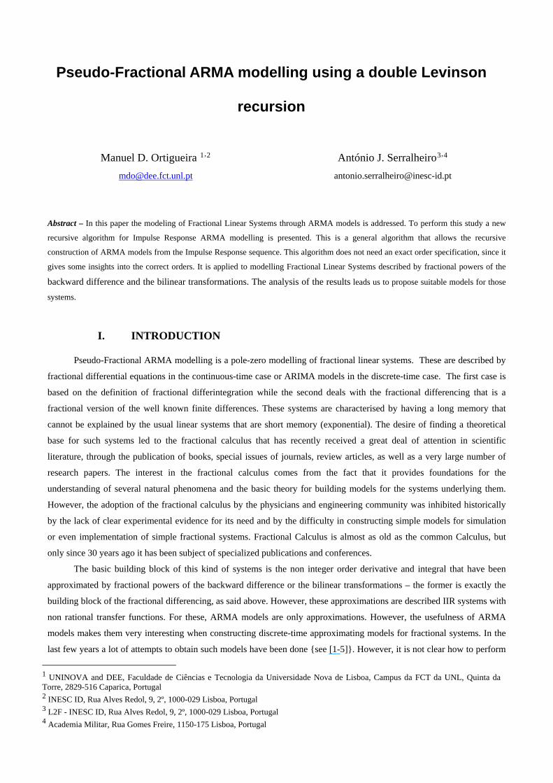
Pseudo-Fractional ARMA modelling using a double Levinson

recursion

Manuel D. Ortigueira 1,2 António J. Serralheiro3,4

mdo@dee.fct.unl.pt antonio.serralheiro@inesc-id.pt

1 UNINOVA and DEE, Faculdade de Ciências e Tecnologia da Universidade Nova de Lisboa, Campus da FCT da UNL, Quinta da Torre, 2829-516 Caparica, Portugal 2 INESC ID, Rua Alves Redol, 9, 2º, 1000-029 Lisboa, Portugal 3 L2F - INESC ID, Rua Alves Redol, 9, 2º, 1000-029 Lisboa, Portugal 4 Academia Militar, Rua Gomes Freire, 1150-175 Lisboa, Portugal

Abstract – In this paper the modeling of Fractional Linear Systems through ARMA models is addressed. To perform this study a new

recursive algorithm for Impulse Response ARMA modelling is presented. This is a general algorithm that allows the recursive

construction of ARMA models from the Impulse Response sequence. This algorithm does not need an exact order specification, since it

gives some insights into the correct orders. It is applied to modelling Fractional Linear Systems described by fractional powers of the

backward difference and the bilinear transformations. The analysis of the results leads us to propose suitable models for those

systems.

I. INTRODUCTION

Pseudo-Fractional ARMA modelling is a pole-zero modelling of fractional linear systems. These are described by

fractional differential equations in the continuous-time case or ARIMA models in the discrete-time case. The first case is

based on the definition of fractional differintegration while the second deals with the fractional differencing that is a

fractional version of the well known finite differences. These systems are characterised by having a long memory that

cannot be explained by the usual linear systems that are short memory (exponential). The desire of finding a theoretical

base for such systems led to the fractional calculus that has recently received a great deal of attention in scientific

literature, through the publication of books, special issues of journals, review articles, as well as a very large number of

research papers. The interest in the fractional calculus comes from the fact that it provides foundations for the

understanding of several natural phenomena and the basic theory for building models for the systems underlying them.

However, the adoption of the fractional calculus by the physicians and engineering community was inhibited historically

by the lack of clear experimental evidence for its need and by the difficulty in constructing simple models for simulation

or even implementation of simple fractional systems. Fractional Calculus is almost as old as the common Calculus, but

only since 30 years ago it has been subject of specialized publications and conferences.

The basic building block of this kind of systems is the non integer order derivative and integral that have been

approximated by fractional powers of the backward difference or the bilinear transformations – the former is exactly the

building block of the fractional differencing, as said above. However, these approximations are described IIR systems with

non rational transfer functions. For these, ARMA models are only approximations. However, the usefulness of ARMA

models makes them very interesting when constructing discrete-time approximating models for fractional systems. In the

last few years a lot of attempts to obtain such models have been done {see [1-5]}. However, it is not clear how to perform

such modelling neither how to choose the most suitable orders, although there are a lot of algorithms, mainly in the

stochastic case. In Impulse Response modelling the well known Padé algorithm is frequently used [6]. In this paper we

shall not be concerned with the estimation task involved in ARMA modelling; instead, we are going to look at the

underlying structure of the ARMA model in order to find alternative relations to obtain the ARMA parameters from the

Impulse Response. To be more specific, consider the usual theoretical approach for computing the ARMA(N,M)

parameters from the Impulse Response, hn:

∑i=0

N ai hj-i =

⎩⎨⎧bj j ≥ 0; …; M 0 j>M

(1)

where ai and bi are, respectively, the AR and MA parameters. A close look into equation (1) shows that, to compute the

ARMA(N,M) parameters, we only need the first N+M+1 values of the Impulse Response{h(n), n = 0, ... , N+M}. Here we

propose a new description of the double Levinson recursion presented in [7]. The algorithm consists of the recursive

solution of the system obtained from (1) with j = M to j = N+M for the AR coefficients followed by the use of the first

M+1 equations to obtain the MA parameters. This algorithm gives us the possibility of determining the orders of the

systems when looking at the pattern formed by a sequence of coefficients. We applied this algorithm in (pseudo) fractional

ARMA modelling and we observed that the pattern does not point clearly the orders, but give us some insights into

minimum orders.

The recursive algorithm is presented in section II, where we also present two examples of its application. In

section III we describe the results concerning fractional modelling. Last but not least, we will present some conclusions in

section IV.

II. THE ALGORITHM

The procedure we are going to describe is very similar to the one presented in [7] but, instead of using the matrix

formulation, we adopt a Schur-like description [8] since it is more direct and easier to implement. To begin with, we

consider (1) and introduce a function fN;M(j), j = 0, 1, … , given by:

fNM(j) = ∑

i=0

N a

NM(i) h

j+M-i (2)

where we enhance the orders N and M. According to (1) this function has gaps for j = 1, 2, … N. For N = 0, we thus have:

f0;M(j) = hj+M

j = 0, 1, … (3)

The algorithm described in [7] uses an adjoint system [9]. Here, we introduce an adjoint function defined by:

gNM(j) = ∑

i=0

N γ

NM(i) hN-j+M-i

(4)

with

g0;M(j) = h-j+M j = 0, 1, … (5)

As it is clear, gN;M(j) has gaps for j = 1, 2,…, N, too. The solution of (1) is recursively constructed for successive values

of N from N = 1 to N = N0, where N0 is a positive integer. To do this, assume that we have constructed the (N-1)th order

functions fN-1;M(j) and gN-1;M(j) j = 0, 1, … We will construct the Nth order functions by the recursions:

fN;M(j) = fN-1;M(j) + KN;M gN-1;M(N-j) (6) and gN;M(j) = gN-1;M(j) + HN;M fN-1;M(N-j) (7) where KN;M and HN;M are obtained by forcing both functions to have a gap at j = N. We obtain

KNM = -

fN-1M (N)

gN-1M (0)

(8)

HN;M = - gN-1M (N)

fN-1M (0)

(9)

As it is easy to verify, we have also:

gN;M(0)= fN-1;M(0)( )1 - KN;M.HN;M (10) If the system with Impulse Response hn is really an ARMA(N0,M0), we will have

bj = fN0;M0(j - M0) j=0, …, M0 (11)

For the AR coefficients we use (2), (4), (6), and (7) and the KN;M and HN;M sequences to obtain the so-called Double

Levinson recursion [7]:

aN;M(i) = aN-1;M(i) + KN;M γN-1;M(N-i) (12) and γN;M(i) = γN-1;M(i) + HN;M aN-1;M(N-i) (13) with i = 0, 1, …, N. KN;M and HN;M are Generalized Reflection Coefficients. To get some insights into the algorithm we

will describe an application to an ARMA(6,4) model. This has the Impulse Response represented in the upper half of

figure 1. In the lower part we present the function fN;M(j), j = 0, 1, … for N = M = 4. As it can be seen, we inserted 4

gaps, but there are still non zero values for j > 4, clearly meaning that we are using too low orders.

0 5 10 15 20 25 30 35 40 45 50 -4

-2

0

2

4

0 5 10 15 20 25 30 35 40 45 50 -2

-1

0

1

2

hn

fN,M(j)

j

n

Figure 1 - Impulse Response hn of a ARMA(6,4) system (top) and fN;M(j), j = 0, 1, … (bottom) of an

ARMA(4,4) model

In figure 2, we repeat the situation but now the constructed model is an ARMA(6,4). As it can be seen, now the gaps

collapsed the function for all the values above M. The nonzero values are the MA coefficients.

0 5 10 15 20 25 30 35 40 45 50-4

-2

0

2

4

0 5 10 15 20 25 30 35 40 45 50-1

-0.5

0

0.5

1

n

j

hn

fN,M(j)

Figure 2 - Impulse Response hn of an ARMA(6,4) system (top) and fN;M(j), j = 0, 1, … (bottom) of an

ARMA(6,4) model.

The Double Levinson recursion supplies us with a very important result, which will be useful in determining the orders of

the model. This result is stated in the following theorem (for proof, see [2]:)

Theorem

Let M ≥ 0 be an integer constant and AN;M(z) and ΓN;M+1(z) the Z Transforms of aN;M(i) and γN;M+1(i) . The Nth

degree polynomials AN;M(z) and ΓN;M+1(z) corresponding to M and M+1 zeros, respectively, are, up to a constant,

reverse polynomials:

ΓN;M+1(z)= φ.z-N; .AN;M(z-1) (14)

φ being the last coefficient of ΓN;M+1(z).

As consequence of this theorem we have:

HN;M+1.KN;M=1 (15) Its proof being immediate from the theorem. This result is very interesting since it allows us to compute the correct orders:

• it is enough to run the algorithm for N,M values ranging from 0 to N0, M0 higher than the expected orders.

• For the correct AR order and the correct plus one MA order the product is one.

To exemplify this assertions, we will consider the following two examples.

Example 1 – AR case: consider an AR(3) with coefficients a = [1 -1.0871 1.1961 -0.4512]. In table 1 we show the

HN;M.KN;M product pattern for N, M = 0, 1, 2, 3, 4 , where "hv" means a high value obtained when the determinant of the

underlying matrix is close to zero (small values of fN;M(0) after a product almost equal to one). This happens when the

orders are oversized. From the table we conclude easily that the system is indeed an AR(3). It is interesting to remark that

if we compute the poles and zero corresponding to an ARMA(4,1), the extra pole is cancelled by the zero (as it should be.)

N\M 1 2 3 4

1 -0.012 hv 0.0082 -2.5803

2 0.6571 hv 1.1446 1.0401

3 1 hv 1 1

4 Hv 6.6935 0.2955 -2.1107

Table 1 – HN;M.KN;M product pattern for the AR(3) case

Example 2 – ARMA case: we consider now an ARMA(3,2) system defined by the previous AR parameters (example 1)

and with b = [1 1.2 -1.6] as MA parameters. As before, table 2 showing the HN;M.KN;M product pattern for N,M = 0,

1, 2 , 3, 4, suggests the correct orders. It is important to refer that:

a) Although the system is not minimum phase, we obtain the correct MA parameters;

b) If the MA order is the correct one but the AR one is oversized, there is no problem since the extra coefficients are

zero.

The application of this algorithm to the pole/zero modelling of integer order continuous-time systems is also possible. To

do it we only have to substitute above the Impulse Response by the sequence hn = (-1)n

n! mn, n = 0, 1, … , where mn is the

sequence of the momenta of the Impulse Response of the continuous-time system given by: mn = ⌡⌠0

∞

h(t)tn dt .

N\M 1 2 3 4

1 -0.0592 62.5179 0.0652 -1.7805

2 0.1984 0.9592 0.8598 0.9575

3 0.0422 -0.9930 1 1

4 0.0165 0 hv 0.8159

Table 2 – HN;M.KN;M product pattern for the ARMA(3,2) case.

The importance of (14) lies on the bridge it establishes between two different MA order polynomials. As consequence of

this theorem we have, from (13) [10]:

AN-1;M(z) = AN;M-1(z) + μN;Mz-1; .AN-1;M-1(z) (16)

where μN;M is obtained by forcing the Nth order coefficient to be zero:

μN;M = - aN

M-1(N)

aN-1M-1(N-1)

(17)

The recursion (16) is very interesting since it allows us to compute the AR part of a given ARMA(N0,M0) from a sequence

of AR models with orders ranging from 1 to N0 + M0. Using (2) we obtain

fN-1;M(j)= fN;M-1(j+1) + μN;M fN-1;M-1(j) (18) that allows us to compute the MA parameters from fN;0(j), resulting from the Levinson recursion (12) with M = 0. In our

applications we preferred to compute the MA parameters from (1), though.

We applied the recursion (16) to the model used in example 1. Immediately at the first recursion (M = 1), all the

polynomial with degree greater than or equal to 4 reproduced the AR polynomial we were looking for. All the extra

coefficients were zero. The same happened with the second at M = 2. When we go beyond the correct MA order the

coefficient (17) becomes very high due to a division by a very small value (theoretically, zero).

III. APPLICATION TO PSEUDO-FRACTIONAL MODELLING

In this section, we assess the estimation of ARMA models for approximating discrete-time fractional models. We

considered the fractional difference

Hbd(z) = ( )1 – z-1 α, |z|>1 (19)

and the Tustin (bilinear)

Hbil(z)=⎝⎛

⎠⎞1 - z-1

1 + z-1α |z|>1 (20)

as approximations to the α order differintegrator. For each one, we applied the algorithms described above and tried to

find patterns that pointed us towards minima orders. We used only values of |α| < 1, because the other cases correspond to

join integer order poles and/or zeros to the ARMA model obtained with the fractional part of α.

The introduction of gaps in the function fN;M(j), j = 0, 1, … is presented in figure 3 for backward differences with order

α= -0.4. We present the results obtained with an ARMA(6,4) and ARMA(4,6). As it can be seen, the values of the function

above 4 are almost zero, meaning that, although the original system is not ARMA, it can be modelled with an ARMA. For

the bilinear case, the results are similar. With this in mind we are going to study the behaviour of product HN;M+1.KN;M

through the recursion progression.

0 5 10 15 20 25 30 35 40 45 50-3

-2

-1 0

1

2

0 5 10 15 20 25 30 35 40 45 500

0.2 0.4

0.6 0.8

1 hn

fN,M(j) n

j

Figure 3 - Impulse Response hn of a backward difference system (top) and fN;M(j), j = 0, 1, … (bottom)

of an ARMA(4,4) and an ARMA(6,4) models.

The product HN;M+1.KN;M pattern does not tell much but, and as in the previous tables, we find that the lower diagonal

values were smaller than those in the upper diagonal in both cases (19) and (20). This suggests that the MA order is more

important than the AR one. In the following tables, to better illustrate the behaviour of such patterns for the backwards

difference and bilinear, all the values less than 0.9 were represented by a “0”, whereas values between 0.9 and 1.1 were

represented by “1” and, finally, the values above 1.1 were represented by “2”.

N/M 1 2 3 4 5 6 7 8 9 10

1 0 2 2 2 1 1 1 1 1 1

2 0 0 2 2 2 2 2 1 1 1

3 0 0 0 2 2 2 2 2 2 2

4 0 0 0 0 2 2 2 2 2 2

5 0 0 0 0 0 2 2 2 2 2

6 0 0 0 0 0 0 2 2 2 2

7 0 0 0 0 0 0 0 2 2 2

8 0 0 0 0 0 0 0 0 2 2

9 0 0 0 0 0 0 0 0 0 2

10 0 0 0 0 0 0 0 0 0 0

Table 3 – HN;M.KN;M product pattern for the ARMA(10,10) corresponding to the backward difference

case.

N/M 1 2 3 4 5 6 7 8 9 10

1 0 2 0 2 0 2 0 2 0 2

2 0 0 2 0 2 0 2 0 2 1

3 0 0 0 2 0 2 0 2 0 2

4 0 0 0 0 2 0 2 0 2 0

5 0 0 0 0 0 2 0 2 0 2

6 0 0 0 0 0 0 2 0 2 0

7 0 0 0 0 0 0 0 2 0 2

8 0 0 0 0 0 0 0 0 2 0

9 0 0 0 0 0 0 0 0 0 2

10 0 0 0 0 0 0 0 0 0 0

Table 4 – HN;M.KN;M product pattern for the ARMA(10,10) corresponding to the bilinear case

To try to find other insights into the orders, we ran the recursive algorithm, allowing us to conclude that:

a) Small values of the coefficient μN;M in (17) point to correct N and M orders;

b) Very high values of μN;M mean that, at least the MA order is higher than the correct. In this situation we

must decrease it. This situation corresponds to unstable model;

c) The observation of the μN;M pattern suggests an ARMA(N,N) model;

d) In the difference case, the poles and zeros of the ARMA(N,N) model are always positive and interlaced;

e) In the bilinear case, the poles and zeros of the ARMA(N,N) model are symmetric;

f) Our simulations pointed out to values of N from 7 to 10. For most situations the approximation is good

in both time and frequency domains.

g) Smaller values of α results in better amplitude frequency response approximations to the exact model,

the largest amplitude deviations occurring in the low-frequency regions for the difference case. For the

cases where |α| > 0.5, leading to a worst amplitude response modelling, one can always model them as a

combination of two models, thus forcing the “new” fractional to be of order (1 - α). The additional

integer term corresponds to either an integrator or a differenciator that results in an extra (1 - z-1) -1 or

(1 - z-1) factor, respectively.

Iter.

Iter.

Iter.

Iter. Iter. Iter.

μ μ μ

μ μ μ

Figure 4 – the behaviour of the μN;M as a tool for orders choice, for the differentiator (above) and

integrator (below), with α = 0.1 (left), α =0 .5 (middle) and α = 0.9 (right).”Iter” means model iteration.

Phase (radians)

Magnitude (dB)

Frequency

Frequency

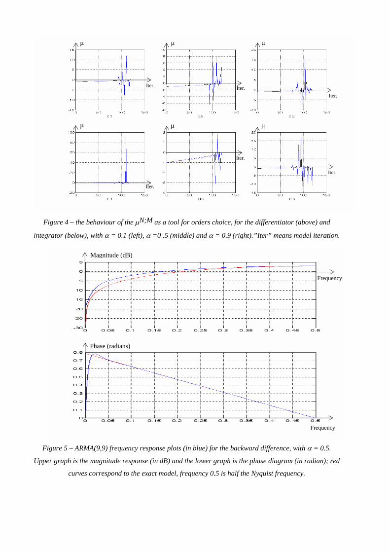
Figure 5 – ARMA(9,9) frequency response plots (in blue) for the backward difference, with α = 0.5.

Upper graph is the magnitude response (in dB) and the lower graph is the phase diagram (in radian); red

curves correspond to the exact model, frequency 0.5 is half the Nyquist frequency.

Frequency

Frequency

Phase (radians)

Magnitude (dB)

Figure 6 – ARMA(9,9) frequency response plots (in blue) for bilinear, with α = 0.5. Upper graph is the

magnitude response (in dB) and the lower graph is the phase diagram (in radian); red curves correspond

to the exact model, frequency 0.5 is half the Nyquist frequency.

We made also a study of the pole-zero distribution (figures 7 and 8) and found that:

a) In the backward difference case (models N,N) the poles and zeros are positive real. With higher orders complex

poles and zeros may appear (above N = M= 9);

b) In the bilinear case, the poles and zeros are real. We did not find complex poles or zeros, unless N = M > 16;

c) In the bilinear case, and for some α, we obtained unstable models for some N, M < N;

d) If the pole order is the same of the zero order, the poles and zeros are interlaced. In the bilinear case, they are

symmetric to each other;

e) If the orders are not equal, the “extra” poles or zeros tend to appear near zero.

0.2

0.4

0.6

0.8

1

30

210

60

240

90

270

120

300

150

330

180 0

Figure 7 – ARMA(N,M) polar pole-zero plots for the backward differences with α = 0.8 for N, M = 10.

0.2

0.4

0.6

0.8

1

30

210

60

240

90

270

120

300

150

330

180 0

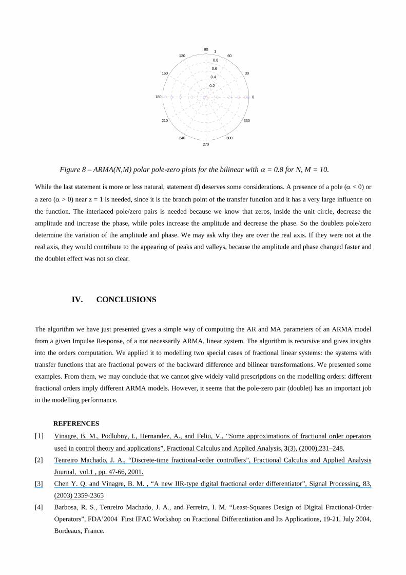
Figure 8 – ARMA(N,M) polar pole-zero plots for the bilinear with α = 0.8 for N, M = 10.

While the last statement is more or less natural, statement d) deserves some considerations. A presence of a pole (α < 0) or

a zero (α > 0) near z = 1 is needed, since it is the branch point of the transfer function and it has a very large influence on

the function. The interlaced pole/zero pairs is needed because we know that zeros, inside the unit circle, decrease the

amplitude and increase the phase, while poles increase the amplitude and decrease the phase. So the doublets pole/zero

determine the variation of the amplitude and phase. We may ask why they are over the real axis. If they were not at the

real axis, they would contribute to the appearing of peaks and valleys, because the amplitude and phase changed faster and

the doublet effect was not so clear.

IV. CONCLUSIONS

The algorithm we have just presented gives a simple way of computing the AR and MA parameters of an ARMA model

from a given Impulse Response, of a not necessarily ARMA, linear system. The algorithm is recursive and gives insights

into the orders computation. We applied it to modelling two special cases of fractional linear systems: the systems with

transfer functions that are fractional powers of the backward difference and bilinear transformations. We presented some

examples. From them, we may conclude that we cannot give widely valid prescriptions on the modelling orders: different

fractional orders imply different ARMA models. However, it seems that the pole-zero pair (doublet) has an important job

in the modelling performance.

REFERENCES

[1] Vinagre, B. M., Podlubny, I., Hernandez, A., and Feliu, V., “Some approximations of fractional order operators

used in control theory and applications”, Fractional Calculus and Applied Analysis, 3(3), (2000),231–248.

[2] Tenreiro Machado, J. A., “Discrete-time fractional-order controllers”, Fractional Calculus and Applied Analysis

Journal, vol.1 , pp. 47-66, 2001.

[3] Chen Y. Q. and Vinagre, B. M. , “A new IIR-type digital fractional order differentiator”, Signal Processing, 83,

(2003) 2359-2365

[4] Barbosa, R. S., Tenreiro Machado, J. A., and Ferreira, I. M. “Least-Squares Design of Digital Fractional-Order

Operators”, FDA’2004 First IFAC Workshop on Fractional Differentiation and Its Applications, 19-21, July 2004,

Bordeaux, France.

[5] Ostalczyk, P., “Fundamental properties of the fractional-order discrete-time integrator”, Signal Processing, 83,

(2003) 2367-2376

[6] Kumar, K. “On the Identification of Autoregressive Moving Average Models”, Journal of Control and Intelligent

Systems, Vol. 28, No2, pp 41-46, 2000.

[7] Ortigueira, M. D. and Tribolet, J. M. "On the Double Levinson Recursion Formulation of ARMA Spectral

Estimation," Proc. of IEEE ICASSP, 1983.

[8] Robinson, E. A. and Treitel, S. " Maximum Entropy and the Relationship of the Partial Autocorrelation to the

Reflection Coefficients of a Layered System, " IEEE Trans. on ASSP, Vol. 28, No. 2, April 1980.

[9] Carayannis, G., Kaloupsidis, N. and Manolakis, D. G. "Fast Algorithms for a Class of Linear Equations," IEEE

Trans. on ASSP, Vol.30, No.2, pp. 227-239, 1982.

[10] Ortigueira,M.D. "ARMA Realization from the Reflection Coefficient Sequence", Signal Processing, vol. 32 No. 3,

June 1993.

[11] Baillie R. T. and M. L. King Fractional Differencing and Long Memory Processes, Journal of Econometrics,

Volume 73, Issue 1, Pages 1-324 (July 1996)