IEEJ TRANSACTIONS ON ELECTRICAL AND ELECTRONIC ENGINEERINGIEEJ Trans 2015Published online in Wiley Online Library (wileyonlinelibrary.com). DOI:10.1002/tee.22087

Paper

Pseudo Bond Graph Model of Thermal Transfers Sustained by Ice Quantityof a Domestic Refrigerator for Energy Saving Application

Emna Aridhi∗a Non-member

Mehdi Abbes∗∗ Non-member

Saad Maarouf∗∗∗ Non-member

Radhi Mhiri∗∗∗ Non-memberAbdelkader Mami∗ Non-member

This paper presents a study on the use of ice to improve the energy efficiency of a domestic refrigerator by applying a pseudobond graph model that describes the thermal transfers sustained by a quantity of ice introduced inside the cavity of refrigeration.The use of ice resulted in a global energy saving of 4.68%. The effect of ice was found to be more significant during thetransitional regime. It reduced the response time to reach the stable average temperature from 15 h to only 3.5 h compared towhen not using ice. This achievement did not cost additional electrical power, but rather allowed a saving of electrical energyof 76.73%. However, during the steady state, a reduction in the energy efficiency was noted. An improvement in the coolingby keeping the temperature inside the refrigerator more homogeneous is also proved. The model has two inputs: the outsidetemperature, and the modulated temperature of the evaporator. This latter determines the functioning of the compressor cycle.The model describes the thermal transfers by natural convection inside the refrigerator. Two experiments were carried out tomake a performance comparison and to prove the influence of ice in cooling and energy saving. We used real measurements tomodulate the evaporator temperature source in the pseudo bond graph model. The simulation results show the effectiveness ofthe proposed approach. © 2015 Institute of Electrical Engineers of Japan. Published by John Wiley & Sons, Inc.

Keywords: bond graph, thermal transfers, refrigerator, ice, energy consumption, energy saving

Received 18 April 2014; Revised 14 August 2014

1. Introduction

Nowadays, energy consumption and pollution pose big problemsthat scientists attempt to reduce by using renewable resourcessuch as solar, biomass, hydro, wind, and geothermal power. Infact, these resources are abundant and sustainable and improvepublic health and environmental quality. Importantly, ice presents asignificant renewable energy source, mostly in cooling. Therefore,many countries that have a very cold climate in winter can exploitthis free ‘cold’ to chill aliments or other products through coolingsystems like refrigerators or cold rooms, which are sources ofsignificant electricity consumption, especially big appliances, andhugely used around the world. Hence, a system should be designedin order to interconnect the internal refrigerators’ cavities and theoutside atmosphere. This system will allow circulating the freecold air outside in the walls of the appliance to the extent ofdecreasing the temperature of the ambient surroundings and thenthe refrigeration compartment. From this point of view, the mainobjective of the current investigation is to make a feasibility studyof using ice as a significant and promising solution to minimizethe electrical energy consumed by domestic refrigerators. Thepaper shows that the introduction of a quantity of ice into adomestic fridge can reduce the energy consumption and improvethe cooling quality. For this reason, it is interesting to model

a Correspondence to: Emna Aridhi. E-mail: aridhi_emna@yahoo.fr

* Department of Physics, Faculty of Sciences of Tunis, Tunis El Manar,Tunisia

** Department of Automatics, National School of Engineering of Tunis,Tunis El Manar, Tunisia

*** Ecole de technologie superieure, Montreal, Quebec, Canada

the thermal transfers inside these appliances and to show thebehavior of the internal air temperature under the influence ofthe ice placed inside. This ice quantity can later be replaced bythe free cold airflow coming from the outside through the systemmentioned above.

Several studies have investigated thermal transfers inside staticrefrigerators and those with a fan, empty or full of products [1–5].They have shown that the thermal transfers are essentially relatedto natural convection between the internal walls and air. Math-ematical and CFD (computational fluid dynamics) models havebeen developed to compute the temperature and inner air veloc-ity [6]. These models describe the thermal transfer between theevaporator wall (cold wall) and the other walls (hot walls), aswell as between the internal air and the insulation walls inside andoutside. Other works have studied the air velocity in the refrig-erator [7] and the thermal transfers between the inner air and theload placed inside [4,5].

To the best of our knowledge, the introduction of the ice inrefrigerators has not been studied yet. Researchers have mainlyfocused on improving the thermal transfers inside in order toensure good cooling and allowing better preservation of food.They consider that the temperature is not homogenous and thatit depends on the frequency of the door opening and closure,the filled volume, the temperature and the humidity of the roomair, the thermostat regulation, the ON/OFF compressor cycles,and the refrigerator dimensions. This improvement is reachedby adding a fan, which homogenizes the temperature inside therefrigerator [1]. Nonetheless, the use of a fan costs additionalenergy consumption [8]. Hence, it is interesting to find otherways of cooling based on the use of renewable energy such asice and solar energy. For instance, solar absorption refrigerators

© 2015 Institute of Electrical Engineers of Japan. Published by John Wiley & Sons, Inc.

E. ARIDHI ET AL.

Table I. External dimensions of the refrigerator and the loads inside

Ice container wall Evaporator wall Refrigeration cavity Water container Hot walls

Length = 0.377 m Length = 0.614 m Length = 0.477 m Length = 0.22 m Length = 0.814 mWidth = 0.2 m Width = 0.477 m Width = 0.438 m Width = 0.2 m Width = 0.438 mHeight = 0.16 m Thickness = 0.002 m Height = 0.814 m Height = 0.21 m Thickness = 0.02 mThickness = 0.003 m Thickness = 0.002 m

consume less electricity than static refrigerators [9]. Furthermore,novel household refrigerators with shape-stabilized PCM (phasechange material) heat storage condensers also allow energy savingof ∼12% [10].

Thermal transfers by natural convection inside domestic refrig-erators have a complex dynamic behavior and nonlinearaspect [11]. Therefore, we use the bond graph approach to illus-trate them by applying the thermal equations existing in theliterature of heat storage and thermal transfers at the level ofvertical, parallel, and oblique walls [12,13]. It is an easy andsimple graphical method for the modeling of physical processesand multidisciplinary dynamic engineering systems by a directedgraph consisting of idealized associated elements based on theprinciple of power conservation [14–16]. It is a unified repre-sentation language that allows showing up explicitly the powerflows. It makes possible the energetic study, the coupling betweenvariables of different physical domains clearer, and the build-ing of models for multi-disciplinary systems simpler. Therefore,bond graph models provide very useful insights into the struc-tures of dynamic systems [17]. Moreover, this approach leadsto a systematic construction of mathematical models. Thus, itwill be possible to apply control processes in order to min-imize the energy consumption and to control the internal airtemperature.

In this paper, we present a pseudo bond graph model ofthermal transfers by conduction and convection inside a loadedrefrigeration cavity, at the cold and hot walls’ level, between theice quantity, the internal air, and the water container. Hence, itillustrates thermal losses at walls’ level and heat storage inside therefrigerator, ice container, and water container.

The rest of the paper is structured as follows: in Section 2,we present the refrigerator used in the experiments, specify theexternal dimensions, and explain the thermal phenomena insidethe refrigeration compartment. Section 3 describes the bond graphapproach. Section 4 enlightens the experimental environment.

Section 5 illustrates the simulation and comparison results. Thelast section is devoted to conclusions.

2. The Refrigerator

2.1. Presentation A domestic static refrigerator (withoutventilation) was used in this work. It consists of a bottom-mountedfreezer and a refrigeration compartment above it, which is whatwe are interested in. Its volume is 170 l and has a hermeticcompressor.

The external dimensions of the refrigeration cavity (cold andhot walls) as well as those of the containers of ice and water aregiven in Table I.

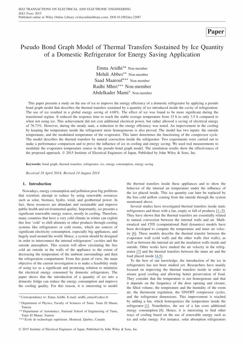
2.2. Thermal phenomena The thermal phenomena tak-ing place inside the refrigeration compartment are sketched inFig. 1.

• The transfer by natural convection inside the refrigerator. Thecold air near the evaporator flows downward and the hot air,near the door and the other side walls, flows upwards.

• The heat storage inside the water and the internal air.• Thermal losses by convection between the internal air and the

outside through hot walls.• Heat transfer by convection and conduction between the ice

quantity and the internal air through the ice container walls.The natural convection, inside the refrigeration compartment, isinfluenced by the heat flow of ice.

• A thermal exchange existing between the water container anda flow of cooling that comes from the ice. These flows happenin the entire domain by convection: the particles of wet airpropagate and strike the water container walls. Thus, a transferby conduction by direct contact takes place.

• Thermal losses by conduction at the water container walls andthe evaporator wall level.

The propagationdirection of the aircoming from theevaporator

Refrigerationcompartment

Glass shelves

Water container

Heat transfer inside therefrigerator and the water

Heat transfer byconvection

Heat transfer byconduction andconvection at theice container walllevel

Hot wallEvaporator wall

Ice

The propagationdirection of thehot air

Freezer

Fig. 1. The thermal transfers inside the refrigeration compartment

2 IEEJ Trans (2015)

PSEUDO BOND GRAPH MODEL OF THERMAL TRANSFERS INSIDE A REFRIGERATOR

Ice

storageC element

.

The temperaturesource at the

evaporator walllevel

The evaporator wall

ConductionR Element

The hot walls

Convection and storage

The outsidetemperature

R Element C Element

Internal air

storageC element

The water container

storageC element

The ice container wall

Convection and conductionR element

Tice Qice

.Trefrigerator Qice

.Tout Qout

.Trefrigerator Hrefrigerator

.Trefrigerator Qrefrigerator

.Trefrigerator Qevapo

.Tevapo Qevapo

.Twater Hrefrigerator

The water container wall

Convection and conductionR element

Fig. 2. The word bond graph model

3. The Pseudo Bond Graph Approach

3.1. Model presentation and assumptions The pseudobond graph model describes the thermal transfers by conduc-tion and convection inside the refrigeration cavity and the water,thermal losses at the wall level, and the heat storage. They arerespectively modeled by R and C elements.

The following assumptions are made for the pseudo bond graphmodel:

• The model does not present the transfers inside the evaporatorbut only at its wall level.

• The internal air flow and the ice flow are assumed to beincompressible and laminar because the air velocity inside thefridge is about 0.04 m.s−1 [6].

• The transfers by radiation are neglected. Indeed, the appli-ance is placed in a dark room and is not exposed tothe light. The refrigerator door is kept closed during theexperiments. Therefore, the lamp in the refrigeration cavityis off.

• All the physical properties of the air and the plastic of thecontainers’ walls are supposed constants.

• We take the same initial temperatures and the mass of waterand ice used in the experiments.

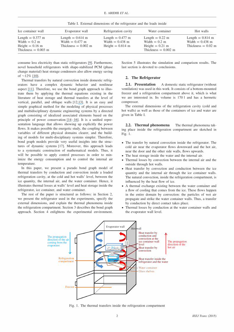
3.2. Word bond graph model The word bond graphmodel is presented in Fig. 2. It shows the system components,thermal sources and variables, and the energy propagation direc-tion.

The evaporator is modulated as an effort source of tem-perature (MSe), and the ice quantity is modeled by a Celement.

The model describes the thermal losses by conduction at theevaporator wall level and by conduction and convection at theice container wall level. It illustrates the heat storage inside the

refrigerator and the water. Moreover, it presents the thermal lossesby conduction and convection at the water container wall level.It also illustrates the thermal losses by convection and the heatstorage at the hot walls’ level under the influence of the outsidetemperature Tout.

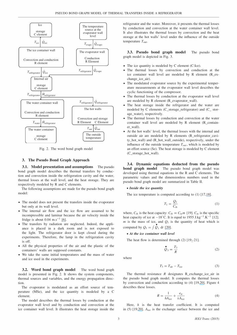
3.3. Pseudo bond graph model The pseudo bondgraph model is depicted in Fig. 3.

• The ice quantity is modeled by C element (C:Ice).• The thermal losses by convection and conduction at the

ice container wall level are modeled by R element (R_ex-change_ice_air).

• The modulated evaporator source by the experimental temper-ature measurements at the evaporator wall level describes thecyclic functioning of the compressor.

• The thermal losses by conduction at the evaporator wall levelare modeled by R element (R_evaporator_wall).

• The heat storage inside the refrigerator and the water aremodeled by C elements (C_storage_refrigerator) and (C_ stor-age_water), respectively.

• The thermal losses by conduction and convection at the watercontainer wall level are modeled by R element (R_contain-er_wall).

• At the hot walls’ level, the thermal losses with the internal andoutside air are modeled by R elements (R_refrigerator_cavi-ty_hot_wall) and (R_hot_wall_outside), respectively, under theinfluence of the outside temperature Tout , which is modeled byan effort source (Se). The heat storage is modeled by C element(C_storage_hot_wall).

3.4. Dynamic equations deducted from the pseudobond graph model The pseudo bond graph model wasdeveloped using thermal equations in the R and C elements. Theparametric values and the dimensionless numbers used in thepseudo bond graph model are summarized in Table II.

• Inside the ice quantity

The ice temperature is computed according to (1) [17,18].

T1 = Q1

Cth(1)

where, Cth is the heat capacity: Cth = Cm m [19]. Cm is the specificheat capacity of ice at −18◦C. It is equal to 1955 J.kg−1.K−1 [12].m is the mass of ice, and Q1 is the quantity of heat which is

computed by Q1 = ∫ •Q1 dt [20].

• At the ice container wall level

The heat flow is determined through (2) [19–21].

•Q3 = T3

R(2)

where

T3 = Tair − Tice (3)

The thermal resistance R designates R_exchange_ice_air inthe pseudo bond graph model. It computes the thermal lossesby convection and conduction according to (4) [19,20]. Figure 4describes these losses.

R = 1

hAice+ eic

λAice(4)

Here, h is the heat transfer coefficient. It is computedin (5) [19,20]. Aice is the exchange surface between the ice and

3 IEEJ Trans (2015)

E. ARIDHI ET AL.

C: ice

1

2

4

6 1315

1 0 1 0

14

12

10

111 R: R_evaporator_wall

R: R_refrigerator_cavity_hot_wall

R: R_hot_wall_outsideC: C_storage_hot_wall

16 18

17 19 20

8

3

R_exchange_ice_air

C_storage_refrigerator

R_container_wall

C_storage_water

0

1

0

0

1

R

C

C

R

5

7

9

Mse: Tevap

Se: Tout

Fig. 3. Pseudo bond graph model of thermal transfers inside the refrigerator

Table II. Parameter values of the refrigerator model

At the ice containerwall level

At the evaporatorwall level

Inside therefrigerator

Inside thewater

At the watercontainer wall

level At the other walls’ level

λ = 0.027 W.m−1.K−1 λ = 0.03 W.m−1.K−1 Cv = 1004 J.kg−1.K−1 Cvw = 4203J.kg−1.K−1

λ = 0.03 W.m−1.K−1 λ = 0.03 W.m−1.K−1

ρair = 1.275 kg.m−3 Pr = 0.7179 C = 3200 J.kg−1.K−1

ρair = 1.188 kg.m−3

ν = 135.5 × 10−7 m2.s−1 at 0◦C ν = 153.5 × 10−7 m2.s−1at 20◦Ca = 188.3 × 10−7 m2.s−1 at 0◦C a = 214.7 × 10−7 m2.s−1 at 20◦Cβ = 3.674 × 10−3 K−1 at 0◦C β = 3.421 × 10−3 K−1 at 20◦C

g = 9.81 m.s−2 g = 9.81 m.s−2

Pr = 0.7179

Internal air

eic

Ice

Conduction Convection

Placstic wallThermal resistances

R_exchange_ice_air

Fig. 4. Thermal losses at the ice container wall level

the internal air, eic is the ice container wall thickness, and λ is itsthermal conductivity.

h = Nuloc.λ

L(5)

where Nu loc is the local Nusselt number, λ is the thermalconductivity of the plastic container wall, and L is its length.

In the current investigation, the average Nusselt number Nu isexpressed at the ice container wall level following the correla-tion [22] given by

Nu = 0.67Ra14[

1 + ( 0.437Pr

) 916

] 49

(6)

It is worth noting that, in the current investigation, the averageNusselt number Nu results from the integration of Nu loc definedin (5).

Ra is the Rayleigh number in the case of natural convection. Itis computed in (7) [13], and Pr is the Prandt number of air at 0◦C.

Ra = gβL3T3

av(7)

• At the evaporator wall level

The heat flow is computed following (8) [19–21].

•Q11 = T11

R(8)

with

T11 = Tair − Tevap (9)

The thermal resistance R expresses R_evaporator_wall, and it isdetermined in (10) [8].

R = 1

hAevap(10)

where h is the heat transfer coefficient and Aevp is the evaporatorwall surface. h is calculated in (5), with L = Levap, and Nu isdetermined in (6) in the case of a vertical plate, at the levelof which there is a constant surface flow [22]. Pr is the Prandtnumber of air at 0◦C , and Ra is computed in (7), with L = Levap.

• Inside the refrigeration cavity

The temperature inside the refrigerator is computed accordingto (11) [18,19].

T5 = H5

mairCv(11)

where Cv is the specific heat capacity of air at 0◦C [12]; H5 is

the enthalpy of air and it is computed by H5 = ∫ •H 5 dt [20]. mair

is the mass of internal air. It is determined in (12) [19,21].

mair = volair.ρair (12)

4 IEEJ Trans (2015)

PSEUDO BOND GRAPH MODEL OF THERMAL TRANSFERS INSIDE A REFRIGERATOR

The inner air flowSurface Surface

ehw

Insulation layer

The hot wall

The outsideflow

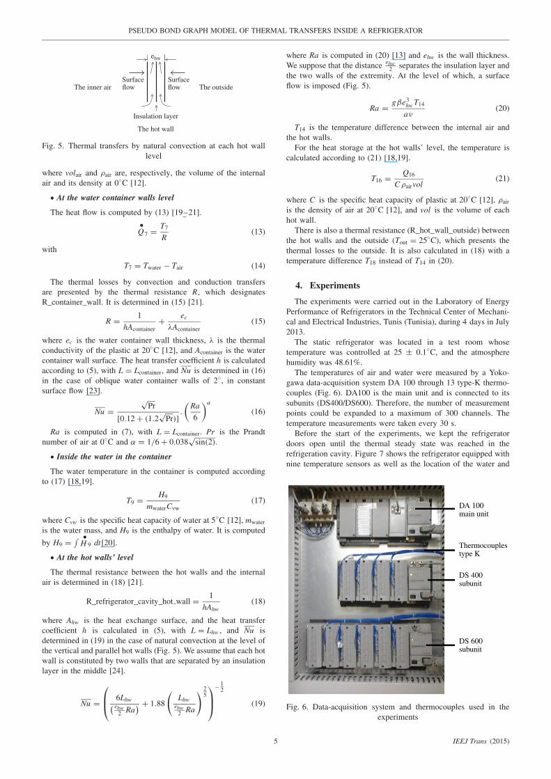
Fig. 5. Thermal transfers by natural convection at each hot walllevel

where volair and ρair are, respectively, the volume of the internalair and its density at 0◦C [12].

• At the water container walls level

The heat flow is computed by (13) [19–21].

•Q7 = T7

R(13)

with

T7 = Twater − Tair (14)

The thermal losses by convection and conduction transfersare presented by the thermal resistance R, which designatesR_container_wall. It is determined in (15) [21].

R = 1

hAcontainer+ ec

λAcontainer(15)

where ec is the water container wall thickness, λ is the thermalconductivity of the plastic at 20◦C [12], and Acontainer is the watercontainer wall surface. The heat transfer coefficient h is calculatedaccording to (5), with L = Lcontainer, and Nu is determined in (16)in the case of oblique water container walls of 2◦, in constantsurface flow [23].

Nu =√

Pr

[0.12 + (1.2√

Pr)].

(Ra

6

)α

(16)

Ra is computed in (7), with L = Lcontainer. Pr is the Prandtnumber of air at 0◦C and α = 1/6 + 0.038

√sin(2).

• Inside the water in the container

The water temperature in the container is computed accordingto (17) [18,19].

T9 = H9

mwaterCvw(17)

where Cvw is the specific heat capacity of water at 5◦C [12], mwater

is the water mass, and H9 is the enthalpy of water. It is computed

by H9 = ∫ •H 9 dt[20].

• At the hot walls’ level

The thermal resistance between the hot walls and the internalair is determined in (18) [21].

R_refrigerator_cavity_hot wall = 1

hAhw(18)

where Ahw is the heat exchange surface, and the heat transfercoefficient h is calculated in (5), with L = Lhw , and Nu isdetermined in (19) in the case of natural convection at the level ofthe vertical and parallel hot walls (Fig. 5). We assume that each hotwall is constituted by two walls that are separated by an insulationlayer in the middle [24].

Nu =

⎛⎜⎝ 6Lhw( ehw

2 Ra) + 1.88

(Lhw

ehw2 Ra

) 25

⎞⎟⎠

− 12

(19)

where Ra is computed in (20) [13] and ehw is the wall thickness.We suppose that the distance ehw

2 separates the insulation layer andthe two walls of the extremity. At the level of which, a surfaceflow is imposed (Fig. 5).

Ra = gβe3hw T14

aν(20)

T14 is the temperature difference between the internal air andthe hot walls.

For the heat storage at the hot walls’ level, the temperature iscalculated according to (21) [18,19].

T16 = Q16

C ρairvol(21)

where C is the specific heat capacity of plastic at 20◦C [12], ρair

is the density of air at 20◦C [12], and vol is the volume of eachhot wall.

There is also a thermal resistance (R_hot_wall_outside) betweenthe hot walls and the outside (Tout = 25◦C), which presents thethermal losses to the outside. It is also calculated in (18) with atemperature difference T18 instead of T14 in (20).

4. Experiments

The experiments were carried out in the Laboratory of EnergyPerformance of Refrigerators in the Technical Center of Mechani-cal and Electrical Industries, Tunis (Tunisia), during 4 days in July2013.

The static refrigerator was located in a test room whosetemperature was controlled at 25 ± 0.1◦C, and the atmospherehumidity was 48.61%.

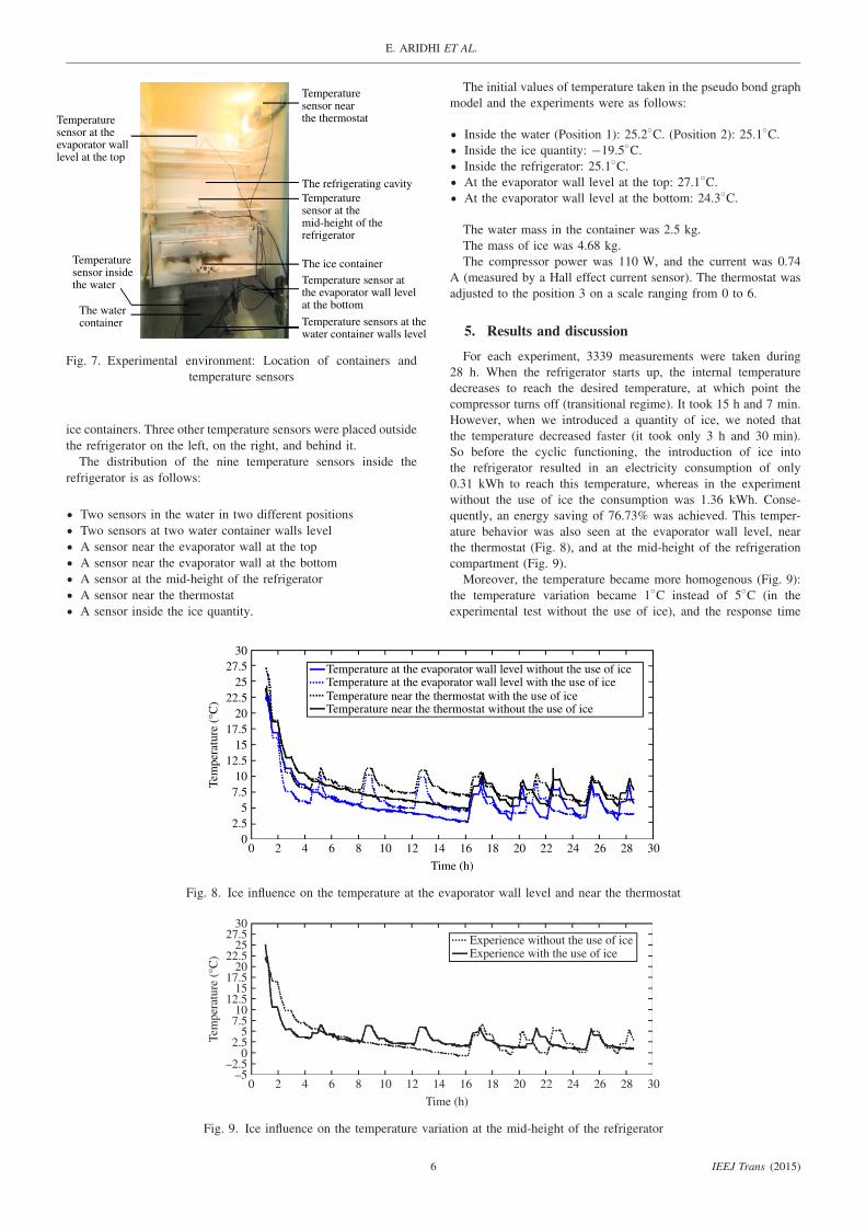
The temperatures of air and water were measured by a Yoko-gawa data-acquisition system DA 100 through 13 type-K thermo-couples (Fig. 6). DA100 is the main unit and is connected to itssubunits (DS400/DS600). Therefore, the number of measurementpoints could be expanded to a maximum of 300 channels. Thetemperature measurements were taken every 30 s.

Before the start of the experiments, we kept the refrigeratordoors open until the thermal steady state was reached in therefrigeration cavity. Figure 7 shows the refrigerator equipped withnine temperature sensors as well as the location of the water and

DA 100main unit

DS 400subunit

DS 600subunit

Thermocouplestype K

Fig. 6. Data-acquisition system and thermocouples used in theexperiments

5 IEEJ Trans (2015)

E. ARIDHI ET AL.

Temperaturesensor at theevaporator walllevel at the top

Temperaturesensor nearthe thermostat

The ice container

The refrigerating cavity

Temperature sensor at themid-height of the refrigerator

Temperature sensor atthe evaporator wall levelat the bottom

Temperature sensors at thewater container walls level

Temperaturesensor insidethe water

The watercontainer

Fig. 7. Experimental environment: Location of containers andtemperature sensors

ice containers. Three other temperature sensors were placed outsidethe refrigerator on the left, on the right, and behind it.

The distribution of the nine temperature sensors inside therefrigerator is as follows:

• Two sensors in the water in two different positions• Two sensors at two water container walls level• A sensor near the evaporator wall at the top• A sensor near the evaporator wall at the bottom• A sensor at the mid-height of the refrigerator• A sensor near the thermostat• A sensor inside the ice quantity.

The initial values of temperature taken in the pseudo bond graphmodel and the experiments were as follows:

• Inside the water (Position 1): 25.2◦C. (Position 2): 25.1◦C.• Inside the ice quantity: −19.5◦C.• Inside the refrigerator: 25.1◦C.• At the evaporator wall level at the top: 27.1◦C.• At the evaporator wall level at the bottom: 24.3◦C.

The water mass in the container was 2.5 kg.The mass of ice was 4.68 kg.The compressor power was 110 W, and the current was 0.74

A (measured by a Hall effect current sensor). The thermostat wasadjusted to the position 3 on a scale ranging from 0 to 6.

5. Results and discussion

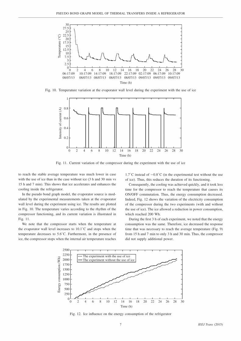
For each experiment, 3339 measurements were taken during28 h. When the refrigerator starts up, the internal temperaturedecreases to reach the desired temperature, at which point thecompressor turns off (transitional regime). It took 15 h and 7 min.However, when we introduced a quantity of ice, we noted thatthe temperature decreased faster (it took only 3 h and 30 min).So before the cyclic functioning, the introduction of ice intothe refrigerator resulted in an electricity consumption of only0.31 kWh to reach this temperature, whereas in the experimentwithout the use of ice the consumption was 1.36 kWh. Conse-quently, an energy saving of 76.73% was achieved. This temper-ature behavior was also seen at the evaporator wall level, nearthe thermostat (Fig. 8), and at the mid-height of the refrigerationcompartment (Fig. 9).

Moreover, the temperature became more homogenous (Fig. 9):the temperature variation became 1◦C instead of 5◦C (in theexperimental test without the use of ice), and the response time

30

27.5

25

22.5

20

17.5

Tem

per

atu

re (

°C)

15

12.5

10

7.5

5

2.5

00 2 4 6 8 10 12 14

Temperature at the evaporator wall level without the use of iceTemperature at the evaporator wall level with the use of iceTemperature near the thermostat with the use of iceTemperature near the thermostat without the use of ice

Time (h)

16 18 20 22 24 26 28 30

Fig. 8. Ice influence on the temperature at the evaporator wall level and near the thermostat

3027.5

2522.5

2017.5

Tem

per

atu

re (

°C)

1512.5

107.5

52.5

0–2.5

–5

Experience without the use of iceExperience with the use of ice

0 2 4 6 8 10 12 14

Time (h)

16 18 20 22 24 26 28 30

Fig. 9. Ice influence on the temperature variation at the mid-height of the refrigerator

6 IEEJ Trans (2015)

PSEUDO BOND GRAPH MODEL OF THERMAL TRANSFERS INSIDE A REFRIGERATOR

3027.5

2522.5

2017.5

Tem

per

atu

re (

°C)

1512.5

107.5

52.5

00 2 4 6 8 10 12 14

Time (h)

06:17:09

08/07/13

10:17:09

08/07/13

14:17:09

08/07/13

18:17:09

08/07/13

22:17:09

08/07/13

02:17:09

09/07/13

06:17:09

09/07/13

10:17:09

09/07/13

16 18 20 22 24 26 28 30

Fig. 10. Temperature variation at the evaporator wall level during the experiment with the use of ice

0 2 4 6 8 10 12 14

Time (h)

Inte

nsi

ty o

f cu

rren

t (A

)

16 18 20 22 24 26 28 30

1

0.8

0.6

0.4

0.2

0

Fig. 11. Current variation of the compressor during the experiment with the use of ice

to reach the stable average temperature was much lower in casewith the use of ice than in the case without ice (3 h and 30 min vs15 h and 7 min). This shows that ice accelerates and enhances thecooling inside the refrigerator.

In the pseudo bond graph model, the evaporator source is mod-ulated by the experimental measurements taken at the evaporatorwall level during the experiment using ice. The results are plottedin Fig. 10. The temperature varies according to the rhythm of thecompressor functioning, and its current variation is illustrated inFig. 11.

We note that the compressor starts when the temperature atthe evaporator wall level increases to 10.1◦C and stops when thetemperature decreases to 5.6◦C. Furthermore, in the presence ofice, the compressor stops when the internal air temperature reaches

1.7◦C instead of −0.8◦C (in the experimental test without the useof ice). Thus, this reduces the duration of its functioning.

Consequently, the cooling was achieved quickly, and it took lesstime for the compressor to reach the temperature that causes itsON/OFF commutation. Thus, the energy consumption decreased.Indeed, Fig. 12 shows the variation of the electricity consumptionof the compressor during the two experiments (with and withoutthe use of ice). The ice allowed a reduction in power consumption,which reached 200 Wh.

During the first 3 h of each experiment, we noted that the energyconsumption was the same. Therefore, ice decreased the responsetime that was necessary to reach the average temperature (Fig. 9)from 15 h and 7 min to only 3 h and 30 min. Thus, the compressordid not supply additional power.

The experiment with the use of iceThe experiment without the use of ice

En

erg

y c

on

sum

pti

on

(W

h)

0 2 4 6 8 10 12 14

Time (h)

16 18 20 22 24 26 28 30

2500

2250

2000

1750

1500

1250

1000

750

500

250

0

Fig. 12. Ice influence on the energy consumption of the refrigerator

7 IEEJ Trans (2015)

E. ARIDHI ET AL.

Table III. Ice performance on compressor functioning and energy consumption

Experience withoutthe use of ice

Experience with the useof ice

Transitional regimeDuration 15 h and 7 min 3 h and 30 minTotal electricity consumption (kWh) 1.36Electricity consumption (kWh) 1.36 0.31Rate of the compressor functioning (%) 100 25Rate of electricity consumption (%) 100 23.27Rate of energy saving (%) 76.73Steady state: cyclic functioningDuration 12 h and 41 min 24 h and 18 minTotal electricity consumption (kWh) 1.66Electricity consumption (kWh) 0.7 1.66Rate of the compressor functioning (%) 66.71 83.23Rate of electricity consumption (%) 42.16 100Ratio between the electricity consumption and duration (kW) 1.53 × 10−5 1.89 × 10−5

Functioning during 28 hOne stop duration 45 min 40 minTotal duration of stop 3 h and 9 min 4 h and 37 minTotal duration of functioning “Ton” 25 h and 3 min 23 h and 45 minTotal electricity consumption (kWh) 2.75Electricity consumption during “Ton” (kWh) 2.06 1.93Rate of the compressor functioning (%) 88.15 83.47Rate of electricity consumption during “Ton” (%) 75.01 70.33Rate of energy saving (%) 4.68

Table III shows a comparison between the experimental results.It shows the influence of ice on the duration of ON/OFFcompressor functioning and before it, during the transitionalregime.

The energy consumption [kWh] is computed according to (22).

EConsumption =kf∑

k=ki

Te .P .u(k)

3600(22)

where Te is the sampling time (in our case, Te = 30 s), P isthe power [kWh] at a given moment, u is the control signal of thecompressor (it takes the value 0 or 1), ki is the first moment, andkf is the last moment. The division by 3600 is done in order toobtain the result in hours.

The compressor functioning “Rate” is determined by (23).

Rate (%) = Ton

Ttotal.100 (23)

where Ton is the duration of the compressor functioning, and Ttotal

is the total duration of each experiment or the studied regime.

The production of ice also requires a certain amount of energy,which we do not consider in our calculations. In our experience,the ice is used to simulate climatic conditions in Nordic countrieswhere the temperature of the ambient air goes below zero overa large part of the year. Under these conditions, the ‘cold’ is forfree, and our solution becomes very advantageous.

Ice allowed reducing the duration of the compressor functioningto 1 h and 18 min and the electric consumption to 0.13 kWh.Therefore, a global saving of energy of 4.68% could be achieved.During the transitional regime, this duration was also reduced toabout 3 h and 30 min. Then, a saving electrical energy of 76.73%was obtained. However, this duration was longer in the steady statein the presence of the ice.

On the other hand, the ice temperature variation is shown inFig. 13. We note that it stabilized at 0◦C during the experimentwith the use of ice. Consequently, it continued to cool the environ-ment in the refrigeration compartment. Furthermore, the pseudobond graph model computed correctly the ice temperature. Weobtained good accordance. Nonetheless, a temperature differenceof about 0.625◦C was noted.

Tem

per

atu

re (

°C)

Pseudo bond graph model resultsExperiment with the use of ice

0 2 4 6 8 10 12 14

Time (h)

16 18 20 22 24 26 28 30

5

2.5

0

–2.5

–5

–7.5

–10

–12.5

–15

–17.5

–20

Fig. 13. Simulation results of the experiments and the pseudo bond graph model of the ice temperature

8 IEEJ Trans (2015)

PSEUDO BOND GRAPH MODEL OF THERMAL TRANSFERS INSIDE A REFRIGERATOR

3027.5

2522.5

2017.5

Tem

per

ature

(°C

)

1512.5

107.5

52.5

0

Bond graph model resultsExperimental results

0 2 4 6 8 10 12 14

Time (h)

06:17:09

08/07/13

10:17:09

08/07/13

14:17:09

08/07/13

18:17:09

08/07/13

22:17:09

08/07/13

02:17:09

09/07/13

06:17:09

09/07/13

10:17:09

09/07/13

16 18 20 22 24 26 28 30

Fig. 14. Simulation results of the experiments and the pseudo bond graph model of the internal air temperature

30

27.5

25

22.5

20

17.5

Tem

per

ature

(°C

)

15

12.5

10

7.5

5

2.5

0

Bond graph model resultsExperimental results

0 2 4 6 8 10 12 14

Time (h)

06:17:09

08/07/13

10:17:09

08/07/13

14:17:09

08/07/13

18:17:09

08/07/13

22:17:09

08/07/13

02:17:09

09/07/13

06:17:09

09/07/13

10:17:09

09/07/13

16 18 20 22 24 26 28 30

Fig. 15. Simulation results of the experiments and the pseudo bond graph model of the water temperature

Figure 14 compares the experimental measurements of thetemperature inside the refrigerator with the numerical valuescalculated by the pseudo bond graph model, which was realizedusing the 20-sim software. The temperature difference is onlyabout 0.34◦C.

The internal air temperature varies between 1.7 and 5.8◦Caccording to the rhythm of the compressor functioning.

Figure 15 also compares the experimental measurements of thewater temperature with those obtained from the pseudo bondgraph model. They decrease from 25.1 to 1.73◦C. The temperaturedifference is about 0.2◦C.

If we increase the ice quantity inside the refrigerator, the coolingwill be more rapid. In fact, when we increased the mass of ice to

10 kg in the pseudo bond graph model, the response time necessaryto reach the stable ice temperature was longer than that in casewhen the mass of the ice was 4.68 kg (12 h vs 4 h) (Fig. 16). Thecooling is more accentuated thereafter.

In addition, the water temperature decreased by 3.5◦C in thetransitional regime and by 1.7◦C in the steady state (Fig. 17),compared with the measurements during the experiment withoutthe use of ice.

Likewise, the internal air temperature decreased by 0.6◦C in thetransitional regime and by 1.6◦C in the steady state (Fig. 18).

The increase of the ice quantity has no effect on the responsetime because, in the pseudo bond graph model, the effort source(the temperature near the evaporator wall) is modulated by the

0 2 4 6 8 10 12 14

Time (h)

16 18 20 22 24 26 28 30

Tem

per

ature

(°C

)

5

2.5

0

–2.5

–5

–7.5

–10

–12.5

–15

–17.5

–20

Pseudo bond graph model results for mass of ice 4.68 kgPseudo bond graph model results for mass of ice 10 kgExperiment with the use of ice

Fig. 16. Variation of ice temperature for different masses

9 IEEJ Trans (2015)

E. ARIDHI ET AL.

3027.5

2522.5

2017.5

Tem

per

ature

(°C

)

1512.5

107.5

52.5

0

Experimental results without the use of iceBond graph model results

0 2 4 6 8 10 12 14 16 18 20 22 24 26 28 30

Time (h)

11:14:28

02/07/13

15:14:28

02/07/13

19:14:28

02/07/13

23:14:28

02/07/13

03:14:28

03/07/13

07:14:28

03/07/13

11:14:28

03/07/13

15:14:28

03/07/13

Fig. 17. Increase influence of the mass of ice on water temperature computed by the pseudo bond graph model, compared with theexperimental results without the use of ice

2522.5

2017.5

Tem

per

ature

(°C

)

1512.5

107.5

52.5

–2.5–5

0

Experimental results without the use of iceBond graph results for mass of ice 10kg

0 2 4 6 8 10 12 14

Time (h)

11:14:28

02/07/13

15:14:28

02/07/13

19:14:28

02/07/13

23:14:28

02/07/13

03:14:28

03/07/13

07:14:28

03/07/13

11:14:28

03/07/13

15:14:28

03/07/13

16 18 20 22 24 26 28 30

Fig. 18. Increase influence of the mass of ice on the internal air temperature computed by the pseudo bond graph model, compared withthe experimental results without the use of ice

experimental measurements for the mass of ice of 4.68 kg. We donot have the measurements for the mass of 10 kg.

The pseudo bond graph model will be enhanced by introducingthe models of the evaporator and its wall in order to eliminatethe dependence of modulating the evaporator temperature source(MSe) by the real measurements. Thereby, the model will becomemore flexible and generalized.

6. Conclusions and Future Work

In this paper, we used the pseudo bond graph approach tomodel thermal transfers inside a static loaded refrigerator underthe influence of an ice quantity placed inside. Thermal losses atthe ice container, water container, and cold and hot walls level, andheat storage in the refrigeration cavity and water were considered.The introduction of ice resulted in a global energy saving of about4.68% and enhanced the cooling by making the temperature insidethe refrigeration compartment more homogenous. The responsetime, that is, the time at which the compressor stops for the firsttime, decreased to about 75% during the transitional regime, whichallowed an energy saving of ∼76.73% without the need to applyadditional electric power. These results were deduced from twoexperiments (with and without the use of ice). The energy requiredto produce the ice was not taken into account in our calculationsbecause ice is in any case used to simulate climatic conditionsin countries that are exposed to considerable snowfalls. Underthese conditions, the cooling is free. The simulation also showedgood coherence between the pseudo bond graph model results andthe experimental values. In the pseudo bond graph model, theincrease in the mass of ice tends to intensify the cooling inside therefrigerator and the water in the container.

Future work will be devoted to controlling the temperatureinside the static refrigerator by applying a smart control processto the compressor.

Nomenclature

a Thermal diffusivity of air (m2.s−1)Acontainer Water container wall surface (m2)Aevap Evaporator wall surface (m2)Aice Ice Container wall surface (m2)Ahw Heat exchange surface at the hot

walls’ level(m2)

Cth Heat capacity (J.K−1)Cm Specific heat capacity of ice at

−18◦C(J.kg−1.K−1)

C Specific heat capacity of plasticat 20◦C

(J.kg−1.K−1)

Cv Specific heat capacity of air at 0◦C (J.kg−1.K−1)Cvw Specific heat capacity of water at

5◦C(J.kg−1.K−1)

e Evaporator wall thickness (m)ec Water Container wall thickness (m)eic Ice container wall thickness (m)ehw Hot wall thickness (m)g Acceleration due to the gravity (m.s−2)h Heat transfer coefficient (W.m−2.K−1)H Enthalpy (J)L Ice container wall length (m)Levap Evaporator wall length (m)Lcontainer Water Container wall length (m)

10 IEEJ Trans (2015)

PSEUDO BOND GRAPH MODEL OF THERMAL TRANSFERS INSIDE A REFRIGERATOR

Lhw Hot walls length (m)mair Mass of internal air (kg)mwater Water mass (kg)Q Quantity of heat (J)•Q Heat flow (J.s−1)Tout Outside temperature (◦C) or (K)Tair Internal air temperature (◦C) or (K)Tice Ice temperature (◦C) or (K)Twater Water temperature (◦C) or (K)Tevap Evaporator wall temperature (◦C) or (K)vol air Volume of internal air (m3)vol Volume of each hot wall (m3)

Dimensionless numbersNu Average Nusselt numberNu loc Local Nusselt numberPr Prandt number of air at 0◦CRa Rayleigh number

Greek symbolsρair Density of internal air at 0◦C (kg.m−3)λ Thermal conductivity of the plastic

at 20◦C(W.m−1.K−1)

ν Kinematic viscosity of the air (m2.s−1)β Coefficient of volume expansion of

air(K−1)

References

(1) Guo-Liang D, Hong-Tao Q, Zhi-Li L. Ways to improve thermaluniformity inside a refrigerator. Applied Thermal Engineering 2004;24(13):1827–1840.

(2) Gupta JK, Ram Gopal M, Chakraborty S. Modeling of a domesticfrost-free refrigerator. International Journal of Refrigeration 2007;30(2):311–322.

(3) Stephen JJ, Evans J. The temperature performance of domesticrefrigerators. Food Refrigeration and Process Engineering 1992;15(5):313–319.

(4) Laguerre O, Flick D. Heat transfer by natural convection in domesticrefrigerators. Journal of Food Engineering 2004; 62(1):79–88.

(5) Laguerre O, Flick D. Temperature prediction in domestic refrigera-tors: Deterministic and stochastic approaches. International Journalof Refrigeration 2010; 33(1):41–51.

(6) Laguerre O, Ben Amara S, Charrier-Mojtabi M-C, Lartigue B,Flick D. Experimental study of air flow by natural convection in aclosed cavity: Application in a domestic refrigerator. Journal of FoodEngineering 2008; 85(4):547–560.

(7) Laguerre O, Ben Amara S, Moureh J, Flick D. Numerical simulationof air flow and heat transfer in domestic refrigerators. Journal of FoodEngineering 2007; 81(1):144–156.

(8) Zoughaib A, Clodic D. Comparison of energy consumption of venti-lated and natural convection evaporators of refrigerators and freezers.International Refrigeration and Air Conditioning Conference, Schoolof Mechanical Engineering, Purdue University, France, 2002.

(9) Ziegler F, Spindler U. An ammonia refrigerator with an absorptioncircuit as economizer. International Journal of Refrigeration 1993;16(4):230–239.

(10) Cheng W, Yuan X. Numerical analysis of a novel household refriger-ator with shape-stabilized PCM (phase change material) heat storagecondensers. Energy Journal 2013; 59:265–276.

(11) Brown FT. Bond-graph based simulation of thermodynamic mod-els. Journal of Dynamic Systems, Measurement, and Control 2010;132(6):1–3. DOI:10.1115/1.4002484.

(12) Baehr HD, Stephan K. Heat and Mass Transfer. Springer-Verlag:Berlin, Heidelberg; 2006.

(13) Padet J. Convection thermique et massique -Nombre de Nusselt:partie 1, be8206. Techniques de l’Ingenieur 2012; 1–25.

(14) Birkett S, Thoma J, Roe P. A pedagogical analysis of bond graph andlinear graph physical system models. Mathematical and ComputerModelling of Dynamical Systems 2006; 12(2–3):107–125.

(15) Balino JL, Larreteguy AE, Gandolfo Raso EF. A general bond graphapproach for computational fluid dynamics. Simulation ModelingPractice and Theory 2006; 14(7):884–908.

(16) Thoma J. Thermofluid systems by multi-bondgraphs. Journal of theFranklin Institute 1992; 329(6):1000–1009.

(17) Thoma J, Ould Bouamama B. Modelling and Simulation in Thermaland Chemical Engineering. Bond Graph Approach. Springer Verlag:Berlin; 2000.

(18) Borutzky W. Bond Graph Methodology Development and Analysisof Multidisciplinary Dynamic System Models, Springer-Verlag: Lon-don; 2010.

(19) Gawthrop PJ. Thermal modelling using mixed energy and pseudobond graphs. Proceedings of the Institution of Mechanical Engi-neers, Part I: Journal of Systems and Control Engineering 1999;213:201–215.

(20) Ould Bouamama B, Samantaray AK. Model-Based Process Supervi-sion: A Bond Graph Approach. Springer Verlag: Berlin; 2008.

(21) Verge M, Jaume D. Modelisation Structuree des Systemes Avec LesBond Graphs. Technip: Paris; 2004.

(22) Churchill SW, Ozoe H. Correlations for laminar forced convectionwith uniform heating in flow over a plate and in developing andfully developed flow in a tube. Journal of Heat Transfer 2010;95(1):78–84.

(23) Chen TS, Tien JP, Armaly BF. Natural convection on horizontal,inclined and vertical plates with variable surface temperature orheat flux. International Journal of Heat and Mass Transfer 1986;29(10):1465–1478.

(24) Churchill SW, Usagi R. A general expression for the correlation ofrates of transfer and other phenomena. American Institute of ChemicalEngineers 1972; 18(6):1121–1128.

Emna Aridhi (Non-member) was born in Tunis, Tunisia, in 1986.She received the Master’s degree in Electron-ics from the Faculty of Sciences of Tunis in2011. Currently, she is pursuing the Ph.D. degreein Electronics with the Faculty of Sciences ofTunis, in the laboratory of Analysis and ControlSystems (ACS), the National School of Engi-neering of Tunis (ENIT). Her research interests

include modeling by bond graph approach of the cooling systemsand control algorithm implementation of industrial processes onFPGA targets.

Mehdi Abbes (Non-member) was born in Paris, France, in 1978.He received the B.Sc. degree in Electronicsand Instrumentation from the High School ofSciences and Techniques of Tunis, the M.Sc.degree in Measurements and Instrumentationfrom the High Institute of Applied Sciencesand Technology, Tunis, and the Ph.D. degree inElectrical Engineering from the National School

of Engineering, Tunis, in 2001, 2004 and 2009, respectively.He is currently an Assistant Professor with the High School ofSciences and Technology, Hammam-Sousse, Tunisia. His mainresearch interests include bond graph modeling of thermo fluidsystems, reduction order methods for large-scale systems, andcontrol algorithms in microelectronics.

Saad Maarouf (Non-member) received the Bachelor’s and Mas-ter’s degrees in Electrical Engineering fromEcole Polytechnique of Montreal, Canada, andthe Ph.D. degree in Electrical Engineering fromMcGill University, Canada, in 1982, 1984, and1988, respectively. He joined Ecole de Tech-nologie Superieure, Montreal, in 1987, where heis teaching control theory and robotics courses.

His research interests include nonlinear control and optimizationapplied to robotics and power system.

11 IEEJ Trans (2015)

E. ARIDHI ET AL.

Radhi Mhiri (Non-member) received the M.Sc. and Ph.D. degreesin Automatic Control from the Tunis Univer-sity (ENSET), Tunisia, and the Habilitation inElectrical Engineering from the Tunis El-ManarUniversity (ENIT), Tunisia, in 2000. He is cur-rently a Full Professor with the Department ofPhysics, ENIT. He is also a techno-pedagogicaladvisor collaborating in the remote laboratory

project and developing of innovative teaching approaches at theEcole de Technologie Superieure (ETS), Department of ElectricalEngineering, University of Quebec, Montreal. His current researchinterests include feedback control systems and control theory,hybrid systems, e-learning, active learning approaches and remotelaboratory.

Abdelkader Mami (Non-member) was born in Tunisia. Hereceived his Dissertation H.D.R (Enabling ToDirect Research) from the University of Lille,France, in 2003. He is currently a Professor withthe Faculty of Sciences of Tunis (FST) and aScientific Advisor in the Faculty of Science ofTunis (Tunisia). He is a President of commutatedthesis of electronics in the Faculty of sciences of

Tunis, and the person in charge for the research group of analysisand command systems in the ACS laboratory, ENIT, Tunis.

12 IEEJ Trans (2015)