DOCUMENT RESUME

ED 113 011 PS cm 000

AUTHCF Smith, Marshall S.TITLE Some Short Term Effects of Project Head Start: A

Preliminary Report on the Second Year of PlannedVariation--1970-71.

INSTITUTION Huron 'Inst., Cambridge, Mass.SPONS AGENCY Office of Child Development (DREW), Washington,

D.C.REPOFT NO OCD-H-1926PUB DATE Jan 73NOTE 277p.; for related documents, see PS 008 001-002 and

ED 082 834-835

EDRS PRICE MF-S0.76 HC-$14.59 Plus PostageDESCRIPTORS Achievement Gains; *Comparative Analysis;

*Compensatory Education Programs; *CurriculumEialuation; Data Analysis; Demography; *EarlyChildhood Education; Longitudinal Studies; *ProgramEvaluation; Race; Tables (Data)

IDENTIFIERS *Project Head Start

ABSTRACTThis preliminary report evaluates the secondyear,

1970-71, of Head Start Planned Variation (HSPV), covering researchmethodology, description of the models, characteristics of thechildren, classrooms and sites, estimated overall effects of the HeadStart experience, differences in the effects of PV and comparisonclassrooms, and short term effects of 11 Head Start program models.An attempt is made to answer the questions: (1) Wbat are the shortterm effects of a Head Start experience oh children? (2) Are therediscernible differences between the effects on children of a IISPVexperience and a conventional Head. Start experience? (3) Do PV modelsdiffer in their effects on Head Start children? Five outcome measures

__Itgre used: three measures of cognitive achievement, one of general\intelligence, and one of motor control. Major findings indicatedthat: the Head Start experience substantially increased children'stest scores on all five.outcome measures; that children who had priorpreschool experience gained less overall than children whose firstyear of preschool was in Head Start in 1970-71; and that there seemedto be no consistent differences among Mexican American, black, andwhite children in their Head Start gains on the five outcomemeasures. No differences in effects were foundbetween the HSPVprograms and the comparison Head Start programs. (GO)

********************************************************.***************Documents.acquired by ERIC include many informal-unpublished

* materials not available from other sources. ERIC makes every effort ** to obtain the best copy, ,available. Nevertheless, items of marginal ** reproducibility are often encountered and this affects the quality- ** of the microfiche and hardcopy reproductions ERIC makes available ** via the ERIC. Document Reproduction Service (EDRS) . EDRS is rot* responsible for the quality of the original document. Reproductions ** supplied by EDRS are the best that can be made from the original.********************************************************************

DIFAItINIONT Of NIACINSTA/CATION &AIL PANENATIONAL INSTITUTI Of

AOUCATION

!0 EXACTLY AS NECE',.E :4 1. 56

PORsof4 OR cw,morto Gs#,:htT POINTS el: VIE*

':'ATILT 00 NOT NUEI ,o' OKF AL NiTrehAt,

'AT10N Pcsrf"4

SOME SHORT TERM EFFECTS OF PROJECT HEAD START:A PRELIMINARY REPORT ON THE SECOND YEAR OF

PLANNED VARIATION -- 1970-71

JANUARY, 1973

MARSHALL S. SMITH

HURON INSTITUTECAMBRIDGE, MASSACHUSETTS

This document was prepared for Grant # H 1926 fromthe Office of Child Development, Department of Health,Education and Welfare, U.S. Government. The concluslonsand recommendat%ons in this report are those of thegrantee and do not necessarily reflect the views of anyfederal agency.

The project director was Marshall S. Smith.

Project staff included:

Mary Jo BaneCDBarbara BehrendtAnthony BrykJohn ButlerThomas CervaDavid Cohenoc)Jane DavidHelen Featherstone

c) Nat xhan FoxDavid Gordon

CII:1) Deborah GordonSharon HauckGregory Jackson

tag

4fl

Carol LukasRobert McMeekinAnne-MonaghanDavid NapiorAnn TaylorDeborah WalkerHerbert WeisbergJack WiggingCicero Wilson,Cynthia WohllebJoy Wolfe /

Stanley YutkinsDiane Zipperman

TA LE 01' CC;1',M'

CHAPTER 1 Introduction

BackgroundPurpose of ReportLimitations of ReportStrengths of the StildvStrategy for AnalysisOrganization of the Report

S

CHAPTER II Design, Data.Collection ACtivitiesand the Curriculum Approaches

Page

1

4

6

101114

Overview 16Design 16Data Collection Activities 19Descriptions of Data Collection Instruments 22The Curriculum Approaches (Models) 34

CHAPTER III Characteristics of Children, Classroomsand Sites in the 1970-71 PlannedVariations Sample

Introduction 42The Thirty-Seven Site Planned Variations Sample 42DesCription of the Comparison Sample 49Generation of the Analysis Sample 53Characteristics of the Analysis Sample 58Differences Between the Planned Variations and 66

Comparison Analysis SamplesPre-test Score Differences Between the Planned 70

Variations and Comparison Samples

CHAPTER IV Estimated Overall Effects of the HeadStart Experience

Overall Descriptive Changes in Bead-Start 85Children during the 1970-71 Preschool Year

Estimated Effects of the Head Start Experience 92Interpretations and Conclusions 102

CHAPTER V Some Methodological Considerations

Introduction 104The Choice of\a, Unit of Analysis 104

Reduction of Bias 110Procedures 116

CHAPTER VI Overall Differences in the-Effectsof PV and Comparison Classrooms

Introduction 130Differences between the PV and CoMparison 132

Samples -- Observed Overall and Sub-group Changes

Some Regression Analyses with a PV/Comparison 137Croup Membership Variable, and a Number ofCovariates

Results From Some Exact Least SquaresSolutions of Unbalanced Two Way Analyses 145of Covariance

PV/Comparison Group Differences Using 151Matched Samples

Conclusions 159

CHAPTER VII Short-Term Effects of Eleven Head StartProgram Models

Introduction 162Expectations about the Data 162Type I and Type II Error 169Procedures for Analysis and Interpretation 172Book 3D 177Book 4A 188PSI 194Stanford-Binet 198MotoT Inhibition

, 209Summary of the Effectiveness of Different 218

Planned Variation Models

CHAPTER VIII -Major Conclusions 224

References 232

Appendix A bescription of Variables 235

t

SOME SHORT TERM EFFECTS OF PROJECT HEAD START:A PRELIMINARY REPORT ON THE SECOND YEAR OF

PLANNED VARIATION -- 1970-71

I. INTRODUCTION

Background

During the early months of 1969 the Office of Child

Development planned a three wave longitudinal study de-

signed to assess the relative impacts of a variety of

preschool curricula. The study was called Head Start

Planned Variation (HSPV) and began in fall 1969. Plans

called for the systematic assignment of---Ariumber of well-

developed'curricula, each to two or more sites throughout

the country. Selected sites were to meet three criteria.

First, each site was to contain an on-going Head

Start Program. No funds were allocated for serving chil-

dren other than those already being served by Head Start.

Second, each site was to draw participant children

from a preschool population living largely within the

attendance area of a school or schools where older chil-

dren attended a Follow-Through program.* By fall 1969

* Follow-Through is an intensive early elementary (K-3) com-pensatory program designed to enrich the experiences of eco-nomically poor children -- particularly poor children whohave had Head Start experiences. Originally intended to bea national program, Follow-Through was designated as an ex-perimental effort in 1968, one year after it was initiated.By 1969 there were over 170 school districts with Follow-Through programs.

a..

-2-

most Follow-Through schools had adopted one of a number of

well-,defined educational curricula. These programs were

being evaluated by the Office of Education. Children

entering selected Follow-Through schools during the years

1969-1972 were to be tested at entrance and longitudinally

followed and tested until they completed Follow-Through at

the end of third grade.

Third, the selected Head Start site had to agree to

, adopt the curriculum model being used in thP Follow-Through

schools in its area. Aid in implementing the models was

to be provided by consultants responsibl to the original

architects of the models. In additio tra funds for

purchasing equipment and for hiring teacher aides were to

be provided to the selected Head Start classes. Overall,

the cost of implementing the Planned Variations model is

estimated to be $350.00 per child above the cost of con-

ventional Head Start (see McMeekin, forthcoming, for a

detailed estimate of the extra costs). Since many of the

Follow-Through curricula were adopted from programs origin-

ally designed for pre - schools, the use of them in Head

Start programs was appropriate.

Sixteen sites were selected for inclusion in the

Planned Variations study during the 1969-70 school year.

Eight curriculum models were represented, each' by two sites,

and formed the sample for the first wave of the study. The

second wave of the study, the school year 1970-71, included

IHHO

-3-

thirty-seven sites. Since one of the original 16 sites had

dropped out of the study, this meant that 22 new Planned

Variation sites were added in 1970-71. Fourteen of the 22

new sites followed one of the original eight models and

were located in a Follow-Through area. Of the remaining

eight new sites three were in Follow-Through locations (one

in each of three models) and five were lOcated in sites

without Follow-Through schools. The final five followed a

curriculum designed by the parents and staff of the chil-

dren in the site in collaboration with a consultant from

the Office of Child Development. The third wave of the

study (1971-72) involved the same sites as the second wave

with two exceptions: two sites were dropped and one was

added.

The design of the Planned Variations study called for

children in all three waves to be tested at the beginning

and end of their Head Start experience. Following Head

Start, the children would enter the Follow-Through program

in their community and be evaluated at the beginning and

throughout their Follow-Through experience. The records

of the Head Start and Follow-Through testings could then

be linked. The linkage would provide data for a longitud-

inal assessment of the combined pre-school and early ele-

mentary experiences of the Planned Variation children.

Testing was also planned for other groups of Head

Start children in every Planned Variation site. These chil-

) 41 4.: r7

- 4

dren would attend Head Start classes without a designated

curriculum component and serve as a local comparispn group

for the study of the Planned Variations. Mead Star classes.

With some excepti6ns this strategy was followed fOr all

waves of the Planned Variations study. The comparison

children were also to be included in the Follow-Through

evaluation.

Progress reports on Planned Variations were planned

at three times during the course of the study: first

the end of the Head Start experience for each of the three

waves of children; second, at various times during the

Follow-Through experiences of the three waves; and third,

in 1976, after the third wave of Head Start children had

completed Follow-Through. A preliminary report on the

first wave (1969-70) was prepared in 1971 by the Stanford

Research Institute for the Office of Child DeVelopment.

The present report is one of a set of preliminary

reports on the second wave of Head Start Planned Variations.

Final reports, to be available in September 1973, will

review the one-year data in all three waves of Planned

Variations.

Purpose of the Report

This report attempts to answer three questions:

1. What are the short term effects of a Head Start

ext,erience on children.?

2. Are there discernable differences between the effects

on children of a Head Start Planned Variations exper-

ience and a conventional Head Start experience?

3. Do Planned Variation models differ in their effects

on Head Start children?

In all instances the measured effects we discuss here are

narrowly defined. Specifically, we are concerned with three

measures of cognitive achievement, one measure of intelli-

gence and one measure of motor control. No attempt is made

to introduce data about the many other areas which a pre-

school experience might influence.

This report has been prepared in conjunction with three

other reports about Wave Two of Planned Variations. One

report considers the process and success of implementing the

Planned Variation curricula in the various sites. A second

report presents a detailed summary of the various measuring

.instruments used in all three waves of the Planned Variations

study. A third report explores the.possibility that differ-

ent characteristics of children interact with particular curri-

cula to produce different results. This final report ana-

lyzes children in both Waves One and Two of the study.

No report in this series attempts an overall systematic

review of the preschool literature. For this the interested

reader should see Datta (1971), Stearns (1972) or White et

al. (1972). And no report in the series attempts to provide

a detailed descr i rti.cn of the twelve Planned Varia

For this the read r should e Xaccoby and Zenner (1971

the Rainbow series fished by tine Office of Child Deve-

lopment (1972)

Limitation- ort

It is impossible for a report of this nature to capture

the richness and complexity cf a child's Head-Start experience.

The best we can do is to report

very narrow range of effects of

ummary estimates for a

resumably different pre-

school experiences. Four SIPecific constraints on the value

of this study should. be not .d at the outset.

1. Like almost all stu ies of school effects, we assume

a production model o the preschool process. An

analysis of this nature requires us to initially

measure certain inputs of the child and his class-

room which we think may be important, make assump-

tions about the homogeneity of children's experi-

ences within a,given.classroom, and then gather

some output measurements_on_the_child at the end.r

of his preschool experience. Then, after controlling

for relevant initial differences among children, we

compare groups of children on our output measures.0

For the most part we make no attempt to understand

the diversity of experiences that children bring or

have in their preschools. One reason for the

fi it 0

-

narrowness of our approach s the lack of a consistent

theory of child developr%entv another reason for it is

the lack of a strategy of analysis which is sufficiently

complex to deal with more than the skeleton of reality.

2. The lack of a consistent theory of child development

is reflected in the sparsity and limitations of the

measures used in this study. As we noted e-arlier we

will report only on four measures of thecognitive

area and one measure of motor control.* Though these.

measures are among the best to be found, they still

have only questionable validity. (See Chapter 2 and

the report "The Quality of the Data)

In order to justify comparisons among curricula we

have to make assumptions abut the integrity of the

various curricula in different sites. The initial

assumptions are: first, that the various preschool

curricula do create discernably different class-

room environments; and second, that the-cUrricula

are exportable -- that is, that they can be implemented

in various-classrooms around the country. These

* Two other child output measures were included in the 1970-71data collection. The reasons for their exclusion here areoutlined in Chapter 2.

a. assurptionv, are dicusse in the. reltort on

mentaion IL Planne4 Variatonz, 11M-7.1". As

that report i%oints out they are neither trial nor

always valid, Ely and large, hemever, we plunqe ahead

and accept then a valid, (O given these asnp-

tions -:em,,I(;ht be able to attribute differeno,,1 In

child cutputs to the InflUence of the different model-

4. ProL1e ten from the study der gn, Firot,

as uesoribed ahove, 'Planned Variation sites were

not random j assiqn'ed'to medels. Rather, he'sites

were selected on two criteria unrelated to the

requirements for an adequate experimental dezig and

then given the opportunity t accept or reject the

assigned currieulur. Noreoverover the local cuni.tyhad control over the specification of which claszes

within a site were to erploy'the Planned. Variationz

(PV) curriculu m. ince the selection of comparison

clases within the ?V sites occurred after telet.ln of

the Planned Variation classes, the treat**. (PV

and comparlon (NPV cie z cannot be aqune,U to te

randc m. samples draiim fr= the same populatio Thun,

ranuomization did net occur at either of the two

critical design points -- at the leveri4 of asiqnment

curricula to siteS or at the levO, of asigment of

1

tratment and ccmparison oup s within sites.

W -dczization we must rely on statist,

techniques to control for the influences of factors

with the selection processe inc.'e we do

not have a clear '.:nderstanding o the motivations and

mechanit:Nr, which ',guided the various:among' site and

thin- site a5sichfrent proce,:lurest our approach must

be to ccntrni much iw pssible the variA§Mes which

miltgl be relewint. If or developmental theory were

adequate an the number of mplications of each cum-

culum large en*uqn, non-rardomization might not be a

serious problem. But our theory is not adequate to

fully t4.,,wify all pg7wsib:e important and uncontrolled

influences. 4!,,nd f:'ven our try were adequate,. the

narer replicens of each . curriculum in the 4--1;10y

proy t,v) mall to accommdate all of the nece-

ssary cnntro. 7:he rf,qatively few replications fcr,

each or I; leads to intance,s where treatmento

currtcul drN htv parti,:tlly and fully confounded

wit ,rp,',:1-rtant ant: mastred 6ntroi vari

able. "7- the

-10-

Strengths of the St

Granting the above, what particular- strengths does this

study bring to the analysis of the effects of preschools on

economically poor children?- To answer this we have only to

look at previous research in the area. Three characteristics

of the Planned Variations study stand out.

1. There is an attempt in Planned Variations to system-)

atically vary the preschool environments of children

in a number of locations around, the country. Prior

to this, national studies of preschool have looked

only at naturally occurring differences among class-

room environments. (See Westinghouse-Ohio, 1968 or

The Study of Natural Variations in Head Start," 1969.)

There have been studies of systematically varied pre-

school environments in single locations (see Bissell,

. 1970 for a summary) but never before has there been

a national study of this sort.

.' We have great confidence in the care and accuracy of

the'dat,a, gathered in this study. -While many studies

have gatINQred pre- and post-test data, and information

on children and teachers 'characteristics, no data

collection effort for a national study has been as

-ofully administered and conducted. For a review

of the data collection procedures see "The Quality of

the Planned Variations Data."

Th&rlanned Variations study, has multiple replications.

11-

Among waves there is replication of the success of

particular sites and curriculum models. ,Within waves

there are generally two or more sites using the same

model. Though models were not randomly assigned

to sites, the fact that both form of replication

exist serves to greatly increase our confidence in

the validity of measured effects of the various pre-

school models.* As far as we know there is no other

study of preschools with a planned strategy of cur -

riculum replication.

Strategy for Analysis

The strategy for analysis is dictated in large part by

the constraints on the study. First, we will focus principally

on the analysis of cognitive growth. To do otherwise would

be to seriously overplay the existing data. In doing this we

recognize that me are not even attempting to capture the rich-

ness. of a preschool experience or the largest part of the

differences among preschools.

Second, we display the data in a more complete manner than

is normally done. The limitation of theory that we bring to

the analysis should not foreclose the possibility that other

people could bring other theories and questions to put to the

data. Though cumbersome, the intent is to let others explore,

their favorite issues.

* In fact there is a paradox hare. Were the models randomlyassigned, implying that sites were forced to accept a parti-cular model, we might find'it hard to generalize from theresults to a situation where sites had a free choice of whichmodel to choose. 5

-12-

Third, the lack of a true experimental design puts the

analysis of the data into a never-never land. Had we random

assignment of curricula (treatments) to sites, then a compari-

son of treatments would yield us unbiased estimates. If we

had random assignment of classes to PV and NPV groups within

sites, then a comparison of the two sets of classes would

yield unbiased estimates. If we had two-random samples of

children from the same population --.one going to Head Start and one

not, then estimates of the general effects. of a Head Start experience

would be unbiased. But we have no random assignment, so all

estimates are biased in some unknown fashion. Estimation of

effects thus becomes an art instead of a science. There are

numerous statistical techniques to help -reduce bias (matching,

covariance, blocking, crossed designs and standardization

techniques). Each may be'helpful depending on the adequacy of

the structural model we are trying to fit. That is where'the

essential problem lies, for we have no a Eriall way of determin-

ing which is the best analytic model. Given this state of

affairs, we follow Tukey's advice: "As in the famous discussion`

between Student and Fisher and the interjections by Sir Harold

Jeffreys, it may not be a bad thing to use all the allowed prini-

ciples of witchcraft and not just one set." '(Tukey, in press,

p. 112.)

We will not use all of the principles of methodological

witchcraft but we do use a number. In particular, our strategies

for removing bias in the data depend on (1) our choice of a

-13-

statistical model; (2) our choice of variables; and (3) our

assessment of the, accuracy with which the data are measured.

Different decisions in these areas of judgment lead to a

variety of estimates of "effects." To some extent tfie vari-

ability of the estimates will aid in our determination of

confidence about the magnitude of the effects. Thus the

variability of results from different analyses gives us a

sense of confidence. limits for the reported effects. Such an

approach will generally inspire caution in. interpretation, for

most of the effects found in this study are small. On the

other hand, large-effects which turn out to be robust -- in-

sensitive to variations in analysis methods -- presumably

should inspire confidence.

As we note later, estimates of statistical confidence in

this study are compromised in a number of ways. First, we

report a large number of comparisons. The effective signifi-

cance level for any one comparison is thereby reduced. We

also note that we carried out a larger number of comparisons

that remain unreported. Second, the variety of methods and

models used on the same data lead to statistical estimates which

are not independent of another. Third,*the lack of random

assignment at any level leads us to make ex post facto argu-

ments about the representativeness of the data for any given

population. To the extent that our arguments are inaccurate,

our inferences to larger populations based on sample estimates

may be both biased and statistically imprecise.

k7

-14-

Organization of:=4he Report

This report contains seven additional chapters and

assorted appendices. With the exception of Appendix A, all

appendices are a separate volume. Chapter II sets out

an overview of the study design, describes the data collection

instruments and procedures, and contains.a brief discussion

of each of the twelve curriculum models. Chapter III describes

characteri4tics of the sample of children, classrooms, an4

sites. We consider two issues in detail. First, We explain

our reason for reducing the original total sample of

6300 childrett to an analysis sample of 2235 children. Second,

we focus on problems posed by the final analysis sample.

A number of exemplary tables are included in Chapter III.

ChaPter IV attempts to estimate the average effects of

a Head Start experience on children. The procedure used is

primarily descriptive. Our strategy is three-fold. First

we pregent actual gains for various groups of children. Second

we estimate what would have happened to the scores of children-

had they not been exposed to Head Start. Third we present

comparisons of the expected to the actual gains for the vari-

ous groups of children. Appendix B contains supplemental

tables for this chapter.

Chapter V discusses a variety of analysis problems.

First it considers the issue of an appropriate unit of analysis.

.Second, it generally describes strategies for overcoming

biases in estimating differences among non-randomly selected

grups. Third it describes in detail two analysis strategies

used in Chapters VI and VII.) k

-15-

_

_Chapter VI considers the question of differences betWeen

the effects of Planrted Variation Head Start and conventional

.Head Start experiences. To answer this question we disre-

gard differences among Planried Variations curricula and

contrast children in PV classes with children in NPV classes.

Various subsets of these two groups are also contrasted.

Appendix-C supplements Chapter VI with extra tables.

Chapter VII focuses on the issue of differences among

curricula. The data for this issue are re-

ce ing chapters and new summary statistics are generated by

other analytic techniques. Appendix D supplements

Chapter VII..

Chapter VIII summarizes the preceding discussions.

Though a summary, it also pinpaints the major findings of

the analyses and raises questions regarding their importance

and:stability. In particular.we focus on four major results

of the study: (1) the magnitude of the overall estimated

effects of the Head Start experience; (2) the overall similarity

of the effects among the different programs; (3) the strength

of one model in imparting specific information; and (4) the

extraordinary success that one curriculum seems to have in

raising the IQ level of children. Appendix contains an

extensive discussion of the fourth result.'

A

Overview:

DESIGN,,

Chapter II

DATA COLLECTION ACTIVITIES ANDTHE CURRICULUM APPROACHES

__p_ter_cle-sc the overall design of the PlannedThis cha

Variation Wa

tion of the

approaches

of the ch

Design:

1970-7

were

pari

cl

0

ve Two study. It also includes a brief descrip-

measures used in the study and of the 12 curriculum

. The next chapter describes the characteristics

ildren and their classrooms.

hirty-seven sites had Planned Variation (PV) curricula in

1. Twelve curricula (models) were represented. There

comparison classes at 14 of the 37 sites (on-site com-

son) and at seven locations not having Planned Variation

asses (off-site comparisons). Table II-1 displays this

nformation. Columns 1, 2 and 3 of Table II-1 show the names

f the twelve curricula, a site code for each site, and the

location of the site. The first two digits of the site

code refer to the model (e.g. all Bank Street sites have

codes beginning with 05). The second two digits specify

the site within the model '(TuSkegee is site 0510). With the .

exception of the Enabler model, which is unique to the PV

study, the model and site codes were assign3d as part of

the Follow-Through evaluation and contain no information

o

other than identification of model and site.

Column 5 of Table II-1 contains the year of entry

of the site into the Planned Variation study. Fifteen of

the thirty-seven sites were also in Planned Variation in

1969. Columns 6 and 7 show the numb/er of classrooms in

the site. Column 6 shows the number of Planned Variation/

classes. Column 7 shows the numbe/r of comparison classes.

Blanks in column 6 indicate that the site was an "off -site

comparison" site. Note that the off-site comparisons are

paired with Planned Variation sites and are given the same

site code number as a Planned Variation site. Blanks in

column 7 indicate that there were no comparison classrooms

at that site.

A few things should be noted from the table. First,

three of the twelve models have only one site (Pittsburgh,

REC, and N.Y.U.). Though. these models are included in

analyses when possible, confidence about their effects will

necessarily be lesS than for the other models. Since there

is no site level replication for these models, effects of

the model and of the specific site cannot be separated.

Second, there is an uneven distribution of Planned Variation

and comparison classrooms among the sites. As we point out

in the next chapter, however, not all of the classes were

tested -- the tested sample levels out the number of class-

rooms per site. Third, only 14 of the 37 Planned Variation

) tt t; 21

-18-

TABLE II-1

HEAD START COMMUNITIES 1970-71

CURRICOLHM MODELSPONSOR

SITECODE

SI'fli

COMNTTYTESTING

LEVEL

YEAR SITEJOINED STUDY

NUMBER OFPV CLASSES

NUMBER OF CO-PARISON CLASFFS

02,02 Buffalo I 70 11

Nimnicht 02.04 Duluth III 70 9

(Far West " St.,Cloud III 70' 2

Laboratories) 02.05 Fresno III 70 4

02.09 Salt Lake I 69 6

02.13 Tacoma II 70 7

03.08 LaFayette III 69 17

Henderson . " Albany III 69 4

(Tucson) 03.09 'Lakewood I 69 8

03.16 Lincoln III 70 7

05.01 Boulder III 7W 4

Bank 05.10 Tuskcgcc I 69 12

Street 05.11 Wilmington II 69 9

" DeLaWar II 69

05.12 Elmira III 70 7 3

Becker & 07.03 E. St. Louis III 69 9 4

Englcmann 07.11 Tupelo III 69 4 4

(Oregon) 07.14 E. Las Vegas, NM II 70 5

" W. Las Vegas, NM II 70 4

08.02 Oraibi IIII 69 7

Bushell " Acmes III 69 4

(Kansas) 08.04 Portagevillo III 69 4 4

08.08 Mo4nds, Ill. II 70 5 2

09.02 Ft. Walton Bch. III 69 5

Weikart " Pensacola III 69 3

(Hi- Scope) 09.04 Central Oz I .69 16

09.06 Greeley III 70 4 3

09A0 Seattle II 70 6 3

10.01 Jacksonville I 69 3

Gordon 10.02 Jonesboro. III 69 3 3

10.07 Chattanooga III 70 9 4

10.10. Houston II 70 7 4

11.05 Washington III 69 5 4

EDC 11.06 Paterson II 70 4 4

11.08 Johnston Co. III 69 6 4

Pittsburgh 12.03 Lock Haven III 70 7

" Mif:lenburg III 70

ItEC 20.01 Kansas City III 70 8

N.Y.U. 27.01 St. Thomas, VI I 70 4

27.04 Billings II 70 5

27.05 Colorado Spr. 1 70 6

Enablers 27.0327.02

Bellows PallsNewburgh

I/

1

7070

6

8

27.01 Purrto rico I 70 6

-19-

sites have on-site comparison groups. Though 7 more Planned

Variation sites have matching off-site comparisons, 17

Planned Variation sites have no matched comparison groups

at all. Fourth, inspection of Table II-1 reveals that

while the sites are generally spread around the country,

for some models there is little spread in site ldcation.

For example, all of the Gordon sites are in the South.

Each of these observations serves to complicate the

analysis. Thus, while the structure of the design- -

sites nested within models and Planned Variation and

comparison classes nested with sites--appears relatively

straightforward, there are complications involved in

carrying out a conventional analysis.

Data Collection Activities

Column 4 in Table II-1 indicates the level of

testing and evaluation carried out in the various sites.

Primarily because of economic constraints, not all

children in all sites were tested on the full range of

measures. There were three levels of evaluation activities.

Table 11-2 describes the activities at each of the three

levels. Level I is the most basic. Nine Planned

Variation sites fit this category. Only one comparison.

site is in Level I. No data gathering at this level

involved the children. Teachers completed demographic

information forms and filled out the California Social

20

Table 11-2

Three Levels of Planned Variation Evaluation Activities

Level of Evaluation Data Collection Period

Level I Pall Spring

1). Teacher completed classroom informationforms -- for child demographic data X X

2) Teacher completed California SocialCompetency Scale -- one for eachchild X

3) Sponsor ratings of Level of Implement-ation X X X

4) Head Start Directors ratings of Levelof Implementation.

S) Teacher and Teacher Aide survey- X

Level II (includes all activities in Level I and the following)

6) Classroom observations X

7) Basic Child Test Battery, X

a. Preschool Inventoryb. Nit1 Book 3D

c. NYU Book 4Ad. Motor Inhibition Test

X

X

8) Child completed Ethnic Heritage Test X X

Level III (includes all activities in Levels I and II and the following)

9) Stanford-Binet testing on random ono-half of children in all tested classes X X

10) 8-Blocks Sort Task -- given to otherrandom one-half of children in alltested classes X

11) Parent Interviews -- administered toparents of children taking the 8-BloCkSort Task X

12) Tntcnsive Case'Studfcs (U. of Maryland)X

o it 4

-21-

competency Scale for each child in their classrooms in

both the fall and spring, and both teachers and teacher

aides responded to a questionnaire requesting information

about their own backgrounds, teaching experiences and

attitudes. In addition, model Spon8ors and Head Start

Directors rated the level of implementation, in the class-

rooMs in each site.

All data collected at Level I was also collected

at Level II. In addition, three other sets of data were

gathered at Level II. Classroom observations were made

in both the fall and spring by observers using the SRI

Classroom Observation Instrument (see report on

"Implementation in Planned Variation--1970-71"). All

children in tested classrooms were administered the Basic

Test Battery in both the fall and spring. Four tests

were included in the Basic Battery--the Caldwell Preschool

Inventory (PSI), NYU Booklet 3D, NYU Booklet 4A and the

Motor Inhibition Test. Finally, black and Spanish

children whose parents were willing took a test assess7,

ing their knowledge of their ethnic heritage. Ten

Planned Variation sites were classified as Level.II.

Of the ten sites, four had on-site comparison classes which

were also tested at Level II. Finally, twoof the ten Planned

Variation sites had off-site comparison classes tested

at Level II.

Level es had all' the data collection carried

out in Level I a :e ii .-itcs and, in additic:?n, four'

other activities Werc ad One randomly chosen half

of the children In each teSted Level zfl classroom were

administered the Stanford .net in both the Fall and the.

Spring the same chi514011 received the test both times.

The children in the oer halt of the class, along with one

of their parents or gu*rdians, were administered. the 8=

Block Sort Task in 'the Spring. Additionally,t e parents

or guardians of th hildren in this group completed a

parent questionnaiW which asked about att&tude s toward

Head tar, their hi1d and the Planned Variation model

used in their Child's classroom. Finally, a all number

of children in each of the Planned Variation Level 111 site

formed the sample for an intensive case study carried out

and reported by the 7'nxverty of Meryl nd tCC Head -Sta

Planned Variation Case Studies --'1970-7.1. Eighteen

Planned Variation, ten on-site w4;parison, and five off-.

site comparison. site were assigned to Level ZII,

Descriptions of Data tollection instrument

"The Quality of Planned Vat it-;n Dasta"

detail many of the nstruints used in ;:tudy. Th

report on "ImpleentatIon in Planned VariatIon

descri es in detail most o± the irst. We urge readers

who w' more than a cursory description to refer to those

reportl In this section, we merely indicate the r ncipalit ofn nstruments, briefly describe how they were

used in tJ ection and note whether we will be

using data from them in this report.'

Before describing the instruments, some nn ... should

be made 6f the strategy for data collection used by the

Stanford Research Institute. For questionnaires completed by

teachers, teacher aides and Head Start directors, the approach

was to request that the forms be filled out and to pay the

respondents a small stipend for their tin e. f the forms

were incomplete or patently inaccurate they were returned

to the pers9n who filled them out with a request for clan

fication. In some instances-, as with the Classroom infor-

mation For filled out by the teacher, this process was

repeated a number of tis . .enerally 'a site co-ordinator

was present to encourage teachers and Head Start directors

to finih their forms quickly and accurately.

The site coordinator was also responsible for

g, training, and oyerseeing a staff of localtesters.

Site coordinators were local pe6ple initially trained. at

SRI headquarters in Menlo Park, Cal 4' The reason for

using local testers was to insure that sufficient

rapport existed between teachers and children. By

and large, !,;R2 ;:wsonnel visited every site du.ing the

-24-

testing period to answer questions about procedures and to

evaluate the quality of. the teSting. The main exception to

this general -procedure was the Stanford-Binet testings.

Here, certified testers from as near the local sites as

possible werehired to do the testing.

The classroom observations were also carried our by

,ally hired personnel after they had been extensively

trained by SRI personnel. The Case Studies were completed

by students and faculty-from the University of Maryland.

T.sters and observers were instructed to fill out a

short questionnaire after they had tested each child,in-

dicating problems with the test session. The responses

to these questibnnaires have proved to be very useful in

the data cleaning effort preceeding data analysis. When

the data were gathered from the sites, they were returned

to SRI and subjected to a careful screening before being

placed on IBM cards and subsequently on magnetic tape.

By and large, we have been very pleased with the quality

of the data. For an evaluation of the data gathered in

1T:71-72, the reader is referred to "The Quality of the Data

in Plannd Variation -- 1969-724.

The following briefly describes each of the instruments

used, in 1970-71. We also indicate the extent of each instru-

ment s .usc in this and other reports in this series.

-25--

1. Classroom Information Form: This instrument was used

to gather information about the background and family

characteristics of every child in the sample. Teachers

completed the instrument by gathering information from

Head Start application blanks and interviews with

parents. A validity study of selected items from a similar

form used in 1971-72 yielded encouraging results (see "The

Quality of the Data"). Information from this forivis heavily

used in this report and in the report "Cognitive Effects of

Preschool Programs on Different Types of Children".

2. California Preschool Social Competency Scale: This is

a teacher completed rating scale of 30 items designed to

"measure-the adequacy of preschool children's interpersonal

behavior and the degree to which they assume social respon-

sibility" (Levine et al., 1969, p.3). An extensive des-

cription of the measure is included in "The Quality of the

Planned Variation Data". This measure is only briefly

analyzed in this report. Completion of the scale by

teachers suggested to us/that among classroom and among

site comparisons would be illegitimate. The reason is

simply that teachers may consider their own classrooms

as the reference group for rating students. Since the

compositions of classrooms vary greatly, the ratings may

lose comparability when they are taken out of the immedi-

ate context of their classroom.

1; 9

-26-

3. Sponsor Ratings of Implementation: This rating form

is fully described and analyzed in the report on "Implementation".

4. Head Start Directors Ratings of Implementation: This form

is similar to the Sponsor Rating except that it was completed

by the Head Start Director. It is discussed in the report

on "Implementation".

5. Teacher and Teacher Aide Survey: These forms assess

teacher and teacher aide background, teaching experiences and

attitudes towards the Planned Variations model. They are

extensively analyzed in the "Implementation" report: In

this report, we .use some items taken from these

surveys.

6. Classroom Observation Instrument: This is a broad range

objective observation instrument developed at the Stanford

Research Institute to assess the degree of implementation

of classroom processes and child outcomes, in the various

programs. Trouble with the coding on the classroom obser-

vation tape limited our use of this important instrument.

An analysis of some results. from it are included in the

i0

-27-

report on "Implementation" and an extensive analysis of

its uae in 1971-72 is under preparation by SRI.

7. Basic Child Test Battery: Four tests are included in

this battery. The results from these tests are extensively

analyzed in this report. Additionally, results from one

of the tests, the Caldwell Preschool Inventory, are used

in the report on "Cognitive Effects of. Preschool Programs on

Different Types of Children". Complete description& of the tests

are in "The Quality of the Planned Variation Data".The fOur tests are:

a. Caldwell Preschool Inventory. (PSI) The PSI was

developed to assess general achievement in pre-

school in areas deemed necessary for later success

in school. Specifically developed for. preschool

populations, 64 items tap areas of general knowledge,

listening and word meanings, listening andcomp-

rehension, writing, copying, quantitative skills,

and speaking and labeling. Though the test was

originally designed to have four factors, factor

analyses of our data revealed only one factor which

seemed to cut across all areas tapped by the test.

Consequently, we simply summed the items to create a

score on the test. Internal (KR-,20)-reliability is

roughly .90. (See "The Quality of the Planned Varia-

tion Data".) By and large, we consider this test

a measure of general achievement in preschool.

e r;.

-28-

The scoring procedure for the test is not normed,

for age and as a consequence, pre-scores on the

PSI are highly and positively correlated with the

age that the child enters the program. The PSI

also correlates roughly 0.50 with the Stanford-

Binet, which in turn has a slightly negative

correlation with age. The Stanford-Binet IQ

score is obtained by dividing .a calculated Mental

age by chronological age -- the division by age

makes the IQ score comparable across ages. The

Mental age score taken alone can be thought of as

the Binet score uncorrected for age. Mental age

on the Binet correlates roughly .75 with the PSI.

Assuming both tests have a reliability of .9, we

find that the correlation among the "true score"

parts of the PSI and the Binet score unadjusted

for age is roughly .83*. Though this correlation

is far from perfect," it uggests that the two tests

are tapping somewhat the lame domain.

b. NYU Book 3b. The NYU boc4etS were designed to measure

areas of specific preschool achievement. Book 3D

*The sample used for Chese estimates and other estimates onfollowing pages of this chapter was the same sample used for_the 'borrelation matrix on Page 120 of"Th&Quality of thePlanned Variation Data" for estimates of the reliabilitiesof the two tests.

.. ... .... o 39

-29-

is designed to tap achieVement in pre-math (seven

items), pre-science (seven items), and linguistic

concepts (five items assessing knowledge of pre-

positions). Both NYU booklets (3D and 4A) were

extracted by SRI from the Early Childhood Inventories

deVeloped by A. Collier and J. Victor at the Institute

for Developmental Studies at the NYU School of Educa-

tion. Two scoring systems are used in the analyses

in this report. First, a simple summary score

obtained by adding together all correctly answered

items is used. A factor analysis of the Book 3D

suggested that there was only one stable, interpretable

factor.* Estimates of internal reliability for the

total score are generally in the range,of 0.60-0.70.

In this report we use 0.65 as a reliability estimate

for individual scores. Moreover, the single score

seems to have .a ceiling problem for some groups of

older children on the post-test results. See "The

Quality of the Planned Variation Data" for discussions

of these issues. Second, a set of scores is obtained

by considering the three sub-tests as criterion-

referenced measures. Using these measures, we

report the percentages of children'in various sites

*A factor analysis of Books 3D and 4A together convinced,us to keep the tests separated for analytic purposes.

03 3

-30-

and models for each sub-test who obtain either

a perfect score or only one item incorrect at post-

test time. We also report the percentages of

children in these groups who fail to get more than/

one item correct on each sub-test.

A score derived from a summing of correct

items for Book 3D bears a very strong relationship

to the PSI. By and large, different Sub-samples of

the data reveal correlations of about 0.70 at pre-

test time (see page 176 of "The Quality of the

Planned Variation Data"). Adjustment of this

correlation for the reliabilities of the two tests

(PSI reliability roughly 0.90 and Book 3D relia-

bility is roughly 0.65 yields a corrected correla-

tion coefficient of roughly 0.95 indicating that the

two tests are tapping almost entirely the same domains.

c. NYU Book 4A. This test is designed to tap achieve-

ment in three areas: knowledge of alphabet names

(nine items); knowledge of numeral names (six items);

and knowledge of shape names (three itens). The

development of scores for this test was similar to

the development of scores for the Book 3D: A

single summary score.is analyzed in this report

along with three criterion-referenced measures. With

the exception of the third sub -test we follow the

same rul

for Boo

that

ly..to

Book

roug

thi

le

-31-

es for creating our criteria, as we did

k 3D. In the third sub-test,. we required

the student answer all three questions correct-

meet the criterion. The single score on

4A has an internal reliability of

hly 0.65 for the pre-test. To some extent

s reliability is reduced by a minor floor prob-

m in the Fall testing. For all groups the Book 4A

cores were positively skewed in the Fall and more

normally distributed in the Spring. Pre-test scores

for Book 4A and the PSI correlate roughly 0.45-0.50,

with the Book 3D the correlations are roughly 0.40=

0.45 and with the Stanford-Binet, the correlations

are roughly 0.40. Overall, then, though the Book 4A

is assessing somewhat similar areas as thePSI,

16ok 3D and the Stanford-Binet, there is considerable residu-

al unique variance associated with the test.

d. Motor Inhibition Test. This test was developed by

Hagen and Degerman (see Maccoby et al., 1965) to measure

a child's ability to inhibit movement when the task

demands it. Three tasks are used to assess inhi-

bition, the Draw a Line slowly task, the Walk slowly

task, and the Pull Truck slowly task. Fotir pre-

liminary items assess the child's understanding of

the concepts of slow and fast. A substantial, propor-

-32-

tion of the sample of children in this study

(over 50%) failed to answer two or more of the

four pre-test items correctly, in either the Fall

or Spring, indicating that these children did not

understand the two concepts. The scores on the'

Motor Inhibition test were not analyzed for these

children. Analyse:, of the three sub-tests indicated

that the first two tasks yielded scores that cor-

related roughly 0.46. Correlations of the first

two tasks with the third task were roughly 0.24.

The low correlations with the third sub-task indi-

cated to us that it was either unreliable or was

measuring something other than the other two sub-

tasks. Consequently, we formed a measure of the

Motor Inhibition by summing the amounts.of time in

seconds taken to complete the first two sub-tasks.

Following Maccoby's lead and an inspection-of the

data, the log of this score was then taken. The log

transformation removed the strong positive skewness

from the new scores. This final score correlates

in the 0.30 to 0.40 range with the NYU 3D and PSI

and in the 0.15-0.20 range with the Book 4A and

the Stanford-Binet.

-33-

8. Ethnic Heritage Test: Two tests were actually used

here. The Ethnic Identity Questionnaire (EIQ) was developed

by Manuel Ramirez III at the University of California,

Riverside, to investigate the ethnic identity of Mexican-

American children and the Children's Cultural Awareness

Scale (CCAS) was developed by Edward J. Barnes at the

University of Pittsburgh to explore the cultural awareness

of Black children in the Head Start Planned Variation Study.

Scores from neither test are used in this report.

9. Stanford-Binet: The Stanford-Binet Intelligence

Scale is a well-known measure of "general intelligence".

The 1960 revision was used'in this study. A single

measure of IQ is used il this report. After extensive

checking for matched pre- and post- birthdates and valid

items, the score was calculated by dividing a child's

Mental Age derived from the test-by his chronological age

in months and then corrected for age-related fluctuations

in variance using the revised Pinneau tables (see Terman

and Merrill, 1960).

10. 8-Block Sort Task Test: The Eight Block Sort Task

is a measure of maternal teaching style and interaction

styles between mother and child. The score used in this

report ranges from 0-8 points and indicates the success

of the mother in teaching the sorting tasks to the child.

(See "The Quality of the Planned Variations Data" for an

extensive discussion of this measure.)11 4 7

-34-

11. Parent Interviews: This measure assesses parents'

attitudes toward their children, Head Start and Planned

Variations curricula. Although the interviews were con-

ducted with only a small number of children, some of the .

items in the interview are analyzed in this report.

12. Intensive Case Studies: In all three years of

Planned Variations, students and staff of the University

of Maryland's Institute for Child Study did extensive case

studies of a few selected children in Planned Variations.

(See Dittman and Kyle, in press, for'a report of these

efforts.)

The Curriculum Approaches (Models)

This section briefly describes-the twelve models used

in the Planned Variations study in 1970-71. As we noted

earlier, each of the approaches, with the exception of the

Enabler model, has been developed and is sponsored by

some group of people in a University or private corpora-

tion. The descriptions are intended to reflect the goals

and expectations of the sponsors rather than to be .a

critical analysis. As presented, they are idealized

descriptions of the twelve treatments. These sponsored

approaches were included in Head Start Planned VariatiOns

because they were considered to be promising methods for

working with disadvantaged children and families and be-

cause they were unique in some significant way. Neverthe-

less, the sponsors share common orientations. All of them

) fi 11;4 S

-35-

seek to develop children's learning abilities. All are

convinced of the importance of individual and small group

instruction and frequent interchange between children and

concerned adults. All attempt to make learning interest-

ing and relevant to the child's cultural background. All

believe that the child's success in learning'is inseparable

from his self-esteem, motivation, autonomy, and environ-

mental support, and all attempt to promote successful

development in these domains while fostering academic goals.

The sponsors differ among themselves chiefly in the priorities

which they assign to these objectives and in the sequences

through which they pursue them.

It is important to recognize that the concept of

Planned Variation was not intended as a means of finding

a single "best" method for educating disadvantaged children.

A wide variety of groups of children are included in this

study, art cl a program that is appropriate for some may not

be appropriate for others. Some approaches, for -example,

are primarily concerned with parental involvement and

community control, while others place primary emphasis

on the curriculum, the teacher, and the classroom. The

following paragraphs briefly attempt to capture the emphasis

of each model.

EDC wlen Edw-ation Crri.,:allEducational ::sevelopment Cr.rn.,§ratif.:,n

... ° owior Contact: Goorge lie:in,

!DC .ha an cpcn apf:rcaoh derived fr= the

Brit Sh primary v,ctal eorie chil .tevolcT;-

ment It beieve thati learniz,if ilerlitted by active

participaton in te rzrrcetx,5. rnc,veS a

setting in which.thur i,JLrang,": t%aterials and actte

from which the child can chose. A4J.7ademle skilin are

developed in a soti-dzrected w:ay tnr,,)ugh classroom experi

ences. T1 Lob c the tcacr Is one of leading tne child

to extend . hiu own work and qcnerally involves working with

an individa child or small group,

ThaystomatIci Princrnle5 Proqn,Am(Engelmann-Becker)University of Oregon

an!,or Cont,It: Wesley Peckcrr

The primary focus thc' :::ngelmann-licker program

is en promoting skilis and cOncepts evential to reading,

arithmotic and lah(p_zale achieve:nent, with part7ular

emphauis on remedying language deficiencies. The in

tochnique are programmed materials, cured raid-

fire drillr;, and puitive reinforcomnt5 of reward and

praise to encouraqu dori4ired 1ttern',7,: of behavior: ?mall

study groups of five to ten e4114rn are organi'Jed by

teacheru accordiw3, to ability eveu in order to facilit

presentation of 1-attened learning materials and tr: el

verbal rwsTonse from bhildren,

4 fi

Tne bank S,t eet C*114.,o of-riiAucatIns__AEEE9AL7L1ank St.reet L;olleg of Education

pnor Contact Elizabeth Gilkvsen

The Ba.A Street i.ipoach empha e both 1carntngand

..ocaai-----emotinal development of chaldren on the. premise4

that they -are antertwaned. The teacher functions as a

supportive ault wh= the child can trusts and teaches by

relating and expanding upnn eac4 child's response to hiS

experiences The cIassr,-A% is viewed as a t-+Ie environ-

ment and wrktoor, for th cnlid in which he u encouraged

to exdore, 7-ake choices and carry oat plan Academic

0

!Aills arc preented In the context of ciaszroom experiences.

The Behavir Analy-11;4 Arnre,a,Support and i3eveiopment C6nter tor FOit iowThrough, Univerityof Kansas

Eponsor Centact roL 8uzhel:

The Sehavacl a:4rach has three predominan

F:,rr,t it erfhav,i 3ca6cmac and social skills.

Indivadualzed are pr try

teachlnl

reinfrer-*%t_

T,Jkc:,1 uf-Ae ot positzw.

,c04 cuuc., r1_A ';,k,f; excnanqe ,It f.,;,p1c.15 parent

';r3

ar4 tg,

-38-

Indlviduallv Prescribed Instruction and the Primar EducationE1721. (T)jr.)Learning Research and :evelopment Center,,Univ. of Pittsburgh

Sooesor Contact: Lauren Resnick'

The IP approach provides an individualized program

of instruction for each child which teaches him academic \

[ 1

skills and concepts in the areas ot language, perceptualt

.motor mastexy, classification, and reasoning. The material's

are sequenced to reflect the natural order in which children

accidire key ills and conce pts,' Diagnostic tests determine

each child's strengths and weaknesses and are used by the

teacher to prescribe instructional materials appropriate

to his needs. Positive reinforcement, both social and

concrete, i given continually for success in learning.

The Responsive environments Cororation Model (REC)Responsive Environments Corporat

alau2I Contact.: Lori Caudle

The REC. moddl uses specially designed, .self-correcting

multi-sensory learning materials which strengthen school

readiness skills in language and reading. They are designed

to teach basic concepts while allowing children to make

choims, work indeponently, ;4 set goals for themselves.

Teaching ma4:nine :,i. in the form of "talking typewriters"

and "talkInv page:" involve children in learning_ by seeing,

tracin14, typing, imitating and discriminating among sights

and sounds and by 1;cord :71,4 and listening to their own

on

t

-39-

The Florida Parent Educator ModelUniversity of Florida

Sponsor Contact: Ira Gordon

The Florida approach is not a specific classroom

instructional model but is desig ed to work directly in the

home. It focuses on the parent, believing that the parent

is the key agent in a child's development. The major goals

of the program are to-de'velop educational competence in

the child and to develop an atmosphere in the home which

will foster continued growth. An important role is played

by paraprofessionals called parent educators. The parent

educator spends half-time with the teacher in the class-

room and the other half making home visits. The home visit

involves bringing tasks into the home and instructing the

mother how to teach them to the child.

The Tucson Early Education Model'University of Arizona

Sponsor Contact: Ron Henderson

The Tucson model has a flexible-child-oriented

curriculum which focuses simultaneously on four areas of

development: language competency, intellectual skills,

motivational skills and societal skills. Emphasis is

placed more on learning to learn skills than on specific

content. The content is individually determined by a child's

environment and interests. The classroom is arranged in

interest centers for small groups. The teacher's role is

to work on a one-to-one basis with the child, arrange the

classroom setting and encourage interactions between the

child, his environment and others. ) 4 3

-40--

Responsive Educational Program.Far West Laboratory. for Educational Research and Development

Sponsor Contact: Glen Nimnicht

The Responsive Educational model emphasizes self-.

rewarding learning activities and a structured environment

responsive to a child's needs anp interests. The model

encourages the child to make in'terrelated discoveries

about his social world and physical environment and

stresses the importance ofet.he development of a healthy

self-concept. The classroom is a controlled environment

in which the child is free to explore various learning

centers,. games and activities. Problem solving and concept

formation as well as sensory and perceptual acuity are

stressed and the pace of all learning activities is set

by the child for himself.

Cognitively Oriented Curriculum.Hi/Scope Educational Foundation

Sponsor Contact: David Weikart

The Cognitively Oriented Curriculum combines Piagetian

theory and an open classroom approach. It uses a cognitively

oriented curriculum and emphasizes the process of learning

rather than particular subject matter. It stresses a

child's active involvement in learning activities. The

teacher takes an active role. Additionally, home training

is seefNas a t of the program and the teacher suggests

taskS-for the mother to preSent to the child at home.

4 4

-41-

The Enabler ModelOffice of Child Development-

Sponsor Contact: Jenny Klein

The Enabler Model does not involve affiliation with

a particular instructional approach. It is build on goals

prescribed by each community for itself. The development

and implementation'of this model are facilitated by the

assistance of an OCD consultant who takes a very active

role in all aspects of the program. .Thus projects with

the Enabler Model may differ considerably in the approach

and style of their educational tactics, but all share

a commitment to high levels of parent participation in

policy making, program planning and classroom operation.

The'Independent Learner Model\New York University

Sponsor Contact: Don Wolfe

In the Independent Learner model, learning occurs

principally in-structured small-group instructional "games"

where children of different ability levels teach one

another and become relatively independent of the teacher.

The verbal interactions among children are implicit in

the process and are a direct stimulus to language develop-

ment. Experiences in phonics blending.and decoding skills

stimulate reading ability and language-math-logic games

such as Cuisenaire rods and matrix boards promote mathematical

comprehension.

0 f$,4 5

CHAPTER III

CHARACTERISTICS OF CHILDREN, CLASSROOMS ANTY'SITESIN THE 1970-71 PLANNED VARIATIONS SAMPLE

Introduction:

This chapter has six sections. The first section de-

scribes the 37 Planned Variation sites. After criteria for the

selection of sites are discussed, characteristics of the child-

ren in the sites are summarized for each site: Additionally,

data on location and structural characteristics of the sites

are shown. The second section describes the comparison sites

in the same way. Section three describes the strategy used to

reduce the total sample to a working analysis sample. Section

four describes the analysis sample by child characteristics and

classroom characteristics. Section five contrasts the Planned

Variation and Comparison analysis samples. Section six reports

analyses comparing pre-scores in the Planned Variation and

Comparison samples.

I The Thirty-Seven Site Planned Variations Sample

The selection of the thirty-seven Planned. Variation sites

had a large part in determining the overall design of the study.

Although we briefly mentioned the distribution of sites by

models and testing level in the second chapter, it is useful to

give an overview of this information before we discuss the

criteria used to select the sites.

4

Models

v wta

Totals

-43-

Table III-1 shows the number of sites for each of the

twelve models in the study. The models are cross-classified

by the level of testing used in the study. Four things should

be noted in Table III-1. First, for analysis purposes there

are really only 11 models. The Virgin 'elands it the only

NYU site and it is a Level I. Second, tWO other models (Pitts-

burgh and REC) have only one site. Although we carry out

extensive analyses of the outcomes of the programs in these

sites, inferences about the effects of the models are weakened

by the fact that there is no experimental replication. Third,

there is no Level III Enabler site. Thus, we have no Stanford-

Binet or 8-Block Sort data for this model. Fourth, for the

remaining eight models an attempt was made to have at least

two Level III sites and one Level II site per model.

II

III

TABLE III-1

Distribution of Planned Variation SitesWithin Models by Testing Level

4;to0 00

oM

4;(1)

A:

0o010W10.m

tvA.

u0 0

0

raMwH

1-1 0 0 0.1 g i )4 9 H C.)0 0 (0 $4 0 ..-1 0 A ad X I 0

Lk E4 IA 0 X LC C., 43 H 104 112 Total

2 1 1 1 1 1 2 9

1 1 1 1 1 1 1 3 10

2 2 2 2 2 2 .2 2 1 1 18

5 3 4 3 3 4 4 3 1 1 1 5

) OA 7

-44-

In Chapter I we described three criteria that Planned

Variation sites had to meet in ordei to be included in the

study. Briefly, each site had to have. existing Head Start

classes, each site had to be located in an area that fed into

the Follow-Through school or schools, and each had to adopt

the curriculum model used in the Follow-Through school: With

the exception of the Enabler model sites, the same criteria

applied in 1970-71 as in 1969-70. Other criteria, however,

were also used in 1976-71. The expansion from 16 to 37, sites

refleCted a variety of design and political constraints.

In addition to the three previous constraints, the

choice was influenced by an attempt to have three or more

sites for each of the original eight models, by an attempt to

expand the number of models from the original eight, and for

reasons of geographic representation. A final constraint was

imposed by the budget of the study. One result of these often

conflicting constraints was that the characteristics of sites

within models differed from model to model. Table 111-2 dis-

plays the 37 sites grouped by model and contains some summary

structural and demographic information about them. As noted

earlier, at least demographic and the California test inform-

ation were gathered in each of these sites.

A few things are clear from Table 111-2. First, there is

wide geographic diversity. All regions of the nation are'rep-

resented. Second, large Northern cities are clearly unrepre-

sente. There are no sites, for example, in New York City,

! q.

IMIN

ER

IMIN

alliill:

,-

-

-

nissusomisuisuis

=slam

118111119111111111111111111119111111911119111111111111111111111111111SU

ISSIESM

S1

11111111111111111111111111111111111111111111111111111111111119111111111111111911111111111191

IMM

INE

MPIM

MIIIIIIN

Al

3

IME

NIM

ME

NN

ER

ME

NE

El

aiii

-46--

TABLE 111-2(cont'd)

...

--

r JNSOR

r.., ,-1

in -.ft) .Vi

1.F.o 4,ea C.1

1LS

(440 V1

16

rV

P..P.

il.it

N

.2 -8..cQ

cE in0oct:

0ek

to4: .2

a Wtd 0#§

1.4CO

0

''i

-1.,0.10\

4

MI

i-MN

4,0iCODE 57TH

\

Pitts-b-r'h

12.05 Lock Haven III NU 120 K 15.8 51.4 0.6_ 0.0 \8 0.0 98.3-

!MC

_ .

20.01 Kansas City III NU' 178 K 7.4 54.3 0.0'..42.4 0.6 22.0

6._

,34.51

N....V.U.'

.

26.01 St. Thomas, VI I -R 1-91 K 11.1 ST.5 92.0 4.3 0.0 ,0 0 3.7

E_ablers 27.04 Billings II NU 82 1 9.8 66-.3 1.7' 0,0 23.2 6.1\ 64,'6

27.05 Colorado Sp. II NU 108 K 6-..5 -55.8 33.3 0.0 41.7' 0.9 '24.127.03 Bellows Falls II NR 103 K,1 10.7 55.6 0.0 0.0 0.0 0.0 100.027.02 Newburgh I NU' 135 Kr- 0.7 52.5 '-79.3 5-.2 0.0 0.0 15.627.01 Puerto Rico I -U 104 K 4.8 64.7 0.0 160.0 'Co 0.0 0.0

- TOTAL 4974 14.2. 56.6 47.0 3.6 8.2 2.7 37.9

* The first code is either N or S, standing for North or the old South;the second code is either U or R, standing for either Urban or Rural.

5 0

-47-

Philadelphia, Chicago, San Franciico or Detroit. The cities

z. epresenting the North -- e.g., Buffalo, Salt Lake, Elmira,

WiD ington, and others -- should probably not be thought of

as miler to the large metropolises.

Th\rd, sites and models differ in n4rogats characteris-

tics of, children. Some sites are predominahtly Black while

others are predominantly white or Mexican AMarican. In some

sites most of the children have had preschool axperiehce --

in others none -have. This hplds for models as well; in the

Florida model, for example, very few of the children had prior

preschool experience while .n other models a considerable percent-

age of children had previously attended preschool.. By and large,

children in the SoUth are older and the probability of a child

having had previOus preschool experience is slightly greater if

he is in the,South. A number of Southern sites* and one

Northern site (Billings) 'send their children directly into first

grade from preschool -- we call these Entering First sites (El

sites). Chattanooga, Central Ozarks and Bellows Falls graduate

children into both Entering First and Entering Kindergarten

classes. The majority of Chattanooga children enter El

classes and the site is classified as El for analysis purposes.

Central Ozarks is a Level I site and is not included in the

analysis (see next section). The majority of children from

Bellows Falls enter EK classes and the sits is classified. ER

for analysis purposes. Variation in age among the sites is

very highly correlated with elementary grade entering level

(El/EK). Older children attend El sites and younger children

attend EK sites. At the classroom level the morrelation between

*LaFayette, Tuskegee, Tupelo, E.Johnston County.

Las Vegas, Jonesboro, and

-48-

mean class age and an El/EK site level dichotomous variable

ids 0.922*. The reason for this high correlation is clear --

by and large, the Head Start experience directly precedes ele-

mentary school and most first grades enroll children at age

six .while most kindergartens enroll children at age five.

We have focused on the variation among sites in

ethnic background, preschool experience and El/EK because these

variables are used extensively for control and stratifying pur-

poses in the analyses described in later chapters. Each of the

variables has a powerful relation to test scores and test score

gains. , Analyses contained in the report "Cognitive Effects of

Preschool Programs on Different Types of Children" suggest that

there may be important model interactions with both preschool

experience and ethnic background.

Finally, there are both logical and empirical reasons for

distinguishing El sites from EK sites in the analysis. Since

the El sites are primarily Southern and involve older children,

entering level might be viewed as .a proxy for region and ace.

Moreover, it is not difficult to imagine that preschool teachersi

in El sites go about their jobs somewhat differently than do

6

preschool teachers in EK sites. The fact that children in,E1

sites will directly enter first grade might make the teachers

conscious of a responsibility to prepare their children for

beginning reading and arithmetic. Teachers in EK sites might

* The sample used here is the analysis sample of 166 classesdescribed in a later section of this chapter.

2

well end up relying on kindergarten to share part of that

responsibility.

II Dcssriation of the Compariso,, Satnlc,

Table 111-3 des-riDes the comparison sample sites -- in

the same terms as the PV sample in Table 111-2. There

are 22 comparison sites described in this table. All but One

(St. Thomas) are either Level II or Level III tested sites.

The remarks in the preceding section about the diversity

among Planned Variation sites in ethnic composition, propor-

tion of children who have previously attended preschool, and

age apply equally to the comparison sites. Although-,there is

great diversity among the sites, however, a brief comparison

of Tables 111-2 and 111-3 suggests that there is considerable

similarity within locations between Planned Variation class-

rooms and comparison classrooms. The similarity between mean

ages of the paired Planned Variation and comparison sites is

particularly great, and, while the pairing by sites does not

always eliminate differences in racial composition and pre-

school experience, it clearly has some effect on these variables.

The selection of comparison sites deserves some discussion.

By and large, there was an attempt to obtain a comparison site

for each of the Planned Variation sites. The idea was to find

Head Start classes not funded by Planned Variation in a nearby

location_for each PV site. In theory, the comparison classes

could exist in the same centers as the PV classes, though in

practice this did not occur in 1970-71. When a reasonably

lit q, 3

=

T4511, 111 -

OAract6rtv.1cs of 1;en4 St.urt C=parlull SIttoTotal 5arplo 1970-71

4 ' 1

r

ir...vi r

:; 00 114..i..-....

ii

4 =.4,;t, !,2,S., Y ,:,,,,, : e ,,, ,. `,1_ P 10-7 1 0 It ,;-l' ._k.,1 _.1,J1.,_ ....4, .4.,....-.a..,,...oc.. , - 1.t.---tjc.6,--,-

-", " il.I-, ;:, ,:l.! ,i., .4,.' ; 1.,i , , .' , ; .

.

'117-.4:717 7 7,..._._:-:,........,,,z., ;-.,_:: C-7

,i_L35,...-1_1,,A- kru 17 k... ,r, 23 .,.,_.ii_,..4.4,.;.1...: .A4.42i1 th,..r,,U 1 33 g, 12' 4 ; -4281L41,LLL.LIi:6R i. 2......T.

0 VI.. 320 ,,o,,=,,L3 3,,,L1 tS.-I.S, A .t".

, 1!,.L... 1:J' 4__.1.5--,t6' ---eg,Lt ri)

--,-,....,. ,.:.6:-...

;.,r 7.1 ...,111 0 0 4. 7`---:.7.--.__A,,,..,._,,...._,,_ .1Vis......,........ las

4-,, ......ilinc..Inei-.......

.1 t? ,

0 07-0-1.._

i'i)

.4

701 41.

sro k;irt S

r Ifo i .g,c

'1..3..0 2_2, --is 9) ,!.!,:::-,,, ,,

Ct.

. 1`.:L_ LIP.11 rt *;4! r". 67, 52.1

.76.,0 67.

_Lr0.1___Li j,c.':-.2, 1212._

53.0

, 7 4;

2L iZ1 thl,e,

121.9 .0 SS, 6

* 77' N or tv.IrImg far srth ar Ott eldthe f4ectnJ :f4zY4C .t;;Mer tT Of R, ItrgAt.fl for oltthlr 1V.71 kt5.01 .

4$

compar,thle nit Start Yere tot.nd in th Piannel2

Variation f.-nity, z.47- tc: ve the ce2 were chosen to

haw tetc

ne4d Start claszes with=

to go outzide of the

munaty ,mvicarison children. In this

raAncr. on be 1Nnerally controlicd in

the t-lv.1.1, no coxpariset classez

wh7-rr to finl corfarion-classe

°Me stztly r.f:f cc;Ttp.ariLcn sites wn 1,7

th.It the ccnparist,li

wIll c:afx,c--: all refTqct'L e

tv,7 4.11

-

-

case, whatcver biases existed in the initial selection of

Follow Through schools were communicated to the PV classes.

In othe r tcs, the Head start and-CAP personnel could.

choose from among a variety of Head Start centers all within

Follow Through attendance zones. Since no clear guidelines

existed to determine their choice of PV classes, their selec-

tin cQull h,ave introduced bias into the study. Speculation

in this area is very diffir.ult . Sin have no direct way

understan what biases exist in the sample, our strategy

is t,f: ccritrol for as rruch as possible and hope that we are

directly controllin the biases or that our control variables

tre strongly associated with the bias.

The second problem with the argument that the comparison

b different from he IV classes except with

repet differe:i-z. created by the PV curriculum arises

fr cntaminatcn. This issue only arise

ppc were both r nd comparison classes are tested.

Briefly, it f7.ters fr.'m the fact that facilities and consulti.

services available to olv a select group of classes within a

community an to other clanses may create a situation that

is irtclvraL:.y rirally and cl taUy for Head Start directors

and othrr s,,l-cpervisory personnel. In the case of the Planned.

"lariatin ,t.,dy, the I": claL-.srocn :ere receiving extra equip-

m.ent an the terf,; were receiving extra in-service and

prorvcs: tr,lining beyond that availably with the normal level

of n tn ck=unIty. In these circumstances,

-53-

It would not be unnatural for a Head Start director to let some

of the equipment intended for PV model classes make its way

into comparison classes. And it is natural for Head Start di-

rectors to let comparison teachers attend some pre-service and

'in-service training sessions. This situation might be aggra-

vated in a community where the Head Start director was enamoured

of the particular model being used in the model classes and not

particularly impressed by the importance of the evaluation.

Over the course of the year 1970-71, reports from the OCD con-

sultants indicated that some contamination was occurring. When

this evidence was known to SRI and OCD before sample selection

for 1970-71, care was taken to exclude heavily contaminated

classes from the comparison sample.

It is, however, practically impossible to estimate even

roughly the effect that the contamination had in the various

communities so, by and large, we ignore the problem in this

report. If this type of study is to be done again, some sys-

tematic way of estimating the influence of contamination should

be devised.

III Generation of the Analysis Sample

One problem faced in all analyses of large data bases is

the creation of the sample used for analysis purposes. For a

variety of reasons, all data is not usable in all analyses.

Throughout this report, we will focus on one particular sample

of 2,235 children. The reduction from the original sample of

1 4 7

-54-

6,297 rostered children to the sample of 2,235 children had

two'main steps. Fitst, we eliminated certain entire sites from

the total sample and also eliminated all children in classes

which were not tested in the evaluation. Second, we eliminated

some children in the remaining sites and classes because of

missing data.

The focus for analysis in this report is on objective

measures of the effects of different pre-school experiences on

children. The major measures assessing these effects are the

four cognitive tests and the Motor. Inhibition test. The Cali-

fornia measure, as noted in The Quality of the Data, should be

viewed as a subjective child assessment. As such, it presum-

ably has within-classroom validity but lacks across classroom

validity. Since the children in Level I tested sites wete'not

administered any of the four cognitive tests or the Motor

bition test, there was no reason to include them in an analysis

prepared to assess the effects of the cognitive tests. The

elimination of the Level .I sites reduced the sample from 6;397

children to 4,864 students.- Another reduction in size resulted

from the elimination of two PV sites and one comparison site.

Specifically, we eliminated from the general analysis sample

both Oraibi and Fresno. The reason for eliminating Oraibi and

its comparison site Acoma was simply that we felt they were

not comparable either with other sites or with each other.

Both Oraibi and Acoma are American Indian reservations in the

Southwest United States. We felt, for reasons of different

A it q q

-55--

languages, cultures and experiences that neither site was com-

parable to the other sites in the analysis sample, and we felt

Vt 4-an quagos and cultures that the twoo.

'each other.

The second site eliminated from the analysis was Fresno.

Fresno underwent considerable controversy during the school

year over its Planned Variation model and at year's end,

decided not to continue the model in the third year of study.

This controversy not only seemed to affect the nature of the

pre-school program as reported by the OCD consultant, but also

influenced the quality cf the data collection. After deliber-

ation with SRI personnel responsible for the data collection,

we decided that too many unknown biases existed in the Fresno

data to make it a legitimate candidate for inclusion in the

general analysis. There were no comparison classes in Fresno.

Both of these sites were excluded on the basis of intui-

tion and subjective analysis rather than empirical data, thus

there is room for argument on the validity of the decisions.

The elimination of these two sites and the comparison

classes in Acoma reduced the sample from 4,684 children to

4,650 students.

The next step was to eliminate the non-tested classrooms

from the analy:is. This reduced the sample to 3,131 children.

After this step, the number of classrooms was not reduced,

though the number of children was reduced. We then eliminated

all children who did not have a valid pre-test or post-test

k i9

-56-

score on at least one, test in the Basic Battery. One result

of this was to eliminate all children who either left or

entered the classes during the year. Thus a child was retained

at this stage if he had a valid Fall or ,Spring score for either

the PSI, Book 3D, Book 4A or the Miotor Inhibition Test. A

valid score was determined by the tester.

The next step was to eliminate all children who did not

have a valid pre-test and post -test score on at least one of

the following measures: PSI, Book 3D, BoOk 4A, Motor Inhibi-

tion, California, Stanford-Binet. Three final steps were

taken. First,, we eliminated all children who did not have a

legitimate code for the background variables sex, age, pre-

school experience and race. TheSe variables were necessary as

key stratifying variables and would be difficUlt.either to

treat as missing values or to impute scores to. Second, we

eliminated all children with an ethnic or racial origin other

than Black, white or Mexican-American. Specifically, we re-

moved Puerto Ricans, American Indians, Orientals and, other non-

Caucasian children from the sample. Our reasoning was that

there were too few children in these groups for which to make

reasonable comparisons. There were a total of only 47 American

Indians, 31 Puerto Ricans, and less than 10 Orientals and other

non-Caucasians in the sites included in the analysis sample.

Third, we eliminated 22 children whose ages were under 44 months

or over 74 months. These children were seen as distinct out-

lyers and not at all representative of the rest,of the sample.

-57-

This concluded our sample reduction and left us with 2,235

children.

It is reasonable to expect that had other analysts been

responsible for the analysis, they would have developed dif-

ferent decision rules. Our justification for those we deve-

loped was that they seemed at the time to be reasonable. One

indication that our-sample reduction was not extreme comes

from the fact that only 2,567 children received the basic bat-

tery (in our selected sites) in the fall of 1970. Of these

children, we retained 2,235 children, or 87%. Thus'only 13%

of the possible candidates for7inclusion based on Fall tests

alone were eliminated for one of the following reasons: (1) they

did not remain in the class during the entire school year;

(2) they did not recieve a Spring Basic battery; (3) they did

not have valid scores in both the fall and the spring on one of

the tests; (4) they were missing data on sex, pre-school exper-

ience, race or age; (5) they were in under-represented minority

groups; (6) they were outlyers in terms of age. This seems

like an extraordinarily low percentage of missing data-elimi-

nated cases for a study of the size and complexity of the 1970-

_71 HSPV study. Another indication comes from the fact that

there were 166 classes in the retained sites tested in the fall

of 1970 and there are 166 classes retained in the analyses re-

ported here. Thus, from the point of view of using the class-

room as the unit of analysis, no data was lost -- although the

classroom aggregates were computed on less than .the overall

-58-

possible number of cases. One class, for example, had only

3 eligible children, 3 classes had 4 eligible children, and

3 classes 5 eligible children. Over 70% of the classes, how-

ever, had over 10 eligible children, and the average class

size of eligible children was 13.46.

IV Characteristics of the Analysis Sample

A. Child Characteristics

Table 111-4 shows aggregate percentages and means for a

variety of characteristics by site in the final analysis

sample of Planned Variation children. Table 111-5 shows the

same data for the comparisOn sample of children. The child

background characteristics shown are those which were found to

have the strongest relationships to the test variables used in

this report. They can be divided into three groups. The first

group are child characteristics -- specifically, age, race and

sex. The second group are family background characteristics --

family income, size of household, and extent of mother's edu-

cation. The third group contains only one variable -- the

child's prior experience in preschools. Also shown in the

tables are the number of children in the site and the testing

level of the site.

B. Classroom Characteristics

Tables III -6A and III-7A show means of classroom means by

site for selected variables in the PV and NPV analysis sample

respectively. Two groups of variables are shown. The first

ti 2

1

0u1

043CP 43r0

O I,

O 0

'TO71

0 to

4-I

A0

tfl>,

it 0ro

0O 0

O (I)

$-4ri0a)

A

roro

ChCh

wi

aracteristics

ildren in

th Children

I:AZ

LE

.I.J-1.-%

# of

'ran

Yen

%;:re-

scll.

.

mean

age

%J

Mex.

1

,Amer.Lhite

-..

%

Black

*

mean

moth-

er's

educ.

*."

mean

;_:,_*i

house-.(in

hold hun-

size

dreasm.ale

56.5

i

'.

,..c.,-

i

51.5i

51.1.

39.4

40.01

51.01

48.21

45.71

51.91

54.3:

43.6i

1I

55.6!

48.01

1

1

,

48.3;

33.9:

53.7

1!

38.5

.56.0'

47.7'

65.0

35.0

55.7

30.0,

45.2

48.8

45.8

51.2

of

the Final

as the Planned Variation

Analysis Sample

Unit of Analysis

(Test.

SITE

(Level

CODE

SPONSOR

Nimnic t

Tucson

Bank

Street

Becker &

Engle-

mann

Bushell

Weikart

Gordon

EDC

Pitts-

bur.,

REC

Enablers

I1

I.1,

02.13

03..08,LaFayette

03.16

05.01

05.11

05.12

07.-03

07.11

07.14.

08.04

08.03

09.02

09.06

09.10

10.02

10.07

'0.10

I 11.05

111.06

i 11.03

1 12.03

i

23.,-11

27.4

127.Z5

i "103

I

Du u

1

Tacoma

Lincoln

Boulder

Wilmington

Elmira

E.St.Louis

Tupelo

E.LasVegas,

Por.tageville

Younds, Ill.

Ft.Walton

eac:.1

Greeley

Seattle

S.mesboro

Chatta-

.

ncoca

:::::).7.stcn'

":7ash'tc.n.

Pa--..erEGn

Sohnster.Co.

:Loc:: Haven

......r.s.

Clt,,

'21.1.11ings

Colo.Sp;.s.

'',.ilv,:s IFls.

IIIII

III.

III

IIIII

III

III

IIIII

IIIII

III

IIIII

III

IIIII

IIIII

III

III

i-TI

IIIIII

I

3347

66

70495635

778155

63

50

5839

413950

44

206070

48

56

41

4741

12.1

27.7

71.2

2.9

0.0

10.7

74.3

0.0

27.2

1.8

3.2

8.0

0.0

10.3

14.6

0.0

0.0

0.0

30.0

0.0

35.7

37.5

10.7

4.9

4.3

9.8

56.

55.

64.

54.9

55.

52.5

54.0

53.6

64.5

64.4

55.

54.

53.0

56.1

54.6

67.1

66.2

56.1

51.3

53.1

66.6

53.1

54.4

66.5

56.0

58.1

0.0

2.1

0.0

5.7

40.8

0..

0.0

0.0

90.9

0.1

0.1

0.0

84.6

0.0

0.0

0.0

22.71

0.01

0.01

0.01

OA

42.9

29.3

42.61

87.9

53.2

75.4

84.3

57.1

1.

51.4

0.0

28.4

9.1

58."

30.0

24:11

15.4

41.5

64.34

12.01

2.3

5.0.0

47.1

100.0

19'.6

63.4

21.3

100.0.

12.

44.

24.

10.1

2.4

98.

48.:

100.1

71.:

0.1

41.

70.1

75.'

0.1

58.-

35.'

88.

75.

95.

100.

52.0.

37.

7.1

36.o.q

10.2

11.1

11.1

11.2

10.5

10.4

11.4

11.9

9.5

9.7

9.7

10.6

10.1

9.4

11.4

8.7

10.1

10.1

11.0

10.0

'9.3

10.4

9.8

10.1

10.2

10.5

5.5

5.4

3.9

5.5

5.3

4.9

5.2

5.2

6.1

6.2

5.7

5.8

6,4

.5.1

4.7

6.1

5.7

3.7

4.5

5.5

5.9

6.3

6.1

6.1

5.6'

5.01

42.1

48.6

46.2

39.8

28.1

46.7

93.7

39.3

35.3

34.3

40.1

33.1

'35.4

69.8

34.8

27.7

31.3

41.3

48.8

36.5

40.5'

,65.9

37.2

37.1

80.4-

T37

115

.,0.0!

.._ r

-p-1

471,4 10 ,2

c 5

45 1

48.3

1

1

rs

1

saco

TABLE 111-5

Characteristics of Comparison

Children in the Final Analysis

with Children as the Unitof

Analysis

OSPONSOR

0.

Ninnicht

0Tucson

Onark

co

Ctreet

00

1Becker 5

cc

.3.) i

Engle-

°

r0

mann

0O m

mBushell

0

ro g

Si ,44 >

Weikart

-.

rd O W

O In C

D0 .11

Gordon

W C

.) 0S-1 Wrd

,rk

O 0 $4

ccro

roS

140O

EBC

E' -4

4C

.)E

n

.0

.cE

-4 0 E-4

Pitts-

4:

4:

brch

0

1

CODE-

'SITE

02.34 1St. Cloud

03.08 Albany

1

05.01iRoulder

05.11DcLaWar

03,121:11min.:

07.11 :'.1".,1210

07.14 %.1.asVcgas,

NY.

Stlid1

of

iehild

evel ren

III

III

II

III

51

6312

.51

45

III

59

III

51

II

70

Its

OS.CE..::c.,:nds, Ill.

II

C9.02 :znzaccla

jrzaley

65.12 F.:attle

10.0: .7.1nnsboro

*::c.,stch

=hs0ca.

zrsch

II

5117

51

3727

3664

pre-

mean

sch.

age

11.8

57.8

33.3

64.7

25.0

53.7

2.0

52.2

0.0

54.2

0.0

53.9

62.7

65.0

7.1

64.7

31.4

55.4

58.8

54.8

27.5

59.3

5.4

55.2

77.8, 53.3

5.6

67.3

25.0

66.5

55.6

48,

81.3

33

17.9

28

0.0

64

31.3

52.1

52.6

66.8

35

25.7

54.2

Mex. A

Amer.qhite

1

0.4.00.0

3.2

4.8

25.0 41.7

0.0 37.3

0.0 64.4

0.0

5.1

0.0 29.4

l00.q

0.0

%

Black

mean

'moth-

er's

educ.

rya.n.

mean

cc;:,..e

nousurn

1

hold hz:n-

fe-

size

-1

drces male

48.1

45.1:11

35.2

49.21

1

42.9

50.01

39.1

52.91

**99.0

51.1

1

5.3

82.9

50.8:

6.3

30.5

49.01

6.0

52.6

57.11

33.6

45.11

64.1

58.8

28.9

41.2

55.5

54.11

86.5

51.9

31.4

47.41

34.8

51.6

41.

39.6

1

43.5

60.7

0.0

92,1

33.3

62.7

35.6

94'.9

70.6

0.0

0.0 37.3

62.7

0.1 82.4

17.6

i

O.

9.8

90.2

51.

48.6

0.0

0.1

18.5

81.5

0.

83.3

16.7

0.0 100.0

16./

0.0

83.3

0.9

0.0 100.0

0..

0.0 190.0

0.0 29.7

70.3

0.0100.0

0.0

i

10.7

6.8

10.2

5.9

11.3

5.9

10.9

5.2

10.2

5.2

12.4

9.2

10.6

9.8

5 2

10.4

5.6

9:8

5.7

9.7

5.6

12.9

3.6

8.8

6.7

11.0

5.9

10.6

4.9

9.7

6.7

11.01

4.9

37.$

9.1:

6.0

34.2

51.6

10.1: 5.3

50.0

54.3

899

24.9

59.0

11.J 30.0

59.6

10.2

5.7

47.Q

49.8

1

TABLE III-6-A

Characteristics of Planned Varia-

tions--Children in the Final

Analysis Sanple with

Classroom

as the Unit

of Analysis

r:est.

i

SPONSC2

CCD

ST Z

/Leval

Ninnicht

u2.04 Duluth

,III

02.13 Tacoma

II

Tucson

Bank

Street

Becker &

Enc,r1e-

mann

Btshall

Weikart

03.03 Larayette

03.16 Lincoln

05.01 2oulder

05.11'Wilmington

,05.12 Zlmira

07.03 E.St.Louis

07.11 Tupelo

07.14 E.LasVegas,

NM

03.04 ?ortageville

08.08 ',:ounds,

03.02 Ft.WcAton

Deac'n

C9.06 Craciey

09.13 sc,ttle

Gordon

10.0E ionasboro

Chazta-

nr.oz:a

13.13 dou.itcn

EDC

11.C3

11.33 Patarsan

\

11.32 3chnstonCo.

12.03 Lock :.ay.:

REC

Cizy

EnatLrs

Y.

1.33 ..olc.Spgs.

1- 33'11c.,s

1

anormar

III

III

' of

%

.las- are-

nean

ses

sch.

age

I

Mex.-I 1

Amer. ::ite 21ack

444

10.6

28.7

70.6

42.9

0.0

10.1

73.5

0.0

27.3

1.9

43.1

47.6

I

40.0-

49.1

4.12.2

434

0.0

0.0

0.0

40.6

0.0

35.3

437.6

4!10.6

47.1

43.7

4'

7.7

56.2

55,3

64.6

55.0

55.3

52.5

53.6

53.8

64.6

64.4

55 4

54 7

53.0

56.1

54.3

67.1

65.91

56.4

51.6

53.2

66.6

53.1

54.4

0.0

1.8

0.0

6.0

40.7

0.0

0.0

0.0

0.0

91.7

0.0

0.0

00

87.1

49.8

12.9

48.5

77.2

22.8

84.5

9.5

57.6

1.8

1.81 98.2

50.7, 49.3

0.01100.0

28.31 71.7

8.31

0.0

58.4'

32.61

23.8:

87.0 13.0:

0.0 41.8

41.61

67.4

76.2'

0.0

58.2

0.0 64.1'

35.9'

0.0 25.0:

75.6

32.

2.1

65.4

lgLC1)

o.ci

47.6.

52.4

0.4100.0

3.d

42.8 21.7

35.5

66.5

27.4 66.7

5.8

55.8

43.1!

18.0

38.9

58.3

0.0' 100.0-

n_a

112,

..ra I:loth- hou:.: -/..

,.

ar's

hol,a

educ. sizt

9.S

6.1;

43.4

4S:7

:3.1

13.4S

-- 21

10.0

5.5

50.3

51.3

11.0

5.5143.2

50.2!

12.4

3.9

36.9

39.4,

11.2

5.51 46.1

39.9'

10.5

5.3:

38.9

50.8:

48.3'

10.4

4.1

34.3

1

11.4

5.2i 42.8

45.6:

11.9

4.91 62,0

51.01

9.4

6.11

31.3

54.11

9.6

6.2!

31.1

43.2'

9.7

5.7

34.8

55.8

10.6

5.8;

45.4

48.2

10.1,

6.4

33.0

9.2

9.4

5.0

36.3

37./

11.5

4.7

37.d

55.7

8.7

6.1

31.

38.5

9.9

5.0

26.4

53.5

9:5

3:9!

27.

50.0

11.2

4.1!

41.

59.6

10.0

5.4

48.5

36.5

9.3

5.9

36.3

54.7

10.4.

6.3.

52.4

49.4

6.2

34.6

4",.

5.6

36.2

52..

5.0

39.7

52.3

',1.4

1.3

.TABLE III-7A-,

Characteristics or Comparison,

Children ln the Final

Analysis

Sample with Classroom as

the-

Unit of Analysis.

SPONSOR

CODE

SITE

.i

Nirnicht IC2.04 1St.

Cloud

Tucson

I 03.081iAlhany

B enle

(o.011Doulder

Street

!i)5.11c1.-War

10-3.121i--!Lra

ia

B ucker &

l',7.c.3,!%:'t.-.7.,,lis

117.

:Tn::!-!le!

EeSt.

4,CtIIIT

TT

!III

;:IT

TTT

Engle-

mann

;07.14!..sVet3.a3 ,

!11

1

of

clas-

ses24143444

Wcikart

Gordon

EDC

)

;-0.7.2.

1.3i.uo

113.:12o

10.J7 C:1.7.-.1ta-

11!) . :,1 '::,-..,. ;cr.

ill.J3,.!ten.

i!1.1.08',Zennster.Ce.

,

:

.,..

I: '

III..

IIIII

.....

423333444144

1.:.-..r.

65

II

I

pre-

sch.

mean

age

1;

tAmenphlte Black

I1

,,.-

ren irean

%.,

...:

i

er"s incld

educ.jsize ;ie

8.6

57.0

0.0

100.0

0.0

10.71

tt

6.9 47.5 !41.3

35.9

64.8

7.1

4.21

88.7

10. 1.5.9

31.3

52.5

25.0

53.7

25.0

41.7

33.

11.31

5,9 42.2 '50.0

2.1

52.2

0.0

38.9

61.1

10.9;

5.2

39.4 t531

0.0

54.0

0.0

.71,1

28.9

40.2,

5.3 ;63.4

55.0

0.0

53.9

0.0

5.1!

94.9

12.4;

5.3

63.8

5i.1

62.9

65.0

0.0

29.1'

70.9

9.2!

6.3

29.5

49.4

7.7

64.7

100.0

o.of

0.0

10.9!

6.0

36.1

57,6

33.7

55.4

0.0

36.9

63.1

9.4

5.3-

34.5 !

44:4

57.6

54.8

0.0

82.6

17.4

10.5

5.6

! 53.4 .

59.7

27.5

59.3

0.0

9.8

90.Z

9.7

41.2'

5.3

55.2! 50.9

49.1'

0.0

9.7

5.6

55.6

53.8,

71.4

53.5a

0.0

15.3

84.7

12.9

3.6.' 82.0! 49.6

6.3

67.7;

0.0

77.4

22.9

6.8: 29 1! .47.2

21.4

66.41

0.1

0.01100.0 11,r

5.9

30 5i 50.7'

76.1i 55.7;

30.6!

1

0.0

69.4

10.3

4.1

36.0

41.3

18.3

52.1;

0.0!

0.0

52:6:

0.0!

3.0

=,,,,,,,

100.0

130.

-11.0

6.7,

37.2.44.1

4.9

35.4'

uC!..7

t. 28.7

66.7

0.6

30.2

69.8

9.6.3

35...

.=:1.D

25.2

54.2

0.0

100.0

3.0

5.:

4:.3

26.71 58.5. 11.2,

31.6'57.2

10.3

5.6

39.2

50.1

It.

I!

31

I

-63-

are site level means of classroom means, computed by equally

weighting each of the classrooms in a site. For those vani

ables which are common tp Tables 111-4 and 111-5, the means of

classroom means will vary slightly from the means computed on

individuals, since the number of children per classroom varies

within sites. By and large, however, inspection of the two

sets of tables suggests that the differences are small. A set

of variables not common to Tables 111-4 and 111-5 are included

in Tables III-6B and III-7B. These are variables which refer

specifically to classrooms. In particular, we include here

the percentage of white teachers, the percentage of certified

teachers and the mean years of experience of the teachers in

Head Start and of the teacher aides. Also included are a mean

index of the classroom levels of implementation in February

and May, 1971, as seen by the sponsor and a mean rating of the

staff working conditions by the teachers. Finally, the admi

nistrative arrangement of the Center is included (whether the

Center is administratively run by a CAP agency or by the pub-

lic schools) and where the center is located (in a public

school or CAP location).

Although these variables are certainly not sufficien

paint a complete picture of the various sites and classrooms,

they should give the reader some feeling of the variations among

sites on a number of classroom-relevant variables.

'IstZt

W.Nia Ttlat?ilr vv.,1 kr Plat.c4 wsr;w:1;Flag, AfwIrgs

ri

gl:: Ig1 f; 4,:.

14=-'-"*"""i"'-'

tl 4,4) **".

i .14 V 44

A Vi. al

4 V ti15: l'ar'I aota.

-'-,

1

g e

41 II- r.0. kzi,

.;

,1iw., t-rV 4.,w .4tE U .

,,_41 Vija44 I.! .

,

"it,

)0 '

6$,rdi

1

g

I

I ,

,:ii''

1...

ic,

.,4

k

4.

2,O4*....t..-r

V WL,,, I; - tnetnal,i

- '---_ _.....4-....

,-satStrvat

,,Otr.l

a al_ t,____Th 4'1 , _

Ind '11-174 .1"::,', '77i r- MilligriM16-; ti..s_ 4.., 4)

- Tri ..---171C-11- ' l C 4!

CM111104u.simairmit _ ,

jaillittalariMmureARv..v -

,-,

, t, it 4 ii,,,tb -it- ., ININIttammitAll. , I-

EL.. ° 4 ' tltjjlltaalkjtajatjlltnllr- .76

,.. IT il ,i 10 tailltION1111/111%.10iff 'iU ii. 11 artI-s'-; leI *

I. ,a)1-- ,

I 0-, WOO'attil,* tiseariamavaratUlittaLlimumilLaitc

1-.

,

t,,,Waltan tt..

, . 1 -- :

141111WW1111.4111.101111MBR011iidaillEt-ialiLailLit '

Glit. 's. Ina ie rt 4 ;KW 4 103181 "

-I- 1111141111111011111Mattitallatt as= 's l MillinallaialltittillitiAll

2 tiliii.81111 '11.11111112tillirk1110111iLEAPMa

MalEikail1110110,kitiiiitillit

. - 1.,.., 4, , en )140,441771.i.7. Houston ,itlill IIIKIIINillittALLIIIILWIZJUIMAIIIin Witiiiintaititjoritclar

.1.010.0111114Kal0_

4,.., ;,

titlaWaltILLIE..

litiaLLIN4,11-

1

LAINEVIII:.'_ , 1 -1.-

CI

-:- 4 '2 Was a ton

WE_ .

MB 111:137 T i.r'ir ,,,, 1.41.1111Wit1

.b

i.:, , - ell R -' ,

-01a , ,

. ajlitEjl . , ;la l__,

1._l_:1_:_: __'l _ii04111fl

' -.4 a,;1/ 4.s,

34,ft

c:f..0

.11

tif*

4.

Tvon

jui.04, arm A

olipp,g)

to'

Id so'.4t0-44-A

tinitx,wit

toows ,53T

cmA

qW

44-1.:411Tpw

:-.43 6c.I. 144SjQ

W, 1.741V

X,M

'

,

1,3

047

440

46 VP444

i.g01174q,

744)ka

.aoqi3vez,

,.

g),In(E

')1,,,.,,,mrg

V Differenc-n between the P1medEilaaa_anE_EtE

Tables :11-6 and I:I

Co

indicate that th P1aime d Varia-

tions a4d Corparinc;n analysis p1e are, 2!11 essentially

equivalent en '.::warz P.;3e in the classroor . sexual composition of

the classrcr,rr, and c the three measures of family background

OAZOMOv Hoehn:d and Mother' Education). There are,

htwevez# ove-11 differences in the ethnic composition and the

preschcl eNpt.trenm of children in the two samples. Specific-

ally, the ?V s plc ha f- propDrti,,naIly 1ewer Black and more

white chi_dren ar wt.J11 as fewcr-children with pre-schco. ex-

perielcP. The feerce etweer the PV and comparison

9roup rear* ai'e-not fiy e/iminated when only paired Planned

Variation and compariScn siteo are ccntracted. Albany 10308)

for examp e, the comparison site'paired in the desIgn with

LaFayette. The 'em classroom percentage of Blacks in Albany

la 88. ut'..1Zt the m;-an clasnrsm percentage for LaFayette

only 22.8k. 7. rather larqe nurxt=r of examples like this could

be shcwn kven fvr the variatler_- which show no overall d1*

ference9 Iftweg rinr-4=?d Var;aton and Comparizon analy

7zarplen,

Athc.;.r. c;!;ifivrence an Inputr, bvtt4e(N%.

the 1"V IMtrt. the two !

th,e zlatos,rvcrn a:7i the unit 3f

the zte whl=eh haw

PV 44' a

-67-

analysis of variance-s-. a model factor was crossed with PV/comparison.

Table 111-8 shows the amount of variation in the background and teacher

characteristic .variables attributable to models, PV/comparison,

interaction, and within cells. Four things should be noted

about this table. First, for all but two of the variables

(Percent Mexican-American and Household Size) there are sta-

tistically significant model to model differences. This sug-

gests that the composition of the sites within models differ

rather radically from model to model. Second, there are no

overall statistically significant differences between the PV

and comparison groups."Taken as a whole for locations with

both PV and comparison classes, the PV and comparison groupS

are remarkably similar on the variables described in these

tables. Third, for only two variables are there statistically

significant interactions between the models and the PV/compar-

ison factor in the table. This suggests that the PV and romper-

iaon grcups within models arc remarkably similar. Fourth, it

should be mentsoned that most of the variation.on each of these

variables lies within cells. Model to model variation plus

PVicomparason variation plun the variation attributed to Inter-

national between the two main factor s never accounts for more

than 4O of the total varlation and generally accounts for let.s

than 30 Of Ihc- total varlat:ion.

One impl?(7aticr a these insG

are arTortant tiori.nts nf achleverent 41ncV'33

'Wg* k144it; croupo wt11.1n 11',.,f;e:s will co a 1',7,noil wFb"*.n."Oxamervov. .

-68-

TABLE 111-8

Percentages of Variation:

(1) Among models (both PV and comparison classrooms together);

(2) Between PV and comparison groups pooled across models;

(3) Due to interaction between models and PV/comparison groups;

(4) Within cells.

Classrooms are the unit of analysis. The design is as un-weighted means crossed model by PV/comparison using onlythose sites in the analysis sample which haVe both a PV anda comparison group of classes. The sum of the four sourcesof variation for each variable is 100%.

PERC E NTAGES OF VAR I ATION

Age 38.5*** 0.18df=8 df=1

Preschool 15.24** 0.50Experience df=8 df=1

exican- 11.32 0.06American df=8 df=1

Black 29.57*** 0.66American dfv8 df=1

Household 8.82 1.99Size df;8 df:-1

Income 18.90.*** 34df;f,

Mother's 4.17 0.G5Educatig di

1/E'4

24**df-6

0.29df=8

5.29**df=8

0.83df=8

5.69df=8

12.97*df=8

3.42

3.78

0.0//6f 3

.29**cif

61.03df=124

68.96dfr124

87.79df=124

64.0724

76.22df=124

77.64

-69-

Table 111-8

(Cont'd)

PERCENTAGES OF VARIATIONVariable (1) Among (2) Bet. PV & (3) Inter- (4) Within

Models Compar. Grps. action Cells

Teacher 13.00* 1.98 6.49 78.53

Heads tart df=e df=l df=8 df=108

Experience

Teacher 19.35** 0.03 5.26 75.37

Certification df=a df=1 df=8 df=111

Staff Working 16.69** 1.15 3.72 78.44

Conditions df=8 df=1 df=8 df=115

Teacher Aide 15.66** 0.15 4.44 79.75

Year in HS df=8 df=l df=8 df=100

* *

Or**

Statistically significant beyond the .05 level

Statistically significant beyond the .01 level

Statistically aign,i.ficant beyond the .001 level

-14 '

-70-

towards equalizing the PV and comparison groups on important

input factors. A second implication is that the composition

of classrooms within models differs dramaticall from model

to model and therefore that even pooling sites within models

will not make the models equivalent on these variables.

VI Pre-Test Score Differences Between the Planned Variationsand Comparison Samples

Still another way of looking at initial differences be-

tween the PV and Comparison groups is to directly contrast the

two groups on their pre-test scores. In order to give the

reader a feel for the pre-test data we carried out these com-

parisons in a number of ways. First, we show the overall mean

differences in pre-test scores and their variances for the two

groups. Second, we divide the children into twelve groups (by

ethnicity, preschool experience and entering level) for each

sample and present mean and variance differences for each of

the twelve groups. Third, we move to the classroom level and

show overall means and variances for the two groups on each of

the tests. Fourth, we present the results of regression analyses

using the pre-test scores as dependent variables, with a PV/com-

parison group dummy variable and a series of background charac-

teristics a ar4dependo nt bles. Fifth and finally, we pre-

sent results frm a m°.;1 tivazi atc analysis of variance with

three pre-test 5cor depe variables, and a series of

background var..4ables an covariatee, for a de

iron crot,.sed witn r..4Verall

gn with PV/compar-

u on these

-71-

analyses is that after the introduction of a few controls there

are almost no differences between the PV and comparison groups

on the pre-test variables.

Table 111-9 below shows the simple contrast between the means

and variances for the overall PV and comparison groups for five

pre-test variables. Table 111-9 indicates that there are a few

significant differences between the overall PV and comparison

groups on pre-test means and variances. Specifically, three

of the ten statistical tests revealed differences at the .05

level. There are no significant differences on the PSI, the

Stanford-Binet and the Motor Inhibition tests. The variances

for the PV and Comparison groups on the Book 3D and the Book 4A

tests are statistically different, with the comparison group

each time having the largest variance. It must be noted that while the

variances for these two tests are significantly different, the

ratios of the two sets of variances are very small -- the large number

of degrees of freedom made the statistical tests very sensitive to

small differences. Finally there is a statistically significant

difference between the overall PV and comparison means on the Book

4A favoring the comparison group. Again, however, the differ-

ence is small ( roughly one tenth of the pooled standard devia-

tion) which indicates the power of a large sample in detecting

small differences. Se earlier pointed out clear overall dif-

ferences between the samples in input characteristics which

might be causing these differenc specifically in the over-

11 percentages of children who are in their first and second

ft ; 5

-72--

Table 111-9

Differences between the PV and Comparison groupanalysis sample in means and variances of 5 pre-test scores. Children are the unit of analysis.Only children with a valid pre- and post-test onthe particular variable being-,compared-were usedin the analysis.

Test VariableBook 3D 1 Book 4A PSI Stanford-

BinetMotor

Inhibition

PV N 1188 1178 1197 389 465

Comparison N 805 803 806 297 300

PV mean 11.851 5.548 35.498 90.511 5.047

Comparison mean 1-.103 5.889 35.835 90.042 5.116

Difference be-tween PV andComparison mean -0.252 -0.341* -0.337 0.469 -0.069

PV variance 9.746 10.063 151.221 184.289 0.294

Comparisonvariance 11.092 11.403 142.014 176.839 0.274

Ratio of PV and'Comparison var-iance 1.1381* 1.1331* 1.0648 1.0421 1,0729

* Statistically significant beyond the .05 level

F The largest variance was the numerator for this test.

-73--

year of pre-school. We might imagine that this difference

(which favored the comparison children) could easily explain

the few differences in pre-scores that we see on the uncon-

trolled pooled samples.

In a second set of analyses we disaggregated the children

in the classrooms for both samples and divided each sample into

twelve groups. Our stratification procedure took two levels

of piior preschool experience (no and yes), three ethnic cate-

gories (Mexican-American, Caucasian and Black) and two levels

of entering grade (El and EK). We then separately compared the

Planned Variation and Comparison samples for each of ten groups

(two groups were left out due to sample sizes less than ten) on

means for all four of the cognitive tests and the Motor Inhibition

test (see Table III-10). This gave us a total of 50 indepen-

dent comparisons. We found only 4 comparisons to be statistic-

ally significant beyond the .05 significance level -- none were

significant beyond the .01 level. Specifically we found that

(1) white children with no preschool experient in Entering

Kindergarten classes in Planned Variations scored higher than

their corresponding comparison group with Stanford-Binet;

(2) Black children with no preschool experience in Entering

Kindergarten classes in the comparison sample scored higher t

the correspondir.g Planned Variations group both the Book 3D

and the Stanford Onot tests; (1) Black children with preschool

experience in Entering first

scoxed higher than the correo,po

the comparison group

ned Variations group en

*ow

4.1

Grou

-74-

Table III-10

Pre-Test Mean Differences and Variance Ratiosfor 12 Groups of PV_And-CompArison Children

11C1-Pre=Test sr

eats

Ethnicity -Pie,Sch.Ex..

Ent.Gr.

E24A

MeanDiff.

Var.Ratio

BUDMeanDiff.

Var.

Ratio

PSIRatan

Diff.

Var.Ratio

SR

WanDiff:

Var.Ratio

MI

MoanDiff.

Var.Retie.

Mex.-Amer. no El 0.058 -1.21 0.522 '1.04 1.291 41.20 --.. --- -0.036 1.50

41109 41.109 41.409 41.61

Mex.-Amer. no EX -0.064 1.43 0.803 1,14 -0.389 1.78 -2.193 1,17 0.180 1.06

df99 df104 df.104 df38 41440

White no El -0.429 1.12 -0,068 -1.02 4.207* 1.17 -3.51$ 1.48 0.144 1.15

41.156 41.156 df155 df63 df.101

White no EX -0,129 -1.06 -0.209 1.05 1.772 41.21 1.872 -1.49' -0.006 1.08

41.416 41.420 41424 d14$ 4f167

Black no El -0.699 1.06 -0.290 1.07 0.551 1.08 0.578 1.48 -0.096 '

41.248 41.248 41.250 4127 41114

Block no EK -0.088 -1.04 -0.657° 1.19 ,629 1,13 - 4.193V-1.04 -0.178 1.27

df554 41.555 d1559 41.162 olf134

Mex.-Amer. you 81 ... ... ... ... ..,

Mex.-Amer. yes EE --- --- --- ... ... ... ... ..,

White :yes E1 -1.832 -1.0$ -0.468 * -1.037 41,13 4.392 -1 0 -0.105 1.50

41.6, df.67 df.67 41020 41.45

White yea EX -1.77 .26 -0.792 1.04\% -3.872 1.94 8.179 1.01 0.001

41.72 41.73 4673 41.25 41.31

Slack yes El -1,711 -1.24 0.532 1.29 -1.437 '1.05 0,623 s.I.Z1 -0.118

41.109 41109 41.109 41.46 41.48

Black yes EK 0.3S6 -1.19 -0.261 -2.312 1.07- 5.972 .4,01 -0.295 ,:7

dfwi!I 41.112 41#113 df.27 dfwiA

F All differences are expressed with the PV groups as positive and the Caparisongroup 1111 negative Sis'ilarly, the variance retie', while all greeter than 1.00,are given a sign -- a positive sign indicates that the PV variance is larger' and

negative sign that the Comparison gr,zp is larger.

statisticelly #igniftoant at the ,05 1ete1

-75-

Book 4A. No differences in means were found for the Motor

Inhibition test.

The large number of statistical tests carried out and

the very few number of statistically significant results, leads

us to suspect that these differences might have bcqurred.by

chance. The fact, however, that two of the statistically sig-

nificant findings occurred for one group, and that the tendency

for the other tests for these groups to go in the same direc-

tion for all three tests though the t's are less than one, sugoests

that there may be a difference between the comparisons and

Planned Variation samples for Black children with no preschool

experience in Entering Kindergarten classes. Overall, though,

a general coficlusion is that the Planned Variation and Comparison

groups are essentially similar on pre-test mean. scores.

We then compared the variances for the groups. Five of

the fifty variance ratios were statistically significant at

that .05 level, with two of the five having greater variances

in the comparison group. There doest seem to be any pattern.

to the differences in variance. Book 4A is the only test for

which there is not s iqnificant difference in variances. For

Blacks with prior preschool and EF".where there are two statistic-

ally signi.ficant variance ratios, the Comparison group hap the

larger variatior, for one group and the smaller for the othcr.

Since no patterns exist and there are only five significant dif-

ferences none re hing a hiqher level of significance than

our cone -son abt differences arro variances is the sarT.

-76-,-2

our conclusion about differences among means -- that the PV and

Comparison groups are overall very similar.

The third approach was to contrast classroom means and

variances for the overall PV and Comparison samples. These data

are shown in Table III--11. There are no statistically signi-

ficant differences between the means and variances of the over-

all PV and Comparison groups on any of the five pre-test vari-

ables.

Although no differences exist between classroom means in

an uncontrolled state, there may be differences after controlling

for some relevant variables. This situation was tested in the

final two analyses presented here. In the first analysis presen-:

tedinTable III-12,we ran a set of five regressions with the

five pr-test variables AS the dependent variables. In each

fgaation 'the variable of principal interest was a PV/Comparison

dummy variable. There Nere 7 major control variables -- Mean

Classroom Age, Percent Mexican-American, Percent Black, Percent

with Previous Preschool 4xperience Mean Income, Mean Household

Size and Mean Mother s Education. In no equation did, the dummy

'vale representing membersh:,.;,- 'f,he PV or v.mparison group

enter with. .a statistically sio coefficient.*

The fifth see whether there are

'Weaiso ran. these efivatnfl;T: .1ct:ticrthere be .different slopefor the o*ntrol variableS the, PV Mid 'qoptpaispn.i/Foup,s. Theewere no serious diffexe:ncef.; laetwen the presented'reilults and theresults of_thse run. In partular, in no instance was thodummy-PV/compariGon variabl Statistically significant.

-77-

Table 11

Differences between the PV and Comparison tbtalanalysis sample in overall means and variance oneach of fiveltpre-tests. Classrooms are the unitof analysis. Only classrooms with valid pre-and post-test scores on the particular vgriablebeing compared are used in the analysis.g'

Bock 3D Boo. PS/ S or*Binet

otorInhibition

PV N 101 101 101 61 : 87

Comparison N 65 65 65 47 59

PV Mean 11,792 5.572 35.081 90.591- 5.002

Comparison mean 11.993 5.788 5.384 90.299 5.060

Diff. betweenPV and compa-rison mean -0.201 0.2IE -0.303 0.292 .058

PV variance 2.981 2,263 54.194 66.359 0.149

Comparisonvariance 2.436 2.534 47.484 54.466 0.154

Ratio of PV andcomparisonvariance 1.2237 1U7 . 1.2348

There are no statistically significant diOferences in mean orvariance 'between the PV and Comparison groups.

Standar&zed rati rci,,Fesston aie.fficient for a PV/Covari'i,ot gvt,54.,

rnember5hp varlab:. for. falie rly-testf,, The otweralt otassra=

veans satrplt control van:0)11es were atso

tPe equ3tion Percent Pre%,ics rre,zn(ito Percent ,,Felic..n-Areric,

Percent Sla6,,, Mean A-Pe t4t,T71 Houwl,olld Size ond Mean4 , t

MDther's Eduostion..r

Test

PSI

Book 3P

Book 4A

S-B

MotorInhibition

Cr_vre-rJer;tr bwiluee,r,

0,V2onpitrisonoand tes* var.

g7Tt.npi--Min 'i,,taEZrd 1..N7inf:7,J,T

,Iqosgresson Co- errog ofeffielent raw CD- entinW

l':;tan,,at 1 aw efttibnIL. , tvta:

aed 4:At;,on----*--

11

4"

I).

1

-,P.L,'S 4.4Z31

,411t

F The Prfir.,.,J,on 1-araaN tqirl t stbn&, forclmnershlp 1.r, the PV

StatIo.4;cM:!,, t=.e:yo,1 tF.T.%e

btkit'.1.5t14411 sUt

tf.(,e4t

::,11111A

"(ri7 (,7(AlffIT5

appvD4c1;,, wx1

they

alvo had ev:-.(p4g1t-,i(f

t.1L 7,;;T-4t af-,,a1.4nflp

545 5545

;Vi&03.in '4g-,(!7,1a1

--t.,o,Ni.,TvGted ( .;etcali

thre ff:26..11

. V4fi ag,1 ii(;

45;

".; q-iJ °:

f%t fig1.;1 C1-41/ 4V46.2)

teta *14,414,41, tb=!tft, a* ,41 at taa

uft4

",te aall V41.11 Y11,.I.#41*

--*.'1'X' l'''f',.41' :',i

". 7 '4. '. ,. --..,',.. '', ', -4 -,-., . V;. , ir'-',-; ff:'1,',.1* 'il P' V:::..,;11';`,`

. .

.,...,.......,,,,4,-,:...,,,7 -,4,,7,=-, ,.*,..., ...,,7,,,,7 ,a,.,..7.-----,,--------4..--...-----.....,..-4......,,,....,- ,..--....--.----....-:--, -, : ', : .: .-, ., -.-.,, -:- '-,4- f7.',''., ' :.' .".`,.-.-, '' ; t '', L',.,.; !0 d .: i.'rg)

, 0 ,

li

,

,. , i:

111

..

Ikt;,..,,,..,74.

.'..,..

-.' --

, -,.

.

;....'"

4,

, .

'F 0.q.

;.,

I

f

-4. .:

.

..:1.-, 1

Ai,

:;.,

,;!,,,

,

','`-4.,

,,,-,-,41

,

r. ''..- '

....

,-.:.T1'

,

. '.','.

...6 46

-'

.L.,,

:;;:',:'

i

,411

34

i,..

1;4

. :, ... ,.; ;,

-...,---,),.!-4,,, ..!... ..,,''. ,-- .,.., -,.s t.. S, ?,-, .,, 4, ? :-. 1,, ,m q. -,- --- :-, g ,,,,I.i., I,

n: t. .

tk'

"-74.4,011;16,', ,

,'_*-1,/, ,`

"*I0 ;

-", .' .!! ,Zirrt':11

.;; 4 .

' T 7

r-4! y r

4T* ;1 '7,9,:,E,;

4-:11,";"4 "r -

, -41

fr77.4:0

r i4 'A It A: 4:: ;..a ).;;

tsf,'"Uf_- . V' F., /3,-) F.' , !;

E. *, '.

/.r.:y.k 4. 1, . t 4 , t t.

'al;:42'r 14t,

4 S1',tr,.1 're t-

*,"' 7

17 ,

ft 4"' 1" .

r r _

t-fa4 ; g' -**

t. Pita ; .*- *.-

f -It ,

r

1 J J.r ,1!

rr, ...4

*-

4' *!7' r.

7 ?..; f:f!

" Z r *e .f.4** t

I1-lir- -tr. A t.... 514.;',1 -1-4 .,, 5,- 4 :_1. . . t," :- '', .," .', 1- iT 4.

.i:-.)r- :.,,i. no, ,:::,!. -ft. r ;., f '''',. .'.',1' .4 -: ,.., 0I. 4,4i-o1r.T)r."7'L "ii c, -. .. dq., t,.:f.....,

:.' ".. 6 , ; ',' ' ' ... : . ' 1: "."',', % ' 4 . ,' ,. .:, 5 .. .:: ,1*.. 9 ', r f-,',t-r4a1:.-"terr, , 71,

r-.0Vt..,.,'Y,, :4 t.,'7.',..; , ..1 41. ,,,,.*. .., ...... -...- -..,...,,,

-'wv....7*--.. 1 -.- t.-. -.,-., :',-., .. i..* ,-,. .4

... ' . .e- ,: ." ',.:. 'f, '...2. e

'',...: ;70 ii '. .o1; .1: :. ,,-,-,74, :: ..,,'.

---7

.:.' ......, -... 4 .- -.',4' ". .' 47 r',,,- 4'..--,-,->: ''-il.,4.1f-,..

44 . , ,. 6 ' ,, r, '-,,' '..; ' I, "'., ',...-.- t ,'<41.".

It. :':',ii- 4. ::i 4.,,,,....',, ...,..:,

4''.1 4 4.- P '!1,1., '',:' 4 .-'4 4 , . t . ', ",;; ,.. '- ' ''.i F .. 4. : .:, . , 4'' , i; ., :..:' .

."-"' 4. V-:,-,':'' F'i4 :'; . '7'.. .i' 1 , * ,o,.1. -,; * ''''". '?..,.: '.?.;j '-', i '

'4i, T4 Fr: 2

. t

t 6

r.4 t4r4

T.'%7 f,ss -I

a*fr. -44 r re

1' 1; ..- 7 ,

44.

t t.

I

I

aan

;

4

(

29£

'44,11f 4 .

Tr40f, )

t*/,p4' z 4

lfl 14a41

4

tho'N r.4* t!":11 4 'vol t,,

1,,itto**. .t. t 1 t ht.

4 It uti t.

r V4'

14,,114..,, it 6)1r 1!!- oHrzi,,

1'1 1'14 ',ft', ,,-crIpp ,111111

'Or I 14 Wit,41-

tt44!'.11 t t. 7,, ilg,t 11:4.1r4ti"t

(Yt''jgat d tt : v ' "; 1114' ratii't

wh A t 4 ,44rdr,,,

TilAk I 4' f,,,, 5,11 7

t*ff -IP,* tz: ;1 nr 1!:Nts 4 4 44

andi

t " 7ic,. A 1 1 V ' 4,17 A" 11.

I, 41 4 I .7% 4" r, 1,1'14 47-A fgy hu'lf',t -

t 4 f i,,141f I

,f41t t tt 4I.417'

A i ta4:''t

It* 144,41, it 4 t

oixv

*

4410'4 ;

t

,.

t" 4j4 44014', ,t14 4 y

t 4 4-4,4 t ", * 4, ,

t

A toinTil.,!*.' , * H ,

r

.4 4r, "

-,1-74.7,. 4,* :*,!"

°

.t14414'14 ".,1- ..

'19

TAOLE tV-1,

1.c1V4-4 .4Ilt fut. 4.1,14to'Asa 1' ,JJ 1. r,41111f

d. i% v,10, )101p.ii ztj!t, Ipprpr,ont the- table, Fach vellra,.,nut ZID44I I he. au klyeth thi3

(4084.414.4, s4.04041(..at4U Ap5uif tellunt U to outImnto Penn)

4:411!4

1107,4444 ,4

(0.4,01441

tif

. .., ....

1,71-4" 4' !. ;I .,p VII AP.01.tc:A

t .0,1+:, : ,,,-.0. 44 : 1 .f, i t fl... ...,_. . , ..._

t

4,41,44 Ft,

ti4:4

ft.",

VI

VI., 0.4

VA 0

Fh )1,0

ty

' 11 )11

14;1'

A

C.,

4,K4

17

1! -

'471

4 S

A411

4

IA 141 PtrotWooh FitatIfvt

Ontnn Wityl

4 RITT

o 48101 71

R

1 7 p415 10

0', 077,11 1r lr.

44

!it744 rt! li4.

'74 4

,4 #

VT4 11

.

4:44

t 4 t F F 4t1,1 it ."4 1 ',I ttltt'i

P.,$)t.4 orc4 h*F 4h4. 411A th ht laton4 ttl t, k 4!, 4 0111 04 74 er-t4h-1.1,. fo-ot; r t

4 qt", !a.F3 4i fq4FP.

t.!:;:o !I AD 4. it:

1,4 t U4

tiO 64",""k t. it it #.

to4 4

Hi t t tolt

t wht

4't. #.44t141 4:4 03140 n1141.4:4'74; ,01711 4

':paH; (n.-4I'atF y Acr:slt It !;5)4tt

". 4 t t 0.#21,01

t;IskiI yfit tiF Lr T,p-4 -tn't

tilr-f ,,'F 7 ktt /01'001. h,'Gt,JA ;

f110:11 F 4

t t t6y

.4 F. r o tI411 "A. tkii;4 t,''6':,t

fti

f":

I, 0 '

pI

4.4

#

p.

tt04: 4111 It 0 014,14i, - #::

t*,".f.t,,«"0:0"".

" 4 4.4 4 F.: 1 t t ,=

0

"I" II f: '

1!4'..,.. 4

.7..

k'

1. nodn n n .. f a . jf

ts h4, , ":`,, n

1:61

ha r

a Y t

a a,aaaak,

a

1. ;471.. '4 at

j.. :."

^ `^1

.tr''11r1)

."C -t,307fki'

1311'.

a.

r 7 a7".

,iatt a, a - a

tia

ht ;kr- .7

3

r

41A

-7,t77-7:, 7, 7.- T7, 7, :7, . .71 7:7"

t-tiJ

g-- g' A 7's

4 1 ik`t

ft

4

p

tH,

rt 1 '1

ft:"',

ft

c:7

ft

-7,31,4P.f

a.

X

Z{1.4;1:

.

- a=.

pro-, .1,

Att 0:1-z

.

t trse

q: 4 Ianis

;In t

chtLdirk,,t-i].

be t

ttt.V1

jftTh

tl'wIlz]

Ttae

on

ft

one -half of the children have reached criterion on each

of the subtests at post-test time. For the entering first grade

children who have attended preschool, the percentage reaching

criterion is closer to 75% on the average though it must

be rioted that the percentages for these children are initially

quite a bit higher than for the other children. e again,

there is a clelr pattern of greater gains for the El children

with a less consistent pattelrn of greater changes for the

Children wrio have not had a !prior preschool experience.

The use of percentages oaf children reaching criterion

is an exploratory and descriptive way of presenting the data

gathered in this study. By and large, its utility rests

on the adequacy of the criterion and on the feel for the data

that it gives to the reader. There are a number pf statisti-

cal tests that we might have applied to these data but since

ur principal purpose was descriptive and our criteria arbi-

trary, we felt that applying inferential statistics might not

be justified.

II. Estimated Effects of the Head Start Experience

This section attempts to cstimate changes attributable

to the Head Start experience. In Table IV-4 "gains" are

expressed in terms of a difference between an actual and an

expected score on the particular test. The *expected" score

is intended to represent the score the child would have

received had he not attended Head Start. Since an appropriate

1 i° si

14 0 CI0. r

'0O 0 :.4 .44.4.

-93-

TABLE IV-4

Overall Gain for children in the normStudy in 1970-71. "Gain' eve cc.7nrted-an "Emneeted tItst cc -zrc:', AnVir3Fir-FETITTra.c.,v,,e nto estimate mean "lainS.")

ftiII n2

4004 D"Gain"

00 4A

ariat,:ionv s,;htractino

Score."

If

M.t0rhib.

M-J No El

M-A

Ahte No El

Whte. No Ek

Bik. No El

6 Blk. No Ek

7 M-A Yes El.

M.A Yes

9 Whte. Yes El

*0 Whte. Yes Ek

'1 _Blk. Yes El

12 Blk. Yes Ek

1 8

Gainc26.7TT-IL- 111

0.40*----106

4.7157

4.0426

8.4252

6.4561

7.169

8.875

7.3111

-0.7*115.,

2.4250

1.05571

110

0.4*69

2.475

2.6III

1.9101/

4.7158

1.9418

/250

556

3.4

2.7

69

74

1.7 4.8111, 111

-0.2* 1.1114 113

0.19

6

tall 0int

9.322 40

8.00.14103

0.287--- 169

0.40136

0.38136

*44.1:1111:

1- arab oa

0.05*47

0.4733

0.03*50

0.4716

TOTAL 5.4-2003

Spgaie

1.2---19932.8

2.7---19814.5

0.26765

0.56

7.0147

9.6,129

10.4164

401.

8.448

2.0.*

29

8.7686

12.2

* Indicates gain not statistically significantly greaterthan zero beyond the .05 level.

control group did not exist in the study -- that is, a group of

children who did not attend Head Start -- we had to estimate

expected maturational growth by using age variations in

the children in the study. Briefly, the procedure was

as follows. First, the Children were-divided into the 12

groups*represented in the tables. Second, the pre-test

scores of these children on all of the five test variables

were used as dependent variables in 60 separate regression

equations (1 for each of the 5 pre-test variables for

each of the 12 groups). This gave us the relationships

among the test score and the independent variables prior

to the time the children entered Head Start. The independ-

ent variables for each analysis were age, sex, family in-

come, household size, mothers' education and appropriate

dummy variables to control for missing data. By using the/

coefficients for these equations and the original data, \*N.

we arrived at an "expected" pre-score for each child.

Within each of the 12 sub-groups, the mean of the expected

pre-scores equals the mean of the actual pre-scores.

The regression analysis estimates the effect of age

with controls, for the three stratifying variables and

their interactions as well as for the other variables in.

the regressioniequations (sex and family background).

Therefore, witli respect to the relationship between age

and the score on a particular test, it can be argued that

the coefficient for age (expressed as the average change9

-95-

per month in a group) in each equation reflects the rate

of growth for the children in each group prior to their

entering Head Start. (The assumptions for this argument

are discussed in later paragraphs). In other words, the

average expected difference between a child at 48 months

and at 56 months without Head Start is reflected in the

coefficient for age for his particular group. We then

can estimate what we would expect a child's score on a

test to be 7 months after entering a Head Start program

if the program has no effect at all. This assumes that

the relationship between the test scores and the independ-

entent variables remains during the Head Start. program as it

was prior to the Head Start experience.

The analysis required two more steps: estimating an

expected post-test score-and finding the difference between

the expected and observed post-test scores. First, for

each child in each group on all five tests we estimated an

expected post-test score by adding to his pre-test score

the product of the number of months he was in the program

and the age coefficient for his group. This expected

post-test score reflects an estimate of the child's change

assuming no Head Start effect. We then sta'Aracted this

expected post-test score from his observed post-test score

and computed group means. The mean diffelences between

expected and observed post-test scores are then interpreted

'

-96-

as the effect of Head Start above and beyond the effect

expected by maturation alone.

In somewhat more precise terms the procedure was as

follows: (1) Divide the children into'the 12 groups.

Consider now one group (Black children with no prior4

Preschool experience who will enter public school kinder-

garten) and one test (the PSI). The procedure for this

group and test was the same as for all other tests and

groups. '(2) A simple linear regression using PSIIpre-

score as the dependent variable on ages -six, size of house-

hold, income of family, mothers' education, a dummy variable

for missing cases on mothers' education, a dummy variable

for missing cases on income, and a dummy variable for

missing cases on household size. Complete data were'avail-.

able for age, sex and PSI pre-score. Following Cohen (1970),

the other independent variables were given their observed

values unless there was no information for the child on a

variable. In this instance, the variable was given the value

of zero. Dummy variables were then computed for each of

the three variables with missing values. .The-dummy variables

were coded'with a 1 if the data were missing and a. zero if

the data were present in the original variable. Thus, if a

child had a value for mothers' education, he would be

assigned that value on his variable 'mothers' education' and

a zero on the 'mothers' education'dummy variable. If, on the

! hi 1:

-97-

other hand, he had no observed value for mothers' education

. he would be assigned a zero on the mothers' eduCation

variable and a one on the mothers' education dummy variable.

For the group and test'we are considering, the final

equation was as follows:

PSI pre = b0 + Sage* Age+ bsex* Sex 4' billisize *HHsize +

b1 *Income = bmE*Mothers' Education + bmED*Mothers'

, Education Dummy + bip*Income dummy+ bHHD *Household

Size Dummy

or the xpected PSI pre-score" for a child equals a

constant (b0) plus a coefficient for age (bage) times the

child's age plus a coefficient for sex (bsex) times the

child's sex (1=male/2=female),plus a coefficient for size

of household (bmisize) times the number of persons in the

child's household plus a coefficient for the child's

family income (b1) times the family income etc. The

coefficients for the group of 620 children were:

by = -32.606 bage = 0.7652*** bsex = 1.9911*

billisize = 0.0119 bincome = 0.0738*** bME = 1.4338***

bMED = 18.2855*** bit) = -1.2671 bHHD = -0.8753

One * indicates statistical significance at the .05 level;

Three *'s indicates statistical significance' at the .001 level.

-98-

The equations were run on all children in the pre-

test analysis sample within a group. The key to the genera-

tion of an expected pOst-test score for a child is in the

coefficient for age (here it is 0.7652 and is statisti-

cally significant beyond the .001 level). The interpreta-

tion of this coefficient is that on the average for this

group, children's scores increase by 0.7652 pciints for

every month of age. In other words, in this sample,

children who are 60 months old; score 5 x 0.7652 or 3.826

points higher than children who are 55 months old. If we

assume that other things are equal then a child's score

would increase naturally over the period of time that he is

attending preschool -- specifically, it would increase

naturally 0.7652 points per month while he is attending

Head Start.

Granting the assumptions that other things are roughly

equal and that the relationships hold for the various age

levels,we can compute an expected post-test score for.each

child -- a test score which reflects only natural growth

and does not reflect the Head 'Start intervention. To do

this we calculated, for each child, the number of months

between pre and post-test. We then took his pre-test score

and added to it the number of months between pre and post -test

i 4)3

-99-

times the coefficient for age (0 7652). For analyses

'which retain the original twelve group composition, we

could have used the alternative procedure of taking a

child's "expected" pre-test, score and adding to it the

product of .the number of months he was in the program

times the coefficient for age. Since 'there was roughly

8+ Monthsj)etWeen'pre and post-teSt time, the average gain

attributable to natural maturation was roughly 6.4 points.

This procedure was carried out for each of the children in

the group with a valid post-test score (561 children).

Each of these children's predicted pleOtest scores was

then subtracted from his observed post-test score and a

mean for the entire group of children who had both valid.

pre and post-test scores was calculated. Group means for

these differences were then calculated and the results

are presented in Table TV-4.

A number of things should be noted about Table IV -4.

First, almost all of the estimated gains-in Table IV -4

are statistically significantly greater than zero. Only

nine of the forty-nine compariSons shown in the Table do1

not reach significance. 'Second, for the PSI and Book 3D tests,

the estimated "gains" attributable to Head Start (see Table 1v-4)

are roughly one-half the total gains shown in Table IV-1. This'

illidicates that one-half of the .totai_gain_is_estimated to be

attributable to Head Start while the other half is attributable

to maturation. Thus, in effect, the children double their rate

1 41 i) 4

of growth on these tests during their months in Head Start.

For the Book 4A and Motor Inhibition tests the Head Start

experience accounts for roughly 70% of the total gain. For

these tests the children are tripling their rate of growth

during Head Start.

Third, by and large, the estimated gains shown in

Table IV-4 for the Stanford-Binet greater than the gains

in Table IV-l. On the average,' the estimated gains are 85%

larger than the actual gains. This indicates that the

coefficients for age for the Stanford-Binet are generally

negative. In other words, older children at pre-test time

on the average have lower StanfOrd-Binet scores than younger

children. If the assumptions for this estimation procedure

hold, then, it appears as if Head Start arrests a deteriora-

tion in Stanford-Binet scores and additionally accelerates

the rate of growth of Mental Age as assessed by the Binet.

The arresting plus the acceleration appears to be on the

order of two-thirds of a standard deviation.

Fourth, there seem to be no consistent differences

in estimated gains between children with and without

a prior preschool experience. Fifth, there are greater

15

101-

d o, ins for El chi :Aron the PSI, Book 3D and

Book 4A tests.

101....VNIIMAIMaMMA111.......11.

There are no differences between El and Ek

children on the Stanford Binet and Ek children ter.d to gain

more on Motor Inhibi xth, there seem to be no

consistent patterns of differential ains for the three

ethnic gra-

A variety of ssurptions were made in this analysis.

First, we have no way of cont oiling for the effect of pre-

test sensitization on the chi en. It may be that the

specific effect of taking tre pre-test contributes to the

post-test score. .",4:_!cond, we !-eve to make the assumption

that there is no differential selection of older and younger

children within groups -- thal: is, we must assume, for

example, that the older children in a group were not more

nor less clever than the younger children. There is no way

of controlling for this. Third., we must make the assumption

that the coefficients for ago ,are unbiased. We have no

assurance of this aside from the fact that we have physically

controlled for ethnicity, preschool experiences, and entering

grade and their interactionsas well as the variables in the

equation. Yet even these rather 'extensive controls do not

assure that the age coefficients are unbiased.

If there were pre-test sensitizatiOn, the "estimated

gains" in Table IV-4 would be overestimated. If there were

1

selection effects into Road Start programs favoring more.

clever younger children and less clever older children, the

"estimated gains" would again be overestimated. If, however,

4:e

the selection procedure operated in the other directions

the estimated gains would be underestima,ed Bias in the .

age coefficients could lead to either under over estima-

tion of "gains". Our best guess is that the combination of

these influences probably leads to a sli-ht.overestimate

of the "gains" shown in Table IV-4. Yet even if the

"gain were halved the overall increased-growth rate would

still boon the order of 25% ior the psi and Book 3D tests, over

33% for tn;,: Book 4A and tne Motor Inhibition_tetts and the

natural loss on the Stanford-Binet would be arrested.

Into ns and Cone u

The two central purpose s chapter were first, to

describe the overall changes in test scores for the total

sample of Head Start children and second, to estimate to

what degree the \changes can be attributed to the Head Start

experience. Data. summarizing these efforts are contained

in Chapter IV-5. Column 1 of that table shows the average

total gain for children in the overall analysis sample for

the five outcome measures. Column 2 thowsethe portion of the

total gain attributable to natural maturation (the estimated

amount of gain that would have occurred had the children

not been in Head. Start). -Column 3 shows the.estimated

amount of gain attributable to Head Start. All estimates in

in this table are expressed in standard deviations of the

pre-scores of the tests.

* ,$ 4

ABLE, :V-5

Gains for tne t-ota analysis sample on 5 outcomemeasures. Observed gains are partitioned into twocomponents --, gains attributable to maturation andgainsattrlbutable o n Head Start experieneeAll gains are expresged in individual level pre-test standard deviations.

Test

served Attr letogain maturation

(total) (estimated)

Attributable t.J.,Head Start

ated))(estim

PSI 0.942 0.496

...._______

0.446

Book 3D 0.727 0.363 0.364

Book 4A L151 0.313 0.818

Motor 0.36 0.10 0.26Inhibit on

Stanford- 3.148 -0.296 0.644Binet

,

-__

r103a-

Conclusions fgom.th table are ztraigt.tforward.

Observed gains for the .give tests varied from a low of

about 0.35 standard dv tion the Stanford-Binet to

1.15 standard deviations on the Bobk 4A test. In all

instance the gin.-attributable to the Head Start exper

fence indicated t during Head Start-the Children at

least double'their normal, rate of rowth. F1r the PSI and

Book 3) te.ts, th.4, total "Coins are estimated to be evenly

divided beq:ween aturation and the Head Start experience.

For the Book 4A and the Motor Inhibition tests the Head

Start experience accounts for over two third; of the total

gains, Finally, coe the Stpnford-Binet, the estimates

indicate that the Re0 Start experience arrested a decline

of roughly 0.1 0.arz.ar6 cVation s and additionally increased

chi/drents scs).,y anothr 0.,15 standard deviations.

The tx.t..f tho ct.;:tpte,r4 oInt out a variety of untested

assumptions-underIytng th,, procedures used. to reach these

etimat.vi. W su*oct that the procedures may hav produced

slight ovetimat. the ot'r(!ct of ht Read Start exper-

ience. Yet eve ha:vk% the 4.n5.. attr lutable to Head Start

would retwl*_ In of a zta ial aqnitude Indicating

7at leat tc,,rn .kt.f,-:ct of ,ad Start on

the zeasurf.,i

In thocourc rc1:. rc!ileh.in;,1 e'stmat.es throo other

issues were: a4,1rid-:.: chater. The fit5t of

issueti had to lah.s txi 4 1!:ew thfferent

es761 chlidret; 1:.4 the sample. Specifically we found that:,- it ti

-103b-

1. Children with prior Head Start experience averaged lower

overall gains than children without prior Head Start

experience. Thus, the overall effect of a second

year of Head Start seems to be less than-the effect

of the first year. An indication that we must be

careful in'making this inference stems from.the fact

that our estimates of the gains attributable to

Head Start for the children enrolled in a first

and second year of preschool).peem to be roughly

equal (see Table'IV-4). Thus, the difference in

overall gains for the two groups may be attributed

to differences in the gains expected from natural

maturation. Our interpretation of this is that the

first year of Head Start acted as an homogenizing

experience on children (at least with regard to

measured outcomes). In our analysis such an effect

would reduce the differences between the prescores

of children of different ages who have had a prior

Head Start experience thereby lowering our estimates

of the rate of growth that such children would have

had without a. second year of Head Start.

Z. Children who will enter first grade directly from

Head Start tend to gain more overall than children who

will enter kindergarten though the effect is pronounced

only for the Book 4A. When the gains attributable to

t it i

the Head Start experience are considered it appears

as if children in El sites profit more from Head

Start on the PSI, Book 3D and Book 4A. We can

speculate that, two things are occurring here. First,

teachers of children kn'El sites may feel a strong

obligation to prepare their children academically

while teachers of future kindergarten children may

not feel such 4n obligation. Second, since the7

children who will enter first grade are generally

older than the children who will enter kindergarten

the effect may simply be due to greyer maturational

readiness for instruction.

There are no differences between El and Ek

children on the Stanford-Binet while the Ek chidlren

tend to gain more on the Motor Inhibition test.

3. There are no discernable patterns of differences

among the gains for the t,hree ethnic groups studied"

here:

The second set of issues briefly addressed in this chapter

has to do with ways of presenting gains. Tables IV-2 and IV-3

present data for th, Book 4A and Book 3D subtests structured

as criterion referenced tasks. Theprocedure is exploratory.

Finally, we examined the pre and post-test variances for

each of.the five outcome measures used in the study. With one

exception the post-test variance was smaller than the pre-test

variance indicating that the fan spread hypothesis is probably

incorrect for these data.

Chapter V

SOME METHODOLOGICAL CONSIDERATIONS

Introduction:

For many "true" experiments there is a clearcut

"best" method for analysis. The analysis strategy flows

logically from the structure of the experimental design

and the hypotheses of the experimenter. When, however,

the experimental design is compromised as is Planned

Variation's, the choice of an analysis strategy becomes

less obvious. This chapter considerg issues in selecting

analysis strategies for the Planned Variation study.

It is divided into three parts. The first part discusses

what unit of analysis is appropriate. The second part

considers strategies for reducing bias in estimates of

differences between groups: The third part describes

three analysis procedures used in later chapters of this

report.

I. The Choice of a Unit of Analysis

One issue prior to the selection of appropriatei

analysis strategies'is that of choosing a unit of anaiysjis.

In this study the choice is among models, sites, class -1

rooms, and children. Three considerations in making t is

decision are: practical considerations (what is needed

to answer certain questions);- constraints imposed by the

experimental design; and the conceptual framework (how

the application of the treatment is perceived). These

considerations are discussed below.

(1) Pint, we wanted to select a unit of analysis

that would loOcommon to most of the questions wewere

asking. Thelpossible units of analysis are models, sites,

classrooms and children. For each of these we could dis\---

tinguish among PV and comparison groups and thus' any

could be used for the analyses presented in Chapter VI

(analyses contrasting overall PV and comparison effects).

But for analyses presented in Chapter VII (comparisons

among curricula), we could not use the model as the unit

of analysis since we would have no error term for testing

the significance of differences among the models. Thus,

we needed to choose among sites, classrooms and children.

(2) A second consideration had to do with the

sampling design used in the study. In order to obtain

estimates of the' variability of model to model differences,

we need more than one observation for each model. The

natural level of replication in this design is the site;

however, there are two serious problems with this

choice. First, the original design was conceived on a

three level nested design (sites within models, classrooms-

within sites, and children within classrooms; the PV/

_comparison factor would cross sites within models).

Theoretically, in this design, sites would be a random

factor, and variation among sites within models would be

-106-

the appropriate error term for testing the variation among

models. However, since sites were not randomly assigned

within models, they cannot technically be considered a

random factor. And as our analyses in Chapter III

indicated, sites cannot even be argued to approximate a

random factor since sites within some models are clearly

different from sites within other models. Unfortunately,

this argument applies to classrooms and children as well,

since kleither involved random assignment.*

The,second problem relates specifically to sites.

Two models'have no replidation at the site level and six

models haVe no site replication for the 'Level III testing.

The lack of replication of sites for some models leaves

us without an estimate of the error term for those models.

Although it might be argued that we should limit our

analyses only to those models which have replications, we

decided rather to note the problem and temper our conclu-

sions about the effects of the models rather than to eliminate

them from the analyses. Since there were no compelling

*The point is that there is no intrinsic reason in the originalsampling procedure for choosing sites as the appropriate unitof analysis over classrooms or individuals. In order to makeinferential assessments of model to model differences, we mustmake the assumption that the chosed unit analysis was a randomfactor--that the sample of sites, classrooms or children wasrandomly drawn from some larger sample. Given the samplingprocedure there is no reason to select any of the possible unitsas more closely approximating a random factor than any other.For those readers wishing to contend that inferential statisticscannot be employed without a clear indication that our unit of

\\analysis is a random factor, we suggest that they use the'significance testing as an heuristic device.

' I 4

-107-

reasons associated with the design, we therefore

ruled out the selection of sites as the unit.

This leaves us with either the classroom of the

individual as the appropriate unit. Two4rguments con-

vinced us that classrooms were desirable.' First, one of

the problems faced in any experiment of this sort is the

problem of fallible data. Of particular concern here

is the-reliability of the various independent measures

(the reliability of the dependent variables is of less

concern). If we use the individual as the unit of analysis

there is a considerable amount of error in the assess-

ment of any of the background and pre-test characteristics

of the child. For some measures. there is little error

(sex, race and age are examples). For other. measures,

the reliability ranges from roughly 0.65 to 0.90 depend-

ing on the characteristic. If we move to the classroom

as the unit of analysis we aggregate individual observa-

tions. Given the assumption that the errors of measurement

are randomly distributed with a mean of zero, the aggrega-

tion should serve to cancel out some of' the error and

make our measures more reliable. By and\ large at the

classroom level the reliability of our measures can be

estimated to range from roughly 0.85 to 0.99--a substantial

improvement over a range. from 0.65 to 0.90*

*Take for example the PSI pre-test and the Book 36 pre-teSt.In Chapter II we indicated that their respective reliabilitiesfor indiViduals were roughly 0.90 and 0.70. *.Roughly 37% ofthe PSI pre-test variance. ies between.classes and roughly26% of the Book 3D variance lies between classes. If we

)

-108-

The high reliability estimates obtained by aggregating

into classroom means gives us the advantage in our analysis

of not having to correct our independent variables by

the reliability coefficients.

The second concern that led us to classrooms as the

appropriate unit'stemmed from our desire to use a number

of measures collected on the classroom as the unit.

These included teacher and teacher aide characteristics,

and estimates of the degree to which the classes were

implemented. Had we used the child as the unit of analysis

we would haVe been seriously overestimating the number

of degrees.of freedom available for these variables.

(3) On conceptual as well as statistical grounds

it seems reasonable to select the classroom as the appro-

priate unit. By and large, a child's experience in Head

Start is confined to one classroom, one teacher and one

teacher aide. There is a great deal of variation within

sites in the characteristic of the teachers and aides, and

so it might be argued that children in different class-

assume the class size to be constant and roughly 12 (a bitof an underestimate) we can use Shaycroft's (1962). formulaeto estimate the respective classroom reliabilities as roughly0.98 for the PSI and roughly 0.90 for the Book 3D. ,Shay-croft's formula is: 1-raa s.2 where

r-- = 1 ( ) ( a2aasa2

ra is the estimated group selectivity, ra is the estimatedindividual reliability, n = the number of 8hildren in theclasses, sa2 = the'variance for individuals, and s-i2 = thevariance for the classrooms.

I 6

-109-

rooms within sites undergo different experiences. This

argument is strengthened when we recall the tremendous

variation within sites in the sponsor's estimates of the

level of implementation. Although it might also be rightly.

argued that different children within the same classroom

undergo different experiences and therefore should be

treated separately in an analysis, we have no information

on what causes these differences (as we might have if we

had carried out classroom observations on individual

children). 'Thus there seems little purpose in not aggregat-

ing the children to the classroom level where we might be

able to distinguish among group experiences.

Overall, then, the decision was to choose the class-

room as the unit of analysis. One byproduct of this deci-

sion over the choice of the site as the unit was to increase

the number of degrees of ,freedom that we had to work with,

thereby allowing more control variables to be entered in

our analysis. In this sense the choice of the classroom

represents a compromise between the site and- the individual--

with the individual ostensibly giving us the most degrees

of freedom to play with and the site giving us the fewest.

i t

-110--

II. Reduction of Bias

In Chapters VI and VII we are concerned with the prob-

lem of comparing groups on a number of outcome measures.

For reasons discussed above most analyses use the classroom

as the unit of analysis. Ideally, we would have wanted

classrooms randomly assigned to groups., Randomization

would have insured that the probability that groups dif-

fered initially on any variable, measured or unmeasured,

was small. Thus we would have had confidence in the

results of direct comparisons on outcome measures because

we could assume that the groups differed on treatment only- -

comparisons among groups could be assumed to be unbiased.

Unfortunately, sites were not randomly assigned to

models and classrooms within sites were not randomly

assigned to PV and comparison status. Data presented in

Chapters II and III demonstrate that the composition of

sites within models and of PV and comparison classrooms

within sites differ in a number of possibly important ways.

In the absence of randomization, no statistical method can

control for all possible variables which may influence thec`

outcome measure. If we can isolate and measure those

variables* which seem important, however, we can attempt

to control for, biases using a variety of analysis

strategies.

Our approach to choosing an analysis strategy was

agnostic. We don't know the "best way" to answer the

questions addressed in this report. Thus we present data

*Such variables are called concomitant variables or covariates.I I S

from a number of analyses which use different methods of

controlling for possible biases in the data. Different

analyses, however, often lead to somewhat different

estimates of the effects in which we are interested. Some

estimated effects are consistent across different analyses

and are therefore quite compelling. Others are more

sensitive to the nature of/the analysis and are therefore

lesS compelling, though often suggestive. One result of

this approach is to give us r ugh "confidence intervals"

for the sensitivity of estimates to different analytic

approaches.

The data used to compare groups incthis study consist

of pre- and post-test scores, background characteristicg.;"

and teacher and site characteristics. In comparing groups

on post-test scores we generally want to'control for as_

many important differences among the groups as possible:*

Three approaches are taken here to control for differences:

cross - tabulation, covariance and matching.

*The availability of pre-test scores as concomitant vari-ables is a great advantage, but it is not at all clearhow to handle them. We may simply treat a pre-test as anyother covariate,' or we may look directly at "gain" scores--differences between pre- and post-test scores. The majoradvantage of the latter is simplicity and ease of inter-pretation. On the other hand, if the relationship betweenpre- and post-test scores is complex, the obvious inter-pretation may be quite misleading. In calculating thegain score we arbitrarily fix the relationship betweenpre- and post-test to be 1.00--thus a differenCe of onepoint in the pre-test is fixed to be associated with adifference of one point on the post-test. This may notalways be accurate. For example, suppose that childrenwith a pre-test score of 10 end up on the average with apost-test score of 15, while children with a pre-test of

i9

-112-

The simplest approach to comparing groups is to. form

sub-classes by cross- tabulating observations on several

concomitant variables and calculating pre- and post-test

means and standard deviations (and possibly other summary

statistics) for the resulting subgroups. In Chapters III

and IV, for example, we divided the data into twelve

subgroups, stratifying on ethnicity, prior preschool

experience, and entering grade level. Direct comparisons

were made between corresponding subclasses of the dif-

ferent groups. Such comparisons will be unbiased with

respect to the variables used in the cross-tabulation.

While this approach is simple and the resulting statistics

easily understandable, it generates a mass of information

which may be difficult to use. Note that the more we

subdivide our original groups the more control we exercise

over possible biases, but the fewer observations we have

per subgroups. Thus the price of greater bias control

is loss of precision in our estimates.

We must always face this dilemma unless we are willing

to assume more structure in the way the covariates affect

the outcome measure. Our second approach does exactly this.

In using the general linear model or the analysis of

20 end up on the average with 30. HEre a one point dif-ference in the pre-test is associated with a 1.5 pointdifference on the post-test. Using the pre-test'as acovariate where we let the data fix the relationship helpsus to deal with situations of this kind.

U

-113-

covariance (ANCOVA), we assume that the relationship

between the outcome measure and the covariate has a

particular mathematical form. If this assumaion is

approximately correct, we Can make efficient comparisons

while controlling simultaneously for many variables.

The assumption is that the expected outcome Measure

(dependent variable) value is a linear function of a set

of independent variables. These independent variables

may be continuous variables, dummy variables,standing

for membership in various classificatory groupings

(e.g., Ek/E1), or variables representing interactions _

among measured variables or transformations of them.

Thus we can use ANCOVA to express post-test score as a

function of variables corresponding to membership in the .

groups we wish to compare as well as a variety of co-

variates. It is then possible to calculate the propor-

tion of the post-test variance attributable to various

independent variables. In particular, we can estimate

the variance explained by group membership over and above

that explained by the covariates and test its significance.

We can.also estimate and test the significance of dif-

ferences between pairs of group means adjusted for dif-

ferences in the covariates. Thus if the linear model is

approximately correct, we have a powerful and flexible

tool for group comparison.

One problerr with ANCOVA, in addition to possible

departures from the assumptions of the linear model, is

.,

/

that low rc-liablItty of/the covariates can introduce

biases into the estir*tes and tests of group differences.

But the main difficulty with ANCOVA i the necessity to

specify the form of the r,14-ionship between the outcome

variable and the/covariate. Our, third approach avoids

this problem.

This ,approach involves finding pairs of classrooms

in. different groups which are close -to the same on their

values of variez.y of covariaies. Regardless of the

lationship between the covariate and the outcome measure,

any diIference between the outcome scores of the members

of.the pair cannot iJc tttriuted to differences on thf?.

covariates, if the matching procedure is exact. Thus

each pair provides an unbias comparison between two

groups. S2nc47k in practic wdl.almost never be

possible t.,* find exact r!,chc, the --officiency of the

matching proced -.4.1111 on our ability to find

"good" match. 7.'hi-can he a srious p problev,

the functional form linderlying the ANCOVA

approximately corrct, it much more e.fficient than

matching. Matchin, on other hand, has the advantage

of robusts; i It rquires very minimal assump-

tions to be val. A minor drawback of matching in that

even though it ty :.:ontrcls for any sort c,f cori

plex relationhp bctween oui:_ce and covari,rt, .itgives no information abut th nturc of these ivlationhip.

Finally, t.orf. :c;:rious rh1e cn u in cylnectmn

eft

with unreliability of the covariates . Matching on fallible

cova:riates can lead to regress cm artifacts which distort

the observed differences between groups. In general the

larger the differences among covariate means for the groups

40 are comparing and the lower the reliability, the more

pronounced will be the effect of the regression artifact.

In summary, we will rely on three sets of analyses.

The first, cross-tabulation, has the advantages of ease

of-,i-nterpretation and lack of assumptions about the nature

of the relanonsh ps between the concomitant variables and

the outcome measures. Its disadva:ltage stems from a lack

of precision from all sap- sizes created by subdividing

original groups on a number of concomitant variables.

The second 'procedure, analysis ot covariance, gains its

.strength crom a set of assumptions which specify the func-

tional relationAlps between the concomitant and outcome

variablvs. If the assumptions are reasonably acotarate

this method should both reduce biases 'and offer far greater

precision than the first approach- The third approach,

matching, again takes us off the hook of specifying the

functional betWeen concomitant and outcome

variables but leaves us without anywhere near the loss of

precision :sf the crosw-tabulation approach. The drawback of

the final method is that unlike cross-tabulation-we do not

generate they data to.describe the relationships.

-116-

III. Preedures

Our epproach to prpgenting observed post-test scores,

"gain SCOVQ:.; and "gain score differences" needs no explan-

ation. Sem exrlanatioh, however 4 required for the other

two set

The an ng the generii linear model may be

divided into to categories. Both use the classroom as

the unit of analysis. In the first category are analyses

in kl_;PeTtIpli. re9rv;:sion format with post-test classroom

aggregates as dependent variables and aggregate pre-scores,

Child characteristics and teacher and site characteristics

as covariates. We use this approach in'both the analysis of

overall dLfferences between pv and Comparison classrooms and

in contrasting PV models.

Additionally, in the analysis of overall differences

between PV and Comparison classrooms we allow the covariates.

to take on different weights for each of the PV and Comparison

groups. Briefly, we enter all of the covariates with a

dijamy valiables standing for memberships in the PV or Compari-

son group. The covariates are assigned. observed values,

unless there is missing data, in which case the subsequent

r:orrelations and regressions are calculated on the missing

dataArtatrix.* Taken alone, the resulting equation allows

*One advantage in using classroom aggreaates is that there isveryJ.ittle missing data." Our assumption has to be, of course,'that there is no bSas in the aggregates even though some datais not available for all children in the classroom.

-117--

for one set of relationships between the covariates and

the outcome measures within each of the PV and Comparison

groups. We then enter a new set of the same covariates,

this time giving them a value of zero if the observation is

in the comparison group and the observed value of the

observation if it is in the PV group. This procedure allows

for different relationships between the outcome measures

and the covariates for the PV and Comparison groups. This

may be thought of as accomodating interactions between the

covariates and the PV'and Comparison groups in their effects,

on the outcome variables.

In the regression analyses contrasting different

curriculum models we take a somewhat different approach.

Here we create dummy membership,variables for each of the

models and evaluate the magnitude of the resulting coeffi-

cients against an overall adjusted comparison group effect.

In these analyses we only allow for differential relationships

among the groups on two Variables (the PSI pre-test score

and the proportion of children with a prior preschool experi-

ence). Introduction of other interactions proved too

unwieldy and not worthy of the bother.

The second'set of analyses with the linear model approach

used a multivariate analysis of a variance framework. This

allows us to examine a number of dependent variables simul-

taneously. For the study of differences between PV and Compari-

son classrooms we used a two factor design (models by PV/

" 5

-118-

Comparison). Only classrooms in sites with both a PV and

a Comparison group were included in the design. This gave

us an eighteen cell design (9 models by PV / Comparison). The

interpretation of the model to model differences in this

design is difficult since both the PV and Comparison means

are pooled to come up with a model effect. However, the_PV/

Comparison contrast gives us an overall estimate of the

differential effectiveness of the two groups and the inter-

action terms give us some idea Of whether there are model

to model differences in the relationship between the compari-

son and PV groups.

When we compare curriculum approaches within the

analysis of variance framework, two multivariate analysis

approaches are used. First, we directly compare the px,

model groups in a one way analysis of covariance format.

This is a straightforward approach but given the differences

between models that we pointed out in earlier chapters, it

might be misleading. Thus, we also carried out a one way

design with nested PV and Comparison groups within models.

This let us make one degree of freedom contrasts between PV

and Comparison groups within a model. Again, only classrooms

within sites with both PV and Comparison groups were used.*

*In all of the multivariate analyses we present both univeriateand multivariate tests of significance and use a variety ofchild aggregates, teacher characteristics, and site characteristicsas covariates. The analysis of variance approach is an exactleast squares solution for unbalanced designs. The particularmethod used calls for estimation of effects by equally weightingall appropriate cell means. Covariance adjustments are carriedout around an unweighted mean of the cell means for the covariates.

t

-119-

Two problems should be noted with these multivariate

analyses. First, although we introduce a variety of covar-

iates, we do not test for homogeneity of the regression

surfaces. Second, we do not take complete advantage of theN,

match between PV and Comparison groups within sites. To

do this we would have been required to use the site as the

unit of analysis and carry out a repeated measures design --

we rejected this for reasons given above. Our only attempts

to account for the match within sites was to eliminate

from some analyses sites without both PV and Comparison group

and to include as covariates some site level characteristics

such as the variable assessing entering elementary grade

level (El/EK).

The third set of analyses used matched PV,and Compari-

son classrooms. As we remarked earlier our purpose was to

develop an analysis strategy which did not require our

initially specifying the functional' relationship between the

covariates and the dependent variables and which did not

entail the loss of precision resulting from cross-tabulation

techniques. Although we matched at both the individual

level and in three ways at the classroom level we, present

results from only two of the classroom matches. Results

from the other matches were highly consistent with thoSe

reported. We first present the procedures used for matching

and then consider details of the analysis. Four steps were

required in creat:ng the matched samples. The steps involved

-120-

solving a number of theoretical and practical problems.

Since there are few, precedents in the literature we go into

considerable detail both to justify and to explain our

admittedly ad hoc procedures.

1) The first step was to decide upon a set of variables

to match with. A number of regression analyses carried

out on both gain scores and post-test scores suggested

that we use seven background characteristics and the pre-'

test scores themselves as matching variables. The seven

aggregate background characteristics were mean age in the

classroom, percent black, percent Mexican-American, mean

income, mean household size, mean mother's educatiO and

percent with prior preschool experience. In order to have

observdtions for all classrooms we estimated observations for the

very few missing data points by assigning them the mean for the

overall group. Three pre-tests were chosen--PSI, Book 3D and Book

4A. Data were present for all observations for these

variables. Although the use cF the pie-test scores in

matching greatly increases the precision of the matching

it also increases the possibilA ,y that regression artifacts

will influence the estimation o. effects. As a consequence

we carried out matching procedures on two sets of variables--

for the seven background characteristics with the three

pre-test means and for the seven background characteristics

alone. Due to the very. high estimations of reliability

for all of our aggregate variables we think that the chance

=121-

of regression artifacts seriously affecting the estimates

is small and therefore we favor the ten variable match.-

Nonetheless, matching with both sets of variables gives

the reader the opportunity to make up his own mind.

2) The second step was-to develop a method for simul-

taneously matching on a number (either seven or ten) of

variables. Two strategies came to mind. The first required

ordering the variables in a particular priority and then

matching classrooms in a step-wise fshion on-these vari-

ables. Thus we might have first grouped PV and Comparison

classrooms by categories of preschool experience and then

within the categories create further subgroups on mean

mother's education, etc. until all matching variables had

been exhausted. We rejected this'approach, however, for

two reasons. We found it difficult to order the variables

and we found it difficult to create meaningful categories of

the variables -- which due to the aggregation were by and

large, continuous. A second strategy, therefore, was adopted.

In general, this approach required locating each of the PV

and Comparison classrooms in multi-dimensional space defined

by the matching variables. Once all of the classrooms are

located in this space we can then argue that similar class-

rOoms are close to each other while quite different classrooms

are far-apart from each other. Following this logic, we

Could then match PV and Comparison classrooms by choosing

nearby pairs. Actually carrying out this procedure was

:z 9

-122-

difficult, however, for the patching variables are inter-

correlated. To calculate distances among points in a space

defined by correlated dimensions requires working with some

fairly complicated covariance terms -- something we didn't

want to do. Calculating the distance, however, between points

in a space defined by uncorrelated or orthogonal dimensions

is quite straightforward as Pythagorus demonstrated a long

time ago. We therefore solved our problem by generating a

number of orthogonal variables to define a subspace within

the space defined by the original matching variables. The

technique used for this was principal components analysis.

All 166 classrooms in the final analysis sample were obser-

vations in this analysis.. ---Our procedure was to carry out

the principal components analysis and to retain for matching

purposes only components with a latent root greater than one.

We then calculated scores for each of the classrooms on

each of the components, retaining the differential weight

of the size of the latent root. This resulted in five

component scores for each classroom for the ten variable

analysis and four scores for the seven variables analysis.

Within the separate analyses, the sets of scores were uncorrelated.,

Moreover, we have some assurance that they are reasonably

reliable. ASide from the fact that the original observations

were classroom aggregates and therefore generally of high

reliability,the component scores can be viewed as probably

-123-

having gieater reliability than the individual variables

since they are linear composites of a number of highly

correlated variables. Moreover, the elimination of some of

the factors with latent roots les-s than 1.0 may have

removed some of the random noise from the matching variables.

3. Third, after component scores were calculated for

each of the classrooms, a distance matrix was constructed.

The distance matrix had PV classrooms as one dimension and

comparison classrooms as the other. Each cell in the

matrix contained the distance between a PV classroom and a

comparison classroom. The distances between classrooms

were computed by taking the square root of the sum of the

squared differences between the component scores of the

classrooms.

4. Fourth, once we had the distance matrix, we needed

to find the "best" matches. This is not a trivial problem

as Rubin (1971) points out. But finding'the strategy for

the bestfit was not the only problem. First, we wanted to

match not only on the vari-bles included in the compondnts

analysis, but also on the entering grade level of the site.

Second, we faced the problem of having many more PV class-

rooms than Comparison classrooms. Ifwe wanted to find a

match for every PV classroom we would be required to use

some comparison classrooms two or more times. How were we

; II

-124--

to deal with duplications? Third, we had to decide upon

some criteria for evaluating the quality of bur matches;

The first problem was easily resolved -- we only matched

classrooms if they were from sites with the same entering

grade level; they we only matched EK PV classes with EK

comparison classes. The second problem was somewhat more

complicated. Our resolution of the problem of duplicate

comparison classrdoms was to treat PV models separately.

The procedure took the entire set of PV classrooms within

a model and then searched for the "best" match for each

classroom from the entire set of comparison classrooms.

No duplications were allowed within PV models. The idea

was to not constrain the number of degrees of freedom for con--

ttasts within models. This approach essentially created eleven

separate sub-experiments, each comprised of PV classrooms

within a model matched with comparison classroOms from the

entire pool of comparison classrooms. Since there were at

most twelve PV classrooms within a model and 65 comparison

classrooms, we had a lot of leeway in our matching to accomo-

date extreme PV classrooms.

Third, we chose a least squares criterion for evaluating

alternative matches. Our argument was based on the fact

that we were matching the PV classrooms within a model

altogether rather than independently -- since we did not

allow duplicates within models.. We therefore needed an

overall measure of the average differences among different

-1257

combinations of matched PV and zomparison classrooms in

order to get some idea of the best combination for models.

We chose the criteria to be the minimum value of the sum

of the squared instances between the matched PV and compar-

ison classrooms. Another possibility was to choose the

minimum sum of the distances between matched PV and compari-

son classrooms. In practice the two seem to result in

essentially equivalent matches. With all these decisions

made, we only needed to find the "best" matches. We did

not solve the problem -- like Rubin, we settled on heuristic

devices.* We used four general strategies.

In each of the following steps we deal with the models

separately. The first step in each strategy was to select

for each PV classroom in a model the 12 closest comparison

classrooms. We called this a "reduced" distance matrix.

If there was no overlap in the closest matches we were all

set -- we simply chose the closest ones. If however, there

were comparison classrooms that were closest to more than

one PV classroom, we had to figure out some way of selecting

the best combination of matches. One approach started by

taking the shortcut distance between any of the PV and compari-

son classrooms and accepting that as one matched pair of

classrooms. Since we did not allow duplicate comparison

classrooms within a model, we then had to eliminate from the

reduced distance matrix all occurences of the matched compari-

son classroom. After that step was carried out, we again

*For those of you whd think this is a silf11sk, we111

-126-

selected'the closest match etc. for all of the PV classrooms.

Once we had matched each of the PV classrooms with a compari-

son classroom, we then computed a sum of the squared distances.

The second approach used was to select the PV.classroom

that had the worst match in terms of distance with any of

the comparison classrooms. This PV classroom was matched

with its nearest comparison classroom,' the comparison class-

room was eliminated from the reduced distance matrix and the

process was repeated for the PV classroom with the next worst

match. A sum of squared distances was then computed for this

procedure. We might call the first procedure a heuristic

maximin procedure and the second a minimax procedure.

The third approach was to select a PV classroom randomly

and match it with its closest comparison classroom. Then

the comparison. classroom would be eliminated from the reduced

distance matrix and,another random PV classroom chosen, etc.

A Sum of squared distance was then calculated for this

procedure. The fourth procedure took the best result from

the other procedures and tried out a limited power approach

to see whether the Overall sum of squares could be reduced.

In general, the power procedure slightly improved

upon other procedures. We might note that there were con-

siderable differences in the sums of squares of the distances

for the four procedures. Within each model, then, a heuristically

"best "'matched set of PV and Comparison classrooms were chosen.

44

-127-

This procedure was carried out independently twice --

for the 10 variable, five component solution and for the 7

variable, 4 component solution. Additionally, for each

solution, the matching procedure was carried out separately

for the sample of all Level II and III sites and for the

sample of only Level III sites. We had to carry out the

Level III only matches to insure that we could

analyze the Stanford-Binet.

To analyze the data we decided upon a one

successfully

way nested

analysis of variance with one covariate. Our procedure

treated each of the sites as a level in a one way design

using the difference between the matched PV and comparison

post-test classroom means as the dependent variable and

the difference between the matched PV and comparison pre-

test means as the covariate. Correction for the reliability

of the covariate were carried out using the Lord-Porter

(see Porter, 1972) technique. Because we knew a priori that

the grand mean for the covariate should La zero Asince it

is a difference between pre-score means for matched classrooms)

We calculated the covariance adjustment around a zero mean rather

than around an observed grand mean. Overall PV/Comparison

contrasts and model effects were calculated bypooling

unweighted adjusted means across' the sites.

All of this sounds pretty complicated for a simple one

way analysis of variance with covariance adjustment. Un-

fortunately, little theory and thought have been given to

the .practical problems of dealing with matching in quasi-

experiments of this sort and,#pla,ionseguence many of our4 41 ti

-128-

procedures seem more than a little ad hoc. Yet for a

number of reasons it seems to us that this procedure outlined

above might cont-ribute a lot of power to our analyses.

First, it allows us to deal with two _very practical

analysis problems. As-we pointed out in Chapter IT we

have no comparison classrooms for two model.; -- the tnablers

and REC. Moreover, two other sitas we lacked either

on-site or off-site comparison classrooms. Since direct

comparisons among models seems to be a weak approach

because the sites within odels seem to differ on some

important characteristics -- we have tended to place cur

reliance on an indirect comparixon among models, mediated

through' the contrast between models and their comparisonYo,

classrooms, But to carry out th1 procedure we need some

assurance that the ?V and comparison classrooms are some-

what equivalent. Pairing by location does this for those

sites with both ?V and comparison classrooms but it does

nothing for the Enablers, REC.end the two other sites without

comparison classrooms. Only a mat ing strategy could allow

us to place these problem sites in an analysis contras

models with comparison classrooms, Second, even or sits

which have both ?V and comparison classrooms, certain pro

exist in the analysis. As we noted, without the site as

the unit of analysis, there is no natural way to 'use the

pairing by location to reduce the error term in our analysie

classrooms are, not matched within sites and often theta are

variables

more PV than comparison

than b loc t

omparison classroot. Matching classroom by.4i44;

-129-

problems. The matched classrooms pairs can be treated as

the unit of analysis 64,d Lhe design becomes balanced with

regard to comParisons within models.

Third, as we notod earlier th matching procedure

as a strategy for control does not require us to specify

the functional relationship between the control variables

and ,-he outcome variables as other control procedures,

relying coalpletely on the general linear model. This s

us as an extremely important argument granting, of course,

that we have chosen the right variables to match with.

One final remark. Two principal problems that analysts

have raised about matching stem from issues of the reliabi-

lity of theliovar ates and the similarity of the matching

covariates i- the two samples in their distributed charac-

ter's ics. By and large, we think the variables used for

matching are extremely reliable , and by and larg e the

characterics of the cpmariatc5 in the samples being

matched a: very tlim1-1,1r (s'oe Captt':rs 11 and III). Yet

It tiii v:(!t approitiate to watch out for extreme cases :n

our analys of th m,:4tched

In thi...! neut twO -;haptr ue th t? procedure t; outlined

41t4, oCn,ir t lottio)n of whether there 6"I'C

1,ATtOil d tCCt_ betwocn PV and Comparison clat4s-

Ct-.0,pt.2r V:: f.c.xu.e':; t-4.; ik:estrw,: of modiel to modvi

vi $

Chapter VI

OVERALL DIFFERENCES IN THE EFFECTS OF PVAND OMPARISON CLASSROOMS

Introductiun :

The eleven preschool models in the-Planned

variation stuay nave somewnat differing emphases on the

\outcomes MCAS red in this study. We might therefore

expect to find outcome differences among Planned Variation

classrooms. But this does not imply that we would expect

an outcome averaged acr6ss all PV classrooms to be signifi-

cantly different from an average of all Comparison classroons.

Because the expected differences among models are lost

in looking at overall averages, it is difficult to attach much

substantive meaning to a contrast of all PV classes versus

all Comparison classes. If the degree of curriculum emphases

in a measured domain does affect the outcome, then a pre-

diction that the average of all PV classes would show more

change than the average of all Comparison classes requires

the assumption that the modal emphasis in this domain is

greater for the PV classrooms. We have no way of obtaining

this information and thus no way of knowing whether to

expect PV classrooms on the average to "do better" or "do

worsen on our measures than the Comparison classrooms.

The main reason for contrasting the overall effects of

PV and Comparison classes is to determine.whether the effect

of the extra $350.00 per child spent on children in PV class-

rooms has an effect on measured outcomes. For while we

cannot identify modal curriculum emphases for the two groups,

we can speculate that the additional personnel and materials

available to the PV classrooms might have an effect.

This chapter reports a series of analyses on the differ-

ential effects of PV and Compari.sbri-classes , obapterz has

four sections. In the first section we contrast raw "gains

for the total PV and Comparison groups and for 12 subgroups

within each. The child is the unit of analysis. The

purpose of these contrasts is to give the reader some feel

for observed differences before we carry out procedures

of control and adjustment. Section II reports on a series

of regression analyses which have a PV/Comparison dummy

variable and a set of background and teacher characteristics

(with separate slopes for PV and COmpariSon groups if necessary)

as independent variables. In Section III, we report on

a series of two-way analyses of variance. The approach used

is a multivariate exact least squares solution with models

as one factor and PV/Comparison as the second factor. In

Section IV, we report two sets of one-way nested analyses

of covariance using matched samples with adjustments for

fallible covariates.

EaCh of the reported analyses offers some slightly

different information about the .effects of PV

and Comparison classes. As a consequence, there are slight

.i9

-132-

differences in the estimates of effects. The

general conclusion that can be reached from all of these

analyses is that there are no differences between the PV

and Comparison groups in effects on the measured outcomes.

This wasnot an unexpected funding and in no way implies

that Planned Variations is'a failure. For at no time was

an objective of the Planned Variation study to demonstrate

that the simple infusion of funds into preschools would have

an effect. Rather the intent of the Head Start Planned

Variation study has been to'investigate differences in the

processes and outcomes of different preschool curriculum

models. To do this, the Planned Variation strategy required

that preschool curricula be selected and studied for a variety

of reasons -- not solely because they all intended to maximize

outcomes on the variables we have measured.

"I. Differences.between the PV and Comparison samples --Observed overall subgroup_changes.

In Table VI-1 we present some overall descriptive stat-

istics for the PV and Comparison groups. As discussed in

earlier chapters, there is considerable similarity between

the PV and Comparison groups on pre and post-test means and

variances. The only test which looks very different for the

two groups is the Stanford-Binet. Here we see that PV

children, on_the average, increase.their ;Binet scores by

Pre-Test Mean

Post-Test Mean

Pre-Test Stand

ard Deviation

Post-Test Stand-

ard Deviation

N's

TABLE VI-1

Some selected statistics for overall

PV and Comparison

samples for five tests:

The individual child is the

unit of analysis.

The sample is the total analysis

sample

described in chapter III.

TESTS

Book 3D

Book 4A

PV

PSI

Motor

Stanford-

Inhibition

Binet

PV

Comp.

PV

Comp.

Comp.

PV

Comp.

PV

Comp.

11.851

12.103

5.548

5.e89

35.498

35.835

5.047

5.116

90.511

90.042

14.229

14.508

9.566

9.471

46.558

47.690

5.395

5.482

96.490

92.975

3.330

3.122

3.172

3.377

12.297

12.917

0:-542

0.524

13.575

13.298

---.

3.132

2.942

4.719

4.749

10.326

10.300

0.594

0..528

13.308

12.683

1188

805

1178

803

1197

N 806

465

300

389

297

1

-134-

roughly six points while Comparison children increase their

Hinet scores by only three points. This difference,. of three

points is roughly 20-25% of the standard deviation of the

Hinet for these groups and/ roughly 18-20% of the standard''

deviation for the Binet-for the nation as a whole.- None of

the other differences in overall observed gains exceeds

10-12% of the standard deviation for its test.

Table VI-2 shows tests of significance for the differences

in overall mean gain (at the bottom of the Table) and for 12

subgroups of.cildr-e$1.* Three. overall differences in "observed

gains" are statistically significant at the .05 level or

beyond. Two pf the. significant differences favor the PV

group (Book 4A and the Stanford-Binet) and one favors the-

comparison group (PSI). However, neither the Book 4A or

the PSI difference is of sufficient magnitude to be of

great interest -- in neither case does the difference exceed

one-tenth of the post-test standard deviation.

In the body of Table VI-2 we observe nine statistically

significant differences out of forty-nine possible. For

three of the groups two tests show statistically significant

differences. Mexican American children without preschool

*The figures in Table VI-2 are differences of differencescores. The computation of the scores had two steps. First,the pretest mean for the PV group was subtracted from the post-test mean for the PV group giving us the ,PV mean "observedgains". Then the pre-test mean for the comparison group wassubtracted from-the-post-test mean for groupgiving us the comparison group mean "observed gain". Thecomparison "observed gain" was then subtracted from the 'PV"observed gain", giving the differences presented in Table VI-2.

; 4 2

ift

TABLE VI -2

Differences

1("

valid

between PV and comparison groups in observed "gain"

scores. Values in table are

post

- PVpre) -

1

(comp. post 6 comp. pre)1 means and N's

for the group.' Only children with

pre and post-test scores yere used in the calculations..

.,..

GROUP

TEST

Prior

Entering

Ethnicity

Preschool

Grade

Book 3D

Book 4A

PSI

M-I

S-B

Mexican-

No

El

x= 0.705

1.499*

1.455

0.721***

American

diff

ay7.7-109

109

109

61

Mexican-

No

Ek

-1.043

1.422

-1.758

-0.160

5.037

American

104

99

104

20

38

White

No

El

0.009

0.442

-2.585*

b.013

1.831

156

156

155

101

63

White

Ek

0.097

0.652

-0.823

-0.187

1.021

-----145

420

416

424

167

Black

No

El

-0.199

0.791

0.311

-0.245*

-3.039 *

248

248

250

114

127

Black

No

Ek

0.080

-0.068

-2.016**

-0.138

10.100***

555

554

559

103

162

Mexican-

Yes

El

American

Mexican-

Yes

Ek

American

White

Yes

El

0.356

0.560

2.920

0.045

-1.729

67

67

67

45

29

White

Yes

Ek

0.966

2.010*

0.249

-0.255

0.924

73

72

73

31

25

Black

Yes

El

-0.558

2.413**

1.286

-0.181

-1.487

109

109

109

48

46

Black

Yes

Ek

-0.112

-0.668

-----111

-1.232

0.273

----1,

i -1.453

12

13

27

TOTALS

-0.027

0.436 *

-0.795*

-D.OIS

3.046***

1991

1979

2001

763

6S4

4IstAtipVelly

1.05

*grptigricalls,

sirmifIca-t

_01

-136-

experience in El sites appear to gain more in the PV classds

on the Book 4A test and on the Motor Inhibition test. Black

children without prior preschool in El sites appear to do

better in Comparison classes than in PV classes on the Motor

Inhibition and the Stanford-Binet tests. And black

children without preschool experience in EK sites tend to

gain far more on the Stanford-Binet if they are in PV

classes but they tend to gain less on the PSI if they are in

PV classes. The other three significant differences are

scattered among the remaining seven groups.

There appears to be only one consistent pattern in this_

table. There is a modest tendency for PV children with prior

preschool experience to do somewhat better relative to their

Comparison groups than PV children without prior preschool exp-

erience do relative to their comparison group. This holds for

all tests but the Stanford-Binet. Perhaps Head Start programs

with systematically planned curricula are more effective

for second year preschool students relative to conventional

Head Start curricula, than they are for first year preschool

students.

The overall comparisons at the bottom of Table VI-2 are con-

trolled only for the pre-test (and assume a perfect relationship

between pre and post-test.) The contrasts in the body of

Table VI-2 control physically for ethnicity, prior preschool

:1 k 4

experience, entering grade and their interactions as well

as for the pre-test (again assuming a perfect relationship

between pre and post test). When we contrasted the PV and

Comparison gains controlling only for the pre-test, we

found statistically significant differences on three of the

five variables, two favoring the PV group. Yet when we

look more closely at the data and introduce the three control

variables we find only 9 of the 49 contrasts statistically sia-

nificant with 6 of the 9 favoring the Comparison qr9up.

The essential message here is that the introduction of controls

tends both to reduce the proportion of statistically

significant findings and to cloud the question of whether the

PV or the Comparison children are, on the average, gaining

more. This suggests that observed differences between the PV

and Comparison groups may be due more to initial and controll-

able differences. between the composition of the two groups

than to the effects of their Head Start experiences. In the

following sections we pursue this issue..

II.. Some regression ana'ses with a PV/Comparison groupmembership variable, and a number of covariates.

The issue addressed is whether there are stat-

stically significant PV/Comparison group differences which

express themselves in a general linear model framework with

the classroom, as the unit of analysis. The approach

is straightforward. In multiple regression terms, we

9 14. 5

-138-

examine the coefficient for a dummy variable (indicating

membership in either a PV or a Comparison class) which is

entered in a regression equation with a number of control

variables assessing classroom aggregate'characteristics of

children, teacher and site characteristics and 1.1t post-,

as the dependent variable. The two groUps are

allowed to have separate coefficients for each Of the dummy

variables.*

Another perhaps simpler way of looking at this analysis

is to think of it as a two group\anaiysis of covariance --

in this instance the two groups are the PV and Comparison

groups and the covariates are. the "control" variables listed

in the footnote below.

*For the PSI, Book 3D and Book 4A we present results from 2analyseg. In analysis 1 on the total sample of classrooms-vc use PSI pre, Book 3D pre, Book4A pre, percent female,percent prior preschool, mean age, mean income, mean mother'seducation, mean household size, percent Mexican American, per-cent Black, years teacher experience in Head Start, teacherrace, teacher aide years in Head Start, teacher certification,average staff working conditions, and whether the site is Elor EK as control variables. In analysis .2 we limit the sampleto the Level III sites and use the Stanford-Binet pre-score asan additional control variable. We also use the Stanford-Binetpost-score as a dependent variable in this set of analyses.For the Motor Inhibition post -test we limit the sample to theclasses with valid pre and post Motor Inhibition and use thePSI, Book 3D, Book 4A and Motor Inhibition pretests aswell as the other child aggregate, teacher and site character-istics as control variables. In all of the analyses we allowfor separate slopes for the PV and comparison groups. FollowingCohen (1971) our procedure for doing this was to calculate twosets of control variables (or covariates). The first set haveobserved values for both the PV and comparison groups. Thesecond set are assigned a value of zero of the classroom isa comparison classroom and the observed value if the unit isa PV classroom. The first set of covariates are forced into theequation and we then let as many of the second set (whichassess differential slopes) of covariates enter as possible.

it 1.4 6

-139-

Three separate sets of analyses were carried out. In

analysis set 1 the dependent variables were the PSI, Book 3D,

and Book 4A. The total sample of classrooms was used for this

analysis. Analysis 2 utilizes only classrooms in the Level III

sites. The dependent variables were the Stanford-Binet, the

PSI, Book 3D and Book 4A. Analysis 3 was conducted on the sample

of classrooms with valid Motor Inhibition pre and post-test

scores. The Motor Inhibition test was the only dependent vari-

able for analysis 3.

Table VI-3 gives pre and post-test N's, means and standard

deviations for the five tests used in the analyses. Data from

these analyses are shown in Table VI-4. In columns 1 and 2 are

zero-order correlations of the dummy PV/Comparison group mem-

bership variable with pre- and post-test scores respectively.

None of the correlations is statistically significant and none

of the differences between the pre and post-test correlations is

llignificantly different from zero -- though the post-test cor-

relation for the Stanford-Binet approaches statistical signifi-

cance as does the difference between the pre and post-test

correlations for the Stanford-Binet.

Column 3 contains the standa dized regression coefficients

for the group membership dummy vafiable for the total equations

-- allowing for separate coefficients on the covariates for the

two groups. Column 4 contains the same group membership standard-

ized coefficients for an equation allowing for no group byco-

variate interactions (i.e. only one slope for each covariate is

allowed;) In no instance does the group membership coefficient

reach statistical significance. Clearly the PV/Comparison member-

ship variable has little prsdAstive power in these equations.7

TABLE VI-3

Some selected statistics for Pre and post-test

for both

the PV and comparison groups.

Classroom as the unit of

analysis.

Test

PV

NComp.

N

PV

Pretest

Mean

Comp.

Pretest

Mean

PV

Pretest

SD

Comp.

Pretest

SD

PV

Post-

test

mean

Comp.

Post-

test

mean

PV

Post-

test

SD

Comp.

Post-

Test

SD

PSI (Analysis 1)

101

65

35.081

35.384

7.362

6.891

45.962

46.930

6.593

6.937

Book 3D (Analysis 1)

101

65

11.792

11.993

1.708

1.561

14.075

14.351

1.864

1.753

Book 4A (Analysis 1)

101

65

5.572

5.788

1.504

1.592

9.242

9.208

2.854

2.895

PSI (Analysis 2)

61

47

35.324

35.649

7.105

6.952

46.455

47.632

5.965

6.735

Book 3D (Analysis 2)

61

47

11.923

12.066

1.734

1.502

14.187

14.590

1.684

1.777

Book 4D (Analysis 2)

61

47

5.544

5.700

1.574

1.324

9.443

9.520

2.827

2.774

Motor Inhibition

87

59

5.002

5.060

0.387

0.429

5.379

5.380

0.377

0.358

(Analysis 3)

Stanford-Binet

...

_.

...

61

47

90.591

90.299

8.146

7.380

96.401

93.547

I7.904

7.234

na ysis

TABLE VI -4

Some statistics for a set of regression equationswith

post-tests as dependent variables and

a large number of

control variablesT

.The independent variable of interest

was a dummy (PV/comprison) group

membership vary able. +

Classrooms are the unit of analysis.

See Table VI-3 for

other related statistics.

7

Test

PSI (Analysis.1)

Book 3D (Analysis

Book 4D (Analysis

PSI (Analysis 2)

Book 3D (Analysis

Book 4A (Analysis

Motbr Inhibition

(Analysis 3)

Stanford-Binet

(Analysis 2)

Zero-order correla-

tions of (PV/Compari-

son) dummy variables

with test variables

Standardized Regres-

sion'Coefficient

Overall

%age of

variance

explained

by total

equation

79.0

71.7

All vari-

ables in

equation +

(tot.eq.)-

Allowing

for only

1 slope

(red.e .)

Pre-test

Post -test.

I)

-.021

-.059

-.070

-.074

-.081

-.063

-.057

-.068

1)

-.068

.006

.018

.009

69.6

-.023

-.092

-.034

-.046

80.3

2)

-.043

-.115

-.080

-.087

77.8

2)

-.052

-.014

.014

.002

70.9

-.069

-.002

_025

.028

42.4

.018

.183

.123

.112

57.8

-142-

Notes to bic., VI -4

PV is coddd 1, comparison is coded 0.

All covariates were entered as though the regress'planes were entirely parallel. Then as many PV covariate

.

as necessary were entered to adjust for differences inslopes. Stepping was terminated when the standard errorof the equation reached its lowest point.

T. For analysis I the covariates were PSI, Book 3D and Book 4Apretests, percent female, Nrcent priorc,preschool, meanage, mean income, mean mothers education, mean householdsize, percent Mexican American, percent black, years teachrexperience in Head,Start, teacher certification, averstaff working conditions, teacher aide years of expertere,and whether the site is an El or EK site For analyssthe Stanford-Binet pre-test was an additional covariate.For analysis 3 the Motor Inhibition test was an additionalcovariate -- in analysis 3 the Stanord-Binet pre-test wasnot used.

I

1-

-143-

di L:eteeh the t4tarldardized coefficientsfor the entire equatIc JtA tcr the egaltiQns allowing for only

overa'.! i.%L,efflo..eht tr e4cn covarlate rcflects the factthat in ::_f-r;e tew <-4,f te r7 or 'ao covariates Nyea tiXit

1111,7 group tn i o the

ec,47pazisah :n !!neral, the provision ford;Iffer=c:It -c very little explainedvarlan

W,r.7h provide for only one

tne appear to operate cliff-

ezentli- thnt the same- from eq-

kcLalont3 with very

c.hanle in thePV/Cc4.,%:,arivcn cocfficint, that

t,,var..ate.l. and an outcorle measurarc T?nrally ft the- C:;:,:tpari group, inotnr

: .tre r few important inter-

grup varianle.*

dt t of t

did 4.1.:1 orthe'aftr the

forf. rinJ

ihtende7, 71.4'-4

r;.

; W4-T.4

4 k4 11:

V.,71 ;Nf-,:-- r ,31,1I-H

;;

t

; ft. Ip 'W,hcn wc! 4re

t

-144-

Column 5 in Table VI-4 shows the percentages of variation ex-

ned by the total equations. The percentages range from 42.2%

. for the Motor Inhaktion to slightly over 80% for the PSI

in analysis 2. In all instances the equations are highly

significant and indicate that while'tlie simple linear model

does not explain all of the variation it does very well

yn most instances.

(t

Three conclusions eclusions can be, reached from his section.

KLEaliwhen dealina with the room as the unit of analya

sis and with the entire sam. le, there are no statistically

significant differene s between the PV and Comparison

1E.2,9r,s_ e i her hout controls or after extensive linear

controls for any of the five

Secona, at :.easf for the PV/Comparison

rAst,it looks as if f

Nimemd

cores,

r sonATato slopllL)r.:the two groups is,

.a7, efficient as clrovidina for separate slo

ert for the various covariates. Thi

e of the oovit--J, varizthie CPSI,

fln f.itiv o: ti' eluati-ns account f,,

the c1,1';!;roar t clati,ro,i, variation

c.,ver_ uf thee varh101., in toth

exlain 4.:,.,, and 57.81 (.4 the

foq' th4, cn and the Stanford

t ret;pertzvey, indicIteri a rea,-.c)nably

ne.ir adO.t

Ueal wtt, analy:,1,-.1 2 and tDr thevov:4rityN fkQ0M, ;1'0; few io;a horn the Ovez.alfit In .iomv:wiat better with 1A):%v of the separate slope go fficicntsadded, the overall gain in precision seems slight. t

-145-

IV. Results from some Exact Least Squares Solutions ofUnbalanced Two Way Analyses of Covariance

This section reports statistics from three exact least

squares solutions of Unbalan6ed Two Factor analyses of

covariance. The two factors are Models (9 levels) and

PV/Comparison classes. The samples include only classes

from sites with both PV and Comparison classes.

Classes are pooled across sites into models. Only nine

models are represented--REC and the Enablers are left

out of the analyses. Data from the three analyses are

presented in Table VI-6.

For analysis 1 the dependent variables were the PSI,

Book 3D and Book 4A. Covariates are listed in Table VI-6

and with one exception, are the same as those used in the

regression analyses reported in the preceding section 'of

this chapter. The first two columns show the overall PV

and comparison group N's -- the number of classrooms used

in the analysis. Columns 3 and 4 show the estimated

combined means for the PV group as a whole and for the

Comparison group as a whole. These means can be interpreted

as the unweighted average of the nine adjusted cell means

for the levels of the PV/Comparison factor. Column 5

shows the estimated effect--the difference between the two

combined means. The adjustments are calculated around

unweighted means of the covariates.

A comparison of the adjusted means in Table VI-6 and

the raw means presented in Table VI-1 shows a strong

similarity even though the samples were slightly different.11

1

-146-

(the sample used in Table VI-6 is smaller due to

the elimination, of classrooms in sites without a

comparison group), eVOTn though the means in Table VI-6

were unweighted avera4eSO4:tne means in Table VI-1

were weighted averages of dIiitt,44 alld

even though one set of means was aditrittX

others were not. The magnitude of means for the

PV and comparison groups seem remarkably stable even

.given changes in samples, methods of estimation and

methods of adjustment.

Of the three estimated differences for analysis

1 only the PV/Comparison contrast for Book 3D shows

statistically significant results. The difference

(-.470), favoring the comparison group, is roughly

0.15 of the standard deviation of the individual

_post-Book 3D test and is significant at the 0.05

level'. However, since the PV/Comparison effect is

correlated with the model to model effects, the PV/

Comparison effect does not reach significance when

the model to model differences are taken out first

(see the F test for PV/Comparison group differences).

More0RitIcPlyilyri6Qverall multivariate test for differences

between the PV and caVgarison mean vectors is not

statistically significant. This indicates that the

Book ip effect is marginal at best. For neither of the

other two variables does anOestimated difference" reach

fi1 4

-147-

even 10% of the post-test standard deviation.

The last two columns of this table indicate the

overall univariate F tests for the interaction term and

for model to model differences. In no case was the uni-

variate F for interactions statistically significant

though the multivariate test for interactions did reach

statistical significance--P <.05. This indicates first,

that we are generally justified in interpreting main

effects, and second, that there is a strong correspondence

between the adjusted means for the PV and comparison groups

within models as well as overall. The significant multi-

variate F for interactions, of course, tempers this final

conclusion.

The last column indicates that for the PSI there are

strong model to model differences in adjusted means; of

course, these means are calculated by pooling both PV

and comparison group classrooms and, therefore, interpreta-

tion is difficult. The univariate F's for model to model

differences for the other two variables are not statistically

significant. The overall multivariate F for model to model

differences is highly significant.

Analysis 2 used a sample of only classrooms in the Level

III tested sites, again eliminating those classrooms in sites

without comparison groups. The reduction of the sample to

only Level III sites allows us to include the Stanford

Binet in the analyses--the post-test is included as a

dependent variable and the pre-test as a covariate. Other

' it )5

7148-

than the sample reduction and the addition of the Stanford-

Binet analysis 2 is the same as analysis 1.

Analysis 2 adds little information about the PSI,

Book 3D and Book 4A except to indicate that the addition

of the pre-test Binet as a covariate and the change in

,the sample results in a non-significant estimated differ-

ence in the PV/COmparison contrast for the Book 3D

test. The magnitude of the Book 3D difference (now

-0.366), however, changed only slightly from the previous

analysis.

The largest change in differences can be seen for Book

4A--it goes from an estimated difference of 0.332

in analysis 1 to an estimated difference of -0.018 in analysis 2 --

neither effect is statistically significant. Once

again the univariate interaction effects are all

insignificant. In contrast to analysis 1, however, the

Book 3D test as well as the PSI showed statistically

significant differences among models. The Stanford-Binet

also showed statistically significant model to model

differences.

In analysis 3, four post-tests were included as dependent

variables: PSI, Book 3D, Book 4A and the Motor Inhibition.

Table VI-6- shows results only for the Motor Inhibition test.

For. the Motor Inhibition there are no significant differences fOr

either the PV/Comparison or the Univariate Interaction-contrast.

The univariate test of model to model differences is statisti-

cally significant at the .01 level.

"

-148a:.

By and large these findings are consistent with the

findings in earlier sections of this chapter. There is

little indication of statistically significant PV /Comp-

arison group differences. The only exception. to this is

the small statistically significant effect found for the

Book 3D test on analysis 1.

-149-

TABLE VI-6

N's, Estimated Combined Means and Estimated Effects fora PV/Comparison 1 degree of freedom contrast. Design isa crossed two way analysis of covariance; nine models byPV/Comparison. Tests of significance for the estimatedeffects are shown in the Table. Tests for significanceof PV/Comparison by model interaction and for overallmodel to model differences are also shown--note thatmodel to model differences pool PV and Comparison groupstogether. Only sites with both PV and Comparison groupsare included in the analyses. The classroom is the unitof analysis. See footnote for the listing of the covar-iates.+

.M

rd 4-1W . M

.04.1

rd 34.1

U

MWU

0 0 M W $4 W 0 0el 'in CU 4- 0 t tt-i 64 41 W

la rig 4r-o' 2 T) 8 '(') 7334-

o+ 0 1-1 Wo H 'H 5 o o c.) (1) 0 v9-1U .0 $4 4 rd 0 N. C) el fiz1 14-+

4 41 M fr:1 $4 W W > Z 4.I 0 eiZ 'el > CU (L) 0 4- P W W C.) 5 rd

4-1 0 ti-i ttl W P 0

4.1M

Z ii5

t(ti 0CO)

ms $44, l'i5 1-1

5 kw',14-44- -I

3.4 W0 IS4

IS-I IS-I

3.4 $40 oil

-4-I 4-I

P 1-10 (llIS-I '0

W > 0 W 0 0 0 rd to CI -,-I 0 oE-1 a 0 c i i 5 4 - I U U et 41 ''''' W CI rs4 H W E

PSI 77 65 46.12 47.00 -0.885 1.99 1.31 4.23*(Analysis 1)

Book 3D*1*. 77 65 14.05 14.52 -0.470* 3.18 0.55 1.36(Analysis 1)

Book 4A 77 65 9.38 9.05 0.332 0.49 1.87 1.16(Analysis 1)

PSI 53 47 46.83 47.64 -0.812 2.01 1.69 3.86**(Analysis 2)

Book 3D 53 47 14.28 14.65 -0.366 3.24 0.49 3.19**(Analysis 2)

Book 4A 53 47 9.403 9.422 -0.018 0.67 1.96 0.94(Analysis 2)

Motor Inhib. 64 59 5.337 5.415 -0.078 1.25 1.i5 3.09**(Analysis 3Stanford- 53 47 94.35 94.77 -0.422 0.01 1.01 3.81**Binet(Analysis 3)

4

-150-

+The covariates for Analysis 1 are PSI,Pre-test, Book 3Dpre-test, Book 4A pre-test, mean age, % Black, %-Mexican-American, % female, % prior preschool, mean income, meanhousehold size, mean mother's education, teacher experience,in Head Start, teacher certification, average staff war:k-ing conditions, experience of teacher aide in HS and adummy variable for El/EK. For Analysis 2 all of the samecovariates were used and the Stanford-Binet pre-test wasadded. For Analysis 3 the same covariates as Analysis 1were used with the addition of the Motor Inhibition pre-test.

++Notes on Multivariate F-Tests.1. In all instances the multivariates F for models

were statistically significant beyond the .001 level.2. In no instance was the multivariate F for the PV/

Comparison contrast statistically significant.3. In all instances the multivariate F for interaction

was statistically significant .03 4 p <.05,though in no instance-was a univariate F significant

+++ In analysis 1 the estimated effect for the PV/Compi., soncontrast was statistically significant at the .05 levelfavoring the comparison group. Since, however, this effectis correlated with model effects and model effects wereremoved before it was the F-test for significance was lessthan the value required for statistical significance atthe .05 level. It was significant at the p < .08 level.

* = statistically significant at the .05 level** = statistically significant at the .01 level.

-151-

V. PV/Comparison group differences using Matched Samples

In Chapter V we described the procedure used to match

Comparison classrooms with PV classrooms. Here we present

data from two setsof analyses each on two matched samples

of classrooms. In the first samples matching was carried

out on seven background and three pre-test variables.

In the second sample matching was carried out using

only the seven background characteristics (see Chapter

`V for a description of the variables).

The first set of analyses for each sample was carried

out on the total final analysis sample of PV classrooms

and their. matched Comparison classrooms. Four dependent

variables were used in this analysis; PSI post-test,

Book 3D post-test, Book 4A post-test and Motor Inhibition

post-test. The dependent variables are calculated by

subtracting the comparison classroom mean from its

matched PV classroom mean. For the PSI, Book 3D and Book

4A, the sample is 101 matched classrooms divided

among 26 sites. For the Motor Inhibition test, due to

missing data, we have only 75 matched classrooms in 23

sites for the first sample and 76 classrooms in 25 sites

for the second sample.* The second set of analyses were

*The matching was carried out without regard to whether theMotor Inhibition test had a valid pre- and post-score forboth the PV and matched comparison classrooms. Thus theusable number of classrooms is somewhat less than the totalpossible number of PV classrooms with a valid pre- and post-Motor Inhibition score.

4 If

7152-

carried out only on the Level III sites. The dependent

variables were the Book 3D, Book 4A and Stanford-Binet

mean difference scores. For Stanford-Binet this gave us

61 classrooms in 16 sites and for the other variables

we have 62 classrooms in 16 sites for this analysis.

For all analyses one covariate was used--the covariate,

was the pre -test score for the particular dependent vari-

able being used. The covariate was calculated by subtract-

ing the comparison classroom pre-test mean from its matched

PV classroom mean. Furthermore, in each analysis three3.

. different levels of estimated reliability of the covariate

were "corrected for" (1.00, 0.80 and 0.60). The rationale

for "correcting" for the reliability of the covariate

here and not other analyses was that the procedure of

taking a difference score of matched pairs of classrooms

produces covariates which are substantially less

reliable than the original aggregated means.*

*The procedure used to adj-ust the covariates for unreliabilitywas the Lord-Porter (Porter, 1972) formula. Though this pro-cedure produces the correct effect estimates it probably doesnot produce the correct standard error--it is probably a con-servative estimate. By and large, however, we are less concernedwith statistical significance than with the estimation of effects.We can estimate the reliability of a difference score using thefollowing formula:

ro = raa rbb 2rab

2(1 - rab)

ro = reliability of the differencewhere raa= reliability of PV scores

rbb= reliability of Comp. scoresrab= correlation between matched

PV and comparison classes

An example of this for the PSI in analysis 1 for the firstsample we have:

.97 .97 - 2(.622)

2(1 .822)

ro = 0.8314

(continued on p. 153)

-153-

Table VI-7 presents data from the analyses on the two

samples. Consider analysis .1 first. Here we have matched

on the seven background variables and the three pre-test

variables. Columns 1 and 2 show the classrooms and sites

in the analyses. Columns 3 and 4 show the observed matched

difference scores for the covariate (the mean difference

between the comparison and matched PV classroom means

ignoring the sites). By and large these differences--whn

compared with the standard deviations for the pre-tests

taking the individual or the classroom as the unit of

analysis--are small (see Tables VI-1 and VI-3). Only

for the Stanford-Binet is there a difference in matched

pre-test scores exceeding 0.10 standard deviations of

the individual pre-test scores.

Given the correlations between the matched PV and Comparisonpost-tests shown in the last column of Table VI-7 and theestimated reliabilities given in Chpater II and Chapter V weestimate that all of the reliabilities of the covariates liein the range of 0.60 to 1.0. Thus we have used three estimates(0.60, 0.80 and 1.00) of the reliability of the tests--in orderto obtain some idea of the impact of the correction procedures.We should note that this approach to correcting for the reliabilityof the covariate (in' addition to probably overestimating the stand-ard error) ignores the critical problem of choosing an appropriateoriginal reliability estimate--should we choose an internal relia-bility estimate, a test-retest estimate over what period of time, ora parallel forms reliability estimate again over what period oftime? Our reason for ignoring the issue is that we have only oneestimate of the reliability of the tests--an internal KR-20estimate. Though we might have adopted Campbell and Erlenbac:hersapproach of adjusting the reliability until the coefficient cfthe covariate was 1.0 this seemed inappropriate if we also pre-sent the overall "gain" scores--since this was all the proce(urcsupplies us with.

As we point out in Chapter V the adjustment for the covar7iate takes place within each site around a covariate mean ofzero. The estimated coefficient is taken fro=~the_ pooled within regression of the dependent variable on thecovariate.

o 2

-154-

Moreover, as we might have expected from previous

. analyses the mean differences between the PV and matched

comparison post-test classroom means are not great,

,indicating that there is little difference in the. effects

; Of PV and comparison classrooms overall. Columns 5, 6,

t and 7 show the estimated.differences between the PV and

Comparison groups after covariance adjustment. Differences

are shown for three levels of reliability (1.0, 0.80 and

0.60). The estimated mean differences were arrived at

by pooling the unweighted adjusted means of the sites

across all of the sites. Columns 8, 9 and 10 show the

standard errors for the estimated differences.* Only one

test in the sample 1 analyses, the Book 3D et in

analysis 2, (Level III 'sites only) reaches statistical

significance. The adjtistment for the reliability of the

covariate appears to do little to this estimateit ranges

from -0.4674 to -0.4950 favoring the Comparison,group.

This is a similar finding to that reported from the multi-

variate analysis of variance. In both instances-we find

one of the estimates of the Book 3D differences to be

statistically significant at the 0.05 level, favoring the

Comparison group, with a magnitude of ro.ghly 0.50 points

or one-sixth of the post-test standard deviation for

individual children:

..*1MIWIII.O.M..*The number of degrees of freedom for the estimates-are equalto. 1 and N-k-I where N is equal to the number of classrooms,and K is equal to the number of sites. Thus for-analysis Iusing the PSI the number of degrees o freedom are 1 and 74--(c.to be statistically significant beyond he 0.O5 level theratio of the difference to the standard error has to be

greater than 1.99.

=155-

Column 11 shows an F statistic for the test of homogeneity

regression slopes within the ss in the analysis. For

one of the analyseb using sample 1 the F t statistically

significant at the 0.05 level indicating that the within

coefficients for the separate sites are statistically

different, from one another, and therefore, that adjustment

procedures may be inappropriate. Finally, column 12

shows the correlation between the matched classrooms on

the particular pr testthus, for the PST in analysis

the matching produced a correlation f 0.781 between the

PV and Comparison claEsrooms.

The data for the second matched sample are presented

in the second halt of Table VI , Here, PV classrooms

were matched with comn a-Grooms on. seven aTaregate

background characteristics. The formar this haaf of

the tabletable is the same.as far the-first half.

however, a few differences in results. Fist, note that

the matching was much less effective here especially for

three pre-test variables that were included in the match-

ing variables for sale 1. Thus, the two correlatioas

for matched PSI classroms for this sample are 0.2 and

0.48 while for the ether saple they were 0082 anJ 0.86

Second, note that ty and large the pre-test mean thfferenCes

(column 1) are vQry il4r to. the mean differences in

sample I. The chIcf exceptIon to this Is the PS 11 differc;xc

for the Level IU sites analysis 2) The dIfferc!rl'oe be

ween the PV and ompAr-ison matched means is roughly 092

points for this sample and only 0.21 points for sample I-

i) I

lerng noer t the mated ffe ences once again

there are stati tically s gnificantt differences favoring

thtf_cprIparison group for Book 3D .in he LeVel I I sites

. ,

statIztica significant a e 0.05 evil A

2).. ill three of the estimated differences

nd met of c n istently signi

9

the Stanford-Sinet, this tire

rant to the ' 13ook 3D effec

ant results occur

avoring the PV group .

these

eal by the.seem to b ialuenced a

ability 'Icorrections° cam,'

high estimated rvli:ability of the Stanford

n the cdvariate.

Binet on classroom means (roughly 0 94Y and the low

intercorrelatian between the sups o: Classrooms

is prObably close to 0.85 (s9e u a n,preceding

footnc%te). odicates that. the best estimate of the

.differences s probably' around 2.0 points or roughly

one Sixth -he standard 'deviation of Stanford,Binet

viduai ost test scores. This est mate i roughly

1 the >stiarated difference found for the anford-

pie_ analysi

5tdt111.4

For.b6th ana.

4.4 ty e

stag t o iy igni.f lc a t is rag the

qrcilup These dif f r n y ((of ,, and.

I '7 Fainto are 0

o the P

TAULE VI-7

.-

S l cted statistics from a

is-way nested analysis of covariance with Match

clatsromml.

Classrooms are the Unit of Analysis..

Thellepeadent variables

taking the differences between the means of PV and Comparison matched classr

testa.

Per eatkenalysis the cevariate pretest difference corresponds to the post-

is used to form the dependent variable. Jrhus, for the PSI analysis the PSI pre-test

between PV and Comparison matched clessroois is the covariateOf Three levels. of reliab

are assumed for the covariatis. 'Tor eech level thiJgord-Porter correction :in u5ed.

omperison

ted by

pre

which

ferenc&.

sty

1UDOUMIISTALW21114111J5Ctabl on:lpitariables

0un

41ho

W

2

PV/Ccmarison

Differences

Reliability begel4

100

0080

0.60

.1.11.11hlrig

roil 5Rock 3D

IR:AA 4A

PSI.

M4tor Inbib.

An4ysis 2

Trti;wet-1I1)

30

k 4A

101

26

-0.1468

1144

4x.12 .1

./e2

101

2a

.0104

.4521

.4639

.q4;640

.4641

,251 5

101

.9462

.5782

,0553

.27ZI

.saa

75

22 µ .0922

.0112

.061c.,

610

.0876

.0514

d 0inet

514 O.

62

16

5 -.4950c -.4846* -.44

.19$,

62

16

4..06111,0147

-.01.

A601

62

16

3 -.9312

-09537

7099

01132

41 .16

.3039 ''.700S

.8261 '1.034

-04T1

"Test

Ana

* 2 it

n 7

able-

as

1as

asla

is

aI C

114a)

I4)

II 414.1II

MU

Z 44

4: m -a

2r4

.4

iiiiiiiiriri-

(Levels II, III)

Book 3D

101

36

4884 -.1976

-.1382

.1250

029

.1630

.1+631

.1634

1.76*

Book 4A

101

26

-.0698

9.2736

.2822

.2965

.2857

.2857

.2158

1.11*

PSI

101

16

1.1130

3-.6462

-.8429 - 1.17074 .4944

.4977

.504t- 2.080

Motor Inhib.

76

25

.0135

.0610

.0590

.0568

.0533

.0510

.0511' .0511

0.14

ibt04

Mr/Comparison

*sfar:

Difference

Standard Errors

aReliability Levels

Reliability Levels

1.0

0.80

0.60

1.0

0.10

0.60

0Anal sic 2

.mot

Ate4e1=Iu)

Book 3D

Book 4A

PSI

Stanford-

Binet

62

16

.0913

61

16

-.1149

62

16

.9229

61

16

1.5061

.3919

-.441641 = «4689* - .5034*

.2025

.2033

/.44

.0280

.4331

44114

.0739' .:15411

.3550 ',3554

0,,55

.35r6 -14614 1.2478 - 1,.5886, .6689

.4716

.6816

1.48

.9053

1.469* 24985* 2.4198s .9022

.9092

.9242

2.19*

statistically al niiiaant at

h.05 IeVel

statistically signiiic 4At at the .01 level

o statistically 3si

ificant et

.001 level

of the PSI aggregate classroom scores and the relatively

low Correlation between matched PV and Comparison pre-test

classroom means probably indicates that the *bests

estimate of the reliability of the covariate is 0.80 --

a value which does not produce statistically significant

differences between the PV and Comparison means.

Conclusions:-

Our conclusions from this chapter are quite simple.

By and large, we find no important differences betweell,th

plr anttcomparison groups in their overall effects on the

measured outcomes. We reach this conclusion in spite of

the fact ,that_in one analysis or another there are

statistically significant differences between the two

groups for,each of the outcome measures. Consider the

measures one at a time, for analyses of overall diffe

among the Pltand Comparison groups.

1) Psi: ',Though there were sta

the COmparison group in a few of the `con

s chapter, the vast majority of the on

ati tieally significant. Non

ed differences between.the groups were

of 0.75 points favoring the comparir

ally significant

tra

many of the

in the general a

group I f we wor to make a best het on ;pme real dif

ference between PV and comparison sample we would gue=

that the compar..x n chi ldreng on erage, outperformed

give or take a pthe roughly O.

negli

-1607

at the high end it is roughly 20% of the standard deviation

of the PSI post-test.

(2) Book 3D: This is the only test where a modest

case can be made for a consistent difference favoring the

Comparison groups Although no differences occurred

inthe contrast of raw gains or in the regression

analyses statistically significant difference's occurred

n three the six c ntrasts-in the other two sets of

nalyses. All of the significant idifferences favored the

comparison group with the modal difference being roughly

0.40 points or l4%'of the-post-test standard deviation

for Book 3D. The largest estimated difference for this

test was roughly 0.50 points favoring the comparison

group and the smalles t roughly a zero difference.

3) Book 4A: Estimated differences between the PV

and Compar iox group;

fav ring the comparis

is

stars

ugn they genera

(4) r Inn

overall fferencez

f

for this test range from 0.027 pain

n group to 0.44 points--a statistically

favor). g the PV group. in almost.

were very small

vcdr the PV group.

tance in an a a

V and Comparts

ant

41.rity of 41 rence E. favor

nce being roughly

mat,;urve

PV grf,v-,11p ac?g.

(5) Stanford-Binet: This is the only test for which

an argument can be made that the PV group outperformed

the Comparison group. The maximum difference between the

two groups occurred in the analysis of differences between ob-1

served -gains"--a difference of three points which is * stica ly

significant beyond the 0.001 level. The bulk of this

difference is accounted for by one sub-group--blacks with

no prior preschool experience who will enter kindergarten

"gained" ten points more in PV than in Comparison classes.

No statistically significant differences occurred in the

regression analyses, the multivariate analyses of variance

or in the analyses of sample 1 of the matched data. For

the analyses in sample 2 of the matched data statistically

significant differences of roughly two points occurred

favoring the PV group. With the exception of the

multivariate analyses of variance where there was a dif

ference of 0.422 points favoring the Comparison group a

of the other differences favored the PV group with the

age difference being roughly 1.0 points.

Chapter VII

SHORT-TERM EFFECTS OF ELEVEN HEAD STARTPROGRAM MODELS.

Introduction:

This chapter-contrasts the impacts of eleven Head

Start curriculum models on five measured child outcome

variables. Two broad analysis strategies are used

model effects are directly contrasted; and differential

model effects are inferred by contrasting each model

with a matching Comparison sample. The results of the

analyses are presented in sections four through nine of

this-chapter. sections four through eight consider the

fiv6 outcome measures separately and section nine summarizes

the results by model. Before we present the results

however, we will consider some expectations we bring to this

study and their implications for our analysis and inter-

pretation of the data. Section one presents our broad

expectations or hypotheses about the data. Section two

discusses the issues of Type rand Type II error--of

ding differences when, in fact, there are no differences,

of finding no differences when in fact, there are

differences. Section three outlines the procedures

used for analysis and interpretation in the chapter.

Du

nu __wt he Data:

pact decade a M465- ve amount of --urvey evidence

nu inscum fated sugcle tirlg that existing var

=1634'

elementary and secondary school resources (including curriculum)

bear little relationship to variations among children in their

scores on standardized achievement and IC) tests. (See,

for example, Jencks et 41., 1972; Mosteller and Moynihan,

1972; Colman et al.,..,1966; ISR study, in press; Children

and Their Primary Schools, 1967, Racial isolation in the

Public Schools) 1967; Averch et al., 1972.) These works

corroborate fifty years of experimental research which

indicate that there are few differences among curricula

in effectiveness. Reports from Follow Through Planned

Variations P:SO support the thesis that experimental

manipulation of elementary school curricula produces

roughly uniform effects on children's standardized

achievement test scores (see SRI, 1972).

Work with preschool curricula has not been as

extensive though the trend is the same. Wei.kart, 1970,

for example, found that three thferent preschool curricula

produced roughly equivalent short-term effects on

children's test spores.* DeLorenzo, 1969, in a study

of drfferent preschool curricula, found few important

short-term differences in effects. Other investilators

Otarnes# 4968 for example) have found some evidence of

differenttal impacts but her samples were small and heir

Weikart found equivalent "gaine, it should benoted that they were vql, large, supporting our arguement,of the Overall 3Wort-torm effect of preachoOl.o)4)erieno:'. .

ti I

results may have reflected sample biases. Finally, the first

year results `from Head Start Planned 'Variations (SRI, 1971)

seem to indicate that there are differential effects

of types of preschool programs on children's test scores

though the differences found were small and the investigators

indicate that they may reflect uncontrolled biases in

the samples.

On the basis of this past. search, then, we did

not initially expect to find many instances of differential

curriculum effects =standardized tests. Two interpreta-

tions of prev1ous findings are relevant to this study and

supported our expectations of few differences.' The first

in4olves the degree to which different curricula actually

alter the experiences of school children. The second

stems from the limitations of standardized tests.

With regard to the first we stress that the finding

school or preschool variation in curriculum ears

relation to variations in outcomeb Avs not mean

that schools have no effect.

find the data presented

would

f -p c)ool versus no preschool to be convinci

d the argument that without chool few children

long d v w wn. However, al- find compelling

the argument that to

.hat the r curri,c'11141;

ve, to the con, no krewhool.

Aart hi2 dre the vohooi y

extent. preschools, no matter

kingly homoqenotis

r almof,t

qh ly 1 50

-165-

days 1ong the "school' day is roughly four hours long,

the adult child ratio is roughly eight to one, the environ-

'ment is safe and pleasant and rich with opportunity.

Moreover most preschool teachers are warm, love children,

and have a sense that they are important to the general

well-being of all children. These facts suggest that

the gross similarities among preschools ruIEL greatly over-

shadow their differences.

The relative homogeneity of preschool, environments

can help to explain the insensitivity of standardized

tests to existing variations in curricula. Generally

standardized tests are required to'have adequate psycho-

metric properties

must be appropriate to a wide range, individual differences

for an entire tested sample. Thus, they

mong children and consequently be somewhat

subtle variations in experience. Moreover

tests like the Stanford-Binet are designed

traits which by definition only change undo

.0%treme differences in cond ition > >.

Overall hen, we should not be su

insensitive-to

standardized. IQ

o measure stable

elatively

d that

rent preschools have s.iailar e* facts on children

suspect that, by and la e, rust tandardized tests

ted by the gros expel nces of ehildren, and are

e a fe ^Led by tivel fr minor variations in

Atm

not r eaat that preschool* are not important

caching. This relative home-

-166-

or that they do not have an effect on children. Rather,

as assessed by standardized achievement and IQ tests, it

suggests that hey-will have roughly equal impacts on children.

The authors, of this report have been involved in

evaluating the effects of schooling for the past five years.

It would be misleading to assume that this experience has

not influenced our expectations.- In short, when we began

the study we were very skeptical about whether different

preschool curricula have different short-term or long-term

impact6 on standardized test scores. In part this skeptic

has stayed with us. This led us to an overall initial

iexpectation:

Cl) We expected to in no differences among 'the

curricula in their impact on standardized test'scores.

Put another way, we anticipated that the data would permi

rejection of the null hypothesis of no differences among models.

Yet et against this skepticism are the experiences

trips by some of us to different sites of discussions

h span ors and the firm belief that variations in

eniv onmept have an impact on children and adults.

Our trips and our oiscussions have convinced manY of us

that there are relatively ma3 rences in inputs

among the models inputs as gross az materials and

as subtXt as different ways that adults relate to chi ld,r en.

Much of the data for this nee -us ns is presented in t

Inelementation' Variations 1970-71,,

rt points out that models are notWhile t

-167-

as systematically different as we might hive expected

from talking with sponsors, it also gives evidence that

the choice of model substantially influences the every

day activities of children in.Head Start centers.A

If we acknowledge that there are systematic differences

among models in their inputs and that differences among

environments do affect child- outcomes we are but a short

way from rejecting our initial expectat.on. The next still

would be to argue that theenvironmental differenePs

fostered by the variation in inputs among models bear'

tion to standardized test scores.

e our task is somewhat more dif icult. Forme

have t idea how much variation in inputs is necessary

to create differences in measured outputs. The only data

n has been st arized in White et al. 1971,

These data tentati rely suggest that highly structured

school programs usin reinforcement principles might

have some notice npact

school -iences-. Moreover

other dif rences curriculum make

on test scores over and aboVe

White

eagle

we

ipt.

models hi

e" program CUniver sit

ttsburgh). Other

cadc,_ c teaching,

turedo not iccr,.._; c o

and academac

If we accept oir general conclusion that most

variations in curricula will have little differential

effect on test scores and adopt as a possibilitx White s

argument that emphasis on academic structure and dr4.11

might have an effect can formulate a second more

tentative expectation:

2) we expect to find no differences be

eight less academically-oriented Head Start models.on s o

term academic measures .of output. Those three r de

however, which stress academic drill and reinforce

nciples, might appear more "effective" than the others

on standardized measures of achievement.

Of perhaps more importance, however,/ is soinethi*

lied. by both expe tations. ire think it extremely

unlikeli that any of the models will be less effective

than the comparigon Head.Start'programs. By and large

conventional Head Start programs do not have a structured

academic emphasis. Their goals are broad and as Boyd

(1966) noted, Head Start directors ".reveal A preference

for a supportive unstructured, socialization program'

rather thah a structured,

In, this sense they

&mot place heavy emphas

earlier aruument,

differonc hetwc

effects of the ei

drill and reinforcer

ormatiOnal program.t:

to the eight PV mode

academic drill. Followi

w would expect to find no

_on achievemen and the

hicks do not stress apadmic

pies.

II Up_elsncLUE8I.1EiGiven our general expectation that ;there will be e*

di ences among models in ,effects on cognitive ouicomes*

we are inclined to, be skeptical about rejecting a null

hypothesis of no differences.

if the data:suggest that somerr

than their comparison class°

This is particularly true

models are less effective

Our skepticism suggests

conservative strategy. It suggests that we shoyId

minimize the ehance of Type I error, of finding differe

when no differences exist., This strategy* however*

the disadvantage/ given the fixed sizes of the sarples,

ximizing the possibility of lI error - or not d

tooting di when in tact, they do occur.

While a consetvat:ive strategy is suggested by otx

expebtatiOns* it might not be' fully j stified. kcon

be made teat previous research

u1ux variation should not deferral

egy for analysis and.interpretation in this

orgued, for example

curricula has ever

lanned ;Par

"efiectiv

comp

no other Ludy of

great a diversity.nd the fore g ev

did not occur

d not appear in ti,5

hdve an obligation

out of data rata

rea-on- to ;`e lieve

dy. AM r*

tthan covwr

in the gu;:5. a zr,,,-ative ,;trateqy, It

the ©h.,,n.2 err,,4'r 4ncv,.f.1-r tyQt,,,(!ntlaily

Arportat pa.4;:terh',4

We tfaC. 4tlurA:?ntc and by WA

large th' deterl.r. avz.zzach talken In the cpanitn

,L.1)h Z7itfere

-7o.n hcww:er, two tacton:,

z[J, the ners,Ity

t,1.5tWACt.: ,data, .Tht

tfi take

'taare' 'hJesseL7.

bao* of

.e tha tf4ere ltrfrenc

Amt,n4 tt.4*, le,a1 ew.m.dt*

report,

baatIo 4:0.h ,';Ittg2t 74,7,1,-, KZ tr.we

thAt ffv ! a .=-;,r a tbstant..ve-

witure w*;,t n.n

t.1n4

biaue5

of

faf;a4.,,Lh,citk.

achievere

t showing short

that attenpt to.

and attain inform

de Ls to be less "'el

conventional Head :Star lasses

eel that such a fi,Idimg ,could lead to

about' tikelr eventual *effectivene

dr

same

e way that

le c do

than most

nsibly 'by 4

cap just

dhaVe

iveness for all_

stifig on

-2)roac

,tjent that we

-- well as long

Etu

to permt our

rade..

shq curt

fiA ns

p.'s anG we th

ri9dc do.*

hyrist4_

eyv

or auNuY4ption ofbcang carricd 04t hcr t aarc atter,ptIng tep pax ":1z . farcg

Clearly* thu fact tha O del.;

maxamize -hort tcrm dchlevererAt-whthat 6ur 4t4 do not meet thli; ar>zur

T4° .m%eirthe daffer

maAuro.6 cout.:;(,Ategv=

aro,

-172-.,..

.,,I

.i'`

',' *,

the modelz. t ,..--',1mply ze4n5 that we do n4t tAve !r5affent1 1

evidence to zoLlidly demonstrate that there:Oro dIffetence.,

!

1

s*ccond, a.3 14;e, have otreaze6 thr aghout thiC epoort; our_ s. .,4

range of o:.*tc,;;;,7-4- rea5arezi *o -4ever *.v livIttf4 Dlljerent4 .

,

maeli. pro ,..3ri:gr,v. vay well have s4Ostant alav 'Ifferen Inpaot5 ..

on outogre aumaour-.2d in thzzi 4study

We 4a,'74..f. c;tratogies fr

FirA* dat,4 Ero --7)-vJztety of analysesate Ot.g*layed.,,

thi -b o determne c:tirateo 4

\ .

tenoitie to 6:iiffterent analytic approacheo nd:wh*c.-b.

erAitna)wo 4.r*,.? Zect-Inff we. fgc-46 Atteni.o on.,

rew4t5 ttiat ifcrencs ath.Pr

t an cjift wir4:4cta ,4,1,4,1"442 dgfferPnc#n exarfipl,

A -4.41:43

t 04'2 tO intc,r

from lts cx.,,par4Lg6n

than 10 t oigni ntIy

diEfetent,'

The .c6c4 ,Sionit6gneow,1170

tg Aat.**.r4--of the- fol.*6WiA

Pilevtive t.caimpa j1.* tf4f,-,yWtiv,ariate-cpvara

v.A

* The to pin,;-:=riae Type : err4rito' for rejfi:ctioh -of- the mnficl tvpot4- .7417J-

at. a very.ii.ow SiAtg we are n<'...4t

f.f4.

th.in dat4 ,-Type

rcilevr unmeasured .1-

ttx gri rc r

f,r,:,;Jr$44, A wills zign

our interpreaccount for

tiveTugv eri.it;+

preoent.

$

tgr

5ite3 zr4 the final analysi, simple. the reans arc

unweighteA. averaw of the A1,37;mom reans. --Tablez 20,3

and 4 f ftt estiratesi.

For Qf ana',11-.., are 'represented. The first utro

the , anIt a alrialyts--'two analyses are

cf,-,40,11741 wrall-PV group --f,..74t4in

c :L i,vparison C,DrittYt5; the PV

arol'(7174rparion 1V44-X:; on ,r.pie:'gain" wh'iie the

-404

n Chapter The "let" eotiriite'

. .

-fgr the-lirzm cgalcolated by the .f.911f.-40t-ing f4M4laq..

-1,( V p-65t ran PV pre-tfst rean - Momparition pos.t74

(7.)n pre-test tre,,,340,,' a sirpie

differonf-.,.i differentes. 5f:!":7;:e4rel effect estioute

caZ41,4ted ti arDrc,, c.45gpie.x. ranar tult the idea is

The est irate equal(L7, fPV post.-teiit

rean Pt! tt ptPV lete-t ;t v;,-an) - 4.Cor

ob5erved-EAtn kO5t-e5t rci(P4: pre-telst gnserve

vte *bc,,crve6' t'ean - Cvvpatioon pre

Ahther 3j cmqe. ing thin iz to

i4c,are Gonttai4tA,J:;'the Jitterenf betwech the .)18.

obGerer_11. expetted:gair1

and e.x.pf±,f1.c.!., .The' ali,.:4,'11,31f each of these analy.-Ne

.

.resiz coil'hpatability c4f, theAN'. and g.7,1'mpario,p)h

grours w -ffer in thil=.; .rvgar.4-

441fiene in tt c aifferby

,f6r exarple, thcl WetA.IT:V T.Tarioto

--PylgrOup 45ince'hou0t- of as quite

thfr\e is only one _ m rison site for the two Elf sites

andkt j "off-site". The "effect -mato._ r% for these, 1

anafyse ray, therefore, not be valid for the Far West

model, ahes'e data are presented in the Second table for

each nutcore measure,

The second et of "effect estimate?," stems from a

direct comparison of PV classroom within model 411 a

maitivari,Ite analysiil of covariance framework, Corpariso..;701KT

Sites are riot inf,Auded in'this analysis,

The third net of analyses oontranv3137 Comparison

classmomn. Two approaches are 45ed. One treats all of

theComparin.aSses together "',5-4- model ",and tests

forllifferences between the'PV models and the oVerall.,

Head Stir rodel in.-a linear regref23sien

framework, The other takes PV and CoMparison groups by

radel5 us:dal:3_00y tb95e. whgh iin-both PV and

Coomp,Jrin A multivaeiate analySiu of covariane!e

usvd and one degree' of freclop.'v,intraf-A* betwq-7;,,u anl.

COMparis6n'claNYE. are' cai;'riri 'out for each- r94e1, Data

from the vieGond'and thtrd 1 are in the

third tabl, of e4ch fiection-

The fourth table- dist4lay data from the analyvies of

matchee PV and Comparison plaes, We preent obse.we4 .

andovariance ad-:iwLited dif1erence.,7; wydel to both the

five .-and facror analsrie5,'

Our approacto interpretation. ef the data 1,tr.i;-

stralhtforward.

00.1.13 cs.

-176-

Eder

test means and go. for bo

The

cases aid the

per tilci; 3re

model diffe ncef;'

"observed qi.rd Too cot

arie

difference in

PV arcs: Compari,on groups.

of the'data--extr

,wear; Up 25th and 75th

do we co

41/ g4 Comparrson woo

r "oriisrved7expec 1

the,adjnImed

model to:

rec,tilt and to

w' ru* rize the 01

IV. Qok

Table VI

by , t

PV p

leve

of Compa

.0.444.4.3

77.

aye Book' D

PV 1 Compar The rant

It tm 8.8 to 14.8 ro hly two individual

e ranqcd deviatr (Se Chapter III

r tt t means i somewhat smal from

have a range of le,P,N than two 0.94

The middl fifty percent ari

itres u differ ley Iesis than two

s c 11.06 to

PV sae

1.4 Indivadaal gtan,

Comparison

3.44 t i,ntt

ains"

ngrng

24 to 1.06

c range

from 0 54 to

lrd devicition.

the PV

94 to - 95

lead to --ilucttou

vn to

pu

both tvi-;h

difterence5*

we will

larat

among'AtouPt4

TABU VII

MANIA *gato* Toottestapot eatrvilt),0011 group*.of clasu&rt *wow

0u-testroma ore

re,

4

0

.

12.312.97 42.60

73.10

.

0

u

11./611.02

2 9.00 5

1. 3

60

0 42A6

0707.3 4

4En s WA on%

Ve nli

.

1'1.60x'101146

3

ly3.11

224 4

0

-0..

v ,

41

---1U .r.--WI L),,

01 06PenorwoGreel4yrenttle

r

0?V

WICOtc3

Annv,N4ton

.

3.701.52

.102.3 4

rm AM*346.

. .

L.1.411

12.502.10.2.46

2.0S

10.70 ,

. ,

t. toil

2 L

,,antta

WM M tt:q It a 3 cp

4

in our anaI.ys

ations. When PV sites are eked at within models the

effect of aggregating ece apparent. Thetmodel with

the site gaining the least is EDC. Yet both of the

other EDC sitel yield "gains the middle fifty percen

range. And thi model containing the site with the largest

ughiy .4 individual standard devi

gain B .ghfS :ope )

A112 in, /lc.

re than one

ly

ve pe

models. therel,re*

Siderab matter toti

redel

Column; 1 and

PV model plan ga

odes a site whose n"

....WgeAkt

the top twenty-five percent and

Streeti has two sites in the bottom

The var ati.on in gains* within

es model to model differences

to site differences.

to 2.93 pv int n--a opread of

deviatic*3 CQmparison r o-

ange

1.62 ti

len

1 2 clearly makes this poin

table vary from .49 points

ghl 0.5 individual standard

"g ins* also have a

rd dev.a from

*In Table VII 1 (,..'!1aw ,o ± an w13

meanz. In Table VII- Indlgtyreld model r%;ans. Thus', there mayonsintent rec6ultz If t%e reader corparinconGi5tencle5 reoult ftQm unc4ua1 nu

clasaroor5 and f teo.

nd Compart n groups

uotty Of large ffe-en,

o y elde aggregatedall sveNtrqly

ably fl

Ildren

ColohVolum;

lade

TABLZ VII

PV children /A he model. .

Cor,parison children In model

COIWA e biti4cen Colunn 1 and Crib N7s 2.(A tcs that PV children gained rorethe ita r 4 4

Cotu*n 4 CW, 41 bobs n PV end Coovsclion childrenin *bar d-v,ipec

The individus is the o tit of amelysie.

(observed a Tected.*wales* co arise,(Observed- pertt a';,

a4n_

far 6a

46.:.. i .

wwzDvr.

.624

Arizona...-------

Sank St.

2x40 - 2

,

U..ofOr n 0

2

--040

Ifor of

Kansas .

..........-

Hfghf...Sqe'.-----

.

1.Lofrlorich$

0.92

2 0.14 0 37

tOC6

2 .

t

-thablet

--

at the ,A175. levelat the 41 levelanalyeis sample care used

9-

becemes even clearer Column 3 shows differences between

PV and CoMparison group "gains" within models, The

differences in "gains* ruhge from -0.62 point,' _;1,Voring

a Compari,zon group) to 0.73 7oints aavoring a V model)

None di the differenCes are 4tatrstically significant.

Moreover tIele largest d fferenc --a "oring the Comparison

group ray be due to an inappropr ate match between PV and

Copaio group srte it'aris'es in'a model where there

were two PV sites and only one Conparison site (an oft-site"

Cor,pari5on at that).

Column 4 show5 the differencee, between Obrved

and Expected" mean gains for the PV and C parsn qrøup& ,

wxthin models. The range of differences is from

favoring the Comparison group to a.92 favoring the PV

group. I this instance, the ;altrodu Lion of control

variablez increased the spread of. differences 'One of te

differences isstatistcall., significant 4for Ule Arzpha

.rOdel_favoring the emparion. grup),, Interpretation 'of

thiF zignificaht findingis however* since it

mAy be due to inapv-opriate CoAparison groups. For .only

.-one bf the two _pv oites in the Ame na m6del is there

atOmparion ite'and, it is an Off -4e Comparison. More-.

over,-on. of Ariz.3na sltez- had '9aine tQp-

tweny-five percent of the -ite in distribution While

the qthci had,'gai;,157 in. the .middle fitty peroent The

ite" COmp:Irion group hatd thelQurth. largezt

-180-

o par son groups ending up with an '11)serve

an of,lb 75, roughly the points above its 4cpected

ept score. This was the largest difference between

*obs rved* and *expecied" post-tes site means. It

seems, thcm that in th.,,s analysis the Arizona s

had the misfortune of being contrasted with one part' nu;

s data

ffective as other

fective Comparison site. To conclude from

the Arizona model is not as

rt

les anon

5U gests

he modeli than

haw

fercnce bet een the

by contr ing

*effective PV

poi ti (0,92

toughly -0

,ctive

Corp *r son sr

PV model (judged

up) with the e.

del tOn a difference of I 3

91) iut evea this difference

rd deviat ns- not trivial but certain`

aiveri the Inothedological problem ag 0'

05,

a variety of

effects # a ,.. 0 t= t -antThe cote of the dis U55Are W111 C41SS the resultscomprehen5lve fazhlon thant4 be abilf- to.taililliarize tused for each of the five o

ngeablyholdmakeohe Book .30 a

eye deserve--bye d.er> with soe measure2,.

ffeated

apter;nlng clearzes in as

Qt the analyoc

analyses th 3D da The result";

are presentedr Five contrast y e statis

cant results Four.different types of analyses are repre--sented in the 108 contrastz.* A complete summary o the

all and lnsignl cant

route we w 11 bri

*data would produce a litany of

difference,4.

interpret the four

a few pattern

ntead of going

ova.mu i4ari

ate F

o aa1c .andcn ,point out

een. V r

d wean. ue UZed-14.4-) 4Zi ,,,,W

e ':y .6.:1 o coval r4r Ille 6vera 4 ivar

ing that e

one t rc odolkl

fre?re artx, no

,...atez,f are

t2

5 and

fr-i=t A, F # a it ..

3

;:s

4g

w4nt tcy' 41,4,V

dOnt.cfaUer,an,overall

TABLE WI771ZZine

' Mei 'effct° eetiretee for the test. Celunne 1-4 shoe differencesbetween %Ideeested- eedel ream and 6t2MC Standard. Column 1 zhoesthe eleple centreete tetween the PV model "Ad3usted" means and an un-weighted erend eeen of the model 'mane for an exact leautequares, oneway ANCeNA. Cetenaz 2 and 3 she regression coefficieots for eacgmcdel in 3n aneleie where All if ,the cm :aerie= elasses are pealedtoleteer to form a conga ;.eon 4meder'. The regeessien coefaetents canbe theueht of ae repretenting the ditfetence between the ;$1404zted"' PVmodel re ens And the °Adjeuttr Comparison *radial veins. Coluen 2 shwsthe.ceefficeente for a regression analysis not allowing' for IsePnreteslope coefficients for the eovarieten for the afferent meedels. Colt=3 shoes the ceefficiente allowing' for separate model evefficeents forthe 1"S pro-teet and for percent prior peeschool, Column 4 shows the.

differceee between Wand CoMparieon group "a4justeeemeans withinmodelle for sites with both a re_ and a Compariebn g up. The estimatesre 1 degree of t x&edom contrests in the framework one we-YeANPV;e

design. eCelumn 5 eh we the PV and Comparison n laerteteentaYsese

A note falleeing the Teble llete tte cevariates aver in the analy 4.Ina ,a11 eeelyeee the clausroom is the uniteof Analea See text(eliaptere V and VU) for further discussioreof the

el

.

Est eeffecteer weid PV ere:

-

EQtin teedOf PV dclsagain pooleda . cna je 1k

fftctts

sere-lnT bttu1C

P contrastPV V. Sitecomp.peolFt if model

WeetLahoratrav

bnub

0n09 0.12 -1.0

Aeizona 0 0.06 0.05 .53 4 4

B M OtE. .41 -0.48 0.34 -0.01 l,1 8

U. of -0.03 0.38 0.01 2

U. ofIterer_High..E.0.W.2

U. orifde

-062 -0.70 -0.27

. 0 -0.10 l2

-

ee

_

-0.71

. -0.79;

-0.

-0.71

-0 #73

11.

11

11.

9C

u f.

Eillttomz,:-0 44

4 0.25 0.4 0.10 4

eeee_0.4 0 0.2

0r 4 12 -0.23

14.18

O.toS111114.16 14.29

nd Peen 13.97

TABLE ViI-3

Page 2)

*- Statis ically significant at the .08 level** Statistically signifi ant at' the .01 level*** Statistically signif'cant 'at: the .001 level

1. Only PV classrooms are included in this analysis.The multivariate F wi, h the PSI, Book 3D, and Book 4Ain the analysis is 2 36; significant at the .001 level.The overall mu/tiva irate F for Book 3D is 0.87, whichis not statistical y significant.

-2.- Both analyses were: in the regression framework withthe pooled Compa*ison,plassrooms as the "dummy variable"left out of the egres ion. Analysis 1 chid not containseparati slope oeffic ents for the various models.Analysis,2 all wed for eparate slope coefficients forPSI pre-score rd_ prior preschool experience. AnalysisI explained 7 3% of th total.variation;Imalysis2explained 76.0% of the total variation.

3... Only si. es with both V and Comparison classrooms(on or off- ite) were inc ,sided in this analysis.

Note: All' analyses includ d the f6llowing covariables:

6/1

PSI pre-t st mean, Book 3D pre-test, mean, Book 4A pre-test-mean, mean age4 perce t black,\percnt Mexican-Americant percent female, 4an incole, mean householdsize,' taacher experience in Read Start, teacher certifi-cation, !Mean mother's education, petOnt prior preschool,average/staff working condi4ons whether the site is Elor Ek. In the analyses in cOlumn 1 the variable "siteadminidtered by CAP or by Public School was also included.In'theiregression analyses in columns s2 and 3 teacherrace was included. In analys s of the StanfordBinet,the Oanforcr-Binet pre-test w s allow included as a covaate--plese analyses used only evel III sites. Inanalysis of the Motor Inhibiti n only classrooms pithvalid Motor Inhibition scores or both. fall and springwereiinaudid.

I i

,,.A.,__1122.bus the contrast betweenComparison mean;uses only thethe Comparison cla'ses in LafAlbany.'

that fob some models the relationship between the covariates

and Boo D differed from the overall pooled relationship.

The efect of the separate-slope coefficients was to ,change

some o1 the adjusted differen between, the model 00ans

and the pooled, Comparison mean Specifically separate

slope r oefficients for PSI pre score entered for Banic

Streets University of Oregon\ a d for the Enablers no

in each of these easel the "ad

model changed rather substanti

three cases did it reach stati

two other models, however, the

.fates >slightly changed their

son group, shifting them from

in the column 3 regression to

magnitude in the column 4 ana

Florida and EDC models have

Smaller than the "adjuste

usted difference" forihe

lly though in none oelkhe

tical significance.

effect of the new covO'

lationship tq the ComOri-

a non-significant sta

statistically signi

ysis. The University

nt

djusted-means" signifiOantly

omparison" mean at theS.40

(3) Column 4 of Table V 3 _shows one degree p freer

omparison model means 4,djusted

for covariates. The sample presents only those.PVland:

CompariSon\clasSes in sites w th both'PV and COmpar

classes.* None of the contra ts are statistically

dom contrasts between PV and

ificant.

e Arizona model mean and`; its

Py a a es in Lafayette andette's off-site CompariOon,

(4) Tables VII-4A and 4B. show data from matched PV

and Comparison classroolf, alyses. In Table VII-AA none

Aof the contrasts between PV model means and their

matched Comparison class means is statistically signifi

cant (see columns 4-6). In Table VII-4B one set of con-

trasts shows significant results.. In these analyses it

appears as .f the High/ Scope model is significantly more

effective the: its Comparison.cla es. No other con-,

trasts are statistically significant.

The vett=...sjita e of

cant conlastsjatnlables the lack.of any robust

"effects" (model that show si nificant results in a-1r5

mitty4A1111142),and, the overall similarity of he

observsLilLasfgt the different PV models and Compariso

here are few important differences

Book 315 te"St.

There are, ho wever, a n of patterns in t data

which can be reported.

(I). First, we find no data to support our "tentative"

expectation about -the speciaa effectiveness of highly

structured, academically oriented, models. No contrast

involving these models showed statistically significant re-

suits. Although in all three of the models (University of

Kansas, University of Oregon and University of Pittsburgh)

all. PV sites fell in the middle fifty percent or upper

AMU V ,'4A

6 for Matched Clesere Analy s is of 800le30Factor Match

er, V f,r descriptaicin of matching proced 041.)

Coen 3 she s the n#mber of matched pairs of cies rooms fortheZmodel, elm= 2 shows the coveriateMeans for each model(Mt pre-test ,latched Coeparison pre-test) . Column 3 shoostbe,unietooted dependent variable mews for each model (PVpost-toot - Matched Comparison poet-test). Columns 4p 5 and6 show aer;usted dependent vatiablec for each eodel (the DVad34Sted for the covariate) under throe conditions of esti..mates of the rdliability of the covariaii (column 3 estimatesthe relist4lity as 1.00. co7uon 4 an 0.80 and column 5 as0.60) . The Lord-Porter correction is used to °correct* thecovariete,for its reliability.

Kii-we,Leborat

CoverWOW.Pe-TestCualop. PreTest

na u e7-7-1703Wst4WbraiiiiweVr---1-ranee I

PV Poet-Tese- COmp.osteTest 'Rel.

(PV Post-Test e Coop. PostTest)AtteistetteeeTeLit ceverim_eci9Covariete 1 Covaria 7te Covariate

4 1,0011141. e 0.80 Rel. e C.40

-0.25 -0.09 0.06 0.04

ona -0x48 -0.13 -0.15 -0

Hank -8t.; ill 0.22 -0.47 0,44 -0.44 -0.43

411 v° °11 'i12

0111.1.1194_........:.

bilwiQi'8*Wm

0.13 4 4.36 0.36 - 0.3

0.01 : -0.05 -0-.07 -0.

H 2Sect

0.33 0.25 0.23 0.2

De v.Florid

0.04 -0.51 -0.51 -0.31 -0.50

1 ,-0.47 -0.48 4.48 48

lXn v. ° 44Pittdour W

-0.93 0.21 -0,30 -0 33 -0.36

4 -0.28 Iliggilll2

Enablers 2 0.34 0.38 4.41 0.42_

0.44

6tatistieel y the-.05 leveltatistically agnificent at the .01 levelatistically ignificantat the .001 level

1The overall correlation between PV pre- and Comparieon pre-testmatched classroom measured g .781. The overall P for the test ofhomogeneity of the covariate to-gig:lesion coefficient 0 3.07.,

2The regression coefficient for the coveriate for the analysis withreliability (rtt) estimated.as 1.00 - -0.11; with rtt estimated as0.80 the coefficient a -.14; for rtt e =6, the coefficient e -.18.

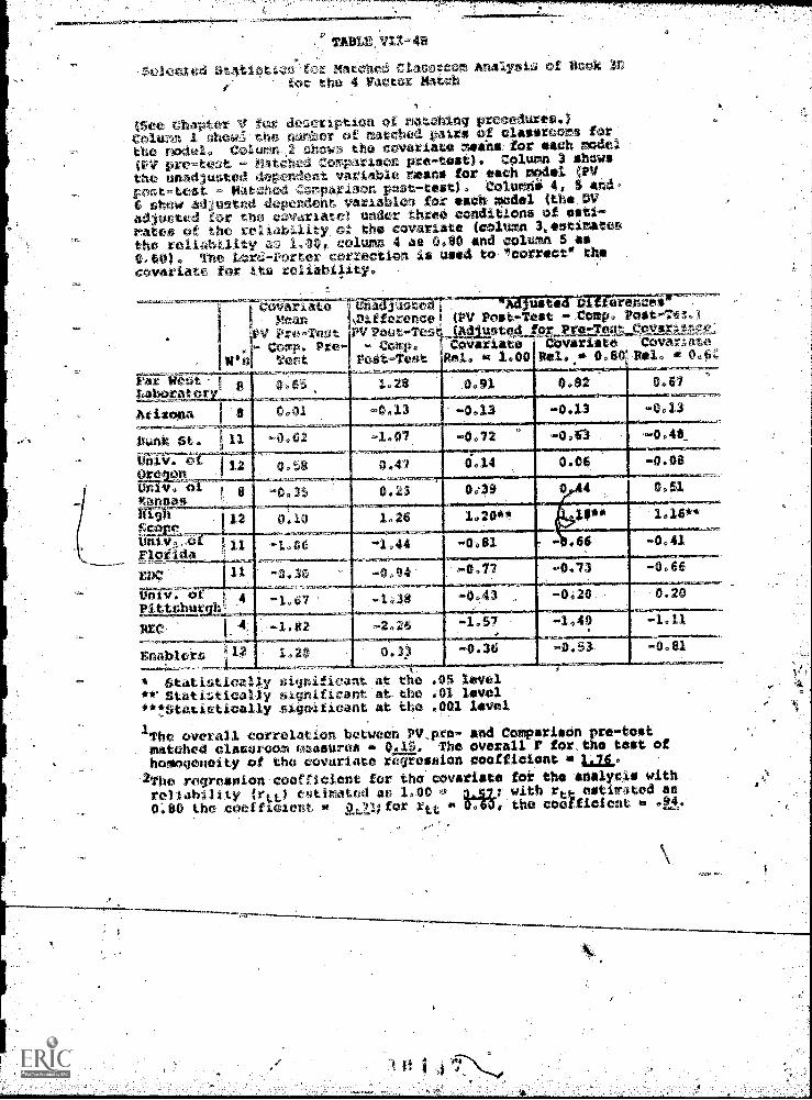
.d Clasorcom, Analysis of Rook 04 IreiCtOK .Mitch

chA a e r fiption of matching cedures.)

lime 1 g VG't. r of matched pairs of classrooms forthe model. Colas rhos the covariate .mans: for each model

ff,V pre-teat - NotChed Comparison pre-test). Column 3 showsthe unadjusted dependent variable rues for tads model OWpost-test - Matched Corparinon post-test) . Columni 4, S and

6 show adjusted dependent variables for each model (the o-DV

adjusted for the .eovariate! under three conditions of esti-

mates of the reliabillty.of the covoriate (cOlumn 30nitimatesthe reliability a5' 1.00. column 4 as 0.80 and coluMn S as

0.60) . The Lord-Porter correction is used to 'correct' the

covariate for Its

,

1

FriNo- 1 RLabors

aye i -TouCorp. Pre-

'

.

V -To,

-Tes

_,_

WA IP Ati!

(PI/ Post.efest Comp. o Ad usted fort. Pre-Toot CpxmlpivCoariate

Rel. Jaz 1.00COveriateRel. a 0.80

CoVar;.ateRel. iii 0.6C

0,011111101111

0 91 0.92 0.67

Arizo na R 0.01 -0.13 '...0 3 -0.13 -0.13

bask St..Gair--0

11 0.62 -1.07 -0,72 -0)63 -0.48.

0.58 0.47 6.14 0.00 08

Um v. 01kansas ,

0.35 0.23 049 0 4 1

R179

S .

0 6 1..2000110-

6**

0 -Fleas d

-1 06 -1.44 -0.01 .4.41

0.30 -0.94 ,..,0.17 -0.73 -.0 6

b h.67 -108 -0.43 , -0.20 .20

. 2 -20,6 4

Vhohlers---4-----

l2 1.20 tt.13,

-0.36 -0.53. - ge

* Statistically significant at .06 level.1v Statistically significant at the .01 level**!S atistically sigoificant at the .001 level

1The overall Correlation between PV,pre- and Compel' son pre-testmatched classroom peasure .1Ss 0 0. The overall F, for. the test ofhomogeneity of the covurlote regression coefficient **Lai.2The regression coefficient for the cOveriste for the analysis withreliability Ow estimated are 1.10 0 Hit with r4 estiMated an

0;80 the coefficient if mil; for rtt the coo ficicht n .94,

t °mflve percent in terms of gatns their Compare son

ups did al most as well--only one _parts n site of

for this group of ii el fell e bottom twenty-

five percent in term of a When we look tlt

model level data we find t at, on the average, the Kansas

and Pittsburgh PV classes gained slightly more than their

Comparison groups,i terms cf both "observed" gains and

°observed-expected" gains, why le the University of Oregon

model only held its own with its Compari ons. This

pattern, however, does not hold for the different analyse

Oregon, for example, appears above average in the analysis

directly comparing models, equal to or slightly above

average in the comparisons with the poled Comparison

classes, almost exactly average in the one degree of

dom contrasts with Comparison classes in the same sites,slightly above average in the five factor matching analyses

and just about average ain the four factor matching analyses.

The estimates of theeffectiveness of the Kansas model vary

somewhat mores in the cUrect contrasts among models

Kansas appears average, in the analyses with the Pooled

Comparison classes it appears below average, in the con-

trast with Comparison groups in the same sites it is

slightly below average, in the five factor' match t is

roughly average and in the four factor matched,analyses

Pitt s,

above v rage in the direct contrasts among PV classrooms.

t

the contra t against the pooled C mpariso class

-about vera' in the one degree of freedom contrast

ts Compdrison t and slightly below average in

analyses of=th two matched sample analyses. Certainly

these data offer no support f r our tentative exP+ ectation.

(2) Four other models,(Far West Laborat ry, Arizona

sank Street and the Enablers) show mixed patterns of re-'

With the acaption of the Arizona model there are

no statistically _nificant contrasts for any of the

models--the one significant result for Ariz a was dis

cussed earlier. On the basis of these data we ee no

reason to argue thAt any of then differ from the

average in effectiVeness on theBoo D test.

(3) Two other models (High/Scope and REC) also show

mixed pattern's of results b 1- ch instance-some set of

contrasts is of sufficient magn tude t. deserve attention.

The High/Scope model is particularly interesting. Three

PV sites are included in the analyses. On the average,

the pre-test means for the High/Scope PV sites are beloif

the overall Comparison mean, the mean for 'heir own on

location Comparison si tessand the overall p mean. Two o

the sites have the largest observed gains ih,:the sample

while the third site ranks in the bottom twenty-five per-

cent of observed gains. All three g2TpArson bites for

this model have average "observed" gains.k

In the comparison of "observed* aainE the Jigh /Scgpo

-186-

TV sites co Me out looking somewhat better than their

Comparison sites even though there is one "Weak" PV site.

HowqVar, when "adjusted poSt test means for the PV site

are contrasted to either Ca) their own Compa i-son s

"adjusted post-test reans", (b) to the overall C parison

group adjusted post-test ran' or (c) to the overall PV

"adjusted post -test mean", the model appear nly average.

In short the "adjustments do not compensate entirely

for the initia4.11 s low scores. This may be appropriate

and ihe.estimatea _effects may be unbiits d. If we had

complete faith in our "adjustor we would Yudge the

High/Scope model to be of only average effectiveness

The results of the matched analyses, hto,wever, suggest

that we may be 4underadjus ti ng". In both of the ^Matched,

analyses the High/Scope PV- 'classes look somewhat )eater

then their matched CoMp4rison classes. In the five factor

sample-analyses the differences are small but in the

four factor m4tich they are large and,statistically signi7

ficant. Our inclioation in this case is to equivocate--A

the High/ScoPe model may be more effective than average

but our data is not strong enough to be convincing.

The situation r the MC modelis.also ambiguous. .

Here our basic problem is that there is only one PV site

and 'no Comparison site; The one P7 site, however scores

in the bott m twenty-five percent of the sites in terms

o obseived "gains giiiiag the model thei7Secend lowest

model obsert;ed" gains. When contrast with the overall.

1 7-

yv "arbusLed post-test mea and the- overall

Comparison ad3usted p st« tot mean" the REC site looks

but average. In the matched analyses h «weveri the REC

site off. looking very badly-showing differences

favoring. Comparison group of roughly 0.33., to 0.50

dividual standard deviation... Since there is nly one

ite none f the contrasts are statistically significant

although they are cledrly gut of the ordinary.

(4) The final two models (EDC and Florida) eac

show consigtent patterns ofzesults. All estimates for

EDC suggest that i.t is somewhat 1 so effective than the,

1

other, r_adel an&theCOmpatriso Start group p--the

differences are all within the r e of -.47 to -.77 points.

As we noted earlier this entire observed effect seems to

he due tc22a9)atlsitenkD. In this site the

children actually appear to-have "lost" information

(their average,"gain" was -4).24). Two things should be

noted about this site. First, of an original 85 children

the site only twenty were included in the final analysis

ample--for whatever reason the remainder were excluded

(see Chapter III for pos ibie reasons). This gives uS

only an average of four children per class. Second,

according to the CCD consultant this site underwent great

turmoil 1during the school year. The turmoil was perceived

as having a substantial effect on the teachers, advis ry

staff and on the children. Taken together these, two

factors suggest tb us that the data from this site should

ek,

Pre-tnut matT, nwn ' e 0,,144t-test ITMMI

nccin2 tA4x-2 fot PV gtows. SIN* arounu,,T446WA 6ITA.Tro of aagmtc, ,400. , ,

M;r:.r.wc4,ty

lit

f:1,11 104t

,____.0-4- h0 .04 St. Cla

.___13_,_Iracora

3.040

3 87

lAgsgn (17.-arra-Tar4yet o03.08 AlloAy03.16 14 J

.. 6.

96 29

0

4.61,

4

4

29 rot79 1Z70, *05.1t 1 ,-9 VA05.r85,121 1

4

.

1

49

b-:0.$6

-,2.15

4;

4

ark,;?r&Vficji16-

t`.742444

-

0.0407.11 1,

p7.11 Vtgos07,14 c-

055 6.96 6035.s.14

, _,

b4Gboli On 't108.00

,;ISF771Oin09061.10

p,,z .

-w711.T.tTRT:a-7-__

- tzw o^i

rosacolabpi

17attle,

.

6.eo6036'ts.

,3.I74.79

b 6664 69.44

I4239

.

.496---4.02

.,

7O81,75

8

.

4

4k-,7,5-FgET6- 0, 1 '.6:11E-L-foro

Cattolwoq41;:,1Lton

Lu4

orgp_

006kl-cm_,,______,

I 12.03

lungtf,Dra

_on,3crib,prAtr, Co. z

5.6050/9

.

60925033

0

2.363J0

.t3

0.1.6

7.9 4.i

:

'IMiffic S' %

tn0fiTro .o4

1 'MOS27.0

© E-

.., 2 o lo

4 V6.098.01

,394.S8

.

2

cpw,Adereu re'p

tiie En

OTid

pattern of t7,1ve wg.th exceptl

g?.E` f

obLwrve ,-i6V where

bettt

-analy

CorRa,a-

Ard

o.

Oro to do as w sli

Corpariso

howeker, the Flo 'V

In only one

al -a contra'5t r

contrast

raugtay rty

yqualtiv-less effective than the oth

n thc? Book 11) testL ttiouah t

to be convincin . One model MichiS

effective thou h anain we are unconvin

ot :.cirK.Ten6luoTh

E2Y-ILM2ASK

We tect

differences, amon vac otbtr m aels.

Book

Site to

PlannoJd-Variati sites ra_

o o 17 to S.01 pdints o the Book 4A

i id I stand

ranged from pre-teGt ans of 5.

thirty, me.percent o an ;:.nc.izv

ComPari, had te

9.44, roughly.1.75

the- om pari

S ndard deviations. The middle SO% of

test means ranged from 5.39 to.A..18 or

less than thirty =three percent of a standard deviation. .

Thus 'though it appears as if there is a' wide range of vari-

ati n in ore-teqt means to )bulk of the sites fall in a very

narrow range

"Ibserved g me b:ehave in a somewhat ifferent way.

. 1The range of PV gains is from -0.14 7.8, while the range

of Comparison site 'observed g froM -0.16 to 704

pointseach range representing roughly 2.4 Individual stan-

hard

ranges'fr m 2.30

While the middle

The middle if anent of PV gains"

o 5e08b roughly 1.90 standard deviations

ty percent rallge of Comparigon "gains

s from 2..03 to 3» '9e roughly 0.6 standard deviations. On

4'44'

.the,surfaceethes

Compa son- site may differ greatly n'their

fferences suggest that &Me PV an

ffeptiveness.

in.impa ti g

with the aver

owledge o letters numbeis and skaPe.naies

PV sites appearing slightly more effective

When s tes are examined within models the differences

attenuate as the :4, 4 for the Book 3 test. The model-withra

is again EDC Me same site

lye "gains on the Boot'"`-3D t st). The

the. lowest "g antwhich showed the-mega

result6'from thkssite will be discounted-for the reasons

-

given earliier. OCalso has the site

'"gains" though.

classes for th.

t the second lmaL_

t should be- noted that the on-sit Go pars son

e had the l,a.`gc t average gains of any-ol,

90-

he':PV or Comparison

s two sites in th

gains." Finally,

ites in the top

sites. Only o e PV model (the Enablers)

bottom twenty-five percent of average

esmodel (Kansas) has each of its twos

y-five percent of average

ences

Table VII-

/hfor the PV model and their Comparison sites. The range in

"observed' gainefor 'models for book 4A is considerably -latger

than for Book 3D. The PV model 'showing the smallest "gains"

is Bank Street (1,88 points) while the largesegaineare

made by the Kansas model (6.06 points). This is a difference

ows model to4flodel differences in gains".

of roughly 1.4 individuarstandard deviations. A similar

range exists whensW model "observed gains." are contrasted

to their-Comparison groups' "observed. gains. Here the range

.is five points, from -0.85 points, favoring the Comparison

group from Bank Street, to 4.19 points, favoring the -Kansas

PV model. Thiree of the contrasts show statistically

fican results favoring..the 1W gtoupS (the Arizona, U. of

Oregon and U. of Khnsas models). Similar results occur in

the contrasts between PV and Comp ,&rison "observed-expected

gains. rt Again the range is roUghly,five points and the same

three,pVtodels show favorable Statistically significant

results. In neither set of contrasts in Table VI176 is a

Comparis. n set of Classrooms significantly more effective than

the PV model classrooms.

Column 1 shows the in gain for PV children in the Model:ColuMn 2 shows the'mcan gain for Comparison children in Model

.location. .

Column 3 shown the difforence between Column 1 and COluMn .2.(11 positive score indioatcs ghat PV children gai.ned morethan Comparison children).

ColuMn 4 shown the difference between PV and Compari*en childrenin tahserved-expetcd gains.

The individual is the unit of analysis.'

Model

PV !_Gains"PV Comparison Comparison

"Gai 3" "Gains' ."Gains"

PV(0 *erlied-expeeted)"gains"comparisoh(ohseryed7expeeted)

. ens".SD =3.91 3.15

Far West 3.60 Zill 0.68 0.86

Laborator W.67 -, 46_

4.16 3.71hrieona 5.33 3.56 1.78** 1.43*

132 61

rank :St.3.72

.86 2.713.70

-0.85 ..'0.71

1 944.06 3.62

U. of 5.40 4.08 1.32** 1 39**** :

Or co 168182---7-

4.01 --YTSU. of 6.06 1.87 . 4.19*** 44P.**Kan .1s 105 61

*I 4.12High 2.39 3.15 -0.76 -0.45

P..(41(1.--______121 96

4.66 4.36U. of 4.64 4.72 -0.08 -0.03

Florida 110 1234.58- 5.19

MC 4.25 4.19 0.06 0.09138 123

3.47 3.42U. of 3.48 , 2.39 1.09 1.23Pittshunth 7 31___42

. 3.60 '

Rix 2.7149

3.19tnablors 2.50

115Statistically signtficant at the .05 level

** Statistically significant at the ."01 level*** Statistically signifidant at the .001 level

I All children in the basic analysis sample were used(see Chapter III)

f}

-7,""'

C- "Adjusted Differences Between Groups"

The patterns of.results for the Book 4A test are 'on-

sidetably clearer than for the Bodk 3D test. Of the 108

contrasts made in Tables VII-7 and VII-Betwenty are sta-,

tistically significant. Ten of ,the twenty statistically

significant 4ifferences occur:for one model (U. of Kansas);

the other ten statistically significant differences are

scattered over four models. 'Four patterns-stand out in the_

data.

1) The University of Kansas model appears to be con-

siderably more effective than the Comparison classes and than

the other models in imparti g information tested by the Book

4A test. The Kansas model, in every analysis has the highest

estimated "effect." .ItSiaverage "observed gain" ii-roughly

0.75 points higher than the next nearest model. It exceeds

its Comparison groupS by over four points in both "observed"

and "observed7expected" gains. In the direct, contrast between

models its "adjusted effect" exceeds the overall PV mean by

2.71 points. The smallest estimated effects for this model/

occur in the regression analys4s contrasting PV model adjpsted

means" with the overall pooled Comparison mean --these "4

mated effects" are roughly 2.23 points. in the other analyses

the range of "estimated effects" is froin 3.11 to 3.88 /lints.

There seems to be little question but that,the Kansas model 1-

was.more effective than the average of the other models and 4

ri 7

than the Comparison classes in 197b -71 for the Book 4A test

The effect seems to be on the order of 0.70 to 1.3 inWviduA

level standard deviations.

.2) Both the University of Oregon and the Univ

Pittslprgh models -show positive "es4mAted effects"

statistical contrasts. Though stati$tically significant-inon

a few instances the pattern of effects, together with the

University of Kansas findingi strongly suggeSt that the

highly structured and academically oriehted models are some-

what more successful than the Comparison classes andlthan

most of the other models in impartingto children knowledge

of letters, numbers, and shape names

3) None of the other models consistently have positive

'estimated effects," though Far West and Arizona each exceed

their comparison groups in the matched classroom analyses

by a substantialomargin. The analyses in Table VII-7 indicate,

howevei, that Far West and Arizona have only average effect-

iveness.

4) Two models show moderately consistent patterns of

negative "effects" (REC and Enablers). Two of the Enabler

sites had "observed gains" in the bottom quartile of site

"gains." When contrasted with the overall PV mean, the

"adjusted mean" for the Enabler model was roughly one point

lower. In contrast to the overall Comparison group they were

significantly different, with an effect of roughly -1.4 poihts

s

Model effect" estimates for the test. Columns 1-4 show differencesbetween "adjusted"PV model means and some standard." Column 1 showsthe simple contrasts, between the PV model *adjustednmeanS and an un____weighted grand mean of the model meant for an exact least squares andwayiiNCOVA. Columns-2 and 3 show regression toofficients for.dachmodal in an analysis where all of the comparis0A classes are pooled

.

`together to form a comparison "model ".., The regression coefficients can.be thought of as representing the difference betWeen the !'adjusted" PVmodel meant and the *adjusted" COmOarison "mOdermeans. Column 2 showsthe coefficients fora regression anelysis-not4eliowing for separateelope coefficients for the covariates for the different models. COlumn":,J shows .he coeffitientt allowing for separate model coefficients forthe I'sI pre-teut and for perceht prior prelehool. Column 4 shows thedifference between PV and Comparison group "adjUsted* means*ithinsodels:for sites with both a PV and a Comparison group. The estimatesare 1 degree of freedorOtontratts in the fratewerk of a one -way ANCOVAdetign, Column 5 shows the PV and ComparisW0'0 for column 4 analysis.A note following the Table lists,the covariatee used in the analysis.In aIlvanalysesthe classroom is the unit of analysis. See text(Chaptdrs V and VII) for further discussion of the approaChes,

---

\

Model.

Estim.effectsaround PV un-weighted mean

Estimated effectsof PV modelsagainst pooledcompar. classes?'analusis

I er contrastPV v. site

comp.pooleby models

PVN

1

Comp.me .= a

rar WestLaboratory,

-0.54n=8

-0. -0. ,0 4

Arizona -0.858

0.13 0.03 -.28 4 4

Bank St.,

11 0.09 1.10 -.06 11 8

U. orOregon

1.76*12

l". flyw-8

0 9

2.22**

1.07

2.24 **

0.95

3.11**

12

8

12

6U. ofKanqanHighf;c6l"'..U. ofrloridd

-2.40***12

-0.92 -0.84,

-0.47 li 9

-0.6711

-0.73 -1.26 -0.63 11 11

nue -0.1711

-0.00 -0.08 -1.22 11 9

U. ofrlynburgh

Hee

2.214

1,75-

1.77 1.45 4 4

-1.374

'1.10-4,

.1.42

enablers -0.9212

-1.69** -1.37*...2_

Grand mean 9.23 9.23 9.23 9.25

//

t

TABLE VII 7

(Page 2)

Statistically significant at the ,.05 levelStatistically significant at the .01 levelStatistically significant at the ;001 level

1. Only PV classrooms are included in this analysis.The multivariate F with the PSI, Book 3D, and Book 4Ain the analysis, is 2.36; significant at the .001 level.The overall multivariate r for Book 4A is 3.70, signi-ficant at the .001 level.

2. Both analyses were in the regression framework withthe pooled comparison classrooms' as the "dummy variable"left out of the regression. Analysis 1 did not contain,separate slope coefficients for the various models.Analysis 2 allowed for:separate slope coefficients icor

PSI pre-score and prior, preschool experience. AnalysisI explained 70.6% of the total variation; analysis 2explained 73.4% of the total variation.

3. Only sites with both PV and CalparA.son classrooms:(.on or off-site) were included in "this aftalysis.

.

Note: All analyses included the4following'cdvariables;PSI pre-test mean, Book 3D pre-test mean, Book 4A pre-tLst mean, mean age, percent black, percent Mexican-American, percent female, mean income, meanhouseholdsize, teacher experience in Head Start, teacher certifi-cation, mean mother's education, percent prior preschool,average staff working conditions, whether the site is El ,

or Ek. In the analyses in column I thevariable "siteadministered by CAP or by Public SChool" was also included.In 'the regression analyses in columns 2 nd 3 teacherreace was included. In analyses of the tanfor4-Binet,the Stanford-Binet pre-test was also included as a covariate--these,,analyses used only. Level III site's. In analysesof the Motor Inhibition only classrooms with valid MotorInhibition scores for both .fall and spring were included.

IOW

TABLE yx;78A

for Matched Classroom Analyfor the 5 Factor Match

(See Chapter V for descriptidh of matching precedures).Column 1 shows the number of:matched pairs of oloporoorio forthe model. Column 2 shows the coverlet° mans for each model(PV pre.tent. Matched Comparison preuteSt), ColuMW3 showsthe unadjusted dependeht Variable means for each mod01.1PVpest-test - Matched Comparison,post.test). Columns 4, Vand6 show adjUated dependent verihble5 for each model (tho DVadjusted for the covariate) under three conditions of esti-Mateo of the reliability of ;the covariate (001u0o 3 istiMetesthe, reliability as 1.00, column 4' as 0.00and column 3: asV.60). The ford-Porter correction DJ used to "correct" thecovariate for its asliability. A

*---a---ravar.ttwte0na3ustedMeae

PV Pre-TestL comp. pre

Test

DiffereneePVPost-Test- Comp.st-Test

-"Adjusted(PV Post-Test(Adiustod

Differences'* Comp.-Post-Teat)

pp tre.TestCovariateRel. - 0.80

Covartance)CovariateRel. - 0.6t

CovariateRel. 1.00

Far . bLaborato 0.54 0.81 0.82 0.82 0.82

Arizona 8 -0.98 0.44 44 0.44 0.43

Dank St. 11 0.83 .0.10 0.10----

0.11 0.11

U0 v. ofOregon

-0. 9 0.97 - 0.97 0.97 0.97

Univ. of 8Kansas

ff145-------77

lnn5.--C----un v. of ,11Florida

-0.53 1.54 3.23*** 3.2 *** 3.23*

-0.06 0.17 0.17 0.17 . 7

-0.32 '-0.2 -0.24 -0.24 -0.24

EDC 11

Uni-v7 0 4Pittubur h

0.13

1.31

0.57

2.76

0.58

2.77*

0.58 0.58

2.77* 2.70*

MC 4 -0.4 -2 -2.50* -2:58* - 2.59*

Vnablers 12 0.24)

-0.62 -0.62 -0.61 -0.61

* Statistically significant at Che .05 level4* Statistically signifitant-at the .01 level***statistically.significant at the .001Jevel

1 ,

The overall correlation between PV prOr;'and Comparison pre -test.matched classroom measures .= .51. The overall F for the test of`homogeneity of the covariate re-gresslen coefficient . 0.78.

2The regression coefficient for the,e0variate for the analysii withreliability (rtt) estimated as 1.00 = -0.00; with rtt, estimated as0.80 the coefficient =,..01; for rtt = B717, the coefficient = -. 01-

VZ1-88

Selo t' cs for Matofor theA

fed Classroom analysis oittor Match

(See ChaptiXr V for description of matching prooedUres0Column 1 shows the number of matched. pairt of 4aissroomsthe model. Column / shoWn:the cavariate Means for each Model(PV pre-test - Matched Cr4pariton pre-test). Column 3 showthe unadjusted dependent-Variable means for each model (PVpost-tent - matched CoMpnrison post-toot:) -. COlumns 4, 5 an ,

6 show adjusted dependent variables for each model (the- DV ,

adjusted:for the covarate) under three conditlent of esti-mates of the reliability of the covariate (coluMn3natimaretthe reliability an 1.001 column 4 as 0.00 and column 5-at0.60). The Lord-Porter.ebrrection is used to *correct" thecovariate for:its reliability, `

Cove letMean

. 1 3 1 , Pro -Tent

Comp. Pres Test

uiajiastedUr

DifferencePV Post -Test'- Comp.

Post -Test

Adjusted(PV Post-Test(AdjuatedCovaiiate '

ltel. e 1.00

Differences- Comp..Post-Tes-)

fog_pre-TestCoverlet°Rel. e 0.80

Cqy atince:CovaiLate

Rel. 0.6C

Far WeftLabara4or

8 .2 2.01 1 0.90 0

ZOild .00 0.75 1.48 1.66 1.97

Rank St. 11 0.26 -1.05, -1 .25 -1.29 37

Un v.Oregon

12 0.24 0.56 0.38 4 0.27

Univ. ofKansas

8 -0.06 3.80 85*** .86***

fiTibScoUniv. oFlorida

12 0.37 0.88 0.60 0.54 0.42

11 -1.26 -1.15 -0.23 -0.01 0.30

EDC

iiiiiw. aPittsbu h

11 -0.50 -0.84 -0.47 -0,38 -0.22

4 -0,19 1.09 1.23 1,27 I,

AEC 4 - -2.07 -0.94 -0.65 -0.10

Lnabler U2 0.9 -0.38 -1.07 1.24 -1.53

* Statistically_ .** Statistically***c'tatistically si

ificant at the .05 levelificant at the .01 ievelficant at the .001 level

The overall correlation between pre- and Comparison pre-testMatched classroom measures =-0.15. The overall F. for the test ofhomogeneity of: the covariate regression coefficient x 0.91-

2The regression Coetficient for thocovariate for' the analysis withreliability (rtt) estimated as 1.00 0.73 with rtt estimated asb.80 the'coefficient- = .91; for rtt 4 0.66, the coefficient r7 1.2

1

. .

or roughly 0.50 standard deviations. In contrast 4th

matched Comparison samples their "effects" ranged tpm -0.60

to -1.53. Though only two of the contrasts were spuficant

the overall pattern does sUggest that the Enab -Odel

was not as effective as the other Head Start prograMs as

assessed by the Book 4A test. .

The results for the REC model are less clear,-- The

lack of replication for this model again makes itS,effects

difficult to assess. Children in this-model "galined" 2.71

points on the average on the Book 4A test, piaci40

em thirdthem

from the bottom in terms

the Overall PV mean, the

of mean model gains. C4mpared to

adjusted REC "effect" iè -1.37 points

while contrasted to the. overall Comparison adjusted mean, the

effect was- positive (roughly 1.4 points). In the two matched

classroom analyses it had negative "estimated differences."

In the five factor sample' analysis the negative differences

are considerable (about 2.58 points or roughly 0.80 standarddo

z

deviations). The four factor sample analyses yield much

smaller negative differences. As in the case of the Book 3D

test, we are am'biv.leht about reaching conclusions about REC,

since it has only one site.

In sliMmary, there is a clearly exemplary model with

respect to the Book 4A test. The University of Kansas model

exceeds all other models and the Comparison classes in all

analyses by a substantial margin. Moreover, there appears to

) 3

(University Of Oregon and Uni-

7gityver ofPittsburshL2Etjglyl±f2Etive on this

outcome measure. 'There is some evidence that the Enabler

model and the REC, model are hot as effective as the other

Head Start programs but the'evidence is not at all concltisive..

VI. The Preschool Inventory,

Site to Site Differences (See Tabl-VIIT,9)

Differences among PV sites in PSI pre-score means range

from 23.71 to 49.05 points, roughly 2.5 standard deviations.

The middle fifty percent, however, range from only 29.98

to 37.77 points or about 0.80 individual standard deviations.

Comparison site pre -test means are somewhat more closely

bunched, ranging from 26.49 to 45.,95 points, about 1.9

standard deviations wh the middle fifty percent range

from 30.80 to 39.60 poi ts or 0.90 standard deviations.

These initial differences among the sites are comparable

to the size of the differences found for the Book 4A test.

The differences in relative "gains,' however, are considerably

smaller. For the PV sites the range of "observed" gains'is

from 2.08 to 17.0 points, roughly 1.4_standard deviations'o

the-individual test scores. This contrasts with a difference

of 2.4 standard deviations for the Book 4A test. Comparison

site "gains" have a similar range = =from 6.72 to 19.07 points,

1.3 individual standard deviations. The middle fifty percent

TABLE VII -9

Praisehool,Inven or

t Bann and moan "gains" (post-tact an p a

y s3,te for PV and Comparison groups. Site rasaaverages of classrpommeans.

0

Om.

S Cnmmunity02. 402.0402.23

D uSt. CloudTacoma

ice-II

37.56

36.0237

10.56

8.458 2.

Tucs .003.0803.16

LarayetteAlbanyLincoln

11XI'II 34.07

40,3311.84

j.1.47

Dank 05.0105.1105.11

.12

SainerWilmingtonDeLaWarElmira

II1IZZI

25.74

33.2328.1830.80

9.72

7.79

ckerE 910-mann

0 .0311.1107.1407.14

S. St. LouisTupeloE. Las VegasW.,Las Ve as

1IliII

.

45.2436.29

.

45, 5

37.57 7

9.19.12

9.10

2 4

4

4

u08.08 ParXagav aMounds, 1. 1111111011111011 0.10.13RN 2

Corgi

.0209.0209.0609.10

Pt. 1 ItoPensacolaGreeley

AILI,1

23.72

4044540.43

31.3841.5043.24

17.0

2.0112

12.916.72

3

0.1210.0710.10

JonesboroChattanoogaHotaston

IIIIIIII

36.4135.8228.54

39.887-6131.67

11 9911.48

42

2.010.'118 00

4

4

I-. .

11.0611.0'3

ngtoPatersonJohnston Co.

,

I

.

27.9845,12

.429.4439.66

109.968.98

415.126.46 4 4

;

12.03- 12.03

Luck H cMitt I

IMMOMitalINIIMiallihal

6.

9.157.71

11111

MIHor ,40.0: ganso C: 1

taw 1/ .47,0427.0527.03

Hil ingfiColorado I.D.Bollo

711

It.

.

34.8249 OS

of the PV e gains r

a difference.of unde

Om *.15 to 2.56

tandard deviati:ons. e

middle fifty percent of Comparisi6n site gains range ,

from'10.28 to 12.49 points, under 0.30 standard devia-

tions. ,Clearly the majority of sites :in this study are

closely bunched in terms of "gains" on the PSI test.

None of the PV models has more than one site in the.

bott m twenty-five percent of the distribution of PSI

"gains" thigh the Enabler model has one site at thet. .

25th percentile and one below. .The third Enabler si

however, has a "gain of 16..58 Points,. placing it,

second in "observed' mcng sites. Moreover, the

model containing the site with ,the smiles "gain"

is also the model with the site haVing the largest

" "gain'". This model ligh/S.c_opeihpra-tweTsites above

the 75th pc

other modl.

centile in .gAins-6\.--.---This -happens for no

Differences

fable 10 diSploys. model, t del di ,-f n es in

PV and Corjparison "gains"' on. the P81.. For the PV'mode16.

the "observed ga range from 9.19. to 13.10-points

roughly 0.40standa viations.

.When PV and Comparison classes wi thin mode

compared on observed PSI ains tho'differences range from

1.64 points favoring the University of Pittsburgh model

to -5.24 points favoring theComporison group for the

t7,74'airt, ,r:7:14-11

the daffereee

11%

An oblfvq.47-7)-Twat,e0inaividuAl 1,J 0c), unIi of.anA

olin 2ed-it,Ore

,..10 ,PV ken it Cory nAt14xon

0

a

Fd r WPW,.Lotpiatcfv

9 .19q-'

14 . 43----- ' 5.2,4 "-

aaisoAlti7,ond .

.

Pat* -522

P,,e.

ofUrclgen

11 22

_

Jai .

7

.

_ --O.'

a -_,6 .4g1,40

n33 rp ,Poi541

0161,

0.44

_

0.40.,.----,.-,

...

r ,

i. -4020A 30***

IL- ofpA

, 4S..

1.64 2.18

PF:L:I

ab37.1-&

-, .a....

'pe.tptt2

lcwol.01 Uwe,.

nAfici'Tot dt'tt,c) ltvoldodlyi751c c.5eitTle,

-196-

West model. I we eliminate the Far West model from our

consIderati,on because of inappropriate on-site comparisons

the range if haled f going from 1.64 to -2.35 (the latter

being fr the Oregon model). The °observed-expected"

diffnces ..ar essentially similar to the observed."

differences.

Them is some indication from Table VII-g10 that the

Fr West Laboratoryf the Univerzaty of Oregon and the

EDC models are somewhat less than average in their

effectivenused°V.assessed by the PSI. The Far West and

the EDC models have the' smallest mbdefgainef both being

smaller than any of the Comparison4grbup"gains" While.

the Universzty f Oregon PV model has gai& in the-

average range:* its Comparison gr up has the second

largest average gain" among. the Comparison groups.

C. Adiust D fferences

the 108 contrasts in Tables Vu-11 and VII 12

anly nine reach statistical significance. More ye r,

there are no clear patterns of results as there 'were for'

the Book 4A test. The lack of interesting results an

most clearly be seen by looking at the matchecl classro

results ih Table Z2. Of the 66 contrasts' in this Table

only one reaches statisticd1 significance and that only

when the rp/iablity of the covariate is atsured to be

only 0.60-undo4Ctedly an underestimate (see Chapter VI)..

0.i

Model *effect" estir :for the test. Column.. 1-4 show differencesbetween "adjusted" PV model means and SOTO standard. Column 1 showsthe simple contrasts-between the PV model "adjusted" means and an un-weighted grand mean of the model means for an exact leatt squares oneway ANCOVA. Columns 2 and 3 show regression coefficients for eachmodel in an analysis where all of the comparison classes are pooledtogether to form a comparison "model". The regression'coefficients canbe thought of as representing the difference between the "adjusted" PVmodel reaps and the "adjusted" Comparison "yodel" means. Column 2 showsthe oefficients for a regression analysis not allowing for separateslope coefficients for the covarzates for the different models. Column3 shows the coefficients allowing for separate model coefficients forthe PS/ pretest and for percent prior preschool. Column 4 shows thedifference between PV and Comparison group "adjusted" means withinmodels for sites with both a PV and'A Comparison group. The estimatesarel degree of freelem contrasts in the framework of a one way ANCOVAdelign. Column 5 shows the PV and-Comparison n's.for colossi 4 analysis.A note following the Table lists the covarietes used in'the analysis.In 411 analyses the classroom is the unit of analysis. See text(Chapters V and VII) for further discutsion of the approaches.

Model

toeffectsaround PV un-

'ht cd man

Estimated effectsof PV modelsagainst pooledco. ar. class

DP contrastPV v. sitecomp.poole1w models

PV Comp.Nana. s a Ar n

ciFV67:,taboret;

.=0.46 .

Nm8 -2.01 -5.00 4 .2

Arizona. 0.208 0.47 0.09 4

Same S -0.7311

-0,77 -0.72 11 8

U. ofQX$1110

012 0.19 ' 5.44** 73.34* 12 12

U. of 2.25 0;26' T-0.25. 0;9i 8 6

hi0.kqPIIP _____

. of

412 0.49 -0.30 0.36 12 9

11 4-2.96* ..2.85* -2.14 11 .11

Ebe 11 -2.54*' -0.96 11 9

CPit A

0.2:1 0.93 3.22 4

1.15

e 70.94. .

:26

Grand Moan45.54 -46.34 46.34 46.56

TABLE VII -11

(Page 2)

Statistically significant at the .05 level** Statistically significant at the .01 level*** Statistically significant at the .001 level

1. Only PV classrooms are included in this analysis. Themultivariate F with the PSI, Book 3D and Book 4A in theanalysis is 2.36; significant at the .001 level. Theoverall univariate F for the PSI is 2.27, significant atthe .05 level.

2. ,Both analyses were in the regression framework withthe pooled Comparison classrooms as the "dummy variable"left out of the regression. Analysis 1 did not containseparate slope coefficients for the various models.Analysis 2 allowed for separate slope coefficients for PSIpre-score and Prior Preschool Experience. Analysis 1explained 78.1% of the total variation; analysis 2 ex-plained 81.4% of the total variation.

3. Only sites with both PV and Comparison classrooms(on or off-site) were included !:1 this analysis.

Note: All analyses included the following covariables:PSI pre-test mean, Book 3D pre-test mean, Book 4A pre.test mean, mean age, percent black, percent Mexican-American, percent female, mean income, mean household size,teacher experience in Head Start, teacher certification,mean mother's education, percent prior preschool, average_staff working conditions, whether the site is El or Ek.In the analyses in column 1Npie4 varialj.e "site administeredby CAP or by Public School" was also iacluded. In theregression-analyses in columns 2 and 3 teacher race wasincluded. In analyses of the Stanford-Binet, the Stanford-Binet pre-test was also included as a covariate--theseanalyses used only Level III sites. In analyses of theMotor Inhibition only classrooms with valid Motor Inhibi-tidn scores for both fall and spring were.included.

TABLE VII- 12A

Selected Statistics for Matched Classroom Analysis of the PSIfor the 5 Factor Match

(See Chapter V for description of matching.procedures.)Column 1 shows the number of matched pairs of classrooms forthe model. ColuMn 2 shows the covariate means for each model(PV-pre-test - Matched Comparison pre-test): Col..mn 3 showsthe unadjusted dependent variable means for each model (PV'post -test - Matched Comparison post-test). Columns 4, 5 and6 show adjusted dependent Variable for each model (the DVadjUsted for the covariate) under three conditions of esti-mates of the reliability of the covariate (column 3 estimatesthe reliability. as 1.00, column 4 as 0.80 and column 5 as

'0.60). The Lord-Porter correction is used to "correct" thecovariate for its reliability.'

IPcovariate-MeanV Pre-Test

_- CoMp. Pre-N's Test

UnadjustedDifferencePVPost-Test_,(Adjusted- Comp.

Post-Test

"Adjusted(PV Post-Test

CovariateRel..= 1.00

Differences'- Comp. Post-Test)

for Pre-Test Covariance'CovariateRel. = 0.80

'CovariateRel. .= 0.6C

Far West 1 8Laboratory

. 1.09 -1.18 -1.76 -1.90 -2.15

Arizona 1 S -0.02 2.57 2.58 2.58 2.58

Bank St. 1 11 -0.75 -1.41 -1.02 -0.92 -0.75

Un V. of1 12

Drogen1.55 0.8'6 0.04 -.0.17 -0.51

Univ. of i

Kansas j

4.71 3.71 1.20 0.57 -0.47

High1 12

Scope2.04 2.12 1.03 0.76 0.31

Drilv. of i 11Florida I

0.20 .-0.35 -0.46 -6.48 -0.53

EDC 111 -0,64 -0.54 -0.20,,.

-0.11%

0.03.

Univ. of :

4Pittsburgh'

0.92 1.39 0.90 '0.78rA0.57

REC 1 4 -0.58 -2.82 -2.51 -2.43 -2:30

Enablers 1 12 1.621

1.14 0.28 0.06' -0.30

* Statistically significant at the .05-level** Statistically significant at the .01 leVel***Statistically significant at the .001 level

1The overall correlation between PV pre- and Comparison pre-testmatched classroom measures = 0.82 The overall F for the test ofhomogeneity of the covariate regression'eoefficient * 0.75

2The regression coefficient for the covariate for the.analksis with-reliability (rtL) estimated as 1.00 = 0.53; with rtt estimated as0.80 the coefficient' =' .67; for rtt = 670,'thecoagicient =

1

TABLE VII1213

Selected Statistics for Matched Classroom Analysis'of the PSIfor'ihe 4'Factor Match

(See Chapter V for description of matching procedures.)COlumn-1 shoWs the number of matched pairs of clasaroomq forthe model. Column 2 shows the covariate .means for. each Model(PV pretest - Matched Comparison pretest). Column 3 showstbe unadjusted dependent variable means fOr each model (PVpost-test - Matched Comparison post-test). Columns 4, 5 and.6'show adjusted dependent variables'for each model (the DVadjusted for the covariate) under three conditions of esti-

_ mates of the reliability of the covariate (column 3estiMatesthe `reliability as 1.00, column 4 as 0.80 and colUmn 5 as0.60). .The Lord-Porter correction is used to "correct" the

,coVariate for its reliability.

ICovariateMean

PV Pre-TestP- Comp. Pre-

N's Test

Unadjusted'Difference'PV Post-Test- .Comp,

Post-Test

"Adjusted(PV Post-Test(AcIlusted

Differe- Comp.

for Pre-TestCoVariateRel. * 0.80

des"P st-Tcs6)

1Covailateel. is 0.6C

CovaiiateRel. me 1.00

Far West I 8Laboratory

8.03 2.67 -1.09 ..2.03 -3.60

Arizona 1.39 0.75 -0.28 -0.54 ) 0.98

Bank,St.. Igi -2.39 -4.11 -2.31 -1.87 -1.12

Univ. ofOregon

12 1.59 0.72 -0.48 -0.77 -1.27

Univ. ofKansas

8 6.12 4.75 0.16 -0.98 -2.90

HighScope

12 4.43' 5.78 2.46 1.6 0.25

Univ. of 11Florida

-2.51 -3.67 -1.78 -1. 1 -0.52

EDC ill -2.25 -1.77 -0.08 0 34 1.04

Univ. of4Pittsburgh -4.14 -5.71 -2.60 - .83 -0.54

REC 4 -4.45 -4 56.-1.22 0.39 1.01

Enablers 12 4.74 2.23 -1.33 -2.21 -3.69*

* Statistically significant at.the-.05 level** StatistIcallY significant at'thel 41 level***StaListically significant at the .001 level

1The overall correlation between PV pte!;; and CoMpariSon pre-test'matched classroom measures = The overall F for the test ofhoMogeneity of the covariate regression. oefficient *2.08.

he regression coefficient for the devariate:for the analysis withpliability (rtt) estimated. as-1.00 = 0.754iwith rtt estimated as0,8,0 the coefficient = 0.94; for rtt =:-0.60,'the coefficient = 1.25,

1122

-197-

Three rough patterns can be suggested, however.

(1) First there is no indication of special effect-

iveness for the academically oriented, highly structured

models on PSI gains. Although PittsbUrgh does have the

highest model "gain" its contrasts with other models and

Comparison classrooms suggests that, as a model, it is

of only average effectiveness. Similarly-both the Kansas

and Oregon models show only average effects.

(2) The Arizona, High/Scope, REC and Enablers models

also show inconsistent and generally average results.

While these models appear similar when their sites are

Aggregated they are quite different when individual sites

are examined. For example, both Arizona sites have

observed gains in the middle range of site gains while

the High/Scope sites show great variance in their obserVed

gains, as do the Enabler sites.

(3) Eor West Laboratories, Bank Street, the Univer-,,

sity of Florida, and EDC show generally negative estimates

of effects though few.bf the contrasts are significant

and occasionally even of a positive 8ign. Both. EDC and

the University .of Florida show stat significant

negative estimates when contrasted t the other PV models

and to the overall pooled Comparison classes. Far West

and Bank Street do not show statistically significant re-

sults though, with one exception for each model, all of

their effects are in a negative direction. The, effects,

howuver, are very small, never exceeding 0.30 standard devi-

.

ations when the Comparison group is appropriate. Our general

conclusions, therefore, is to assume that the models are all

of roughly equal effectiveness.

The lack of clear die-rthCes amo-nimaciels in their

effectiveness as assessed by the PSI. may be due tothe

nature of the test. It, more than.any of the other tests. ,

examined here, was designed to tap the generalldimensions

of a preschool-experience. As such. it should be less

Sensitive than other tests like Book 4A to specific-

differences in curricula. One indication of this is the

relatively small range of differen.ces in observed gains

among the sites. It could well be that this testis

inappropriate for an analysis of differences'among

curricula. Although it may serve a general puipose in

pointing out particularly weak or strong sites (note

the High/Scope site differences) it perhaps is better

suited for analyses of individual differences among

types of children. The report "Cognitive Effects of

Preschool Programs on Different types of Children%y/

explores this issue in detail.

VII. The Stanford-Binet

A. Site to Site Differences:

Table VII-13 shows site pre-:test means and observed

gains for both PV and Comparison groups. Only the Sixteen

Leve1,111 sites arc included in the analyses of the Stanford-

- Binet. This excludes the Enabler model and reduces the

maximum niambef of sites per model to two PV pre .test

i) 2 2 4

. -

TABLE VII- 13

Stanford-Binet

Pre-test'moans and mean "gains (post-test mean - pre-testmean) by site for PV and.Compariaon groups. Site means areunweighted averages of classroom means. .

Sponsor Code Community

0 2! 0 ina, 0 .A

ppyonr.C14.0 2

co g us0. 0 0a. o0 U 4,

>Clo

0U

Nimnicht 02.0402.0402.13

DuluthSt. CloudTacoma

IIIIII/I

90.1698.61

4.504.44

4

Tucson 03.08 Lafayette III 90.33 5.72' 303.08 Albany . III 88.75. 2.30 4

03.16 Lincoln III 94.88 3-07 4

Bank St. 05.01 Boulder III 99.76 L01.80 -1.5.3 -0.22 4 105.11 Wilmington II05.11 DeLaWar II05.12 Elmira III 96.15 98.63 -1.80 2.39 3 3

Becker & 07.03 H, St. Louis III 92.00 99.56 5.81 0.13 4 4

Engle- 07.11 Tupelo III 4.95 91.77 -0.57 0.59 4 4

mann 07114 E. Las Vegas II07.14 W. Las Vegas II

Bushell 08.04 Portageville' III 91.70 87.51 2.70 1.20 4

08.08 Mounds, Ill.-- II .

Wt.ikart 09.02 onPt. WaltB. III 77.40 30.59 4

09.02 Pensacola III 12.524E' 7.39 3

09.06 Greeley III 87.62-4. 96.52 "12.05 7.36 4 3

09.10 Seattle. IIGordon 10.02 Jonesboro /// 80.04 53.4( 9.62 7.73 3

10.07 Chattanooga /ii 78.55 86.77 1.61 2.94 4-- 4'

10.10 Houston II

HOC 11.05 Washington III 93.8i 116.64%.u.37- -0.47 4 4

11.06 Paterson II11.08 Johnston Co. III 86.95 86.14 5.08 4.97' 4

Pitts- 12.03 Lock Haven III -915'4/ b.S 4

burgh 12.03 Mifflenbur III 86.80 5.66

REC 20.01 .Kt nsaq City III i 4

Enablors 21.04 13111ings II27.05 Colorado Sp. II-27.03 Bellows Palls II .

-199-

means range from 77.4 to 99.76 poihts--a range of roughly

1.7 individual standard deviations in this sample or from

a very low "normal" level to the national average in terms -

of national norms. The Comparison site range is almost

as large--from 82.52 to 101.80 points. The middle fifty

percent of the PV sites,range from 87.62 to 94.95 points,

a difference of roughly 0.5 standard deviations, while the

middle fifty percent for the Comparison group range from

86.80 to 96.80 points. Thus although there area few

sites with very low pre-test means, by and large, the

sites cluster between one-third and one standard devia-'r

tion below the national mean.

Observed gains for the PV sites range froM -1.53 to

30.59 points. The latter, however, is an extreme

without it the range is reduced to -1.53 t6-12.V378nt's,

a gap of about one standard.deviation. The Comparison

site range of observed gains is not even as large as

this redu-ed range, going from -0.47 to 7.73 points. Whin

we look at the middle fifty percent range of gains the

PV spread becomes only about 4.6 points, from 2.70 to

7.33 points while the Comparison site spread is also

about 4.6 points, ranging from 1.20 to 5.66-points--roughly

0.35 standard deviations.

When we look at sites within models the, spread does

not reduce quite so muchas it does for the other tests.

One model (Bank Street) has two PV sites in the bottom

quartile while another (High/Scope) has the two sites

making'the greatest-gains. Of note, however, is the fact

that the Comparison sites for Bank Street also gain very

little (relative to the other sites) while the Comparison

sites for High/Scope are both in the top quartile of

CoMfiarison site gains.

B. Model to Model Differences:

The spread in model to model"gains"is shown clearly

in Table VII-14. The High/Scope PV model far outgains

any of the other PV models, averaging 23.4 points in "gains"

while Bank Street lags behind with an average "gain" of

-1.73 points.* Two other PV models show higher than

'average gains--both the University bf Pittsburgh and. REC

show gains of slightly over eight points. Ail of the

other PV modelsogain between 2.5 and 5.24 points, a

difference of less than 1/4 of a standard deviation

of individual test scores. The Comparison groups show

less variation with the Bank Street Comparison group

having the smallest/ "gains" (-0.65 points) and the High/

Scope Comparison group the largest (7.18 points).

-In the cOntrasts-betweerithe obserVed and the "observed-

expected" gains for the PV and. Comparison groups the High/

*When interpreting these gains it is important to rememberthat we expect some deterioration in Stanford-Binet overthe seven months a child is in preschool. Thus, all ofthe models are producing slight positive effects (seeChapter IV).

Model

'TABU III -14

Model Statistics for the Stanford-Binet

Column I shows the mean an for PV children Sn theColumn 2 shows the mom' ciain for Comparison children in mocha'

1ocation:--Column 3 show s the difference between Column 1 and Column 2.

(A, positive sct..re indicates that PV V-ch4ldren gained morethan ComParison children).

Column 4 shows 'the difference between PV and Comparison children. in observed-expected gains.

The individual. is the unit. of analysis.1

ti

PV"Gains"

PV "Gains"-Comparison: -Comparison"Caine ' n "

PV(observed-expected)"gains"-comparison(observed-expeeled1

SD=11.71 8.02Far West 3.32 3.71 -0.39 -0.10Laboratory N=13 11_ .

8.77 9.I0Arizona 4.14 2.30 1.84 0.58

57

259.10 7.71

Bank St. -1.73 -0.65 -1.08 -0.3736 15

9.52 9.41U. of 2.49 0.25 2.25 1.72Oregon 77 55

9.34 , 9.93U. of 2.72 0.92 1.80 1.22Kansas 27 25 r

12.37 7.78High 23.54 7.18 16.37*** 16.58***&alio: 47 40

9.47- 9,79U. of .5.24 4.24 1.00 -0.53Florida 43 51

8.41 10.21EDC 3.43 2.73 0,70 0.67

47 5212.17 7.30

U. of 8.23 4.74 3.49E 1.75Pitthnuuh 21 15.

9.10RKC 8.09

23

Knablers .

......- . . - .

**Statist ally _significant. at_the-OOL level

1A13 children in the basic analysis sample were used(see Chapter III)

ScoPe PV model stands out as clearly different from all

of the others with an advantage favoring the PV group

of roughly 16.5 points. None of the other measured

differences exceeds 3.5 points. Thus, in terms of

'simple gains and differences between ?V and Comparison

groups there is only one main finding in this data--

the High/Scope model appears to be extraordinarily

effective in raisin d-Binet scores at least in

the short run. Other than that there'are no differences

of note in the data shown n Table VII-14.

C. "Adjusted Differences Between Groups"i',

When the data in Tables VII-15 and VII-16 are examined,

the picture becomes only slightly more complex. Six

PV models require little attention; .Far West. Laboratories,

Arizona, Oregon, Kansas, Florida and EDC all show small

and inconsistent effects,. Note that this group includes

two of the highly structured academically oriented models,

an indication that this approach is not necessarily more

effective than other approaches when the Stanford-Binet

is the outcome measure. In the following we consider the-

four remaining models.

(1) The University of Pittsburgh model-had observed gains

averaging over eight points. Although it appears less effective

than the average PV model, see Column 1, Table VII-15) it shows

positive effects in all of the other contrasts, in Tables VII-15

and VII-16. Of the eight other contrasts five show

TME VII 13ptanford-Stnet.-

Model "effect* estimates for the test. Columns 1-4 shoW-differencesbetween "ed3usted* PV model ear and'. standard.. Coluen'l chewsthe simple contrasts between the PV =del ,"adjusted" means and anun-weighted grand mean .of .the Model mans f r an exact least-squares one

way ANCOVA. Colemns,2 and 3 showsegressionroefficients. for eachmodel in an analysis where all-of the corparison classes are pooledtogether, to form a.corparison- "model". The regression coofficibntsi can

be thought of as representing the difference between the "adjusted' PVmodel means and the "adjusted* Comparison 'model" mans. Column' 2 shows

the coefficients for &regression analysis not allowing for separateslope coefficients for the covariates for the different models,- Column3 shows the coefficienta allowing for separate model coefficie4s-lorthe PSI pre-teit and for percent prior preschool. Column 4 Wows thedifference between PV and Comparison group "adjusted" means withinmodels for sites With both a PV and a ComparisenAroUp. The eStimatesare 1 degree of freedoM contrasts in the framework of a one way COVAdesign. Column S shOws the PV and-Comparison nes for coluMn 4 .analysis.A note following the Table 'lists the eovariatee used in the analysis.-In all analySes the classrceM is the unit of analysis. See teSt,(Chapters V and VII) for further discussion of the 'approaches...

ModelPiiiWsLab0r o

Ent %aa.effecftaaround un-wresl kited as

s imated effectsof PV modelsagainst pooledco aro clasaea2r 1, An Mm

Dr contras;JIM v. sitecomp.poolebv. models

_

PV Corp.N

-0, @3r4 1111=11111111111111 -2.04 4 2

Arizona 1.637 -1.30 0.43 3 4

Bank St. -3.341111111111 -3013

7

0-6.64

111.1=11.11110,I1

U.n 4 -2 11131=

10.06**

4

tDirh__

.8 .

filoth10_,

EnC

7 - .

_

1111111111111111 -°'00=0 4

U. of- 9.08* 4 4

RIX 1 2 10.97***IIIIIIIIIII

Unablert, 1111111111111M1111.196.90 95.16 . 4

,

aY

t1(17777'777-r

stStdsta

icallyticallyacally s

TABLE VII-25

(Page 2)

ant at the .0ant at the .0-cant a the .00

1. Ot PV cla are included_multiv . ate F w th the PSI, Bock 3D,Binetiin te regrsion as 2.9 saglevel.. The overall F for the .g nfosignilficant at the .001 level.

2 h analyses were in thethe .pooled C papa: is n classroOmleft Out. of ehe regression. .AnalsepArate slopd effacients for thAnalybin 2 allowed fca.r separate slPSI' jprescore and P3. explained 70.7% of

(on

evelevellevel

analysts. The4A and St ant rdt at the, .001

et is 7.$0

scion framework withthe,'dUmmy variable'.4) I did not containvarious models.

no coefficients forPreschool Experience. Analysis

e' total variation

ly sites with both PV and Comparoff-sate) were in luded in this

n calt's'

eg Al l analyses included the 1 w i ng aovari ablesgpre-test mean, Book 3D pre-tept man, Book 4A pre-mean, mean age, percent black, percent Mexican

American, percent female,,mean income, we householdsize, teachei' exneraence in ticad Stmt, teachercettificataon, mean mother's educat percent prierpre drool, average staff working co (ins, whetherthe site is tl or 1:%. In the analy,4 e th column 1 thevariable "site edministered b.,' CAP or by Public School"was also included. in the regression analyses in columns2 and 3 teacher race wan included. In analy ses of theStanford-Banet the Stanford-Bine* pre-test was alsoincluded as a covariate--these analyses used only LevelIII :iites. In analyses oE the Motor 3nh bition nlyclassrooms with valid Motor Inhibition scores for

both tail and Apr ang were included.

TABLE

Selected Stat 5 for Hatched Ci4OEMOMStanfo. -01n0t, for the S Factor

y la for the

17.

(Sea Chapter V for dencriptich of matching procodures0Column 1 *ht-Ai3 the hurrer of matched Pairs of Classrooms for

the redel. Celoqn 2 lihOuq the covariate,means ror each 'model

(PV pre-refit - Matched C ipartaonpre-te,at). Column 3 show;the unadluuted degcndent variable rOang for each model (PVrz4t-tet.t- hatched Coroartuon pant-tent . Columna 4o 5 andG ehow a4w,5t!td, derenftht.varOblea fir each model (the DVad anted fer the covartatO under three conditions of esti-matez of tlifo rollAbil44ty ef the covariate4(column,3 estimates

of 1000, eau= 4 an 0.80 and column 6 as'0.60Y. The Lord-'o: ter,eorrection is uzed to "correct* tRe,covarigitti for its reliability.

4

.

.----..--,.par WO9t.b.

rang=

4 w

40,X0 ateMa a 1

ri Prey snt- CvIn °6 h

!refit

aiTiCtiudiaTlricarlastedf DifferencelPVPost-Tepi- Corp.oat-Tout

(PV RO6t-TestaillItetedCovariateRel m 1.00

Differeneee- Comp. Pot -Testl

Apr Pro-Tpfitspyaxtame, Covariato CovariateRel. lw 0.8 Rel. 0.61

9.00 --10.1g, 7.80* -6.26

ATiVAPA -2.27 -1. m0.70 -0A56 2

Bank St. 0.1 2 '-5.46A

nc . Twi ii 8 0.18 1.70 1.66 1.62

t v.1 4

Itatfias-1).4-: 6

SetUnFlorida

- .01111111111111111,161111 -3'

CT . -a .7.. ,

q

may. TA- 4- *,,,ls

t21135bg'f.Sa____--,4- _

Pp:

13.1S 10.57** 9.7

2.56 2.76

___..----

f'nahltr::,

.

* rlAwtitA,k4 aci;am.,,,,. At &he 00f,) level

** ntc.zom!..6c:4l-,7 fAw4 ic-at at tha 411 levelr,Atilaua.j/Nt. et law

;At 4,;-ce-fT17:77- 1N4V.4L,,QP/r4 gaV pc- and Corparlion pre -teat,,,.St --uAertff - Wito overall V ter the teat of

trco4",:,;PACOT,1 coeffiele t m

1Dr the tovariate for the analyt,in '4th1f!,, 1.4n , vith eatir,Aed At

g,N TG. '; 0,64, 0e, coefficient w 2.4,v

ABLE, VII- sss

Statistics for etched Classroom Analysis of theStanford-Bine for the 4 Factor Match

(See Chapter Vsfor description of matching procedures.)Column .1 shows the iftwobei -! matched pairs of classrooms forthe model. Column 2 shove theocovariate means for.each model(PV pre-test - Matched, Compasison pre-test).. Column 3 showsthe unadjusted dependent variable means for each model (PVpbst-test - Matched-Comparisbn poststest).. Columns 4..5 and6 show adjusted dependent variables for each model (the DVadjusted for the covssiate) under three conditions of esti-mates of the reliability of the sevesiate (column 3 °titivatesthis rellObility an 1.00, column 4 as 0.80 entl'colssn 5 as0.60).. 'The Lord-Porter correction is used to ."correct" theeeveriate for its reliability.

Cc"'-8teTV Pro -Teat

Comp. Pre-Test

grlti=IS/Post-Tess- Comp.Post-Test

'Adjust'ed(PV post -Vest_(Ad ustedCovaEiste 1

Rel. r 1.00"

Differences": t!;estr

for Pre-Test_CosesiansesCovert° Covariatele

Bel. r 0.80 Rel. s 0.60

FaborsarL 4 -7.64

3

NM-1.10

-1.40

1.24

-0.13 \''''1s-

Arizona

Bank St. 7 6.49-8'14 111:111111

..5.52 -7.31**

Univ. o0 oUnK

8

4

2083 1111;1101111-0,03

- .

.89 1.10

-0.45 -0.59

0Sbn viPio

-5.29

IIIIIIIIII-2.00

10.59 14.10*** 14.98s** 16.44***

-8'39-2.79 -1.83 -0.22

PDC -0.92 0.41 0.74

UnPst

RAC p4

Lnablero

MM.11111111111ME

8.09

1.18

6.57 MEM 5.56

4.653.26

IIIIIII.Statistically significant at the .05 level

** Stet ''tiesIly significant at the. .01-level***ota cally significant at the .001 level

. .

1The overcall correlation between PV pre- and Comparison pre -testratchod clausroom measures s 0.29. The overall F for the test of

s. homogeneity Of the covariate regression coefficient 2.19.

The regresoion coefficient for the coveriato for the analysis with(r,t) 0,itimokra as 1.00 s 0.60, with 'A estimated. WI

0.80 the. coeffsetent 0;83; for rtt's riai,-the coefficient a 1.11.

-202-

statistically significant results--no difference is less

than 5.6 points.or roughly one-half a standard deviation.

Although it is difficult to draw a conclusion about

Pittsburgh since it has only one site, there is*a strong

Head.Start programs in imparting gains on the Stanford-

indication that it is more effective than the Comparison

Stanford-

Binet.

(2) The REC model showed an average gain of -slightly

over seven points. When placed in an analysis directly

contrasting PV models,the REC model shows'a highly

significant effect of 17.20 points. In contrast with

the overall Comparison group it also shows a statistically

significant effect of 10.97 points. In the matched sample

analyses, however, the REC model does not show a large

effect (it never exceeds 4.65 paints) although in all

Instances the.direetion of the effect is positive.

We are unclear about the cause of this rather dramatic

;set of differences between estimated effects.from dif-

"ferent analyses. Presumably, it has something to do

with the form and nature of the covariates used in the

analyses. Whatever the reason, however, there is clearly

an indication that the REC model may be more effective

than most PV and Comparison Head Start prOgraMs. It is

important, though, to remember that there is only one REC

site so it is impossible for us to reach a firm conclusion

about the model.

(3) The Bank Street model had the smallest "gains"

. on the Stanford-Binet of any of the,PV models. Both

Bank Street sites had similar pre-test and gain scores.

Inthe.analyses detcribed in Tables VII-15 and VII-16

Bank Street shows a consistently negative effect, ranging

from -11.33 to -3.13 points. Of ,the nine contrasts five

are statistically significant. If we disregard the largest

negative effect-because it ocpurs in the PV model to model con-

trasts,(the analysis we have,least confidence in) the range is from

roughly -7.5 to -3.13 points. The only reason we have not to con-.

clude that the model is, less effective than the other

from the extraordinarily high pre-test means in both of its

sites for PV and Comparison groups. Although these sites

show moderately high pre-test means for the other outcome.

. measures, they do not come''close to approximating the

relative magnitudes of the Stanford-Binet pre-scores.

This suggests that the Bank Street site pre-scores for

both PV and Comparison children may be over-inflated--

perhaps because of an over-zealous tester. This would

give the childreff in these sites little opportunity to show

impressive gains on the Stanford-Binet. A somewhat more

conventional interpretation might be that a regression

artifact was working on the Bank Street scores,--the high

initial scores would have to be due to substantial positive

errOrs in both sites for this explanation to work. Since

the average classroom N for the Stanford-Binet analyses

2 3 5

dels stemt,

-204-

is only about five this explanation may-be plausible. Our

inclination, then, is not to each a firm conclusion about

the Bank Street model's effectiveness ..for the Stanford-

Binet as the outcome measure.

(4) The High/Scope model shows dramatic 'positive

effects in all analyses of the Stanford-Binet. Estimates

of adjusted differences range from 10 to 17 points -!

from 0.7,-to 1.3 standard deviations. This effect is

comparable in magnitude to the effect found for the

University of Kansas model on the Book 4A teat but it

potentially is far more important. Its special importance

stems from the aracteristics of the outcome measure.

The Stanford-Binet was developed to tap general intelli-

gence--a trait that by defiAtion is not sensitive to

slight changes in environment .Moreover, in practice,

Stanford-Binet scores are geneally difficult. to change

very substantially. Yet herd we `see an estimated change

-of almost a standard.deviation' in magnitude effected

over a 'seven month preschool program. What accounts for

this effect?

Three issues are important. The first,two have to do

with the data and the third has to do with the nature of

the High/Scope program. First, although the High/Scope

PV sites ranked first and second in observed gains there

was aAlkamatic difference between the two sites. In one

site the average gain was roughly 30 points--of some

importance is the fact that the four classes in this

site had gains of almost equal magnitude. The'second

site averaged gains of only twelve points. Although

both gains are impressive in magnitUde the difference

between themsuggests that the effects of the High/Scope

program may be sensitive. to differences among sites in

such things as pupil composition or location. In thisI

instance the.site with the thirty point gains is located

'in the rural South, has a racial composition of roughly

70% black and 30% white with none of the children having

previously attended preschool. The other High/Scope site

is located in a small urban northern city and has a racial

composition of about three-quarters Mexican-American,

about one-sixth of whom had previously attended preschool.

Second, the pre-score mean for the children in the

southern rural site was the lowest of the sit&pre-score

means. On the one hand, this suggests' that a regression

artifact might account for some of the thirty-point gain.

Even supposing, however, that the Binet had a reliability

of only 0.70 (undoubtedly an underestimate for even the

individual test administration much less classroom

aggregated means) and assuming that the "true" population

pre-test nean was 95 (probably an overestimate since it

exceeds the overall pre-test mean for the entire PV sample), then

the regression effect would account for a little over five points

of the thlirty point gain.*

On tne other nano, however, tnere is some inaependent

'information suggesting that the low pre-test scores are

valid. For each of the other academic outcome measures

discussed in this chapter the southern rural High/Scope

site had either the lowest or second lowest pre-test

site mean. Since these tests were given by other testers

than those who gave the Stanford-Binet, there is good

reason to believe that the pre-scores on the Binet are

roughly accurate. In the other High/Scope site, the pre

score mean for the Binet is close to the overall PV sample

mean 'and is consistent with the other outcome measures.

This suggests there is little chance of a regression effect

for this site..

*Knowing the observed mean,_ reliability and population mean,we can estimate the magnitude of the regression effect. Inthis instance, we have.an observed mean of about 77, we havetaken a lower bound for a possible reliability (0.70) and wehave taken a high estimate of a population mean (95). Ourapproach, therefore, will overestimate the regression effect.The general formulation is that the regression effect isequal to 1.0 reliability times thq difference between thepopulation mean and the observed sample mean. In this casewe have: .

regression effect = (1.0 0.70) x (95 - 77).= 5.4 points

-207-

This argument also deals in part with some observa-

tions made by SRI personnel at the southern rural site.

Apparently, the fall Stanford-Binet tester was very

efficient about his work, spent little time with the

children and as a consequence, appa4ently had little.

rapport with them. The spring tester, however, was loved

by the children and spent a much longer period of time

administering.the test: ThediOerence in style might

account for some of.the gain. Itis possible that the

fall tester was obtaining underestimates of the "true"

scores while the spring tester was obtaining-overestimates..

The very low pre-test scores for. the other outcome measures,

however, suggest that the fall tester was probably not

particularly *biased. A possible bias on the part of the

spring tester cannot be so easily-dealt.with. We note that

for both the BoOk 3D and the PSI outcomes 'the gain,sCores

for this site were either near the largest or the largest.

This, however, does not account for a thirty point Binet

gain. Our:best guess is that roughly ten of the thirty points

areprobably due to a combination of tester and regression

effects. There do not seem to be any peculiarities about

the testers in the other High/Scope site. Thus, we-estimate

that the true gain.for-the southern rural site is roughly

20 points while the "true gain" for the northern urban site

is roughly 12 points,:_.

9

-208-

Third, there is some preliminary indication that,

the children in the High/Scope sites are getting certain

items correct on the Stanford-Binet post-test that

children in other programs are not getting right. These

items have to do with differences and similarities --

concepts that are an integral part of the High/Scope

curriculvm An analysis of this issue as Well as of

possible tester bias is included in an appendix to this

report.

In--summary, we conclude that the High/Scope model

is particularly effective in producing gains on the Stanford-

Binet.. We estimate the "true observed gain" to be in the range of 15,

to 20 points while the, differences between High/Scope and

conventional Head Start gains range from 10 17 points

with a "true" effect probably closer to the bottom end of

that range.. We reached no firm conclusions indicating,

positive or negative effects for any, of the other models

though there is some indication at Bank Street may be

less-effective. than other model and that the University of

Pittsburgh and the REC models may be slightly more effective.

4 0

VIII. Motor Inhibition

A. Site to Site. Differences

Table VII-17 shows site pre-test means aic d observed

gains on the Motor Inhibition test.* Pre-test mans for

the PV sites range from 4.48 to 5.71, roughly 1. individual

level standard deviations. Comparison site pre-tes

means have a range of similar size, from 4.25 to 5.6.

Although the comparison sitedistribution of means is

slightly lower overall than the PV distribution the middle

.50% of the.means of the two groups overlap almost per-.

fectly., The middle range of the PV means goes from 4.79

to 5.19 while the Comparison site middle range is from

4.77 to 5.23roughly 0.9 standard deviations in both

instances.

In terms of "gains" the PV site distribution is con-

siderably tighter than the Comparison site distribution.

*As described in Chapter III a child's score on this. testwas calculated in a somewhat complicated way. First, inorder for a.test score to be included in the analysis thechild had to answer correctly two or more out of four ques-tions developed to assess whether he understood the words"slow"'and "fast ". The sample used here contains onlychildren who met this'criteria in both the Fall and Springtestings. Additionally, the tester had to certify both,test administrations as valid. The test is comprised ofthree sections: "draw a line", "walk slowly", and "truckpull". In each section the child is asked to complete the

- task at normal speed and "slowly". We eliminated the"truck pull" task from the analysis for psychometric rea-

--sons,----A-c-hild-' s -seore-w-as---c-alculated-by -taking The logof the sum of the "slow" times (in tenths of a second)for the other two tasks.

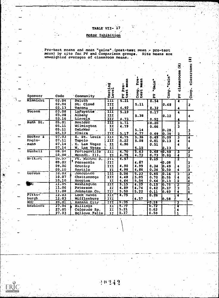
Sponsor

TABLE VII- 17

Motor Inhibition

Pre-test means and mean "gaiass(post-test mean pre-testMean) by site fora PV and Comparison groups. Site means areunweighted averages of classroom Means. .

Code Community 140 041

0 0CLo

14 41

00VIJ

A0U

z 20

1 1.40

E 4

Nm

m ,..4

so 010

opi . O> oN

N mnicht 02.0402.0402.13

Du utSt; CloudTacoma

I

III-II

.

4.925.11

0.54

0.320.68

4

42

Tucson 03.08 LaFayette III 5.29 0.1703.08 Albany III 5.38 0.12 403.16 Lincoln III 4.73

Hank St. 05.01 Boulder III 5.71 -0.20 305.11 Wilmington II 4.79 0.66 305.11 DeLaWar ._ II 5.14 0.28, 305.12 Elmira III 5.17 4.77 0.49 J0.39 3 3

Becker 6 07.03 E. St. Louis III 4.75 5.36 0.49 0.09 3 4Engle- 07.11 Tupelo III 5.22 5.08 0.01 0.13 4 4mann 07.14 . E. Las Vegas II 4.96 0.51 4

07.14 W. Las Vegas II 5.15 0.13 4IRMTial- 00.04 PortWarne III 4.70 5.63 0.48 -0.5' 3 .2

08.08 . Mounds, T31. II 4.75 4.72 0.73 0.80 4 2We 09.07 Vt. Walton H. III. 4.57 0.15 2

09.02 I' Pensacola III 4.87 -0.08. 209,06 Greeley III 4.90 4.99 0.34 0.49 4 309.10 Seottic /1 4.96 4.86 0,34 0.50 4 3

Gordon 10.02 EXCEVoro 111 5.06 5.23 0.45 0.16 3 310.07 Chattanooga III 4.48 5.05 0.70 0.55 4 410.10 Houston II 4.64 5.54 0.44 0.13 2 4

OFK: 11.0c- Was ingion III . I. 0. 5 311.06 Paterson II 4.89 4.74 0.42 0.17 3 111.08 Johnston Co. III 5.50 5.22 0.11 0.60 4 4

Pitts; 12.03 Lock Haven III` . 4.75 0.26 4burgh 12.03 Mifflenburg III 4.57 , 0.58 4RAC 20.01 . Kansas Cit III 5.15- ',0.16 3kiialers 2 .04 Billings II s 0.

27.05 Colorado Sp. II 5.21 0.62 427.03 Bellows Pails II 5.37 0.50 1

The overall range of PV gains is from -.20 to 0.72, or

roughly one standard deviation. The Comparison site

,range of gains is from -.59 to 0.80, about 1.4 standard.

deviations. The middle 50% of the PV distribution is

only slightly more.tightly bunched than the middle 50%

of the Comparison group. The PV range is from 0.15 to

0.52 points (.7 standard deviations) while the Comparison

site gains range from 0.13 to 0.58 points (0.90 standard

deviations).

Relative to the other tests, the variations of mean

site gains for the Motor Inhibition test is larger than

for the PSI and somewhat smaller than for the Book 4A test.

Since the degree of variation of gains appears to be re-

lated to the occurrence of clear "effects" in the data

this indicates that there may be some effects for the

Motor Inhibition test.

When sites within models are examined two models

stand out as having a clear pattern of large observed

gains. The University of Kansas model has the site with

the largest average gains of all the PV sites and a sec-

ond site with a gain just below the 75th percentile level.

In the Enabler model two of the three sites show gains

well above the 75th percentile of PV gains and the third

te is only very slightly below the top 25 percent. On the

low end of the scale the EDC model has two sites slightly

-211-

below the 25th percenti Note also that the only site

in the REC model shows a loss of -0.16 points, p/acing

it at the very low end of the distribution of site gains.

Sites in the 'other models seem t show little pattern

with most models having both relatively high and lcw

scoring sites..

B. Model to Model Differences

The same four models stand out in Table VII-18.

The University of Kansas and the Enabler models have the

two largest mean gath scores while EDC and REC show the

smallest gains". The overall range of gains for tbe PV

models is roughly 1.4 standard deviations from 4.06 to

0.64 points. Since onl. four children in the R.= Model

cowed valid scores we will eliminate this model from

future discussion of this' te The range without REC

from 0.21 to.O.64, about 8 of an individual standard

deviation.

A contrast of the PV model gain means with the mean

of their Comparison groups shows two statistically- sign

ficant differences each favoring the Comparison group.

The mean gain for the Far lest PV group is 0.36 while its

*recall that the weans in Table VII -18 are calculated bpooling all children in all of the sites of a model wailt!17 site mans in Table VII-17 are means of classroom means.Since there are cilfrent numbers of children in differentclassrooms the two ways of aggregating scores occasionallyproduce sanwhat different results. Thus, the average class-room mean gain for the REC site is 0.16 while the-averageindividual gain is -0.06.

47E3 tr< 1

CU711,fE4 04161ten t the r

CqJrN44@o.gt ,Ildren in

Coqvg'm 4vd 2, ,

4541;:it,S1 faNildrot gpiPad

Ce.4/1 4if6g6,e( t PV Ccnpar E1a0 Ctql0M00_= ?.A

4M tigitof

TV'

aerv.-,Ia-e14.

Naii.7W-ev7,,W4,175etva,-*v.atfl

nag.- Nt'5t

:44.,.,t,.

6,1;6-Th3,:i, ,

,f)4

2

_

-0-4* -0,26

0.:1Z

---- 8

0.44(5.116

6

Noo!k

_____-----

0.0tit 10 -g424

----- 2.,:'

1. t ;;_

-,----,-

70.

.12 : 0,,n*.

0615'

--_

..

397

,/

AA S =0,17

--

3**...

,____

"416 0,47

, ----q---

",,,F-tti.

-212

Cora s n gr uE has a njean gain cf 00 64 yielding a di f--

f 0.28 points s atistiC'ally significant at theBran

0.05 iev o in only one of the two Far West cites

has a Compa on g up an off site comparison) the dif-

ference may well r Lect unwon fled sampling bias 'Indevd

the means West PV si which :gas a Comparisod

*' group .54, opiy 0.14 pints bet eti its . Coparison_

group roan._ Our ihelinatioa is to attribute this 1 ffer

nee to chance. The -gocond model showinga sAgn. cant

1Mienca di f,6 renee 0.-33 -s avorinq

t.

the Comparison .1 oup .

tWConp-ris«gain IQ:Bs

magion to-

Qbservedi 1E4%

-nd CorTari,

t;h6w a. Gignificant

tinues to

An©tIlwz c

Since all tt ree of the EDC,site

hd n oach instance thd PV

.1 the Compari n. children there

ct 'may be .valid.

contrasted fo.

t this

`7

oans

ranee

matiql dos not

Todel con

F'antly less than its C.mpar

a.) c this

'c ptufrn. childre,z e University o Oregren model

app©ar

isvt- /foal/ Iy 0. 30

Of trit6z ildrcn

the u4

qnficantlyrore than their Comparisons

revea that this diaferen

due mare to the poor ihowing

c4f Oregipn "V pJ1 id

to j rong showing for

of the three

MC

Oregon Compd n sites gains fall below or at the 25th

percentile.sf,

Since the Lnthler group does not have Comparison

sites there is no way of knowing from this table whether

its pffectiveness is duo to the model or to the samples

of children in the Enabler sites. The Univ.. of Kansas

PV model, which has the largest observed "gains", does

only slightly better than its Comparison group in the con-

trasts in Table VII-18. It must be noted, however, that

only 11 of the Comp4rispn-children in the Univ. of Kansas

sites had vaUdpre and post Motor 'Inhibition scores.

* djusted ffereaE2,21212.9_9:112RPs"

Tables VII-1g, 19 and 20 contain 97 contrasts.

Thirteen are dtatistidally significant. The results pre-

sent a very mixed,picture. No model stand S out as clearly

more effective than others. The results however,

seem to follow three general patterns.

Th. Si Todels (Far West, Univ. of Arizona, Univ. of

Oregon, igAdope, Univ. of Florida and EDC) 'show.genu-

inely mixed results. In some instances the "effect esti-

mateor these rodels are positive, in other.instances

negative. Only one of the 54 estimates for these models

is statistically ç.ignificwt. The generally small esti-

mates,anA the mixed pattern of results indicate to us,

that them are n( compelling differences among these models.

! f) 24t

With regard to ree of the six-model tkis conclusi n _

-214-

should not be surprising. The_gaia score data in Tables

VII-17 and VII-18 indicated that the Univ. of Arizona,

High Scope and:the University of Florida PV programs were

only of average effectiveness. There were, however, indi-

cations that the other models might be somewhat different.

In particular we pointed out that Far West did not seem

to do quite so, well as its Comparison group.. Our expla-

nation for this rested upon potential differences between

the PV and Comparison groups. Based upon the data in

Tables VII-19 and VII-20 this eXplanation appears valid.

A second model (EDC) also did not seem as effective as

it Comparison group. For EDC we had no ready explana-

tion for the difference. And when EDC is contrasted in

the Multivariate Analysis of Variance with is Comparison

group (see column 4, Table VII-19) the PV group still ap-

pears somewhat less effective, though_ the difference is

not statistically significant. Yet when the EDC PV model

is compared with other PV models, with the Comparison

classes in general, or with matched Comparison classes

there do not appear to be any differences. The third

model (Univ. of Oregon) appeared somewhatjnore effective

than its Compa-rli&H -51-abQb in the gatn. so analyses.

However, when the Univ. of Or3gon is contrasted with

other groups it kffects seem to disappear.

2). Two models (Univ. of Pittsburgh and REC)\seem

to be systematically less effective than the, other Models.

st 2,

TABLE VII- 19

Motor Inhibition

Model "effect" estimates for the test. Columns .1-4 show differencesbetween "adjusted" PV model means and sole standard. Column 1 showsthe simple contrasts between the PV model "adjusted" means and an un-weighted grand moan of the model means for an exact least squares cneway ANCOVA. Columns 2 and 3 show regression coefficients for eachmodel in an analysis where all of the comparison classes are pooledtogether to form a comparison "model". The regression coefficients canbe thought of as representing the difference between the "adjusted" PVmodel means and the "adjusted" Comparison "model" means. Column 2 5:-.awsthe coefficients for a regres4on analysis not allowing for separateslope coefficients for the covariates for the different models. Cclumn3 shows the coefficients allowing for separate modelcoefficients fDrthe PSI pre-test and for percent prior preschool. Column 4 shows thedifference between PV and Comparison group "adjusted" means withinmodels for sites with both a PV and a Comparison group. The estimatesare 1 degree of freedom contrasts in the framework of a one way ANCOVAdesign. Column 5 shows the PV and Comparison n's for columd 4 analysis.A note following the Table lisps the covariates used in the analysis.In all an4lyses the classroom is the unit of analysis. SEC test(chapters V and VII) for further discussion of the approaches.

14004' i

liar' Ili!s

Labora r

nst oeffeetnaround pV un-Vg.ifalte6 rw!nn

Estimated affectsof PV models ,

against pooledcomonr. oltnse92

DF contrastPV v. sitecomp.000ledby models-'

PVN

1

i

Comp.N

---1-- -..--N...---'ann1"1. , PrOlVaig

-0.35 N=8 0.07 -0.18 4 2 %

Arizona -0.30 8 -0.12 -0.09 4 4 ,

Bank St. 0.470** 9 0.30* 0.40* 6 6

U. ofOre.on

-0.02 11 -0.14 0.36 1 12

U. ofKansar.Uiell

-0.07 9 . -0.06 -0.04 7 4

-0.2 -0.27 -0.19 0 8

Li. ofF]orldil

-0.14 9 -0.07 -0. 7 9 11

gOC

6:' of

p.i.ti.A0-40

PVC

Lnabbrs

-0.05 , -0.23 9 8

-U.31

0.'..6""

4

3

-0.23 -0.25

0.00

9 0.24, ,......_

orand Peon5.38 5.38

OA

" 1 9

',,TABLE VII -19

* Statistically significant at the .05 14vel** Statistically significant at the .01 level*** Statistically significant at the .001 level

1. Only PV classrooms are included in this analysis.The multivariate F with the -PSI, Book 3D, Book 4A and .

Motor Inhibition in the analysis is 2.43; significantat the .001 level. The overall univariate F for theMotor-Inhibition is 2.62, significant at the .001 level.

2. Both analyses were in the regression framework withthe pooled Comparison classrooms as .the "dummy variable"left out of the regression. Analysis 1 did not "containseparate slope coefficients for .the various models.Analysis 2 allowed for separate slope coefficients forPSI pre-score and Prior Preschool Experience. AnalySis1 explained 47.2% of tika6,total variation.

-mor,

3. Only sites with both PV and Comparison classrooms(on or off-site) were included in this analysis.

Note: All analyses included the following covariables:PSI pre-test mean, Book 3D pre-test mean, Book 4A -pre-test mean, mean'age, percent black, percent Mexican -American, percent female, mean income, mean householdsize, teacher experience in Head Start, teacher certifi-cation, mean mother's education, percent prior preschool,average staff working conditions, whether the site isEl or Ek. In the analyses in column 1 the variable"site administered by CAP or by Public School", wasalso included. In analyses of the Stanford-Binet, theStanford-Binet pre-test was also included as acovariate--these analyses used only Level III sites. In analysesof the Motor Inhibition only classrooms with valid MotorInhibition scores for both fall and spring were included.

TABLE VII-20A

Selected Statistics for Matched Classroom Analysis of theMotor Inhibition for the 5 Factor Match

(See Chapter V for description of matching procedures.)Column 1 showsthe number of matched pairs of classrooms forthe model. Column 2 shows the eovariate means for each model(PV pre-test.- Matched Comparison pre-test). Column 3 showsthe unadjusted dependent variable means for ,each model. (PVpest-test - Matched Comparison post-test). Columns 4, 5 and6 show adjusted-dependent variables for each model (the DVadjusted for the covariate),under three conditions of. esti-mates of the reliability of the coVariate (column 3.estimatesthe reliabitityas 300, column 4 as 0.80 and colimin 5 as0.60). The Lord-Porter correction is used to "correct" thecovariete for its reliability.

! CovariateMean

PV Pre-Test.- Comp. Pre-

N's, Test

Far West I 7Laboratory

Arizona 8

0.04

-0.22

Bank St.

Univ.Oregon

olKon;,.e.

Witt!!9-

!troy.ot 7

Yloilda

111

0.08

-0.27

-0.46

-G.04

J.DC:

Pi tt. sburgh

RMC

Lnablers

-0.38

-0.01

0.20

0.57

Unadjusted . "Adjusted DifferencesDifference (PV Post-Test - Corp. Post-Tes-)PV Post-Test (Adjusted for Pref:eft_Co....ance- Comp. -Cover let° Covariate Cevan.atc

Post -Test. Rel. = 1.001Rel. = 0.80 Rel. = 0.6'.

0.03 44

-0.04

0.3

-0.12

0,11

-0.09

-0.18

-0.01

-0.28

0.03

0.31

0.01

0.07

0.29.

0.02

0.34

-0.08

0.02

0.00

-0,39

-0.27

0.25

0.01

0.10

0.28

0.05

0.40*

-0.07

0.07

0,00'

-0.42

-0.34

-0.00----

0.15

0,26

0.11

0.50**

-0.06

0.15

0,01

-0,46

-0.47

0,24 0.21

* Statislical)y significant at the .05 level** f;tatistica)7y significant at the .01 level*00f;taListically significant at the .001 level

1The overalltr.itehed c)at,homogeneity

regre%siretiabilily'0.1:0 the coe

correlation between PV pre- and Comparison pre-gest:,roar measures = (L2.2. The overall F for the test ofof the covariate regression coefficient = Lok,

on coeffacint for Ulu cov,?rinte for the analysis with0' 0 e:4,v,Ited a:: 1.00 0,523 with rt,. etiri4Led ;if;, u rA; for rtt r 0.60, the coetficlent;

1$ -! ,) 1.

TABLE VII-204

Selected Statistics for Matched. Classroom Analysisof theMotor Inhibition for, he 4 Factor Match

(See Chapter V for description of matching procedures.)Column 1 shows the'number of matched pairs of classrooms forthe model. Column 2 shows the covariate means for each model.(PV pre-test Matched Comparison preetest) Column 3 showsthe unadjusted dependent variable means_for each model (PV

- Matched Comparison post-test). 417UMna'A-And6 show adjusted dependent variables for each model.(theAjV

. adjusted for the covariate) under three conditions of esti-mates of the reliability of the covariate (column 3 est;Imatesthe reliability as 1.00, column 4 as 0.80 and-column 5s

'0.60).= The Lord- Porter correction is used to "correct" thecovariate for its reliability.

I

1

1141;

CovariateMean

PV Pre-Test- Comp. Pre

Test

UnajustedDifferencePVC Posh -Test

,.. CoMp.

Post-Test

Ajuste(PV Post-Test(Adjusted for

D erencesComp,

Pre7TastCovariate7r-CovariateRel. 0.80IRel.

0.32

Post-Test)Covariance

se 0.6C

0.29

CovariateRel. = 1.00

Far West5Laboratory 0.15 0.41 0.34

Arizona 17 0.04 -0.01 -0;03 -0,03 -0.04

Bank St. r 8 0.17 0.25. 0.17 0.16. 0.12

Univ. of I0Orylon

-0.20 --0.24 -0.14 -0.12 -0.09

Univ. of 16illai fth fl

25 _. _0.24 0.36* 0,39* '.0.44*

VITib

f;c0PZ 1 9

Ueiv.-Of--.9Florid., '

0.00 (1.16 0.16 -0.16 0.16

-,0.26 -0.07 0.06 0.09 0.14

EDC i9i

0.11 -0.08 -0.13 -0.14 -0.17

univ.u r.g

ofhPittalb

-0.11 -0.55 -0.50* -0.49 -0.47

Rix 3 0.45 -0.21 -0.42 -0.47 -0.56*

Enablers 8 0.39 0.54 0.35* 0.30 0.23

* Statistically significant at the .05 level** Statistically significant at the. .01 level** *Statistically significant at tee .001 level

The overall correlation between PV pre- and Comparison pre-test'matched clal.sroom measures P 0.0g. The overall F for the test ofhomogeneity of the covariate regression coefficient - 0.84.

2The regres!;ion coefficient for the covariate for the analysis withre)iohi)ixr, fru). estitted as l.00_= 0.47; with rt estimated as0.00 the coefficient rtt-e 4.0, the coefficient.e Q,22.

) 2

-215-

REC will not be considered since the sample size is so

small. The University of Pittsburgh model, like REC, has

only one site so we cannot make strong claims about its

effects. Yet for all but one of the contrasts in Tables

VII-18 through VII-20 the estimated effect for this model

is negative. Of the negative estimates the range is

from -.23 to -.50 or from one-half to one individual

level standard deviation. Due to the relatively small

number of children (18) and the small number of classes

(4) only one of the effects is Statistically significant.

Our conclusion is to suspend judgement about the effec-:

tiveness of the Pittsburgh model for this outcome measure.

3). Three models (Bank Street, University of Kansas and the

Enablers) appear to be of above average effectiveness in teaching

motor control. Although bank Street appeared only to be

as equally effective as its ComParlson group in Tables

VII-17 and VII-18 it has a consistently positive pattern

of effects in the contrasts in the other tables. All

three of the contrasts in Table VII-19 are statistically

significant indicating that the Bank St. PV classes

generally have children exhibiting greater motor control

than the other PV model classes, than the Comparison

classes in general and than its Comparison classes located

in the same sites (the elimination of one of the PV sites

because it lacked a Comparison-group of classes accounts

for the difference between the effects in column 4 of Table

*

-216-

VII-19 and the effects in Table VII-18). In the matched

classroom analyses none of the effects for the Sat.& St.

PV group are statistically significant although they are

all positive. The overall range of effects for,Tables

VII-19 and VII-20'are from 0.12 to 0.47, The University

of Kansas also seems to show a generally positive set

of effect estimates. We noted earlier that both of the

Kansas PV sites had relatively large observed gains. We

also noted that the Kansas Comparison sample of children

was particularly small. This suggests that we should

disregard the contrasts in Tables VII -17 and VII -18 and

in column 4 of Table VII -l9. If we do this we find posi-

tive contrasts for'six of the eight other instances with

significant results in five of the six positive cases. All

six of the positive contrasts are for the matched classroom

analyses where the range of effect estimates is from

0.34 to 0.50 points -- --from two-thirds to a full standard

deviation. When, however, the Kansas PV classrooms are

contrasted directly with the other PV model classrooms

or with the Comparison-classes overall the estimated

effect for the model is essentially zero. This contra-

diction in results may stem from the very low pre-score

means for thd Kansas PV sites.

As we noted earlier the Enabler sites all seem to provide

greater overall gains than average on the Motor Inhibition.

Moreover, when the Enabler model is contrasted w the other

models effect the largest. Finally in the matched

analyses the effect for the Enabler model is always positive

and while significant in only one of the contrasts never has

an effect of less than 0.40 standard deviatiens.

We tend to be optimistic about positive effects for

bath the Bank Street and University of Kansas PV models though

we cannot reach a firm conclusion. Our optimism stems in part

from the xults presented here an in part from the fact

that it makes sense for both of these models to have an effect

on a child's motor control. Although a Bank Street classroom

is not structured in the same sense as a University of Kansas

classroom (with academic drill) it generally has a quite for-

malized set of conventions regarding the nature of adult-child

and child-child interactions. Children are taught to have

respect for others and to be self-conscious about their

aggressive behavior. Such instruction should bear a relation

to motor control and the ishibition of impulsive behavior. The -

Motor Inhibition test should tap this dimension. Similarly,

the reinforcement principles effected by the University of

Kansas model might tend to encourage children to increase their

motor control. We have no explanation for the apparent success

of the Enabler model on the Motor Inhibition.

In summa , there do not seem to be an models which are

de

0

that the Uni-

effective---Enabler mld

models.

nitively more or less effoctvo in aidinc in the devel-

I. The is

-ity of Pittsburgh mode

however,

ative le

nd the

hen the other

-21$-

IX. Summary of the Effectiveness of Different Planned

Variation Models

Table VII-21 crudely summarizes our findings re-

garding differential model effectiveness. The eleven PV

models are the roes of the table while the five outcome

measures are each represented by a column of the table.

The cell entries Indicate effectiveness relative to the

other PV models and to appropriate conventional Head

Start classrooms. Four. categories are used to indicate

whether.the model is: a). Probably less effective than

average; b). Of average effectiveness; c). Probably more

effective than average; and d). Almost certainly more

effective than average. Six general conclusiohs may be

reached after inspection of this table.

11. We began this chapter with a major expectation:

that there will be few strong differences among the models

in effectiveness as assessed by our five outcome measures.

By and large this expectation was realized. Table VII -2I

clearly indicates that for each. of the outcome measures

we have classified the majority, of the models as having

average effectiveness. Moreover no model stands out as

either more r less effective than the others on more

than twO.of the five outcomes. In the c

there nners or losers.

TABLE MY -21

Summary of. Planned Variation Model Effectiveness on i'iveOutcome Measures

Zero (0) indicates model is of average effectiveness onoutcome measure.

Minus.(-) indicates model Ea be of below average effec-

tiveness.Plus (+) indicates model LISIT be of above average effec-

tiveness.Double plus (44) indicates model probably highly

effective.

ModelBook Book3D 4A PSI

Stanford MotorBinet Inhibition

Far WestLaboratory

0 0 0 t 0

Arizona 0 0 0

_-_-----

0

Bank St. 0 0 0 - 4-

Univ. ofOregp.-

Univ.Kansas

0

_ __ _

6 e0 ++ 0

Univ. oflorlla

- 0 0 0 0

E 0 0 0 0 0

Univ. ofP ttsbur i!

4- 0.

REC - 0

Enablers

.

-219-

2). _rete'mveeeatimrucjazyin th chapter was that is which e*rphasized

academic drill cdmbined with systematic reinforceMent

would be more éffectivaoutbo,

dels on the four

ures. This pectationCo. itive aized only_for one four cognitive reasures. Only

for the Book4A measurea test assessing knowledge f

letters, numerals and shape names--is there evidence

of greater effectiveness for the models emphasizing

drill and reinforcement. The University of Kansas model

is the cit example of this finding. We found it

to be clearly superior t all .of the other models and

to the Comparison classes in its effectivenes in raising

Book4A test scores. The to other models we rated as

erphasizing acaderic_drill Wnivaxsity of Oregon and- Ufa-

vty of Pit ,'.urqh) both appear to be above average

in their ract on this test; No other rtiel has ,11-4

Above awrage effect fr this test.

On the other conitive test :5 there is no indication oe

special effectiveness of these three models. Only the Utii--

versity of Pttsbu rgh rsdel on the Stanford net shows an

other than -4verage efiect. These findings are at some

variance with the findings of other researchers in the pre

school area see Bissell, 2970 and White, et al, 1972).

These researchers nthcated that there ray be .a general

pitive effect of :=tructured academac exphasis and

0

220-

drill on c tive Or data wever# indicate

that the,e ,t is e fic rather than general. In

particular Lt appears as if this approach ay Liu, M3fC ef-

fective for zgparting inforTration that is eaBily taught

through systematic drill while it is nly of average

effectiveness in other cognitive areas. Of the four

c gnitive tt the Bo(4)k4A 'test most clearly asoesseo

specific Gkills. The her tt particularly thP PSI

and the Sanford Binet# asse eneral informat _on and

cognitive functioning.

3) c1ory 'ands out

than the otherstThe Ai h-Sco PV model appears se

ffe

.,s

inet scres

'dividua

t a e, points#

'ard devi-z .The

ave. age effect of other PV and Comparison'ncfti iz dn

the order of to to three'points r roughly 0.2 standa

deviations. The effect of the High Scope mGdel 4s par=

telly strong in c Southern rural site he the

re4sured average gate is slightly over thirty points.

Ahhough we c probably attribute wne of the neasured

gain to tuster and regression effe-ts the 'correc

gain to s'ill on th t. order crVa very substanLal twenty

points. Prelimtnar anal ye s of the item prafilPs of

children in the High Scope zites indicates thr',--the gains

may vIrtly be c4ttriLated to tne gf High

" 4 fi

-221-

Scope model on the concepts,of simIlartties and differ-,

icuces. (See Butlert in preparation' as a separately bound.

appendix to this mpot.

. The particular e feess of e High Scope modeL

on the Stanford Binet does not appear to generalize to

other out com;. measurez used here For three of the

ur t iteot s the model appears to b© of only

average effectiveness. Oh Ow fourth test Boole3b# there

om:e indicati n that the High Scope model may bo of

above aVerago effectiveners but no firm; co Lion may

bo reached from the data.

4). Two *fvthe eleven models (University of Pitts&

burghandREC) accomnt for 4©%. of the 1 cello inTable

V11-2! where there in an indication that a model has

other than average-effectritenoss on an outcome masure.

Pittsl'omrh appearG above average on ihe Book4A and Stan

ford Binet tests and be1e4 average on the Motor Inhibi

tion test. REC appears below average *n the Book30 and

Book4m tes,- and above average w the Stanford Binet.

No other mdel is rated .as other than average on m'ie

than t140 o the mPa,:-Jures. Three things are common to

MC and l'ittsburlb. Each "ase some forml of programmed

inntrm'ton. each a first year model 1970-71 and

each ha5 only one te in this study. Althbugh the first

two comrn elevents mAzbe important our inclination is

to vie the fact thJit each ..Te has enly one site a.r: the

tit 4'1

-222-

0principal Eeascin that these deis have more than their

share. of "other than averageu effects.. As we note through-

out the chapter it i common for models with two or more

-ites to show considerable site to site variation in

effects. This may be due to differential effectiveness

the models in 'ifferent sites or to uncontrolled

biases in our data Wnatever the reason our_inclinati

to be very skeptical about attributing clear effects

any model with only one site.

5). MI models are rate a as showing average effec-$

tiveness on the PSI test. We had not expected this

result since our preliminary analyses of the PSI indicated

that it is probably our mist reliable measure. In retro-

spect however, we suspect that the reason for the lack

of deer differences among models on the PSI is due to

the nature of the test itself f. The PSI was develoried asa general test to assess the oveiall irnpa©t of preschools

on childrbn,.- As such it attempts to measure A wide range

of skills probably rendering it relatively inSensitive

to particular differences among curricula. Thus it is

probably nore appropriate to the tasks of assessing the

overall avexage impact of preschools e Chapter IV

and of individual differerees among chi d -en (st "Cogni-

tive Effcectz, of ccool Models on Different Types of

ChildreW').

t I

-223--

6). Three models (Bank Street, the Univergity of Kansas

and the Enabler models) appear to be above avex4ge in effective-

ness as assessed by the Motor Inhibition test. 1We argue in

section VIII of this chapter that there are sub tantive reasons

for the result relating to the curricula of B Striet and

the University of Kansas. We do not know why e Enabler model'

appeared more effective thanmost other models.:

Chapter VIII

MAJOR CONCLU

This dhapter iiefly summarizes major conclusi

the report. An extensive surmary of this report and the

other three preliminary reports on Head Start Planned

Variation, 1970-71 is being prepared by the Huron Institute.*

Three main questions were addressed in this report;

Wit are the short t. m effects of a Head Start

experience on Children?

2. Are there discernable differences between the

effects on children of a Head Start Planned Vara'a-

tions experience and a conventional Head Start

experience?

o Planned Variation rcodels differ in their effects

, on Head Start Ctildrn?

Five meaz-dIred out.colN ,Tect4-o 4,;d to afesp each tion.

The PSI i5 agfInertamdardized achiever9nt test for re

chooi chialdren. The NM BorA 3 YU Ego?. 4A ar

of pecific ac hicnent area. Vie 5tanford-Bir4et In; a

1.4?1.1 kncwn tet of flen#2rai The Mtor inhI6i-

;Thc) fAhcr tc r6pratf, 54-:,rier,:; are t74nef-n4N3 with ,.4wp

q1;2ality tk#,' the of inplekritation id intrafAin5ootwen char,4ctr.Acs whih affefA ci.70nitironoutc,r,

4 0

-225-

tion test assesses a child

beh

With .regard to the question of short term effects of

Head Start we reach four conclusions. (See Chapter IV for

details)

1.

a control motor

ia

sures

On four of the five outcome measures children

scores were estimated to increase "naturally" over

the seven or eight wonths of the Head Start pro-,

gram. Thus, even had the children not been exposed

to Head Starts their scores would have risen. For

two of these measures (PSI and Book 3D) the Head

Start experience was estimated to double the "natural"

rate of growth. For two Ma= masurP Book 4A and

the rotor Inhibition tests) the Head tart experience

was estigated to better than tEijEkr the "natural"

rate of grvwth, Increments attributable to flea

art ranqed from 0.26 ,;;tan&Ard d..tiation7; (for ti

Motf.lr Innibition test) to 0.85 standard d6viatic)m

(for tne 4A te,.,;t', On. the fifth mex;ure, thc4

StanfGrd-inet, cur r:esAir.;:ltes indicate that the

fxoret5 of t;niidren in Ich saff-pie wolild have "natura_

fiecreasd by abriAit 0,20 7.tanar4rd leviatcno had ti-47

atten4d lead Start experic:n7c

tha furthf.'r incra7,

,7226-

d S, scores

ma9.11212:ipstandard deviations.

2. Children who had a prior preschool experience

gained less overall ("natural" + Head

related growth) than children for whom 1970-71

Head Start was their first year of preschool. This

effect held for all outcome'veasures. and for most

of the subgroups studied in Chapter IV. ;f, however,

we allocate the total gains for the two groups of

children between. "natural growth" and the Head Start

experience, we find that the effect attributable

to Head Start are roughly equal for children with

and without prior preschool experience. This indicates

that the expected "natural growth" for children

with prior preschool experience is less than for

children without prior preschool. The prior

preschool experience appeared to reduce differ-

1.1

env in IL.2t t;corG between children of different

ageG. In other Words* 4 COMMOft preschool exper-

ience p4rtially es the effect of aqe

diffemnces among children on the five outcome

meao ,5we'fiupport for this notion comes; from

the fa0., that ,,),arinceG Jr of the five outcome

re_laGure are z,or-,ewh;At r3valler at po5t-Wit ttme than

at pm-tef;:;t tiae, 7hi5 indicatev, that diffren

-227-

among children are Ieso at the end of the preschool

program than they are at the beginning of the program.

Preschools may have a 'fan-close" rather than a

"fan-opread" effect on children.

Children who would enter first grade (El) directly

from Head Start tend to gain more than children who

would enter kindergarten (Ek) directly from Head

Start on the Book 4A, Book 3D, PSI and Stanford'-

Binet tents. On the Motor Inhibition test the Ek

children gained more. (The average age of El

children when they entered Head, Start was 6 months

Ek children were roughly one year younger.) The

greater gain for El children was moot pronounced

for the Book 41 test and least for the Stanford-

Binet. When the gains attributable to Head Start

were examined, the effect appears to strengthen,

though they are still small for the Stanford-Binet.

These effect; ore probabJy due to -a coMbination of

two thinqn. First, the :larger gains atributabieto Head :Jort for El children on the cognitive

r(la!,3ure -r. and particularly the Book 4A tout (a mea,..Jure

of lotter, numeralq, and shape names) may be due

to older chiWren's advanced academic readinetn.

Second, there may he :a greater in by Head..Start..

teochern an El ten preparing children for reading

and arithrvtic.

-228-

4. There seem to be no consistent differences among

Mexican American, black and white children in

their Head Start gains on the five outcome milasures.

In Chapter IV we diicuzin the methodological procedures

used to arrive at these conclur,idns. Since we did not have

a group of "control" children (children who did not have the

benefit of an Head Start experience) our estimation procedures

relied on natural variations in prescores for children of

different ages. The reader, therefore, is warned to treat

these data as rough estimates and to. evaluate for himself the

assumptions of the procedures,

The second major question regards overall differences

in effects for Planned Variation and conventional Head Start

programs. This question in addressed in Chapter VI. At

the beginning of that chapter we argue, that the question ha

very little importance. For while we might expect there to

be differences among PV program', in their effects on the five

outcome meaures, we have little reauon to suspect that there

should be ortteat le di between an overall PV f fect

and an overall Pffeet of conventional Head Start program.

This gne5tion, like mo3t total program impact, que5Ltenq,

totalIV ob9cureT, differene among trealment,;,

111 to 7

-229

The sole rationale for studying the question was to deter

mine whether the extra funds allocated to PV Head Start

program had a consistent effect on the measured outcomes.

Our conclusion supports the findings of a large number of

recent research efforts which have failed to detect any

systematic relationship of gross expenditures to variations

in outcomes.. We conclude there are no effee3.e=

between the PV proijrcums -n the C

Head Start programs on any of the five outcome measures.

The third question addresses differences among PV pro-

grams in their effects or Head Start children. We reach four

major conclusions i7n this area. (See Chapter VU for details).

L There are a relatively small number of differences

in effects among PV programs that are of sufficient

stability and size for us to reject a null hypothesis

of no differences. This i n a conservative statement..

Wo recognize that there say be many more 'true"

drfferences among the tmdela on the Le outcomc

wigrasuro3 than we report We alno recognize that

there are undookAably ontcomvdifference anong the

wodel in domain5 whc7';re we !acted mea$iure.

The frw difference5 wo found are scattered

an dIrterent urndf,715 and d ifferent outcow weanqre5

m.,A0

than he tw

tJ,..141 MAW cm

-230-

2. One en' ative expectation r analyi was that

wodels which med systemat.c o.rcement EL.920Am

and which er7pha5i4mod acadeolic drill would

Itmiilot_effect_irhan_the other

outemec,,. On three of the c

LloOk 3D and.the Stanfort:

was not co..tirmed. O

ectationtest

4A) therz, a ttEau_lndication that the

tatt:o valia ef the three models which

fit this eviterion, one (Unive sity of Kansas) stando

out a he.nq mne effective than all other models

iv irpartivg ,lAncw1cdge of letters, numerals, and

,shape narTc!,. as pea5nred hy 4A. The effect

of the Tgdel was -11 the 'raer of 0,75 to 1.0_

standard deviations. The two other mcdcis al6o

fittiop the criterion Mniversity e Oregon and

Univerity of Pitth , were clearly i*ove the

avera;:.;, of- the- ' in cffeOt 7....11e6 on

the Book 4A outo:z-- attlre.

,. one 11let Uiiqh ,5,47.z..7.q was clearly 'more effective

,han other tel iv cainq on the Starfo,..,,..., .,

57\t gain7., for. childrcn

in the lia('P Navei rot1.011y- 12 to l5

voints -trne' ga$i.n5 for the other PodelJ;

at';er.,1(020. to 4 points. An Alppenaix to

reasonc, t701.7 the success- of the

Nr9h Sccpe oll&l on t Stanfordet.

4* Cter tinds the data, were lesz drardatio

than th;n41.ierpity ai 'Kansas' r:cdel effect en Book

4A culd rzdal effec*- on the Stant:ord-

Fqnet. Ca one outona reasure (the PSI), we found

no roidol 'z',1,43nifieantly fron the others.

For the other outoomc reasures we found indicationz

that two or three roaols showed either a)oye or

averaile effectives. ln vztansances#

the neffeett Which differed for the avaraqe radc

CO r,Me °effeeto" to be related to the

structure and. content. o; the mAels.

oo .ro this 17,

ir

that ffe

at

4144, 14-4. 0:

the e t000than cIeneraki

d1fferentl,a1 'Icffc:3'r' for t

,3t eiclqApei *

of

IF4 ti

curri.zut,,z,

t4at

4A ,711 roaT,o.t.

cf 177. -1 ffcl,.

at71.74.

REFERENCES

Averch, H. A0 ,. et al. cfA 3, al review '1San a Monica, Caii. n a2

Bachmane J. & Johnstone L. IlLeipnip_nillEg_LlolesoencBost.cn Allyn

Bissell, J. The ffectu of poll progranz,-%..., ..-

dissertaticr,e tV:,-if4 ;cver5ity Graduate hcol odctonr, 1976.

Boyd, J. Pr -Fea

ResEducat'

-6g aci itiese New Jersev

CiCereillg Gcp 'at .1act of Headalua ieadtvevoprt West ng cu

University. Contracttte OUi o Economic Opportunity)

one D.C.c Off iae of Econorac Opp twit 1

Colepane JareE;* et.al.U., S. Departent c. 7.tucaOffice of Education.* 0E-38001 e fltEducaticnal Washingtone D.C.z;Cove=rent Prir,tins, Office4, 1966.

Collere A, & Victore J.Earlv C CNew York City 147,stitutc tCrNeW Yoga University Schoo'

tv. of --,%; a ion 1 nortuni

Datta, L. A rcpzvt cn c%T-atuaticT1 5tudies of Project HeadStart. ralit thc 1,?6,9 Arerican Poycholo-gical COrNentione Washington* D.C.

Di Loren.17.

wa

o 6 for

tiOn* I

Dittv._Uniwraity

-4'ase

Jc-nt7.kue C.,

40

t,e-rfc-1-rk2

'nroc4IPIn cr. vrecc',..,7,1-

Re.o u, laevatirat,,.tare* 1969.

-233-

Levine, et . C1foi aManuh Palo Al

CQoriCist";

Maccoby E. E., et al. Activity level and intellectuafunctioninc in norral preschool children. ChildDevelopment, 1'65, 36, p. 761-770.

Maccoby, Ee. E. & tellner, M.7t o Prcet li

-:t: it

catioru3 taroourt

.eMeekin, R. Costs Analysis of Plan ed Variation Head Startodels. The Huron tnstitute, in preparation,

Mosteller, F. & Moynihan, D.P., eds. 21saialLt4-a:OPPollali. New Yorkg Random House, 1P

Plowden, Children and Their Primar° Schoola. Ce.=.:4tral

Advisory C uncil tor Education, Londonz Her VOesty sStationery Office, 1967Q

Porter, A. G. How Errors o Mea*;urerent affect ANOVA.,=OVA and regression anal-'.yses. Paper presented atthe 1971 AZRA,conventi n.

Rainbow Serips. U. Sc Departrent o Health, ducation andWelfare, Of of Child Developrent, 1972..

Rubin. D. Matoh to rtrove ba n 0Tpchnica a ..c, 14,of Statrs res, Harvard University.'

Shaycroft, Marion. The statistica/ characteriotics of,chaD1 reans. Tn Flanagan et, al, Studies of Op

Areri Co univrzIty,o7FTITEEiile 196,2.

-,ford Research Znstitute vto c the*1

-44 ',0444c6i, ar. ,% P

Stanford Research 71/r.,17,1prentation of Planned,Variation i W-,'11TE177,5717-1:76Ti176167,a7072

,earns, M. S oorJ he effect of_

tariiie5.rent,. 14%.

a

Terman# L. M. & MiJr* 12 # M. A.Scale; Manual r the T ; vision Form 14-:1. BostoncHoughton-Miffitn* .

The StbidvOffice o

ono in Head Start 1969.

Tukeye J. W. Dizcussion on Terporal changes in treatrent -effect correlation. In Mass (Ed.) Proceeding2, of the1971 Invitatlonn Conference on TP t4 YIrtPriTi

I.47ew Jeisey, i pree;s.

United States Civil Pighto Commis6ion.litt h GIs. Wa2hingtone DC.

Weikarte D. P. Pr=,____la9jscnt,1interve!_9inarre of the Perr-P Precacol,Pro ect. Ann Artor#Mic. a_z Canpus Pt tion3e

Weikart* D. P. Rplationship of curridullim# tea hinglearning in preschool education. In J. C. StanleyPrescheol P- tn* for he ivtc& paltimore;!Johns Hopki.s U iv-rs

l. Federal Pr Irarg f r Y utv Childrvew a crplenUations. NclBuron Inotit

I" 1 C-U COF-L' ndl

yii

-F VAR/ABLES

this

orb

child depending on the

47:4,12st have had a valid pve and post-test

,kjy, outc.:0;47,T ts1.74,asure Validity w

re axe

'evenen teot QS W3 S

concepts

-t assezninrt

ap.12 P.? aR"

vf °ntili

. Motor 2nhibition -- a ricazure 4s5escJing

ability t© contrvl h tor behavior,

no Cialld Ch4actrir4t cTe,

All p-fliazure o child c4-.a acterizticb: .0-2 Laken from

,.(ze Chapter II). Childthe Clazsfoo Infrmati-n

characteritic* wka4.7 e iclatd :J"QT on the ridividual Ieve

and er te claro= aggeevate level. The dezcription

At the clasrcfJ lewo4z4 g

a ..iT4 of the er 'rc. f:vr the children in the

revs WAS corltd. 7n instanccii where the ch,;aactvriotic

v",,n a bin4r,'' vriable the claysroom man can

aliso be 'thought as, proportion or pvrcentaq.

.i.:;10;,!% were I ,and. lere coded @.

2 Fa©i2 rierally two Thlm,;Ty varitat1-01 were used

tndicatin whethcr tn,,L. child was lac or not, and

Affgrican

Motnci? Edvy, ..4Qn A variable a.Qssing the nutr

of ye rz of shc6nn,7 a child' rether has complyted.

Tn6., ranc; is frn 6-2& Indicating number of year5 Gf

Gcnool,

4.

Ag4to ee of The mawim= v;L11. Tor the

-237-

or re- tcr than 9900.60.

A ,a, iable aAdating the hurber

ons living in the cid ou hold.

6. Pre5choo c,32nc -- A varIib di atlng,

whether or not a child had

prior to entering Head Start in 1970,

proCo1 experi(2ne-e'

-- A w,_4riable indicting a Child'5 age in

11,71.0,1 Oatezier 1 1570.

C. TeachAr Ct,Jra_Qratzcz

7..c14#.,r az,z7;cteri tAc, variaac:-; werc taken frwr

the tQadlt. trra fer-7- Ctapter

2, rr A variable indicating the

ycarl,

,4n Head :tit pror if

, tc,. A 44

that the teacher haz

r-b-116,7, indicating

w.7;'ither ;40t a tecer fied by th..

or aia a pte,Lcneoa

tLf,;;JJ,iltr

17: in4catinq wio:;thcr the

238-

4, te,st122,7) r=;t:,)ff Wor;Alnp Cn rt r:dcw3

,7,47.taure of tacnt,r;' evaluatln5

\ D, .erience tfThis variablE- ti,lken from the Teacher Aide

quostionnlire the n of years of e.-vrif;,n,

44 10 A 5umPary

their worklnq

P4-4,7469 I...,

E. Site,

1. '.%Site adInlni7AcrrA ty a CAP or Public rir.tool',

Thi variable was ten from an Head 5tt:Art

Glues ionnaire, It aL5esoes t.h adIT4nitrativa,

structure of the Head Stawt CPrItPr whether;

advinitAered a (uciolminity

the public q3cbq,

aqtion r,wirair, or

either fct or an_pter

#,znder'7,atf*er varatl,le ft*n

te Head Start ict,-;-,:,r's lutp.at...iormaitc, .it indicator;

wm:4,,ther m:itr-.11ority ef cdrc r. a win iTatef4

Qf kandQrg.:irten diTectiy after

4*,