Profit Analysis of Green Products in New Product Development

Mohammad Reza Gholizadeh Toochaei

A Thesis

in

The Department

of

Mechanical and Industrial Engineering

Presented in Partial Fulfillment of the Requirements

for the Degree of Master of Applied Science (Industrial Engineering) at

Concordia University

Montreal, Quebec, Canada

May 2015

© Mohammad Reza Gholizadeh Toochaei, 2015

CONCORDIA UNIVERSITY

School of Graduate Studies

This is to certify that the thesis prepared

By: Mohammad Reza Gholizadeh Toochaei

Entitled: Profit Analysis of Green Products in New Product Development

and submitted in partial fulfillment of the requirements for the degree of

Master of Applied Science in Industrial Engineering

complies with the regulations of the University and meets the accepted standards with respect to

originality and quality.

Signed by the final examining committee:

Dr. Javad Dargahi Chair

Dr. Gerard J. Gouw Examiner

Dr. Ahmet Satir Examiner

Dr. Nadia Bhuiyan Supervisor

Approved by

Chair of Department or Graduate Program Director

Dean of Faculty

Date:

iii

Abstract

Profit Analysis of Green Products in New Product Development Process

Mohammad Reza Gholizadeh Toochaei

The increasingly negative effects of product development and manufacture on the environment

are pushing firms to move towards producing new generations of products, i.e. green products.

However, the financial effect of green products in the future is a main concern for managers in

charge of new product development (NPD) projects. This research focuses on profit analysis of a

new product, which is designed based on recyclability, environmentally friendly disposal, and an

energy and emission efficiency strategy, in order to equip decision makers with a proper forecast

of profitability of such green new products. In this research, first, a primary mixed integer model

is proposed to assess the trade-off analysis of green products based on the Cost Volume Profit

model in a life-cycle framework. Then, the model is developed based on dynamic programming

and a quantitative choice model is applied in the automotive industry. Finally, two numerical

examples are used to evaluate the models. The results show the interaction between profitability

and environment-friendly attributes of products based on recyclability, disassembly, and an

environmentally friendly disposal strategy. It also provides a decision support methodology for

management in order to decide about the future of the project during the business analysis stage

of the new product development process.

iv

Acknowledgment

I would like to express my deepest appreciation to my mentor and supervisor Professor Nadia

Bhuiyan who has taught me how to think about sophisticated issues. I learnt how to perform an

applied research, to train engineers through teaching courses, to lead a research group, and to

communicate in the scientific environment. Influence of Professor Bhuiyan on my scholarly life

is undoubtable and my gratitude and respect for her extends beyond words.

I am grateful of the supervisory committee, Professor Ahmet Satir (Concordia University, John

Molson School of Business), Professor Gerard J. Gouw (Concordia University, Mechanical and

Industrial Engineering), and Professor Javad Dargahi (Concordia University, Mechanical and

Industrial Engineering), for their advices to keep me on the right track. I thank Dr. Manaf

Zargoush (University of San Francisco, School of Management) in particular for his inspiring

suggestion through my studies.

Getting master’s degree in Industrial Engineering was the biggest challenge of my life and I

could not imagine accomplishing the work without the support of my family and friends. Special

thanks to my lovely mother, my wonderful wife, and magnificent brother.

And now,

“It is better to leave all the science

It is better to hang my heart to tress of my love

Before the faith takes my blood

It is better to pour the blood of grapes into the bowl”

Kayyam Neishaboori

M. Reza Gholizadeh Toochaei

May 2015

v

Contents

LIST OF FIGURES ................................................................................................................................ VII

LIST OF TABLES ................................................................................................................................. VIII

INTRODUCTION ....................................................................................................................................... 1

1.1 BACKGROUND...................................................................................................................................... 1

1. 2 NEW PRODUCT DEVELOPMENT .......................................................................................................... 3

1. 3 BUSINESS ANALYSIS ........................................................................................................................... 4

1.4 PRODUCT LIFE-CYCLE ......................................................................................................................... 6

1.5 OBJECTIVES AND METHODOLOGY ....................................................................................................... 8

1.6 THESIS STRUCTURE ............................................................................................................................. 9

2. LITERATURE REVIEW ..................................................................................................................... 10

2.1 DESIGN FOR THE ENVIRONMENT (DFE) ............................................................................................ 10

Energy and emission efficiency ........................................................................................................... 14

Recyclability and environmental friendly disposal ............................................................................. 15

Reduced packaging .............................................................................................................................. 16

Previous Researches ............................................................................................................................ 16

2.2 SUMMARY .......................................................................................................................................... 18

3. TRADE-OFF ANALYSIS OF GREEN PRODUCTS BASED ON LIFE-CYCLE THINKING ... 20

3.1 MODEL ASSUMPTIONS ....................................................................................................................... 22

3.2 MATHEMATICAL MODEL ................................................................................................................... 23

3.3 MODEL DESCRIPTION ........................................................................................................................ 27

3.3.1 Recycling costs ........................................................................................................................... 29

3.3.2 Recycling Benefits ...................................................................................................................... 31

3.3.3 Product Development Cost ......................................................................................................... 32

vi

3.3.4 Carbon Price .............................................................................................................................. 32

3.3.5 Production cost ........................................................................................................................... 34

3.3.6 Holding Cost and Backlogged Cost ........................................................................................... 35

3.4 NUMERICAL EXAMPLE ....................................................................................................................... 36

4. A DYNAMIC MODEL FOR PROFIT ANALYSIS OF NEW GREEN PRODUCT

DEVELOPMENT IN THE AUTOMOTIVE INDUSTRY .................................................................... 41

4.1 MODEL’S ASSUMPTIONS .................................................................................................................... 41

4.2 DYNAMIC MODEL .............................................................................................................................. 44

4.2.1 Stage: .......................................................................................................................................... 46

4.2.2 State Variable: ............................................................................................................................ 46

4.2.3 Decision Variable: ..................................................................................................................... 47

4.2.4 Transition function: .................................................................................................................... 47

4.2.5 Objective function ....................................................................................................................... 51

4.3 NUMERICAL EXAMPLE ....................................................................................................................... 52

5. CONCLUSIONS, LIMITATIONS, AND OPPORTUNITIES FOR FUTURE RESEARCH ........ 64

5.1 CONCLUSIONS .................................................................................................................................... 64

5.2 LIMITATIONS AND FUTURE RESEARCH .............................................................................................. 67

BIBLIOGRAPHY ..................................................................................................................................... 68

APPENDIX A ............................................................................................................................................ 75

APPENDIX B ............................................................................................................................................. 77

APPENDIX C ............................................................................................................................................ 78

vii

List of Figures

Figure 1 Booz, Allen, and Hamilton’s classic new product development process model (Booz, et al., 1982)

....................................................................................................................................................................... 3

Figure 2 Concepts of financial projection (Barrios & Kenntoft, 2008) ......................................................... 5

Figure 3 A new product’s life-cycle (Giudice, et al., 2006; Vezzoli & Manzini, 2008) ............................... 7

Figure 4 DFE guideline based on a product’s life-cycle stage (Ulrich & Eppinger, 2012) ........................ 12

Figure 5 Three main strategies of DFE in North America’s industries (Industry Canada, 2009) ............... 13

Figure 6 Cost and revenue parameters of green products proposed as components of the model ............. 21

Figure 7 Recycling process of products in product life-cycle ..................................................................... 27

Figure 8 Stepwise function of Carbon Tax.................................................................................................. 33

Figure 9 Energy use of a typical production system (Pears, 2004) ............................................................ 34

Figure 10 breakeven point and sensitive analysis of profit to the Alpha .................................................... 40

Figure 11 Life-cycle process of a green product designed based on recyclability strategy ........................ 42

Figure 12 a new product’s demand based on its maturity in the market ..................................................... 48

Figure 13 Return function ........................................................................................................................... 50

Figure 14 Number of cars in the numerical example .................................................................................. 53

Figure 15 Potential solutions to develop two cars with three level of greenness. First number of each node

represents the level of greenness of first product and second number represents the level of greenness of

second product. ............................................................................................................................................ 55

Figure 16 Sensitivity analysis of demand to the λ1..................................................................................... 60

Figure 17 Sensitivity analysis of profit to the λ1 ........................................................................................ 60

Figure 18 Sensitivity analysis of demand to the initial development budget .............................................. 62

Figure 19 Sensitivity analysis of profit to the initial development budget .................................................. 62

viii

List of Tables

Table 1 Fiksel’s four principal strategies in DFE (Fiksel, 2011) ................................................................ 13

Table 2 CO2 emission by using different fuels in industry (EIA, Environment, 2013)............................... 14

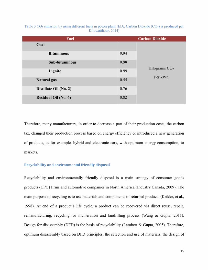
Table 3 CO2 emission by using different fuels in power plant (EIA, Carbon Dioxide (CO2) is produced per

Kilowatthour, 2014) .................................................................................................................................... 15

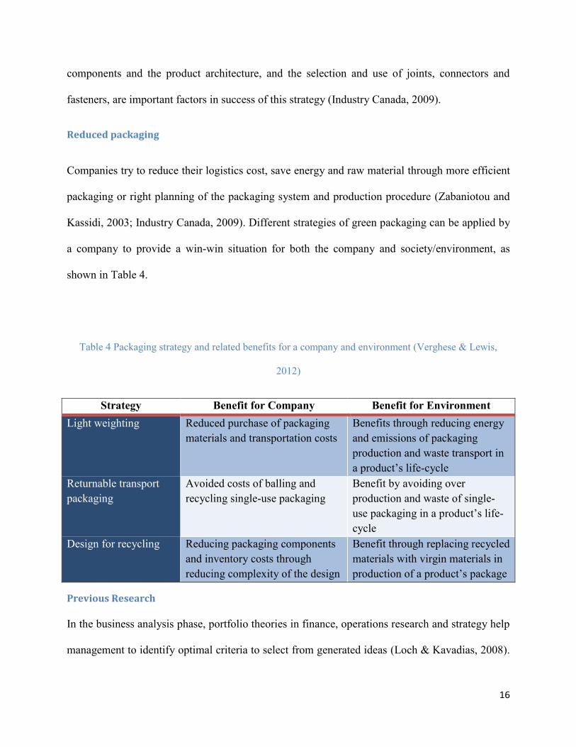
Table 4 Packaging strategy and related benefits for a company and environment (Verghese & Lewis,

2012)............................................................................................................................................................ 16

Table 5 Indices, sets, etc. of mathematical model ....................................................................................... 23

Table 6 Recycling process of blender’s components in the numerical example ......................................... 36

Table 7 Results of numerical example based on all stages of the product life-cycle .................................. 38

Table 8 Results of numerical example based on production stage of the product life-cycle ...................... 38

Table 9 Three main modules of a car at the numerical example ................................................................. 52

Table 10 Each car’s sub-class based on level of greenness at the numerical example ............................... 53

Table 11 Maximum profit and total demand of the company from the product family .............................. 56

Table 12 Result of development of product A in each year ........................................................................ 56

Table 13 Result of development of product B in each year ........................................................................ 57

Table 14 Result of development of product C in each year ........................................................................ 58

Table 15 Sensitivity analysis of demand and profit to the λ1 ..................................................................... 59

Table 16 Sensitivity analysis of demand and profit to the initial development budget ............................... 61

1

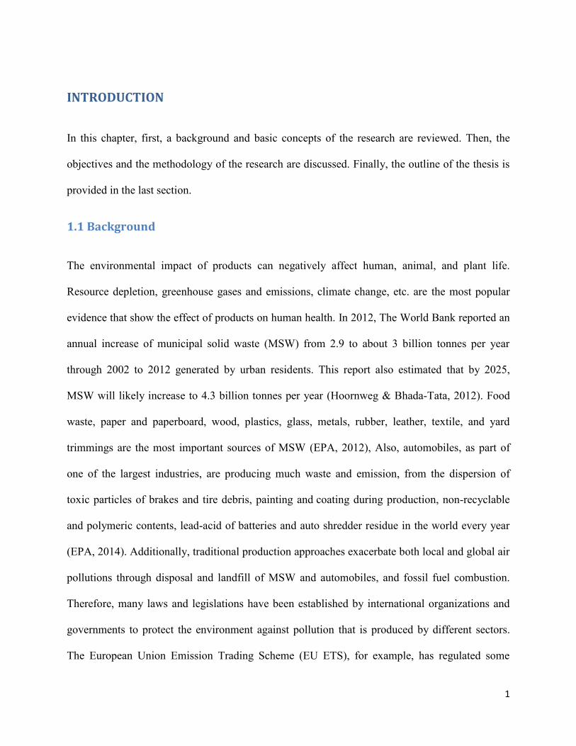
INTRODUCTION

In this chapter, first, a background and basic concepts of the research are reviewed. Then, the

objectives and the methodology of the research are discussed. Finally, the outline of the thesis is

provided in the last section.

1.1 Background

The environmental impact of products can negatively affect human, animal, and plant life.

Resource depletion, greenhouse gases and emissions, climate change, etc. are the most popular

evidence that show the effect of products on human health. In 2012, The World Bank reported an

annual increase of municipal solid waste (MSW) from 2.9 to about 3 billion tonnes per year

through 2002 to 2012 generated by urban residents. This report also estimated that by 2025,

MSW will likely increase to 4.3 billion tonnes per year (Hoornweg & Bhada-Tata, 2012). Food

waste, paper and paperboard, wood, plastics, glass, metals, rubber, leather, textile, and yard

trimmings are the most important sources of MSW (EPA, 2012), Also, automobiles, as part of

one of the largest industries, are producing much waste and emission, from the dispersion of

toxic particles of brakes and tire debris, painting and coating during production, non-recyclable

and polymeric contents, lead-acid of batteries and auto shredder residue in the world every year

(EPA, 2014). Additionally, traditional production approaches exacerbate both local and global air

pollutions through disposal and landfill of MSW and automobiles, and fossil fuel combustion.

Therefore, many laws and legislations have been established by international organizations and

governments to protect the environment against pollution that is produced by different sectors.

The European Union Emission Trading Scheme (EU ETS), for example, has regulated some

2

targets, known as the 20-20-20 package, to restrict and control manufacturing enterprises’ CO2

emissions and air pollution generation of its country members by 2020 (IEA, 2009). The US

Environmental Protection Agency established some standards in order to control local pollution

of industries against the occurrence of carboxyhemoglobin levels in human blood associated with

health effects of concern (EPA, 2011). These environmental legislations help countries to provide

some parameters to define the level of corporate responsibility and accountability of companies

(D`Souza, et al., 2006). To address these concerns, manufacturing enterprises have to modify

their business or production process in order to be aligned with environmental policies. At the

same time, the number of consumers that would rather purchase a ‘green’ or environmentally

friendly product over a comparably priced ordinary product has boosted since 2008 (Savale, et

al., 2012). In the automotive industry, for example, the sale of hybrid and electric cars has

increased up to 426,000 units in the U.S. at the end of September 2013, 30% greater than the

same period in 2012 (Shahan, 2013). Also, car manufacturers expect to sell about 6,000,000

electric cars by 2020 around the world (IEA, 2013). Thus, many companies adopt sustainable

practices in their product designs and production processes to increase corporate responsibility,

create product differentiation, and grow customer demand for environmentally friendly and

energy efficient products (Industry Canada, 2009).

Since 1970, Design for Environment (DFE) has been introduced as a most effective way to

minimize environmental impacts, while it can improve products’ quality (Ulrich & Eppinger,

2012). DFE is a type of product design that provides a practical method to minimize the

environmental impact of a product (Ulrich & Eppinger, 2012; Wang & Gupta, 2011). Today DFE

can be applied even on all parts of a product (Wasik, 1996). Therefore, it offers numerous

opportunities for manufacturers to fulfill DFE strategies on a part or all parts of the product.

3

Nevertheless, the product development process is highly uncertain and is a high investment

process in many industries (Gerhard, et al., 2008). Thus, manufacturers try to reduce risk and to

control uncertainty of implementation of each strategy through financial analysis of a new

product in different stages of the development process.

1. 2 New Product Development

Different scholars have proposed different variations of the NPD process (Cooper, 1988; Zirger

& Maidique, 1990; Gerhard, Brem, & Voigt, 2008; Ulrich & Eppinger, 2012). According to

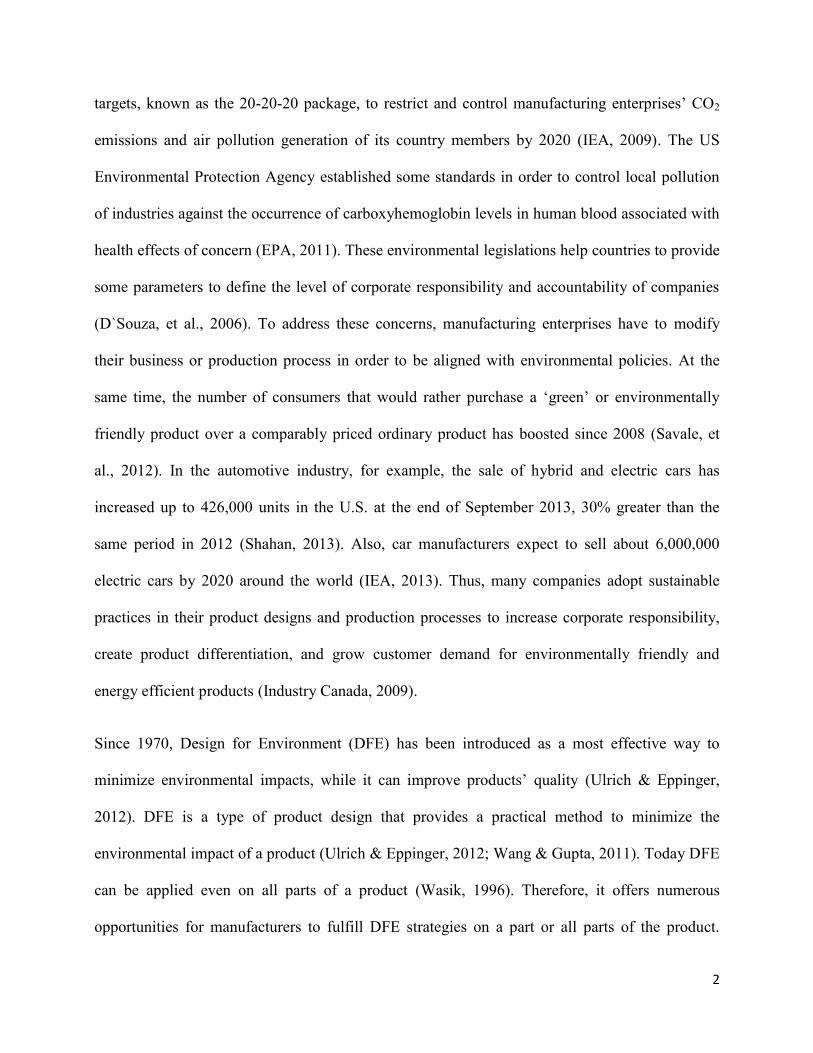
Booz, Allen, and Hamilton’s (1992) classic model, a new product can be developed in seven

stages, as illustrated in Figure 1.

Figure 1 Booz, Allen, and Hamilton’s classic new product development process model (Booz, et al., 1982)

In the first stage, a company has to define missions and objectives that new products must

achieve to satisfy consumers’ needs. The second stage of the process is generating a pool of ideas

from any potential idea source based on goals and objectives that are determined in the first stage.

Screening and Evaluation is the third stage of the new product development process, where an

idea generated in the second stage has to be analysed based on its potential contribution to the

market. The remaining ideas of stage three have to be assessed in the business analysis stage in

4

order to identify the financial situation of product ideas’ launch on the market and decide whether

to develop the idea into a new product or not. In the development stage, an idea that successfully

met all conditions of previous stages will be transferred into a real world product offering. In this

stage, different prototypes are built for laboratory testing and test marketing. Finally, in

commercialization, a new product is introduced to the market, while the new product’s bugs

should quickly be resolved (Booz, et al., 1982).

This process can be divided into predevelopment (strategy, idea generation, screening and

evaluation, and business analysis) and development (development, testing and

commercialization) (Cooper, 1988). The predevelopment phase has a significant effect on new

product success or failure (Cooper, 1988; Booz, et al., 1982). Hence, financial evaluation of a

new product has to be done in the predevelopment phase, because after this point it is very

difficult and expensive to turn back (Cooper, 1988; Gerhard, Brem, & Voigt, 2008).

1. 3 Business Analysis

Many factors beyond product specifications and performance can affect the product’s success on

the market (Annacchino, 2003). Sometimes, for instance, consumers struggle to change their

behavior towards green purchases. This can occur due to brand loyalty, habit, lack of

information, lifestyle, etc. (Young, et al., 2010). Thus, business analysis helps decision makers to

identify other associated factors which affect the success of a new product on the market, such as:

barriers to entry, current and potential competitors, target markets, market growth information,

financial projections, etc., before development begins (Booz, et al., 1982).

As previously mentioned, the business analysis as a last part of predevelopment helps decision

makers to assess the capability of ideas, which are selected in the screening and evaluation stage

5

of the NPD process, for translation into viable offerings (Booz, et al., 1982). The purpose of

financial projection in business analysis is to clarify the future demand, costs, sales and

profitability of the new product for decision makers (Havaldar, 2014). The financial projection of

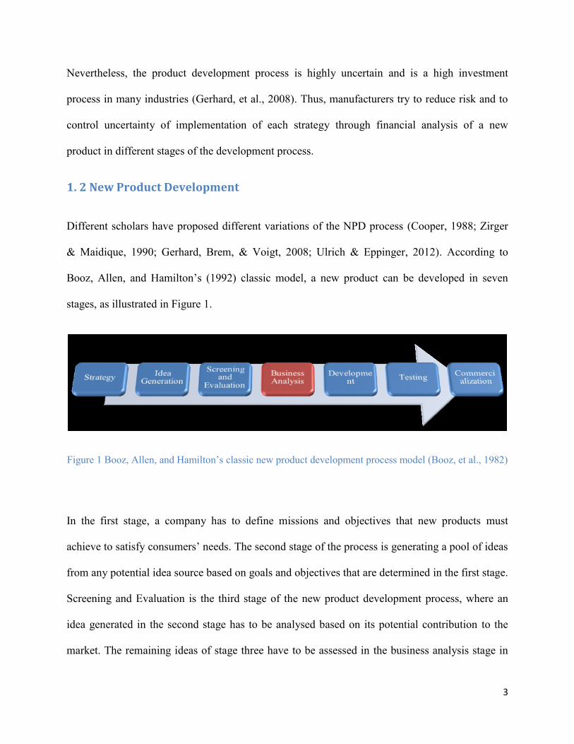
a new product can be broadly categorized into five sections:

Figure 2 Concepts of financial projection (Barrios & Kenntoft, 2008)

As illustrated in Figure 2, the first step of business analysis is sales forecasting. In sales

forecasting, a company estimates total potential market and a new product’s demand in each time

period. Besides sales forecasting, cannibalization of sales helps decision makers to estimate the

degree that the new product can cannibalize the sales of the existing products of the company

(Barrios & Kenntoft, 2008). In the next step, companies have to estimate the new product’s cost.

Cost estimation includes direct costs, investment costs, and overhead costs (Lancaster &

Massingham, 2011). Profit projection is another part of the financial analysis that includes break-

even analysis. Profit projection is determined based on cost estimation and sales forecasting.

Although environmental burdens, competitiveness among companies, and, most importantly,

6

social responsibility could be regarded as significant factors of greening manufactured products

among companies (Albino, Balice and Dangelico 2009, Industry Canada 2009), the

implementation of DFE strategies need different facilities that affect production factors and

product development processes with dissimilar costs for the company. A company’s main goal is

to define strategies to achieve maximum benefits given threats and opportunities that exist in the

related industry. Moreover, profitability of a company is related to its ability to introduce

products that are successful on the market (Kumar & Chatterjee , 2013). Thus, different

verification methods either through physical tests or numerical calculations are needed to assess

the acceptability of a design strategy and compliance with the environment of a new product, as

with other products. In this stage, a profit analysis, as an analytical method, helps managers to

compare different design approaches based on estimated cost and performance (Fiksel, 2011).

Based on this analysis, companies can have a proper forecast of economic effects (profitability)

of the project before introducing the products to the market. Eventually, the risk of related to each

outcome should be assessed by some techniques and processes (Barrios & Kenntoft, 2008).

1.4 Product Life-Cycle

In a green product, “life-cycle thinking is the basis of DFE” (Fiksel, 2011; Ulrich & Eppinger,

2012). The recycling process is a parameter that cannot be considered in the short-term. It takes

place at the end of the product life. Thus, the product life cycle analysis, as opposed to a cross-

sectional analysis, can provide a proper forecast of associated costs and revenues of the product

in the future. Ulrich and Eppinger (2012) proposed a natural life cycle and a product life cycle for

sustainable products. The product life cycle consists of extraction and processing of raw

materials, production, distribution, use, and recovery of the used product. The natural life cycle,

however, represents the effect of each material on nature and reproduction of raw materials after

7

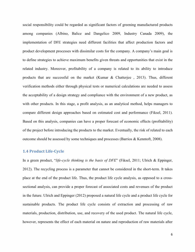
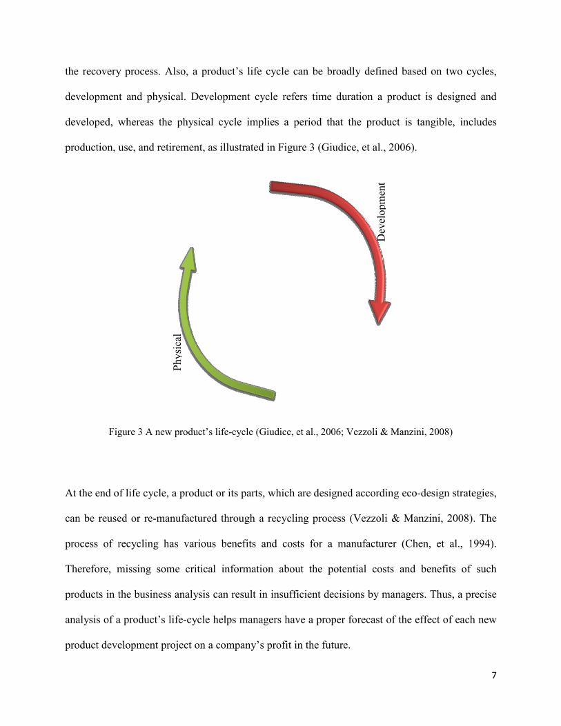
the recovery process. Also, a product’s life cycle can be broadly defined based on two cycles,

development and physical. Development cycle refers time duration a product is designed and

developed, whereas the physical cycle implies a period that the product is tangible, includes

production, use, and retirement, as illustrated in Figure 3 (Giudice, et al., 2006).

Figure 3 A new product’s life-cycle (Giudice, et al., 2006; Vezzoli & Manzini, 2008)

At the end of life cycle, a product or its parts, which are designed according eco-design strategies,

can be reused or re-manufactured through a recycling process (Vezzoli & Manzini, 2008). The

process of recycling has various benefits and costs for a manufacturer (Chen, et al., 1994).

Therefore, missing some critical information about the potential costs and benefits of such

products in the business analysis can result in insufficient decisions by managers. Thus, a precise

analysis of a product’s life-cycle helps managers have a proper forecast of the effect of each new

product development project on a company’s profit in the future.

Physi

cal

Dev

elopm

ent

8

1.5 Objectives and Methodology

This research aims to develop a comprehensive model to estimate the profit of a new green

product in the business analysis stage of an NPD process. The model presented here is based on

design for environment (DFE) strategies of the government of Canada (Industry Canada, 2009)

for simple products such as electronic appliances and complex products such as automobiles. In

order to achieve this, a dynamic model in terms of a life-cycle framework is proposed

First, DFE principles, goals, and strategies’ literature in NPD are reviewed. Second, the trade-off

and profit analysis methods of sustainable products are examined and gaps and opportunities, and

effective parameters of consumers’ demand in green products are identified. Third, DFE

strategies and green products’ demand are analyzed in order to formulate a green product’s

related costs and revenues and consumers’ demand in the product’s life-cycle. Fourth, a mixed

integer model is proposed based on deterministic parameters for a simple new green product.

Finally, the model is developed based on dynamic programming and qualitative choice models

for the automotive industry.

The model is designed based on energy and emission efficiency, recyclability and environmental

friendly disposal strategies. In the model, a product’s life-cycle costs are broadly divided into

four categories: recycling cost, development cost, production cost, and emission tax. The

product’s revenues are defined in three categories: revenue of used parts, revenue of recycled

materials, and sales revenue, in its life-cycle. Then, the model is developed for a dynamic

situation and effective parameters of consumers’ demand are formulated based on a Generalized

Extreme Value (GEV) model.

9

1.6 Thesis Structure

The research presented in this thesis is organized in four chapters. In the next chapter, the

literature on the design for environment and profit analysis of green products is reviewed. In the

third chapter, a mixed integer model is proposed for trade-off analysis of new green products. In

the fourth chapter, the model is developed based on the Bellman equation and Generalized

Extreme Value (GEV) models. Finally, in chapter five, conclusions, limitations, and

opportunities for future research are presented.

10

2. Literature Review

In this chapter, a review of design for environment literature is presented.

2.1 Design for the Environment (DFE)

Firms try to improve their competitive advantage via product innovation to survive in a globally

competitive world. The main goal of innovation, based on initial functionality and cost of

technology, is to meet demand requirements of consumers or to reduce the price of a product

(Adner & Levinthal, 2001). In green products, however, the aim of innovation is reducing

environmental impact and improving product performance, which may increase or decrease the

price of the product. Nevertheless, companies are trying to produce new products to be either

more durable and energy efficient or more recyclable in order to add more value for their

consumers through long-term environmental benefits (Wasik, 1996). Since the 1990s, a new type

of design for X, called design for the environment (DFE), was proposed by scholars to designers

in order to consider their social and environmental responsibilities instead of only commercial

interests. In the DFE approach, a systematic practice has been applied by companies to maintain

or improve their product’s quality while reducing environmental impact (Ulrich & Eppinger,

2012). To achieve this goal, different rules can be defined by a company. In 2006, Luttropp and

Lagerstedt recommended The Ten Golden Rules, as eco-design guidelines in the process of

product development (Luttropp & Lagerstedt, 2006):

1. “Do not use toxic substances and utilize closed loops for necessary but toxic ones.

2. Minimize energy and resource consumption in the production phase and transport through

improved housekeeping.

11

3. Use structural features and high quality materials to minimize weight in products if such

choices do not interfere with necessary flexibility, impact strength or other functional

priorities.

4. Minimize energy and resource consumption in the usage phase, especially for products

with the most significant aspects in the usage phase.

5. Promote repair and upgrading, especially for system-dependent products. (e.g. cell

phones, computers and CD players).

6. Promote long life, especially for products with significant environmental aspects outside

of the usage phase.

7. Invest in better materials, surface treatments or structural arrangements to protect

products from dirt, corrosion and wear, thereby ensuring reduced maintenance and longer

product life.

8. Prearrange upgrading, repair and recycling through access ability, labelling, modules,

breaking points and manuals.

9. Promote upgrading, repair and recycling by using few, simple, recycled, not blended

materials and no alloys.

10. Use as few joining elements as possible and use screws, adhesives, welding, snap fits,

geometric locking, etc. according to the life cycle scenario.”

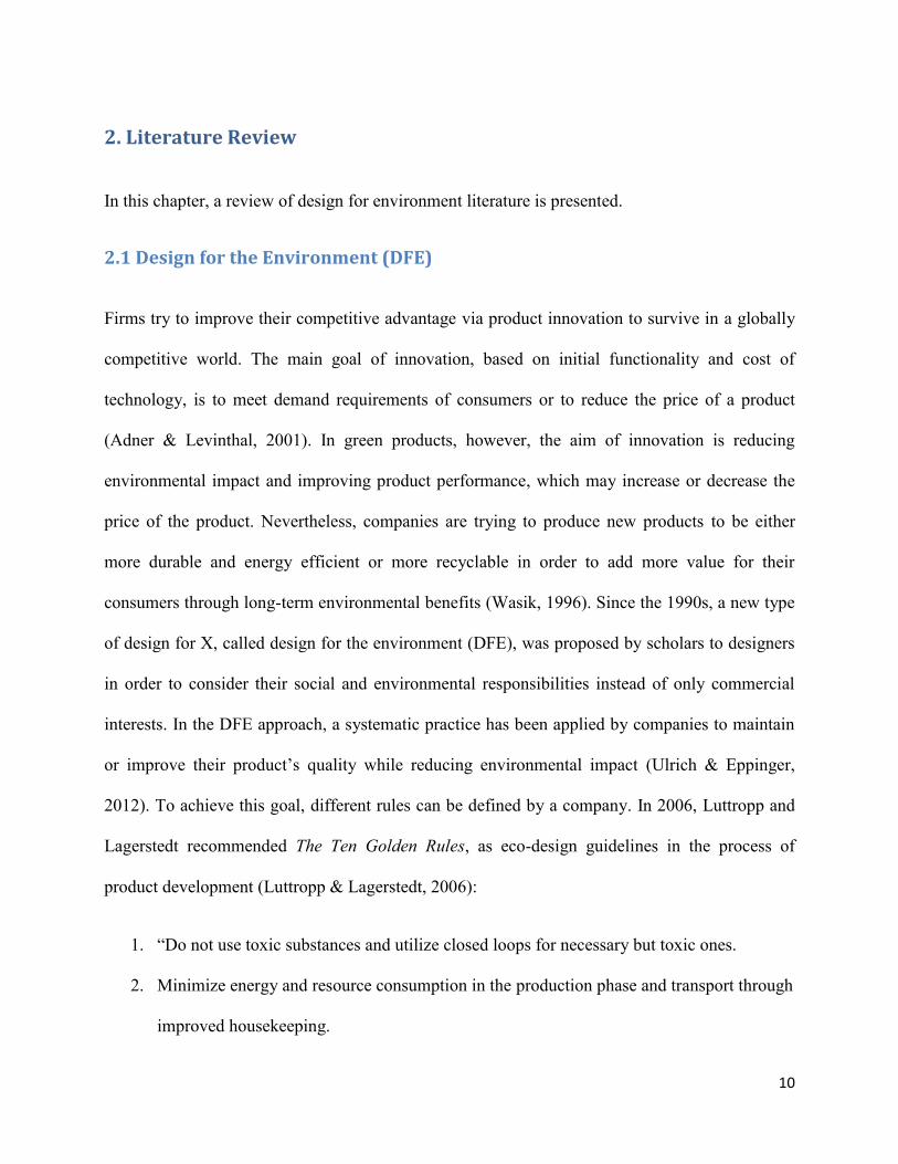
Also, some authors proposed DFE guidelines based on physical life-cycle stages, as illustrated in

Figure 4 (Ulrich & Eppinger, 2012).

12

Figure 4 DFE guideline based on a product’s life-cycle stage (Ulrich & Eppinger, 2012)

Based on such rules, different strategies are proposed to develop environmentally friendly

products. Hart (1997) identified three strategies to address environmental sustainability

challenges: (1) pollution prevention, (2) product stewardship and (3) clean technology (Albino, et

al., 2009). Boons (2002) proposed six options to reduce the ecological impact of a product in

product chain management: (1) Material Reduction, (2) Material Substitution, (3) Material

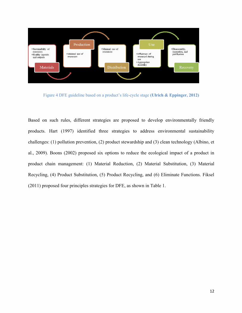
Recycling, (4) Product Substitution, (5) Product Recycling, and (6) Eliminate Functions. Fiksel

(2011) proposed four principles strategies for DFE, as shown in Table 1.

13

Table 1 Fiksel’s four principal strategies in DFE (Fiksel, 2011)

Strategy Guideline

Design for dematerialization

Design for energy and material conservation

Design for source reduction

Design for servicization

Design for detoxification

Design for release reduction

Design for hazard reduction

Design for benign waste disposition

Design for revalorization

Design for product recovery

Design for product disassembly

Design for recyclability

Design for capital protection & renewal

Design for human capital

Design for natural capital

Design for economic capital

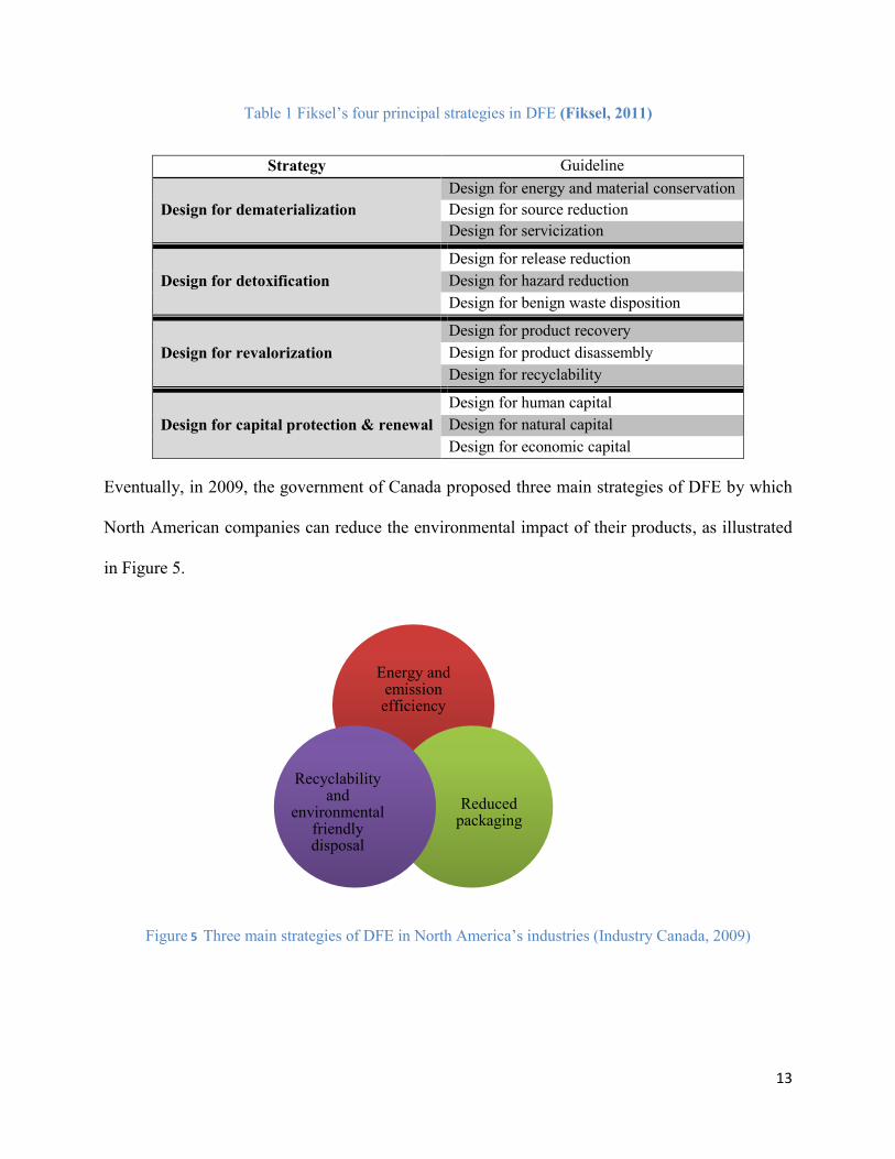
Eventually, in 2009, the government of Canada proposed three main strategies of DFE by which

North American companies can reduce the environmental impact of their products, as illustrated

in Figure 5.

Figure 5 Three main strategies of DFE in North America’s industries (Industry Canada, 2009)

Energy and emission efficiency

Reduced packaging

Recyclability and

environmental friendly disposal

14

Energy and emission efficiency

In 2011, while the use of energy produced 83% of greenhouse gases, 51% of this energy was

used by industries worldwide (IEA, 2013). In many countries, governments decided to reduce

emissions of products via forcing individuals, businesses, industry and others to pay a part of the

cost of negative effects of fuel consumption through a carbon tax (British Columbia, 2014).

Carbon price or carbon tax is the amount that must be paid as a tax or the permit cost in exchange

for the equivalent CO2 emission per tonne of greenhouse gases (British Columbia, 2014). The

main sources of carbon dioxide emissions in industrial plants are combustion of fossil fuels (e.g.

coal, oil and natural gas) and chemical reactions that do not involve combustion (such as

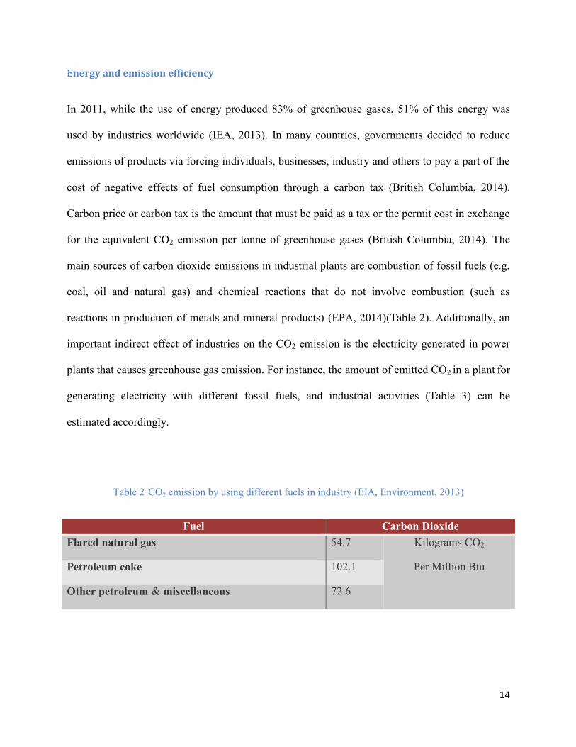
reactions in production of metals and mineral products) (EPA, 2014)(Table 2). Additionally, an

important indirect effect of industries on the CO2 emission is the electricity generated in power

plants that causes greenhouse gas emission. For instance, the amount of emitted CO2 in a plant for

generating electricity with different fossil fuels, and industrial activities (Table 3) can be

estimated accordingly.

Table 2 CO2 emission by using different fuels in industry (EIA, Environment, 2013)

Fuel Carbon Dioxide

Flared natural gas 54.7 Kilograms CO2

Per Million Btu Petroleum coke 102.1

Other petroleum & miscellaneous 72.6

15

Table 3 CO2 emission by using different fuels in power plant (EIA, Carbon Dioxide (CO2) is produced per

Kilowatthour, 2014)

Fuel Carbon Dioxide

Coal

Kilograms CO2

Per kWh

Bituminous 0.94

Sub-bituminous 0.98

Lignite 0.99

Natural gas 0.55

Distillate Oil (No. 2) 0.76

Residual Oil (No. 6) 0.82

Therefore, many manufacturers, in order to decrease a part of their production costs, the carbon

tax, changed their production process based on energy efficiency or introduced a new generation

of products, as for example, hybrid and electronic cars, with optimum energy consumption, to

markets.

Recyclability and environmental friendly disposal

Recyclability and environmentally friendly disposal is a main strategy of consumer goods

products (CPG) firms and automotive companies in North America (Industry Canada, 2009). The

main purpose of recycling is to use materials and components of returned products (Krikke, et al.,

1998). At end of a product’s life cycle, a product can be recovered via direct reuse, repair,

remanufacturing, recycling, or incineration and landfilling process (Wang & Gupta, 2011).

Design for disassembly (DFD) is the basis of recyclability (Lambert & Gupta, 2005). Therefore,

optimum disassembly based on DFD principles, the selection and use of materials, the design of

16

components and the product architecture, and the selection and use of joints, connectors and

fasteners, are important factors in success of this strategy (Industry Canada, 2009).

Reduced packaging

Companies try to reduce their logistics cost, save energy and raw material through more efficient

packaging or right planning of the packaging system and production procedure (Zabaniotou and

Kassidi, 2003; Industry Canada, 2009). Different strategies of green packaging can be applied by

a company to provide a win-win situation for both the company and society/environment, as

shown in Table 4.

Table 4 Packaging strategy and related benefits for a company and environment (Verghese & Lewis,

2012)

Strategy Benefit for Company Benefit for Environment

Light weighting Reduced purchase of packaging

materials and transportation costs

Benefits through reducing energy

and emissions of packaging

production and waste transport in

a product’s life-cycle

Returnable transport

packaging

Avoided costs of balling and

recycling single-use packaging

Benefit by avoiding over

production and waste of single-

use packaging in a product’s life-

cycle

Design for recycling Reducing packaging components

and inventory costs through

reducing complexity of the design

Benefit through replacing recycled

materials with virgin materials in

production of a product’s package

Previous Research

In the business analysis phase, portfolio theories in finance, operations research and strategy help

management to identify optimal criteria to select from generated ideas (Loch & Kavadias, 2008).

17

These concepts are used by many scholars for analyzing the financial situation of NPD projects.

Chao, Kavadias, and Gaimon (2009) proposed a dynamic model to allocate resources to NPD

programs in a portfolio with a focus on how funding authorities and incentives affect a manager’s

decisions. Kleber (2006) introduced a dynamic model for assessing the financial impact of

investment decisions regarding product recovery based on product life cycle and a returns

availability cycle. Also, Repenning (2000) developed a dynamic model for the allocation of

resources between current and future projects in multi-project development environment. These

papers focused on either different aspects of portfolio theories that affect managers’ decisions or

individual product performance, such as: sales, profit, development cost, and production cost, in

business analysis of NPD projects. A development project’s success, however, is related to

portfolio decisions, such as resource allocation (Loch & Kavadias, 2008), analysis of individual

product performance, such as cost saving (Adner & Levinthal, 2001), and many different

performance determinants; such as: barriers to entry, current and potential competitors, target

markets, market growth information, etc. (Booz, et al., 1982). Also, many scholars focused on

profit analysis of green products based on the level of production. Chen, Navin-Chandra, and

Prinz (1994) proposed a Cost-Volume-Profit (C-V-P) model of recycling to assess the balance

between costs and revenues of disassembly and recycling of a product. Also, Tsai et al. (2012)

developed a mathematical model for a green product mix decision based on activity-based

costing to evaluate the benefits of expanding various types of capacity. The paper focused on

traditional manufacturing costs (machine, labour, and material) and piecewise CO2 emission cost

as the main parameters of a green product mix decision. Raz, Druehl, and Blass (2013) proposed

an analytical model to find the production quantity of products which should be designed for the

environment, based on the newsvendor model. It focuses on eco-efficient innovations in the

manufacturing stage and demand-enhancing innovations. These studies only focused on a

18

particular stage of a product’s life while, as mentioned before, life-cycle thinking needs to be the

basis of DFE (Ulrich & Eppinger, 2012). Many studies have focused on Life-Cycle Cost (LCC)

approaches (Ribeiro, Peças, & Henriques, 2013; Kirkham, 2005; Asselin-Balençon & Jolliet ,

2014; Krozer, 2008); however they attempt to introduce different methodologies to estimate a

product cost at different stages of the product life-cycle, but do not give attention to how life-

cycle approaches can be useful for decision makers to assess optimum production levels for

maximizing the profit of the company in all stages of the product life-cycle.

2.2 Summary

In sustainable products, which are designed based on DFE strategies, different hidden costs and

revenues have to be considered in profit analysis. Previous studies mostly focused on production

costs and sales revenue of products in the business analysis of a new product. All the hidden costs

and revenues can affect the decision of decision makers about the future of a new product

development project. Also, these studies do not provide a comprehensive model to evaluate the

effect of different parameters (number of products produced and recycled, demand for green

products) on a green product’s profitability. Although each of these parameters is investigated in

separate research, there is a gap in better understanding their combined effect on the net profit of

a company.

This thesis focuses on the profit analysis of green products based on life-cycle framework to

answer some critical questions for helping decision makers to estimate the profitability of a new

product which is designed for the environment. Some of these questions include: How many

products should be produced based on market demand at a given period in the future? How many

of the products sold have to be recycled by the company in future periods when a product is

designed based on a recyclability and environmentally friendly disposal strategy? What is the

19

effect of these decisions on the company’s profit in the future? The model presented in this thesis

pays specific attention to the economic impact of a newly designed product upon related

environmental parameters, such as: energy consumption, recycling cost and revenue, and carbon

price which is the amount paid to the government as a tax due to statutory regulations. Thus,

management can decide about the future of their new products based on the results of the trade-

off analysis. In sum, the primary model can determine how many products should be produced

and how many of them should be recycled in order to maximize the profit of the companies with

employ the potential costs and benefits of recyclability, disassembly, and environmentally

friendly disposal strategy. Then, the developed model considers the effect of portfolio decisions,

individual product performance and other performance determinants together in order to improve

the reliability of the decisions in the profit analysis of a new green product.

20

3. Trade-off Analysis of Green Products Based on Life-Cycle Thinking

In the trade-off analysis process of new products, five basic cash flows can be defined (Chase, et

al., 2006): (1) Development cost, (2) Ramp-up cost, (3) Marketing cost, (4) Production cost, and

(5) Sales revenue. In the life cycle approach, however, costs and revenues of a product life cycle

can occur in three phases; development, use, and recycling or reprocessing. Development

includes production, sales, and the product development process, while use and recycling phases,

as a subsequent cost, include recycling cost (Niemann, et al., 2009). Our model focuses on the

development and recycling phases. The related costs of these phases can be broadly divided into

three categories: Product Development Process Cost, Production Cost, and Recycling Cost.

Analogous to costs, revenues also can be allocated via product sale and used parts and recycled

materials in the recycling process.

Furthermore, the main effect of the implementation of the recycling process in the product life

cycle is reducing the environmental impact of a product via conserving natural resources and

decreasing the amount of harmful effects in the manufacturing process (Bajpai, 2014). Also, the

energy needed to recycle many materials and components of a product is less than the energy

required to produce it originally (Morris, 1996). In the paper industry, for example, every tonne

of recycled fibre that displaces a tonne of virgin fibre will bring 27% of total energy consumption

saving for a company (Bajpai, 2014). The energy consumption, fuel for manufacturing, directly

affects pollution emissions. Thus, companies can reduce their pollution emission via energy

conserved. Hence, we need to consider other parameters related to energy consumption and

recycling activities as part of cash flows in the product development project. Thus the cost of

disassembly, cost of shredding, revenue of used parts, revenue of recycled material, etc. and

21

benefit of energy reduction from energy saving as effective parameters have to be considered in

the estimation of profits.

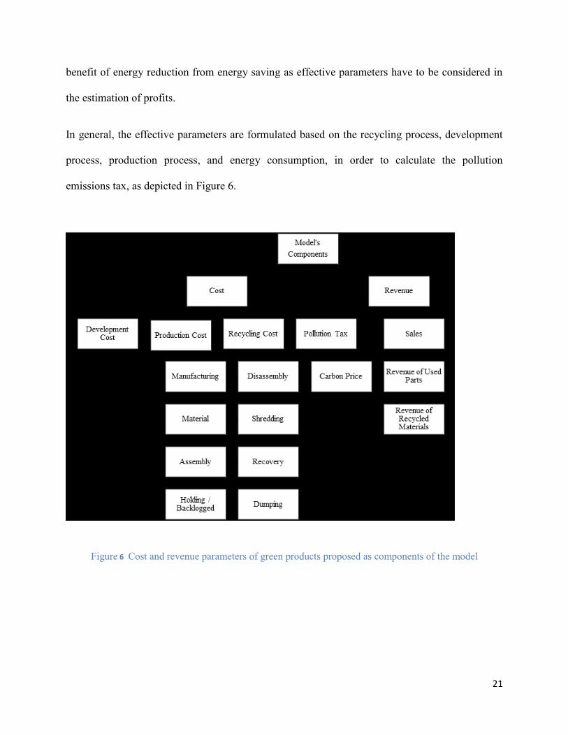
In general, the effective parameters are formulated based on the recycling process, development

process, production process, and energy consumption, in order to calculate the pollution

emissions tax, as depicted in Figure 6.

Figure 6 Cost and revenue parameters of green products proposed as components of the model

22

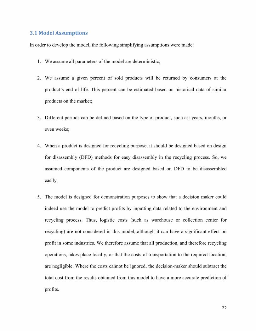
3.1 Model Assumptions

In order to develop the model, the following simplifying assumptions were made:

1. We assume all parameters of the model are deterministic;

2. We assume a given percent of sold products will be returned by consumers at the

product’s end of life. This percent can be estimated based on historical data of similar

products on the market;

3. Different periods can be defined based on the type of product, such as: years, months, or

even weeks;

4. When a product is designed for recycling purpose, it should be designed based on design

for disassembly (DFD) methods for easy disassembly in the recycling process. So, we

assumed components of the product are designed based on DFD to be disassembled

easily.

5. The model is designed for demonstration purposes to show that a decision maker could

indeed use the model to predict profits by inputting data related to the environment and

recycling process. Thus, logistic costs (such as warehouse or collection center for

recycling) are not considered in this model, although it can have a significant effect on

profit in some industries. We therefore assume that all production, and therefore recycling

operations, takes place locally, or that the costs of transportation to the required location,

are negligible. Where the costs cannot be ignored, the decision-maker should subtract the

total cost from the results obtained from this model to have a more accurate prediction of

profits.

23

6. The unit selling prices are constant for the product.

3.2 Mathematical Model

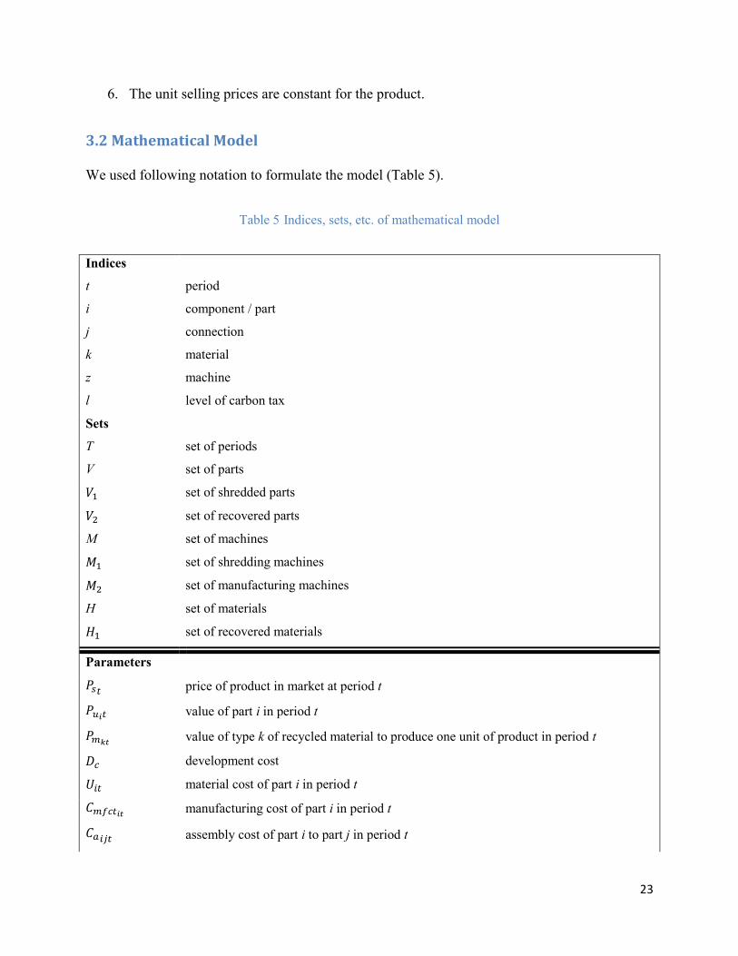
We used following notation to formulate the model (Table 5).

Table 5 Indices, sets, etc. of mathematical model

Indices

t period

i component / part

j connection

k material

z machine

l level of carbon tax

Sets

T set of periods

V set of parts

𝑉1 set of shredded parts

𝑉2 set of recovered parts

M set of machines

𝑀1 set of shredding machines

𝑀2 set of manufacturing machines

H set of materials

𝐻1 set of recovered materials

Parameters

𝑃𝑠𝑡 price of product in market at period t

𝑃𝑢𝑖𝑡 value of part i in period t

𝑃𝑚𝑘𝑡 value of type k of recycled material to produce one unit of product in period t

𝐷𝑐 development cost

𝑈𝑖𝑡 material cost of part i in period t

𝐶𝑚𝑓𝑐𝑡𝑖𝑡 manufacturing cost of part i in period t

𝐶𝑎𝑖𝑗𝑡 assembly cost of part i to part j in period t

24

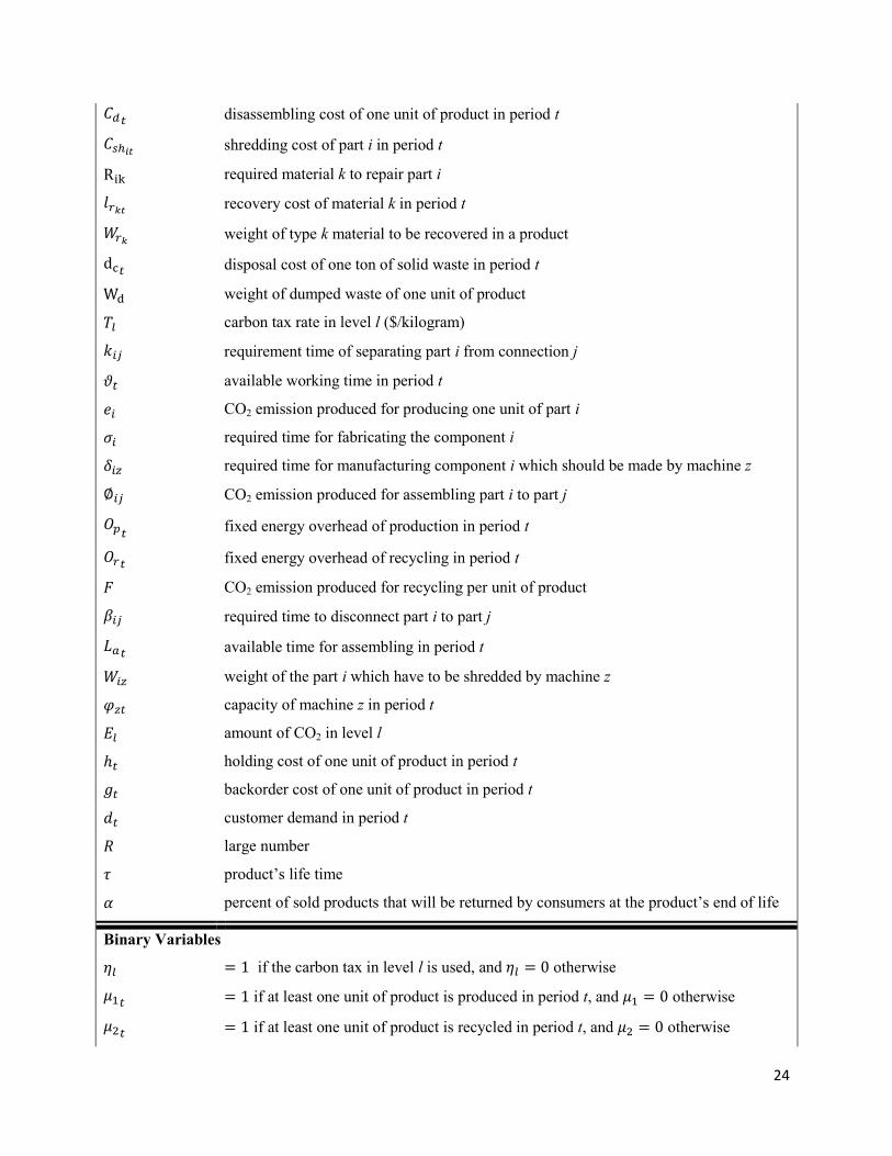
𝐶𝑑𝑡 disassembling cost of one unit of product in period t

𝐶𝑠ℎ𝑖𝑡 shredding cost of part i in period t

Rik required material k to repair part i

𝑙𝑟𝑘𝑡 recovery cost of material k in period t

𝑊𝑟𝑘 weight of type k material to be recovered in a product

dc𝑡 disposal cost of one ton of solid waste in period t

Wd weight of dumped waste of one unit of product

𝑇𝑙 carbon tax rate in level l ($/kilogram)

𝑘𝑖𝑗 requirement time of separating part i from connection j

𝜗𝑡 available working time in period t

𝑒𝑖 CO2 emission produced for producing one unit of part i

𝜎𝑖 required time for fabricating the component i

𝛿𝑖𝑧 required time for manufacturing component i which should be made by machine z

∅𝑖𝑗 CO2 emission produced for assembling part i to part j

𝑂𝑝𝑡 fixed energy overhead of production in period t

𝑂𝑟𝑡 fixed energy overhead of recycling in period t

𝐹 CO2 emission produced for recycling per unit of product

𝛽𝑖𝑗 required time to disconnect part i to part j

𝐿𝑎𝑡 available time for assembling in period t

𝑊𝑖𝑧 weight of the part i which have to be shredded by machine z

𝜑𝑧𝑡 capacity of machine z in period t

𝐸𝑙 amount of CO2 in level l

ℎ𝑡 holding cost of one unit of product in period t

𝑔𝑡 backorder cost of one unit of product in period t

𝑑𝑡 customer demand in period t

𝑅 large number

𝜏 product’s life time

𝛼 percent of sold products that will be returned by consumers at the product’s end of life

Binary Variables

𝜂𝑙 = 1 if the carbon tax in level l is used, and 𝜂𝑙 = 0 otherwise

𝜇1𝑡 = 1 if at least one unit of product is produced in period t, and 𝜇1 = 0 otherwise

𝜇2𝑡 = 1 if at least one unit of product is recycled in period t, and 𝜇2 = 0 otherwise

25

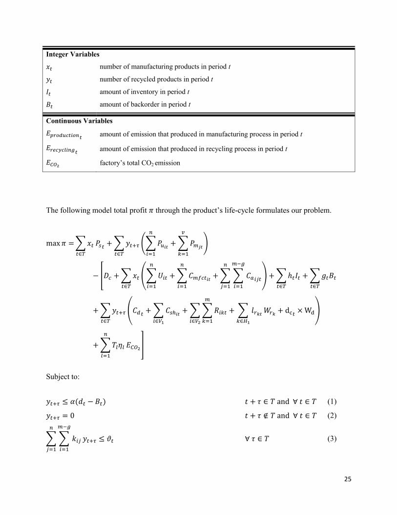
Integer Variables

𝑥𝑡 number of manufacturing products in period t

𝑦𝑡 number of recycled products in period t

𝐼𝑡 amount of inventory in period t

𝐵𝑡 amount of backorder in period t

Continuous Variables

𝐸𝑝𝑟𝑜𝑑𝑢𝑐𝑡𝑖𝑜𝑛𝑡 amount of emission that produced in manufacturing process in period t

𝐸𝑟𝑒𝑐𝑦𝑐𝑙𝑖𝑛𝑔𝑡 amount of emission that produced in recycling process in period t

𝐸𝐶𝑂2 factory’s total CO2 emission

The following model total profit 𝜋 through the product’s life-cycle formulates our problem.

max 𝜋 = ∑ 𝑥𝑡

𝑡∈𝑇

𝑃𝑠𝑡+ ∑ 𝑦𝑡+𝜏

𝑡∈𝑇

(∑ 𝑃𝑢𝑖𝑡

𝑛

𝑖=1

+ ∑ 𝑃𝑚𝑗𝑡

𝑣

𝑘=1

)

− [𝐷𝑐 + ∑ 𝑥𝑡

𝑡∈𝑇

(∑ 𝑈𝑖𝑡

𝑛

𝑖=1

+ ∑ 𝐶𝑚𝑓𝑐𝑡𝑖𝑡

𝑛

𝑖=1

+ ∑ ∑ 𝐶𝑎𝑖𝑗𝑡

𝑚−𝑔

𝑖=1

𝑛

𝑗=1

) + ∑ ℎ𝑡𝐼𝑡

𝑡∈𝑇

+ ∑ 𝑔𝑡𝐵𝑡

𝑡∈𝑇

+ ∑ 𝑦𝑡+𝜏

𝑡∈𝑇

(𝐶𝑑𝑡+ ∑ 𝐶𝑠ℎ𝑖𝑡

𝑖∈𝑉1

+ ∑ ∑ 𝑅𝑖𝑘𝑡

𝑚

𝑘=1𝑖∈𝑉2

+ ∑ 𝑙𝑟𝑘𝑡

𝑘∈𝐻1

𝑊𝑟𝑘+ dc𝑡

× Wd)

+ ∑ 𝑇𝑙𝜂𝑙

𝑛

𝑙=1

𝐸𝐶𝑂2]

Subject to:

𝑦𝑡+𝜏 ≤ 𝛼(𝑑𝑡 − 𝐵𝑡) 𝑡 + 𝜏 ∈ 𝑇 and ∀ 𝑡 ∈ 𝑇 (1)

𝑦𝑡+𝜏 = 0 𝑡 + 𝜏 ∉ 𝑇 and ∀ 𝑡 ∈ 𝑇 (2)

∑ ∑ 𝑘𝑖𝑗

𝑚−𝑔

𝑖=1

𝑛

𝑗=1

𝑦𝑡+𝜏 ≤ 𝜗𝑡 ∀ 𝜏 ∈ 𝑇 (3)

26

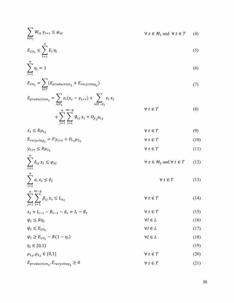
∑ 𝑊𝑖𝑧

𝑖∈𝑉1

𝑦𝑡+𝜏 ≤ 𝜑𝑧𝑡 ∀ 𝑧 ∈ 𝑀1 and ∀ 𝑡 ∈ 𝑇 (4)

𝐸𝐶𝑂2≤ ∑ 𝐸𝑙

𝑛

𝑙=1

𝜂𝑙 (5)

∑ 𝜂𝑙

𝑛

𝑙=1

= 1 (6)

𝐸𝐶𝑂2= ∑(𝐸𝑝𝑟𝑜𝑑𝑢𝑐𝑡𝑖𝑜𝑛𝑡

+ 𝐸𝑟𝑒𝑐𝑦𝑐𝑙𝑖𝑛𝑔𝑡)

𝑡∈𝑇

(7)

𝐸𝑝𝑟𝑜𝑑𝑢𝑐𝑡𝑖𝑜𝑛𝑡= ∑ 𝑒𝑖(𝑥𝑡 − 𝑦𝑡+𝜏)

𝑖∈𝑉2

+ ∑ 𝑒𝑖

𝑖∈𝑉−𝑉2

𝑥𝑡

+ ∑ ∑ ∅𝑖𝑗

𝑚−𝑔

𝑖=1

𝑛

𝑗=1

𝑥𝑡 + 𝑂𝑝𝑡𝜇1𝑡

∀ 𝑡 ∈ 𝑇 (8)

𝑥𝑡 ≤ 𝑅𝜇1𝑡 ∀ 𝑡 ∈ 𝑇 (9)

𝐸𝑟𝑒𝑐𝑦𝑐𝑖𝑛𝑔𝑡= 𝐹𝑦𝑡+𝜏 + 𝑂𝑟𝑡

𝜇2𝑡 ∀ 𝑡 ∈ 𝑇 (10)

𝑦𝑡+𝜏 ≤ 𝑅𝜇2𝑡 ∀ 𝑡 ∈ 𝑇 (11)

∑ 𝛿𝑖𝑧

𝑛

𝑖=1

𝑥𝑡 ≤ 𝜑𝑧𝑡 ∀ 𝑧 ∈ 𝑀2 and ∀ 𝑡 ∈ 𝑇 (12)

∑ 𝜎𝑖

𝑛

𝑖=1

𝑥𝑡 ≤ 𝜗𝑡 ∀ 𝑡 ∈ 𝑇 (13)

∑ ∑ 𝛽𝑖𝑗

𝑚−𝑔

𝑖=1

𝑛

𝑗=1

𝑥𝑡 ≤ 𝐿𝑎𝑡 ∀ 𝑡 ∈ 𝑇 (14)

𝑥𝑡 + 𝐼𝑡−1 − 𝐵𝑡−1 − 𝑑𝑡 = 𝐼𝑡 − 𝐵𝑡 ∀ 𝑡 ∈ 𝑇 (15)

𝜓𝑙 ≤ 𝑅𝜂𝑙 ∀𝑙 ∈ 𝐿 (16)

𝜓𝑙 ≤ 𝐸𝐶𝑂2 ∀𝑙 ∈ 𝐿 (17)

𝜓𝑙 ≥ 𝐸𝐶𝑂2− 𝑅(1 − 𝜂𝑙) ∀𝑙 ∈ 𝐿 (18)

𝜂𝑙 ∈ {0,1} (19)

𝜇1𝑡, 𝜇2𝑡

∈ {0,1} ∀ 𝑡 ∈ 𝑇 (20)

𝐸𝑝𝑟𝑜𝑑𝑢𝑐𝑡𝑖𝑜𝑛𝑡, 𝐸𝑟𝑒𝑐𝑦𝑐𝑙𝑖𝑛𝑔𝑡

≥ 0 ∀ 𝑡 ∈ 𝑇 (21)

27

𝐸𝐶𝑂2≥ 0 (22)

𝑥𝑡, 𝑦𝑡, 𝐼𝑡, 𝐵𝑡 ≥ 0 𝑖𝑛𝑡𝑒𝑔𝑒𝑟 ∀ 𝑡 ∈ 𝑇 (23)

3.3 Model Description

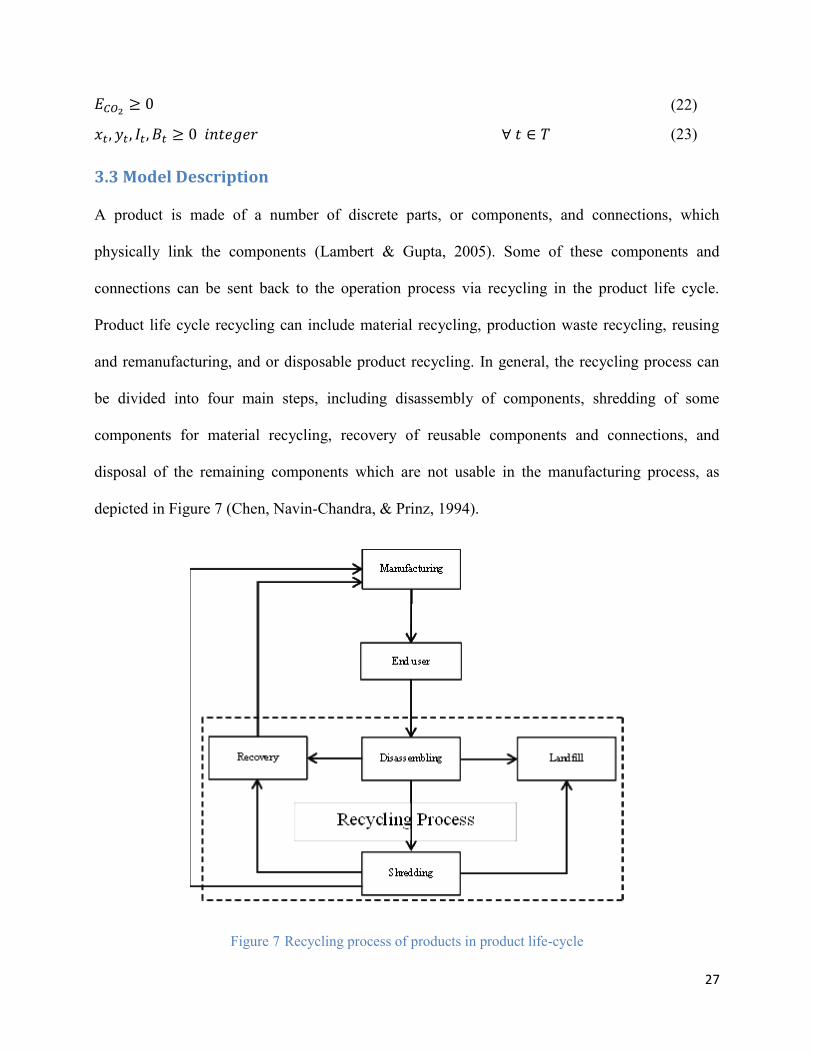
A product is made of a number of discrete parts, or components, and connections, which

physically link the components (Lambert & Gupta, 2005). Some of these components and

connections can be sent back to the operation process via recycling in the product life cycle.

Product life cycle recycling can include material recycling, production waste recycling, reusing

and remanufacturing, and or disposable product recycling. In general, the recycling process can

be divided into four main steps, including disassembly of components, shredding of some

components for material recycling, recovery of reusable components and connections, and

disposal of the remaining components which are not usable in the manufacturing process, as

depicted in Figure 7 (Chen, Navin-Chandra, & Prinz, 1994).

Figure 7 Recycling process of products in product life-cycle

28

The model’s objective is to maximize the total profit of company through the product’s life-cycle.

The objective function is comprised of costs subtracted from revenues. Revenues include sales

revenue and recycling revenue (revenue of used parts and recycled materials), while costs include

product development cost, production cost (material cost, manufacturing cot, and assembly cost),

holding cost, backlogged cost, recycling cost (disassembly cost, shredding cost, recovery cost,

and disposal cost), and carbon price.

As per our assumption, only a given percent of sold products, Alpha (𝛼), will be returned by

consumers at the product’s end of life. Although we assumed 𝛼 can be estimate based on

historical data of similar products on the market, the company needs to determine the minimum

of alpha to assess the risk of its investment. Breakeven analysis is a tool to help decision-makers

determine the point at which a company has no additional profit from NPD (Radomes Jr &

Arango , 2015). To estimate this point, decision makers need to compare total environmental and

operation costs of a new product with that of existing (old) product (Kiatkittipong , et al., 2008).

In this paper, breakeven point helps decision-makers to find out the minimum number of

products that have to be recycled.

Although the model does not calculate the breakeven point of recycling process, the point can be

estimated based on analysis of the profit’s sensitivity to Alpha, as shown in the numerical

example. Thus, constraints (1) and (2) restrict number of recycling products in each period based

on historical data of similar products on the market with respect to breakeven point of recycling

process.

29

3.3.1 Recycling costs

Typically, a company needs to install a set of machines and assign a group of workers in order to

separate the desired components and retrieval of usable components from accumulated products.

Consequently, recycling of a product has a given cost for the company in each stage. So, the

recycling cost comprises cost of disassembly, cost of shredding, cost of recovery, and cost of

disposal. Also, the company will be faced by some limitations due to machines and labor work

capacities which are typically captured by working time.

3.3.1.1 Cost of disassembly

Disassembly is a systematic method of removing desired parts from a product, without any

damage to the parts (Giudice, et al., 2006). It consists of four main tasks, including getting

access, moving, removing, and collecting components (Lambert & Gupta, 2005). These tasks are

costed either through labor or automation.

The disassembly process is a time consuming process in which product parts will be separated by

machines or labor. Total requirement time of separating part i from connection j can be defined

through ∑ ∑ 𝑘𝑖𝑗𝑚−𝑔𝑖=1

𝑛𝑗=1 where n represents the number of different type of connections and m is

the number of same type of joints in products, and g represents number of joints that connect

parts of the same material (Chen, et al., 1994). Constraint (3) restricts the number of products that

can be disassembled according to available working time in period t (𝜗𝑡).

3.3.1.2 Cost of shredding

After disassembling the desired parts, some of these components cannot be repaired for reuse

while their raw materials can be returned in the production process. These components could be

shredded, breaking components at particle size into small pieces, via milling, grinding, etc. in

30

order to increase the material’s homogeneity (Lambert & Gupta, 2005). The cost of shredding has

to be estimated for each part separately since different types of parts which need different

shredding methods might exist.

Also, a limitation should be defined for the number of products according to the maximum

capacity shredding machine z in period t (𝜑𝑧𝑡) based on the weight of the part i which has to be

shredded by machine z (𝑊𝑖𝑧), as shown in constraint (4).

3.3.1.3 Cost of recovery

Some parts are worked on at the end of a product’s useful life. The use of the secondary materials

reduces environmental impact (Lambert & Gupta, 2005). So companies try to return some

reusable parts or materials to the production process via recovery. In general, the recovery

process includes recycling of materials in the manufacturing process and reuse of parts in

assembly process. After disassembly, both shredded materials and disassembled parts need to be

repaired before being returned to the production process. However, the effective factor of

accounting a component recovery cost is its suitability for recovery. It can be determined by

companies based on durability and separability. Thus, after selection testing, proper parts and

materials will be sent for a recovery process. The cost of recovery becomes expensive with

increasing depth of recovery operation. Thus, it is important to determine the volume of recovery

(Giudice, et al., 2006). Hence, the cost of recovery for materials in each period can be calculated

via material recovery cost of type k material in period t (𝑙𝑟𝑘𝑡), k may be steel, plastics, etc. based

on weight of type k material to be recovered in a product (𝑊𝑟𝑘) (Chen, et al., 1994). Furthermore,

recovery cost of parts can be calculated based on the sum of the cost of required materials to

repair part i in period t (Rikt).

31

3.3.1.4 Cost of disposal

Once the suitable components and materials have been recovered, the useless parts of the product

will be sent to waste disposal sites. The waste will be dumped via incineration or landfill.

Incineration can bring energy recovery while it is reducing the waste volume (Lambert & Gupta,

2005). Many wastes have organic materials which can be burnt in an incinerator. So, the

produced energy can be recovered via a boiler, for example, to generation electricity. Finally, the

rest of the waste will be sent to landfill sites. In fact, landfill is the least attractive option in waste

management (Williams, 2005). We assumed the same cost for incineration and landfill, to model

the disposal cost of materials and components, based on the weight of dumped waste of the

product (Wd). Disposal cost can thus be estimated via Equation (6) (Chen, et al., 1994).

3.3.2 Recycling Benefits

As mentioned before, some parts and materials of recycled products can be returned to the

production process via recovery. Thus, two types of revenues can be defined based on recycling

of reusable parts or the recycled materials (Chen, Navin-Chandra, & Prinz, 1994). Each type of

revenue can be formulated according to following parameters.

3.3.2.1 Revenue of used parts

Some parts and modules of a product can be reused in the product’s end-of-life as spare parts or

in other items (Lambert & Gupta, 2005). All the usable parts will be recovered to be reused in

new products. Thus, instead of each part which is used in the new products, companies acquire

given revenues according to value of the part. Revenue of used parts for a product can be

estimated based on total value of recovered parts that used in the product.

32

3.3.2.2 Revenue of recycled material

An important part of recycling is the recovery of materials out of scrap from end-of-life products

(Lambert & Gupta, 2005). Recovered materials can be returned to the production process with

other raw materials. That’s why these are as valuable as recovered parts for companies. Hence,

revenue of recycled materials can be estimated from total value of recovered materials in

producing of a product.

3.3.3 Product Development Cost

New product development is a multi-stage process ( Murthy, et al., 2008), whereby each stage of

this process needs a given budget which is typically calculated based on the number of people

that work as a project team, duration of the development project, and tools that are needed for

production up to the design process (Ulrich & Eppinger, 2012). These costs are not related to the

number of products. So the development costs are considered as fixed costs.

3.3.4 Carbon Price

A carbon price or carbon tax is the amount that must be paid as a tax or the permit cost in

exchange to the equivalent CO2 emission per tonne of greenhouse gases (British Columbia,

2014). Different kinds of energy are used in manufacturing and assembly processes. The amount

of emitted carbon dioxide (CO2) can be calculated based on the consumed energy. However,

carbon tax of used energy is calculated based on policies and legislations in different areas. For

example, in British Columbia (Canada) the carbon tax rates by fuels where natural gas used in

stationary engines of factories has a price of 5.7¢ per cubic metre or about $1.5 per gigajoule

(Tax Bulletin of British Columbia, 2013), while, in Australia the carbon tax is based on the total

emitted carbon dioxide which was about 23$/tonne in 2012 (Australian Government, 2012).

33

In general, the total carbon tax of a factory varies with different countries’ policies regarding the

initial permits and excessively produced carbon dioxide. Carbon price rates in different countries

are similar to the governmental tax which can be even piecewise, stepwise or a linear function

depending on the carbon dioxide emission.

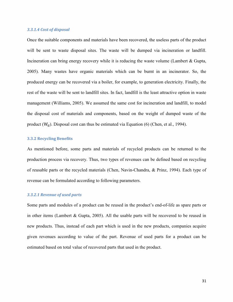
In this model, we assume a stepwise function in order to calculate the manufacturer’s carbon tax,

as shown in Figure 8. Thus the carbon tax is calculated based on the amount of factory’s total

CO2 emission (ECO2) and the carbon tax rate in level l (Tl). Constraints (5) and (6), also, restrict

the model to select proper carbon tax rate level based on the amount of CO2.

Figure 8 Stepwise function of Carbon Tax

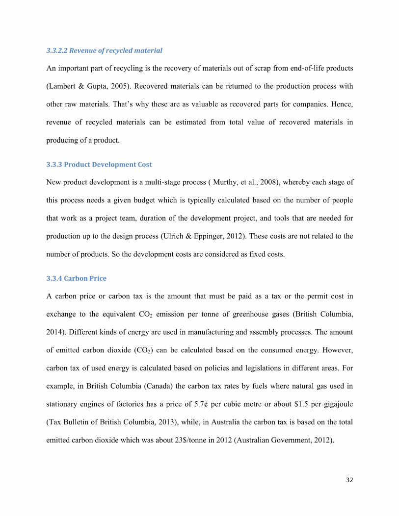
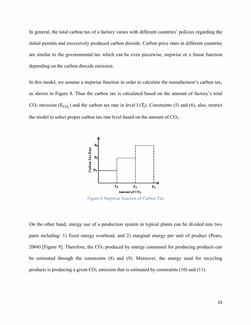
On the other hand, energy use of a production system in typical plants can be divided into two

parts including: 1) fixed energy overhead, and 2) marginal energy per unit of product (Pears,

2004) [Figure 9]. Therefore, the CO2 produced by energy consumed for producing products can

be estimated through the constraints (8) and (9). Moreover, the energy used for recycling

products is producing a given CO2 emission that is estimated by constraints (10) and (11).

34

Figure 9 Energy use of a typical production system (Pears, 2004)

3.3.5 Production cost

When a product is designed based on recycling capability, production cost can be defined

according to three main parameters; material cost, manufacturing cost, and assembly cost

(Giudice, et al., 2006). Also, a company may have inventory or backorder according to customer

demand, so holding and backlogged cost can occur based on a difference between the amount

demanded and the amount of produced in each period.

3.3.5.1 Materials Cost

Material cost can be defined as the related cost of materials per unit of products in period t.

3.3.5.2 Manufacturing Cost

Two main parameters of manufacturing are labor and machine costs. Cost and limitation of

production can be assessed based on these parameters.

In a production process different type of machines will be used to assemble or form the

components of the product, so a set of machines (B) with a limited capacity (𝜑𝑧𝑡) are considered

35

in order to produce the component of products in period t. Constraint (12) limits the number of

products produced according to capacity of the machines. Likewise, a company has a limited

work force in a manufacturing process. This limitation can be captured by time. Constraint (13)

restricts the number of products according to available working hours in period t (𝜗𝑡).

3.3.5.3 Assembly Cost

Assembly cost can be calculated based on total cost of connecting parts i and j together. The

number of products can be limited in the assembly process according to constraint (14). Also, just

as in the disassembly process, a given time (𝛽𝑖𝑗) is needed to connect between part i and j.

3.3.6 Holding Cost and Backlogged Cost

Holding cost and backlogged cost occur when a manufacturer will be faced with positive stock

due to shortage of demand (inventory) or negative stock because of excess demand (backorder) in

each period.

The number of products is restricted by demand in each period, as shown in constraint (15).

The final model is non-linear because ηl is a binary variable and ECO2 is a continuous variable. It

can be solved either by non-linear programming or by linear programming through constraints

(16), (17), and (18), which are linearizing the model by defining ψl = ηlECO2, where, ψl is a

continuous variable (ψl ≥ 0).

36

3.4 Numerical example

An electric juicer producer decides to develop a current model (A-0) of a blender which has

about $2,300,000 annual profit. It should be noted again that the logistic costs are not considered

in the annual profit of the company. The producer wants to introduce a new model (A-1) with

recyclable capability which is designed based on new materials which are compatible with the

environment and it can be disassembled easily. We assumed that the company is operating from

its current, local facilities to collect products at the products’ end of life with negligible cost for

the transportation to the recycling process, so the same logistic costs can be considered for the

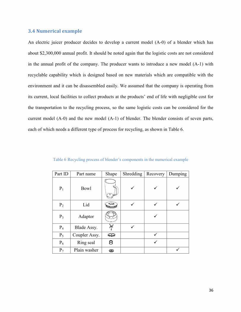
current model (A-0) and the new model (A-1) of blender. The blender consists of seven parts,

each of which needs a different type of process for recycling, as shown in Table 6.

Table 6 Recycling process of blender’s components in the numerical example

Part ID Part name Shape Shredding Recovery Dumping

P1 Bowl

P2 Lid

P3 Adaptor

P4 Blade Assy.

P5 Coupler Assy.

P6 Ring seal

P7 Plain washer

37

Before starting the test and prototype processes, managers need a proper forecast of the economic

performance of this product in the future based on a trade-off analysis. They need useful

information in this step (such as: number of products that have to be produced, number of

recycled products and the amount of CO2 emission based on produced and recycled products) in

order to take a decision about the future of the project. Also, they expect a maximum of 40

percent of the total products sold in each period to be returned for recycling at the end of the

product’s life. Based on a given data (which is generated according to a realistic data from an

electronic appliances manufacturer in Iran, as shown in appendix A), crucial information can be

obtained via the model presented in order to help the managers make decisions.

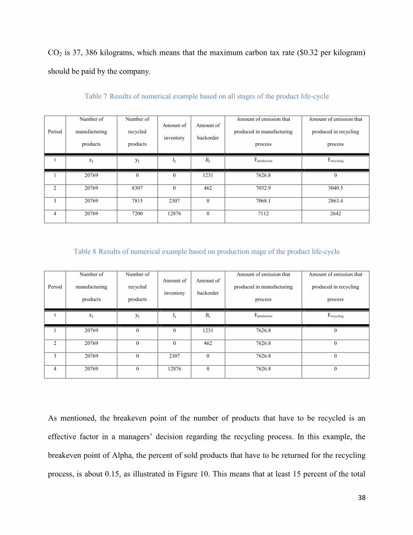
This problem is solved using CPLEX (OPL 12.5.1.0 model), as shown in the Appendix B. The

result shows (Table 7) that the company needs to produce and sell 20,769 units of the product

seasonally while it will have 1231 units and 462 units of backordered demand in season one and

season two respectively and 2307 units and 12,876 units inventory at season three and season

four respectively according to the current demand of the product in each season in the market.

Also, 23,322 units (23322=8307+7815+7200) should be collected for recycling in a year.

Eventually, the company can achieve greater than $2,383,000 annual profits which is about 3.7%

greater than of the company’s current annual profit, from this product. However, if we do not

consider the recycling stage of products (end of products’ life-cycle), results show (Table 8) the

company can achieved less than $2,252,000 annual profit which is about 2.1% less than of the

company’s current annual profit. Therefore, the managers can be assured that continuing the

development project will not only decrease the environmental impact, but the company will also

obtain increased profits, whereas the project has to be stopped based on the particular stage (i.e.

production stage) analysis. Also, the results show some useful information. For instance, the total

38

CO2 is 37, 386 kilograms, which means that the maximum carbon tax rate ($0.32 per kilogram)

should be paid by the company.

Table 7 Results of numerical example based on all stages of the product life-cycle

Period

Number of

manufacturing

products

Number of

recycled

products

Amount of

inventory

Amount of

backorder

Amount of emission that

produced in manufacturing

process

Amount of emission that

produced in recycling

process

t 𝑥𝑡 𝑦𝑡 𝐼𝑡 𝐵𝑡 Eproduction Erecycling

1 20769 0 0 1231 7626.8 0

2 20769 8307 0 462 7032.9 3040.5

3 20769 7815 2307 0 7068.1 2863.4

4 20769 7200 12876 0 7112 2642

Table 8 Results of numerical example based on production stage of the product life-cycle

Period

Number of

manufacturing

products

Number of

recycled

products

Amount of

inventory

Amount of

backorder

Amount of emission that

produced in manufacturing

process

Amount of emission that

produced in recycling

process

t 𝑥𝑡 𝑦𝑡 𝐼𝑡 𝐵𝑡 Eproduction Erecycling

1 20769 0 0 1231 7626.8 0

2 20769 0 0 462 7626.8 0

3 20769 0 2307 0 7626.8 0

4 20769 0 12876 0 7626.8 0

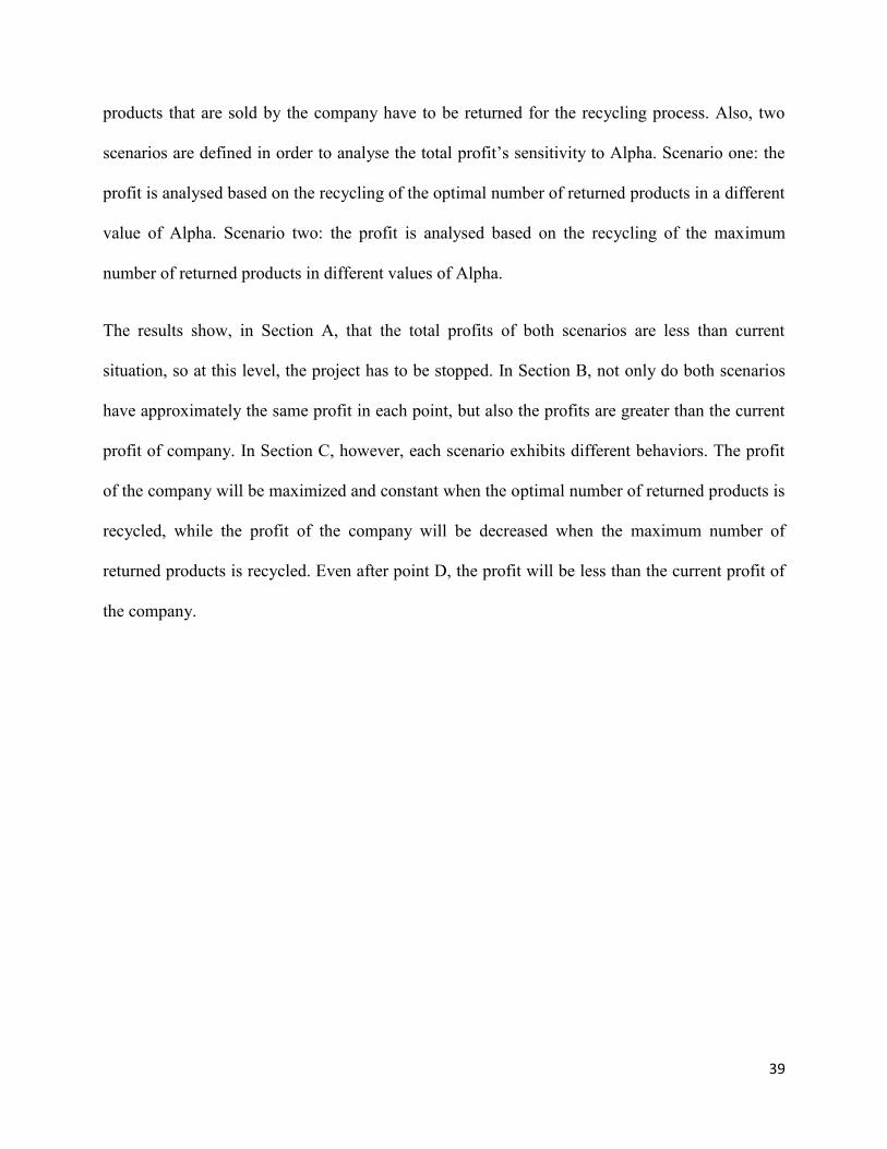
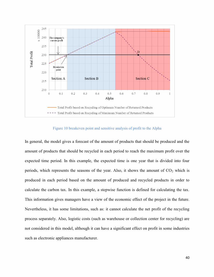
As mentioned, the breakeven point of the number of products that have to be recycled is an

effective factor in a managers’ decision regarding the recycling process. In this example, the

breakeven point of Alpha, the percent of sold products that have to be returned for the recycling

process, is about 0.15, as illustrated in Figure 10. This means that at least 15 percent of the total

39

products that are sold by the company have to be returned for the recycling process. Also, two

scenarios are defined in order to analyse the total profit’s sensitivity to Alpha. Scenario one: the

profit is analysed based on the recycling of the optimal number of returned products in a different

value of Alpha. Scenario two: the profit is analysed based on the recycling of the maximum

number of returned products in different values of Alpha.

The results show, in Section A, that the total profits of both scenarios are less than current

situation, so at this level, the project has to be stopped. In Section B, not only do both scenarios

have approximately the same profit in each point, but also the profits are greater than the current

profit of company. In Section C, however, each scenario exhibits different behaviors. The profit

of the company will be maximized and constant when the optimal number of returned products is

recycled, while the profit of the company will be decreased when the maximum number of

returned products is recycled. Even after point D, the profit will be less than the current profit of

the company.

40

Figure 10 breakeven point and sensitive analysis of profit to the Alpha

In general, the model gives a forecast of the amount of products that should be produced and the

amount of products that should be recycled in each period to reach the maximum profit over the

expected time period. In this example, the expected time is one year that is divided into four

periods, which represents the seasons of the year. Also, it shows the amount of CO2 which is

produced in each period based on the amount of produced and recycled products in order to

calculate the carbon tax. In this example, a stepwise function is defined for calculating the tax.

This information gives managers have a view of the economic effect of the project in the future.

Nevertheless, it has some limitations, such as: it cannot calculate the net profit of the recycling

process separately. Also, logistic costs (such as warehouse or collection center for recycling) are

not considered in this model, although it can have a significant effect on profit in some industries

such as electronic appliances manufacturer.

41

4. A Dynamic model for Profit Analysis of New Green Product

Development in the Automotive Industry

In Chapter 3, a general framework was introduced by a mixed-integer model for profit analysis of

sustainable products based on the life-cycle thinking, while we considered deterministic demand

for the model. However, in reality, the product demand is subject to uncertainties (i.e.,

stochastic). In this chapter of the thesis, the primary model is further developed based on a

stochastic demand and the best policy, which represents the level of greenness for a product in

each period of time, to reach maximum profit. Thus, a dynamic model is proposed, based on

dynamic programming and qualitative choice models, to support decision makers to analyze the

profit of a set of products, which are designed based on DFE strategies. The model considers the

effect of different parameters, such as: sensitivity to environment and salary of a consumer,

maintenance and operating cost, and price of a product, etc., on the product’s demand in order to

recognize the characteristics of potential consumers to achieve optimum demand. Also, the model

helps decision makers to control the mid-term and long-term strategies of each NPD project

through budget allocation.

4.1 Model’s Assumptions

A dynamic model is proposed to analyze the profit of a company that decides to develop a set of

its current automobiles based on DFE strategies.

The problem is formulated based on the following assumptions:

1. As mentioned, in 2009 Government of Canada with the Design Exchange (DX) and Canadian

Manufacturers and Exporters (CME) assessed North American’s industries’ practices in DFE

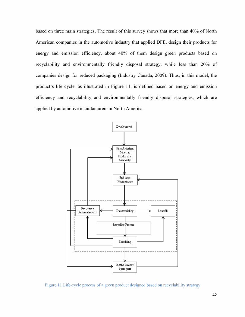
42

based on three main strategies. The result of this survey shows that more than 40% of North

American companies in the automotive industry that applied DFE, design their products for

energy and emission efficiency, about 40% of them design green products based on

recyclability and environmentally friendly disposal strategy, while less than 20% of

companies design for reduced packaging (Industry Canada, 2009). Thus, in this model, the

product’s life cycle, as illustrated in Figure 11, is defined based on energy and emission

efficiency and recyclability and environmentally friendly disposal strategies, which are

applied by automotive manufacturers in North America.

Figure 11 Life-cycle process of a green product designed based on recyclability strategy

43

2. The model is designed based on a product family-based approach, since automotive

companies like many firms in other industries prefer to develop a family of products in order

to tackle intense competition and rapid technological advances, and to decrease the

development cost and risk (Loch & Kavadias, 2008; Jiao, Simpson, & Siddique, 2007). A

product family-based approach helps to decrease fixed costs of design and procurement of a

product’s components through the idea of platform-based design (Gupta & Krishnan, 1999).

In the automotive industry, for instance, a platform can be designed based on recyclability

and an environmentally friendly disposal strategy and use it for different types of cars.

Likewise, an engine can be designed based on energy and emission efficiency strategy for use

in different hybrid cars. Thus the model is defined based on a set of vehicles that can be

developed as a product family denoted V.

3. The level of environmental performance of a product can be introduced based on

environmentally friendly materials, recycled content, recyclability, clean energy, emissions,

and returnable and recyclable packaging (Ulrich & Eppinger, 2012). Thus, we assumed a sub-

class of vehicles can be introduced to the market in different levels of environmental

performance in each period. For example, the class one of car type A (Model A1) can be

introduced to the market in year one if 25% of the total components of car is developed based

on DFE strategies. Also, the class A2 will be presented when the company designed the 50%

of total components of the car based on DFE strategies and so forth. Therefore, the last class

represents the entirely environmental friendly car that all the components are designed based

on DFE strategies.

4. No production capacity is assumed for the model, so unlimited vehicles can be produced and

recycled in each time period.

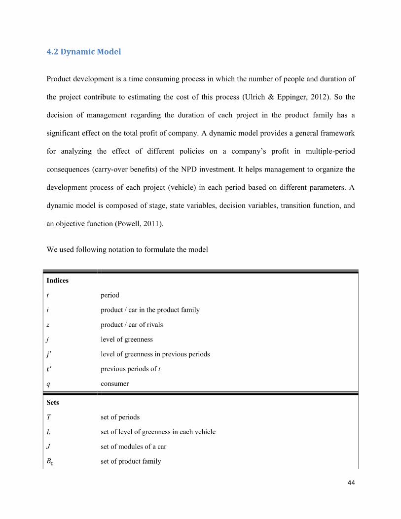
44

4.2 Dynamic Model

Product development is a time consuming process in which the number of people and duration of

the project contribute to estimating the cost of this process (Ulrich & Eppinger, 2012). So the

decision of management regarding the duration of each project in the product family has a

significant effect on the total profit of company. A dynamic model provides a general framework

for analyzing the effect of different policies on a company’s profit in multiple-period

consequences (carry-over benefits) of the NPD investment. It helps management to organize the

development process of each project (vehicle) in each period based on different parameters. A

dynamic model is composed of stage, state variables, decision variables, transition function, and

an objective function (Powell, 2011).

We used following notation to formulate the model

Indices

t period

i product / car in the product family

z product / car of rivals

j level of greenness

𝑗′ level of greenness in previous periods

𝑡′ previous periods of t

q consumer

Sets

T set of periods

𝐿 set of level of greenness in each vehicle

J set of modules of a car

𝐵𝜍 set of product family

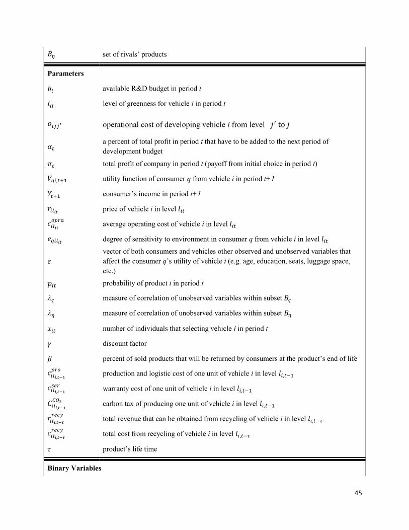
45

𝐵𝜂 set of rivals’ products

Parameters

𝑏𝑡 available R&D budget in period t

𝑙𝑖𝑡 level of greenness for vehicle i in period t

𝑜𝑖𝑗𝑗′ operational cost of developing vehicle i from level 𝑗′ to 𝑗

𝛼𝑡 a percent of total profit in period t that have to be added to the next period of

development budget

𝜋𝑡 total profit of company in period t (payoff from initial choice in period t)

𝑉𝑞𝑖,𝑡+1 utility function of consumer q from vehicle i in period t+1

𝑌𝑡+1 consumer’s income in period t+1

𝑟𝑖𝑙𝑖𝑡 price of vehicle i in level 𝑙𝑖𝑡

𝑐𝑖𝑙𝑖𝑡

𝑜𝑝𝑟𝑎 average operating cost of vehicle i in level 𝑙𝑖𝑡

𝑒𝑞𝑖𝑙𝑖𝑡 degree of sensitivity to environment in consumer q from vehicle i in level 𝑙𝑖𝑡

휀

vector of both consumers and vehicles other observed and unobserved variables that

affect the consumer q’s utility of vehicle i (e.g. age, education, seats, luggage space,

etc.)

𝑝𝑖𝑡 probability of product i in period t

𝜆𝜍 measure of correlation of unobserved variables within subset 𝐵𝜍

𝜆𝜂 measure of correlation of unobserved variables within subset 𝐵𝜂

𝑥𝑖𝑡 number of individuals that selecting vehicle i in period t

𝛾 discount factor

𝛽 percent of sold products that will be returned by consumers at the product’s end of life

𝑐𝑖𝑙𝑖,𝑡−1

𝑝𝑟𝑜 production and logistic cost of one unit of vehicle i in level 𝑙𝑖,𝑡−1

𝑐𝑖𝑙𝑖,𝑡−1

𝑠𝑒𝑟 warranty cost of one unit of vehicle i in level 𝑙𝑖,𝑡−1

𝐶𝑖𝑙𝑖,𝑡−1

𝐶𝑂2 carbon tax of producing one unit of vehicle i in level 𝑙𝑖,𝑡−1

𝑟𝑖𝑙𝑖,𝑡−𝜏

𝑟𝑒𝑐𝑦 total revenue that can be obtained from recycling of vehicle i in level 𝑙𝑖,𝑡−𝜏

𝑐𝑖𝑙𝑖,𝑡−𝜏

𝑟𝑒𝑐𝑦 total cost from recycling of vehicle i in level 𝑙𝑖,𝑡−𝜏

𝜏 product’s life time

Binary Variables

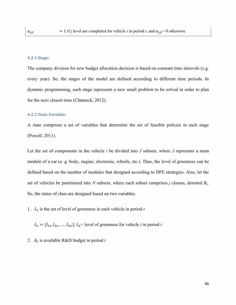
46

𝑎𝑖𝑗𝑡 = 1 if j level are completed for vehicle i in period t, and 𝑎𝑖𝑗𝑡= 0 otherwise

4.2.1 Stage:

The company division for new budget allocation decision is based on constant time intervals (e.g.

every year). So, the stages of the model are defined according to different time periods. In

dynamic programming, each stage represents a new small problem to be solved in order to plan

for the next closest time (Chinneck, 2012).

4.2.2 State Variable:

A state comprises a set of variables that determine the set of feasible policies in each stage

(Powell, 2011).

Let the set of components in the vehicle i be divided into J subsets, where J represents a main

module of a car (e. g. body, engine, electronic, wheels, etc.). Thus, the level of greenness can be

defined based on the number of modules that designed according to DFE strategies. Also, let the

set of vehicles be partitioned into N subsets, where each subset comprises j classes, denoted 𝐵𝑖.

So, the states of class are designed based on two variables.

1. 𝐿𝑡 is the set of level of greenness in each vehicle in period t

𝐿𝑡 = {𝑙1𝑡, 𝑙2𝑡,, … , 𝑙𝑁𝑡}; 𝑙𝑖𝑡= level of greenness for vehicle i in period t

2. 𝑏𝑡 is available R&D budget in period t

47

4.2.3 Decision Variable:

We assumed the R&D is given for each class of vehicle i, so, following decision variable can be

defined for the model.

𝑎𝑖𝑗𝑡= 1 if j level are completed for vehicle i in period t, and 𝑎𝑖𝑗𝑡= 0 otherwise

4.2.4 Transition function:

The transition function explains the relation between the next state of the process and the current

state of the process and the current decision taken (Bradley, et al., 1977). So, the transition of

number of completed levels for vehicle i in period t+1 can formulate based on Equation (24).

𝑙𝑖,𝑡+1 = max {𝑗𝐼𝑎𝑖𝑗𝑡, 𝑙𝑖𝑡} (24)

Equation (25) restricts the model to make infeasible solution.

𝑎𝑖𝑗′𝑡′ ≤ 1 − 𝑎𝑖𝑗𝑡 𝑗′ < 𝑗 𝑎𝑛𝑑 𝑡′ < 𝑡 ∀ 𝑖 = {1, … , 𝑁} (25)

We assumed, a given percent of total profit of company will be added to the development budget

in the next stage, while the development budget in first period (t=0) is given. Thus, the transition

function of available development budget in time t+1 can be described based on Equations (26).

𝑏𝑡+1 = 𝑏𝑡 − ∑ ∑ 𝑜𝑖𝑗𝑗′

𝐿

𝑗=𝑙𝑖𝑡+1

𝑎𝑖𝑗𝑡

𝑁

𝑖=1

+ 𝛼𝑡𝜋𝑡 𝑗′ = 𝑙𝑖𝑡 (26)

We have limited development budget in time t that have to be allocated to each project. In order

to avoided infeasible decisions, budget is restricted at period t, as shown in Equation (27):

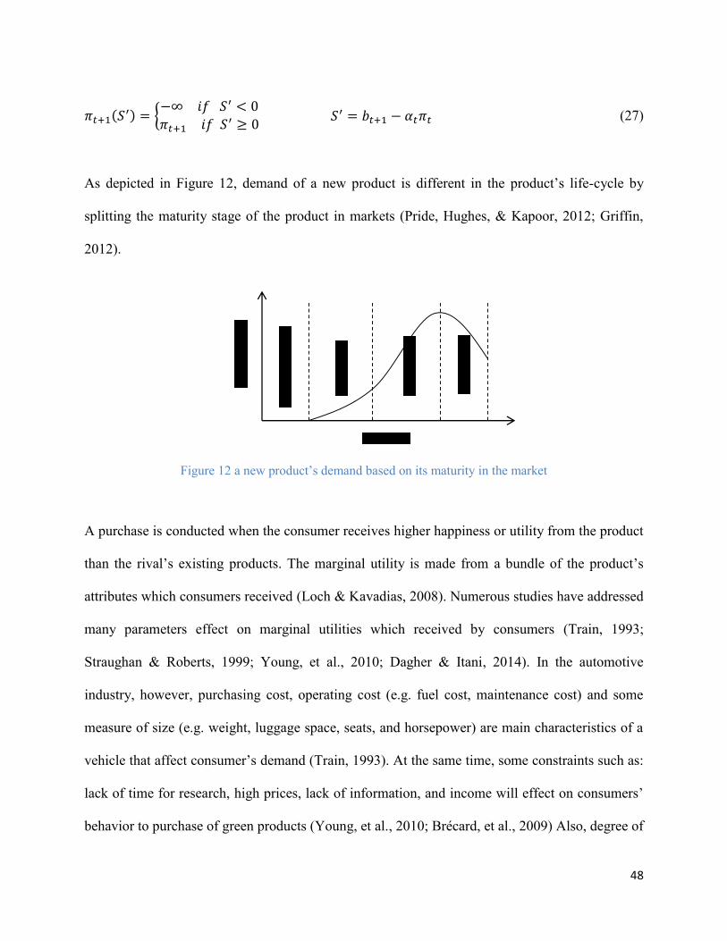
48

𝜋𝑡+1(𝑆′) = {−∞ 𝑖𝑓 𝑆′ < 0

𝜋𝑡+1 𝑖𝑓 𝑆′ ≥ 0 𝑆′ = 𝑏𝑡+1 − 𝛼𝑡𝜋𝑡 (27)

As depicted in Figure 12, demand of a new product is different in the product’s life-cycle by

splitting the maturity stage of the product in markets (Pride, Hughes, & Kapoor, 2012; Griffin,

2012).

Figure 12 a new product’s demand based on its maturity in the market

A purchase is conducted when the consumer receives higher happiness or utility from the product

than the rival’s existing products. The marginal utility is made from a bundle of the product’s

attributes which consumers received (Loch & Kavadias, 2008). Numerous studies have addressed

many parameters effect on marginal utilities which received by consumers (Train, 1993;

Straughan & Roberts, 1999; Young, et al., 2010; Dagher & Itani, 2014). In the automotive

industry, however, purchasing cost, operating cost (e.g. fuel cost, maintenance cost) and some

measure of size (e.g. weight, luggage space, seats, and horsepower) are main characteristics of a

vehicle that affect consumer’s demand (Train, 1993). At the same time, some constraints such as:

lack of time for research, high prices, lack of information, and income will effect on consumers’

behavior to purchase of green products (Young, et al., 2010; Brécard, et al., 2009) Also, degree of

Dec

lin

e

Mat

uri

ty

Dev

elo

pm

ent

Gro

wth

Dem

and

Time

49

sensitivity to impact of a product on environment can be seen by consumers as a specific feature

(Brécard, et al., 2009). According to these parameters, the indirect utility function of vehicle i for

consumer q in time t+1 can be defined by Equation (28)

𝑉𝑞𝑖,𝑡+1 = 𝑓 (𝑌𝑡+1, 𝑟𝑖𝑙𝑖𝑡, 𝑐𝑖𝑙𝑖𝑡

𝑜𝑝𝑟𝑎, 𝑒𝑞𝑖𝑙𝑖𝑡, 휀) (28)

Eventually, for estimating the probability of demand in each stage we used a disaggregate model,

where the emphasis is on individual decision making, instead of aggregate models, which

describe markets as a whole, for demand of green products based on Generalized Extreme Value

(GEV) models. The GEV are qualitative choice models that calculate the probability that a

consumer selects a specific alternative from a set of alternatives based on the correlation between

unobserved parameters in each alternative. It means the probability of each alternative would

increase when another alternative in the same subset is removed. (Train, 1993). A nested logit

model is appropriate model of GEV models for this problem, because based on this model the

available vehicles in markets can be clustered into K subsets, for any vehicle i and z in different

subset that is i in 𝐵𝜍 and z in 𝐵𝜂, where 𝜍 ≠ 𝜂, the choice probability of vehicle i by consumer q

in time t be calculated based on Equation (29) (Train, 2009).

𝑝𝑖𝑡 =𝑒𝑉𝑖𝑡 𝜆𝜍⁄ (∑ 𝑒𝑉𝑧𝑡 𝜆𝜍⁄

𝑧∈𝐵𝜍)𝜆𝜍−1

∑ (∑ 𝑒𝑉𝑧𝑡 𝜆𝜂⁄𝑧∈𝐵𝜂

)𝜆𝜂𝑁𝜂=1

(29)

Therefore, the transition function of demand for vehicle i in time t+1, the probably (Pr) of 𝑑𝑖𝑡+1,

in a potential market of size n can be calculated by binomial distribution at period t+1, as shown

in Equation (30).

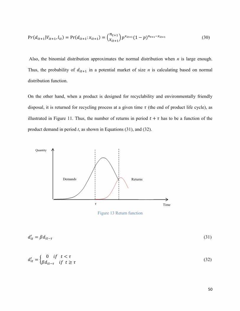
50

P𝑟(𝑑𝑖𝑡+1|𝑉𝑖𝑡+1, 𝑙𝑖𝑡) = Pr(𝑑𝑖𝑡+1: 𝑥𝑖𝑡+1) = (𝑛𝑡+1

𝑥𝑖𝑡+1) 𝑝𝑥𝑖𝑡+1(1 − 𝑝)𝑛𝑡+1−𝑥𝑖𝑡+1 (30)

Also, the binomial distribution approximates the normal distribution when n is large enough.

Thus, the probability of 𝑑𝑖𝑡+1 in a potential market of size n is calculating based on normal

distribution function.

On the other hand, when a product is designed for recyclability and environmentally friendly

disposal, it is returned for recycling process at a given time 𝜏 (the end of product life cycle), as

illustrated in Figure 11. Thus, the number of returns in period 𝑡 + 𝜏 has to be a function of the

product demand in period t, as shown in Equations (31), and (32).

Figure 13 Return function

𝑑𝑖𝑡′ = 𝛽𝑑𝑖𝑡−𝜏 (31)

𝑑𝑖𝑡′ = {

0 𝑖𝑓 𝑡 < 𝜏𝛽𝑑𝑖𝑡−𝜏 𝑖𝑓 𝑡 ≥ 𝜏

(32)

𝜏

Returns Demands

Time

Quantity

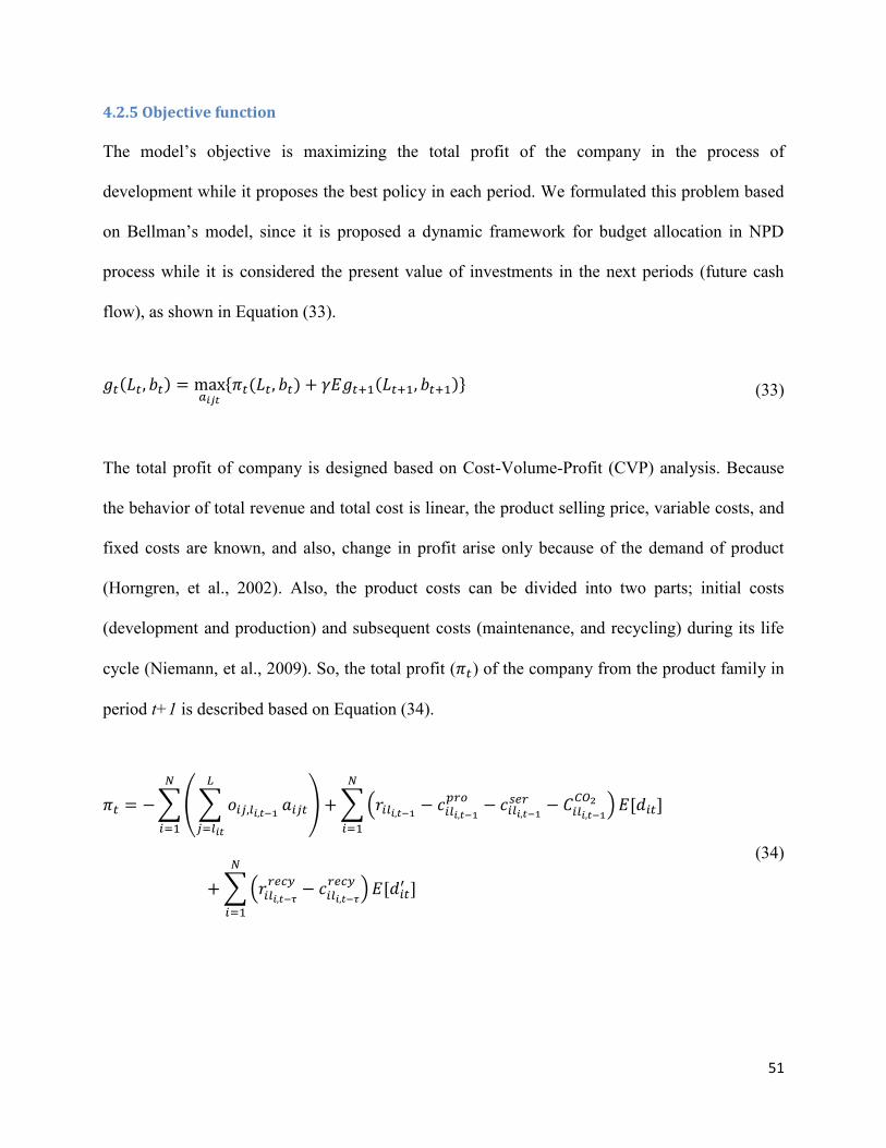
51

4.2.5 Objective function

The model’s objective is maximizing the total profit of the company in the process of

development while it proposes the best policy in each period. We formulated this problem based

on Bellman’s model, since it is proposed a dynamic framework for budget allocation in NPD

process while it is considered the present value of investments in the next periods (future cash

flow), as shown in Equation (33).

𝑔𝑡(𝐿𝑡, 𝑏𝑡) = max𝑎𝑖𝑗𝑡

{𝜋𝑡(𝐿𝑡, 𝑏𝑡) + 𝛾𝐸𝑔𝑡+1(𝐿𝑡+1, 𝑏𝑡+1)} (33)

The total profit of company is designed based on Cost-Volume-Profit (CVP) analysis. Because

the behavior of total revenue and total cost is linear, the product selling price, variable costs, and

fixed costs are known, and also, change in profit arise only because of the demand of product

(Horngren, et al., 2002). Also, the product costs can be divided into two parts; initial costs

(development and production) and subsequent costs (maintenance, and recycling) during its life

cycle (Niemann, et al., 2009). So, the total profit (𝜋𝑡) of the company from the product family in

period t+1 is described based on Equation (34).

𝜋𝑡 = − ∑ ( ∑ 𝑜𝑖𝑗,𝑙𝑖,𝑡−1

𝐿

𝑗=𝑙𝑖𝑡

𝑎𝑖𝑗𝑡)

𝑁

𝑖=1

+ ∑ (𝑟𝑖𝑙𝑖,𝑡−1− 𝑐𝑖𝑙𝑖,𝑡−1

𝑝𝑟𝑜 − 𝑐𝑖𝑙𝑖,𝑡−1

𝑠𝑒𝑟 − 𝐶𝑖𝑙𝑖,𝑡−1

𝐶𝑂2 ) 𝐸[𝑑𝑖𝑡]

𝑁

𝑖=1

+ ∑ (𝑟𝑖𝑙𝑖,𝑡−𝜏

𝑟𝑒𝑐𝑦− 𝑐𝑖𝑙𝑖,𝑡−𝜏

𝑟𝑒𝑐𝑦) 𝐸[𝑑𝑖𝑡

′ ]

𝑁

𝑖=1

(34)

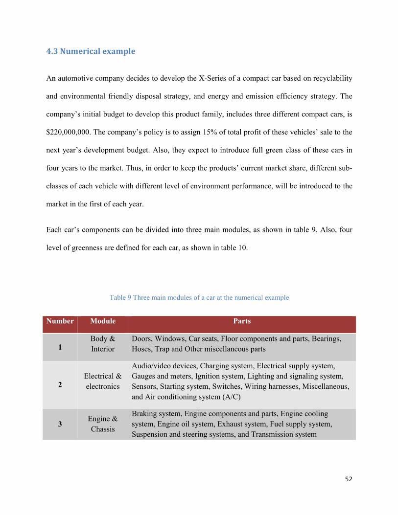
52

4.3 Numerical example

An automotive company decides to develop the X-Series of a compact car based on recyclability

and environmental friendly disposal strategy, and energy and emission efficiency strategy. The

company’s initial budget to develop this product family, includes three different compact cars, is

$220,000,000. The company’s policy is to assign 15% of total profit of these vehicles’ sale to the

next year’s development budget. Also, they expect to introduce full green class of these cars in

four years to the market. Thus, in order to keep the products’ current market share, different sub-

classes of each vehicle with different level of environment performance, will be introduced to the

market in the first of each year.

Each car’s components can be divided into three main modules, as shown in table 9. Also, four

level of greenness are defined for each car, as shown in table 10.

Table 9 Three main modules of a car at the numerical example

Number Module Parts

1 Body &

Interior

Doors, Windows, Car seats, Floor components and parts, Bearings,

Hoses, Trap and Other miscellaneous parts

2 Electrical &

electronics

Audio/video devices, Charging system, Electrical supply system,

Gauges and meters, Ignition system, Lighting and signaling system,

Sensors, Starting system, Switches, Wiring harnesses, Miscellaneous,

and Air conditioning system (A/C)

3 Engine &

Chassis

Braking system, Engine components and parts, Engine cooling

system, Engine oil system, Exhaust system, Fuel supply system,

Suspension and steering systems, and Transmission system

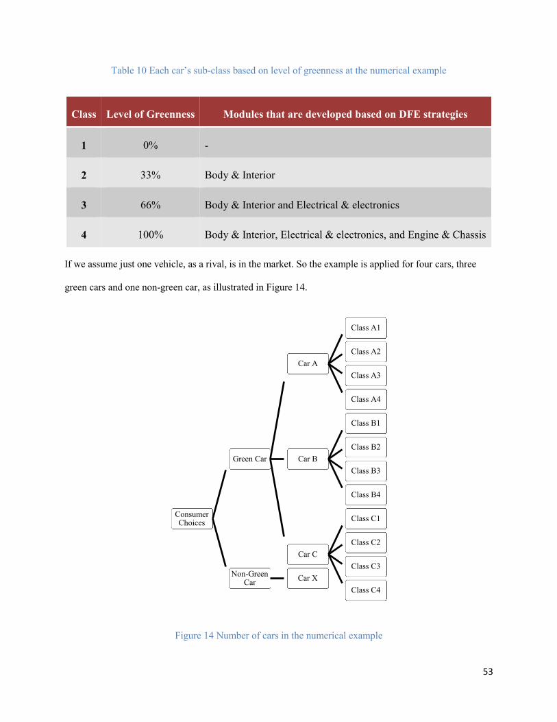
53

Table 10 Each car’s sub-class based on level of greenness at the numerical example

Class Level of Greenness Modules that are developed based on DFE strategies

1 0% -

2 33% Body & Interior

3 66% Body & Interior and Electrical & electronics

4 100% Body & Interior, Electrical & electronics, and Engine & Chassis

If we assume just one vehicle, as a rival, is in the market. So the example is applied for four cars, three

green cars and one non-green car, as illustrated in Figure 14.

Figure 14 Number of cars in the numerical example

Consumer Choices

Green Car

Car A

Class A1

Class A2

Class A3

Class A4

Car B

Class B1

Class B2

Class B3

Class B4

Car C

Class C1

Class C2

Class C3

Class C4

Non-Green Car

Car X

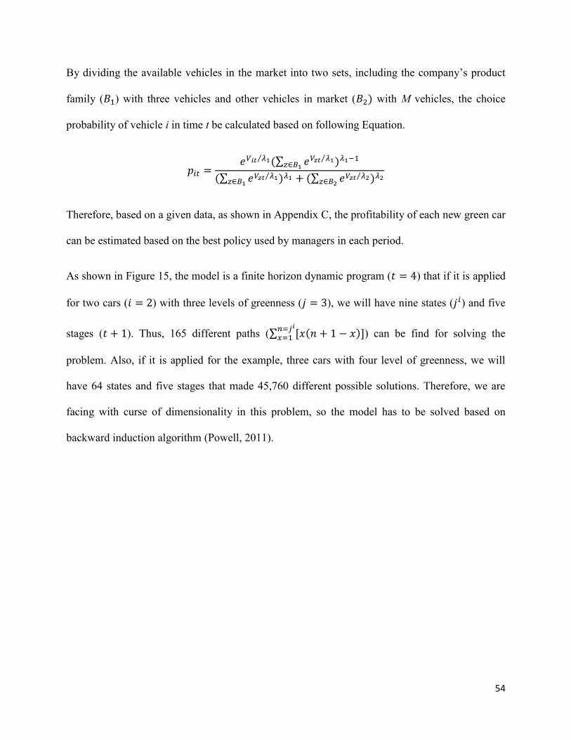
54

By dividing the available vehicles in the market into two sets, including the company’s product

family (𝐵1) with three vehicles and other vehicles in market (𝐵2) with M vehicles, the choice

probability of vehicle i in time t be calculated based on following Equation.

𝑝𝑖𝑡 =𝑒𝑉𝑖𝑡 𝜆1⁄ (∑ 𝑒𝑉𝑧𝑡 𝜆1⁄

𝑧∈𝐵1)𝜆1−1

(∑ 𝑒𝑉𝑧𝑡 𝜆1⁄𝑧∈𝐵1

)𝜆1 + (∑ 𝑒𝑉𝑧𝑡 𝜆2⁄𝑧∈𝐵2

)𝜆2

Therefore, based on a given data, as shown in Appendix C, the profitability of each new green car

can be estimated based on the best policy used by managers in each period.

As shown in Figure 15, the model is a finite horizon dynamic program (𝑡 = 4) that if it is applied

for two cars (𝑖 = 2) with three levels of greenness (𝑗 = 3), we will have nine states (𝑗𝑖) and five

stages (𝑡 + 1). Thus, 165 different paths (∑ [𝑥(𝑛 + 1 − 𝑥)]𝑛=𝑗𝑖

𝑥=1 ) can be find for solving the

problem. Also, if it is applied for the example, three cars with four level of greenness, we will

have 64 states and five stages that made 45,760 different possible solutions. Therefore, we are

facing with curse of dimensionality in this problem, so the model has to be solved based on

backward induction algorithm (Powell, 2011).

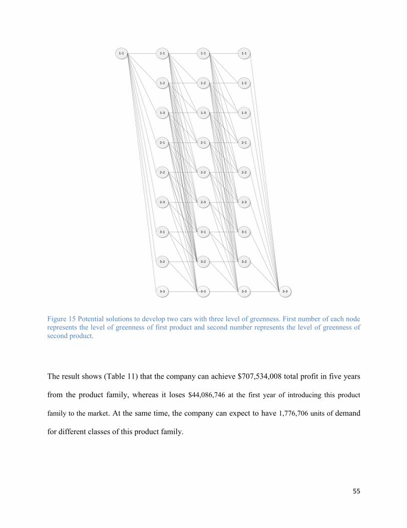
55

1-1 1-1 1-1

1-2

1-3

1-2

1-3

3-3

2-1 2-1

2-2 2-2

2-3 2-3

3-1 3-1

3-2

3-3

3-2

3-3

3-2

3-1

2-3

2-2

2-1

1-3

1-2

1-1

3-3

Figure 15 Potential solutions to develop two cars with three level of greenness. First number of each node

represents the level of greenness of first product and second number represents the level of greenness of

second product.

The result shows (Table 11) that the company can achieve $707,534,008 total profit in five years

from the product family, whereas it loses $44,086,746 at the first year of introducing this product

family to the market. At the same time, the company can expect to have 1,776,706 units of demand

for different classes of this product family.

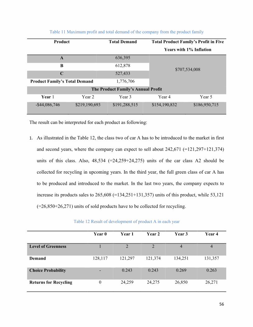
56

Table 11 Maximum profit and total demand of the company from the product family

Product Total Demand Total Product Family’s Profit in Five

Years with 1% Inflation

A 636,395

$707,534,008 B 612,878

C 527,433

Product Family’s Total Demand 1,776,706

The Product Family’s Annual Profit

Year 1 Year 2 Year 3 Year 4 Year 5

-$44,086,746 $219,190,693 $191,288,515 $154,190,832 $186,950,715

The result can be interpreted for each product as following:

1. As illustrated in the Table 12, the class two of car A has to be introduced to the market in first

and second years, where the company can expect to sell about 242,671 (=121,297+121,374)

units of this class. Also, 48,534 (=24,259+24,275) units of the car class A2 should be

collected for recycling in upcoming years. In the third year, the full green class of car A has

to be produced and introduced to the market. In the last two years, the company expects to

increase its products sales to 265,608 (=134,251+131,357) units of this product, while 53,121

(=26,850+26,271) units of sold products have to be collected for recycling.

Table 12 Result of development of product A in each year

Year 0 Year 1 Year 2 Year 3 Year 4

Level of Greenness 1 2 2 4 4

Demand 128,117 121,297 121,374 134,251 131,357

Choice Probability - 0.243 0.243 0.269 0.263

Returns for Recycling 0 24,259 24,275 26,850 26,271

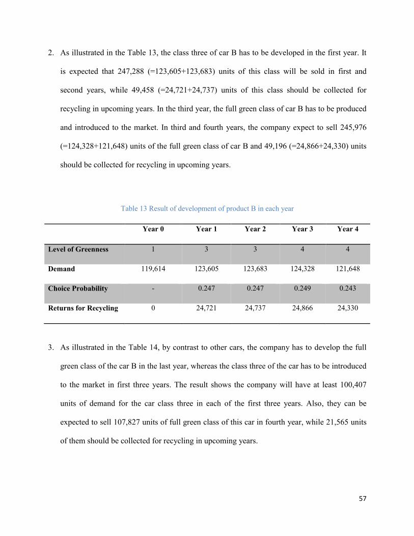
57

2. As illustrated in the Table 13, the class three of car B has to be developed in the first year. It

is expected that 247,288 (=123,605+123,683) units of this class will be sold in first and

second years, while 49,458 (=24,721+24,737) units of this class should be collected for

recycling in upcoming years. In the third year, the full green class of car B has to be produced

and introduced to the market. In third and fourth years, the company expect to sell 245,976

(=124,328+121,648) units of the full green class of car B and 49,196 (=24,866+24,330) units

should be collected for recycling in upcoming years.

Table 13 Result of development of product B in each year

Year 0 Year 1 Year 2 Year 3 Year 4

Level of Greenness 1 3 3 4 4

Demand 119,614 123,605 123,683 124,328 121,648

Choice Probability - 0.247 0.247 0.249 0.243

Returns for Recycling 0 24,721 24,737 24,866 24,330

3. As illustrated in the Table 14, by contrast to other cars, the company has to develop the full

green class of the car B in the last year, whereas the class three of the car has to be introduced

to the market in first three years. The result shows the company will have at least 100,407

units of demand for the car class three in each of the first three years. Also, they can be

expected to sell 107,827 units of full green class of this car in fourth year, while 21,565 units

of them should be collected for recycling in upcoming years.

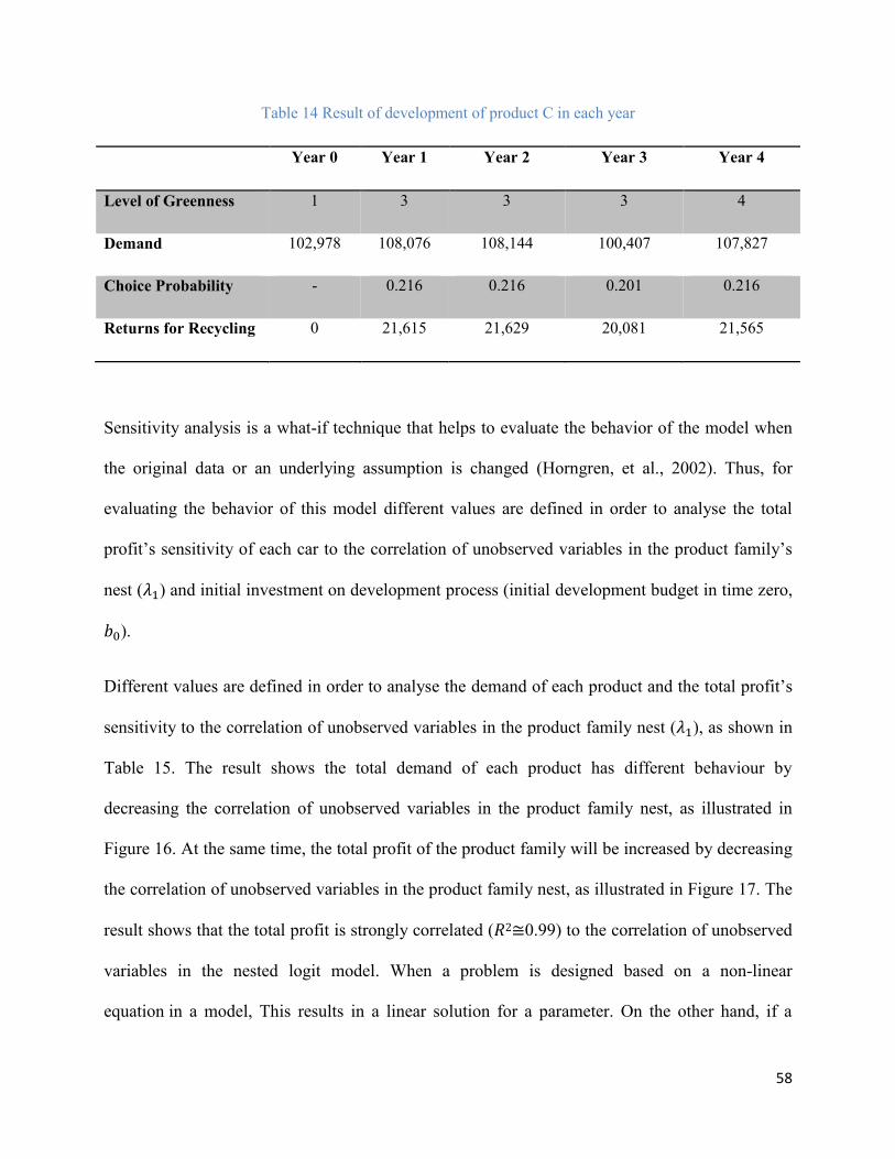
58

Table 14 Result of development of product C in each year

Year 0 Year 1 Year 2 Year 3 Year 4

Level of Greenness 1 3 3 3 4

Demand 102,978 108,076 108,144 100,407 107,827

Choice Probability - 0.216 0.216 0.201 0.216

Returns for Recycling 0 21,615 21,629 20,081 21,565

Sensitivity analysis is a what-if technique that helps to evaluate the behavior of the model when

the original data or an underlying assumption is changed (Horngren, et al., 2002). Thus, for

evaluating the behavior of this model different values are defined in order to analyse the total

profit’s sensitivity of each car to the correlation of unobserved variables in the product family’s

nest (𝜆1) and initial investment on development process (initial development budget in time zero,

𝑏0).

Different values are defined in order to analyse the demand of each product and the total profit’s

sensitivity to the correlation of unobserved variables in the product family nest (𝜆1), as shown in

Table 15. The result shows the total demand of each product has different behaviour by

decreasing the correlation of unobserved variables in the product family nest, as illustrated in

Figure 16. At the same time, the total profit of the product family will be increased by decreasing

the correlation of unobserved variables in the product family nest, as illustrated in Figure 17. The

result shows that the total profit is strongly correlated (𝑅2≅0.99) to the correlation of unobserved

variables in the nested logit model. When a problem is designed based on a non-linear

equation in a model, This results in a linear solution for a parameter. On the other hand, if a

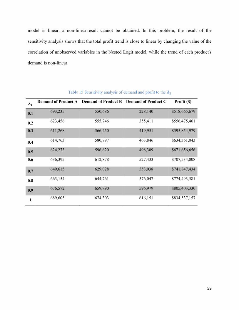
59

model is linear, a non-linear result cannot be obtained. In this problem, the result of the

sensitivity analysis shows that the total profit trend is close to linear by changing the value of the

correlation of unobserved variables in the Nested Logit model, while the trend of each product's

demand is non-linear.

Table 15 Sensitivity analysis of demand and profit to the 𝝀𝟏

𝝀𝟏 Demand of Product A Demand of Product B Demand of Product C Profit ($)

0.1 693,235 550,686 228,140 $518,665,679

0.2 623,456 555,746 355,411 $556,475,461

0.3 611,268 566,450 419,951 $595,854,979

0.4 614,763 580,797 463,846 $634,361,043

0.5 624,273 596,620 498,309 $671,656,656

0.6 636,395 612,878 527,433 $707,534,008

0.7 649,615 629,028 553,038 $741,847,434

0.8 663,154 644,761 576,047 $774,493,581

0.9 676,572 659,890 596,979 $805,403,330

1 689,605 674,303 616,151 $834,537,157

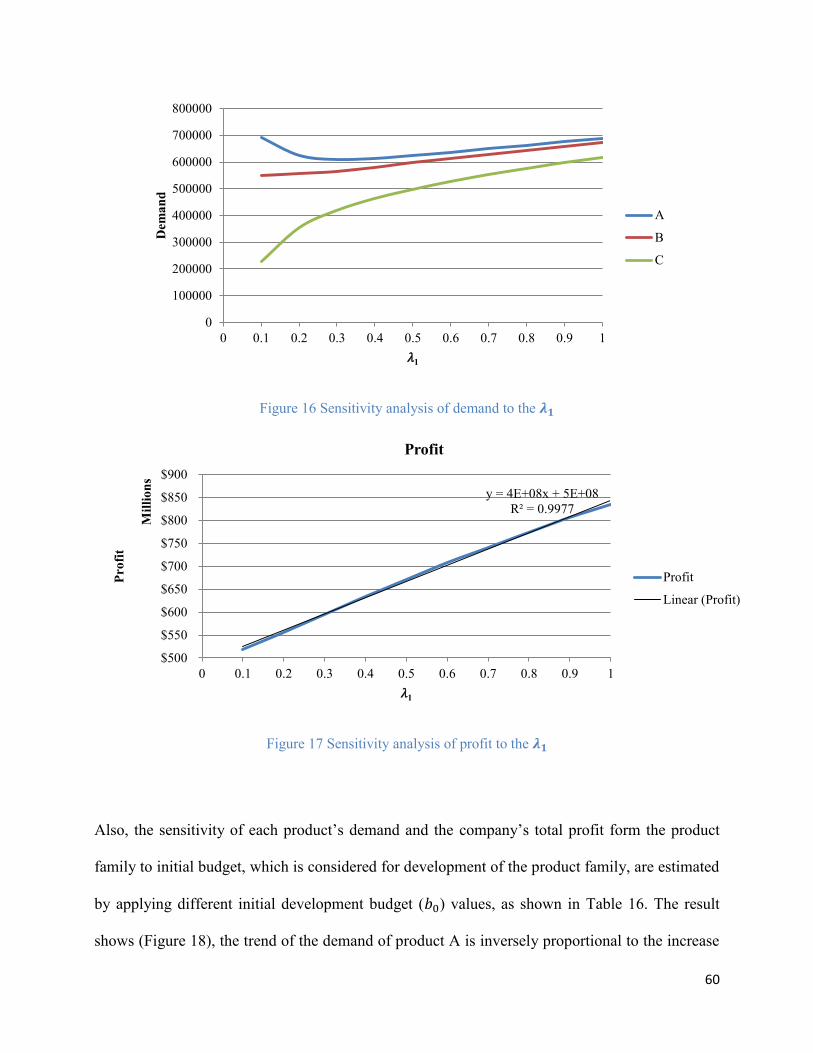
60

Figure 16 Sensitivity analysis of demand to the 𝝀𝟏

Figure 17 Sensitivity analysis of profit to the 𝝀𝟏

Also, the sensitivity of each product’s demand and the company’s total profit form the product

family to initial budget, which is considered for development of the product family, are estimated

by applying different initial development budget (𝑏0) values, as shown in Table 16. The result

shows (Figure 18), the trend of the demand of product A is inversely proportional to the increase

0

100000

200000

300000

400000

500000

600000

700000

800000

0 0.1 0.2 0.3 0.4 0.5 0.6 0.7 0.8 0.9 1

Dem

an

d

𝜆1

A

B

C

y = 4E+08x + 5E+08

R² = 0.9977

$500

$550

$600

$650

$700

$750

$800

$850

$900

0 0.1 0.2 0.3 0.4 0.5 0.6 0.7 0.8 0.9 1

Pro

fit

Mil

lio

ns

𝜆1

Profit

Profit

Linear (Profit)

61

in initial budget, whereas the trend of the demand of product C is proportional. The trend of the

demand of product B, however, is irregular to the increase the initial development budget value.

In addition, sensitivity analysis of profit to the initial development budget shows the trend of total

profit is proportional to the increase in initial budget.

Table 16 Sensitivity analysis of demand and profit to the initial development budget

Initial

Budget ($)

Demand of Product

A

Demand of Product

B

Demand of Product

C Profit ($)

150,000,000 660,333 585,341 517,185 $565,824,296

160,000,000 660,333 585,341 517,185 $575,824,296

170,000,000 660,333 585,341 517,185 $585,824,296

180,000,000 644,857 621,236 505,598 $656,309,274

190,000,000 644,857 621,236 505,598 $666,309,274

200,000,000 629,756 615,654 529,674 $687,534,008

210,000,000 629,756 615,654 529,674 $697,534,008

220,000,000 636,395 612,878 527,433 $707,534,008

230,000,000 621,043 606,842 552,533 $720,977,893

240,000,000 627,603 604,195 550,188 $730,977,893

250,000,000 627,603 604,195 550,188 $740,977,893

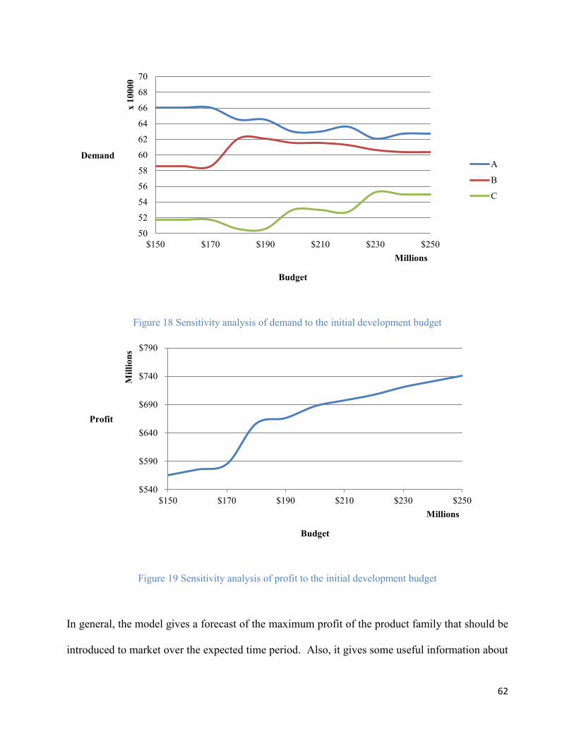
62

Figure 18 Sensitivity analysis of demand to the initial development budget

Figure 19 Sensitivity analysis of profit to the initial development budget

In general, the model gives a forecast of the maximum profit of the product family that should be

introduced to market over the expected time period. Also, it gives some useful information about

50

52

54

56

58

60

62

64

66

68

70

$150 $170 $190 $210 $230 $250

Demand

x 1

00

00

Budget

Millions

A

B

C

$540

$590

$640

$690

$740

$790

$150 $170 $190 $210 $230 $250

Profit

Mil

lio

ns

Budget

Millions

63

the potential demand of each type of product and the amount of products that should be recycled

in upcoming years. In the numerical example, the expected time is four years. Also, it shows the

level of greenness for each product in each period in order to reach maximum benefit for the

company. At the end, two sensitivity analyses are done to evaluate the behavior of the model

when the original data of some parameters are changed. This information gives managers have a

view of the effect of different parameters on a product’s demand and the project’s profit in the

future.

64

5. Conclusions, limitations, and opportunities for future research

In this chapter, conclusions of the research, limitations, and future research opportunities are

discussed.

5.1 Conclusions

Firms are encouraged to develop a new generation of products, i.e. green products, to avoid

harmful impacts of their current design and manufacturing processes on the environment.

However, the future financial effect of green products is the main concern of managers in charge

of new product development (NPD) projects. Business analysis is one of the most important

stages of NPD that shows the perspective of new products after launching in the market. Precise

financial analysis of a product in this stage equips decision makers with proper forecasts of the

product.

In this thesis, a comprehensive model is proposed for analyzing the trade-off between potential

costs and revenues in environmental friendly products, which are designed based on recyclability,

disassembly, and an environmentally friendly disposal strategy. First, a primary mixed integer

model is designed based on cost and revenue parameters throughout the product life cycle, from

development to disposal. The model’s constraints present some major limitations that companies

are facing in their production and recycling processes, in addition to effects of these limitations

on economical parameters. The crucial point of this model is the consideration of product

development and recycling costs in addition to manufacturing cost, which affects the managers’

decision in the production process. Also, we attempted to reflect different aspects of typical

problems that companies are faced with in production and recycling processes such as: machine

and labor limitations, and carbon tax.

65

A generalized model has been designed so that it is applicable in many CPG manufacturers such

as electronics, toy, and furniture industries. It can help managers to calculate the optimum

production and recycling amount of the product, with respect to the factory’s throughput, to reach

the maximum profit. Also, it releases very useful information about the amount of emission

produced in product manufacturing and recycling processes. Managers can compare this

information with the current situation of the product and decide about the continuation of the

product development project. A numerical example, in the electronic appliance industry, is

presented in order to show how a manager can use the model’s results. The primary model’s

parameters are divided into three main parts: development and production, CO2 emission, and

recycling. Development, manufacturing, assembly, and material costs are identified as basic

parameters in development and production. Also, disassembly, shredding, recovery, and disposal

costs are defined as fundamental parameters of recycling a product. Finally we considered two

different parameters (emission produced for producing and emission produced for recycling) to

measure total CO2 emission tax in stepwise model. The primary model makes two main

contributions: on the theoretical side, we offer a comprehensive model for analyzing the trade-off

between profitability and recyclability, disassembly, and environmentally friendly disposal

attributes of green products in all stages of the product life-cycle. On the managerial side, it

provides a decision support methodology for management in order to decide about the future of

an NPD project in the design stage.

The primary model is further developed using dynamic programming approach. A dynamic

model is proposed to help decision makers to forecast the profit of a family of products, which is

designed based on recyclability, disassembly, and an environmentally friendly disposal strategy,

based on each product’s cash flow in its life-cycle. The model is designed for a product, such as

66

an automobile, that different generation that can be introduced to the market in each period. We

assumed different level of greenness for a car that can be produced and introduced to the market.

According to the model, a company can schedule the process of development of products to reach

maximum profit in a given time. Thus, the model helps managers to identify accurate policy to

introduce a new product with different level of greenness to the market according to the

company’s R&D budget constraint in each time. In addition, managers can estimate the demand

of each class of products based on selected policy in each period. A numerical example, in the

automotive industry, is defined in order to show how the model works and how managers can use

from the model’s results. The dynamic model’s variables are divided into two main parts: state

and decision variables. Level of greenness in each vehicle and available R&D budget in each

period are identified as state variables. Also, a binary variable is defined to make a decision about

the levels have to be completed in each vehicle. Finally the nested logit model, which is an

appropriate model of GEV models, is used to model the demand of each product based on the

consumers’ utility function. The utility function parameters can be defined based on product

specifications and target market attributes. In this model, the consumer’s average income, the

product’s price, average operation cost and the degree of sensitivity to environment in a

consumer are considered as main parameters which affect the consumer’s demand of sustainable

products in the automotive industry. The dynamic model also makes two main contributions: on

the theoretical side, we offer a comprehensive model for analyzing the profit of a group of

products with the same attributes, while the full green generation of all products have to be

introduced to the market after a given period time. Also, it shows the interaction between the

level of environmental performance and demand on green products in the automotive industry.

On the managerial side, it provides a decision support methodology for decision makers to

67

analyze the new green product’s profitability and demand in the business analysis stage of NPD

process.

5.2 Limitations and future research

The model’s limitations can be categorized into conceptual and technical levels. On the

conceptual side, the model has some limitations such as: it cannot calculate the net profit of the

recycling process separately. Also, logistic costs (such as warehouse or collection center for

recycling) are not considered in this model, although it can have an effect on profit in some

industries. In addition, it does not consider actions and reactions of competitors against a

company’s decisions. Next, the technology change effects are not considered. Moreover, the risk

of each outcome is not reflected in the process. On the technical side, curse of dimensionality is a

main limitation of dynamic programming. Thus, coding and solving of the dynamic model were

two technical limitations of our research. Eventually, to calculate the demand of each vehicle in

reality, many parameters such as education, age, sex etc. can affect the consumer’s utility

function.

For future investigation, the model can be:

1. Developed by considering technology and competitors’ effects on the probability of new

product success. Thus, the model has to be formulated based on infinite horizon dynamic

programming and dynamic game models.

2. Applied for each step of a new green product development according to minimum

development cost or time.

3. Customized for other industries (i.e. dairy industry, aerospace) to find green product

development process and calculation of emission tax.

68

Bibliography

Adner, R. & Levinthal, D., 2001. Demand Heterogeneity and Technology Evolution: Implications for

Product and Process Innovation. Management Science, May, 47(5), 611-628.

Albino, V., Balice, A. & Dangelico, R. M., 2009. Environmental Strategies and Green Product

Development: an Overview on Sustainability-Driven Companies. Business Strategy and the Environment,

February , 18(2), 83-96.

Annacchino, M. A., 2003. New Product Development: From Initial Idea to Product Management..

Butterworth-Heinemann.

Asselin-Balençon , A. C. & Jolliet , O., 2014. Metrics and indices to assess the life cycle costs and

greenhouse gas impacts of a dairy digester. Journal of Cleaner Production, Volume 79, 98–107.

Australian Government, 2012. Guide to Carbon Price Liability Under the Clean Energy Act 2011,

Northern Territory: the Clean Energy Regulator.

Bajpai, P., 2014. Environmental Aspects of Recycling. Recycling and Deinking of Recovered Paper, 271-

282.

Barrios, L. & Kenntoft, J., 2008. The Business Analysis Process of New Product Development- a study of

small and medium size enterprises, Master Thesis. UMU School of Business.

Boons, F., 2002. Greening products: a framework for product chain management. Journal of Cleaner

Production, 10(5), 495–505.

Booz, Allen & Hamilton, 1982. New product management for the 1980’s. New York: Booz, Allen &

Hamilton, Inc..

Bradley, S. P., Hax, A. C. & Magnanti, T. L., 1977. Applied Mathematical Programming. Addison-

Wesley Publishing Company.

Brécard, D. et al., 2009. Determinants of demand for green products: An application to eco-label demand

for fish in Europe. Ecological Economics, 69(1), 115–125.

British Columbia, 2014. Ministry of Finance. [Online]

Available at: http://www.fin.gov.bc.ca/tbs/tp/climate/A1.htm

[Accessed 19 March 2014].

69

British Columbia, 2014. Tax Rates on Fuels (MFT-CT 005). [Online]

Available at: http://www.sbr.gov.bc.ca/documents_library/bulletins/mft-ct_005.pdf

Chao, R. O., Kavadias, S. & Gaimon, C., 2009. Revenue Driven Resource Allocation: Funding Authority,

Incentives, and New Product Development Portfolio Management. Management Science, September,

55(9), 1556–1569.

Chase, R. B., Jacobs, F. R. & Aquilano, N. J., 2006. Operations Management for competitive advantage.

New York: Mc Graw-Hill.

Chen, R. W., Navin-Chandra, D. & Prinz, F. B., 1994. A cost-benefit analysis model of product design for

recyclability and its application. Components, Packaging, and Manufacturing Technology, Part A, IEEE

Transactions on 17(4), 502-507.

Chinneck, J. W., 2012. Practical Optimization: A Gentle Introduction, Carleton University: s.n.

Cooper, R. G., 1988. Predevelopment Activities Determine New Product Success. Industrial Marketing

Management, 17(3), 237-247.

D`Souza, C., Taghian, M., Lamb, P. & Peretiatkos, R., 2006. Green Products and Corporate Strategy: an

Empirical Investigation. Society and business review, 1(2), 144-157.

Dagher, G. K. & Itani, O., 2014. Factors influencing green purchasing behaviour: Empirical evidence

from the Lebanese consumers. Journal of Consumer Behaviour, 13(3), 188–195.

EIA, 2013. Environment. [Online]

Available at: http://www.eia.gov/environment/emissions/co2_vol_mass.cfm

[Accessed 18 March 2014].

EIA, 2014. Carbon Dioxide (CO2) is Produced Per Kilowatthour. [Online]

Available at: http://www.eia.gov/tools/faqs/faq.cfm?id=74&t=11

[Accessed 18 March 2014].

EIA, 2014. FREQUENTLY ASKED QUESTIONS. [Online]

Available at: http://www.eia.gov/tools/faqs/faq.cfm?id=74&t=11

[Accessed 18 March 2014].

70

EPA, 2012. Municipal Solid Waste. [Online]

Available at: http://www.epa.gov/epawaste/nonhaz/municipal/

[Accessed 24 December 2014].

EPA, 2014. Environmental Impacts from Automobiles. [Online]

Available at: http://yosemite.epa.gov/r10/owcm.nsf/Product+Stewardship/autos-impacts

[Accessed 8 September 2014].

EPA, 2014. Overview of Greenhouse Gases (Carbon Dioxide Emissions). [Online]

Available at: http://www.epa.gov/climatechange/ghgemissions/gases/co2.html#Reducing

[Accessed 19 March 2014].

Fiksel, J., 2011. Design for Environment: A Guide to Sustainable Product Development. Second ed. New

York: McGraw-Hill.

Gerhard, D., Brem, A. & Voigt, K.-I., 2008. Product development in the automotive industry: crutical

success drivers for technological innovations. Int. J. Technology Marketing, 3(3), pp. 203-222.

Giudice, F., La Rosa, G. & Risitano, A., 2006. Product Design for the Environment, A Life Cycle

Approach. New York: Taylor & Francis Group.

Griffin, R. W., 2012. Management. South-Western: Cengage Learning.

Gupta, S. & Krishnan, V. V., 1999. Integrated Component and Supplier Selection for A Product Family.

Production and Operations Management, 8(2), pp. 163-182.

Havaldar, K. K., 2014. Business Marketing: Text and Cases. 4th ed. Delhi: McGraw Hill Education

(India) Private Limited.

Hoornweg , D. & Bhada-Tata, P., 2012. What a Waste: a Global Review of Solid Waste Management,

Washington: World Bank.

Horngren, C. T., Bhimani, A., Datar, S. M. & Foster, G., 2002. Management and Cost Accounting. Upper

Saddle River(New Jersey): Financial Times/Prentice-Hall lnc..

IEA, 2009. World Energy Outlook, Paris: IEA.

IEA, 2013. CO2 Emissions from Fuel Combustion, Highlights. Paris: OECD/IEA.

71

IEA, April 2013. Global EV Outlook; Understanding the Electric Vehicle Landscape to 2020, s.l.:

International Energy Egency.

Industry Canada, 2009. Design for Environment: Innovating to Compete. [Online]

Available at: http://www.ic.gc.ca/eic/site/dsib-dsib.nsf/eng/h_oq01764.html

[Accessed 19 January 2014].

Jiao, J. R., Simpson, T. W. & Siddique, Z., 2007. Product family design and platform-based product

development:a state-of-the-art review. Journal of Intelligent Manufacturing, February, 18(1), 5-29.

Kiatkittipong , W., Wongsuchoto , P., Meevasana , K. & Pavasant , P., 2008. When to buy new

electrical/electronic products?. Journal of Cleaner Production, 16(13), 1339–1345.

Kirkham, R. J., 2005. Re‐Engineering The Whole Life Cycle Costing Process. Construction Management

and Economics, 23(1), 9-14.

Kleber, R., 2006. The integral decision on production/remanufacturing technology and investment time in

product recovery. OR Spectrum, January, 28(1), 21–51.

Krikke, H. R., Harten, A. V. & Schuur, P. C., 1998. On a Medium Term Product Recovery and Disposal

Strategy for Durable Assembly Products. International Journal of Production Research, 36(1), 111-140.

Krozer, Y., 2008. Life Cycle Costing For Innovations In Product Chains. Journal of Cleaner Production,

16(3), 310–321.

Kumar , S. & Chatterjee , A. K., 2013. A Profit Maximizing Mathematical Model for Pricing and

Selecting Optimal Product Line. Computers & Industrial Engineering, 64(2), 545–551.

Lambert, A. J. D. & Gupta, S. M., 2005. Disassembly modeling for assembly, maintenance reuse, and

recycling. Boca Raton, London, New York, Washington, D.C.: CRC Press.

Lancaster, G. & Massingham, L., 2011. Essentials of Marketing Management. New York: Routledge.

Lipman, T. E., & Delucchi, M. A., 2006. A retail and lifecycle cost analysis of hybrid electric vehicles.

Transportation Research Part D: Transport and Environment, 11(2), 115-132.

Loch, C. H. & Kavadias, S., 2008. Handbook of New Product Development Management. Oxford,

Burlington: Elsevier.

72

Luttropp, C. & Lagerstedt, J., 2006. Ecodesign and The Ten Golden Rules: Generic Advice for Merging

Environmental Aspects into Product Development. Journal of Cleaner Production, Volume 14, 1396-

1408.

Morris, J., 1996. Recycling versus incineration: an energy conservation analysis. Journal of Hazardous

Materials, Volume 47, 277-293.

Murthy, D. N. P., Rausand, M. & Østeras, T., 2008. Product Reliability : Specification and Performance.

Dordrecht: Springer.

Niemann, J., Westk¨amper, E. & Tichkiewitch, S., 2009. Design of Sustainable Product Life Cycles.

Verlag Berlin Heidelberg: Springer.

Pears, A., 2004. Energy efficiency–its potential: some perspectives and experiences. Paris, s.n.

Powell, W. B., 2011. Approximate Dynamic Programming: Solving the Curses of Dimensionality. Second

Edition ed. Hoboken, New Jersey: John Wiley & Sons, Inc..

Pride, W. M., Hughes, R. J. & Kapoor, J. R., 2012. Introduction to business. South-Western: Cengage

Learning.

Radomes Jr, A. A. & Arango , S., 2015. Renewable Energy Technology Diffusion: An Analysis Of

Photovoltaic-System Support Schemes In Medellín, Colombia. Journal of Cleaner Production. Volume

92, 152–161.

Repenning, N. P., 2000. A dynamic model of resource allocation in multi-project research and

development systems. System Dynamics Review, 16(3), 173–212.

Ribeiro, I., Peças, P. & Henriques, E., 2013. Incorporating Tool Design Into a Comprehensive Life Cycle

Cost Framework Using The Case of Injection Molding. Journal of Cleaner Production, Volume 53, 297–

309.

Savale, T. K., Sharma , A. F. & Patil, P. U., 2012. Green Marketing: Opportunities And Challenges. New

York, Foundation of Computer Science, iccia - Number 4.

Shahan, Z., 2013. 100% Electric Car Sales Up 447.95% In US In 2013. [Online]

Available at: http://evobsession.com/100-electric-car-sales-447-95-us-2013/

[Accessed 16 September 2014].

73

Sharma, A. & Iyer, G. R., 2012. Resource-constrained product development: Implications for green

marketing and green supply chains. Industrial Marketing Management, 41(4), 599–608.

Straughan, R. D. & Roberts, J. A., 1999. Environmental Segmentation Alternatives: A Look At Green

Consumer Behavior In The New Millennium. Journal of Consumer Marketing, 16(6), 558-575.

Tax Bulletin of British Columbia, 2013. Tax Rates on Fuels, Motor Fuel Tax Act and Carbon Tax Act,

Brithish Columbia: Ministry of Finance.

Train, K. E., 1993. Qualitative Choice Analysis: Theory, Econometrics, and an Application to Automobile

Demand. Cambridge, Massachusetts, London: The MIT press.

Train, K. E., 2009. Discrete Choice Methods with Simulation. New York: Cambridge University Press.

Tsai, W.-H.et al., 2012. Applying a mathematical programming approach for a green product mix

decision. International Journal of Production Research, 1171-1184.

U.S. Department of Energy's Clean Cities program, 2015. Alternative Fuels Data Center. [Online]

Available at: http://www.afdc.energy.gov/calc/ [Accessed 8 May 2015].

U. S. Environmental Protection Agancy, 2011. Review of National Ambient Air Quality Standards for

Carbon Monoxide; Final Rule. Federal Register, 30 August, 76(169),54294.

Ulrich, K. T. & Eppinger, S. D., 2012. Product Design and Development. New York: McGraw-Hill.

Vezzoli, C. & Manzini, E., 2008. Design and Innovation for Sustainability. Milan : Springer.

Wang, H.-F. & Gupta, S. M., 2011. Green Supply Chain Management (Product Life Cycle Approach).

McGraw-Hill.

Wasik, J. F., 1996. Green Marketing and Management. Cambridge: Blackwell.

Williams, P. T., 2005. Waste Treatment and Disposal. 2nd ed. Chichester: John Wiley & Sons Ltd.

Young, W., Hwang, K., McDonald, S. & Oates, C. J., 2010. Sustainable Consumption: Green Consumer

Behaviour when Purchasing Products. Sustainable Development, January/February , 18(1), 20-31.

Zabaniotou , A. & Kassidi , E., 2003. Life Cycle Assessment Applied to Egg Packaging Made from

Polystyrene and Recycled Paper. Journal of Cleaner Production, 11(5), 549–559.

74

Zirger, B. J. & Maidique, M. A., 1990. A Model of New Product Development: An Empirical Test.

Management Science, July, 36(7), 867-883.

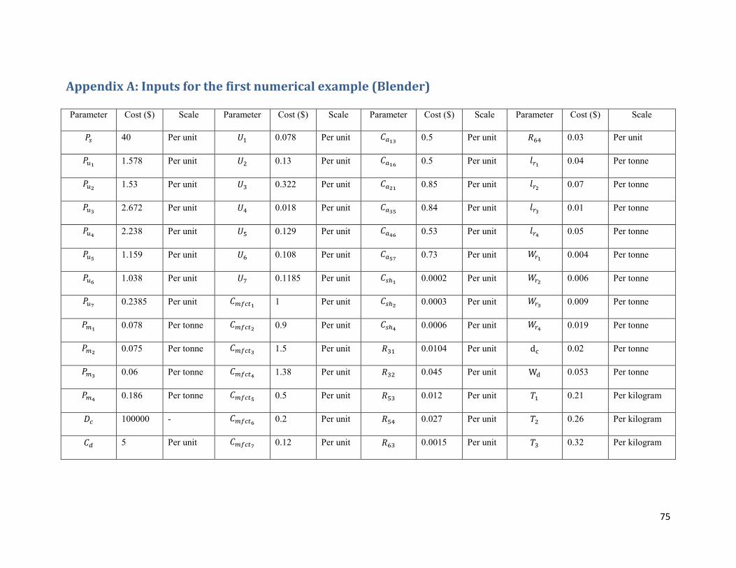
75

Appendix A: Inputs for the first numerical example (Blender)

Parameter Cost ($) Scale Parameter Cost ($) Scale Parameter Cost ($) Scale Parameter Cost ($) Scale

𝑃𝑠 40 Per unit 𝑈1 0.078 Per unit 𝐶𝑎13 0.5 Per unit 𝑅64 0.03 Per unit

𝑃𝑢1 1.578 Per unit 𝑈2 0.13 Per unit 𝐶𝑎16

0.5 Per unit 𝑙𝑟1 0.04 Per tonne

𝑃𝑢2 1.53 Per unit 𝑈3 0.322 Per unit 𝐶𝑎21

0.85 Per unit 𝑙𝑟2 0.07 Per tonne

𝑃𝑢3 2.672 Per unit 𝑈4 0.018 Per unit 𝐶𝑎35

0.84 Per unit 𝑙𝑟3 0.01 Per tonne

𝑃𝑢4 2.238 Per unit 𝑈5 0.129 Per unit 𝐶𝑎46

0.53 Per unit 𝑙𝑟4 0.05 Per tonne

𝑃𝑢5 1.159 Per unit 𝑈6 0.108 Per unit 𝐶𝑎57

0.73 Per unit 𝑊𝑟1 0.004 Per tonne

𝑃𝑢6 1.038 Per unit 𝑈7 0.1185 Per unit 𝐶𝑠ℎ1

0.0002 Per unit 𝑊𝑟2 0.006 Per tonne

𝑃𝑢7 0.2385 Per unit 𝐶𝑚𝑓𝑐𝑡1

1 Per unit 𝐶𝑠ℎ2 0.0003 Per unit 𝑊𝑟3

0.009 Per tonne

𝑃𝑚1 0.078 Per tonne 𝐶𝑚𝑓𝑐𝑡2

0.9 Per unit 𝐶𝑠ℎ4 0.0006 Per unit 𝑊𝑟4

0.019 Per tonne

𝑃𝑚2 0.075 Per tonne 𝐶𝑚𝑓𝑐𝑡3

1.5 Per unit 𝑅31 0.0104 Per unit dc 0.02 Per tonne

𝑃𝑚3 0.06 Per tonne 𝐶𝑚𝑓𝑐𝑡4

1.38 Per unit 𝑅32 0.045 Per unit Wd 0.053 Per tonne

𝑃𝑚4 0.186 Per tonne 𝐶𝑚𝑓𝑐𝑡5

0.5 Per unit 𝑅53 0.012 Per unit 𝑇1 0.21 Per kilogram

𝐷𝑐 100000 - 𝐶𝑚𝑓𝑐𝑡6 0.2 Per unit 𝑅54 0.027 Per unit 𝑇2 0.26 Per kilogram

𝐶𝑑 5 Per unit 𝐶𝑚𝑓𝑐𝑡7 0.12 Per unit 𝑅63 0.0015 Per unit 𝑇3 0.32 Per kilogram

76

Parameter Amount Scale Parameter Amount Scale Parameter Amount Scale Parameter Amount Scale

𝜗 962 hours per week ∅46 0.007 kilogram 𝐹 0.36 kilogram 𝜎5 48 Sec.

𝑡12 10 Sec. ∅57 0.09 kilogram 𝑂𝑟 50 kilogram 𝜎6 10 Sec.

𝑡13 25 Sec. 𝛿21 19 Sec. 𝜑1 5.79 hours per day 𝜎7 12 Sec.

𝑡16 31 Sec. 𝛿22 12 Sec. 𝜑2 5.18 hours per day 𝐸1 20000 kilogram

𝑡35 12 Sec. 𝛿31 21 Sec. 𝜑3 5.34 hours per day 𝐸2 30000 kilogram

𝑡46 8 Sec. 𝛿32 16 Sec. 𝜑4 5.26 hours per day 𝐸3 400000 kilogram

𝑡57 27 Sec. 𝛿43 5 Sec. 𝜑5 9615 Kilogram per week 𝛼 0.4 -

𝑒1 0.017 kilogram 𝛿44 9 Sec. 𝜑6 7500 Kilogram per week 𝐿𝑎 2991 hours per week

𝑒2 0.014 kilogram 𝛿53 4 Sec. 𝛽12 10 Sec. 𝛿11 12 Sec.

𝑒3 0.027 kilogram 𝛿54 10 Sec. 𝛽13 25 Sec. 𝛿12 5 Sec.

𝑒4 0.09 kilogram 𝛿63 3 Sec. 𝛽16 31 Sec. 𝑑1 22000 product

𝑒5 0.0175 kilogram 𝛿64 1 Sec. 𝛽35 12 Sec. 𝑑2 20000 product

𝑒6 0.027 kilogram 𝛿73 1 Sec. 𝛽46 8 Sec. 𝑑3 18000 product

𝑒7 0.1 kilogram 𝛿74 1 Sec. 𝛽57 27 Sec. 𝑑4 10500 product

∅12 0.012 kilogram 𝑊15 0.03 kilogram 𝜎1 20 Sec.

∅13 0.017 kilogram 𝑊25 0.05 kilogram 𝜎2 16 Sec. h 5 product

∅16 0.012 kilogram 𝑊46 0.012 kilogram 𝜎3 29 Sec. g 10 product

∅35 0.016 kilogram 𝑂𝑝 1000 kilogram 𝜎4 39 Sec. 𝜏 1 year

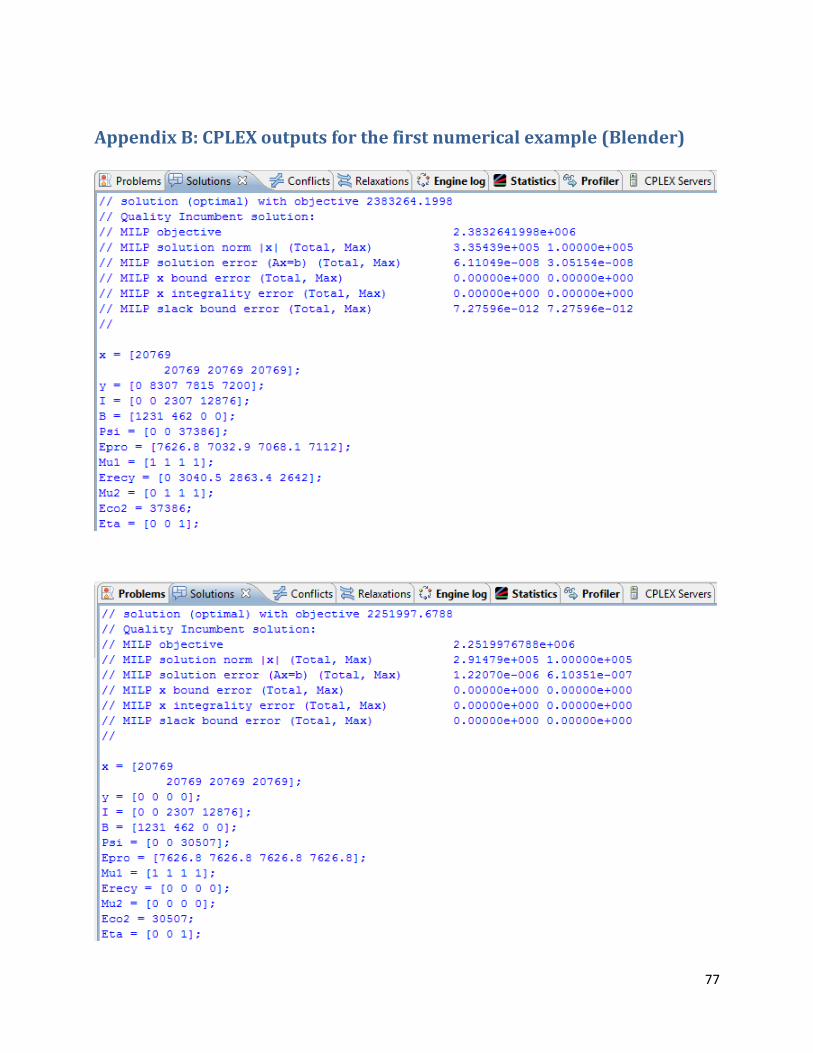
77

Appendix B: CPLEX outputs for the first numerical example (Blender)

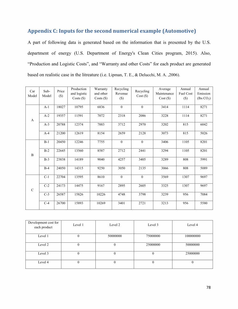
78

Appendix C: Inputs for the second numerical example (Automotive)

A part of following data is generated based on the information that is presented by the U.S.

department of energy (U.S. Department of Energy's Clean Cities program, 2015). Also,

“Production and Logistic Costs”, and “Warranty and other Costs” for each product are generated

based on realistic case in the litreature (i.e. Lipman, T. E., & Delucchi, M. A. ,2006).

Car

Model

Sub-

Model

Price

($)

Production

and logistic

Costs ($)

Warranty

and other

Costs ($)

Recycling

Revenue

($)

Recycling

Cost ($)

Average

Maintenance

Cost ($)

Annual

Fuel Cost

($)

Annual

Emission

(lbs CO2)

A

A-1 18027 10795 6836 0 0 3414 1114 8271

A-2 19357 11591 7072 2318 2086 3228 1114 8271

A-3 20788 12374 7883 3712 2970 3202 815 6042

A-4 21200 12619 8154 2659 2128 3073 815 5026

B

B-1 20450 12246 7755 0 0 3406 1105 8201

B-2 22645 13560 8587 2712 2441 3294 1105 8201

B-3 23838 14189 9040 4257 3405 3289 808 5991

B-4 24050 14315 9250 3050 2135 3066 808 5089

C

C-1 22704 13595 8610 0 0 3569 1307 9697

C-2 24173 14475 9167 2895 2605 3325 1307 9697

C-3 26587 15826 10226 4748 3798 3239 956 7084

C-4 26700 15893 10269 3401 2721 3213 956 5580

Development cost for

each product Level 1 Level 2 Level 3 Level 4

Level 1 0 50000000 75000000 100000000

Level 2 0 0 25000000 50000000

Level 3 0 0 0 25000000

Level 4 0 0 0 0

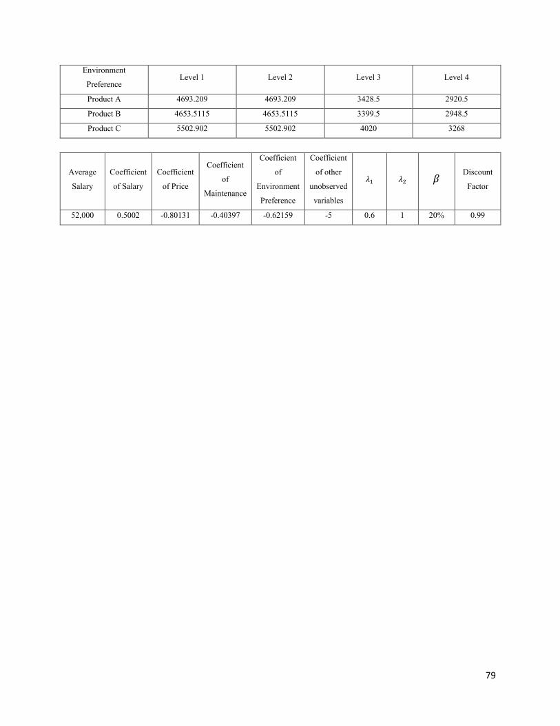
79

Environment

Preference Level 1 Level 2 Level 3 Level 4

Product A 4693.209 4693.209 3428.5 2920.5

Product B 4653.5115 4653.5115 3399.5 2948.5

Product C 5502.902 5502.902 4020 3268

Average

Salary

Coefficient

of Salary

Coefficient

of Price

Coefficient

of

Maintenance

Coefficient

of

Environment

Preference

Coefficient

of other

unobserved

variables

𝜆1 𝜆2 𝛽 Discount

Factor

52,000 0.5002 -0.80131 -0.40397 -0.62159 -5 0.6 1 20% 0.99