1

Welfare Measurement Biases and Product

Differentiation in Agriculture: An Example From the

EU15 Beef Sector

Maria Priscila Ramos, Sophie Drogue, Stephan MaretteUMR Economie Publique,INRA-INAPG

Paris, July 2005

Abstract

This paper examines the impact of two different model specifications on welfare estimations. Amodel specification that takes into account product differentiation is compared to a specificationwhere the product differentiation is overlooked. The welfare comparison under both specificationsshow some biases of aggregation as well as ambiguous results: the welfare under one specificationmay be larger or lower than the welfare under the alternative assumption. In order to illustrateour theoretical conclusions, we present an application to the EU15 beef market. We show that thewelfare when the product differentiation is taken into account is smaller than the welfare when theproduct differentiation is omitted.

Keywords: product differentiation, beef demand, European Union, welfare.

2

INTRODUCTION

From the multiplication of varieties for fresh products to the food safety requirements, product dif-ferentiation is now widespread in agricultural markets. This empirical fact raises the question of thequantification of consumers’ welfare in a context where both quality and variety matter for producersand consumers.

Many empirical models consider that agricultural products are homogeneous goods. This is par-ticularly the case in most of the partial equilibrium models that are often used to analyze agriculturalmarkets, for outlooks as well as policy simulations purposes (e.g. the AGLINK model developed bythe Organization for Economic Co-operation and Development, the FAPRI model developed by theFood and Agricultural Policy Research Institute). Indeed, the assumption of “homogenous” goods isgenerally used due to the lack of detailed information. The availability of data is usually the limitingfactor in estimating demand curves or elasticities. In this case, series of prices and quantities forproducts are very often aggregated without considering quality differences.

However, policy analysis and cost-benefit analysis without enough precision regarding the dataare likely to be doomed to failure, since quality/variety matter for issues such as trade, generic ad-vertising, functional food or food safety (...) Introducing product differentiation in a more precisefunctional form consists in estimating refined own-price effects (or elasticities) and new cross-priceeffects (or elasticities) among products.

In this article, we seek to answer the following question: should we get more precise data for wel-fare estimations? Are aggregation biases significant when product differentiation is overlooked? Avery simple framework is introduced for tackling this issue of product differentiation and the relatedwelfare measure. First, a theoretical comparison of welfare’s values is undertaken under two differentmodel specifications. A linear functional form of the demand is considered for specifying the prod-uct differentiation model (Spence 1976). The alternative model with products considered as similaror “homogeneous” is built from the previous one via an aggregation of prices and quantities. Thecomparison of welfare estimation under both specification exhibits an ambiguous result. Dependingon the parameter values, the welfare with the product differentiation specification is lower or largerthan the welfare under the homogenous product specification.

Then, a calibration of the previous models is realized by considering econometric estimations ofprice elasticities for the two different specifications. The beef market in the European Union (EU15)has been chosen since quality and price differences are large and matter for consumers. We showthat the welfare under the “homogeneous” product specification is greater than the welfare underthe product differentiation specification. The welfare is overestimated under the “homogeneous”product specification compared to the product differentiation specification. This result contradictthe common belief regarding the considerations around product differentiation and it suggests signif-icant biases coming from the absence of precise data. The collection of more precise data regardingthe market segmentation is valuable for the analysis, since we show significant differences betweenboth model specifications.

Section 1 presents the different model specifications. Section 2 presents an empirical case fromthe European Union (EU15) beef market. Section 3 discusses some extensions around this topic.Finally, we conclude about the relevance of using an adequate model of product differentiation anddata for agricultural products in welfare measurement terms.

1 TWO SIMPLE MODEL SPECIFICATIONS

1.1 Product differentiation specification

For simplicity, we introduce a model with two imperfect substitutes that only differ according thequality. The demand for each quality depend on its own price and the price of the substitute. Theexpression of demands qdi for the two substitutes (i = 1, 2) takes the form given by equations 1 and2.

qd1 = α− βp1 + δp2 (1)

3

qd2 = ω − ϕp2 + ψp1 (2)

These demand functions come from the maximization of individual quadratic utility subject tobudget constraint (Spence 1976, Vives 1999). The positive parameters α and ω are the intercepts, βand ϕ show the negative slope of the demand functions and, the positive δ and ψ capture the sub-stitution between varieties. The bigger δ and ψ values, the greater the substitutability level betweenqualities. However, the parameter’s values of the own-price effect must be bigger than the parame-ter’s values of the cross-price effect in order to assure the utility function’s concavity (Vives 1999).Specific values for demand parameters leads to well-known frameworks of product differentiationspecification (Spence 1976).

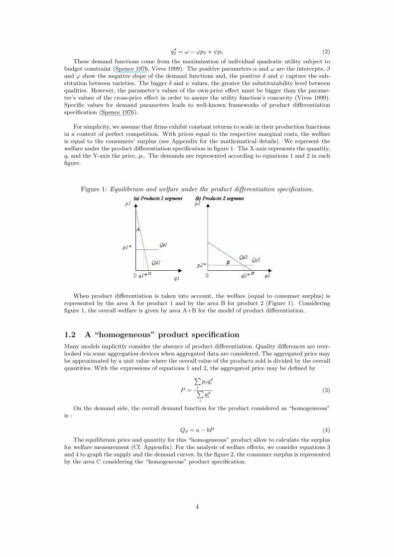
For simplicity, we assume that firms exhibit constant returns to scale in their production functionsin a context of perfect competition. With prices equal to the respective marginal costs, the welfareis equal to the consumers’ surplus (see Appendix for the mathematical details). We represent thewelfare under the product differentiation specification in figure 1. The X-axis represents the quantity,qi and the Y-axis the price, pi. The demands are represented according to equations 1 and 2 in eachfigure.

Figure 1: Equilibrium and welfare under the product differentiation specification.

When product differentiation is taken into account, the welfare (equal to consumer surplus) isrepresented by the area A for product 1 and by the area B for product 2 (Figure 1). Consideringfigure 1, the overall welfare is given by area A+B for the model of product differentiation.

1.2 A “homogeneous” product specification

Many models implicitly consider the absence of product differentiation. Quality differences are over-looked via some aggregation devices when aggregated data are considered. The aggregated price maybe approximated by a unit value where the overall value of the products sold is divided by the overallquantities. With the expressions of equations 1 and 2, the aggregated price may be defined by

P =

∑i

piqdi∑

i

qdi(3)

On the demand side, the overall demand function for the product considered as “homogeneous”is :

Qd = a− bP (4)

The equilibrium price and quantity for this “homogeneous” product allow to calculate the surplusfor welfare measurement (Cf. Appendix). For the analysis of welfare effects, we consider equations 3and 4 to graph the supply and the demand curves. In the figure 2, the consumer surplus is representedby the area C considering the “homogeneous” product specification.

4

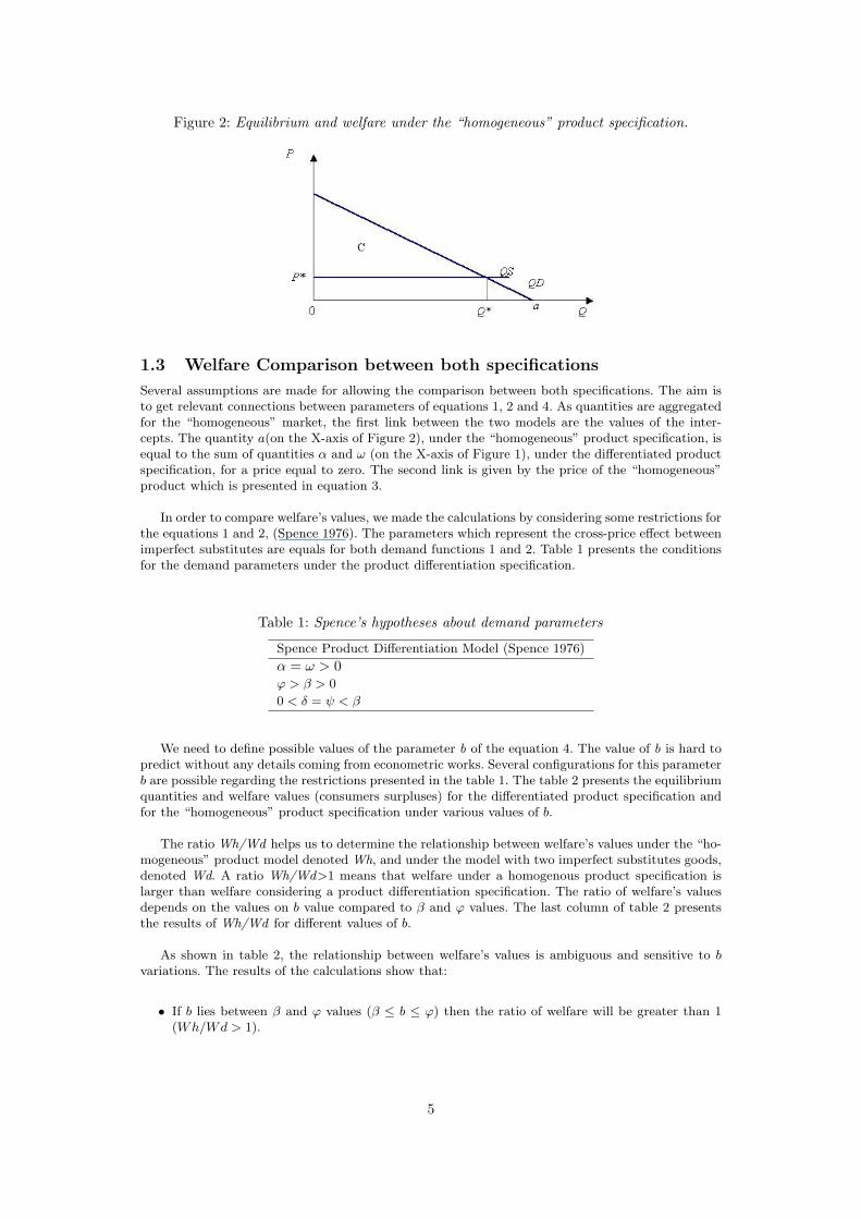
Figure 2: Equilibrium and welfare under the “homogeneous” product specification.

1.3 Welfare Comparison between both specifications

Several assumptions are made for allowing the comparison between both specifications. The aim isto get relevant connections between parameters of equations 1, 2 and 4. As quantities are aggregatedfor the “homogeneous” market, the first link between the two models are the values of the inter-cepts. The quantity a(on the X-axis of Figure 2), under the “homogeneous” product specification, isequal to the sum of quantities α and ω (on the X-axis of Figure 1), under the differentiated productspecification, for a price equal to zero. The second link is given by the price of the “homogeneous”product which is presented in equation 3.

In order to compare welfare’s values, we made the calculations by considering some restrictions forthe equations 1 and 2, (Spence 1976). The parameters which represent the cross-price effect betweenimperfect substitutes are equals for both demand functions 1 and 2. Table 1 presents the conditionsfor the demand parameters under the product differentiation specification.

Table 1: Spence’s hypotheses about demand parameters

Spence Product Differentiation Model (Spence 1976)

α = ω > 0ϕ > β > 0

0 < δ = ψ < β

We need to define possible values of the parameter b of the equation 4. The value of b is hard topredict without any details coming from econometric works. Several configurations for this parameterb are possible regarding the restrictions presented in the table 1. The table 2 presents the equilibriumquantities and welfare values (consumers surpluses) for the differentiated product specification andfor the “homogeneous” product specification under various values of b.

The ratio Wh/Wd helps us to determine the relationship between welfare’s values under the “ho-mogeneous” product model denoted Wh, and under the model with two imperfect substitutes goods,denoted Wd. A ratio Wh/Wd>1 means that welfare under a homogenous product specification islarger than welfare considering a product differentiation specification. The ratio of welfare’s valuesdepends on the values on b value compared to β and ϕ values. The last column of table 2 presentsthe results of Wh/Wd for different values of b.

As shown in table 2, the relationship between welfare’s values is ambiguous and sensitive to bvariations. The results of the calculations show that:

• If b lies between β and ϕ values (β ≤ b ≤ ϕ) then the ratio of welfare will be greater than 1(Wh/Wd > 1).

5

Table 2: Welfare under both specifications.

Product differentiation specificationα = ω β ϕ δ = ψ p∗1 p∗2 q∗1 q∗2 WD

10 1 1.5 0.5 4 2 7 9 51.5

Homogenous product specification Wh/Wda b P ∗ Q∗ WH

20 β = 1 3 17.25 146.633 2.85β+ϕ

2= 1.25 3 16.4 107.66 2.09

ϕ = 1.5 3 15.69 82.03 1.59β2

+ ϕ = 2 3 14.25 50.77 0.99

β + ϕ = 2.5 3 12.81 32.83 0.64

• The ratio of welfare will be smaller than 1 (Wh/Wd < 1) if the parameters b is greater thanβ2

+ ϕ.

• And finally, the ratio of welfare will be approximately equal to 1 (Wh/Wd ≈ 1) only for bvalues close to β

2+ ϕ.

The welfare results under different b values show the consequences of different aggregation hy-potheses on welfare. Moreover, the data aggregation and the use of non detailed data may lead tosome biases in welfare measurement.

These results suggest complex variations in welfare measurement (under or overestimation of wel-fare) and a possible bias in its calculation (Anderson 1985). The aggregation data and the omission ofproduct differentiation lead us to a biased welfare analysis. Furthermore, in table 2 the relationshipbetween Wh and Wd depends on the relationship between b, β and ϕ parameters. Consequently, thisrelationship is not straightforward, it is ambiguous and fragile.

2 APPLICATION TO THE EU-15 BEEF MARKET

In this section we try to measure the welfare bias when the product differentiation is overlooked. Forthat we apply our theoretical analysis to the EU beef market, where product differentiation mattersfor consumers.

2.1 Estimation of beef demand elasticities

The literature about beef demand elasticities shows different results depending on countries andperiods.

For the USA, Schroeder, Marsh and Minstert display a review of selected studies estimating beefdemand with time-series data. Estimates range between -0.28 and -0.85 most falling between -0.40and -0.70. Their own estimate of beef demand own-price elasticity is equal to -0.608. They concludethat demand for beef is inelastic and, as consumer incomes rise, beef demand will remain inelasticespecially for high-quality cuts which have few substitutes (Schroeder T.C. 2000). More particularly,Lusk, Marsh, Schroeder and Fox have calculated demand price elasticities for US beef demand. Twotypes of beef are modelled, “Choice beef” which could be considered as high-quality beef (hq) and“Select beef” as low-quality (lq). Choice and Select beef have own-price elasticities (hqhq, lqlq) ofdemand equal to -0.43 and -0.63 and cross-price elasticities (hqlq, lqhq) of 0.196 and 0.269 respec-tively. This paper shows a substitution between beef qualities in the US demand and the high-qualitydemand is more inelastic than the low-quality demand (Lusk and Fox 2001).

Van Eeno, Peterson and Purcell (Van Eeno E. and W. 2000) summarize the estimations fromTvedt, Reed, Maligaya and Bobst about own-price elasticities of beef demand in different parts of

6

the world (namely, US, Japan, Mexico, Korea, New Zealand and Rest of the World). These esti-mates range from -1.840 to -0.036 and from -1.816 to 0.005 for respectively high (hqhq) and low(lqlq) quality meat. Cross-price elasticities range from 0.026 to 0.757 and from 0.005 to 1.292 forrespectively hqlq and lqhq. These estimations show a great dispersion due to the difference of beefdemand elasticities from a country to another. For the US, these elasticities are -0.774 for hqhq,-1.816 for lqlq, 0.728 for hqlq and 1.292 for lqhq. These results contrast with the precedent in theorder of magnitude but they lead to some similar conclusions. The two qualities are substitutes andhigh-quality is more inelastic than low-quality beef demand. Then the demand for low-quality beefis more responsive to the price of high-quality meat than the contrary (Tvedt and Bobst 1991).

The literature on European beef market also shows great differences between own-price elastic-ities from a European country to another. For Great Britain, Tiffin and Tiffin find an own-priceelasticity of demand for beef equal to -1.642, (Tiffin and Tiffin 1999), while Fousekis and Revellestimate a beef price elasticity equal to -0.49, (Fousekis and Revell 2002). The periods they usefor the estimation are different and surely the BSE crises have affected the beef demand elasticityin Great Britain. In Spain, Laajimi and Albisu find an own-price elasticity close to unity (-0.97),(Laajimi and Albisu 1997), while Gracia and Albisu obtain a more inelastic beef demand (-0.66),(Gracia and Albisu 1998). In Norway, Rickertsen estimates an uncompensated demand price elastic-ity for beef demand of -0.87, (Rickertsen 1996). In Europe as in the US, the beef demand is inelastic.Unfortunately, the literature about beef elasticities in Europe doesn’t consider quality differentiation.

In the European Union quality matters for beef consumers and a system of carcass classificationhas been introduced. For that reason we decided, first to estimate demand elasticities by beef qualityand then to test our theoretical results in the European beef market.

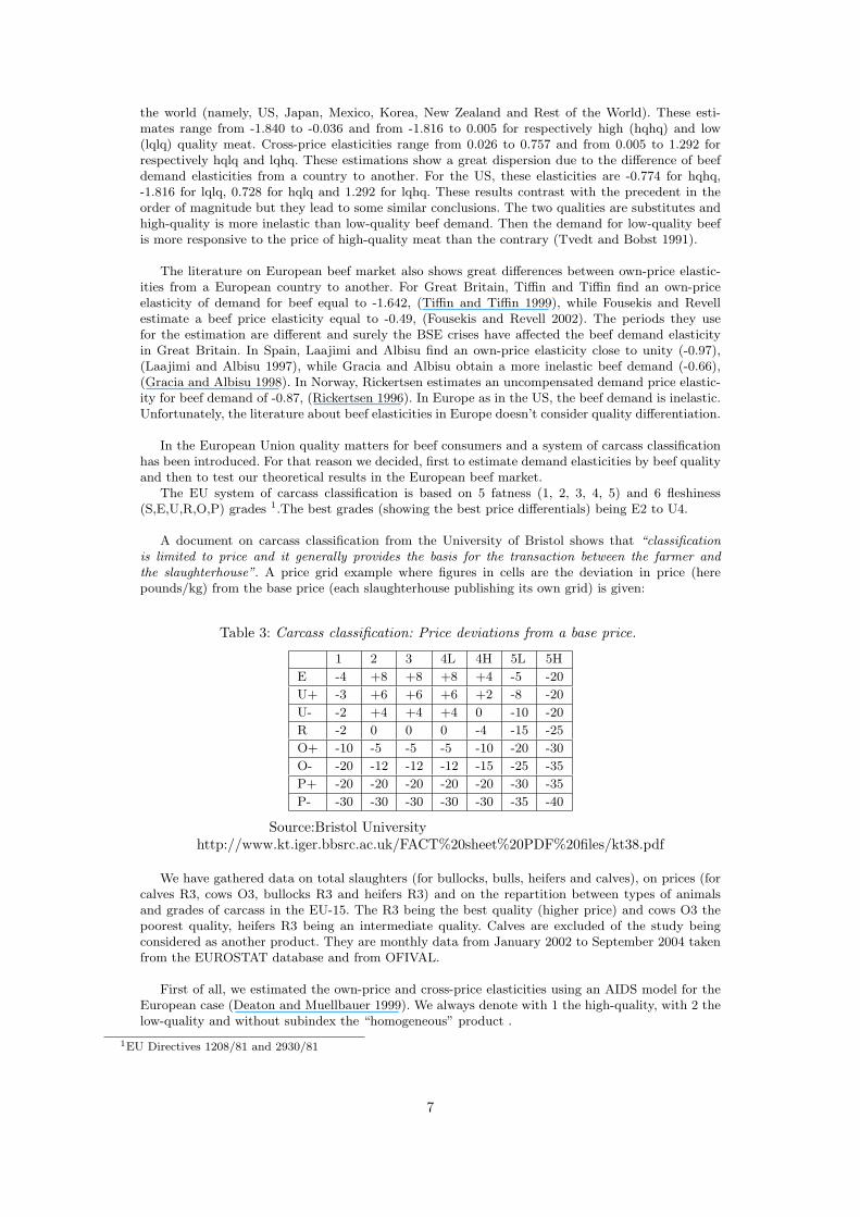
The EU system of carcass classification is based on 5 fatness (1, 2, 3, 4, 5) and 6 fleshiness(S,E,U,R,O,P) grades 1.The best grades (showing the best price differentials) being E2 to U4.

A document on carcass classification from the University of Bristol shows that “classificationis limited to price and it generally provides the basis for the transaction between the farmer andthe slaughterhouse”. A price grid example where figures in cells are the deviation in price (herepounds/kg) from the base price (each slaughterhouse publishing its own grid) is given:

Table 3: Carcass classification: Price deviations from a base price.

1 2 3 4L 4H 5L 5H

E -4 +8 +8 +8 +4 -5 -20

U+ -3 +6 +6 +6 +2 -8 -20

U- -2 +4 +4 +4 0 -10 -20

R -2 0 0 0 -4 -15 -25

O+ -10 -5 -5 -5 -10 -20 -30

O- -20 -12 -12 -12 -15 -25 -35

P+ -20 -20 -20 -20 -20 -30 -35

P- -30 -30 -30 -30 -30 -35 -40

Source:Bristol Universityhttp://www.kt.iger.bbsrc.ac.uk/FACT%20sheet%20PDF%20files/kt38.pdf

We have gathered data on total slaughters (for bullocks, bulls, heifers and calves), on prices (forcalves R3, cows O3, bullocks R3 and heifers R3) and on the repartition between types of animalsand grades of carcass in the EU-15. The R3 being the best quality (higher price) and cows O3 thepoorest quality, heifers R3 being an intermediate quality. Calves are excluded of the study beingconsidered as another product. They are monthly data from January 2002 to September 2004 takenfrom the EUROSTAT database and from OFIVAL.

First of all, we estimated the own-price and cross-price elasticities using an AIDS model for theEuropean case (Deaton and Muellbauer 1999). We always denote with 1 the high-quality, with 2 thelow-quality and without subindex the “homogeneous” product .

1EU Directives 1208/81 and 2930/81

7

Table 4: Price Elasticities at Point of Means

ε11 -0.64507237ε22 -0.46120619ε12 -0.36891746ε21 -0.51836205ε -0.29596631

The own-price elasticity values at the equilibrium points show that the demand of high-qualitybeef is more elastic than the demand of low-quality beef in the EU15 (Table 4). Moreover, the cross-elasticities show a complementary relationship between high and low-quality beef. The low-qualitybeef demand is more responsive to high-quality price variation than contrary. These results drawparticular conclusions on the European beef consumers behavior.

If the price of the high-quality rises, EU consumers will substitute it by other high-quality meat,such as high-quality pork, lamb or fish. Furthermore, high-quality beef is consumed in special occa-sions and not on a frequent basis.

A similar analysis may be done for low-quality beef. It seems obvious that low-quality beef de-mand is more inelastic as it is consumed more frequently being the main source of protein in theEuropean diet. Even though the low-quality price increases, people will consume it because of itsnutritional characteristics.

The “homogeneous” beef elasticity is closed to the low-quality beef own-price elasticity, howeverit is more inelastic than it. This result shows a more inelastic beef demand in the EU compared tothe empirical evidences presented above, which is due to the data aggregation (Anderson 1985).

2.2 Parameters Calibration of the Demand Functions

We have calibrated the parameters of the demand functions using average values of prices 2 andquantities for the period January 2002-September 2004.

Table 5: Definition and Average values of the variables used in the parameters calibration.

Variables Definitions Units Average Values

qd1 Demand of high-quality beef (bullock R3) kg 303298478

qd2 Demand of low-quality beef (cows O3) kg 304309489

Qd Demand of beef (aggregation of the other two qualities) kg 607607967

p1 Real price of high-quality beef euro/kg 2.72

p2 Real price of low-quality beef euro.kg 1.86

P Real price of the aggregated beef euro/kg 2.29

Source:Eurostat/Ofival

The calibrated parameters are presented in the next demand equations:

A) Product differentiation specification:

q1 = 610840050− 71971282p1 − 60163352.6p2 (5)

q2 = 602401399.5− 75464589.02p2 − 58026885.49p1 (6)

B) “Homogeneous” product specification:

2Prices are deflated by the Price Index for Meat and the GDP per capita by the General Price Index for Consumer forFood.

8

Q = 787439454− 78585279P (7)

The calibrated parameters show a complementarity relationship between the two qualities asthe sign of the cross-price elasticity predicts. β and ϕ parameters are greater than δ and ψ, so theconcavity of the utility function is guaranteed. The ϕ value is greater than β and α is next to ωaccording to Spence parameters hypotheses.

We observe that the value of b parameter of the “homogeneous” beef demand lies between ϕ andβ2

+ϕ values. Then, according to the relationship between parameters b, β and ϕ, we may infer thatwelfare under the “homogeneous” product specification will be greater than the welfare under theproduct differentiation specification.

In the next section we will show the coherence between our theoretical result (subsection 1.3)and this application case to EU15 beef market.

For that, the next step is to use the equations 5, 6 and 7 to calculate welfare’s values under bothspecification and compare them.

2.3 Welfare measurement and Welfare Biases

We have calculated the welfare (consumer surplus) under both specification (equations 5, 6, 7). Thenwe have measure the welfare ratio 3 to compare them and to explain the relationship between them,

Table 6: Welfare Results in the case of the EU15’s beef market.

Product differentiation specification Homogenous product specification Wh/Wd

Welfare 2471032329.8 1252635165.3 1.97267

Under constant returns to scale, when the b demand parameter for the homogenous product de-mand is greater than ϕ and smaller than β

2+ϕ, the welfare ratio will be greater than 1 (see Table 2). In

this particular case the welfare under a “homogeneous” product specification is greater than the wel-fare calculated for a product differentiation specification. The aggregation of two qualities/varietieswhen product differentiation matters induces a bias in welfare measurement (Anderson 1985).

3 EXTENSIONS

In defining analytical framework, we have made many restrictive assumptions for simplicity. In orderto test the robustness of our results we consider the following extensions.

1. In the model we assume linear demand functions. Other functional forms like Cobb-Douglasor Constant Elasticity of Substitution (CES) are often used to introduce the non-linearity ineconomic functions. For that reason, we have tested our results under a CES demand system,always keeping the rest of the hypotheses about demand parameters and market structure.For the theoretical case we obtained the same ambiguity for the welfare ratio (Table 7). Theonly difference between the linear and the CES cases is the inflexion point: for the linear caseWhWd

≈ 1 for b ≈ 2 and for the CES case WhWd

≈ 1 for b ≈ 1.146.

2. Perfect competition is a strong hypothesis in our model. For that reason, we have tested theresults under imperfect competition. We consider monopoly power in the “homogeneous” prod-uct specification and Bertrand duopoly for the specification of product differentiation. We keeplinear demand functions and their hypotheses about the parameters. In this particular case theambiguity about the welfare ratio values is found too (Table 8).

3Wh/Wd, where Wh is the welfare under the “homogeneous” product specification and Wd is the welfare under theproduct differentiation specification.

9

Table 7: Welfare under both specifications with CES demand functions.

Product differentiation specificationα = ω β ϕ δ = ψ p∗1 p∗2 q∗1 q∗2 WD

10 1 1.5 0.5 4 2 3.53553 7.07107 28.4483

Homogenous product specification Wh/Wda b P ∗ Q∗ WH

20 β > b = 0.5 3 12.2474 187.662 6.59661

β = 1 3 7.5 40.2981 1.41654

b ≈ 1.146 3 6.49935 28.4761 1.00098β+ϕ

2= 1.25 3 5.86907 22.6034 0.794542

ϕ = 1.5 3 4.59279 13.5404 0.475966β2

+ ϕ = 2 3 2.8125 5.5 0.193333

β + ϕ = 2.5 3 1.7223 2.47261 0.0869157

Table 8: Welfare under Monopoly and Duopoly market structure.

Product differentiation specificationα = ω β ϕ δ = ψ p∗1 p∗2 q∗1 q∗2 WD

10 1 1.5 0.5 8.34783 5.3913 4.34783 6.08696 21.8021

Homogenous product specification Wh/Wda b P ∗ Q∗ WH

20 β > b = 0.5 23 8.5 72.25 3.31389

β = 1 11.5 8.5 2898

1.65695β+ϕ

2= 1.25 9.2 8.5 28.9 1.32556

ϕ = 1.5 7.66667 8.5 24.0833 1.10463

b ≈ 1.657 6.94025 8.5 21.8014 0.999968β2

+ ϕ = 2 5.777 8.5 28916

0.828474

β + ϕ = 2.5 4.6 8.5 14.45 0.662779

3. The application case in this paper considers the European beef market. However, welfare anal-ysis is a decisional approach in the case of trade agreement. For that reason and continuing inthe beef sector, it would be interesting to test the same application to the possible free tradeagreement between the European Union (EU) and the MERCOSUR, because the quality dif-ferentiation is important in their bilateral trade. The issue is particularly sensitive in the beefsector, since beef production is an important component of farm income in a very large num-ber of family farms in Europe. There is a considerable interrogation on the effects of potentialliberalization and the possibility that beef from Argentina and Brazil (where the productionis increasing rapidly) could wipe out EU production is put forward by farmers associations.Another interesting aspect in beef trade between the EU and Mercosur is that beef faces dif-ferentiated tariffs at the entry of the EU according to the quality of beef. The tariff of thelow-quality beef is higher than the tariff of the high-quality beef.

Anderson treats the bias in welfare measurement due to data aggregation. For that reason,he introduces many varieties of cheese to analyze US cheese import from different countries.The disaggregation by exporting countries is considered too in this paper in order to minimizebiases (Anderson 1985).

CONCLUSION

Welfare measurement is the basic analysis in applied economy, even more in public economy. For thatreason it is important to emphasize the risks of over or under-estimation in welfare measurementdepending on the modelling assumptions and data.

10

The literature states that the welfare is larger if goods are characterized by product differentiationunder monopolistic competition than if goods are homogeneous, because of “love for variety”.

In our paper, we justify the necessity of introducing quality product differentiation in agriculturalmarkets, but always keeping some basic characteristics of these markets (decreasing/constant returnto scale, perfect competition, many producers and many consumers for all qualities).

Considering these hypotheses, we compare welfare effects under an “homogeneous” product spec-ification and under a product differentiation specification. We show that the relationship betweenthe welfare’s values in these two cases is not straightforward. The fragility and the ambiguity of theresults depends on demand parameters and the relationship between them.

Regarding the ambiguity in the results, it is very difficult to draw general conclusions. However,we may infer that under constant returns to scale, if b (demand parameter of the “homogeneous”product) lies between β and β

2+ϕ (demand parameters of quality differentiated product), the welfare

ratio is greater than 1 and if b is greater than β2

+ ϕ (for example b = β + ϕ), the welfare ratio issmaller than 1.

The previous relationship between demand parameters has been found under others hypotheseslike, non-linear demand functions (CES) and under imperfect competition assumption (monopolyand duopoly).

Our hypotheses are confirmed in the case of EU15 beef market. The aggregation assumptiongenerates a bias in the welfare measurement.

On the basis of these findings we consider that it is essential to differentiate between vari-eties/qualities in agricultural goods in order to compute welfare effects correctly and to avoid calcu-lation biases. An agricultural product generally shows cross-prices effects which aren’t negligible, soif we consider agricultural product as “homogeneous” products, we may omit the interaction effectsbetween varieties/qualities of the same product. Consequently, We can over or under-estimate welfareeffects, which may carry out to erroneous political decisions.

References

Anderson, James (1985) ‘The relative inefficiency of quotas: The cheese case.’ The American Eco-nomic Review 75(1), 178–190

Deaton, Angus, and John Muellbauer (1999) Economics and consumer behavior, cambridge universitypress ed. (Cambridge: Cambridge University Press)

Fousekis, Panos, and Brian J. Revell (2002) ‘Primary demand for red meats in the united kingdom.’Cahiers d’conomie et sociologie rurale 63, 31–50

Gracia, A., and L. M. Albisu (1998) ‘The demand for meat and fish in spain: Urban and rural areas.’Agricultural Economics 19(3), 359–366

Laajimi, Abderraouf, and Luis Miguel Albisu (1997) ‘La demande de viandes et de poissons enespagne: une analyse micro-conomique.’ Cahiers d’conomie et sociologie rurale 42-43, 71–90

Lusk, J.L., T.L. Marsh T.C. Schroeder, and J.A. Fox (2001) ‘”wholesale demand for usda qualitygraded boxed beef”.’ Journal of Agricultural and Resource Economics Vol. 26(1), 91–106

Rickertsen, Kyrre (1996) ‘Strcutural change and the demand for meat and fish in norway.’ Europeanreview of agricultural economics 23, 316–330

Schroeder T.C., Marsh T. L., Minstert J. (2000) ‘Beef demand determinants: A research summery.’Technical Report, Kansas State University - Department of Agricultural Economics

Spence, Michael (1976) ‘Product differentiation and welfare.’ American Economic Review 66(2), 407–414

Tiffin, Abigail, and Richard Tiffin (1999) ‘Estimates of food demand elasticities for great britan:1972-1994.’ Journal of Agricultural Economics 50(1), 140–147

Tvedt, D., M. Reed A. Maligaya, and B. Bobst (1991) ‘Elasticities in world meat markets.’ TechnicalReport, University of Kentucky

11

Van Eeno E., Peterson E., and Purcell W. (2000) ‘Impact of exports on the us beef industry.’ ResearchBulletin 2-2000

Vives, Xavier (1999) Oligopoly Pricing, asco typesetters, hong kong ed. (Massachusetts: MIT)

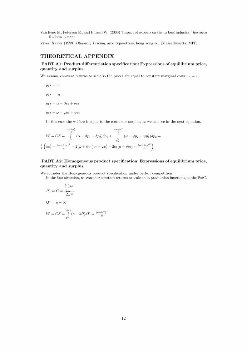
THEORETICAL APPENDIX

PART A1: Product differentiation specification: Expressions of equilibrium price,quantity and surplus.

We assume constant returns to scale,so the prices are equal to constant marginal costs: pi = ci.

p1∗ = c1

p2∗ = c2

q1∗ = α− βc1 + δc2

q2∗ = ω − ϕc2 + ψc1

In this case the welfare is equal to the consumer surplus, as we can see in the next equation.

W = CS =

α+δp∗2β∫p∗1

(α− βp1 + δp∗2)dp1 +

ω+ψp∗1ϕ∫p∗2

(ω − ϕp2 + ψp∗1)dp2 =

12

(βc21 + (ω+ψc1)2

ϕ− 2(ω + ψc1)c2 + ϕc22 − 2c1(α+ δc2) + (α+δc2)2

β

)PART A2: Homogeneous product specification: Expressions of equilibrium price,quantity and surplus.

We consider the Homogeneous product specification under perfect competition.In the first situation, we consider constant returns to scale en in production functions, so the P=C.

P ∗ = C =

∑i

qici∑i

qi

Q∗ = a− bC

W = CS =a/b∫P∗

(a− bP )dP = (a−bC)2

2b

12