Process EngineeringTraining Program

MODULE 4Process Measurement and Testing

Section ContentI Process Information and Plant Testing2 Mill Testing3 FLS Comminution Manual4 The Physics of Air5 BSI Conversion Factors and Tables6 Back to Cement Plant Basics7 Test Method Formulae and Nomeclature- GEL8 Combustion and Efficiency

PresentationsPhysics of Air

Process Engineering

Training Program

MODULE 4

Process Measurement and TestingSection Content

I Process Information and Plant Testing

2 Mill Testing

3 FLS Comminution Manual

4 The Physics of Air

5 BSI Conversion Factors and Tables

6 Back to Cement Plant Basics

7 Wl.ool Gas Flow Measurement by Pitot Static Tube

8 W1.002 Temperature Measurement Using a Thermocouple

9 WI.003 Gas Flow Measurement Using a Vane Anemometer

10 WI.008 Static Pressure Measurement

11 WI.009 Weighfeeder and Conveyor Belt Load Verification

12 WII.013 Kiln Shell Heat Loss Determination

13 WI.014 Measurement and Calculation of Inleaking Air

14 Test Method Formulae and Nomeclature- GEL

15 Combustion and Efficiency

16 Code of Federal Regulations Parts 1900 - 1910

Blue Circle Cement

PROCESS ENGINEERINGTRAINING PROGRAM

Module 4

Section 1

Process Information and Plant Testing

PROCESS INFORMATION AND PLANT TESTING

1. Introduction

2. Processing of Available Information

3. Equipment and Techniques for Plant Measurement

4. Plant Testing - Methods

PROCESS INFORMATION AND PLANT TESTING

1. INTRODUCTION

A reliable, accurate source of process information is the key to plant control. By analysis of the availableinformation, either by manual or computerized methods, the trends which develop on a plant can be determinedand action taken to restore efficient operation. In addition, info mat ion is also necessary to identify if plantmodification has been successful. Without proper evaluation of the situation before and after modification,misleading conclusions can be drawn. This paper will discuss the processing and use of normal plantinformation sources and also specify methods used to carry out plant testing.

2. PROCESSING OF AVAILABLE INFORMATION

2.1 General

The prime source of information on the majority of works is the plant log-sheet. This should be as briefas possible but record all essential data. Space should be allowed to average relevant operating data. Wherecomputer systems exist which will automatically record hourly plant status, this can be used to present a dailylog. Whether this replaces a written log will vary from plant to plant, but writing down of data hourly can oftendraw an operator's attention to a deviation from normal conditions. Daily averages can also be producedautomatically from a computerized system but care must be taken to avoid the averaging of irrelevant data. Adaily average oxygen which includes one hour when the instrument was in service and three hours of kiln stopand subsequent warm-up is of no value.

The processing of the raw data can be a time consuming procedure and direct input of this data into amicrocomputer is a useful development. Once the information has then been inputted manipulation to give therequired analysis of the plant performance becomes a simpler exercise. The presentation of the processed data isimportant. An approach based on graphical presentation more easily identifies the trends which are important ona cement plant. The frequency with which the graphs are produced will depend on the area concerned. It is rarefor the trends in a cement mill to merit better than monthly analysis, but the kiln is a case for a more 'frequentobservation.

The Following sections outline some recommended data which should be processed on plant. They arenot exhaustive lists, however, and Individual plants will have different needs.

2.2 Crushing

The majority of crushers have two functions:

a) To reduce material to a required size, at the required rate and at a minimum power consumption.

b) To have a minimum cost of maintenance, which largely depends on wear rate for high speedcrushers.

A crusher log sheet must include hours run, kW consumed, tons processed and stops/reasons for,although the tonnage may have been back-calculated from loads or stocks. The laboratory must regularly (atleast once per week but depends largely on crusher wear rate) analyze the size of both material in and out. ManyCrushers fail to produce for reasons of excessive feed size rather than some internal deficiency. Care in thesampling procedure is important. Samples taken from belts tend to be segregated across the width of the beltand it is often easier to sample the coarser material at the edge.

The maintenance department must record the quantities of make-up weld used in repair or check theloss in weight of sample impact bars or hammers. This will enable a picture of wear rates to be formed. Theanalysis of crusher information is a simple process. Loss of output may derive from a failure to deliversufficient feed to the crusher or a more basic change in material characteristics. The power consumption andabrasion figures can be used as back-up for any change in raw mill behavior and also to analyze the effect of anychanges made to crusher operation or wear materials. A typical analysis of crusher operation is shown in Fig.l.

2.3 Raw Milling

Raw mills have three prime functions.a) To mill raw materials at the required rate, to the required size and with minimum power

consumption.

b) Other than wet process mills, to dry raw materials to the required moisture.

c) To perform these functions at the lowest repair cost. A combination of log sheet,laboratory analysis and maintenance information is needed to analyze mill performance.

2.3.1 Grinding

To assess grinding performance a log sheet wi11 need to give the percentage of each material processed,mi11 feed rare, hours run ( reasons for stops), kW consumed and -fuel used (if applicable). The laboratory mustanalyze feed and product size. In cases where product residue variations are large a corrected figure for kWh/tcan then be produced as shown in Table 1 and used in the raw mill analysis in Fig.2.

Given this information it becomes a simple matter to analyze the primary reasons which may reduce milloutput or increase power consumption. Examples would be:

a) If mill output falls but specific power consumption remains constant, then a lack of mediaweight is most probable and the percentage mill motor power drawn will be less.

b) If mill efficiency falls then this may be due to an incorrect media size distribution whichwould require an axial test (see "Mill Testing" paper). Raw material feed size may have beenallowed to increase or a harder material may be arriving from the quarry. Crusher data mayhelp in this analysis but. suspected changes in material quality will need to be confirmed in aGrindability Test. On closed circuit mills the recirculating load or separator efficiency mayhave reduced. Plant testing according to the methods shown in "Mill Testing" will then beneeded but is obviously important that comparative data is also taken when the mill isoperating well.

Vertical spindle mills require much of the same data when assessing grinding capacity but additionaldata on roller and table wear will be necessary. As wear has an unpredictable effect on vertical spindle millefficiency, historical data will be needed before firm predictions can be made on the relationship between wearand efficiency, but having assembled this data it can be used (to optimize the timing of changes to roller andtable components.

2.3.2 Drying

Poor quality of drying may show as an inability of the mill to produce the required product moisture forhandling in the raw meal System, or the symptoms may be first seen in the raw mill efficiency. In both casesdata an mill feed and product' residue, mill outlet and inlet temperatures and mill differential pressure willneed to be considered. In the majority of cases, provided neither the raw feed moisture does not exceed that onwhich the mill design was based, poor drying will be due to lack of gas flow to the mill. Section 4.1 containsdetails of methods for testing mill circuits for inleaking air and restrictions to gas flow. Both will reduce millgas flow and lower drying capacity. If required, a full heat balance is also included in Section 4.1. If the mill fancapacity is suspected, section 4.2 details a method for determining if thefan condition is adequate.

2.3.3 Running Time, Costs and Reoairs

Although the majority of mil I costs are not process related, it is necessary to assess the relationshipbetween materials used in the mill diaphragms, lining and media, and the resulting wear to these elements.Together with mill motor power drawn, the volume load of the media must be measured regularly according tothe methods given in “Mill Testing”. Quantities, sizes and quality of make up media is recorded as shown inFig.3 in order to assess wear of new qualities, and regular checks should be kept of diaphragm and lining wearin order to predict replacement dates.

The analysis of down-time is necessary on plants where raw mill availability is important, but is alsoadvisable on other mills as it may be valuable to identify repetitive repair costs.

2.4 Blending

A blending system has one prime objective; to reduce the short term chemical variations which appear inraw mill product. As such an analysis of chemical variability in and out is the most direct measure of blendingtank effect. It is necessary that the chemical analysis is carried out on an identical time basis in and out andstandard deviation is used as a better measure of variability than range. Any of the compounds or derived terms(LSF, SR) can be used in these expressions. If the same time basis is not available for in and out sampling then acorrection according to Table 2 may be applied. After any necessary correction a blending effect can becalculated.

Blending effect = standard deviation (1 hr sampling of raw meal in)standard deviation (1 hr sampling of raw meal out)

Deficiencies in blending effect alone are the basis on which batch systems are evaluated. Poor ordeteriorating performance of a batch blender normally requires a check of the timing of valves which feed air todifferent sections or a check of airflow as detailed in section 4.3. In extreme cases a silo internal inspection maybe necessary to determine if available air is leaking from a broken connection etc.

In the case of continuous silos, blending effect requires a more complex formula:

Blending Efficiency = σin x λ x 1

σout 2π T

where σin = standard deviation (1 hour) of raw meal in

σout = standard deviation (1 hour) of raw meal out

λ = wavelength of chemical variations entering

T = silo residence time = Tons capacityTons throughput

The interpretation of wavelength is the most difficult feature. An example is given in Fig.4.

It is clear from the formula that blending efficiency can be effected by changes in the frequency of feedvariations around the set point and by changes in throughput. If the blending efficiency shows a pronouncedchange then testing of airflow as detailed in section 4.3 is needed. Internal inspection of 'he silo would follow ifthe airflow shows blocked tiles or convasses. Low pressure of supply air may be due to broken pipes etc.

A -final diagnosis of blending tank behavior, for both continuous or batch systems, may require a tracertest. This comprises adding a trace material to the tank feed and determining the behavior of this material withinthe system. Details are given in section 4.3.

2.5 Kiln and Cooler

The requirements for a kiln/cooler are that it should:

a) produce at the required output and with the maximum possible available running time

b) have the best possible fuel efficiency

c) have the lowest possible repair costs, most significantly in terms of refractory and chainrepairs.

Kiln log sheets or computer data, lab analysis and maintenance records need to record sufficient data tobe able to analyze these requirements.

2.5.1 Production and_Fuel_Efficiency

As low production and high fuel consumption are often closely connected the data collection systemmust have a minimum of information which would include the kiln feed and fuel rates, hours run, reasons forstops, oxygen and carbon monoxide levels, feed moistures (wet process) exit suction (kiln and preheater), exit

temperature and any cooling water used 'in the kiln or preheater in addition if kiln NOx is available this should

be recorded. In general any variables which are in automatic control need not be recorded unless frequentchanges are made to set point.

The laboratory records must include a kiln feed analysis and residue, product free "'me and 503 and fuelanalysis as supplied and, if different, as fired.

The information available will produce the initial analysis of kiln/cooler operation in the form shown inFig .5, and this alone will often give the reason For lost production.

Some typical reasons for lost production which can be observed are:

a) Change of feed quality or residue. Relationships between the feed quality and production/fuelconsumption will vary between plants and even kiln processes on a single plant. It is importantthat this relationship is established, if approximately, for any kiln. An example taken from a UKpreheater plant is:

1% LSF equivalent to 0.8% production or 6 kcal/kg clinker

0.1 SR equivalent to 1% production.

b) Change of fuel quality or residue. Again it is difficult to be specific about the effect onproduction/fuel consumption of fuel quality but Table 3 gives some approximations of the effectsof coal moisture on fuel consumption for a direct fired kiln. Pulverised fuel residue is a moredifficult effect to describe as only in an extreme form will carbon monoxide start to be presenttogether with reasonable oxygen levels. However, if the general rule of a 90 micron residue onehalf of volatile matter is observed the kiln flame will not suffer in this respect.

c) Cooler. A deterioration in cooler performance will damage kiln performance. If this is suspectedthen the recommended action consists of a test for cooler efficiency. Details of the method for agrate cooler are contained in section 4.4 and similar concepts can be applied to planetary androtary coolers. In all cases it is important to have historical data for comparison purposes.

d) Inleaking Air. A frequent cause of lost production is inleaking air. Section 4.4 details methods ofassessment.

e) Fan Capacity. Wear or modification can reduce fan capacity. Section 4.2 contains details ofassessment.

f) Build-up. The additional restriction to gas flow caused by build up can normally be determinedby the suctions at kiln exit and where applicable, preheater exit or fan inlet. If these restrictionsare due to changes in alkali contents in the kiln feed an analysis of the alkali cycles may berequired. Section 4.4 gives details of this and the plant testing methods to deter-mine the locationof any build-up.

g) Heat Transfer. One of the important changes which will occur in long dry and wet kilns iswear to the chain system. In order to assess this factor chain weighing as shown in the"Wet Kilns"' paper will be needed. Monitoring of the need for chain maintenance is

possible from kiln exit temperature but correction of the temperature is necessary to allowfor the effects of inleaking air, water sprays, changes in kiln production etc. Table 4 givesan example of the calculation of ''corrected'' kiln exit temperature.

Other factors than these will also influence kiln performance and section 4.4 gives other planttesting procedures which should be carried out on a regular basis, not uniquely when a problemoccurs.

Before any significant changes are made to raw material components, raw meal composition orresidue a combinability test is a useful guide to kiln behavior with the new mix. A regular repeattest is recommended.

2.5.2 Refractories

Detailed discussion of refractory types and wear is beyond the scope of this paper but the methods ofanalyzing refractory life are included.

It is obviously important that details of refractory zones replaced, time of the original in service, qualityof refractory used and any refractory test drillings should be kept in a comprehensive log. Analysis of the resultsof changes to refractory life for different qualities of brick can then be assessed after allowing for other majorfactors which may have contributed to life. With a reasonable fund of information some works have formulateda method of predictive control. An example is shown in Table 5. if additional information is available on shelltemperatures, such as from the modern scanning systems, then a picture can be built up of the formation andloss of coating and this can be correlated to loss of refractory and possibly also to changing kiln feed quality,frequent kiln stops etc.

2.5.3 Running Time

A detailed analysis of kiln lost time is essential. In the case of -planned stops some assessment of therepairs carried out which would have caused lost time is desirable.

2.6 Cement Mill

Cement mills have three prime functions:

a) To mill clinker and any additives at the required rate, surface area and residue.

b) To produce cement at an acceptable temperature.

c) To perform these functions at the lowest Possible cost.

2.6.1 Grinding

To assess grinding performance the log sheet will need to give the total feed rate, percentage of eachcomponent, hours run (reasons ,or stops) and kW consumed. Laboratory analysis is of cement surface area,residue and mill feed size. Surface area production can be calculated as:

Surface area (as m2/t) = M2/kWh kWh/t

An example of cement mill data is shown in Fig.6.

The normal faults of falling grinding efficiency are similar to raw milling. Example of poor efficiencyare essentially identical to raw milling and similar conclusions can be drawn.

2.6.2 Mill Ventilation

One feature of cement mills which does differ from raw mills is the effect which both excessively coldand hot running can cause Both extremes can lead to coated media and poor grinding efficiency. Detection isfrom mill operating temperatures and the axial test described in the “Mill Testing” paper. The area of the millwhich is ineffective will be identified by a small surface area increase across the affected mill length. The mostcommon fault is the over-hot condition when cement temperatures exceed 1200C. This is also an importantfactor in avoiding gypsum dehydration and customer complaints on handling bagged cement. The commoncauses of hot cements mills are:

a) hot clinker feed. Data on the cooler performance will be useful in this respect.

b) Inadequate cooling water flow. 'the maximum quantity of water which should be used inthe mill is limited to 4% on clinker. This includes moisture in the mill feed.

c) Poor mill ventilation. The most common fault is most easily identified by an inleaking airtest as described in section 4.5. Additional testing may be necessary to determine airflowrestrictions and mill fan condition.

2.6.3 Running Time, Costs and Repairs

The analysis of mill internal wear, costs and running times are as per raw mills.

3. EQUIPMENT AND TECHNIQUES FOR PLANT MEASUREMENT

The Majority of the equipment should be available on any plant, but only the larger plants will justify themore expensive equipment.

3.1 Temperature

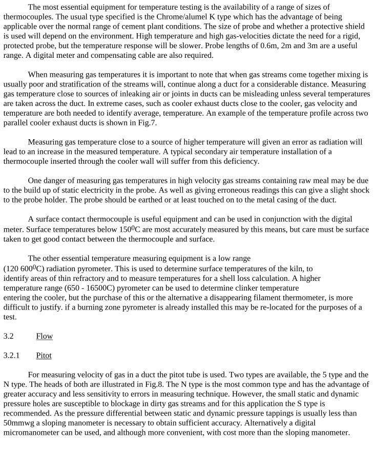
The most essential equipment for temperature testing is the availability of a range of sizes ofthermocouples. The usual type specified is the Chrome/alumel K type which has the advantage of beingapplicable over the normal range of cement plant conditions. The size of probe and whether a protective shieldis used will depend on the environment. High temperature and high gas-velocities dictate the need for a rigid,protected probe, but the temperature response will be slower. Probe lengths of 0.6m, 2m and 3m are a usefulrange. A digital meter and compensating cable are also required.

When measuring gas temperatures it is important to note that when gas streams come together mixing isusually poor and stratification of the streams will, continue along a duct for a considerable distance. Measuringgas temperature close to sources of inleaking air or joints in ducts can be misleading unless several temperaturesare taken across the duct. In extreme cases, such as cooler exhaust ducts close to the cooler, gas velocity andtemperature are both needed to identify average, temperature. An example of the temperature profile across twoparallel cooler exhaust ducts is shown in Fig.7.

Measuring gas temperature close to a source of higher temperature will given an error as radiation willlead to an increase in the measured temperature. A typical secondary air temperature installation of athermocouple inserted through the cooler wall will suffer from this deficiency.

One danger of measuring gas temperatures in high velocity gas streams containing raw meal may be dueto the build up of static electricity in the probe. As well as giving erroneous readings this can give a slight shockto the probe holder. The probe should be earthed or at least touched on to the metal casing of the duct.

A surface contact thermocouple is useful equipment and can be used in conjunction with the digitalmeter. Surface temperatures below 1500C are most accurately measured by this means, but care must be surfacetaken to get good contact between the thermocouple and surface.

The other essential temperature measuring equipment is a low range(120 6000C) radiation pyrometer. This is used to determine surface temperatures of the kiln, toidentify areas of thin refractory and to measure temperatures for a shell loss calculation. A highertemperature range (650 - 16500C) pyrometer can be used to determine clinker temperatureentering the cooler, but the purchase of this or the alternative a disappearing filament thermometer, is moredifficult to justify. if a burning zone pyrometer is already installed this may be re-located for the purposes of atest.

3.2 Flow

3.2.1 Pitot

For measuring velocity of gas in a duct the pitot tube is used. Two types are available, the 5 type and theN type. The heads of both are illustrated in Fig.8. The N type is the most common type and has the advantage ofgreater accuracy and less sensitivity to errors in measuring technique. However, the small static and dynamicpressure holes are susceptible to blockage in dirty gas streams and for this application the S type isrecommended. As the pressure differential between static and dynamic pressure tappings is usually less than50mmwg a sloping manometer is necessary to obtain sufficient accuracy. Alternatively a digitalmicromanometer can be used, and although more convenient, with cost more than the sloping manometer.

The conditions which must be met for accurate pitot measurement require that the point at which thepitot survey is made must be 5 x duct diameter downstream and 2 x duct diameter upstream of any bend,constriction, fan or damper etc which would disturb the air flow pattern. These conditions are rarely achievablein a cement plant situation and a compromise which allows for greater error is normally accepted. Theimportance of the upstream requirement is most often ignored in practice, and it is better to preserve the ratio of2:1 in duct lengths if possible.

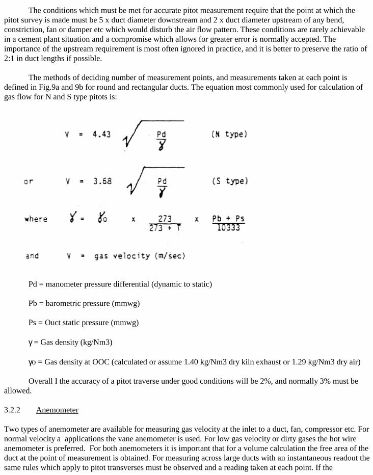
The methods of deciding number of measurement points, and measurements taken at each point isdefined in Fig.9a and 9b for round and rectangular ducts. The equation most commonly used for calculation ofgas flow for N and S type pitots is:

Pd = manometer pressure differential (dynamic to static)

Pb = barometric pressure (mmwg)

Ps = Ouct static pressure (mmwg)

γ = Gas density (kg/Nm3)

γo = Gas density at OOC (calculated or assume 1.40 kg/Nm3 dry kiln exhaust or 1.29 kg/Nm3 dry air)

Overall I the accuracy of a pitot traverse under good conditions will be 2%, and normally 3% must beallowed.

3.2.2 Anemometer

Two types of anemometer are available for measuring gas velocity at the inlet to a duct, fan, compressor etc. Fornormal velocity a applications the vane anemometer is used. For low gas velocity or dirty gases the hot wireanemometer is preferred. For both anemometers it is important that for a volume calculation the free area of theduct at the point of measurement is obtained. For measuring across large ducts with an instantaneous readout thesame rules which apply to pitot transverses must be observed and a reading taken at each point. If the

anemometer has a cumulative readout then the system described in Fig.10 can be used. Anemometers will beaccurate to ±5% if maintained in good working order.

3.3 Suction

A variety of probes are available from the simple open ended 'tube to the static tapping of 'the N typemanometer. A manometer is also required, either liquid column or digital type.

The more sophisticated designs of probe are for situations where gas velocity is high and the angle atwhich an open-ended tube is held to the gas stream would affect results. If, for example, an open-ended tubewas inclined 'towards the gas stream some dynamic I head would be measured and the static suction readingwould be reduced.

3.4 Oxygen and Carbon Monoxide

Two types of equipment exist for measuring oxygen and carbon monoxide. One is the Orsat equipment,which uses solutions of potassium hydroxide, alkaline pyrogallol and cuprous chloride in hydrochloric acid toabsorb carton dioxide, oxygen and carbon monoxide respectively. The quantity of gas absorbed from the samplecan be used to determine the proportion of each gas in the sample. A more modern development is the portablegas analyzer which measures oxygen and combustibles in a gas stream which is Pumped through an electricalfuel cell and a combustion cell respectively. The modern equipment has the advantage of continuous samplingand a more rapid result. It is also fully portable and requires a minimum of setting up. The disadvantage is thatthe measurement is of combustibles which can include a contribution from methane, hydrogen, hydrogensulphide etc as well as carbon monoxide. This limits the application if checking of carbon monoxide meters isrequired.

As with temperature measurements, proper selecting of sampling points is required or misleading resultswill be obtained. If using an Orsat and measuring near a source of inleaking air several samples will be neededacross the duct to ensure accuracy. With the continuous sampler measurement at several points and averagingresults will be required.

4. PLANT TESTING - MTHODS

This section describes in greater detail some of the methods of plant testing which may be used todiagnose the reasons for changes in plant performance. As stated previously it is important with many of thetests that comparable results taken during normal operation are available.

4.1 Raw Mill

The tests described in this section can, in many cases, be equally applied to coal mill circuits.

4.1.1 Inleaking Air

In order to carry out an inleaking air survey on a raw milling system either actual measurements of thegasflow at various points may be made, using a pitot tube, or measurements of the percentage of oxygen in thegas may be made, using a portable oxygen analyzer, or a combination of these techniques may be used. Thechoice of method may be dictated by the availability and dimensions of measuring points.

Where actual gasflows can be measured, the quantity of inleaking air between two points in the millingcircuit can be obtained by difference after the two measurements are referred to the same temperature andpressure and corrected for any change in state, e.g. vaporization of moisture.

Where a portable oxygen analyzer is used, the inleaking air into the gas stream flowing from point A topoint B is given by:

Inleaking air = B – A x100%20.9-B

Where B = % O2 at point B

A = % O2 at point A

Fig.11 illustrates a ball mill in closed circuit with a static separator, the raw meal being separated fromthe gas steam by four cyclones.

Typical measuring points might be A to G as shown.

Points A & B would give the inleaking air through the air sea]

Points B & C would give the inleaking air through 'the mill inlet and outlet seals

Points D & E would give the inleaking air into the separator

Points F & G would give the inleaking air into the cyclones Points A & G would give the inleaking airinto the whole circuit.

(Note that this is not equal to the sum of the four individual inleaks).

Fig.12 shows a roller mill with product collection by a cyclone followed by an electrostatic precipitator.

Typical measuring points might be A to F as shown.

Points A & B would give 'the inleaking air into the mill (including via the raw feed airlock.)Points C & D would give the inleaking air into the cyclonePoints E & F would give the inleaking air into the precipitator.

4.1.2 Suctions Across System

A series of static pressure measurements along a duct or a system of ductwork, fans and other items ofplant can reveal restrictions to gasflow such as partly blocked ducts, dampers which are partly closed eventhough indicating fully open externally, etc.

A sudden rise in suction when measurements are being taken in the direct-ion of gasflow (or vice versa)indicates that an obstruction has just been passed.

4.1.3 Mill Gas Flows

The best means of determining raw mill gas flow depends on the arrangement of the gas ducts but ifadequate measurement points exist close to mill inlet a pitot survey alone will be sufficient. Measurement ofgas flow at the mill outlet is often difficult due to the heavy dust concentration blocking the pitot and it is advi-sable to measure flow closer to the mill fan. in this case a survey of inleaking air will also be needed so that theactual mill gas flow can be calculated. An example would be:

Measured gas flow at mill fan 1,417m3/minSuction at mill fan 50mmwgOxygen at mill fan 14.0%

Temperature at mill fan 116 oCSuction at mill inlet 50mmwgOxygen at mill inlet 10.0%

Temperature at mill inlet 343oC

Percentage of inleaking air = O2 fan - 02, inlet

O2 air - 02, fan

= 14.0 - 10.0 20.9 - 14.0

= 58.0%

Mill inlet flow = fan flow x Temperature inlet + 460Temperature fan + 460

x Atmospheric Pressure - Suction at mill inlet x 100Atmospheric Pressure - Suction at fan 100 + % inleak

= 1,417 x (343 + 273) x (10333 - 50) x 100(116 + 273-) (10333 – 500) x 158

= 1485 m3/min at 343oC

4.1.4 Miscellaneous

The details of test procedures for axial testing, media grading and percentage volume load, separatorefficiency and recirculating load are contained in the Mill Testing Paper. An example of a raw mill heat balanceis contained in the Mill Systems Paper.

4.2 Fans

The first step to establish if a fan is working to design capacity is to obtain the fan curve, and if notavailable on site, to consult the manufacturers. The conditions for which the curve is constructed are alsonecessary i.e.:

a) Is the curve for static or total pressure? Normally static curves are supplied which means that the pressuredifference across the fan is from dynamic inlet to static outlet heat. Total pressure is static to static.

b) What gas density is specified?

c) What fan speed is specified?

Fig.13 shows a typical manufacturers fan curve. To check fan operation the following data must be taken.

a) Fan shaft speed. Taken by tachometer or by a stroboscopic system.b) Fan operating temperature. As most fans suffer from some inleak, which cools the gas, and also

inefficiency, which heats the gas, it is advisable to measure inlet and outlet temperatures and use anaverage.

c) Fan capacity volume. Whether the fan volume is measured at inlet or outlet will normally depend onaccess to sample points but inlet is usually preferred as this will also yield the data for dynamic heat -it thefan inlet.

d) Fan operating heads. Static head is measured at fan outlet and dynamic heat at inlet if fan static pressure isspecified.

e) Fan motor power. Taken either from the kilowatt hour meter or ammeter (check accuracy).

The following example demonstrates the calculation necessary to check fan performance.

Fan shaft speed 952 rpm

Fan inlet temperature 260oC

Fan outlet temperature 263oCFan volume 1,417m3/minFan inlet suction - 508 mmwgFan inlet dynamic head - 493 mmwgFan outlet suction - 13 mmwgFan motor current 32.4 ampsFan motor voltage 3.30 kVPower factor 0.9ran motor efficiency 0.37

Calculation:Fan shaft power (input) = 145 kW

Fan average temperature = 261.5oCFan static pressure = - 493 - (13)

departure from this, such as shown in Fig.14, would signify inadequate mixing.

Continuous silos are treated as continuous flow stirred rank reactors and the average residence time mustbe determined from the calculated half-life i.e. the time at which one half of the added tracer is calculated tohave left the silo. Fig.14 gives a test result which shows poor mixing and hence blending efficiency.

4.4 Kiln

4.4.1 Suctions

As with raw mills static pressure measurement can reveal restrictions to gas flow. Figs.16 and 17 showthe results of pressure surveys on two wet process kilns which are identical in size but have different chainsystems. In the case of kiln I (Fig.16). the static suction rises from 109 mmWG at the precipitator outlet to 155mmWG at the ILD fan inlet, a difference of 46 mmWG. For kiln 2 (Fig.17) it rises from 137 mmWG to 206mmWG, a difference of 69 mmWG. It is clear that the pressure drop is high for both kilns but particularly so forkiln 2, where a partly blocked duct or partly closed damper is suspected. Internal inspection is required toconfirm these findings.

4.4.2 Temperatures

Measurement of temperature in a kiln system can be valuable for several reasons. Some examples are:

a) As an alternative to oxygen analysis to determine inleaking air. Although a kiln exhaust systembetween the kiln exit and main fan will lose some gas temperature by radiation and convection,the principal loss in temperature will be dilution by cold air. An approximation of inleaking aircan thus be determined by temperature.

b) To determine short-circuiting of raw meal beneath a distribution box or plate in a preheater. Bymeasuring the gas temperature between 2 and 4ft beneath the distribution plate any deviationfrom the normal gas temperature may signify corrosion of the plate etc. An example is shown inFig.18.

c) As a check on control room temperature readings.

4.4.3 Inleaking Air

The portable oxygen analyzer is the most useful instrument for kiln inleaking air surveys.

If possible the first measuring point should be at the kiln back-end. Care should be taken to ensure thatthe gas sample is taken from inside the kiln, and not from the back-end chamber where it could be contaminatedby inleaking air from the back-end seal.

A Sample from the back-end chamber may allow the inleaking air from the seal to be calculated, butobtaining a good gas sample is not easy as good mixing between the kiln exhaust gases and the inleaking air willnot have been possible in the short distance involved.

For dry process kilns an oxygen analysis at the preheater exit will allow calculation of the inleaking airinto the preheater system.

For wet process kilns, readings may be made at various points between the back-end and the stack asshown in Fig.16 and 17.

4.4.4 Cooler Testing

4.4.4.1 Cooler Air Balance

Airflow through the cooling fans can be measured either by anemometer at the fan inlet or by pitot tubeat the fan outlet provided that a measuring point can be found on a straight section of duct not too close to thefan.

The primary air fan flow can be measured in a similar way to the above.

The exhaust fan airflow may be determined using a pitot tube. A series of measurements should betaken, certainly at least two, and the average taken as conditions in the cooler will vary.

The quantity of secondary air passing into the kiln is not directly measurable and will have to becalculated. This may be done from first principles if an analysis of the kiln fuel is known. More secondary airthan theoretically required by the fuel actually passes up the kiln as the presence of back-end oxygen indicates.E.g. at 2% back-end oxygen 10% excess air passes up the kiln. Details of the method of calculation of thesecondary and excess air quantities from first principles are given in the Heat Balances paper. As a reasonableapproximation published values of the theoretical air requirements for various fuels may be used, e.g.

British steam coals 0.1 kg air/kg coal

Heavy fuel oil 3,500 sec Redwood No 1 3.7 kg air/kg coalThe quantity of air inleaking via the kiln hood should be included in the air balance - from experience a

figure of 5% of the secondary air quantity is a reasonable approximation. The cooler air balance then is:

Air from cooling fans + hood inleak = Secondary air + Exhaust air

Since the fan curve is defined at 960 rpm and 327oC it will be necessary to correct the fan curves to themeasured conditions using the table.CHANGE ALTERATION

Fan Pressure Volume PowerDensity α density No change α density

Speed α speed 2 α speed α speed 3

Fan Size α dim 2 α dim3 α dim 5Fan Size α dim 2 α dim3 α dim 5Fan Size α dim 2 α dim3 α dim 5

the fan curve shown in Fig.13 is modified for actual conditions. Comparing the measured data with the modifiedcurve it can be seen in this example that the actual fan performance corresponds well to the specification. Alsopossible is to correct the operating point measured to specified fan conditions and check that this point lays onthe original curve.

4.3 Blending

If blending performance is poor or deteriorating then the first check on plant must be to investigate theair flow to the silo aeration system. A test using an anemometer to measure the air flow at the compressor inletstogether with noting the pressure supplied to the silo will indicate if the compressor is failing to deliver thecorrect volume, or if high pressure and low flow are due to blocked tiles, pipes or canvas.

If the air flows, pressure and any changeovers of air flow between sections of the silo are as designedthen a silo tracer test may be useful to determine the flow of material in the silo. This comprises the addition ofa tracer substance to the silo feed and frequent sampling of the silo product to determine the concentration of thetracer in the product. Fig.14 and 15 shows a typical test result for batch and continuous silos. The interpretationof the graph differs for batch and continuous. The design of the batch silo is that the tracer in the product shouldtheoretically be at an average concentration throughout the discharge period. Anywhere in each case the airquantity is expressed as kg per unit time.

Example of Cooler Air Balance

This is for a wet process grate cooler where a quantity of hot air is drawn off the cooler for use in thecoal milling circuit. It is cooled by the addition of ambient air before being drawn into the mill and it all passesinto the kiln as primary air.

Data Clinker throughput 41 tph

Airflows - fan 1 261 m3/min at 28oC

- fan 2 752 m3/min at 32oC

- fan 3 528 m3/min at 24oC

- fan 4 377 m3/min at 21oC

- fan 5 313 m3/min at 20oC

- cooler exhaust 1412 m3/min at 133oC

- to coal mill 673 m3/min at 300oC

- primary air 485 m3/min at 90oC

Dry coal consumption =150 kg/min from volumetric feeder calibration and coal density

Back end oxygen = 2%

Calculation of secondary air from cooler

Fan Size α dim 2 α dim3 α dim 5

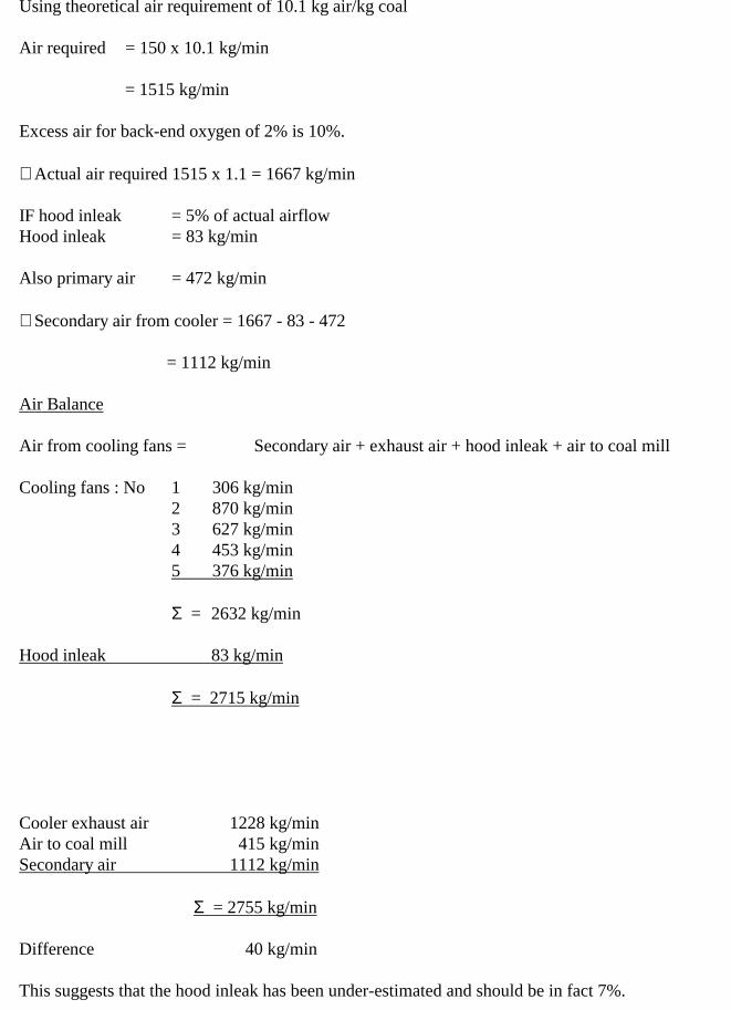
Using theoretical air requirement of 10.1 kg air/kg coal

Air required = 150 x 10.1 kg/min

= 1515 kg/min

Excess air for back-end oxygen of 2% is 10%.

∴ Actual air required 1515 x 1.1 = 1667 kg/min

IF hood inleak = 5% of actual airflowHood inleak = 83 kg/min

Also primary air = 472 kg/min

∴ Secondary air from cooler = 1667 - 83 - 472

= 1112 kg/min

Air Balance

Air from cooling fans = Secondary air + exhaust air + hood inleak + air to coal mill

Cooling fans : No 1 306 kg/min2 870 kg/min3 627 kg/min4 453 kg/min5 376 kg/min

Σ = 2632 kg/min

Hood inleak 83 kg/min

Σ = 2715 kg/min

Cooler exhaust air 1228 kg/minAir to coal mill 415 kg/minSecondary air 1112 kg/min

Σ = 2755 kg/min

Difference 40 kg/min

This suggests that the hood inleak has been under-estimated and should be in fact 7%.

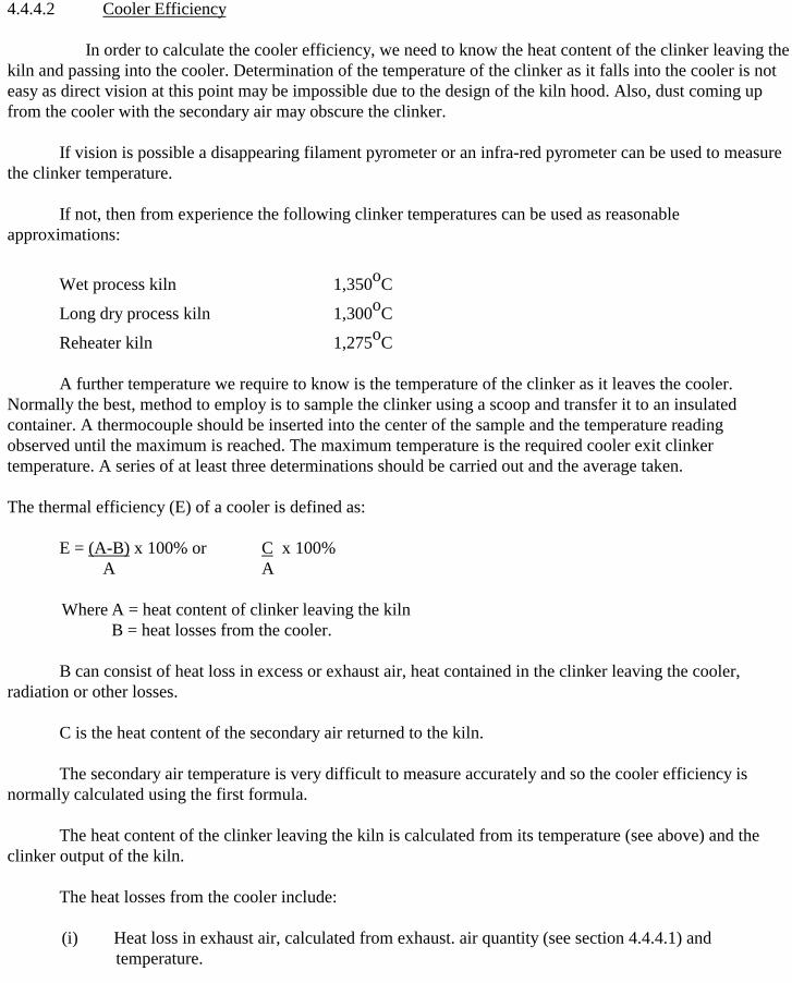
4.4.4.2 Cooler Efficiency

In order to calculate the cooler efficiency, we need to know the heat content of the clinker leaving thekiln and passing into the cooler. Determination of the temperature of the clinker as it falls into the cooler is noteasy as direct vision at this point may be impossible due to the design of the kiln hood. Also, dust coming upfrom the cooler with the secondary air may obscure the clinker.

If vision is possible a disappearing filament pyrometer or an infra-red pyrometer can be used to measurethe clinker temperature.

If not, then from experience the following clinker temperatures can be used as reasonableapproximations:

Wet process kiln 1,350oC

Long dry process kiln 1,300oC

Reheater kiln 1,275oC

A further temperature we require to know is the temperature of the clinker as it leaves the cooler.Normally the best, method to employ is to sample the clinker using a scoop and transfer it to an insulatedcontainer. A thermocouple should be inserted into the center of the sample and the temperature readingobserved until the maximum is reached. The maximum temperature is the required cooler exit clinkertemperature. A series of at least three determinations should be carried out and the average taken.

The thermal efficiency (E) of a cooler is defined as:

E = (A-B) x 100% or C x 100% A A

Where A = heat content of clinker leaving the kilnB = heat losses from the cooler.

B can consist of heat loss in excess or exhaust air, heat contained in the clinker leaving the cooler,radiation or other losses.

C is the heat content of the secondary air returned to the kiln.

The secondary air temperature is very difficult to measure accurately and so the cooler efficiency isnormally calculated using the first formula.

The heat content of the clinker leaving the kiln is calculated from its temperature (see above) and theclinker output of the kiln.

The heat losses from the cooler include:

(i) Heat loss in exhaust air, calculated from exhaust. air quantity (see section 4.4.4.1) and temperature.

(ii) Heat in clinker leaving cooler, calculated from clinker output and temperature (see above).

(iii) Heat lost by radiation and convection from cooler shell (see Heat Balances paper)

Example of Cooler Efficiency Calculation

The data for the example of a Cooler Air Balance will be used again here, together with the following:

Clinker temperature at cooler exit = 100oC

Clinker temperature at kiln exit = 1276oC

A heat balance over the cooler can now be constructed using 'the principles described in the heat balance

paper. The datum temperature used is 0oC.

Heat In

Cooling fans : No.1 3.0 kcal/kg2 9.8 kcal/kg3 5.3 kcal/kg4 3.3 kcal/kg5 3.2 kcal/kg

= 24.6 kcal/kg

Hood inleak @ 28oC 0.8 kcal/kgClinker from kiln 315.2 kcal/kg

= 340.6 kcal/kg

Heat Out

Radiation & Convection, determined as described later 14.8 kcal/kgClinker from cooler 24.7 kcal/kgCooler exhaust air 56.4 kcal/kgTo coal mill 43.0 kcal/kgSecondary air (by difference) 201.7 kcal/kg

= 340.6 kcal/kg

Cooler thermal efficiency E = (A - B) x 100%A

A = heat content of clinker leaving kiln = 315.2 kcal/kg

B = heat losses = Heat in radiation and convection + clinker from cooler + cooler exhaust air +air to coal mill

ie B = 14.8 + 24.7 + 56.4 + 43.0 = 138.9 kcal/kg

∴ E = 315.2 - 138.9 x 100 = 55.9%315.2

4.4.5 Alkali Cycles

Changes in behavior in a kiln system may occur as a result of alteration to alkali balances within a kilnsystem. It is beyond the scope of this paper to discuss the factors which might effect alkali cycles but the effectof a higher level of alkali in the kiln feed and dust can be to increase the frequency of build-up within the kiln orpreheater, form coating on the plates of a precipitator which will decrease the efficiency of the precipitator orincrease the pressure drop through a bag filter.

Sampling to establish the alkali cycles within a kiln system requires that the samples are taken atrelevant points within the system. Fig.19a shows the points at which samples need to be taken on a wet processkiln if a full alkali balance is required. Fig.19b is the type of cycle diagram which can be constructed from thelaboratory analysis. A separate cycle diagram should be constructed for each of the species. As with otherinformation it is important that data on alkali cycles should be available under normal running conditions suchthat any change to operating conditions, dust return, raw materials etc can be monitored.

4.4.6 Heat Balance

The reasons why heat balances are useful to the cement plant operator and the way in which they arecalculated, are covered in detail in the Heat Balances paper. It is the purpose of this section solely to indicatehow the raw data required for these calculations can be obtained.

The data listed below is that required for the heat balance on a wet process kiln with grate coolerincluded in the Heat Balances paper, but similar information is needed whatever process or fuel type is beingused.

(1) Clinker output - normally calculated from kiln feed using a feed to clinker ratio calculated for along period of time. Make sure that this ratio has not been "modified" to make a clinker stockcorrection.

(2) Raw coal consumption - Very often no raw coal weigher exists and the coal feed to the kiln is ona volumetric basis. This can sometimes be calibrated and a coal density used to give a lb/hourfigure. Any errors in the raw coal consumption will show up in the failure of the heat balancecalculations to balance and an iterative procedure can be used to correct the coal input, Oil andgas flows to kilns are usually metered and it is only necessary to read the flow rate at the time ofthe test.

(3) Slurry moisture (or raw meal moisture) - can be determined by the works laboratory on a sampletaken at the time of the heat balances.

(4) Dust loss - it is usually possible to direct the precipitator dust into a lorry and to weigh severalhours' dust on the works weighbridge.

(5) Clinker temperature leaving cooler - procedure described in section 4.4.4.2.

(6) Exhaust air from cooler

- quantity by pitot tube, see section 4.4.4.1- temperature by thermometer.

(7) Kiln exit gas temperature - the value of this variable will be available to the kiln burner but,unless the back-end thermocouple is known to be accurate, it should be checked using athermometer.

(8) Kiln exit gas analysis - 02 and CO can be determined using a portable combustion optimizer. AnOrsat will give 02, CO and C02. An average of several readings should be used.

(9) Temperatures of slurry (raw meal), coal and air at cooler -by thermometer.

(10) Coal - moisture can be determined by works laboratory on a sample taken at the time of the heatbalance.

- calorific value by works laboratory or fuel supplier.- analysis by works laboratory or fuel supplier.

(11) Clinker analysis - by works laboratory. Average of hourly samples during period of test.

(12) Raw meal and dust analyses - by works laboratory. Average of hourly samples during period oftest.

(13) Kiln shell losses - Using an infra-red pyrometer the kiln shell temperature should be measured atten feet intervals along the length of the kiln. At each measuring point, the maximum andminimum shells temperatures should be recorded. Table 6, together with figures 11c and 1ld inthe Heat Balances paper, allow the heat lost from the kiln shell to be calculated.

Example for one 3 meter long section of shell

Maximum temperature 254oC

Minimum temperature 211o CDiameter of kiln shell (external) 6 metersMeasuring interval 3 metersWind Medium

Ambient temperature 20oC

From figure 11c of Heat Balances paper:

Heat loss = 4650 kcal/m2/hourArea of shell section = π.6.3 = 56.5m2

∴ Heat loss = 262,000 kcal/hour

This procedure is repeated for each 3 meter section of shell and 'the individual heat losses are totaled.

(14) Cooler shell losses - These can be calculated in a similar way to the kiln shell losses, whether thecooler is cylindrical or square section.

4.5 Cement Mill

4.5.1 Suction

As with the raw mill, a survey of suctions through the cement mill system can identify blockages,failures in dampers etc.

4.5.2 Inleak

In cement milling, air is the only gas involved so the portable oxygen analyzer is of no help to us. Atpoints where the measurement of airflow by pitot tube is difficult, e.g. at the mill inlet because of the presenceor reed chutes, conveyors and feeders, it may be necessary to use vane or hot wire anemometers.

A further method of measuring the airflow is by the injection of an inert gas tracer. The practice is toinject a known quantity of tracer into the air stream and measure the concentration of this at a point furtherdownstream. For a cement mill the tracer is injected at the mill inlet and its concentration is measured at the milloutlet.

Fig.20 shows the principle of the nitrous oxide tracer method in use to determine airflow through a mill.

The airflow is calculated as in the following example.

N2O volume : If N20 input = x m3/hour at TgOC

Volume at sample point = x (273 + Ts) m3/hour (273 + Tg)

Where TsOC is the sample temperature.

Air volume : If air volume = V m3/hour at TsOC

then Parts per million N20 = x (273 + Ts)(273 + Tg) x 106

V

So if P is the value of parts 6 per million N20 from the detector,then V = x (273 + TS) 106 m3/hour

P (273 + Tg)

e.g. If Ts = 15.5OCTg = OOCx = 0.072 m3/hourP = 49 parts per million N20 from detector

Then V = 0.072 x 288.5 x 106 = 1,552m3/hour49 x 273

The determination of the airflow at the mill inlet, as well as being the basic measurement of airflow inthe mill circuit to which the inleaking air volumes may be related, also allows the number of air changes perminute in the mill to be calculated. Only the mill inlet airflow is free of the likelihood of inleaking air.

Measurements of airflow at other points in the cement mill system are normally carried out using thepitot tube.

4.5.3 Mill Gas Flows

It is seldom that adequate measuring points are available for measurement of mill air flow. With aminority of cement mills air ventilation can be measured at the mill inlet using an anemometer. However, thistype is relatively rare and as with raw mills, the best technique requires measurement of the inleaking air intothe mill system together with an air volume at a convenient measuring point. The actual air entering the mill canthen be back-calculated.

4.5.4 Heat Balance

Refer to Appendix of "Milling Systems" paper.

4.5.5 Miscellaneous

The methods used for axial testing, media grading, separator efficiency and circulating load areexplained in the "Mill Testing" paper.

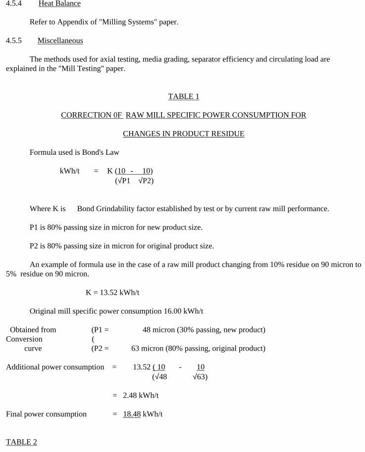
TABLE 1

CORRECTION 0F RAW MILL SPECIFIC POWER CONSUMPTION FOR

CHANGES IN PRODUCT RESIDUE

Formula used is Bond's Law

kWh/t = K (10 - 10) (√P1 √P2)

Where K is Bond Grindability factor established by test or by current raw mill performance.

P1 is 80% passing size in micron for new product size.

P2 is 80% passing size in micron for original product size.

An example of formula use in the case of a raw mill product changing from 10% residue on 90 micron to5% residue on 90 micron.

K = 13.52 kWh/t

Original mill specific power consumption 16.00 kWh/t

Obtained from (P1 = 48 micron (30% passing, new product)Conversion (

curve (P2 = 63 micron (80% passing, original product)

Additional power consumption = 13.52 ( 10 - 10 (√48 √63)

= 2.48 kWh/t

Final power consumption = 18.48 kWh/t

TABLE 2

CORRECTI0N OF BLENDING AND KILN FEED SAMPLES

0bjective: To correct the 24 hour standard deviation of differing sample frequency to a common basis,usually I hour frequency.

For example: 24 hour standard deviation of kiln feed LSF

= 2.02 sampled every 2 hours.

To correct to 1 hour basis multiply by

= 2 .02 x 1 .14

= 2.30

TABLE 3

EFFECT OF COAL MOISTURE AND ASH VS FUEL CONSUMPTION FOR WET

AND PREHEATER PROCESS KILNS

A. PREHEATER

B. WET

TABLE 4

CALCULATI0N OF CORRECTED BACK END TEMPERATURE

Measured kiln exit temperature 260oCKiln production 768 tpdMeasured water flow 83 kg/minKiln exit oxygen 2.0%Kiln fuel consumption 1167 kcal/kgFeed calcium carbonate 78.0%

1. Calculation of gas quantities

kg/kg clinker

C02 ex feed 0.5485 ex fuel 0.4408

TOTAL 0.9893

N2 ex combustion gas 1.2547 ex excess air 0.1511

TOTAL 1.4158

02 ex excess air 0.0612H20 ex coal 0.0180 ex feed 0.0032

TOTAL 0.0212

2. Total heat content of gases to kiln exit

Heat content = (0.9893 x 0.245

above 0oC + 1.4158 x 0.2500+ 0.0612 x 0.232) x T+ 0.0212 x 0.460 x (T - 100) + 0.0212 x 658

= 0.6203T + 13.0

TABLE 4 CONTINUED

3 Total heat content of gases ex kiln (including water)

22 water = 83 kg/min

Kiln production = 542 kg/min

∴ water spray = 0.1533 kg water/kg clinker

Heat content = (0.9893 x 0.230 + (1.4158 x 0.249 + (0.0612 x 0.227) x 260 + (0.1745 x 657 + 0.1745 x 0.450 x 160)

= 154.4 + 127.2

= 281.6

4. "Real" kiln exit temperature

0.6203T + 13.0 = 281.5

∴ T = 433oC

TABLE 5

SAMPLE OF PREDICTED LIFE OF REFRACTORY

BASED ON 1980 1986 DATA

ZOINE LIFE(in from nose) (weeks)

0 - 1.5 311.5 - 3.0 37

1st tyre 3.0 - 4.5 274.5 - 6.0 286.0 - 7.5 227.5 - 9.0 239.0 - 10.5 2710.5 - 12.0 3312.0 - 13.5 3213.5 - 15.0 4115.0 - 16.5 4016.5 - 19.0 37

2nd tyre 18.0 - 20.0 3320.0 - 21.5 4821.5 - 23.0 6923.0 - 24.5 9324.5 - 26.0 11626,0 - 27.5 12827.5 - 29.0 1252-9.0 - 30.5 10330.5 - 32.0 14532.0 - 33.5 153

3rd tyre 33.5 - 35.0 15535.0 - 36.5 180

TABLE 6L0SS OF HEAT By CONVECTION AND RADIATION

MAXIMUMTEMPRATURE

oC

MINIMUMTEMPERATURE

oC

HEAT LOSSESFROM CHARTS

kcal/m3/h

AREA OFSHELL

m2

TOTALLOSSES

kcal/h

1 254 211 235.4 4650 56.5 262,00023456789

10111213141516171819202122232425

CRUSHER

FIGURE 7 - Temperature profile of Cooler ExhaustDust

TEMPERATURE PROFILE OF COOLER EXHAUST DUCT

FIGURE 9a AND 9b PITOT TRAVERSE POINTSRound and rectangular Ducts

Note:Diameters given in mm and all measuring points quoted as fraction of Diameter.

For rectangular cross sections an effective diameter of Def = 0.5 x (H + B) is calculated, then use thenumber of measuring points as tabulated above.

e.g. A duct measures 1000 mm by 600 mm

Def = 0.5 x (1000 + 600) = 800 mm

Corresponding to 2 x 6 i.e. 12 measuring points distributed as shown.

FIGURE 10 - Helical pattern to be described on circular inlet duct to fans. Describe one helix into centre andreturn to start through same pattern. Move anemometer at equal velocity throughout.

Approximate traverse time 1-1.5 mins total.

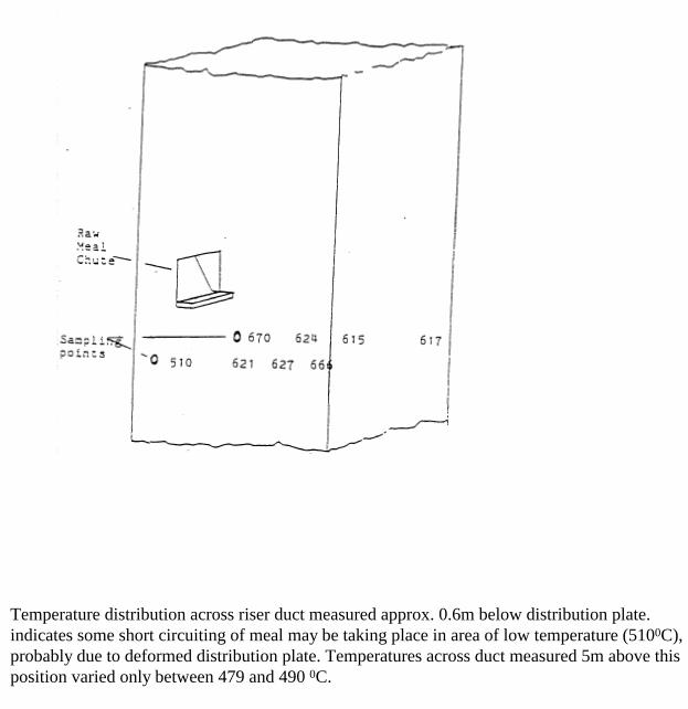
FIGURE 18- Temperature distribution across riser duct measured approx. 0.6m below distribution plate.indicates some short circuiting of meal may be taking place in area of low temperature (5100C),probably due to deformed distribution plate. Temperatures across duct measured 5m above thisposition varied only between 479 and 490 0C.

FIGURE 19- a) samples necessary in wet process kiln to obtain alkali balance. Note a proportion of thefilter dust discarde the remainder insufflated.

b) Alka1i cycle for the kiln. Each of K20, Na20 , Cl, SO3 has a separate diagram and thewidth of the strip represents a mass flow of the material.

Blue Circle Cement

PROCESS ENGINEERINGTRAINING PROGRAM

Module 4

Section 2

Mill Testing

1 INTRODUCTION

The efficiency of grinding depends upon a number of factors, and a variation of one or more ofthese causes deterioration of mill performance. If this goes unchecked very inefficient grindingoccurs resulting in a very poor quality mill product. Careful routine observation of mill residuesand power used for the grinding process will show when efficiency begins to fall off and whether athorough check on performance is necessary.

2 MONITORING MILL PERFORMANCE

In order to monitor a mills performance, the following data is required:1. Mill Throughput2. Power Drawn3. Mill Product Quality4. Feed Grindability5. Mill Temperature/ProductTemperature6. Mill Air Flow/Cooling

Much of the above information should normally be recorded as part of the Works routine procedures. Whereroutine data is unobtainable or is suspect then the following tests and checks may be carried out.

2.1 MILL THROUGHPUT TESTS

2.1.1 WEIGH FEEDERS

All too often weigh feeders can give a misleading picture of a mills throughput. Direct readings of the millthroughput from a weigh feeder or totaliser are subject to possible errors in the calibration of the feeder.Regular checks on the calibration of feeders in accordance with manufacturers recommended procedures canreduce the degree of error.

A simple method of checking the accuracy of a weigh feeder is by measuring the weight of material over aknown length of belt under steady feed conditions, knowing the belt speed enables the throughput to beestimated. Sufficient length of belt must be sampled and account taken of any cyclic variation in feed rate if thismethod is to be accurate.

Chain tests can be used to check the accuracy of weigh feeders. After zeroing the scale, the weigherbelt is loaded up with a set of chains which are calibrated to cover the weighing range of the scales.The scale indicator and recorder can be checked from a knowledge of the chain loading and beltspeed.

2.1.2 SALT TESTS

Another method for determining throughput is the salt test, where salt is used as a tracerthrough the mill. Under steady conditions a constant amount oil salt is added to the mill feed and therise in chloride level of the mill product is observed. A typical procedure for a Salt Test on a cementmill would be as follows:

1 ) Sample the mill feed and finished cement for approximately 30 minutes before starting the testin order to establish control conditions.

2) When the mill is running steadily add accurately measured equal quantities of salt at regularintervals for a period of two hours. The addition rate of rate should be approximately 0.5% of themill output per minute.

3) Sample the mill product at regular intervals for up to 3 hours.4) Analyze the samples for chloride using the chromate direct titration method. Determine the

purity of the salt added and determine the chloride content of the clinker and gypsum feed.

5) Plot a graph of % CI against time and note the steady average value to which the chloride levelrises. (M) as shown in Figure 14.1.

6) Determine the output by the following mass balance where:

X = Chloride entering mill in kg/miny = Cement Mill OutputZ = % Chloride in the cement prior to salt additionM = % Chloride in the cement after salt addition

M= X + Zy x 100Then NaCl X + y

Cl

From which y may be calculated

(NaCl)y = X(100_- M Cl

M - 100Z

2.1.3 CEMENT WEIGH OFF

In this test the cement mills product is diverted into an empty clean silo where it can be separately packedoff and weighed. For valid results, the test must be run for sufficiently long time, i.e. at least 24 hours.Errors will arise if the silo used cannot be effectively emptied out before and after the test due to build up.

2.1.4 CLINKER DROP TESTS AND VOLUME MEASUREMENTS

In cases where space allows for the collection of feed belt material, a drop test may be carried out bydiverting the material through some form, of by-pass into a preweighed dumper. By collecting the feedmaterial over a known period the mill throughput can be estimated.

Another method which is not particularly accurate but which can be used to give a rough guide to milloutput, is the method of measuring the fall in level of clinker in a feed hopper, whilst the mill is runningwith a steady feed.

Samples are taken during the test to determine the clinker bulk density and the SO3 level in the clinker andfinished cement. An SO3 mass balance then enables the gypsum addition rate to be calculated whilst theclinker throughput is estimated from the bulk density and fall in volume in the hopper. Errors arise in thismethod from level measurements and differences in the degree of compaction and segregation affectswhich may alter the bulk density of clinker in the hopper from that measured on the feed belt.

2.2 POWER DRAWN

The most useful method of checking the power drawn by a mill is by taking routine readings from anintegrating kWh meter. Such readings are very often taken on a weekly basis. Spot checks can be made bytiming a number of revolutions of the disc of the kWh meter and applying the appropriate correction factor forthe meter. If neither of these tests can be carried out, then an estimate of the power drawn can be made fromammeter readings. A knowledge of the voltage and power factor enables the power drawn to be deducedthough such estimates are often subject to large errors. From records of the mill throughput and the powerdrawn, the power consumption in kWh/tonnes is calculated.

Power = (sq. root of 3) V.I Cos θ, where V = Voltage, I = Current, Cos θ = power factor

2.3 MILL PRODUCT QUALITY

When referring to a mills output, reference should also be made to those quality aspects which can affect theoutput. It is normal to check a cement mills product for surface area and sieve residues at 90 and 300 microns. Arecord of S03 content is important as the form of sulphate addition, whether it be gypsum or anhydrite can havea significant effect on mill outputs by altering the grindability of the feed.

2.4 FEED GRINDABILITY

Changes in the grindability of the clinker can affect mill performance and so it is advisable to carry outgrindability tests on the clinker at regular intervals. When carrying out- axial tests on a mill, as will be describedin greater detail later on in this paper, it is recommended that approximately 50 kg of average clinker sample istaken for a grindability test to be carried out. The result of this test enables the actual mill performance to becompared with the theoretical performance and is useful in showing how efficiently the mill and individualchambers are performing, highlighting areas of the mill where the performance can be improved by alterationsto the mill charge etc.

2.5 TEMPERATURE

Problems arise when hot clinker is fed to a mill or the mills cooling system i.e. induced draught or water injectiondo not function properly. Thermocouples can be used to monitor both feed and product temperatures and thelatter can be used to control a water injection control loop.

2.6 AIR FLOW Closed

Open 2-3 vols/min

For adequate ventilation, the quantity of air through the mill should be 2-3 volume changes of air perminute. Here the term volume refers to the free volume above the charge in the mill and estimates are made

using a standard temperature of 110o C. There are a number of difficulties involved in making measurements of air flow through a mill.Measurements taken around the ducting leading to the dust filtering plant can be meaningless if the mill haspoor seals as the resultant air flow figures are more likely to indicate inleak rather than ventilation air flow.

Measurements recently taken at one U.K. Works indicated that whilst the air flow through the cement millfiltering plants was adequate, only 20% of this air flow was actually being drawn through the mill owing topoor mill outlet seals. Pitot measurements in this region suffer from problems of blocking pitot tubes due todust and humidity. To measure the quantity of air actually flowing through the mill, an anemometer can beused at the mill inlet with the feed rate off the mill. Draught indicators may be provided at the mill inlet togive some rough idea of the quantity of cooling air through the mill. The differential pressure across acement mill being typically 40-60 mm w.g.

Another method of assessing the air flow through the mill is to use nitrous oxide into the mill inlet as a tracer.The concentration of N20 in the exit air is measured using an infra red detector. Figure 14.2 shows 'hearrangement for N20 tracer testing on a mill.

If either the routine performance data or any of the above tests show that there has been a deterioration in theperformance of a particular mill, then it is advisable to carry out a more detailed examination into the internalstate of the mill as well as an axial test.

3 AXIAL SAMPLING TESTS

An axial sampling test is a means of determining how well a mill is grinding along its length. Such a 'Lest canhighlight areas within the mill where the grinding is not being carried out as efficiently as it should be. Whencoupled with the results for grindability test it is then possible to compare the overall performance of the mill aswell as individual mill chambers with the theoretical performance predicted.

3.1 PROCFDURE FOR AN AXIAL TEST

a. Sample the mill feed and product' under steady conditions for approximately 40 minutes prior tostopping the mill. Record the mill output and power consumption.

b. Stop both the mill and the feeder simultaneously. If the feed is stopped before the mill then theresidual material within the mill will be ground finer than normal and this will make the overall millefficiency appear higher than it actually is.

c. After allowing sufficient time for cooling, enter the mill and take axial samples. Divide up the millinternally into sampling points approximately 10 per chamber or typically 50 cm apart. Samples shouldalso be taken at the diaphragms. At each point on the axis, an average sample should be taken of thematerial along a line at right angles to the axis of the mill. The material should be taken from points afew inches below the ball charge and not from the surface. In the case of a three chambered mill, takelarger samples in the first and second chambers than in the third chamber.

d. Allow the samples to cool before measuring the surface area in the case of a cement mill, or sieveresidues in the case of a raw mill. The coarser samples whose surface area cannot be measured directlymust be graded and their surface areas calculated from Figure 14.3. For a cement mill, a check shouldalso be made on sieve residue of samples throughout the mill.

e. Measure the height above the charge and calculate the % volume loading from Figure 14.4. From thisthe weight of media in each chamber can be calculated using a value for the average media bulk density,if none is available then a bulk density of approximately 4480 kg/m3 can be assumed. The height abovethe charge is best measured with the filling slightly run down, otherwise a false high value for volumeload will be obtained.

f. Using the power equation, calculate the power absorbed by each mill chamber and for the mill overall.Compare this with the figures obtained from the kWh meters.

Ratio

Net/Gross = 0.9 → 0.95 Avg = 0.93

Nett kW = 0.2846 D.A.W.N. D = Mill diameter inside the

W = Weight of media in tonnes lining in metres

N = Mill speed in rev/min A = 1.073-J where J is thefractional volume loading

Gross @ motor

CLINKERB.S.

GRADESIEVE

mm SURFACE AREAm2/kg

+ 3"/4 +19 0 - 2-3/4” + 3"/8 - 19 +9.5 0 - 3

-3/8” + 3"/16 - 9.5 +4.8 0 - 6

-3/16” + 7 - 4.8 +2.4 1 - 1

- 7 + 14 - 2.4 +1.2 1 - 83

-14 + 25 - 1.2 +0.6 3 - 46

-25 + 52 - 0.6 +0.3 6 - 42

-52 +100 - 0.3 +0.15 17 - 8

-100 - 0.15 Measured directly(Lea Nurse)

Fig. 14.3 Surface Area of Different Clinker Grades

g. Plot an axial graph of surface area (cement mill) or residue (raw mill) against the mill length or thenett kW drawn. Normally one plots surface area against nett kW drawn with a cement mill wherewe are concerned with the rate at which surface area is produced for the power absorbed along themill. If theweight of charge per unit length is the same throughout the mill then surface area can beplotted against mill length. However, more often than not this is not the case with mills of morethan one chamber where the volume load can vary between the chambers.

The axial graph should show a steady rise, smooth curve, in surface area along the mill. If the graphcontains any flat sections or sections where the rate of surface production is low as indicated by ashallow slope of the graph, then this indicates areas of the mill where 'the efficiency is low due to:

Compare to grindability (theoretical)

Incorrect ball size

Insufficient charge

Blocked diaphragms

h. Calculate the surface production for the mill overall as well as the surface production for theindividual chambers using the following formula

Surface Production = (SB - SA) T. 103

P

where SA = Surface area (m 2 /kg) of material entering mill or mill chamber

SB = Surface area of material leaving mill or mill chamber

T = Tonnage (tph)

P = Power drawn by mill/chamber (kW)

The efficiency of the mill or chamber is expressed by the relationship

Efficiency = 100 x Actual surface productionTheoretical surface production

The theoretical surface production is predicted from the grindability curve for the feed materials. The methodof calculating the theoretical performance is somewhat involved and a worked example is given in Appendix3 - It is assumed that a reasonable rate of surface production for a mill grinding standard clinker up to asurface area of 250 m 3 /kg is 115 x 102 m2/kWh. From this base figure, making due corrections for surfacearea and grindability the theoretical performance can be predicted for the mill.

i. Take samples of the media in each chamber. Dig into the load in order to obtain these and take severalsamples along the axis of the mill particularly in the case where the mill has a classifyinglining fitted.

Record the weight, number and size of the media withdrawn from the mill together withthe sampling position. Plot a graph of average ball diameter against distance along millaxis.

j. Carry out a size grading of the feed clinker. This is important when determining the sizeof media to be added to the mills first chamber. Usually the maximum feed size dictatesthe maximum ball size that should be added to the first chamber of the mill, forexample, for 19 mm clinker the typical maximum media size is approximately 90 mm.

4 AXIAL TEST FOR A CEMENT MILL - PRACTICAL EXAMPLE

Figure 14.5 shows the results of two axial tests carried out on a 2,500 kW cement mill. The solid line representsthe results with the mill producing 55.8 tph cement at a power consumption of 44.8 kWh/tonne. This line showsa poor rate of surface production in the third chamber. If the mill tonnage was raised in order to reach theguarantee of 60 tph, then the first chamber diaphragm blocked. It was therefore decided to add an additional 2tonnes of 60 mm media to the first chamber.

The smaller sized media was chosen owing to the small feed size of the clinker. To improve the performance ofthe third chamber, some 7 tonnes of 19 mm media were added. This resulted in the following alterations to themills load:

Weight of Charge MediaBefore After Size Range

1st chamber 45 47 100 - 60 mm2nd chamber 39 39 50 - 30 mm3rd chamber 88 95 25 - 19 mm

TOTAL 172 181

The resulting improvement in mill output led to an increase in output from 55.8 to 62 tph as well as a reductionin power consumption from 44.8 to 41.1 kWh/tonne, a saving of 3.7 kWh/tonne. It can be seen that the resultsof a second axial test carried out after the above media additions, show a gradual rise in surface area throughoutthe mill and that the areas of poor surface production have been eliminated.

5 MILL INSPECTION AND MAINTENANCE

During an axial test or as part of a programme of routine mill maintenance, it is usual to carry out anexamination of 'the mill internals. Special attention should be paid to the following points:

5.1.1 LINING PLATES

Examine the plates for any signs of wear, coating and breakage. Normally one expects a reasonably long lifefrom lining plates and it is important to keep an eye out for any unexpected wear or breakages so thatsuppliers quality can be checked.

5.1.2 DIAPHRAGMS

Examine the diaphragm for any breakages, wear and blockage. If the diaphragm shows signs of blockage then itis important to determine what has caused the blockage as this can affect what action needs to be taken, forexample, the presence of nibs could indicate the absence of sufficient quantities of larger size media.

5.1.3 MEDIA

Inspect the media for wear and breakages. From the results of the axial test ball grading, check the gradingagainst the specified grading if this exists and from this determine what sized media should be added or whetheror not the charge should be regraded. Note any differences between the media levels in each chamber since toogreat a step up in level can cause hold ups along the mill unless a lifter type diaphragm is used. Note any coatingof the media due to poor mill ventilation or moisture.

5.1.4 VOIDAGE FILLING

During an axial test check whether the feed material fills the voids of the balls. Overfilling may indicatediaphragm blockages and a restriction to flow whilst under-filling could be causing excessive ball wear andheat generation. If a mill has been brought down for examination due to a specific fault, for example, itsoutput has fallen or nibs are present in the product, then there are a number of possible explanations for this.Appendix 1 lists some common cement mill faults together with their possible causes and remedies.

5.5 THE IMPORTANCE OF REGULAR MILL MAINTENANCE AND THEUSE OF AXIAL TESTS

Figure 14.6 illustrates the importance of regularly maintaining the correct level of charge in a mill by indicatingwhat happens when the charge is allowed to run down in a dry raw mill, over a period of time. It can be seenthat as the power drawn by the mill has fallen due to wear on the charge, the tonnage has fallen and thekWh/tonne have risen.

Approximately £9,000 per annum could be saved on power costs by restoring the mill to its previousperformance. In addition to power savings there would have been additional benefits due to increased rawmeal availability.

By regularly monitoring the mills performance and by carrying out axial tests from time to time, it shouldbe possible to determine the optimum performance from a mill. In addition to providing information onhow efficiently the grinding process is being carried out within a given mill, axial tests also enable aninsight to be given into the effect of other process changes which can affect the mills performance. Forexample, 'he effects of clinker pre-crushing, changes in gypsum addition rate and feeding cooler clinkerto cement mills can all be investigated more thoroughly by means of axial tests.

There is a tendency to only consider carrying out an axial test and other mill tests when something has'gone wrong' and a mill is not performing as well as it should. However it is equally important to carryout axial tests when a mill is performing well so that we can establish why it is performing well. Bycarrying out axial tests on a regular basis it is possible to build up a record of mill operating data, thereby,enabling factors such as optimum charge grading to be determined.

6 WET RAW MILL TESTING

The principles behind cement mill testing apply equally to wet mill testing. The test methods differ only indetail due to the differences between the physical properties of a slurry compared with a fine powder such ascement or raw meal. In a wet mill, or for that matter, a dry raw mill, we are more concerned with the residueof the milled material and not its surface area.It is possible to carry out an axial test on a wet mill although these tests tend to be carried out less frequentlythan tests on cement mills. This is partly due to the difficulties that arise when sampling within the mill.

6.1 AXIAL SAMPLING TESTS ON A WET MILLIt is not so straightforward carrying out an axial test on a wet mill as it is on a cement mill. The procedureis similar to an axial test on a cement mill with the following differences:

a. It is necessary to sample the mill as quickly as possible as the slurry will settle out quite quickly within the mill and it is often necessary to dig down below the load.

b. The samples should be wet sieved at 90 and 300 microns and moisture determinations carried out.

c. Plot the axial sample curve for 90 and 300 micron sieve residues against mill length or powerdrawn.

The power drawn is assumed proportional to distance along any chamber but can vary betweenindividual chambers depending upon the volume loading and can be calculated as follows:

Nett kW 0.9 x 0.2846 D (1.073-J)

where 0.9 represents a typical figure for the slip factor in wet grinding.

d. The tests for measuring power are the same as shown previously. A simple method for checking the output is as follows:

Run the mill's product into an empty slurry mixer for several hours with the mill under steady feedconditions. Measure the depth of the slurry in the mixer before and after the test and determine theaverage slurry moisture and density. From the mixers dimensions, the total volume of slurry and hencethe weight of dry raw materials can be calculated.

e. If the mill has been stopped because of a specific fault or it is known that its performance hasdeteriorated, then an inspection of the mill internals is required. Appendix 2 lists some common wetraw mill faults together with possible explanations and the remedial action that can be taken to curethem.

7 AXIAL TEST FOR A WET RAW MILL – PRACTICAL EXAMPLE

Figure 14.7 shows the results of axial tests carried out on two 3,000 HP wet raw mills. The mills were of thesame design and were charged with approximately the same overall quantity of media. No. I mill was fittedwith three Danula rings which were not fitted in No. 2 mill. The distribution of the charge was also differentwith No. I mill having proportionally more media in its first chamber. From the following table it will be seenthat the performance of No. I mill is superior to No. 2 mill:

Mill No. Dry TPH kWh/tonne % Residue300 µm 90 µm

1 122.9 17.6 1.8 14.32 115.9 18.1 3.3 15.3

It can be seen that the residues are generally lower throughout the length of No. 1 mill compared with No. 2mill. No. I mill was better grinding downmaterial which would end up as residue on the 300 µm sieve bypreparing a finer feed to the mills second chamber.

In this case, it can be seen how axial tests can be used to highlight differences in the grinding action betweensimilar mills. The tests are particularly useful in cases where, for example, it is known that one mill of particulargroup of similar mills is known to perform consistently better than its neighbours. Axial tests can be used to giveindications why differences occur, and thereby enable the optimum operating parameters such as charge quantityand grading to be determined.

APPENDIX 1

CEMENT MILL FAULTS

1. OUTPUT DESCREASES Possible cause

a. Increase in clinker hardness and

b. Mill Charge too

c. Mill volume loading too

d. Too small bodies used for make

e. Diaphragm slots partially

f. Fractured

Remedy

Examine raw feed composition andkiln burning conditions.

Dump charge, regrade and make upnew charge.

Measure each chamber and addcorrect tonnage of new bodies.

Charge should be dumped andregraded, or (Less satisfactory) uselargest bodies for make up.

Inspect Diaphragms cleanslots. Further action as in

Replace section

e. Coating forming

d. Diaphragm slots too worn Replace as soon as possible, (withsteel diaphragms, weld bar intoworst slots as a temporary measure).Reduce mill temperature. Use dryerfeed. Increase mill ventilation.

Measure each chamber and addcorrect tonnage of new bodies.

Make up with smaller media e.g.50/50 of the two smallest sizes.

Remedy

Examine raw feed composition andkiln burning conditions.

c. Mill Volume Loading too low

b. Grinding media too large

2. CEMENT TOO COARSEPossible cause

a. increase in clinker hardnessand size

3. CEMENT TOO FINEPossible cause

a. Output decreased

b. Last chamber media too small

c. Diaphragm slots practically blocked

4. MILL FILLSPossible cause

a. Harder Feed Clinker

b. Too much feed

c. Worn grinding media infirst chamber

d. Choked diaphragm(s)

e. Coating forming

5. MILL EMPTIESPossible cause

a. insufficient feed

b. First diaphragm slots worn

c. Decrease in clinker hardness and size

RemedySee section 1 b, d and e.

Dump and recharge or make upwith large media.

Locate source of blockage by soundand examine diaphragm. Furtheraction see section 6.

Remedy

Check raw feed composition and kilnburning conditions. Increase lst chamberpiece weight

Run without feed until chamber soundis normal. Then use slightly reducedfeed. (If mill fills again consider (a) (c)and (d))

Section lb

See section 6

See section 8

Remedy

Increase feed slowly

See section 2d.

Check raw feed composition and kilnburning conditions decrease lstchamber piece weight.

d. Media in last chamber too Dump charge and refill withlarge charge of smaller piece weight.

Note: If a mill fills severely, clearing is difficult due to the excessive temperature rise that resultsfrom running with reduced ventilation and feed. A little grinding aid poured into each chamberthrough the man door in turn (starting with the last chamber) accelerates the clearing.

6. CHOKED DIAPHRAGMS Remedy Possible cause

a. Steel diaphragm slots closed by Burn/grind out slots to originalmetal flow width, replace diaphragm soonest

b. Tramp metal in feed Greater care and tidiness when scrapmetal is handled and repairs are carried

c. Grinding body pieces formed out in proximity to clinker store andin mill clinker handling systems.

d. Over worn grinding media Examine cast iron and very hardgrinding media for casting faults and

e. Clinker nibs excessive brittleness. Inspect millfor very large bodies mixed with very

f. Coating forming in slots small bodies (if found, dump charge).

Dump charge and make up with newSee section 7See section 8

7. CLINKER NIBS IN CEPENT RemedyPossible cause

a. 1st chamber diaphragm slots Replace soonesttoo worn

b. 1st chamber diaphragm has Repair as necessaryopen crack/is ill fittingor loose

c. Exceptionally hard and/or Examine raw meal quality and burninglarge size feed control (if permanent, increase ball

size in 1st chamber).

d. Maximum ball size in 2nd increase piece weight by adding 70mmchamber too small balls.

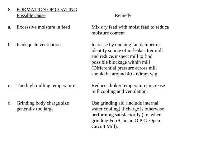
8. FORMATION OF COATINGPossible cause Remedy

a. Excessive moisture in feed Mix dry feed with moist feed to reducemoisture content

b. Inadequate ventilation Increase by opening fan damper oridentify source of in-leaks after milland reduce. inspect mill to findpossible blockage within mill(Differential pressure across millshould be around 40 - 60mm w.g.

c. Too high milling temperature Reduce clinker temperature, increasemill cooling and ventilation.

d. Grinding body charge size Use grinding aid (include internalgenerally too large water cooling) if charge is otherwise

performing satisfactorily (i.e. whengrinding Ferr/C in an O.P.C. OpenCircuit Mill).

APPENDIX 2

WET RAW MILL FAULT FINDING AND TUNING

CHECK LIST

1. DECREASE IN OUTPUT Remedy Possible Cause

a. Raw feed increase in size Check operation and efficiency ofcrushers and screens if in closedcircuit system.

b. Raw feed increase in hardness 1. Check quarry operation andpossibility of avoiding hard stone.2. Make fresh grindability tests.3. Investigate operation of crushersto see if they can be uprated4. Put larger top sized balls in thefirst chamber, but not at the expenseof the liners.

c. Mill charge too worn 1. Make up with larger balls2. Dump charge, regrade and make upnew charge

d. Mill volume loading too low Power drawn by the mill will below. Measure up each chamber and addcorrect tonnage of new grinding media 50/50mix of two largest balls in the chamberis suggested.

e. Too small media used for make up 1. Make up with largest balls2. Dump charge, regrade and recharge

f. Diaphragm slots partially blocked 1. Inspect diaphragm, clean slots.

Look "or the causes of the blockage.

2. Ensure grinding media is large enough.

g. Fractured diaphragm 1. Replace broken section(s) 2. Examine the charge in each chamber on either side of the fracture. Readjust volume loadings and ball gradings necessary.

h. Slurry moisture or viscosity 1. If the slurry moisture is toonot at specified level high the viscosity will be low and

flushing may occur which will affect theslurry residues.

2. If the slurry moisture is too lowthe viscosity will be high causing flowproblems through the mill and reducingthe grinding efficiency.

2. SLURRY RESIDUES TOO HIGHPossible causes Remedy

a. Raw feed increase in size See 1.a.

b. Raw feed increase in hardness See 1.b.

c. Grinding media too small May be necessary to increase "piece"size in final chamber. Study the resultsof axial sample text.

d. Mill volume loading too low 1. Power drawn by the mill will be low. Check kWh meter. 2. Measure up each chamber and add thetonnage of new media to re-establishcorrect grading.

e. Diaphragm slots too worn 1. Coarse residues will not be retainedlong enough in the mill to be ground.2. Replace diaphragm as soon as possible.3. Weld bar into worst slots as atemporary measure only. Take care touse compatible metals. Iron diaphragmmay not be suitable for welding.

f. Lining plates worn or damaged Check condition of lining plates and replace asnecessary. If rubber lining is damaged renew asnecessary.

1. See sectionl(c)

d. Blocked diaphragm(s) 1.See section l(f) 3(b)

2. Ifthe whole mill fills up the mill

discharge must be blocked. Restricteddischarge will cause up-stream chambersto fill but the down stream chamberswill probably empty.

e. Slurry moisture too low and/ 1. Increase slurry moisture to theor slurry too thick correct level

2. Check slurry viscosity

f. Slurry over-ground 1. There may be an unusual increasein slurry viscosity due to an unusuallyfine particle size distribution2. Look at raw mix proportions i.e.too much clay or3. See 4(d)

3. SLURRY TOO FINE Possible causes

a. Output decrease

b. Diaphragm slots practically blocked

Remedy

1. Increase feed2. See sections 1(c) (e) & (f)

1.Outlet diaphragm may beblocked and needs to be cleared2. Look for possible causes of blockage3. Listen to mill sound to find blockageposition. This may be difficult with arubber lined mill

Remedy4. MILL FILLS UP Possiblecauses

a. First chamber fills up

May be due to an increasein feed size or hardness.(Slurry coming back overmill feed end)

Problem may be caused by top 2 or 3% offeed only, being too hard or too large forfirst chamber media. (See la & b)

b. Feed rate too high 1. Stop feed and run mill until problemeases. Then run at slightly reduced feed. 2.If mill fills again consider 4 (a) (c) & (d)

c. Worn grinding media in first chamber

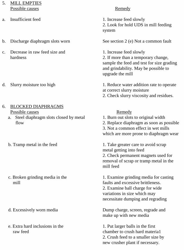
5. MILL EMPTIESPossible causes Remedy

a. Insufficient feed 1. Increase feed slowly2. Look for hold UDS in mill feedingsystem

b. Discharge diaphragm slots worn See section 2 (e) Not a common fault

c. Decrease in raw feed size and 1. Increase feed slowlyhardness 2. If more than a temporary change,

sample the feed and test for size gradingand grindability. May be possible toupgrade the mill

d. Slurry moisture too high 1. Reduce water addition rate to operateat correct slurry moisture2. Check slurry viscosity and residues.

6. BLOCKED DIAPHRAGMS Possible causes Remedya. Steel diaphragm slots closed by metal 1. Burn out slots to original width

flow 2. Replace diaphragm as soon as possible3. Not a common effect in wet millswhich are more prone to diaphragm wear

b. Tramp metal in the feed 1. Take greater care to avoid scrapmetal getting into feed2. Check permanent magnets used forremoval of scrap or tramp metal in themill feed

c. Broken grinding media in the 1. Examine grinding media for casting mill faults and excessive brittleness.

2. Examine ball charge for widevariations in size which maynecessitate dumping and regrading

d. Excessively worn media Dump charge, screen, regrade andmake up with new media

e. Extra hard inclusions in the 1. Put larger balls in the first raw feed chamber to crush hard materia1

2. Crush feed to a smaller size bynew crusher plant if necessary.

14.33APPENDIX 3

AXIAL TEST - WORKED EXAMPLE ON A CEMENT MILL

SUMMARY

It is intended to install Slegten lining plates in this mill. in order to assess the effect of this change, acomprehensive mill test has been carried out under present operating conditions.Data collected shows the mill to be generally satisfactory. Overall grinding efficiency is high, thoughbetter results could be obtained from the first chamber by removal of undersize charge.

The Waytrol feeder is operating well, and gives a fairly constant feed. Variations in surface area from themill are likely to be due to gypsum feed and occasionally stock clinker rather than the feed itself.

There was little evidence of media segregation, which should be obtained after the Slegten liners have beeninstalled. Segregation should slightly increase grinding efficiency, giving some advantage in output.

TEST PROCEDURE

The mill was stopped on full load and opened. Axial samples were taken from each chamber, the millcharge was measured up, and samples of grinding media were taken at the beginning and end of eachchamber. The linings and diaphragms were inspected, The mill was then "closed up" and grindingrecommenced.

When the mill had settled down and was grinding to its normal surface area, a salt test was carried out. Salt wasadded at the rate of 3 lbs/minute for about two hours; after twenty minutes of salt addition cement samples weretaken at the discharge end of the mill at intervals of two minutes, for about two hours. During this test thepower consumption of the mill was determined, the Waytrol Clinker Feeder setting and gypsum setting noted,and an average sample of the clinker feed to the mill taken for grindability tests. In addition, the speed of theWaytrol feed belt was determined in order that the T.P.H. of clinker feed to the mill could be calculated.

In order to have a check on the accuracy of the salt test, the output of the mill was turned into an empty silo atthe start of the test for about eight hours. The silo was then measured, thus enabling the output to be calculatedfrom the tons/feet run of the silo.

MILL – INSPECTION

TESTING OF SAMPLES

1. AXIAL SAMPLES

The surface area of each sample was determined by air permeability apparatus, and where necessary, by sieveanalysis. These results are tabulated in Tables 14.1 and 14.2 plot of surface/mill lengths is shown in Fig.14.8.

2. SAMPLES OF GRINDING MEDIA

A grading analysis was done on each sample used and reported in Table 14.3 and Fig. 14.9. Hardness testswere done on the various sizes of media in each sample, and these results are to be seen in Table 14.4.

3. SALT TEST CEMENT SAMPLES

The surface area of each sample was determined. The samples were also analysed for sodium chloride contentusing the direct silver nitrate titration method. It was necessary to make corrections to these results, since KirtonLindsey cement contains small amounts of sulphide.

A 5 gm sample of cement was taken for analysis, and the salt purity was 99.4% NaCl. The results werecalculated directly to T.P.H. of cement, and are shown in Table 14.5. An averaged plot of T.P.H./Surface Areais made in Fig. 14.10.

4. CLINKER SAMPLE

A grindability test was done on the sample of clinker collected during the Salt Test.

Sufficient gypsum was added to bring the % SO3 up to the same value as it was during the Salt Test, and inorder to do this the average clinker and the average Salt Test sample were analyzed for SO3 content. Thegrindability curve is Fig. 14.11.

Chamber Height above charge Condition ofdiaphragm

Condition oflining plates

1 56” Showing sign of Some plates inwear, but clear poor condition

2 62” “ Fair condition3 60 ½ “ “ Fair condition

MILL DATAClinker Feed Setting 41.9Clinker Feed Belt Speed 4.2 secs/ftGypsum Feed-Setting 5.7Average Clinker SO3 0.8%Average Cement S03 3.35%Gross Power 578 kW = 775 H.P.Nett Power (approx.) 540 kW

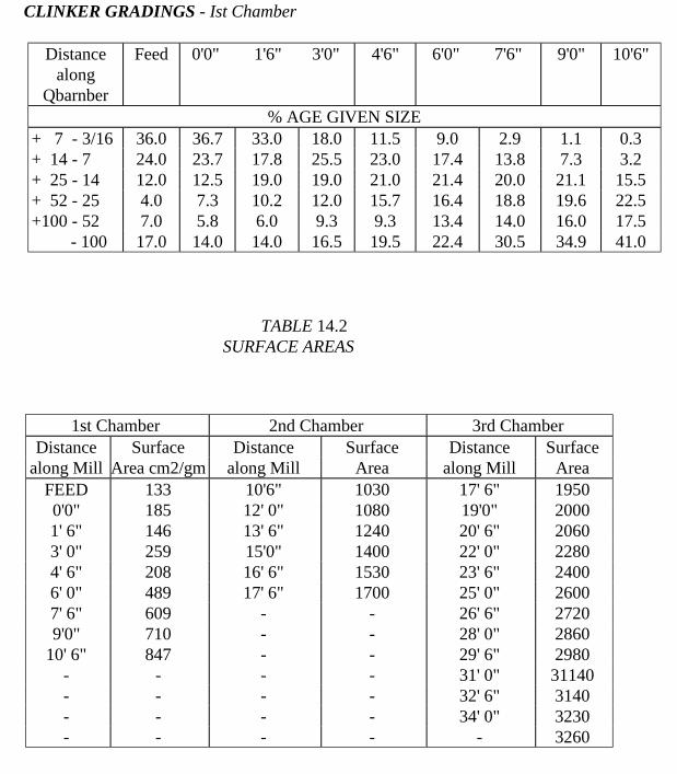
1st Chamber 2nd Chamber 3rd ChamberDistance Surface Distance Surface Distance Surface

along Mill Area cm2/gm along Mill Area along Mill AreaFEED 133 10'6" 1030 17' 6" 19500'0" 185 12' 0" 1080 19'0" 20001' 6" 146 13' 6" 1240 20' 6" 20603' 0" 259 15'0" 1400 22' 0" 22804' 6" 208 16' 6" 1530 23' 6" 24006' 0" 489 17' 6" 1700 25' 0" 26007' 6" 609 - - 26' 6" 27209'0" 710 - - 28' 0" 2860

10' 6" 847 - - 29' 6" 2980- - - - 31' 0" 31140- - - - 32' 6" 3140- - - - 34' 0" 3230- - - - - 3260

CLINKER GRADINGS - Ist Chamber

TABLE 14.1

Distancealong

Qbarnber

Feed 0'0" 1'6" 3'0" 4'6" 6'0" 7'6" 9'0" 10'6"

% AGE GIVEN SIZE+ 7 - 3/16 36.0 36.7 33.0 18.0 11.5 9.0 2.9 1.1 0.3+ 14 - 7 24.0 23.7 17.8 25.5 23.0 17.4 13.8 7.3 3.2+ 25 - 14 12.0 12.5 19.0 19.0 21.0 21.4 20.0 21.1 15.5+ 52 - 25 4.0 7.3 10.2 12.0 15.7 16.4 18.8 19.6 22.5+100 - 52 7.0 5.8 6.0 9.3 9.3 13.4 14.0 16.0 17.5 - 100 17.0 14.0 14.0 16.5 19.5 22.4 30.5 34.9 41.0

TABLE 14.2SURFACE AREAS

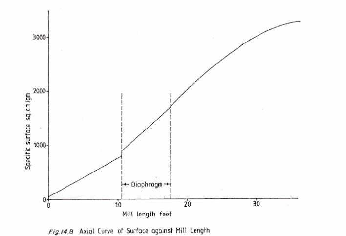
1st Chamber 2nd Chamber 3rd Chamber

Dia (ins) V.P.H. No. Dia (ins) V.P.H. No. Dia (ins) V.P.H. No.

3 316 3 359 3/4 4892 3/4 359 2 1/4 312 1/2 5162 1/4 322 2 312

1 3/4 387

TABLE 14.3

GRINDING MEDIA SAMPLES

%AGE FINER THAN GIVEN SIZEDiameter 1st Chamber - Balls 2nd Chamber - Balls 3rd Chamber -Ins. Cylindrical Media

0'-0" 10'-6" 0'-0" 7'- 0" 0' - 6" 13' 6" - 18' 63 3/4 100.0 100.03 1/2 93.6 96.93 1/4 66.3 66.5 100.03 56.9 57.5 61.2 100.02 3/4 50.3 51.4 52.7 92.72 1/2 32.3 30.1 41.2 66.52 1/4 6.6 15.5 19.2 46.32 0 0 6.8 20.71 3/4 - - 1.7 5.51 1/2 - 0 07/8 100.0 100.03/4 53.0 33.95/8 20.3 16.81/2 4.0 8.43/8 0 0

TABLE 14.4VICKERS PYRAMID HARDNESS NUMBERS

Sample. M/S N/10 Cement Surface Sample M/S N/10 Cement SurfaceNumber AgNO3 Tons / Hr. Area Number. AgNO3 Tons / Hr. Area

68.7 68.7AgNO3 AgNO3

- Blank -BlankBLANK 0.30

0 1.85 44.3 3370 32 4.35 17.0 33801 2.55 30.5 3370 33 4.15 17.8 33502 3.00 25.4 3380 34 4.05 18.3 32903 3.55 21.1 3370 35 4.30 17.2 32404 3.65 20.5 3360 36 4.30 17.2 32305 3.85 19.4 3360 37 4.00 18.6 31906 4.00 18.6 3370 38 3.95 18.8 31807 4.15 17.8 3390 39 3.90 19.0 31108 4.20 17.6 3370 40 3.80 19.6 31509 4.25 17.4 3370 41 3.80 19.6 315010 4.25 17.4 3400 42 3.90 19.0 315011 4.25 17.4 3430 43 4.05 18.3 317012 4.40 16.8 3390 44 4.10 18.1 316013 4.25 17.4 3400 45 4.00 13.6 323014 4.20 17.6 3400 46 4.10 18.1 325015 4.20 17.6 3400 47 4.35 17.0 324016 4.15 17.8 3420 48 4.10 18.1 325017 4.10 18.1 3420 49 3.95 18.8 331018 4.30 17.2 3420 50 4.20 17.6 332019 4.35 17.0 3490 51 4.10 18.1 334020 4.25 17.4 3510 52 4.15 17.8 336021 4.20 17.6 3510 53 4.40 16.8 341022 4.10 18.1 3530 54 4.15 17.8 346023 4.35 17.0 3540 55 4.40 16.8 344024 4.40 16.8 3540 56 4.30 17.2 349025 4.40 16.8 3520 57 4.30 17.2 347026 4.25 17.4 3490 58 4.35 17.0 347027 4.35 17.0 3510 59 4.40 16.8 347028 4.20 17.6 3470 60 4.25 17.4 346029 4.25 17.4 3480 61 4.15 17.8 346030 4.05 18.3 3420 62 3.85 19.3 343031 4.10 18.1 3400 63 3.90 19.0 3460

TABLE 14.5RESULTS Of TESTS ON MILL SAMPLES TAKEN DURING THE

SALT TEST

CALCULATION OF MILL OUTPUT

1. FROM FEEDER SETTING

Belt Speed = 4.2 secs/ft= 857.143 ft/hr

Clinker Feed = 41.9 lbs/ft run of belt

Rate = 41.9 x 857.14 tons/hr 2240

= 16.03 tons/hr

Clinker SO3 = 0.80 37.00 3.35

Cement SO3 = 3.35 3.35 0.80

Gypsum SO3 = 37.00 33.65 2.55

Gypsum added = 2.55 x 16.03 1.22 tons/hr33.65

Cement output = 33.65 x 16.03 17.25 tons/hr at 3375 cms/gm specific surface.

2. BY SALT TEST

The output is obtained from Fig.14.10, i.e. Cement Output = 17.74 TPH at 3375 cm2 /gm Specific Surface.

3. BY SILO MEASUREMENT

124 tons of cement were collected in eight hours, and the average specific surface area was 3370 cm2 /gm i.e. Cement Output = 15 ½ TPH at 3370 cm2 /gm.

COMPARISON

Output by TPHWeigh Feeder 17.25Salt Test 17.74Silo Measurement 15.50

AXIAL CURVES

ACTUAL AXIAL CURVES

Where the weight of charge/ft run of mill length is constant, the amount of power used for surface productionmay be taken to be directly proportional to the length along the mill, and hence a plot of surface area againstmill length is identical with a plot of surface area against the nett kW used. In this case the weight of charge/ftrun of mill is not constant for the three chambers, and as it is more correct to plot surface area against nett kW,the charge weight in each chamber has been calculated, and the nett power divided in the ratios of these weights.

From this information Table 14.7 was constructed, and a plot made of the surface area against nett kW- See Fig. 14.12.

CALCULATION OF THEORETICAL AXIAL CURVE

Theoretically, for a mill operating at 100% efficiency, the surface area production rate for "standard clinker" at2500 cm2 /gm = 115 x 106 cm2 /kWh.

The surface area production rate may be estimated for a change in surface area along a mill from the standardcurve for standard clinker and from the grindability curve for any other clinker.

The basic expression used is:

Surface area production rate

= Standard rate x Energy Ratio x Surface produced.

The "Energy Ratio" is determined from the grindability curve by reading off the number of revolutions (of thetest mill) at the initial and final surfaces and ratio-ing the difference to the data from the standard curve.

For example, in the case of standard clinker(s) being ground to 920 cm2 /gm from the initial surface area of 130cm2 /gm.

Surface production for standard clinker

= 115 x 106 x Revs (130-2500)s x (920 - 130)Revs (130 - 920)s (2500 - 130)

Similarly for any other clinker (A) using the grindability curve andcomparing it to standard clinker.

Surface produced

= 115 x 106 x Revs (130-2500)s x 790 x 1 Revs (130 - 920)s 2370 Grindability A

= 115 x 106 x Revs (130-2500)s x 790 x Revs (130 - 920)sRevs (130 - 920)s 2370 Revs (130 - 920)A

= 115 x 106 x Revs (130-2500)s x 790 ---------------------------- (1)Revs (130 - 920)s 2370

CALCULATION OF MILL EFFICIENCY

in the case of the mill under consideration at the time of the stoppage, the surface area of the product was 3260.From graph 14.10 this corresponds to an output of 18.38 tph. Details of mill loading are given in Table14.6.

CHAMBER HEIGHT ABOVECHARGE INS

%VOLUMELOADING

VOLUMEft3

WEIGHT OFCHARGE

TONS

NETT KW NETT Kwper 18"

1 56 31 423 15.8 178 25.43

2 62 22 279 7.29 82 17057

3 60.5 24.5 746 24.89 280 22.7

TOTAL 1448 47.98 540

IN THE FIRST CHAMBER

Surface area of material entering = 130 cm2 /gmSurface area of material leaving = 920 cm2 /gmSurface area produced = 790 cm2 /gm

Total surface area = 18.38 x 1.016 x 10 6 x 790 cm 2 /hour. The first chamber is equivalent to 178 kW of the540 nett kW used by the mill.

Surface produced/kWh = 18.38 x 1.016 x 106 x 790178

= 82.88 x 106 cm2 /kWh

From the standard curve and the grindability curve Figs.14.13 and 14.11

Theoretical surface production in 1st chamber (using expression (1))= 115 x 106 x (57.0 – 3.0) x 790 (15.8 - 0) 2370

= 131.0 x 10 6 cm 2 /kWh

Therefore efficiency of chamber = Actual surface production x 100Theoretical surface production

TABLE 14.7

Length along Mill Nett Kilowatts Surface Area

0' 0" 0 1331' 6" 25.4 1463' 0" 50.9 2594' 6" 76.3 2086' 0" 101.7 4897' 6" 127.2 6099' 0" 152.6 71010' 0" 178 847

2nd Chamber0' 0" 178 10301' 6" 105.6 10803' 0" 213.1 12404' 6" 230.7 14006' 0" 248.3 15307' 0" 260 1700

3rd Chamber0' 0" 260 19501' 6" 282.7 20003' 0" 305.4 20604' 6" 328.1 22806' 0" 350.8 24007' 6" 373.5 26009' 0" 396.2 272010' 6" 418.9 286012' 0" 441.6 298013' 6" 464.3 304015' 0" 487 314016' 6" 509.7 323018' 0" 540 3260

TABLE 14.8THEORETICAL RATE OF SURFACE PRODUCTION

kWh Revs, (x - 130) Surface Area

0 0.1403 13050 7.02 500100 14.03 860150 21.05 1190178 24.97. 1370200 28.06 1540250 35.08 1850260 36.48 1900300 42.09 2150350 49.11 2450400 56.12 2710450 63.14 2950500 70.15 3180540 75.76 3370

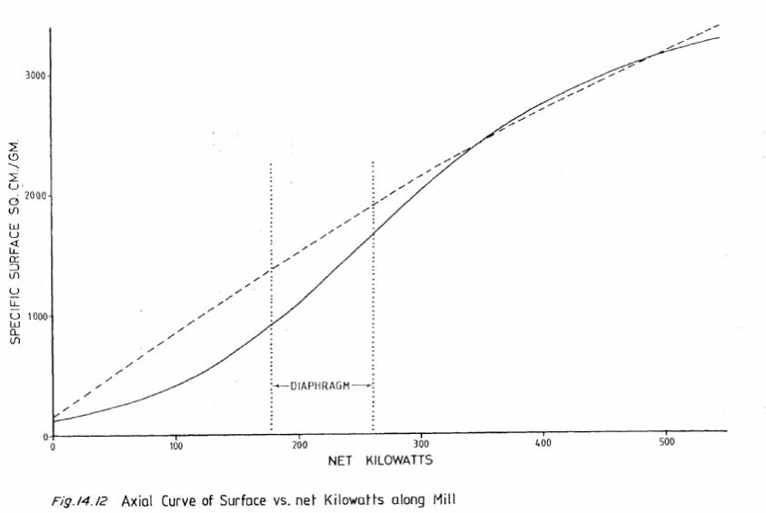
For 1st chamber, efficiency

= 82.88 x 106 x 100 131.0 x 106

= 63.3%

Grindability of clinker over the surface range in the 1st chamber

= (15.8 - 0) = 15.8 x 100 = 87.8% (21.0 -3) 18.0

IN 2ND CHAMBER

Surface area of material entering = 920Surface area of material leaving = 1660Surface area produced in chamber = 740 cm2 /gm.Total surface produced = 740 x 18.38 x 1.016 x 10 6 sq.cms./hr.

2nd chamber is equivalent to 82 kW

Surface produced / kWh = 18.38 x 1.016 x 106 x 740 = 167.8 x 106 cm2 /kWh82

Theoretical production should be:

115 x 106 x 740 x R(2500 - 130)S x R(1660 - 920)S 2370 R(1660 - 920)S R(1660 - 920)A

115 x 106 x 740 x 54.0 x 16.92 124.5 x 106 sq.cms./kWh 2370 16.92 15.55

Efficiency of 2nd Chamber = 167.8 x 106 x 100 = 134.8% x124.5 x 106

Grindability over the surface range in the 2nd chamber

Revs. (1660 - 920)A = 15.55 = 91.8% (1660 - 920)S 16.92

3RD CHAMBER

Surface material entering = 1660Surface material leaving = 3260Surface produced in chamber = 1600 sq.cms./gm.

Total surface produced = 18.38 x 10.016 x 106 x 1600

3rd chamber is equivalent to 280 kW

Surface produced/kWh = 18.38 x 10.016 x 106 x 1600 = 106.5 x 106 sq.cm./kWh280

Theoretical production 115 x 106 x 1600 x Revs (2500 - 130)S x Revs (3260-1600)2370 Revs (3260 - 1660)S Revs (3260-1600)

=115 x 106 x 1660 x 54 x 40.42 2370 40.42 41.7

Efficiency of 3rd chamber = 106.5 x 106 x 100 = 106.0% 100.5 x 106

OVERALLSurface material entering = 130Surface material leaving = 3260Surface produced in Mill = 3130 sq.cms./hr.

Total surface produced = 18.38 x 1.016 x 106 x 3130 sq.cms./hr.

Total kW = 540

Chamber Actual Surface Prod.sq.cm./kWh x 106

Theoretical SurfaceProd.sq.cm./kWh

Efficiency %

1 82.8 130.8 63.52 167.8 124.5 134.83 106.5 100.5 106

overall 108 112.9 95.7

Surface produced/ kWh 18.38 x 1.016 x 106 x 3130 = 108.0 x 10 6 sq.cm./ kWh 540

Theoretical production = 115 x 106 6 x 3130 x 54.0 x 75.3 = 112.9 x 10 6 cm 2 /kWh 2370 75.3 72.6

overall efficiency = 108.0 x 106 x 100 = 95.7%112.9 x 106

CONCLUSIONS

Mill Efficiency

The overall efficiency is quite good, however the first chamber has a low efficiency, especially compared withthe second chamber which is highly efficient. The third chamber is also satisfactory.

The low efficiency in the first. chamber may be due in part to the percentage of minus 21/2" media present, andif this were removed and replaced by 31/2" more work would be done in this chamber.

Grindability

The grindability is low, but is accounted for by the high percentage of gypsum which was added to simulateactual mill conditions of high % SO3 content in the cement. The higher the gypsum content, the lower thegrindability and bigger the output at a given surface.

Mill Output

The output determined from the weighfeeder and the salt test are in very close agreement. The figure obtainedby silo measurement is lower, but is subject to several inaccuracies, i.e time lost in changing silos, measurementof cement in the silo and an inaccurate figure for tons/ft. of silo heights.

it would seem that 171/2 T.P.H. would be a fair value for the output of the mill at 3375 cm.2 /gm. surface area.

Grinding Media

The hardness figures for the media in all three chambers are reasonable for the type of media used. Ideally themedia in chambers 1 and 2 could do to be harder, the optimum hardness range is between 400 and 650 Vickers.

Mill Power Consumption

At 171/2 tons/hr. the power consumed is 33 kWh /ton.

Mill Filters

The filter was in-operative at the time of the test due to holes in the filter cloth. The filter is of the old Sly Type,with no continuous cleaning facility.

Mill Operation

The mill has very few troubles, and in general is working very satisfactorily

APPENDIX

ESSENTIAL PRECONDITIONS FOR USE OF FINER MEDIA GRADINGS IN CHAMBERTWO OF CEMENT MILLS

(1) The first chamber charge should be in good condition and Oroduce following typical fineness ofsamples prior to the intermediate diaphragm.

Sieve Size % Cumulative Residue2.36mm 1%1.18mm 6%300um 20%

When determining this fineness - take large samples and do not ignore any unground clinker nibs present. if nibsare present - check first chamber charge grading and coarsen up with extra 90/80mm instead of 70mm media.

(2) The first chamber should have an efficient reverse step/lifter type lining - recommended typetypically the Magotteaux reverse step or similar.

(3) The diaphragm slots must be clear and even with no excessive gaps which can allow coarse materialsinto chamber 2.

(4) Check chamber 2 axial sampling curve for any signs of nibs/coarse material ex chamber I which caninhibit fine grinding characteristics. Figure 1 shows an example of two mills, one with an efficient andone with an Lnefficient, first chamber. Notice how the second chamber of the latter mill has to carry outsome of the crushing action which should have been carried out in chamber 1.

(5) The mill must be adequately vented, i.e. with typically 5 air changes per minute or 0.4 kg air/kg cement.

(6) Avoid high milling temperatures above 120oC which can Cause in the second chamber. Coating canadversely affect performance of finer charges.

APPENDIX I

CEMENT MILL FAULTS

1. OUTPUT DECREASES

Possible Cause Remedy

a. Increase in clinker hardness Examine raw feed composition andand size kiln burning conditions.

b. Mill Charge too worn Dump charge, regrade and make up newcharge.

c. Mill volume loading too low Measure each chamber and add correcttonnage of new bodies.

d. Too small bodies used for make Charge should be dumped and up regraded, or (less satisfactory) use largest bodies for make up.

e. Diaphragm slots partially Inspect diaphragms clean slots.blocked Further action as in Section 6.

f. Fractured Diaphragm Replace section(s).

2. CEMENT TOO COARSE

Possible Cause RemedyI

a. Increase in clinker hardness Examine raw feed composition and and size kiln burning conditions.

b. Grinding media too large Make up with smaller media e.g.50/50 of the two smallest sizes.

c. Mill Volume Loading too low Measure each chamber and add correcttonnage of new bodies.

d. Diaphragms slots too worn Replace as soon as possible, (with steel diaphragms,weld bar into worst slots as a temporary measure).

e. Coating forming Reduce mill temperature. Use dryerfeed. Increase mill ventilation.

3 CEMENT TOO FINE

Possible cause Remedy

a. Output decreased See section 1b, d and e.

b. Last chamber media too small Dump and recharge or make up with large media.

c. Diaphragm slots practically Locate source of blockage by sound blocked andexamine diaphragm. Further action see section 6.

4. MILL FILLSPossible cause Remedy

a. Harder Feed Clinker Check raw feed composition and kiln burning conditions. increase 1st chamber piece weight.

b. Too much feed Run without feed until chamber sound isnormal. Then use slightly reduced feed.(If miIl fills again consider (a) (c) and (d)).

c. Worn grinding media in Section 1b. first chamber

d. Choked diaphragm(s) See section 6.

e. Coating forming See section 8.

5. MILL EMPTIES

Possible cause Remedy

a. Insufficient feed Increase feed slowly.

b. First diaphragm slots worn See section 2d.

c. Decrease in clinker hardness Check raw feed composition and kiln and size burning conditions decrease 1st

chamber piece weight

d. Media in last chamber too Dump charge and refill with charge large of smaller piece weight.

Note: If a mill fills severely, clearing is difficult due to the excessive temperature rise that results fromrunning with reduced ventilation and feed A little grinding aid poured into each chamber through the man doorin turn (starting with the last chamber) accelerates the clearing.

6. CHOKED DIAPHRAGMS

Possible cause Remedya. Steel diaphragm slots closed Burn/grind out slots to original by metal flow

width, replace diaphragm soonest. Use "harder"materials specification rather than steel.

b. Tramp metal in feed Greater care and tidiness when scrap metal ishandled and repairs are carried out in proximity toclinker store and clinker handling systems.

C. Grinding body pieces formed Examine cast iron and very hard grinding mediain mill for casting faults and excessive brittleness. Inspect

mill for very large bodies mixedwith very smallbodies (if found, dump charge).

d. Over worn grinding media Dump charge and make up with new

e. Clinker nibs See section 7.

f. Coating forming in slots See section 8.

7. CLINKER NIBS IN CEMENT

Possible cause Remedy

a. 1st chamber diaphragm slots too worn Replace soonest.

b. 1st chamber diaphragm has open Repair as necessarycrack/is ill fitting or loose

c. Exceptionally hard and/or Examine raw meal quality and burning large size feed control (if permanent, increase ball

size in 1st chamber).

d. Maximum ball size in 2nd Increase piece weight by adding 70mm balls. chamber too small (Extreme case only -concentrate efforts an

correcting first chamber performance.)

.

FORMATION OF COATING

Possible cause Remedy

a. Excessive moisture in feed Mix dry feed with moist reed to reduce moisture content

b. Inadequate ventilation Increase by opening fan damper or identify source of in-leaks aftermill and reduce. Inspect mill to find possible blockage within mill(Differential pressure across mill should be as per section 2.6.)

c. Too high milling temperature Reduce clinker temperature, increase mill cooling and ventilation.

d. Grinding body charge size Use grinding aid (include internal water cooling) if charge is other generally too large wise performing satisfactorily (i.e. when grinding Ferr/C in an OPC Open

Circuit Mill).

APPENDIX 2

THE FINENESS OF SAMPLES TAKEN IMMEDIATELY PRIOR

TO THE FIRST CHAMBER DIAPHRAGM.

(i) Sampling Method

It is important to use common sense when taking samples within a mill. If visual inspection of the materialshows it to be relatively fine then small (200 gm) samples will suffice for carrying out sieve analysis. However,if large quantities of nibs are present it is advisable to take larger samples ie around 0.5 – 1 kg in weight.

(ii) Sample Analysis

Coarse samples should be graded through the convenient sieve sizes available on site. A recommended range forraw mill and cement mill testing are as follows:

Sieve Size Notes

76mm Choose coarse sieve sizes to suit typical50mm feed size of stone or clinker to the25mm mill. Of particular importance for raw12mm mill assessment.6 mm

Microns 2,360 Important for analyzing samples prior to

the intermediate diaphragm in raw/cement mills

1,180 Important for analysing samples prior tothe intermediate diaphragm in raw/cement mills

300 Important for analysing samples prior to theintermediate diaphragm in raw/cement mills

90 Use for mass balance calculations around 75 raw mill circuits

45 Important for analyzing samples ex cementmill second chambers. Do not normallyuse for raw mill testing. Use for massbalance calculations around cement millcircuits.

If the above sizes are not available an site then seek to obtain these otherwise use the nearest equivalent sievesizes.

(iii) Fineness of Samples Immediately Prior to the Intermediate Diaphragm

(a) Cement Mills

The first chamber of a cement mill should crush the clinker/gypsum to sufficient fineness to pass throughthe intermediate diaphragm and be finely ground in the second chamber of the mill. As a rough guide,cement mills (open and closed circuit) with efficient first chamber grinding characteristics should aim toachieve the following fineness immediately prior to the diaphragm.

Sieve Size Typical Cumulative % retained an Sieve

2.36mm 1% (maximum 4%)

1.18mm 6%

300um 20%

This is an approximate guide only. It takes no account of (i) open/closed circuit mill operation (ii) the levelof recalculating load (iii) the intermediate diaphragm slot size above figures are based upon experienceswith mills of 6-8mm intermediate slot size.

Despite this, it is a useful rule of thumb for establishing how efficiently a first chamber is crushing downthe feed. if the above levels of fineness are not achieved then the mills second chamber will have to carryout part of the crushing which should have been done in Chamber 1.

(b) Raw Mills

The above figures can also be applied to raw mills but' must be treated with greater caution.

Some raw mill designs feature the use of short length to diameter ratios, high recirculating loads, largediaphragm slots (12 - 15mm ) with these mills the prediaphragm samples are usually coarser than thoseshown above.

For example, typical prediaphragm samples from three central discharge closed circuit mills having 12mmslot sizes gave the

following results.

Cumulative % residue Millon 300 Micron Sieve

33 (A) Efficient first chamber handling fine stone - mill underun - capable of slightly higher output

43 (B) Typical mill installation - efficient first chamber handling reasonable size stone

72 (C) Mill with first chamber over filled due to coarse feed size and inadequate ball size. Extra 90mm or even 100mm media required to improve crushing action

As can be seen, in the case of this design of a mill a more realistic target reside would be around 40% retainedon 300 micron ie twice the residue considered acceptable for a cement mill.

APPENDIX III

EXAMPLE OF HOW THE VOLUME LOADING WITHIN A MILL CAN BE AFFECTED

BY THE ACCUMULATION OF UNGROUND MATERIAL

(i) Background

The following results were obtained on a 4200 kW raw mill which -was designed to produce 220 tph rawmeal. The mill was crash stopped after running at 75% of its design load during commissioning. It wasdecided to carry out an axial sampling test on the mill before raising the charge to 90% load. The mill wascrash stopped and it was noted that the first chamber was very full of unground stone. Later on the millwas run out and the height above charge measurements were rechecked.

(ii) Apparent First Chamber Volume Loading Following Crash Stop

Average height above charge (H) = 3.07m

inside lining diameter of chamber (D) = 4.42m

H / D = 3.07 = 0.6954.42

"Apparent" volume load = 25.5%

(iii) Volume Loading After Mill Was Run Out

Average height above charge (H) = 3.275m

H / D = 0.74

Volume load = 20%.

Tonnage of media loaded into mill = 88 tonnes

Chamber internal volume = 92.1m3

Volume of media =3251 x 0.2 18.42m3

Media density 88.0 = 4.78 t/m3

18.42

(iv) Apparent Media Density

Due to the presence of nibs occupying approximately 25.5 - 20.0 = 5.5% of the internal volume of themill, the apparent media density is less than that shown above ie Volume of media plus nibs = 92.1 x0.255 = 23.49m3

Apparent media density 38.0 = 3.75 t/m323.49

(v) Conclusions

Hence, unless the volume loading of the chamber had been checked with the mill run out it would haveappeared that the chamber contained more media than it actually did ie

92.1 x 0.255 x 4.78 = 112.3 tonnes

Another means of crosschecking the actual media loaded is to calculate 'the kW drawn for each chamberusing the power formula and crosschecking these results against the figures from the mill kWh meter.

APPENDIX IV

AXIAL SAMPLING CURVES FOR CEMENT MILL

SECONO CHAMBERS - SIEVE RESIDUES

GENERAL

In addition to examining the surface area versus nett kW drawn/chamber length relationship for the secondchamber of a cement mill, it is also useful to examine the sieve residue relationship.

This is best examined by using a 45 micron sieve or even finer sieves such as 32 and 25 micron sieves if theseare available.

Very often, the axial sampling curves for second chambers show a steady reduction in 90 and 300 micronresidue throughout the chamber. This gives the impression of efficient grinding taking place. However,cement is predominantly finer than 45/32 micron and to assess the fine grinding efficient, these sieve residesshould also be examined.

Fig.8 shows axial sampling curves for two closed circuit cement mills. Mill A was an efficient mill using finemedia (25 - 15mm) in its second chamber. The material leaving the first chamber of this mill was fine andwithin the guidelines shown id Appendix 11.

Mill B used a fairly conventional media grading consisting of 60mm to 17mm media. The mill also had a formof classifying lining which did not function well and resulting in reverse classification of the media.

Comparing the 45 um residue shows that the material at the inlet to the chamber was or similar fineness iearound 50% cumulative residue.

However, the chamber outlet samples were as follows:

Mill Mill Outlet % Residue Reduction in residue 45 micron across chamber

A 46% 4%B 28% 22%

This shows the superior fine grinding characteristics of the finer media used in conjunction with an efficient firstchamber charge in Mill A.

To improve mill B to give a similar performance would have involved costly replacement of the liner/charge. Itwas therefore decided to reduce the average replacement media size from 60mm to 25mm size and replace someof the coarser 60mm media by the available 25-17mm media.

APPENDIX V

MASS BALANCE ON A RAW MILLING CIRCUIT

GENERAL

The example chosen to demonstrate mass balance calculations on a milling circuit is that of a double rotatormill. It was felt that this represents one of the more complex closed circuit milling systems available whichcould best illustrate some of the techniques/problems involved. Generally speaking, most closed circuitcement/raw milling systems should be simpler to evaluate than the example shown.

Mill Circuit Samples

Sample % Cumulative retained on90 micron sieve

(i) Rejects from static separator 68.00

(ii) Fines from cyclone after static separator 9.24

(iii) Rejects from Wedag separator (feed to 76.22chamber 2)

(iv) Feed to Wedag separator 52.90

(V) Mill central discharge 49.50

(Vi) Fines from Wedag separator 2.70

(vii) Finished raw meal 6.30

MASS BALANCE CALCULATIONS

(i) Mill Throughput

Mill feed rate = 42.8 tph (from totaliser readings prior to test)Feed moisture = 3.1%Dry tonnage = 42.8 x 0.969 = 41.5 tph

(ii) Finished Raw Meal

Dry tonnage = 41.5 tphThe Finished raw meal consists of (a) Fines ex cyclone

(b) Fines ex Wedag separator

Let x = tph of fines ex Wedag separator

∴ (41.5 - x) = tph fines ex cyclone

Mass balance on 90 micron residue

(2.7) + (41.5 - x) 9.24 = 41.5 (6.30)

= 18.7 tph

Hence fines ex cyclone = 41.50 - 18.7 = 22.8 tph

(iii) Rejects Feed to the Separator

The feed to the separator consists of mill discharge material together with rejects from the static separator.

Basis 1 tph of separator feed

let y = tph of material ex mill central discharge

Mass balance on 90 micron residue

y(49.5) + (1-y) 66.0 = 52.90 x 1.0

y = 0.79

ie 79% of the feed to the separator consists of material from the mill central discharge.

(iv) Separator Performance

Table A gives the formulae used for evaluating separator performance.

(a) % Recirculating Load

Circulation factor = C = 76.22 - 2.70 = 3.1576.22 - 52.90

Recirculating load = C - 1 = 2.15 ie 215%

(b) Fines Efficiency

= 100(100 - 2.7) = 65.6%315 - (2.70 + 2.15 x 76.22)

(c) Coarse Efficiency

= 100 (2.15 x 76.22) = 98.4%2.7 + 2.15 x 76.22

The coarse (or rejection) efficiency is good. The fines efficiency is on the low side due to the fine cutpoint of the separator (2-3% plus 90 micron as opposed to 5.0% + 90 micron target - see comments inconclusions section). The recirculating load estimate does not agree with that indicated by the rejectsweigher (109%). However, the two cannot be directly compared (see section vii below)

( v ) Mass Balance Over Separator

Fines ex separator = 18.7 tph

Let rejects = R tph

Balance on 90 micron residues

(R + 18.7) 52.9 = R (76.22) + 18.7 (2.7)

R = 40.3 tph

Hence separator feed = 40.3 + 18.7 = 59.0 tph

(Vi) Rejects ex Static Separator

These form 21% of feed to separator = 59.0 x 0.21 = 12.4 tph

Hence mill central discharge = 59 - 12.4 = 46.6 tph

(vii) Indicated Versus Actual Recirculating Load

(a) Indicated

Mill rejects weigher = 45.1 tph

Mill feed dry = 41 .5 tph

Hence indicated recirculating load = 45.1 x 100 = 109%41.5

(b) Estimated

Calculated rejects ex Wedag = 40.3 tph

Mill feed = 41 .5 tph

Estimated recirculating load = 40.3 = 97%41.5

These are within the errors of accuracy that can be expected.

(vii) Mass Balance

Fig.A gives the completed Mass Balance.

CONCLUSIONS

The above mass balance must be treated cautiously for the following reasons. These illustrate some of theproblems with calculating circuit mass balances.

1. The estimated fines from the cyclone is 22.8 tph or 55% of the finished raw meal. This is mostprobably an over-estimate. Normally one would expect only 3014 of the product to cone from thiscyclone.

2. The mass balances are carried out using 90 micron residues. Considering the very fine productproduced by the Wedag separator it may be advisable to use a finer sieve size for constructing themass balance. It is best to carry out further sieve gradings on say 45 or 75 um residues to see whichresults relate best to the measured rejects flow rate.

3. In the example shown, the Wedag separator was producing a finer product in order to compensate forthe coarser product from the cyclone after the static separator. The target residue was 5% on 90 micron.This proved to be useful information. After the test the static separator was inspected internally and itwas found that the suspended "bob" beneath the central cone of the separator was misaligned. This wassubsequently put right and finer resides resulted.

4. To carry out a full assessment of the separator performance the efficiency figures should be estimatedover the full range of particle size results. Reference to a single residue efficiency will only give a veryrough guide to separator performance. When comparing results from the same mill, reference should bemade to the level of recirculating load, ie an apparently poor fines efficiency result may simply be afeature of operation with high recirculating loads rather 'than any fault with the separator itself.Construct TROMP curves for the separator product using full psd analysis.

5. When two fines or rejects streams are mixed (as in the above example) if the analysis of the materialsbefore and after mixing is similar then it becomes very difficult to estimate their respective tonnages. Ifsieve residues are no helpful - try tracer techniques or check for any chemical variation.

6. To improve accuracy - several samples should be taken from the circuit and analyzed.

TABLE A

SEPARATOR EFFICIENCY AND MILL RECIRCULATING LOAD FORMULAE

(i) DEFINITI0N OF TERMSC = Circulation Figurewhere recirculating load (C-1)100% cumulative residue in feed to separator

FE = %cumulative residue in feed to separatorFI = %cumulative residue in feed ex separatorR = %cumulative residue in rejects ex separator

(ii) CIRCULATTION FIGURE

C = R – FIR - FE

(iii) FINE EFFICIENCY

100(100 - FI) %100.0 - [FI + (C-1).R]

(iv) COARSE EFFICIENCY

= 100 (C-1) R % FI + (C-1)R

(v) OVERALL EFFICIENCY

= Fines Efficiency x Coarse Efficiency %100

Blue Circle Cement

PROCESS ENGINEERINGTRAINING PROGRAM

Module 4

Section 3

FLS Comminution Manual

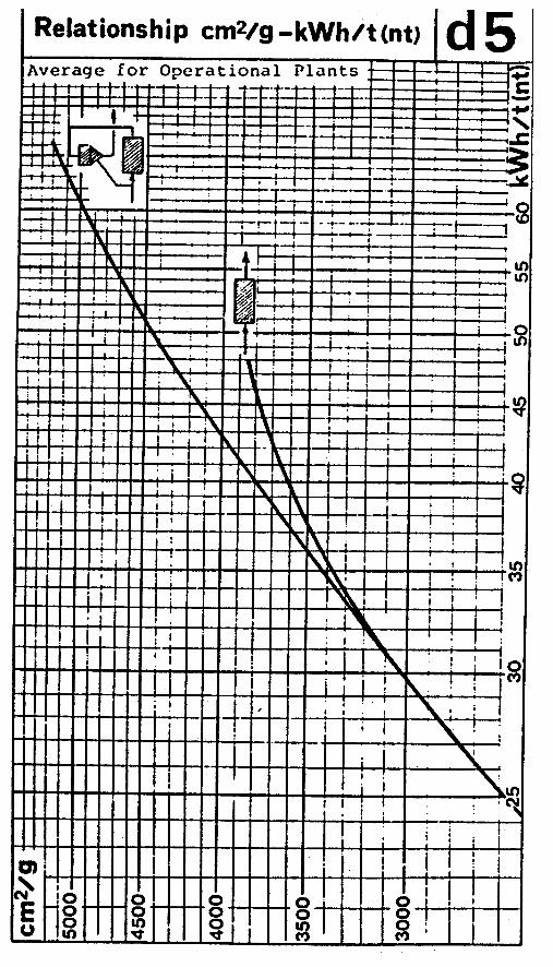
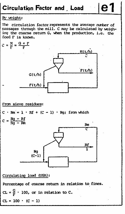
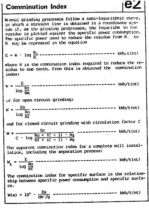
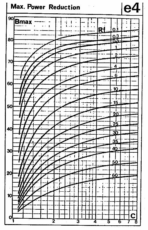
Blue Circle Cement

PROCESS ENGINEERINGTRAINING PROGRAM

Module 4

Section 4

The Physics of Air

“ T H E P H Y S I C S O F A I R ”

THIS MANUAL WASCOMPILED FROM A SERIES OF

LECTURES GIVEN BY

JAMES W. MAYMANAGER OF TECHNICAL RELATIONS

CLEAN AIR GROUPAMERICAN AIR FILTER CO.

PRICE $2.00

American Air Kilter COMPANY, INC.

2 1 5 C E N T R A L A V E N U E , L O U I S V I L L E 8, K E N T U C K Y

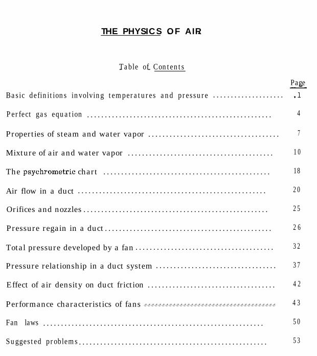
THE PHYSICS OF AIR- -

Table of Contents- -

Page

Basic definitions involving temperatures and pressure . . . . . . . . . . . . . . . . . . . . .l

Perfect gas equation . . . . . . . . . . . . . . . . . . . . . . . . . . . . . . . . . . . . . . . . . . . . . . . . . . . . 4

Properties of steam and water vapor . . . . . . . . . . . . . . . . . . . . . . . . . . . . . . . . . . . . . 7

Mixture of air and water vapor . . . . . . . . . . . . . . . . . . . . . . . . . . . . . . . . . . . . . . . . . 1 0

The psychrometric chart . . . . . . . . . . . . . . . . . . . . . . . . . . . . . . . . . . . . . . . . . . . . . . . 18

Air flow in a duct . . . . . . . . . . . . . . . . . . . . . . . . . . . . . . . . . . . . . . . . . . . . . . . . . . . . . 2 0

Orifices and nozzles . . . . . . . . . . . . . . . . . . . . . . . . . . . . . . . . . . . . . . . . . . . . . . . . . . . . 2 5

Pressure regain in a duct . . . . . . . . . . . . . . . . . . . . . . . . . . . . . . . . . . . . . . . . . . . . . . . 2 6

Total pressure developed by a fan . . . . . . . . . . . . . . . . . . . . . . . . . . . . . . . . . . . . . . . 3 2

Pressure relationship in a duct system . . . . . . . . . . . . . . . . . . . . . . . . . . . . . . . . . . 3 7

Effect of air density on duct friction . . . . . . . . . . . . . . . . . . . . . . . . . . . . . . . . . . . . 4 2

Performance characteristics of fans ..................................... 4 3

Fan laws . . . . . . . . . . . . . . . . . . . . . . . . . . . . . . . . . . . . . . . . . . . . . . . . . . . . . . . . . . . . . . 5 0

Suggested problems. . . . . . . . . . . . . . . . . . . . . . . . . . . . . . . . . . . . . . . . . . . . . . . . . . . . . 5 3

THE PHYSICS OF AIR

Since the majority of products manufactured by the American Air Filter Companyare designed to treat air in some form, shape, or manner - it behooves us to have athorough knowledge concerning the various properties of air and water vapor, how theseproperties are determined, how air flow is produced and measured, etc.

It would probably be well to first start with the definition of certain terms which wewill be using in our various discussions. These terms may be new to some of yougentlemen, but they are very fundamental in their application and I am sure that youwill find them easy to grasp and to apply.

BASIC DEFINITIONS - Temperature: Let us start out with a term with which we arefamiliar, such as temperature. Temperature, by definition, is a measure of the intensityof heat and is no indication of the quantity involved. There are several temperaturescales, but the one used by the Engineering Profession is “Degrees Fahrenheit. ” On thistemperature scale the freezing point of water is 320 F. , and the boiling point is 212O F.The physicist and the chemist generally think in terms of degrees Centigrade, so weshould spend a moment to discuss the relationship between Centigrade and Fahrenheit.On the Centigrade scale the freezing point of water is O” C. and the boiling point is100° C. You will immediately note that the difference between the freezing point and theboiling point of water is 180° on the Fahrenheit scale but only 100° on the Centigradescale, so if we had a temperature reading of 20° Centigrade and we wanted to convertit into degrees Fahrenheit, we would use the expression:

Degrees F = (9/5 T,) + 32 = (9/5 x 20) + 32 = 68’ F.or conversely: Degrees C = 5/9 (Tf - 32 )

As we mentioned, the term “temperature” is an indication of the intensity of heatin an object and indirectly reflects the amount of movement of the molecules which makeup the body. As the molecular movement slows down, a point would theoretically bereached at which there is no molecular movement and this is said to be absolute zero,and on the Fahrenheit scale is 459.60 below O” F. This is an important relationship : adone which you should remember, because any calculation involving the ratio of temper-atures must be done on an absolute temperature basis which means that 460° must bealgebraically added to the temperature in degrees Fahrenheit in order to determine thenumber of degrees above absolute zero. On the Centigrade scale the point of absolutezero is -273.1 below 0’ C.

Instruments which are ordinarily used for measuring temperatures include mercury,gas, and resistance thermometers; thermocouples; radiation, gas and optical pyrometers;Seger cones, etc.

Heat: Whereas temperature in degrees is an indication of the intensity of heat, the BritishThermal Unit or m is the accepted unit of heat quantity. A Btu is frequently defined asthe heat required to raise one pound of water through lo F., but a more accurate defi-nition is that 1 Btu equals l/180 of the amount of heat required to raise the temperatureof a pound of water from 32O F. to 2120 F.

-l-

The following example will serve to indicate the fundamental difference betweenquantity of heat and intensity of heat:

Given 50 lbs. of water and 50 lbs. of cast iron - each to be heatedthrough a temperature rise of lOOoF. - Determine the heat addedto each substance:

Average amount of heat required to raise the temperature of 1 lb.of water through 1°F. = 1 Btu.Heat added to water = 1 x 50 x 100 = 5000 Btu.

Average amount of heat required to raise the temperature of 1 lb.of cast iron through 1°F. = 0.12 Btu.Heat added to cast iron = 0.12 x 50 x 100 = 600 Btu.

In this example the weight of material and the temperature rise werethe same in each case, but the quantity of heat added differed con-siderably due to the nature of the substances. Had the same amountof heat been added to the cast iron as was added to the water thetemperature rise of the iron would have been 5000 f (50 x 0.12) = 833’F.

Specific Heat: The foregoing illustration introduced another basic term with which we mustbecome familiar and that is “Specific Heat. I’ The specific heat of any substance is theratio of the heat required to raise a unit weight of the substance lo F., to the quantityof heat required to raise the temperature of the same weight of water through lo F. InCGS units the average specific heat of water equals 1 calorie/gram/deg. C. Since thespecific heat of water may be considered to be 1, we may then say that the specific heator thermal capacity is the quantity of heat required to raise 1 pound of the substancethrough 1°F. For any given material, the specific heat will vary somewhat dependingupon the range of temperature involved. This is particularly true for gases but cangenerally be disregarded unless the temperature range is wide or precise calculationsare involved. In dealing with air, there are actually two types of specific heat to beconsidered. There is the specific heat at constant pressure, which is the one used mostlyin air conditioning, and the specific heat at constant volume. The approximate valuesof each are 0.241 and 0.173 BTU respectively. Specific heat at constant pressure isthe greater because the increase in the air volume due to the addition of heat meansthat external work has been done against the pressure that is present. Some datum isalways necessary when making heat content determinations and if this datum is not def-initely stated, it is generally understood to be O’F.

Find the quantity of heat required to raise the temperature of 100 lbs.of ice from O°F. to 32OF. Specific heat of ice = 0.5100 x (32-O) x 0.5 = 1600 Btu.

Pressure: Let us now take up another group of definitions which are important for athorough understanding of the properties of air. These have to do with “pressure.”

Air is such a commonplace thing that we are seldom conscious of its existence. Wemust, however, realize that air has weight, it exerts a pressure, and everything that wedo takes place in an ocean of air. The earth as a planet is completely surrounded by anenvelope of air, or atmosphere, as we frequently refer to it. The pressure exerted bythe atmosphere is termed “atmospheric pressure”, and is generally expressed in termsof force per unit area. Atmospheric pressure is measured above zero absolute pressureor above a perfect vacuum.

-2-

The pressure of the atmosphere varies with the elevation above sea level, weatherconditions, etc. , and since it is such a variable quantity, it has been necessary to definestandard atmospheric pressure so that it can serve as a basis of comparison in engineer-ing formula, etc. This standard atmospheric pressure is supposed to be measured at sealevel and by definition is equivalent to 29.92” of mercury per square inch. This meansthat a column of air one square inch in cross section and extending up into the sky tothe limit of our atmosphere would exert just enough ‘weight to counter-balance the weightof a column of mercury 1 square inch in cross section and 29.92” in height. The follow-ing illustration shows this relationship:

The height of mercury standing in the tubewill be exactly equal to the pressure of theatmosphere pushing down on the surface ofthe mercury in the beaker.

As a matter of fact atmospheric pressure is frequently measured by an instrumentusing mercury, precisely as shown in the above illustration and this device is referredto as a mercurial barometer. There is another type of barometer in general use whichuses no fluid and the pressure of the air is measured by a linkage which is attached tothe elastic side of a box or chamber which has been exhausted of air. This type of in-strument is called an “aneroid” barometer, which means “no fluid.”

In the above illustration we talked about the pressure of air as measured in terms ofinches of mercury, but we should also be familiar with the other units in which air pressureis frequently measured. Standard atmospheric pressure (which is theoretically the airpressure at sea level) is also equal to 14.7 lb. per square inch and this gives us arelationship of 14.7/29.92 = 0.491 lbs. per square inch for each inch of mercury column.In many pressure determinations, the unit “inches of mercury” is too large for the valueof the pressure being measured (for the same reason that it would be absurd to measurethe weight of a parcel post package in tons - therefore, we use pounds and ounces) andso we need a smaller unit of measurement such as “inches of water.” Since mercury is13.6 times as heavy as water, then 1” of mercury = 13.6” of water. Standard atmos-pheric pressure of 29.92” of mercury is therefore equivalent to approximately 407” ofwater per square inch. When pressure is measured in a steam boiler for example, thepressure is measured above or below the atmosphere and such pressure is always ex-pressed as gauge pressure and is frequently abbreviated p. s. i. g. meaning pounds per squareinch gauge. In order to determine the absolute pressure or the pressure above zero, itis necessary to algebraically add the gauge pressure to the atmospheric or barometricpressure. Absolute pressure is frequently abbreviated p. s. i. a. (pounds per square inchabsolute.) Always be sure that each pressure is expressed in the same units, as it isabsolutely fatal to try to add inches of mercury to pounds per sq. in. or to add inches of waterto inches of mercury.

In dealing with air flow the pressures are frequently quite minute and are almostalways expressed in terms of inches of water. such pressures are referred to as “gaugepressure” or pressure above or below atmosphere. The phrase “gauge pressure” is derivedfrom the fact that this pressure is generally measured with some type of gauge. In measur-

-3-

ing these pressures we sometimes use an ordinary U-tube which has been filled with waterand the water in the two sides will deflect in accordance with the pressure differentialbeing measured. If the pressure in question involves the deflection of a fraction of aninch, a U-tube would not be a very accurate measuring device, so in these instances wegenerally use as a gauge a device which is referred to as a “manometer” or draft gauge.This instrument is fundamentally the same as a U-tube except that one leg is bent out ata very obtuse angle in order to magnify the deflection or displacement of the liquid. In-stead of water, most gauges of this type use a light colored mineral oil which will alsoamplify the deflection for a given amount of pressure. In practically all cases these gaugesare calibrated to read in terms of inches of water, so we must thoroughly familiarize our-selves with this unit of pressure measurement.

Specific Volume: In addition to the foregoing we should become familiar with the term“specific volume, ‘I which generally refers to the volume occupied by one pound of a sub-stance. A gas such as air expands or contracts quite readily with changes in temperatureand pressure, therefore, the number of cubic feet occupied by a pound of air (or its spe-cific volume) must take these properties into consideration. Assume the temperature ofthe air within this room is 75O F. and a barometer pressure of 29.2” of mercury. There-fore, the specific volume of the air is about 13.9 cu. ft. per pound. This room roughlymeasures 20 ft. by 36 ft. with a 7-l/2 ft. ceiling, and multiplying these three valuestogether gives a volume of 5,400 cu. ft. Since we said that each pound of air wouldoccupy 13.9 cu. ft. - this room would then calculate to contain 389 lbs. of air. Whena man says he is under pressure, it is certainly true of air pressure. The reciprocalof specific volume is specific weight, which is the weight in pounds of 1 cubic foot ofthe substance at some stated condition.

PERFECT GAS EQUATION: All matter is composed of molecules which are defined as thesmallest sub-division of matter that retains its original characteristics. Molecules mayin turn be sub-divided into atoms but these atoms will no longer have the same character-istics as the original substance. For example, a molecule of water will behave preciselyas water does, but each molecule consists of atoms of hydrogen and oxygen, which takenindividually will bear no resemblance to water. According to the general accepted theory,all molecules are in continuous motion and the magnitude of this motion is a function ofthe temperature, with the higher the temperature, the greater the velocity of molecularmovement. Solid bodies have rigidity because the molecules vibrate continuously, but donot change their position relative to adjacent molecules. In a liquid all molecules havegreater freedom, however, the forces of cohesion are strong enough so that there is notendency for the molecules to separate. In the case of a gas, such as air, the moleculesare at a much greater distance apart and tend to diffuse and disperse indefinitely unlessprevented by a constraining vessel.

The atmosphere of our earth is a mechanical mixture of several gases, the pro-portion of which varies slightly in different localities. The chief constituents of air areoxygen, nitrogen, argon and water vapor; with slight traces of other gases such ascarbon dioxide, hydrogen, neon, etc.

In studying air and its properties, our problem actually divides itself into two parts,Dry air follows very closely the fundamental laws dealing with a perfect gas, but thewater vapor (which is actually low pressure steam) obeys the laws which are peculiar tovapors. In studying the behavior of dry air, we should first consider Boyles Law andCharles Law. Boyles Law states that for a perfect gas, when the temperature remains

constant the volume will decrease as the pressure is increased; or at a constant temper-ature, the volume will vary inversely as the pressure. Charles Law also deals with aperfect gas and states that if the pressure remains constant and the temperature varies,the volume of the gas will increase directly as the absolute temperature. By combiningthese two laws we arrive at a characteristic equation for a perfect gas which states that:

PQ = RT for 1 pound of the gas, or

PQ = WRT for W pounds of the gas

where: P = the absolute pressure in pounds per square foot- -

*Q = the tot 1a volume of the gas in cubic feet

W = the total weight of the gas in pounds

R = Gas constant

T = the absolute temperature = (460 + t) o F.

This gas constant (R) has an interesting derivation. For any individual gas, the’ constant(R) multiplied by the molecular weight of the gas (M) is always equal to 1545.4. Withthis basic relationship we can, therefore, compute the constant (R) for any gas by divid-ing 1545.4 by the molecular weight of the gas. It was previously mentioned that air is amechanical mixture of several gases and has approximately the following volume relation-ship -

Constituent

Oxygen (02)

Nitrogen (N2)

Argon (A)

Part by Volume

.210

.781

.009

1.000

Molecular Wt.

x 3 2

x 2 8

x 39.9

Proportion of Mole. Wt.

6.72

21.866

0.355

28.941

The total apparent molecular weight of the air mixture is 28.941 and the gas constant(R) for air is, therefore, 1545.4/28.941 = 53.34

At this point it might be of interest to mention the relationship involving molecularweight and specific volume.

* The letter l’V’l will be reserved to represent Velocity.

-5-

The volume of a pound molecule, or mol, of any gas at normal conditions is a def-inite number and is equal to 359 cu. ft. This means that for any gas a mol, which isequal to the molecular weight expressed as pounds, will always occupy 359 cu. ft. at abarometric pressure of 29.92” of mercury and at a temperature of 32O F. You will notethat this represents so-called “normal conditions” as used in chemistry. In air condition-ing work we usually refer to normal or standard conditions as representing a barometricpressure of 29.92” of mercury, and a temperature of 700 F.

Using the above relationship for molecular weight, specific volumes may be calcu-lated as indicated by the following examples:

The atomic weight of oxygen is equal to 16, so for 02, themolecular weight would be 2 x 16 = 32Specific volume of O2 = 359/32 = 11.22 cu. ft. per pound (at 32O F. and 29.92” Hg.)

Molecular weight of CO2 = 12 + (2 x 16) = 44Specific volume = 359/44 = 8.16 cu. ft. per pound (at 320 F. and 29.92” Hg.)

We previously calculated the molecular weight of air to be 28.941.Specific volume of air at 29.92” Hg and 32O F. = 359/28.941 = 12.4 cu. ft. /lb.This value can be checked directly from a psychrometric chart. If it is desiredto obtain the specific volume of air at 70° F. and standard barometric pressure,we would then multiply the specific volume at 32O F. by the ratio of absolutetemperatures:

12 4 x (460 + 70). (460 + 32) = 13.35 cu. ft. per pound

The Perfect Gas Equation is a very useful relationship as will be shown by the follow-ing illustrations:

(a) Given 1 lb. of air at 700 F. and 29.92” Hg.sp. Vol. = 13.35 cu. ft. per lb.If the pressure is increased to 5 lbs. per sq. in gauge, and the temperatureremains constant, what is the volume then occupied by the pound of air?According to Boylesl Law:

14.7Q =(14.7+5.0)

x 13.35 = 9.95 cu. ft. per lb.

If the air at the original condition was cooled to O” F. , what would be its volume?According to Charles’ Law:& _ (460 + 0 )

- (460 + 70) x 13.35 = 11.58 cu. ft. per lb.

(b) Assume 1 pound of air at standard atmospheric pressure of 14.7 lb. per sq. in.occupies 11.58 cu. ft. Using the Perfect Gas Equation, determine the temperatureof the air in degrees Fahrenheit.

PQ=WRT

(Absolute) T = 2 = 14* : z :F3i 11* 58= 460° T (Deg. F) = 460 - 460 = O°F..

(c) Given 1 lb. of air at 70° F. and under a pressure of 5 lbs. per sq. in gauge.Determine the specific volume occupied by 1 lb. of air using the Perfect GasEquation:

WRT 1 x 53.34 x (460 + 70)P Q = W R T Q = p= (14.7 + 5) x 144

= 9.95 cu. ft. per lb.

(d) An inflated automobile tire contains 0.5 lbs of air which occupies a volume of1.82 cu. ft. at a pressure of 40 psig and a temperature of 750 F. The barometricpressure is 14.4 lbs. per sq. in.

Using Charles’ Law, calculate the resulting gage pressure in the tire if it isheated to a temperature of 130° F. , assuming the volume remains constant.Check by using the perfect gas equation.

V = Const. Pl Tl-=-P 2 T 2

PIT2 _ (40 + 14.4) x (460 + 130) _ 14 4p2 = -Ti-- (460+ 75)

.

= 60 - 14.4 = 45.6 psig.

Check: P WRT= 0.50 x 53.34 x 5 9 0= = 6. -8 1.82 x 144

14.4 = 45.6 psig

Since the atmosphere is a mechanical mixture of several gases, plus water vapor,the atmospheric pressure which we measure with a barometer is the sum of the pressuresexerted by the individual components. This is a very important relationship in our studyof the properties of air and water vapor, and is known as Dalton’s Law. Briefly it statesthat two or more gases or vapors can occupy the same volume at the same time, andthe total pressure of the mixture is the sum of the partial pressures of the constituents.This law is particularly important as we study the relationship between dry air and watervapor.

WATER VAPOR OR STEAM: Let us first discuss some of the properties of water vaporwhich will be significant to us later. We are all familiar with the process of water boil-ing in an open vessel. Starting with water at 32O F., as we add heat the temperature ofthe water will continue to rise until the temperature of 212O F. is reached and the waterbegins to boil (at standard atmospheric pressure. ) At this point the temperature will re-main constant until all the water has boiled off or disappeared. We must realize, how-ever, that evaporation of the water was also occuring during the entire heating-up period.At the low temperatures the rate of evaporation was very slow with the evaporation in-creasing as the temperature of the water increased. The important point is that a verydefinite quantity of heat was required to change the water from the liquid state to thevapor state and this quantity of heat was dependent upon the temperature (or pressure) ofthe water.

From the molecular standpoint, vaporization means the flying off of molecules againstthe forces of molecular attraction provided by the water. If we take a vessel partiallyfilled with water and cover it with a tight lid, the liberated vapor will be confined abovethe surface of the liquid. If the water in the vessel is maintained at some constant tem-

- 7 -

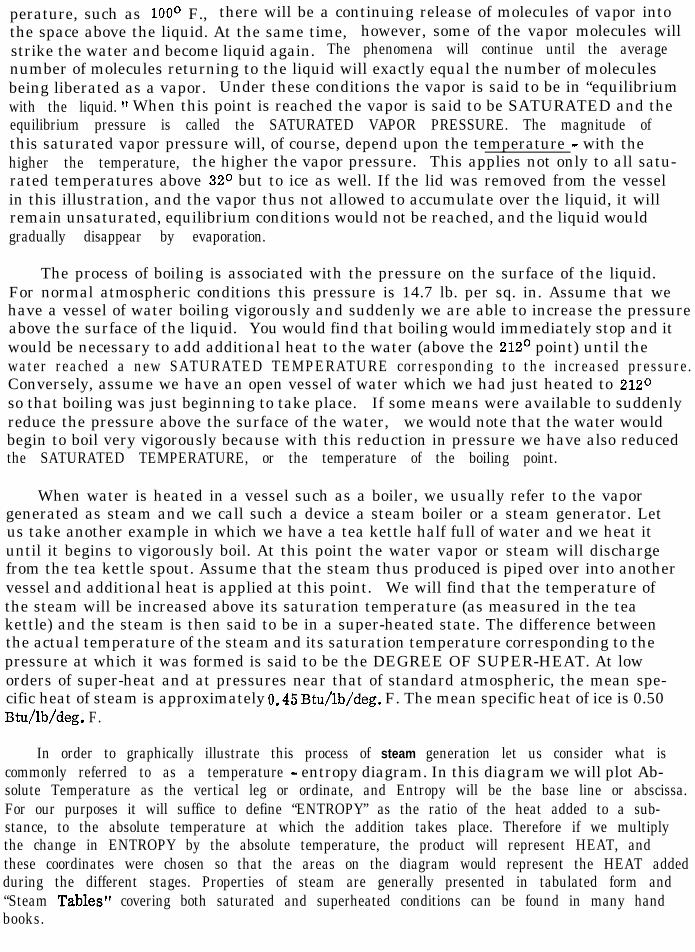
perature, such as 100° F., there will be a continuing release of molecules of vapor intothe space above the liquid. At the same time, however, some of the vapor molecules willstrike the water and become liquid again. The phenomena will continue until the averagenumber of molecules returning to the liquid will exactly equal the number of moleculesbeing liberated as a vapor. Under these conditions the vapor is said to be in “equilibriumwith the liquid. ” When this point is reached the vapor is said to be SATURATED and theequilibrium pressure is called the SATURATED VAPOR PRESSURE. The magnitude ofthis saturated vapor pressure will, of course, depend upon the temperature - with thehigher the temperature, the higher the vapor pressure. This applies not only to all satu-rated temperatures above 32O but to ice as well. If the lid was removed from the vesselin this illustration, and the vapor thus not allowed to accumulate over the liquid, it willremain unsaturated, equilibrium conditions would not be reached, and the liquid wouldgradually disappear by evaporation.

The process of boiling is associated with the pressure on the surface of the liquid.For normal atmospheric conditions this pressure is 14.7 lb. per sq. in. Assume that wehave a vessel of water boiling vigorously and suddenly we are able to increase the pressureabove the surface of the liquid. You would find that boiling would immediately stop and itwould be necessary to add additional heat to the water (above the 212’ point) until thewater reached a new SATURATED TEMPERATURE corresponding to the increased pressure.Conversely, assume we have an open vessel of water which we had just heated to 212Oso that boiling was just beginning to take place. If some means were available to suddenlyreduce the pressure above the surface of the water, we would note that the water wouldbegin to boil very vigorously because with this reduction in pressure we have also reducedthe SATURATED TEMPERATURE, or the temperature of the boiling point.

When water is heated in a vessel such as a boiler, we usually refer to the vaporgenerated as steam and we call such a device a steam boiler or a steam generator. Letus take another example in which we have a tea kettle half full of water and we heat ituntil it begins to vigorously boil. At this point the water vapor or steam will dischargefrom the tea kettle spout. Assume that the steam thus produced is piped over into anothervessel and additional heat is applied at this point. We will find that the temperature ofthe steam will be increased above its saturation temperature (as measured in the teakettle) and the steam is then said to be in a super-heated state. The difference betweenthe actual temperature of the steam and its saturation temperature corresponding to thepressure at which it was formed is said to be the DEGREE OF SUPER-HEAT. At loworders of super-heat and at pressures near that of standard atmospheric, the mean spe-cific heat of steam is approximately 0,45 Btu/lb/deg. F. The mean specific heat of ice is 0.50Btu/lb/deg. F.

In order to graphically illustrate this process of steam generation let us consider what iscommonly referred to as a temperature - entropy diagram. In this diagram we will plot Ab-solute Temperature as the vertical leg or ordinate, and Entropy will be the base line or abscissa.For our purposes it will suffice to define “ENTROPY” as the ratio of the heat added to a sub-stance, to the absolute temperature at which the addition takes place. Therefore if we multiplythe change in ENTROPY by the absolute temperature, the product will represent HEAT, andthese coordinates were chosen so that the areas on the diagram would represent the HEAT addedduring the different stages. Properties of steam are generally presented in tabulated form and

, “Steam Tables” covering both saturated and superheated conditions can be found in many handbooks.

ENTROPY

P

ff

K

C

S

The line AL is known as the liquid line and BC is the saturated vapor line. If wewould extend the liquid and vapor lines until they intersect, such as point X - it wouldrepresent the critical point above which we could no longer liquify the steam by the appli-cation of pressure. This point represents a temperature of 7060 F. and an absolute pressureof 3206 lb. per sq. in. As an example in the use of this diagram let us assume that we aregenerating steam in a boiler at 3# gauge pressure. The saturation temperature at thispressure is 222O F. Starting with water at 32’ F. such as point A, our liquid follows theline AL to point D which represents the temperature of 222’ F. corresponding to the sat-uration temperature at 3# gauge pressure. At this condition we have added to each poundof water the heat equivalent to the area under the curve AD. This is referred to as theHEAT OF THE LIQUID and is equal to 190 Btu per pound. At point D the liquid is exertingits maximum tendency to be transformed into the vapor state. By that we mean at pointD the water is still liquid but any further addition of heat will cause a change in statethereby transforming it from a liquid to a vapor - or steam. This change in state occursat a constant temperature as indicated by line DE. At point E on the vapor line, thepound of water has been transformed into steam and the area below line DE will repre-sent the LATENT HEAT OF VAPORIZATION or the heat required to change a pound ofwater from a liquid at 222O F. into steam at 2220 F. You will note that we have intro-duced the term “latent heat”. The dictionary definition of the word lllatent’l states that itmeans “present but not visible or apparent. 11 The latent heat of steam, therefore, isheat which has been applied in order to effect a change of state (from a liquid to a vapor),but the presence of this heat would not be reflected in a temperature reading, becauseduring this change of state process - the temperature remains constant as indicated byline DE. However, if we later condense this steam into water, such as is done in aSteam radiator, we will reclaim this latent heat and it can be used for space heating, etc.

The latent heat of vaporization for steam at 3# gauge pressure is 966 Btu per poundand the heat content of a pound of steam at point E will, therefore, be the sum of theheat of the liquid plus the latent heat of vaporization = 190 + 966 = 1156 Btu’s per pound

- 9 -

of steam. You will note that the liquid line AL and the vapor line BC are converging (andactually intersect at point X as indicated.) Consequently the latent heat of evaporation de-creases as the saturation temperature (or the saturation pressure) increases. At the criti-cal point X, the water would instantaneously flash or vaporize into steam without the addi-tion of any heat or vaporization. The temperature and pressure would have to be 706O F.and 3206# per sq. in. gauge, respectively, as previously stated.

After point E is reached, if we were to continue to add heat to the vapor, our steamwould follow the line EF which is the super-heat line at constant pressure and the areato the right of the vapor line BC is known as the super heat region. At point F the heatof super-heat added to each pound of steam would be equivalent to the area under line EF.If you assume point F to represent a temperature of 250° F., the heat of super-heat isequal to 13 Btu’s per pound. The number of degrees of super-heat are 250 - 222 = 28’ F.On the basis of the actual Btu’s of super-heat involved you will note that the average spe-cific heat of the steam calculates to be 0.465 Btu/lb/deg. which approximates the valueof 0.45 previously referred to.

At point F the total heat in one pound of our steam in now equal to the sum of theheat of the liquid plus the latent heat of vaporization plus the heat of super-heat and =190 t 966 t 13 = 1169 Btu per pound.

Down in the range of vapor pressures and temperatures associated with air condi-tioning, we have the same processes for the formation of vapor which is present, as wehave just covered in our steam discussion. Thus if our liquid is heated to 70° F. alongthe liquid line AG and vaporized or evaporated along the constant temperature line GK wehave added the heat of the liquid and the latent heat of vaporization just as we did in theexample dealing with our steam boiler at 3# gauge pressure. Point K represents the con-dition of the water vapor in air saturated at 70° F. and any further addition of heat wouldcause the saturated water vapor to become super-heated at constant pressure to somepoint such as P. Let us assume for a moment that point P represents 80° F. (whichwould be the dry bulb temperature of the air in an air-vapor mixture.) Under this condi-tion the water vapor in the air is actually super-heated above point K. In this examplethe amount of super-heat would be loo and point K would correspond to the dew pointtemperature - or the temperature at which air becomes saturated without the gain or lossof any moisture. In air conditioning the water vapor in the air is in a super-heated statethe majority of the time and we are, therefore, concerned mostly with the conditions ofthe vapor either on or to the right of the saturation BC and it is in this area in whichour psychrometric charts are plotted. While this temperature entropy-diagram could verywell serve as a psychrometric chart, it would have to be constructed in such detail asto be impractical.

MIXTURES OF AIR & WATER VAPOR: When we spoke of air being a mechanical mixture,mention was made of the fact that the over-all or total atmospheric pressure was madeup of the sum of the pressures of the individual components. For our work in air condi-tioning we will group all the dry components together and refer to them as r’Air” and wewill then have only the water vapor component to consider separately.

In other words: Pt = Pa + Pv which states that the total atmospheric pressure is 1equal to the partial pressure of the air plus the partial pressureof the water vapor.

_j

- 10 -.)

Since we have already developed the basic equation combining thelaws of Boyles and Charles, to wit: PQ = WRT, it might be wellto determine the value of the gas constant R when our pressureunits are expressed in terms of inches of mercury per squareinch.The volume occupied by 1 lb. of air at a temperature of 70° F.and a pressure of 14.7 lb/sq. in. = 13.35 cu. ft. Since 14.7 lb.per sq. in. = 29.92” Hg, the gas constant R for dry air whenthe pressure is expressed in inches of mercury is:

R=z = 29.92 x 13.35 _ o 7531 x 530 - *

In air conditioning we have two mixture conditions to contend with, insofar as thewater vapor component is concerned. There is the condition of saturated water vapor(when the air is saturated); and the condition where the air in unsaturated or when thewater vapor present is in a superheated state. We shall work out a number of examplesfor both of these conditions and shall then check them against the psychrometric chart.

It has been previously mentioned that at low temperatures, the water vapor or steamwill behave almost as a perfect gas, and under these conditions it obeys the same lawsas for air. When dealing with water vapor we may use the expression PvQ, = WR,T,,where the subscript (v) identifies the water vapor component. Where the pressure is ex-pressed in pounds per sq. ft., the gas constant R for water vapor = 85.72. With thepressure expressed in inches of mercury, the equation reduces to PvQv = 1.21 TV.This latter expression applies to 1 lb. of vapor since the value of W (weight) hasbeen omitted.

SATURATED CONDITIONS: Given one pound of dry air at 70° F. and 29.92” of mercurypressure and to this air has been added sufficient water vapor to saturate it. Please notethe term “pound of dry air” - as this is the basis for all determinations made on thepsychrometric chart. The reason for this is quite apparent. If you had a pound of airwhich consists of a mixture of air and water vapor you can well see that would be aninfinite number of dry air weight and water vapor weight which when added together wouldmake one pound. Because of this infinite number of possible combinations - it would mater-ially complicate a psychrometric chart if a “pound of mixture” was used as the basis.On the other hand, however, with all properties being based on one pound of dry air, plusthe moisture present; it is only necessary to take into consideration the varying weight ofwater vapor. In actual practice the only property which generally needs to be correctedto a “pound of the mixture basis *’ is specific volume or density.

Let us reconsider our reference example of one pound of dry air at a temperature of70’ F. and under standard barometric conditions of 29.92” of mercury. Solving in ourperfect gas equation, the volume calculates to be 13.35 cu. ft. which is the volume occupiedby one pound of dry air at the conditions specified. However, when this air is saturatedwith water vapor, the pressure exerted by the dry air component will no longer be 29.92”Hg, but will be the reading of the barometer less the pressure exerted by the water vapor.For the properties of water vapor, let us refer to a steam table and at 70° F. we notethat the pressure of saturated steam (or water vapor) is 0.74” of mercury and that thevolume occupied by pound of water vapor at this condition is 868 cu. ft. Since the totalpressure of the mixture is 29.92” of mercury, the pressure exerted by the dry air onlyis 29.92” - 0.74 = 29.18 Hg. It was originally calculated that the volume occupied by one

- 11 -

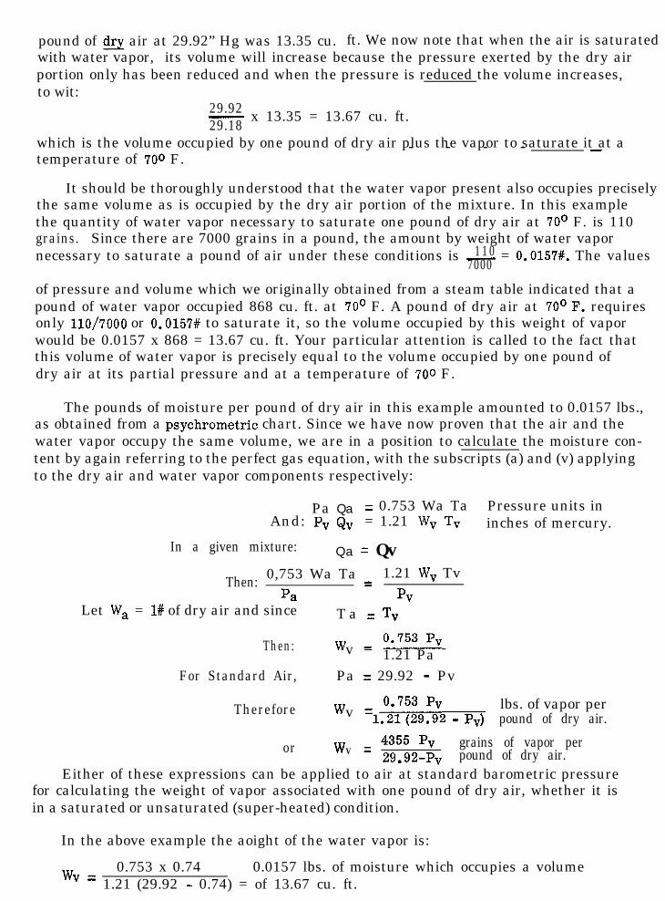
pound of dry air at 29.92” Hg was 13.35 cu. ft. We now note that when the air is saturatedwith water vapor, its volume will increase because the pressure exerted by the dry airportion only has been reduced and when the pressure is reduced the volume increases,to wit:

29.92- x 13.35 = 13.67 cu. ft.29.18

which is the volume occupied by one pound of dry air plus the vapor to saturate it at a- - - - -temperature of 700 F.

It should be thoroughly understood that the water vapor present also occupies preciselythe same volume as is occupied by the dry air portion of the mixture. In this examplethe quantity of water vapor necessary to saturate one pound of dry air at 70° F. is 110grains. Since there are 7000 grains in a pound, the amount by weight of water vapornecessary to saturate a pound of air under these conditions is -1 1 0

7000= 0.0157#. The values

of pressure and volume which we originally obtained from a steam table indicated that apound of water vapor occupied 868 cu. ft. at 70° F. A pound of dry air at 70’ F. requiresonly 110/7000 or 0.0157# to saturate it, so the volume occupied by this weight of vaporwould be 0.0157 x 868 = 13.67 cu. ft. Your particular attention is called to the fact thatthis volume of water vapor is precisely equal to the volume occupied by one pound ofdry air at its partial pressure and at a temperature of 700 F.

The pounds of moisture per pound of dry air in this example amounted to 0.0157 lbs.,as obtained from a psychrometric chart. Since we have now proven that the air and thewater vapor occupy the same volume, we are in a position to calculate the moisture con-tent by again referring to the perfect gas equation, with the subscripts (a) and (v) applyingto the dry air and water vapor components respectively:

Pa Qa = 0.753 Wa TaAnd: Pv Qv = 1.21 WV TV

Pressure units ininches of mercury.

In a given mixture: Qa = Qv

Then: 0,753 Wa Ta _ 1.21 WV Tv-Pa PV

Let Wa = l# of dry air and since T a = TV

Then: w -0.753Pvv - 1.21 Pa

For Standard Air, Pa = 29.92 - Pv

Therefore w -0.753Pvv - lbs. of vapor per

1.21pg.92 - pv) pound of dry air.

or wV

= 4355 pv grains of vapor per29.92-Pv pound of dry air.

Either of these expressions can be applied to air at standard barometric pressurefor calculating the weight of vapor associated with one pound of dry air, whether it isin a saturated or unsaturated (super-heated) condition.

In the above example the aoight of the water vapor is:

WV = 0.753 x 0.74 0.0157 lbs. of moisture which occupies a volume1.21 (29.92 - 0.74) = of 13.67 cu. ft.

The total weight of dry air plus vapor involved in this example is 1 + 0.0157 = 1.0157lb. The volume occupied by 1 lb. of the mixture is i’&-$$$ = 13.46 cu. ft.. ,

As previously mentioned, the mixture basis may he used whenever precise calculationsinvolving specific volume or density are involved.

ABSOLUTE HUMIDITY is the actual weight of water vapor (in grains or pounds) per cu.ft. of mixture. SPECIFIC HUMIDITY is the weight of water vapor (in grains or pounds) mixedwith one pound of dry air. The use of specific humidity rather than absolute humidity fre-quently simplifies the calculations. Although the results will not be absolutely accurate, forall practical purposes the error which is introduced can generally be ignored.

Dr. Carrier has proposed the following equation for solving for the partial pressureof the water vapor at any given wet and dry bulb temperature:

Pv = Psv - (pb - p,,) (td - tw)2800 - 1.3 t,

Where Pv = Pressure of the water vapor at the unsaturated condition.

P sv = Pressure of the saturated water vapor at the wet bulb temp.

Pb = Barometric pressure

td = Dry bulb temperature

t, = Wet bulb temperature

Example: Given air at 750 dry bulb and 600 wet bulb at an atmosphericpressure of 29.92 in. Hg. determine the partial pressure ofthe water vapor.

Psv = 0.5218 in. Hg. - Saturation pressure of the water vapor at600 F. wet bulb.

P, = 0.5218 -(29.92 - 0.5218) ( ‘75 - 60)

2800 - (1.3 x 60)

= 0.3604 in. Hg. - Partial pressure of the water vapor

(This value can be checked from a chart or table bydetermining the saturation pressure at the dew pointtemperature.)

It should be noted that when air is saturated at a given temperature - such as at ‘70°,that same temperature will also correspond to the Dew Point. This is a very importantterm in air conditioning and one with which we must become familiar. Again by definition,the dew point temperature is the temperature at which the air becomes saturated with-out the gain or loss of moisture. In this example if the air is cooled only a fraction ofa degree below 70, some of the moisture will condense out in the form of droplets ofwater (such as fog or dew), and the moisture content will then be reduced and the dewpoint temperature will be lowered.

Conversely if the air is heated above 70° F. so that additional moisture can be added -the temperature of the dew point will be raised. Let us, therefore, remember that thedew point temperature of the air is a function of the moisture content, and if the moisturecontent remains constant, the temperature of the dew point will not change. Therefore,

- 13 -

in an air-vapor mixture the dew point temperature corresponds to the saturation conditionsof the vapor or steam as given in steam tables.

TOTAL HEAT: Another property of a saturated mixture of air and water vapor that wewill find useful is called the “total heat content”. It consists of the sum of the sensibleheat content of the dry air above a pre-determined reference point plus the sensibleheat of the water from which the vapor was formed, plus the latent heat of vaporizationof the weight of water required to saturate the air at any given condition. In determin-ing the total heat content of an air-vapor misture, it is customary to base the sensibleheat in one pound of dry air above the datum of O” F, and the heat in the water fromwhich the vapor was formed is based upon the datum of 32O F. In this expression fortotal heat we have used the terms sensible heat and latent heat and we should becomecompletely familiar with these two terms. Whenever we add heat to a substance we in-crease its temperature and the heat thus added is known as sensible heat, because itcan be “sensed1 by touch or its presence can be detected by a thermometer. Heat maybe added to a body without any change of temperature provided a change of state takesplace, such as from a solid to a liquid or from a liquid to a vapor, and the heat thusadded is known as latent heat. For example,- - when ice melts into water, the heat ab-sorbed during the melting process (which takes place at a constant temperature of 32OF.at standard atmospheric pressure) is known as “latent heat of fusion”. When water isboiled and changed into steam, the heat required for this change of state is known asthe “latent heat of vaporization”. At standard atmospheric pressure the boiling point ofwater is 212O and the latent heat of vaporization required to vaporize a pound of wateris *971,7 Btu per pound. The value of the latent heat of vaporization decreases with anincrease in pressure and saturation temperature. You will recall from our T-S diagramthat the latent heat of vaporization is 0 at a saturation temperature of 706O F.

From the previous definition, the equation for total heat (H) for 1 pound of dry airsaturated with moisture then becomes;

H- 0.241 (T-O) + [WV x 1 x (T - 32jj t (WV L)

where: 0.241 = mean specific heat of dry air - Btu/lb/deg. F.

T = Saturation Temperature, - Deg. F.

WV = the weight of the water vapor in lbs. required to saturate a poundof dry air at the temperature under consideration

L = latent heat of vaporization at the saturation temperature - Btu perpound

Based upon our previous example of saturated air at 70’ F., the total heat contentwould calculate to be:

H= 0.241 (70 - 0)-l 0.0157 (70 - 32) + (0.0157 x 1052.8)(Sensible Ht.) (Sensible Ht. ) ( Latent Ht. )

= 16.88+ 0.60 + 16.57 = 34.05 Btu per pound of dry air saturatedat 70° F.

*Values given in different “Steam Tables” and fbr “air-vapor mixtures” may vary slightly depending upon source material.

- 14 -

The value of heat content canof air and saturated water vapor.apply to saturated conditions only.

UNSATURATED CONDITIONS: Up to this point we have dealt primarily with saturated

be found in most tables having to do with the mixtureIt should be borne in mind, however, that these tables

mixture of air and water vapor, but most of the conditions encountered in practice involveair in an unsaturated state (or where the vapor is super-heated). Water vapor which ismixed with air is known as “humidity” and technical literature may refer to severaldifferent types. As previously defined SPECIFIC HUMIDITY refers to the weight ofwater vapor (expressed in grams or in pounds) which is associated with a pound of dryair at some stated dry bulb temperature. The ratio of the weight of water vapor mixedwith a pound of dry air to the weight of water vapor which the air could contain ifsaturated at the same dry bulb temperature is frequently referred to as “percent satu-ration” and is so indicated on the AAF Psychrometric Chart. This ratio may also bereferred to as percentage humidity.

RELATIVE HUMIDITY is another term which is widely used and may be defined at theratio of the partial pressure of the water vapor at a given temperature, to the vaporpressure corresponding to saturation at that temperature. It may also be defined asthe ratio of the weight of water vapor per cubic foot of dry air to the weight corres-ponding to saturation conditions. At the temperature of the dew point, the percentsaturation and the relative humidity will always be 100%.

Given air at a temperature of 800 F. and at a percent saturation of 50%.If this air were saturated at its dry bulb temperature of 80° F., the spe-cific humidity or weight of moisture per pound of dry air would be 155.5grains.

Since the percent saturation is 50%, the weight of water vapor per poundof dry air would be 155.5 x 0.5 = 77.8 grains. At this specific humiditythe dew point temperature is 60.2O F,

You will recall that this dew point represents the lowest temperature to which theair could be cooled without giving up any of its original moisture.

The total heat content of an unsaturated mixture of air must also take into consider-ation the heat of super-heat of the vapor, in addition to the heat in the dry air, the heatof the liquid, and the latent heat of vaporization - all of which we previously discussed.It is important to remember that the latent heat of vaporization must be based upon thedew point temperature.

Let us determine the heat content per pound of dry air at 80’ F. and percentagehumidity of 50. We previously determined that the dew point temperature under theseconditions was 60.2’ and the latent heat of vaporization at this dew point temperatureis 1058.7 Btu Per pound of vapor. The pounds of moisture per pound of dry air at thisdew point temperature is 0.011:

Total heat (H) = [0.241 x 1 x (80 - oi + [l x 0.011 (60.2 - 32)l+ (0.011 x 1059.7) + [0.45 x o.Oll(80 - 60.2)l

= 19.28 + 0.310 + 11.66 + 0.098= 31.35~ Btu/lb of dry air

- 15 -

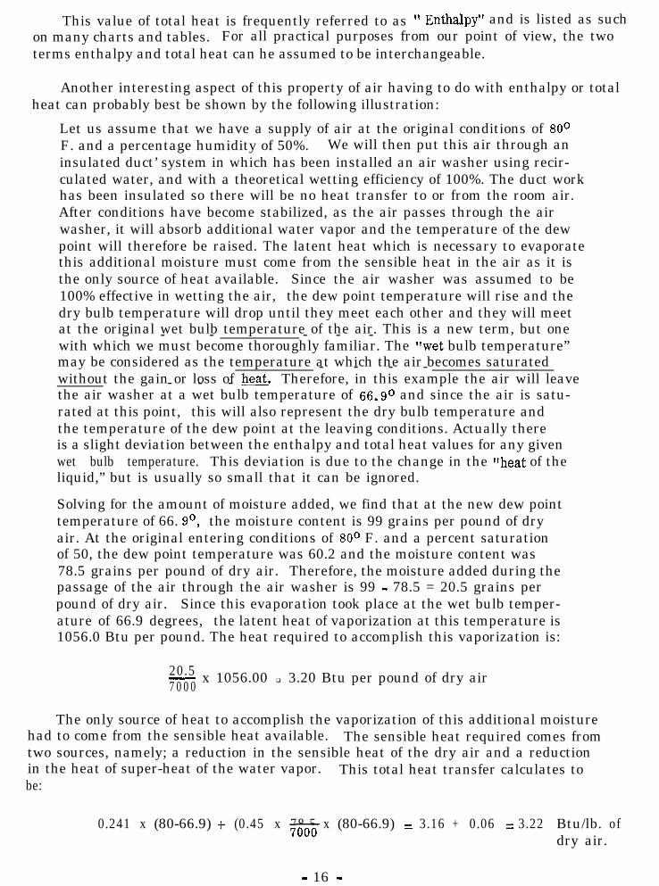
This value of total heat is frequently referred to as ” Enthalpy” and is listed as suchon many charts and tables. For all practical purposes from our point of view, the twoterms enthalpy and total heat can he assumed to be interchangeable.

Another interesting aspect of this property of air having to do with enthalpy or totalheat can probably best be shown by the following illustration:

Let us assume that we have a supply of air at the original conditions of 80°F. and a percentage humidity of 50%. We will then put this air through aninsulated duct’ system in which has been installed an air washer using recir-culated water, and with a theoretical wetting efficiency of 100%. The duct workhas been insulated so there will be no heat transfer to or from the room air.After conditions have become stabilized, as the air passes through the airwasher, it will absorb additional water vapor and the temperature of the dewpoint will therefore be raised. The latent heat which is necessary to evaporatethis additional moisture must come from the sensible heat in the air as it isthe only source of heat available. Since the air washer was assumed to be100% effective in wetting the air, the dew point temperature will rise and thedry bulb temperature will drop until they meet each other and they will meetat the original wet bulb temperature of the air. This is a new term, but one- - - - -with which we must become thoroughly familiar. The “wet bulb temperature”may be considered as the temperature at which the air becomes saturated- - - -without the gain or loss of heat.- - - Therefore, in this example the air will leavethe air washer at a wet bulb temperature of 66.9O and since the air is satu-rated at this point, this will also represent the dry bulb temperature andthe temperature of the dew point at the leaving conditions. Actually thereis a slight deviation between the enthalpy and total heat values for any givenwet bulb temperature. This deviation is due to the change in the “heat of theliquid,” but is usually so small that it can be ignored.

Solving for the amount of moisture added, we find that at the new dew pointtemperature of 66. go, the moisture content is 99 grains per pound of dryair. At the original entering conditions of 80° F. and a percent saturationof 50, the dew point temperature was 60.2 and the moisture content was78.5 grains per pound of dry air. Therefore, the moisture added during thepassage of the air through the air washer is 99 - 78.5 = 20.5 grains perpound of dry air. Since this evaporation took place at the wet bulb temper-ature of 66.9 degrees, the latent heat of vaporization at this temperature is1056.0 Btu per pound. The heat required to accomplish this vaporization is:

20.5- x 1056.00 q

7 0 0 03.20 Btu per pound of dry air

The only source of heat to accomplish the vaporization of this additional moisturehad to come from the sensible heat available. The sensible heat required comes fromtwo sources, namely; a reduction in the sensible heat of the dry air and a reductionin the heat of super-heat of the water vapor. This total heat transfer calculates tobe:

0.241 x (80-66.9) + (0.45 x 78.57ooo x (80-66.9) = 3.16 + 0.06 = 3.22 Btu/lb. ofdry air.

- 16 -

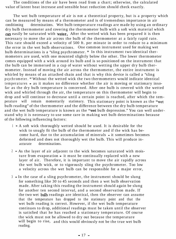
The conditions of the air have been read from a chart; otherwise, the calculatedvalue of latent heat increase and sensible heat reduction should check exactly.

The wet bulb temperature of air is not a theoretical property, but is a property whichcan be measured by means of a thermometer and is of tremendous importance in airconditioning determinations. Wet bulb temperature readings are made by using an ordinarydry bulb thermometer and covering the thermometer bulb with a soft wick material whichcan easily be saturated with .water. After the wetted wick has been prepared it is thennecessary to move the air across the bulb of the thermometer at a fairly rapid rate.This rate should exceed a velocity of 500 ft. per minute in order to reduce to a minimumthe error in the wet bulb observations. One common instrument used for making wetbulb determinations is a “sling psychrometer. I1 In this instrument two identical ther-mometers are used, with one mounted slightly below the other. The lower thermometercomes equipped with a wick around its bulb and is so positioned on the instrument thatthe bulb can be immersed in a cup of water without wetting the upper dry bulb ther-mometer. Instead of moving the air across the thermometer, the entire instrument iswhirled by means of an attached chain and that is why this device is called a “slingpsychrometer. ‘I Without the wetted wick the two thermometers would indicate identicaltemperatures - as it makes no difference whether the air is moving or stationary inso-far as the dry bulb temperature is concerned. After one bulb is covered with the wettedwick and whirled through the air, the temperature on this thermometer will begin todrop and will continue to decrease until a certain point is reached, after which the tem-perature will remain momentarily stationary. This stationary point is known as the “wetbulb reading” of the thermometer and the difference between the dry bulb temperatureand the wet bulb temperature is known as the “wet bulb depression.” You can well under-stand why it is necessary to use some care in making wet bulb determinations becauseof the following influencing factors:

1 - A soft wick thoroughly wetted should be used. It is desirable for thewick to snugly fit the bulb of the thermometer and if the wick has be-come hard, due to the accumulation of minerals - it sometimes becomesdeformed and does not thoroughly wet the bulb. This will produce in-accurate determinations.

2 - As the layer of air adjacent to the wick becomes saturated with mois-ture from evaporation - it must be continually replaced with a newlayer of air. Therefore, it is important to move the air rapidly acrossthe wet bulb wick, or to vigorously sling the psychrometer. Too lowa velocity across the wet bulb can be responsible for a major error,

3 - In the case of a sling psychrometer, the instrument should be slungfor something like 30 to 45 seconds and then a wet bulb observationmade. After taking this reading the instrument should again be slungfor another ten second interval, and a second observation made. Ifthe two wet bulb readings are identical, then the observer can assumethat the temperature has dropped to the stationary point and that thewet bulb reading is correct. However, if the wet bulb temperaturecontinues to drop, additional readings must be taken until the observeris satisfied that he has reached a stationary temperature. Of coursethe wick must not be allowed to dry out because the temperaturewill begin to rise, and this would obviously not be the true wet bulbreading.

- 17 -

PS

YC

HR

OM

ET

RIC

C

HA

RT

Barometric Pressure 29.92”

Hg

.

$

28J\

\‘,\ ,i0

65 70

75 80

8590

95 100

105110

115Dry Bulb Tem

peratures - OF

- 18 -

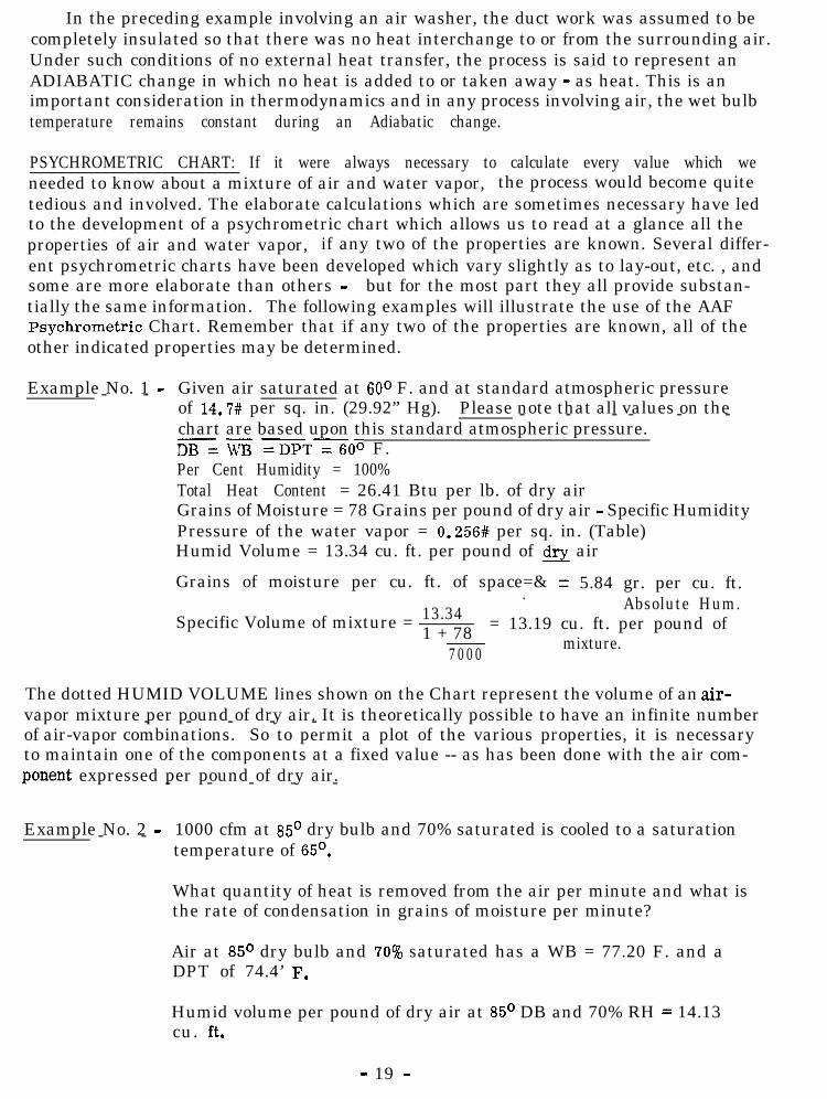
In the preceding example involving an air washer, the duct work was assumed to becompletely insulated so that there was no heat interchange to or from the surrounding air.Under such conditions of no external heat transfer, the process is said to represent anADIABATIC change in which no heat is added to or taken away - as heat. This is animportant consideration in thermodynamics and in any process involving air, the wet bulbtemperature remains constant during an Adiabatic change.

PSYCHROMETRIC CHART: If it were always necessary to calculate every value which weneeded to know about a mixture of air and water vapor, the process would become quitetedious and involved. The elaborate calculations which are sometimes necessary have ledto the development of a psychrometric chart which allows us to read at a glance all theproperties of air and water vapor, if any two of the properties are known. Several differ-ent psychrometric charts have been developed which vary slightly as to lay-out, etc. , andsome are more elaborate than others - but for the most part they all provide substan-tially the same information. The following examples will illustrate the use of the AAFPsychrometric Chart. Remember that if any two of the properties are known, all of theother indicated properties may be determined.

Example No. 1 -- - Given air saturated at 60° F. and at standard atmospheric pressureof 14.7# per sq. in. (29.92” Hg). Please note that all values on the- - - - - -chart are based upon this standard atmospheric pressure.DB ii&i =DPT=OO F.Per Cent Humidity = 100%Total Heat Content = 26.41 Btu per lb. of dry airGrains of Moisture = 78 Grains per pound of dry air - Specific HumidityPressure of the water vapor = 0.256# per sq. in. (Table)Humid Volume = 13.34 cu. ft. per pound of dry air

Grains of moisture per cu. ft. of space=& = 5.84 gr. per cu. ft..

13.34 Absolute Hum.Specific Volume of mixture =

1 + 78 = 13.19 cu. ft. per pound of

7 0 0 0mixture.

The dotted HUMID VOLUME lines shown on the Chart represent the volume of an air-vapor mixture per pound of dry air. It is theoretically possible to have an infinite number- - - - -of air-vapor combinations. So to permit a plot of the various properties, it is necessaryto maintain one of the components at a fixed value -- as has been done with the air com-ponent expressed per pound of dry air.- - - - -

Example No. 2 -- - 1000 cfm at 85’ dry bulb and 70% saturated is cooled to a saturationtemperature of 65’.

What quantity of heat is removed from the air per minute and what isthe rate of condensation in grains of moisture per minute?

Air at 85O dry bulb and 70% saturated has a WB = 77.20 F. and aDPT of 74.4’ F.

Humid volume per pound of dry air at 85O DB and 70% RH = 14.13cu. ft.

- 19 -

1000 cfm14.13 = 70.8 lbs. of dry air per minute circulated.

Total heat per pound of dry air at 85’ F. and 70% Saturated(77. lo WE%) = 40.8 Btu/lb.

Total heat per pound of dry air at65O F. and saturated = 30.0 Btu/lb.

Heat to be removed = 10.8 Btu per lb. of dry air,

Total heat removed from the air = 10.8 x 70.8 = 765 Btu/Min.

Air at 85O F. and 7@~ Sat. (DPT = 74.4’ F.) = 129 grains per lb. -dry air.

Moisture content of air saturated at 65 o = 93 grains per lb. -dry air.

Moisture removed = 36 grains per lb. -dry air.

Total amount of condensation = 7i:o-x 70.8 = 0.365 lb. of water per minute.

Since one pint of water = 1.042 lbs.

0.365 _ 0.35 pints of water condensed per minute1.042 from each 1000 CFM

On the right-hand side of your chart is a scale labeled l*Sensible Heat Factor.” In airconditioning problems, it represents the sensible heat percentage of the total heat gain.Knowing the sensible heat factor for a given room and the desired room conditions, it ispossible to draw a sensible heat ratio line through the required state point. This linethen determines the various combinations of dry and wet bulb temperatures that can beused to provide the desired room condition.

AIR FLOW: When a fluid such as air is moved through a duct a certain pressure or headis necessary to start and maintain flow. This total head or pressure has two components;static pressure and velocity pressure. STATIC PRESSURE is that pressure which tends tocollapse or burst the duct, and is used in part to overcome the frictional resistance ofthe air against the duct surface as well as the resistance offered by such obstructions ascoils, filters, dust collectors, elbows, etc. In general the value of the static pressure isnot sufficient to significantly change the volume of air at the ordinary pressures found infan work. As an example the static pressure of 1” of water corresponds to a change ofless than l/4 of 1% in the volume of the air. VELOCITY PRESSURE is that pressurenecessary to maintain movement of the air, or, as the name implies, is that pressure neces-sary to give the air its velocity and is always considered as positive in sign. Under cer-tain conditions of operation it is possible for either of these components to be equal tozero but both individually can never equal zero when the fan is in operation. If a dischargeor inlet duct on a fan is completely closed, only static pressure or potential energy ispresent on the discharge or suction side. This is manifest by the air pressure tending toburst or collapse the duct. If a fan is operated with no duct system connected to either

- 20 -

side, all the available energy would be utilized to produce flow, and the static pressurewould be zero insofar as the duct resistance is concerned.

Static pressure, velocity pressure and total pressure are all interrelated. If a gasflowing through a duct system undergoes an increase in velocity, a part of the staticpressure available at that point is used to create the additional velocity pressure neces-sary. Conversely, if the velocity is reduced at some point, a part of the kinetic energyor velocity pressure at that point will be converted into potential energy or static pressure.Static and velocity pressure are, therefore, mutually convertible but this conversion isgenerally accompanied by an energy loss due to turbulence, shock, etc., and only underrare circumstances is this conversion 100% efficient. Loss of conversion is usually appre-ciably greater as air is decelerated than where acceleration takes place in a similar ductsection.

At a given point in any duct system, the STATIC PRESSURE, VELOCITY PRESSURE,and TOTAL PRESSURE are mathematically related as follows:

TOTAL PRESSURE = Static Pressure + Velocity Pressure.

It should be realized that when pressures are measured on the discharge side of a fan,the static pressure is usually positive, and this pressure added to the velocity pressurewill give the total pressure at that point.

When the pressure determinations are made on the suction side of the fan the staticpressure is negative because it is less than atmospheric pressure, and this negativestatic pressure represents the pressure necessary to produce flow at that point. In orderfor this flow to be produced, enough suction must be created to not only overcome theresistance to flow but also to give the air its velocity.

In determining total pressure, confusion can frequently be avoided by basing all calcu-lations on absolute pressures. Absolute total pressure would then be the sum of the ab-solute static pressure and the velocity pressure. As previously defined the absolute pressureis always obtained by adding atmospheric pressure to gauge pressure. You will recallthat standard atmospheric pressure is equal to 29.92” Hg; 14.7# per sq. in.; 407” wateror 28,200 ft. of standard air.

PRESSURE MEASUREMENTS: Another method of defining STATIC PRESSURE is to saythat it is the pressure measured at right angles to the direction of air flow. Therefore,any connection to a duct for measuring static pressure must be made in such a manneras to read only the pressure component at right angles to the flow. This is usually doneby drilling a small hole (l/16!’ diameter is sufficient) in the side of the duct in whichmeasurement is to be made. If the inside of the duct adjacent to this hole is perfectlysmooth and if there is no turbulence, the reading obtained will not be influenced byvelocity and will indicate the static pressure above atmosphere on the discharge side ofthe fan and below atmosphere on the suction side of the fan. In general, most low pressuredeterminations are made in terms of “inches of water”. This simply means that the headof water as read on the draft gauge exactly balances the head of air producing the pressure.Inches of water is the generally accepted unit used in all air flow calculations. It shouldbe remembered that at any point in a duct system the static pressure throughout the crosssection should be constant. Sometimes due to obstructions or erratic conditions, the flow ofair will be SO turbulent at the point of measurement and one reading of the static pressure may

- 21 -

not give a true average. Under conditions of this kind, several readings should be taken in aplane perpendicular to the duct wall and averaged, or a better location for making the pressuredeterminations should be selected.

The TOTAL PRESSURE existing in a duct is measured by means of an impact tube. Inreality an impact tube is simply a piece of tubing of small internal bore with a short leg bentat right angles to the remainder of the tube. The end of the short leg should be cut squarelyacross and the walls at that point ground to a thin edge. If such a tube is inserted in a duct,with the short leg placed parallel to the longitudinal axis of the duct and with the open end facing- - - - - -into the air stream, a small column of air will impinge into the mouth of the tube. The pressure- - -corresponding to that required to give the air its velocity will add algebraically to the staticpressure already existing in the duct and, therefore, readings taken with this type of tubewill indicate total pressure.

In order to determine the VELOCITY PRESSURE component, it is necessary to subtractthe static pressure from the total pressure and this difference will be the velocity pressure,bearing in mind that the velocity pressure is always looked upon as being positive in sign.

In air flow measurements one single instrument is generally used to measure both staticand total pressure. This instrument is known as a PITOT TUBE and is, in reality, a tube with-in a tube with the center tube representing the impact portion used for measuring total pressure,and with the outer tube sealed at the impact end and provided with small holes at right angles tothe direction of flow for measuring the static pressure. Separate readings of the static and totalpressure may be made with a tube of this type, or this tube may be connected differentially toboth sides of a draft gauge to read the velocity pressure directly. The measurement of thestatic, velocity, and total pressures on both sides of a fan or Roto-Clone are indicated inFigures 1 and. 2.

The velocity distribution across a given section in a duct is never uniform. Even in thecase of a long straight section of duct, the velocity is a maximum in the region of the centerand reduces in value towards the duct surface. Since readings taken with a Pitot Tube indicatethe velocity pressure at the point of measurement, several determinations should be madein order to arrive at the average velocity pressure existing throughout the cross section. Inthe case of a round duct,a traverse across the duct is generally made in two planes at rightangles to each other. The duct should be divided into a number of equal concentric areas andreadings should be taken at the centers of each concentric area. The number of readings tobe made vary with the diameter of the duct. In the case of a rectangular duct, the cross sec-tion should be divided into imaginary rectangular areas and readings should be made at thecenter of these. Reference to the “GUIDE11 published by the American Society of HeatingRefrigerating & Air-Conditioning Engineers will indicate a convenient means for calculat-ing the centers of the imaginary areas and will show the recommended number of read-ings to be taken in different size ducts.

For field measurement, the VP range in small ducts can frequently be obtained withsufficient accuracy by noting the average VP as the Pitot Tube is slowly moved across theduct.

Other instruments which are used for making velocity determinations include anemo-meters (both vane and hot wire), velometers, etc. These instruments generally read velocitydirect, but care should be exercised to apply any calibration factors which are generally

- 22 -

(FAN)I

8

I

STATICPRESSURE

IMPACTT U B E-I- TOTAL

PRESSURE

FIG. I PRESSURE MEASUREMENTS F I G . 2 PRESSURE MEASUREMENTSON DISCHARGE SIDE OF ROTO-CLONE. ON SUCTION SIDE OF ROTO-CLONE.

TOTALPRESSURE

(FAN)\ 1

4AIR

/I FLOW

=lTOTWBE

STATICPRESSURE

-(B- A)

VELOCITYPRESSURE

IMPACTT U B E TuB

1

rOTALPRESSURE

supplied with the individual instruments. A more detailedmay be found in the ASHRAE GUIDE.

CALCULATION OF AIR VELOCITY: You will recall fromfreely falling body is given by the equation Vs =

f--2 gh

where V, = velocity in ft. per secondh = head in ft.

Physics that the equation of a

g = acceleration due to gravity = 32.2 ft/sec/sec.

or Velocity, fpm = V = 60 2 ghf-

discussion of these instruments

Vp x 62.3If head is expressed in inches water gauge, then h = 12 x w

where Vp = velocity pressure of air in inches of waterVP/12 = velocity pressure of air in feet of water

62.3 = density of water - lb/cu. ft.w = density of air - lb/cu. ft.

or Velocity, fpm = V = 60/e = 1096.2~

For STANDARD AIR - w = 0.075 lbs/cu. ft.

then V (ft/min) = 1096.2 = 4005 vpc

= 4005 fpm Velocity, when Vp = 1” wg.

The above expression is based upon air at standard conditions, but can generally beemployed unless there is a marked deviation. For conditions varying considerably fromthose of “standard”, it should be recalled that the density of air varies directly as thebarometric pressure and inversely as the absolute temperature.

= 1.327B Where460 + T

B = Barometric Press. In. Hg.T = Temperature - Deg. F

It will be seen from the above that the velocity calculation involves the square rootof the average velocity pressure. Therefore, in arriving at the average velocity pressureexisting at a given cross section in a duct, it is necessary to take the individual velocitypressure readings obtained from a pitot tube traverse and average the square root of eachof these readings. This average value should then be squared to obtain the averagevelocity pressure at that point.

I I

2Avg. VP= ~+fit”JVP3+~~+“JVP5+~~

6The volume of air flow is always equal to the product of the cross sectional area of

the duct and the average velocity of flow at that section:

Thus: Q = AVwhere: Q. = Quantity of flow in cubic feet per slinute

A = Area of duct cross section in square feetV = Average Velocity of flow in feet per minute

- 24 -

ORIFICES AND FLOW NOZZLES: If a constriction is placed at the end of a duct or in aduct through which a fluid is flowing, the velocity of the fluid will increase through theconstriction and the static pressure will be reduced. The reduction in the static pressureis proportional to the velocity because a portion of the static pressure has been convert-ed into velocity pressure. Such a constriction is generally referred to as an orifice.Orifices may be made with a well rounded entrance (usually referred to as shapedorifices or nozzles ) , or they may simply be a thin plate with a hole in the center.In the case of a thin plate orifice the air is, of course, restricted in cross sectionin passing through the orifice opening, and this restriction continues for a shortdistance down stream from the orifice. The final cross-section of the stream issmaller than the orifice opening and is generally referred to as the “Vena Contracta. I’

If the static pressure measurements are made up-stream and down-stream from anorifice, the pressure difference, or orifice pressure drop (OPD) will represent the velocitypressure equivalent to the increased velocity and this value can be substituted in thestandard velocity equation. Theoretically the velocity will be highest at the “Vena Con-tracta” , but since it is not possible to measure the area of the stream at that point, itis necessary to apply a correction factor which is designated as the “COEFFICIENT OFDISCHARGE”. The coefficient of discharge takes into consideration the velocity of approach(if any), the contraction of the air stream, etc. , and must be determined by experiment. Itwill vary with the design of the orifice, its location in the system, and the ratio of orificearea to pipe area.

The general equation for determining flow by means of an orifice is:

Q = 4005 cd A?JOPD (Air at Standard Conditions)where: Q = Volume of air in cu. ft. per minute

cd = Coefficient of discharge for the orifice in questionA = Area of Orifice in sq. ft.

OPD = Orifice pressure drop-inches water gage.

There are several methods of locating the pressure taps in pipes. Generally they eachconsist of a l/16” drilled hole with the inner surface perfectly smooth in order not to createturbulence in the air stream. One widely used arrangement is referred to as “Corner Taps”which derives its name from the fact that the static taps are drilled into the corners formedby the orifice plate and the pipe. In some cases a circular slot is formed in the pipe flange andthe taps connect with the slotted chamber. Please note that the above expression applies to air atllstandard conditions11 but again is sufficiently accurate for most determinations unless thetemperature or pressure deviates considerably from that of standard air.

It should be realized that although an orifice may be inserted in a duct system, the re-sistance against which the fan is working does not necessarily include the total drop acrossthe orifice. As previously mentioned, the difference in the static pressure on each side of theorifice is proportional to the increase in velocity of the air through the orifice, but after the airleaves the orifice it expands in cross section to again fill the duct and the velocity of theair thus decreases. This decrease in velocity means that a portion of the energy necessary toProduce the high velocity through the orifice will be converted back into static pressure. Thisconversion of velocity pressure into static pressure, or “regain”, is accompanied by someenergy loss, the amount of loss being a function of the type of orifice used.

The foregoing discussion is based upon low pressure operation which is the type with whichwe will be principally concerned. In unusual applications special consideration may be re-quired regarding the effects of compression; manometer or draft gauge corrections due to highambient temperatures, etc.

- 25 -

PRESSURE REGAIN IN A DUCT SYSTEM

The regain of pressure in a duct system is possible because static pressure and velocitypressure are mutually convertible. As a general rule, this conversion is accompanied bysome energy loss and the amount of this loss is a function of the geometry of the transi-tion piece (the more abrupt the change in velocity, the greater the loss) and whether theair is being accelerated or decelerated. In most handbooks, the loss is generally express-ed as a percentage of the difference between the velocity pressures in the entrance andthe exit of the transition piece. One minus the loss, expressed as a decimal fraction, isthe efficiency of the energy conversion, or “regain”.

The following examples will illustrate the influence of regain on the static pressure invarious typical duct arrangements. In each example is plotted the total pressure and staticpressure in order to show their relationship at various points in each system.

Example (1) - Duct work located on the discharge side of the fan.Velocity transfer from low to high.- - -

FAN,

I, 0.3”,1_ RES.=0.5” c

The over-all resistance of the system is the sum of the individual resistances = 0.5 + 0.3+ 1.0 = 1.8” w.g.

The static pressure at the fan discharge will be equal to the total resi.stance of the ductwork plus any additional static pressure required for conversion into velocity pressure.Since the velocity pressure at point “D” is 2” w.g. , as compared to only 1” w.g. at thefan discharge, the additional static pressure required for conversion into velocity pressureis therefore 1”. The static pressure at the fan outlet “A” then becomes 1.8” + 1” = 2.8”w. g.

The total pressure at any point is made up of the velocity pressure at the discharge endof the duct (point “D”) plus the duct losses up to that point. The total pressure at point“A” is therefore 3.8” w.g. and consists of the 2” VP at the duct discharge plus the 1.8”of duct resistance. The relationship between SP and TP at each point in the system is asindicated.

The air horsepower generated by the fan is a function of the quantity of air being handledand the pressure developed, and is usually based upon total pressure. In this example,the TP at the fan inlet is assumed to be 0 because thCe;; is ;o duct work indicated. Theair horsepower supplied by the fan would then equal x .8

6 3 5 6 . All of the values are

positive in sign because they are measured above atmospheric pressure.

Example (2) - Duct work located on the discharge side of the fan.Velocity transfer from high to low.- -

6 RES-0.5” RES. = LO”

2<

. @5 +4-

4 +3 - -3 2.L$ +2II I

I II -Y I --- -~-- 037 A-c--' -----eyIc-

1’. f.f? I -,, I

The over-all duct system is identical with that shown in Figure 1 so the resistance againequals 1.8” w.g. At point “C” the static pressure equals 1” w.g. and the velocity pressureequals 1” w. g. In moving from point “B” to point “C”, the air slows down from a VP of2” to a VP of 1” and the difference of 1” in the velocity pressure is available for con-version into static pressure at point *‘B’*. If the transition in flow from “B” to “C” tookplace with no loss (1000/o regain), the SP at l’B” would be 1” - 1” = 0. However, theenergy transfer is only 70% efficient (0.3” loss). Therefore, the SP at “B” equals 0 4- 0.3”= 0.3” w. g.

The total pressure at the fan discharge is equal to 2.8” w.g. , which again consists ofthe 1” VP at the duct discharge (point “D*‘) plus the 1.8” w.g. duct resistance. Assumingno suction duct, the TP at the fan inlet equals 0, so the over-all TP of the fan is 2.8”w.g. The air horsepower would be determined in the conventional manner.

Particular attention is called to the fact that for the same volume of air, the air horse-power is less in Example (2) than in Example (1)) although the duct resistance is thesame in each case. This difference in AHP is, of course, due to the velocity pressurecomponent of the total pressure. In Example (1)) the air had a velocity pressure of 2”w.g. at the point of discharge from the duct. In Example (2), the discharge velocitypressure is only 1” w.g. and this difference in discharge velocity pressure accounts forthe lower air horsepower in Example (2). Again, it will be noted that the TP at any pointin the duct system includes the VP at the discharge end of the duct plus the duct lossesup to that point. As indicated, the total pressure at point “A” consists of the VP of 1”at the duct discharge plus the 1.8” duct resistance, or a TP of 2.8” w.g.

- 27 -

Example (3) - Duct work located on the suction side of the fan.Velocity transfer from low to high.- -

VP=I”

RES. = I”

VP=2”

RES. =OS” 3

Q

On the suction side of a fan, the total pressure is a measure of the over-all resistanceto air flow. In this example, the total resistance again adds up to 1.8” w. g. , the sameas it did when the duct work was on the discharge side of the fan as shown in Examples(1) and (2). The static pressure at the fan inlet, point “D”, is equal to the velocitypressure at the fan inlet plus the total &&s%e to that point. This adds up to 3.8” W. g.static pressure. Since we are working on the suction side of the fan, the pressures arenegative in sign, or below atmospheric pressure.

In going from point “B1’ to point “C”, the air is accelerated and the velocity pressure isshown as being doubled. The additional energy required by the higher velocity pressureis supplied at the expense of the static pressure. Therefore, the SP at point “C?l is lower(remember it is negative) than the SP at point “B” by the amount of the transition lossplus the difference in the VP at the entrance and exit of the transition piece, or lowerby total of 1.3” w. g. The air horsepower generated by the fan is again a function of thetotal pressure across the fan. Since most fans have approximately the same inlet anddischarge area, it will be assumed that the velocity pressure at the fan discharge isalso 2” w.g. , which will then be the total pressure on the discharge side of the fan. Thetotal pressure developed by the fan is then equal to the total pressure at the fan dis-charge plus the total pressure at the fan inlet (disregarding the sign) or 3.8” w. g. It willbe noted from the diagram that this is also the value of the static pressure at the faninlet. This circumstance is due to the fact that the inlet and discharge areas of the fanwere assumed to be equal. The air horsepower has the same value as in Example (1).

Example (4) - Duct Work located on the suction side of the fan.Velocity transfer from high to low.- -

> VP=2” 56 VP= I” FAN,

I A* RES.=OS” -l.o.s-&

‘ I ,hCIFRES.= 1.0”

-I

- 2

-3

-41 I I 1

In this example, the only duct work encountered is again located on the suction side ofthe fan and the total pressure is a measure of the sum of the individual resistances, or1.8” w. g. The SP at the fan inlet, point “Dl’, is equal to the VP at the fan inlet plus- -the duct resistance (or total pressure) up to that point. This amounts to 2.8” w.g. andis, of course, negative in sign on the suction side of the fan.

In going from point “B’l to point “C’l, the air slows down as indicated by the differenceof 1” w.g. in the VP at these two points. This difference is available for conversioninto static pressure at point “C”. If the transition from “Bl’ to “C” was accomplishedwith no loss (100% regain) the SP at ‘lC” would be -2.5 + 1.0 = -1.5” w.g. Since theenergy transfer is only 70% efficient (0.3” w.g. loss) the SP at point “C” = -1.5 + (-0.3)= -1.8” w.g.

Again, the air horsepower developed depends upon the TP to be supplied by the fan. As-suming the velocity pressure in the fan discharge to be 1” w.g. (the same as at the faninlet), the TP across the fan will be 2.8” w.g. Again it will be noted that this is equalin value to the static pressure at the fan inlet. The air horsepower calculates to be thesame as indicated in Example (2).

- 29 -

Example (5) - Duct work located on discharge side of fan.Velocity changes as indicated.

_ RES.=0.5* ,_0.4’:, RES.=I.O” -.

From the sketch the duct work is again all located on. the discharge side of the fan. Thetotal pressure at the fan discharge (point “A”) is equal to the velocity pressure at thedischarge end of the duct (point “F’l) plus the accumulated resistances. These add up to1.0 + 1.0 + 0.4+ 0.5+ 0.3 + 1.0 = 4.2” w.g.

The static pressure regain between point ‘ID” and point “E” is identical to the situationencountered in Example (2). If there was no energy loss in the transition piece the staticpressure at “D” would be 0 because the difference in VP of 1” would show up as staticpressure regain. However, the transition is only 60% efficient, which means a loss of.4” w.g., so the SP at point “D” = 0 + 0.4 = 0.4” w. g.

The conversion of static pressure into velocity pressure between points “Brl and “C” isthe same as occured in Example (1). There must be sufficient static pressure at point“B1* to furnish the additional velocity pressure required at point “C”. In addition, thetransformation of energy between these two points is accompanied by a loss of 0.3” w.g.Since the SP at point “C” equals 0.9” w.g. , the SP at point “B” = 0.9 t 0.3 t 1.0 =2.2” w. g. The air horsepower developed by the fan would be calculated in the conventionalmanner. Since there is no duct work on the suction side of the fan, the total pressureagainst which the fan is operating will be 4.2” w.g.

- 30 -

Example (6) - Duct work located on the suction side of the fan.Velocity changes as indicated.

RES.= LO* RES. =O. 5”I RES.= 1.0” _

83.2

4 . 2

Since the duct work is all on the suction side of the fan, the SP at the fan inlet (point“F”) is equal to the VP at the fan inlet plus the total duct resistance up to that joint.This equals -4.2” SP, since the static pressure on the suction side of the fan is alwaysnegative. The duct system is the same as was used in Example (5) and therefore, it hasthe same over-all resistance of 3.2” w.g. If it is again assumed that the inlet and dis-charge of the fan are of equal areas, the total pressure across the fan will be the sameas in Example (5) and in each case the fan will deliver the same air horsepower whenhandling equal volumes of air.

The static pressure conversion between points llB1’ and “C1’ is the same as discussed inExample (3). There must be sufficient SP at point ‘*B” to furnish the additional VP re-quired at point llC1l. In addition, the energy transfer between these two points is accom-panied by a loss of 0.3” w. g. Since the static pressure at “B” = -2” w. g. , the SP atpoint l*C1* = -2.0 + (-1.0) + (-0.3) = -3.3” w.g.

The static pressure regain between points “D” and I1 E” is identical to the Situation dis-

cussed in Example (4). If there was no loss in the transition piece, the 1” difference invelocity pressure would all be regained as static pressure at point “E” and the SP atthat point would be -2.8” w. g. However, the transition is only 60% efficient (0.4” W.g.loss) so the SP at point “El1 = -2.8 + (-0.4) = -3.2” w. g.

Air handling systems involving duct work on both the suction and discharge sides of thefan can be evaluated in the manner just described with each side being considered in-dividually. The over-all total pressure or static pressure against which the fan is operat-ing can then be easily determined.

- 31 -

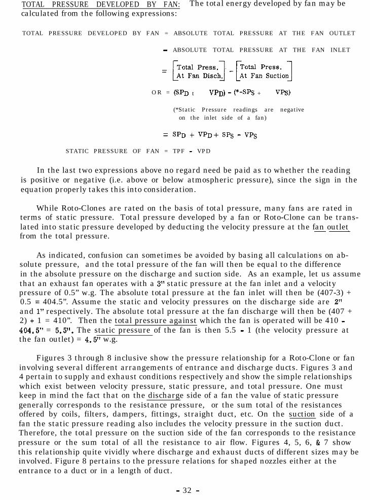
TOTAL PRESSURE DEVELOPED BY FAN: The total energy developed by fan may becalculated from the following expressions:

TOTAL PRESSURE DEVELOPED BY FAN = ABSOLUTE TOTAL PRESSURE AT THE FAN OUTLET

- ABSOLUTE TOTAL PRESSURE AT THE FAN INLET

O R = (SPD t VPD) - (*-sps + vps)

(*Static Pressure readings are negativeon the inlet side of a fan)

= SPD + vPD+ SPs - VPs

STATIC PRESSURE OF FAN = TPF - VPD

In the last two expressions above no regard need be paid as to whether the readingis positive or negative (i.e. above or below atmospheric pressure), since the sign in theequation properly takes this into consideration.

While Roto-Clones are rated on the basis of total pressure, many fans are rated interms of static pressure. Total pressure developed by a fan or Roto-Clone can be trans-lated into static pressure developed by deducting the velocity pressure at the fan outlet-~from the total pressure.

As indicated, confusion can sometimes be avoided by basing all calculations on ab-solute pressure, and the total pressure of the fan will then be equal to the differencein the absolute pressure on the discharge and suction side. As an example, let us assumethat an exhaust fan operates with a 3” static pressure at the fan inlet and a velocitypressure of 0.5” w.g. The absolute total pressure at the fan inlet will then be (407-3) +0.5 = 404.5”. Assume the static and velocity pressures on the discharge side are 2”and 1” respectively. The absolute total pressure at the fan discharge will then be (407 +2) + 1 = 410”. Then the total pressure against which the fan is operated will be 410 -404.5” = 5.5”. The static pressure of the fan is then 5.5 - 1 (the velocity pressure atthe fan outlet) = 4.5” w.g.

Figures 3 through 8 inclusive show the pressure relationship for a Roto-Clone or faninvolving several different arrangements of entrance and discharge ducts. Figures 3 and4 pertain to supply and exhaust conditions respectively and show the simple relationshipswhich exist between velocity pressure, static pressure, and total pressure. One mustkeep in mind the fact that on the discharge side of a fan the value of static pressuregenerally corresponds to the resistance pressure, or the sum total of the resistancesoffered by coils, filters, dampers, fittings, straight duct, etc. On the suction side of afan the static pressure reading also includes the velocity pressure in the suction duct.Therefore, the total pressure on the suction side of the fan corresponds to the resistancepressure or the sum total of all the resistance to air flow. Figures 4, 5, 6, & 7 showthis relationship quite vividly where discharge and exhaust ducts of different sizes may beinvolved. Figure 8 pertains to the pressure relations for shaped nozzles either at theentrance to a duct or in a length of duct.

- 32 -

PRESSURE MEASUREMENTS

Due to turbulenceReading probably

Unreliable

S.P.n

T== v. P. = 1”

- + 3” s. P.v. P. = 1”

b+ 4” T.P .

0Fan

FIGURE 3

1 /j -4” S.P. (-SP + VP = -TP)Since -SP + VP = -TP

- VP = 1”

a -4” s. P.J v. P. = 1”-.

BLOWING OR DISCHARGING(No Suction Duct)

TP = SP + VP

Note: In actual fan test, Valuesof TP and SP should becorrected for duct frictionfrom fan discharge to pitottube.

EXHAUSTING

Then TP = Res. Press.on suction side

But total Suction = SP,= -4”(Must include both VP, and

TP, )-3” T.P.

FIGURE 4

- 33 -

I--

F IVPD = 1” c----c

I(A)

IIu ‘-2” T P

-3” s. P.VPs = 1”

+ 3” s. P.cd

(B)

ON SUCTION SIDE-SP + VP = -TPStatic Press. isnegative

t 4” T. P.VpD = 4 - 3 = 1”

Absolute Press. - Suction4 0 7-+- 1” VP Connecting points408 (A) and (B) to

-3” SP differential gageTPS = 405” W.G. should check TP of Fan

STATIC PRESS.OF FAN =TPF -VPD=6-lz5”W.G.

= SPD + SPS - VPS= 3” + 3” - l”= 5” W.G.

(Disregard Sign)

FIGURE 5

- VPD = 1” L

l.l u ’ TPS = -2.5”

SPS = -3” SPD = 2” c

VPS- VPs=3 - 2 . 5 TPD = 3”0.5”

1

= 0.5” vpD= 3 - 2 =I”(VP alwaysconsideredpositive)

If VPs is negligible then:TPS = SPs (Because VPS approaches 0)

and SPFs SPD+ SPs (Disregard Sign)

FIGURE 6

- 34 -

DISCHARGE & SUCTION DUCTS(Equal Area on Inlet & Discharge)

Absolute Press. - Discharge:4 0 7+ 1” VP4 0 8t 3” SP

TPD = 411” WG

TOTAL PRESSURE OF FAN:

TPF = TPD - TPS= 411” - 405” = 6” W.G.= (SPD $ vp,) - wps + VP,)= (3” + 1”) - (-3” + 1”)= 6” W.G.

It should be noted that when inlet &outlet areas are equal,the SPS + SPD = TPFan

= 3” + 3” = 6” (Disregard Sign)

SUCTION DUCT LARGER THANDISCHARGE DUCT

TOTAL PRESS. OF FAN:- -

TPF = SPD + VPD + SPS ‘- VPS=2+1+3-0.5= 5.5” W.G.

Or =TPD + TPS=3 + 2.5 = 5.5” W.G.

STATIC PRESS. OF FAN:S P F = SPD + -%S-vPS

=2+3 - 0.5 = 4.5” W.G.(Disregard Sign)

DISCHARGE DUCT LARGER THAN SUCTION DUCT

SPS = -4’E4 0 7-4+1

Abs. TPS =404”

SPD = 2”n

VPD = 0. 5” r

4 0 7

TPS = -3” +2+0.5

SPS = -4” SPD = 2°C Abs. TPD 409.5

-SPS + VPs = TPSTPD = 2.5”

-4” + 1” = -3” VpD = 2. 5” - 2”

(Resistance= 0.5”

Pressure)

TOTAL PRESS. OF FAN STATIC PRESS. OF FAN- - - ~

= (sPD+ VP,) - (-sPs+ VPS)= s,?,, + VPD + SPS - vps=2 + 0.5 + 4 - 1 = 5.5”

or = 409.5 - 404 = 5.5” W.G.or = TPS t TPD

3+2 5 =5 5” W G. . .(Disregard Sign)

= TPF - VPD=5.5 - .5 = 5.0” W.G.

o r = SPD + SPS - VPS=2+4 - 1 = 5 0”W G. .

(disregard Sign)

The reason that in instances of this kind the differences in the static pressure readingstaken at the inlet and outlet will be greater than the total pressure produced by the fanis due to the fact that a certain amount of static pressure may be produced by conver-sion from velocity pressure.

SUM OF STATIC PRESS. READINGS = 2 + 4 = 6” (Disregarding Sign)

It should be noted that if the inlet is smaller than the outlet, the sum of thestatic pressure on each side of the fan will be greater than the TP of fan.

FIGURE 7

- 35 -

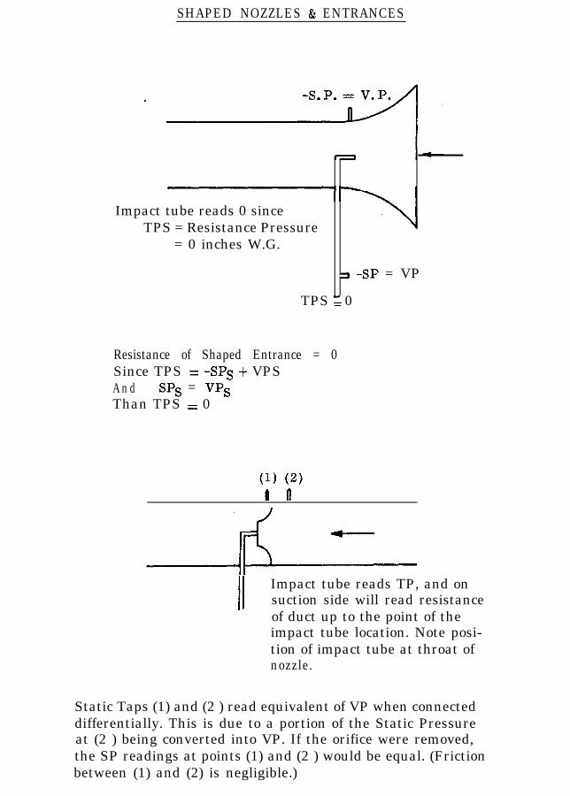
SHAPED NOZZLES & ENTRANCES

Impact tube reads 0 sinceTPS = Resistance Pressure

= 0 inches W.G.

3 -SP = VP

TPS = 0

Resistance of Shaped Entrance = 0Since TPS = -SPS + VPSA n d SPS = VPSThan TPS = 0

2II Impact tube reads TP, and on

suction side will read resistanceof duct up to the point of theimpact tube location. Note posi-tion of impact tube at throat ofnozzle.

Static Taps (1) and (2 ) read equivalent of VP when connecteddifferentially. This is due to a portion of the Static Pressureat (2 ) being converted into VP. If the orifice were removed,the SP readings at points (1) and (2 ) would be equal. (Frictionbetween (1) and (2) is negligible.)

FIGURE 8

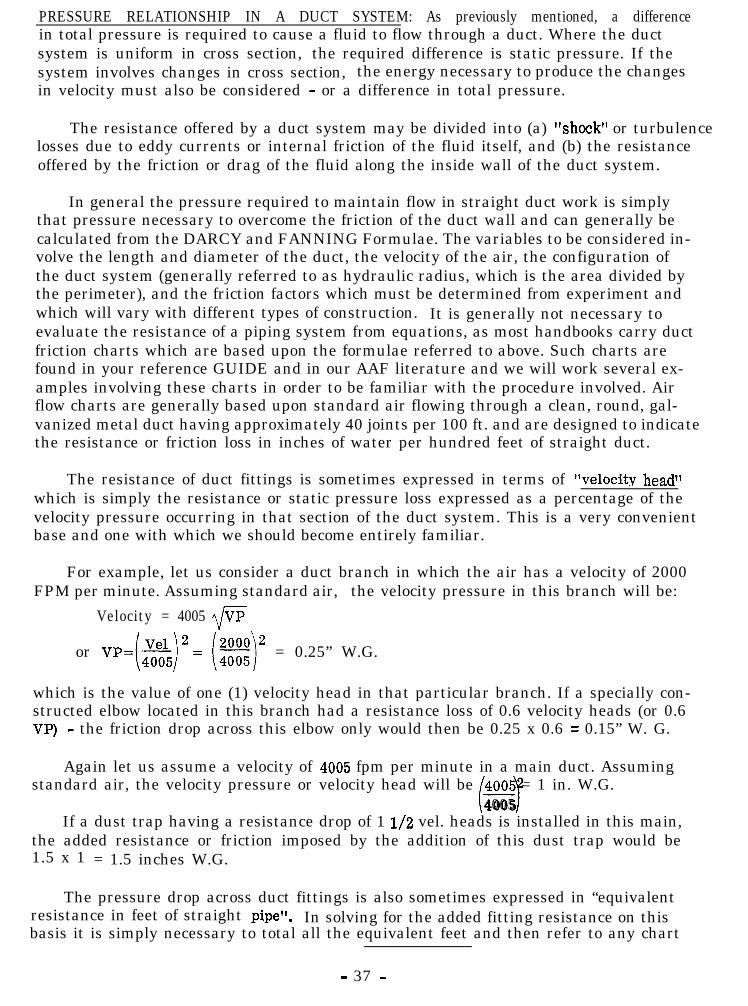
PRESSURE RELATIONSHIP IN A DUCT SYSTEM: As previously mentioned, a differencein total pressure is required to cause a fluid to flow through a duct. Where the ductsystem is uniform in cross section, the required difference is static pressure. If thesystem involves changes in cross section, the energy necessary to produce the changesin velocity must also be considered - or a difference in total pressure.

The resistance offered by a duct system may be divided into (a) “shock” or turbulencelosses due to eddy currents or internal friction of the fluid itself, and (b) the resistanceoffered by the friction or drag of the fluid along the inside wall of the duct system.

In general the pressure required to maintain flow in straight duct work is simplythat pressure necessary to overcome the friction of the duct wall and can generally becalculated from the DARCY and FANNING Formulae. The variables to be considered in-volve the length and diameter of the duct, the velocity of the air, the configuration ofthe duct system (generally referred to as hydraulic radius, which is the area divided bythe perimeter), and the friction factors which must be determined from experiment andwhich will vary with different types of construction. It is generally not necessary toevaluate the resistance of a piping system from equations, as most handbooks carry ductfriction charts which are based upon the formulae referred to above. Such charts arefound in your reference GUIDE and in our AAF literature and we will work several ex-amples involving these charts in order to be familiar with the procedure involved. Airflow charts are generally based upon standard air flowing through a clean, round, gal-vanized metal duct having approximately 40 joints per 100 ft. and are designed to indicatethe resistance or friction loss in inches of water per hundred feet of straight duct.

The resistance of duct fittings is sometimes expressed in terms of ~~velocity head”which is simply the resistance or static pressure loss expressed as a percentage of thevelocity pressure occurring in that section of the duct system. This is a very convenientbase and one with which we should become entirely familiar.

For example, let us consider a duct branch in which the air has a velocity of 2000FPM per minute. Assuming standard air, the velocity pressure in this branch will be:

Velocity = 4005 J/E

or VP=(sj2= (E)” = 0.25” W.G.

which is the value of one (1) velocity head in that particular branch. If a specially con-structed elbow located in this branch had a resistance loss of 0.6 velocity heads (or 0.6VP) - the friction drop across this elbow only would then be 0.25 x 0.6 = 0.15” W. G.

Again let us assume a velocity of 4005 fpm per minute in a main duct. Assumingstandard air, the velocity pressure or velocity head will be 4005 = 1 in. W.G.

l-74005If a dust trap having a resistance drop of 1 l/2 vel. heads is installed in this main,

the added resistance or friction imposed by the addition of this dust trap would be1.5 x 1 = 1.5 inches W.G.

The pressure drop across duct fittings is also sometimes expressed in “equivalentresistance in feet of straight pipe”. In solving for the added fitting resistance on thisbasis it is simply necessary to total all the equivalent feet and then refer to any chart

- 37 -

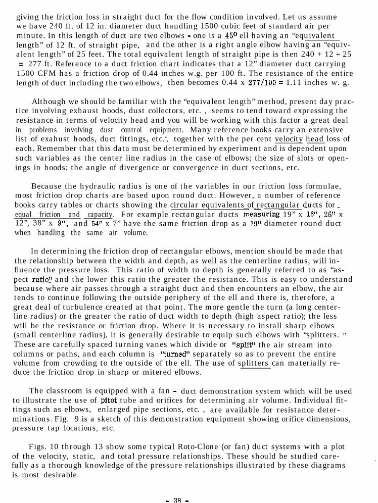
giving the friction loss in straight duct for the flow condition involved. Let us assumewe have 240 ft. of 12 in. diameter duct handling 1500 cubic feet of standard air perminute. In this length of duct are two elbows - one is a 450 ell having an “equivalentlength” of 12 ft. of straight pipe, and the other is a right angle elbow having an “equiv-alent length” of 25 feet. The total equivalent length of straight pipe is then 240 + 12 + 25= 277 ft. Reference to a duct friction chart indicates that a 12” diameter duct carrying

1500 CFM has a friction drop of 0.44 inches w.g. per 100 ft. The resistance of the entirelength of duct including the two elbows, then becomes 0.44 x 277/100 = 1.11 inches w. g.

Although we should be familiar with the “equivalent length” method, present day prac-tice involving exhaust hoods, dust collectors, etc. , seems to tend toward expressing theresistance in terms of velocity head and you will be working with this factor a great dealin problems involving dust control equipment. Many reference books carry an extensivelist of exahust hoods, duct fittings, etc.‘, together with the per cent velocity head loss ofeach. Remember that this data must be determined by experiment and is dependent uponsuch variables as the center line radius in the case of elbows; the size of slots or open-ings in hoods; the angle of divergence or convergence in duct sections, etc.

Because the hydraulic radius is one of the variables in our friction loss formulae,most friction drop charts are based upon round duct. However, a number of referencebooks carry tables or charts showing the circular equivalents of rectangular ducts for- -equal friction and capacity. For example rectangular ducts measuring 19” x 16*‘, 26” x12”, 38” x 9”, and 54” x 7” have the same friction drop as a 19” diameter round ductwhen handling the same air volume.

In determining the friction drop of rectangular elbows, mention should be made thatthe relationship between the width and depth, as well as the centerline radius, will in-fluence the pressure loss. This ratio of width to depth is generally referred to as “as-pect ratio” and the lower this ratio the greater the resistance. This is easy to understand- -because where air passes through a straight duct and then encounters an elbow, the airtends to continue following the outside periphery of the ell and there is, therefore, agreat deal of turbulence created at that point. The more gentle the turn (a long center-line radius) or the greater the ratio of duct width to depth (high aspect ratio); the lesswill be the resistance or friction drop. Where it is necessary to install sharp elbows(small centerline radius), it is generally desirable to equip such elbows with “splitters. ”These are carefully spaced turning vanes which divide or “split” the air stream intocolumns or paths, and each column is “tUrned separately so as to prevent the entirevolume from crowding to the outside of the ell. The use of splitters can materially re-duce the friction drop in sharp or mitered elbows.

The classroom is equipped with a fan - duct demonstration system which will be usedto illustrate the use of pitot tube and orifices for determining air volume. Individual fit-tings such as elbows, enlarged pipe sections, etc. , are available for resistance deter-minations. Fig. 9 is a sketch of this demonstration equipment showing orifice dimensions,pressure tap locations, etc.

Figs. 10 through 13 show some typical Roto-Clone (or fan) duct systems with a plotof the velocity, static, and total pressure relationships. These should be studied care-fully as a thorough knowledge of the pressure relationships illustrated by these diagramsis most desirable.

- 38 -

NOTE: INSIDE DIAMETER OF BOTH INLET A DISCHARGE DUCT ;= 3& IN.

-L. l,, + - - - 7

- - -, .I;II19 u -+‘. 1i’ I

U I ’2 -’i

E D G E O R I F I C E

F U R PITOT

I “0~ T R A V E R S E

-6EVERAL F I T T I N G SA V A I L A B L E F O RC O N N E C T I N G A TTHIS POINT TODETERMINE AIRF L O W R E S I S T A N C E .

CLASSROOM DEMONSTRATION EQUIPMENT

FIGURE 9

ORIFICEH O L D E R

+SHARP E D G E

I N L E T O R I F I C E SO F l:2;A 3”AREAVAILABLE.

ORIF LOSS= \1.78 V f? IN ORIF

FIGURE IO

-DUCT RES.=0.25” _

-I L J

FIGURE I I

SHAPED ORIFICE

E:TsRAoNCEL

FIGURE 12TAKEN FROM‘DESIGN OF ROTO-CaNEDUST CONTROL SYSTEMS”J.W.M. l2-2- 57

- 40 -

+2

+ I

O-

- l

- 2

-7

- 4

4 B C GF t

I I

- v.l? =0.75” 1

EFF. TRANS. 507, RESIST. OFLOSS=O. 125”

ORIF. LOSSDUCT RES.= 0.25”

0.6V.F!=O.75’~

I K

’ 0

1 -I

- 2

- 3

FIGURE 13_ TAKEN FROM*DESIGN OF ROTO-CLONE ,,l33.5; C;NFO$,SYSTEMS

. . * - -

EFFECT OF AIR DENSITY ON FRICTION LOSS: On occasions it may be necessary todetermine the friction drop in a duct system when handling air at a density which deviatesconsiderably from that of standard conditions. Problems of this nature require specialtreatment and usually fit into one of the two following categories:

1 . -Where the system is handling a given volume of air at some off-standard conditionof density - the resistance or pressure drop can be calculated by first determiningthe friction on the basis of the same volume of air at standard conditions, using atypical chart for determining friction drop in straight ducts. The value from the chartmust then be corrected by multiplying by the ratio of densities. Let us assume thatwe have a system of duct work handling 1000 CFM of air at 250°F. through a 12”diameter duct. Reference to a friction loss chart will indicate a drop of 0.2” w.g.per 100 feet of straight duct for standard air at 70°F. You will recall that the densityof standard air is 0.075 lbs/cu. ft. Air at 250’F. and standard atmospheric pressurehas a density of 0.056 lbs. per cu. ft. The friction drop per 100 ft. of straight ductfor the 250°F. temperature air then calculates to be 0.2 x (0.056) = 0.15” w.g.

(0.075)2 . -In the second condition let us assume that a duct system originally handled 3000 CFM

of 70° air through a 20” diameter duct with a resultant velocity of 1375 feet per min.The friction drop under these conditions was 0.13” w. g. per 100 ft. of straight duct(value taken from friction chart). Due to a change in the process, the duct system isto handle the same weight of air but at an elevated temperature of 250°F., and ourproblem is to find the new resistance of the system at the elevated temperature.

At the original conditions of flow the velocity = 1096.21 E

or VP = .075 = 0.118” w.g.VW

Since the drop per hundred feet from the chart was 0.13” w. g. , then0.13/O. 118 = 1.1 velocity heads loss per 100 feet.

From the ratio of densities, the new volume at 250’F. is0 . 0 7 5

3ooo x 0.056 - 4020 CFM or a new velocity of 1845 FPM.

At this increased

the new VP = 0.056

Since the drop per 100 feet is 1.1 velocity heads, the resistance per 100 feet ofstraight duct at the elevated temperature is 1.1 x 0.159 = 0.174” w.g.

Where extreme temperature conditions exist it may be necessary to consider the changein the viscosity of the air since in gases the viscosity increases with an increase in tem-perature.

CHECK: A simpler solution to Example 2 is to remember that the velocity pressure isinversely proportional to the square of the ratio of densities (since it varies as the squareof the velocity). For the same velocity, however, the velocity pressure varies directly asthe ratio of densities. Therefore, in condition #2 where the velocity and density both varywe will find that the influence of decreased density (first power) will partially offset theinfluence of increased velocity (second power) and the friction drop will, therefore, varyinversely as the ratio of densities:

or 0.075- x 0.13 = 0.174” w.g. friction loss per 100 ft. of straight pipe.0.056

- 42 -

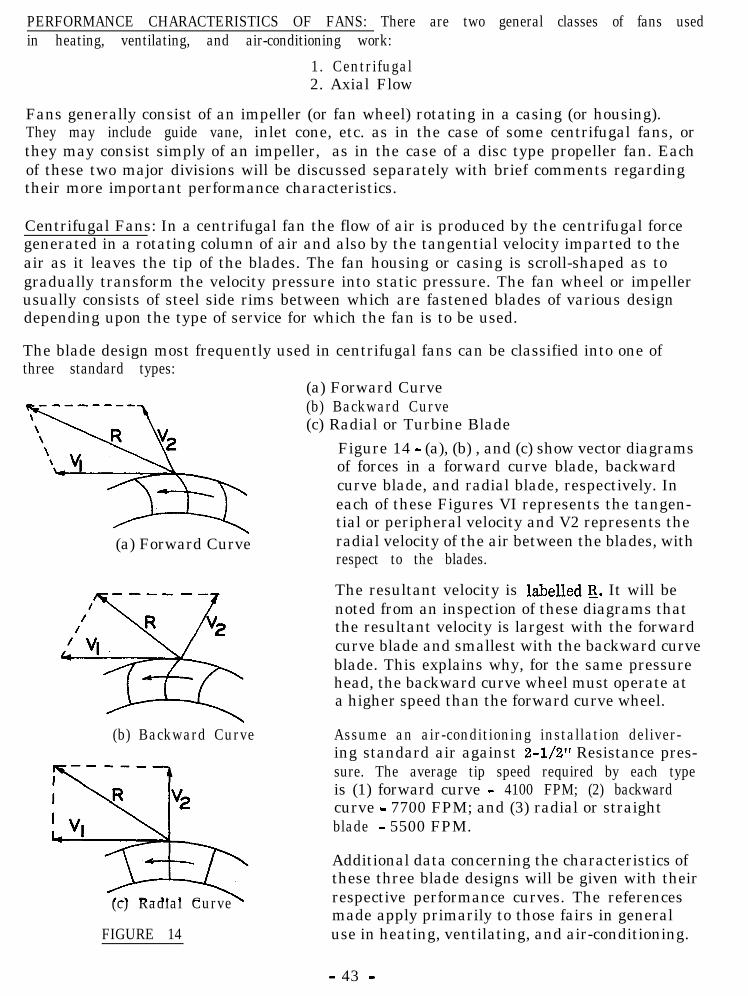
PERFORMANCE CHARACTERISTICS OF FANS: There are two general classes of fans usedin heating, ventilating, and air-conditioning work:

1. Centrifugal2. Axial Flow

Fans generally consist of an impeller (or fan wheel) rotating in a casing (or housing).They may include guide vane, inlet cone, etc. as in the case of some centrifugal fans, orthey may consist simply of an impeller, as in the case of a disc type propeller fan. Eachof these two major divisions will be discussed separately with brief comments regardingtheir more important performance characteristics.

Centrifugal Fans: In a centrifugal fan the flow of air is produced by the centrifugal forcegenerated in a rotating column of air and also by the tangential velocity imparted to theair as it leaves the tip of the blades. The fan housing or casing is scroll-shaped as togradually transform the velocity pressure into static pressure. The fan wheel or impellerusually consists of steel side rims between which are fastened blades of various designdepending upon the type of service for which the fan is to be used.

The blade design most frequently used in centrifugal fans can be classified into one ofthree standard types:

(a) Forward Curve

(b) Backward Curve

(c) Radial Curve

FIGURE 14

(a) Forward Curve(b) Backward Curve(c) Radial or Turbine Blade

Figure 14 - (a), (b) , and (c) show vector diagramsof forces in a forward curve blade, backwardcurve blade, and radial blade, respectively. Ineach of these Figures VI represents the tangen-tial or peripheral velocity and V2 represents theradial velocity of the air between the blades, withrespect to the blades.

The resultant velocity is labelled R_. It will benoted from an inspection of these diagrams thatthe resultant velocity is largest with the forwardcurve blade and smallest with the backward curveblade. This explains why, for the same pressurehead, the backward curve wheel must operate ata higher speed than the forward curve wheel.

Assume an air-conditioning installation deliver-ing standard air against 2-l/2” Resistance pres-sure. The average tip speed required by each typeis (1) forward curve - 4100 FPM; (2) backwardcurve - 7700 FPM; and (3) radial or straightblade - 5500 FPM.

Additional data concerning the characteristics ofthese three blade designs will be given with theirrespective performance curves. The referencesmade apply primarily to those fairs in generaluse in heating, ventilating, and air-conditioning.

- 43 -

Axial flow fans include those fans which produce motion of the air by the thrusteffect of the inclined blades. The air enters axially at the leading edge of the blade,and the flow is essentially parallel to the impeller shaft. In addition the air is given arotating motion about the shaft axis as a center. Fans in this category are usually classi-fied into (a) disc or propeller, (b) tubeaxial, and (c) vaneaxial. Most propeller fansoperate without a housing and consequently the static pressure developed is low as thereis little opportunity for the conversion of velocity pressure into static pressure.

A tubeaxial fan consists of relatively large hub with helical blades rotating within acylinder, and will operate against resistances of 2 or 3 inches of water. Vaneaxial fansconsist of an axial flow impeller within a cylinder, combined with a set of guide vaneslocated either before or after the impeller. The presence of these guide vanes assist inrecovering the energy imparted as tangential acceleration and therefore fans of this designare available which will operate against pressures in excess of 15 inches of water.

The following performance curves will illustrate some of the most important charac-teristics of the different types of fans used in heating and ventilating work. In each figurethe static pressure, static efficiency, and horsepower are plotted as the ordinate and airvolume is plotted as the abscissa, all at constant speed. Each of the type fans discussedwill include references to identifying characteristics. Please remember that there aremany different types of blade designs which are available in both centrifugal and axialflow fans, but this discussion will be limited to four basic types.

Typical characteristic of a FORWARD CURVEBLADE centrifugal fan is shown in Figure 15.This fan is perhaps the most widely used typeemployed in general ventilating work. It oper-ates at slow speed, is quiet and cheap, and islight in weight with small space requirements.The forward curve blade fan is slightly lessefficient than the other types and is somewhatunstable at the middle operating range. In somecases there is a hesitancy to use these fans inparallel as one will tend to hog the load fromanother. This, however, is for the most partdenied by the manufacturers. It will be noted

dfrom the curve that there is a rising horse-

tipower characteristic which would indicate thatan oversize motor be used as a precautionagainst the motor being overloaded. This is

AIR VOLUME - C. F. M. perhaps not as serious as may first appear.

FIGURE 15Assume that the static pressure of the systemis suddenly reduced which would immediatelycause the fan to handle more air. An increase

in the air volume would cause an increase in horsepower, but at the same time wouldalso cause an increase in static pressure with the subsequent effect of reducing the airvolume which in turn would influence the horsepower, so that the actual increase in horse-power requirements due to the original decrease in resistance pressure would not be aslarge as might be anticipated.

- 44 -

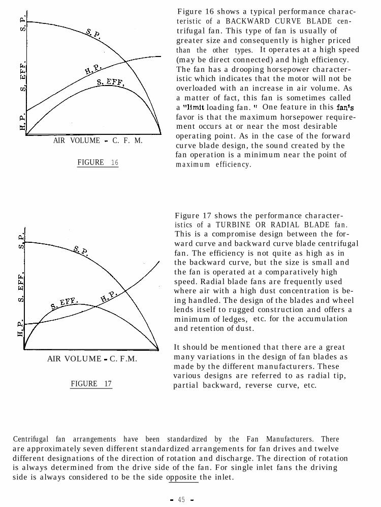
Figure 16 shows a typical performance charac-teristic of a BACKWARD CURVE BLADE cen-trifugal fan. This type of fan is usually ofgreater size and consequently is higher pricedthan the other types. It operates at a high speed(may be direct connected) and high efficiency.The fan has a drooping horsepower character-istic which indicates that the motor will not beoverloaded with an increase in air volume. Asa matter of fact, this fan is sometimes calleda “limit loading fan. ” One feature in this fanlsfavor is that the maximum horsepower require-ment occurs at or near the most desirable

AIR VOLUME - C. F. M.

FIGURE 16

operating point. As in the case of the forwardcurve blade design, the sound created by thefan operation is a minimum near the point ofmaximum efficiency.

Figure 17 shows the performance character-istics of a TURBINE OR RADIAL BLADE fan.This is a compromise design between the for-ward curve and backward curve blade centrifugalfan. The efficiency is not quite as high as inthe backward curve, but the size is small andthe fan is operated at a comparatively highspeed. Radial blade fans are frequently usedwhere air with a high dust concentration is be-ing handled. The design of the blades and wheellends itself to rugged construction and offers aminimum of ledges, etc. for the accumulationand retention of dust.

AIR VOLUME - C. F.M.

FIGURE 17

It should be mentioned that there are a greatmany variations in the design of fan blades asmade by the different manufacturers. Thesevarious designs are referred to as radial tip,partial backward, reverse curve, etc.

Centrifugal fan arrangements have been standardized by the Fan Manufacturers. Thereare approximately seven different standardized arrangements for fan drives and twelvedifferent designations of the direction of rotation and discharge. The direction of rotationis always determined from the drive side of the fan. For single inlet fans the drivingside is always considered to be the side opposite the inlet.

- 45 -

Fig. 18 shows a typical performance curve, for an AXIAL FLOW FAN of the propeller

type l As previously mentioned, propellertype fans are designed to handle large volumesof air at very low resistance to flow. Theother designs of axial flow fans, however,will operate satisfactorily against appreciableresistance. One of the distinguishing charac-teristics of axial flow fans is that they gener-ally have a drooping horsepower curve, withthe horsepower being a maximum at no flow.The inherent advantage of the axial flow fanis its simplicity, which is, in turn, reflectedin a minimum of weight and in small size.Since in most cases these fans are direct

AIR VOLUME - C. F.M. driven, the motor is in the air stream andFIGURE 18 the use of totally enclosed motors is gener-

ally recommended - even when the air isrelatively clean. Air temperature is also a

limiting factor. The primary disadvantage of axial flow fans is that they are relativelynoisy. The noise problem is further aggravated by the fact that there is generally presenta distinct pitch note. Unfortunately the human ear appears unusually sensitive to this pitchnote and this fact has limited their use to some extent in public buildings.

p

B C

The useful energy added to the flowing airstream per unit of time is ordinarily desig-nated as air horsepower (X.H. P.) Air horse-power is therefore the hp. output of the fan.If a fan delivers X cu. ft. of air per minuteagainst Y resistance, the resulting product

. XY represents the ft. - lbs. of energy added% to the air stream. This may be diagrammat-

z ically illustrated by means of a pressure-PC volume diagram or indicator card. Volume

4in C. F.M. is plotted horizontally and abso-lute pressure in pounds per square foot ver-tically. This is shown graphically in Fig. 19

AIR VOLUME - C. F. M. where the area ABCDEA represents the workdone on the air in compressing and moving

FIGURE 19 the volume of air. The area representingwork may be considered to be made up of

two parts; the work of compression BCDB, and the work of delivery ABDEA. The com-pression phase from C to D follows the low of adiabatic compression so that the line fromC to D is a curve of exponential form (with n = 1.2 to 1.3). In actual performance thearea under the compression line CD is very small compared to the area under the deliveryline DE because of the low compression ratios encountered. For this reason it may beneglected in horsepower calculations without introducing any appreciable error. Consider-ing the indicator card to be rectangular, the work is given by the product of the lengthin C. F.M. times the height in pounds per Square Foot. The resulting product is in foot-pounds and may be readily converted to horsepower by dividing by 33,000. ( 1 H. P. =33,000 ft. - lbs. per min.)

- 46 -

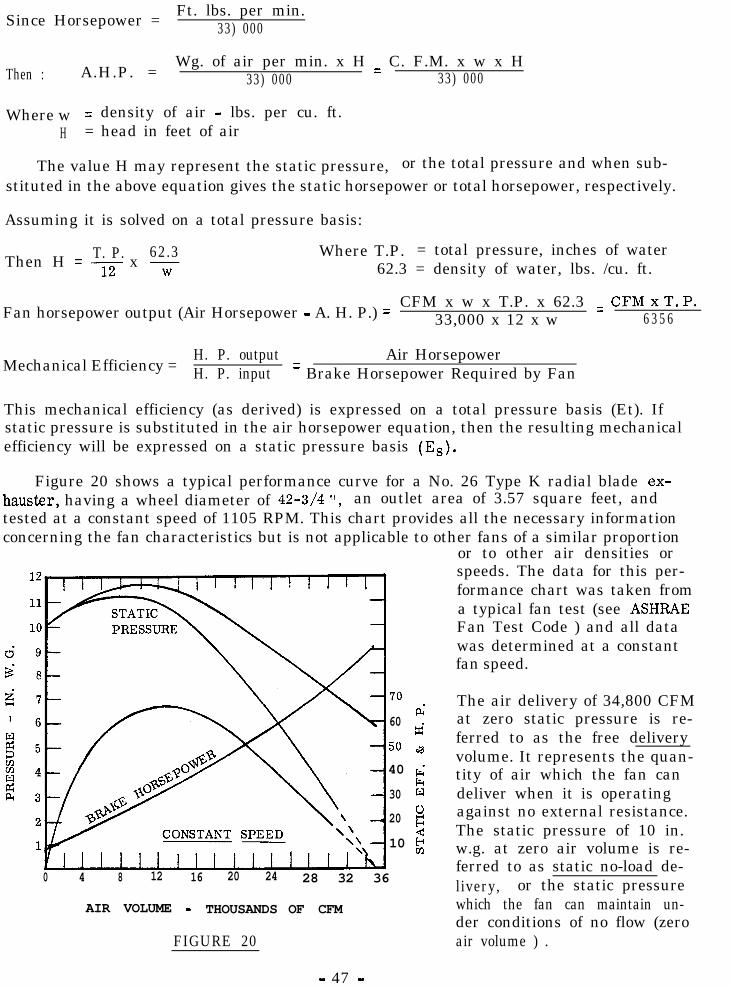
Since Horsepower =Ft. lbs. per min.

33) 000

Then : A.H.P. =Wg. of air per min. x H = C. F.M. x w x H

33) 000 33) 000

Where w = density of air - lbs. per cu. ft.H = head in feet of air

The value H may represent the static pressure, or the total pressure and when sub-stituted in the above equation gives the static horsepower or total horsepower, respectively.

Assuming it is solved on a total pressure basis:

T. P. 62.3Then H = 12 x w

Where T.P. = total pressure, inches of water62.3 = density of water, lbs. /cu. ft.

Fan horsepower output (Air Horsepower - A. H. P.) =CFM x w x T.P. x 62.3 = CFMxT.P.

33,000 x 12 x w 6 3 5 6

Mechanical Efficiency =H. P. output Air HorsepowerH. P. input = Brake Horsepower Required by Fan

This mechanical efficiency (as derived) is expressed on a total pressure basis (Et). Ifstatic pressure is substituted in the air horsepower equation, then the resulting mechanicalefficiency will be expressed on a static pressure basis (Es).

Figure 20 shows a typical performance curve for a No. 26 Type K radial blade ex-hauster, having a wheel diameter of 42-3/4 It, an outlet area of 3.57 square feet, andtested at a constant speed of 1105 RPM. This chart provides all the necessary informationconcerning the fan characteristics but is not applicable to other fans of a similar proportion

or to other air densities orspeeds. The data for this per-formance chart was taken froma typical fan test (see ASHRAEFan Test Code ) and all datawas determined at a constantfan speed.

0 4 8 12 16 20 24

AIR VOLUME - THOUSANDS

FIGURE 20

28 32 36

OF CFM

d60

ti50 a40 g

30 E

20 s2

10 $

The air delivery of 34,800 CFMat zero static pressure is re-ferred to as the free deliveryvolume. It represents the quan-tity of air which the fan candeliver when it is operatingagainst no external resistance.The static pressure of 10 in.w.g. at zero air volume is re-ferred to as static no-load de-livery, or the static pressurewhich the fan can maintain un-der conditions of no flow (zeroair volume ) .

- 47 -

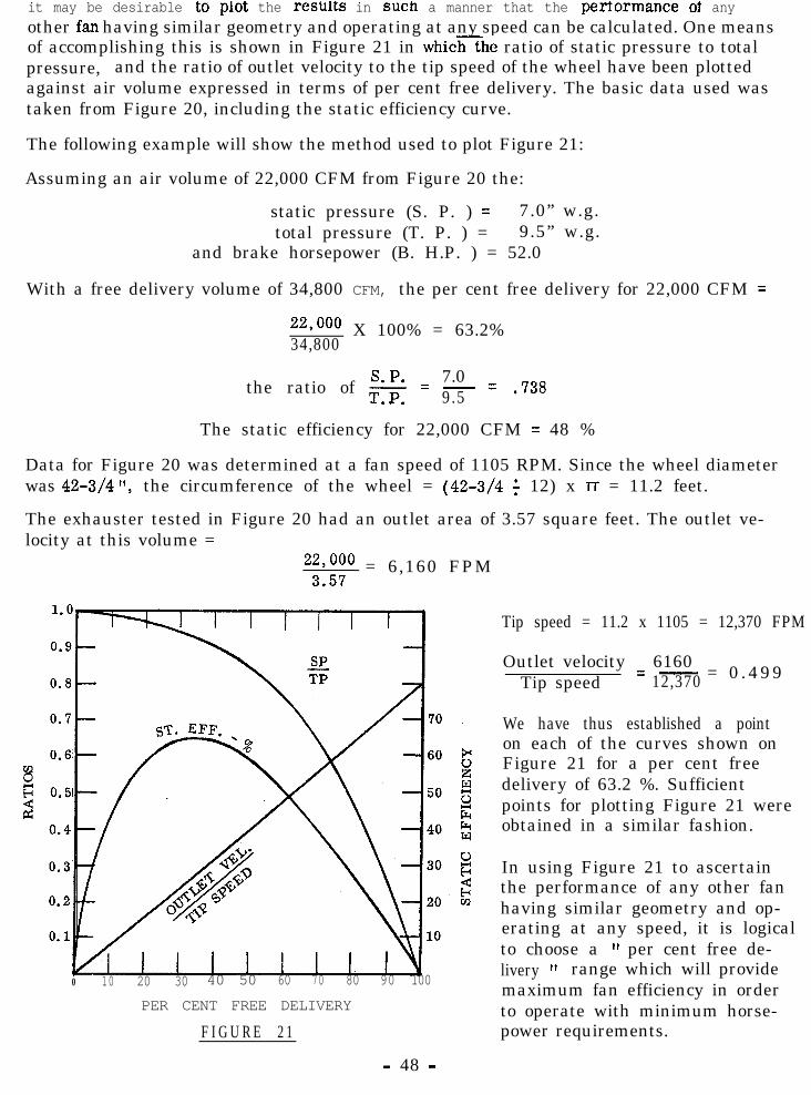
it may be desirable t0 plot the results in SUCh a manner that the peITOrmaIICe 01 anyother fan having similar geometry and operating at any speed can be calculated. One meansof accomplishing this is shown in Figure 21 in whicEhe ratio of static pressure to totalpressure, and the ratio of outlet velocity to the tip speed of the wheel have been plottedagainst air volume expressed in terms of per cent free delivery. The basic data used wastaken from Figure 20, including the static efficiency curve.

The following example will show the method used to plot Figure 21:

Assuming an air volume of 22,000 CFM from Figure 20 the:

static pressure (S. P. ) = 7.0” w.g.total pressure (T. P. ) = 9.5” w.g.

and brake horsepower (B. H.P. ) = 52.0

With a free delivery volume of 34,800 CFM, the per cent free delivery for 22,000 CFM =

22pooo X 100% = 63.2%34,800

7.0the ratio of s = - =9.5 .738. .

The static efficiency for 22,000 CFM = 48 %

Data for Figure 20 was determined at a fan speed of 1105 RPM. Since the wheel diameterwas 42-3/4 It, the circumference of the wheel = (42-3/4 f 12) x TT = 11.2 feet.

The exhauster tested in Figure 20 had an outlet area of 3.57 square feet. The outlet ve-locity at this volume =

2;Y;;o = 6,160 FPM.

0 10 20 30 40 50 60 70 80 90 100

PER CENT FREE DELIVERY

F I G U R E 2 1

- 48 -

Tip speed = 11.2 x 1105 = 12,370 FPM

Outlet velocity = 6160Tip speed - = 0 .49912,370

We have thus established a pointon each of the curves shown onFigure 21 for a per cent freedelivery of 63.2 %. Sufficientpoints for plotting Figure 21 wereobtained in a similar fashion.

In using Figure 21 to ascertainthe performance of any other fanhaving similar geometry and op-erating at any speed, it is logicalto choose a l1 per cent free de-livery It range which will providemaximum fan efficiency in orderto operate with minimum horse-power requirements.

c;plv1 aga.mb:L a SLa.LIc: prabaurc WI I& w . g.111tz tsiuUlilubu51- l b LU IJG 1;‘lUBtT“ LU UJxlI-aLc a.L

its maximum static efficiency of 66% (as indicated by Figure 20).

Determine : a) wheel diameter (or exhauster size)b) fan speedc) brake horsepower

At 66 % static efficiency the per cent free delivery = 35% and E = 0.935. (Fig. 21). .

12Therefore, T. P. = oq5 = - =0.935 12.84” w. g..

Velocity pressure at the fan discharge = T. P. - S. P. = 12.84 - 12 = 0.84” w.g.

Outlet velocity = 4,005 v= = 4,005 v= = 3650 FPM.

Outlet area = air volume _ 28,000outlet velocity 3,650

= 7.67 sq. ft.

From the Type K Exhauster bulletin, a size 38 has an outlet area of 7.75 sq. ft. andwould be chosen. The wheel diameter for this size exhauster is 62-‘7/16 inches.

From Figure 21 the ratio of outlet velocity to tip speed for 35% free delivery is 0.28.

Then : Tip speed =Outlet velocity 3,650

0.28 = - = 13,040 FPM0.28

R P M tip speed x 12 13,040 x 12=wheel diameter x TT = 62-7/16 x -IT = 800 RPM

Brake horsepower = 28,000x 12

=6 356 x9

o . 66 8 0 H . P.

SLIDE RULE METHOD: The Type K exhauster bulletin indicates that the volume handled byany given size covers a wide range of outlet velocities. It will be noted that the averageoutlet velocity where higher static pressures are required is in the order of 4,000 FPM.For 28,000 CFM the outlet area would then be 28,000 /4,000 = 7 sq. ft. The neareststandard size exhauster having this outlet area (or larger) is a size 38 which has anoutlet area of 7.75 sq. ft. and a wheel diameter of 62-7/16 inches (from bulletin),

Equivalent air volume for a size 26 exhauster = base wheel diameter 2new wheel diameter x required CFM

x 28,000 = 13,200 CFM

Set the 12 It S. P. on Scale A (square scale) and set the equivalent air volume of 13,200on Scale C (sliding scale). Move indicator until the relationship between S. P. and airvolume corresponds to the same relationship as read from Figure 20. This point is12,500 CFM at 10.75” S. P. and 66% static efficiency. This is the only point which willmatch the S.P. pressure-volume relationship of Figure 20, and is sometimes referred toas the It Rating Point 11.

Fan speed ofsize 38 exhauster =

=

Brake Horsepower =

equivalent air volumerating point volume

base wheel diameter x base RPMx new wheel diameter

13,200 42-3/41 2 , 5 0 0 x 62-7/16 x ‘lo5 = 8oo RPM

CFM x S. P. x 126356 x =

28,000M.E. =6356 x 0.66 8o B*H.P*

In practice it may be desirable to check another size exhauster to arrive at the most eco-nomical choice from the point of view of capital investment and horsepower requirements.

- 49 -

There are certain well recognized laws which apply to the performance of bothcentrifugal and axial flow fans, used either as blowers or exhausters. These lawsare based upon the relationship that for all practical purposes in the range used, afan may be considered a constant displacement machine. That is, against any givenresistance, each revolution of the fan will move the same quantity of air.

All fan laws are based upon the fundamental consideration that fan efficiencies re-main constant and therefore when one or more conditions are varied the rest will varyaccordingly. Their use is necessarily restricted to fans of the same design and geo-metrical shape. There are quite a number of useful fan laws which are given in mosthandbooks and textbooks. Only a few of the more important relations will be mentioned.

For a given fan size, piping system, and air density:

QX=Ql

- - - - - - (1)

SP2

SP1--- - - - (2)

------ (3)

Q23

Ql------ (4)

SP22

spl------ (5 )

e-_-m_ (6)

where Ql, SPl, and HP1 represent the volume, static pressure, and horsepower,respectively, of the known conditions, and Q 2, SP 2, and HP 2 represent the desired con-ditions. In E q&ions 4, 5, and 6, the value D represents the diameter of the wheel ininches with Dl the known value.

It should again be pointed out that the characteristic fan performance curves shownin Figures 15, 16, 17, and 18, are each plotted at constant speed. For performanceconditions at other speeds it is necessary to apply the Fan Laws as discussed above. This- -can perhaps be best illustrated by an example involving Duct - Fan Characteristics asshown in Figure 22.

Assume a duct system which is to handle 11,000 CFM, has a static pressure loss of0.77 I1 w. g. This is indicated by Point (T) on Duct Resistance Curve I1 A It (Figure22). Let us further assume that we have chosen a backward curved blade fan to supplythis air and that the fan is to be directly connected to a motor operating at 575 RPM.Curve 11 D fY is the static pressure curve for the fan and is plotted for the chosen oper-ating speed of 575 RPM. It is evident that only one condition satisfies both the fanand duct characteristics, and this occurs at Point (R) where the two curves intersectand represents a static pressure of 0.98 It at 12,400 CFM. At this air volume it willbe seen from curve ” E I’ that 3.08 horsepower will be required.

- 50 -

83MO

d

3StlO

H

I I

!2

I/ I

I I

I w

w

I Y

I

- 51 -

If it is desired to obtain the exact flow for which the duct system was designed(11,000 CFM at 0.77” S. P.) either of two methods may be followed: Namely, by damper-ing or by changing the fan speed. It will be found that changing the speed will result ina lower horsepower requirement, but will necessitate a belt drive or a variable speedmotor. If we pursue the damper method it will be noted that at 11,000 CFM the fanstatic pressure is 1.16” and, therefore, a damper equivalent to (1.16 - 0.77) = 0.39”will be required. Curve “B” would be the new duct resistance curve if this damper wasadded. The necessary horsepower from Curve “E” is 2.99.

If instead of dampering, we reduce the fan speed in the ratio of 11,000/12,400 itwill be found that a fan speed of 510 RPM will satisfy our requirements and the staticpressure relationship at this new speed has been plotted as Curve “C1’. It should be ob-served that the rating Point (R) moves back along the duct resistance curve to Point (T).At this point the fan will be delivering 11,000 CFM at a static pressure of 0.77” w.g.and at a speed of 510 RPM. The new horsepower requirement at this condition must bedetermined by applying the fan law and will amount to 2.15 horsepower.

*****

- 52 -

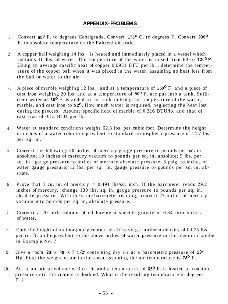
APPENDIX-PROBLEMS

1. Convert 60° F. to degrees Centigrade. Convert 175’ C. to degrees F. Convert 290°F. to absolute temperature on the Fahrenheit scale.

2. A copper ball weighing 14 lbs. is heated and immediately placed in a vessel whichcontains 10 lbs. of water. The temperature of the water is raised from 60 to 120°F.Using an average specific heat of copper 0.0951 BTU per lb. , determine the temper-ature of the copper ball when it was placed in the water, assuming no heat loss fromthe ball or water to the air.

3 . A piece of marble weighing 12 lbs. and at a temperature of 150’ F. and a piece ofcast iron weighing 20 lbs. and at a temperature of 80° F. are put into a tank. Suffi-cient water at 85’ F. is added to the tank to bring the temperature of the water,marble, and cast iron to 92O. How much water is required, neglecting the heat lostduring the process. Assume specific heat of marble of 0.216 BTU/lb. and that ofcast iron of 0.12 BTU per lb.

4. Water at standard conditions weighs 62.3 lbs. per cubic foot. Determine the heightin inches of a water column equivalent to standard atmospheric pressure of 14.7 lbs.per sq. in.

5 . Convert the following: 20 inches of mercury gauge pressure to pounds per sq. in.absolute; 10 inches of mercury vacuum to pounds per sq. in. absolute; 5 lbs. persq. in. gauge pressure to inches of mercury absolute pressure; 3 psig. to inches ofwater gauge pressure; 12 lbs. per sq. in. gauge pressure to pounds per sq. in. ab-solute.

6 . Prove that 1 cu. in. of mercury = 0.491 lbs/sq. inch. If the barometer reads 29.2inches of mercury, change 130 lbs. sq. in. gauge pressure to pounds per sq. in.absolute pressure. With the same barometer reading, convert 27 inches of mercuryvacuum into pounds per sq. in, absolute pressure.

7 . Convert a 20 inch column of oil having a specific gravity of 0.84 into inchesof water.

8 . Find the height of an imaginary column of air having a uniform density of 0.075 lbs.per cu. ft. and equivalent to the above inches of water pressure in the plenum chamberin Example No. 7.

9. Give a room 20’ x 36’ x 7 l/2’ containing dry air at a barometric pressure of 29”Hg. Find the weight of air in the room assuming the air temperature is 75’ F.

10. Air at an initial volume of 3 cu. ft. and a temperature of 65’ F. is heated at constantpressure until the volume is doubled. What is the resulting temperature in degreesF. ?

- 53 -

Appendix - Problems

11.

12.

13.

14.

15.

16.

17.

18.

19.

20.

Given air an initial pressure of 28 lbs. per sq. in. absolute and an initial temper-ature of 90° F. It is cooled at constant volume to a temperature of 50° F. What isthe resulting pressure?

A tank whose volume is 60 cu. ft. contains air at a pressure of 100 lbs. per sq.in. absolute and a temperature of 80° F. How many pounds of air does the tankcontain?

An automobile tire has a mean diameter of 32” and a width of 6”. It is inflated toa pressure 50 lbs. per sq. in. gauge at a temperature of 70° F. Atmosphericpressure is 14.2 lbs. per sq. in.

a . How many pounds of air does the tire contain?b . Assuming there was no change in volume, what would be the gauge

pressure of the air in the tire if it was heated by the sun to a tem-perature of 120’ F. ?

A given quantity of air at a temperature of 60° F. and a pressure of 16 lbs. persq. in. absolute has a volume of 4 cu. ft. What would be the new volume of thesame air if the pressure is increased to 60 lbs. per sq. in. absolute with the tem-perature being held constant?

Given 10 cu. ft. of air at a temperature of 700 F. and at a pressure of 16 lbs. persq. in. absolute - What is the pressure of this air if the volume is increased to50 cu. ft. at a constant temperature of 70° F. ?

A tank contains 180 cu. ft. of air at a temperature of 90° F. and a pressure of 170lbs. per sq. in. absolute.

a . What is the weight of air in the tank?b. How many cu. ft. would this air occupy at a standard atmospheric

pressure of 14.7 lbs. per sq. in. absolute and at a temperatureof 95O F. ?

The volume of a quantity of air at 80° F. and a pressure of 14 lbs. per sq. in.absolute is 18 cu. ft. What would be the temperature of this air if the volume isreduced to 5 cu. ft. and the pressure is increased to 70 lbs. per sq. in. absolute?

If 3600 BTU is added to 3 lbs. of water which is at a temperature of 180°F. andat a pressure of 20 lbs. per sq. in. absolute, what are the resulting temperatureand state of fluid?

If 5 lbs. of steam at 212O F. and 20 lbs. of water at 70’ F. are mixed together atatmospheric pressure, what is the resulting temperature and state of the mixture?

Assume .lO lbs. of steam at a pressure of 28 lbs. per sq. in. absolute and a tem-perature of 290° F. is mixed with 10 lbs. of water at 180’ F. If the pressure re-mains constant, what is the resulting state of the mixture?

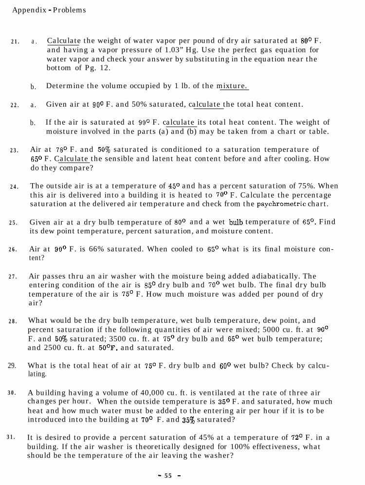
Appendix - Problems

21.

22.

23.

24.

25.

26.

27.

28.

29.

30.

31.

a . Calculate the weight of water vapor per pound of dry air saturated at 80° F.and having a vapor pressure of 1.03” Hg. Use the perfect gas equation forwater vapor and check your answer by substituting in the equation near thebottom of Pg. 12.

b. Determine the volume occupied by 1 lb. of the mixture.

a. Given air at 90° F. and 50% saturated, calculate the total heat content.

b. If the air is saturated at 90° F. calculate its total heat content. The weight ofmoisture involved in the parts (a) and (b) may be taken from a chart or table.

Air at 78O F. and 50% saturated is conditioned to a saturation temperature of650 F. Calculate the sensible and latent heat content before and after cooling. Howdo they compare?

The outside air is at a temperature of 450 and has a percent saturation of 75%. Whenthis air is delivered into a building it is heated to 70° F. Calculate the percentagesaturation at the delivered air temperature and check from the psychrometric chart.

Given air at a dry bulb temperature of 80° and a wet bulb temperature of 65’. Findits dew point temperature, percent saturation, and moisture content.

Air at 90° F. is 66% saturated. When cooled to 65’ what is its final moisture con-tent?

Air passes thru an air washer with the moisture being added adiabatically. Theentering condition of the air is 85O dry bulb and 70° wet bulb. The final dry bulbtemperature of the air is 75O F. How much moisture was added per pound of dryair?

What would be the dry bulb temperature, wet bulb temperature, dew point, andpercent saturation if the following quantities of air were mixed; 5000 cu. ft. at 90’F. and 50% saturated; 3500 cu. ft. at 75O dry bulb and 65’ wet bulb temperature;and 2500 cu. ft. at 50°F. and saturated.

What is the total heat of air at 75O F. dry bulb and 60° wet bulb? Check by calcu-lating.

A building having a volume of 40,000 cu. ft. is ventilated at the rate of three airchanges per hour. When the outside temperature is 35O F. and saturated, how muchheat and how much water must be added to the entering air per hour if it is to beintroduced into the building at 70° F. and 35% saturated?

It is desired to provide a percent saturation of 45% at a temperature of 72O F. in abuilding. If the air washer is theoretically designed for 100% effectiveness, whatshould be the temperature of the air leaving the washer?

- 55 -

Appendix - Problems

32.

33.

34.

35.

36.

37.

38.

39.

40.

Given air at a barometric pressure of 29.2” Hg. and a dry bulb temperature of85O F. Calculate the velocity and volume of air in a 12” diameter duct having anaverage velocity pressure of 0.54” w. g.

Given an inlet orifice 6” in diameter and handling standard air. The orifice pressuredrop 1.7” w.g. and the coefficient of the discharge is 0.61. Determine the volumeof air being handled.

Given a fan discharge duct of 8” diameter, in which the velocity pressure is 2.6”w.g. The air then expands through a transition piece into a 9-l/4” diameter ductwith a resulting velocity pressure of l-1/2” w.g. If the transition piece has a 40 %loss, determine the static pressure and total pressure relationships in the smalland large duct sections if the pressure loss due to friction is 0.5” and 1” respec-tively.

Given a fan having an inlet duct and discharge duct. The inlet duct has a frictionloss of 1” of water and a velocity pressure of 2” w.g. The discharge duct has afriction loss of 2-l/2” of water and a velocity pressure of 2” w.g. Determine thefollowing:

a . Static pressure at the fan inletb. Static pressure at the fan outletc. Total pressure at the fan inletd. Total pressure at the fan outlet 6e. Static pressure across fan t

f. Total pressure across fan f

g. If the volume of air handled is 50,000 CFM and the fan efficiency is 68%,what is the air HP and ,what is the brake HP of the fan?

What is the friction loss in 120 ft. of 45” diameter duct having two long radiuselbows and carrying 15,000 CFM of air?

A fan delivers 12,000 CFM against a static pressure of l-1/4” w.g. , at a speedof 420 RMP, and draws 4 horsepower. It is desired to increase the fan output to15,000 CFM. What will be the speed, horsepower, and static pressure for theincreased output?

A fan delivers 3,000 CFM of air at a static pressure of 1.0” of water. What isthe static air horsepower, and how much shaft horsepower is required if the staticfan efficiency is 60% at this load?

A fan is delivering 23,000 CFM against a static pressure of 2” of water. The brakehorsepower is 11.6 and speed 377 RPM. It is desired to increase the delivery to27,400 CFM through the same piping system. What are the new speed, horsepower,and static pressure?

A fan exhausts 27,000 CFM through a 29.3” diam. duct connected to the suction sideof the fan. At the fan inlet the SP measures -3.87” W.G. If the speed of the fan isincreased so that it exhausts 32,400 CFM - what is the friction loss through the ex-haust duct at the increased volume? Calculate all values.

Blue Circle Cement

PROCESS ENGINEERINGTRAINING PROGRAM

Module 4

Section 5

Conversion Factors and Tables

Conversion Table

Volumetric Flowrate

cubic metre per second

(m3/s)

cubic metre per hour

(m3/h)litre per minute

(l/min)cubic foot per minute (cfm)

US gallon per minute (US

gpm)UK gallon per minute (gpm)

1cubic metre per second (m3/s)

= 1 3600 60000 2119 15850 13200

1cubic metre per hour (m3/h)

= 0.000278 1 16.667 0.5886 4.4029 3.6667

1litre per minute (l/min)

= 1.66667E-05 0.06 1 0.03531 0.2642 0.2200

1cubic foot per minute (cfm)

= 0.000471921 1.69901 28.32 1 7.4805 6.2305

1US gallon per minute (US gpm)

= 6.30915E-05 0.2271 3.7854 0.13368 1 0.8328

1UK gallon per minute (gpm)

= 7.57576E-05 0.2727 4.5455 0.16050 1.2008 1

Conversion TablePower & Specific Fuel Consumption kilowatt (kW)

metric horsepower

(hP)horsepower

(hP)

kilocalorie per kilogramme

(kCal/kg)Btu per pound

(Btu/lb)

Milion Btu per short ton (MBtu/st)

1 kilowatt (kW) = 1 1.360 1.341

1metric horsepower (hP)

= 0.7355 1 0.9863

1 horsepower (hP) = 0.7457 1.0139 1

1kilocalorie per kilogramme (kCal/kg)

= 1 1.8 0.0036

1Btu per pound (Btu/lb)

= 0.55556 1 500

1Milion Btu per short ton (MBtu/st)

= 277.778 0.002 1

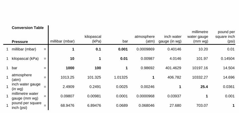
Conversion Table

Pressure millibar (mbar)kilopascal

(kPa) baratmosphere

(atm)inch water

gauge (in wg)

millimetre water gauge

(mm wg)

pound per square inch

(psi)

1 millibar (mbar) = 1 0.1 0.001 0.0009869 0.40146 10.20 0.01

1 kilopascal (kPa) = 10 1 0.01 0.00987 4.0146 101.97 0.14504

1 bar = 1000 100 1 0.98692 401.4629 10197.16 14.504

1atmosphere (atm)

= 1013.25 101.325 1.01325 1 406.782 10332.27 14.696

1inch water gauge (in wg)

= 2.4909 0.2491 0.0025 0.00246 1 25.4 0.0361

1millimetre water gauge (mm wg)

= 0.09807 0.00981 0.0001 0.0000968 0.03937 1 0.001

1pound per square inch (psi)

= 68.9476 6.89476 0.0689 0.068046 27.680 703.07 1

Conversion TableLength Millimetre Metre inch foot yard mile

1 Millimetre = 1 0.001 0.03937 0.0033 0.0011 6.21371E-07

1 Metre = 1000 1 39.370 3.2808 1.0936 0.000621

1 inch = 25.4 0.0254 1 0.0833 0.0278 1.57828E-05

1 foot = 304.8 0.3048 12 1 0.3333 0.00019

1 yard = 914.4 0.9144 36 3 1 0.00057

1 mile = 1,609,344 1,609.34 63,360 5,280 1,760 1

Conversion Table

Linear Velocitymetre per

second (m/s)kilometre per

hour (kph)foot per

second (fps)foot per minute

(fpmmile per hour

(mph)

1metre per second (m/s)

= 1 3.6 3.2808 196.8504 2.2369

1kilometre per hour (kph)

= 0.27778 1 0.9113 54.681 0.6214

1foot per second (fps)

= 0.3048 1.0973 1 60 0.6818

1foot per minute (fpm

= 0.00508 0.0183 0.01667 1 0.0114

1mile per hour (mph)

= 0.44704 1.6093 1.4667 88 1

Conversion Table

Mass Flowratekilogram per

second (kg/s)metric tonne

per hour (te/h)pound per

second (lb/s)pound per hour (lb/h)

short ton per hour (stph)

1kilogram per second (kg/s)

= 1 3.6 2.2046 7936.64 3.968

1metric tonne per hour (te/h)

= 0.27778 1 0.6124 2204.62 1.1023

1pound per second (lb/s)

= 0.4536 1.63293 1 3600 1.8

1pound per hour (lb/h)

= 0.0001260 0.0001260 0.0002778 1 0.0005

1short ton per hour (stph)

= 0.2520 0.9072 0.5556 2000 1

Conversion TableMass kilogram (kg) metric tonne ounce (oz) pound (lb) short ton (st)

1 kilogram (kg) = 1 0.001 3,527.40 2.2046 0.001102

1 metric tonne = 1,000 1 3,527,399 2204.62 1.102311

1 ounce (oz) = 2.83E-04 2.83E-07 1 0.0625 3.125E-07

1 pound (lb) = 0.45359 0.000454 16 1 0.0005

1 short ton (st) = 907.185 0.90719 3,200,004 2000 1

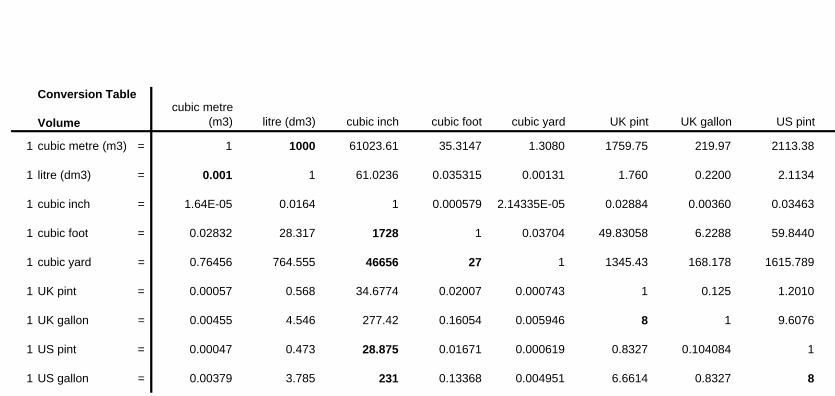
Conversion Table

Volumecubic metre

(m3) litre (dm3) cubic inch cubic foot cubic yard UK pint UK gallon US pint US gallon

1 cubic metre (m3) = 1 1000 61023.61 35.3147 1.3080 1759.75 219.97 2113.38 264.17

1 litre (dm3) = 0.001 1 61.0236 0.035315 0.00131 1.760 0.2200 2.1134 0.2642

1 cubic inch = 1.64E-05 0.0164 1 0.000579 2.14335E-05 0.02884 0.00360 0.03463 0.00433

1 cubic foot = 0.02832 28.317 1728 1 0.03704 49.83058 6.2288 59.8440 7.48049

1 cubic yard = 0.76456 764.555 46656 27 1 1345.43 168.178 1615.789 201.9734

1 UK pint = 0.00057 0.568 34.6774 0.02007 0.000743 1 0.125 1.2010 0.1501

1 UK gallon = 0.00455 4.546 277.42 0.16054 0.005946 8 1 9.6076 1.20095

1 US pint = 0.00047 0.473 28.875 0.01671 0.000619 0.8327 0.104084 1 0.125

1 US gallon = 0.00379 3.785 231 0.13368 0.004951 6.6614 0.8327 8 1

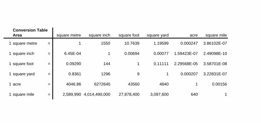
Conversion TableArea square metre square inch square foot square yard acre square mile

1 square metre = 1 1550 10.7639 1.19599 0.000247 3.86102E-07

1 square inch = 6.45E-04 1 0.00694 0.00077 1.59423E-07 2.49098E-10

1 square foot = 0.09290 144 1 0.11111 2.29568E-05 3.58701E-08

1 square yard = 0.8361 1296 9 1 0.000207 3.22831E-07

1 acre = 4046.86 6272640 43560 4840 1 0.00156

1 square mile = 2,589,990 4,014,490,000 27,878,400 3,097,600 640 1

Blue Circle Cement

PROCESS ENGINEERINGTRAINING PROGRAM

Module 4

Section 6

Back To Cement Basics

Blue Circle Cement

PROCESS ENGINEERINGTRAINING PROGRAM

Module 4

Section 7

Test Method Formulae and NomenclatureGEL

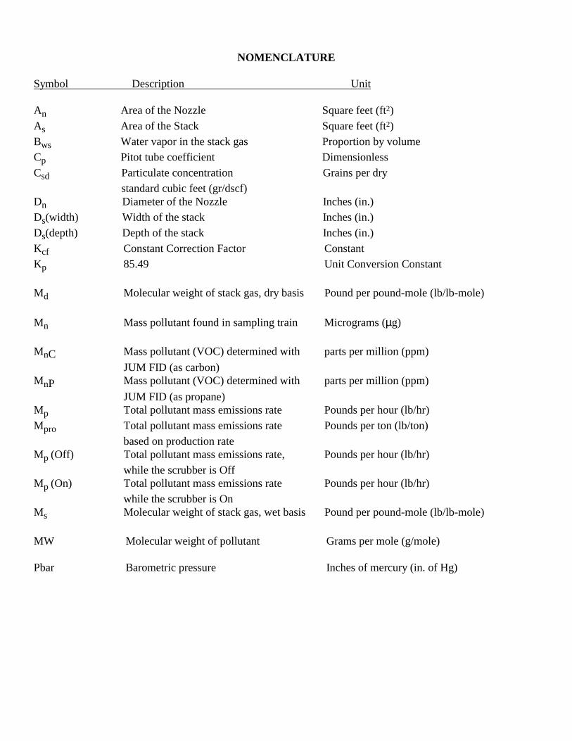
NOMENCLATURE

Symbol Description Unit

An Area of the Nozzle Square feet (ft2)

As Area of the Stack Square feet (ft2)

Bws Water vapor in the stack gas Proportion by volume

Cp Pitot tube coefficient Dimensionless

Csd Particulate concentration Grains per dry

standard cubic feet (gr/dscf)Dn Diameter of the Nozzle Inches (in.)

Ds(width) Width of the stack Inches (in.)

Ds(depth) Depth of the stack Inches (in.)

Kcf Constant Correction Factor Constant

Kp 85.49 Unit Conversion Constant

Md Molecular weight of stack gas, dry basis Pound per pound-mole (lb/lb-mole)

Mn Mass pollutant found in sampling train Micrograms (µg)

MnC Mass pollutant (VOC) determined with parts per million (ppm)

JUM FID (as carbon)MnP Mass pollutant (VOC) determined with parts per million (ppm)

JUM FID (as propane)Mp Total pollutant mass emissions rate Pounds per hour (lb/hr)

Mpro Total pollutant mass emissions rate Pounds per ton (lb/ton)

based on production rateMp (Off) Total pollutant mass emissions rate, Pounds per hour (lb/hr)

while the scrubber is OffMp (On) Total pollutant mass emissions rate Pounds per hour (lb/hr)

while the scrubber is OnMs Molecular weight of stack gas, wet basis Pound per pound-mole (lb/lb-mole)

MW Molecular weight of pollutant Grams per mole (g/mole)

Pbar Barometric pressure Inches of mercury (in. of Hg)

NOMENCLATURE(continued)

Symbol Description Unit

Pg Pressure of stack gas (static pressure) Inches of water (in. of H20)

Ps Absolute stack gas pressure Pound per pound-mole (lb/lb-mole)

Pstd Standard pressure, 68oF Inches of mercury (in. of Hg)

Qgw Wet volumetric stack gas flow rate at Actual cubic feet/hour (acf/hr)

actual conditions

Qsd Dry Volumetric Stack Gas Flow Rate Dry standard cubic feet per hour

corrected to Standard Conditions (dscf/hr)

Qsd(avg) Dry Volumetric Stack Gas Flow Rate Dry standard cubic feet per hour

corrected to Standard Conditions (dscf/hr)Flow average of, before and after flowmeasurement

Tm Absolute dry gas meter temperature Degrees Rankine (oR)

(oF + 460) = oR

Ts Absolute stack temperature Degrees Rankine (oR)

(oF + 460) = oR

Tstd Standard temperature (528oR) Degrees Rankine (oR)

Vlc Volume of water vapor condensed in Milligrams (mg)

the impingers

Vm Volume of gas sample as measured by the Dry cubic feet (dcf)

dry gas meter

Vmstd Volume of gas sample as measured by the Dry standard cubic feet (dscf)

dry gas meter, corrected to standardconditions

Vmstd (Total) Volume of gas sample as measured by the Dry standard cubic feet (dscf)

dry gas meter, corrected to standardconditions

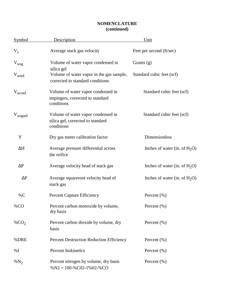
NOMENCLATURE(continued)

Symbol Description Unit

Vs Average stack gas velocity Feet per second (ft/sec)

Vwsg Volume of water vapor condensed in Grams (g)

silica gelVwstd Volume of water vapor in the gas sample, Standard cubic feet (scf)

corrected to standard conditions

Vwcstd Volume of water vapor condensed in Standard cubic feet (scf)

impingers, corrected to standardconditions

Vwsgstd Volume of water vapor condensed in Standard cubic feet (scf)

silica gel, corrected to standardconditions

Y Dry gas meter calibration factor Dimensionless

∆H Average pressure differential across Inches of water (in. of H2O)

the orifice

∆P Average velocity head of stack gas Inches of water (in. of H2O)

∆P Average squareroot velocity head of Inches of water (in. of H2O)

stack gas

%C Percent Capture Efficiency Percent (%)

%CO Percent carbon monoxide by volume, Percent (%)dry basis

%CO2 Percent carbon dioxide by volume, dry Percent (%)

basis

%DRE Percent Destruction Reduction Efficiency Percent (%)

%I Percent Isokinetics Percent (%)

%N2 Percent nitrogen by volume, dry basis Percent (%)

%N2 = 100-%C02-1%02-%CO

NOMENCLATURE(continued)

Symbol Description Unit

%02 Percent oxygen by volume, Percent (%)

dry basis%02 Corr Percent oxygen Correction Factor Percent (%)

%Scrubber Percent Scrubber Efficiency Percent (%)Total sampling time Minutes (min)

pi, 7c = 3.1416 Constant

TEST METHODS FORMULAS

I. AREA

Area of Stack, Square feet (Round Stack)

=

2

22

in 144

ft

4

ðDs As

π = 3.1416

Area of Stack, Square feet (Square Stack)

( )( ) ( )( )

=

2

2

in 144

ftdepthDswidthDs As

Area of Nozzle, Square feet

=

2

22

in 144

ft

4

ð Dn An

π = 3.1416

II. TEMPERATURE CONVERSIONS

Dry Gas Meter Temperature, Degrees Rankin

Tm[oR] = Tm[oF] + 460

Stack Temperature, Degrees Rankin

Ts[oR] = Ts[oF] + 460

III. VOLUME OF AIR COLLECTED

Volume of Dry Gas Sample, Corrected to Standard Conditions

( )( )

∆Η+=

Pstd13.6 Pbar

YVm Vmstd

IV. MOISTURE DETERMINATION

Volume of Water Vapor Condensed in Impingers, Corrected to Standard Conditions

Vwcstd = Vlc x 0.04707

Volume of Water Vapor Condensed in Silica Gel, Corrected to Standard Conditions

Vwsgstd = Vwsg x 0.04715

Water Vapor in the Stack Gas, Proportion by Volume

++

+=VmstdVwsgstdVwcstd

VwsgstdVwcstdBws

V. TOTAL VOLUME

VmstdVwsgstdVwcstdVmstd TOTAL ++=

VI. MOLECULAR WEIGHT OF STACK GAS

Nitrogen Content of Stack Gas, Percent

CO%O%CO%100N% 222 −−−=

Dry Molecular Weight of the Stack Gas

)CO%N(%28.0)O(%32.0)CO(%44.0Md 222 +++=

Wet Molecular Weight of the Stack Gas

Ms = (Md)(1-Bws) + 18(Bws)

VII. FLOW DETERMINATIONS

Absolute Stack Gas Pressure

+=

6.13

PgPbarPs

Average Stack Gas Velocity, Feet per Second

( )Ms Ps

Ts(Kp)(Cp) Vs

×∆Ρ=

( )

( )( )OH inchesR

Hg inchesmolelb

lb

sec

ft 85.49 Kp

2o

−=

Wet Volumetric Stack Gas Flow Rate, Actual Conditions, cubic feet per hour

=

hr

sec 3600(Vs)(As) Qaw

Dry Volumetric Stack Gas Flow Rate, Corrected to Standard Conditions, cubic feet per hour

( )

−

=

Pstd

Tstd

Ts

PsBws1

hr

sec 3600(Vs)(As) Qsd

VIII. ISOKINETICS DETERMINATION

Isokinetics Sampling Rate, Percent

( ) 100Tstd Bws-1èAn Ps Vs 60

Pstd Vmstd Ts %I ×

=

IX. POLLUTANT DETERMINATIONS

Conversion from Parts per million (ppm) to Micrograms (µg)

( ) ( )( )

µ=µ OH ml

OH g1)ml Vcatch(

g

gppmPollutant Mn

2

2g

Concentration of Pollutant, gr/dscf → lb/hr

=

ìg 000,000,1

g

g

gr 432.15

Vmstd

MnCsd

Emission Rate for Pollutant, gr/dscf → lb/hr

=

gr 7000

lb(Csd)(Qsd) Mp

Emission Rate for Pollutant based on Production Rate, lb/hr → lb/ton

=

P

MpMpro

Emission Rate of Compounds, Standard Flowrate, Corrected to Standard Conditions, ppm → lb/hr (dry basis)

=

6.453

lb

mole

MWg

m 02404.0

mole

dscf 315.35

m)Qsd(

1,000,000

Mn Mp

3

3

Emission Rate of Compounds, Standard Flowrate, Corrected to Standard Conditions, ppm → lb/hr (wet basis)

=

6.453

lb

mole

MWg

Pstd

Tstd

Ts

Ps

m 02404.0

mole

dscf 315.35

m)Qaw(

1,000,000

Mn Mp

3

3

Concentration of Carbon Monoxide, Corrected for Carbon Dioxide, ppm

[ ] [ ]( )

−=

100

CO%1coMncoMn 2

Concentration of Pollutant, Corrected for Moisture, ppm

−=

Bws1

MnMn

Concentration of Volatile Organic Compounds, Corrected to Standard Conditions, ppm as Carbon

[ ]( )

−

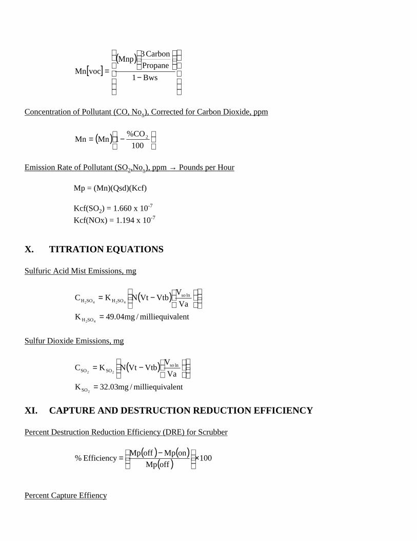
=Bws1

Propane

Carbon 3Mnp

vocMn

Concentration of Pollutant (CO, Nox), Corrected for Carbon Dioxide, ppm

( )

−=

100

CO%1MnMn 2

Emission Rate of Pollutant (SO2,Nox), ppm → Pounds per Hour

Mp = (Mn)(Qsd)(Kcf)

Kcf(SO2) = 1.660 x 10-7

Kcf(NOx) = 1.194 x 10-7

X. TITRATION EQUATIONS

Sulfuric Acid Mist Emissions, mg

( )

−=

Va

VVtbVtNKC lnso

SOHSOH 4242

alentmilliequiv/mg04.49K42SOH =

Sulfur Dioxide Emissions, mg

( )

alentmilliequiv/mg03.32K

Va

VVtbVtNKC

2

22

SO

lnsoSOSO

=

−=

XI. CAPTURE AND DESTRUCTION REDUCTION EFFICIENCY

Percent Destruction Reduction Efficiency (DRE) for Scrubber

( ) ( )( ) 100offMp

onMpoffMp Efficiency % ×

−=

Percent Capture Effiency

( )( ) 100inMp

outMp Capture % ×=

Percent Destruction Reduction Efficiency (DRE)

( ) ( )( ) 100inMp

outMpinMp DRE % ×−=

XII. ADDITIONAL EQUATIONS

∆H Determination

per EPA:

( ) PPm Ts Ms

Ps Tm Md Bws-1 Cp @ Dn 72.846 224 ∆

∆Η=∆Η

Nozzle Diameter

( )0.75 Qm :where

P Ps

Ms Ts

Bws-1 Cp Tm

Pm Qm 0358.0Dn

=∆

=

Excess Air

( )( ) 100

(CO) 5.0O%N0.264

CO% 05.0O%EA%

22

2 ×

+−

−=

Leak Rate Adjustment

( ) ( ) ( )

θθ−−−= ∑

=

N

2i

pLa-Lp-iLaLi-èLaLlVmVm

Raw Isokinetics

( )

θ

∆Η+

+

=Ps VsAn 60

6.13Pb

Tm

VmVlc 002676.0

100I%

Expressing Concentration as ppm

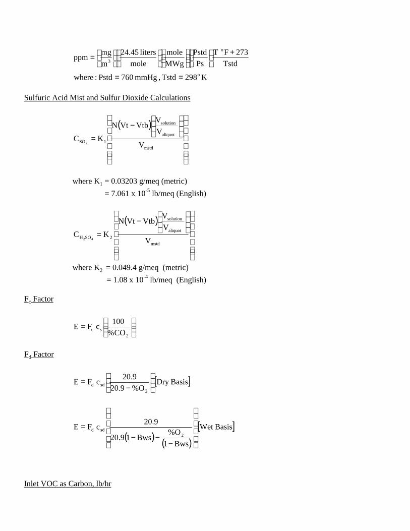
K298Tstd , mmHg 760Pstd:where

Tstd

273F T

Ps

Pstd

MWg

mole

mole

liters 45.24

m

mgppm

o

o

3

==

+

=

Sulfuric Acid Mist and Sulfur Dioxide Calculations

( )

−

=mstd

aliquot

solution

1SO V

V

VVtbVtN

KC2

where K1 = 0.03203 g/meq (metric)

= 7.061 x 10-5 lb/meq (English)

( )

−

=mstd

aliquot

solution

2SOH V

V

VVtbVtN

KC42

where K2 = 0.049.4 g/meq (metric)

= 1.08 x 10-4 lb/meq (English)

Fc Factor

=

2sc CO%

100c FE

Fd Factor

[ ]BasisDry O%9.20

9.20c FE

2sdd

−

=

( ) ( )[ ]BasisWet

Bws1

O%Bws19.20

9.20c FE

2sdd

−−−

=

Inlet VOC as Carbon, lb/hr

=

kerosene lb

VOC lbs 86.0

hour

mins 60

kerosene gal

kerosene lbs 84.6

(mins) timerun

oseneker galsCvoci

Outlet VOC as Carbon

=

g6.453

lb

mole

carbon g12

m 02404.0

mole

cf 315.35

m

hour

cf

parts10

background - ppm measuredC

3

3

6voco

Blue Circle Cement

PROCESS ENGINEERINGTRAINING PROGRAM

Module 4

Section 8

Combustion and Efficiency

3695 Interstate Park WayRivera Beach, FL 33404-5998

Phone 407-842-1900Fax 407-842-0742

COMBUSTION & EFFICIENCY

Understanding combustion and the measurements of combustion are essential in determining proper andeconomical operation of a boiler. Guides are provided for various fuels to assist you in evaluating your boiler.Periodic evaluations will aid you in keeping fuel and operating costs at a minimum.

CS600/9-86

INTRODUCTION

Flue gas analysis has been commonly used for many years, but with todays increasing fuel costs, it is moreimportant than ever to be familiar with the basic principle of combustion and analysis. This knowledge, even inthe smallest of boilers and furnaces, can reduce operating costs, fuel consumption, and other maintenanceconsiderations included. To understand why and how, one must first take a look at the basic principles ofcombustion. Then, the virtues of analysis become meaningful.

FUEL

Many fuels are available, but they all share some common principles; that is, typically that they arehydrocarbons (any compound that is comprised of atoms of hydrogen and carbon) or compounds (or free)hydrogen or carbon. Natural gas, fuel oil, coal, wood, bagasse, and others all fall into this category. These fuelsdiffer in their ratios of hydrogen to carbon and in how they are bound together. A less common fuel is sulfur,and although it will not be discussed, there are small amounts of it in the heavier (less pure) fuel oils and inmost coals.

AIR

When air is used for combustion to provide the necessary oxygen, consideration must be given to nitrogen sinceair is mostly that. It is generally accepted that air is 79.05% nitrogen with other minor constituents and 20.95%oxygen. This represents a ratio of 79.05:20.95 or' 3.773:1 parts of nitrogen to oxygen in air. Another way ofstating this is that for every one mole of oxygen required for combustion, 3.773 moles of nitrogen will bepresent (mole % equals volume %). While nitrogen is generally inert (excepting some generation of oxidescategorized as NOx), it still must be accounted for.

THEORETICAL AIR REQUIREMENT

To first understand combustion, the theoretical air requirements for completely burning carbon and methane aregiven as examples.

The air requirement for completely combusting one mole of carbon is one mole of oxygen and 3.773 moles ofnitrogen. Combustion changes the carbon (C) and oxygen (02) to carbon dioxide (CO2) while releasing heat(expressed as BTU's or calories). The nitrogen remains unchanged. The gaseous product of combustion are thenone mole Of C02 and 3.773 moles of N2. Compared to the total combusted volume (1 mole CO2 + 3.773 molesN2 = 4.773 total moles), C02 represents (1 / 4.773) x 100 = 20.95%. No excess oxygen is present. See Figure 1.

The air requirement for completely combusting one mole of methane (CH4) is two moles of oxygen and 2 x3.773 = 7.546 moles of nitrogen. Combustion changes the carbon and half the oxygen to C02 and the remainingoxygen with hydrogen to water vapor (H20). The nitrogen again remains unchanged. The gaseous products ofcombustion are therefore one mole of C02, two moles Of H20, and.7.546 moles of nitrogen. Compared to thetotal combusted volume (1 + 2 + 7.546 = 10.546), C02 constitutes (1 / 10.546)x 100 = 9.48%. Since water wasincluded in the calculated analysis, the 9.48% C02 is on a "wet" basis. A C02 analyzer that did not cool theproducts of combustion below condensing temperatures would make this analysis. However, an analyzer such as

the Orsat can condense (by cooling) most of the water from the sample before analysis. This "dry" analysis forC02 would be computed from a total volume of 1 mole C02 + 7.546 moles N2 = 8.546 total moles. DryCO2 = (1 / 8.546)x 100 = 11.70%. Again, no excess oxygen is present. See Figure 1.

In both of the examples, complete (stoichiometric) combustion was attained. Just enough air was supplied toburn all of the fuel without having any excess oxygen. If less air had been provided, all of the fuel would nothave been combusted (and hence wasted). If more air had been provided, extra volumes of combustion gaseswould have been generated. The more volume of flue gas there is, the harder it is to capture the heat in it.

NOTE: Unless stated otherwise, all data and calculations are at standard conditions.

EXCESS AIR AND HEAT

While it would be theoretically desirable to operate a boiler at stoichiometric conditions, it is not possible to doso due to inadequate mixing of fuel and air at different firing levels and due to safety related factors. Poor burnermixing can lead to complete combustion (0% excess air) in some parts of the flame, while other parts are fuelrich (< 0% excess air) or air rich (> 0% excess air). Therefore, to keep from losing unburnt fuel, burners are runat greater than zero excess air levels. How high, is a function of the burner and boiler design and maintenance.

To illustrate the effects of various excess air levels, return to the example with methane at -10%, 0% and +50%excess air levels.

At -10% excess air, 90% of the air required for stoichiometric combustion is used. See Figure 2. Because thereis less nitrogen (with less air), less heat is lost in it. However, since there is not enough oxygen for completecombustion, all of the fuel hydrogen and carbon cannot be changed to H20 and C02. Some of the fuel becomesfree hydrogen (H2) and free carbon monoxide (CO). Instead of just losing BTU's up the stack as unrecoveredheat, BTU's are also lost as unburned fuel (H2 and CO)t As shown in Figure 2, while methane has 1013BTU's/CU.FT. available for combustion, 64.4 BTU's have been lost as CO and 65 BTU's have been lost at H2

(a 13% fuel loss). The remaining 883.6 BTU's (per cubic foot of methane) are released as heat in 9.791 cubicfeet of flue gas.At 0% excess air, no BTU's are lost in combustible gases. All 1013 BTU's (per cubic foot of methane) arereleased as heat in 10.546 cubic feet of flue gas.

*NOTE: In the heat loss tables in this publication, fuel losses have been included with total heat loss forexcess air levels below 0%.

At +50% excess air levels, notice that the mole quantities Of C02 and H20 are the same as at 0% excess airlevels. What has changed is that now there is excess oxygen (02) and more excess nitrogen (N2). See Figure 4.One mole of oxygen and (11.319 - 7.546) = 3.773 moles of nitrogen have been added that did not have to beheated at 0% excess air levels. All 10131BTU's (per cubic foot of methane) are available, but in 15.319 cubicfeet of flue gas.

It becomes evident that at higher excess air levels the heat of combustion gets diluted into increasing volumes offlue gas (mostly N2 and 0-2). As flue gas volume (and velocity) increases, less heat can be captured throughheat exchange surfaces within a boiler (a loss in efficiency has developed). It is therefore desirable to operate asclose to 0% excess air as it is practical and safe to without generating smoke* or significant gaseouscombustibles (as CO or H2).

Only one loss decreases when operating at below 0% excess air levels, the amount of heat lost in the water (ofcombustion) as steam** (over 1000 BTU's per pound). It is normally impractical to recover this heat since itrequires cooling to condensing temperatures. When condensate forms in flue gas, corrosion becomes more of aproblem.

**NOTE In the heat loss tables in this publication, steam losses in the water of combustion have been includedwith the total heat loss.

*NOTE Smoke (or soot) is carbon in its solid form (ie, a solid combustible). Every pound of carbon generatedis a loss of over 14,000 BTU's.

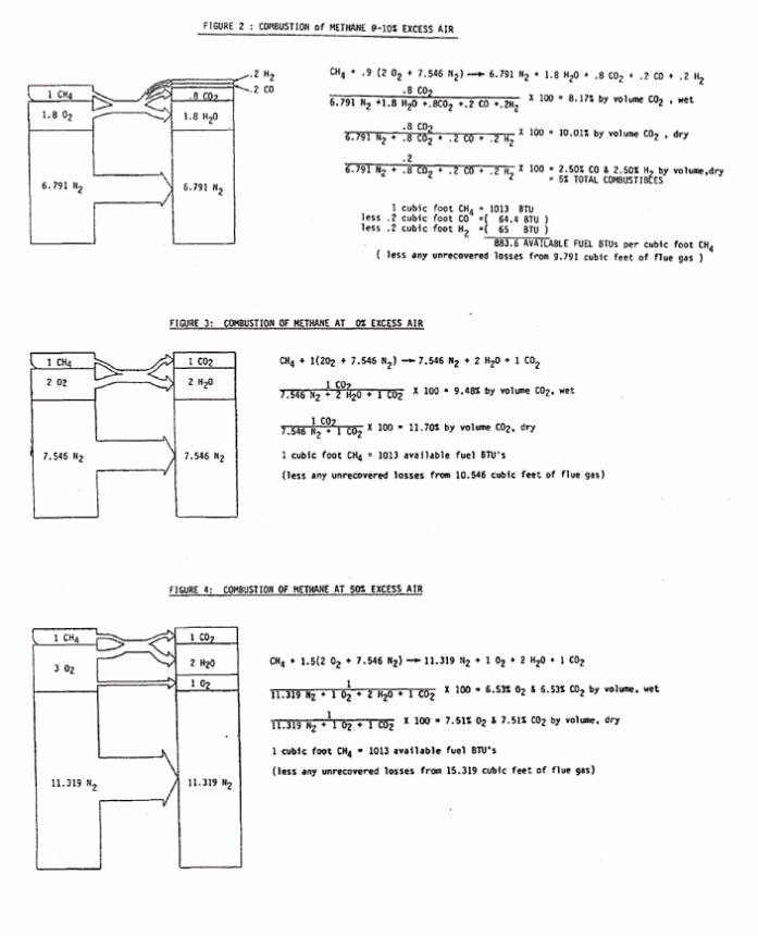
THEORETICAL EXCESS AIR CURVES

In calculating excess oxygen and carbon dioxide for several excess air values of methane combustion, itbecomes apparent that this data can be more meaningful if plotted in graph form. A useful form of graph isshown in Figure 5.

By using a graph like this (made for the specific fuel being used), it can be seen that if you can analyze either thepercent oxygen or carbon dioxide in the flue gas, you can determine the percent excess air at which a particularboiler is being operated. It can also be seen that ideally, operation should be at the point of maximum carbondioxide and zero oxygen (near the stoichiometric point). However, there are some things to watch for in doingthis.

Most burner/boiler combinations are limited in how close they can be adjusted toward stoichiometry. This isparticularly true in many older designs. Due to conditions such as poor fuel-air mixing and flame temperaturevariations, combustible gases can be generated when there is still an excess of oxygen. Therefore, for optimalefficiency and safety, it may be necessary to operate at 5 or even 10% excess air. An example of curve shiftingthen can occur is given in Figure 6.

Notice (in the encircled area of Figure 6) that oxygen exists to the left of stoichiometry and combustibles existto the right. Since conditions of overlap can (and do) occur, the user of analytical instruments must be careful toknow all of the information (and not just part) when making critical adjustments to a boiler or burner.

ANALYZER SELECTION

Flue gas analyzers have been in use over a century now, so they are nothing new. Probably the first analyzer onthe market was the Orsat (Joseph Hays sold his first one in 1908). While it is a relatively simple analyzer, it canprovide the user with relatively dry measurements of carbon dioxide (C02), oxygen (02) and carbon monoxide(CO).

How dry any analysis of wet gasses can be is a function of temperature. At 5o C (41oF) a saturated gas sample

contains about 1% water vapor . . At 20oC (68oF) it is 2% H 0, at 30oC (86oF) it is 4% H 0 and at 40 oc

(104oF) it can contain 7% water vapor.

The Hays Republic model 621 Orsat operates by removing a gas sample from the flue with a rubber squeezebulb (hand pump). The sample is cooled, trapped, and its volume measured in a glass burette. The sample isthen passed through absorbing chemicals that have an affinity for C02, then O2 and then CO. After eachabsorption procedure the gas sample is measured and its volume compared to that of the original sample. Thedifference in volume before and after absorption gives the exact measurement of the percentage of gas in thesample. See Figure 7.

Because of the construction of the hand Orsat, it is a useful portable analyzer for making boiler tune-ups when acost justification for an on-line analyzer can not be made, or when a "standard" analysis is required.

The next evolutionary analyzer to follow the Orsat was the automatic C02 analyzer. It provides a continuousanalysis Of C02 for indication (or recording) and for manual adjustments to the fuel-air ratio (% excess air).While an analysis of C02 is very useful if one also knows combustibles (CO or CO and H2), the CO2 analyzerhas limited use as a lone analyzer when operating a boiler near stoichiometry. C02 peaks at a maximum value atstoichiometry, and decreased to the left (inefficient combustibles side) and right side. In our methane example,dry C02 values peak at 11.7%. At -10% excess air, dry C02 is 10%. Dry C02 is also measured at 10% at +15%excess air. Therefore, if you controlled to 10% CO2 you may be fairly efficient (at +15% excess air) or fairlyinefficient (at -10% excess air).

Another drawback to C02 monitors, is that as the hydrocarbon make-up of a fuel changes, so does the peak valueof carbon dioxide in the flue. For the fuels in the excess air curves in the back of this publication, C02 (dry)peaks at 12.1% for natural gas, 15.6% for #2 Fuel Oil, 16.8% for #6 Fuel Oil, 18.5% for sub-bituminous coal,and at 18.7% for semi-bituminous coal. This means that there should be a change in control point for boilersthat change from one fuel to another. Even worse, if a boiler is fired with two fuels simultaneously, the controlpoint shifts as the ratio of the two fuels changes.

HYDROCARBON RATIO

The hydrocarbon ratio is a useful tool for those that monitor C02. It is simply the ratio of hydrogen to carbon(by weight) in the fuel. Fuels that have a large amount of hydrogen (compared to carbon) have a relatively largehydrocarbon ratio. The natural gas listed in the excess air curves in this publication has a H:C Ratio of 0.309.Fuels that are mostly carbon have a low ratio. The semi-bituminous coal has a H:C ratio of 0.058.

In using a set of excess air curves that do not have a close match in chemical composition to the fuel beingused, select the fuel that has a hydrocarbon ratio closest to your own. Then the C02 curves will be a closeapproximation to what you can expect.

OXYGEN ANALYZERS

Oxygen analyzers have some advantages over carbon dioxide analyzers for monitoring or control. Regardless ofthe fuel being used, stoichiometry is achieved at zero O2, and O2 does not increase again at negative excess airlevels. Also, measured O2 for various fuels correlates very closely to the same excess air levels. This means thatfor boilers that alternate fuels (or fire multiple fuels) the oxygen control point may shift very little or not at all.The chief limitation to this is that in a particular boiler, the oil burners may not be as efficient as the gasburners. Then the oxygen control point for oil will not be as low as for gas (in order to avoid generatingcombustibles).

There are several different types of oxygen flue gas analyzers on the market. It has already been mentioned thatthe Orsat measures oxygen through a chemical absorption process.

Paramagnetic designs rely on the composition of the oxygen molecule to cause it to be attracted towards largemagnets (N2 and C02 are not paramagnetic molecules). Inaccuracies of analysis can be caused by thediamagnetic properties of certain background gases. While these analyzers can be quite reliable, they requirerather complex sample systems to condition the gas for the analyzer. These sample systems can be rather costlyto purchase and maintain. Also, depending on the particular design of any one analyzer, the oxygen reading canbe affected by the presence of combustible gases. When using one of these analyzers for low excess air levels, asensitive combustibles analyzer should also be used.

Another common oxygen analyzer is the electro-chemical type with disposable semi-permeable membrane cell.The cells are quite compact and usually do not require a power source (they generate their own output in thepresence of O2). However, because of their galvanic nature, the sensors typically have a life of about six months.Their chief use is in portable analyzers. Like the Orsat, their O2 analysis is generally unaffected by combustibles.Therefore, a good portable should include a sensitive combustibles analyzer. Their analysis may be affected byCO2 and oxides of nitrogen and sulfur.

The oxygen analyzers discussed so far all require sample systems; complex ones for on-line analyzers or simpleones for portables. (these sample systems can be responsible for significant errors in analysis due to leaks andinsufficient cooling). They also should be used with sensitive combustibles analyzers when used for making lowexcess air level adjustments. However, one type of analyzer needs neither of these;..the in-situ Zirconium Oxide.

ZIRCONIUM OXIDE ANALYZERS

The heart of these analyzers is a ceramic (Zirconium Oxide) cell with porous platinum electrodes. In thepresence of high temperatures, the sensor will allow oxygen ions to pass through it (provided there is adifference in oxygen partial pressure across it). This ionic flow can be measured with' suitable electronics toprovide indication and outputs for control and recording purposes.

The successful Hays Republic OXYPROBETM , OXY-MIZERTM and high temperature analyzer all use the

same zirconium oxide sensor assembly. The cell is controlled to a very precisely held temperature near 1500oF

(815 oC) that allows it to respond very closely with theoretical outputs. This makes these analyzers extremelystable and easy to calibrate.* Also, their modular characteristics make them extremely flexible (see Figure 8).

One feature of zirconium oxide analyzers is that since they operate at relatively high temperatures, they can beinserted directly into a flue duct or stack without a conventional sampling system. The sample system is part ofthe analyzer and not an add-on requirement for analysis. The in-situ analyzers require no more than an effectivefilter to protect the cell from soot and fly ash. The Hays Republic OXYPROBETM and OXY-MIZERTM haveeven been designed with a filter deflector and air foils to keep their filters clean.

* For further information on these analyzers, call or write Hays Republic regarding Models A10007,A10018, and A10021 zirconium oxide analyzers.

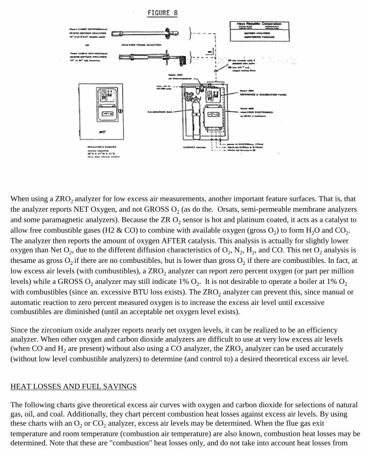
When using a ZRO2 analyzer for low excess air measurements, another important feature surfaces. That is, thatthe analyzer reports NET Oxygen, and not GROSS O2 (as do the. Orsats, semi-permeable membrane analyzersand some paramagnetic analyzers). Because the ZR O2 sensor is hot and platinum coated, it acts as a catalyst toallow free combustible gases (H2 & CO) to combine with available oxygen (gross O2) to form H2O and CO2.The analyzer then reports the amount of oxygen AFTER catalysis. This analysis is actually for slightly loweroxygen than Net O2, due to the different diffusion characteristics of O2, N2, H2, and CO. This net O2 analysis isthesame as gross O2 if there are no combustibles, but is lower than gross O2 if there are combustibles. In fact, atlow excess air levels (with combustibles), a ZRO2 analyzer can report zero percent oxygen (or part per millionlevels) while a GROSS O2 analyzer may still indicate 1% O2. It is not desirable to operate a boiler at 1% O2

with combustibles (since an. excessive BTU loss exists). The ZRO2 analyzer can prevent this, since manual orautomatic reaction to zero percent measured oxygen is to increase the excess air level until excessivecombustibles are diminished (until an acceptable net oxygen level exists).

Since the zirconium oxide analyzer reports nearly net oxygen levels, it can be realized to be an efficiencyanalyzer. When other oxygen and carbon dioxide analyzers are difficult to use at very low excess air levels(when CO and H2 are present) without also using a CO analyzer, the ZRO2 analyzer can be used accurately(without low level combustible analyzers) to determine (and control to) a desired theoretical excess air level.

HEAT LOSSES AND FUEL SAVINGS

The following charts give theoretical excess air curves with oxygen and carbon dioxide for selections of naturalgas, oil, and coal. Additionally, they chart percent combustion heat losses against excess air levels. By usingthese charts with an O2 or CO2 analyzer, excess air levels may be determined. When the flue gas exittemperature and room temperature (combustion air temperature) are also known, combustion heat losses may bedetermined. Note that these are "combustion" heat losses only, and do not take into account heat losses from

leaky valves, leaky steam traps or feedwater blow down, these are losses only in heat going "up the stack" (orwherever the temperature measurement was made).

A combustion efficiency analyzer such as the Hays Republic Model A10022 makes the assumption that percentefficiency is 100 minus the combustion heat loss. While this is not a measure of the total boiler efficiency, it is ameasure of the combustion heat "use efficiency" of the boiler. These efficiency computations are automaticallymade and can be used to calculate fuel and money savings, just as done in the following explanation andexample.

PROCEDURE

At a given boiler load:

1) Measure the percent O2 or CO2 in the flue gas.2) Measure the temperature of the flue gas.3) Measure the combustion air inlet temperature.

With these measurements, refer to the appropriate chart for the fuel being used. If you know the actualcomposition or hydrocarbon ratio of your fuel, use the chart for the fuel closest to your own. Otherwise, use thechart with the appropriate fuel name.

1) Locate the percent gas volume (measured with the flue gas analyzer) on the lower side scale, anddraw a line across the chart to intersect the curve for the gas measured. Note that the dry O2 and CO2

curves for the Orsat are for fully condensed samples (use of 40oF cold water in the burette jacket andin the leveling bottle will allow within 1% of reading of a truly dry analysis). The wet O2 curve is forthe OXYPROBETM or OXY-MIZERTM (or other in-situ analyzer) with dry combustion air.

2) From the gas intersect point, draw a vertical (up and down) line to intersect the ∆T curves and the %Excess Air scale. The percent excess air may now be read.

3) Subtract the measured room temperature (combustion air) from the measured flue gas temperature toobtain the differential temperature (∆T) across the boiler. Draw a horizontal line across from theintersect point with the proper ∆T line and the vertical line made in the previous step. It may benecessary to interpolate the ∆T curves to obtain the best accuracy. Read the % Combustion HeatLoss where this line intersects the scale. This number subtracted from 100 is the combustion heatuse efficiency of the boiler.

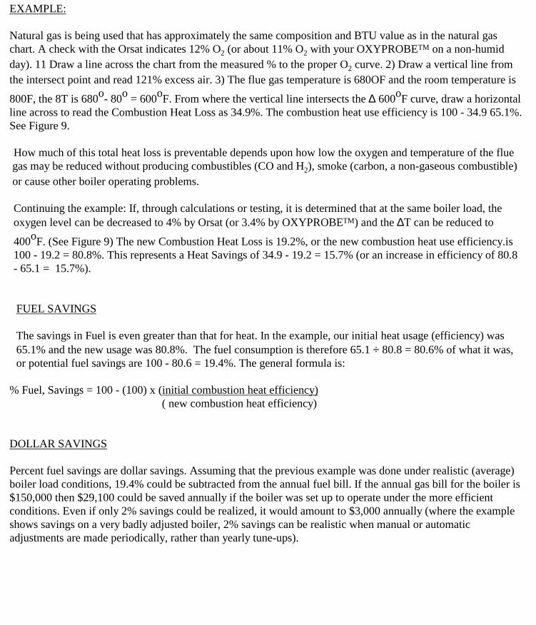
EXAMPLE:

Natural gas is being used that has approximately the same composition and BTU value as in the natural gaschart. A check with the Orsat indicates 12% O2 (or about 11% O2 with your OXYPROBETM on a non-humidday). 11 Draw a line across the chart from the measured % to the proper O2 curve. 2) Draw a vertical line fromthe intersect point and read 121% excess air. 3) The flue gas temperature is 680OF and the room temperature is

800F, the 8T is 680o- 80o = 600oF. From where the vertical line intersects the ∆ 600oF curve, draw a horizontalline across to read the Combustion Heat Loss as 34.9%. The combustion heat use efficiency is 100 - 34.9 65.1%.See Figure 9.

How much of this total heat loss is preventable depends upon how low the oxygen and temperature of the fluegas may be reduced without producing combustibles (CO and H2), smoke (carbon, a non-gaseous combustible)or cause other boiler operating problems.

Continuing the example: If, through calculations or testing, it is determined that at the same boiler load, theoxygen level can be decreased to 4% by Orsat (or 3.4% by OXYPROBETM) and the ∆T can be reduced to

400oF. (See Figure 9) The new Combustion Heat Loss is 19.2%, or the new combustion heat use efficiency.is100 - 19.2 = 80.8%. This represents a Heat Savings of 34.9 - 19.2 = 15.7% (or an increase in efficiency of 80.8- 65.1 = 15.7%).

FUEL SAVINGS

The savings in Fuel is even greater than that for heat. In the example, our initial heat usage (efficiency) was65.1% and the new usage was 80.8%. The fuel consumption is therefore 65.1 ÷ 80.8 = 80.6% of what it was,or potential fuel savings are 100 - 80.6 = 19.4%. The general formula is:

% Fuel, Savings = 100 - (100) x (initial combustion heat efficiency) ( new combustion heat efficiency)

DOLLAR SAVINGS

Percent fuel savings are dollar savings. Assuming that the previous example was done under realistic (average)boiler load conditions, 19.4% could be subtracted from the annual fuel bill. If the annual gas bill for the boiler is$150,000 then $29,100 could be saved annually if the boiler was set up to operate under the more efficientconditions. Even if only 2% savings could be realized, it would amount to $3,000 annually (where the exampleshows savings on a very badly adjusted boiler, 2% savings can be realistic when manual or automaticadjustments are made periodically, rather than yearly tune-ups).

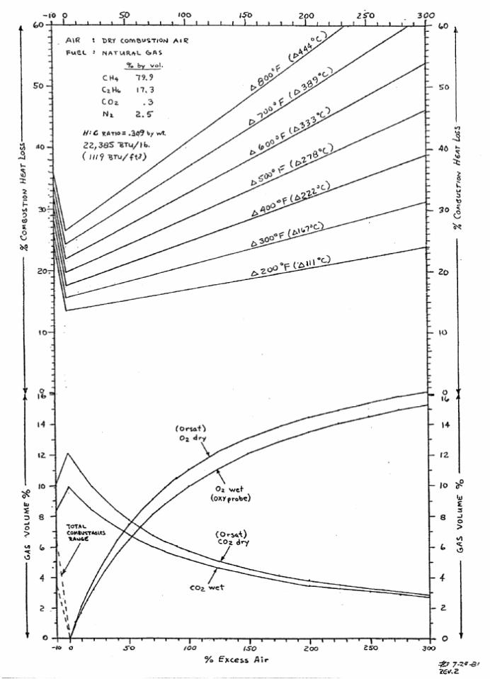
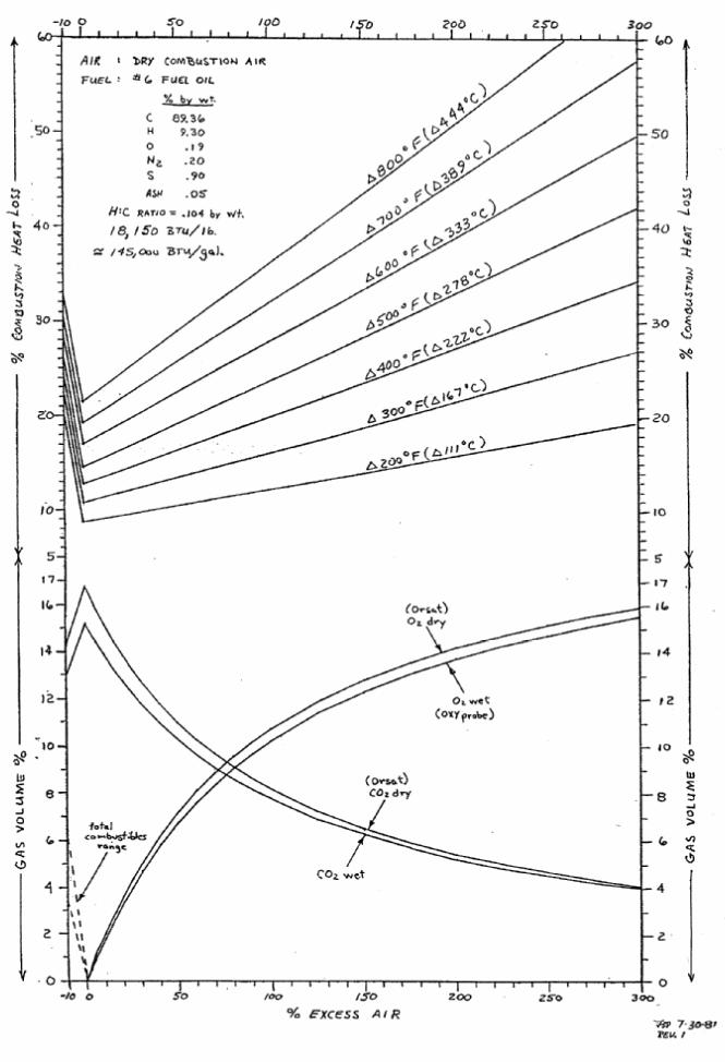
Blue Circle Cement

PROCESS ENGINEERING TRAININGPROGRAM

PRESENTATION

The Physics of Air

The Physics Of Air

Cement Manufacturing Process

■ Big Rocks - Bash to bits make powder

■ Burn powder until semi-molten

■ Cool (almost) molten material to little rocks

■ Little Rocks - Bash the living daylights outof - add some gypsum

■ = Product to sell to customer - Cement

Cement

■ Customer adds water and aggregate

■ Makes Big Rocks again !!!

■ (One) Common denominator

■ AIRFLOW

Units

■ Imperial - SI - US - Need to be able toconvert between

■ Temperature– Celcius - Fahrenheit

– C = (F*5/9) - 32

■ Pressure– inches / mm wg, mbar, kPa, atm

– 1 Atm = 101.325 kPa = 1013.25 mBar = 10330mm wg

Units / Air

■ ‘Normal’ Conditions

■ NTP = 0 C, 1 Atm

■ Air Composition– 78.1% N2

– 21% O2

– 0.9% Ar, + Trace other gases - CO2, H2, O3, Neetc.

■ Dry air acts as a ‘Perfect’ gas

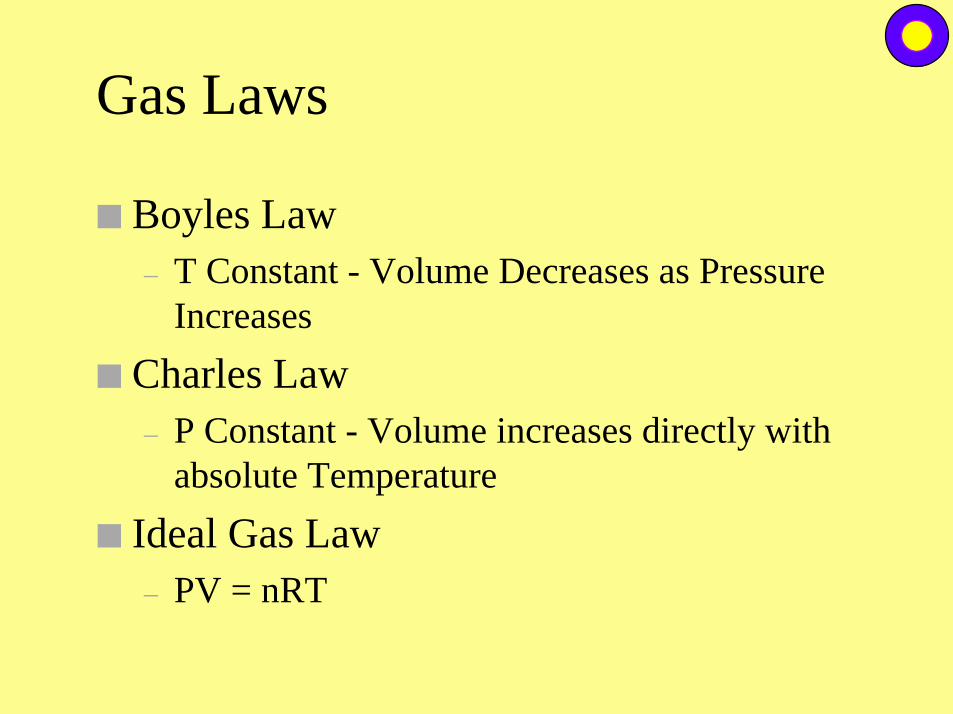
Gas Laws

■ Boyles Law– T Constant - Volume Decreases as Pressure

Increases

■ Charles Law– P Constant - Volume increases directly with

absolute Temperature

■ Ideal Gas Law– PV = nRT

Airflow

■ Air moves from High Pressure to lowpressure, requires certain P to start &maintain flow in a duct

■ Total Pressure = Static Pressure + VelocityPressure

■ Static Pressure - overcomes friction /obstacles -

■ Velocity Pressure - Pressure needed tomaintain air movement

Bernoulli’s Theorem

■ Conservation of energy– PE1 + KE1 = PE2 + KE2 + Losses

– Potential Energy ~ Static Pressure

– Kinetic Energy ~ Velocity Pressure

lhg

vhz

g

vhz +++=++

22

22

22

21

11

Airflow

■ Static & velocity Pressures interchangeable- but not 100% efficient due to frictionlosses

■ Pressures measured as ‘Gauge’ - relative toatmospheric– Static - at right angles to flow

– Velocity - in line with flow

Pressure loss / regain

■ Static & velocity Pressures interchangeable- but not 100% efficient due to frictionlosses