Programa de Doctorado “Matematicas”

PhD Dissertation

Problemas de Homogeneizacioncon Alto Contraste

High-Contrast Homogenization Problems

Author

Antonio Jesus Pallares Martın

Supervisor

Prof. Dr. Juan Casado Dıaz

Co-supervisors

Prof. Dr. Manuel Luna

Laynez

Prof. Dr. Marc Briane

September 15, 2016

This work has been supported by Ministerio de Economıa y Competitividad(Spain), grant MTM2011–24457. Programa de FPI del Ministerio de Economıa yCompetitividad, reference BES–2012–055158.

A mi princesa Marta

Agradecimientos

A mis directores Manuel Luna Laynez y Juan Casado Dıaz por su paciencia y por to-do el tiempo dedicado. A mi director Marc Briane por su ayuda durante mi estanciaen Rennes.

A todos los miembros del departamento de Ecuaciones Diferenciales y AnalisisNumerico. En especial, a todos los becarios y a Henrique Barbosa, Leandro y Tarc-yana, por hacer tan agradable un lugar de trabajo, por los buenos momentos y porel trato recibido.

A mis amigos por seguir ahı despues de tantos anos.A los familiares de Marta por su enorme ayuda durante estos anos y por hacerme

sentir como uno mas de la familia.A toda mi familia, tanto los que estan como los que se fueron, por su apoyo, su

ayuda y su comprension en todos los momentos de mi vida.Y especialmente a Marta por aconsejarme, acompanarme, valorarme y motivar-

me. Por iluminar mi camino y apoyarme en los momentos mas difıciles. Por estarsiempre a mi lado.

Sin vosotros esta tesis no habrıa sido posible. A todos, gracias.

7

Contents

Introduction 11

Introduccion 27

Bibliography 43

1 High-contrast homogenization of linear systems of partial di↵eren-tial equations 511.1 Introduction . . . . . . . . . . . . . . . . . . . . . . . . . . . . . . . . 521.2 Main result . . . . . . . . . . . . . . . . . . . . . . . . . . . . . . . . 551.3 A first homogenization result . . . . . . . . . . . . . . . . . . . . . . 601.4 Integral representation of the limit . . . . . . . . . . . . . . . . . . . 66Bibliography . . . . . . . . . . . . . . . . . . . . . . . . . . . . . . . . . . 70

2 Homogenization of equi-coercive nonlinear energies defined on vector-valued functions, with non-uniformly bounded coe�cients 732.1 Introduction . . . . . . . . . . . . . . . . . . . . . . . . . . . . . . . . 742.2 Statement of the results and examples . . . . . . . . . . . . . . . . . 77

2.2.1 The main results . . . . . . . . . . . . . . . . . . . . . . . . . 772.2.2 Auxiliary lemmas . . . . . . . . . . . . . . . . . . . . . . . . . 802.2.3 Examples . . . . . . . . . . . . . . . . . . . . . . . . . . . . . 83

2.3 Proof of the results . . . . . . . . . . . . . . . . . . . . . . . . . . . . 872.3.1 Proof of the main results . . . . . . . . . . . . . . . . . . . . . 872.3.2 Proof of the lemmas . . . . . . . . . . . . . . . . . . . . . . . 90

Bibliography . . . . . . . . . . . . . . . . . . . . . . . . . . . . . . . . . . 97

3 Asymptotic behavior of the linear elasticity system with varyingand unbounded coe�cients in a thin beam 1013.1 Introduction . . . . . . . . . . . . . . . . . . . . . . . . . . . . . . . . 1023.2 The homogenization result . . . . . . . . . . . . . . . . . . . . . . . . 1063.3 Proof of the results . . . . . . . . . . . . . . . . . . . . . . . . . . . . 111Bibliography . . . . . . . . . . . . . . . . . . . . . . . . . . . . . . . . . . 128

4 Homogenization of weakly equicoercive integral functionals in three-dimensional elasticity 1314.1 Introduction . . . . . . . . . . . . . . . . . . . . . . . . . . . . . . . . 132

9

10 Contents

4.2 The �-convergence results . . . . . . . . . . . . . . . . . . . . . . . . 1364.2.1 Generic examples of tensors satisfying ⇤(L)�0 and ⇤per(L)>0 1374.2.2 Relaxation of condition ⇤per(L) > 0 . . . . . . . . . . . . . . . 138

4.3 Loss of ellipticity in three-dimensional linear elasticity through thehomogenization of a laminate . . . . . . . . . . . . . . . . . . . . . . 1404.3.1 Rank-one lamination . . . . . . . . . . . . . . . . . . . . . . . 1424.3.2 Rank-two lamination . . . . . . . . . . . . . . . . . . . . . . . 153

Appendix . . . . . . . . . . . . . . . . . . . . . . . . . . . . . . . . . . . . 160Bibliography . . . . . . . . . . . . . . . . . . . . . . . . . . . . . . . . . . 164

Introduction

In the production of certain composite materials, the mixture of the components iscarried out at a microscopic level or, more precisely, at a mesoscopic level (small fromthe macroscopic point of view but su�ciently large to neglect the quantum e↵ects).The first di�culty involved is the numerical resolution of the partial di↵erentialequations that describe the behaviour of the related physical quantities. It would benecessary to use meshes whose elements are small compared to the measure of thestructures formed by the components of the mixture. This would lead to systemsof equations whose large sizes make their direct resolution virtually unattainable.Both physicians and engineers have usually tackled this kind of problems by insertingsome small parameters with the purpose of making an asymptotic expansion withrespect to them. As a consequence, they obtain much simpler problems whosesolutions provide a good approximation of the solution to the original problem.In many occasions, a later mathematical justification for the resulting models hasbeen obtained, proving some convergence results in certain functional spaces. Inmathematics, the homogenization theory is the field that deals with this type ofquestions.

As an example, we recall the perhaps most classical result in the theory of homo-genization. We consider the electric material obtained upon periodic repetition of acell with small period " > 0. The electrostatic theory states that the electrostaticpotential u" is a solution to

� div�A⇣x"

⌘ru"

�= ⇢ in ⌦, (1)

where ⌦ is an open subset of RN (N = 2, 3 in practice) and ⇢ is the charge density.The matrix of coe�cients A depends on the dielectric constant of the medium andis YN -periodic (where YN is the unit cube of RN). In order to have the uniqueness ofsolution to (1), an additional boundary condition is clearly needed. The generationof materials under this procedure is very common in engineering.

The method of asymptotic expansions (see e.g. [9], [65], [71], [84], [85]) appliedto this problem consists in assuming that the function u" admits an expansion ofthe type

u"(x) ⇠ u0(x) + "u1

⇣x,

x

"

⌘+ "2u2

⇣x,

x

"

⌘+ · · · ,

with u1, u2, . . . periodic with respect to their second variable. By replacing it in (1)and identifying the coe�cients with the same power of ", one formally obtains thatu0 is a solution to

� div(Ahru0) = ⇢ in ⌦, (2)

11

12

where Ah (the homogenized matrix) is defined by

Ah⇠ =

Z

YN

A(⇠ +ryw⇠) dy, 8 ⇠ 2 RN , (3)

with w⇠ solution to ⇢ �div (Arw⇠) = 0 in RN ,w⇠ YN -periodic.

In addition, it is possible to prove

u1(x, y) = wru0(x)(y).

The previous result explains the term homogenization. Whereas in (1) we had astrongly heterogeneous material, the constant matrix Ah in (2) corresponds to ahomogeneous material. Note also that the numerical resolution of u0 and u1 ismuch simpler than that of u". From a more theoretical point of view and on themacroscopic side, the electric properties of the material corresponding to A(x/") aresimilar to the properties of the material modelled by Ah. If, for instance, the matrixA is the outcome of the mixture of two materials, i.e. there exist a measurable setZ ⇢ YN and two matrices A1, A2 such that

A(y) = A1�Z(y) + A2(1� �Z(y)), a.e. y 2 YN ,

then, we build a new material, corresponding to Ah, whose properties depend notonly on the proportion of the two mixed material (i.e. the measure of Z) but alsoon their geometric arrangement. Therefore, even if A1 and A2 are scalar matricescorresponding to isotropic materials (i.e. their properties do not depend on thedirection), the homogenized matrix Ah does not need to be scalar.

Even though the method described above for obtaining Ah is formal, some con-vergence results can be found in [9] and [65]. In fact, due to its importance inarchitecture and engineering, many methods have been developed in order to math-ematically solve problems with some periodicity assumption like the one above. Wewould like to highlight the two-scale convergence and the unfolding methods ([2],[4], [34], [36], [41], [81]).The previous example shows how the process of obtaining new materials throughthe mixture of existing ones can be analysed using highly oscillating distributions.This is done by studying the asymptotic behaviour of PDE with varying coe�cients.Although we talked about a periodic problem before, it is also of great importanceto know the behaviour of similar problems under no periodicity condition in orderto be able to obtain more general materials. In this context, the first question thatarises is whether or not the kind of equations that we are dealing with is stable inthe limit. Otherwise we would need more general models.To our knowledge, the first results regarding the stability in the limit of a sequenceof PDE with varying coe�cients deal with the case of a sequence of second-orderelliptic linear equations in the divergence form. S. Spagnolo showed in [87] (see also

Introduction 13

[52]) that if the sequence of symmetric matrix-valued functions An is bounded inL1(⌦)N⇥N and is uniformly elliptic in the sense that there exists ↵ > 0 satisfying

An⇠ · ⇠ � ↵|⇠|2, 8n 2 N, 8 ⇠ 2 RN , a.e. ⌦, (4)

then there exist a subsequence of An, still denoted by An, and a symmetric matrixfunction A 2 L1(⌦)N⇥N also fulfilling (4) such that for every f 2 H�1(⌦), thesolutions to (

�div (Anrun) = f in ⌦,

un = 0 on @⌦,(5)

weakly converge in H10 (⌦) to the solution u of the problem obtained upon substitu-

tion of An by A. The extension of this result to the corresponding parabolic operatoris also shown in the cited reference (the extension to the hyperbolic case appearsin [43]). F. Murat and L. Tartar later generalised this result to the case of generalmatrices without any assumption of symmetry ([76]), also proving the convergenceof Anrun to Aru in L2(⌦)N . This result can be easily extended to systems ofelliptic equations and, especially to the linear elasticity system that describes theelastic deformation of a solid (supposing that the derivatives of the deformations arenegligible). We refer to the works of G. Francfort [59], E. Sanchez-Palencia [85] andG. Duvaut (unavailable reference). The proof of this result relies on the oscillatingfunctions method and the key idea is to use specific sequences of test functions (thepreviously mentioned two-scale convergence is also based on this idea). An essentialtool in this proof is the div-curl theorem, which is the best known result of thecompensated compactness theory, also introduced by F. Murat and L. Tartar ([77],[89]). The div-curl theorem states that for p 2 (1,1), if

�n * � in Lp(⌦)N , ⌧n * ⌧ in Lp0(⌦)N ,

div �n ! div � in W�1,p(⌦), curl ⌧n * curl ⌧ in W�1,p0(⌦)N⇥N ,(6)

then�n · ⌧n * � · ⌧ in D0(⌦).

Although the convergence result for (5) is usually stated with homogeneous Dirichletboundary conditions as we did, it also holds for other kinds of boundary conditions.In addition, the result is local in the sense that the value of the homogenized matrixA in an arbitrary open subset of ⌦ only depends on the values of An in that subset.Some extensions to nonlinear equations can be found e.g. in [82] and [53].

It is also worth mentioning that this sort of results is applied to the resolutionof optimal material design problems by providing relaxed formulations (see e.g. [2],[35], [80]).

A common question that emerges from the cited results is what happens if thesequence An is not uniformly bounded or uniformly elliptic. This is known as high-contrast homogenization.

A very useful tool that allows to tackle this kind of problems is the �-convergencethat was introduced by E. De Giorgi (see e.g. [12], [14], [48], [51]). Let X be a metricspace (the definition can be extended to non metric spaces) and Fn : X ! R[{+1}

14

a sequence of functionals, Fn is said to �-converge to F in X if the two followingconditions hold:

8<

:

xn ! x in X =) lim infn!1

Fn(xn) � F (x),

8 x 2 X, 9xn ! x such that lim supn!1

Fn(xn) F (x).

The most important result in the �-convergence theory states that if Fn reaches aminimum at xn and the sequence xn is compact in X, then every limit point of xn

is a point of minimum of F . Therefore, if we go back to problem (5) and assumethat An is symmetric, then un is a solution if and only if it is a solution to

minu2H1

0 (⌦)

⇢Z

⌦

Anru ·ru dx� 2hf, ui�.

Furthermore, taking into account that, thanks to (4), the solutions to (5) arebounded in L2(⌦), we can conclude that the result by S. Spagnolo can be deducedby showing (assuming that the right-hand side belongs to L2(⌦))

u 7!

Z

⌦

�Anru ·ru� 2fu

�dx

���!u 7!

Z

⌦

�Aru ·ru� 2fu

�dx

�in L2(⌦),

or, equivalently (as a consequence of considering f as an element of the dual ofL2(⌦))

u 7!

Z

⌦

Anru ·ru dx

���!u 7!

Z

⌦

Aru ·ru dx

�in L2(⌦).

This formulation has the advantage that the functional

u 7!Z

⌦

Anru ·ru dx, (7)

is well defined even though the integral might be infinite. This allows to work withthe case of An not being in L1(⌦)N⇥N more easily. However, the disadvantage isthat it must be possible to write the problem as a minimization problem.

As a classic example of applicability of the theory of �-convergence to the res-olution of homogenization problems, we point out the work [33] by L. Carbone andC. Sbordone, where they analyse the �-convergence in L1(⌦) of the sequence offunctionals

u 7!Z

⌦

Fn(x, u,ru) dx, (8)

with Fn : ⌦ ⇥ R ⇥ RN ! R a sequence of Caratheodory functions (measurable inthe first variable and continuous in the other two), convex with respect to the lastvariable and such that

0 Fn(x, s, ⇠) an(x)(1 + |s|p + |⇠|p), 8 (s, ⇠) 2 R⇥ RN , a.e. x 2 ⌦, (9)

Introduction 15

with p > 1 and an bounded in L1(⌦). The authors show that, for a subsequence of n,there exists the �-limit of these functionals in L1(⌦) and that it admits an integralrepresentation of the same type, at least for the regular functions. Moreover, if anis equi-integrable then the �-limit in L1(⌦) coincides with the �-limit in L1(⌦). Inaddition the homogenization process is local as in the previous cases.

If we wanted to apply this result to the convergence of minima, then these func-tionals would need to attain a minimum and, also, these minima would have to becontained in a compact set of the considered topology. Thus, if an is equi-integrable,it is enough to have the boundedness of the sequence of minima in W 1,1(⌦). Thiscan be achieved imposing some suitable coercivity condition, for instance,

0 bn(x)|⇠|p Fn(x, s, ⇠), 8 (s, ⇠) 2 R⇥ RN , a.e. x 2 ⌦, b� 1

pn bounded in Lp0(⌦).

If an were only bounded in L1(⌦), we would need the sequence of minima to becompact in L1(⌦), which, essentially, would mean to take p > N and a coercivitycondition such as

↵|⇠|p Fn(x, s, ⇠), 8 (s, ⇠) 2 R⇥ RN , a.e. x 2 ⌦, ↵ > 0.

As an example, the results in [33] can be applied to problem (5), deducing that, forN � 2 and An symmetric satisfying

bn(x)|⇠|2 An(x)⇠ · ⇠ an(x)|⇠|2, 8 ⇠ 2 RN , a.e. x 2 ⌦,an, bn � 0, an bounded in L1(⌦), equi-integrable, b�1

n bounded in L1(⌦),

and f regular enough, then the solutions to (5) converge weakly-⇤ in BV (⌦) to thesolution to a problem of the same type.

In [56] (see also [8], [28]) V. N. Fenchenko and E. Ya. Khruslov provide anexample where an is a function bounded in L1(⌦) (but not equi-integrable) with⌦ = ! ⇥ (0, 1) and ! is an open bounded subset of R2, satisfying that the solutionsto (

�div (anrun) = f in ⌦,

un = 0 on @⌦,

converge in H10 (⌦)-weak to the solution to8<

:��u+ 2⇡

✓u+

Z 1

0

h(x3, t)u(x1, x2, t)dt

◆= f in ⌦,

u = 0 on @⌦,

where h is a nonzero function. This is a case where the limit equation changes.In the limit we find a term of zero order and a nonlocal term. A general resultin the same vein has been obtained by U. Mosco in [74] where, making use of theBeurling-Deny representation formula of Dirichlet forms ([10]), it is proved that the�-limit in L2(⌦) of the sequence of functionals given by (7), with An nonnegative,bounded in L1(⌦)N⇥N and symmetric, converge to a functional of the type

u 7!Z

⌦

Aru ·ru dµ(x) +

Z

⌦

u2d⌫(x) +

Z

⌦⇥⌦

�u(x)� u(y)

�2d⌘(x, y), (10)

16

with µ, ⌫ and ⌘ nonnegative bounded Borel measures. In general, the homogeniz-ation process thus leads us to nonlocal terms even if one starts with strongly localterms.

Thanks to a generalisation of the div-curl theorem, it has been proved later in[17], [19] that, in dimension N = 2, assuming that An is uniformly elliptic, thetwo last terms are actually zero, i.e. the functional does not change of form upon�-convergence and thus, the homogeneization process remains local. This resulthas been subsequently generalised in [20], where the authors show that it is noteven necessary to impose the condition of boundedness in L1(⌦)N⇥N . Some relatedresults concerning equations in the periodic case and the appearance of zero-orderterms can be found in [13] and [21] respectively. All these works make use of certainrecent results of uniform convergence for the solutions to elliptic PDE ([22], [72]).In fact, with these ideas it has been obtained in [23] an extension of the resultsby L. Carbone and C. Sbordone in [33] where the condition p > N � 1 (insteadof p > N) implies the equivalence between the �-limit in L1(⌦) and L1(⌦) of thefunctionals defined by (8).

The results of uniform convergence in the references [13], [20], [21], [23] and [33]rely on the maximum principle, and so does the Beurling-Deny formula that leadsto expression (10). For this reason, the generalisation of these results to the caseof systems of equations does not hold. As a consequence, contrary to (10), theabsence of a uniform bound of the coe�cients in the linear elasticity may cause theappearance of second-order derivatives in the �-limit as proved by C. Pideri andP. Seppecher in [83]. Furthermore, M. Camar-Eddine and P. Seppecher showed in[32] that it is possible to reach any lower-semicontinuous quadratic functional thatvanishes for the rigid movements.

Due to the lack of the maximum principle, there are not general results, to ourknowledge, about what assumptions of boundedness or ellipticity on the coe�cientsare needed in order for a system of PDE to keep its structure in the limit and forthe homogenization process to be local. It is worth mentioning the existence ofsome particular results for the linear case via �-convergence. For N = 2, it hasbeen proved in [18] the stability of the linear elasticity system assuming that thecoe�cients are uniformly elliptic and bounded in L1. This result is based on thegeneralisation of the div-curl theorem in [26]. Another result relative to a generalelliptic system corresponding to M equations in an open set ⌦ ⇢ RN has beenobtained in [24], where the authors consider a sequence of coe�cients tensors An

such that there exists another sequence of uniformly elliptic and bounded tensorsBn in such a way that An�Bn strongly converges to zero in L1(⌦;L(RM⇥N)). Notethat the uniform ellipticity is imposed in an integral way, i.e.

↵

Z

⌦

|Du|2dx Z

⌦

AnDu : Dudx, 8 u 2 H10 (⌦)

M , (11)

with ↵ > 0. It is known (see e.g. [48]) that this implies

An⇠ : ⇠ � ↵|⇠|2, 8 ⇠ 2 RM⇥N , Rank(⇠) = 1, a.e. ⌦, (12)

and thus, in the case of equations (M = 1), it is equivalent to (4). However, thisis not the case for systems. In order to distinguish these cases, in the literature,

Introduction 17

it is common to say that a tensor which satisfies (12) is strongly elliptic whereas,in the case when this condition holds for all ⇠ 2 RM⇥N , then it is said to be verystrongly elliptic. The theory of compensated compactness shows that if An is aregular function in ⌦ then conditions (12) and (11) are equivalent.

The main problem that we are going to tackle in the two first chapters of thisthesis is to obtain some ellipticity and/or boundedness conditions in an arbitrarydimension, for linear and nonlinear systems, that lead to a local limit system. Forthat, we will make use of certain extensions of the div-curl theorem ([25], [26]).In the third chapter we will go on with this question but when there is also areduction of dimension in the domain. Namely, we consider the elasticity systemfor the thin beam ⌦" = (0, 1) ⇥ ("!) where ! is an open bounded regular subsetof RN�1. Contrary to the previous chapters where the problem is posed in a fixeddomain, now we intend to deduce a uni-dimensional limit system. This is a classicalproblem in engineering. When trying to directly solve a problem of PDE posedin a domain where at least one of the dimensions is much smaller than the rest,we usually come across the previously mentioned di�culty of having to use veryfine meshes. The idea in homogenization is to approximate the solutions of theproblem by those of a problem posed in a domain of smaller dimension. Therefore,in the case of a beam, the problem that is usually solved, consists in two uncoupledelliptic equations of fourth order. From the mathematical point of view (see e.g.[68], [92]) these equations are obtained by passing to the limit in the elasticitysystem corresponding to a homogeneous isotropic material in dimension 3 when thethickness of the beam tens to zero. The solution to the limit problem provides anapproximation of the transverse deformations of the beam. More generally, in [79](see also [37]) the authors consider an elasticity tensor of the form A(x1, x2/", x3/"),where A is an element of L1((0, 1) ⇥ !;L(R3⇥3

s )) and satisfies the usual ellipticitycondition. This allows, for instance, to deal with materials in which there is akernel of a certain material surrounded by another one. In this case the obtainedapproximation of the deformation is more complex.

Continuing the discussion from the beginning of this introduction, an importantproblem is to know what happens when the thin domain (beam or plate) is formedby an arbitrary mixture of materials. This leads to the study of the asymptoticbehaviour of a problem of PDE posed in a thin domain ⌦", where " > 0 is a smallvalue that measures the thickness and where the coe�cients also depend on ". Upto our knowledge, this problem has not been studied so deeply as the case wherethere is a fixed domain. Nonetheless, we can refer to some related works such as[5], [30] and [86], where the authors analyse this problem under certain periodicityconditions. As it has been previously explained, this allows to deal with materialsthat are usually present in engineering. However, if we were interested in deducingwhat materials can be constructed upon the mixture of given ones, we would needto remove the conditions of periodicity. In the case of di↵usion problems in a beam(0, 1) ⇥ ("!) and assuming uniform ellipticity and boundedness, the problem hasbeen studied in [45] under certain conditions on the structure that allow to apply aresult of the div-curl type as well as in [39] for a general setting. In this last reference,the authors deal with very general right-hand-side terms and deduce a limit system

18

posed in the domain (0, 1) ⇥ ! which is nonlocal in general. When we restrict toright-hand-side terms that do not strongly oscillate in the variables corresponding tothe degenerating dimensions, the limit problem is reduced to a one-dimensional localproblem. For the study of the asymptotic behaviour of the elasticity system withvariable coe�cients in a degenerating domain, we cite [50] where the case of a beam! ⇥ (0, ") with ! ⇢ R2 open and bounded, is considered. Under suitable conditionsof isotropy and assuming that the coe�cients are uniformly elliptic and bounded, itis obtained a fourth-order limit equation corresponding to the vertical displacement,which is similar to the usual case studied in engineering for plates formed by isotropicmaterials. The case when there is no isotropy but the coe�cients only depend on theheight variable is analysed in [62]. In the limit system for this case it is not possibleto uncouple, in general, the deformations in the horizontal and vertical variables.

Along this introduction, we have mentioned many cases for which the structureof a problem of PDE, where the coe�cients are variable, is preserved in the limit.Nevertheless, there are notable examples where some important properties are lostin the limiting process. This can be used to construct materials with very particularproperties. In this sense, we analyse the di↵erence between local and global coerciv-ity that we mentioned above when we talked about the homogenization of systems.It is a known result that the formula of periodic homogenization (3) remains truefor systems by imposing integral (instead of pointwise) coercivity. Moreover, for thecase M = N it has been proved in [61] that it su�ces to have the existence of ↵ > 0such that (for A YN -periodic)

8>><

>>:

Z

YN

ADu : Dudy � ↵

Z

YN

|Du|2dy, 8 u 2 H1loc(RN) YN -periodic,

Z

RN

ADu : Dudy � 0, 8 u 2 D(RN)N .

(13)

An interesting question is what properties of ellipticity are fulfilled by the homo-genised tensor. S. Gutierrez proves in [64] that, a certain homogenization scheme(called 1⇤-convergence in [27]) applied to the lamination of a strongly elliptic iso-tropic material, in the sense that (12) holds, and a very strongly elliptic isotropicmaterial (i.e. that (12) holds for all ⇠ 2 RN⇥N), can lead to a limit material thatdoes not even satisfy the strong ellipticity condition. S. Gutierrez carries out thisstudy for the two- and three-dimensional cases. In some cases in dimension 3, it isin fact necessary to perform a second lamination with a third material (that canbe chosen very strongly elliptic). However, the process followed by S. Gutierrez re-quires a priori bounds in L2 for the sequence of deformations, which is incompatiblewith the assumption of weak coercivity. Therefore, S. Gutierrez’ result does notaddress the asymptotic behaviour of the corresponding sequence of systems of PDE.In [27], the authors provide, for the two-dimensional case, a justification of this res-ult in terms of �-convergence and show the canonical character of the laminationperformed by S. Gutierrez. Recall that if the tensor functions x 7! A(x/") fulfilledthe uniform integral ellipticity condition

Z

⌦

A⇣x"

⌘Du : Dudx � ↵

Z

⌦

|Du|2 dx, 8 u 2 C1c (⌦)N , (14)

Introduction 19

with ↵ > 0 (independent of "), then the �-limit would also satisfy this property.This means that the tensor A constructed by S. Gutierrez does not satisfy condition(14), although each one of the homogeneous phases of A does. As it has beenpointed out by M. Briane and G. Francfort in [27], there exist tensor functionsA : RN ! L(RN⇥N) with jump discontinuities such that (12) holds for ⌦ = RN

but where condition (11) fails. This can be easily seen with the change of variabley = x/". This means that the equivalence between the two definitions that wementioned before for a regular tensor function A is not true in general.

In the fourth chapter of this thesis we provide justification for the results byS. Gutierrez in the three-dimensional case through the �-convergence theory.

In the exposition that we have conducted so far, we have introduced the di↵erentproblems that interest us in the present PhD project, their motivation and theexisting related results carried out by other authors. In addition, we have outlinedthe precise questions that we intend to tackle. In what follows, we provide an explicitdescription of the problems that we study in each chapter of this PhD project, theresults that we have obtained as well as the di�culties that arose and the methodsand tools that we used to overcome them.

Chapter 1

We consider ⌦ an open bounded subset of RN , N � 2, and an integer numberM � 1. In this chapter we study the asymptotic behaviour of the following ellipticlinear problems (

�Div (AnDun) = fn in ⌦,

un = 0 on @⌦.(15)

Our purpose is to give conditions of integrability and ellipticity on the sequence oftensor functions An 2 Lp(⌦;L(RM⇥N)) in order for the homogenized problem to beof the same type, at least for su�ciently regular elements, and in order to have a localhomogenization process. As mentioned above, in the case of equations (M = 1),it is enough to have A�1

n bounded in L1(⌦)N⇥N and An bounded in L1(⌦)N⇥N andequi-integrable. In fact, the result is not true if the condition of equi-integrabilityof An is removed. The proof of these results uses the maximum principle and thus,it is not valid for systems.

In our case, we first show the existence of an abstract homogenization resultwhen the coe�cients An only fulfil

An bounded in L1(⌦;L(RM⇥N)), (16)

An⇠ : ⇠ � 0, 8 ⇠ 2 RM⇥N , (17)

9K > 0,

Z

⌦

|Du|dx K

✓Z

⌦

AnDu : Dudx

◆ 12

, 8 u 2 W 1,10 (⌦)M . (18)

20

In the proof we use some estimates which are based on the theory of �-convergenceapplied to the symmetric part of An. For that, we also assume that the skew-symmetric part of An can be uniformly controlled by the symmetric part, namely,

9R > 0, |An⇠ : ⌘| R|An⇠ : ⇠| 12 |An⌘ : ⌘| 12 , 8⇠, ⌘ 2 RM⇥N , 8n 2 N, a.e. ⌦. (19)

Moreover, note that thanks to condition (16) we can assume the existence of a 2M(⌦) such that

|An| ⇤* a en M(⌦). (20)

The mentioned theorem (see Theorem 1.16 for further details) states

Theorem 0.1. Assume An 2 L1(⌦;L(RM⇥N)) satisfies (16), (17), (18) and (19).Then, there exist a subsequence of n, still denoted by n, a Hilbert space H ⇢W 1,1

0 (⌦)M and a continuous linear operator ⌃ : H ! L1a(⌦)

M⇥N such that forevery sequence fn weakly-⇤ converging to f in L1(⌦)M , the unique solution to (15)satisfies

un⇤* u in BV (⌦)M ,

AnDun⇤* ⌃(u)a in M(⌦)M⇥N . (21)

Observe that (21), together with the convergence of fn, establishes that u is asolution to the equation

�Div�⌃(u)a

�= f in ⌦,

and thus, it gives the existence of a limit equation. However, it does not yield arepresentation of ⌃. We recall that even for the case M = 1, the limit ⌃ is nonlocalin general, and therefore it does not have the form of ⌃(u) = ADu for some tensorfunction A.

The result that we show in this chapter (Theorem 1.16) is actually more generaland, additionally, it gives the convergence of the energies in the sense that thereexists a continuous bilinear operator B : H ⇥ H ! M(⌦) such that if un is as inthe theorem and vn is a sequence in W 1,1

0 (⌦)M that fulfils

vn⇤* v in BV (⌦)M , lim sup

n!1

Z

⌦

AnDvn : Dvn dx < +1,

thenAnDun : Dvn

⇤* B(u, v) in M(⌦).

Furthermore, this operator B is related to ⌃ by

B(u, v) = ⌃(u) : Dv a in ⌦, 8 v 2 C10(⌦)

M ,

and u is the unique solution to

8<

:

u 2 H,Z

⌦

dB(u, v) =Z

⌦

f · v dx, 8 v 2 H.

Introduction 21

Observe that the ellipticity condition (18) on An is integral instead of pointwise.As mentioned above, these two conditions are not equivalent in the case of systems.This allows us to apply our results to the linear elasticity, where pointwise ellipticityfails. A su�cient pointwise condition in order to have (18) would be to impose A�1

n

bounded in L1(⌦;L(RM⇥N)).In order to have a local representation of the operator ⌃ (and of B) it is necessary

to assume some integrability conditions on An. The obtained result is based on thediv-curl theorem in [26], which, contrary to the classical result (see (6)), is applicableto the case of �n bounded in Lp(⌦)N and ⌧n bounded in Lq(⌦)N with

1

p+

1

q 1 +

1

N. (22)

We have (see Theorem 1.11 for further details)

Theorem 0.2. Under the assumptions of Theorem 0.1, let us also assume that

An bounded in Lp(⌦;L(RM⇥N)), p 2N

2,1�,

Z

⌦

|Du|rdx Z

⌦

�n(AnDu : Du)r2dx, 8u 2 W 1,r

0 (⌦)M , 8n 2 N,

with

r =2Np

(N + 2)p�N, �n bounded in L

22�r (⌦),

then there exists A 2 Lp(⌦;L(RM⇥N)) such that

⌃(u)a = ADu, 8 u 2 H \W 1, 2pp�1 (⌦)M .

It is worth pointing out that if a weaker integrability is imposed on An (i.e. smal-ler p), then a stronger ellipticity (larger r) is required for the integral representationand, conversely, a stronger integrability condition would allow a weaker ellipticity.

In addition, this theorem also includes, in particular, the results in [18] for thetwo-dimensional elasticity system with coe�cients uniformly elliptic and boundedin L1, which also uses the version of the div-curl theorem in [26].

Chapter 2

As in the previous chapter, we consider an open bounded set ⌦ ⇢ RN with N � 2and an integer number M � 1. In this chapter we analyse the �-limit in Lp(⌦)M ,p > 1, of sequences of nonlinear functionals defined over vector functions of the type

Fn(v) :=

Z

⌦

Fn(x,Dv) dx for v 2 W 1,p0 (⌦)M . (23)

22

We assume that the energy densities Fn : ⌦ ⇥ RM⇥N ! [0,1) are Caratheodoryfunctions such that there exist ↵, �, � > 0 and two sequences of non-negative meas-urable functions hn, an, with hn bounded in L1(⌦) and an bounded in Lr(⌦), where

(r > N�1

p, if 1 < p N � 1,

r = 1, if p > N � 1,

satisfying the following assumptions of (integral) ellipticity, growth and Lipschit-zianity

Fn(·, 0) = 0, a.e. ⌦, (24)Z

⌦

Fn(x,Du) dx � ↵

Z

⌦

|Du|p dx� �, 8u 2 W 1,p0 (⌦)M , (25)

Fn(x,�⇠) hn(x) + �Fn(x, ⇠), 8� 2 [0, 1], 8⇠ 2 RM⇥N , a.e. x 2 ⌦, (26)8><

>:

��Fn(x, ⇠)� Fn(x, ⌘)��

�hn(x) + Fn(x, ⇠) + Fn(x, ⌘) + |⇠|p + |⌘|p�p�1p an(x)

1p |⇠ � ⌘|,

8 ⇠, ⌘ 2 RM⇥N , a.e. x 2 ⌦.(27)

Condition (24) implies that the functionals (23) reach a minimum for v = 0 whichis usual in nonlinear elasticity. This means that in the equilibrium (no displace-ments) the elastic energy is zero. Concerning the rest of the assumptions, they arealso fulfilled in the usual models of nonlinear elasticity, for instance, some hyper-elastic materials such as the Saint Venant-Kirchho↵ materials and some Ogden’stype hyper-elastic materials ([40], Vol. 1). As a prototypical example, consider

Fn(x, ⇠) = |An(x)⇠s : ⇠s|p2 , 8 ⇠ 2 RM⇥N , a.e. x 2 ⌦,

with ⇠s the symmetric part of ⇠. In this case, one can take

an(x) = |An(x)|p2 ,

which shows that an essentially measures how big the coe�cients are.We do not impose the convexity of Fn with respect to its second variable as

it is usual in equations. In fact, it is known that the �-limit of a sequence offunctionals in a given topology agrees with the �-limit of the lower-semicontinuoushull of these functionals. It is also known that if a functional of the type (23) islower semicontinuous for the topology of Lp(⌦) then Fn, as a function of its secondvariable, is convex for the rank-one matrices (Fn is rank-one convex). For this reason,contrary to the case of equations, the assumption of convexity is more restrictive forsystems.

As a consequence of the nonlinearity of the problem, the div-curl theorem cannotbe applied directly as we did in the previous chapter. Nevertheless, we make use ofa lemma in [25] which is essential for the proof of the version of the div-curl theoremthat appears in the same reference. It is a compactness result for bounded sequencesin W 1,q based on the embedding W 1,q(SN�1) ⇢ Lq⇤(SN�1), where SN�1 is the unit

Introduction 23

sphere of RN�1. Whereas in the div-curl theorem in [26] condition (22) is assumed,in [25] it is only necessary to have

1

p+

1

q< 1 +

1

N � 1.

As a result, if we applied the results in this chapter to the linear case (i.e. Fn

quadratic with respect to its second variable), we could improve the main theoremof the previous chapter when r = 2, An symmetric and N � 3, showing that theassumption p � N/2 can be relaxed by replacing it by p > (N � 1)/2.

The main results of this chapter (see Theorems 2.3 and 2.4 for further details)show the existence of a function F : ⌦⇥RM⇥N ! R which satisfies similar propertiesto those of Fn such that, at least for regular functions, the �-limit F in Lp(⌦)M ofthe sequence Fn satisfies

F (v) =

Z

⌦

F (x,Dv) dx.

Furthermore, the result is local in the sense that the value of F in an open subsetof ⌦ only depends on the value of Fn in that subset.

Chapter 3

In this chapter we consider the linear elasticity system posed in a thin beam ofthickness " > 0, ⌦" := (0, 1)⇥ ("!), when the tensor of coe�cients also depends on". Specifically, we study the problem

(� div(A"e(u")) = h" in ⌦",

A"e(u")⌫ = 0 on (0, 1)⇥ ("@!),(28)

where ! ⇢ RN�1 is a regular, connected, bounded domain (in practice N = 2, 3),⌫ is the unitary outward normal vector to ! on @!, u" is the deformation of thebeam, e(u") is the strain tensor and h" = (h",1, h0

") is the exterior force that will beassumed of the type

h",1(x) = f1

✓x1,

x0

"

◆, h0

"(x) = "f 0✓x1,

x0

"

◆+ g0

✓x1,

x0

"

◆, a.e. x 2 ⌦",

with f 2 L2(⌦)N and g0 2 L2(⌦)N�1 (where ⌦ := ⌦1) such that

Z

!

g0dy0 = 0, a.e. y1 2 (0, 1).

Observe that, in order to have the uniqueness of solution, it would be necessary toimpose some boundary condition on {0, 1} ⇥ ("!). Our results remain true withdi↵erent boundary conditions.

24

Our aim is to find a one-dimensional limit system whose solution provides an approx-imation of the solutions to (28) without any assumption of isotropy or homogeneityon the elasticity coe�cients A".

For the sake of simplicity, we assume uniform ellipticity, that is

9↵ > 0, A"⇠ : ⇠ � ↵|⇠|2, 8⇠ 2 RN⇥Ns , a.e. (0, 1)⇥ ("!).

Nevertheless, as done in the previous chapters, we do not require the coe�cients tobe uniformly bounded. Namely, we just impose

"kA"kL1(⌦";L(RN⇥Ns )) ! 0, kA"kL1(⌦";L(RN⇥N

s )) bounded.

The main result that we obtain (see Theorem 3.1) gives an approximation forthe solutions of the type

8>>>>><

>>>>>:

u",1(x) ⇠ u1(x1)�NX

j=2

duj

dx1(x1)

xj

",

u",j(x) ⇠ 1

"uj(x1) +

NX

i=2

Zji(x1)xi

", j 2 {2, · · · , N}.

(29)

This approximation consists in the sum of a deformation of Bernouilli-Navier’s typegiven by the function u = (u1, . . . , uN) plus a torsion term given by the matrixfunction Z, which is skew-symmetric. The latter corresponds to an infinitesimalrotation around the axis of the beam. We show that the functions u and Z aresolutions to a one-dimensional linear system that, in variational form, reads as8>>>>>><

>>>>>>:

Z 1

0

Ae0(u, Z) :e0(u, Z) dy1 =1

|!|Z

⌦

✓f1

✓u1 � du0

dy1· y0◆+ f 0 · u0 + g0 · (Z y0)

◆dy,

8(u, Z) 2 H10 (0, 1)⇥H2

0 (0, 1)N�1 ⇥H1

0 (0, 1;R(N�1)⇥(N�1)sk ),

with

Z 1

0

Ae0(u, Z) : e0(u, Z) dx1 < 1,

(30)where the subindex sk refers to skew-symmetric matrices and the operator e0 isdefined by

e0(u, Z) :=

0

BBB@

du1

dx1

✓d2u0

dx21

◆T

d2u0

dx21

dZ

dx1

1

CCCA.

In addition, the tensor function A belongs to L1(0, 1;L(RN⇥Ns1sk0

)) and is such thatthere exist �, � > 0 and a 2 L1(0, 1), a � 0, satisfying

|AE| ��AE : E

� 12a

12 , 8E 2 RN⇥N

s1sk0, a.e. (0, 1),

|E|2 �AE : E, 8E 2 RN⇥Ns1sk0

, a.e. (0, 1),

Introduction 25

where RN⇥Ns1sk0

is the subspace of the matrices M 2 RN⇥N that satisfy

M1i = Mi1, i = 1, . . . , N, Mij = �Mji, i, j = 2, . . . , N.

Observe that, even though the sequence A" is only bounded in L1, the limit tensorA also belongs to L1. The proof of this result is an adaptation of the classical proofof the H-convergence theorem by F. Murat and L. Tartar (cf. [76, 91]) combinedwith a decomposition result for sequences of deformations in thin domains that canbe found in [38].The limit system (30) provides a general model for strongly heterogeneous beamsthat do not satisfy any isotropy condition. Recall that for a homogeneous isotropicmaterial, the model used in architecture or engineering corresponds (in dimension3) to a system of two fourth-order equations (given by the functions u2 and u3 in(30)).

Chapter 4

In this chapter we focus on the homogenization, via �-convergence, of weakly coer-cive integral energies with densities L(x/")Dv : Dv, where L 2 L1

per(YN ;Ls(RN⇥Ns ))

is a periodic, symmetric, tensor function.

This chapter is divided into two main parts.

In the first part of Chapter 4, we analyse condition (13) (with A replaced by L)which, as previously mentioned, is enough in order for the periodic homogenizationformula (3) to hold for systems. In [27], the authors give a class of examples indimension 2 that fulfil (13) but such that L is not very strongly elliptic (i.e. (12)does not hold for all ⇠ 2 RN⇥N). Following the same ideas, in Theorem 4.4 we showa set of mixtures in dimension 3 that satisfy (13) and are not very strongly elliptic.In addition, Theorem 4.5 improves condition (13) showing that it is enough to have

Z

RN

LDu : Dudy � 0, 8 u 2 D(RN)N . (31)

for the �-convergence result to hold true.The second part of this chapter focuses on the loss of strong ellipticity through

the homogenization process in the case of linear elasticity in dimension 3. We makea deep study of the lamination process carried out by S. Gutierrez in [64] and we tryto justify it, in terms of �-convergence, by using Theorem 4.5. In order to apply thistheorem we need the relaxed functional coercivity (31) and, for that, we make useof the translation method for the null-Lagrangians. This method consists in findinga matrix D 2 R3⇥3 such that

LM : M +D : Adj(M) � 0 8M 2 R3⇥3, a.e. YN , (32)

as it was done in [27] for the two-dimensional case. Surprisingly, contrary to whathappens in dimension 2, we prove in Theorem 4.8 that if a strongly elliptic, lam-inated (i.e. L(y) = L(y1)) material fulfils (32), then it is impossible to obtain an

26

e↵ective material for which the strong ellipticity condition fails. Therefore, we needto perform a second lamination (in a new direction), as done by S. Gutierrez in[64], in order to produce a limit material that losses strong ellipticity. Indeed, The-orem 4.14 shows that there exist certain strongly elliptic materials for which thestrong ellipticity can be lost after a rank-two lamination with some specific verystrongly elliptic materials.

Introduccion

En la elaboracion de ciertos materiales compuestos, la mezcla de los distintos com-ponentes se realiza a nivel microscopico, o mas exactamente mesoscopico (pequenodesde el punto de vista macroscopico pero suficientemente grande para que se pue-dan despreciar los efectos cuanticos). La primera dificultad que esto entrana es laresolucion numerica de las ecuaciones en derivadas parciales que describen el com-portamiento de las distintas magnitudes fısicas relacionadas. Para ello, es necesariousar mallas cuyos elementos sean pequenos con respecto a la medida de las estructu-ras que forman los compuestos que aparecen en la mezcla. Esto da lugar a sistemasde ecuaciones tan grandes que su resolucion directa puede ser imposible. Tanto fısi-cos como ingenieros han atacado usualmente este tipo de problemas mediante laintroduccion de pequenos parametros con la idea de mas tarde llevar a cabo undesarrollo asintotico con respecto a ellos. Ello conduce a la resolucion de problemasmucho mas simples, los cuales proporcionan una buena aproximacion de la soluciondel problema original. En muchos casos, se ha dado posteriormente justificacionmatematica a los distintos modelos aproximados obtenidos, probandose resultadosde convergencia en ciertos espacios funcionales. La parte de la Matematica que seocupa de este tipo de cuestiones se conoce como teorıa de la homogeneizacion.

Como ejemplo recordamos el que probablemente es el problema mas clasico enhomogeneizacion. Por fijar ideas consideramos un material electrico que se obtie-ne repitiendo una celula de forma periodica con un pequeno periodo " > 0. Lasecuaciones de la electrostatica nos dicen que el potencial electrico u" es solucion de

� div�A⇣x"

⌘ru"

�= ⇢ en ⌦, (1)

donde ⌦ es un abierto de RN (en la practica N = 2, 3) y ⇢ es la densidad de carga. Lamatriz de coeficientes A depende de la constante dielectrica del medio y es periodicade periodo el cubo unidad. Claramente, a fin de tener unicidad de solucion para(1) es necesario anadir alguna condicion de contorno. La construccion de materialesmediante este procedimiento es usual en Ingenierıa.

El metodo de desarrollos asintoticos (ver e.g. [9], [65], [71], [84], [85]) aplicado aeste problema consiste en suponer que la funcion u" admite un desarrollo del tipo

u"(x) ⇠ u0(x) + "u1

⇣x,

x

"

⌘+ "2u2

⇣x,

x

"

⌘+ · · · ,

con las funciones u1, u2, . . . periodicas en la segunda variable. Sustituyendo en (1) eigualando los coeficientes con el mismo exponente en " se obtiene formalmente que

27

28

u0 es solucion del problema

� div(Ahru0) = ⇢ en ⌦, (2)

donde Ah (matriz homogeneizada) viene dada por

Ah⇠ =

Z

YN

A(⇠ +ryw⇠) dy, 8 ⇠ 2 RN , (3)

con w⇠ solucion de

⇢ �div (Arw⇠) = 0 en RN ,w⇠ periodica de periodo el cubo unidad YN .

Ademas se puede probaru1(x, y) = wru0(x)(y).

El resultado anterior nos da una muestra de por que usar el termino homogenei-zacion. Mientras que en (1) nos encontrabamos con un material fuertemente hete-rogeneo, en (2) nos encontramos con un material homogeneo dado por la matrizconstante Ah. Observar que la resolucion numerica de las funciones u0 y u1 es mu-cho mas simple que la de u". El resultado merece tambien ser analizado desde unpunto de vista mas teorico. Desde el punto de vista macroscopico, las propiedadeselectricas del material correspondiente a la matriz A(x/") son similares a las delmaterial correspondiente a Ah. Si pensamos por ejemplo que la matriz A se obtienemezclando dos materiales, i.e. existen Z ⇢ YN medible y A1, A2 matrices tales que

A(y) = A1�Z(y) + A2(1� �Z(y)), e.c.t. y 2 YN ,

entonces, al mezclar estos materiales hemos construido uno nuevo, correspondientea la matriz Ah, cuyas propiedades no dependen solamente de la proporcion de ambos(i.e. de la medida de Z) sino tambien de su disposicion geometrica. Ası por ejemploaunque A1 y A2 sean matrices escalares, correspondientes a materiales isotropos(i.e. sus propiedades no dependen de la direccion), la matriz Ah no tiene por que serescalar.

Aunque el metodo descrito anteriormente para la obtencion de Ah es formal,resultados de convergencia se pueden encontrar por ejemplo en [9] y [65]. De hechodebido a su importancia especialmente en Ingenierıa y Arquitectura, se han desa-rrollado diversos metodos para poder resolver matematicamente problemas como elanterior donde hay algun tipo de periodicidad. Destacar los metodos de convergenciaen dos escalas y “unfolding” ([2], [4], [34], [36], [41], [81]).

El ejemplo anterior nos muestra como podemos analizar desde el punto de vis-ta matematico la obtencion de nuevos materiales mediante la mezcla de otros yaexistentes, usando distribuciones que suelen ser altamente oscilantes. La idea esestudiar la convergencia de ecuaciones en derivadas parciales con coeficientes va-riables. Si bien en el caso anterior nos encontrabamos con un problema periodico,a fin de obtener materiales generales, es importante conocer que ocurre cuando nohay ningun tipo de periodicidad. La primera pregunta que surge es si el tipo de

Introduccion 29

ecuaciones que estamos considerando es estable cuando pasamos al lımite. En casocontrario deberemos usar modelos mas generales.

Los primeros resultados, en nuestro conocimiento, referentes a la estabilidad enel paso al lımite de una sucesion de EDP con coeficientes variables, se refieren alcaso de una sucesion de ecuaciones lineales elıpticas de segundo orden escritas enforma de divergencia. Ası, en [87] (ver tambien [52]) S. Spagnolo mostro que si An

es una sucesion acotada en L1(⌦)N⇥N con valores en las matrices simetricas y talque es uniformemente elıptica en el sentido de que existe ↵ > 0 con

An⇠ · ⇠ � ↵|⇠|2, 8n 2 N, 8 ⇠ 2 RN , e.c.t. ⌦, (4)

entonces, existe una subsucesion de An, que seguimos denotando por An, y unafuncion matricial simtrica A 2 L1(⌦)N⇥N , verificando tambien (4), tal que paratoda f 2 H�1(⌦), las soluciones de

(�div (Anrun) = f en ⌦,

un = 0 sobre @⌦,(5)

convergen en H10 (⌦) debil hacia la solucion u del problema resultante de cambiar

An por A. Se muestra ademas como el resultado se extiende al operador parabolicocorrespondiente (la extension al caso hiperbolico aparece en [43]). F. Murat y L. Tar-tar extendieron mas adelante este resultado al caso de matrices no necesariamentesimetricas ([76]) mostrando ademas que se tiene la convergencia de Anrun a Aru enL2(⌦)N . El resultado se extiende facilmente a sistemas de ecuaciones elıpticas y enparticular al sistema de la elasticidad lineal que nos describe la deformacion elasticade un solido (suponiendo que las derivadas de las deformaciones son pequenas). Eneste sentido mencionamos los trabajos de G. Francfort [59], E. Sanchez-Palencia [85]y G. Duvaut (referencia no disponible). La demostracion de este resultado se basaen lo que actualmente se denomina metodo de las funciones oscilantes y consiste enusar sucesiones especiales de funciones test (la convergencia en dos escalas mencio-nada anteriormente tambien se basa en esta idea). Una herramienta importante enla demostracion es el teorema del div-rot que es el resultado mas conocido de lo quese conoce como compacidad por compensacion, tambien introducida por F. Muraty L. Tartar ([77], [89]) y que establece que dado p 2 (1,1), si

�n * � en Lp(⌦)N , ⌧n * ⌧ en Lp0(⌦)N ,

div �n ! div � en W�1,p(⌦), rot ⌧n * rot ⌧ en W�1,p0(⌦)N⇥N ,(6)

entonces�n · ⌧n * � · ⌧ en D0(⌦).

Aunque el resultado de convergencia para (5) se suele enunciar, tal y como hemoshecho, con condiciones de contorno de tipo Dirichlet homogeneas, tambien es ciertocon otras condiciones de contorno. Ademas es local en el sentido de que el valor dela matriz A en un subconjunto abierto arbitrario de ⌦ solo depende de los valoresde An en ese conjunto. Extensiones a ecuaciones no lineales aparecen por ejemploen [53] y [82].

30

Mencionar que este tipo de resultados se usa en la resolucion de problemas dediseno optimo de materiales proporcionando formulaciones relajadas (ver e.g. [2],[35], [80]).

Una pregunta que surge a partir de los resultados mencionados es que ocurre sila sucesion An no esta uniformemente acotada y/o no es uniformemente elıptica. Eslo que se conoce como homogeneizacion con alto contraste.

Una herramienta importante para tratar con este tipo de problemas es la �-convergencia introducida por E. De Giorgi (ver e.g. [12], [14], [48], [51]). Dado unespacio metrico X (la definicion se extiende a espacios no metricos) y una sucesionde funcionales Fn : X ! R [ {+1}, se dice que Fn �-converge a F en X si secumple 8

<

:

xn ! x en X =) lım infn!1

Fn(xn) � F (x),

8 x 2 X, 9xn ! x tal que lım supn!1

Fn(xn) F (x).

El resultado mas importante de la �-convergencia establece que si Fn alcanza mınimoen xn y si la sucesion xn es compacta enX, entonces todos los puntos de acumulacionde xn son puntos de mınimo para F . Ası, si volvemos al problema (5) y suponemosAn simetrica, sabemos que un es solucion si y solo si lo es del problema

mınu2H1

0 (⌦)

⇢Z

⌦

Anru ·ru dx� 2hf, ui�.

Teniendo ademas en cuenta que gracias a (4) las soluciones de (5) estan acotadas enH1

0 (⌦) y por tanto son compactas en L2(⌦), deducimos que el resultado de S. Spag-nolo se puede obtener probando (suponemos el segundo miembro en L2(⌦))u 7!

Z

⌦

�Anru ·ru� 2fu

�dx

���!u 7!

Z

⌦

�Aru ·ru� 2fu

�dx

�en L2(⌦),

o equivalentemente (es consecuencia de considerar f en el dual de L2(⌦)) a queu 7!

Z

⌦

Anru ·ru dx

���!u 7!

Z

⌦

Aru ·ru dx

�en L2(⌦).

Una ventaja de esta formulacion es que el funcional

u 7!Z

⌦

Anru ·ru dx, (7)

esta bien definido aunque la integral pueda ser infinita, lo que permite tratar masfacilmente el caso en que An no esta en L1(⌦)N⇥N . La desventaja es que el problematiene que poder plantearse como un problema de mınimo.

Como ejemplo clasico de aplicacion de la teorıa de �-convergencia a la resolu-cion de problemas de homogeneizacion, destacamos el artıculo [33] de L. Carboney C. Sbordone, donde se estudia la �-convergencia en L1(⌦) de la sucesion defuncionales

u 7!Z

⌦

Fn(x, u,ru) dx, (8)

Introduccion 31

con Fn : ⌦⇥R⇥RN ! R una sucesion de funciones de Caratheodory (medibles enla primera variable y continuas en las otras dos), convexas en la ultima variable ytales que se verifica

0 Fn(x, s, ⇠) an(x)(1 + |s|p + |⇠|p), 8 (s, ⇠) 2 R⇥ RN , e.c.t. x 2 ⌦, (9)

con p > 1 y an acotada en L1(⌦). Los autores muestran que, para una subsucesion den, existe el �-lımite de estos funcionales en L1(⌦) y que al menos para las funcionesregulares admite una representacion integral del mismo tipo. Ademas, si an es equi-integrable entonces el �-lımite en L1(⌦) coincide con el �-lımite en L1(⌦). Comentarque como en los casos anteriores, el proceso de homogeneizacion es ademas local.

Si queremos aplicar este resultado a la convergencia de mınimos, necesitamostambien que estos funcionales admitan mınimo y que los mınimos se encuentrenen un compacto de la topologıa que estamos considerando. Ası, si suponemos anequi-integrable, nos basta que la sucesion de mınimos este acotada en W 1,1(⌦), loque se puede obtener mediante alguna hipotesis de coercitividad adecuada como porejemplo

0 bn(x)|⇠|p Fn(x, s, ⇠), 8 (s, ⇠) 2 R⇥RN , e.c.t. x 2 ⌦, b�1p

n acotado en Lp0(⌦).

Si an esta solo acotada en L1(⌦) necesitamos que la sucesion de mınimos sea com-pacta en L1(⌦), lo que nos llevara esencialmente a tomar p > N y una hipotesis decoercitividad tal como

↵|⇠|p Fn(x, s, ⇠), 8 (s, ⇠) 2 R⇥ RN , e.c.t. x 2 ⌦, ↵ > 0.

Como ejemplo se pueden aplicar los resultados de [33] al problema (5), deduciendoseque para N � 2 y An simetrica, verificando

bn(x)|⇠|2 An(x)⇠ · ⇠ an(x)|⇠|2, 8 ⇠ 2 RN , e.c.t. x 2 ⌦,an, bn � 0, an acotada en L1(⌦), equi-integrable, b�1

n acotada en L1(⌦),

y f suficientemente regular, las soluciones de (5) convergen ⇤-debil en BV (⌦) haciala solucion de un problema del mismo tipo.

En [56] (ver tambien [8], [28]) V. N. Fenchenko y E. Ya. Khruslov muestran unejemplo de una funcion an � 1, acotada en L1(⌦) (pero no equi-integrable) con⌦ = ! ⇥ (0, 1), ! ⇢ R2 abierto acotado, tal que las soluciones del problema

(�div (anrun) = f en ⌦,

un = 0 sobre @⌦,

convergen debilmente en H10 (⌦) hacia la solucion de

8<

:��u+ 2⇡

✓u+

Z 1

0

h(x3, t)u(x1, x2, t)dt

◆= f en ⌦,

u = 0 sobre @⌦,

32

con h una funcion no nula. Vemos por tanto como ahora la ecuacion cambia deforma. En el lımite encontramos un termino de orden cero y un termino no local.Un resultado general en este sentido ha sido obtenido por U. Mosco en [74], dondeusando la formula de representacion de Beurling-Deny para formas de Dirichlet ([10])se prueba que el �-lımite en L2(⌦) de la sucesion de funcionales definidos por (7)con An no negativa, acotada en L1(⌦)N⇥N y simetrica converge hacia un funcionaldel tipo

u 7!Z

⌦

Aru ·ru dµ(x) +

Z

⌦

u2d⌫(x) +

Z

⌦⇥⌦

�u(x)� u(y)

�2d⌘(x, y), (10)

con µ, ⌫ y ⌘ medidas Borelianas no negativas y acotadas. En general, el procesode homogeneizacion lleva a la aparicion de terminos no locales incluso partiendo determinos fuertemente locales.

Gracias a una generalizacion del teorema del div-rot se ha probado mas tardeen [17], [19] que en realidad en dimension N = 2, suponiendo An uniformementeelıptica, los dos ultimos terminos son siempre nulos, i.e. el funcional no cambia deforma por �-convergencia y el proceso de homogeneizacion sigue siendo local. Esteresultado ha sido generalizado posteriormente en [20] mostrando que ni siquiera esnecesario suponer la acotacion en L1(⌦)N⇥N . Resultados relacionados referentes aecuaciones en el caso periodico y a la aparicion de terminos de orden cero puedenencontrarse en [13] y [21] respectivamente. Todos estos trabajos usan ciertos resul-tados recientes de convergencia uniforme para las soluciones de EDP elıpticas ([22],[72]). De hecho con estas ideas se ha obtenido en [23] una extension de los resulta-dos de L. Carbone y C. Sbordone en [33] donde se muestra que para la equivalenciaentre el �-lımite en L1(⌦) y L1(⌦) de los funcionales que aparecen en (8) basta enrealidad tomar p > N � 1 en lugar de p > N .

Los resultados de convergencia uniforme que se usan en las referencias [13], [20],[21], [23] y [33] estan basados en el principio del maximo. Tambien la formula deBeurling-Deny que conduce a la expresion (10) esta basada en el. Ello hace que enprincipio no se puedan generalizar los resultados que aparecen en estos trabajos alcaso de sistemas de ecuaciones. Ası, contrariamente a (10), en el caso de la elasti-cidad lineal la ausencia de acotacion uniforme de los coeficientes puede provocar laaparicion en el �-lımite de derivadas de segundo orden como probaron C. Pideri yP. Seppecher en [83]. Es mas, M. Camar-Eddine y P. Seppecher probaron en [32] quese puede alcanzar cualquier funcional cuadratico semicontinuo inferiormente que seanulo para los movimientos rıgidos.

Debido a la falta de principio del maximo, no hay resultados generales, en nuestroconocimiento, acerca de que hipotesis de acotacion o elipticidad son necesarias enlos coeficientes de un sistema de EDP de forma que en el lımite mantenga su estruc-tura y el proceso de homogeneizacion sea local. Comentar la existencia de algunosresultados particulares en el caso lineal usando �-convergencia. Ası, para N = 2,se ha probado en [18] la estabilidad del sistema de la elasticidad lineal suponiendoque los coeficientes son uniformemente elıpticos y acotados en L1. El resultado sebasa en la generalizacion del teorema del div-rot que aparece en [26]. Otro resultadorelativo a un sistema elıptico general correspondiente a M ecuaciones en un abierto

Introduccion 33

⌦ de RN ha sido obtenido en [24] donde se supone que el tensor de coeficientes An

es tal que existe otra sucesion de tensores Bn uniformemente elıpticos y acotados deforma que An �Bn converge fuertemente a cero en L1(⌦;L(RM⇥N)). Comentar quela elipticidad uniforme solo se impone en forma integral, i.e.

↵

Z

⌦

|Du|2dx Z

⌦

AnDu : Dudx, 8 u 2 H10 (⌦)

M , (11)

con ↵ > 0. Es conocido (ver e.g. [48]) que esto implica

An⇠ : ⇠ � ↵|⇠|2, 8 ⇠ 2 RM⇥N , Rang(⇠) = 1, e.c.t. ⌦, (12)

y por tanto en el caso de ecuaciones, M = 1, es equivalente a (4). Sin embargoesto no es ası para sistemas. Para distinguir estos casos, en la literatura, es usualdecir que un tensor que verifica la condicion (12) es fuertemente elıptico mientrasque en el caso en que esta condicion es satisfecha para todo ⇠ 2 RM⇥N , se dice quees muy fuertemente elıptico. Cuando An es una funcion regular en ⌦, la teorıa decompacidad por compensacion (ver e.g. [76], [89]) muestra que (12) es equivalentea (11).

El problema principal en el que nos interesamos en los dos primeros capıtulosde la tesis es obtener condiciones de elipticidad y/o acotacion generales en dimen-sion arbitraria, primero para sistemas lineales y posteriormente para no lineales, queconduzcan a un sistema lımite local para lo que usaremos extensiones del teoremadel div-rot ([25], [26]). En el tercer capıtulo continuaremos con esta cuestion peroen el caso en que ademas hay una reduccion de dimension. Concretamente consi-deraremos el sistema de la elasticidad para barras delgadas ⌦" = (0, 1) ⇥ ("!) con! un abierto acotado regular de RN�1. A diferencia de los casos mencionados ante-riormente donde el abierto en el que planteamos la ecuacion esta fijo, ahora lo quese pretende es obtener un problema lımite uni-dimensional. Esta es una cuestionclasica en Ingenierıa. Al tratar de resolver directamente un problema de EDP en undominio donde al menos una de sus dimensiones es mucho menor que las demas,nos encontramos con la dificultad anteriormente mencionada de tener que utilizarmallas muy finas. La idea es aproximar las soluciones del problema por las de otroplanteado en un dominio con menor dimension. Ası, en el caso de vigas, el proble-ma que se resuelve usualmente consiste en un sistema formado por dos ecuacioneselıpticas de cuarto orden desacopladas. Desde el punto de vista matematico (vere.g. [68], [92]) estas ecuaciones se obtienen pasando al lımite cuando el grosor dela viga tiende a cero en el sistema de la elasticidad correspondiente a un materialhomogeneo e isotropo en dimension 3 y su solucion proporciona una aproximacionde las deformaciones transversales a la viga. Mas generalmente, en [79] (ver tambien[37]) se ha considerado el caso de un tensor de la forma A(x1, x2/", x3/"), dondeA pertenece a L1((0, 1) ⇥ !;L(R3⇥3

s )) y verifica la hipotesis de elipticidad usual.Esto permite por ejemplo tratar con materiales en los que aparece un nucleo deun determinado material rodeado por otro. En este caso los autores obtienen unaaproximacion mas compleja de las soluciones.

Siguiendo con la discusion planteada al principio de esta introduccion, un pro-blema importante es saber que ocurre cuando el dominio delgado (viga o placa) esta

34

formado por una mezcla arbitraria de materiales. Esto lleva a estudiar el compor-tamiento asintotico de un problema de EDP planteado en un dominio delgado ⌦",con " > 0 un valor pequeno, que nos mide el grosor, en el cual los coeficientes tam-bien dependen de ". Aunque en nuestro conocimiento este problema no ha sido tanestudiado como el caso en que el dominio esta fijo, podemos sin embargo referen-ciar ciertos trabajos en este sentido. Ası, en [5], [30] y [86] se analiza este problemaimponiendo ciertas hipotesis de periodicidad. Como ya explicamos anteriormente,esto permite tratar con varios materiales que aparecen usualmente en Ingenierıa.Sin embargo, si queremos saber que tipo de materiales generales se pueden obtenera partir de unos dados tendremos que eliminar la hipotesis de periodicidad. En elcaso de problemas de difusion en una viga (0, 1) ⇥ ("!) e imponiendo hipotesis deelipticidad y acotacion uniformes, el problema ha sido tratado en [45] bajo ciertashipotesis de estructura que permiten aplicar un resultado de tipo div-rot y en [39]de forma general. En esta ultima referencia se trata con segundos miembros muygenerales que conducen a un sistema lımite planteado en el dominio (0, 1)⇥!, el cuales no local en general. Cuando nos restringimos a segundos miembros que no oscilanfuertemente en la variable correspondiente a las dimensiones que estan degenerando,se puede comprobar como el problema se reduce a un problema local unidimensional.En el caso del comportamiento asintotico del sistema de la elasticidad con coeficien-tes variables en un dominio que degenera, debemos citar la referencia [50] donde seconsidera el caso de una placa ! ⇥ (0, ") con ! ⇢ R2 abierto regular. Imponiendociertas hipotesis de isotropıa y suponiendo que los coeficientes son uniformementeelıpticos y acotados, se obtiene una ecuacion lımite de cuarto orden correspondienteal desplazamiento vertical, lo que es similar al caso que normalmente se trata en In-genierıa para placas formadas por materiales isotropos. En [62] se considera el casoen que no hay ninguna isotropıa pero los coeficientes solo dependen de la variable enaltura de la placa. Ahora en el sistema lımite no se pueden desacoplar en general lasdeformaciones en las variables horizontal y vertical y por tanto el problema lımitetiene una estructura distinta.

A lo largo de esta introduccion hemos visto como en muchos casos la estructurade un problema de EDP donde los coeficientes varıan se conserva por paso al lımite.Sin embargo algunos ejemplos notables conducen a casos en los cuales algunas pro-piedades importantes no se conservan. Ello puede ser usado para obtener materialescon caracterısticas muy particulares. En este sentido, consideramos la diferencia en-tre coercitividad local y coercitividad global que expusimos anteriormente al hablarde la homogeneizacion de sistemas. Recordar que la formula de homogeneizacionperiodica del comienzo de esta introduccion, (3), sigue siendo cierta para sistemasimponiendo la coercitividad integral en lugar de la puntual. Mas aun, en el casoM = N , ha sido mostrado en [61] que el resultado es cierto imponiendo simple-mente la existencia de ↵ > 0 tal que (para A periodica de periodo el cubo unidadYN)8>><

>>:

Z

YN

ADu :Dudy � ↵

Z

YN

|Du|2dy, 8 u2H1loc(RN) periodica de periodo YN ,

Z

RN

ADu :Dudy � 0, 8 u 2 D(RN)N .

(13)

Introduccion 35

Una importante pregunta es que propiedades de elipticidad verifica el tensorhomogeneizado. S. Gutierrez en [64] prueba que, en un cierto marco de homogenei-zacion (llamado 1⇤-convergencia en [27]), a partir de la laminacion de un materialisotropo fuertemente elıptico, en el sentido de que se satisface (12), con uno muyfuertemente elıptico (i.e. que (12) se verifica para toda ⇠ 2 RN⇥N), se puede obtenerun material para el cual ni siquiera la elipticidad fuerte es satisfecha. S. Gutierrezrealiza este estudio en los casos bidimensional y tridimensional. En algunos casosen dimension 3, es necesario ademas realizar una segunda laminacion con un tercermaterial (que puede ser elegido muy fuertemente elıptico). Sin embargo, el procesoseguido por S. Gutierrez requiere cotas a priori en L2 para la sucesion de deforma-ciones, lo cual es incompatible con la hipotesis de coercitividad debil. Por tanto, elresultado de S. Gutierrez no se refiere al paso al lımite en la sucesion de sistemasde EDP correspondientes. En [27] los autores proporcionan en el caso bidimensio-nal una justificacion de este resultado en terminos de �-convergencia y muestran elcaracter canonico de la laminacion llevada a cabo por S. Gutierrez. En este sentidorecordar que si las funciones tensoriales x 7! A(x/") verificaran la propiedad deelipticidad integral uniforme

Z

⌦

A⇣x"

⌘Du : Dudx � ↵

Z

⌦

|Du|2 dx, 8 u 2 C1c (⌦)N , (14)

con ↵ positiva (independiente de "), el �-lımite tambien verificarıa esta propiedad.Esto significa que el tensor A propuesto por S. Gutierrez no cumple (14), aunque sılo cumple cada una de las fases que constituyen el tensor A. Tal y como observanM. Briane y G. Francfort en [27], realizando el cambio de variables y = x/", estosignifica que existen funciones tensoriales A : RN ! L(RN⇥N), con discontinuidadesde salto, las cuales verifican (12) con ⌦ = RN pero no cumplen (11). Es decir, laequivalencia entre estas definiciones que expusimos anteriormente para A regular,no es cierta en general.

En el cuarto capıtulo de la presente memoria formalizamos los resultados deS. Gutierrez en el caso tridimensional en el marco de la �-convergencia.

En la exposicion que hemos llevado a cabo anteriormente hemos realizado unaintroduccion a los distintos problemas que nos interesan en la presente memoria,su motivacion y lo resultados previos obtenidos por otros autores. Tambien hemosesquematizado cuales son las cuestiones precisas que pretendemos abordar. Rea-lizamos a continuacion una descripcion explıcita, desglosada por capıtulos, de losdistintos resultados que hemos obtenido a lo largo de la memoria, las dificultadesque se presentan y los metodos que hemos usado para abordarlas:

Capıtulo 1

Consideramos ⌦ un subconjunto abierto y acotado de RN , N � 2, y un numeroentero M � 1. En este capıtulo nos proponemos obtener condiciones de integrabi-lidad y elipticidad sobre la sucesion de funciones tensoriales An 2 Lp(⌦;L(RM⇥N))

36

de forma que podamos asegurar que el problema homogeneizado correspondiente alos problemas elıpticos lineales

(�Div (AnDun) = fn en ⌦,

un = 0 sobre @⌦,(15)

sea del mismo tipo, al menos para las funciones suficientemente regulares y queademas el proceso de homogeneizacion sea local. Como se ha mencionado anterior-mente, en el caso de ecuaciones (M = 1), basta que A�1

n este acotado en L1(⌦)N⇥N

y An este acotado en L1(⌦)N⇥N y sea equi-integrable. El resultado ademas es falsosi se elimina la hipotesis de equi-integrabilidad. La demostracion de estos resultadosusa el principio del maximo que no es valido para sistemas.

En nuestro caso, comenzamos probando la existencia de un resultado abstractode homogeneizacion cuando los coeficientes An solamente verifican las propiedades

An acotado en L1(⌦;L(RM⇥N)), (16)

An⇠ : ⇠ � 0, 8 ⇠ 2 RM⇥N , (17)

9K > 0,

Z

⌦

|Du|dx K

✓Z

⌦

AnDu : Dudx

◆ 12

, 8 u 2 W 1,10 (⌦)M . (18)

La demostracion usa estimaciones que estan basadas en la teorıa de la �-convergenciaaplicada a la parte simetrica de An. Para ello, suponemos tambien que la parte an-tisimetrica de An esta uniformemente controlada por su parte simetrica, concreta-mente

9R > 0, |An⇠ : ⌘| R|An⇠ : ⇠| 12 |An⌘ : ⌘| 12 , 8⇠, ⌘ 2 RM⇥N , 8n 2 N, e.c.t. ⌦. (19)

Observar tambien que gracias a (16) podemos suponer la existencia de a 2 M(⌦)tal que

|An| ⇤* a en M(⌦). (20)

El teorema en cuestion establece (ver Teorema 1.16 para mas detalles)

Theorem 0.1. Supongamos que An 2 L1(⌦;L(RM⇥N)) verifica (16), (17), (18)y (19). Entonces, existe una subsucesion de n, que seguimos denotando por n, unespacio del Hilbert H ⇢ W 1,1

0 (⌦)M y un operador lineal continuo ⌃ : H ! L1a(⌦)

M⇥N

tal que para toda sucesion fn que converge ⇤-debil a f en L1(⌦)M , se tiene que launica solucion de (15) verifica

un⇤* u en BV (⌦)M ,

AnDun⇤* ⌃(u)a en M(⌦)M⇥N . (21)

Observar que (21) junto con la convergencia de fn, establece que u es solucionde la ecuacion

�Div�⌃(u)a

�= f en ⌦,

Introduccion 37

y por tanto nos proporciona la existencia de una ecuacion lımite. Sin embargo notenemos una representacion de ⌃. Recordamos que ya en el caso M = 1 se tiene que⌃ es en general no local y por tanto no es de la forma ⌃(u) = ADu para una ciertafuncion tensorial A.

El resultado que probamos en el capıtulo (Teorema 1.16) es en realidad masgeneral y en particular proporciona tambien la convergencia de las energıas en elsentido de que existe un operador bilineal, continuo B : H ⇥H ! M(⌦) tal que siun es como en el teorema y vn es una sucesion en W 1,1

0 (⌦)M tal que

vn⇤* v en BV (⌦)M , lım sup

n!1

Z

⌦

AnDvn : Dvn dx < +1,

entoncesAnDun : Dvn

⇤* B(u, v) en M(⌦).

Ademas, este operador B esta relacionado con ⌃ mediante

B(u, v) = ⌃(u) : Dv a en ⌦, 8 v 2 C10(⌦)

M ,

y se tiene que u es la unica solucion de

8<

:

u 2 H,Z

⌦

dB(u, v) =Z

⌦

f · v dx, 8 v 2 H.

Notese tambien que la condicion de elipticidad (18) sobre An esta escrita en formaintegral y no en forma puntual. Como ya hemos indicado anteriormente, estas doscondiciones no son equivalentes en el caso de sistemas. Esto permite, en particular,aplicar nuestros resultados al caso de la elasticidad lineal, donde la elipticidad pun-tual falla. Una condicion puntual suficiente para asegurar (18) serıa imponer queA�1

n estuviese acotada en L1(⌦;L(RM⇥N)).A fin de obtener una representacion local para el operador ⌃ (y para B) es

necesario suponer algunas hipotesis de integrabilidad sobre An. El resultado queobtenemos esta basado en el teorema del div-rot que aparece en [26], el cual adiferencia del caso clasico (ver (6)) permite tratar el caso �n acotado en Lp(⌦)N y⌧n acotado en Lq(⌦)N con

1

p+

1

q 1 +

1

N. (22)

Se tiene (ver Teorema 1.11 para mas detalles)

Theorem 0.2. En las condiciones del Teorema 0.1, supongamos ademas

An acotada en Lp(⌦;L(RM⇥N)), p 2N

2,1�,

Z

⌦

|Du|rdx Z

⌦

�n(AnDu : Du)r2dx, 8u 2 W 1,r

0 (⌦)M , 8n 2 N,

38

con

r =2Np

(N + 2)p�N, �n acotada en L

22�r (⌦),

entonces existe A 2 Lp(⌦;L(RM⇥N)) tal que

⌃(u)a = ADu, 8 u 2 H \W 1, 2pp�1 (⌦)M .

Notese tambien que si imponemos una menor integrabilidad de An (p mas pe-queno), necesitamos una elipticidad mas fuerte (r mayor) para la representacionintegral, y al contrario, tener mayor integrabilidad permite una elipticidad menor.

Comentar que este teorema incluye, en particular, los resultados obtenidos en[18] para el sistema de la elasticidad en dimension 2 con coeficientes uniformementeelıpticos y acotados en L1, teorema que tambien usa la version del div-rot que apareceen [26].

Capıtulo 2

Como en el capıtulo anterior, consideramos un subconjunto abierto y acotado ⌦ ⇢RN con N � 2 y un numero entero M � 1. En este capıtulo analizamos el �-lımiteen Lp(⌦)M , p > 1, de sucesiones de funcionales no lineales definidos sobre funcionesvectoriales del tipo

Fn(v) :=

Z

⌦

Fn(x,Dv) dx para v 2 W 1,p0 (⌦)M . (23)

Suponemos que las densidades de energıa Fn : ⌦⇥RM⇥N ! [0,1) son funciones deCaratheodory tales que existen ↵, �, � > 0 y dos sucesiones de funciones mediblesno negativas hn, an, con hn acotada en L1(⌦) y an acotada en Lr(⌦), donde

(r > N�1

p, si 1 < p N � 1,

r = 1, si p > N � 1.

de forma que se satisfacen las siguientes hipotesis de elipticidad (integral), creci-miento y Lipschitzianidad

Fn(·, 0) = 0, e.c.t. ⌦, (24)Z

⌦

Fn(x,Du) dx � ↵

Z

⌦

|Du|p dx� �, 8u 2 W 1,p0 (⌦)M , (25)

Fn(x,�⇠) hn(x) + �Fn(x, ⇠), 8� 2 [0, 1], 8⇠ 2 RM⇥N , e.c.t. x 2 ⌦, (26)8><

>:

��Fn(x, ⇠)� Fn(x, ⌘)��

�hn(x) + Fn(x, ⇠) + Fn(x, ⌘) + |⇠|p + |⌘|p�p�1p an(x)

1p |⇠ � ⌘|,

8 ⇠, ⌘ 2 RM⇥N , e.c.t. x 2 ⌦.(27)

La hipotesis (24) implica que los funcionales definidos por (23) alcanzan un mınimopara v = 0, lo cual es usual en elasticidad no lineal. Esto significa que en la posicion

Introduccion 39

de reposo (sin desplazamientos) la energıa elastica es nula. Respecto a las demashipotesis, tambien se satisfacen en modelos usuales en elasticidad no lineal comopor ejemplo ciertos materiales hiperelasticos como los materiales de Saint Venant-Kirchho↵ y algunos materiales de tipo Ogden ([40], Vol. 1). Como ejemplo modeloconsiderar

Fn(x, ⇠) = |An(x)⇠s : ⇠s|p2 , 8 ⇠ 2 RM⇥N , e.c.t. x 2 ⌦,

con ⇠s la parte simetrica de ⇠. En este caso se puede tomar

an(x) = |An(x)|p2 ,

lo que nos muestra que an mide esencialmente como de grandes son los coeficientes.Remarcar que no se impone la convexidad de Fn en la segunda variable como

es normal en los trabajos dedicados a ecuaciones. En realidad, es conocido queel �-lımite de una sucesion de funcionales en una determinada topologıa coincidecon el �-lımite de la envolvente semicontinua inferior de estos funcionales. Por otraparte se sabe que si un funcional del tipo (23) es semicontinuo inferiormente parala topologıa de Lp(⌦) entonces, Fn como funcion de la segunda variable es convexasobre las matrices de rango 1 (rango-1 convexa). Por ello la hipotesis de convexidadno es restrictiva en el caso de ecuaciones pero sı para sistemas.

Debido a la no-linealidad del problema no se puede aplicar, como en el capıtuloanterior, el teorema del div-rot. Sin embargo, usamos un lema que aparece en [25],el cual es fundamental para probar la version del teorema del div-rot que apareceen esta referencia. Se trata de un resultado de compacidad para sucesiones acotadasen W 1,q basado en la inyeccion W 1,q(SN�1) ⇢ Lq⇤(SN�1), donde SN�1 es la esferaunidad en RN�1. Mientras que en el teorema del div-rot que aparece en [26] seimponıa (22), en [25] solo se necesita

1

p+

1

q< 1 +

1

N � 1.

Gracias a esto, si aplicamos los resultados de este capıtulo al caso lineal (Fn cuadrati-co en la segunda variable), podemos mejorar el teorema principal del capıtulo ante-rior cuando r = 2, An simetricas y N � 3, mostrando que la hipotesis p � N/2 sepuede relajar a p > (N � 1)/2.

Los resultados principales de este capıtulo (ver Teoremas 2.3 y 2.4 para masdetalles) muestran la existencia de una funcion F : ⌦⇥RM⇥N ! R verificando pro-piedades similares a las de Fn de forma que, al menos sobre las funciones regulares,el funcional �-lımite F en Lp(⌦)M de la sucesion Fn verifica

F (v) =

Z

⌦

F (x,Dv) dx.

Ademas el resultado es local en el sentido que el valor de F en un subconjuntoabierto de ⌦ solo depende del valor de Fn en este subconjunto.

40

Capıtulo 3

En este capıtulo consideramos el sistema de la elasticidad lineal en una viga degrosor " > 0, ⌦" := (0, 1) ⇥ ("!), cuando el tensor de coeficientes tambien varıacon ". En concreto, estudiamos el problema

(� div(A"e(u")) = h" en ⌦",

A"e(u")⌫ = 0 sobre (0, 1)⇥ ("@!),(28)

donde ! ⇢ RN�1 es un dominio regular, conexo y acotado (en la practica N = 2, 3),⌫ es el vector normal unitario exterior a ! sobre @!, u" es la deformacion de la viga,e(u") es el tensor de esfuerzos y h" = (h",1, h0

") es la fuerza externa que se supone dela forma

h",1(x) = f1

✓x1,

x0

"

◆, h0

"(x) = "f 0✓x1,

x0

"

◆+ g0

✓x1,

x0

"

◆, e.c.t. x 2 ⌦",

con f 2 L2(⌦)N y g0 2 L2(⌦)N�1 (donde ⌦ := ⌦1) tal queZ

!

g0dy0 = 0, e.c.t. y1 2 (0, 1).

Observese que para tener la unicidad de solucion serıa necesario imponer tambiencondiciones de frontera sobre {0, 1} ⇥ ("!). Nuestros resultados permiten trabajarcon distintas condiciones en este conjunto.Nuestro objetivo es encontrar un sistema lımite en dimension 1 cuya solucion aproxi-me las soluciones de (28) sin imponer ninguna hipotesis de isotropıa ni homogeneidadsobre los coeficientes de elasticidad A".

Para simplificar, suponemos la hipotesis de elipticidad uniforme

9↵ > 0, A"⇠ : ⇠ � ↵|⇠|2, 8⇠ 2 RN⇥Ns , e.c.t. (0, 1)⇥ ("!),

pero, como en los capıtulos anteriores, no imponemos que los coeficientes estenuniformemente acotados. Concretamente solo imponemos

"kA"kL1(⌦";L(RN⇥Ns )) ! 0, kA"kL1(⌦";L(RN⇥N

s )) acotada.

El resultado principal que obtenemos (vease Teorema 3.1) proporciona una apro-ximacion de las soluciones del tipo

8>>>>><

>>>>>:

u",1(x) ⇠ u1(x1)�NX

j=2

duj

dx1(x1)

xj

",

u",j(x) ⇠ 1

"uj(x1) +

NX

i=2

Zji(x1)xi

", j 2 {2, · · · , N},

(29)

que consiste en la suma de una deformacion de tipo Bernouilli-Navier dada por lafuncion u = (u1, . . . , uN) mas un termino de torsion dado por la funcion matricial Z,

Introduccion 41

la cual es antisimetrica. Este ultimo se corresponde con una rotacion infinitesimalalrededor del eje de la viga. Probamos que las funciones u y Z son soluciones de unsistema lineal unidimensional que en forma variacional se puede escribir como8>>>>>><

>>>>>>:

Z 1

0

Ae0(u, Z) :e0(u, Z) dy1 =1

|!|Z

⌦

✓f1

✓u1 � du0

dy1· y0◆+ f 0 · u0 + g0 · (Z y0)

◆dy,

8(u, Z) 2 H10 (0, 1)⇥H2

0 (0, 1)N�1 ⇥H1

0 (0, 1;R(N�1)⇥(N�1)sk ),

con

Z 1

0

Ae0(u, Z) : e0(u, Z) dx1 < 1,

(30)donde el subındice sk se refiere a matrices antisimetricas y donde el operador e0 estadado por

e0(u, Z) :=

0

BBB@

du1

dx1

✓d2u0

dx21

◆T

d2u0

dx21

dZ

dx1

1

CCCA.

Ademas la funcion tensorial A esta en L1(0, 1;L(RN⇥Ns1sk0

)) y es tal que existen �, � > 0y a 2 L1(0, 1), no negativa tales que

|AE| ��AE : E

� 12a

12 , 8E 2 RN⇥N

s1sk0, e.c.t. (0, 1),

|E|2 �AE : E, 8E 2 RN⇥Ns1sk0

, e.c.t. (0, 1),

donde RN⇥Ns1sk0

son las matrices M 2 RN⇥N tales que

M1i = Mi1, i = 1, . . . , N, Mij = �Mji, i, j = 2, . . . , N.

Observar que aunque la sucesion A" esta acotada solo en L1, el tensor lımite Atiene los coeficientes en L1. La prueba de este resultado es una adaptacion de laprueba clasica del teorema de H-convergencia de F. Murat y L. Tartar (cf. [76, 91])combinado con un resultado de descomposicion para sucesiones de deformaciones endominios finos que puede encontrarse en [38].El sistema lımite (30) proporciona un modelo general para vigas fuertemente hete-rogeneas que no verifican ninguna hipotesis de isotropıa. Recordar que en el caso deun material isotropo homogeneo, el sistema que se usa en Arquitectura o Ingenierıacorresponde (en dimension 3) a dos ecuaciones de cuarto orden (que proporcionarıanlas funciones u2 y u3 que aparecen en (30)).

Capıtulo 4

En este capıtulo nos centramos en la homogeneizacion por medio de �-convergenciade energıas integrales debilmente coercitivas con densidades L(x/")Dv : Dv, dondeL 2 L1

per(YN ;Ls(RN⇥Ns )) es una funcion tensorial simetrica periodica.

42

Este capıtulo esta dividido en dos partes bien diferenciadas.

En la primera parte del Capıtulo 4, analizamos la condicion (13) (con A reempla-zado por L) que, como expusimos anteriormente, es suficiente para que la formulade homogeneizacion periodica (3) se verifique para sistemas. En [27], los autorespresentan una clase de ejemplos en dimension 2 que verifican (13) pero tales queL no es muy fuertemente elıptica (es decir, no verifica (12) para todo ⇠ 2 RN⇥N).Siguiendo las mismas ideas, en el Teorema 4.4 proporcionamos un conjunto de mez-clas en dimension 3 que satisfacen (13) y no son muy fuertemente elıpticas. Ademas,con el Teorema 4.5 proporcionamos una mejora de la condicion (13) obteniendo elmismo resultado de �-convergencia suponiendo unicamente que se verifica

Z

RN

LDu : Dudy � 0, 8 u 2 D(RN)N . (31)

En la segunda parte del capıtulo, analizamos la perdida de elipticidad fuerte atraves de la homogeneizacion en el caso de la elasticidad lineal en dimension 3. Hace-mos un estudio exhaustivo del proceso de laminacion llevado a cabo por S. Gutierrezen [64] e intentamos darle justificacion, en terminos de �-convergencia, haciendo usodel Teorema 4.5. Para poder aplicar este teorema necesitamos tener la condicionrelajada de coercitividad funcional (31) y para obtenerla empleamos el metodo detraslacion para los Lagrangianos nulos cuadraticos, es decir, probar la existencia deuna matriz D 2 R3⇥3 tal que

LM : M +D : Adj(M) � 0 8M 2 R3⇥3, e.c.t. YN , (32)

al igual que se hizo en [27] en el caso bidimensional. Sorprendentemente, al con-trario de lo que ocurre para dimension 2, en el Teorema 4.8 probamos que si unmaterial fuertemente elıptico con estructura laminada (i.e. L(y) = L(y1)) satisfacela condicion (32), entonces es imposible obtener un material efectivo para el que lacondicion de elipticidad fuerte falle. Este resultado justifica la necesidad de realizaruna segunda laminacion (en una nueva direccion) como hizo S. Gutierrez en [64]para poder generar materiales lımite que perdieran la elipticidad fuerte. Efectiva-mente, en el Teorema 4.14 probamos la existencia de ciertos materiales fuertementeelıpticos para los que la elipticidad fuerte puede perderse tras un proceso de lami-nacion de segundo rango (en dos pasos) si es mezclado con determinados materialesque pueden ser incluso muy fuertemente elıpticos.

Bibliography

Bibliografıa

[1] E. Acerbi and N. Fusco: An approximation lemma for W 1,p functions, Ma-terial instabilities in continuum mechanics, e.d. J. Ball, Oxford Univ. Press,New York, 1988, 1–5.

[2] G. Allaire: Homogeneization and two-scale convergence, SIAM J. Math.Anal. 23 (1992), 1482–1518.

[3] G. Allaire: Shape optimization by the homogenization method, Appl. Math.Sci. 146, Springer-Verlag, New York, 2002.

[4] T. Arbogast, J. Douglas and U. Hornung: Derivation of the doubleporosity model of single phase flow via homogenization theory, SIAM J. Math.Anal. 21 (1990), 823–836.

[5] J. F. Babadjian and M. Baıa: 3D–2D analysis of a thin film with periodicmicrostructure, Proc. Roy. Soc. Edinburgh Sect. A 136 (2006), 223–243.

[6] J. M. Ball: Convexity conditions and existence theorems in nonlinear elasti-city, Arch. Rational Mech. Anal. 63 (1977), 337–403.

[7] J. M. Ball and F. Murat: W 1,p-quasiconvexity and variational problems formultiple integrals, J. Funct. Anal. 58 (1984), 225–253.

[8] M. Bellieud and G. Bouchitte: Homogenization of elliptic problems in afiber reinforced structure. Nonlocal e↵ects, Ann. Scuola Norm. Sup. Pisa Cl.Sci. 26 (1998), 407–436.

[9] A. Bensoussan, J. L. Lions and G. Papanicolau: Asymptotic Analysisfor Periodic Structures, Studies in Mathematics and its Applications 5, North-Holland, Amsterdam, 1978.

[10] A. Beurling and J. Deny: Espaces de Dirichlet, Acta Matematica 99 (1958),203–224.

[11] J. Bourgain and H. Brezis: New estimates for elliptic equations and Hodgetype systems, J. Eur. Math. Soc. 9 (2007), 277–315.

43

44 Bibliografıa

[12] A. Braides: �-convergence for Beginners, Oxford University Press, Oxford,2002.

[13] A. Braides, M. Briane and J. Casado Dıaz: Homogenization of non-uniformly bounded periodic di↵usion energies in dimension two, Nonlinearity22 (2009), 1459-1480.

[14] A. Braides and A. Defraceschi: Homogenization of Multiple Integrals,Clarendon Press, Oxford, 1998.

[15] H. Brezis: Functional Analysis, Sobolev Spaces and Partial Di↵erential Equa-tions, Springer, New York, 2011.

[16] H. Brezis and H. Nguyen: The Jacobian determinant revisited, Invent.Math. 185 (2011), 17–54.

[17] M. Briane: Nonlocal e↵ects in two-dimensional conductivity, Arch. Rat. Mech.Anal. 182 (2006), 255–267.

[18] M. Briane and M. Camar-Eddine: Homogenization of two-dimensionalelasticity problems with very sti↵ coe�cients, J. Math. Pures Appl. 88 (2007),483–505.

[19] M. Briane and J. Casado-Dıaz: Two-dimensional div-curl results: applica-tion to the lack of nonlocal e↵ects in homogenization, Comm. Part. Di↵. Equ.32 (2007), 935-969.

[20] M. Briane and J. Casado-Dıaz: Asymptotic behavior of equicoercive dif-fusion energies in two dimension, Calc. Var. Partial Di↵erential Equations 29(2007), 455–479.

[21] M. Briane and J. Casado-Dıaz: Compactness of sequences of two-dimensional energies with a zero-order term. Application to three-dimensionalnonlocal e↵ects, Calc. Var. Partial Di↵erential Equations 33 (2008), 463–492.

[22] M. Briane and J. Casado-Dıaz: Uniform convergence of sequences of so-lutions of two-dimensional linear elliptic equations with unbounded coe�cients,J. Di↵. Equations 245 (2008), 2038-2054.

[23] M. Briane and J. Casado-Dıaz: Homogenization of convex functionalswhich are weakly coercive and not equibounded from above, Ann. I.H.P. (C)Non Lin. Anal. 30 (2013), 547–571.

[24] M. Briane and J. Casado-Dıaz: Homogenization of systems with equi-integrable coe�cients, ESAIM: COCV 20 (2014), 1214-1223.

[25] M. Briane and J. Casado-Dıaz: A new div-curl result. Applications to thehomogenization of elliptic systems and to the weak continuity of the Jacobian,J. Di↵. Equations 260 (2016), 5678–5725.

Bibliography 45

[26] M. Briane, J. Casado-Dıaz and F. Murat: The Div-Curl lemma “trenteans apres”: an extension and an application to the G-convergence of unboundedmonotone operators, J. Math. Pures Appl. 91 (2009), 476–494.

[27] M. Briane and G. A. Francfort: Loss of ellipticity through homogenizationin linear elasticity, Math. Models Methods Appl. Sci. 25 (2015), 905–928.

[28] M. Briane and N. Tchou: Fibered microstructures for some nonlocal Diri-chlet forms, Ann. Scuola Norm. Sup. Pisa Cl. Sci. 30 (2001), 681–711.

[29] G. Buttazzo and G. Dal Maso: �-limits of integral functionals, J. AnalyseMath. 37 (1980), 145–185.

[30] D. Caillerie: Homogeneisation des equations de la di↵usion stationnaire dansles domaines cylindriques aplatis, RAIRO Anal. Numer. 15 (1981), 295–319.

[31] M. Camar-Eddine and P. Seppecher: Closure of the set of di↵usion fun-ctionals with respect to the Mosco-convergence, Math. Models Methods Appl.Sci. 12 (2002), 1153–1176.

[32] M. Camar-Eddine and P. Seppecher: Determination of the closure of theset of elasticity functionals, Arch. Ration. Mech. Anal. 170 (2003), 211–245.

[33] L. Carbone and C. Sbordone: Some properties of �-limits of integral fun-ctionals, Ann. Mate. Pura Appl. 122 (1979), 1–60.

[34] J. Casado-Dıaz: Two-scale convergence for nonlinear Dirichlet problems inperforated domains, Proc. Roy. Soc. Edimburgh Sect. A 130 (2000), 249–276.

[35] J. Casado-Dıaz, J. Couce-Calvo and J.D. Martın-Gomez: Relaxationof a control problem in the coe�cients with a functional of quadratic growth inthe gradient, SIAM J. Control Optim. 47 (2008), 1428-1459.

[36] J. Casado-Dıaz and I. Gayte: The Two-scale convergence method appliedto generalized Besicovitch spaces, Proc. R. Soc. Lond. Sect. A 458 (2002), 2925–2946.

[37] J. Casado-Dıaz and M. Luna-Laynez: Homogenization of the anisotropicheterogeneous linearized elasticity system in thin reticulated structure, Proc.Roy. Soc. Edinburgh Sect. A 134 (2004), 1041–1083.

[38] J. Casado-Dıaz, M. Luna-Laynez and F. J. Suarez-Grau: Decomposi-tion result for thin domains and applications, to appear.

[39] J. Casado-Dıaz, F. Murat and A. Sili: Homogenization and correctorsfor monotone problems in cylinders of small diameter, Ann. Inst. H. PoincareAnal. Non Lineaire 30 (2013), 519–545.

[40] P. G. Ciarlet: Mathematical Elasticity, Vols I and II, North-Holland, Ams-terdam, 1988.

46 Bibliografıa

[41] D. Cioranescu, A. Damlamian and G. Griso: Periodic unfolding andhomogenization, C.R. Acad. Sci. Paris, Ser. I 335 (2002), 99 –104.

[42] R. Coifman, P. L. Lions, Y. Meyer and S. Semmes: Compensated com-pactness and Hardy spaces, J. Math. Pures Appl. 72 (1993), 247–286.

[43] F. Colombini and S. Spagnolo: On the convergence of solutions of hyper-bolic equations, Comm. Partial Di↵erential Equations 3 (1978), 77–103.

[44] S. Conti, G. Dolzmann and S. Muller: The div-curl lemma for sequenceswhose divergence and curl are compact in W�1,1, C. R. Math. Acad. Sci. Paris349 (2011), 175-178.

[45] P. Courilleau and J. Mossino: Compensated compactness for nonlinear ho-mogenization and reduction of dimension, Calc. Var. Partial Di↵erential Equa-tions 29 (2004), 65–91.

[46] B. Dacorogna: Direct methods in the calculus of variations, Applied Mathe-matical Sciences 78, Springer-Verlag, Berlin, 1989.

[47] B. Dacorogna and F. Murat: On the optimality of certain Sobolev ex-ponents for the weak continuity of determinants, J. Funct. Anal. 105 (1992),42-62.

[48] G. Dal Maso: An introduction to �-convergence, Birkhauser, Boston, 1993.

[49] A. Damlamian and M. Vogelius: Homogenization limits of the equationsof elasticity in thin domains, SIAM J. Math. Anal. 18 (1987), 435–451.

[50] A. Damlamian and M. Vogelius: Homogenization limits of di↵usion equa-tions in thin domains, RAIRO Model. Math. Anal. Numer. 22 (1988), 53–74.

[51] E. De Giorgi and T. Franzoni: Su un tipo di convergenza variazionale,Rend. Acc. Naz. Lincei Roma 58 (1975), 842–850.

[52] E. De Giorgi and S. Spagnolo: Sulla convergenza degli integrali dell’energiaper operatori ellitici del secondo ordine, Boll. Un. Mat. Ital. 8 (1973), 391–411.

[53] T. Del Vecchio: On the homogenization in a class of pseudomonotone ope-rators in divergence form, Boll. Un. Mat. Ital. 7 (1991), 369–388.

[54] G. Duvaut: Mecanique des Milieux Continus, Masson, Paris, 1990.

[55] L. C. Evans and R. G. Gariepy: Measure Theory and Fine Properties ofFunctions, Studies in Advances Mathematics, CRC Press, Boca Raton, 1992.

[56] V. N. Fenchenko and E. Ya. Khruslov: Asymptotic behavior of solutionsof di↵erential equations with a strongly oscillating coe�cient matrix that doesnot satisfy a uniform boundedness condition. Dokl. AN Ukr. SSR. 95 (1981),24–27.

Bibliography 47

[57] G. B. Folland: Real Analysis, Modern Techniques and Their Applications,John Wiley and Sons, Inc. New York, 1999.

[58] I. Fonseca, G. Leoni and J. Maly: Weak continuity and lower semiconti-nuity results for determinants, Arch. Ration. Mech. Anal. 178 (2005), 411-448.

[59] G. A. Francfort: Homogenisation of a class of fourth order equations withapplications to incompressible elasticity, Proc. Roy. Soc. Edinburgh Sect. A 120(1992), 25–46.

[60] G. Geymonat, F. Krasucki and J. J. Marigo: Stress distribution in an-isotropic elastic composite beams, in Applications of Multiple Scalingsin Mechanics, ed. by P.G. Ciarlet, E. Sanchez-Palencia, Masson, Pa-ris, 1987, 118-133.

[61] G. Geymonat, S. Muller and N. Triantafyllidis: Homogenization ofnon-linearly elastic materials, microscopic bifurcation and macroscopic loss ofrank-one convexity, Arch. Rational Mech. Anal. 122 (1993), 231-290.

[62] R. Gustafsson and J. Mossino: Explicit limits for nonperiodic homogeniza-tion and reduction of dimension, C. R. Acad. Sci. Paris I 334 (2002), 977–982.

[63] B. Gustafsson and J. Mossino: Compensated compactness for homogeniza-tion and reduction of dimension: The case of elastic laminates, Asympt. Anal.47 (2006), 139–169.

[64] S. Gutierrez: Laminations in Linearized Elasticity: The Isotropic Non-veryStrongly Elliptic Case, Journal of Elasticity 53 (1999), 215-256.

[65] V. V. Jikov, S. M. Kozlov and O. A. Oleinik: Homogenization of di↵e-rential operators and integral functionals, Springer-Verlag, Berlin, 1994.

[66] E. Ya. Khruslov: Homogenized models of composite media, in Com-posite Media and Homogenization Theory, ed. by G. Dal Maso andG.F. Dell’Antonio: Progress in Nonlinear Di↵erential Equations and Their Ap-plications, Birkhauser 1991, 159–182.

[67] E. Ya. Khruslov and V. A. Marchenko: Homogenization of Partial Di↵e-rential Equations, Vol. 46, Progress in Mathematical Physics. Birkhauser, Bos-ton (2006).

[68] H. Le Dret: Convergence of displacements and stresses in linearly elasticslender rods as the thickness goes to zero, Asympt. Anal. 10 (1995), 367–402.

[69] M. Lenczner: Homogeneisation d’un circuit electrique, C. R. Acad. Sci. ParisSer. IIb 324 (1997), 537–542.

[70] J. L. Lions: Quelques m ethodes de resolution des problemes aux limites nonlineaires, Dunod, Gauthier-Villars, Paris, 1969.

48 Bibliografıa

[71] J. L. Lions: Perturbations Singulieres dans les Probemes aux Limites en enControle Optimal, Lecture Notes in Mathematics, 323, Springer-Verlag, Berlin,1973.

[72] J. J. Manfredi: Weakly monotone functions, J. Geom. Anal. 4 (1994), 393-402.

[73] C. B. Morrey: Multiple integrals in the calculus of variations, Die Grundleh-ren der mathematischen Wissenschaften, Springer-Verlag, New York, 1966.

[74] U. Mosco: Composite media and asymptotic Dirichlet forms, J. Func. Anal.123 (1994), 368-421.

[75] F. Murat: Un contre-exemple pour le probleme du controle dans les coe�-cients, C.R.Acad. Sci. Paris Ser. I 273 (1971), 708–711.

[76] F. Murat: H-convergence, Seminaire d’Analyse Fonctionelle et Numerique.Universite d’Alger; 1977-1978, multicopied, 34pp.; English translation: Mu-rat F, Tartar L. H-convergence in Topics in the Mathematical Modelling ofComposite Materials, ed. by Cherkaev L and Kohn RV. Progr. NonlinearDi↵erential Equations Appl., vol. 31, Birkhauser: Boston; 1998: 21–43.

[77] F. Murat: Compacite par compensation, Ann. Scuola. Norm. Sup. Pisa Cl.Sci., Serie IV 5 (1978), 489–507.

[78] F. Murat and A. Sili: Problemes montones dans des cylindres de faiblediametre formes de materiaux heterogenes, C.R. Acad. Sci. Paris Ser. I 320(1995), 1199-1204.

[79] F. Murat and A. Sili: Comportement asymptotique des solutions du systemede l’elasticite linearisee anisotrope heterogene dans des cylindres minces, C. R.Acad. Sci. Paris Ser. I 328 (1999), 179–184.

[80] F. Murat and L. Tartar: Calcul des variations et homogeneisation, in Lesmethodes de l’homogeneisation: theorie et applications en physique, Eirolles, Pa-ris, 1985, 319-369. English translation : F. Murat and L. Tartar: Calculusof variations and homogenization, in Topics in the Mathematical Modelling ofComposite Materials, eds. L. Cherkaev and R.V. Kohn, Progress in Non-linear Di↵. Equ. and their Appl., 31, Birkauser, Boston, 1998, 139-174.

[81] G. Nguetseng: A general convergence result for a functional related to thetheory of homogenization, SIAM J. Math. Anal. 20 (1989), 608–623.

[82] A. Pankov: G-Convergence and Homogenization of Nonlinear Partial Di↵e-rential Operators, Math. Appl. 422, Kluwer, London, 1997.

[83] C. Pideri and P. Seppecher: A second gradient material resulting from thehomogenization of an heterogeneous linear elastic medium, Continuum Mech.and Thermodyn. 9 (1997), 241-257.

Bibliography 49

[84] J. Sanchez-Hubert and E. Sanchez-Palencia: Introduction aux Metho-des Asymptotiques et a l’Homogeneisation, Masson, Paris, 1992.

[85] E. Sanchez-Palencia: Nonhomogeneous Media and Vibration Theory, Lec-ture Notes in Physics 127, Springer-Verlag, Berlin-New York, 1980.

[86] A. Sili: Homogenization of the linearized system of elasticity in anisotropicheterogeneous thin cylinders, Math. Methods Appl. Sci. 25 (2002), 263–288.

[87] S. Spagnolo: Sulla convergenza di soluzioni di equazioni paraboliche ed ellit-tiche, Ann. Sc. Norm. Super. Pisa Cl. Sci. 22 (1968), 571–597.

[88] G. Stampacchia: Le probleme de Dirichlet pour les equations elliptiques dusecond ordre a coe�cients discontinus, Ann. Inst. Fourier 15 (1965), 189-258.

[89] L. Tartar: Compensated compactness and applications to partial di↵erentialequations, Nonlinear Analysis and Mechanics: Heriot Watt Symposium IV, Pit-man, San Francisco, 1979, 136–212.

[90] L. Tartar: An introduction to Sobolev spaces and interpolation spaces, LectureNotes of the Unione Matematica Italiana, Springer-Verlag, Berlin Heidelberg,2007.

[91] L. Tartar: The General Theory of Homogenization: A Personalized Introduc-tion, Lecture Notes of the Unione Matematica Italiana, Springer-Verlag, BerlinHeidelberg, 2009.

[92] L. Trabucho and J. M. Viano: Mathematical Modelling of Rods, Handbookof Numerical Analysis, IV, North-Holland, Amsterdam, 1996.

[93] K. Yosida: Functional Analysis, Springer-Verlag, Berlin, 1980.

Chapter 1

High-contrast homogenization oflinear systems of partialdi↵erential equations

A. Pallares-Martın†

† Dpto. de Ecuaciones Diferenciales y Analisis Numerico,Facultad de Matematicas, C. Tarfia s/n,

41012 Sevilla, Spain.e-mail: ajpallares@us.es

Published in Mathematical Methods in the Applied Sciences.

Abstract.

We give some integrability conditions for the coe�cients of a sequence of ellipticsystems with varying coe�cients in order to get the stability for homogenization.In the case of equations, it is well known that equi-integrability and bound in L1 isenough for this purpose, however this is based on the maximum principle and then,it does not work for systems. Here, we use an extension of the Murat-Tartar div-curlLemma due to M. Briane, J. Casado-Dıaz and F. Murat in order to get the stabilityby homogenization for systems uniformly elliptic, with bounded coe�cients in L

N2 ,

with N the dimension of the space. We also show that a weaker ellipticity conditioncan be assumed but then, we need a stronger integrability for the coe�cients.

51

52 1.1. Introduction

1.1 Introduction

Composite materials play an important role in many branches of Mechanics, Phys-ics, Chemistry and Engineering. In such materials, some physical parameters, suchas the conductivity or the elasticity coe�cients, are usually discontinuous and maypresent oscillations between the characteristic values of each one of their compon-ents. When these components are very mixed, these parameters vary very rapidly,complicating then the microscopic structure of the material. It is reasonable to thinkthat a good approximation of the macroscopic behaviour of such heterogeneous ma-terials can be achieved by making the parameter ", which describes the fineness ofthe microscopic structure, tend to zero in the equation describing phenomena, forinstance, elasticity or thermal conductivity. The homogenization theory (see e.g.[1]) finds its purpose in performing this limit process. It provides a good math-ematical framework for the analysis of composite media with complete generalitywithout imposing any geometric or periodicity assumptions. Homogenization prob-lems have been studied by mathematicians since the seventies and by physicists andengineers since earlier, although they only focused their interest on very specificcases such as periodic structures. For non-necessarily periodic problems, the mostclassical results refer to a sequence of elliptic problems with uniformly elliptic anduniformly bounded varying di↵usion matrices. We refer to S. Spagnolo ([2]) in thecase of symmetric matrices and to F. Murat and L. Tartar ([3]) in the general case.Assuming ⌦ a bounded open set in RN and An bounded in L1(⌦)N⇥N , such thatthere exists ↵ > 0 with

An⇠ · ⇠ � ↵|⇠|2, 8n 2 N, 8 ⇠ 2 RN , a.e. in ⌦, (1.1)

it is proved the existence of A 2 L1(⌦)N⇥N also satisfying (1.1) and a subsequenceof n, still denoted by n, such that for every f 2 H�1(⌦), the solutions of

(�div (Anrun) = f in ⌦,

un = 0 on @⌦,(1.2)

converge weakly in H10 (⌦) to the solution of the analogous problem with An replaced

by A. Other boundary conditions can also be considered. For the case of matricesnon-necesarily bounded in L1(⌦)N⇥N we refer to [4], where it is studied the �-limitin L1(⌦) of the sequence of functionals

v 7!Z

⌦

fn(x, v,rv) dx.

Assuming fn convex in the second variable and such that there exist p > 1 and hn

bounded in L1(⌦) and equi-integrable such that

0 fn(x, s, ⇠) hn(x) (1 + |s|p + |⇠|p) , 8 (s, ⇠) 2 R⇥ RN , a.e. x 2 ⌦,

it is proved that the �-limit of these functionals has the same structure, at leastfor smooth functions v. Applied to fn = An(x)⇠ · ⇠, this result implies that the

Chapter 1. High-contrast homogenization of linear systems of partial di↵erentialequations 53

limit equation of (1.2) is still of the same form for An symmetric, bounded andequi-integrable in L1(⌦)N⇥N and satisfying an elliptic condition in such way thatthe sequence of solutions of (1.2) becomes compact in L1(⌦).

If N � 3 and An is bounded in L1(⌦)N⇥N but not equi-integrable, the limitproblem of (1.2) is not of the same type anymore. Some counterexamples can befound in [5], [6], [7]. A general result about the structure of the limit in this casecan be found in [8]. If N = 2, it has been proved in [9] (see also [10], [11]) that thestability by homogenization of problem (1.2) holds without any bound on An.

The results in [4] and [9] are based on the maximum principle and therefore,they cannot be extended to systems. For this reason the stability of (1.2) when thefunction un is valued in RM , with M > 1 and An is a sequence of tensors boundedin L1(⌦;L(RM⇥N)) and equi-integrable is an open question to our knowledge. Apartial result in this sense has been obtained in [12], where it is proved by assumingthat there exists a sequence of tensor functions Bn uniformly bounded and uniformlyelliptic (in an integral way) such that kAn � BnkL1(⌦;L(RM⇥N )) tends to zero.

A useful tool in homogenization which does not use the maximum principleis the div-curl Lemma by F. Murat and L. Tartar ([13], [14]) which was alreadyused in [3]. An extension of this result is presented in [15], where it is applied tothe homogenization of monotone operators in W 1,N(⌦)N , showing that in this casea bound of the coe�cients in L1(⌦) (without the equi-integrability condition) isenough to get a local homogenization result. In the case of systems, this result hasalso been applied in [16] to get the homogenization of the linear elasticity systemin dimension 2, with bounded coe�cients in L1(⌦). A related result has also beenused in [17] to carry out the homogenization of the plate equation and the Stokessystem in dimension 2.

Our purpose in the present paper is to use the div-curl Lemma in [15] to givesome su�cient conditions on the integrability and ellipticity of the tensor functionsAn assuring that the homogenized system corresponding to the problems

(�Div(AnDun) = f in ⌦,

un = 0 on ⌦,(1.3)

has the same structure at least for smooth functions. Contrary to the above men-tioned papers which are also based on the div-curl Lemma, here the reasoning isdi↵erent. Instead of applying the G-convergence theory, we show that, assum-ing that the non-symmetric part of An can be controlled by the symmetric one,the �-convergence theory allows us to get an abstract non-local homogenizationresult for problem (1.3) (see Theorem 1.16) which just assumes An bounded inL1(⌦;L(RM⇥N)) and uniformly elliptic in W 1,1

0 (⌦)M . Then, using the div-curlLemma we show that the homogenization result becomes local if An is boundedin Lp(⌦;L(RM⇥N)) for some p � N/2, non-negative, and is such that

Z

⌦

|Du|rdx Z

⌦

�n(AnDu : Du)r2dx, (1.4)

for r = 2Np/((N + 2)p � N) and �n bounded in L2

2�r (⌦). Assumption (1.4) holds

if we suppose that A�1n is bounded in L

Np2p�N (⌦;L(RM⇥N)), which is a pointwise hy-

54 1.1. Introduction

pothesis while (1.4) is an integral one. In the case of equations, pointwise ellipticityand integral ellipticity are equivalent but this is not true for systems. We observethat if we impose a weaker integrability on An we need a stronger ellipticity and re-ciprocally. Namely, assuming uniform ellipticity in H1

0 (⌦), we just need An bounded

in LN2 (⌦;L(RM⇥N)), while assuming ellipticity in W 1, 2N

N+2 (⌦), we need An boundedin L1(⌦;L(RM⇥N)).

More generally than (1.3), we can replace f by a sequence of right-hand sides fnwhich can vary with n and converges in a certain sense we define in Section 1.2 (seeDefinition 1.8).

Our results apply in particular to the linear elasticity system (where pointwiseellipticity does not hold), extending the results obtained in [16] for N = 2.

Finally, we recall that, in the homogenization of the elasticity system, if we donot impose any bound in the coe�cients, then it has been proved in [18] that anyquadratic semicontiunous functional in L2 can be obtained as �-limit.

Notation

• |E| denotes the Lebesgue measure of any measurable set E ⇢ RN .

• : denotes the euclidean inner product in RM⇥N , i.e. ⇠ : ⌘ = tr(⇠T⌘) for any⇠, ⌘ 2 RM⇥N .

• Du denotes the Jacobian matrix of a function u valued in RM . For M = 1,we denote Du as ru, the gradient of u.

• |⇠| denotes the euclidean norm of a matrix ⇠ 2 RM⇥N , i.e. |⇠| = |⇠ : ⇠| 12 .• RN⇥N

s denotes the space of symmetric matrices in RN .

• L(X) denotes the space of linear functions from the space X into itself.

• |A| denotes the norm of A 2 L(RM⇥N) induced by the euclidean norm ofRM⇥N , i.e.

|A| = sup⇠2RM⇥N\{0}

|A⇠||⇠|

• At denotes the transposed tensor of A 2 L(RM⇥N)

• As denotes the symmetric part of a tensor A 2 L(RM⇥N). It also denotes thesymmetric part of a matrix A 2 RN⇥N .

• M(⌦) denotes the space of bounded Radon measures in the bounded open set⌦ ⇢ RN , which is the dual space of the continuous functions in ⌦, vanishingon @⌦, C0

0(⌦).

• M(⌦) denotes the space of Radon measures in ⌦, with ⌦ ⇢ RN open andbounded. It is the dual space of the continuous functions in ⌦, C0(⌦).

• REfdµ denotes the integral of f with respect to a measure µ in a set E. If µ

is the Lebesgue measure, we just writeREfdx.

Chapter 1. High-contrast homogenization of linear systems of partial di↵erentialequations 55

1.2 Main result

In the present section let us state the main result of the paper, Theorem 1.11. Itrefers to the asymptotic behavior of the solutions of the sequence of elliptic partialdi↵erential systems given by

(�Div(AnDun) = fn in ⌦,

un = 0 on @⌦.(1.5)

where ⌦ is a bounded open set of RN and un is valued in RM , M � 1. In thecase M = 1, assuming that the coe�cient tensors An are bounded in L1(⌦;L(RN))and equi-integrable and imposing some ellipticity conditions in such way that thesolutions of (1.5) become compact in L1(⌦), it is well known that the limit problemof (1.5) has the same structure (see e.g. [3], [2], [4]). Moreover, in dimension 2, somebound on An needs to be imposed ([9]). However the proof of these results is basedon the maximum principle and thus it does not work for the case of elliptic systemsconsidered here. Our purpose is to get some integrability and ellipticity conditionson An in order to have the stability by homogenization of the solutions of (1.5).

Let us assume the existence of R > 0, p 2 [N2 ,1], and �n 2 L2

2�r (⌦), with

r =2Np

(N + 2)p�N2

2N

N + 2, 2

�, (1.6)

�n � 0, such that{An} is bounded in Lp(⌦;L(RM⇥N)), (1.7)

An⇠ : ⇠ � 0, 8 ⇠ 2 RM⇥N , 8n 2 N, a.e. in ⌦, (1.8)

|An⇠ : ⌘| R|An⇠ : ⇠| 12 |An⌘ : ⌘| 12 , 8⇠, ⌘ 2 RM⇥N , 8n 2 N, a.e. in ⌦, (1.9)

{�n} is bounded in L2

2�r (⌦), (1.10)Z

⌦

|Du|rdx Z

⌦

�n(AnDu : Du)r2dx, 8u 2 W 1,r

0 (⌦)M , 8n 2 N. (1.11)

Remark 1.1. The tensors An are not necessarily supposed to be symmetric butassumption (1.9) means that the antisymmetric part of An can be controlled by thesymmetric one. We observe that this assumption always holds in the classical setting,i.e. when An is bounded in L1(⌦;L(RM⇥N)) and uniformly elliptic.

Remark 1.2. Assumption (1.11) is an ellipticity condition on An. If M = 1 (seee.g. [19]), it is equivalent to assuming that

|⇠|2 |�n| 2rAn⇠ : ⇠, 8 ⇠ 2 RN , a.e. in ⌦. (1.12)

However this is not true for M � 2. In fact, for the most classical example ofelliptic system, the ellipticity system, assumption (1.12) does not hold because An

vanishes on the antisymmetric matrices. In fact, as a model example of a sequence

56 1.2. Main result

An satisfying the above assumptions we can consider the following example in linearelasticity:

Let Bn be a bounded sequence in Lp(⌦;L(RN⇥Ns )), p 2 [N/2,1] if N > 2,

p 2 [1,1) if N = 2, such that B�1n is bounded in L

Np2p�N (⌦;L(RN⇥N

s )), and suchthat (1.9) is satisfied with An replaced by Bn. Then, defining An 2 Lp(⌦;L(RN⇥N))by

An⇠ = Bn⇠s, 8 ⇠ 2 RN⇥N , a.e. in ⌦,

and taking into account that Korn’s inequality impliesZ

⌦

|Du|rdx C

Z

⌦

|e(u)|rdx

C

Z

⌦

��B�1n

�� r2 �Bne(u) : e(u)� r

2dx, 8 u 2 W 1,r0 (⌦)N ,

it is simple to check that An satisfies Assumptions (1.8),..., (1.11).

Observe that if Bn is assumed to be just bounded in LN2 (⌦;L(RN⇥N

s )), then weneed B�1

n to be bounded in L1(⌦;L(RN⇥Ns )) which is equivalent to assuming that

Bn is uniformly elliptic. By assuming a stronger integrability on Bn we can weakenthe ellipticity condition to B�1

n being just bounded in LN2 (⌦;L(RN⇥N

s )), which cor-responds to Bn bounded in L1(⌦;L(RN⇥N

s )).

Since the sequence of tensor functions An is not assumed to be necessarily sym-metric, problem (1.5) cannot be written in general as a minimum problem. There-fore, the asymptotic behavior of this problem is not reduced to the study of the�-convergence of a certain sequence of functionals. However, thanks to assumption(1.9) which permits to estimate the skew-symmetric part of An from its symmetricpart, we will show that the �-convergence theory can be used to simplify the studyof (1.5).

We recall the definition of �-convergence (see [20], [19], [21]).

Definition 1.3. Let X be a metric space. A sequence of functionals Fn : X ! Ris said to �-converge to a functional F : X ! R (denoted by Fn

�! F ) if for everyx 2 X, we have

(i) for every sequence xn converging to x in X

F (x) lim infn!1

Fn(xn),

(ii) there exists a sequence xn converging to x in X such that

lim supn!1

Fn(xn) F (x).

This sequence is said to be a recovery sequence for x.

In order to apply the �-convergence theory to problem (1.5), we introduce

Chapter 1. High-contrast homogenization of linear systems of partial di↵erentialequations 57

Definition 1.4. For every n 2 N, we define Fn : W 1,r0 (⌦)M ! [0,1] by

Fn(u) =

Z

⌦

AnDu : Dudx, 8 u 2 W 1,r0 (⌦)M . (1.13)

The domain of Fn is denoted by Hn

Hn =

⇢u 2 W 1,r

0 (⌦)M :

Z

⌦

Fn(u) < +1�

=

⇢u 2 W 1,r

0 (⌦)M :

Z

⌦

AnDu : Dudx < +1�.

(1.14)

It is a Hilbert space endowed with the norm

kukHn =

✓Z

⌦

AnDu : Dudx

◆ 12

, 8 u 2 Hn. (1.15)

Since W 1,r0 (⌦)M endowed with the norm of Lr(⌦)M is a separable metric space,

and Fn is non-negative and quadratic, Theorem 8.5 in [19] allows us to extracta subsequence of Fn, still denoted as Fn, such that there exists a non-negativequadratic functional F : W 1,r

0 (⌦)M ! [0,+1] , which satisfies

Fn�! F. (1.16)

We also recall that F is lower semicontinuous in W 1,r0 (⌦)M endowed with the topo-

logy of Lr(⌦)M and that, similarly to Fn, the space

H = D(F ) =�u 2 W 1,r

0 (⌦)M : F (u) < +1 ,is a Hilbert space endowed with the norm

kukH = F (u)12 , 8 u 2 H. (1.17)

We aso introduceDH =

�Du : u 2 H

. (1.18)

Remark 1.5. Thanks to assumption (1.11), if un 2 W 1,r0 (⌦)M is such that Fn(un)

is bounded, then un is bounded in W 1,r0 (⌦)M . Thus, by the Rellich-Kondrachov

compactness theorem, we get the existence of a subsequence of un which convergesstrongly in Lr(⌦)M . This is the main reason for taking the �-convergence in thetopology of Lr(⌦)M . Indeed, we observe that

un ! u in Lr(⌦)M

Fn(un) C

)=) un * u

8<

:weakly in W 1,r

0 (⌦)M if r > 1,

weakly-⇤ in BV (⌦)M if r = 1,(1.19)

and thus the �-convergence of Fn in the topology of Lr(⌦)M is equivalent to the �-convergence in the weak topology of W 1,r

0 (⌦)M if r > 1 or BV (⌦)M weak-⇤ if r = 1(and then N = 2, p = 1), but this is not a convergence in a metric space. Thus,it is simpler to work with the convergence in Lr(⌦)M . We refer to ([19]) for thedefinition of �-convergence in an arbitrary topology not necessarily metric.

58 1.2. Main result

Using the spaces Hn we can also give the definition of solution for problem (1.5),which we will use in what follows.

Definition 1.6. Given fn 2 H 0n, we say that un 2 Hn is the solution of problem

(1.5) if it satisfiesZ

⌦

AnDun : Dv dx = hfn, viH0n,Hn , 8v 2 Hn. (1.20)

Remark 1.7. The existence and uniqueness of solution for problem (1.5) is a simpleconsequence of Lax-Milgram’s theorem.

Let us introduce the following convergences for elements in the varying spacesHn and H 0

n.

Definition 1.8. Given a sequence vn 2 Hn, and v 2 H we say that vn Hn-convergesweakly to v if

kvnkHn bounded, vn ! v in Lr(⌦)M . (1.21)

Given fn 2 H 0n, we say that fn H 0

n-converges to f 2 H 0 if

hfn, vniH0n,Hn ! hf, viH0,H , 8 vn 2 Hn which Hn-converges weakly to v. (1.22)

Remark 1.9. As we observed in Remark 1.5, the conditions in (1.21) imply that vnconverges weakly to v in W 1,r

0 (⌦)M if r > 1 or in BV (⌦)M weak-⇤ if r = 1. Thus,the simpler example of a weakly Hn-converging sequence fn is given by a sequencewhich converges in W�1,r0(⌦)M .

Remark 1.10. We will see in Proposition 1.18 below that if fn H 0n-converges to f ,

then kfnkHn is bounded. In particular this implies that the solution un of problem(1.5) is such that kunkHn is bounded.

We are now in position to give the main result of the paper.

Theorem 1.11. Assume that An satisfies (1.7)–(1.11), with p > 1. Then, thereexist a subsequence of n, still denoted by n, a continuous bilinear operator B : DH⇥DH ! M(⌦), a linear operator ⌃ : DH ! L

2p1+p (⌦)M⇥N and a tensor function

A 2 Lp(⌦;L(RM⇥N)) with the following properties:

B(Du,Du) � 0 in ⌦, (1.23)

Z

⌦

' d|B(Du,Dv)| R

✓Z

⌦

' dB(Du,Du)

◆ 12✓Z

⌦

' dB(Dv,Dv)

◆ 12

, (1.24)

for every u, v 2 H and every ' 2 C0(⌦), ' � 0.

kuk2H Z

⌦

dB(Du,Du), 8 u 2 H, (1.25)

Z

⌦

|Du|rdx ⇣lim infn!1

k�nkL

22�r (⌦)

⌘✓Z

⌦

dB(Du,Du)

◆ r2

, 8 u 2 H, (1.26)

Chapter 1. High-contrast homogenization of linear systems of partial di↵erentialequations 59

kB(Du,Du)kM(⌦) R4kuk2H , 8 u 2 H, (1.27)

k⌃(Du)kL

2p1+p (⌦)M⇥N

R1+5p2p lim inf

n!1kAnk

12

Lp(⌦,L(RM⇥N )kukH , 8 u 2 H, (1.28)

B(Du,Dv) = ⌃(Du) :Dv a.e. in !, 8!⇢⌦ open, 8 u2H, 8 v2H\W 1, 2pp�1 (!)M .

(1.29)

⌃(Du) = ADu a.e. in !, 8! ⇢ ⌦ open, 8 u 2 H \W 1, 2pp�1 (!)M . (1.30)

Moreover, the operators B and ⌃ provide the following homogenization result for(1.5):

Let fn 2 H 0n be a sequence which H 0

n-converges to a functional f 2 H 0 and let un

be the weak solution of (1.5). Then, defining u 2 H as the unique solution ofZ

⌦

dB(Du,Dv) = hf, viH0,H , 8v 2 H, (1.31)

we haveun Hn-converges weakly to u, (1.32)

AnDun * ⌃(Du) in L2p1+p (⌦)M⇥N , (1.33)

AnDun :Dvn⇤* B(Du,Dv) in M(⌦), 8 vn 2 Hn which Hn-converges weakly to v.

(1.34)If p = 1 the result is analogous but now, taking a subsequence of n such that thereexists a 2 M(⌦), such that

kAnk ⇤* a weakly-⇤ in M(⌦), (1.35)

we have that ⌃ is a linear operator from DH into M(⌦)M⇥N , A 2 L1a (⌦,L(RM⇥N)).

Moreover, the following changes must be taken into account:In (1.26),

R⌦ |Du| dx must be replaced by kDuk⌦.

In (1.28), the norm of ⌃(Du) must be taken in M(⌦).In (1.29), v must be taken in H \ C1(!) and the equality B(Du,Dv) = ⌃(Du) :

Dv holds in the sense of the measures in !.In (1.30), u must be taken in H \ C1(!) and the equality ⌃(Du) = ADu holds

in the sense of the measures in !.In (1.33) the convergence holds in the weak-⇤ sense of the measures in ⌦.

Remark 1.12. The equality p = 1 can only hold for N = 2.

Remark 1.13. From (1.29) and (1.31) we get that u is a solution of

�Div⌃(Du) = f (1.36)

in the sense of the distributions in ⌦, which thanks to (1.30) also implies

�DivADu = f in ⌦, (1.37)

if u is smooth enough.

60 1.3. A first homogenization result

Remark 1.14. Assertion (1.33) gives the convergence of the flux while (1.34) givesthe convergence of the energy. Equalities (1.29) and (1.30) imply that if u and v aresmooth enough, then B is given by

B(Du,Dv) = ADu : Dv a.e. in ⌦.

Moreover, the operators ⌃ and B are strongly local in the following sense:Assume u1, u2, v1, v2 2 H, ! ⇢ ⌦ open such that u1 = u2, v1 = v2 in !, then

⌃(Du1) = ⌃(Du2), B(Du1, Dv1) = B(Du2, Dv2) in !.

Indeed, thanks to (1.30), we have

⌃(Du1)� ⌃(Du2) = ⌃(D(u1 � u2)) = ⌃(0) = 0 in !,

while (1.29) and (1.30) give

B(Du1, Dv1)� B(Du2, Dv2) = B(D(u1 � u2), Dv1)� B(Du2, D(v2 � v1))

= ⌃(D(u1 � u2)) : Dv1 � ⌃(Du2) : D(v2 � v1) = 0 in !.

1.3 A first homogenization result

In this section, let us give a first homogenization result for problem (1.5) justby assuming boundness for the coe�cients in L1(⌦;L(RM⇥N)) and ellipticity onW 1,1(⌦)M . Even for the case of equations it is well known that these assumptionsare not enough to get a local limit (see e.g. ([7])). Thus, we just have a globalhomogenization theorem.

The assumptions on the coe�cients we make in the present section are given by(1.8), (1.9) and

{An} is bounded in L1(⌦;L(RM⇥N)), (1.38)

9K > 0 :

Z

⌦

|Du|dx K

✓Z

⌦

AnDu : Dudx

◆ 12

, 8u 2 W 1,10 (⌦)M , 8n 2 N.

(1.39)

Remark 1.15. Thanks to (1.38) and Theorem 8.5 in [19], extracting a subsequenceif necessary, we can assume the existence of a 2 M(⌦) and a quadratic functionalF : BV (⌦)M ! (0,1] such that (1.16) and (1.35) hold. We will assume in thefollowing that we have taken such a subsequence.

The main result of the present section is given by the following theorem

Theorem 1.16. Assume that An satisfies (1.8), (1.9), (1.38) and (1.39). Then,there exist a subsequence of n, still denoted by n, a continuous bilinear operatorB : H ⇥ H ! M(⌦) and a linear operator ⌃ : H ! L1

a(⌦)M⇥N with the following

properties:B(u, u) � 0 in ⌦, 8u 2 H, (1.40)

Chapter 1. High-contrast homogenization of linear systems of partial di↵erentialequations 61

kuk2H Z

⌦

dB(u, u), 8 u 2 H, (1.41)

kB(u, u)kM(⌦) R4kuk2H , 8 u 2 H, (1.42)

k⌃(u)kL1a(⌦)N R3kakM(⌦)kukH , 8 u 2 H, (1.43)

Z

⌦

' d|B(u, v)|R

✓Z

⌦

' dB(u, u)◆1

2✓Z

⌦

' dB(v, v)◆1

2

, 8 u, v2H, 8'2C0(⌦), '�0,

(1.44)Z

⌦

|Du| dx K

✓Z

⌦

dB(u, u)◆ 1

2

, 8 u 2 H, (1.45)

B(u, v) = ⌃(u) : Dv in ⌦, 8u 2 H, 8 v 2 C1(⌦)M . (1.46)

Moreover, the operators B and ⌃ provide the following homogenization result for(1.5):

Let fn 2 H 0n be a sequence which H 0

n-converges to a functional f 2 H 0 and let un

be the weak solution of (1.5). Then, defining u 2 H as the unique solution ofZ

⌦

dB(u, v) = hf, viH0,H , 8v 2 H, (1.47)

we haveun Hn-converges weakly to u, (1.48)

AnDun⇤* ⌃(u)a in BV (⌦), (1.49)

AnDun : Dvn⇤* B(u, v) in M(⌦), 8 vn 2 Hn which Hn-converges weakly to v.

(1.50)

The rest of this section is devoted to the proof of Theorem 1.16.We start with the following inequality.

Lemma 1.17. If An satisfies (1.9) and (1.38), then, for every n 2 N, every u 2W 1,1(⌦)M , and every ' 2 C0(⌦), ' � 0 in ⌦, we have

Z

⌦

|AnDu|' dx R

✓Z

⌦

|An|' dx

◆ 12✓Z

⌦

AnDu : Du'dx

◆ 12

. (1.51)

Proof. We can assume AnDu : Du in L1(!), otherwise (1.51) is obvious. Ap-plying (1.9) and Cauchy-Schwarz inequality, we haveZ

⌦

|AnDu|' dx =

Z

⌦

sup|⌘|=1

|AnDu : ⌘|' dx R

Z

⌦

|AsnDu : Du| 12 sup

|⌘|=1|As

n⌘ : ⌘| 12' dx

R

Z

⌦

|AnDu : Du| 12 |An| 12' dx R

✓Z

⌦

|An|' dx

◆ 12✓Z

⌦

AnDu : Du' dx

◆ 12

.

(1.52)

⇤Let us now prove the following result which in particular shows that a H 0

n-converging sequence has bounded norm, as we mentioned in Remark 1.10.

62 1.3. A first homogenization result

Proposition 1.18. Assume that the sequence An satisfies (1.8), (1.9), (1.38) and(1.39). Then, every sequence fn which H 0

n-converges to some f 2 H 0 satisfies

9 limn!1

kfnkH0n= kfkH0 . (1.53)

Proof. By the Riesz Theorem, we know that the sequence un solution of

(�Div(As

nDun) = fn in ⌦,

un = 0 on @⌦,(1.54)

is such that for all n 2 NkunkHn = kfnkH0

n, (1.55)

hfn, un

kunkHn

iH0n,Hn =

1

kunkHn

Z

⌦

AsnDun : Dun dx = kfnkH0

n. (1.56)

Since ����un

kunkHn

����Hn

= 1, 8n 2 N,

thanks to (1.39), there exist a subsequence of n, still denoted by n, and w 2 BV (⌦)M

such that un/kunkHn converges weakly-⇤ to w in BV (⌦)M . Combined with (1.55),(1.56) and the definition of H 0

n-convergence, this shows

limn!1

kunkHn = limn!1

kfnkHn = hf, wiH0,H . (1.57)

In particular

un = kunkHn

un

kunkHn

⇤* u := hf, wiH0,Hw in BV (⌦)M , kunkHn bounded.

Using that un is defined by (1.54), we get that un is a recovery sequence for u andtherefore,

limn!1

kunkHn = limn!1

Fn(un)12 = F (u)

12 = kukH , (u, v)H = hf, viH0,H 8 v 2 H,

By the Riesz Theorem kukH = kfkH0 and thus

limn!1

kfnkH0n= lim

n!1kunkHn = kukH = kfkH0 .

⇤Proof of Theorem 1.16. We divide the proof into four steps.

Step 1. We fix a sequence fn 2 H 0n and an element f 2 H 0 in the conditions of

(1.22), and we denote by un the solution of (1.5). Let us prove that

lim supn!1

Z

⌦

AnDun : Dun dx kfk2H0 , (1.58)

Chapter 1. High-contrast homogenization of linear systems of partial di↵erentialequations 63

and that there exist a subsequence of n, still denoted by n, a function u 2 H and afunction ⌅ 2 L1

a(⌦)M⇥N such that

un Hn-converges to u, (1.59)

AnDun⇤* ⌅a weakly-⇤ in M(⌦)M⇥N , (1.60)

withkuk2H hf, uiH0,H , (1.61)

1

R2kfkH0 kukH kfkH0 , (1.62)

k⌅kL1a(⌦)M⇥N RkakM(⌦)kfkH0 . (1.63)

To prove these results, we use un as test function in (1.5). We get

lim supn!1

kunkHn = lim supn!1

✓Z

⌦

AnDun : Dun dx

◆ 12

kfkH0 . (1.64)

By (1.39) and (1.51) with ' = 1, this proves the existence of a subsequence of n,u 2 H, and � 2 M(⌦)M⇥N which satisfy (1.59) and

AnDun⇤* � in M(⌦)M⇥N . (1.65)

Moreover, we observe that (1.51) showsZ

⌦

' d|�| R

✓Z

⌦

' da

◆kfkH0 , 8' 2 C0(⌦). (1.66)

Thus � is absolutely continuous with respect to a and then, by the Radon-Nikodymtheorem, there exists ⌅ 2 L1

a(⌦)M⇥N such that � = ⌅a. Combined with (1.65), this

proves (1.60). Moreover, taking ' = 1, we get (1.63).On the other hand, by definition of �-convergence and (1.64), we have

kuk2H lim infn!1

Z

⌦

AnDun : Dun dx = hf, uiH0,H .

This proves (1.61) and then, the second inequality in (1.62). For the first one, usingRiesz Theorem, we define u 2 H by

(u, v)H = hf, viH0,H , 8 v 2 H,

where (·, ·)H denotes the inner product in H. Taking a recovery sequence un for u,as test function in (1.5) and using (1.9) and (1.64), we have,

kfk2H0 = hf, uiH0,H

= limn!1

Z

⌦

AnDun : Dun dx

R limn!1

✓Z

⌦

AnDun : Dun dx

◆ 12✓Z

⌦

AnDun : Dun dx

◆ 12

= Rhf, ui12H0,HkfkH0 .

64 1.3. A first homogenization result

This showskfk2H0 R2hf, uiH0,H R2kfkH0kukH ,

and then the first inequality in (1.62).

Step 2. Let Z be a countable dense subset of C0(⌦)M . Observe that Z is dense inH 0 because if v 2 H is such that hz, viH0,H = 0, for every z 2 Z, then

Z

⌦

zv dx = 0, 8z 2 Z,

and therefore v = 0 a.e. in ⌦.We define SZ as the vector space generated by Z. Let us denote by wf

n thesolution of (1.5) with right-hand side f 2 SZ. Using Step 1 and a diagonal argument,we deduce the existence of a subsequence of n, wf 2 H and ⌥f 2 L1

a(⌦)M⇥N such

that (1.59)–(1.63) hold, for every f 2 SZ, with un, u and ⌅ replaced by wfn, w

f and⌥f respectively. Taking into account that AnDwf

n : Dwgn is bounded in L1(⌦), for

every f and g in Z, we can also assume the existence of Qf,g 2 M(⌦) such that

AnDwfn : Dwg

n⇤* Qf,g in M(⌦), 8 f, g 2 SZ. (1.67)

It is clear that the operators f 2 SZ 7! wf 2 H, f 2 SZ 7! ⌥f 2 L1a(⌦)

M⇥N arelinear and the operator (f, g) 2 SZ ⇥ SZ 7! Qf,g 2 M(⌦) is bilinear. Moreover, by(1.9) and (1.58), we have

kQf,fkM(⌦) kfk2H0 , (1.68)

Z

⌦

' d|Qf,g| R

✓Z

⌦

' dQf,f

◆ 12✓Z

⌦

' dQg,g

◆ 12

, 8' 2 C0(⌦), ' � 0, (1.69)

while (1.61), (1.62) and (1.63) give

kwfk2H hf, wfiH0,H , (1.70)

1

R2kfkH0 kwfkH kfkH0 , (1.71)

k⌥fkL1a(⌦)M⇥N RkakM(⌦)kfkH0 . (1.72)

Reasoning by density, we deduce that these operators can be extended to continuousoperators on H 0, still denoted the same way.

Since the linear function f 2 H 0 7! wf 2 H satisfies (1.71), we can apply Lax-Milgram’s theorem to deduce that this function is one-to-one with a continuousinverse denoted by L. We define B : H ⇥H ! M(⌦) and ⌃ : H ! L1

a(⌦)M⇥N by

B(u, v) = QLu,Lv, ⌃(u) = ⌥Lu. (1.73)

By (1.68)–(1.72) and Qf,f being non-negative for every f 2 H 0, we easily deduce(1.40), (1.41), (1.42), (1.43) and (1.44).

For u 2 H, with u = wf for some f 2 SZ, properties (1.44) and (1.45) easilyfollow from (1.9), (1.39) and AnDwf

n : Dwfn converging weakly-⇤ to B(u, u) inM(⌦).

By continuity, these properties are in fact true for every u 2 H.

Chapter 1. High-contrast homogenization of linear systems of partial di↵erentialequations 65

Step 3. We consider f 2 SZ and a sequence vn which Hn-converges weakly to afunction v. Using vn �wg

n, with g 2 SZ as test function in the equation satisfied bywf

n, taking into account the definition (1.67) of Qf,g and passing to the limit, we get

limn!1

Z

⌦

AnDwfn : Dvn dx�

Z

⌦

dQf,g = limn!1

Z

⌦

AnDwfn : D(vn � wg

n) dx

= hf, v � wgiH0,H .

Replacing in this equality g by a sequence gn which H 0n-converges to Lv, and taking

into account the continuity of the function (f, g) 7! Qf,g and definition (1.73) of B,we have then proved

Z

⌦

dB(wf , v) = limn!1

Z

⌦

AnDwfn : Dvn dx, (1.74)

for every f 2 SZ and every sequence vn which Hn-converges weakly in H 0 to v. Inparticular, for every v 2 C1(⌦), we haveZ

⌦

⌃(wf ) : Dv da =

Z

⌦

⌥f : Dv da = limn!1

Z

⌦

AnDwfn : Dv dx =

Z

⌦

dB(wf , v).

Reasoning by density, this proves (1.46).

Step 4. Let fn 2 H 0n be a sequence which H 0

n-converges to a functional f 2 H 0

and let un be the weak solution of (1.5). We also consider a sequence vn whichHn-converges weakly to some function v 2 H. By using Step 1, we know that thereexist a subsequence of n, u 2 H and ⌅ 2 L1

a(⌦)M⇥N such that (1.59) and (1.60)

hold. Since AnDun : Dvn is bounded in L1(⌦) we can also assume the existence of⇤ 2 M(⌦) such that AnDun : Dvn converges weakly-⇤ in M(⌦) to ⇤. Taking intoaccount (1.9) and (1.58), (1.62), (1.63) with fn replaced by fn � g, we deduce

ku� wgkH kf � gkH0 , k⌅� ⌃(wg)kL1a(⌦)M⇥N RkakM(⌦)kf � gkH0 ,

k⇤�Qg,LvkM(⌦) lim supn!1

Z

⌦

AnD(un � wgn) : Dvn dx

Rkf � gkH0

✓Z

⌦

AnDvn : Dvn dx

◆ 12

.

Then, by continuity and density, and definition (1.73) of B and ⌃ we get

u = wf , ⌅ = ⌃(u), ⇤ = B(u, v).In particular, we have (1.49) and (1.50), which taking into account that

Z

⌦

dB(u, v) = limn!1

Z

⌦

AnDun : Dvn dx = limn!1

hfn, vniH0n,Hn = hf, viH0,H ,

and the arbitrariness of v, allow us to conclude that u is a solution of (1.47). Sincethis solution is unique by Lax-Milgram’s Theorem, we conclude that it is not neces-sary to extract any further subsequence from the one considered in Step 2. ⇤

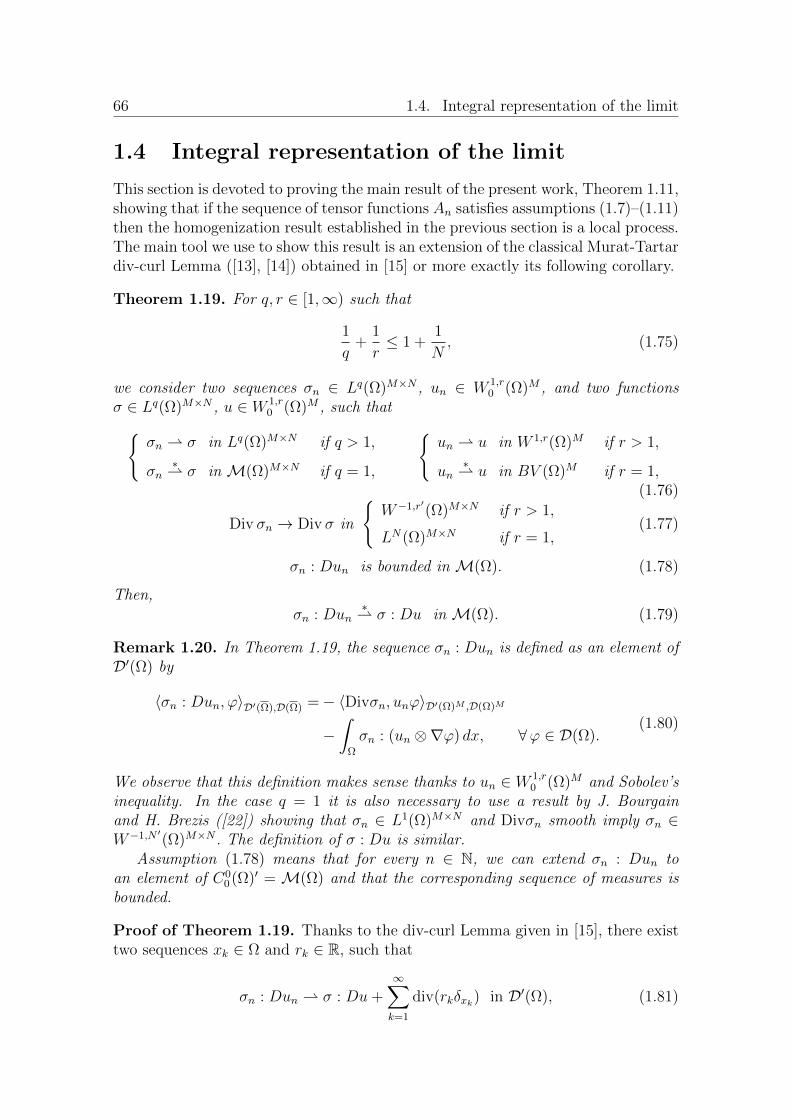
66 1.4. Integral representation of the limit

1.4 Integral representation of the limit

This section is devoted to proving the main result of the present work, Theorem 1.11,showing that if the sequence of tensor functions An satisfies assumptions (1.7)–(1.11)then the homogenization result established in the previous section is a local process.The main tool we use to show this result is an extension of the classical Murat-Tartardiv-curl Lemma ([13], [14]) obtained in [15] or more exactly its following corollary.

Theorem 1.19. For q, r 2 [1,1) such that

1

q+

1

r 1 +

1

N, (1.75)

we consider two sequences �n 2 Lq(⌦)M⇥N , un 2 W 1,r0 (⌦)M , and two functions

� 2 Lq(⌦)M⇥N , u 2 W 1,r0 (⌦)M , such that

(�n * � in Lq(⌦)M⇥N if q > 1,

�n⇤* � in M(⌦)M⇥N if q = 1,

(un * u in W 1,r(⌦)M if r > 1,

un⇤* u in BV (⌦)M if r = 1,

(1.76)

Div �n ! Div � in

(W�1,r0(⌦)M⇥N if r > 1,

LN(⌦)M⇥N if r = 1,(1.77)

�n : Dun is bounded in M(⌦). (1.78)

Then,�n : Dun

⇤* � : Du in M(⌦). (1.79)

Remark 1.20. In Theorem 1.19, the sequence �n : Dun is defined as an element ofD0(⌦) by

h�n : Dun,'iD0(⌦),D(⌦) =� hDiv�n, un'iD0(⌦)M ,D(⌦)M

�Z

⌦

�n : (un ⌦r') dx, 8' 2 D(⌦).(1.80)

We observe that this definition makes sense thanks to un 2 W 1,r0 (⌦)M and Sobolev’s

inequality. In the case q = 1 it is also necessary to use a result by J. Bourgainand H. Brezis ([22]) showing that �n 2 L1(⌦)M⇥N and Div�n smooth imply �n 2W�1,N 0

(⌦)M⇥N . The definition of � : Du is similar.Assumption (1.78) means that for every n 2 N, we can extend �n : Dun to

an element of C00(⌦)

0 = M(⌦) and that the corresponding sequence of measures isbounded.

Proof of Theorem 1.19. Thanks to the div-curl Lemma given in [15], there existtwo sequences xk 2 ⌦ and rk 2 R, such that

�n : Dun * � : Du+1X

k=1

div(rk�xk) in D0(⌦), (1.81)

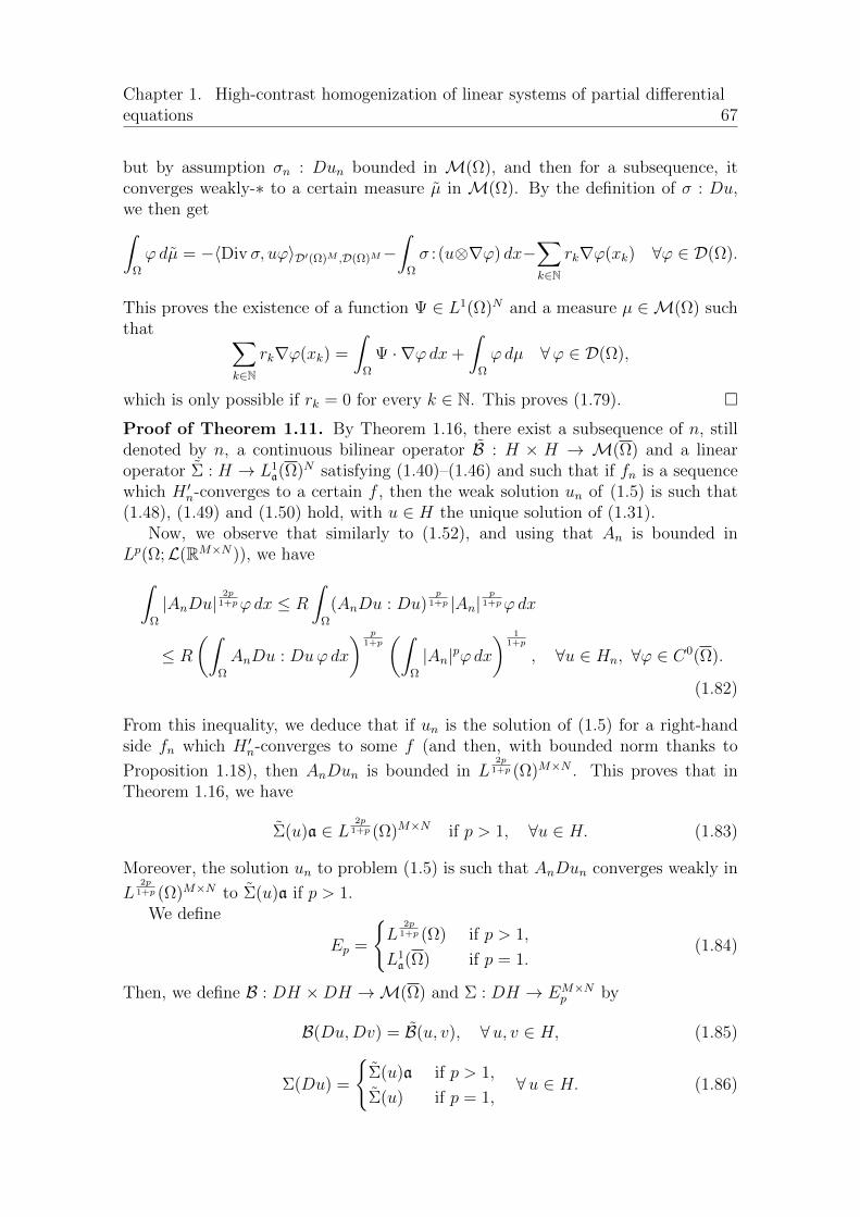
Chapter 1. High-contrast homogenization of linear systems of partial di↵erentialequations 67

but by assumption �n : Dun bounded in M(⌦), and then for a subsequence, itconverges weakly-⇤ to a certain measure µ in M(⌦). By the definition of � : Du,we then getZ

⌦

' dµ = �hDiv �, u'iD0(⌦)M ,D(⌦)M�Z

⌦

� : (u⌦r') dx�X

k2N

rkr'(xk) 8' 2 D(⌦).

This proves the existence of a function 2 L1(⌦)N and a measure µ 2 M(⌦) suchthat X

k2N

rkr'(xk) =

Z

⌦

·r' dx+

Z

⌦

' dµ 8' 2 D(⌦),

which is only possible if rk = 0 for every k 2 N. This proves (1.79). ⇤Proof of Theorem 1.11. By Theorem 1.16, there exist a subsequence of n, stilldenoted by n, a continuous bilinear operator B : H ⇥ H ! M(⌦) and a linearoperator ⌃ : H ! L1

a(⌦)N satisfying (1.40)–(1.46) and such that if fn is a sequence

which H 0n-converges to a certain f , then the weak solution un of (1.5) is such that

(1.48), (1.49) and (1.50) hold, with u 2 H the unique solution of (1.31).Now, we observe that similarly to (1.52), and using that An is bounded in

Lp(⌦;L(RM⇥N)), we have

Z

⌦

|AnDu| 2p1+p' dx R

Z

⌦

(AnDu : Du)p

1+p |An|p

1+p' dx

R

✓Z

⌦

AnDu : Du' dx

◆ p1+p✓Z

⌦

|An|p' dx

◆ 11+p

, 8u 2 Hn, 8' 2 C0(⌦).

(1.82)

From this inequality, we deduce that if un is the solution of (1.5) for a right-handside fn which H 0

n-converges to some f (and then, with bounded norm thanks to

Proposition 1.18), then AnDun is bounded in L2p1+p (⌦)M⇥N . This proves that in

Theorem 1.16, we have

⌃(u)a 2 L2p1+p (⌦)M⇥N if p > 1, 8u 2 H. (1.83)

Moreover, the solution un to problem (1.5) is such that AnDun converges weakly in

L2p1+p (⌦)M⇥N to ⌃(u)a if p > 1.We define

Ep =

(L

2p1+p (⌦) if p > 1,

L1a(⌦) if p = 1.

(1.84)

Then, we define B : DH ⇥DH ! M(⌦) and ⌃ : DH ! EM⇥Np by

B(Du,Dv) = B(u, v), 8 u, v 2 H, (1.85)

⌃(Du) =

(⌃(u)a if p > 1,

⌃(u) if p = 1,8 u 2 H. (1.86)

68 1.4. Integral representation of the limit

Thanks to (1.40)–(1.46) and (1.82), it is clear that (1.23)–(1.28) hold. Therefore, inorder to show Theorem 1.11, it just remains to prove (1.29) and the existence of atensor function A 2 Lp(⌦;L(RM⇥N)), if p > 1, A 2 L1

a (⌦;L(RM⇥N)) if p = 1, suchthat (1.30) holds. This will be given in the following three steps.

Step 1. Let us prove that for every u 2 H, every ! ⇢ ⌦ open and every v 2 H with

v 2(W 1, 2p

p�1 (!)M if p > 1,

C1(!)M if p = 1,(1.87)

we have

B(Du,Dv) =

(⌃(Du) : Dv if p > 1,

⌃(Du) : Dv a if p = 1,in !. (1.88)

To prove this result, we first assume that there exists f 2 C0(⌦)M such thatZ

⌦

dB(Du,Dw) =

Z

⌦

fw dx 8w 2 H, (1.89)

and we consider the solution un of (1.5) with right-hand side f . We know that un

Hn-converges weakly to u. Consider also a sequence vn which Hn-converges weaklyto v. Since AnDun : Dvn is bounded in M(⌦), we can apply Theorem 1.19 in ! to�n = AnDun. Taking into account (1.33) and (1.34), we then deduce that for every' 2 D(!), we have

Z

⌦

' dB(Du,Dv) = limn!1

Z

⌦

AnDun : Dvn' dx =

(R⌦⌃(Du) : Dv ' dx if p > 1,R⌦⌃(Du) : Dv ' da if p = 1.

This proves (1.88) for u satisfying (1.89), with f 2 C0(⌦)M . The general case thenfollows by using that the space of such u is dense in H and that B(·, Dv) and ⌃ arecontinuous in DH.

Step 2. Assume p > 1. We introduce the measure ap as (it is well defined up to asubsequence)

|An|p ⇤* ap in M(⌦),

and observe that (1.82) impliesZ

⌦

|⌃(Du)| 2p1+p' dx

R

✓Z

⌦

' dB(Du,Du)

◆ p1+p✓Z

⌦

' dap

◆ 11+p

, 8' 2 C0(⌦), ' � 0,

(1.90)

and then, using (1.88) and Holder’s inequality, we deduce that for ! ⇢ ⌦ open and

u 2 H \W 1, 2pp�1 (!), we have

Z

!

' dB(Du,Du)

R1+p2p

✓Z

!

' dB(Du,Du)

◆12✓Z

!

' dap

◆ 12p✓Z

!

|Du| 2pp�1' dx

◆p�12p

, 8' 2 C00(!), ' � 0,

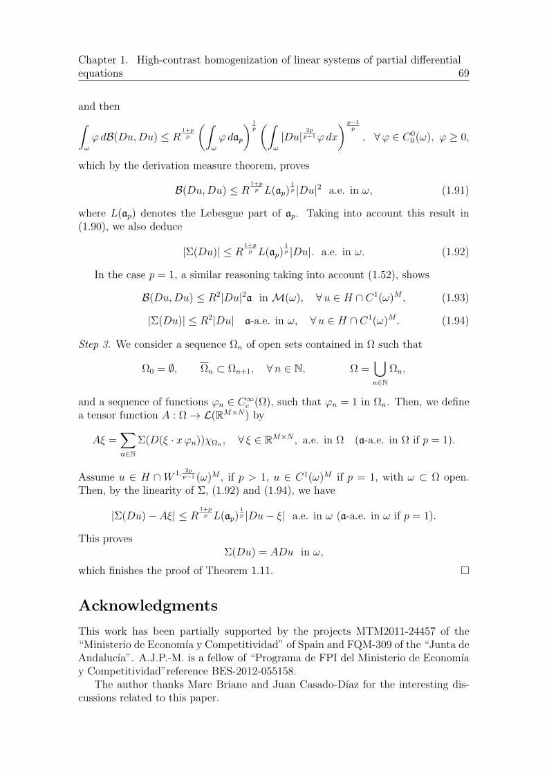
Chapter 1. High-contrast homogenization of linear systems of partial di↵erentialequations 69

and then

Z

!

' dB(Du,Du) R1+pp

✓Z

!

' dap

◆ 1p✓Z

!

|Du| 2pp�1' dx

◆ p�1p

, 8' 2 C00(!), ' � 0,

which by the derivation measure theorem, proves

B(Du,Du) R1+pp L(ap)

1p |Du|2 a.e. in !, (1.91)

where L(ap) denotes the Lebesgue part of ap. Taking into account this result in(1.90), we also deduce

|⌃(Du)| R1+pp L(ap)

1p |Du|. a.e. in !. (1.92)

In the case p = 1, a similar reasoning taking into account (1.52), shows

B(Du,Du) R2|Du|2a in M(!), 8 u 2 H \ C1(!)M , (1.93)

|⌃(Du)| R2|Du| a-a.e. in !, 8 u 2 H \ C1(!)M . (1.94)

Step 3. We consider a sequence ⌦n of open sets contained in ⌦ such that

⌦0 = ;, ⌦n ⇢ ⌦n+1, 8n 2 N, ⌦ =[

n2N

⌦n,

and a sequence of functions 'n 2 C1c (⌦), such that 'n = 1 in ⌦n. Then, we define

a tensor function A : ⌦! L(RM⇥N) by

A⇠ =X

n2N

⌃(D(⇠ · x'n))�⌦n , 8 ⇠ 2 RM⇥N , a.e. in ⌦ (a-a.e. in ⌦ if p = 1).

Assume u 2 H \ W 1, 2pp�1 (!)M , if p > 1, u 2 C1(!)M if p = 1, with ! ⇢ ⌦ open.

Then, by the linearity of ⌃, (1.92) and (1.94), we have

|⌃(Du)� A⇠| R1+pp L(ap)

1p |Du� ⇠| a.e. in ! (a-a.e. in ! if p = 1).

This proves⌃(Du) = ADu in !,

which finishes the proof of Theorem 1.11. ⇤

Acknowledgments

This work has been partially supported by the projects MTM2011-24457 of the“Ministerio de Economıa y Competitividad” of Spain and FQM-309 of the “Junta deAndalucıa”. A.J.P.-M. is a fellow of “Programa de FPI del Ministerio de Economıay Competitividad”reference BES-2012-055158.

The author thanks Marc Briane and Juan Casado-Dıaz for the interesting dis-cussions related to this paper.

70 Bibliography

Bibliography

[1] Tartar L. The General Theory of Homogenization. A Personalized Introduc-tion. Lect. Notes Unione Mat. Ital., Springer-Verlag: Berlin, Heidelberg; 2009.

[2] Spagnolo S. Sulla convergenza di soluzioni di equazioni paraboliche ed ellit-tiche. Ann. Sc. Norm. Super. Pisa Cl. Sci. 1968; 22 (3):571-597.

[3] Murat F. H-convergence in: Seminaire d’Analyse Fonctionelle et Numerique.Universite d’Alger; 1977-1978, multicopied, 34pp.; English translation: MuratF, Tartar L. H-convergence in: Topics in the Mathematical Modelling ofComposite Materials, Ed. by Cherkaev L, Kohn RV. Progr. Nonlinear Dif-ferential Equations Appl., vol. 31, Birkhauser: Boston; 1998: 21-43.

[4] Carbone L, Sbordone C. Some properties of �-limits of integral functionals.Ann. Mat. Pura Appl. 1979: 122 (4):1-60. DOI:10.1007/BF02411687.

[5] Bellieud M, Bouchitte G. Homogenization of elliptic problems in a fiberreinforced structure. Nonlocal e↵ects, Ann. Scuola Norm. Sup. Pisa Cl. Sci.1998; 26 (4):407-436.

[6] Briane M, Tchou N. Fibered microstructures for some nonlocal Dirichletforms. Ann. Scuola Norm. Sup. Pisa Cl. Sci. 2001; 30 (4):681-711.

[7] Fenchenko VN, Khruslov EYa. Asymptotic behavior of solutions of dif-ferential equations with a strongly oscillating coe�cient matrix that does notsatisfy a uniform boundedness condition. Dokl. AN Ukr. SSR. 1981; 95 (4):24-27.

[8] Mosco U. Composite media and asymptotic Dirichlet forms. J. FunctionalAnalysis. 1994; 123 (2):368-421. DOI:10.1006/jfan.1994.1093.

[9] Briane M, Casado-Dıaz J. Asymptotic behavior of equicoercive di↵usionenergies in two dimension. Calc. Var. Partial Di↵erential Equations. 2007; 29(4):455-479. DOI: 10.1007/s00526-006-0074-5.

[10] Briane M. Nonlocal e↵ects in two-dimensional conductivity. Arch. Rat. Mech.Anal. 2006; 182 (2):255-267. DOI: 10.1007/s00205-006-0427-4.

[11] Briane M, Casado-Dıaz J. Two-dimensional div-curl results: applicationto the lack of nonlocal e↵ects in homogenization. Comm. Part. Di↵. Equ. 2007;32: 935-969. DOI: 10.1080/03605300600910423.

[12] Briane M, Casado-Dıaz J. Homogenization of systems with equi-integrable coe�cients. ESAIM: COCV. 2014; 20 (4):1214-1223. DOI:10.1051/cocv/2014013.

[13] Murat F. Compacite par compensation. Ann. Scuola. Norm. Sup. Pisa Cl.Sci., Serie IV. 1978; 5 (3):489-507.

Chapter 1. High-contrast homogenization of linear systems of partial di↵erentialequations 71

[14] Tartar L. Compensated compactness and applications to partial di↵erentialequations. Nonlinear Analysis and Mechanics: Heriot Watt Symposium IV.Pitman: San Francisco; 1979: 136-212.

[15] Briane M, Casado-Diaz J, Murat F. The Div-Curl lemma ”trente ansapres”: an extension and an application to the G-convergence of unboun-ded monotone operators. J. Math. Pures Appl. 2009; 91 (9):476-494. DOI:10.1016/j.matpur.2009.01.002.

[16] Briane M, Camar-Eddine M. Homogenization of two-dimensional elasticityproblems with very sti↵ coe�cients. J. Math. Pures Appl. 2007; 88: 483-505.DOI: 10.1016/j.matpur.2007.09.003.

[17] Briane M, Casado-Dıaz J. Homogenization of sti↵ plates and two-dimensional high-viscosity Stokes equations. Arch. Rational Mech. Anal. 2012;205 (3):753-794. DOI: 10.1007/s00205-012-0520-9.

[18] Camar-Eddine M, Seppecher P. Determination of the closure of the set ofelasticity functionals. Arch. Ration. Mech. Anal. 2003; 170 (3):211-245. DOI:10.1007/s00205-003-0272-7.

[19] Dal Maso G. An Introduction to �-convergence. Birkhauser: Boston; 1993.

[20] Braides A. �-convergence for Beginners. Oxford University Press: Oxford;2002.

[21] De Giorgi E. �-convergenza eG-convergenza. Boll. Unione Mat. Ital. A. 1977;14 (5):213-220.

[22] Bourgain J, Brezis H. New estimates for elliptic equations and Hodge typesystems. J. Eur. Math. Soc. 2007; 9 (2):277-315. DOI: 10.4171/JEMS/80.

Chapter 2

Homogenization of equi-coercivenonlinear energies defined onvector-valued functions, withnon-uniformly boundedcoe�cients

M. Briane† J. Casado-Dıaz‡ M. Luna-Laynez‡ A. Pallares-Martın‡

† IRMAR & INSA Rennes,Centre de Mathematiques, INSA, 20 avenue des Buttes de Coesmes,

35708 Rennes Cedex 7, France.e-mail: mbriane@insa-rennes.fr

‡ Dpto. de Ecuaciones Diferenciales y Analisis Numerico,Facultad de Matematicas, C. Tarfıa s/n,

41012 Sevilla, Spain.e-mail: jcasadod@us.es, mllaynez@us.es, ajpallares@us.es

Submitted for publication.

Abstract.

The present paper deals with the asymptotic behavior of equi-coercive sequences{Fn} of nonlinear functionals defined over vector-valued functions in W 1,p

0 (⌦)M ,where p > 1, M � 1, and ⌦ is a bounded open set of RN , N � 2. The strongly localenergy density Fn(·, Du) of the functional Fn satisfies a Lipschitz condition withrespect to the second variable, which is controlled by a positive sequence {an} whichis only bounded in some suitable space Lr(⌦). We prove that the sequence {Fn} �-converges for the strong topology of Lp(⌦)M to a functional F which has a strongly

73

74 2.1. Introduction

local density F (·, Du) for su�ciently regular functions u. This compactness resultextends former results on the topic, which are based either on maximum principlearguments in the nonlinear scalar case, or adapted div-curl lemmas in the linearcase. Here, the vectorial character and the nonlinearity of the problem need a newapproach based on a careful analysis of the asymptotic minimizers associated withthe functional Fn. The relevance of the conditions which are imposed to the energydensity Fn(·, Du), is illustrated by several examples including some classical hyper-elastic energies.

2.1 Introduction

In this paper we study the asymptotic behavior of the sequence of nonlinear func-tionals, including some hyper-elastic energies (see the examples of Section 2.2.3),defined on vector-valued functions by

Fn(v) :=

Z

⌦

Fn(x,Dv) dx for v 2 W 1,p0 (⌦)M , with p 2 (1,1), M � 1, (2.1)

in a bounded open set ⌦ of RN , N � 2. The sequence Fn is assumed to be equi-coercive. Moreover, the associated density Fn(·, ⇠) satisfies some Lipschitz conditionwith respect to ⇠ 2 RM⇥N , and its coe�cients are not uniformly bounded in ⌦.

The linear scalar case, i.e. when Fn(·, ⇠) is quadratic with respect to ⇠ 2 RN

(M = 1), with uniformly bounded coe�cients was widely investigated in the seven-ties through G-convergence by Spagnolo [33], extended by Murat and Tartar with H-convergence [28, 35], and alternatively through �-convergence by De Giorgi [22, 23](see also [21, 4]). The linear elasticity case was probably first derived by Duvaut(unavailable reference), and can be found in [32, 25]. In the nonlinear scalar casethe first compactness results are due to Carbone, Sbordone [17] and Buttazzo, DalMaso [14] by a �-convergence approach assuming the L1-equi-integrability of thecoe�cients. More recently, these results were extended in [5, 9, 10] relaxing the L1-boundedness of the coe�cients but assuming that p > N�1 if N � 3, showing thenthe uniform convergence of the minimizers thanks to the maximum principle. In allthese works the scalar framework combined with the condition p > N�1 if N � 3and the equi-coercivity of the functionals, induce in terms of the �-convergence forthe strong topology of Lp(⌦), a limit energy F of the same nature satisfying

F (v) :=

Z

⌦

F (x,Dv) d⌫ for v 2 W, (2.2)

where C1c (⌦)

M ⇢ W is some suitable subspace of W 1,p0 (⌦)M , and ⌫ is some Radon

measure on ⌦. Removing the L1-equi-integrability of the coe�cients in the three-dimensional linear scalar case (note that p = N�1 = 2 in this case), Fenchenko andKhruslov [24] (see also [26]) were, up to our knowledge, the first to obtain a violationof the compactness result due to the appearance of local and nonlocal terms in thelimit energy F . This seminal work was also revisited by Bellieud and Bouchitte [2].Actually, the local and nonlocal terms in addition to the classical strongly local term

Chapter 2. Homogenization of equi-coercive nonlinear energies defined onvector-valued functions, with non-uniformly bounded coe�cients 75

come from the Beurling-Deny [3] representation formula of a Dirichlet form, and arisenaturally in the homogenization process as shown by Mosco [27]. The complete pic-ture of the attainable energies was obtained by Camar-Eddine and Seppecher [15] inthe linear scalar case. The elasticity case is much more intricate even in the linearframework, since the loss of uniform boundedness of the elastic coe�cients may in-duce the appearance of second gradient terms as Seppecher and Pideri proved in [30].The situation is dramatically di↵erent from the scalar case, since the Beurling-Denyformula does not hold in the vector-valued case. In fact, Camar-Eddine and Sep-pecher [16] proved that any lower semi-continuous quadratic functional vanishingon the rigid displacements, can be attained. Compactness results were obtained inthe linear elasticity case using some (strong) equi-integrability of the coe�cients in[11], and using various extensions of the classical Murat-Tartar [28] div-curl resultin [7, 13, 12, 29] (which were themselves initiated in the former works [6, 9] of thetwo first authors).

In our context the vectorial character of the problem and its nonlinearity pre-vent us from using the uniform convergence of [10] and the div-curl lemma of [12],which are (up to our knowledge) the more recent general compactness results on thetopic. We assume that the nonnegative energy density Fn(·, ⇠) of the functional (2.1)attains its minimum at ⇠ = 0, and satisfies the following Lipschitz condition withrespect to ⇠ 2 RM⇥N :

( ��Fn(x, ⇠)�Fn(x, ⌘)�� �hn(x)+Fn(x, ⇠)+Fn(x, ⌘)+|⇠|p+|⌘|p�

p�1p an(x)

1p |⇠�⌘|

8 ⇠, ⌘ 2 RM⇥N , a.e. x 2 ⌦,

which is controlled by a positive function an(·) (see the whole set of conditions (2.3)to (2.8) below). The sequence {an} is assumed to be bounded in Lr(⌦) for somer > (N�1)/p if 1 < p N�1, and bounded in L1(⌦) if p > N�1. Note that forp > N�1 our condition is better than the L1-equi-integrability used in the scalarcase of [17, 14], but not for 1 < p N�1. Under these assumptions we prove (seeTheorem 2.4) that the sequence {Fn} of (2.1) �-converges for the strong topologyof Lp(⌦)M (see Definition 2.1) to a functional of type (2.2) with

W ⇢(

W 1, prr�1 (⌦)M if 1 < p N�1,

C1(⌦)M if p > N�1,

and

⌫ =

(Lebesgue measure if 1 < p N�1,

M (⌦) ⇤ � limn!1

an if p > N�1.

Various types of boundary conditions can be taken into account in this �-convergence approach.

A preliminary result (see Theorem 2.3) allows us to prove that the sequenceof energy density {Fn(·, Dun)} converges in the sense of Radon measures to somestrongly local energy density F (·, Du), when un is an asymptotic minimizer for Fn oflimit u (see definition (2.17)). The proof of this new compactness result is based on

76 2.1. Introduction

an extension (see Lemma 2.6) of the fundamental estimate for recovery sequences in�-convergence (see, e.g., [21], Chapters 18, 19), which provides a bound (see (2.26))satisfied by the weak-⇤ limit of {Fn(·, Dun)} with respect to the weak-⇤ limit ofany sequence {Fn(·, Dvn)} such that the sequence {vn � un} converges weakly to 0in W 1,p

0 (⌦)M . Rather than using fixed smooth cut-o↵ functions as in the classicalfundamental estimate, here we need to consider sequences of radial cut-o↵ functions'n whose gradient has support in n-dependent sets on which un � u satisfies someuniform estimate with respect to the radial coordinate (see Lemma 2.11 and itsproof). This allows us to control the zero-order term r'n(un � u), when we putthe trial function 'n(un � u) in the functional Fn of (2.1). The uniform estimateis a consequence of the Sobolev compact embedding for the (N �1)-dimensionalsphere, and explains the role of the exponent r > (N�1)/p if 1 < p N�1. Asimilar argument was used in the linear case [12] to obtain a new div-curl lemmawhich is the key-ingredient for the compactness of quadratic elasticity functionalsof type (2.1).

Notations

• RN⇥Ns denotes the set of the symmetric matrices in RN⇥N .

• For any ⇠ 2 RN⇥N , ⇠T is the transposed matrix of ⇠, and ⇠s := 12(⇠+ ⇠

T ) is thesymmetrized matrix of ⇠.

• IN denotes the unit matrix of RN⇥N .

• · denotes the scalar product in RN , and : denotes the scalar product in RM⇥N

defined by⇠ : ⌘ := tr (⇠T⌘) for ⇠, ⌘ 2 RM⇥N ,

where tr is the trace.

• | · | denotes both the euclidian norm in RN , and the Frobenius norm in RM⇥N ,i.e.

|⇠| := �tr (⇠T ⇠)� 12 for ⇠ 2 RM⇥N .

• For a bounded open set ! ⇢ RN , M (!) denotes the space of the Radonmeasures on ! with bounded total variation. It agrees with the dual space ofC0

0(!), namely the space of the continuous functions in ! which vanish on @!.Moreover, M (!) denotes the space of the Radon measures on !. It agreeswith the dual space of C0(!).

• For any measures ⇣, µ 2 M (!), with ! ⇢ RN , open, bounded, we define⇣µ 2 L1

µ(⌦) as the derivative of ⇣ with respect to µ. When µ is the Lebesguemeasure, we write ⇣L.

• C is a positive constant which may vary from line to line.

• On is a real sequence which tends to zero as n tends to infinity. It can varyfrom line to line.

Chapter 2. Homogenization of equi-coercive nonlinear energies defined onvector-valued functions, with non-uniformly bounded coe�cients 77

Recall the definition of the De Giorgi �-convergence (see, e.g., [21, 4] for furtherdetails).

Definition 2.1. Let V be a metric space, and let Fn,F : V ! [0,1], n 2 N, befunctionals defined on V . The sequence {Fn} is said to �-converge to F for thetopology of V in a set W ⇢ V and we write

Fn�* F in W,

if

- the �-liminf inequality holds

8 v 2 W, 8 vn ! v in V, F (v) lim infn!1

Fn(vn),

- the �-limsup inequality holds

8v 2 W, 9 vn ! v in V, F (v) = limn!1

Fn(vn).

Any sequence vn satisfying (2.1) is called a recovery sequence for Fn of limit v.

2.2 Statement of the results and examples

2.2.1 The main results

Consider a bounded open set ⌦ ⇢ RN with N � 2, M a positive integer, a sequenceof nonnegative Caratheodory functions Fn : ⌦ ⇥ RM⇥N ! [0,1), and p > 1 withthe following properties:

• There exist two constants ↵ > 0 and � � 0 such thatZ

⌦

Fn(x,Du) dx � ↵

Z

⌦

|Du|p dx� �, 8 u 2 W 1,p0 (⌦)M , (2.3)

andFn(·, 0) = 0 a.e. in ⌦. (2.4)

• There exist two sequences of measurable functions hn, an � 0, and a constant� > 0 such that

hn is bounded in L1(⌦), (2.5)

an is bounded in Lr(⌦) with

8<

:r >

N�1

p, if 1 < p N�1

r = 1, if p > N�1,

(2.6)

78 2.2. Statement of the results and examples

8><

>:

��Fn(x, ⇠)� Fn(x, ⌘)��

�hn(x) + Fn(x, ⇠) + Fn(x, ⌘) + |⇠|p + |⌘|p�p�1p an(x)

1p |⇠ � ⌘|

8 ⇠, ⌘ 2 RM⇥N , a.e. x 2 ⌦,(2.7)

and

Fn(x,�⇠) hn(x) + � Fn(x, ⇠), 8� 2 [0, 1], 8 ⇠ 2 RM⇥N , a.e. x 2 ⌦. (2.8)

Remark 2.2. From (2.7) and Young’s inequality, we get that

Fn(x, ⇠) Fn(x, ⌘)+�hn(x)+Fn(x, ⇠)+Fn(x, ⌘)+|⇠|p+|⌘|p�

p�1p an(x)

1p |⇠ � ⌘|

Fn(x, ⌘)+p� 1

p

�hn(x)+Fn(x, ⇠)+Fn(x, ⌘)+|⇠|p+|⌘|p�+1

pan(x) |⇠�⌘|p,

and then(Fn(x, ⇠) (p�1)hn(x) + (2p�1)Fn(x, ⌘) + (p�1)

�|⇠|p + |⌘|p�+ an(x) |⇠ � ⌘|p,8 ⇠, ⌘ 2 RM⇥N , a.e. x 2 ⌦.

(2.9)In particular, taking ⌘ = 0, we have

Fn(x, ⇠) (p� 1)hn(x) +�p� 1 + an(x)

� |⇠|p, 8 ⇠ 2 RM⇥N , a.e. x 2 ⌦, (2.10)

where the right-hand side is a bounded sequence in L1(⌦).

From now on, we assume that

arn⇤* a in M (⌦) and hn

⇤* h in M (⌦). (2.11)

The paper deals with the asymptotic behavior of the sequence of functionals

Fn(v) :=

Z

⌦

Fn(x,Dv) dx for v 2 W 1,p(⌦)M . (2.12)

First of all, we have the following result on the convergence of the energy densityFn(·, Dun), where un is an asymptotic minimizer associated with functional (2.12).

Theorem 2.3. Let Fn : ⌦⇥RM⇥N ! [0,1) be a sequence of Caratheodory functionssatisfying (2.3) to (2.8). Then, there exist a function F : ⌦ ⇥ RM⇥N ! R and asubsequence of n, still denoted by n, such that for any ⇠, ⌘ 2 RN ,

(F (·, ⇠) is Lebesgue measurable, if 1 < p N�1

F (·, ⇠) is a-measurable, if p > N�1,(2.13)

Chapter 2. Homogenization of equi-coercive nonlinear energies defined onvector-valued functions, with non-uniformly bounded coe�cients 79

��F (x, ⇠)� F (x, ⌘)��

8>>>>><

>>>>>:

C�hL+F (x, ⇠)+F (x, ⌘)+(1 + (aL)

1r )(|⇠|p + |⌘|p)�

p�1p ·

· (aL)1pr|⇠ � ⌘| a.e. in ⌦

if 1 < p N�1,

C�1 + ha + F (x, ⇠) + F (x, ⌘) + |⇠|p + |⌘|p�

p�1p ·

· |⇠ � ⌘| a-a.e. in ⌦if p >N�1,

(2.14)and

F (·, 0) = 0 a.e. in ⌦. (2.15)

For any open set ! ⇢ ⌦, and any sequence {un} in W 1,p(!)M which convergesweakly in W 1,p(!)M to a function u satisfying

u 2(

W 1, prr�1 (!)M , if 1 < p N�1

C1(!)M , if p > N�1,(2.16)

and such that

9 limn!1

Z

!

Fn(x,Dun) dx

= min

⇢lim infn!1

Z

!

Fn(x,Dwn) dx : wn � un * 0 in W 1,p0 (!)M

�< 1,

(2.17)

we have

Fn(·, Dun)⇤*

(F (·, Du), if 1 < p N�1

F (·, Du)a, if p > N�1in M (!). (2.18)

From Theorem 2.3 we may deduce the �-limit (see Definition 2.1) of the sequenceof functionals (2.12) with various boundary conditions.

Theorem 2.4. Let Fn : ⌦⇥RM⇥N ! [0,1) be a sequence of Caratheodory functionssatisfying (2.3) to (2.8). Let ! be an open set such that ! ⇢⇢ ⌦, and let V be asubset of W 1,p(!)M such that

8 u 2 V, 8 v 2 W 1,p0 (!)M , u+ v 2 V. (2.19)

Define the functional F Vn : V ! [0,1) by

F Vn (v) :=

Z

!

Fn(x,Dv) dx for v 2 V. (2.20)

Assume that the open set ! satisfies( |@!| = 0, if 1 < p N�1

a(@!) = 0, if p > N�1.(2.21)

80 2.2. Statement of the results and examples

Then, for the subsequence of n (still denoted by n) obtained in Theorem 2.3 we get

8>><

>>:

F Vn

�* F V :=

Z

!

F (x,Dv) dx in V \W 1, prr�1 (!)M , if 1 < p N�1

F Vn

�* F V :=

Z

!

F (x,Dv) dx in V \ C1(!)M , if p > N�1,

(2.22)

for the strong topology of Lp(!)M , where F is given by convergence (2.18).

Remark 2.5. The condition (2.21) on the open set ! is not so restrictive. Indeed,for any family (!)i2I of open sets of ⌦ with two by two disjoint boundaries, at mosta countable subfamily of (@!)i2I does not satisfy (2.21).

2.2.2 Auxiliary lemmas

The proof of Theorem 2.3 is based on the following lemma which provides an estimateof the energy density for asymptotic minimizers. In our context it is equivalent to thefundamental estimate for recovery sequences (see Definition 2.1) in �-convergencetheory (see, e.g., [21], Chapters 18, 19).

Lemma 2.6. Let Fn : ⌦⇥RM⇥N ! [0,1) be a sequence of Caratheodory functionssatisfying (2.3) to (2.8). Consider an open set ! ⇢ ⌦, and a sequence {un} ⇢W 1,p(!)M converging weakly in W 1,p(!)M to a function u satisfying (2.16), andsuch that

Fn(·, Dun)⇤* µ in M (!),

|Dun|p ⇤* % in M (!).

Then, the measure % satisfies

% (

C�|Du|p + |Du|p(aL)

1r + h+ µ+ aL

�a.e. in !, if 1 < p N�1

C�|Du|pa+ h+ µ+ a

�a-a.e. in !, if p > N�1.

(2.23)Moreover if un satisfies

9 limn!1

Z

!

Fn(x,Dun) dx

= min

⇢lim infn!1

Z

!

Fn(x,Dwn) dx : wn � un * 0 in W 1,p0 (!)M

�,

(2.24)

then for any sequence {vn} ⇢ W 1,p(!)M which converges weakly in W 1,p(!)M to afunction

v 2(

W 1, prr�1 (!)M , if 1 < p N�1

C1(!)M , if p > N�1,

and such thatFn(·, Dvn)

⇤* ⌫ in M (!), (2.25)

Chapter 2. Homogenization of equi-coercive nonlinear energies defined onvector-valued functions, with non-uniformly bounded coe�cients 81

|Dvn|p ⇤* $ in M (!),

we have

µ

8>>>>><

>>>>>:

⌫ + C�hL + ⌫L +$L + (1 + (aL)

1r )|D(u� v)|p�

p�1p ·

· (aL)1pr |D(u� v)| a.e. in !

if 1 < p N�1,

⌫ + C�1 + ha + ⌫a +$a + |D(u� v)|p�

p�1p ·

· a |D(u� v)| a-a.e. in !if p > N�1.

(2.26)

We can improve the statement of Lemma 2.6 if we add a non-homogeneousDirichlet boundary condition on @!.

Lemma 2.7. Let ! be an open set such that ! ⇢⇢ ⌦, and let u be a functionsatisfying

u 2(

W 1, prr�1 (⌦)M , if 1 < p N�1

C1(⌦)M , if p > N�1.(2.27)

Let {un} and {vn} be two sequences in W 1,p(!)M , such that un satisfies condition(2.24) and

un � u, vn � u 2 W 1,p0 (!)M ,

Fn(·, Dun)⇤* µ and Fn(·, Dvn)

⇤* ⌫ in M (!), (2.28)

|Dun|p ⇤* % and |Dvn|p ⇤

* $ in M (!). (2.29)

Then, estimates (2.23) and (2.26) hold in !.

Remark 2.8. Condition (2.24) means that un is a recovery sequence in ! for thefunctional

w 2 W 1,p(!)M 7!Z

!

Fn(x,Dw) dx, (2.30)

with the Dirichlet condition w�un 2 W 1,p0 (!)M . Since w = un clearly satisfies w�

un 2 W 1,p0 (!)M , this makes un a recovery sequence without imposing any boundary

condition. In particular, condition (2.24) is fulfilled if for a fixed f 2 W�1,p(!)M ,un satisfiesZ

!

Fn(x,Dun) dx = min

⇢Z

!

Fn

�x,D(un + v)

�dx� hf, vi : v 2 W 1,p

0 (!)M�.

Assuming the di↵erentiability of Fn with respect to the second variable, it followsthat un satisfies the variational equation

Z

!

D⇠Fn(x,Dun) : Dv dx� hf, vi = 0, 8 v 2 W 1,p0 (!)M ,

i.e. un is a solution of

�Div�D⇠Fn(x,Du)

�= f in !,

82 2.2. Statement of the results and examples

where no boundary condition is imposed.Assumption (2.24) allows us to take into account very general boundary con-

ditions. For example, if un is a recovery sequence for (2.30) with (non necessar-ily homogeneous) Dirichlet or Neumann boundary condition, then it also satisfies(2.24).

Remark 2.9. Condition (2.24) is equivalent to the asymptotic minimizer propertysatisfied by un:Z

!

Fn(x,Dun) dx Z

!

Fn(x,Dwn) dx+On, 8wn with wn�un * 0 in W 1,p0 (!)M .

We can check that if un satisfies this condition in !, then un satisfies it in anyopen subset ! ⇢ !. To this end, it is enough to consider for a sequence wn withwn � un 2 W 1,p

0 (!)M , the extension

wn :=

⇢wn in !un in ! \ !.

Corollary 2.10. Let Fn : ⌦ ⇥ RM⇥N ! [0,1) be a sequence of Caratheodoryfunctions satisfying (2.3) to (2.8). Consider two open sets !1,!2 ⇢ ⌦ such that!1 \ !2 6= Ø, a sequence un converging weakly in W 1,p(!1)M to a function u and asequence vn converging weakly in W 1,p(!2)M to a function v, such that

u, v 2(

W 1, prr�1 (!1 \ !2)

M , if 1 < p N�1

C1(!1 \ !2)M , if p > N�1,

|Dun|p ⇤* %, Fn(·, Dun)

⇤* µ in M (!1),

|Dvn|p ⇤* $, Fn(·, Dvn)

⇤* ⌫ in M (!2),

9 limn!1

Z

!1

Fn(x,Dun) dx

= min

⇢lim infn!1

Z

!1

Fn(x,Dwn) dx : wn � un * 0 in W 1,p0 (!1)

M

�,

9 limn!1

Z

!2

Fn(x,Dvn) dx

= min

⇢lim infn!1

Z

!2

Fn(x,Dwn) dx : wn � vn * 0 in W 1,p0 (!2)

M

�.

Then, we have

|µ� ⌫| 8>>>>><

>>>>>:

C�hL+µL+⌫L+%L+$L+(1 + (aL)

1r )|D(u� v)|p�

p�1p ·

· (aL)1pr|D(u� v)| a.e. in !1 \ !2

if 1< p N�1,

C�1 + ha + µa + ⌫a + %a +$a + |D(u� v)|p�

p�1p ·

· a |D(u� v)| a-a.e. in !1 \ !2

if p >N�1.

(2.31)

Chapter 2. Homogenization of equi-coercive nonlinear energies defined onvector-valued functions, with non-uniformly bounded coe�cients 83

Lemma 2.6 is itself based on the following compactness result.

Lemma 2.11. Let Fn : ⌦⇥RM⇥N ! [0,1) be a sequence of Caratheodory functionssatisfying (2.3) to (2.8), and let ! be an open subset of ⌦. Consider a sequence{⇠n} ⇢ Lp(!)M⇥N such that

Fn(·, ⇠n) ⇤* ⇤ and |⇠n|p ⇤

* ⌅ in M (!). (2.32)

• If 1 < p N�1 and the sequence {⇢n} converges strongly to ⇢ in Lprr�1 (!)M⇥N ,

then there exist a subsequence of n and a function # 2 L1(!) such that

Fn(·, ⇠n + ⇢n)� Fn(·, ⇠n)* # weakly in L1(!), (2.33)

where # satisfies

|#| C�hL + ⇤L + ⌅L + (1 + (aL)

1r )|⇢|p�

p�1p (aL)

1pr |⇢| a.e. in !. (2.34)

• If p > N�1 and the sequence {⇢n} converges strongly to ⇢ in C0(!)M⇥N , thenthere exist a subsequence of n and a function # 2 L1

a(!) such that

Fn(·, ⇠n + ⇢n)⇤* ⇤+ #a in M (!),

where # satisfies

|#| C�1 + ha + ⇤a + ⌅a + |⇢|p�

p�1p |⇢| a-a.e. in !. (2.35)

2.2.3 Examples

In this section we give three examples of functionals Fn satisfying the assumptions(2.3) to (2.8) of Theorem 2.3.

1. The first example illuminates the Lipschitz estimate (2.7). It is also based ona functional coercivity of type (2.3) rather than a pointwise coercivity.

2. The second example deals with the Saint Venant-Kirchho↵ hyper-elastic energy(see, e.g., [18] Chapter 4).

3. The third example deals with an Ogden’s type hyper-elastic energy (see, e.g.,[18] Chapter 4).

Let ⌦ be a bounded set of RN , N � 2. We denote for any function u : ⌦! RN ,

e(u) := 12

�Du+DuT

�, E(u) := 1

2

�Du+DuT +DuTDu

�,

C(u) := (IN +Du)T (IN +Du).(2.36)

84 2.2. Statement of the results and examples

Example 1

Let p 2 (1,1), and let An be a sequence of symmetric tensor-valued functions inL1�⌦;L (RN⇥N

s )�. We consider the energy density function defined by

Fn(x, ⇠) :=��An(x)⇠

s : ⇠s�� p2 a.e. x 2 ⌦, 8 ⇠ 2 RN⇥N .

We assume that there exists ↵ > 0 such that

An(x)⇠ : ⇠ � ↵ |⇠|2, a.e. x 2 ⌦, 8 ⇠ 2 RN⇥Ns , (2.37)

and that

|An| p2 is bounded in Lr(⌦) with r defined by (2.6). (2.38)

Then, the density Fn and the associated functional

Fn(u) :=

Z

⌦

��Ane(u) : e(u)�� p2dx for u 2 W 1,p

0 (⌦)N ,

satisfy the conditions (2.3) to (2.8) of Theorem 2.3.

Proof. Using successively (2.37) and the Korn inequality in W 1,p0 (⌦)N for p > 1 (see,

e.g., [34]), we have for any u 2 W 1,p0 (⌦)N ,

Fn(u) =

Z

⌦

��Ane(u) : e(u)�� p2 dx � ↵

Z

⌦

|e(u)|p dx � ↵C

Z

⌦

|Du|p dx,

which implies (2.3). Conditions (3.14) and (2.8) are immediate. It remains to provecondition (2.7) with estimate (2.6). Taking into account that

|D⇠Fn(x, ⇠)| = p��(An(x)⇠

s : ⇠s)p�22 An(x)⇠

s��

p��An(x)⇠

s : ⇠s| p�12 |An(x)| 12 , 8 ⇠ 2 RN⇥N , a.e. x 2 ⌦,

then using the mean value theorem and Holder’s inequality, we get

��Fn(x, ⇠)� Fn(x, ⌘)�� p

⇣(An⇠

s : ⇠s)12 + (An⌘

s : ⌘s)12

⌘p�1

|An| 12 |⇠s � ⌘s|

p 2(p�1)2

p�Fn(x, ⇠) + Fn(x, ⌘)

� p�1p |An| 12 |⇠ � ⌘|,

for every ⇠, ⌘ 2 RN⇥N and a.e. x 2 ⌦. This implies estimate (2.7) with hn = 0 andan = |An| p2 bounded in Lr(⌦).

The two next examples belong to the class of hyper-elastic materials (see, e.g.,[18], Chapter 4).

Chapter 2. Homogenization of equi-coercive nonlinear energies defined onvector-valued functions, with non-uniformly bounded coe�cients 85

Example 2

For N = 3, we consider the Saint Venant-Kirchho↵ energy density defined by

Fn(x, ⇠) :=�n(x)

2

⇥tr�E(⇠)

�⇤2+ µn(x)

��E(⇠)��2, a.e. x 2 ⌦, 8 ⇠ 2 R3⇥3, (2.39)

where E(⇠) := 12

�⇠ + ⇠T + ⇠T ⇠

�, and �n, µn are the Lame coe�cients.

We assume that there exists a constant C > 1 such that

�n, µn � 0 a.e. in ⌦, ess-inf⌦

(�n + µn) > C�1,

Z

⌦

(�n + µn) dx C. (2.40)

Then, the density Fn and the associated functional (see definition (2.36))

Fn(u) :=

Z

⌦

✓�n2

⇥tr�E(u)

�⇤2+ µn

��E(u)��2◆dx for u 2 W 1,4

0 (⌦)3, (2.41)

satisfy the conditions (2.3) to (2.8) of Theorem 2.3.

Proof. There exists a constant C > 1 such that we have for a.e. x 2 ⌦ and any⇠ 2 R3⇥3,

C�1(�n +µn) |⇠|4 �C (�n +µn) Fn(x, ⇠) C (�n +µn) |⇠|4 +C (�n +µn). (2.42)

Hence, we deduce that for a.e. x 2 ⌦ and any ⇠, ⌘ 2 R3⇥3,��Fn(x, ⇠)� Fn(x, ⌘)

��

C (�n + µn)�1 + |⇠|2 + |⌘|2� 3

2 |⇠ � ⌘|

= C⇣(�n + µn)

12 + (�n + µn)

12 |⇠|2 + (�n + µn)

12 |⌘|2

⌘ 32(�n + µn)

14 |⇠ � ⌘|

C⇣(�n + µn)

12 + Fn(x, ⇠)

12 + Fn(x, ⌘)

12

⌘ 32(�n + µn)

14 |⇠ � ⌘|

C��n + µn + Fn(x, ⇠) + Fn(x, ⌘)

� 34 (�n + µn)

14 |⇠ � ⌘|,

which implies estimate (2.7) with p = 4 and hn = an = �n + µn, while (2.5) and(2.6) are a straightforward consequence of (2.40). Moreover, by the first inequality of(2.42) combined with (2.40) we get that the functional (2.41) satisfies the coercivitycondition (2.3). Condition (3.14) is immediate. Finally, since we have

⇥tr�E(�⇠)

�⇤2+��E(�⇠)

��2 C�1 + |⇠|4�, 8� 2 [0, 1], 8 ⇠ 2 R3⇥3,

condition (2.8) follows from the first inequality of (2.42), which concludes the proofof the second example.

Remark 2.12. The default of the Saint Venant-Kirchho↵ model is that the functionFn(x, ·) of (2.39) is not polyconvex (see [31]). Hence, we do not know if it isquasiconvex, or equivalently, if the functional Fn of (2.41) is lower semi-continuousfor the weak topology of W 1,4(⌦)3 (see, e.g. [20], Chapter 4, for the notions ofpolyconvexity and quasiconvexity).

86 2.2. Statement of the results and examples

Example 3

For N = 3 and p 2 [2,1), we consider the Ogden’s type energy density defined by

Fn(x, ⇠) := an(x)htr�C(⇠)

p2 � I3

�i+a.e. x 2 ⌦, 8 ⇠ 2 R3⇥3, (2.43)

where C(⇠) := (I3 + ⇠)T (I3 + ⇠), and t+ := max (t, 0) for t 2 R. We assume thatthere exists a constant C > 1 such that

ess-inf⌦

an > C�1 and

Z

⌦

arn dx C with

(r > 1, if p = 2

r = 1, if p > 2.(2.44)

Then, the density Fn and the associated functional (see definition (2.36))

Fn(u) :=

Z

⌦

an(x)htr�C(u)

p2 � I3

�i+dx for u 2 W 1,p

0 (⌦)3, (2.45)

satisfy the conditions (2.3) to (2.8) of Theorem 2.3.

Proof. There exists a constant C > 1 such that we have for a.e. x 2 ⌦ and any⇠ 2 R3⇥3,

C�1an |⇠|p � C an Fn(x, ⇠) C an |⇠|p + C an. (2.46)

This combined with the fact that the (well-ordered) eigenvalues of a symmetricmatrix are Lipschitz functions (see, e.g., [19], Theorem 2.3-2), implies that for a.e.x 2 ⌦ and any ⇠, ⌘ 2 RN , we have

��Fn(x, ⇠)� Fn(x, ⌘)�� C an(1 + |⇠|+ |⌘|)p�1|⇠ � ⌘|

C�an + an|⇠|p + an|⌘|p

� p�1p a

1pn |⇠ � ⌘|

C�an + Fn(x, ⇠) + Fn(x, ⌘)

� p�1p a

1pn |⇠ � ⌘|,

which implies estimate (2.7) with hn = an, while (2.5) and (2.6) are a straightfor-ward consequence of (2.44). Moreover, by the first inequality of (2.46) combinedwith (2.44) we get that the functional (2.45) satisfies the coercivity condition (2.3).Condition (3.14) is immediate. Finally, since we have

tr�C(�⇠)

p2� C

�1 + |⇠|p�, 8� 2 [0, 1], 8 ⇠ 2 R3⇥3,

condition (2.8) follows from the first inequality of (2.46), which concludes the proofof the third example.

Remark 2.13. Contrary to Example 2, the function Fn(x, ·) of (2.43) is polyconvexsince it is the composition of the Ogden density energy defined for a.e. x 2 ⌦, by

Wn(x, ⇠) := an(x)htr�C(⇠)

p2 � I3

�i+for ⇠ 2 R3⇥3, (2.47)

which is known to be polyconvex (see [1]), by the non-decreasing convex function t 7!t+. However, in contrast with (2.47) the function (2.43) does attain its minimum at⇠ = 0, namely in the absence of strain.

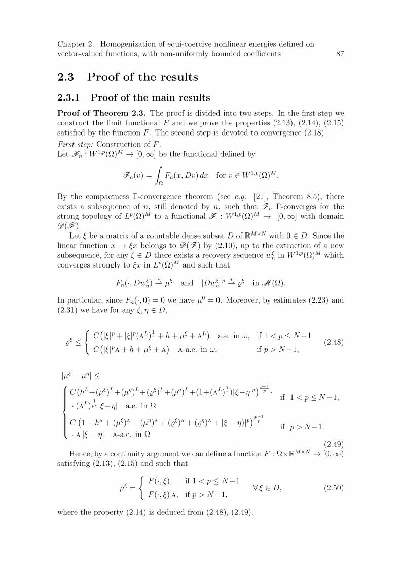
Chapter 2. Homogenization of equi-coercive nonlinear energies defined onvector-valued functions, with non-uniformly bounded coe�cients 87

2.3 Proof of the results

2.3.1 Proof of the main results

Proof of Theorem 2.3. The proof is divided into two steps. In the first step weconstruct the limit functional F and we prove the properties (2.13), (2.14), (2.15)satisfied by the function F . The second step is devoted to convergence (2.18).

First step: Construction of F .Let Fn : W 1,p(⌦)M ! [0,1] be the functional defined by

Fn(v) =

Z

⌦

Fn(x,Dv) dx for v 2 W 1,p(⌦)M .

By the compactness �-convergence theorem (see e.g. [21], Theorem 8.5), thereexists a subsequence of n, still denoted by n, such that Fn �-converges for thestrong topology of Lp(⌦)M to a functional F : W 1,p(⌦)M ! [0,1] with domainD(F ).

Let ⇠ be a matrix of a countable dense subset D of RM⇥N with 0 2 D. Since thelinear function x 7! ⇠x belongs to D(F ) by (2.10), up to the extraction of a newsubsequence, for any ⇠ 2 D there exists a recovery sequence w⇠

n in W 1,p(⌦)M whichconverges strongly to ⇠x in Lp(⌦)M and such that

Fn(·, Dw⇠n)

⇤* µ⇠ and |Dw⇠

n|p ⇤* %⇠ in M (⌦).

In particular, since Fn(·, 0) = 0 we have µ0 = 0. Moreover, by estimates (2.23) and(2.31) we have for any ⇠, ⌘ 2 D,

%⇠ (

C�|⇠|p + |⇠|p(aL)

1r + h+ µ⇠ + aL

�a.e. in !, if 1 < p N�1

C�|⇠|pa+ h+ µ⇠ + a

�a-a.e. in !, if p > N�1,

(2.48)

|µ⇠ � µ⌘| 8>>>>><

>>>>>:

C�hL+(µ⇠)L+(µ⌘)L+(%⇠)L+(⇢⌘)L+(1+(aL)

1r )|⇠�⌘|p�

p�1p ·

· (aL)1pr |⇠�⌘| a.e. in ⌦

if 1 < p N�1,

C�1 + ha + (µ⇠)a + (µ⌘)a + (%⇠)a + (%⌘)a + |⇠ � ⌘)|p�

p�1p ·

· a |⇠ � ⌘| a-a.e. in ⌦if p >N�1.

(2.49)Hence, by a continuity argument we can define a function F : ⌦⇥RM⇥N ! [0,1)

satisfying (2.13), (2.15) and such that

µ⇠ =

(F (·, ⇠), if 1 < p N�1

F (·, ⇠)a, if p > N�1,8 ⇠ 2 D, (2.50)

where the property (2.14) is deduced from (2.48), (2.49).

88 2.3. Proof of the results

Second step: Proof of convergence (2.18).

Let ! be an open set of ⌦, let {un} be a sequence fulfilling (2.17), which convergesweakly inW 1,p(!)M to a function u satisfying (2.16), and let ⇠ 2 D. Since Fn(·, Dun)is bounded in L1(⌦), there exists a subsequence of n, still denoted by n, such that

Fn(·, Dun)⇤* µ and |Dun|p ⇤

* % in M (⌦). (2.51)

Applying Corollary 2.10 to the sequences un and vn = w⇠n, we have

|µ� µ⇠| 8>>>>><

>>>>>:

C�hL+µL+(µ⇠)L+%L+(%⇠)L+(1 + (aL)

1r )|Du� ⇠|p�

p�1p ·

· (aL)1pr|Du� ⇠| a.e. in !

if 1 < p N�1,

C�1 + ha + µa + (µ⇠)a + %a + (%⇠)a + |Du� ⇠|p�

p�1p ·

· a |Du� ⇠| a-a.e. in !if p >N�1.

Using (2.48), (2.50) and the continuity of F (x, ⇠) with respect to ⇠, we get that

µ =

(F (·, Du), if 1 < p N�1

F (·, Du)a, if p > N�1.(2.52)

Note that since the limit µ is completely determined by F , the first convergence of(2.51) holds for the whole sequence, which concludes the proof. ⇤

Proof of Theorem 2.4. The proof is divided into two steps.

First step: The case where V = {u}+W 1,p0 (!)M .

Fix a function u satisfying (2.27), and define the set V := {u} + W 1,p0 (!)M . Let

u 2 V such that

u 2(

W 1, prr�1 (!)M , if 1 < p N�1

C1(!)M , if p > N�1.

which is extended by u in ⌦ \ !, and consider a recovery sequence {un} for F Vn

of limit u. There exists a subsequence of n, still denoted by n, such that the firstconvergences of (2.28) and (2.29) hold. By Theorem 2.3 convergences (2.18) aresatisfied in !, which implies (2.52). Now, applying the estimate (2.26) of Lemma 2.7with un and vn = u, it follows that

µ ⌫ in ! with Fn(·, Dvn)⇤* ⌫ in M (⌦),

where the convergence holds up to a subsequence. Then, using estimate (2.7) with⌘ = 0 and Holder’s inequality, we have for any ' 2 L1�⌦; [0, 1]

�with compact

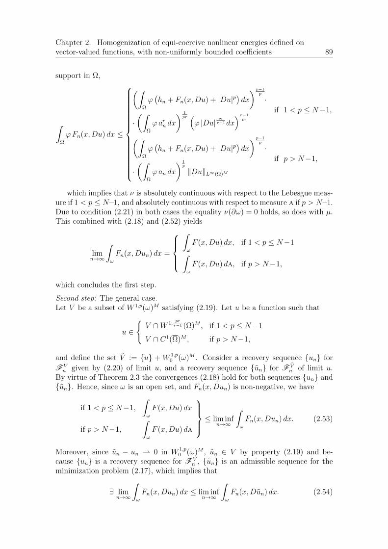
Chapter 2. Homogenization of equi-coercive nonlinear energies defined onvector-valued functions, with non-uniformly bounded coe�cients 89

support in ⌦,

Z

⌦

'Fn(x,Du) dx

8>>>>>>>>>>>>>><

>>>>>>>>>>>>>>:

✓Z

⌦

'�hn + Fn(x,Du) + |Du|p� dx

◆ p�1p

·

·✓Z

⌦

' arn dx

◆ 1pr ⇣

' |Du| prr�1dx

⌘ r�1pr

if 1 < p N�1,

✓Z

⌦

'�hn + Fn(x,Du) + |Du|p� dx

◆ p�1p

·

·✓Z

⌦

' an dx

◆ 1p

kDukL1(⌦)M

if p > N�1,

which implies that ⌫ is absolutely continuous with respect to the Lebesgue meas-ure if 1 < p N�1, and absolutely continuous with respect to measure a if p > N�1.Due to condition (2.21) in both cases the equality ⌫(@!) = 0 holds, so does with µ.This combined with (2.18) and (2.52) yields

limn!1

Z

!

Fn(x,Dun) dx =

8>><

>>:

Z

!

F (x,Du) dx, if 1 < p N�1

Z

!

F (x,Du) da, if p > N�1,

which concludes the first step.

Second step: The general case.Let V be a subset of W 1,p(!)M satisfying (2.19). Let u be a function such that

u 2(

V \W 1, prr�1 (⌦)M , if 1 < p N�1

V \ C1(⌦)M , if p > N�1,

and define the set V := {u} + W 1,p0 (!)M . Consider a recovery sequence {un} for

F Vn given by (2.20) of limit u, and a recovery sequence {un} for F V

n of limit u.By virtue of Theorem 2.3 the convergences (2.18) hold for both sequences {un} and{un}. Hence, since ! is an open set, and Fn(x,Dun) is non-negative, we have

if 1 < p N�1,

Z

!

F (x,Du) dx

if p > N�1,

Z

!

F (x,Du) da

9>>=

>>; lim inf

n!1

Z

!

Fn(x,Dun) dx. (2.53)

Moreover, since un � un * 0 in W 1,p0 (!)M , un 2 V by property (2.19) and be-

cause {un} is a recovery sequence for F Vn , {un} is an admissible sequence for the

minimization problem (2.17), which implies that

9 limn!1

Z

!

Fn(x,Dun) dx lim infn!1

Z

!

Fn(x,Dun) dx. (2.54)

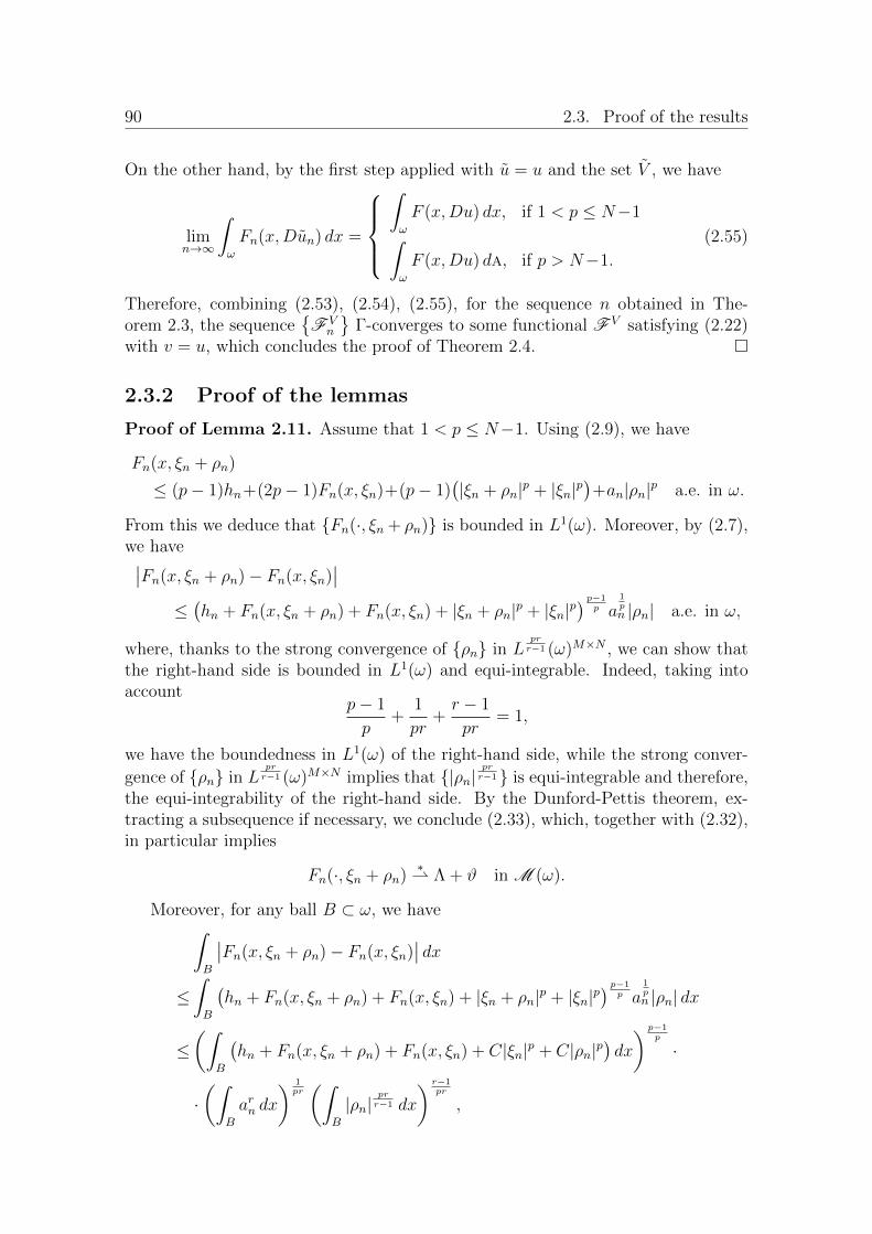
90 2.3. Proof of the results

On the other hand, by the first step applied with u = u and the set V , we have

limn!1

Z

!

Fn(x,Dun) dx =

8>><

>>:

Z

!

F (x,Du) dx, if 1 < p N�1

Z

!

F (x,Du) da, if p > N�1.

(2.55)

Therefore, combining (2.53), (2.54), (2.55), for the sequence n obtained in The-orem 2.3, the sequence

�F V

n

�-converges to some functional F V satisfying (2.22)

with v = u, which concludes the proof of Theorem 2.4. ⇤

2.3.2 Proof of the lemmas

Proof of Lemma 2.11. Assume that 1 < p N�1. Using (2.9), we have

Fn(x, ⇠n + ⇢n)

(p� 1)hn+(2p� 1)Fn(x, ⇠n)+(p� 1)�|⇠n + ⇢n|p + |⇠n|p

�+an|⇢n|p a.e. in !.

From this we deduce that {Fn(·, ⇠n + ⇢n)} is bounded in L1(!). Moreover, by (2.7),we have��Fn(x, ⇠n + ⇢n)� Fn(x, ⇠n)

��

�hn + Fn(x, ⇠n + ⇢n) + Fn(x, ⇠n) + |⇠n + ⇢n|p + |⇠n|p� p�1

p a1pn |⇢n| a.e. in !,

where, thanks to the strong convergence of {⇢n} in Lprr�1 (!)M⇥N , we can show that

the right-hand side is bounded in L1(!) and equi-integrable. Indeed, taking intoaccount

p� 1

p+

1

pr+

r � 1

pr= 1,

we have the boundedness in L1(!) of the right-hand side, while the strong conver-gence of {⇢n} in L

prr�1 (!)M⇥N implies that {|⇢n|

prr�1} is equi-integrable and therefore,

the equi-integrability of the right-hand side. By the Dunford-Pettis theorem, ex-tracting a subsequence if necessary, we conclude (2.33), which, together with (2.32),in particular implies

Fn(·, ⇠n + ⇢n)⇤* ⇤+ # in M (!).

Moreover, for any ball B ⇢ !, we haveZ

B

��Fn(x, ⇠n + ⇢n)� Fn(x, ⇠n)�� dx

Z

B

�hn + Fn(x, ⇠n + ⇢n) + Fn(x, ⇠n) + |⇠n + ⇢n|p + |⇠n|p

� p�1p a

1pn |⇢n| dx

✓Z

B

�hn + Fn(x, ⇠n + ⇢n) + Fn(x, ⇠n) + C|⇠n|p + C|⇢n|p

�dx

◆ p�1p

·

·✓Z

B

arn dx

◆ 1pr✓Z

B

|⇢n|prr�1 dx

◆ r�1pr

,

Chapter 2. Homogenization of equi-coercive nonlinear energies defined onvector-valued functions, with non-uniformly bounded coe�cients 91

which, passing to the limit, implies

Z

B

|#|dx ✓(h+ 2⇤+ #+ C⌅)(B) + C

Z

B

|⇢|pdx◆ p�1

p

a(B)1pr

✓Z

B

|⇢| prr�1dx

◆ r�1pr

,

and then, dividing by |B|, the measures di↵erentiation theorem shows that

|#| �hL + 2⇤L + #+ C⌅+ C|⇢|p�p�1p (aL)

1pr |⇢| a.e. in !. (2.56)

Using Young’s inequality in (2.56)

|#| p� 1

p

�hL + 2⇤L + #+ C⌅L + C|⇢|p�+ 1

p(aL)

1r |⇢|p a.e. in !,

and then|#| C

�hL + ⇤L + ⌅L + (1 + (aL)

1r )|⇢|p� a.e. in !,

which substituted in (2.56) shows (2.34).

Assume now that p > N�1. Again, using (2.9) we deduce that {Fn(·, ⇠n + ⇢n)}is bounded in L1(!), and thanks to (2.7) we get��Fn(x, ⇠n + ⇢n)� Fn(x, ⇠n)

��

�hn + Fn(x, ⇠n + ⇢n) + Fn(x, ⇠n) + |⇠n + ⇢n|p + |⇠n|p� p�1

p a1pn |⇢n| a.e. in !.

Consequently, the sequence {Fn(·, ⇠n + ⇢n) � Fn(·, ⇠n)} is bounded in L1(!). Ex-tracting a subsequence if necessary, the sequence {Fn(·, ⇠n+⇢n)�Fn(·, ⇠n)} weakly-⇤converges in M (!) to a measure ⇥, which, together with (2.32), implies

Fn(·, ⇠n + ⇢n)⇤* ⇤+⇥ in M (!).

Furthermore, if E is a measurable subset of !, then, using Holder’s inequality, wehave

Z

E

��Fn(x, ⇠n + ⇢n)� Fn(x, ⇠n)�� dx

Z

E

�hn + Fn(x, ⇠n + ⇢n) + Fn(x, ⇠n) + |⇠n + ⇢n|p + |⇠n|p

� p�1p a

1pn |⇢n| dx

✓Ck⇢nkpL1(!)M⇥N +

Z

E

�hn + Fn(x, ⇠n + ⇢n) + Fn(x, ⇠n) + C|⇠n|p

�dx

◆ p�1p

·

·✓Z

E

andx

◆ 1p

k⇢nkL1(!)M⇥N ,

which, passing to the limit, shows that ⇥ is absolutely continuous with respect toa. By the Radon-Nikodym theorem, there exists # 2 L1

a(!) such that

⇥ = #a in M (!).

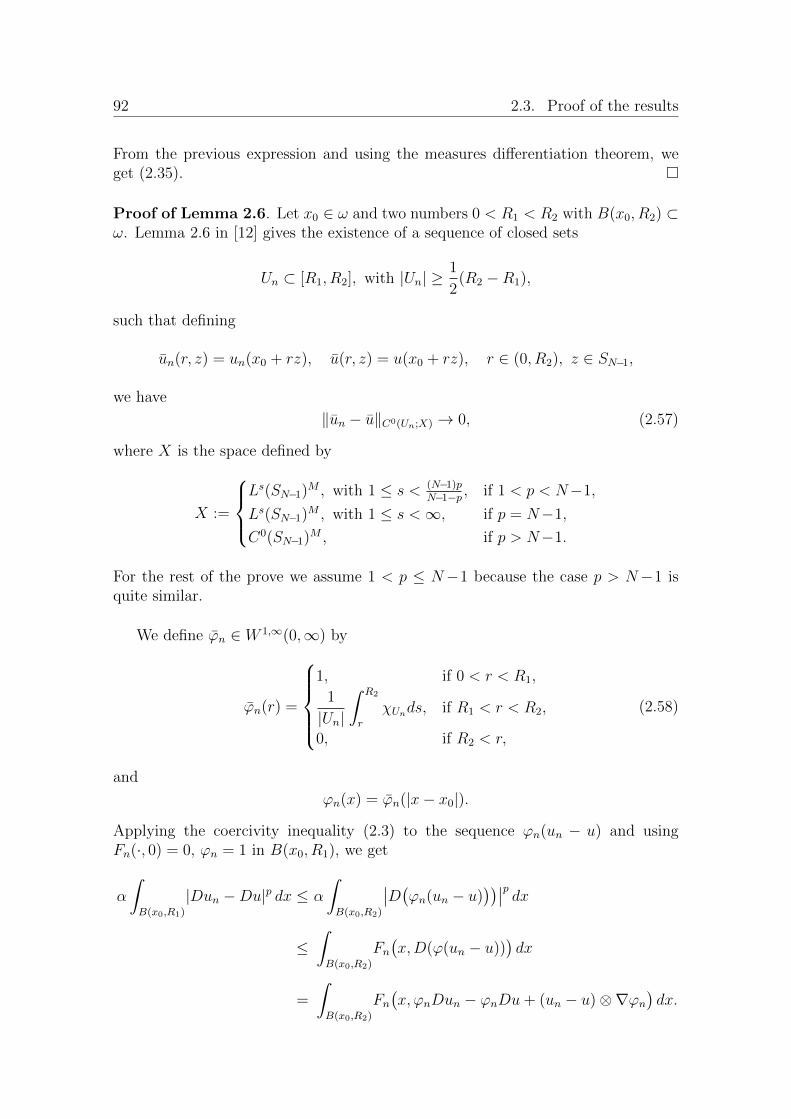
92 2.3. Proof of the results

From the previous expression and using the measures di↵erentiation theorem, weget (2.35). ⇤

Proof of Lemma 2.6. Let x0 2 ! and two numbers 0 < R1 < R2 with B(x0, R2) ⇢!. Lemma 2.6 in [12] gives the existence of a sequence of closed sets

Un ⇢ [R1, R2], with |Un| � 1

2(R2 �R1),

such that defining

un(r, z) = un(x0 + rz), u(r, z) = u(x0 + rz), r 2 (0, R2), z 2 SN�1,

we have

kun � ukC0(Un;X) ! 0, (2.57)

where X is the space defined by

X :=

8><

>:

Ls(SN�1)M , with 1 s < (N�1)pN�1�p

, if 1 < p < N�1,

Ls(SN�1)M , with 1 s < 1, if p = N�1,

C0(SN�1)M , if p > N�1.

For the rest of the prove we assume 1 < p N�1 because the case p > N�1 isquite similar.

We define 'n 2 W 1,1(0,1) by

'n(r) =

8>>><

>>>:

1, if 0 < r < R1,1

|Un|Z R2

r

�Unds, if R1 < r < R2,

0, if R2 < r,

(2.58)

and

'n(x) = 'n(|x� x0|).Applying the coercivity inequality (2.3) to the sequence 'n(un � u) and usingFn(·, 0) = 0, 'n = 1 in B(x0, R1), we get

↵

Z

B(x0,R1)

|Dun �Du|p dx ↵

Z

B(x0,R2)

��D�'n(un � u)

����p dx

Z

B(x0,R2)

Fn

�x,D('(un � u))

�dx

=

Z

B(x0,R2)

Fn

�x,'nDun � 'nDu+ (un � u)⌦r'n

�dx.

Chapter 2. Homogenization of equi-coercive nonlinear energies defined onvector-valued functions, with non-uniformly bounded coe�cients 93

By the convergence (2.33) with ⇠n := 'nDun, ⇢n := �'nDu+ (un � u)⌦r'n, andby estimate (2.8) we obtain up to a subsequence

limn!1

Z

B(x0,R2)

Fn

�x,'nDun � 'nDu+ (un � u)⌦r'n

�dx

limn!1

Z

B(x0,R2)

Fn

�x,'nDun) dx+

Z

B(x0,R2)

# dx

C(h+ µ)�B(x0, R2)

�+

Z

B(x0,R2)

# dx,

with

|#| C�hL + µL + %L + (1 + (aL)

1r )|Du|p�

p�1p (aL)

1pr |Du| a.e. in !.

Indeed, thanks to (2.57) the sequence (un � u) ⌦ r'n converges strongly to 0 inL

prr�1 (!)M⇥N taking into account the inequality

(N � 1)p

N � 1� p� pr

r � 1.

Hence, we deduce from the previous estimates that

%�B(x0, R1)

� C(h+µ)�B(x0, R2)

�+C

Z

B(x0,R1)

|Du|p dx

+C

Z

B(x0,R2)

⇣�hL+µL+%L+(1+(aL)

1r )|Du|p�

p�1p (aL)

1pr |Du|

⌘dx.

Taking R2 such that(h+ µ)

�{|x� x0| = R2}�= 0,

which holds true except for a countable set Ex0 ⇢�0, dist(x0, @!)

�, and making R1

tend to R2, we get that

%�B(x0, R2)

� C(h+µ)�B(x0, R2)

�+C

Z

B(x0,R2)

|Du|p dx

+C

Z

B(x0,R2)

⇣�hL+µL+%L+(1+(aL)

1r )|Du|p�

p�1p (aL)

1pr |Du|

⌘dx,

for any R2 2�0, dist(x0, @!)

� \ Ex0 . Then, by the measures di↵erentiation theoremit follows that

% C (|Du|p + h+ µ) + C⇣�

hL + µL + %L + (1 + (aL)1r )|Du|p�

p�1p

⌘(aL)

1pr |Du|.

Finally, the Young inequality yields the desired estimate (2.23).Now consider {un} and {vn} as in the statement of the lemma. Let x0 2 ! and

0 < R0 < R1 < R2 with B(x0, R2) ⇢ !. Again using Lemma 2.6 in [12] there existtwo sequences of closed sets

Vn ⇢ [R0, R1], Un ⇢ [R1, R2],

94 2.3. Proof of the results

with

|Vn| � 1

2(R1 �R0), |Un| � 1

2(R2 �R1),

such that defining

un(r, z) = un(x0 + rz), vn(r, z) = vn(x0 + rz), r 2 (0, R2), z 2 SN�1,

u(r, z) = u(x0 + rz), v(r, z) = v(x0 + rz), r 2 (0, R2), z 2 SN�1,

we havekun � ukC0(Un;X) ! 0, kvn � vkC0(Vn;X) ! 0.

Then, consider the function 'n defined by (2.58) and the function n 2 W 1,1(0,1)defined by

n(r) =

8>>><

>>>:

1, if 0 < r < R0,1

|Vn|Z R1

r

�Vnds, if R0 < r < R1,

0, if R1 < r.

From these sequences we define wn 2 W 1,p(!)M by

wn = n(vn � v + u) + 'n(1� n)u+ (1� 'n)un,

with'n(x) = 'n(|x� x0|), n(x) = n(|x� x0|),

i.e.

wn =

8>>><

>>>:

vn � v + u, if |x� x0| < R0,

n(vn � v) + u, if R0 < |x� x0| < R1,

'nu+ (1� 'n)un, if R1 < |x� x0| < R2,

un, if R2 < |x� x0|, x 2 !.

(2.59)

It is clear that, for a subsequence, wn converges a.e. to u. Using then thatwn � un is in W 1,p

0 (!)M and that, thanks to 'n, n bounded in W 1,1(⌦), wn isbounded in W 1,p(!)M , we get

wn � un * 0 weakly in W 1,p0 (!).

Thus, from (2.24) we deduceZ

!

Fn(x,Dun) dx

Z

!

Fn(x,Dwn) dx+On

=

Z

B(x0,R0)

Fn

�x,D(vn � v + u)

�dx+

Z

{R2<|x�x0|}\!Fn(x,Dun) dx

+

Z

{R0<|x�x0|<R1}Fn

�x, nD(vn � v) +Du+ (vn � v)⌦r n

�dx

+

Z

{R1<|x�x0|<R2}Fn

�x,'nDu+ (1� 'n)Dun + (u� un)⌦r'n

�dx+On,

Chapter 2. Homogenization of equi-coercive nonlinear energies defined onvector-valued functions, with non-uniformly bounded coe�cients 95

what implies, in particular

Z

B(x0,R2)

Fn(x,Dun) dx

Z

B(x0,R0)

Fn

�x,D(vn � v + u)

�dx

+

Z

{R0<|x�x0|<R1}Fn

�x, nD(vn � v) +Du+ (vn � v)⌦r n

�dx

+

Z

{R1<|x�x0|<R2}Fn

�x,'nDu+ (1� 'n)Dun + (u� un)⌦r'n

�dx+On.

(2.60)

To estimate the first term on the right-hand side of this inequality, we use Lemma2.11 with ⇠n = Dvn, ⇢n = D(�v + u), which take into account (2.25), gives

Z

B(x0,R0)

Fn

�x,D(vn�v+u)

�dx

⌫�B(x0, R0)

�

+ C

Z

B(x0,R0)

�hL+⌫L+$L+(1+(aL)

1r )|D(u�v)|p�

p�1p (aL)

1pr |D(u�v)| dx+On.

(2.61)For the second term, we use again Lemma 2.11 with ⇠n = nDvn and ⇢n = � nDv+Du+ (vn � v)⌦r n. Therefore, up to subsequence it holds

Z

{R0<|x�x0|<R1}Fn

�x, nD(vn � v) +Du+ (vn � v)⌦r n

�dx

C(h+ ⌫ +$)�{R0 |x� x0| R1}

�

+ C

Z

{R0<|x�x0|<R1}

�hL + ⌫L +$L + (1 + (aL)

1r )(|Dv|p + |Du|p)�

p�1p ·

· (aL)1pr (|Du|+ |Dv|) dx+On.

(2.62)

The third term is analogously estimated by Lemma 2.11 with ⇠n = (1�'n)Dun and⇢n = 'nDu+ (u� un)⌦r'n. Extracting a subsequence if necessary, it yields

Z

{R1<|x�x0|<R2}Fn

�x,'nDu+ (1� 'n)Dun + (u� un)⌦r'n

�dx

C(h+ µ+ %)�{R1 |x� x0| R2}

�

+ C

Z

{R1<|x�x0|<R2}

�hL + µL + %L + (1 + (aL)

1r )|Du|p�

p�1p (aL)

1pr |Du|dx+On.

(2.63)

96 2.3. Proof of the results

From (3.52), (2.61), (2.62) and (2.63) we deduce that

µ�B(x0, R2)

�

⌫�B(x0, R0)

�

+ C

Z

B(x0,R0)

�hL + ⌫L +$ + (1 + (aL)

1r )|D(u� v)|p�

p�1p (aL)

1pr |D(u� v)|dx

+ C(h+ ⌫ +$)�{R0 |x� x0| R1}

�

+ C

Z

{R0<|x�x0|<R1}

�hL + ⌫L +$L + (1 + (aL)

1r )(|Dv|p + |Du|p)�

p�1p ·

· (aL)1pr (|Du|+ |Dv|) dx

+ C(h+ µ+ %)�{R1 |x� x0| R2}

�

+ C

Z

{R1<|x�x0|<R2}

�hL + µL + %L + (1 + (aL)

1r )|Du|p�

p�1p (aL)

1pr |Du|dx.

(2.64)Taking R0 such that

(h+ ⌫ +$ + µ+ %)�{|x� x0| = R0}

�= 0,

which holds true except for a countable set Ex0 ⇢ �0, dist(x0, @!)

�, and making

R1, R2 tend to R0, from (2.64) we deduce that

µ�B(x0, R0)

�

⌫�B(x0, R0)

�

+ C

Z

B(x0,R0)

�hL + ⌫L +$L + (1 + (aL)

1r )|D(u� v)|p�

p�1p (aL)

1pr |D(u� v)|dx,

for any R0 2�0, dist(x0, @!)

�\Ex0 (observe that the right term in the integral is welldefined as an element of L1(!)). Therefore, the measures di↵erentiation theoremshows (2.26).

⇤

Proof of Lemma 2.7. The proof is the same as the proof of Lemma 2.6 choosingany point x0 in ⌦ rather than !, extending the functions un, vn by u in ⌦ \ !, andthen noting that the function wn defined by (2.59) in ⌦ is also equal to u in ⌦ \ !.⇤

Proof of Corollary 2.10. Assume that 1 < p N�1. Applying Lemma 2.6 with! = !1 (see also Remark 2.8 about the subsets of !) we obtain

µ ⌫ +C�hL + ⌫L +$L + (1+ (aL)

1r )|D(u� v)p|�

p�1p (aL)

1pr |D(u� v)| in !1 \!2.

Chapter 2. Homogenization of equi-coercive nonlinear energies defined onvector-valued functions, with non-uniformly bounded coe�cients 97

Analogously with ! = !2, we get

⌫ µ+C�hL + µL + %L + (1+ (aL)

1r )|D(u� v)p|�

p�1p (aL)

1pr |D(u� v)| in !1 \ !2.

These two expressions prove the first estimate of (2.31). The proof of the secondestimate is similar. ⇤

Acknowledgement. The authors are grateful for support from the Spanish Min-isterio de Economıa y Competitividad through Project MTM2011-24457, and fromthe Institut de Recherche Mathematique de Rennes. The first author thanks theUniversidad de Sevilla for hospitality during his stay April 18 - May 3 2016, andthe second author thanks the Institut de Mathematiques Appliquees de Rennes forhospitality during his stay June 29 - July 10 2015.

Bibliography

[1] J.M. Ball: “Convexity conditions and existence theorems in nonlinear elasti-city”, Arch. Rational Mech. Anal., 63 (1977), 337-403.

[2] M. Bellieud & G. Bouchitte: “Homogenization of elliptic problems in afiber reinforced structure. Nonlocal e↵ects”, Ann. Scuola Norm. Sup. Pisa Cl.Sci., 26 (4) (1998), 407-436.

[3] A. Beurling & J. Deny: “Espaces de Dirichlet”, Acta Matematica, 99(1958), 203-224.

[4] A. Braides: �-convergence for Beginners, Oxford University Press, Oxford2002, pp. 218.

[5] A. Braides, M. Briane, & J. Casado Dıaz: “Homogenization of non-uniformly bounded periodic di↵usion energies in dimension two”, Nonlinearity,22 (2009), 1459-1480.

[6] M. Briane: “Nonlocal e↵ects in two-dimensional conductivity”, Arch. Rat.Mech. Anal., 182 (2) (2006), 255-267.

[7] M. Briane & M. Camar-Eddine: “Homogenization of two-dimensionalelasticity problems with very sti↵ coe�cients”, J. Math. Pures Appl., 88 (2007),483-505.

[8] M. Briane & J. Casado Dıaz: “Two-dimensional div-curl results. Applica-tion to the lack of nonlocal e↵ects in homogenization”, Com. Part. Di↵. Equ.,32 (2007), 935-969.

[9] M. Briane & J. Casado Dıaz: “Asymptotic behavior of equicoercive dif-fusion energies in two dimension”, Calc. Var. Part. Di↵. Equa., 29 (4) (2007),455-479.

98 Bibliography

[10] M. Briane & J. Casado Dıaz : “Homogenization of convex functionalswhich are weakly coercive and not equibounded from above”, Ann. I.H.P. (C)Non Lin. Anal., 30 (4) (2013), 547-571.

[11] M. Briane & J. Casado Dıaz : “Homogenization of systems with equi-integrable coe�cients”, ESAIM: COCV, 20 (4) (2014), 1214-1223.

[12] M. Briane & J. Casado-Diaz: “A new div-curl result. Applications to thehomogenization of elliptic systems and to the weak continuity of the Jacobian”,to appear in J. Di↵. Equa.

[13] M. Briane, J. Casado Dıaz & F. Murat: “The div-curl lemma ‘trenteans apres’: an extension and an application to the G-convergence of unboundedmonotone operators”, J. Math. Pures Appl., 91 (2009), 476-494.

[14] G. Buttazzo & G. Dal Maso: “�-limits of integral functionals”, J. AnalyseMath., 37 (1980), 145-185.

[15] M. Camar-Eddine & P. Seppecher: “Closure of the set of di↵usion func-tionals with respect to the Mosco-convergence”, Math. Models Methods Appl.Sci., 12 (8) (2002), 1153-1176.

[16] M. Camar-Eddine & P. Seppecher: “Determination of the closure of theset of elasticity functionals”, Arch. Ration. Mech. Anal., 170 (3) (2003), 211-245.

[17] L. Carbone & C. Sbordone: “Some properties of �-limits of integral func-tionals”, Ann. Mate. Pura Appl., 122 (1979), 1-60.

[18] P.G. Ciarlet: Mathematical Elasticity, Vol. I: Three-dimensional elasticity.Studies in Mathematics and its Applications 20, North-Holland Publishing Co.,Amsterdam 1988, pp. 451.

[19] P.G. Ciarlet: Introduction a l’analyse numerique matricielle et al’optimisation (French) [Introduction to matrix numerical analysis and optim-ization], Mathematiques Appliquees pour la Maıtrise [Applied Mathematics forthe Master’s Degree] Masson, Paris 1982, 279 pp.

[20] B. Dacorogna: Direct methods in the calculus of variations, Applied Math-ematical Sciences 78, Springer-Verlag, Berlin 1989, pp. 308.

[21] G. Dal Maso: An introduction to �-convergence, Birkhauser, Boston 1993,pp. 341.

[22] E. De Giorgi: “Sulla convergenza di alcune successioni di integrali del tipodell’area”, Rend. Mat. Roma, 8 (1975), 277-294.

[23] E. De Giorgi & T. Franzoni: “Su un tipo di convergenza variazionale”,Rend. Acc. Naz. Lincei Roma, 58 (6) (1975), 842-850.

Chapter 2. Homogenization of equi-coercive nonlinear energies defined onvector-valued functions, with non-uniformly bounded coe�cients 99

[24] V.N. Fenchenko & E.Ya. Khruslov: “Asymptotic behavior of solutionsof di↵erential equations with strongly oscillating matrix of coe�cients whichdoes not satisfy the condition of uniform boundedness”, Dokl. AN Ukr.SSR, 4(1981).

[25] G.A. Francfort: “Homogenisation of a class of fourth order equations withapplication to incompressible elasticity”, Proc. Roy. Soc. Edinburgh Sect. A,120 (1-2) (1992), 25-46.

[26] E.Ya. Khruslov: “Homogenized models of composite media”, Composite Me-dia and Homogenization Theory, ed. by G. Dal Maso and G.F. Dell’Antonio,in Progress in Nonlinear Di↵erential Equations and Their Applications,Birkhauser 1991, 159-182.

[27] U. Mosco: “Composite media and asymptotic Dirichlet forms”, J. Func.Anal., 123 (2) (1994), 368-421.

[28] F. Murat: “H-convergence”, Seminaire d’Analyse Fonctionnelle etNumerique, 1977-78, Universite d’Alger, multicopied, 34 pp. English transla-tion : F. Murat & L. Tartar: “H-convergence”, Topics in the MathematicalModelling of Composite Materials, ed. by L. Cherkaev & R.V. Kohn, Progress inNonlinear Di↵erential Equations and their Applications, 31, Birkauser, Boston1998, 21-43.

[29] A. Pallares-Martın: “High-Contrast homogenization of linear systems ofpartial di↵erential equations”, to appear in Math. Meth. Appl. Sc.

[30] C. Pideri & P. Seppecher: “A second gradient material resulting from thehomogenization of an heterogeneous linear elastic medium”, Continuum Mech.and Thermodyn., 9 (5) (1997), 241-257.

[31] A. Raoult: “Nonpolyconvexity of the stored energy function of a Saint-Venant-Kirchho↵”, Material. Apl. Mat., 31 (6) (1986), 417-419.

[32] E. Sanchez-Palencia: Nonhomogeneous Media and Vibration Theory, Lec-ture Notes in Physics 127, Springer-Verlag, Berlin-New York 1980, pp. 398.

[33] S. Spagnolo: “Sulla convergenza di soluzioni di equazioni paraboliche edellittiche”, Ann. Scuola Norm. Sup. Pisa Cl. Sci., 22 (3) (1968), 571-597.

[34] R. Temam: Problemes mathematiques en plasticite, (French) [Mathematicalproblems in plasticity], Methodes Mathematiques de l’Informatique [Mathem-atical Methods of Information Science] 12, Gauthier-Villars, Montrouge 1983,pp. 353.

[35] L. Tartar: The General Theory of Homogenization: A Personalized Introduc-tion, Lecture Notes of the Unione Matematica Italiana, Springer-Verlag, BerlinHeidelberg 2009, pp. 471.

Chapter 3

Asymptotic behavior of the linearelasticity system with varying andunbounded coe�cients in a thinbeam

J. Casado-Dıaz† M. Luna-Laynez† A. Pallares-Martın†

† Dpto. de Ecuaciones Diferenciales y Analisis Numerico,Facultad de Matematicas, C. Tarfıa s/n,

41012 Sevilla, Spain.e-mail: jcasadod@us.es, mllaynez@us.es, ajpallares@us.es

Submitted for publication.

Abstract.

We study the asymptotic behavior of the solutions of the linear elasticity systemin a thin beam of thickness " > 0, when " tends to zero. The elasticity tensor alsovaries with ", and it is assumed to be uniformly elliptic but non-uniformly bounded.Namely, we just impose that its norm in L1 is an infinitesimal of 1/" and its normin L1 is bounded. We obtain an homogenized problem corresponding to a linearsystem in one dimension. It gives an approximation of the solution of the problemin the thin beam which consists in the sum of a Bernouilli-Navier’s deformationplus a torsion term. This limit system provides a general asymptotic model forthe behavior of an elastic beam composed by the mixture, at a mesoscopic level,of several materials, and therefore, which does not satisfy any homogeneity and/orisotropy conditions.

101

102 3.1. Introduction

3.1 Introduction

Obtaining an asymptotic model for the behavior of an elastic beam of thickness" > 0 is a very classical problem due to its huge interest in engineering. The idea isto approximate the deformation by the solution of a di↵erential system in dimensionone, which is much simpler to deal with from a numerical point of view. Such anordinary di↵erential system is usually composed by two uncoupled linear equationsof fourth order, which describe the asymptotic behavior of the deformations in theorthogonal directions to the axis of the beam. From a mathematical point of viewthis system can be obtained by passing to the limit when " tends to zero in theelasticity system (see e.g. [19], [29])

( �div�� trace(e(u"))I + 2µ e(u")

�= f" in (0, 1)⇥ ("!),

�� trace(e(u"))I + 2µ e(u")

�⌫ = 0 on (0, 1)⇥ ("@!),

(3.1)

where ! is a smooth, connected, bounded domain in RN�1 (usually N = 2, 3), ⌫ isthe unitary outward normal vector to ! on @!, �, µ > 0 are the Lame constans, u"

is the deformation of the beam, e(u") := (Du +DuT )/2 is the strain tensor and f"is the exterior force which is usually supposed of the form

f",1(x) = f1(x1), f",j(x) = "fj(x1), j 2 {2, · · · , N}. (3.2)

By also adding certain boundaries conditions on the extremities of the beam (de-pending for example on whether the corresponding base is fixed or not) the classicalmodel provides the following approximation for the deformation on the orthogonaldirections to the axis of the beam:

u",j(x) ⇠ 1

"uj(x1), j 2 {2, · · · , N}, (3.3)

with uj solution to the ordinary di↵erential equation

2µ(�N + 2µ)

�(N � 1) + 2µIjd4uj

dx41

= fj in (0, 1), (3.4)

where Ij is the inertial momentum of ! in the j-th direction divided by |!| (it isassumed that the center of mass of ! is zero and that the axes are inertial). Theseequations are usually known as the beam equations. It is also possible to get thefollowing approximation for the deformation in the direction x1,

u",1(x) ⇠ u1(x1)�NX

j=2

duj

dx1

xj

", (3.5)

with u1 solution to

� 2µ(�N + 2µ)

�(N � 1) + 2µ

d2u1

dx21

= f1 in (0, 1). (3.6)

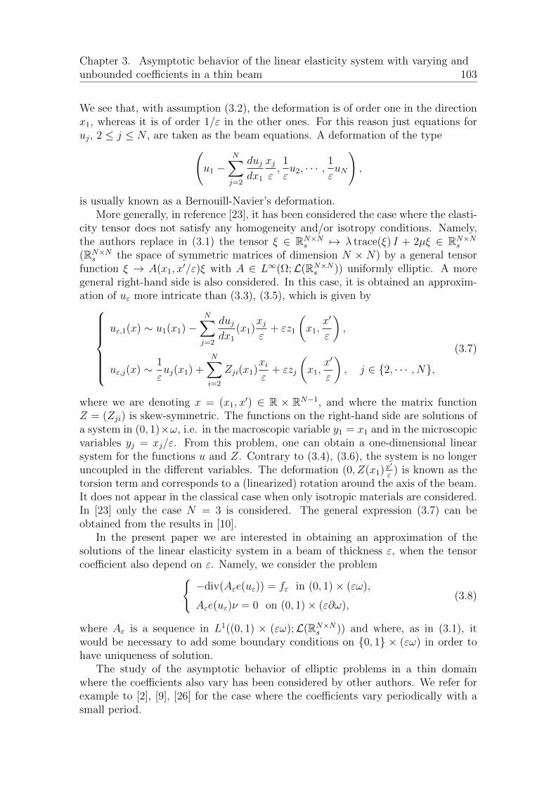
Chapter 3. Asymptotic behavior of the linear elasticity system with varying andunbounded coe�cients in a thin beam 103

We see that, with assumption (3.2), the deformation is of order one in the directionx1, whereas it is of order 1/" in the other ones. For this reason just equations foruj, 2 j N , are taken as the beam equations. A deformation of the type

u1 �

NX

j=2

duj

dx1

xj

",1

"u2, · · · , 1

"uN

!,

is usually known as a Bernouill-Navier’s deformation.More generally, in reference [23], it has been considered the case where the elasti-

city tensor does not satisfy any homogeneity and/or isotropy conditions. Namely,the authors replace in (3.1) the tensor ⇠ 2 RN⇥N

s 7! � trace(⇠) I + 2µ⇠ 2 RN⇥Ns

(RN⇥Ns the space of symmetric matrices of dimension N ⇥ N) by a general tensor

function ⇠ ! A(x1, x0/")⇠ with A 2 L1(⌦;L(RN⇥Ns )) uniformly elliptic. A more

general right-hand side is also considered. In this case, it is obtained an approxim-ation of u" more intricate than (3.3), (3.5), which is given by8>>>>><

>>>>>:

u",1(x) ⇠ u1(x1)�NX

j=2

duj

dx1(x1)

xj

"+ "z1

✓x1,

x0

"

◆,

u",j(x) ⇠ 1

"uj(x1) +

NX

i=2

Zji(x1)xi

"+ "zj

✓x1,

x0

"

◆, j 2 {2, · · · , N},

(3.7)

where we are denoting x = (x1, x0) 2 R ⇥ RN�1, and where the matrix functionZ = (Zji) is skew-symmetric. The functions on the right-hand side are solutions ofa system in (0, 1)⇥!, i.e. in the macroscopic variable y1 = x1 and in the microscopicvariables yj = xj/". From this problem, one can obtain a one-dimensional linearsystem for the functions u and Z. Contrary to (3.4), (3.6), the system is no longeruncoupled in the di↵erent variables. The deformation (0, Z(x1)

x0

") is known as the

torsion term and corresponds to a (linearized) rotation around the axis of the beam.It does not appear in the classical case when only isotropic materials are considered.In [23] only the case N = 3 is considered. The general expression (3.7) can beobtained from the results in [10].

In the present paper we are interested in obtaining an approximation of thesolutions of the linear elasticity system in a beam of thickness ", when the tensorcoe�cient also depend on ". Namely, we consider the problem

( �div(A"e(u")) = f" in (0, 1)⇥ ("!),

A"e(u")⌫ = 0 on (0, 1)⇥ ("@!),(3.8)

where A" is a sequence in L1((0, 1) ⇥ ("!);L(RN⇥Ns )) and where, as in (3.1), it

would be necessary to add some boundary conditions on {0, 1} ⇥ ("!) in order tohave uniqueness of solution.

The study of the asymptotic behavior of elliptic problems in a thin domainwhere the coe�cients also vary has been considered by other authors. We refer forexample to [2], [9], [26] for the case where the coe�cients vary periodically with asmall period.

104 3.1. Introduction

When no periodicity is assumed we give the following references. For the caseof a linear di↵usion equation in a plate in dimension 3, (the case of a beam wouldbe very similar) the problem has been considered in [15] by assuming the sequenceof coe�cients matrices uniformly elliptic and bounded. The authors show thatthe solutions can be approximated by those of a partial di↵erential equation indimension 2. Some expressions for this limit equation have been obtained in [17]under special assumptions on the coe�cients. An extension to non-linear di↵usionequations has been obtained in [13]. The case of a nonlinear monotone equation ina beam (0, 1)⇥ ("!), where the coe�cients also depend on ", has been considered in[12], assuming the coe�cients uniformly elliptic and bounded. In [12]a right-handside of the form f"(x) = f(x1, x0/") + divG(x1, x0/") is considered, and due to thepresence of the function G, the limit problem is no more a one-dimensional problem.

For the linear elasticity system, the problem has been considered in [14] for aplate !⇥ (�", ") in dimension 3 (here ! is a smooth, connected, bounded domain inR2), assuming certain isotropy conditions of the coe�cients and also that they areuniformly elliptic and bounded. Thanks to these isotropy conditions, the authorsshow that the deformation of the plate along the directions of the plane x3 = 0can be approximated by the solution of a fourth order equation in dimension two.This is similar to the case of an isotropic beam described at the beginning of theintroduction. The problem has also been studied in [18] without assuming isotropicconditions but supposing that the coe�cients only depend on the variable x3. Now,the approximation of the solutions is of the form

u",1(x) ⇠ u1(x1, x2)� @x1u3(x1, x2)x3

", u",2(x) ⇠ u2(x1, x2)� @x2u3(x1, x2)

x3

",

u",3(x) ⇠ 1

"u3(x1, x2).

A deformation with the form of this approximation is called a Kirchho↵-Love de-formation. It is the analogous for a plate to the Bernouilli-Navier deformation fora beam. Now the authors find a linear system for u1, u2, u3, which is no longeruncoupled as in [14].

In our case our aim is to obtain a limit system in dimension one which approx-imates the solutions of (3.8) without imposing any isotropy and/or homogeneityconditions on the tensor function A". We assume the ellipticity condition (3.16)below but for the upper bound we just assume that the norm in L1 of A" is aninfinitesimal with respect to 1/", (3.15), and that the coe�cients are bounded in L1,(3.14). However, in our knowledge the results are new even in the case of uniformlybounded coe�cients. We obtain an approximation of the solutions similar to (3.7),but eliminating the term corresponding to the function z, which is of order ". Thefunctions u and Z are the solutions to a linear system in dimension one.

As it is well known (see e.g. [1], [28]) the interest of taking A" depending on "(homogenization problem) is to describe the behavior of beams composed by mix-tures of di↵erent materials at a microscopic (or more exactly mesoscopic) level. Thehomogenization process gives an approximation of these mixtures by a generalizedmaterial represented by the homogenized tensor. In our case, the coe�cient tensorcorresponding to the limit system in dimension one. Therefore, our results provide a

Chapter 3. Asymptotic behavior of the linear elasticity system with varying andunbounded coe�cients in a thin beam 105

general model for the behavior of a beam composed by a general mixture of mater-ials. It can be used to study optimal design problems in a beam. The fact that thecoe�cients are not uniformly bounded means that we are considering high-contrasthomogenization problems. We recall that if there is not reduction of dimension,then, contrary to our result, by assuming the coe�cients just bounded in L1 we getnon-local terms in the limit problem for N � 3, [3], [16] (but not for N < 2, seee.g. [4], [5], [25]). Some local homogenization results where there is not reductionof dimension, but assuming the coe�cients bounded in a certain Lp with p > 1 areobtained in [6], [7], [8].

To finish we also observe that although no equi-integrability for the coe�cientsis assumed, the limit tensor we find is in L1, i.e. it does not contain any measuresupported on sets with null Lebesgue measure.

Notations

• We denote by e1, · · · , eN the usual basis in RN .

• For any vector u 2 RN , we will use the following decomposition

u =

✓u1

u0

◆,

where u1 2 R and u0 2 RN�1. We will also denote by u0 a vector in RN whosefirst component vanishes. In this way, the above decomposition can be alsowritten as u = u1e1 + u0.

• For any matrix M , we denote by MT the transposed matrix of M .

• : denotes the euclidean inner product in RN⇥N , i.e. M1 : M2 = trace(MT1 M2).

• RN⇥Ns denotes the space of symmetric matrices of dimension N ⇥N .

• RN⇥Nsk denotes the space of skew-symmetric matrices of dimension N ⇥N .

• RN⇥Ns1sk0

denotes the space of matrices M 2 RN⇥N such that

(M1i = Mi1, for i = 1, . . . , N,

Mij = �Mji, for i, j = 2, . . . , N.

• e(v) denotes the symmetric part of the derivative of a function v, i.e.

e(v) =1

2(Dv +DvT ).

• For a set U ⇢ RN , M(U) denotes the space of Radon measures on U withbounded total variation. If U is bounded and open, it agrees with the dualspace of C0

0(U). If U is compact, it agrees with the dual space of C0(U).

106 3.2. The homogenization result

• For any measure a 2 M(U), we define aL 2 L1(U) as the derivative of a withrespect to the Lebesgue measure.

• For a Lipschitz open set O ⇢ RN and a set F ⇢ @O, we denote by HkF (O) the

space of functions in Hk(O), such that their derivatives of order less or equalthan k � 1 vanish on F .

• We denote by C a generic constant which can change from line to line.

• We denote by O" an arbitrary sequence of real numbers which tends to zerowhen " tends to zero. It can change from line to line.

3.2 The homogenization result

Let ! ⇢ RN�1 be a Lipschitz connected bounded open set, with N � 2. Then, for" > 0 we define the thin beam ⌦" by

⌦" = (0, 1)⇥ ("!). (3.9)

The extremities of ⌦" are denoted by �", i.e.

�" = {0, 1}⇥ ("!). (3.10)

When " = 1, we will just write ⌦ and � instead of ⌦1 and �1 respectively.The coordinate system is chosen in such way that the origin is the center of mass

of ! and the coordinates axes in the x0 variables coincide with the inertial axes of!, i.e. such that ! satisfies Z

!

y0dy0 = 0, (3.11)

Z

!

yiyj dy0 = 0, 2 i, j N, i 6= j. (3.12)

We define the diagonal matrix I (it corresponds to the inertia matrix of ! dividedby |!|) by

I =

0

BB@

I2

. . .

IN

1

CCA , with Ii =1

|!|Z

!

y2i dy0, 2 i N. (3.13)

In the domain ⌦" we will consider a linear elastic problem where the coe�cientsalso depend on ". Our purpose is to approximate its solutions for those of a one-dimensional problem.

We will assume that the coe�cients of the elasticity system are given by a se-quence of tensors A" 2 L1(⌦";L(RN⇥N

s )) which satisfies the following three prop-erties:

1

|⌦"|Z

⌦"

|A"|dx C, (3.14)

Chapter 3. Asymptotic behavior of the linear elasticity system with varying andunbounded coe�cients in a thin beam 107

"kA"kL1(⌦";L(RN⇥Ns )) ! 0, (3.15)

9↵ > 0, A"⇠ : ⇠ � ↵|⇠|2, 8 ⇠ 2 RN⇥Ns , a.e. in ⌦". (3.16)

Then, we will deal with a sequence u" 2 H1(⌦")N , which satisfies the linear elasticitysystem ( �div(A"e(u")) = h" in ⌦",

A"e(u")⌫" = 0 on @⌦" \ �".(3.17)

Here ⌫" denotes the unit outward normal to ⌦" on @⌦" and h" = (h",1, h0") is defined

by

h",1(x) = f",1

✓x1,

x0

"

◆, h0

"(x) = "f 0"

✓x1,

x0

"

◆+ g0"

✓x1,

x0

"

◆, a.e. x 2 ⌦", (3.18)

with f" 2 L2(⌦)N and g0" 2 L2(⌦)N�1 such thatZ

!

g0"dy0 = 0, a.e. y1 2 (0, 1), (3.19)

9 f 2 L2(⌦)N with f" * f in L2(⌦)N , (3.20)

9 g0 2 L2(⌦)N�1 with g0" * g0 in L2(⌦)N�1. (3.21)

Since we have not imposed any boundary condition on �", we will also need toassume some bounds for u" = (u",1, u0

"). Namely, we suppose there exists C > 0such that

1

|⌦"|Z

⌦"

A"e(u") : e(u") dx C, (3.22)

mina2[0,1]

(k(u",1, "u

0")kL2({a}⇥"!)N+

����u0" �

1

|"!|Z

{a}⇥"!

u0" dx

0����L2({a}⇥"!)N�1

)!C|"!| 12 .

(3.23)Our main result is given by Theorem 3.1 below. Before stating it, we introduce thefollowing notation:For u = (u1, u0) 2 H1(0, 1)⇥H2(0, 1)N�1 and Z 2 H1(0, 1;R(N�1)⇥(N�1)

sk ), we denote

e0(u, Z) :=

0

BBB@

du1

dx1

✓d2u0

dx21

◆T

d2u0

dx21

dZ

dx1

1

CCCA2 L2(0, 1;RN⇥N

s1sk0). (3.24)

Theorem 3.1. Let A" be a sequence of tensor functions in L1(⌦";L(RN⇥Ns )) which

satisfy (3.14), (3.15) and (3.16). Then there exist � > 0, which only depends on !,a constant �, which only depends on ↵ and !, a subsequence of ", still denoted by", a 2 M(0, 1) and A 2 L1(0, 1;L(RN⇥N

s1sk0)) with

1

|"!|Z

"!

|A"| dx0 ⇤* a in M(0, 1), (3.25)

108 3.2. The homogenization result

|AE| ��AE : E

� 12�aL� 1

2 , 8E 2 RN⇥Ns1sk0

, a.e. in (0, 1), (3.26)

|E|2 �AE : E, 8E 2 RN⇥Ns1sk0

, a.e. in (0, 1), (3.27)

such that the following homogenization result holds:Let h" be a sequence given by (3.18) with f" 2 L2(⌦)N , g0" 2 L2(⌦)N�1 satis-

fying (3.19), (3.20) and (3.21). If u" 2 H1(⌦")N satisfies (3.17), (3.22) and(3.23), then, for a subsequence of ", there exist u 2 H1(0, 1) ⇥ H2(0, 1)N�1 and

Z 2 H1(0, 1;R(N�1)⇥(N�1)sk ), with

Z 1

0

Ae0(u, Z) : e0(u, Z) dx1 < 1, (3.28)

which satisfy the variational equation8>>>>>><

>>>>>>:

Z 1

0

Ae0(u, Z) :e0(u, Z) dy1 =1

|!|Z

⌦

✓f1

✓u1 � du0

dy1· y0◆+ f 0 · u0 + g0 · (Z y0)

◆dy,

8(u, Z) 2 H10 (0, 1)⇥H2

0 (0, 1)N�1 ⇥H1

0 (0, 1;R(N�1)⇥(N�1)sk ),

with

Z 1

0

Ae0(u, Z) : e0(u, Z) dx1 < 1,

(3.29)and provide the following approximation of u"

lim"!0

1

|⌦"|Z

⌦"

����u",1 � u1 +du0

dx1· x

0

"

����2

+��"u0

" � u0��2 +����"@x1u

0" �

du0

dx1

����2

+ |"Dx0u0" � Z|2 +

����u0" �

1

|"!|Z

"!

u0"dz

0 � Zx0

"

����2!dx = 0.

(3.30)

Remark 3.2. Theorem 3.1 provides the approximation of u"

u",1(x) ⇠ u1(x1)� du0

dx1· x

0

", u0

"(x) ⇠1

"u0(x1) + Z(x1)

x0

", a.e. in ⌦",

in the sense that (3.30) holds. The right-hand side is the sum of the two deformations(u1 � du0

dx1· x0

", 1"u0) and (0, Z x0

"). The first one corresponds to a Bernouilli-Navier’s

deformation, which usually appears in the asymptotic description of the deformationof a beam. The second one is known as the torsion term and corresponds to aninfinitesimal rotation around the axis of the beam.

Statement (3.30) can be improved by adding some weak convergences in Sobolevspaces which are interesting for example in order to deduce boundary conditionsfor the functions u and Z. However, to do this we need to write the correspondingconvergences in a fixed domain. As usual this can be carried out by using the changesof variables y1 = x1, y0 = x0/". Namely, for the sequence u" in Theorem 3.1, wedefine U" 2 H1(⌦)N as

U"(y) = u"(y1, "y0) a.e. y 2 ⌦.

Chapter 3. Asymptotic behavior of the linear elasticity system with varying andunbounded coe�cients in a thin beam 109

Then, we have 8>>><

>>>:

U",1 * u1 in H1(⌦),

"U 0" ! u0 in H1(⌦)N�1,

U 0" �

1

|!|Z

!

U 0" d⌧

0 * Zy0 in H1(⌦)N�1.

(3.31)

Remark 3.3. In the proof of Theorem 3.1 (see (3.68) and (3.89)), we will alsoprove that if u" is in the conditions of the theorem and u" is another sequence whichsatisfies

1

|⌦"|Z

⌦"

|e(u")|2dx C,

and (3.30) with u and Z replaced by some other functions u, Z then

9 lim"!0

1

|⌦"|Z

⌦"

A"e(u") :e(u")' dx =

Z 1

0

Ae0(u, Z) :e0(u, Z)' dx1, 8' 2 C10 (0, 1).

(3.32)In this assertion, we have used that (3.22) and (3.30) also imply (3.23), which iseasy to check by using Theorem 3.9 below. In particular, we can take u" = u" to getthe convergence of the energies.

Remark 3.4. We observe that although (3.14) only provides an estimate for A" inL1 (it just implies (3.25)), the coe�cient tensor A in the limit problem (3.29) isin L1, i.e. it does not contain any measure which is not absolutely continuous withrespect to the Lebesgue measure. Indeed, inequality (3.26) provides the estimate

|A| �2aL a.e. in (0, 1).

In particular, if aL belongs to L1(0, 1), we have that A is in L1(0, 1;L(RN⇥Ns1sk0

)).

Remark 3.5. Variational equation (3.29) can be written as the partial di↵erentialsystem8>>>>>>><

>>>>>>>:

� d

dx1

⇥Ae0(u, Z)

⇤11

=1

|!|Z

!

f1 dy0 in (0, 1),

d2

dx21

⇥Ae0(u, Z)

⇤1j=

1

|!|Z

!

(f1yj + f 0j) dy

0 in (0, 1), 8 j 2 {2, · · · , N},

� d

dx1

⇥Ae0(u, Z)

⇤ij=

1

2|!|Z

!

�giyj � gjyi) dy

0 in (0, 1), 8 i, j 2 {2, · · · , N}, i<j,

(3.33)where we recall that e0(u, Z) contains derivatives of first orden in u1 and Z andderivatives of second order in u0.

It is worth comparing system (3.33) to the classical system for a beam, which iscomposed by N � 1 ordinary di↵erential equations of fourth order (see e.g. ([29]).Indeed, it corresponds to taking

A"⇠ = � trace(⇠)I + 2µ⇠, 8 ⇠ 2 RN⇥Ns . (3.34)

110 3.2. The homogenization result

where � and µ are two positive constants (the Lame constants). In this case, we canprove that system (3.33) reduces to

8>>>>>>><

>>>>>>>:

�Ed2u1

dx21

=1

|!|Z

!

f1 dy0 in (0, 1),

E I d4u0

dx41

=1

|!|Z

!

(f1y0 + f 0) dy0 in (0, 1),

�Bd2Z

dx21

=1

|!|Z

!

g0 ⌦ y0 � y0 ⌦ g0

2dy0 in (0, 1),

(3.35)

where E is the Young modulus

E =2µ(�N + 2µ)

�(N � 1) + 2µ,

and B is an elliptic tensor in L(R(N�1)⇥(N�1)sk ) which depends on ↵, � and !. In

particular, in this case, system (3.33) is uncoupled in the variables u1, u0 and Z.Taking the functions f1 and g0 as the null functions and choosing appropriate bound-ary conditions on {0, 1} in (3.35), we have that the first and third equation just giveu1 = 0, Z = 0 and then we recuperate the classical equation for a beam

E I d4u0

dx41

=1

|!|Z

!

f 0 dy0,

where usually f 0 is also chosen independent of the variable y0. However, we remarkthat even if the tensor functions A" are taken independent of ", the limit problemwritten in the variables u and Z has the general form provided by (3.33). This resultcan be deduced from [23], where it is studied the asymptotic behavior of a beam withfixed coe�cients but without assuming any homogeneity or isotropy condition.

Remark 3.6. System (3.33) implies that the elements⇥Ae0(u,Z)

⇤11

and⇥Ae0(u,Z)

⇤ij

with i, j 2 {2, · · · , N}, i < j are in H1(0, 1) while the elements⇥Ae0(u, Z)

⇤1j,

with j 2 {2, · · · , N} are in H2(0, 1). Taking into account (3.27), this also provesthat e0(u, Z) is in L1(0, 1;RN⇥N

s1sk0) and then that (u, Z) belongs to W 1,1(0, 1) ⇥

W 2,1(0, 1)N�1 ⇥W 1,1(0, 1;R(N�1)⇥(N�1)sk ).

In Theorem 3.1 we have not assumed any symmetry condition for the tensormatrices A". However, from the physical point of view it is known that in order tohave the conservation of the angular momentum, it is necessary to have A" symmet-ric, i.e. such that

A"E1 : E2 = A"E2 : E1, 8E1, E2 2 RN⇥Ns .

In this case it is possible to show that the tensor A which appears in Theorem 3.1also satisfies the symmetry condition

AE1 : E2 = AE2 : E1, 8E1, E2 2 RN⇥Ns1sk0

.

More generally, we have the following result.

Chapter 3. Asymptotic behavior of the linear elasticity system with varying andunbounded coe�cients in a thin beam 111

Proposition 3.7. Let A" be in the conditions of Theorem 3.1 and consider thesubsequence of " and the functions A, a which appear in the thesis of the theorem.Then, Theorem 3.1 also holds by replacing A" by AT

" and A by AT .

In Theorem 3.1 we have preferred to not impose any boundary condition on �" toshow that the equation satisfied by the functions u and Z does not depend on them.As a consequence, it is now possible to get a homogenization result for di↵erentboundary conditions such as Dirichlet, Neumann or Robin conditions on �". As anexample we state in the following corollary a result corresponding to homogeneousDirichlet boundary conditions.

Corollary 3.8. Let A" be in the conditions of Theorem 3.1 and consider the sub-sequence of " and the functions A, a which appear in the thesis of the theorem. Then,for every sequence h" given by (3.18) with f" 2 L2(⌦)N , g0" 2 L2(⌦)N�1 satisfying(3.19), (3.20) and (3.21), the unique solution u" to

8>><

>>:

�div(A"e(u")) = h" in ⌦",

A"e(u")⌫" = 0 on @⌦" \ �",

u" = 0 on �",

(3.36)

satisfies (3.30) with (u, Z) the unique solution to the variational problem

8>>>>>>>>>>>>>><

>>>>>>>>>>>>>>:

(u, Z) 2 H10 (0, 1)⇥H2

0 (0, 1)N�1 ⇥H1

0 (0, 1;R(N�1)⇥(N�1)s1sk0

),

with

Z 1

0

Ae0(u, Z) : e0(u, Z) dx1 < 1Z 1

0

Ae0(u, Z) :e0(u, Z) dy1=1

|!|Z

⌦

✓f1

✓u1 � du0

dy1· y0◆+ f 0 · u0 + g0 · (Z y0)

◆dy,

8(u, Z) 2 H10 (0, 1)⇥H2

0 (0, 1)N�1 ⇥H1

0 (0, 1;R(N�1)⇥(N�1)s1sk0

),

with

Z 1

0

Ae0(u, Z) : e0(u, Z) dx1 < 1.

(3.37)

3.3 Proof of the results

The present section is devoted to proving the di↵erent results stated in the previousone. An important result to do this is the following theorem. It is a particular caseof a decomposition result for a sequence of deformations in a thin domain, whichhas been proved in [11].

Theorem 3.9. We consider a Lipschitz connected bounded open set ! ⇢ RN�1,and define ⌦" by (3.9), then, there exists a constant C > 0 independent of ", suchthat for every u" 2 H1(⌦")N there exist q" 2 RN , Q" 2 RN⇥N

sk , b0" 2 H2(0, 1)N�1,

112 3.3. Proof of the results

Z" 2 H1(0, 1;R(N�1)⇥(N�1)sk ) and w" 2 H1(⌦")N , satisfying

u" = q" +Q"x+1

"

0

b0"

!+

0

@ 0 � db0"dx1

0 Z"

1

A

0

@0

x0

"

1

A+ w" in ⌦", (3.38)

with

kb0"kH2(0,1)N�1+kZ"kH1(0,1;R(N�1)⇥(N�1)sk )

+1

|⌦"| 12kw"kH1(⌦")N C

|⌦"| 12ke(u")kL2(⌦";RN⇥N

s ).

(3.39)

Theorem 3.9 is an improvement of Korn’s inequality in a thin beam. It providesa decomposition of u" as the sum of a “linearized” rigid movement given by the twofirst terms on the right-hand side of (3.38), a sequence w" whose norm in H1(⌦")N

is bounded by the norm of e(u") in L2(⌦";RN⇥Ns ) and a term (sum of the third and

fourth terms in (3.38)) whose norm in H1(⌦")N is bounded by the norm of e(u") inL2(⌦";RN⇥N

s ) divided by ", which has a very particular structure. Clearly it impliesthe following classical estimate from Korn’s inequality in a beam.

Corollary 3.10. We consider a Lipschitz connected bounded open set ! ⇢ RN�1,and define ⌦" by (3.9), then, there exists C > 0 independent of ", such that for everyu" 2 H1(⌦")N there exist q" 2 RN and Q" 2 RN⇥N

sk , which satisfy

ku" � q" �Q"xkH1(⌦")N C

"ke(u")kL2(⌦";RN⇥N

s ). (3.40)

As usual, since every sequence u" of the form u" = q" + Q"x, with q" 2 RN andQ" 2 RN⇥N

sk satisfies that e(u") = 0, Theorem 3.9 and Corollary 3.10 do not provideany bound for the corresponding “linearized” rigid movement. In order to eliminatethis term we need to get some extra information about u". In this way, we have thefollowing result.

Theorem 3.11. We consider a Lipschitz connected bounded open set ! ⇢ RN�1

which satisfies (3.11) and (3.12), and define ⌦" by (3.9), then, there exists a con-stant C > 0 independent of ", such that for every u" 2 H1(⌦")N there exist

b0" 2 H2(0, 1)N�1, Z" 2 H1(0, 1;R(N�1)⇥(N�1)sk ) and w" 2 H1(⌦")N , satisfying

u" =1

"

0

b0"

!+

0

@ 0 � db0"dx1

0 Z"

1

A

0

@0

x0

"

1

A+ w" in ⌦", (3.41)

with

kb0"kH2(0,1)N + kZ"kH1(0,1;R(N�1)⇥(N�1)sk )

+1

|⌦"| 12kw"kH1(⌦")N

C

|⌦"| 12

ke(u")kL2(⌦";RN⇥N

s )

+ mina2[0,1]

(k(u",1, "u

0")kL2({a}⇥"!)N +

����u0" �

1

|"!|Z

{a}⇥"!

u0" dx

0����L2({a}⇥"!)N�1

)!.

(3.42)

Chapter 3. Asymptotic behavior of the linear elasticity system with varying andunbounded coe�cients in a thin beam 113

Moreover, the following Korn’s type inequality holds

ku",1kL2(⌦") + "ku0"kL2(⌦")N�1 + "kDu"kL2(⌦")N⇥N C

ke(u")kL2(⌦")N⇥N

+ mina2[0,1]

(k(u",1, "u

0")kL2({a}⇥"!)N +

����u0" �

1

|"!|Z

{a}⇥"!

u0" dx

0����L2({a}⇥"!)N�1

)!.

(3.43)

Proof. It is enough to prove (3.42) because (3.43) follows immediately from it.Applying Theorem 3.9, we can find q" 2 RN , Q" 2 RN⇥N

sk , b0" 2 H2(0, 1)N�1,

Z" 2 H1(0, 1;R(N�1)⇥(N�1)sk ) and w" 2 H1(⌦")N , such that (3.38) and (3.39) hold

with q", Q", b0", Z" and w" replaced by q", Q", b0", Z" and w" respectively. In partic-ular, taking into account properties (3.11) and (3.12) of !, for every a 2 [0, 1], wehave

q",1 =1

|"!|Z

{a}⇥"!

�u",1 � w",1

�dz0, a.e in ⌦",

q0" +�Q"e1

�0a =

1

|"!|Z

{a}⇥"!

✓u0" �

1

"b0" � w0

"

◆dz0, a.e in ⌦",

"(Q")1jIj =1

|"!|Z

{a}⇥"!

(u",1 � w",1)xj

"dx0 +

db0",jdx1

(a)Ij, 8 j 2 {2, · · · , N},

"(Q"ej)0Ij =

1

|"!|Z

{a}⇥"!

(u0" � w0

")xj

"dx0 � Z"(a)ejIj, 8 j 2 {2, · · · , N}.

Recalling here that Q" is skew-symmetric (and then (Q")1j = �(Q")j1) and using

Z

{a}⇥"!

' xj dx0 =

Z

{a}⇥"!

✓'� 1

|"!|Z

{a}⇥"!

' dz0◆xj dx

0, 8 j 2 {2, · · · , N},

1

|"!|����Z

{a}⇥"!

' dx0����

1

|⌦"| 12k'kH1(⌦"), 8' 2 H1(⌦"),

we easily deduce the result by taking

b0" = "q0" + "(Q"e1)0x1 + b0", Z" = "Q0

" + Z", w" = q",1e1 + w".

We also recall the following result.

Lemma 3.12. Let w" be a sequence in H1(⌦") such that there exists C > 0 whichsatisfies

1

|⌦"|Z

⌦"

�|w"|2 + |rw"|2�dx C, 8 " > 0. (3.44)

114 3.3. Proof of the results

Then, there exist a subsequence of ", still denoted by ", w 2 H1(0, 1) and z 2L2(0, 1;H1(!)) such that the sequence w" 2 H1(⌦) defined by

w"(y) = w"(y1, "y0), a.e. y 2 ⌦, (3.45)

satisfies

w" * w in H1(⌦),1

"ry0w" * ry0z in L2(⌦)N�1. (3.46)

Proof. The result is proved in [22], but not explicitly stated, it has also been used inother works such as [12]. Therefore, we just give a sketch of the proof. It is enoughto use the decomposition w" = w" + z", with

w"(x) =1

|"!|Z

"!

w"(x1, z0) dz0 a.e. x 2 ⌦",

and z" = w" � w", where we observe that by Poincare-Wirtinger’s inequality, thesecond term satisfies Z

⌦"

|z"|2dx C"2Z

⌦"

|rx0w"|2dx.

Then use the change of variables y1 = x1, y0 = x0/" which transforms ⌦" in ⌦ andtake the weak limit in H1(⌦) and L2(0, 1;H1(!)) respectively, of each of the twosequences (which exist for a subsequence of ").

We are now in position to prove Theorem 3.1. The proof is an adaptation ofthe classical proof of the Murat-Tartar H-convergence theorem ([20], [28]) combinedwith decomposition (3.41).

Proof of Theorem 3.1. Let us divide the proof into several steps. Step 1 is devotedto proving (3.30) and obtaining a convergence result for A"e(u"). In Step 2 we showthat the weak limit of A"e(u") satisfies a limit di↵erential problem. In particular thisis used in Step 3 to prove that it satisfies better smoothness properties. Followingthe ideas of the proof of the classical H-convergence compactness result, in Step 4we adapt the div-curl lemma to our problem. In Steps 5, 6 we introduce the tensorA and prove estimates (3.26) and (3.27), whereas in Step 7 we conclude that thelimit problem can be formulated as (3.29).

Step 1. We consider a sequence h" 2 L2(⌦")N defined through (3.18), with f" 2L2(⌦)N and g0" 2 L2(⌦)N�1 satisfying (3.19), (3.20) and (3.21). Then, we take asequence u", which satisfies (3.17), (3.22) and (3.23).

By Theorem 3.11, there exist b0" 2 H2(0, 1)N�1, Z" 2 H1(0, 1;R(N�1)⇥(N�1)sk ) and

w" 2 H1(⌦")N , satisfying (3.41), with

kb0"kH2(0,1)N + kZ"kH1(0,1;R(N�1)⇥(N�1)sk )

+1

|⌦"| 12kw"kH1(⌦")N C. (3.47)

Then, taking into account Lemma 3.12 for the third term, we deduce the exist-ence of u0 2 H2(0, 1)N�1, Z 2 H1(0, 1;R(N�1)⇥(N�1)

sk ), w 2 H1(0, 1)N and z 2L2(0, 1;H1(!))N such that defining w" by (3.45), we have

b0" * u0 weakly in H2(0, 1)N�1, (3.48)

Chapter 3. Asymptotic behavior of the linear elasticity system with varying andunbounded coe�cients in a thin beam 115

Z" * Z weakly in H1(0, 1;R(N�1)⇥(N�1)sk ), (3.49)

w" * w weakly in H1(⌦)N , (3.50)

1

"Dy0w" * Dy0z weakly in L2(⌦)N⇥(N�1). (3.51)

We will denoteu1 := w1. (3.52)

Let us prove that these convergences imply (3.30). Using the change of variables

y1 = x1, y0 =x0

", (3.53)

and denoting U"(y) = u"(y1, "y0), a.e. y 2 ⌦, we can write (3.41) as

U",1 = �db0"dy1

· y0 + w",1, U 0" =

1

"b0" + Z"y

0 + w0" a.e. in ⌦.

From (3.48), (3.49), (3.50), (3.51) and the fact that w only depends on the firstvariable, we deduce (3.31). Then, thanks to the Rellich-Kondrachov’s compactnesstheorem, we have the following strong convergences

U",1 ! �du0

dy1· y0 + u1 in L2(⌦), "U 0

" ! u0 in H1(⌦)N�1,

Dy0U0" ! Z in L2(⌦)(N�1)⇥(N�1), U 0

" �1

|!|Z

!

U 0"(y1, ⌧

0) d⌧ 0 ! Zy0 in L2(⌦)N�1.

Using again the change of variables (3.53) to return to ⌦", we get (3.30).To finish this step, let us also get a convergence result for A"e(u"). Using

1

|⌦"|Z

⌦"

|A"e(u")|dx 1

|⌦"|Z

⌦"

�A"e(u") : e(u")

� 12 |A"| 12dx

✓

1

|⌦"|Z

⌦"

A"e(u") : e(u")dx

◆ 12✓

1

|⌦"|Z

⌦"

|A"|dx◆ 1

2

,

and taking into account (3.14) and (3.22), we have

1

|⌦"|Z

⌦"

|A"e(u")|dx C. (3.54)

Using the change of variables (3.53), this implies that �" 2 L2(⌦;RN⇥Ns ) defined by

�"(y) =�A"e(u")

�(y1, "y

0), a.e. y 2 ⌦, (3.55)

is bounded in L1(⌦;RN⇥Ns ) and therefore we can also take the subsequence of " such

that there exists � 2 M(⌦;RN⇥Ns ) satisfying

�"⇤* � weakly-⇤ in M((0, 1)⇥ !;RN⇥N

s ), (3.56)

116 3.3. Proof of the results

(the dual of C00(0, 1;C

0(!;RN⇥Ns ))). Moreover, taking into account (3.15) and (3.22),

we also have

lim"!0

"2

|⌦"|Z

⌦"

|A"e(u")|2dx = 0. (3.57)

Step 2. Let us obtain a first di↵erential equation for the function � defined by(3.56). For this purpose, given u 2 C1

0 (0, 1)N , Z 2 C10 (0, 1;R(N�1)⇥(N�1)

sk ) andz 2 C1

0 (0, 1;C1(!))N , we define ⇣" 2 H1�"(⌦")N as

8>>><

>>>:

⇣",1(x) = u1(x1)� du0

dx1(x1) · x

0

"+ "z1

✓x1,

x0

"

◆,

⇣ 0"(x) =1

"u0(x1) + Z(x1)

x0

"+ "z0

✓x1,

x0

"

◆,

a.e. x 2 ⌦". (3.58)

We observe that we can write

⇣",1 = u1(x1)� du0

dx1(x1) · x

0

"+ r",1,

"⇣ 0" = u0(x1) + r0",

e(⇣") =

0

BBBBB@

du1

dx1� d2u0

dx21

· x0

"

1

2

ry0 z1

✓x1,

x0

"

◆+

dZ

dx1

x0

"

!T

1

2

ry0 z1

✓x1,

x0

"

◆+

dZ

dx1

x0

"

!ey0(z

0)

✓x1,

x0

"

◆

1

CCCCCA+R",

where

kr"kL1(⌦")N + kR"kL1(⌦";RN⇥Ns ) C".

Taking ⇣" as test function in (3.17), dividing by |⌦"|, using the change of variables(3.53), recalling the definition (3.55) of �", and taking into account (3.19), we get

1

|!|Z

⌦

�" :

0

BBBBB@

du1

dy1� d2u0

dy21· y0 1

2

ry0 z1 +

dZ

dy1y0!T

1

2

ry0 z1 +

dZ

dy1y0!

ey0(z0)

1

CCCCCAdy

=1

|!|Z

⌦

✓f1,"

✓u1 � du0

dy1· y0◆+ f 0

" · u0 + g0" · (Zy0)◆

dy +O".

Thanks to (3.56), (3.20) and (3.21), we can pass to the limit in " in this equality to

Chapter 3. Asymptotic behavior of the linear elasticity system with varying andunbounded coe�cients in a thin beam 117

deduce

1

|!|Z

⌦

0

BBBBB@

du1

dy1� d2u0

dy21· y0 1

2

ry0 z1 +

dZ

dy1y0!T

1

2

ry0 z1 +

dZ

dy1y0!

ey0(z0)

1

CCCCCA: d�

=1

|!|Z

⌦

✓f1

✓u1 � du0

dy1· y0◆+ f 0 · u0 + g0 · (Z y0)

◆dy.

(3.59)

By density, this equality holds for every u02C20(0, 1)

N�1, Z2C10(0, 1;R

(N�1)⇥(N�1)sk ),

u1 2 C10(0, 1) and z 2 C0

0(0, 1;C1(!))N .

Step 3. Let us use (3.59) to get some di↵erential equations for the components of�. They will be used in particular to get some regularity results for �.

Taking in (3.59) u = z = 0, and recalling that � is symmetric and Z skew-symmetric, we get

X

2i,jN

1

|!|Z 1

0

✓Z

!

yjd�1i

◆dZij

dy1dy1 =

1

|!|X

2i,jN

Z 1

0

Zij

✓Z

!

giyjdy0◆dy1,

for every Z 2 C10(0, 1;R

(N�1)⇥(N�1)sk ), which proves

� 1

|!|d

dy1

Z

!

(yjd�1i � yid�1j) =

Z

!

(giyj � gjyi)dy0 in (0, 1), 8 i, j 2 {2, · · · , N}.

(3.60)In particular

Rij :=1

|!|Z

!

(yid�ij � yjd�ji) 2 H1(0, 1), 8 i, j 2 {2, · · · , N}, (3.61)

and therefore, in (3.59) we can take Z 2 W 1,10 (0, 1;R(N�1)⇥(N�1)

sk ).Analogously, taking u1 = 0, z = 0, Z = 0 in (3.59), we get

� d2

dy21

Z

!

y0d�11 =d

dy1

Z

!

(f1y0)dy0 +

Z

!

f 0 dy0 in (0, 1), (3.62)

which implies that

q0 := � 1

|!|Z

!

y0d�11 2 H1(0, 1)N�1, (3.63)

and then that (3.59) holds true with u0 2 W 2,10 (0, 1)N�1. Finally, taking u0 = 0,

z0 = 0, Z = 0, we get

� d

dy1

Z

!

d�11 =

Z

!

f1 dy0 in (0, 1), (3.64)

which proves

p :=1

|!|Z

!

d�11 2 H1(0, 1), (3.65)

118 3.3. Proof of the results

and then that (3.59) holds true with u1 just in W 1,10 (0, 1). From now on, we denote

⇤ :=

0

B@p

1

2(q0)T

1

2q0 R

1

CA 2 H1(0, 1;RN⇥Ns1sk0

). (3.66)

With this notation, taking into account definitions (3.61), (3.63) and (3.65) of R, q0

and p, we can write (3.59) as

Z 1

0

⇤ : e0(u, Z) dy1 +1

|!|Z

⌦

0

B@0

1

2(ry0 z1)

T

1

2ry0 z1 ey0(z

0)

1

CA : d�

=1

|!|Z

⌦

✓f1

✓u1 � du0

dy1· y0◆+ f 0 · u0 + g0 · (Z y0)

◆dy,

(3.67)

for every u1 2 W 1,10 (0, 1), u0 2 W 2,1

0 (0, 1)N�1, Z 2 W 1,10 (0, 1;R(N�1)⇥(N�1)

sk ) andz 2 C0

0(0, 1;C1(!))N .

Step 4. Let us now obtain the analogous of the div-curl lemma for our framework:We consider another sequence u" which satisfies

1

|⌦"|Z

⌦

|e(u")|2 dx C,

and (3.23) (but it is not necessarily the solution of any di↵erential system) and it

is such that there exist u 2 H1(0, 1) ⇥H2(0, 1)N�1 and Z 2 H1(0, 1;R(N�1)⇥(N�1)sk )

which satisfy (3.30) with u and Z replaced by u and Z respectively. Let us provethat we have

lim"!0

1

|⌦"|Z

⌦"

A"e(u") : e(u")' dx =

Z 1

0

⇤ : e0(u, Z)' dx1, 8' 2 C10 (0, 1). (3.68)

Reasoning as in Step 1, we know that u" satisfy (3.41) for certain functions b0",Z" and w". Extracting a subsequence if necessary, and defining

w"(y) = w"(y1, "y0), (3.69)

(it is the analogous to (3.45)), we also know that there exist u0 2 H2(0, 1)N�1,

Z 2 H1(0, 1;R(N�1)⇥(N�1)sk ), w 2 H1(0, 1)N and z 2 L2(0, 1;H1(!))N , such that

the analogous to (3.48), (3.49), (3.50), (3.51) and (3.52) are satisfied. We denoteu1 := w1.

For ' 2 C10 (0, 1), we define u" 2 H1

�"(⌦")N by

8<

:u",1 = � d

dx1

�'b0"� · x

0

"+ 'w",1,

u0" = ' u0

",

a.e. in ⌦".

Chapter 3. Asymptotic behavior of the linear elasticity system with varying andunbounded coe�cients in a thin beam 119

We observee(u") = 'e(u") + S", (3.70)

with

S" =

0

BBBB@

d'

dx1w",1 �

2d'

dx1

db0"dx1

+d2'

dx21

b0"

!· x

0

"

1

2

d'

dx1

✓Z"

x0

"+ w0

"

◆T

1

2

d'

dx1

✓Z"

x0

"+ w0

"

◆0

1

CCCCA.

Let us study the asymptotic behavior of S". For this purpose, we use the change ofvariables (3.53), namely, we introduce ⌅" 2 L2(⌦;RN⇥N

s ) by

⌅"(y) = S"(y1, "y0),

which can be decomposed as⌅" = ⌅

1" + ⌅

2",

with (see (3.69) for the definition of w")

⌅1"=

0

BBBB@

d'

dy1

1

|!|Z

!

w",1 d⌘0� 2d'

dy1

db0"dy1

+d2'

dy21b0"

!·y0 1

2

d'

dy1

✓Z" y

0+1

|!|Z

!

w0" d⌘

0◆T

1

2

d'

dy1

✓Z" y

0 +1

|!|Z

!

w0" d⌘

0◆

0

1

CCCCA,

⌅2" =

d'

dy1

0

BBB@

✓w",1 � 1

|!|Z

!

w",1 d⌘0◆

1

2

✓w0

" �1

|!|Z

!

w0" d⌘

0◆T

1

2

✓w0

" �1

|!|Z

!

w0" d⌘

0◆

0

1

CCCA.

For ⌅1", we use (3.48), (3.49), (3.50), w depending only on the first variable, and the

compact embedding of H1(0, 1) into C0([0, 1]) to prove

⌅1" ! ⌅1 :=

0

BB@

d'

dy1u1 �

✓2d'

dy1

du0

dy1+

d2'

dy21u0◆· y0 1

2

d'

dy1

⇣Z y0 + w0

⌘T

1

2

d'

dy1

⇣Z y0 + w0

⌘0

1

CCA ,

(3.71)in C0

0(0, 1;C0(!)). For ⌅2

", we use Poincare-Wirtinger’s inequality which gives

1

|⌦|Z

⌦

����w" � 1

|!|Z

!

w" d⌘0����2

dy C

|⌦|Z

⌦

|Dy0w"|2 dy = C"2

|⌦"|Z

⌦"

|Dx0w"|2dx,

and then, thanks to (3.47), we get

k⌅2"kL2(⌦;RN⇥N

s ) C". (3.72)

120 3.3. Proof of the results

Now, we take u" as test function in (3.17), we divide by |⌦"| and then we usethe change of variables (3.53). Taking into account (3.70), (3.56), (3.57), (3.71) and(3.72), we can then pass to the limit in " to get

lim"!0

1

|⌦"|Z

⌦"

A"e(u") :e(u")' dx =1

|!|Z

⌦

✓f1

✓� d

dy1(' u0) · y0+ 'u1

◆+ 'f 0 · u0

◆dy

+1

|!|Z

⌦

' g0 · (Zy0) dy0 � 1

|!|Z

⌦

⌅1 : d�.

In the first and second terms of this equality, we use (3.59) with u replaced by 'u,z1 replaced by d'

dy1w0 · y0, Z replaced by 'Z and z0 replaced by the null function.

This gives

lim"!0

1

|⌦"|Z

⌦"

A"e(u") :e(u")' dx =1

|!|Z

⌦

'

0

BBBB@

du1

dy1� d2u0

dy21· y0 1

2

dZ

dy1y0!T

1

2

dZ

dy1y0 0

1

CCCCA:d�,

which, using the definitions (4.1) and (3.24) of ⇤ and the operator e0, is equivalentto (3.68).

Step 5. Let us now obtain some estimates for ⇤.For every ' 2 C1

0 (0, 1), ' � 0, recalling the definition (3.25) of a and (3.68), wehave

1

|!|Z

⌦

|�"|' dy

✓

1

|!|Z

⌦

�A"e(u") : e(u")

�(y1, "y

0)' dy

◆ 12✓

1

|!|Z 1

0

Z

!

|A"|(y1, "y0)' dy0dy1

◆ 12

=

✓1

|"!|Z

⌦"

�A"e(u") : e(u")

�' dx

◆ 12✓

1

|"!|Z 1

0

Z

"!

|A"|' dx0dx1

◆ 12

=

✓Z 1

0

⇤ : e0(u, Z)' dx1

◆ 12✓Z 1

0

' da

◆ 12

+O",

and therefore, using the definition (3.56) of �, we get

1

|!|Z

⌦

' d|�| ✓Z 1

0

⇤ : e0(u, Z)' dx1

◆ 12✓Z 1

0

' da

◆ 12

, 8' 2 C10 (0, 1), ' � 0,

which using definitions (3.61), (3.63) and (3.65) of the compontents R, q and p of ⇤also proves the existence of a constant � which only depends on ! such that

Z 1

0

|⇤|' dx1 �

✓Z 1

0

⇤ : e0(u, Z)' dx1

◆ 12✓Z 1

0

' da

◆ 12

, 8' 2 C10 (0, 1), ' � 0.

Chapter 3. Asymptotic behavior of the linear elasticity system with varying andunbounded coe�cients in a thin beam 121

Using the measures derivation theorem and recalling that the components of ⇤belong to H1(0, 1) we get

|⇤| � (⇤ : e0(u, Z))12�aL� 1

2 , a.e. in (0, 1). (3.73)

On the other hand, using (3.16) combined with (3.68), we have

lim"!0

↵

|⌦"|Z

⌦"

|e(u")|2' dx Z 1

0

⇤ : e0(u, Z)' dx1, 8' 2 C10 (0, 1), ' � 0,

which taking into account (3.41), (3.48), (3.49), (3.50), (3.51), and using the semi-continuity properties of the weak convergence, implies

↵

|!|Z

⌦

����du1

dx1� d2u0

dx21

· y0����2

+1

2

����ry0z1 +dZ

dx1y0����2

+ |ey0(z0)|2!' dy

Z 1

0

⇤ : e0(u, Z)' dx1, 8' 2 C10 (0, 1), ' � 0,

which gives

↵

|!|Z

!

����du1

dx1� d2u0

dx21

· y0����2

+1

2

����ry0z1 +dZ

dy1y0����2

+ |ey0(z0)|2!dy0

⇤ : e0(u, Z), a.e. in (0, 1).

(3.74)

The first term on the left-hand side satisfies, thanks to (3.11), (3.12) and definition(3.13) of I,

1

|!|Z

!

����du1

dx1� d2u0

dx21

· y0����2

dy0 =

����du1

dx1

����2

+NX

j=2

Ij

����d2uj

dx21

����2

. (3.75)

For the second term, we take a function 2 C10 (!) such that

Z

!

dy0 = 1.

Then, we observe that thanks to Z valued in R(N�1)⇥(N�1)sk , we have

2dZik

dx1=

Z

!

�ry0z1+dZ

dy1y0�·�@yi ek�@yk ei

�dy0 a.e. in (0, 1), 8i, k 2 {2, · · · , N},

which proves the existence of a constant C depending only on ! such that����dZik

dx1

����2

C

Z

!

����ry0z1 +dZ

dy1y0����2

dy0, a.e. in (0, 1), 8i, k 2 {2, · · · , N}. (3.76)

Using (3.75) and (3.76) in (3.74) and recalling the definition (3.24) of the operatore0, we then deduce the existence of a constant � depending only on ↵ and ! suchthat

|e0(u, Z)|2 ��⇤ : e0(u, Z)

�, a.e. in (0, 1). (3.77)

122 3.3. Proof of the results

Recalling that ⇤ belongs to H1(0, 1;RN⇥Ns1sk0

), we deduce from this inequality that

e0(u, Z) 2 L1(0, 1;RN⇥Ns1sk0

). (3.78)

Step 6. We consider E 2 RN⇥Ns1sk0

, which we decompose as

E =

E11 (E 0

1)T

E 01 E 0

!,

with E11 2 R, E 01 2 RN�1, E 0 2 R(N�1)⇥(N�1)

sk . For m 2 N, we define uE,m" as the

unique solution to8>>>>>>><

>>>>>>>:

�div(A"e(uE,m" )) +m

✓uE,m",1 � E11x1 + x1E

01 ·

x0

"

◆e1

+m

|"!|NX

l=2

Z

"!

✓(uE,m

" )0 � x1E0⌘

0

"

◆⌘l"d⌘0

xl

"= 0 in ⌦",

uE,m" = 0 on {0}⇥ "!, A"e(u

E,m" )⌫" = 0 on @⌦" \

�{0}⇥ "!�.

(3.79)The existence and uniqueness of solution for this equation is a simple application ofLax-Milgram’s theorem combined with Korn’s inequality.

In order to obtain a previous estimate for uE,m" , we multiply the equation by

✓uE,m",1 � E11x1 + x1E

01 ·

x0

"

◆e1 +

✓(uE,m

" )0 � x21

2"E 0

1 � x1E0x

0

"

◆.

Thanks to (3.11), we getZ

⌦"

A"e(uE,m" ) : e(uE,m

" ) dx+m

Z

⌦"

����uE,m",1 � E11x1 + x1E

01 ·

x0

"

����2

dx

+m

|"!|NX

l=2

Z 1

0

����Z

"!

✓(uE,m

" )0 � x1E0⌘

0

"

◆⌘l"d⌘0����2

dx1

=R⌦"

A"e(uE,m" ) :

0

BB@E11 � E 0

1 ·x0

"

1

2

✓E 0x

0

"

◆T

1

2E 0x

0

"0

1

CCA dx,

which, using Young’s inequality, gives

1

2

Z

⌦"

A"e(uE,m" ) : e(uE,m

" ) dx+m

Z

⌦"

����uE,m",1 � E11x1 + x1E

01 ·

x0

"

����2

dx

+m

|"!|NX

l=2

Z 1

0

����Z

"!

✓(uE,m

" )0 � x1E0⌘

0

"

◆⌘l"d⌘0����2

dx1

1

2

Z

⌦"

A"

0

BB@E11 � E 0

1 ·x0

"

1

2

✓E 0x

0

"

◆T

1

2E 0x

0

"0

1

CCA :

0

BB@E11 � E 0

1 ·x0

"

1

2

✓E 0x

0

"

◆T

1

2E 0x

0

"0

1

CCA dx.

Chapter 3. Asymptotic behavior of the linear elasticity system with varying andunbounded coe�cients in a thin beam 123

Taking into account (3.14), we then deduce

1

2|⌦"|Z

⌦"

A"e(uE,m" ) : e(uE,m

" ) dx+m

|⌦"|Z

⌦"

����uE,m",1 � E11x1 + x1E

01 ·

x0

"

����2

dx

+mNX

l=2

Z 1

0

����1

|"!|Z

"!

✓(uE,m

" )0 � x1E0⌘

0

"

◆⌘l"d⌘0����2

dx1 C|E|2.(3.80)

In particular, uE,m" satifies (3.22) and since it vanishes on x1 = 0, it also satisfies

(3.23). This allows us to decompose uE,m" as in (3.41), with b0", w" and Z" replaced by

(bE,m" )0, wE,m

" and ZE,m" . Up to a subsequence of ", still denoted by ", we can assume

the existence of (uE,m)0, ZE,m, wE,m, zE,m, and �E,m such that the analogous to(3.48), (3.49), (3.50), (3.51) hold. As above, we will denote wE,m

1 as uE,m1 . Moreover,

by linearity we can take the subsequence of " independent of E.Using the decomposition of uE,m

" and taking into account (3.11), (3.12) and(3.13), we observe that the sequence uE,m

" satisfies (3.17), with h" replaced by hE,m" ,

defined by

hE,m",1 (x) = fE,m

",1

✓x1,

x0

"

◆,�hE,m"

�0=�gE,m"

�0✓x1,

x0

"

◆,

with

fE,m",1 (y) := �m

✓�✓d(bE,m

" )0

dy1� y1E

01

◆· y0 + wE,m

",1 (y1, "y0)� E11y1

◆a.e. y 2 ⌦,

and

(gE,m" )0(y) := �m

NX

l=2

�(ZE,m

" )0 � y1E0�elIlyl �m

NX

l=2

1

|"!|Z

"!

�wE,m

"

�0 ⌘l"d⌘0yl,

which, taking into account (3.11) and Poincare-Wirtinger’s inequality, imply����Z

"!

�wE,m

"

�0 ⌘l"d⌘0���� =

����Z

"!

✓�wE,m

"

�0 � 1

|"!|Z

"!

�wE,m

"

�0dµ0◆⌘l"d⌘0����

C"3✓Z

"!

���D⌘0�wE,m

"

�0���2

d⌘0◆ 1

2

.

Thus, we have

fE,m",1 ! fE,m

1 := �m

✓�✓d(uE,m)0

dy1� y1E

01

◆· y0 + uE,m

1 � E11y1

◆in L2(⌦),

(gE,m" )0 ! �m

NX

l=2

�(ZE,m)0 � y1E

0�elIlyl in L2(⌦)N�1.

This allows us to apply Steps 3 and 4 to uE,m" and, taking into account the boundary

conditions imposed to uE,m" , to deduce that the corresponding function ⇤E,m 2

124 3.3. Proof of the results

H1(0, 1;RN⇥Ns1sk0

) given by (4.1) with pE,m, (qE,m)0 and RE,m given by (3.65), (3.63)and (3.61) respectively, satisfies

|⇤E,m| ��⇤E,m : e0(u

E,m, ZE,m)� 1

2�aL� 1

2 , a.e. in (0, 1), (3.81)

��e0(uE,m, ZE,m)��2 �

�⇤E,m : e0(u

E,m, ZE,m)�, a.e. in (0, 1), (3.82)

8>>>>>><

>>>>>>:

Z 1

0

⇤E,m : e0(u, Z) dx1 +m

Z 1

0

⇣uE,m1 � E11x1

⌘u1dx1

+m

Z 1

0

I✓d(uE,m)0

dx1� x1E

01

◆· du

0

dx1dx1 +m

Z 1

0

�(ZE,m � E 0x1)I

�: Z dy1 = 0,

8 u1 2 W 1,1{0}(0, 1), u0 2 W 2,1

{0}(0, 1)N�1, Z 2 W 1,1

{0}(0, 1;R(N�1)⇥(N�1)sk ).

(3.83)Moreover, passing to the limit in (3.80), thanks to (3.68), we have

1

2

Z 1

0

⇤E,m :e0(uE,m, ZE,m) dx1+

m

|⌦|Z

⌦

�����uE,m1 � E11y1 �

d�uE,m

�0

dy1� y1E

0

!y0

�����

2

dy

+mNX

l=2

Z 1

0

����1

|!|Z

!

�ZE,m � x1E

0� y0 yl dy0����2

dx1 C|E|2,

which taking into account (3.11) and (3.12) can also be written as

Z 1

0

⇤E,m :e0(uE,m, ZE,m) dx1+m

Z 1

0

���uE,m1 �E11x1

���2

dx1+m

Z 1

0

����d(uE,m)0

dx1�E 0

1x1

����2

dx1

+m

Z 1

0

��ZE,m � x1E0��2 dx1 C|E|2.

(3.84)From (3.82) and (3.84), taking m converging to 1, we deduce

8>>><

>>>:

uE,m1 * E11x1 weakly in H2

{0}(0, 1),

(uE,m)0 *1

2E 0

1x21 weakly in H2

{0}(0, 1)N�1,

ZE,m * E 0x1 weakly in H1{0}(0, 1;R

(N�1)⇥(N�1)sk ).

(3.85)

By (3.81), aL 2 L1(0, 1) and (3.84), we also deduce that ⇤E,m is bounded inL1(0, 1;RN⇥N

s1sk0) and is equi-integrable. Therefore, by linearity, we can extract a

subsequence of m, still denoted by m, such that there exist A 2 L1(0, 1;L(RN⇥Ns1sk0

))satisfying

⇤E,m * AE weakly in L1(0, 1;RN⇥Ns1sk0

), 8E 2 RN⇥Ns1sk0

. (3.86)

Let us also show the inequality

lim supm!1

Z 1

0

⇤E,m :e0(uE,m, ZE,m)' dx1

Z 1

0

AE :E ' dx1, 8' 2 C1([0, 1]), ' � 0.

(3.87)

Chapter 3. Asymptotic behavior of the linear elasticity system with varying andunbounded coe�cients in a thin beam 125

For this purpose, given ' 2 C1([0, 1]), ' � 0, we take as test function in (3.83)

8>>><

>>>:

u1 = '�uE,m1 � E11x1

�,

u0 =

Z x1

0

'(t)

✓d(uE,m)0

dt(t)� E 0

1t

◆dt,

Z = '(ZE,m � E 0x1).

We get

Z 1

0

⇤E,m : e0(uE,m, ZE,m)' dx1 �

Z 1

0

⇤E,m : E ' dx1

+

Z 1

0

⇤E,m :

0

BBB@

uE,m1 � E11x1

✓d(uE,m)0

dx1� E 0

1x1

◆T

d(uE,m)0

dx1� E 0

1x1 ZE,m � E 0x1

1

CCCAd'

dx1dx1

+m

Z 1

0

⇣uE,m1 �E11x1

⌘2' dx1+m

Z 1

0

I✓d(uE,m)0

dx1�x1E

01

◆·✓d(uE,m)0

dx1�x1E

01

◆dx1

+m

Z 1

0

�(ZE,m � E 0x1)I

�: (ZE,m � E 0x1) dx1 = 0.

Thanks to (3.85), (3.86) and the compact embedding of H1(0, 1) into C0([0, 1]), wecan pass to the limit in the first and second terms of this equality. By also usingthat the three last terms are non-negative, we conclude(3.87).

By (3.86), (3.87), (3.81), (3.82) and the semicontiuity of the norm for the weakconvergence we deduce that A satisfies (3.26) and (3.27).

Step 7. Let us now finish the proof of the theorem by showing that if u" is asequence which satisfies (3.17) and (3.23), with h" 2 L2(⌦")N defined by (3.18), andf" 2 L2(⌦)N and g0" 2 L2(⌦)N�1 satisfying (3.19), (3.20) and (3.21), then the matrixfunction ⇤ defined by (4.1) is given by

⇤ = Ae0(u, Z),

with u, Z defined by (3.48), (3.49), (3.50) and (3.52), which combined with (3.67)with z = 0 shows that (u, Z) satisfies (3.37). For this purpose, we observe that bylinearity, for every E 2 RN⇥N

s1sk0, and every m 2 N, the sequence u" � um,E

" , with um,E"

defined by (3.79), is also the solution to a problem similar to (3.17) and satisfiesproperties (3.22) and (3.23). Applying then (3.73) to this sequence, we deduce theinequality

��⇤� ⇤E,m�� C

⇣�⇤� ⇤E,m

�: e0(u� uE,m, Z � ZE,m)

⌘ 12(aL)

12 , a.e. in (0, 1).

Multiplying this inequality by ' 2 C1([0, 1]), ' � 0, integrating in (0, 1), using the

126 3.3. Proof of the results

Cauchy-Schwarz inequality and developing the factors, we get

Z 1

0

��⇤� ⇤E,m��' dx1 C

✓Z 1

0

aL' dx1

◆ 12

·✓Z 1

0

⇣⇤ :e0(u, Z)�⇤ :e0(uE,m,ZE,m)�⇤E,m :e0(u, Z)+⇤

E,m :e0(uE,m,ZE,m)

⌘'dx1

◆ 12

.

(3.88)Let us pass to the limit when m tends to infintiy, in the di↵erent terms of the lastfactor. For the second term we use that ⇤ 2 H1(0, 1;RN⇥N

s1sk0) ⇢ L2(0, 1;RN⇥N

s1sk0) and

(3.85), which implyZ 1

0

⇤ : e0(uE,m, ZE,m)' dx1 !

Z 1

0

⇤ : E ' dx1.

In the third term we use (3.86) and (3.78) to getZ 1

0

⇤E,m : e0(u, Z)' dx1 !Z 1

0

(AE) : e0(u, Z)' dx1.

In the fourth term, we use (3.87). Therefore, using also the semicontinuity of thenorm for the weak convergence in L1(0, 1) in the left-hand side of (3.88) we haveproved

Z 1

0

|⇤� AE|' dx1 C

✓Z 1

0

aL' dx1

◆ 12✓Z 1

0

(⇤� AE) : (e0(u, Z)� E)' dx1

◆ 12

,

for all ' 2 C1([0, 1]), ' � 0, which implies

|⇤� AE| C�aL� 1

2�(⇤� AE) : (e0(u, Z)� E)

� 12 , 8E 2 RN⇥N

s1sk0, a e. in (0, 1).

This proves⇤ = Ae0(u, Z), a.e in (0, 1). (3.89)

Proof of Proposition 3.7. For every E 2 RN⇥Ns1sk0

, m 2 N and " > 0, we consider thefunction uE,m

" defined by (3.79), which satisfies (3.30), with u, Z replaced by uE,m,ZE,m, solution to (3.83), where thanks to (3.89), we now know that

⇤E,m = Ae0(uE,m, ZE,m) (3.90)

(and then (3.83) has a unique solution). On the other hand, we define uE,m" as the

solution to (3.79) when A" is replaced by AT" . By applying Theorem 3.1 to AT

" , wecan also assume the existence of functions uE,m, ZE,m A, which are the analogousto uE,m, ZE,m and A. By (3.32) applied to the two sequences uE,m

" and uE,m" , with

E, E 2 RN⇥Ns1sk0

,m, m 2 N, we haveZ 1

0

Ae0(uE,m, ZE,m) : e0(u

E,m, ZE,m)' dx = lim"!0

1

|⌦"|Z

⌦"

A"e(uE,m" ) : e(uE,m

" )' dx

= lim"!0

1

|⌦"|Z

⌦"

A"e(uE,m" ) :e(uE,m

" )' dx =

Z 1

0

Ae0(uE,m, ZE,m) :e0(u

E,m, ZE,m)' dx,

Chapter 3. Asymptotic behavior of the linear elasticity system with varying andunbounded coe�cients in a thin beam 127

for every ' 2 C10 (0, 1), which proves

Ae0(uE,m, ZE,m) : e0(u

E,m, ZE,m) = Ae0(uE,m, ZE,m) : e0(u

E,m, ZE,m) a.e. in (0, 1).

Taking into account Remark 3.6, we know that for every E 2 RN⇥Ns1sk0

and m 2 N,the functions Ae0(uE,m, ZE,m) and e0(uE,m, ZE,m) are in L1(0, 1;RN⇥N

s1sk0). Therefore,

taking into account (3.85) and (3.86), applied to the sequence uE,m, combined with(3.90) we can pass to the limit when m tends to infinity in the above equality todeduce

AE : e0(uE, ZE) = Ae0(u

E,m, ZE,m) : E a.e. in (0, 1). (3.91)

Now, for K > 0 we take

AK =�x1 2 (0, 1) : |A(x1)E| K

.

Using again (3.85) and (3.86) but now applied to uE,m, we can pass to the limit inm in (3.91) restricted to AK to deduce

AE : E = AE : E a.e. in AK , 8K > 0,

and then, passing to the limit when K tends to infinity

AE : E = AE : E a.e. in (0, 1), 8E, E 2 RN⇥Ns1s0k

,

which givesAE = AT E a.e. in (0, 1), 8 E 2 RN⇥N

s1s0k,

and then proves the equality A = AT .

Proof of Corollary 3.8. Since u" vanishes on x1 = 0, the second term on the right-hand side of (3.43) vanishes. Therefore, taking u" as test function in (3.36), weget

1

|⌦"|Z

⌦"

A"e(u") : e(u") dx

C

|⌦"|

Z

⌦"

����f"✓x1,

x0

"

◆����2

+

����g0"

✓x1,

x0

"

◆����2!dx

! 12 ✓Z

⌦"

|e(u")|2dx◆ 1

2

= C

✓1

|⌦"|Z

⌦"

�|f"|2 + |g0"|2�dx

◆ 12✓

1

|⌦"|Z

⌦"

|e(u")|2dx◆ 1

2

.

(3.92)

By (3.16), this proves

1

|⌦"|Z

⌦"

A"e(u") : e(u") dx C,

which proves that u" satisfies (3.22). Since u" vanishes on x1 = 0, it also satisfies(3.23). Therefore, u" is in the conditions of Theorem 3.1. Applying this theoremand taking into account (3.31), which gives the boundary conditions for u and Z,we conclude the thesis of the corollary.

128 Bibliography

Bibliography

[1] G. Allaire, Shape optimization by the homogenization method. Appl. Math. Sci.146, Springer-Verlag, New York, 2002.

[2] J. F. Babadjian and M. Baıa, 3D–2D analysis of a thin film with periodic mi-crostructure, Proc. Roy. Soc. Edinburgh Sect. A, 136 (2006), 223–243.

[3] M. Bellieud and G. Bouchitte, Homogenization of elliptic problems in a fiberreinforced structure. Nonlocal e↵ects, Ann. Scuola Norm. Sup. Pisa Cl. Sci., 26(4) (1998), 407-436.

[4] M. Briane and M. Camar-Eddine, Homogenization of two-dimensional elasticityproblems with very sti↵ coe�cients, J. Math. Pures Appl., 88 (2007), 483-505.

[5] M. Briane and J. Casado Dıaz, Two-dimensional div-curl results. Application tothe lack of nonlocal e↵ects in homogenization, Com. Part. Di↵. Equ., 32 (2007),935-969.

[6] M. Briane and J. Casado Dıaz, Homogenization of systems with equi-integrablecoe�cients, ESAIM: COCV, 20 (4) (2014), 1214-1223.

[7] M. Briane & J. Casado-Diaz, A new div-curl result. Applications to the homo-genization of elliptic systems and to the weak continuity of the Jacobian, J. Di↵.Equations 260 (2016), 5678–5725.

[8] M. Briane, J. Casado-Dıaz, M. Luna-Laynez and A. Pallares-Martın, Homogen-ization of equi-coercive nonlinear energies defined on vector-valued functions,with non-uniformly bounded coe�cients. To appear.

[9] D. Caillerie, Homogeneisation des equations de la di↵usion stationnaire dansles domaines cylindriques aplatis, RAIRO Anal. Numer., 15 (1981), 295–319.

[10] J. Casado-Dıaz and M. Luna-Laynez, Homogenization of the anisotropic het-erogeneous linearized elasticity system in thin reticulated structure, Proc. Roy.Soc. Edinburgh A, 134 (2004), 1041–1083.

[11] J. Casado-Dıaz, M. Luna-Laynez and F. J. Suarez-Grau, Decomposition resultfor thin domains and applications, to appear.

[12] J. Casado-Dıaz, F. Murat and A. Sili, Homogenization and correctors for mono-tone problems in cylinders of small diameter. Ann. Inst. H. Poincare Anal. NonLineaire, 30 (2013), 519–545.

[13] P. Courilleau and J. Mossino, Compensated compactness for nonlinear homo-genization and reduction of dimension, Calc. Var. Partial Di↵erential Equations29 (2004) 65–91.

[14] A. Damlamian and M. Vogelius, Homogenization limits of the equations ofelasticity in thin domains, SIAM J. Math. Anal., 18 (1987), 435–451.

Chapter 3. Asymptotic behavior of the linear elasticity system with varying andunbounded coe�cients in a thin beam 129

[15] A. Damlamian and M. Vogelius, Homogenization limits of di↵usion equationsin thin domains, RAIRO Model. Math. Anal. Numer., 22 (1988), 53–74.

[16] V.N. Fenchenko and E.Ya. Khruslov, Asymptotic behavior of solutions of dif-ferential equations with strongly oscillating matrix of coe�cients which does notsatisfy the condition of uniform boundedness, Dokl. AN Ukr.SSR, 4 (1981).

[17] R. Gustafsson and J. Mossino, Explicit limits for nonperiodic homogenizationand reduction of dimension, C. R. Acad. Sci. Paris I 334 (2002) 977–982.

[18] B. Gustafsson and J. Mossino, Compensated compactness for homogenizationand reduction of dimension: The case of elastic laminates, Asymp. Anal., 47(2006), 139–169.

[19] H. Le Dret, Convergence of displacements and stresses in linearly elastic slenderrods as the thickness goes to zero, Asympt. Anal., 10 (1995), 367–402.

[20] F. Murat , H-convergence, Seminaire d’Analyse Fonctionnelle et Numerique,1977-78, Universite d’Alger, multicopied, 34 pp. English translation : F. Muratand L. Tartar: H-convergence, in Topics in the Mathematical Modelling of Com-posite Materials, ed. by L. Cherkaev and R.V. Kohn, Progress in Nonlinear Dif-ferential Equations and their Applications, 31, Birkauser, Boston 1998, 21–43.

[21] F. Murat, Compacite par compensation, Ann. Scuola. Norm. Sup. Pisa, SerieIV, 5 (3) (1978), 489–507.

[22] F. Murat and A. Sili, Problemes monotones dans des cylindres de faible diametreformes de materiaux heterogenes, C. R. Acad. Sci. Paris Ser. I, 320 (1995),1199–1204.

[23] F. Murat and A. Sili, Comportement asymptotique des solutions du systemede l’elasticite linearisee anisotrope heterogene dans des cylindres minces, C. R.Acad. Sci. Paris Ser. I, 328 (1999), 179–184.

[24] F. Murat, Compacite par compensation”, Ann. Scuola. Norm. Sup. Pisa, SerieIV, 5 (3) (1978), 489-507.

[25] A. Pallares-Martın, High-Contrast homogenization of linear systems of par-tial di↵erential equations, Math. Meth. Appl. Sc. (to appear).

[26] A. Sili, Homogenization of the linearized system of elasticity in anisotropic het-erogeneous thin cylinders, Math. Methods Appl. Sci., 25 (2002), 263–288.

[27] L. Tartar, Compensated compactness and applications to partial di↵erentialequations, in Nonlinear Analysis and Mechanics, Heriot Watt Symposium IV,Pitman, San Francisco (1979), 136–212.

[28] L. Tartar, The General Theory of Homogenization: A Personalized Introduc-tion, Lecture Notes of the Unione Matematica Italiana, Springer-Verlag, BerlinHeidelberg 2009.

130 Bibliography

[29] L. Trabucho and J. M. Viano, Mathematical Modelling of Rods, Handbook ofNumerical Analysis, IV, North-Holland, Amsterdam, 1996.

Chapter 4

Homogenization of weaklyequicoercive integral functionals inthree-dimensional elasticity

M. Briane† A. Pallares-Martın‡

† IRMAR & INSA Rennes,Centre de Mathematiques, INSA, 20 avenue des Buttes de Coesmes,

35708 Rennes Cedex 7, France.e-mail: mbriane@insa-rennes.fr

‡ Dpto. de Ecuaciones Diferenciales y Analisis Numerico,Facultad de Matematicas, C. Tarfıa s/n,

41012 Sevilla, Spain.e-mail: ajpallares@us.es

Submitted for publication.

Abstract.

This paper deals with the homogenization through �-convergence of weakly coerciveintegral energies with the oscillating density L(x/")rv : rv in three-dimensionalelasticity. The energies are weakly coercive in the sense where the classical functionalcoercivity satisfied by the periodic tensor L (using smooth test functions v withcompact support in R3) which reads as ⇤(L) > 0, is replaced by the relaxed condition⇤(L) � 0. Surprisingly, we prove that contrary to the two-dimensional case of [2]which seems a priori more constrained, the homogenized tensor L0 remains stronglyelliptic, or equivalently ⇤(L0) > 0, for any tensor L = L(y1) satisfying L(y)M :M + D : Cof(M) � 0, a.e. y 2 R3, 8M 2 R3⇥3, for some matrix D 2 R3⇥3

(which implies ⇤(L) � 0), and the periodic functional coercivity (using smooth test

131

132 4.1. Introduction

functions v with periodic gradients) which reads as ⇤per(L) > 0. Moreover, we derivethe loss of strong ellipticity for the homogenized tensor using a rank-two lamination,which justifies by �-convergence the formal procedure of [8].

4.1 Introduction

In this paper, for a bounded domain ⌦ of R3 and for a periodic symmetric tensor-valued function L = L(y), we study the homogenization of the elasticity energy

v 2 H10 (⌦;R3) 7!

Z

⌦

L(x/")rv ·rv dx as "! 0, (4.1)

especially when the tensor L is weakly coercive (see below). It is shown in [10, 4]that for any periodic symmetric tensor-valued function L = L(y) satisfying thefunctional coercivity, i.e.

⇤(L) := inf

⇢Z

R3

Lrv : rv dy, v 2 C1c (R3;R3),

Z

R3

|rv|2 dy = 1

�> 0, (4.2)

and for any f 2 H�1(⌦;R3), the elasticity system

⇢ � div�L(x/")ru"

�= f in ⌦

u" = 0 on @⌦,(4.3)

H-converges as "! 0 in the sense of Murat-Tartar [3] to the elasticity system withthe so-called homogenized tensor L0 defined by

L0M :M := inf

⇢Z

Y3

L(M +rv) : (M +rv) dy, v 2 H1per(Y3;R3)

�for M 2 R3⇥3.

(4.4)Equivalently, under the functional coercivity (4.2) the energy (4.1) �-converges forthe weak topology of H1

0 (⌦;R3) (see Definition 4.2) to the functional

v 2 H10 (⌦;R3) 7!

Z

⌦

L0rv : rv dx. (4.5)

The functional coercivity (4.2), which is a nonlocal condition satisfied by the sym-metric tensor L, is implied by the very strong ellipticity, i.e. the local condition

↵vse(L) := ess-infy2R3

�min{L(y)M : M, M 2 R3⇥3

s , |M | = 1}� > 0, (4.6)

and the converse is not true in general. Moreover, condition (4.2) implies the strongellipticity, i.e.

↵se(L) := ess-infy2R3

�min{L(y)(a⌦ b) : (a⌦ b), a, b 2 R3, |a| = |b| = 1}� > 0, (4.7)

but contrary to the scalar case, the converse is not true in general.

Chapter 4. Homogenization of weakly equicoercive integral functionals inthree-dimensional elasticity 133

Here, we focus on the case where the tensor L is weakly coercive, i.e. relaxing thecondition ⇤(L) > 0 by ⇤(L) � 0. In this case the homogenization of the elasticitysystem (4.3) associated with the energy (4.1) is badly posed in general, since onehas no a priori L2-bound on the stress tensor ru" (assuming the existence of asolution u" to the elasticity system (4.3)) due to the loss of coercivity. However, itwas shown by Geymonat et al. [7] that the previous �-convergence result still holdswhen ⇤(L) � 0, under the extra condition of periodic functional coercivity, i.e.

⇤per(L) := inf

⇢Z

Y3

Lrv : rv dy, v 2 H1per(Y3;R3),

Z

Y3

|rv|2 dy = 1

�> 0. (4.8)

Furthermore, using the Murat-Tartar 1⇤-convergence for tensors which depend onlyon one direction (see [3] in the conductivity case, see [8, Section 3] and [2, Lemma 3.1]in the elasticity case) Gutierrez [8, Proposition 1] derived in two and three dimen-sions a 1-periodic rank-one laminate with two isotropic phases whose tensor is

L1(y1) = �1(y1)La +�1� �(y1)

�Lb for y1 2 R, (4.9)

which is strongly elliptic, i.e. ↵se(L) > 0, and weakly coercive, i.e. ⇤(L) � 0, butsuch that the homogenized tensor L0 (in fact the homogenized tensor induced by1⇤-convergence which is shown to agree with L0 in the step 4 of the proof of The-orem 4.14) is not strongly elliptic, i.e. ↵se(L0) = 0. However, the 1⇤-convergenceprocess used by Gutierrez in [8] needs to have a priori L2-bounds for the sequence ofdeformations, which is not compatible with the weak coercivity assumption. There-fore, Gutierrez’ approach is not a H-convergence process applied to the elasticitysystem (4.3). Francfort and the first author [2] obtained in dimension two a similarloss of ellipticity through a homogenization process using the �-convergence ap-proach of [7] from a more generic (with respect to (4.9)) 1-periodic isotropic tensorL = L(y1) satisfying

⇤(L) = 0, ⇤per(L) > 0 and ↵se(L0) = 0. (4.10)

They also showed that Gutierrez’ lamination is the only one among rank-one lam-inates which implies such a loss of strong ellipticity.

The aim of the paper is to extend the result of [2] to dimension three, namelyjustifying the loss of ellipticity of [8] by a homogenization process. The natural ideais to find as in [2] a 1-periodic isotropic tensor L = L(y1) satisfying (4.10). Firstly, inorder to check the relaxed functional coercivity ⇤(L) � 0, we apply the translationmethod used in [2], which consists in adding to the elastic energy density a suitablenull lagrangian such that the following pointwise inequality holds for some matrixD 2 R3⇥3:

LM : M +D : Cof(M) � 0, 8M 2 R3⇥3. (4.11)

Note that in dimension two the translation method reduces to adding the termd det(M) with one coe�cient d, rather than a (3⇥ 3)-matrix D in dimension three.But surprisingly, and contrary to the two-dimensional case of [2], we prove (see The-orem 4.8) that for any 1-periodic tensor L = L(y1), condition (4.11) combined with

134 4.1. Introduction

⇤per(L) > 0 actually implies that ↵se(L0) > 0, making impossible the loss of ellipt-icity through homogenization. This specificity was already observed by Gutierrez[8] in the particular case of isotropic two-phase rank-one laminates (4.9), where cer-tain regimes satisfied by the Lame coe�cients of the isotropic phases La,Lb are notcompatible with the desired equality ↵se(L0) = 0.

To overcome this di�culty Gutierrez [8] considered a rank-two laminate obtainedby mixing in the direction y2 the homogenized tensor L⇤

1 of L1(y1) defined by (4.9),with a very strongly elliptic isotropic tensor Lc. In the present context we derivea similar loss of ellipticity by rank-two lamination, but justifying it through homo-genization still using a �-convergence procedure (see Theorem 4.14). However, theproof is rather delicate, since we have to choose the isotropic materials a, b, c so thatthe 1-periodic rank-one laminate tensor L2 in the direction y2 obtained after thefirst rank-one lamination of La,Lb in the direction y1, namely

L2(y2) = �2(y2)L⇤1 +

�1� �2(y2)

�Lc for y2 2 R, (4.12)

satisfies⇤(L2) � 0 and ↵se(L0

2) = 0, (4.13)

where L02 is the homogenized tensor defined by formula (4.4) with L = L2. Moreover,

the condition ⇤(L2) � 0 without ⇤per(L2) > 0 (which seems very intricate to check)needs to extend the �-convergence result of [7, Theorem 3.1(i)]. However, Braidesand the first author have proved (see Theorem 4.5) that the �-convergence resultfor the energy (4.1) holds true under the sole condition ⇤(L) � 0.

The paper is divided in two sections. In the first section we prove the �-convergence result for (4.1) under the assumption ⇤(L) � 0, and without thecondition ⇤per(L) > 0. The second section is devoted to the main results of thepaper: In Section 4.3.1 we prove the strong ellipticity of the homogenized tensor L0

for any isotropic tensor L = L(y1) satisfying both the two conditions (4.11) (whichimplies ⇤(L) � 0) and ⇤per(L) > 0. In Section 4.3.2 we show the loss ellipticity byhomogenization using a suitable rank-two laminate tensor L2 of type (4.12), and the�-convergence result under the sole condition ⇤(L2) � 0. Finally, the Appendix isdevoted to the proof of Theorem 4.4.

Notations

• The space dimension is denoted by N � 2, but most of the time it will beN = 3.

• RN⇥Ns denotes the set of the symmetric matrices in RN⇥N .

• IN denotes the identity matrix of RN⇥N .

• For any M 2 RN⇥N , MT denotes the transposed of M , and M s denotes thesymmetrized matrix of M .

• : denotes the Frobenius inner product in RN⇥N , i.e. M : M 0 := tr(MTM 0) forM,M 0 2 RN⇥N .

Chapter 4. Homogenization of weakly equicoercive integral functionals inthree-dimensional elasticity 135

• Ls(RN⇥N) denotes the space of the symmetric tensors L on RN⇥N satisfying

LM = LM s 2 RN⇥Ns and LM : M 0 = LM 0 : M, 8M,M 0 2 RN⇥N

s .

In terms of the entries Lijkl of L, this is equivalent to Lijkl = Ljikl = Lklij forany i, j, k, l 2 {1, . . . , N}.

• Is denotes the unit tensor of Ls(RN⇥N) defined by IsM := M s for M 2 RN⇥N .

• Mij denotes the (i, j) entry of the matrix M 2 RN⇥N .

• M ij denotes the (N�1)⇥ (N�1)-matrix resulting from deleting the i-th rowand the j-th column of the matrix M 2 RN⇥N for i, j 2 {1, . . . , N}.

• Cof(M) denotes the cofactors matrix of M 2 RN⇥N , i.e. the matrix withentries (CofM)ij = (�1)i+j det(M ij) for i, j 2 {1, . . . , N}.

• adj(M) denotes the adjugate matrix of M 2 RN⇥N , i.e. adj(M) = (CofM)T .

• YN := [0, 1)N denotes the unit cube of RN .

• e(u) denotes the symmetric part of the gradient of u,ru, for u2W 1,p(RN ;RN).

Let L 2 L1per

�YN ;Ls(RN⇥N)

�be a YN -periodic symmetric tensor-valued function.

In the whole paper we will use the following ellipticity constants related to the tensorL (see [7, Section 3] for further details):

• ↵se(L) denotes the best ellipticity constant for L, i.e.

↵se(L) := ess-infy2YN

�min{L(y)(a⌦ b) : (a⌦ b), a, b 2 RN , |a| = |b| = 1}�.

• ↵vse(L) denotes the best constant of very strong ellipticity of L, i.e.

↵vse(L) := ess-infy2YN

�min{L(y)M : M, M 2 RN⇥N

s , |M | = 1}�.

• ⇤(L) denotes the global functional coercivity constant for L, i.e.

⇤(L) := inf

⇢Z

RN

Lrv : rv dy, v 2 C1c (RN ;RN),

Z

RN

|rv|2 dy = 1

�.

• ⇤per(L) denotes the functional coercivity constant of L with respect to YN -periodic deformations, i.e.

⇤per(L) := inf

⇢Z

YN

Lrv : rv dy, v 2 H1per(YN ;RN),

Z

YN

|rv|2 dy = 1

�.

Remark 4.1.

136 4.2. The �-convergence results

• The very strong ellipticity implies the strong ellipticity, i.e. for any tensor L,

↵vse(L) > 0 ) ↵se(L) > 0.

• According to [7, Theorem 3.3(i)], if ↵se(L) > 0, then the following inequalitieshold:

⇤(L) ⇤per(L) ↵se(L). (4.14)

• Using a Fourier transform we get that for any constant tensor L0,

↵se(L0) > 0 , ⇤(L0) > 0.

In the sequel will always assume the strong ellipticity of the tensor L, i.e. ↵se(L) > 0.We conclude this section with the definition of �-convergence of a sequence of

functionals (see, e.g., [6, 1]):

Definition 4.2. Let X be a reflexive Banach space endowed with the metrizableweak topology on bounded sets of X, and let F " : X ! R be a "-indexed sequence offunctionals. The sequence F " is said to �-converge to the functional F 0 : X ! Rfor the weak topology of X, and we denote F " ��X

* F 0, if for any u 2 X,

• 8u" * u, F 0(u) lim inf"!0

F "(u"),

• 9 u" * u, F 0(u) = lim"!0

F "(u").

Such a sequence u" is called a recovery sequence.

4.2 The �-convergence results

It is stated in [10, Ch. 6, Sect. 11] that the first homogenization result in linearelasticity can be found in the Duvaut work (unavailable reference). It claims thatif the tensor L is very strongly elliptic, i.e. ↵vse(L) > 0, then the solution u" 2H1

0 (⌦;R3) to the elasticity system (4.3) satisfies8><

>:

u" * u weakly in H10 (⌦;R3),

L"ru" * L0ru weakly in L2(⌦;R3⇥3),

� div(L0ru) = f,

(4.15)

where L0 is given by

L0M :M := inf

⇢Z

Y3

L(M +rv) : (M +rv) dy, v 2 H1per(Y3;R3)

�for M 2 R3⇥3,

(4.16)which is attained when ⇤per(L) > 0. The previous homogenization result actuallyholds under the weaker assumption of functional coercivity, i.e. ⇤(L) > 0, as shownin [4].

Chapter 4. Homogenization of weakly equicoercive integral functionals inthree-dimensional elasticity 137

Otherwise, from the point of view of the elastic energy consider the functionals

F "(v) :=

Z

⌦

L(x/")rv : rv dx, (4.17)

F 0(v) :=

Z

⌦

L0rv : rv dx for v 2 H1(⌦,R3). (4.18)

Then, the following homogenization result [7, Theorem 3.4(i)] through the �-conver-gence of energy (4.17), allows us to relax the very strong ellipticity of L.

Theorem 4.3 (Geymonat et al. [7]). Under the conditions

⇤(L) � 0 and ⇤per(L) > 0,

one has

F " ��H10 (⌦;R3)* F 0,

for the weak topology of H10 (⌦;R3), where L0 is given by (4.16).

4.2.1 Generic examples of tensors satisfying ⇤(L) � 0 and⇤per(L)>0

Reference [2] provides a class of isotropic strongly elliptic tensors for which Theorem4.3 applies. However, this work is restricted to dimension two. We are going toextend the result [2, Theorem 2.2] to dimension three.

Let us assume that there exist p > 0 phases Zi, i = 1, . . . , p satisfying8>>>><

>>>>:

Zi is open, connected and Lipschitz for any i 2 {1, . . . , p},Zi \ Zj = Ø 8 i 6= j 2 {1, . . . , p},

Y 3 =p[

i=1

Zi,

(4.19)

such that the tensor L satisfies8<

:

L(y)M = �(y) tr(M)I3 + 2µ(y)M, 8 y 2 Y3, 8M 2 R3⇥3s ,

�(y) = �i, µ(y) = µi in Zi, 8 i 2 {1, . . . , p},µi > 0, 2µi + �i > 0, 8 i 2 {1, . . . , p}.

(4.20)

We further assume the existence of d > 0 such that

� mini=1,...,p

{2µi + 3�i} d 4 mini=1,...,p

{µi}. (4.21)

Now, we define the following subsets of indexes8<

:

I := {i 2 {1, . . . , p} : d = 4µi},J := {j 2 {1, . . . , p} : 2µj + 3�j = �d},K := {1, . . . , p} \ (I [ J).

(4.22)

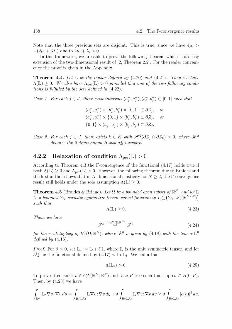
138 4.2. The �-convergence results

Note that the three previous sets are disjoint. This is true, since we have 4µi >�(2µi + 3�i) due to 2µi + �i > 0.

In this framework, we are able to prove the following theorem which is an easyextension of the two-dimensional result of [2, Theorem 2.2]. For the reader conveni-ence the proof is given in the Appendix.

Theorem 4.4. Let L be the tensor defined by (4.20) and (4.21). Then we have⇤(L) � 0. We also have ⇤per(L) > 0 provided that one of the two following condi-tions is fulfilled by the sets defined in (4.22):

Case 1. For each j 2 J , there exist intervals (a�j , a+j ), (b

�j , b

+j ) ⇢ [0, 1] such that

(a�j , a+j )⇥ (b�j , b

+j )⇥ {0, 1} ⇢ @Zj, or

(a�j , a+j )⇥ {0, 1}⇥ (b�j , b

+j ) ⇢ @Zj, or

{0, 1}⇥ (a�j , a+j )⇥ (b�j , b

+j ) ⇢ @Zj.

Case 2. For each j 2 J , there exists k 2 K with H 2(@Zj \ @Zk) > 0, where H 2

denotes the 2-dimensional Hausdor↵ measure.

4.2.2 Relaxation of condition ⇤per(L) > 0

According to Theorem 4.3 the �-convergence of the functional (4.17) holds true ifboth ⇤(L) � 0 and ⇤per(L) > 0. However, the following theorem due to Braides andthe first author shows that in N -dimensional elasticity for N � 2, the �-convergenceresult still holds under the sole assumption ⇤(L) � 0.

Theorem 4.5 (Braides & Briane). Let ⌦ be a bounded open subset of RN , and let Lbe a bounded YN -periodic symmetric tensor-valued function in L1

per

�YN ;Ls(RN⇥N)

�

such that⇤(L) � 0. (4.23)

Then, we have

F " ��H10 (⌦;RN )* F 0, (4.24)

for the weak toplogy of H10 (⌦;RN), where F 0 is given by (4.18) with the tensor L0

defined by (4.16).

Proof. For � > 0, set L� := L + � Is where Is is the unit symmetric tensor, and letF "

� be the functional defined by (4.17) with L�. We claim that

⇤(L�) > 0. (4.25)

To prove it consider v 2 C1c (RN ;RN) and take R > 0 such that supp v ⇢ B(0, R).

Then, by (4.23) we have

Z

RN

L�rv :rv dy =

Z

B(0,R)

Lrv :rv dy + �

Z

B(0,R)

Isrv :rv dy � �

Z

B(0,R)

|e(v)|2 dy.

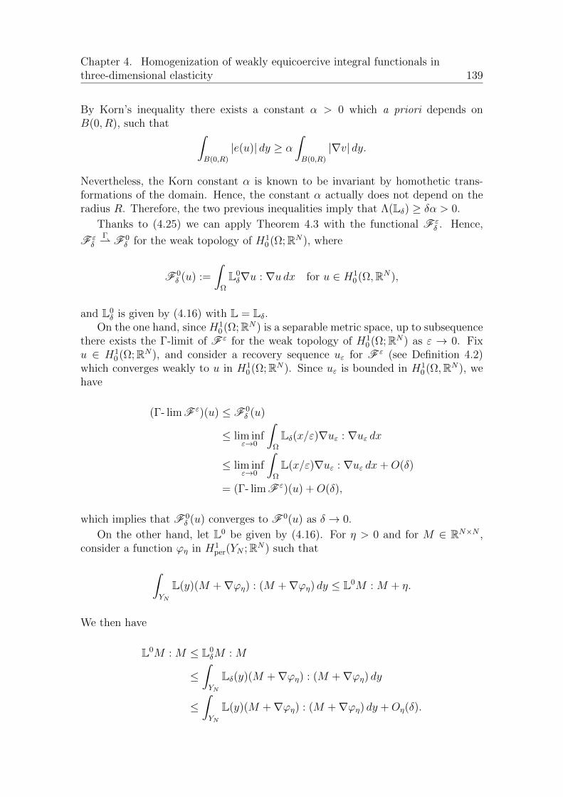
Chapter 4. Homogenization of weakly equicoercive integral functionals inthree-dimensional elasticity 139

By Korn’s inequality there exists a constant ↵ > 0 which a priori depends onB(0, R), such that

Z

B(0,R)

|e(u)| dy � ↵

Z

B(0,R)

|rv| dy.

Nevertheless, the Korn constant ↵ is known to be invariant by homothetic trans-formations of the domain. Hence, the constant ↵ actually does not depend on theradius R. Therefore, the two previous inequalities imply that ⇤(L�) � �↵ > 0.

Thanks to (4.25) we can apply Theorem 4.3 with the functional F "� . Hence,

F "�

�* F 0

� for the weak topology of H10 (⌦;RN), where

F 0� (u) :=

Z

⌦

L0�ru : ru dx for u 2 H1

0 (⌦,RN),

and L0� is given by (4.16) with L = L�.

On the one hand, since H10 (⌦;RN) is a separable metric space, up to subsequence

there exists the �-limit of F " for the weak topology of H10 (⌦;RN) as " ! 0. Fix

u 2 H10 (⌦;RN), and consider a recovery sequence u" for F " (see Definition 4.2)

which converges weakly to u in H10 (⌦;RN). Since u" is bounded in H1

0 (⌦,RN), wehave

(�- limF ")(u) F 0� (u)

lim inf"!0

Z

⌦

L�(x/")ru" : ru" dx

lim inf"!0

Z

⌦

L(x/")ru" : ru" dx+O(�)

= (�- limF ")(u) +O(�),

which implies that F 0� (u) converges to F 0(u) as � ! 0.

On the other hand, let L0 be given by (4.16). For ⌘ > 0 and for M 2 RN⇥N ,consider a function '⌘ in H1

per(YN ;RN) such that

Z

YN

L(y)(M +r'⌘) : (M +r'⌘) dy L0M : M + ⌘.

We then have

L0M : M L0�M : M

Z

YN

L�(y)(M +r'⌘) : (M +r'⌘) dy

Z

YN

L(y)(M +r'⌘) : (M +r'⌘) dy +O⌘(�).

1404.3. Loss of ellipticity in three-dimensional linear elasticity through the

homogenization of a laminate

Hence, making � tend to 0 for a fixed ⌘, we obtain

L0M : M lim inf�!0

(L0�M : M)

lim sup�!0

(L0�M : M)

Z

YN

L(y)(M +r'⌘) : (M +r'⌘) dy

L0M : M + ⌘.

Due to the arbitrariness of ⌘, we get that L0� converges to L0 as � ! 0.

Therefore, by the Lebesgue dominated convergence theorem we conclude thatfor any u 2 H1

0 (⌦;RN),

F 0(u) = lim�!0

F 0� (u) = lim

�!0

Z

⌦

L0�ru : ru dx =

Z

⌦

L0ru : ru dx.

4.3 Loss of ellipticity in three-dimensional linear

elasticity through the homogenization of a lam-

inate

In this section we will construct an example of a three-dimensional strong ellipticmaterial L which is weakly coercive, i.e. ⇤(L) � 0, but for which the strongellipticity is lost through homogenization. Firstly, let us recall the following resultdue to Gutierrez [8].

Proposition 4.6 (Gutierrez [8]). For any strongly, but not semi-very strongly el-liptic isotropic material, referred to as material a, there are very strongly ellipticisotropic materials such that if we laminate them with material a, in appropriatelychosen proportions and directions, we generate an e↵ective elasticity tensor that isnot strongly elliptic.

Remark 4.7 (Isotropic tensors). The elasticity tensor L 2 L1�Y3;Ls(R3⇥3)�of an

isotropic material is given by

L(y)M = �(y) tr(M)I3 + 2µ(y)M, for y 2 Y3 and M 2 R3⇥3s ,

where � and µ are the Lame coe�cients of L.As a consequence, we have

↵se(L) = ess-infy2Y3

�min{µ(y), 2µ(y) + �(y)}�,

↵vse(L) = ess-infy2Y3

�min{µ(y), 2µ(y) + 3�(y)}�.

Chapter 4. Homogenization of weakly equicoercive integral functionals inthree-dimensional elasticity 141

Here is a summary of the proof of Proposition 4.6. Consider two isotropic,homogeneous tensors La and Lb such that La is strongly elliptic, i.e.

�a + 2µa > 0, µa > 0,

but not semi-very strongly elliptic, i.e.

3�a + 2µa < 0.

and such that Lb is very strongly elliptic, i.e.

3�b + 2µb > 0, µb > 0.

Considering the rank-one laminate in the direction y1 mixing La with volume fraction✓1 2 (0, 1) and Lb with volume fraction (1�✓1), Gutierrez [8] proved that the e↵ectivetensor L⇤

1 in the sense of Murat-Tartar 1⇤-convergence (see, e.g., [8, Section 3])satisfies the following properties:

• If 0 µa + �a, then

↵se(L⇤1) > 0.

• If �µb µa + �a < 0, then

↵se(L⇤1)

8><

>:

= 0 if µb = �µa � �a,

� 0 if � µa � �a < µb �14(2µa + 3�a),

> 0 if � 14(2µa + 3�a) < µb.

• The case µa + �a < �µb is disposed of, since L⇤1 does not even satisfy the

Legendre-Hadamard condition.

In the case where ↵se(L⇤1) > 0, Gutierrez (see [8, Section 5.2]) performed a second

lamination in the direction y2 mixing the anisotropic material generated by the firstlamination with volume fraction ✓2 2 (0, 1), and a suitable very strongly ellipticisotropic material (Lc, µc,�c) with volume fraction (1� ✓2). In this way he deriveda rank-two laminate of e↵ective tensor L⇤

2 which is not strongly elliptic.In this section we will try to find a general class of periodic laminates for which

the strong ellipticity is lost through homogenization. To this end we will extendto dimension three the rank-one lamination approach of [2] performed in dimensiontwo. However, the outcome is surprisingly di↵erent from that of the two-dimensionalcase of [2]. Indeed, we will prove in the first subsection that it is not possible to losestrong ellipticity by a rank-one lamination through homogenization following thetwo-dimensional approach of [2]. This is the reason why we will perform a secondlamination in the second part of the section.

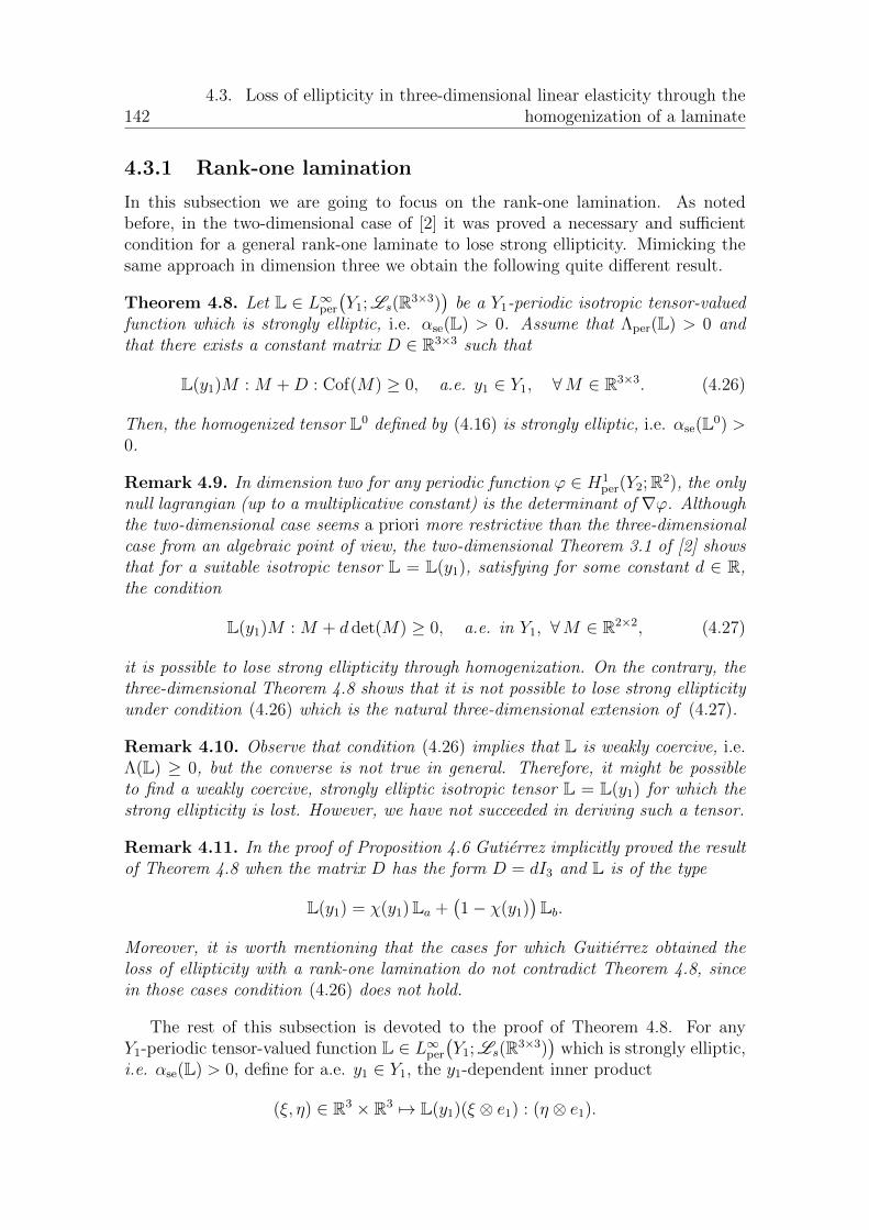
1424.3. Loss of ellipticity in three-dimensional linear elasticity through the

homogenization of a laminate

4.3.1 Rank-one lamination

In this subsection we are going to focus on the rank-one lamination. As notedbefore, in the two-dimensional case of [2] it was proved a necessary and su�cientcondition for a general rank-one laminate to lose strong ellipticity. Mimicking thesame approach in dimension three we obtain the following quite di↵erent result.

Theorem 4.8. Let L 2 L1per

�Y1;Ls(R3⇥3)

�be a Y1-periodic isotropic tensor-valued

function which is strongly elliptic, i.e. ↵se(L) > 0. Assume that ⇤per(L) > 0 andthat there exists a constant matrix D 2 R3⇥3 such that

L(y1)M : M +D : Cof(M) � 0, a.e. y1 2 Y1, 8M 2 R3⇥3. (4.26)

Then, the homogenized tensor L0 defined by (4.16) is strongly elliptic, i.e. ↵se(L0) >0.

Remark 4.9. In dimension two for any periodic function ' 2 H1per(Y2;R2), the only

null lagrangian (up to a multiplicative constant) is the determinant of r'. Althoughthe two-dimensional case seems a priori more restrictive than the three-dimensionalcase from an algebraic point of view, the two-dimensional Theorem 3.1 of [2] showsthat for a suitable isotropic tensor L = L(y1), satisfying for some constant d 2 R,the condition

L(y1)M : M + d det(M) � 0, a.e. in Y1, 8M 2 R2⇥2, (4.27)

it is possible to lose strong ellipticity through homogenization. On the contrary, thethree-dimensional Theorem 4.8 shows that it is not possible to lose strong ellipticityunder condition (4.26) which is the natural three-dimensional extension of (4.27).

Remark 4.10. Observe that condition (4.26) implies that L is weakly coercive, i.e.⇤(L) � 0, but the converse is not true in general. Therefore, it might be possibleto find a weakly coercive, strongly elliptic isotropic tensor L = L(y1) for which thestrong ellipticity is lost. However, we have not succeeded in deriving such a tensor.

Remark 4.11. In the proof of Proposition 4.6 Gutierrez implicitly proved the resultof Theorem 4.8 when the matrix D has the form D = dI3 and L is of the type

L(y1) = �(y1)La +�1� �(y1)

�Lb.

Moreover, it is worth mentioning that the cases for which Guitierrez obtained theloss of ellipticity with a rank-one lamination do not contradict Theorem 4.8, sincein those cases condition (4.26) does not hold.

The rest of this subsection is devoted to the proof of Theorem 4.8. For anyY1-periodic tensor-valued function L 2 L1

per

�Y1;Ls(R3⇥3)

�which is strongly elliptic,

i.e. ↵se(L) > 0, define for a.e. y1 2 Y1, the y1-dependent inner product

(⇠, ⌘) 2 R3 ⇥ R3 7! L(y1)(⇠ ⌦ e1) : (⌘ ⌦ e1).

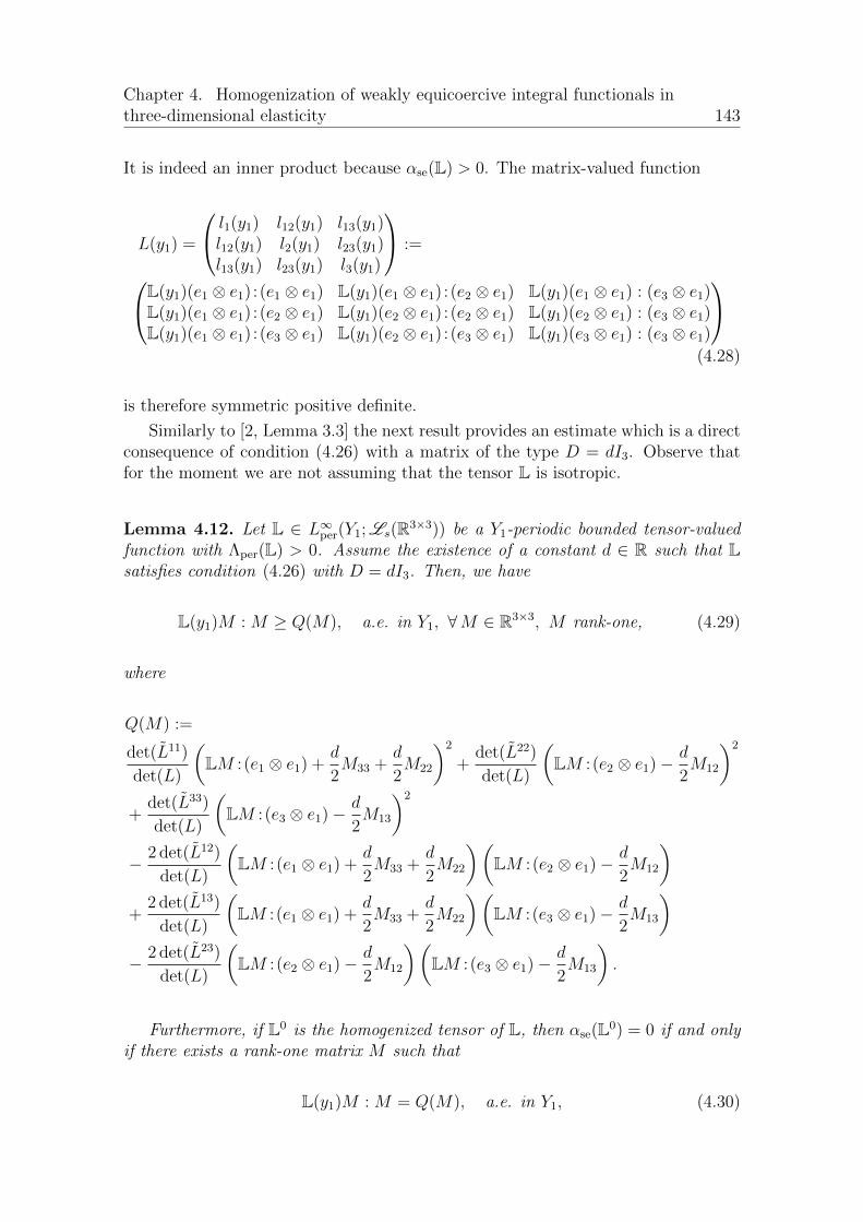
Chapter 4. Homogenization of weakly equicoercive integral functionals inthree-dimensional elasticity 143

It is indeed an inner product because ↵se(L) > 0. The matrix-valued function

L(y1) =

0

@l1(y1) l12(y1) l13(y1)l12(y1) l2(y1) l23(y1)l13(y1) l23(y1) l3(y1)

1

A :=

0

@L(y1)(e1 ⌦ e1) : (e1 ⌦ e1) L(y1)(e1 ⌦ e1) : (e2 ⌦ e1) L(y1)(e1 ⌦ e1) : (e3 ⌦ e1)L(y1)(e1 ⌦ e1) : (e2 ⌦ e1) L(y1)(e2 ⌦ e1) : (e2 ⌦ e1) L(y1)(e2 ⌦ e1) : (e3 ⌦ e1)L(y1)(e1 ⌦ e1) : (e3 ⌦ e1) L(y1)(e2 ⌦ e1) : (e3 ⌦ e1) L(y1)(e3 ⌦ e1) : (e3 ⌦ e1)

1

A

(4.28)

is therefore symmetric positive definite.

Similarly to [2, Lemma 3.3] the next result provides an estimate which is a directconsequence of condition (4.26) with a matrix of the type D = dI3. Observe thatfor the moment we are not assuming that the tensor L is isotropic.

Lemma 4.12. Let L 2 L1per(Y1;Ls(R3⇥3)) be a Y1-periodic bounded tensor-valued

function with ⇤per(L) > 0. Assume the existence of a constant d 2 R such that Lsatisfies condition (4.26) with D = dI3. Then, we have

L(y1)M : M � Q(M), a.e. in Y1, 8M 2 R3⇥3, M rank-one, (4.29)

where

Q(M) :=

det(L11)

det(L)

✓LM : (e1 ⌦ e1) +

d

2M33 +

d

2M22

◆2

+det(L22)

det(L)

✓LM : (e2 ⌦ e1)� d

2M12

◆2

+det(L33)

det(L)

✓LM : (e3 ⌦ e1)� d

2M13

◆2

� 2 det(L12)

det(L)

✓LM : (e1 ⌦ e1) +

d

2M33 +

d

2M22

◆✓LM : (e2 ⌦ e1)� d

2M12

◆

+2det(L13)

det(L)

✓LM : (e1 ⌦ e1) +

d

2M33 +

d

2M22

◆✓LM : (e3 ⌦ e1)� d

2M13

◆

� 2 det(L23)

det(L)

✓LM : (e2 ⌦ e1)� d

2M12

◆✓LM : (e3 ⌦ e1)� d

2M13

◆.

Furthermore, if L0 is the homogenized tensor of L, then ↵se(L0) = 0 if and onlyif there exists a rank-one matrix M such that

L(y1)M : M = Q(M), a.e. in Y1, (4.30)

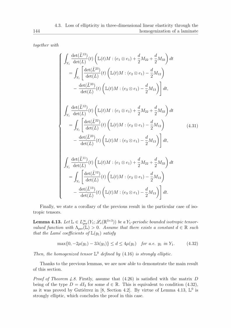
1444.3. Loss of ellipticity in three-dimensional linear elasticity through the

homogenization of a laminate

together with

8>>>>>>>>>>>>>>>>>>>>>>>>>>>>>>>>>>>>>>>>>>>>>><

>>>>>>>>>>>>>>>>>>>>>>>>>>>>>>>>>>>>>>>>>>>>>>:

Z

Y1

det(L13)

det(L)(t)

✓L(t)M : (e1 ⌦ e1) +

d

2M22 +

d

2M33

◆dt

=

Z

Y1

"det(L23)

det(L)(t)

✓L(t)M : (e2 ⌦ e1)� d

2M12

◆

� det(L33)

det(L)(t)

✓L(t)M : (e3 ⌦ e1)� d

2M13

◆#dt,

Z

Y1

det(L12)

det(L)(t)

✓L(t)M : (e1 ⌦ e1) +

d

2M22 +

d

2M33

◆dt

=

Z

Y1

"det(L22)

det(L)(t)

✓L(t)M : (e2 ⌦ e1)� d

2M12

◆

� det(L23)

det(L)(t)

✓L(t)M : (e3 ⌦ e1)� d

2M13

◆#dt,

Z

Y1

det(L11)

det(L)(t)

✓L(t)M : (e1 ⌦ e1) +

d

2M22 +

d

2M33

◆dt

=

Z

Y1

"det(L12)

det(L)(t)

✓L(t)M : (e2 ⌦ e1)� d

2M12

◆

� det(L13)

det(L)(t)

✓L(t)M : (e3 ⌦ e1)� d

2M13

◆#dt.

(4.31)

Finally, we state a corollary of the previous result in the particular case of iso-tropic tensors.

Lemma 4.13. Let L 2 L1per(Y1;Ls(R3⇥3)) be a Y1-periodic bounded isotropic tensor-

valued function with ⇤per(L) > 0. Assume that there exists a constant d 2 R suchthat the Lame coe�cients of L(y1) satisfy

max{0,�2µ(y1)� 3�(y1)} d 4µ(y1) for a.e. y1 in Y1. (4.32)

Then, the homogenized tensor L0 defined by (4.16) is strongly elliptic.

Thanks to the previous lemmas, we are now able to demonstrate the main resultof this section.

Proof of Theorem 4.8. Firstly, assume that (4.26) is satisfied with the matrix Dbeing of the type D = dI3 for some d 2 R. This is equivalent to condition (4.32),as it was proved by Gutierrez in [8, Section 4.2]. By virtue of Lemma 4.13, L0 isstrongly elliptic, which concludes the proof in this case.

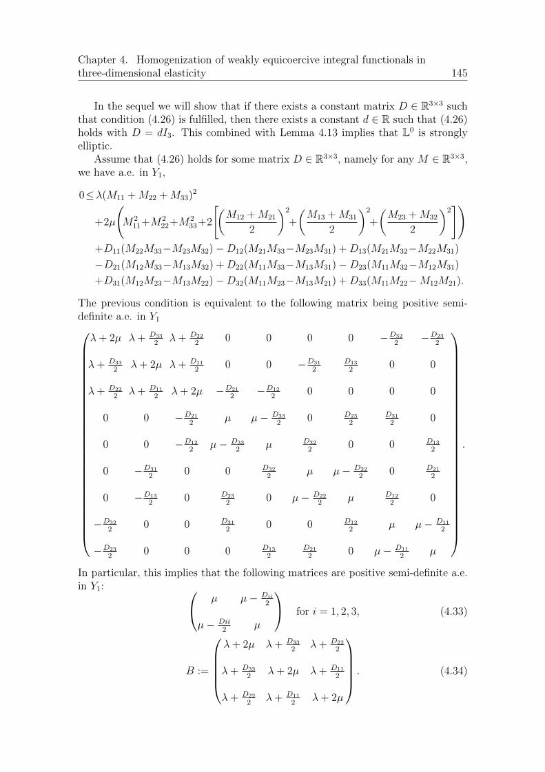
Chapter 4. Homogenization of weakly equicoercive integral functionals inthree-dimensional elasticity 145

In the sequel we will show that if there exists a constant matrix D 2 R3⇥3 suchthat condition (4.26) is fulfilled, then there exists a constant d 2 R such that (4.26)holds with D = dI3. This combined with Lemma 4.13 implies that L0 is stronglyelliptic.

Assume that (4.26) holds for some matrix D 2 R3⇥3, namely for any M 2 R3⇥3,we have a.e. in Y1,

0�(M11 +M22 +M33)2

+2µ

M2

11+M222+M2

33+2

"✓M12 +M21

2

◆2

+

✓M13 +M31

2

◆2

+

✓M23 +M32

2

◆2#!

+D11(M22M33�M23M32)�D12(M21M33�M23M31) +D13(M21M32�M22M31)

�D21(M12M33�M13M32) +D22(M11M33�M13M31)�D23(M11M32�M12M31)

+D31(M12M23�M13M22)�D32(M11M23�M13M21) +D33(M11M22�M12M21).

The previous condition is equivalent to the following matrix being positive semi-definite a.e. in Y1

0

BBBBBBBBBBBBBBBBBBBBBBBBBBBB@

�+ 2µ �+ D332 �+ D22

2 0 0 0 0 �D322 �D23

2

�+ D332 �+ 2µ �+ D11

2 0 0 �D312

D132 0 0

�+ D222 �+ D11

2 �+ 2µ �D212 �D12

2 0 0 0 0

0 0 �D212 µ µ� D33

2 0 D232

D312 0

0 0 �D122 µ� D33

2 µ D322 0 0 D13

2

0 �D312 0 0 D32

2 µ µ� D222 0 D21

2

0 �D132 0 D23

2 0 µ� D222 µ D12

2 0

�D322 0 0 D31

2 0 0 D122 µ µ� D11

2

�D232 0 0 0 D13

2D212 0 µ� D11

2 µ

1

CCCCCCCCCCCCCCCCCCCCCCCCCCCCA

.

In particular, this implies that the following matrices are positive semi-definite a.e.in Y1: 0

@µ µ� Dii

2

µ� Dii2 µ

1

A for i = 1, 2, 3, (4.33)

B :=

0

BBBB@

�+ 2µ �+ D332 �+ D22

2

�+ D332 �+ 2µ �+ D11

2

�+ D222 �+ D11

2 �+ 2µ

1

CCCCA. (4.34)

1464.3. Loss of ellipticity in three-dimensional linear elasticity through the

homogenization of a laminate

Now, we will prove that there exists i 2 {1, 2, 3} such that

� ess-infy12Y1

{2µ(y1) + 3�(y1)} Dii 4 ess-infy12Y1

{µ(y1)}. (4.35)

Note that we can assume

ess-infy12Y1

{2µ(y1) + 3�(y1)} < 0. (4.36)

Otherwise, since the matrix (4.33) is positive semi-definite, or equivalently

0 Dii 4 ess-infy12Y1

{µ(y1)} for i = 1, 2, 3, (4.37)

condition (4.35) holds immediately.We assume by contradiction that (4.35) is violated for any i = 1, 2, 3. Since the

matrix B defined by (4.34) is positive semi-definite, we get for any i = 1, 2, 3,

������

�+ 2µ �+ Dii2

�+ Dii2 �+ 2µ

������� 0 a.e. in Y1,

which is equivalent to

� 4 ess-infy12Y1

{µ(y1) + �(y1)} Dii 4 ess-infy12Y1

{µ(y1)} for i = 1, 2, 3.

Since by assumption (4.35) is not satisfied for any i = 1, 2, 3 and (4.37) holds, thenthe previous condition yields

�4 ess-infy12Y1

{µ(y1)+�(y1)} Dii < � ess-infy12Y1

{2µ(y1)+3�(y1)} for i = 1, 2, 3. (4.38)

Set d := maxi=1,2,3{Dii}. By (4.38) there exists " > 0 such that

d+ " < � ess-infy12Y1

{2µ(y1) + 3�(y1)}. (4.39)

Define the set P" ⇢ Y1 by

P" :=

⇢x1 2 Y1 : 2µ(x1) + 3�(x1) < ess-inf

y12Y1

{2µ(y1) + 3�(y1)}+ "

�.

It is clear that |P"| > 0, and from (4.39) and the definition of P" we obtain

d+ " < � ess-infy12Y1

{2µ(y1) + 3�(y1)} < ��2µ(x1) + 3�(x1)�+ " a.e. x1 2 P",

which leads to

�(x1) +d

2< �1

2

��(x1) + 2µ(x1)

�< 0 a.e. x1 2 P". (4.40)

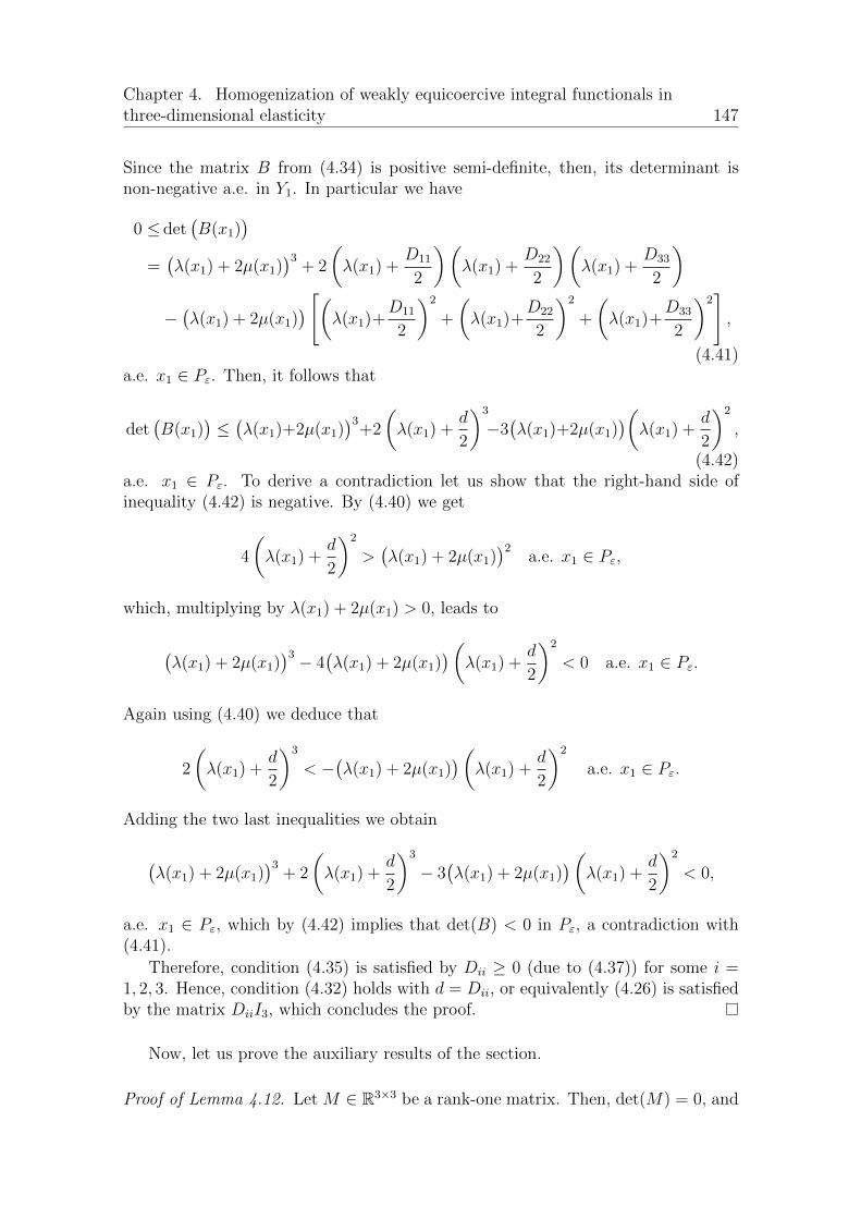
Chapter 4. Homogenization of weakly equicoercive integral functionals inthree-dimensional elasticity 147

Since the matrix B from (4.34) is positive semi-definite, then, its determinant isnon-negative a.e. in Y1. In particular we have

0 det�B(x1)

�

=��(x1) + 2µ(x1)

�3+ 2

✓�(x1) +

D11

2

◆✓�(x1) +

D22

2

◆✓�(x1) +

D33

2

◆

� ��(x1) + 2µ(x1)�"✓

�(x1)+D11

2

◆2

+

✓�(x1)+

D22

2

◆2

+

✓�(x1)+

D33

2

◆2#,

(4.41)a.e. x1 2 P". Then, it follows that

det�B(x1)

� ��(x1)+2µ(x1)�3+2

✓�(x1) +

d

2

◆3

�3��(x1)+2µ(x1)

�✓�(x1) +

d

2

◆2

,

(4.42)a.e. x1 2 P". To derive a contradiction let us show that the right-hand side ofinequality (4.42) is negative. By (4.40) we get

4

✓�(x1) +

d

2

◆2

>��(x1) + 2µ(x1)

�2a.e. x1 2 P",

which, multiplying by �(x1) + 2µ(x1) > 0, leads to

��(x1) + 2µ(x1)

�3 � 4��(x1) + 2µ(x1)

�✓�(x1) +

d

2

◆2

< 0 a.e. x1 2 P".

Again using (4.40) we deduce that

2

✓�(x1) +

d

2

◆3

< ���(x1) + 2µ(x1)�✓

�(x1) +d

2

◆2

a.e. x1 2 P".

Adding the two last inequalities we obtain

��(x1) + 2µ(x1)

�3+ 2

✓�(x1) +

d

2

◆3

� 3��(x1) + 2µ(x1)

�✓�(x1) +

d

2

◆2

< 0,

a.e. x1 2 P", which by (4.42) implies that det(B) < 0 in P", a contradiction with(4.41).

Therefore, condition (4.35) is satisfied by Dii � 0 (due to (4.37)) for some i =1, 2, 3. Hence, condition (4.32) holds with d = Dii, or equivalently (4.26) is satisfiedby the matrix DiiI3, which concludes the proof.

Now, let us prove the auxiliary results of the section.

Proof of Lemma 4.12. Let M 2 R3⇥3 be a rank-one matrix. Then, det(M) = 0, and

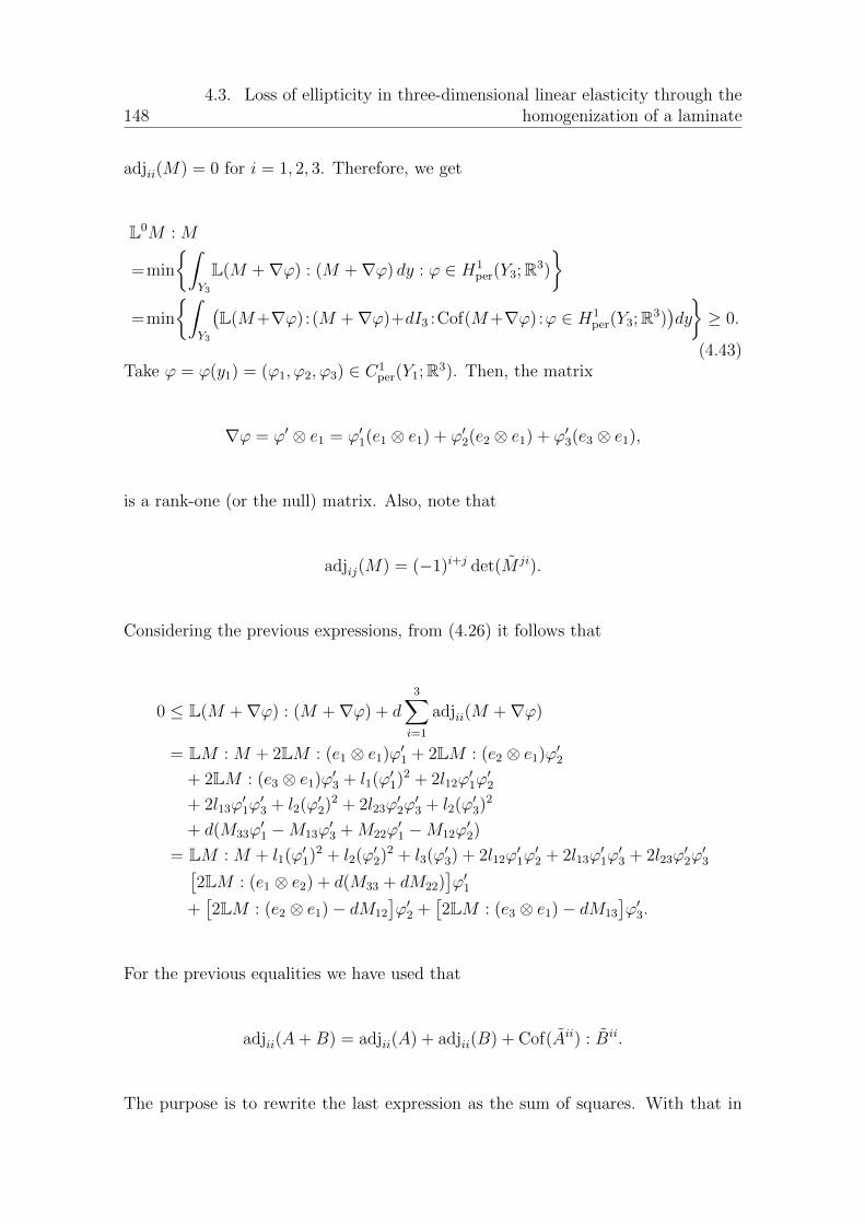
1484.3. Loss of ellipticity in three-dimensional linear elasticity through the

homogenization of a laminate

adjii(M) = 0 for i = 1, 2, 3. Therefore, we get

L0M : M

=min

⇢Z

Y3

L(M +r') : (M +r') dy : ' 2 H1per(Y3;R3)

�

=min

⇢Z

Y3

�L(M+r') : (M +r')+dI3 :Cof(M+r') :' 2 H1

per(Y3;R3)�dy

�� 0.

(4.43)Take ' = '(y1) = ('1,'2,'3) 2 C1

per(Y1;R3). Then, the matrix

r' = '0 ⌦ e1 = '01(e1 ⌦ e1) + '0

2(e2 ⌦ e1) + '03(e3 ⌦ e1),

is a rank-one (or the null) matrix. Also, note that

adjij(M) = (�1)i+j det(M ji).

Considering the previous expressions, from (4.26) it follows that

0 L(M +r') : (M +r') + d3X

i=1

adjii(M +r')

= LM : M + 2LM : (e1 ⌦ e1)'01 + 2LM : (e2 ⌦ e1)'

02

+ 2LM : (e3 ⌦ e1)'03 + l1('

01)

2 + 2l12'01'

02

+ 2l13'01'

03 + l2('

02)

2 + 2l23'02'

03 + l2('

03)

2

+ d(M33'01 �M13'

03 +M22'

01 �M12'

02)

= LM : M + l1('01)

2 + l2('02)

2 + l3('03) + 2l12'

01'

02 + 2l13'

01'

03 + 2l23'

02'

03⇥

2LM : (e1 ⌦ e2) + d(M33 + dM22)⇤'01

+⇥2LM : (e2 ⌦ e1)� dM12

⇤'02 +

⇥2LM : (e3 ⌦ e1)� dM13

⇤'03.

For the previous equalities we have used that

adjii(A+B) = adjii(A) + adjii(B) + Cof(Aii) : Bii.

The purpose is to rewrite the last expression as the sum of squares. With that in

Chapter 4. Homogenization of weakly equicoercive integral functionals inthree-dimensional elasticity 149

mind, one obtains

0 L(M +r') : (M +r') + dI3 : Cof(M +r')= LM : M �Q(M)

+ l1

'01 +

l12l1'02 +

l13l1'03 +

1

l1

✓LM : (e1 ⌦ e1) +

d

2M22 +

d

2M33

◆�2

+det(L33)

l1

"'02 +

det(L23)

det(L33)'03 �

l12

det(L33)

✓LM : (e1 ⌦ e1) +

d

2M22 +

d

2M33

◆

+l1

det(L33)

✓LM : (e2 ⌦ e1)� d

2M12

◆�2

+det(L)

det(L33)

"'03 +

det(L13)

det(L)

✓LM : (e1 ⌦ e1) +

d

2M22 +

d

2M33

◆

�det(L23)

det(L)

✓LM : (e2 ⌦ e1)� d

2M12

◆

+det(L33)

det(L)

✓LM : (e3 ⌦ e1)� d

2M13

◆#2.

(4.44)Since '0

1,'02 and '0

3 can be chosen arbitrarily, the three square brackets in theprevious equality can be equated to 0 at any Lebesgue point y1 2 Y1 of L, and thus(4.29) holds. Using a density argument the previous equality also holds a.e. in Y1,for any ' 2 H1

per(Y1;R3).

Now, we are going to prove the second part of Lemma 4.12. Assume L0 is notstrongly elliptic. Then, there exists a rank-one matrix M such that L0M : M = 0.Taking into account expressions (4.43) the minimizer vM associated with L0M : M(see [2, Lemma 3.2]) satisfies vM = vM(y1) and

0 = L0M : M =

Z

Y1

L(t)(M + v0M(t)⌦ e1) : (M + v0M(t)⌦ e1)dt

=

Z

Y1

⇥L(t)(M +rvM(t)) : (M +rvM(t)) + dI3 : Cof(M +rvM)

⇤dt.

The first inequality in (4.44) implies that the integrand of the previous expressionmust be pointwisely 0, and thus the inequality in (4.44) for ' = vM is actually anequality. From this we deduce

LM : M = Q(M),

1504.3. Loss of ellipticity in three-dimensional linear elasticity through the

homogenization of a laminate

and8>>>>>>>>>>>>>>>>>>>>>><

>>>>>>>>>>>>>>>>>>>>>>:

0 = (v0M)1 +l12l1(v0M)2 +

l13l1(v0M)3 +

1

l1

✓LM : (e1 ⌦ e1) +

d

2M22 +

d

2M33

◆,

0 = (v0M)2 +det(L23)

det(L33)(v0M)3 � l12

det(L33)

✓LM : (e1 ⌦ e1) +

d

2M22 +

d

2M33

◆

+l1

det(L33)

✓LM : (e2 ⌦ e1)� d

2M12

◆,

0 = (v0M)3 +det(L13)

det(L)

✓LM : (e1 ⌦ e1) +

d

2M22 +

d

2M33

◆

� det(L23)

det(L)

✓LM : (e2 ⌦ e1)� d

2M12

◆

+det(L33)

det(L)

✓LM : (e3 ⌦ e1)� d

2M13

◆.

(4.45)Since vM is Y1-periodic, we have

Z

Y1

(v0M)i dy1 = 0 i = 1, 2, 3.

Integrating the third equality in (4.45) we obtain the first equality in (4.31). Repla-cing (v0M)3 in the second equality of (4.45), we end up getting the second equalityin (4.31). Finally, replacing (v0M)2 and (v0M)3 in the first equality of (4.45) it yieldsthe last equality in (4.31).

Conversely, let us assume that equalities (4.30) and (4.31) hold. Considering thefirst equation in (4.31), taking into account that the all the integrands belong toL1(Y1), there exists a function '3 2 W 1,1

per (Y1) such that, a.e. in Y1, it holds

0 = '03 +

det(L13)

det(L)

✓LM : (e1 ⌦ e1) +

d

2M22 +

d

2M33

◆� det(L23)

det(L)

✓LM : (e2 ⌦ e1)� d

2M12

◆

+det(L33)

det(L)

✓LM : (e3 ⌦ e1)� d

2M13

◆.

Repeating the argument with the second and the third equation of (4.31), we getthe existence of functions '2 and '1 in W 1,1

per (Y1) respectively, such that

'02 +

det(L23)

det(L33)'03 �

l12

det(L33)

✓LM : (e1 ⌦ e1) +

d

2M22 +

d

2M33

◆+

l1

det(L33)

✓LM : (e2 ⌦ e1)� d

2M12

◆= 0,

'01 +

l12l1'02 +

l13l1'03 +

1

l1

✓LM : (e1 ⌦ e1) +

d

2M22 +

d

2M33

◆= 0.

These three equalities together with (4.30) imply the equality in (4.44), and thus by(4.43) it follows that

0 =

Z

Y1

�L(M +r') : (M +r') + dI3 : Cof(M +r')� dy1 � L0M : M � 0,

Chapter 4. Homogenization of weakly equicoercive integral functionals inthree-dimensional elasticity 151

which shows that L0 is not strongly elliptic.Finally, due to the equality L0M : M = L0MT : MT , conditions (4.30) and

(4.31) are equivalent to the similar equalities replacing M by MT .

Proof of Lemma 4.13. Since L is isotropic, condition (4.32) is equivalent to the con-dition (4.26) with D = dI3. As a consequence, (4.32) implies ⇤(L) � 0. By [7,Corollary 3.5], we have ↵se(L0) � ⇤(L). Therefore, we get that ↵se(L0) � 0.

Assume that L0 is not strongly elliptic, i.e. ↵se(L0) = 0. Then, there exists arank-one matrix M := ⇠ ⌦ ⌘ in R3⇥3, with ⇠, ⌘ 2 R3 \ {0}, such that L0M : M = 0.

Since L is isotropic, the matrix L defined in (4.28) is

L =

0

@�+ 2µ 0 0

0 µ 00 0 µ

1

A .

Moreover, the following equalities hold

Mij = ⇠i⌘j i, j 2 {1, 2, 3},LM : (e1 ⌦ e1) = (�+ 2µ)⇠i⌘1 + �(⇠2⌘2 + ⇠3⌘3),

LM : (e2 ⌦ e1) = µ(⇠1⌘2 + ⇠2⌘1),LM : (e3 ⌦ e1) = µ(⇠1⌘· + ⇠3⌘1),

LM : M = (�+ µ)(⇠ : ⌘)2 + µ|⇠|2|⌘|2.Because L0M : M = 0, from equalities (4.30) and (4.31) in Lemma 4.12 we obtaina.e. in Y1

(�+ µ)(⇠ : ⌘)2 + µ|⇠|2|⌘|2

=1

�+ 2µ

(�+ 2µ)⇠1µ1 + �(⇠2⌘2 + ⇠3⌘3) +

d

2(⇠2⌘2 + ⇠3⌘3)

�2

+1

µ

µ(⇠1⌘2 + ⇠2⌘1)� d

2⇠1⌘2

�2+

1

µ

µ(⇠1⌘3 + ⇠3⌘1)� d

2⇠1⌘3

�2,

(4.46)

together with

0 = ⇠1⌘3 + ⇠3⌘1 � ⇠1⌘32

Z

Y1

d

µ(t) dt, (4.47)

0 = ⇠1⌘2 + ⇠2⌘1 � ⇠1⌘22

Z

Y1

d

µ(t) dt, (4.48)

0 = ⇠1⌘1 + (⇠2⌘2 + ⇠3⌘3)

Z

Y1

�+ d2

�+ 2µ(t) dt. (4.49)

After some calculations, from (4.46) we get

(�+ 2µ)2 � (�+ d2)

2

�+ 2µ(⇠2⌘2+⇠3⌘3)

2+µ(⇠2⌘3�⇠3⌘2)2+d(µ� d

4)

µ⇠21(⌘

22+⌘

23) = 0, (4.50)

a.e. in Y1. Observe that, since L is isotropic and (strictly) strongly elliptic in Y1,we have

µ > 0, 2µ+ � > 0 a.e. in Y1,

1524.3. Loss of ellipticity in three-dimensional linear elasticity through the

homogenization of a laminate

which implies that

(�+ 2µ)2 �✓�+

d

2

◆2

� 0 a.e. in Y1.

Hence, taking into account assumption (4.32), equality (4.50) implies the followingthree conditions:

"(�+ 2µ)2 �

✓�+

d

2

◆2#(⇠2⌘2 + ⇠3⌘3)

2 = 0 a.e. in Y1, (4.51)

⇠2⌘3 = ⇠3⌘2, (4.52)

d

✓µ� d

4

◆⇠21(⌘

22 + ⌘23) = 0 a.e. in Y1. (4.53)

We will now prove by contradiction that we cannot have d = 4µ a.e. in Y1.Otherwise, equalities (4.47), (4.48) and (4.49) can be written as

8><

>:

0 = ⇠1⌘3 � ⇠3⌘1,

0 = ⇠1⌘2 � ⇠2⌘1,

0 = ⇠1⌘1 + ⇠2⌘2 + ⇠3⌘3.

(4.54)

Under these conditions, if ⌘1 6= 0, then the first and second equalities of (4.54) leadto

⇠3 = ⌘3⇠1⌘1, ⇠2 = ⌘2

⇠1⌘1.

Replacing ⇠2 and ⇠3 in the third equality in (4.54), we obtain

⇠1(⌘21 + ⌘22 + ⌘23) = 0.

Since ⌘ 6= 0, we get ⇠1 = 0. This implies that ⇠2 = ⇠3 = 0, a contradiction with ⇠ 6= 0.Therefore, we have necessarily ⌘1 = 0. Moreover, using the two first equalities of(4.54) and the fact that ⌘ 6= 0, we obtain ⇠1 = 0. As a consequence, (4.54) reducesto

⇠2⌘2 + ⇠3⌘3 = 0. (4.55)

If ⌘2 6= 0, then using (4.52) we get

⇠3 = ⇠2⌘3⌘2,

and replacing ⇠3 in the previous equality, it yields

⇠2(⌘22 + ⌘23) = 0.

Again, since ⌘ 6= 0, we have ⇠2 = 0. Using (4.52) and the assumption ⌘2 6= 0, itfollows that ⇠3 = 0, again a contradiction with ⇠, ⌘ 6= 0. Thus, we have necessarily⌘2 = 0. Taking into account that ⌘1 = ⌘2 = 0 we have ⌘3 6= 0, hence from (4.55)

Chapter 4. Homogenization of weakly equicoercive integral functionals inthree-dimensional elasticity 153

we deduce that ⇠3 = 0. Now (4.52) is written as ⇠2⌘3 = 0. However, recall that⇠1 = ⇠3 = ⌘1 = ⌘2 = 0. This implies that either ⇠ = 0 or ⌘ = 0, a contradiction.

We have just shown that the set {d < 4µ} has a positive Lebesgue measure.Similarly, we can check that d > 0. Using (4.51) and (4.53) together with 0 < d 4µ, we deduce that

⇠2⌘2 + ⇠3⌘3 = ⇠21(⌘22 + ⌘23) = 0,

which combined with (4.49) also gives ⇠1⌘1 = 0. As above, using the three previousequalities, (4.47), (4.48) and (4.52), we get a contradiction with the fact that ⇠, ⌘ 6= 0.Therefore, we have proved that L0 is strongly elliptic if (4.32) holds for some d.

4.3.2 Rank-two lamination

In the proof of Proposition 4.6 for dimension three [8, Section 5.2], Gutierrez per-formed a rank-one laminate mixing a strongly elliptic but not semi-very stronglyisotropic material La, and a very strongly elliptic isotropic material Lb. However,as it was noted at the beginning of the section, there are some cases for which thestrong ellipticity of the homogenized tensor is not lost after this first lamination.In fact, our Theorem 4.8 shows that for a general rank-one laminate, it is not pos-sible to lose the strong ellipticity through homogenization if there exists a matrixD 2 R3⇥3 satisfying condition (4.26). As done in [8], we need to perform a secondlamination with a third material Lc which can be very strongly elliptic, in order tolose the strong ellipticity in those cases.

Our purpose is to justify Gutierrez’ approach using formally 1⇤-convergence (see[8, Section 3]), by a homogenization procedure using the �-convergence result ofTheorem 4.5.

Theorem 4.14. For any strongly elliptic but not semi-very strongly elliptic isotropictensor La whose Lame coe�cients satisfy

4µa + 3�a > 0, (4.56)

there exist two very strongly elliptic isotropic tensors Lb,Lc and volume fractions✓1, ✓2 2 (0, 1) such that the tensor L2 obtained by laminating in the direction y2 thee↵ective tensor L⇤

1 – firstly obtained by laminating in the direction y1 the tensors La,Lb with proportions ✓1, 1 � ✓1 – and the tensor Lc with proportions ✓2 and 1 � ✓2respectively, namely

L2(y2) := �2(y2)L⇤1 +

�1� �2(y2)

�Lc for y2 2 Y1, (4.57)

satisfies⇤(L2) = 0, (4.58)

and Z

⌦

L2(x2/")rv : rv dx��H1

0 (⌦)3

*

Z

⌦

L02rv : rv dx, (4.59)

where the homogenized tensor L02 is not strongly elliptic, i.e.

↵se(L02) = 0. (4.60)

1544.3. Loss of ellipticity in three-dimensional linear elasticity through the

homogenization of a laminate

Remark 4.15. Theorem 4.14 shows that for certain strongly elliptic but not verystrongly elliptic isotropic tensors, namely those whose Lame parameters fulfil (4.56),it is possible to find two very strongly elliptic isotropic tensors for which the homo-genization process through �-convergence using a rank-two lamination leads to theloss of ellipticity of the e↵ective tensor.

Proof of Theorem 4.14. We divide the proof into four steps.

Step 1. Choice of La, Lb, ✓1, ✓2.

Let La be a strongly elliptic but not semi-very strongly elliptic isotropic tensorsatisfying (4.56). Our aim is to find two very strongly isotropic tensors Lb,Lc and twovolume fractions ✓1, ✓2 such that the strong ellipticity is lost through homogenizationusing a rank-two lamination.

Let �1,�2 : R ! {0, 1} be two 1-periodic characteristic functions such that

Z

Y1

�1(y1) dy1 = ✓1 and

Z

Y1

�2(y2) dy2 = ✓2,

where ✓1, ✓2 2 (0, 1) will be chosen later.

The 1⇤-convergence procedure of [8, Section 5.2] applied to the tensor

L1(y1) := �1(y1)La +�1� �1(y1)

�Lb for y1 2 Y1, (4.61)

yields a non-isotropic e↵ective tensor L⇤1. The computations of [8, Section 5.2] lead

to an explicit expression of the tensor L⇤1 whose non-zero entries are

(L⇤1)1111 =

1

A,

(L⇤1)1122 = (L⇤

1)2211 = (L⇤1)1133 = (L⇤

1)3311 =B

A,

(L⇤1)1212 = (L⇤

1)1221 = (L⇤1)2112 = (L⇤

1)2121 =1

E,

(L⇤1)1313 = (L⇤

1)1331 = (L⇤1)3113 = (L⇤

1)3131 =1

E,

(L⇤1)2222 =

B2

A+ 2(C +D),

(L⇤1)2233 = (L⇤

1)3322 =B2

A+ 2D,

(L⇤1)2323 = (L⇤

1)2332 = (L⇤1)3223 = (L⇤

1)3232 = C,

(L⇤1)3333 =

B2

A+ 2(C +D),

(4.62)

Chapter 4. Homogenization of weakly equicoercive integral functionals inthree-dimensional elasticity 155

where

A =✓1

2µa + �a+

1� ✓12µb + �b

,

B =✓1�a

2µa + �a+

(1� ✓1)�b2µb + �b

,

C = ✓1µa + (1� ✓1)µb,

D =✓1µa�a2µa + �a

+(1� ✓1)µb�b2µb + �b

,

E =✓1µa

+1� ✓1µb

.

(4.63)

Now, let us specify the choice of the two very strongly elliptic isotropic tensorsLb, Lc, and the volume fractions ✓1, ✓2. For the Lame parameters of material c wedenote �c = ↵cµc as done in [8]. We assume that

� 1

4(2µa + 3�a) µb <

µa(2µa + 3�a)

3�a, (4.64)

�b >2µ2

b�aµa(2µa + 3�a)� 3µb�a

, (4.65)

✓1 =��b(2µa + �a)

2(µb�a � µa�b), (4.66)

↵c � �D

C +D, (4.67)

µc = C↵c(C + 2D)

D(1 + ↵c), (4.68)

and

✓2 =↵c(C +D)

↵c(C +D)�D(2 + ↵c). (4.69)

Observe that, thanks to the first inequality in (4.64), the tensor L1 given by (4.61)satisfies ⇤(L1) � 0 (see [8, Section 4.2]). Hence, by Theorem 4.8 the homogenizedtensor L⇤

1 is strongly elliptic. This justifies the first lamination from the point ofview of homogenization through �-convergence.

To conclude the first step, let us check that the previous conditions satisfy theassumptions of Theorem 4.14. The tensor La is strongly elliptic but not semi-verystrongly elliptic, i.e.

µa > 0, 2µa + 3�a < 0,

which implies that µb > 0. The fact that necessarily �a < 0 together with (4.64)implies that �b > 0 thanks to (4.65), and thus Lb is very strongly elliptic. Thevolume fraction ✓1 clearly belongs to (0, 1), since (4.66) reads as

✓1 =�b(2µa + �a)

�b(2µa + �a)� �a(2µb + �b).

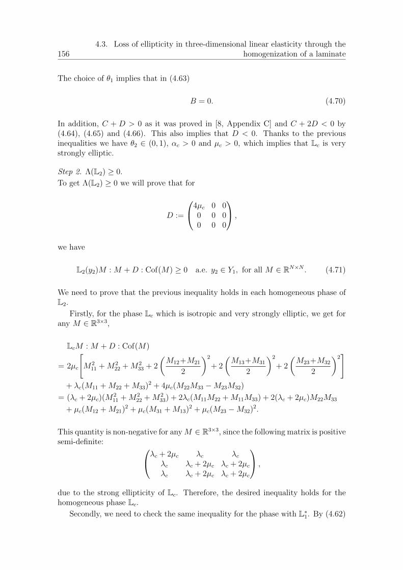
1564.3. Loss of ellipticity in three-dimensional linear elasticity through the

homogenization of a laminate

The choice of ✓1 implies that in (4.63)

B = 0. (4.70)

In addition, C + D > 0 as it was proved in [8, Appendix C] and C + 2D < 0 by(4.64), (4.65) and (4.66). This also implies that D < 0. Thanks to the previousinequalities we have ✓2 2 (0, 1), ↵c > 0 and µc > 0, which implies that Lc is verystrongly elliptic.

Step 2. ⇤(L2) � 0.

To get ⇤(L2) � 0 we will prove that for

D :=

0

@4µc 0 00 0 00 0 0

1

A ,

we have

L2(y2)M : M +D : Cof(M) � 0 a.e. y2 2 Y1, for all M 2 RN⇥N . (4.71)

We need to prove that the previous inequality holds in each homogeneous phase ofL2.

Firstly, for the phase Lc which is isotropic and very strongly elliptic, we get forany M 2 R3⇥3,

LcM : M +D : Cof(M)

= 2µc

"M2

11 +M222 +M2

33 + 2

✓M12+M21

2

◆2

+ 2

✓M13+M31

2

◆2

+ 2

✓M23+M32

2

◆2#

+ �c(M11 +M22 +M33)2 + 4µc(M22M33 �M23M32)

= (�c + 2µc)(M211 +M2

22 +M233) + 2�c(M11M22 +M11M33) + 2(�c + 2µc)M22M33

+ µc(M12 +M21)2 + µc(M31 +M13)

2 + µc(M23 �M32)2.

This quantity is non-negative for anyM 2 R3⇥3, since the following matrix is positivesemi-definite:

0

@�c + 2µc �c �c

�c �c + 2µc �c + 2µc

�c �c + 2µc �c + 2µc

1

A ,

due to the strong ellipticity of Lc. Therefore, the desired inequality holds for thehomogeneous phase Lc.

Secondly, we need to check the same inequality for the phase with L⇤1. By (4.62)

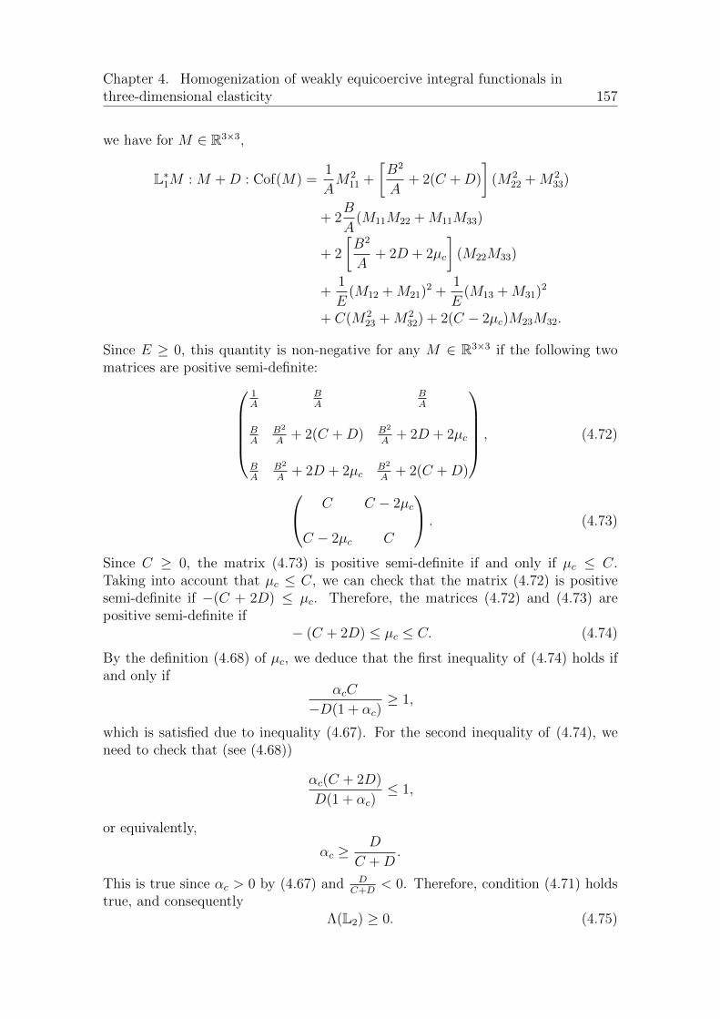
Chapter 4. Homogenization of weakly equicoercive integral functionals inthree-dimensional elasticity 157

we have for M 2 R3⇥3,

L⇤1M : M +D : Cof(M) =

1

AM2

11 +

B2

A+ 2(C +D)

�(M2

22 +M233)

+ 2B

A(M11M22 +M11M33)

+ 2

B2

A+ 2D + 2µc

�(M22M33)

+1

E(M12 +M21)

2 +1

E(M13 +M31)

2

+ C(M223 +M2

32) + 2(C � 2µc)M23M32.

Since E � 0, this quantity is non-negative for any M 2 R3⇥3 if the following twomatrices are positive semi-definite:

0

BBBB@

1A

BA

BA

BA

B2

A+ 2(C +D) B2

A+ 2D + 2µc

BA

B2

A+ 2D + 2µc

B2

A+ 2(C +D)

1

CCCCA, (4.72)

0

@C C � 2µc

C � 2µc C

1

A . (4.73)

Since C � 0, the matrix (4.73) is positive semi-definite if and only if µc C.Taking into account that µc C, we can check that the matrix (4.72) is positivesemi-definite if �(C + 2D) µc. Therefore, the matrices (4.72) and (4.73) arepositive semi-definite if

� (C + 2D) µc C. (4.74)

By the definition (4.68) of µc, we deduce that the first inequality of (4.74) holds ifand only if

↵cC

�D(1 + ↵c)� 1,

which is satisfied due to inequality (4.67). For the second inequality of (4.74), weneed to check that (see (4.68))

↵c(C + 2D)

D(1 + ↵c) 1,

or equivalently,

↵c � D

C +D.

This is true since ↵c > 0 by (4.67) and DC+D

< 0. Therefore, condition (4.71) holdstrue, and consequently

⇤(L2) � 0. (4.75)

1584.3. Loss of ellipticity in three-dimensional linear elasticity through the

homogenization of a laminate

Step 3. L2 loses the strong ellipticity through homogenization.On the one hand, due to ⇤(L2) � 0, by virtue of Theorem 4.5 the �-convergence(4.59) holds with the homogenized tensor L0

2 which is given by the minimizationformula (4.16) replacing L by L2.

On the other hand, following Gutierrez’ 1⇤-convergence procedure we obtain ahomogenized tensor L⇤

2 such that (see [8, Section 5.2] for the expression of L⇤2)

L⇤2(e3 ⌦ e3) : (e3 ⌦ e3) = I1 +

G21

F1,

where by (4.70),

I1 = 4(1� ✓2)1 + ↵c

2 + ↵c

+ 2✓2CC + 2D

C +D,

G1 = (1� ✓2)↵c

2 + ↵c

+ ✓2D

C +D,

F1 6= 0.

It is not di�cult to check that the choice of Lb, Lc, ✓1, ✓2 leads to I1 = G1 = 0,which yields

L⇤2(e3 ⌦ e3) : (e3 ⌦ e3) = 0. (4.76)

To conclude the proof it is enough to show that

L⇤2 = L0

2. (4.77)

Indeed, thanks to L⇤2 = L0

2 equality (4.76) implies the loss of ellipticity (4.60), and(4.60) implies ⇤(L2) 0. This combined with (4.75) finally shows the desired lossof functional coercivity (4.58).

Step 4. L⇤2 = L0

2.By formally using 1⇤-convergence in terms of [2, Lemma 3.1], Gutierrez’s computa-tions for the tensor L⇤

2 in [8, Section 5.2] can be written as

8>>>>>>>>>><

>>>>>>>>>>:

A�1[L⇤2] =

Z 1

0

A�1[L2](t) dt,

A�1im[L⇤

2](L⇤2)2mkl =

Z 1

0

�A�1

im[L2](t)(L2)2mkl(t)�dt,

(L⇤2)ijkl � (L⇤

2)ij2mA�1mn[L⇤

2](L⇤2)2nkl

=

Z 1

0

�(L2)ijkl(t)� (L2)ij2m(t)A

�1mn[L2](t)(L2)2nkl(t)

�dt,

(4.78)

where in the present context, for any L 2 L1per(Y1;Ls(R3⇥3)), A[L] 2 L1

per(Y1;R3⇥3s )

is defined by

A[L](y2)⇠ := [L(y2)(⇠ ⌦ e2)]e2 for y2 2 Y1 and ⇠ 2 R3.

Chapter 4. Homogenization of weakly equicoercive integral functionals inthree-dimensional elasticity 159

By focusing on the first equality of (4.78) we have

A�1[L⇤2] =

Z 1

0

A�1[L2](t) dt = ✓2A�1[L⇤

1] + (1� ✓2)A�1[Lc], (4.79)

where all the quantities are finite. Now, similarly to the proof of Theorem 4.5 weconsider the perturbation of L2 defined by

L� := L2 + � Is for � > 0. (4.80)

On the one hand, due to ⇤(L�) > 0 (which by (4.14) implies 0 < ⇤per(L�) ↵se(L�)),thanks to [2, Lemma 3.2] the 1⇤-limit L⇤

� of L� and the homogenized tensor L0� of L�

defined by (4.16) agree. Then, applying [2, Lemma 3.1] with L� we get that

A�1[L⇤� ] =

Z 1

0

A�1[L�](t)dt = ✓2A�1[L⇤

1 + � Is] + (1� ✓2)A�1[Lc + � Is]. (4.81)

Observe that we have

A[L⇤1 + � Is] � A[L⇤

1],

A[L⇤1 + � Is] ! A[L⇤

1] as � ! 0,

where the previous inequality must be understood in the sense of the quadraticforms. This combined with the fact that both L⇤

1 + � Is and L⇤1 are strongly elliptic

tensors (which implies that the previous matrices are positive definite), yields

A�1[L⇤1 + � Is] A�1[L⇤

1],

and thus,A�1[L⇤

1 + � Is] ! A�1[L⇤1] as � ! 0.

Similarly, we haveA�1[Lc + � Is] ! A�1[Lc] as � ! 0.

Hence, from the two previous convergences and taking into account (4.79), (4.81),we deduce that

A�1[L⇤� ] ! A�1[L⇤

2] as � ! 0.

On the other hand, following the proof of Theorem 4.5 we have

L⇤� = L0

� ! L02 as � ! 0.

Therefore, we obtain the equality

A�1[L02] = A�1[L⇤

2]. (4.82)

Using similar arguments, we can prove that L02 and L⇤

2 satisfy for any i, j, k, l 2{1, 2, 3},

A�1im[L⇤

2](L⇤2)2mkl = A�1

im[L02](L0

2)2mkl, (4.83)

(L⇤2)ijkl � (L⇤

2)ij2mA�1mn[L⇤

2](L⇤2)2nkl = (L0

2)ijkl � (L02)ij2mA

�1mn[L0

2](L02)2nkl. (4.84)

Since the set of equalities (4.78) completely determine the tensor L⇤2, equalities

(4.82), (4.83), (4.84) thus imply the desired equality (4.77), which concludes theproof.

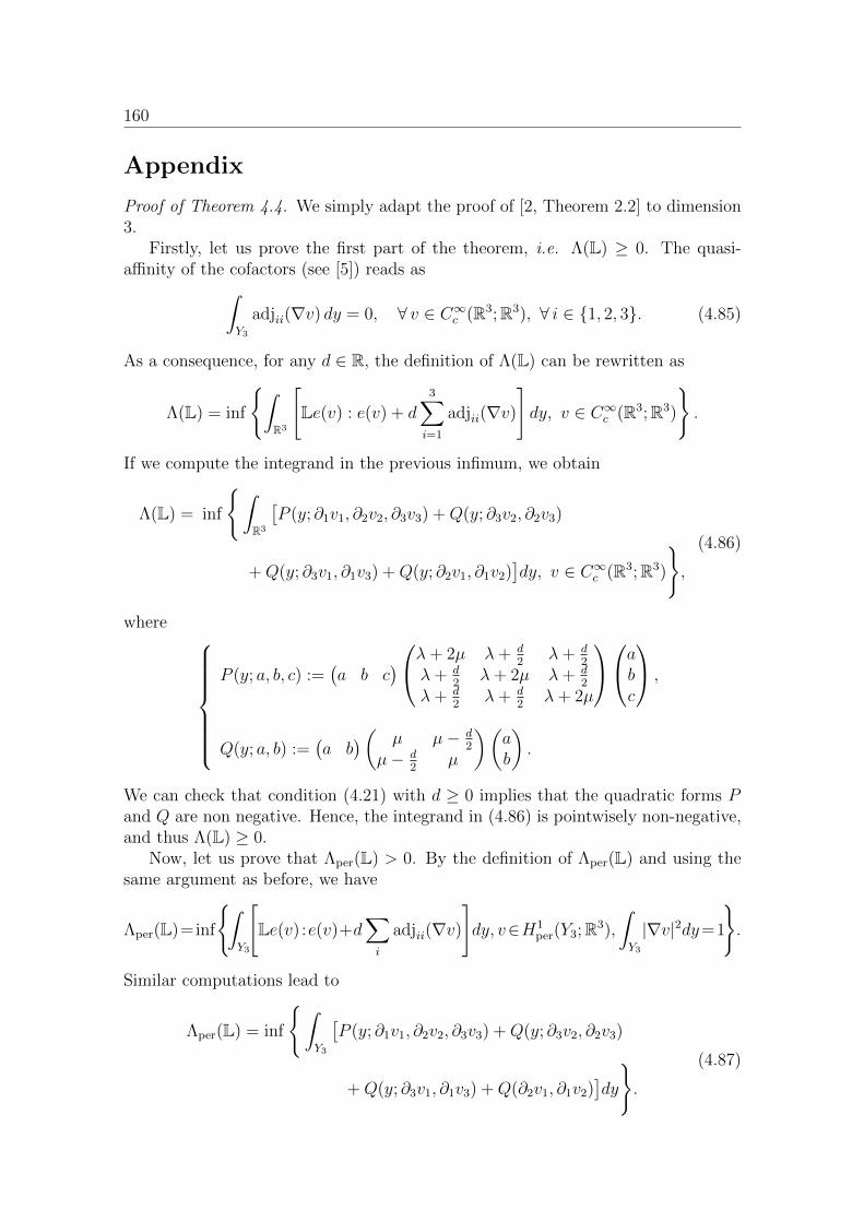
160

Appendix

Proof of Theorem 4.4. We simply adapt the proof of [2, Theorem 2.2] to dimension3.

Firstly, let us prove the first part of the theorem, i.e. ⇤(L) � 0. The quasi-a�nity of the cofactors (see [5]) reads as

Z

Y3

adjii(rv) dy = 0, 8 v 2 C1c (R3;R3), 8 i 2 {1, 2, 3}. (4.85)

As a consequence, for any d 2 R, the definition of ⇤(L) can be rewritten as

⇤(L) = inf

(Z

R3

"Le(v) : e(v) + d

3X

i=1

adjii(rv)

#dy, v 2 C1

c (R3;R3)

).

If we compute the integrand in the previous infimum, we obtain

⇤(L) = inf

(Z

R3

⇥P (y; @1v1, @2v2, @3v3) +Q(y; @3v2, @2v3)

+Q(y; @3v1, @1v3) +Q(y; @2v1, @1v2)⇤dy, v 2 C1

c (R3;R3)

),

(4.86)

where8>>>>>><

>>>>>>:

P (y; a, b, c) :=�a b c

�0

@�+ 2µ �+ d

2 �+ d2

�+ d2 �+ 2µ �+ d

2�+ d

2 �+ d2 �+ 2µ

1

A

0

@abc

1

A ,

Q(y; a, b) :=�a b

�✓ µ µ� d2

µ� d2 µ

◆✓ab

◆.

We can check that condition (4.21) with d � 0 implies that the quadratic forms Pand Q are non negative. Hence, the integrand in (4.86) is pointwisely non-negative,and thus ⇤(L) � 0.

Now, let us prove that ⇤per(L) > 0. By the definition of ⇤per(L) and using thesame argument as before, we have

⇤per(L)=inf

(Z

Y3

"Le(v) :e(v)+d

X

i

adjii(rv)

#dy, v2H1

per(Y3;R3),

Z

Y3

|rv|2dy=1

).

Similar computations lead to

⇤per(L) = inf

(Z

Y3

⇥P (y; @1v1, @2v2, @3v3) +Q(y; @3v2, @2v3)

+Q(y; @3v1, @1v3) +Q(@2v1, @1v2)⇤dy

).

(4.87)

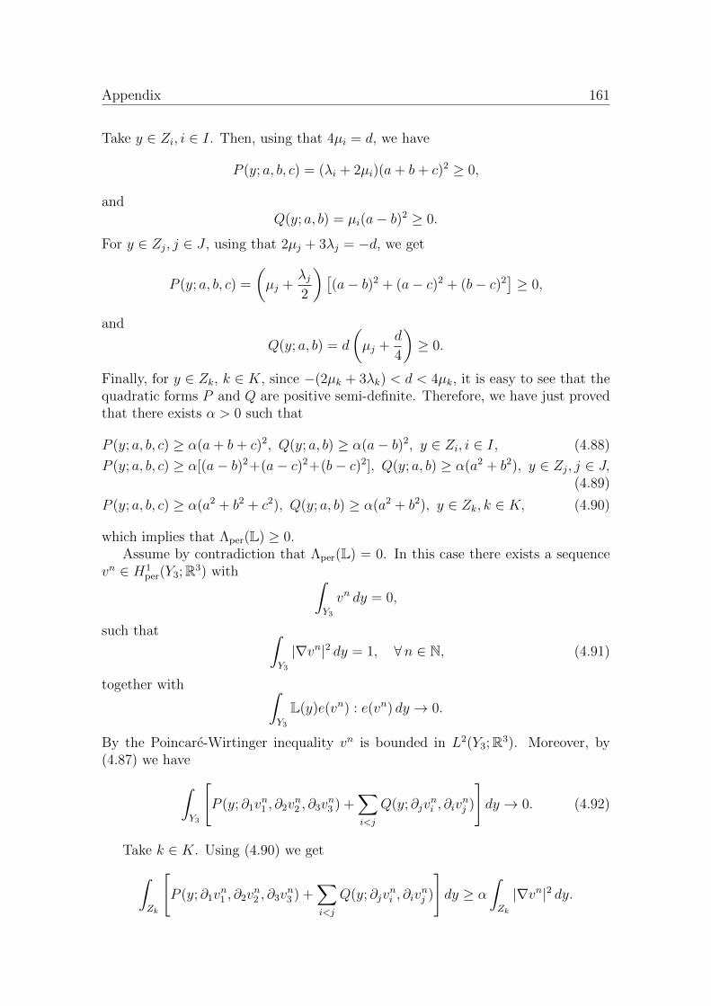
Appendix 161

Take y 2 Zi, i 2 I. Then, using that 4µi = d, we have

P (y; a, b, c) = (�i + 2µi)(a+ b+ c)2 � 0,

andQ(y; a, b) = µi(a� b)2 � 0.

For y 2 Zj, j 2 J , using that 2µj + 3�j = �d, we get

P (y; a, b, c) =

✓µj +

�j2

◆⇥(a� b)2 + (a� c)2 + (b� c)2

⇤ � 0,

and

Q(y; a, b) = d

✓µj +

d

4

◆� 0.

Finally, for y 2 Zk, k 2 K, since �(2µk + 3�k) < d < 4µk, it is easy to see that thequadratic forms P and Q are positive semi-definite. Therefore, we have just provedthat there exists ↵ > 0 such that

P (y; a, b, c) � ↵(a+ b+ c)2, Q(y; a, b) � ↵(a� b)2, y 2 Zi, i 2 I, (4.88)

P (y; a, b, c) � ↵[(a� b)2+(a� c)2+(b� c)2], Q(y; a, b) � ↵(a2 + b2), y 2 Zj, j 2 J,(4.89)

P (y; a, b, c) � ↵(a2 + b2 + c2), Q(y; a, b) � ↵(a2 + b2), y 2 Zk, k 2 K, (4.90)

which implies that ⇤per(L) � 0.Assume by contradiction that ⇤per(L) = 0. In this case there exists a sequence

vn 2 H1per(Y3;R3) with Z

Y3

vn dy = 0,

such that Z

Y3

|rvn|2 dy = 1, 8n 2 N, (4.91)

together with Z

Y3

L(y)e(vn) : e(vn) dy ! 0.

By the Poincare-Wirtinger inequality vn is bounded in L2(Y3;R3). Moreover, by(4.87) we have

Z

Y3

"P (y; @1v

n1 , @2v

n2 , @3v

n3 ) +

X

i<j

Q(y; @jvni , @iv

nj )

#dy ! 0. (4.92)

Take k 2 K. Using (4.90) we get

Z

Zk

"P (y; @1v

n1 , @2v

n2 , @3v

n3 ) +

X

i<j

Q(y; @jvni , @iv

nj )

#dy � ↵

Z

Zk

|rvn|2 dy.

162

Then, using (4.92) and the fact that both P and Q are non negative, it follows thatZ

Zk

|rvn|2 dy ! 0 8 k 2 K,

and therefore

limn!1

X

k2K

Z

Zk

X

q,r=1,2,3

(@rvnq )

2 dy = 0. (4.93)

Next, take j 2 J . By (4.89) we obtain

Z

Zj

"P (y; @1v

n1 , @2v

n2 , @3v

n3 ) +

X

i<k

Q(y; @kvni , @iv

nk )

#dy

� ↵

Z

Zj

X

i<k

⇥(@iv

ni � @kv

nk )

2 + (@kvni )

2 + (@ivnk )

2⇤dy.

Again using (4.92) and the non-negativity of P and Q we get

limn!1

Z

Zj

⇥(@iv

ni � @kv

nk )

2 + (@kvni )

2 + (@ivnk )

2⇤= 0 for i, k 2 {1, 2, 3}, i < k.

(4.94)From (4.94) and the continuity of the operator @1 : L2(Zj) ! H�1(Zj) we deducethat

(@2(@1v

n1 ) = @1(@2v

n1 ) ! 0 strongly in H�1(Zj),

@1(@1vn1 ) = @1(@1v

n1 � @2v

n2 ) + @2(@1v

n2 ) ! 0 strongly in H�1(Zj).

(4.95)

By (4.91) we also have@1v

n1 is bounded in L2(Zj). (4.96)

However, thanks to Korn’s Lemma (see, e.g., [9]) the following norms are equivalentin L2(Zj): (

kr · kH�1(Zj ;R3) + k · kH�1(Zj),

k · kL2(Zj).

Hence, from estimates (4.95), (4.96) and the compact embedding of L2 into H�1, itfollows that

@1vn1 is strongly convergent in L2(Zj).

Furthermore, by (4.95) and the fact that Zj is connected for all j, there exists cj 2 Rsuch that

@1vn1 ! cj strongly in L2(Zj),

which combined with (4.94) yields

rvn ! cjI3 strongly in L2(Zj)3.

Since vn is bounded in L2(Y3;R3), we can conclude that there exists Vj 2 R3 suchthat

vn ! v := cjy + Vj strongly in H�1(Zj;R3). (4.97)

Appendix 163

In Case 1, by the periodicity of the limit cjy + Vj it is necessary to have cj = 0.In Case 2, since Zk is connected, by (4.93) there exists a constant ck such that

vn converges to �Zjv + �Zkck strongly in H1(Zj [Zk). Hence, since the sets Zj and

Zk are regular, the trace of v must be equal to ck a.e. on @Zj \ @Zk. Therefore, theonly way for cjy+Vj to remain constant on a set of non-null H 2-measure is to havecj = 0.

In both cases this implies that rvn converges strongly to 0 in L2(Zj;R3⇥3), andthus

limn!1

X

j2J

Z

Zj

X

r,q=1,2,3

(@qvnr )

2dy = 0. (4.98)

Finally, take i 2 I. By (4.88) we have

Z

Zi

"P (y; @1v

n1 , @2v

n2 , @3v

n3 ) +

X

r<q

Q(y; @qvnr , @rv

nq )

#dy �

↵

Z

Zi

⇥(@1v

n1 + @2v

n2 + @3v

n3 )

2+(@2vn1 + @1v

n2 )

2+(@3vn1 + @1v

n3 )

2+(@3vn2 + @2v

n3 )

2⇤dy.

By virtue of (4.92) we also have

Z

Zi

⇥(@1v

n1 +@2v

n2 +@3v

n3 )

2+(@2vn1 +@1v

n2 )

2+(@3vn1 +@1v

n3 )

2+(@3vn2 +@2v

n3 )

2⇤dy ! 0,

(4.99)as n ! 1. Limits (4.98), (4.93) combined with (4.85) yield

limn!1

X

i2I

Z

Zi

3X

r=1

adjrr(rvn)dy = 0.

Therefore, upon subtracting this quantity to the sum over i 2 I of (4.99) we concludethat

limn!1

X

i2I

Z

Zi

3X

r,q=1

(@qvnr )

2dy = 0. (4.100)

Finally, limits (4.98), (4.93) and (4.100) contradict condition (4.91). The proof isthus complete.

Acknowledgments. The authors wish to thank A. Braides for the helpful The-orem 4.5.This work has been partially supported by the project MTM2011-24457 of the “Min-isterio de Economıa y Competitividad” of Spain, and the project FQM-309 of the“Junta de Andalucıa”. A.P.-M. is a fellow of “Programa de FPI del Ministerio deEconomıa y Competitividad” reference BES-2012-055158. A.P.-M. is grateful to theInstitut de Mathematiques Appliquees de Rennes for its hospitality, where this workwas carried out during his stay March 2 - June 29 2015.

164 Bibliography

Bibliography

[1] A. Braides: �-convergence for Beginners, Oxford University Press, Oxford,2002.

[2] M. Briane, G.A. Francfort: “Loss of ellipticity through homogenizationin linear elasticity”, Math. Models Methods Appl. Sci., 25 (5) (2015), 905-928.

[3] F. Murat: “H-convergence”, Seminaire d’Analyse Fonctionnelle etNumerique, 1977-78, Universite d’Alger, multicopied, 34 pp. English transla-tion : F. Murat & L. Tartar, “H-convergence”, Topics in the MathematicalModelling of Composite Materials, ed. by L. Cherkaev & R.V. Kohn, Progressin Nonlinear Di↵erential Equations and their Applications, 31, Birkhauser, Bo-ston (1998), 21-43.

[4] G.A. Francfort: “Homogenisation of a class of fourth order equations withapplications to incompressible elasticity”, Proc. Roy. Soc. Edinburgh Sect. A,120 (1-2) (1992), 25-46.

[5] B. Dacorogna: Direct methods in the calculus of variations, Second edition,Applied Mathematical Sciences, 78. Springer, New York, 2008, pp. 619.

[6] G. Dal Maso: An introduction to �-convergence, Birkhauser, Boston, 1993.

[7] G. Geymonat, S. Muller & N. Triantafyllidis: “Homogenization ofnon-linearly elastic materials, microscopic bifurcation and macroscopic loss ofrank-one convexity”, Arch. Rational Mech. Anal., 122 (3) (1993), 231-290.

[8] S. Gutierrez: “Laminations in Linearized Elasticity: The Isotropic Non-veryStrongly Elliptic Case”, J. Elasticity, 53 (1999), 215-256.

[9] J. Necas: “Sur les normes equivalentes dans W k(⌦) et sur la coercivitedes formes formellement positives”, Seminaire de mathematiques superieures,Equations aux derivees partielles, 19 (1966), 101-108.

[10] E Sanchez-Palencia: Nonhomogeneous Media and Vibration Theory, Lec-ture Notes in Physics 127, Springer-Verlag, Berlin-New York, 1980, pp. 398.