Privacy, Access Control, and Integrity for Large Graph ...

Purdue UniversityPurdue e-Pubs

Open Access Dissertations Theses and Dissertations

January 2016

Privacy, Access Control, and Integrity for LargeGraph DatabasesMuhammad Umer ArshadPurdue University

Follow this and additional works at: https://docs.lib.purdue.edu/open_access_dissertations

This document has been made available through Purdue e-Pubs, a service of the Purdue University Libraries. Please contact [email protected] foradditional information.

Recommended CitationArshad, Muhammad Umer, "Privacy, Access Control, and Integrity for Large Graph Databases" (2016). Open Access Dissertations.1359.https://docs.lib.purdue.edu/open_access_dissertations/1359

https://docs.lib.purdue.edu?utm_source=docs.lib.purdue.edu%2Fopen_access_dissertations%2F1359&utm_medium=PDF&utm_campaign=PDFCoverPages

https://docs.lib.purdue.edu/open_access_dissertations?utm_source=docs.lib.purdue.edu%2Fopen_access_dissertations%2F1359&utm_medium=PDF&utm_campaign=PDFCoverPages

https://docs.lib.purdue.edu/etd?utm_source=docs.lib.purdue.edu%2Fopen_access_dissertations%2F1359&utm_medium=PDF&utm_campaign=PDFCoverPages

https://docs.lib.purdue.edu/open_access_dissertations?utm_source=docs.lib.purdue.edu%2Fopen_access_dissertations%2F1359&utm_medium=PDF&utm_campaign=PDFCoverPages

https://docs.lib.purdue.edu/open_access_dissertations/1359?utm_source=docs.lib.purdue.edu%2Fopen_access_dissertations%2F1359&utm_medium=PDF&utm_campaign=PDFCoverPages

PRIVACY, ACCESS CONTROL, AND INTEGRITY FOR LARGE GRAPH

DATABASES

A Dissertation

Submitted to the Faculty

of

Purdue University

by

Muhammad Umer Arshad

In Partial Fulfillment of the

Requirements for the Degree

of

Doctor of Philosophy

December 2016

Purdue University

West Lafayette, Indiana

ii

To my dear parents, Shaista Bano and Arshad Mumtaz, for a lifetime of sacrifice.

To my beloved sisters, for their profound love and prayers.

iii

ACKNOWLEDGMENTS

All praise is due to Allah, Lord of the Worlds, without whom I would not exist, and

without whom I would not have begun and could not have completed this dissertation.

To my parents, Shaista Bano and Dr. Arshad Mumtaz, I thank you for the large

sacrifices you made for me. The living example of your lives taught me how to succeed

in doing hard things, and inspired me to reach this far. I often thought this task was

beyond me, but you both knew it was within my reach. My mother’s prayers and her

words of wisdom guided me through tough times during this journey. Despite limited

resources, my father’s selfless life of hard work, devotion, and dedication to provide

quality education to all of his children has been my inspiration. He fostered in me

a tenacious drive to learn and purse excellence in all I should do. His exemplary

passion for teaching students of medicine is highly admired by his students, and I

hope someday I may be a small fraction so well regarded. I love you dad so much.

My parents, I fall short of words to express my gratitude towards you.

To my dear sisters, Dr. Ayesha, Amana, and Fatima, I will always be there for

you and am glad each of you went a long way during all those years I have been

away. My time with Amana here at Purdue University was the best time I have had

here. To my uncle, Dr. Muhammad Naeem Ayyaz, I convey my utmost respect and

admiration of him for always sharing his words of wisdom with me. To my maternal

aunts, I thank them for the pure love they have given me.

To my advisors, Prof. Arif Ghafoor and Prof. Krishna Madhavan, I express my

deepest gratitude for their invaluable guidance and support at each step of my grad-

uate studies at Purdue University. Prof. Ghafoor gave me the freedom to explore the

field while training me to become an independent thinker, and constantly encouraged

me to dig deeper into my research ideas. From him, I also learned the skill which is

the capacity to be useful to others. I am forever indebted to Prof. Krishna Madhavan

iv

for his unequivocal help and encouragement, especially during the later part of my

Ph.D. He is an e↵ective communicator, a strategic thinker, and above all a very nice

human being. Thank you again Prof. Madhavan, for channeling my energies in the

right direction to accomplish my dissertation.

I have benefited immensely from Prof. Walid Aref’s unique approach to systems-

oriented research. The influence of his work has been instrumental to my success at

multiple industrial positions. He has been a great source of inspiration, and I have

always learned from him in our research interactions. He has had a profound impact

on my thought process and overall personality.

I thank Prof. Yung-Hsiang Lu for serving on my doctoral advising committee as

well as on all my examining committees. His questions were always intriguing, and

in formulating my reply, they helped me to clarify my ideas. I appreciate his candid

constructive feedback, comments, and our many insightful discussions.

I am also fortunate to have worked with Prof. Elisa Bertino from whom I learned

much despite our short research interaction. She always respected and encouraged

me, and it was a pleasure interacting with her. I am grateful for her continuing

support and am deeply moved by her strong work ethics.

I am obliged to Dr. Ashish Kundu, IBM T. J. Watson Research Center, for

introducing me to some challenging research problems and for being an excellent

research collaborator.

My internships at VMWare, Yahoo!, and EMC2 have been a great learning expe-

rience for me. I thank my mentors, Dr. Raj Yavatkar, Don Newell, Boaz Shaham,

Lars Anderson, Tavit Ohanian, and Ann Wong for many stimulating discussions.

My special thanks go to Dr. Nasir Bilal for always motiving me, for introducing

me to some life-changing books, for being my swimming instructor, and for all the

wonderful times we have had together at Purdue University.

So many more colleagues and friends must go unacknowledged here. Know that

you are remembered for your friendship and support.

In closing, I restate that all praise is due to Allah, Lord of the Worlds.

v

TABLE OF CONTENTS

Page

LIST OF TABLES . . . . . . . . . . . . . . . . . . . . . . . . . . . . . . . . viii

LIST OF FIGURES . . . . . . . . . . . . . . . . . . . . . . . . . . . . . . . ix

ABBREVIATIONS . . . . . . . . . . . . . . . . . . . . . . . . . . . . . . . . xi

ABSTRACT . . . . . . . . . . . . . . . . . . . . . . . . . . . . . . . . . . . xii

1 INTRODUCTION . . . . . . . . . . . . . . . . . . . . . . . . . . . . . . 1

1.1 Motivation . . . . . . . . . . . . . . . . . . . . . . . . . . . . . . . . 1

1.2 Research Contributions . . . . . . . . . . . . . . . . . . . . . . . . . 3

1.3 Organization . . . . . . . . . . . . . . . . . . . . . . . . . . . . . . 4

2 BACKGROUND . . . . . . . . . . . . . . . . . . . . . . . . . . . . . . . 5

2.1 The Data Model . . . . . . . . . . . . . . . . . . . . . . . . . . . . 5

2.2 Graph Anonymization Definitions . . . . . . . . . . . . . . . . . . . 6

2.3 Role-based Access Control . . . . . . . . . . . . . . . . . . . . . . . 7

2.4 Message Authentication Codes (MACs) . . . . . . . . . . . . . . . . 8

3 A PRIVACYMECHANISM FOR ACCESS CONTROLLED GRAPH DATA 10

3.1 Introduction . . . . . . . . . . . . . . . . . . . . . . . . . . . . . . . 10

3.2 Background . . . . . . . . . . . . . . . . . . . . . . . . . . . . . . . 12

3.2.1 Access Control Model for Graph Data . . . . . . . . . . . . 12

3.2.2 Imprecision Bound for Roles . . . . . . . . . . . . . . . . . . 14

3.2.3 Information Loss and Utility Measure for Anonymized GraphData . . . . . . . . . . . . . . . . . . . . . . . . . . . . . . . 16

3.3 Problem Description . . . . . . . . . . . . . . . . . . . . . . . . . . 18

3.3.1 The k-BGP Problem . . . . . . . . . . . . . . . . . . . . . . 18

3.3.2 Privacy-Enhanced Access Control . . . . . . . . . . . . . . . 20

3.4 Heuristics for the k-BGP Problem . . . . . . . . . . . . . . . . . . . 22

vi

Page

3.4.1 Two-Stage Heuristic 1 (TSH1) . . . . . . . . . . . . . . . . . 22

3.4.2 Two-Stage Heuristic 2 (TSH2): A Scalable Approach . . . . 24

3.5 Performance and Security Analysis . . . . . . . . . . . . . . . . . . 28

3.5.1 Performance Evaluation . . . . . . . . . . . . . . . . . . . . 28

3.5.2 Security Analysis . . . . . . . . . . . . . . . . . . . . . . . . 39

3.6 Related Work . . . . . . . . . . . . . . . . . . . . . . . . . . . . . . 42

3.7 Summary . . . . . . . . . . . . . . . . . . . . . . . . . . . . . . . . 44

4 EFFICIENT AND SCALABLE INTEGRITY VERIFICATION OF DATAAND QUERY RESULTS FOR GRAPH DATABASES . . . . . . . . . . 45

4.1 Introduction . . . . . . . . . . . . . . . . . . . . . . . . . . . . . . . 45

4.1.1 Contributions . . . . . . . . . . . . . . . . . . . . . . . . . . 47

4.1.2 Organization . . . . . . . . . . . . . . . . . . . . . . . . . . 48

4.2 Background and Desiderata of HMACs for Graphs . . . . . . . . . . 49

4.2.1 Data Model . . . . . . . . . . . . . . . . . . . . . . . . . . . 49

4.2.2 Graph Data Publishing and Query Model . . . . . . . . . . 49

4.2.3 Threat Model . . . . . . . . . . . . . . . . . . . . . . . . . . 52

4.2.4 Desiderata of MACs for Graphs . . . . . . . . . . . . . . . . 52

4.3 HMACs for Graphs (gHMAC) . . . . . . . . . . . . . . . . . . . . . 54

4.3.1 Formal Definition . . . . . . . . . . . . . . . . . . . . . . . . 54

4.3.2 HMAC Scheme for Graphs . . . . . . . . . . . . . . . . . . . 55

4.3.3 Illustration of How gHMAC Works . . . . . . . . . . . . . . . 56

4.4 Redactable HMACs for Graphs (rgHMAC) and Query Processing . 59

4.4.1 Formal Definition . . . . . . . . . . . . . . . . . . . . . . . . 59

4.4.2 Redactable HMAC Scheme for Graphs . . . . . . . . . . . . 61

4.4.3 Illustration of How rgHMAC Works . . . . . . . . . . . . . . 67

4.4.4 Fail-stop and Fail-warn gHMAC and rgHMAC . . . . . . . . . . 67

4.5 Security Analysis . . . . . . . . . . . . . . . . . . . . . . . . . . . . 69

4.5.1 Security of gHMAC . . . . . . . . . . . . . . . . . . . . . . . 69

vii

Page

4.5.2 Security of rgHMAC . . . . . . . . . . . . . . . . . . . . . . 72

4.6 Performance Analysis . . . . . . . . . . . . . . . . . . . . . . . . . . 74

4.6.1 Complexity Analysis . . . . . . . . . . . . . . . . . . . . . . 74

4.6.2 Performance Evaluation . . . . . . . . . . . . . . . . . . . . 75

4.7 Related Work . . . . . . . . . . . . . . . . . . . . . . . . . . . . . . 82

4.8 Summary . . . . . . . . . . . . . . . . . . . . . . . . . . . . . . . . 84

5 CONCLUSIONS . . . . . . . . . . . . . . . . . . . . . . . . . . . . . . . 86

5.1 Summary of Contributions . . . . . . . . . . . . . . . . . . . . . . . 86

5.2 Limitations of the Proposed Methodologies . . . . . . . . . . . . . . 87

5.3 Future Work . . . . . . . . . . . . . . . . . . . . . . . . . . . . . . . 87

5.3.1 A Privacy Mechanism for Access-Controlled Dynamic GraphDatabases . . . . . . . . . . . . . . . . . . . . . . . . . . . . 88

5.3.2 Integrity Verification for Dynamic Graph Databases . . . . . 88

5.3.3 Aggregation-based Schemes for Graph Data Integrity . . . . 89

REFERENCES . . . . . . . . . . . . . . . . . . . . . . . . . . . . . . . . . . 90

A: Proof of Theorem 3.3.1 . . . . . . . . . . . . . . . . . . . . . . . . . . . . 95

B: Proof of Theorem 3.5.1 . . . . . . . . . . . . . . . . . . . . . . . . . . . . 101

VITA . . . . . . . . . . . . . . . . . . . . . . . . . . . . . . . . . . . . . . . 104

viii

LIST OF TABLES

Table Page

2.1 Generalization for k anonymity . . . . . . . . . . . . . . . . . . . . . . 6

2.2 Access control policy . . . . . . . . . . . . . . . . . . . . . . . . . . . . 8

3.1 Published graph view for roles . . . . . . . . . . . . . . . . . . . . . . . 14

3.2 Comparison of proposed heuristics . . . . . . . . . . . . . . . . . . . . 38

4.1 Di↵erent graph datasets . . . . . . . . . . . . . . . . . . . . . . . . . . 74

ix

LIST OF FIGURES

Figure Page

3.1 A graph and its corresponding published view. . . . . . . . . . . . . . . 13

3.2 Satisfying role bounds with minimum structural information loss. . . . 19

3.3 A framework for the proposed privacy-preserving access control mecha-nism for graph data. . . . . . . . . . . . . . . . . . . . . . . . . . . . . 21

3.4 E↵ect of BR on the % of role bound-violations for k = 5. . . . . . . . . 30

3.5 E↵ect of k on the # of role bound-violations for BR = 20%. . . . . . . 31

3.6 E↵ect of k on role imprecision SD. . . . . . . . . . . . . . . . . . . . . 33

3.7 E↵ect of k on the # of role bound-violations for BR = 20% and R = 500. 34

3.8 E↵ect of k on information loss for ego-Facebook and |R| = 50. . . . . 35

3.9 E↵ect of k on information loss for P2PNutella and |R| = 80. . . . . . . 37

3.10 E↵ect of k on information loss for com-Youtube and |R| = 500. . . . . 38

3.11 E↵ect of k on data utility. . . . . . . . . . . . . . . . . . . . . . . . . . 38

3.12 (a) The e↵ect of QA = {[0 � 32], [0 � 0], [0 � 2], [0 � 3], [0 � 333], [0 �32], [0 � 4], [0 � 331]} on Pr(Re-id(x)). (b) The e↵ect of % increase inquery QA = {A1, A6} dimension on Pr(Re-id(x)). . . . . . . . . . . . 40

3.13 (a) Pr(Re-id(x)) vs query QA(QS) for k = 7; (b) Pr(Re-id(x)) vs queryQS(QA) for k = 7; (c) Pr(Re-id(x)) vs query QA(QS) for k = 9; (d)Pr(Re-id(x)) vs query QS(QA) for k = 9; . . . . . . . . . . . . . . . . 41

4.1 Graphs: (a) DAG, (b) Graph with cycle v2 ! v3 ! v5 ! v4 ! v2, and(c) DAG with multiple sources {v1, v7}. . . . . . . . . . . . . . . . . . . 46

4.2 System model for publishing and querying graph data. . . . . . . . . . 50

4.3 An example of subgraph query matching. . . . . . . . . . . . . . . . . . 51

4.4 A DAG with source node id = 1, (b) Computation of out-xor(u), andu.outList() of vertices. . . . . . . . . . . . . . . . . . . . . . . . . . . 59

4.5 (a) A DAG where the shadowed part with dotted boundary is the subgraphG� that the user receives as part of query result. (b) Verification objectset vo-out computation for vertices in V�. . . . . . . . . . . . . . . . . . 66

x

Figure Page

4.6 Fail-stop / Fail-warn integrity verification example. . . . . . . . . . . . 68

4.7 gHMAC: Time to compute graph HMAC tag. . . . . . . . . . . . . . . . 76

4.8 gVrfy: Time to verify graph integrity using HMAC tag. . . . . . . . . 77

4.9 rgHMAC: Time to compute graph HMAC tag. . . . . . . . . . . . . . . . 78

4.10 gRedact: Time to compute query result R and verification object VO. 78

4.11 rgVrfy: Time to verify the integrity of query result R. . . . . . . . . . 79

4.12 Comparison with [53]. . . . . . . . . . . . . . . . . . . . . . . . . . . . 81

1 Partition into triangles di↵erent cases: (a) All graph vertices included inshaded partitions, solution to X3C exists; (b) Some graph vertices notincluded in shaded partitions, solution to X3C does not exist. . . . . . 97

2 Partitions of size 3, 4 and 5 points. . . . . . . . . . . . . . . . . . . . . 98

xi

ABBREVIATIONS

PPM Privacy Protection Mechanism

ACM Access Control Mechanism

HMAC Hash Message Authentication Code

PPT Probabilistic Polynomial Time

xii

ABSTRACT

Arshad, Muhammad PhD, Purdue University, December 2016. Privacy, Access Con-trol, and Integrity for Large Graph Databases. Major Professors: Arif Ghafoor andKrishna Madhavan.

Graph data are extensively utilized in social networks, collaboration networks, geo-social

networks, and communication networks. Their growing usage in cyberspaces poses daunting

security and privacy challenges. Data publication requires privacy-protection mechanisms

to guard against information breaches. In addition, access control mechanisms can be used

to allow controlled sharing of data. Provision of privacy-protection, access control, and

data integrity for graph data require a holistic approach for data management and secure

query processing. This thesis presents such an approach. In particular, the thesis addresses

two notable challenges for graph databases, which are: i) how to ensure users’ privacy in

published graph data under an access control policy enforcement, and ii) how to verify the

integrity and query results of graph datasets.

To address the first challenge, a privacy-protection framework under role-based access

control (RBAC) policy constraints is proposed. The design of such a framework poses

a trade-o↵ problem, which is proved to be NP-complete. Novel heuristic solutions are

provided to solve the constraint problem. To the best of our knowledge, this is the first

scheme that studies the trade-o↵ between RBAC policy constraints and privacy-protection

for graph data. To address the second challenge, a cryptographic security model based on

Hash Message Authentic Codes (HMACs) is proposed. The model ensures integrity and

completeness verification of data and query results under both two-party and third-party

data distribution environments. Unique solutions based on HMACs for integrity verification

of graph data are developed and detailed security analysis is provided for the proposed

schemes. Extensive experimental evaluations are conducted to illustrate the performance

of proposed algorithms.

1

1. INTRODUCTION

1.1 Motivation

Graph data has become increasingly important in recent years because of its

widespread use in various applications. Some leading examples are online social net-

works (OSN), Web, collaboration networks, and communication networks [1]. The

nodes of a graph represent entities, while their connections capture various relation-

ships among them. The semantics assigned with nodes and links in the graph data

vary significantly across application domains. For example, a social network is usu-

ally represented by a set of users, where links may capture friendship relationships; a

co-authorship network, on the other hand, describes scientific publications and their

collaboration links, etc.

The analysis of published graph data is used extensively by researchers in di↵erent

disciplines to extract useful knowledge and information. For example, epidemiologists

study disease spread patterns based on users’ social contact information; sociologists

and psychologists can verify the social structure and human behavior pattern; mining

algorithms are used to discover various patterns in these graphs; and advertisers can

accurately infer users’ preference profiles for targeted advertisements [2], [3]. This

data is published to stakeholders and authorized users.

Due to strong correlation among users’ social identities, privacy poses a major

challenge in data storage, processing, and publishing. The sensitive nature of data

raises privacy challenges as users’ private information may be revealed in published

graph data [4]. Privacy-preservation for sensitive data entails enforcement of privacy

policies and the provision for su�cient protection against identity disclosure [5].

Data anonymization has been studied extensively and adopted widely for pro-

tecting users’ privacy in graph data publishing [2], [3]. Simply removing the node

2

identifiers in social networks does not provide protection against structure-based re-

identification attacks [4]. Backstorm et al. [4] present a family of active and passive

attacks that work based on the uniqueness of some small random subgraphs embedded

in a network. The adversary may link this distinctive structure, random subgraph, to

some set of targeted individuals. In the anonymized published graph, the adversary

then traces the injected subgraph in the original graph. In case of only one such sub-

graph in the original graph, the targets that are connected to this subgraph can be

successfully re-identified and the edges between them are disclosed. In [6], Narayanan

et al. present a scalable two-phase de-anonymization (DA) process for social networks.

In the first phase, some seed nodes are identified between the anonymized and aux-

iliary graphs. In the second phase, the identified seed nodes are used in an iterative

DA propagation process based on both graphs’ structural characteristics. A detailed

comparison of di↵erent protection schemes against de-anonymization attacks is given

in [7].

Due to the high cost of hosting large volumes of data and performing data-intensive

computations, the owners of graph databases often outsource their data to a third-

party service provider [8] that o↵ers data services on behalf of the data owners [9].

Generally, outsourcing also o↵ers performance-oriented and scalable data services [10].

A leading example is the cloud computing paradigm. Other examples include Amazon

EC2, Amazon AWS, Google Cloud Service, and “Database-as-a-Service” [8], [10],

[11].

However, data outsourcing can pose serious data security challenges. The biggest

challenge is to ensure integrity of the data in the presence of untrusted service

providers [8], [9], [12]. Any tampering with data or query results presented to a

user can be perceived by the user as a violation of the Quality of Service (QoS) [13]

integrity requirements. However, verifying the integrity of graph data poses a signif-

icant security challenge [14].

3

1.2 Research Contributions

In this dissertation, we address the aforementioned challenges of privacy, access

control, and data integrity for graph datasets. In particular, we make two main

research contributions.

A privacy mechanism for access-controlled graph databases: A framework

for privacy-enhanced access-controlled graph dataset is presented. The framework

provides privacy protection through k-anonymization under the access restrictions

imposed by the RBAC policy. The k-anonymous bi-objective graph partitioning (k-

BGP) problem is formulated and hardness results are presented. E�cient heuristics

have been developed to solve the problem. A detailed security analysis of the scheme

is conducted and the proposed algorithms has been empirically evaluated.

Integrity verification of data and query results for graph databases:

Two security notions – HMACs for graphs for two-party data sharing, and redactable

HMACs for graphs for third-party data sharing are developed. The proposed schemes

can support “fail-stop” and “fail-warn” integrity assurance (Section 4.2.4) mecha-

nisms that can result in substantial saving in the cost incurred for integrity verification

and data re-transfer of compromised graphs. Formal definitions and constructions of

HMACs for graphs and redactable HMACs for graphs are provided. The proposed

schemes are shown to be secure to protect the graphs and redacted graphs from being

compromised. Experimental results on real-world graph datasets demonstrate that

HMACs for graphs and redactable HMACs graphs are highly e�cient compared to

digital signature-based schemes for graphs and the proposed schemes are linear in the

number of vertices and edges in the graph. Therefore, the proposed schemes are e�-

cient both in processing time and in the transmission of result set R and verification

objects VO to the client/user.

4

1.3 Organization

The remainder of this dissertation is organized as follows:

In Chapter 2, relevant background concepts related to privacy, role-based access

control (RBAC), and Hash Message Authentication Codes (HMACs) are introduced.

In Chapter 3, a framework for privacy-preserving access-controlled graph datasets

is presented. Privacy and access constraints are formulated as the k-anonymous

bi-objective graph partitioning (k-BGP) problem. Hardness results are presented

and empirical evaluation is conducted for the proposed heuristics. In Chapter 4,

the problem of graph data and query results integrity verification using HMACs is

investigated. E�cient integrity verification schemes are proposed. A detailed security

analysis of schemes is presented along with empirical evaluation on real-world graph

datasets. Chapter 5 concludes the dissertation with suggestions for future work.

5

2. BACKGROUND

2.1 The Data Model

We consider a simple undirected graph data model, G = (V,E), where V =

{v1, v2, . . . , vN} is the set of nodes and E ✓�V2

�is the set of edges1. Each node

corresponds to an individual in the underlying group of people, while an edge that

connects two nodes describes a relationship between two corresponding individuals.

In addition to the structural data that is given by E, each node is described by

a set of attributes (descriptive data) that can be classified in the following three

categories:

• Identifier. Attributes, e.g., name and ssn, that uniquely identify an entity.

These attributes are completely removed from an anonymized graph.

• Quasi-identifier (QI). Attributes, e.g., birth date, zip code and gender, that can

be joined with external information available to some adversary to reveal the

personal identity of an individual.

• Sensitive attribute. Attributes, e.g., disease and income, that are assumed to

be unknown to an intruder. They are assumed to cause a privacy breach if

associated to a unique individual.

The combination of QIs could be used for unique identification by mean of linking

attacks [15]. Hence, they should be generalized in order to thwart such attacks.

Definition 2.1.1 Let A1, A2, . . . , Ad be a collection of QI attributes. Then a graph

is defined as G = hV,E, T i, where E 2�V2

�is the structural information (edges),

1�V2

�denotes the set of all unordered pairs of elements from V .

6

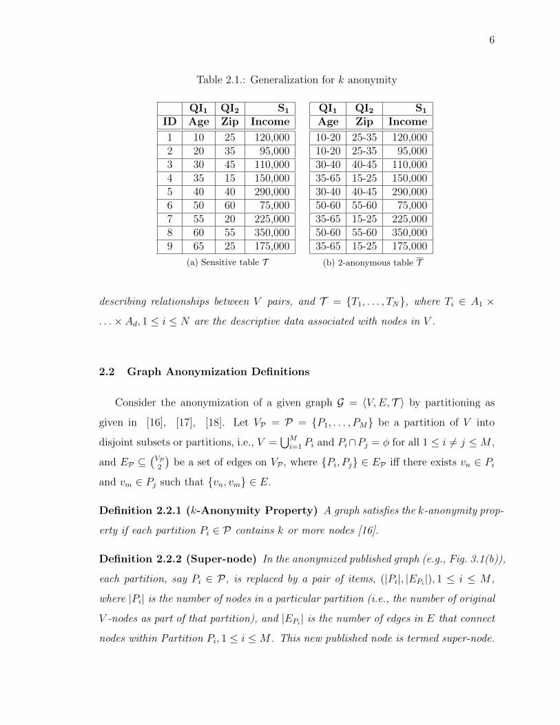
Table 2.1.: Generalization for k anonymity

QI1 QI2 S1

ID Age Zip Income

1 10 25 120,0002 20 35 95,0003 30 45 110,0004 35 15 150,0005 40 40 290,0006 50 60 75,0007 55 20 225,0008 60 55 350,0009 65 25 175,000

(a) Sensitive table T

QI1 QI2 S1

Age Zip Income

10-20 25-35 120,00010-20 25-35 95,00030-40 40-45 110,00035-65 15-25 150,00030-40 40-45 290,00050-60 55-60 75,00035-65 15-25 225,00050-60 55-60 350,00035-65 15-25 175,000

(b) 2-anonymous table T

describing relationships between V pairs, and T = {T1, . . . , TN}, where Ti 2 A1 ⇥. . .⇥ Ad, 1 i N are the descriptive data associated with nodes in V .

2.2 Graph Anonymization Definitions

Consider the anonymization of a given graph G = hV,E, T i by partitioning as

given in [16], [17], [18]. Let VP = P = {P1, . . . , PM} be a partition of V into

disjoint subsets or partitions, i.e., V =SM

i=1 Pi and Pi\Pj = � for all 1 i 6= j M ,

and EP ✓�VP2

�be a set of edges on VP , where {Pi, Pj} 2 EP i↵ there exists vn 2 Pi

and vm 2 Pj such that {vn, vm} 2 E.

Definition 2.2.1 (k-Anonymity Property) A graph satisfies the k-anonymity prop-

erty if each partition Pi 2 P contains k or more nodes [16].

Definition 2.2.2 (Super-node) In the anonymized published graph (e.g., Fig. 3.1(b)),

each partition, say Pi 2 P, is replaced by a pair of items, (|Pi|, |EPi |), 1 i M ,

where |Pi| is the number of nodes in a particular partition (i.e., the number of original

V -nodes as part of that partition), and |EPi | is the number of edges in E that connect

nodes within Partition Pi, 1 i M . This new published node is termed super-node.

7

Definition 2.2.3 (Super-edge) In the anonymized published graph (e.g., Fig. 3.1(b)),

each edge, say (Pi, Pj) 2 EP , is labeled by a weight |EPi,Pj |, which stands for the num-

ber of edges in E that connect a node in Pi to a node in Pj. This new published edge

is termed a super-edge.

We assume that all the QI attributes have numerical values and use the hierarchical-

free generalization [19] that generalizes the set of tuples present in a partition, say Pi,

with the smallest interval that includes all the initial values, also called the minimal

covering tuple, for that partition.

Definition 2.2.4 (Anonymized graph [16]) Let G = hV,E, T i be a graph with

vertex attributes, and let A1, . . . , Ad be the generalization taxonomies for d QI at-

tributes A1, . . . , Ad. Then, given a partitioning VP of V , the anonymized graph is

defined as GP = hVP , EP , T i, where:

• EP ✓�VP2

�is a set of edges on VP , where {Pi, Pj} 2 EP i↵ there exists vn 2 Pi

and vm 2 Pj such that {vn, vm} 2 E;

• The partitions in VP are labeled by their sizes and the number of their intra-

cluster edges (|Pi|, |EPi |), while the edges in EP are labeled by the corresponding

number of inter-cluster edges, |EPiPj |, in E where 1 i 6= j M ;

• T = {T 1, . . . , TM}, where T i is the minimal record in A1 ⇥ . . . ⇥ Ad that gen-

eralizes all QI tuples of individuals in Pi, 1 i M . Table 2.1(b) shows a

2-anonymous partitioning for a dataset with QI attributes Age and Zip.

2.3 Role-based Access Control

Role-based access control (RBAC) allows defining permissions on objects based on

roles in an organization. An RBAC policy configuration is composed of a set of Users

(U), a set of Roles (R), and a set of Permissions (P). For the graph model, we assume

that the set of permissions for a role are the selection predicates on the QI attributes

8

Table 2.2.: Access control policy

Role Permission Authorized Query Predicate (View)

Role1 X Age = 15-45 ^ Zip = 20-30Role2 Y Age = 30-45 ^ Zip = 25-45Role3 Z Age = 50-60 ^ Zip = 55-60

that the role is authorized to execute [20]. Among the authorized tuple subset, a

user is free to set any selection condition on the sensitive attribute. The user-to-

role assignment (UA) is a user-to-role (U ⇥R) mapping and the role-to-permission

assignment (PA) is a role-to-permission (R⇥ P) mapping.

Definition 2.3.1 (RBAC Policy) An RBAC policy ⇢ is a tuple hU ,R,P , UA, PAi.

In practice, when a user assigned to a role executes a query, the tuples that satisfy

the conjunction of query predicate and the permission are returned [5], [21]. Consider

for example Table 2.2 where Role1 has been assigned permission X with authorized

query predicate Age = 15-45 ^ Zip = 20-30.

2.4 Message Authentication Codes (MACs)

A MAC is a cryptographic checksum on data that takes as input a message m

and a secret key k and produces an output called authentication tag t = H(k,m).

The Hash Message Authentication Code (HMAC) algorithm is a shared-key se-

curity algorithm that uses a cryptographic hash function as an underlying function

and is used to verify data integrity and data-origin authentication. HMAC can be

used with any iterative cryptographic hash function (e.g., MD5, SHA-1, etc.) in

combination with a shared secret key. HMAC has been implemented in widely used

security protocols including SSL, TLS, SSH, and IPsec [22]. It is also used as a PRF2

for key-derivation, as in TLS [23] and IKE (the Internet Key Exchange protocol of

2A PRF is an e�cient deterministic function and takes two inputs k and m. Its output is computa-tionally indistinguishable from truly random output.

9

IPsec) [24]. HMAC is also used as a PRF in a standard for one-time passwords [25].

This is the basis for Google authenticator . The main operation of HMAC is:

HMACk(m) = H((k � opad)||H((k � ipad)||m)), (2.1)

where opad (outer padding) is a constant byte 0x36, ipad (inner padding) is a

constant byte 0x5c [26], and � is bitwise eXclusive-OR (X-OR) operator.

Attacks

The most common attack on MACs is a forgery attack, in which an adversary can

produce a valid (message, tag) pair without knowing the secret key k. For MACs that

are based on iterative hash functions and use a compression function f : {0, 1}n+m !{0, 1}n, there is a birthday-type forgery attack [27] that requires about O(2n/2) MAC

queries to its generation oracle, where n is the length of authentication tag.

Security

The cryptographic strength of HMAC depends on the properties of the underly-

ing hash function [28]. As we have mentioned, the most common attack against

HMACs is brute force to uncover the secret key. To have a secure MAC func-

tion, we want to have unforgeability ; that is, without knowing the secret key k, it

should be hard for an adversary A to find a pair (m, t) such that t = MACk(m),

even if A has access to some other valid (message, tag) pairs. Unfortunately, for

a secure hash function MACk(m) = H(k||m) does not guarantee that the MAC

function is unforgeable. Since H is computed using the Merkle–Dagmard construc-

tion, the graph MAC designed in this way is completely insecure, as it is quite

easy, given a valid pair (m, t), to create an (m0, t0), which is still valid. HMAC

HMACk(m) = H((k�opad)||H((k�ipad)||m)) avoids the above problem using two

layers of hashing [26].

10

3. A PRIVACY MECHANISM FOR ACCESS

CONTROLLED GRAPH DATA

3.1 Introduction

Data anonymization schemes provide privacy-protection for published graph data.

However, the data publisher may use an authorization mechanism for controlling ac-

cess to data by group of users [29]. Access control policies provide additional safe-

guard against data breaches and are used to ensure that only authorized published

information is available to end-users based on their assigned role. Roles are abstract

descriptions of privileges for users accessing data in OSNs [30]. We assume a Role-

Based Access Control (RBAC) [31] administration model for the policy enforcement.

RBAC assigns access privileges to end-users based on their predefined roles. A leading

example in OSN services is Facebook1, which provides privacy features by allowing

the user to dictate access to their private information by employing fine-grained access

control policies [32], [33]. In OSN, either a centralized authority, a reference monitor,

decentralized authorities, or users themselves can carry out policy enforcement. We

consider a graph data publishing framework that provides safeguard against data pri-

vacy breach through anonymization while enforcing access rules to satisfy the security

protection requirements specified by the data publisher.

Since k-anonymization is a generalization approach, at the time of creating k-

anonymous partitions, we show that access control privileges might need be relaxed

to ensure k-anonymity privacy requirement with a relatively stronger guarantee. The

issue is, in order to accommodate imprecision bound false-positive tuples need to be

reduced that result in increased average partition sizes. Relaxing access control re-

quirement implies a slight increase in the scope of the privilege set associated with a

1https://www.facebook.com/policy.php

11

role. Likewise, under strict policy the privacy is relatively weak compared to relaxed

semantics as we try to reduce false-negative tuples resulting in decreased average par-

tition sizes. This exhibits a trade-o↵ between privacy and access control. However, re-

laxing access control requirement should be bounded by access control administrator.

Discussion on access control model and policies is given in Sections 3.2.1 and 3.3.2.

Generally, high privacy is achieved at the cost of increased information loss [34]. A key

challenge is to ensure k-anonymity privacy protection of individuals within published

graph data and preserve data utility while enforcing an access control policy. For-

mally, given a set of roles with their associated imprecision bounds and a k-anonymity

requirement, the challenge is anonymize dataset such that maximum number of roles

satisfy their imprecision bounds and minimum information loss is incurred. For this,

we propose a k-anonymous Bi-objective Graph Partitioning (k-BGP) problem and

give hardness results (Section 3.3.1). This is a unique problem that has not been

considered earlier.

The chapter makes the following contributions:

• We formulate the k-BGP problem and give hardness results. Two heuristics

TSH1 and TSH2 are developed to solve the constraint problem.

• We provide empirical evaluation of the proposed heuristics with a benchmark

algorithm [35] from design perspective in terms of meeting privacy and access

control requirements with minimum information loss.

• Within the context of k-BGP problem, we present an architecture framework

elaborating how access control and privacy can be integrated (Section 3.3.2).

• We evaluate the proposed framework from security perspective and present a

probabilistic analysis for re-identification risk.

The rest of this chapter is organized as follows. Section 3.2 presents the needed

definitions and discusses the information loss measure. The problem formulation and

the access control framework are discussed in Section 3.3. In Section 3.4, we present

12

the proposed heuristics for k-BGP problem. Section 3.5 provides performance eval-

uation and security analysis. Section 3.6 overviews the related work and Section 3.7

contains the summary of research contributions.

3.2 Background

3.2.1 Access Control Model for Graph Data

In this section, we discuss the semantics of role/query predicate evaluation with

respect to access control. For the query predicate evaluation over a graph, say G,a vertex is added to the output result if all its attribute values satisfy the query

predicate. Moreover, the edges between the result vertex set are also returned as an

output. Here, we only consider conjunctive queries, where each query represents the

d-dimensional hyper-rectangle. The semantics for query evaluation on an anonymized

graph GP need to be defined. When a partition, say P , is fully included in the query

region, all the partition nodes and their associated edges are returned as part of

the query result. However, when a partition and a query partially overlap, there is

an uncertainty in the query evaluation. In this case, there can be several possible

semantics. The following three options are generally used:

1. Uniform. Assuming the uniform distribution of nodes in the overlapping parti-

tions, the result returns the nodes according to the ratio of overlap between the

query and the partition, and the edges between these nodes. Most of the litera-

ture uses the uniform distribution semantics to compare anonymity techniques

over selection tasks [19].

2. Overlap. This includes all nodes and their associated edges in the partitions

that overlap the role/query. This option will add false positives to the original

role/query result.

13

10! 30! 40! 50! 60!20!

10!

60!

50!

40!

30!

20!(10, 25)!

(35, 15)!

(55, 20)!

(65, 25)!

(20, 35)!

(30, 45)!

(40, 40)!

(55, 60)!

(60, 55)!

10! 30! 40! 50! 60!20!

10!

60!

50!

40!

30!

20!

P1!

P2!

P3!

P4!

(10, 25)!

(35, 15)!(55, 20)!

(65, 25)!

(20, 35)!

(30, 45)!

(40, 40)!

(50, 60)!

(60, 55)!

Age!

Zip!

60! P4!

10! 30! 40! 50! 60!20!

10!

50!

40!

30!

20!

P1!

P2!

P3!(2, 1)!

(2, 1)!

(2, 1)!

(3, 0)!([10-20], [25-35])! ([35-65], [15-25])!

([30-45], [40-50])!

([50-60], [55-60])!

2!3!

2!

Age!

Zip!

(a) Original partitioned graph

10! 30! 40! 50! 60!20!

10!

60!

50!

40!

30!

20!(10, 25)!

(35, 15)!

(55, 20)!

(65, 25)!

(20, 35)!

(30, 45)!

(40, 40)!

(55, 60)!

(60, 55)!

10! 30! 40! 50! 60!20!

10!

60!

50!

40!

30!

20!

P1!

P2!

P3!

P4!

(10, 25)!

(35, 15)!(55, 20)!

(65, 25)!

(20, 35)!

(30, 45)!

(40, 40)!

(50, 60)!

(60, 55)!

Age!

Zip!

60! P4!

10! 30! 40! 50! 60!20!

10!

50!

40!

30!

20!

P1!

P2!

P3!(2, 1)!

(2, 1)!

(2, 1)!

(3, 0)!([10-20], [25-35])! ([35-65], [15-25])!

([30-45], [40-50])!

([50-60], [55-60])!

2!3!

2!

Age!

Zip!

(b) Anonymized graph GP

Fig. 3.1.: A graph and its corresponding published view.

3. Enclosed. This discards all nodes and their associated edges in all those par-

titions that partially overlap the role/query region. This option yields false

negatives with respect to the original role/query result.

For the remainder of this paper, we assume Overlap semantics as defined above.

Example 1 Consider the social network graph in Fig. 3.1(a) with 9 vertices and

10 edges with each vertex containing the two QI attribute values Age and Zip for

individuals in the graph. Table 2.1(b) shows the 2-anonymous partitioning of these

vertex attributes. In the anonymized published graph in Fig. 3.1(b), Partition (super-

node) P1 contains two verities and one edge represented as (2, 1); moreover, the min

and max values of the QI attributes are represented as a generalized tuple ([10�20, 25�35]). similarly, Partition P2 is represented by the pair (2, 1) and the generalized tuple

([30�40, 40�45]); P3 is represented by the pair (3, 0) and the generalized tuple ([35�65, 15 � 25]); and Partition P4 is represented by the pair (2, 1) and generalized tuple

14

Table 3.1.: Published graph view for roles

Roles Super NodesGeneralized Tuples

SuperEdgesAge Zip

Role1 ! XP1(2, 1) 10-20 25-35 |EP1P3 | = 2P3(3, 0) 35-65 15-25

Role2 ! YP2(2, 1) 30-40 40-45 |EP2P3 | = 3P3(2, 1) 35-65 15-25

Role3 ! Z P4(2, 1) 50-60 55-60 NULL

([50�60, 55�60]). Now, consider the inter-partition edges in the published anonymized

graph. There are two edges between Partitions P1 and P3 represented by |EP1,P3 | = 2;

Similarly, |EP2,P3 | = 3 and |EP2,P4 | = 2. According to an access control policy, as

given in Table 2.2, with permission set {X, Y, Z} and its associated authorized query

predicates, the published graph view for role set {Role1, Role2, Role3} is as given in

Table 3.1. Since permission X assigned to Role1 overlaps two Partitions P1 and

P3, Role1 gets access to two super-nodes P1(2, 1) and P3(3, 0) and one super-edge

|EP1P3 | = 2 as part of the published graph along with their generalized tuples. Notice

that the published super-nodes contain the information about the number of nodes

and edges present within the partition. However, the access control policy ultimately

determines how much access to shared published data is allowed.

In this section, we give the definitions for role imprecision bound and describe the

information loss measure for the whole anonymized graph data.

3.2.2 Imprecision Bound for Roles

Let vn be a vertex in graph G with d QI attributes, A1, . . . , Ad. Vertex vn can be

expressed as a d-dimensional vector {vn(1), . . . , vn(d)}, where vn(j) is the value of thejth attribute. Let DAi be the domain of QI attribute QIi, then vn 2 DA1⇥ . . .⇥DAd

.

Any d-dimensional partition Pi of the QI attribute domain space can be defined as a d-

15

dimensional vector of closed intervals {IPi1 , . . . , IPi

d }. The closed interval IPij is further

defined as [aPij , bPi

j ], where aPij is the start of the interval and bPi

j is the end of interval.

To publish a partition, each node vn in a Partition, say Pi, is replaced by the minimum

bounding intervals {IPi1 , . . . , IPi

d } of the partition to which the node belongs. A vertex,

say vn, belongs to a Partition, say Pl, if 8vn(i), vn(i) 2 IPli : aPl

i vn(i) bPli .

Consider a set of roles R, where Ri 2 R is defined by a Boolean function of predi-

cates on the set of QI attributes A1, . . . , Ad. A role defines a space in the domain of QI

attributes DA1 ⇥ . . .⇥DAdand can be represented by a d-dimensional rectangle or a

set of non-overlapping d-dimensional rectangles. To simplify the notation, we assume

that a role, say Rj, is a single d-dimensional rectangle represented by {IRj

1 , . . . , IRj

d }.A vertex, say vn, belongs to Rj if 8vn(i), vn(i) 2 I

Rj

i : aRj

i vn(i) bRj

i . Role Rj

and Partition Pl overlap if 8IRj

i , 8IPli , a

Rj

i 2 IPli or aPl

i 2 IRj

i .

Definition 3.2.1 (Role Imprecision) Role imprecision is defined as the di↵erence

between the number of nodes returned by a role/query evaluated on an anonymized

graph GP and the number of nodes for the same role/query on the original graph G.The imprecision for role/query Ri is denoted by IRi,

IRi = |Ri(GP)|� |Ri(G)|, where

|Ri(GP)| =X

8Pj2P overlaps Ri

|Pj|.

The Role Ri is evaluated over GP by including all the nodes in the P 2 P that

overlap the role region.

Definition 3.2.2 (Role Imprecision Bound) The role imprecision bound, denoted

by BRi, is the maximum tolerable imprecision by a a role Ri and is preset by the access

control administrator.

16

3.2.3 Information Loss and Utility Measure for Anonymized Graph Data

Given a graph, say G = hV,E, T i, and a partitioning, say P , of G’s nodes, the

information loss IL(P) associated with replacing G by the corresponding partitioned

network, GP = hVP , EP , T i, is defined as the weighted sum of two metrics,

IL(P) = w.ILD(P) + (1� w).ILS(P), (3.1)

where w 2 [0, 1] is a weighting parameter, ILD(P) is the descriptive information

loss that is caused by generalizing the exact QI records T to T , while ILS(P) is

the structural information loss that is caused by collapsing all nodes of V in a given

partition of VP to one super-node.

We use the same measure of information loss as proposed in [16]. For the descrip-

tive information loss, we utilize the Loss Metric (LM) measure [36], [37]. Assume

that an original node, say vn 2 V , belongs to a partition, Pi 2 P ; then vn’s QI

record, Tn = (Tn(1), . . . , Tn(d)), is generalized to T i = (T i(1), . . . , T i(d)), where d is

the number of QI attributes. The LM associates the following loss of information

with each of the nodes in a partition, say Pi,

ILD(Pi) =1

d

dX

j=1

|T i(j)|� 1

|Aj|� 1, (3.2)

where |T i(j)| is the size of the subset T i(j) that generalizes the original value

Tn(j), and |Ad| is the number of values in the domain of attribute Ad.

Notice that ILD(Pi) ranges between zero and one, where ILD(Pi) = 0 i↵ all

records in Pi are equal, and no generalization is applied, while ILD(Pi) = 1 i↵ all

records in Pi are so far o↵ that all attributes in the generalized record have to be

totally suppressed. The overall LM information is the result of averaging ILD(Pi) for

all partitions in P , i.e.,

ILD(P) =1

N.

MX

i=1

|Pi|.ILD(Pi). (3.3)

17

No generalization means maximum descriptive data utility, UD(P). Hence, UD(P)

is defined as UD(P) = 1� ILD(P).

Structural information loss can be categorized into two types:

• Intra-partition information loss: Given a partition, say Pi 2 P , the struc-

ture of Pi in the original graph is lost, and is replaced by the number of nodes

in Pi, and the number |EPi | of edges in E that connect nodes in Pi. The corre-

sponding information loss is quantified as the probability of wrongly identifying

a pair of nodes in Pi as an edge or as a non-connected pair, and it is evaluated

as follows:

ILS,1(Pi) = 2|EPi |.✓1� 2|EPi |

|Pi|(|Pi|� 1)

◆. (3.4)

• Inter-partition information loss: Given two partitions, say Pi, Pj 2 P , the

structure of edges that connect nodes from Pi to nodes in Pj is lost, and is

replaced by the number |EPiPj | of edges between nodes in these two partitions.

The inter-partition information loss is quantified as the probability of wrongly

identifying a pair of nodes in Pi and Pj as an edge or as a non-connected pair,

and is evaluated as follows:

ILS,2(Pi, Pj) = 2.|EPi,Pj |.✓1�

|EPi,Pj ||Pi||Pj|

◆. (3.5)

Then, the overall structural information loss for partitioning P = {P1, P2, . . . , PM}is evaluated as follows:

ILS(P) =4

N(N � 1)

2

4MX

i=1

ILS,1(Pi) +X

1i 6=jM

ILS,2(Pi, Pj)

3

5 , (3.6)

where the normalizing factor 4N(N�1) guarantees that ILS(P) ranges between zero

and one. The maximal value of one occurs when all edge counters (|EPi | and |EPi,Pj |)fall in the middle of the intervals where they range (i.e., |EPi | =

�|Pi|2

�/2) and |EPi,Pj | =

|Pi||Pj|/2 for all 1 i 6= j M).

18

In an anonymized Graph, say GP = hVP = P , EP , T i, the structural utility US(P)

is defined as US(P) = 1� ILS(P). A generalized graph summarizes the structure of

the original graph. Let us consider two extreme cases:

One-to-one correspondence between nodes and super-nodes: This means each super-

node contains only one node (i.e., no intra-edge) and a pair of super-nodes does not

contain more than one inter-edge. The original graph structure is maintained as it is.

According to the structural loss formulation, the intra-partition loss, ILS,1(Pi) = 0,

for each partition as there is no intra-edge present within super-nodes; similarly, the

inter-partition loss, ILS,2(Pi, Pj) = 0, for all super-node pairs as there is at most one

inter-edge present between them. This results in ILS(P) = 0. Thus, the minimum

structural loss ILS(P) value corresponds to maximum structural utility US.

Generalized graph contains a single super-node: Under this case, the only informa-

tion revealed about the input graph is its size (number of nodes) and density (number

of edges). The user has absolutely no structural information available; hence we have

very low structural utility US value. In this case, inter-partition loss component,

ILS,2(Pi, Pj) = 0 as there are no inter-edges. The overall structural loss will be deter-

mined by the single super-node, i.e., ILS(P ) = ILS,1(P ) = 2e(1� 2e|P ||P�1|). Therefore,

structural utility can be defined as US = 1 � ILS(P ) value, i.e., a higher structural

loss means a lower structural data utility and vice versa.

3.3 Problem Description

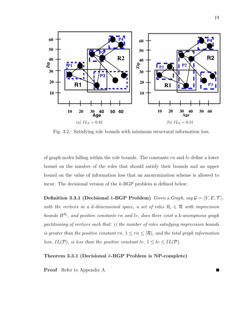
3.3.1 The k-BGP Problem

We show that finding a k-anonymous graph partitioning that satisfies the role

imprecision bounds for the maximum number of roles while achieving minimal overall

information loss, IL(P), is NP-hard. The cardinality of a Role, say Ri, is the number

19

10! 30! 40! 50! 60!20!

10!

60!

50!

40!

30!

20!

P1!

P2!

P3!

P4!

R1!

R2!

Age!

Zip!

(a) ILS = 0.42

10! 30! 40! 50! 60!20!

10!

60!

50!

40!

30!

20!

P1! P2!

P3!

P4!

R1!

R2!

Age!

Zip!

(b) ILS = 0.51

Fig. 3.2.: Satisfying role bounds with minimum structural information loss.

of graph nodes falling within the role bounds. The constants rn and lv define a lower

bound on the number of the roles that should satisfy their bounds and an upper

bound on the value of information loss that an anonymization scheme is allowed to

incur. The decisional version of the k-BGP problem is defined below:

Definition 3.3.1 (Decisional k-BGP Problem) Given a Graph, say G = hV,E, T i,with the vertices in a d-dimensional space, a set of roles Ri 2 R with imprecision

bounds BRi, and positive constants rn and lv, does there exist a k-anonymous graph

partitioning of vertices such that: i) the number of roles satisfying imprecision bounds

is greater than the positive constant rn, 1 rn |R|, and the total graph information

loss, IL(P), is less than the positive constant lv, 1 lv IL(P).

Theorem 3.3.1 (Decisional k-BGP Problem is NP-complete)

Proof Refer to Appendix A.

20

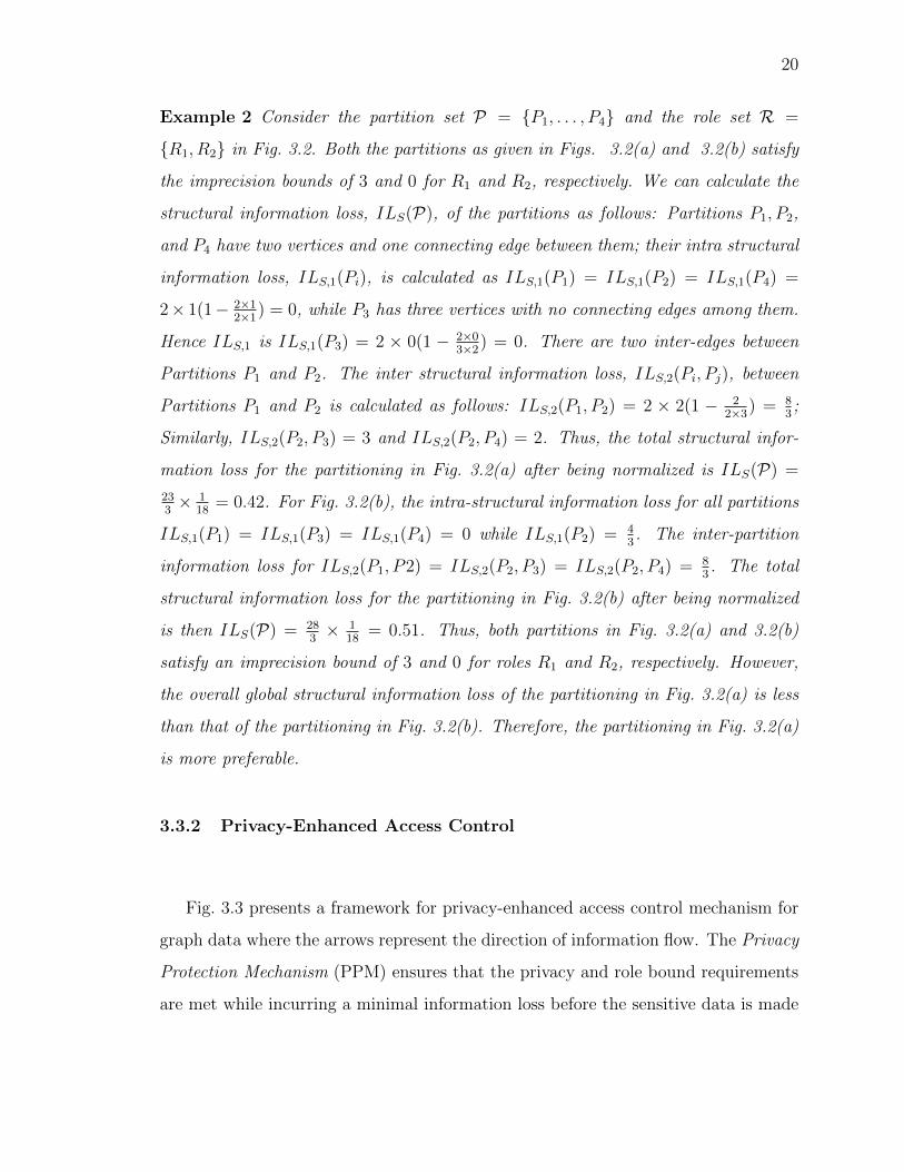
Example 2 Consider the partition set P = {P1, . . . , P4} and the role set R =

{R1, R2} in Fig. 3.2. Both the partitions as given in Figs. 3.2(a) and 3.2(b) satisfy

the imprecision bounds of 3 and 0 for R1 and R2, respectively. We can calculate the

structural information loss, ILS(P), of the partitions as follows: Partitions P1, P2,

and P4 have two vertices and one connecting edge between them; their intra structural

information loss, ILS,1(Pi), is calculated as ILS,1(P1) = ILS,1(P2) = ILS,1(P4) =

2⇥ 1(1� 2⇥12⇥1) = 0, while P3 has three vertices with no connecting edges among them.

Hence ILS,1 is ILS,1(P3) = 2 ⇥ 0(1 � 2⇥03⇥2) = 0. There are two inter-edges between

Partitions P1 and P2. The inter structural information loss, ILS,2(Pi, Pj), between

Partitions P1 and P2 is calculated as follows: ILS,2(P1, P2) = 2 ⇥ 2(1 � 22⇥3) = 8

3 ;

Similarly, ILS,2(P2, P3) = 3 and ILS,2(P2, P4) = 2. Thus, the total structural infor-

mation loss for the partitioning in Fig. 3.2(a) after being normalized is ILS(P) =

233 ⇥

118 = 0.42. For Fig. 3.2(b), the intra-structural information loss for all partitions

ILS,1(P1) = ILS,1(P3) = ILS,1(P4) = 0 while ILS,1(P2) = 43 . The inter-partition

information loss for ILS,2(P1, P2) = ILS,2(P2, P3) = ILS,2(P2, P4) = 83 . The total

structural information loss for the partitioning in Fig. 3.2(b) after being normalized

is then ILS(P) = 283 ⇥

118 = 0.51. Thus, both partitions in Fig. 3.2(a) and 3.2(b)

satisfy an imprecision bound of 3 and 0 for roles R1 and R2, respectively. However,

the overall global structural information loss of the partitioning in Fig. 3.2(a) is less

than that of the partitioning in Fig. 3.2(b). Therefore, the partitioning in Fig. 3.2(a)

is more preferable.

3.3.2 Privacy-Enhanced Access Control

Fig. 3.3 presents a framework for privacy-enhanced access control mechanism for

graph data where the arrows represent the direction of information flow. The Privacy

Protection Mechanism (PPM) ensures that the privacy and role bound requirements

are met while incurring a minimal information loss before the sensitive data is made

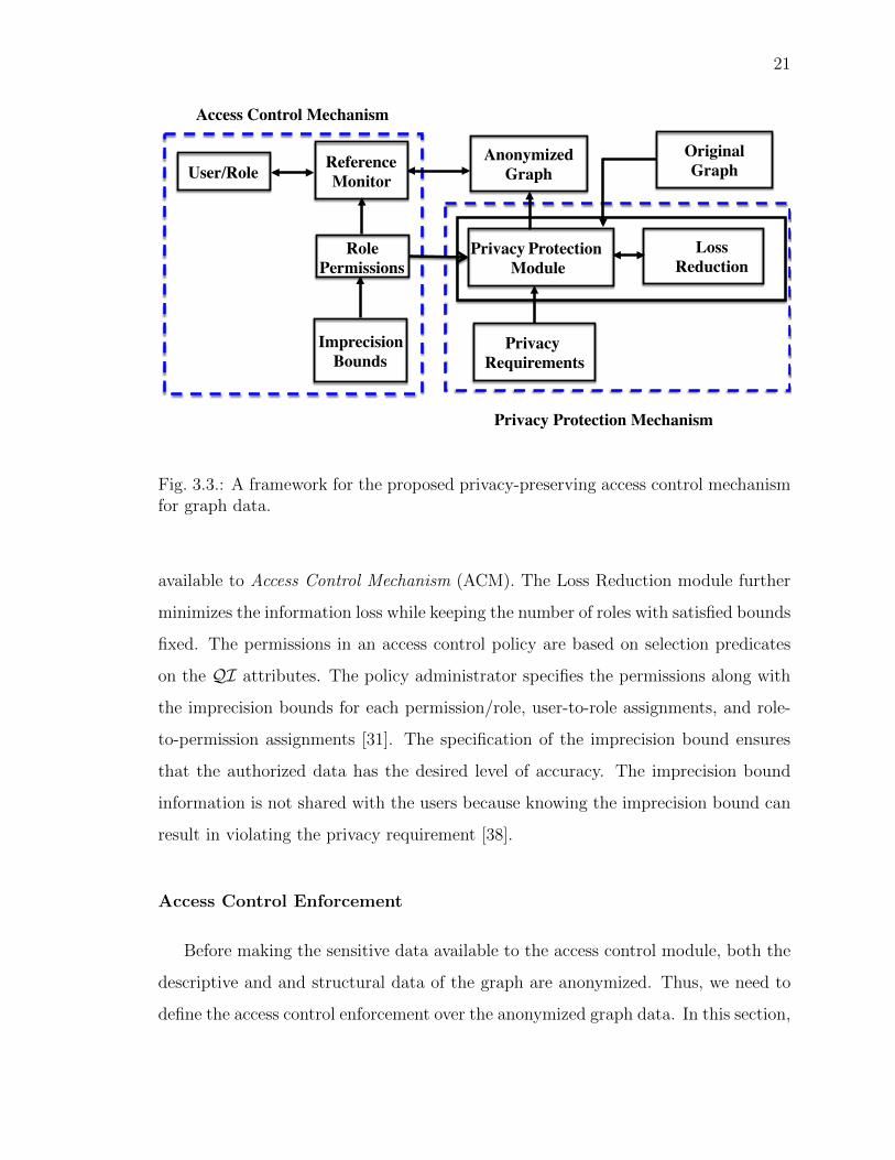
21

Anonymized!Graph!

Loss!Reduction!

User/Role! Reference !Monitor!

Role!Permissions!

Imprecision!Bounds!

Access Control Mechanism!

Privacy Protection !Module!

Privacy !Requirements!

Privacy Protection Mechanism !

Original!Graph!

Fig. 3.3.: A framework for the proposed privacy-preserving access control mechanismfor graph data.

available to Access Control Mechanism (ACM). The Loss Reduction module further

minimizes the information loss while keeping the number of roles with satisfied bounds

fixed. The permissions in an access control policy are based on selection predicates

on the QI attributes. The policy administrator specifies the permissions along with

the imprecision bounds for each permission/role, user-to-role assignments, and role-

to-permission assignments [31]. The specification of the imprecision bound ensures

that the authorized data has the desired level of accuracy. The imprecision bound

information is not shared with the users because knowing the imprecision bound can

result in violating the privacy requirement [38].

Access Control Enforcement

Before making the sensitive data available to the access control module, both the

descriptive and and structural data of the graph are anonymized. Thus, we need to

define the access control enforcement over the anonymized graph data. In this section,

22

we discuss the Relaxed and Strict access control enforcement policies (employed by

the Reference Monitor in Fig. 3.3) over the anonymized graph.

1. Relaxed: Relaxed access control uses overlap semantics to allow access to all

partitions that overlap a role/ permission.

2. Strict. Strict access control uses enclosed semantics to allow access to only those

partitions that are fully enclosed by the role/permission.

In this paper, the focus is on relaxed enforcement. In particular, when partitions

comprising the shared data between overlapping roles, say Ri, Rj 2 R, may contain

some non-shared data that is exclusively privileged to an individual role, say Ri; In

that case, the scope of the privilege set Ri is slightly increased resulting in relaxed

access control mechanism. We refer the reader to [38] for a detailed discussion of

these policies.

3.4 Heuristics for the k-BGP Problem

In this section, we present two algorithms based on greedy heuristics for graph

anonymization with minimal information loss under a given role/query workload with

their associated imprecision bounds. In the first stage, the vertices of the graph Gare partitioned recursively using a kd-tree [39] until the resulting partition sizes are

between k and 2k. The leaf nodes of the kd-tree are the partitions that are mapped

to super-nodes in the partitioned graph GP . The second stage of the heuristics (Al-

gorithm 3) further tries to minimize the information loss by rearranging the vertices

across P partitions under the following constraints: i) the number of role bounds

satisfied in first stage is not violated, and ii) each partition satisfies the k-anonymity

constraint.

3.4.1 Two-Stage Heuristic 1 (TSH1)

Lemma 3.4.1 The time complexity of TSH1 is O(d|R|2n2).

23

Algorithm 1: TSH1

Input: G = hV,E, T i, k, R, and BRj

Output: GP = hVP = P , EP , T i

1 CP G(V )); /* Initialize the set of Candidate Partitions. */

2 foreach CPi 2 CP do

3 Find the set RO of roles that overlap CPi such that IROj

CPi> 0;

4 Sort roles RO in increasing order of BRj ;

5 while the feasible cut is not found do

6 Select role from RO;

7 Create role cuts in each dimension;

8 Select dimension and cut having least overall imprecision for all roles in

R;

9 if Feasible cut found then

10 Create new partitions and add to CP ;

11 else

12 Split CPi recursively along the median till the anonymity requirement

is satisfied ;

13 Compact new partitions and add to P ;

14 GP = ConstraintRepartitioning(G, P);

15 return GP .

24

Proof The time complexity of the first stage of TSH1 is derived by multiplying

the depth of the kd-tree by the amount of work performed at each level. The

height of the kd-tree in the worst case is nk , when each partition is exactly of size

k. In the worst case, at each partition level, we may have to check all roles for

a feasible cut, which leads to a d|R|2n complexity. Thus, the time complexity of

the first stage is O(d|R|2n2). The time complexity of the second stage, procedure

ConstraintRepartitioning (Algorithm 3), is O(d|R|n). For each partition Pa 2 Pthe algorithm considers |PkNN(Pa)| = 2d nearest neighbor partitions2, 3 as the candi-

date destination partition Pb 2 PkNN(Pa). This has a time complexity of 2d|P| log |P|for all partitions P . The time complexity of procedure RoleBoundViolations (Algo-

rithm 4) is O(d|R|n) as for each source partition Pa we consider only |PkNN(Pa)| = 2d

neighboring partition for imprecision calculation. Thus, the overall time complex-

ity of the second stage is O(dnk log

nk + d|R|nk ) as log n

k << |R|, this simplifies to

O(d|R|n). Adding the time complexities of both stages, the overall complexity of

TSH1 is O(d|R|2n2 + d|R|n) ⇡ O(d|R|2n2).

3.4.2 Two-Stage Heuristic 2 (TSH2): A Scalable Approach

In the Two-Stage Heuristic 2 algorithm (TSH2, for short), we modify TSH1 so

that time complexity of O(d|R|n log n) can be achieved in contrast to the O(d|R|2n2)

time complexity for TSH1. Because the complexity is subquadratic in network size

n and number of roles R, the TSH2 algorithm provides a scalable approach. This

heuristic only considers a role with the lowest imprecision bound to check the role cuts

for a given Partition, say Pi, and updates the role bounds as the partitions are added

to the output. The update is carried out by subtracting the imprecision IROj

CPi> 0

from the imprecision bound BRj of each role, for a Partition, say Pi. For example, if

a partition of size k has imprecision 10 and 15 for roles R1 and R2 with imprecision

bound BR1 = 70 and BR2 = 90, then the bounds are updated to BR1 = 60 and

2The complexity to find kNN using a Kd-tree is O(k logN) [39]3We consider only partition median points while finding the kNN partitions.

25

Algorithm 2: TSH2: A Scalable Approach

Input: G = hV,E, T i, k, R, BRj


1 CP G(V )); /* Initialize the set of Candidate Partitions. */

2 foreach CPi 2 CP do

3 // Depth-first (preorder) traversal

4 Find the set of roles RO that overlap CPi such that IROj

CPi> 0;

5 Select role from RO with smallest BRj ;

6 Create role cuts in each dimension;

7 Reject cuts with skewed partitions;

8 Select the dimension and the cut having the least overall imprecision for all

roles in R;

9 if Feasible cut found then

10 Create new partitions and add to CP ;

11 else

12 Split CPi recursively along the median till anonymity requirement is

satisfied ;

13 Compact new partitions and add to P ;

14 Update BRj according to IRj , 8Rj 2 R

15 GP = ConstraintRepartitioning(G, P);

16 return GP .

26

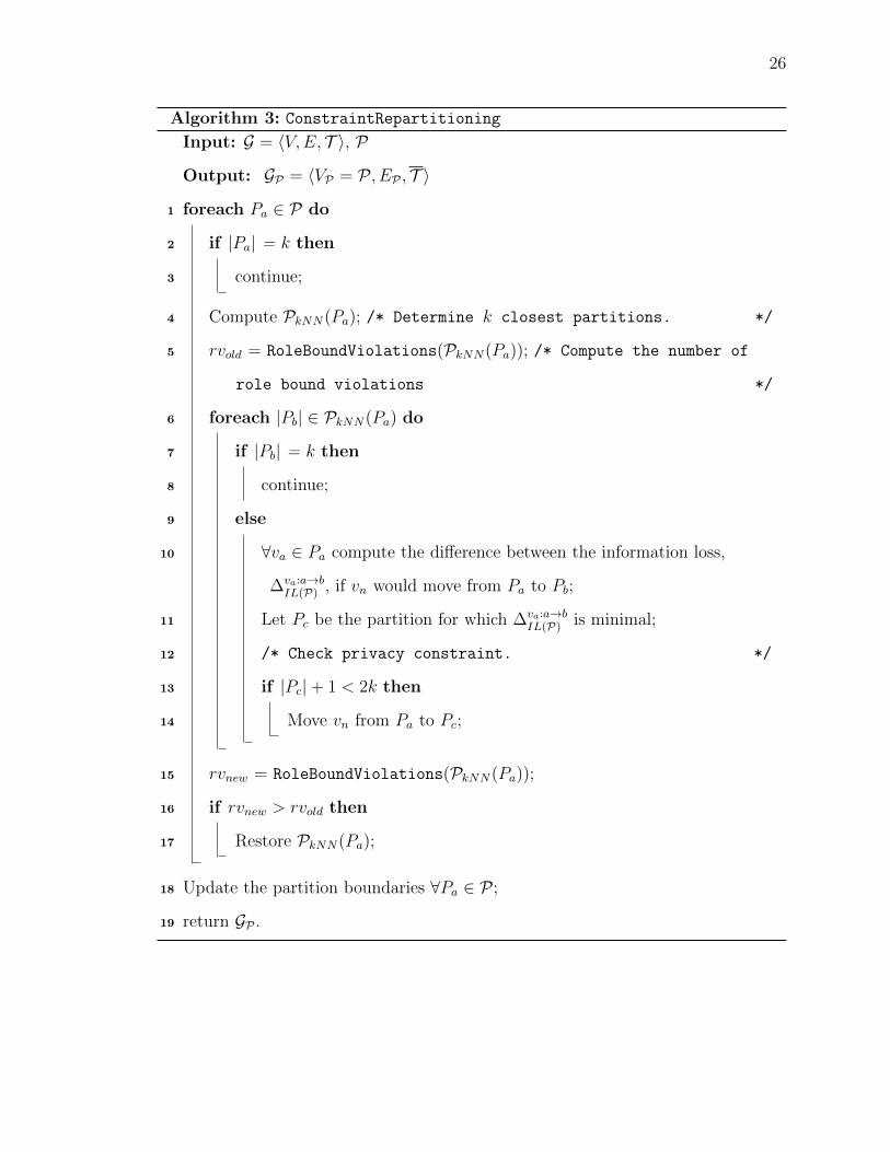
Algorithm 3: ConstraintRepartitioning

Input: G = hV,E, T i, P


1 foreach Pa 2 P do

2 if |Pa| = k then

3 continue;

4 Compute PkNN(Pa); /* Determine k closest partitions. */

5 rvold = RoleBoundViolations(PkNN(Pa)); /* Compute the number of

role bound violations */

6 foreach |Pb| 2 PkNN(Pa) do

7 if |Pb| = k then

8 continue;

9 else

10 8va 2 Pa compute the di↵erence between the information loss,

�va:a!bIL(P) , if vn would move from Pa to Pb;

11 Let Pc be the partition for which �va:a!bIL(P) is minimal;

12 /* Check privacy constraint. */

13 if |Pc|+ 1 < 2k then

14 Move vn from Pa to Pc;

15 rvnew = RoleBoundViolations(PkNN(Pa));

16 if rvnew > rvold then

17 Restore PkNN(Pa);

18 Update the partition boundaries 8Pa 2 P ;

19 return GP .

27

Algorithm 4: RoleBoundViolationsInput: P ,R

Output: Inew

1 Inew = 0;

2 foreach r 2 R do

3 foreach p 2 P do

4 Inew = Inew + Irp ; /* Compute imprecision of overlapping roles

and partitions. */

5 return Inew.

BR2 = 75, respectively. Also, in TSH2, highly skewed partitions are rejected, i.e.,

role cuts are only feasible when the size ratio of the resulting partitions is not highly

skewed. We use a skew ratio of 1:99 for TSH2 as a threshold. If a cut results in one

partition having size greater than hundred times the other, then the cut is ignored.

Algorithm 2 (TSH2) has four di↵erences compared to TSH1. First, the kd-tree

traversal for the foreach loop in Lines 2-14 is based on preorder traversal. The

preorder traversal ensures that a given partition is recursively split till the leaf nodes

are reached. Then, the role bounds are updated. Second, in Line 14, the role bounds

are updated as the partitions are being added to P . Third, in Line 5 of Algorithm 2,

we use only one role for the candidate cut and fourth in Line 7, the partition size

ratio condition is checked to reject skewed partition cuts. If no feasible role cut is

found, then the partition is split using the median cut approach as in Line 12.

Lemma 3.4.2 The time complexity of TSH2 is O(d|R|n log n).

Proof The depth of the kd-tree for TSH2 is log 10099

n. The work performed at each

level of the kd-tree is O(d|R|n) as we consider only one role for a feasible cut. Then,

the time complexity of the first stage is O(d|R|n lg n). As the time complexity of

28

Algorithm 3 is O(d|R|n), the overall time complexity of TSH2 is O(d|R|n log n +

d|R|n) ⇡ O(d|R|n log n).

3.5 Performance and Security Analysis

This section evaluates the proposed framework (Fig. 3.3) for system design per-

formance as well as security analysis perspective. Section 3.5.1 presents performance

evaluation for the proposed heuristics in terms of meeting the desired access con-

trol and privacy requirements with minimum information loss. Section 3.5.2 provides

security analysis of the proposed framework from an attack perspective.

3.5.1 Performance Evaluation

This section presents a comparative assessment of the overall performance evalu-

ation of the proposed heuristics TSH1 and TSH2 in terms of satisfying access control

and privacy requirements and incurring minimum information loss.

Experiments have been conducted on a 2.4 GHz Intel Core i5 with 8 GB of 1600

MHz DDR3 SDRAM running Mac OS X operating system. All algorithms have been

implemented using Java 1.7. We present two di↵erent sets of experimental results. In

the first set of experimental results ‘Number of Role Violations’, we study the e↵ect

of anonymity parameter k on the number of role bound-violations, which is an access

control requirement. In the second set of experimental results ‘Information Loss Due

to Anonymization’, we study the changes in information loss value due to parameter

k.

Datasets and RBAC Policy

In the experimental results, we use the following real graph topologies: ego-Facebook,

p2p-Gnutella04, and com-Youtube available at Stanford Network Analysis Project

29

(SNAP)4.We populate the vertices of these graphs (similar to [40]) with the Census

dataset from IPUMS5. The dataset is extracted for the Year 2001 using the following

attributes: Age, Gender, Marital status, Race, Birth place, Language, Occupation,

and Income. The categorical data values have already been converted to numeric

values. The first seven attributes are used as the QI attributes and are assigned to

graph nodes while Income is considered as a sensitive attribute.

Role Workload Generation

We generate 50, 80, and 500 roles as the workload/permissions for the ego-Facebook,

p2p-Gnutella04, and com-Youtube datasets, respectively. The roles are generated

according to the approach of [38], which selects two attribute tuples randomly from

the attribute tuple space and forms a role by making a bounding box of two tu-

ples. The generated role workload may be overlapped. A highly overlapped workload

means more sharing between roles, which signifies less data sensitivity and vice versa.

We can further classify this workload into three classes: low-overlap (LO), medium-

overlap (MO), and high-overlap (HO) and study the e↵ect of degree of overlap between

workloads on the proposed heuristics. If the overlap is between 10-20%, we consider

this as LO; if the overlap is between 40-50%, we consider this as MO; and similarly,

for an overlap in the range 80-90%, we classify this as HO. The average role size for

the 50 roles under LO, MO, and HO is 81, 124, and 145, respectively. Similarly, for

80 roles, the corresponding roles sizes for LO, MO, and HO workload are 153, 201,

and 263, respectively.

Number of Role Violations

4http://snap.stanford.edu/data/5https://usa.ipums.org/usa/

30

0

20

40

60

80

100

5 10 15 20 25

% o

f R

ole

s B

ou

nd

-Vio

late

d

Role Bound

LO

MO

HO

(a) TSH1, |R| = 50

0

20

40

60

80

100

5 10 15 20 25

% o

f R

ole

s B

ou

nd

-Vio

late

d

Role Bound

LO

MO

HO

(b) TSH2, |R| = 50

Fig. 3.4.: E↵ect of BR on the % of role bound-violations for k = 5.

In this subsection, we evaluate the e↵ect of anonymity parameter k on the num-

ber of role bound-violations for the two proposed heuristics and compare the results

against TDSM [19] algorithm.

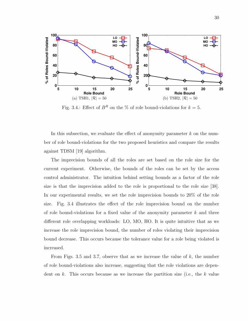
The imprecision bounds of all the roles are set based on the role size for the

current experiment. Otherwise, the bounds of the roles can be set by the access

control administrator. The intuition behind setting bounds as a factor of the role

size is that the imprecision added to the role is proportional to the role size [38].

In our experimental results, we set the role imprecision bounds to 20% of the role

size. Fig. 3.4 illustrates the e↵ect of the role imprecision bound on the number

of role bound-violations for a fixed value of the anonymity parameter k and three

di↵erent role overlapping workloads: LO, MO, HO. It is quite intuitive that as we

increase the role imprecision bound, the number of roles violating their imprecision

bound decrease. This occurs because the tolerance value for a role being violated is

increased.

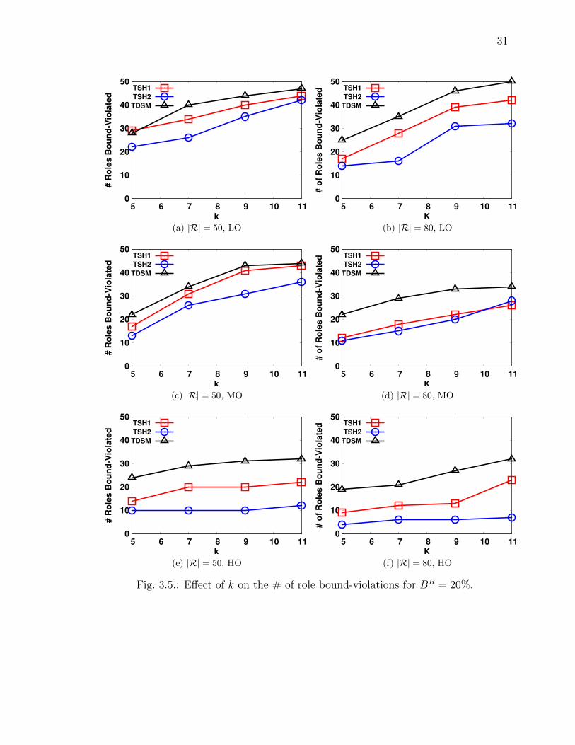
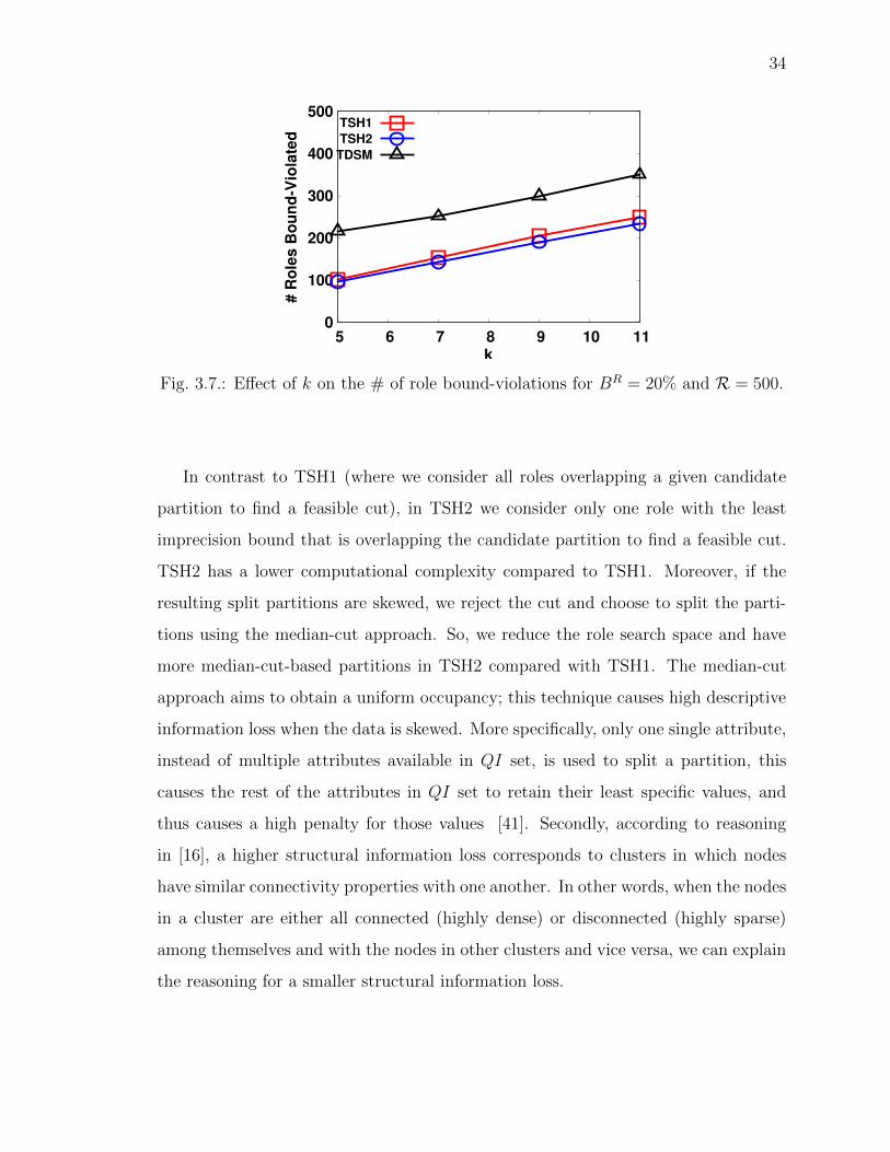
From Figs. 3.5 and 3.7, observe that as we increase the value of k, the number

of role bound-violations also increase, suggesting that the role violations are depen-

dent on k. This occurs because as we increase the partition size (i.e., the k value

31

0

10

20

30

40

50

5 6 7 8 9 10 11

# R

ole

s B

ou

nd

-Vio

late

d

k

TSH1

TSH2

TDSM

(a) |R| = 50, LO

0

10

20

30

40

50

5 6 7 8 9 10 11

# o

f R

ole

s B

ou

nd

-Vio

late

d

K

TSH1

TSH2

TDSM

(b) |R| = 80, LO

0

10

20

30

40

50

5 6 7 8 9 10 11

# R

ole

s B

ou

nd

-Vio

late

d

k

TSH1

TSH2

TDSM

(c) |R| = 50, MO

0

10

20

30

40

50

5 6 7 8 9 10 11

# o

f R

ole

s B

ou

nd

-Vio

late

d

K

TSH1

TSH2

TDSM

(d) |R| = 80, MO

0

10

20

30

40

50

5 6 7 8 9 10 11

# R

ole

s B

ou

nd

-Vio

late

d

k

TSH1

TSH2

TDSM

(e) |R| = 50, HO

0

10

20

30

40

50

5 6 7 8 9 10 11

# o

f R

ole

s B

ou

nd

-Vio

late

d

K

TSH1

TSH2

TDSM

(f) |R| = 80, HO

Fig. 3.5.: E↵ect of k on the # of role bound-violations for BR = 20%.

32

is increased), more roles are now overlapping the partitions, resulting in increased

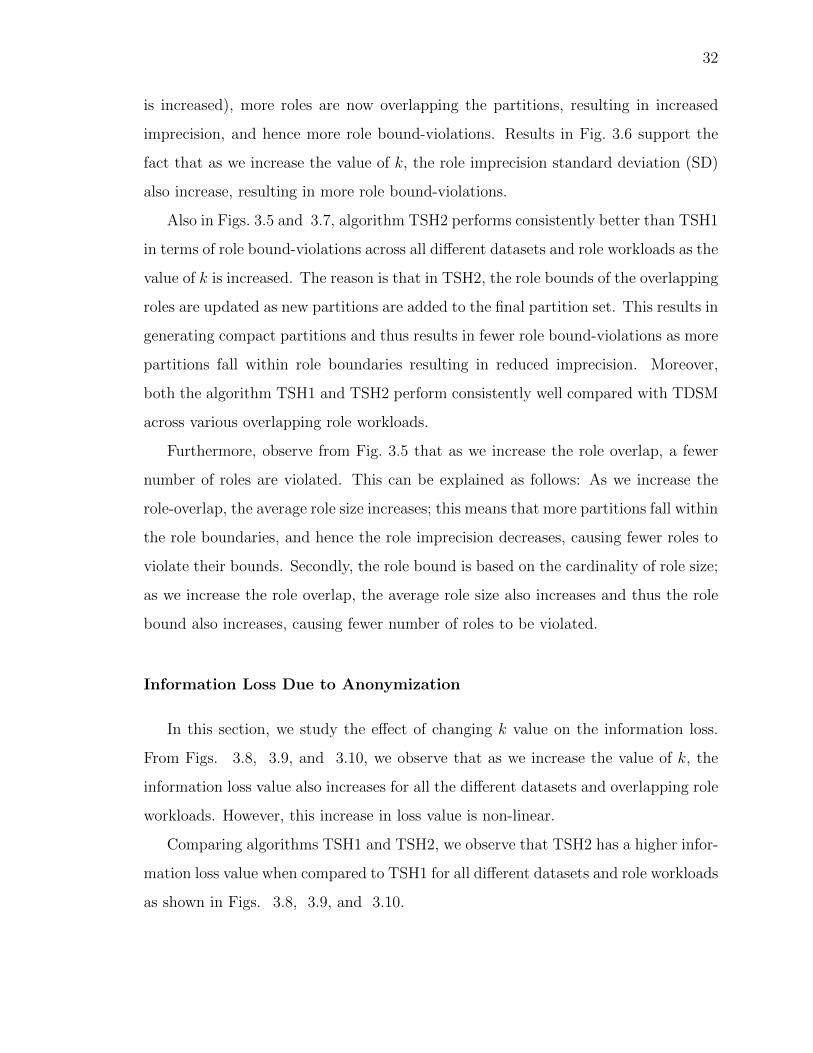
imprecision, and hence more role bound-violations. Results in Fig. 3.6 support the

fact that as we increase the value of k, the role imprecision standard deviation (SD)

also increase, resulting in more role bound-violations.

Also in Figs. 3.5 and 3.7, algorithm TSH2 performs consistently better than TSH1

in terms of role bound-violations across all di↵erent datasets and role workloads as the

value of k is increased. The reason is that in TSH2, the role bounds of the overlapping

roles are updated as new partitions are added to the final partition set. This results in

generating compact partitions and thus results in fewer role bound-violations as more

partitions fall within role boundaries resulting in reduced imprecision. Moreover,

both the algorithm TSH1 and TSH2 perform consistently well compared with TDSM

across various overlapping role workloads.

Furthermore, observe from Fig. 3.5 that as we increase the role overlap, a fewer

number of roles are violated. This can be explained as follows: As we increase the

role-overlap, the average role size increases; this means that more partitions fall within

the role boundaries, and hence the role imprecision decreases, causing fewer roles to

violate their bounds. Secondly, the role bound is based on the cardinality of role size;

as we increase the role overlap, the average role size also increases and thus the role

bound also increases, causing fewer number of roles to be violated.

Information Loss Due to Anonymization

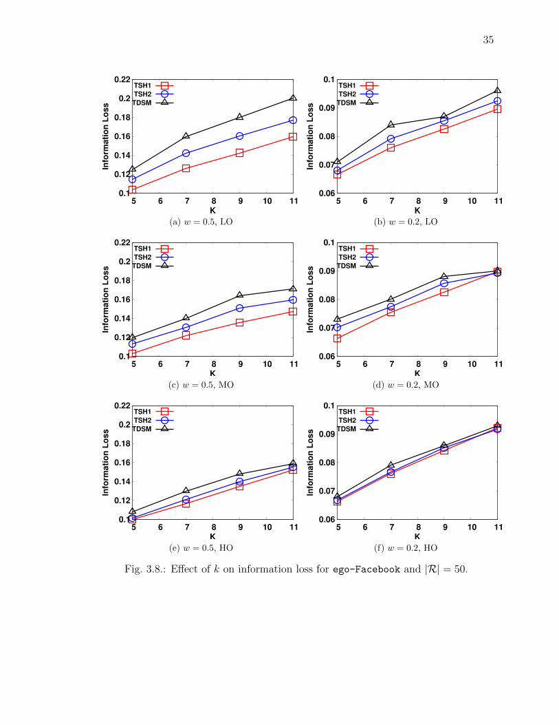
In this section, we study the e↵ect of changing k value on the information loss.

From Figs. 3.8, 3.9, and 3.10, we observe that as we increase the value of k, the

information loss value also increases for all the di↵erent datasets and overlapping role

workloads. However, this increase in loss value is non-linear.

Comparing algorithms TSH1 and TSH2, we observe that TSH2 has a higher infor-

mation loss value when compared to TSH1 for all di↵erent datasets and role workloads

as shown in Figs. 3.8, 3.9, and 3.10.

33

0

10

20

30

40

50

5 6 7 8 9 10 11

Ro

le im

pre

cis

ion

SD

K

TSH1

TSH2

TDSM

(a) |R| = 50, LO

0

10

20

30

40

50

60

70

5 6 7 8 9 10 11

Ro

le im

pre

cis

ion

SD

K

TSH1

TSH2

TSH2

(b) |R| = 80, LO

0

10

20

30

40

50

5 6 7 8 9 10 11

Ro

le im

pre

cis

ion

SD

K

TSH1

TSH2

TDSM

(c) |R| = 50, MO

0

10

20

30

40

50

60

70

5 6 7 8 9 10 11

Ro

le im

pre

cis

ion

SD

K

TSH1

TSH2

TSH2

(d) |R| = 80, MO

0

10

20

30

40

50

5 6 7 8 9 10 11

Ro

le im

pre

cis

ion

SD

K

TSH1

TSH2

TDSM

(e) |R| = 50, HO

0

10

20

30

40

50

60

70

5 6 7 8 9 10 11

Ro

le im

pre

cis

ion

SD

K

TSH1

TSH2

TSH2

(f) |R| = 80, HO

Fig. 3.6.: E↵ect of k on role imprecision SD.

34

0

100

200

300

400

500

5 6 7 8 9 10 11

# R

ole

s B

ou

nd

-Vio

late

d

k

TSH1

TSH2

TDSM

Fig. 3.7.: E↵ect of k on the # of role bound-violations for BR = 20% and R = 500.

In contrast to TSH1 (where we consider all roles overlapping a given candidate

partition to find a feasible cut), in TSH2 we consider only one role with the least

imprecision bound that is overlapping the candidate partition to find a feasible cut.

TSH2 has a lower computational complexity compared to TSH1. Moreover, if the

resulting split partitions are skewed, we reject the cut and choose to split the parti-

tions using the median-cut approach. So, we reduce the role search space and have

more median-cut-based partitions in TSH2 compared with TSH1. The median-cut

approach aims to obtain a uniform occupancy; this technique causes high descriptive

information loss when the data is skewed. More specifically, only one single attribute,

instead of multiple attributes available in QI set, is used to split a partition, this

causes the rest of the attributes in QI set to retain their least specific values, and

thus causes a high penalty for those values [41]. Secondly, according to reasoning

in [16], a higher structural information loss corresponds to clusters in which nodes

have similar connectivity properties with one another. In other words, when the nodes

in a cluster are either all connected (highly dense) or disconnected (highly sparse)

among themselves and with the nodes in other clusters and vice versa, we can explain

the reasoning for a smaller structural information loss.

35

0.1

0.12

0.14

0.16

0.18

0.2

0.22

5 6 7 8 9 10 11

Info

rma

tio

n L

os

s

K

TSH1

TSH2

TDSM

(a) w = 0.5, LO

0.06

0.07

0.08

0.09

0.1

5 6 7 8 9 10 11

Info

rma

tio

n L

os

s

K

TSH1

TSH2

TDSM

(b) w = 0.2, LO

0.1

0.12

0.14

0.16

0.18

0.2

0.22

5 6 7 8 9 10 11

Info

rmati

on

Lo

ss

K

TSH1

TSH2

TDSM

(c) w = 0.5, MO

0.06

0.07

0.08

0.09

0.1

5 6 7 8 9 10 11

Info

rmati

on

Lo

ss

K

TSH1

TSH2

TDSM

(d) w = 0.2, MO

0.1

0.12

0.14

0.16

0.18

0.2

0.22

5 6 7 8 9 10 11

Info

rmati

on

Lo

ss

K

TSH1

TSH2

TDSM

(e) w = 0.5, HO

0.06

0.07

0.08

0.09

0.1

5 6 7 8 9 10 11

Info

rmati

on

Lo

ss

K

TSH1

TSH2

TDSM

(f) w = 0.2, HO

Fig. 3.8.: E↵ect of k on information loss for ego-Facebook and |R| = 50.

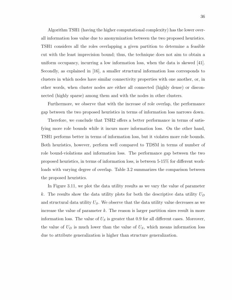
36

Algorithm TSH1 (having the higher computational complexity) has the lower over-

all information loss value due to anonymization between the two proposed heuristics.

TSH1 considers all the roles overlapping a given partition to determine a feasible

cut with the least imprecision bound; thus, the technique does not aim to obtain a

uniform occupancy, incurring a low information loss, when the data is skewed [41].

Secondly, as explained in [16], a smaller structural information loss corresponds to

clusters in which nodes have similar connectivity properties with one another, or, in

other words, when cluster nodes are either all connected (highly dense) or discon-

nected (highly sparse) among them and with the nodes in other clusters.

Furthermore, we observe that with the increase of role overlap, the performance

gap between the two proposed heuristics in terms of information loss narrows down.

Therefore, we conclude that TSH2 o↵ers a better performance in terms of satis-

fying more role bounds while it incurs more information loss. On the other hand,

TSH1 performs better in terms of information loss, but it violates more role bounds.

Both heuristics, however, perform well compared to TDSM in terms of number of

role bound-violations and information loss. The performance gap between the two

proposed heuristics, in terms of information loss, is between 5-15% for di↵erent work-

loads with varying degree of overlap. Table 3.2 summarizes the comparison between

the proposed heuristics.

In Figure 3.11, we plot the data utility results as we vary the value of parameter

k. The results show the data utility plots for both the descriptive data utility UD

and structural data utility US. We observe that the data utility value decreases as we

increase the value of parameter k. The reason is larger partition sizes result in more

information loss. The value of US is greater that 0.9 for all di↵erent cases. Moreover,

the value of UD is much lower than the value of US, which means information loss

due to attribute generalization is higher than structure generalization.

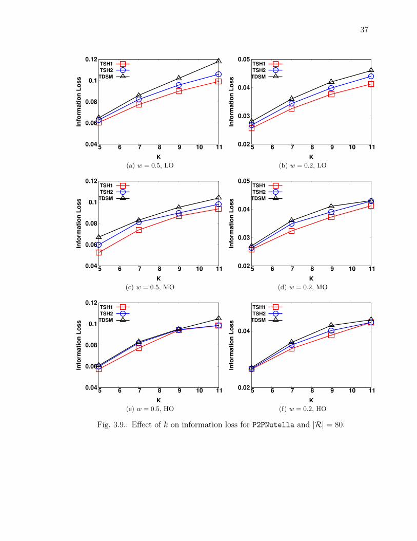
37

0.04

0.06

0.08

0.1

0.12

5 6 7 8 9 10 11

Info

rma

tio

n L

os

s

K

TSH1

TSH2

TDSM

(a) w = 0.5, LO

0.02

0.03

0.04

0.05

5 6 7 8 9 10 11

Info

rma

tio

n L

os

s

K

TSH1

TSH2

TDSM

(b) w = 0.2, LO

0.04

0.06

0.08

0.1

0.12

5 6 7 8 9 10 11

Info

rmati

on

Lo

ss

K

TSH1

TSH2

TDSM

(c) w = 0.5, MO

0.02

0.03

0.04

0.05

5 6 7 8 9 10 11

Info

rmati

on

Lo

ss

K

TSH1

TSH2

TDSM

(d) w = 0.2, MO

0.04

0.06

0.08

0.1

0.12

5 6 7 8 9 10 11

Info

rmati

on

Lo

ss

K

TSH1

TSH2

TDSM

(e) w = 0.5, HO

0.02

0.04

5 6 7 8 9 10 11

Info

rmati

on

Lo

ss

K

TSH1

TSH2

TDSM

(f) w = 0.2, HO

Fig. 3.9.: E↵ect of k on information loss for P2PNutella and |R| = 80.

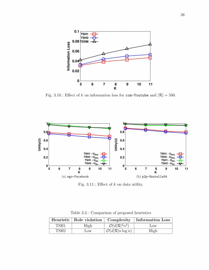
38

0

0.02

0.04

0.06

0.08

0.1

5 6 7 8 9 10 11

Info

rma

tio

n L

os

s

K

TSH1

TSH2

TDSM

Fig. 3.10.: E↵ect of k on information loss for com-Youtube and |R| = 500.

0

0.2

0.4

0.6

0.8

1

5 6 7 8 9 10 11

Uti

lity

(U)

K

TSH1 - UDes.

TSH2 - UDes.

TSH1 - UStr.

TSH2 - UStr.

(a) ego-Facebook

0

0.2

0.4

0.6

0.8

1

5 6 7 8 9 10 11

Uti

lity

(U)

K

TSH1 - UDes.

TSH2 - UDes.

TSH1 - UStr.

TSH2 - UStr.

(b) p2p-Gnutella04

Fig. 3.11.: E↵ect of k on data utility.

Table 3.2.: Comparison of proposed heuristics

Heuristic Role violation Complexity Information Loss

TSH1 High O(d|R|2n2) LowTSH2 Low O(d|R|n log n) High

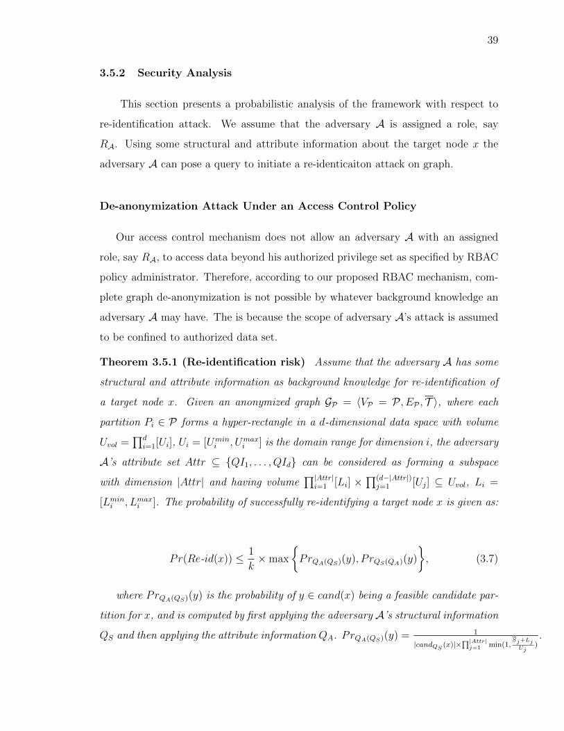
39

3.5.2 Security Analysis

This section presents a probabilistic analysis of the framework with respect to

re-identification attack. We assume that the adversary A is assigned a role, say

RA. Using some structural and attribute information about the target node x the

adversary A can pose a query to initiate a re-identicaiton attack on graph.

De-anonymization Attack Under an Access Control Policy

Our access control mechanism does not allow an adversary A with an assigned

role, say RA, to access data beyond his authorized privilege set as specified by RBAC

policy administrator. Therefore, according to our proposed RBAC mechanism, com-

plete graph de-anonymization is not possible by whatever background knowledge an

adversary A may have. The is because the scope of adversary A’s attack is assumed

to be confined to authorized data set.

Theorem 3.5.1 (Re-identification risk) Assume that the adversary A has some

structural and attribute information as background knowledge for re-identification of

a target node x. Given an anonymized graph GP = hVP = P , EP , T i, where each

partition Pi 2 P forms a hyper-rectangle in a d-dimensional data space with volume

Uvol =Qd

i=1[Ui], Ui = [Umini , Umax

i ] is the domain range for dimension i, the adversary

A’s attribute set Attr ✓ {QI1, . . . , QId} can be considered as forming a subspace

with dimension |Attr| and having volumeQ|Attr|

i=1 [Li] ⇥Q(d�|Attr|)

j=1 [Uj] ✓ Uvol, Li =

[Lmini , Lmax

i ]. The probability of successfully re-identifying a target node x is given as:

Pr(Re-id(x)) 1

k⇥max

⇢PrQA(QS)(y), P rQS(QA)(y)

�, (3.7)

where PrQA(QS)(y) is the probability of y 2 cand(x) being a feasible candidate par-

tition for x, and is computed by first applying the adversary A’s structural information

QS and then applying the attribute information QA. PrQA(QS)(y) =1

|candQS(x)|⇥Q|Attr|

j=1 min(1,Sj+Lj

Uj).

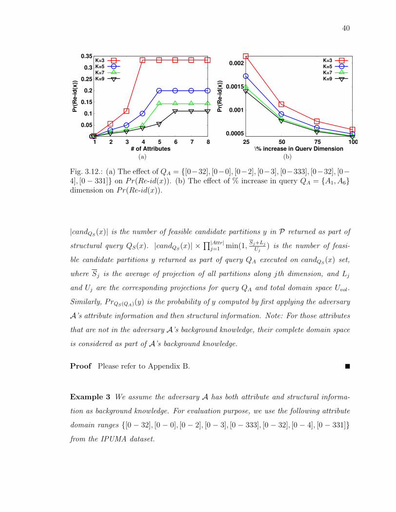
40

0

0.05

0.1

0.15

0.2

0.25

0.3

0.35

1 2 3 4 5 6 7 8

Pr(

Re-i

d(x

))

# of Attributes

K=3

K=5

K=7

K=9

(a)

0.0005

0.001

0.0015

0.002

25 50 75 100

Pr(

Re-i

d(x

))

\% increase in Query Dimension

K=3

K=5

K=7

K=9

(b)

Fig. 3.12.: (a) The e↵ect of QA = {[0�32], [0�0], [0�2], [0�3], [0�333], [0�32], [0�4], [0� 331]} on Pr(Re-id(x)). (b) The e↵ect of % increase in query QA = {A1, A6}dimension on Pr(Re-id(x)).

|candQS(x)| is the number of feasible candidate partitions y in P returned as part of

structural query QS(x). |candQS(x)| ⇥Q|Attr|

j=1 min(1, Sj+Lj

Uj) is the number of feasi-

ble candidate partitions y returned as part of query QA executed on candQS(x) set,

where Sj is the average of projection of all partitions along jth dimension, and Lj

and Uj are the corresponding projections for query QA and total domain space Uvol.

Similarly, PrQS(QA)(y) is the probability of y computed by first applying the adversary

A’s attribute information and then structural information. Note: For those attributes

that are not in the adversary A’s background knowledge, their complete domain space

is considered as part of A’s background knowledge.

Proof Please refer to Appendix B.

Example 3 We assume the adversary A has both attribute and structural informa-

tion as background knowledge. For evaluation purpose, we use the following attribute

domain ranges {[0 � 32], [0 � 0], [0 � 2], [0 � 3], [0 � 333], [0 � 32], [0 � 4], [0 � 331]}from the IPUMA dataset.

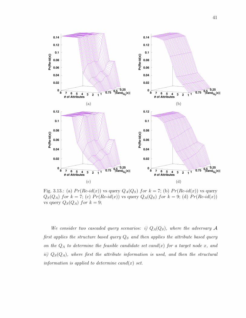
41

1 2 3 4 5 6 7 8

# of Attributes

0.25 0.5

0.75 1 |candQS

(x)| 0

0.02

0.04

0.06

0.08

0.1

0.12

0.14

Pr(

Re-i

d(x

))

(a)

1 2 3 4 5 6 7 8

# of Attributes

0.25 0.5

0.75 1 |candQS

(x)| 0

0.02

0.04

0.06

0.08

0.1

0.12

0.14

Pr(

Re-i

d(x

))

(b)

1 2 3 4 5 6 7 8

# of Attributes

0.25 0.5

0.75 1 |candQS

(x)| 0

0.02

0.04

0.06

0.08

0.1

0.12

Pr(

Re-i

d(x

))

(c)

1 2 3 4 5 6 7 8

# of Attributes

0.25 0.5

0.75 1 |candQS

(x)| 0

0.02

0.04

0.06

0.08

0.1

0.12

Pr(

Re-i

d(x

))

(d)

Fig. 3.13.: (a) Pr(Re-id(x)) vs query QA(QS) for k = 7; (b) Pr(Re-id(x)) vs queryQS(QA) for k = 7; (c) Pr(Re-id(x)) vs query QA(QS) for k = 9; (d) Pr(Re-id(x))vs query QS(QA) for k = 9;

We consider two cascaded query scenarios: i) QA(QS), where the adversary Afirst applies the structure based query QS and then applies the attribute based query

on the QA to determine the feasible candidate set cand(x) for a target node x, and

ii) QS(QA), where first the attribute information is used, and then the structural

information is applied to determine cand(x) set.

42

Fig. 3.12(a) shows the e↵ect of changing the number of attributes in query QA

on re-identification probability. We observe that increasing the number of attributes

results in higher Pr(Re-id(x)) value. This is because, more background attribute

knowledge helps reduce |candA(x)| size, thus resulting in a higher Pr(Re-id(x)) value.

Fig. 3.12(b) studies the e↵ect of increasing the range query dimension on the Pr(Re-id(x))

value. The number of attributes in adversary A’s background knowledge are kept fixed

to attribute A1 = [0 � 32] and A6 = [0 � 32]. We observe that Pr(Re-id(x)) value

reduces as the volume of range query QA increases for a fixed number of attributes.

This is because, a large number of candidate partitions are returned resulting in lower

Pr(Re-id(x)) value.

Fig. 3.13(a)-(d) show the e↵ect of cascaded queries QA(QS) and QS(QA) on re-

identification probability Pr(Re-id(x)). Increasing the value of k generates less num-

ber of cand(x) partitions resulting in higher 1|cand(x)| value and reduces 1

k value. There-

fore, the overall value of Pr(Re-id(x)) is reduced. From Fig. 3.13(a), (d) we observe

that cascaded query QA(QS) results in higher Pr(Re-id(x)) value compared to cas-

caded query QS(QA) value. The reason being complete graph GP has less structural

discrepancy compared to graph obtained by first running attributed based query QA,

thus resulting in better filtration of candidates. Therefore, plots in Figs. 3.13(a) and

3.13(c) give higher value Pr(Re-id(x)) compared to Figs. 3.13(b) and 3.13(d) for

query QS(QA).

However, it is intuitive that having both attribute and structure information im-

proves the re-identification probability as the joint background knowledge results in

reduced candidate partition size cand(x) for a target node x.

3.6 Related Work

Although a number of anonymization schemes have been proposed for protecting

users’ privacy in published graph data (e.g., [42], [17], [43], [44], [45], [46], [47],

43

[48], [49]), they implicitly assume that there is no authorization mechanism in place

for controlling access to data by group of users.

Almost all OSN services allow users to dictate sharing their profile information to

viewers through fine-grained, customized policies. For example, pErsona [32] hides

private data with attribute-based encryption (ABE) schemes. xAccess [33] presents

an automated RBAC policy specification mechanism to capture the implicit privacy

preference of social site users. Semantically interpretable functional “social roles”

are extracted from static network structure based on identified social roles, confiden-

tiality setting of personal data, and predefined user-permission assignments. Yuan

et al. [42] introduce a framework which provides privacy-preserving services based

on the user’s personal privacy requirements. Specifically, the formulation combines

the label generalization and the structure modification techniques by adding “noise”

edges or nodes in a way that satisfy privacy protection requirements. We consider a

data publishing framework where a centralized authority enforces the authorization

constraints through RBAC policy while providing data privacy protection through

anonymiation.

For the state-of-the art techniques in graph data anonymization and their classifi-

cation, we refer the reader to recent survey papers [2], [3]. Our graph anonymization

technique falls under the category of graph generalization/clustering based technique

[16], [17], [47]. Under this scheme, the graph is first partitioned into subgraphs.

Then, each subgraph is replaced by a super-node, which may be connected by super-

edges. The number of nodes in each super-node, along with the density of edges that

exist within and across super-nodes are published. Since the size of each cluster is

at least k, the probability of re-identifying a user can be bounded to at most 1k . Hay

et al. [17] propose an aggregation based graph anonymization algorithm, and study

the extent of node re-identification based on structural information using three types

of structural queries as an adversary background knowledge on anonymized graphs.

Bhagat et al. [47] design a class-based anonymization algorithm, which groups the

entities into classes and masks the mapping between entities and the nodes that rep-

44

resent them in the anonymized graph. Our work is perhaps closest in philosophy

to [16], which proposes a greedy optimization solution that can be tuned to control

information loss. Their clustering algorithm takes into consideration loss of both node

labels and structure information. However, the interplay between access-control and

privacy-protection mechanisms has been missing.

Di↵erential Privacy (DP) [48] is another popular privacy protection approach,

where noise is added to query results to satisfy privacy constraints. However, DP is

viable for privacy-preserving data mining (PPDM) and it is still an open question if

it can practically support privacy-preserving data publishing (PPDP) [50].

3.7 Summary

We present a framework for privacy-enhanced access-controlled graph data. The

access control policies define the selection predicates available to roles/queries and

their associated imprecision bounds. Only authorized role/query predicates on sen-

sitive data are allowed by the access control mechanism. The privacy protection and

loss reduction module anonymizes the graph data such that maximum number of

roles satisfy their imprecision bounds and minimum information loss is incurred. For

this, we formulate a k-anonymous Bi-objective Graph Partitioning (k-BGP) problem

and give hardness results. Two heuristics TSH1 and TSH2 are developed to solve the

constraint problem. We provide empirical evaluation of the proposed heuristics with

a benchmark algorithm [35] from design perspective in terms of meeting privacy and

access control requirements with minimum information loss. Within the context of

k-BGP problem, we present an architecture framework elaborating how access control

and privacy can be integrated. We evaluate the proposed framework from security

perspective and present a probabilistic analysis for re-identification risk.

45

4. EFFICIENT AND SCALABLE INTEGRITY

VERIFICATION OF DATA AND QUERY RESULTS FOR

GRAPH DATABASES

4.1 Introduction

Graphs are used for representing and understanding objects and their relationships

for numerous applications. Recent years have seen the emergence of many large graph

datasets. The most well known example is the Web, which now contains more than 50

billion Web pages and more than one trillion unique URLs 1. Other leading examples

include social networks, biological networks, semantic Web, XML documents, and

financial databases [51], [52].

To address this challenge, we propose two integrity verification schemes for graph

data using message authentication codes (MACs). MACs have been a fundamental

functionality for many recent developments in cryptography. These codes are used

for establishing an SSL/TLS connection and for ensuring the integrity of shared data

among multiple untrusted parties [22], [23]. Traditionally MAC functions handle mes-

sages as bit-strings and generate a MAC tag or “cryptographic checksum” to ensure

the integrity of input messages. We propose a methodology based on MACs for graph

data in order to verify the integrity of graph dataset. In the case of standard MAC-

based schemes (e.g., MACs, HashMACs, and HMACs), a message is either shared

completely or not shared at all with the user. In contrast, when graphs are used,

a user may receive part(s) of a graph in form of a query result(s). A major advan-

tage of using HMACs for graphs and redactable graphs is reduced computational

requirements and processing time as compared to the digital signature-based mech-

anisms [53]. Digital signatures support not only integrity of data but also security

1http://www.worldwidewebsize.com

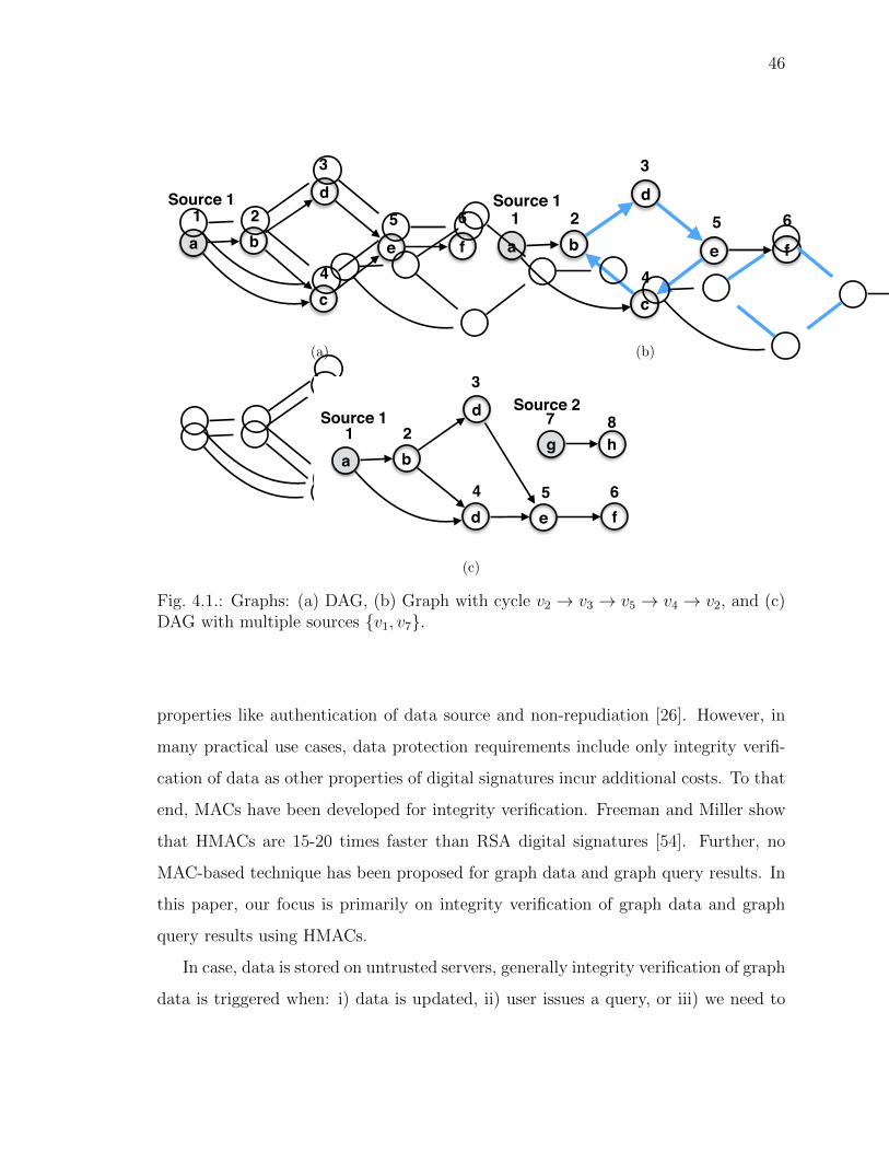
46

f

b

d

c

a e f

1 2

4

3

5 6Source 1

b

d

c

a e f

1 2

4

3

5 6Source 1

b

d

d

a

e f

1 2

4

3

5 6

Source 1g h7 8

Source 2

(a)

f

b

d

c

a e f

1 2

4

3

5 6Source 1

b

d

c

a e f

1 2

4

3

5 6Source 1

b

d

d

a

e f

1 2

4

3

5 6

Source 1g h7 8

Source 2(b)

f

b

d

c

a e f

1 2

4

3

5 6Source 1

b

d

c

a e f

1 2

4

3

5 6Source 1

b

d

d

a

e f

1 2

4

3

5 6

Source 1g h7 8

Source 2

(c)

Fig. 4.1.: Graphs: (a) DAG, (b) Graph with cycle v2 ! v3 ! v5 ! v4 ! v2, and (c)DAG with multiple sources {v1, v7}.

properties like authentication of data source and non-repudiation [26]. However, in

many practical use cases, data protection requirements include only integrity verifi-

cation of data as other properties of digital signatures incur additional costs. To that

end, MACs have been developed for integrity verification. Freeman and Miller show

that HMACs are 15-20 times faster than RSA digital signatures [54]. Further, no

MAC-based technique has been proposed for graph data and graph query results. In

this paper, our focus is primarily on integrity verification of graph data and graph

query results using HMACs.

In case, data is stored on untrusted servers, generally integrity verification of graph

data is triggered when: i) data is updated, ii) user issues a query, or iii) we need to

47

verify two graphs are identical2. Recently, hashing schemes have been proposed for

integrity verification of directed graphs [56]. Hashing is used as a core function for

integrity verification for all MAC-based schemes (e.g., HMACs and HashMACs) and

hash-and-sign methodology. HMACs are shown to be much times faster than RSA

digital signatures [54]. Therefore, in case integrity of graph data is to be assured

without losing on e�ciency, cost and simplicity of implementation, it is preferable

to use schemes which do not employ digital signature-based techniques due to their

higher computational and processing cost. Merkle hash technique (MHT) has been

proposed as an approach for computing hashes for trees [57] and has been extended

for directed acyclic graphs (DAGs) [58]. MACs for trees, DAGs, and cyclic graphs

have not been well-studied in the literature. We present two e�cient MAC-based

schemes for integrity verification of graph data and query results. The schemes can

be used by real-world graph database systems. In addition, we formally define MAC-

based schemes for graph data, and analyze the security properties (Section 4.5) with

respect to tampering of graph data in terms of its structure as well as data attributes.

4.1.1 Contributions

In summary, this chapter makes the following contributions:

• We have developed two schemes for graph data integrity verification

– HMACs for graphs for two-party data sharing, and

– Redactable HMACs for graphs for third-party data sharing.

• The proposed schemes can support “fail-stop” and “fail-warn” integrity as-

surance (Section 4.2.4) mechanisms, which can result in substantial saving in

the cost incurred for integrity verification and data re-transfer of compromised

graphs.

2Identical graphs are isomorphic graphs, but the reverse is not true [55].

48

• We provide formal definitions and constructions of HMACs for graphs and

redactable HMACs for graphs.

• We prove that the proposed schemes are secure and protect the graphs and

redacted graphs from being compromised.

• Experimental results on real-world graph datasets show that HMACs for graphs

and redactable HMACs graphs are highly e�cient compared to digital signature-

based schemes for graphs.

• The computational complexity of the proposed schemes is linear in the number

of vertices and edges in the graph. We compute one HMAC value and two

other verification objects for redaction as part of the query results that are

shared with the verifier. Therefore, our scheme is e�cient both in processing

time and in the transmission of result set R and verification objects VO to the

client/user.

4.1.2 Organization

The rest of the chapter is organized as follows: Section 4.2 introduces background

and desiderata of HMACs for graphs. Section 4.3 and 4.4 introduce the schemes

HMAC for graphs (gHMAC) and redactable HMAC for graphs (rgHMAC), give their for-

mal definitions, and describe the constructions. Section 4.5 gives the security analysis

of the schemes. The complexity analysis and performance analysis are presented in

Section 4.6. Section 4.7 overviews the related work and Section 4.8 contains conclud-

ing remarks.

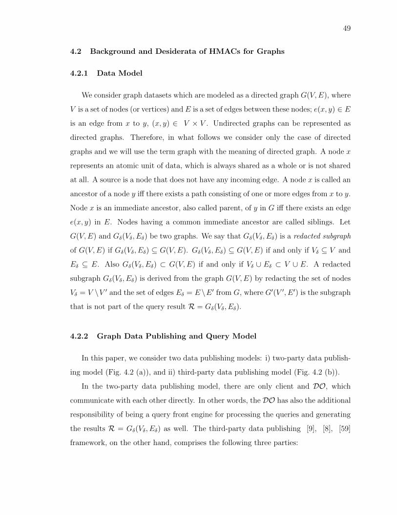
49

4.2 Background and Desiderata of HMACs for Graphs

4.2.1 Data Model

We consider graph datasets which are modeled as a directed graph G(V,E), where

V is a set of nodes (or vertices) and E is a set of edges between these nodes; e(x, y) 2 E

is an edge from x to y, (x, y) 2 V ⇥ V . Undirected graphs can be represented as

directed graphs. Therefore, in what follows we consider only the case of directed

graphs and we will use the term graph with the meaning of directed graph. A node x

represents an atomic unit of data, which is always shared as a whole or is not shared

at all. A source is a node that does not have any incoming edge. A node x is called an

ancestor of a node y i↵ there exists a path consisting of one or more edges from x to y.

Node x is an immediate ancestor, also called parent, of y in G i↵ there exists an edge

e(x, y) in E. Nodes having a common immediate ancestor are called siblings. Let

G(V,E) and G�(V�, E�) be two graphs. We say that G�(V�, E�) is a redacted subgraph

of G(V,E) if G�(V�, E�) ✓ G(V,E). G�(V�, E�) ✓ G(V,E) if and only if V� ✓ V and

E� ✓ E. Also G�(V�, E�) ⇢ G(V,E) if and only if V� [ E� ⇢ V [ E. A redacted

subgraph G�(V�, E�) is derived from the graph G(V,E) by redacting the set of nodes

V� = V \V 0 and the set of edges E� = E \E 0 from G, where G0(V 0, E 0) is the subgraph

that is not part of the query result R = G�(V�, E�).

4.2.2 Graph Data Publishing and Query Model

In this paper, we consider two data publishing models: i) two-party data publish-

ing model (Fig. 4.2 (a)), and ii) third-party data publishing model (Fig. 4.2 (b)).

In the two-party data publishing model, there are only client and DO, which

communicate with each other directly. In other words, the DO has also the additional

responsibility of being a query front engine for processing the queries and generating

the results R = G�(V�, E�) as well. The third-party data publishing [9], [8], [59]

framework, on the other hand, comprises the following three parties:

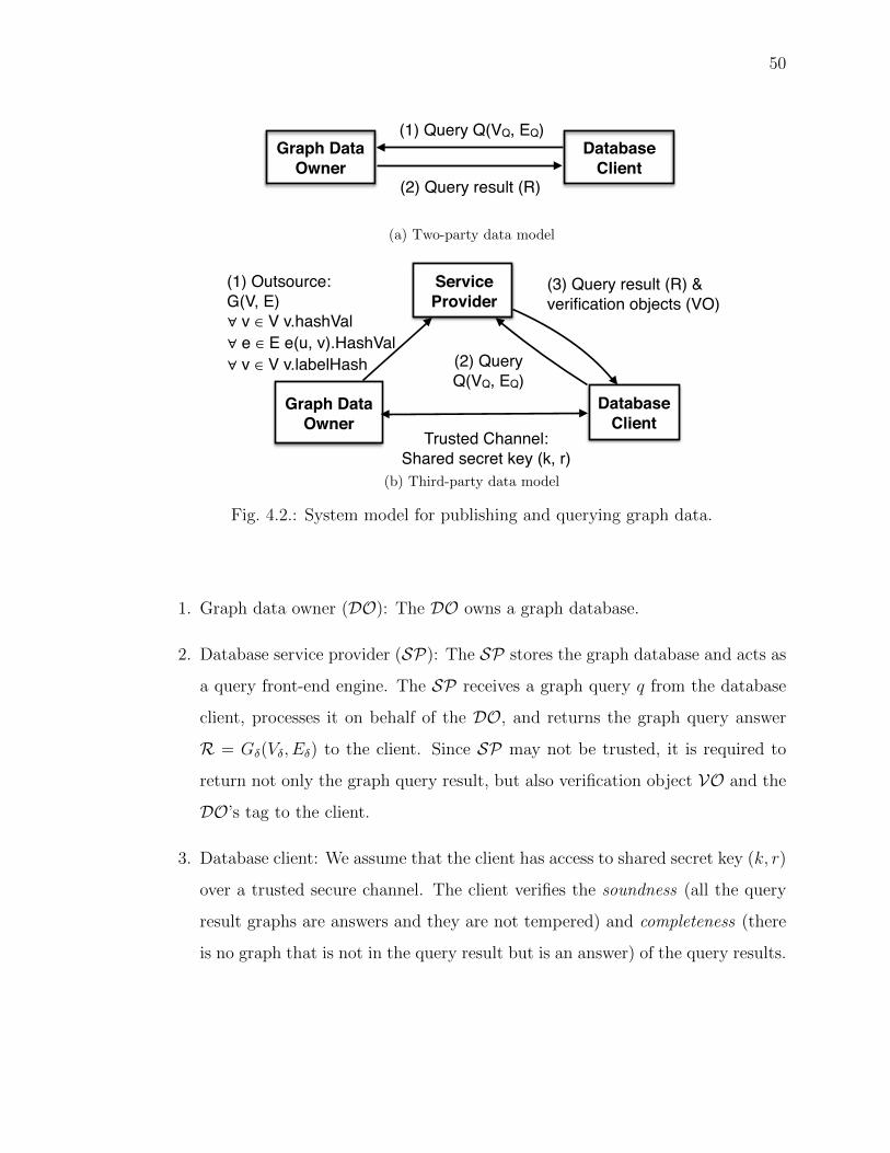
50

Graph Data!Owner

Database!Client

(1) Query Q(VQ, EQ)

(2) Query result (R)

(a) Two-party data model

Database!Client

Graph Data !Owner

Service!Provider!

(1) Outsource:!G(V, E)!∀ v ∈ V v.hashVal!∀ e ∈ E e(u, v).HashVal!∀ v ∈ V v.labelHash (2) Query !

Q(VQ, EQ)

(3) Query result (R) & !verification objects (VO)

Trusted Channel: !Shared secret key (k, r)

(b) Third-party data model

Fig. 4.2.: System model for publishing and querying graph data.

1. Graph data owner (DO): The DO owns a graph database.

2. Database service provider (SP): The SP stores the graph database and acts as

a query front-end engine. The SP receives a graph query q from the database

client, processes it on behalf of the DO, and returns the graph query answer

R = G�(V�, E�) to the client. Since SP may not be trusted, it is required to

return not only the graph query result, but also verification object VO and the

DO’s tag to the client.

3. Database client: We assume that the client has access to shared secret key (k, r)

over a trusted secure channel. The client verifies the soundness (all the query

result graphs are answers and they are not tempered) and completeness (there

is no graph that is not in the query result but is an answer) of the query results.

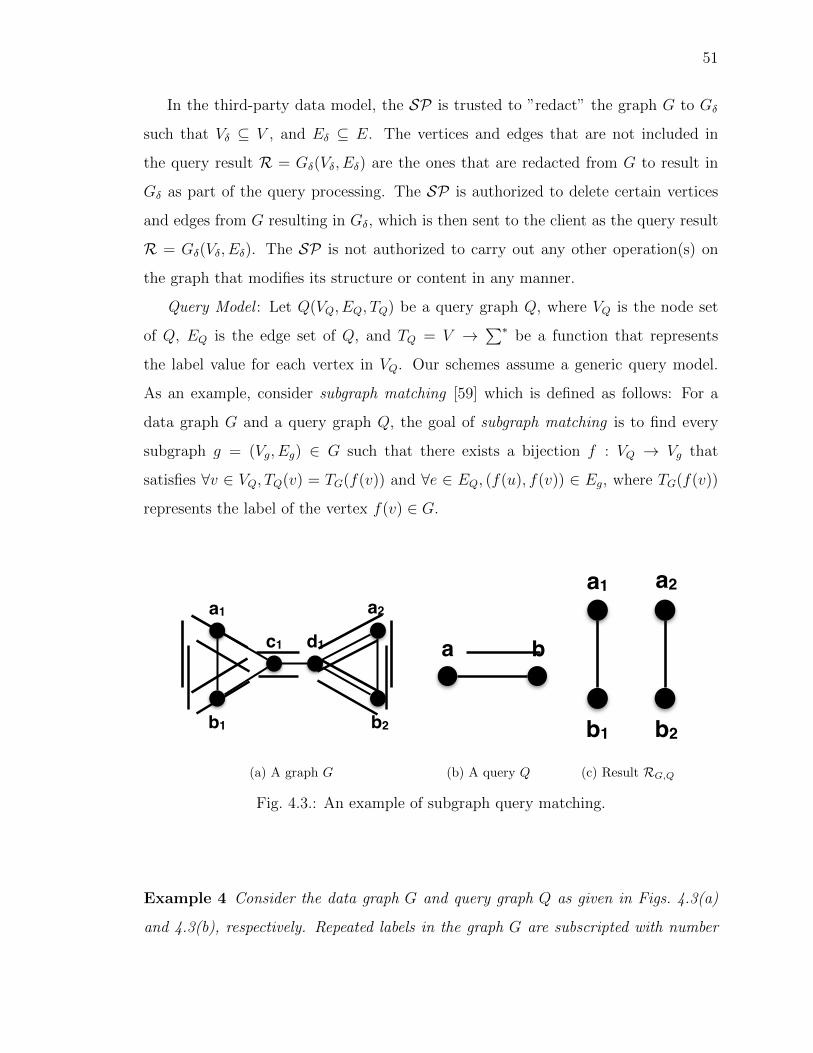
51

In the third-party data model, the SP is trusted to ”redact” the graph G to G�

such that V� ✓ V , and E� ✓ E. The vertices and edges that are not included in

the query result R = G�(V�, E�) are the ones that are redacted from G to result in

G� as part of the query processing. The SP is authorized to delete certain vertices

and edges from G resulting in G�, which is then sent to the client as the query result

R = G�(V�, E�). The SP is not authorized to carry out any other operation(s) on

the graph that modifies its structure or content in any manner.

Query Model : Let Q(VQ, EQ, TQ) be a query graph Q, where VQ is the node set

of Q, EQ is the edge set of Q, and TQ = V !P⇤ be a function that represents

the label value for each vertex in VQ. Our schemes assume a generic query model.

As an example, consider subgraph matching [59] which is defined as follows: For a

data graph G and a query graph Q, the goal of subgraph matching is to find every

subgraph g = (Vg, Eg) 2 G such that there exists a bijection f : VQ ! Vg that

satisfies 8v 2 VQ, TQ(v) = TG(f(v)) and 8e 2 EQ, (f(u), f(v)) 2 Eg, where TG(f(v))

represents the label of the vertex f(v) 2 G.

a1 a2

b2

d1c1

b1

ba

a2

b2

a1

b1

(a) A graph G

a1 a2

b2

d1c1

b1

ba

a2

b2

a1

b1(b) A query Q

a1 a2

b2

d1c1

b1

ba

a2

b2

a1

b1(c) Result RG,Q

Fig. 4.3.: An example of subgraph query matching.

Example 4 Consider the data graph G and query graph Q as given in Figs. 4.3(a)

and 4.3(b), respectively. Repeated labels in the graph G are subscripted with number

52

i. The query graph Q matches two instances on data graph G and the output result

RG,Q = {(a1, b1), (a2, b2)} is shown in Fig. 4.3(c).

As part of our scheme user does not receive any duplicate vertices or edges in the

result R.

4.2.3 Threat Model

For a two-party data model (Fig. 4.2 (a)), we assume a trusted data model in

which both the DO and the client have access to the shared secret key (k, r). The

owner of the graph data computes the gHMAC using the shared secret key (k, r), and

the client/receiver of the graph data verifies the gHMAC using the key (k, r).

For a third-party data model (Fig. 4.2 (b)), we assume a semi-trusted model in

which the SP may not be completely trusted and it does not have access to the

gHMAC key k, but it can compute the query results. The SP may be the potential

adversary A or another adversary A who may have attacked and hacked the SP .

Under this model, we assume that the client and DO can exchange the shared secret

key k over a secure trusted channel.

4.2.4 Desiderata of MACs for Graphs

Challenges: The challenges in computing HMAC of a graph in contrast to com-

puting HMAC of a monolithic message bit-string are as follows:

• The graph is a semi-structured data object and is more complex than a sequen-

tial string/chain of bits in a monolithic message. How we ensure integrity of

the graph data depends on how we incorporate the edges and vertices in the

graph and the order, if any, between the nodes computing the HMACs.

• How can a verifier re-compute the same HMAC tag value as the value computed

by the DO? Graphs can be traversed in many ways by di↵erent parties. One

53

needs to ensure that the verifier follows exactly the same traversal order as the

HMAC computing entity, DO, follows.

• How to ensure ensure integrity of each vertex and its structural position, i.e.,

the order between the sibling vertices?

• How to ensure integrity of each edge?

• The HMAC-based computation and verification schemes for graph data should

be quite e�cient especially in contrast to the digital signature-based schemes,

because for monolithic messages, HMAC-based schemes are more e�cient than

digital signature-based schemes.

Fail-stop HMACs: Integrity assurance of graphs opens up new challenges which

are not faced for the integrity assurance of monolithic messages – bit-strings. One

of these challenges is fail-stop integrity verification. Since graphs have vertices and

edges, the integrity verification process need to be terminated as soon as integrity of

a vertex or an edge is found to be compromised; thus saving computational cost (such

as cost of query processing in a cloud) and time, resulting in improved performance

requirements. Such saving can be substantial for large graph datasets. We can develop

HMACs that are fail-stop. Fail-stop HMACs should stop as soon as they determine

a compromise.

Fail-warn HMACs: Another variant of this type of integrity assurance is fail-

warn integrity verification. The integrity verification proceeds even after finding a

compromised vertex or edge, and outputs a set of all such vertices and edges that are

corrupted. The verifier/client may then request the data provider only those vertices

and edges that are compromised instead of requesting the complete data again. That

shall result in more e�cient and cost-e↵ective database services, network usage and

quality of service.

Redactable HMACs: Given a graph, often part(s) of the graph are sent to a

client as part of a query result. It thus may be necessary for the verifier to be able to

54

verify the integrity of such subgraph(s) using HMAC without the need to have access

to the graph itself. It is a challenging problem especially for HMACs because, unlike

in digital signatures, the key is symmetric, and thus no part of the key can be shared

with the SP , such as a cloud service. An HMAC-based scheme should be redactable

in the sense that a verifier can verify the integrity of the redacted graphs, i.e., the

subgraphs, with few integrity verification objects VO from the SP . In other words,

the SP does not have access to the secret key.

4.3 HMACs for Graphs (gHMAC)

4.3.1 Formal Definition

In this section, we provide the formal definition of hash message authentication

code for graphs (gHMAC).

Definition 4.3.1 (HMAC for Graph (gHMAC)) Given a graph G(V,E) with

vertex set V and edge set E, let g⇧ be a gHMAC for graph G, and let ⇧H = (GenH, H)

be a hash function with output length `. The scheme g⇧ consists of three polynomial-

time algorithms g⇧ ⌘ (gGen, gHmac, gVrfy) and is defined as follows:

1. gGen: On input 1n, the algorithm chooses a uniform k 2 {0, 1}n and runs

GenH(1n) to obtain a random r to generate the key (k, r).

2. gHmac: The algorithm takes as input a graph G(V,E) and a key (k, r) and

outputs a graph tag tG value and a source list SourceList of vertices. The

SourceList is the list of source vertices for traversing di↵erent components of

the graph, in case the components are disconnected. We write this as

(tG, SourceList) gHmac(k,r)(G(V,E)).

55

3. gVrfy: The algorithm takes as input a graph G(V,E), a tag tG, a key (k, r),

and a SourceList. The algorithm outputs a bit b, with b = 1 meaning valid,

and b = 0 meaning invalid. We write this as

b gVrfy(k,r)(tG, G(V,E), SourceList).

4.3.2 HMAC Scheme for Graphs

Overview of Our Scheme

HMAC scheme, gHMAC, takes a graph G(V,E) and a shared secret key (k, r) as its

input. The key (k, r) that has two parts – k which is the secret key used in HMACs

and r which is a random bit-string (� 128 bits). The gHMAC algorithm outputs an

HMAC value referred to as tag tG for the graph G(V,E) and a list of source nodes

SourceList generated during the graph traversal. The scheme traverses the graph in

DFS order and computes the graph hash ghash value after visiting each node. During

the traversal, it computes an integrity identifier, referred to as xor-out(u), for each

node u 2 G. The identifier is used to carry out “local integrity assurance” for that

node. Also during the graph traversal a list u.outList() is maintained to track the

order in which siblings of a node, say u, are visited. The scheme is highly e�cient,

as it performs a single graph traversal to compute tag tG for graph G.

Detailed Description

The Algorithm 5 (gHMAC) initially marks all the vertices of G as unvisited and then

employs a DFS traversal to recursively visit all the unvisited vertices of the graph.

While visiting a particular vertex, say u, during a DFS traversal, the algorithm com-

putes out-xor(u) value, which is exclusive-or � of the label hash values labelHash of

all the descendant nodes of vertex u, and recursively calls the DFS algorithm. Once

a node is finally visited, the algorithm computes the ghash value by taking a hash of

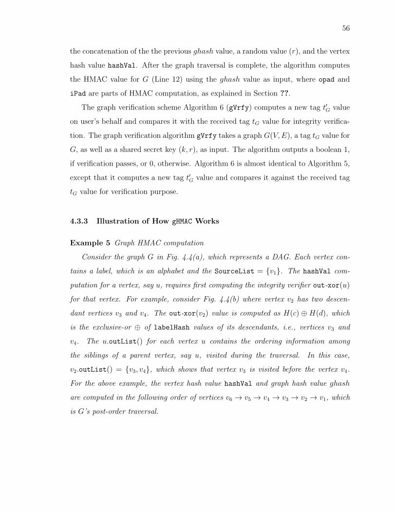
56

the concatenation of the the previous ghash value, a random value (r), and the vertex

hash value hashVal. After the graph traversal is complete, the algorithm computes

the HMAC value for G (Line 12) using the ghash value as input, where opad and

iPad are parts of HMAC computation, as explained in Section ??.

The graph verification scheme Algorithm 6 (gVrfy) computes a new tag t0G value

on user’s behalf and compares it with the received tag tG value for integrity verifica-

tion. The graph verification algorithm gVrfy takes a graph G(V,E), a tag tG value for

G, as well as a shared secret key (k, r), as input. The algorithm outputs a boolean 1,

if verification passes, or 0, otherwise. Algorithm 6 is almost identical to Algorithm 5,

except that it computes a new tag t0G value and compares it against the received tag

tG value for verification purpose.

4.3.3 Illustration of How gHMAC Works

Example 5 Graph HMAC computation

Consider the graph G in Fig. 4.4(a), which represents a DAG. Each vertex con-

tains a label, which is an alphabet and the SourceList = {v1}. The hashVal com-

putation for a vertex, say u, requires first computing the integrity verifier out-xor(u)

for that vertex. For example, consider Fig. 4.4(b) where vertex v2 has two descen-

dant vertices v3 and v4. The out-xor(v2) value is computed as H(c) � H(d), which

is the exclusive-or � of labelHash values of its descendants, i.e., vertices v3 and

v4. The u.outList() for each vertex u contains the ordering information among

the siblings of a parent vertex, say u, visited during the traversal. In this case,

v2.outList() = {v3, v4}, which shows that vertex v3 is visited before the vertex v4.

For the above example, the vertex hash value hashVal and graph hash value ghash

are computed in the following order of vertices v6 ! v5 ! v4 ! v3 ! v2 ! v1, which

is G’s post-order traversal.

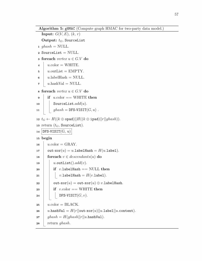
57

Algorithm 5: gHMAC (Compute graph HMAC for two-party data model.)

Input: G(V,E), (k, r)

Output: tG, SourceList

1 ghash = NULL.

2 SourceList = NULL.

3 foreach vertex u 2 G.V do

4 u.color = WHITE.

5 u.outList = EMPTY.

6 u.labelHash = NULL.

7 u.hashVal = NULL.


9 if u.color == WHITE then

10 SourceList.add(u).

11 ghash = DFS-VISIT(G, u) .

12 tG H((k � opad)||H((k � ipad)||r||ghash)).13 return (tG, SourceList).

14 DFS-VISIT(G, u)

15 begin

16 u.color = GRAY.

17 out-xor(u) = u.labelHash = H(u.label).

18 foreach v 2 descendants(u) do

19 u.outList().add(v).

20 if v.labelHash == NULL then

21 v.labelHash = H(v.label).

22 out-xor(u) = out-xor(u)� v.labelHash.

23 if v.color == WHITE then

24 DFS-VISIT(G, v).

25 u.color = BLACK.

26 u.hashVal = H(r||out-xor(u)||u.label||u.content).27 ghash = H(ghash||r||u.hashVal).28 return ghash.

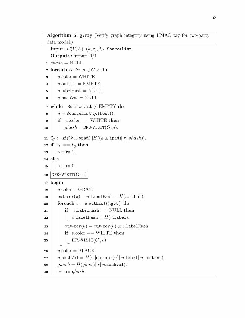
58

Algorithm 6: gVrfy (Verify graph integrity using HMAC tag for two-party

data model.)

Input: G(V,E), (k, r), tG, SourceList

Output: Output: 0/1

1 ghash = NULL.


3 u.color = WHITE.


5 u.labelHash = NULL.

6 u.hashVal = NULL.

7 while SourceList 6= EMPTY do

8 u = SourceList.getNext().


10 ghash = DFS-VISIT(G, u).

11 t0G H((k � opad)||H((k � ipad)||r||ghash)).12 if tG == t0G then

13 return 1.

14 else

15 return 0.

16 DFS-VISIT(G, u)

17 begin

18 u.color = GRAY.

19 out-xor(u) = u.labelHash = H(u.label).

20 foreach v = u.outList().get() do

21 if v.labelHash == NULL then

22 v.labelHash = H(v.label).

23 out-xor(u) = out-xor(u)� v.labelHash.


25 DFS-VISIT(G0, v).

26 u.color = BLACK.

27 u.hashVal = H(r||out-xor(u)||u.label||u.content).28 ghash = H(ghash||r||u.hashVal).29 return ghash.

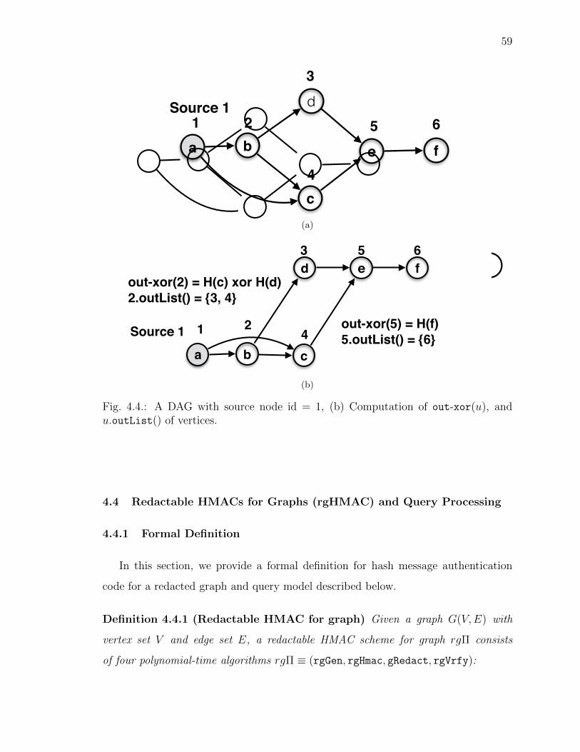
59

b

d

c

a e f

1 2

4

3

5 6Source 1

b

d

ca

e f

1 24

3 5 6

Source 1

out-xor(2) = H(c) xor H(d)!2.outList() = {3, 4}

out-xor(5) = H(f)!5.outList() = {6}

(a)

b

d

c

a e f

1 2

4

3

5 6Source 1

b

d

ca

e f

1 24

3 5 6

Source 1

out-xor(2) = H(c) xor H(d)!2.outList() = {3, 4}

out-xor(5) = H(f)!5.outList() = {6}

(b)

Fig. 4.4.: A DAG with source node id = 1, (b) Computation of out-xor(u), andu.outList() of vertices.

4.4 Redactable HMACs for Graphs (rgHMAC) and Query Processing

4.4.1 Formal Definition

In this section, we provide a formal definition for hash message authentication

code for a redacted graph and query model described below.

Definition 4.4.1 (Redactable HMAC for graph) Given a graph G(V,E) with

vertex set V and edge set E, a redactable HMAC scheme for graph rg⇧ consists

of four polynomial-time algorithms rg⇧ ⌘ (rgGen, rgHmac, gRedact, rgVrfy):

60

1. rgGen: On input 1n, this algorithm chooses a uniform k 2 {0, 1}n and runs

GenH(1n) to obtain a random r to generate the key is (k, r).

2. rgHmac: The tag-generation algorithm takes a graph G(V,E) and the key (k, r)

as its input, and outputs a pair (tG, SourceList), where tG is a tag for graph

and SourceList is the list of source vertices for traversing di↵erent components

of the graph, in case the components are disconnected. Since the algorithm may

be randomized, we write this input/output behavior as

(tG, SourceList) rgHmac(k,r)(G(V,E)).

3. gRedact: The redaction algorithm takes a graph G(V,E), set of nodes V 0� ✓ V ,

set of edges E 0� ✓ E, source list SourceList of vertices, a set of vertex hash

values VH = {u.hashVal|v 2 G.V }, and a set of edge hash values EH =

{e(u, v).hashVal|e(u, v) 2 G.E} as its input. The algorithm outputs a redacted

graph G�(V�, E�)3, where G�(V�, E�) is derived from G(V,E) consisting of ver-

tices in V� = V \ V 0� and E� = E \ E 0

�, a source list of vertices SourceList�,

and two verification objects: vo-g and vo-out. We represent the algorithm to

generate the required query output as follow:

(G�(V�, E�)| {z }R

, SourceList�, vo-g, vo-out| {z }VO

)

gRedact(G(V,E), SourceList, V 0� , E

0�,HV ,HE).

4. rgVrfy: The deterministic verification algorithm takes as input the query result

G�(V�, E�), a tag tG�, a key (k, r), a source list SourceList� of vertices, and

two verification objects: vo-g and vo-out. The algorithm outputs a bit b, with

3Note: As mentioned earlier R = G�(V�, E�) is the result of user query. The query result alsoincludes the required VO.

61

b = 1 meaning the result is valid, and b = 0 meaning the result is invalid.

We write this validation of query result as

b rgVrfy(k,r)(tG�, G�(V�, E�), vo-g, vo-out).

4.4.2 Redactable HMAC Scheme for Graphs

Overview of Our Scheme

In this section, we provide the construction for rgHMAC scheme. The third-party

SP follows the redaction model discussed earlier in Section 4.2.4. As the third-party

does not have access to the shared secret key (k, r), the challenge is to develop a

scheme for generating a tag tG value for redacted graph G�. In particular, we gener-

ate two di↵erent hash values: e(u, v).hashVal for edges and u.hashVal for vertices.

Expensive operations for computing ghash value are not desirable. Therefore, the

exclusive-or � operator, which is both commutative and associative can be utilized

in combination with vertex and edge hash values. The exclusive-or � operator is

purely used for confidentiality purpose and, in this case, as part of our scheme, it acts

as a mechanism for integrity preservation.

Detailed Description

The proposed HMAC scheme rgHMAC (Algorithm 7) takes as input a graphG(V,E),

a shared secret key that has two parts (k, r) – k is the secret key used in HMACs

and r is a random bit-string (� 128 bits). The algorithm outputs an rgHMAC value

referred to as tag tG for G, and a list of source nodes SourceList generated during

the graph traversal. Initially, all the vertices are marked as unvisited. The algorithm

carries out a DFS traversal on the unvisited vertices to compute the vertex hash val-

ues v.hashVal for all v 2 V and the edge hash values e(u, v).hashVal for all e 2 E. In

addition, during traversal, a list u.outList is maintained to track the order in which

62

Algorithm 7: rgHMAC (Compute graph HMAC for third-party data model.)

Input: G(V,E), (k, r)

Output: tG, SourceList

1 ghash = r.


3 u.color = WHITE.


5 u.hashVal = NULL.



8 SourceList.add(u).

9 ghash = DFS-VISIT(G, u).

10 tG H((k � opad)||H((k � ipad)||r||ghash)).11 return (tG, SourceList).

12 DFS-VISIT(G, u)

13 begin

14 u.color = GRAY.

15 out-xor(u) = 1.

16 foreach v 2 descendants(u) do

17 u.outList().add(v).

18 e(u, v).hashVal = H(r||u.label||v.label).19 out-xor(u) = out-xor(u)� e(u, v).hashVal.


21 DFS-VISIT(G, v).

22 u.color = BLACK.

23 u.hashVal = H(r||out-xor(u)||u.label||u.content).24 ghash = ghash� u.hashVal.

25 return ghash.

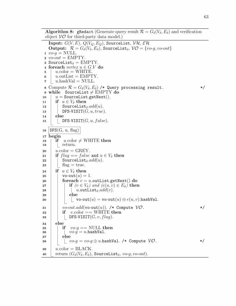
63

Algorithm 8: gRedact (Generate query result R = G�(V�, E�) and verificationobject VO for third-party data model.)

Input: G(V,E), Q(VQ, EQ), SourceList, VH, EHOutput: R = G�(V�, E�), SourceList�, VO = {vo-g, vo-out}

1 vo-g = NULL.2 vo-out = EMPTY.3 SourceList� = EMPTY.4 foreach vertex u 2 G.V do5 u.color = WHITE.6 u.outList = EMPTY.7 u.hashVal = NULL.

8 Compute R = G�(V�, E�) /* Query processing result. */9 while SourceList 6= EMPTY do

10 u = SourceList.getNext().11 if u 2 V� then12 SourceList�.add(u).13 DFS-VISIT(G, u, true).14 else15 DFS-VISIT(G, u, false).

16 DFS(G, u, flag)17 begin18 if u.color 6= WHITE then19 return.20 u.color = GREY.21 if flag == false and u 2 V� then22 SourceList�.add(u).23 flag = true.24 if u 2 V� then25 vo-out(u) = 1.26 foreach v = u.outList.getNext() do27 if (v 2 V�) and (e(u, v) 2 E�) then28 u.outList�.add(v).29 else30 vo-out(u) = vo-out(u)� e(u, v).hashVal.

31 vo-out.add(vo-out(u)). /* Compute VO. */32 if v.color == WHITE then33 DFS-VISIT(G, v, flag).

34 else35 if vo-g == NULL then36 vo-g = u.hashVal.37 else38 vo-g = vo-g � u.hashVal. /* Compute VO. */

39 u.color = BLACK.40 return (G�(V�, E�), SourceList�, vo-g, vo-out).

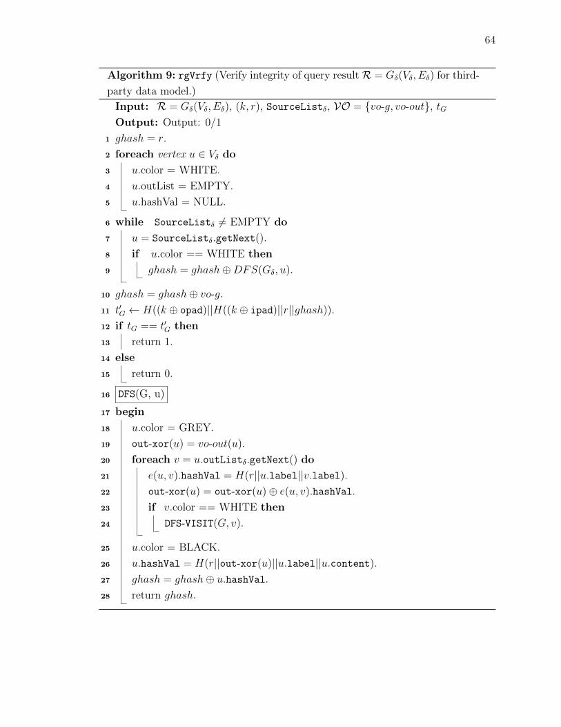
64

Algorithm 9: rgVrfy (Verify integrity of query result R = G�(V�, E�) for third-

party data model.)

Input: R = G�(V�, E�), (k, r), SourceList�, VO = {vo-g, vo-out}, tGOutput: Output: 0/1

1 ghash = r.

2 foreach vertex u 2 V� do

3 u.color = WHITE.


5 u.hashVal = NULL.

6 while SourceList� 6= EMPTY do

7 u = SourceList�.getNext().


9 ghash = ghash�DFS(G�, u).

10 ghash = ghash� vo-g.

11 t0G H((k � opad)||H((k � ipad)||r||ghash)).12 if tG == t0G then

13 return 1.

14 else

15 return 0.

16 DFS(G, u)

17 begin

18 u.color = GREY.

19 out-xor(u) = vo-out(u).

20 foreach v = u.outList�.getNext() do

21 e(u, v).hashVal = H(r||u.label||v.label).22 out-xor(u) = out-xor(u)� e(u, v).hashVal.


24 DFS-VISIT(G, v).

25 u.color = BLACK.

26 u.hashVal = H(r||out-xor(u)||u.label||u.content).27 ghash = ghash� u.hashVal.

28 return ghash.

65

the siblings of a node, say u, are visited. The ghash value is computed recursively

by taking the exclusive-or � of u.hashVal value with the previously computed ghash

value.

The algorithm gRedact (Algorithm 8) is executed by the third-party data distrib-

utor, which does not have access to shared secret key k, which poses a challenge to

generate a ghash value. An approach is to use the � operator in combination with

the hashVal. Algorithm 8 takes as input a graph G(V,E), a vertex set V 0� , an edge

set E 0�, a set of vertex hash values VH = {v.hashVal|v 2 G.V } and a set of edge hash

values EH = {e(u, v).hashVal|e 2 G.E}. The algorithm outputs a redacted graph

G�(V�, E�), a list of source nodes SourceList�, a verification object vo-g for graph ,

and the set of verification objects vo-out. The algorithm carries out a DFS traver-

sal to compute the verification objects vo-g and vo-out during the graph traversal.

During the graph traversal, for each vertex u 2 V� a verification object vo-out(u) is

computed, which contains the � of label hash values of those ancestors of u that are

not present in the set V�. Similarly, for those vertices which are in u /2 V� the algo-

rithm computes the verification object vo-g, by performing exclusive-or � operation

on the vertex hash value hashVal of those vertices which are not in the set V�.

The algorithm rgVrfy (Algorithm 9) performs the graph verification. It takes

as input a graph G�(V�, E�), a tag tG, a shared secret key k, a random number

r, a verification object vo-g for graph G(V,E), and the sets of verification object

vo-out. The algorithm outputs a boolean 1, in case of verification process success, or

0, otherwise. The main idea of the verification algorithm rgVrfy is to compute the

value for ghash� for the redacted graph G�(V�, E�) first and then an exclusive-or �with verification object vo-g value to compute the ghash value of the complete graph

G. The algorithm computes a new tag t0G using this ghash value and compares it

against tG for integrity verification. The algorithm performs a DFS traversal on the

graph G�, which is received as part of the query result, and computes the integrity

verifier out-xor(u) for each vertex v 2 V�. Notice out-xor(u) is initialized with

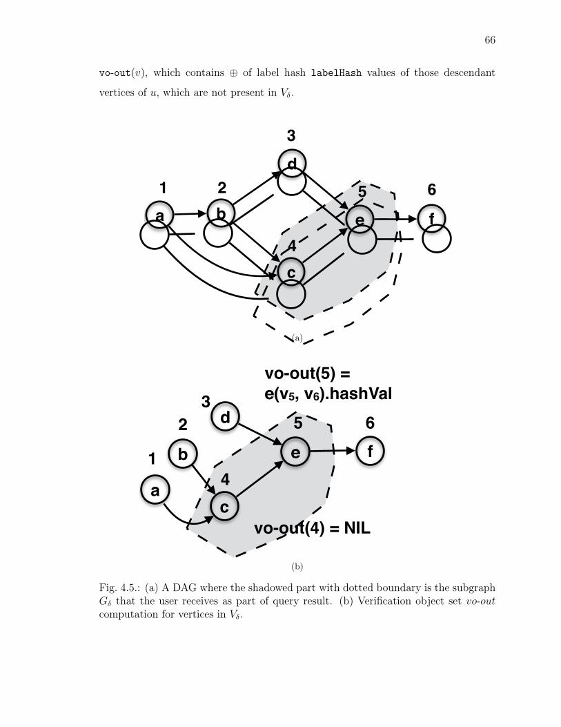
66

vo-out(v), which contains � of label hash labelHash values of those descendant

vertices of u, which are not present in V�.

b

d

c

a e f

1 2

4

3

5 6

b

d

ca

e f1

2

4

35

vo-out(4) = NIL

vo-out(5) = !e(v5, v6).hashVal

6

(a)

b

d

c

a e f

1 2

4

3

5 6

b

d

ca

e f1

2

4

35

vo-out(4) = NIL


6

(b)

Fig. 4.5.: (a) A DAG where the shadowed part with dotted boundary is the subgraphG� that the user receives as part of query result. (b) Verification object set vo-outcomputation for vertices in V�.

67

4.4.3 Illustration of How rgHMAC Works

Example 6 (Generation of VO for query result R = G�(V�, E�)) Consider the

graph in Fig. 4.5(a), which is a DAG. Each vertex is labeled with an alphabet. Suppose

the shaded part of the graph with dotted boundary is the subgraph G�(V�, E�), which

the user receives as part of the query result R. The algorithm gRedact determines

the sets V� = {v4, v5} and V \ V� = {v1, v2, v3, v6} as part of the query processing

step. The user receives the graph G� and two sets of verification objects, which are

vo-g, and vo-out, as part of query result. For all the vertices that are not part of

the query result R (i.e., v /2 V�), the verification object vo-g computes exclusive-or

� of the vertex hash values hashVal in a post-order fashion, vo-g = v6.hashVal �v3.hashVal � v2.hashVal � v1.hashVal. On the other hand, for the set of vertices

that are in V� = {v4, v5}, the algorithm computes vo-out(u), which considers only

those descendants of a vertex, say u 2 V�, which are not not present in V�. For

example, from Fig. 4.5(b), we can notice that vertex v4 has no descendants outside

the set V�, while vertex v5 has only one descendant vertex v6 outside the set V�.

Therefore, the verification object vo-out(v4) = NULL as this vertex has no descendant

and vo-out(v6) = e(v5, v6).hashVal.

4.4.4 Fail-stop and Fail-warn gHMAC and rgHMAC

One of the key advantages of the proposed HMAC-based schemes is that the

HMAC verification process correctly identifies if a node or edge has been compro-

mised. In particular,if a node is compromised with respect to its label or content, the

node can be identified by computing the hash value of the label and content of the

node along with the r. Similarly, if an edge e(x, y) is tampered, the out-xor(x) will

be incorrect, resulting in an incorrect hashVal computed for x. Furthermore, the end

vertices of the edge are considered to be compromised.

In case of tampering, the following steps can be taken:

• Fail-stop: Stop the verification processes soon as the first compromise is found.

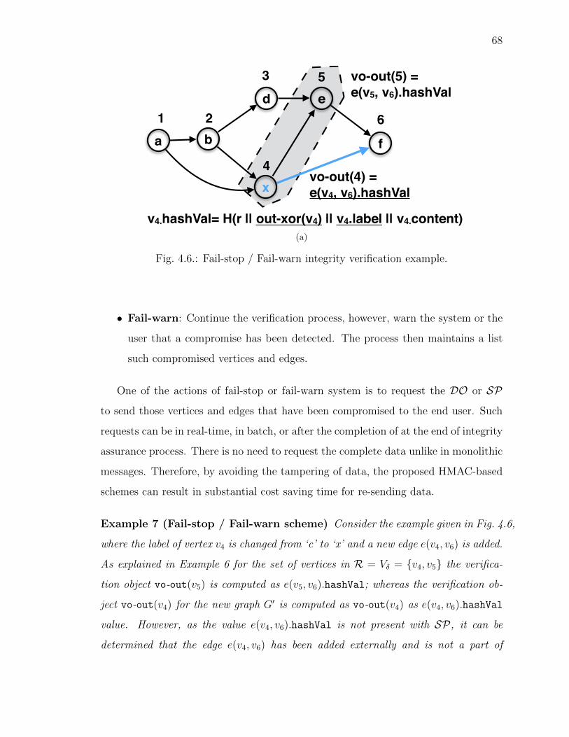
68

b

d

a

e

f

1 2

4

3 5

6

x



v4.hashVal= H(r || out-xor(v4) || v4.label || v4.content)(a)

Fig. 4.6.: Fail-stop / Fail-warn integrity verification example.

• Fail-warn: Continue the verification process, however, warn the system or the

user that a compromise has been detected. The process then maintains a list

such compromised vertices and edges.

One of the actions of fail-stop or fail-warn system is to request the DO or SPto send those vertices and edges that have been compromised to the end user. Such

requests can be in real-time, in batch, or after the completion of at the end of integrity

assurance process. There is no need to request the complete data unlike in monolithic

messages. Therefore, by avoiding the tampering of data, the proposed HMAC-based

schemes can result in substantial cost saving time for re-sending data.

Example 7 (Fail-stop / Fail-warn scheme) Consider the example given in Fig. 4.6,

where the label of vertex v4 is changed from ‘c’ to ‘x’ and a new edge e(v4, v6) is added.

As explained in Example 6 for the set of vertices in R = V� = {v4, v5} the verifica-

tion object vo-out(v5) is computed as e(v5, v6).hashVal; whereas the verification ob-

ject vo-out(v4) for the new graph G0 is computed as vo-out(v4) as e(v4, v6).hashVal

value. However, as the value e(v4, v6).hashVal is not present with SP, it can be

determined that the edge e(v4, v6) has been added externally and is not a part of

69

the original graph. For the set of vertices V \ V� = {v1, v2, v3, v6} the verification

object vo-g is computed as exclusive-or � of the vertex hash values hashVal in post-

order fashion, vo-g = v6.hashVal � v3.hashVal � v2.hashVal � v1.hashVal. During

the vo-g computation vertex v2’s hash value hashVal is computed as v2.hashVal =

H(r||out-xor(v2)||v2.label||v2.content), where out-xor(v2) = e(v2, v3).hashVal �e(v2, v4).hashVal. e(v2, v4).hashVal will not evaluate to a correct value as v4 has a

tampered label ‘x’ resulting in an incorrect value for v4.hashVal as determined by SP.

Therefore, SP can continue the execution of algorithm and keep track of values that

have been modified or stop the execution.

4.5 Security Analysis

In this section, we review the security of gHMAC and rgHMAC schemes. We

present two lemmas with their proofs.

4.5.1 Security of gHMAC

Lemma 4.5.1 Let the hash function H be an implementation of a random oracle,

and gh refer to the gHMAC of graph G(V,E). Under the random oracle model, and

under the assumption that the secret key is known only to the DO and the client, the

gHMAC scheme is secure, i.e., a probabilistic polynomial-time (PPT) adversary Acannot compute gh0 as the gHMAC of G0(V 0, E 0) such that gh = gh0.

Proof Suppose the adversary A can compute gh0 for a di↵erent graph G0 such that

gh = gh0. Consider the case that adversary A has modified G in an unauthorized

manner that resulted in G0. Following unauthorized modifications of the graph may

be carried out by adversary A:

• Label modification: Suppose the label of a vertex x x.label is modified to

x.label0; then gh = gh0 if and only if (1) and (2) are true: (1) out-xor(x) =

out-xor(x)0, which is true, i↵ H(x.label) = H(x.label0), and (2) x.hashVal =

70

x.hashVal0, which is true, i↵ H(r||out-xor(x)||x.label||x.content) =H(r||out-xor(x)||x.label0||x.content). In order for (1) and (2) to be true,

adversary A has to carry out pre-image attacks on the hash function H, which,

however, contradicts our assumption that H is a random oracle.

• Content modification: The argument follows the reasoning for label mod-

ification above. Suppose the content of a vertex x x.content is modified to

x.content0; then gh = gh0 if and only if the following is true: x.hashVal =

x.hashVal0, which is true, i↵ H(r||out-xor(x)||x.label||x.content)= H(r||out-xor(x)||x.label||x.content0). In order for it to be true, adversary

A has to carry out pre-image attacks on the hash function H, which, however,

contradicts our assumption that H is a random oracle.

• Vertex insertion: Consider that a vertex z is added to the graph G(V,E) by

adversary A in order to result in a compromised graph G0 where z 2 V 0 and

gh = gh0. This implies that at the end of traversal of vertex z, the computed

ghash0 value (that does include z.hashVal) is identical to that of ghash, which

does not include z.hashVal as per Algorithm 5 line 27. It is possible, however,

if and only if, adversary A has been successful in carrying out pre-image attacks

on the hash function H, which, however, contradicts our assumption that H is

a random oracle.

• Vertex deletion: Consider that a vertex z is deleted from the graph G(V,E)

by adversary A in order to result in a compromised graph G0 where z 2 V ^z /2 V 0 and gh = gh0. This implies that at the end of traversal of graph G0,

the computed ghash0 value (that does not include z.hashVal) is identical to

that of ghash, which includes z.hashVal as per Algorithm 5 line 27. It is

possible, however, if and only if, adversary A has been successful in carrying

out pre-image attacks on the hash function H, which, however, contradicts our

assumption that H is a random oracle.

71

• Edge insertion: An edge e(x, y) is added to the graph G(V,E) by adversary

A in order to result in a compromised graph G0 where e(x, y) /2 G and x, y

are in both G and G0. If either of x, y are vertices inserted by adversary Ain G0 and are not in G, then it can be addressed as per the arguments for

vertex insertion above. However, out-xor(x) 6= out-xor(x)0 because out-xor(x)

contains y.labelHash0. Thus, (1) x.hashVal 6= x.hashVal0, and (2) ghash 6=ghash0. (1) and (2) are true if and only if adversary A has been successful

in carrying out pre-image attacks on the hash function H, which, however,

contradicts our assumption that H is a random oracle.

• Edge deletion: An edge e(x, y) is deleted by adversary A from G such that

e(x, y) /2 G0 and x, y are in both G and G0. If either of x, y are vertices inserted

by adversary A in G0 and are not in G, then this can be addressed as per

the arguments for vertex insertion above. However, out-xor(x) 6= out-xor(x)0

because out-xor(x)0 does not include y.labelHash. Thus, (1) x.hashVal 6=x.hashVal0, and (2) ghash0 6= ghash of G. (1) and (2) are true if and only if

adversary A has been successful in carrying out pre-image attacks on the hash

function H, which, however, contradicts our assumption that H is a random

oracle.

• Edge modification: An edge e(x, y) 2 G is modified by adversary A to

e(x, z) 2 G0 such that z is a node in G and G0 and there is no edge from

x to z in G. However, out-xor(x) 6= out-xor(x)0, because out-xor(x)0 does

not contain y.labelHash, but contains z.labelHash. Thus, (1) x.hashVal 6=x.hashVal0, (2) z.hashVal 6= z.hashVal0, (3) y.hashVal 6= y.hashVal0, and (4)

ghash 6= ghash0. (1), (2), (3), and (4) are true if and only if adversary Ahas been successful in carrying out pre-image attacks on the hash function H,

which, however, contradicts our assumption that H is a random oracle. Any

edge modification, such as e(x, y) is modified to e(y, x), can also be reasoned as

72

above. If more than one edges and vertices are modified, then the arguments

above can be extrapolated to the ones above. Thus, the proof follows.

4.5.2 Security of rgHMAC

Lemma 4.5.2 Let the hash function H be an implementation of a random oracle

and gh refer to the rgHMAC of graph G(V,E). Under the random oracle model, and

under the assumption that the secret key is known only to the DO and the client, the

rgHMAC scheme is secure, i.e., a PPT adversary A (assumption is adversary A is not

the third-party data publisher that can redact G to G�) cannot compute gh0 as the

rgHMAC of G0(V 0, E 0) such that gh = gh0.

Proof For PPT adversary that is not in the third-party data publisher SP , the

proofs follow from Lemma 1.For PPT adversary that is the third-party data publisher

SP , the proofs are as follows. Suppose the adversaryA can compute gh0 for a di↵erent

graph G0 such that gh = gh0. Consider the case that adversary A modified G in an

unauthorized manner that resulted in G0. The following unauthorized modification

of the graph may be carried out by adversary A:

• Insertion of vertices: One or more vertices w1, w2, . . . , wm may be inserted

to G� resulting in the updated graph G0�, where wi /2 V , 1 i m. Consider

one vertex w1 being added by adversary A in G� resulting in G0�. Adversary A

updates all other values as needed. vo-g0 is computed by the adversary A as

vo-g � w1.hashVal, so that computation of ghash (Line 10 of Algorithm 9) by

the client/verifier cancels out the w1.hashVal computed and �-ed with ghash

during the DFS traversal (Line 27 of the Algorithm 9). Note that w1.hashVal�vo-g0 results in vo-g by the property of exclusive-or � operator (i.e., r1� r2� r2

= r1). However, in order to be able to compute w1.hashVal, the adversary

A either (1) knows random r, which is part of secret key (k, r), or (2) can

73

assign w1.label and/or w1.content such that w1.hashVal as computed by the

adversary A matches with the value as computed by the verifier (Line 27 in

Algorithm 9). (1) contradicts our assumption that the secret key is known only

to the DO and client/verifier, and (2) contradicts our assumption that H is a

random oracle. Without loss of generality, the argument can be extended to

insertion of multiple vertices w1, w2, . . . , wm.

• Label, content, or edge modification: Label, content, or edges of G� are

modified by adversary A that results in G0�. However, random r (part of secret

key (k, r)), which is known only by the DO and client, is used for computing

hashVal of the vertices and edges. Therefore, if adversary A can compute vo-g0,

vo-out0 so that G0� can be verified against gh, then either adversary A is aware

of r or adversary A has been able to find a pre-image attack on H. The former

contradicts our assumption that (k, r) is secret and known only to the DOand client and is not available to SP including any other entities. The latter

contradicts our assumption thatH is a random oracle, and thus proves the point

that label, contents, or edges cannot be modified by adversary A including the

semi-honest service provider SP .

• Deletion of vertices and edges: Lemma 4.5.1 applies to deletion of vertices

and edges by adversary A other than the SP that is authorized to carry out

such operations4. Thus the proof follows.

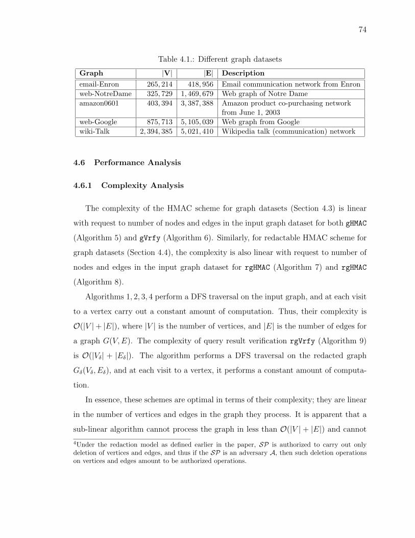
74

Table 4.1.: Di↵erent graph datasets

Graph |V| |E| Description

email-Enron 265, 214 418, 956 Email communication network from Enronweb-NotreDame 325, 729 1, 469, 679 Web graph of Notre Dameamazon0601 403, 394 3, 387, 388 Amazon product co-purchasing network

from June 1, 2003web-Google 875, 713 5, 105, 039 Web graph from Googlewiki-Talk 2, 394, 385 5, 021, 410 Wikipedia talk (communication) network

4.6 Performance Analysis

4.6.1 Complexity Analysis

The complexity of the HMAC scheme for graph datasets (Section 4.3) is linear

with request to number of nodes and edges in the input graph dataset for both gHMAC

(Algorithm 5) and gVrfy (Algorithm 6). Similarly, for redactable HMAC scheme for

graph datasets (Section 4.4), the complexity is also linear with request to number of

nodes and edges in the input graph dataset for rgHMAC (Algorithm 7) and rgHMAC

(Algorithm 8).

Algorithms 1, 2, 3, 4 perform a DFS traversal on the input graph, and at each visit

to a vertex carry out a constant amount of computation. Thus, their complexity is

O(|V |+ |E|), where |V | is the number of vertices, and |E| is the number of edges for

a graph G(V,E). The complexity of query result verification rgVrfy (Algorithm 9)

is O(|V�| + |E�|). The algorithm performs a DFS traversal on the redacted graph

G�(V�, E�), and at each visit to a vertex, it performs a constant amount of computa-

tion.

In essence, these schemes are optimal in terms of their complexity; they are linear

in the number of vertices and edges in the graph they process. It is apparent that a

sub-linear algorithm cannot process the graph in less than O(|V | + |E|) and cannot

4Under the redaction model as defined earlier in the paper, SP is authorized to carry out onlydeletion of vertices and edges, and thus if the SP is an adversary A, then such deletion operationson vertices and edges amount to be authorized operations.

75

carry out integrity assurance of all the vertices and edges in a graph. Thus, a O(|V |+|E|) complexity is the best complexity that an integrity assurance scheme for graphs

can achieve.

4.6.2 Performance Evaluation

In this section, we present detailed evaluation of results for the performance of the

proposed schemes. We provide two sets of results for two-party data publishing model:

i) computation of graph HMAC tag (gHMAC), and ii) verification of graph integrity

using HMAC tag (gVrfy) for graph HMAC-based scheme; and three di↵erent sets

of results for third-party data publishing model: i) computation of graph HMAC

tag (rgHMAC), ii) generation of query result R = G� and verification object VO(gRedact), and iii) verifying the integrity of graph query result (rgVrfy) for redacted

graph HMAC-based scheme.

Experimental Setup

Running Platform: We have conducted all our experiments on Intel(R) Xeon(R)

CPU E5-2620 v3 2.40 GHz machine with 24 Cores and 188G byte RAM. All algo-

rithms have been implemented using Java 1.7. We used JGraphT-0.9.1 (a free Java

Graph Library)5 API as graph processing library. We provided JVM with the follow-

ing parameters: �Xms4G for min heap size and �Xmx8G for max heap size. Therefore,

we do not use all the available RAM.

Datasets: We have used real-world datasets available at Stanford Large Network

Dataset Collection6 for our experiments. Table 4.1 shows the specification of datasets.

The largest graph, wiki-Talk, has about 2M vertices and 5M edges.

Workload Generation: For our experiments, we use JGraphT library Subgraph

class to generate subgraphs G0(V 0, E 0) of varying sizes and determine the result set

5http://jgrapht.org

6http://snap.stanford.edu

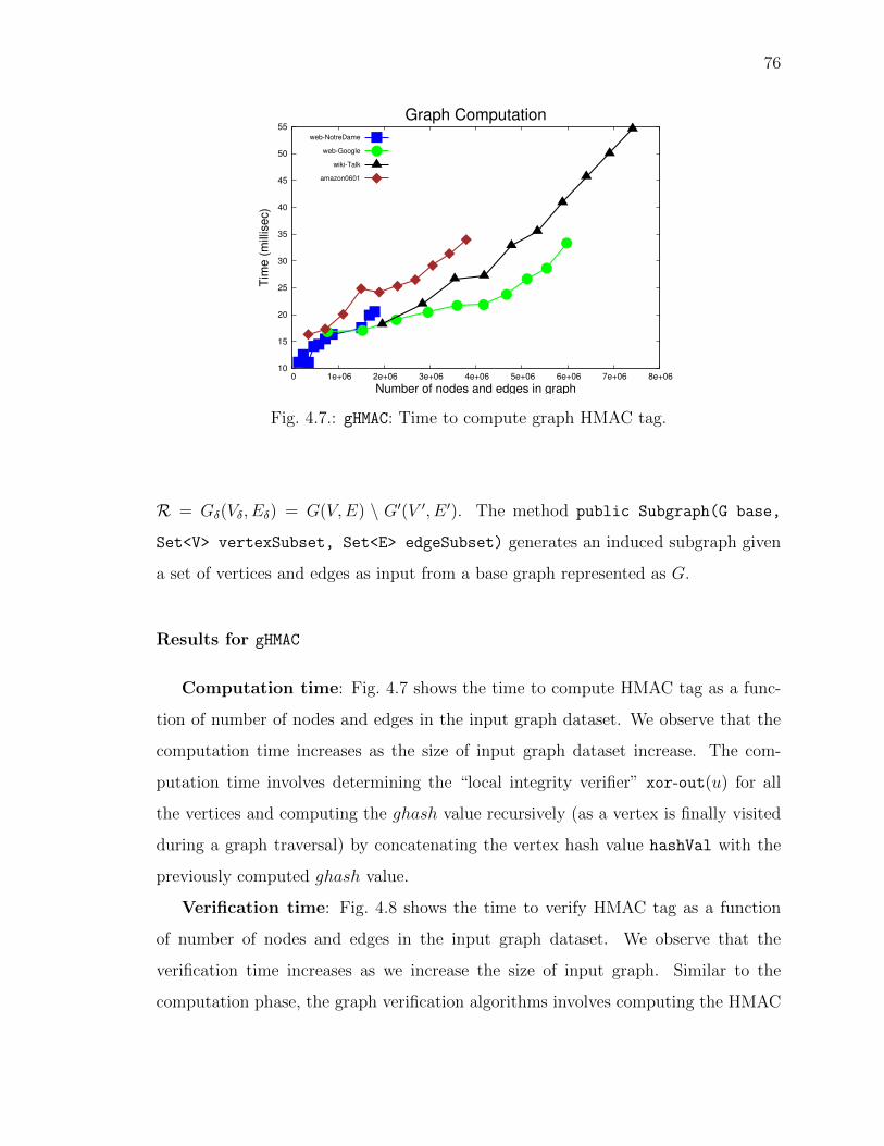
76

10

15

20

25

30

35

40

45

50

55

0 1e+06 2e+06 3e+06 4e+06 5e+06 6e+06 7e+06 8e+06

Tim

e (

mill

ise

c)

Number of nodes and edges in graph

Graph Computationweb-NotreDame

web-Google

wiki-Talk

amazon0601

Fig. 4.7.: gHMAC: Time to compute graph HMAC tag.

R = G�(V�, E�) = G(V,E) \ G0(V 0, E 0). The method public Subgraph(G base,

Set<V> vertexSubset, Set<E> edgeSubset) generates an induced subgraph given

a set of vertices and edges as input from a base graph represented as G.

Results for gHMAC

Computation time: Fig. 4.7 shows the time to compute HMAC tag as a func-

tion of number of nodes and edges in the input graph dataset. We observe that the

computation time increases as the size of input graph dataset increase. The com-

putation time involves determining the “local integrity verifier” xor-out(u) for all

the vertices and computing the ghash value recursively (as a vertex is finally visited

during a graph traversal) by concatenating the vertex hash value hashVal with the

previously computed ghash value.

Verification time: Fig. 4.8 shows the time to verify HMAC tag as a function

of number of nodes and edges in the input graph dataset. We observe that the

verification time increases as we increase the size of input graph. Similar to the

computation phase, the graph verification algorithms involves computing the HMAC

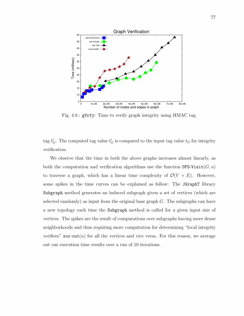
77

5

10

15

20

25

30

35

40

45

50

55

0 1e+06 2e+06 3e+06 4e+06 5e+06 6e+06 7e+06 8e+06

Tim

e (

mill

ise

c)


Graph Verificationweb-NotreDame

web-Google

wiki-Talk

amazon0601

Fig. 4.8.: gVrfy: Time to verify graph integrity using HMAC tag.

tag t0G. The computed tag value t0G is compared to the input tag value tG for integrity

verification.

We observe that the time in both the above graphs increases almost linearly, as

both the computation and verification algorithms use the function DFS-Visit(G, u)

to traverse a graph, which has a linear time complexity of O(V + E). However,

some spikes in the time curves can be explained as follow: The JGraphT library

Subgraph method generates an induced subgraph given a set of vertices (which are

selected randomly) as input from the original base graph G. The subgraphs can have

a new topology each time the Subgraph method is called for a given input size of

vertices. The spikes are the result of computations over subgraphs having more dense

neighborhoods and thus requiring more computation for determining “local integrity

verifiers” xor-out(u) for all the vertices and vice versa. For this reason, we average

out our execution time results over a run of 10 iterations.

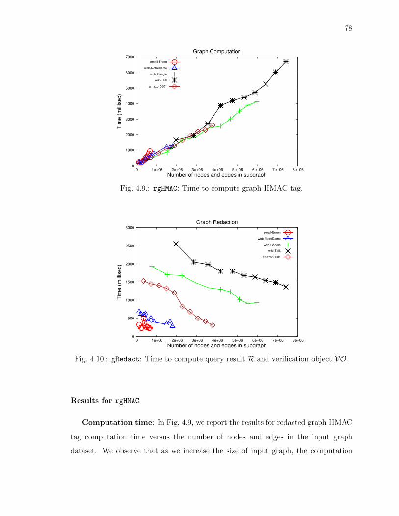
78

0

1000

2000

3000

4000

5000

6000

7000

0 1e+06 2e+06 3e+06 4e+06 5e+06 6e+06 7e+06 8e+06

Tim

e (

mill

ise

c)

Number of nodes and edges in subgraph

Graph Computation

email-Enron

web-NotreDame

web-Google

wiki-Talk

amazon0601

Fig. 4.9.: rgHMAC: Time to compute graph HMAC tag.

0

500

1000

1500

2000

2500

3000

0 1e+06 2e+06 3e+06 4e+06 5e+06 6e+06 7e+06 8e+06

Tim

e (

mill

ise

c)

Number of nodes and edges in subgraph

Graph Redaction

email-Enron

web-NotreDame

web-Google

wiki-Talk

amazon0601

Fig. 4.10.: gRedact: Time to compute query result R and verification object VO.

Results for rgHMAC

Computation time: In Fig. 4.9, we report the results for redacted graph HMAC

tag computation time versus the number of nodes and edges in the input graph

dataset. We observe that as we increase the size of input graph, the computation

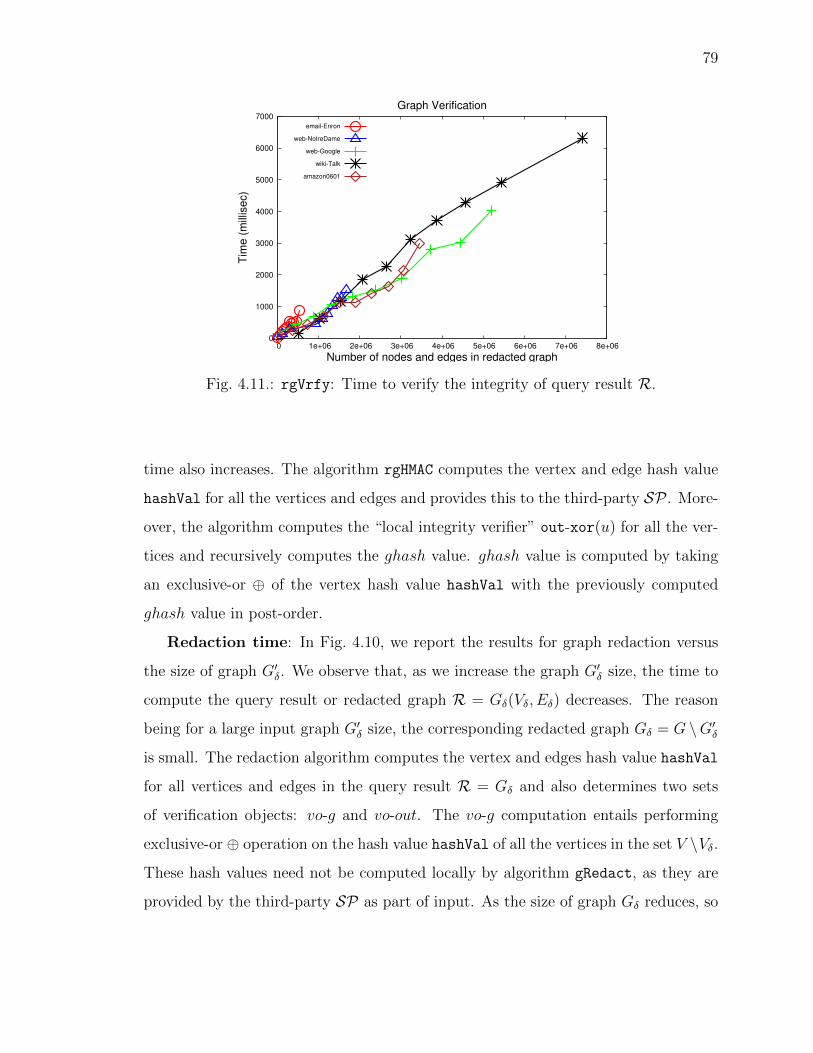
79

0

1000

2000

3000

4000

5000

6000

7000

0 1e+06 2e+06 3e+06 4e+06 5e+06 6e+06 7e+06 8e+06

Tim

e (

mill

ise

c)

Number of nodes and edges in redacted graph

Graph Verification

email-Enron

web-NotreDame

web-Google

wiki-Talk

amazon0601

Fig. 4.11.: rgVrfy: Time to verify the integrity of query result R.

time also increases. The algorithm rgHMAC computes the vertex and edge hash value

hashVal for all the vertices and edges and provides this to the third-party SP . More-

over, the algorithm computes the “local integrity verifier” out-xor(u) for all the ver-

tices and recursively computes the ghash value. ghash value is computed by taking

an exclusive-or � of the vertex hash value hashVal with the previously computed

ghash value in post-order.

Redaction time: In Fig. 4.10, we report the results for graph redaction versus

the size of graph G0�. We observe that, as we increase the graph G0

� size, the time to

compute the query result or redacted graph R = G�(V�, E�) decreases. The reason

being for a large input graph G0� size, the corresponding redacted graph G� = G \G0

�

is small. The redaction algorithm computes the vertex and edges hash value hashVal

for all vertices and edges in the query result R = G� and also determines two sets

of verification objects: vo-g and vo-out. The vo-g computation entails performing

exclusive-or � operation on the hash value hashVal of all the vertices in the set V \V�.

These hash values need not be computed locally by algorithm gRedact, as they are

provided by the third-party SP as part of input. As the size of graph G� reduces, so

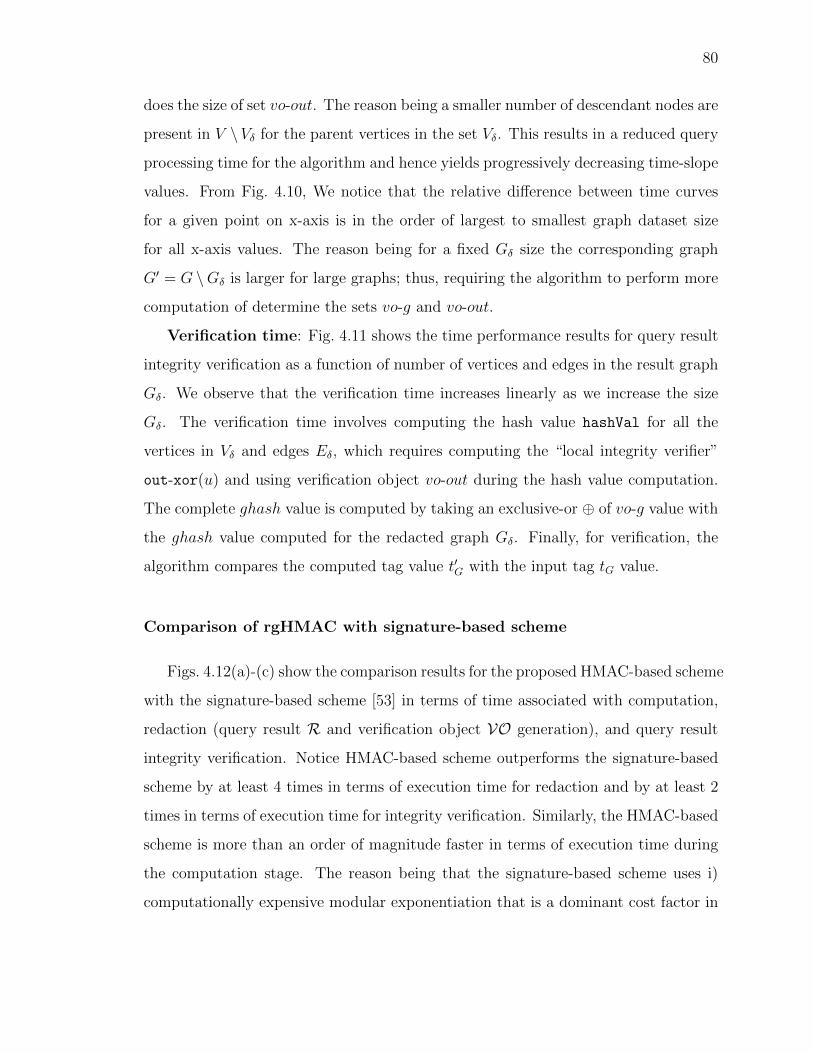
80

does the size of set vo-out. The reason being a smaller number of descendant nodes are

present in V \V� for the parent vertices in the set V�. This results in a reduced query

processing time for the algorithm and hence yields progressively decreasing time-slope

values. From Fig. 4.10, We notice that the relative di↵erence between time curves

for a given point on x-axis is in the order of largest to smallest graph dataset size

for all x-axis values. The reason being for a fixed G� size the corresponding graph

G0 = G \G� is larger for large graphs; thus, requiring the algorithm to perform more

computation of determine the sets vo-g and vo-out.

Verification time: Fig. 4.11 shows the time performance results for query result

integrity verification as a function of number of vertices and edges in the result graph

G�. We observe that the verification time increases linearly as we increase the size

G�. The verification time involves computing the hash value hashVal for all the

vertices in V� and edges E�, which requires computing the “local integrity verifier”

out-xor(u) and using verification object vo-out during the hash value computation.

The complete ghash value is computed by taking an exclusive-or � of vo-g value with

the ghash value computed for the redacted graph G�. Finally, for verification, the

algorithm compares the computed tag value t0G with the input tag tG value.

Comparison of rgHMAC with signature-based scheme

Figs. 4.12(a)-(c) show the comparison results for the proposed HMAC-based scheme

with the signature-based scheme [53] in terms of time associated with computation,

redaction (query result R and verification object VO generation), and query result

integrity verification. Notice HMAC-based scheme outperforms the signature-based

scheme by at least 4 times in terms of execution time for redaction and by at least 2

times in terms of execution time for integrity verification. Similarly, the HMAC-based

scheme is more than an order of magnitude faster in terms of execution time during

the computation stage. The reason being that the signature-based scheme uses i)

computationally expensive modular exponentiation that is a dominant cost factor in

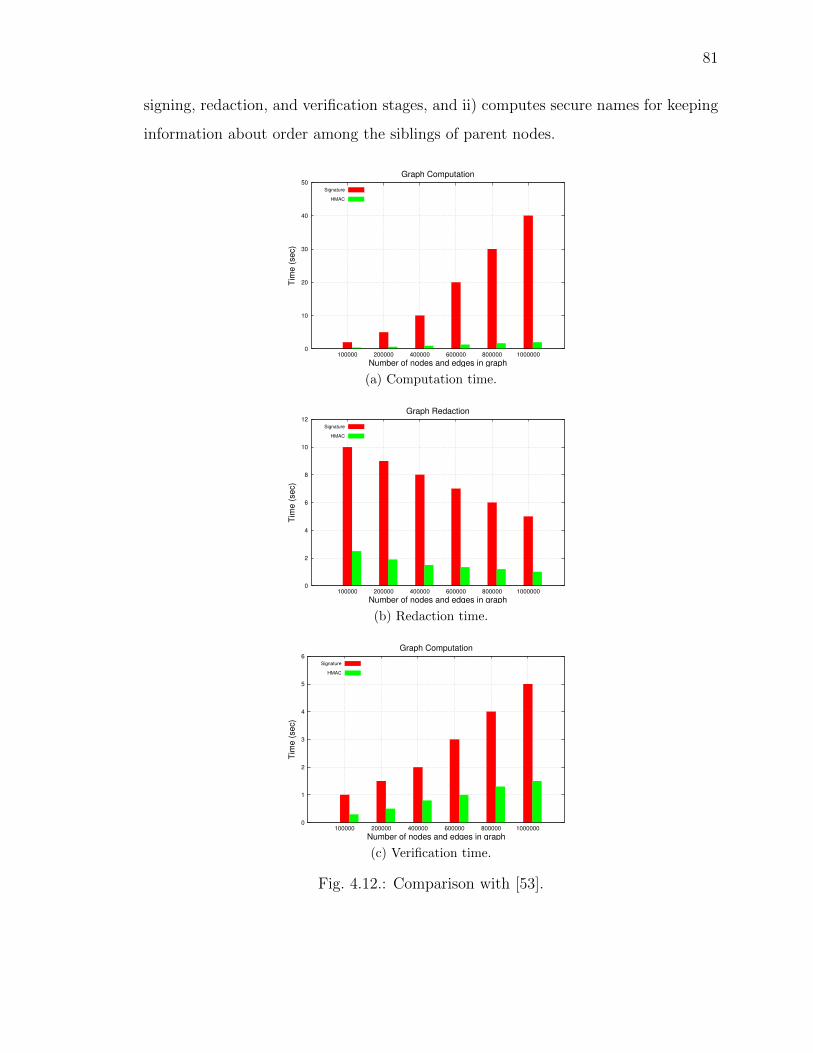
81

signing, redaction, and verification stages, and ii) computes secure names for keeping

information about order among the siblings of parent nodes.

0

10

20

30

40

50

100000 200000 400000 600000 800000 1000000

Tim

e (

sec)


Graph Computation

Signature

HMAC

(a) Computation time.

0

2

4

6

8

10

12

100000 200000 400000 600000 800000 1000000

Tim

e (

sec)


Graph Redaction

Signature

HMAC

(b) Redaction time.

0

1

2

3

4

5

6

100000 200000 400000 600000 800000 1000000

Tim

e (

sec)


Graph Computation

Signature

HMAC

(c) Verification time.

Fig. 4.12.: Comparison with [53].

82

4.7 Related Work

The problem of integrity verification of graph data and graph query result(s) is

an important problem that has been fueled by the growing applications of graph

datasets in a wide range of applications. However, integrity verification of graph data

and graph query results using HMACs has been studied for the first time in the paper.

Merkle hash trees (MHT) is one of the most widely used techniques [60] for in-

tegrity assurance of DAGs [61] and for query result verification [8]. In [56], the au-

thors define the formal security models of hashing schemes for graphs, and perfectly

collision-resistant hashing schemes for graphs. They proposed the first constructions

for general graphs that includes not only trees and graphs but also graphs with cycles

and forests. The schemes uses pre- and post-order numbers of vertices to convert

a cyclic graph into a two-level MHT (called e�cient-tree). The proposed scheme is

linear in the number of vertices and edges in the graph dataset. A structure-based

routing scheme for XML-data dissemination to users under an access control policy is

presented in [62]. The scheme proposes the notion of encrypted post-order numbers

to support the integrity and confidentiality requirements of XML content. [63] pro-

poses an integrity assurance technique referred to as ‘structural signatures scheme’ for

trees in order to compute signatures of redactable subtrees. The scheme is based on

the structure of the tree as defined by tree traversals (pre-order, post-order, in-order)

and is defined using a randomized notion of such traversal numbers. With respect

to MHT, it incurs comparable cost for signing the trees and incurs lower cost for

user-side integrity verification. However, (1) a formal security model for the proposed

scheme is not given, and (2) it is quite expensive in terms of the number of signatures

computed, which are linear in the size of the tree/graph. [64] proposes a formal model

for the notion of structural signatures for trees and have given a construction for the

authentication of subtrees, which is linear in the number of nodes and quadratic in

the number of siblings per node.

83

We have proposed two HMAC based data integrity verification schemes for graph

and redacted graphs; we give formal definitions and show our schemes are linear in

the number of vertices and edges in the graphs. [65] proposes two schemes on how

to authenticate DAGs and directed cyclic graphs without leaking, which are the first

such schemes in the literature. The schemes are based on the structure of graph as

defined by DFS traversals and aggregate signatures (Computational Di�e-Hellman

problem). The schemes minimize the number of authentication units that a user must

receive in order to perform verification to O(1). The security of such schemes is based

on the security of cryptographic hash function (random oracles) and aggregate sig-

natures. [53] proposed a formal security model for leakage-free redactable signatures

(LFRS) that is general enough to address authentication of not only trees but also

graph and forests (disconnected trees/graphs). They also formally define the notion

of secure names, which felicitate verification of ordering between sibling/nodes. Their

proposed construction has linear complexity and outputs only one signature (optimal)

that is stored, transmitted and used for authentication of a tree, graph and forest.

[66] describe integrity and confidentiality preserving schemes for a DAG model of

provenance database. Digital signature are used to sign the nodes and the relation-

ships between them. An access control model based on paths on the provenance graph

is proposed to preserve confidentiality of the nodes and edges in the provenance graph

Fan et al. [8] present a framework for authentication of subgraph query services in out-

sourced graph databases. They propose an index Interaction-aware Feature-subgraph

Tree (IFTree) to minimize I/O cost associated with filtering-and-verification require-

ment for processing subgraph query. In addition, IFTree is extended to authenticate

subgraph query. The proposed extension is called MIFTree.

Digital signatures support not only integrity of data but also security properties

like authentication of data source and non-repudiation [54]. However, in many prac-

tical contexts, data protection requirements include only integrity verification of data

as other properties of digital signatures incur additional costs. To that end, MACs

have been developed for integrity verification as they have been shown to be more

84

faster than RSA digital signatures [54]. There has been no wok on HMACs for graph

data and graph query result(s). Therefore, the focus of this paper is to develop the

notion of HMACs for graphs and graph query results. The proposed schemes exploit

the security properties of XOR operator (especially when applied a key (k, r), one-

way hash functions, and DFS traversal of graphs) in an e�cient yet provable manner.

We provide formal definitions and constructions for the proposed schemes, and our

experimental results in Section 4.6 corroborate that our schemes are more e�cient

than previously proposed digital signature-based schemes.

4.8 Summary

Graphs are used for representing and understanding objects and their relation-

ships for numerous applications. Graph databases are being used for managing sev-

eral types of linked data. Some leading examples include social networks, biological

networks, semantic Web, XML documents, and financial databases. However, the ex-

isting integrity assurance schemes for such data are neither scalable nor e�cient – such

schemes for graph data are based on digital signature schemes. In this paper, we have

proposed two e�cient integrity verification schemes – the first HMAC-based schemes

for graphs and query results for graphs. The schemes exploit the security properties

of � operator (especially when applied with a key (k, r), one-way hash functions, and

depth-first traversal of graphs) in an e�cient yet provable manner. The schemes rely

on the local/global integrity verifiers of vertices and edges. The proposed schemes can

prove to satisfy the security requirement in terms of structural/attribute modification

to the graphs and redacted graphs. Our schemes are linear in the number of vertices

and edges in the graphs, i.e., they have optimal complexity. We compute one HMAC

value for gHMAC scheme and two other verification objects for redaction for rgHMAC

scheme that are shared with the verifier. Therefore, our scheme is e�cient both in

processing time for query result and verification object transmission to the user. Our

experiments show that HMAC-based schemes are e�cient as compared to the digital

85

signature-based schemes for same size of graphs. Moreover, computing HMACs for

graphs as large as 8 million vertices and edges takes as little as 55 milliseconds.

86

5. CONCLUSIONS

Section 5.1 summarizes the research contributions of this dissertation, Section 5.2

discusses the limitations of proposed methodologies, and and Section 5.3 proposes

directions for the future research work.

5.1 Summary of Contributions

This dissertation addresses two notable challenges for graph databases; i) how to

ensure users’ privacy in published graph data under access control policy enforcement,

and ii) how to verify the integrity and query results of graph datasets under both two-

party and third-party data distribution environments.

To address the first challenge, a graph data publishing framework has been pro-

posed that provides safeguard against data privacy breach through anonymization

while enforcing access rules to satisfy the security protection requirements specified

by the data publisher. We prove that the design of this framework poses a conflicting

goal between privacy and access control. We formulate the privacy and access con-

straints on graph data as the k-anonymous bi-objective graph partitioning (k-BGP)

problem. We show that the problem is NP-complete and provide new heuristic solu-

tions. To the best of our knowledge, this is the first scheme that studies the interplay

between RBAC policy constraints and privacy protection for graph data.

To address the second challenge, a cryptographic security model based on Hash

Message Authentication Codes (HMAC) has been proposed. The model ensures in-

tegrity and completeness verification of data and query results under both two-party

and third-party data distribution environments. Unique solutions based on HMACs

for integrity verification of graph datasets are developed and detailed security analy-

87

sis of the proposed schemes is provided. Extensive experimental evaluation has been

conducted to illustrate the performance of the proposed algorithms.

5.2 Limitations of the Proposed Methodologies

For the research presented in this dissertation, we have made several assumptions

regarding the database environment which in practical life may need to be overcome

in order to develop viable solutions for privacy, access control, and integrity for graph

databases. Some of the limitations and assumptions include the following: We have

made the assumption that the data graph model is static. However, this assumption

may not hold for several application areas as mentioned in Chapter 1. For example,

OSNs can change and evolve frequently over time. Such dynamic changes in graph

databases are not addressed in our research methodology.

The privacy-enhanced access control mechanism presented in Chapter 3 assumes

a relaxed access control policy. The interaction between privacy and strict access

control policy has not been addressed in our work.

For the integrity verification schemes for graph databases and query results pre-

sented in Chapter 4, we do not assume any access control mechanism and primarily

focus on integrity verification of problem. In reality access control mechanism is gen-

erally an added layer of security in addition to integrity verification system. The

interaction between integrity and access control methods has not been discussed in

this dissertation.

5.3 Future Work

Below we provide some directions for future work.

88

5.3.1 A Privacy Mechanism for Access-Controlled Dynamic Graph Databases

In a dynamic scenario, the graph structure may need to be updated because of the

addition or removal of vertices and edges. Adding or removing new information while

simultaneously meeting the privacy and access control requirements is a challenge

that requires further research.

Employing a strict access control policy instead of a relaxed access control policy

for a shared role workload requires the dataset to be partitioned into two types of

groups: i) shared data region, and ii) non-shared data region. However, generating k-

anonymous partitions for both these groups separately requires developing intelligent

partitioning schemes to address corner cases due to non-uniform partitions being

generated. This is a challenge that requires further research.

5.3.2 Integrity Verification for Dynamic Graph Databases

In a dynamic scenario, the graph structure may need to be updated because of ad-

dition or removal of vertices and edges. Adding or removing new information requires

re-computing the integrity value for the updated graph database. Re-computing a

new integrity value by just considering the added or removed vertices and edges is

a challenge that requires further research. Moreover, the VO value may not remain

valid and drastically impact the security guarantees for updated query results. Re-

computing a new VO value by by just considering the added or removed vertices and

edges is a challenge that requires further research

The VO computation may not be possible under an access control policy enforce-

ment as a role is not able to see data beyond its privilege set.

89

5.3.3 Aggregation-based Schemes for Graph Data Integrity

The integrity verification schemes for graph databases and query results presented

in Chapter 4 consider the whole graph for computing the integrity value. Computing

the integrity of an aggregated graph is a challenge that requires further research.

Our proposed integrity verification schemes have linear time complexity O(V +E).

Developing sub-linear time complexity algorithms for large graph databases that do

not need to consider the whole graph for integrity verification is a challenge that

requires further research.

REFERENCES

90

REFERENCES

[1] H. Zakerzadeh, C. C. Aggarwal, and K. Barker, “Big graph privacy,” in Proc. ofthe Workshops of the EDBT/ICDT, 2015, pp. 255–262.

[2] J. Casas-Roma, J. Herrera-Joancomartı, and V. Torra, “A survey of graph-modification techniques for privacy-preserving on networks,” Artificial Intelli-gence Review, pp. 1–26, 2016.

[3] X. Wu, X. Ying, K. Liu, and L. Chen, “A survey of privacy-preservation ofgraphs and social networks,” in Managing and Mining Graph Data. Springer,2010, pp. 421–453.

[4] L. Backstrom, C. Dwork, and J. Kleinberg, “Wherefore art thou r3579x?:anonymized social networks, hidden patterns, and structural steganography,”in Proc. of Int’l Conf. on World Wide Web (WWW), 2007, pp. 181–190.

[5] E. Bertino and R. Sandhu, “Database security-concepts, approaches, and chal-lenges,” IEEE Trans. on Dependable and Secure Computing, vol. 2, no. 1, pp.2–19, 2005.

[6] A. Narayanan and V. Shmatikov, “De-anonymizing social networks,” in IEEESymp. on S & P, 2009, pp. 173–187.

[7] S. Ji, W. Li, P. Mittal, X. Hu, and R. Beyah, “Secgraph: A uniform and open-source evaluation system for graph data anonymization and de-anonymization,”in 24th USENIX Security Symposium (USENIX Security 15), 2015, pp. 303–318.

[8] Z. Fan, Y. Peng, B. Choi, J. Xu, and S. S. Bhowmick, “Towards e�cient au-thenticated subgraph query f in outsourced graph databases,” IEEE Trans. onServices Computing, vol. 7, no. 4, pp. 696–713, 2014.

[9] M. J. Atallah, Y. Cho, and A. Kundu, “E�cient data authentication in anenvironment of untrusted third-party distributors,” in Proc. of Int’l Conf. onData Eng. (ICDE), 2008, pp. 696–704.

[10] H. Hacigumus, B. Iyer, and S. Mehrotra, “Providing database as a service,” inProc. of Int’l Conf. on Data Eng. (ICDE), 2002, pp. 29–38.

[11] A. Amazon, “Amazon web services,” Available in: http:// aws.amazon.com/ es/ec2/ (November 2012), 2010.

[12] A. J. Feldman, A. Blankstein, M. J. Freedman, and E. W. Felten, “Privacy andintegrity are possible in the untrusted cloud.” IEEE Data Eng. Bull., vol. 35,no. 4, pp. 73–82, 2012.

[13] D. Menasce et al., “Qos issues in web services,” IEEE Internet Computing, vol. 6,no. 6, pp. 72–75, 2002.

91

[14] M. L. Yiu, E. Lo, and D. Yung, “Authentication of moving knn queries,” in Proc.of Int’l Conf. on Data Eng. (ICDE), 2011, pp. 565–576.

[15] L. Sweeney, “k-anonymity: A model for protecting privacy,” Int’l Journal ofUncertainty, Fuzziness and Knowledge-Based Systems, vol. 10, no. 05, pp. 557–570, 2002.

[16] A. Campan and T. M. Truta, “Data and structural k-anonymity in social net-works,” in Privacy, Security, and Trust in KDD. Springer, 2009, pp. 33–54.

[17] M. Hay, G. Miklau, D. Jensen, D. Towsley, and P. Weis, “Resisting structuralre-identification in anonymized social networks,” Proc. of the VLDB Endow.(PVLDB), vol. 1, no. 1, pp. 102–114, 2008.

[18] E. Zheleva and L. Getoor, “Preserving the privacy of sensitive relationships ingraph data,” in Privacy, Security, and Trust in KDD. Springer, 2008, pp.153–171.

[19] K. LeFevre, D. J. DeWitt, and R. Ramakrishnan, “Mondrian multidimensionalk-anonymity,” in Proc. of IEEE 22nd Int’l Conf. on Data Eng. (ICDE), 2006,pp. 25–25.

[20] S. Chaudhuri, T. Dutta, and S. Sudarshan, “Fine grained authorization throughpredicated grants,” in Proc. of IEEE 23rd Int’l Conf. on Data Eng. (ICDE),2007, pp. 1174–1183.

[21] S. Rizvi, A. Mendelzon, S. Sudarshan, and P. Roy, “Extending query rewritingtechniques for fine-grained access control,” in Proc. ACM Int’l Conf. Manage-ment of Data (SIGMOD), 2004, pp. 551–562.

[22] S. Contini and Y. L. Yin, “Forgery and partial key-recovery attacks on hmacand nmac using hash collisions,” in Advances in Cryptology–ASIACRYPT 2006.Springer, 2006, pp. 37–53.

[23] T. Dierks and C. Allen, “RFC 2246: The TLS protocol version 1.0,” 1999.

[24] D. Harkins, D. Carrel et al., “The internet key exchange (IKE),” RFC 2409,november, Tech. Rep., 1998.

[25] D. M’Raihi, M. Bellare, F. Hoornaert, D. Naccache, and O. Ranen, “Hotp: Anhmac-based one-time password algorithm,” Tech. Rep., 2005.

[26] J. Katz and Y. Lindell, Introduction to modern cryptography. CRC Press, 2014.

[27] M. Bellare, R. Canetti, and H. Krawczyk, “Pseudorandom functions revisited:The cascade construction and its concrete security,” in Symp. on Foundations ofComputer Science (FOCS), 1996, pp. 514–523.

[28] H. Krawczyk, M. Bellare, and R. Canetti, “RFC 2104: HMAC: Keyed-hashingfor message authentication,” 1997.

[29] S. Chaudhuri, R. Kaushik, and R. Ramamurthy, “Database access control andprivacy: Is there a common ground?” in CIDR, 2011, pp. 96–103.

[30] R. Sayaf and D. Clarke, “Access control models for online social networks,” SocialNetwork Engineering for Secure Web Data and Services, pp. 32–65, 2012.

92

[31] D. F. Ferraiolo, R. Sandhu, S. Gavrila, D. R. Kuhn, and R. Chandramouli, “Pro-posed NIST standard for role-based access control,” ACM Trans. on Informationand Syst. Security (TISSEC), vol. 4, no. 3, pp. 224–274, 2001.

[32] R. Baden, A. Bender, N. Spring, B. Bhattacharjee, and D. Starin, “Persona:an online social network with user-defined privacy,” in Proc. ACM SIGCOMM,2009, pp. 135–146.

[33] T. Wang, M. Srivatsa, and L. Liu, “Fine-grained access control of personal data,”in Proc. of ACM Symp. on Access Control Models and Technologies (SACMAT),2012, pp. 145–156.

[34] G. Ghinita, P. Karras, P. Kalnis, and N. Mamoulis, “Fast data anonymizationwith low information loss,” in Proceedings of the 33rd International Conferenceon Very Large Data Bases, University of Vienna, Austria, September 23-27,2007, 2007, pp. 758–769.

[35] K. LeFevre, D. J. DeWitt, and R. Ramakrishnan, “Workload-aware anonymiza-tion techniques for large-scale datasets,” ACM Trans. on Database Syst. (TODS),vol. 33, no. 3, p. 17, 2008.

[36] M. E. Nergiz and C. Clifton, “Thoughts on k-anonymization,” Data & KnowledgeEngineering, vol. 63, no. 3, pp. 622–645, 2007.

[37] V. S. Iyengar, “Transforming data to satisfy privacy constraints,” in Proc. ACMSIGKDD, 2002, pp. 279–288.

[38] Z. Pervaiz, W. G. Aref, A. Ghafoor, and N. Prabhu, “Accuracy-constrainedprivacy-preserving access control mechanism for relational data,” IEEE Trans.on Knowledge and Data Eng., vol. 26, no. 4, pp. 795–807, 2014.

[39] J. H. Friedman, J. L. Bentley, and R. A. Finkel, “An algorithm for finding bestmatches in logarithmic expected time,” ACM Trans. on Mathematical Software(TOMS), vol. 3, no. 3, pp. 209–226, 1977.

[40] T. Tassa and D. J. Cohen, “Anonymization of centralized and distributed socialnetworks by sequential clustering,” IEEE Trans. on Knowledge and Data Eng.,vol. 25, no. 2, pp. 311–324, 2013.

[41] V. Ayala-Rivera, P. McDonagh, T. Cerqueus, and L. Murphy, “A systematiccomparison and evaluation of k-anonymization algorithms for practitioners,”Transactions on Data Privacy, vol. 7, no. 3, pp. 337–370, 2014.

[42] M. Yuan, L. Chen, and P. S. Yu, “Personalized privacy protection in socialnetworks,” Proc. of the VLDB Endow. (PVLDB), vol. 4, no. 2, pp. 141–150,2010.

[43] B. Zhou and J. Pei, “Preserving privacy in social networks against neighborhoodattacks,” in Proc. of IEEE 28th Int’l Conf. on Data Eng. (ICDE), 2008, pp.506–515.

[44] K. Liu and E. Terzi, “Towards identity anonymization on graphs,” in Proc. ACMInt’l Conf. Management of Data (SIGMOD), 2008, pp. 93–106.

93

[45] L. Zou, L. Chen, and M. T. Ozsu, “K-automorphism: A general framework forprivacy preserving network publication,” Proc. of the VLDB Endow. (PVLDB),vol. 2, no. 1, pp. 946–957, 2009.

[46] J. Cheng, A. W.-c. Fu, and J. Liu, “K-isomorphism: privacy preserving networkpublication against structural attacks,” in Proc. ACM Int’l Conf. Managementof Data (SIGMOD), 2010, pp. 459–470.

[47] S. Bhagat, G. Cormode, B. Krishnamurthy, and D. Srivastava, “Class-basedgraph anonymization for social network data,” Proc. of the VLDB Endow.(PVLDB), vol. 2, no. 1, pp. 766–777, 2009.

[48] C. Dwork, “Di↵erential privacy: A survey of results,” in Int’l Conf. on Theoryand Applications of Models of Computation. Springer, 2008, pp. 1–19.

[49] P. Mittal, C. Papamanthou, and D. X. Song, “Preserving link privacy in socialnetwork based systems,” in 20th Annual Network and Distributed System Se-curity Symposium, NDSS 2013, San Diego, California, USA, February 24-27,2013, 2013.

[50] C. Clifton and T. Tassa, “On syntactic anonymity and di↵erential privacy,”Trans. Data Privacy, vol. 6, no. 2, pp. 161–183, 2013.

[51] H. V. Jagadish and F. Olken, “Database management for life sciences research,”SIGMOD Rec., vol. 33, no. 2, pp. 15–20, 2004.

[52] Y. Zhou, H. Cheng, and J. X. Yu, “Graph clustering based on struc-tural/attribute similarities,” Proc. of VLDB Endow. (PVLDB), vol. 2, no. 1,pp. 718–729, 2009.

[53] A. Kundu, M. J. Atallah, and E. Bertino, “E�cient leakage-free authenticationof trees, graphs and forests.” IACR Cryptology ePrint Archive, vol. 2012, p. 36,2012.

[54] W. E. Freeman and E. L. Miller, “An experimental analysis of cryptographicoverhead in performance-critical systems,” in Proc. of Int’l Symp. on Model-ing, Analysis and Simulation of Computer and Telecommunication (MASCOTS),1999, pp. 348–357.

[55] T. H. Cormen, C. E. Leiserson, R. L. Rivest, and C. Stein, Introduction toAlgorithms, 3rd Ed. MIT Press, 2009.

[56] M. U. Arshad, A. Kundu, E. Bertino, K. Madhavan, and A. Ghafoor, “Securityof graph data: hashing schemes and definitions,” in Proc. of ACM Conf. on Dataand Application Security and Privacy (CODASPY), 2014, pp. 223–234.

[57] R. C. Merkle, “A certified digital signature,” in CRYPTO, 1989, pp. 218–238.

[58] C. Martel, G. Nuckolls, P. Devanbu, M. Gertz, A. Kwong, and S. G. Stubblebine,“A general model for authenticated data structures,” Algorithmica, vol. 39, pp.21–41, 2004.

[59] Z. Fan, B. Choi, Q. Chen, J. Xu, H. Hu, and S. S. Bhowmick, “Structure-preserving subgraph query services,” IEEE Trans. Knowl. Data Eng., vol. 27,no. 8, pp. 2275–2290, 2015.

94

[60] R. C. Merkle, “A certified digital signature,” in CRYPTO, 1989, pp. 218–238.

[61] C. Martel, G. Nuckolls, P. Devanbu, M. Gertz, A. Kwong, and S. G. Stubblebine,“A general model for authenticated data structures,” Algorithmica, vol. 39, no. 1,pp. 21–41, 2004.

[62] A. Kundu and E. Bertino, “Secure dissemination of XML content using structure-based routing,” in Int’l Conf. on Enterprise Distributed Object Computing(EDOC), 2006, pp. 153–164.

[63] ——, “Structural signatures for tree data structures,” Proc. of the VLDB Endow.(PVLDB), vol. 1, no. 1, pp. 138–150, 2008.

[64] C. Brzuska, H. Busch, O. Dagdelen, M. Fischlin, M. Franz, S. Katzenbeisser,M. Manulis, C. Onete, A. Peter, B. Poettering, and D. Schroder, “Redactablesignatures for tree-structured data: Definitions and constructions,” in Int’l Conf.on Applied Cryptography and Network Security (ACNS), 2010, pp. 87–104.

[65] A. Kundu and E. Bertino, “How to authenticate graphs without leaking,” in Int’lConf. on Extending Database Technology (EDBT), 2010, pp. 609–620.

[66] A. Syalim, T. Nishide, and K. Sakurai, “Preserving integrity and confidential-ity of a directed acyclic graph model of provenance,” in Data and ApplicationsSecurity and Privacy XXIV. Springer, 2010, pp. 311–318.

[67] M. E. Dyer and A. M. Frieze, “Planar 3DM is NP-complete,” Journal of Algo-rithms, vol. 7, no. 2, pp. 174–184, 1986.

[68] P. Rosenstiehl and R. E. Tarjan, “Rectilinear planar layouts and bipolar orien-tations of planar graphs,” Discrete & Computational Geometry, vol. 1, no. 1, pp.343–353, 1986.

[69] N. Mamoulis and D. Papadias, “Selectivity estimation of complex spatialqueries,” in Int’l Symp. on Spatial and Temporal Databases. Springer, 2001,pp. 155–174.

[70] Y. Tao, J. Sun, and D. Papadias, “Analysis of predictive spatio-temporalqueries,” ACM Trans. on Database Syst. (TODS), vol. 28, no. 4, pp. 295–336,2003.

APPENDICES

95

A: Proof of Theorem 3.3.1

Proof of Theorem 3.3.1: To prove this theorem, we use Theorem 3.1 [38] and need to

first prove that Planer k-anonymous Graph Partitioning with Minimal ILS(P)(Planar

AGPMIL, for short) is NP-hard. The proof of Theorem 3.3.1 will follow as a direct

consequence of above two proofs.

First, we state that the AGPMIL is NP-hard in the plane, and then generalize

this result to the multidimensional Euclidean space.

PLANAR k-ANONYMOUS GRAPH PARTITIONINGWITH MINIMUM

ILS(P)(Planar AGPMIL)

INSTANCE: A planar graph G with a set X of n points/vertices in the plane; an

integer k, n > k.

QUESTION: Is there a clustering of X into a set of non-overlapping partitions

P = {P1, . . . , PM} such that |Pi| � k, and the structural information loss ILS(P)

minimal?

Our NP-completeness proof of (Planar AGPMIL) is based on reduction from the

following special version of the exact cover problem that is shown to be NP-complete

by Dyer and Frieze [67].

PLANAR EXACT COVER BY 3-SETS (Planar X3C)

INSTANCE:

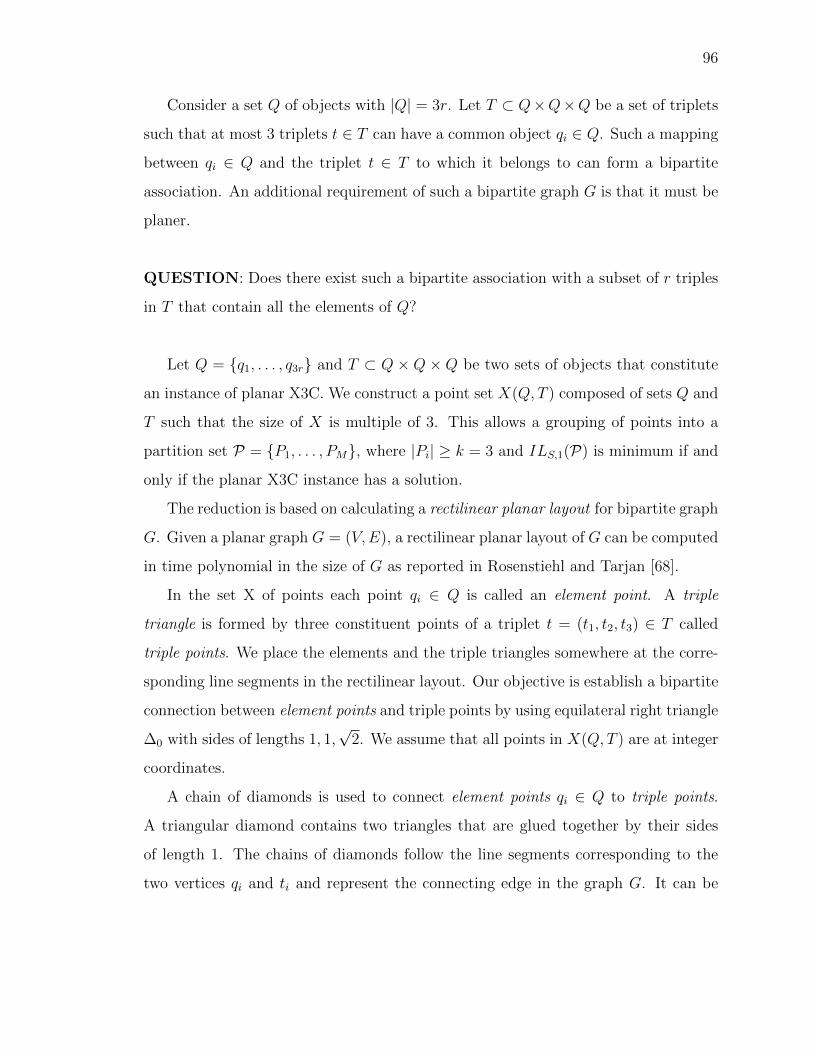
96

Consider a set Q of objects with |Q| = 3r. Let T ⇢ Q⇥Q⇥Q be a set of triplets

such that at most 3 triplets t 2 T can have a common object qi 2 Q. Such a mapping

between qi 2 Q and the triplet t 2 T to which it belongs to can form a bipartite

association. An additional requirement of such a bipartite graph G is that it must be

planer.

QUESTION: Does there exist such a bipartite association with a subset of r triples

in T that contain all the elements of Q?

Let Q = {q1, . . . , q3r} and T ⇢ Q ⇥ Q ⇥ Q be two sets of objects that constitute

an instance of planar X3C. We construct a point set X(Q, T ) composed of sets Q and

T such that the size of X is multiple of 3. This allows a grouping of points into a

partition set P = {P1, . . . , PM}, where |Pi| � k = 3 and ILS,1(P) is minimum if and

only if the planar X3C instance has a solution.

The reduction is based on calculating a rectilinear planar layout for bipartite graph

G. Given a planar graph G = (V,E), a rectilinear planar layout of G can be computed

in time polynomial in the size of G as reported in Rosenstiehl and Tarjan [68].

In the set X of points each point qi 2 Q is called an element point. A triple

triangle is formed by three constituent points of a triplet t = (t1, t2, t3) 2 T called

triple points. We place the elements and the triple triangles somewhere at the corre-

sponding line segments in the rectilinear layout. Our objective is establish a bipartite

connection between element points and triple points by using equilateral right triangle

�0 with sides of lengths 1, 1,p2. We assume that all points in X(Q, T ) are at integer

coordinates.

A chain of diamonds is used to connect element points qi 2 Q to triple points.

A triangular diamond contains two triangles that are glued together by their sides

of length 1. The chains of diamonds follow the line segments corresponding to the

two vertices qi and ti and represent the connecting edge in the graph G. It can be

97

q1! q2!

q3!

q1!

q5 q6

q1! q2!

q3!

q4!q5!

q6

q4!

q6!q5

(a)

q1! q2!

q3!

q1!

q5! q6!

q1! q2!

q3!

q4!

q6!q5!

q4!

q6!q5!

(b)

Fig. 1.: Partition into triangles di↵erent cases: (a) All graph vertices included inshaded partitions, solution to X3C exists; (b) Some graph vertices not included inshaded partitions, solution to X3C does not exist.

easily checked that this construction can be performed in polynomial time and |X| ismultiple of 3.

We assume that an enlarging procedure has been used on the rectilinear layout of

graph G by multiplying all coordinates with a large positive integer. This ensures

i) two distinct chains are generated su�ciently away from each other, and ii) an

element point and its corresponding triple points can be connected exactly by a chain

of diamonds.

We now prove that the set of points X(Q, T ) can be partitioned into P =

{P1, . . . , PM}, such that |Pi| � k and the ILS,1(P) is minimum if and only if Planar

X3C problem has a solution.

Let us consider only partitions of size 3, 4 and 5 points. Fig. 2 shows di↵erent par-

tition configurations generated with size 3, 4 and 5 points. Due to space limitation, we

do not list any other possible groups. Fig. 2(a) states that no three points in X(Q, T )

98

(a) (b) (c)

Fig. 2.: Partitions of size 3, 4 and 5 points.

are at a distance less that 1 andp2 from each other, so the minimum ILS,1(P) for a

partition with three vertices with three edges using 2|EPi |.�1 � 2|EPi

|Pi(|Pi|�1)

�= 0; Simi-

larly, for partitions of size 4, and 5 having 5 and 6 edges in Fig. 2(b) and Fig. 2(c),

respectively, the minimum ILS,1(P) can be calculated as 53 and 24

5 . Hence, it is easily

observed that the partitioning of point set X has the minimal ILS,1(Pi) = 0⇥ p = 0

if all partitions are of size 3, where p is determined by reconstruction.

Finally, we claim that the partitioning of point set X into triangles with minimum

intra-partition structural information loss ILS,1(P) is possible if and only if Planar

X3C has a solution.

(If) We assume that there exists a partitioning of points X(Q, T ) into triangles

with minimal ILS,1(P) = 0⇥ p = 0. Consider some element point qi 2 Q, contained

in exactly one partition (triangle) belonging to a chain of diamonds. Every other

triangle must form a partition, and the corresponding point ti on the other end of the

chain cannot be covered by any triangle in this chain. Therefore, the corresponding

three triple points must form another partition. However, the triangle(s) in the other

chain(s) going away from qi will cover the corresponding triple points, so these points

cannot form a partition in the partitioning. This way, we may assign to each qi 2 Q a

unique triple in T . On the other hand, if we assign one qi to some triple, the other two

elements in this triple must be assigned to this triple also. For the other paths that

99

are excluded from qi; may be they contain qj that is not contained in any other triple.

But this case cannot happen because we have a partition with minimal information

loss, each qi is in one partition (Fig. 1(a)). Obviously, this yields a solution to Planar

X3C.

(Only if) We now assume that the Planar X3C has a solution T 0 ✓ T . We

construct a partitioning as follows. As a first step, each triple is mapped to a triple

triangle as a partition in the partitioning set, while on the other hand all triples in

T \T 0 are not. This uniquely determines which triangles in the chains are part of the

partitioning. Since T 0 is a solution of Planar X3C, every element point in X(Q, T ) is

exactly in one group.

Thus, it has been have shown that partitioning of X into partitions of three points

with minimum ILS,1(P) is possible if and only if Planar X3C problem has a solution.

Therefore, the partitioning of P with |Pi| � 3 has minimum ILS,1(P) if and only if

Planar X3C problem allows a solution. This implies that the NP-complete problem

(Planar X3C) is not harder than partitioning a set of points X into partitions Pi, such

that |Pi| � 3 and ILS,1(P) is minimum. Since ILS,1(P) is due to a restricted version

of the problem (i.e., where we do not consider the inter-partition edges, |EPi,Pj | = �

) and this restricted version of problem contains a known NP-complete problem as a

special case therefore, Planar AGPMIL is NP-hard in a plane.

We can now easily extend the results to show that a partitioning ofX(Q, T ) points

into partitions Pi with |Pi| � 3 with minimum ILS(P) is NP-hard in a the Euclidean

space with dimensions � 2.

The proof of Theorem 3.3.1 now follows directly from the above theorem and

Theorem 3.1 [38]. Zahid et al. [38] prove that finding k-anonymous partitioning

with imprecision bounds is NP-complete. We have shown that k-anonymous graph

partitioning with minimum ILS(P) is NP-complete. Therefore, the decisional k-BGP

problem is NP-complete with either or both constraints.

Example 8 Suppose Q = {q1, q2, q3, q4, q5, q6} and C = {{q1, q2, q3}, {q4, q5, q6}, {q1, q5, q6}}.The solution to PX3C instance consists of {{q1, q2, q3}, {q4, q5, q6}} since these two 3-

100

element sets provide an exact cover for Q. It can be noticed from the construction in

Fig. 1(a), the solution shown by shaded triangles is the only solution to the AGPMIL

problem.

If we attempt to construct some other partition of the induced graph into disjoint

triangles (e.g., Fig. 1(b)), we end up with one or more of the q0is 2 {q1, q2, q3, q4, q5, q6}not being included in any of the shaded triangles. In other words, we do not generate

a partition with desired properties. It can be noticed from Fig. 1(b), that vertices

{q2, q3, q4} are not included in any partition.

101

B: Proof of Theorem 3.5.1

Proof We assume that the adversary A has both the structural and attribute infor-

mation as background knowledge for re-identification of a target node x. Suppose the

adversary A executes a structural query QS(x) [69] to determine the set of feasible

candidate partitions candQS(x). With no other information, the adversary A then

may choose any partition y 2 candQS(x) arbitrarily. The probability of a particular

candidate partition y for node a x, therefore, can be given as:

PrQS(y) =1

|candQS(x)|. (1)

In addition, as mentioned above, the adversary A may also have some attribute

Attr ✓ {QI1, . . . , QId} information as background knowledge for the target node x.

Given a set N of d-dimensional data points enclosed in a volume Uvol =Qd

i=1[Ui],

where [Umini , Umax

i ] is the range of domain in dimension i, the proposed algorithms

partition the data space into |P| hyper-rectangles as a result of k-anonymous par-

titioning. The adversary A may then execute a query QA to determine the fea-

sible candidate partitions candA(x). The query QA can be considered as forming

a subspace with dimension |Attr| and having volumeQ|Attr|

i=1 [Li] ⇥Q(d�|Attr|)

j=1 [Ui] ✓Uvol, Li = [Lmin

i , Lmaxi ]. The size of the set candQA(x) can be determined by com-

puting the number of partitions that intersect a query QA and is estimated as:


j=1 min⇣1, Sj+Lj

Uj

⌘according to [70], where Sj is the average length

of projections of all partitions Pj 2 P along dimensions j and Lj and Uj are the

corresponding projections for query QA and total domain space Uvol along dimen-

sion j. The probability that a partition, say Pi, intersects a query QA is given as:Q|Attr|

j=1 min⇣1, Sj+Lj

Uj

⌘, where the product term, also known as the Minkowski sum,

determines the selectivity of the query QA. It is quite intuitive that increasing the

102

dimension or the number of attributes of query QA has the e↵ect of reducing the size

of candA(x) set. The probability of a candidate y 2 cand(x) is given as follows:

PrQA(QS)(y) =1


j=1 min⇣1, Sj+Lj

Uj

⌘ . (2)

Similarly, the adversary A may first execute the query QA on P set to deter-

mine the number of feasible candidates as: candQA(x) = |P|⇥Q|Attr|

j=1 min⇣1, Sj+Lj

Uj

⌘

and then may apply the the structural query QS on candQA(x) to further refine the

candidate set.

PrQS(QA) =1

candQS(x). (3)

The disclosure-risk of a node x depends on the size of the set |cand(x)| and the

likelihood of candidates. The exact re-identification of a target node x by an adversary

A requires the identification of a single candidate partition y 2 candQ(x).

Therefore, combining equations (2) and (3), the probability of a candidate y 2candQ(x) for x is upper-bounded by:

Pr(y) max

⇢PrQS(QA)(y), P rQA(QS)(y)

�. (4)

As the total number of candidate nodes per partition is k, the probability of

successfully identifying a target node x given a candidate partition y is given as:

Pr(x|y) = 1

k. (5)

Therefore, combining Equations (4) and (5) the probability of re-identifying a

node x is given as:

Pr(Re-id(x)) 1

k⇥min

⇢PrQS(QA)(y), P rQA(QS)(y)

�.

104

VITA

Muhammad Umer Arshad was born in Nizamabad, District Gujranwala, Pakistan,

in 1980. He completed his B.Sc., and M.Sc., degrees in Electrical Engineering (EE)

from University of Engineering and Technology (UET), Lahore, Pakistan, in 2002,

and 2005, respectively. Before joining Purdue in Fall 2006, he was a Lecturer in the

EE Department of UET, Lahore. While at Purdue, he completed an MS degree in

Computer Engineering (CE) in Fall 2014. During his Ph.D., he has had the opportu-

nity to work at VMWare, Yahoo!, and EMC2 as an intern in their cloud computing

divisions. His broad research interests are in areas related to Data Infrastructure

Systems, Cloud Computing, and Information Security & Privacy.

Privacy, Access Control, and Integrity for Large Graph ...

Documents

Transcript of Privacy, Access Control, and Integrity for Large Graph ...