Initial version: January 1997 Current version: May 1997

PRICING BONDS AND BOND OPTIONS WITH DEFAULT RISK

E. Barone(*), G. Barone-Adesi(**) and Antonio Castagna(***)

SUMMARY

The pricing of bonds and bond options with default risk is analyzed in the general equilibrium model of Cox, Ingersoll, and Ross (Cir, 1985). This model is extended by means of an additional parameter in order to deal with financial and credit risk simultaneously. The estimation of such a parameter, which can be considered as the market equivalent of an agencies� bond rating, allows to extract from current quotes the market perceptions of firm�s credit risk.

The general pricing model for defaultable zero-coupon bond is derived in a simple discrete-time setting while a more rigorous treatment, in a continuous-time setting, is contained in the Appendix A. Defaultable bonds may be valued by discounting the promised terminal payoff at a default-risk-adjusted interest rate, i.e. the risk-free rate plus a default-risk premium, or by discounting the ex-pected terminal payoff at a risk-free interest rate.

The availability of an integrated model allows for the pricing of default-free options written on defaultable bonds and of vulnerable options written either on default-free bonds or defaultable bonds. Valuation is performed under different contractual provisions dealing with the event of de-fault: their impact on options prices is investigated and several numerical examples are given.

A comparison between our results and those given by Jarrow and Turnbull (1995) is also pre-sented.

CONTENTS

1. INTRODUCTION 1

2. TWO DIFFERENT APPROACHES 2

3. DEFAULT-RISKY CONTRACTS 3

4. AN EXTENDED VERSION OF THE CIR UNIVARIATE MODEL 9 4.1 Defaultable Discount Bonds 9 4.2 Defaultable Coupon Bonds 11

5. OPTIONS ON DEFAULTABLE BONDS AND VULNERABLE OPTIONS 11 5.1 Default-free options on defaultable bonds 12

European options on risky zero-coupon bonds. 12 European options on defaultable coupon bonds. 14

5.2 Vulnerable options on (risk-free or defaultable) bonds. 15 6. AN APPLICATION 16

6.1 Bond pricing 17 Estimation 18

6.2 Options on defaultable bond 19 7. CONCLUSIONS 21

REFERENCES 22

APPENDIX A 24

APPENDIX B 31

1. INTRODUCTION

In a 1975 article on bank funds management, Fisher Black gave the following example to stress the relevance of default-risk premiums when the probability of default is high and the recovery ratio in a default is null:

For example, suppose the bank is asked to make a loan on a project whose success or failure is independent of the state of the economy. The project is the only collateral for the loan. If it succeeds, the loan will be paid back with interest. If the project fails, the entire amount loaned will be lost. There is a 2⁄3 chance that the pro-ject will succeed, and a 1⁄3 chance that the project will fail. The loan is for one year, and the one year riskless interest rate is 6 percent. The interest rate on this loan should be 59 percent plus the charge for administering the loan. If the interest rate is 59 percent, then the expected return on the loan will be 6 percent. [2⁄3 1.59 = 1.06.] Since the β of the collateral is zero, the β of the loan will be zero, and it is appropriate that its expected return be equal to the riskless interest rate.

Probabilities of default and recovery ratios may be based on past experience (historical values) or may be extracted from current market quotes (implied values).1 For example, in a historical approach based on Moody�s data for years 1970 through 1993, the probability that an issuer will default in the first year after holding the Baa rating is 0.1% while the probability that it will default by the fifth year is 1.7%.2 Besides, Moody�s has reported an average recovery rate for defaulted senior secured bonds, covering the period 1974-1994, of 53.11 percent of par. This rate reduces to 49.86 percent for senior unsecured bonds and to 32.83 percent for subordinated bonds.3

There is some evidence that, in their rating activity, the agencies stress the probability of de-fault and place little weight on the fractional loss on default.4 Whatever is the method underlying the perception of default risk by the rating agencies, their assessment is anyway discrete in grades and in time, since a limited number of bond grade categories are considered and ratings revisions are made at discrete times.5

In order to deal with financial and credit risk simultaneously, we extended the univariate Cox, Ingersoll, and Ross (Cir, 1985) model following Duffie and Singleton (1995a) and Duffie and Huang (1995), hereon D&H and D&S, respectively. In particular, we assume that market percep-tions of firm�s credit risk change continuously and that they are summarized by an additional bond-specific credit parameter that can be estimated from market quotes of risk-free and defaultable bond prices. This credit parameter can be considered as the market equivalent of an agency rating, with the notable difference that it is continuous in grade and time.

The availability of such a measure allows to evaluate interest rate derivatives dependent on de-faultable assets and Otc (vulnerable) interest rate derivatives in a way consistent with the valuation of corporate bonds.

The outline of the paper is the following. In Section 2 a brief review of the existing approaches to price corporate bonds is provided. In Section 3 the �reduced-form� approach to credit risk is de-veloped in a simple discrete-time setting and the credit spread�s economic significance is investi-gated. The results of this section are applied to the continuous-time setting of Cir model in Section 4, where the term structure of risky interest rates is derived. In Section 5 pricing formulas for default-free options written on defaultable bonds and for vulnerable options written either on risk-free or de-faultable bonds are provided, under alternative assumptions about the contractual provisions ruling the event of default. Some applications and the comparison with the Jarrow and Turnbull (1995)

1 «For our purposes, we define default as a missed interest or principal payment, filing for protection from creditors, or the completion of a distressed exchange offer where investors are forced to accept a package of securities that are of lower economic value than originally promised.» [Fons and Carty (1995, p. 35)]. 2 See Fons and Carty (1995, Figures 11-12, p. 41). 3 See Fons and Carty (1995, Table 2, p. 36). 4 See Duffie and Singleton (1995a, note 8, p.18). 5 Duffie and Singleton (1995a, p. 18): «Casual observation ... suggests that the yield spread of a given bond may fluc-tuate dramatically during periods over which it has a constant credit rating.»

- 2 -

model (hereon J&T), in Section 6, conclude the paper. Appendix A contains the model�s formal description and the proofs while Appendix B contains some tables.

2. TWO DIFFERENT APPROACHES

Two approaches have been followed in literature to evaluate defaultable claims.6 In a �structural� or �firm value� approach, the time of default, the probability of default and the expected fractional loss on default are modeled considering the stochastic processes for the firm�s assets and liabilities. In a �reduced-form� or �hazard rate� approach the event �default� is directly modeled.

The �structural� approach views credit-risky securities as compound options on the firm�s as-sets.7 More specifically, the �structural� approach defines the event of default as �the first time the market value of the obligor�s assets falls below the market value of his liabilities�.8 Assets and li-abilities are modeled as diffusion processes observable by investors. This setup has been originally put forward by Black and Scholes (1973), Merton (1974), Black and Cox (1976). In particular, these authors assumed that the term structure of (default-free) interest rates is deterministic (and flat). Extensions and refinements of Merton�s model are given by Black and Cox (1976), Lee (1981), Pitts and Selby (1983) and lastly by Leland (1994), Longstaff and Schwartz (1995) and Leland and Toft (1996).9

The structural approach is difficult to implement. First, the issuer�s assets and liabilities are of-ten not traded in financial markets, so that their value is not directly observable and the estimation of the relevant parameters becomes problematic. Second, under this approach, corporate debt must be valued simultaneously with every other senior liability of the firm. Therefore, it is computationally very demanding. Third, it could be impractical to deal with corporate-level data when one has to analyse many bonds issued by different firms.

The second approach treats the event of default in a �reduced-form�. Instead of trying to model the process of the entire capital structure of the firm, the default time is directly modeled as an un-predictable event (namely a Poisson process) which can occur according to a given hazard rate. The �reduced-form� approach can be a good alternative to the �structural� approach for several reasons: it is more tractable and easy to implement than the latter, especially when the issuer�s balance sheet is not so simplified as in theory. Second, as pointed out by Duffie and Singleton (1995a), «it is fre-quently inappropriate to assume ... that default is necessarily determined by comparing assets and liabilities. Some issuers default for reasons of �illiquidity�, or as is sometimes the case for sovereign debt, for general economic and political considerations».

The first contribution to the �reduced-form� approach has been given by Ramaswamy and Sundaresan (1986), who assumed that i) defaultable bonds can be valued by discounting the prom-ised pay-off using risk-adjusted interest rates and that ii) the instantaneous default risk premium fol-lows a mean-reverting square root process.10 D&H (1995) and D&S (1995a) formally justified the assumption of discounting promised payments using risk-adjusted interest rates.11 Madan and Unal (1994) and J&T (1995a,b) also contributed to the �reduced-form� approach.

This paper follows the lines of the model by D&S (1995a) and D&H (1995). Such a model, be-ing similar to those commonly used to price risk-free bonds and derivatives, allows for an easy

6 Cooper and Mello (1995) developed a model that shows the equivalence of the two approaches. 7 In this paper we use the term �risky� and �defaultable� interchangeably, in both cases referring to a claim whose issuer may default. Thus the term �risk�, when it is not differently defined, should be intended as �credit risk�. 8 In some cases a default-trigger value of the assets is defined as a function of the firm�s liabilities. 9 See also Ho and Singer (1982), Johnson and Stulz (1987), Chance (1990), Cooper and Mello (1991), Hull and White (1995a,b,c). 10 The case for mean-reversion is given by Fama (1986) whose results show that credit spreads in money market in-struments are related to the stage of the business cycle. 11 The formal justification of the adjusted-short rate model, given by Duffie and Singleton (1995a) either in a simple discrete setting (Section 4) or in a general setting (Appendix A), seems not to give support to the critique formulated by J&T (1995a, note 1) to the approach followed by Ramaswamy and Sundaresan (1986).

- 3 -

evaluation of defaultable claims.12 In its first version, bankruptcy may be dealt with by adding a con-stant spread to the risk-free instantaneous rate; in the second version, the spread is assumed to de-pend on the instantaneous rate, so that the probability of default is modelled by directly imposing a stochastic process to the resulting risk-adjusted interest rate. The other model�s assumptions are the following: i) the occurrence of default causes a sudden loss of a given fraction of the claim�s market value; ii) the residual value is immediately paid by the party whom the value of the claim is negative to; iii) the price process falls to 0 and stops.

Some other studies, such as Jarrow, Lando and Turnbull (1994) and J&T (1995a), alternatively assume that, after deafult, the creditors are paid (at the natural maturities) a fractional recovery of the par value of the promised payments. Therefore, J&T�s approach does not consider the so-called �ac-celeration clause�, whose application involves the �acceleration� of claims in the sense that all firm�s debt becomes immediately payable.13

In order to price credit-risky securities, J&T use a forex currency analogy:14 a defaultable bond (or more generally a contingent claim) is considered equal to a foreign security whose value is con-verted into the domestic currency by an exchange rate which may vary between 0 (default & null re-covery ratio) and 1 (no default or default & unit recovery ratio).

Bankruptcy is treated by exogenously imposing a given probability distribution for the ex-change rate at the time of default. If factors affecting the value of the claim and factors affecting the time of default are independent, then the value of a defaultable bond is given by the product between the price of the corresponding risk-free bond and the �exchange rate�. This property flows from the fact that, when assuming independence between defaults and values, the expected value of a product (default by value of the claim) is equal to the product of the expected values.

In the J&T model, the residual ex-default value of a bond is supposed to be paid only at its natural expiration. As a consequence: i) the price process does not stop on bankruptcy but it goes on after a downward shift; ii) the exchange rate becomes constant and equal to the recovery ratio; iii) the value of the default-risky bond is equal to the price of the risk-free bond times the recovery ratio.

J&T obtained closed-form formulas for default-risky bonds and vulnerable European call op-tions written either on risk-free or risky zero-coupon bonds; they also obtained a closed-form solu-tion for the value of a default-free European call option written on a risky zero-coupon bond as a lin-ear combination of the value of two distinct European options on otherwise identical default-free bonds.15

In the next sections we assume a constant default risk premium and derive pricing formulas for default-free European options written on risky bonds and for vulnerable European options written either on risk-free or risky bonds.

3. DEFAULT-RISKY CONTRACTS

Following Hull and White (1995b), default-risky contracts may be split in three classes:

1. Default-free contracts written on credit-risky underlying assets (e.g. exchange-traded options on a corporate bond);

12 D&S (1995a) provided closed-form formulas for risky bonds, either assuming a constant default risk premium or an interest rate dependent premium. D&H (1995) have shown how to price an interest-rate swap when both parties can default: in this case the adjusted interest-rate is of a switching type, depending on the value of the contract at any time during the life of the swap itself. A similar switching type adjusted interest rate can be used to discount the pay-off of any claim (e.g. forwards) whose value may be either positive or negative to both parties during the contractual life. 13 J&T (1995, note 7, p. 58) defend the generality of their approach: «This acceleration of debt can be partially incor-porated into our model by recognizing that different risk classes of debt within the same firm can have different re-covery rates at different times (δt�s). δt can be greater for those classes of debt that would receive larger payoffs at different times due to acceleration.» 14 J&T (1995a, p.56): «The foreign currency analogy is useful because foreign currency option pricing techniques are well-understood ... and these same techniques can now be applied in a modified form to price derivatives involving credit risk.» 15 J&T (1995a, p.78): «This result is important because it allows one to compute option values on risky debt using software developed for riskless debt.»

- 4 -

2. Credit-risky contracts written on default-free underlying assets (e.g. interest-rate swaps); 3. Credit-risky contracts written on credit-risky underlying assets (e.g. embedded options in a cor-

porate bond).

Table 1 gives the entire set of combinations between (risk-free or risky) obligors and (risk-free or risky) underlying assets, while enumerating some examples for each case.

For all these contracts, the expected loss in the event of default depends on:

a) The no-default value of the contract;16 b) The recovery ratio.

In what follows we describe, in an intuitive way, the general pricing model for valuing corporate bonds: it can be useful also to price other kinds of risky contracts as we will see in next sections. We show why replacing the risk-free discount rate with a default risk-adjusted interest rate is justified when defaultable claims have to be priced. An important assumption that is generally made is the following:

Assumption 1: The state variables determining the values of the underlying asset and the state vari-ables determining the occurrence of defaults and the fractional recovery thereof are independent.17

To keep things simple, we start the analysis in a discrete-time setting. Let J be the t-time value of a default-risky claim which pays the sum X at maturity T; the interval [t, T] is divided in m periods of length ∆t.

Assumption 2: The issuer�s default is supposed to be an unpredictable event which can occur at a risk-neutral (annual) hazard rate equal to h. This means that, over the interval ∆t, the (conditional risk-neutral) probability of default is h∆t. At the default time τ, the market value of the claim is re-duced by a fractional loss equal to L and the residual value is immediately paid by the obligor.

At any time, the conditional expected rate of loss is given by s = Lh∆t, that is the loss severity times the probability of default over the next interval. Both h and L are assumed to be constant.

The price of the claim can be determined in the usual risk neutral setting: a general valuation formula is given by the sum of the expected cash flows discounted at the risk-free interest rates. In the discrete-time setting we are working in, a binomial tree can be employed for evaluation. The backward recursive procedure prices the claim in node (i, j) by discounting its expected future value at the risk-free interest rate ri, j. At time T � ∆t, the claim�s value at node (i, j) is given by

16 The party which the contract�s value is negative for has no credit exposure and bears no credit risk. In general, the exposure on a derivative contract can be regarded as the payoff from an option with a strike price of zero. 17 Hull and White (1995c): «The independence assumption is defensible when the counterparty is a large financial institution ... When corporates are involved, the independence assumption may be harder to defend - for example, if a company�s fortunes are closely tied to the price of a commodity and the derivative is also contingent on the commod-ity�s price. ... We consider that the independence assumption provides a good starting point for an evaluation of the impact of credit risk, and a basis for incorporating credit risk into the systems used by financial institutions.»

TABLE 1 Credit-riskiness of contracts

Obligor

risk-free risky

risk-

free Exchange traded op-

tions on Treasury bonds, Treasury bond futures, etc.

Interest rate swaps, forward rate agree-ments, vulnerable op-tions on Treasury bonds, etc.

Und

erly

ing

Asse

t

risky

Exchange traded op-tions on corporate bonds, corporate bond futures, etc.

Embedded options on corporate bonds, vul-nerable options on corporate bonds, etc.

- 5 -

[ ]tr

thLthXJji ∆+

∆−+−∆=,1

1)1()1(

(1)

The value of the claim is the ex-default payoff times the probability of default plus the promised payoff times the probability of survival, everything being discounted at the riskless interest rate pre-vailing at each node. The procedure goes back in this way until the starting node is reached.

For instance, consider a 2-year defaultable zero-coupon bond: the entire numerical procedure is shown in Figure 1. The contractual life of the bond has been divided into two periods, so that ∆t = 1; default can occur at a (risk neutral) hazard rate h = 3% per annum and on default the fractional loss of the bond�s market value is L = 70%. At time t = 0 the (annually compounded) risk-free interest rate is 10% and it is assumed to rise at 12% or to go down at 8% after 1 year with the same probabil-ity (0.5). The promised payoff at maturity is X = 100. The value of the bond in the upper node of the middle layers is given by:

[ ]12.01

103.0)7.01(97.0100+

×−+×=DP

(2)

The result is 87.41. A similar calculation is performed for the lower node, obtaining 90.65. The pre-sent value of the bond is given in the starting node: again the two values of the middle layer are ad-justed for the chance of default and then the expected value is discounted at 10% riskless rate. Na-mely, for the upper node the default adjusted value is:

[ ] 57.8503.0)7.01(97.041.87 =×−+×=DP (3)

while for the lower node:

[ ] 75.8803.0)7.01(97.064.90 =×−+×=DP (4)

r = 10%79.24 = (0.5 × 85.57 + 0.5 × 88.75)/1.1

97.9 = 100 × [0.97 + (1 - 0.7) × 0.03]

97.9 = 100 × [0.97 + (1 - 0.7) × 0.03]

97.9 = 100 × [0.97 + (1 - 0.7) × 0.03]

r = 8%90.64 = 97.9/1.08

88.75 = 90.64 × 0.979

r = 12%87.41 = 97.9/1.12

85.57 = 87.41 × 0.979

Note: The zero coupon bond�s life has been divided into 2 periods of 1 year length. The probability of default is h = 0.03 p.a.; the fractional loss of the market value of the bond when bankruptcy occurs is L = 0.7. The interest rate is assumed to move downward or upward from a given node with same probability equal to 0.5.

Figure 1 Lattice tree for valuing a 2 year defaultable zero coupon bond

- 6 -

Discounting at 10% interest rate the expected value of the first year (0.5 × 85.57 + 0.5 × 88.75) we get the current value of 79.24.

From this example it is clear that one can safely think that the pricing procedure is similar to that used to value a risk-free claim, except that the discount rate is an adjusted interest rate, which we denote with R. Actually, by Equation (1), we can write:

[ ]

trthLth

tR ∆+∆−+−∆=

∆+ 1)1()1(

11

(5)

Solving (5) for R∆t:

thLth

tLhtrtR∆−+−∆

∆+∆=∆1)1(

(6)

Thus R is the adjusted interest rate to be used in the backward recursive procedure by substituting it to the original risk-free rate r.

The continuous analogue of R is obtained by taking the limit in (6) for ∆t → 0. The continu-ously compounding default-risk adjusted short rate process is R = r + s, where s has been defined before as the expected loss rate. This is a relevant result, since it makes possible to value defaultable claim by simply adjusting the discounting interest rate. So, after the adjustment, any model previ-ously developed to price risk-free claims can be applied. Although this is a heuristic analysis a more rigorous demonstration, contained in Appendix A, shows that it is correct and defensible.

Alternatively, instead of the interest rate adjustment, one may think that the cash flows prom-ised by the security are adjusted for bankruptcy likelihood: in this case the discount rate is the risk-less rate. This approach is still clear from (1), where the adjusted payoff is:

[ ] tLhXXthLthXX ∆⋅−=∆−+−∆= )1()1(' (7)

It can be seen that the adjusted payoff is equal to the payoff from a corresponding risk-free claim plus the value of the expected loss resulting from default.

The spread s on the risk-free interest rate can be considered as the credit spread on an instanta-neously maturing claim: in fact the yield of this claim is R, which compared with r gives the credit spread. We call this spread the default risk premium in order to distinguish it from what is generally denoted as the credit spread for a security: this also is the difference between the yield to maturity of the defaultable claim and the yield to maturity of an otherwise identical risk-free claim and it de-pends on the default risk premium. We now try to take some economic insights for the credit spread by examining a more general claim than the one of the previous example: a coupon bond. Suppose that Pc

D is the current value of this bond and that it promises m cash flows consisting of both coupon and capital installment. The price of this bond is:

∑∑==

==m

j

Djj

m

jj

Dj

Dc aPaPP

11 (8)

where Pj = 1/[(1+r1) ... (1+rj)] is the price of a default free zero-coupon bond with maturity at the date of the j-th cash flow aj. Pj

D = Pj(1 � Ljhj) is the price of a defaultable coupon bond with maturity at the date of the j-th cash flow and aj

D = aj(1-Ljhj) is the j-th cash flow adjusted for the default risk; hj is the probability of default relative to the j-th cash flow while Lj is the fractional loss for the j-th cash flow if bankruptcy occurs. Equation (8) expresses the price of the coupon bond both as the sum of the promised cash flows discounted at an adjusted interest rate (i.e. the discount factor multiplied by the expected recovery ratio) or alternatively as the sum of the promised cash flows adjusted for default risk discounted at the risk-free rate. Equation (8) can be also written as:

∑∑==

−=m

jjjj

m

jjj

Dc LhaPaPP

11 (9)

where the first summation is the value of an otherwise identical to PcD default free bond and the sec-

ond summation is the expected present value of losses on bankruptcy.

- 7 -

The promised yield to maturity of the coupon bond, denoted by Y, is the rate that solves the fol-lowing expression:

∑= +

=m

jjj

Dc a

YP

1 )1(1

(10)

where PcDis the market price of the bond. Equation (10) holds under the assumption that the bond is

hold until maturity or bankruptcy, if it occurs first. Consider now a general amortization plan with the j-th cash flow given by:

jjj KcFa += (11)

where c is the coupon rate; Fj is the residual debt before the j-th payment (F1 = 1 and Fm+1 = 0); Kj is the j-th capital installment paid back (Kj = Fj � Fj+1). Typically, for a traded bond, Fj = 1 for j = 1, ..., m so that Kj = 0 for j = 1, ..., m � 1 and Km = 1 for j = m.

If the bond quotes at par then, from (11), its coupon rate c equals its promised yield to maturity Y. The credit spread of the defaultable bond is defined as the difference between its par coupon rate and the par coupon rate of the corresponding risk-free bond.

A risk-free bond will quote at par if the coupon rate c is chosen so that:

∑∑∑===

+=+=m

jjj

m

jjj

m

jjjj KPFPcKcFP

111)(1

(12)

from which:

∑

∑

=

=−

= m

jjj

m

jjj

FP

KPc

1

11

(13)

Substituting c in (11) and then in (9) we get:

∑=

=−=m

jjjjj

Dc hLaPPg

11

(14)

where g is the present value of the expected losses when the risk-free bond quotes at par. For a corresponding defaultable coupon bond let

jjD

j KFcb += (15)

be the amortization plan. Let cD be chosen so that the risky bond quotes at par, that is:

∑∑∑∑====

+=+==m

jj

Dj

m

jj

Dj

m

j

Djj

DDj

m

j

Dj KPFPcKFcPP

1111)(1

(16)

The value of cD is:

∑

∑

=

=−

= m

jj

Dj

m

jj

Dj

D

FP

KPc

1

11

(17)

Define v = cD � c as the credit spread: it must be the quantity that allows to compensate for the ex-pected losses if default occurs. Differently said, the cash flows deriving from the credit spread must be equal to the current value of the expected losses; formally:

- 8 -

∑=

=m

jj

Dj FPvg

1 (18)

and then:

∑

∑

∑=

=

=

== m

jj

Dj

m

jjjj

m

jj

Dj FP

LhaP

FP

gv

1

1

1

(19)

It is easy to show that (18) is satisfied. In fact:

∑ ∑

∑ ∑∑∑

= =

= ===

=−=−=

=−=−−+=−=

m

j

Dc

m

jj

Djj

Dj

m

j

m

jjj

Djjjj

DDj

m

jj

Dj

Dm

jj

Dj

gPaPbP

abPKcFKFcPFPccFPv

1 1

1 111

1

)()()(

(20)

In conclusion the spread on the risk-free rate generates cash flows which perfectly offset the ex-pected suffered losses. The holder of the bond needs not to provide any other reserve to hedge the chance of default because losses will not be greater than the accrued cash flows deriving from the spread. To prove this, Table 2 is provided. A defaultable 5-year coupon bond of 1$ par value has been issued by a firm which has a constant annual default probability of 5%; the starting term struc-ture of interest rate until the fifth year is given in the second column. The coupon has been set equal to 0.100431 so that the bond quotes at par: the par coupon has been derived through (17) since also the discount factors P and P* are provided in the table. Consider also a similar default free coupon bond: its coupon has been set equal to 0.10690 so that it quotes at par too.

In the seventh and in the eighth column the present value of the cash flows are shown respec-tively for the defaultable bond and the risk-free bond: cash flows are simply the coupon in the first 4 years and the coupon plus the principal amount in the fifth year. The sixth column contains the pre-sent value of the expected losses calculated through Equation (14) while the last column shows the present value of the revenues from the credit spread determined as the difference between the pre-sent value of the cash flows for each year.

What has been previously formally proved is confirmed. In fact the sum of the current value of expected losses (0.07) is exactly the same as the sum of the current value of the revenues flowing from the spread.

The model described in this section can be easily extended by considering a supplementary spread on the risk-free rate reflecting additional payments due to �illiquidity� effects. In next section we apply the general framework presented here to the Cir model including also this second spread.

TABLE 2 The relationship between the credit spread and the expected losses

Present value of

Year r (%)

h (%)

P P* Expected Losses

Cash flows from risk-free bond

Cash flows from risky

bond

Credit spread

1 10 5 0.91 0.89 0.001826 0.0913007 0.1101467 0.020672 2 11 5 0.82 0.79 0.003290 0.0822529 0.0972061 0.018243 3 10 5 0.74 0.70 0.004487 0.0747753 0.0865282 0.016239 4 9 5 0.68 0.63 0.060134 0.7516711 0.7061190 0.014582

Total 20 0.070000 1.0000000 1.0000000 0.070000

- 9 -

4. AN EXTENDED VERSION OF THE CIR UNIVARIATE MODEL

In this section we derive pricing formulas for zero-coupon bonds and coupon bonds. Relying on proofs contained in Appendix A, we assume that the bond-specific �default-and-

liquidity-adjusted� short rate, Ri,j, is given by

jiji rR ,, η+= (21)

where r is the default-free instantaneous interest rate on money and ηi,j is a premium reflecting credit and liquidity risks. We refer to it as the default risk premium even if it could also include a compo-nent due to liquidity risks.

We further assume that the premium is constant and equal to:18

) , ... 1, = and , ... 1, = ()(, iijijji NjMiLhl +=η (22)

where lij and (Lh)ij are bond-specific parameters reflecting the liquidity risk and the credit risk (M is the number of issuers and Ni is the number of bonds issued by the i-th issuer). The bondholder is as-sumed to collect additional payments at a bond-specific rate ηij = lij + (Lh)ij as a compensation for assuming liquidity and credit risks.

The dynamics for r is that specified by Cox, Ingersoll and Ross (1985):

( ) dzrdtrdr σθκ +−= (23)

The time-t value of any defaultable claim J(r, t) is the solution of the following partial differential equation (pde), subject to the appropriate terminal and boundary conditions:

( ) 021 2 =−+−+ krJrJrJJ rrrt σβα

(24)

Equation (24) is equal to the pde relative to a risk-free claim with the �default-and-liquidity-adjusted� interest rate R substituting the risk-free interest rate r. The notation about i and j has been suppressed, but it should be stressed that we are referring to a claim characterized by a given liquid-ity risk and whose issuer has a given credit standing.

Now we concentrate on the derivation of the formula for the spot price of a defaultable zero-coupon bond: by this formula the whole term structure of the risky interest rates relative to the j-th bond of the i-th issuer is obtained.

4.1 Defaultable Discount Bonds

Let PD(R, t; s) be the value, at time t, of a defaultable discount bond, with unit face value and matur-ity at time s: it is the solution of the pde (24), with J(r, t) = PD(r, t), subject to the appropriate termi-nal condition [PD(R, s; s) = 1]:19

( ) ( ) ( )rt,k;TBkk ket,k;TAr,t,k;TP −= (25)

where:

18 Duffie and Huang (1995 pp. 12, 14) assume that the spread is affine in the short-term Libor rate, ρt, and they model the latter in the same way that Cox, Ingersoll and Ross (1985) modeled the short rate r. As a result the default risk premium ηt between counterparties A and B in a swap is a linear function of ρt, that is ηt = c + bρt, and is stochastic. 19 We follow the same notation as in Barone and Risa (1995). Our valuation formulas are expressed in terms of R∞ ≡ 2κθ(γ + β), β ≡ κ + λ and σ², with γ being equal to β 2 + 2σ2. We believe that R∞, the asymptotic long-term rate, al-lows more intuition than the alternative given by κθ; in fact, it makes it easier to understand the effects of the parame-ters: r and R∞ are the two extremes of the term structure of interest rates, while β acts mainly on the latter�s slope and σ impacts primarily on the term structure of price volatilities.

- 10 -

( ) ζ

k

τβγ

kk

kk

kk

W

γeA(t,k;s)

≡

+

22

(26)

( ) [ ]W

et,k;sBk

τγ

kkk 12 −≡

(27)

( ) ( )[ ] γeβγt,k;sW kτγ

kkk kk 21 +−+≡ (28)

ζσ

βγζ =∞

+≡ Rk

k

kkk 2

(29)

The modified price formula is more general than the original provided by Cir (1985) for risk-free ze-ro-coupon bonds, since the latter can be obtained from (25) for η = 0.

The delta (∆), gamma (Γ) and theta (Θ) of the bond price in (25) are:20

DDr BPP −=≡∆ (30)

DDrr PBP 2=≡Γ (31)

( )

−+−+=≡Θ rBBBPP DD

t 2221

21 222 βσζση

(32)

The ∆ represents the sensitivity of the price of the risky bond to changes of the risk-free interest rate: it should be noted that the sensitivity is subject to two opposite effects act at the same time. This can be seen easily from Equation (9) where the price of a risky bond has been decomposed into an oth-erwise identical risk-free bond minus the present value of the expected losses. In fact if the risk-free interest rate increases, for example, the price of the risk-free bond decreases but so also the present value of the expected losses does. However the variation of the price of the risk-free bond is greater than that of the present value of the expected losses so that the usual inverse relation between the price of a bond (even if it is risky) and interest rates still holds.

The sensitivity of the zero-coupon bond to changes of the credit and liquidity risk is the deriva-tive of the pricing formula respect to the default risk spread η:

DDη t)P(sPΗ −−=≡

(33)

The term structure of (continuously compounded) interest rates is given by:

( ) ( )[ ] ( )[ ] ( ) η+−

+−

−=−

−=tsstB

tsstA

tsstPstR

D ;;ln;ln;

(34)

where R(t; t) ≡ R. Taking the limit of R(t, T) for T → ∞ gives

( ) η+=∞ ∞RtR ; (35)

The value of a defaultable discount bond is a decreasing function of η: the higher the η, the more the bond is risky and the lower is its price. The yield curve thus shifts upward for increasing values of η, with a parallel shift that is evident in (34).

The term structure of credit spreads is flat and it is equal to η. Although it may seem that this feature is a weakness of the model, it should be stressed that the term structure of credit spreads is

20 Substituting for (30), (31) and (33) shows that Equation (24) holds.

- 11 -

referred to a class of bonds with equal probability of issuer�s bankruptcy and equal loss severity. If all the liabilities of a firm are considered, they may have different recovery ratios so that, even if the default probability is constant, the real term structure of credit spreads of the firm could be not flat. Actually, we may determine a multiplicity of term structure for a given issuer as a function of the bond-specific parameter η. In other terms the extra parameters ηij allow the perfect-fit of the model to the (issuer-specific) term structure of interest rates.

From (34), the derivative of R(t, s) with respect to maturity s

( )( )[ ] ( )

( )2

ln;ln;

ts

PP

P

sts

stP

sstR

DD

Dt

D

−

+=

∂−

∂−=

∂∂

(36)

is positive, null or negative if

( ) ( ) ( ) BrArBBBPP

P DD

Dt −+−+−+=+ ln22

21

21ln 222 βσζση

(37)

is positive, null or negative. Setting (37) equal to 0 and solving for r, it may be shown that the yield curve is upward sloping, downward sloping or has a hump at maturity τ if r is, respectively, lower, higher or equal to φ(t; τ), where the latter is defined by the following equation:

( ) ( ) ( )[ ]( ) ( ) ( ) 2;12;

;ln22;;22

2

−++++=

τβτστηζσττφ

tBtBtAtBt

(38)

4.2 Defaultable Coupon Bonds

Defaultable coupon bonds may be valued as a linear combination of defaultable discount bonds. In fact, as noticed by Duffie and Singleton (1995a, p.24): «For a defaultable asset, such as a coupon bond, with a series of payments Xk at Tk, assuming no default by Tk, for 1 ≤ k ≤ K, the claim to all K payments has a value equal to the sum of the values of each, in this setting in which h and L are exo-genously given processes. ... This linearity property does not hold, however, for the more general ca-se in which h or L may depend on the value of the claim itself».21

Let PcD(R, t, s) be the value at time t of a risky bond promising n coupon payments equal to c

and final payment of the principal amount of 1 at the maturity in s. The pricing formula is:

∑=

=m

ii

Dj

Dc ttRPaTtRP

1);,();,(

(39)

where ti are denotes the date of the i-th payment. Also the sensitivities with respect the model parameters are linear combination of the sensitivi-

ties of defaultable discount bonds.

5. OPTIONS ON DEFAULTABLE BONDS AND VULNERABLE OPTIONS

Options on defaultable bonds can be either risk-free (e.g.: exchange traded options), or vulnerable (e.g.: options written by a financial institution). These latter can be also written on risk-free assets or on a financial variable, such as a foreign exchange. Pricing formulas will be provided under different contractual provisions regarding the event �default� for both cases. 21 The latter is the case, for instance, of swaps between two counterparties with asymmetric credit risk. In this case, as noticed by Duffie and Huang (1995, p.2, 8): «When the swap value is positive for a given counterparty, it is the de-fault characteristics (default hazard rate and fractional loss given default) of the other counterparty that are relevant. ... The default-adjusted short rate R has a switching-type dependence on the swap value V. The default-free short rate r is adjusted by the default risk premium si of that counterparty i with negative swap value.» Therefore, in order to value swaps using standard term structure models one has to make the assumption of symmetric counterparty credit risk.

- 12 -

5.1 Default-free options on defaultable bonds

It may seem that options written by default-free counterparties on defaultable assets are of little prac-tical interest, because exchange traded options are in most of cases written on risk free assets. Never-theless it will be shown that vulnerable options (which can surely be written on defaultable assets) are dependent on default free options, so that these will turn out to be useful for vulnerable options pricing.

In order to value default-free options we keep the assumptions made in Section 3; besides fur-ther assumptions are made regarding the contractual provisions determining which are the effects of the occurrence of default on the option. Two cases are considered: The first case is when the option is unprotected in the sense given in the following

Assumption 3: If the underlying bond�s issuer defaults before expiration then the option expires worthless.

The option has been termed unprotected because the holder loses the right to exercise if bankruptcy occurs, since the bond has already been paid back (net of the fractional loss) by the issuer and does not exist at option�s expiration.

The second case to be considered is when options are protected in the following sense:

Assumption 4: If bankruptcy occurs at any time before expiration, then the holder can immediately exercise the option.

Under this assumption the holder keeps the right to exercise the option in any case, since if default occurs contractual provisions entail the sudden expiration of the option itself. Clearly the option will be exercised if it is in the money given the price of the bond net of the fractional loss.

European options on risky zero-coupon bonds.

Suppose we want to price a call option under Assumption 3. Let cD(r, t; T, s, K) be the value of a risk-free European call option at time t with expiration in T; the underlying asset is a defaultable zero-coupon bond with maturity in s and the strike price is K. The value of the call is the solution of the pde (24) with the adjusted-interest rate R replaced by r, and with terminal condition:

[ ]0,),(max),,;,( KsTPKSTTrc DD −= ≤τT1 (40)

This is the usual terminal condition for a call option, except that it is multiplied by the indicator function equal to 1 if in T bankruptcy has not yet occurred and 0 otherwise. The call option�s value is:

[ ]);;*('););/(*(),,();,(),,;,( 22 rrKrrsTtGTtrPKSTtrc D ξδνδχξδϕνϕδχ −= (41)

where:

.',),(),(ln*

2,),(

4,),(2

,),(

14),(),,(

)()(

2

)(2

2

),()()(

KeKsTBKesTAr

TtWe

sTBTtB

esTAeSTtG

tThTs

tT

rsTBTstTh

−−−−

−

−−−−−

=

=

==+

==

=

η

γ

ϕξζη

ζνγξδ

δϕσ

δ

ϕ

(42)

and P(r, t; T) = A(t,T)e-B(t,T)r is the price of a risk-free zero-coupon bond. The proof is in Appendix A. The two components of η (assuming that the �liquidity� premium l = 0), that is the loss severity

L and the instantaneous default probability h, enter in the defaultable bond pricing formula only as a product so that, using only data on not defaulted bonds, it is not possible to determine their separate contribution to default risk premiums.22 But in (41) G(t, T, s), which is the expected price (under the forward risk adjusted probability measure) of the risky bond, contains only the hazard rate h sepa-

22 Duffie and Singleton (1995a, p.6).

- 13 -

rated from the loss severity L. The exponential e�h(T � t) is the likelihood of bond�s survival between time t and the expiration of the option: it is multiplied by the value of the bond at time T. The likeli-hood of default does not appear because it is multiplied by 0 which is the value of the option if bank-ruptcy has occurred before T.

Thus, if options on defaultable bonds are traded, then the two components of the default risk premium can be separately estimated (if l = 0): differently said, the implied probability of default and the implied recovery ratio can be extracted from option market prices. Actually, default statistics are usually standardized to a common benchmark represented by senior security debt. But companies issue different kinds of debt with different degree of seniority so that each liability is characterized by its own recovery ratio. Under these circumstances it could be interesting to extract from market option prices the implied recovery ratios and the implied default likelihood expected by investors for a given bond. If the �liquidity� premium is greater than 0, then it is possible to get from market pri-ces only the default rate h.

If Assumption 4 holds then a closed form formula could not be derived. Indeed if options are protected they cannot be defined as completely European, because if default occurs the holder does not have to wait until natural expiration to exercise his right. In Appendix A it is shown that the value of a protected call option CD(r, t; T, s, K) is given by this formula:

∫

−−+=

T

tDDD dv

LKsvtrcLhKsTtrcKsTtrC

1,,;,)1(),,;,(),,;,(

(43)

Formula (43) is similar to an American call option formula. In fact it shows that a protected call is the sum of two components: the first one is an otherwise unprotected call, whereas the second one is a premium for the early exercise if default occurs. This premium is similar to that of an American option since it is the expected value in case of an early exercise, but with some relevant differences: First, while an American call is exercised before expiration if the interest rate cross the early exercise boundary, the early exercise of a protected call is triggered by an external event (the default of the bond�s issuer) and it is not influenced by the evolution of the interest rate (under Assumption 1). That is the reason why the integral involves the whole value of the otherwise identical unprotected option and not only the value of the option in the stopping region as it is the case when an American option is valued. Second, the price of the underlying bond is net of the fractional loss because it is supposed that the option is exercised immediately at the time of default. Moreover the option�s value is multiplied by h in order to take in account the chance of default during the life of the option.

Now, let uD(r,t;T,s,K) be the value at time t of an unprotected (i.e. Assumption 3 holds) Euro-pean put option with expiration in T, strike price K and written on a zero-coupon bond with maturity in s. It is the solution to the pde (24) with terminal condition:

[ ]0),,(max),,;,( sTPKKSTTru DD −= ≤τT1 (44)

By a proof similar to that for the price of a call option given in Appendix A, it is possible to show that the value of the put is:

[ ] ( )( )[ ]{ }rrsTtGrrKTtrPKSTtruD ϕδξνϕδχδξνδχ ;;/1),,();;(1');,(),,;,( *2*2 −−−= (45)

where the notation is the same used for call options. It should be noted that the usual put-call parity does not hold when the underlying asset is de-

faultable, although it is possible to establish the following �put-call symmetry� between European unprotected call and European unprotected put:

( ) ( ) ( ) ( ) ( ) ';,,,;,,,;,,,;, KTtrPsTtGTtrPKSTtruKSTtrc DD −=− (46)

If Assumption 4 holds, then it can be shown that the price of a protected put option UD(r,t;T,s,K) is:

∫

−−+=

T

tDDD dv

LKsvtruLhKsTtruKsTtrU

1,,;,)1(),,;,(),,;,(

(47)

The proof of (47) has been omitted because it is virtually identical to the proof of (43). Also the pro-tected put option pricing formula has an American option formula fashion: considerations similar to

- 14 -

those regarding protected call are valid for puts too. Unfortunately protected call and put pricing formulas are not closed form. The put-call parity cannot be established neither in this case.

European options on defaultable coupon bonds.

Options on risky coupon bonds can be obtained by the method of Jamshidian (1989). Consider an unprotected European call: it is the solution of (24) with terminal condition:

−= ∑=

≤

n

ii

Di

Dc KtTRPaKsTTrc

10,);,(max),,;,( τT1

(48)

where ai is the cash flow paid by the claim at time ti, for all ti > T, including the terminal principal amount. The notation is similar to that used for options on zero-coupon bonds. Since only one stochastic factor enters in the �max� operator, the following decomposition holds:

[ ]0,);,(max),,;,(1

iiD

n

ii

Dc KtTRPaKsTTrc −= ≤

=∑ τT1

(49)

where Ki = PD(R*, T; ti) and R* is the solution to ΣaiPD(R*, T; ti) = K. Therefore the pricing formula for defaultable call coupon bond options is:

),,;,(),,;,(1

iiD

n

ii

Dc KtTtrcaKsTtrc ∑

==

(50)

For unprotected put options on coupon bond pricing formula is similar to (50). The same decomposi-tion holds also for protected options.

In Figure 2 the prices of European bond call and put options as a function of the parameter h are plotted. Since this parameter influences not only the price of the option but the price of the un-derlying bond too, the strike price has been set so that every option is at the money for any value of h, which ranges from 0.01 to 0.20.

For the chosen value of L (0.5) the protected and unprotected call have the same value: they both are an increasing function of h. This may seem counter intuitive but it should be noted that also the underlying bond�s price is a decreasing function of h and the mean reverting feature of the Cir model may produce an higher likelihood of a positive option�s value at expiration. For the same rea-son and for the opposite effects an unprotected put is a decreasing function of h. The protected put,

0

0.01

0.02

0.03

0.04

0.05

0.06

0.07

0.01 0.06 0.11 0.16

h

Option value

Protected put

Unprotected and protected call

Unprotected put

Note: Model�s parameters are r = 0.05, R = 0.06, σ = 0.04, β = 0.10, L = 0.6. The strike price has been set so that the option is at the money. The expiration is 1 year. The underlying defaultable bond has a 10-year maturity and a coupon rate equal to 0.09.

Figure 2 Risk free options prices as function of h.

- 15 -

instead, is an increasing function because the higher h is, the higher the probability to exercise prior to maturity is: in this case almost surely the put will be deep in-the-money, given that L = 0.5.

Figure 3 shows the prices of European bond call and put options as a function of L, which ranges from 0 to 0.99. The parameter h has been set equal to 0.05, whereas the strike price has been set so that options are at the money in any case. The behavior of the various options with respect to L is quite similar to that with respect to h: the explanation is also the same given before.

5.2 Vulnerable options on (risk-free or defaultable) bonds.

Vulnerable options can be written either on a risk-free asset or a risky asset (in this case Assumption 3 or Assumption 4 may hold). Typically they are OTC options and are written by a defaultable party: if bankruptcy of the writer occurs before option�s expiration, say in τ, then the holder can be given different chances of recovery according contractual provisions. For this reason three different recov-ery scenarios will be next examined, assuming that the instantaneous default rate for the writer is hc, in any case. Proofs are in Appendix A.

Before analyzing the option pricing in the three scenarios, we state an assumption holding when the underlying contract is defaultable:

Assumption 5: The default of the writer of a vulnerable option and the default of the issuer of the defaultable underlying asset are independent events.

Now we can move on to price a vulnerable option under the following

Assumption 6: if writer�s default occurs before option�s expiration then the buyer suffers a frac-tional loss Lc of the option�s market value and the writer immediately pays the residual value back.

In this case the vulnerable option can be valued in the same way a defaultable bond is valued: it is the solution of the pde (24) with Rc = r +Lchc. The terminal condition depends on the value of the underlying asset which can in turn be another defaultable claim, so that two different default risk premiums must be managed. Nonetheless things still keep being rather simple and difficulties even-tually arise only in estimating the premiums.

The vulnerable European call option value is equal to a corresponding risk-free call option mul-tiplied by a factor α:

),,;,(),,;,( KsTtrcKsTtRc cV α= (51)

where:

0

0.01

0.02

0.03

0.04

0.05

0.06

0.01 0.11 0.21 0.31 0.41 0.51 0.61 0.71 0.81 0.91

L

Optionvalue Protected put

Unprotected put

Unprotected and protected call

Note: Model�s parameters are r = 0.05, R = 0.06, σ = 0.04, β = 0.10, h = 0.05. The strike price has been set so that each option is at the money. The expiration is 1 year. The underlying defaultable bond has a 10-year maturity and a coupon rate equal to 0.09.

Figure 3 Risk free options prices as function of L.

- 16 -

),,(

),,(TtrP

TtRP cD=α

(52)

The notation is the same used for default-free options. The factor α is the ratio of a defaultable zero-coupon bond corresponding to an adjusted interest-rate equal to Rc and a risk-free zero-coupon bond. A similar result has been obtained in a different way by Hull and White (1995a). Also J&T obtained a similar pricing formula, but in their framework on default occurrence the holder recoveries a frac-tion of the option moneyness only at the expiration. We will examine this possibility in what follows. The similarity of the formulas flows from the different assumptions stated for zero-coupon bonds: in fact, J&T assume that also the bond�s holder must wait until maturity for recovery whereas in our model the residual bond�s market value is immediately paid back by the issuer on bankruptcy.

Formula (51) is very attractive, due to its simplicity. Pricing formulas for vulnerable European puts under Assumption 6 are identical to (51), with the price of a risk-free put replacing the price of the call.

As a second recovery scenario we assume that:

Assumption 7. If writer�s default occurs before option�s expiration then the buyer recoveries imme-diately a fraction (1 � Lc) of the option�s moneyness at the time of default.

Rich (1996) has made an equal assumption. The difference between Assumption 6 and Assumption 7 is that in the first case the option�s holder recoveries a fraction of the market value of the option on default, whereas in the second he recoveries only the intrinsic value of the option at the time of de-fault.

Under this assumption the value of a vulnerable European call is:

∫ −−−− −+=T

tvThcctThV dvKsvtrceLhKsTtrceKsTtrc cc ),,;,()1(),,;,(),,;,( )()(

(53)

Equation (53) shows that the vulnerable option is the sum of the value of an otherwise identical risk free option multiplied by the probability of writer�s survival plus the expected value of the option moneyness on default (net of the fractional loss Lc). This is not a closed form formula, so that nu-merical procedures are required to solve it.

As a third case we slightly change Assumption 6 in the following way:

Assumption 8. If writer�s default occurs before option�s expiration then the buyer recoveries a frac-tion (1 � Lc) of the option�s moneyness at the expiration.

This assumption is equal to that of J&T. Actually our pricing formula is identical to their formula (60), p. 79, apart from the different notation. The value of a vulnerable European call is given by:

( ) )1)(,,;,(1),,;,(),,;,( )()( ctThtThV LKsTtrceKsTtrceKsTtrc cc −−+= −−−− (54)

This is simply the discounted expected value of the terminal payoff at expiration given the probabil-ity of the writer�s default during the contractual life: the whole payoff is multiplied by the likelihood of survival, while the payoff net of the fractional loss is multiplied by the likelihood of bankruptcy.

We have referred to vulnerable calls: vulnerable European put options can be valued by means of formulas similar to the previous ones, by substituting the risk-free put price to call price.

In Figure 4 the prices of vulnerable bond call and put options valued under Assumption 6 are plotted as a function of hc that ranges from 0.01 to 0.2. Vulnerable options prices valued under the other two assumptions are not displayed because they behave in the same manner with respect to hc. As expected, both vulnerable calls and puts are decreasing function of the hazard rate: the higher it is, the more likely the holder will suffer a fractional loss of the option value. This is true also regard-ing the parameter Lc, as it is clear in Figure 5.

6. AN APPLICATION

In this section we first apply our approach to coupon bonds, then we present some example of op-tions� prices produced by our formulas for given parameters� values. A comparison between the ex-tended Cir bond and option prices and those generated by the J&T is also presented.

- 17 -

6.1 Bond pricing

Before implementing our model on real data we first present a brief comparison with the J&T model. Table 3 and Table 4 show theoretical (unit face value) zero coupon and (unit face value) coupon bond prices generated by the two model. The starting risk-free zero rates term structure is assumed to be perfect-fitted by the CIR model with parameters� values indicated in the notes of the tables. The same term structure is taken as given in the J&T model.

For given loss severity and hazard rate, the J&T prices are higher than extended Cir�s ones. This is due to the fact that if default occurs, in the J&T model, the bond�s holder receives the recov-ery value only at the maturity of the bond; meanwhile the net value is reinvested at the risk-free rate. On the contrary, in the extended Cir model the net value of the bond is immediately recovered.

Now we present a method to estimate credit risk parameters from market prices. We illustrate it using data on Treasuries and high-yield bonds.

0

0,005

0,01

0,015

0,02

0,025

0,03

0,035

0,01 0,06 0,11 0,16

h

Option value

Vulnerable put

Vulnerable call

Note: Model�s parameters are r = 0.05, R = 0.06, σ = 0.04, β = 0.10, Lc = 0.6. The strike price has been set so that each option is at the money. The expiration is 1 year. The underlying risk-free bond has a 10-year maturity and a coupon rate equal to 0.09.

Figure 4 Vulnerable options price as function of hc.

0

0,005

0,01

0,015

0,02

0,025

0,03

0,035

0,02 0,12 0,22 0,32 0,42 0,52 0,62 0,72 0,82 0,92

L

Option's value

Vulnerable put

Vulnerable call

Note: Model�s parameters are r = 0.05, R = 0.06, σ = 0.04, β = 0.10, hc = 0.05. The strike price has been set so that each option is at the money. The expiration is 1 year. The underlying risk-free bond has a 10-year maturity and a coupon rate equal to 0.09.

Figure 5 Vulnerable options� price as function of Lc.

- 18 -

Data on high-yield bonds are those provided on Reuters screens by MKI, a corporate bond bro-ker located in New York. Bid and ask prices on page 1MKQ have been daily recorded for a period of about four months. Prices refer to �benchmark� bonds that the MKI brokers feel best represent the high-yield sector. The �benchmark� issues are reviewed daily to determine the most active issues in the sector. Every day 22 issues are listed. In the entire period 25 issues have been considered: the list of these bonds and their features is contained in Table a1. Their maturities are up to about 8 years. The face value is 100 for all of them.

Estimation

The model has been estimated in two steps:

1. First we estimated r, R∞, σ and β following a methodology similar to that used by Brown and Dybvig (1986) and Barone, Cuoco and Zautzik (1991), on the base of Treasuries quotes;23

2. Then, we estimated ηij for each bond through a Newton-Raphson procedure based on the quotes of high-yield bonds.

23 Duffie and Singleton (1995b), in their empirical analysis of interest rate swap yields, modeled the default and li-quidity adjusted short-rate process R as a linear combination of two independent square-root diffusions. We use in-stead a single factor square-root model, not imposing intertermporal constraints in estimating its parameters.

TABLE 3 Theoretical zero-coupon prices

Years to maturity

Default free zero-coupon prices

Extended CIR model

Jarrow and Turnbull model

1 0.950576 0.927106 0.927396 2 0.902473 0.858459 0.859532 3 0.855892 0.794049 0.796283 4 0.810974 0.733800 0.737472 5 0.767809 0.677589 0.682890 6 0.726450 0.625261 0.632308 7 0.686917 0.576637 0.585489 8 0.649207 0.531525 0.542191 9 0.613299 0.489729 0.502178

10 0.579157 0.451048 0.465217

Note: CIR model�s parameters are: r = 0.05, R = 0.06, σ = 0.04, β= 0.10, h = 0.05, L = 0.6. The resulting term structures is assumed to perfect-fit the actual one and has been taken as the starting term structure for the application of the Jarrow & Turnbull model.

TABLE 4 Theoretical coupon bond prices

Time to maturity Extended CIR model Jarrow and Turnbull model

1 1.012162 1.012468 2 1.022297 1.023463 3 1.030776 1.033277 4 1.037902 1.042137 5 1.043917 1.050220 6 1.049018 1.057663 7 1.053365 1.064570 8 1.057087 1.071025 9 1.060288 1.077089

10 1.063055 1.082813

Note: CIR model�s parameters are: r = 0.05, R = 0.06, σ = 0.04, β= 0.10, h = 0.05, L = 0.6. The coupon rate is 0.09.

- 19 -

We assume that the model holds and estimate its parameters only on current market data at the end of each day. Statistics for the model parameters can be found in Table a2 and their time series are shown in Figure 6.

Table a3 contains statistics for the default risk premium for all the bonds. They show that de-fault risk premiums may be not stable: volatility of premiums� changes ranges from a minimum of 0.44% to a maximum of 67.81%. It cannot be established a relation between default risk premium volatility and default risk premium level: for instance, Grand Union bond (9/1/95 - 9/1/04) has the lowest volatility and the highest level.

In Table a4 end of period default risk premiums are shown. They can be compared to agencies ratings in order to investigate their relation with market perceptions of credit risk. For example, two issues of Fort Howard Corp. are rated B2 while the Geneva Steel bond is rated B1 (Moody�s rat-ings). Nevertheless η is 3.40% and 3.44% for the first two and 7.84% for the latter, even though its issuer has a better credit standing according to the rating agencies. However, it is possible that the default risk premium is influenced by a high liquidity risk and that credit risk perception follows, or is slightly different from, agencies� ratings for the two issuers.

6.2 Options on defaultable bond

Real prices for options written on the bonds we have analyzed before were not available, so some simulations will be performed. Since we want to isolate the effect of the extra parameters on options� prices, all the Cir model parameters are kept constant except the hazard rate h and the loss severity L, which vary into a range between 0.02 and 0.08 in the first case and between 0 and 0.95 for the second. These two parameters will be referred to the underlying bond and its issuer in the case of de-fault-free options written on risky bonds and to the option itself and its writer in the case of vulner-able options. Every option has a strike price set so that it is at the money. Pricing formulas that are not closed form have been calculated by numerical integration: we used the Romberg�s method whose routine is provided in Press et al. (1992).

Figure 6 Time series of model parameters� estimates

- 20 -

In Table a5 and Table a6 are shown risk-free (respectively, unprotected and protected) call op-tion prices on a defaultable coupon bond with maturity 10 years and coupon rate 0.09 paid semi-annually. The delta�s of the options with respect to the underlying bonds are also shown: they are calculated numerically as the ratio of the delta of the options with respect to the interest rate to the delta of the underlying bonds with respect the interest rate.

Few words are in order to explain why options have been priced also for L = 0. In fact, when bonds are valued, if h or L is 0 then their prices are equal to equivalent risk-free bonds� prices (R = r) so that one may think that this is also the case for options, but it is not true. Default-free options writ-ten on a defaultable bonds are equal to options written on risk-free bonds only if h = 0 while they are different if L = 0. This is due to the fact that the two parameters enter in the option pricing formulas separately and not only as a product.

As one may expect, protected call options� prices are equal to unprotected options prices for medium or high values of the loss severity. This is easy to understand: if the price of the underlying bond suffers a relative large loss, it is likely that the option will be worthless at the time of default. The premium for the early exercise at the time of bankruptcy has, therefore, no value. If the loss is relatively small or even null, the option is more likely to be in the money if default occurs; then the premium for the early exercise has a positive value and protected call prices are higher than unpro-tected call prices, although the differences are very small.

In Table a7 and Table a8 the prices of, respectively, unprotected and protected put options are shown. In this case the premium for the possibility to exercise the option on the default has a great value. The higher L is, the more the put will be in the money when bankruptcy occurs. The protected put can be even six times more valuable than an otherwise identical unprotected put for high values L. Contractual provisions are, in this case, very important for determining the fair value of the op-tions.

Table a9 and Table a10 present a comparison between, respectively, call option prices and put options prices generated by the J&T model (1995, formula 54) and those generated by our formulas. The risky zero rates term structure in Table 3 has been taken as given for the J&T model; the ex-tended Cir is also assumed to perfect-fit this starting term structure. The strike prices have been set so that options are at the money. Besides the volatility parameter in the J&T option pricing formula, denoted here by σ*, has been adjusted so that it is to some extent equivalent to the σ of the extended Cir model. Since the forward bond price volatility σ*(s � T) enters in the J&T option pricing formula, the following relation has been used to obtain σ*:

[ ]

)(

),(),(*

TsrTtBstB

−

−=

σσ

(55)

The numerator of this expression is the forward price volatility (at time T ) of a zero-coupon bond maturing in s in the Cir model. This is only a first approximation because coupon bond options are valued, hence forward coupon bond prices should be employed instead of forward zero-coupon bond prices.

J&T call option prices are generally higher for longer options� expirations, because in this model negative interest rates are not avoided and their likelihood increases as time passes. Higher option prices respects to the Cir model are generated for high values of L. If the loss severity is low then the Cir model produces higher call prices and differences tend to reduce. Also J&T put prices are higher than unprotected put prices, while the inverse is true for protected puts: in this case the percent difference dramatically reduces.

Table a11 - Table a13 contain vulnerable call prices under the three different recovery scenar-ios we have assumed as possible. The underlying bond is risk-free, in order to make these options comparable with otherwise identical default-free options. As expected, for shorter expiration dates, vulnerable options priced under Assumption 5 are more valuable than those priced under Assumption 6: in fact, in the first case the holder recoveries not only the intrinsic value of the option but also a fraction of the time value. For longer expiration dates the converse is true; to understand this, one should remember that a coupon bond is a security which pays periodically a dividend (the coupon). In this case, from the American option pricing theory, we know that the option can be worth (just an instant before the coupon payment) just its intrinsic value and the early exercise re-sults optimal. This explains also why the vulnerable option valued in the second recovery scenario is

- 21 -

more valuable than that valued in the first recovery scenario when the time to expiration increase and so does the number of coupon payments.

Vulnerable calls priced under Assumption 8 are more valuable then those priced in the first and in the second recovery scenario, but for longer expiration dates they are less valuable than those priced in the second recovery scenario for the same reasons we have explained before.

Table a14 - Table a16 show vulnerable put option prices: there are little differences between the puts valued in the first and in the third recovery scenario, whereas puts valued in the second re-covery scenario always have a lower price than the other two cases.

Table a17 - Table a18 contain the percent difference between a risk-free option and an other-wise identical vulnerable option. The price of vulnerable options is lower than the price of default-free options or equal when the parameters L is 0. Nevertheless, under Assumption 7, vulnerable call options are more valuable than default-free options for low or null values of the loss severity. The reason once again is the possibility of the early exercise at the time of default: this gives the option an American feature and makes it more valuable than an otherwise identical risk-free European call.

Finally, Table a19 and Table a20 show a comparison between vulnerable options� prices gen-erated by the J&T model and those generated by ours. J&T prices are higher either for calls and for puts. The percent difference is wide and tends to increase as time to expiration increases in the case of vulnerable calls, whereas it is rather small and decreases for longer expiration dates in the case of vulnerable puts.

7. CONCLUSIONS

In this paper it has been shown how to price corporate bonds in the Cir univariate general equilib-rium model following the �reduced� approach. The choice of an univariate term structure approach is justified by the need of simplicity required for practical application. Moreover, when properly ca-librated to market prices, an univariate model behaves well in pricing and hedging interest rate sensitive securities (Hull and White, 1995d).

Along these lines, the Cir model�s parameters have been estimated on the base of the daily quotes of the Treasury and of high yields bonds. We have presented a method to extract from market data the default risk premium and we have applied it for 25 high-yield bonds over a period of about 4 months.

The default risk premiums can be also used to consistently price other contracts with default-able counterparties. As an example of one side relevant default risk contracts, pricing formulas for default-free options written on defaultable bonds and vulnerable options have been provided. Several assumptions have been made regarding the contractual provisions dealing with the event of default: for default-free options the protection against bankruptcy (that is: the possibility to exercise at the time of default) has been considered, while for vulnerable options three different recovery scenarios have been analyzed. An important result deriving from these formulas is that if options on risky bonds are traded then it is possible to extract from market prices the implied loss severity and the in-stantaneous default rate. Unfortunately some pricing formulas are not closed form, so that numerical procedure must be implemented: fast and efficient procedures have not been analyzed in this work, but they will be the object of future research.

The extension of this approach to the pricing of contracts with two side relevant default risk, such as swaps or forward contracts, is conceptually easy and allows for a consistent valuation of a variety of interest rate sensitive securities; one disadvantage is that numerical procedures are re-quired in most of cases. This will also be the object of future research.

- 22 -

REFERENCES

BARONE, E., and RISA, S., �The Valuation of Floaters and Options on Floaters under Special Repo Rates,� Working Paper, Istituto Mobiliare Italiano, November 1995.

BARONE, E., CUOCO, D., and ZAUTZIK, E., �Term Structure Estimation Using the Cox, Ingersoll and Ross Model: the Case of Italian Treasury Bonds,� Journal of Fixed Income, December 1991.

BLACK, F., �Bank Funds Management in an Efficient Market�, Journal of Financial Economics, no. 2, 1975.

BLACK, F., and COX, J., �Valuing Corporate Securities: Some Effects of Bond Indenture Provisions,� Journal of Finance, vol. 31, pp. 351-367, May 1976.

BLACK, F., and SCHOLES, M., �The Pricing of Options and Corporate Liabilities,� Journal of Political Economy, vol. 81, pp. 637-654, January-March 1973.

BROWN, S., and DYBVIG, P., �The Empirical Implications of the Cox, Ingersoll, Ross Theory of the Term Structure of Interest Rates,� Journal of Finance, pp. 617-632, July 1986.

CHANCE, D., �Default Risk and the Duration of Zero-coupon bonds,� Journal of Finance, vol. 45, no. 1, pp. 265-274, March 1990.

COOPER, I. A., and MELLO, A. S., �The Default Risk of Swaps,� Journal of Finance, vol. 46, no. 2, pp. 597-620, June 1991.

COOPER, I. A., and MELLO, A. S., �Netting and the Design of Financial Contracts with Default Risk,� Working Paper 205, London Business School, Institute of Finance and Accounting, 1995.

COX, J. C., INGERSOLL, J. E. and ROSS, S. A., �A Theory of the Term Structure of Interest Rates,� Econometrica, vol. 53, pp. 385-408, March 1985.

DUFFIE, D., and HUANG, M., �Swap Rates and Credit Quality,� Working Paper, Stanford University, Graduate School of Business, June 1, 1995.

DUFFIE, D., and SINGLETON, K. J., �Modeling Term Structures of Defaultable Bonds,� Working Paper, Stanford University, Graduate School of Business, August 20, 1995a.

DUFFIE, D., and SINGLETON, K. J., �An Econometric Model of the Term Structure of Interest Rate Swap Yields,� Working Paper, Stanford University, Graduate School of Business, September 18, 1995b.

FAMA, E. F., �Term Premiums and Default Premiums in Money Markets�, Journal of Financial Econom-ics, vol. 17, pp. 175-196, September 1986.

FONS, J. S., and CARTY, L. V., �Probability of Default: A Derivatives Perspective,� in Derivative Credit Risk - Advances in Measurement and Management, Chapter 3, pp. 35-47, Risk Publications, Lon-don, 1995.

HO, T., and SINGER, R., �Bond Indenture Provisions and the Risk of Corporate Debt�, Journal of Finan-cial Economics, vol. 10, pp. 375-406, 1982.

HULL, J., and WHITE, A., �The Impact of Default Risk on the Prices of Options and Other Derivative Se-curities,� Journal of Banking and Finance, vol 19, pp. 299-322, 1995a.

HULL, J., and WHITE, A., �Introduction,� in Derivative Credit Risk - Advances in Measurement and Man-agement, Chapter 5, pp. 67-71, Risk Publications, London, 1995b.

HULL, J., and WHITE, A., �The Price of Default,� in Derivative Credit Risk - Advances in Measurement and Management, Chapter 5, pp. 79-82, Risk Publications, London, 1995c.

JAMSHIDIAN, F., �An Exact Bond Option Formula�, Journal of Finance, pp. 205-209, March 1989.

JAMSHIDIAN, F., �Pricing of Contingent Claims in the One-Factor Term Structure Model�, Merrill Lynch Working Paper, 1987.

JARROW, R. A., LANDO, D., and TURNBULL, S. M., �A Markov Model for the Term Structure of Credit Spreads�, Working Paper, Graduate School of Management, Cornell University.

JARROW, R. A., and TURNBULL, S. M., �Pricing Derivatives on Financial Securities Subject to Credit Risk,� Journal of Finance, vol. 50, no. 1, pp. 53-85, March 1995a.

- 23 -

JOHNSON, N.L., and KOTZ, S., Distributions in Statistics: Continuous Univariate Distributions, Boston, Houghton Miffin Company, 1970.

JOHNSON, H., and STULZ, R., �The Pricing of Options with Default Risk,� Journal of Finance, vol. 42, no. 2, pp. 267-280, June 1987.

KUSHNER, H., Stochastic Stability and Control, New York: Academic Press, 1967.

LELAND, H. E., �Corporate Debt Value, Bond Covenants, and Optimal Capital Structure�, Journal of Fi-nance, vol. 49, pp. 1213-1252, 1994.

LELAND, H. E., and TOFT, K. B., �Optimal Capital Structure, Endogenous Bankruptcy, and the Term Structure of Credit Spreads�, Journal of Finance, vol. 51, no. 3, July 1996.

LEE, C. J., �The Pricing of Corporate Debt: A Note,� Journal of Finance, vol. 36, pp. 1187-1189, De-cember 1981.

LONGSTAFF, F. A., and SCHWARTZ, E. S., �A Simply Approach to Valuing Risky Fixed and Floating Rate Debt, Journal of Finance, vol. 42, pp. 789-819, 1995.

MADAN, D. B., and UNAL, H., �Pricing the Risks of Default,� Working Paper 94-16, The Wharton Finan-cial Institutions Center, University of Pennsylvania, 1994.

MERTON, R. C., �On the Pricing of Corporate Debt: The Risk Structure of Interest Rates,� Journal of Fi-nance, vol. 29, pp. 449-470, 1974.

PITTS, C. G. C., and SELBY, M. J. P., �The Pricing of Corporate Debt: A Further Note,� Journal of Fi-nance, vol. 38, no. 4, pp. 1311-1313, September 1983.

PRESS, W. H., TEUKOLSKY, S. A., VETTERLING, W. T., FLANNERY, B. P., Numerical Recipes in C: the art of scientific computing, Cambridge, Cambridge University Press, 1992.

RAMASWAMY, K., and SUNDARESAN, S. M., �The Valuation of Floating-Rate Instruments: Theory and Evidence,� Journal of Financial Economics, vol. 17, pp. 251-272, December 1986.

RENDLEMAN, R. J., �Share and Share Unlike,� Risk, vol. 6, no. 2, pp. 50-54, February 1993.

RICH, D., �The Valuation and Behavior of Black-Sholes Options Subject to Intertemporal Default Risk�, Review of Derivatives Research, vol. 1, pp. 25-59, 1996.

- 24 -

APPENDIX A

In this appendix we prove the basic result of Section 3 and an additional result (Proposition 2) which allows to derive a closed form formula for European options on defaultable bonds. Complete proof for the vulnerable options pricing formula is also provided.

Let Λt = 1t ≥ τ be the indicator function of the event �default� at time τ. It is a stochastic process and specifically it is a Poisson process. If h is assumed to be the (risk neutral) instantaneous arrival intensity rate, then we have that:

2),(yprobabilitwith

yprobabilitwith11yprobabilitwith0

≥=Λ=Λ

−=Λ

NdtNdhdtd

hdtd

0

(a1)

Also, E[dΛt] = hdt. Define now two processes: the price process St and the value process Vt, with St being a martingale under an equivalent probability measure Q. The process Vt is identical to the price process before default occurs, that is St = Vt1t < τ. If we assume that after bankruptcy the price process falls to 0 and stay trapped there, it can be written:

τ>= tSt ,0 (a2)

Applying the Ito�s lemma and the analogous lemma for the Poisson process (Kushner, 1967, p.15), one gets the following dynamics for the process St:

Λ−++= dSSdzdtdS tSS ][ τσµ (a3)

where µS is the drift of the process we need not to determine now. Taking expectation of (a3):

])[(][ Λ−+= dSSEdtdSE tS τµ (a4)

Since Sτ = 0, we have that the last term of the expression is equal to E[�St dΛ] and can be written as:

hdtSdEdSEdSE ttt −=Λ=Λ−=Λ− ][]1[][ (a5)

This means that the drift of the price process is:

hdtSdt tS −µ (a6)

Define the discounted gain process (price appreciation plus dividends) Πt deriving from holding dur-ing the interval [0, t] a defaultable claim whose value is denoted by Vt:

∫ Λ−+=Π −−− ∫∫ t

ssdur

tdsr

t dVLeVes

ut

s

0)1(00 τ<t1

(a7)

The first addend is the discounted value of the claim if default has not occurred between 0 and t whi-le the second addend is the discounted value at default (if it occurs between 0 and t) considering also the fractional loss of the market price of the claim. It should be noted that the first term behaves e-xactly like the price process: in fact it falls to 0 after default occurs and it remains trapped at 0. The drift of Vt1t < τ is identical to that of St. Applying Ito�s lemma and supposing that ∆Vt ∆Θt = 0 for e-very t:

dzσedL)V(e)dthVµrV(ed Vdsr

tdsr

tVtdsr

t

ts

ts

ts ∫∫∫ −

−−

≤≤≤− +Λ−+−+−=Π 000 1τtτtτt 111

(a8)

Simplifying and imposing Πt to be a martingale under the Q-measure (dΠt = 0):

0][]1)1[()1(][ =Λ=Λ−+−+−=Π −≤≤≤ dEdVLEdthVrVdE ttVtt τtττ 11µττ (a9)

and then:

0)1()(][ =−+−+−=Π −≤≤≤ hdtVLdthVrVdE ttVtt τtτtτt 111 µ (a10)

from which the drift of the risk-neutral value process for Vt is obtained

- 25 -

RVVLhrV =+= )(µ (a11)

In a general fashion the dynamics for the value process can therefore be written as:

dmdtVRdV ttt += (a12)

where dm is a martingale under the Q-measure. From (a12) the value at time t of a risky claim with promised pay off X at maturity T is:

= ∫− XeEVT

t sdsRQt

(a13)

where expectation is calculated under the probability measure Q. Equation (a13) confirms what has been derived heuristically in Section 3: valuation of defaultable claims can be performed by the u-sual method after replacing the risk-free rate with an adjusted one.

Next proposition will be crucial for pricing options on defaultable claims and generally securi-ties whose value is contingent on defaultable claims.

Proposition 1. Let h be constant and positive. The expected value at time T of a risky security with maturity in S, calculated at time t, in absence of bankruptcy of the issuer between 0 and t, is equal to:

[ ] [ ]tTtt)h(T

tτTTt VEeVE FF −−≤ =1 (a14)

Proof. Every expectation will be taken according to the risk neutral measure although the final result is valid under any probability measure because it is independent from the drift of the security�s value process.

Noting from (a12) that µV = RVdt and that 1t ≤ τ = (1 � Λ) we obtain:

[ ] ,tttttttt dmdVdtRVdVdVVd +Λ−=Λ−= ≤≤≤ τtτtτt 111 (a15)

where dm' is some martingale under the Q-measure. Since t ≤ τ, taking the expectation under the Q-measure:

[ ] ttQt VhRdVE )( −=≤τt1 (a16)

from which, considering also (a13):

[ ]

=

= ∫∫∫ −−−≤ tFFF1 τT

dshTtt

dshRdsRttTt

T

t

T

t sT

t s eVEXeeEVE )(

(a17)

The proposition has been proved because h is assumed to be constant. It is now possible to price a risk-free option written on a defaultable claim.

Proposition 2. The price at time t of an unprotected European call option expiring in T written on a risky zero coupon bond with maturity in s (s > T ) and strike price K is

[ ]);;*('););/(*(),,(),,(),;,,( 22 rrKrrsTtGTtrPKSTtrcD ζηνδχϕζηνϕδχ −= (a18)

where the notation is that of Section 4.

Proof The price of an option is the solution of the pde (16) given the appropriate terminal and boundary conditions; its stochastic representation is:

[ ])0,);,(max();,(),;,,( KsTRPTtrPEKsTtrc DQt

D −= ≤τT1 (a19)

Where the expectation has been taken under the risk neutral probability measure Q. Under this meas-ure the risk-free interest rate is distributed as:

[ ] );;()()(Prob 2 rrtrTrQ υνψχ= (a20)

- 26 -

where:

)()/(2 )1(

42 tTtT

ee

−−−−

=−

== ββ

ψυσ

βψζν

(a21)

and χ2(x; a; b) is the noncentral chi-square cumulative distribution function with a degree of freedom and noncentrality parameter b.

With another change of measure equation (a19) can be simplified by extracting from the expec-tation operator E the discount factor P(r, t; T) (Jamshidian, 1987); the new probability measure de-noted by Y makes forward prices martingales and thus it is called forward risk adjusted. Under this probability measure the risk-free interest rate is distributed as:

[ ] );;()()(Prob 2 rrtrTrY δξνδχ= (a22)

where:

),(

4),(

1422

)(2

2 TtWe

TtB

tT−===

γγξσ

δζν

(a23)

Making (a19) explicit and performing the change of measure to Y, one gets:

∫ −= ≤*

0);;());),(((

);,(),;,,( r

DD

dxrxqKsTxRPTtrP

KsTtrc δξνδδ τT1

(a24)

where q(x, a, b) denotes the noncentral chi-square density function with the parameters defined as before; r* is the value of the instantaneous risk-free rate making the price of the zero coupon bond at the expiration of the option equal to the strike price: for values of the interest rate lower than r* the price of the zero coupon bond is higher than the strike price K and the option is exercised. This ex-plains the integration interval. From (a24) one gets:

∫ ≤≤ −=*

02 );;*();;();),((

);,(),;,,( r

DD

rrKdxrxqsTxRPTtrP

KsTtrc δξνδχδξνδδ τTτT 11

(a25)

Now, from the definition of the chi-square density function, in the version given by equation 3 of chapter 28 of Johnson and Kotz (1970), for a, b, c, d, and f positive and constant, the following holds:

[ ])2/(;);2(][);;( abdbcabxqeEdcxbqe axax ++= −− (a26)

By this result it is possible to solve the first part of the integral; in fact

( ) ( ) ( )rsTBDT

DT esTAsTRP ,;;, −

≤≤ = ττ 11 (a27)

with

( ) ( ) ( )stAestA tsD ,; −−= η (a28)

so that:

[ ] );));,(2(*();,();;();),(( 2*

0rsTBrsTRPEdxrxqsTxRP DY

tr

D ϕδξνδχδξνδδ += ≤≤∫ τTτT 11

(a29)

from which applying proposition 1 and calculating the expected value under the probability measure Y:

[ ] [ ]);,();,( )( sTRPEesTRPE DYt

tThDYt

−−≤ =τT1 (a30)

From (17):

[ ] [ ]rsTBYt

DtThDYt eEsTAesTRPE ),()( ),();,( −−−

≤ =τT1 (a31)

- 27 -

The expected value under the forward-risk adjusted measure of the exponential has been calculated by Jamshidian (1987), obtaining:

[ ] rsTBDtThYt esTAesTRPE ξϕζϕ ),()( ),();,( −−−

≤ =τT1 (a32)

Defining:

rsTBDtTh esTAesTtG ξϕζϕ ),()( ),(),,( −−−= (a33)

and substituting in (a29) the first part of the integral (a24) is solved. The second part is can be solved considering 1T ≤ τK as a special case of Proposition 1. In fact:

[ ] ')( KKeKEK tTh === −−≤≤ τTτT 11 (a34)

Substituting in (a24) Proposition 2 is completely proved. Now we prove the pricing formula for protected call options.

Proposition 3. The price at time t of a protected European call option expiring in T written on a risky zero coupon bond with maturity in s (s > T) and strike price K, is

∫

−−+=

T

tDDD dv

LKsvtrcLhKsTtrcKsTtrC

1,,;,)1(),,;,(),,;,(

(a35)

Proof. Let Πt be the value of the discounted gain process for holding a protected call option C on a defaultable zero coupon bond over the interval [0, t]:

[ ]∫ Λ−−+=Π +−≤

− ∫∫ tv

DdurDt

dsrt dKLsvRPeCe

uu

ts

0t )1)(;,(1 00 τ (a36)

where

[ ] [ ]0,)1)(;,(max)1)(;,( KLsvRPKLsvRP DD −−=−− +

(a37)

The first addend is the discounted value of the call if bankruptcy has not occurred yet in t, whereas the second addend is the cash flow deriving from exercising the call (if it is in the money) if default occurred between 0 and t. Clearly, the cash flow is positive only if the price of the bond, net of the fractional loss L, is greater than the exercise price K.

Applying Ito�s lemma to (a36):

[ ]

[ ] dzedKLstRPe

dthCrCed

cdsr

tDdur

Dtc

Dt

dsrt

ts

tu

ts

σ

µ τττ

∫∫

∫

−+−

≤≤≤−

+Λ−−+

+−+−=Π

00

0

)1)(;,(

111 ttt

(a38)

Taking the relevant expectation under the Q-measure and imposing Πt to be a martingale:

[ ] [ ] [ ][ ] [ ] 01)1)(;,(111 ttt =Λ=Λ−−+−+−=Π +≤≤≤ t

DDtc

Dtt dEdKLstRPEdthCrCdE τττ µ (a39)

then

[ ] [ ] [ ] 0)1)(;,( =−−+−+−=Π +≤≤≤ hdtKLstRPEdthCrCdE DD

tcDtt τtτtτt 111 µ (a40)

Therefore the drift of the value process of the protected call must be:

[ ] 0)1)(;,()( =−−−+= + hdtKLstRPEdtChr DDtcµ (a41)

The resulting pde for the value of the call is:

[ ] [ ] 0)1)(;,()(21)( 2 =−−++−++−+ + hKLstRPEChrrCrCC DDD

rrDr

Dt σλκκθ

(a42)

whose solution has the following stochastic representation:

- 28 -

[ ]

[ ]∫

−−+

+

−=

+−−−

+−−−

∫

∫

T

tDdurQvTh

DdvrQtThD

hdvKLsvRPeEe

KsTRPeEeC

v

t u

T

t v

)1)(;,(

);,(

)(

)(

(a43)

The first part is the value of an otherwise identical unprotected call option, so that the valuation for-mula can be written as:

C r t T s K c r t T s K h L c r t v s KL

dvD D D

t

T( , ; , , ) ( , ; , , ) ( ) , ; , ,= + −

−

∫1

1 (a44)

Proposition 4. The price at time t of a vulnerable call option expiring in T written on a risky or a risk-free zero coupon bond with maturity in s (s > T ) and strike price K is:

),,;,(),,;,( KsTtrcKsTtRc CV α= (a45)

where:

),,(

),,(TtrP

TtRP cD=α

(a46)

if Assumption 6 holds,

∫ −−−− −+=T

tvThcctThV dvKsvtrceLhKsTtrceKsTtrc cc ),,;,()1(),,;,(),,;,( )()(

(a47)

if Assumption 7 holds,

( ) )1)(,,;,(1),,;,(),,;,( )()( ctThtThV LKsTtrceKsTtrceKsTtrc cc −−+= −−−− (a48)

if Assumption 8 holds.

Proof. Let Ψ(t) be the recovery the holder receives if the writer defaults during the option�s life. This sum can be paid by the writer at time of bankruptcy or at the natural expiration. Suppose that the writer can default with a (risk neutral) hazard rate hc. Further let Πt be the value of the discounted gain process for holding a protected call option c on a defaultable zero coupon bond over the interval [0, t]:

∫ ΛΨ+=Π +−≤

− ∫∫ tv

durVt

dvrt dvece

vu

tv

0t )(1 00 τ (a49)

Applying Ito�s lemma to (a49) and imposing the martingality condition, the drift of the option must be:

[ ] 0)()( =Ψ−+= hdttEdtchr Vtcµ (a50)

The fundamental valuation equation is therefore:

[ ] [ ] 0)()(21)( 2 =Ψ++−++−+ cVcV

rrVr

Vt htEchrrcrcc σλκκθ

(a51)

whose solution is:

∫

Ψ+

= ∫∫ −−−−−−T

tcdurQvThdvrQtThV dvhveEeXeEec

v

t ucT

t vc )()()(

(a52)

where X is the terminal pay off. Now, under Assumption 5, Ψ(t) = (1 � Lc)c(t), where Lc is the fractional loss of the market

value of the call in the event of default. Substituting Ψ(t) in (a51) the stochastic representation of the solution is:

- 29 -

= ∫− XeEKsTtRcT

tCv dvRQ

tCV ),;,,(

(a53)

where Rc = r + hcLc and X = 1T ≤ τ1 max(VT � K, 0) if the underlying asset is risky (τ1 is the instant of the underlying asset�s issuer), or X = max(VT � K, 0) if the underlying asset is risk-free. In order to make easier to compute the expectation in (a53), a change of probability measure is performed so that the discount factor can be extracted from the expectation operator. The change of measure fol-lows the same lines of Jamshidian (1987, appendix).

Consider a zero coupon bond with maturity in T issued by the writer of the option and whose fractional loss of its market price on default is equal to Lc. Under these circumstances the value of this bond is

∫−=T

tcv dvRcD eTtRP ),,(

(a54)

Define now the forward price of the option as G = cV(Rc)/PD(Rc): applying Ito�s lemma to this frac-tion the drift and the variance of G are obtained:

GGr rRPRcRPRPG cDcVcDCD /)()()(2

)( σσσσσµ −=−= (a55)

)()(/ cDcV RPRcrG GGr σσσσ −== (a56)

where

ffr rf /σσ = (a57)

Since G is a function of r, again by Ito�s lemma, the following holds:

[ ] GGrrGG rrrtG /))(21( 2 λκκϑσµ +−++=

(a58)

from which:

[ ] GGrGGrrGG rRPrrrt cD //))(21( )(

2 σσλκκϑσ −=+−++

(a59)

Then:

[ ] 0)),()((21 22 =++−++ rrrt GrTtBrGG σλκκϑσ

(a60)

which is the KBE of the of the forward price of the option given the interest rate dynamics:

( )[ ]{ } dzrdtrTtBdr σσλκκθ +++−= ),(2 (a61)

This is the same dynamics obtained by Jamshidian (1987) so that the new probability measure is equivalent to the forward risk adjusted measure Y seen before. Thus we are able to extract the dis-count factor from the expectation operator changing the original risk neutral measure Q to the meas-ure Y:

[ ]XETtRPKsTtRc Yt

CDCV ),,(),;,,( = (a62)

This result allows to use all existing formulas to value risk-free options (when discounting the termi-nal pay off is involved) simply by replacing the default risk adjusted discount factor PD(Rc, t, T ) to the risk-free discount factor P(r, t; T ). Formally:

( ) ( )KsTtrcKsTtRc cV ,;,,,;,, α= (a63)

where:

- 30 -

),,(

),,(TtrP

TtRP cD=α

(a64)

and C(·) the value of an otherwise identical risk-free option. This concludes the proof for the first case.

Under Assumption 6

( ) ( ) ( )[ ]0,,,max1 KstrPLt c −−=Ψ (a65)

or

( ) ( ) ( )[ ]0,,,max1 KstrPLt c −−=Ψ ≤ 1τt1 (a66)

if the option is written on a defaultable asset (τ1 is the time of default of the underlying asset�s is-suer). Thus equation (a52) yields the pricing formula (38) for the second case.

If Assumption 7 holds, then

0)( =Ψ v (a67)

for t < v < T and

[ ]0,),,(max)1()( KsTrPLT c −−=Ψ (a68)

Hence the solution to (a62) has the following representation:

+

= ∫∫ −≥

−≤ XeEXeEc

Tv

Tv dvrQdvrQD 00 τTτT 11

(a69)

Calculation of the expectation obtains the third result (a slight modification of proposition 1 can be used for the second expectation).

- 31 -

APPENDIX B TABLE a1 High-Yield Bonds.

Cusip High Yield Bond Issue Date Maturity Coupon Rate

Amount Issued (billion dollars)

029717AG0 AMERICAN STANDARD 5/28/92 5/15/04 11.375 250 029717AJ4 AMERICAN STANDARD 6/1/93 6/1/05 10.5 750.65 099733AA5 BORG-WARNER SECURITY CRP 5/3/93 5/1/03 9.125 150 170032AJ5 CHIQUITA BRANDS 12/3/91 1/15/04 9.625 250 210741AF1 CONTAINER CORP 12/14/89 12/1/99 13.5 350 210741AJ3 CONTAINER CORP 4/15/93 4/1/03 9.75 500 297015AB5 ESSEX GROUP 5/7/93 5/1/03 10 200 347460AD9 FORT HOWARD CORP 11/1/88 11/1/00 12.625 383.91 347460AK3 FORT HOWARD CORP 2/9/94 2/1/06 9 650 347460AH0 FORT HOWARD CORP 3/22/93 3/15/03 10 300 372252AC0 GENEVA STEEL 2/1/94 1/15/04 9.5 190 386532AD7 GRAND UNION CO 7/22/92 7/15/02 12.25 500 386532AJ4 GRAND UNION CO 9/1/95 9/1/04 12 595.48 486168AC1 KAUFMAN & BROAD HOME CRP 5/6/93 5/1/03 9.375 175 501044AX9 KROGER CO 5/1/92 5/1/99 10 250 65332VAA1 NEXTEL COMMUNICATIONS 8/24/93 9/1/03 11.5 528.86 690768AU0 OWENS-ILL INC. 12/19/91 12/1/03 11 1000 751253AB1 RALPHS GROCERY 7/29/92 7/15/02 10.25 300 751258AA2 RALPHS GROCERY CO 6/14/95 6/15/04 10.45 350 786514AC3 SAFEWAY INC 11/20/91 12/1/01 10 300 812139AA1 SEALY CORP 5/7/93 5/1/03 9.5 200 861589AC3 STONE CONTAINER 9/1/89 9/1/99 11.5 230 862099AA6 STOP & SHOP COS. 2/11/92 2/1/02 9.75 250 902646AA6 UDC HOMES 5/7/93 4/30/03 11.75 115 903293AK4 USG CORP 5/6/93 12/15/02 10.25 339.9

Note: The listed issues are those quoted on Reuters by MKI in the period from 9/1/95 to 1/18/96. Source: Reuters, Bloomberg

- 32 -

TABLE a2 Estimates of Model Parameters.

Instantaneous Rate (r)

Long-Term Asymptotic Rate

(R) Volatility

(σ)

Speed of Adjustment

(β)

Average 0.053655 0.069566 0.024793 0.132556 Minimum 0.046741 0.059278 0.000640 0.004546 Maximum 0.059094 0.074142 0.081972 0.231791

Note: Model parameters have been daily estimated on the base of the quotes of Treasuries (Bills, Notes and Bonds). Quotes havebeen taken from Reuters. TABLE a3 Estimates of the default risk premium ηij (9/1/95 - 1/18/96).

Cusip High Yield Bond Average Max Min Volatility

029717AG0 AMERICAN STANDARD 3.40% 4.30% 3.10% 8.94% 029717AJ4 AMERICAN STANDARD 7.50% 8.40% 6.60% 4.15% 099733AA5 BORG-WARNER SECURITY CRP 5.60% 6.10% 5.20% 2.71% 170032AJ5 CHIQUITA BRANDS 3.40% 4.00% 3.10% 8.84% 210741AF1 CONTAINER CORP 7.40% 7.60% 7.20% 2.33% 210741AJ3 CONTAINER CORP 3.30% 4.40% 2.50% 7.99% 297015AB5 ESSEX GROUP 3.30% 3.80% 3.00% 4.54% 347460AD9 FORT HOWARD CORP 8.10% 8.30% 7.90% 2.00% 347460AK3 FORT HOWARD CORP 3.40% 3.70% 3.00% 5.43% 347460AH0 FORT HOWARD CORP 3.50% 3.80% 3.20% 8.89% 372252AC0 GENEVA STEEL 8.20% 9.20% 7.30% 4.08% 386532AD7 GRAND UNION CO 33.30% 33.50% 33.00% 0.48% 386532AJ4 GRAND UNION CO 7.20% 9.20% 5.80% 68.91% 486168AC1 KAUFMAN & BROAD HOME CRP 3.70% 4.20% 3.30% 4.66% 501044AX9 KROGER CO 3.10% 4.90% 0.90% 49.10% 65332VAA1 NEXTEL COMMUNICATIONS 15.70% 16.30% 14.80% 2.77% 690768AU0 OWENS-ILL INC. 2.90% 3.70% 2.60% 14.09% 751253AB1 RALPHS GROCERY 3.60% 3.80% 3.50% 14.75% 751258AA2 RALPHS GROCERY CO 4.20% 4.60% 3.80% 11.29% 786514AC3 SAFEWAY INC 2.20% 3.10% 1.60% 20.03% 812139AA1 SEALY CORP 3.60% 4.10% 3.30% 6.17% 861589AC3 STONE CONTAINER 4.40% 5.20% 4.00% 5.87% 862099AA6 STOP & SHOP COS. 2.00% 2.90% 1.80% 17.80% 90264-6AA6 UDC HOMES 10.50% 11.00% 10.00% 2.00% 903293AK4 USG CORP 3.80% 4.20% 3.50% 5.33%

Note: All values are in basis points. The column �Volatility� shows the standard deviation p.a. of the changes of the default riskpremium.

- 33 -

TABLE a4 End-of-period default risk premiums ηij for high-yield bonds (9/1/95 - 1/18/96).

Agency Rating Cusip High Yield Bond Coupon

Rate Quote Default Risk Premium(η) Moody S&P

029717AG0 AMERICAN STANDARD 11.375 111.00 3.68% Ba3 BB- 029717AJ4 AMERICAN STANDARD 10.5 86.19 7.19% B1 B+ 099733AA5 BORG-WARNER SECURITY CRP 9.125 86.50 6.11% Caa B- 170032AJ5 CHIQUITA BRANDS 9.625 102.13 3.50% B1 B+ 210741AF1 CONTAINER CORP 13.5 - - - - 210741AJ3 CONTAINER CORP 9.75 99.00 4.22% B1 B+ 297015AB5 ESSEX GROUP 10 102.75 3.75% B1 B+ 347460AD9 FORT HOWARD CORP 12.625 - - - - 347460AK3 FORT HOWARD CORP 9 99.50 3.40% B2 B 347460AH0 FORT HOWARD CORP 10 104.50 3.44% B2 B 372252AC0 GENEVA STEEL 9.5 79.50 7.84% B1 B 386532AD7 GRAND UNION CO 12.25 - - - - 386532AJ4 GRAND UNION CO 12 86.50 8.76% B3 B- 486168AC1 KAUFMAN & BROAD HOME CRP 9.375 100.50 3.57% Ba3 BB- 501044AX9 KROGER CO 10 108.58 1.72% Ba3 BB- 65332VAA1 NEXTEL COMMUNICATIONS 11.5 63.00 15.04% B3 CCC- 690768AU0 OWENS-ILL INC. 11 113.75 2.86% Ba3 BB 751253AB1 RALPHS GROCERY 10.25 - - B3 - 751258AA2 RALPHS GROCERY CO 10.45 103.50 4.04% B1 B 786514AC3 SAFEWAY INC 10 112.88 1.95% Ba2 BB+ 812139AA1 SEALY CORP 9.5 98.25 4.11% B1 B+ 861589AC3 STONE CONTAINER 11.5 102.50 5.15% B2 B 862099AA6 STOP & SHOP COS. 9.75 109.50 2.19% Ba2 BB+ 902646AA6 UDC HOMES 11.75 78.00 10.98% Caa - 903293AK4 USG CORP 10.25 101.75 4.19% - -

Note: The listed issues are those quoted on Reuters by MKI in the period from 9/1/95 to 1/18/96. The ratings used by Moody and Standard & Poor (S&P) are, respectively, Aaa, Aa1, Aa2, Aa3, A1, A2, A3, Baa1, Baa2, Baa3, Ba1, Ba2, Ba3, B1, B2, B3, Caa, Ca, C and AAA, AA+, AA-, A+, A-, BBB+, BBB-, BB+, BB-, B+, B-, CCC, CC, C. Empty entries are referred to bonds not quoted on the last day of the period. TABLE a5 Unprotected defaultable bond call prices and delta�s

Years to expiration

0.5 1.0 2.0 L h

Call ∆P Call ∆P Call ∆P

0.95 0.02 0.009305 0.376131 0.010642 0.306622 0.010013 0.205042 0.95 0.05 0.009800 0.453010 0.013082 0.409643 0.016612 0.337370 0.95 0.08 0.009802 0.519600 0.014490 0.496333 0.021614 0.441737 0.50 0.02 0.008999 0.348768 0.009615 0.270080 0.007803 0.160473 0.50 0.05 0.009342 0.388342 0.010965 0.321412 0.010903 0.222717 0.50 0.08 0.009538 0.425484 0.012065 0.369436 0.013862 0.281840 0.05 0.02 0.008645 0.321299 0.008559 0.234425 0.005826 0.120352 0.05 0.05 0.008577 0.321023 0.008478 0.233180 0.005780 0.119297 0.05 0.08 0.008509 0.320687 0.008394 0.231840 0.005725 0.118092 0.00 0.02 0.008603 0.318250 0.008441 0.230542 0.005624 0.116226 0.00 0.05 0.008475 0.313512 0.008191 0.223729 0.005296 0.109458 0.00 0.08 0.008349 0.308844 0.007949 0.217117 0.004988 0.103083

Note: Model�s parameters are r = 0.05, R = 0.06, σ = 0.04, β = 0.10. The parameters h and L are referred to the underlying bondwhose maturity is 10 years and whose coupon rate is equal to 0.09. The strike price has been chosen so that each option is at themoney. The columns ∆P show the delta of the price of the option with respect to the underlying bond�s price: it is obtained as theratio of the delta of the call with respect to the interest rate to the delta of the bond with respect to the interest rate.

- 34 -

TABLE a6 Protected defaultable bond call prices and delta�s

Years to expiration

0.5 1.0 2.0 L h

Call ∆P Call ∆P Call ∆P

0.95 0.02 0.009305 0.376131 0.010642 0.306622 0.010013 0.205042 0.95 0.05 0.009800 0.453010 0.013082 0.409643 0.016612 0.337370 0.95 0.08 0.009802 0.519600 0.014490 0.496333 0.021614 0.441737 0.50 0.02 0.008999 0.348768 0.009615 0.270080 0.007803 0.160473 0.50 0.05 0.009342 0.388342 0.010965 0.321412 0.010903 0.222717 0.50 0.08 0.009538 0.425484 0.012065 0.369436 0.013862 0.281840 0.05 0.02 0.008645 0.321328 0.008562 0.234593 0.005837 0.120809 0.05 0.05 0.008578 0.321096 0.008485 0.233609 0.005807 0.120465 0.05 0.08 0.008510 0.320805 0.008405 0.232537 0.005769 0.120002 0.00 0.02 0.008671 0.322080 0.008595 0.237085 0.005921 0.126131 0.00 0.05 0.008644 0.323021 0.008572 0.239872 0.006017 0.133649 0.00 0.08 0.008616 0.323954 0.008548 0.242608 0.006108 0.140907

Note: Model�s parameters are r = 0.05, R = 0.06, σ = 0.04, β = 0.10. The parameters h and L are referred to the underlying bondwhose maturity is 10 years and whose coupon rate is equal to 0.09. The strike price has been chosen so that each option is at themoney. The columns ∆P show the delta of the price of the option with respect to the underlying bond�s price: it is obtained as theratio of the delta of the call with respect to the interest rate to the delta of the bond with respect to the interest rate. TABLE a7 Unprotected defaultable bond put prices and delta�s

Years to expiration

0.5 1.0 2.0 L h

Put ∆P Put ∆P Put ∆P

0.95 0.02 0.015001 -0.517762 0.021474 -0.489422 0.029659 -0.417929 0.95 0.05 0.009049 -0.436365 0.011326 -0.379863 0.012276 -0.281053 0.95 0.08 0.005524 -0.364529 0.005976 -0.285260 0.004871 -0.169388 0.50 0.02 0.017533 -0.542180 0.025964 -0.520235 0.037877 -0.451660 0.50 0.05 0.013321 -0.494145 0.018344 -0.454764 0.023623 -0.370737 0.50 0.08 0.010134 -0.448431 0.012913 -0.392492 0.014437 -0.292801 0.05 0.02 0.020493 -0.566649 0.031328 -0.550075 0.047950 -0.480870 0.05 0.05 0.019670 -0.554201 0.029470 -0.529080 0.043445 -0.448629 0.05 0.08 0.018880 -0.541994 0.027720 -0.508808 0.039353 -0.418376 0.00 0.02 0.020851 -0.569361 0.031983 -0.553307 0.049195 -0.483779 0.00 0.05 0.020541 -0.560884 0.031038 -0.536954 0.046331 -0.455606 0.00 0.08 0.020235 -0.552534 0.030121 -0.521085 0.043632 -0.429074

Note: Model�s parameters are r = 0.05, R = 0.06, σ = 0.04, β = 0.10. The parameters h and L are referred to the underlying bondwhose maturity is 10 years and whose coupon rate is equal to 0.09. The strike price has been chosen so that each option is at themoney. The columns ∆P show the delta of the price of the option with respect to the underlying bond�s price: it is obtained as theratio of the delta of the call with respect to the interest rate to the delta of the bond with respect to the interest rate.

- 35 -

TABLE a8 Protected defaultable bond put prices and delta�s

Years to expiration

0.5 1.0 2.0 L h

Put ∆P Put ∆P Put ∆P

0.95 0.02 0.025348 -0.517744 0.041810 -0.488428 0.068941 -0.412548 0.95 0.05 0.030202 -0.436276 0.052594 -0.377260 0.090829 -0.267527 0.95 0.08 0.033482 -0.364307 0.060114 -0.280872 0.106449 -0.147497 0.50 0.02 0.023355 -0.546650 0.037446 -0.528179 0.060206 -0.463945 0.50 0.05 0.026309 -0.505256 0.043730 -0.474421 0.072115 -0.400989 0.50 0.08 0.028732 -0.466107 0.048942 -0.423614 0.082073 -0.340436 0.05 0.02 0.021170 -0.575558 0.032769 -0.566713 0.051154 -0.510079 0.05 0.05 0.021325 -0.576316 0.032960 -0.570093 0.051044 -0.519722 0.05 0.08 0.021472 -0.577128 0.033128 -0.573515 0.050890 -0.529145 0.00 0.02 0.020983 -0.574964 0.032381 -0.564550 0.050414 -0.505454 0.00 0.05 0.020866 -0.574786 0.032015 -0.564644 0.049267 -0.508236 0.00 0.08 0.020750 -0.574609 0.031656 -0.564731 0.048162 -0.510885

Note: Model�s parameters are r = 0.05, R = 0.06, σ = 0.04, β = 0.10. The parameters h and L are referred to the underlying bondwhose maturity is 10 years and whose coupon rate is equal to 0.09. The strike price has been chosen so that each option is at themoney. The columns ∆P show the delta of the price of the option with respect to the underlying bond�s price: it is obtained as theratio of the delta of the call with respect to the interest rate to the delta of the bond with respect to the interest rate. TABLE a9 Comparison between Jarrow and Turnbull risk-free calls written on a defaultable bond and extended CIR risk-free calls written on a defaultable bond

Years to expiration

0.5 1.0 2.0 L h

Call Diffa Diffb Call Diffa Diffb Call Diffa Diffb

0.95 0.02 0.009254 -0.6% -0.6% 0.011884 10.5% 10.5% 0.015342 34.7% 34.7% 0.95 0.05 0.011206 12.5% 12.5% 0.017560 25.5% 25.5% 0.029213 43.1% 43.1% 0.95 0.08 0.012481 21.5% 21.5% 0.021295 32.0% 32.0% 0.038031 43.2% 43.2% 0.50 0.02 0.008474 -6.2% -6.2% 0.009688 0.8% 0.8% 0.010123 22.9% 22.9% 0.50 0.05 0.009190 -1.7% -1.7% 0.011964 8.4% 8.4% 0.015634 30.3% 30.3% 0.50 0.08 0.009688 1.5% 1.5% 0.013569 11.1% 11.1% 0.019261 28.0% 28.0% 0.05 0.02 0.007948 -8.8% -8.8% 0.008133 -5.2% -5.3% 0.006565 11.3% 11.1% 0.05 0.05 0.007877 -8.9% -8.9% 0.008070 -5.1% -5.1% 0.006568 12.0% 11.6% 0.05 0.08 0.007807 -9.0% -9.0% 0.008004 -4.9% -5.0% 0.006551 12.6% 11.9% 0.00 0.02 0.007984 -7.8% -8.6% 0.008156 -3.5% -5.4% 0.006531 13.9% 9.3% 0.00 0.05 0.007984 -6.1% -8.3% 0.008156 -0.4% -5.1% 0.006531 18.9% 7.9% 0.00 0.08 0.007984 -4.6% -7.9% 0.008156 2.5% -4.8% 0.006531 23.6% 6.5%

Note: Model�s parameters are r = 0.05, R = 0.06, σ = 0.04, β = 0.10. The parameters h and L are referred to the defaultable underly-ing bond whose maturity is 10 years and whose coupon rate is equal to 0.09. The strike price has been chosen so that each option isat the money. Column Call reports the price of the risk-free defaultable-bond calls obtained by the Jarrow and Turnbull (1995) model. Column Diffa contains the percent difference between the Jarrow and Turnbull risk-free option price and the exetended CIR unpro-tected risk-free option price , Diffb contains the same for protected risk-free option prices.

- 36 -

TABLE a10 Comparison between Jarrow and Turnbull risk-free puts written on a defaultable bond and extended CIR risk-free puts written on a defaultable bond

Years to expiration

0.5 1.0 2.0 L h

Put Diffa Diffb Put Diffa Diffb Put Diffa Diffb

0.95 0.02 0.024067 37.7% -5.3% 0.038456 44.2% -8.7% 0.057936 48.8% -19.0% 0.95 0.05 0.029824 69.7% -1.3% 0.050565 77.6% -4.0% 0.080885 84.8% -12.3% 0.95 0.08 0.03389 83.7% 1.2% 0.058851 89.8% -2.1% 0.095642 94.9% -11.3% 0.50 0.02 0.021749 19.4% -7.4% 0.033604 22.7% -11.4% 0.048806 22.4% -23.4% 0.50 0.05 0.024482 45.6% -7.5% 0.039316 53.3% -11.2% 0.059236 60.1% -21.7% 0.50 0.08 0.026478 61.7% -8.5% 0.043410 70.3% -12.7% 0.066244 78.2% -23.9% 0.05 0.02 0.01968 -4.1% -7.6% 0.029376 -6.6% -11.6% 0.041288 -16.1% -23.9% 0.05 0.05 0.019811 0.7% -7.6% 0.029660 0.6% -11.1% 0.041792 -4.0% -22.1% 0.05 0.08 0.019892 5.1% -7.9% 0.029847 7.1% -11.0% 0.042125 6.6% -20.8% 0.00 0.02 0.019544 -6.7% -7.4% 0.029101 -9.9% -11.3% 0.040811 -20.5% -23.5% 0.00 0.05 0.019544 -5.1% -6.8% 0.029101 -6.7% -10.0% 0.040811 -13.5% -20.7% 0.00 0.08 0.019544 -3.5% -6.2% 0.029101 -3.5% -8.8% 0.040811 -6.9% -18.0%

Note: Model�s parameters are r = 0.05, R = 0.06, σ = 0.04, β = 0.10. The parameters h and L are referred to the defaultable underly-ing bond whose maturity is 10 years and whose coupon rate is equal to 0.09. The strike price has been chosen so that each option isat the money. Column Put reports the price of the risk-free defaultable-bond puts obtained by the Jarrow and Turnbull (1995) model. Column Diffa contains the percent difference between the Jarrow and Turnbull risk-free option price and the exetended CIR unpro-tected risk-free option price , Diffb contains the same for protected risk-free option prices. TABLE a11 Vulnerable risk free bond call prices and delta�s: fml. (37)

Years to expiration

0.5 1.0 2.0 L h

Call ∆P Call ∆P Call ∆P

0.95 0.02 0.008607 0.318409 0.008449 0.230773 0.005635 0.116459 0.95 0.05 0.008485 0.313904 0.008212 0.224289 0.005323 0.110006 0.95 0.08 0.008365 0.309462 0.007981 0.217987 0.005028 0.103911 0.50 0.02 0.008646 0.319845 0.008526 0.232859 0.005737 0.118574 0.50 0.05 0.008581 0.317455 0.008399 0.229392 0.005568 0.115070 0.50 0.08 0.008517 0.315083 0.008274 0.225977 0.005403 0.111669 0.05 0.02 0.008685 0.321287 0.008603 0.234964 0.005841 0.120728 0.05 0.05 0.008678 0.321047 0.008590 0.234612 0.005824 0.120366 0.05 0.08 0.008672 0.320806 0.008577 0.234261 0.005806 0.120006 0.00 0.02 0.008689 0.321448 0.008611 0.235200 0.005853 0.120970 0.00 0.05 0.008689 0.321448 0.008611 0.235200 0.005853 0.120970 0.00 0.08 0.008689 0.321448 0.008611 0.235200 0.005853 0.120970

Note: Model�s parameters are r = 0.05, R = 0.06, σ = 0.04, β = 0.10. The parameters h and L are referred to the option and to theoption�s writer. The underlying bond has a maturity of 10 years and the coupon rate is equal to 0.09. The strike price has been cho-sen so that each option is at the money. The columns ∆P show the delta of the price of the option with respect to the underlyingbond�s price: it is obtained as the ratio of the delta of the call with respect to the interest rate to the delta of the bond with respect tothe interest rate.

- 37 -

TABLE a12 Vulnerable risk free bond call prices and delta�s: fml. (38)

Years to expiration

0.5 1.0 2.0 L h

Call ∆P Call ∆P Call ∆P

0.95 0.02 0.008606 0.318441 0.008448 0.230869 0.005638 0.116717 0.95 0.05 0.008483 0.313986 0.008210 0.224531 0.005332 0.110642 0.95 0.08 0.008362 0.309598 0.007979 0.218380 0.005044 0.104912 0.50 0.02 0.008637 0.320164 0.008518 0.233807 0.005772 0.121137 0.50 0.05 0.008559 0.318259 0.008382 0.231755 0.005656 0.121300 0.50 0.08 0.008483 0.316379 0.008251 0.229748 0.005547 0.121365 0.05 0.02 0.008668 0.321886 0.008588 0.236744 0.005906 0.125556 0.05 0.05 0.008636 0.322531 0.008554 0.238979 0.005980 0.131958 0.05 0.08 0.008604 0.323161 0.008522 0.241116 0.006051 0.137819 0.00 0.02 0.008671 0.322078 0.008596 0.237071 0.005920 0.126047 0.00 0.05 0.008644 0.323006 0.008573 0.239781 0.006016 0.133142 0.00 0.08 0.008618 0.323915 0.008552 0.242380 0.006107 0.139647

Note: Model�s parameters are r = 0.05, R = 0.06, σ = 0.04, β = 0.10. The parameters h and L are referred to the option and to theoption�s writer. The underlying bond has a maturity of 10 years and the coupon rate is equal to 0.09. The strike price has been cho-sen so that each option is at the money. The columns ∆P show the delta of the price of the option with respect to the underlyingbond�s price: it is obtained as the ratio of the delta of the call with respect to the interest rate to the delta of the bond with respect tothe interest rate. TABLE a13 Vulnerable risk free bond call prices and delta�s fml. (39)

Years to expiration

0.5 1.0 2.0 L h

Call ∆P Call ∆P Call ∆P

0.95 0.02 0.008607 0.318410 0.008449 0.230775 0.005635 0.116463 0.95 0.05 0.008486 0.313908 0.008212 0.224302 0.005324 0.110033 0.95 0.08 0.008366 0.309474 0.007982 0.218021 0.005031 0.103978 0.50 0.02 0.008646 0.319849 0.008526 0.232871 0.005738 0.118598 0.50 0.05 0.008582 0.317480 0.008401 0.229464 0.005575 0.115214 0.50 0.08 0.008519 0.315146 0.008280 0.226158 0.005420 0.112027 0.05 0.02 0.008685 0.321288 0.008603 0.234967 0.005842 0.120732 0.05 0.05 0.008679 0.321051 0.008590 0.234626 0.005825 0.120394 0.05 0.08 0.008672 0.320818 0.008578 0.234295 0.005810 0.120075 0.00 0.02 0.008689 0.321448 0.008611 0.235200 0.005853 0.120970 0.00 0.05 0.008689 0.321448 0.008611 0.235200 0.005853 0.120970 0.00 0.08 0.008689 0.321448 0.008611 0.235200 0.005853 0.120970

Note: Model�s parameters are r = 0.05, R = 0.06, σ = 0.04, β = 0.10. The parameters h and L are referred to the option and to theoption�s writer. The underlying bond has a maturity of 10 years and the coupon rate is equal to 0.09. The strike price has been cho-sen so that each option is at the money. The columns ∆P show the delta of the price of the option with respect to the underlyingbond�s price: it is obtained as the ratio of the delta of the call with respect to the interest rate to the delta of the bond with respect tothe interest rate.

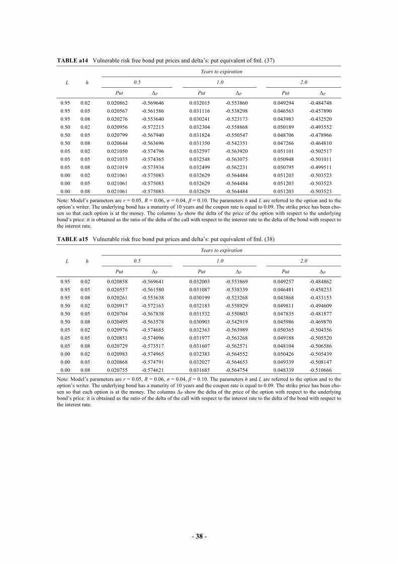
- 38 -

TABLE a14 Vulnerable risk free bond put prices and delta�s: put equivalent of fml. (37)

Years to expiration

0.5 1.0 2.0 L h

Put ∆P Put ∆P Put ∆P

0.95 0.02 0.020862 -0.569646 0.032015 -0.553860 0.049294 -0.484748 0.95 0.05 0.020567 -0.561586 0.031116 -0.538298 0.046563 -0.457890 0.95 0.08 0.020276 -0.553640 0.030241 -0.523173 0.043983 -0.432520 0.50 0.02 0.020956 -0.572215 0.032304 -0.558868 0.050189 -0.493552 0.50 0.05 0.020799 -0.567940 0.031824 -0.550547 0.048706 -0.478966 0.50 0.08 0.020644 -0.563696 0.031350 -0.542351 0.047266 -0.464810 0.05 0.02 0.021050 -0.574796 0.032597 -0.563920 0.051101 -0.502517 0.05 0.05 0.021035 -0.574365 0.032548 -0.563075 0.050948 -0.501011 0.05 0.08 0.021019 -0.573934 0.032499 -0.562231 0.050795 -0.499511 0.00 0.02 0.021061 -0.575083 0.032629 -0.564484 0.051203 -0.503523 0.00 0.05 0.021061 -0.575083 0.032629 -0.564484 0.051203 -0.503523 0.00 0.08 0.021061 -0.575083 0.032629 -0.564484 0.051203 -0.503523

Note: Model�s parameters are r = 0.05, R = 0.06, σ = 0.04, β = 0.10. The parameters h and L are referred to the option and to theoption�s writer. The underlying bond has a maturity of 10 years and the coupon rate is equal to 0.09. The strike price has been cho-sen so that each option is at the money. The columns ∆P show the delta of the price of the option with respect to the underlyingbond�s price: it is obtained as the ratio of the delta of the call with respect to the interest rate to the delta of the bond with respect tothe interest rate. TABLE a15 Vulnerable risk free bond put prices and delta�s: put equivalent of fml. (38)

Years to expiration

0.5 1.0 2.0 L h

Put ∆P Put ∆P Put ∆P

0.95 0.02 0.020858 -0.569641 0.032003 -0.553869 0.049257 -0.484862 0.95 0.05 0.020557 -0.561580 0.031087 -0.538339 0.046481 -0.458233 0.95 0.08 0.020261 -0.553638 0.030199 -0.523268 0.043868 -0.433153 0.50 0.02 0.020917 -0.572163 0.032183 -0.558929 0.049811 -0.494609 0.50 0.05 0.020704 -0.567838 0.031532 -0.550803 0.047835 -0.481877 0.50 0.08 0.020495 -0.563578 0.030903 -0.542919 0.045986 -0.469870 0.05 0.02 0.020976 -0.574685 0.032363 -0.563989 0.050365 -0.504356 0.05 0.05 0.020851 -0.574096 0.031977 -0.563268 0.049188 -0.505520 0.05 0.08 0.020729 -0.573517 0.031607 -0.562571 0.048104 -0.506586 0.00 0.02 0.020983 -0.574965 0.032383 -0.564552 0.050426 -0.505439 0.00 0.05 0.020868 -0.574791 0.032027 -0.564653 0.049339 -0.508147 0.00 0.08 0.020755 -0.574621 0.031685 -0.564754 0.048339 -0.510666

Note: Model�s parameters are r = 0.05, R = 0.06, σ = 0.04, β = 0.10. The parameters h and L are referred to the option and to theoption�s writer. The underlying bond has a maturity of 10 years and the coupon rate is equal to 0.09. The strike price has been cho-sen so that each option is at the money. The columns ∆P show the delta of the price of the option with respect to the underlyingbond�s price: it is obtained as the ratio of the delta of the call with respect to the interest rate to the delta of the bond with respect tothe interest rate.

- 39 -

TABLE a16 Vulnerable risk free bond put prices and delta�s put equivalent of fml. (39)

Years to expiration

0.5 1.0 2.0 L h

Put ∆P Put ∆P Put ∆P

0.95 0.02 0.020862 -0.569647 0.032015 -0.553866 0.049296 -0.484767 0.95 0.05 0.020567 -0.561594 0.031117 -0.538331 0.046574 -0.458002 0.95 0.08 0.020276 -0.553661 0.030246 -0.523255 0.044011 -0.432796 0.50 0.02 0.020956 -0.572222 0.032306 -0.558896 0.050199 -0.493651 0.50 0.05 0.020801 -0.567984 0.031833 -0.550719 0.048767 -0.479565 0.50 0.08 0.020648 -0.563809 0.031375 -0.542784 0.047418 -0.466298 0.05 0.02 0.021051 -0.574797 0.032597 -0.563925 0.051103 -0.502536 0.05 0.05 0.021035 -0.574373 0.032550 -0.563108 0.050960 -0.501127 0.05 0.08 0.021020 -0.573956 0.032504 -0.562314 0.050825 -0.499800 0.00 0.02 0.021061 -0.575083 0.032629 -0.564484 0.051203 -0.503523 0.00 0.05 0.021061 -0.575083 0.032629 -0.564484 0.051203 -0.503523 0.00 0.08 0.021061 -0.575083 0.032629 -0.564484 0.051203 -0.503523

Note: Model�s parameters are r = 0.05, R = 0.06, σ = 0.04, β = 0.10. The parameters h and L are referred to the option and to theoption�s writer. The underlying bond has a maturity of 10 years and the coupon rate is equal to 0.09. The strike price has been cho-sen so that each option is at the money. The columns ∆P show the delta of the price of the option with respect to the underlyingbond�s price: it is obtained as the ratio of the delta of the call with respect to the interest rate to the delta of the bond with respect tothe interest rate. TABLE a17 Comparison between risk free call and vulnerable call prices under different recovery scenarios

Years to expiration

0.5 1.0 2.0 L h

Call Diffa Diffb Diffc Call Diffa Diffb Diffc Call Diffa Diffb Diffc

0.95 0.02 0.008689 0.9% 1.0% 0.9% 0.008611 1.9% 1.9% 1.9% 0.005853 3.7% 3.7% 3.7%0.95 0.05 0.008689 2.3% 2.4% 2.3% 0.008611 4.6% 4.6% 4.6% 0.005853 9.1% 8.9% 9.0%0.95 0.08 0.008689 3.7% 3.8% 3.7% 0.008611 7.3% 7.3% 7.3% 0.005853 14.1% 13.8% 14.0%0.50 0.02 0.008689 0.5% 0.6% 0.5% 0.008611 1.0% 1.1% 1.0% 0.005853 2.0% 1.3% 2.0%0.50 0.05 0.008689 1.2% 1.5% 1.2% 0.008611 2.5% 2.6% 2.4% 0.005853 4.9% 3.0% 4.7%0.50 0.08 0.008689 2.0% 2.3% 2.0% 0.008611 3.9% 4.1% 3.8% 0.005853 7.7% 4.4% 7.4%0.05 0.02 0.008689 0.0% 0.2% 0.0% 0.008611 0.1% 0.3% 0.1% 0.005853 0.2% -1.0% 0.2%0.05 0.05 0.008689 0.1% 0.6% 0.1% 0.008611 0.2% 0.6% 0.2% 0.005853 0.5% -2.8% 0.5%0.05 0.08 0.008689 0.2% 0.9% 0.2% 0.008611 0.4% 0.8% 0.4% 0.005853 0.8% -4.9% 0.7%0.00 0.02 0.008689 0.0% 0.2% 0.0% 0.008611 0.0% 0.2% 0.0% 0.005853 0.0% -1.2% 0.0%0.00 0.05 0.008689 0.0% 0.5% 0.0% 0.008611 0.0% 0.3% 0.0% 0.005853 0.0% -3.4% 0.0%0.00 0.08 0.008689 0.0% 0.8% 0.0% 0.008611 0.0% 0.4% 0.0% 0.005853 0.0% -5.9% 0.0%

Note: Model�s parameters are r = 0.05, R = 0.06, σ = 0.04, β = 0.10. The parameters h and L are referred to the vulnerable optionand to the option�s writer. The underlying bond has a maturity of 10 years and the coupon rate is equal to 0.09. The strike price hasbeen chosen so that each option is at the money. The columns ∆P show the delta of the price of the option with respect to the under-lying bond�s price: it is obtained as the ratio of the delta of the call with respect to the interest rate to the delta of the bond with re-spect to the interest rate. Column Call reports the price of default free bond calls. Column Diffa contains the percent difference between a risk-free option and an otherwise identical vulnerable option valued in thefirst recovery scenario, Diffb contains the same in the second recovery scenario and Diffc in the third recovery scenario.

- 40 -

TABLE a18 Comparison between risk free put and vulnerable put prices under different recovery scenarios

Years to expiration

0.5 1.0 2.0 L h

Put Diffa Diffb Diffc Put Diffa Diffb Diffc Put Diffa Diffb Diffc

0.95 0.02 0.021061 0.9% 1.0% 0.9% 0.032629 1.9% 1.9% 1.9% 0.051203 3.7% 3.8% 3.7%0.95 0.05 0.021061 2.3% 2.4% 2.3% 0.032629 4.6% 4.7% 4.6% 0.051203 9.1% 9.2% 9.0%0.95 0.08 0.021061 3.7% 3.8% 3.7% 0.032629 7.3% 7.4% 7.3% 0.051203 14.1% 14.3% 14.0%0.50 0.02 0.021061 0.5% 0.7% 0.5% 0.032629 1.0% 1.4% 1.0% 0.051203 2.0% 2.7% 2.0%0.50 0.05 0.021061 1.2% 1.7% 1.2% 0.032629 2.5% 3.4% 2.4% 0.051203 4.9% 6.6% 4.8%0.50 0.08 0.021061 2.0% 2.7% 2.0% 0.032629 3.9% 5.3% 3.8% 0.051203 7.7% 10.2% 7.4%0.05 0.02 0.021061 0.1% 0.4% 0.0% 0.032629 0.1% 0.8% 0.1% 0.051203 0.2% 1.6% 0.2%0.05 0.05 0.021061 0.1% 1.0% 0.1% 0.032629 0.2% 2.0% 0.2% 0.051203 0.5% 3.9% 0.5%0.05 0.08 0.021061 0.2% 1.6% 0.2% 0.032629 0.4% 3.1% 0.4% 0.051203 0.8% 6.1% 0.7%0.00 0.02 0.021061 0.0% 0.4% 0.0% 0.032629 0.0% 0.8% 0.0% 0.051203 0.0% 1.5% 0.0%0.00 0.05 0.021061 0.0% 0.9% 0.0% 0.032629 0.0% 1.8% 0.0% 0.051203 0.0% 3.6% 0.0%0.00 0.08 0.021061 0.0% 1.5% 0.0% 0.032629 0.0% 2.9% 0.0% 0.051203 0.0% 5.6% 0.0%

Note: Model�s parameters are r = 0.05, R = 0.06, σ = 0.04, β = 0.10. The parameters h and L are referred to the vulnerable optionand to the option�s writer. The underlying bond has a maturity of 10 years and the coupon rate is equal to 0.09. The strike price hasbeen chosen so that each option is at the money. The columns ∆P show the delta of the price of the option with respect to the under-lying bond�s price: it is obtained as the ratio of the delta of the call with respect to the interest rate to the delta of the bond with re-spect to the interest rate. Column Put reports the price of default free bond puts. Column Diffa contains the percent difference between a risk-free option and an otherwise identical vulnerable option valued in thefirst recovery scenario, Diffb contains the same in the second recovery scenario and Diffc in the third recovery scenario. TABLE a19 Comparison between Jarrow and Turnbull vulnerable call and extended CIR vulnerable call prices under different recovery scenarios

Years to expiration

0.5 1.0 2.0 L h

Call Diffa Diffb Diffc Call Diffa Diffb Diffc Call Diffa Diffb Diffc

0.95 0.02 0.007627 -12.8% -12.8% -12.8% 0.007137 -18.4% -18.4% -18.4% 0.004209 -33.9% -34.0% -33.9%0.95 0.05 0.007519 -12.8% -12.8% -12.9% 0.006936 -18.4% -18.4% -18.4% 0.003976 -33.9% -34.1% -33.9%0.95 0.08 0.007413 -12.8% -12.8% -12.9% 0.006742 -18.4% -18.3% -18.4% 0.003757 -33.8% -34.3% -33.9%0.50 0.02 0.007661 -12.9% -12.7% -12.9% 0.007201 -18.4% -18.3% -18.4% 0.004286 -33.9% -34.7% -33.9%0.50 0.05 0.007605 -12.8% -12.5% -12.8% 0.007096 -18.4% -18.1% -18.4% 0.004163 -33.7% -35.9% -33.9%0.50 0.08 0.007549 -12.8% -12.4% -12.8% 0.006994 -18.3% -18.0% -18.4% 0.004048 -33.5% -37.0% -33.9%0.05 0.02 0.007696 -12.9% -12.6% -12.9% 0.007266 -18.4% -18.2% -18.4% 0.004363 -33.9% -35.4% -33.9%0.05 0.05 0.007690 -12.8% -12.3% -12.9% 0.007256 -18.4% -17.9% -18.4% 0.004351 -33.9% -37.4% -33.9%0.05 0.08 0.007685 -12.8% -12.0% -12.8% 0.007245 -18.4% -17.6% -18.4% 0.004339 -33.8% -39.5% -33.9%0.00 0.02 0.007700 -12.8% -12.6% -12.8% 0.007273 -18.4% -18.2% -18.4% 0.004371 -33.9% -35.4% -33.9%0.00 0.05 0.007700 -12.8% -12.3% -12.8% 0.007273 -18.4% -17.9% -18.4% 0.004371 -33.9% -37.6% -33.9%0.00 0.08 0.007700 -12.8% -11.9% -12.8% 0.007273 -18.4% -17.6% -18.4% 0.004371 -33.9% -39.7% -33.9%

Note: Model�s parameters are r = 0.05, R = 0.06, σ = 0.04, β = 0.10. The parameters h and L are referred to the vulnerable option and to the option�s writer. The underlying bond has a maturity of 10 years and the coupon rate is equal to 0.09. The strike price hasbeen chosen so that each option is at the money. The columns ∆P show the delta of the price of the option with respect to the underlying bond�s price: it is obtained as the ratio of the delta of the call with respect to the interest rate to the delta of the bondwith respect to the interest rate. Column Call reports the price of vulnerable bond calls obtained by the Jarrow and Turnbull (1995) model. Column Diffa contains the percent difference between the Jarrow and Turnbull vulnerable option and the exetended CIR vulnerableoption valued in the first recovery scenario, Diffb contains the same in the second recovery scenario and Diffc in the third recovery scenario.

- 41 -

TABLE a20 Comparison between Jarrow and Turnbull vulnerable put and extended CIR vulnerable put prices un-der different recovery scenarios

Years to expiration

0.5 1.0 2.0 L h

Put Diffa Diffb Diffc Put Diffa Diffb Diffc Put Diffa Diffb Diffc

0.95 0.02 0.019882 -4.9% -4.9% -4.9% 0.030703 -4.3% -4.2% -4.3% 0.047869 -3.0% -2.9% -3.0%0.95 0.05 0.019601 -4.9% -4.9% -4.9% 0.029841 -4.3% -4.2% -4.3% 0.045226 -3.0% -2.8% -3.0%0.95 0.08 0.019324 -4.9% -4.8% -4.9% 0.029006 -4.3% -4.1% -4.3% 0.042737 -2.9% -2.6% -3.0%0.50 0.02 0.019971 -4.9% -4.7% -4.9% 0.030981 -4.3% -3.9% -4.3% 0.048747 -3.0% -2.2% -3.0%0.50 0.05 0.019824 -4.9% -4.4% -4.9% 0.030528 -4.2% -3.3% -4.3% 0.047356 -2.9% -1.0% -3.0%0.50 0.08 0.019678 -4.9% -4.2% -4.9% 0.030088 -4.2% -2.7% -4.3% 0.046046 -2.6% 0.1% -3.0%0.05 0.02 0.020061 -4.9% -4.6% -4.9% 0.031260 -4.3% -3.5% -4.3% 0.049624 -3.0% -1.5% -3.0%0.05 0.05 0.020047 -4.9% -4.0% -4.9% 0.031215 -4.3% -2.4% -4.3% 0.049485 -3.0% 0.6% -3.0%0.05 0.08 0.020032 -4.9% -3.5% -4.9% 0.031171 -4.3% -1.4% -4.3% 0.049354 -2.9% 2.5% -3.0%0.00 0.02 0.020071 -4.9% -4.5% -4.9% 0.031291 -4.3% -3.5% -4.3% 0.049722 -3.0% -1.4% -3.0%0.00 0.05 0.020071 -4.9% -4.0% -4.9% 0.031291 -4.3% -2.4% -4.3% 0.049722 -3.0% 0.8% -3.0%0.00 0.08 0.020071 -4.9% -3.4% -4.9% 0.031291 -4.3% -1.3% -4.3% 0.049722 -3.0% 2.8% -3.0%

Note: Model�s parameters are r = 0.05, R = 0.06, σ = 0.04, β = 0.10. The parameters h and L are referred to the vulnerable optionsand to the option�s writer. The underlying bond has a maturity of 10 years and the coupon rate is equal to 0.09. The strike price hasbeen chosen so that each option is at the money. The columns ∆P show the delta of the price of the option with respect to the under-lying bond�s price: it is obtained as the ratio of the delta of the call with respect to the interest rate to the delta of the bond with re-spect to the interest rate. Column Put reports the price of vulnerable bond puts obtained by the Jarrow and Turnbull (1995) model. Column Diffa contains the percent difference between the Jarrow and Turnbull vulnerable option and the exetended CIR vulnerableoption valued in the first recovery scenario, Diffb contains the same in the second recovery scenario and Diffc in the third recoveryscenario.