Prepared for submission to JHEP

More on thermal probes of a

strongly coupled anisotropic plasma

Viktor Jahnke,a Andres Luna,b Leonardo Patino,b and Diego Trancanellia

aInstituto de Fısica, Universidade de Sao Paulo, 05314-970 Sao Paulo, BrazilbDepartamento de Fısica, Facultad de Ciencias, Universidad Nacional Autonoma de Mexico, A.P.

50-542, Mexico D.F. 04510, Mexico

E-mail: viktor@if.usp.br, andresluna@ciencias.unam.mx,

leopj@ciencias.unam.mx, dtrancan@fma.if.usp.br

Abstract: We extend the analysis of 1211.2199, where the photon production rate of

an anisotropic strongly coupled plasma with Nf Nc massless quarks was considered. We

allow here for non-vanishing quark masses and study how these affect the spectral densities

and conductivities. We also compute another important probe of the plasma, the dilepton

production rate. We consider generic angles between the anisotropic direction and the

photon and dilepton wave vectors, as well as arbitrary quark masses and arbitrary values

of the anisotropy parameter. Generically, the anisotropy increases the production rate of

both photons and dileptons, compared with an isotropic plasma at the same temperature.

Keywords: Gauge-gravity correspondence, Holography and quark-gluon plasmas

arX

iv:1

311.

5513

v3 [

hep-

th]

19

Jan

2014

Contents

1 Introduction 1

2 Photon and dilepton production in an anisotropic plasma 3

2.1 Gravity set-up 5

2.2 Quark masses 9

3 Photon production with massive quarks from holography 10

3.1 Spectral density for the polarization ε(1) 11

3.2 Spectral density for the polarization ε(2) 12

3.3 Total photon production rate 15

4 Dilepton production from holography 16

4.1 Isotropic limit 19

4.2 Dilepton spectral density χ(1) 20

4.3 Dilepton spectral density χ(2) 20

4.4 Total dilepton production rate 26

5 Discussion 26

A Solutions for E1 and E2 35

B Explicit near-boundary-expansion for the action (4.17) 38

1 Introduction

The quark-gluon plasma (QGP) produced in the relativistic scattering of heavy ions at

RHIC [1, 2] and LHC [3] seemingly behaves as a strongly coupled fluid [4, 5], thus ren-

dering a perturbative approach in small αS problematic. In the absence of other reliable

computational tools,1 it is then interesting to apply the AdS/CFT correspondence [6–8]

to such a system and try to extract qualitative feature of its strongly coupled dynamics

and, possibly, model independent quantities, such as the shear viscosity to entropy density

ratio [9].

Besides being strongly coupled, the QGP also exhibits another important characteristic

which is worth modeling in a holographic setup, namely the presence of a spatial anisotropy

in the initial stages of the evolution. Such an anisotropy has recently been described

at strong coupling via a type IIB supergravity black brane solution with an anisotropic

1The lattice approach to QCD is the preferred choice for studying thermodynamics and equations of

state, but is not particularly well suited to compute dynamical quantities such as transport coefficients.

– 1 –

horizon [10, 11].2 Understanding how this anisotropy affects various physical observables

has recently received some attention. Quantities that have been studied include the shear

viscosity to entropy density ratio [13, 14], the drag force experienced by a heavy quark

[15, 16], the energy lost by a quark rotating in the transverse plane [17], the stopping

distance of a light probe [18], the jet quenching parameter of the medium [16, 19, 20],

the potential between a quark and antiquark pair, both static [16, 19, 21, 22] and in

a plasma wind [21], including its imaginary part [23], Langevin diffusion and Brownian

motion [24, 25], chiral symmetry breaking [26], and the production of thermal photons

[27–29].3

This last observable is particularly interesting since it furnishes valuable data about

the conditions of the in-medium location of production of the photons. This is because,

given the limited spatial extend of the plasma and the weakness of the electromagnetic

interaction, photons produced in the plasma escape from it virtually unperturbed. Some

of the holographic studies of this quantity include [31–44].4 Here we extend the analysis

started in [27] in two different directions.

First, we consider non-equatorial embeddings of the flavor D7-branes introduced in

[27], corresponding to quarks with non-vanishing masses, thus making our analysis closer

to the real-world system. We allow for arbitrary values of the anisotropy parameter a/T

and for arbitrary angles between the photon wave vectors and the anisotropic direction, or

beam direction. We also study the DC conductivity as a function of the quark mass. We

find that, in general, an anisotropic plasma glows brighter than its isotropic counterpart

at the same temperature. This holds for all values of the quark masses and for all angles

between the anisotropic direction and the photon wave vector. This same computation

for a specific value of the anisotropy and for wave vectors either parallel or perpendicular

to the anisotropic direction has already been performed in [28], where a strong, external

magnetic field was also included.

As a second extension of [27], we study thermal production, via virtual photon decay,

of lepton/antilepton pairs (dileptons) in the same background. This quantity is also of

phenomenological interest and is obtained by considering time-like momenta for the emitted

particles, which can be massive. Compared to the photon production calculation, there is

now an extra parameter, namely the magnitude of the spatial momentum. We find that the

dilepton production rate is generically larger than the corresponding rate of an isotropic

plasma at the same temperature, except for a small range of anisotropies, if the quark mass

and the frequency are sufficiently large. These quantities are generically monotonically

dependent (either increasing or decreasing) on the angle between the momentum and the

anisotropic direction.

The paper is organized as follows. In Sec. 2 we review how to compute the production

rate of photons and dileptons in an anisotropic plasma first in the gauge theory side and

then via holography using the anisotropic background of [10, 11]. In Sec. 3 we present our

2This geometry is the finite temperature generalization of the geometry found in [12].3For a review of many of these studies, see [30].4At weak coupling, this has been studied in the presence of anisotropy in, for example, [45].

– 2 –

results for the spectral densities, conductivities, and total production rates for photons in

a plasma with massive quarks. In Sec. 4 we do the same for dileptons, which is essentially

the extension of the previous computation to the case in which the emitted particles have

a time-like momentum, rather than a light-like one. We discuss our results in Sec. 5. We

relegate to two appendices some technical details of the computation.

2 Photon and dilepton production in an anisotropic plasma

Here we briefly recall the basic setup of [27]. The gauge theory we shall consider is obtained

via an isotropy-breaking deformation of four-dimensional N = 4 super Yang-Mills (SYM)

with gauge group SU(Nc), at large Nc and large ’t Hooft coupling λ = g2YMNc. The

deformation consists in including in the action a theta-term which depends linearly on one

of the spatial directions, say z, [12]

SSU(Nc) = SN=4 +1

8π2

∫θ(z) TrF ∧ F , θ(z) ∝ z , (2.1)

where the proportionality constant in θ(z) has dimensions of energy and will be related

to the parameter a that we shall introduce in the next subsection. The rotational SO(3)

symmetry in the space directions is broken by the new term down to SO(2) in the xy-plane.

For this reason we shall call the z-direction the longitudinal (or anisotropic) direction,

while x and y will be the transverse directions. This theory has matter fields in the adjoint

representation of the gauge group. We can also introduce Nf flavors of scalars Φa and

fermions Ψa in the fundamental representation, with the index a = 1, . . . , Nf. With an

abuse of language, we will refer to these fundamental fields indistinctly as ‘quarks’.

To study photon production we turn on a dynamical photon by including a U(1) kinetic

term in the action (2.1) and a coupling to the fields that we want to be charged under this

Abelian symmetry. In order to realize a situation as similar to QCD as possible, we require

that only the fundamental fields be charged, while the adjoint fields are to remain neutral.

We do not know the gravitational dual of the full SU(Nc) × U(1) theory, but fortunately

this will not be necessary for our purposes. It was in fact shown in [31] that to compute

the two-point correlation function of the electromagnetic current to leading order in the

electromagnetic coupling αEM, it is enough to consider the SU(Nc) theory only, whose dual

is known from [10, 11]. Our computation will then be to leading order in αEM, since the

coupling of the photons to the surrounding medium is small, but fully non-perturbative in

the ’t Hooft coupling λ of the SU(Nc) theory.

In general, photon production in differential form is given by the expression [31, 33, 46]

dΓγ

d~k=

e2

(2π)32|~k|Φ(k)ηµν χµν(k)

∣∣∣k0=|~k|

, (2.2)

with ηµν the Minkowski metric (our convention is (− + ++)), kµ = (k0,~k) the photon

null momentum and Φ(k) the distribution function, which for thermal equilibrium, as in

– 3 –

our case, reduces to the Bose-Einstein distribution nB(k0) = 1/(ek0/T − 1). The spectral

density is χµν(k) = −2 Im GRµν(k), with

GRµν(k) = −i

∫d4x e−ik·x Θ(t)〈[JEM

µ (x), JEMν (0)]〉 (2.3)

the retarded correlator of two electro-magnetic currents JEMµ .

If the theory also includes fermions bearing electric charge e`, these can be produced

in particle/antiparticle pairs (called dileptons in the following) via virtual photon decay

processes. The spectral density above can then be used to compute the dilepton production

rate by means of the expression [46]

dΓ`¯

dk=

e2e`2

(2π)46π|k|5Φ(k) Θ(k0)Θ(−k2 − 4m`

2)(−k2 − 4m`2)1/2(−k2 + 2m`

2)ηµν χµν(k) ,

(2.4)

where m` is the mass of the lepton/antilepton and the spectral function is now evaluated

on the time-like four-momentum kµ of the virtual photon.

A consequence of the Ward identity kµχµν = 0 for null kµ is that, for the photon

production rate, only the transverse spectral functions contribute. A simple way to extract

this contribution is by not taking the whole trace as in (2.2), but by summing over the

projections into the polarization vectors for the photon that are mutually orthogonal and

orthogonal to ~k:

dΓγ

d~k=

e2

(2π)32|~k|Φ(k)

∑s=1,2

εµ(s)(~k) εν(s)(

~k)χµν(k)∣∣∣k0=|~k|

. (2.5)

Each term of the sum stands for the number of photons emitted with polarization vector

~ε(s).

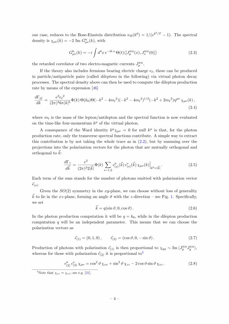
Given the SO(2) symmetry in the xy-plane, we can choose without loss of generality~k to lie in the xz-plane, forming an angle ϑ with the z-direction – see Fig. 1. Specifically,

we set~k = q(sinϑ, 0, cosϑ) . (2.6)

In the photon production computation it will be q = k0, while in the dilepton production

computation q will be an independent parameter. This means that we can choose the

polarization vectors as

~ε(1) = (0, 1, 0) , ~ε(2) = (cosϑ, 0,− sinϑ) . (2.7)

Production of photons with polarization ~ε(1) is then proportional to χyy ∼ Im 〈JEMy JEM

y 〉,whereas for those with polarization ~ε(2) it is proportional to5

εµ(2) εν(2) χµν = cos2 ϑχxx + sin2 ϑχzz − 2 cosϑ sinϑχxz . (2.8)

5Note that χxz = χzx; see e.g. [31].

– 4 –

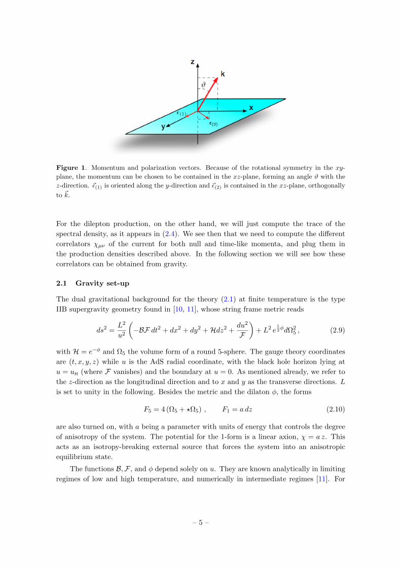
Figure 1. Momentum and polarization vectors. Because of the rotational symmetry in the xy-

plane, the momentum can be chosen to be contained in the xz-plane, forming an angle ϑ with the

z-direction. ~ε(1) is oriented along the y-direction and ~ε(2) is contained in the xz-plane, orthogonally

to ~k.

For the dilepton production, on the other hand, we will just compute the trace of the

spectral density, as it appears in (2.4). We see then that we need to compute the different

correlators χµν of the current for both null and time-like momenta, and plug them in

the production densities described above. In the following section we will see how these

correlators can be obtained from gravity.

2.1 Gravity set-up

The dual gravitational background for the theory (2.1) at finite temperature is the type

IIB supergravity geometry found in [10, 11], whose string frame metric reads

ds2 =L2

u2

(−BF dt2 + dx2 + dy2 +Hdz2 +

du2

F

)+ L2 e

12φdΩ2

5 , (2.9)

with H = e−φ and Ω5 the volume form of a round 5-sphere. The gauge theory coordinates

are (t, x, y, z) while u is the AdS radial coordinate, with the black hole horizon lying at

u = uH (where F vanishes) and the boundary at u = 0. As mentioned already, we refer to

the z-direction as the longitudinal direction and to x and y as the transverse directions. L

is set to unity in the following. Besides the metric and the dilaton φ, the forms

F5 = 4 (Ω5 + ?Ω5) , F1 = a dz (2.10)

are also turned on, with a being a parameter with units of energy that controls the degree

of anisotropy of the system. The potential for the 1-form is a linear axion, χ = a z. This

acts as an isotropy-breaking external source that forces the system into an anisotropic

equilibrium state.

The functions B,F , and φ depend solely on u. They are known analytically in limiting

regimes of low and high temperature, and numerically in intermediate regimes [11]. For

– 5 –

-4 -2 0 2 40.0

0.2

0.4

0.6

0.8

1.0

1.2

log(a/T )lo

g(s/s

iso)

Figure 2. Log-log plot of the entropy density as a function of a/T . The dashed blue line is a

straight line with slope 1/3.

u→ 0 (independently of the value of a) they asymptote to the AdS5×S5 metric, F = B =

H = 1 and φ = 0, while for a = 0 they reduce to the black D3-brane solution

B = H = 1 , φ = χ = 0 , F = 1− u4

u4H

, (2.11)

which has temperature and entropy density given by [47]

Tiso =1

πuH

, siso =π2

2N2

c T3 . (2.12)

The temperature and entropy density of the anisotropic geometry are given by [11]

T =e−

12φH√BH(16 + a2u2

He72φH)

16πuH

, s =N2

c

2πu3H

e−54φH , (2.13)

where φH ≡ φ(u = uH) and BH ≡ B(u = uH). As depicted in Fig. 2, the entropy density

of the system interpolates smoothly between the isotropic scaling above for small a/T and

the scaling [11, 12]

s ' 3.21N2c T

3( aT

) 13, (2.14)

for large a/T , the transition between the two behaviors taking place at approximately

a/T ' 3.7. The space can then be interpreted as a domain-wall-like solution interpolating

between an AdS geometry in the UV and a Lifshitz-like geometry in the IR, with the

radial position at which the transition takes place being set by the anisotropic scale a:

when T a the horizon lies in the asymptotic AdS region with scaling (2.12), whereas for

T a it lies in the anisotropic region with scaling (2.14).

It might be useful to compare the anisotropy introduced in this setup with the anisotropy

of other holographic models, or even weak coupling computations. To do this one could

consider the following ratio [21]

α =4E + P⊥ − PL

3Ts, (2.15)

where E is the energy density and P⊥, PL are the transverse and longitudinal pressures,

respectively. These quantities are presented in great detail in [11]. For the isotropic N = 4

– 6 –

5 10 15 20

1

-2

-4

-6

-8

-10

-12

a/T

α

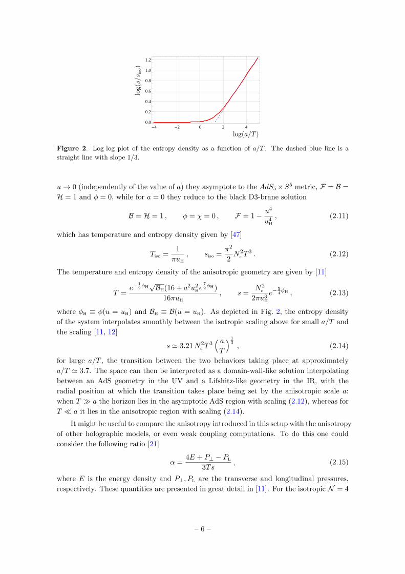
Figure 3. Ratio (2.15) as a function of a/T . The blue dots are the actual values of the ratio, and

the red curve is the fit (2.16).

super Yang-Mills plasma α = 1, whereas for 0 < a/T . 20 the ratio is well approximated

by the expression

α ' 1− 0.0036( aT

)2− 0.000072

( aT

)4, (2.16)

as shown in Fig. 3.

A feature of the anisotropic geometry of [10, 11] is the presence of a conformal anomaly

that appears during the renormalization of the theory, introducing a reference scale µ. This

anomaly implies that some physical quantities (such as, for example, the energy density

and pressures) do not depend only on the ratio a/T , but on two independent dimensionless

ratios that can be built out of a, T , and µ. Fortunately, as we shall see in the following,

all the quantities computed in this paper are not affected by this anomaly and will be

independent of µ.6

The introduction of Nf flavors of quarks is achieved by placing Nf probe D7-branes in

the background (2.9). To keep the system in a deconfined phase we will work with ‘black-

hole embeddings’ [48] for the D7 branes. The complete system can then be thought of as

a D3/D7 system with two different kinds of D7-branes, one kind sourcing the anisotropy

[11, 12]7 and the other kind sourcing flavor [49, 50]; see [27]. As argued in [31], at leading

order in αEM it suffices to evaluate the correlators needed for (2.2) and (2.4) in the SU(Nc)

gauge theory with no dynamical photons. At strong ’t Hooft coupling and large Nc, these

correlators can be calculated holographically, as we explain now.

Let Am (m = 0, . . . , 7) be the gauge field associated to the overall U(1) ⊂ U(Nf) gauge

symmetry on the D7-branes. Upon dimensional reduction on the 3-sphere wrapped by the

flavor D7-branes, Am gives rise to a massless gauge field (Aµ, Au), three massless scalars,

and a tower of massive Kaluza-Klein (KK) modes. All these fields propagate on the five

non-compact dimensions of the D7-branes. We will work in the gauge Au = 0,8 and we

6The same happens for the quantity α introduced in (2.15), which does not depend on a and T separately,

but only on the combination a/T .7These ND7 branes are smeared homogeneously along the z-direction and can be thought of as giving

rise to a density nD7 = ND7/Lz of extended charges, with Lz being the (infinite) length of the z-direction.

This charge density is related to the anisotropy parameter a through a = g2YMnD7/4π [11].8This gauge choice will be immaterial in the following, since we shall switch to gauge invariant quantities,

but it has the advantage of simplifying our formulas.

– 7 –

will consistently set the scalars and the higher KK modes to zero, since these are not of

interest here. According to the prescription of [7, 8], correlation functions of JEMµ can be

calculated by varying the string partition function with respect to the value of Aµ at the

boundary of the spacetime (2.9).

We now proceed to write down the action for the D7-branes. It is easy to realize

that there is no Wess-Zumino coupling of the branes to the background F5, because of

the particular brane orientation that has been chosen, nor a coupling to the background

axion, which would be quartic in the U(1) field strength F = dA [27]. This means that the

Dirac-Born-Infeld (DBI) action is all we need to consider:

S = −Nf TD7

∫D7

d8σ e−φ√−det (g + 2π`2sF ) , (2.17)

where g is the induced metric on the D7-branes and TD7 = 1/(2π`s)7gs`s is the D7-brane

tension. To obtain the equations of motion for Aµ, it suffices to expand the action above

and use the quadratic part only:

S = −NfTD7

∫D7

d8σ e−φ√−det g

(2π`2s)2

4F 2 , (2.18)

where F 2 = FmnFmn. The embedding of the branes inside the S5 of the geometry can be

parametrized by the polar angle ξ of the S5 with cos ξ ≡ ψ(u). The induced metric on the

branes is then given by

ds2D7 =

1

u2

(−FB dt2 + dx2 + dy2 +H dz2

)+

1− ψ2 + u2Fe12φψ′2

u2F(1− ψ2)du2

+e12φ(1− ψ2)dΩ2

3 . (2.19)

After the dimensional reduction on the three-sphere, the action reduces to

S = −KD7

∫dt d3~xduM FmnFmn (2.20)

where

M =e−

34φ√B

u5

(1− ψ2

)√1− ψ2 + u2Fe

φ2ψ′2,

KD7 = 2π4NfTD7`4s =

1

16π2NcNf , (2.21)

and Fm is restricted to the components m = (µ, u).

As argued in [33, 48], in order to calculate the photon emission rate, we may con-

sistently proceed by finding the embedding of the D7-branes that extremizes (2.17) in the

absence of the gauge field, and then solving for the gauge field perturbations propagating

on that embedding considered as a fixed background. By checking that the gauge field

obtained in this way does not grow beyond the perturbation limit, we can ensure that no

modes of the metric or of the background fields will be excited when following this proce-

dure. We set to zero the components of the gauge field on the three-sphere wrapped by

– 8 –

the D7-branes and Fourier decompose the remaining as

Aµ(t, ~x, u) =

∫dk0d~k

(2π)4e−ik

0t+i~k·~xAµ(k0,~k, u) , ~k = (kx, 0, kz) = q(sinϑ, 0, cosϑ) .

(2.22)

This is possible because the state we consider, although anisotropic, is translationally

invariant along the gauge theory directions [11]. As mentioned above, in the photon pro-

duction computation it will be q = k0, while in the dilepton production computation q will

be an independent parameter.

Doing so, the equations for the gauge field deriving from (2.20) split into the following

decoupled equation for Ay (primes denote derivatives with respect to u)(MguugyyA′y

)′ −Mgyy(gttk2

0 + gxxk2x + gzzk2

z

)Ay = 0 , (2.23)

together with a coupled system of three equations for the remaining components At,x,z:

(MguugttA′t)′ −Mgtt [gxxkx(kxAt − k0Ax) + gzzkz(kzAt − k0Az)] = 0 , (2.24)

(MguugxxA′x)′ −Mgxx[gttk0(k0Ax − kxAt) + gzzkz(kzAx − kxAz)

]= 0 , (2.25)

(MguugzzA′z)′ −Mgzz

[gttk0(k0Az − kzAt) + gxxkx(kxAz − kzAx)

]= 0 . (2.26)

The inverse metric can be read off directly from (2.19). Equations (2.23)-(2.26) constitute

the set of equations that we shall solve in the next sections, with the appropriate boundary

conditions, to obtain the correlation functions of the electromagnetic currents JEMµ .

2.2 Quark masses

Given that both M and guu depend on ψ, we need to know this embedding function of the

D7-branes to solve (2.23)-(2.26). The action (2.20) for the D7-branes in the absence of the

gauge field, takes the form

Sψ = −KD7

∫dt d~x duM0

(1− ψ2

)√1− ψ2 + u2Fe

φ2ψ′2, (2.27)

where

M0 =e−

34φ√B

u5. (2.28)

By varying Sψ with respect to ψ(u) one obtains the equation for the D7-branes embeddingM0

(1− ψ2

)u2Fe

φ2ψ′√

1− ψ2 + u2Feφ2ψ′2

′ +M03ψ(1− ψ2

)+ 2u2Fe

φ2ψψ′2√

1− ψ2 + u2Feφ2ψ′2

= 0 . (2.29)

This equation can be solved near the boundary u = 0 using the near-boundary expansions

of the metric [11]

F = 1 +11

24a2u2 + F4u

4 +7

12a4u4log u+O

(u6),

– 9 –

B = 1− 11

24a2u2 + B4u

4 − 7

12a4u4log u+O

(u6),

φ = −a2

2u2 +

(1152B4 + 121a4

4032

)u4 − a4

6u4logu+O

(u6), (2.30)

where F4 and B4 are integration constants which are undetermined by the boundary equa-

tions of motion, but that can be read off from the numerics [11]. The result for the

near-boundary expansion of ψ(u) is

ψ = ψ1u+

(ψ3 +

5

24a2ψ1logu

)u3 +O

(u5), (2.31)

where ψ1 and ψ3 are related to the quark mass and condensate, respectively. To solve

(2.29), we follow [33] and specify the boundary conditions at the horizon as ψ(uH) = ψH

and ψ′(uH) = 0. We determine ψ1 and ψ3 by fitting the numerical solution near the

boundary. The relation between ψ1 and the quark mass is given by [33]

Mq =√λT uH

ψ1√2, (2.32)

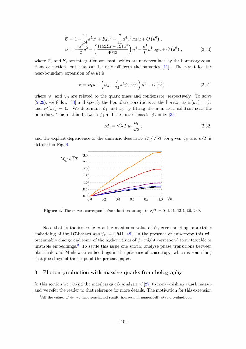
and the explicit dependence of the dimensionless ratio Mq/√λT for given ψH and a/T is

detailed in Fig. 4.

0.0 0.2 0.4 0.6 0.8 1.00.0

0.5

1.0

1.5

2.0

2.5

3.0Mq/√λT

ψH

Figure 4. The curves correspond, from bottom to top, to a/T = 0, 4.41, 12.2, 86, 249.

Note that in the isotropic case the maximum value of ψH corresponding to a stable

embedding of the D7-branes was ψH = 0.941 [48]. In the presence of anisotropy this will

presumably change and some of the higher values of ψH might correspond to metastable or

unstable embeddings.9 To settle this issue one should analyze phase transitions between

black-hole and Minkowski embeddings in the presence of anisotropy, which is something

that goes beyond the scope of the present paper.

3 Photon production with massive quarks from holography

In this section we extend the massless quark analysis of [27] to non-vanishing quark masses

and we refer the reader to that reference for more details. The motivation for this extension9All the values of ψH we have considered result, however, in numerically stable evaluations.

– 10 –

is to bring our analysis closer to the real-world system studied in the RHIC and LHC

experiments.

To compute the various correlation functions,10 we start by writing the boundary

action as

Sε = −2KD7

∫dt d~x

[Mguu

(gttAtA

′t + gxxAxA

′x + gyyAyA

′y + gzzAzA

′z

)]u=ε

, (3.1)

where the limit ε→ 0 is intended.

3.1 Spectral density for the polarization ε(1)

As in the massless case, the spectral density χyy ≡ χ(1) is the easiest to compute, since

Ay does not couple to any other mode. The calculation is very similar to the one in [27],

the only difference being that now the induced metric has a non-trivial brane embedding,

ψ(u) 6= 0, contained in the new expression for M and guu.

Before proceeding further, we recall the isotropic result of [33], since ultimately we want

to understand whether the presence of an anisotropy increases or decreases the isotropic

photon production and conductivity. Unfortunately, it does not seem possible to obtain

analytical results for the spectral density when the quark mass is not zero. One then

needs to resort to numerics. In order to compare an anisotropic plasma with the isotropic

one, we need that both be at the same temperature. We fix the temperature in the

isotropic case by adjusting the position of the black hole horizon, since Tiso = 1/πuH.

We then obtain isotropic plots corresponding to the particular temperatures used in the

anisotropic geometry. More specifically, we are using T = 0.33, 0.36, 0.48, 0.58 which are

the temperatures for the geometries with a/T = 4.41, 12.2, 86, and 249, respectively, that

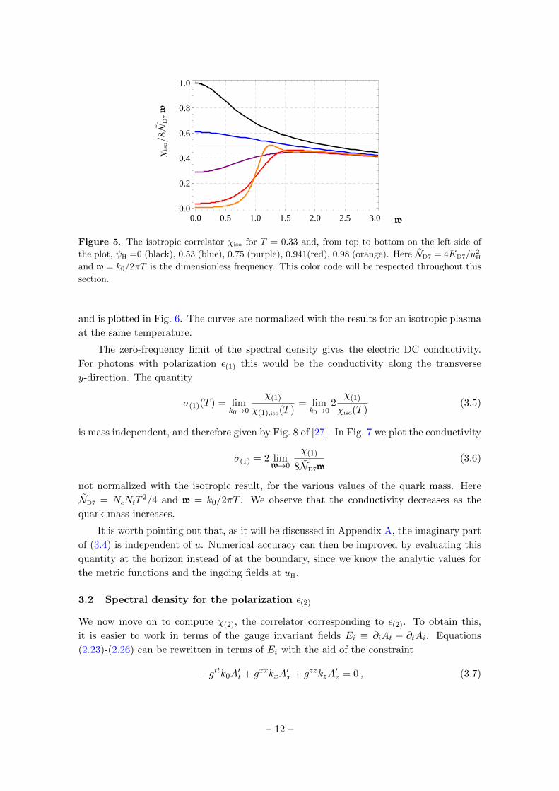
we consider below. The results for T = 0.33 are plotted in Fig. 5, for the various masses

of interest.

In principle we could also compare the anisotropic plasma with an isotropic plasma at

the same entropy density but different temperature. We have checked that the quantities

studied in this paper do not depend strongly on whether the comparison is made at the same

temperature or at the same entropy density, unlike what happened for other observables,

as the ones studied in [15, 20, 21]. For this reason we do not include here plots with curves

normalized with an isotropic plasma with the same entropy density.

The correlation function is given by

GRyy = − 4KD7

|Ay (k0, 0)|2limu→0

Q (u)A∗y (k0, u)A′y (k0, u) , (3.2)

where

Q (u) ≡Mguugyy. (3.3)

The spectral density then reads

χ(1) =NcNf

2π2 |Ay (k0, 0)|2Im lim

u→0Q (u)A∗y (k0, u)A′y (k0, u) , (3.4)

10The original references for this prescription include [51–54].

– 11 –

0.0 0.5 1.0 1.5 2.0 2.5 3.00.0

0.2

0.4

0.6

0.8

1.0

χiso/8N

D7w

w

Figure 5. The isotropic correlator χiso for T = 0.33 and, from top to bottom on the left side of

the plot, ψH =0 (black), 0.53 (blue), 0.75 (purple), 0.941(red), 0.98 (orange). Here ND7 = 4KD7/u2H

and w = k0/2πT is the dimensionless frequency. This color code will be respected throughout this

section.

and is plotted in Fig. 6. The curves are normalized with the results for an isotropic plasma

at the same temperature.

The zero-frequency limit of the spectral density gives the electric DC conductivity.

For photons with polarization ε(1) this would be the conductivity along the transverse

y-direction. The quantity

σ(1)(T ) = limk0→0

χ(1)

χ(1),iso(T )= lim

k0→02χ(1)

χiso(T )(3.5)

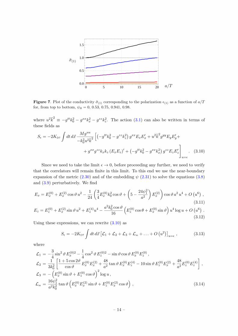
is mass independent, and therefore given by Fig. 8 of [27]. In Fig. 7 we plot the conductivity

σ(1) = 2 limw→0

χ(1)

8ND7w(3.6)

not normalized with the isotropic result, for the various values of the quark mass. Here

ND7 = NcNfT2/4 and w = k0/2πT . We observe that the conductivity decreases as the

quark mass increases.

It is worth pointing out that, as it will be discussed in Appendix A, the imaginary part

of (3.4) is independent of u. Numerical accuracy can then be improved by evaluating this

quantity at the horizon instead of at the boundary, since we know the analytic values for

the metric functions and the ingoing fields at uH.

3.2 Spectral density for the polarization ε(2)

We now move on to compute χ(2), the correlator corresponding to ε(2). To obtain this,

it is easier to work in terms of the gauge invariant fields Ei ≡ ∂iAt − ∂tAi. Equations

(2.23)-(2.26) can be rewritten in terms of Ei with the aid of the constraint

− gttk0A′t + gxxkxA

′x + gzzkzA

′z = 0 , (3.7)

– 12 –

0.0 0.5 1.0 1.5 2.0 2.5

0.55

0.60

0.65

0.70

0.75

0.80

0.0 0.5 1.0 1.5 2.0 2.50.6

0.8

1.0

1.2

1.4

1.6

1.8

2.0

χ(1

)/χ

iso(T

)

w

χ(1

)/χ

iso(T

)

w(a) (b)

0.0 0.5 1.0 1.5 2.0 2.5 3.0

2

4

6

8

10

12

0.0 0.5 1.0 1.5 2.0 2.5 3.0

5

10

15

20

25

χ(1

)/χ

iso(T

)

w

χ(1

)/χ

iso(T

)

w(c) (d)

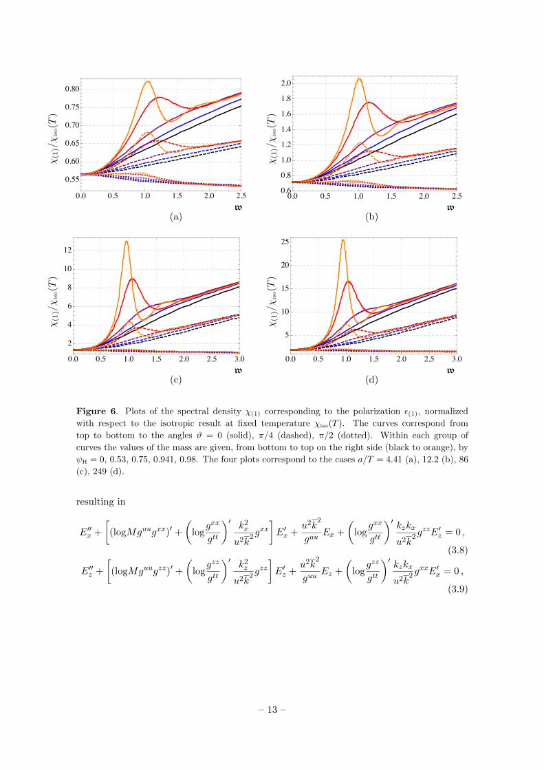
Figure 6. Plots of the spectral density χ(1) corresponding to the polarization ε(1), normalized

with respect to the isotropic result at fixed temperature χiso(T ). The curves correspond from

top to bottom to the angles ϑ = 0 (solid), π/4 (dashed), π/2 (dotted). Within each group of

curves the values of the mass are given, from bottom to top on the right side (black to orange), by

ψH = 0, 0.53, 0.75, 0.941, 0.98. The four plots correspond to the cases a/T = 4.41 (a), 12.2 (b), 86

(c), 249 (d).

resulting in

E′′x +

[(logMguugxx)′ +

(log

gxx

gtt

)′ k2x

u2k2 g

xx

]E′x +

u2k2

guuEx +

(log

gxx

gtt

)′ kzkxu2k

2 gzzE′z = 0 ,

(3.8)

E′′z +

[(logMguugzz)′ +

(log

gzz

gtt

)′ k2z

u2k2 g

zz

]E′z +

u2k2

guuEz +

(log

gzz

gtt

)′ kzkxu2k

2 gxxE′x = 0 ,

(3.9)

– 13 –

0 5 10 15 200.0

0.5

1.0

1.5

σ(1)

a/T

Figure 7. Plot of the conductivity σ(1) corresponding to the polarization ε(1) as a function of a/T

for, from top to bottom, ψH = 0, 0.53, 0.75, 0.941, 0.98.

where u2k2 ≡ −gttk2

0 − gxxk2x − gzzk2

z . The action (3.1) can also be written in terms of

these fields as

Sε = −2KD7

∫dt d~x

Mguu

−k20u

2k2

[(−gttk2

0 − gzzk2z

)gxxExE

′x + u2k

2gyyEyE

′y+

+ gxxgzzkxkz (ExEz)′ +(−gttk2

0 − gxxk2x

)gzzEzE

′z

]u=ε

. (3.10)

Since we need to take the limit ε→ 0, before proceeding any further, we need to verify

that the correlators will remain finite in this limit. To this end we use the near-boundary

expansion of the metric (2.30) and of the embedding ψ (2.31) to solve the equations (3.8)

and (3.9) perturbatively. We find

Ex = E(0)x + E(2)

x cosϑu2 − 1

24

(3

4E(0)x k2

0 cosϑ+

(5− 24ψ2

1

a2

)E(2)x

)cosϑa2 u4 +O

(u6),

(3.11)

Ez = E(0)z + E(2)

x sinϑu2 + E(4)z u4 − a2k2

0 cosϑ

16

(E(0)z cos θ + E(0)

x sinϑ)u4 log u+O

(u6).

(3.12)

Using these expressions, we can rewrite (3.10) as

Sε = −2KD7

∫dt d~x

[L1 + L2 + L3 + Lm + . . .+O

(u2)]u=ε

, (3.13)

where

L1 = −3

4sin2 ϑE(0)2

x − 1

4cos2 ϑE(0)2

z − sinϑ cosϑE(0)x E(0)

z ,

L2 =1

3k20

[1 + 5 cos 2ϑ

cosϑE(0)x E(2)

x +48

a2tanϑE(0)

x E(4)z − 10 sinϑE(0)

z E(2)x +

48

a2E(0)z E(4)

z

],

L3 = −(E(0)x sinϑ+ E(0)

z cosϑ)2

log u ,

Lm =16ψ2

1

a2k20

tanϑ(E(0)x E(2)

x sinϑ+ E(0)z E(2)

x cosϑ), (3.14)

– 14 –

and the ellipsis stands for the terms in the y-components that have been already dealt

with. Notice that L1, L2, L3 are the same as in the ψ = 0 case of [27].

The contribution of Lm to the production of photons with polarization ε(2) is propor-

tional to

cos2 ϑδ2Lm

δE(0)2x

+ sin2 ϑδ2Lm

δE(0)2z

− 2 sinϑ cosϑδ2Lm

δE(0)z δE

(0)x

= 0 , (3.15)

and therefore vanishes identically, and so does the divergent term L3, as shown in [27]. We

obtain then the simple result

χ(2) ≡ εµ(2)ε

ν(2)χµν = 16KD7Im

[cosϑ

δE(2)x

δE(0)x

− sinϑδE

(2)x

δE(0)z

]. (3.16)

We can now proceed as in [27] to determine how E(2)x varies with respect of E

(0)x and E

(0)z .

Alternatively, we will explain in Appendix A how to apply the technology developed in [55]

to obtain χ(2) using the values of the fields at the horizon. As a check of our results, we

have verified that we obtain the same results using both methods. We display the results

in Fig. 8 for various values of the anisotropy, of the angles, and of the quark masses.

For photons with polarization along ε(2), the conductivity

σ(2)(T ) = limk0→0

χ(2)

χ(2),iso(T )= lim

k0→02χ(2)

χiso(T )(3.17)

depends not only on the anisotropy and quark mass, as was the case for the polarization

along the y-direction, but also on the angle ϑ. If we normalize with respect to the isotropic

case, the conductivity does not depend on the quark masses and is therefore identical to the

one depicted in Figs. 11 and 12 of [27]. We can then define unnormalized conductivities,

as done above for σ(1),

σ(2) = 2 limw→0

χ(2)

8ND7w, (3.18)

which do depend on the masses and are reported in Figs. 9 (as a function of a/T for fixed

ϑ) and 10 (as a function of ϑ for fixed a/T ).

3.3 Total photon production rate

We have now all the ingredients to calculate the total emission rate (2.5). We convert this

quantity to the emission rate per unit photon energy in a infinitesimal angle around ϑ.

Using that the photon momentum is light-like, we have

−1

2αEMNcNfT 3

dΓγd cosϑ dk0

=w

2NcNfT 2

1

e2πw − 1

(χ(1) + χ(2)

), (3.19)

which is plotted in Fig. 11 for different values of a/T , ϑ and ψH. The isotropic result at

the same temperature cannot be calculated analytically, since we only have a numerical

solution for ψ. So, we calculated this quantity numerically and the results are shown in

the figures as coarsely dashed curves. We observe that, even in the massive quark case, the

anisotropic plasma emits more photons, in total, than the corresponding isotropic plasma

at the same temperature.

– 15 –

0.0 0.5 1.0 1.5 2.0 2.5

0.5

0.6

0.7

0.8

0.0 0.5 1.0 1.5 2.0 2.5

0.5

1.0

1.5

2.0

χ(2

)/χ

iso(T

)

w

χ(2

)/χ

iso(T

)

w(a) (b)

0.0 0.5 1.0 1.5 2.0 2.5 3.00

2

4

6

8

10

12

0.0 0.5 1.0 1.5 2.0 2.50

5

10

15

20

25

30

χ(2

)/χ

iso(T

)

w

χ(2

)/χ

iso(T

)

w(c) (d)

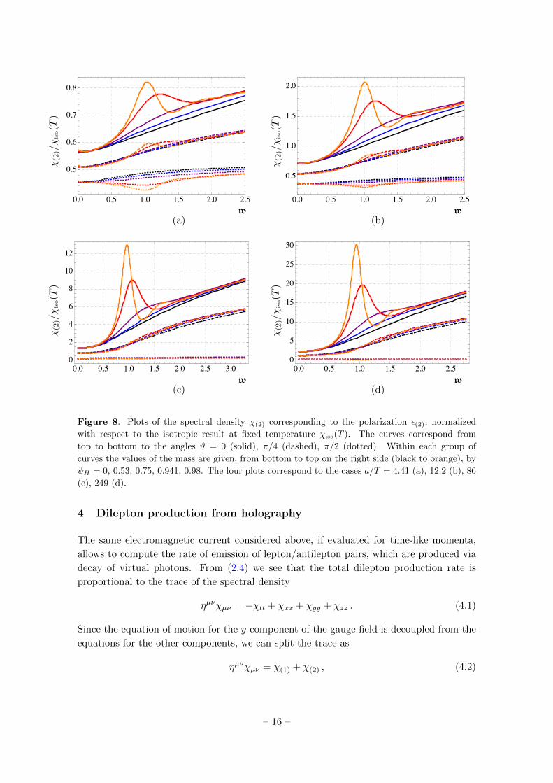
Figure 8. Plots of the spectral density χ(2) corresponding to the polarization ε(2), normalized

with respect to the isotropic result at fixed temperature χiso(T ). The curves correspond from

top to bottom to the angles ϑ = 0 (solid), π/4 (dashed), π/2 (dotted). Within each group of

curves the values of the mass are given, from bottom to top on the right side (black to orange), by

ψH = 0, 0.53, 0.75, 0.941, 0.98. The four plots correspond to the cases a/T = 4.41 (a), 12.2 (b), 86

(c), 249 (d).

4 Dilepton production from holography

The same electromagnetic current considered above, if evaluated for time-like momenta,

allows to compute the rate of emission of lepton/antilepton pairs, which are produced via

decay of virtual photons. From (2.4) we see that the total dilepton production rate is

proportional to the trace of the spectral density

ηµνχµν = −χtt + χxx + χyy + χzz . (4.1)

Since the equation of motion for the y-component of the gauge field is decoupled from the

equations for the other components, we can split the trace as

ηµνχµν = χ(1) + χ(2) , (4.2)

– 16 –

0 2 4 6 8 10 120.0

0.2

0.4

0.6

0.8

1.0

1.2

1.4σ(2)

a/T

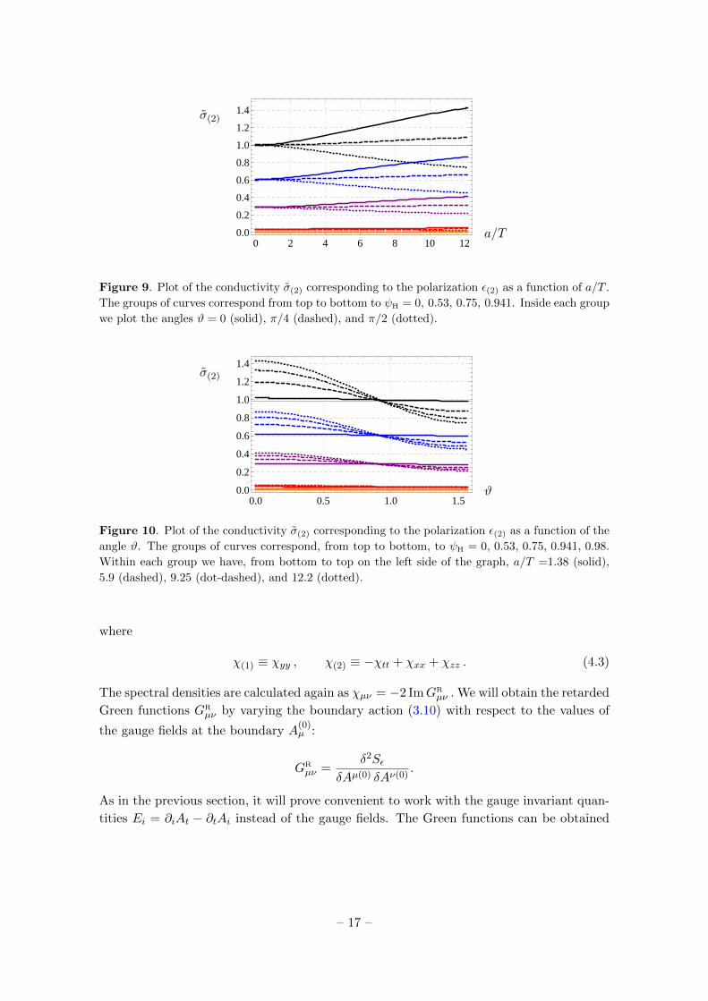
Figure 9. Plot of the conductivity σ(2) corresponding to the polarization ε(2) as a function of a/T .

The groups of curves correspond from top to bottom to ψH = 0, 0.53, 0.75, 0.941. Inside each group

we plot the angles ϑ = 0 (solid), π/4 (dashed), and π/2 (dotted).

0.0 0.5 1.0 1.50.0

0.2

0.4

0.6

0.8

1.0

1.2

1.4σ(2)

ϑ

Figure 10. Plot of the conductivity σ(2) corresponding to the polarization ε(2) as a function of the

angle ϑ. The groups of curves correspond, from top to bottom, to ψH = 0, 0.53, 0.75, 0.941, 0.98.

Within each group we have, from bottom to top on the left side of the graph, a/T =1.38 (solid),

5.9 (dashed), 9.25 (dot-dashed), and 12.2 (dotted).

where

χ(1) ≡ χyy , χ(2) ≡ −χtt + χxx + χzz . (4.3)

The spectral densities are calculated again as χµν = −2 ImGRµν . We will obtain the retarded

Green functions GRµν by varying the boundary action (3.10) with respect to the values of

the gauge fields at the boundary A(0)µ :

GRµν =

δ2Sε

δAµ(0) δAν(0).

As in the previous section, it will prove convenient to work with the gauge invariant quan-

tities Ei = ∂iAt − ∂tAi instead of the gauge fields. The Green functions can be obtained

– 17 –

0.0 0.2 0.4 0.6 0.8 1.0 1.2 1.40.000

0.005

0.010

0.015

0.0 0.2 0.4 0.6 0.8 1.0 1.2 1.40.000

0.005

0.010

0.015

0.020

−1

2αEMN

cN

fT3

dΓγ

dco

sϑdk0

w

−1

2αEMN

cN

fT3

dΓγ

dco

sϑdk0

w(a) (b)

0.0 0.2 0.4 0.6 0.8 1.0 1.20.00

0.01

0.02

0.03

0.04

0.0 0.2 0.4 0.6 0.8 1.0 1.20.00

0.01

0.02

0.03

0.04

0.05

0.06

0.07

−1

2αEMN

cN

fT3

dΓγ

dco

sϑdk0

w

−1

2αEMN

cN

fT3

dΓγ

dco

sϑdk0

w(c) (d)

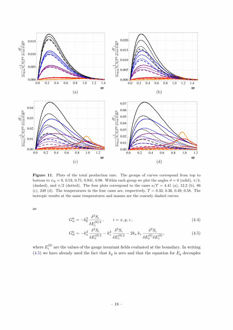
Figure 11. Plots of the total production rate. The groups of curves correspond from top to

bottom to ψH = 0, 0.53, 0.75, 0.941, 0.98. Within each group we plot the angles ϑ = 0 (solid), π/4,

(dashed), and π/2 (dotted). The four plots correspond to the cases a/T = 4.41 (a), 12.2 (b), 86

(c), 249 (d). The temperatures in the four cases are, respectively, T = 0.33, 0.36, 0.49, 0.58. The

isotropic results at the same temperatures and masses are the coarsely dashed curves.

as

GRii = −k2

0

δ2Sε

δE(0) 2i

, i = x, y, z , (4.4)

GRtt = −k2

x

δ2Sε

δE(0) 2x

− k2z

δ2Sε

δE(0) 2z

− 2kx kzδ2Sε

δE(0)x δE

(0)z

, (4.5)

where E(0)i are the values of the gauge invariant fields evaluated at the boundary. In writing

(4.5) we have already used the fact that ky is zero and that the equation for Ey decouples

– 18 –

from the rest. We arrive at

χ(1) = 2 Im

[k2

0

δ2Sε

δE(0) 2y

], (4.6)

χ(2) = −2 Im

[(k2x − k2

0)δ2Sε

δE(0)2x

+ (k2z − k2

0)δ2Sε

δE(0)2z

+ 2 kx kzδ2Sε

δE(0)x δE

(0)z

]. (4.7)

In terms of the spectral densities the latter equation is

χ(2) =

(1− k2

x

k20

)χxx +

(1− k2

z

k20

)χzz − 2

kxkzk2

0

χxz . (4.8)

When light-like momentum is considered, the previous calculation coincides, as it should,

with the one for the photon production. For dilepton production, the spatial part of the

momentum will be given by ~k = q(sinϑ, 0, cosϑ) for q < k0, and the equation (4.7) will

read

χ(2) = −2 Im

[(q2sin2ϑ− k2

0)δ2Sε

δE(0)2x

+ (q2cos2ϑ− k20)

δ2Sε

δE(0)2z

+ 2 q2sinϑ cosϑδ2Sε

δE(0)x δE

(0)z

].

(4.9)

As a warm up, we will begin by performing the calculation in the isotropic limit. This

will be used to normalize the results for the anisotropic plasma.

4.1 Isotropic limit

In the isotropic limit (2.11) we can use the SO(3) symmetry to set ϑ = π/2, fixing the

spatial component of k in the x-direction. We have kx = q, ky = kz = 0 which simplifies

the equations above to

χ(1)iso = χyy,iso , χ(2)iso =

(1− q2

k20

)χxx,iso + χzz,iso. (4.10)

We will compute χyy repeating the same steps used in the photon production for

polarization ε(1). This spectral density reads

χ(1)iso

8ND7w=

1

2πTk0 |Ay,iso(k, 0)|2Im lim

u→uHQ(u)A′y,iso(k, u)A∗y,iso(k, u) (4.11)

where Q(u) was defined in (3.3) and Ay,iso solves equation (2.23), in the isotropic limit

(2.11) but with q 6= k0.

To compute χxx,iso and χzz,iso, we make two observations. First, for ϑ = π/2, equations

(3.8) and (3.9) decouple from each other. Second, the action (3.10) will have no mixed

terms, so we can vary the action with respect to Ex,iso and Ez,iso in a similar fashion to

what has been done for Ay,iso, and get

χxx,iso

8ND7w=

k0

2πT |Ex,iso(k, 0)|2Im lim

u→uHQx(u)E′x,iso(k, u)E∗x,iso(k, u) , (4.12)

χzz,iso

8ND7w=

k0

2πT |Ez,iso(k, 0)|2Im lim

u→uHQz(u)E′z,iso(k, u)E∗z,iso(k, u) , (4.13)

– 19 –

0.0 0.5 1.0 1.5 2.0 2.5 3.00

1

2

3

4

0.0 0.5 1.0 1.5 2.0 2.5 3.00

2

4

6

8

χ(1

)iso/8N

D7w

w

χ(2

)iso/8N

D7w

w

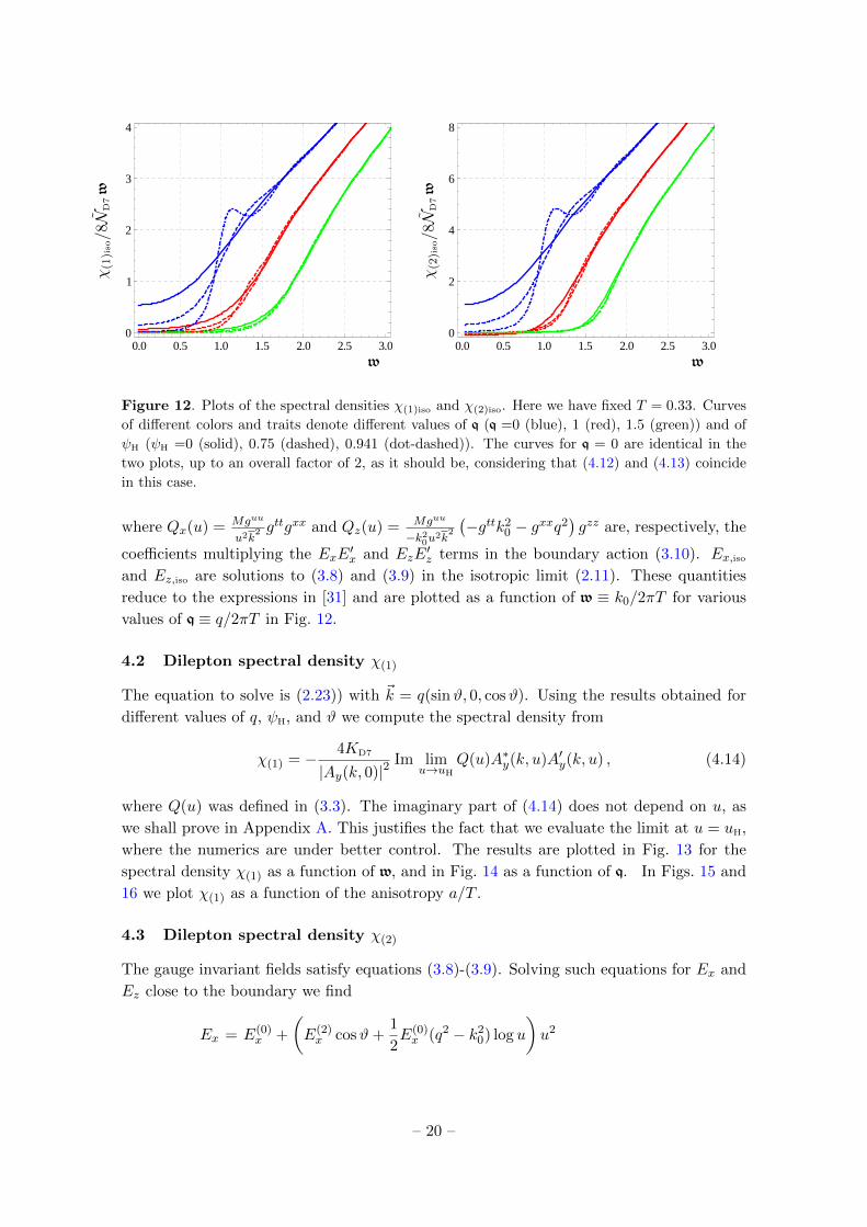
Figure 12. Plots of the spectral densities χ(1)iso and χ(2)iso. Here we have fixed T = 0.33. Curves

of different colors and traits denote different values of q (q =0 (blue), 1 (red), 1.5 (green)) and of

ψH (ψH =0 (solid), 0.75 (dashed), 0.941 (dot-dashed)). The curves for q = 0 are identical in the

two plots, up to an overall factor of 2, as it should be, considering that (4.12) and (4.13) coincide

in this case.

where Qx(u) = Mguu

u2k2 g

ttgxx and Qz(u) = Mguu

−k20u2k2

(−gttk2

0 − gxxq2)gzz are, respectively, the

coefficients multiplying the ExE′x and EzE

′z terms in the boundary action (3.10). Ex,iso

and Ez,iso are solutions to (3.8) and (3.9) in the isotropic limit (2.11). These quantities

reduce to the expressions in [31] and are plotted as a function of w ≡ k0/2πT for various

values of q ≡ q/2πT in Fig. 12.

4.2 Dilepton spectral density χ(1)

The equation to solve is (2.23)) with ~k = q(sinϑ, 0, cosϑ). Using the results obtained for

different values of q, ψH, and ϑ we compute the spectral density from

χ(1) = − 4KD7

|Ay(k, 0)|2Im lim

u→uHQ(u)A∗y(k, u)A′y(k, u) , (4.14)

where Q(u) was defined in (3.3). The imaginary part of (4.14) does not depend on u, as

we shall prove in Appendix A. This justifies the fact that we evaluate the limit at u = uH,

where the numerics are under better control. The results are plotted in Fig. 13 for the

spectral density χ(1) as a function of w, and in Fig. 14 as a function of q. In Figs. 15 and

16 we plot χ(1) as a function of the anisotropy a/T .

4.3 Dilepton spectral density χ(2)

The gauge invariant fields satisfy equations (3.8)-(3.9). Solving such equations for Ex and

Ez close to the boundary we find

Ex = E(0)x +

(E(2)x cosϑ+

1

2E(0)x (q2 − k2

0) log u

)u2

– 20 –

0.0 0.5 1.0 1.5 2.01.0

1.2

1.4

1.6

1.8

2.0

1.0 1.2 1.4 1.6 1.8 2.0 2.21.0

1.2

1.4

1.6

1.8

1.6 1.8 2.0 2.21.0

1.2

1.4

1.6

1.8

2.0

2.2

χ(1

)/χ

(1)iso

(T)

w

χ(1

)/χ

(1)iso

(T)

w

χ(1

)/χ

(1)iso

(T)

w(a) (b) (c)

0.0 0.5 1.0 1.5 2.01.0

1.2

1.4

1.6

1.8

2.0

1.0 1.2 1.4 1.6 1.8 2.0 2.21.0

1.2

1.4

1.6

1.8

1.6 1.8 2.0 2.21.0

1.2

1.4

1.6

1.8

2.0

2.2

χ(1

)/χ

(1)iso

(T)

w

χ(1

)/χ

(1)iso

(T)

w

χ(1

)/χ

(1)iso

(T)

w(d) (e) (f)

0.0 0.5 1.0 1.5 2.01.0

1.5

2.0

2.5

1.0 1.2 1.4 1.6 1.8 2.0 2.21.0

1.5

2.0

2.5

1.6 1.8 2.0 2.21.0

1.2

1.4

1.6

1.8

2.0

2.2

χ(1

)/χ

(1)iso

(T)

w

χ(1

)/χ

(1)iso

(T)

w

χ(1

)/χ

(1)iso

(T)

w(g) (h) (i)

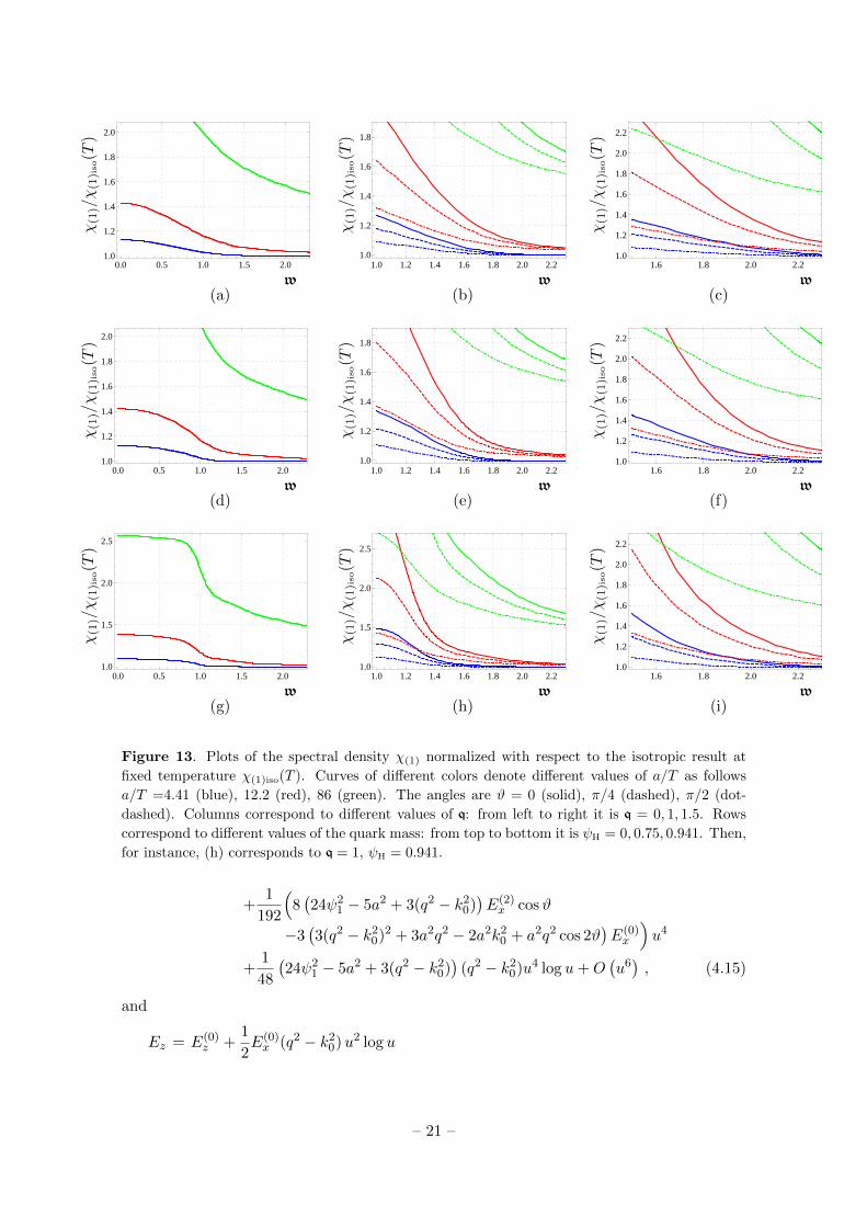
Figure 13. Plots of the spectral density χ(1) normalized with respect to the isotropic result at

fixed temperature χ(1)iso(T ). Curves of different colors denote different values of a/T as follows

a/T =4.41 (blue), 12.2 (red), 86 (green). The angles are ϑ = 0 (solid), π/4 (dashed), π/2 (dot-

dashed). Columns correspond to different values of q: from left to right it is q = 0, 1, 1.5. Rows

correspond to different values of the quark mass: from top to bottom it is ψH = 0, 0.75, 0.941. Then,

for instance, (h) corresponds to q = 1, ψH = 0.941.

+1

192

(8(24ψ2

1 − 5a2 + 3(q2 − k20))E(2)x cosϑ

−3(3(q2 − k2

0)2 + 3a2q2 − 2a2k20 + a2q2 cos 2ϑ

)E(0)x

)u4

+1

48

(24ψ2

1 − 5a2 + 3(q2 − k20))

(q2 − k20)u4 log u+O

(u6), (4.15)

and

Ez = E(0)z +

1

2E(0)x (q2 − k2

0)u2 log u

– 21 –

0.0 0.1 0.2 0.3 0.4 0.5

1.5

2.0

2.5

3.0

3.5

0.0 0.2 0.4 0.6 0.8 1.01.0

1.5

2.0

2.5

3.0

3.5

0.0 0.2 0.4 0.6 0.8 1.0 1.2 1.41.0

1.5

2.0

2.5

χ(1

)/χ

(1)iso

(T)

q

χ(1

)/χ

(1)iso

(T)

q

χ(1

)/χ

(1)iso

(T)

q(a) (b) (c)

0.0 0.1 0.2 0.3 0.4 0.5

1.5

2.0

2.5

3.0

3.5

0.0 0.2 0.4 0.6 0.8 1.01.0

1.5

2.0

2.5

3.0

3.5

4.0

0.0 0.2 0.4 0.6 0.8 1.0 1.2 1.41.0

1.5

2.0

2.5

χ(1

)/χ

(1)iso

(T)

q

χ(1

)/χ

(1)iso

(T)

q

χ(1

)/χ

(1)iso

(T)

q(d) (e) (f)

0.0 0.1 0.2 0.3 0.4 0.51.0

1.5

2.0

2.5

3.0

3.5

4.0

0.0 0.2 0.4 0.6 0.8 1.01.0

1.5

2.0

2.5

3.0

3.5

4.0

0.0 0.2 0.4 0.6 0.8 1.0 1.2 1.41.0

1.5

2.0

2.5

χ(1

)/χ

(1)iso

(T)

q

χ(1

)/χ

(1)iso

(T)

q

χ(1

)/χ

(1)iso

(T)

q(g) (h) (i)

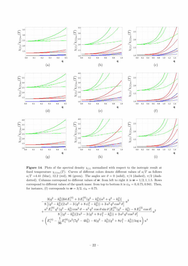
Figure 14. Plots of the spectral density χ(1) normalized with respect to the isotropic result at

fixed temperature χ(1)iso(T ). Curves of different colors denote different values of a/T as follows

a/T =4.41 (blue), 12.2 (red), 86 (green). The angles are ϑ = 0 (solid), π/4 (dashed), π/2 (dash-

dotted). Columns correspond to different values of w: from left to right it is w = 1/2, 1, 1.5. Rows

correspond to different values of the quark mass: from top to bottom it is ψH = 0, 0.75, 0.941. Then,

for instance, (f) corresponds to w = 3/2, ψH = 0.75.

− 3(q2 − k20)[64E

(4)z + 3E

(0)z (q2 − k2

0)(a2 + q2 − k20)]

8[(q2 − k2

0)(2 a2 − 3 (q2 + 8ψ21 − k2

0)) + 3 a2 q2 cos2 ϑ] u2

+a2E

(0)z q2 (q2 − k2

0) cos2 ϑ− a2 q2 cosϑ sinϑ [E(0)x (q2 − k2

0)− 8E(2)x cosϑ]

8[(q2 − k2

0)(2 a2 − 3 (q2 + 8ψ21 − k2

0)) + 3 a2 q2 cos2 ϑ] u2

+

(E(4)z −

1

96E(0)z (a2(7q2 − 4k2

0)− 6(q2 − k20)(q2 + 8ψ2

1 − k20)) log u

)u4

– 22 –

0 5 10 15 20 251.0

1.2

1.4

1.6

1.8

2.0

2.2

0 5 10 15 20 251.0

1.2

1.4

1.6

1.8

2.0

0 5 10 15 20 251.0

1.1

1.2

1.3

1.4

χ(1

)/χ

(1)iso

(T)

a/T

χ(1

)/χ

(1)iso

(T)

a/T

χ(1

)/χ

(1)iso

(T)

a/T(a) (b) (c)

0 5 10 15 20 251.0

1.2

1.4

1.6

1.8

2.0

2.2

0 5 10 15 20 251.0

1.2

1.4

1.6

1.8

2.0

2.2

0 5 10 15 20 251.00

1.05

1.10

1.15

1.20

1.25

χ(1

)/χ

(1)iso

(T)

a/T

χ(1

)/χ

(1)iso

(T)

a/T

χ(1

)/χ

(1)iso

(T)

a/T(d) (e) (f)

0 5 10 15 20 251.0

1.2

1.4

1.6

1.8

2.0

2.2

2.4

0 5 10 15 20 251.0

1.2

1.4

1.6

1.8

2.0

0 5 10 15 20 251.00

1.05

1.10

1.15

1.20

1.25

χ(1

)/χ

(1)iso

(T)

a/T

χ(1

)/χ

(1)iso

(T)

a/T

χ(1

)/χ

(1)iso

(T)

a/T(g) (h) (i)

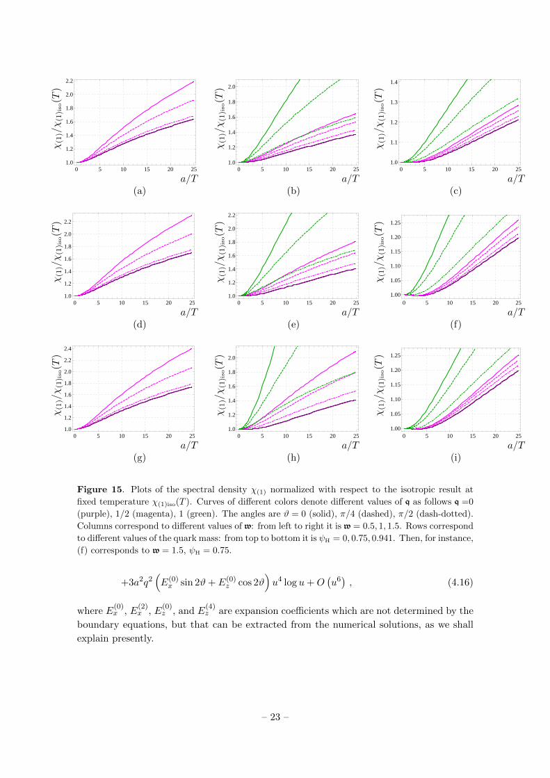
Figure 15. Plots of the spectral density χ(1) normalized with respect to the isotropic result at

fixed temperature χ(1)iso(T ). Curves of different colors denote different values of q as follows q =0

(purple), 1/2 (magenta), 1 (green). The angles are ϑ = 0 (solid), π/4 (dashed), π/2 (dash-dotted).

Columns correspond to different values of w: from left to right it is w = 0.5, 1, 1.5. Rows correspond

to different values of the quark mass: from top to bottom it is ψH = 0, 0.75, 0.941. Then, for instance,

(f) corresponds to w = 1.5, ψH = 0.75.

+3a2q2(E(0)x sin 2ϑ+ E(0)

z cos 2ϑ)u4 log u+O

(u6), (4.16)

where E(0)x , E

(2)x , E

(0)z , and E

(4)z are expansion coefficients which are not determined by the

boundary equations, but that can be extracted from the numerical solutions, as we shall

explain presently.

– 23 –

0 5 10 15 20 251.0

1.1

1.2

1.3

1.4

1.5

1.6

0 5 10 15 20 251.0

1.2

1.4

1.6

1.8

0 5 10 15 20 251.0

1.2

1.4

1.6

1.8

2.0

2.2

2.4

χ(1

)/χ

(1)iso

(T)

a/T

χ(1

)/χ

(1)iso

(T)

a/T

χ(1

)/χ

(1)iso

(T)

a/T(a) (b) (c)

0 5 10 15 20 251.0

1.1

1.2

1.3

1.4

1.5

0 5 10 15 20 251.0

1.2

1.4

1.6

1.8

0 5 10 15 20 251.0

1.5

2.0

2.5

χ(1

)/χ

(1)iso

(T)

a/T

χ(1

)/χ

(1)iso

(T)

a/T

χ(1

)/χ

(1)iso

(T)

a/T(d) (e) (f)

0 5 10 15 20 251.0

1.1

1.2

1.3

1.4

0 5 10 15 20 251.0

1.2

1.4

1.6

1.8

2.0

0 5 10 15 20 251.0

1.2

1.4

1.6

1.8

2.0

2.2

2.4

χ(1

)/χ

(1)iso

(T)

a/T

χ(1

)/χ

(1)iso

(T)

a/T

χ(1

)/χ

(1)iso

(T)

a/T(g) (h) (i)

Figure 16. Plots of the spectral density χ(1) normalized with respect to the isotropic result at fixed

temperature χ(1)iso(T ). Curves of different colors denote different values of w as follows w =1/2

(black), 1 (brown), 3/2 (blue). The angles are ϑ = 0 (solid), π/4 (dashed), π/2 (dash-dotted).

Columns correspond to different values of q: from left to right it is q = 0, 0.5, 1. Rows correspond to

different values of the quark mass: from top to bottom it is ψ0 = 0, 0.75, 0.941. Then, for instance,

(f) corresponds to q = 1, ψH = 0.75.

Using these expressions, we can write the boundary action as

Sε = −2KD7

∫dt d~x

[L1 + L2 + L3 + . . .+O

(u2)]u=ε

, (4.17)

– 24 –

where

L1 = A1E(0) 2x +B1E

(0) 2z + C1E

(0)x E(0)

z ,

L2 = A2E(0)x E(2)

x +B2E(0)x E(2)

x + C2E(0)x E(2)

x +D2E(0)x E(2)

x ,

L3 = − log u

k20

[(E(0) 2

x + E(0) 2z ) k2

0 + (E(0)x cosϑ− E(0)

z sinϑ)2 q2], (4.18)

and Ai, Bi, Ci (i = 1, 2) and D2 are given by (B.3) in Appendix B. The contributions of L1

and L3 to the Green’s functions are real, so they don’t enter in the computation of χ(2).

Defining

S2 = −2KD7

∫dt d~xL2 ,

we can write

δ2S2

δE(0) 2x

= 2A2δE

(2)x

δE(0)x

+ 2B2δE

(4)z

δE(0)x

,

δ2S2

δE(0) 2z

= 2C2δE

(2)x

δE(0)z

+ 2D2δE

(4)z

δ,

δ2S2

δE(0)x δE

(0)z

= A2δE

(2)x

δE(0)z

+B2δE

(4)z

δE(0)z

+ C2δE

(2)x

δE(0)x

+D2δE

(4)z

δE(0)x

. (4.19)

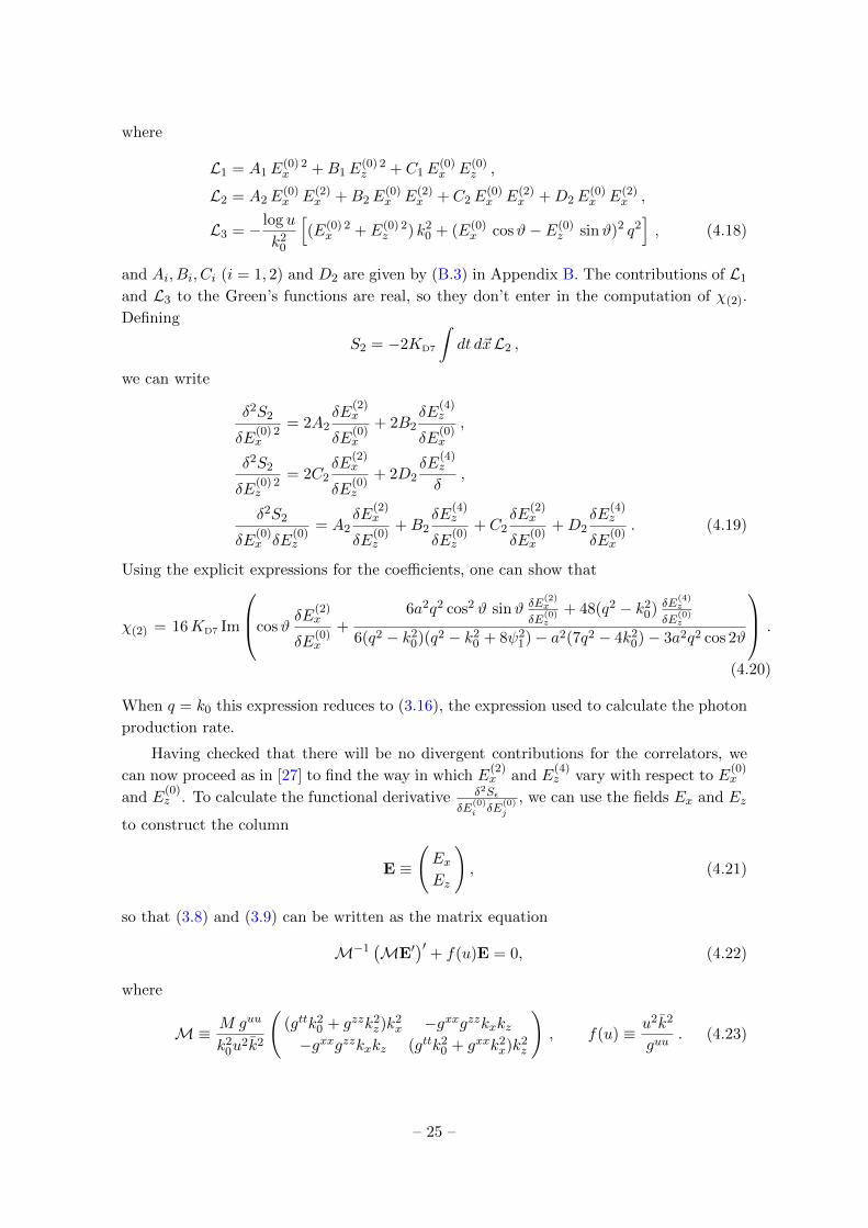
Using the explicit expressions for the coefficients, one can show that

χ(2) = 16KD7 Im

cosϑδE

(2)x

δE(0)x

+6a2q2 cos2 ϑ sinϑ δE

(2)x

δE(0)z

+ 48(q2 − k20) δE

(4)z

δE(0)z

6(q2 − k20)(q2 − k2

0 + 8ψ21)− a2(7q2 − 4k2

0)− 3a2q2 cos 2ϑ

.

(4.20)

When q = k0 this expression reduces to (3.16), the expression used to calculate the photon

production rate.

Having checked that there will be no divergent contributions for the correlators, we

can now proceed as in [27] to find the way in which E(2)x and E

(4)z vary with respect to E

(0)x

and E(0)z . To calculate the functional derivative δ2Sε

δE(0)i δE

(0)j

, we can use the fields Ex and Ez

to construct the column

E ≡

(ExEz

), (4.21)

so that (3.8) and (3.9) can be written as the matrix equation

M−1(ME′

)′+ f(u)E = 0, (4.22)

where

M≡ M guu

k20u

2k2

((gttk2

0 + gzzk2z)k

2x −gxxgzzkxkz

−gxxgzzkxkz (gttk20 + gxxk2

x)k2z

), f(u) ≡ u2k2

guu. (4.23)

– 25 –

We can also write the boundary action (excluding the part with AyA′y) as

Sε = −2KD7

∫dt d~x

[ETME′

]u=ε

. (4.24)

Notice that if we can find two linearly independent solutions to (4.22), E1 and E2,

such that at the boundary they reduce to E1|bdry = (1 0)T and E2|bdry = (0 1)T, and we

arrange them as the columns of a 2 × 2 matrix E ≡ (E1 E2), then, given that (4.22) is

linear, its general solution Esol will be given by

Esol = E(0)x E1 + E(0)

z E2 = E

(E

(0)x

E(0)z

). (4.25)

Using (4.25) we can write the boundary action (4.24) as

Sε = −2KD7

∫dt d~x

[(E(0)

x E(0)z )ME ′

(E

(0)x

E(0)z

)]u=ε

, (4.26)

where the fact that E becomes the identity matrix at the boundary has been used. From

(4.26) we see that the variation δ2Sε

δE(0)i δE

(0)j

, and hence the Green’s function GRij , is given

by the ij component of the matrix ME ′. As will be seen in Appendix A, this way of

writing the variation of the action permits to express the imaginary part of the integrand

in (4.26), which is all we need to compute the spectral densities, in terms of u-independent

quantities. The evaluation can then be done at the horizon, where the numerics are under

better control. In Appendix A we also elaborate on how to construct the solutions necessary

to carry out this procedure.

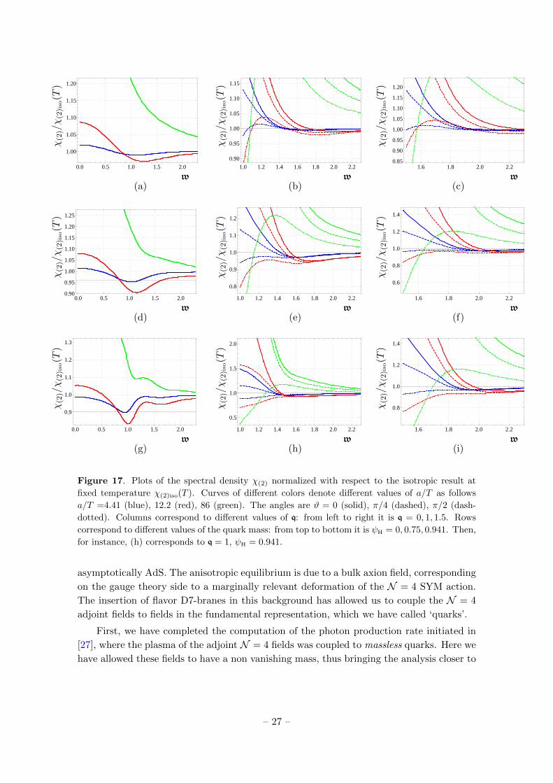
With this ground work in place, we use these expressions to numerically obtain the

dilepton production rate for different values of q, ψH, and ϑ. In Fig. 17 we plot the spectral

density χ(2) as a function of w, normalized with the corresponding spectral density χ(2)iso

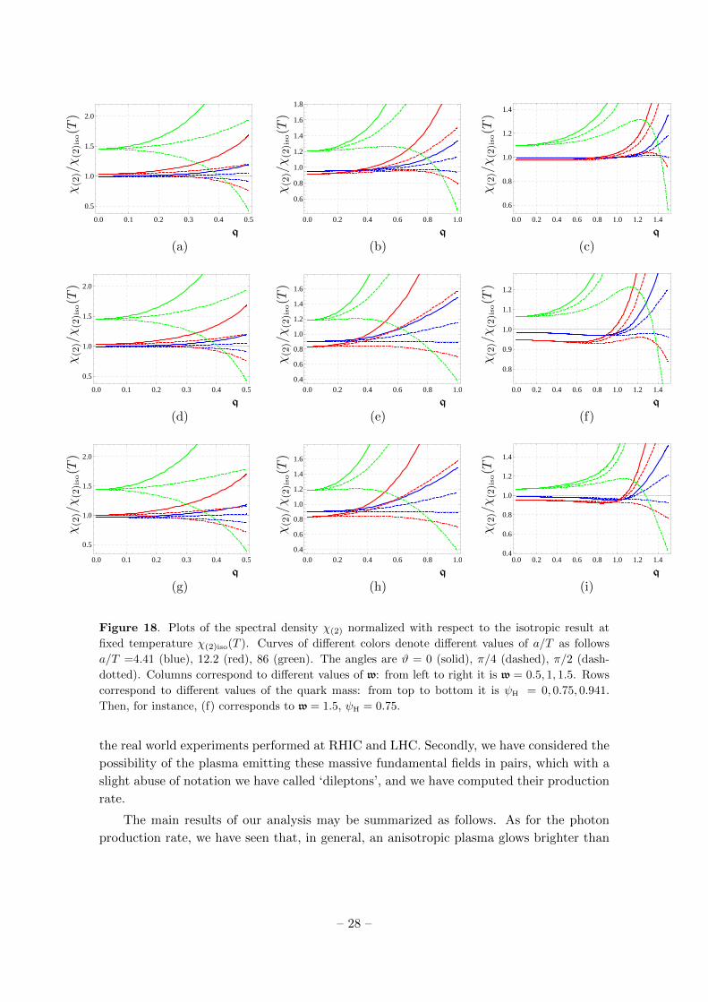
for an isotropic plasma at the same temperature. The same quantity as a function of q is

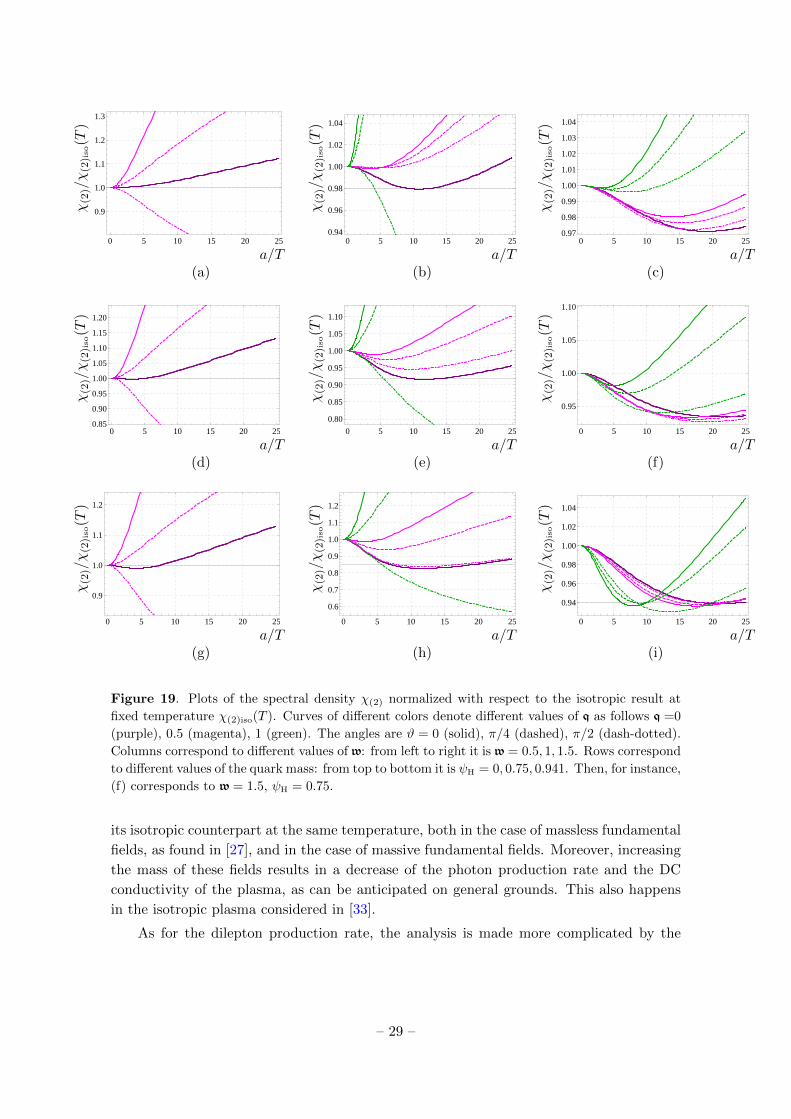
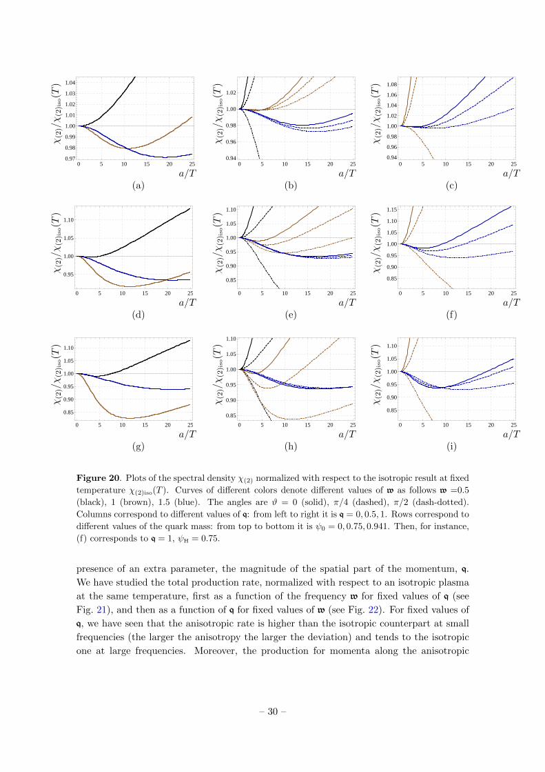
plotted in Fig. 18. In Figs. 19 and 20 we plot χ(2) as a function of the anisotropy a/T .

4.4 Total dilepton production rate

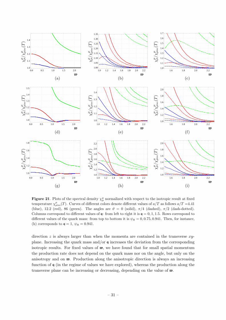
In Fig. 21 we plot the trace of the spectral density χµµ as a function of w, normalized with

the corresponding trace χµµiso for an isotropic plasma at the same temperature. The same

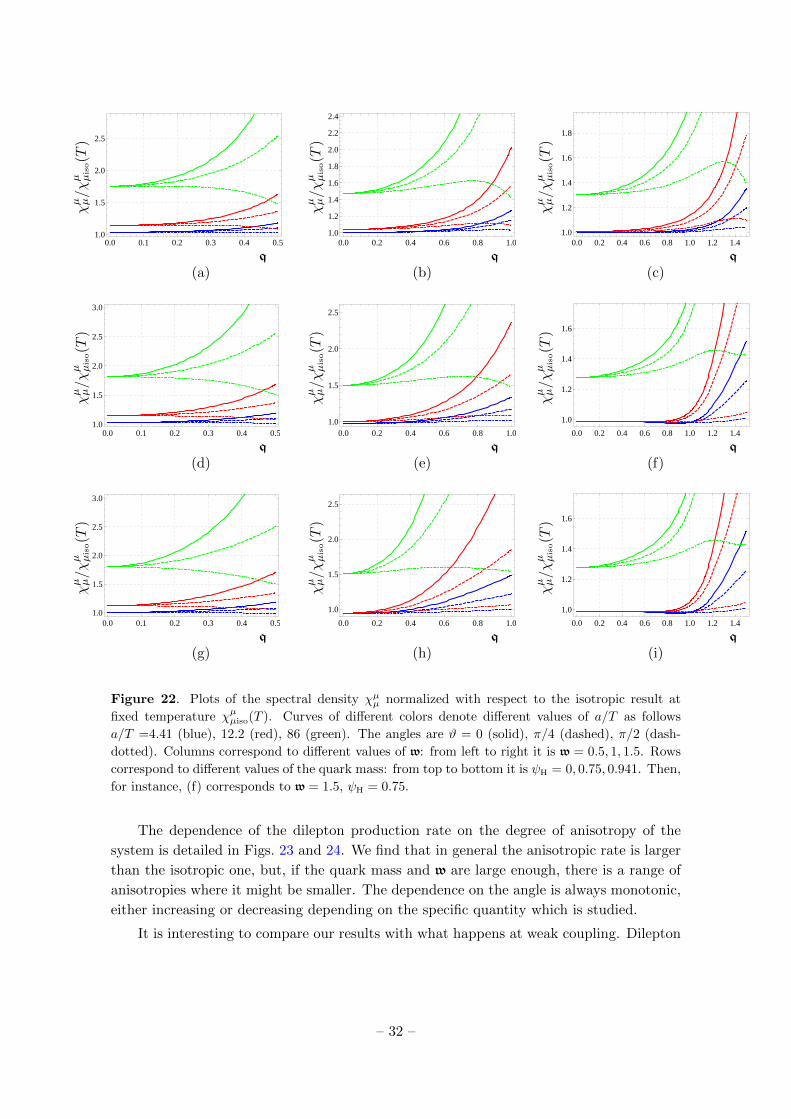
quantity as a function of q is plotted in Fig. 22, and in Figs. 23 and 24 as a function of the

anisotropy parameter a/T .

5 Discussion

In this paper we have studied two important phenomenological probes of a strongly coupled

anisotropic plasma, namely the in-medium production of photons and of dileptons. In order

to model the plasma at strong coupling, we have used the dual anisotropic black brane

solution found in [10, 11]. This geometry is static, regular on and outside the horizon, and

– 26 –

0.0 0.5 1.0 1.5 2.0

1.00

1.05

1.10

1.15

1.20

1.0 1.2 1.4 1.6 1.8 2.0 2.2

0.90

0.95

1.00

1.05

1.10

1.15

1.6 1.8 2.0 2.20.85

0.90

0.95

1.00

1.05

1.10

1.15

1.20

χ(2

)/χ

(2)iso

(T)

w

χ(2

)/χ

(2)iso

(T)

w

χ(2

)/χ

(2)iso

(T)

w(a) (b) (c)

0.0 0.5 1.0 1.5 2.00.90

0.95

1.00

1.05

1.10

1.15

1.20

1.25

1.0 1.2 1.4 1.6 1.8 2.0 2.2

0.8

0.9

1.0

1.1

1.2

1.6 1.8 2.0 2.2

0.6

0.8

1.0

1.2

1.4

χ(2

)/χ

(2)iso

(T)

w

χ(2

)/χ

(2)iso

(T)

w

χ(2

)/χ

(2)iso

(T)

w(d) (e) (f)

0.0 0.5 1.0 1.5 2.0

0.9

1.0

1.1

1.2

1.3

1.0 1.2 1.4 1.6 1.8 2.0 2.2

0.5

1.0

1.5

2.0

1.6 1.8 2.0 2.2

0.8

1.0

1.2

1.4

χ(2

)/χ

(2)iso

(T)

w

χ(2

)/χ

(2)iso

(T)

w

χ(2

)/χ

(2)iso

(T)

w(g) (h) (i)

Figure 17. Plots of the spectral density χ(2) normalized with respect to the isotropic result at

fixed temperature χ(2)iso(T ). Curves of different colors denote different values of a/T as follows

a/T =4.41 (blue), 12.2 (red), 86 (green). The angles are ϑ = 0 (solid), π/4 (dashed), π/2 (dash-

dotted). Columns correspond to different values of q: from left to right it is q = 0, 1, 1.5. Rows

correspond to different values of the quark mass: from top to bottom it is ψH = 0, 0.75, 0.941. Then,

for instance, (h) corresponds to q = 1, ψH = 0.941.

asymptotically AdS. The anisotropic equilibrium is due to a bulk axion field, corresponding

on the gauge theory side to a marginally relevant deformation of the N = 4 SYM action.

The insertion of flavor D7-branes in this background has allowed us to couple the N = 4

adjoint fields to fields in the fundamental representation, which we have called ‘quarks’.

First, we have completed the computation of the photon production rate initiated in

[27], where the plasma of the adjoint N = 4 fields was coupled to massless quarks. Here we

have allowed these fields to have a non vanishing mass, thus bringing the analysis closer to

– 27 –

0.0 0.1 0.2 0.3 0.4 0.5

0.5

1.0

1.5

2.0

0.0 0.2 0.4 0.6 0.8 1.0

0.6

0.8

1.0

1.2

1.4

1.6

1.8

0.0 0.2 0.4 0.6 0.8 1.0 1.2 1.4

0.6

0.8

1.0

1.2

1.4

χ(2

)/χ

(2)iso

(T)

q

χ(2

)/χ

(2)iso

(T)

q

χ(2

)/χ

(2)iso

(T)

q(a) (b) (c)

0.0 0.1 0.2 0.3 0.4 0.5

0.5

1.0

1.5

2.0

0.0 0.2 0.4 0.6 0.8 1.00.4

0.6

0.8

1.0

1.2

1.4

1.6

0.0 0.2 0.4 0.6 0.8 1.0 1.2 1.4

0.8

0.9

1.0

1.1

1.2

χ(2

)/χ

(2)iso

(T)

q

χ(2

)/χ

(2)iso

(T)

q

χ(2

)/χ

(2)iso

(T)

q(d) (e) (f)

0.0 0.1 0.2 0.3 0.4 0.5

0.5

1.0

1.5

2.0

0.0 0.2 0.4 0.6 0.8 1.00.4

0.6

0.8

1.0

1.2

1.4

1.6

0.0 0.2 0.4 0.6 0.8 1.0 1.2 1.40.4

0.6

0.8

1.0

1.2

1.4

χ(2

)/χ

(2)iso

(T)

q

χ(2

)/χ

(2)iso

(T)

q

χ(2

)/χ

(2)iso

(T)

q(g) (h) (i)

Figure 18. Plots of the spectral density χ(2) normalized with respect to the isotropic result at

fixed temperature χ(2)iso(T ). Curves of different colors denote different values of a/T as follows

a/T =4.41 (blue), 12.2 (red), 86 (green). The angles are ϑ = 0 (solid), π/4 (dashed), π/2 (dash-

dotted). Columns correspond to different values of w: from left to right it is w = 0.5, 1, 1.5. Rows

correspond to different values of the quark mass: from top to bottom it is ψH = 0, 0.75, 0.941.

Then, for instance, (f) corresponds to w = 1.5, ψH = 0.75.

the real world experiments performed at RHIC and LHC. Secondly, we have considered the

possibility of the plasma emitting these massive fundamental fields in pairs, which with a

slight abuse of notation we have called ‘dileptons’, and we have computed their production

rate.

The main results of our analysis may be summarized as follows. As for the photon

production rate, we have seen that, in general, an anisotropic plasma glows brighter than

– 28 –

0 5 10 15 20 25

0.9

1.0

1.1

1.2

1.3

0 5 10 15 20 250.94

0.96

0.98

1.00

1.02

1.04

0 5 10 15 20 250.97

0.98

0.99

1.00

1.01

1.02

1.03

1.04

χ(2

)/χ

(2)iso

(T)

a/T

χ(2

)/χ

(2)iso

(T)

a/T

χ(2

)/χ

(2)iso

(T)

a/T(a) (b) (c)

0 5 10 15 20 250.85

0.90

0.95

1.00

1.05

1.10

1.15

1.20

0 5 10 15 20 25

0.80

0.85

0.90

0.95

1.00

1.05

1.10

0 5 10 15 20 25

0.95

1.00

1.05

1.10

χ(2

)/χ

(2)iso

(T)

a/T

χ(2

)/χ

(2)iso

(T)

a/T

χ(2

)/χ

(2)iso

(T)

a/T(d) (e) (f)

0 5 10 15 20 25

0.9

1.0

1.1

1.2

0 5 10 15 20 25

0.6

0.7

0.8

0.9

1.0

1.1

1.2

0 5 10 15 20 25

0.94

0.96

0.98

1.00

1.02

1.04

χ(2

)/χ

(2)iso

(T)

a/T

χ(2

)/χ

(2)iso

(T)

a/T

χ(2

)/χ

(2)iso

(T)

a/T(g) (h) (i)

Figure 19. Plots of the spectral density χ(2) normalized with respect to the isotropic result at

fixed temperature χ(2)iso(T ). Curves of different colors denote different values of q as follows q =0

(purple), 0.5 (magenta), 1 (green). The angles are ϑ = 0 (solid), π/4 (dashed), π/2 (dash-dotted).

Columns correspond to different values of w: from left to right it is w = 0.5, 1, 1.5. Rows correspond

to different values of the quark mass: from top to bottom it is ψH = 0, 0.75, 0.941. Then, for instance,

(f) corresponds to w = 1.5, ψH = 0.75.

its isotropic counterpart at the same temperature, both in the case of massless fundamental

fields, as found in [27], and in the case of massive fundamental fields. Moreover, increasing

the mass of these fields results in a decrease of the photon production rate and the DC

conductivity of the plasma, as can be anticipated on general grounds. This also happens

in the isotropic plasma considered in [33].

As for the dilepton production rate, the analysis is made more complicated by the

– 29 –

0 5 10 15 20 250.97

0.98

0.99

1.00

1.01

1.02

1.03

1.04

0 5 10 15 20 250.94

0.96

0.98

1.00

1.02

0 5 10 15 20 250.94

0.96

0.98

1.00

1.02

1.04

1.06

1.08

χ(2

)/χ

(2)iso

(T)

a/T

χ(2

)/χ

(2)iso

(T)

a/T

χ(2

)/χ

(2)iso

(T)

a/T(a) (b) (c)

0 5 10 15 20 25

0.95

1.00

1.05

1.10

0 5 10 15 20 25

0.85

0.90

0.95

1.00

1.05

1.10

0 5 10 15 20 25

0.85

0.90

0.95

1.00

1.05

1.10

1.15

χ(2

)/χ

(2)iso

(T)

a/T

χ(2

)/χ

(2)iso

(T)

a/T

χ(2

)/χ

(2)iso

(T)

a/T(d) (e) (f)

0 5 10 15 20 25

0.85

0.90

0.95

1.00

1.05

1.10

0 5 10 15 20 25

0.85

0.90

0.95

1.00

1.05

1.10

0 5 10 15 20 25

0.85

0.90

0.95

1.00

1.05

1.10

χ(2

)/χ

(2)iso

(T)

a/T

χ(2

)/χ

(2)iso

(T)

a/T

χ(2

)/χ

(2)iso

(T)

a/T(g) (h) (i)

Figure 20. Plots of the spectral density χ(2) normalized with respect to the isotropic result at fixed

temperature χ(2)iso(T ). Curves of different colors denote different values of w as follows w =0.5

(black), 1 (brown), 1.5 (blue). The angles are ϑ = 0 (solid), π/4 (dashed), π/2 (dash-dotted).

Columns correspond to different values of q: from left to right it is q = 0, 0.5, 1. Rows correspond to

different values of the quark mass: from top to bottom it is ψ0 = 0, 0.75, 0.941. Then, for instance,

(f) corresponds to q = 1, ψH = 0.75.

presence of an extra parameter, the magnitude of the spatial part of the momentum, q.

We have studied the total production rate, normalized with respect to an isotropic plasma

at the same temperature, first as a function of the frequency w for fixed values of q (see

Fig. 21), and then as a function of q for fixed values of w (see Fig. 22). For fixed values of

q, we have seen that the anisotropic rate is higher than the isotropic counterpart at small

frequencies (the larger the anisotropy the larger the deviation) and tends to the isotropic

one at large frequencies. Moreover, the production for momenta along the anisotropic

– 30 –

0.0 0.5 1.0 1.5 2.01.0

1.1

1.2

1.3

1.4

1.0 1.2 1.4 1.6 1.8 2.0 2.21.00

1.05

1.10

1.15

1.20

1.25

1.30

1.35

1.6 1.8 2.0 2.21.0

1.1

1.2

1.3

1.4

1.5

1.6

1.7

χµ µ/χ

µ µiso(T

)

w

χµ µ/χ

µ µiso(T

)

w

χµ µ/χ

µ µiso(T

)

w(a) (b) (c)

0.0 0.5 1.0 1.5 2.0

1.0

1.1

1.2

1.3

1.4

1.5

1.0 1.2 1.4 1.6 1.8 2.0 2.2

1.0

1.1

1.2

1.3

1.4

1.6 1.8 2.0 2.21.0

1.2

1.4

1.6

1.8

2.0

χµ µ/χ

µ µiso(T

)

w

χµ µ/χµ µiso(T

)

w

χµ µ/χµ µiso(T

)

w(d) (e) (f)

0.0 0.5 1.0 1.5 2.0

1.0

1.2

1.4

1.6

1.8

1.0 1.2 1.4 1.6 1.8 2.0 2.21.0

1.2

1.4

1.6

1.8

2.0

2.2

1.6 1.8 2.0 2.21.0

1.2

1.4

1.6

1.8

2.0

χµ µ/χ

µ µiso(T

)

w

χµ µ/χ

µ µiso(T

)

w

χµ µ/χ

µ µiso(T

)

w(g) (h) (i)

Figure 21. Plots of the spectral density χµµ normalized with respect to the isotropic result at fixed

temperature χµµiso(T ). Curves of different colors denote different values of a/T as follows a/T =4.41

(blue), 12.2 (red), 86 (green). The angles are ϑ = 0 (solid), π/4 (dashed), π/2 (dash-dotted).

Columns correspond to different values of q: from left to right it is q = 0, 1, 1.5. Rows correspond to

different values of the quark mass: from top to bottom it is ψH = 0, 0.75, 0.941. Then, for instance,

(h) corresponds to q = 1, ψH = 0.941.

direction z is always larger than when the momenta are contained in the transverse xy-

plane. Increasing the quark mass and/or q increases the deviation from the corresponding

isotropic results. For fixed values of w, we have found that for small spatial momentum

the production rate does not depend on the quark mass nor on the angle, but only on the

anisotropy and on w. Production along the anisotropic direction is always an increasing

function of q (in the regime of values we have explored), whereas the production along the

transverse plane can be increasing or decreasing, depending on the value of w.

– 31 –

0.0 0.1 0.2 0.3 0.4 0.51.0

1.5

2.0

2.5

0.0 0.2 0.4 0.6 0.8 1.01.0

1.2

1.4

1.6

1.8

2.0

2.2

2.4

0.0 0.2 0.4 0.6 0.8 1.0 1.2 1.41.0

1.2

1.4

1.6

1.8

χµ µ/χ

µ µiso(T

)

q

χµ µ/χ

µ µiso(T

)

q

χµ µ/χ

µ µiso(T

)

q(a) (b) (c)

0.0 0.1 0.2 0.3 0.4 0.51.0

1.5

2.0

2.5

3.0

0.0 0.2 0.4 0.6 0.8 1.01.0

1.5

2.0

2.5

0.0 0.2 0.4 0.6 0.8 1.0 1.2 1.4

1.0

1.2

1.4

1.6

χµ µ/χ

µ µiso(T

)

q

χµ µ/χ

µ µiso(T

)

q

χµ µ/χ

µ µiso(T

)

q(d) (e) (f)

0.0 0.1 0.2 0.3 0.4 0.51.0

1.5

2.0

2.5

3.0

0.0 0.2 0.4 0.6 0.8 1.0

1.0

1.5

2.0

2.5

0.0 0.2 0.4 0.6 0.8 1.0 1.2 1.4

1.0

1.2

1.4

1.6

χµ µ/χ

µ µiso(T

)

q

χµ µ/χ

µ µiso(T

)

q

χµ µ/χ

µ µiso(T

)

q(g) (h) (i)

Figure 22. Plots of the spectral density χµµ normalized with respect to the isotropic result at

fixed temperature χµµiso(T ). Curves of different colors denote different values of a/T as follows

a/T =4.41 (blue), 12.2 (red), 86 (green). The angles are ϑ = 0 (solid), π/4 (dashed), π/2 (dash-

dotted). Columns correspond to different values of w: from left to right it is w = 0.5, 1, 1.5. Rows

correspond to different values of the quark mass: from top to bottom it is ψH = 0, 0.75, 0.941. Then,

for instance, (f) corresponds to w = 1.5, ψH = 0.75.

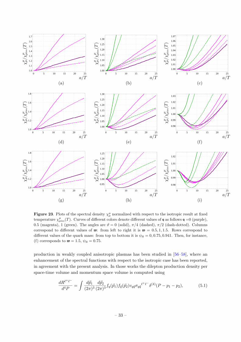
The dependence of the dilepton production rate on the degree of anisotropy of the

system is detailed in Figs. 23 and 24. We find that in general the anisotropic rate is larger

than the isotropic one, but, if the quark mass and w are large enough, there is a range of

anisotropies where it might be smaller. The dependence on the angle is always monotonic,

either increasing or decreasing depending on the specific quantity which is studied.

It is interesting to compare our results with what happens at weak coupling. Dilepton

– 32 –

0 5 10 15 20 251.0

1.1

1.2

1.3

1.4

1.5

1.6

1.7

0 5 10 15 20 251.00

1.05

1.10

1.15

1.20

1.25

1.30

0 5 10 15 20 25

1.00

1.01

1.02

1.03

1.04

1.05

1.06

1.07

χµ µ/χ

µ µiso(T

)

a/T

χµ µ/χµ µiso(T

)

a/T

χµ µ/χµ µiso(T

)

a/T(a) (b) (c)

0 5 10 15 20 251.0

1.2

1.4

1.6

1.8

0 5 10 15 20 25

1.00

1.05

1.10

1.15

1.20

1.25

1.30

0 5 10 15 20 25

0.98

0.99

1.00

1.01

1.02

1.03

χµ µ/χ

µ µiso(T

)

a/T

χµ µ/χ

µ µiso(T

)

a/T

χµ µ/χ

µ µiso(T

)

a/T(d) (e) (f)

0 5 10 15 20 251.0

1.2

1.4

1.6

1.8

0 5 10 15 20 25

0.95

1.00

1.05

1.10

1.15

1.20

1.25

0 5 10 15 20 25

0.98

0.99

1.00

1.01

1.02

χµ µ/χ

µ µiso(T

)

a/T

χµ µ/χ

µ µiso(T

)

a/T

χµ µ/χ

µ µiso(T

)

a/T(g) (h) (i)

Figure 23. Plots of the spectral density χµµ normalized with respect to the isotropic result at fixed

temperature χµµiso(T ). Curves of different colors denote different values of q as follows q =0 (purple),

0.5 (magenta), 1 (green). The angles are ϑ = 0 (solid), π/4 (dashed), π/2 (dash-dotted). Columns

correspond to different values of w: from left to right it is w = 0.5, 1, 1.5. Rows correspond to

different values of the quark mass: from top to bottom it is ψH = 0, 0.75, 0.941. Then, for instance,

(f) corresponds to w = 1.5, ψH = 0.75.

production in weakly coupled anisotropic plasmas has been studied in [56–58], where an

enhancement of the spectral functions with respect to the isotropic case has been reported,

in agreement with the present analysis. In those works the dilepton production density per

space-time volume and momentum space volume is computed using

dR`+`−

d4P=

∫d~p1

(2π)3

d~p2

(2π)3fq(~p1)fq(~p2)vqqσqq

`+`−δ(4)(P − p1 − p2), (5.1)

– 33 –

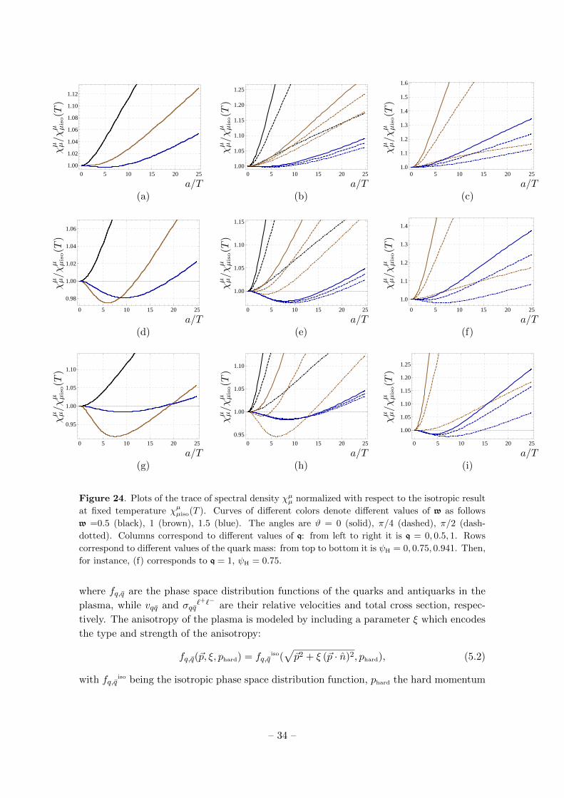
0 5 10 15 20 25

1.00

1.02

1.04

1.06

1.08

1.10

1.12

0 5 10 15 20 251.00

1.05

1.10

1.15

1.20

1.25

0 5 10 15 20 251.0

1.1

1.2

1.3

1.4

1.5

1.6

χµ µ/χ

µ µiso(T

)

a/T

χµ µ/χ

µ µiso(T

)

a/T

χµ µ/χ

µ µiso(T

)

a/T(a) (b) (c)

0 5 10 15 20 25

0.98

1.00

1.02

1.04

1.06

0 5 10 15 20 25

1.00

1.05

1.10

1.15

0 5 10 15 20 25

1.0

1.1

1.2

1.3

1.4

χµ µ/χ

µ µiso(T

)

a/T

χµ µ/χ

µ µiso(T

)

a/T

χµ µ/χ

µ µiso(T

)

a/T(d) (e) (f)

0 5 10 15 20 25

0.95

1.00

1.05

1.10

0 5 10 15 20 25

0.95

1.00

1.05

1.10

0 5 10 15 20 25

1.00

1.05

1.10

1.15

1.20

1.25

χµ µ/χ

µ µiso(T

)

a/T

χµ µ/χ

µ µiso(T

)

a/T

χµ µ/χ

µ µiso(T

)

a/T(g) (h) (i)

Figure 24. Plots of the trace of spectral density χµµ normalized with respect to the isotropic result

at fixed temperature χµµiso(T ). Curves of different colors denote different values of w as follows

w =0.5 (black), 1 (brown), 1.5 (blue). The angles are ϑ = 0 (solid), π/4 (dashed), π/2 (dash-

dotted). Columns correspond to different values of q: from left to right it is q = 0, 0.5, 1. Rows

correspond to different values of the quark mass: from top to bottom it is ψH = 0, 0.75, 0.941. Then,

for instance, (f) corresponds to q = 1, ψH = 0.75.

where fq,q are the phase space distribution functions of the quarks and antiquarks in the

plasma, while vqq and σqq`+`− are their relative velocities and total cross section, respec-

tively. The anisotropy of the plasma is modeled by including a parameter ξ which encodes

the type and strength of the anisotropy:

fq,q(~p, ξ, phard) = fq,qiso(√~p2 + ξ (~p · n)2, phard), (5.2)

with fq,qiso being the isotropic phase space distribution function, phard the hard momentum

– 34 –

scale (which can be identified with the temperature T when ξ = 0), and n defining the

anisotropic direction. What we provide in the present work is a non perturbative expression

for the factors fq,q(~p, ξ, phard) used in the small coupling calculations. It is interesting

to note that the enhancement of dilepton production appears to be a robust feature of

anisotropic plasmas, which is present both at weak and strong coupling. Of course, the

source of anisotropy in [56–58] is different than the one we have used in this paper, so

that comparisons have to be taken with a grain of salt. Nonetheless, these comparisons

certainly motivate further analysis.

As for the generality of our results, we observe that while we have used a very specific

source of anisotropy, namely a non-trivial axion, we expect our results to be quite general.

We observe in fact that the equations of motion for the gauge fields (2.23)-(2.26) are solely

dependent on the metric and dilaton, meaning that any source of anisotropy that gives rise

to similar metric and dilaton (and no Kalb-Ramond field) will produce qualitatively similar

results for the photon and dilepton production rates. It would be interesting, nonetheless,

to compute these quantities in as many anisotropic backgrounds as possible, including e.g.

the one of [59, 60], to understand which features are really model-independent and therefore

the most likely to be realized in the real-world QGP.

One thing we have left open is to determine what is the maximum value of ψH which

results in a stable embedding of the flavor D7-branes. To address this question one needs

to perform a careful analysis of the phase transition between the black hole and Minkowski

embedding of the branes [48]. This requires comparing the free energy of the system in the

two phases. To do that one would presumably need to perform from scratch the holographic

renormalization process done in [61] for the axion-dilaton gravity, including this time also

the DBI action for the branes. The UV limit (ε→ 0) and the probe brane limit (Nf/Nc → 0)

do not in fact commute, in principle. This is because the dilaton of [10, 11] vanishes at

the boundary and the introduction of additional D7-branes sources a dilaton that blows

up before reaching the boundary; see e.g. [62]. This means that no matter how small

Nf/Nc is, it eventually overtakes the asymptotics and one cannot simply try to renormalize

the D7-brane action in the fixed anisotropic background (as made evident by the fact that

there do not seem to be enough counterterms to cancel all the divergences).

Acknowledgements

We thank Mariano Chernicoff, Daniel Fernandez, Mauricio Martınez, and Yiannis Pa-

padimitriou for useful discussions. We are supported in part by CNPq (VJ and DT), by

FAPESP grant 2013/02775-0 (DT), and by DGAPA-UNAM grant IN117012 (AL and LP).

A Solutions for E1 and E2

In this appendix we describe how to construct the two linearly independent solutions E1

and E2 used in subsection 4.3.

– 35 –

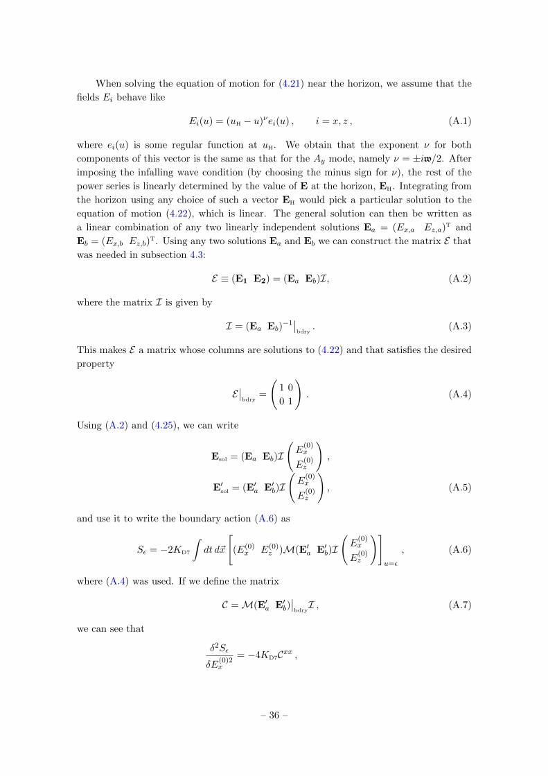
When solving the equation of motion for (4.21) near the horizon, we assume that the

fields Ei behave like

Ei(u) = (uH − u)νei(u) , i = x, z , (A.1)

where ei(u) is some regular function at uH. We obtain that the exponent ν for both

components of this vector is the same as that for the Ay mode, namely ν = ±iw/2. After

imposing the infalling wave condition (by choosing the minus sign for ν), the rest of the

power series is linearly determined by the value of E at the horizon, EH. Integrating from

the horizon using any choice of such a vector EH would pick a particular solution to the

equation of motion (4.22), which is linear. The general solution can then be written as

a linear combination of any two linearly independent solutions Ea = (Ex,a Ez,a)T and

Eb = (Ex,b Ez,b)T. Using any two solutions Ea and Eb we can construct the matrix E that

was needed in subsection 4.3:

E ≡ (E1 E2) = (Ea Eb)I, (A.2)

where the matrix I is given by

I = (Ea Eb)−1∣∣bdry

. (A.3)

This makes E a matrix whose columns are solutions to (4.22) and that satisfies the desired

property

E∣∣bdry

=

(1 0

0 1

). (A.4)

Using (A.2) and (4.25), we can write

Esol = (Ea Eb)I

(E

(0)x

E(0)z

),

E′sol = (E′a E′b)I

(E

(0)x

E(0)z

), (A.5)

and use it to write the boundary action (A.6) as

Sε = −2KD7

∫dt d~x

[(E(0)

x E(0)z )M(E′a E′b)I

(E

(0)x

E(0)z

)]u=ε

, (A.6)

where (A.4) was used. If we define the matrix

C =M(E′a E′b)∣∣bdryI , (A.7)

we can see that

δ2Sε

δE(0)2x

= −4KD7Cxx ,

– 36 –

δ2Sε

δE(0)2z

= −4KD7Czz ,

δ2Sε

δE(0)z δE

(0)x

= −2KD7(Czx + Cxz) . (A.8)

Using the technology developed in [55], we will now see how to obtain the imaginary

parts of the components of C from u-independent quantities that can be computed at the

horizon, so that all of the information of the boundary is encoded exclusively in I. The

first step is to show that the matrix C ≡ E†ME ′−E† ′ME is u-independent. To prove this,

we start by multiplying (4.22) on the left by M to obtain(ME′

)′+ f(u)ME = 0, (A.9)

which implies that the equation (ME ′

)′+ f(u)ME = 0 (A.10)

holds for the matrix E . If we multiply (A.10) on the left by E† and subtract from it its

transpose conjugate multiplied on the right by E , we are left with

E†(ME ′

)′ − (E†′M)′ E = 0 . (A.11)

Since

E†(ME ′

)′ − (E†′M)′ E =(E†ME ′ − E† ′ME

)′, (A.12)

equation (A.11) proves that C is indeed u-independent. Notice now that, since E reduces

to the identity matrix at the boundary, we have

C =(E†ME ′ − E† ′ME

) ∣∣H

=(E†ME ′ − E† ′ME

) ∣∣bdry

=(ME ′ − E† ′M

) ∣∣bdry

= C − C† . (A.13)

With (A.13) we can finally write

Cxx = 2i Im Cxx , (A.14)

Czz = 2i Im Czz , (A.15)

Cxz + Czx = 2i Im (Cxz + Czx) , (A.16)

which achieves the desired result of writing the imaginary parts of the correlators in terms

of M and E evaluated at the horizon, leaving only I to be evaluated at the boundary.

The final expression for χ(2) can then be obtained by inserting (A.8) into (4.7), and

using (A.14)-(A.16) to write

χ(2) = −4KD7i(

(k20 − q2 sin2 ϑ)Cxx + (k2

0 − q2 cos2 ϑ)Czz − 2q2 cosϑ sinϑ(Cxz + Czx)).

(A.17)

– 37 –

B Explicit near-boundary-expansion for the action (4.17)

We report here the explicit expression for the boundary action, eq. (4.17). The action

reads

Sε = −2KD7

∫dt d~x

[L1 + L2 + L3 + . . .+O

(u2)]u=ε

, (B.1)

where

L1 = A1E(0)2x +B1E

(0)2z + C1E

(0)x E(0)

z ,

L2 = A2E(0)x E(2)

x +B2E(0)x E(2)

x + C2E(0)x E(2)

x +D2E(0)x E(2)

x ,

L3 = − log u

k20

[(E(0)2

x + E(0)2z ) k2

0 + (E(0)x cosϑ− E(0)

z sinϑ)2 q2], (B.2)

and the various expansion coefficients are given by

A1 =(q2 − k2

0)(2a2 − 3(q2 − k20 + 8ψ2

1))

2(q2 − k20)(q2 − k2

0 + 8ψ21)− 6a2 q2 cos2 ϑ

+

+6a2q4cos4ϑ− q2cos2ϑ[6(q2 − k2

0)(q2 − k20 + 8ψ2

1)− a2(4q2 − 10k20) + 3a2q2cos2ϑ]

4k20[(q2 − k2

0)(2a2 − 3(q2 − k20 + 8ψ2

1)) + 3a2q2cos2ϑ],

B1 =

((5a2 + 15q2 + 48ψ2

1 − 15k20)(q2 − k2

0)− 3a2q2cos2ϑ)

(q2sin2ϑ− k20)

4k20[(q2 − k2

0)(2a2 − 3(q2 − k20 + 8ψ2

1)) + 3a2q2cos2ϑ],

C1 =q2[3(7q2 − 7k2

0 + 32ψ21)(q2 − k2

0)− 2a2(q2 + 2k20)− 6a2q2 cos 2ϑ] sin 2ϑ

8k20((q2 − k2

0)(2a2 − 3(q2 − k20 + 8ψ2

1)) + 3a2q2cos2ϑ),

A2 =2 cosϑ[3(q2 − 2k2

0)(q2 − k20 + 8ψ2

1)− a2(5q2 − 4k20)− q2(5a2 − 3(q2 − k2

0 + 8ψ21)) cos 2ϑ]

k20[6(q2 − k2

0)(q2 + 8ψ21 − k2

0)− a2(7q2 − 4k20)− 3a2q2 cos 2ϑ]

,

B2 = − 48q2 sin 2ϑ

k20[6(q2 − k2

0)(q2 − k20 + 8ψ2

1)− a2(7q2 − 4k20)− 3a2q2 cos 2ϑ]

,

C2 =4q2(5a2 − 3(q2 − k2

0 + 8ψ21))cos2ϑ sinϑ

k20[6(q2 − k2

0)(q2 − k20 + 8ψ2

1)− a2(7q2 − 4k20)− 3a2q2 cos 2ϑ]

,

D2 =96(q2 sin2 ϑ− k2

0)

k20[6(q2 − k2

0)(q2 − k20 + 8ψ2

1)− a2(7q2 − 4k20)− 3a2q2 cos 2ϑ]

. (B.3)

References

[1] J. Adams et al. [STAR Collaboration], “Experimental and theoretical challenges in the

search for the quark gluon plasma: The STAR collaboration’s critical assessment of the

evidence from RHIC collisions,” Nucl. Phys. A 757, 102 (2005) [arXiv:nucl-ex/0501009].

[2] K. Adcox et al. [PHENIX Collaboration], “Formation of dense partonic matter in relativistic

nucleus nucleus collisions at RHIC: Experimental evaluation by the PHENIX collaboration,”

Nucl. Phys. A 757, 184 (2005) [arXiv:nucl-ex/0410003].

[3] Proceedings of Quark Matter 2011: J. Phys. GG 38, number 12 (December 2011).

[4] E. Shuryak, “Why does the quark gluon plasma at RHIC behave as a nearly ideal fluid?,”

Prog. Part. Nucl. Phys. 53, 273 (2004) [arXiv:hep-ph/0312227].

[5] E. V. Shuryak, “What RHIC experiments and theory tell us about properties of quark-gluon

plasma?,” Nucl. Phys. A 750, 64 (2005) [arXiv:hep-ph/0405066].

– 38 –

[6] J. M. Maldacena, “The Large N limit of superconformal field theories and supergravity,”

Adv. Theor. Math. Phys. 2, 231-252 (1998) [hep-th/9711200].

[7] S. S. Gubser, I. R. Klebanov, A. M. Polyakov, “Gauge theory correlators from noncritical

string theory,” Phys. Lett. B428, 105-114 (1998) [hep-th/9802109].

[8] E. Witten, “Anti-de Sitter space and holography,” Adv. Theor. Math. Phys. 2, 253-291

(1998) [hep-th/9802150].

[9] P. Kovtun, D. T. Son and A. O. Starinets, “Viscosity in strongly interacting quantum field

theories from black hole physics,” Phys. Rev. Lett. 94, 111601 (2005) [hep-th/0405231].

[10] D. Mateos and D. Trancanelli, “The anisotropic N=4 super Yang-Mills plasma and its

instabilities,” Phys. Rev. Lett. 107, 101601 (2011) [arXiv:1105.3472 [hep-th]].

[11] D. Mateos and D. Trancanelli, “Thermodynamics and Instabilities of a Strongly Coupled

Anisotropic Plasma,” JHEP 1107, 054 (2011) [arXiv:1106.1637 [hep-th]].

[12] T. Azeyanagi, W. Li and T. Takayanagi, “On String Theory Duals of Lifshitz-like Fixed

Points,” JHEP 0906, 084 (2009) [arXiv:0905.0688 [hep-th]].

[13] A. Rebhan and D. Steineder, “Violation of the Holographic Viscosity Bound in a Strongly

Coupled Anisotropic Plasma,” Phys. Rev. Lett. 108, 021601 (2012) [arXiv:1110.6825

[hep-th]].

[14] K. A. Mamo, “Holographic Wilsonian RG Flow of the Shear Viscosity to Entropy Ratio in

Strongly Coupled Anisotropic Plasma,” JHEP 1210, 070 (2012) [arXiv:1205.1797 [hep-th]].

[15] M. Chernicoff, D. Fernandez, D. Mateos and D. Trancanelli, “Drag force in a strongly

coupled anisotropic plasma,” JHEP 1208, 100 (2012) [arXiv:1202.3696 [hep-th]].

[16] D. Giataganas, “Probing strongly coupled anisotropic plasma,” JHEP 1207, 031 (2012)

[arXiv:1202.4436 [hep-th]].

[17] K. B. Fadafan and H. Soltanpanahi, “Energy loss in a strongly coupled anisotropic plasma,”

JHEP 1210, 085 (2012) [arXiv:1206.2271 [hep-th]].

[18] B. Muller and D. -L. Yan, “Light Probes in a Strongly Coupled Anisotropic Plasma,” Phys.

Rev. D 87, 046004 (2013) [arXiv:1210.2095 [hep-th]].

[19] A. Rebhan and D. Steineder, “Probing Two Holographic Models of Strongly Coupled

Anisotropic Plasma,” JHEP 1208, 020 (2012) [arXiv:1205.4684 [hep-th]].

[20] M. Chernicoff, D. Fernandez, D. Mateos and D. Trancanelli, “Jet quenching in a strongly

coupled anisotropic plasma,” JHEP 1208, 041 (2012) [arXiv:1203.0561 [hep-th]].

[21] M. Chernicoff, D. Fernandez, D. Mateos and D. Trancanelli, “Quarkonium dissociation by

anisotropy,” JHEP 1301, 170 (2013) [arXiv:1208.2672 [hep-th]].

[22] S. Chakraborty and N. Haque, “Holographic quark-antiquark potential in hot, anisotropic

Yang-Mills plasma,” Nucl. Phys. B 874, 821 (2013) [arXiv:1212.2769 [hep-th]].

[23] K. B. Fadafan, D. Giataganas and H. Soltanpanahi, “The Imaginary Part of the Static

Potential in Strongly Coupled Anisotropic Plasma,” arXiv:1306.2929 [hep-th].

[24] D. Giataganas and H. Soltanpanahi, “Universal properties of the Langevin diffusion

coefficients,” arXiv:1310.6725 [hep-th].

[25] S. Chakrabortty, S. Chakraborty and N. Haque, “Brownian motion in strongly coupled,

anisotropic Yang-Mills plasma: A holographic approach,” arXiv:1311.5023 [hep-th].

– 39 –

[26] M. Ali-Akbari and H. Ebrahim, “Chiral Symmetry Breaking: To Probe Anisotropy and

Magnetic Field in QGP,” arXiv:1309.4715 [hep-th].

[27] L. Patino and D. Trancanelli, “Thermal photon production in a strongly coupled anisotropic

plasma,” JHEP 1302, 154 (2013) [arXiv:1211.2199 [hep-th]].

[28] S. -Y. Wu and D. -L. Yang, “Holographic Photon Production with Magnetic Field in

Anisotropic Plasmas,” JHEP 1308, 032 (2013) [arXiv:1305.5509 [hep-th]].

[29] G. Arciniega, P. Ortega and L. Patino, “Brighter Branes, enhancement of photon production

by strong magnetic fields in the gauge/gravity correspondence,” arXiv:1307.1153 [hep-th].

[30] D. Giataganas, “Observables in Strongly Coupled Anisotropic Theories,” PoS Corfu 2012,

122 (2013) [arXiv:1306.1404 [hep-th]].

[31] S. Caron-Huot, P. Kovtun, G. D. Moore, A. Starinets and L. G. Yaffe, “Photon and dilepton

production in supersymmetric Yang-Mills plasma,” JHEP 0612, 015 (2006)

[hep-th/0607237].

[32] A. Parnachev and D. A. Sahakyan, “Photoemission with Chemical Potential from QCD

Gravity Dual,” Nucl. Phys. B 768, 177 (2007) [hep-th/0610247].

[33] D. Mateos and L. Patino, “Bright branes for strongly coupled plasmas,” JHEP 0711, 025

(2007) [arXiv:0709.2168 [hep-th]].

[34] A. Nata Atmaja and K. Schalm, “Photon and Dilepton Production in Soft Wall AdS/QCD,”

JHEP 1008, 124 (2010) [arXiv:0802.1460 [hep-th]].

[35] Y. Y. Bu, “Photoproduction and conductivity in dense holographic QCD,” Phys. Rev. D 86,

026003 (2012); “Electromagnetic signature in holographic plasma with B field,” Phys. Rev.

D 87, 026005 (2013).

[36] K. Jo and S. -J. Sin, “Photo-emission rate of sQGP at finite density,” Phys. Rev. D 83,

026004 (2011) [arXiv:1005.0200 [hep-th]].

[37] B. Hassanain and M. Schvellinger, “Plasma conductivity at finite coupling,” JHEP 1201,

114 (2012) [arXiv:1108.6306 [hep-th]].

[38] B. Hassanain and M. Schvellinger, “Diagnostics of plasma photoemission at strong coupling,”

Phys. Rev. D 85, 086007 (2012) [arXiv:1110.0526 [hep-th]].

[39] R. Baier, S. A. Stricker, O. Taanila and A. Vuorinen, “Production of Prompt Photons:

Holographic Duality and Thermalization,” Phys. Rev. D 86, 081901 (2012) [arXiv:1207.1116

[hep-ph]].

[40] D. Steineder, S. A. Stricker and A. Vuorinen, “Holographic Thermalization at Intermediate

Coupling,” Phys. Rev. Lett. 110, no. 10, 101601 (2013) [arXiv:1209.0291 [hep-ph]].

[41] B. Hassanain and M. Schvellinger, “Plasma photoemission from string theory,” JHEP 1212,

095 (2012) [arXiv:1209.0427 [hep-th]].

[42] K. A. Mamo, “Enhanced thermal photon and dilepton production in strongly coupled N = 4

SYM plasma in strong magnetic field,” JHEP 1308, 083 (2013) [arXiv:1210.7428 [hep-th]].

[43] H. -U. Yee, “Flows and polarization of early photons with magnetic field at strong coupling,”

Phys. Rev. D 88, 026001 (2013) [arXiv:1303.3571 [nucl-th]].

[44] D. Steineder, S. A. Stricker and A. Vuorinen, “Probing the pattern of holographic

thermalization with photons,” JHEP 1307, 014 (2013) [arXiv:1304.3404 [hep-ph]].

– 40 –

[45] B. Schenke and M. Strickland, “Photon production from an anisotropic quark-gluon

plasma,” Phys. Rev. D 76, 025023 (2007) [hep-ph/0611332].

[46] M. Le Bellac, “Thermal Field Theory,” Cambridge University Press (1996).

[47] S. S. Gubser, I. R. Klebanov and A. W. Peet, “Entropy and temperature of black 3-branes,”

Phys. Rev. D 54, 3915 (1996) [hep-th/9602135].

[48] D. Mateos, R. C. Myers and R. M. Thomson, “Thermodynamics of the brane,” JHEP 0705,

067 (2007) [hep-th/0701132].

[49] A. Karch and L. Randall, “Open and closed string interpretation of SUSY CFT’s on branes

with boundaries,” JHEP 0106, 063 (2001) [hep-th/0105132].

[50] A. Karch and E. Katz, “Adding flavor to AdS / CFT,” JHEP 0206, 043 (2002)

[hep-th/0205236].

[51] D. T. Son and A. O. Starinets, “Minkowski space correlators in AdS/CFT correspondence:

Recipe and applications,” JHEP 0209, 042 (2002) [hep-th/0205051].

[52] G. Policastro, D. T. Son and A. O. Starinets, “From AdS/CFT correspondence to

hydrodynamics,” JHEP 0209, 043 (2002) [arXiv:hep-th/0205052].

[53] G. Policastro, D. T. Son and A. O. Starinets, “From AdS/CFT correspondence to

hydrodynamics. 2. Sound waves,” JHEP 0212, 054 (2002) [hep-th/0210220].

[54] P. K. Kovtun and A. O. Starinets, “Quasinormal modes and holography,” Phys. Rev. D 72,

086009 (2005) [hep-th/0506184].

[55] M. Kaminski, K. Landsteiner, J. Mas, J. P. Shock and J. Tarrio, “Holographic Operator

Mixing and Quasinormal Modes on the Brane,” JHEP 1002, 021 (2010) [arXiv:0911.3610

[hep-th]].

[56] M. Martinez and M. Strickland, “Measuring QGP thermalization time with dileptons,” Phys.

Rev. Lett. 100, 102301 (2008) [arXiv:0709.3576 [hep-ph]].

[57] M. Martinez and M. Strickland, “Pre-equilibrium dilepton production from an anisotropic

quark-gluon plasma,” Phys. Rev. C 78, 034917 (2008) [arXiv:0805.4552 [hep-ph]].

[58] M. Martinez and M. Strickland, “Suppression of forward dilepton production from an

anisotropic quark-gluon plasma,” Eur. Phys. J. C 61, 905 (2009) [arXiv:0808.3969 [hep-ph]].

[59] R. A. Janik and P. Witaszczyk, “Towards the description of anisotropic plasma at strong

coupling,” JHEP 0809, 026 (2008) [arXiv:0806.2141 [hep-th]].

[60] A. Rebhan and D. Steineder, “Electromagnetic signatures of a strongly coupled anisotropic

plasma,” JHEP 1108, 153 (2011) [arXiv:1106.3539 [hep-th]].

[61] I. Papadimitriou, “Holographic Renormalization of general dilaton-axion gravity,” JHEP

1108, 119 (2011) [arXiv:1106.4826 [hep-th]].

[62] A. Magana, J. Mas, L. Mazzanti and J. Tarrio, “Probes on D3-D7 Quark-Gluon Plasmas,”

JHEP 1207, 058 (2012) [arXiv:1205.6176 [hep-th]].

– 41 –