No-arbitrage bounds on American Put Optionswith a single maturity

by

Premal ShahB. Tech. & M. Tech., Electrical Engineering

Indian Institute of Technology (IIT) Bombay,(2003),Mumbai

Submitted to the Sloan School of Managementin partial fulfillment of the requirements for the degree of

Master of Science in Operations Research

at the

MASSACHUSETTS INSTITUTE OF TECHNOLOGY

June 2006

©() Massachusetts Institute of Technology 2006. All rights reserved.

,/ A. . t , J

Author .............................. V.Sloan School of Management

'-,. May 22, 2006

Certified by ......................... ...Dimitris J. Bertsimas

Boeing Professor of Operations Research, Sloan School ofManagement

Thesis Supervisor

Accepted by ............................ ..... .......I7 - James B. Orlin

Edward Pennell Brooks Professor of Operations Research, Codirector,

MASSACHUSETTS INSTITUTi- OF TECHNOLOY

JUL 2 4 2006

Operations Research Center

ARCHIVES

LIBRARIES

__~~~~~~~~~~~~~~~~~~~~~~~~~~~~1

I

I

No-arbitrage bounds on American Put Options with a single

maturity

by

Premal Shah

B. Tech. & M. Tech., Electrical Engineering (2003),

Indian Institute of Technology (IIT) Bombay, Mumbai

Submitted to the Sloan School of Managementon May 22, 2006, in partial fulfillment of the

requirements for the degree ofMaster of Science in Operations Research

AbstractWe consider in this thesis the problem of pricing American Put Options in a model-free framework where we do not make any assumptions about the price dynamicsof the underlying except those implied by the no-arbitrage conditions. Our goalis to obtain bounds on the price of an American put option with a given strikeand maturity directly from the prices of other American put options with the samematurity but different strikes and the current price of the underlying. We proceedby first investigating the structural properties of the price curve of American PutOptions of a fixed maturity and derive necessary and sufficient conditions that strike- price pairs of these options must satisfy in order to exclude arbitrage. Using theseconditions, we can find tight bounds on the price of the option of interest by solving avery tractable Linear Programming Problem. We then apply the methods developedto real market data. We observe that the quality of bounds that we obtain compareswell with the quoted bid-ask spreads in most cases.

Thesis Supervisor: Dimitris J. BertsimasTitle: Boeing Professor of Operations Research, Sloan School of Management

3

4

Acknowledgments

I would like to express my sincere gratitude towards Prof. Dimitris Bertsimas for

his guidance and support, without him this work would have been but an exercise in

fultility. I am also thankful to Prof. David Gamarnik for his encouragement and

interest - discussions with him about the problem always refined mly understanding.

I am also thankful to Theta Aye for carefully reading this dissertation - it now

has fewer errors. Thanks to Theta also for being so much fun and cheerful! I would

also like to express my gratitude towards the Operations Research Center adminis-

trators - Paulette Mosley, Laura Rose and Andrew Carvalho - their efficiency

and co-operation have made things so much easier. Thanks also to fellow ORCers -

Ilan, Yunqing (Kelly), Vinh, Dung, Mike, Rajiv, Ruben, Carine, Pranava,

Shobhit, Nelson, Carol, Pavithra, Theo, Yann, Elodie, Katy, Rags, Pallav,

Dmitriy, Dave, Doug, Dan, Margret, Kostas, Lincoln, Karima, ... for the

countless wonderful moments inside and outside ORC.

Thanks also to the entire Kajra-re gang - Tara Sainath, Natasha Singh, Tara

Bhandari, Rajiv Menjoge, Aditya Undurti, Kranthi Vistakula, Sukant Mit-

tal, Neha Soni, Nicholas Miller, Jennifer Fang, Vikas Sharma, Saba Gul,

Tulika Khemani, M V Kartik, Saba Ghole; who made no positive contributions

to this thesis, but their jokes, energy and liveliness brightened this semester up for

me! Them and friends like Mira Chokshi, Mithila Azad, Nandan Bhat, Pra-

fulla Krishna have made the days at MIT and Boston some of the most memorable

and enjovable ones of my life. I am also thankful to Sangam and the '05 executive

council fellow members - Vivek Jaiswal, Saurabh Tejwani, Biraja Kanungo for

helping to re-create here Holi, Diwali and all other things that I missed from home.

Thanks is also due to Saurabh Tejwani, Mukul Agarwal, Sudhir Chiluveru,

Riccardo Merello, Anatoly who have made dornms so much more homely.

Finally and most importantly, I shall always remain indebted to my parents, my

sister Payal and lmy relatives - their love, support and care have made everything

possib)le.

6

Contents

Contents 7

List of Figures 9

List of Tables 11

1 Introduction 13

1.1 Background . . . . . . . . . . . . . . . . . . . . . . . . . . . ... 13

1.2 Related Work ............................... 16

1.3 Outline ................................... 16

2 Model 19

2.1 Problem Definition ............................ 21

3 Necessary Conditions on the Price Curve 23

3.1 Elementary Necessary Conditions ................... . 23

3.2 Strict Necessary Conditions ....................... 26

4 Sufficient Conditions 31

4.1 Sufficiency Conditions for European Call Options .......... . 31

4.2 Proof of Sufficiency .. . . . . . . . . . . . . . . . . . . ...... 32

5 Algorithm to find bounds on the Price of an American Put 39

5.1 Conditions for Strike-Price Pairs ..................... 39

5.2 Algorithm to find Bounls ........................ 41

7

6 Numerical Illustrations 45

6.1 Modifications . . . . . . . . . . . . . . . . . . . .......... 45

6.2 Data .................................... 47

6.3 Quality of BouIds ....... ...................... 48

6.4 Impact of Information ................... ....... 51

6.5 Comparison for different Maturities . . . . . . . . . . . . . . ..... 52

7 Conclusions and Final Remarks 55

A Existence of an Optimal Exercise Policy 57

B Bounds from Bid-Ask Quotes 61

Bibliography 63

8

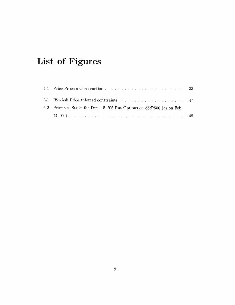
List of Figures

4-1 Price Process Construction ........................ 33

6-1 Bid-Ask Price enforced constraints ................... 47

6-2 Price v/s Strike for Dec. 15, '06 Put Options on S&P500 (as on Feh.

14, '06) .................................. . 48

9

10

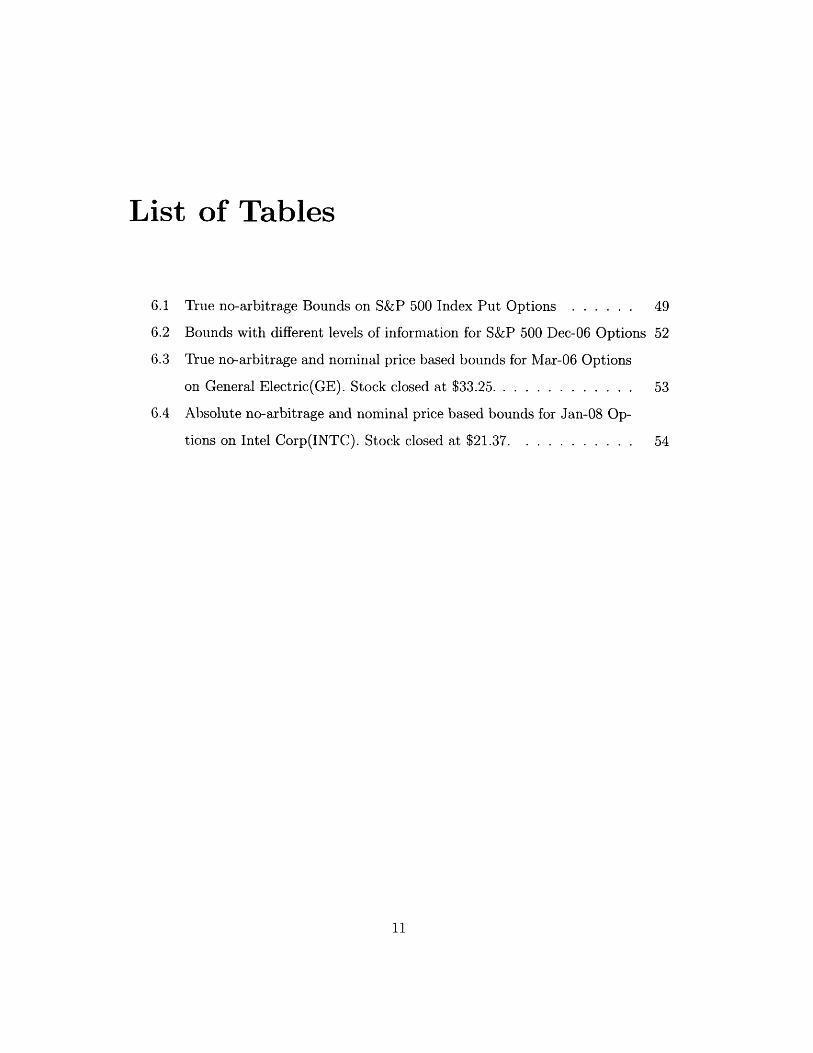
List of Tables

6.1 True no-arbitrage Bounds on S&P 500 Index Put Options ...... 49

6.2 Bounds with different levels of information for S&P 500 Dec-06 Options 52

6.3 True no-arbitrage and nominal price based bounds for Mar-06 Options

on General Electric(GE). Stock closed at $33.25 . ............ 53

6.4 Absolute no-arbitrage and nominal price based bounds for Jan-08 Op-

tions on Intel Corp(INTC). Stock closed at $21.37. .......... 54

11

12

Chapter 1

Introduction

Derivative securities or derivatives are securities whose payoffs are linked to price(s)

of other asset(s) called the underlying. Derivatives facilitate hedging, speculating

and other investnment objectives and help to make the financial markets richer or

in somewhat loose terms 'more complete'. Because of the contractual nature of a

derivative, which makes its payoff a function of the price(s) of the underlying, it's

own price, in principle, can be determined if the price dynamics of the underlying

asset(s) are known. Derivatives such as options are actively traded in many markets,

and as such, pricing of derivatives is a problem of significant practical interest.

1.1 Background

The landmark Black and Scholes option pricing formula was probably the first widely

noted attempt to price a derivative security. The formula that first appeared in [1]

priced a European option (both calls and puts) on a common stock and the approach

was based on modeling the price dynamics of the underlying and then inferring the

price of the security from this model within the no-arbitrage framework. Prices

of the underlying asset in the Black-Scholes framework are assumed to follow a log-

normal Brownian XMotion. Under this assumption, the price-dynamics of the asset are

completely specified by two parameters, the drift and the volatility of stock returns.

Note that, the price dynaimics are not known but assumed to be log-normal in a quite

13

adhoc fashion. These assunmptions might be reasonable to a certain extent but are

far from accurate. I fact, practitioners make many adjustments to the basic Black-

Scholes model such as using different volatilities for different strikes, before applying it

to price options ill real markets. Other models of stock price dynamics that refine the

somewhat simplistic assumptions of the Black-Scholes model to better accommodate

the observed prices of the securities in the market have also been proposed. See

[2] for a survey of some of the more commonly used models and their efficacy in

practice. Amongst these are mean-reverting, stochastic volatility models and others.

In general, these more sophisticated models have more parameters (rather than the

two present in the Black-Scholes model) and make it possible to incorporate more

of the information conveyed by the market. This is because, to price a derivative

security using a price dynamics model, one would follow a two-step process. The

first step involves calibrating the assumed price dynamics model on the underlying.

This is done by attuning the parameters of the model (the degrees of freedom) so

as to make its predictions fit observed prices of highly liquid derivative securities

linked to the underlying. One then uses the calibrated model to price not-so-liquid

derivatives of interest. Although this approach gives a single value price for the

security of interest, the assumptions that are implicitly made are difficult to justify

or verify. Pricing of securities in markets is always relative, wherein one takes the

prices of certain instruments as given to infer or estimate the value of others. A

price dynamics model provides a framework to interpret and re-use the information

provided by market signals (prices of reliable or liquid securities). However, it does

not transparently reflect this information about asset prices that is revealed through

the market observed prices, (and is therefore more trustworthy,) but combines it with

that arising out of imposing a certain price dynamics belief model on the asset prices

(which is always suspect). 1M\oreover, as it is difficult to isolate the degree of individual

impact of these two factors that are used to derive the final price, the model based

approach, in a sense, 'coltalinates' information conveyed by the market.

Another approach to derivatives pricing that has gained popularity recently, is the

model-free approach - i.e.. one which does away with making any assumptions on the

14

price dynamics of the underlying altogether. Tile only assumption made is that of

no-arbitrage, a fairly robust assumption in the context of derivative pricing. In their

seminal work, Cox and Ross [3] and Harrison and Kreps [4], show that the condition

of no-arbitrage is in fact equivalent to that of the existence of a probability measure

(called the Equivalent Martingale Measure or the Risk Neutral Measure), with respect

to which the discounted asset prices are martingales. In the model-free approach, one

is interested in finding the maximum and minimum price that a derivative security of

interest might take without creating an arbitrage opportunity. While this approach

typically would not give a single number for the asset price (unless the markets are

complete), it faithfully represents the market implied information about the security

price. It also gives an indication about how deep the market is in that security through

the size of the price-bracketing interval. Another advantage is that this approach is

also often useful to identify real-arbitrage opportunities if they exist in the market,

unlike the price-model based approach.

The work in this thesis is concerned with coming up with a model-free approach to

price a practically important class of derivative securities - the American Put Options.

American Put Options are actively traded on different exchanges for a variety of asset

classes. However, pricing an American Put Option is a difficult problem even while

assuming a price dynamics model for the underlying. This is because unlike its

call counterpart, the American Call1 , an early exercise can indeed be optimal for an

American Put, and hence the price of an American Put should be and is typically more

than that of a European Put Option on the same asset and with the same strike and

maturity. As a result there is no simple or 'closed form formula' known for pricing the

American Put Option for any of the commonly used price dynamics models, though

this can be clone numerically for a given model, by solving a conceptually simple but

computationally unattractive Dynamic Programming Problem.

1 Assuiingll the stock is non-dividend paying, conditional Jensen's inequality directly leads to theconclusion that tern-inal exercise policy for an American Call is always Optimal.

15

1.2 Related Work

AMiuch work about pricing American Put Options has been devoted to the problem of

obtaining good estimates of the price/value of an American Put Option efficiently.

An indicative, but by no means exhaustive sample can be obtained through a study

of [5, 6, 7, 8, 9, 10]. For a survey and comparison of various methods, refer to [11]. In

this context, deriving bounds on the prices of an American Put Option can be useful

not only in terms of the advantages that the model-free pricing method has to offer,

but also as a computational scheme for pricing an American Put Option, provided

the algorithms to derive the price bounds on American Put Option turn out to be

efficient.

The idea of relaxing distributional assumptions on asset prices is indeed not new.

Lo [12] derived bounds on the price of European Options given the mean and the

variance of the underlying stock, under the risk neutral price measure. Grundy [13]

generalized this approach to the case when the first and the kth moments of the stock

price are known. Later, Bertsimas and Popescu [14] derived tight bounds on the price

of a European Call Option, given prices of other options on the same stock, with the

same maturity, using a convex optimization approach. In [15] and [16], Bertsimas

and Bushueva derived tight bounds on the prices of European Options, given prices

of other European Options with possibly different maturities. D' Aspremont and El

Ghaoui [17] solved the problem of finding the bounds on the price of a European

basket call option, given prices of other similar baskets. All the above works however

address the problem of finding bounds on the price of a European-style option.

1.3 Outline

In the rest of the thesis, we exposit the problem of deriving bounds on the price of an

American Put Option with a given strike and maturity using only the no-arbitrage

conditions. WVe consider a setting where the imarket information set consists just

the current price of the underlying and prices of other American Put Options on it

16

that have the same maturity but different strikes. Our method is essentiallyv non-

parametric i.e., it does not refer to or make use of any quantities such as 'implied

volatilities'. In Chapter 2, we outline the discrete time model used in this paper.

In Chapter 3, we derive the necessary conditions on the prices of American Put

Options. In Chapter 4, we derive the main result of this paper, Theorem 4.2, about

the necessary and sufficient conditions that American Put Option Prices must satisfy.

We then use this theorem to develop algorithms to find tight bounds on the price of an

American Put Option, given the price of other Put Options with the same maturity

in Chapter 5. We illustrate our results with numerical examples in Chapter 6 and

conclude with remarks on future directions in Chapter 7. The problem addressed in

this thesis - using no arbitrage conditions to derive bounds on prices of an American

Put Option has dual objectives

* Using a more robust framework for pricing American Put Options that uses

only information implied by the markets.

* To explore if there are efficient procedures to compute bounds on price of an

American Put Options, which have been otherwise computationally demanding

to valuate.

17

18

Chapter 2

Model

We consider a discrete time model with periods 1, 2, 3,..., where all price changes

occur a.t period boundaries (ends). Without loss of generality, we assume the period

length to be 1. An American Put Option, parametrized by an exercise strike K and a

maturity T, is a security that allows (but does not require) the holder to sell one share

of an underlying asset, (say stock,) at a price K at any time t < T, irrespective of its

prevailing market price. Let St denote the price of the asset at time t. Let r > 0 be

the risk free rate for one period. Then P < 1 is the one period discount factor

(assumed to be constant 2). We will also assume that the underlying does not pay

dividends. Let Q denote a risk-neutral measure, i.e., any measure under which the

discounted stock price process, 3tSt, is a martingale. Let r denote an exercise policy

for an American Put Option. To be a valid exercise policy, T must be a stopping-rule,

(note that this constraint can be enforced even without specifying a measure for the

price process). For notational convenience we require that the option is always struck,

i.e.; r < T and upon exercise at time t, the payoff is (K - St)+. The value or the yield

of the optiol with strike K, under an exercise policy 7, will be denoted by AT(K, T).

1We shall assume that r > 0, as we would expect in reality. If r = 0 or r < 0 then ;3 > 1 andEQ[p3T(K - S7.)

+] > EQ[/3t(K - St) +] Vt < T. The inequality holds even when we replace t ) astopping tilne. . Ilence exercising at T is always optimal. The problem is then the same as that ofpIricing a European Put. Option. which has been studied before.

2 This asslllltiol is wlog, as one can otherwise construct periods in such a way that discoluntilngover each periodl is the salle.

19

Given a risk-neutral measure Q, we then have,

AT(K,T) = EQ[fi3(K-ST)+].

The value/price of the American Put Option with strike K and maturity T, is then

given by

AT(K) = supEQ[fi(K - Sr)+].

The same notation, AT(-), will also be used to denote the value of the option, the

meaning of which would be clear from the context - when r is not explicitly stated

as an argument. The set of optimal policies is defined as

{rT(K)} = argmaxxEQ[3(K- S)+].r<T

Apriori, it is not known if an optimal exercise policy exists. Thus {T(K)} may as well

be empty. Since all price-changes occur at period boundaries and / < 1, if {4T(K)} is

non-empty, then there always exists an optimal exercise policy Tr(K) in which one will

exercise with a positive probability only at times in {0, 1, 2,..., T}. Hence, we restrict

ourselves to consider only those exercise policies that allow striking in {0, 1, 2, ... , T}.

This leads to what is referred to in financial markets as a Bermudan Option. By

increasing the refinement of a period, this approximation can be made arbitrarily

accurate. Further, wlog, we can also assume that, r(K) < T : K > ST,(K). This

allows us to exclude from consideration possible degenerate policies without any loss

of optimality. We can further restrict the set of exercise policies that we need to

consider. Let C refer to the class of exercise policies, that can lead to exercise only at

times in {0, 1,2,..., T}, satisfy Tr(K) < T => K > ST,(K) and are non-randomized.

A policy T is non-randomized if the event T < t is deterministic given S1, S2,..., St,

or in other words, at any time t one either strikes the option or does not strike, there

is no mixing. Proposition A.1 in Appendix A shows that an optimal r belonging to

C always exists. Thus {r(K)} is non-empty V K in our setting. We will henceforth

20

consider only policies belonging to class C. Although, an optimal exercise policy

within C exists, it may not necessarily be unique. Wve will use T-(K) to refer to any

optimal exercise policy rather than a specific optimal policy. Also for any optimal

exercise policy T (K), it follows that AT(K) = AT(K, T (K)).

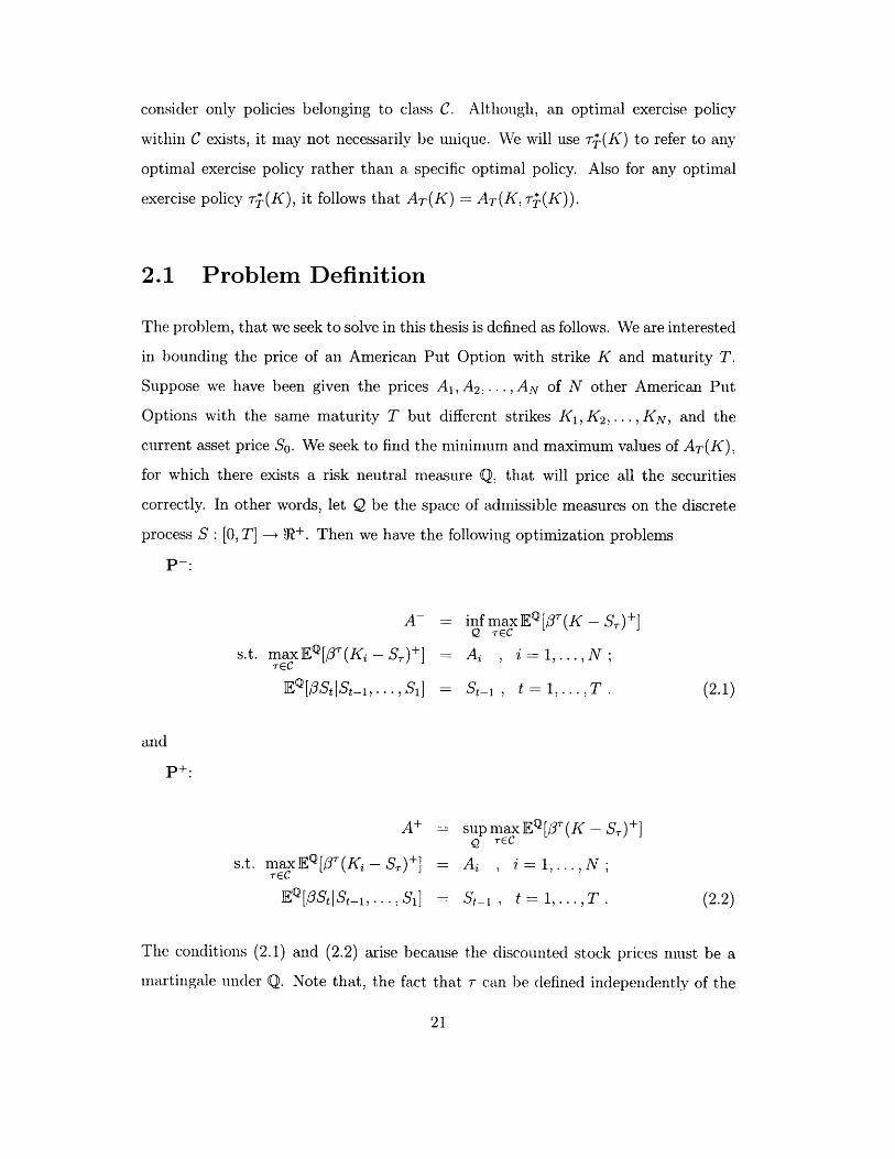
2.1 Problem Definition

The problem, that we seek to solve in this thesis is defined as follows. We are interested

in bounding the price of an American Put Option with strike K and maturity T.

Suppose we have been given the prices A 1, A 2 . . ,AN of N other American Put

Options with the same maturity T but different strikes K1,K 2,...,KN, and the

current asset price So. We seek to find the minimum and maximum values of AT(K),

for which there exists a risk neutral measure Q, that will price all the securities

correctly. In other words, let Q be the space of admissible measures on the discrete

process S: [0, T] - +. Then we have the following optimization problems

P-:

s.t. maxEQ[/3r(Ki - S,)+]rEC

EQ[St[St_,... , S]

A+

s.t. maxEQ[d3(Ki - S) + ]rEC

EQ[ [PS St,_1... S]

= infmax EQ[3'(K -S)+]Q EC

= Ai , i=1,...,N;

= St_, t=1,...,T

sup max EQ [ (K - S) +]Q EC

= Ai, i=1,...,N;= St-I, t=I,...,T.

The conditions (2.1) and (2.2) arise because the cliscountedl stock prices must be a

martingale undler Q. Note that, the fact that r can e defined independently of the

21

and

(2.1)

(2.2)

measure Q, allows us to formulate the problem in the stated form.

Problems P- and P+ are not explicit optimization problems but encompass sub-

optimization problems that are known to be not amenable to analytical solutions or

fast computational procedures. Hence, we approach these problems in an indirect

way, by finding structural properties of the price envelope AT(.). Specifically, we seek

to find consistency conditions on the prices, i.e., conditions that are necessary and

sufficient for the existence of a no-arbitrage measure Q.

22

Chapter 3

Necessary Conditions on the Price

Curve

We denote by AT(-), the price function, i.e., the price of the American Put Option

as a function of the strike, with maturity T held constant. In this chapter, we will

derive a set of necessary conditions that the price function must satisfy. For this we

will it find useful to translate back and forth between properties of optimal exercise

policies and their implications for AT(.). We begin with some basic straightforward

conditions, that AT (.) must satisfy to avoid arbitrage opportunities.

3.1 Elementary Necessary Conditions

The following conditions on option prices and optimal exercise policies are immediate.

(N1) Option Price is greater than its intrinsic value:

AT(K) > (K-So) +. (3.1)

(N2) AT(K) is increasing in K. This follows trivially as for K2 > K1,

A7 .(K 2) >

23

AT(-[E, -(K,))

AT (,, r (K,) = A(K).

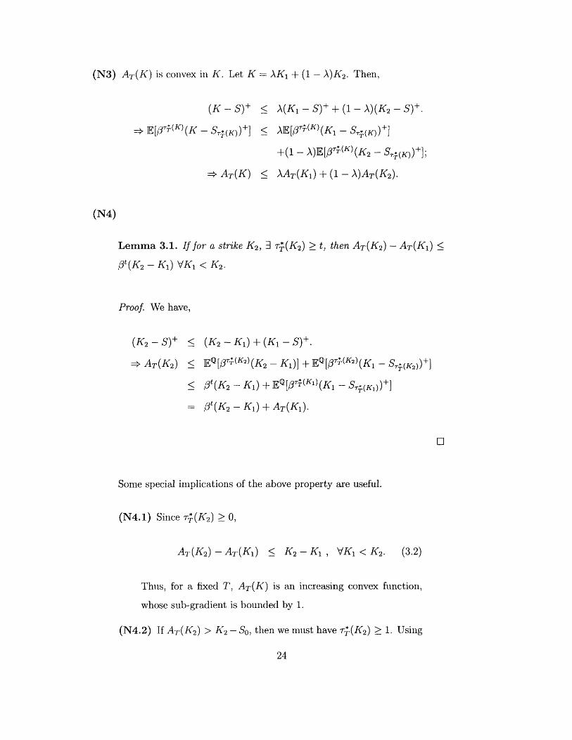
(N3) AT(K) is convex in K. Let K = K1+ (1 - A)K2. Then,

(K - S)+ < A(K - S) + (1 - )(K2 - S)+

=> E[/3(K' (K - ST(K))+] < AE[S3(K)(K1 - S(K)) + ]

+( - A)E[ T(K)(K2 - S(K))+];

= AT(K) < AAT(Kl) + (1 -)AT(K 2 )

(N4)

Lemma 3.1. If for a strike K2 , 3 Tr(K2 ) > t, then AT(K 2) - AT(K1) <

/3t(K2 - K1 ) VK1 < K 2.

Proof. We have,

(K2-S)+ < (K2-K1) + (K1-S)+ .

= AT(K2) < EQ[3T(K2(K2 - K1 )] + E Q[f+P(K2)(K1 - S,(K,))+ ]

< 3t(K2 - K1 ) + E [T(K )(K1 - S(K1))]

= pt(K2 -K1 ) + AT(K1).

O

Some special implications of the above property are useful.

(N4.1) Since Tr(K2 ) > 0,

AT(K 2) - AT(K1) < K 2 - K 1 , VK1 < K2.

Thus, for a fixed T, AT(K) is an increasing convex function,

whose sub-gradient is bounded by 1.

(N4.2) If AT(K 2) > K 2 - SO, then we imust have T(K 2) > 1. Using

24

(3.2)

Lemma 3.1, then we conclude

AT(K2) > K2 - SO = AT(K 2) - AT(KI) < 3(K2 - K1) , VK1 < K 2.

(3.3)

(N4.3) We have either AT(K) = K - So or AT(K) > K - So.

Suppose the latter is true. Then by (3.3),

AT(K)-AT(O) < 3K.

X K-S < K,Soi.e., K <

Hence, we must have

AT(K) = K-So, VK > 0 (3.4)

(N5)

Lemma 3.2. Suppose K' > K, then 3 an optimal policy T(K') s.t.

T.(K') < Tr(K) for all T(K) i.e., if in a given state exercising a put

option with strike K is optimal, it must also be optimal to exercise any

option that has strike K' > K. This holds irrespective of the price dy-

narmics process St.

Proof. We prove this on a path by path basis. Let w refer to a sample

path in the evolution process. Suppose for some measure Q. a path a =

(S1, 52, .., St) is such that T(K, ) = t. If rT(K', w) < t- 1 or t = T

then we are done. Else, let AT(K, w, t) and AT(K', w, t). be the time t

prices of the two options for the sample path w. Since it is optimal to

exercise the option with strike K at t on w, AT(K', ca, t) = K - St and

K > St. Then by (3.2) applied to the American Put Option prices at

25

time t on path w,

AT(K',w,t) < AT(K,w,t)+(K'-K)

< K-St + K'-K< K'-St.

But this is precisely, the value yield under the policy of exercising the

option with strike K' immediately. Hence, AT(K', w, t) = K' - St and

T(K', w) = t is an optimal exercise policy. This concludes the proof.

(N6) Define,

K* inf{K > O: AT(K) = K- So} . (3.5)

(Note K* is well defined in light of (3.4) and K* < lSO.) Then, as AT(K)

is convex, and therefore continuous, AT(K*) = K* - So. Thus = 0 is

optimal at K*. Then using Lemma 3.2,

AT(K') = AT(K', O) = K'- So, VK' > K*. (3.6)

Condition (3.6), in fact, can also be seen to follow directly from (3.1) and

(3.2).

3.2 Strict Necessary Conditions

Our goal is to find a complete set of necessary conditions or a set of conditions

which is also sufficient. It would be useful to anticipate their form. Clearly, all

the conditions derived in Section 3.1 must somehow be incorporated in any set of

Sufficient Conditions that we enlist. Moreover, apriori, since only Option Prices and

not Exercise Policies (in fact one can observe but one sample path of an Exercise

Policy) are observable, we must state all the conditions solely in terms of the prices.

26

As we shall see later in Chapter 4. the simple conditions that we have derived so far,

with just a. little strengthening, also turn out to be sufficient.

The strengthening that is needed is that (3.3) holds for K 2 = K* (as defined in

(3.5)) with a strict inequality, or equivalently at K*, AT(.) admits a sub- gradient that

is strictly less than 3. Interestingly, this condition of strict inequality also turns out

to be a necessary condition. This result follows from the following two observations.

One, we know that T = 0 is not an optimal exercise policy for strikes K < K*

(hence for these strikes, we must have optimal policies TT * (K) > 1.), while it is an

optimal exercise policy for strikes K > K*. Continuity arguments then imply that

at the transition point K*, there exist at least two distinct optimal exercise policies,

one of which, say , does not lead to immediate exercise. Then, from Lemn-a 3.1, we

can conclude readily, that a left sub-gradient to the price curve AT(') at K* satisfies

<2.Two, suppose we take a strike K' just less than K*, and exercise the American

Option with strike K' using the non-immediate optimal exercise policy for K*, i.e., t.

Then, along any sample path our payoffs from the two options will differ by at most

/3(K*-K'). Now, the expected difference between the payoffs can be 3(K*-K'), only

if under X, option with strike K* is always exercised with a positive payoff. However,

the event that the option with strike K* is not exercised with a strictly positive must

happen with a non-zero probability. Because if the option is always exercised with a

positive payoff, then as the option exercise policy is a stopping time, on an average

the discounted stock price faced upon exercise must be So, which would then make

the option value AT(K*) < 3K* - So < K* - So. This then immediately yields the

condition that the left sub-gradient at K* must be strictly less than . We now make

this informal discussion forinal.

Strict Necessary Conditions

We shall first prove the following useful lemma.

Lemma 3.3. (a) The set A { : {Tr.(K)} = {O}} is an open interval, i.e., the

set of all K for 'which the only optimal policy is to strike immediately is open.

27

(b) The set B (K: {O >0 T7(K)}} is an open interval or empty, i.e., the set of

all K for which exercising immediately is sub-optimal is open (or empty).

Proof. (a) Suppose K c A, i.e., {(r(K)} = {O}. Consider the problem

AO(K) = supEQ[ 3(K- Sf)].r>l

We can show, using techniques similar to those of Proposition A.1 in Appen-

dix A, that an optimal solution to the above problem exists. (We omit the

proof, here.) Let be the optimal solution to the above problem. Then, by

assumption, A = AT(K) - AT(K, ?) = K - So - AT(K, T) > 0.

Now consider the option with strike K' = K - . For any policy > 1,

AT(K', ) < AT(K, T)

< AT(K, )

= AT(K)- A < AT(K', 0).

Thus, it follows that {T~(K')} = {O}. We already know that for any r > 1, and

K' > K, AT(K', 7) < AT(K, 7) + 3(K' - K) < AT(K) + K' - K. Thus for all

K' > K, {T(K)} = {O}. This shows that A = {K: {Tr(K)} = {0}} is either

empty or open. Finally, as for K > SL, T = 0 is the only optimal policy, we

know that the set is not empty, and hence must be an open interval.

(b) Suppose K E B, i.e., r = 0 is not an optimal exercise policy at K. It then follows

directly from Condition (3.6) in Section 3.1, that for any K' < K, 0 ¢ { T(K)},

i.e., K' E B. By the sub-optiniality of T = O at K, A AT(K) - (K- So)+ > 0.

Then consider the option with strike K' = K + A. It follows

AAT(K',O) = AT(K, ) +

2

< A(K)

< AT(K').

28

Thus the set B = {I: {0 T r(K)}} is an open interval or elpty'.

Corollary 3.1. Thle set {K: {O} C {T(K)}} y 0 and in particular, at K*. there 3

an optimal exercise policy T~(K) satisfying Tr(K) > 1. Also, 0 E {T-(K*)}.

Proof. Froln Lenlnma 3.3, it is clear that the sets A and B defined there are such that

Ac n Bc 0. On the other hand, an optimal exercise policy nmst exist for every

K > 0. This means that 3 K which have at least two optimal exercise policies, one of

which satisfies = 0, and another > 1. Further, this is true of K* as by definition

(3.5), K* A and K* B, which are open sets. Cl

Corollary 3.1 when combined with the following lemma, yields the necessary

strengthening of the conditions derived so far.

Lemma 3.4. Suppose 3 < 1. Then, if r(K) > 1, I(K < ST-(K)) > 0.

Proof. Suppose the lemma is not true and P(K <

probability 1. Then,

AT(K) = EQ [3r (K)(K -

= E[O3T(K) (K -

< OK-So

< K-So.

S-(K)) = 0 X~ K > S(K) with

S4(K)) ]

STT(K))]

which is of course a contradiction. We made use of the fact that E[T'Sr] = So, if

,3tSt is a martingale and if T is a bounded stopping time (sometimes also referred to

as the Optional Stopping Theorem). D1

Corollary 3.2. 3 a sub-gradient v < to AT(.) at K*.

'We could also have proved this property by showing that the complement of the set of interestmust be closed as A(K) is a convex and hence a continuous function. Note that this = 0 C{T* (K*. T)).

29

Proof. First note that, for K > K*,

AT(K)-AIT(K*) = K-K*

> V(K-K*).

for any v < 1 and in particular any v < 3. Thus all we need to show in order to

prove the result is that 3v < 3 s.t. AT(K*) - AT(K) < v(K* - K), VK < K*. From

Corollary 3.1, we know 3 T* > 1 which is optimal for the option with strike K*. From

Lemma 3.4, then q = IP[(K - S,.)+ = 0] > 0. Then, for K < K*,

AT(K*) = EQ[3r*(K* - S*) +]

Pr[K* > S,] EQ [3'*(K* - S,*)IK* > S,.]

< (1 - q)3(K* - K) + Pr[K* > S]IEQ [p3r* (K - ST*)IK* > ST]

< (1-q)3(K* - K) + Pr[K > S,*]IEQ[/T*(K - S)IK > S]

= (1 - q)/3(K* - K) + EQ[3* (K - S,)+]

< (1 - q)P(K* - K) + AT(K).

As q > 0, we must have AT(K*) - AT(K) < (1 - q)P(K - K*), V K < K*. Thus 3

a sub-gradient v = (1 - q)/3 < 3, to AT(.) at K*. Using this condition for K = 0, we

get K* < 1s. O

In the next chapter, we show that Corollary 3.2, together with the conditions

derived in Section 3.1, are not only necessary but also sufficient.

30

Chapter 4

Sufficient Conditions

In this chapter, we formally show that the conditions (N1:N6) listed in Section 3.1 and

Corollary 3.2 are sufficient as well. Since these conditions were not all independent,

we will also reduce them to a convenient minimal set. This chapter summarizes the

key results derived in this thesis in the form of Theorem 4.2.

4.1 Sufficiency Conditions for European Call Op-

tions

To prove Theorem 4.2, we will use the following theorem that was proved in [15].

This theorem gives (necessary and) sufficient conditions for a function to be a price

curve of European Call Options with time to maturity 1 period. For easy reference,

we state the theorem here in a formn applicable to our setting, without proof.

Theorem 4.1. Let C: + -+ + be a function such that

1. C(-) is non-increasing;

2. C(.) is convex;

3. limK, C(K) = O;

4 C(K) > C(O) - 3K

31

Then, 3 a random variable S > 0 s.t. C(K) = E[(S - 3K)+].

4.2 Proof of Sufficiency

Theorem 4.2. Let AT(K) denote the price of an American Put Option with maturity

T as a function of its strike K. Let So, be the initial (time 0) asset price. Then there

exists a martingale measure consistent with the pricing of the American Put Options

if

(C1) AT(O) = 0.

(C2) AT(K) > (K- So)+.

(C3) AT(K) is increasing in K.

(C4) AT(K) is convex in K.

(C5) Let K* = inf{K : A(K, T) K - So}. Then such a K* exists and

moreover K* < S . Also,

AT(K) = K-So, K> K*; (4.1)

AT(K*)-As (K) < (K* - K) , K < K*;

for some v < , i.e., 3 a sub-gradient v, to AT(K) at K* s.t. v < /.

Proof. Before, we proceed to give a formal proof, we discuss the basic idea underlying

our approach. We showed the necessity of all the conditions listed above in Chapter 3.

Hence, all we need to show is that these conditions are also sufficient. Using Theorem

4.1, we will argue that upto the point K*, conditions that apply to AT(.) are consistent

with those needed to construct a European Put Option of Maturity 1. Also, for all

strikes beyond K*, from (4.1), A7T(.) I)ecoimes the same as option's intrinsic value.

This means that volatility should not play a role for these higher strikes. We will

then try to construct an essentially one-chlange price process such that the European

32

Put Option Prices (with niaturitv 1) are the samle as the given American Put Option

Prices i the region K < K* but are less than thenl for K > K*. If the discounted

prices remainled constant after period 1 then it is clear that this price process would

explain AT(-). Such a construction is possible only if F(K*) < 1, where F(.), is the

distribution of underlying's price at t = 1 implied by the European Put Option Prices

with maturity 1. Now the left-gradient to the European Put option price curve at any

strike K is simply !3F(K). Since, the European Put Option prices are to match AT(-)

for K < K*, the condition F(K*) < 1, is the same as Condition (C5). Fortunately,

this strictness condition, as we know, is also a necessary condition. Figure 4-1 gives

a graphi-cal view of the construction.

Price Process Construction

American Option

- - - European Option ('- - - -Intrinsic Value

.. .........................................................

/ //

/

/.......---- -slope=|

0 5 10 15 20 K*Strike

25 :30 35 40

Figure 4-1: Price Process Construction

We will now formally construct a martingale measure consistent with AT(-). As

in(licate(l before, we will construct one for which - 7r.() < 1 V IK. Let v be as defined

33

20

18

16

14

12

· 10L..

8

6

4

2

0 - , , _ , r

f

.

in the statement of the theorem. Define C(.) as follows.

C(K)

AT(K) - (,3K - So) if (0 < K < K*);

(C(K*) - (/3 - v)(K - K*))+

= (-(,3 - v)K + (1 - v)K*)+ if (K > K*).

(4.2)

Then, we claim that C(.) satisfies all the conditions in Theorem 4.1. First note

that C(.) is a continuous function by construction.

* Non-negativity:

C(.) is non-negative for K > K* by definition. For K < K*, note that

C(K) = AT(K)-(3K-So)

> AT(K)- (K- So)+

> O.

by Condition (C2).

* Non increasingness:

Again as v < 3, non-increasingness in (K*, oo) follows from the definition of

C(-). Consider K1, K 2 : K1 < K2 < K*. Since v < is a sub-gradient at K* to

AT(.), and as AT(-) is convex by Condition (C4), 3 a sub-gradient i < v < <

to AT(.) at K1. Then

AT(K 2)-AT(K1) < VI(K2 - K1)

< 3(K2 -K1 ).

= AT(K2) - (K 2 - S AT(K) - (K 1 - So).

=* C(K2) < C(K1).

Thus C(-) is also decreasing in [0, K*]. As C(.) is continuous at K*, it follows

that it is a non-increasing function.

34

* Convexity:

C(.) is convex in the domain [0, K*] as AT(-) is a convex function. It is also

convex in (K*, oc) by construction. Further, we note that, C(.) is continuous

and has a left sub-gradient v at K*, which is less than a right sub-gradient

at K*. Hence C(.) is a convex function.

· limK,, C(K) = 0 :

By construction, C(K) = 0 for K > _VK*. Hence lim : C(K) = .

· C(K) > C(0)- OK

Suppose K < K*. Then,

C(K) -C(O) = AT(K) -/3i> -3K.

as AT(K) > 0. Now for K > K*, note that

C(K) > C(K*) - (3 - v)(K - K*)

> (o) - EK* - ,(K - K*)

= c(O)-UK.

Using Theorem 4.1, then there exists a random variable X > 0 s.t. E[(X - 3K)+] =

C(K). Now we define a risk neutral measure on St,. for which AT(.) will be an

American Put Option price curve. This measure can be described in terms of the

d(ynalnics of St under the same, which are given as follows:

d XS1 = S

S1St =/Ot-I '

35

if . I < t < T.

First, we verify that this process is a martingale. We have

E[t'St. ISt_,.L, S1]

E[S, ]

= ,'3S = 3t-1St_ if t > 1, and

= E[X]

= C(0) = So , by construction.

Let AT(.) denote the American Put Option Price Curve for this process. We claim

that an optimal exercise policy T* < 1 exists for all strikes. This is because, for r > 1

P'(K - S)+ =: (K S 1 - )

= (,-3T-1K _ Si)+

< /(K-Si) +

Thus for / < 1, if is optimal to exercise at > 1 for some sample path w, it must

also be optimal to exercise at -r = 1 for that sample path. Then, wlog, we can take

{Tr(K)} C {0, 1}. Note that AT(K, 0) = (K - So)+ and AT(K, 1) = E[3(K- S)+].

By the Put-Call parity,

E[/(K -S1)+] = E[(S 1 - 3K)+] + (K - So)

= E[(X - K)+] + (K - So)

= C(K) + (OK - So).

Hence, AT(K, 1) = { AT(K)(-( - )K + (1 - )K*)+ +/OK - So

if K < K*;

if K > K*.

As AT(K) > K - So for

AT(K) for K < K*. For

K < K*, it follows that AT(K, 1) > AT(K, 0) ~ AT(K) =

K > K*, we have

AT(K, 1) = ((K - K*) - 3K + K*)+ +/3K - So

< ((K - K*) K -SK + '*)+ + K - So

- K-So.

36

Hence for > K*, AT(K, 1) < AT(K, 0) AT(K) = - S = AT(K). This means

that AT(K) = AT(K) VK. O

If we compare the necessary and sufficient conditions from Theorem 4.2 to those for

European Put options with maturity T, then Conditions (C1), (C3) (increasingness)

and (C4) (convexity) apply to the latter as well. WVe, in fact, also have counterparts

to conditions (C2) and (C5). If we denote by ET(K), the price of a European Put

option of maturity T and strike K, then we will have ET(K) > (3Td _- S)+. Also,

even for European Put Options, if for some KE, ET(KE) -= TKE -SO, then ET(K) =

/3'K - So, V K > KE. However such a KE need not exist for a European Put Option,

unlike the American Put Option case1. We observe that the conditions for AT(.) are

closer to those for El(.) (European Put Options with maturity 1) rather than the

ones for E7T(.). Indeed, an interesting observation from Theorem 4.2 is that the time

to maturity T, in fact, does not figure in the set of necessary and sufficient conditions.

As a final remark, in the proof of Theorem 4.2, we constructed one measure that

was consistent with an American put option price curve AT(.) satisfying the conditions

listed therein. However, this measure need not be the only one consistent with AT(.).

'However. we do require limK, ET(K) - (TK - So) = 0.

37

38

Chapter 5

Algorithm to find bounds on the

Price of an American Put

In this chapter, we translate the conditions that we derived in terms of the entire price

curve AT(.) to their implications on discrete samples from this curve, i.e., strike and

price point pairs. This translation is loss-less in the sense that we have equivalent

necessary and sufficient no-arbitrage conditions that can be expressed in terms of

discrete points on the AT(-) curve. We then extend the results derived in Chapters

3 and 4 to derive tight no-arbitrage bounds on an American Put option with a given

maturity andl strike, based on prices of other put options with the same maturity and

different strikes K1, K2 , ... , KN and the current underlying price So, i.e., we achieve

our goal of' solving problems P- and P+ defined in Chapter 2.

5.1 Conditions for Strike-Price Pairs

Proposition 5.1. Given N+1 American options with distinct strikes Ko = 0, K1, K2,

...,K!V, s.t. 0 = K < K1 < K2 < ... < KN and prices Ao = O, Al, A2, ., AN re-

spectl;ively an initial underlying price S; there exists a martingale measure consistent

with the option prices iff the conditions listed below are satisfied. Wllog. assume that

the strike-price pair ( = , K - S) exists as a data point'.

'If this pair cannot be accommodated, then there is an arbitrage olpportullity.

39

1. Ai > (Ki-S) + , i = O,...,N

AA 2-A 21 i2. Define li K-K 1 Then 0 < i- < li i 1...N.

3. Let i* = min<i<N{i: Ai = Ki - So}. Then,

Ai = Ki - So , Vi > i*;

li* < i;

li*-1 < /3.

Further, if Ki* = K, then li*-1 < li*.

Proof. Suppose there exists a martingale measure Q. The necessity of Conditions 1,

2, 3 follows immediately from Theorem 4.2. We only remark about the qualification

for Condition 3.

Suppose AT(K) is the American Put Price function for Q, then Ki*-l < K* < Ki*

if Ki* < K and Ki*l1 < K* < Ki* if Ki* = K. Suppose, Ki* = K. Then

Ai* - Ai*-,Ki - Ki*_lK* - Ki.-_ AT(K*) - AT(Ki_l) + i* - K* AT(Ki*) - AT(K*)Ki* - Ki*_1 K* - Ki*_1 Ki* - Ki- Ki* - K*K*- Ki_1 K* 1 + i* --K*

- Ki.- Ki* -1 Ki-Ki*_> li*-1.

To prove sufficiency, let A = 1L. Then, 0 < A < 1, if Ki* < K and O < A < 1, if

Ki. < K. Add, if necessary, the point (K*,A*) = (Ki*- -(Ki*-Ki*-1),IK*-So) to

data (Ki, Ai) and consider the piecewise linear function passing through these points.

The left derivative of this function at I* is

A* - Ai,_

K* - So - (Ai* - l(K* - Ki*_))A(K* - Ki.- )

40

,\+li. - 1

If A < 1, the right derivative is

Ai. - A*Ki- *

Also,if A = 1, then m.+ = 1 trivially. Thus the resulting function is convex. Moreover

as li*_1 < and A < 1 when Ki = K s /* < K, this function satisfies all the

properties to be a valid American Put Price function as listed in Theorem 4.2, with

K* = K*. Thus a price process fitting the given option prices exists. O

5.2 Algorithm to find Bounds

Now we are ready, to solve the problems P- and P+ defined in Chapter 2. We

assume that we have been given data in the augmented form described in Proposition

5.1 and the conditions listed therein are satisfied (else there must exist an arbitrage

opportunity). We are interested in finding the upper bound A + and the lower bound

A-- on the price of an option that has strike K. Consider the following exhaustive

cases:

1. 3 i s.t. K < Ki and Ai = 0. As AT(K) is non-negative and increasing, it then

follows trivially that A+ = A- = 0 in this case.

2. K > Ki.. This = K > K*, which in turn = A+ = A- = K - So.

3. K < Ki*_l. Then K < K*. In this case, let j > 1 be such that Kj_ < K < Kj.

Then the only conditions that the price A of the option must satisfy are

A > Ajl + Ilj-l (K-Kj_),

A > Aj-Ij+ (Kj-K),

41

A > Aj -(Kj - K),

A < Aj_ +1j(K- Kj_-).

These are simple linear constraints and the problems P- and P+ are almost

standard linear programming problems but for the strict inequality in the third

constraint. The problems are feasible as Ij+l > Ij > Ij-1 and 3 > Ij > j_l. For

the problem P+, only the last constraint in fact will be active. We have

A- = max(Aj + j_l(K - Kj_), Aj - Ij+l(Kj - K), Aj - 3(Kj - K));

A+ = Aj + j(K- Kj_x).

Also, note that if A- = Aj - (Kj - K), then although the bound A- is tight,

there doesn't exist an optimal solution, i.e., 3 Q under which the optimal price

is realized.

4. Ki*.- < K < Ki* and Ki < K. Then the conditions that the price A for the

option must satisfy are

A > Ai._1 + li_(K -Ki.-_),

A > Ai.-(Ki.-K),

A < Ai_.- + li.(K- Ki.-)),

A < Ai*_ +(K- Ki.-l).

Again the problems P- and P+ are almost standard linear but for the strict

inequality in the last constraint. These problems are also feasible. And

A- = max{Ai._1 + li*_(K - Ki._), Ai - (Ki. - K)};

A+ = Ai.-1 + (K- Ki_1) min(li,f).

Again, if 3 < i*, then the bound A + is tight but there is no optimal solution.

42

5. KIi*_ < K < Ki* and Ki* =' K. Then K* < Ki.. Then the conditions that the

price A for the option must satisfy are

A > Ai*-1 + i*- 1(K - fi*-),

A > Ai*-(Ki*-K),

A < Ai*-_+li*(K-Ki*-l),

A < Ai*_1 + (K-F i*).

We have

A- = max{Ai*_1 + li*1(K - Ki*l),Ai -('i - K)};

A+ = Ai*_1 + (K- Ki._l)min(li*,f).

Again, the bound A + is tight but there is no optimal solution.

Thus, the problems P- and P+ that we defined in Chapter 2, can, in fact, be solved

very efficiently using a rather simple algorithm and in effect one has closed form

expressions for the bounds.

43

44

Chapter 6

Numerical Illustrations

In this chapter, we provide numerical examples of bounds computed on select option

prices using actual market data. Our purpose is three-fold:

* To explore the quality of bounds that we have derived and their usefulness in a

real-life setting.

* To see how efficient the markets are and if arbitrage opportunities exist.

* To see how deep the markets are. We can get an idea of the deepness or liquidity

in the markets by comparing the spread of bid-ask quotes with the spread of

no-arbitrage bounds that we compute.

We, however, will first need to somewhat adapt the algorithm discussed in Section

5.2 to apply it to market data.

6.1 Modifications

IMarkets of the real world do not directly fit our framework that we described in

Chapter 2. There are two important differences between the markets and our model.

First, note that our model is based on a discrete time approximation, i.e., the bounds

were derived for a Bermudan approxinmationl to the American Put Option rather

than the American Put option itself. The quality of the approximation improves

45

as the discretization intervals become smaller. A fallout of the tightening of this

approximation is that the value of J3 approaches 1. As this happens, we have in

effect a relaxation of Condition 3 in Proposition 5.1. Interestingly this leads to the

conclusion that the risk-free interest rate, which makes the pricing of an American Put

Option a complicated exercise doesn't feature directly in the computation of bounds

that are based on the prices of other Put Options of the same maturity. The effect of

the interest rates on the price of the option is an indirect one and is conveyed only

through the prices of other put options and the constraints they impose on the price

of the option of interest. With this modification, the primary constraint that we must

test for no-arbitrage in American Put option prices is that of convexity. Note that

this is also a sufficient condition. Another implication of this refinement is that to find

bounds on the price of an option with strike K, we need only 'local' price information,

or more precisely, only the prices of options with two nearest strikes above and below

K matter. This is of course assuming that the prices of these options are known

accurately. This, however, is the second significant point of departure of the model

from the markets. Markets have frictions and can indicate only a range for the price

(bid-ask spreads) and not the price itself accurately. There are two approaches that

we may use to address this issue, and we will use both to compute bounds. The

first and the simpler approach is to take a point estimate of the fair price using the

bid-ask quotes. For example, we can use their average as the 'true' price. We shall

refer to the bounds computed using this approach as 'nominal' bounds. The other,

stricter approach is to interpret the bid and ask quotes as lower and upper envelopes

respectively on the option prices. For no arbitrage to hold, then these envelopes must

be such that they allow a convex function to 'pass through' them. See Figure 6.1

for an illustration. This concept can be made formal and bounds can be computed

based on the bid ask quotes by solving a simple linear programming problem, which

is given in Appendix B. We will refer to the bounds computed using this approach

as the 'true' no-arbitrage bounds.

46

Bid-Ask Prices

20

18

16

14

12

o 10

8

6

4

2

0

0 5 10 15 20 25

Strikes

Figure 6-1: Bid-Ask Price enforced constraints

6.2 Data

We used data as on close of Feb 14, '06 on 3 types of Options - the American Put Op-

tions on the S&P500 Index maturing on Dec. 15, '06. traded on the CBOE (Chicago

Board Options Exchange), which have a relatively deep market, the American Put

Options on General Electric (GE) Stocks maturing on Mar 17, '06 - an option that

would have a rather low volatility and American Put Options on Intel Corp. Stock

maturing on Jan 17, '08 - which would be likely to be nmore volatile. The latter two

options are relatively iluch less liquid and are traded on the American Exchange

(AXMEX). We obtilned all our quotes from Yahoo! Finance [18].

47

6.3 Quality of Bounds

We first compute the true no-arbitrage implied bounds on the S&P-500 options based

on the bid and ask quotes. Figure 6.3 plots the bid and ask prices against the strikes.

For each strike, we take the bid-ask quotes of all other strikes and solve the program

in Appendix B to compute the true no-arbitrage upper and lower bounds on its price.

A comparison of the true no-arbitrage bounds with the bid-ask quotes for that strike

allows us to check if any arbitrage opportunities existed.

The results of our computations are tabulated in Table 6.1. The index (underlying)

had closed at 126.41.

1 year Puts on S&P500

$20

$18

$16

$14

, $12

o $10

o $8

$6

$4

$2

$0

Figure 6-2: Price v/s'06)

120 130 140 150

Strike for Dec. 15, '06 Put Options on S&P500 (as on Feb. 14,

48

60 70 80 90 100 110

Strike

Table 6.1: True no-arbitrage Bounds on S&P 500 Index Put

Options

Lower Bound

0.00

0.00

0.00

0.00

0.00

0.00

0.15

0.20

0.21

0.29

0.43

0.48

0.53

0.61

0.69

0.83

0.92

1.00

1.19

1.33

1.43

1.59

1.69

1.89

2.02

2.23

Upper Bound

0.04

0.04

0.05

0.08

0.10

0.18

0.26

0.28

0.31

0.43

0.55

0.60

0.65

0.75

0.83

0.97

1.06

1.15

1.35

1.47

1.58

1.72

1.85

2.02

2.18

2.37

Continued on next page

-19

Strike

60

65

70

75

80

85

90

91

92

95

98

99

100

102

103

105

106

107

109

110

111

112

113

114

115

116

Volume

0

0

0

0

1000

0

6

10

40

50

300

10

10

2

10

3

8

10

100

2135

1223

10

120

500

8

1

Bid

0.00

0.00

0.00

0.00

0.00

0.05

0.15

0.20

0.25

0.30

0.45

0.50

0.55

0.65

0.70

0.85

0.95

1.05

1.25

1.35

1.50

1.60

1.75

1.90

2.10

2.25

Ask

0.05

0.05

0.05

0.05

0.10

0.15

0.25

0.30

0.30

0.40

0.55

0.60

0.65

0.75

0.80

1.00

1.05

1.15

1.35

1.45

1.60

1.70

1.85

2.00

2.20

2.35

-

Table 6.1 - continued from previous page

Lower Bound

2.39

2.60

2.81

3.02

3.29

3.53

3.82

4.14

4.45

4.77

5.08

5.57

5.93

6.47

6.88

7.40

7.95

8.63

9.20

9.97

10.58

11.45

12.20

13.10

14.00

14.90

17.50

Upper Bound

2.55

2.75

2.98

3.20

3.45

3.73

4.00

4.33

4.65

5.03

5.40

5.80

6.25

6.70

7.20

7.75

8.30

8.90

9.55

10.23

10.95

11.73

12.55

13.40

14.30

15.28

18.20

We found that while there were no arbitrage opportunities in the market, the

50

Strike

117

118

119

120

121

122

123

124

125

126

127

128

129

130

131

132

133

134

135

136

137

138

139

140

141

142

145

Volume

120

4

5

1

1

13

1

11

132

3

1

1

2

167

68

484

1

20

62

2500

1

1

1522

390

1969

250

100

Bid

2.45

2.65

2.85

3.10

3.30

3.60

3.90

4.20

4.50

4.80

5.20

5.60

6.10

6.50

7.00

7.50

8.10

8.70

9.40

10.00

10.80

11.50

12.30

13.20

14.10

15.00

17.90

Ask

2.55

2.75

2.95

3.20

3.50

3.70

4.00

4.30

4.70

5.00

5.40

5.80

6.20

6.70

7.20

7.70

8.30

8.90

9.50

10.20

11.00

11.70

12.50

13.40

14.30

15.20

18.20

bounds we dlerivedl are close to the bid-ask quotes in many cases. This is especially

true of the upper boundls which are in some cases even lower than the quoted Ask

price, indicating that the markets for these options are unusually wide and illiquid

and that for options, the demand forces are in general stronger than the supply forces.

6.4 Impact of Information

Next, we examine the efficacy of our methods for market-makers. There are usually

a few options that are traded more frequently than others and whose prices may be

considered reliable. Market-makers use the prices of these options to arrive at the

prices of other options. To mimic this procedure we take the data in Table 6.1, but

instead of using the bid and ask prices directly, we compute the nominal price of an

option as a simple average of the quoted bid and ask prices. This is because for highly

liquid options, the bid-ask gap is usually small and the mid-point a good indicator

of the fair-price of the option. To investigate the strengths of the bounds and their

dependency on data and possible noise effects, we group the options in three classes

based on their liquidity or traded volumes (Table 6.1 also gives the traded volume in

number of contracts traded for different options.):

* Class A contains options whose volume exceeded 100 contracts,

* Class B contains those whose volume is between 10 and 100 contracts, and

* Class C contains the remaining options with volume less than 10 contracts.

We than take a few strikes in Class C, and derive the bounds on their prices in the

following 3 settings,

1. All other option prices are considered to be reliable,

2. Only class A and class B options are considered reliable

3. Only class A options are reliable signals.

51

Table 6.2: Bounds with different levels of information for S&P 500 Dec-06 Options

In all the three settings, we use the nominal prices and not the bid-ask quotes directly

as before. The computed 'nominal' bounds are shown in the Table 6.4. We see that

in most cases, information conveyed through Class C option prices doesn't refine

the bounds much; although ignoring Class B option prices can result in a significant

weakening of the bounds. The results seem to indicate that in general the derived

bounds are quite robust to sub-sampling and one can ignore the noisy information in

the quotes of illiquid options without a significant loss in efficacy.

6.5 Comparison for different Maturities

In Table 6.3, we compute the true no-arbitrage bounds (using the bid-ask quotes

directly) and nominal bounds (taking the mid-point of the bid-ask quotes as the

nominal 'price') for put options on the GE stock maturing in roughly 1 - month,

using the same methods as described for the of S&P 500 Options. These options are

characterized by low volatilities because of their imminent expiry. We note that the

bounds given are very narrow for most strikes. We also note an inversion for some

strikes in the bounds computed using 'nominal' prices i.e., the upper bound implied

is in fact less than the lower bound. If the nominal prices can be taken as fair-values

then this implies a mis-pricing in the options. This mis-pricing however has to be

large enough to allow arbitrage opportunities given the wide bid-ask spreads. Also,

52

Option Data All Options Class A,B Options Class A Options

Strike Volume Bid Ask Lower Upper Lower Upper Lower Upper75 0 0.00 0.05 0.03 0.04 0.00 0.05 0.00 0.0590 6 0.15 0.25 0.23 0.23 0.23 0.23 0.06 0.30

105 3 0.85 1.00 0.90 0.92 0.90 0.93 0.90 1.01115 8 2.10 2.20 2.10 2.13 2.10 2.13 2.10 2.13118 4 2.65 2.75 2.70 2.70 2.68 2.73 2.68 2.76120 1 3.10 3.20 3.15 3.15 3.05 3.19 3.05 3.29123 1 3.90 4.00 3.90 3.95 3.90 3.95 3.80 4.08127 1 5.20 5.40 5.25 5.30 5.30 5.40 5.13 5.40129 2 6.10 6.20 6.10 6.15 6.10 6.20 6.10 6.20137 1 10.80 11.00 10.80 10.85 10.75 10.87 10.73 10.87

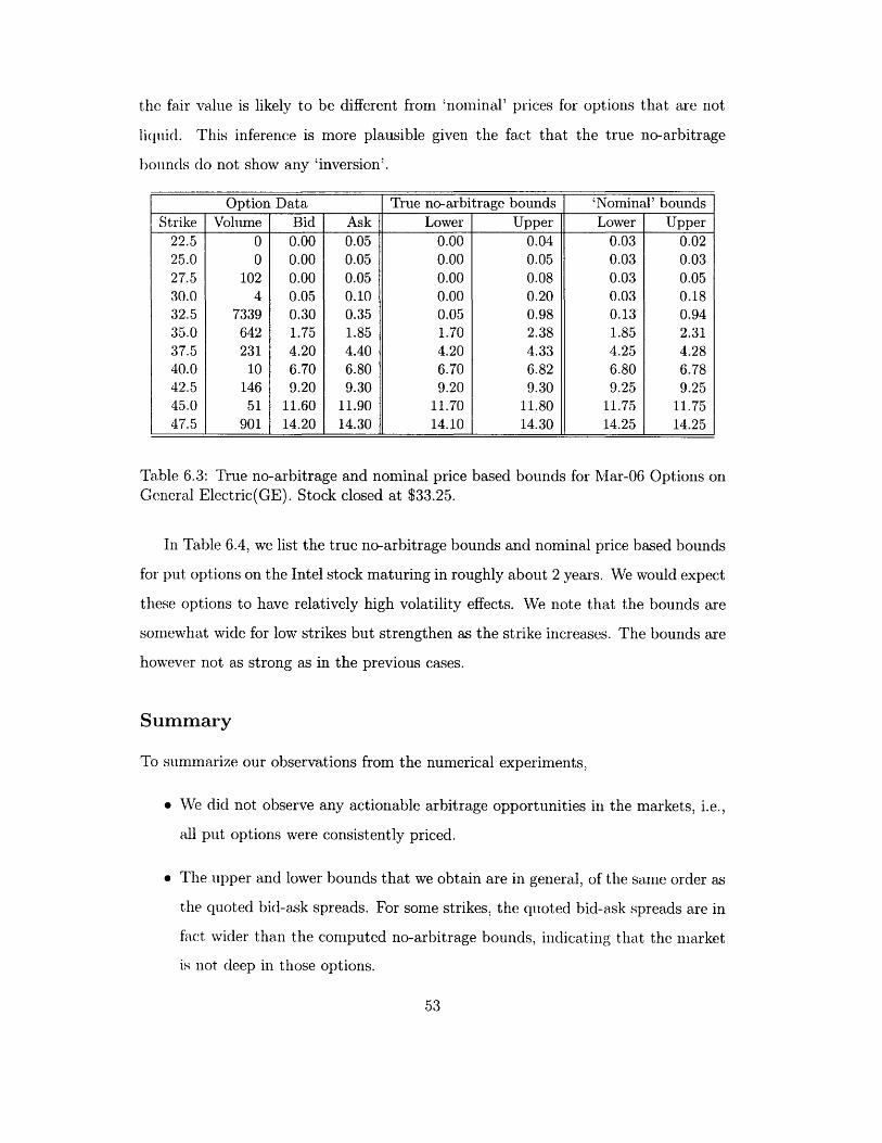
the fair value is likely to be different from 'nominal' prices for options that are not

liquid. This inference is more plausible given the fact that the true no-arbitrage

boun(ls do not show any 'inversion'.

Table 6.3: True no-arbitrage and nominal priceGeneral Electric(GE). Stock closed at $33.25.

based bounds for Mar-06 Options on

In Table 6.4, we list the true no-arbitrage bounds and nominal price based bounds

for put options on the Intel stock maturing in roughly about 2 years. We would expect

these options to have relatively high volatility effects. We note that the bounds are

somewhat wide for low strikes but strengthen as the strike increases. The bounds are

however not as strong as in the previous cases.

Summary

To summarize our observations from the numerical experiments,

*· Ve did not observe any actionable arbitrage opportunities in the markets, i.e.,

all put options were consistently priced.

* The upper and lower bounds that we obtain are in general, of the same order as

the quoted bid-ask spreads. For some strikes, the quoted bid-ask spreads are in

fact wider than the computed no-arbitrage bounds, indicating that the market

is not deep in those options.

53

Option Data True no-arbitrage bounds 'Nominal' boundsStrike Volume Bid Ask Lower Upper Lower Upper

22.5 0 0.00 0.05 0.00 0.04 0.03 0.0225.0 0 0.00 0.05 0.00 0.05 0.03 0.0327.5 102 0.00 0.05 0.00 0.08 0.03 0.0530.0 4 0.05 0.10 0.00 0.20 0.03 0.1832.5 7339 0.30 0.35 0.05 0.98 0.13 0.9435.0 642 1.75 1.85 1.70 2.38 1.85 2.3137.5 231 4.20 4.40 4.20 4.33 4.25 4.2840.0 10 6.70 6.80 6.70 6.82 6.80 6.7842.5 146 9.20 9.30 9.20 9.30 9.25 9.2545.0 51 11.60 11.90 11.70 11.80 11.75 11.7547.5 901 14.20 14.30 14.10 14.30 14.25 14.25

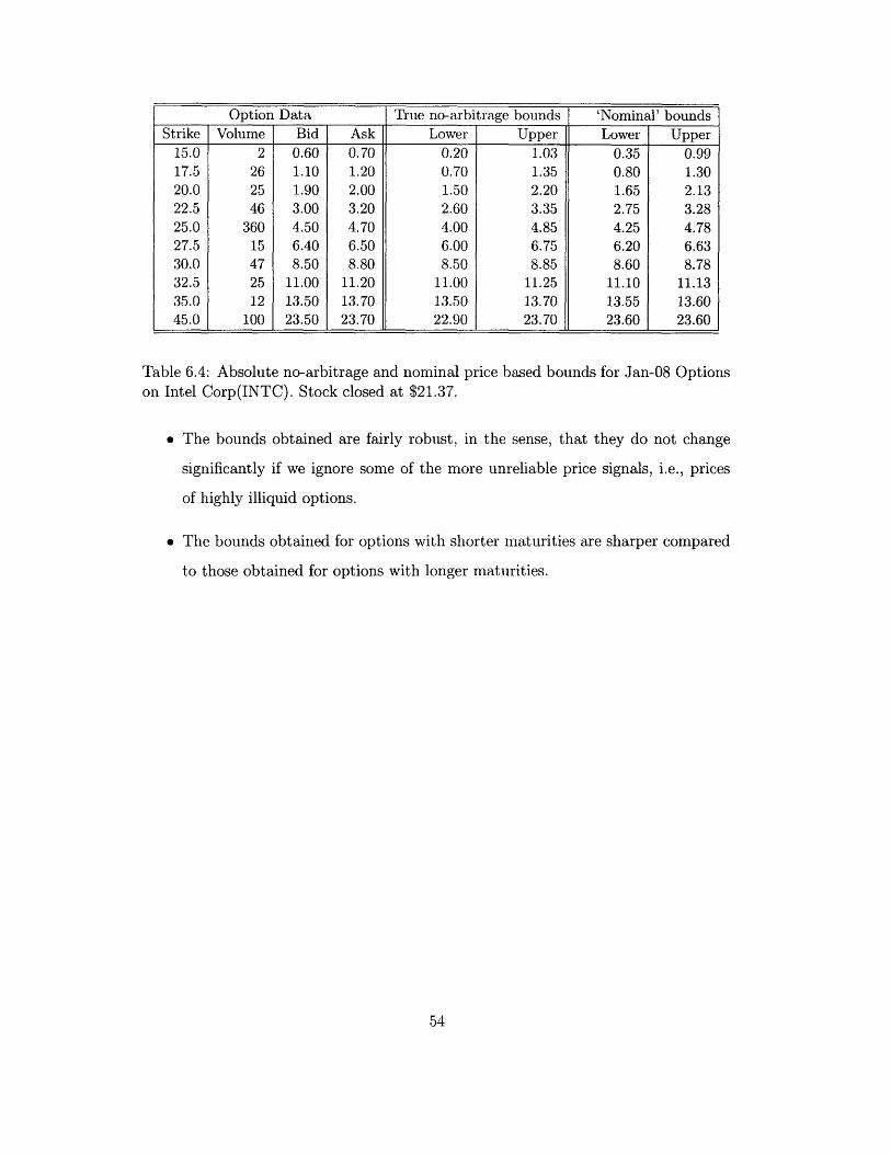
Table 6.4: Absolute no-arbitrage and nominal priceon Intel Corp(INTC). Stock closed at $21.37.

based bounds for Jan-08 Options

* The bounds obtained are fairly robust, in the sense, that they do not change

significantly if we ignore some of the more unreliable price signals, i.e., prices

of highly illiquid options.

* The bounds obtained for options with shorter maturities are sharper compared

to those obtained for options with longer maturities.

54

Option Data True no-arbitrage bounds 'Nominal' boundsStrike Volume Bid Ask Lower Upper Lower Upper

15.0 2 0.60 0.70 0.20 1.03 0.35 0.9917.5 26 1.10 1.20 0.70 1.35 0.80 1.3020.0 25 1.90 2.00 1.50 2.20 1.65 2.1322.5 46 3.00 3.20 2.60 3.35 2.75 3.2825.0 360 4.50 4.70 4.00 4.85 4.25 4.7827.5 15 6.40 6.50 6.00 6.75 6.20 6.6330.0 47 8.50 8.80 8.50 8.85 8.60 8.7832.5 25 11.00 11.20 11.00 11.25 11.10 11.1335.0 12 13.50 13.70 13.50 13.70 13.55 13.6045.0 100 23.50 23.70 22.90 23.70 23.60 23.60

Chapter 7

Conclusions and Final Remarks

We derived in this thesis, the necessary and sufficient conditions that prices of Amer-

ican Put Options on a non-dividend paying stock must satisfy to be consistent i.e.,

allow no arbitrage. We discover that these conditions are surprisingly few and sim-

ple. Using these conditions, we then derive the bounds on the price of an American

Put option of a specified strike, given the price of other American Put Options with

the same maturity. The problem of finding bounds can be cast as a simple linear

programming problem that can be solved directly using the algorithm presented in

Section 5.2. We also applied our results to data obtained from real markets. Our

methods could be readily modified, with only a little increase in complexity, to ac-

commodate the form in which price information is available in real markets, i.e., a

bid-ask interval. We discover that in mnost cases, especially for options with relatively

moderate volatilities, the bounds are quite strong compared to the quoted bid-ask

spreads.

'We have, however, accounted only for the effect of one particular type of derivative

security on the American Put Option Price, that is the prices of other American Put

Options having the same maturity. It will be interesting to see how the bounds

obtained can be tightened if it were possible to constrain the prices using additional

information from other derivative securities linked to the underlying.

55

56

Appendix A

Existence of an Optimal Exercise

Policy

Proposition A.1. Given an American Put Option with strike K, maturity T and

a r'isk neutral measure Q for the underlying stock price process, an optimal exercise

policy T* satisfying the following properties exists

1. * is non-randomized i.e., given a path w of the stock prices, at any time t,

T* (U, t) = 1 or T*(w, t) = 0, where T*(w, t) is the optimal probability of exercise

at time t for the path w.

2. r*(w, t) = 1 = t = T or K > St.

Proof. Let F denote the space of exercise policies and Y d that of non-randomized

exercise policies. w denotes a particular evolution of stock prices i.e., the vector

(So, S, .... ST). For t > s, let w :t denote the vector (S8, SS+...,St). Let T(W, t)

denote the probability that the option is exercised at time t, for sample path w, under

the policy T. T E F = % RT+ _ [0, 1]T+1 is a valid exercise policy (i.e., a stopping

time) iff

1. l'r:t (.,t) = t)

2. t =:iO:t => (LI, t): T.(aj2, t).

57

Further T E Fd if T(w) E {0, 1} Vw, t. Also,

T

AT(K, T) = E E [t( -St)+()]t=O

AT(K() = sup EQ t (K - St)+T(W)].7EF t=0

We first prove the existence of a non-randomized optimal exercise policy. Property

2 would then follow from a straightforward argument. Suppose the support set of

the process St is finite. Then, clearly Fd, the the set of non-randomized exercise

policies is finite and a randomized exercise policy is just a convex combination of

non-randomized exercise policies. It then follows that an optimal exercise policy

belonging to Fd exists by simple Linear Programming Theory. Suppose the state

space for St is not finite. In this case, we can use induction on T and the dynamic

programming principle to prove the existence of a non-randomized T*. For T = 1, this

follows alnlost immediately, as payoffs from all exercise policies can be characterized

in terms of a parameter p : 0 < p < 1 as

EQ[;r(K - ST)+] = p(K- So)+ + (1 -p)E'Q[(K- 1)+]

< max((K - S0)+,EQ[(K - S1)+]).

Thus one of 0 : To0(, 0) = 1, 0(w, 1) = 0 Vw or rl1 : Ti(W, 0) = 0, Tl(W, 1) = 1 Vw is an

optimal policy and hence the hypothesis holds for T = 1. Assume it is true for T = m

for some mn and consider the case when T = m + 1. At t = 1, then by the induction

hypothesis, for all possible values of S1 a henceforth non-randomized optimal exercise

policy, _ (SI, 1 l:r+l, t) exists. Let Vm-_(sl) denote the value of the corresponding

American Put Option that can be exercised anywhere in periods 1, 2,., , for all

paths w : S = .sl. Then set

T *(W,) = 1,

T *(W,t) = 0, Vt> 1;

58

if K - So > 3IE'[V,,,_ (S1)] ad

T*(W,O) = 0,

T*(W,t) = T1m_1(S, l+ 1 ,t - 1) Vt > 1;

otherwise.

From the principle of optimality, it follows that * so defined must be optimal. Fur-

ther, it also non-randomized by construction and the induction hypothesis.

Finally. if r* violates property 2 of the proposition, then consider a modification

r*, s.t.,

), | 7T*(w, t) if t < T-1 and T*(w, t) = or St < K;

0 if t < T- 1 and r*(w, t) = 1 and St > K.T-1

T*(w,T) = - ]*(,, t).t=l

It can be immediately verified that AT(W, T*) > AT(W, T*) = AT(K). Thus, we always

have a non-randomized optimal policy satisfying property 2 as well.

As r* is non-randomized, and the option (by our notational convention) is always

struck, we can alternatively describe r*(w) unambiguously by the time when the

option is exercised on path w i.e., *(w) E {O, 1, 2,.. ., T}. This is the notation that

we use in the thesis. E

59

60

Appendix B

Bounds from Bid-Ask Quotes

Suppose, we have been given a set of N + strikes KO, K 1, K 2, . ., KN and the

corresponding bid (Bo, B 1 ,..., BN) and ask quotes (Ao, A 1,..., AN) for all but one

of them, say strike KJ, as well as the initial stock price So. We also assume wlog,

that 0 = K0 < K1 < ... < KN. Then the linear program given below enforces the

convexity and other no arbitrage constraints to give the upper and lower no-arbitrage

bounds on the price of the option with strike KJ.

nmaXPo,PI,...,P,v / min,P , ...,PN PJs.t.

Po =

Bi < Pi < Ai

Pi > (Ki-So) +

K+,-K, (P+i- Pi) > -Ki 1 -Pi-1)0 < K (Pi-Pi-,) < 1- K -Ki -

, i ,...,J-1, J+ .. , N;

, i =O,..., N;

, i= 1,...,N-1;, i= 1,...,N.

61

62

Bibliography

[1] F. Black and M. Scholes. The Pricing of Options and Corporate Liabilities.

Journal of Political Economy, pages 637-654, 1973.

[2] G Bakshi, C Cao, Z Chen. Empirical Performance of Alternative Option Pricing

Models . The Journal of Finance, March 1997.

[3] J. Cox and S. Ross. The valuation of options for alternative stochastic processes.

Journal of Financial Economics, pages 145--166, 1976.

[4] M. Harrison and D. Kreps. Martingales and arbitrage in multiperiod security

markets. Journal of Economic Theory, pages 381--408, 1979.

[5] Robert Geske and Herb E Johnson. The American put valued analytically.

Journal of Finance, XXXIX(5), December 1984.

[6] Jacka, Saul. Optimal stopping and the American put. Math. Finance, 1:1--14,

1991.

[7] I. J. Kim. The analytic valuation of american options. Review of Finacial Studies,

3:547--572, 1990.

[8] M.A.H. Dempster, J. P. Hutton . Pricing Anlerican Stock Options by Linear

Programming. Mathematical Finance, 9(3):229- 254, July 1999.

[9] Negjiu Ju. Pricing an American option by approximating its early exercise

boundary as a multipiece exponential finction. Review of Finacial Studies,

11(3):627-646, 1998.

63

[10] Jingzhi Huang, Marti Subrahmanyan, and George Yu. Pricing and Hedging

American Options: A Recursive Integration Method. Review of Financial Stud-

ies, 9:277-300, 1996.

[11] Mark Broadie and Jerome Detemple. American option valuation: New bounds,

approximations, and a comparison of existing methods. Review of Finacial Stud-

ies, 9(4):1211-1250, 1996.

[12] A. Lo. Semiparametric upper bounds for option prices and expected payoffs.

Journal of Financial Economics, pages 373-388, 1987.

[13] B. Grundy. Option prices and the underlying asset's return distribution. J.

Finance, 46(3):1045--1070, 1991.

[14] D. Bertsimas and I. Popescu. On the relation between option and stock prices:

a convex optimization approach. Operations Research, 50(2):358-274, 2002.

[15] Dimitris Bertsimas and Natasha Bushueva. Options Pricing Without Price Dy-

namics: A Geometric Approach. working paper, August 2004.

[16] Dimitris Bertsimas and Natasha Bushueva. Options Pricing Without Price Dy-

namics: A Probabilistic Approach. submitted to Math. of OR, August 2004.

[17] A. d'Aspremont and L. El Ghaoui. Static arbitrage bounds on basket option

prices. Mathematics arXiv Working Paper No. math. OC/0302243., February

2003.

[18] Yahoo! Finance. http://finance.yahoo.com.

64