Energy Economics 42 (2014) 101–114

Contents lists available at ScienceDirect

Energy Economics

j ourna l homepage: www.e lsev ie r .com/ locate /eneco

Preference heterogeneity for renewable energy technology

James Yoo a,⁎, Richard C. Ready b,1

a Department of Economics & Business, Bethany College, Bethany, WV 26032, USAb Department of Agricultural Economics, Sociology and Education, Pennsylvania State University, University Park, PA 16802, USA

⁎ Corresponding author. Tel.: +1 602 705 7311.E-mail addresses: jyoo@bethanywv.edu (J. Yoo), rread

1 Tel.: +1 814 863 5575; fax: +1 814 865 3746.

0140-9883/$ – see front matter © 2013 Elsevier B.V. All rihttp://dx.doi.org/10.1016/j.eneco.2013.12.007

a b s t r a c t

a r t i c l e i n f o

Article history:Received 25 November 2012Received in revised form 26 October 2013Accepted 10 December 2013Available online 17 December 2013

JEL Classification:Q2Q4Q28Q42Q48Q51

Keywords:Renewable energyIndividual-specific willingness-to-payRandom parameter modelLatent class modelHybrid random parameter-latent class model

This study explores heterogeneity in individual willingness to pay (WTP) for a public good using several differentvariants of the multinomial logit (MNL) model for stated choice data. These include a simple MNL model withinteraction terms between respondent characteristics and attribute levels, a latent class model, a random param-eter (mixed) logit model, and a hybrid random parameter-latent class model. The public good valued was an in-crease in renewable electricity generation. The models consistently show that preferences over renewabletechnologies are heterogeneous among respondents, but that the degree of heterogeneity differs for different re-newable technologies. Specifically, preferences over solar power appear to be more heterogeneous acrossrespondents than preferences for other renewable technologies. Comparing across models, the random parame-ter logit model and the hybrid random parameter-latent class model fit the choice data best and did the best jobcapturing preference heterogeneity.

© 2013 Elsevier B.V. All rights reserved.

1. Introduction

Random utility models (McFadden, 1974) have a wide range of ap-plication in the analysis of choice data including recreational demandchoice (Boxall and Adamovicz, 2002; Scarpa and Thiene, 2005; Train,1998), stated choice valuation (Borchers et al., 2007; Revelt and Train,2000; Scarpa and Willis, 2010), transportation choice (Greene andHensher, 2003; Shen, 2010), and marketing (Swait and Adamowicz,2001). Analyzing choice data with random utility models is often doneby estimating a simple Multinomial Logit Model (MNL), which assumesthat preferences are homogeneous across the population. The assump-tion of homogeneous preferences, however, is problematic since eachperson is unique in terms of habit, education background, characteris-tics, and income level, which might be correlated with preferencesover non-market goods. Failure to incorporate the unique nature ofeach consumer in estimating discrete choice models would mask het-erogeneity in preferences and could lead to biased estimates of averagepreferences over the population.

Several different extensions of the MNL discrete choice modelhave been developed that can accommodate consumer preference

y@psu.edu (R.C. Ready).

ghts reserved.

heterogeneity for non-market goods. Some of these also relax the IIA(Independence of Irrelevant Alternatives) assumption. The simplestand most commonly used approach is to interact attribute levels withmeasured individual characteristics to see whether people with differ-ent characteristics exhibit different preferences within the MNLmodel. This approach retains the unrealistic assumptions of the MNLmodel such as IIA and uncorrelated unobserved error over time. TheIIA property assumes that the choice of alternatives A and B is not influ-enced by the addition or exclusion of the third choice, C. In general, thismay not be a realistic assumption and create a problem of leading amodel to erroneously predict the probability of choosing one alternativeover the other. Also, assumption of uncorrelated errors might be prob-lematicwhen using a panel data because a person's choicemight be cor-related across repeated choice through learning or fatigue effects. Twomodels that allow for preference heterogeneity and that relax the IIA as-sumption and/or uncorrelated error terms are the random parameterlogit (RPL) model (Greene and Hensher, 2003; McFadden and Train,2000; Train, 1998), also known as the mixed logit model, and latentclass models (LCM) (Boxall and Adamovicz, 2002; Milon and Scrogin,2006; Scarpa and Thiene, 2005; Swait and Adamowicz, 2001), alsoknown as finite mixture models. Each model has strengths andweaknesses. LCM models are less flexible than RPL models, but havean advantage when it comes to computational simplicity. The con-tinuous representation of preference variation in the RPL might be

2 In RPL, if a distribution of random coefficient is degenerate, then the integral termwillvanish leaving a simple logit formbehind. In LCM, if coefficients across different classes arethe same, then the latent classmodel is reduced to theMNL. In that sense,MNL is a specialform of both LCM and RPL (MNL is nested within LCM and RPL).

3 Greene and Hensher (2003) plotted choice probabilities under LCM and RPL for eachalternative and investigated the relationship between choice probabilities for RPL andthose for LCM via OLS. They found that there is a weak relation between two models.

4 Shen's non-nested test is based on an AIC proposed by Ben-Akiva and Swait (1986).The test procedure is as follows: Suppose there are 2 models (model 1 and model 2)and K1 and K2 represent the number of parameters in model 1 and model 2, respectively.Also define L0, L1 and L2 represent the likelihood value for constant-only model, the likeli-hood value at convergence for model 1, and likelihood value at convergence for model 2,

respectively. Then, fitness measure for model j is expressed as: ρ2j ¼ 1− L j−K j

L0: An upper

bound for probability that model 1 is chosen as the true model despitemodel 2 being true

is then given byPr ρ22−ρ2

1 Nz� �

≤ Φ − −2zL0 þ K1 þ K2ð Þð Þ12h i

;where z represents the dif-

ference between ρ22 and ρ22.

102 J. Yoo, R.C. Ready / Energy Economics 42 (2014) 101–114

inappropriate when the sample consists of discrete groups with differ-ent group-specific tastes. The discrete representation of preference var-iation in the LCM cannot capture within-class heterogeneity. Usingeither of thesemodels could oversimplify the taste variation of the sam-pled respondents (Allenby and Rossi, 1998; Bujosa et al., 2010; Wedelet al., 1999). A hybrid model that combines both continuous and dis-crete representation of taste variation was first proposed by Bujosaet al. (2010). They find that this hybridmodel fits best in terms of statis-tical goodness-of-fit.

In this research, we estimate several different discrete choice modelsthat accommodate preference heterogeneity. These models include theMNL model with interactions between choice attributes and respondentcharacteristics, a LCM, a RPLmodel, and a hybrid RPL–LCM. Thesemodelsare compared in terms of how well they fit the data and their ability toidentify heterogeneity in WTP. This research includes two advancesover previous studies that have explored preference heterogeneity indiscrete choice data. First, the LCM developed here places specific restric-tions on parameter values for certain latent classes. These restrictions aremotivated by previous research that shows that some respondents, whenfaced with a complex choice task, focus their attention on a restricted setof attributes, and ignore other attributes that are less salient to them(Blamey et al., 2001). We extend Scarpa et al. (2009) model of attributenon-attendance in our LCM. Second, following Greene and Hensher(2010), our hybrid RPL–LCM is estimated in a way that accounts for thepanel nature of stated choice data, but extends their hybrid model by in-corporating the same types of restrictions on the preference parametersfor certain latent classes. Finally, this is the first study to compare all ofthe above mentioned models based on their ability to capture heteroge-neity in individual WTP, and therefore represents an extension of whatBeharry-Borg and Scarpa (2010) did.

This study, specifically, estimates Pennsylvania residents' preferenceover different renewable electricity production technologies and theirwillingness to pay (WTP) for an increase in renewable electricity pro-duction. Our results build on previous studies that have estimatedWTP for increased renewable energy production (Borchers et al.,2007; Farha, 1999). We explore both the meanWTP for each of severaldifferent generation technologies and the degree of heterogeneityamong respondents' individual for each technology.

Information on mean WTP for individual renewable technologies isimportant from a policy perspective. Currently, Pennsylvania has inforce an Alternative Energy Portfolio Standard (AEPS) to promoterenewable energy production. The current AEPS policy specifies a min-imum for the amount of electricity that must come from renewable andalternative sources, setting minimum standards for renewable content.The AEPS includes a carve-out (technology-specificminimum) for solar,but does not set individual requirements for other renewable technolo-gies such as wind, hydroelectric power and biomass. If Pennsylvaniaresidents prefer some renewable technologies over others, that pref-erence could be reflected in differential requirements in the AEPS. IfPennsylvania residents have negative views toward some renewableenergy technologies, the current AEPS could force them to pay fortechnologies that they do not want.

It is equally important to know how WTP varies across the pop-ulation, which is the main focus of this research. We find thatmean WTP for some renewable technologies is positive, but thatWTP exhibits heterogeneity such that an important proportion ofthe population has negative WTP for the technology. This result sug-gests that, while the average resident would support a policy thatincreases renewable energy production, an important proportionof residents could oppose such a policy. Policy makers in Pennsylva-nia should consider the entire distribution of preferences, ratherthan focusing only on the mean preference.

The paper is organized as follows. Section 2 reviews previous litera-ture on two topics: comparisons of LCM and RPL models and attributenon-attendance behavior. Section 3 presents themodels thatwill be es-timated in this study, followed by descriptions of the goods being valued

and of the survey methodology. Section 4 discusses the results andSection 5 presents a summary and discusses implications of the research.

2. Literature review

2.1. Previous studies on the RPL, LCM, and RPL–LCM models

Both the RPL and LCM models relax some of the restrictions of theMNL model, but they do so in different ways. Since MNL is nested withinboth of these twomodels,2 comparisons betweenMNL and RPL and be-tweenMNL and LCM are feasible using likelihood ratio tests. Many recentstudies (Beharry-Borg and Scarpa, 2010; Greene and Hensher, 2003;Kosenius, 2010; Shen, 2010) conclude that the LCM and the RPL both im-prove statistical fit relative to MNL. One exception is Provencher andBishop (2004). However, a direct comparison between RPL and LCM can-not be made based on a likelihood ratio test, because one model is notnested within the other. In order to compare these two models, differ-ent approaches have been developed.

Greene andHensher (2003) compare LCMandRPLmodels by lookingat choice elasticities for a change in travel times, mean willingness-to-pay estimates, and choice probability plots,3 and find that respondents'behavioral sensitivity to an attribute (changes in travel time) is reducedin the LCM relative to the RPL, although other measures such as choiceprobability plots andwillingness to pay valuations yield similar patternsfor both models. Shen (2010) adds a non-nested test4 and predictionsuccess indices to investigation of the choice probabilities, WTP valua-tions, and choice probability plots to test which model is better. Shefinds that the LCM is superior to the RPL in terms of these twomeasures.Shen (2010) and Greene and Hensher (2003) show that LCM fits betterthan RPL based on statistical goodness-of-fit.

Kosenius (2010) investigated consumer's preference heterogeneityfor water quality attributes using RPL and LCM. In order to comparethe two models, the author presents WTPs for 3 potential future nutri-ent reduction scenarios. Rather than focusing on statistical measures,Kosenius focused on the heterogeneity of WTP of a representativerespondent. They conclude that a LCM was indisputably superior interms of capturing the relative importance order of each attribute withindifferent classes. However, the sample in that study was not representa-tive of the population. They conclude that the RPL is better than theLCMwhen the sample is weighted to correct for sampling bias. Althoughtheir study was the first attempt to explore aspects of RPL and LCM otherthan statistical goodness-of-fit, the heterogeneity of individual WTP wasnot considered in their study.

Beharry-Borg and Scarpa (2010) were the first study to compareLCM and RPL based on individual WTP. They use 2 sub-samples, snor-kelers andnon-snorkelers, in a study valuing quality change in Caribbeancoastal waters. They found that an LCM outperformed a RPL model forthe snorkeler sample, but that the LCM did not behave well for thenon-snorkeler sample. They did not directly compare RPL and LCMbased on individual WTP within each subsample.

103J. Yoo, R.C. Ready / Energy Economics 42 (2014) 101–114

Greene and Hensher (2010) and Bujosa et al. (2010) compare RPL,LCM, and a hybrid RPL–LCM based on statistical goodness-of-fit andindividual-specific parameters using transportation choices and recrea-tional trip data, respectively. One difference between the two studies isthat the latter does not account for the panel nature of choice data, whilethe former incorporates it in the model. Both studies estimated hybridRPL–LCM models with two latent classes. Both studies find that thehybrid RPL–LCM fits better than MNL, LCM, and RPL models.

2.2. Previous studies on attribute non-attendance

In a stated choice experiment, respondents are asked to answer asequence of questions that consist of multiple alternatives, in whicheach alternative is described by attributes and their levels. The experi-ment assumes that each respondent makes trade-offs among the levelsof each attribute across all alternatives, and he or she is expected to selectthe most preferred alternative. In other words, all respondents are as-sumed to pay attention to the level of all attributes. The ability of respon-dents tomake trade-offs among attributes is represented by the propertyof substitutability or continuity (Freeman, 1993), which is the central tothe economic concept of value (McIntosh and Ryan, 2002). When thisproperty is violated, discrete choice valuation is confrontedwith some se-rious problems. First, respondents that violate the property of continuitycannot be represented by a conventional utility function (Campbell,2008; Lancsar and Louviere, 2006). Second, without continuity, therewill be no trade-off between two different attributes, and WTP cannotbe computed (Campbell, 2008).

Several studies (DeShazo and Fermo, 2002; Hensher and Rose,2009; Rosenberger et al., 2003; Sælensminde, 2006) have foundthat the continuity assumption sometimes fails in discrete choice ex-periments. This implies that some respondents behave as if they donot care about the level of some attributes, resulting in zero marginalutility for those attributes. Scarpa et al. (2009) investigate the possi-ble existence of non-attendance to attributes using four different la-tent class models. They classify respondents into groups usingspecial notation: TA (total attendance—all attributes are simulta-neously considered), TNA (total non-attendance—respondent doesnot consider any of the attribute levels), PNA1 (partial non-attendance ignoring one attribute), PNA2 (partial non-attendanceignoring the cost attribute and one non-monetary attribute), andPNA3 (partial non-attendance ignoring the cost attribute and 2non-monetary attributes). They compare different models that in-corporate different combinations of latent classes following each ofthese behaviors. They find that less than 0.1% of the sample caresabout all attributes (TA), while most respondents seem to ignore atleast 2 out of their 5 attributes. In their study, 80 to 90% of respon-dents ignore the cost attribute, raising doubt about the validity ofchoice experiments in terms of calculating WTP.

What might cause discontinuous preference or attribute non-attendance in a choice experiment? By the nature of choice experiments,choice tasks are complicated, so that respondents might not understandhow to make trade-offs between certain attributes of environmentalgoods. Due to this complexity, respondents might decide to simplifychoice tasks by constantly choosing alternatives with attributes theyconsider to be important and favorable (Blamey et al., 2001; Caussadeet al., 2005; Luce et al., 2000). Sælensminde (2006) investigates lexico-graphic choice behavior of respondents in a choice experiment, definedas situations where a respondent consistently chooses the alternativethat is best with respect to one attribute, e.g. lowest price. He discoversthat respondents exhibit lexicographic preferences as a consequence ofsimplification of the choice task when there is a high number of attri-butes and respondents have no prior information about the attributes.DeShazo and Fermo (2002) examine the relationship between choicecomplexity and respondents' choice consistency, and find that choicecomplexity significantly affects choice consistency. Other studies(Jacoby et al., 1974; Keller and Staelin, 1987) find that the number of

attributes and the number of levels of attributes can make choicedecisions more complicated, affecting choice consistency. There is alsoevidence (Rosenberger et al., 2003) that the strength of a person'sdisposition, attitude, and belief can explain discontinuous choicebehavior.

Non-attribute attendance behavior is investigated in this studythrough estimating a latent classmodel that includes latent classeswithrestrictions on parameters consistent with attribute non-attendance.

3. Methodology

3.1. Models

In this section, 5 different econometric models are presented.The MNL is the most basic and commonly used choice model. Itstheoretical foundation is the random utility model (Manski, 1977;McFadden, 1974). According to random utility theory, the utility of con-sumer i choosing alternative j is expressed as:

Uij ¼ Vij þ eij ð1Þ

where Vij is a deterministic component and eij is a stochastic compo-nent. This model is called a random utility model because the utilitya person receives depends to some degree on random factors.

Assuming thatVij is a linear function of observed characteristics of al-ternative j and that the stochastic component follows a type 1 extremevalue, the probability that individual i chooses alternative j over k fromaset of J options is expressed as:

Prob UijNUik;∀k� �

¼exp βXij

� �X J

l¼1exp βXilð Þ;

ð2Þ

where Xij is a vector of choice attributes, and β is a vector of preferenceparameters (marginal utilities) to be estimated. Individual characteris-tics of the consumer variables cannot enter into choice utility alone be-cause individual characteristics are invariant across choice alternatives,and therefore do not affect choice probabilities. They can only enterthrough interactions with choice attributes (Champ et al., 2003). Thisgenerates the new relationship, where the marginal utility of a choiceattribute is a function of the individual characteristics. Incorporatingrespondent characteristics/attribute level interactions can help identifysystematic heterogeneity in preferences that is tied to respondentcharacteristics. An MNL model with interactions between choice attri-butes and respondent characteristics will be called here the MNL-INTmodel.

A latent classmodel, also called a finite/mixturemodel, assumes thatthere are C segments in the population. Preferences differ among thesegments, but are homogeneous within each segment. The latent classmodel probabilistically assigns each respondent to a segment accordingto covariates (individual characteristics) and choice behavior. Supposeindividual i, who belongs to class c, chooses alternative j in a choiceoccasion k. The utility of this respondent is expressed as:

Uijkjc ¼ Xijkβc þ eijkjc: ð3Þ

Xijk is a vector of choice attributes, eijk|c is an unobserved componentwithin a class, and βc is a class-specific vector of parameters to be esti-mated. Assuming IIA holds within a class, the probability of respondenti choosing alternative l in a choice occasion, k, is:

Pilkjc ¼exp Xilkβcð ÞX Jj¼1

exp Xijkβc

� �:

ð4Þ

104 J. Yoo, R.C. Ready / Energy Economics 42 (2014) 101–114

In a LCM, it is necessary to specify a function that defines the proba-bility of class membership in each class for each respondent. The classmembership probability of individual i being classified to class C canalso be modeled as a multinomial logit:

Pic ¼exp θcZið ÞXCc¼1

exp θc Zið ÞÞð5Þ

where θc is a class specific parameter vector and Zi includes individualcharacteristics (income, age, etc.) of respondent, i. This class-specificparameter shows the influence of individual characteristics on the prob-ability of being in a class c. By combining the conditional choice probabil-ity, Pijk|c with membership probability, Pic and taking the expectationover all classes, the joint unconditional probability for the choicesmade by individual i could be constructed as follows:

Pi ¼XC

c¼1PicPijkjch i

¼XC

c¼1

exp θcZið ÞXc¼1

exp θcZið Þ

!�∏K

k¼1exp Xilkβcð ÞX

j¼i

exp Xijkβc

� �0BBB@

1CCCAð6Þ

where k = 1,…K are the choices faced by respondent i. Eq. (6) then isindividual is contribution to the likelihood function. Vectors of parame-ters θ and β for all classes are obtained bymaximizing the log-likelihoodfunction with respect to those parameters. In order to select the appro-priate number of classes, the Bayesian information criterion (Roederet al., 1999) and Akaike information criterion could be used. With

vectors of parameters θ̂ and β̂� �

obtained, the posterior estimate of

the class membership probabilities, Hci, can be calculated as follows:

Hci ¼ð

exp θ̂cZi

� �X

c¼1exp θ̂cZi

� � ∏Kk¼1

exp eβcXilk

� �X

j¼1exp β̂cXijk

� �0@ 1A�

XCc¼1

ðexp θ̂cZi

� �X

c¼1exp θ̂cZi

� � ∏Kk¼1

exp β̂cXilk

� �X

j¼1exp β̂cXijk

� �0@ 1A24 35:

ð7Þ

Hci is called an individual-specific estimate of the class probability(Greene and Hensher, 2003), conditional on estimated choice probabil-ity. The posterior individual-specific WTP is given by:

E WTPið Þ ¼XC

c¼1Hci −

β dc;attribute

βdc;cost0@ 1A: ð8Þ

The latent classmodel introduced above is the generalized latent classmodel, in which people conventionally estimate LCMs with differentclasses (2 class, 3class, 4class, etc.), and select the model that is consid-ered the best in terms of AIC, BIC, and AIC-3 criteria. As usually estimated,no restrictions are placed on βc vectors. In this study, however, a restrict-ed 4 class latent classmodel (R4LCM) is proposed. Parameter restrictionsare imposed on the marginal utilities in some classes consistent with apriori conjectures regarding attribute non-attendance. The four classesin the model are as follows. In the attribute non-attendance class(ANA), all the utility parameters are restricted to zeros. A respondent inthe ANA class will choose randomly from the options without regard toattribute level. In the zero WTP (ZWTP) class, parameters are restrictedsuch that all parameters except the cost parameter are set equal tozero. Members of this class will always choose the cheapest option avail-able, and will have zero WTP for all attributes. The third and fourth clas-ses have no restrictions imposed, but have different parameter values.We find that one class tends to have low WTP for all attributes, whilethe other has higher WTP, and call the two classes the low WTP class

(LWTP) and high WTP class (HWTP). Hence, the log-likelihood functionfor R4LCM is expressed as follows

lnL ¼XNi¼1

lnP ¼XN

i¼1ln½ 1

3

� �NC exp ZiθANAð ÞX4c¼1

Ziθcð Þ

0@ 1Aþ∏NC

i¼1

exp Xilcostβprice

� �X3

j¼1Xijcostβprice

0@ 1A exp ZiθZWTPð ÞX4c¼1

Ziθcð Þ

0@ 1Aþ∏NC

i¼1exp XilkβLWTPð ÞX3

j¼1XijkβLWTP

0@ 1A 1X4c¼1

Ziθcð Þ

þ∏NCi¼1

exp XilkβHWTPð ÞX3j¼1

XijkβHWTP

0@ 1A exp ZiθZWTPð ÞX4c¼1

Ziθcð Þ

ð9Þ

where NC represents the number of choice questions that individual ifaced.

For the purpose of ease of interpretability, membership parametersfor LWTP are constrained to zeros (i.e., the LWTP class is the baselineclass).

Aswith the LCM, the randomparameter logit (RPL)model allows forparameters of attributes to vary across respondents. It overcomes threelimitations of the standard MNL by allowing for random taste variation,unrestricted substitution patterns, and correlation in unobserved fac-tors (Train, 1998). Each parameter for each attribute is assumed to berandom, following a specific distribution. The log-likelihood functionfor the random parameter model does not have a closed form, so a sim-ulation method is used. The utility associated with individual is choos-ing alternative j in choice occasion k is denoted by

Uijk ¼ βiXijk þ eijk ð10Þ

whereXijk is a vector of choice attributes and eijk is a stochastic componentunobserved (iid) by the econometrician. The vector Xijk can include inter-action terms between choice attributes and the characteristics of the per-son making the choice, in which case we designate the model as a RPLwith interactions (RPL-INT). In order to incorporate the correlation acrossalternative and across choice occasion and taste variation across respon-dents, the individual-specific parameter vector βi is partitioned into twoparts, b, representing the average of taste in the population, and, ηirepresenting the deviation of individual taste from average taste in thepopulation. Utility can then be re-written as:

Uijk ¼ bXijk þ ηiXijk þ eijk: ð11Þ

Hence, the actual conditional probability of individual i choosing alterna-tive j is:

Pij Ωð Þ ¼Z

∏Kk¼1

exp βXilkð ÞXjexp βXijk

� �24 35 f βjΩð Þdβ: ð12Þ

The goal is to estimate the population parameterΩ, representing thepopulation parameters that explains the distribution of individual pa-rameters. The integral term cannot be handled by the conventionalmaximum likelihood procedure. Instead, choice probabilities are ap-proximated through simulation.

The simulated log-likelihood function is,

SLL Ωð ÞXN

n¼1ln

1R

Xr¼1

Li¼1……R βrijΩ� �: ð13Þ

where R is a number of draws from the distribution and βri|Ω is a vector ofβs obtained from r-th draw from the distribution, f(β|Ω) for individual i.The parameters are estimated by choosing Ω that maximizes SLL(Ω).

5 Tier I source: photovoltaic energy, solar-thermal energy, wind, low-impact hydro,geothermal, biomass, biologically derived methane gas, coal-mine methane and fuel cells.Tier II source: waste coal, distributed generation (DG) systems, demand-side manage-ment, large-scale hydro, municipal solid waste, wood pulping and manufacturingbyproducts, and integrated gasification combined cycle (IGCC) coal technology.

105J. Yoo, R.C. Ready / Energy Economics 42 (2014) 101–114

Once the population parameters are obtained, one can generateBayesian estimates of individual-specific preferences by deriving theconditional distribution based on the observed choices and the param-eters obtained from the previous steps (Hensher and Green, 2003;Revelt and Train, 2000). The prior information is the set of parametersobtained. Given that prior information, an individual-specific WTP canbe derived by calculating:

E WTPið Þ ¼

1R

XRr¼1

βi;attribute

βi;cost∏K

k¼1exp βXilkð ÞXjexp βXijk

� �24 35

1R

XRr¼1

∏Kk¼1

exp βXilkð ÞXjexp βXijk

� �24 35:

ð14Þ

Both the LCM and the RPL model allow for variation in the β victoramong individuals. The LCM assumes that respondents fall into classesand that every member of a given class has the same β victor. The RPLmodel assumes that each respondent has a unique β victor, and that thedistribution of β is the same for all respondents. A hybrid LCM–RPLmodel assumes that respondents fall into discrete classes, as in the LCM,but allows for variation in βwithin each class. Themodel simultaneous-ly classifies respondents into a number of segments depending onindividual characteristics or attitudinal tendency, and estimates utilityparameters based on random parameter model procedure within eachclass.

The log-likelihood function for RPL–LCM is expressed as:

lnL ¼XN

i¼1lnPi ¼

XNi¼1

lnXC

c¼1

exp θcZið ÞXc¼1

exp θcZið ÞÞ � �∏Kk¼1 Πikjc� �

0@ 35:24

ð15Þ

Eq. (15) is exactly same as Eq. (6) except that the conditional choiceprobability Πik|c now takes an open form as,

Πikjc ¼Z

exp Xilkβcð ÞXj¼1

exp Xijkβc

� �f βcð Þdβc

: ð16Þ

3.2. Policy context and good valued: renewable energy in Pennsylvania

Pennsylvania relies largely on coal (48% of total electricity generat-ed) and nuclear power (35%) for its electricity needs. In 2009, renew-able sources accounted for 2.7% of total electricity generation inPennsylvania, up from 2.3% in the early 1990s (US EIA, 2011a), thoughstill far below the national average of 10.6% (US EIA, 2010). The domi-nant renewable electricity sources are hydropower (1.2% of total gener-ation), municipal solid waste and landfill gas (0.7%), wind (0.5%) andbiomass (0.3%) (US EIA, 2011b).

Like many states, Pennsylvania has adopted a renewable energyportfolio standard that requires electricity supplies to source a specificpercentage of their electricity from renewable energy sources.Pennsylvania's standard, adopted in 2004, differs from most portfoliostandards in that it allows for production of unconventional, nonrenew-able sources. The Pennsylvania program is called the Alternative EnergyPortfolio Standard (AEPS), and requires that electric distributioncompanies and electric generation suppliers source 18% of theirusing electricity from renewable and alternative energy sources bythe year 2020. Under this law, there are two types of energy sources,called, “Tiers”. The AEPS requires that utility companies generate8% of their electricity from “Tier I” energy sources, which includemost renewable technologies such as wind, solar and hydropower,and 10% from “Tier II” sources by 2020 (U.S. Energy Information

Agency, EIA, 2010).5 Electricity distribution companies or genera-tion suppliers who do not themselves generate enough alternativeenergy to meet the AEPS requirements can buy alternative energycredits from other suppliers who generate more than their requiredamount. Within Tier I, there is a special carve out for solar power,whereby 0.5% of total electricity generated must come from solarby 2020.

So far, AEPS requirements have been met with relative ease.AEPS targets are being exceeded, and are expected to continue to beexceeded for the next few years (PUC, 2011). There have been proposalsto increase the renewable energy targets of the AEPS and/or to speedup the schedule for reaching those targets (for example, PennsylvaniaHouse Bill 1580). In this study, respondents are presented with choicesamong different AEPS policies that result in different combinationsof renewable energy production, allowing estimation of WTP for in-creases in different types of renewable energy. Knowledge of the prefer-ences of residents for different types of electricity generation, and theirWTP to increase renewable electricity generation, would be usefulwhen considering such proposed changes to the AEPS.

3.3. Survey data

The survey instrument (questionnaire) used in this survey was de-signed based on a review of instruments used in previous studies andbased on insights gained from two focus groups, one conducted in arural community, the other conducted in an urban community. The sur-veywas administered as amail questionnaire, and included four sections.The first section asks respondents a series of agree/disagree statementsmeasuring respondents' attitudes toward issues related to renewable en-ergy production in Pennsylvania. The second section asked respondentsto rate different electricity generation technologies according to their im-pacts on scenery and land, local air quality, jobs in Pennsylvania, globalclimate, and the overall impact of each generation technology. In total,10 electricity generation technologies were rated by respondents. Thethird section included the choice experiment (CE) questions, describedin more detail below. Section 4 asks agree/disagree questions related torenewable energy policy, and elicits individual characteristics of the re-spondents such as age, income, and education.

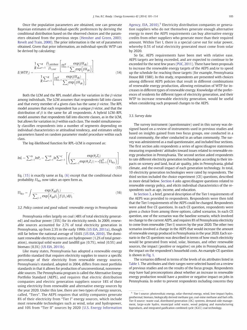
In Section 3, a brief, general description of the Tier I requirements ofthe AEPS was provided to respondents. Respondents were then toldthat the Tier I requirements of the AEPS could be changed. Respondentswere asked five CE questions. In each CE question, respondents weregiven a choice from among three options, called scenarios. In each CEquestion, one of the scenarios was the baseline scenario, which involvedno change to the current AEPS, and requires 8% of Pennsylvania electricityto come from renewable (Tier I) sources by the year 2020. The other twoscenarios involved a change in the AEPS that would increase the amountof renewable energy produced in Pennsylvania in the year 2020. Each sce-nario in the CE questions was described in terms of howmuch electricitywould be generated from wind, solar, biomass, and other renewablesources, the impact (positive or negative) on jobs in Pennsylvania, andthe impact on the respondent's household costs. An example CE questionis shown in Fig. 1.

The scenarios differed in terms of the levels of six attributes listed inTable 1. The attributes and their ranges were selected based on a reviewof previous studies and on the results of the focus groups. Respondentsmay have had preconceptions about whether an increase in renewableenergy production would have a positive or negative impact on jobs inPennsylvania. In order to prevent respondents including concerns they

Fig. 1. Sample choice experiment question.

106 J. Yoo, R.C. Ready / Energy Economics 42 (2014) 101–114

have over job impacts in theirWTP for renewable energy, impact on jobswas included as a separate attribute.

The level of the attributes in each scenario in each CE questionwas chosen to generate an experimental design that would providethe maximum possible information about respondent preferences overthe attributes. The experimental design was performed using the modi-fied Fedorov algorithm (Cook and Nachtsheim, 1980; Fedorov, 1972;Zwerina et al., 1996) via SAS macro (% Choiceff). Four different versionsof the survey were ultimately constructed. The versions differed in thelevels of the attributes in each CE question, so that a total of 20 differentCE questions were presented to respondents.

The survey was pretested in the field in November 2010 with asmall sample (50 urban and 50 rural residents), using two survey ver-sions. The response rate was 50%, and item non-response rates wereacceptably low. Data from the pretest was used to estimate a preliminaryMNL model. Based on this model, two more survey versions wereconstructed to provide a richer experimental design. Full survey imple-mentation used the same method as the pretest, and began in January2011. The Penn State Survey Research Center (SRC) purchased a mailinglist of randomly chosen PA residents. Surveysweremailed to an addition-al 1500 PA residents (900 rural, and 600 urban). In order to improvethe response rate, a $2 cash incentive was included in the survey. Seven

Table 1Description of attributes used in choice experiment.

Attribute Description

Solar Percentage of electricity generated from solar power in PennWind Percentage of electricity generated from wind power in PennBiomass Percentage of electricity generated from biomass combustionOther renewables Percentage of electricity generated from other renewable souJob impact Impact on jobs in PennsylvaniaCost Additional cost to household through higher electricity bills a

to ten days after the initial mailing, a postcard reminder was sent. A sec-ond survey was sent to non-respondents after another seven to fourteendays.

Returns were accepted until March, 21st. Responses returned afterthat date were not included to avoid responses made after the incidentat the Fukushima nuclear plant in Japan. By that cutoff date, across boththe pretest and the main survey, 783 completed surveys were returned(271 from urban areas, and 512 from rural areas). An additional 47 sur-veyswere returned as deceased or as bad addresses, yielding a 50.4% re-sponse rate. Item response varied from question to question. In theanalysis below, sample sizes are adjusted in each analysis to includeall respondents who answered the relevant questions. Nine respon-dents did not answer any CE questions, and 34 respondents answeredsome but not all of the CE questions. These item nonresponses, coupledwith missing responses to attitudinal questions and individual charac-teristics, produced a final sample of 654 respondents with 3412 CEchoices for estimation of preference models.

3.4. Principle component analysis of preferences

In Sections 2 and 4 of the survey, respondents were asked23 agree/disagree questions to measure their attitudes toward

Range of values Baseline value

sylvania by 2020 0.5%–1.4% 0.5%sylvania by 2020 2.8%–4.6% 2.8%in Pennsylvania by 2020 1.5%–2.8% 1.5%rces in Pennsylvania by 2020 3.2%–4.7% 3.2%

−3000–+3000 0nd/or taxes, per month $0–$25 $0

Table 2Principle component analysis coefficients.

Item(1 = strongly disagree, 5 = strongly agree, except as noted)

Principle component

Pro-Environment Pro-AEPS Cost Concern

As a society, we should be using less oil, coal, and natural gas in order to reduce environmental impacts on land, water,and air quality.

0.68 0.37 −0.14

Carbon dioxide from burning coal, oil, and natural gas is causing global warming. 0.82 0.15 −0.15If global warming does occur, it would be bad for people and/or the environment. 0.81 0.17 −0.06How would you describe yourself politically? (1 = Liberal, 5-Conservative) −0.60 −0.10 0.10I want more of Pennsylvania's electricity supply to come from renewable sources. 0.49 0.56 0.01Overall, I think that the AEPS is a good policy for Pennsylvania. 0.07 0.86 −0.17The AEPS should be made stronger, with a higher required amount of renewable energy than current law. 0.33 0.75 −0.02I cannot afford to pay any more for my electricity than I do now. −0.07 −0.05 0.93I would be opposed to any change to the AEPS that would increase how much I pay for electricity and taxes, even ifthe increase was small.

−0.23 −0.28 0.83

107J. Yoo, R.C. Ready / Energy Economics 42 (2014) 101–114

renewable energy and renewable energy policy. It is desirable to ex-plore how WTP for renewable energy relates to differences in atti-tudes, as this is a potentially important source of preferenceheterogeneity, but it is not practical to include 23 different attitudemeasures, particularly because there is duplication and overlapamong questions. A principal component analysis was conductedon 8 attitudinal questions and 1 political tendency variable to identifya limited set of dimensions along which attitudes vary. Three compo-nents were identified. Each component is calculated as a linear combina-tion of the 9 measures. Component weights are assigned such that thethree components are not correlated across respondents. The estimatedweights for each measure are shown in Table 2.

Weights with absolute value greater than 0.5, shown in bold inTable 2, indicate that there is a strong relationship between themeasureand the component. Based on the measures that are strongly related toeach component, it is possible to interpret each component. The first

Table 3Parameter estimates from MNL and MNL_INT model.

Coefficient(MNL) Coefficient(MNL_INT)

Intercept parametersSolar 0.163(0.084)⁎ 0.299(0.096)⁎⁎⁎

Wind 0.368(0.052)⁎⁎⁎ 0.409(0.066)⁎⁎⁎

Biomass 0.034(0.062) −0.029(0.073)Other renewable 0.359(0.047)⁎⁎⁎ 0.399(0.053)⁎⁎⁎

Job gain 0.413(0.034)⁎⁎⁎ 0.462(0.039)⁎⁎⁎

Avoiding job loss 0.648(0.039)⁎⁎⁎ 0.565(0.042)⁎⁎⁎

Cost −0.075(0.006)⁎⁎⁎ −0.085(0.007)⁎⁎⁎

Interaction parametersSolar_Pro-Environment – 0.451(0.089)⁎⁎⁎

Wind_Pro-Environment – 0.32(0.059)⁎⁎⁎

Biomass_Pro-Environment – 0.253(0.063)⁎⁎⁎

Other_Renewable_Pro-Environment 0.235(0.05)⁎⁎⁎

Job_Gain_Pro-Environment 0.104(0.038)⁎⁎

Avoiding_Job_Loss_Pro-Environment – 0.063(0.042)Solar_Pro-AEPS – 0.625(0.099)⁎⁎⁎

Wind_Pro-AEPS – 0.482(0.067)⁎⁎⁎

Biomass_Pro-AEPS – 0.289(0.07)⁎⁎⁎

Other_Renewable_Pro-AEPS – 0.339(0.055)⁎⁎⁎

Job_Gain_Pro-AEPS – 0.145(0.042)⁎⁎⁎

Avoiding_Job_Loss_Pro-AEPS – 0.008(0.046)Solar_Cost-Concern – −0.553(0.088)⁎⁎⁎

Wind_Cost-Concern – −0.503(0.06)⁎⁎⁎

Biomass_Cost-Concern – −0.427(0.064)⁎⁎⁎

Other_Renewable_Cost-Concern – −0.314(0.05)⁎⁎⁎

Job_Gain_Cost-Concern – −0.175(0.039)⁎⁎⁎

Avoiding_Job_Loss_Cost-Concern – −0.143(0.041)⁎⁎⁎

Log-likelihood −2983.234 −2375.393AIC 8970.702 7201.2BIC 3011.527 2476.4N 3241 3241

⁎ Significance at 5% level.⁎⁎ Significance at 1% level.⁎⁎⁎ Significance at 0.1% level.

component is positively related to three attitudinal questions measuringconcern over environmental quality, and negatively related to conserva-tive political ideology. We label this component “Pro-Environment”. Thesecond component is positively related to three attitudinal questionsmeasuring desire to increase renewable energy production. We labelthis component “Pro-AEPS.” The third component is related to two attitu-dinal questions about concerns over electricity costs. We label this com-ponent “Cost-Concern.” For each respondent, values of each of threecomponents were calculated.

4. Results and discussion

4.1. MNL and MNL_INT estimation results

The first models estimatedwere theMNLmodel and theMNLmodelwith interactions (MNL_INT) model. The MNL_INT model is often esti-mated as an alternative to a simple MNL to capture systematic prefer-ence heterogeneity. In this study, the individual characteristicsinteracted with the attribute levels were the three principle compo-nents scores. Table 3 presents the estimated coefficients from the MNLand theMNL_INT estimation. Consistent across bothmodels, the resultsshow that all coefficients are significant except the intercept coefficientfor biomass energy. The results fromMNL_INT estimation show that allinteraction terms are statistically significant except the interactions be-tween avoiding job loss and the Pro-Environment and Pro-AEPScomponents.

The MNL_INT model has the capability of deriving individual WTPestimators for each respondent in the sample conditional on the calcu-lated levels of the principle components. Fig. 2 describes theWTP distri-bution for renewable energy through kernel density plots. The kerneldensity plot is a useful tool for describing the distribution of WTP foreach attribute non-parametrically without any assumption of the un-derlying distribution (Greene and Hensher, 2003). Table 7 representsthe summary statistics and the proportion of positive values of individ-ual WTP.

Fig. 2 reveals that individual WTP for all renewable energy exhibitsunimodal distributions with both positive and negative values. It is ofinterest to compare the means of the WTP distributions shown inFig. 2. BecauseWTP for each individual is calculated as a ratio of estimat-ed parameters, its sampling distribution is difficult to derive. Instead,empirical distributions of mean WTP were generated using a MonteCarlo approach described by Krinsky and Robb (1986). The Krinskyand Robb approach is frequently used because it is computationallyless intensive than bootstrap and jackknife methods. The procedure re-quires drawing a large number (in our case, N = 5000) of parametervectors from the multivariate normal distribution with a mean and co-variance matrix equal to those of the estimated parameter vector βfrom the MNL model, and calculating WTP for each individual for eachsimulated β vector. The simulated sampling distribution of WTP wasused in two ways. First, 95% confidence intervals of mean WTP for

Fig. 2. Kernel density plot for renewable energy technologies (MNL_INT).

108 J. Yoo, R.C. Ready / Energy Economics 42 (2014) 101–114

each technology were obtained by dropping 2.5% of the simulatedobservations on both tails. Second, a convolution method (Poe,Severence-Lossin and Welsh 1994) was used to test whether meanWTP estimates are significantly different among different technologies.

Wind power has the highest mean WTP among renewable energytechnologies, followed closely by “other renewable,” then solar. Biomasshas the lowestmeanWTP.MeanWTP forwind energy is not significant-ly different from mean WTP for “other renewable” energy, but meanWTP for both wind and “other renewable” is significantly larger thanmeanWTP for either solar or biomass. ThemeanWTP for solar is signif-icantly higher than the meanWTP for biomass. MeanWTP to avoid joblosses is higher than mean WTP for job gains.

Heterogeneity in preferences is evidenced by the dispersion (standarddeviation) ofWTP among individuals. Differences among technologies inthe standard deviation of MWTP can also be tested using a convolutiontest. The standard deviation of MWTP across households is significantlylarger (p b 0.05) for solar than for any of the other three technologies,

Table 4Parameter estimates from Restricted 4-Latent-Class Model (reference class: LWTP).

ANA class ZWT

Marginal utilitiesSolarWindBiomassOtherPositiveNegativeCost −0.6

Class membership parametersConstant −2.546(0.843)⁎⁎ −2.5Age 0.033(0.01)⁎⁎ 0.0Certainty 0.117(0.062) 0.0Pro-Environment 0.479(0.165)⁎⁎ −0.8Pro-AEPS 0.692(0.214)⁎⁎ −0.9Cost-Concern −0.506(0.177)⁎⁎ 1.1Log-likelihoodAIC −2013.949BIC 6140.8N 2147.3

3241Posterior membership probability 23.26% 23.20

⁎ Significance at 5% level.⁎⁎ Significance at 1% level.⁎⁎⁎ Significance at 0.1% level.

and significantly larger for wind power than for biomass combustionor “other renewable” sources. The degree of heterogeneity is also signif-icantly different between biomass combustion and “other renewable”sources.

With heterogeneous preferences, some respondents have negativeestimated WTP for each renewable energy technology. Table 7 showsthat the positive portion of individual WTP is highest for “other renew-able,” followed by wind, solar, and biomass among renewable energytechnologies. The proportion of respondents with positive WTP for jobgains is less than that for avoiding job loss.

4.2. R4LCM estimation results

Estimated parameters for the R4LCMmodel are presented in Table 4.The LWTP class was set as the baseline class. For the other three classes,positive (negative) membership parameters imply that respondentswith higher values of that characteristic are more (less) likely to fall

P class LWTP class HWTP class

−0.272(0.525) 2.466(0.44)⁎⁎⁎

2.074(0.341)⁎⁎⁎ 2.344(0.346)⁎⁎⁎

−0.607(0.0.486) 0.104(0.374)1.624(0.298)⁎⁎⁎ 2.046(0.276)⁎⁎⁎

0.387(0.18)⁎⁎ 0.53(0.18)⁎⁎

6.829(4.862) 4.457(0.491)⁎⁎⁎

81(0.062)⁎⁎⁎ −0.265(0.034)⁎⁎⁎ −0.073(0.025)⁎⁎

79(0.939)⁎⁎ 0.021(0.01) ⁎

21(0.013) 0.157(0.073)⁎

76(0.067) 0.793(1.174)⁎⁎⁎

07(0.209)⁎⁎⁎ 1.144(0.224)⁎⁎⁎

19(0.219)⁎⁎⁎ −1.156(0.185)⁎⁎⁎

04(0.264)⁎⁎⁎

% 18.80% 34.73%

Fig. 3. Kernel density plot for renewable energy technologies (R4LCM).

109J. Yoo, R.C. Ready / Energy Economics 42 (2014) 101–114

into that non-reference class relative to reference class. Five respondentcharacteristics were included as determinants of class membership:age, the three principle component scores, and ameasure of respondentcertainty. Each respondent was asked to express the certainty level of

Table 5Parameter estimates from RPL and RPL_INT models.

Variable Coefficient (RPL) Coefficient (RPL_INT)

Mean parameterSolar 0.518(0.326) 0.973(0.259)⁎⁎⁎

Wind 1.621(0.219)⁎⁎⁎ 1.138(0.183)⁎⁎⁎

Biomass 0.448(0.218) 0.055(0.195)Other 1.379(0.144)⁎⁎⁎ 1.161(0.116)⁎⁎⁎

Positive 0.656(0.124)⁎⁎⁎ 0.537(0.096)⁎⁎⁎

Negative 2.997(0.303)⁎⁎⁎ 2.974(0.319)⁎⁎⁎

Cost −0.214(0.02)⁎⁎⁎ −0.169(0.017)⁎⁎⁎

Interaction parametersSolar_Pro-Environment 0.818(0.233)⁎⁎⁎

Wind_Pro-Environment 0.791(0.161)⁎⁎⁎

Biomass_Pro-Environment 0.567(0.162)⁎⁎⁎

Other_Pro-Environment 0.374(0.09)⁎⁎⁎

Job Gain Pro-Environment 0.23(0.093)⁎⁎

Avoiding Job Loss Pro-Environment 0.132(0.151)Solar_Pro-AEPS 1.263(0.265)⁎⁎⁎

Wind_Pro-AEPS 1.245(0.197)⁎⁎⁎

Biomass_Pro-AEPS 0.628(0.168)⁎⁎⁎

Other_Pro-AEPS 0.526(0.103)⁎⁎⁎

Job Gain Pro-AEPS 0.329(0.108)⁎⁎

Avoiding Job Loss Pro-AEPS −0.239(0.172)Solar_Cost-Concern −1.164(.246)⁎⁎⁎

Wind_Cost-Concern −1.282(0.179)⁎⁎⁎

Biomass_Cost-Concern −0.902(0.155)⁎⁎⁎

Other_Cost-Concern −0.456(0.09)⁎⁎⁎

Job Gain Cost-Concern −0.398(0.099)⁎⁎⁎

Avoiding Job Loss Cost-Concern −0.025(0.159)

Standard deviation parametersSolar_std 4.582(0.471)⁎⁎⁎ 2.908(0.317)⁎⁎⁎

Wind_std 3.005(0.274)⁎⁎⁎ 2.109(0.221)⁎⁎⁎

Biomass_std 1.636(0.223)⁎⁎⁎ 1.341(0.232)⁎⁎⁎

Other_std 0.994(0.171)⁎⁎ 0.546(0.182)⁎⁎⁎

Positive_std 2.164(0.199)⁎⁎⁎ 1.255(0.132)⁎⁎⁎

Negative_std 2.666(0.278)⁎⁎⁎ 2.507(0.281)⁎⁎⁎

Log-likelihood −2300.515 −1995.843AIC 6940.5 6080.5BIC 2353.1 2120.8N 3241 3241

⁎⁎ Significance at 5% level.⁎⁎⁎ Significance at 1% level.

his or her choice on a scale of 1 to 10 after each choice question. The cer-tainty measure is created by averaging all certainty levels for each re-spondent. Other demographic variables such as rural/urban, gender,education, and income were found not to significantly predict classmembership.

The coefficient on the cost attribute is negative and significant acrossall classes, which is consistentwith economic theory. The coefficients onwind power, other renewable energy, and job gains are all positive andsignificant in both LWTP and HWTP classes. The coefficients on solarand biomass are negative, but insignificant in LWTP class, while the co-efficient on solar energy is positive and significant in HWTP class. Ingeneral, respondents with higher “Pro-AEPS” and “Pro-Environment”scores are more likely to belong to the HWTP and ANA class, and lesslikely to belong to the ZWTP class. Respondentswith higher level of cer-tainty about their choices are slightlymore likely to belong to theHWTPclass relative to the LWTP class. Respondents with higher “Cost-Con-cern” scores are more likely to belong to the ZWTP class, and less likelyto belong to the HWTP class or the ANA class.

The membership probabilities summarized in Table 4 are the aver-age posterior membership probabilities, calculated based on both theobserved choices and values of the five individual characteristics. Theestimated share of respondents in the ANA class (23.26%) is largerthan that (5.1%) from Scarpa et al. (2009). Scarpa et al. (2009) includedadditional classes that exhibited partial non-attendance, so smallershare of respondents in the ANA class in their study is not surprising.

People in the LWTP class exhibit positive and significant WTP forwind, “other renewable,” and job gains, but not for solar, biomass oravoided job losses. People in the HWTP class exhibit positive and signif-icant preference for all attributes except biomass. The difference in pref-erences over solar energy between the HWTP and the LWTP class isconsistent with the finding from the MNL_INT model that preferencesover solar power aremore heterogeneous than for the other three tech-nologies. People in both the HWTP and LWTP classes have lowWTP forbiomass, a result that is also consistent with theMNL_INT results. How-ever, the location of the three peaks for biomass energy is not signifi-cantly different from each other, so that it is not possible to say thatpreferences for biomass energy show heterogeneity across classes.

Fig. 3 shows the distribution of individualWTP for renewable energyattributes derived from the R4LCM. Preferences for the ANAclass are ex-cluded, and the probabilities of the other three classes are rescaled toequal 1. Fig. 3 shows that the distribution ofWTP for each renewable en-ergy technology is tri-modal, with one peak at WTP = 0 for the ZWTP,one for the LWTP class, and one for theHWTP class. Fig. 3 shows that theLWTP and HWTP peaks are both located at positive WTP values, while

Fig. 4. Kernel density plot for renewable energy technologies (RPL_INT).

110 J. Yoo, R.C. Ready / Energy Economics 42 (2014) 101–114

the peaks for biomass are both close to zero. The HWTP peak for solar ishigher than for the other three technologies, but the LWTP peak is neg-ative, consistent with the result from the MNL_INTmodel that solar ex-hibits the most heterogeneity in preferences. The distribution forbiomass shows the least heterogeneity, with all three peaks near zero.A convolution test shows that the differences in dispersion amongsolar, wind, and “other renewable” are statistically significant. Table 7shows mean and standard deviation of WTP across all classes exceptthe ANA class, and the proportion of respondents with positive WTP.All respondents have positive individual WTP for wind power and“other renewable” energy. However, a large proportion of the sampleappears to have negative individual WTP for solar (39.3%).

Table 6Parameter estimates from 3-Class RPL–LCM (reference class: ZWTP).

ANA class

Mean parametersSolar –

Wind –

Biomass –

Other renewable –

Job gains –

Avoiding job loss –

cost –

Standard deviation parametersSolar_std –

Wind_std –

Biomass_std –

Other renewable_std –

Job gains_std –

Avoiding job loss_std –

Class membershipConstant 0.397(0.11)Age 0.005(0.0144)Pro-Environment 0.97(0.222)⁎⁎⁎

Pro-AEPS 1.062(0.226)⁎⁎⁎

Cost-Concern −1.142(0.233)⁎⁎⁎

Certainty 0.021(0.078)Log-likelihood −2010.38AIC 6109.1BIC 2115.5N 3241Posterior membership probability 10.6%

⁎⁎ Significance at 5% level.⁎⁎⁎ Significance at 1% level.

4.3. RPL and RPL_INT estimation results

The first issue for estimating a RPL model is to determine howmanydraws to use for simulation. Hensher and Green (2003) found that 500draws were more than necessary. A sensitivity test here showed that400 Halton draws are enough to obtain stable estimates. The secondissue is to determinewhich variables are random. Conventional practiceis to estimate an RPL model in which all attributes except cost are ran-dom, and see if the standard deviation parameter of each variable is sta-tistically significant. The results in this study show that standarddeviation parameters of all attributes are statistically significant atleast the 5% confidence level, hence random. Third, an appropriate

ZWTP class PWTP class

– 2.148(0.497)⁎⁎⁎

– 3.914(0.569)⁎⁎⁎

– 0.889(0.336)⁎⁎

– 2.236(0.284)⁎⁎⁎

– 0.773(0.165)⁎⁎⁎

– 5.77(0.95)⁎⁎⁎

1.172(0.039)⁎⁎⁎ −0.477(0.042)⁎⁎⁎

– 4.511(0.658)⁎⁎⁎

– 2.062(0.417)⁎⁎⁎

– 1.203(0.411)⁎⁎⁎

– 0.408(0.414)– 0.997(0.226)⁎⁎⁎

– 4.828(0.794)⁎⁎⁎

– 1.023(0.767)⁎⁎

– −0.004(0.009)– 1.17(0.159)⁎⁎⁎

– 1.529(0.172)⁎⁎⁎

– −1.722(0.179)⁎⁎⁎

– 0.073(0.058)

30% 59.4%

Fig. 5. Kernel density plot for renewable energy technologies (RPL_LCM).

111J. Yoo, R.C. Ready / Energy Economics 42 (2014) 101–114

distribution for each attribute must be specified. The normal distribu-tion is the most frequently used in the literature (Beharry-Borg andScarpa, 2010; Hensher and Green, 2003; Kosenius, 2010; Shen, 2010),and was used here. The normal distribution allows individual WTP foreach technology to be either positive or negative, which is plausiblefor these goods.

Table 5 shows the estimated coefficients from both the RPL andRPL_INT models. Mean coefficients for all attributes are statistically sig-nificant except solar and biomass energy in the RPLmodel, and biomass

Table 7Summary statistics of individual WTP derived from all models (654 respondents).

Attribute Mean Standard deviation Positive

MNL_INTSolar 3.580 11.242 66.3%Wind 4.909 9.092 72.2%Biomass −0.323 6.794 49.3%Other 4.751 6.146 79.9%Positive job impact 5.481 2.957 95.2%Negative job impact 6.719 1.844 100%

R4LCMSolar 16.631 16.478 39.3%Wind 17.674 14.188 100%Biomass −0.295 0.502 53.8%Other 15.279 12.483 100%Positive job impact 3.931 3.252 100%Negative job impact 35.916 25.742 100%

RPL_INTSolar 5.827 14.999 61.2%Wind 6.977 13.791 66%Biomass 0.397 8.060 50.8%Other 6.874 4.803 90.5%Positive job impact 3.126 5.871 60.3%Negative job impact 17.697 9.846 91.4%

RPL_LCMSolar 5.181 7.682 67.3%Wind 7.274 4.127 99.6%Biomass 2.093 1.555 96.9%Other 3.908 1.675 100%Positive job impact 1.887 1.845 80.9%Negative job impact 11.504 6.844 91.5%

in the RPL_INT model. Standard deviation parameters of solar and bio-mass energy are both significant in both models, showing there existsheterogeneity of respondents' preference for these energy technologies.The statistical evidence that there exists heterogeneity of respondents'preference for biomass energy is important because this informationcould not be unambiguously demonstrated in the R4LCM. In this sense,the RPL model provides more information than the R4LCM modelabout heterogeneity in preferences for biomass energy.

One notable difference between the RPL and RPL_INTmodels is thatthe mean coefficient on solar is positive and significant in the RPL_INTmodel, while it is not in RPL model. The coefficient on biomass is notsignificant in either model. The standard deviation parameters are allsignificant in bothmodels, showing that there exists preference hetero-geneity of all attributes. Standard deviation parameters for the RPL_INTare smaller than for RPL, because some heterogeneity is captured by theinteraction terms. A log-likelihood ratio test rejects the null hypothesisthat all interaction terms in the RPL_INT model equal zero, supportingthe RPL_INT model. Hence, the focus is placed on the RPL_INT modelin this section.

Parameter estimates derived from RPL_INT were used to obtainindividual-specific posterior WTP estimates, conditional on observedchoices, as shown in Eq. (14). Kernel density plots of individual-specific WTP are shown in Fig. 4 for the RPL_INT model. Consistentwith the MNL_INT and R4LCM models, the heterogeneity of individualWTP estimates is largest for solar, followed by wind, biomass, and“other renewable” technology. A convolution test shows that the differ-ences in standard deviation of individualMWTP among solar, wind, bio-mass, and “other renewable” were statistically significant.

Table 8Comparison of models based on statistical goodness-of-fit.

Model Log-likelihood AIC BIC

MNL_INT −2375.393 7201.2 2476.4R4LCM 2013.949 6140.8 2147.3RPL −2300.515 6940.5 2353.1RPL_INT −1995.843 6080.5 2120.8RPL_LCM −2010.38 6109.1 2115.5

112 J. Yoo, R.C. Ready / Energy Economics 42 (2014) 101–114

Table 7 summarizes the proportion of respondents who have posi-tive WTP for each attribute for the RPL_INT model. Almost half of re-spondents have negative WTP for biomass technology, explaining whythe population mean coefficient for biomass is insignificant. However,the proportion of respondents who have positive WTP for solar energyis higher than the proportion of respondents with negative WTP. A Z-test for proportion shows that this difference is statistically significant,explaining the reason why the coefficient on solar energy is positiveand significant for RPL_INT.

4.4. Hybrid RPL–LCM estimation results

Bujosa et al. (2010) estimated a hybrid RPL–LCMmodel with 2 clas-ses. Within each class, they allowed variation of each parameter. How-ever, the model they estimated does not account for the panel natureof the data. Greene and Hensher (2010) incorporated the panel natureof choice data and estimated a 2-class RPL–LCM. In this study, a3-class RPL–LCM model is estimated, but with restrictions on the pa-rameters of two of the classes (the ANA and ZWTP class). In contrastto the LCM, the high and low WTP classes are now collapsed into oneclass, named the positive WTP (PWTP) class, which is modeled withrandom parameters. Table 6 shows the estimated coefficients fromRPL–LCM, with the ZWTP class as the reference class.

The class membership predictions show a similar pattern as in theR4LCM, though the RPL–LCM model predicts fewer members in theANA class than did the R4LCM. For the PWTP class, the class member-ship parameters for all three principle components are significant andhave expected signs. For the ANA class, the parameters for the threeprinciple components are all significant with the same sign as foundin the R4LCM. In contrast to the R4LCM results, the certainty measureand age turn out to be insignificant for both classes.

The mean marginal utility parameter estimates from this hybridmodel differ from the R4LCM, RPL, and RPL_INT in a few ways. First, incontrast to the other models, mean marginal utilities for biomass arenow significantly positive, though small relative to the other technolo-gies. Second, the standard deviation parameter for “other renewables”is not statistically significant, suggesting that preferences over that tech-nology do not show heterogeneity within the PWTP class, althoughthere is heterogeneity overall because of the existence of ZWTP class.

Fig. 5 presents WTP distributions for the RPL_LCM model. Since“other renewables” have an insignificant standard deviation parameter,it was excluded from kernel density plots. The distributions in Fig. 5show two peaks, one for the ZWTP class and the other for the PWTPclass. The heterogeneity of individual WTP is again largest for solar en-ergy, followed by wind and then by biomass technology, consistentwith the findings from other models. The differences in standard devia-tion of individual WTP among the renewable technologies were all sta-tistically significant (P-value b 0.001).

Table 7 summarizes the proportion of respondents who have posi-tive preference for each attribute for the RPL_LCM. In contrast to othermodels, the proportion of positive WTP is higher than the proportionof negative WTP for all attributes, including biomass.

4.5. Comparison of the models

Table 8 summarizes goodness-of-fit measures for each model. TheMNL_INT and the RPL models fit the data worst. They have the highestvalues of AIC and BIC, and highest absolute value of log-likelihood atconvergence relative to other models. The two models that fit the databest were the RPL_LCM and the RPL_INT models.

A ranking between the RPL_LCM and the RPL_INT model could notbe made unambiguously based on the goodness-of-fit measures. TheRPL_INT has slightly lower values of AIC and log-likelihood value atconvergence relative to RPL–LCM, while RPL–LCM has a slightly lowervalue of BIC. The similarity in goodness of fit between the RPL–LCMand the RPL-INT is in contrast to the findings of Greene and Hensher

(2010) and Bujosa et al (2010), who found that the RPL–LCM fits muchbetter than RPL. Their RPL models did not include interactions terms,suggesting that those terms in our RPL_INT model capture importantheterogeneity that was not captured by the RPL model alone. Indeed,our RPL model performed much worse than the RPL–LCM or theRPL_INT. This suggests that estimating an RPL model without either in-teractions or latent classes is not sufficient to fully capture heterogene-ity in preferences.

It is not possible to choose between the RPL–LCM and the RPL_INTmodels based on goodness of fit. The two models provide differentpictures of howWTP varies across the population. The R4LCM suggestsa possible segmentation of the population. This model reveals that thenumber of respondents that exhibit highWTP formost renewable tech-nologies is almost as twice the number of respondents that have lowWTP for renewable technologies. In contrast, the RPL_INT model, byits construction, tends to suggest that preferences are distributedunimodally. The RPL_LCM model also provides richer insights on non-attribute attendance behavior of respondents (ANA and ZWTP class),which accounted for an important portion of total respondents.

All models show that the heterogeneity of respondents' WTP is larg-est for solar technology. In fact, all models suggest that solar technologyis the technology that has the largest proportion of respondents whohave very high WTP and the largest proportion of respondents whohave large, negative WTP (i.e. distribution of solar has the fattest righthand and left hand tails). Our analysis reveals that there is somethingabout solar technology that elicits both the strongest positive and stron-gest negative preferences.

The MNL_INT and RPL_INT models produced both positive and neg-ative WTP for wind and “other renewable” technologies while theR4LCM produced only positive WTP for those. In the RPL–LCM, almostall respondents (99.6%) appeared to have positive WTP for wind tech-nology. The true nature of respondents' preference for wind power isunknown, though previous studies find that wind power provides forboth amenity and disamenity impact. The results from the MNL_INTand the RPL_INT models are more consistent with those from previousliterature (Ek, 2005; Ladenburg and Dubgaard, 2007).

Asmentioned earlier, all models provide valuable information aboutthe relative ranking of the degrees of heterogeneity toward renewabletechnologies. Consistent across all models, solar technology turns outto exhibit the largest heterogeneity, followed by wind, biomass, and“other renewables.” The RPL–LCM, the most flexible specification, con-veys unique information about the heterogeneity of respondents'WTP, and suggests that there does not exist heterogeneity in respon-dents' WTP for “other renewables”within the class where respondentsare willing to pay for renewable energy production.

5. Summary and implications

The primary goal of this study is to compare the ability of severalcommonly used discrete choice models to capture the heterogeneityof respondents' WTP for renewable energy technologies. It shouldbe noted that all of the models considered here are parametric, that isthey impose a parametric structure on the systematic utility or assump-tions about the distribution about the unobserved components ofutility. Another body of studies has developed discrete choice methodsin which utility functions and/or the distribution of the unobservedcomponent utility are non-parametric (Bajari et al., 2007; Hall et al.,2004).

Several discrete choice models are estimated and compared.All models show that heterogeneity in preferences is largest for solar en-ergy while it is relatively smaller for biomass and “other renewables.”However, each model has its own strengths and weaknesses in termsof their capability of revealing individual WTP and their statisticalperformance.

The MNL_INT model only captures heterogeneity in individual WTPthat is tied to differences in measurable respondent attributes. In this

113J. Yoo, R.C. Ready / Energy Economics 42 (2014) 101–114

study, those attributes included principle component scores based onagree–disagree questions, and thus capture some of the differences inattitudes across the respondent population. However, the MNL_INTmodel cannot capture heterogeneity that is not tied to thosemeasurablerespondent attributes, and it fit worst in terms of statistical goodness-of-fit. The R4LCM also relies on respondent attributes to motivate het-erogeneity in WTP, but introduces the idea that respondents couldbelong to different groups with different preferences and/or choice be-havior. The R4LCM combines classes with different preferences andclasses that ignore some of the attributes when answering the choicequestions. A unique discovery from this model is that there exists aclass of respondents that has positive and significant WTP for solar en-ergy. The R4LCM fits better than the MNL_INT. However, the R4LCMhas three problems. First, the R4LCM does not capture possible negativeWTP for technologies, such as wind power, that can have both amenityand disamenity impacts. This does not necessarily mean that respon-dents in our sample should have both positive and negative WTP forwind, because the true nature of WTP heterogeneity for wind powerin Pennsylvania is unknown. It should be kept in mind that individualWTP for R4LCM was calculated by weighting membership probabilityby corresponding WTP of each attribute in each class, and summingover classes. Each person is both probabilistically in the high WTP andlow WTP class. It is not possible to determine whether any individualrespondent is truly in the HWTP or LWTP class.

The RPL and RPL_INTmodels allow for random taste variation acrossrespondents. The model results suggest some improvements over theR4LCM. Specifically, the RPL and RPL_INT produce both positive andnegative values of respondents' preference forwindpower, solar energyand biomass energy, consistent with expectations.

In terms of statistical goodness-of-fit, the RPL–LCM and RPL-INTmodels fit better than other models. Both models provide for richinformation on the heterogeneity of individual preference for renewableenergy. However, they differ in terms of how they motivate and modelheterogeneity.The RPL-INT model motivates heterogeneity throughtwo sources: measurable differences in respondent characteristics andrandomvariation inmarginal utilities. The RPL–LCMmotivates heteroge-neity through a combination of class membership and random variationin preferences.

It is difficult to unambiguously conclude which model is better forour data. The RPL–LCMmight better capture our intuition about respon-dents' preference by incorporating within-class heterogeneity into alatent class model. RPL-INT might better identify the source of respon-dents' heterogeneity through interactions and better capture the varia-tion of degree of heterogeneity by energy types.

Regardless of which model is chosen, our results consistentlyshow that there is important heterogeneity in WTP for increased re-newable energy production. Heterogeneity in WTP has implicationsfor building political support for policies to increase renewable energyproduction. It is important to remember that even if averageWTP to in-crease renewable energy production exceeds average costs, not allresidents will view a policy to increase renewable energy productionpositively.

The observed heterogeneity in WTP is particularly interesting forsolar power and for biomass combustion. Heterogeneity in WTP isgreatest for solar power. WTP for solar power is more strongly correlat-ed with Pro-Environment and Pro-AEPS attitudes than isWTP for wind,biomass combustion, or other types of renewable energy. The MNL-INTmodel reveals that residents who care about the environment and whosupport renewable energy policies prefer solar power over all otherrenewable technologies, while residents who care less about the envi-ronment and who do not support renewable energy policies viewsolar power as their least-preferred renewable technology. Thereseem to be unique aspects about solar power that make residentswith strong Pro-Environment attitudes like it best and make residentswith the least Pro-Environment attitudes like it least. In contrast, WTPfor increased biomass combustion is consistently close to zero, with a

small degree of heterogeneity. Apparently, attitudes toward biomasscombustion are not favorable, and are fairly consistent across thepopulation.

From a policy perspective, this result suggests that revisions to theAEPS might consider whether biomass combustion should continue tobe treated the same as wind power or hydropower. If the AEPS require-ments are met through increased combustion of biomass, the net bene-fit to Pennsylvania residents could be negative.

References

Allenby, G.M., Rossi, P.E., 1998. Marketing models of consumer heterogeneity. J. Econ. 89(1–2), 57–78.

Bajari, Patrick, Fox, J.T., Ryan, S.P., 2007. Linear regression of discrete choice models withnonparametric distributions of random coefficients. Am. Econ. Rev. 97 (2), 459–463.

Beharry-Borg, N., Scarpa, R., 2010. Valuing quantity changes in Caribbean Coastal Watersfor heterogeneous beach visitors. Ecol. Econ. 69 (5), 1124–1139.

Ben-Akiva, M.E., Swait, J.D., 1986. The akaike likelihood ratio index. Transpo. Sci. 20 (2),133–136.

Blamey, R.K., Bennett, J.W., Louviere, J.J., Morrison,M.D., Rolfe, J.C., 2001. Attributes causal-ity in environmental choice modeling. Environ. Resour. Econ. 23, 167–186.

Borchers, A.M., Duke, J.M., Parsons, G.R., 2007. Does willingness to pay for green energydiffer by source? Energy Policy 35 (6), 3327–3334.

Boxall, P.C., Adamovicz, W., 2002. Understanding heterogeneous preferences in randomutility models: a latent class approach. Environ. Resour. Econ. 23 (4), 421–446.

Bujosa, A., Riera, A., Hicks, R.L., 2010. Combining discrete and continuous representations ofpreference heterogeneity: a latent class approach. Environ. Resour. Econ. 47, 477–493.

Campbell, D., 2008. Incorporating discontinuous preferences into the analysis of discretechoice experiments. Environ. Resour. Econ. 41, 401–417.

Caussade, S., Ortuzar, J.D., Rizzi, L.I., Hensher, D.A., 2005. Assessing the influence of designdimensions on stated choice experiment estimates. Trans. Res. B 39, 621–640.

Champ, P.A., Boyle, K., Brown, T.C., 2003. A Primer on Nonmarket Valuation. Kluwer Aca-demic Press, Boston.

Cook, R.D., Nachtsheim, C.J., 1980. A comparison of algorithms for constructing exact D-optimal designs. Technometrics 22, 315–324.

Deshazo, J.R., Fermo, G., 2002. Designing choice sets for stated preference methods:the effect of complexity on choice consistency. J. Environ. Econ. Manag. 44, 123–143.

Ek, K., 2005. Public and private attitudes towards “green” electricity: the case of Swedishwind power. Energy Policy 33 (13), 1677–1689.

Farha, B., 1999. Willingness to pay for electricity from renewable resources: a review ofutility market research. NREL/TP-550-26148.National Renewable Energy Laboratory,Golden, CO.

Fedorov, V.V., 1972. Theory of Optimal Designs. Academic Press, New York.Freeman, A.M., 1993. The measurement of environmental and resource values: theory

and methods. Resources for the Future. (Washington, D.C.).Greene, W.H., Hensher, D.A., 2003. A latent class model for discrete choice analysis: con-

trasts with mixed logit. Transp. Res. B 37, 681–698.Greene, W.H., Hensher, D.A., 2010. Revealing additional dimension of preference hetero-

geneity in a latent class mixed multinomial logit model. Working paper.Hall, P., Racine, J., Li, Q., 2004. Cross-validation and the estimation of conditional probabil-

ity densities. J. Am. Stat. Assoc. 99 (468), 1015–1026.Hensher, D.A., Green, W.H., 2003. The mixed logit model: the state of practice. Transpor-

tation 30, 133–176.Hensher, A.D., Rose, J.M., 2009. Simplifying choice through attribute preservation or non-

attendance: implications for willingness to pay. Transp. Res. E 45, 583–590.Jacoby, J., Speller, D., Berning, C., 1974. Brand choice behavior as a function of information

load: replication and extension. J. Consum. Res. 1, 33–42.Keller, K.L., Staelin, R., 1987. Effect of quality and quantity of information on decision and

effectiveness. J. Consum. Res. 14, 200–213.Kosenius, A.K., 2010. Heterogeneous preferences for water quality attributes: the case of

Eutrophication in the gulf of Finland, the Baltic Sea. Ecol. Econ. 69, 528–538.Krinsky, I., Robb, A.L., 1986. On approximating the statistical properties of elasticities. Rev.

Econ. Stat. 68, 715–719.Ladenburg, J., Dubgaard, A., 2007. Willingness to pay for reduced visual disamenities from

offshore wind farms in Denmark. Energy Policy 35 (8), 4059–4071.Lancsar, E., Louviere, J.J., 2006. Deleting ‘irrational’ responses from discrete choice

experiments: a case of investigating or imposing preferences? Health Econ. 15,797–811.

Luce, M.F., Payne, J.W., Bettman, J.R., 2000. Coping with unfavorable attributes in choice.Organ. Behav. Hum. Decis. Process. 81 (2), 274–299.

Manski, C., 1977. The structure of random utility models. Theor. Decis. 8 (3), 229–254.McFadden, D., 1974. Conditional logit analysis of qualitative choice behavior. In:

Zarembka, P. (Ed.), Frontiers in Econometrics. Academic Press, New York.McFadden, D., Train, K., 2000. Mixed MNL models for discrete response. J. Appl. Econ. 15,

447–470.McIntosh, E., Ryan, M., 2002. Using discrete choice experiments to derive welfare esti-

mates for the provision of elective surgery: implications of discontinuous prefer-ences. J. Econ. Psychol. 23, 367–382.

Milon, J.W., Scrogin, D., 2006. Latent preferences and valuation of wetland ecosystem res-toration. Ecol. Econ. 56 (2), 162–175.

Pennsylvania Utilities Commission (PUC), 2011. 2010 Annual Report; Alternative energyPortfolio Standards Act of 2004. Harrisburg, PA.

114 J. Yoo, R.C. Ready / Energy Economics 42 (2014) 101–114

Poe, G.L., Severence-Lossin, E.K., Welsh, M.P., 1994. Measuring the difference (X-Y) ofsimulated distributions: a convolutions approach. Am. J. Agric. Econ. 76, 904–915.

Provencher, B., Bishop, R.C., 2004. Does accounting for preference heterogeneity improvethe forecasting of a random utility model? A case study. J. Environ. Econ. Manag. 48(1), 793–810.

Revelt, D., Train, K., 2000. Consumer-specific taste parameters and mixed logit: house-holds' choice of electricity supplier. Department of Economics, Working Paper Series2050731. Department of Economics, Institute for Business and Economics Research,UC Berkeley.

Roeder, K., Lynch, K.G., Nagin, D.S., 1999. Modeling uncertainty in latent class member-ship: a case study in criminology. J. Am. Stat. Assoc. 94, 766–776.

Rosenberger, R.S., Peterson, G.L., Clarke, A., Brown, C., 2003. Measuring dispositions forlexicographic preferences of environmental goods: integrating economics, psycholo-gy, and ethics. Ecol. Econ. 44 (1), 63–76.

Sælensminde, K., 2006. Causes and consequences of lexicographic choices in a statedchoice studies. Ecol. Econ. 59, 331–340.

Scarpa, R., Thiene, M., 2005. Destination choicemodels for rock climbing in the Northeast-ern Alps: a latent-class approach based on intensity of preference. Land Econ. 853,426–444.

Scarpa, R., Willis, Ken, 2010. Willingness-to-pay for renewable energy: primary and dis-cretionary choice of British households' for micro-generation technologies. EnergyEcon. 32 (1), 129–136.

Scarpa, R., Gilbride, T.J., Campbell, D., Hensher, D.A., 2009. Modeling attribute non-attendance in choice experiments for rural landscape valuation. Eur. Rev. Agric.Econ. 36 (2), 151–174.

Shen, J., 2010. Latent class model or mixed logit model? A comparison by transport modechoice data. Appl. Econ. 41, 2915–2924.

Swait, J., Adamowicz, 2001. The influence of task complexity on consumer choice: a latentclass model of decision strategy switching. J. Consum. Res. 28, 135–148.

Train, K., 1998. Recreation demand models with taste differences over people. Land Econ.74 (2), 230–239.

U.S. Energy Information Agency (EIA), 2010. Electric power annual with data for 2009.Table ES1—Summary Statistics for the United States. (Washington, DC).

U.S. Energy Information Agency (EIA), 2011a. Pennsylvania renewable electricity profile;Table 1—2009. Summary Renewable Electric Power Industry Statistics (Pennsylvania).(Washington, DC).

U.S. Energy Information Agency (EIA), 2011b. Average monthly electricity consumption,prices, and bills by state. excel spreadsheet. (Downloaded from http://www.eia.gov/tools/faqs/faq.cfm?id=97&t=3 on June 16, 2011).

Wedel, M., Arora, N., Bemmaor, A., Chiang, J., Elrod, T., Johnson, R., Lenk, P., Neslin, S.,Poulsen, C.S., 1999. Discrete and continuous representations of unobserved heteroge-neity in choice modeling. Mark. Lett. 10 (3), 219–232.

Zwerina, K., Huber, J., Kuhfeld, W.F., 1996. A general method for constructing efficientchoice designs. Working Paper. Fugua School of Business, Duke University, Durham.