sustainability

Article

Prediction of the Rate of Penetration while DrillingHorizontal Carbonate Reservoirs Using theSelf-Adaptive Artificial Neural Networks Technique

Ahmad Al-AbdulJabbar 1, Salaheldin Elkatatny 1,* , Ahmed Abdulhamid Mahmoud 1,Tamer Moussa 1, Dhafer Al-Shehri 1 , Mahmoud Abughaban 2 and Abdullah Al-Yami 2

1 Petroleum Department, College of Petroleum Engineering & Geosciences, King Fahd University ofPetroleum & Minerals, Dhahran 31261, Saudi Arabia; g200679600@kfupm.edu.sa (A.A.-A.);g201205160@kfupm.edu.sa (A.A.M.); g201105270@kfupm.edu.sa (T.M.); alshehrida@kfupm.edu.sa (D.A.-S.)

2 EXPEC Advanced Research Center (ARC), Dhahran 31311, Saudi Arabia;mahmoud.abughaban@aramco.com (M.A.); abdullah.yami.4@aramco.com (A.A.-Y.)

* Correspondence: elkatatny@kfupm.edu.sa; Tel.: +966-594663692

Received: 15 January 2020; Accepted: 11 February 2020; Published: 13 February 2020

Abstract: Rate of penetration (ROP) is one of the most important drilling parameters for optimizingthe cost of drilling hydrocarbon wells. In this study, a new empirical correlation based on anoptimized artificial neural network (ANN) model was developed to predict ROP alongside horizontaldrilling of carbonate reservoirs as a function of drilling parameters, such as rotation speed, torque,and weight-on-bit, combined with conventional well logs, including gamma-ray, deep resistivity,and formation bulk density. The ANN model was trained using 3000 data points collected fromWell-A and optimized using the self-adaptive differential evolution (SaDE) algorithm. The optimizedANN model predicted ROP for the training dataset with an average absolute percentage error (AAPE)of 5.12% and a correlation coefficient (R) of 0.960. A new empirical correlation for ROP was developedbased on the weights and biases of the optimized ANN model. The developed correlation was testedon another dataset collected from Well-A, where it predicted ROP with AAPE and R values of 5.80%and 0.951, respectively. The developed correlation was then validated using unseen data collectedfrom Well-B, where it predicted ROP with an AAPE of 5.29% and a high R of 0.956. The ANN-basedcorrelation outperformed all previous correlations of ROP estimation that were developed based onlinear regression, including a recent model developed by Osgouei that predicted the ROP for thevalidation data with a high AAPE of 14.60% and a low R of 0.629.

Keywords: rate of penetration; drilling optimization; carbonate reservoir; horizontal wells

1. Introduction

The total cost of drilling a hydrocarbon well is time-dependent [1]. Rig time, which is affectedby many factors, such as rate of penetration (ROP), is considered the most critical parameter fordetermining the total cost of drilling. Optimizing ROP has a significant impact on reducing the totalcost [2].

ROP is affected by several parameters, which can be categorized into controllable anduncontrollable parameters [3]. The controllable parameters include weight-on-bit (WOB), rotationspeed (RPM), pumping rate (GPM), torque (T), and standpipe pressure (SPP) [4,5]. All abbreviationsare listed in Appendix A. The uncontrollable parameters include bit size and drilling fluid type, density,and rheological properties. The uncontrollable parameters affect each other, which complicates thequantification of their effect on ROP [6].

Sustainability 2020, 12, 1376; doi:10.3390/su12041376 www.mdpi.com/journal/sustainability

Sustainability 2020, 12, 1376 2 of 19

Several models have been generated to predict ROP, bue the accuracy of these models variesdue to variation in the drilling parameters considered in each model, which considerably limits theirapplicability [7,8]. The main issue is how the drilling parameters control and affect the ROP [9].Therefore, understanding the drilling data behavior is considered to be a key factor in the generationof a good ROP prediction model.

ROP prediction models can be classified into two categories, i.e., traditional models using empiricalcorrelations and data-driven models [10]. The traditional models are mathematical functions based onlinear regression, while the data-driven models use artificial intelligence (AI) techniques to evaluateROP as a function of the drilling parameters, formation characteristics, and/or drilling fluid properties.

1.1. Linear Regression-Based Correlations for Rate of Penetration Estimation

The first mathematical equation for ROP estimation (Equation (1)) was developed by Maurer forrolling cutter bits [11] and to predict the ROP based on the rock strength, WOB, RPM, and drill bit size.

ROP =k

S2

(WOB

db−

Wt

db

)2

RPM (1)

where ROP is in (ft/hr), K is the proportionality constant, S represents the rock compressive strength,WOB is in (Klbf), Wt is the threshold bit weight, which is very small compared to the WOB and couldbe considered equal to zero for simplification, and db is the drill bit diameter (in).

Bingham [12] developed another ROP model (Equation (2)) to include the effect of rock strength inthe proportionality constant and replaced the second constant in Equation (1) with a varying exponent.

ROP = k(

WOBdb

)a5

RPM (2)

where K is the proportionality constant, including the effect of rock strength, and a5 is the WOBexponent.

Neither Maurer’s [11] nor Bingham’s [12] correlations consider the effect of formation compaction,bit hydraulics, differential pressure, and bit wear on ROP change, which lowers the predictabilityaccuracy of ROP these correlations.

Bourgoyne and Young [13] developed the correlation in Equation (3) for drilling optimizationand ROP estimation based on a multiple regression analysis of detailed drilling data. In this model,the authors improved ROP predictability by considering the effect of formation strength, depth,compaction, the pressure differential in the bottom hole, bit diameter, WOB, RPM, bit wear, and bithydraulics on the ROP.

dDdt

= e[a1+∑8

j=2 a jx j] (3)

where D is the true vertical depth of the well (ft), t is the time, the coefficients a1–a8 are related tothe drilling parameters, x1–x8 denote dimensionless drilling parameters calculated from the actualcollected drilling variables, a1 represents the formation strength parameter, a2x2 and a3x3 account forthe formation compaction, a4x4 models the effect of the differential pressure, a5x5 accounts the effectof the WOB and bit diameter, a6x6 considers the effect of the RPM, a7x7 models the effect of drill-bittooth wear, and a8x8 accounts for the bit hydraulic jet impact. The variable xj can be calculated usingEquations (4)–(10):

x2 = 10, 000−D (4)

x3 = D0.69(gp − 9.0

)(5)

x4 = D(gp − ECD

)(6)

Sustainability 2020, 12, 1376 3 of 19

x5 = ln[

WOB/db − (WOB/db)t

4.0− (WOB/db)t

](7)

x6 = ln[RPM

100

](8)

x7 = −h (9)

x8 =ρ q

350 µ dn(10)

where gp denotes the pore pressure gradient of the well (lb/gal), ECD is the equivalent circulationdensity of the drilling mud at depth D (lb/gal), h is the fractional tooth height worn away, ρ is thedensity of the drilling fluid (lb/gal), q represents the flow rate (gal/min), µ is the drilling fluid viscosity(cP), and dn represents the bit nozzle diameter (in).

Osgouei [6] used linear regression to modify Bourgoyne and Young’s model to enable predictionof the ROP for directional and inclined boreholes. This model can be used for holes drilled with eitherroller cone or polycrystalline diamond compact (PDC) bits. In their model, Osgouei [6] consideredadditional drilling parameters to account for inclination and redefined the same parameters in case aPDC bit was used instead of a roller cone bit. The generalized form of the Osgouei model is summarizedin Equation (11).

ROP = e[a1+∑11

j=2 a jx j] (11)

where the functions a2x2–a8x8 are revised forms of the parameters considered by Bourgoyne and Young’smodel and the functions a9x9–a11x11 account for the hole cleaning conditions, which considerablyaffect ROP and well drillability, especially in directional and inclined wells [14]. The variables x3–x7

are defined in the same way as in Equations (5)–(9), x2 and x8 can be calculated according to Equations(12) and (13), respectively, and x9–x11 can be calculated using Equations (14)–(19).

x2 = 8800−D (12)

x8 = ln[ F j

1000

](13)

For roller cone bits,

x9 = ln[

Abed/Awell

0.2

](14)

x10 =

[vactualvcritical

](15)

x11 = ln[ cc

100

](16)

For PDC bits,

x9 = ln[

Abed/Awell

0.35

](17)

x10 =

[vactualvcritical

](18)

x11 = ln[ cc

25

](19)

where Abed and Awell are the cross-sectional areas of the cutting’s bed and drilled hole (in), respectively,vactual and vcritical are the actual and critical velocities of the cuttings, respectively, and cc is the annularcutting’s concentration. As reported by Osgouei [6], ROP can be estimated with an error of ±25%compared to the actual ROP, which is considerably high.

Sustainability 2020, 12, 1376 4 of 19

1.2. Application of Artificial Intelligence for Rate of Penetration Estimation

AI techniques are used extensively in applications related to different engineering and scientificresearch areas [15–20], including in the petroleum industry where they can solve complicated problemssuch as prediction of drill bit wear from drilling parameters [21], real-time predictions of alterations indrilling fluid rheology [22,23], lithology identification [24], prediction of total organic carbon for theevaluation of unconventional resources [25–29], estimation of the oil recovery factor [30,31], estimationof pore and fracture pressures [32,33], evaluation of the static Young’s modulus [34–36], estimation ofthe reservoir porosity [37], evaluation of the bubble point pressure [38], and the prediction of formationtops [39].

The use of AI techniques for ROP prediction was suggested by Bilgesu et al. [40] to overcomethe weakness of the empirical correlations and to improve the accuracy of ROP predictability.Bilgesu et al. [40] developed two artificial neural network (ANN) models for ROP estimation innine different formations drilled in several vertical wells in the United States. The first model estimatedROP as a function of bit type and diameter, formation type, bit tooth and bearing wear, mud circulation,gross hours of drilling, footage, WOB, and RPM, while the second model excluded the bit toothand bearing wear from the inputs. The authors reported that both models predicted ROP with veryhigh accuracy.

Two ANN models were developed by Amar and Ibrahim [41] to estimate ROP as a function of thedepth, WOB, RPM, tooth wear, Reynolds number function, ECD, and pore gradient. Both ANN-basedmodels predicted ROP with very low average absolute percentage error (AAPE) compared with theavailable ROP correlations that were developed based on linear regression.

Coupling of the different AI models with linear regression for ROP optimization for horizontalwells was suggested by Mantha and Samuel [42]. In their models, Mantha and Samuel [42] used RPM,WOB, GPM, and gamma-ray (GR) logs as inputs to estimate ROP. All suggested models predictedthe ROP with high accuracy compared to actual field-measured ROP. No empirical correlations wereextracted from these suggested models, and it is still difficult for authors to extract them in order totest future data.

Elkatatny [43] was the first to develop an empirical correlation for ROP estimation for verticalwells based on the extracted weights and biases of the optimized ANN model. The developedempirical correlation evaluated ROP as a function of the RPM, WOB, T, GPM, and standpipe pressure(SPP) combined with drilling fluid properties, including mud density (MW) and plastic viscosity(PV). Elkatatny’s [43] correlation predicted ROP with an AAPE of only 4% compared to other ROPcorrelations, which predicted ROP using the same data considered by Elkatatny [43] with an AAPE ofmore than 10%.

Another model for ROP estimation based on support vector machines was developed byAhmed et al. [44]. This model estimated ROP based on RPM, WOB, T, GPM, and SPP and drilling fluidproperties of the MW, PV, funnel viscosity, and solid concentrations. This model also estimated ROPaccurately, with an AAPE of only 2.83%.

This study aimed to develop a new empirical correlation for ROP estimation in horizontal wellsand carbonate formations as a function of RPM, T, and WOB, combined with conventional well log dataincluding GR, deep resistivity (DR), and formation bulk density (RHOB). The correlations developedin this study were based on the weights and biases of the trained ANN model, which was optimizedusing the self-adaptive differential evolution (SaDE) algorithm.

2. Methods

Artificial neural networks (ANN) are a computing system designed to mimic the way biologicalsystems such as human or animal brains are behaving [45,46]. ANNs were developed to help withclassification, identification, estimation, and decision-making in various situations using a machineprogram. In this study, the simplest ANN form, multi-layered perceptron, which consists of a singleinput layer, single or multiple learning layers, and one output layer, was used. Firstly, the ANN

Sustainability 2020, 12, 1376 5 of 19

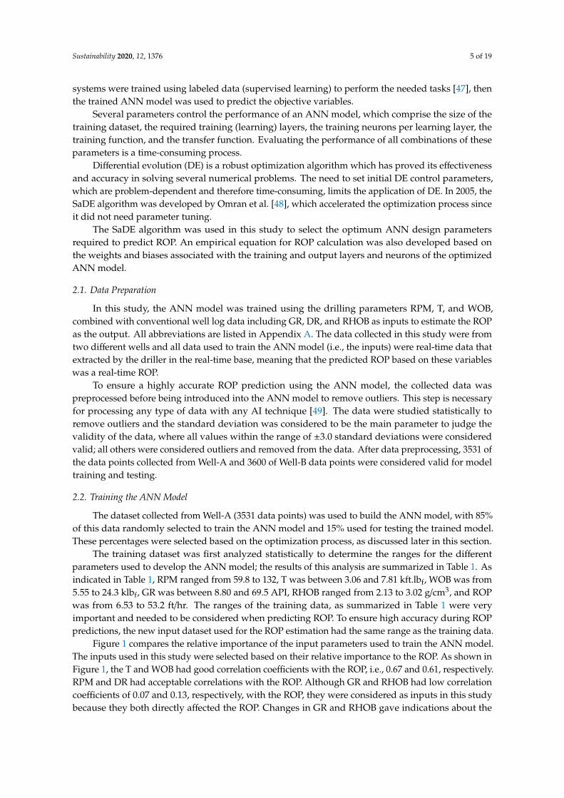
systems were trained using labeled data (supervised learning) to perform the needed tasks [47], thenthe trained ANN model was used to predict the objective variables.

Several parameters control the performance of an ANN model, which comprise the size of thetraining dataset, the required training (learning) layers, the training neurons per learning layer, thetraining function, and the transfer function. Evaluating the performance of all combinations of theseparameters is a time-consuming process.

Differential evolution (DE) is a robust optimization algorithm which has proved its effectivenessand accuracy in solving several numerical problems. The need to set initial DE control parameters,which are problem-dependent and therefore time-consuming, limits the application of DE. In 2005, theSaDE algorithm was developed by Omran et al. [48], which accelerated the optimization process sinceit did not need parameter tuning.

The SaDE algorithm was used in this study to select the optimum ANN design parametersrequired to predict ROP. An empirical equation for ROP calculation was also developed based onthe weights and biases associated with the training and output layers and neurons of the optimizedANN model.

2.1. Data Preparation

In this study, the ANN model was trained using the drilling parameters RPM, T, and WOB,combined with conventional well log data including GR, DR, and RHOB as inputs to estimate the ROPas the output. All abbreviations are listed in Appendix A. The data collected in this study were fromtwo different wells and all data used to train the ANN model (i.e., the inputs) were real-time data thatextracted by the driller in the real-time base, meaning that the predicted ROP based on these variableswas a real-time ROP.

To ensure a highly accurate ROP prediction using the ANN model, the collected data waspreprocessed before being introduced into the ANN model to remove outliers. This step is necessaryfor processing any type of data with any AI technique [49]. The data were studied statistically toremove outliers and the standard deviation was considered to be the main parameter to judge thevalidity of the data, where all values within the range of ±3.0 standard deviations were consideredvalid; all others were considered outliers and removed from the data. After data preprocessing, 3531 ofthe data points collected from Well-A and 3600 of Well-B data points were considered valid for modeltraining and testing.

2.2. Training the ANN Model

The dataset collected from Well-A (3531 data points) was used to build the ANN model, with 85%of this data randomly selected to train the ANN model and 15% used for testing the trained model.These percentages were selected based on the optimization process, as discussed later in this section.

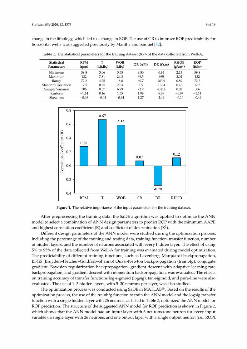
The training dataset was first analyzed statistically to determine the ranges for the differentparameters used to develop the ANN model; the results of this analysis are summarized in Table 1. Asindicated in Table 1, RPM ranged from 59.8 to 132, T was between 3.06 and 7.81 kft.lbf, WOB was from5.55 to 24.3 klbf, GR was between 8.80 and 69.5 API, RHOB ranged from 2.13 to 3.02 g/cm3, and ROPwas from 6.53 to 53.2 ft/hr. The ranges of the training data, as summarized in Table 1 were veryimportant and needed to be considered when predicting ROP. To ensure high accuracy during ROPpredictions, the new input dataset used for the ROP estimation had the same range as the training data.

Figure 1 compares the relative importance of the input parameters used to train the ANN model.The inputs used in this study were selected based on their relative importance to the ROP. As shown inFigure 1, the T and WOB had good correlation coefficients with the ROP, i.e., 0.67 and 0.61, respectively.RPM and DR had acceptable correlations with the ROP. Although GR and RHOB had low correlationcoefficients of 0.07 and 0.13, respectively, with the ROP, they were considered as inputs in this studybecause they both directly affected the ROP. Changes in GR and RHOB gave indications about the

Sustainability 2020, 12, 1376 6 of 19

change in the lithology, which led to a change in ROP. The use of GR to improve ROP predictability forhorizontal wells was suggested previously by Mantha and Samuel [42].

Table 1. The statistical parameters for the training dataset (85% of the data collected from Well-A).

StatisticalParameters

RPM(rpm)

T(kft.lbf)

WOB(klbf)

GR (API) DR (Ω.m) RHOB(g/cm3)

ROP(ft/hr)

Minimum 59.8 3.06 5.55 8.80 0.64 2.13 59.8Maximum 132 7.81 24.3 69.5 965 3.02 132

Range 72.2 4.75 18.8 60.7 963.9 0.89 72.2Standard Deviation 17.5 0.75 2.64 8.5 212.4 0.16 17.5

Sample Variance 306 0.57 6.99 72.9 45114 0.02 306Kurtosis −1.14 0.16 1.55 1.96 6.09 −0.87 −1.14

Skewness −0.49 −0.44 −0.94 1.27 2.49 −0.10 −0.49

Sustainability 2019, 9, x FOR PEER REVIEW 6 of 20

Sustainability 2019, 12, x; doi: FOR PEER REVIEW www.mdpi.com/journal/Sustainability

Table 1. The statistical parameters for the training dataset (85% of the data collected from Well-A).

Statistical Parameters RPM

(rpm)

T

(kft.lbf)

WOB

(klbf)

GR

(API) DR (Ω.m) RHOB (g/cm3)

ROP

(ft/hr)

Minimum 59.8 3.06 5.55 8.80 0.64 2.13 59.8

Maximum 132 7.81 24.3 69.5 965 3.02 132

Range 72.2 4.75 18.8 60.7 963.9 0.89 72.2

Standard Deviation 17.5 0.75 2.64 8.5 212.4 0.16 17.5

Sample Variance 306 0.57 6.99 72.9 45114 0.02 306

Kurtosis −1.14 0.16 1.55 1.96 6.09 −0.87 −1.14

Skewness −0.49 −0.44 −0.94 1.27 2.49 −0.10 −0.49

Figure 1 compares the relative importance of the input parameters used to train the ANN model.

The inputs used in this study were selected based on their relative importance to the ROP. As shown

in Figure 1, the T and WOB had good correlation coefficients with the ROP, i.e., 0.67 and 0.61,

respectively. RPM and DR had acceptable correlations with the ROP. Although GR and RHOB had

low correlation coefficients of 0.07 and 0.13, respectively, with the ROP, they were considered as

inputs in this study because they both directly affected the ROP. Changes in GR and RHOB gave

indications about the change in the lithology, which led to a change in ROP. The use of GR to improve

ROP predictability for horizontal wells was suggested previously by Mantha and Samuel [42].

Figure 1. The relative importance of the input parameters for the training dataset.

After preprocessing the training data, the SaDE algorithm was applied to optimize the ANN

model to select a combination of ANN design parameters to predict ROP with the minimum AAPE

and highest correlation coefficient (R) and coefficient of determination (R2).

Different design parameters of the ANN model were studied during the optimization process,

including the percentage of the training and testing data, training function, transfer function, number

of hidden layers, and the number of neurons associated with every hidden layer. The effect of using

5% to 95% of the data collected from Well-A for training was evaluated during model optimization.

The predictability of different training functions, such as Levenberg–Marquardt backpropagation,

BFGS (Broyden–Fletcher–Goldfarb–Shanno) Quasi-Newton backpropagation (trainbfg), conjugate

gradient, Bayesian regularization backpropagation, gradient descent with adaptive learning rate

backpropagation, and gradient descent with momentum backpropagation, was evaluated. The effects

Figure 1. The relative importance of the input parameters for the training dataset.

After preprocessing the training data, the SaDE algorithm was applied to optimize the ANNmodel to select a combination of ANN design parameters to predict ROP with the minimum AAPEand highest correlation coefficient (R) and coefficient of determination (R2).

Different design parameters of the ANN model were studied during the optimization process,including the percentage of the training and testing data, training function, transfer function, numberof hidden layers, and the number of neurons associated with every hidden layer. The effect of using5% to 95% of the data collected from Well-A for training was evaluated during model optimization.The predictability of different training functions, such as Levenberg–Marquardt backpropagation,BFGS (Broyden–Fletcher–Goldfarb–Shanno) Quasi-Newton backpropagation (trainbfg), conjugategradient, Bayesian regularization backpropagation, gradient descent with adaptive learning ratebackpropagation, and gradient descent with momentum backpropagation, was evaluated. The effectson training accuracy of transfer functions log-sigmoid (logsig), tan-sigmoid, and pure-line were alsoevaluated. The use of 1–3 hidden layers, with 5–30 neurons per layer, was also studied.

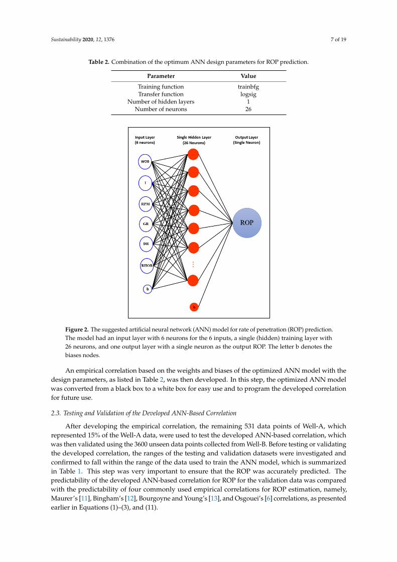
The optimization process was conducted using SaDE in MATLAB®. Based on the results of theoptimization process, the use of the trainbfg function to train the ANN model and the logsig transferfunction with a single hidden layer with 26 neurons, as listed in Table 2, optimized the ANN model forROP prediction. The structure of the suggested ANN model for ROP prediction is shown in Figure 2,which shows that the ANN model had an input layer with 6 neurons (one neuron for every inputvariable), a single layer with 26 neurons, and one output layer with a single output neuron (i.e., ROP).

Sustainability 2020, 12, 1376 7 of 19

Table 2. Combination of the optimum ANN design parameters for ROP prediction.

Parameter Value

Training function trainbfgTransfer function logsig

Number of hidden layers 1Number of neurons 26

Sustainability 2019, 9, x FOR PEER REVIEW 7 of 20

Sustainability 2019, 12, x; doi: FOR PEER REVIEW www.mdpi.com/journal/Sustainability

on training accuracy of transfer functions log-sigmoid (logsig), tan-sigmoid, and pure-line were also

evaluated. The use of 1–3 hidden layers, with 5–30 neurons per layer, was also studied.

The optimization process was conducted using SaDE in MATLAB® . Based on the results of the

optimization process, the use of the trainbfg function to train the ANN model and the logsig transfer

function with a single hidden layer with 26 neurons, as listed in Table 2, optimized the ANN model

for ROP prediction. The structure of the suggested ANN model for ROP prediction is shown in Figure

2, which shows that the ANN model had an input layer with 6 neurons (one neuron for every input

variable), a single layer with 26 neurons, and one output layer with a single output neuron (i.e., ROP).

Table 2. Combination of the optimum ANN design parameters for ROP prediction.

Parameter Value

Training function trainbfg

Transfer function logsig

Number of hidden layers 1

Number of neurons 26

Figure 2. The suggested artificial neural network (ANN) model for rate of penetration (ROP)

prediction. The model had an input layer with 6 neurons for the 6 inputs, a single (hidden) training

layer with 26 neurons, and one output layer with a single neuron as the output ROP. The letter b

denotes the biases nodes.

An empirical correlation based on the weights and biases of the optimized ANN model with the

design parameters, as listed in Table 2, was then developed. In this step, the optimized ANN model

was converted from a black box to a white box for easy use and to program the developed correlation

for future use.

2.3. Testing and Validation of the Developed ANN-Based Correlation

Figure 2. The suggested artificial neural network (ANN) model for rate of penetration (ROP) prediction.The model had an input layer with 6 neurons for the 6 inputs, a single (hidden) training layer with26 neurons, and one output layer with a single neuron as the output ROP. The letter b denotes thebiases nodes.

An empirical correlation based on the weights and biases of the optimized ANN model with thedesign parameters, as listed in Table 2, was then developed. In this step, the optimized ANN modelwas converted from a black box to a white box for easy use and to program the developed correlationfor future use.

2.3. Testing and Validation of the Developed ANN-Based Correlation

After developing the empirical correlation, the remaining 531 data points of Well-A, whichrepresented 15% of the Well-A data, were used to test the developed ANN-based correlation, whichwas then validated using the 3600 unseen data points collected from Well-B. Before testing or validatingthe developed correlation, the ranges of the testing and validation datasets were investigated andconfirmed to fall within the range of the data used to train the ANN model, which is summarizedin Table 1. This step was very important to ensure that the ROP was accurately predicted. Thepredictability of the developed ANN-based correlation for ROP for the validation data was comparedwith the predictability of four commonly used empirical correlations for ROP estimation, namely,Maurer’s [11], Bingham’s [12], Bourgoyne and Young’s [13], and Osgouei’s [6] correlations, as presentedearlier in Equations (1)–(3), and (11).

Sustainability 2020, 12, 1376 8 of 19

2.4. Evaluation Criteria

Four metrics were considered in this study to evaluate the predictive power of the developedANN model and ANN-based empirical correlation for ROP estimation, namely, AAPE, R2,R, and a visualization check of the match between the actual and the predicted ROP. Thesemetrics were considered sufficient to evaluate the predictability of the ROP for training, testing,and validation datasets.

3. Results and Discussion

3.1. Training the ANN model

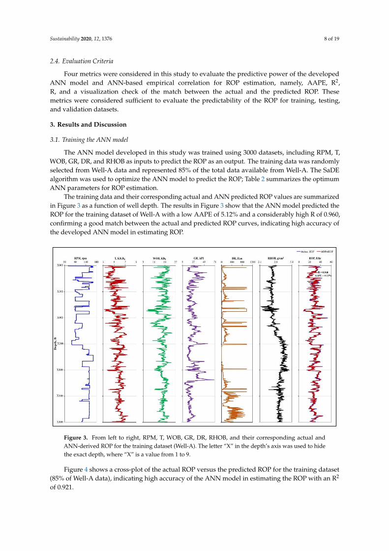
The ANN model developed in this study was trained using 3000 datasets, including RPM, T,WOB, GR, DR, and RHOB as inputs to predict the ROP as an output. The training data was randomlyselected from Well-A data and represented 85% of the total data available from Well-A. The SaDEalgorithm was used to optimize the ANN model to predict the ROP; Table 2 summarizes the optimumANN parameters for ROP estimation.

The training data and their corresponding actual and ANN predicted ROP values are summarizedin Figure 3 as a function of well depth. The results in Figure 3 show that the ANN model predicted theROP for the training dataset of Well-A with a low AAPE of 5.12% and a considerably high R of 0.960,confirming a good match between the actual and predicted ROP curves, indicating high accuracy ofthe developed ANN model in estimating ROP.Sustainability 2019, 9, x FOR PEER REVIEW 9 of 20

Sustainability 2019, 12, x; doi: FOR PEER REVIEW www.mdpi.com/journal/Sustainability

Figure 3. From left to right, RPM, T, WOB, GR, DR, RHOB, and their corresponding actual and ANN-

derived ROP for the training dataset (Well-A). The letter “X” in the depth’s axis was used to hide the

exact depth, where “X” is a value from 1 to 9.

Figure 4 shows a cross-plot of the actual ROP versus the predicted ROP for the training dataset

(85% of Well-A data), indicating high accuracy of the ANN model in estimating the ROP with an R2

of 0.921.

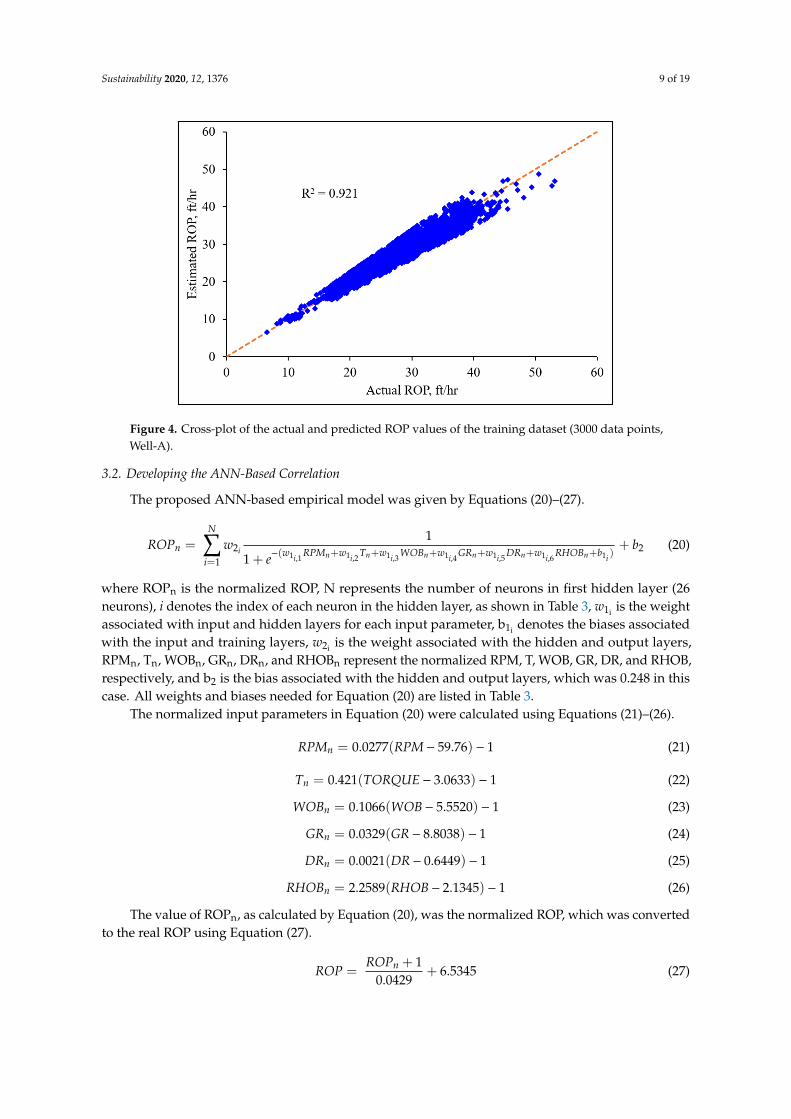
Figure 4. Cross-plot of the actual and predicted ROP values of the training dataset (3000 data points,

Well-A).

3.2. Developing the ANN-Based Correlation

The proposed ANN-based empirical model was given by Equations (20)–(27).

Figure 3. From left to right, RPM, T, WOB, GR, DR, RHOB, and their corresponding actual andANN-derived ROP for the training dataset (Well-A). The letter “X” in the depth’s axis was used to hidethe exact depth, where “X” is a value from 1 to 9.

Figure 4 shows a cross-plot of the actual ROP versus the predicted ROP for the training dataset(85% of Well-A data), indicating high accuracy of the ANN model in estimating the ROP with an R2

of 0.921.

Sustainability 2020, 12, 1376 9 of 19

Sustainability 2019, 9, x FOR PEER REVIEW 9 of 20

Sustainability 2019, 12, x; doi: FOR PEER REVIEW www.mdpi.com/journal/Sustainability

Figure 3. From left to right, RPM, T, WOB, GR, DR, RHOB, and their corresponding actual and ANN-

derived ROP for the training dataset (Well-A). The letter “X” in the depth’s axis was used to hide the

exact depth, where “X” is a value from 1 to 9.

Figure 4 shows a cross-plot of the actual ROP versus the predicted ROP for the training dataset

(85% of Well-A data), indicating high accuracy of the ANN model in estimating the ROP with an R2

of 0.921.

Figure 4. Cross-plot of the actual and predicted ROP values of the training dataset (3000 data points,

Well-A).

3.2. Developing the ANN-Based Correlation

The proposed ANN-based empirical model was given by Equations (20)–(27).

Figure 4. Cross-plot of the actual and predicted ROP values of the training dataset (3000 data points,Well-A).

3.2. Developing the ANN-Based Correlation

The proposed ANN-based empirical model was given by Equations (20)–(27).

ROPn =N∑

i=1

w2i

1

1 + e−(w1i,1 RPMn+w1i,2 Tn+w1i,3 WOBn+w1i,4 GRn+w1i,5 DRn+w1i,6 RHOBn+b1i )+ b2 (20)

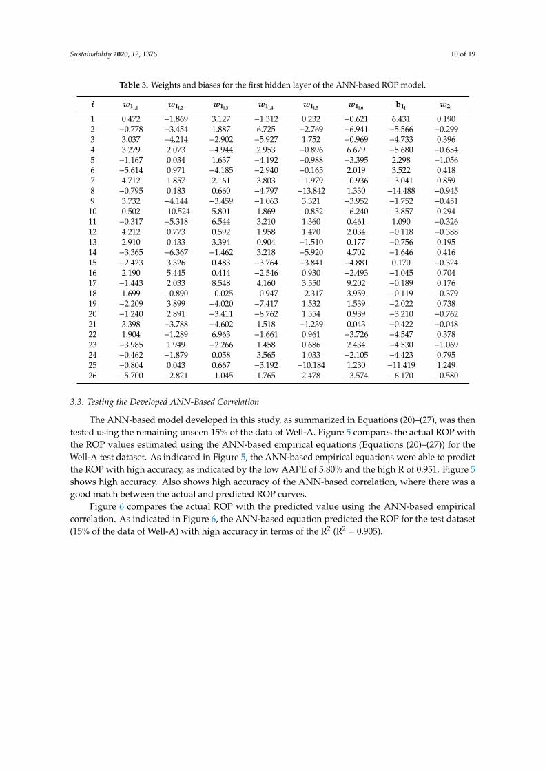
where ROPn is the normalized ROP, N represents the number of neurons in first hidden layer (26neurons), i denotes the index of each neuron in the hidden layer, as shown in Table 3, w1i is the weightassociated with input and hidden layers for each input parameter, b1i denotes the biases associatedwith the input and training layers, w2i is the weight associated with the hidden and output layers,RPMn, Tn, WOBn, GRn, DRn, and RHOBn represent the normalized RPM, T, WOB, GR, DR, and RHOB,respectively, and b2 is the bias associated with the hidden and output layers, which was 0.248 in thiscase. All weights and biases needed for Equation (20) are listed in Table 3.

The normalized input parameters in Equation (20) were calculated using Equations (21)–(26).

RPMn = 0.0277(RPM− 59.76) − 1 (21)

Tn = 0.421(TORQUE− 3.0633) − 1 (22)

WOBn = 0.1066(WOB− 5.5520) − 1 (23)

GRn = 0.0329(GR− 8.8038) − 1 (24)

DRn = 0.0021(DR− 0.6449) − 1 (25)

RHOBn = 2.2589(RHOB− 2.1345) − 1 (26)

The value of ROPn, as calculated by Equation (20), was the normalized ROP, which was convertedto the real ROP using Equation (27).

ROP =ROPn + 1

0.0429+ 6.5345 (27)

Sustainability 2020, 12, 1376 10 of 19

Table 3. Weights and biases for the first hidden layer of the ANN-based ROP model.

i w1i,1 w1i,2 w1i,3 w1i,4 w1i,5 w1i,6 b1i w2i

1 0.472 −1.869 3.127 −1.312 0.232 −0.621 6.431 0.1902 −0.778 −3.454 1.887 6.725 −2.769 −6.941 −5.566 −0.2993 3.037 −4.214 −2.902 −5.927 1.752 −0.969 −4.733 0.3964 3.279 2.073 −4.944 2.953 −0.896 6.679 −5.680 −0.6545 −1.167 0.034 1.637 −4.192 −0.988 −3.395 2.298 −1.0566 −5.614 0.971 −4.185 −2.940 −0.165 2.019 3.522 0.4187 4.712 1.857 2.161 3.803 −1.979 −0.936 −3.041 0.8598 −0.795 0.183 0.660 −4.797 −13.842 1.330 −14.488 −0.9459 3.732 −4.144 −3.459 −1.063 3.321 −3.952 −1.752 −0.451

10 0.502 −10.524 5.801 1.869 −0.852 −6.240 −3.857 0.29411 −0.317 −5.318 6.544 3.210 1.360 0.461 1.090 −0.32612 4.212 0.773 0.592 1.958 1.470 2.034 −0.118 −0.38813 2.910 0.433 3.394 0.904 −1.510 0.177 −0.756 0.19514 −3.365 −6.367 −1.462 3.218 −5.920 4.702 −1.646 0.41615 −2.423 3.326 0.483 −3.764 −3.841 −4.881 0.170 −0.32416 2.190 5.445 0.414 −2.546 0.930 −2.493 −1.045 0.70417 −1.443 2.033 8.548 4.160 3.550 9.202 −0.189 0.17618 1.699 −0.890 −0.025 −0.947 −2.317 3.959 −0.119 −0.37919 −2.209 3.899 −4.020 −7.417 1.532 1.539 −2.022 0.73820 −1.240 2.891 −3.411 −8.762 1.554 0.939 −3.210 −0.76221 3.398 −3.788 −4.602 1.518 −1.239 0.043 −0.422 −0.04822 1.904 −1.289 6.963 −1.661 0.961 −3.726 −4.547 0.37823 −3.985 1.949 −2.266 1.458 0.686 2.434 −4.530 −1.06924 −0.462 −1.879 0.058 3.565 1.033 −2.105 −4.423 0.79525 −0.804 0.043 0.667 −3.192 −10.184 1.230 −11.419 1.24926 −5.700 −2.821 −1.045 1.765 2.478 −3.574 −6.170 −0.580

3.3. Testing the Developed ANN-Based Correlation

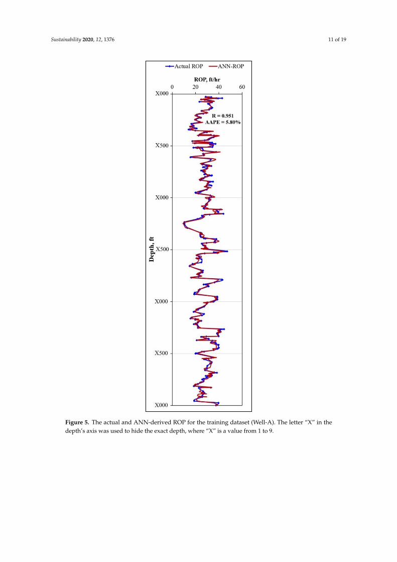
The ANN-based model developed in this study, as summarized in Equations (20)–(27), was thentested using the remaining unseen 15% of the data of Well-A. Figure 5 compares the actual ROP withthe ROP values estimated using the ANN-based empirical equations (Equations (20)–(27)) for theWell-A test dataset. As indicated in Figure 5, the ANN-based empirical equations were able to predictthe ROP with high accuracy, as indicated by the low AAPE of 5.80% and the high R of 0.951. Figure 5shows high accuracy. Also shows high accuracy of the ANN-based correlation, where there was agood match between the actual and predicted ROP curves.

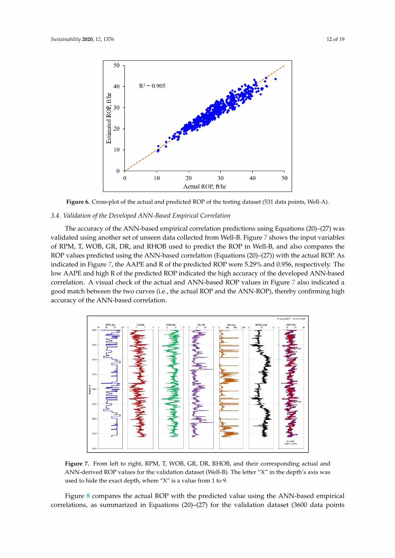
Figure 6 compares the actual ROP with the predicted value using the ANN-based empiricalcorrelation. As indicated in Figure 6, the ANN-based equation predicted the ROP for the test dataset(15% of the data of Well-A) with high accuracy in terms of the R2 (R2 = 0.905).

Sustainability 2020, 12, 1376 11 of 19Sustainability 2019, 9, x FOR PEER REVIEW 12 of 20

Sustainability 2019, 12, x; doi: FOR PEER REVIEW www.mdpi.com/journal/Sustainability

Figure 5. The actual and ANN-derived ROP for the training dataset (Well-A). The letter “X” in the

depth’s axis was used to hide the exact depth, where “X” is a value from 1 to 9.

Figure 6 compares the actual ROP with the predicted value using the ANN-based empirical

correlation. As indicated in Figure 6, the ANN-based equation predicted the ROP for the test dataset

(15% of the data of Well-A) with high accuracy in terms of the R2 (R2 = 0.905).

Figure 5. The actual and ANN-derived ROP for the training dataset (Well-A). The letter “X” in thedepth’s axis was used to hide the exact depth, where “X” is a value from 1 to 9.

Sustainability 2020, 12, 1376 12 of 19

Sustainability 2019, 9, x FOR PEER REVIEW 13 of 20

Sustainability 2019, 12, x; doi: FOR PEER REVIEW www.mdpi.com/journal/Sustainability

Figure 6. Cross-plot of the actual and predicted ROP of the testing dataset (531 data points, Well-A).

3.4. Validation of the Developed ANN-Based Empirical Correlation

The accuracy of the ANN-based empirical correlation predictions using Equations (20)–(27) was

validated using another set of unseen data collected from Well-B. Figure 7 shows the input variables

of RPM, T, WOB, GR, DR, and RHOB used to predict the ROP in Well-B, and also compares the ROP

values predicted using the ANN-based correlation (Equations (20)–(27)) with the actual ROP. As

indicated in Figure 7, the AAPE and R of the predicted ROP were 5.29% and 0.956, respectively. The

low AAPE and high R of the predicted ROP indicated the high accuracy of the developed ANN-based

correlation. A visual check of the actual and ANN-based ROP values in Figure 7 also indicated a good

match between the two curves (i.e., the actual ROP and the ANN-ROP), thereby confirming high

accuracy of the ANN-based correlation.

Figure 6. Cross-plot of the actual and predicted ROP of the testing dataset (531 data points, Well-A).

3.4. Validation of the Developed ANN-Based Empirical Correlation

The accuracy of the ANN-based empirical correlation predictions using Equations (20)–(27) wasvalidated using another set of unseen data collected from Well-B. Figure 7 shows the input variablesof RPM, T, WOB, GR, DR, and RHOB used to predict the ROP in Well-B, and also compares theROP values predicted using the ANN-based correlation (Equations (20)–(27)) with the actual ROP. Asindicated in Figure 7, the AAPE and R of the predicted ROP were 5.29% and 0.956, respectively. Thelow AAPE and high R of the predicted ROP indicated the high accuracy of the developed ANN-basedcorrelation. A visual check of the actual and ANN-based ROP values in Figure 7 also indicated agood match between the two curves (i.e., the actual ROP and the ANN-ROP), thereby confirming highaccuracy of the ANN-based correlation.Sustainability 2019, 9, x FOR PEER REVIEW 14 of 20

Sustainability 2019, 12, x; doi: FOR PEER REVIEW www.mdpi.com/journal/Sustainability

Figure 7. From left to right, RPM, T, WOB, GR, DR, RHOB, and their corresponding actual and ANN-

derived ROP values for the validation dataset (Well-B). The letter “X” in the depth’s axis was used to

hide the exact depth, where “X” is a value from 1 to 9.

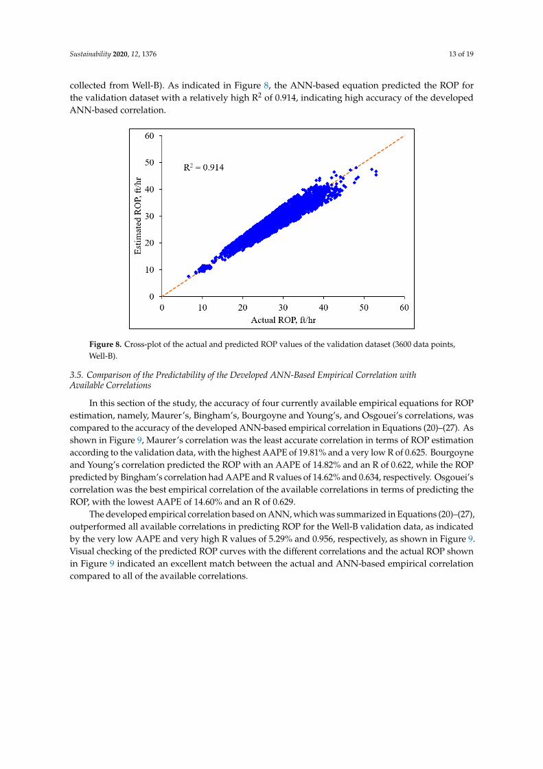
Figure 8 compares the actual ROP with the predicted value using the ANN-based empirical

correlations, as summarized in Equations (20)–(27) for the validation dataset (3600 data points

collected from Well-B). As indicated in Figure 8, the ANN-based equation predicted the ROP for the

validation dataset with a relatively high R2 of 0.914, indicating high accuracy of the developed ANN-

based correlation.

Figure 8. Cross-plot of the actual and predicted ROP values of the validation dataset (3600 data points,

Well-B).

3.5. Comparison of the Predictability of the Developed ANN-Based Empirical Correlation with Available

Correlations

In this section of the study, the accuracy of four currently available empirical equations for ROP

estimation, namely, Maurer’s, Bingham’s, Bourgoyne and Young’s, and Osgouei’s correlations, was

Figure 7. From left to right, RPM, T, WOB, GR, DR, RHOB, and their corresponding actual andANN-derived ROP values for the validation dataset (Well-B). The letter “X” in the depth’s axis wasused to hide the exact depth, where “X” is a value from 1 to 9.

Figure 8 compares the actual ROP with the predicted value using the ANN-based empiricalcorrelations, as summarized in Equations (20)–(27) for the validation dataset (3600 data points

Sustainability 2020, 12, 1376 13 of 19

collected from Well-B). As indicated in Figure 8, the ANN-based equation predicted the ROP forthe validation dataset with a relatively high R2 of 0.914, indicating high accuracy of the developedANN-based correlation.

Sustainability 2019, 9, x FOR PEER REVIEW 14 of 20

Sustainability 2019, 12, x; doi: FOR PEER REVIEW www.mdpi.com/journal/Sustainability

Figure 7. From left to right, RPM, T, WOB, GR, DR, RHOB, and their corresponding actual and ANN-

derived ROP values for the validation dataset (Well-B). The letter “X” in the depth’s axis was used to

hide the exact depth, where “X” is a value from 1 to 9.

Figure 8 compares the actual ROP with the predicted value using the ANN-based empirical

correlations, as summarized in Equations (20)–(27) for the validation dataset (3600 data points

collected from Well-B). As indicated in Figure 8, the ANN-based equation predicted the ROP for the

validation dataset with a relatively high R2 of 0.914, indicating high accuracy of the developed ANN-

based correlation.

Figure 8. Cross-plot of the actual and predicted ROP values of the validation dataset (3600 data points,

Well-B).

3.5. Comparison of the Predictability of the Developed ANN-Based Empirical Correlation with Available

Correlations

In this section of the study, the accuracy of four currently available empirical equations for ROP

estimation, namely, Maurer’s, Bingham’s, Bourgoyne and Young’s, and Osgouei’s correlations, was

Figure 8. Cross-plot of the actual and predicted ROP values of the validation dataset (3600 data points,Well-B).

3.5. Comparison of the Predictability of the Developed ANN-Based Empirical Correlation withAvailable Correlations

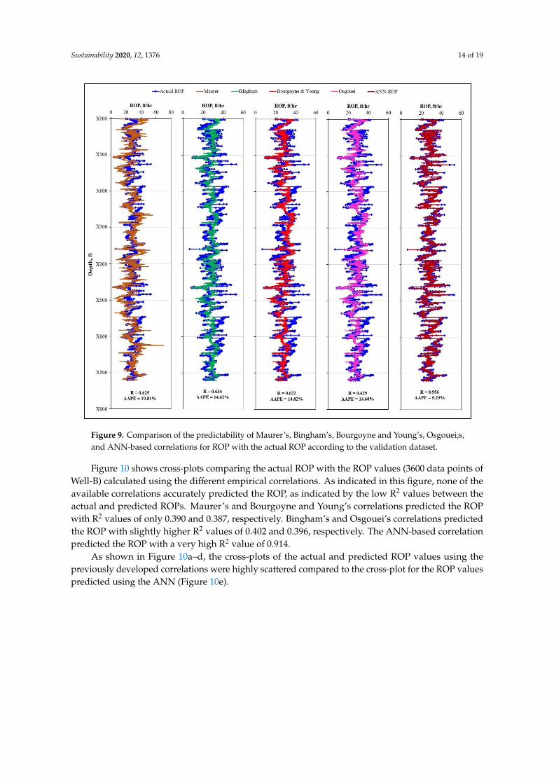
In this section of the study, the accuracy of four currently available empirical equations for ROPestimation, namely, Maurer’s, Bingham’s, Bourgoyne and Young’s, and Osgouei’s correlations, wascompared to the accuracy of the developed ANN-based empirical correlation in Equations (20)–(27). Asshown in Figure 9, Maurer’s correlation was the least accurate correlation in terms of ROP estimationaccording to the validation data, with the highest AAPE of 19.81% and a very low R of 0.625. Bourgoyneand Young’s correlation predicted the ROP with an AAPE of 14.82% and an R of 0.622, while the ROPpredicted by Bingham’s correlation had AAPE and R values of 14.62% and 0.634, respectively. Osgouei’scorrelation was the best empirical correlation of the available correlations in terms of predicting theROP, with the lowest AAPE of 14.60% and an R of 0.629.

The developed empirical correlation based on ANN, which was summarized in Equations (20)–(27),outperformed all available correlations in predicting ROP for the Well-B validation data, as indicatedby the very low AAPE and very high R values of 5.29% and 0.956, respectively, as shown in Figure 9.Visual checking of the predicted ROP curves with the different correlations and the actual ROP shownin Figure 9 indicated an excellent match between the actual and ANN-based empirical correlationcompared to all of the available correlations.

Sustainability 2020, 12, 1376 14 of 19

Sustainability 2019, 9, x FOR PEER REVIEW 15 of 20

Sustainability 2019, 12, x; doi: FOR PEER REVIEW www.mdpi.com/journal/Sustainability

compared to the accuracy of the developed ANN-based empirical correlation in Equations (20)–(27).

As shown in Figure 9, Maurer’s correlation was the least accurate correlation in terms of ROP

estimation according to the validation data, with the highest AAPE of 19.81% and a very low R of

0.625. Bourgoyne and Young’s correlation predicted the ROP with an AAPE of 14.82% and an R of

0.622, while the ROP predicted by Bingham’s correlation had AAPE and R values of 14.62% and 0.634,

respectively. Osgouei’s correlation was the best empirical correlation of the available correlations in

terms of predicting the ROP, with the lowest AAPE of 14.60% and an R of 0.629.

Figure 9. Comparison of the predictability of Maurer’s, Bingham’s, Bourgoyne and Young’s,

Osgouei;s, and ANN-based correlations for ROP with the actual ROP according to the validation

dataset.

The developed empirical correlation based on ANN, which was summarized in Equations (20)–

(27), outperformed all available correlations in predicting ROP for the Well-B validation data, as

indicated by the very low AAPE and very high R values of 5.29% and 0.956, respectively, as shown

in Figure 9. Visual checking of the predicted ROP curves with the different correlations and the actual

ROP shown in Figure 9 indicated an excellent match between the actual and ANN-based empirical

correlation compared to all of the available correlations.

Figure 10 shows cross-plots comparing the actual ROP with the ROP values (3600 data points of

Well-B) calculated using the different empirical correlations. As indicated in this figure, none of the

available correlations accurately predicted the ROP, as indicated by the low R2 values between the

actual and predicted ROPs. Maurer’s and Bourgoyne and Young’s correlations predicted the ROP

with R2 values of only 0.390 and 0.387, respectively. Bingham’s and Osgouei’s correlations predicted

Figure 9. Comparison of the predictability of Maurer’s, Bingham’s, Bourgoyne and Young’s, Osgouei;s,and ANN-based correlations for ROP with the actual ROP according to the validation dataset.

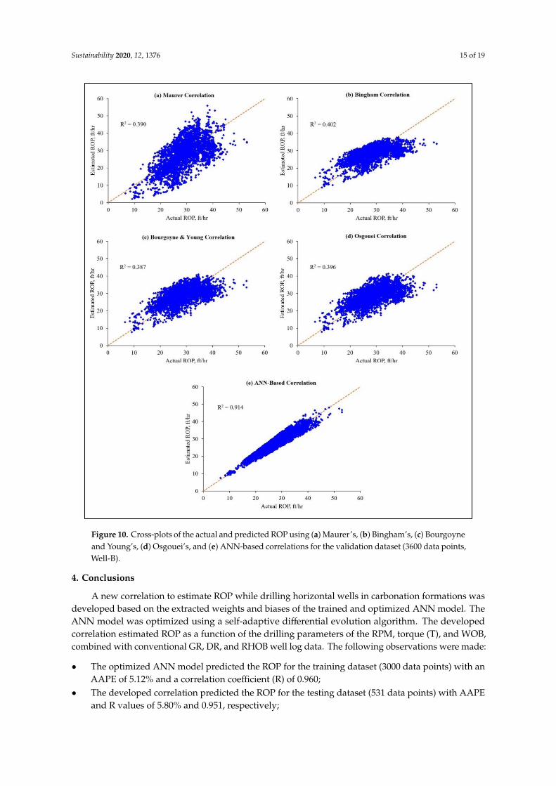
Figure 10 shows cross-plots comparing the actual ROP with the ROP values (3600 data points ofWell-B) calculated using the different empirical correlations. As indicated in this figure, none of theavailable correlations accurately predicted the ROP, as indicated by the low R2 values between theactual and predicted ROPs. Maurer’s and Bourgoyne and Young’s correlations predicted the ROPwith R2 values of only 0.390 and 0.387, respectively. Bingham’s and Osgouei’s correlations predictedthe ROP with slightly higher R2 values of 0.402 and 0.396, respectively. The ANN-based correlationpredicted the ROP with a very high R2 value of 0.914.

As shown in Figure 10a–d, the cross-plots of the actual and predicted ROP values using thepreviously developed correlations were highly scattered compared to the cross-plot for the ROP valuespredicted using the ANN (Figure 10e).

Sustainability 2020, 12, 1376 15 of 19

Sustainability 2019, 9, x FOR PEER REVIEW 16 of 20

Sustainability 2019, 12, x; doi: FOR PEER REVIEW www.mdpi.com/journal/Sustainability

the ROP with slightly higher R2 values of 0.402 and 0.396, respectively. The ANN-based correlation

predicted the ROP with a very high R2 value of 0.914.

As shown in Figure 10a–d, the cross-plots of the actual and predicted ROP values using the

previously developed correlations were highly scattered compared to the cross-plot for the ROP

values predicted using the ANN (Figure 10e).

Figure 10. Cross-plots of the actual and predicted ROP using (a) Maurer’s, (b) Bingham’s, (c)

Bourgoyne and Young’s, (d) Osgouei’s, and (e) ANN-based correlations for the validation dataset

(3600 data points, Well-B).

4. Conclusions

A new correlation to estimate ROP while drilling horizontal wells in carbonation formations was

developed based on the extracted weights and biases of the trained and optimized ANN model. The

ANN model was optimized using a self-adaptive differential evolution algorithm. The developed

correlation estimated ROP as a function of the drilling parameters of the RPM, torque (T), and WOB,

combined with conventional GR, DR, and RHOB well log data. The following observations were

made:

Figure 10. Cross-plots of the actual and predicted ROP using (a) Maurer’s, (b) Bingham’s, (c) Bourgoyneand Young’s, (d) Osgouei’s, and (e) ANN-based correlations for the validation dataset (3600 data points,Well-B).

4. Conclusions

A new correlation to estimate ROP while drilling horizontal wells in carbonation formations wasdeveloped based on the extracted weights and biases of the trained and optimized ANN model. TheANN model was optimized using a self-adaptive differential evolution algorithm. The developedcorrelation estimated ROP as a function of the drilling parameters of the RPM, torque (T), and WOB,combined with conventional GR, DR, and RHOB well log data. The following observations were made:

• The optimized ANN model predicted the ROP for the training dataset (3000 data points) with anAAPE of 5.12% and a correlation coefficient (R) of 0.960;

• The developed correlation predicted the ROP for the testing dataset (531 data points) with AAPEand R values of 5.80% and 0.951, respectively;

Sustainability 2020, 12, 1376 16 of 19

• The developed ROP correlation outperformed a recently developed empirical correlation forestimating ROP in directional wells (the Osgouei model), which predicted the ROP for thevalidation data with a high AAPE and a low R of 14.60% and 0.629, respectively;

• The developed correlation predicted ROP for the validation dataset of Well-B (3600 data points)with an AAPE of only 5.26% and a high R of 0.956.

Author Contributions: Conceptualization, S.E; data preparation, S.E., A.A.-A., and A.A.M.; model development,A.A.-A., and T.M.; results analysis, A.A.M.; writing—original draft preparation, A.A.M.; writing—review andediting, S.E., M.A., D.A.-S., and A.A.-Y.; supervision, S.E. All authors read and agreed to the published version ofthe manuscript.

Funding: This research was funded by [Saudi Aramco] grant number [CIPR2321].

Acknowledgments: Authors would like to acknowledge the College of Petroleum and Geoscience at King FahdUniversity of Petroleum and Minerals and Saudi Aramco for the support and permission to publish this work. Wealso acknowledge Saudi Aramco for funding this research under project number CIPR2321.

Conflicts of Interest: The authors declare no conflict of interest.

Appendix A

AAPE Average Absolute Percentage Error

AI Artificial IntelligenceANN Artificial Neural Network

DE Differential EvolutionDR Deep Resistivity

ECD Equivalent Circulation DensityGPM Pumping RateGR Gamma Ray

logsig log-sigmoidMW Mud DensityPV Plastic ViscosityR Correlation CoefficientR2 Coefficient of Determination

RHOB Formation Bulk DensityROP Rate of PenetrationRPM Rotation SpeedSaDE Self-Adaptive Differential EvolutionSPP Standpipe PressureSVM Support Vector Machine

T Torquetrainbfg BFGS Quasi-Newton Backpropagation

WOB Weight-on-Bit

References

1. Lyons, W.C.; Plisga, G.J. Standard Handbook of Petroleum and Natural Gas. Engineering, 2nd ed.; Gulf ProfessionalPublishing: Woburn, MA, USA, 2004; ISBN 10: 0750677856.

2. Barbosa, L.F.F.M.; Nascimento, A.; Mathias, M.H.; de Carvalho, J.A., Jr. Machine learning methods appliedto drilling rate of penetration prediction and optimization-A review. J. Pet. Sci. Eng. 2019, 183, 106332.[CrossRef]

3. Hossain, M.E.; Al-Majed, A.A. Fundamentals of Sustainable Drilling Engineering, 1st ed.; Wiley-Scrivener:Austin, TX, USA, 2015; ISBN 10: 0470878177.

4. Eren, T.; Ozbayoglu, M.E. Real time optimization of drilling parameters during drilling operations.In Proceedings of the SPE Oil and Gas India Conference and Exhibition, Mumbai, India, 20–22 January 2010.SPE-129126-MS. [CrossRef]

Sustainability 2020, 12, 1376 17 of 19

5. Payette, G.S.; Spivey, B.J.; Wang, L.; Bailey, J.R.; Sanderson, D.; Kong, R.; Pawson, M.; Eddy, A. Real-timewell-site based surveillance and optimization platform for drilling: Technology, basic workflows and fieldresults. In Proceedings of the SPE/IADC Drilling Conference and Exhibition, The Hague, The Netherlands,14–16 March 2017. SPE-184615-MS. [CrossRef]

6. Osgouei, R.E. Rate of Penetration Estimation Model for Directional and Horizontal Wells. Master’s Thesis,Middle East Technical University, Ankara, Turkey, 2007.

7. Soares, C.; Daigle, H.; Gray, K. Evaluation of PDC bit ROP models and the effect of rock strength on modelcoefficients. J. Nat. Gas Sci. Eng. 2016, 34, 1225–1236. [CrossRef]

8. Soares, C.; Gray, K. Real-time predictive capabilities of analytical and machine learning rate of penetration(ROP) models. J. Pet. Sci. Eng. 2019, 172, 934–959. [CrossRef]

9. Mitchell, R.F.; Miska, S.Z. Fundamentals of Drilling Engineering; Society of Petroleum Engineers: Richardson,TX, USA, 2011; ASIN: B01L0O8WJA.

10. Hegde, C.; Daigle, H.; Millwater, H.; Gray, K. Analysis of Rate of Penetration (ROP) Prediction in DrillingUsing Physics-Based and Data-Driven Models. J. Pet. Sci. Eng. 2017, 159, 295–306. [CrossRef]

11. Maurer, W. The “perfect-cleaning” theory of rotary drilling. J. Pet. Technol. 1962, 14, 1270–1274. [CrossRef]12. Bingham, M.G. A New Approach to Interpreting Rock Drillability; Petroleum Publishing Co.: Tulsa, OK, USA,

1965.13. Bourgoyne, A.; Young, F.S. A multiple regression approach to optimal drilling and abnormal pressure

detection. Soc. Pet. Eng. J. 1974, 14, 371–384. [CrossRef]14. Mahmoud, A.A.; Elzenary, M.; Elkatatny, S. New Hybrid Hole Cleaning Model for Vertical and Deviated

Wells. J. Energy Resour. Technol. 2020, 142, 034501. [CrossRef]15. Hag Elsafi, S. Artificial Neural Networks (ANNs) for flood forecasting at Dongola Station in the River Nile,

Sudan. Alex. Eng. J. 2014, 53, 655–662. [CrossRef]16. Babikir, H.A.; Abd Elaziz, M.; Elsheikh, A.H.; Showaib, E.A.; Elhadary, M.; Wu, D.; Liu, Y. Noise prediction

of axial piston pump based on different valve materials using a modified artificial neural network model.Alex. Eng. J. 2019, 58, 1077–1087. [CrossRef]

17. Nayak, S.C.; Misra, B.B.; Behera, H.S. Artificial chemical reaction optimization based neural net for virtualdata position exploration for efficient financial time series forecasting. Ain Shams Eng. J. 2018, 9, 1731–1744.[CrossRef]

18. Jana, G.C.; Swetapadma, A.; Pattnaik, P.K. Enhancing the performance of motor imagery classification todesign a robust brain computer interface using feed forward back-propagation neural network. Ain ShamsEng. J. 2018, 9, 2871–2878. [CrossRef]

19. Abdelwahed, M.F.; Mohamed, A.E.; Saleh, M.A. Solving the motion planning problem using learningexperience through case-based reasoning and machine learning algorithms. Ain Shams Eng. J. 2019, in press.[CrossRef]

20. Abd Elrehim, M.Z.; Eid, M.A.; Sayed, M.G. Structural optimization of concrete arch bridges using GeneticAlgorithms. Ain Shams Eng. J. 2019, 10, 507–516. [CrossRef]

21. Arehart, R.A. Drill-bit diagnosis with neural networks. SPE Comput. Appl. 1990, 2, 24–28. [CrossRef]22. Abdelgawad, K.; Elkatatny, S.; Moussa, T.; Mahmoud, M.; Patil, S. Real Time Determination of Rheological

Properties of Spud Drilling Fluids Using a Hybrid Artificial Intelligence Technique. J. Energy Resour. Technol.2018. [CrossRef]

23. Elkatatny, S.M. Real Time Prediction of Rheological Parameters of KCl Water-Based Drilling Fluid UsingArtificial Neural Networks. Arab. J. Sci. Eng. 2017, 42, 1655–1665. [CrossRef]

24. Ren, X.; Hou, J.; Song, S.; Liu, Y.; Chen, D.; Wang, X.; Dou, L. Lithology identification using well logs: Amethod by integrating artificial neural networks and sedimentary patterns. J. Pet. Sci. Eng. 2019, 182, 106336.[CrossRef]

25. Mahmoud, A.A.; Elkatatny, S.; Ali, A.; Abouelresh, M.; Abdulraheem, A. Evaluation of the Total OrganicCarbon (TOC) Using Different Artificial Intelligence Techniques. Sustainability 2019, 11, 5643. [CrossRef]

26. Mahmoud, A.A.; Elkatatny, S.; Abdulraheem, A.; Mahmoud, M.; Ibrahim, O.; Ali, A. New Technique toDetermine the Total Organic Carbon Based on Well Logs Using Artificial Neural Network (White Box).In Proceedings of the 2017 SPE Kingdom of Saudi Arabia Annual Technical Symposium and Exhibition,Dammam, Saudi Arabia, 24–27 April 2017. SPE-188016-MS. [CrossRef]

Sustainability 2020, 12, 1376 18 of 19

27. Mahmoud, A.A.; Elkatatny, S.; Ali, A.; Abouelresh, M.; Abdulraheem, A. New Robust Model to Evaluate theTotal Organic Carbon Using Fuzzy Logic. In Proceedings of the SPE Kuwait Oil & Gas Show and Conference,Mishref, Kuwait, 13–16 October 2019. SPE-198130-MS. [CrossRef]

28. Mahmoud, A.A.; Elkatatny, S.; Mahmoud, M.; Abouelresh, M.; Abdulraheem, A.; Ali, A. Determination ofthe total organic carbon (TOC) based on conventional well logs using artificial neural network. Int. J. CoalGeol. 2017, 179, 72–80. [CrossRef]

29. Mahmoud, A.A.; Elkatatny, S.; Abouelresh, M.; Abdulraheem, A.; Ali, A. Estimation of the Total OrganicCarbon Using Functional Neural Networks and Support Vector Machine. In Proceedings of the 12thInternational Petroleum Technology Conference and Exhibition, Dhahran, Saudi Arabia, 13–15 January 2020.IPTC-19659-MS. [CrossRef]

30. Mahmoud, A.A.; Elkatatny, S.; Chen, W.; Abdulraheem, A. Estimation of Oil Recovery Factor for Water DriveSandy Reservoirs through Applications of Artificial Intelligence. Energies 2019, 12, 3671. [CrossRef]

31. Mahmoud, A.A.; Elkatatny, S.; Abdulraheem, A.; Mahmoud, M. Application of Artificial IntelligenceTechniques in Estimating Oil Recovery Factor for Water Drive Sandy Reservoirs. In Proceedings of the 2017SPE Kuwait Oil & Gas Show and Conference, Kuwait City, Kuwait, 15–18 October 2017. SPE-187621-MS.[CrossRef]

32. Ahmed, A.S.; Mahmoud, A.A.; Elkatatny, S. Fracture Pressure Prediction Using Radial Basis Function. InProceedings of the AADE National Technical Conference and Exhibition, Denver, CO, USA, 9–10 April 2019.AADE-19-NTCE-061.

33. Ahmed, A.S.; Mahmoud, A.A.; Elkatatny, S.; Mahmoud, M.; Abdulraheem, A. Prediction of Pore and FracturePressures Using Support Vector Machine. In Proceedings of the 2019 International Petroleum TechnologyConference, Beijing, China, 26–28 March 2019. IPTC-19523-MS. [CrossRef]

34. Mahmoud, A.A.; Elkatatny, S.; Ali, A.; Moussa, T. Estimation of Static Young’s Modulus for SandstoneFormation Using Artificial Neural Networks. Energies 2019, 12, 2125. [CrossRef]

35. Mahmoud, A.A.; Elkatatny, S.; Ali, A.; Moussa, T. A Self-adaptive Artificial Neural Network Technique toEstimate Static Young’s Modulus Based on Well Logs. In Proceedings of the Oman Petroleum & EnergyShow, Muscat, Oman, 9–11 March 2020. SPE-200139-MS. [CrossRef]

36. Elkatatny, S.; Tariq, Z.; Mahmoud, M.; Abdulraheem, A.; Mohamed, I. An integrated approach for estimatingstatic Young’s modulus using artificial intelligence tools. Neural Comput. Appl. 2019, 31, 4123. [CrossRef]

37. Elkatatny, S.; Tariq, Z.; Mahmoud, M.; Abdulraheem, A. New insights into porosity determination usingartificial intelligence techniques for carbonate reservoirs. Petroleum 2018, 4, 408–418. [CrossRef]

38. Elkatatny, S.; Aloosh, R.; Tariq, Z.; Mahmoud, M.; Abdulraheem, A. Development of a New Correlation forBubble Point Pressure in Oil Reservoirs using Artificial Intelligence Technique. In Proceedings of the SPEKingdom of Saudi Arabia Annual Technical Symposium and Exhibition, Dammam, Saudi Arabia, 24–27April 2017. [CrossRef]

39. Elkatatny, S.; Al-AbdulJabbar, A.; Mahmoud, A.A. New Robust Model to Estimate the Formation Tops inReal-Time Using Artificial Neural Networks (ANN). Petrophysics 2019, 60, 825–837. [CrossRef]

40. Bilgesu, H.; Tetrick, L.; Altmis, U.; Mohaghegh, S.; Ameri, S. A new approach for the prediction of rate ofpenetration (ROP) values. In Proceedings of the SPE Eastern Regional Meeting, Lexington, Kentucky, 22–24October 1997. SPE-39231-MS. [CrossRef]

41. Amar, K.; Ibrahim, A. Rate of penetration prediction and optimization using advances in artificial neuralnetworks, a comparative study. In Proceedings of the 4th International Joint Conference on ComputationalIntelligence, Barcelona, Spain, 5–7 October 2012; pp. 647–652. [CrossRef]

42. Mantha, B.; Samuel, R. ROP Optimization Using Artificial Intelligence Techniques with Statistical RegressionCoupling. In Proceedings of the SPE Annual Technical Conference and Exhibition, Dubai, UAE, 26–28September 2016. SPE-181382-MS. [CrossRef]

43. Elkatatny, S. New Approach to Optimize the Rate of Penetration Using Artificial Neural Network. Arab. J.Sci. Eng. 2018, 43, 6297–6304. [CrossRef]

44. Ahmed, A.S.; Salaheldin, E.; Abdulraheem, A.; Mahmoud, M.; Ali, A.Z.; Mohamed, I.M. Prediction of Rateof Penetration of Deep and Tight Formation Using Support Vector Machine. In Proceedings of the SPEKingdom of Saudi Arabia Annual Technical Symposium and Exhibition, Dammam, Saudi Arabia, 23–26April 2018. SPE-192316-MS. [CrossRef]

Sustainability 2020, 12, 1376 19 of 19

45. Monjezi, M.; Dehghani, H. Evaluation of effect of blasting pattern parameters on back break using neuralnetworks. Int. J. Rock Mech. Min. Sci. 2008, 45, 1446–1453. [CrossRef]

46. Angelini, E.; Ludovici, A. CDS Evaluation Model with Neural Networks. J. Serv. Sci. Manag. 2009, 2, 15.[CrossRef]

47. Gurney, K. An Introduction to Neural Networks; UCL Press Limited: London, UK, 1997; ISBN 0-203-45151-1.48. Omran, M.G.H.; Salman, A.; Engelbrecht, A.P. Self-adaptive Differential Evolution. In Computational

Intelligence and Security; CIS 2005; Lecture Notes in Computer Science; Hao, Y., Liu, J., Wang, Y., Cheung, Y.-M.,Yin, H., Jiao, L., Ma, J., Eds.; Springer: Berlin/Heidelberg, Germany, 2005; Volume 3801.

49. Al-Anazi, A.F.; Gates, I.D. A support vector machine algorithm to classify lithofacies and model permeabilityin heterogeneous reservoirs. Eng. Geol. 2010, 114, 267–277. [CrossRef]

© 2020 by the authors. Licensee MDPI, Basel, Switzerland. This article is an open accessarticle distributed under the terms and conditions of the Creative Commons Attribution(CC BY) license (http://creativecommons.org/licenses/by/4.0/).