Accepted Manuscript

Title: A Computational Intelligence Scheme for the Predictionof the Daily Peak Load

Authors: Jawad Nagi, Keem Siah Yap, Farrukh Nagi, SiehKiong Tiong, Syed Khaleel Ahmed

PII: S1568-4946(11)00266-3DOI: doi:10.1016/j.asoc.2011.07.005Reference: ASOC 1252

To appear in: Applied Soft Computing

Received date: 9-11-2009Revised date: 21-4-2011Accepted date: 17-7-2011

Please cite this article as: J. Nagi, K.S. Yap, F. Nagi, S.K. Tiong, S.K. Ahmed, AComputational Intelligence Scheme for the Prediction of the Daily Peak Load, AppliedSoft Computing Journal (2010), doi:10.1016/j.asoc.2011.07.005

This is a PDF file of an unedited manuscript that has been accepted for publication.As a service to our customers we are providing this early version of the manuscript.The manuscript will undergo copyediting, typesetting, and review of the resulting proofbefore it is published in its final form. Please note that during the production processerrors may be discovered which could affect the content, and all legal disclaimers thatapply to the journal pertain.

Page 1 of 41

Accep

ted

Man

uscr

ipt

1

A Computational Intelligence Scheme for the Prediction of the Daily Peak Load

Jawad Nagi a*, Keem Siah Yap b, Farrukh Nagi c, Sieh Kiong Tiong b,

Syed Khaleel Ahmed b

a Dalle Molle Institute for Artificial Intelligence (IDSIA), CH-6928 Manno–Lugano, Ticino, Switzerland

b Department of Electronics and Communication Engineering,

University Tenaga Nasional, 43000 Kajang, Selangor, Malaysia

c Department of Mechanical Engineering, University Tenaga Nasional, 43000 Kajang, Selangor, Malaysia

Abstract

Forecasting of future electricity demand is very important for decision making in power system operation and planning. In recent years, due to privatization and deregulation of the power industry, accurate electricity forecasting has become an important research area for efficient electricity production. This paper presents a time series approach for mid-term load forecasting (MTLF) in order to predict the daily peak load for the next month. The proposed method employs a computational intelligence scheme based on the self-organizing map (SOM) and support vector machine (SVM). According to the similarity degree of the time series load data, SOM is used as a clustering tool to cluster the training data into two subsets, using the Kohonen rule. As a novel machine learning technique, the support vector regression (SVR) is used to fit the testing data based on the clustered subsets, for predicting the daily peak load. Our proposed SOM-SVR load forecasting model is evaluated in MATLAB on the electricity load dataset provided by the Eastern Slovakian Electricity Corporation, which was used in the 2001 European Network on Intelligent Technologies (EUNITE) load forecasting competition. Power load data obtained from (i) Tenaga Nasional Berhad (TNB) for peninsular Malaysia and (ii) PJM for the eastern interconnection grid of the United States of America is used to benchmark the performance of our proposed model. Experimental results obtained indicate that our proposed SOM-SVR technique gives significantly good prediction accuracy for MTLF compared to previously researched findings using the EUNITE, Malaysian and PJM electricity load datasets. Keywords: Computational intelligence; Mid-term load forecasting; Daily peak load; Self-organizing map; Support vector machine.

____________ * Corresponding author. Tel.: (+41) (0)767-7548-75 E-mail addresses: jawad@idsia.ch, yapkeem@uniten.edu.my, farrukh@uniten.edu.my, siehkiong@uniten.edu.my, syedkhaleel@uniten.edu.my.

Page 2 of 41

Accep

ted

Man

uscr

ipt

2

1. Introduction Load forecasting is a key instrument in power system operation and planning. Many operational decisions in power systems such as: unit commitment, economic dispatch, automatic generation control, security assessment, maintenance scheduling, and energy commercialization depend on the future behavior of loads. In particular, with the rise of deregulation and free competition of the electric power industry all around the world, load forecasting has become more important than ever before [1]. Along with the power system privatized and deregulated, the issue of accurately forecasting electricity load has received more attention in recent years. The error of electricity load forecasting increases operational costs [2–4]. Overestimation of future load results in excess supply, which is not welcome to the international energy network. In contrast, underestimation of load leads to failure in providing enough reserve and implies high costs. Thus, adequate electricity production requires each member of the global co-operation being able to forecast its demands accurately [5]. During the last four decades, a wide variety of techniques have been used for the problem of load forecasting [6–8]. Such a long experience in dealing with the load forecasting problem has revealed time series modeling approaches based on statistical methods and artificial neural networks (ANNs). Statistical models include moving average and exponential smoothing methods such as: multi-linear regression models, stochastic process, data mining approaches, autoregressive moving average (ARMA) models, Box-Jenkins’ methods, and Kalman filtering-based methods [9–15]. Since, load time series are usually nonlinear functions of exogenous variables; therefore, to incorporate non-linearity, ANNs have received much attention in solving problems of load forecasting [16–19]. ANN based methods have reported fairly good performances in forecasting. However, two major risks in using ANN models are the possibilities of less or excessive training data approximation, i.e. under-fitting and over-fitting, which increase the out-of-sample forecasting errors. Hence, due to the empirical nature of ANNs their application is cumbersome and time consuming. Recently, new machine learning techniques such as the support vector machines (SVMs) have been used for load prediction and electricity price forecasting, and have achieved good performances [20],[21]. SVM, namely, support vector regression (SVR) is a powerful machine learning technique used for regression, which is based on recent advances in statistical learning theory [22]. Established on the structural risk minimization (SRM) principle (estimate a function by minimizing an upper bound of the generalization error), SVMs have shown to be very resistant to the under-fitting and over-fitting problems caused by ANNs [20]. In recent times, a Multi-Layer Perceptron SVM (MLP-SVM) was introduced in literature [23]. Compared to standard SVM, MLP-SVM or Hidden Space Support Vector Machine (HSSVM) [24] can adopt to more kinds of kernel functions that are not satisfied by Mercer’s conditions, because the positive definite property of the kernel function is not a necessary condition [24]. From the viewpoint of Mercer’s condition, MLP-SVM’s are less attractive because they are not sufficiently understood for which values of the hidden layer parameters the condition is satisfied [23]. Moreover, the drawbacks of the MLP-SVM in comparison to a standard SVM approach are their higher computational

Page 3 of 41

Accep

ted

Man

uscr

ipt

3

complexity, the problem of tuning a large number of parameters in the hidden layer and the problem of selecting the optimum number of hidden units [23]. Due to these reasons MLP-SVM’s and their higher computation complexity, the choice of using standard SVM, namely SVR is considerably more suitable for the problem of MTLF. In this paper, we present our approach on the problem of MTLF in order to predict the daily peak load for the next month. Our study develops a computational intelligence scheme of the Self Organizing Map (SOM) and Support Vector Regression (SVR) using the electricity load data from the 2001 European Network on Intelligent Technologies (EUNITE) competition [25]. In order to evaluate the performance of our forecasting technique, power load data obtained from (i) Tenaga Nasional Berhad (TNB) for peninsular Malaysia and (ii) PJM for the eastern interconnection grid of the United States of America is used to benchmark the performance of the proposed SOM-SVR model. In our proposed model the SOM is applied to cluster the training data into separate subsets using the Kohonen rule. According to the similarity of time series samples the SOM clustered data is further used to fit the SVR model. Comparisons of recently proposed MTLF results as reported by authors on the EUNITE dataset have been conducted. The theoretical parts are addressed in Sections 2 to 5. Section 6 presents the development and implementation of the SOM-SVR load forecasting model. Section 7 shows experimental results and Section 8 presents concluding remarks. 2. Recent Approaches to Load Forecasting In the last few decades, there have been widespread references with regards to efforts improving the accuracy of forecasting methods. One of these methods is a weather-insensitive approach which uses historical load data. It is famously known as the Box-Jenkins’ Autoregressive Integrated Moving Average (ARIMA) method discussed in [14] and [26–28]. Christianse [29] and Park et al. [30] proposed exponential smoothing models by Fourier series transformation to forecast electricity load. Douglas et al. [31] considered verifying the impacts of a forecasting model in terms of temperature. To avoid variable selection problems, Azadeh et al. [32] employed a fuzzy system to provide an ideal rule-base to determine the type of ARMA models that can be used. Wang et al. [33] proposed a hybrid Autoregressive and Moving Average with Exogenous variables (ARMAX) model with Particle Swarm Optimization (PSO) to efficiently solve the problem of trapping into local minimum caused by exogenous variables. To achieve better accuracy of load forecasting, state space and Kalman filtering methods have been developed to reduce the difference between the actual load and the predicted load [34–36]. Moghram and Rahman [37] proposed a model based on historical data to construct the periodic load. Recently, Al-Hamadi and Soliman [38] employed a fuzzy rule-based logic by utilizing a moving window of current values of weather data, and historical load data to estimate the optimal fuzzy parameters for the hourly load of the day. Amjady [39] proposed a hybrid model of the Forecast-Aided State Estimator (FASE) and the Multi-Layer Perceptron Neural Network (MLPNN), to forecast the short-term bus load of power systems.

Page 4 of 41

Accep

ted

Man

uscr

ipt

4

Regression models construct a causal-effect relationship between electricity load and independent variables. The most popular model is the linear regression, proposed by Asbury [40], considering the weather variable into his model. Papalexopoulos and Hesterberg [10] added holiday and temperature factors into their proposed model. Soliman et al. [41] proposed a multivariate linear regression model for load forecasting, including temperature, wind and humidity factors. Mirasgedis et al. [42] incorporated weather meteorological variables such as: relative humidity, heating and cooling to forecast the electricity demand in Greece. In contrast, Mohamed and Bodger [43] employed economic and geographic variables such as: GDP, electricity price and population to forecast the electricity consumption in New Zealand. Recently, Tsekouras et al. [44] introduced a non-linear multivariable regression approach to forecast the annual load by considering correlation analysis to select appropriate input variables. In the recent decade, many researchers have tried to apply machine learning techniques to improve the accuracy of load forecasting. Rahman and Bhatnagar [45] constructed a Knowledge-Based Expert System (KBES) approach to electricity load forecasting by simulating the experiences of the system operators [46]. Recently, applications of the Fuzzy Inference System (FIS) and fuzzy set theory have received attention in load forecasting. Ying and Pan [47] introduced an Adaptive Neuro-Fuzzy Inference System (ANFIS) by looking for the mapping relation between the input and output data to. In addition, Pai [48] and Pandian et al. [49] employed fuzzy approaches to obtain superior performance in terms of load forecasting accuracy. ANNs have been applied to improve the accuracy of load forecasting. Park et al. [50] proposed a Back-Propagation Neural Network (BPNN) for daily load forecasting. Novak [51] applied the Radial Basis Function Neural Network (RBFNN) to forecast electricity load. Darbellay and Slama [52] applied ANNs to predict the regional electricity load in Czechoslovakia. Abdel-Aal [53] proposed an abductive network to conduct a one-hour ahead load forecast for five years. Hsu and Chen [54] employed an ANN model to forecast the regional electricity load in Taiwan. Recently, load forecasting applications of ANNs hybrid with statistical methods and other intelligence techniques have received a lot of attention. These include ANN models combined with: Bayesian inference [55,56], Self-organizing Map (SOM) [57,58], Wavelet transform [59,60], PSO [61] and Dynamic mechanism [62]. Other machine learning techniques such as Support Vector Machines (SVMs), are a promising technique for classification problems. SVMs implement the Structural Risk Minimization (SRM) principle [63], which minimizes the training error and maximizes the confidence interval, resulting in a good generalization performance [64]. With the introduction of Vapniks’ ξ-insensitive loss function [65], SVMs have been extended to solving nonlinear regression estimation problems, and can be considered as successful tools for forecasting problems. SVMs have been recently applied by researchers to solve load forecasting problems. Cao [66] used the SVM experts for time series forecasting. Cao and Gu [67] proposed a Dynamic SVM (DSVM) model to deal with non-stationary time series problems. Tay and Cao [68] used SVMs for forecasting the financial time series. Hong and Pai [69] applied SVMs to predict engine reliability. For electricity load forecasting, Chen et al. [20] are the pioneers for proposing the SVM model, which was the winning entry of the 2001

Page 5 of 41

Accep

ted

Man

uscr

ipt

5

EUNITE competition [25]. Pai and Hong [70] employed the concepts of Jordan recurrent neural networks to construct a recurrent SVR model for regional long-term load forecasting (LTLF) in Taiwan. Similarly, Pai and Hong [71] proposed a hybrid model composed of the SVR and the Simulated Annealing (SA) algorithm to forecast Taiwan’s LTLF. In more recent times, Yuancheng et al. [72] used the Least-Squares SVM (LS-SVM) for 24 hour ahead short-term load forecasting (STLF). Wu and Zhang [73] used LS-SVM with the Chaos theory for load forecasting. SVM based on grey relation analysis was used by Nui et al. [74] for daily load forecasting. In addition, Nui et al. [75] used a combination of SVM and ANN and found that the combination of SVM and ANN produced better results when combined together. SVMs with reduced input dimensions used for load forecasting were proposed by Tao et al. [76]. A comparison of STLF on the ability of SVM verses BPNNs is given in by Zhang [77], concluding the superiority of SVM in load forecasting problems. 3. EUNITE Data Analysis 3.1. EUNITE Competition Data In 2001, the European Network on Intelligent Technologies (EUNITE) organized a competition on the problem of electricity load forecasting [25]. The information used in the competition contains data from the Eastern Slovakian Electricity Corporation for two years, i.e., from January 1, 1997 until December 31, 1998, which is as follows:

Half-hourly electricity load Daily average temperature Annual holidays

Fig. 1. Half-hourly load data of March 21, 1997. Half-hourly load data represents consumption over an entire day, i.e. 48 consumption values.

Page 6 of 41

Accep

ted

Man

uscr

ipt

6

The load, temperature and holiday information obtained from the EUNITE competition dataset [25] is listed in Table 1. The objective of the competition is to predict the daily peak electricity load for the 31 days of January 1999 using the given historical data for the preceding two years, i.e. 1997 and 1999. For representation of the EUNITE load data, the half-hourly load of March 21, 1997 is indicated in Figure 1. Since 48 consumption values of half-hourly load do not contribute effectively for prediction of the daily peak load, therefore, the maximum half-hourly load of each day was selected as the daily peak load, as indicated in Table 1. 3.2. Data Analysis Observations regarding the EUNITE competition data were investigated to determine the relationship between the load data and other information such as, temperature and annual holidays. The following observations are concluded for the given data. 3.2.1. Load Data Table 1 Data from the 2001 EUNITE competition [25]. Data was provided by the Eastern Slovakian Electricity Corporation.

Data Content and Format Description

Date Half-hourly load Daily peak load Year Month Day 00:30 01:30..(etc)

Train (Load)

97 1 1 797 784.....(etc) 805

································ ·······················(etc) ······

98 12 31 716 690.....(etc) 738

Predict (Load)

99 1 1 751 714.....(etc) 793

································ ·······················(etc) ······

99 1 31 712 694.....(etc) 762

Year Month Day Temp (°C)

Train (Temperature)

97 1 1 -7.6

································ ·······

98 12 31 -8.7

Predict (Temperature)

99 1 1 -10.7

································ ·······

99 1 31 -6.0

Train Predict

Holidays

01/01/1997 01/01/1998 01/01/1999

··················· ··················· ···················

31/12/1997 31/12/1998 31/12/1999

Through simple analysis of the graphs representing the yearly load data, it is observed that the electricity load follows seasonal patterns, i.e. high demand of electricity in the winter (September through March) while low demand in the summer (April through August) [20]. This pattern implies the relationship between the electricity usage and weather conditions in different seasons, as indicated in Figure 2 and Figure 3. Secondly,

Page 7 of 41

Accep

ted

Man

uscr

ipt

7

another load pattern is observed, where load periodicity exists in the profile of every week, i.e., the load demand on the weekend (Saturday and Sunday) is usually lower than that on weekdays [20] (Monday through Friday), as shown in Figure 4. In addition, electricity demand on Saturday is a little higher than that on Sunday, and the peak load usually occurs in the middle of the week, i.e., on Wednesday.

Fig. 2. Daily peak load from January 1, 1997 until December 31, 1998. Load data represents a period of two years ― EUNITE data. 3.2.2. Temperature Data By analyzing the temperature data, it is observed that the load data has seasonal variation, which indicates a great influence in climatic conditions. A negative correlation between the daily peak load and daily temperature is observed from the two year historical data. The correlation coefficient is found to be -0.8676 [20] as indicated in Figure 5. This observation concludes that electricity consumption in the summer is lower than in the winter (due to the use of heaters in the winter), as lower temperature causes higher electricity demands. 3.2.3. Holiday Effects Local events, including holidays and festivities, also affect the load demand. These events may lead to a higher load demand for the extra usage of electricity. From the two year historical load data, it is observed that the load demand usually reduces on holidays. Further analysis reveals that the load demand also depends on the type of holiday. On some major public holidays such as Christmas or New Year, the demand for electricity is affected more compared to other holidays [20].

Page 8 of 41

Accep

ted

Man

uscr

ipt

8

Fig. 3. Daily temperature from January 1, 1997 until December 31, 1998. Temperature data represents a period of two years ― EUNITE data. 3.3. Mean Absolute Percentage Error The accuracy of load forecasting depends upon the error metric, the Mean Absolute Percentage Error (MAPE) of the predicted result. MAPE is defined by the following expression [20]:

100 1

1

n

i ia

ipia

L

LL

NMAPE (1)

where Lia and Lip are the actual and the predicted values of the daily peak load on the ith day of January 1999 respectively, and N is the number of days in January 1999. 3.4. Magnitude of Maximum Error The Magnitude of Maximum Error (MAX) is an additional error metric used in the EUNITE competition, for comparison of the prediction accuracy. MAX is defined by the following expression [25]:

ipia LLMAX max (2) where Lia and Lip are the actual and the predicted values of the daily peak load on the ith day of January 1999 respectively for i = 1,2,3…31 and max represents the maximum value.

Page 9 of 41

Accep

ted

Man

uscr

ipt

9

Fig. 4. Daily peak load for the month of January 1997 and January 1998. Load data for January represents a period of 31 days ― EUNITE data.

Fig. 5. Correlation between daily peak load and the daily temperature from January 1, 1997 until December 31, 1998. Correlation coefficient is: -0.8676 [20] ― EUNITE data.

Page 10 of 41

Accep

ted

Man

uscr

ipt

10

4. Self-Organizing Map The self-organizing map (SOM) introduced by Kohonen in the 1980s is also referred to as a Kohonen Map [78]. The SOM is an unsupervised artificial neural network (ANN), which learns the distribution of a set of patterns without any class information. SOMs nonlinearly project high-dimensional data onto a low-dimensional grid [79–82]. SOMs have been used in numerous applications since they were initially proposed. SOM initially focused on applications such as: engineering [81], image processing [82–85], process monitoring and control [86,87], speech recognition [88,89], and flaw detection in machinery [90]. Recently, SOM applications in other fields have emerged including business and management, such as: information retrieval [91,92], medical diagnosis [93,94], time series prediction [95,96], optimization [97], as well as financial forecasting and management [98–100]. The SOM projected data preserves the topological order in the input space; hence, similar data patterns in the input space are assigned to the same map unit or nearby units on the trained map. The core process of the projection is first, for each input pattern, determining its best matching unit (BMU) from the map units. The BMU is the unit that is most similar to the input pattern. In short, the two key steps in training an SOM are: (1) Determining the BMU and, (2) Updating the BMU and its neighbours [101]. Specifically, consider the SOM algorithm [102] as a nonlinear, ordered and smooth mapping of an n-dimensional input space to an m-dimensional output space. In the output space, each neuron or unit of the SOM is represented by a codebook vector, mi = [mi1, mi2,…,min]T Rn, where mik is the value of the kth component. The projection of an input pattern x = [x1, x2,…,xn]T Rn is achieved by assigning x to the closest codebook vector mc with respect to a general distance measure d(x, mi) [101], where mc is the winning neuron [103]. The method for determining the BMU, ‘c’, with respect to an input pattern x is to identify the unit that is most similar to x. The distance function is employed to measure the similarity. The smaller the distance is, the more similar the neurons are. Formally, the BMU of an input x is defined as [101]:

),(minarg ii mxdc (3)

where mi is a unit on the map. The typical method for computing the distance d(x, mi) is by using the Euclidean distance function, defined by:

21

1

2)(),(

n

k

ikkii mxmxmxd (4)

During SOM training, the winning neuron and all the neurons in its neighbourhood may adapt their codebook vectors. In the sequential SOM algorithm, the rate of adaptation is steered by a monotonically decreasing and time-dependent function α(t), which is known as the incremental learning rate [103]. The neighbourhood function hci(t) is centered on the best-matching neuron. Both σ(t) and hci(t) are monotonically

Page 11 of 41

Accep

ted

Man

uscr

ipt

11

decreasing functions of time. A typical smooth neighbourhood function is the Gaussian function, is defined by:

2

2

)(2exp)(

t

rrth

ic

ci (5)

where 0 < σ(t) < 1 is the width of the Gaussian kernel representing the size of the neighbourhood and ||rc-ri||2 is the distance between the winning neuron and the neuron i, with rc and ri representing the 2D positions of neurons c and i on the SOM grid. Thus, the main steps of the sequential SOM training are as follows [103]:

1. Initialize the codebook vectors mi(0) of all neurons. 2. Determine the winning neuron mc(t) for the input x, using the Euclidean distance

measure d(x, mi). 3. Update the codebook vectors:

)()()()()()1( tmtxthttmtm iciii (6)

4. Repeat the last two steps until a predefined number of steps are reached.

The sequential SOM training is usually performed in two phases. The first phase is characterized by choosing large learning rate and neighbourhood radius parameters, and the second phase is used to fine-tune the codebook vectors by setting smaller starting values for σ(t) and hci(t). 5. Support Vector Regression Support vector machines (SVMs) introduced by Vapnik in the 1960s, are based on the foundation of the statistical learning theory [63]. SVMs are a set of related supervised machine learning methods used for classification, which have recently become an active area of intense research with extensions to regression and density estimation [64]. SVMs employ the structural risk minimization (SRM) principle to overcome intrinsic limitations of ANNs. Support vector regression (SVR) in SVMs can be used for time series prediction, which is useful for problems characterized by non-linearity, high dimension and local minima. SVRs have been successfully employed to solve regression problems such as: time series modelling [66, 67], financial forecasting [68], electricity load forecasting [70–77] and non-linear control systems [104]. The basic concept of SVR is to map the input data, x, non-linearly into a higher dimensional feature space. Hence, given a set of data G = (xi , di) for i = 1,…,N, where xi is the ith input vector to the SVR, di is the actual ith output value, and N represents the total number of data patterns, the SVR function is defined by:

bxwxfy )()(

(7)

Page 12 of 41

Accep

ted

Man

uscr

ipt

12

where φ(x) is the feature that is non-linearly mapped from the input space, x. The coefficients w and b are the support vector (SV) weight and bias respectively, which are calculated by minimizing the following regularized risk function:

2/),()/()(2

1

wydLNCCR ii

N

i

(8)

where,

otherwiseyd

ydydL

,

, 0),(

(9)

Here, parameters C and ε are prescribed parameters. In (8) Lε(d, y) is the ε-insensitive loss function, as illustrated in Figure 6. The loss equals zero if the forecasted value is within the ε-tube [105,106], as indicated in (9). The second term ||w||2/2 in (8), measures the flatness of the function.

Fig. 6. The linear ε-insensitive loss function of ε-SVR.

Therefore, C specifies the trade-off between the empirical risk and the model flatness. Both C and ε are user-determined parameters. Two positive slack variables ξ and ξ*, represent the distance from the actual values to the corresponding boundary values of the ε-tube, are introduced as shown in Figure 7. Then the regularized risk function in (8) is transformed into the following constrained form:

N

i

iiCwwR1

*2* 2/),,( (10)

subject to the constraints,

,0 ,

, )(

, )(

*

*

*

ii

iiii

iiii

bxwd

dbxw

Ni

Ni

Ni

, ...,2,1

, ..., 2, 1

, ..., 2, 1

Page 13 of 41

Accep

ted

Man

uscr

ipt

13

Fig 7. The intensive band ±ε and slack variables ξi and ξi* for ε-SVR. This constrained optimization problem in (10) is solved using the following primal Lagrangian form:

),,,,,,,( ***

iiiiiibwL

N

i

iiCw1

*2)(

2

1

N

i

iiii dbxw1

)(

N

i

iii bxwdi

1

** )(

N

i

iiii

1

** (11)

where (11) is minimized with respect to the primal variables w, b, ξ and ξ* and maximized with respect to the non-negative Lagrange multipliers αi, αi*, βi and βi*. Therefore, (12–15) are obtained:

N

i

iii xww

L

1

* ,0)( (12)

N

i

iiwb

L

1

* ,0 (13)

0

ii

i

CL

(14)

0**

*

ii

i

CL

(15)

Finally, the Karush-Kuhn-Tucker (KKT) conditions are applied to the regression and (10) yields the dual Lagrangian by substituting (12–15) into (11). Then, the dual Lagrangian (16) is obtained by the following expression:

Page 14 of 41

Accep

ted

Man

uscr

ipt

14

),()()(2

1)()(),( *

1 1

*

1

*

1

**

jijj

N

i

N

i

ii

N

i

ii

N

i

iiiii xxKd

(16)

subject to the constraints,

0 )(

1

*

N

i

ii

NiCi ,...,2,1, 0

NiCi ,...,2,1, 0 *

The Lagrange multipliers in (16) satisfy the equality (βi · βi*) = 0. Lagrange multipliers βi and βi* are calculated and an optimal desired weight vector of the regression hyperplane is given by the following expression:

N

i

ii xw1

** )()( (17)

Hence the regression function is expressed by:

l

i

iii bxxKxf1

** ),()(),,( (18)

In (18), K(x, xi) is called the kernel function. The value of the kernel is equal to the inner product of the two vectors x and xi in the feature space φ(x) and φ(xi), i.e., K(x, xi) = φ(x)·φ(xi). Four of the popular SVM kernel functions used in this experiment are [107] as follows:

1. Linear kernel: i

T

i xxxxK ),( (19)

2. Polynomial kernel:

), (),( d

i

T

i rxxxxK 0 (20)

3. Radial basis function (RBF―Gaussian) kernel:

,exp),(2

ixxyxK 0 (21)

4. Sigmoidal kernel:

), tanh(),( rxxyxK i

T 0 (22)

In general, it is difficult to determine the type of kernel function to use for specific data patterns [106,108]. However, any function that satisfies Mercer’s condition by Vapnik [63] can be used as a kernel function in SVMs. The selection of three (3) parameters, ε, C and γ of ε-SVR are important to the forecasting accuracy. As an example, if C is chosen as too large (approximated to

Page 15 of 41

Accep

ted

Man

uscr

ipt

15

infinity), then the objective is to minimize the empirical risk, Lε(d, y) without the model flatness in the optimization formulation in (10). The parameter ε controls the width of the ε-insensitive loss function, which is used to fit the training data. Large ε values result in a more flat regression estimated function. The parameter γ controls the width of Gaussian function, which reflects the distribution range of x values in the training data. There are a lot of existing practical approaches for parameter selection of ε, C and γ such as, user-defined based on prior knowledge and experience, cross-validation (CV), asymptotical optimization [109] and grid search [107]. For experiments in this paper, LIBSVM [110], a library for support vector machines, is used. The selection of optimal ε-SVR parameters ε, C and γ is achieved using the Grid Search method suggested by Hsu et al. in [107], which is discussed in Section 6.7. 6. Methodology 6.1. Attribute Selection Our proposed load forecasting model is based on the past daily peak loads (historical consumption data) as one of the candidate input variables. The best input features for our forecasting model are those which have the highest correlation with the output variable (i.e. peak load of the next day) and the highest degree of linear independency. Thus, the most effective candidate inputs with minimum redundancy are selected as the model attributes. For the purpose of attribute selection, a two step correlation analysis employed in [114] is used in this research study, which is described as follows:

a) In the first step, the correlation between each candidate input and output variable is computed, where higher correlation indicates more effective candidates. If the correlation index between a candidate variable and the output feature is greater than a prespecified value then this candidate is retained for the next step; else, it is not considered any further [114].

b) In the second step, for the retained candidates, a cross-correlation analysis is performed. If the correlation index between any two candidate variables is smaller than a prespecified value then both variables are retained; else, only the variable with the largest correlation with respect to the output is retained, while the other is not considered any further [114].

This correlation analysis is applied to the candidate inputs, i.e. the past daily peak loads and daily temperatures, excluding the major calendar indicators: type of day and annual holidays. The type of days and annual holidays are excluded from the two step correlation analysis, since these indicators are composed using binary variables and have low correlation with the output feature, even in the normalized form. However, the indicator can be still useful to separate different kinds of days.

Page 16 of 41

Accep

ted

Man

uscr

ipt

16

Retained candidates after the two steps of the correlation analysis are selected as the input features of the forecasting method. The proposed two step correlation analysis resulted in the best feature selection and forecast accuracies, due to consideration of linear independency of candidate inputs in addition to their correlation. The four attributes used in the SOM-SVR modelling process are mentioned below. 6.1.1. Daily Peak Load Since, past load demand affects and implies the future load demand, therefore, including the past daily peak load as a key attribute, will greatly influence improvement in the forecasting performance. 6.1.2. Daily Temperature As previously indicated through our data analysis in Figure 5, the electricity load and the temperature have a causal relationship (high correlation) between each other. Therefore, the daily temperature is used as an attribute in the forecasting model. 6.1.3. Type of Day Weekly periodicity of the electricity load is noticed through load data analysis as shown in Figure 4. As the electricity demand on holidays is observed to be lower than on non-holidays, therefore, encoding information of the type of day (calendar indicator) into the forecasting model will benefit performance of the model. 6.1.4. Annual Holidays As it is commonly understood that annual holidays, local events and festivities contribute significantly towards the electricity load demand, hence, inclusion of annual holidays as a calendar indicator in the forecasting model will have a significant impact on the prediction accuracy. 6.2. Data Normalization The daily peak power load and the daily temperature data needs to be represented in a normalized scale for SVR training and prediction. Thus, all feature data are linearly scaled in the range of [0, 1] using the following expression:

)(

)(

minmax

min

XX

XXX N

(23)

Page 17 of 41

Accep

ted

Man

uscr

ipt

17

where X is the load or temperature feature data, Xmin represents the smallest value in the feature data X, and Xmax represents the largest value in the feature data X. 6.3. Time Series Modelling for Weekly Periodicity The daily peak electricity load for the preceding two years is introduced into the forecasting model with the concept of a time series. If xi for i = 1,2,…,730 is the historical peak load data of two years from January 1, 1997 until December 31, 1998 and yi is the respective target value for training, then the target vector yi includes several next load values based on weekly periodicity. Therefore, xi can be represented as a training load matrix ‘R’, in the form:

)729()725()724()723(

)728()724()723()722(

)8()4()3()2(

)7()3()2()1(

iiii

iiii

iiii

iiii

xxxx

xxxx

xxxx

xxxx

R

(24)

where R consists of 723 × 7 load values. The first column in the R corresponds to the historical load data for the preceding two years, excluding the last week. The second column in the R is shifted one day ahead with respect to the first column. The third column is shifted two days ahead with respect to the first column, and so on with the last column being shifted six days ahead, such that all 7 columns contain 723 load values. Similarly, the target vector, yi is represented by the vector S, in the form:

)730(

)729(

)9(

)8(

i

i

i

i

x

x

x

x

S (25)

where S consists of 723 load data values. The target vector S is shifted one day ahead with respect to the last column in the training load matrix, R, i.e., the vector S is a continuation of the one day ahead day-shifting sequence from the matrix, R. Therefore, S represents a weekly periodicity consumption pattern in accordance with R, for the last 723 days of the preceding two years. 6.4. Data Representation After formulation of the training matrix ‘R’ and target vector ‘S’, all feature attributes are selected in a proper combination to prepare the training dataset. In the training dataset,

Page 18 of 41

Accep

ted

Man

uscr

ipt

18

a training sample [i.e., xi in (10)] encoded for a particular ith day is in the following format:

(26) where peak load represents the training matrix ‘R’, temperature represents the daily temperature, type of day represents the day in the week, and annual holidays represents the public holidays. To represent the calendar information, seven binary attributes are used to encode the ‘day type’ from Monday through Sunday, where the current day is represented by 1 and all other digits are set to 0. Similarly, ‘annual holidays’ are represented using one binary digit, where 1 is used to represent a public holiday and 0 represents no public holiday. 6.5. Load Forecasting Model A computational intelligence scheme based the SOM and SVR is applied to reconstruct the dynamics of electricity load forecasting using a time series approach. The proposed SOM-SVR load forecasting model is shown in Figure 8.

Page 19 of 41

Accep

ted

Man

uscr

ipt

19

Training matrix clustered into two subsets

Subset 1: L1, T1, D1, H1, V1

Subset 2: L2, T2, D2, H2, V2

Euclidean distance comparison of:

Cluster centers of the training data and testing data

Testing matrix Historical and/or

currently predicted data for one week

Two cluster centres selected randomly

based on the training data subsets

Predicted electricity load for the 31 days of January

SVR models

Subset 1 Subset 2

ε-SVR1 Training

using Subset 1

ε-SVR2 Training

using Subset 2

ε-SVR1 Prediction

ε-SVR2 Prediction

Ttrain

Dtrain

Htrain

Dtest Htest Ltest Ttest

Vtrain

Vtest

Trainin

g matrix

Histo

rical data o

f the p

recedin

g

two

years exclud

ing th

e last wee

k

Self-O

rganizin

g Map

SOM

d1 < d2 d2 <= d1

Ltrain

Fig. 8. Flowchart of the proposed SOM-SVR load forecasting model. Parameter subscript train denotes the ‘training data’ and subscript test denotes the ‘testing data’. In Figure 8, the subscripts train and test represent the training and testing data respectively. The parameter L represents the daily peak load matrix, T represents the daily temperature, D represents the type of day, H represents the annual holidays, and V represents the target vector in correspondence with L.

Page 20 of 41

Accep

ted

Man

uscr

ipt

20

The load forecasting model proposed in Figure 8 is based on hybrid architecture of the SOM and the ε-SVR. The SOM is used as a clustering tool to cluster the training data into two subsets, using the Kohonen rule. The reason for using two subsets is obtained from the fact that, two years of historical data is used to construct the forecasting model. After clustering is complete, two ε-SVRs (one for each training subset) are employed to fit the clustered data appropriately for SVR training. The Euclidean distance between the cluster centres and testing samples is used as a measure to select the appropriate ε-SVR model for predicting the peak daily load. The forecasting model presented in this research study is developed using MATLAB R2009b. The computer used for testing is a 2.40 GHz Quad-core processor with 4 GB of RAM. The SOM is implemented using the MATLAB Neural Network Toolbox and the SVR was implemented using LIBSVM [110]. 6.6. SOM Clustering As indicated in Figure 8, in the first stage the SOM is employed as a gating network to identify the switching or piece-wise stationary characteristics of the training data. Firstly, two cluster centres for the two year historical training data are randomly selected based on the training data space. The SOM is applied to cluster the space of the two year historical training data into two different subsets with similar properties, as shown in Figure 8. This process leads to the decomposition of the normalized training data into two subgroups as indicated in Figure 9. Each clustered subset is considered as a stationary time series data. The SOM parameters selected for the clustering process are indicated in Table 2. Table 2 SOM parameters selected for the clustering of training data. Parameters are selected by iterating different combinations using trial and error.

Parameter Description Value

αi Initial learning rate 0.96

wp Winning neuron criteria 10exp(10)

E Training iterations 55

As the incremental learning rate, αf of a SOM (based on the size of the neighbourhood radius) calculates the winning neuron, the following expression is used to calculate αf on each iteration:

)02.0()(

e

if e

(27)

Page 21 of 41

Accep

ted

Man

uscr

ipt

21

Fig. 9. Two year historical data clustered into two subsets in a supervised manner using the Kohonen rule ― EUNITE data.

6.7. Model Training Each training sample consists of 17 features, which includes the following: 8 normalized peak load values (7 normalized peak load data from the training load matrix, R and 1 normalized peak load data from the target vector, S), 1 normalized temperature data, 7 binary digits representing the type of day and 1 binary digit representing the annual holiday, in the format, illustrated in eq. (26). Thus, the training matrix is composed of 723 × 17 normalized feature values (17 features from the first 723 days of the preceding two years). SVR training involves training two ε-SVR models (ε-SVR1 and ε-SVR2) with the training matrix. The reason for selecting ‘two ε-SVR’ models is due to the fact that the historical data is clustered into two subsets. The two ε-SVRs select the clustered training data appropriately between themselves for training, based on the two cluster centres. Training data for the ε-SVRs is indicated in Table 3. Optimal SVR parameters, (C, γ) were selected using the Grid Search method proposed by Hsu et al. in [107]. Grid Search is implemented by generating exponentially growing sequences of parameters (C, γ) and iterating them for all possible combinations to find the optimal SVR hyper-parameter set. The best ‘ε’ parameter for the SVR models was determined using the highest 10-fold cross-validation (CV) accuracy obtained. CV is used as a measure to evaluate the fitting provided by each parameter value set during grid search in order to avoid over-fitting.

Page 22 of 41

Accep

ted

Man

uscr

ipt

22

Table 3 Training data for the ε-SVR. Training data corresponds to the training matrix, represented in the format illustrated in eq. (26).

Input Parameter Detail description

1–7 Ltrain Daily peak load data matrix, R in eq. (24) obtained using the historical load data of the preceding two years.

8 Ttrain Daily temperature vector obtained using the temperature data of the preceding two years.

9–15 Dtrain Type of day binary matrix representing calendar information for the preceding two years with seven binary attributes.

16 Htrain Annual holiday vector for the preceding two years representing the public holidays with one binary attribute.

17 Vtrain Target vector S, in eq. (25) obtained using the historical load data of the preceding two years.

6.8. Model Testing During the prediction phase, model attributes for January 1999 such as temperature data, type of day and annual holidays need to be encoded in the testing data. The type of day information is obtained from a calendar and annual/public holidays for January 1999 are provided in the 2001 EUNITE competition data. The temperature information for January 1999 is not provided. In order to encode the temperature data in our testing entries, we need to predict or estimate the temperature of January 1999. Temperature forecast is not easy, especially with limited data. We employ a straightforward idea for temperature prediction which is taken from [20]. This involves using the average of the past temperature data for the estimation. The daily temperature of the past four years for the 2001 EUNITE competition is provided by the Eastern Slovakian Electricity Corporation. Hence, the temperature of each of the 31 days in January 1999 is estimated by averaging the past January daily temperature data from 1995 to 1998. Each testing sample consist of 16 features, which includes the following: 7 normalized peak load values (7 normalized peak load data of the last 7 days from the preceding two years), 1 normalized temperature data, 7 binary digits representing the type of day and 1 binary digit representing the annual holiday, in the format illustrated in eq. (26). Thus, the testing matrix is composed of 7 × 16 normalized feature values. Feature information in the testing matrix includes:

1. Initially for predicting the first day of January 1, 1999, the daily peak load data consists of the last week load of the preceding two years, i.e. from December 25, 1998 until December 31, 1998.

2. The daily temperature data consists of the January 1999 temperature data from January 1, 1999 until January 31, 1999.

3. The calendar information comprises of all the type of days, for the 31 days of January 1999.

4. The annual holidays include all public holidays for the month of January 1999.

Page 23 of 41

Accep

ted

Man

uscr

ipt

23

The training load matrix, R includes the training vector, S for SVR training (see Table 3). For SVR testing, the testing vector in the testing matrix was set to 0, i.e. Vtest = 0 (see Table 4). This is because no likely prediction values for the testing data are currently known or can be estimated. Testing data for the ε-SVRs is indicated in Table 4. Table 4 Testing data for the ε-SVR. Testing data corresponds to the testing matrix represented in the format illustrated in eq. (26).

Input Parameter Detail description

1–7 Ltest Daily peak “historical” and/or “currently predicted” load data vector for one week data.

8 Ttest Daily temperature for the current day of January 1999 to be predicted.

9–15 Dtest Type of day vector representing calendar information for the current day of January 1999 to be predicted.

16 Htest Annual holiday vector representing public holidays for the current day of January 1999 to be predicted.

- Vtest Target vector for the testing matrix, set to 0 (no current values for the testing data are known).

6.9. Daily Peak Load Prediction The steps involved for predicting the electricity load of the 31 days of January 1999 with the testing data (outlined in Table 4) are as follows:

1. Two Euclidean distances (d1, d2) are computed between the two cluster centres and for each testing sample (see Figure 8).

2. The logical comparison of the Euclidean distances provides the decision of selecting the appropriate ε-SVR trained model to fit the testing sample.

3. If distance d1 < d2 then ε-SVR1 is selected for prediction of the daily peak load, else if distance d2 <= d1 then ε-SVR2 is selected for prediction.

4. After selection of the appropriate ε-SVR, the electricity load for the 31 days of January 1999 is predicted on a daily basis.

5. For the first prediction of January 1, 1999, the last week load data from the preceding two years (December 25, 1998 until December 31, 1998) is used with the temperature and the calendar information of January 1, 1999. This is the first SVR testing sample.

6. To predict the peak load of January 2, 1999, the load data from December 26, 1998 until December 31, 1998 and the predicted peak load of January 1, 1999 is used with the temperature and the calendar information of January 2, 1999. This is the second SVR testing sample.

7. The peak load of January 3, 1999 is predicted in a similar way as for the case of the first two days of January. The historical load data from December 27, 1998 until December 31, 1998 and the predicted peak load of the first two days of January 1999 are used with the temperature and the calendar information of January 3, 1999. This is the third SVR testing sample.

Page 24 of 41

Accep

ted

Man

uscr

ipt

24

8. The ‘one day shifting’ sequence in the load data, as indicated in steps (5), (6) and (7), follows the same procedure for predicting the peak load for remaining days of January 1999.

9. The last prediction, January 31, 1999 is predicted using the last seven predicted days of January 1999. This means that peak load data from January 24, 1999 until January 30, 1999, is used with the temperature and the calendar information of January 31, 1999. This is the last SVR testing sample.

10. The 31 daily peak loads predicted by the two ε-SVRs, contribute to the predicted electricity load for the month of January 1999.

7. Experimental Results 7.1. SVR Kernel Selection The behaviour of four different SVM kernels, namely: linear, polynomial, radial basis function (RBF) and sigmoidal on the accuracy of prediction (MAPE) is observed using 10-fold CV. Experimentally, by iterating various parameter ε values, the best value obtaining the highest CV accuracy was found to be ε = 0.12.

Fig. 10. Comparison of the predicted electricity load for January 1999 using different SVM kernels ― EUNITE data. In this experiment, default parameter values for all SVM kernels defined in (19–22) were used and results obtained are given in Table 5. Results obtained indicated that the best prediction accuracy was obtained using the RBF kernel, resulting in a MAPE of 1.32%. From this point onwards, all experiments were performed using the RBF kernel. The comparison plot of the predicted electricity load of January 1999 using different kernels is shown in Figure 10.

Page 25 of 41

Accep

ted

Man

uscr

ipt

25

Table 5 Prediction accuracy of forecasting model using different SVM kernels.

Kernel type Kernel parameters MAPE

Linear No parameters 2.19%

Polynomial C = 100, γ = 0.001, r = 0, d = 3 1.77%

RBF C = 100, γ = 0.001 1.32%

Sigmoidal C = 100, γ = 0.001, r = 0 2.33%

7.2. SVR Parameter Optimization Using the RBF kernel, two parameters (C, γ) need to be determined in SVM. For this study, the Grid Search method proposed by Hsu et al. in [107] is used in LIBSVM [110] for SVR hyper-parameter optimization. In the Grid Search, exponentially growing sequences of parameters (C, γ) were used to identify SVR parameters obtaining the highest prediction accuracy (lowest MAPE). Sequences of parameters, C = [21, 22, 23,…,220] and γ = [2-1, 2-2, 2-3,…,2-20] were used for 100 × 100 = 10,000 combinations. For each pair of (C, γ) the validation performance was measured using 10-fold CV accuracy. Experimentally it was found that: C1 = 1068.84, γ1 = 0.0017, C2 = 252.73 and γ2 = 0.0058 for ε-SVR1 and ε-SVR2 respectively obtained the highest 10-fold CV accuracy of 96.47%, for a MAPE of 0.97% and MAX of 13.50 MW. 7.3. Model Evaluation Using EUNITE Data With Other Techniques A comparative study of our proposed model with other machine learning techniques was performed using the EUNITE data. Our proposed SOM-SVR method was compared with two different prediction techniques: (1) SVR and (2) ML-BPNN. The prediction accuracy of our proposed model compared with the different prediction techniques for predicting the electricity load of January 1999 is shown in Table 6. Figure 11 shows the comparison plot of the predicted electricity load of January 1999 using the SOM-SVR, SVR and ML-BPNN techniques. Results obtained in Table 6 indicate that the prediction accuracy of the ML-BPNN is not satisfactory. This is due to the problems of local minima and over-fitting associated with ANNs, which tends to decrease the generalization performance for unseen data. Our proposed SOM-SVR model proves to be superior in terms of the MAPE compared to the SVR model. This is due to the presence of the SOM in our model, which fits the clustered training data into the appropriate ε-SVRs based on the Euclidean distance. Table 6 Comparison of the forecasting accuracy using different prediction techniques.

Method MAPE Type

ML-BPNN 3.31% Comparison technique

SVR 1.89% Comparison technique

SOM-SVR 0.97% Proposed technique

Page 26 of 41

Accep

ted

Man

uscr

ipt

26

Fig. 11. Comparison plot of predicted electricity load for January 1999 using SOM-SVR, SVR, and ML-BPNN techniques ― EUNITE data. To further evaluate performance of our proposed model, results from the 2001 EUNITE competition were compared with that of our proposed model. Table 7 compares the results of our proposed SOM-SVR model with the results of the winner of the competition. The results in Table 7 indicate that our proposed forecasting model outperforms the winning model in the EUNITE competition, by achieving a lower MAPE and a lower MAX. The winning model was proposed by Lin et al. in [20, 111], as shown in Figure 12 [25]. Figure 12 indicates the results of the 2001 EUNITE competition. Complete reports of the competition can be found in [25].

Fig. 12. Results of the 2001 EUNITE competition indicating MAPE and the MAX metrics [25]. Winning model was proposed by Lin et al. in [20].

Page 27 of 41

Accep

ted

Man

uscr

ipt

27

Table 7 Comparison of our proposed SOM-SVR forecasting model with the 2001 EUNITE competition winner.

Method MAPE MAX Reference

SVR 1.95% 51.42 [20], [111]

SOM-SVR 0.97% 13.50 Proposed method

For the purpose of a comparative study, recently proposed load forecasting techniques as reported by authors on the 2001 EUNITE data are indicated with their results in Table 8. From the tabulated, it is indicated that our proposed SOM-SVR load forecasting model outperforms other load forecasting approaches in [73,76] and [112–121] with promising results. The results obtained indicate that, better forecasting accuracy is possible when the training data is clustered and a distance measure is used for the selecting a non-linear regression model to fit the testing samples based on similar properties. A comparison plot of the actual and predicted electricity load for January 1999 is given in Figure 13. Table 8 Comparison of proposed forecasting model with recently proposed load forecasting techniques using the EUNITE data.

No. Method MAPE Reference

1. Locally Linear Model Tree 1.98% [121]

2. SVM-GA 1.93% [112]

3. Autonomous ANN 1.75% [118]

4. Floating Search + SVM 1.70% [76]

5. MLP-NN + Levenberg–Marquardt 1.60% [114]

6. Feedforward and Feedback ANN 1.58% [116]

7. Auto-Regressive Recurrent ANN 1.57% [115]

8. Local Prediction Framework + SVR 1.52% [117]

9. Feedforward ANN 1.42% [113]

10. SOFNN + Bilevel Optimization 1.40% [119]

11. LS-SVM + Chaos Theory 1.10% [73]

12. DLS-SVM 1.08% [120]

- SOM-SVR 0.97% Proposed model

Page 28 of 41

Accep

ted

Man

uscr

ipt

28

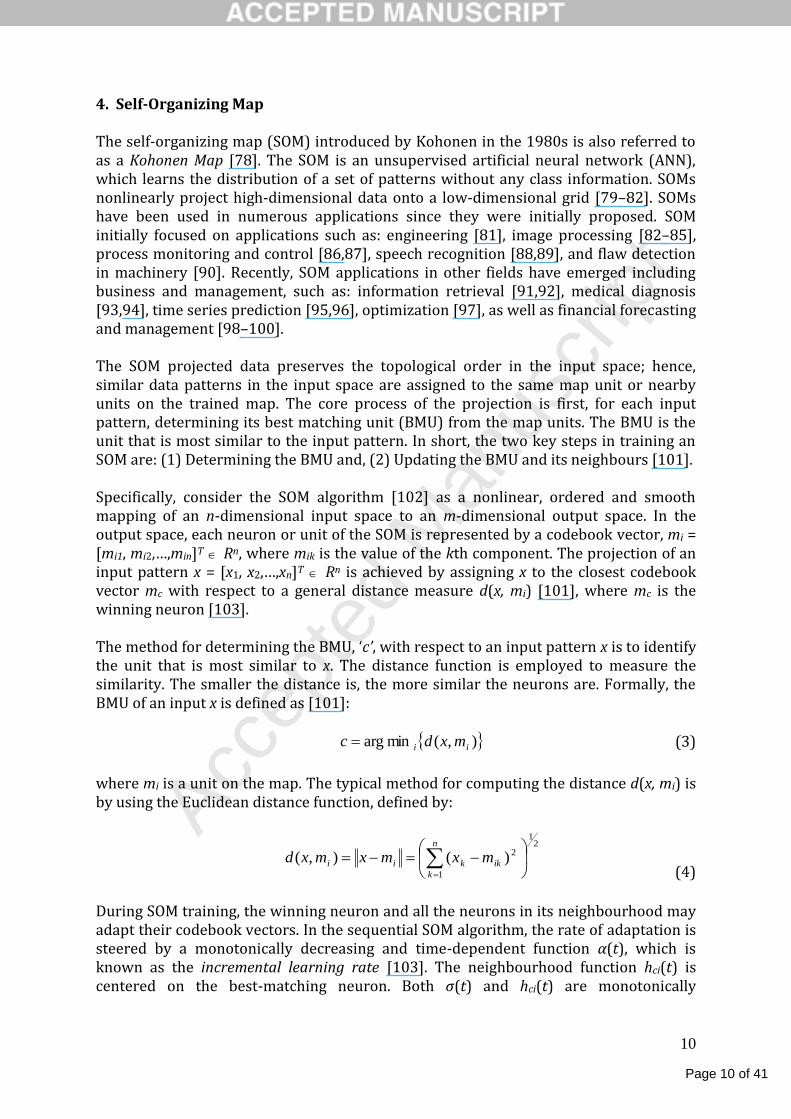
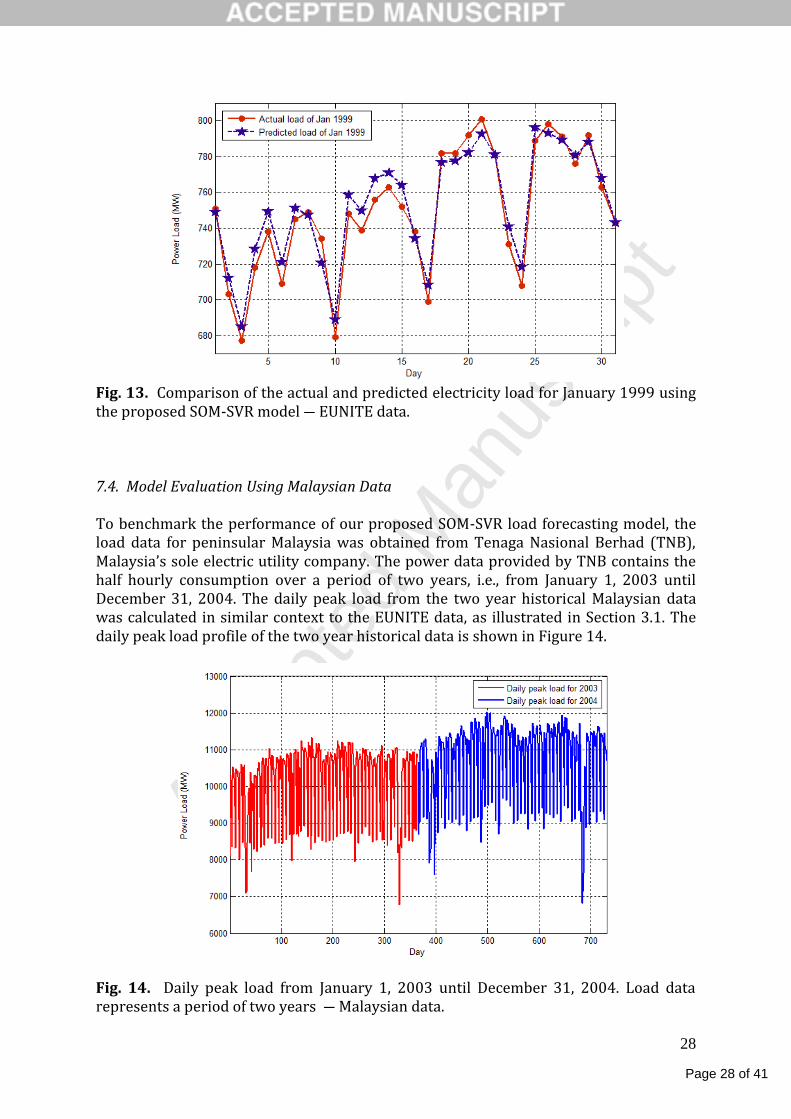
Fig. 13. Comparison of the actual and predicted electricity load for January 1999 using the proposed SOM-SVR model ― EUNITE data. 7.4. Model Evaluation Using Malaysian Data To benchmark the performance of our proposed SOM-SVR load forecasting model, the load data for peninsular Malaysia was obtained from Tenaga Nasional Berhad (TNB), Malaysia’s sole electric utility company. The power data provided by TNB contains the half hourly consumption over a period of two years, i.e., from January 1, 2003 until December 31, 2004. The daily peak load from the two year historical Malaysian data was calculated in similar context to the EUNITE data, as illustrated in Section 3.1. The daily peak load profile of the two year historical data is shown in Figure 14.

Fig. 14. Daily peak load from January 1, 2003 until December 31, 2004. Load data represents a period of two years ― Malaysian data.

Page 29 of 41

Accep

ted

Man

uscr

ipt

29

Similarly as with the EUNITE data in Section 3.2.1, load periodicity for the Malaysian data exists in the profile of every week, i.e., the load demand on weekends is usually lower than that on weekdays and the peak load usually occurs during the middle of the week, as indicated in Figure 15.

Fig. 15. Daily peak load for the month of January 2003 and January 2004. Load data for January represents a period of 31 days ― Malaysian data. Using the Malaysian power load data for the two years of 2003 and 2004, we apply a similar procedure as with the case of the EUNITE data, i.e. to predict the daily peak electricity load for the 31 days of January 2005. Our proposed SOM-SVR model requires additional attributes other than the load data, such as temperature, type of day and annual holiday information. The type of day and Malaysian annual/public holidays information for the two years was retrieved from online calendar systems. The data for the daily temperature of peninsular Malaysia for the two years of 2003 and 2004 is not available. As peninsular Malaysia is positioned in the equatorial zone, this guarantees it a classic tropical climate with relative humidity levels. The weather in Malaysia is fairly hot, averaging around 30°C (86°F) throughout the year. Due to the unavailability of Malaysian daily temperature data and considering temperature (climate) stability in Malaysia throughout the year, we have considered to omit the temperature information from the model attributes as it will not have a significant impact the forecasting accuracy. Hence, the remaining attributes selected to build the SOM-SVR model for the Malaysian power load data are:

(28)

Page 30 of 41

Accep

ted

Man

uscr

ipt

30

Fig. 16. Comparison of the actual and predicted electricity load for January 2005 using the proposed SOM-SVR model ― Malaysian data. Our proposed SOM-SVR model using the feature attributes in eq. (28) was evaluated using the Malaysian load data with the RBF kernel and Grid Search method indicated in Section 6.7. The best value of MAPE for the proposed model using the Malaysian power data was found to be 1.04% using ε = 0.2. To obtain this lowest value of MAPE, the SVR parameters are: C1 = 541.65, γ1 = 0.0134, C2 = 1452.78 and γ2 = 0.00034 for ε-SVR1 and ε-SVR2 respectively. This significantly low value of MAPE supports our interest in justifying that our proposed model has the capability to produce good prediction results for MTLF problems. 7.5. Model Evaluation Using PJM Data PJM which operates an electricity transmission and distribution system is part of the eastern interconnection grid of the United States of America, which is the world's largest competitive wholesale electricity market [122]. PJM considers forecasts of load growth and additions of demand response as interconnection requests for new and planned retirements of existing generating plants, and solutions to mitigate congestion on the transmission and distribution system. The load data for the PJM Mid-Atlantic Region (PJM-E) was obtained online from the PJM website [123]. The online PJM power data contains the hourly consumption load from 1998 until the present day. For the case of experiments in this paper, we acquired the latest PJM-E power data over a period of two years, i.e. from January 1, 2009 until December 31, 2010. The daily peak load from the two year historical PJM-E data was calculated in similar context to the EUNITE data, as indicated in Section 3.1. The daily peak load profile of the two year historical data is shown in Figure 17. As observed from Figure 17, the daily peak load for the year of 2010 indicates a significant growth from the year of 2009.

Page 31 of 41

Accep

ted

Man

uscr

ipt

31

Fig. 17. Daily peak load from January 1, 2009 until December 31, 2010. Load data represents a period of two years ― PJM-E data. Similarly as with the EUNITE data (see Figure 4) and the Malaysian data (see Figure 15), a form of load periodicity for the PJM-E data exists in the profile of every week, as shown in Figure 18, which is discussed in Section 3.2.1 earlier. The PJM-E power load data in Figure 17 for the two years of 2009 and 2010 is used with the proposed SOM-SVR model in Figure 8 to predict the daily peak electricity load for the 31 days of January 2011, similar to the case of the Malaysian and EUNITE datasets. Since our SOM-SVR model requires additional attributes such as temperature, type of day and annual holiday information, the type of day and annual/public United States holiday information for the two years was retrieved from online calendar systems.

Fig. 18. Daily peak load for the month of January 2009 and January 2010. Load data for January represents a period of 31 days ― PJM-E data.

Page 32 of 41

Accep

ted

Man

uscr

ipt

32

The daily temperature data of the United States is available for the years of 2009 and 2010. However, since the PJM eastern interconnection grid serves a large area of eastern United States, i.e. from Michigan and Pennsylvania in the north to Tennessee in the south, the temperature and climate between in the northern and central parts of the United States have significant differences. Moreover, the PJM interconnection areas near the coast lines, i.e. from and New Jersey and Delaware in the north to North Carolina in the south, have significant temperature changes as compared to the non-coastal areas. Due to these limitations, we have considered omitting the temperature information from the model attributes. So, the remaining attributes selected to build the SOM-SVR model for the PJM-E power load data are the same as for the Malaysian data, as represented by eq. (28).

Fig. 19. Comparison of the actual and predicted electricity load for January 2011 using the proposed SOM-SVR model ― PJM-E data. Our proposed SOM-SVR model using the feature attributes in eq. (28) was evaluated using the PJM-E data with the RBF kernel and Grid Search method illustrated in Section 6.7. The best value of MAPE for the proposed model using the PJM-E power data was found to be 1.07% using ε = 0.15. To obtain this lowest value of MAPE, the SVR parameters are: C1 = 372.86, γ1 = 0.00682, C2 = 125.64 and γ2 = 0.0653 for ε-SVR1 and ε-SVR2 respectively. This low value of MAPE supports our interest in justifying that our proposed model gives can produce good prediction results for MTLF problems. Table 9 Comparison of our SOM-SVR model’s prediction results using different electricity load datasets.

Dataset Training

Data Data to Predict

MAPE

Eastern Slovakian Electricity Corp. (EUNITE) [25] 1997, 1998 Jan. 1999 0.97%

Peninsular Malaysia Power Load 2003, 2004 Jan. 2005 1.04%

PJM Mid-Atlantic Region (PJM-E) [123] 2009, 2010 Jan. 2011 1.07%

Average MAPE - - 1.02%

Page 33 of 41

Accep

ted

Man

uscr

ipt

33

From the results obtained in Section 7.3, 7.4 and 7.5, Table 9 summaries the results of our proposed SOM-SVR model, which indicates that our proposed model gives an average MAPE of approximately 1% after testing with three different electricity load datasets. Since our proposed model is a simple implementation for MTLF applications, i.e., by fixing two centres of the SOM and without spending much time on optimization of unknown SOM and SVR parameters, our proposed model has shown to achieve relatively good prediction results for MTLF. 8. Conclusion Mid-term load forecasting (MTLF) is a newer aspect of power system load forecasting. Different kinds of forecasting such as prediction of the daily peak load, daily energy consumption, and monthly electricity consumption, and annual peak load have been proposed previously by researchers. This paper focuses on daily peak load prediction for the next month. In this paper a computational intelligence scheme based the SOM and SVR is applied to reconstruct the dynamics of electricity load forecasting using a time series approach. The SOM is used as a clustering tool to cluster the training data into two subsets, using the Kohonen rule. The reason for using two subsets is obtained from the fact that, two years of historical data is used to construct the forecasting model. After clustering is complete, two ε-SVRs (one for each subset) are employed to fit the clustered data appropriately for SVR training. The Euclidean distance between the cluster centres and testing samples is used as a measure to select the appropriate ε-SVR model for predicting the peak daily load. The proposed SOM-SVR technique is applied on the EUNITE competition data [25] to predict the month-ahead electricity load of January 1999, which demonstrates the effectiveness and efficiency of the clustering and prediction technique in contrast to others. In order to evaluate the performance of our forecasting technique, power load data obtained from (i) Tenaga Nasional Berhad (TNB) for peninsular Malaysia and (ii) PJM for the eastern interconnection grid of the United States of America is used to benchmark the performance of the proposed SOM-SVR model. The empirical results obtained reveal the capability of the proposed model for load prediction. Experimental results reveal that by introducing the load data as a time series and using calendar attributes (type of day and annual holidays) in the forecasting model, the future load demand can be predicted more accurately. Other prediction techniques using the SVR and the ML-BPNN were used to compare the prediction accuracy with the proposed model. Results obtained indicated that the proposed SOM-SVR model outperforms the other two approaches in terms of the MAPE. Furthermore, comparison with the winning model of the EUNITE competition proposed by Lin et al. in [20,111] and other load forecasting techniques using the EUNITE data in [73,76] and [112–121] prove that our proposed forecasting model has better prediction accuracy compared to the other approaches. Experimental results obtained from testing the SOM-SVR model with the EUNITE, Malaysian and PJM datasets achieves low MAPE values of 0.97%, 1.04% and 1.07% respectively, giving an average MAPE of approximately 1%,

Page 34 of 41

Accep

ted

Man

uscr

ipt

34

which indicates that our proposed model gives significantly good prediction accuracy for MTLF compared to previously researched findings. Although forecasting of electricity load has reached a comfortable state of performance with errors of 1-3% in recent years [8], this problem is still considered a difficult task that comprehensive and general solutions are far from easy. For a specific system, the best performances can only be achieved if a deep investigation of the inherent characteristics of the system has been carried out, as in our proposed work. Acknowledgements The authors would like to thank EUNITE for bringing the problem of MTLF to our attention, which inspires us to conduct research on load forecasting. We would like to express our gratitude the Eastern Slovakian Electricity Corporation and PJM for providing the data to be useful in this research study. In addition, we would like to thank Tenaga Nasional Berhad (TNB) Malaysia, for providing the power load data of peninsular Malaysia in order to support this research study. Lastly, the authors would like to thank the editor and reviewers for their careful review of the paper and their constructive remarks and suggestions.

References [1] S. Fan and L. Chen, “Short-Term Load Forecasting based on Adaptive Hybrid

Method”, IEEE Transactions on Power Systems, vol. 21, no. 1, 2006, pp. 392–401. [2] D.W. Bunn, “Forecasting loads and prices in competitive power markets”,

Proceedings of the IEEE, vol. 88, no. 2, 2000, pp. 163–169. [3] A.P. Douglas, A.M. Breipohl, F.N. Lee, R. Adapa, “Risk due to load forecast

uncertainty in short term power system planning”, IEEE Transactions on Power Systems, vol. 13, no. 4, 1998, 1493–1499.

[4] G. Gross, F.D. Galiana, “Short term load forecasting”, Proceedings of the IEEE, vol. 75, no. 12, 1987, pp. 1558–1573.

[5] W.-C. Hong, P.-F. Pai, C.-T. Chen, and C.-S. Lin, “Electricity load forecasting by using support vector machines with simulated annealing algorithm” in Proc. of the 17th IMACS World Congress Scientific Computation, Applied Mathematics and Simulation (IMACS) 2005, Jul. 11–15, 2005.

[6] E. Gonzalez-Romera, M. A. Jaramillo-Moran, D. Carmona-Fernandez, “Monthly electric energy demand forecasting based on trend extraction”, IEEE Transactions on Power Systems, vol. 21, no. 4, 2006, pp. 1946–1953.

[7] N. Amjady, D. Farrokhzad, M. Modarres, “Optimal reliable operation of hydrothermal power systems with random unit outages”, IEEE Transactions on Power Systems, vol. 18, no. 4, 2003, pp. 279–287.

[8] H. S. Hippert, C. E. Pedreira, and R. Castro, “Neural networks for shortterm load forecasting: A review and evaluation”, IEEE Transactions on Power Systems, vol. 16, no. 1, 2001, pp. 44–55.

Page 35 of 41

Accep

ted

Man

uscr

ipt

35

[9] T. Haida and S. Muto, “Regression based peak load forecasting using a transformation technique”, IEEE Transactions on Power Systems, vol. 9, no. 4, 1994, pp. 1788–1794.

[10] A. D. Papalexopoulos and T. C. Hesterberg, “A regression-based approach to short-term load forecasting”, IEEE Transactions on Power Systems, vol. 5, no. 4, 1990, pp. 1535–1550.

[11] S. Rahman and O. Hazim, “A generalized knowledge-based short term load-forecasting technique”, IEEE Transactions on Power Systems, vol. 8, no. 2, 1993, pp. 508–514.

[12] S. J. Huang and K. R. Shih, “Short-term load forecasting via ARMA model identification including non-Gaussian process considerations”, IEEE Transactions on Power Systems, vol. 18, no. 2, 2003, pp. 673–679.

[13] H. Wu and C. Lu, “A data mining approach for spatial modeling in small area load forecast”, IEEE Transactions on Power Systems, vol. 17, no. 2, 2003, pp. 516–521.

[14] G. E. P. Box and G. M. Jenkins, Time Series Analysis—Forecasting and Control. San Francisco, CA: Holden-Day, 1976.

[15] D. G. Infield and D. C. Hill, “Optimal smoothing for trend removal in short term electricity demand forecasting”, IEEE Transactions on Power Systems, vol. 13, no. 3, 1998, pp. 1115–1120.

[16] A. Khotanzad, R. C. Hwang, A. Abaye, and D. Maratukulam, “An adaptive modular artificial neural network hourly load forecaster and its implementation at electric utilities”, IEEE Transactions on Power Systems, vol. 10, no. 3, 1995, pp. 1716–1722.

[17] T. Czernichow, A. Piras, K. Imhof, P. Caire, Y. Jaccard, B. Dorizzi, and A. Germond, “Short term electrical load forecasting with artificial neural networks”, Eng. Intell. Syst., vol. 2, 1996, pp. 85–99.

[18] L. M. Saini and M. K. Soni, “Artificial neural network-based peak load forecasting using conjugate gradient methods”, IEEE Transactions on Power Systems, vol. 12, no. 3, 2002, pp. 907–912.

[19] S. Fan, C. X. Mao, and L. N. Chen, “Peak load forecasting using the self-organizing map”, in Advances in Neural Networks (ISNN) 2005. New York: Springer-Verlag, 2005, pt. III, pp. 640–649.

[20] B.-J. Chen, M.-W. Chang, and C.-J. Lin, “Load forecasting using support vector machines: A study on EUNITE competition 2001”, IEEE Transactions on Power Systems, vol. 19, no. 4, 2004, pp. 1821–1830.

[21] S. Fan, C. X. Mao, and L. N. Chen, “Next-day electricity price forecasting using a hybrid network”, IET Generation, Transmission and Distribution, vol. 1, no. 1, 2007, pp. 176–182.

[22] C. Cortes and V. Vapnik, “Support-vector network”, Machine Learning, vol. 20, 1995, pp. 273–297.

[23] J. A. K. Suykens and J. Vandewalle, “Training multiplayer perceptron classifiers based on a modified support vector method”, IEEE Transactions on Neural Networks, vol. 10, no. 4, 1999, pp. 907–911.

[24] L. Zhang, W. Zhou, L. Jiao, "Hidden Space Support Vector Machines", IEEE Transactions on Neural Networks, vol. 15, no. 6, 2004, pp. 1424–1434.

[25] EUropean Network on Intelligent TEchnologies for Smart Adaptive Systems. Available at: http://www.eunite.org/. The competition page is: http://neuron.tuke.sk/competition/

Page 36 of 41

Accep

ted

Man

uscr

ipt

36

[26] J. F. Chen, W. M. Wang, C. M. Huang, “Analysis of an adaptive time-series autoregressive moving-average (ARMA) model for short-term load forecasting”, Electric Power Syst. Res., vol. 34, no. 3, 1995, pp. 187–196.

[27] S. Vemuri, D. Hill, R. Balasubramanian, “Load forecasting using stochastic models”, in Proc. of the 8th Power Industrial Computing Application Conference, 1973, pp. 31–37.

[28] H. Wang, N.N. Schulz, “Using AMR data for load estimation for distribution system analysis”, Electric Power Syst. Res., vol. 76, no. 5, 2006, pp. 336–342.

[29] W. R. Christianse, “Short term load forecasting using general exponential smoothing”, IEEE Transactions on Power Apparatus Systems, PAS-90 (1971), pp. 900–911.

[30] J. H. Park, Y. M. Park, K. Y. Lee, “Composite modeling for adaptive short-term load forecasting”, IEEE Transactions on Power Systems, vol. 6, no. 1, 1991, pp. 450–457.

[31] A. P. Douglas, A. M. Breipohl, F. N. Lee, R. Adapa, “The impact of temperature forecast uncertainty on Bayesian load forecasting”, IEEE Transactions Power Systems, vol. 13, no. 4, 1998, pp. 1507–1513.

[32] A. Azadeh, M. Saberi, S.F. Ghaderi, A. Gitiforouz, V. Ebrahimipour, “Improved estimation of electricity demand function by integration of fuzzy system and data mining approach”, Energy Convers. Manage., vol. 49, no. 8, 2008, pp. 2165–2177.

[33] B. Wang, N.-L. Tai, H.-Q. Zhai, J. Ye, J.-D. Zhu, and L.-B. Qi, “A new ARMAX model based on evolutionary algorithm and particle swarm optimization for short-term load forecasting”, Electric Power Syst. Res., vol. 78, no. 10, 2008, pp. 1679–1685.

[34] R. G. Brown, Introduction to Random Signal Analysis and Kalman Filtering, John Wiley & Sons, Inc., New York, 1983.

[35] A. Gelb, Applied Optimal Estimation, The MIT Press, MA, 1974. [36] D. J. Trudnowski, W.L. McReynolds, J.M. Johnson, “Real-time very short-term load

prediction for power-system automatic generation control”, IEEE Transactions on Control System Technology, vol. 9, no. 2, 2001, pp. 254–260.

[37] I. Moghram, S. Rahman, “Analysis and evaluation of five short-term load forecasting techniques”, IEEE Transactions on Power Systems, vol. 4, no. 4, 1989, pp. 1484–1491.

[38] H. M. Al-Hamadi, S. A. Soliman, “Fuzzy short-term electric load forecasting using Kalman filter”, IEEE Proceedings Generation, Transmission and Distribution, vol. 153, no. 2, 2006, pp. 217–227.

[39] N. Amjady, “Short-term bus load forecasting of power systems by a new hybrid method”, IEEE Transactions on Power Systems, vol. 22, no. 1, 2007, pp. 333–341.

[40] C. Asbury, “Weather load model for electric demand energy forecasting”, IEEE Transactions on Power Apparatus and Systems, PAS-94 (1975) pp. 1111–1116.

[41] S. A. Soliman, S. Persaud, K. El-Nagar, M. E. El-Hawary, “Application of least absolute value parameter estimation based on linear programming to short-term load forecasting”, International Journal of Electrical Power Energy System, vol. 19, no. 3, 1997, pp. 209–216.

[42] S. Mirasgedis, Y. Safaridis, E. Georgopoulou, D. P. Lalas, M. Moschovits, F. Karagiannis, D. Papakonstantinou, “Models for mid-term electricity demand forecasting incorporating weather influences”, Energy, vol. 31, no. 2–3, 2006, pp. 208–227.

[43] Z. Mohamed, P. Bodger, “Forecasting electricity consumption in New Zealand using economic and demographic variables”, Energy, vol. 30, no. 10, 2005, pp. 1833–1843.

Page 37 of 41

Accep

ted

Man

uscr

ipt

37

[44] G. J. Tsekouras, E. N. Dialynas, N. D. Hatziargyriou, S. Kavatza, “A non-linear multivariable regression model for midterm energy forecasting of power systems”, Electric Power Syst. Res., vol. 77, no. 12, 2007, pp. 1560–1568.

[45] S. Rahman, R. Bhatnagar, “An expert system based algorithm for short-term load forecasting”, IEEE Transactions on Power Systems, vol. 3 no. 2, 1998, pp. 392–399.

[46] C. C. Chiu, L. J. Kao, D. F. Cook “Combining a neural network with a rule-based expert system approach for short-term power load forecasting in Taiwan”, Expert System Applications, vol. 13, no. 4, 1997, pp. 299–305.

[47] L.-C. Ying, M.-C. Pan, “Using adaptive network based fuzzy inference system to forecast regional electricity loads”, Energy Conversion Management, vol. 49, no. 2, 2008, pp. 205–211.

[48] P.-F. Pai, “Hybrid ellipsoidal fuzzy systems in forecasting regional electricity loads”, Energy Conversion Management, vol. 47, no. 15–16, 2006, pp. 2283–2289.

[49] S. C. Pandian, K. Duraiswamy, C. C. A. Rajan, N. Kanagaraj, “Fuzzy approach for short term load forecasting”, Electric Power Syst. Res., vol. 76, no. 6–7, 2006, pp. 541–548.

[50] D. C. Park, M. A. El-Sharkawi, R. J. Marks II., L. E. Atlas, M. J. Damborg, “Electric load forecasting using an artificial neural network”, IEEE Transactions on Power Systems, vol. 6, no. 2, 1991, pp. 442–449.

[51] B. Novak, “Superfast autoconfiguring artificial neural networks and their application to power systems”, Electric Power Syst. Res., vol. 35, no. 1, 1995, pp. 11–16.

[52] G. A. Darbellay, M. Slama, “Forecasting the short-term demand for electricity – do neural networks stand a better chance?”, International Journal of Forecasting, vol. 16, no. 1, 2000, pp. 71–83.

[53] R. E. Abdel-Aal, “Short-term hourly load forecasting using abductive networks”, IEEE Transactions on Power Systems, vol. 19, no. 1, 2004, pp. 164–173.

[54] C. C. Hsu, C. Y. Chen, “Regional load forecasting in Taiwan – application of artificial neural networks”, Energy Conversion Management, vol. 44, no. 12, 2003, pp. 1941–1949.

[55] L. M. Saini, “Peak load forecasting using Bayesian regularization, Resilient and adaptive backpropagation learning based artificial neural networks”, Electric Power Syst. Res., vol. 78, no. 7, 2008, pp. 1302–1310.

[56] P. Lauret, E. Fock, R.N. Randrianarivony, J.-F. Manicom-Ramsamy, “Bayesian neural network approach to short time load forecasting”, Energy Conversion Management, vol. 49, no. 5, 2008, pp. 1156–1166.

[57] M. R. Amin-Naseri, A. R. Soroush, “Combined use of unsupervised and supervised learning for daily peak load forecasting”, Energy Conversion Management, vol. 49, no. 6, 2008, pp. 1302–1308.

[58] O. A. S. Carpinteiro, R. C. Leme, A. C. Z. de Souza, C. A. M. Pinheiro, E. M. Moreira, “Long-term load forecasting via a hierarchical neural model with time integrators”, Electric Power Syst. Res., vol. 77, no. 3–4, 2007, pp. 371–378.

[59] J. Cao, X. Lin, “Study of hourly and daily solar irradiation forecast using diagonal recurrent wavelet neural networks”, Energy Conversion Management, vol. 49, no. 6, 2008, pp. 1396–1406.

[60] N. Tai, J. Stenzel, H. Wu, “Techniques of applying wavelet transform into combined model for short-term load forecasting”, Electric Power Syst. Res., vol. 76, no. 6–7, 2006, pp. 525–533.

Page 38 of 41

Accep

ted

Man

uscr

ipt

38

[61] M. El-Telbany, F. El-Karmi, “Short-term forecasting of Jordanian electricity demand using particle swarm optimization”, Electric Power Syst. Res., vol. 78, no. 3, 2008, pp. 425–433.

[62] M. Ghiassi, D.K. Zimbra, H. Saidane, “Medium term system load forecasting with a dynamic artificial neural network model”, Electric Power Syst. Res., vol. 76, no. 5, 2006, pp. 302–316.

[63] V. Vapnik. The Nature of Statistic Learning Theory, Springer–Verlag, New York, 1995.

[64] V. Vapnik. Statistical Learning Theory. New York: Wiley, 1998. [65] V. Vapnik, S. Golowich, A. Smola, “Support vector machine for function

approximation, regression estimation, and signal processing”, in Advances in Neural Information Processing Systems 9, eds. M. Mozer, M. Jordan, T. Petsche, pp. 281–287, Cambridge, MA, MIT Press.

[66] L. Cao, “Support vector machines experts for time series forecasting”, Neurcomputing, vol. 51, 2003, pp. 321–339.

[67] L. Cao, Q. Gu, “Dynamic support vector machines for non-stationary time series forecasting”, Intel. Data Anal., vol. 6, 2002, pp. 67–83.

[68] F. E. H. Tay, L. Cao, “Application of support vector machines in financial time series forecasting”, Omega, vol. 29, no. 4, 2001, pp. 309–317.

[69] W. C. Hong, P. F. Pai, “Predicting engine reliability by support vector machines”, International Journal of Advance Manufacturing Technology, vol. 28, no. 1–2, 2006, pp. 154–161.

[70] P.-F. Pai, W.-C. Hong, “Forecasting regional electric load based on recurrent support vector machines with genetic algorithms”, Electric Power Syst. Res., vol. 74, no. 3, 2005, pp. 417–425.

[71] P.-F. Pai, W.-C. Hong, “Support vector machines with simulated annealing algorithms in electricity load forecasting”, Energy Conversion Management, vol. 46, no. 17, 2005, pp. 2669–2688.

[72] L. Yuancheng, F. Tingjian, and Y. Erkeng, “Short-term electrical load forecasting using least squares support vector machines”, in Proc. of the IEEE International Conference on Power System Technology, 2002.

[73] H. Wu, and X. Chang, “Power Load Forecasting with Least Squares Support Vector Machines and Chaos Theory”, in Proc of the 6th World Congress on Intelligent Control and Automation, Jun. 21–23, 2006, Dalian, China.

[74] D.-X. Niu, Q. Wang, and J.-C. Li, “Research on support vector machine model based on grey relation analysis for daily load forecasting”, in Proc. of the International Conference on Machine Learning and Cybernetic, 2005.

[75] D.-X. Niu, Q. Wanq, and J.-C. L, "Short term load forecasting model using support vector machine based on artificial neural network”, in Proc. of the International Conference on Machine Learning and Cybernetics, Guangzhou, 2005.

[76] X. Tao, H. Renmu, W. Peng, and X. Dongjie, “Input Dimension Reduction for Load Forecasting Based on Support Vector Machine”, in Proc. of the 2004 IEEE International Conference on Electric Utility Deregulation, Restructuring and Power Technologies (DRPT), 2004, Hong Kong, China, pp. 510–513.

[77] M.-G. Zhang, “Short-term load forecasting based on support vector machines regression”, in Proc. of the International Conference on Machine Learning and Cybernetics, 2005.

[78] J. Nagi, S. K. Ahmed, F. Nagi, “A MATLAB based Face Recognition System using Image Processing and Neural Networks”, in Proc. of the 4th International Colloquium on

Page 39 of 41

Accep

ted

Man

uscr

ipt

39

Signal Processing and its Applications (CSPA) 2008, Kuala Lumpur, March 2008, pp. 83–88.

[79] T. Kohonen, “The self-organizing map”, Proceedings of the IEEE, vol. 78, no. 9, 1990, pp. 1464–1480.

[80] T. Kohonen, E. Oja, O. Simula, A. Visa, J. Kangas, “Engineering applications of the self-organizing map”, Proceedings of the IEEE, vol. 84, no. 10, 1996, pp. 1358–1384.

[81] J. Vesanto, E. Alhoniemi, J. Himberg, K. Kiviluoto, and J. Parviainen, “Self-organizing map for data mining in Matlab: The SOM toolbox”, Simulation News Europe, vol. 25, no. 54, 1999.

[82] A. Visa, “A texture classifier based on neural network principles”, in Proc. of the International Joint Conference on Neural Networks, San Diego, CA, 1990, pp. 491–496.

[83] C.-H. Chang, P. Xu, R. Xiao, and T. Srikanthan, “New adaptive color quantization method based on self-organizing maps”, IEEE Transactions on Neural Networks, vol. 16, no. 1, 2005, pp. 237–249.

[84] G. Dong and M. Xie, “Color clustering and learning for image segmentation based on neural networks”, IEEE Transactions on Neural Networks, vol. 16, no. 4, 2005, pp. 925–936.

[85] X. Tan, S. Chen, Z.-H. Zhou, and F. Zhang, “Recognizing partially occluded, expression variant faces from single training image per person with SOM and Soft k-NN ensemble”, IEEE Transactions on Neural Networks, vol. 16, no. 4, 2005, pp. 875–886.

[86] M. Kasslin, J. Kangas, and O. Simula, “Process state monitoring using self-organizing maps”, in Artificial Neural Networks, eds., I. Aleksander, J. Taylor, Amsterdam, The Netherlands: North-Holland, 1992, vol. 2, pp. 1532–1534.

[87] O. Simula and J. Kangas, “Process monitoring and visualization using self-organizing maps”, in Neural Networks for Chemical Engineers, ed., A. B. Bulsari, New York: Elsevier, 1995.

[88] J. Mantysalo, K. Torkkola, and T. Kohonen, “Mapping context dependent acoustic information into context independent form by LVQ”, Speech Commun., vol. 14, no. 2, 1994, pp. 119–130.

[89] H. Guterman, A. Cohen, and I. Lapidot, “Unsupervised speaker recognition based on competition between self-organizing maps”, IEEE Transactions on Neural Networks, vol. 13, no. 4, 2002, pp. 877–887.

[90] M. Vapola, O. Simula, T. Kohonen, and P. Merilainen, “Representation and identification of fault conditions of an aesthesia system by means of the self-organizing map”, in Proc. of the International Conference on Artificial Neural Networks (ICANN), 1994, pp. 246–249.

[91] K. Lagus, T. Honkela, S. Kaski, and T. Kohonen, “Self-organizing maps of document collections: A new approach to interactive exploration”, in Proc. of the 2nd International Conference on Knowledge Discovery and Data Mining, 1996, pp. 238–243.

[92] T. Kohonen, S. Kaski, K. Lagus, J. Salojarvi, J. Honkela, V. Paatero, and A. Saarela, “Self-organization of a massive document collection”, IEEE Transactions on Neural Networks, vol. 11, no. 3, 2000, pp. 574–585.

[93] D. R. Chen, R. F. Chang, and Y. L. Huang, “Breast cancer diagnosis using self-organizing map for sonography”, Ultrasound Med. Biol., vol. 1, no. 26, 2000, pp. 405–411.

Page 40 of 41

Accep

ted

Man

uscr

ipt

40

[94] A. A. Kramer, D. Lee, and R. C. Axelrod, “Use of a Kohonen neural network to characterize respiratory patients for medical intervention”, in Proc. of the IEEE Artificial Neural Networks in Medicine and Biology (ANNIMAB) Conference, Goteborg, Sweden, 2000, pp. 192–196.

[95] A. Hirose and T. Nagashima, “Predictive self-organizing map for vector quantization of migratory signals and its application to mobile communications”, IEEE Transactions on Neural Networks, vol. 14, no. 6, 2003, pp. 1532–1540.

[96] G. A. Barreto and A. F. R. Araujo, “Identification and control of dynamical systems using the self-organizing map”, IEEE Transactions on Neural Networks, vol. 15, no. 5, 2004, pp. 1244–1259.

[97] M. Milano, P. Koumoutsakos, and J. Schmidhuber, “Self-organizing nets for optimization”, IEEE Transactions on Neural Networks, vol. 15, no. 3, 2004, pp. 758–765.

[98] N. Kasabov, D. Deng, L. Erzegovezi, M. Fedrizzi, and A. Beber, “Online decision making and prediction of financial and macroeconomic parameters on the case study of the European monetary union”, in Proc. of the IEEE ICSC Symposium on Neural Computation, 2000.

[99] G. J. Deboeck, “Modeling nonlinear market dynamics for intra-day trading”, Neural-Network-World, vol. 1, no. 10, 2000, pp. 3–27.

[100]S. Kaski, J. Sinkkonen, and J. Peltonen, “Bankruptcy analysis with selforganizing maps in learning metrics”, IEEE Transactions on Neural Networks, vol. 12, no. 4, 2001, pp. 936–947.

[101]C.-C. Hsu, “Generalizing Self-Organizing Map for Categorical Data”, IEEE Transactions on Neural Networks, vol. 17, no. 2, 2006, pp. 294–304.

[102]T. Kohonen, Self-Organizing Maps, ser. Information Sciences, third edition, New York: Springer-Verlag, 2001.

[103]D. Brugger, M. Bogdan, and W. Rosenstiel, “Automatic Cluster Detection in Kohonen’s SOM”, IEEE Transactions on Neural Networks, vol. 19, no. 3, 2008, pp. 442–459.

[104]A. Kulkarni, V. K. Jayaraman, and B. D. Kulkarni, “Control of chaotic dynamical systems using support vector machines”, Phys. Lett. A, vol. 317, 2003, pp. 429–435.

[105]H. Drucker, C.J.C. Burges, L. Kaufman, A. Smola, V.N. Vapnik, “Support vector regression machines”, in Advances in Neural Information Processing Systems 9, eds. M. Mozer, M. Jordan, T. Petsche, pp. 281–287, Cambridge, MA, MIT Press.

[106]K. Vojislav, Learning and Soft Computing – Support Vector Machines, Neural Networks and Fuzzy Logic Models, The MIT Press, MA, 2001.

[107]C.-W. Hsu, C.-C. Chang, and C.-J. Lin. A Practical Guide to Support Vector Classification. Technical report, Dept. of Computer Science, National Taiwan University, 2003.

[108]S. Amari, and S. Wu, “Improving support vector machine classifiers by modifying kernel functions”, Neural Networks, vol. 12, no. 6, 1999, pp. 783–789.

[109]V. Cherkassky, and Y. Ma, “Practical selection of SVM parameters and noise estimation for SVM regression”, Neural Networks, vol. 17, no. 1, 2004, pp. 113–126.

[110]C.-C. Chang and C.-J. Lin. LIBSVM: A Library for Support Vector Machines [Online]. Available at: http://www.csie.ntu.edu.tw/~cjlin/libsvm

[111]M.-W. Chang, B.-J. Chen and C.-J. Lin, “EUNITE Network Competition: Electricity Load Forecasting” November 2001. Winner of the 2001 EUNITE worldwide competition on electricity load prediction.

Page 41 of 41

Accep

ted

Man

uscr

ipt

41

[112]S. Rahat Abbas and M. Arif, “Electric Load Forecasting using Support Vector Machines Optimized by Genetic Algorithm”, in Proc. of the Multitopic Conference (INMIC) 2006, Dec. 2006, pp. 395–399.

[113]D. Ortiz-Arroyo, M. K. Skov, and Q. Huynh, “Accurate Electricity Load Forecasting with Artificial Neural Networks”, in Proc. of the 2005 International Conference on Computation Intelligence for Modelling, Control and Automation (CIMCA-IAWTIC) 2005.

[114]N. Amjady and F. Keynia, “Mid-term load forecasting of power systems by a new prediction method”, Energy Conversion and Management, vol. 49, no. 10, 2008, pp. 2678–2687.

[115]T. Rashid, B. Q. Huang, M-T. Kechadi and B. Gleeson, “Auto-regressive Recurrent Neural Network”, International Journal of Computational Intelligence, vol. 3, no. 1, 2007, pp. 36–44.

[116]T. Rashid and T. Kechadi, “A Practical Approach for Electricity Load Forecasting” Proceedings of World Academy of Science, Engineering and Technology, vol. 5, 2005, pp. 201–205.

[117]E. E. El-Attar, J. Y. Goulermas, Q. H. Wu, "Forecasting electric daily peak load based on local prediction", Power & Energy Society (PES) General Meeting, Jul. 26-30, 2009, pp. 1–6.

[118]V. H. Ferreira and A. P. A. da Silva, “Toward estimation autonomous neural network-based electric load forecasters”, IEEE Transactions on Power Systems, vol. 22, no. 5, 2007, pp. 1554–1562.

[119]H. Mao, X.-J. Zeng, G. Leng, Y.-J. Zhai, and J. A. Keane, "Short-Term and Midterm Load Forecasting Using a Bilevel Optimization Model", IEEE Transactions on Power Systems, vol. 24, no. 2, 2009, pp. 1080–1090.

[120]D.-X. Niu, W. Li, L.-M. Cheng, X.-H. Gu, "Mid-term Load Forecasting Based on Dyanmic Least Squares SVMs", in Proc. of the Seventh International Conference on Machine Learning and Cybernetics, Kunming, Jul. 12-15, 2008.

[121]A. R. Koushki, M. N. Maralloo, B. Hashemitabar, C. Lucas, "Load Forecasting With The Aid of Neuro-Fuzzy Modelling", in Proc. of Seventh International Conference on Computer Science and Information Technologies, Sept. 28, 2009, Yerevan, Armenia.

[122]J. Rosellóna, Z. Myslíkováa, E. Zenónc, “Incentives for transmission investment in the PJM electricity market: FTRs or regulation (or both?)”, Utilities Policy, vol. 19, no. 1, The 8th Conference on Applied Infrastructure Research – INFRADAY, Jan. 2011, pp. 3–13.

[123]PJM Hourly Load Data, 2011 [Online]. Available at: http://www.pjm.com/markets-and-operations/energy/real-time/loadhryr.aspx