pratik joshi performance evaluation of 802.11p protocol for ...
85
PRATIK JOSHI PERFORMANCE EVALUATION OF 802.11P PROTOCOL FOR EMERGENCY APPLICATION Master of Science Thesis Examiner: Professor, Dr. Yevgeni Koucheryavy Senior Research Fellow, Dr. Dmitri Moltchanov Topic approved by the Faculty Council of Com- puting and Electrical Engineering on May 5th, 2014
-
Upload
khangminh22 -
Category
Documents
-
view
0 -
download
0
Transcript of pratik joshi performance evaluation of 802.11p protocol for ...

PRATIK JOSHI
PERFORMANCE EVALUATION OF 802.11P PROTOCOL FOR
EMERGENCY APPLICATION
Master of Science Thesis
Examiner: Professor, Dr. Yevgeni Koucheryavy Senior Research Fellow, Dr. Dmitri Moltchanov Topic approved by the Faculty Council of Com-puting and Electrical Engineering on May 5th, 2014

i
ABSTRACT TAMPERE UNIVERSITY OF TECHNOLOGY Master of Science Degree Programme in Information Technology Joshi, Pratik: Performance evaluation of 802.11p protocol for emergency ap-plication Master of Science Thesis, 57 pages, 9 Appendix pages May 2014 Major: Communication Engineering Examiner(s): Professor, Dr. Yevgeni Koucheryavy
Senior Research Fellow, Dr. Dmitry Moltchanov Keywords: Vehicular Ad-Hoc Network, VANET, 802.11p, performance evalua-tion, Network Simulator, NS2 Vehicle manufacturers have adopted this technology to assist the drivers drive their car
like alarming the driver if he is close to some object while driving or safely parking the
car to name a few. However, the main difference in an Adhoc network that involves a
vehicle is the mobility factor. A vehicle is constantly in motion varying its location with
time which means constant change in its position and surroundings. With the increase in
the number of vehicles running in the road the probability of road accidents increases.
The aim of the vehicle manufacturers and government agencies is to provide safe driv-
ing experience to save lives and assets.
Sensor nodes has gone a long way from being just a technology to being an integral
part of our life and its no surprise that vehicle manufacturers have incorporated them to
create VANET that has a dedicated 802.11p protocol. In this essay based on my thesis,
we show that 802.11p protocol is performing as per expected and all the nodes receive
packet as should be the case. Simulation is done using an open source, discrete event
driven tool called NS2 where a node generates and transmits a packet which is passed
on by the other nodes. The simulation is performed considering node distance, retrans-
mission attempt, and contention window. The results were analysed on the basis of con-
figuration parameter mentioned. We evaluate the performance of 802.11p protocol by
studying the output based on the node distance, retransmission attempt, and contention
window. The graph generated from the simulation showed that all nodes receives a mes-
sage which shows that 802.11p protocol is in fact working as intended. The most sur-
prising result was that all of the nodes received the packet generated by the first node.

ii
PREFACE
This Master of Science Thesis has been written to fulfil the Degree completion require-
ment of Master of Science Degree in Information Technology from Tampere University
of Technology, Tampere, Finland. I would like to thank the people who have helped me
during this time to accomplish the work.
First of all I would like to thank my supervisors Professor Dr. Yevgeni Koucherya-
vy and Senior Research Fellow, Dr. Dmitri Moltchanov for granting me the opportunity
to work under them. I also owe them a sincere debt of gratitude for their valuable guid-
ance during the whole time. I am utterly grateful for their endless patience while dis-
cussing the ideas and also the scrutiny that they provided during the simulation phase.
Thousands of miles away, my family back home in Kathmandu, Nepal deserve my
heartfelt gratitude and thanks for supporting and guiding me in every phase of my life.
Finally, I would also like to thank my friends Prajwal Osti, Sandeep Tamrakar, Manik
Madhikermi, and Gautam Raj Moktan for providing me valuable support and suggestion
during my thesis phase.
Tampere, 29.01.2015
Pratik Joshi

iii
TABLE OF CONTENTS
Abstract .............................................................................................................................. i
Preface ............................................................................................................................... ii
Table of Contents ............................................................................................................. iii
Table of Figures ................................................................................................................ v
List of Tables................................................................................................................... vii
1. Introduction ............................................................................................................... 1
1.1 Motivation ......................................................................................................... 3
1.2 Research objective ............................................................................................ 3
1.3 Structure of thesis .............................................................................................. 4
2. Vehicular Adhoc network (VANET) ........................................................................ 5
2.1 Introduction to VANET .................................................................................... 5
2.2 TCP/IP model .................................................................................................... 7
2.3 The 802 Universe .............................................................................................. 8
2.4 The 802.11 Protocol ........................................................................................ 11
2.4.1 Dedicated Short Range Communication (DSRC) ............................. 12
2.4.2 802.11 MAC Layer amendments ....................................................... 14
2.4.3 802.11 PHY Layer amendments ........................................................ 16
2.4.4 IEEE 1609 – Standard for WAVE ..................................................... 17
2.5 Ad-hoc Routing Protocols ............................................................................... 20
2.5.1 Proactive Routing .............................................................................. 21
2.5.2 Reactive Routing................................................................................ 22
2.6 Chapter Summary............................................................................................ 23
3. Simulation Framework ............................................................................................ 25
3.1 NS2 Architecture ............................................................................................. 26
3.2 Basic NS2 flow ............................................................................................... 28
3.3 Installing NS2 ................................................................................................. 28
3.4 TCL Simulation Script .................................................................................... 29
3.5 Simulation Concept ......................................................................................... 30
3.5.1 Network configuration phase ............................................................. 30
3.5.2 Simulation Phase................................................................................ 31
3.6 Wireless Simulation based on 802.11p ........................................................... 31
3.6.1 Node ................................................................................................... 31
3.6.2 Traffic Generator ............................................................................... 32
3.6.3 Packet header ..................................................................................... 33
3.6.4 Network stack .................................................................................... 33
3.7 Trace File ........................................................................................................ 35
3.8 Summary ......................................................................................................... 38
4. Numerical Results ................................................................................................... 39
4.1 Simulation Scenario ........................................................................................ 39
4.2 TCL script and output trace file ...................................................................... 40

iv
4.3 Graph ............................................................................................................... 42
4.3.1 Time Based Analysis ......................................................................... 44
4.3.2 Distance based analysis ..................................................................... 51
5. Conclusion .............................................................................................................. 56
6. References ............................................................................................................... 58
Appendix A ..................................................................................................................... 63
Appendix B ..................................................................................................................... 64
Appendix C ..................................................................................................................... 69
Appendix D ..................................................................................................................... 71

v
TABLE OF FIGURES FIGURE 2.1-1: VEHICLE-TO-VEHICLE AND VEHICLE-TO-INFRASTRUCTURE 6
FIGURE 2.2-1: OSI MODEL VS TCP/IP MODEL ......................................................... 7
FIGURE 2.3-1: 802 IN LLC, MAC AND PHY LAYERS ............................................... 8
FIGURE 2.4-1: BASIC V2V COMMUNICATION SCENARIO ................................. 13
FIGURE 2.4-2: DSRC CHANNEL SYNCHRONIZATION SCHEME BY IEEE1609 14
FIGURE 2.4-3: 802.11 MAC LAYER AMENDMENTS .............................................. 16
FIGURE 2.4-4: 802.11P PHY LAYER AMENDMENTS ............................................. 17
FIGURE 2.4-5: WIRELESS ACCESS IN VEHICULAR ENVIRONMENTS (WAVE),
IEEE 1609, IEEE 802.11P AND THE OSI REFERENCE MODEL ..................... 18
FIGURE 3.1-1: NS2 CLASS DIAGRAM HANDLE ..................................................... 26
FIGURE 3.1-2: BASIC NS2 ARCHITECTURE ........................................................... 27
FIGURE 3.1-3: DIRECTORY STRUCTURE OF NS2 ................................................. 28
FIGURE 3.2-1: BASIC NS2 FLOWCHART ................................................................. 28
FIGURE 3.6-1: BASIC ARCHITECTURE OF A NODE ............................................. 32
FIGURE 3.6-2: OVERVIEW OF PACKET HEADER STACK USED IN
SIMULATION ........................................................................................................ 33
FIGURE 4.1-1: SCENARIO FOR PACKETS TRAVELLING IN THE NODE
NETWORK ............................................................................................................. 40
FIGURE 4.3-1: PROBABILITY TO REACH 500 METERS WITHIN 1 SECOND .... 44
FIGURE 4.3-2: PROBABILITY TO REACH 500M WITHIN 2 SECONDS ............... 45
FIGURE 4.3-3: PROBABILITY TO REACH 1000M: WITHIN 1 SEC ....................... 45
FIGURE 4.3-4: PROBABILITY TO REACH 1000M WITHIN 2 SECONDS ............. 46
FIGURE 4.3-5: PROBABILITY OF CARS HAVING A MESSAGE WITHIN 1
SECOND FOR RETRANSMISSION ATTEMPT 1 AND CONTENTION
WINDOW (0, 8)...................................................................................................... 46
FIGURE 4.3-6: PROBABILITY OF CARS HAVING A MESSAGE WITHIN 1
SECOND FOR RETRANSMISSION ATTEMPT 1 AND CONTENTION
WINDOW (0, 8)...................................................................................................... 47
FIGURE 4.3-7: PROBABILITY OF CARS HAVING A MESSAGE WITHIN 1
SECOND FOR NODE DISTANCE OF 5M AND RETRANSMISSION
ATTEMPT 1 ........................................................................................................... 48
FIGURE 4.3-8: PROBABILITY OF CARS HAVING A MESSAGE WITHIN 1
SECOND FOR NODE DISTANCE 5M RETRANSMISSION ATTEMPT 5 ...... 48
FIGURE 4.3-9: PROBABILITY OF CARS HAVING A MESSAGE WITHIN 1
SECOND FOR NODE DISTANCE 5M AND CONTENTION WINDOW (0, 8) 49
FIGURE 4.3-10: PROBABILITY OF CARS HAVING A MESSAGE WITHIN 1
SECOND FOR NODE DISTANCE 5M AND CONTENTION WINDOW (0, 8) 49
FIGURE 4.3-11: PROBABILITY OF CARS HAVING A MESSAGE WITHIN 2
SECOND FOR RETRANSMISSION ATTEMPT 1 AND CONTENTION
WINDOW (0, 8)...................................................................................................... 50

vi
FIGURE 4.3-12: PROBABILITY OF CARS HAVING A MESSAGE WITHIN 2
SECOND FOR NODE DISTANCE 5 METER AND RETRANSMISSION
ATTEMPT 1 ........................................................................................................... 51
FIGURE 4.3-13: PROBABILITY OF CARS HAVING A MESSAGE WITHIN 2
SECOND FOR NODE DISTANCE 5 METERS AND CONTENTION WINDOW
(0, 8) ........................................................................................................................ 51
FIGURE 4.3-14: AVERAGE TIME TO REACH 500 METERS .................................. 52
FIGURE 4.3-15: AVERAGE TIME TO REACH 1000 METERS ................................ 52
FIGURE 4.3-16: DISTANCE BASED DISTRIBUTION OF CARS RECEIVING
MESSAGE AT 500 METERS FOR RETRANSMISSION ATTEMPT 1 ............. 53
FIGURE 4.3-17: DISTANCE BASED DISTRIBUTION OF CARS RECEIVING
MESSAGE AT 500 METERS FOR RETRANSMISSION ATTEMPT 5 ............. 53
FIGURE 4.3-18: DISTRIBUTION OF CARS HAVING MESSAGE FOR NODE
DISTANCE 500 METERS, RETRANSMISSION ATTEMPT 5, AND
CONTENTION WINDOW (0, 32) ......................................................................... 54
FIGURE 4.3-19: DISTRIBUTION OF CARS RECEIVING MESSAGE AT 1000
METERS FOR NODE DISTANCE 5 METERS, RETRANSMISSION ATTEMPT
1, AND CONTENTION WINDOW (0, 8) ............................................................. 54
FIGURE 4.3-20: DISTRIBUTION OF CARS RECEIVING MESSAGE AT 1000
METERS FOR NODE DISTANCE 50 METERS, RETRANSMISSION
ATTEMPT 5, AND CONTENTION WINDOW (0, 32) ........................................ 55
FIGURE 4.3-21: PROBABILITY OF A CAR RECEIVING A MESSAGE WITHIN
500 METER ............................................................................................................ 55

vii
LIST OF TABLES TABLE 1.1-1: GLOBAL OVERVIEW OF COMMUNICATION SYSTEM FOR
VANET ..................................................................................................................... 2
TABLE 2.3-1: SUMMARY OF IEEE 802 STANDARDS ............................................ 11
TABLE 2.4-1: IEEE 1609 STANDARDS ...................................................................... 20

1
1. INTRODUCTION
Modern advancement in communication technology, particularly in wireless communi-
cations, and digital electronics has enabled the development of low cost, low power,
multifunctional sensor nodes that are small in size and are able to communicate in short
distances. The ensemble of these tiny sensor nodes consists of the sensing components,
the data processing components, and the communicating components, and together they
form the sensor networks that can communicate with other sensor net-works/servers. At
a high level, these sensor nodes can be placed either near to or far away from the phe-
nomenon being sensed. The location of these sensors has to be engineered for the best
possible output.
With the advancement in fabrication technology and communication protocols, the
deployments of these sensor nodes are increasing by the day. Vehicle manufacturers
have welcomed this technology and have deployed these sensor nodes in their cars to
aid drivers to park their vehicles without causing any damage to or by their vehicle. The
use of these nodes has then been expanded to enable communications among the vehi-
cles. This could be done not only when the vehicle is stationary but also when it is in
motion.
A vehicle in motion is constantly varying its location with time. This highlights the
constant changes in its current position and the surroundings, like traffic conditions and
routes to name a few. Moreover, as the number of vehicles increases, so does the proba-
bility of road accidents. These accidents have various causes, e.g., road status (e.g. road
condition, speed limit, road maintenance work status), entertainment (e.g. internet
browsing, chatting with nearest car), local information (e.g. traffic status on a particular
road, parking space, fuel prices, nearest service station location), and car information
(e.g. car parts status, engine status, engine and brake oil status). One of the major cate-
gory of interest for the vehicle manufacturers would be driver assistance and car safety.
One of the main aims of the automobile manufacturers and the government agencies
has been to ensure road safety and at the same time effectively manage the flow of traf-
fic on the road. As wireless communication systems and sensor networks evolve, auton-
omous communication among vehicles is also becoming a reality. These planned vehic-
ular communications in wireless environment is called the Intelligent Transportation
System (ITS).
There are various ways to communicate and exchange important information among
the vehicles and/or roadside unit. However, in the current thesis we will be focussing on
vehicle-to-vehicle communications. There have been lots of promising technologies
proposed to aid vehicular communications, which may include the non-vehicular enti-

2
ties such as smartphones, bicycles, and even backpacks. These entities could have gadg-
ets that would alert incoming vehicles about their proximity greatly reducing the chanc-
es of accidents/fatalities especially in a blind corner. A lot of acronyms have been as-
signed to such technologies like V2V, V2I (vehicle-to-infrastructure), C2C (car-to-car),
ITS (Intelligent Transportation System) etc. Since this thesis work is focussed mainly
on inter-vehicle communications, we will be using the terms V2V (Vehicle-to-Vehicle)
for VANET (Vehicular Adhoc Network) interchangeably in later the sections of the
thesis to refer to autonomous (i.e., without any human intervention) communications
between vehicles.
The high level general comparison of communication system for vehicular network
has been distinguished as ([46], 2012):
Japan USA Europe
Standard/Committee ITS-Forum, ARIB IEEE802.11p/1609.x,
ASTM
CEN/ETSI EN302
663
Frequency range 755- 765 MHz 5850-5925 MHz 5855-5925 MHz
Bandwidth 80 MHz 75 MHz 20 MHz
No. of Channels One 10 MHz
channel
Seven 10 MHz chan-
nels (Two 20 MHz
channels formed by
combining 10 MHz
channels)
Seven 10 MHz
channels
Channel Separation 5 MHz 10 MHz 5 MHz
Modulation OFDM
Data rate per chan-
nel
3 – 18 Mbit/sec 3 – 27 Mbits/sec
Output power 20 dBm (Antenna
input)
23 – 33 dBm (EIRP)
Coverage 30 meters 1000 meters 15-20 meters
Communications Half/Full Duplex,
One direction mul-
ticasting service
(broadcast without
ACK)
Half Duplex, One direction multicasting
service, One to
Multi communication, Simplex communi-
cation (broadcast without ACK, multicast,
unicast with ACK)
Upper protocol ARIB STD-T109 WAVE (IEEE 1609) /
TCP/IP
ETSI EN 302 665
(incl. e.g.
GeoNetworking)
TCP/UDP/IP
Table 1.1-1: Global overview of communication system for VANET
ARIB: Association of Radio Industries and Businesses
CEN: European Committee for Standardization
ASTM: American Society for Testing and Materials

3
ETSI: European Telecommunication Standard Institute
OFDM: Orthogonal Frequency Division Multiplexing
WAVE: Wireless Access in Vehicular Environment
1.1 Motivation
An Adhoc network has a collection of mobile nodes without predetermined mobile
nodes. An Adhoc network is instantaneous, without fixed topology. One of the main
advantages of an Adhoc network is that a node can join or leave a network at will. Be-
cause of this instantaneous feature there are various complication related to routing al-
gorithm, protocols, performance, efficiency, et cetera.
The increasing interest by the vehicle manufacturing companies has led to finding
solutions which resulted in a real world research rather than being just another fancy
theory. As ITS and VANETs are moving forward the need for a highly efficient, accu-
rate, and effective localization technique is eminent. The introduction of driverless ve-
hicles also helps to prove our statement for a need of separate vehicular protocols.
802.11p protocol was hence introduced for that particular reason.
However, the motive behind this thesis research is to determine the efficiency for
VANET protocol used in vehicular networks. The EU specifications for ITS will be
discussed in section below. Despite being separated as the protocol to be used in vehicu-
lar communications, this thesis work will try to point out the feasibility (or perfor-
mance) protocol being used (i.e. 802.11p) by examining packet loss probabilities in a
V2V network by simulating it in NS2 with the 802.11p environment available in the
simulator. In order to verify the performance of the protocol three main parameters were
considered namely distance between the nodes, contention window, and retransmission
attempt.
Despite knowing that the protocol performance in reality is significantly lower than
in simulation, the plan to move ahead with this research is to determine the packet de-
livery status in simulation scenario, which helps us determine the efficiency of current
protocol being used. The simulator being used, uses the described features for packet
transmission in a wireless scenario along with the features of the protocol being used.
This research will be a good opportunity to study packet transmission and 802.11p pro-
tocol that are currently the standards for a vehicular network.
1.2 Research objective
The number of cars deployed in roads is increasing day by day. Using the potential of
an Adhoc network, the availability of power (battery of the car), and the increasing den-
sity of cars in both city and highway roads that helps maintain the connection to form a
network, the prospect of vehicular communication is a highly attractive topic. Especial-
ly, in transmitting emergency messages to other vehicles. This triggers a lot of diverse
things ranging from fuel efficiency to traffic management and saving valuable lives.

4
The main objective for this thesis research is to determine how 802.11p protocol can
be used for emergency application in VANET. The research is based on simulating sce-
narios in NS2. The results and discussions made in Chapter 4 would be based on the
simulation results.
The main limitation for this thesis topic is the assumption that wireless scenario and
802.11p protocol is implemented properly at the back end. We will not change or edit
the wireless and 802.11p implementation in NS2 (ns-2.34).
1.3 Structure of thesis
This thesis work consists of five chapters. Chapter 2 provides a general introduction to
Vehicular Adhoc Network (VANET) where the 802.11p protocol has been discussed
along with a brief introduction to OSI model. A chart of 802.11 protocol family has also
been provided. Chapter 3 gives insight into the Network Simulator 2 (NS2) which has
been used to simulate the VANET scenarios. Chapter 4 provides the scenarios used in
the simulation for the thesis. It also contains the results and the discussion. Chapter 5
concludes whether the emergency messages used to send in VANET is feasible or not.

5 5
2. VEHICULAR ADHOC NETWORK (VANET)
A new kind of ad hoc network known as Vehicular Ad hoc network (VANET) is gain-
ing popularity among researchers and car manufacturers. VANETs are wireless net-
works among vehicles to exchange information.. Naturally, one of the main communi-
ties that have very high stakes in this field are the car manufacturing companies. One of
their main aims is to produce vehicles that can communicate with each other in near
future. Consequently, they have focussed in the development of VANET protocols,
which is a subset of a larger group of protocols developed for a more general Mobile Ad
Hoc Networks (MANET). In this chapter we will discuss the VANET, the protocol used
in VANET including a brief introduction on the OSI layered model.
2.1 Introduction to VANET
It all started with the Fleet-Net project in mid-2001 where the Ad Hoc network scene
was largely dominated by a huge number of MANET protocols. All the undergoing re-
search was under the Internet Engineering Task Force (IETF,
http://datatracker.ietf.org/wg/manet/charter/). IETF was responsible for standardizing
the network operating protocols. Early MANET research focused on the network layer
as the network hardware was already available and everything above the IP layer was
already there as well. These protocols for MANET were tailored to transport IP unicast
datagrams, which enabled a variety of IP applications to run transparently over the ex-
isting networks. The network device with all the layers of OSI model was readily avail-
able in the market. The main challenge in MANET was the communication among the
nodes outside of their radio range possibly by using their respective neighbours as the
forwarders. The methods used to communicate in MANET has many unrealistic as-
sumptions that can make it very hard, if not impossible, to work in real-case scenarios.
The people behind IETF MANET soon realised that proposing a protocol to meet the
standards would require tremendous amount of effort. They also knew that a protocol
that could cope with random node movements could also cope with correlated move-
ments of the nodes. Additionally, they were also trying to reduce the number of candi-
date protocols. This created a chance for researchers to start a research on vehicles
which acted like nodes with movements as MANET which they termed as VANET.
Wireless networks can be categorized into infrastructure-based (cellular phones) and
infrastructure-less (sensor network). Typical wireless network used in cellular phones
and wireless local area is an infrastructure-based network which uses base station or

6
access point as coordinator for communication. In an infrastructure less network there is
no need of base station as each node can act as a transceiver.
There are various components in a vehicular network. Generally, vehicular network
system components may consist of an On-Board Equipment (OBE) also called On-
Board Unit (OBU) and Road-Side Equipment (RSE) or the Road-Side Unit (RSU). The
OBU is a network device located in the moving vehicle and connected to both the wire-
less network and to the in-vehicle network. RSU can be described as a device installed
in the side-road infrastructure (e.g. light pole and road signs). The latter connects the
moving vehicle to the access network, which in turn is connected to the core network.
This means that, OBU is for Vehicle-To-Vehicle (V2V) where the nodes connected to
the vehicles communicate with each other whereas RSU is for Vehicle-To-Infrastructure
(V2I) which means the nodes connected to some other sensory device on the road side
communicate with each other as illustrated in Figure 2.1-1: Vehicle-To-Vehicle and
Vehicle-To-Infrastructure.
Figure 2.1-1: Vehicle-To-Vehicle and Vehicle-To-Infrastructure
V2V communication mainly includes the safety applications and the traffic
Management applications. E.g. If there is a collision of two cars in a road then a notifi-
cation might be sent to other vehicles approaching the location where the accident hap-
pened. The drivers can either avoid taking the route or in some cases they might also be
able to avoid their own vehicle colliding with the already damaged vehicle. The very
important safety applications help to relay important messages like (traffic situation,
road accidents, rerouting etc.). They have very time sensitive needs and possess a very
high priority. These applications are generally catered to by the Wireless Access in Ve-
hicular Environment (WAVE) technology, which enables vehicles to communicate with
each other by using the Control Channel (CCH) and Service Channel (SCH) which will
be discussed later in the chapter.

7
2.2 TCP/IP model
In order to introduce 802.11 we must first discuss about the OSI model. The 802 family
has a common Logical Link Control Layer (LLC), which is standardized in 802.2 fami-
lies (Logical Link Control Specification). The OSI (Figure 2.2-1) model states that the
Internet Protocol (IP) is layered on top of the LLC with its routing protocols.
The OSI (Open system Interconnection) model was the first reference model to de-
scribe the protocol stacks for computer network developed by ISO (International Stand-
ards Organization). Although not implemented in current systems, the layering concept
of OSI model philosophy has laid a strong foundation for further development in com-
puter networking. TCP/IP model was created independently as it represents the real
world network layering. It consists of four basic layers.
Layer 4: Application layer which acts as the final points at the host for commu-
nication session.
Layer 3: Host-to-Host Layer which manages movement of data between network
devices in the network.
Layer 2: Link Layer implements a protocol responsible for data delivery across a
communication link. E.g. Ethernet, Point-to-Point Protocol (PPP), and
IEEE802.11 (i.e., WiFi). The three main responsibilities are:
o Flow control to regulate transmission speed in the communication link
o Error control to ensure data integrity
o Multiplexing / de-multiplexing combines multiple data flows into and
extracts data flows from a communication link
Layer 1: Consists of network interface and the hardware section where the phys-
ical data deals with the transmission of data with certain predefined transmission
power, modulation scheme, etc.
Figure 2.2-1: OSI model vs TCP/IP model

8
A comparison of OSI and TCP/IP layer can be seen in Figure 2.2-1: OSI model vs
TCP/IP model.
2.3 The 802 Universe
To answer the need for a standard protocol to be used in the wireless devices, the 802.11
protocol was introduced. It was specifically designed to handle the Local Area Net-
works (LAN) and Metropolitan Area Networks (MAN) ([39], 2010). The number 802 is
also believed to be designated because the first meeting was held in February, 1980 for
the LAN/MAN Standard Committee (LMSC). LMSC (or IEEE Project 802) develops
LAN and MAN standards, mainly for the lowest two layers of the Reference Model for
Open Systems Interconnection (OSI) [Figure 2.2-1: OSI model vs TCP/IP model]. The
802.11-2007 standard and its amendments provide a rich feature set for wireless com-
munications. Thus, 802.11 has turned out to be the universal answers to devices that
uses low-cost chipsets and support high data rates. In this section we will discuss in
brief the 802 standard and its types. But before that, let us start with a brief history of
how 802.11p was determined to be used in vehicular networks.
802 handles the LAN/MAN, but more specifically it targets the physical (PHY) and
the medium access control (MAC) layers. ([39], 2010), ([22], 2008)
We recall that the media Access Control layer (MAC) and the corresponding physi-
cal layer (PHY) are categorised under same subgroup as mentioned earlier in TCP/IP
model. Let us consider the pictorial representation of Data Link Layer and Physical
Layer as shown in Figure 2.3-1: 802 in LLC, MAC and PHY layers where the 802 pro-
tocols are used.
Figure 2.3-1: 802 in LLC, MAC and PHY layers
When WLAN (Wireless Local Area Network) was first envisioned, it seemed like
just another PHY layer of one of the available standards. Hence, IEEE’s 802.3 (Ether-
net) was the most feasible standard that could be implemented for WLAN. The 802.3
was a contention-based protocol where the nodes can communicate with each other us-
ing the same channel without any pre-coordination. But it soon became clear that trans-

9
mission in the radio medium was very different than the well-behaved wired medium.
One of the main reasons for the discrepancy was the attenuation in the radio channel,
which was large even over a short distance. This was not the case in the well-behaved
wired system. Therefore, the Carrier Sense Multiple Access Collision Detection
(CSMA/CD) was inapplicable for WLANS.
After the contention based 802.3’s use was considered inapplicable, the next candi-
date was 802.4 which had coordinated medium access ([35], 2007). The token bus con-
cept was considered superior than 802.3’s contention based scheme. This also turned
out to be inapplicable as it was already shown in the 1990s that the token bus concept is
very difficult to implement in handling the tokens in radio networks. Thus the standard-
ization body realized that for wireless communication to be possible it will have to have
its very own MAC protocol. Consequently, on March 21, 1991, the standardization
body approved the 802.11 project.
The 802 is subdivided into 22 parts that covers the physical and the data link parts of
networking. To explain all would be out of scope of this thesis work, however summa-
rizing the 802 universe in a table as below*:
*IEEE Status page: http://standards.ieee.org/develop/project/status.txt
*http://grouper.ieee.org/groups/802/802%20overview.pdf
*IEEE-802-Wireless-Standards-Fast-Reference
802 Overview Basics of physical and logical networking concepts.
802.1 Bridging LAN/MAN bridging and management. Covers manage-ment and the lower sub-layers of OSI Layer 2, including MAC-based bridging (Media Access Control), virtual LANs and port-based access control.
802.2 Logical Link Commonly referred to as the LLC or Logical Link Control specification. The LLC is the top sub-layer in the data-link layer, OSI Layer 2. Interfaces with the network Layer 3.
802.3 Ethernet The core of the 802 specifications. Provides asynchronous networking using "carrier sense, multiple access with collision detect" (CSMA/CD) over coax, twisted-pair cop-per, and fiber media. Current speeds range from 10 Mbps to 10 Gbps. Click for a list of the "hot" 802.3 technologies.
802.4 Token Bus Disbanded
802.5 Token Ring The original token-passing standard for twisted-pair, shielded copper cables. Supports copper and fiber cabling from 4 Mbps to 100 Mbps. Often called "IBM Token-Ring."
802.6 Distributed queue dual bus (DQDB)
Superseded **Revision of 802.1D-1990 edition (ISO/IEC 10038). 802.1D incorporates P802.1p and P802.12e. It also incorporates and supersedes published standards 802.1j and 802.6k. Superseded by 802.1D-2004. (IEEE status page.)
802.7 Broadband LAN Practices Withdrawn Standard. Withdrawn Date: Feb 07, 2003. No longer endorsed by the IEEE. (IEEE status page.)
802.8 Fiber Optic Practices Withdrawn PAR. Standards project no longer endorsed by the IEEE. (IEEE status page.)

10
802 Overview Basics of physical and logical networking concepts.
802.9 Integrated Services LAN Withdrawn PAR. Standards project no longer endorsed by the IEEE. (IEEE status page.)
802.1 Interoperable LAN secu-rity
Superseded **Contains: IEEE Standard 802.10b-1992. (IEEE status page.)
802.11 Wi-Fi Wireless LAN Media Access Control and Physical Layer specification. 802.11a, b, g, etc. are amendments to the original 802.11 standard. Products that implement 802.11 standards must pass tests and are referred to as "Wi-Fi certified."
802.11a Specifies a PHY that operates in the 5 GHz U-NII band in the US - initially 5.15-5.35 AND 5.725-5.85 - since ex-panded to additional frequencies Uses Orthogonal Frequency-Division Multiplexing Enhanced data speed to 54 Mbps Ratified after 802.11b
802.11b Enhancement to 802.11 that added higher data rate modes to the DSSS (Direct Sequence Spread Spectrum) already defined in the original 802.11 standard Boosted data speed to 11 Mbps 22 MHz Bandwidth yields 3 non-overlaping channels in the frequency range of 2.400 GHz to 2.4835 GHz
802.11d Enhancement to 802.11a and 802.11b that allows for global roaming Particulars can be set at Media Access Control (MAC) layer
802.11e Enhancement to 802.11 that includes quality of service (QoS) features Facilitates prioritization of data, voice, and video trans-missions
802.11g Extends the maximum data rate of WLAN devices that operate in the 2.4 GHz band, in a fashion that permits interoperation with 802.11b devices Uses OFDM Modulation (Orthogonal FDM) Operates at up to 54 megabits per second (Mbps), with fall-back speeds that include the "b" speeds
802.11h Enhancement to 802.11a that resolves interference is-sues Dynamic frequency selection (DFS) Transmit power control (TPC)
802.11i Enhancement to 802.11 that offers additional security for WLAN applications Defines more robust encryption, authentication, and key exchange, as well as options for key caching and pre-authentication
802.11j Japanese regulatory extensions to 802.11a specification Frequency range 4.9 GHz to 5.0 GHz
802.11k Radio resource measurements for networks using 802.11 family specifications
802.11m Maintenance of 802.11 family specifications Corrections and amendments to existing documentation

11
802 Overview Basics of physical and logical networking concepts.
802.11n Higher-speed standards Several competing and non-compatible technologies; often called "pre-n" Top speeds claimed of 108, 240, and 350+ MHz Competing proposals come from the groups, EWC, TGn Sync, and WWiSE and are all variations based on MIMO (multiple input, multiple output)
802.11x Mis-used "generic" term for 802.11 family specifications
802.12 Demand Priority Increases Ethernet data rate to 100 Mbps by controlling media utilization.
802.13 Not used Not used
802.14 Cable modems Withdrawn PAR. Standards project no longer endorsed by the IEEE.
802.15 Wireless Personal Area Networks
Communications specification that was approved in early 2002 by the IEEE for wireless personal area networks (WPANs).
802.15.1 Bluetooth Short range (10m) wireless technology for cordless mouse, keyboard, and hands-free headset at 2.4 GHz.
802.15.3a
UWB Short range, high-bandwidth "ultra wideband" link
802.15.4 ZigBee Short range wireless sensor networks
802.15.5 Mesh Network Extension of network coverage without increasing the transmit power or the receiver sensitivity Enhanced reliability via route redundancy Easier network configuration - Better device battery life
802.16 Wireless Metropolitan Area Networks
This family of standards covers Fixed and Mobile Broad-band Wireless Access methods used to create Wireless Metropolitan Area Networks (WMANs.) Connects Base Stations to the Internet using OFDM in unlicensed (900 MHz, 2.4, 5.8 GHz) or licensed (700 MHz, 2.5 – 3.6 GHz) frequency bands. Products that implement 802.16 stand-ards can undergo WiMAX certification testing.
802.17 Resilient Packet Ring IEEE working group description
802.18 Radio Regulatory TAG IEEE 802.18 standards committee
802.19 Coexistence IEEE 802.19 Coexistence Technical Advisory Group
802.2 Mobile Broadband Wire-less Access
IEEE 802.20 mission and project scope
802.21 Media Independent Handoff
IEEE 802.21 mission and project scope
802.22 Wireless Regional Area Network
IEEE 802.22 mission and project scope
Table 2.3-1: Summary of IEEE 802 Standards
2.4 The 802.11 Protocol
The IEEE 802.11 WLAN protocols are part of the 802 family that standardizes the Lo-
cal Area Network (LAN) and the Metropolitan Area Network (MAN). ([53], 2002)

12
The first 802.11 standard was published in 1997, by the 802 Working Group, which
baselines the PHY layer to work in three ways. Frequency Hopping Spread Spectrum
(FHSS), Direct Sequence Spread Spectrum (DSSS) in the unlicensed 2.4 GHz band, and
an infrared PHY at 316-353 THz. All three ways provide 1Mbps basic data rate with 2
Mbps optional mode. As of now the infrared option is not available commercially. ([30],
2012), ([31], 2010)
Similar to 802.3, basic 802.11 MAC operates according to a listen-before-talk
scheme and is known as the Distributed Coordination Function (DCF). It implements
collision avoidance technique (CSMA/CA) rather than the collision detection
(CSMA/CD) technique. When data are being transmitted in a radio environment, it is
very difficult to detect if any collision has occurred or not. To mitigate this ambiguity,
the 802.11 standard implements the CSMA/CA mechanism/protocol where the device
that implements 802.11 protocol waits for a certain back-off interval time before (rather
than after as in CSMA/CD) each node transmits a packets. The original 802.11 standard
also specifies the point coordination function (PCF) that uses the so-called point coordi-
nator (PC) that operates during the so-called contention-free period. However, PCF is
not known for its robustness against one of the well-known common issue called the
Hidden Node problem ([37], 2005), where a node appears to be hidden from another
node because of transmission range. Therefore, the manufacturers have not implement-
ed it very widely in their devices. ([17], 2005), ([31], 2010)
Since the first publication of 802.11 standards, the Working Group has received
numerous feedbacks where the manufacturers have generally complained that the proto-
cols used in products failed to meet the expected level of compatibility among devices.
E.g., nowadays the term Wired Equivalent Privacy (WEP) key is common in mobile
devices. However, when the WEP key was first incorporated, the standards failed to
decrypt the messages among the devices between different vendors. This proved to be a
big obstacle, for both the manufacturers and the working group, to overcome if 802.11
were to be implemented successfully to meet the requirements. This led to formation of
the Wireless Ethernet Compatibility Alliance (WECA) in 1999, which was later re-
named as the Wi-Fi Alliance (WFA) in 2003. The WFA and the working group worked
in tandem to revise the original 802.11 standard draft, which led to numerous amend-
ments in the PHY and the MAC layers. We shall not delve into the details of the pro-
posed amendments. However, a summary of the amendments in the PHY and the MAC
layers might shed some light on how the 802.11p came into existence will be provided
in chapter 2.3.2 802.11 MAC Layer amendments and Chapter 2.3.3 802.11 PHY Layer
amendments. ([30], 2012)
2.4.1 Dedicated Short Range Communication (DSRC)
There are many standards that can relate to wireless transmission in vehicular environ-
ments. These standards range from the protocols for the transponder equipment to the
security mechanisms needed while communication, routing techniques, addressing
mechanisms, and other interoperability issues. The WiFi standards, defined in 802.11,

13
can support vehicular communication in the infrastructure mode (e.g. V2I) however this
is useful for the devices or the vehicles that do not require any safety protocols. This is
because the connection to the network is lost (or reconnection is required) when moving
from one hot spot to the other. However, modifications were made so that the protocols
can have less latency and higher reliability at high speeds. This led to the development
of Dedicated Short Range Communication (DSRC) which forms the basis of V2V
communication.
DSCR can be described as a radio technology which is WiFi-like (sometimes called
WiFi but it is more accurate to say WiFi-like because of its feature to communicate in
the medium and short ranges) in ad hoc mode designed to support V2V communication
(high speed communication). It boasts a multi-hop local broadcast technology that oper-
ates in 5.9 GHz frequency that has a 100 meter range with 10 ms end-to-end delay. The
frequency is allocated by the Federal Communications Commission (FCC) to increase
traveller safety and to reduce fuel consumption and pollution. It is also designed to sup-
port V2V and V2I communications by enhancing the 802.11a standard. DSRC was de-
signed for high rate data transfers and low latency, which is being used by the car manu-
facturers to communicate automotive safety applications. However, the car manufactur-
ers have introduced non-safety applications (multi-media downloading, toll collection,
etc.) as well which will enable DSRC to have a commercial value. However applica-
tions are intended for the V2I mode. In the thesis, we will focus on the safety applica-
tion or the emergency messages on V2V. DSRC uses IEEE 802.11p as its PHY and
MAC layers; it is largely a half-clocked IEEE 802.11a with small modifications in the
quality-of-service (QoS) aspects by taking a few elements from the IEEE 802.11e
standard.
Considering a typical road scenario shown in the Figure 2.4-1: Basic V2V commu-
nication scenario below where the red lines indicate the messages being transmitted to
nearby cars.
Figure 2.4-1: Basic V2V communication scenario
As mentioned earlier, the DSRC works at 5.9 GHz with a 75 MHz spectrum. The 75
MHz spectrum is divided into 7 channels of 10 MHz bandwidth as shown in Figure
2.4-2: DSRC Channel Synchronization scheme by IEEE1609. The remaining 5 MHz is
used as guard bands which acts as a shield from interference and also as the boundary
for the spectrum. Here one of the channels is reserved exclusively for emergency appli-

14
cations and is called the Control Channel (CCH). The remaining six channels are Ser-
vice Channels (SCH), which can be used for either safety or non-safety related applica-
tions. The safety applications are given higher priority the over non-safety applications
in order to avoid their possible performance degradations and at the same time to save
lives by warning drivers of imminent dangers or events. It is mandatory for the devices
to synchronize their safety and non-safety transmissions. The DSCRC channel synchro-
nization scheme specified in IEEE1609 is explained in Figure XXX:
Figure 2.4-2: DSRC Channel Synchronization scheme by IEEE1609
In the DSRC channel, the safety CCH channel is sandwiched between two clusters
of non-safety SCH channels on each side, starting with guard intervals that allows the
device to channel switching and synchronization accuracy. Each node has two trans-
ceivers: one always operating over CCH and the other operating over one of the six
SCHs. It is generally believed that the transmission power levels on the CCH and SCHs
are fixed and known to all nodes. However, if multiple nodes within the same commu-
nication range try to send safety messages then collisions might occur. ([48], 2013),
([48], 2013), ([38], 2014)
2.4.2 802.11 MAC Layer amendments
The success of 802.11 lies in the MAC operation based on the DCF protocol. Due to its
robust and highly adaptable nature in varying conditions, it has managed to cover most-
ly desired needs. Overprovisioning its capacity is the main factor for 802.11 to gain
huge success. The available data rate was sufficient enough to cover the original appli-
cations thus eliminating the need of complex resource scheduling and management al-
gorithms. However, this might change with its growing popularity as the WLANs are
expected to reach their maximum capacity soon. With the widespread use of applica-
tions that feature voice and video streaming, Quality of Service (QOS) is being tested to
its limit. This might strongly suggest the need of traffic differentiation and network
management. ([39], 2010)
These problems have led to the introduction of 802.11e in which basically support
for QoS is introduced. As mentioned above, the WEP was not working properly and that
was one of the issues when 802.11 was introduced. ([1], 2003)The 802.11e protocol,
introduced as a new medium access scheme, provided the Hybrid Coordination Func-
tion (HCF), where hybrid relates to the fact that the protocol supported both the central-
ized and the distributed control. The working group then introduced 802.11aa for au-
dio/video bridging that develops the general principles for time-synchronized low-

15
latency streaming services in 802 networks. The 802.11aa protocol allows for gracefully
degrading the stream quality in case of insufficient channel capacity which is very
common in areas where several WLANs overlap. The 802.11e and n standards were
introduced for MAC efficiency enhancements. Both these standards can work in tan-
dem. The 802.11e devices transmit consecutive frames without intermediate acknowl-
edgment frames (ACKs) required by receiver. The 802.11n offers frame aggregation
and reduced inter-frame spacing that reduces transmission idle periods between consec-
utive frames. The 802.11 e and 802.11z standards offer Direct Link Setup (DLS). How-
ever, DLS capable access point (APs) are not available in market as they are not part of
WFA’s WMM (WiFi Multi Media) certification. The 802.11z standard is targeting the
definition of an AP-independent DLS setup. The 802.11r protocol targets the support for
handoff which is very useful in highly mobile devices. It provides roaming support for
these highly mobile devices or APs which and aims to substantially reduce the duration
of connection loss. Devices may register in advance with neighbour APs which helps in
negotiating the security and QoS related settings. The 802.11i and 802.11w standards
are for security enhancements. The WEP encryption scheme caused a lot of trouble
when introduced as different products from different vendors were not interoperable. In
order to communicate between these devices, data packets were sent unencrypted.
Companies used IP based Virtual Private Network (VPNs) to send data packet. Thus
WFA started its 802.11i which implements the Wi-Fi Protected Access (WPA) certifica-
tion feature that allows firmware only, hardware compatible upgrades of existing devic-
es. The 802.11w standard targets authenticated and encrypted management frames.
Meanwhile, 802.11w is extending the 802.11i framework to close the gap compatibility.
Similarly, 802.11D, h, and y were introduced for spectrum regulatory requirements.
Furthermore, 802.11c, f, k, s, v were introduced for 802 integration and network man-
agement. Due to the convergence of WLAN and cellular mobile phones, 802.11 re-
quired a framework that is compatible with external networks. This was provided by the
802.11u standard which offers emergency call handling (e.g. 911 or 112 over voice over
IP, VOIP), QoS adaptation, and support for handover and virtual networks. This proto-
col allows multiple network operators by an AP in one broadcast frame without the need
for one MAC address and broadcast frame per operator. ([39], 2010)
As is clear by now 802.11p, enables communication between devices moving at ve-
hicular speed of up to 200 km/h which is a part of Wireless Access in Vehicular Envi-
ronments (WAVE) framework. The 802.11p standard not just defines the MAC layer
but also the PHY layer, which will be discussed in the latter part of this section. The
802.11p protocol defines the lower part of the MAC layer, while IEEE 1609 family of
standards addresses the upper part of the MAC (1609.4), networking (1609.3), security
(1609.2), resource management (1609.1), communication management (1609.5), and
overall architecture (1609.0). With the maximum communication range of 1 km, the
time for data exchange between two moving devices is limited to a few seconds before
connectivity is lost. As connectivity time is short, devices neither associate nor authenti-
cate before data exchange. Instead, devices join WAVE networks using an internal de-

16
vice procedure, without any frame exchange on the wireless medium. Lack of associa-
tion/authentication exposes the data communication to security risks: this is handled by
the dedicated security entity specified by 1609.2. As specified in 1609.4, the WAVE
system works on a multi-frequency-channel basis consisting of a control channel for
safety applications and service channels for non-safety applications. Thus, global syn-
chronization is crucial to vehicular ad hoc networks for coordinating multichannel ac-
cesses. 802.11p enhances the timing synchronization function to facilitate global timing
synchronization based on an external source like GPS. To meet vehicles’ privacy re-
quirements (e.g., to avoid being traceable along a journey), a device’s randomly chosen
MAC address is changed regularly. ([39], 2010) ([49], 2009)
Figure 2.4-3: 802.11 MAC layer amendments
2.4.3 802.11 PHY Layer amendments
Now let us focus on the PHY related amendments. As mentioned above, the 802.11
PHY works in DSSS (Direct Sequence Spread Spectrum) and FHSS (Frequency Hop-
ping Spread Spectrum) excluding the infrared option. DSSS and FHSS are not interop-
erable which made both the option equally feasible for commercial applications. The
FHSS PHY is also used in HomeRF Group for voice and data services. The data rate for
2nd Gen FHSS PHY was 10 Mbps. On the other hand DSSS PHY had data rates as high
as 11Mbps. This caused the DSSS to supersede the FHSS thus become the main tech-
nology used in 802.11 PHY. ([21], 2010), ([30], 2012), ([31], 2010)
Due to different devices operating in different frequencies, it was impossible for
every device to communicate with each other. This led to subdivision of the basic
802.11-2007 standard. To summarize the amendments, 802.11a, g, h, and j were intro-
duced for Orthogonal Frequency Division Multiplexing (OFDM) in WLAN. These
standards were used for devices operating in 5 GHz/54 Mbps, 2.4 GHz/33 Mbps, 5GHz,
and 4.9 GHz and 5 GHz with 10 MHz bandwidth respectively. The 802.11n standard

17
was introduced for high throughput to give the same experience as that of Fast Ethernet.
It can deliver up to 600 Mbps data rate and its standards are derived from Fast Ethernet
(802.11u). The 802.11ac and 802.11ad were introduced for very high throughput that
complies with the International Telecommunication Union’s (ITU) requirements. They
can deliver greater than 1Gbps throughput. The 802.11y standard was introduced for the
wide area coverage that operates within 3.65–3.7 GHz. With up to 20 W output power,
systems applying a so-called contention-based protocol may provide wide-range cover-
age. ([39], 2010)
The interested standard for this thesis work 802.11p standard proposal was accepted
in 2003 and it was specifically amended and created for Vehicular communications. It
operates at 5.85–5.925 GHz ITS band in the United States and the newly allocated
5.855–5.905 GHz band in Europe. Its PHY is identical to OFDM-based 802.11a. How-
ever, in addition to the traditional 20 MHz, 802.11p can optionally operate with reduced
10 MHz channel spacing in order to compensate for the increased delay spread in out-
door vehicular environments. With 10 MHz channel spacing, the maximum PHY data
rate supported is halved to 27 Mb/s. To allow for longer communication distance, max-
imum radio output power may be increased up to 760 mW. Due to the harsh environ-
mental conditions, 802.11p requires radios to be operable in an extended temperature
range from –40°C to 85°C. In the MAC section we focus on the features necessary to
meet specific needs that limit latency (e.g., for safety-related applications). ([39], 2010)
([12], 2011) ([31], 2010)
Figure 2.4-4: 802.11p PHY layer amendments
2.4.4 IEEE 1609 – Standard for WAVE
After discussing the 802.11 section of the 802 universe along with the communication
service, IEEE1609 plays a vital role in making 802.11p efficient and successful by con-
trolling the traffic in the data link and network layer of the OSI model (which has been
mentioned before). Currently devices with wireless connection with data rates of up to
18
54Mbps have been considered “decent” in vehicular environment. However, because of
the mobile nature of the vehicles the information regarding driving environments, ve-
hicular speeds, traffic patterns, and likewise changes rapidly as compared to a wired
network. This causes a great amount of network overheads in the traditional IEEE
802.11 MAC scheme. The handshake (the process of communicating with different de-
vice in another network) that needs to be done between different networks at a very
short interval brings in an extra layer of complexity and extra overheads. To address this
problem, the DSRC was modified to form a completely different standard called the
IEEE 802.11p WAVE. It is also worth mentioning that DSRC as was more regional.
However, WAVE was introduced to be universal. IEEE 802.11p, despite its advantages,
is limited by the scope of IEEE 802.11 which strictly works at the MAC and PHY lay-
ers. The upper layers during the wireless communications is handled by the IEEE1609
standards that helps in addressing the issues as mentioned before in this section.
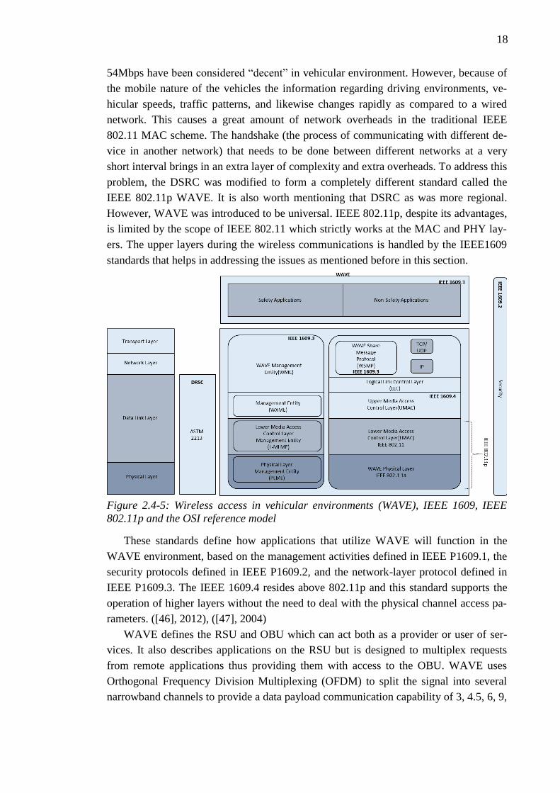
Figure 2.4-5: Wireless access in vehicular environments (WAVE), IEEE 1609, IEEE
802.11p and the OSI reference model
These standards define how applications that utilize WAVE will function in the
WAVE environment, based on the management activities defined in IEEE P1609.1, the
security protocols defined in IEEE P1609.2, and the network-layer protocol defined in
IEEE P1609.3. The IEEE 1609.4 resides above 802.11p and this standard supports the
operation of higher layers without the need to deal with the physical channel access pa-
rameters. ([46], 2012), ([47], 2004)
WAVE defines the RSU and OBU which can act both as a provider or user of ser-
vices. It also describes applications on the RSU but is designed to multiplex requests
from remote applications thus providing them with access to the OBU. WAVE uses
Orthogonal Frequency Division Multiplexing (OFDM) to split the signal into several
narrowband channels to provide a data payload communication capability of 3, 4.5, 6, 9,

19
12, 18, 24 and 27 Mbps in 10 MHz channels. A brief summary of IEEE 1609 standard
is mentioned in the table below. ([46], 2012), ([50], 2007)
IEEE
Standard
Reference Description
IEEE
Standard
1609
IEEE Standard 1455-1999
(1999). IEEE standard for mes-
sage sets for vehicle/roadside
communications (pp. 1–130).
Defines the overall architecture,
communication model, manage-
ment structure, security mecha-
nisms and physical access for wire-
less communications in the vehicu-
lar environment, the basic architec-
tural components such as OBU,
RSU, and the WAVE interface.
IEEE
Standard
1609.1-
2006
IEEE Standard 1609.1-2006
(2006). IEEE trial-use standard
for wireless access in vehicular
environments (WAVE)—
resource manager (pp. 1–63).
Enables interoperability of WAVE
applications, describes major com-
ponents of the WAVE architecture,
and defines command and storage
message formats.
IEEE
Standard
1609.2-
2006
IEEE Standard 1609.2-2006
(2006). IEEE trial-use standard
for wireless access in vehicular
environments—security services
for applications and management
messages (pp. 1–105).
Describes security services for
WAVE management and applica-
tion messages to prevent attacks
such as eavesdropping, spoofing,
alteration, and replay.
IEEE
Standard
1609.3-
2007
IEEE Standard 1609.3-2007
(2007). IEEE trial-use standard
for wireless access in vehicular
environments (WAVE)—
networking services (pp. 1–87).
Specifies addressing and routing
services within a WAVE system to
enable secure data exchange, ena-
bles multiple stacks of upper/lower
layers above/below WAVE net-
working services and defines
WAVE Short Message Protocol
(WSMP) as an alternative to IP for
WAVE applications.
IEEE
Standard
1609.4-
2006
IEEE Standard 1609.4-2006
(2006). IEEE trial-use standard
for wireless access in vehicular
environments (WAVE)—
multichannel operation (pp. 1–
74).
Describes enhancements made to
the 802.11 Media Access Control
Layer to support WAVE.

20
IEEE
Standard
Reference Description
IEEE
Standard
802.16e
IEEE Standard 802.16-2004
(2004). IEEE standard for local
and metropolitan area networks,
part 16: air interface for fixed
broadband wireless access sys-
tems.
Enables interoperable multi-vendor
broadband wireless access prod-
ucts.
Table 2.4-1: IEEE 1609 standards
2.5 Ad-hoc Routing Protocols
After explaining the 802 universe, where we also discussed 802.11 and IEEE 1609,
communication scheme, and amendments, it is obvious that standardization plays a key
role devices from different manufacturers communicating with each other. To make a
standard is not an easy task. But standardizing simplifies product use and its develop-
ment, reduces costs, and enables the manufacturers to create multiple devices that can
connect with each other. This guarantees the interoperability and interconnectivity of
products that in turn helps the users to compare and choose the product. One of the main
reason for a standard to be successful and useful is because of its routing algorithm.
VANET is a specific class of Ad Hoc network and the routing protocols used in MA-
NET has been implemented in VANET.
In recent years VANET has been a topic of big interest not only for researchers but
also for commercial manufacturers. Address based and topology based algorithm are
widely accepted means of routing where each node is assigned an address. Since the
general information like topology, vehicle density, mobility patterns, etc. are changing
rapidly in a vehicular environment, it is almost impossible for the traditional routing
protocols of MANET to assign a unique address to all the vehicles. Hence, small en-
hancements or changes have been done to this protocol that makes the routing algorithm
usable in vehicular environment.
Improvements in technologies in recent years have enabled the development of sen-
sor nodes which are smaller, cheaper, power efficient, and multifunctional. These sensor
nodes have the capabilities to sense, process data, and communicate without being per-
manently tethered with other similar nodes. These sensors can be deployed in a large
number that form a certain network topology. The main difference from the traditional
network is that the position and the location of the nodes can change with time as they
can be mobile as well. This suggests that these nodes should have the capability of self-
organizing.
It has already been mentioned that for a protocol to be usable the routing protocol
plays a vital role. In an infrastructure-less network these routing protocols can be divid-
ed into two types (Proactive and Reactive routing) which will be explained in the com-
ing section.

21
2.5.1 Proactive Routing
Proactive routing protocols maintain routes to all the destinations even if they are not
needed, i.e. it maintains all routes to all destinations at all times. To correct the route
information consistently, a node must periodically send control packets to update the
table, which means that proactive routing protocols consume bandwidth unnecessarily
as the control packets are sent out even when there is no data traffic. On the other hand,
the advantage of this protocol is that the nodes can send data with lower delay.
Proactive routing protocols use standard distance-vector routing (e.g., Destination-
Sequenced Distance Vector (DSDV) routing) or link-state routing strategies (e.g., Op-
timized Link State Routing protocol (OLSR) and Topology Broadcast-based on Re-
verse-Path Forwarding (TBRPF)). They maintain and update information about routes
among all nodes of a given network at all times even if the paths are not used. Route
updates are periodically performed regardless of network load, bandwidth constraints,
and network size. Despite lower delay, the main drawback of such approaches is that the
maintenance of unused paths may occupy a significant part of the available bandwidth if
the topology of the network changes frequently. Since a network between vehicles is
extremely dynamic, proactive routing algorithms are often inefficient. ([45], 2008),
([46], 2012)
DSDV is a table-driven algorithm based on the classical Bellman-Ford routing
mechanism ([2], 1996), ([36], 1997)where the algorithm has been improved to allow
freedom from loops in routing table i.e. each node maintains the shortest path to destina-
tion and the first node on this shortest path. It has already been mentioned that every
node maintains a record of the routing table which can be visualised as below. Here
every entry in a node is given a sequence number that allows the nodes to recognize the
stale routes preventing routing loops.
DSDV is characterised by:
Routes to the destination are available at each node in the routing table (RT)
RTs are exchanged between neighbours at regular intervals
RTs are also exchanged when significant changes in local topology are ob-
served by a node
RTs are updated as incremental updates or full dumps. Incremental updates
take place when a node does not observe significant changes in a local to-
pology whereas full dumps take place when significant changes in the local
topology are observed
Theses update techniques help make the routing algorithm a viable option, provided
that the sensor nodes have a decent memory size. Incremental updates help to renew the
RT information since the last full dump. The full dump carries all the available routing
information and can require multiple network protocol data units (NPDUs). NPDU also
ensures that less traffic is generated. During the time of occasional movement, these
packets are also transferred occasionally. The mobile nodes also contain an additional
table in which they stack the data sent in the incremental routing information packets

22
which contains the sequence number of the information received regarding the destina-
tion, the number of hops to the destination, address of the destination, as well as a new
sequence number unique to the broadcast. It automatically uses the route with the most
recent sequence number. If the two updates have the same sequence number, the route
with the smaller metric is used for the shortest path. The nodes also record the settling
time of routes, or the weighted average time that routes to a destination will vary before
the route with the best metric is received.
Because of the extra overheads, this technique is not useful in a network with large
number of nodes, despite low latency and delay as the overhead increases by O(n^2).
2.5.2 Reactive Routing
Reactive routing protocols implement route determination on a per demand or need-to
basis and maintain only the routes that are currently in use, thereby reducing the over-
heads as only a subset of the available routes is being used at any time. Communication
among vehicles will use only a very limited number of routes and thus this reactive
routing is particularly suitable for VANET application scenario. Consequently, the route
updates with extra information is not required, which lowers the storage requirements as
only the routes in cache are stored. However, this protocol also has its disadvantages
which are listed below:
High delay of route setup process as routes are established on-demand
Low scalability with no route updates
Dynamic Source routing (DSR) and Ad Hoc On demand Distance Vector (AODV)
are the most common routing protocols for reactive routing.
AODV is an advanced form of DSDV and belongs to class of Distance Vector rout-
ing protocols (DV). In a DV every node knows its neighbours and the costs to reach
them. A node maintains its own routing table, storing all nodes in the network, the dis-
tance, and the next hop to them. If a node is not reachable, the distance to it is set to
infinity. Every node periodically sends its whole routing table to its neighbours which
enables them to check if there is a useful route to another node using this neighbour as
the next hop. When a link breaks, Count-To-Infinity (typically occurs in Bellman-Ford)
may occur ([11]), ([13], 2012). AODV supports unicast, broadcast, and multicast with-
out the assistance of any other protocols. Count-To-Infinity and loop problems are
solved by using sequence numbers and registering costs. In AODV every hop has con-
stant cost of one. Routes that are unused age very quickly in order to accommodate the
movement of the mobile nodes. Link breakages can locally be repaired very efficiently.
AODV treats an IP address just as a unique identifier. This can easily be done by setting
the subnet mask to 255.255.255.255. Only one router in each of them is responsible to
operate AODV for the whole subnet which also serves as the default gateway. It has to
maintain a sequence number for the whole subnet and to forward every packet. For
AODV to be usable in a larger heterogeneous network, it requires hierarchical routing
on top of it.

23
One distinguishing feature of AODV is its use of a destination sequence number for
each route entry ([3], 2002). The destination sequence number is created by the destina-
tion to be included along with any route information it sends to requesting nodes. Using
destination sequence numbers ensures loop freedom. Given the choice between two
routes to a destination, a requesting node is required to select the one with the greatest
sequence number.
Route Requests (RREQs), Route Replies (RREPs), and Route Errors (RERRs) are
the message types defined by AODV. When a node does not have a valid route to desti-
nation an RREQ is forwarded. When intermediate node receives the RREQ packet it
checks whether the packet has a valid route to destination or not. If it has then the node
forwards it, if not then the node prepares an RREP message. If the RREQ is received
multiple times then the Broadcast ID (BcastID) and Source ID (SrcID) are compared
and the duplicate copies are simply discarded. When RREQ is forwarded, the address of
previous node and its BcastID are stored, which are needed to forward packets to the
source. If the RREP is not received by the node within a certain period of time, this en-
try is deleted from the node memory. Either the destination node or the intermediate
node responds with valid route. When RREQ is forwarded back, the address of the pre-
vious node and its BcastID are stored which are necessary to forward packets to the
destination. In case of a link break, the end nodes are notified by an unwanted RREP
with the hop count set to infinity. The end node deletes entries and establishes a new
path using a new BcastID, where the link status is observed using the link-level beacons
or link-level acknowledgements (ACKs). ([9], 2010), ([10], 2011)
The Dynamic Source Routing protocol (DSR) is a simple and efficient on-demand
routing protocol designed specifically for use in multi-hop wireless ad hoc networks of
mobile nodes. The network that implements DSR is completely self-organizing and self-
configuring, requiring no existing network infrastructure or administration. The DSR
protocol is composed of two main mechanisms that work together to allow the discov-
ery and maintenance of source routes in the ad hoc network:
Route Discovery is the mechanism by which a source node S wishing to send a
packet to a destination node D obtains a source route to D.
Route Discovery is used only when S attempts to send a packet to D and does
not already know a route to D.
This means that during the route contraction phase, DSR floods RREQ packets in
the network. The intermediate nodes forward only the non-redundant RREQs, following
which the destination node replies with an RREQ. The RREQ packet contains the path
traversed by RREQ packet. The receiver responds only to the first RREQ (i.e. if it is not
a duplicate one).
2.6 Chapter Summary
In this chapter we discussed about VANET where it is evident by now that this thesis
work is interested in the infrastructure less V2V network. Because of the interest in the

24
field of VANET a specific protocol called 802.11p has been introduced to meet the
specification and requirement of VANET. 802.11 is a set of MAC and PHY layer speci-
fication for implementation of WLAN in a device maintained by the IEEE LAN/MAN
standard committee and 802.11p aided by IEEE 1609 is the further MAC and PHY
amendment version of 802.11 that defines the vehicular communication system called
WAVE. The routing protocol in VANET are reactive routing techniques that maintains
a routing table which are currently being used.

5. Kirjoitusprosessin eteneminen 25
3. SIMULATION FRAMEWORK
Network Simulator Version 2 (NS2), is an open-source, event driven simulation tool
running on Unix-like operating system (OS) which is useful in studying the dynamic
nature of communication networks. Simulation of wired as well as wireless network
functions and protocols (e.g., routing algorithms, TCP, UDP) can be done using NS2
([22], 2008). In general, NS2 provides users with a way of specifying such network pro-
tocols and simulating their corresponding behaviours.
NS2 is a discrete event simulator that targets networking research and provides sub-
stantial support for simulation of the various aspects of a modern communication net-
work, like packet routing, unicast and multicast packet delivery, etc., that use protocols
such as UDP, TCP, RTP and SRM over the wired and the wireless networks. Needless
to say, it supports multiple protocols and possesses the capability of graphically detail-
ing the network traffic. It also implements several algorithms used in routing and queu-
ing like LAN routing and fair queuing, etc. ([22], 2008), ([26], 2003)
NS2 was a popular choice in the networking research community which is based on
the REAL network simulator created by the University of California and Cornell Uni-
versity in 1989. REAL is used for studying the dynamic behaviour of flows and conges-
tion control schemes in packet-switched data networks. In 1995 NS development was
funded by the Defence Advanced Research Projects Agency, DARPA, through the
VINT project at LBL, Xerox PARC, UCB, and USC/ISI. The inclusions of codes from
the UCB Daedelus and CMU Monarch projects and Sun Microsystems have added the
wireless capabilities to ns-2.
In a wireless setting, a list-based improvement for NS-2 involving maintaining a
double linked list to organize mobile nodes based on their X-coordinates was proposed
by Valery Naumov. He proposed that when sending a packet, only those nodes are con-
sidered, which are within a circle corresponding to the carrier-sense threshold energy
level, below which a node cannot hear the packet. This increased the performance by
about four to 20 times, depending on the size of the topology. ([37], 2005)
NS-2 is available on several platforms such as FreeBSD, Linux, SunOS and Solaris.
NS-2 also builds and runs under Windows with Cygwin. Simple scenarios should run
on any reasonable machine; however, simulations involving a large number of nodes
obviously benefit from large amounts of memory and fast CPU’s.
The main objective of this chapter is to provide the readers with insights into the
NS2 architecture on the basis of ns-2.34 which is used for simulating the scenarios cre-
ated for this thesis work. In particular, Section 3.1 presents the basic architecture of

5. Kirjoitusprosessin eteneminen 26
NS2. The information on NS2 installation is given in Section 3.2. Section 3.4 shows
NS2 directories and conventions. Section 3.5 shows the main steps in NS2 simulation.
Various examples on NS2 can be found at:
1M. Greis. Tutorial for the Network Simulator NS2. [Online]. Avail-
able: http://www.isi.edu/nsnam/ns/tutorial/
J. Chung and M. Claypool. Ns by example. [Online]. Available:
http://nile.wpi.edu/NS/
The Network Simulator Wiki–Contributed Code. [Online]. Availa-
ble: http://nsnam.isi.edu/nsnam/index.php/Contributed_Code
3.1 NS2 Architecture
Ns-2 is a discrete event simulator that makes use of both TCL and C++ programming
language. One of the most important parts of DES is the scheduler as it schedules the
events and calls the appropriate event handler methods when they occur. In NS2, there
are five schedulers available in the simulator, each of which is implemented by using a
different data structure: a simple linked-list, heap, calendar queue (default) and a special
type called ''real-time''. The scheduler runs by selecting the next earliest event, execut-
ing it to completion, and returning to execute the next event. The units of time used by
the scheduler are seconds. ([40], 2005)
An event is handled by calling the appropriate Handler class. The most important
Handler is NsObject (Network Simulator Object) with TclObject (Tool Command Lan-
guage) as its twin in the OTcl (Object-oriented Tool Command Language) world. They
provide all the basic functions allowing objects to interact one with another. For this
purpose the receive function group is mainly used. For handling OTcl statements in
C++, NsObjects provide the so-called command function. NsObject is the parent class
for some important classes as the Classifier, the Connector and the TraceFile class.
Figure 3.1-1: NS2 class diagram handle
1It also has a detailed description on documentation, finding documentation on ns, nam, Tcl, and C++. It
is recommended for beginners to read this website for further insight on NS2.

5. Kirjoitusprosessin eteneminen 27
Figure 3.1-1: NS2 class diagram handle is provided so that it will be of some help to
understand the NS2 architecture which has been explained in brief in the following par-
agraphs.
NS2 provides users with an executable command “.ns” which takes an input argu-
ment, the name of a TCL simulation scripting file with file extension “.TCL”. The TCL
simulation script acts as an input argument of an NS2 executable command ns which
results in a simulation trace file as output. The trace file can be used to plot graph (using
xgraph feature) and/or to create animation (using nam feature). Figure 3.1-2: Basic NS2
architecture explains in brief the NS2 architecture.
Figure 3.1-2: Basic NS2 architecture
NS2 consists of two key languages: C++ and Object-oriented Tool Command Lan-
guage (OTcl). C++ defines the internal mechanism (i.e. a backend) of the simulation
objects whereas the OTcl sets up simulation by assembling and configuring the objects
as well as scheduling discrete events (i.e., a frontend). The C++ and the OTcl are linked
together using TclCL (TCL with classes). Mapped to a C++ object, variables in the
OTcl domains are sometimes referred to as handles. Conceptually, a handle (e.g. n as a
Node handle) is just a string (e.g. _o10) in the OTcl domain, and does not contain any
functionality. Instead, the functionality (e.g., receiving a packet) is defined in the
mapped C++ object (e.g., of class Connector). In the OTcl domain, a handle acts as a
frontend which interacts with users and other OTcl objects. It may define its own proce-
dures and variables to facilitate the interaction. Note that the member procedures and
variables in the OTcl domain are called instance procedures (instprocs) and instance
variables (instvars), respectively. To summarize, the need of two languages is because
C++ handles the detailed simulations of protocols effectively (packet headers, bytes,
and algorithm implementation) whereas TCL, a scripting language, varies the parame-
ters or configurations and quickly explore the changing scenarios as iteration time is
more important than the run-time of the part of task.
It is very useful if the directories and conventions used in NS2 are also mentioned
here. This section covers the general convention used in NS2 that is pertinent to our
work. The installation of NS2 will be covered in brief in next section.
The NS2 all-in-one package is used for installation to reduce the complexity during
installation. All the necessary packages are archived in the ns-allinone-2.x.tar.gz, where
x is for the version. For the simulation purposes, we have used ns-allinone-2.35.tar.gz.
If any other packages or patches need to be used then they should be downloaded sepa-
rately or written by the user.

5. Kirjoitusprosessin eteneminen 28
The ns-allinone-2.35.tar.gz is installed in the ns-allinone-2.35 folder. The graphical
representation of the directories is shown in Figure 3.1-3: Directory structure of NS2:
Figure 3.1-3: Directory structure of NS2
3.2 Basic NS2 flow
As mentioned previously, the NS2 is controlled by TCL scripts with all the parameters
and configurations provided. The TCL script specifies how and where the files need to
be loaded as well as the path to the trace files, usually with extension nam (Network
animator) and a tr (trace) file, which are usually the output of a simulation. The general
NS2 flow can be represented pictorially as shown in Figure 3.2-1: Basic NS2 flowchart:
Figure 3.2-1: Basic NS2 flowchart
3.3 Installing NS2
This section gives information on where to download the latest NS2 package, documen-
tation on installation and similar relevant things. NS2 is a free simulation tool, which
can be obtained from source forge location provided below. It runs on various platforms
including UNIX (or Linux), Windows, and Mac systems. Having been developed in the
UNIX environment, it comes as no surprise that NS2 is installed and run most smoothly

5. Kirjoitusprosessin eteneminen 29
in a UNIX-like environment. Unless otherwise specified, the discussion in this book is
based on a Linux system.
NS2 source codes are distributed in two forms: the all-in-one suite and the compo-
nent-wise. With the all-in-one package, users get all the required components along with
some optional components. This is basically a recommended choice for the beginners.
This package provides an “install” script which configures the NS2 environment and
creates NS2 executable file using the “make” utility.
The latest version of ns2 is used which has been downloaded from:
http://sourceforge.net/projects/nsnam/files/allinone/ns-allinone-2.35/ns-allinone-
2.35.tar.gz/download
The instructions for installation
UNIX: http://www.isi.edu/nsnam/ns/
Windows:
http://nsnam.isi.edu/nsnam/index.php/Running_Ns_and_Nam_Under_Windows
_9x/2000/XP_Using_Cygwin
The installation process and difficulties faced will not be discussed in this thesis.
3.4 TCL Simulation Script
In this section we will introduce TCL and then mention about the simulation script used
for simulation. However, we will discuss the most basic features of a generic simulation
script rather than the one use in the simulation carried out as a part of the thesis. These
information have been taken from the TCL/tk documentation which can be downloaded
for free at [http://www.TCL.tk/doc/]. A detailed TCL simulation script used for simula-
tion can be found in ([22], 2008) and ([26], 2003).
As already mentioned, the TCL simulation script is used for configuring and param-
eterizing (manipulating) a simulation in NS2. TCL is an open source programming lan-
guage that provides users with the basic features found in any other programming lan-
guage like variables, control structures, and procedures. TCL was created by Jhon
Ousterhout. TCL is a very flexible programming language that can be used with any
other programming language ([26], 2003). TCL is a mixture of:
LISP/Scheme (mainly for its tail recursion capabilities)
C (control structures, expr syntax)
UNIX shells (with better structuring)
The TCL simulation script is a sequence of commands separated by newlines or
semicolons. All commands are strings which is a list of words separated by space. Word
is a string that begins and ends with the braces ({}).Arithmetic and logical expressions
are not part of the TCL language itself, but the language of the expr command (also
used in some arguments of the, if, for, and while commands) is basically equivalent to
C's expressions, with infix operators and functions. Here are some basic syntax rules in
TCL.

5. Kirjoitusprosessin eteneminen 30
Semi colons and newlines are command separators. Close brackets are command
terminators during command substitution (see below) unless quoted.
A command is evaluated in two steps. First, the TCL interpreter breaks the
command into words and then performs substitutions. The first word is used to
locate a command procedure to carry out the command, then all of the words of
the command are passed to the command procedure.
Words of a command are separated by white spaces.
The first character of a word denotes its type. If it is a double quote (“) it must
have a matching closing double quote. All the characters inside the closing dou-
ble quote is considered as normal characters or string.
If the first character is the open brace ({) then it should also be closed by the
matching closing brace and they can be nested that there can be multiple pair of
open braces within an open brace.
The words between a pair of open big bracket ([) performs command substitu-
tion. E.g. set y [set x 0] [incr x] [incr x]. Here, the value of y is set as 012.
This means the order of substitution is from left to right and one at a time as
shown in above example.
Words with dollar sign ($) performs variable substitution. E.g. $name(index)
where name gives the name of an array variable and index gives the name of an
element within that array. Name must contain only letters, digits, underscores,
and namespace separators, and may be an empty string. Command substitutions,
variable substitutions, and backslash substitutions are performed on the charac-
ters of index.
A word with a backslash (\) gives backslash substitution. E.g. \n is for newline,
\b for backspace, \t for tab, \v for vertical tab and so on.
Comments should always start with a hashtag (#). All the words are considered
as characters and the compiler and interpreter ignores the line.
The data types are also similar to the ones found in any other programming lan-
guage. The data types available are strings, lists, numbers, Booleans, characters, and
internal representation (the interpreter will choose between string and structured repre-
sentation based on the situation). The TCL script used for simulation can be found in the
3.5 Simulation Concept
The NS2 simulation consists of two parts, the network configuration phase and simula-
tion phase.
3.5.1 Network configuration phase
When the TCL script is compiled in NS2 it first constructs a network and schedules
chain of events called “at-events” which corresponds to all the lines in the TCL script
before executing the instproc run{} of the simulator object “ns”. The initial chain of

5. Kirjoitusprosessin eteneminen 31
events corresponds to those events that are scheduled to happen at certain period of time
during the simulation. E.g. start PBC (Periodic Broadcasting) traffic at 0.1 seconds. It is
also worth notifying that each event has its own execution time and a reference to the
next event along with its own execution time.
3.5.2 Simulation Phase
In this phase NS2 moves along each line and executes them chronologically right after
calling the instproc run {}. E.g. PBC traffic starts at 0.1 seconds which in turn creates
another event of PBC traffic at say 0.5 seconds. In between the time frame NS2 simu-
lates the internal events created by the compiler. This is also termed as “dispatching an
event”. All this happens in a chronological order hence the user should always be aware
about which step to follow while writing a TCL simulation script in NS2.
This phase continues until the instproc halt {} is called which marks the end of “dis-
patching an event”.
3.6 Wireless Simulation based on 802.11p
The NS2 was first used in a wireless simulation in the CMU Monarch Project
(http://www.monarch.cs.rice.edu/) in 1998 and since then NS2 has proved to be a very
popular simulation tool for wireless research. A lot of extensions to the original imple-
mentations have been made, as well as numerous bugs in the original implementation
have been fixed. The feature of this network simulation tool is it can enable a user to
define an arbitrary network that has nodes, links, routers, etc. The nodes are provided
with protocol sets called “agent” which sets the tone of packet transmission. In NS2 the
links between two communicating points can be wired, wireless, or satellite. We will
use the “wireless” feature of NS2. The output of these features can be interpreted in a
user-friendly way in NS2 with the help of a graphical visualizer called Network Anima-
tor (NAM), that uses the files with extension “.nam” to get more insights into the pack-
ets travelling in the network.
In this section we will talk about the basic wireless TCL model used in NS2 with a
special case for 802.11p. The basic wireless model can be categorised as node and net-
work stack where network stack comprises of link layer, address resolution protocol
(ARP), interface queue, and the physical (PHY) and MAC layer parameters.
3.6.1 Node
The wireless model in NS2 has a node type “mobile” at its core. These nodes are as-
sisted by supporting features that help in multi-hop Adhoc network simulations. The
MobileNode object is a split object for class MobileNode which is derived from class
Node. The basic features of Node are incorporated in class MobileNode along with mo-
bility in a defined topology and the ability to be a transceiver in a wireless channel. The
main purpose of creating a MobileNode is to use it in a wireless scenario i.e. link-less
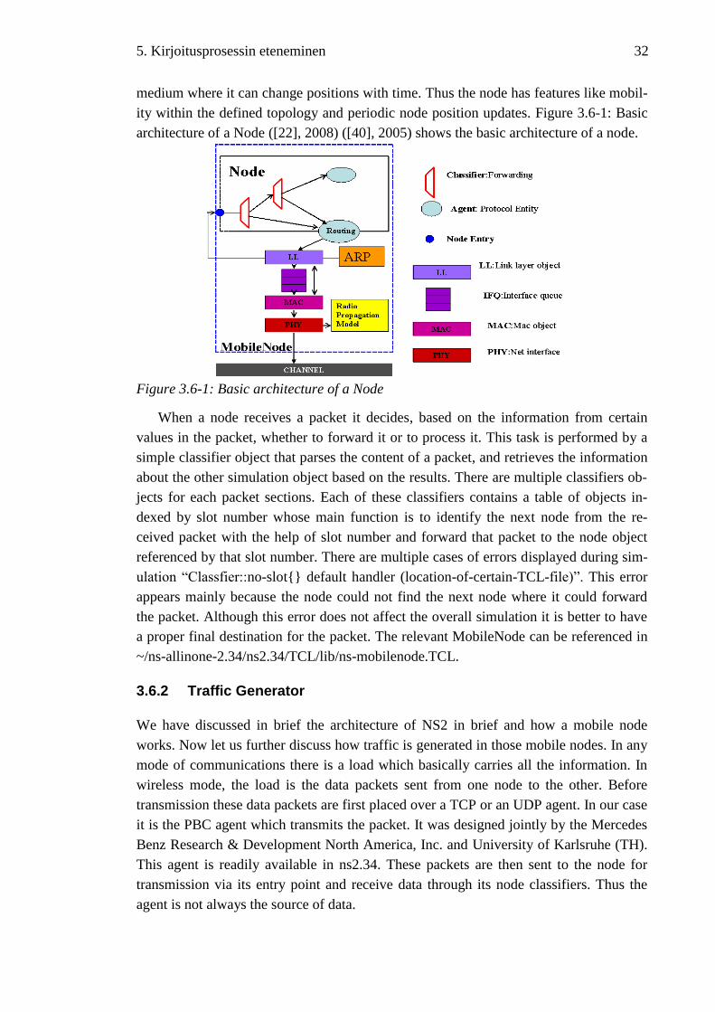
5. Kirjoitusprosessin eteneminen 32
medium where it can change positions with time. Thus the node has features like mobil-
ity within the defined topology and periodic node position updates. Figure 3.6-1: Basic
architecture of a Node ([22], 2008) ([40], 2005) shows the basic architecture of a node.
Figure 3.6-1: Basic architecture of a Node
When a node receives a packet it decides, based on the information from certain
values in the packet, whether to forward it or to process it. This task is performed by a
simple classifier object that parses the content of a packet, and retrieves the information
about the other simulation object based on the results. There are multiple classifiers ob-
jects for each packet sections. Each of these classifiers contains a table of objects in-
dexed by slot number whose main function is to identify the next node from the re-
ceived packet with the help of slot number and forward that packet to the node object
referenced by that slot number. There are multiple cases of errors displayed during sim-
ulation “Classfier::no-slot{} default handler (location-of-certain-TCL-file)”. This error
appears mainly because the node could not find the next node where it could forward
the packet. Although this error does not affect the overall simulation it is better to have
a proper final destination for the packet. The relevant MobileNode can be referenced in
~/ns-allinone-2.34/ns2.34/TCL/lib/ns-mobilenode.TCL.
3.6.2 Traffic Generator
We have discussed in brief the architecture of NS2 in brief and how a mobile node
works. Now let us further discuss how traffic is generated in those mobile nodes. In any
mode of communications there is a load which basically carries all the information. In
wireless mode, the load is the data packets sent from one node to the other. Before
transmission these data packets are first placed over a TCP or an UDP agent. In our case
it is the PBC agent which transmits the packet. It was designed jointly by the Mercedes
Benz Research & Development North America, Inc. and University of Karlsruhe (TH).
This agent is readily available in ns2.34. These packets are then sent to the node for
transmission via its entry point and receive data through its node classifiers. Thus the
agent is not always the source of data.
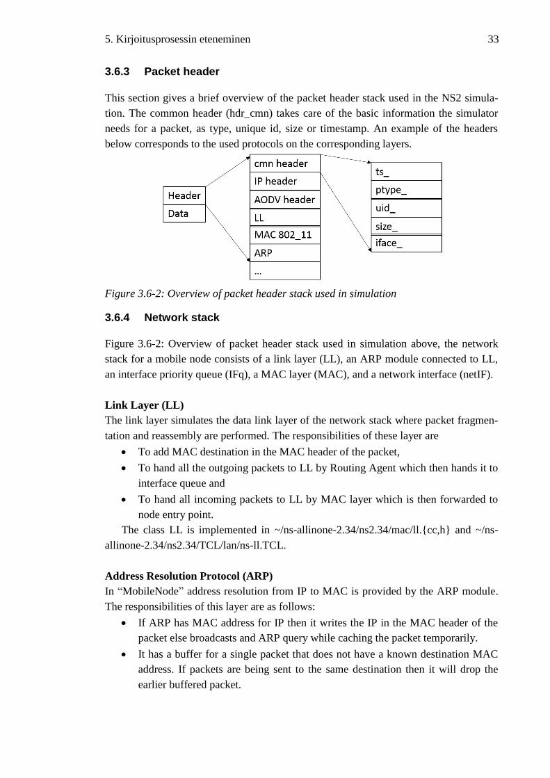
5. Kirjoitusprosessin eteneminen 33
3.6.3 Packet header
This section gives a brief overview of the packet header stack used in the NS2 simula-
tion. The common header (hdr_cmn) takes care of the basic information the simulator
needs for a packet, as type, unique id, size or timestamp. An example of the headers
below corresponds to the used protocols on the corresponding layers.
Figure 3.6-2: Overview of packet header stack used in simulation
3.6.4 Network stack
Figure 3.6-2: Overview of packet header stack used in simulation above, the network
stack for a mobile node consists of a link layer (LL), an ARP module connected to LL,
an interface priority queue (IFq), a MAC layer (MAC), and a network interface (netIF).
Link Layer (LL)
The link layer simulates the data link layer of the network stack where packet fragmen-
tation and reassembly are performed. The responsibilities of these layer are
To add MAC destination in the MAC header of the packet,
To hand all the outgoing packets to LL by Routing Agent which then hands it to
interface queue and
To hand all incoming packets to LL by MAC layer which is then forwarded to
node entry point.
The class LL is implemented in ~/ns-allinone-2.34/ns2.34/mac/ll.{cc,h} and ~/ns-
allinone-2.34/ns2.34/TCL/lan/ns-ll.TCL.
Address Resolution Protocol (ARP)
In “MobileNode” address resolution from IP to MAC is provided by the ARP module.
The responsibilities of this layer are as follows:
If ARP has MAC address for IP then it writes the IP in the MAC header of the
packet else broadcasts and ARP query while caching the packet temporarily.
It has a buffer for a single packet that does not have a known destination MAC
address. If packets are being sent to the same destination then it will drop the
earlier buffered packet.

5. Kirjoitusprosessin eteneminen 34
The class ARPTable is implemented in ~/ns-allinone-2.34/ns2.34/arp.{cc,h} and
~/ns-allinone-2.34/ns2.34/TCL/lib/ns-mobilenode.TCL.
Interface queue
The location of a packet (priority) in a queue in the network stack is done by the class
“PriQueue”. It supports running a filter over all packets in the queue and removes those
with a specified destination address. It is implemented in ~/ns-allinone-
2.34/ns2.34/priqueue.{cc,h} for interface queue.
MAC layer
Historically, ns-2 (prior to release ns-2.33) has used the implementation of IEEE 802.11
distributed coordination function (DCF) from CMU. Starting with ns-2.33, several
802.11 implementations are available like:
802.11 DCF from CMU
802.11 infrastructure extensions
802.11Ext
dei80211mr
We will be using the 802.11Ext which was developed by Mercedes-Benz Research
and Development North America and University of Karlsruhe which was called
Mac802_11Ext and WirelessPhyExt, respectively. Its features are
structured design of MAC functionality modules: transmission, reception,
transmission coordination, reception coordination, backoff manager, and channel
state monitor,
cumulative SINR computation, MAC frame capture capabilities, multiple modu-
lation scheme support, packet drop tracing at the PHY layer, Nakagami fading
model, etc.
This model should be used as a replacement for the existing models. The example
scripts show how to do this.
Key files: apps/pbc.{cc,h}, mac/mac-802_11Ext.{cc,h}, mac/wireless-
phyExt.{cc,h}, mobile/nakagami.{cc,h}
Documentation: http://dsn.tm.uni-karlsruhe.de/Overhaul_NS-2.php
Example scripts: ~/ns-allinone-2.34/ns2.34/TCL/ex/802.11/ directory: IEEE802-
11a.TCL, IEEE802-11p.TCL, broadcast_validation.TCL, and
unicast_validation.TCL
Test suite: ~/ns-allinone-2.34/ns2.34/TCL/test/test-suite-wireless-lan-newnode-
80211Ext.TCL
Network interface
This layer serves as a hardware interface used by mobile node to access the channel.
This interface handles collisions and the radio propagation model from where the pack-
ets transmitted by other nodes are received. It indexes the transmitted packet with meta-

5. Kirjoitusprosessin eteneminen 35
data like transmitting power, wavelength, etc. This meta-data is used by propagation
model in the receiving network interface to determine if the packet has the required
power to be received, captured, or detected. It is implemented in ~/ns-allinone-
2.34/ns2.34/mac/phy.{cc.h} and ~/ns-allinone-2.34/ns2.34/mac/wireless-phy.{cc,h} for
network interface implementations.
Radio Propagation Model
It uses Friis-space attenuation (1/r2) at near distances and an approximation of Two Ray
Ground (1/r4) at far distances. The approximation assumes specular reflection off a flat
ground plane. Implemented in ~/ns-allinone-2.34/ns2.34/mobile/tworayground.{cc,h}.
Antenna
An omni-directional antenna having unity gain is used by mobile nodes. It is imple-
mented at ~/ns-allinone-2.34/ns2.34/mobile/antenna.{cc,h} and ~/ns-allinone-
2.34/ns2.34/mobile/omni-antenna.{cc,h}
3.7 Trace File
As mentioned earlier NS2 has trace files as output. There are two types of trace files
Normal trace file ($ns_ trace-all commands), extension: .tr
Revised format for wireless traces ($ns use-newtrace), extension: .tr
NAM trace file ($ns_ nam-traceall), extension: .nam
The normal trace file is optimal to study the protocol because it consists of all the
data generated during the simulation. In the trace file every line corresponds to one sin-
gle event during the simulation. The line starts with the most general parameters and
ends with specific ones. While simulation it is uncommon for the trace file to be quite
large in size (in this case ~56 GB).
This command should be called before the universal trace command “$ns trace-all
trace-fd”. Primitive “use-newtrace” sets up new format for wireless tracing by setting a
simulator variable called “newTraceFormat”. Currently this new trace support is availa-
ble for wireless simulations only. Example of the new trace format obtained from the
simulation file is shown below:
s -t 0.000000000 -Hs 0 -Hd -1 -Ni 0 -Nx 0.00 -Ny 50.00 -Nz 0.00 -Ne -1.000000 -Nl
AGT -Nw --- -Ma 0 -Md 0 -Ms 0 -Mt 0 -Is 0.0 -Id -1.0 -It PBC -Il 500 -If 0 -Ii 0 -Iv 32
r -t 0.000802167 -Hs 1 -Hd -1 -Ni 1 -Nx 50.00 -Ny 50.00 -Nz 0.00 -Ne -1.000000 -Nl
AGT -Nw --- -Ma 0 -Md ffffffff -Ms 0 -Mt 0 -Is 0.0 -Id -1.0 -It PBC -Il 500 -If 0 -Ii 0 -
Iv 32
The various event that are shown in the output has specific meaning ([26], 2003),
([42], 2007).
Event Type Description
s send
r receive

5. Kirjoitusprosessin eteneminen 36
Event Type Description
d drop
f forward
-t time
-t *(global
Node property
tags
Description
-Ni node id
-Nx node's x-coordinate
-Ny node's y-coordinate
-Nz node's z-coordinate
-Ne node energy level
-Nl trace level, such as AGT, RTR, MAC
-Nw Reason for the packet to be dropped:
"END": DROP_END_OF_SIMULATION
"COL": DROP_MAC_COLLISION
"DUP": DROP_MAC_DUPLICATE
"ERR": DROP_MAC_PACKET_ERROR
"RET": DROP_MAC_RETRY_COUNT_EXCEEDED
"STA": DROP_MAC_INVALID_STATE
"BSY": DROP_MAC_BUSY
"NRTE": DROP_RTR_NO_ROUTE i.e. no route is available.
"LOOP": DROP_RTR_ROUTE_LOOP i.e. there is a routing loop
"TTL": DROP_RTR_TTL i.e. TTL has reached zero.
"TOUT": DROP_RTR_QTIMEOUT i.e. packet has expired.
"CBK": DROP_RTR_MAC_CALLBACK
"IFQ": DROP_IFQ_QFULL i.e. no buffer space in IFQ.
"ARP": DROP_IFQ_ARP_FULL i.e. dropped by ARP
"OUT": DROP_OUTSIDE_SUBNET i.e. dropped by base sta-
tions on receiving routing updates from nodes outside its domain.
Packet info at
IP level
The tags for this field start with a leading "-I"
-Is source address.source port number
-Id dest address.dest port number
-It packet type
-Il packet size
-If flow id
-Ii unique id
-Iv ttl value
Next hop info next hop info and the tag starts with a leading "-H"
-Hs id for this node

5. Kirjoitusprosessin eteneminen 37
Event Type Description
-Hd id for next hop towards the destination
MAC layer
information
starts with a leading "-M"
-Ma duration
-Md dst's ethernet address
-Ms src's ethernet address
-Mt ethernet type
Packet info at
application
level
Application type like ARP and TCP. Type of Adhoc routing proto-
col like PUMA, DSR, AODV, etc being traced. Starts with "-P".
For -Parp
-Po ARP Request/Reply
-Pm src mac address
-Ps src address
-Pa dst mac address
-Pd dst address
Adhoc routing
protocol
Dynamic source routing “-Pdsr”
-Pn how many nodes traversed
-Pq routing request flag
-Pi route request sequence number
-Pp routing reply flag
-Pl reply length
-Pe src of srcrouting->dst of the source routing
-Pw error report flag ?
-Pm number of errors
-Pc report to whom
-Pb link error from linka->linkb
Constant bit
rate
-Pcbr
-Pi sequence number
-Pf how many times this pkt was forwarded
-Po optimal number of forwards
-P tcp
TCP flow info -Ptcp
-Ps seq number
-Pa ack number
-Pf how many times this pkt was forwarded
-Po optimal number of forwards

5. Kirjoitusprosessin eteneminen 38
The NAM trace file is a subset of a normal trace file with the suffix ".nam". It con-
tains information for visualizing packet flow and node movement for use with the NAM
tool which is a TCL/Tk based animation tool for viewing network simulation traces and
real world packet trace data. NAM was created for users to be able to read large anima-
tion data sets in visual format and which can be extended, so that it could be used in
different network visualization situations.
As covering the details of trace file would not be relevant for the thesis work hence
for further details on the trace file please refer to:
http://nsnam.isi.edu/nsnam/index.php/NS-2_Trace_Formats.
cmu-trace.h and cmu-trace.cc file located at ~/ns-allinone-2.35/ns-2.35trace
After taking a walk through about NS2, it can be understood that it is real time dis-
crete event open source software that has a very rich infrastructure for both developing
and implementing various protocols. NS2 provides a platform to study interaction be-
tween protocols in a controlled environment. Being an open source it is evident that
NS2 supports extensions as well.
Despite having all these positives, there are certain negatives for NS2 as well. The
most important downside of NS2 is that because it is a large system, it has a steep learn-
ing curve. Although, the use of two different programming languages for two different
purposes does make things very helpful, it is sometimes confusing even to the experts.
However, an active community of experts lend their helping hand to the beginners by
providing manuals, video tutorials, blogs, etc., and maintaining an active mailing list.
Even then the information available on these places is not exhaustive and the best way
to familiarize with NS2 is to experiment with it first hand, which helps to develop an
intuitive grasp on the internal workings of the simulator.
When comparing the negatives with the positives, the positives weighed far more
than the negatives hence NS2 was the preferred simulation tool.
3.8 Summary
In this chapter we learned about the various core section of simulation framework which
is NS2. The information on this section is based on the version ns-2.34 on a Fedora 20
Heisenberg version. There are certain conventions which needs to be followed while
using ns2.34. Being open source it is very important for NS2 to maintain a directory
structure which also has C++ files that is used by the TCL simulation script. The node
created in wireless mode is different from the normal mode because of mobility factor
and periodic node position update. There are various network layer components which
needs to be described in tcl file during simulation. When a simple TCL script is run in
the network then the script is compiled on top-down approach. Each line in the TCL
script is then executed in a chronological order to provide us with the output results.

5. Kirjoitusprosessin eteneminen 39
4. NUMERICAL RESULTS
Simulation is the art of using tools – physical or conceptual models, or computer hard-
ware and software, to attempt to create the illusion of reality. The discipline has in re-
cent years expanded to include the modelling of systems that rely on human factors and
therefore possess a large proportion of uncertainty, such as social, economic or com-
mercial systems. These new applications make the discipline of modelling and simula-
tion a field of dynamic growth and new research. ([35], 2007)
This chapter describes the TCL script and the simulation techniques used for this
thesis work. For this thesis purpose we first decided that the scenario would be an ad
hoc network of stationary vehicles i.e. mobility factor was not considered. We have also
taken into account the distance between each node which is assumed to be constant at
the beginning of the simulation. The basic parameters that we are concerned with during
the simulation are:
a. distance between nodes,
b. coverage area of a single node (emitted/transmitter energy),
c. channel model,
d. the number of retransmissions allowed,
e. Contention Window,
f. packet broadcasting
The main goal of this thesis work is to determine different packet loss probabilities
in a V2V network by simulating it in NS2 with the 802.11p environment available in
the simulator. We have already discussed the basics of the simulation tool NS2 in Sec-
tion 3, while the nature of V2V network that has been considered has been discussed in
Section 2.
In this chapter we will discuss the simulation script that results in the intended out-
put. The basics of 802.11 and the simulation program as described in chapter 2 and 3
will be helpful in creating the scenario and getting the result which will be mentioned in
this chapter.
4.1 Simulation Scenario
Before getting into the TCL script, it is important to discuss about the scenario. Recall
that the main focus of this thesis work is to calculate the packet loss probabilities in a
vehicular network. Keeping this in mind it is important to note that a vehicle transmit-
ting packet must have at least one node within the range of its transmission. From here

5. Kirjoitusprosessin eteneminen 40
on we will refer the vehicles as “node” in order to make it compatible with NS2 termi-
nology.
We consider a very simple situation where the number of nodes is finite and station-
ary. By eliminating the movement we are focussing on the more simple and basic situa-
tion to strengthen our results for the efficiency of the 802.11p protocol in a vehicular
network. A node network lined up in a single lane with certain distance “d” is consid-
ered where the first node transmits a packet in the safety channel (SCH, chapter 2.3.1
Dedicated Short Range Communication (DSRC)). We have a considered a network
where the nodes are stationary. The packets transmitted by the first node is then passed
on by the following nodes. The pictorial representation is provided in Figure 4.1-1: Sce-
nario for packets travelling in the node network.
Figure 4.1-1: Scenario for packets travelling in the node network
The blue dots in Figure 4.1-1: Scenario for packets travelling in the node network
are the nodes placed at a uniform distance “d”. The black, green, and yellow arrow de-
notes the packet being broadcasted. The red arc denotes the range of node_(first). The
ideal case is that all packets generated by node_(first) reaches node_(last). However,
this is not the case in real world because of various reasons. In simulation mode the
packets might fail to reach all the nodes. However, simulation mode might be different
from real mode and the results will vary from the real case.
4.2 TCL script and output trace file
In simulation, a global variable is accessible by any function or entity in the system, and
basically keeps track of some common values of the simulation ([22], 2008). In the con-
text of computer networks, such variables might represent, for example, the length of
the packet queue in a single-server network, the total busy air time of the wireless net-
work, or the total number of packets transmitted. As mentioned earlier in Chapter 3, a
TCL file is a scripting language that makes use of the C++ file to simulate the environ-
ment. The TCL file for this thesis work takes seven parameters as its arguments.
Distance between nodes: 5, 10, 20, and 50
Retransmission attempt: 1, 3, and 5
Filename to give a unique filename for every output
Minimum contention window: set to 0 in all cases
Maximum contention window: 8, 16, and 32
Number of nodes: 250, 150, 70, and 40

5. Kirjoitusprosessin eteneminen 41
Seed: All simulation run with same seed would give same output. Hence, the
counter was set as the seed.
In order to create 802.11p environment for the simulation we used the IEEE802-
11p.tcl file readily available in ns2.34 located at ~ns-allinone-2.34/ns-
2.34/tcl/ex/802.11/IEEE802-11p.tcl. Its content can be found in Appendix A.
While creating a node there were few assumptions made. The “Configure RF model
parameters” and “Node configuration options” section in Appendix B defines the nature
of the node. We considered the antenna to be Omni directional in nature with a height of
1.5 meters. The basic tow ray ground propagation model is considered which is dis-
cussed in Network Stack of Chapter 3. The range of transmission of each node is set to
80 meters which corresponds to 0.0003108 watt power. The parameters which makes
the node act in the 802.11p protocol are the physical network interface and MAC. These
parameters uses the Mac/802_11Ext and Phy/WirelessPhyExt feature of NS2. These
parameters were specially designed for nodes that would be used in 802.11p scenario.
Two dimensional flat grid topography with dimension 2000-by-200.
Despite the reactive routing protocol available in the NS2 we chose to use DumbA-
gent because in NS2 simulation as the network layer protocol when no routing is re-
quired in the test scenario. In DumbAgent, it is assumed that the simulation scenario in
use is such that each source and destination node are directly neighbours and within one
hop distance from each other and hence require no routing techniques.
The trace file generated uses the new trace format as discussed in the section Trace
File of chapter 3.
There are two different kind of nodes defined for the simulation. The first node was
the packet generator and rest of the nodes were repeaters that received the packet and
retransmitted it according to the value of retransmission attempt. The section “PBC
Agents Definition” of Appendix B explains the two different types of nodes. It uses the
agent called PBC, discussed in the section Traffic Generator.
We have discussed in brief the architecture of NS2 in brief and how a mobile node
works. Now let us further discuss how traffic is generated in those mobile nodes. In any
mode of communications there is a load which basically carries all the information. In
wireless mode, the load is the data packets sent from one node to the other. Before
transmission these data packets are first placed over a TCP or an UDP agent. In our case
it is the PBC agent which transmits the packet. It was designed jointly by the Mercedes
Benz Research & Development North America, Inc. and University of Karlsruhe (TH).
This agent is readily available in ns2.34. These packets are then sent to the node for
transmission via its entry point and receive data through its node classifiers. Thus the
agent is not always the source of data. The modified code for PBC can be found in Ap-
pendix C and Appendix D.
When the first node is created the parameters that needs to be defined while creat-
ing the packet creator node are:
Payload size: 500 bytes
Periodic Broadcast Interval: 0.01 seconds

5. Kirjoitusprosessin eteneminen 42
Periodic Broadcast Variance 0.01 seconds
Modulation Scheme 1, QPSK (Quadrature Phase Shift Keying)
Because a single packet is being generated we use the single broadcast feature
In order for the packet to use the CCH channel with safety message the packet
type is set to 0 and the channel number is set to -99
For the repeater nodes, the parameter “Repeater” is set as ON. This parameter is not
available in the original PBC file and was created specifically for the thesis project. The
additional repeater function has following features:
Receive the message generated by the first node
Retransmit the message as per the retransmission attempt value
Same message is received multiple time however while transmitting the latest
received message is transmitted.
The repeater node does not generate its own message and rather act as a relay
The new trace file generates output file as mentioned in the section Trace File of
Chapter 3. An aggregate of 1000 simulation for each scenario will be discussed in the
next section.
4.3 Graph
The results generated were analysed on the basis of time and distance. This section will
describe the methodologies to transform the TCL output into graphs. Thereafter we will
discuss the graphs generated in each of the case highlighted below.
For Time based metric (Probability measure)
Probability to reach 500 meters within 1 second
o Extract the earliest reception time of the packet for a node, node id and
coordinates of the node from the resulting trace file.
o For the node located at 500 meter, count the total number of experiments
where the packets reached 500 meters before 1 second and store them in
a counter.
o Probability of reaching 500 meters within 1 second is given by dividing
the value of the counter obtained from step "b.i" by total number of ex-
periment
Probability = (total number of experiments where the packets reached 500 me-
ters before 1 second) / (total number of experiment)
Same procedure followed for:
Probability to reach 500 meters within 1 second
Probability to reach 1000 meters within 2 second
Probability to reach 1000 meters within 2 second
For Time based metric (Distribution of cars having a message within 1 second and
500 meters)

5. Kirjoitusprosessin eteneminen 43
Extract the earliest reception time of the packet for a node, node id and coordi-
nates of the node from the trace file.
Create an array for the unique nodes present in the file. (for x-axis)
Count the total number of times a node has received message within 1 second
Probability to get the message within 1 second
Probability (t <= 1 second) = (Total number of times a node has received mes-
sage within 1 second) / (the total number of nodes)
Note: Probability (t <= 1 second) for all the nodes is calculated for the scenario.
Same procedure is applied for:
Distribution of cars having a message within 2 second and 500 meters
Distribution of cars having a message within 1 second at 1000 meters
Distribution of cars having a message within 2 second and 1000 meters
For the distance-based metric, for 500 meters:
Mean time to reach 500 meters
Extract the earliest reception time of the packet for a node, node id and coordi-
nates of the node from the trace file.
Take a sum of the time at 500 meters
Take a sum of number of occurrence of 500 from the file.
Divide b by c.
I.e. Mean time to reach 500 meters = (Sum of times at 500 meters) / (sum of oc-
currence of 500)
Same procedure is repeated for mean time to reach 1000 meters.
Distribution of time to reach 500 meters
Extract the earliest reception time of the packet for a node, node id and coordi-
nates of the node from the trace file.
Note the time when packet reaches 500 meters in all the simulation output file.
Same procedure for distribution time to reach 1000 meters.
Distribution of cars having message when it reaches 500 meters
Extract the earliest reception time of the packet for a node, node id and coordi-
nates of the node from the trace file.
Determine number of nodes till 500 meters (x-axis)
Check the time “t” at which packet was received by node at 500 meters.
If the nodes that lies at distances less than 500 meters have received the packet
within the time “t” increase the counter by 1 else do nothing.
Divide the total counter value by the number of experiments (i.e. 1000 in our
case). This will give a normalized value of the number of time packet was re-
ceived at 500 meters.
Same procedure for distribution of cars having message when it reaches 1000 meters.

5. Kirjoitusprosessin eteneminen 44
4.3.1 Time Based Analysis
Time based probability to reach 500 and 1000 meters with 1 and 2 seconds
In this section we will discuss the probability to reach 500 meter within 1 second. The
graph generated are for retransmission attempts (1, 3, and 5) keeping the distance con-
stant at 500 meters and changing the contention window. In the end of this section is
given a combination of graph for distance 5, 10, 20, and 50 at different retransmission
attempt and contention window.
In the graph “probability to reach 500 meters within 1 second) we can see that as
distance increases the probability decreases, which is obvious and expected. The x-axis
denotes “retransmission” and “contention window” in the format “retransmis-
sion_contentionwindow”.
Figure 4.3-1: Probability to reach 500 meters within 1 second
In Figure 4.3-1: Probability to reach 500 meters within 1 second, the graph is a little
different when distance between nodes is 10 meters. The probability changes slightly
starting from 3_8. The other graph pattern are almost straight line which means that
probability changes slightly with a change in retransmission and contention window
value. However, a significant change in the probability is seen when nodes are at dis-
tance 10 meters.
0.000000
0.200000
0.400000
0.600000
0.800000
1.000000
1.200000
1_8 1_16 1_32 3_8 3_16 3_32 5_8 5_16 5_32
Prob to reach 500 meters within 1 second
5 mts
10 mts
20 mts
50 mts

5. Kirjoitusprosessin eteneminen 45
Figure 4.3-2: Probability to reach 500m within 2 seconds
Taking the second case is the probability to reach 500 meters within 2 second. We
can see that the probability hovers around 1 for node distance 5 and 10 meters. Howev-
er, there is a slight increase in probability when node distance is at 20 meters. The value
changes for 1_32 and 3_8. The other values are almost linear. When the node distance is
50 meters the probability is almost 0 for the packet to reach 500 meters within 2 second.
Figure 4.3-3: Probability to reach 1000m: within 1 sec
In Figure 4.3-3: Probability to reach 1000m: within 1 sec, the values at 5 meters dis-
tance depicted by the red line shows gradual rise in probability until it falls when re-
transmission attempt is 3 and contention window is (0,8). The probability rises at re-
transmission attempt is 3 and contention window is (0, 16). From 3_16 onwards there is
a gradual decrease in probability to reach 1000 meters within 1 second. However it
again rises steeply at 5_32. Although the probability fluctuates between 0.12 and 0.16
we can see that retransmission attempt and contention window plays a key role perfor-
mance of IEEE802.11p protocol in vehicular environment when nodes are at a distance
5 meters.
As compared to Figure 4.3-3: Probability to reach 1000m: within 1 sec the graph
shown in Figure 4.3-4: Probability to reach 1000m within 2 seconds increases signifi-
cantly for the packet to reach 1000 meters within 2 second. The plot in this case is inter-
0.000000
0.200000
0.400000
0.600000
0.800000
1.000000
1.200000
1_8 1_16 1_32 3_8 3_16 3_32 5_8 5_16 5_32
Prob to reach 500m: within 2 sec
5 mts
10 mts
20 mts
50 mts
0.000000
0.020000
0.040000
0.060000
0.080000
0.100000
0.120000
0.140000
0.160000
0.180000
1_8 1_16 1_32 3_8 3_16 3_32 5_8 5_16 5_32
Prob to reach 1000m: within 1 sec
5 mts
10 mts
20 mts
50 mts

5. Kirjoitusprosessin eteneminen 46
esting at node distance 20 meters as we can see fluctuation at 3_8 and onwards. The
probability decrease with the increase in node distance.
Figure 4.3-4: Probability to reach 1000m within 2 seconds
Time based distribution (probability) of cars having a message within 1 second at
500 and 1000 meters
In this section we will discuss the time based probability of cars having a message with-
in 1 second at 500 meters and 1000 meters. The graphs were generated using combina-
tion of node distance, retransmission, and contention window. Only 3 graphs were con-
sidered because all the graphs were of similar nature which shows that the probability of
the node receiving the message was of similar nature.
The graphs generated based on the combination of the parameters node distance, re-
transmission attempt and contention window.
For retransmission attempt 1 and contention window (0, 8):
Figure 4.3-5: Probability of cars having a message within 1 second for retransmission
attempt 1 and contention window (0, 8)
This graph in Figure 4.3-5: Probability of cars having a message within 1 second for
retransmission attempt 1 and contention window (0, 8) depicts how distance between
nodes changes the distribution of cars having a message for a fixed retransmission and
0.000000
0.200000
0.400000
0.600000
0.800000
1.000000
1.200000
1_8 1_16 1_32 3_8 3_16 3_32 5_8 5_16 5_32
Prob to reach 1000m: within 2 sec
5 mts
10 mts
20 mts
50 mts

5. Kirjoitusprosessin eteneminen 47
contention window. The x axis corresponds to the node number. We can see that as the
distance increases the probability decreases for a node to have messages.
Figure 4.3-6: Probability of cars having a message within 1 second for retransmission
attempt 1 and contention window (0, 8)
Considering the highest possible value for retransmission and contention window
we can see that the graph in Figure 4.3-6: Probability of cars having a message within 1
second for retransmission attempt 1 and contention window (0, 8) is almost similar to
the previous graph above, which shows that node distance plays a more prominent role
in packet delivery than retransmission and contention window as shown in Figure 4.3-6:
Probability of cars having a message within 1 second for retransmission attempt 1 and
contention window (0, 8).
Now considering the graphs for contention window (0, 8) as shown in Figure 4.3-7:
Probability of cars having a message within 1 second for node distance of 5m and re-
transmission attempt 1, we can see that the values are very close to each other. Howev-
er, on further analysis of the data we can see that all lines intersect at around node 130.
The contention window plays a key role starting from node 160 as the probability is
greater for higher contention window which shows that higher contention window helps
prevent collision of packet in the network.

5. Kirjoitusprosessin eteneminen 48
Figure 4.3-7: Probability of cars having a message within 1 second for node distance of
5m and retransmission attempt 1
The following graph for higher retransmission attempt (i.e. max value 5) depicts that
with increase in retransmission attempt the probability to reach the node at far away
distances is almost similar to each other and does not depend on contention window as
was the case above when retransmission attempt was 1.
Figure 4.3-8: Probability of cars having a message within 1 second for node distance
5m retransmission attempt 5
When the graph in Figure 4.3-8: Probability of cars having a message within 1 sec-
ond for node distance 5m retransmission attempt 5 is analysed we can see that more

5. Kirjoitusprosessin eteneminen 49
retransmission attempt means more collision around node number 140. However re-
transmission attempt 3 give better performance overall.
In Figure 4.3-9: Probability of cars having a message within 1 second for node dis-
tance 5m and contention window (0, 8) and Figure 4.3-10: Probability of cars having a
message within 1 second for node distance 5m and contention window (0, 8), if we in-
crease the contention window at same node distance (5 meters) we can see that proba-
bility for cars to have message within 1 second changes uniformly except at the nodes at
around 150. This might be due to high chances of collision at high retransmission at-
tempt.
Figure 4.3-9: Probability of cars having a message within 1 second for node distance
5m and contention window (0, 8)
Figure 4.3-10: Probability of cars having a message within 1 second for node distance
5m and contention window (0, 8)

5. Kirjoitusprosessin eteneminen 50
Time based distribution (probability) of cars having a message within 2 second at
500 and 1000 meters
In this section we will discuss the probability of cars having a message within 2 sec-
onds. As the time frame has doubled we should expect more nodes having a message
than in previous section when the time frame was only 1 second. Deduction from the
graphs generated based on the combination of node distance, retransmission attempt,
and contention window will be made as in previous section.
As expected we can see that the probability of cars having a message within 1 sec-
ond is very close to 1 considering the node distance only, as shown in Figure 4.3-11:
Probability of cars having a message within 2 second for retransmission attempt 1 and
contention window (0, 8). However the probability decreases gradually from node 150
onwards. The most notable deduction from the graph is probability with retransmission
attempt 3 is greater than that of 5. This might be due to greater number of packets avail-
able in the network which results in higher probability of collision when nodes retrans-
mits 5 times.
Figure 4.3-11: Probability of cars having a message within 2 second for retransmission
attempt 1 and contention window (0, 8)
The graph generated for the combination of retransmission attempt and contention
window gives similar result in all cases i.e. all nodes received message with decreasing
probability with increasing node distance.
Considering the contention window, the probability when the node distances be-
tween nodes are short ranges around 1. However at far away nodes (200 and forward)
the probability decreases gradually. However, when contention window is 8 the proba-
bility of cars having the message after 2 second is the highest. This might be because of
lower chances of packet collision as seen on Figure 4.3-12: Probability of cars having a
message within 2 second for node distance 5 meter and retransmission attempt 1

5. Kirjoitusprosessin eteneminen 51
Figure 4.3-12: Probability of cars having a message within 2 second for node distance
5 meter and retransmission attempt 1
Consider the retransmission window, when node distance is 5 meters and contention
window is (0, 8) as shown in Figure 4.3-13: Probability of cars having a message within
2 second for node distance 5 meters and contention window (0, 8):
Figure 4.3-13: Probability of cars having a message within 2 second for node distance
5 meters and contention window (0, 8)
Similarly, the graph depicts that retransmission attempt 3 provides the highest effi-
ciency when nodes are close to each other.
4.3.2 Distance based analysis
Distance based average time at 500 and 1000 meters
In this section we will discuss about the mean time and distribution of cars to have the
message at 500 and 1000 meters respectively. The x axis is a combination of retrans-
mission attempt and contention window.

5. Kirjoitusprosessin eteneminen 52
The graphs for the mean time to reach 500 meters is shown in Figure 4.3-14: Aver-
age time to reach 500 meters:
Figure 4.3-14: Average time to reach 500 meters
Figure 4.3-14: Average time to reach 500 meters shows that at lesser contention
window highest retransmission value gives the highest mean time for the packet to
reach 500 meter distance. All nodes have received the emergency packet which shows
that when the nodes are densely packed then the average time to reach the distance in-
creases with increase in node distance.
The graph for the average time to reach 1000 meters is as shown in Figure 4.3-15:
Average time to reach 1000 meters. It is clear that the emergency messages require a
very long time to reach 1000 meters if the node distance are high which might be fatal
for a driver.
Figure 4.3-15: Average time to reach 1000 meters
Distance based distribution of cars having message within 500 meters
In this section we will discuss the normalized distribution of time. A total of 1000 simu-
lations were run for each combination of node distance, retransmission attempt, and
contention window. The x-axis denotes the normalized frequency and y-axis denotes the
time when packet was received at the node.
0
1
2
3
4
5
1_8 1_16 1_32 3_8 3_16 3_32 5_8 5_16 5_32
Avg time to reach 500m
5 meters
10 meters
20 meters
50 meters
0
2
4
6
8
10
1_8 1_16 1_32 3_8 3_16 3_32 5_8 5_16 5_32
Avg time to reach 1000m

5. Kirjoitusprosessin eteneminen 53
When the nodes are densely packed at 5 meters distance with contention window of
size (0,8) and retransmission attempt 1 the normalised distribution graph generated is
shown in Figure 4.3-16: Distance based distribution of cars receiving message at 500
meters for retransmission attempt 1.
Figure 4.3-16: Distance based distribution of cars receiving message at 500 meters for
retransmission attempt 1
We can see that most of the receiving was done within 0.4 to 0.8 seconds after the first
packet was transmitted by the first node. Similarly for maximum retransmission the
graph obtained was:
Figure 4.3-17: Distance based distribution of cars receiving message at 500 meters for
retransmission attempt 5
Which shows that most of the packet receiving was done at around 0.6 seconds,
while the other time distribution
Considering a highest possible values for node distance i.e. 50 meters, retransmis-
sion attempt 5, and contention window of size (0, 32) the graph generated is given in

5. Kirjoitusprosessin eteneminen 54
Figure 4.3-18: Distribution of cars having message for node distance 500 meters,
retransmission attempt 5, and contention window (0, 32):
Figure 4.3-18: Distribution of cars having message for node distance 500 meters,
retransmission attempt 5, and contention window (0, 32)
Comparing the graphs we can see that the packet delivery ration when nodes are
placed far apart increases significantly which might result in failure for the driver to
receive information at time.
Distance based distribution of cars having message within 1000 meters
Similarly distribution of cars receiving the message by 1000 meters is shown in Figure
4.3-19: Distribution of cars receiving message at 1000 meters for node distance 5 me-
ters, retransmission attempt 1, and contention window (0, 8):
Figure 4.3-19: Distribution of cars receiving message at 1000 meters for node distance
5 meters, retransmission attempt 1, and contention window (0, 8)
The distribution of cars receiving the message is centred around 1.25 seconds. Consider-
ing the maximum values for node distance, contention window and retransmission at-
tempt the distribution observed is shown in Figure 4.3-20: Distribution of cars receiving

5. Kirjoitusprosessin eteneminen 55
message at 1000 meters for node distance 50 meters, retransmission attempt 5, and con-
tention window (0, 32):
Figure 4.3-20: Distribution of cars receiving message at 1000 meters for node distance
50 meters, retransmission attempt 5, and contention window (0, 32)
Distribution of cars having message when it reaches 500 and 1000 meters
In this section we will discuss about the probability of the nodes receiving a message by
the end of the simulation. The graph obtained for the nodes having a message within
500 meter distance is shown in Figure 4.3-21: Probability of a car receiving a message
within 500 meter
Figure 4.3-21: Probability of a car receiving a message within 500 meter
The graph shows that all nodes received a message within 500 meters distance for all
combination of node distance, retransmission attempt, and contention window. Similar
graph was obtained for 1000 meters and all combinations of node distance, retransmis-
sion attempt, and contention window.

5. Kirjoitusprosessin eteneminen 56
5. CONCLUSION
Simulation was performed using the IEEE802.11p model available in the open source
event driven Network Simulator 2 (version ns-2.34). The agent used for the simulation
is periodic broadcasting (PBC). Since PBC generates its own message and transmits
them, this agent was used only for the first node to generate a message. For the rest of
the node to act as a repeater, the PBC feature of ns-2.34 was modified to meet the need
and requirements of this thesis work. A repeater node would only receive the message
generated by the first node and retransmits them based on the retransmission attempt.
Because the protocol IEEE802.11p was readily available in ns2.34, the default PHY and
MAC features were used to create the VANET environment. Despite being a VANET
environment the mobility of the nodes were not considered, i.e. all nodes were station-
ary. This created the most basic scenario which would provide us date for packet trans-
mission. The main objective of the thesis work is to confirm the message receiving
probability of the nodes in the network and the packet delivery rate at different node
distance, retransmission attempt, and contention window. The values of these parame-
ters are:
Node distance: 5, 10, 20, 50
Retransmission attempt: 1, 3, 5
Contention window: (0, 8), (0,16), (0, 32)
From the graphs we can conclude that:
The probability of a packet to reach 500 meters distance within 1 second in-
creases with the increase in node distance. The lowest probability to reach the
destination was found at retransmission attempt 3 and contention window (0,
16). Despite larger contention window, the probability of the packet to reach 500
meters and 1000 meters was high. In order to increase the performance the com-
bination of retransmission attempt 3 or higher, and contention window (0, 16) or
higher should be avoided.
The probability of a packet to reach 1000 meters distance within 2 seconds de-
creased sharply with increasing node distance. This shows that the performance
of the network for packet delivery is still not optimum in sparse network when
only nodes transfers message.
For sparse network i.e. when node distance are high, the probability for a packet
to reach 1000 meters distance within 1 second was very low. This confirms that
the protocol is inefficient for sparse network. Similar was the case when time
frame was increased to 2 seconds.

5. Kirjoitusprosessin eteneminen 57
In a dense network, contention window plays a vital role in improving the prob-
ability of a node to receive a message especially at the centre region of the net-
work.
Whereas in a sparse network, retransmission attempt played a vital role in im-
proving the probability of a node to receive a message.
The distribution of time period for a packet to reach the node for all the graphs
received for Distance based analysis shows that for the same node distance and
contention window, the time for a node to receive the message concentrated on
one region. In the graph for node distance 5 meters and contention window (0,8),
for different values of retransmission attempt the time concentrated on 0.6 sec-
onds. This shows that most of the nodes received the packet at a certain time in-
terval which means the drivers have been alerted at almost the same time.
The most interesting graph was Figure 4.3-21: Probability of a car receiving a
message within 500 meter, which showed the packet receiving probability of all
the nodes. This graph showed that all nodes received packets i.e. IEEE802.11p
has a very high packet delivery ratio and a very low packet drop rate. This shows
the high efficiency of 802.11p protocol in VANET.
These conclusions showed the performance of 802.11p in VANET was highly satisfac-
tory with 100% packet delivery ratio. Despite having a high performance rate, in order
to increase the packet delivery mean time and probabilities few considerations should be
made for retransmission and contention window value.
5. Kirjoitusprosessin eteneminen 58
6. REFERENCES
[1]. (2003). Analysis of IEEE 802.11 e for QoS support in wireless LANs by Mangold,
Stefan and Choi, Sunghyun and Hiertz, Guido R and Klein, Ole and Walke,
Bernhard. Wireless Communications, IEEE, 10(6), 40-50.
[10]. (2011). Comparative Study of Adhoc Routing Protocol AODV, DSR and DSDV
in Mobile Adhoc NETwork by Lego, Kapang and Sutradhar, Dipankar.
[11]. (n.d.). Destination-Sequenced Distance Vector (DSDV) Protocol by Guoyou He.
Mobile Networks and Applications.
[12]. (2011). Enhancements of ieee 802.11 p protocol for access control on a vanet
control channel by Stanica, Razvan and Chaput, Emmanuel and Beylot, A-L.
Communications (ICC), 2011 IEEE International Conference on, (pp. 1-5).
[13]. (2012). Ensuring fair access in IEEE 802.11 p-based vehicle-to-infrastructure
networks by Harigovindan, Vettath Pathayapurayil and Babu, Anchare V and
Jacob, Lillykutty. EURASIP Journal on Wireless Communications and
Networking, 2012(1), 1-17.
[14]. (2007). Evaluation of communication distance of broadcast messages in a
vehicular ad-hoc network using IEEE 802.11 p by Stibor, Lothar and Zang,
Yunpeng and Reumerman, H-J. Wireless Communications and Networking
Conference, 2007. WCNC 2007. IEEE, (pp. 254-257).
[15]. (2008). Evaluation of the IEEE 802.11 p MAC method for vehicle-to-vehicle
communication by Bilstrup, Katrin and Uhlemann, Elisabeth and Strom, Erik G
and Bilstrup, Urban. Vehicular Technology Conference, 2008. VTC 2008-Fall.
IEEE 68th, (pp. 1-5).
[16]. (2008). How much of dsrc is available for non-safety use? by Wang, Zhe and
Hassan, Mahbub. Proceedings of the fifth ACM international workshop on
VehiculAr Inter-NETworking, (pp. 23-29).
[17]. (2005). IEEE 802.11 handbook: a designer's companion by O'hara, Bob and
Petrick, Al. IEEE Standards Association.
[18]. (2008). IEEE 802.11 p: Towards an international standard for wireless access in
vehicular environments by Jiang, Daniel and Delgrossi, Luca. Vehicular
Technology Conference, 2008. VTC Spring 2008. IEEE, (pp. 2036-2040).
[19]. (2008). IEEE 802.11 p modeling in NS-2 by Gukhool, Balkrishna Sharma and
Cherkaoui, Soumaya. Local Computer Networks, 2008. LCN 2008. 33rd IEEE
Conference on, (pp. 622-626).

5. Kirjoitusprosessin eteneminen 59
[2]. (1996). An efficient routing protocol for wireless networks by Murthy, Shree and
Garcia-Luna-Aceves, Jose Joaquin. Mobile Networks and Applications, 1(2),
183-197.
[20]. (2008). IEEE 802.11 p performance evaluation and protocol enhancement by
Wang, Yi and Ahmed, Akram and Krishnamachari, Bhaskar and Psounis,
Konstantinos. Vehicular Electronics and Safety, 2008. ICVES 2008. IEEE
International Conference on, (pp. 317-322).
[21]. (2010). IEEE Standard for Information Technology--Telecommunications and
information exchange between systems--Local and metropolitan area networks--
Specific requirements--Part 11: Wireless LAN Medium Access Control (MAC)
and Physical Layer (PHY) specifications Amendment 6: Wireless Access in
Vehicular Environments by IEEE 802.11 Working Group and others. IEEE Std,
802, 11p.
[22]. (2008). Introduction to Network Simulator NS2 by Issariyakul, Teerawat and
Hossain, Ekram.
[23]. (2008). Measuring the performance of IEEE 802.11 p using ns-2 simulator for
vehicular networks by Murray, Todd and Cojocari, Michael and Fu, Huirong.
Electro/Information Technology, 2008. EIT 2008. IEEE International
Conference on, (pp. 498-503).
[24]. (2012). Mobility impact in IEEE 802.11 p infrastructureless vehicular networks by
Alasmary, Waleed and Zhuang, Weihua. Ad Hoc Networks, 10(2), 222-230.
[25]. (2014). Modeling and simulation: the computer science of illusion by Raczynski,
Stanislaw. John Wiley \& Sons.
[26]. (2003). NS Simulators for beginners by Eitan Altman and Tania Jiminex. NS
Simulators for beginners by Eitan Altman and Tania Jiminex.
[27]. (2007). Overhaul of ieee 802.11 modeling and simulation in ns-2 by Chen, Qi and
Schmidt-Eisenlohr, Felix and Jiang, Daniel and Torrent-Moreno, Marc and
Delgrossi, Luca and Hartenstein, Hannes. Proceedings of the 10th ACM
Symposium on Modeling, analysis, and simulation of wireless and mobile
systems, (pp. 159-168).
[28]. (n.d.). Overview and Guide to the IEEE 802 LMSC: Ahmad, Aftab. Wireless and
Mobile Data Networks, 333-341.
[29]. (2013). Overview of Wireless Access in Vehicular Environment (WAVE)
protocols and standards: Ahmed, Shereen AM and Ariffin, Sharifah HS and
Fisal, Norsheila. Indian Journal of Science and Technology, 6(7), 4994-5001.
[3]. (2002). AODV Multicast Features by Salmi, Janne. Retrieved from
http://www.niksula.hut.fi/~janski/iwork/
[30]. (2012). Part 11: Wireless LAN Medium Access Control (MAC) and Physical
Layer (PHY) Specifications by LAN/MAN_Standards_Committee. Part 11:
Wireless LAN Medium Access Control (MAC) and Physical Layer (PHY)
Specifications by LAN/MAN_Standards_Committee.

5. Kirjoitusprosessin eteneminen 60
[31]. (2010). Part 11: Wireless LAN Medium Access Control (MAC) and Physical
Layer Ammendment 6: Wireless Access in Vehicular Environment by
LAN/MAN_Standards_Committee. Part 11: Wireless LAN Medium Access
Control (MAC) and Physical Layer Ammendment 6: Wireless Access in
Vehicular Environment by LAN/MAN_Standards_Committee.
[32]. (2013). Performance Analysis and Enhancement of the DSRC for VANET's Safety
Applications by Hafeez, Khalid Abdel and Zhao, Lian and Ma, Bobby and
Mark, Jon W. Vehicular Technology, IEEE Transactions on, 62(7), 3069-3083.
[33]. (2013). Performance evaluation of multi-channel operation IEEE 1609. 4 based on
multi-hop dissemination by Perdana, Doan and Sari, Riri Fitri. IJCSNS, 13(3),
42.
[34]. (2007). Performance evaluation of the IEEE 802.11 p WAVE communication
standard by Eichler, Stephan. Vehicular Technology Conference, 2007. VTC-
2007 Fall. 2007 IEEE 66th, (pp. 2199-2203).
[35]. (2007).
[36]. (1997). Routing in clustered multihop, mobile wireless networks with fading
channel by Chiang, Ching-Chuan and Wu, Hsiao-Kuang and Liu, Winston and
Gerla, Mario. proceedings of IEEE SICON, 97, pp. 197-211.
[37]. (2005). Scalability of routing methods in ad hoc networks by Naumov, Valery and
Gross, Thomas. Performance Evaluation, 62(1), 193-209. Retrieved from
http://www.sciencedirect.com/science/article/pii/S0166531605001033
[38]. (2014). TDMA-Based Control Channel Access for IEEE 802.11 p in VANETs by
Yang, Weidong and Liu, Wei and Li, Pan and Sun, Limin. International Journal
of Distributed Sensor Networks, 2014.
[39]. (2010). The IEEE 802.11 universe by Hiertz, Guido R and Denteneer, Dee and
Stibor, Lothar and Zang, Yunpeng and Costa, Xavier Perez and Walke,
Bernhard. Communications Magazine, IEEE, 48(1), 62-70.
[4]. (2009). A performance evaluation of warning message dissemination in 802.11 p
based VANETs by Martinez, Francisco J and Cano, J-C and Calafate, CT and
Manzoni, Pietro. Local Computer Networks, 2009. LCN 2009. IEEE 34th
Conference on, (pp. 221-224).
[40]. (2005). The ns Manual (formerly ns Notes and Documentation) by Fall, Kevin and
Varadhan, Kannan. The VINT project, 47.
[41]. (2001). Towards high performance modeling of the 802.11 wireless protocol by
Liu, Jason and Nicol, David M and Perrone, L Felipe and Liljenstam, Michael.
Simulation Conference, 2001. Proceedings of the Winter, 2, pp. 1315-1320.
[42]. (2007). Tutorial on ns2 by Greis, Marc. Ns-2 the Colloborative Effort of VINT
Project by UC Berkeley, LBL, USC/ISI, and Xerox PARC.< URL: http://www.
isi. edu/nsnam/ns/tutorial/index. html, 54.
[43]. (2008). VANET: Superior system for content distribution in vehicular network
applications by Karim, Rezwana and others. Rutgers University, Department of
Computer Science, Tech. Rep.

5. Kirjoitusprosessin eteneminen 61
[44]. (2004). Vehicle-to-vehicle safety messaging in DSRC by Xu, Qing and Mak, Tony
and Ko, Jeff and Sengupta, Raja. Proceedings of the 1st ACM international
workshop on Vehicular ad hoc networks, (pp. 19-28).
[45]. (2008). Vehicular ad hoc networks: A new challenge for localization-based
systems by Boukerche, Azzedine and Oliveira, Horacio ABF and Nakamura,
Eduardo F and Loureiro, Antonio AF. Computer communications, 31(12), 2838-
2849.
[46]. (2012). Vehicular ad hoc networks (VANETS): status, results, and challenges:
Zeadally, Sherali and Hunt, Ray and Chen, Yuh-Shyan and Irwin, Angela and
Hassan, Aamir. Telecommunication Systems, 50(4), 217-241.
[47]. (2004). Vehicular Ad hoc Networks - Engineering and simulation of mobile ad hoc
routing protocols for VANET on highways and in cities by Rainer Baumann.
Master's thesis.
[48]. (2013). Vehicular communications using DSRC: challenges, enhancements, and
evolution by Wu, Xinzhou and Subramanian, Sundar and Guha, Ratul and
White, R and Li, Junyi and Lu, K and Bucceri, Anthony and Zhang, Tao.
[49]. (2009). Vehicular communication systems: Enabling technologies, applications,
and future outlook on intelligent transportation by Papadimitratos, Panos and La
Fortelle, A and Evenssen, Knut and Brignolo, Roberto and Cosenza, Stefano.
Communications Magazine, IEEE, 47(11), 84-95.
[5]. (2007). A solicitation-based IEEE 802.11 p MAC protocol for roadside to vehicular
networks by Choi, Nakjung and Choi, Sungjoon and Seok, Yongho and Kwon,
Taekyoung and Choi, Yanghee. 2007 Mobile Networking for Vehicular
Environments, (pp. 91-96).
[50]. (2007). Vehicular mobility simulation for VANETs by Fiore, Marco and Harri,
Jerome and Filali, Fethi and Bonnet, Christian. Simulation Symposium, 2007.
ANSS'07. 40th Annual, (pp. 301-309).
[51]. (2011). Vehicular networking: A survey and tutorial on requirements,
architectures, challenges, standards and solutions by Karagiannis, Georgios and
Altintas, Onur and Ekici, Eylem and Heijenk, Geert and Jarupan, Boangoat and
Lin, Kenneth and Weil, Timothy. Communications Surveys \& Tutorials, IEEE,
13(4), 584-616.
[52]. (2009). Wave: a tutorial by Uzcategui, R and Acosta-Marum, Guillermo.
Communications Magazine, IEEE, 47(5), 126-133.
[53]. (2002). Wireless sensor networks: a survey by Akyildiz, Ian F and Su, Weilian and
Sankarasubramaniam, Yogesh and Cayirci, Erdal. Computer networks, 38(4),
393-422.
[6]. (2014). A Study of Vanet Security Issues and Protocols by Juneja, Ronak and
Sharma, Mona. International Journal of Research, 1(8), 1402-1406.
[7]. (2008). A tutorial survey on vehicular ad hoc networks by Hartenstein, Hannes and
Laberteaux, Kenneth P. Communications Magazine, IEEE, 46(6), 164-171.

5. Kirjoitusprosessin eteneminen 62
[8]. (2009). A VANET-based emergency vehicle warning system by Buchenscheit,
Andreas and Schaub, Florian and Kargl, Frank and Weber, Michael. Vehicular
Networking Conference (VNC), 2009 IEEE, (pp. 1-8).
[9]. (2010). Comparative performance analysis of DSDV, AODV and DSR routing
protocols in MANET using NS2 by Tuteja, Asma and Gujral, Rajneesh and
Thalia, Sunil. Advances in Computer Engineering (ACE), 2010 International
Conference on, (pp. 330-333).

63
APPENDIX A #802.11p default parameters
Phy/WirelessPhyExt set CSThresh_ 3.162e-12 ;#-85 dBm Wireless interface
sensitivity (sensitivity defined in the standard)
Phy/WirelessPhyExt set Pt_ 0.001
Phy/WirelessPhyExt set freq_ 5.9e+9
Phy/WirelessPhyExt set noise_floor_ 1.26e-13 ;#-99 dBm for 10MHz band-
width
Phy/WirelessPhyExt set L_ 1.0 ;#default radio circuit gain/loss
Phy/WirelessPhyExt set PowerMonitorThresh_ 6.310e-14 ;#-102dBm power moni-
tor sensitivity
Phy/WirelessPhyExt set HeaderDuration_ 0.000040 ;#40 us
Phy/WirelessPhyExt set BasicModulationScheme_ 0
Phy/WirelessPhyExt set PreambleCaptureSwitch_ 1
Phy/WirelessPhyExt set DataCaptureSwitch_ 0
Phy/WirelessPhyExt set SINR_PreambleCapture_ 2.5118; ;# 4 dB
Phy/WirelessPhyExt set SINR_DataCapture_ 100.0; ;# 10 dB
Phy/WirelessPhyExt set trace_dist_ 1e6 ;# PHY trace until distance of 1
Mio. km ("infinty")
Phy/WirelessPhyExt set PHY_DBG_ 0
Mac/802_11Ext set CWMin_ 0
Mac/802_11Ext set CWMax_ 16
Mac/802_11Ext set SlotTime_ 0.000013
Mac/802_11Ext set SIFS_ 0.000032
Mac/802_11Ext set ShortRetryLimit_ 7
Mac/802_11Ext set LongRetryLimit_ 4
Mac/802_11Ext set HeaderDuration_ 0.000040
Mac/802_11Ext set SymbolDuration_ 0.000008
Mac/802_11Ext set BasicModulationScheme_ 0
Mac/802_11Ext set use_802_11a_flag_ true
Mac/802_11Ext set RTSThreshold_ 2346
Mac/802_11Ext set MAC_DBG 0

64
APPENDIX B #=== Input parameters =====================================
set val(nd) [lindex $argv 0]; #distance between nodes
set val(retx) [lindex $argv 1]; #retransmission attempt for repeater
set val(filename) [lindex $argv 2]; #for different output file name
set val(cwmin) [lindex $argv 3]; #Contention Window (mininum)
set val(cwmax) [lindex $argv 4]; #Contention Window (maximum)
set val(num) [lindex $argv 5]; #number of nodes
set val(random) [lindex $argv 6]; #random number for seed
set nodedist $val(nd);
set retransmission $val(retx);
set fn $val(filename);
set cwmin $val(cwmin);
set cwmax $val(cwmax);
set random $val(random);
$defaultRNG seed $random;#deterministic into Random
#=== 802.11p default parameters ===========================
#~/ns-allinone-2.35/ns-2.35/tcl/ex/802.11/IEEE802-11p.tcl
Phy/WirelessPhyExt set CSThresh_ 3.162e-12 ;#-85 dBm Wireless interface
sensitivity (sensitivity defined in the standard)
Phy/WirelessPhyExt set Pt_ 0.0003108 ;#0.00000051 for distCST_ 80.0
mts range
Phy/WirelessPhyExt set freq_ 5.9e+9
Phy/WirelessPhyExt set noise_floor_ 1.26e-13 ;#-99 dBm for 10MHz band-
width
Phy/WirelessPhyExt set L_ 1.0 ;#default radio circuit gain/loss
Phy/WirelessPhyExt set PowerMonitorThresh_ 6.310e-14 ;#-102dBm power moni-
tor sensitivity
Phy/WirelessPhyExt set HeaderDuration_ 0.000040 ;#40 us
Phy/WirelessPhyExt set BasicModulationScheme_ 0
Phy/WirelessPhyExt set PreambleCaptureSwitch_ 1
Phy/WirelessPhyExt set DataCaptureSwitch_ 0
Phy/WirelessPhyExt set SINR_PreambleCapture_ 2.5118; ;# 4 dB
Phy/WirelessPhyExt set SINR_DataCapture_ 100.0; ;# 10 dB
Phy/WirelessPhyExt set trace_dist_ 1e6 ;# PHY trace until distance of 1
Mio. km ("infinty")

65
Phy/WirelessPhyExt set PHY_DBG_ 0
Mac/802_11Ext set CWMin_ $cwmin
Mac/802_11Ext set CWMax_ $cwmax
Mac/802_11Ext set SlotTime_ 0.000013
Mac/802_11Ext set SIFS_ 0.000032
Mac/802_11Ext set ShortRetryLimit_ 7
Mac/802_11Ext set LongRetryLimit_ 4
Mac/802_11Ext set HeaderDuration_ 0.000040
Mac/802_11Ext set SymbolDuration_ 0.000008
Mac/802_11Ext set BasicModulationScheme_ 0
Mac/802_11Ext set use_802_11a_flag_ true
Mac/802_11Ext set RTSThreshold_ 2346
Mac/802_11Ext set MAC_DBG 0
#=== Configure RF model parameters ========================
Antenna/OmniAntenna set Gt_ 1.0
Antenna/OmniAntenna set Gr_ 1.0
#=== Node configuration options ===========================
set val(chan) Channel/WirelessChannel;# channel type
set val(prop) Propagation/TwoRayGround;# radio-propagation model
set val(netif) Phy/WirelessPhyExt;# network interface type
set val(mac) Mac/802_11Ext;# MAC type
set val(ifq) Queue/DropTail/PriQueue;# interface queue type
set val(ll) LL;# link layer type
set val(ant) Antenna/OmniAntenna;# antenna model
set val(ifqlen) 20;# max packet in ifq
set val(nn) $val(num);# number of mobilenodes
set val(x) 2000;# X dimension of topography
set val(y) 200;# Y dimension of topography
set val(stop) 100;# time of simulation end
set val(rtg) DumbAgent;# routing protocol
#=== Create a ns simulator ================================
set ns_ [new Simulator]
#=== Setup topography object ==============================
set topo [new Topography]

66
$topo load_flatgrid $val(x) $val(y)
set god_ [create-god $val(nn)]
$god_ off
#=== Open the NS trace file ===============================
set tracefile [open out_$fn.tr w]
$ns_ use-newtrace
$ns_ trace-all $tracefile
#=== Open the NAM trace file ==============================
set namfile [open out_$fn.nam w]
$ns_ namtrace-all-wireless $namfile $val(x) $val(y)
#=== Configure the Nodes ==================================
set chan [new $val(chan)]
$ns_ node-config -adhocRouting $val(rtg) \
-llType $val(ll) \
-macType $val(mac) \
-ifqType $val(ifq) \
-ifqLen $val(ifqlen) \
-antType $val(ant) \
-propType $val(prop) \
-phyType $val(netif) \
-channel $chan \
-topoInstance $topo \
-agentTrace ON \
-routerTrace OFF \
-macTrace OFF\
-phyTrace OFF
#=== Creating node objects ================================
for {set i 0} {$i < $val(nn) } { incr i } {
set ID_($i) $i
set node_($i) [$ns_ node]
$node_($i) set id_ $ID_($i)
$node_($i) set address_ $ID_($i)
$node_($i) set X_ [expr $i * $nodedist]
$node_($i) set Y_ 50
$node_($i) set Z_ 0.0

67
$node_($i) random-motion 0;# disable random motion
}
#=== PBC Agents Definition ================================
for {set i 0} {$i < 1 } { incr i } {
set agent_($i) [new Agent/PBC]
$ns_ attach-agent $node_($i) $agent_($i)
$agent_($i) set payloadSize 500
$agent_($i) set periodicBroadcastInterval 0.01
$agent_($i) set periodicBroadcastVariance 0.01
$agent_($i) set modulationScheme 1
$agent_($i) singleBroadcast
#packetType (0 = safety, 1 = service)
#Safety Type packet, set the channel number to -99
$agent_($i) set channel_ -99
$agent_($i) set type_dsrc_ 0
}
for {set i 1} {$i < $val(nn)} { incr i } {
set agent_($i) [new Agent/PBC]
$ns_ attach-agent $node_($i) $agent_($i)
$agent_($i) set payloadSize 500
$agent_($i) set periodicBroadcastInterval 0.5
$agent_($i) set periodicBroadcastVariance 0.05
#$agent_($i) set modulationScheme 1
$agent_($i) Repeater ON $retransmission
#packetType (0 = safety, 1 = service)
#Safety Type packet, set the channel number to -99
$agent_($i) set channel_ -99
$agent_($i) set type_dsrc_ 0
}
#=== Define node initial position in nam ==================
for {set i 0} {$i < $val(nn) } { incr i } {
$ns_ initial_node_pos $node_($i) 0
}
#=== Define a 'finish' procedure ==========================
proc finish {} {

68
global ns_ tracefile namfile
$ns_ flush-trace
close $tracefile
close $namfile
#exec nam scenario1.nam &
}
#=== Tell node to stop ====================================
for {set i 0} {$i < $val(nn) } { incr i } {
$ns_ at $val(stop).0 "$node_($i) reset";
}
$ns_ at $val(stop) "$ns_ nam-end-wireless $val(stop)"
$ns_ at $val(stop) "finish"
$ns_ at $val(stop).0002 "puts \"End Simulation\" ; $ns_ halt"
puts "Starting Simulation..."
$ns_ run

69
APPENDIX C Original “pbc.h” has a copyright 2007 of Mercedes-Benz Research & Development
North America, Inc. and University of Karlsruhe (TH).
#ifndef ns_pbc_h
#define ns_pbc_h
#include "agent.h"
#include "tclcl.h"
#include "packet.h"
#include "address.h"
#include "ip.h"
struct hdr_pbc {
double send_time;
static int offset_; // required by PacketHeaderManager
inline static int& offset() { return offset_; }
inline static hdr_pbc* access(const Packet* p) {
return (hdr_pbc*) p->access(offset_);
}
};
class PBCAgent;
class PBCTimer : public Handler {
public:
PBCTimer(PBCAgent* ag, double p = 1) : agent(ag), period(p) {
started = 0;
}
void start(void);
void stop(void);
void setPeriod(double p);
void setVariance(double v);
void handle(Event *e);
protected:
int started;
Event intr;
PBCAgent *agent;
double period;

70
double variance;
};
class PBCAgent : public Agent {
friend class PBCTimer;
public:
PBCAgent();
~PBCAgent();
virtual int command(int argc, const char*const* argv);
virtual void recv(Packet*, Handler*);
void singleBroadcast();
void singleUnicast(int addr);
void repeat();
bool periodicBroadcast;
bool single_Broadcast;
bool fl_sent;
bool fl_received;
bool fl_repeater;
int retransmit_count;
int max_retransmit_count;
Packet *rcv_pkt;
hdr_cmn *rcv_cmnhdr;
hdr_pbc *rcv_pbchdr;
hdr_ip *rcv_iphdr;
double msgInterval;
double msgVariance;
private:
PBCTimer timer;
int size;
int modulationScheme;
};
#endif // ns_pbc_h

71
APPENDIX D Original “pbc.h” has a copyright 2007 of Mercedes-Benz Research & Development
North America, Inc. and University of Karlsruhe (TH).
#include <iostream>
#include "random.h"
#include "pbc.h"
int hdr_pbc::offset_;
/**********************TCL Classes***************************/
static class PBCHeaderClass : public PacketHeaderClass {
public:
PBCHeaderClass() : PacketHeaderClass("PacketHeader/PBC",
sizeof(hdr_pbc)) {
bind_offset(&hdr_pbc::offset_);
}
} class_pbchdr;
static class PBCClass : public TclClass {
public:
PBCClass() : TclClass("Agent/PBC") {}
TclObject* create(int, const char*const*) {
return (new PBCAgent());
}
} class_pbc;
/**********************PBC Agent****Constructor*************************/
PBCAgent::PBCAgent() : Agent(PT_PBC), timer(this)
{
bind("payloadSize", &size);
bind("periodicBroadcastVariance", &msgVariance);
bind("periodicBroadcastInterval", &msgInterval);
bind("modulationScheme",&modulationScheme);
periodicBroadcast = false;
retransmit_count = 0;
single_Broadcast = false;
fl_repeater = false;
}

72
PBCAgent::~PBCAgent()
{
}
/**********************PBC Agent****Member functions
*************************/
void PBCAgent::singleBroadcast()
{
Packet* pkt = allocpkt();
hdr_cmn *cmnhdr = hdr_cmn::access(pkt);
hdr_pbc* pbchdr = hdr_pbc::access(pkt);
hdr_ip* iphdr = hdr_ip::access(pkt);
cmnhdr->next_hop() = IP_BROADCAST;
cmnhdr->size() = size;
iphdr->src_.addr_ = here_.addr_; //LL will fill MAC addresses in the MAC header
iphdr->dst_.addr_ = IP_BROADCAST;
iphdr->dst_.port_ = this->port();
pbchdr->send_time = Scheduler::instance().clock();
switch (modulationScheme)
{
case BPSK: cmnhdr->mod_scheme_ = BPSK;break;
case QPSK: cmnhdr->mod_scheme_ = QPSK;break;
case QAM16: cmnhdr->mod_scheme_ = QAM16;break;
case QAM64: cmnhdr->mod_scheme_ = QAM64;break;
default :
cmnhdr->mod_scheme_ = BPSK;
}
send(pkt,0);
}
void PBCAgent::repeat()
{
Packet* pkt = allocpkt();
hdr_cmn *cmnhdr = hdr_cmn::access(pkt);
hdr_pbc* pbchdr = hdr_pbc::access(pkt);
hdr_ip* iphdr = hdr_ip::access(pkt);

73
cmnhdr->next_hop() = rcv_cmnhdr->next_hop();
cmnhdr->uid() = rcv_cmnhdr->uid();
cmnhdr->size() = rcv_cmnhdr->size();
iphdr->src_.addr_ = here_.addr_; //LL will fill MAC addresses in the MAC header
iphdr->dst_.addr_ = IP_BROADCAST;
iphdr->dst_.port_ = this->port();
pbchdr->send_time = Scheduler::instance().clock();
cmnhdr->mod_scheme_ = rcv_cmnhdr->mod_scheme_;
retransmit_count ++;
send(pkt,0);
}
void PBCAgent::singleUnicast(int addr)
{
Packet* pkt = allocpkt();
hdr_cmn *cmnhdr = hdr_cmn::access(pkt);
hdr_pbc* pbchdr = hdr_pbc::access(pkt);
hdr_ip* iphdr = hdr_ip::access(pkt);
cmnhdr->addr_type() = NS_AF_ILINK;
cmnhdr->next_hop() = (u_int32_t)(addr);
cmnhdr->size() = size;
iphdr->src_.addr_ = here_.addr_; //MAC will fill this address
iphdr->dst_.addr_ = (u_int32_t)(addr);
iphdr->dst_.port_ = this->port();
pbchdr->send_time = Scheduler::instance().clock();
switch (modulationScheme)
{
case BPSK: cmnhdr->mod_scheme_ = BPSK;break;
case QPSK: cmnhdr->mod_scheme_ = QPSK;break;
case QAM16: cmnhdr->mod_scheme_ = QAM16;break;
case QAM64: cmnhdr->mod_scheme_ = QAM64;break;

74
default :
cmnhdr->mod_scheme_ = BPSK;
}
send(pkt,0);
}
void PBCAgent::recv(Packet* pkt, Handler*)
{
rcv_cmnhdr = hdr_cmn::access(pkt);
rcv_pbchdr = hdr_pbc::access(pkt);
rcv_iphdr = hdr_ip::access(pkt);
if ((retransmit_count< max_retransmit_count) && fl_repeater) {
if (retransmit_count == 0) {
timer.start();
}
}
}
/*************************PBC Timer *******************/
/****asyn_start() start() stop() setPeriod()***********/
void
PBCTimer::start(void)
{
if(!started)
{
Scheduler &s = Scheduler::instance();
started = 1;
variance = agent->msgVariance;
period = agent->msgInterval;
double offset = Random::uniform(0.0,period);
s.schedule(this, &intr, offset);
}
}
void PBCTimer::stop(void)
{
Scheduler &s = Scheduler::instance();

75
if(started)
{
s.cancel(&intr);
}
started = 0;
}
void PBCTimer::setVariance(double v)
{
if(v >= 0) variance = v;
}
void PBCTimer::setPeriod(double p)
{
if(p >= 0) period = p;
}
void PBCTimer::handle(Event *e)
{
if(agent->periodicBroadcast)
{
agent->singleBroadcast();
Scheduler &s = Scheduler::instance();
double t = period - variance + Random::uniform(variance*2);
s.schedule(this, &intr, t>0.0 ? t : 0.0);
}
else if (agent->fl_repeater && (agent->retransmit_count< agent-
>max_retransmit_count))
{
agent->repeat();
Scheduler &s = Scheduler::instance();
double t = period - variance + Random::uniform(variance*2);
s.schedule(this, &intr, t>0.0 ? t : 0.0);
} else if(agent->single_Broadcast) {
agent->singleBroadcast();
}
}

76
/**********************************************************************
***/
int PBCAgent::command(int argc, const char*const* argv)
{
if (argc == 2)
{
if (strcmp(argv[1], "singleBroadcast") == 0)
{
single_Broadcast = true;
singleBroadcast();
return (TCL_OK);
}
if (strcmp(argv[1], "stop") == 0)
{
timer.stop();
return (TCL_OK);
}
}
if (argc == 3)
{
if(strcmp(argv[1],"unicast")==0)
{
int addr =atoi(argv[2]);
singleUnicast(addr);
return TCL_OK;
}
if(strcmp(argv[1],"PeriodicBroadcast") ==0)
{
if (strcmp(argv[2],"ON") == 0 )
{
periodicBroadcast = true;
timer.start();
return TCL_OK;
}
if(strcmp(argv[2],"OFF") ==0 )
{
periodicBroadcast = false;

77
timer.stop();
return TCL_OK;
}
}
}
if (argc == 4)
{
if(strcmp(argv[1],"Repeater") ==0)
{
if (strcmp(argv[2],"ON") == 0 )
{
fl_repeater = true;
fl_sent = 0;
fl_received = false;
max_retransmit_count = atoi(argv[3]);
return TCL_OK;
}
if(strcmp(argv[2],"OFF") ==0 )
{
fl_repeater = false;
fl_sent = false;
fl_received = false;
return TCL_OK;
}
}
}
// If the command hasn't been processed by PBCAgent()::command,
// call the command() function for the base class
return (Agent::command(argc, argv));}