Practical Algorithms for 3D Computer Graphics - X-Files
517
-
Upload
khangminh22 -
Category
Documents
-
view
1 -
download
0
Transcript of Practical Algorithms for 3D Computer Graphics - X-Files

PRACTICAL ALGORITHMS FOR
3D COMPUTER GRAPHICS
S E C O N D E D I T I O N
K18939_FM.indd 1 11/15/13 1:51 PM

This page intentionally left blankThis page intentionally left blank

PRACTICAL ALGORITHMS FOR
3D COMPUTER GRAPHICS
S E C O N D E D I T I O N
R. STUART FERGUSONTHE QUEEN’S UINVERSITY OF BELFAST
UK
Boca Raton London New York
CRC Press is an imprint of theTaylor & Francis Group, an informa business
A N A K P E T E R S B O O K
K18939_FM.indd 3 11/15/13 1:51 PM

CRC PressTaylor & Francis Group6000 Broken Sound Parkway NW, Suite 300Boca Raton, FL 33487-2742
© 2014 by Taylor & Francis Group, LLCCRC Press is an imprint of Taylor & Francis Group, an Informa business
No claim to original U.S. Government worksVersion Date: 20131112
International Standard Book Number-13: 978-1-4665-8253-8 (eBook - PDF)
This book contains information obtained from authentic and highly regarded sources. Reasonable efforts have been made to publish reliable data and information, but the author and publisher cannot assume responsibility for the validity of all materials or the consequences of their use. The authors and publishers have attempted to trace the copyright holders of all material reproduced in this publication and apologize to copyright holders if permission to publish in this form has not been obtained. If any copyright material has not been acknowledged please write and let us know so we may rectify in any future reprint.
Except as permitted under U.S. Copyright Law, no part of this book may be reprinted, reproduced, transmitted, or utilized in any form by any electronic, mechanical, or other means, now known or hereafter invented, including photocopying, microfilming, and recording, or in any information storage or retrieval system, without written permission from the publishers.
For permission to photocopy or use material electronically from this work, please access www.copyright.com (http://www.copyright.com/) or contact the Copyright Clearance Center, Inc. (CCC), 222 Rosewood Drive, Danvers, MA 01923, 978-750-8400. CCC is a not-for-profit organization that provides licenses and registration for a variety of users. For organizations that have been granted a photocopy license by the CCC, a separate system of payment has been arranged.
Trademark Notice: Product or corporate names may be trademarks or registered trademarks, and are used only for identification and explanation without intent to infringe.
Visit the Taylor & Francis Web site athttp://www.taylorandfrancis.com
and the CRC Press Web site athttp://www.crcpress.com

Contents
Preface ix
I Basic principles 1
1 Introduction 3
1.1 A note on mathematics for 3D computer graphics . . . . . . . . 4
1.2 Getting up to speed and following up . . . . . . . . . . . . . . . 5
1.3 Assumed knowledge . . . . . . . . . . . . . . . . . . . . . . . . 7
1.4 Computer graphics and computer games . . . . . . . . . . . . . 8
1.5 The full spectrum . . . . . . . . . . . . . . . . . . . . . . . . . . 9
2 Basic theory and mathematical results 11
2.1 Coordinate systems . . . . . . . . . . . . . . . . . . . . . . . . . 11
2.2 Vectors . . . . . . . . . . . . . . . . . . . . . . . . . . . . . . . 14
2.3 Homogeneous coordinates . . . . . . . . . . . . . . . . . . . . . 14
2.4 The line in vector form . . . . . . . . . . . . . . . . . . . . . . . 16
2.5 The plane . . . . . . . . . . . . . . . . . . . . . . . . . . . . . . 17
2.6 Intersection of a line and a plane . . . . . . . . . . . . . . . . . 18
2.7 Closest distance of a point from a line . . . . . . . . . . . . . . 19
2.8 Closest distance of approach between two lines . . . . . . . . . 20
2.9 Reflection in a plane . . . . . . . . . . . . . . . . . . . . . . . . 21
2.10 Refraction at a plane . . . . . . . . . . . . . . . . . . . . . . . 22
2.11 Intersection of a line with primitive shapes . . . . . . . . . . . . 23
2.12 Transformations . . . . . . . . . . . . . . . . . . . . . . . . . . 26
2.13 Parametric curves . . . . . . . . . . . . . . . . . . . . . . . . . 41
2.14 Interpolation . . . . . . . . . . . . . . . . . . . . . . . . . . . . 42
2.15 Bezier curves . . . . . . . . . . . . . . . . . . . . . . . . . . . . 46
2.16 Splines . . . . . . . . . . . . . . . . . . . . . . . . . . . . . . . 50
2.17 Parametric surfaces . . . . . . . . . . . . . . . . . . . . . . . . 56
2.18 Angular interpolation (quaternions) . . . . . . . . . . . . . . . 58
v

vi CONTENTS
3 Data structures for 3D graphics 69
3.1 Integer coordinates . . . . . . . . . . . . . . . . . . . . . . . . 693.2 Vertices and polygons . . . . . . . . . . . . . . . . . . . . . . . 703.3 Algorithms for editing arrays of structures . . . . . . . . . . . 763.4 Making an edge list from a list of polygonal faces . . . . . . . 793.5 Finding adjacent polygons . . . . . . . . . . . . . . . . . . . . 813.6 Finding polygons adjacent to edges . . . . . . . . . . . . . . . 84
4 Basic visualization 87
4.1 The rendering pipeline . . . . . . . . . . . . . . . . . . . . . . . 884.2 Hidden surface drawing and rasterization . . . . . . . . . . . . 924.3 Anti-aliasing . . . . . . . . . . . . . . . . . . . . . . . . . . . . 1104.4 Lighting and shading . . . . . . . . . . . . . . . . . . . . . . . . 1144.5 Materials and shaders . . . . . . . . . . . . . . . . . . . . . . . 1284.6 Image and texture mapping . . . . . . . . . . . . . . . . . . . . 1344.7 Perlin noise . . . . . . . . . . . . . . . . . . . . . . . . . . . . . 1444.8 Pseudo shadows . . . . . . . . . . . . . . . . . . . . . . . . . . 1494.9 Line drawing . . . . . . . . . . . . . . . . . . . . . . . . . . . . 1544.10 Tricks and tips . . . . . . . . . . . . . . . . . . . . . . . . . . . 163
5 Realistic visualization 165
5.1 Radiometric lighting and shading . . . . . . . . . . . . . . . . 1675.2 Ray tracing . . . . . . . . . . . . . . . . . . . . . . . . . . . . . 1685.3 Ray tracing optimization . . . . . . . . . . . . . . . . . . . . . . 1715.4 Multi-threading and parallel processing . . . . . . . . . . . . . 184
6 Computer animation 187
6.1 Keyframes (tweening) . . . . . . . . . . . . . . . . . . . . . . . 1876.2 Animating rigid motion . . . . . . . . . . . . . . . . . . . . . . 1896.3 Character animation . . . . . . . . . . . . . . . . . . . . . . . . 2026.4 Inverse kinematics . . . . . . . . . . . . . . . . . . . . . . . . . 2156.5 Physics . . . . . . . . . . . . . . . . . . . . . . . . . . . . . . . 2376.6 Animating cloth and hair . . . . . . . . . . . . . . . . . . . . . 2466.7 Particle modeling . . . . . . . . . . . . . . . . . . . . . . . . . 252
II Practical 3D graphics 259
7 Real-time 3D: OpenGL 263
7.1 The basics . . . . . . . . . . . . . . . . . . . . . . . . . . . . . 2667.2 Native programming . . . . . . . . . . . . . . . . . . . . . . . . 2737.3 The GL shading language . . . . . . . . . . . . . . . . . . . . . 2777.4 The P-buffer and framebuffer objects . . . . . . . . . . . . . . . 2907.5 Rendering a particle system using OpenGL . . . . . . . . . . . 290

CONTENTS vii
7.6 Summing up . . . . . . . . . . . . . . . . . . . . . . . . . . . . 292
8 Mobile 3D: OpenGLES 293
8.1 OpenGLES . . . . . . . . . . . . . . . . . . . . . . . . . . . . . 2948.2 3D on iOS . . . . . . . . . . . . . . . . . . . . . . . . . . . . . . 2968.3 3D on Android . . . . . . . . . . . . . . . . . . . . . . . . . . . 3048.4 Summing up . . . . . . . . . . . . . . . . . . . . . . . . . . . . 313
9 The complete package: OpenFX 319
9.1 Using OpenFX . . . . . . . . . . . . . . . . . . . . . . . . . . . 3219.2 The OpenFX files and folders structure . . . . . . . . . . . . . 3249.3 Coordinate system and units . . . . . . . . . . . . . . . . . . . 3279.4 User interface implementation . . . . . . . . . . . . . . . . . . 3289.5 The Animation module . . . . . . . . . . . . . . . . . . . . . . 3319.6 The Designer module . . . . . . . . . . . . . . . . . . . . . . . . 3419.7 The Renderer module . . . . . . . . . . . . . . . . . . . . . . . 3509.8 Adding to the software . . . . . . . . . . . . . . . . . . . . . . . 3629.9 Continuing to dissect OpenFX . . . . . . . . . . . . . . . . . . 369
III Practical algorithms for modeling and procedural textures 371
10 Modeling with polygonal datasets 375
10.1 Triangulating polygons . . . . . . . . . . . . . . . . . . . . . . 37610.2 Triangulating polygons with holes . . . . . . . . . . . . . . . . 38510.3 Subdividing polygonal facets . . . . . . . . . . . . . . . . . . . 39110.4 Lofting . . . . . . . . . . . . . . . . . . . . . . . . . . . . . . . . 39410.5 Surfaces of revolution . . . . . . . . . . . . . . . . . . . . . . . 40010.6 Beveling . . . . . . . . . . . . . . . . . . . . . . . . . . . . . . . 40110.7 Orienting surface normals . . . . . . . . . . . . . . . . . . . . . 40510.8 Delaunay triangulation . . . . . . . . . . . . . . . . . . . . . . 40710.9 Boolean modeling . . . . . . . . . . . . . . . . . . . . . . . . . 41310.10Metaball modeling and marching cubes . . . . . . . . . . . . . 42910.11Texture coordinate generation . . . . . . . . . . . . . . . . . . . 44210.12Building polygonal primitives . . . . . . . . . . . . . . . . . . . 451
11 Algorithms for procedural textures 453
11.1 A standard interface . . . . . . . . . . . . . . . . . . . . . . . . 45411.2 CPU textures . . . . . . . . . . . . . . . . . . . . . . . . . . . . 46311.3 GPU textures . . . . . . . . . . . . . . . . . . . . . . . . . . . 49211.4 Fur and short hair . . . . . . . . . . . . . . . . . . . . . . . . . 497
Bibliography 499
Index 504

This page intentionally left blankThis page intentionally left blank

Preface
Taken as a whole, the topics covered in this book will enable you to create acomplete suite of programs for three-dimensional computer animation, modelingand image synthesis. It is about practical algorithms for each stage in the creativeprocess. The text takes you from the construction of polygonal models of objects(real or imaginary) through rigid body animation into hierarchical characteranimation and finally down the rendering pipeline for the synthesis of realisticimages of the models you build.
The content of the first edition of the book, published in 2001, arose from myexperience of working on two comprehensive commercial 3D animation and mod-eling application programs (Envisage 3D and SoftFX) for the personal computerin the 1990s. In that time the capabilities of both the hardware and software forcreating computer graphics increased almost unimaginably.
Back in 2001 it was hard to envisage how radically the graphics scene wouldchange again as the special purpose graphics processors (GPUs) rolled out, withever increasing capabilities. Since 2001 we have been finding new and excitingways to take advantage of the advancements in graphics technology throughan open source 3D animation and modeling program called OpenFX and ininvestigating how to enhance the immersive experience with virtual reality [59].I am sure that the computer games of the future will have to interact with allthe human senses and not just our sight. Glimpses of this are here now in theNintendo Wii and the Microsoft Kinect.
Getting the opportunity to bring this book up to date in a second editionis a marvelous opportunity to include some interesting algorithms that wereeither still to be found useful or had a very low profile back in 2001. Whilstalgorithms and most of the basic principles of computer graphics remain thesame, the practicalities have changed unrecognizably in the last twelve years.So the second edition allows us to look at implementations in a new way andpart II of the first edition has been completely re-written with three new chapterscovering the modern approach to real-time 3D programming and an introductioninto 3D graphics for mobile devices.
I’ve chosen in part II to focus on OpenGL as the preferred API for gainingaccess to the high-speed hardware, primarily because of its simplicity, long pedi-gree and platform independence. Many books cover OpenGL in great depth and
ix

x Preface
we have only space in the text to distill and focus on the most important aspectsof using the API in practice. But hopefully you will find it useful to see howmuch can be achieved in a few lines of computer code.
We can also take the opportunity of having the source code of OpenFXavailable to demonstrate how to deploy our algorithms in practice and get themost out of the programmable graphics hardware through its two renderingengines, one based on the principles we cover in part I and the other on GPUacceleration. One of the new chapters provides a rich set of clues to the designof OpenFX and with the narrative that it provides you should be able to takethe OpenFX source code and, for example, write your own radiosity renderer.
As with OpenGL, we do not have space to present long listings in our discus-sion on OpenFX, so the listings that do appear in the book have been curtailedto focus on the most important members of the key data structures and the entrypoints and variables used in the functions that constitute in the primary pathsof execution in the program.
Like 3D computer graphics, publishing is evolving and so to get the mostout of the book please use its website too. Computer codes are more usefulin machine readable form, and some topics can benefit from additional briefingpapers that we don’t have space to include. The example projects associatedwith part II are only mentioned briefly in the text, but they are accompanied bya comprehensive narrative on the website, including building instructions andplatform specifics that really need to be kept up to date on almost a month-by-month basis.
Target readership
I hope that this book will be useful for anyone embarking on a graphics researchprogram, starting work on a new 3D computer game, beginning a career in anindustry associated with computer graphics or just wanting a reference to a rangeof useful graphics algorithms.
I would also hope that the algorithms presented in part III might prove usefulfor more experienced professional software developers, typically any of you whowish to write plug-in modules for any 3D application program or shader code fora games engine commercially available today.
References to websites and other Internet resources
In this edition we are not going to provide references in the form of URLs. Weare only providing one URL, and that is to the website for the book. On ourwebsite you will find a list of the web references we use in the book; by doingthis we can continually update the web references and remove or re-vector any

Preface xi
links that become outdated, and even add new ones. So, our web address is:http://www.pa3dcg.org/ and for OpenFX: www.openfx.org.
Acknowledgments
In this second edition I would especially like to thank Sarah Chow at Taylor &Francis, not only for offering me the opportunity to update the original book,but also for providing encouragement and very helpful support over the last fewmonths that I have been working on the new book. I’d of course also like tothank Taylor & Francis CRC Press for publishing the work, and its editorial andproduction team, who have smoothed the production process.
I am very grateful to “JM,” who reviewed the manuscript and made, in anamazingly short time, some really valuable observations on how the draft couldbe improved and reorganized.
I’d also like to reiterate my thanks to those who provided invaluable encour-agement to start the project and see it through to first edition: Dan Sprevak,Quamer and Mary Hossain and Ron Praver. And of course, the book wouldnever have seen the light of day without the support of Alice and Klaus Petersat A K Peters.
Finally, I’d of course like to thank my chums at Queen’s University, especiallythe members of the Pensioners’ Tea Club, Karen, Merivyn, George and Mr.Moore, who actually are not real pensioners at all, they keep me just on theright side of sanity.

This page intentionally left blankThis page intentionally left blank

Part I
Basic principles

This page intentionally left blankThis page intentionally left blank

1Introduction
Computer graphics embraces a broad spectrum of topics including such thingsas image processing, photo editing, a myriad of types of computer games and ofcourse special effects for the movies and TV. Even a word processor or presen-tation package could be said to fall into the category of a graphics program.
Three-dimensional computer graphics (3DCG), the topic covered in this book,began as a separate discipline in the early 1980s where those few fortunate in-dividuals who had access to computing hardware costing tens or hundreds ofthousands of dollars began to experiment with the wondrous science of pro-ducing, through mathematics alone, pictures that in many cases could not bedistinguished from a photograph. The “Voyager” animations of Jim Blinn forNASA were perhaps the first really well publicized use of computer graphics.The title from a television program of the period sums up perfectly the subjectof computer graphics: It was Painting by Numbers.
We can think of four main applications for 3DCG: computer-aided design,scientific visualization, the ever growing entertainment businesses (cinema andTV animation) and computer games.
There is some overlap between these categories. At the level of the mathe-matical theory on which graphics algorithms are based they are exactly the same.At the program level however it is usually possible to identify an application asbelonging to one of these four categories.
1. In a computer-aided design (CAD) application the most important featureis to be able to use the graphics to present accurate and detailed plans thathave the potential to be used for further engineering or architectural work.
2. Scientific visualization is the process of using graphics to illustrate ex-perimental or theoretical data with the aim of bringing into focus trends,anomalies, or special features that might otherwise go unnoticed if they arepresented in simple tabular form or by lists of numbers. In this categoryone might include medical imaging, interpreting physical phenomena andpresentations of weather or economic forecasts.
3. Computer animation for the entertainment industry is itself a broad subjectwhere the primary driver is to produce realistic pictures or sequences of
3

4 1. Introduction
pictures that would be very difficult, impossible or too expensive to obtainby conventional means. The movie, TV and advertising industries haveadopted this use of 3D computer animation with great enthusiasm andtherefore perhaps it is they who provided the main driving force behindthe rapid improvements in realism that can be achieved with 3DCG.
4. In the case of computer game development fast and furious is the watch-word, with as many twists and turns as can be accomplished in real-time.The quality of images produced from game rendering engines improves atwhat seems like a constantly accelerating pace and the ingenuity of thegame programmers ensures that this is a very active area of computergraphics research and development.
Essentially, this book is targeted at those who work on applications un-der the broad heading of computer animation, rendering and 3D modeling. Ifyou are interested in scientific visualization the book by Schroeder, Martin andLorensen [77] is an extensive and valuable resource. Many of their algorithmscomplement those described here (in chapter 10) and they provide readily adapt-able code. In the engineering arena, 3D modeling software is used to designeverything from plastic bottles to aircraft. Nowadays the CAD design toolsalso offer some excellent product visualizations as well as the rigorous technicaldrawings and plans. With the drawing parts of packages such as Solid Edge [73]achieving maturity the latest developments in these packages has tended to takethem into the realm of analysis, for such things as stresses and strains, usingmathematical techniques such as finite elements. From the graphics point ofview visualizing the results of analysis closes the circle into scientific visualiza-tion again. As a result CAD type software lies somewhat outside the scope ofthis book. Our discussions on the topic will be limited to modeling with prim-itive planar shapes. The essentials of computer-aided geometric design are wellcovered in Farin’s book [29] and information on solid modeling for CAD/CAM(computer-aided manufacture) can be found in the book by Mortenson [62].
For computer game developers the key element is the ability to render largenumbers of polygons in real time. This is probably the most rapidly advancingarea of application development and virtually every computer game now relieson the dedicated graphics hardware. A clear distinction is starting to emergewith, on one hand, ever more powerful console systems, whilst on the other hand,3D games are starting to become popular as cell phone apps. Nearly everythingthat we discuss in this book has utility on the technical side of the computergames business.
1.1 A note on mathematics for 3D computer graphics
Geometry is the foundation on which computer graphics and specifically 3DCGis built. A familiarity with the basic concepts of geometry and what I can only

1.2. Getting up to speed and following up 5
express as a “feel” for three dimensions will make the understanding of existing,and creation of new, 3D algorithms much more straightforward.
In this book only two assumptions are made about the reader’s mathematicalprowess. First, that you have an appreciation of the Cartesian frame of referencewhich is used to map three-dimensional space and second, you know the rulesfor manipulating vectors and matrices. For any reader who wishes to brush upon their vector geometry a general introduction is given by Kindle [49].
A recent and excellent compendium of all aspects of the mathematics used incomputer graphics is given by Lengyel [54], and the timeless classic NumericalRecipes by Press et al. [74] is a hugely valuable resource of source code for algo-rithms that solve more mathematical problems than we need to think about forcomputer graphics. And it has excellent accompanying computer codes as well.
1.2 Getting up to speed and following up
This book is not a general introduction to the subject of computer graphics (CG)or even to 3DCG. If you want to acquire background knowledge of hardware,software packages or the current state of what is now a huge industry there aremany other excellent sources of information available.
The quantity of reference material that is available and our access to it haschanged utterly since the first edition of the book was published. I think it isfair to say that there is nothing you cannot find out about 3D computer graphicsin the semi-infinite universe of the the World Wide Web. A search engine maybe a magnificent and powerful tool, but only if you have a clue about what youare looking for. So there remains a real need for the carefully crafted book, andthe classic references have as much value today as they did a decade ago.
Of course, it would be quite ridiculous to dismiss the World Wide Web’ssemi-infinite library and resources, but its real value comes about because it letsyou get what you need, when you need it. But we must be selective and havea pointer to follow. This is not as easy as it sound, because pages move, pagesget changed, and pages get deleted or become outdated. Our aim is to preserveas much longevity in this book as we can, so all our web references will appearthrough our online content. There are only two web addresses you need to openthe door: the book’s website (the address is quoted in the Preface) and that ofour open-source 3D application OpenFX (also referenced in the Preface).
As we’ve just discussed, there will always be a need to refer to some of theclassic texts of computer graphics. They not only offer an insight into howthe topic evolved but they also provide some of the best explanations for themajor breakthroughs in 3D graphics. The following sections cover books that Ipersonally have found very useful in my work.

6 1. Introduction
1.2.1 Classic references
Many of the references cited in the first edition are timeless classics, and althoughsome may be out of print, all can be obtained in a good library or with the clickof a mouse from a secondhand bookstore. Some of the most useful ones, thenand now are: Real-Time Rendering by Akenine-Moller and Haines [1], whichdescribes the most important algorithms in the rendering pipeline and provideslinks to a wealth of research material. It has proved very popular and severalrevisions continue to be printed regularly. Watt [89] provides a good introductionto the main concepts of 3D computer graphics, and a comprehensive (but a bitdated) reference on all aspects of CG is that of Foley, Van Dam, Feiner andHughes [31]. The book by Watt and Watt [87] is useful for filling in specificdetails on rendering and animation. For the mathematically inclined a rigorousevaluation on a very broad range of CG algorithms can be found in Eberly’sbook [21].
1.2.2 Specialist references
If you cannot find the algorithm you are looking for in the chapters formingpart III then try looking into the five volumes of the Graphics Gems series [6,34,41,50,66].
The GPU Gems series [30, 64, 71] and the GPU Pro [27] series reinvigoratemany of the classic Graphics Gems and packages them for GPU programming.Unfortunately, the GPU Gems series tend to be a bit hard to follow in placesand it takes a bit more effort to get good value from the ideas presented there.
As already alluded, computer graphics publications have, in recent years,been carrying titles referring to the programmable graphics hardware (the Graph-ics Processing Unit, GPU) or to programming for computer games, but unlessthey are practical works focusing on OpenGL or DirectX programming, they arepretty much presenting the same material as in the classics. However there canbe subtle differences of emphasis and terminology and reading the way differentauthors present the same idea can often lead to a eureka moment. Game En-gine Architecture by Gregory [36] was one of the first books to put the focus onrendering algorithms specifically tailored for computer games programs.
Writing programs for the GPU (called shaders) has virtually become a sciencein itself and many of the ideas put forward in Programming Vertex and PixelShaders [28], Shaders for Game Programmers and Artists [53], ShaderX 3 [24],ShaderX 4 [25] and ShaderX 5 [26] provide fascinating reading. Some gems ofparticular use for game developers can be found in Deloura’s volume, GameProgramming Gems [20].
For background and to complement the procedural textures described inchapter 11, the book by Ebert et al. [23] is ideal. It goes on to explore theuse of fractals in computer graphics and demonstrates the techniques of volumeshading and hypertextures with which realistic images of hair and fur can becreated.

1.3. Assumed knowledge 7
1.2.3 Practical references
Probably the best and most practically useful book in relation to geometricmodeling algorithms is O’Rourke’s Computational Geometry [65], which providesa useful alternative view of some of the modeling algorithms that we discuss inchapter 10 and its C code is a masterful implementation of the algorithms.
We already mentioned The Visualization Toolkit by Martin and Lorensen [77],an extremely useful library of software and not just a book. And of course the(code with) Numerical Recipes in C++ [74] is a delight to have on hand whenyou need code for a mathematical algorithm.
The OpenGL books, the Red Book [82] and the OpenGL SuperBible [78],form a powerful duo of reference and how-to material. There is nothing thesebooks will not show you how to do in real-time 3D graphics with OpenGL.
There are many practically useful references one can call on in the arena ofprogramming the mobile and tablet devices. These specific texts will be identifiedin chapter 8.
And of course, we could not end this section without mentioning the WorldWide Web, but there are just far too many useful references to acknowledge here.And anyway, who wants a 256 character web reference in a book? Consult ourwebsite for a collection of our favorite links.
1.3 Assumed knowledge
As stated earlier the assumption is that the reader is familiar with the conceptsof the vector and has a basic knowledge of coordinate geometry. Some experienceof using 3D graphics application software would also be an advantage, at leastenough to know the significance of the terms vertex, face/facet, polygon and pixel.
For the programming sections, a knowledge of a C like programming lan-guage is essential, but since most languages have C (or C++) like syntax someprogramming experience in any language should let you get to grips with all thepractical material. The biggest real challenge in developing computer programscomes in devising algorithms for tasks so that they can be carried out by therather stupid computer, which after all can only do three things: move, add, anddecide which of two things to do next, depending on what the outcome of the addwas, think about it! 1
The chapter on graphics programming for mobile devices has to develop itsexamples using the the C++ like languages of: Objective-C, in the case of Apple’siOS devices, and JAVA for the myriad of Android phones and tablets.
1And the second biggest challenge is not in coding up the algorithm in C, Java, Fortran,Python, Basic and so on. It is in knowing what Application Programmer Interface (API)function to use to get the computer’s operating system or library to give you control of its userinterface and peripherals: screen, disk, mouse, keyboard, WiFi and so forth.
8 1. Introduction
To be able to make full use of the Windows example programs, it would bea decided advantage if you have used one of the versions of the Visual StudioIntegrated Development Environment (IDE) and the Windows (Win32) Soft-ware Development Kit (SDK). For iOS programming there is little alternativebut to develop within the Xcode project environment, and whilst Android appli-cations can be built with commands in a shell or terminal using makefiles, therecommended IDE is one of the versions of Eclipse.
However, when you strip away the details, Visual Studio, Xcode and Eclipseall do basically the same thing and in pretty much the same way, so if you’ve usedone of them, getting started with another is eased considerably. On the downside, mobile device application development is a rapidly evolving scene; not onlydo system versions change every two or three months but the APIs and even thedevelopment environments do too. We are fortunate that, by choosing to focusour mobile programming discussions on the mature OpenGL standard, even ifeverything else changes, our programs for 3D should not be affected too much.
1.4 Computer graphics and computer games
The theory of computer graphics is now a fairly mature subject, so it is possibleto reflect on and examine the mathematics and algorithms safe in the knowledgethat they have longevity. The ever increasing computer power and its availabilityallow the quest for perfection to continue, but the frenetic pace of fundamentalresearch in the 1980s and ’90s has relaxed a little. This is not true in the computergames world; the frenzy continues, perhaps with a little more emphasis now oninteracting with the non-visual senses, for example as is done in games that makeuse of the Nintendo Wii-mote, balance board or the Microsoft Kinect.
Despite the interest in new sensors, touch and feel devices and stereoscopy,the games developers are still striving for greater realism in real-time graphics.The current best thinking is that the specialized programmable hardware, theGPU, will continue to improve. GPU manufacturers continue to release evermore powerful processors. One day soon you will be able to ray-trace a millionpolygons in real-time. Real-time graphics programing forms a significant part ofthis book.
Programming a GPU poses its own challenges and despite the hardware’sstandard provision of many of the basic algorithms of 3D graphics, it is essentialthat you are completely comfortable with the fundamentals in order to squeezethat last few cycles out of the processor; to make your game more realistic andexciting than the next guy’s game. Gaming is not just about realistic graphics.The importance of movement and its physical simulation are a vital part of therealism quest. In this book we rank computer animation and realistic physicaldynamics as being just as important as realistic rendering. It says a lot, to learnthat games developer companies make use of many more artists and actors thanthey do programmers and software engineers.

1.5. The full spectrum 9
1.5 The full spectrum
This book covers the full spectrum of 3D computer graphics. Starting with ablank canvas we must have tools to build numerical descriptions of objects andembed them in a virtual universe, or at least be able to mesh, optimize anddecorate the point cloud delivered by a laser scanner. Just having a numericaldescription of the buildings of a city, the people in it, the mountains of themoon or the flowers in the garden, is like having a computer with no screen,so we must be able to turn the numbers into a beautiful picture. But not evena crystal clear snapshot can do justice to simulating reality. We must also beable to move around, look at things and watch, while the virtual world and itsinhabitants go about their lives. Being able to do these things from a basic setof numbers is what this book is about.
The word practical in the title highlights the aim of taking the algorithms ofcomputer graphics all the way from their theoretical origins right through intoa practical implementation. The book has a companion website where a suite ofpractical codes and references can be found. And, to really reinforce the focuson practical programs a chapter is devoted to lifting the lid on the OpenFXopen source software package to show how it does its modeling, animation, andvisualization. After reading chapter 9 you will be able to delve into the OpenFXsource code, modify it and use it as a platform for all sorts of interesting projects.
The book is divided into three parts. The first, “basic principles,” coversthe key concepts of 3D computer graphics. After this brief introduction thefocus moves to the fundamental mathematical ideas (chapter 2) that lie at theheart of all the other algorithms discussed in the book. Personally, I find it verysatisfying that in just a few pages we can set out all the maths you need toproduce beautiful photo-realistic pictures.
A computer-generated image of a 3D universe requires that the objects whichinhabit it are described using numbers and stored in some form of structureddatabase. Chapter 3 discusses the pros and cons of 3D data organization anddescribes several algorithms that are useful in manipulating faceted models ofthe universe’s inhabitants.
Chapters 4 and 5 cover the topic of rendering and take a step-by-step ap-proach to the design of algorithms, from the fastest scanline Z buffer procedureto the high-quality ray-traced approach. I have tried to include those little thingsthat generally get overlooked in the grand theoretical texts but are of practicalimportance, for example, how to optimize your 3D data for ray tracing.
The principles of computer animation discussed in chapter 6 have resonancesnot just in the business of making animated movies because, when they are usedin real-time they underlie some of the vital features of a computer game’s engine.Chapter 6 outlines the basic principles of animation techniques and discussescharacter animation and other motions governed by the laws of physics ratherthan by having to move them by hand. The principles of inverse kinematics are

10 1. Introduction
introduced and presented in a way specific to computer animation and for usein computer games.
Part II is devoted to the topic of real-time 3D rendering, and dissecting theOpenFX software. In chapter 7 we look at how to use the OpenGL library totake maximum advantage of the computer hardware specifically designed for 3Dgraphics. With the growth of the use of the so-called smart-phone and the factthat these devices include specialist hardware for rendering 3D graphics, it seemsvery timely to show how easy it is to move a 3D application from the desktopinto the pocket. Chapter 8 will show you how to build an environment on themost popular mobile devices for deploying a 3D game or other 3D application.To complete part II, chapter 9 examines the code for OpenFX, which is an opensource, fully functional, 3D modeling, animation and visualization applicationprogram that puts into practice the algorithms of the book.
Part III is intended for the professional plug-in or game engine developer andprovides (hopefully) a rich collection of algorithms covering such diverse topicsas polygonal modeling procedures (chapter 10) and procedural textures for usewith a photo-realistic Z buffer or ray tracing renderer (chapter 11), or in thefragment programs of a GPU.
The chapter on pseudo three-dimensional video transition effects from thefirst edition has been removed and may now be found in an updated form on thebook’s website.
The subject of 3D graphics has matured very significantly since the firstedition of the book was written back in 2001. Twelve years on, despite the manynew algorithms and vast advances in hardware, the core algorithms are just asvalid as they were back then, so that’s where we will start—read on.

2Basic theory and mathematical
results
This chapter describes the essential mathematical concepts that form the basisfor most 3D computer graphics theory. It also establishes the notation and con-ventions that will be used throughout the book. There are many texts that cover3D computer graphics in great detail, and if you are unfamiliar with the detailsconsidered in this chapter consult other references [2, 15, 89]. For books thatcover the mathematical theory in more detail you might consult Foley et al. [31],Rogers and Adams [76] or Mortenson [61].
If you wish you can skip directly to chapter 4 where the main topics of thebook begin with details of algorithms for the rendering pipeline. Refer back tothe appropriate sections in this chapter when required.
2.1 Coordinate systems
A coordinate system provides a numerical frame of reference for the 3D universein which we will develop our ideas and algorithms. Two coordinate systems areparticularly useful to us, the ubiquitous Cartesian (x, y, z) rectilinear system andthe spherical polar (r, θ, φ) or (angular) system. Cartesian coordinates are themost commonly used, but angular coordinates are particularly helpful when itcomes to directing 3D animations where it is not only important to say wheresomething is located but also in which direction it is looking or moving.
2.1.1 Cartesian
Figure 2.1 illustrates the Cartesian system. Any point P is uniquely specifiedby a triple of numbers (a, b, c). Mutually perpendicular coordinate axes areconventionally labeled x, y and z. For the point P the numbers a, b and c canbe thought of as distances we need to move in order to travel from the origin tothe point P . (Move a units along the x axis then b units parallel to the y axisand finally c units parallel to the z axis.)
11

12 2. Basic theory and mathematical results
Left-HandedCoordinate System
Two Equivalent Right-HandedCoordinate Systems
X
Ya
b
c
PX
Z
Z
Y
Y
Z
X
Figure 2.1: Right- and left-handed coordinate systems with the z axis vertical.
In the Cartesian system the axes can be orientated in either a left- or right-handed sense. A right-handed convention is consistent with the vector crossproduct and all algorithms and formulae used in this book assume a right-handedconvention.
2.1.2 Spherical polar
Figure 2.2 shows the conventional spherical polar coordinate system in relationto the Cartesian axes. r is a measure of the distance from the origin to a pointin space. The angles θ and φ are taken relative to the z and x axes respectively.Unlike the Cartesian x, y and z values, which all take the same units, sphericalpolar coordinates use both distance and angle measures. Importantly, there aresome points in space that do not have a unique one-to-one relationship with an(r, θ, φ) coordinate value. For example points lying on the positive z axis canhave any value of φ; (100, 0, 0) and (100, 0, π) both represent the same point.
Also, the range of values which (r, θ, φ) can take is limited. The radial dis-tance r is such that it is always positive 0 ≤ r < ∞, θ lies in the range 0 ≤ θ ≤ πand φ takes values 0 ≤ φ < 2π. There is no unique way to specify a range for φ;one could equally well choose −π ≤ φ < π, but to avoid confusion it is best toadhere rigidly to one interval.
It is quite straightforward to change from one coordinate system to the other.When the point P in figure 2.2 is expressed as (r, θ, φ) the Cartesian coordinates(x, y, z) are given by the trigonometric expressions:
x = r sin θ cosφ
y = r sin θ sinφ
z = r cos θ

2.1. Coordinate systems 13
x
y
z
r
P
θ
φ
Figure 2.2: The spherical polar coordinate system.
Conversion from Cartesian to spherical coordinates is a little more tricky; itrequires an algorithm that tests for the special cases where P lies very close tothe z axis. A suitable implementation is presented in listing 2.1.
i f (x2 + y2) < ǫ {r =| z |
θ = 0φ = 0
}else {
r =√
x2 + y2 + z2
θ = arcsin(√
x2 + y2/r)i f (y < 0) {
φ = 2π −ATAN2(y, x)}else {
φ = ATAN2(y, x)}
}
Listing 2.1: Algorithm for conversion from Cartesian to spherical coordinates.
The parameter ǫ is necessary because no computer can calculate with totalaccuracy. What value is chosen depends on the relative size of the largest andsmallest measurements. For example a 3D animation of atomic and molecularprocesses would have a very different value of ǫ from one illustrating planetarydynamics.

14 2. Basic theory and mathematical results
The function ATAN2(y, x) is provided in the libraries of many computerlanguages. It returns a value in the range (−π, π), which is the angle made withthe x axis by a line from (0, 0) to (x, y). In the first quadrant this is equivalentto arctan(y/x), which is of course not defined at π/2.
2.2 Vectors
The vector, the key to all 3D work, is a triple of real numbers (in most computerlanguages these are usually called floating point numbers) and is noted in abold typeface, e.g., P or p. When hand written (and in the figures of this book)vectors are noted with an underscore, e.g., P .
Care must be taken to differentiate between two ways in which we use vectorsin computer graphics: see figure 2.3.
• Position VectorA position vector runs from the origin of coordinates (0, 0, 0) to a point
(x, y, z) and its length gives the distance of the point from the origin. Its compo-nents are given by (x, y, z). The essential concept to understand about a positionvector is that it is anchored to specific coordinates (points in space). The set ofpoints or vertices that are used to describe the shape of all models in 3D graphicscan be thought of as position vectors.
Thus a point with coordinates (x, y, z) can also be identified as the end pointof a position vector p. We shall often refer to a point as (x, y, z) or p.
• Direction VectorA direction vector differs from a position vector in that it is not anchored
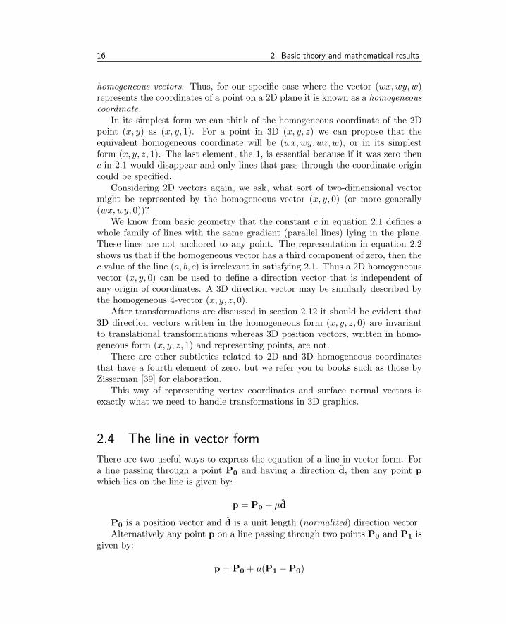
to specific coordinates. Frequently direction vectors are used in a form wherethey have unit length; in this case they are said to be normalized. The mostcommon application of a direction vector in 3D computer graphics is to specifythe orientation of a surface or ray direction. For this we use a direction vector atright angles (normal) and pointing away from the surface. Such normal vectorsare the key to calculating lighting and surface shading effects.
2.3 Homogeneous coordinates
Section 2.2 focused on two ways of using vectors that are particularly pertinent in3D computer graphics. However vectors are a much more general mathematicalconcept, an n-tuple of numbers (a1, a2, .., an), where n > 1 is a vector. A one-dimensional array in a computer program is a vector; a single column matrix[a1, a2, a3, ...an]
T is also a vector.One of the most obvious differences between position and direction vectors
is that directions are independent of any translational transformation, whereasthe coordinates of a point in 3-space are certainly not independent when the

2.3. Homogeneous coordinates 15
Position vectorsfor points P and Q Direction vector d
x
y
z
x
y
z
d
P(x1, y1, z1)
Q(x2, y2, z2)Q
P
d
Figure 2.3: Position and direction vectors.
point is moved. In order to be able to treat these vectors consistently we needto introduce the concept of homogeneous coordinates. Since 3D vectors area logical extension of 2D vectors, and it is easier to understand the conceptof homogeneous coordinates in 2D, we will consider these. Hopefully you willbe comfortable with the idea of extending them to 3D by adding in a thirdcomponent, the result of which we present without rigorous proof.
A general two-dimensional line is represented by the well-known equation:
ax+ by + c = 0 (2.1)
Any point in a plane (xp, yp) that lies on the line must satisfy 2.1, that is,axp + byp + c must be identically zero. It is quite legitimate to write 2.1 usingmatrix notation:
[a, b, c][x, y, 1]T (2.2)
This conveys the same information as 2.1, but it can now be clearly seen that twopairs of triple numbers are involved, (a, b, c) and (x, y, 1) Any triple of numbersconforms to the definition of a 3-vector and so the line in 2.1 is fully definedby the vector (a, b, c). The triple (x, y, 1) is also a 3-vector and represents anypoint that satisfies the equation, i.e., lies on the line in 2.1, for example the point(xp, yp, 1).
Equation 2.1 and the line it represents is unchanged if we multiply it by aconstant, say w to give:
wax+ wby + wc = 0 (2.3)
or equivalently:[a, b, c][wx,wy,w]T (2.4)
From this it is clear that, in this situation, the family of vectors (wx,wy,w)for any w are equivalent. Vectors with this property are called (in the trade)
16 2. Basic theory and mathematical results
homogeneous vectors. Thus, for our specific case where the vector (wx,wy,w)represents the coordinates of a point on a 2D plane it is known as a homogeneouscoordinate.
In its simplest form we can think of the homogeneous coordinate of the 2Dpoint (x, y) as (x, y, 1). For a point in 3D (x, y, z) we can propose that theequivalent homogeneous coordinate will be (wx,wy,wz, w), or in its simplestform (x, y, z, 1). The last element, the 1, is essential because if it was zero thenc in 2.1 would disappear and only lines that pass through the coordinate origincould be specified.
Considering 2D vectors again, we ask, what sort of two-dimensional vectormight be represented by the homogeneous vector (x, y, 0) (or more generally(wx,wy, 0))?
We know from basic geometry that the constant c in equation 2.1 defines awhole family of lines with the same gradient (parallel lines) lying in the plane.These lines are not anchored to any point. The representation in equation 2.2shows us that if the homogeneous vector has a third component of zero, then thec value of the line (a, b, c) is irrelevant in satisfying 2.1. Thus a 2D homogeneousvector (x, y, 0) can be used to define a direction vector that is independent ofany origin of coordinates. A 3D direction vector may be similarly described bythe homogeneous 4-vector (x, y, z, 0).
After transformations are discussed in section 2.12 it should be evident that3D direction vectors written in the homogeneous form (x, y, z, 0) are invariantto translational transformations whereas 3D position vectors, written in homo-geneous form (x, y, z, 1) and representing points, are not.
There are other subtleties related to 2D and 3D homogeneous coordinatesthat have a fourth element of zero, but we refer you to books such as those byZisserman [39] for elaboration.
This way of representing vertex coordinates and surface normal vectors isexactly what we need to handle transformations in 3D graphics.
2.4 The line in vector form
There are two useful ways to express the equation of a line in vector form. Fora line passing through a point P0 and having a direction d, then any point pwhich lies on the line is given by:
p = P0 + µd
P0 is a position vector and d is a unit length (normalized) direction vector.Alternatively any point p on a line passing through two points P0 and P1 is
given by:
p = P0 + µ(P1 −P0)

2.5. The plane 17
x
y
x
y
z z
P0
P0
P1
Line
d
Line
Figure 2.4: Specifying a line.
The parameter µ takes values in the range −∞ < µ < ∞. Note that whenµ = 0 then p = P0.
On a line passing through two points p = P0 when µ = 0 and p = P1 whenµ = 1.0.
Using two points to express an equation for the line is useful when we needto consider a finite segment of a line. (There are many examples where we needto use segments of lines such as calculating the point of intersection between aline segment and a plane.)
Thus if we need to consider a line segment we can assign P0 and P1 to thesegment end points with the consequence that any point on the line p will onlybe part of the segment if its value for µ in the equation above lies in the interval[0, 1].
2.5 The plane
A plane is completely specified by giving a point on the plane P0, and thedirection n perpendicular to the plane.
To write an equation to represent the plane we can use the fact that thevector (p−P0) which lies in the plane must be at right angles to the normal tothe plane, thus:
(p−P0) · n = 0
Alternatively a plane could be specified by taking three points, P2, P1 andP0, lying in the plane. Provided they are not co-linear it is valid to write theequation of the plane as:

18 2. Basic theory and mathematical results
x
x
y
P0
P0 P1
P2
n
y
z
z
Figure 2.5: Specifying a plane.
(p−P0) ·(P2 −P0)× (P1 −P0)
| (P2 −P0)× (P1 −P0) |= 0
Figure 2.5 illustrates these two specifications for a plane. It should be notedthat these equations apply to planes that extend to infinity in all directions. Weshall see later that the intersection of a line with a bounded plane plays a veryimportant role in rendering and modeling algorithms.
2.6 Intersection of a line and a plane
The intersection of a line and a plane is a point pi that satisfies the equation ofthe line and the equation of the plane simultaneously. For the line p = Pl + µdand the plane (p−Pp) · n = 0 the point of intersection pI is given by:
i f (|d · n| < ǫ) there is no intersectionelse {
µ =(Pp −Pl) · n
d · npI = Pl + µd}
Note that we must first test to see whether the line and plane actually inter-sect. The parameter ǫ allows for the numerical accuracy of computer calculationsand since d and n are of unit length ǫ should be of the order of the machinearithmetic precision.

2.7. Closest distance of a point from a line 19
a = P0 −Pp
b = P1 −Pp
da = a · ndb = b · ni f |da| ≤ ǫ0 and |db| ≤ ǫ0 {both P0 and P1 lie in the plane
}else {
dab = dadbi f dab < ǫ1 {The line crosses the plane
}else {
The line does not cross the plane}
}
Listing 2.2: Algorithm to determine whether the line joining two points crosses a plane.
2.6.1 Intersection of a line segment with a plane
Given a line segment joining P0 to P1 and a plane (p−Pp) · n = 0 the algorithmof figure 2.2 determines whether the plane and line intersect. Note that this doesnot actually calculate the point of intersection. It is a good idea to separate thecalculation of an intersection point by first testing whether there will be onebefore going on to determine the point. This is especially useful when we needto consider clipping, see section 4.2.6.
The parameters ǫ0 and ǫ1 are again chosen as non-zero values because of thenumerical accuracy of floating point calculations.
2.7 Closest distance of a point from a line
Consider the line L passing through the points P1 and P2 as shown in figure 2.6.To find the closest distance, l, of the point p from L we recognize that theprojection of the vector p − P1 onto PL allows us to find the point, q, on Lwhich is closest to p. Thus, the closest distance is given by the steps:
Let d = (P2 −P1)
then µ =(p−P1) · d
d · d and q = P1 + µd
thus l = |p− q|When (µ < 0 or µ > 1.0) {
p is closer to the line outside of the segment from P1 to P2
}

20 2. Basic theory and mathematical results
x
z
y
d
P1
P2
L
l
p
q
Figure 2.6: Closest distance of a point from a line segment.
As illustrated in figure 2.6 it is only when 0 < µ < 1 that the perpendicularfrom p to the line meets the position vector d, i.e., between the points P1, P2.
This algorithm is useful for a 3D application program where it is necessaryto interactively pick a line by touching it, or pointing to it on a display with auser input device such as a mouse.
2.8 Closest distance of approach between two lines
In three-dimensional space two arbitrary lines rarely intersect. However it isuseful to be able to find the closest distance of approach between them. In thegeometry shown in figure 2.7 the segment AA′ (vector b) joins the points ofclosest approach between the lines:
p = P1 + λr
p = P2 + µd
At the points of closest approach b is perpendicular to both lines and therefore:b · d = 0 and b · r = 0.
To determine the length of b consider the alternative ways of specifying thepoint x, i.e., following alternative paths from O to x:
x = P1 + λr
x = P2 + µd+ b
Thus:µd− b = λr+ (P1 −P2) (2.5)

2.9. Reflection in a plane 21
Line 1
Line 2
P2
P1
x
b
A
A´d
r
x
y
z
O
^
^
Figure 2.7: Closest distance of approach between two lines.
Once λ and µ are determined the length of b is readily found:
l =∣
∣
∣P1 + λr− (P2 + µd)
∣
∣
∣(2.6)
Taking the dot product of 2.5 with r will eliminate b and give an expression forλ:
λ = µ(d · r)− (P1 −P2) · r (2.7)
The dot product of 2.5 with d eliminates b and substituting λ using 2.7 gives:
µ =((P1 −P2) · d)− ((P1 −P2) · r)(d · r)
1− (d · r)2(2.8)
With µ known 2.7 gives λ and then the distance of closest approach followsfrom 2.6.
Note: If the lines are parallel∣
∣(d · r)∣
∣ < ǫ (where ǫ is the machine tolerance ofzero, approximately 1×10⁻⁶ for single precision calculations), then the algorithmis terminated before it reaches equation 2.8.
2.9 Reflection in a plane
In many rendering algorithms there is a requirement to calculate a reflecteddirection given an incident direction and a plane of reflection. The vectors weneed to consider in this calculation are of the direction type and assumed to beof unit length.
If the incident vector is din, the reflection vector is dout and the surfacenormal is n, we can calculate the reflected vector by recognizing that becausedout and din are normalized (the argument would work equally well provided

22 2. Basic theory and mathematical results
Reflective Surface
θ
θ
^dout
^din
^n
Figure 2.8: Incident and reflection vector.
dout and din are the same length) then vector (dout − din) is co-linear with n;figure 2.8 illustrates this, therefore:
dout − din = αn (2.9)
where α is a scalar factor. As the incident and reflected angles are equal
dout · n = −din · n (2.10)
Taking the dot product of both sides of Equation 2.9 with n, substituting inequation 2.10 and using the fact that n is normalized we obtain for the reflecteddirection:
dout = din − 2(din · n)n
2.10 Refraction at a plane
Photo-realistic renderers require to be able to simulate transparent surfaceswhere rays of light are refracted as they pass through the boundary betweenmaterials of different refractive index. Figure 2.9 shows a refractive surface withan incident vector di, surface normal n and refracted vector dr. All three vectorsare of the direction type.
The physical model of refraction is expressed in Snell’s law which states:
nr
ni
=sin θisin θr

2.11. Intersection of a line with primitive shapes 23
where ni and nr are transmission constants for the media in which the incidentand refracted light rays travel. Snell’s law can also be written in vector form:
ni(di × n) = nr(dr × n)
Since di, dr and n all lie in a plane, dr can be expressed as a linear combinationof di and n:
dr = αdi + βn (2.11)
Taking the vector product of both sides of equation 2.11 with n and substitutingit for the right-hand side of the vector form of Snell’s law gives a value for αwhich is:
α =ni
nr
The dot product of both sides of equation 2.11 produce a quadratic in β:
dr · dr = 1 = α2 + 2αβ(n · di) + β2
Only one of the roots of this equation is a physically meaningful solution. Theappropriate root is determined by considering an incident ray perpendicular tothe surface. Once this is done the meaningful value of β is substituted into 2.11and rearranged to give a two step calculation for the refracted direction:
r = (n · di)2 +
(
nr
ni
)2
− 1
dr =ni
nr
(
(√r − n · di)n+ di
)
Note that if the term r is negative, reflection (section 2.9) rather than refractionoccurs.
2.11 Intersection of a line with primitive shapes
Many 3D algorithms (rendering and modeling) require the calculation of thepoint of intersection between a line and a fundamental shape called a primitive.We have already dealt with the calculation of the intersection between a line anda plane. If the plane is bounded we get a primitive shape called a planar polygon.Most 3D rendering and modeling application programs use polygons that haveeither three sides (triangles) or four sides (quadrilaterals). Triangular polygonsare by far the most common because it is always possible to reduce an n sidedpolygon to a set of triangles. Most of the modeling algorithms in this book willrefer to triangular polygons. An algorithm to reduce an n sided polygon to a setof triangular polygons is given in chapter 10.
Other important primitive shapes are the planar disc and the volume solids,the sphere and cylinder. There are more complex shapes that can still be termed

24 2. Basic theory and mathematical results
x
y
^z
p
θr
RefractiveBoundary
θi
dr
^di
n
Figure 2.9: Tracing a refracted ray. Note that the incident, refracted and surfacenormal directions all lie in a plane.
primitive though they are used much less frequently. It is possible to set upanalytic expressions for shapes made by lofting a curve along an axis or bysweeping a curve round an axis; see Burger and Gillies [15] for examples. Thereare a large number of other primitive shapes such as Bezier, spline and NURBSpatches and subdivision surfaces to mention a few.
In this section we will examine the most important intersection in the contextof software that uses planar polygons as the basic unit for modeling objects.
2.11.1 Intersection of a line with a triangular polygon
This calculation is used time and time again in modeling algorithms (Booleans,capping and normal calculations) and in rendering algorithms (image and tex-ture mapping and in ray tracing). The importance of determining whether anintersection occurs in the interior of the polygon, near one of its vertices, or atone of its edges, or indeed just squeaks by outside, cannot be over emphasized.
This section gives an algorithm that can be used determine whether a lineintersects a triangular polygon. It also classifies the point of intersection as beinginternal, or a point close to one of the vertices or within some small distance froman edge.
The geometry of the problem is shown in figure 2.10. The point Pi gives theintersection between a line and a plane. The plane is defined by the points P0,P1 and P2, as described in section 2.6. They also identify the vertices of thetriangular polygon. Vectors u and v are along two of the edges of the triangleunder consideration. Provided u and v are not co-linear the vector w,
w = Pi −P0

2.11. Intersection of a line with primitive shapes 25
Pi
u
w
v
P0
P2
P1
x
O
z
y
Figure 2.10: Intersection of line and triangular polygon.
lies in the plane and can be expressed as a linear combination of u and v:
w = αu+ βv (2.12)
Once α and β have been calculated a set of tests will reveal whether Pi liesinside or outside the triangular polygon with vertices at P0, P1 and P2.
Algorithm overview:
1. To find Pi we use the method described in section 2.6.
2. To calculate α and β take the dot product of 2.12 with u and v respectively.After a little algebra the results can be expressed as:
α =(w · u)(v · v)− (w · v)(u · v)
(u · u)(v · v)− (u · v)2
β =(w · v)(u · u)− (w · u)(u · v)
(u · u)(v · v)− (u · v)2
Since both expressions have the same denominator it need only be calcu-lated once. Products such as (w · v) occur more than once and thereforeassigning these to temporary variables will speed up the calculation. Itis very worthwhile optimizing the speed of this calculation because it liesat the core of many time critical steps in a rendering algorithm, particu-larly image and texture mapping functions. C++ code for this importantfunction is available with the book.
The pre-calculation of (u ·u)(v ·v)− (u ·v)2 is important, because shouldit turn out to be too close to zero we cannot obtain values for α or β. Thisproblem occurs when one of the sides of the triangle is of zero length. In

26 2. Basic theory and mathematical results
practice a triangle where this happens can be ignored because if one of itssides has zero length, it has zero area and will therefore not be visible in arendered image.
3. Return hit code as follows:
i f (α < −0.001 or α > 1.001 orβ < −0.001 or β > 1.001) miss polygon
i f ((α+ β) > 1.001) miss polygon beyond edge P1 → P2
i f (α ≥ 0.0005 and α ≤ 0.9995and β ≥ 0.0005 and β ≤ 0.9995and (α+ β) ≤ 0.9995) inside polygon
else i f (α < 0.0005) {along edge P0 → P1
i f (β < 0.0005) at vertex P0
else ( i f β > 0.9995) at vertex P1
else On edge P0 → P1 not near vertex}else i f (β < 0.0005) {along edge P0 → P2
i f (α < 0.0005) at vertex P0
else i f (α > 0.9995) at vertex P2
else On edge P0 → P2 not near vertex}else i f ((α+ β) > 0.9995) on edge P1 → P2
else miss polygon
Note that the parameters −0.001 and so on are not dependent on theabsolute size of the triangle because α and β are numbers in the range[0, 1].
Alternative algorithms for ray/triangle intersection are shown in Badouel [34]and Moller [60].
2.12 Transformations
Transformations have two purposes in 3D graphics: to modify the position vectorof a vertex and change the orientation of a direction vector. It is useful to expressa transformation in the form of a matrix. In the previous sections we discussedvectors; a vector itself is just a special case of a matrix. If you are unfamiliarwith matrices, vectors or linear algebra in general it might be useful to consultother references [7, 17,57].
The vectors we have used so far apply to the 3D universe and thus havethree components (x, y, z). In matrix form they also have three elements and

2.12. Transformations 27
are written in a single column:
xyz
This matrix is said to have three rows and one column, a 3× 1 matrix. Matricescan have any number of rows and columns; for example a 4× 4 matrix might berepresented by:
a00 a01 a02 a03a10 a11 a12 a13a20 a21 a22 a23a30 a31 a32 a33
It turns out that all the transformations appropriate for computer graphics work,moving, rotating, scaling etc., can be represented by a matrix of size 4× 4. Ma-trices are mathematical objects and have their own algebra just as real numbersdo. You can add, multiply and invert a matrix.
Several different notations are used to represent a matrix. Throughout thistext we will use the [ ] bracket notation. When we discussed vectors we used abold type to represent a vector as a single entity. When we want to representa matrix as an individual entity we will use the notation of a capital letter insquare brackets, e.g., [P ]. Since a 3D vector and a 3 × 1 matrix represent thesame thing we will use the symbols P and [P ] interchangeably.
If a transformation is represented by a matrix [T ], a point p is transformedto a new point p′ by matrix multiplication according to the rule:
[p′] = [T ][p]
The order in which the matrices are multiplied is important; [T ][p] is differentfrom [p][T ], and indeed one of these may not even be defined.
There are two important points which are particularly relevant when usingmatrix transformations in 3D graphics applications:
1. How to multiply matrices of different sizes.
2. The importance of the order in which matrices are multiplied.
The second point will be dealt with in section 2.12.4. As for the first point,to multiply two matrices the number of columns in the first must equal thenumber of rows in the second. For example a matrix of size 3 × 3 and 3 × 1may be multiplied giving a matrix of size 3 × 1. However a 4 × 4 and a 3 × 1matrix cannot be multiplied. This poses a small problem for us because vectorsare represented by 3 × 1 matrices and transformations are represented as 4× 4matrices.
The problem is solved by using homogeneous coordinates in the transfor-mations. We will not make use of all the extra flexibility that working in ho-mogeneous coordinates offers and restrict ourselves to taking advantage of the

28 2. Basic theory and mathematical results
promotion of a 3D coordinate by adding a fourth component of unity to thevectors that represent positions. Thus the first three elements of a homogeneouscoordinate are the familiar (x, y, z) values and the fourth is set to ‘1’ so thatnow a vector appears as a 4 × 1 matrix. A transformation applied to a vectorin homogeneous coordinate form results in another homogeneous coordinate vec-tor. For all the work in this book the fourth component of vectors will be setto unity and thus they can be transformed by 4 × 4 matrices. We will also usetransformations that leave the fourth component unchanged. Thus the vector pwith components (p0, p1, p2) is expressed in homogeneous coordinates as:
p =
p0p1p21
Note that many texts use the fourth component for certain transformationsand the OpenGL library (used in chapter 7) also offers facilities to use a non-unity value.
The transformation of p into p′ by the matrix [T ] can be written as:
p′0p′1p′21
=
t00 t01 t02 t03t10 t11 t12 t13t20 t21 t22 t23t30 t31 t32 t33
p0p1p21
2.12.1 Translation
The transformation:
[Tt] =
1 0 0 dx0 1 0 dy0 0 1 dz0 0 0 1
moves the point with coordinates (x, y, z) to the point with coordinates (x +dx, y + dy, z + dz).
The translated point [p′] = [Tt][p] or:
1 0 0 dx0 1 0 dy0 0 1 dz0 0 0 1
xyz1
=
x+ dxy + dyz + dz
1

2.12. Transformations 29
2.12.2 Scaling
The transformation matrix:
[Ts] =
sx 0 0 00 sy 0 00 0 sz 00 0 0 1
scales (expands or contracts) a position vector p with components (x, y, z) bythe factors sx along the x axis, sy along the y axis and sz along the z axis. Thescaled vector of p′ is [p′] = [Ts][p].
2.12.3 Rotation
A rotation is specified by an axis of rotation and the angle of the rotation. Itis a fairly simple trigonometric calculation to obtain a transformation matrixfor a rotation about one of the coordinate axes. When the rotation is to beperformed around an arbitrary vector based at a given point, the transformationmatrix must be assembled from a combination of rotations about the Cartesiancoordinate axes and possibly a translation.
Rotate about the z axis To rotate round the z axis by an angle θ, the transfor-mation matrix is:
[Tz(θ)] =
cosθ −sinθ 0 0sinθ cosθ 0 00 0 1 00 0 0 1
(2.13)
We can see how the rotational transformations are obtained by consideringa positive (anti-clockwise) rotation of a point P by θ round the z axis (whichpoints out of the page). Before rotation P lies at a distance l from the originand at an angle φ to the x axis, see figure 2.12. The (x, y) coordinate of P is(l cosφ, l sinφ). After rotation by θ P is moved to P′ and its coordinates are(l cos(φ + θ), l sin(φ + θ)). Expanding the trigonometric sum gives expressionsfor the coordinates of P′:
Px′ = l cosφ cos θ − l sinφ sin θ
Py′ = l cosφ sin θ + l sinφ cos θ
Since l cosφ is the x coordinate of P and l sinφ is the y coordinate of P thecoordinates of P′ become:
Px′ = Px cos θ − Py sin θ
Py′ = Px sin θ + Py cos θ

30 2. Basic theory and mathematical results
Viewed with the axis of rotation pointing out of the page
Rotation roundthe Z axis
Rotation roundthe X axis
Rotation roundthe Y axis
x
x
y
z z z
y y
x x
P
P
P
P´
P´
P´
y z x
zyθ θ
θθ
θ
θ
Figure 2.11: Rotations, anti-clockwise looking along the axis of rotation, toward theorigin.
Writing this in matrix form we have:[
Px′
Py′
]
=
[
cos θ − sin θsin θ cos θ
] [
Px
Py
]
There is no change in the z component of P and thus this result can beexpanded into the familiar 4×4 matrix form by simply inserting the appropriateterms to give:
Px′
Py′
Pz′
1
=
cos θ − sin θ 0 0sin θ cos θ 0 00 0 1 00 0 0 1
Px
Py
Pz
1
Rotation about the y axis To rotate round the y axis by an angle θ, the transfor-mation matrix is:
[Ty(θ)] =
cosθ 0 sinθ 00 1 0 0
−sinθ 0 cosθ 00 0 0 1

2.12. Transformations 31
x
φ + θ
P´
P
y
φ
Figure 2.12: Rotation of point P by an angle θ round the z axis.
Rotation about the x axis To rotate round the x axis by an angle θ, the transfor-mation matrix is:
[Tx(θ)] =
1 0 0 00 cosθ −sinθ 00 sinθ cosθ 00 0 0 1
Note that as illustrated in figure 2.11 θ is positive if the rotation takes placein a clockwise sense when looking from the origin along the axis of rotation. Thisis consistent with a right-handed coordinate system.
2.12.4 Combining transformations
Section 2.12 introduced the key concept of a transformation applied to a positionvector. In many cases we are interested in what happens when several operationsare applied in sequence to a model or one of its points (vertices). For example:move the point P 10 units forward, rotate it 20 degrees round the z axis and shiftit 15 units along the x axis. Each transformation is represented by a single 4× 4matrix and the compound transformation is constructed as a sequence of singletransformations as follows:
[p′] = [T1] [p]
[p′′] = [T2] [p′]
[p′′′] = [T3] [p′′]
where [p′] and [p′′] are intermediate position vectors and [p′′′] is the end vectorafter the application of the three transformations. The above sequence can becombined into:
[p′′′] = [T3][T2][T1][p]

32 2. Basic theory and mathematical results
x
x xx
y
y yy
z
z z z
z
y
x
Rotate roundx by π/2 Rotate round
z by π/2
Rotate round
z by π/4
Rotate round
z by π/2
P´
P´
P
P´
P´
Figure 2.13: Effect of transformations applied in a different order.
The product of the transformations [T3][T2][T1] gives a single matrix [T ]. Com-bining transformations in this way has a wonderful efficiency: If a large model has50,000 vertices and we need to apply 10 transformations, by combining the trans-formations into a single matrix, 450,000 matrix multiplications can be avoided.
It is important to remember that the result of applying a sequence of trans-formations depends on the order in which they are applied. [T3][T2][T1] is notthe same compound transformation as [T2][T3][T1]. Figure 2.13 shows the effectof applying the transformations in a different order.
There is one subtle point about transformations that ought to be stressed.The parameters of a transformation (angle of rotation, etc.) are all relativeto a global frame of reference. It is sometimes useful to think in terms of alocal frame of reference that is itself transformed relative to a global frame andthis idea will be explored when we discuss key frame and character animation.However it is important to bear in mind that when a final scene is assembled forrendering, all coordinates must be specified in the same frame of reference.

2.12. Transformations 33
Afterrotation
Beforerotation
Axis ofrotation
y
P0
P1
x
z
Figure 2.14: Rotation round an arbitrary vector.
2.12.5 Rotation about an arbitrary axis
The transformation corresponding to rotation of an angle α around an arbitraryvector (for example that shown between the two points P0 and P1 in figure 2.14)cannot readily be written in a form similar to the rotation matrices about thecoordinate axes.
One way to obtain the desired transformation matrix is through the combi-nation of a sequence of basic translation and rotation matrices. (Once a single4 × 4 matrix has been obtained representing the composite transformations itcan be used in the same way as any other transformation matrix.)
The following outlines an algorithm to construct a transformation matrix togenerate a rotation by an angle α around a vector in the direction P1 −P0:
1. Translate P0 to the origin of coordinates.
2. Align rotation axis P1 −P0 with the x axis.
3. Rotate by angle α round x axis.
4. Make inverse transformation to undo the rotations of step two.
5. Translate origin of coordinates back to P0 to undo the translation of stepone.
The full algorithm is given in listing 2.3. Moller and Haines [1] give a morerobust method of rotating around any axis.
It is possible to combine rotational transformations together into a single 3×3matrix in the case of a rotation by θ around a directional vector u = [ux, uy, uz]
T .In this case any translational element would have to be removed first and thenre-applied and θ is anti-clockwise when looking in the direction of u. Thus:
[T (θ)] = [I]cosθ + sin θ[Tc] + (1− cos θ)[Tt] (2.14)

34 2. Basic theory and mathematical results
Let d = P1 −P0
[T1] = a translation by −P0
dxy = d2x + d2yi f dxy < ǫ {rotation axis is in the z directioni f dz > 0 make [T2] a rotation about z by α
else [T2]is a rotation about z by −α[T3]is a translation by P0
return the product [T3][T2][T1]}dxy =
√
dxyi f dx = 0 and dy > 0 φ = π/2else i f dx = 0 and dy < 0 φ = −π/2else φ = ATAN2(dy, dx)θ = ATAN2(dz, dxy)[T2]is a rotation about z by −φ[T3]is a rotation about y by −θ[T4]is a rotation about x by α[T5]is a rotation about y by θ[T6]is a rotation about z by φ[T7]is a translation by P0
Multiply the transformation matrices to give the final result[T ] = [T7][T6][T5][T4][T3][T2][T1]
Listing 2.3: Algorithm for rotation round an arbitrary axis. dx, dy and dz are thecomponents of vector d.
where:
[Tc] =
0 −uz uy
uz 0 −ux
−uy ux 0
is the cross product matrix and:
[Tt] =
u2x uxuy uxuz
uyux u2y uyuz
uzux uzuy u2z
is the tensor product. This neat expression is a matrix form of Rodrigues’ rota-tion formulae.
2.12.6 Rotational change of frame of reference
In working with objects that have curved surfaces, or even those with flat surfacesthat are not orientated in the direction of one of the axes of the global frame ofreference, it is sometimes desirable to define a local frame of reference on every

2.12. Transformations 35
(a) (b) (c)
x
x
yn
nnzz
by
z
x
t
tt
bP
PP
Figure 2.15: Surface local coordinates: (a) A point on an object with position P inthe global (world) frame of reference has a surface local frame of reference, (b) in atwo-dimensional section. (c) The relative orientations of the local and global frames ofreference.
point on the surface. For any point on a surface P the normal vector n is usedto define the orientation of the surface and is an important variable in all thelighting models.
The normal is defined through its components (nx, ny, nz) relative to theglobal frame of reference. However locally at the surface, the normal is alwaysvertical. If we can define two other mutually perpendicular vectors at P wewould have a frame of reference in which the normal was always vertical andany other point or direction could be defined with respect to the local frameof reference. Such a local frame of reference is important when the texturingprocedures of image mapping, and especially bump mapping (see section 4.6.2),are considered. Figure 2.15 illustrates the relationship between the local frameof reference and the global frame of reference.
A complete frame of reference requires two additional coordinate vectors. Ifwe stipulate that the frame of reference is orthogonal, then only one additionalvector is really needed. It must be perpendicular to n and thus it lies in the planeof the surface at P. In texture mapping applications, this additional vector isalso used to define one of the edges of the map. Even curved surfaces tend tobe locally flat when one is close enough to P. This additional vector lying inthe surface is termed the tangent vector t. The third vector is easily obtainedby taking the cross product: b = n × t. Each of these local frame vectors arespecified by their components in the global frame of reference, thus: (nx, ny, nz),(tx, ty, tz) and (bx, by, bz).
Given a local frame of reference’s basis vectors it is easy to build a rotationaltransformation that will transform any direction vector, defined in the local frameof reference, to its equivalent direction defined in terms of the global frame ofreference’s basis vector. If the direction d is specified relative to the local frameby its components (du, dv, dw) then in terms of its direction in the global frameof reference it will be given by d′ = dun+dvt+dwb. This linear transformation

36 2. Basic theory and mathematical results
can be expressed as a 3× 3 matrix:
dx′
dy′
dz′
=
tx bx nx
ty by ny
tz bz nz
dudvdw
(2.15)
Equation 2.15 transforms a direction vector specified in the surface localframe of reference to the equivalent in the global frame, that is local to global[d′] = [Tlg][d]. However in order to determine the direction of a vector, forexample the relative location of a light to P, the transformation needed is theone from the global to the local reference frame, that is, [Tgl], the inverse of[Tlg]. It is a well known result that for rotational transformations the inverse ofits matrix representation is simply its transpose, that is [Tgl] = [Tlg]
−1 = [Tlg]T .
Thus when the surface normal and surface tangent vectors are known at apoint P, any direction vector, specified relative to the global frame of reference,can be transformed into a direction vector relative to the surface local referenceframe by multiplying it by the matrix:
tx ty tzbx by bznx ny bz
(2.16)
Note: This only applies to direction vectors, so for example if we want to get therelative direction of a light at Lp to the surface at P (both specified in a globalframe of reference), it is the direction vector Lp −P that has to be transformedwith the matrix in equation 2.16.
2.12.7 Viewing transformation
Before rendering any view of a 3D scene (see chapter 4) one has to decide fromwhere to view/photograph the scene and in which direction to look (point thecamera). This is like setting up a camera to take a picture. Once the camerais set we just click the shutter. The camera projects the image as seen in theviewfinder onto the photographic film and the image is rendered. This is a twostage process: the projection stage will be discussed in section 2.12.8, and nowwe will consider how to set a viewpoint and direction of view.
In mathematical terms we need to construct a suitable transformation thatwill allow us to choose a viewpoint (place to set up the camera) and directionof view (direction in which to point the camera). Once we have this view trans-formation it can be combined with any other transformations that need to beapplied to the scene or to objects in the scene.
We have already seen how to construct transformation matrices that moveor rotate points in a scene. In the same way that basic transformation matriceswere combined in section 2.12.5 to create an arbitrary rotation we can build asingle matrix, [To], that will transform all the points (vertices) in a scene in such

2.12. Transformations 37
After alignment to the x axisthe direction of view is still
tilted by angle α to the right.
Direction of view
View point
(cameral location)
z
y
x
O
x
z
y
y
z
x
O
θ
α
φ
Figure 2.16: Viewpoint and direction of view.
a way that the projection of an image becomes a simple standard process. To dothis we arrange that the camera is fixed at the center of the universe, (0, 0, 0),and locked off to point in the direction (1, 0, 0) (along the x axis).
There is nothing special about the direction (1, 0, 0); we could equally wellhave chosen to fix the camera to look in the direction (0, 1, 0), the y axis, or even(0, 0, 1), the z axis. But since we have chosen to let z represent the up directionand it is not a good idea to look directly up, (0, 0, 1) would be a poor choice forviewing. (Note: The OpenGL and Direct3D software libraries for 3D graphicshave their z axis parallel to the viewing direction.)
Once [To] has been determined it is applied to all objects in the scene. Ifnecessary [To] can be combined with other transformation matrices to give asingle composite transformation [T ].
A viewing transformation depends on:
1. Position of the view point (camera location). (A vector po, see figure 2.16.)
2. The direction in which we wish to look: north, south, east or west. This ismeasured by an angle φ which is relative to the x axis and lies in the xyplane. φ is positive to the right of the x axis when looking along x fromthe view point.
3. The amount by which we look up or down. The angle θ measures thisrelative to the xy plane. It is positive when looking down. Note that whendetermining a viewing transformation the effect of looking up or downcomes into play after the direction of view has been accounted for andtherefore it is equivalent to a rotation around the y axis.
4. The degree to which our head is tilted to the left or right. This is measuredby the angle α. To be consistent with the right-handed frame of reference

38 2. Basic theory and mathematical results
and sense of rotation α is positive when the camera tilts to the right as itlooks from po along the x axis.
A viewing transformation appears to operate in reverse to ordinary transfor-mations. For example, if you tilt your head to the left, the world appears totilt to the right. Note carefully that the angle θ is positive if we are lookingdown, and negative if we are looking up. If you prefer, you can think of: φ asthe heading, θ as the pitch and α as the degree of banking. The viewingtransformations are also combined in the reverse order to the order in whicha transformation is assembled for objects placed in a scene. In that case therotation around x is applied first and the translation by po is applied last.
Given the parameters po, φ, θ and α (illustrated in figure 2.16) the transfor-mation [To] is constructed by the following algorithm:
Place observer at (0, 0, 0) with the transformation:[T1] = a translation by −po
Rotate the direction of observation into the xz plane with:[T2] = a rotation about z by −φ
Align the direction of observation to the x axis with:[T3] = a rotation about y by −θ
Straighten the camera up with transformation:[T4] = a rotation about x by −α
Multiply the individual transformation matrices to giveone composite matrix representing the viewing transformation:[T0] = [T4][T3][T2][T1]
2.12.8 Projection
We saw in section 2.12.7 that after setting up a camera to record an image theview must be projected onto film or electronic sensing device. In the conventionalcamera this is done with a lens arrangement or simply a pinhole. One could alsoimagine holding a sheet of glass in front of the viewer and then having themtrace on it what they see as they look through it. What is drawn on the glassis what we would like the computer to produce: a 2D picture of the scene. It’seven showing the right way up as in figure 2.17.
It is straightforward to formulate expressions needed to perform this (non-linear) transformation. A little thought must be given to dealing with caseswhere parts of the scene go behind the viewer or are partly in and partly outof the field of view (this topic is discussed in section 4.2.6). The field of view(illustrated in figure 2.18) governs how much of the scene you see; it can bechanged. In photography telephoto and fish-eye lenses have different fields ofview. For example the common 50mm lens has a field of view of 45.9◦. Becauseof its shape as a truncated pyramid with a regular base the volume enclosed bythe field of view is known as a frustum.
One thing we can do with a projective transformation is to adjust the aspectratio. The aspect ratio is the ratio of height to width of the rendered image.

2.12. Transformations 39
Viewing plane
Y
X
Figure 2.17: Project the scene onto the viewing plane. The resulting two-dimensionalimage is then recorded or displayed.
For television work it is 4 : 3 and 16 : 9 for basic cine film. The aspect ratio isrelated to the vertical and horizontal resolution of the recorded image. Get thisrelationship wrong and your spheres will look egg shaped.
Before formulating expressions to represent the projection we need to definethe coordinate system in use for the projection plane. It has become almostuniversal (however not in the OpenGL library discussed in chapter 7) to rep-resent the computer display as a pair of integers in the range 0 → (Xmax − 1)horizontally and 0 → (Ymax − 1) vertically. The coordinate origin (0, 0) is in thetop left corner, see figure 2.17.
The distance of the projection plane from the viewpoint can be chosen ar-bitrarily; setting it to one unit simplifies the calculations. Thus if the plane ofprojection is located at (1, 0, 0) and orientated parallel to the yz plane (i.e., theviewer is looking along the x axis) then the screen coordinates (Xs, Ys) for theprojection of a point (x, y, z) are given by:
Xs =Xmax
2− y
xsx (2.17)
Ys =Ymax
2− z
xsy (2.18)
The parameters sx and sy are scale values to allow for different aspect ratios andfields of view. This effectively lets us change the zoom settings for the camera.

40 2. Basic theory and mathematical results
Direction of view
x
y
Viewpoint
φ
Figure 2.18: The field of view φ governs how much of the scene is visible to a cameralocated at the viewpoint. Narrowing the field of view is equivalent to using a zoomlens.
Obviously, Xs and Ys must satisfy 0 ≤ Xs < Xmax and 0 ≤ Ys < Ymax.If ff (measured in mm) is the focal length of the desired camera lens and the
aspect ratio is Ax : Ay then:
sx =Xmax
2
ff21.22
Ax
sy =Ymax
2
ff21.22
Ay
The numerical factor 21.2 is a constant to allow us to specify ff in standardmm units. For a camera lens of focal length ff the field of view θ can be expressedas:
θ ≃ 2ATAN2(21.22, ff )
Any point (x, y, z) for which x < 1 will not be transformed correctly byequations 2.17 and 2.18 and steps must be made to eliminate them before theprojection is applied. This process is called clipping. How the clipping is donedepends on whether a wireframe or shaded solid is to be rendered and it isdiscussed in section 4.2.6.
It is possible to express the perspective transformation as a 4 × 4 matrix.However, when the matrix is applied to a point’s homogeneous coordinate inorder to find its projected location on the viewing plane, one has to remember todivide the first three components by the fourth before using the 3D coordinatevalue. Since the projection plane is usually chosen to be perpendicular to one ofthe coordinate axes, then the value along that axis will become the location of
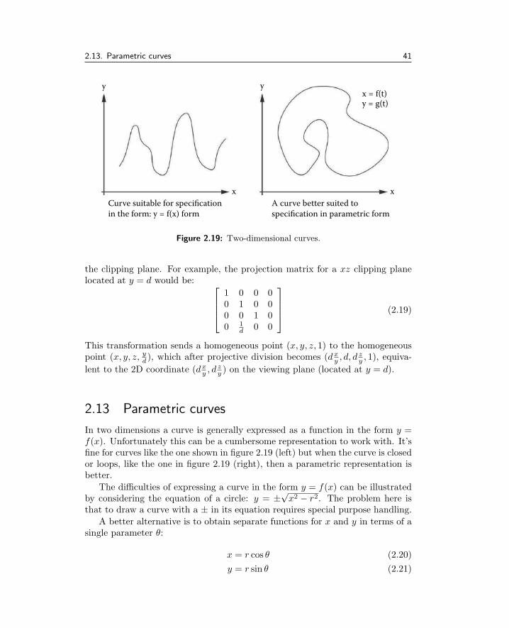
2.13. Parametric curves 41
Curve suitable for specificationin the form: y = f(x) form
A curve better suited tospecification in parametric form
x x
yyx = f(t)y = g(t)
Figure 2.19: Two-dimensional curves.
the clipping plane. For example, the projection matrix for a xz clipping planelocated at y = d would be:
1 0 0 00 1 0 00 0 1 00 1
d0 0
(2.19)
This transformation sends a homogeneous point (x, y, z, 1) to the homogeneouspoint (x, y, z, y
d), which after projective division becomes (dx
y, d, d z
y, 1), equiva-
lent to the 2D coordinate (dxy, d z
y) on the viewing plane (located at y = d).
2.13 Parametric curves
In two dimensions a curve is generally expressed as a function in the form y =f(x). Unfortunately this can be a cumbersome representation to work with. It’sfine for curves like the one shown in figure 2.19 (left) but when the curve is closedor loops, like the one in figure 2.19 (right), then a parametric representation isbetter.
The difficulties of expressing a curve in the form y = f(x) can be illustratedby considering the equation of a circle: y = ±
√x2 − r2. The problem here is
that to draw a curve with a ± in its equation requires special purpose handling.
A better alternative is to obtain separate functions for x and y in terms of asingle parameter θ:
x = r cos θ (2.20)
y = r sin θ (2.21)

42 2. Basic theory and mathematical results
Start ofcurve: τ = 0
P
P (x,y,z) = P(u(τ), v(τ), w(τ))
x
z
y
Figure 2.20: A three-dimensional parametric curve.
where θ is an angle in the range [0, 2π). Equations 2.20 and 2.21 are wellbehaved: given a θ each returns one value only. This is ideal for plotting becauseit wouldn’t matter if the curve twisted, turned or looped.
Actually, since angles are measured in radians, and radians are a measure ofthe arc length of a unit circle, θ could also be thought of as a length along thecurve.
The idea of the parameter having a physical meaning like length is a veryuseful one for curves in both two and three dimensions. We shall use it in sec-tion 6.2.2 when studying the animation of objects following paths. An alternativeand equally useful parameter is time.
Equations 2.20 and 2.21 are specific to a two-dimensional circular curve. Forwork in three dimensions a set of parametric functions that apply to a generalcurve can be written in the form:
x = u(τ) (2.22)
y = v(τ) (2.23)
z = w(τ) (2.24)
Here τ is the parameter. Any curve (we shall call it a path) in 3D space, beit a straight line, a Bezier curve, a cubic spline or even a curve constructed frompieces of other curves, can be specified by three functions. Figure 2.20 illustratesa typical three-dimensional parametric curve.
2.14 Interpolation
Suppose we have a set of data containing n (n > 1) pairs of values (x0, y0),(x1, y1), (x2, y2), ... (xi, yy), ... (xn−1, yn−1). These can be plotted on a two-dimensional diagram as shown in figure 2.21. Joining the points (xi, yi) together
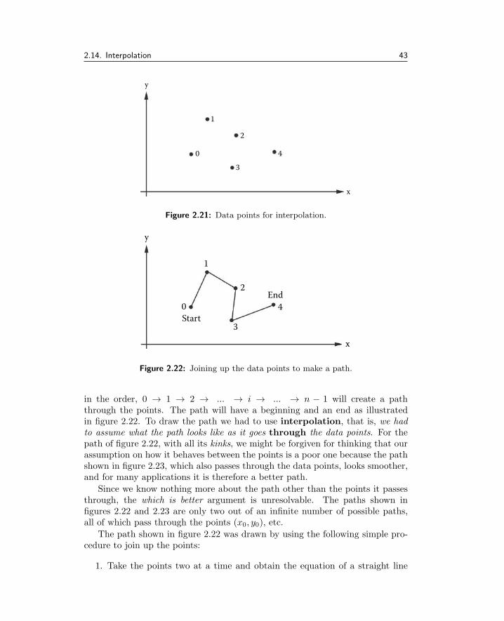
2.14. Interpolation 43
3
0
1
2
4
x
y
Figure 2.21: Data points for interpolation.
Start
End
3
2
1
0
y
x
4
Figure 2.22: Joining up the data points to make a path.
in the order, 0 → 1 → 2 → ... → i → ... → n − 1 will create a paththrough the points. The path will have a beginning and an end as illustratedin figure 2.22. To draw the path we had to use interpolation, that is, we hadto assume what the path looks like as it goes through the data points. For thepath of figure 2.22, with all its kinks, we might be forgiven for thinking that ourassumption on how it behaves between the points is a poor one because the pathshown in figure 2.23, which also passes through the data points, looks smoother,and for many applications it is therefore a better path.
Since we know nothing more about the path other than the points it passesthrough, the which is better argument is unresolvable. The paths shown infigures 2.22 and 2.23 are only two out of an infinite number of possible paths,all of which pass through the points (x0, y0), etc.
The path shown in figure 2.22 was drawn by using the following simple pro-cedure to join up the points:
1. Take the points two at a time and obtain the equation of a straight line
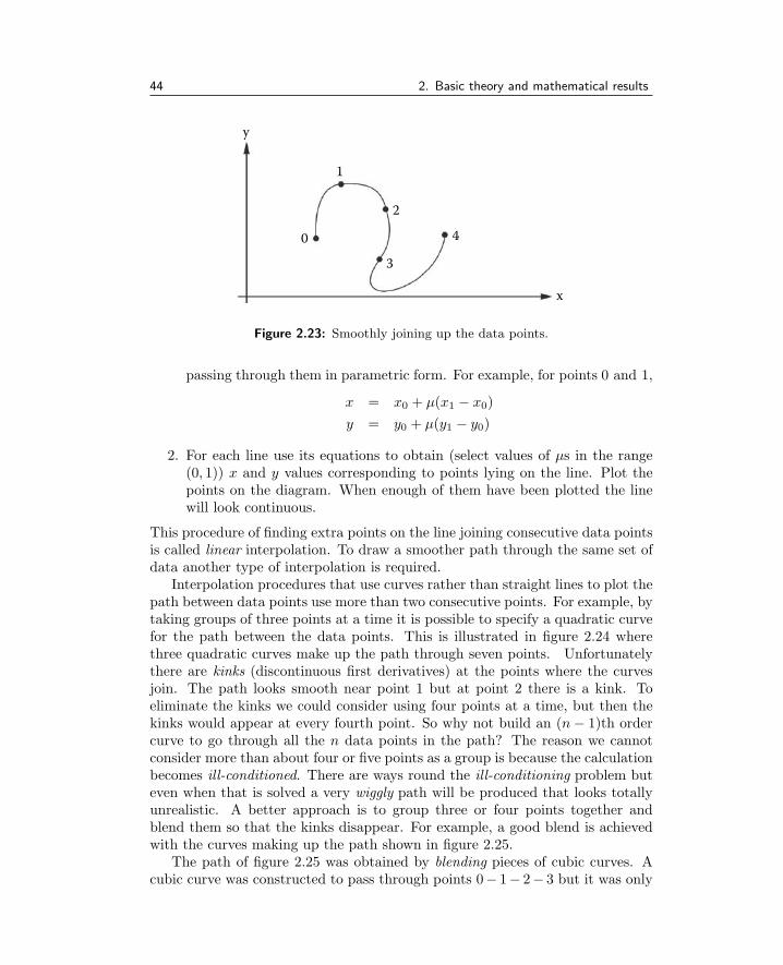
44 2. Basic theory and mathematical results
3
0
1
2
4
x
y
Figure 2.23: Smoothly joining up the data points.
passing through them in parametric form. For example, for points 0 and 1,
x = x0 + µ(x1 − x0)
y = y0 + µ(y1 − y0)
2. For each line use its equations to obtain (select values of µs in the range(0, 1)) x and y values corresponding to points lying on the line. Plot thepoints on the diagram. When enough of them have been plotted the linewill look continuous.
This procedure of finding extra points on the line joining consecutive data pointsis called linear interpolation. To draw a smoother path through the same set ofdata another type of interpolation is required.
Interpolation procedures that use curves rather than straight lines to plot thepath between data points use more than two consecutive points. For example, bytaking groups of three points at a time it is possible to specify a quadratic curvefor the path between the data points. This is illustrated in figure 2.24 wherethree quadratic curves make up the path through seven points. Unfortunatelythere are kinks (discontinuous first derivatives) at the points where the curvesjoin. The path looks smooth near point 1 but at point 2 there is a kink. Toeliminate the kinks we could consider using four points at a time, but then thekinks would appear at every fourth point. So why not build an (n− 1)th ordercurve to go through all the n data points in the path? The reason we cannotconsider more than about four or five points as a group is because the calculationbecomes ill-conditioned. There are ways round the ill-conditioning problem buteven when that is solved a very wiggly path will be produced that looks totallyunrealistic. A better approach is to group three or four points together andblend them so that the kinks disappear. For example, a good blend is achievedwith the curves making up the path shown in figure 2.25.
The path of figure 2.25 was obtained by blending pieces of cubic curves. Acubic curve was constructed to pass through points 0− 1− 2− 3 but it was only

2.14. Interpolation 45
3
0
1
2
4
5
6
x
y
Figure 2.24: Quadratic interpolation using points (0− 1− 2) and then (2− 3− 4), etc.
3
0
1
2
4
6
5
x
y
Figure 2.25: Blending cubic curves to make a smooth path.
used to draw that part of the path between points 0 − 2. Another cubic wasdesigned to pass through points 1− 2− 3− 4 but this time it was used to draw(by interpolation from the cubic) the piece of the path between points 2− 3.
There are more elaborate ways to blend curves together and much analysishas been done on the topic. A detailed discussion of such issues can be found inBurger and Gillies [15].
An alternative but effectively similar strategy to that of blending pieces ofcurves together over a range of points is to insist that at all data points, theslope or gradient of the curve is the same on both sides of the point. This willeliminate kinks such as those that are so obvious in figure 2.24.
2.14.1 Linear interpolation
Given two points with position vectors P0 and P1 any point lying on a straightline between them satisfies:
p = P0 + µ(P1 −P0)

46 2. Basic theory and mathematical results
End of curve
Start of curve
Off curvecontrol points
Figure 2.26: Basic Bezier curve with two control points on and two control points offthe curve.
Choosing µ such that 0 ≤ µ ≤ 1 returns a linearly interpolated point. Whenµ = 1
2 then p = P 1
2
will lie midway between P0 and P1.
In terms of the (x, y, z) coordinates of p three interpolating equations can bewritten as
x = x0 + µ(x1 − x0)
y = y0 + µ(y1 − y0)
z = z0 + µ(z1 − z0)
(x0, y0, z0) are the coordinates of P0 and (x1, y1, z1) is P1.
2.14.2 Quadratic interpolation
Quadratic interpolation fits a quadratic to three points P0, P1 and P2 to betaken together. The equation
p = (2(P2 −P0)− 4(P1 −P0))µ2 − ((P2 −P0)− 4(P1 −P0))µ+P0
gives the point p as µ varies between 0 and 1. When µ = 12 the point is p = P1
and p = P2 is reached when µ = 1.Note that in this case µ is not the length of the curve.
2.15 Bezier curves
In the preceding discussion on interpolation it was assumed that to describe apath by a number of component curves they all pass through points from which

2.15. Bezier curves 47
End
Start
Other control points
Figure 2.27: Bezier curve with two control points (knots) on and n − 2 other knots(control points).
their shape was derived. This doesn’t have to be the case. It is true however,that for computer graphics work, it is likely that our interest is in paths andcurves that do pass through all their control points. Nevertheless there is oneimportant exception, the Bezier curve.
Curves of this form are named after Pierre Bezier, who worked for the Frenchcompany Renault and first used them in the design of automobiles. Today per-haps their most common usage is to provide a mathematical descriptions oftypefaces and scalable character fonts for the printing industry. The text youare reading was printed by instructing a printer to fill in the outline of eachcharacter that has been described by a closed path made up from straight lineand Bezier curve segments. PostScript and TrueType fonts that are used by vir-tually every personal computer to display and print text are specific variants ofthis method of describing character and other shapes. Figure 2.26 shows a basicBezier curve constructed from four points. It is readily seen that the curve itselfonly passes through the first and last point. Bezier curves can have as manycontrol points as desired but only the first and last will lie on the curve. For allBezier curves the direction of the curve as it leaves the first point is toward thesecond (off curve) point. The direction in which the curve approached the lastpoint is from the penultimate one, see figure 2.29. Many books and journal arti-cles refer to the control points of Bezier and spline curves as knots. Figure 2.27shows a Bezier curve with n knots (control points).
As the number of knots in a Bezier curve increase the properties that makeit so useful become diluted, the curve just gets lazy and meanders from start tofinish paying little heed to the intervening knots. The most useful Bezier curveturns out to be the simplest 4 knot curve. These 4 knot curves can be readilyjoined together to make the most complex shapes. Figure 2.28 shows a pathwith four Bezier segments. Using Bezier segments has the advantage that whilst
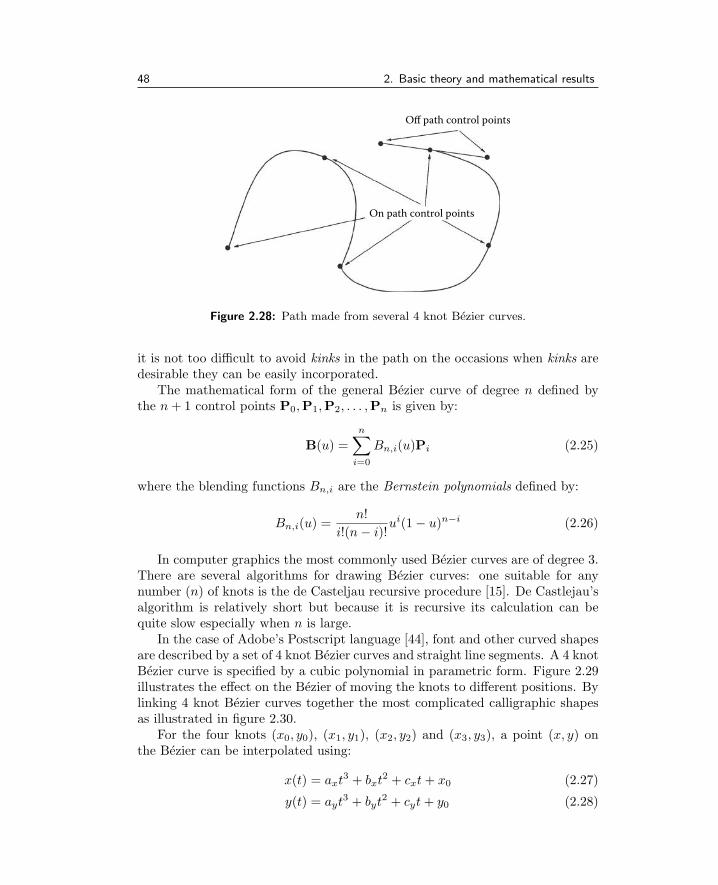
48 2. Basic theory and mathematical results
Off path control points
On path control points
Figure 2.28: Path made from several 4 knot Bezier curves.
it is not too difficult to avoid kinks in the path on the occasions when kinks aredesirable they can be easily incorporated.
The mathematical form of the general Bezier curve of degree n defined bythe n+ 1 control points P0,P1,P2, . . . ,Pn is given by:
B(u) =
n∑
i=0
Bn,i(u)Pi (2.25)
where the blending functions Bn,i are the Bernstein polynomials defined by:
Bn,i(u) =n!
i!(n− i)!ui(1− u)n−i (2.26)
In computer graphics the most commonly used Bezier curves are of degree 3.There are several algorithms for drawing Bezier curves: one suitable for anynumber (n) of knots is the de Casteljau recursive procedure [15]. De Castlejau’salgorithm is relatively short but because it is recursive its calculation can bequite slow especially when n is large.
In the case of Adobe’s Postscript language [44], font and other curved shapesare described by a set of 4 knot Bezier curves and straight line segments. A 4 knotBezier curve is specified by a cubic polynomial in parametric form. Figure 2.29illustrates the effect on the Bezier of moving the knots to different positions. Bylinking 4 knot Bezier curves together the most complicated calligraphic shapesas illustrated in figure 2.30.
For the four knots (x0, y0), (x1, y1), (x2, y2) and (x3, y3), a point (x, y) onthe Bezier can be interpolated using:
x(t) = axt3 + bxt
2 + cxt+ x0 (2.27)
y(t) = ayt3 + byt
2 + cyt+ y0 (2.28)

2.15. Bezier curves 49
(x3, y3)(x0, y0)
(x0, y0)(x0, y0)
(x3, y3)
(x2, y2)
(x2, y2)
(x2, y2)
(x3, y3)
(x1, y1)(x1, y1)(x1, y1)
Figure 2.29: Two-dimensional Bezier curves showing the effect of different placementof the intermediate points (the knots).
Figure 2.30: Calligraphic shape (the letters CG) made from many 4 knot Bezier curves.
where t is the parameter and
x1 = x0 +cx3
(2.29)
x2 = x1 +cx + bx
3(2.30)
x3 = x0 + ax + bx + cx (2.31)
Usually the (x0, y0), (x1, y1) etc. are known. ax, bx and cx can be calculatedby rearranging equations 2.29, 2.30 and 2.31 to give:
cx = 3(x1 − x0)
bx = 3(x2 − 2x1 + x0)
ax = x3 + 3(x1 − x2)− x0
Similar expression for ay, by etc., can be obtained.
Equations 2.27 and 2.28 are readily extended to give a description of a 4 knotcurve in three dimensions. The knots are specified by position vectors and theinterpolated points can be obtained by varying the parameter t.

50 2. Basic theory and mathematical results
2.16 Splines
Spline is a term that owes it origins to the flexible strip of wood draftsmen usedto use to draw curves. Weights would hold the spline in place at the pointson the drawing which the curve must pass through. Tracing along the woodenstrips produced a smooth and pleasing curve. An examination of the propertiesof the physical spline suggests a suitable mathematical model for it is a cubicfunction. A good example of a cubic function is the Hermite curve which isspecified in terms of the curve passing through two end points at which twotangent directions are also specified.
The spline that will be examined in this section has the greatest utility incomputer graphics because it is constructed so that it passes through all the datapoints. Since a cubic curve requires four parameters to define it, a spline curvethat will fit through more than four data points is usually handled piecewise,where four data points are taken in turn, with the spline function used to de-termine the course of the curve between the middle two. This form of piecewisespline is ofter referred to as a Catmull-Rom spline.
A cubic spline is written in the form:
p(τ) = K3τ3 +K2τ
2 +K1τ +K0 (2.32)
or equivalently (to speed up its calculation)
p(τ) = (((K3τ +K2)τ +K1)τ +K0)
The unknown vector constants K0, K1, K2 and K3 have to been determined;their components are independent of each other. τ is a parameter having values inthe interval [0, 1] such that when τ = 0, p(0) = Pi, and when τ = 1, p(1) = Pi+1
To determine the unknown vector constants we impose four conditions on 2.32:
1. The spline passes through the point Pi at the start of the curve.
2. The spline passes through the point Pi+1 at the end of the curve.
3. The derivative P′i of the spline at Pi is given.
4. The derivative P′i+1 of the spline at Pi+1 is given.
These apply to each of the components of p, i.e., for its x component we needto consider the values: xi , xi+1, x
′i , x
′i+1. Differentiating equation 2.32 w.r.t.
τ gives:
p′(τ) = 3K3τ2 + 2K2τ +K1 (2.33)
Substituting for xi and xi+1 in (2.32) with τ = 0 and τ = 1 respectively andthen with x′
i and x′i+1 in (2.33) while τ = 0 and τ = 1 gives four simultaneous

2.16. Splines 51
equations for the x component of the Ks. Written in matrix form these are:
0 0 0 11 1 1 10 0 1 03 2 1 0
K3x
K2x
K1x
K0x
=
xi
xi+1
x′i
x′i+1
On solution the following expressions are obtained:
K3x = 2xi − 2xi+1 + x′i + x′
i+1
K2x = −3xi + 3xi+1 − 2x′i − x′
i+1
K1x = x′i
K0x = xi
If Pi and Pi+1 are part of a set of points making up a path, such as, ... Pi−1,Pi, Pi+1, Pi+2 ..., the Ks are obtained using the value of p at Pi−1, Pi, Pi+1
and Pi+2 as follows:
K3x = −1
2xi−1 +
3
2xi −
3
2xi+1 +
1
2xi+2 (2.34)
K2x = xi−1 −5
2xi + 2xi+1 −
1
2xi+2 (2.35)
K1x = −1
2xi−1 +
1
2xi+1 (2.36)
K0x = xi (2.37)
Similar expressions may be written for K3y , K3z , etc., and thus the constantvectors Ki become:
Ki =
Kix
Kiy
Kiz
for i = 0, 1, 2, 3.In summary: The calculations we used to obtain the Ki vectors are local.
That is, they only depend on coordinates of the two points between which thecubic is used for interpolation and the two other nearest neighbors. Therefore,when we draw pieces of a path with many points, segments can be drawn inde-pendently. There is no need to take a global view of the whole path in order todraw just a little piece of it.
A couple of notes on splines:
• Extending this type of spline for use in three dimensions is relatively easy.A parameter, τ , replaces the variable x and there are two additional poly-nomials, one in each of the other coordinates.
• Usually τ takes integer values at the control points, i.e. −1, 0, 1, 2. In thiscase there is no relationship between the parameter τ and the distancebetween the points.

52 2. Basic theory and mathematical results
Lagrangepolynomial
Spline
Figure 2.31: Effect of displacing a control point on the shape of spline and Lagrangepolynomials.
2.16.1 The natural spline
An alternative view of the calculation of the spline constants arises by consid-ering all the fixed points of the spline together in a single step. A set of cubiccurves, one for each pair of fixed points, is still obtained but the blending isdone implicitly and the overall curve is smooth and well behaved. Well behavedmeans that if one of the control points is moved the curve will change shape onlyin its vicinity. Far away, the shape of the curve will not be affected. Contrastthis with other interpolation methods, Lagrange polynomial interpolation forexample: If a Lagrange polynomial is fitted to the data a change in one controlpoint will show a ripple effect throughout the curve. Some examples of this effectare shown in figure 2.31 where spline and Lagrangian interpolating functions arecompared.
To study the idea of a global spline curve we shall examine a two-dimensionalset of n points, (xi, yi), where the data is ordered so that x0 < x1 < x2 < ... <xn−2 < xn−1. Figure 2.32 illustrates the setup.
For the ith interval, between the points (xi, yi) and (xi+1, yi+1), the form ofthe cubic is:
y = ai(x− xi)3 + bi(x− xi)
2 + ci(x− xi) + di (2.38)
This curve must be satisfied by both (xi, yi) and (xi+1, yi+1). Blending isachieved by assuming that at (xi, yi) the slope and curvature are the same asin the previous interval (between points (xi−1, yi−1) and (xi, yi)). Slope andcurvature are given by first and second derivatives respectively.

2.16. Splines 53
h1
01
2
(xi, yi)
i
n–2
n–1
x
y
Figure 2.32: A two-dimensional spline curve passing through n data points.
Letting hi = (xi+1 − xi) and Si represent the second derivative at the point(xi, yi) an equation in which the Sis are unknown may be written for a generalpoint i,
hi−1Si−1 + 2(hi−1 + hi)Si + hiSi+1 = 6
(
yi+1 − yihi
− yi − yi−1
hi−1
)
(2.39)
Equation (2.39) is obtained by differentiating (2.38) twice, rearranging and mak-ing use of the assumptions about slope and curvature at point i.
Since equation (2.39) applies at the points on the spline (except the first andlast) a set of n−2 simultaneous equations may be written for the n values of Si,that is, an equation for each of the internal points 1, 2, ... (n− 2).
A set of n− 2 equations in n unknowns does not have a unique solution andso two additional equations, for S0 and Sn−1, are obtained by specifying somepertinent end conditions. Possible end conditions are:
1. The end cubics approach linearity, S0 = Sn−1 = 0, the so-called naturalboundary conditions.
2. The end cubics approach parabolas, S0 = S1 and Sn−1 = Sn−2.
3. S0 is a linear extrapolation from S1 and S2, and Sn−1 is a linear extrapo-lation from Sn−3 and Sn−2.
Using the natural boundary conditions a set of n − 2 linear equations inn − 2 unknowns (the Si) are established. In matrix form, these are written as[H][S] = [Y ] where:

54 2. Basic theory and mathematical results
[H] =
2(h0 + h1) h1 0 0 .. 0h1 2(h1 + h2) h2 0 .. 00 h2 2(h2 + h3) h3
.. .. .. .. .. ..0 .. 0 hn−4 2(hn−4 + hn−3) hn−3
0 .. 0 0 hn−3 2(hn−3 + hn−2)
[S] =
S1
S2
S3
..
..Sn−2
[Y ] = 6
(
y2 − y1h1
− y1 − y0h0
)
(
y3 − y2h2
− y2 − y1h1
)
(
y4 − y3h3
− y3 − y2h2
)
..
..(
yn−1 − yn−2
hn−2− yn−2 − yn−3
hn−3
)
The matrix [H] is very sparse (it has many zero elements) and tridiagonal. Linearequations with this structure are amenable to very rapid solution by using analgorithm such as the one in McCalla [58].
Once the Si have been found the constants ai, bi, ci and di in equation 2.38are obtained from:
ai =Si+1 − Si
6hi
bi =Si
2
ci =yi+1 − yi
hi
− 2hiSi + hiSi+1
6di = yi
After that, the cubic polynomial equation (2.38) is used to yield values for ygiven x in the interval between (xi, yi) and (xi+1, yi+1).

2.16. Splines 55
2.16.2 Other splines
Splines come in many flavors. The basis splines, uniform B-spline, non-uniformB-splines and recursive B-splines have other mathematical properties that makethem useful in different situations. The common feature among all these splinesis that they are constructed piecewise by blending together a series of functionsBi(t) within each of the pieces. The Bi(t) are called the basis functions, hencethe B in the name. They are functions of a single parameter t. It is then possibleto determine the location of any point on the curve defined by n+1 control pointsfrom:
P(t) =
n∑
i=0
Ni(t)Pi (2.40)
where the Pi are the control points and, in the case of the uniform B-splines:
Ni(t) =
B0(t− ti+1) if t ∈ [ti+1, ti+2)B1(t− ti) if t ∈ [ti, ti+1)B2(t− ti−1) if t ∈ [ti−1, ti)B3(t− ti−2) if t ∈ [ti−2, ti−1)0 otherwise
(2.41)
Of course, any single piece in which of P(t) is to be determined is only affectedby four control points. Thus for segment k
Pk(t) =3∑
i=0
Ni+k−1(t)Pi+k−1 (2.42)
The ti values in equation 2.41 are called the knot values, since they correspondto the parameter at each of the curve’s knots. The knots are the points on thecurve where it begins and ends as well as those points where the pieces of thespline join together. Thus a curve with n+1 control points will have n−1 knots.The full collection of knot values for a curve is known as the knot vector.
In B-splines the ti are equally spaced; in the non-uniform B-splines they maytake any value of t, even the same value. The Bi(t) are determined so that theproperties we require for the spline are satisfied. In the case of the non-uniformand rational B-splines the Ni(t) are determined through a recursive formula thatalso depends on the order of the curve, which for cubic splines is 3.
To plot a B-spline curve specified by n+1 control points, incremental valuesof the parameter t ∈ [0, n− 1] are substituted into 2.40 and the resulting pointsP joined up. For example, for a curve with 8 control points, the uniform B-splineknot vector will be [0, 1, 2, 3, 4, 5] and there will be 5 segments.
We have only touched on the rich mathematics of spline curves in this section.Bartels et al. [8] present a useful general study of spline theory for both curvesand surfaces. They introduce the highly useful non-uniform rational B-spline(NURBS) that has proved its utility in CAD applications. Lengyel [54] providesa detailed derivation of the basis functions for all splines in the family.

56 2. Basic theory and mathematical results
Control points
Moved control points
Oblique view of patch
Oblique viewPolygonal mesh
Patch
Figure 2.33: A basic NURBS patch is controlled by its network of control points.(Taken from OpenFX.)
2.17 Parametric surfaces
In section 2.16 methods of working with curves in computer graphics were dis-cussed. The Bezier and spline curves introduced there can be extrapolated intoa two-dimensional space to facilitate modeling curved surfaces. However, Bezierand simple polynomial based curves cannot model every form of curve, for exam-ple a circle cannot be exactly modeled by a Bezier curve. Rational polynomials(one polynomial divided by another) offer the potential to model any shape.Extending rational polynomials into a two variable parameter space offers thepotential to represent a surface with any degree of curvature. Making up mod-els from patches described by rational polynomials with the added constraintsof position, tangent and curvature continuity offers the potential to model anyshapes. Two-dimensional NURBS fulfills all the requirements for patch modelingand have proved popular with CAD designers. Most CAD tools and 3D model-ing software offers the facility to use NURBS surfaces, which are straightforwardextensions of NURBS curves.
NURBS patches are specified in terms of their control points. Figure 2.33illustrates a 2D patch with its control points and how it is possible to move

2.17. Parametric surfaces 57
the control points interactively to distort the patch into shape to be modeled,whilst the control points of a NURBS patch are the main way in which the patchof a CAD software program is specified by the designer. There are two otherattributes that are needed for a full specification of the patch, the knot and theorder. The order of a NURBS patch is the number of control points used in thecalculation of the coordinate of any point on the patch. The knots determinehow the control points affect the patch. They effectively give weight to how muchinfluence the control points have on determining the coordinate of any point onthe surface.
By definition, NURBS patches are 2D surfaces embedded in 3D space, theshape of which is determined by a network of control points pi,j(x, y, z). Thecontrol points are arranged in a 2D grid of surface local coordinates (u, v), where0 ≤ u ≤ 1 and 0 ≤ v ≤ 1. The 3D location of any point on the surface P ofa patch is obtained by specifying a value of the patch local coordinate system(u0, v0), and use:
P(u, v) =
k∑
i=1
l∑
j=1
Ri,j(u, v)pi,j (2.43)
Here, R(u, v) is the rational polynomial that gives a NURBS its properties, lis the number of control points across the surface in the u direction,and l thenumber in the v direction.
To generate a polygonal mesh for a NURBS patch, a regular array of (u, v)coordinates is passed through equation 2.43 to give an array of 3D coordinatesthat are connected together in a polygonal mesh, an example of which is depictedin figure 2.34.
The term Ri,j(u, v) in equation 2.43 is obtained through a combination ofbasis functions, Ni,n, which are polynomials of degree n. The degree of polyno-mial may be chosen depending on the desired properties, curvature etc., of thesurface, and based on this, additional control points are brought into play in cal-culating R(u, v). Typically Ni,n (where i identifies a control point) is obtainedin a recursive formulation:
Ni,n = fNi,n−1 + gNi+1,n−1
f is a linear function that rises from 0 to 1 and g falls from 1 to 0 over theintervals where N is non-zero. Ni,0 is a constant function with a value of 1 overthe interval between control points [i, i+ 1] and 0 elsewhere.
Bringing these terms together allows the expression for Ri,j(u, v) to be eval-uated:
Ri,j(u, v) =Ni,n(u)Nj,m(v)wi,j
∑kp=1
∑lq=1 Np,n(u)Nq,m(v)wp,q
(2.44)
wi,j is the control point’s weighting value. For a good practical implementa-tion of the NURBS patch see Peterson’s Graphics Gem [41] and further details

58 2. Basic theory and mathematical results
Control pointsPatches
Polygonalmesh
Shaded view
Figure 2.34: NURBS patches can take up any curvature. In this figure, 32 patches arecombined to form the model of a highly curved surface. For visualization purposes thepatches are converted to a polygonal mesh of the most suitable resolution, which mightbe viewpoint dependent.
of the basic mathematics of NURBS curves and surfaces may be obtained inLengyel [54].
2.18 Angular interpolation (quaternions)
Implicit in the previous discussion on interpolation was the use of the Cartesiancoordinate system. This is ideal for interpolating position vectors. On the otherhand there are many scenarios where it will be required to interpolate directionvectors.
Consider the following:
You are standing on the top of a hill with a camera on a motorizedtripod looking North. You wish to set the camera so that it pans roundto face East taking pictures every 10◦.

2.18. Angular interpolation (quaternions) 59
Two possible interpolation angles
θ2θ2θ2
θ1 θi θ1θ1
θi
Figure 2.35: In this example of angular interpolation there are two possible values foran angle bisecting the angles θ1 and θ2.
This is a job for angular interpolation, first direction 0◦, last direction 90◦, and8 intermediate steps. In this case linear interpolation of the angle is the naturalway to obtain the directions to use for the intermediate shots. As we shall seewhen we consider computer animation a combination of interpolated positionsand interpolated angles is a very efficient method of directing the action.
Angles are cyclic of period 2π, therefore the angle α is the same angle asα+2π, α+4π, . . . , α+2nπ. This makes interpolation a little tricky. As shownin figure 2.35 there are two possible solutions to the problem of finding the angle,θi, that lies half way between the two angles θ1 and θ2.
This problem of interpolation gets more complex when three dimensions areinvolved. First, to be able to specify an arbitrary orientation three angles areneeded. Section 2.12.7 introduced three measures that describe the orientationof a camera observing a collection of objects. There they were referred to asheading, pitch and roll (bank). Three angles specifying an orientation are knownas Euler angles. However, there are 12 possible conventions for describing Eulerangles making their specification rather confusing. We will choose the conventionfor orientation illustrated in figure 2.36. Thus, in three dimensions, interpolationbetween two orientations reduces to the problem of obtaining the triple (φ, θ, α)given two or more sets of angles (φ0, θ0, α0), (φ1, θ1, α1), etc.
Unfortunately, orientations specified with Euler angles (φ, θ, α) cannot be in-terpolated in the same way that positions are interpolated because of the periodicway in which angles are defined. This poses something of a problem; however anexcellent solution has been waiting in the wings since 1843 when Hamilton [37]developed the mathematics of the quaternion as part of his attempt to find ageneralization of the complex number. The significance of the quaternion forcomputer graphics was first recognized by Shoemake [81].
For the work in this book it is unnecessary to explore the details of the quater-nion in depth. We are only interested in using quaternions to help us achieveangular interpolation between given orientations and this simply requires that we

60 2. Basic theory and mathematical results
Viewed fromthe rear
(looking forward)
Heading pitch androll directions
y
y
z
θ
x
z
x
Viewed frombelow
(looking up)
Viewed from theright hand side(looking left)
y
φ
α
x
z
P
Figure 2.36: One set of Euler angles (φ, θ, φ) used to specify orientation. In each ofthe views the third axis is directed into the page. Each angle is specified by a radianmeasure relative to a base axis and is considered to be positive when the orientationis clockwise if observed from the coordinate origin while looking in the direction ofthe base axis. For computer animation work it is appropriate to think of an object ashaving a rest orientation, say directed along the x axis without any tilt (roll or bank).To pivot the object into some other orientation a series of rotations are applied untilit has taken up the orientation specified by the Euler angles (φ, θ, α) relative to thereference direction.
can interpolate between quaternions and switch back and forth1 between equiv-alent representations of orientation, i.e., Euler angles, quaternions and rotationmatrices.
2.18.1 The quaternion
A quaternion q is an ordered pair (w,v) of a scalar and three-dimensional vectorv with components (x, y, z). Like vectors, a unit length or normalized quaternionmust satisfy:
w2 + x2 + y2 + z2 = 1
1Users of application software generally prefer to specify orientations in terms of Eulerangles, pitch, elevation and headings rather than as abstract quaternions.
2.18. Angular interpolation (quaternions) 61
Quaternions have their own algebra with rules for addition and multiplication.Addition is straightforward: add the scalar components and the vector compo-nents. Multiplication is more interesting. Given two quaternions q1 and q2 theproduct is the quaternion:
q1q2 = (w,v) = (w1w2 − v1 · v2, w1v2 + w2v1 + v1 × v2)
A conjugate quaternion to q is defined as q = (w,−v). Thus, the squaredmagnitude of q is:
qq = |q|2 = w2 + |v|2
Note that if q is of unit magnitude its inverse q−1 equals its conjugate, q−1 = qand qq = 1.
2.18.2 Quaternions and rotations
We have seen in section 2.12.3 that the action of rotating a vector r from oneorientation to another may be expressed in terms of the application of a trans-formation matrix [R], which when applied to r to r′ = [R]r gives it a new orien-tation. The matrix [R] is independent of r and will perform the same (relative)rotation on any other vector.
One can write [R] in terms of a succession of Euler angle rotations, i.e., as afunction [R(φ, θ, α)] (the order being vital). However, the same rotation can beachieved by specifying [R] in terms of a unit vector n and a single angle γ. Thatis, r is transformed into r′ by rotating it round n through γ.
The angle γ is positive when the rotation takes place in a clockwise directionwhen viewed along n from its base. The two equivalent rotations may be writtenas:
r′ = [R(φ, θ, α)]r
r′ = [R′(γ, n)]r
At first sight it might seem difficult to appreciate that the same transformationcan be achieved by specifying a single rotation round one axis as opposed tothree rotations round three orthogonal axes; figure 2.37 illustrates this process.There are also a whole range of other subtleties surrounding this issue that areonly really resolved through the use of quaternions; Wolf [38] discusses these indepth.
It is also quite difficult to imagine how (γ, n) might be calculated given themore naturally intuitive and easier to specify Euler angles (φ, θ, α). However,there is a need for methods to switch from one representation to another.
In a number of important situations it is necessary to use the (γ, n)representation. For example the Virtual Reality Modeling Language(VRML) [40] uses the (γ, n) specification to define the orientationadopted by an object in a virtual world.

62 2. Basic theory and mathematical results
(a)
xx
y
r
z
r´
r´
r´r
z
x
y
n
rb
ra
ra
y
θ
α
rb
r
x
y
z
z
φ
(b)
γ
Figure 2.37: Rotation about an arbitrary axis, n, chosen to point in a direction thatis at right angles to both the initial and final results. (b) will achieve the same resultas three consecutive rotations around orthogonal basis vectors (a). Here r is the initialvector and r′ the result after re-orientation. ra and rb are intermediate steps.
Watt and Watt [86] derive an expression that gives some insight into thesignificance of the (γ, n) specification of a rotational transform by determining[R]r in terms of (γ, n):
r′ = [R]r = cos γr+ (1− cos γ)(n · r)n+ (sin γ)n× r (2.45)
This expression is the vital link between rotational transformations and the useof quaternions to represent them. To see this consider two quaternions:
1. p = (0, r), a quaternion formed by setting its scalar part to zero and itsvector part to r (the vector we wish to transform)
2. q = (w,v), an arbitrary quaternion with unit magnitude: qq = qq−1 = 1
The product qpq−1 gives the quaternion:
qpq−1 = (0, ((w2 − (v · v))r+ 2(v · r)v + 2w(v × r))) (2.46)
Since q is an arbitrary quaternion of unit magnitude there is no loss of gen-erality by expressing it in the form:
q = (cos(γ
2
)
, sin(γ
2
)
n) (2.47)

2.18. Angular interpolation (quaternions) 63
Substitute cos(γ
2
)
for w and sin(γ
2
)
n for v in equation 2.46. The vector part
of qpq−1 is identical, term for term, with the rotation expressed by equation 2.45.Therefore if we express a rotation in the form [R(γ, n)] its action on a vector ris equivalent to operating the following four steps:
1. Promote the vector r to the quaternion p = (0, r).
2. Express [R(γ, n)] as the quaternion q = (cosγ
2, sin
γ
2n).
3. Evaluate the quaternion product p′ = qpq−1.
4. Extract the transformed vector r′ from the vector component of p′ = (0, r′).(Note that the scalar component of operations such as these will always bezero.)
This isn’t the end of our story of quaternions because, just as rotationaltransformations in matrix form may be combined into a single matrix, rotationsin quaternion form may be combined into a single quaternion by multiplying theirindividual quaternion representations together. For example consider rotations[R1] and [R2] represented by quaternions q1 and q2 respectively. Applying themin turn to p′ = q1pq
−11 and p′′ = q2p
′q−12 gives:
p′′ = q2p′q−1
2
p′′ = q2(q1pq−11 )q−1
2
p′′ = (q2q1)p(q−11 q−1
2 )
p′′ = qcpq−1c
Here qc = q2q1 and as quaternions satisfy (q2q1)−1 = q−1
1 q−12 . We can write
(q−11 q−1
2 ) = (q2q1)−1.
2.18.3 Converting Euler angles to quaternions
From the Euler angles (φ, θ, α) shown in figure 2.36 a quaternion that encapsu-lates the same information is constructed by writing quaternions for rotation φabout the z, θ about the y and α about the x axes:
qx =[
cosα
2, sin
α
2, 0, 0
]
qy =
[
cosθ
2, 0, sin
θ
2, 0
]
qz =
[
cosφ
2, 0, 0, sin
φ
2
]

64 2. Basic theory and mathematical results
and then multiplying them together as q = qzqyqx. The components of q are:
w = cosα
2cos
θ
2cos
φ
2+ sin
α
2sin
θ
2sin
φ
2
x = sinα
2cos
θ
2cos
φ
2− cos
α
2sin
θ
2sin
φ
2
y = cosα
2sin
θ
2cos
φ
2+ sin
α
2cos
θ
2sin
φ
2
z = cosα
2cos
θ
2sin
φ
2− sin
α
2sin
θ
2cos
φ
2
2.18.4 Converting a quaternion to a matrix
In section 2.12.3 it was shown that a rotational transformation in matrix formcould be applied to a position vector to pivot it into a new orientation [p′] =[Tθ][p]. A quaternion contains rotational information but it cannot be directlyapplied to a position vector in the same way that a matrix can. Thereforeit is useful to have a method of expressing the rotational information in thequaternion directly as a matrix which, in turn can be used to rotate positionvectors.
For a normalized quaternion [w, x, y, z] the corresponding 4× 4 matrix is:
1− 2y2 − 2z2 2xy + 2wz 2xz − 2wy 02xy − 2wz 1− 2x2 − 2z2 2yz + 2wx 02xz + 2wy 2yz − 2wx 1− 2x2 − 2y2 0
0 0 0 1
It is important to note that a 4× 4 matrix can encapsulate positional trans-formations as well as rotational ones. A unit quaternion only describes purerotations. So, when quaternions are combined the complex rotation they repre-sent is with respect to axes passing through the coordinate origin (0, 0, 0).
2.18.5 Converting a matrix to a quaternion
If the rotational matrix is given by:
[M ] =
a00 a01 a02 0a10 a11 a12 0a20 a21 a22 00 0 0 1
and the quaternion q by:q = [w, x, y, z]
Shoemake’s [81] algorithm in listing 2.4 obtains q given [M ]. The parameter ǫis the machine precision of zero. A reasonable choice would be 10−6 for floatingpoint calculations. Note only elements of [M ] that contribute to the rotation areconsidered in the algorithm.

2.18. Angular interpolation (quaternions) 65
w = 1
4(1 + a00 + a11 + a22)
i f w > ǫ {w =
√w w4 =
1
4wx = w4(a12 − a21) y = w4(a20 − a02) z = w4(a01 − a10)
}else {w = 0x = − 1
2(a11 + a22)
i f x > ǫ {x =
√x x2 =
1
2xy = x2a01 z = x2a02
}else {
x = 0 y = 1
2(1− a22)
i f y > ǫ {y =
√y z =
a12
2y}else {
y = 0 z = 1}
}}
Listing 2.4: An algorithm for the conversion of rotational transformation matrix Mwith coefficients ai,j to the quaternion q with coefficients (w, x, y, z).
2.18.6 Converting a quaternion to Euler angles
To convert the quaternion to the equivalent Euler angles, first convert the quater-nion to an equivalent matrix, and then use the matrix to Euler angle conversionalgorithm. Sadly matrix to Euler angle conversion is unavoidably ill-defined be-cause the calculations involve inverse trigonometric functions. To achieve thisconversion use the algorithm shown in listing 2.5 which converts the matrix [M ]with elements aij to Euler angles (φ, θ, α).
The angles (φ, θ, φ) lie in the interval [−π, π] but they can be biased to [0, 2π]or some other suitable range if required.
2.18.7 Interpolating quaternions
One major advantage of using quaternions in 3D computer graphics is that the in-terpolation between two orientations defined by the Euler angles, say (φ0, θ0, α0)and (φ1, θ1, α1), is easily done when the orientations are expressed in a quater-nion form. It is not possible to interpolate between two orientations when theyare specified as a rotation matrices. To illustrate the advantage of quaternionswe recall that linear interpolation between two position vectors gives a straight

66 2. Basic theory and mathematical results
sin θ = −a02
cos θ =√
1− sin2 θi f | cos θ| < ǫ {It is not possible to distinguish heading from pitch and the convention thatφ is 0 is assumed, thus:sinα = −a21 cosα = a11
sinφ = 0 cosφ = 1}else {
sinα =a12
cos θcosα =
a22
cos θsinφ =
a01
cos θcosφ =
a00
cos θ}α = ATAN2(sinα, cosα)θ = ATAN2(sin θ, cos θ)φ = ATAN2(sinφ, cosφ)
Listing 2.5: Conversion from rotational transformation matrix to the equivalent Eulerangles of rotation.
line and in Cartesian geometry a straight line is the shortest path between twopoints. A similarly simple interpolation for quaternions is desirable. Thereforefor quaternions the question arises: What is equivalent to a straight line?
A clue to the answer comes from the concept of latitude and longitude. Lati-tude and longitude are angular directions from the center of the earth to a pointon its surface whose position is to be specified. Thus a pair of values (lat,long)represent a point on the earth’s surface. To go from one place to another bythe shortest route one follows a great circle, illustrated in figure 2.38. The greatcircle is the line of intersection between a sphere and a plane that passes throughthe center of the sphere. Intercontinental flight paths for aircraft follow greatcircles; for example the flight path between London and Tokyo passes close to theNorth Pole. We can therefore say that just as the shortest distance between twopoints in a Cartesian frame of reference is by a straight line, the shortest distancebetween two (latitude, longitude) coordinates is along a path following a greatcircle. The (latitude, longitude) coordinates at intermediate points on the greatcircle are determined by interpolation, in this case by spherical interpolation.
Quaternions are used for this interpolation. We think of the end points ofthe path being specified by quaternions, q0 and q1. From these a quaternion qiis interpolated for any point on the great circle joining q0 to q1. Conversion of qiback to (latitude, longitude) allows the path to be plotted. In terms of angularinterpolation we may think of latitude and longitude as simply two of the Eulerangles. When extended to the full set (φ, θ, α) a smooth interpolation along theequivalent of a great circle is the result.

2.18. Angular interpolation (quaternions) 67
AB = Great Circle
XY = Points on Great Circle
S
A
x
C
y
N
B
NS = Poles
C = Centre
Figure 2.38: A great circle gives a path of shortest distance between two points on thesurface of a sphere. The arc between points X and Y is the shortest path.
σ = w0w1 + x0x1 + y0y1 + z0z1i f σ > 1{
normalize q0 and q1 bydividing the components of q0 and q1 by σ
}θ = cos−1(σ)i f |θ| < ǫ {
β0 = 1− µ β1 = µ}
else {β0 =
sin(1− µ)θ
sin θβ1 =
sinµθ
sin θ}wi = β0w0 + β1w1
xi = β0z0 + β1x1 yi = β0y0 + β1y1 zi = β0z0 + β1z1
Listing 2.6: Implementation of the slerp function.
Using the concept of moving along a great circle as a guide to angular in-terpolation a spherical interpolation function, slerp(), may be derived. Theform of this function that works for interpolating between quaternions q0 =[w0, x0, y0, z0] and q1 = [w1, x1, y1, z1] is given by Shoemake [81] as:
slerp(µ, q0, q1) =sin(1− µ)θ
sin θq0 +
sinµθ
sin θq1
where µ, the interpolation parameter, takes values in the range [0, 1]. The angleθ is obtained from: cos θ = q0 · q1 = w0w1 + x0x1 + y0y1 + z0z1. The algo-rithmic implementation in listing 2.6 of the slerp() function for the interpolatedquaternion qi = [wi, xi, yi, zi] avoids the problem of division by zero when θ isclose to zero.

This page intentionally left blankThis page intentionally left blank

3Data structures for 3D graphics
The visual appearance of 3D models representing all kinds of objects is dictatedby the properties of their surfaces with color being the most important. Oftenthe surface of a model is constructed by building it up from a series of primitiveshapes. A polygon with three sides (a triangle) is the simplest form of primitiveshape. In chapter 2 other simple primitives like the sphere were discussed. Todayin computer-aided design (CAD) application programs more complex surfaceshapes referred to as patches have proved popular. These include Bezier andNURBS (non-uniform rational B-spline) patches which have curved edges andcontinuously varying internal curvature. A model can usually be accuratelyrepresented by combining a lot fewer of these more sophisticated surface shapes.Whether using primitive polygons or curved patches to describe a model there areadvantages and disadvantages. The simplest polygon is fast to render and easyto manipulate; the more complex patches usually give a better approximation tothe original object, especially if it has many curved parts. Occasionally, it is amatter of personal preference which sort of patch to use. For example, a cube ismodeled just as effectively with triangular polygons as it is with Bezier patches.Figure 3.1 shows the famous Utah teapot in polygonal and Bezier patch form.
Whatever type of patch is used to describe the surface of a 3D model it mustbe located in space, which means attaching it to three or more vertices or pointssomewhere in 3D space. With appropriate transformations applied to the vertexcoordinates a visualization (more commonly called a rendering) can be producedon the computer monitor or other output device.
3.1 Integer coordinates
When the topic of coordinate systems is discussed, Cartesian or possibly polar arethe words that come to mind. Very little thought is given to the numbers systemused to map out the spaces; it is more or less taken for granted that floating pointdecimals will be used. In the perfect world of mathematics there is no need to
69

70 3. Data structures for 3D graphics
Figure 3.1: Polygonal and Bezier patch surface representations.
pay the slightest thought to approximation; if two numbers are equal, then theyare equal, and their magnitude is irrelevant. Unfortunately, in the practical andimperfect world where calculations have to be done by machine, the behavior ofnumbers is far from perfect. Only in the case of the integer numbers (lying insidethe range of precision of the computer’s word length) can one really say that xis equal to y when they are being compared in a computer program; otherwiseall one can really say is that if |x − y| < ǫ we will accept the fact that x and yare equal.
Being able to say that x equals y is an essential part of most of the algorithmsused in computer graphics: Does this edge hit that polygon, is often a keyquestion. Three-dimensional computer graphics is founded on 3D geometry,and 3D geometry is very good at finding those situations where our numericalmathematics is challenged the most: Does the line hit the polygon on its edge,or inside, is a very hard question to answer. Using one computer that calculatesto an accuracy of ten decimal places may give a different answer to one thatcalculates to 20 places of decimals. For this reason we often choose to store thecoordinate data for vertices and other points using integers, and where possibleworking with algorithms that manipulate things using only integers, we can thensay with certainty whether x equals y or whether two lines actually are parallelor not.
A number of the most significant computational geometry algorithms used inCGI are written to work best with integer coordinates; see O’Rourke [65]. TheOpenFX program (chapter 9) uses integer coordinates to record its 3D data.
3.2 Vertices and polygons
The minimal description of a 3D model requires a list of surface patches and alist of vertex coordinates. Each entry in the surface patch list must identify thevertices to which it is connected and have some way of allowing its surface totake on the appearance of wood, marble, glass or chrome etc. Indeed, one ofthe most popular ways to provide a comprehensive set of surface attributes is

3.2. Vertices and polygons 71
for each surface patch to store an index into a table of materials. The materialprovides a color and many other properties. With careful choice of parameteran extremely realistic look to the model can be achieved.
Despite the fact that real-time shading can now be done routinely on basicpersonal computers it can still be useful to use a wireframe display when design-ing interactive 3D animations or complex models. Shaded rendering is done ina subsequent step to whatever degree of realism is required, a process that cantake minutes or even hours.
A wireframe model is a set of straight lines that join vertices together. Theedges of each polygonal surface constitute the members of this set. Sometimes itcan be useful to maintain a separate list of edges rather than to have to generateit from the polygons each time a drawing of the wireframe is made. This policyhas the advantage of a faster display and since edges are not normally rendered,they can be used to link various parts of a model together for editing purposes.
There are three alternative schemes for storing the geometric description ofa model:
1. For the n vertices of each surface polygon store n integers. Each integeridentifies an entry in the vertex list. For each entry in the vertex liststore the coordinates (x, y, z) of a position vector. Most 3D programsstore (x, y, z) as single precision floating point numbers, but a few useintegers. If polygon edges are needed then they can be obtained by pairingconsecutive vertices.
2. For each surface polygon that is connected to n vertices store n integers.Each integer identifies an entry in the vertex list. For each entry in thevertex list store a position vector giving its (x, y, z) coordinates. If requireda separate list for the m edges can be included. It holds two integers foreach edge that index entries in the vertex list.
3. For each surface polygon with k edges store k integers identifying the en-try in an edge list. An edge list identifies connections between vertices.Normally edges are part of the boundaries of polygons but it is possible tohave edges in a model that have no connection with its polygonal surfaces.These will show up in a wireframe drawing of the model but will not bevisible in either a hidden line or shaded rendering. For each edge, storetwo integers to index entries in the vertex list corresponding to the verticesat the end of the edge. For each entry in the vertex list store a positionvector giving its (x, y, z) coordinates.
These organizations are summarized in figure 3.2.
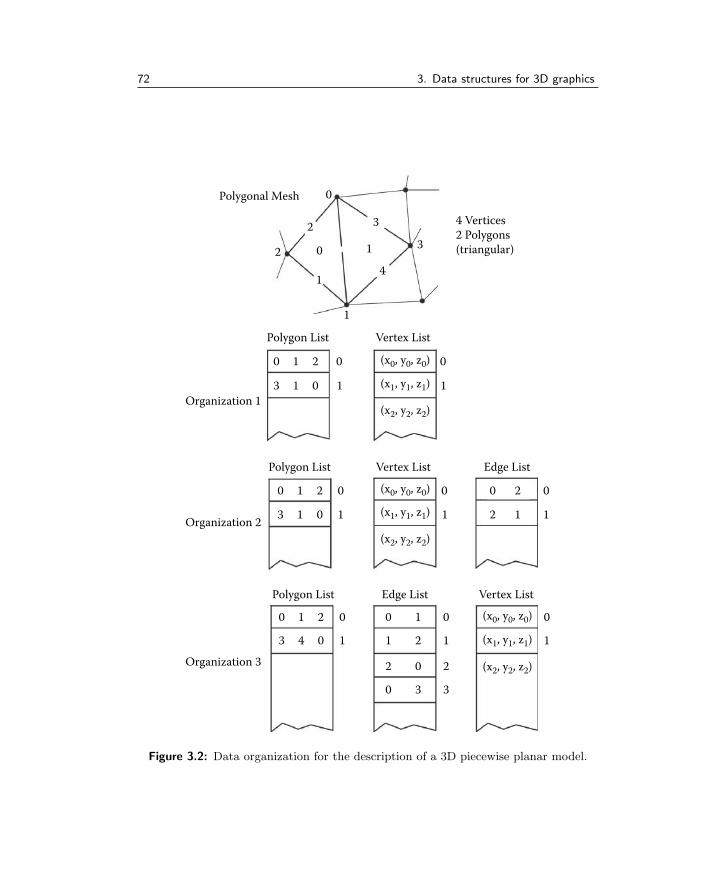
72 3. Data structures for 3D graphics
Organization 3
0 0 0 01
3
2
0
1
4 1
0 0
3
2
0
1
1
0
3
2
2
2 3
3
41
1
1
0
0
0
1
1
1
1 1
0
12
0 2
2
0
1
0
(x0, y0, z0)
(x1, y1, z1)
(x2, y2, z2)
(x0, y0, z0)
(x1, y1, z1)
(x2, y2, z2)
(x0, y0, z0)
(x1, y1, z1)
(x2, y2, z2)
1
0
1
0
1
1
0 33
2 20
Organization 2
Organization 1
Polygon List
Polygon List
Vertex List
Vertex List Edge List
Polygon List Edge List Vertex List
4 Vertices2 Polygons(triangular)
Polygonal Mesh
Figure 3.2: Data organization for the description of a 3D piecewise planar model.

3.2. Vertices and polygons 73
To complete the requirements for a useful data structure we add a mate-rial index for each polygon and texture coordinates to every vertex. Texturecoordinates allow a two-dimensional frame of reference to cover the surface of amodel, rather like the way latitude and longitude are a two-dimensional coordi-nate system that are used to reference any point on the surface of the earth (a3D spheroid). Just using a two-dimensional texture coordinate for each vertexhas a slight disadvantage because the texturing is only visible in the polygonsattached to the vertices; therefore if two adjacent polygons share a common pairof vertices it is not possible to provide a different mapping in the two polygons.Despite the addition of 2n numbers per N-gon it is better to record the texturecoordinates for all the vertices of a polygon with the polygon.
There is also a good case to be made for including an additional three-dimensional texture coordinate system. It might be local to the whole objectmesh, or apply to all surfaces with a specific material, or be defined on a per-vertex, or per-polygon-vertex basis. The reason for this inclusion is that pro-cedural shaders are often three-dimensional; an object might look like it wascarved out of marble, granite etc., rather than just look like the material wasjust painted over its surface.
In addition to this information it is a good idea to add a few temporary vari-ables to the structure for use by modeling and rendering algorithms. For exam-ple, some of the algorithms described in chapter 10 require additional membersin the data structures for vertices, edges and faces.
3.2.1 Skeletons, bones and materials
Partitioning a polygonal model into sub-units that are linked in a parent–child–grandchild relationship is useful. For example hierarchical linkages are verysignificant in character animation. An easily implemented and practically usefulscheme is one that is analogous to the familiar file-store structure of computersystems, i.e. a root directory with files and subdirectories which themselves con-tain files and subdirectories and so on to whatever depth you like.
A doubly linked list of hierarchy entries is the best way to organize this data.In addition to previous and next pointers each entry will have a pointer to itsparent, see figure 3.3. Other data can easily be appended to the structure asnecessary. When using the structure for character animation or to referenceparts of big model the entries can be given symbolic names, an example of whichis shown in figure 3.3.
To complete a hierarchical description every polygon or vertex in the modelis identified with one of the hierarchical names. A similar concept is one in whichfiles on a computer disk are identified by the folders in which they are stored.
In a connected network of vertices and facets it is probably more useful toassociate vertices, rather than polygons with one of the hierarchical names. Toimplement this association the vertex data structure shown in figure 3.10 must beextended with the entry hid where, for a vertex hid, identifies which hierarchical

74 3. Data structures for 3D graphics
name the vertex is associated with. The new structure is shown in figure 3.4. Abasic version of a structure that specifies a polygonal surface patch is illustratedin figure 3.5.
Grandchild
Child
Parent Head
Body
Left Foot
Left LegHand
Arm
Figure 3.3: A hierarchical data structure for editing and character animation.
p position vector of vertexν, µ surface texture coordinatesx temporary integer indexn number of adjacent verticesVadj list of adjacent verticeshid pointer to hierarchical element vertex is assigned to
Figure 3.4: Vertex data structure with hierarchical identifier.
Vid list of vertex ids to which polygon is attachedidmat pointer to a material in materials listidmap pointer to a texture map in the list of image maps(νi, µi) texture coordinates for each vertexn normal to surface plane
Figure 3.5: Typical surface patch data structure.
Notes:
1. The hierarchical names do not record any information about which verticesare assigned to them. Thus if it becomes necessary to modify the vertexlists (by adding or deleting for example) there is no need to update thehierarchy. However, the converse is not true. If a name in the hierarchy
3.2. Vertices and polygons 75
is removed then all the vertices must be checked for any reference to thedeleted hierarchical name and that reference removed.
2. When used for character animation, assigning each vertex to be attachedto only one bone is not always the best strategy. For example, a vertexin the mesh of a forearm of a character that lies close to the elbow shouldhave its position influenced to a certain extent by the bone in the upperarm. There are two ways in which we might try to enhance the model.First, it is easy to arrange that the movement of any of the bones in theskeleton could influence a displacement of a vertex in proportion to theirdistance from the vertex, with the added possibility of weighting how aparticular bone amplifies or attenuates its influence. Or second, a list ofbones (instead of just one) can be assigned to influence each vertex andonly those in the list used to modify the movement of the vertex, againpossibly in proportion to their distance from the vertex.
Both approaches have advantages and it is a good idea to assign extra at-tributes to each bone’s data structure (see figure 3.3), so that additionally:(1) a weight, (2) a range of influence and possibly (3) a rate of influencethat declines with distance, may be attributed to each bone. Also, sinceboth two- and four-legged animals can be modeled with at most two bonesinfluencing a third, the inclusion of a second vertex pointer per vertexwould allow the influence of sufficient bones to be applied without beingpolluted by influence from other bones, just because they happen to beclose by, but not directly connected.
3.2.2 Material data structures
In section 3.2 it was pointed out that in order to provide details of a surfacetexture the most efficient way is to maintain a list of materials, any one ofwhich can be applied to the surface. The efficiency of this scheme is easily seenbecause there will always be a very much larger number of polygons definingan object’s shape than there will be materials from which that surface could bebuilt. Another advantage could ensue because separating the material data fromthe geometric data allows the number of properties that define the material tobe increased (or decreased) without the need to modify the geometry describingstructures.
The most basic material property that should be included to describe a sur-face is its color, but there are many other possibilities, e.g., its transparencyand reflectivity. These will be discussed later in the book. Painting an imageacross a surface is perhaps the next most significant technique of giving textureto a surface that would otherwise look very unrealistic if just left a plain color.Painting a picture from an image file is usually referred to as texture mapping orimage mapping and it plays a very important role, because an image map canalso be used to simulate reflectivity, surface roughness and transparency. It is

76 3. Data structures for 3D graphics
probably worth separating the image map from the other material properties byusing a separate list. Then one or the other or both can be applied to the samesurface.
Often materials, or image maps, or texture maps, or algorithmic textures, arejust called shaders, but whatever they are called they play an equally importantrole to the geometry that describes an object’s shape.
3.3 Algorithms for editing arrays of structures
When a modeling tool requires making many changes to the contents of its vertex,edge and face data, an organization based on a doubly linked list is very efficient,for example when deleting a vertex from the middle of the list. However, when itis not possible to use a doubly linked list data organization, fast editing functionsare needed for things like inserting and or removing items from a basic indexedlist.
For 3D data, the order in which polygons and vertices appear in a list isusually unimportant. Therefore, when items are added to a list, they can simplybe tagged on to the end. Of course, the memory has to be dynamically extendedto accommodate the extra items. To delete items from the list is more complexand if not done efficiently can be unacceptably time consuming. This sectionpresents a very efficient algorithm for the removal of one or more items fromanywhere in a list of vertex or polygon data structures.
n–1 n0 1 2 3
Figure 3.6: Array of polygon structures numbered 1 to n.
Figure 3.6 illustrates a representation of the list of polygon structures. Thoseto be deleted are marked with a *. Each structure will be composed of perhaps16 to 32 bytes. The last entry n could be removed simply by reallocating thememory space to hold n − 1 polygons, but to eliminate polygon 2 the datafor polygons 3 to n must be shifted to lower memory before the memory isreallocated. However this shifting operation is very slow and it gets slower ifthere are other entries to be removed later. Note that the vertex and polygonlists are dependent, because each polygon list entry points to an entry in thevertex list; therefore if the vertex list is modified, even if the polygon list isnot, the polygon vertex identifiers will need to be updated, a process termedre-vectoring.
A very fast scheme can be developed by using the fact that the order of itemsin the list is unimportant. In this case all that has to be done is to copy the

3.3. Algorithms for editing arrays of structures 77
last entry in the list into the place held by the item to be deleted. The list maythen be shortened by one entry. If several items are deleted the reduction in thesize of the list is done in one step. In the example shown in figure 3.6 copy itemn− 1 to item 2 (remember item n is also to be deleted).
2 3 n–1
n–2n–1
n
Copy
Shorten
10
0 1 3
Figure 3.7: Deleting two items from the list of structures.
The whole of the structure can be copied with one call to a fast memory copyfunction (usually available as part of any system API, Application ProgrammingInterface). The algorithm works through the list and when it finds an entry tobe deleted it copies an entry from the end of the list and shortens the list byone. See the examples illustrated in figures 3.7 and 3.8. When all the entrieshave been processed one call to the reallocation function tidies up the memory.
The algorithm for removing unwanted entries from a list of Poly structureswith Npolys entries is summarized in listing 3.1.
Note that by not indexing k when the structure is to be deleted we get thechance to immediately delete the one replacing it if it too is flagged for deletion.
This algorithm can be applied to the polygon and vertex lists in exactly thesame way. However, as mentioned above, any change to the vertex list willinvalidate entries in the polygon and edge lists that point to items in the vertexlist. For example, if a polygon is attached to vertices 100, 101, 102 in the vertexlist but vertex 2 is removed from the list then vertices indexed as 100, 102 or 103may have moved to a different place in the vertex list. So, if we don’t fix upthe polygon data a memory violation will probably occur; at the very least themodel will be a mess.
The fix is easily done by employing a dummy index variable in the vertexstructure. As the algorithm steps through the vertex list copying down from theend to over-write the entries to be erased, it writes into the dummy index of thecopied entry the location where the copy has moved to. At the end of the pass,but before the vertex list is resized, the polygon list is scanned again so that

78 3. Data structures for 3D graphics
743890
0 1 2 3 4 5 6 7 8 9
0 1
Shorten and re-number
Copy
2 3 4 5
Figure 3.8: Deleting multiple items from the list.
i = 0 ,k = 0 and newN = Npolysr epeat while i < Npolys {
i f Poly(k) flagged for deletion {i f i < Npolys− 1 {
copy size of Poly structure (bytes)from Poly(newN − 1) to Poly(k)
}newN = newN − 1
}else k = k + 1i = i+ 1
}Npolys = newN
Listing 3.1: Outline of an algorithm to remove unwanted entries from a list of NpolyPoly structures. The unwanted entries will be flagged in some convenient manner.
each reference to an entry in the vertex list is tested. If it points to one of thevertices that has been moved then it is replaced by the new location (stored inthe dummy index) that was determined in the first pass. Memory reallocationcompletes the algorithm. This algorithm is shown in detail in listing 3.2.
Such a scheme is very efficient and uses as few operations as possible whenremoving items from a 3D data structure which has been stored in a contiguousmemory block.

3.4. Making an edge list from a list of polygonal faces 79
3.4 Making an edge list from a list of polygonal faces
When producing a wireframe drawing of a model or converting between the dataformats of alternative 3D CAD and animation packages it is important to beable to build a list of edges from a list of polygons.
It is straightforward to make a list of edges by creating one edge for eachpolygon side, but most polygons will share edges. The task of removing multipleentries from the edge list becomes excessively time consuming as the number ofpolygons increases. In the case of n polygons approximately 3n2 tests need tobe performed to make sure that the same edge is not recorded more than oncein the edge list. When dealing with more than a few hundred polygons it isessential to find a more efficient procedure.
The following gives the outline of an algorithm that deals with the issue moreefficiently:
• For each vertex i in the model set up a list to hold the identity of othervertices in the model attached to vertex i by an edge. Initially these listswill be empty.
• Take each polygon in the model in turn and with every edge of the polygonconsider the vertices at both ends of the edge.
• Label the vertices j and k. For vertex j look at j’s list of adjacent vertices.If it is empty or does not contain vertex k then add k to j’s list. For vertexk look at its list of adjacent vertices and if it is empty or does not containvertex j then add j to k’s list.
• When all the polygons have been examined consider each vertex in turn.Call the current one i. For vertex i create an edge between vertex i and allthe vertices in i’s list of attached vertices. For an example see figure 3.9.
Vertex
0
1
2
3
n
.
.
Vertex attached to...
0
1
2
3
n
.
.
Edges
0 – 1
0 – 2
0 – 3
1 – 4
1 – 9
1 – 6
1,2,3
1,4,6,9
...
7,11,19
Figure 3.9: Building an edge list from a polygon list.
The advantage of this procedure comes from the fact that the number ofcomparison tests will be much fewer than would be required by the simplisticapproach of checking all polygons against all polygons.

80 3. Data structures for 3D graphics
Erase items from the Polygon list but don’trelease the recovered memory yets e t i = 0 ,k = 0 ,j = 0 and newN = Nvertsr epeat while i < Nverts {
i f V ert(k) f l a gg ed for d e l e t i o n {i f i < Nverts− 1 {
copy size of V ert structure (bytes) from V ert(newN − 1) to V ert(k)V ert(newN − 1).x = j (extra index in V ert structure)
}newN = newN − 1
}else {
k = k + 1j = j + 1
}i = i+ 1
}Nvert = newN
Now process the dependent Poly data structure to fix it ups e t i = 0repeat while i < Npolys {
s e t j = 0repeat while j < NvertPerPoly {
i f Poly(i).Vid(j) ≥ Nvert {Poly(i).Vid(j) = V ert(Poly(i).Vid(j)).x
}j = j + 1
}i = i+ 1
}
To finish: Tidy up the memory allocation for Poly and V ert structures
Listing 3.2: Details of the algorithm to remove unwanted entries from a polygonaldatabase when the database uses a contiguous list rather than a doubly linked list torecord the polygons and vertices.
To accommodate the adjacency list it is necessary to augment the vertexdata structure with two items, n and Vadj as shown in figure 3.10. Vadj is adynamically sized array of vertex identifiers.
Pseudo-code for the above algorithm is given in listings 3.3 and 3.4. Part 1of the algorithm calls to a subroutine which inserts vertices in the adjacency listand extends it if necessary.
In the subroutine (part 2) the adjacency lists for vertices V1 and V2 are checked.If an entry is already present in the list the subroutine returns immediately.

3.5. Finding adjacent polygons 81
p position vector of vertexν, µ surface texture coordinatesx temporary integer indexn number of adjacent verticesVadj list of adjacent vertices
Figure 3.10: Entries in the vertex data structure.
Part 1 Recordings e t i = 0 and repeat while i < Npolys {
I n s e r t I nVe r t exL i s t (Poly(i).Vid(0), Poly(i).Vid(1))I n s e r t I nVe r t exL i s t (Poly(i).Vid(1), Poly(i).Vid(2))I n s e r t I nVe r t exL i s t (Poly(i).Vid(2), Poly(i).Vid(0))i = i+ 1
}
Part 2 Building Edgess e t i = 0 and repeat while i < Nvert {
i f V ert(i).n > 0 {s e t j = 0 and repeat while j < V ert(i).n {Create edge between vertices i and Nvert(i).Vadj(j)
j = j + 1}
}i = i+ 1
}
Listing 3.3: Part 1 of the algorithm to make an edge list from a list of connectedpolygonal facets.
3.5 Finding adjacent polygons
Some of the algorithms to be discussed in later chapters require that every poly-gon (in a mesh model) knows the identity of its neighboring polygons. A neigh-boring polygon is one that shares an edge. For the example in figure 3.11 poly-gons 1 and 2 share an edge as do polygons 2 and 3.
Algorithms that need this information include:
• Delaunay triangulation.
• Subdivision of surfaces.
• Algorithms to make surface normal orientations consistent.
Like the procedure for finding edges given a set of polygons (section 3.4) findingadjacent polygons can be a prohibitively lengthy task if an exhaustive comparisonis used.
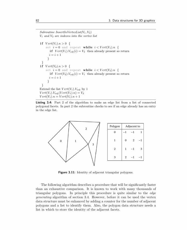
82 3. Data structures for 3D graphics
Subroutine InsertInVertexList(V1, V2)V1 and V2 are indexes into the vertex list
i f V ert(V1).n > 0 {s e t i = 0 and repeat while i < V ert(V1).n {
i f V ert(V1).Vadj(i) = V2 then already present so returni = i+ 1
}}i f V ert(V2).n > 0 {
s e t i = 0 and repeat while i < V ert(V2).n {i f V ert(V2).Vadj(i) = V1 then already present so returni = i+ 1
}}
Extend the list V ert(V1).Vadj by 1V ert(V1).Vadj(V ert(V1).n) = V2
V ert(V1).n = V ert(V1).n+ 1
Listing 3.4: Part 2 of the algorithm to make an edge list from a list of connectedpolygonal facets. In part 2 the subroutine checks to see if an edge already has an entryin the edge list.
3 2 –1 –1
2 1 –1 3
1 0 2 –1
0
0 1
2
3
–1
Polygon Adjacent to
–1 1
Figure 3.11: Identity of adjacent triangular polygons.
The following algorithm describes a procedure that will be significantly fasterthan an exhaustive comparison. It is known to work with many thousands oftriangular polygons. In principle this procedure is quite similar to the edgegenerating algorithm of section 3.4. However, before it can be used the vertexdata structure must be enhanced by adding a counter for the number of adjacentpolygons and a list to identify them. Also, the polygon data structure needs alist in which to store the identity of the adjacent facets.

3.5. Finding adjacent polygons 83
In the case of a triangular polygon the adjacent facet identifier list will berequired to hold up to a maximum of three integers. When polygons have oneor more edges that are not adjacent to other polygons this can be flagged bystoring a −1 as the identity of the neighboring polygon. The augmented datastructures are illustrated in figure 3.12.
p position vector of vertexν, µ surface texture coordinatesx temporary integer indexnV number of adjacent verticesVadj list of adjacent verticeshid pointer to hierarchical element to assign vertex tonF number of adjacent polygonsFadj list of adjacent polygons
Vid list of vertex ids to which polygon is attachedidmat pointer to a material in materials listidmap pointer to a texture map in the list of image mapsAid(3) list of the ids of polygons with a common siden normal to surface plane
Figure 3.12: Vertex and polygon data structures to accommodate calculation andstorage of polygon adjacency information.
The detailed pseudo-code implementation of the algorithm is presented inlistings 3.5 and 3.6. However, before presenting the algorithm in detail thefollowing gives a simple overview:
1. For each vertex create a list to hold the identity of polygons which areattached to it. Initially all the lists will be empty.
2. Work through all the triangular polygons, j, and consider each of its ver-tices in turn. For each vertex (call it k) of j add j to k’s polygon adjacencylist Fadj . (For each vertex this builds up a list of which polygon is attachedto which vertex.)
3. Again work through all the polygons, call the current one j, and then takingeach side in turn, identify the two vertices to which it is attached. Call themi1 and i2. For vertices i1 and i2, look through each one’s list of attachedpolygons and see if any have an edge between i1 and i2 (remembering

84 3. Data structures for 3D graphics
to exclude the current polygon j). If they have, then this is the polygonadjacent to polygon j along the side between vertices i1 and i2. This can bedone by checking all polygons adjacent to i1 against all polygons adjacentto i2 and if they have a polygon in common it can only be polygon j oranother one with vertices i1 and i2 in common, which is the one adjacentto polygon j.
Part 1: Build polygon adjacency list for each vertexs e t i = 0 and repeat while i < Npolys {
s e t j = 0 and repeat while j < 3 {id = Poly(i).Vid
n = V ert(id).nF
extend the list V ert(id).Fadj to n+ 1 spacesV ert(id).FAdj(n) = iV ert(id).nF = n+ 1j = j + 1
}i = i+ 1
}
Listing 3.5: Part 1 of the algorithm to make a list of polygons attached to each vertexfrom a Facet/Vertex 3D database.
3.6 Finding polygons adjacent to edges
Some of the algorithms to be discussed in later chapters require that every edgeknows the identity of its neighboring polygons. For most closed surfaces ap-proximated by a network of polygons an edge will have at most two neighboringpolygons.
The algorithm itself is very similar to that for finding polygons adjacent topolygons, described in section 3.5, and example code implementation can beobtained from the website.

3.6. Finding polygons adjacent to edges 85
Part 2: Build polygon adjacency list for each polygoni1 and i2 are vertex id’s for polygon edgesset i = 0 and repeat while i < Npolys {
set l = 0 and repeat while l < 3 {check all polygons adjacent to i1 and i2 to see if any of themhave an adjacent polygon in common (it must not be of course be i)Poly(i).Aid(l) = −1 /∗ record −1 if nothing adjacent ∗/i f l = 0 {
i1 = Poly(i).Vid(0)i2 = Poly(i).Vid(1)
}else i f l = 1 {i1 = Poly(i).Vid(1)i2 = Poly(i).Vid(2)
}else i f l = 2 {i1 = Poly(i).Vid(2)i2 = Poly(i).Vid(0)
}i f V ert(i1).nF > 0 and V ert(i2).nF > 0 {s e t j = 0 and repeat while j < V ert(i1).nF {t = V ert(i1).Fadj(j)s e t k=0 and repeat while k < V ert(i2).nF {
u = V ert(i2).Fadj(k)u and v are polygons adjacent to i1 and i2, if they are the samethen the edge between i1 and i2 is a boundary of polygonst and u. it is either i or the desired polygoni f u = t and u 6= i {
Poly(i).Aid(l) = ujump to l a b e l /* no need to continue */
}k = k + 1}
j = j + 1}
}l a b e l :
l = l + 1}
i = i+ 1}
Listing 3.6: Part 2 of the algorithm to make a list of adjacent polygons from aFacet/Vertex 3D database.

This page intentionally left blankThis page intentionally left blank

4Basic visualization
In this chapter the mathematical principles of chapter 2 and the structures ofchapter 3 come together to produce a collection of algorithms that are used tosynthesize images from purely numerical data so that the viewer should instantlybe able to exclaim “That’s a . . . !” This synthesis is termed rendering, andfrom the scientific point of view this is a mathematical modeling process of theway light interacts with surfaces, how light travels to the observer’s location andhow they perceive it.
In the decade or so since publication of the first edition of this book themajor mathematical models used in the rendering process have been refined butnot radically changed. Most of the physical models and their mathematical im-plementations were worked out in the 20th century. What has changed andcontinues to change is the power of the computer used to carry out the calcu-lations. The invention of the specialized graphics processor, the GPU, lies atthe heart of these changes and it has enabled visualization models that werepreviously thought to be impractical to use to become mainstream. Of course,the primary purpose of the GPU is in rendering images in real-time which isprincipally fueled by the huge market for computer games.
Good as it is, the GPU is still orders of magnitude too slow to calculate in real-time a complete physical model of the light transport process. Even to be ableto model some of the most important rendering challenges GPU shaders1 haveto resort to some empirical and heuristic approximations. The GPU hardware’sarchitecture is designed around the rendering pipeline concept. A number of thealgorithms described in this chapter have their place in the rendering pipeline.Whilst the GPU builds these algorithms in hardware there are always going tobe occasions where a software implementation is still essential, especially if youare looking for images with particular qualities. In fact, because the GPU isprogrammable, a knowledge of the algorithms it uses, how they work and theprinciples that underlie them is essential if you are going to write programs forthe GPU and make the most of its incredible power. The procedural textures(one type of shaders) to be discussed in chapter 11, the OpenGL programs andGPU hardware discussed in chapter 7 and the implementation of an extensible
1The programs that run in a GPU are called shaders.
87

88 4. Basic visualization
software rendering pipeline in chapter 9, can all be ported to GPU programs, butonly if you have a knowledge of the basics that are covered in this chapter.
In the context of computer graphics, rendering is the process of artificiallygenerating a picture of something from a numerical dataset or other form ofspecification. This usually involves billions of calculations as the picture is syn-thesized. Continuing advances in computer technology are allowing pictures tobe produced more and more rapidly. Some algorithms can deliver an image inonly a few milliseconds. However the quest for more and more lifelike picturesrequires calculating processes of rapidly increasing complexity. Consequently,no matter how quickly developments in processor technology deliver increasedperformance, there are always grumblings of discontent among the artists anddesigners who use computer graphics in their work.
From the point of view of describing algorithms for the rendering task thereis a point where a quantum leap in the time it takes to render a picture (animage) occurs. Thus it is useful to classify rendering algorithms in two groups:those that are very fast and those that are not. At one end of the fast renderingspectrum are the real-time rendering engines. Engine is a term with its originin the computer games industry where rendering a standard TV or video sizedimage usually takes a few milliseconds. The real-time engines are relying moreand more on the GPU hardware and programmer APIs like OpenGL [82] orDirectX. See for example Sherrod and Jones [79] which is focused on the latestversion of DirectX.
It is interesting to note that most of the recent books in the area of real-timegraphics tend to place their focus on 3D games programing, which just goesto highlight the dominance of computer games within the 3D graphics scene.A comprehensive introduction to the algorithms for real-time rendering may befound in Akenine-Moller and Haines [1], and an excellent and comprehensivesource of demonstrator programs exemplifying all aspects of OpenGL is theOpenGL SuperBible [78]. We highlight the most salient features of OpenGL inchapter 7 and especially how to use it with the rapidly emerging market of tabletcomputers and mobile phones in chapter 8.
More realistic rendering (the subject of chapter 5) still requires minutes, orpossibly hours, to generate a single picture; however in many cases the result is sogood that it is impossible to tell a computer-generated image from a photographof the real thing.
4.1 The rendering pipeline
The rendering algorithm is termed a pipeline because the steps that are under-taken can be thought of as a progression through a series of actions that areperformed in a specific order and with never any need to take a step back, orrepeat a step. As the operations of one step are being performed on some of the

4.1. The rendering pipeline 89
Figure 4.1: An example of the input to and output from a renderer.
object/scene description data, say at the start of the pipeline, other parts of thedata can be undergoing final processing.
4.1.1 The basics of rendering
The basic rendering procedure takes a list of polygons and vertices and producesa picture of the object they represent. The picture (or image) is recorded as anarray (sometimes referred to as a raster) of a large number of little regions ofthe picture called pixels (shortened “picture element”). The raster is organizedinto rows and each row holds a number of pixels.
Each pixel in the array holds a number to give value to the color or intensityat the equivalent location in the image. Because the number of pixels in araster is finite (the pixel value represents a small area, not a single point) therewill always be some inaccuracy when they are used to display the image theyrepresent. The quality of an image is primarily related to the accuracy withwhich the pixel color value is recorded and to the number of pixels in the raster.A raster is regarded as a two-dimensional array with a height and a width. Forexample the high-definition video resolution is of the order of 1920× 1080.
All computer monitors use the three primary colors (red, green and blue)model to represent shades of color. At least 7 bits will be required for eachprimary in order to represent all the ≈ 350, 000 different shades of color that thehuman eye can distinguish. Since computers like to work in byte sized chunkseach pixel is most commonly represented by three bytes, one byte each for thered, green and blue primary colors (the so called 24 bit system).
When making movies where the minimum frame rate is at least 30Hz it isessential that some form of digital compression is brought into play to store the

90 4. Basic visualization
image sequences. A lot of work has been done on image and movie compressionthrough standards like the H264 MPEG-4 encoder algorithm. Most animationsoftware can record its output using at least one form of compression codec.Image and movie compression is outside the scope of this book. June’s book [47]offers some practical code in this area as a starting point for further experiments.The personal computer is now such a powerful video processor and has suchlarge storage capacity that the ability to record, edit and assemble video in highdefinition is quite possible on virtually every machine sold. Coupled with theavailability of a high-definition camera in every phone, everyone has, more or less,a movie production studio on their lap. Now all they need is a 3D animationprogram to allow them to make and mix-in special effects to match Hollywood’sbest efforts.
Even though there are many algorithms that can be classified as renderingprocedures they are probably variations on the general theme set out in thefollowing short list of sequential steps (called the graphics pipeline [12]):
1. Load the data describing objects in the scene into memory (RAM).
2. Use translation, scaling and rotational transformations to move each objectinto their appointed position.
3. Apply the viewing transformation. After this step keep a record of the 3Dcoordinates of each vertex in the scene.
4. Apply the projection transformation to find equivalent coordinates in theviewing plane for all vertices in the scene. Store these 2D projected screencoordinates along with the data recorded in step 3. Store all coordinatedata in floating point form.
Note: The number of instructions the computer must perform in each ofthe preceding steps is primarily proportional to the number of vertices inthe scene.
5. For each pixel in the output raster calculate what is visible and record thisinformation.
The number of instructions the computer must perform in this last stepwill depend on the rendering algorithm but, more importantly, it will beproportional to the number of pixels in the raster. However on some hard-ware the number of times a pixel is overwritten can also make a significantcontribution to the execution time. Therefore, for something even as simpleas a cube (8 vertices and 6 polygons) you might still be drawing it into araster with 500, 000 pixels. Any optimization that can be done in this laststep will be immensely rewarding.
It is usual to retain the pixel information in the computer’s fast memoryuntil the whole raster has been filled. This block of data is called a frame-buffer. Once rendering is complete the contents of the framebuffer can be

4.1. The rendering pipeline 91
transferred to a mass storage device or copied to the screen. The frame-buffer is also an ideal environment in which to carry out additional imageprocessing.
All the renderers we will discuss perform steps 1–4 above and it is only in step 5that significant differences occur. Procedures for the execution of step 5 formthe bulk of the topics to be discussed in this chapter. As we go along we shallsee that most of the calculations that a renderer must perform have already beencovered in chapter 2.
4.1.2 Hardware rendering and the GPU
There is some flexibility in the order in which some of the rendering algorithm’ssteps may be be performed. The graphics hardware has tended to set up itspipeline to perform the steps in the specific order: geometry transformation,lighting, rasterization (to map the points, lines, and polygons in the input dataonto the pixels in the output image), followed by texture and image mapping,and framebuffer operations (hidden surface removal). In a software renderer itis not necessary to stick to the rigid order that hardware imposes. For examplethe lighting model could be applied at the stage where the pixel is being shaded(colored, etc.) instead of before rasterization. Indeed, until the programmableGPU became widely available, the hardware based engines did not do a veryrealistic job of lighting and shading because they only performed a simple Lam-bertian lighting model at the vertices. Figure 4.2 illustrates the key stages inthree variants of the rendering pipeline. Each box is a self contained unit, andin a hardware implementation every stage can be working on different data atthe same time. It also shows where programmability is typically added into thepipeline.
By looking at figure 4.2 is should be easy to see why the programmability isprimarily separated into the vertex and pixel processors. They are at differentparts of the pipeline and are operating on very different entities. It shouldalso be evident that the pixels processing is done further down the pipeline andconsequently there is no way that any output from the pixel processing can befed back to the place where its vertices and the scene geometry are processed.However, the normal direction of information flow does allow for some additionaldata to be passed from the level of the vertex to the level of the pixel and inthis the rasterizer plays an important role. This topic is discussed in section 7.3where OpenGL GPU programming is discussed.
However the pipeline is envisioned, even if it were to do no texturing and nolighting, just to be able to present the viewer with a drawing in which they canperceive a three-dimensional solid object, it is necessary to avoid drawing thoseparts of solid objects that aren’t visible from the viewpoint. This is the topic ofthe next important section.

92 4. Basic visualization
Materialsand
textures
Materialsand
textures
Materialsand
textures
Pixels
(c)
(b)
(a)
Vertices
Fac
es l
ines
po
ints
Fac
es l
ines
po
ints
Fac
es l
ines
po
ints
Vertices
Vertices
Lighting
Lighting
Lighting
Geometrytransform
andproject
Geometrytransform
andproject
Geometrytransform
andproject
Rasterize
Rasterize
Rasterize
Pixel shader programVertex shader program
Pixels
Pixels
Outputbufferscoloralpha
Outputbufferscoloralpha
Outputbufferscoloralpha
Dep
th b
uff
er
Dep
th b
uff
er
Dep
th b
uff
er
Imag
eIm
age
Imag
e
Figure 4.2: The graphics pipeline: (a) This is the basic hardware pipeline in whichall the output buffers are located at the end of the pipeline. The lighting model isapplied on a per-vertex basis, texturing is done on a per-pixel basis. (b) This variationis used in most software implementations because the lighting is done on a per-pixelbasis and the depth (visibility) buffer may be used to eliminate any polygons that arenot visible before any lighting or shading calculations are undertaken. (c) A variationon (a) that illustrates stages in the pipeline that are controlled by the GPU programs.However, because of the programmability, the lighting calculations can be postponeduntil rasterization is performed and the pixels are processed.
4.2 Hidden surface drawing and rasterization
Working with a faceted polygonal specification of an object to be rendered (andafter it has been moved into the required position relative to the observer), thefirst and very simple test for visibility is to remove (cull) any polygons that areat the back of the object when viewed from the observer’s location. The onlyrequirement to ensure that this test always works is that the object is closed andthat there is a consistent labeling of the surface normal vector for each polygon.The usual convention is that the normal n points away from the object, from

4.2. Hidden surface drawing and rasterization 93
Figure 4.3: A hidden surface drawing.
its surface into the outside. Using this convention, the test for a back-face issimply: if (n · v) < 0), then it is a back-face; here v is the viewing directionvector. Sometimes the surface normal for each face is specified explicitly, butoften the direction of n is implied by the order in which the vertices that surroundeach face are stored in the object’s data structure.
A hidden surface drawing is supposed to shade all the pixels lying inside thepolygon after it has been projected onto the viewing plane. However, the onlyinformation available about where the projection of a polygon lies in the viewingplane is where its projected vertices lie.
To shade inside the projected polygons it is necessary to devise a procedurethat will fill all the pixels that lie within the boundary of the polygon. Fillingareas inside a border on a 2D pixel display used to be a very significant task,and is still something that is needed by software like presentation packages thatdraw bar graphics and pie charts, for example. In the context of 3D surfacerendering it is the projections of the polygons onto the viewing plane that needto be filled, a process known as rasterization. Some common algorithms used forrasterization are described in section 4.2.5 after the critically important hiddensurface procedures are described.
In contrast to a wireframe drawing, in which only the visible edges of thepolygons are drawn, the hidden surface procedure attempts to color in the draw-ing so that the edges separating adjacent polygons of the same shading, and alsopolygons that are out of sight (hidden by others), are not shown. For exampleif you look at a solid cube you will be able to see at most 3 of its 6 facets at anyone time, or from any one viewpoint. Unlike a wireframe drawing, where a listof edges is sufficient to complete the drawing, a list of polygons must be used torender a hidden surface picture.

94 4. Basic visualization
Figure 4.4: Examples of non-convex polygons. Any polygon that has a hole in it isalways non-convex.
To construct a hidden surface view, each polygon edge is projected onto theviewing plane; then, instead of just drawing the projected edges, pixels lyinginside the boundary formed by the projected edges of a polygon are given anappropriate color.
Sadly, if all we did was work through the list of polygons sequentially and fillin appropriate pixels it is certain that the drawing would be a mess. At the veryleast we would see parts of the model that should have remained hidden. It isthe purpose of section 4.2 to describe algorithms that will make sure that thoseparts of a model which should be obscured from view never get drawn.
Before considering the hidden surface algorithm it is worth pausing to con-sider the implications of the statement:
Pixels lying inside the boundary formed by the projected edges of apolygon are given an appropriate color.
Finding which pixels lie inside a polygon is itself not always a trivial task espe-cially when the polygon is non-convex. A convex polygon is one in which anypoint in the interior can be joined to any vertex on the boundary by a line thatdoes not cross any edge of the polygon. Because there are so many pixels in araster and in most cases such a high number of polygons are to be filled, any pro-cedure to implement the filling task must be very efficient. We will look at threepotential algorithms in section 4.2.5. An even more important task than fillingpixels within a specified outline is the calculation of the appropriate color withwhich to fill those pixels. Determining the color value for any pixel in the outputraster is the most significant task any rendering algorithm has to perform. Itgoverns the shading, texturing (e.g., wood, marble or decals), and quality of thefinal image.

4.2. Hidden surface drawing and rasterization 95
Sort the list of polygons so that it is ordered by distance from the viewpoint with thepolygon furthest away at the start of the list.
Repeat the following for all polygons in the ordered list {Draw projected polygon into the framebuffer using the proceduredescribed in section 4.2.5.
}
Listing 4.1: An outline of the painter’s rendering algorithm.
4.2.1 The painter’s algorithm
This is the simplest of all the hidden surface rendering techniques. It does notdeliver true hidden surface behavior because it cannot resolve polygons which in-tersect each other or overlap in certain ways. Some shapes that are not amenableto rendering with the painter’s algorithm are illustrated in figure 4.5. It doesgive very good results if there are a large number of similarly sized polygons ina scene because the small inaccuracies are less noticeable.
The painter’s procedure relies on the simple observation that if you painton a surface, you paint over anything that had previously been there, hiding it.Therefore if the list of polygons can be arranged so that those polygons nearestthe viewer occur at the end of the list you can just paint every polygon into theframebuffer and the nearest ones will overwrite those further away. Once all thepolygons have been drawn the result is a hidden surface view. This simple ideacan be summarized in the steps given in listing 4.1, which constitutes a possibleprocedure for step 5 in the basic rendering algorithm of section 4.1.1.
As noted earlier there are occasions where this simple procedure fails. Thereason it fails is that in the depth sorting step we have to assume that eachpolygon is represented by only one depth. Polygons however are not just pointslying at one value of depth. They cover large portions of the projection planewith different areas on the polygon visible in different pixels. Consequently thedepth of the polygon in each of the pixels that it covers will not necessarily bethe same. We really need to look at depth on a pixel-by-pixel basis not on apolygon-by-polygon basis. Therefore, if it were possible to depth sort for everypixel covered by a polygon we would have a true hidden surface procedure. Amethod that accomplishes this is discussed in section 4.2.3.
4.2.2 Sorting
The painter’s algorithm needs to sort a list of items using a specific criterion(depth from observer). There are many good algorithms that perform the sortingrequired by the painter’s algorithm. One that is in common use is the standardquicksort; another is the basic shell sort.

96 4. Basic visualization
Figure 4.5: Polygon arrangements that confuse the painter’s algorithm.
4.2.3 The Z buffer hidden surface algorithm
In the comment at the end of section 4.2.1 the observation was made that thepainter’s algorithm was inadequate because depth sorting was done on a perpolygon basis rather than at every pixel in the raster or framebuffer. Because ofthe very large number of pixels making up the raster it is quite impractical tocarry out a depth sort amongst every polygon for every pixel; this is one of thedrawbacks of a simple ray tracing algorithm. However an alternative procedurethat accomplishes the same task is available, the Z buffer algorithm.
Look at figure 4.6; it shows a polygon and its projection onto the viewingplane where an array of pixels is illustrated. Imagine adding a matching arrayof similar dimension that is capable of recording a real number for each pixel;this is the Z buffer. The main action of the algorithm is to record in the Z bufferat address (i, j) the distance from V the viewpoint, to P the point where a linethrough V and pixel (i, j) intersects polygon k. This action is repeated for allpixels inside the projection of polygon k.
When it comes to drawing another polygon, say l, it too will paint into aset of pixels some of which may overlap those previously filled with data frompolygon k. It is now that the Z buffer comes into play. Before information forpolygon l is written to the pixel at location (i, j) the Z buffer is checked to seewhether polygon l appears to be in front of polygon k. If l is in front of k thenthe data from l is placed in the framebuffer and the Z buffer depth at location(i, j) is updated to take account of l’s depth.
The algorithm is known as the “Z buffer algorithm” because the first pro-grams to use it arranged their frame of reference with the viewpoint at the originand the direction of view aligned along the z axis. In these programs the dis-tance to any point on the polygon from the viewpoint was simply the point’sz coordinate. (OpenGL and Direct3D use this direction for their direction ofview.) The Z buffer algorithm is summarized in listing 4.2.

4.2. Hidden surface drawing and rasterization 97
(x3, y3, z3)
(x2, y2, z2)
(x1, y1, z1)
(X3, Y3)
Scanline j
Projection plane(the screen orframebuffer)
Polygon k
P
(X1, Y1)
Pixel (i, j)
Yz
y
x
Viewpoint (0,0,0)
(X2, Y2)
X
Figure 4.6: Projecting back from the viewpoint through pixel (i, j) leads to a point inthe interior of polygon k. (It is also common, in OpenGL for example, for the viewvector to be aligned with the z axis.)
There are some important details regarding the Z buffer procedure: Followingthe convention established in section 2.12.7 the viewpoint V occurs at (0, 0, 0)and the direction of view is along the x axis. It is therefore the x component ofthe point P that is inserted into the Z buffer.
Note that the x coordinate of P is not quite the same thing as thedistance between V and P . However, so long as one is consistentthis not important and using the x coordinate requires much lesscomputation than the actual Euclidean distance.
To find P , and hence its x coordinate, we call on the ideas of section 2.6 for theintersection of line and plane. The plane in this case is the polygonal facet kwith surface normal n. To find a point in the plane we can choose any of thevertices of polygon k, say P0. It is usual to pre-calculate the normals and recordthem as part of the data structure associated with every polygon as suggestedin chapter 3.

98 4. Basic visualization
Fill the depth buffer at Z(i, j) with a ‘far away’ depth.i.e. Set Z(i, j) = ∞ for all i, j.
Repeat for a l l polygons k {For polygon k find pixels (i, j) covered by it. Fill these with the color ofpolygon k. Use the procedure outlined in section 4.2.5.
With each pixel (i, j) covered by k repeat {Calculate the Depth (∆) of P from V (see figure 4.6)I f ∆ < Z(i, j) {
Set pixel (i, j) to color of polygon kUpdate the depth buffer Z(i, j) = ∆
}}
}
Listing 4.2: The basic ideas of the Z buffer rendering algorithm.
For the equation of the line we know that it originates at (0, 0, 0) and thatit passes through a pixel in the raster given by equations 2.17 and 2.18 in sec-tion 2.12.8. Rearranging these equations and arbitrarily choosing a value ofx = 1 gives the direction vector d, (with components dx, dy, dz):
d =
1(
Xmax
2 −Xs
sx
)
(
Ymax
2 − Ys
sy
)
Following the analysis of section 2.6, the point of intersection is given by P = µdwhere:
µ =P0 · nn · d
Since the x component of d is unity the x component of P is µ and in the frameof reference that we are using this is the value that is written into the Z bufferfor pixel (i, j).
Using general expressions to determine the Z depth is not an efficient wayto do the calculation. It is possible to take advantage of some of the specialcircumstances under which the depth is determined:
1. The constant (P0 ·n) is dependent only on the polygon. It could thereforebe calculated at the same time as the polygon’s normal is determinedand stored along with the normal in the data structure allocated to everypolygon: say we call it ck.

4.2. Hidden surface drawing and rasterization 99
2. Filling pixels one scanline after another implies that those parts of the ex-pression for Z which are independent of the horizontal coordinate need onlybe calculated once per scanline. This will save many arithmetic operationssince most pixels on each scanline will need to have a Z depth determined.The z component of d is constant across the scanline and therefore if welet d2 = nzdz, the calculation of Z at pixel (i, j) simplifies to:
Z =ck
nx + nydy + d2
One division, one multiplication and two additions, quite a significant sav-ing over the direct use of the general expressions.
In practice, graphics hardware often uses normalized depth (after perspec-tive division), because this makes it possible to linearly interpolate depthin screen space from pixel to pixel within the viewport. Screen space andthe viewport are discussed more fully in chapter 7 on OpenGL.
Comments:
1. Since the Z buffer works on a per-pixel basis it solves all the problemsof the painter’s algorithm and (up to the resolution of a pixel) it gives aperfect hidden surface visualization.
2. Spending time determining the color to write into framebuffer or displayon a monitor only to have it be replaced later when a polygon is foundlying closer to the viewpoint is very unsatisfactory. It may have takenquite a bit of effort to calculate that color, shading, texturing etc. Here iswhat might be regarded as an important clue to fast rendering:
First calculate what you can see, then calculate what you do see.
Instead of calculating a pixel’s color and then storing that in the frame-buffer, store the identity of the polygon that can be seen at that pixel.(Imagine you are standing at the viewpoint and are looking at the scenethrough a wire grid held at the projection plane. Through each square youwill see a polygon in the scene.) Once the Z buffer algorithm has run itscourse go through the identity buffer, extract the identity of which poly-gon is visible in the pixel and calculate the appropriate color value, thenwrite that color into the framebuffer. This way the expensive calculationsare not wasted and there may be an advantage when one needs to ap-ply anti-aliasing techniques as described in section 4.3. Perhaps a littlemore memory will be needed but it is certainly worth the expense. Whenmemory resource is scarce the next algorithm is an ideal alternative.

100 4. Basic visualization
repeat for all scanlines, j, in the raster {repeat for all pixels i on scanline, 0 ≤ i < Xmax
Z(i) = ∞ set the scanline Z buffer to a far away depthId(i) = −1 set the polygon ID buffer to indicate no polygon visible
}repeat for all polygons, k, such that 0 ≤ k < Npoly {
i f polygon k does not span scanline j {skip on to next polygon
}find first, i1, and last, i2, pixels covered by polygon k on scanlinej, use the procedure of section 4.2.5.repeat with each i such that i1 ≤ i ≤ i2 {
calculate the depth, ∆, of P (see figure 4.6)i f ∆ < Z(i) {
Id(i) = k record ID of polygon k for pixel i, jZ(i) = ∆ update the depth buffer
}}
}repeat for all i, on scanline j, such that 0 ≤ i < Xmax {
i f Id(i) ≥ 0 set pixel (i, j) to color of polygon Id(i)}
}
Listing 4.3: The scanline Z rendering algorithm.
4.2.4 The scanline Z buffer algorithm
This version of the Z buffer algorithm was preferred in practice because it did notneed to maintain a full screen Z buffer and so would work in the much smallermemory of an early PC. In most respects it involves the same calculations as thefull Z buffer procedure but with a buffer size that is only required to store onerow of pixels, called a scanline, at a time. For example, to generate an imageat a resolution of 1024× 768 requires a full Z and framebuffer of some 786, 000elements (5.25Mb); using a scanline Z procedure one can get away with a storagerequirement for 1, 024 elements or 16kb.
Now of course if the Z buffer is only one row high, it must be applied to eachrow in the raster (with respect to the example above, 768 times). This meansthat every polygon has to be checked every time a raster row is processed. Intheory this should be much slower than using a full Z buffer but in practice thisis not usually the case. To see why just remember that to build up the depthinformation in the Z buffer each polygon has to be scanline filled over a numberof rows anyway. In fact if there is a polygon that nearly fills the whole rasterthen there is almost exactly the same work to do in both full Z and scanline Zprocedures. With a careful organization of the algorithm rendering speed can

4.2. Hidden surface drawing and rasterization 101
approach that of the full Z buffer, especially when the slow step of rendering thepixel (to record what you do see) is taken into account.
A typical implementation of the scanline Z algorithm is given in listing 4.3.The very low memory requirement of the scanline Z buffer algorithm has the
added advantage that if you want to simulate transparent or semi-transparentsurfaces then two or more scanline buffers can be easily accommodated. Separatescanline buffers are used for the opaque and transparent surfaces visible in pixel(i, j). A comparison of the depth between buffers will tell us whether transparentparts of the surface lie in front of the opaque parts or vice versa. Maintainingtwo scanline buffers for transparent surfaces allows two overlapping transparentsurfaces to be rendered correctly. After about four transparency buffers areemployed synthetic images of glass objects can look pretty good.
A trick very often used to draw complex shapes (e.g., trees in an architecturalflyby) is to paint them on transparent quadrilateral polygons and then render thescene. See section 4.6.1 on transparency mapping.
4.2.5 Rasterization and polygon filling
Three potential algorithms that fill a closed polygonal region specified by a set ofcoordinates at the vertices of the boundary, (x0, y0) → (x1, y1) → (x2, y2)... →(xn−2, yn−2) → (xn−1, yn−1) → (x0, y0), are:
1. Recursive Seed Fill
This is the simplest of all the methods but it is also the slowest. A pixelthat lies inside the region to be filled is taken as a seed; it is set to recordthe chosen color. Then the seed’s nearest neighbors are found and witheach in turn this procedure is executed recursively. The process continuesuntil the boundary is reached.
2. Ordered Seed Fill
This is a method that many paint packages use to color in regions of adrawing. The procedure works by first choosing a seed pixel inside theregion to be filled. Each pixel on that row in the raster, to the left andright of the seed, is filled, pixel by pixel, until a boundary is encountered.While scanning that row a series of extra seeds are placed on the rowsabove and below subject to certain conditions. After all the pixels in therow have been filled any additional seeds placed on other rows are processedin exactly the same manner. This algorithm is also recursive but it hasthe advantage that the number of recursive calls is dramatically reduced.A full explanation of this and the Recursive Seed Fill can be found inBurger [15].
3. Scanline Fill
The polygon is filled by stroking across each row in the raster and coloringany pixels on that row if they lie within the polygon, see figure 4.8.

102 4. Basic visualization
Pixels
Figure 4.7: Scanline fill by stroking the rows of the output raster.
Line 1
Line 0
Line 2
(x0, y0)
(x1, y1)
(x2, y2)
x
y
Scanline i
Figure 4.8: Scanline filling a triangular polygon.
This is the most useful filling procedure for a 3D polygon rendering al-gorithm because it works very efficiently for simple convex shapes. Thedrawing stage in a large number of rendering algorithms is commonly per-formed with triangles because a triangle is the simplest polygon and it isalso planar. All triangles are convex. Quadrilaterals are easily divided intotwo triangles and higher order polygons are rare. In any case it is alwayspossible to divide up polygons with more than three sides into two or moretriangular facets.
An algorithm to scanline fill a triangular polygon Let the three vertices projectedonto the view plane have coordinates (x0, y0),(x1, y1) and (x2, y2), and let c bethe color to assign to the pixel. For the geometry illustrated in figure 4.8 thefollowing six step procedure will fill pixels with color c that occur within thetriangle (x0, y0) → (x1, y1) → (x2, y2):

4.2. Hidden surface drawing and rasterization 103
1. Find minimum and maximum y coordinates of the polygon’s vertices:
ymin = min(y0, y1, y2)
and
ymax = max(y0, y1, y2)
2. Find the largest integer i0 such that i0 ≤ ymin and the smallest integer i1such that i1 ≥ ymax. Note that this step requires mixing real and integerarithmetic and therefore care must be exercised in coding these statements.After this step we know that horizontal scanline i, such that i0 ≤ i ≤ i1,will cross the polygon somewhere.
3. For all scanlines i0 ≤ i ≤ i1 repeat the following steps.
4. Consider each of the lines, 0, 1 and 2 in figure 4.8 in turn; if a line crossesthe scanline between the vertices at either end of the segment find the xcoordinate of the intersection with i. If any of the lines are horizontalassume there is no intersection. There will be either two or three suchvalues; three values may occur because one of the vertices of the trianglemay lie on scanline i. To obtain the x coordinate of the intersection betweenscanline i and the side joining (x1, y1) to (x2, y2), for example, a simplified2D line intersection calculation is all that is required. The algorithm givenin listing 4.4 takes advantage of the fact that the scanline is horizontal andthe first thing it does is to check and see if the scanline crosses the triangleat all. (This step will be performed many times, proportional to both thenumber of polygons and the resolution of the framebuffer so the tests areordered with the least common one performed first.)
5. Find the minimum and maximum x coordinates, xmin and xmax of theintersection.
6. Step, j, across the row of pixels from xmin to xmax setting pixel (j, i) tocolor c at each step. Use the nearest integer values of xmin and xmax.
4.2.6 Culling and clipping
For the final two steps (4 and 5) of the basic rendering algorithm to work cor-rectly, it is imperative that the vertices of all facets have an x coordinate x > 0(i.e., in front of the viewpoint) and that the projected coordinates (X,Y ) aresuch that 0 ≤ X < Xmax and 0 ≤ Y < Ymax. In all the topics we have discussedbefore, this has been implicitly assumed. However these conditions are not al-ways satisfied in practice. Indeed in some common uses of 3D graphics, e.g.,walk throughs, these conditions will be met by only a very few of the vertices inthe scene.

104 4. Basic visualization
i f y1 < i and y2 < i then no intersectioni f y1 > i and y2 > i then no intersection∆y = y2 − y1i f |∆y| < 1
2then line horizontal ⇒ no intersection
∆x = x2 − x1
d =(i− y1)∆x
∆yxint = x1 + d
Listing 4.4: Determining the intersection between raster scanline i and the side joiningpoints (x1, y1) to (x2, y2).
In order to reduce the number of calculations and remove artifacts that canoccur when the conditions given earlier are violated it is necessary to performculling and clipping. For our work the term culling will apply to the action ofdiscarding complete polygons, i.e., those polygons with all their vertices outsidethe field of view, or in the case of a wireframe drawing, the vertices at both endsof an edge. Clipping will refer to the action of modifying those polygons (oredges) that are partially in and partially out of the field of view. Culling shouldalways be performed first because it is likely to give you the biggest performancegain.
4.2.7 Culling
For 3D graphics there are three important types of cull:
1. Remove polygons behind the viewpoint.
If the x coordinate of all vertices for polygon k are such that x ≤ 1 thencull polygon k. Note that this is equivalent to removing any polygons thatlie behind the projection plane.
2. Remove polygons projected to lie outside the raster.
If the projected coordinates (X,Y ) for all the vertices of polygon k aresuch that X < 0 or X ≥ Xmax or Y < 0 or Y ≥ Ymax then cull polygon k.
3. Cull any back-faces.
A back-face is any polygon that faces away from the viewpoint. It is calleda back-face because if the model were solid then any polygons facing awayfrom the viewer would be obscured from view by polygons closer to theviewer.
In order to say whether a polygon faces toward or away from an observera convention must be established. The most appropriate convention toapply is one based on the surface normal vector. Every polygon (whichis essentially a bounded plane) has a surface normal vector as defined in

4.2. Hidden surface drawing and rasterization 105
Polygon 1
7
8
2
4
1 1 36
7
1
1
2
4
6 5
3
7 8
6 5
5
8
Vertices6n n
n1
Vertices 1,2,3,4
Figure 4.9: Surface normal vectors for a cube and a plan of the vertices showinga consistent ordering of the vertices round each polygonal face. For example n1 =(P2 −P1)× (P3 −P1).
section 2.5. Since it is possible for a surface normal to point in two oppositedirections it is usual to assume that it is directed so that, in a general sense,it points away from the inside of an object. Figure 4.9 shows a cube withthe normal vectors illustrated.
If the dot product of the normal vector with a vector from the viewpointto a point on the polygon is negative the polygon is said to be a front-face;if the dot product is positive the polygon is a back-face.
Comments:
• There are a number of alternative ways to organize culling. One can usea bounding volume for groups of polygons and organize them in a hi-erarchical way with one bounding volume, containing multiple boundingvolumes containing yet more bounding volumes, etc. Two other cullingtechniques, view frustum cull and occlusion culling, are proving popular ingame engines but their discussion is outside the scope of this chapter. Formore information on these culling techniques consult Akenine-Moller andHaines [1].
• Since the normal to a plane can be determined from the position vectorsof three points in that plane, a consistent ordering of the vertices around apolygon should be observed whenever possible. Figure 4.9 includes a planof a cube with vertex orderings consistent with the outward facing normals.
• A cube has a definite inside and outside, it is solid. Some shapes, particu-

106 4. Basic visualization
larly if in one dimension they are very thin with respect to the other two,might be represented by a single layer of polygons, for example a modelof a CD (compact disk) could be made from a fan of triangles. A modelmade in this way has no sense of inside and outside. In such cases it isnecessary to think of each polygon as double sided and therefore ignoreany back-face culling step altogether.
4.2.8 Clipping
We need to consider clipping in both two and three dimensions. Two-dimensionalclipping is important so that memory access violations do not occur in the screenbuffer. The algorithm due to Sutherland and Cohen and described by Angel [3]has achieved almost universal usage as the most pertinent procedure for drawinglines in a 2D pixelated raster. The algorithm orders the clipping of lines in aseries of tests which eliminate the most common cases first:
1. Both points inside
2. The line does not span the visible area.
The tests are followed by a step to calculate one or two points on the line whereit crosses the boundary of the visible area.
In a 3D rendering algorithm, the 2D tests are applied after each polygon hasbeen projected onto the viewing plane. There is no need for intersection calcu-lations since all drawing occurs on one scanline at a time. Thus, the followingmodifications to the Z buffer algorithm will accomplish 2D clipping:
1. Begin by adding the instructions given in listing 4.5 to the loop that isprocessing the polygons; a flag is used to indicate whether the polygonshould be culled or not.
2. Conclude by inserting the instructions given in listing 4.6 in the procedureto scanline fill the projected polygon.
In a general Z buffer algorithm any 3D clipping should be done before thepolygons are projected onto the viewing plane. Clipping is usually done againsta set of planes that bound a volume. Polygons (or parts of polygons) that lieinside the volume are retained for rendering. A cubic volume is the simplest tocreate but since the field of view establishes a pyramidal shaped volume, this iscommonly used as the clipping volume. This frustum is arranged so that its sidescorrespond to the edges of the field of view. The top and bottom of the frustumform the so-called front and back clipping planes. The front clipping plane isused to prevent polygons from extending to the wrong side of the projectionplane. The front and back clipping planes are at right angles to the directionof view, see figure 4.10. For the purposes of a Z buffer rendering algorithm, itis essential to use the front clipping plane. A back clipping plane is required

4.2. Hidden surface drawing and rasterization 107
While repeating for all polygons k add the following:{
Set flagrepeat for all vertices i of polygon k {
let (X,Y ) be projected coordinates of vertex ii f X ≥ 0 and X < Xmax {\
clear the flag and jump to next polygon}i f Y ≥ 0 and Y < Ymax {
clear the flag and jump to next polygon}
}if the flag is set cull the polygon
}
Listing 4.5: Amendments to the Z buffer algorithm to cull polygons which lie outsidethe field of view.
Check scanline, i, to see if it is inside the raster.i f i < 0 or i ≥ Ymax skip to next scanline
On scanline i polygon k spans pixels x1 to x2.Before setting pixel values apply limits to x1 and x2.
x1 = max(0, x1)x2 = max(0, x2)x1 = min((Xmax − 1), x1)x2 = min((Xmax − 1), x2)
Listing 4.6: Amendments to the Z buffer algorithm to clip polygons partially lyingoutside the field of view.
because the Z buffer has finite resolution, an important point if the Z buffer isimplemented in hardware using 16 or 24 bits per pixel. Other necessary clippingcan be accomplished in the 2D projection plane. For multiple clipping planesit is sufficient to apply them one at a time in succession; for example clip withthe back plane, then the front plane, then the side plane, etc. An interestingapplication of the use of clipping planes is to produce animated cut away views;for example by moving the clipping plane through a model the inside can berevealed gradually.
Clipping a triangular polygon with a clipping plane To see how 3D clipping isachieved we consider the following: Look at figure 4.11. It shows a triangularpolygon ABC which is to be clipped at the plane PP ′ (seen end on). Clippingis accomplished by splitting triangle ABC into two pieces; BDE and ACED.

108 4. Basic visualization
Only this bit of the rectangleis visible after clipping
Rear clipping plane
Front clipping plane
Figure 4.10: Cubic and truncated pyramidal clipping volumes penetrated by a rectan-gular polygon. Only that portion of the rectangle which lies inside the clipping volumewould appear in the rendered image.
Clipping plane
P´x
C
zE
A DB
PXP
A D
E
C
B
Figure 4.11: Clipping a triangular polygon, ABC, with a yz plane at PP ′, at (xp, 0, 0).Clipping divides ABC into two pieces. If the polygons are to remain triangular thepiece ADEC must be divided in two.
The pieces are then either removed from, or added to, the polygon database asnecessary. For example, when PP ′ is the back clipping plane triangles ADEand AEC are added to the database, whilst triangle BDC is removed. PointsD and E are determined by finding the intersection between the lines joiningvertices of the polygon and the clipping plane. The calculation is straightforward(section 2.6 considered a general case) but, since the clipping plane is at rightangles to the x axis and because clipping to such a plane is commonly used,it is worth writing expressions specifically for these particular circumstances.Therefore the intersection point, p, between a line joining points P1 and P2 and

4.2. Hidden surface drawing and rasterization 109
There are three possible cases to consider as illustrated in figure 4.12.
i f edges AB and BC cross PP ′ {calculate point D on edge ABcalculate point E on edge BCRe-label the triangle ABC to have vertices DBEAdd new triangles ADC and DEC to database
}else if edges AB and CA cross PP ′ {
calculate point D on edge ABcalculate point E on edge CARe-label the triangle ABC to have vertices ADEAdd new triangles DBE and BCE to database
}else if edges BC and CA cross PP ′ {
calculate point D on edge CAcalculate point E on edge BCRe-label the triangle ABC to have vertices CDEAdd new triangles DAE and ABE to database
}
This procedure has ensured that there will be an edge actually in theclipping plane. Polygons will lie on one side or the other. No polygonswill span the clipping plane. Despite this it is useful to keep a recordof all polygons because another clipping plane might be added later.A flag can be used to indicate which triangle lies inside theappropriate clipping volume.
Listing 4.7: Algorithm to clip the triangular polygons ABC with a plane PP ′ (seen incross section) as illustrated in figure 4.11.
the yz plane at xp is given by:
px = xp
py = P1y +(xp − P1x)
(P2x − P1x)(P2y − P1y)
pz = P1z +(xp − P1x)
(P2x − P1x)(P2z − P1z)
Once the coordinates of the points D and E are known the algorithm to clipthe triangular polygon ABC is complete and it is given in listing 4.7.

110 4. Basic visualization
BP´
P´P´
CC
E
C
DA
A
PPP B
B
E
E
DD
A
Figure 4.12: Possible configurations for clipping a triangular polygon. Note that infigure 4.7 there is a consistent counterclockwise ordering of the vertices for all the poly-gons created. This is vital for a consistent sense of inside and outside to be maintained.Although the second and third configurations look the same they are in fact differentbecause the clipping plane crossed edges AB and AC in the second but edges BC andAC in the third.
4.3 Anti-aliasing
Aliasing is a term arising from the theory of sampled signals. The manifestationof aliasing depends on how the signal is interpreted, audio, video etc., but in allcases aliasing effects are regarded as undesirable and at least some effort shouldbe devoted to minimizing their interference. Anti-aliasing refers to the stepstaken to minimize the deleterious effects of aliasing. For our purposes the onlysignificant problem with aliasing is due to the fact that the output device orframebuffer is of finite resolution. In computer graphics work the artifacts ofaliasing are often referred to as the jaggies because the finite dimensions of theraster causes a straight line drawn at an angle across it to take on the appearanceof a staircase rather than a straight line. Aliasing artifacts are also a significantproblem in rendering image maps and textures, as discussed in section 4.5.
The obvious way to reduce the aliasing effect is to increase the resolution ofthe raster or framebuffer. An alternative approach is to use the range of color orbrightness provided by the display to smooth out the obvious aliasing artifacts.Figure 4.13 illustrates this alternative technique; on the left it shows a couple ofcharacters from a text font that have been rendered into a pixelated raster. Byfading the edges with lighter shades of gray (shown on the right) the curves looksmoother and angled straight lines look less jagged. At the bottom of figure 4.13the effect of the same technique on a straight line is also illustrated. To consideranti-aliasing further it is useful to investigate procedures to anti-alias the drawingof points, lines and pictures.

4.3. Anti-aliasing 111
Rs Rs
Figure 4.13: Anti-aliasing by fading the brightness in pixels near the edge of lines andshapes.
4.3.1 Anti-aliasing points
In the context of 3D graphics the most common need to draw points in theframebuffer or on a screen is as the result of a particle model of some sort, forexample rain, snow, fireworks etc.
After projection a point p will have coordinates (X,Y ) which are scaledto lie within the dimensions of the raster, but X and Y will be floating pointnumbers and to record a color value it is necessary to fill the best guess pixelat some integer coordinate (Xi, Yj). Unfortunately simply rounding X or Y tothe nearest integer will result in aliasing artifacts. The effect will be especiallynoticeable in a sequence of images where the particles will appear to jitter andmove about in fits and starts.
A point can be successfully anti-aliased by spreading out its color value overnot only the nearest integer pixel but also into those adjacent to it in the raster.For example, if the projected point is at raster coordinates (1.3, 3) and it hasa brightness value of 0.7 (on a [0, 1] scale) pixel the (1, 3) will be assigned abrightness of 0.7 and pixel (2, 3) a brightness of 0.4. This blending will givethe point the appearance of being located to the left side of pixel (1, 3). Usingthe notation given in figure 4.14 the instructions in listing 4.8 will draw, withanti-aliasing, a point P with brightness c.
4.3.2 Anti-aliasing lines
To minimize the aliasing effect when drawing lines in a pixelated raster blendthe brightness in the pixels of adjacent rows and columns (see figure 4.13). Thiscan be accomplished by modifying the Bresenham line drawing algorithm to thatgiven in listing 4.9.
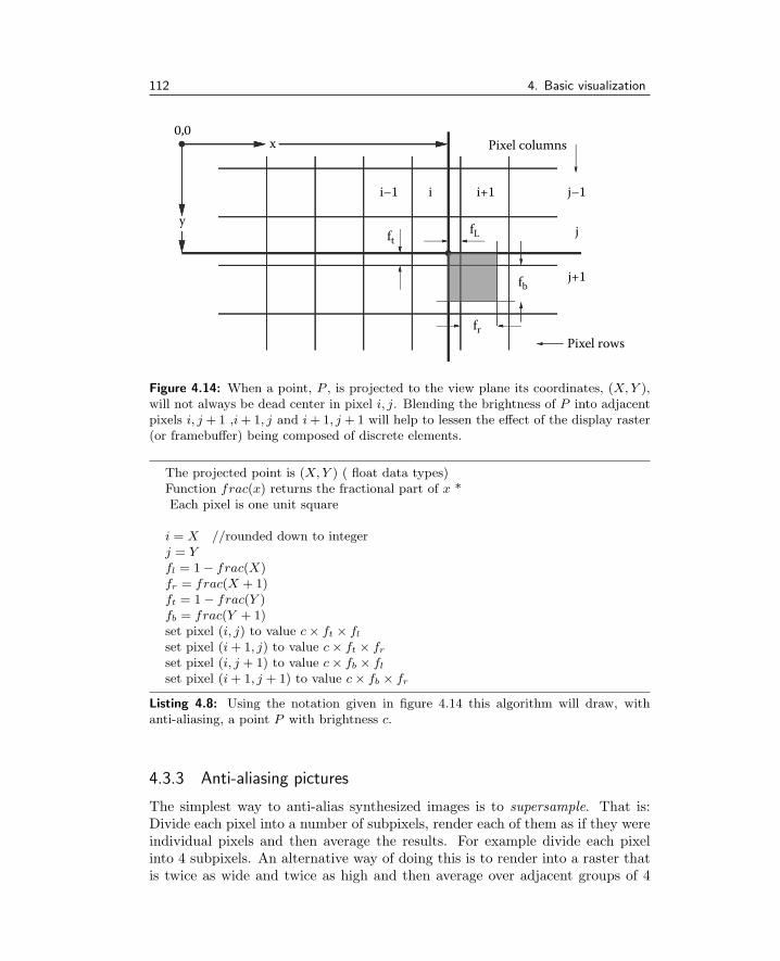
112 4. Basic visualization
Pixel rows
Pixel columns
j+1
i+1i–1
x0,0
y
i j–1
j
fb
fr
ftfL
Figure 4.14: When a point, P , is projected to the view plane its coordinates, (X,Y ),will not always be dead center in pixel i, j. Blending the brightness of P into adjacentpixels i, j + 1 ,i+ 1, j and i+ 1, j + 1 will help to lessen the effect of the display raster(or framebuffer) being composed of discrete elements.
The projected point is (X,Y ) ( float data types)Function frac(x) returns the fractional part of x *Each pixel is one unit square
i = X //rounded down to integerj = Yfl = 1− frac(X)fr = frac(X + 1)ft = 1− frac(Y )fb = frac(Y + 1)set pixel (i, j) to value c× ft × flset pixel (i+ 1, j) to value c× ft × frset pixel (i, j + 1) to value c× fb × flset pixel (i+ 1, j + 1) to value c× fb × fr
Listing 4.8: Using the notation given in figure 4.14 this algorithm will draw, withanti-aliasing, a point P with brightness c.
4.3.3 Anti-aliasing pictures
The simplest way to anti-alias synthesized images is to supersample. That is:Divide each pixel into a number of subpixels, render each of them as if they wereindividual pixels and then average the results. For example divide each pixelinto 4 subpixels. An alternative way of doing this is to render into a raster thatis twice as wide and twice as high and then average over adjacent groups of 4

4.3. Anti-aliasing 113
∆x = x2 − x1
∆y = y2 − y1δ = −∆x/2set x = x1 and y = y1draw pixel at (x, y) with color cwhile x < x2 do {
δ = δ +∆yi f δ ≥ 0 {
y = y + yinc
δ = δ −∆x}x = x+ 1/∗ modi f i ed s e c t i on ∗/draw pixel at (x, y) with color c(1− δ
∆x)
draw pixel at (x, y + 1) with color cδ
∆x/∗ end mod i f i ca t i on ∗/
}
Listing 4.9: A modified Bresenham’s algorithm for rendering anti-aliased lines.
pixels. For example rendering to a raster of 1280× 960 and averaging pixels i, j,i+ 1, j, i, j + 1 and i+ 1, j + 1 will give the same result as rendering to a rasterof 640× 480 with each pixel divided into 4. This box filtering is quick and easyto apply but in theory the best results are obtained from a sin x
xfilter function.
Because a supersample of n requires (n − 1) additional pixel values to bedetermined the rendering process slows down as anti-aliasing is applied. Forexample if it takes one minute to render a frame of TV resolution without anti-aliasing it will take about nine minutes to anti-alias it on a 3 × 3 supersample.Sadly, for a good enough quality TV sized image it is necessary to use at leasta 3× 3 supersample.
There are a couple of tricks that can be employed to accelerate the anti-aliasing process and both of them rely on the fact that the most noticeablealiasing artifacts occur near edges where color or brightness changes occur.
Techniques to accelerate supersampled anti-aliasing
1. Once the first supersample has been obtained for pixel (i, j) the remainingsamples are only rendered if the color differs from that for pixels (i− 1, j)or (i, j − 1) by more than a certain threshold.
2. Use the fact that relatively few calculations are required to determine theidentity of the polygon visible in each of the supersamples for pixel (i, j).If the same polygon appears in each supersample then there is no need toperform the more time consuming work of determining a color value for all

114 4. Basic visualization
Figure 4.15: (Top) Hidden surface visualization of a group of colored spheres madeup from 320 triangular polygons in each sphere, and (bottom) the same view with asimple lighting model.
the supersamples. Simply do it once and record that as the value for pixel(i, j). If different polygons appear in each supersample then we must getcolor values for those that are different and average the results for pixel(i, j).
Using either of these techniques can lead to significantly reduced rendering timeswithout much loss in picture quality.
4.4 Lighting and shading
Figure 4.15(top) illustrates a simple scene of a colored spheres rendered with ahidden surface algorithm. Only those triangular polygons that should be visibleare visible but there is definitely still something not very realistic about theimage: It certainly doesn’t look like a photograph. Figure 4.15 (bottom) showsthe same scene after the simplest possible lighting model has been included inthe renderer and the level of realism is certainly improved.
It is without doubt the way in which light interacts with surfaces of a 3Dmodel that is the most significant effect that we can simulate to provide visual

4.4. Lighting and shading 115
Spotlight
Directional
Point
θ2
θ1
Figure 4.16: Three types of light source.
realism. A hidden surface procedure may determine what you can see but it ismainly the interaction with light that determines what you do see.
To simulate lighting effects it stands to reason that at least the location andcolor of one or more lights must be known. In addition to this we need to classifythe light as being one of the three types illustrated in figure 4.16:
1. A point light source that illuminates in all directions.
2. A directional or parallel light source. In this case the light comes froma specific direction which is the same at all points in the scene. (Theillumination from the sun is an example of this type of illumination.)
3. A spotlight illumination is limited to a small region of the scene. The beamof the spotlight is normally assumed to have a graduated edge so that theillumination is a maximum inside a cone of half angle θ1 and falls to zerointensity inside another cone of half angle θ2, naturally θ2 > θ1.
For a lot of scenes the type 1 source gives the best approximation to the lightingconditions. In simulated outdoor scenes the sun is so far away that its illumina-tion is simulated as a directional light source with all rays arriving at the scenein a parallel direction.
Before proceeding we should consider the format for recording a value for thesurface color and illumination, call it c. In CG programs a model to describecolor must be employed. A detailed description of various color models maybe found in Watt and Watt [87]. The simplest color model that fulfills all therequirements is one with three components, one for each of the primary colors,red, green and blue, the so-called RGB values. Any color the eye can perceivecan be expressed in terms of an RGB triple. Thus c is recorded as cR, cG, cBwhich are usually stored as unsigned 8 bit integers giving a range for each of 256

116 4. Basic visualization
Object
Light
Object
Object
Camera
Figure 4.17: Lights, camera, action. Reflected light finds its way to the observer.
discrete values. For preliminary calculation it is more usual to assume that cR,cG and cB are recorded as floating point numbers in the range [0, 1]. We willalso assume that any light or surface color is also given as an RGB triple in thesame range.
There are other models to describe color. HSV (Hue, Saturation Value), andCMYK (Cyan,Magenta,Yellow, blacK) are alternatives that have advantages incertain situations. It is possible to convert back and forward between any ofthese models if necessary.
To determine the color that is recorded in a pixel the effect of lights needto be combined with the surface properties of the polygon visible in that pixel.The simplest way to do this is to break up the mathematical model for light–surface interaction into a number of terms, each one of which represents a specificphysical phenomenon.
In the following expressions sR, sG, sB represent the color of the surface, andlR, lG, lB the color of the light. Ia, Ic, Id and Is are the four contributions tothe lighting model and we will discuss them shortly. Using this terminology thecolor c calculated for the pixel in question may be expressed as:
cR = IasR + Ic(Is + IdsR)lR (4.1)
cG = IasG + Ic(Is + IdsG)lG (4.2)
cB = IasB + Ic(Is + IdsB)lB (4.3)
Writing the expressions in this form with sR and so forth as separate terms facili-tates the calculation because the surface color may be determined independentlyof the remainder of the terms in the lighting model; indeed it might possibly becalculated in a separate module.
To obtain expressions for the four components in our illumination model(Ia, Ic, Id and Is) we must consider the spatial relationship between the lights,

4.4. Lighting and shading 117
Light
^d
Light^d
n
(a) (b)
n
Figure 4.18: Diffuse illumination. (a) The brightest illumination occurs when theincident light direction is at right angles to the surface. (b) The illumination tends tozero as the direction of the incident light becomes parallel to the surface.
the camera and the action; this is illustrated in figure 4.17. In the followingexpressions we will assume that p is the point to be illuminated on the visiblepolygon which has a surface normal n at p. We will now proceed to considermodels for the components:
1. Ambient reflection (Ia)When there are no lights in a scene the picture will be blank. Including asmall fraction of the surface color, sR and so on, helps to simulate the effectof light reflected from the world around the scene. Without it pictures ofobjects would look like they had been taken in outer space. An imagerendered with an ambient light factor of unity is equivalent to a simplehidden surface drawing such as that which produced the flat look shown infigure 4.15. The component of a lighting model due to ambient reflectionis designated as Ia and it is always constant, i.e., Ia = k.
2. Diffuse reflection (Id)Diffuse lighting is the most significant component of an illumination model.The term reflection is used here because it is light reflected from surfaceswhich enters the camera. The model we choose to describe in this chapteris a simple Lambertian illumination where a polygon is most brightly il-luminated when the incident light strikes the surface at right angles. Theillumination falls to zero when the direction of the beam of light is parallelto the surface. This behavior is known as the Lambert cosine law and isillustrated in figure 4.18. The diffuse illumination component Id for a pointlight source located at Pl is thus given by:
Id =Pl − p
|Pl − p| · n

118 4. Basic visualization
In the case of a directional light source with incident direction d the diffusecomponent becomes:
Id = −d · n
For a spotlight located at Pl, pointing in direction d and having light coneangles θ1 and θ2:
Id =
Pl − p
|Pl − p| · n if θ < θ1(
Pl − p
|Pl − p| · n)(
1− (θ − θ1)
(θ2 − θ1)
)
if θ1 ≤ θ ≤ θ2
0 if θ2 < θ
where cos θ = d·(p−Pl)|(p−Pl)| .
Section 5.1 in chapter 5 delves a little more deeply into the physics ofillumination and offers some pointers to illumination models that are moreaccurate but at the expense of taking longer (sometimes much longer) tocalculate.
3. Specular reflection (Is)It is the specular component of the light reflected from a surface thatmakes it look shiny. In practice the effect of specular reflection is to adda highlight to parts of a model that have been designated as shiny. Thespecular highlight takes the color of the light and not that of the surfaceon which it is visible. To set up a model for specular reflection we need toconsider in a little more detail something of its origin.
A perfect mirror reflects all rays of light perfectly and the angle of reflectionis equal to the angle of incidence. However shiny surfaces that are notperfect mirrors introduce small random fluctuations in the direction of thereflected rays. These random fluctuations in the direction of the reflectedrays of light tend to be small so that they all lie within a cone-shapedvolume that has its apex at the point of reflection and its axis lying inthe direction that a ray would take if the surface was a perfect mirror (seefigure 4.19).
In the lighting model the specular illumination component Is is normallymodeled with the empirical expression suggested by Phong [72]:
Is = cosm φ
in which φ is the angle between the reflection vector and the vector leadingfrom the viewpoint at Pv to p on the surface. To determine φ from theknown geometry shown in figure 4.19 it is necessary to use a few interme-diate steps.
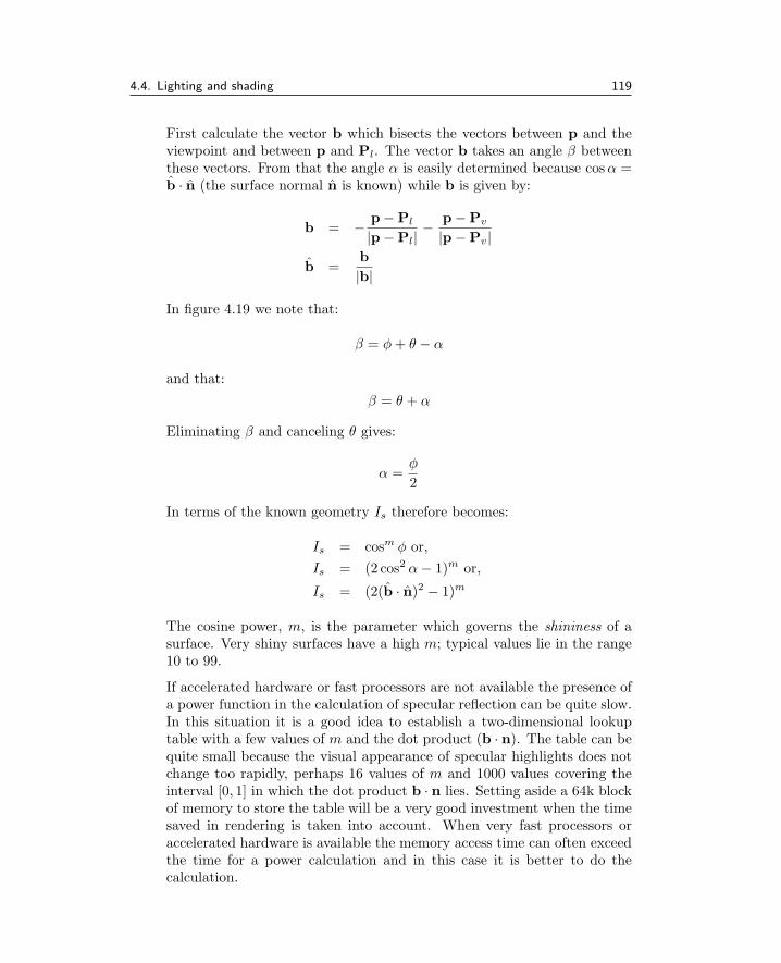
4.4. Lighting and shading 119
First calculate the vector b which bisects the vectors between p and theviewpoint and between p and Pl. The vector b takes an angle β betweenthese vectors. From that the angle α is easily determined because cosα =b · n (the surface normal n is known) while b is given by:
b = − p−Pl
|p−Pl|− p−Pv
|p−Pv|
b =b
|b|
In figure 4.19 we note that:
β = φ+ θ − α
and that:
β = θ + α
Eliminating β and canceling θ gives:
α =φ
2
In terms of the known geometry Is therefore becomes:
Is = cosm φ or,
Is = (2 cos2 α− 1)m or,
Is = (2(b · n)2 − 1)m
The cosine power, m, is the parameter which governs the shininess of asurface. Very shiny surfaces have a high m; typical values lie in the range10 to 99.
If accelerated hardware or fast processors are not available the presence ofa power function in the calculation of specular reflection can be quite slow.In this situation it is a good idea to establish a two-dimensional lookuptable with a few values of m and the dot product (b · n). The table can bequite small because the visual appearance of specular highlights does notchange too rapidly, perhaps 16 values of m and 1000 values covering theinterval [0, 1] in which the dot product b · n lies. Setting aside a 64k blockof memory to store the table will be a very good investment when the timesaved in rendering is taken into account. When very fast processors oraccelerated hardware is available the memory access time can often exceedthe time for a power calculation and in this case it is better to do thecalculation.

120 4. Basic visualization
Light^b
nPL
Pv
β
p
β
φ
Cone ofspecular reflection
θθ
r
α
Figure 4.19: Specular reflection.
4. Depth cueing (Ic)Like any electromagnetic radiation light is attenuated as it travels awayfrom its source. The reflected light (mainly diffuse) arriving at the view-point has traveled from the light source to the object where it was reflectedon to the observer. In theory the light intensity should be attenuated withdistance from its source using an inverse square law but in practice a linearfall-off looks much more realistic. Quite often depth cueing can be omittedentirely from the model with only mildly noticeable effect. A linear modelis usually written in the form:
Ic =1
do + d
where do is a constant and d is the distance of p from the viewpoint.Assuming that the viewpoint is at (0, 0, 0) and the observer is looking alongthe x axis, a good assumption is to let d = px, the x coordinate of p.
If depth cueing is to be used it is also a good idea to perform an exposuretest by examining all the polygons and scaling the light intensities so thatthe maximum is always unity. If this is not done then it can require quitea lot of trial and error testing to generate a picture that is neither under-or overexposed.

4.4. Lighting and shading 121
Figure 4.20: Shading of two similar polygon models of a sphere. Flat shading on theleft and basic Gouraud smooth shading on the right.
Once each component of the illumination model in equation 4.1 is known ageneral expression for the effect of lighting a surface in the scene at some pointp with n lights becomes:
cR = IasR + Ic
n−1∑
i=0
(Is(i) + Id(i)sR)lR(i)
cG = IasG + Ic
n−1∑
i=0
(Is(i) + Id(i)sG)lG(i)
cB = IasB + Ic
n−1∑
i=0
(Is(i) + Id(i)sB)lB(i)
Id and Is depend on the position of light i and on which type of light it is, forexample spotlight. If n > 1 each term in the lighting model must be limited sothat it falls in the range [0, 1], otherwise an overexposed picture will be produced.
Look at figure 4.20. It shows two pictures of the same faceted model of asphere. The one on the right looks smooth (apart from the silhouetted edgeswhich we will discuss later). It is the way a sphere should look. The one onthe left looks like just what it is, a collection of triangular polygons. Althoughthe outline of neither is perfectly circular it is the appearance of the interiorthat first grabs the attention. This example highlights the main drawback ofthe representation of an object with a model made up from polygonal facets. Tomodel a sphere so that it looks smooth by increasing the number (or equivalentlydecreasing the size) of the facets is quite impractical. Tens of thousands of facetswould be required just for a simple sphere. However both the spheres shown infigure 4.20 contain the same number of facets and yet one manages to looksmooth. How?
The answer is the use of a trick that fools the eye by smoothly varying theshading within the polygonal facets. The point has already been made that if

122 4. Basic visualization
Figure 4.21: After lighting and Phong shading have been added to a hidden surfacerendering, the image starts to look much more realistic.
you look at the outlines of both spheres you will see that they are made fromstraight segments. In the case of the smooth looking sphere it is because thediscontinuities in shading between adjacent facets have been eliminated that itlooks smooth. To the eye a discontinuity in shading is much more noticeablethan a small angular change between two edges.
So how is the smooth shading achieved? There are two useful possibili-ties: one, the Phong approach, gives a more realistic look than the other, theGouraud approach. Unfortunately Phong’s shading model achieves its realismat the expense of a greater number of calculations, so we will look at them both.Combining shading with lighting makes another major contribution to obtaininga realistic picture of an object from its numerical model as illustrated in fig-ure 4.21, which shows the effect on the test image of adding a shading procedureto the renderer.
4.4.1 Gouraud shading
To simulate smooth shading across a polygon the Gouraud approach is a twostep process:
1. Calculate the intensity of the light at each vertex of the model.
2. Use a bi-linear interpolation to obtain the intensity at any point within apolygon from the intensity at the vertices of the polygon.
To calculate the light intensity at vertex i, as shown in Figure 4.22, it is necessaryto take account of all the polygons attached to vertex i. Section 4.4 showed howthe intensity of the light falling on a point within a polygon can be calculated.
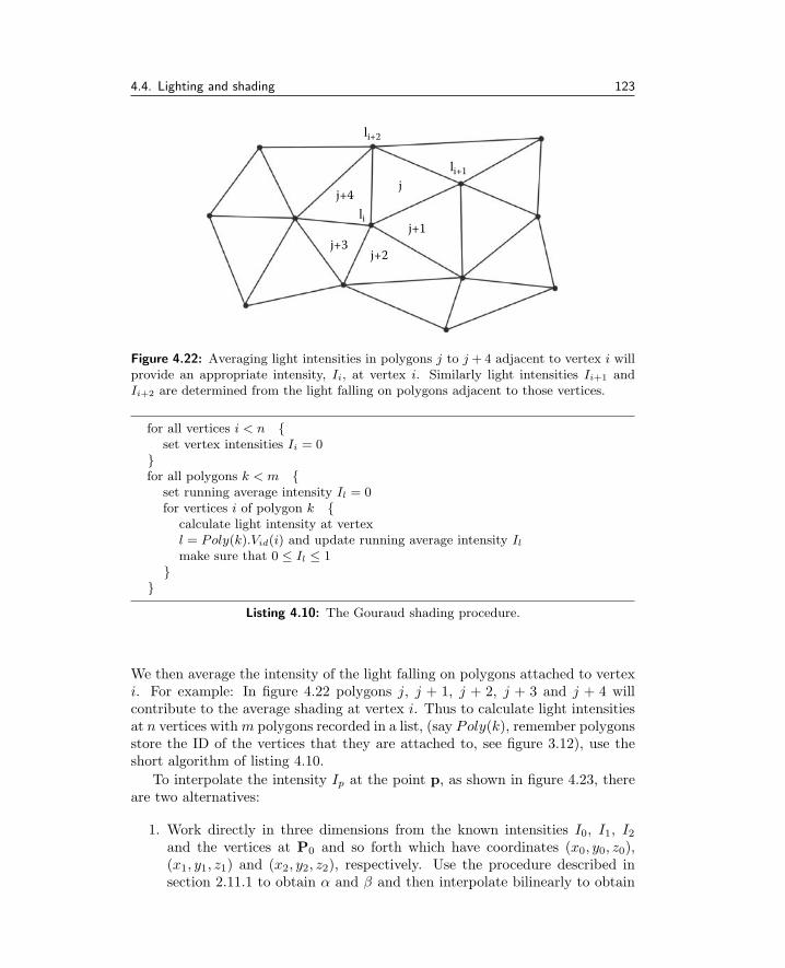
4.4. Lighting and shading 123
j+2j+3
j+4
j+1
li+1
li+2
li
j
Figure 4.22: Averaging light intensities in polygons j to j +4 adjacent to vertex i willprovide an appropriate intensity, Ii, at vertex i. Similarly light intensities Ii+1 andIi+2 are determined from the light falling on polygons adjacent to those vertices.
for all vertices i < n {set vertex intensities Ii = 0
}for all polygons k < m {
set running average intensity Il = 0for vertices i of polygon k {
calculate light intensity at vertexl = Poly(k).Vid(i) and update running average intensity Ilmake sure that 0 ≤ Il ≤ 1
}}
Listing 4.10: The Gouraud shading procedure.
We then average the intensity of the light falling on polygons attached to vertexi. For example: In figure 4.22 polygons j, j + 1, j + 2, j + 3 and j + 4 willcontribute to the average shading at vertex i. Thus to calculate light intensitiesat n vertices withm polygons recorded in a list, (say Poly(k), remember polygonsstore the ID of the vertices that they are attached to, see figure 3.12), use theshort algorithm of listing 4.10.
To interpolate the intensity Ip at the point p, as shown in figure 4.23, thereare two alternatives:
1. Work directly in three dimensions from the known intensities I0, I1, I2and the vertices at P0 and so forth which have coordinates (x0, y0, z0),(x1, y1, z1) and (x2, y2, z2), respectively. Use the procedure described insection 2.11.1 to obtain α and β and then interpolate bilinearly to obtain

124 4. Basic visualization
(X1, Y1)
(X0, Y0)
(x1, y1, z1)
(x2, y2, z2)
(x0, y0, z0)
Scanline
I1
Ip
I0
I2
j j´
Figure 4.23: To calculate the light intensity at an internal point of a triangular polygoninterpolate from the intensity at the polygon’s vertices.
Ip:Ip = I0 + (I2 − I0)α+ (I1 − I0)β
Finding Ip directly in three dimensions is slow. It would be better if wecould do the calculation after the polygon’s vertices have been projectedonto the viewing plane. We can indeed do this because shading is the laststep in the rendering algorithm and all the necessary 3D calculations havealready been carried out. This leads to our second alternative.
2. Use the two-dimensional coordinates after projection of the polygon’s ver-tices to the viewing plane, i.e., to points (X0, Y0), (X1, Y1) and (X2, Y2).Further, because the rendering procedure will normally be filling pixelssequentially across a scanline a few additional arithmetic operations canbe saved by calculating an increment in intensity I which is added to thevalue obtained for the previous pixel on the scanline.
For a triangular polygon, k, which spans scanline j (see figure 4.23) startingat pixel i the intensity Ii,j can be obtained from the following equations:
∆ = (Y2 − Y0)(X1 −X0)− (X2 −X0)(Y1 − Y0)
α =(Y2 − Y0)(i−X0)− (X2 −X0)(j − Y0)
∆
β =(j − Y0)(X1 −X0)− (i−X0)(Y1 − Y0)
∆Ii,j = I0 + α(I1 − I0) + β(I2 − I0)
The intensity in adjacent pixels Ii+1,j and so forth is determined by calcu-lating an increment δI from:
δI =(Y1 − Y2)I0 + (Y2 − Y0)I1 + (Y0 − Y1)I2
∆

4.4. Lighting and shading 125
Then for all the remaining pixels on scanline j covered by polygon k theintensity is given by:
Ii+1,j = Ii,j + δI
4.4.2 Phong shading
The Gouraud shading procedure works well for the diffuse reflection componentof a lighting model but it does not give a good result when specular reflectionis taken into account. Specular highlights occupy quite a small proportion ofa visible surface and the direction of the normal at precisely the visible pointmust be known so that the specular reflection can be determined. Thus Phong’sapproach was to interpolate the surface normal over a polygon rather than in-terpolate the light intensity. In the other aspects the procedure is similar to theGouraud shading algorithm.
Gouraud’s algorithm still has its uses because Phong’s [72] approach requiresmuch more work. The additional calculations include vector instead of scalarinterpolation and a time-consuming square root calculation to normalize theresultant normal before it can be used in the lighting equations. However mostof the additional calculation occurs because the diffuse lighting scalar productmust be evaluated for every pixel covered by the projection of the polygon andnot just its vertices.
Phong shading is done in the following two stages:
1. Calculate a normal vector for each vertex of the model.
2. Use two-dimensional interpolation to determine the normal at any pointwithin a polygon from the normals at the vertices of the polygon.
In stage 1 an analogous procedure to the first step of the Gouraud algorithm isused. In this case however averaging takes place with normal vectors instead ofillumination intensities. Figure 4.24 shows a cross section through a coarse (6sided) approximation of a cylinder. In (a) the facet normals are illustrated, (b)shows the vertex normals obtained by averaging normals from facets connectedto a particular vertex and in (c) the effect of interpolation on normal vectors isshown. A smoothly varying surface normal will interact with the incoming lightbeam to give smoothly varying shading which will also work correctly with themodel for specular highlights.
In stage 2 expressions very similar to those that occur in the Gouraud modelare derived. For a triangular polygon k that spans scanline j at the leftmost

126 4. Basic visualization
(a) (b) (c)
Figure 4.24: In Phong smoothing the surface normals are averaged at the vertices andthen the vertex normals are interpolated over the flat facets to give an illusion of acontinuously varying curvature.
pixel i the normal vector ni,j is given by:
∆ = (Y2 − Y0)(X1 −X0)− (X2 −X0)(Y1 − Y0)
α =(Y2 − Y0)(i−X0)− (X2 −X0)(j − Y0)
∆
β =(j − Y0)(X1 −X0)− (i−X0)(Y1 − Y0)
∆
nx
ny
nz
i,j
=
n0x + α(n1x − n0x) + β(n2x − n0x)n0y + α(n1y − n0y) + β(n2y − n0y)n0z + α(n1z − n0z) + β(n2z − n0z)
ni,j =ni,j
|ni,j |
For the remaining pixels on scanline j, i.e., pixels i+1, i+2 etc., the normals(ni+1,j , ni+2,j) are determined by calculating an incremental vector δn given by:
δnx
δny
δnz
=1
∆
(Y1 − Y2)n0x + (Y2 − Y0)n1x + (Y0 − Y1)n2x
(Y1 − Y2)n0y + (Y2 − Y0)n1y + (Y0 − Y1)n2y
(Y1 − Y2)n0z + (Y2 − Y0)n1z + (Y0 − Y1)n2z
Normals in the remaining pixels on scanline j covered by polygon k are thusdetermined sequentially from:
ni+1,j = ni,j + δn
ni+1,j =ni+1,j
|ni+1,j |
Remember: The normal ni,j found by interpolation in the two-dimensionalprojection plane is still the three-dimensional normal vector at p on polygon k(which is the point visible in pixel (i, j)).

4.4. Lighting and shading 127
(d) (e)
(b)(a) (c)
BA
X´
Xα
α
Figure 4.25: A cross section through a cylinder that has been cut in half along its axis.
Before we finish discussing Phong shading there is one very important pointthat requires a little more thought. Look at figure 4.25: in (a) we see a renderedhalf cylinder approximated by 6 rectangular facets on the curved side and 1rectangular facet on the flat (cut) side; in (b) a plan of the section at planeXX ′ shows the facet normals. Now imagine what happens as stage 1 of Phong’sprocedure is applied. In (c) the averaged vertex normals are shown and (d) givesthe interpolated normals. Even at the points labeled A and B the normal vectorvaries smoothly including round the sharp corner. This is not quite the desiredresult because the corner will be smoothed out and the distinct edge will justmerge into the smooth shading. At points A and B the corners should really beretained. To achieve this make the following modification to the algorithm atstage 1:
• Do not update the running average for the vertex normal unless the angle
α <π
2or the user overrides the decision. (α is illustrated in figure 4.25.)
Figure 4.25(e) shows the effect after this correction is applied. On a practicallevel to achieve this correction the vertex normals must be stored as part ofthe polygon data structures (see chapter 3) because a discontinuity between thenormals of adjacent polygons cannot be represented if a single vector is stored foreach vertex. Thus the data structure associated with each polygon in a model,from figure 3.12, must be updated to that shown in figure 4.26.
128 4. Basic visualization
Vid list of vertex identifiers to which polygon is attachedidmaterial pointer to material in materials listAid(3) list of the id’s of polygons with a common siden normal to surface planeeid list of Phong vertex normals
Figure 4.26: Vertex and polygon data structures with vertex normals eid .
4.5 Materials and shaders
Now we consider how the appearance of objects can be enriched without havingto go to the computational expense of using a more sophisticated lighting model,or by building a much more highly detailed polygonal model. The basic idea issimple enough. Every surface polygon is assigned a number of attributes, such ascolor, roughness, shininess, and transparency. It has become common in graphicsapplication software not to record all the surface attributes for every polygonalfacet in a model. For one thing, a lot of attributes and an excessive number ofpolygons will lead to a requirement for excessive storage; however, in practice,the number of different sets of attributes is likely to be quite smaller, an objectwith 100,000 polygons might only use two colors. Realizing that any face can beassigned a whole range of attributes by building a separate list of materials andthen assigning a material to a face with a single integer identifier reduces thedata storage considerably and significantly increases the flexibility, because, ifthe list of surface attributes were to change, then it is only necessary to changethe format of the few items in the materials list and not the many thousands ofpolygons.
The idea of a materials list fits very neatly with the hardware renderingengines which do not like to have to change their surface attribute states (color,shininess, smoothing etc.) too often. By sending polygons, grouped together bymaterial, along the rendering pipeline one after another, the number of changesof state is kept to a minimum.
So what does a material contain? Even the best images synthesized from apolygonal model still lack the detail and richness of real surfaces. Imperfectionsdue to wear and tear, regular color variations or natural material properties arevery difficult to represent with polygons. Something as simple as text paintedonto surfaces or detailed colored patterns would require polygon meshes to haveprohibitively large numbers of facets and vertices. Two complimentary tech-niques, image mapping and procedural texturing, allow for realistic detail to beadded to the images of polygonal or patched models without increasing the num-ber of polygons.
The terms procedural texture and image map nicely discriminate these twoapproaches, because the procedural (or algorithmic) texture can be thought of asoccupying a volume and the image map as being draped over a surface. The pro-
4.5. Materials and shaders 129
cedural texture matches well with the idea of an extended material description,color is a volume filling attribute, and we can think of the object as being carvedfrom a block of material X. Sometimes the 2D image map and the 3D materialare recorded in separate lists. The OpenFX software considered in chapter 9 doesthis. Other terms are often used in computer graphics to refer to a proceduraltexture or an image map: in OpenGL and DirectX the term texture map is usedinstead of image map. In the last few years the term shader has become popularto describe programs that run in the GPU, and whilst a GPU shader can do alot more than deliver a surface material, texture or image map, the term shaderis often associated with the algorithms accompanying procedural textures.
Image mapping is probably the first choice of the 3D computer artist or CADengineer when faced with the need to enhance a plain mesh model; it can makeeven the simplest model look tremendously lifelike and is the easiest and mostadaptable way to add fine detail. The most popular real-time rendering librariesuse image mapping extensively (see chapter 7). The theory of image mapping isdiscussed in section 4.6.
Procedural or algorithmic textures provide some of the most beautiful sur-faces seen in computer-generated images. They have the advantage over theimage mapping approach that they can be rendered in any resolution and there-fore do not exhibit the problems that an image map can suffer from when itis rendered in close up. They do sometimes however show aliasing effects; seeApodaca and Gritz [4].
The aliasing effect from which mapped images suffer is due to the fact thatthey must be recorded on an array of finite size and thus their pixelated na-ture becomes all too apparent in close up snapshots. Procedural textures havethe additional advantages that they don’t require the large amount of memorythat may be required to record an image nor is the problem that arises whenan essentially flat (two-dimensional) image is mapped on to space filling solidsevident. In section 4.4 equations 4.1, 4.2 and 4.3 described how the surface colorS, at a point p, is combined with the lighting conditions to produce a color valueto represent what is seen at p. The surface color S with its three componentssR, sG, sB can encapsulate not just a plain color but perhaps a blend or someother elaborate combination of shades. However, no matter how complex theprocedure used to calculate S, the only variables on which it may depend arethe position of p, coordinates (x, y, z) or the two-dimensional texture coordinates(X,Y ) first introduced in chapter 3; they are also commonly referred to as theu and v coordinates. This can be expressed formally as:
S = f(x, y, z,X, Y ) (4.4)
It is unusual for f(x, y, z,X, Y ) to depend on x, y, z at the same time as itdepends on X,Y and therefore the term volume texture tends to be used for caseswhere f() is independent of X or Y . Most volume textures tend to be generatedfrom a fixed set of rules, and they are therefore called “procedural textures”.

130 4. Basic visualization
Spherical DotsProcedural Texture
Spherical DotsProcedural Texture
Surface ModeVolume Mode
Figure 4.27: Procedural texture in volume and surface modes. Note the way the dotscling to the surface when texture coordinates are applied to the surface of the shapeand how the shape appears to be carved out of a block of colored spheres when volumecoordinates are used.
When f() is independent of x, y or z the texture is called a surface texture andall image mapping methods fall into this category.
In addition to providing a way to alter the surface color S at p, a texturingprocedure might also modulate the direction of the surface normal or modifythe transparency of the surface. In fact with a combination of these techniquesand some ability to simulate reflections it can become difficult to distinguish arendered image of the model from a photograph of the real thing.
Procedural textures can be used equally easily with functions of the formf(x, y, z) (volume) or f(X,Y ) (surface). Figure 4.27 shows an example of aprocedural texture applied to the same object in volume and surface modes.They are excellent for simulating naturally occurring surfaces, wood, marble,granite, clouds, tree bark, veins, etc. The list is almost endless. Chapter 11details some algorithms to simulate a significant variety of surfaces.
We can establish two general types of procedural texture:
1. Those that use regular geometric patterns.
2. Those that use random patterns.
In many cases an enhanced appearance is achieved by combining the twotypes. The pattern of irregular paving slabs is one such example. Discolored andweathered bricks is another. Indeed this work has been extended to the conceptof volume textures with the possibility of creating realistic clouds, smoke, coral,hair and fur.

4.5. Materials and shaders 131
The input to the algorithm is a position coordinate (x, y, z), themortar % thickness tm and the colors for brick and mortar.The output is a color triple sR, sG, sB and a functionFloor(a) is called to return the nearest lower integer to a.
In the C language Floor would be implemented as follows#de f i n e Floor ( a ) ( ( a ) < 0 .0? ( ( long ) ( a)−1L : ( long ) ( a ) )
if integer part of z is divisible by 2 \{x = x+ 1
2
y = y + 1
2
}x = x− Floor(x)y = y − Floor(y)z = z − Floor(z)
A collection of i f ’s divide the brick from the mortari f z > 1− tm or y > 1− tm or
(y > 1
2− tm and y < 1
2) or
(y < 1
2and ( ( x > 1
2− tm and
x < 1
2) or x > 1− tm ) ) or
(y > 1
2and ( ( x > 1
3− tm and
x < 1
3) or (x > 7
10and x < 7
10+ tm ) ) ) {
return the mortar color}else {
return the brick color}
Listing 4.11: An algorithm that creates a brick and mortar procedural texture. Fora given point p which has coordinates (x, y, z) it determines whether p is inside thebrick or the mortar.
4.5.1 Basic geometric procedural textures
Listing 4.11 presents an algorithm for generating a very simple geometric texture,i.e., a three-dimensional system of bricks and mortar. Other simple textures thatfall into this category include checks, dots, triangular shapes, stars, hexagonalpatterns and even a digital readout such as might appear on a clock.
The algorithm given in listing 4.11 illustrates a compact interface betweenthe texturing function and its host renderer. An input of a position, a small setof parameters and an output of color value are sufficient to control all proceduralfunctions. In fact we could standardize the parameter list so that the same func-tion can be used by scanline, Z buffer or ray tracing renderers interchangeably.In fact texturing functions are ideal candidates for implementation as run timedefinable libraries, as for example DLLs under the Windows operating system.

132 4. Basic visualization
4.5.2 Basic random procedural textures
Simply generating random numbers does not lead to the creation of very in-teresting textures. What is required is a random function which is spatiallycorrelated, that is, the surface attributes at two different locations are similarif the points are close together but if the points are far apart then calculatedsurface attributes will be quite independent of one another.
A random number generator with just these properties was originally pro-posed by Perlin [69] in what turned out to be a seminal paper on the topic.Textures based on Perlin’s ideas call upon one basic function: the noise genera-tor. Section 4.7 explains in detail the elegance of the noise generator algorithm.Given a position, p, the noise generator returns a scalar value in the range [0, 1];we will write it as: u = sNoise(p). This function has the essential propertyquoted above and of equal importance for application in rendering: if called withthe same value of p it returns the same noise, therefore although it has randomproperties they are quite repeatable.
From sNoise(p) three other useful functions are easily derived:
1. A noise generator that returns a vector given a position, v = vNoise(p).
2. A function called turbulence, which is similar to the noise function but issmooth in some places while varying rapidly in others, something like theeffect achieved when two colors of paint are stirred together. u = sTurb(p)generates a scalar turbulence value.
3. v = vTurb(p) returns a vector valued turbulence.
These noise functions have statistical properties (translational and rotationalinvariance) that make them particularly useful for 3D graphics work.
The turbulence functions are examples of a fractal or 1/f noise. They can beeasily calculated by adding basic Perlin noises. The idea is that the noise signal isbuilt up by adding a number of components with the amplitude of each componentinversely proportional to its frequency. Thus low frequency components havelarge amplitude but the high frequency components have small amplitude.
Comment: The fractal noise function can also be useful for building modelsof natural shapes, e.g., trees and mountain landscapes.
There are many ways to implement the Perlin noise function. See Ward’sgem in Avro [6] for example.
One of the shortest and fastest ways to write a Perlin noise generator is toestablish a three-dimensional array of random numbers and then to interpolatelinearly from that to obtain a noise value for a specific point p.
Perhaps the most versatile noise texture is that called bozo (see chapter 11for examples). With appropriate scaling and level setting it can represent manynatural phenomena such as clouds and solar corona. An algorithm for the bozotexture is given in listing 4.12. The appearance of the brick and bozo texturesare illustrated in figure 4.28.

4.5. Materials and shaders 133
Figure 4.28: The brick and bozo textures generated by the algorithms given in list-ings 4.11 and 4.12.
The input to the algorithm is a position coordinate (x, y, z), twothreshold values t1 and t2, three color triplesc1R, c1G, c1B , c1R, c1G, c1B and c1R, c1G, c1Band a turbulence parameter τ which give the texture its swirly look.The output is a color triple sR, sG, sB The Bozo texture is a threshold ofthe noise function. At each threshold a color change occurs.
i f τ 6= 0 {v = vTurb(p)p = p+ τv
}n = sNoise(p)i f n < t1 {
assign color s = c1 (R,G and B)}else i f n < t2 {
assign color s = c2 (R,G and B)}else {
assign color s = c3 (R,G and B)}
Listing 4.12: An algorithm to create a bozo procedural texture. It calls upon the Perlinnoise functions and returns a color setting at a point P with coordinates (x, y, z).
For some practical hints on implementing procedural textures you might con-sult Worley’s book [22].
Procedural textures, especially the noise based ones, give beautiful, richlydetailed and realistic looking effects when the vector noise function is used toperturb the direction of the surface normal at P . Doing this has the effect

134 4. Basic visualization
No rough texture Rough texture addedto cylindrical surface
Figure 4.29: A procedural texture that uses the vNoise() function can be used to bendthe surface normal.
of giving a rough, bumpy, or pitted appearance to the surface because of theway the Phong lighting model interacts with the surface normal. Figure 4.29illustrates a procedural texture that modulates the surface normal to give a roughsurface. The noise function can also be called upon to alter the transparency orreflectivity of the surface at P . When all of these effects are combined some ofthe most visually stunning computer-generated images emerge, even from shapesdescribed with only a few hundred polygons.
Before ending this section it is worth pointing out that in step 2 of therendering algorithm, models are moved or rotated to place them at appropriatepositions in the scene. If any surface of that model is covered with a volumetexture then the position argument to the noise function should be specifiedwith respect to a frame of reference attached to the model and not some globalframe. If a global frame of reference for the argument to the noise function wereused then an animation of a moving model will give the disturbing appearancethat the model is moving through a kind of three-dimensional sea of the texture.
4.6 Image and texture mapping
An image map performs a very similar task to that of a two-dimensional pro-cedural texture. It adds detail to surfaces without the need for a very largenumber of small polygons. In contrast to a procedural texture, image maps pro-vide the model designer much greater control over the appearance of the texture.In essence any image may be used as the source for the image map. (2D draw-ings or scanned photographs are common sources.) This is particularly usefulin product design applications where text, manufacturers’ logos or labels can beadded to a 3D model of the product.
In this section we will consider how two-dimensional pictures are attachedto a polygonal 3D model. Figure 4.31 shows a simple rectangular polygonmapped with a small picture applied in several useful ways and we shall considerthese later.

4.6. Image and texture mapping 135
The expressions needed to determine the color s at a point, p, within atriangular polygon due to the application of an image map are analogous to thosewe obtained when considering a procedural texture applied in surface mode. Ifthe vertices of a triangular polygon are P0, P1 and P2, then s, the color tobe substituted into the lighting model, is determined by executing the followingsteps:
1. Use the coordinates of the vertices of the surface polygon relative to p todetermine parameters α and β, where:
(p−P0) = α(P1 −P0) + β(P2 −P0) (4.5)
Section 2.11.1 explains the necessary analysis.
2. Given texture coordinates of (X0, Y0), (X1, Y1) and (X2, Y2) at P0, P1
and P2, respectively, a texture coordinate for the point p, say (X,Y ), isdetermined by:
X = X0 + α(X1 −X0) + β(X2 −X0) (4.6)
Y = Y0 + α(Y1 − Y0) + β(Y2 − Y0) (4.7)
3. From (X,Y ) an index (i, j) into an array of pixels An,m which record animage of resolution n×m is determined as follows:
i = nearest integer to (nX)
j = nearest integer to (mY )
4. Copy the pixel color from Ai,j to s. How the information in A is storedand addressed is a matter of personal choice as is whether the image istrue color (16.7 million colors), hicolor (65536 colors) or paletted (one byteused to address a palette of 256 colors).
Figure 4.30 illustrates the mapping process.There are two important issues that arise in step 3 above. First to obtain
a valid address in A both i and j must satisfy simultaneously 0 ≤ i < n and0 ≤ j < m or, equivalently, by scaling to a unit square: 0 ≤ X < 1 and0 ≤ Y < 1. Thus the question arises as to how to interpret texture coordinatesthat fall outside the range [0, 1]. There are three possibilities all of which proveuseful. They are:
1. Do not proceed with the mapping process for any point with texture coor-dinates that fall outside the range [0, 1]; just apply a constant color.
2. Use a modulus function to tile the image over the surface so that it isrepeated as many times as necessary to cover the whole surface.

136 4. Basic visualization
O
P2
P0
P1
β
p
α
Figure 4.30: Mapping an image into a rectangle with texture coordinates of (0, 0) at P0,(1, 0) at P1 and (0, 1) at P2. At the point p an appropriate pixel color is determinedfrom the image using the steps given in the text.
Repeated mozaicRepeated image
Texture coordinates
2,01,00,0
Single image
3d R
3d R 3d R
3d R 3d R
3d R
3d R 3d R
3d R
0,1
0,2
Figure 4.31: Different ways of interpreting mapping coordinates over a flat surface.(a) No mapping outside unit rectangle. (b) Tiling by repeatedly copying the imagemap. (c) Mosaic tiling. In this case the image map is carefully arranged so that nodiscontinuous edges are visible when the map is tiled.
3. Tile the image over the surface but choose a group of four copies of theimage to generate blocks that themselves repeat without any seams, i.e.,a mosaic pattern. To generate a mosaic pattern the α and β values inequation 4.6 and 4.7 are modified to αm and βm (a procedure describedin the algorithm of listing 4.13).
These three methods of applying an image map to a polygon’s surface areillustrated in figure 4.31.

4.6. Image and texture mapping 137
the Floor function is given in figure 4.11αm = (float)Floor(α)βm = (float)Floor(β)bx = ((truncate αm)(bitwise AND) 1)by = ((truncate βm)(bitwise AND) 1)αm = α− αm
βm = β − βm
i f bx 6= 0 {i f by 6= 0 {
αm = 1− αm
βm = 1− βm
}else {
αm = 1− αm
}}else i f by 6= 0 {
βm = 1− βm
}
Listing 4.13: Generating a mosaic repeat pattern for seamless image mapping.
The second issue is the rather discontinuous way of rounding the floatingpoint texture coordinates (X,Y ) to the integer address (i, j) (i = truncate(x)and j = truncate(y)) used to pick the color from the image. A better approachis to use a bilinear (or higher order) interpolation to obtain s which takes intoaccount not only the color in pixel (i, j) but also the color in the pixels adjacentto it. Thus, if the texture coordinates at p are (X,Y ) we obtain s by using colorvalues from Ai−1,j , Ai+1,j , Ai,j−1 and Ai,j+1 in addition to the color from Ai,j .The procedure for this is given in listing 4.14.
Notes:
1. Bilinear interpolation gives good results when the image map is being mag-nified but not in cases where the image is being reduced in size, as theobject being mapped moves away from the camera for example.
2. We have not discussed how the vertices are assigned texture coordinates.This topic is covered in chapter 10, section 10.11.
3. The determination of α and β in equation 4.5 is done in three dimensions.Other approaches to texture mapping (as would be done in a hardwarerasterizer for example) will implement the interpolation after projectiononto the viewing plane. In those circumstances the use of a linear interpo-lation to obtain the texture look-up coordinates is incorrect and anotherapproach such as perspective-correct barycentric interpolation [54] wouldneed to be used.

138 4. Basic visualization
δX = X − float (i)δY = Y − float(j)i f δX > 1
2{
δX = δX − 1
2
i f δY > 1
2{
δY = δY − 1
2
s = Ai,j(Ai+i,j −Ai,j)δX + (Ai,j−1 −Ai,j)δY}else {
δY = 1
2− δY
s = Ai,j(Ai+i,j −Ai,j)δX + (Ai,j+1 −Ai,j)δY}
}else {
δX = 1
2− δX
i f δY > 1
2{
δY = δY − 1
2
s = Ai,j(Ai−i,j −Ai,j)δX + (Ai,j−1 −Ai,j)δY}
else {δY = 1
2− δY
s = Ai,j(Ai−i,j −Ai,j)δX + (Ai,j+1 −Ai,j)δY}
}
Listing 4.14: Bilinear interpolation to calculate a color value, s, at texture coordinate(X,Y ) from an image with color recorded in the pixel array A which has dimensionn×m.
4.6.1 Transparency mapping
Transparency mapping follows the same steps as basic image mapping to delivera color value, s, for use at a point p on polygon k. However instead of usings directly as a surface color it is used to control a mixture between the colorsettings for polygon k and a color derived from the next surface recorded in thetransparency buffer. (Remember that the Z buffer algorithm can be modifiedto hold several layers so that if any of them were transparent the underlyingsurface would show through.) Note that when mixing the proportion of s dueto the underlying surface no lighting effects are applied. That is, when youlook through a window from inside a room it is not the light in the room thatgoverns the brightness of the world outside. Figure 4.32 illustrates the use of acombination of two maps applied to a simple quadrilateral polygon. Incidentally,painting trees on glass is a very useful trick for decorating animated tours ofarchitectural fantasies!

4.6. Image and texture mapping 139
Image used forsurface map
Image used fortransparency
map
Figure 4.32: An image of a model with just 11 rectangular polygons (some obscured).Ten of them have both a standard image map and a transparency map applied. Thepolygon representing the ground is made rough by applying a bumpy procedural texture.
4.6.2 Bump mapping
Bump mapping, introduced by Blinn [11], uses the color from an image map tomodulate the direction of the surface normal vector. Again there is a similaritywith those procedural textures that cause the surface normal vectors to tiltaway from the direction determined by the Phong shading model. For examplethis technique can be used to produce the appearance of embossed text. Manyanimators use a sequence of bump maps to give the illusion of waves on thesurface of a lake or the sea although such surfaces are probably more realisticallysimulated by the noise type procedural texture of Perlin [69].
To implement a bump map it is the change in color from one pixel to anotherwhich determines the displacement vector that is added to the surface normalof polygon k at point p. Most of the analysis we need in order to calculate theperturbing vector, ∆n, has been covered already. Bump mapping usually usesthe same texture coordinates as are used for basic image mapping. In fact it isessential to do so in cases where an image and bump map are part of the samematerial; for example a brick surface can look very good with a bump map usedto simulate the effect of differential weathering on brick and mortar.

140 4. Basic visualization
To determine ∆n we need to find incremental vectors parallel to two of thesides of polygon k, call them ∆n1 and ∆n2. Do this by first finding texturecoordinates at points close to p (at p the texture coordinates are (X,Y ) givenby equations 4.6 and 4.7). The easiest way to do this is to make small increments,say δα and δβ , in α and β and use equations (4.6) and (4.7) to obtain texturecoordinates (Xr, Yr) and (Xb, Yb).
Before using the texture coordinates to obtain “bump” values from the mapit is necessary to ensure that the distance in texture space between (X,Y ) and(Xr, Yr) and between (X,Y ) and (Xb, Yb) is small. To achieve this write:
∆t =√
(Xr −X)2 + (Yr − Y )2
Xr = X + δ(Xr −X)
∆t
Yr = Y + δ(Yr − Y )
∆t
and do the same thing to (Xb, Yb). These equations include an additional scalingfactor δ that will be discussed shortly. The next step is to obtain values fromthe bump image at texture coordinates (X,Y ), (Xr, Yr) and (Xb, Yb). Using thebilinear interpolation algorithm given in Figure 4.14 three bump values s0, s1and s2, are obtained. It only remains to construct ∆n and add it to the normal,n, for polygon k. Thus:
d1 = (P1 −P0)
d2 = (P2 −P0)
∆n1 = (s1 − s0)
(
d1
|d1|
)
∆n2 = (s2 − s0)
(
d2
|d2|
)
n = n+ h(∆n1 +∆n2)
n = n/|n|
h is a parameter that facilitates control of the apparent height of the bumps. Itsrange should be [0, 1].
The choice of δ, δα and δβ will determine how well the algorithm performs.They should be chosen so that they are small relative to the texture coordinaterange across the polygon.
4.6.3 Reflection mapping
True reflections can only be simulated with ray tracing or other time-consumingtechniques but for quite a lot of uses a reflection map can visually satisfy allthe requirements. Surfaces made from gold, silver, chrome and even the shiny

4.6. Image and texture mapping 141
paint work on a new automobile can all be realistically simulated with a skillfullycreated reflection map, a technique introduced by Blinn and Newell [10].
An outline of a reflection map algorithm is:
1. With the knowledge that polygon k, at point p, is visible in pixel (i, j)determine the reflection direction d of a line from the viewpoint to p. (Usethe procedure given in section 2.9.)
2. Because step 3 of the basic rendering algorithm transformed the scene sothat the observer is based at the origin (0, 0, 0) and is looking in direction(1, 0, 0) the reflected direction d must be transformed with the inverse ofthe rotational part of the viewing transformation. The necessary inversetransformation can be calculated at the same time as the viewing trans-formation.Note: The inverse transformation must not include any translational com-ponent because d is a direction vector.
3. Get the Euler angles that define the direction of d. These are the heading φwhich lies in the range [−π, π] and pitch θ which lies in the range [−π
2 , π2 ].
Scale the range of φ to cover the width, Xmax, of the reflection image.Scale the range of θ to cover the height, Ymax, of the reflection image.
X =(π + φ)
2πXmax
Y =(π2 − θ)
πYmax
4. Use the bilinear interpolation algorithm of figure 4.14 to obtain a colorvalue s from the image in the vicinity of (X,Y ).
5. Mix s with the other sources contributing to the color seen at pixel (i, j).
You can think of the reflection mapping process as one where the reflectedsurface is located at the center of a hollow sphere with the image map paintedon its inside. Figure 4.33 illustrates the relationship of object to reflection map.Another reflection mapping procedure that gives good results is the cubic envi-ronment due to Greene [35].
When procedural textures, pseudo shadows and reflection maps are added tothe Phong shaded rendering of Figure 4.21 a highly realistic looking image (forexample, figure 4.34) can be generated without having to pay the very heavytime penalty that ray traced rendering procedures impose.
4.6.4 Mip-mapping
Imagine a tiled floor that extends into the far distance with the textured ap-pearance being the result of applying an image map, something like that shown

142 4. Basic visualization
Wrap thereflectionmap roundthe sphere
^
Viewprojection
plane
Viewpoint
d
p
nz
x
Figure 4.33: A reflection map can be thought of as an image painted on the inside ofhollow sphere with the reflective model placed at its center.
Figure 4.34: Final image of models first shown in figure 4.3 now using a pseudo shadow,procedural texture and reflection map.
in figure 4.35(a). Rendering two adjacent pixels near the bottom of the imagewhere the viewing vector intersects the floor close to the camera will most likelyresult in a texture look-up that results in the same color value being obtained.Rendering two adjacent pixels near the top of the image where the viewing vec-tor intersects the floor at a great distance from the viewpoint could result in thetexture look up returning very different color values. The result of this is that anunpleasant moire pattern because the image map sampling is subject to aliasingeffects and the integrating effect of the imperfect natural vision processes is notpresent in the basic mathematical imaging model.

4.6. Image and texture mapping 143
(a) (c)
(b)
Figure 4.35: (a) A checkerboard texture mapped on a plane viewed from an obliqueangle. (b) A mip-map that would be suitable to use for the checker texture in (a). (c)Two polygons located at a far distance from the camera, one using the original textureand the other using the mip-map.
However, it is possible to modify the texture look-up process in a way thatmitigates seeing the aliasing errors. This process is known as mip-mapping. Inmip-mapping the original texture map is augmented by making filtered versionsof the original image drawn at smaller and smaller resolutions, where each copyhas the appearance of being viewed from farther and farther away. Making mip-maps puts control of how a textured surface changes as it moved away from theobserver back in the hands of the artist. For example, a black/white checkertexture applied to a wall in the far distance will probably just look blandly gray,rather than an unpleasant and high contrast moire patter.
Which level of the mip-map to use is determined by using the depth z (dis-tance) to the point on the surface that is to be mapped. When a texture mapvalue is needed, the two levels in the mip-map that bracket z, that is [zmi, zmi+1]are accessed. The color values found in each of the bracketing levels are blendedtogether in the ratio of z to the the interval [zmi, zmi+1]. Figure 4.35(b) showsa mip-map that would be a suitable candidate for a checkerboard texture. It isusual to make the top level image in a mip-map a square with the dimensionof 2n, and each sub-level a dimension of one quarter the size of the level aboveit. This allows the mip-map to be packed into an image that is only twice thesize of the original and allows the lookup software to work with the appropriatelevels without too much extra computation. In figure 4.35(c) the effect of usingthe mip-map is evident. Two polygons (enlarged) are placed far away from thecamera and tiled with the image map. On the left the original image is sampled
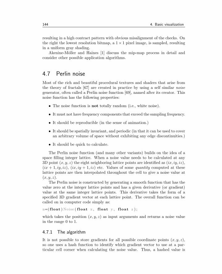
144 4. Basic visualization
resulting in a high contract pattern with obvious misalignment of the checks. Onthe right the lowest resolution bitmap, a 1× 1 pixel image, is sampled, resultingin a uniform gray shading.
Akenine-Moller and Haines [1] discuss the mip-map process in detail andconsider other possible application algorithms.
4.7 Perlin noise
Most of the rich and beautiful procedural textures and shaders that arise fromthe theory of fractals [67] are created in practice by using a self similar noisegenerator, often called a Perlin noise function [69], named after its creator. Thisnoise function has the following properties:
• The noise function is not totally random (i.e., white noise).
• It must not have frequency components that exceed the sampling frequency.
• It should be reproducible (in the sense of animation.)
• It should be spatially invariant, and periodic (in that it can be used to coveran arbitrary volume of space without exhibiting any edge discontinuities.)
• It should be quick to calculate.
The Perlin noise function (and many other variants) builds on the idea of aspace filling integer lattice. When a noise value needs to be calculated at any3D point (x, y, z) the eight neighboring lattice points are identified as (ix, iy, iz),(ix + 1, iy, iz), (ix, iy + 1, iz) etc. Values of some quantity computed at theselattice points are then interpolated throughout the cell to give a noise value at(x, y, z).
The Perlin noise is constructed by generating a smooth function that has thevalue zero at the integer lattice points and has a given derivative (or gradient)value at the same integer lattice points. This derivative takes the form of aspecified 3D gradient vector at each lattice point. The overall function can becalled on in computer code simply as:
n=( f loat ) Noise ( f loat x , f loat y , f loat z ) ;
which takes the position (x, y, z) as input arguments and returns a noise valuein the range 0 to 1.
4.7.1 The algorithm
It is not possible to store gradients for all possible coordinate points (x, y, z),so one uses a hash function to identify which gradient vector to use at a par-ticular cell corner when calculating the noise value. Thus, a hashed value is

4.7. Perlin noise 145
z
y
x
Figure 4.36: The Perlin noise vectors. The 12 vectors are each directed from the centerof the cell toward the mid-points of the cubic cell edges.
used to look up gradient vectors from a manageably sized table. The algorithmfirst calculates the integer coordinates of the base corner of the cell contain-ing (x, y, z), i.e., ix=(int)x; iy=(int)y; iz=(int)z. This cubic cell lies betweenix and ix+1, and iy and iy+1, and iz and iz+1. Thus, the coordinate forwhich the noise value is to be calculated has an offset from the base corner ofdx=x−ix; dy=y−iy; dz=z−iz.
Using ix , iy , iz and dx,dy,dz, the eight weight values are computed, one foreach corner of the cell. Then trilinear interpolation is used to determine a noisevalue at (x, y, z). A corner’s weight is calculated by randomly selecting a specialgradient vector and taking its scalar product with the fractional vector, from(dx, dy, dz), to that corner. This may seem a very simple algorithm but itsimplementation is ingenious and the results of its use speak for themselves.
4.7.2 Defining the gradient vector candidates
Perlin chose 12 possible vectors from which 8 are pseudo-randomly selected, onefor each corner of the cell containing (x, y, z). The directions of the candidatevectors are shown in figure 4.36.
To allow for a quick selection, the list of 12 vectors is augmented by dupli-cating 4 of the vectors, giving a total of 16 candidate gradient vectors. (Doingthis will allow us to select a vector by using the low order 4 bits of a randomnumber to identify one of the 16 possibilities.) The key to removing directional

146 4. Basic visualization
bias in the gradients is to skew the set of gradient directions away from the co-ordinate axes and long diagonals. Note: It is not necessary for the direction ofthe vectors to be random at all, since choosing the 8 corner vectors at randomand combining them provides plenty of randomness.
If we allow any of the x, y, or z coordinates to take values of either 0, 1 or −1we can make 27 different vectors. Of course (0, 0, 0) is not a well formed directionvector, so we must exclude that. Also, if we choose a vector so that: (1) it avoidsthe main axis and long diagonal directions, thereby avoiding the possibility ofaxis-aligned clumping, and (2) it allows the eight dot products to be carried outwithout requiring any multiplications (thus speeding up the calculations), we areleft with 12 candidate vectors from the original 27.
These 12 vectors are defined by the directions from the center of a cube toits edges. They are (1,1,0), (-1,1,0), (1,-1,0), (-1,-1,0), (1,0,1), (-1,0,1), (1,0,-1),(-1,0,-1), (0,1,1), (0,-1,1), (0,1,-1) and (0,-1,-1). As mentioned before, to helpincrease the performance of the process of gradient vector selection, the list of 12vectors is augmented with four additional vectors: (1,1,0), (-1,1,0), (0,-1,1) and(0,-1,-1). These additional vectors form a regular tetrahedron, so adding themredundantly introduces no visual bias in the texture.
4.7.3 Selecting the gradient vectors
At each cell corner we need to pick randomly one of the gradient vectors (fromthe list of 16) and form the scalar product of it with the vector from that cornerto the point at which we wish to calculate the noise value. For example for corner(ix, iy, iz) the vector product must be formed with (dx, dy, dz). Remember thatthe randomness must be reproducible, but we can achieve this and make theselection process very fast if we pre-build a table of random associations betweenthe (ix, iy, iz) cell corner positions and gradient vectors. The table will typicallyhave 256 entries. Each entry corresponds to a different combination of the 8 cellcorners identifiers. The entry to be selected from the table is chosen by passingthe cell corner coordinates (ix, iy, iz) through a hash function (modulo 256.)
4.7.4 Hashing
If the table of pre-computed random numbers contains N (where N is a powerof 2) entries, then any ix, iy, and iz values can be mapped into a value between0 and N − 1 by using: ix mod (N) etc. This is accomplished very rapidly byusing the C/C++ & operator, i.e., ix = ix & (N−1). The result is a mappingof any ix into an integer in the range 0 to N − 1.
A random selection that still ensures that all cases have a possibility of beingselected can be made by: begin with a look-up table populated with the numbersin sequence 0, 1, 2, 3, . . . , 254, 255 then shuffle the sequence randomly. Thefinal table might look like this:
Ntab [ ]={95 ,42 ,81 , . . . 251 ,255 ,11 } ;

4.7. Perlin noise 147
To choose a random vector for integer coordinate ix we simply look up the tablek=Ntab[ ix mod (N−1)] and use vector k from the list. (As there are only 16vectors in the table the actual vector used is k&15.)
To choose one of the vectors based on three lattice corner coordinates, wecan still use a single table by repetition of the look-up three times in succession,as in:
id = Ntab [ Ntab [ Ntab [ i x ] + iy ] + i z ] ;
This hash function is chosen because it returns results that are more irregularthan id=Ntab[ix+iy+iz];, for example.
Note that Ntab has 256 entries whose values lie in the range 0 to 255, so thesum Ntab[ix] + iy could produce a value in the range 0 to 511, which would lieoutside the table. However, if the size of the table is doubled, by appending acopy, then the lookup will function perfectly and the result of looking up a valuefor (ix , iy , iz ) will be a random integer in the range 0 to 255.
4.7.5 Calculating the gradient vector and corner weights
The corner weights are obtained for each corner in turn. A cell corner weight isobtained by calculating the dot product of one of the randomly selected gradientvectors with the vector from that corner to (dx, dy, dz). For example at cellcorner (ix + 1, Iy + 1, iz + 1) the dot product is formed between the gradientvector and (dx− 1, dy − 1, dz − 1).
The random gradient vector look-up and the scalar product calculation canbe done very efficiently in C program code, for example in the function grad (...):
( f loat ) grad ( int ix , int iy , int i z ,f loat dx , f loat dy , f loat dz ){
int id ;f loat u , v , grad ;id=Ntab [ Ntab [ Ntab [ i x&(N−1)]+ iy&(N 1 )]+ i z&(N−1) ] ; // Hash// Modulo 16 divide by mask off the low order 4 bits.id = id & 15 ;i f ( id < 8 | | id == 12 | | id == 13)u=dx ; else u=dy ;i f ( id < 4 | | id == 12 | | id == 13)v=dy ; else v=dz ;i f ( id&1)u = −u ;i f ( id&2)v = −v ;grad = u + v ;return grad ;
}
Note that we have been very careful to define all our gradient vectors so thatthey have the property that any two of their elements will have either the value−1, or +1, and that the third element will always have the value 0. With thisproperty the gradient calculation can be done without doing any multiplication.
The function begins by hashing the integer coordinate (ix, iy, iz) and lookingup a random vector identifier in the range 0 to 255. It then selects one of the

148 4. Basic visualization
16 gradient vectors by extracting and using the four low order bits in the vectoridentifier id.
Since the values of dx, dy and dz all lie in the range [0, 1] and the cell sizeis unity, the output of the grad function could lie in the range [−2, 2]. Thisfunction is applied at the 8 corners of the cell giving rise to 8 gradient values:
g000 = grad ( ix , iy , i z , dx , dy , dz ) ;g100 = grad ( ix+1, iy , i z , dx−1,dy , dz ) ;g010 = grad ( ix , i y +1, i z , dx , dy−1,dz ) ;g110 = grad ( ix+1, i y+1, i z , dx−1,dy−1,dz ) ;g001 = grad ( ix , iy , i z +1, dx , dy , dz−1);g101 = grad ( ix+1, iy , i z +1, dx−1,dy , dz−1);g011 = grad ( ix , i y +1, i z +1, dx , dy−1,dz−1);g111 = grad ( ix+1, i y+1, i z +1, dx−1,dy−1,dz−1);
4.7.6 Interpolation
After calculating the gradient values at the cell corners we need to interpolatethem in order to get the noise value at (x, y, z) (i.e., the point offset by (dx, dy, dz)from (ix, iy, iz)). However, using linear interpolation among the g000, g100,. . . etc. values does not give us a very smooth function, nor does it guaranteethat the noise function has continuous first and second derivatives as (x, y, z)moves from one cell into another.
If we pass (dx, dy, dz) through a polynomial function first, we will gener-ate a smooth variation in the noise value and endow it with the properties ofcontinuous first and second derivatives. The polynomial function:
f(t) = 6t5 − 15t4 + 10t3
(with t in the range [01]) satisfies the requirement.Thus, the interpolation uses the values (wx,wy,wz) at each corner of the
cell, where wx = f(dx), wy = f(dy) and wz = f(dz) and each wx, wy, wzlie in the range [0, 1]. Consequently, given gradient values g000, g100, etc., wecalculate the final value using trilinear interpolation as follows:
( f loat ) l i n I n t ( ( f loat )v , ( f loat ) a , ( f loat )b ) ){//perform the linear interpolation:return v∗a + (1−v )∗b ;
}. .x00 = l i n I n t (wx , g000 , g100 ) ;x10 = l i n I n t (wx , g010 , g110 ) ;x01 = l i n I n t (wx , g001 , g101 ) ;x11 = l i n I n t (wx , g011 , g111 ) ;y0 = l i n I n t (wy , x00 , x10 ) ;y1 = l i n I n t (wy , x01 , x11 ) ;Np = l i n I n t (wz , y0 , y1 ) ;. .
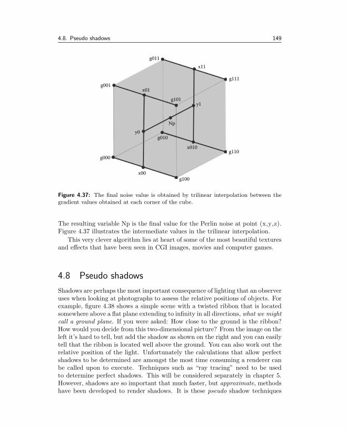
4.8. Pseudo shadows 149
g100x00
g000
g001
g011
x11
g111
g010
Np
y1
y0
x010g110
g101
x01
Figure 4.37: The final noise value is obtained by trilinear interpolation between thegradient values obtained at each corner of the cube.
The resulting variable Np is the final value for the Perlin noise at point (x,y,z).Figure 4.37 illustrates the intermediate values in the trilinear interpolation.
This very clever algorithm lies at heart of some of the most beautiful texturesand effects that have been seen in CGI images, movies and computer games.
4.8 Pseudo shadows
Shadows are perhaps the most important consequence of lighting that an observeruses when looking at photographs to assess the relative positions of objects. Forexample, figure 4.38 shows a simple scene with a twisted ribbon that is locatedsomewhere above a flat plane extending to infinity in all directions, what we mightcall a ground plane. If you were asked: How close to the ground is the ribbon?How would you decide from this two-dimensional picture? From the image on theleft it’s hard to tell, but add the shadow as shown on the right and you can easilytell that the ribbon is located well above the ground. You can also work out therelative position of the light. Unfortunately the calculations that allow perfectshadows to be determined are amongst the most time consuming a renderer canbe called upon to execute. Techniques such as “ray tracing” need to be usedto determine perfect shadows. This will be considered separately in chapter 5.However, shadows are so important that much faster, but approximate, methodshave been developed to render shadows. It is these pseudo shadow techniques

150 4. Basic visualization
Figure 4.38: Adding shadows to a computer-generated image gives the viewer somevery powerful visual clues as to the relative position of objects in a scene.
that will be discussed in this section. The shadow shown in figure 4.38 wasgenerated with just such a technique.
We will consider two approaches to pseudo shadowing which cover most even-tualities. They are planar shadows and shadow maps.
4.8.1 Planar shadows
If the surface on which the shadow falls is flat then it is straightforward to findthe shadow cast by a polygon. Once found the shadow is projected to the viewingplane where a buffer analogous to the Z buffer is used to hold a shadow mask.Because shadows are either on or off, a one byte per pixel mask can accommodateup to 8 different planar shadowed surfaces.
The contents of the shadow mask must be determined in a step that precedesstep 5 in the basic rendering algorithms (section 4.1.1). In the final renderingstep, as the Z or scanline buffers are being filled at pixel i, j, the following testis added:
If the point p on polygon k is visible in pixel i, j and polygon k ispart of one of the planes that has a shadow on it then the shadowbuffer at coordinate i, j is checked to see if polygon k is in shadow ornot. If it is then the color of pixel i, j is dimmed.
Figure 4.39 illustrates the geometry used to produce a shadow mask for theshadow cast on a plane (normal n position Pp) by a triangular polygon (verticesP0, P1 and P2) lit from a point light source at Pl.
In the shadow buffer the shadow cast by a triangular polygon is always tri-angular too. If we let (X0, Y0), (X1, Y1) and (X2, Y2) be the coordinates in theshadow buffer equivalent to vertices P0 etc., we can use a scanline filling pro-cedure to set all the appropriate flags in the shadow buffer. To calculate thecoordinates (X0, Y0) in the shadow buffer equivalent to vertex P0 in the polygon

4.8. Pseudo shadows 151
Viewpoint
zShadow buffer
Shadow cast on planeby triangluar polygon
^
PL
P0 P1P2
Pp
n
(X0, Y0)
y x
Figure 4.39: Filling the shadow mask with the shadow cast on a flat plane by atriangular polygon.
casting the shadow, first obtain the intersection point of the line passing throughPl and P0 and the plane (p−Pp) · n = 0. Then project that point to (X0, Y0)with the same scale factor and aspect ratio used in step 4 of the basic renderingalgorithm. Those calculations are detailed in sections 2.6 and 2.12.8.
Planar shadows have sharply defined edges and are essentially perfect, whichsometimes is an advantage but at other times may lead to less realistic results.The amount of memory required to hold the shadow buffer is not particularlyexcessive and depends on the resolution of the output raster. The disadvantageof planar shadows is that they cannot simulate realistic shadows falling on curvedor non-planar surfaces. Shadow mapped lights, which we will consider next, dogive pretty good looking shadows across any shape of surface.
4.8.2 Shadow maps
Look at figure 4.40. It shows a viewpoint (with associated projection plane) andspotlight directed toward the point p in the scene. The viewpoint is located atthe origin of coordinates and the spotlight is at PL. Imagine now a viewpointat the position of the light source PL which is looking in the direction of thespotlight, toward the target at p. For a field of view that just encloses thespotlight’s cone a projection plane capable of showing everything visible fromthe light’s point of view can be defined. We can use a Z depth buffer associatedwith this imaginary projection plane to help us render a shadow due to thespotlight. This technique requires us to pre-render a view of the scene for eachspotlight and fill its shadow Z buffer, or what we will call its shadow map, as inthe standard Z buffer algorithm.
During rendering of the scene when it comes time to determine if a point plies in shadow or not, we imagine a line from p to PL; it must pass through

152 4. Basic visualization
Projection plane
Spotlight anglePlane of the spotlight buffer
p
PL
Viewpoint
y
z
x
Figure 4.40: A scene with spotlight illumination.
one of the cells in the shadow map associated with the imaginary viewpoint atPL. That cell records the distance of the nearest point in the scene from theimaginary camera (and spotlight), say dmin.
Here then is our test to see if p lies in shadow: if the distance from p to PL
is greater that dmin then point p lies in shadow.
This procedure works because the spotlight shines on a limited area, and soits cone of illumination is bounded and therefore the pseudo camera’s field of viewcan be set to include all parts of the scene illuminated by the spotlight. Becausethe light’s shadow map is of finite resolution the outline of the shadow will besubject to aliasing effects. The more memory allocated to hold the shadow mapor the narrower the angle of the spotlight cone the less noticeable the aliasingwill be. To reduce the visual impact of the aliasing at the edges of the shadow adegree of blurring can be introduced by averaging shadow values over a numberof adjacent cells. This will cause the shadow to have a soft (blurry) edge butthat is sometimes more realistic than the harsh crisp shadows produced by theshadow plane approximation.
To implement this technique the instructions in listing 4.15 are inserted inthe rendering algorithm after the viewing transformation has been performed.Note that the viewing transformation has been applied to the lights too.
For the scene illustrated in figure 4.40 where the spotlight direction is givenby the vector d = p−PL, i.e., a heading of:
φ = ATAN2(dy, dx)
and pitch:
θ = ATAN2(dz,√
d2x + d2y)

4.8. Pseudo shadows 153
Repeat for all spotlights {Build a viewing transformation, [T ] for an imaginary camera located at theposition of the spotlight. Apply [T ] to vertices in scene.Repeat for all polygons k {
Project vertices of polygon k onto the shadow bufferplane and fill each entry with the depth to visible surface.
}}
Listing 4.15: Procedure to fill the shadow map associated with a spotlight.
are used. Transformation [T ] is the product [T ] = [T3][T2][T1] where
[T1] = a translation by −PL
[T2] = a rotation round z axis (up) by −φ
[T3] = a rotation round y axis by −θ
The projection is scaled so that the spotlight’s outer cone (half angle θ2) justfits inside the field of view. Thus, for a shadow buffer resolution of n × n andvertex coordinates (x′, y′, z′), after pre-multiplication by [T ], the shadow buffercoordinates (X,Y ) are obtained from
d =n
2 tan θ2(4.8)
X =n
2− d
y′
x′ (4.9)
Y =n
2− d
z′
x′ (4.10)
The shadow map technique is completed by adding the following actions tothe final rendering step after the surface color, shading and lighting at p havebeen determined; repeat them for all spotlights:
1. Apply transformation [T ] to p to give position (x′, y′, z′), in the frame ofreference where the spotlight is at origin.
2. Apply the projection equations (4.8, 4.9, 4.10) to give (X,Y ) and its nearestinteger indices (Xi, Yi).
3. Extract the shadow distance from the shadow map, dmin = Z(Xi, Yi).
4. If x′ > dmin then p is in shadow with respect to the spotlight.

154 4. Basic visualization
Comment:
While the above procedure works well in most cases it can be subjectto some unpleasant moire patterning. This is due to the fact that eachcell in the shadow map equates to quite a big area in the scene andwithin which there might be a significant depth variation, especiallywhen the resolution of the buffer is low. As a result of this when thetime comes to compare the depth of point p with values in the bufferthen sometimes it will appear to be in and sometimes it will appearto be out of shadow. It is very important to set near and far planesas close to each other as possible as this gives better precision in theshadow map and therefore yields better results.
A simple procedure due to Woo [50] can eliminate the visual distur-bance. To apply it, a second (temporary) copy of the light shadowmap is needed. In this second copy record the depth of the secondclosest polygon from the light and when the full shadow is renderedwe simply average the depth between the two and use this as theshadow depth. In the case when there is only one surface (the sec-ond buffer holds infinity) then it cannot cast shadows on anything soignore it. After each spotlight buffer has been checked the memoryused for the temporary shadow map can be released. One final point:The shadow map only needs to be rebuilt in a non-static scene.
4.9 Line drawing
Before the days of the photographic quality printer and the proliferation of themulti-monitor desktop computer most 3D drawing was presented in line-drawnform. For 3D diagrams in a book or working drawings, or in an equipmentmanual produced by a CAD package, the line-drawn form of a 3D scene orobject still has its uses. Indeed, an outline or (edge and major fold) drawing ofan object is an important component of many automatically generated cartoons.By superimposing an outline drawing on a scene illuminated with ambient lightonly, one has a very passable approximation to the beautiful hand drawn cartoonsgenerated by the skilled artist. Using a lighting model, like the Gooch shading,can enhance the cartoon look by producing appropriate specular highlights, andwhen combined with a hidden surface line drawing, cartoons can be produced onan industrial scale without the need for an artist skilled in the art of perspective.This section will briefly consider the production of line drawn 3D images.
4.9.1 Wireframe
The simplest way to visualize the numerical model for an object is to draw itin wireframe. A wireframe drawing involves relatively few calculations to render

4.9. Line drawing 155
Figure 4.41: A wireframe drawing.
it. The action of step 5 in the rendering algorithm is simply to work through allthe polygons that describe the model and taking each side in turn:
1. Check to see if it has been drawn already.
2. If not identify the vertices it is connected to.
3. Retrieve the screen coordinates determined in step 4 of the rendering al-gorithm.
4. Draw a line connecting these two points in the frame buffer.
If a list of edges in the model is available so much the better since there is noneed to check whether or not the edge has been drawn before.
For a wireframe drawing, such as that shown in figure 4.41, to be recorded inthe framebuffer or drawn on a raster display, a procedure for rendering lines isrequired. Both framebuffer and output display are composed of pixels, thus todraw a line from a to b, the pixels through which the line passes must be givenan appropriate value to represent the color of the line.
The line drawing procedure should be fast and as simple as possible to im-plement. Perhaps the most commonly used procedure yet established is due toBresenham [14] and we will consider this now for the case of a raster equivalentto a two-dimensional array of integer coordinates in the range (0 → Xmax) and(0 → Ymax). The algorithm works incrementally from a starting point (x1, y1)and the first step is to identify in which one of 8 octants the direction of theend point lies. These octants are identified in figure 4.42. How the algorithmproceeds depends on which octant contains the end point of the line in question.
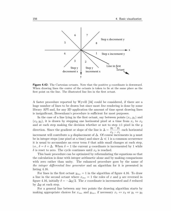
156 4. Basic visualization
2
y
Step yincrement x
Step ydecrement x
3
4
5
6 7
8
Step x decrement y
Step x increment y
Line in first
octant
x1
Figure 4.42: The Cartesian octants. Note that the positive y coordinate is downward.When drawing lines the center of the octants is taken to lie at the same place as thefirst point on the line. The illustrated line lies in the first octant.
A faster procedure reported by Wyvill [34] could be considered, if there are ahuge number of lines to be drawn but since most line rendering is done by somelibrary API and, for any 3D application the amount of time spent drawing linesis insignificant, Bresenham’s procedure is sufficient for most purposes.
In the case of a line lying in the first octant, say between points (x1, y1) and(x2, y2), it is drawn by stepping one horizontal pixel at a time from x1 to x2
and at each step making the decision whether or not to step ±1 pixel in the y
direction. Since the gradient or slope of the line is ∆ =y2 − y1x2 − x1
each horizontal
increment will contribute a y displacement of ∆. Of course increments in y mustbe in integer steps (one pixel at a time) and since ∆ ≪ 1 is a common occurrenceit is usual to accumulate an error term δ that adds small changes at each step,i.e., δ = δ +∆. When δ = 1 the current y coordinate is incremented by 1 whileδ is reset to zero. The cycle continues until x2 is reached.
This basic procedure can be optimized by reformulating the equations so thatthe calculation is done with integer arithmetic alone and by making comparisonswith zero rather than unity. The enhanced procedure goes by the name ofthe integer differential line generator and an algorithm for it is presented inlisting 4.16.
For lines in the first octant yinc = 1 in the algorithm of figure 4.16. To drawa line in the second octant where xinc = 1 the roles of x and y are reversed infigure 4.16, initially δ = −∆y/2. The x coordinate is incremented and δ reducedby ∆y at each step.
For a general line between any two points the drawing algorithm starts bymaking appropriate choices for xinc and yinc, if necessary x1 ↔ x2 or y1 ↔ y2

4.9. Line drawing 157
∆x = x2 − x1
∆y = y2 − y1δ = −∆x/2set x = x1 and y = y1draw pixel at (x, y) with color cwhile x < x2 do {
δ = δ +∆yi f δ ≥ 0 {
y = y + yinc
δ = δ −∆x}x = x+ 1draw pixel at (x, y) with color c
}
Listing 4.16: The basic integer differential line generator algorithm.
∆x = x2 − x1
∆y = y2 − y1i f |∆x| > |∆y| {
i f ∆x < 0 {swap x2 ↔ x1
swap y2 ↔ y1}i f y2 > y1 then yinc = 1else yinc = −1Call the first octant algorithm
}else {
i f ∆y < 0 {swap x2 ↔ x1
swap y2 ↔ y1}i f x2 > x1 then xinc = 1else xinc = −1Call the second octant algorithm
}
Listing 4.17: Algorithm for the drawing of an arbitrarily directed straight line in araster display.
are swapped, and in the final step a call is made to first or second octant linedrawing procedures. This algorithm is presented in listing 4.17.
As a final thought on wireframe drawing it is worth making the following briefcomment: In drawing the wireframe on the projection plane it is assumed that
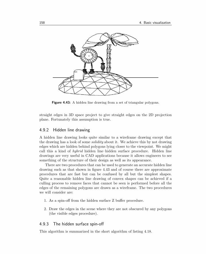
158 4. Basic visualization
Figure 4.43: A hidden line drawing from a set of triangular polygons.
straight edges in 3D space project to give straight edges on the 2D projectionplane. Fortunately this assumption is true.
4.9.2 Hidden line drawing
A hidden line drawing looks quite similar to a wireframe drawing except thatthe drawing has a look of some solidity about it. We achieve this by not drawingedges which are hidden behind polygons lying closer to the viewpoint. We mightcall this a kind of hybrid hidden line–hidden surface procedure. Hidden linedrawings are very useful in CAD applications because it allows engineers to seesomething of the structure of their design as well as its appearance.
There are two procedures that can be used to generate an accurate hidden linedrawing such as that shown in figure 4.43 and of course there are approximateprocedures that are fast but can be confused by all but the simplest shapes.Quite a reasonable hidden line drawing of convex shapes can be achieved if aculling process to remove faces that cannot be seen is performed before all theedges of the remaining polygons are drawn as a wireframe. The two procedureswe will consider are:
1. As a spin-off from the hidden surface Z buffer procedure.
2. Draw the edges in the scene where they are not obscured by any polygons(the visible edges procedure).
4.9.3 The hidden surface spin-off
This algorithm is summarized in the short algorithm of listing 4.18.

4.9. Line drawing 159
Use either the scanline or full Z buffer procedure to record at each pixelthe identity of which polygon is visible.
Work though the raster in the order shown in figure 4.44 and checkfor a change of recorded value both above and to the left of the currentpixel, pixels i− 1, j and i, j − 1
If a difference is detected place a foreground color value in theframebuffer otherwise place a background color.
Listing 4.18: Rendering a hidden surface image as a “spin off” from the basic Z bufferprocedure.
Scan left toright oneach row
Pixel Column iRow
0
j–1
ji–1, j
i, j
i, j–1
1
Figure 4.44: Working through a raster to produce a hidden line drawing.
Working from a Z buffer procedure has the big advantage that it accuratelyrepresents edges in a hidden line drawing which occur because polygons mightintersect. These are edges that can’t exist as entries in any polygon and/or edgelist describing the scene. For example a drawing of a cylinder poking through acube (figure 4.45) will have edges that are not part of any polygon in either thecube or the cylinder.
An interesting effect can be achieved with a hidden line drawing based onhidden surface procedures. It arises because adjacent polygonal faces with nor-mal vectors pointing in the same direction are planar and in most situations littlebenefit is gained by drawing the common edge between adjacent co-planar faces:indeed a picture in which these are omitted can have a much cleaner look. (Thedrawing in figure 4.43 had a few such edges removed.) However edges betweenadjacent polygons should not be omitted if the polygons have different colorseven if they are co-planar. This idea can be pushed to the limit by relaxing theplanarity condition, n1 · n2 = 1, say to: n1 · n2 > θ with θ ≈ 1
2 . Doing this willlead to cartoon like drawings like that in figure 4.46 for example.

160 4. Basic visualization
Edges are introduced where cylinder and cubeintersect. �ey are not in the polygon database
Figure 4.45: A hidden surface drawing showing edges that must be drawn but are notpart of the specification of the models in the drawing.
Figure 4.46: A hidden line drawing with edges drawn only if they are adjacent to thebackground, a different model or another polygon such that (1) the color is differentor (2) the angle between them is > 60◦.
4.9.4 A visible edge hidden line algorithm
Look at figure 4.47 which shows a wireframe drawing of a cube (with the topremoved so that we can see inside it). It has 6 polygons and 12 edges. The edgeslabeled 1, 2, 3, 4, 6, 7, 10, 11, 12 will be fully visible in a hidden line drawing. Edge9 will be partially visible. To decide whether edge i is visible it has to be testedagainst each of the polygons to see whether it lies behind any of them. Howeverit is not sufficient to treat edge visibility as simply either visible or not visible

4.9. Line drawing 161
Places whereprojected
edges cross
105
2
6
117
3
8
9
1
4
12
Projectedvertices
Figure 4.47: Wireframe cube labeling edges and crossovers.
for the whole edge because a case can arise where part of an edge will be visibleand part will be obscured. So, before the visibility test can be made the edgesmust be broken up into appropriate segments.
To see how we can do this look again at figure 4.47, but this time thinkof it purely as a two-dimensional drawing. Anywhere that the lines cross is apotential site for one of the edges to change from being visible to hidden. Thesecrossing points are the only places where the visibility status of an edge canchange. Dividing the lines at these crossing points gives us the segments weneed to test for visibility against the polygons in the model. For example, edge11 will be composed of two segments because it is crossed by edge 5. After theedges have been divided into segments the segments can be tested to see if theyare obscured by any polygons. If a segment is not obscured then it is drawn.
Most of the geometric calculations for this algorithm have been covered inchapter 2 and thus only the logical steps in the algorithm are summarized inlisting 4.19.
As discussed previously this approach to hidden line drawing does not allowfor edges that are introduced by the intersection of polygons. However becausethe output is a list of line segments the drawing can be made on an output devicein any resolution, i.e., it is not subject to the aliasing effect (see section 4.3) thatthe hidden surface algorithms suffer from. Therefore, it is not necessary to renderthe picture again in order to work at a higher resolution. This form of outputis ideal for recording in the device independent encapsulated postscript format.Another useful alternative procedure for the production of hidden line drawingswas developed by Janssen [45].

162 4. Basic visualization
In the 2D projection plane find the intersections of all projectededges with all the other projected edges. For each edge makea list of the segments it is divided into. (Including the coordinatesat the ends of the segments.)
With each line segment make the following tests to see if that segment isvisible, if it is then draw it.
Repeat for every projected edge i {Repeat for every segment j of edge i {
Project back from the ends of segment j to the polygon of whichedge i is a boundary. This gives a depth that can beassociated with the line segment. Call these points p1
and p2 and let their x coordinates be x1 andx2, which we will use as the depths.
Repeat tests 1-3 below for every polygon k {Test 1:In projection: Test if segment j of edge i is inside polygon k.If it is not then move on to the next polygonTest 2:If x1 and x2 are both greater than the maximum x coordinateof vertices of polygon k then segment i is obscured so jumpon to next segment.Test 3:Find the points q1 and q2 on polygon k where thelines from the viewpoint through p1 and p2
intersect it.If the x coordinate of q1 < x1 and the x coordinateof q2 < x2 then segment i is obscured so jump onto the next segment.
}If this point is reached then segment j of edge i is not obscuredso draw it.
}}
Listing 4.19: The visual edges algorithm.

4.10. Tricks and tips 163
4.10 Tricks and tips
The key to fast rendering is smart algorithms but efficient programming can alsohelp. Here are a few tricks and tips to speed up the code.
1. Try not to calculate the same things more than once, particularly if it isa time-consuming calculation. After calculation store it in a temporaryvariable. For example normalizing a vector is slow because it requires areciprocal square root.
2. When rendering, try to calculate as much as possible on a per-polygon basisbefore proceeding to the rendering pass. A big scene may have 200,000polygons and a medium sized anti-aliased image might have the equivalentof 9,000,000 pixels. (This is true for a software renderer; in a hardwarepipeline there may be more pixel processors than vertex processors.)
3. When testing several things that will result in a calculation being avoidedmake the most common test first. See section 4.2.4.
4. Arrange nested loops so that complex calculations are as high in the nestas possible and therefore done as infrequently as possible.
5. Use inline code for short, very often used functions.
6. Sometimes it is more efficient to repeat code than to call a function. Forexample, in C or C++ programs use macros to add, subtract, copy andtake dot and cross products of vectors.
7. Where possible use look up tables. The Perlin noise functions are an ex-cellent case in point. Another candidate is the replacement of the powerfunction in the calculation of specular reflection.

This page intentionally left blankThis page intentionally left blank

5Realistic visualization
To improve on the rendering approach described in chapter 4 the first techniquethat comes to mind is ray tracing. There are other techniques for generatinghigh-quality synthetic images but they will not be discussed here. Ray tracingmay be slow but it does give superb, almost photographic quality, images andbetter algorithms are being developed all the time, so that under certain condi-tions it is even possible to achieve real-time ray tracing. There are many booksthat describe the theory of ray tracing in detail. One of the most cited booksthat comprehensively examines the physics of the rendering process is PhysicallyBased Rendering From Theory to Implementation [70]. Watt [88] in chapters 7and 8 covers all the basics of ray tracing and in Glassner [33] the story is con-tinued. Shirley [80] specializes in realistic ray tracing. A full description of acomplete package is given by Lindley [56] and there are also quite a few goodpublicly available freeware and shareware ray tracing programs with code thatcan be retrieved from many FTP sites and open source repositories.
The idea on which ray tracing is based seems almost too simple to be truebut suppose you could:
Follow the paths taken by particles of light (photons) on their journeyfrom source, through the scene (as they are scattered back and forthbetween objects), and on until they are either captured by a cameraor eye. Or head off to infinity.
Then you would be simulating the physical mechanism that enables us to seeand take photographs.
In practice this is a hopeless task because of the huge number of photonsemitted by a light source and the fact that all but a minute fraction of themwill ever be scattered into the camera. Therefore, ray tracing does it in reverse.It sends feelers or rays from the camera out into the scene. If the feeler raysfind anything, they work back toward the sources of illumination and give usa path for the photons to follow from source to photographic plate. To a firstapproximation the sources of illumination are simply the lights in a scene, butlight can be scattered onto a surface from other adjacent surfaces and in thesimple ray tracing model these are not accounted for. It is possible to feel
165

166 5. Realistic visualization
around, looking for other light emitters, but because the secondary illuminationfeeler rays cannot look in every possible direction, a finite number are dispatchesin pseudo-random directions.
Sometimes all the feeler rays may encounter reflective surfaces and when thathappens they have to follow a new path and continue their journey. There arelots of other things that can happen to feeler rays. Sometimes they may divide,with each sub-ray following separate paths. The way in which the ray tracingalgorithm handles such situations, and the sophistication of the mathematicalmodels it uses for light/surface interaction, governs the quality of the imagesproduced.
So, we can get away with following a few rays of light, but what about the nextquestion: How few? Our digital camera records its image at a finite number ofpixels in a raster and since each pixel holds one value we need send only one feelerray per pixel—well almost. In section 4.3 we saw that pixelated displays sufferfrom aliasing. Ray traced images are no exception and thus they require someanti-aliasing. Dispatching more than one ray per pixel and averaging the resultis equivalent to the technique of super-sampling. Again here, the additionalfeeler rays are dispatches in somewhat random directions. The additional ofa random element in the ray tracing algorithm sometimes endows it with themoniker Monte Carlo ray tracing.
This chapter is primarily concerned with the the ray tracing algorithm be-cause it is very successful, and conceptually it is the simplest realistic visual-ization procedure. The option to render a scene using ray tracing is offered bymost of the mainstream 3D visualization packages, and the code for the OpenFXpackage which is dissected in chapter 9 exemplifies how it can be done in practicewhen rendering objects described by a very large number of planar polygons.
Despite the popularity of the ray tracing algorithm some would argue that itdoes not implement a true model of the illumination process and cannot easilyimage things like the penumbra of soft shadows, particulate light scattering orthe caustics due to light passing through refractive glass. A lot of work has beendone on an alternative approach know as radiosity, and this has been used toproduce some of the most realistic images ever synthesized. However radiosityis not the perfect solution either. It cannot account for specular reflections forexample. Radiosity tends to be explained in abstract mathematical terms inmost texts, but a more practically orientated introduction can be found in thebook by Ashdown [5]. Although quite old it offers a practical perceptive.
Neither ray tracing nor radiosity are perfect rendering algorithms. Recentlyit has been suggested by Jensen [46] that both approaches should be augmentedby a technique called photon mapping to fill in some of the gaps. It is likelythat a hybrid approach will win out. A hybrid rendering engine would includeall three ideas, as well as the basic Z-buffer hidden surface approach, so thatthe advantages of each are used. One thing is certain; whether you go to thecomputational expense of ray tracing or radiosity it is likely that you will want touse a better illumination model than the simple Lambertian cosine law presented
5.1. Radiometric lighting and shading 167
in section 4.4. Before delving in to study ray tracing in detail we will digress alittle in the next section to consider the physics of light-material interaction andhow more elaborate illumination models may be obtained.
5.1 Radiometric lighting and shading
Light is an electromagnetic (EM) radiation and physicists assign it a wave-particle duality, which means that they can model its behavior using either thebehavior of waves or ballistic particles. As observers we mostly perceive light asa reflection from the world around us. This can be the scattered light in a bluesky or the yellow light reflected from a white object lying in the shadow of ayellow object that is in bright sunlight. Accounting for multi-path illuminationrealistically is one of the major challenges in computer graphics. The light thatwe perceive has a wavelength lying in that part of the EM spectrum betweenabout 390nm and 700nm, and what we see when a scene is illuminated is therefection due to the way the light interacts with surface materials.
The way light or any other electromagnetic radiation interacts with a surfaceis usually modeled using the wave approach and is based on the assumption ofconservation of energy in which the incident light is either absorbed, transmitted,or reflected. There can also be an emissive component. This model is known asthe radiometric model as it is valid across the EM spectrum.
A very detailed study of all aspects or the radiometric model of light transportin the context of computer graphics and all other aspects of physical renderingmay be found in Pharr and Humphreys [70], which includes a detailed descriptionof a C++ implementation and some beautiful examples of rendered scenes.
In reality, light enters the scene from the light sources. It bounces aroundthe scene, passes through transparent materials or is absorbed, sometimes tobe re-emitted. Once an equilibrium has been established, every point on everysurface is acting as a small radiator and will be emitting some light, in additionto the active sources (what we call the lights). With the exception of the activeemitters, most of the emission will be due to reflection. Sampling the lightemanating from a point on a surface gives the color that we perceive with oureyes or record in a photograph. Trying to calculate the light emerging from everypoint on a surface due to the illumination from light emerging from every otherpoint on the surface is the essence of the radiosity algorithm.
This book does not delve into the details of radiosity or the radiometricapproach to photo-realistic rendering, however a briefing document on the topicand a closely allied area with high potential, called photon mapping, can beobtained from the website.

168 5. Realistic visualization
5.2 Ray tracing
The standard algorithm for ray tracing follows the first three steps of the basicrendering procedure described in section 4.1.1.
1. Load the data describing objects in the scene to memory.
2. Move each model into its appointed position.
3. Apply the viewing transformation. (Not all ray tracing applications usethis step.)
After step 3 instead of projecting the polygons from the scene onto the viewingplane a ray tracer calculates the direction of a feeler ray, d, from (0, 0, 0) so thatit passes through the point in the projection plane equivalent to pixel (i, j) of thedisplay raster (which is of size Xmax by Ymax). For a projection plane locatedat (1, 0, 0) we can obtain the same field of view for the ray tracer as we get from
the Z buffer renderer by using equations 2.17 and 2.18 to calculate d as follows:
dxdydz
=
1(
Xmax
2 − float(i) + 12
sx
)
(
Ymax
2 − float(j) + 12
sy
)
d = d/|d|
The fraction ( 12 ) is included so that the feeler ray passes through the center ofthe pixel. To jitter the feeler ray for anti-aliasing purposes a different offset inthe range [0, 1] would be used. The scaling factors sx and sy account for field ofview and aspect ratio.
When using ray tracing to render a scene it is inappropriate to cull or clipany model or model facet because rays can bounce back and strike models lyingbehind the camera or out of the field of view.
In the visualization step the feeler ray (origin (0, 0, 0) direction d) is followed(traced) out into the scene until it intersects a polygon. Once the point ofintersection, p, is located the surface properties can be determined and the pixelset to the appropriate color value, a process that is illustrated in figure 5.1.
If on first hit the ray isn’t totally absorbed we can continue to trace its pathuntil it reaches a final destination or is so attenuated that there is nothing tosee. It is usual to do this recursively so that the same code is used to trace allrays, not just those originating from the viewpoint. Each time the ray hits asurface a calculation is made of the illumination using the methods described insections 4.4 and 4.4.2.
While the spotlight shadow effect (described in section 4.8.2) with its softedges is sometimes used by a ray tracer, the normal procedure to trace shadows

5.2. Ray tracing 169
Projection plane
z
x
Row j
Columni
Ray
Scene
p
y
Figure 5.1: Tracing a ray from the viewpoint out through pixel (i, j) until it hits anobject in the scene.
Load model descriptions and move them into position.Apply viewing transformation.Repeat for all rows, j, in the raster {
Repeat for all columns, i, in the raster {Initialize color value, s, (RGB components)
For pixel (i, j) calculate ray direction d
Set ray origin, p, to (0, 0, 0)Call recursive function to return s for pixel (i, j)
DoRay(p, d, s)Copy s into the pixel array at address (i, j)
}}
Listing 5.1: Ray tracing, part 1: Set up the geometry (view direction, etc.), launch afeeler ray for every pixel and store the color it returns.
is done by checking the path from the visible point p to each light source. Ifany facet in a model in the scene intersects this path then p is deemed to be inshadow.
So the full basic ray tracing algorithm can be summarized in the two partspresented in listings 5.1 and 5.2.
Note the recursive use of the DoRay() function in the algorithm of figure 5.2.In the practical implementation of any recursive function care is often taken toensure that the function doesn’t become stuck in an infinite loop. In DoRay()this might happen if a ray hits a reflective surface which bounces it to anotherreflective surface which reflects it back to the first so that it continues to bounce

170 5. Realistic visualization
DoRay(p, d, s) {Find the identity of the polygon, k, that intersects the ray p+ µdat pi and is closest to p.
Calculate surface color ss for polygon k at pi dt
use procedural texture or image map if required
If the material properties of k indicate that it is partiallyreflective or transparent then cast extra rays.
If reflective get reflective direction dr
DoRay(pi, dr, sr ) ;
If transparent get transparent direction dt
DoRay(pi, dt, st )
Get surface normal, ni at pi, use Phong’s interpolationand any procedural or bump mapping if necessary.
From pi send feeler ray to each light source. Test every polygonn the model to see if feeler ray intersectsit. If it does then the surface is in shadow. .
Combine ss with sr and st and apply lighting to givethe final s value that is returned.
}
Listing 5.2: Ray tracing, part 2: The key recursive function DoRay(p, d, s) that doesthe key work of a ray tracing algorithm. For a given ray, origin p, direction d, determinethe color, s, of the surface seen.
back and forward forever unless the mirrors are less than perfect. In practice therecursion must be terminated at some preset depth. For most scenes after threeor four reflections the ray can be assumed to have left the scene.
All the calculations and procedures needed for the steps in the basic raytracing algorithm have already been studied in chapters 2 and 4. Sophisti-cated extensions to the basic algorithm tend to be directed at simulating surfaceproperties, color patterns, transparency lighting and inter-object reflections. Byusing more and more rays a better approximation to ambient lighting conditionsand the penumbra of shadows can be included. The red, green and blue primarycolor model is only an approximation to the continuous spectrum of illuminationfrom natural light. Other color models need to be employed in order to developmore sophisticated physical models of the way light interacts with surfaces. The

5.3. Ray tracing optimization 171
dispersion of light through a prism is one example. Recent developments [68] inprocedural textures can deliver realistic models of smoke plumes, steam, cloud,hair and fur. However it is the realistic shadows and true reflections that are themost significant reasons to call on the use of a ray tracer.
The basic algorithm in figures 5.1 and 5.2 involves an almost impossibly largenumber of calculations when it is applied to rendering realistic models with morethan a few hundred primitive shapes. Note the term primitive shape. This couldinclude spheres, torii, swept or lofted analytic curves and even more complexstructures built by Boolean operations on basic primitives. Nevertheless yourmain observation probably was the hours it took the computer to trace evenan image of moderate resolution. What is worse is that the rendering timeincreases as the number of models in the scene increases, thus if you need torender a scene with models made up from thousands of polygonal facets, a basicray tracing renderer is virtually useless.
So the main question is: Why is ray tracing so much slower? The answerlies in the first two lines of the algorithm given in figure 5.2. For each pixel,test every polygon and find the one closest to the origin of the ray. This ispotentially an enormous number of operations. If the raster is of size n×m andthe scene is described with k polygons, ≈ n×m×k×r (r is the average recursiondepth) testing and swapping operations must be performed. For example, tosynthesize an image of size 640 × 480 using a 2 × 2 anti-aliasing supersamplewith a scene with 20, 000 polygons requires ≈ 24 billion tests. With each testtaking many processor cycles you could be waiting a very long time for the imageto materialize.
The remainder of this chapter is devoted to techniques that can be used tospeed up the ray tracing algorithm. Given favorable circumstances it is possibleto produce ray traced images with thousands of polygons in a fraction of thetime that it would take using the basic algorithm and perhaps only five or tentimes slower than a Z buffer procedure.
5.3 Ray tracing optimization
A huge step in optimizing the ray tracing algorithm would result if we couldreduce the number of pixels through which we need to trace rays. So considerthis: In section 5.2 the ray tracing algorithm was designed so that it used thesame viewpoint, view direction and field of view as the basic Z buffer renderer.As a consequence both rendering algorithms will see the same polygons in thesame pixels. For the most part the same equations and algorithms are used todetermine illumination, Phong shading, procedural texturing and image map-ping. Thus we can use a Z buffer algorithm to render the scene and traceadditional rays to track reflections, refractions, ambient lighting or for shadowdetermination.

172 5. Realistic visualization
5.3.1 Hybrid tracing
Just adding a Z buffer to the ray tracing procedure alone will result in a huge sav-ing in execution time especially if shadow determination is not required. Withoutshadows perhaps as few as 1 to 5 % of the image pixels will need to be traced. Ifshadows are required one of the pseudo techniques described in section 4.8 couldstill be included as an option in a ray tracing renderer.
Another factor that adds to the advantage of a hybrid algorithm is that theshape of most models is such that often (particularly in animated sequences)there can be a substantial proportion of pixels showing the background color.Making a Z buffer rendering first will identify which pixels are showing back-ground and as a result don’t need to be traced at all. Thus, combining Z bufferand ray tracing renderers produces a hybrid tracer which performs the steps:
1. Use the Z or scanline buffer to determine the identity of which polygon isvisible in each pixel. Store the identity in a list.
2. Jump into the ray tracing procedure using the identity of the polygonsfrom the list as the surface of first hit.
3. Continue with the standard ray tracing procedure from there.
Note:
For a hybrid tracer it is probably better to use a scanline Z bufferprocedure. It saves on memory because the additional buffer whichrecords the identity of the visible polygon has to accommodate onlyone row of pixels at a time.
Switching to hybrid tracing is particularly useful in saving execution for thosescenes with a significant amount of background showing. However if a modelshould, after projection, cover the whole raster and every visible point on it re-quires to have its shadow status determined, then other optimization techniqueswill need to be developed as well.
In essence, what all ray tracing optimization techniques try to do is minimizethe number of intersection tests a ray needs to make. This includes secondaryrays and shadow feelers. There are two approaches that have received muchinvestigation:
1. Bounding volumes
2. Spatial subdivision
We will look at both of these but in the case where models are constructed from alarge number of convex planar polygons. Spatial subdivision will probably be theeasiest method to implement, so we will consider that technique in much greaterdetail. Both optimization methods work by creating some form of hierarchicalsubdivision prior to tracing any rays. When it comes to following a ray it ishoped that the use of the hierarchical data will obviate the need for a largenumber of intersection tests.

5.3. Ray tracing optimization 173
Ray misses extent
Ray intersects theextent. �e polygonsin the model must betested.
Bounding extent
Observation point
Ray missesextent
Figure 5.2: A ray need only be tested against surface polygons if it also intersects abounding extent.
Extents Hierarchy
12
34
4 5
3
1
2
6
56
Figure 5.3: Nested bounding volumes and their hierarchical relationship.
5.3.2 Bounding volumes
Bounding volumes, sometimes called extents, are a simple primitive shape, sphereor cube for example, that encloses the whole model. When a ray is traced thefirst hit test is against a very few of these bounding volumes and only whenan intersection occurs is it necessary to test the ray against individual surfacepieces; figure 5.2 illustrates the idea.
Within a bounding volume it is possible to create nested bounding volumesthat gradually break the scene up into smaller and smaller regions with fewerand fewer polygons in each. Figure 5.3 illustrates nested spherical extents andtheir hierarchical relationship. Should a ray not intersect an extent at one levelin the hierarchy then there is no need to test any extent (or polygon boundedby that extent) if it is a descendant of that level.
So the idea of extents is simple in theory but unfortunately it is more difficultto apply it in practice. Look again at the situation in figure 5.2. How would you

174 5. Realistic visualization
Division of space
Collection of objects
Figure 5.4: Subdividing a two-dimensional space into small rectangles so that at mostone object is contained in each.
proceed to generate descendant extents for that model after the first and mostobvious? It is necessary to do so because unless the number of polygon tests canbe limited to a few hundred per extent we will still have an interminable waitfor the image to develop.
A lot of experiments have been conducted on the use of unusual boundingvolumes (see Arvo and Kirk [33], figure 6) but in most cases very good optimiza-tion seems only to be obtained when the shape of the models are known andappropriate extents can be designed. For general work a spatial subdivision isprobably a better bet.
5.3.3 Spatial subdivision
The idea here is again to break up space into a number of small boxes so thatthere are as few polygons in each little box as possible. In many ways a verysimilar idea to that of the bounding extent except that no attempt is made tooptimize the fit of the extent round the whole or parts of a model. In addition,the regularity of the subdivision means that it is easy to trace rays from one boxto another as they pass through the scene.
For explanatory purposes in this section, because it is easier to illustrate thespatial subdivision procedure in two dimensions, most of the diagrams used toillustrate the process are two-dimensional. We should however remember thatin reality the process is taking place in three dimensions.
To begin, consider the scene shown in figure 5.4. On the left it illustrates sixobjects and on the right a spatial subdivision which arranges for each little rect-angle to contain at most one object. The subdivision was produced successivelywith vertical and horizontal cuts so that at any stage rectangles are only dividedif they contain more than one object. From figure 5.4 note the following:

5.3. Ray tracing optimization 175
(l)
(k)
8
7
32
1
6
5
4
Figure 5.5: Part of a model made from a connected network of polygonal facets.
1. The subdivision is hierarchical. It continues until each rectangle holds onlyone object or until you reach a maximum user defined depth.
2. The size of the rectangles are not uniform: some are large, some are small.The size is chosen so that the objective, of “one object in each subdivision”,is achieved with the fewest number of subdivisions. One way to do thisis to recursively choose a dividing line at each step that places half theobjects to the right and half to the left of it.
3. The example shows discrete separated objects.
All this looks great in theory until we come to consider a model made froma connected network of polygonal facets, then we have a bit of a dilemma! Lookat figure 5.5; it shows a small network of connected polygonal facets. No matterhow hard we try (how many times we subdivide), there is no way that we canseparate each polygon so that a rectangle in the subdivision contains only onepolygon. The fact that the polygons are connected is responsible for that. Thevery best we could probably do is associate polygons 1, 2, 3, 4, 5, 6 with rectanglek and polygons 2, 3, 4, 5, 7, 8 with rectangle l. We are going to have to acceptthat in practice a one polygon to one subdivision goal is unattainable. Thereare two possible solutions: Any polygon that spans a subdivision is split. Forexample triangle 2 in figure 5.5 could be split into three smaller triangles, onepiece will be in rectangle l and two pieces will fall in rectangle k; see figure 5.6.This approach will increase the number of triangles in the model and increasethe complexity of the code since image mapping coordinates and so forth willneed to be recalculated. An alternative solution is to accept that in some casesthe maximum limit of number of polygons per subdivision may be exceeded anddesign the subdivision algorithm carefully so that it recognizes when furtherdivision is pointless.

176 5. Realistic visualization
(l)
(k)
84
7
3
1315
21
6 5
15
10
11
1214
9
Figure 5.6: Split any polygon that spans a plane of subdivision.
To develop an algorithm for spatial subdivision we begin with the principlesillustrated in figure 5.4. Thus the procedure starts with a big region that en-closes all polygons: in two dimensions a rectangle, in three dimensions a box.After that, split the region into four (two dimensions) or eight (three dimen-sions). Continue recursively splitting each subdivision until all of them satisfythe terminating condition.
In 3D this algorithm is called octree decomposition, because it divides avolume into sub-units eight at a time.
5.3.4 Octree decomposition
Before developing the algorithm further let us be clear as to the inputs that areavailable and what outputs we require.
The inputs are a list of polygons and a list of vertices typically recordedusing one of the alternative data structures described in chapter 3. The outputwe need is a hierarchical representation of the octree decomposition and for eachsmall box, at the ends of the branches of the octree, a list of the polygons which,at least partially, lie inside it. With this information rays can be traced asthey travel through the scene moving from one box in the octree to another.Figure 5.7 shows a cubic region of space and how that might be divided up intocubic volumes. That particular subdivision would occur as a result of most ofthe polygons being located in one corner at the top of the cube.
The algorithm to build an octree will be based on a recursive function thatcalls itself eight times, once for each branch of the octree. The recursive functionwill consist of a number of short steps. The data structure that we shall use foreach node in the octree is listed in figure 5.8.
The first stage in the octree building algorithm shown in listing 5.3 launchesthe recursive function. After that recursive subdivision proceeds until the full

5.3. Ray tracing optimization 177
Subdivision planes
Octree components
Figure 5.7: The first few subdivisions of a spatial octree decomposition.
xmin, xmax Dimensions of the box associated withymin, ymax octree node k.zmin, zmax
n Number of polygons falling inside box for node k.Poly(i) List of identities of the n polygons falling inside
the box associated with node k.Child(i) List of 8 pointers to child nodes of node k.Parent Pointer to parent node of node k.
Figure 5.8: Data recorded at each node, k, in the octree.
octree has been established; the steps executed within the recursive function aregiven in listing 5.4.
Before illustrating the octree decomposition process with an example, a littlemore detail needs to be given for some of the steps carried out by the recursivefunction of figure 5.4. Consider the following after looking at figure 5.4:
Step 1 The procedure can be terminated if:
1. The number of polygons attached to node O is less than a preset threshold.
2. The size of the box is smaller than a preset minimum.
3. The octree depth has exceeded a preset limit.
Step 2 There are a number of criteria that could be used. A coordinate averagein each of x, y and z at the centroid of the polygons is a logical choice.

178 5. Realistic visualization
Create the first, root, node in the octree.
Determine a bounding box that encloses all the polygons in the model.It might be useful to include a small guard region so that nothingis missed when it comes to tracing rays.
Assign all polygons in the model to the root node’s polygon list.
Assign the child and parent pointers to indicate that this node hasno descendants or parent.
Start the recursive procedure by subdividing the root node.
Call function Xtend (Root ) ;
Listing 5.3: The first step in decomposing the octree creates a root node and launchesthe recursive subdivision.
Step 3 A fairly quick test is needed here. The centroid of each polygon is apossible candidate point with which to test for inclusion in one of the subdividedvolumes.
Step 4 This is the most significant step in the algorithm and will require a testthat is capable of determining if any part of a polygon falls within one of thesubdivisions. The test can be performed in a sequence of increasingly complexchecks with the simplest and most clear cut performed first. The following checksrely on the fact that the box has 12 edges and thus for triangular polygons therewill be an intersection if either: one of the 12 sides of the box intersects thetriangle, or one of the 3 sides of the triangle intersects one of the 6 sides of thebox.
Thus the checks to apply for polygon k against the volume associated withnode i are:
1. If the maximum x coordinate of every vertex of polygon k is less than theminimum x coordinate of the sides of the box for node i then the polygondoes not overlap the box. The same criteria is applied to the y and zcoordinates.
2. If the minimum x coordinate of every vertex of polygon k is greater than themaximum x coordinate of the sides of the box for node i, then the polygonand box do not overlap. The same applies to the y and z coordinates.
3. Having performed these simple checks to eliminate candidate overlaps thereis another quick check that will detect certain overlaps: If any of polygonk’s vertices lies inside the box for node i, then the box and polygon dooverlap.

5.3. Ray tracing optimization 179
Step 1:Check the terminating conditions to see if node O should befurther subdivided or not. If not then exit the function.
Step 2:Using the location of all n polygons assigned to node O findsuitable planes parallel to the x, y, and z axes whichdivide the box associated with node O into 8 smaller boxes.
Step 3:Check to see that the division has accomplished something!i.e. each subdivided box will contain < n polygons.If not then ext
Step 4:Create 8 child nodes for node O and thenrepeat the following for each: 0 ≤ i < 8. {
Step 4a:Indicate that node i has no descendants, no associated polygonsand that it is descended from node O.
Step 4b:Assign bounding limits using the planes determined in step 2.
Step 4c:For all the polygons k, assigned to node O check to seeif they intersect the box associated with child i.If there is an intersection then add k to the polygonlist Poly(nc) = k and increment nc, the counterfor the number of polygons assigned to child i.
}Step 5:Clear the list of polygons associated with node O. All polygons willnow have been reassigned to one or more of node O’s descendants.
Step 6:Extend the octree by calling function Xtend() foreach of node O’s descendants in turn.
Listing 5.4: Function Xtend(O) which uses recursion to subdivide the volume associ-ated with node O.
The following two checks are relatively slow to apply.
4. Each edge of polygon k is tested against each side of the box. This is a two-part check: First determine that the edge crosses the plane containing theside and then check whether the intersection point lies within the boundsof the rectangular side.
Since the box’s sides are conveniently parallel to the reference axes, thegeneral geometry for line–plane intersection described in section 2.6 can beconsiderably simplified. For example if the side lies in the xy plane at zcoordinate z0, and it is bounded between [Xmin−Xmax] and [Ymin−Ymax],then an edge from p0 to p1 may be checked by the following procedure:

180 5. Realistic visualization
i f p1z − p0z < ǫ {return no intersection line does not cross plane
}Let µ =
z0 − p0zp1z − p0z
and α = p0x + µ(p1x − p0x)Then i f α ≤ Xmin or α ≥ Xmax {
return no intersection crosses plane outside box}Let β = p0y + µ(p1y − p0y)i f β ≤ Ymin or β ≥ Ymax {
return no intersection crosses plane outside box}return intersection
5. The 12 edges are checked against the polygon using the line triangle inter-section algorithm described in section 2.11.1.
Even though the above steps have been described for triangular polygonsthere is no reason why the procedure could not be applied to any convex planarpolygon.
5.3.5 A simple octree decomposition example
Let’s examine an example of the construction of an octree from the six connectedtriangular polygons shown in figure 5.9(a). Figures 5.9 and 5.10 illustrate theprogressive subdivision and growth of the octree. For ease of illustration theexample is restricted to two dimensions.
Figure 5.9(b) shows the box associated with the octree’s root node and theidentity of the polygons assigned to the root, at this stage all of them. In 5.9(c)the dividing planes at XX ′ and Y Y ′ are shown as added. Using these planes,polygons are assigned to the nodes of the octree as illustrated in figure 5.10(a).Dividing the area for node A into AA, AB, AC and AD as shown in 5.10(b)produces the assignments given in 5.10(c). After this stage we will assume thatfurther subdivision is unnecessary.
One thing to note about the octree spatial subdivision is that sometimes apolygon cannot be uniquely assigned to only one of the subdivided spaces, i.e.,to one of the nodes of the octree. There are two ways forward. First, the polygoncan simply be assigned to all the octree voxels that it passes through. Of coursethis will increase the number of polygons that need to be tested as a ray traversesthe octree, and it may not be possible to reduce the number of faces in a octreevoxel below an acceptable threshold. Second, as an alternative the polygonscan be split, i.e., clipped, along the sides of the voxel so that each part (itself apolygon) may be assigned to only one node. Splitting a polygon increases thepolygon count and one has to be very careful not to split a polygon when one ofits vertices happens to lie in the splitting plane, or if an edge of a polygon lies in

5.3. Ray tracing optimization 181
(a) (b) (c)R
D
666
1, 2, 3, 4, 5, 6
555
444
333 222
111
B
AR Y C
X X´
Y´
Figure 5.9: Building a very simple octree for 6 connected triangles. (a) The system.(b) The root node, its associated box and octree polygon assignments. (c) Add thedividing lines.
the plane of a split. In these special cases the polygon must be assigned to onlyone of the adjacent octree voxels. Detecting these special cases are facilitated byusing integer coordinates for the vertices and the splitting planes.
Another useful practical trick is to make a copy of the mesh and split thecopy leaving the initial mesh intact. The copy that was split is not used forrendering directly. Each split face in the copy keeps a record of the face it wasbuilt from in the original mesh. When rays are being traced through the octree,the split copy is used for the ray–polygon intersection tests. When the ray hits aface in the split mesh, the pointer to the face that the split face originated fromlets us use the original face to carry out the lighting and shading calculations.By leaving the original mesh intact it is not necessary to fix up vertex normals inthe split mesh, or re-interpolate color intensities or texture coordinates at eachof the vertices created due to the split, hence the code can be shorter and lessprone to errors.
One final comment: The depth of the octree never need grow too deep. Adepth of 20 can accommodate a range of feature sizes as large as from 1 to 106.
5.3.6 Tracing rays through an octree
Once a subdivision of space containing the scene is obtained the basic ray tracingalgorithm can proceed. However it must be modified so that as a ray is tracedthrough the scene, it moves in increments. Each increment takes the ray fromone subdivided volume into the next one along its path, i.e., into one of those

182 5. Realistic visualization
4, 5, 6
1, 2, 4, 3
2, 4, 5, 6
4, 2, 1A
B
R
C
R
AAA 1,2
1,2
2,4
2, 4, 5, 6
1, 2, 4, 3
4, 5, 6
2AB
AC
AD
B
C
DD
(a) (b) (c)
D
CACAA
AB
B
AD
65
4
3
12
Figure 5.10: Continuing the example from figure 5.9. (a) Octree data after first divi-sion. (b) Add the division for node (A). Assume boxes C, D and E have attained theirtarget limit for division so they are not divided again. (c) The octree data and polygonassignments after division of box A.
that are adjacent to the current location of the ray. At each incremental stepthe following actions are carried out:
1. Identify the octree node i which is the node associated with the volume ofspace where the ray is currently located.
2. Test the ray for intersection with any polygons in the list held at node iand record the identity id of the polygon which is closest to the origin ofthe ray. Also note the point of intersection p between polygon id and theray.
3. Using polygon id’s material and the point p calculate appropriate surfacetexture and lighting. If necessary dispatch additional rays to determinereflections, shadows etc.
To determine which node in the octree we should use for i in the above, we haveto descend through the tree starting at its root and taking branches accordingto the rule that p lies within the box associated with that branch and its node.When we can descend no further down the tree: this is node i.
As a simple example consider the case illustrated in figure 5.11 with theequivalent octree given (figure 5.12.) We will assume that the ray originatesat p, so the first set of polygons we need to test for intersection are those thatintersect the rectangle in which p lies. To determine this we start at the root R ofthe octree (figure 5.12), and perform a simple if–then–else test to see whetherp lies in the rectangle associated with R; it does. Next, the same test is applied

5.3. Ray tracing optimization 183
B
DA
CPi Pi
+
^
p
d
p
pi
Figure 5.11: Tracing a ray originating at p through a subdivided space (a two-dimensional representation of the division).
AA
A
R
D
AB AC AD B C DA DB DC DD
Figure 5.12: The hierarchical octree corresponding to the spatial subdivision shown infigure 5.11. (Again this is a two-dimensional representation of an octree.)
to all immediate descendant nodes, those labeled A, B, C and D. The test showsthat p does not lie in A but that it does lie in B. Since B has no descendants,we have reached the end of the search and can proceed to test for intersectionwith any polygon in the list attached to the data structure for octree node B.
If there are no intersections at this stage we need to track the ray into anadjacent box, for this example, the rectangle labeled DA in figure 5.11. This wecan do in three steps:
1. Project the ray in direction d to find the spot on the sides of the boxassociated with node B where the ray leaves box B; call it the point pi.
2. Project the ray forward by a small amount to get another point; call it p+i
given by:p+i = pi +∆d
3. Work down through the octree to find the node whose boundaries are suchthat p+
i lies in its associated box.

184 5. Realistic visualization
Once a new octree node has been identified the process is repeated usingp+i as the starting point for the next increment of the ray.
Notes:
1. The small increment ∆ used to extend the ray into the next box should bechosen carefully. A magnitude somewhat less than the smallest dimensionof the smallest box in the octree will be satisfactory because then there isno chance of p+
i falling in a non-neighboring box. In addition ∆ must begreater than zero so that even glancing rays get into the neighboring box.
2. The time penalty incurred by tracking rays in this way is not as great asit may seem because finding which branch of the octree holds p+
i involveschecking relatively few levels of the tree with quite simple comparison tests.
3. The same tracking procedure can be used equally well for rays that origi-nate as a result of a reflection or refraction and for feeler rays checking forshadows.
5.3.7 Following reflected rays
The procedure set out in section 2.9 deals with reflection by generating a sec-ondary ray with its origin at the point where the primary ray intersects thereflective surface. Like all other rays the secondary ray is passed to the basictracing function DoRay() (figure 5.2). The value DoRay() returns is mixed withlighting and texture values as usual.
5.3.8 Following refracted rays
Using the procedure set out in section 2.10 a secondary ray is generated with itsorigin at the point where the primary ray intersects the transparent surface. Likeall other rays the secondary ray is passed to the basic tracing function DoRay()(figure 5.2). The color value DoRay() returns is mixed with lighting and texturevalues as usual.
5.3.9 Tracing shadows
A feeler ray from the point p where the shadow status is to be tested is trackedthrough the octree subdivision toward each light in the same way as any otherray. If in each subdivision a polygon intersects the ray, then p is deemed to bein shadow and consequently there is no need to follow the ray any further.
5.4 Multi-threading and parallel processing
Multi-threading can be regarded as the modern term for parallel/concurrentprocessing. It allows several tasks, even within the same program, to execute

5.4. Multi-threading and parallel processing 185
at the same time, or appear to execute at the same time. One could perhapssay that the concept was ahead of its time and until recently most computerprograms were not written as multi-threaded applications. However, now multi-threading’s time has come because virtually every new computer is designedaround a multi-core processor that truly allows a program to do several tasks atthe same time.
In theory, ray tracing is an ideal application for implementation in a parallelprocessor because each ray is, to all intents and purposes, independent of all theothers. Thus in systems which provide hardware to take advantage of concurrenttasks it makes sense to design a ray tracing algorithm which farms out thetracing of individual rays to different threads of execution. However, there isno advantage and perhaps even a significant penalty to be incurred if a multi-threaded algorithm is executed by a system with just one processor.
Threaded algorithms must conform to the following standards:
1. Have a separate function which when called carries out all calculations andcan be used re-enterently.
2. Variables needed for temporary use within a thread must not be placed inmemory locations that are available to concurrently executing threads. Inpractice this means storing all intermediate data on a stack.
3. So-called global variables (accessible to all threads) are usable for readonly or write only access, but not read and write unless some kind of lockis applied when working with these data.
In the case of a ray tracing application program, the geometry of a scene maybe recorded in global memory. This description is read and used simultaneouslyby different threads to trace a ray and calculate a pixel color value which isplaced in another globally accessible matrix (the output raster) at an addressunique to each thread.
From a practical point of view perhaps the most significant design decisionfor a multi-processor rendering algorithm is the strategy for dispatching tasksto the host processors. Do we use a separate thread for each pixel, scanline orsomething else? Since we have already stated that it is very undesirable to createmore threads than processors the best idea is to divide the output raster into asmany regions as there are processors in the hardware and direct each processorto render all the pixels in its region. This has a little drawback because part ofthe image might need very little processing, say background only, while anothermight be showing a complex model with multiple reflective surfaces.
A good practical compromise is to use what one might call interlaced scan-lines. For example in a dual processor environment, processor A renders rows 1,3, 5, 7 etc., while processor B renders rows 2, 4, 6, 8 etc. The advantages of thisapproach are first that in any image there will be high correlation between the

186 5. Realistic visualization
content of adjacent rows so calculation times will be very similar for all proces-sors. Second, the overheads of spawning threads will not be too great, as mighthappen if every pixel’s calculation dispatched a new thread.
You can observe this strategy in action in the OpenFX application’s codethat is examined in chapter 9.

6Computer animation
This chapter starts with an introduction to the most commonly used approach to3D computer animation, i.e., keyframe in-betweening (tweening). It shows howthis is used for the animation of rigid body behavior and illustrates possibilitiesfor the extension of the keyframe approach to cover the more complex topic ofcharacter animation. Following the discussion on character animation we willproceed with an explanation of a technique often used for character animation,namely inverse kinematics or IK for short. IK has applications in non-characteranimation but it is probably its association with articulated models (i.e., charac-ters) that animators would find it most useful. Finally there is a discussion anda few examples of aspects of the simulation of realistic motion that arise fromsome basic physical laws.
6.1 Keyframes (tweening)
The idea of the keyframe is well known to paper-and-pencil animators. It isa “description” of a scene at one instant of time, a key instant. Between keyinstants it is assumed that nothing “startling” happens. It is the role of thekey animators to draw the key scenes which are used by a team of others todraw a series of scenes filling in the gaps between the keys so that jumps anddiscontinuities do not appear. This is called “tweening” (derived from the ratherlong and unpronounceable word inbetweening).
To convince an observer that the animation is smooth and flicker free anumber of pictures must be flashed quickly before them. Cine film presents24 pictures per second and television either 25 or 30 per second depending onthe system in use. A 30 minute animated feature will require upward of 54,000images. Each of these pictures, whether for TV or the movies, is known as aframe.
The task of tweening is a fairly monotonous repetitive one and thus it is ideallysuited to some form of automation with a computer. A half-hour animated moviemay only need a couple of thousand keyframes, about 4% of the total length.Some predefined and commonly used actions described by library “scripts” might
187

188 6. Computer animation
cut the work of the animators even further. For example engineering designerscommonly need to visualize their design rotating in front of the camera; a scriptor template for rotation about some specified location at a fixed distance fromthe camera will cut the work of the animator even further.
Thus in computer animation the basic idea is:
Set up a description of a scene (place models, lights and cameras inthree dimensions) for each keyframe. Then use the computer to calcu-late descriptions of the scene for each frame in between the keyframesand render appropriate images.
Most (if not all) computer animation application programs give their usersthe task of describing the state of the action in keyframes and then they dotheir best to describe what happens in the snapshots taken during the remainingframes. This is invariably done by interpolating between the description of atleast two but possibly three or four keyframes.
Applications programs offer quite a lot of diversity in the power they provideto their users and in how they implement the interpolation but most of themoffer the following features:
1. As many models as required can be included in a scene and each canbe independently instructed how to behave. A viewpoint emulates thebehavior of a camera and can take a specific field of view and other lensproperties.
2. Each model is associated with a number of keyframes which specify dif-ferent features of the actions they might undertake. Probably the mostimportant is to specify where in the scene a model is located. The anima-tor specifies which frame is a keyframe and assigns a location the model isto occupy in the scene corresponding to that frame.
3. The animator is allowed some control of parameters governing the interpo-lation algorithm used in determining the position of a model at the timeof the non-keyframe snapshots.
4. Many other actions of a model in an animation can also be described interms of a keyframe with parameter values determined by interpolation.To supplement the specification of position, all application programs givethe animator the option to specify an orientation (or attitude) for the modelin a keyframe. Typically, with the three angles, heading, pitch and roll,the angles will be interpolated during the “tween” frames.
5. The option for hierarchical behavior, for example a formation air display,can be animated by describing the motion of the leading aircraft with theothers instructed to follow it. Hierarchical motion allows quite complexaction to be produced with ease. An aerobatic display by a helicopter is

6.2. Animating rigid motion 189
a good example of hierarchical motion. The fuselage follows the displaypath and the main and tail rotor blades all follow the fuselage whilst atthe same time rotating in appropriate planes which themselves tilt as themachine rolls, dives and loops the loop.
In the remaining sections of this chapter we will investigate some details ofthe theory underlying these features.
6.2 Animating rigid motion
Rigid objects are things like motor vehicles, airplanes, buildings or even peoplewho do not move their arms or legs about. All fly by and walk through typeanimations fall into this category. Rigid motion is the simplest type of animationbecause each model is considered as an immutable entity and the animator onlyhas to specify parameters for its position and orientation.
We saw in section 6.1 that an animation is built up frame by frame withthe position and orientation being either specified (because it is a keyframe) orinterpolated from at least two keyframes. In three dimensions a point in spaceis specified by a position vector, p = (x, y, z). To specify an orientation threeparameters are required. There are a number of possibilities but the schemeillustrated in figure 2.36 where values of heading, pitch and roll (φ, θ, α) are givenis a fairly intuitive and easy to work with description of a model’s orientation.Once the six numbers (x, y, z, φ, θ, α) have been determined for each model atransformation matrix is calculated and inserted into the standard renderingpipeline which then proceeds to paint a picture for that frame. All the otherframes are rendered in the same way.
In an animation it is not only the models in view that exhibit action; someof the most important uses for computer graphics arise because the camera (theviewpoint) can move, pivot and tumble. However it doesn’t matter whether itis a model built from vertices and polygonal facets, or a light or viewpoint, thebehavior of every element associated with a snapshot is uniquely specified by theset of the six numbers (x, y, z, φ, θ, α). Chapter 2, section 2.12.7 describes howto calculate terms in the view matrix, given an (x, y, z, φ, θ, α) for the camera.
Taking all this into account we can write a modified form of the basic ren-dering algorithm first introduced in section 4.1.1 that serves as quite a compre-hensive template for any animation algorithm:
1. Load the description of the action of the animation. The action is describedby a list of keyframes for each participating element; an element is eithera model, a light or camera. Each keyframe will record the position andorientation of an element for a specific frame. For every model participatingin the animation, load its vertex, edge and facet data.
2. Repeat all the remaining steps for every frame i in the animation.

190 6. Computer animation
3. Determine the parameters (x, y, z, φ, θ, α) for the camera in frame i byinterpolation from the record of its keyframes. Build the associated viewingtransformation matrix [Tc] by following the steps given in section 2.12.7.
4. Repeat the following for every model k in the animation:
(a) Determine the parameters (x, y, z, φ, θ, α) for model k at frame i byinterpolation from the record of these at two or more of the model’skeyframes.
(b) Build a transformation matrix, say [Tk], which will be applied to thevertices of model k so that in effect the vertex coordinates of all mod-els participating in the animation will be based on the same globalframe of reference. [Tk] is obtained by the combination of transfor-mations for orientation and position. The orientation transformationis obtained with sequential rotations about the x, y and z axes byangles α, θ and φ, respectively. Moving the model to its position(x, y, z) is given by a translation through po = [x, y, z]
T. Thus [Tk] is
given by:
[Tp] = a translation by po
[Rx(α)] = a rotation about x by α[Ry(θ)] = a rotation about y by θ[Rz(φ)] = a rotation about z by φ[Tk] = [Tp][Rz(φ)][Ry(θ)][Rx(α)]
Note that the rotational transformations are applied before the modelis moved into position.
(c) Combine [Tk] with [Tc] to give a single transformation for applicationto the vertices of model k.
[Tck] = [Tc][Tk]
(d) Apply [Tck] to the vertices of model k. Note that because each framewill probably require a model to alter its location it is essential tohold a copy of the original vertex positions and apply [Tck] to that.
The final two steps below are taken from the basic rendering algorithm ofsection 4.1.1.
5. Apply the projection transformation to all vertices.
6. For each pixel in the output raster determine what is visible and recordthis information.

6.2. Animating rigid motion 191
40
2015
1
Figure 6.1: Using linear interpolation to plot the movement of an object at, andbetween, keyframes. The keyframes are plotted with a • and labeled with the framewhen they occur.
Note:In practice animation software will probably not have one long list ofvertices and facets. There will be several lists, one for each modelin the animation. However, because all vertex coordinates are knownrelative to the same axes (thanks to the application of the [Tck]) nofurther processing is required.
6.2.1 Position tweening
To find the position of any object (camera, light or model) in an animation duringa non-keyframe frame, say i where there are n keyframes such that 0 ≤ i < n,an interpolation of one form or another is performed. The simplest way to dothis is by linearly interpolating from the position in two keyframes.
Using the notation of section 2.14.1, let P0 be the position associated withkeyframe l which is chosen so that l < i and there is no other k such that k < iand k > l. Then find P1 which is the position associated with keyframe mchosen so that m > i and there is no other k such that k > i and k < m. If welet parameter µ be given by:
µ =i− l
m− l
then during frame i the position of the object is given by:
p = P0 + µ(P1 −P0)
For an animation with several keyframes linear interpolation will direct theobject to move from the positions plotted at the keyframes as illustrated infigure 6.1.
There are two things to note about the movement shown in the example offigure 6.1:

192 6. Computer animation
1. The path taken by the object has abrupt changes of direction at a keyframe.In some situations this might be desirable behavior but for most of thetime we would expect a simulation of realistic behavior to make the objectfollow a smooth curve which passes through the points associated with thekeyframes.
2. Unless the ratio of distance between keyframes to time interval betweenkeys is approximately constant in adjacent sections of the path, the ob-ject will appear to move erratically and make abrupt changes of speed atkeyframes. In the example depicted by figure 6.1 it takes approximatelyfour times as long to cover the distance between keyframes 20 and 40 as itdoes to cover twice the distance between keyframes 15 and 20.
Avoiding erratic behavior requires some skill on the part of the animator inchoosing when to make a keyframe and where the associated position should be.As an alternative it is possible to specify a path which is to be followed during aspecific time interval (say between frames fl and fm) and instruct the computerto calculate where a model or camera is during the snapshot at frame i.
Higher order interpolation, e.g., with a quadratic polynomial (section 2.14.2)or a cubic spline (section 2.16), will remove the abrupt changes of directionduring keyframes. It is important to appreciate that for spline interpolation themovement of any element in an animation must be specified by at least fourkeyframes. Splines have the big advantage that they will be well behaved; theycan have their flexibility adjusted by user-specified parameters so that even forthe same control points (at the keyframes) a wide variety of paths are possible.Figure 6.2 illustrates the effect of increasing and decreasing the “tension” in aspline.
To obtain the position p of camera or model during frame i, using a cubicspline requires the position of four keyframes, P−1 in frame a, P0 in frame b,P1 in frame c and P2 in frame d. These must be chosen so that a < b < c < dand b < i < c. This situation is illustrated in figure 6.3.
Equation 2.32 repeated as 6.1 below provides an expression for the determi-nation of any point p on the spline in terms of parameter τ .
p(τ) = K3τ3 +K2τ
2 +K1τ +K0 (6.1)
The constants K0 etc., are determined from P−1, P0, P1 and P2 as given byequations 2.34, 2.35, 2.36 and 2.37.
To make use of the spline it only remains to relate parameter τ to frame i forwhich p is required. Before writing an expression let us consider the following:
1. When τ = 0 equation 6.1 gives p = P0 and this occurs when i = b.
2. If τ = 1 then p = P1 and this occurs when i = c.

6.2. Animating rigid motion 193
Increasingtension
Decreasingtension
Figure 6.2: Changes in the flexibility (or tension) of a spline allow it to represent manypaths through the same control points.
The first relationship between τ and time that one might consider is a linear one,effectively parameterizing the spline by time with:
τ =i− b
c− b
Although this approach is acceptable it can give rise to a problem when the splineis highly curved. To see this look at figure 6.4; it shows part of a spline curvewith four keyframes and three “tween” frames in the interval between the keys.
The curve has a sharp loop between frames 14 and 18. The position of eachtween frame is plotted with a cross and corresponds to τ values of 0.25, 0.5 and0.75. It is evident that the τ values are 0.25 units apart but (and this is theproblem) in the highly curved segment the distance between the points on thecurve corresponding to successive frames is not uniform.
This effect is even more evident on the insert graph of time vs. distancealong curve which shows significant discontinuities near keyframes 14 and 18.Discontinuities such as these are very noticeable to the observer. An objectfollowing this spline will appear to slow down near keyframes and speed up inthe middle of segments. Such disturbing behavior may be minimized by reducingthe curvature of segments but this requires that the number of keyframes beincreased and even then it will not be eliminated.

194 6. Computer animation
d
t
cb
b
d
a
Timeline
a
c
P1
P0
P–1
P2
P
Figure 6.3: Building a spline for interpolation of position in frame i. Below the splinethe figure depicts a “timeline” diagram illustrating the time (in frames) of the oc-currence of position keyframes. Most animation software packages give some form ofgraphical presentation of such information.
Distance/Time
0.25
0.25
0.5
0.5
0.75
0.75
0.75
0.25
0.5
10
14
18
22
Speed/Times
d
t
t
Figure 6.4: Non-uniform distribution of spline interpolated positions for tween frames.The insert graph illustrates the relationship between distance along the curve and time(i.e., which frame).
The reason that tween frames aren’t uniformly distributed along the pathis that the relation between τ and time is not a simple linear one. To achievea uniform velocity between keyframes (or as uniform as is possible given thenumber of tween frames) we need to parameterize the spline not by time but byarc length.

6.2. Animating rigid motion 195
For the spline segment determine the constant vectors K0, K1, K2 and K3
Define the function p(τ) = (((K3τ +K2)τ +K1)τ +K0)
Set n to the number of intervals in the summation, a value between 20and 30 should be accurate enough in context of computer animation.
Set length L = 0Set step counter j = 0Repeat the following while j < n {Calculate the incremental vector using the function p(τ) as follows:
Let τ0 =j
nand τ1 =
(j + 1)
n∆p = p(τ1)− p(τ0)Increment L by the length of ∆p
L = L+ |∆p|j = j + 1
}
Listing 6.1: Calculating the length of a segment of a cubic spline.
The arc length is the length of the segment between two keyframes. Forexample, in the case of the segment between frames 14 and 18 of figure 6.4, ifwe let L be the length of the segment then we need to find τ ’s which give p’s atdistances along the curve of L/4, L/2 and 3L/4 from the point P0.
The phrase “along the curve” is of key importance. The length of a curve isdetermined by working out the distance traveled on the curve from P0, to P1.If we represent the segment between P0 and P1 by the curve C then:
L =
∫
C
ds
This is known as a “line integral” and for our purposes it to be evaluated numer-ically as an approximate sum with n steps. The larger n is the more accurate theapproximation to L. A value for n of between 20 ∼ 50 is usually good enoughfor most animation calculations. Remember that any point on the curve is givenby equation 2.32. An algorithm to determine L based on the simple trapezoidalnumerical integration method is presented in listing 6.1.
This algorithm allows us to calculate L but suppose we were to stop addingwhile j < n. We would get a distance somewhat short of L, say d. Withsome trial and error we could choose to stop (say when j = n′) so that d (the
cumulative distance along C) equals L/4. Suppose we let τ =n′
nand substitute
this in equation 6.1. Then a point p (on C) will be obtained which is at adistance L/4 from P0.

196 6. Computer animation
Use the algorithm given in listing 6.1 to define the function p(τ),calculate the length of the segment L and evaluate the vector constantsKj , 0 ≤ j ≤ 3
Calculate the distance along the spline from point P0 to the point where theobject should be in frame i (assuming uniform speed).
d =
(
i− b
c− b
)
L
Call the function τd = Bisect(d) to determine by iteration the parameterfor substitution in equation 6.1 to give the location on the spline during frame i.p = (((K3τd +K2)τd +K1)τd +K0)
Listing 6.2: An algorithm to determine the position p of an object during keyframei when it follows a path described by a spline.The spline is given by the four pointsP−1 at frame a, P0 at frame b, P1 at frame c and P2 at frame d. Keyframes mustsatisfy the condition a < b < c < d and frame c and d must be chosen so that b < i < c.
By defining τ =n′
nthe algorithm effectively provides a functional relationship
d = f(τ) but to parameterize by arc length we need to know τ given d, i.e.,τ = f−1(d). This cannot be written directly. It can only be obtained by thesystematic equivalent of trial and error, i.e., iteration.
There are many iterative procedures we could use to find a τ that satisfiesf(τ) = d. Since we know that τ = 0 ⇒ d = 0 and τ = 1 ⇒ d = L, the easiestto implement and most reliable procedure is the simple bisection method [32].Bisection may not be the most rapidly convergent procedure for finding the rootof a non-linear equation but when we know that there is only one possible τand that it lies in the interval [0, 1] the bisection method is guaranteed to findthe answer. There is no point in a practical animation program issuing an errormessage “root not found.”
A bisection algorithm to determine the position p during keyframe i by in-terpolation from a spline passing through points P−1 etc., subject to the sameend conditions is given in listings 6.2 and 6.3.
Figures 6.3 and 6.4 illustrated that part of the curve between the centraltwo points of a cubic spline fit through four points lying on the curve. A splinepath must start and end somewhere and when interpolating in the first or lastsegment then the algorithm must be modified. For the example in figure 6.5tween frames 2 through 9 and 21 through 59 fall into this category.
There are a number of possible approaches which can be applied to determinea position near the beginning or end of a spline path. One that works well is tointroduce fictitious control points P′
−1 and P′2 given by:
P′−1 = P0 − (P1 −P0) At the start of spline.
P′2 = P1 + (P1 −P−1) At the end of spline.

6.2. Animating rigid motion 197
Function B i s e c t (d) {Bi s e c t (d) returns a τ in the interval [0, 1] which when substituted inP(τ) will return a point at a distance d from P0. Start by settingsupper and lower bounds for the interval in which τd lies: τ1 = 0 and τ2 = 1.0LOOP:Test whether the interval in which τd lies is small enough so thatthe iteration can be terminated: ǫ < 10−3
i f (τ2 − τ1 < ǫ) jump on to DONE:
Call the function given in listing 6.4 to calculate the distance alongthe spline up to the point determined by τd = 1
2(τ1 + τ2)
dm = SegLength(τd)i f (dm < d) {Reduce the interval size by lowering the upper bound: Set τ2 = τd
}else {Reduce the interval size by raising the lower bound: Set τ1 = τd
}jump back to LOOP: to repeat iteration
DONE:Rreturn the value of τd which is accurate to within ǫ of the exactvalue of τ corresponding to d
}
Listing 6.3: The Bisect() function used by the algorithm in listing 6.2.
1
10
20
60
P–1
P1
Figure 6.5: Interpolating over the first and last segments of a cubic spline.
Finally in this section it is worth stressing the following two points:
1. We have assumed that interpolation is done on groups of four keyframesat a time. For example animating the motion over the 400 frames depictedin figure 6.6 involves interpolation with the following groups of points:

198 6. Computer animation
Tween Frames Use Key Frames
2 to 9 1, 10 and 60 (with fictitious point)11 to 59 1, 10, 60 and 10061 to 99 10, 60, 100 and 200101 to 199 60, 100, 200 and 300201 to 299 100, 200, 300 and 400301 to 400 200, 300 and 400 (with fictitious point)
2. There is no guarantee that the motion in different segments will take placeat the same velocity but at least within a segment it will be constant.
Function SegLength(τd) {
Use the constants K0 etc. and function p(τ) determinedin the algorithm of listing 6.1
Set n to the number of intervals in the summation a value between 20and 30 should be accurate enough.
Set length d = 0 and parameter τ = 0Calculate the increment in parameter ∆τ
∆τ =τdn
Repeat the following while τ < τd {Calculate the incremental vector using the function p(τ)∆p = p(τ +∆τ)− p(τ)
Increment d by the length of ∆p d = d+ |∆p|Increment parameter τ = τ +∆τ
}Return the calculated distance d
}
Listing 6.4: Determining the length of the part of the spline segment up to the pointwhere the parameter τ = τd. This function is similar to the function given in figure 6.1.
6.2.2 Motion along 3D paths
In section 6.2.1 it was observed that it is quite difficult for an animator todescribe a complex three-dimensional movement by placing the object executingthat motion in appropriate locations at key times. Even when the path followedby the object is interpolated from a spline curve the motion may still appearjerky because the ratio of distance between key locations to their time intervalmay vary from interval to interval.
Probably the simplest way to avoid such difficulties is to dispense with thehard and fast rule that during a keyframe the object has to be located exactlyat the location recorded for that keyframe. This can be achieved by defining a

6.2. Animating rigid motion 199
300200
100
60400
10
1
Figure 6.6: An example of position interpolation for a 400 frame animation with 7keyframes.
path along which the object is to move during a preset interval. The shape of thepath is described by as many control points as may be needed to push it throughgiven locations. A model following a path will thus embark on its journey at aspecific frame and arrive at its destination again at a specified time but how itbehaves during its travels is determined by the computer.
To find the location of a model during the interval a calculation similar tothat for a spline segment must be performed (see section 6.2.1). However, for apath the summation applies to the full length of the spline. In cases where thepath is composed of several segments from different cubic splines the summationswitches from spline to spline as it works out the length. For example the pathshown in figure 6.7 contains seven control points; to determine its length involvesrepeating the summation algorithm of figure 6.1 six times using cubic splinespassing through the points:
Path segment Control points
A (-1) 1 2 3B 1 2 3 4C 2 3 4 5D 3 4 5 6E 4 5 6 7F 5 6 7 (8)
Points (-1) and (8) are fictitious points which influence the way in which thepath approaches the points at its start and finish.
Finding where on the path any element may be during frame i uses a pro-cedure similar to that for basic tweening as set out in figure 6.2. The onlysignificant difference is that a path may be composed of several different splinesegments and the one to be used must first be identified before the bisectionalgorithm is applied. Once an appropriate τ has been obtained, equation 6.1yields the location p of any object following the path.
If we assume that the length of the path L is known and each control pointrecords its distance from the start of the curve, determining on which segmentp lies is simply a matter of comparing the distance d (from the start of the

200 6. Computer animation
(–1)
1
A
2 3
B
C
D
E
4 5
6
F
7
(8)
Figure 6.7: A path through seven control points.
curve to p) with the distance of the control points from the start of the path.When two are found which bracket d then they are the ones we need. Thus thedistance d is given by:
d =
(
i− s
f − s
)
L
where s identifies the frame in which the object is at the start of the path andf is the frame where it reaches the end.
6.2.3 Orientation tweening
An overall transformation that places a model in the scene includes componentsof translation and rotation. In this section we turn our attention to how to obtainthe rotation to apply in a tween frame, given known rotations (or attitudes) inadjacent keyframes. The transformation matrix that represents the combinedtranslation and rotation [T ] may be written as the product:
[T ] = [Tp][Ta]
where [Tp] expresses the translational component and [Ta] expresses the rota-tional component. Writing the matrices in this order is equivalent to applyingthe rotation before the translation. Whilst it is possible to use the reverse order,applying the rotation first means that we can interpolate orientations indepen-dently from positions.
Determining the orientation taken by model or camera in a tween frametherefore requires the interpolation of angles. However, angles cannot be inter-polated in the same way that position coordinates are. Section 2.18 discussedthis problem and introduced the quaternion as a mathematical entity with prop-erties that are ideally suited to the specific problem of orientation tweening.

6.2. Animating rigid motion 201
It is how [Ta] is obtained during tween frame k (say [Ta]k) that is the subject ofthis section.
We have seen already that it is not possible to interpolate angles (φ, θ, α) forframe k given angles in adjacent keyframes l and m by saying:
αk = αm
(
k − l
m− l
)
+ αl
Therefore [Ta]k cannot be determined by composing individual rotations:
[Ta]k = [Rz(αk)][Ry(θk)][Rx(αk)]
Neither is it possible to obtain [Ta]k during frame k by interpolating directlywith matrices expressing the orientation at keyframes l and m (see section 2.18).
During the keyframes l and m the matrices [Ta]l and [Ta]m are determinedfrom the known values of (φl, θl, αl) and (φm, θm, αm), respectively. It may notbe possible to interpolate matrices but it is possible to interpolate a quaternionassociated with a rotation matrix. This was discussed in section 2.18.7 where theslerp() function was introduced. Section 2.18 showed how the same orientationcould be expressed in terms of Euler angles (φ, θ, α), a quaternion [w, x, y, z] ora matrix T which pivots the object into that orientation. Algorithms were givenfor conversion from any representation into any other.
The quaternion provides a solution to our angular interpolation problem andits use can be summarized in the following three steps:
1. Given an orientation expressed in Euler angles at two keyframes, l and m,calculate equivalent quaternions ql and qm, using the algorithm given insection 2.18.3.
2. Interpolate a quaternion qk that expresses the orientation in frame k using:
µ =k − l
m− l
ρ = cos−1 ql · qlqk =
sin(1− µ)ρ
sin ρql +
sinµρ
sin ρqm
See section 2.18.7 for details.
3. Use the expressions in section 2.18.4 to obtain [Ta]k given the quaternion qk.
And there we have it: [Ta]k so obtained is a matrix representing the orienta-tion adopted in frame k so that the orientation of any model changes smoothlyduring the interval between keyframes l and m.
In practice it is not essential to record orientation explicitly with Euler angles.Most practical animation software sets up the direction in which a model is

202 6. Computer animation
pointing interactively. In this case the keyframe could record an orientation asa matrix or possibly even as a quaternion directly; there is no need to use Eulerangles. The visual feedback from a refreshed display of the object is usuallysufficient for the animator to decide that the orientation they require has beenadopted.
6.2.4 Hierarchical animation
Hierarchical animation occurs when the action of one element is specified rela-tive to the action of another element. The simplest example of an hierarchicalanimation is for one model to follow another. Using recursive calls, very littleprogramming effort is required to allow an animation program to support hier-archical behavior. The only noteworthy event from a programming point of viewis that an infinite recursion must be prevented. Infinite recursion will occur iffor example an element ends up following itself.
There are an almost infinite variety of ways in which hierarchical links canbe established involving not only the relative positions of elements but also theirorientation. For example it is usually easier for an animator to tell the camerato keep “looking at” some target which can then be instructed to move or followa model. The result is that the model will always remain in the center of thefield of view.
Here is a list of a few potentially useful hierarchical links:
1. One item follows another.
2. One item follows another at a fixed distance from the first.
3. One item follows another with the artificial condition that any of the x, yor z coordinates do not participate in the hierarchical link.
4. One item remains orientated so that its x axis always points at a fixedlocation or at another item.
5. One item rotates round an axis, without the need for orientation tweening,while it moves about.
6. One item’s orientation mimics that of another item.
6.3 Character animation
The computer has proved a very effective tool in generating animated sequences.It has been particularly effective when it is the observer/camera that is mov-ing, for example in fly by or walk through animations. The basic algorithm ofsection 6.2 showed how several models may be placed in a global scene and in-dividually directed how to behave. This approach works very well provided the

6.3. Character animation 203
Figure 6.8: An example of the use of hierarchical links in animation. The figureillustrated has 20 separate models (boxes bounding the models, wireframe and hiddensurface drawings are shown). The models are linked hierarchically. Each model hasbeen instructed to follow another at a point offset relative to the coordinate systemof the one it is following; they have then been aligned individually. Taken together,various arrangements of the models lead to the appearance of a single entity. Tweeningthe orientation between linked models at given key instances (keyframes) will producean animation with the composite object moving smoothly from one pose to another.
model is rigid; in this context rigid means that its behavior is specified by settingonly a few parameters.
Sadly, characters, both human and animal, usually behave in a far from rigidway and in order to make animations that include characters a way must be foundto allow them to behave as realistically as possible. The motion of characters isvery complex but one can think of them as having a “global” behavior similar tothat of a rigid object; they move about from place to place for example. Theyalso have superimposed on their general motion an internal (local) behavior thatarises from internal flexibility. If we insisted on animating every last detail ofa character’s local behavior then it would quickly become quite impossible toachieve anything. Some form of compromise will have to be accepted. In manyways this is a similar problem to that in modeling the fine detail of a surface;polygonal patches cannot be made small enough to represent perfectly every

204 6. Computer animation
detail and other techniques such as image mapping and procedural textures arerequired.
In animation it is possible that some types of action might be initiated algo-rithmically so that the animator does not have to move every vertex in a modelby hand at a few keyframes. Some physical actions such as the flexible behaviorof fabric, plastic deformation, flapping in the wind, twisting and bending etc.,can be simulated directly from the laws of physics. Section 6.5 discusses a fewexamples of this approach to animation.
Perhaps some of the more autonomous behavior of a character might be sim-ulated from a set of rules or repetitive patterns of action. Character animationis still a very active area of research in computer graphics and therefore there isat present no correct answer to the question: what is the best method to adopt?So, what is the best way to proceed? Obviously a stiff wooden performance isunacceptable and the simulation of every muscular twinge is currently imprac-tical; the goal then is to achieve as good a result as practically possible withthe equipment at our disposal and within the resources available for softwaredevelopment, i.e., time. We saw in section 6.2.4 and figure 6.8 that an internalaction can be given to a character by constructing it from many componentswhich behave in a hierarchical way.
A large number of animal species have their movements primarily controlledby some form of skeleton that is in essence hierarchical; for example a finger isattached to a hand which is connected to a lower arm, etc. The skeleton imposesconstraints on how an animal behaves (it cannot suddenly double the length ofits legs for example). For animation purposes the idea of a skeleton is very useful.In traditional clay animation a rigid wire skeleton is embedded in the clay andthis allows the animator to manipulate the model in a realistic way. (The Oscarwinning Wallace and Gromit are excellent examples of clay characters with awireframe skeleton.) We can use a skeleton in computer animation too; it fulfillstwo functions:
1. It provides a rigid framework which can be pivoted, twisted and rotated.Vertices and polygons are assigned to follow a specific bone in the skeletonand thus the model will appear to take up various poses, just as does theclay model.
2. The hierarchical nature of the skeleton allows for natural behavior, forexample pivoting the upper arm about the shoulder in a model of a humanfigure will cause the lower arm and hand to execute the same pivot withoutthe animator having to do it explicitly.
Consider the example shown in figure 6.9, where the model is pictured on theleft, in the center is its skeleton shown as a thick black line and on the right is adiagrammatic representation of the hierarchical links in the skeleton. Using theskeleton, the animator has the option to pivot parts of the model about the endpoints (nodes) of any of its bones. Taking the model in figure 6.9 as an example,

6.3. Character animation 205
bodycentre
toprear
bl-hip
bl-ubl-l
bl-footbr-hip
br-ubr-l
br-foot
fl-hip
fl-hip
fl-u
fl-lfl-foot
fr-ufr-l
fr-footI-neck
neck
head
Front right upper leg (fr-u)
Front right lower leg (fr-l)
Front right foot (fr-foot)
(c)(b)(a)
Front
Figure 6.9: A model with its skeleton: In (a) the model is shown; (b) shows theskeleton (the thick lines). A pivot point is shown at the end of each bone. The thinlines represent boxes that contain all the parts of the model attached to each bone.In (c) a hierarchical representation of all the bones and how they are connected isillustrated.
(a) (b)
Figure 6.10: Pivoting the leg of the model shown in figure 6.9 into two poses.
a rotation of the front right upper leg around the hip joint moves the whole frontright leg (see figure 6.10(a)). If this is followed by rotations of the lower leg andfoot the pose illustrated in figure 6.10(b) results.
Using a skeleton in the context of well-designed interactive software which letsthe animator see what is happening from multiple viewpoints, the key elementsof character animation can be achieved despite the fact that control is restrictedto a mouse and the display is only on a flat screen. In the next four subsectionswe will look at one possible way to describe the skeleton, record its pose andinterpolate between two keyframe poses.

206 6. Computer animation
Hierarchy
2
10
Bone 1
P2
4
3
2 P1
P4
P3
P0
z0
y0
x0
3 4
Figure 6.11: Specifying a rest pose of a skeleton with four bones 1−4. In addition to thepositions Pi of the nodes at the end of the bone, a local frame of reference (xi,yi, zi)is attached to each node. On the right a hierarchical diagram of the skeleton is shown.P0 is a root node which has no bone attached and acts as the base of the skeleton.
6.3.1 Specifying character poses
Any skeleton has what we can term a rest pose, which is simply the form in whichit was created, before any manipulation is applied. The skeleton illustrated infigure 6.9 is in a rest pose. With the knowledge of hierarchical connectivity in askeleton, a position vector giving the location of the end (the node or the joint)of each bone uniquely specifies the skeleton’s rest position. To behave like thewireframe of a clay animation figure any other pose adopted by the skeletonshould satisfy the criteria:
1. Be obtained with a rotational transformation about an axis located at oneof the nodes of the skeleton.
2. If a transformation is deemed to apply to a specific bone, say i, then itmust also be applied to the descendant (child) bones as well.
For example consider the simple skeleton illustrated in figure 6.11; it showsfour bones. Bones 2 and 3 are children to bone 1 and bone 4 is child to bone 3.Each bone is given a coordinate frame of reference (e.g., (x3, y3, z3) for bone 3).(For the purpose of this example the skeleton will be assumed to lie in the planeof the page.) P0 is a node with no associated bone; it acts as the base of theskeleton and is referred to as the root.
Suppose that we wish to move bone 3. The only option is to pivot it arounda direction vector passing through node 1 (to which bone 3 is attached). Wesaw in chapter 2, sections 2.12, 2.12.4 and 2.12.5 how to specify a rotationaltransformation as a 4× 4 matrix, and to combine rotations round different axesto give a single matrix [M ] that encodes information for any sequence of rotations

6.3. Character animation 207
P0
P2 P1
x1y1
y2
z2 z1
z3
y3
x3
x4´
y4´
z4´
P3
P4x2
Figure 6.12: Specifying a pose for the skeleton in figure 6.11 by a rotation of bone 3and its descendants round the node at the end of bone 1.
performed at a point. This matrix takes the form:
[M ] =
a00 a01 a02 0a10 a11 a12 0a20 a21 a22 00 0 0 1
(6.2)
The last row and column contain zeros because there are no translation compo-nents when manipulating a skeleton, and all rotations are relative to a coordinatesystem with its origin at the point around which the skeleton is pivoted.
Once [M ] has been calculated, its application to P3 and P4 will move themto appropriate locations for the new pose. The example pose in figure 6.12 wasobtained by a rotation of π round axis y2. There are a few important observationsthat emerge from this simple example:
1. Node 4 is affected by the transformation because it is descended from node3.
2. Nodes 0, 1 and 2 are unaffected and remain at locations p0, p1 and p2.Importantly the node about which the rotation is made is not disturbedin any way.
3. The coordinate frames of reference attached to nodes 3 and 4 are alsotransformed. They become (x′
3,y′3, z
′3) and (x′
4,y′4, z
′4).
4. Although node 4 (at p4) is moved, its position is unchanged in the localframe of reference attached to node 3.
5. When [M ] is applied to nodes 3 and 4 it is assumed that their coordinatesare expressed in a frame of reference with origin at P1.

208 6. Computer animation
P0
P2 P1
x1y1
y2
z2 z1
z3
y3
x3
x4˝y4˝
z4˝
P3
P4x2
Figure 6.13: Co-positional nodes do not imply that two poses are identical. The nodesin this pose of the skeleton from figure 6.11 are at the same location as the nodes inthe pose shown in figure 6.12 but the local frames of reference do not take the sameorientation.
It is possible to apply additional rotational transformations until any desiredpose is achieved for a specific keyframe in the animation. To attain the pose de-picted in figure 6.10(b) several successive transformations from the rest positionof figure 6.9 were necessary.
Note that even if the position of the nodes in two poses is identical it doesnot mean that the poses are identical. Look at figure 6.13; this shows 4 bones (4nodes) co-positional with the nodes in the pose of figure 6.12. A close inspectionreveals that the local frames of reference are very different. The skeletons lookthe same because they have cylindrical symmetry but a network of polygons andvertices attached to the bones would not necessarily exhibit this property andtherefore the model might look quite different. (The pose depicted in figure 6.13was obtained in two steps, a rotation round x1 followed by rotation round x′
3.)
6.3.2 Interpolating character poses
Character animation using a skeleton is similar in principle to rigid body anima-tion. Given a pose for keyframes l and m we need to determine how the skeletonis posed for some frame k : l < k < m.
In the last section we saw that it might take several operations to manipulatethe skeleton into the desired pose. In interpolating how the skeleton changesbetween the two poses it does not necessarily follow that operations used toposition the skeleton should be mimicked. We would like the character to flowfrom one pose to another with the minimum of fuss. To achieve this we will needto think of interpolating the angular change between linked bones, i.e., betweena child and its parent bone.

6.3. Character animation 209
(b)
(c)
2 3
(a)
3
2
1
0 0
1
0
1
3
2
Figure 6.14: (a) and (b) show two poses of a simple skeleton with three bones. (Thecircles represent the nodes at the end of the bones). (c) shows an interpolated posemidway between (a) and (b).
To see how this will work look at the example in figure 6.14 where two posesof a very simple skeleton are shown. In pose (a) the second and third bones
are orientated π apart from their respective parents. In (b) they areπ
2apart.
Interpolation should proceed smoothly as the skeleton moves from pose (a) topose (b). This is accomplished by changing the angle between bones 1 and 2 and
between bones 2 and 3 simultaneously; in both cases from π toπ
2. Interpolating
in this way leads to the pose depicted in (c) half way through the move.
Note how the angular changes are always relative (child to parent) so thata rotation of a child is expressed in the frame of reference of the parent. Theparent bone and its frame of reference may themselves be pivoting and this inturn adds an additional rotation to any children which accentuates the children’sglobal movement. Simultaneous angular changes in two bones often leads to arealistic motion. The act of raising an arm will involve pivoting the whole armround the shoulder whilst simultaneously bending it at the elbow.
If we extrapolate the two-dimensional concept depicted in figure 6.14 into athree-dimensional one, we will have a pretty good method of simulating “animal”behavior, with the animator required to provide only a few key poses. Indeedit is quite possible to imagine building up a library of poses from which theanimator can choose the appropriate ones for the computer to link together overa specified time interval.
Thus, we return to the question of how to interpolate the difference in theangle between child to parent of the same two bones in two poses. Angularinterpolation has been discussed in chapter 2, section 2.18 and in section 6.2.3where the quaternion was introduced as the mathematical entity of choice for

210 6. Computer animation
ui+1
vi+1vi
wi+1
wiui
i+1
i
Figure 6.15: Part of skeleton at rest. Two bones are shown with their nodes (i andi+ 1) and local coordinate systems.
angular interpolation. In character animation we have the little complication ofdetermining just what are the appropriate quaternions for interpolation. Thiswill be considered in the next section.
6.3.3 Interpolating one bone relative to its parent
Figure 6.15 shows two bones that form part of a simple skeleton that we will usein this section. The skeleton is in its rest position. For each bone their associatednodes i and i+1 and local frames of reference given by basis vectors (ui,vi,wi)and (ui+1,vi+1,wi+1) are illustrated. The local basis vectors are labeled u, vand w so that they are not confused with the global x,y, z coordinate system.
Suppose now that a number of rotations of node i + 1 around the axes atnode i are made so that node i+1 takes up the position and orientation depictedin figure 6.16. The rotational transformation which moves node i + 1 betweenthe two orientations in figures 6.15 and 6.16 can be expressed as a single matrix[M ] of the form given by equation 6.2. The elements a00 etc., of [M ] may becalculated from the local basis vectors in the two orientations, (ui+1,vi+1,wi+1)and (u′
i+1,v′i+1,w
′i+1).
Another way to think about matrix [M ] is that when it is applied to nodei+ 1 at Pi+1 in figure 6.15, it will move node i+ 1 to the new position at P′
i+1
as shown in figure 6.16. Remember, this assumes that the position of node i isused as the origin while executing the rotation.
We can now propose that given [M ] (which pivots node i + 1 from Pi+1 toP′
i+1) the following three-step algorithm will return a matrix [Mk] which pivotsnode i + 1 part way along an arc through Pi+1 and P′
i+1. How far along thearc [Mk] takes Pi+1 depends on the parameter:
τ =k − f
l − f: f ≤ k < l

6.3. Character animation 211
Position beforepivot
i+1
i
i+1
Pi+1
ui+1
u i+1
v i+1
w i+1
P i+1
vi+1
wi+1
wi
ui
vi
Positionafter pivot
Figure 6.16: A combination of rotational movements of node i + 1 around node iproduces another pose of the part of the skeleton given in figure 6.15.
where f and l are the frames in which the movement begins and ends, respec-tively.
The algorithm:
1. Convert the matrix [M ] to an equivalent quaternion qm. (An algorithm forthis appears in section 2.18.5.)
2. Use the slerp function (from section 2.18.7) to obtain a quaternion:
qk = slerp(τ, qi, qm)
qk is a quaternion that holds the same information that in [M ] will pivotPi+1 into its position during frame k.
qi is the unit quaternion. It is used here because Pi+1 is the rest positionfor node i+ 1.
3. Convert qk to the equivalent rotational transformation matrix [Mk] whichwhen applied to Pi+1 will pivot it round Pi into position (for frame k) onthe arc joining Pi+1 to P′
i+1.
6.3.4 Hierarchical interpolation
The previous section demonstrated how angular interpolation is used to animatea child node pivoting around its parent’s axes. In a skeleton there is likely to bea long chain of parent-to-child linkages and any parent bone is thus also likely toexecute some rotation around its own parent. In this scenario we have a situationin which the frame of reference for the orientation of a child relative to its parentis a moving one. This greatly complicates the issue and it is the purpose of this

212 6. Computer animation
0
1 1
0
2
3
2
3
v2
v1
v2
u3˝
u1
v3˝
v1
v3
u2
u1
u3
Figure 6.17: A simple skeleton in two poses with local frames of reference given byvectors u, v and w. All the w vectors are at right angles to both u and v and thereforethey point into the page and thus are not visible in the diagram.
section to develop a strategy for hierarchical interpolation which minimizes thecomplexity.
The main difficulty with a moving frame of reference can be illustrated bylooking back to the example in figure 6.14, which is reproduced in figure 6.17with additional vectors depicting the local frames of reference at the nodes onthe end of the bones.
Consider what happens to node 3 and its frame of reference as the skeletonchanges from the pose on the left to the pose on the right of figure 6.17. Inabsolute terms the vectors u3 and v3 undergo a complete reversal, i.e., u′
3 = −u3
and v′3 = −v3. Interpolating between these two sets of directions is not possible
because node 3 could swing either clockwise or anti-clockwise since the resultwould be the same. It is only by considering the relative change between node3 to its parent (node 2) that it becomes obvious that node 3 must rotate in an
anti-clockwise sense byπ
2round the vector w2.
From this example we can see that the orientation of a child relative toits parent’s frame of reference must be taken into account when performinginterpolation. There are two ways in which this might be done:
1. Use the frames of reference of child and parent to calculate rotationaltransformations that relate:
(a) The child’s frame of reference to the parent’s in the first pose, say[T1].

6.3. Character animation 213
(b) The child’s frame of reference to the parent’s in the second pose, say[T2].
Interpolation proceeds as described in section 6.3.3 between quaternionsrepresenting the matrices [I] and [T2][T1]
−1.
2. Specify every pose in terms of the rest pose. Thus if:
(a) [T1] is a transformation matrix that rotates node i+1 round its parentso as to adopt the first pose, and
(b) [T2] is a transformation matrix that rotates node i+1 round its parentso as to adopt the second pose,
then interpolation proceeds as described in section 6.3.3 between quater-nions representing the matrices [I] and [T2][T1]
−1. If [Mk] is the matrixequivalent to the interpolated quaternion then the product [T1][Mk] is thematrix that pivots node i+ 1 (and all its descendants).
In either of the above approaches we will have a collection of transformationmatrices (one for each node) that describe their local behavior, i.e. relativeto their parent only. To render the model based on the pose of a skeleton,the skeleton itself and the vertices attached to each bone must be moved intoposition.
If we use the second approach as an example then the poses (a) and (b) shownin figure 6.18 are recoded in the sequence of transformations [Ma]1, [Ma]2, [Ma]3and [Mb]1, [Mb]2, [Mb]3, respectively. (An interpolated pose would be determinedby the sequence [Mk]1, [Mk]2, [Mk]3.) To bend the skeleton into poses (a) and(b) the sequence of operations illustrated in figure 6.19 and outlined below isperformed:
1. Start with skeleton at rest.
2. Multiply on the left and right the matrix [Ma]1 by translations [T (−P1)]and [T (P1)], respectively, so that its rotation is centered on skeleton node1 at P1:
[M ′a]1 = [T (P1)][Ma]1[T (−P1)]
Apply transformation [M ′a]1 to skeleton nodes 2 and 3 and all vertices
attached to bones 2 and 3.
This is depicted in figure 6.19(a); note that skeleton nodes P2 and P3 havemoved to P′
2 and P′3.
3. Modify matrix [Ma]2 so that its rotation is centered on skeleton node 2 atP′
2 by pre- and post-multiplying by translations [T (−P′2)] and [T (P′
2)],respectively:
[M ′a]2 = [T (P′
2)][Ma]2[T (−P′2)]

214 6. Computer animation
Pose b
Pose a
2
1
0
0
1
2
Respose [ma1]
[ma2]
[ma3]
[mb1]
[mb2]
[mb3]3
3
3
21
0
Figure 6.18: Specifying a specific pose with a series of rotational transformations basedon the skeleton’s rest position.
Apply transformation [M ′a]2 to skeleton node 3 and all vertices attached
to bone 3.
This is depicted in figure 6.19(b); note that skeleton node P′3 has moved
to P′′3.
4. Modify matrix [Ma]3 so that its rotation is centered on skeleton node 3 atP′′
3 by pre- and post-multiplying by translations [T (−P′′3)] and [T (P′′
3)],respectively:
[M ′a]3 = [T (P1)][Ma]2[T (−P′′
2)]
Apply transformation [M ′a]3 to all vertices attached to bone 3.
This is depicted in figure 6.19(c); note that skeleton node P′′3 has not
moved; only the local frame of reference at node 3 and any vertices attachedto the last bone in the hierarchy will be affected.
It must be stressed that it is only the final result of these successive trans-formations that is rendered or displayed.
6.3.5 The quest for more realistic character animation
A rigid skeleton with polygons and vertices attached to a specific bone is idealfor robots like the model depicted in figure 6.9. It also works pretty well forhuman figures but in reality the surface of an animal might well have a detailedtexture, e.g., hair or fur, and this will tend to move flexibly as muscles expandand contract and skin stretches and bends.
To simulate these effects a polygonated mesh covering the surface of an objectis still quite applicable provided it is fine enough and a procedure is provided to

6.4. Inverse kinematics 215
00 33
321
0
1122
[mb]3[mb]2
(b)2
1
0 0 0 0
1 1 1
2
3
3 32 2
3
(a)
[mb]1
[ma]1
[ma]2 [ma]3
Figure 6.19: Applying the transformations down the chain. Attaining pose (a) fromfigure 6.18 is depicted at the top and pose (b) at the bottom. (This example is discussedin the text.)
the animator that enables them to specify appropriate behavior without havingto move every vertex in the model by hand.
One approach that is used in a few commercial animation packages is to usea “field” which behaves in a way that is analogous to the effect a magnetic orelectric field has on charged or magnetic materials. The effect of the field is pro-portional to the distance from its source and two or more sources can be calledinto play to provide a combined effect. In the context of a polygon/vertex/skele-ton computer model the vertices attached to the bone of a skeleton can havetheir position perturbed by a force proportional to their distance from adjacentbones or other structures (muscles) which themselves might be attached to oneor two adjoining bones in the skeleton.
Another approach to attaining realistic behavior with the minimum of amountof work on the part of the animator is to use goal directed motion. Using this ap-proach the animator does not have to manipulate every bone in the structure toset up a particular pose. For example to make a figure walk, all the animator hasto do is drag the feet into position and the rest of the body will follow. Perhapsthis is a little bit of an oversimplification but it serves to illustrate the intentionof goal directed animation. At the center of goal directed animation lies thetechnique of inverse kinematics which we will discuss in section 6.4. What wehave been investigating thus far is basically called forward kinematics.
6.4 Inverse kinematics
Inverse kinematics or just IK for short is popular as a technique employed byanimators to reduce their workload in setting up complex actions particularly

216 6. Computer animation
those involving hierarchical motion. Just as tweening helps in making it muchquicker to compile animations of many frames by getting the computer to fill inthe gaps between keyframes, IK helps by reducing the number of adjustments ananimator has to make to set up a keyframe. Animating characters with all thecomplexity of posing the figure springs immediately to mind as a good examplebut other actions can also benefit from the application of an IK engine. Theterm IK engine is often used to describe a “black box” mathematical functionwhich applies an IK solution to a specific hierarchically linked set of modelsaccording to IK theory. For example a moving chain or any folding structurecan be animated much more quickly with the help of IK. Animators also use IKto describe complex motions such as a figure riding a bicycle. The figure’s feetare told to follow the pedals and its hands the handlebars. All the animator hasto do is set up the motion of the bicycle itself and the character will follow it.
A good discussion of the basics of IK, the pros and cons of forward versusinverse kinematics and IK applied to skeletons is provided by Watt and Watt [86].They also introduce the theory but leave out some of the detail. In this sectionwe will look in a detailed way at how IK calculations are set up and solved. Wewill adopt a different approach to that of Watt and Watt but we will obtain thesame results.
Perhaps we should begin by stating that IK calculations are not trivial. Theyinvolve solving non-linear systems of equations in which there are always moreunknowns than equations. Thus the system is either poorly constrained or notconstrained at all. As we proceed to look at IK we will see how these problemsare solved and a couple of demonstrator applications are provided to allow youto see the effect of IK in practice.
A 3D computer animation’s use of IK is obviously going to require a 3D IKengine. However it is much simpler to understand a 2D IK engine and thereforethis is where we will begin. The solution of the 3D IK problem follows exactlythe same procedure as that used in 2D. It is only in setting up the problem thatdifferences occur; thus we will use a 2D example to present a method of solution.
6.4.1 The IK problem
Most of the work on which the concept of IK is based originated in the field ofrobotics, robotics in the sense of the machines used in automation and manu-facturing processes. The articulated linkages that form the arms and hands ofmachines designed to fulfill a manipulation role must be able to reach any pointwithin a working region and the hand at the end of the robot’s arm must alsobe able to adopt any orientation.
For a robot used as a surrogate human on a production line an importantfeature of its design is that the hand can approach the working materials at thecorrect angle. To do this there must be enough linkages from the place wherethe robot is anchored to its hand and each link must have sufficient degreesof freedom. If the robot can put its hand in the correct place then the next

6.4. Inverse kinematics 217
question is: how does it get there? It may be starting from a rest position orthe place in which it has just finished a previous task. From the operator’spoint of view it would be very helpful if they only had to move the hand, notadjust every link from base to hand. However the hand must be at the end ofthe articulated linkage and it is the relative orientation of the links that dictatewhere the hand is.
Thus, given the relative orientation of articulated linkages, say Θ (whichrepresents the angles that establish how each link is orientated, e.g., by the set:θ1, θ2, . . . , θn), the location of the end of the articulation X is given by somefunction:
X = f(Θ) (6.3)
This is called forward kinematics because the links are set by the operatorwho gives values to elements of Θ.
However in the ideal operating environment the robot’s operator would liketo set X; thus the problem is: given X can we find a suitable Θ? Posed in thisway it is an inverse kinematic problem. To solve it we must find the inverse ofthe function f() so that we can write equation 6.3 as:
Θ = f−1(X) (6.4)
Thus we can summarize in a single statement the IK problem:
How, given the design of an articulation and a desired position for thelast linkage, do we obtain f−1() and hence from it the configurationof all the links?
It must be stressed that it may not be possible for the articulation to reachthe desired position X and hence we call it a goal.
SinceX andΘ are both vectors we might hope to be able to write equation 6.3in matrix form:
[X] = [A][Θ] (6.5)
and solve it by calculating the inverse of A and hence Θ from the set of linearequations:
[Θ] = [A]−1[X]
Unfortunately f() is in most cases a non-linear function and thus it is not possibleto express equation 6.3 in the form given by equation 6.5. To solve the problemwe must use an iteration technique which is essentially the same as that used forfinding the solution of a set of simultaneous non-linear equations. McCalla [58]describes the usual procedure. The procedure essentially linearizes equation 6.3by expressing it in differential form:
∆X = f ′(Θ)∆Θ (6.6)

218 6. Computer animation
and then incrementally stepping toward the solution. Since f() is a multi-variablefunction f ′() is the Jacobian matrix of partial derivatives given by:
J(Θ) =
∂X1
∂θ1
∂X1
∂θ2...
∂X1
∂θn∂X2
∂θ1
∂X2
∂θ2...
∂X2
∂θn... ... ... ...
∂Xm
∂θ1
∂Xm
∂θ2...
∂Xm
∂θn
By calculating an inverse for J equation 6.6 may be written:
∆Θ = J−1∆X
J is of course dependent on Θ so an initial guess must be made for the values θ1,θ2 . . . , θn. In the case of the IK problem the initial guess is simply the currentconfiguration. After the first step we proceed to find a new Θ by iterating:
Θn+1 = Θn +∆Θ
where n is a count of the number of iterations and at each step J−1 is recalculatedfrom the current Θn.
Iteration will be discussed in detail when we come to consider the procedurefor two-dimensional IK in section 6.4.2, when we will also address some outstand-ing issues such as how an inverse of a non-square Jacobian matrix is obtainedand how we iterate toward the desired goal.
6.4.2 Solving the IK problem in two dimensions
We will look at an example of a three-link articulation. Restricted to two dimen-sions it moves only in the plane of the page. When equations have been obtainedfor this specific case we will see how they may be extended to a system with nlinks. The links are fixed at one end, which we will designate as the origin (0, 0).The other end, at point (x, y), is moved toward a goal point, which it may ormay not reach. Where it gets to is what we hope a solution to the IK problemwill reveal.
A solution of equation 6.4 gives us the orientation of each link in the chainand from that we can find out how close to the goal the end point actually gets.Figure 6.20 illustrates several possible configurations for a three-link articulationand figure 6.21 presents the notation used to specify and solve the three-link IKproblem.
Figure 6.21 shows us that if we know the values of P1 (anchor point), l1, l2,l3 (lengths of the links) and θ1, θ2 and θ3 (the relative orientation between onelink and the next), then the current position of every joint in the link is fullyspecified (including the end point P4).

6.4. Inverse kinematics 219
(1)
(3)
(4)(2)
Figure 6.20: Several possible orientations for a three-link two-dimensional articulatedfigure. In configurations 1 and 2 the articulation reaches to the same end point. Wemay therefore surmise that simply specifying the location of an end point does notguarantee a unique configuration for the links.
P1
P3
End Point
l3
l2
l1
y
θ2
θ1
θ3
P4
P2
x
Figure 6.21: Specifying the three-link articulation. The first link is anchored at (0, 0)and lies at an angle of θ1 to the x axis. The lengths of the links are l1, l2 and l3 andlink 2 makes an angle of θ2 from link 1. The end point P4 lies at coordinate (x, y).
Since P1, l1, l2 and l3 are constant and independent of the orientation of thelinkage, it is only the θi that are the unknowns in our IK function, equation 6.4.For our specific example:
P4 = f(θ1, θ2, θ3)

220 6. Computer animation
Note carefully how θi is specified as an angle measured anti-clockwise fromthe direction in which link (i − 1) is pointing to the direction in which linki is pointing. The first link angle θ1 is referenced to the x axis. Using thisinformation we can write an expression for the (x, y) coordinate of P4:
[
xy
]
=
[
l1 cos(θ1) + l2 cos(θ1 + θ2) + l3 cos(θ1 + θ2 + θ3)l1 sin(θ1) + l2 sin(θ1 + θ2) + l3 sin(θ1 + θ2 + θ3)
]
(6.7)
Equation 6.7 shows that f(θ1, θ2, θ3) is as we suspected, a non-linear function.Therefore we will need to solve the IK problem by linearizing 6.7 and iteratingtoward the desired goal position of P4. The first step in this procedure is toobtain the Jacobian and for the 2D IK problem of three links, this is the 2 × 3matrix:
J =
∂x
∂θ1
∂x
∂θ2
∂x
∂θ3∂y
∂θ1
∂y
∂θ2
∂y
∂θ3
The terms ∂∂θi
are obtained by differentiating equation 6.7 to give:
J =
[
J11 J12 J13J21 J22 J23
]
(6.8)
where:
J11 = −l1 sin(θ1)− l2 sin(θ1 + θ2)− l3 sin(θ1 + θ2 + θ3)
J12 = −l2 sin(θ1 + θ2)− l3 sin(θ1 + θ2 + θ3)
J13 = −l3 sin(θ1 + θ2 + θ3)
J21 = l1 cos(θ1) + l2 cos(θ1 + θ2) + l3 cos(θ1 + θ2 + θ3)
J22 = l2 cos(θ1 + θ2) + l3 cos(θ1 + θ2 + θ3)
J23 = l3 cos(θ1 + θ2 + θ3)
With J calculated we are nearly ready to go through the iteration processthat moves P4 toward its goal. An algorithm for this will be based on theequations:
Θn+1 = Θn + J(Θn)−1
∆X
Xn+1 = f(Θn+1)
Before we can do this we must investigate how J−1 is obtained from J .
The generalized inverse The definition of the inverse of a matrix A is a matrixA−1 such that if |A| 6= 0 then A and A−1 satisfies:
AA−1 = A−1A = I

6.4. Inverse kinematics 221
This definition of the inverse only applies to square matrices. In the case of anymatrix A it is possible to define a generalized inverse A− which satisfies:
AA−A = A (6.9)
If A is square and |A| 6= 0 then A− = A−1. Post-multiplying both sides of 6.9by the transpose of A gives us:
AA−(AAT ) = AAT
AAT is a square matrix and therefore if |AAT | 6= 0 we can find its conventionalinverse (AAT )−1 and write:
AA−(AAT )(AAT )−1 = AAT (AAT )−1 or
AA− = AAT (AAT )−1
The implication here is that for any (not necessarily square) matrix if we needits inverse we may use its (generalized) inverse A− given by:
A− = AT (AAT )−1 (6.10)
This is exactly the expression that we need in order to invert the n×m Jacobianmatrix.
For more information on generalized inverses and their properties and limita-tions consult Bouillion and Odell [13]. Specifically the two points most importantfor IK are the existence of an inverse for AAT and the fact that normally wehave more unknowns than equations (i.e., m > n). The practical implication ofm > n is that the articulation can attain its goal in more than one configuration.
Iterating toward the goal Having found a way to invert J we develop an algorithmto iterate from one configuration toward the goal. A suitable algorithm is givenin listing 6.5.
Step 4 of the algorithm given in listing 6.5 provides the mechanism to testfor convergence of the IK solution procedure. It is based on ensuring that thenorm of the vector ∆X− J(Θ)∆Θ is smaller than a specified threshold:
‖∆X− J(Θ)∆Θ‖ < ǫ
If we substitute for ∆Θ and call J− the generalized inverse of J then in matrixform:
‖(I − JJ−)∆X‖ < ǫ
We use this criteria to determine a ∆X that satisfies the condition on the norm.We also use this to determine whether the iteration can proceed or if we mustaccept that the goal cannot be reached. A simple test on the magnitude of ∆Xwill suffice: when it is less than a given threshold then either the goal has beenreached or it is so small that the end will never get there.

222 6. Computer animation
Start with the linkage configuration defined by the set of angles:θ1, θ2, θ3...θn (which we will write as Θ),and end point located at P i.e. at coordinate (x, y)Apply the steps below to move the end point towards its goal at Pg
(i.e. at :(xg, yg))Step 1 :Calculate the incremental step ∆X = Pg −P
Step 2Calculate J(θ1, θ2, θ3, ...θn) (use the current values of θ1 etc.)Step 3 :Find the inverse of J which we will call J− then:J− = JT (JJT )−1
(if J is a 2× n matrix J− is a n× 2 matrix)Step 4 :Test for a valid convergence of the iteration:i f (‖(I − JJ−)∆X‖ > ǫ) the step towards the goal
the ∆X) is too large, so set ∆X =∆X
2and repeat step 4 until the norm is less than ǫ.If the inequality cannot be satisfied after a certain number of steps then it islikely that the goal cannot be reached and the IK calculations should beterminated ( This step is discussed in more detail in the text)Step 5 :Calculate updated values for the parameters θ1 etc.Θ = Θ+ J−∆X
Θ is the vector of angles for each link [θ1, θ2, ...]T
Step 6 :Calculate the new state of the articulation from θ1, θ2 etc. check the endpoint P4 to see if is close enough to the goal. It is likely that ∆X willhave been reduced by Step 4 and thus the end point will be somewhat shortof the goal. In this case go back and repeat the procedure from Step 1Otherwise we have succeeded in moving P4 to the goal point Pg
Listing 6.5: Iterative algorithm for solving the IK problem to determine the orientationof an articulated linkage in terms of a number of parameters θi given the goal of movingthe end of the articulation from its current position X toward Xgoal.
Equations for a general two-dimensional articulated linkage At the beginning ofthis section we said that it was easy to extend the problem from one involvingthree links to one which can take any number, say n links. In essence we use
the same algorithm but the expressions for (x, y) and the Jacobian terms∂x
∂θibecome:

6.4. Inverse kinematics 223
x =n∑
i=1
li cos(i∑
j=i
θj)
y =
n∑
i=1
li sin(
i∑
j=i
θj)
∂x
∂θk= −
n∑
i=k
li sin(
i∑
j=1
θj)
∂y
∂θk=
n∑
i=k
li cos(i∑
j=1
θj)
k = 1 → n
6.4.3 Solving the IK problem in three-dimensions
All the steps in the solution procedure for the 2D IK problem presented inthe algorithm of figure 6.5 are equally applicable to the three-dimensional IKproblem. The calculation of generalized inverse, iteration toward a goal for theend of the articulation and termination criteria are all the same.
Where the 2D and 3D IK problems differ is in the specification of the orien-tation of the links, the determination of Jacobian and the equations that tell ushow to calculate the location of the joints between links.
Although the change from 2D to 3D involves an increase of only one dimensionthe complexity of the calculations increases to such an extent that we cannotnormally determine the Jacobian by differentiation of analytic expressions. Inthis section we will take an “engineering approach” to obtain the informationwe need. Watt and Watt [86] give a rigorous analysis but basically obtain thesame result although they express it in a different form. No matter what waythe analysis proceeds we recognize that a greater number of variables will beneeded to specify the state of a 3D articulation. You will remember that oneangle per link is sufficient for a 2D articulation, since in that case each link hadonly one degree of freedom, i.e., rotation. In a 3D system with three degrees offreedom for each link we must choose to use three parameters for each link. Itturns out that indeed three parameters per link is sufficient and the three Eulerangles which are sometimes used to define the orientation of objects in the scenebeing rendered by a computer animation program is one possibility.
For our explanation we will start by considering the three-link articulationdepicted in figure 6.22.
Just as in the 2D IK problem we will obtain a differential formulation relatingsmall changes in the orientation of the links to changes in the location of the endpoint. Later we will extend this to accommodate changes in the orientation ofthe local frame of reference at the end of the linkage. Thus as for the 2D case

224 6. Computer animation
P3P1
P4P2
az3
ax3
az4
ax4
ay4
ay2
az2
ay3
ax2az1
ay1
ax1
l3l2l1
Figure 6.22: A three-dimensional articulated linkage. It has an orthogonal frame ofreference given by the basis vectors (ax, ay, az) attached to the joint at the end of eachlink. Any structure associated with a link is regarded as fixed relative to the frame ofreference for that link. As the linkages move and pivot to reach toward a new goal, thelocal frames of reference twist and turn and their bases move. The first link is attachedto a fixed base at P1.
we will write an equation relating a small change in end point to a change inparameters for each linkage:
∆X = J(Θ)∆Θ (6.11)
In this case X is a 3D vector and ∆Θ measures, in some as yet to be definedsense, the orientation of each link. The inverse of equation 6.11 will provide theinformation on how to arrange the linkage so that its end point moves towardits goal.
As far as the iterative steps for the 3D algorithm are concerned theymirror exactly the 2D algorithm; it is only the dimensions of thevectors and matrices that change.
With a solution procedure for the 3D IK problem based on equation 6.11in place we need only consider how the 3D Jacobian is obtained and in whatform ∆Θ must be expressed. Unfortunately the one thing we cannot do is writean analytic expression for X given Θ and obtain J by analytic differentiation.An alternative method will have to be found. It is here that we use a so-called“engineering approach” to determine J . Hopefully the assumptions we make

6.4. Inverse kinematics 225
regarding how a rotation propagates through a linkage and how it affects theend points will be fairly obvious, but if you insist on a rigorous proof then onecan be found in Watt and Watt [86].
Our goal is to write an expression that relates a small change in the ori-entation of each link to a small change in position of the final link: this is J .Two assumptions are made during this calculation and they are justifiable be-cause only infinitesimal changes in link orientation are being considered. Theseassumptions are:
1. In rotational transformations the trigonometric functions sin θ 7→ θ andcos θ 7→ 1 for small θ.
2. The order in which rotational transformation are applied does not affectthe outcome of a rotation.
With these assumptions in mind we proceed by considering the effect of smallchanges in orientation at each link of the structure shown in figure 6.22. Theserotations are made by rotating all links lying farther away from the base of thelinkage by ∆θ around some axis n. In section 2.18.2 it was stated that any rota-tion can be expressed as a single angle of rotation and an axis for that rotation.Equation 2.45 reproduced below as equation 6.12 expresses the equivalence of arotational transformation, acting on an arbitrary vector r, as a matrix R or avector equation for rotation by angle θ round the direction vector n on:
r′ = Rr = cos θr+ (1− cos θ)(n · r)n+ sin θ(n× r) (6.12)
In the limit where rotation is by a very small angle equation 6.12 may bewritten as:
r′ = Rr = r+∆θ(n× r) (6.13)
The incremental change in the position of r given by:
∆r = ∆θ(n× r) (6.14)
We are now in a position to consider the effect on the end of an articulationof incremental rotations at each link. Look at figure 6.24(a); it shows the effecton a three-link structure of a rotation of ∆θ1 round the vector n1 based at pointP1. From equation 6.14 we can calculate that the change in position of P4 bythis single rotation is:
(∆P4)1 = (∆θ1n1)× (P4 −P1)
Figure 6.24(b) shows the effect of subsequently rotating the linkage by ∆θ2round n2 which is based at the point P2. Again equation 6.14 lets us write anexpression for the change in P4 due to that rotation:
(∆P4)2 = (∆θ2n2)× (P4 −P2)

226 6. Computer animation
P2
P1
P1
n2^
n1^
n3^
P3∆θ P4Change inlocation ofend of thearticulation
P2
P3
P4
l1 l2l3
Figure 6.23: The articulated linkage from figure 6.22 before and after a small rotationis applied to each link. The rotation may be specified by giving an angle ∆θ and anaxis n around which the rotation is made.
We can see that a rotation round a vector based at P3 will also have an effecton the position of P4 and that the accumulated change in the position of P4 isthe sum of the effects of rotations round the vectors based at points 1 to 3, thatis:
∆P4 = ∆θ1n1 × (P4 −P1) +∆θ2n2 × (P4 −P2) +∆θ3n3 × (P4 −P3) (6.15)
Equation 6.15 gives a linear relationship between the change in position at theend of an articulation and a rotation applied to each link. We have almostachieved our goal of obtaining the Jacobian matrix.
Before making the final step little further exploration of the result of anincremental rotation defined in equations 6.13 and 6.14 is necessary. One reasonfor this is that we have not explained how the vectors ni are obtained. Weshall now see how these are in fact not needed explicitly because we can workdirectly from the frames of reference (the axi, ayi and azi basis vectors depictedin figure 6.22) attached to the end of every link.
Using the components of n, r and ∆r we can express equation 6.14 as amatrix:
∆rx∆ry∆rz
=
0 −nz∆θ ny∆θnz∆θ 0 −nx∆θ−ny∆θ nx∆θ 0
rxryrz
(6.16)

6.4. Inverse kinematics 227
Arrows and dots show howthe end point moves as eachrotation is applied.
P1
P1
P4n2
n1
P1
(c)
(b)
(a)
P1
P1 P1
n3
P4
Figure 6.24: Accumulating the small rotations occurring at each link of a three-linkarticulation leads to an accumulated change in the position of the end point of thelinkage P4. In (a) the linkage is slightly repositioned by a small rotation round n1. For(b) and (c) the small rotations only apply to links lying between the point of rotationand the end of the articulation at P4.
In section 2.12.3 matrices were given which would rotate a vector by a spec-ified angle around either the x, y or z coordinate axis. If rotations around allthree axes are performed on a vector r we can write a matrix expression for thechange in r:
∆r = (Rx(∆θx)Ry(∆θy)Rz(∆θz)− I)r (6.17)
Rx(∆θx) represents a rotation of ∆θx radians round the x axis. I is the identitymatrix.
For pure rotations R is a 3 × 3 matrix and if as stated in our prerequisiteassumptions cosθ 7→ 1 and sin θ 7→ θ then the rotation matrices for axial rotation

228 6. Computer animation
by angles ∆θx etc., become for x, y and z, respectively:
1 0 00 1 −∆θx0 ∆θx 1
1 0 ∆θy0 1 0
−∆θy 0 1
1 −∆θz 0∆θz 1 00 0 1
Using the assumption that the order of multiplication is unimportant forsmall angle rotations and neglecting second order product terms like ∆θx∆θyequation 6.17 becomes:
∆rx∆ry∆rz
=
0 −∆θz ∆θy∆θz 0 −∆θx−∆θy ∆θx 0
rxryrz
(6.18)
Note the similarity between equations 6.18 and 6.16; if terms such as ∆θx areidentified with terms such as ∆θnx there is a one-to-one correspondence. Thuswe can say that in the case of incremental rotations:
A small rotation of θ around a single axis n can be accomplishedequivalently by performing three small rotations around three basisvectors.
Returning now to equation 6.15 and the term associated with link i:
∆θini × (P4 −Pi)
For the specific three-link example in equation 6.15 i satisfies 1 ≤ i < 4, and wemay express ni in terms of the known basis vectors for frame i as:
∆θi(αaxi + βayi + γazi)× (P4 −Pi)
where α, β and γ are constants. Now, writing α∆θi as ∆θxi , β∆θi as ∆θyi andγ∆θi as ∆θxi we may express ∆θini × (P4 −Pi) as:
∆θxiaxi × (P4 −Pi) + ∆θxiayi × (P4 −Pi) + ∆θxiazi × (P4 −Pi)
Substituting this expression into equation 6.15 for i = 1, i = 2 and i = 3 givesa set of unknowns, the ∆θxi etc. There is a simple linear relationship betweenthem and their contribution to ∆P4 which when written in matrix form givesthe Jacobian that we have been seeking.
[∆P4] =[
Jx1 Jy1 Jz1 Jx2 Jy2 Jz2 Jx3 Jy3 Jz3
]
∆θx1∆θy1∆θz1∆θx2∆θy2∆θz2∆θx3∆θy3∆θz3
(6.19)

6.4. Inverse kinematics 229
where:
Jx1 = ax1 × (P4 −P1)
Jy1 = ay1 × (P4 −P1)
Jz1 = az1 × (P4 −P1)
Jx2 = ax2 × (P4 −P2)
Jy2 = ay2 × (P4 −P2)
Jz2 = az2 × (P4 −P2)
Jx3 = ax3 × (P4 −P3)
Jy3 = ay3 × (P4 −P3)
Jz3 = az3 × (P4 −P3)
From equation 6.19 it is relatively straightforward to see how a Jacobianmatrix can be obtained for an articulation with any number of links. Since ∆P4
is a vector the dimension of the Jacobian for an n link articulation is 3×3n withthe three terms associated to link i given by:
[
... axi × (Pn+1 −Pi) ayi × (Pn+1 −Pi) azi × (Pn+1 −Pi) ...]
Having found a way of calculating the Jacobian for the 3D IK problem wecan summarize the procedure used to apply IK in the manipulation of a 3Darticulated linkage such as that illustrated in figure 6.22. The steps are:
1. A linkage (e.g., the one shown in figure 6.22) is established in its initialconfiguration. The location of the end points of all links are known andthe frames of reference associated with each link are defined. A goal pointfor the end of the link to move toward is given.
2. From the coordinates of end points of each link and the reference framesaxes a Jacobian matrix is calculated and its inverse is used to determinesmall angles of rotation to apply to the structure.
3. The linkage is pivoted by carrying out rotation by these angles around thebasis vectors. This establishes new coordinates for the end points of thelinkage; it also changes the direction of the basis vectors.
4. If the end point has not reached its goal the previous two steps are repeateduntil either the end point does reach its goal or it is not possible for it tomove any closer to the goal. The procedure given in figure 6.5 details theiterative process because it applies equally well to both 2D and 3D IKproblems.
230 6. Computer animation
Setting a goal for the orientation at the end of the chain If you look back atfigure 6.22 you will see that at the end of the chain (the point P4) there is areference frame whose basis vectors are (ax4, ay4, az4). Nothing has been saidabout how they move as P4 is dragged towards its goal. If no prescription isplaced on the base vectors at P4 they will pivot in the same way that the otherbase vectors pivot when the articulation is rotated in the incremental steps whichtake P4 toward its goal.
To obtain an expression for the change in direction of these base vectorsconsider the effect of the incremental changes in equation 6.15 for the examplein figure 6.23. There:
1. A rotation around n1 based at P1 pivots base vectors at P2, P3 and P4.
2. A rotation around n2 based at P2 pivots base vectors at P3 and P4.
3. The rotation experienced by a base vector at P4 is subject to the accumu-lated rotations at all the other joints in the linkage.
To obtain an expression for the effect of accumulated rotations we consideragain equation 6.13 but this time write it in the form of a small rotation roundvector n1:
r′ = r+ (∆θ1n1 × r) (6.20)
A subsequent rotation of r′ round n2 can be expressed in the same terms:
r′′ = r′ + (∆θ2n2 × r′) (6.21)
Substituting for r′ from 6.20 in 6.21 we obtain an expression for the accumulationof two rotations on r:
r′′ = r+ (∆θ2n2 +∆θ1n1)× r+ (∆θ2∆θ1)(n2 × (n1 × r))
For very small rotations second order terms may be neglected giving:
r′′ = r+ (∆θ2n2 +∆θ1n1)× r
Comparing this with equation 6.20 it is evident that the accumulation of tworotations may be expressed as a single rotation around one axis:
∆θn = (∆θ2n2 +∆θ1n1)
Extending the argument by induction results in an expression for the change inr due to n small rotations, it is:
∆r = (
n∑
i=1
∆θini)× r (6.22)

6.4. Inverse kinematics 231
Applying the above results shows that the accumulated rotation at the endof a three-link articulation is equivalent to a single rotation given by:
∆θ4n4 = ∆θ3n3 +∆θ2n2 +∆θ1n1 (6.23)
The ni vectors in equation 6.23 can be expanded in an analogous way tothat used in the derivation of equation 6.15. When this is done equation 6.23becomes:
∆θ4n4 =
i=3∑
i=1
(∆θxiaxi +∆θxiayi +∆θxiazi) (6.24)
Since this involves the same incremental rotations to those of equation 6.19 itis appropriate to augment the Jacobian given in equation 6.24 and solve theposition and orientation problems together. Thus equation 6.19 becomes:
[
∆P4
∆θ4n4
]
=
[
Jx1 Jy1 Jz1 Jx2 Jy2 Jz2 Jx3 Jy3 Jz3
ax1 ay1 az1 ax2 ay2 az2 ax3 ay3 az3
]
∆θx1∆θy1∆θz1∆θx2∆θy2∆θz2∆θx3∆θy3∆θz3
(6.25)(Jx1 etc., are unchanged from equation 6.19.)
By using the solution of equation 6.25 in the iterative algorithm of figure 6.5we have a comprehensive IK solution for a 3D articulated linkage in which itis possible to specify a goal for both the position and the orientation (of thereference frame) at the end point.
An alternative view of the basis vectors Throughout this section we have describedarticulation in terms of a set of position vectors for the end point of each link inthe articulation (the Pi) and a set of basis vectors (the ax, ay, az) located there.However one can take an alternative view of how these positions and bases mightbe determined. Such an alternative view is sometimes useful because of the wayin which most computer animation programs describe the hierarchical linking ofmodels in an articulation.
For example one might want to animate with IK the raising of a “chain”from a heap lying on the ground until it becomes fully extended as shown infigure 6.25 for example. The chain in this example is made up from a numberof “links” and since all the links look the same it is only necessary to build avertex/polygon model for one of them. The vertices in the model are specifiedrelative to the frame of reference used for construction, usually the global frame.

232 6. Computer animation
A single link in thechain built in a globalframe of reference
Figure 6.25: IK is used to animate the raising of a chain from a pile of links on thefloor until it dangles from a hook.
To build the multi-link chain the individual model is copied and then rotatedand/or translated as necessary to assemble the chain.
What we will show in this section is that it is possible to obtain all thenecessary terms for the calculation of the Jacobian in equations 6.19 or 6.25from the same series of transformation matrices used to position copies of amodel in some hierarchical combination such as the chain example.
To see how this is done consider the illustrations in figure 6.26. They depicta series of actions which start from a point P1 located at the origin of the globalframe of reference and proceed as follows:
1. A rotation (say around the vector n1) is applied to P1 and also to a copyof the original basis axes (x,y,z). The rotation is followed by a trans-lation that takes P and the rotated basis frame to P′
1. The compositetransformation [T1] is a 4× 4 matrix:
r11 r12 r13 txr21 r22 r23 tyr31 r32 r33 tz0 0 0 1
The elements rij represent the rotation and the ti the translation.
If we imagine a link existing between P′1 and P1 the illustration labeled (b)
resembles closely a 3D articulated structure with one link. It has an endpoint at P′
1 and a set of basis vectors which are no longer coincident withthe global frame even through they were derived from it. For the momentwe will label these x′
1, y′1 and z′1.
2. Suppose we now repeat the process (i.e., apply a transformation T2 toeffect a rotation round the vector n2 followed by a translation), P′
1 will

6.4. Inverse kinematics 233
z z
y
Rotate
Translate
[T1]
Rotate andtranslate
[T2]
x
^
(a)
P1
n1
n2
z 1
z 1
z 1
P1
P2
P2
P3
P1P1
z2
x2
y2
P1
y 1
y 1
y1
x1
z1
ax3
ay3
az3az2
ax2
ay2
x 1
x 1
y
yy
y
y 1
x 1
y
x
z
zzz
(b)
(c) (d)
x
x x x
P2
P2
Figure 6.26: Assembling an articulation by repeated transformation of a point at theorigin of a global frame of reference and a copy of the global frame’s basis vectors. Theillustrations are discussed in the text.
move to P′′1 and the copy of the original base axes will reorient themselves
as illustrated in (c). A point P2 at the origin in (b) will move to P′2.
Now it doesn’t take too much imagination to recognize the emergence ofa linkage suitable for the application of IK. A comparison between illus-tration (c) and figure 6.22 will show us that illustration (c) is equivalentto a two-link articulated system. A two-link system using the notation offigure 6.22 and mirroring illustration (c) is given in (d) and this illustratesthe one-to-one correspondence. Figure 6.27 gives a table listing the itemswhich correspond.
3. With a correspondence established between the points and bases used inthe derivation of J and the application of a transformation to a point atthe origin and global coordinate frame we can proceed to obtain Pi andaxi etc., directly from the transformation matrices [T1] and [T2].

234 6. Computer animation
Illustration (c) Illustration (d)
Origin P1
P′
2 P2
P′′
1 P3
Global x ax1
Global y ay1
Global z az1
x′
2 ax2
y′
2 ay2
z′2 az2
x′′
1 ax3
y′′
1 ay3
z′′1 az3
Figure 6.27: Table giving correspondence between points and axes in illustrations (c)and (d) of figure 6.26.
Point P1 is at the origin and is just (0, 0, 0), point P2 is given by ap-plying [T2] to (0, 0, 0) and point P3 is given by applying the compositetransformation [T21] = [T2][T1] to (0, 0, 0).
A similar argument applies to the basis vectors, for example ay3 is obtainedby applying [T21] to the vector (0, 1, 0).
Immediately we can see that these simple multiplications have the effectof extracting elements of rows or columns from the appropriate transfor-mation matrix. Thus the matrix which establishes link i is effectively:
(ax)x (ax)y (ax)z Px
(ay)x (ay)y (ay)z Py
(az)x (az)y (az)z Pz
0 0 0 1
where (ax)x is the x component of the ax basis vector for link i and Pi =(Px, Py, Pz).
Finally it is worth just reiterating that these values are extracted from thetransformations that built the linkage by moving a copy of the model fromits reference frame into position along the chain. So for the point at theend of an n link system its location and base axes orientation are read fromthe composite transformation: [T ] = [Tn][Tn−1]...[T2][T1]
6.4.4 The cyclic coordinate descent method
The Jacobian IK algorithm is well defined analytically and can be rigorouslyanalyzed and investigated, but in practice it can sometimes fail to converge. In

6.4. Inverse kinematics 235
Step 1 :Start with the last link in the chain (at the end effector).Step 2 :Set a loop counter to zero. Set the max loop count to some upper limit.Step 3 :Rotate this link so that it points towards the target. Choose an axis ofrotation that is perpendicular to the plane defined by two of the linkagesmeeting at the point of rotation. Do not violate any angle restrictions.Step 4 :Move down the chain (away from the end effector) and go back to Step 2Step 5 :When the base is reached, determine whether the target has been reachedor the loop limit is exceeded. If so, exit; if not, increment the loop counterand repeat from Step 2 .
Listing 6.6: The cyclic coordinate descent iterative algorithm for manipulating an IKchain into position. It works equally well in two or three dimensions.
Base Base Base Base
(a) (b) (c) (d)
0 1 10
2
Target Endeffector
Target Target Target
Figure 6.28: The cyclic coordinate descent algorithm. Iteration round 1 (loop count =1). The original position of the linkage is shown in light grey.
fact, all iterative algorithms can sometimes fail to converge. However, when theJacobian method fails to converge, it goes wrong very obviously. It does not justgrind to a halt; it goes way over the top! For computer animation applications itwould be preferable to have a simple algorithm that can be applied in real timeand is stable and robust.
A heuristic algorithm called the cyclic coordinate descent (CCD) method [90]works well in practice. It is simple to implement and fast enough to use in realtime, even though it doesn’t always give an optimal solution. It consists of thefive steps given in listing 6.6.
The algorithm is best explained with reference to the example given in fig-ures 6.28 and 6.29. The steps are labeled (a) to (h), where (a) is the startingconfiguration. A line joining pivot point 2 to the target shows how the last link

236 6. Computer animation
Base Base Base Base
(e) (f ) (g) (h)
0
1 1
0
2
Target Target Target Target
Figure 6.29: The cyclic coordinate descent algorithm. Iteration round 2 (loop count =2) completes the cycle because the end effector had reached the target.
in the chain should be rotated about an axis perpendicular to the plane in whichlinks 1 and 2 lie. After this rotation, the linkage will lie in the position shownin (b). Next, the linkage is rotated about point 1 so that the end effector lies onthe line joining point 1 to the target point. This results in configuration (c), atwhich time a rotation about the base at point 0 is made to give configuration (d).This completes round 1 of the animation. Figure 6.29 configuration (e) is thesame as figure 6.29(d), and a pivot at point 2 is made to give configuration (f).Further pivots about point 1 result in configuration (g). Finally, a pivot aboutpoint 0 leads to configuration (h), by which time the end effector has reachedthe target and the iteration stops.
Of course, there are many other configurations that would satisfy the goalof the end effector touching the target, but the configuration achieved with theCCD algorithm is the one that feels natural to the human observer. It is alsopossible that in certain circumstances, the end effector may never reach thegoal, but this can be detected by the loop count limit being exceeded. Typically,for real-time work, the loop count should never go beyond five. The Jacobianmethod has the advantage of responding to pushes and pulls on the end effectorin a more natural way. The CCD method tends to move the link closest to theend effector. This is not surprising when you look at the algorithm, because ifa rotation of the last linkage reaches the target, the algorithm can stop. Whenusing these methods interactively, there are noticeable differences in response;the CCD behaves more like a loosely connected chain linkage whilst the Jacobianapproach gives a configuration more like one would imagine from a flexible elasticrod. In practical work, the CCD approach is easy to implement and quite stable,and so is our preferred way of using IK in real-time interactive programs forvirtual reality applications .
A program that illustrates the CCD algorithm in practice is available fromthe website. It consists of a stylized representation of a pair of industrial robotsdesigned to move their tool head to a working position and perform some formof manipulation. In the simulation, the working point’s location and tool head

6.5. Physics 237
Working tool head
Figure 6.30: An inverse kinematic simulation of two idealized 5 degree of freedomrobots performed using the cyclic coordinate descent algorithm.
orientation are set interactively by the user; the articulated linkage then followsthese points. The angular orientation of each of the joints is determined bythe algorithm. A screenshot of the program is illustrated in figure 6.30. Thevisualization was created using a combination of the basic primitive cylindersand cubes rendered using OpenGL and the GLUT and adapted from the basictemplate program presented in section 7.1.5.
6.5 Physics
When computer game programmers discuss animation they talk about physicsbecause in a game the action is not usually pre-scripted and the action is sup-posed to mimic the real world. In the real world how things behave when theymove, how they react when they are subjected to a force, for example gravity,how they stretch and bounce, and how they behave when they collide with some-thing is determined by the basic laws of physics, or to be more precise the lawsof motion.
Often the mathematical models that are to be used to simulate the physicalbehavior of objects and the computer codes derived from them are provided ina library or component that is added to the games engine. This section presentsa few examples of an approach to animation where the action is not specified ina set of keyframes; rather models follow paths, twist, turn, deform or accelerateusing the same physical laws that govern the dynamics of objects in the realworld. Before looking at the examples it is worth considering how such physicalprocesses are used in the context of 3D graphics. There are two main aspects toconsider:
1. How is the effect of a physical process applied to the model?

238 6. Computer animation
2. How is the effect determined given that the animator wants to retain somedegree of control over the action but not to the extent of violating thephysical laws the effect is trying to simulate?
Let’s look at each of these aspects in a little more detail.
How is an effect applied? Since a physical effect usually either moves or distortsthe model in some way it should affect the coordinates of the vertices that givethe model its form. There are two points in the basic animation algorithm whereit is possible to consider introducing the effect of a physical process. Verticescan be displaced either before or after the model is moved into position.
For example the side to side flapping motion of a swimming fish simulated bya lateral wave should be applied to a model of a fish before the fish is directedto swim in circles. In this case the effect acts in the local coordinate frame ofthe model. Alternatively an object falling under gravity might be tumbling asit falls; tumbling is simulated by angular interpolation. In this case the effect ofgravity must act in the global frame of reference; otherwise the object might attimes appear to fall upward.
There is another important issue to consider when using an effect that movesindividual vertices in a model: the number and location of its vertices. This isimportant because there is little point applying a distortion to a model if thevertices are located so far apart that the detail created by the effect is missed.For example, one way to simulate the animation of a wave is to take a planarmesh and apply a time dependent displacement to the vertices in it. Since a flatplane can be represented with a mesh of very few vertices the wave will appearvery rough unless some redundant vertices are built into the original flat plane.This example is illustrated in figure 6.31.
How is an effect controlled? Let’s consider the example of an effect that simulatesthe action of gravity on an object so that it falls to the floor and bounces a coupleof times before coming to rest.
In a keyframe system the animator might direct that the whole action is tooccur over a period of 100 frames and the object is to bounce twice. Unless thedistance from release point to the floor and coefficient of restitution (bounciness)fit the equation of motion under gravity the object will not behave as directedand at the end of the 100 frame period it might be left hanging in mid-air.
The question then is do we let the physics overrule the animator? The answeris equivocal. For the example cited it is possible to achieve a compromise thatlets the animator have control over the duration and number of bounces whilststill giving the appearance of realistic behavior by “massaging” the value usedfor g, the acceleration of gravity.

6.5. Physics 239
(a)
(b)
Figure 6.31: Simulating a radial wave by displacing vertices in a mesh. In (a) the waveis represented by an array of nine vertices whilst in (b) there are 225 vertices. Whenflat (on the left) both meshes have the same appearance whilst it is only the finer meshthat gives a good representation of the wave effect when it is applied.
6.5.1 Standardization
An important practical concern when you need to implement a large variety ofeffects is that they should act through some sort of a common interface.
For physically based effects implemented in the C or C++ languages, oneapproach uses a table of pointers to functions. Each function in the table imple-ments one effect and they all use the same parameters.
The first function parameter defines a range of frames [fs, ff ], over which theeffect acts and from this calculation a parameter τ : 0 ≤ τ < 1 is determined by:
τ =currentframe− fs
ff − fs + 1
Written in this form the effect can be implemented in a way that is independentof the number of integer frames in the interval during which it is to occur. Theother essential parameters are the number of vertices and access to the list ofvertices in the model being affected.
All functions will behave in a standard way such that when τ = 0 the vertexdata will be modified to reflect the initial state of the effect, and when τ = 1the final state is put into effect. The function would be called during two of thesteps in the basic animation algorithm:
1. Before the model is moved into position. (In the coordinate frame of ref-erence used for design and specification of the model.) In this frame ofreference the point (0, 0, 0) is the so-called hold point.
2. After the model has been moved into position but before the viewing trans-formation is applied. (In the global coordinate frame of reference.)

240 6. Computer animation
Time
Bounce #2occurs in
this interval
t2t1t0
d0
d1d2
Figure 6.32: Graph of position against time for an object falling and making severalbounces.
Now we turn to consider three examples of animation effects arising fromsome simple physical laws.
6.5.2 Falling and bouncing
On earth objects fall because they are subject to the constant gravitational forceand if dropped their velocity increases linearly until they hit a solid surfaceat which point they may rebound. In this section we will develop a modelthat conforms to the constraints discussed in the previous section. Our modelwill allow the animator to specify parameters that correspond to useful controlvariables. In this case the control variables of choice are:
1. The height to fall is d0.
2. The number of bounces to be performed is nb.
3. The coefficient of restitution is µ.
The coefficient of restitution is a measure of how elastic the bounce is; it isdefined as:
µ =velocity after impact
velocity before impact
To satisfy our standardization criteria the fall must be completed when theparameter τ = 1.
Figure 6.32 illustrates graphically how a dropped object behaves by plottinga curve of its height above the ground against time since dropped.
In our computer simulation we have two options as to how we apply theeffect to a model built around a network of vertices. The first idea that comesto mind is to treat the model as a single entity and then use the distance fromthe model’s center to the rebound plane for d0. Every vertex in the model is

6.5. Physics 241
moved by the same amount and as a result the whole model behaves as a rigidentity. An alternative idea (and perhaps a more interesting one) treats eachvertex individually so that d is the distance of a vertex to the rebound plane.This can give the illusion of a floppy or flexible model.
The algorithm that we will use must be based on the standard equationsfor motion under constant acceleration but in order to satisfy the constraintsabove we will have to determine an artificial acceleration. In other words g, theacceleration due to gravity, will not be 9.8ms−2. From a visual point of viewthis will not be a problem because the acceleration of an object will still lookquite realistic. To obtain a suitable value of g we recognize that the time to firstimpact t0 is related to the distance fallen d0, by:
d =gt0
2
2
Thus if t0 is known g can be found.Determining t0 involves calculating the time intervals t1, t2, . . . , tnb−1 (illus-
trated in figure 6.32) and using the fact that the overall time is scaled to unitythus we have:
t0 + 2(t1 + t2 + tnb−1) = 1
The relationship between ti and ti+1 is known because ti+1 = µti and thus gmay be determined from:
t0 =1.0
1.0 + 2(µ+ µ2 + . . .+ µnb−1)
g =2d0t20
The height of any rebound di is given by di = µid0 and the position at anyinstant of time (τ) is calculated with the usual expression d = viτ +
12gτ
2, wherevi is the initial velocity for bounce i in which τ will satisfy:
t0 + 2(t1 + ...+ ti) ≤ τ < t0 + 2(t1 + . . .+ ti + ti+1)
6.5.3 Projectiles
The behavior of a projectile forms the basis for the simulation of explosions,fireworks, etc. The same equations governing the behavior of an object fallingunder gravity also apply to a projectile. This time however the projectile is firedwith an initial velocity in the direction d of magnitude V = |d|; see figure 6.35.
Under the influence of gravitational acceleration g and assuming that theprojectile is fired from the point (0, 0, 0) parametric equations for the motion arewritten as:
r = V cosαt
z = −1
2gt2 + V sinαt

242 6. Computer animation
Gravity is assumed to act in the negative z direction and r is a radial coordinatealong the direction in which the projectile will fly.
From the point of view of describing the action in the context of practicalanimation software the initial velocity V and projection angle α are probablyless desirable user controlled parameters than say the point where the projectileis to hit the ground or where it is to reach maximum height. If either of theseare specified then the equations can be rearranged so that not only appropriateV and α are determined internally but the direction in which the projectile islaunched is also uniquely specified.
6.5.4 Explosions
To simulate an object exploding a combination of dynamic motion applied toindividual polygons in the model and some sort of post-process to add a glowor smoke clouds can result in very realistic images. Probably the four mostsignificant elements are:
1. Each polygon from which a model is constructed is treated as a projectileand fired off with a high initial velocity in a direction away from the centerof the explosion.
2. A bright flash of light centered on the site of the explosion is expandedradially away from its origin over a short time interval.
3. A large number of particles (pixels of bright color) are projected away fromthe center of explosion; their color is faded to black after a few frames.
4. Draw a waxing and waning bright halo around and within the polygons asthey fly off; this simulates burning and fire.
The last three effects in this list do not involve polygons or vertices in the modeland are created by processing the image after it has been rendered and stored ina framebuffer. Figures 6.33 and 6.34 illustrate a variety of explosions simulatedby combining one or more of these elements.
Ballistic projectiles To simulate the first element in the list above involves treatingeach polygonal facet in a model as if it were a projectile with the center of thepolygon acting as its center of mass. We can imagine several scenarios:
1. The projectiles are influenced by gravity, falling back to a ground plane.Some polygons will be projected downward and consequently they hit theground at high velocity; they may bounce back up.
2. Polygons might not be affected (noticeably) by gravity, e.g., some fireworkswhich simply burst away radially from the center of explosion and graduallyfade away.

6.5. Physics 243
43
21
Figure 6.33: Simulating an explosion by breaking the model up into its componentpolygons and ballistically firing them off from the center of the explosion. A few of thelarger components are retained as single entities and a bright flare is painted over theimage at the seat of the explosion.
3. Polygons which are not simply point projectiles will be subjected to rota-tional forces causing them to tumble randomly.
4. Because explosion is a time-dependent process, polygons farther away fromthe origin of the explosion will be projected at later times. This simulatesthe action of a shockwave traveling through the model.
One of the most difficult things to achieve with simulations of this type isto provide meaningful control to the animator. For the simulation it is proba-bly desirable that the explosion occurs over a fixed-time interval, say unit time.A function executing the effect moves the polygons into appropriate positionsaccording to some parameter τ (0 ≤ τ ≤ 1) derived from the frame being ren-dered. Other possible control parameters might include how big the effect is tolook (this can be achieved by specifying the maximum displacement a polygon isto achieve or in the case of gravitational influence the maximum height reachedby the projected polygons).
Let us consider the example of an explosion occurring at a point Pe some-where inside an object built from n polygonal facets, the centers of which arelocated at Pi : 0 ≤ i < (n − 1). The direction in which polygon i is projectedis therefore: d = Pi −Pe. Assuming that gravitation forces are significant andthat the animator has specified the explosion must rise to a maximum heightof ∆z above the model’s position and then fall to a ground plane at z = 0 theequations of projectile motion allow us to obtain a value for g (acceleration dueto gravity) that will have all the polygons on the ground at the latest whenτ = 1. The geometry of projectile motion is illustrated in figure 6.35.

244 6. Computer animation
(a) (b)
Figure 6.34: Simulating explosions: The sphere is broken up into its polygonal com-ponents and they are projected away from the point of the blast. In (a) the effect isenhanced by an image processor which uses an alpha channel to draw a fire-like glowround the model. The glow increases in intensity and size as the explosion progresses.In (b) the polygons are blasted out after a delay which is proportional to their distancefrom the seat of the explosion; this simulates a shock front.
The longest time of flight will occur when polygon k (the one with maximumz coordinate) is thrust vertically. Thus from the equations for parabolic motion:
r = V cosαt
z = −1
2gt2 + V sinαt
we can see that the time it takes a projectile to reach its apex is:
V sinα
g
As expected, this will be a maximum when α = π2 . At the apex of its motion
a projectile fired vertically will have zero velocity and the time it takes for it tofall back to the ground, a distance ∆z +∆f ( ∆f = Piz the height of polygon i

6.5. Physics 245
∆f
∆z
d
z
αPi
Figure 6.35: The trajectory of a projectile released from point Pi in direction d.
above ground) is given by:
tfall =
√
2(∆z +∆f)
g
The time it takes a projectile to reach the highest point is determined from theusual equations:
∆z =V sinα
2g
tup =V 2 sin2 α
g
Given:
tup =
√
2∆z
g
By assuming that the total flight time is normalized to unity the accelerationg must be:
g = (√2∆z +
√
2(∆z +∆f))2
and the initial velocity V is:V =
√
2g∆z
Using V and g, the location of all the exploding polygons at any τ is givenby substituting for t in the equations of parabolic motion. Each polygon willhave a different α depending on its position relative to the center of explosion.
Polygons reaching the ground before τ = 1 will need to be prevented fromfalling farther.

246 6. Computer animation
6.6 Animating cloth and hair
These two topics are considered together because some of the same mathematicalprinciples on which their behavior is modeled have similarities. The modeling ofhair and cloth is being discussed in this chapter on animation because both ofthese materials are generally non-rigid and move in an unscripted way accordingto the simple laws of motion and elasticity. Indeed, one of the simplest modelsfor both hair and cloth envisages them as a spring mass system. Alternatively, itis possible to model hair that is soft and semi-rigid in the same way that textureslike fur are simulated; see section 11.4.
Cloth The simulation of animated figures that are wearing loose fitting clothingis a major challenge. It is still the subject of ongoing research and many technicalpapers on new or more realistic models appear regularly in the scientific press.One problem with most of the new sophisticated algorithms is that they are notvery practical. Sometimes they only work when the cloth fulfills certain designconstraints, or perhaps the dynamics are fine, but the collision detection doesnot work well. These problems are considerably accentuated if the simulation isto be part of a real-time application program. To animate cloth realistically inreal-time is still a major challenge. A good and wide-ranging introduction to thechallenges of animating cloth, and some of the best mathematical models canbe found in House and Breen [43]. The extensive list of references in House andBreen [43] is a good place to start following up on the latest state of research.
One approach in which the movement of a cloth texture can be simulated(and that does work very well in practice, is also good for real-time systems andis robust and mostly stable) is through an extension of the spring mass modelfor elastic and Jello-like deformation. In McMenemy [59] chapter 18 a practicalalgorithm and computer code is described for the simulation the deformationof elastic objects. This code works well for objects that enclose a volume andfor objects that are sheet-like. It is the sheet-like objects that interest us here.When some sections of a sheet’s boundary are free to move, as the object ispulled around by another point on or inside the sheet, the whole object producesa motion that quite closely resembles a piece of cloth being moved about. Theonly drawback of this spring-mass model is that it stretches whereas cloth ismostly an inelastic material. However it only takes a minor iterative extensionof the algorithm to effectively remove the elasticity and give a resulting motionthat is a pretty good representation of a piece of cloth being moved around.Before looking at the algorithm’s extension, it is necessary to consider a fewdetails of the spring-mass model.
The mathematical model The mathematical model on which the dynamics ofcloth simulation will be based is that of a spring mass particle system, as illus-trated in figure 6.36. In (a) a 3D shape is represented by a mesh network ofinterconnecting springs along each edge in the shape. The vertices are repre-

6.6. Animating cloth and hair 247
(d)(b)
(a)
(c)
(e)
(f )
p´
p´
Fixedpoint
∆x
F = k∆x
p
p1
F4
F 3
F 2F 1
F 4
F3
F2
F1p
pp2
p 2
Figure 6.36: A spring mass particle system model for elastic deformation. (See thediscussion in the text.)
sented by particles at points such as p. In (b), pulling p away from its originalposition establishes restoring forces in the springs that would tend to return themesh to its original shape when we release the vertex at point p′. In a simpleone-dimensional spring (c), the restoring force is proportional to the extensionin the length of the spring. (d) When two or more springs are connected, allthe non-fixed points such as p1 may move. All new positions must be obtainedsimultaneously; in this 1D case an analytic solution of the math model may beobtained. (e) If the springs form a complex 3D network then the effect of adistortion must be obtained using a numerical solution technique. (f) When thepoint p is moved to p′, the forces in all attached springs will change and theshape of the network will adjust to a new state of equilibrium.
When an object’s surface is constructed as a series of polygonal faces theedges in our mesh correspond to the little springs in the network joining thevertices together. The original configuration of the model is its rest state, andas one or more of the vertices are pulled, the whole network of springs adjuststo take on a new shape, just as they would if the model was built out of realsprings and one of them was pulled or pushed.
The behavior of this network of springs is modeled mathematically by usingthe well-known laws of Hooke and Newton. Hooke’s law says that the restoringforce F in a spring is proportional to the extension in the spring ∆p. That is,F = k∆p, where k is the constant of proportionality. Newton says that theacceleration a of a particle (in this case a vertex in the mesh) with a mass mis proportional to the force applied to it. That is, F = ma. And of course,the acceleration is given by the second derivative of the distance moved, so thisequation can be rewritten as F = m
..p. This differential equation would be
relatively easy to solve for a single vertex and one spring, but in a mesh withhundreds of vertices interconnected by springs in three dimensions, a numericalapproximation to the modeling equations and a computer are needed.

248 6. Computer animation
Several numerical techniques can be used to solve the equations that simu-late how the vertices respond to an applied disturbance (House and Breen [43]discuss this in depth). One technique that is fast and simple and has been usedby physicists for solving dynamic particle problems has also been shown by com-puter game developers to be particularly good for our type of problem. It iscalled Vertlet integration [85], and whilst it allows us to avoid the complexity ofcarrying out an implicit solution for the equations, we can also still avoid someof the instabilities that occur in the simpler explicit solution techniques.
Combining the laws of Hooke and Newton gives a second order differentialequation:
a =..pi=
F
m=
k
m
n∑
j=1
∆(pj − pi) (6.26)
which we must solve at every vertex in the mesh. The term∑n
j=1 ∆(pj − pi)sums the change in the length of each of the n edges that are connected to vertexi. We must discretize equation 6.26 by replacing the second order differential
..pi
with an approximation. The key feature of Vertlet integration recognizes thatthe first order differential of p, that is
.pi, is a velocity and that if we are given
initial values for position and velocity, we can write an iterative pair of equationswhich may be used to determine how a vertex moves in a short time interval ∆t.If p is the current position of a vertex and v is its current velocity then theupdated position p′ and updated velocity v′ are given by:
v′ = v + a∆t
p′ = p+ v′∆t
Normally, the velocity is not calculated explicitly and is approximated by afinite difference expression for the differential. If the previous position is givenby p then v = p−p
∆t. The expression may be re-written to obtain p′ as:
p′ = 2p− p+ a∆t2
And of course, the previous position has to be updated once it as been used.That is, p = p. By substituting for a as given in equation 6.26, the result is aremarkably simple iterative algorithm that can be used to solve for the transientbehavior of a mesh. With the right choice of parameters, it offers a visuallyreasonable approximation to the behavior of a squashy/elastic/flexible object.
The model of equation 6.26 can be slightly improved by adding in the effectof a damper in parallel with the spring. This helps to make the object appearless elastic. It is easy to model this effect mathematically because the damperprovides a force which is proportional to the velocity of a vertex: Fd = kd(p −p)/∆t. This force is added to the spring restoration force in equation 6.26.

6.6. Animating cloth and hair 249
(c)F
(b)
(a)
Fl l
l
l
l
l + ∆l
l + 2∆l
F
Figure 6.37: Applying the relaxation algorithm to eliminate any elasticity in the spring-mass model for cloth materials. In (a) a force F pulls the network of polygons in thedirection of the force; each edge spring extends to reach an equilibrium, shown in (b).In (c) the relaxation has restored each edge to its original length, but the cloth verticeshave taken up new positions.
The stability and type of behavior of the simulation is governed by the choiceof values for the coefficients ∆t, m, k and kd. The code accompanying McMen-emy and Ferguson [59] is a very good base from which to start to build a clothsimulator.
Stiffening things up The spring mass system and its mathematical model is idealfor simulating the behavior of a material that is elastic as it is stretched or pulledaround by points along part of its boundary. There are some numerical issuesrelating to the stability of the equations, especially as the material becomes stiffer(the term stiff equations is not used without reason). This is one reason whymore sophisticated simulations move from an explicit numerical integration to animplicit one. Unfortunately cloth is stiff; it has very little elasticity. Indeed formost types of cloth it should have no elasticity at all. However, as the stiffnesstends to infinity, the problem of stability goes away and it is possible to add avery simple iterative step in the Vertlet algorithm which basically prevents anyof the springs in the spring mass model from extending. Yes, it’s that simple.This approach is called relaxation and it, and variants of it, have been used formany years in the solution of partial differential equations.
To see what this extra step entails, look at figure 6.37 which shows a fewpolygons making up a cloth sheet. One edge of the sheet is fixed and the edge at

250 6. Computer animation
the other end of the sheet is subject to a force (e.g., gravity, or just an inertialforce due to boundary movement) that causes the edge to move. In a springmass elastic model the polygon vertices will move and the sheet will stretch.However, if at the end of each time step, any edge that has changed in lengthis pulled back, by moving the two vertices at each end of the edge back towardeach other, the original length will be restored.
Of course, pulling on one edge will elongate the next and so on, with theseeffects reverberating throughout the whole chain, or in the case of a 2D piece ofcloth, across the whole cloth. So, this process has to be repeated until stabilityhas been restored and all the edges have relaxed to their original length. Thisrefinement takes a number of steps. The refinement process iterates until therelaxation is complete. Fortunately iterative relaxation is a stable numericalprocess that converges rapidly, so it is ideal for use in real-time simulations.When successive relaxation is added to the Vertlet spring-mass model the resultis a very usable model for the dynamic behavior of cloth material.
Several refinements can be applied to the relaxation process. First the Vertlettime step is usually small and consequently during each time step the change inlength of any one spring will be small. Therefore, usually only one relaxationiteration is necessary at each time step. In essence, this just adds a single stepto the calculation. Second, where lengths need to be calculated a square rootoperation is needed, because the edge lengths only change by a very small fractionat each step. An approximation can be used to obtain the root without explicitlycalculating the square root. The approximation is based on a first order Taylorseries expansion of the function f(x) =
√x. If vertices at positions pi and
pi+1 are joined by an elastic edge e, then the length of e is e = (r · r) 1
2 where
r = pi+1−pi. The original length of each side e0 is given by e0 = (r0 ·r0)1
2 , wherer0 is the vector between pi+1 and pi in their original (undisturbed) positions.
Now consider (up to first order) the Taylor expansion for the function f(x) =
x1
2 in the region of a:
f(x) = x1
2 ≈ a1
2 + (x− a)1
2a1
2
(6.27)
If we let x = e2 = r · r and a = e20 in 6.27 then we can write an expressionfor e in terms e0 and r · r:
e ≈ e0 + (r · r− e20)1
2e0
for a small stretch. Written in this way we avoid the calculation of a square rootin determining the length of every edge during every iteration and at every timestep. In an initialization phase, on a one-off basis, the values of e0, e
20 and 1
2e0are calculated for each edge. Listing 6.7 summarizes the steps in the algorithm.
The relaxation algorithm of listing 6.7 discussed in this section makes no at-tempt to prevent cloth-to-object or cloth-to-cloth collision. Adding inter-objectcollision detection, where the cloth drapes itself over solid objects, could be built

6.6. Animating cloth and hair 251
nVertices, (there will be one less edge.)while (1){ while running the model
update the vertex positionsUpdateNextTimestep ( ) ;S leep (T) ; wait T ms until next step
}
void UpdateNextTimestep ( ){dt = t ime s t ep ;Mass = p a r t i c l e mass ;nVer t l e t = dt/nSteps ; number of steps to reach dtfor ( l =0; l<nVer t l e t ; l++){
for ( k=0;k<nRelaxat ions ; k++) relaxationsfor ( i =0; i<nVert i ces −1; i++){
Restore the edges to original length}
}for ( i =1; i<nVer t i c e s ; i++){ Vertlet model
Ccalculate vertex forces due to springs damping etc.Force = getForce ( . . ) ;Calculate new vertex position.Xnew = 2∗Xcurrent − Xold + (dT∗dT/Mass )∗ Force ;Update old and current positionsXold = Xcurrent ; Copy to previousXcurrent = Xnew ; Update current
}}
}
Listing 6.7: The spring-mass Vertlet algorithm with relaxation to restore the originaledges of the polygons.
into the algorithm without adding too much code. Whilst adding a significantnumber of calculations, it is still possible to do a first order collision detectionin real-time unless the colliding objects are very complex. Unfortunately addingintra-object collision detection and preventing self-intersection within the clothmesh will increase the computation time considerably. Except for quite modestlysized cloth meshes the calculation times significantly exceed any processing thatcan be done in real-time.
The argument above was expressed in terms of a network of polygon edges,but the edges do not have to form the boundary of a shape. Joining edgestogether to form a chain of springs with small weights at each joint is just asvalid and will behave stably. A chain of inextensible dynamic segments is anexcellent model for the behavior of long hair when it is anchored at one end.The simulation of hair is discussed next.

252 6. Computer animation
Hair When discussing the practical algorithm for simulating the dynamic behav-ior of cloth, it was suggested the relaxation-Vertlet algorithm could be adaptedto simulate the movement of hair. Thought of as a rigid chain of small segmentsattached at one end (at the root of the hair) and free at the other, each segmentcarries a small mass that is subjected to inertial and gravitational forces. As theroot is moved, the rest of the hair follows with its motion determined using analgorithm similar to that used for cloth in listing 6.7. To be realistic it will benecessary to build the model with many hundreds of individual chains. Unlikethe cloth model, where the polygons of the material can be illuminated in theusual way with a simple Lambertian calculation, the hairs do not have a uniquesurface normal vector to work with in the lighting calculations. One approachto resolving this issue is to assume that the hairs are cylindrical within eachsegment and to derive a lighting model based on the general appearance of acylinder, possibly with some fraction of transparency and translucency.
One of the best real-time simulations of hair can be found in the Nalu demon-stration from nVidia that is described in chapter 22 by Nguyen and Donnelly inGPU Gems 2 [71]. Their chapter explains how a point-sphere collision detec-tion and a dynamical simulation of a small fraction of guide hairs may be usedto reduce the computation time. The behavior of other hairs is determined byinterpolation from the guides.
At SIGGRAPH 2008 a major course called “Realistic Hair Simulation, Ani-mation and Rendering” was organized by Bertails [9]. The notes from this course(150 pages) are readily available from several websites. The course covers thewhole topic from dynamics to rendering and illumination. It is certainly theplace turn next for an in-depth study of this topic.
6.7 Particle modeling
Mesh models are an excellent way of representing solid shapes; even shapes thatdeform internally or move in a very flexible way are well represented by a networkof polygons or lines. However, some things do just not lend themselves to beingrendered from a mesh model description. Flames, breaking waves, smoke, cloudand flowing fluids are all examples of elements that are found in nature andare phenomenon that should definitely be represented in the CGI world. Ofcourse, some of these phenomena can be created using fractals [67] or volumerendering techniques, but often volume rendering techniques just take too long,and thus are very unsuitable for any real-time use. Also, many phenomenonchange continuously with time, and trying to render them volumetrically getsjust too complex. An example of a phenomenon that is not suitable for eithermesh modeling or volumetric rendering is water flowing from a tap, hitting theground, kicking up a spray and flowing away to form a puddle on the floor. Thisis where a particle-based model comes in. By thinking of a phenomenon as acollection of particles, tens, or even hundreds of thousands of particles, all acting

6.7. Particle modeling 253
Figure 6.38: Examples of a particle model in action.
like tiny objects, it is possible to simulate some wonderful effects. The waterfallat the cliff top, the clown having a bucket of water thrown over them at thecircus, the flames and smoke emanating from a pile of burning logs, or the sprayfrom ocean waves breaking over rocks are all readily modeled by a collection ofparticles.
But why is it so simple? It is simple because the particles are modeledas points and there is no need to worry about collision. Each point behaveslike a mini-projectile and is subject only to some very simple dynamics so theirmovement is easily calculated. Of course there is a very large number of particles,but this large number obscures the appearance of the individual particles andthey start to look like they are a single entity. Figure 6.38 illustrates a few

254 6. Computer animation
examples of particle models in action. Even though individual particles behaveautonomously, all the particles participating in a particular effect have propertiesin common. Things such as their trajectory, color, transparency and how theseproperties vary over time (to make them eventually disappear; their lifetime) willall have been defined by the particle generator. To highlight the fact that manythousands of particles will usually collaborate, the term a particle system is usedto describe how the group behaves and is configured. In a practical sense itallows all the properties of the particle system to be defined in a single structurewhich releases individual particles as and when required. See the code examplein section 7.5 and the discussion on OpenFX in section 9.7.5 for greater detailabout implementation.
The idea underlying the simulation of a particle system could not be simpler:Each particle is rendered as a partially transparent, image-mapped polygon thatalways faces the viewer. The movement of the polygon in three dimensions isgoverned by the equations of projectile motion using parameters such as: direc-tion and velocity of ejection, lifetime, and the time dependence of other factorssuch as size, brightness color and transparency. Each particle may be subject toelastic (or inelastic) collision with other objects (but not other particles). Thiscalculation is fast since the particle is considered to be a point. The final impor-tant action in rendering a particle system is how to blend the rendered polygonsinto the image buffer. For example, to render flames, additive blending wouldbe used; to render bubbles in a liquid, replacement blending might be used.
A good way to see how a particle system is configured and controlled is tolook at a specific example: The OpenFX software explored in chapter 9 includesa particle effects simulator. The examples illustrated in figure 6.38 were createdwith it. The OpenFX particle system emits a number of particles with a welldefined set of initial attributes. The particles may be be created on a one-off oron a rolling basis. Their attributes determine how the particles will behave. Astime elapses the individual particles evolve until they are finally exhausted anddisappear.
In each particle system there may be anything from as few as one, to asmany as 10,000 particles. The up (vertical or Z) direction often has a particularsignificance, e.g., smoke rising above a fire. The particles are the only visibleparts of a particle system. They are dynamic and behave like a set of projectilesthat are fired off from the center of the particle system. One good way to initiallythink of a particle system is as a sort of exploding firework; the bright sparksin the firework are the particles, each firework itself is a particle system. Ofcourse a CGI particle system can do more than look like a bursting firework. Itcan arrange for a continuous stream of particles to be ejected from the centerof the particle system. It can arrange for the particles to remain active (alive)for longer. It can arrange for the particle to be ejected with high speed orslow speed. The particles can be affected by pseudo-gravitational forces and/orappear to be affected by a degree of randomness in their ejected direction orspeed, or anything else.

6.7. Particle modeling 255
Figure 6.39: Typical particle image texture maps.
By carefully choosing these settings a wide range of phenomena can be sim-ulated. For example:
• For a firework effect, a short burst of about 20–30 particles is sent offfrom the origin of the particle system in a random radial directions with alifetime of about 2–3 seconds. During this time the particles are subjectedto a gravitational deceleration and they change color and gradually fadeaway (by increasing the transparency). Note that this is a short burst ofparticles.
• For the flame effect, a continuous stream of particles with a small upwardvelocity is emitted. These have a lifetime of a few seconds. During thistime the particles change color and fade away. Emitting more particles persecond results in a brighter flame. As the particles near the end of theirlifetime they fade away. By keeping the velocity low, the particles don’tmove too far away from the center of the flame. The continuous stream ofparticles appears to keep the fire going.
• For a fluid fountain effect, a continuous stream of quite a large number ofparticles are emitted with a high velocity in one specific direction. Theparticles have a lifetime so that they never disappear. The particles aregiven a fixed color and no change is made in their transparency duringtheir lifetime. The particles are subjected to a downward gravitationalacceleration and they should also bounce off the ground or objects in orderto give some illusion of a splash effect.
In addition to the major properties of a particle system (lifetime, etc.) the re-alism is increased by adding some random fluctuations to each of the particle’sparameters. For example, in the firework effect the direction in which the par-ticles are emitted is totally random. In the case where no randomness is givento the direction of particle emission, by default they are ejected vertically. Onelast point concerns the particles themselves. They are not just points of color;they are actually small monochrome bitmaps, like those shown in figure 6.39.
Usually the bitmaps are also used to modulate the transparency of the poly-gons onto which they are painted. In the bitmaps shown in figure 6.39 the pixelsthat are colored white are replaced with the color specified for the particle and

256 6. Computer animation
the bitmap’s alpha channel is used to set the particle’s transparency (white =opaque, black = transparent). So the controls of a particle system consist of set-tings for: emission rate (the number of particles generated per second), speed ofemission, lifetime color alpha (how transparent a particle is), acceleration (grav-ity may speed the particle up, or slow it down), variation in direction of ejection,random fluctuations in the speed, lifetime and color.
The simple idea behind a particle model and its relative ease of implementa-tion focuses attention on the 3D artist. It is up to the artist to choose the valuesof the parameters and settings, for example the color, number of particles etc.Getting a good looking particle system is therefore a problem of usage ratherthan a problem of algorithm or software design. Probably the best thing thesoftware engineer can do is to write a very careful description of the action ofeach of the settings and what various values of these might achieve.
For example, the images in figure 6.40(a) and (b) illustrate what happenswhen a particle system moves during an animation. The particles will keep theirpositions relative to the moving particle system (a) or they can detach from thelocal coordinate system and become free to drift away from the moving object.

6.7. Particle modeling 257
Particles behave as if in frame ofreference of particle system
In the localframe of referencethis is the ‘down’direction; gravityacts in this direction
After creation the particles behaveas if they were moving in a globalframe of reference
Globaldowndirection
Localdowndirection
Particles ejected in this directionin both cases
(c)
(a)
(d)
(b)
Figure 6.40: Top: A particle emitter at the center of the frame is moving from left toright. In (a) the particles remain in the local frame of reference. In (b) the particlesare emitted in the local frame of reference but complete their life by moving in a globalframe of reference. (c) Particles are emitted and continue to move in a local frame ofreference. (d) The particles’ movement switches to a global frame of reference as soonas they leave the emitter.

This page intentionally left blankThis page intentionally left blank

Part II
Practical 3D graphics

This page intentionally left blankThis page intentionally left blank

Introduction to part II
The algorithms discussed in part I are designed to be implemented in a softwarepackage that delivers everything an application needs for building, animatingand visualizing a virtual world. Rather than working up the algorithms intoa contrived program to demonstrate them in practice, this part leads up to adescription of the code in a comprehensive tool that we have been developingfor several years. Chapter 9 opens the door on OpenFX which directly uses allthe algorithms of part I as well as those of the more sophisticated ideas thatare coming in part III. It is our hope that it will be useful for you to see thealgorithms in the context of a wide ranging practical backdrop to all aspects of3D computer graphics. You might consider augmenting OpenFX, say by writinga radiosity-renderer, or simply use it for the exemplification of how modeling,rendering and animation algorithms can be implemented in a practical setting.
Before looking at OpenFX it would leave yawning gaps in any practical con-sideration of 3D graphics if we did not consider how to make use of the algorithmsthat are now implemented in the electronic hardware of nearly every computer,be it a powerful workstation, desktop, laptop, tablet or even a cell phone.
In this book we choose to do this using the highly respected OpenGL ap-plication programmer interface (API). Chapter 7 explains how the renderingalgorithms discussed in part I fit into the OpenGL framework and gives somekey pointers on how to use it. Chapter 8 follows this through for the specificapproach needed when working with the hand-held and tablet devices that havemuch more limited resources.
Whole books cover the topics of chapters 7 and 8, so we choose to focuson only the absolute essentials as we see them: those key features that willhelp you map your algorithm designs onto the hardware and build them intoprototype apps as quickly as possible. The book’s accompanying website containsadditional briefing documents and several highly annotated example projects tofill in the details we do not have space to put in print.
261

This page intentionally left blankThis page intentionally left blank

7Real-time 3D: OpenGL
With the insatiable demand for more and more realistic computer games, atten-tion has focused on hardware acceleration of the rendering pipeline. To derivemaximum benefit from hardware implementations of such things as geometrictransformations, rasterization and shading, application programmers are nowcommonly using standard libraries such as OpenGL and Direct 3D for their 3Dprogramming.
The capabilities of the graphics hardware are rapidly increasing, and to keeppace with this, the software APIs are evolving at an alarming rate. Thus, oneof the major challenges in writing programs is to be aware of these changes andhow they affect your existing and future software creations.
For many years, workstations have had access to the very successful OpenGLAPI. Designed originally by the graphics specialist system manufacturer SiliconGraphics Inc, for UNIX based systems it first appeared on Windows PCs withthe Windows NT version 3.51 release.
The only real alternative in high-level programming to OpenGL is to use Mi-crosoft’s Direct3D. This first appeared in the August 1996 release of the MSDN.Both OpenGL and the Direct3D APIs provide quite a lot of functionality in com-mon but the way this functionality is achieved is somewhat different. AlthoughDirect3D has evolved away from the pure Component Object Model (COM) toprovide its API, the fact that it is restricted to Microsoft platforms means thatwe will not consider it further.
In this chapter we will highlight some essentials of the structure of OpenGLprograms and point you to the book’s website for up-to-date information ondevelopment processes and documented sample projects.
Why do we choose OpenGL to illustrate the practical implementation of 3Dgraphics? Answer: It has a long pedigree of stability, simplicity, powerfulnessand most important it has cross-platform compatibility. which means that thatno one manufacturer or operating system can hold you to ransom.
It is worth mentioning how OpenGL has evolved. In the initial specificationOpenGL was exceptionally powerful and as a result there was little need forradical changes in the API over a long period of time. Small additions occurredin each minor version increment. The developer could call on an API that
263

264 7. Real-time 3D: OpenGL
was rich in functions for manipulating geometry, lighting, image mapping andframe buffer operations. All this functionality was built into the hardware ofthe graphics adapters. Thus, this rendering pipeline became known as the fixedfunctionality pipeline. When (in the early years of the 21st century) the hardwaremanufacturers created graphics pipelines that were user programmable, OpenGLadapted by introducing a new language (called the GL Shading Language, GLSL)for driving the programmable hardware and a few additional API functions toprovide access to the programmable pipeline.
As Silicon Graphics faded from the scene, the Kronos group took up the batonand the rate of change has accelerated in recent years, so that the OpenGL APIkeeps up with the new hardware, including mobile and embedded devices. Thishowever does pose a challenge for the application programmer. If you look atthe most recent edition of the Red Book [82] you will find that the it is verydifferent from the first edition. There has been a particular revolution betweeneditions seven and eight, and many aspects of the original philosophy have beendeprecated.
Evolution continues, with added functionality that makes it more efficient for3D CAD and modeling applications to render using the hardware accelerationand there is a convergence between the versions for workstation/desktop andembedded/mobile devices. Mobile device programming will be considered as aseparate topic in chapter 8.
On the bright side, OpenGL allows for old programs to be maintained, andeven developed, through what is known as the compatibility mode, whilst newerapplications take advantage of the core mode using those features that best suitthe graphics hardware.
It is a good idea to know a little of how the graphics hardware works beforedoing 3D graphics application development with OpenGL because keeping thisinformation in the back of your mind helps in planning how you structure yourprograms and in what way you implement them.
Three main elements—geometry, lighting and mapping (mapping may bereferred to as either texture mapping or image mapping because it makes useof pictures to add detail to the surfaces presented as a mesh of polygons)—constitute the principal stages in the original rendering pipeline; see figure 7.1.The geometry and lighting calculations apply to the vertices. The mapping cal-culations apply to the pixels (OpenGL calls them fragments) just before they arewritten into the output framebuffer. The graphics adapter’s internal memory isused for the storage of images, vertex data and the output framebuffers. Themain input to the pipeline is a stream of vertices. These pass through the trans-formation stage to determine where their two-dimensional projection is placedin the output buffers. The lighting calculations are also done at the same timeon a per-vertex basis. The job of the rasterizer is to determine what pixels in theoutput buffer are covered by any points, lines or polygons. The rasterizer alsointerpolates the vertex-based attributes (such as position, normal, texture coor-dinate and color) and Z depth across a polygon and uses the interpolated data

265
Read backto RAM
Pixels in
Transform& light
Clip
Unpackpixels
Rasterizer
Texture memory
Packpixels
Fragmentprocess
Framebuffer
ops
Fra
me
bu
ffer
Vertices in
Host
Figure 7.1: The original hardware graphics pipeline.
to present a single attribute value and depth to the fragment processing stage.In the fragment stage a texture/image lookup is performed and the pixel colormodified when appropriate. The framebuffer ops stage combines the output ofthe fragment processing stage with the contents of the visible output buffer, anduses the depth buffer to determine whether that pixel should indeed be recordedor discarded.
The graphics hardware depicted in figure 7.1 is immutable, hence the descrip-tion the fixed functionality pipeline. This was the starting point for the evolutionof graphics hardware which has brought increasing stages of user programma-bility into the pipeline, now awarded the same status as the computer’s centralprocessing unit and given the title the GPU (graphics processing unit).
Thus the original pipeline (figure 7.1) has developed into that of figure 7.2where short programs are written in the OpenGL Shading Language (GLSL)and loaded into their respective processors. Some of the programmable stagesshown in figure 7.2 are essential for graphics and others offer enhanced actionsthat will not be discussed further here. It is also probable that in the futureother stages in the pipeline or other functional units may become programmableto facilitate use of the massive parallelization that the GPU offers.
From our point of view it is still vertex and fragment processing that aremost important. The compute unit is used for general processing (at the time ofwriting this is latest addition to the hardware and requires OpenGL version 4.3or later to make use of it). This will not be discussed further.

266 7. Real-time 3D: OpenGL
OpenGL SL
Compiler
OpenGL SL Final blend (depth,stencil. alpha)
Compiler
OpenGL SL
Compiler
Vertex,tesselation &
geometryprocessors
Vertices in
Pixels in Unpackpixels
Clip
Ras
teri
zer
Fragmentprocessor
Pixelprocessor
Fra
me
bu
ffer
Textureram
Computeunit
Pack pixelsRead backto RAM
Ap
pli
cati
on
mem
ory
Figure 7.2: The GPU hardware graphics pipeline. Programs are written in a high-levellanguage, compiled and loaded into their respective processing units.
7.1 The basics
This section delves into a little more detail about the OpenGL approach togeometry manipulation, lighting, and materials and texture/image mapping, andhow it is evolving.
7.1.1 Geometry
The shape of a model is defined by its vertices. The polygonal surface that we seeis either defined by an implicit ordering of the vertices, or can be specified usinga list similar to that described in section 3.2. Individual object models are builtrelative to a local frame of reference (called object coordinates). Several objectscan be combined by applying different transformations to arrange them in aglobal frame of reference (called world coordinates). To setup a viewpoint anddirection of view, a further transformation is applied that has the effect of movingall the objects so that the viewpoint is located to (0, 0, 0) and the direction ofview is along the −z axis. Figure 7.3 illustrates this frame of reference. OpenGLcalls this frame of reference eye coordinates.

7.1. The basics 267
Projection perspective
Orthographicprojection
y
z
z
y
x
z
z
y
y
x
y (up)
z (behind) x (right)
ViewpointDirection of view (–z)
Figure 7.3: The OpenGL coordinate system and default viewing position and direction.The two main types of projection are shown with the shaded front and back clippingplanes.
To produce a 2D picture of the scene a projection matrix is used. Thereare two forms of projection, perspective and orthographic (again illustrated infigure 7.3). OpenGL calls the coordinates (after projection) clip coordinates. Inthe compatibility mode of operation the projection matrix is stored and manip-ulated separately, and simply called the Projection matrix. After the projectiontransformation is applied the coordinates are still three dimensional; in otherwords the division by the depth (the z) coordinate in a perspective projectionhas not yet occurred. OpenGL then clips the polygons so that only those partsof the model lying inside the clipping volume are retained. The clipping volumeis a cuboid in the case of an orthographic projection, and a frustum in the caseof a perspective projection.
The final stage of geometry processing is to carry out the perspective divi-sion (see section 2.12.8). In the case of an orthographic projection the Z coordi-nate is simply ignored. This coordinate division results in each vertex having atwo-dimensional coordinate (called normalized device coordinates) that is thenconverted to the integer window coordinates. Figure 7.3 illustrates this process.
A number of interesting effects can be achieved with the projection matrixby varying its elements: for example, different fields of views, different cam-era aspect ratios, and left-right stereoscopic asymmetry. Originally, and when

268 7. Real-time 3D: OpenGL
working in compatibility mode, this can be handled by some utility functions,gluPerspective( ), glOrtho(); and glFrustum(); but in the core mode thetask of building these various matrices is left to the application program.
How the projection is mapped into the integer window/screen coordinatesis defined by the API function glViewport();. Correctly matching the aspectratio with the window size is important so that circles don’t become ellipses ifthe user changes the dimensions of the output window. This is an essential partof any OpenGL program and will require an adjustment to the Viewport andthe projection’s properties in response to a change in window size.
Turning to consider the model and view matrix, suppose we wish to use thesame model in two different locations in the world coordinate system. Thensuppose that pi is a vertex in the model (represented as a column vector). Wecan re-position and re-orientate this to represent the first instance of the ob-ject with a homogeneous transformation [Tm1]. The second instance’s position(in world coordinates) will be determined by the transformation, [Tm2]. If thetransformation required to view the objects is [Tv] and the camera projectiontransformation is given by [Tp], then the coordinates for vertex pi in the firstinstance of the object prior to perspective division will be given by:
[p′] = [Tp][Tv][Tm1][p]i
and for the second instance it will be given by:
[p′′] = [Tp][Tv][Tm2][p]i
As an example of the application of a projection matrix, suppose that thecoordinates of p′′
i are (0.5, 0.5, 2.0, 1.0) and the window viewport is 100 × 100pixels. Then in an orthographic projection the window coordinates of p′′
i willbe (50, 50) and for a perspective projection it would be (25, 25).
In compatibility mode, the matrix [Tmv] = [Tv][Tm1] is termed the ModelViewmatrix. OpenGL’s transformations take the same form as that discussed insection 2.12, and going forward it is essential that you know how to constructyour own matrices and use them in the programmable stages of the OpenGLpipeline.
In the compatibility mode, and in any hardware that only supports fixedfunctionality, the current transformation is accumulated by successive multipli-cations of an identity matrix by the matrices representing the basic operationsof translation, scale and rotation, using functions like glRotatef(...). Whenyou have access to the programmable pipeline the transformation matrices arecomputed directly by the application itself and fed into the vertex processingstage (as uniform variables).
This discussion sums up the major points about geometry operations inOpenGL, but as a final comment let us consider again the order of the transfor-mations.

7.1. The basics 269
Transformation ordering Section 2.12.4 explained that the order in which a trans-formation is applied is crucial in getting the desired result. As just mentioned,the correct projection onto the viewing plane of a vertex is determined by thecombination of three transformation matrices:
[T ] = [Tp][Tv][Tm] (7.1)
When working in compatibility mode the first transform to be defined in thecode is the last to be applied to a vertex [p]i. Thus the viewing transformationmust be defined first (by a call to gluLookat(..) for example). And, if thevertex is first translated and then rotated within the world coordinate systemwith a composite transformation [Tm] = [Tmr
(θ)][Tmt](dx) then the order of the
function calls to set up the same transformation must be given as:
glOrtho(..); //for an orthographic projectiongluLookat();glRotate( ..);glTranslate();...draw the vertex
When working in core mode and creating your own transformation matrices,say [MV P ] for the combined model, view and projection matrices, they mustbe assembled in the same order as given in equation 7.1. So for the steps in thecode above:
[MV P ] = [P ][V ][Mr(θ)][Mt(dx)] (7.2)
where [V ] is the viewing matrix, [Mr(θ)] is a rotation matrix and [Mt(dx)] is atranslation matrix. This can be done in either the application program itself orin a vertex shader program.
One of the most important aspects of this internal ordering comes aboutwhen we want to pass any transformation matrices into the rendering pipeline,as must now be done in the core mode of operation. The functions that send thetransformation matrices into the pipeline pass their values as a linear array of 16elements. In all computer languages a two-dimensional array is stored linearlyin memory, and in C and C++ the ordering is called row major. This meansthat the order of the storage of a 4× 4 array:
a00 a01 a02 a03a10 a11 a12 a13a20 a21 a22 a23a30 a31 a32 a33
is a00, a01, a02, a03, a10, a11, . . . , etc. where the first subscript identifies the row.Because OpenGL expects its matrices to be presented in column major order,
any 4×4 matrix declared in C or C++ code as M[4][4]; must first be transposedbefore it is passed into either the fixed functionality pipeline or to a GLSL vertexshader program. This is a very important concept.
(The robot simulator project on the website is a good example of combina-tions of transformations in action.)

270 7. Real-time 3D: OpenGL
7.1.2 Lighting
In compatibility mode, when polygons are dispatched into the rendering pipelinethe surface normal vector that accompanies them is used in a basic Lambertianillumination model to generate a light intensity for that vertex. OpenGL onlyallows up to eight lights, and very few hardware systems support that full num-ber. The light intensity calculated at the vertices of a polygon is interpolated inthe rasterizer so that when processing moves into the fragment processing stageit is combined with the material settings to calculate a color value to be writteninto the output framebuffer.
The fixed function pipeline has the option to perform a Gouraud shadingduring rasterization and a very simple specular model may also be used. Inthe programmable pipeline the programmer has complete freedom to define anylighting model they choose. The application must pass information about theposition and attributes of any lights to the appropriate shader programs. Nev-ertheless:
Grouping vertices by their surface color, or by transparency, or tex-ture/image map is a useful pre-processing step, because it reducesthe traffic between host computer and adapter. Also, several repe-titions of the rendering process for the same sets of vertices may berequired in order to achieve a particular effect (e.g., a fur texture).
7.1.3 Texture mapping
As discussed in section 4.6 pictures from image files are often painted across amesh of polygons to provide texture detail that would otherwise not be possibleto see using different materials because the mesh cannot be made sufficientlydetailed. To position the picture in the desired location, the polygons must bemetricized with a two-dimensional coordinate frame of reference. A surface’s 2Dframe of reference is defined by specifying texture coordinates at each vertex ofthe surface’s mesh. Texture coordinate values must be passed into the graphicspipeline. In the fixed functionality pipeline and when using a GPU in com-patibility mode the the texture coordinates are normally set using the functionglTexCoord2f(...); for each vertex in the object. Again in this mode texturecoordinates can also be generated automatically; one of the built-in automatictexture coordinate generators produces coordinates suitable for mapping an im-age to give the illusion that the surface is reflecting any image mapped onto it.In the core mode the texture coordinates for a vertex or a group of vertices arepassed to the vertex shader using the same mechanism as the vertex position co-ordinates and any other vertex attribute such as its surface normal or a surfacecolor.
To use a texture map, the image has first to be loaded into the video card’smemory. Then, before any polygon is rendered with a mapped image, the texturemust be selected and texturing enabled. Shrinking the code down to the absolute

7.1. The basics 271
GLuint nTexture;
glEnable(GL_TEXTURE_2D);// load the texture from a file into computer RAMpix=LoadBmp("picture.bmp",&w,&h);glGenTextures(1, &nTexture);glBindTexture(GL_TEXTURE_2D, nTexture);// install the image into the texture RAMglTexImage2D(GL_TEXTURE_2D, 0, GL_RGB, w, h,
0, GL_RGB, GL_UNSIGNED_BYTE, pix);// how is texture to blend with underlying colorglTexEnvf(GL_TEXTURE_ENV, GL_TEXTURE_ENV_MODE, GL_MODULATE);// how is the texture to be scaledglTexParameteri(GL_TEXTURE_2D, GL_TEXTURE_MAG_FILTER, GL_LINEAR);glTexParameteri(GL_TEXTURE_2D, GL_TEXTURE_MIN_FILTER, GL_LINEAR);// how is the texture to appear outside interval [0,1]glTexParameteri(GL_TEXTURE_2D, GL_TEXTURE_WRAP_S, GL_REPEAT);glTexParameteri(GL_TEXTURE_2D, GL_TEXTURE_WRAP_T, GL_REPEAT);free(pix); // the computer’s memory copy is no longer requiredglDisable(GL_TEXTURE_2D);
Listing 7.1: Loading a texture map image into graphics memory.
glEnable(GL_TEXTURE_2D);glBindTexture(GL_TEXTURE_2D, nTexture);
// draw the object
glDisable(GL_TEXTURE_2D);
Listing 7.2: Using a texture loaded in texture memory and identified by an imageidentifier handle. When using the programmable shaders in the GPU there is a littlemore work involved because the texture must be sampled and the value from it appliedto the fragment.
minimum required to setup and display an image we end up with a two-stepprocess. The two steps in texturing are performed with code such as that shownin listings 7.1 and 7.2, (you can find the whole working program on the website).
Basic texture maps only permit one map to be applied to one group of verticesat one time. This is something of a limitation, especially if you want to simulatea surface that is partially reflective (using a reflection map) and rough (using abump map). Most graphics hardware now supports multi-textures, where severalmaps can be used at the same time on the same vertex group.
7.1.4 Output buffers
A set of framebuffers records several pieces of information about each pixel.
272 7. Real-time 3D: OpenGL
• The Z buffer contains the value of the Z coordinate after the transforma-tions have been applied. This depth is used in the hidden surface deter-mination algorithm. It is possible to configure it so that writing to it, orreading from it can be enabled or disabled as required.
• The stencil buffer can be used to form a mask into the output buffers.
• The accumulation buffer is typically used in an algorithm that rendersmotion blur.
• There are at least two output image buffers to record RGB values foreach pixel. Often a transparency value (an alpha) that allows transparentpolygons to be mixed into the scene is also stored. One of these buffers(the G FRONT) buffer is used by the display hardware to present outputimages to the user. The other (the GL BACK) buffer is targeted for outputby the rendering pipeline (thus the assembly of the image is hidden fromthe user). There might also be one or more GL AUX0 buffers that canbe used for temporary output, and to facilitate stereoscopy some hardwarewill provide front and back versions of a GL LEFT and GL RIGHT buffer.
One point worth highlighting about the output buffers: They will have the samedimensions as the window they are supporting. Thus the largest window that canbe created is equal to the size of the desktop display. This is quite a limitationand OpenGL now supports framebuffer objects (FBOs) and renderbuffer objects(RBOs) to circumvent this limitation. FBOs and RBOs are discussed later insection 7.4. The various buffers can be enabled and disabled as required, withcode such as:
glEnable(GL_DEPTH_TEST);glClear(GL_COLOR_BUFFER_BIT|GL_DEPTH_BUFFER_BIT);glFrontFace(GL_CW);
7.1.5 Practical implementation
When it comes to desktop programs that use OpenGL there are two approaches:write native platform specific code or use one of the environments that abstractthe platform away allowing the application to focus on the core drawing tasks.Currently there are two good libraries that we use for the examples accompanyingthe book (references to these can be found on the website). The GL UtilityToolkit (GLUT) has been around for many years but has not been updatedrecently. A like-for-like replacement called FreeGLUT is well maintained andis recommended in the Red Book. Any application program that is writtenfor the GLUT can be adapted to use FreeGLUT simply by changing libraries.The GLUT/FreeGLUT is readily available for all platforms. Pre-built DLLs areavailable for Windows and pre-built packages can be readily installed on all theGNU/LINUX flavors. On Apple Mac OSX the original GLUT is installed bydefault with the developer tools package.

7.2. Native programming 273
Another platform encapsulating library the GLFW can be an alternative tousing the GLUT/FreeGLUT. It has the slight advantage that it is available forOSX platforms as well as Windows. Currently it does not support menus butthis may change.
In all the abstraction libraries the programming metaphor is for the developerto provide callback handler functions for such things as: a change of screenresolution, a re-drawing of the OpenGL enabled display window and handlingmouse and keyboard events. A simple cross platform example package for thefixed function pipeline using the GLUT/FreeGLUT libraries can be obtainedfrom the website.
A third and pretty-much essential library to include with your OpenGL pro-grams is the GLEW (The GL Extension Wrangler). Many of the functionsintroduced into OpenGL after version 1 have not found their way into the stublibraries on Windows or X-Windows or OSX or within the mobile developmenttools. The only way to gain access to these (extension functions as they arecalled, even though they are mainstream functionality) is to use a few specialplatform dependent functions that delve into the OpenGL drivers and returnpointers to the functions so that the functions can be called. Under Windowsthis function is wglGetProcAddress().
It would be a significant chore to have to call this function repeatedly foreach of the functions now in the OpenGL core model and resolving this issue isprecisely the function of the GLEW library. Once initialized it makes availableto the programmer all the OpenGL API functions under their API name whethera particular platform has them in its DLL or SO library.1
7.2 Native programming
7.2.1 Native Windows
Two approaches may be used to develop a native Windows application:
1. Follow a basic template program that calls directly to the Window’s Appli-cation Programming Interface (the Win32 API) functions as described inthe Software Development Kit (SDK). Such a template will exhibit the corefeatures of message loop, Window Class and message handling function.The API functions are provided in a set of libraries that are implementedas dynamic link libraries (DLLs). Most of the DLLs that an applicationwill use are components of the operating system itself. SHELL32.DLL,
GDI32.DLL and USER32.DLL are examples of these components. The SDKalso includes a large number of “header” files which define constants andprovide prototypes for the myriad of API functions.
1The GLEW is recommended in the Red Book and is likely to be maintained for the fore-seeable future. On Windows it, at time of writing, supports functions at least up to OpenGLversion 4.3.

274 7. Real-time 3D: OpenGL
..case WM_CREATE:{// create the OpenGL display context// based on the normal Windows GDI contextHGLRC hRC;HDC hDC;hDC = GetDC(hWnd);// the properties of surface are defined// in a PixelFormatbSetupPixelFormat(hDC);hRC = wglCreateContext( hDC );wglMakeCurrent( hDC, hRC );...}break;
Listing 7.3: Create a display context for OpenGL, specify a pixel format for the under-lying display surface and carry out any further initialization specific for the application(analogous to that shown in listing refglcode:glutinit).
2. The Microsoft Foundation Class (MFC) library [75] provides a frameworkfor constructing programs by deriving classes from an extensive class hier-archy that encapsulates all the WIN32 API functionality such as toolbarsand dialog boxes. It includes suitable default processing so that an appli-cation program can be built with quite a sophisticated user interface withonly minimal effort on the part of the developer.
These approaches present code that looks very different to the programmer.
An application based on calls to functions in the SDK libraries has an entrypoint in the conventional C language sense. In programs that use the MFClibrary the main elements of a Windows application are hidden inside the libraryclasses.
However, whether one is using the native API or the MFC classes, all theOpenGL code is the same and it can be divided up into the same basic taskscovered in section 7.1.
In native mode the initialization requires a display surface to be created andthis must be attached to the window that is to view the surface. The term dis-play surface is a generic one and applies to all platforms. The window in whichthe OpenGL output appears can be thought of as a view of this surface. The bestplace in the code to perform this initialization is in response to a WM CREATE
message in the message handler function for the window. The steps are shownin listing 7.3. To set up a pixel format, the function shown in listing 7.4 is used.The PixelFormatDescriptor provides the programmer with the opportunity torequest that the display windows are assigned particular properties like stere-oscopy and color depth. Two Windows API functions ChoosePixelFormat(..);and SetPixelFormat(..)’ are used to configure a Windows drawing surface.

7.2. Native programming 275
static BOOL bSetupPixelFormat(HDC hDC){// define the requested formatstatic PIXELFORMATDESCRIPTOR pfd = {sizeof(PIXELFORMATDESCRIPTOR),1, // version numberPFD_DRAW_TO_WINDOW | // support windowPFD_SUPPORT_OPENGL | // support OpenGLPFD_DOUBLEBUFFER, // double bufferedPFD_TYPE_RGBA, // RGBA type24, // 24-bit color depth0, 0, 0, 0, 0, 0, // color bits ignored0, // no alpha buffer0, // shift bit ignored0, // no accumulation buffer0, 0, 0, 0, // accum bits ignored32, // 32-bit z-buffer0, // no stencil buffer0, // no auxiliary bufferPFD_MAIN_PLANE, // main layer0, // reserved0, 0, 0 // layer masks ignored};
int pixelformat;if (WantStereo)pfd.dwFlags |= PFD_STEREO;if ( (pixelformat = ChoosePixelFormat(hDC, &pfd)) == 0 ) {//.. error ...return FALSE;}if (SetPixelFormat(hDC, pixelformat, &pfd) == FALSE) {//... error..return FALSE;}return TRUE;
}
Listing 7.4: Create a pixel format for the display surface. This example shows how tosetup a stereoscopic surface.
A third API function GetPixelFormat(..); may be used to check what pixelformat is currently in use by the window.
Note: It is at the context creation stage that you can choose to configureyour display surface for OpenGL operating in the compatibility mode or the coremode.
To render the 3D scene using OpenGL library functions, appropriate code isadded in the WM PAINT message handler. In the case of an MFC program thesame code is added to the OnPaint(); handler method. In the example shownin listing 7.5 the drawObjects(..); function will apply a transformation for theleft or right eye of a stereoscopic view, or for a monoscopic view, and then callon other code to draw all the objects in the scene.
276 7. Real-time 3D: OpenGL
//case WM_PAINT:HDC hDC;PAINTSTRUCT ps;BeginPaint(hWnd, &ps);// OpenGL codeglClearColor(gbRed,gbGreen,gbBlue,1.0);glClear(GL_COLOR_BUFFER_BIT | GL_DEPTH_BUFFER_BIT);
drawScene(.);
// show the back bufferhDC = wglGetCurrentDC();SwapBuffers(hDC);// end of OpenGL codeEndPaint(hWnd, &ps);break;
Listing 7.5: Render the scene using OpenGL.
7.2.2 Native OSX
Using OpenGL natively on OSX is a little more involved than using the GLUT,but there is a built-in Cocoa class that handles most of the work for us. Derivingan application’s View class from NSOpenGLView will enable that View as anOpenGL rendering surface and provide methods that can be delegated in orderto endow the window with the properties required. Simply by starting with anew Cocoa project in Xcode and adding a view class derived from NSOpenGLView
is all that is required to start building a native OSX OpenGL application.A commentary on, and code for, a basic OSX application may be found on the
website. It is worth mentioning briefly what happens as a Mac OSX applicationprepares to execute. OSX does not use a single .EXE program to store all theexecutable code and resources. It uses a folder called a bundle which is given thefilename extension .APP. OSX hides the contents of the bundle from the user,making it look like a single file. Inside the bundle are two important components:the executable program’s binary code and a NIB file (now called an XIB file). Aswell as describing menus and dialog boxes the XIB file can contain instructionsto tell the loader to create instances of important objects for the application; thelanguage of Cocoa is called Objective C after all. The main(); function of anOSX Cocoa program usually only consists of one line of executable code:
#import <Cocoa/Cocoa.h>int main(int argc, char *argv[]) {
return NSApplicationMain(argc, (const char **) argv);}
The immediate call to NSApplicationMain() causes an object of the applicationclass that is described in the XIB file to be created and its delegated methodapplicationDidFinishLaunching() to be called. With the chain of executionto applicationDidFinishLaunching() confirmed an object of a class derived

7.3. The GL shading language 277
from NSOpenGLView is created. The creation of the object also leads to the auto-matic execution of the intiWithFrame : method where the pixel format forthe display surface is defined and applied to the display surface. The developer issaved some work through the use of the library class NSOpenGLView which hidesmuch of the very low level detail. Once the OpenGL View has been created anySetup(..) method can be called from applicationDidFinishLaunching : tocomplete the application’s own specific initialization.
Unless you are familiar with the Objective-C language and have some Cocoaprogramming experience it might be worth reading Hillegass and Preble [42]which will help build up your knowledge. For a comprehensive explanation ofhow to to use OpenGL on the Mac take a look at the book by Kuehne andSullivan [51].
7.2.3 Native GNU/Linux
OpenGL was devised originally to run on Silicon Graphic’s workstations and so itsits very naturally with the X windows Linux environment. To setup and renderthe ubiquitous teapot using OpenGL into an X window mapped onto an OpenGLdrawing surface takes just a few simple function calls; see the accompanyingexample and commentary on the website.
7.3 The GL shading language
The way forward for OpenGL is now firmly established along the lines of thehardware pipeline described in figure 7.2. Introduced in OpenGL version 2 theprogrammable pipeline opened phenomenal potential in the world of real-time3D applications. Because of the programmability of the pipeline the hardwarehas a lot of the attributes that we would attribute to a computer, thus theprogrammable graphics processor is generally referred to as the GPU. To en-able programs using OpenGL to access this powerful feature of the hardware, aspecial programming language was devised to control the new hardware. Thelanguage has a C-like syntax with some additions to allow programs to matchonto hardware features like vector and matrix arithmetic.
The current syntax of the shading language is fully documented in the RedBook but its syntax has changed since its introduction and it continues to evolveas the hardware improves. Fortunately older shader codes can still be used incompatibility mode. So far, the most significant changes concern the way data(vertices, etc.) is introduced into the pipeline and the way it is passed from stageto stage. Other stages in the pipeline have been endowed with programmabilityin addition to the original vertex and fragment processing steps.
However, for most applications that deal with rendering triangular polygonsthe vertex and fragment processors remain the most important. Fortunately too,nearly all the syntax of the executable statements in the language have remained

278 7. Real-time 3D: OpenGL
constant, so it does not take a lot of effort to upgrade a shader program foruse with the most recent syntax or make it ready for enhancement with tasksperformed in the newer processing stages, such as the tessellation and geometryprocessors.2
With regard to the GLSL syntax, it should not be difficult to follow thelogical statements for anyone who is familiar with C. In our book on virtual real-ity [59] there is a comprehensive introduction to using the GL shading languagein compatibility mode, and our OpenFX software offers a GPU version of itsrenderer that provides all the same features as the software renderer. OpenFXwill be examined in chapter 9.
However, because of the way in which the hardware is designed the GPUs arenot just CPUs, and while this offers advantages it also means that you cannotjust approach the design of a GPU shader program as if it was a normal CPUalgorithmic texture, such as those examined in chapter 11.
So, it is important to appreciate the special features and restrictions whicharise in the GPU because of the close relationship with the language of 3Dgraphics and the need to prevent a shader code from doing anything that doesnot match well with the GPU hardware, for example, trying to access vertexdata in a fragment shader. This is because at the fragment processing stage inthe rendering pipeline, the vertex data has been interpolated by rasterizationand the fragment does not know from which polygon it came. So it is notpossible to determine whether the fragment came from a triangular polygon, ora quadrilateral polygon, or what the coordinates of the polygon’s vertices were.
Perhaps the most important concept in basic shader programming is this:
The output from the vertex shader, which includes all the globallydefined output variables that have been calculated in the vertex shaderor set on a per-vertex basis, are interpolated across a polygon andpassed to the fragment shader as a single value specifically for thatfragment (or pixel) alone.
Looking back at figure 7.2 the two most important stages in the pipeline are:
1. Programmable vertex shaders perform calculations that relate to per-vertexoperations, such as transformations, transients, lighting mapping coordi-nates.
2. Programmable fragment shaders do the calculations for per-fragment oper-ations, such as coloring and texturing. Some lighting can be done in theseprocessors as well.
The term programmable shader is used for all these, even though a vertex shadermay modify the geometry (as in mesh skinning) and have nothing to do with
2We will not discuss any of these new features in this book. Good examples of using thegeometry and tessellation shaders can be found in the Red Book, or at the time of writing inWolff [92].

7.3. The GL shading language 279
surface shading at all. The fragment shader is usually combined with a pixelshader, and they both can be referred to as either fragment or pixel shaders.
Having this hardware picture clear in our minds is very useful when designingGPU programs. It makes it clear why there are restrictions regarding what canand can’t be done in a shader program. It also illustrates why the flow ofexecution is as follows: Run the vertex program first for every vertex and then,later on in the pipeline, run the fragment program. The fact that all verticeshave the same function applied to each of them and that fragment processingcan be done simultaneously allows for massive parallelism to be employed.
Different GPUs from different manufacturers, such as nVidia, Intel and AMD,will require different machine codes to drive the hardware, and so the GLSLcompiler needs to be implemented as part of the graphics device driver which issupplied with a specific GPU. After compilation, the device driver forwards themachine instructions to the hardware.
7.3.1 Sending information into the pipeline
In the original concept of OpenGL vertex data was passed into the pipelineone vertex at a time using functions like glVertex3fv(...). This can be quiteinefficient for various reasons and it soon became clear that it is better to transferblocks of vertices (and other vertex data, like normal vectors) together, holdthem in buffers in the GPU and draw them as a single unit using functionslike glDrawArrays(...) or glDrawElements(...). In version 3 and later thisapproach is defined as core and the old drawing functions have been deprecated.Whilst it is still possible to drive the pipeline in the compatibility model, thepreferred wisdom is to pass the geometry of a model into the pipeline using theprocess of:
• Create one or more vertex array objects (VAO) and/or one or more vertexbuffer(VBO). These buffers exist in graphics memory and are filled withvertex attribute data.
• Fill the vertex buffers with vertex attribute data, e.g. position, normals,colors, texture coordinates, etc.
• Connect the vertex attribute data to named (or indexed) global variablesin the vertex shader code.
• Command the pipeline to draw the contents of a buffer using one of theDraw...() functions.
Whilst this is a simplification, with some necessary detail omitted, it conveysthe essence of the core process.
Listing 7.6 presents an example of a minimal piece of code that an applicationprogram could use in order to load a group of vertices into the rendering pipelineand draw them.

280 7. Real-time 3D: OpenGL
GLfloat vertexbufferdata1[] = { .. }; // some dataGLfloat vertexbufferdata2[] = { .. }; // some data
// create a vertex array object (VAO)glGenVertexArrays(1, &VertexArrayID);glBindVertexArray(VertexArrayID);
// set up a buffer bind it to the VAOglGenBuffers(1, &vertexbuffer);glBindBuffer(GL_ARRAY_BUFFER, vertexbuffer);vertexbuffersize=sizeof(vertexbufferdata1);glBufferData(GL_ARRAY_BUFFER,
vertexbuffersize,vertexbufferdata1,GL_STATIC_DRAW);
glEnableVertexAttribArray(0);glVertexAttribPointer(
0,3,GL_FLOAT,GL_FALSE, 0, (void*)0 );
// repeat for any other buffers as necessary
// draw the vertices in groups of 3 as trianglesglDrawArrays(GL_TRIANGLES, 0, vertexbuffersize/3);
//reload the buffer and draw again with different data// does not have to be the same side
vertexbuffersize=sizeof(vertexbufferdata2);glBufferData(GL_ARRAY_BUFFER,
vertexbuffersize,vertexbufferdata2,GL_STATIC_DRAW);glDrawArrays(GL_TRIANGLES, 0, vertexbuffersize/3);
// unbind and delete buffers when not needed
Listing 7.6: Setting up vertex data using a Vertex Array Object and one or more VertexBuffer Objects.
The preceding itemized steps can pass large quantities of data to the vertexprocessor of the pipeline where it is subjected to the actions of the vertex shadercode. To send smaller items of data, for example the transformation matricesthat move the vertices into position within the global coordinate system, anotherspecial type of variable, called a uniform variable, may be used. Any uniformvariables set in the application program’s code are readable in all the processorsin the pipeline.
7.3.2 Passing information from one shader to another
Within any shader simply qualify global variables that you want to pick up froman earlier stage in the pipeline with the keyword in, and global variables thatyou want to pass down the pipeline with the keyword out.
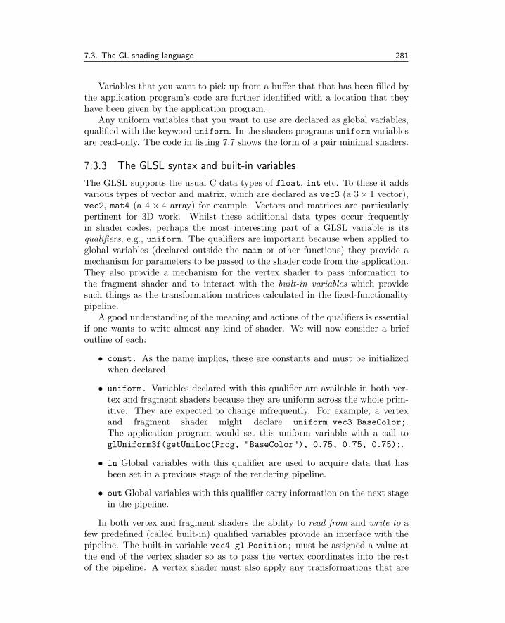
7.3. The GL shading language 281
Variables that you want to pick up from a buffer that that has been filled bythe application program’s code are further identified with a location that theyhave been given by the application program.
Any uniform variables that you want to use are declared as global variables,qualified with the keyword uniform. In the shaders programs uniform variablesare read-only. The code in listing 7.7 shows the form of a pair minimal shaders.
7.3.3 The GLSL syntax and built-in variables
The GLSL supports the usual C data types of float, int etc. To these it addsvarious types of vector and matrix, which are declared as vec3 (a 3× 1 vector),vec2, mat4 (a 4 × 4 array) for example. Vectors and matrices are particularlypertinent for 3D work. Whilst these additional data types occur frequentlyin shader codes, perhaps the most interesting part of a GLSL variable is itsqualifiers, e.g., uniform. The qualifiers are important because when applied toglobal variables (declared outside the main or other functions) they provide amechanism for parameters to be passed to the shader code from the application.They also provide a mechanism for the vertex shader to pass information tothe fragment shader and to interact with the built-in variables which providesuch things as the transformation matrices calculated in the fixed-functionalitypipeline.
A good understanding of the meaning and actions of the qualifiers is essentialif one wants to write almost any kind of shader. We will now consider a briefoutline of each:
• const. As the name implies, these are constants and must be initializedwhen declared,
• uniform. Variables declared with this qualifier are available in both ver-tex and fragment shaders because they are uniform across the whole prim-itive. They are expected to change infrequently. For example, a vertexand fragment shader might declare uniform vec3 BaseColor;.The application program would set this uniform variable with a call toglUniform3f(getUniLoc(Prog, "BaseColor"), 0.75, 0.75, 0.75);.
• in Global variables with this qualifier are used to acquire data that hasbeen set in a previous stage of the rendering pipeline.
• out Global variables with this qualifier carry information on the next stagein the pipeline.
In both vertex and fragment shaders the ability to read from and write to afew predefined (called built-in) qualified variables provide an interface with thepipeline. The built-in variable vec4 gl Position; must be assigned a value atthe end of the vertex shader so as to pass the vertex coordinates into the restof the pipeline. A vertex shader must also apply any transformations that are

282 7. Real-time 3D: OpenGL
#version 330 core
layout(location = 0) in vec3 vertexPosition;
uniform mat4 MVP;
void main(){gl_Position = MVP * vec4(vertexPosition,1);}
#version 330 core
layout(location = 0) out vec4 color;
uniform vec4 Colour;
void main(){color = Colour;
}
Listing 7.7: Minimal shader programs.
in operation. In compatibility mode this can be done with a built-in functioncalled ftransform(); but to conform to the core approach. The best approachis to do-it-yourself by passing in a 4 × 4 matrix through a uniform variablecontaining the appropriate transformation.
In the early versions of the GLSL, named built-in variables played a moresignificant role, but many of these have now been withdrawn.
Thus a minimal pair of shaders can consist of just a couple of lines of code;see listing 7.7.
7.3.4 Template shader codes
The book’s website contains a number of template and example shader codes thatexecute in both compatibility and core modes. These demonstrate in principlehow to set up Phong’s illumination model; some more advanced shader codesare discussed in chapter 11 and in relation to the OpenFX program of chapter 9.
Image mapping In the GLSL, information from texture maps is acquired withthe use of a sampler. We will keep it simple in our example, and show theminimal code required so a shader program pair can paint image texture mapson fragments. The code for these shader programs is given in listing 7.8.
Reflection mapping Many objects exhibit reflection of their environment. List-ing 7.9 shows the outline of a suitable fragment shader. For reflection maps, wedo not want to use any surface lighting models, and so this is omitted.

7.3. The GL shading language 283
// Vertex Shader - for traditional image mapping#version 330 corelayout(location = 0) in vec3 Vertex;layout(location = 1) in vec3 Normal;layout(location = 2) in vec2 Texture;
uniform mat4 MVP;uniform mat4 MV;uniform mat4 NM;uniform vec3 LightPos;
out float Diffuse; // diffuse light intensityout vec2 TexCoord; // texture coordinate (u,v)
void main(){gl_Position = MVP * vec4(Vertex,1); // buit in variablevec3 PP = MV * vec4(Vertex,1); // vertex position world coodinatesvec3 PN = normalize(NM * Normal);// normal vector// light direction vectorvec3 LV = normalize(LightPos-PV);Diffuse = max(dot(LV, PN), 0.0); // diffuse illumination// Get the texture coordinates - choose the first -// we only assign one set anywayTexCoord = Texture; // pass to fragment shader
}
// Fragment Shader - simple 2D texture/image map, diffuse lighting
#version 330 core
layout(location = 0) out vec4 Color;
in float Diffuse; // from vertex shaderin vec2 TexCoord; // from vertex shader
uniform sampler2D Rsf; // from calling program
void main (void){// Get the fragment color by addressing the texture map pixel// date - the "texture2D" built in function takes the texure//sampler "Rsf" // and fragment interpolated texture// coorinates as arguments and the ".RGB" (what SL calls// a "swizzle") extracts the RGB values from the// texture2D() return value.vec3 color = (texture2D(Rsf, TexCoord).rgb * Diffuse);// promote the 3 element RGB vector to a 3 vector and outputColor = vec4 (color, 1.0);
}
Listing 7.8: The image mapping shader program pair.

284 7. Real-time 3D: OpenGL
// Fragment Shader - reflection mapping#version 330 core// pass on the Color into the next pipeline stagelayout(location = 0) out vec4 Color;
const vec3 Xunitvec = vec3 (1.0, 0.0, 0.0);const vec3 Yunitvec = vec3 (0.0, 1.0, 0.0);
// this is our sampler to identify the iamge mapuniform sampler2D RsfEnv;
varying vec3 Normal; // from vertex shadervarying vec3 EyeDir; // from vertex shader
void main(){// Compute reflection vector - built-in function :-)vec3 reflectDir = reflect(EyeDir, Normal);// Compute the addess to use in the image map - we need an// address in the range [0 - 1 ] (angles of looking up /down)vec2 index;index.y = dot(normalize(reflectDir), Yunitvec);reflectDir.y = 0.0;index.x = dot(normalize(reflectDir), Xunitvec) * 0.5;// get the correct range [0 - 1]if (reflectDir.z >= 0.0) index = (index + 1.0) * 0.5;else{index.t = (index.t + 1.0) * 0.5;index.s = (-index.s) * 0.5 + 1.0;}// copy the addressed texture pixel to the outputColour = texture2D(RsfEnv, index);}
Listing 7.9: The reflection map fragment shader.
Bump mapping Our portfolio of shader programs would not be complete withoutthe ability to use an image texture as a source of displacement to the surfacenormal, i.e., bump mapping. Bump mapping requires us to use a sampler2D andprovide a tangent surface vector. Vertex and fragment shaders for bump mappingare given in listing 7.10 and listing 7.11. A few of comments are pertinent to thebump mapping procedure:
• To minimize the work of the fragment shader, the vertex shader calculatesvectors for light direction and viewpoint (eye location) direction in a coor-dinate frame of reference that is in the plane of the polygon which will berendered by the fragment shader (this is called surface-local space).
Figure 7.4 illustrates the principle; in the world (global) coordinate frameof reference, the eye is at the origin. The polygon’s normal (n), tangent (t)and bi-normal (b) are calculated in the global frame of reference. Transfor-mation of all vectors to a surface-local reference frame allows the fragmentshader to perform position-independent lighting calculations because thesurface normal is always given by the vector (0, 0, 1).

7.3. The GL shading language 285
// Vertex Shader - Bump mapping#version 330 core// input vertex attributeslayout(location = 0) in vec3 Position;layout(location = 1) in vec3 Normal;layout(location = 3) in vec3 Tangent;layout(location = 4) in vec2 Texture;layout(location = 5) in vec3 Color;
uniform mat4 MVP; // full transformuniform mat4 MV; // model and viewuniform mat4 NM; // normal transformuniform vec3 LightPos;
// These two vectors pass the direction from vertex to light// and viewpoint (IN A COORD REFERENCE FRAME of the polygon!!!)out vec3 LightDir;out vec3 EyeDir;// this passes surface texture coords to fragment shaderout vec2 TexCoord;// pass on surface colorout vec3 Vcolor;
void main(){gl_Position = MVP * vec4(Position,1); // must pass on// get a coordinate system based in plane of input surfacevec3 n = normalize(NM * Normal);vec3 t = normalize(NM * Tangent);EyeDir = vec3 (MV * vec4(Position,1));// pass on texture coords to fragment shaderTexCoord = Texture;// Get normal, tangent and third vector to make curviliner coord frame// of reference that lies in the plane of the polygon for which we are// processing one of its vertices.vec3 n = normalize(gl_NormalMatrix * gl_Normal);vec3 t = normalize(gl_NormalMatrix * Tangent);vec3 b = cross(n, t);// get the light direction and viewpoint (eye) direction in this new// coordinate frame of reference.vec3 v;vec3 LightPosition=vec3(gl_LightSource[0].position);v.x = dot(LightPosition, t);v.y = dot(LightPosition, b);v.z = dot(LightPosition, n);LightDir = normalize(v);v.x = dot(EyeDir, t);v.y = dot(EyeDir, b);v.z = dot(EyeDir, n);EyeDir = normalize(v);
Listing 7.10: Bump mapping vertex shader program.
By doing this, we ensure that the surface normal vector is always givenby coordinates (0, 0, 1), and thus it is easily displaced (or bumped) in thefragment shader by adding to it the small changes ∆u and ∆v obtainedfrom the bump map.

286 7. Real-time 3D: OpenGL
// Fragment Shader - Bump mapping#version 330 core
layout(location = 0) out vec4 color;
in vec3 LightDir; // input from vertex shaderin vec3 EyeDir;in vec2 TexCoord;// pass on surface colorin vec3 Vcolor;
uniform sampler2D Rsf;
// fraction of light due to specular hightlightsconst float SpecularFactor = 0.5;// range [4.0 - 0.1] bump gradient [large - small]const float Gradient = 4.0;
void main (void){vec3 SurfaceColor = Vcolor; // get the color// get the surface normal perturbation vector// - it is encoded in the texture imagevec2 grad = (texture2D(Rsf, TexCoord).rg);// calculate the new surface normal - perterb in (x,y) planevec3 normDelta=normalize(vec3((grad.x-0.5)*Gradient,(grad.y-0.5)*Gradient,1.0));
// now apply the lighting modelvec3 litColor = SurfaceColor* max(dot(normDelta, LightDir), 0.0);vec3 reflectDir = reflect(LightDir, normDelta);float spec = max(dot(EyeDir, reflectDir), 0.0);spec *= SpecularFactor;litColor = min(litColor + spec, vec3(1.0));color = vec4(litColor, 1.0);}
Listing 7.11: Bump mapping fragment shader program.
To obtain the surface-local coordinates, we first set up a rectilinear co-ordinate system with three basis vectors. We have two of them already:the surface normal n = (nx, ny, nz) and the tangent vector t = (tx, ty, tz)(passed to the vertex shader as a vector attribute from the applicationprogram). The third vector b = (bx, by, bz) (known as the bi-normal) isdefined as b = n × t. Vectors dw (such as viewpoint and light direc-tions) are transformed from world coordinates to the surface-local frameby ds = [Tws]dw where [Tws] is the 3× 3 transformation matrix:
[Tws] =
tx ty tzbx by bznx ny nz
(More details of this transformation can be found in section 2.12.6.)
• The normal displacement is usually encoded as an image map. This isdone by preprocessing the image pixel map after it is read/decoded and

7.3. The GL shading language 287
Surface-local coordinates
v1
v1
n
b
t
v3
LightEye
point
y
z
x
v2
v2
n
z´
y´
Viewpoint
Light
Global coordinates
v3 t
Figure 7.4: Surface local coordinates.
before it is copied into texture memory. It is first converted to a gray-scaleand then the gradient is encoded by storing the ∂nu
∂uas the red pixel com-
ponent and the v gradient (∂nv
∂v) as the green component. The gradient
map is copied to texture memory and thus the surface normal displace-ment vector is easily extracted from the texture by ∆n = (∆n1,∆n2, 0) =(Mr(u, v),Mg(u, v), 0) (where Mr(u, v) is the red component of map Mat texture coordinate (u, v)). Because we are working with a normal nowrelative to the surface-local coordinates n = (0, 0, 1) the coordinates of thedisplaced normal (n = n+∆n) vector are (∆n1,∆n2, 1).
• An alternative method of generating the displacement vector allows it tobe calculated within the fragment shader program. This eliminates thepreprocessing step, at the expense of a little extra GPU processing in thefragment shader. By sampling the texture map at four points that havea small texture coordinate offset, the image’s intensity gradient can beobtained. The following shader code fragment illustrates the idea:

288 7. Real-time 3D: OpenGL
const float d=0.01;// Assumes gray color, get valuefloat y1 = (texture2D(Rsf, TexCoord+vec2( 0.0, d)).r);// above and below sample point.float y2 = (texture2D(Rsf, TexCoord+vec2( 0.0,-d)).r);// and to leftfloat x1 = (texture2D(Rsf, TexCoord+vec2( d, 0.0)).r);// and rightfloat x2 = (texture2D(Rsf, TexCoord+vec2(-d, 0.0)).r);vec3 normDelta=normalize(vec3((y2-y1)*Gradient,
(x1-x2)*Gradient,1.0));
Procedural textures It is in the area of procedural textures that the real power ofthe programmable GPU becomes evident. More or less any texture that can bedescribed algorithmically can be programmed into the GPU and rendered muchfaster than with any software renderer. Chapter 11 provides a rich collection ofalgorithms for procedural textures that are quite amenable to implementationas GPU textures.
7.3.5 Setting up the transformation matrices
With the removal of the internally handled matrix transformations through theGL MODELVIEW and GL PROJECTIONmatrices it is important to be able to replicatetheir behavior in an application’s code. The elements of projection matricesarising from calls to either glOrtho(...) and glFrustum(..) are defined in theRed Book but the utility functions that previously helped us set up a projectionbased on a field of view and a viewpoint that looks at a specific target are notquite so readily available. To achieve the same result of these functions requiresthe functions given in listing 7.12.
The only point worthy of note about listing 7.12 is in the LookAt(..) func-tion where the LookAt transformation is made up of a translation, which positionsthe eye point at (0, 0, 0) and a rotation that aligns the frame of reference of thecamera (defined by the direction between eye and target and an up direction).The rotation matrix is basically the same as that derived in section 2.12.6, how-ever OpenGL defines the y axis to be vertical, so, if we express the up directionas the vector (0, 1, 0) (i.e., along the y axis) we must reverse the order of rows 2and 3 and change the sign of the elements in row 3 (as is done in listing 7.12).
Finally for this section, two very important reminders:
1. The OpenGL world is mapped with a right-handed coordinate system, they axis is vertical, and we observe from (0, 0, 0) looking down the −z axis.
2. Transpose any C/C++ transformation matrices before passing them intothe pipeline.

7.3. The GL shading language 289
#define DEGRAD .. // converts devress to radians#define CROSS(v1,v2,r) .. // vector cross product r=v1*v2#define LENGTH2(a) ... // length of vector// copy matrix toiut=tinstatic void c4to4(GLfloat tin[4][4], GLfloat tout[4][4];//multiply matrix tr=t1*t2static void m4by4(GLfloat t1[4][4],GLfloat t2[4][4],GLfloat tr[4][4]);// set to Identity matrix t = Istatic void null_transform(float t[4][4]);
void gl_Ortho(GLfloat m[4][4], GLfloat l, GLfloat r,GLfloat b, GLfloat t, GLfloat n, GLfloat f ){// l=left r=right b=bottom, t=top, n=near f=farnull_transform(m);m[0][0]= 2.0f/(r-l); m[0][3]= -(r+l)/(r-l);m[1][1]= 2.0f/(t-b); m[1][3]= -(t+b)/(t-b);m[2][2]= -2.0f/(f-n); m[2][3]= -(f+n)/(f-n);
}
void gl_Frustum(GLfloat m[4][4], GLfloat l, GLfloat r,GLfloat b, GLfloat t, GLfloat n, GLfloat f ){// l=left r=right b=bottom, t=top, n=near f=far (clip planes)null_transform(m);m[0][0]= 2.0f*n/(r-l); m[0][2]= (r+l)/(r-l);m[1][1]= 2.0f*n/(t-b); m[1][2]= (t+b)/(t-b);m[2][2]= -(f+n)/(f-n); m[2][3]= -2.0f*f*n/(f-n);m[3][2] = -1; m[3][3]= 0;
}
void glu_Perspective(GLfloat m[4][4], GLfloat fovy,GLfloat a, GLfloat n, GLfloat f ){// fovy = horizontal field of view a = aspect ratio width/height// n = near f = far (clipping planes)GLfloat t,b,l,r;t = n*(GLfloat)tan(DEGRAD*fovy/2.0);b = -t; l = -a*t; r = a*t;gl_Frustum(m,l,r,b,t,n,f);
}
void glu_LookAt(GLfloat m[4][4],GLfloat ex,GLfloat ey,GLfloat ez, // eyeGLfloat cx,GLfloat cy,GLfloat cz, // targetGLfloat ux,GLfloat uy,GLfloat uz){// upGLfloat f[3],s[3],u[3],l,m1[4][4],m2[4][4];null_transform(m); null_transform(m2);f[0]=cx-ex; f[1]=cy-ey; f[2]=cz-ez;u[0]=ux; u[1]=uy; u[2]=uz;l=1.0/LENGTH(f); VECSCALE(l,f,f)CROSS (f,u,s)l=1.0/LENGTH(s); VECSCALE(l,s,s)CROSS (s,f,u)translate(m1,-ex,-ey,-ez); null_transform(m2);m2[0][0]= s[0]; m2[0][1]= s[1]; m2[0][2]= s[2];// re-order because Y Z axes are reversed (Y is UP! )m2[1][0]= u[0]; m2[1][1]= u[1]; m2[1][2]= u[2];m2[2][0]= -f[0]; m2[2][1]= -f[1]; m2[2][2]= -f[2];m4by4(m2,m1,m);
}
Listing 7.12: Creating transformation matrices that match the functionality of the oldGLU utility functions.

290 7. Real-time 3D: OpenGL
7.4 The P-buffer and framebuffer objects
It was mentioned earlier that in addition to the front and back output buffersOpenGL may offer a few additional buffers, AUX0, AUX1 etc. However, manydisplay adapters do not support these buffers. Even if the AUXn buffers aresupported they have a major limitation in that they cannot exceed the currentsize of the output window. More specifically, they cannot exceed the size ofthe underlying drawing surface. An output window is just a system dependentview of the drawing surface OpenGL renders onto a drawing surface attachedto a window. This is a problem if you want to render a scene at a resolutionthat is greater than the desktop size. It is also a major problem if you wantto render to a texture (an image map) to be used later (for example, an imagemay be required at a resolution of twice the maximum window size, and includean automatically generated mip-map, taking its resolution even higher). Beingable to render to very large off-screen buffers of any size has advantages. Themodern way to render into large output buffers that can also be used as texturesfor subsequent mapping is through the use of framebuffer objects (FBOs). Theolder way was through the use of Pixel (or P) buffers. Both of these techniquesare used in the OpenFX renderer (see chapter 9), and a document describinghow to use framebuffer objects is available on the website.
7.5 Rendering a particle system using OpenGL
To round off this chapter on OpenGL programming we return briefly to considerthe practical implementation of a real-time particle system. Section 6.7 lookedinto the very powerful contribution that particle models can play in enrichingCGI movies and computer games. Because of the simplicity of the concept,particle models are ideal for use in real-time applications and OpenGL providesall the capabilities needed for rendering a particle system, i.e. alpha blendedtexture mapping, integrated transformations and a wide range of framebuffercombiner operations.
In this short section a couple of listings provide a framework that can act asa progenitor for a comprehensive particle system. Indeed, the OpenFX particleactor, as described in section 9.7.5, is little more than a scaled up version ofthe ideas given in listings 7.13 and 7.14. Listing 7.13 draws attention to theimportance of a couple of data structures, one for the particle system itself,where its image texture, its number of particles and an array of particles aredefined. The second structure represents each particle and is needed so that theparticle can evolve from its generation by the particle system. The two functionsin listing 7.13 perform the tasks of (1) setting up the particle texture and particlesystem parameters, and (2) updating the position and attributes of each particleas time elapses. The most significant steps in rendering the particle system arepresented in listing 7.14. Each particle is a small texture mapped GL QUAD

7.5. Rendering a particle system using OpenGL 291
// Structures for a particle system
typedef struct ParticleTag {GLfloat p[3]; // positionfloat c[3]; // colourAlpha; //transparency.... // other properties
} Particle;
typedef struct ParticleSystemTag {int type; // image blending typeint np; // number of particlesParticle *P;// list of particlesint iid; // texture map image
} ParticleSystem;
// global texture IDsGLint g_particle_textures[NTEXTURES];
void MakeParticleTextures(void){ // Setup particle textures..// ask for the number of particle image textures neededglGenTextures( nParticleImages, &g_particle_textures[0]);..// load image and copy to GPU txture memory...
}
void UpdateParticle(double time, ParticleSystem *Ps){..// Timed function to take each particle through its// evolution. Details will depend on the nature of// the particle system.for(i=0;i<Ps->np;i++){ // process each particle..}..
}
Listing 7.13: Data structures for a particle system.
that is rendered by modulating how it is blended into the output buffer withthe texture map. How the QUAD is blended is the secret of producing theappearance of hot fire or the spray form breaking waves on the sea shore. Thegeometry transformations must place the particles in the correct location withrespect to the viewpoint and any objects associated with the particle system.However, the transformations must ensure that no rotation is applied to thetextured QUAD and that it is always perpendicular to the viewing direction.
When these simple guidelines are followed, the full beauty of many naturalphenomenon can be brought to the computer screen in real-time, like those infigure 6.38 for example.
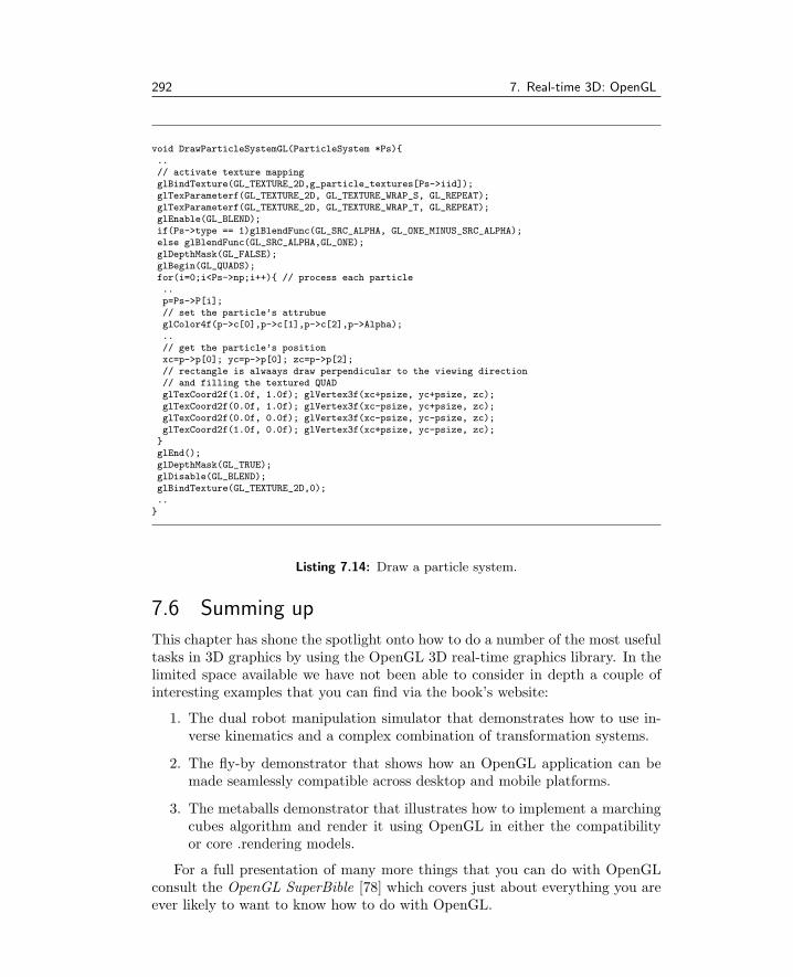
292 7. Real-time 3D: OpenGL
void DrawParticleSystemGL(ParticleSystem *Ps){..// activate texture mappingglBindTexture(GL_TEXTURE_2D,g_particle_textures[Ps->iid]);glTexParameterf(GL_TEXTURE_2D, GL_TEXTURE_WRAP_S, GL_REPEAT);glTexParameterf(GL_TEXTURE_2D, GL_TEXTURE_WRAP_T, GL_REPEAT);glEnable(GL_BLEND);if(Ps->type == 1)glBlendFunc(GL_SRC_ALPHA, GL_ONE_MINUS_SRC_ALPHA);else glBlendFunc(GL_SRC_ALPHA,GL_ONE);glDepthMask(GL_FALSE);glBegin(GL_QUADS);for(i=0;i<Ps->np;i++){ // process each particle..p=Ps->P[i];// set the particle’s attrubueglColor4f(p->c[0],p->c[1],p->c[2],p->Alpha);..// get the particle’s positionxc=p->p[0]; yc=p->p[0]; zc=p->p[2];// rectangle is alwaays draw perpendicular to the viewing direction// and filling the textured QUADglTexCoord2f(1.0f, 1.0f); glVertex3f(xc+psize, yc+psize, zc);glTexCoord2f(0.0f, 1.0f); glVertex3f(xc-psize, yc+psize, zc);glTexCoord2f(0.0f, 0.0f); glVertex3f(xc-psize, yc-psize, zc);glTexCoord2f(1.0f, 0.0f); glVertex3f(xc+psize, yc-psize, zc);
}glEnd();glDepthMask(GL_TRUE);glDisable(GL_BLEND);glBindTexture(GL_TEXTURE_2D,0);..}
Listing 7.14: Draw a particle system.
7.6 Summing up
This chapter has shone the spotlight onto how to do a number of the most usefultasks in 3D graphics by using the OpenGL 3D real-time graphics library. In thelimited space available we have not been able to consider in depth a couple ofinteresting examples that you can find via the book’s website:
1. The dual robot manipulation simulator that demonstrates how to use in-verse kinematics and a complex combination of transformation systems.
2. The fly-by demonstrator that shows how an OpenGL application can bemade seamlessly compatible across desktop and mobile platforms.
3. The metaballs demonstrator that illustrates how to implement a marchingcubes algorithm and render it using OpenGL in either the compatibilityor core .rendering models.
For a full presentation of many more things that you can do with OpenGLconsult the OpenGL SuperBible [78] which covers just about everything you areever likely to want to know how to do with OpenGL.

8Mobile 3D: OpenGLES
This chapter investigates how to extend the power and simplicity of OpenGLin the world of mobile devices, smart phones and tablets. Apps, as they arepopularly known, can be endowed with the same high-powered 3D graphics thatwe have become used to on the desktop and laptop platforms. The distinctionbetween traditional laptop/notebook computers and mobile devices like the Ap-ple iPad or the Google Nexus phone is getting more and more blurred. Is therea significant difference between a notebook using an Intel i7 processor with de-tachable keyboard and touch screen, say running Windows 8, and an iPad withan ARM processor and bluetooth keyboard? Both of these devices have a similarlook and feel, both run the same range of programs, e-mail clients, browsers, pre-sentation software etc. Many Apps depend on high-speed 3D graphics, and notjust the computer game Apps. The powerful geometric transformations of 3Dgraphics can endow applications and even operating systems with lively effectslike spins, page turns, image flips etc.
From the program developer’s perspective there is a very significant differencebetween building apps for the desktop platform and apps for a mobile device. Itis not possible to develop programs for a tablet or phone on the tablet or phonethemselves. It is perfectly possible to develop programs for any Windows 8computer on a Windows 8 computer, but it is not possible to develop programsfor a Windows Phone 8 on a Windows Phone! The same applies to Apple’sdevices and to the Android devices, so this is quite a useful way to classifya platform as either desktop or mobile. Since OpenGL is designated a cross-platform graphics library, the way we will choose to designate a host as a mobile isto say: those platforms that offer the full OpenGL specification are desktops andnotebooks, and those that use OpenGLES as tablet/phones/hand-held devices.
OpenGLES [63] (or OpenGL for Embedded Systems) has a much shorterpedigree than OpenGL. A powerful graphics library capable of rendering in 3Drequires a significant hardware resource; unless a program requires the full powerof a high-end device all mobile devices already do an excellent job. With theexception of a few restrictions, once an application has carried out the specificplatform dependent initialization then the same OpenGL drawing function callscan be used in OpenGLES.
293

294 8. Mobile 3D: OpenGLES
OpenGLES is the 3D drawing system used by Apple’s iOS devices and byGoogle’s Android systems. It was also used by Nokia in the Symbian smart-phones. Unfortunately Microsoft’s current Windows phone uses their Direct3Dgraphics and will not be discussed further here. In this chapter we will brieflyreview the few differences between OpenGL and OpenGLES and then look at acouple of examples that can be used to form templates for some iOS and Androidapps making use of 3D graphics.
8.1 OpenGLES
In the short history of OpenGLES (GLES) the specification has undergone quitea rapid development. This is mainly because the graphics hardware available forembedded systems is catching up fast on the hardware that has been available onthe desktop PCs for some time. Perhaps the most significant change in GLES hasoccurred during the introduction of version 2 when the GLES rendering pipelinebecame programmable.
As the OpenGLES and OpenGL APIs converge, the fixed functionality func-tions in the API are being deprecated. However, the GLES never offered thedisplay list, or the glVertex(..) family of functions, and so it should not re-quire such a radical change in the coding of applications to update them to usethe version 2/3 API as would be required for a very mature desktop program.
The GLES-2 (and subsequent versions, version 3 being the most recent attime of writing) pipeline does not support any fixed functionality, and all appli-cation programs must create a minimal set of shaders. Even GLES 1 uses themodern method of specifying geometry, with polygon lists and/or vertex buffersproviding a better way of defining geometry. These types of structures were dis-cussed in chapter 3 and therefore OpenGLES (and indeed the latest version ofOpenGL) match very well the data structures used in the algorithms describedin part III.
The source codes and projects that accompany this chapter provide examplesof how to use these modern data structures.
An OpenGLES application has to create and initialize a drawing surface andobtain a handle to a rendering context in much the same way that an applicationwould do for the full OpenFX. We will elaborate on the setup phase because, oncea GLES surface has been defined and a drawing/device context obtained for it,the actual process of rendering is platform independent and we can pretty muchuse the same code that we use on the desktop. For example, the usage of texturemapping lighting and shader codes will be identical. Indeed, if you have builtyour desktop programs using the VertexPointer() and glDrawElements() orglDrawArrays(..) functions then OpenGL programs should port seamlessly toGLES.
Listings 8.1, 8.2 and 8.3 highlight the key steps in rendering with theDrawElements() function, that is, the geometry, topology and surface attributes

8.1. OpenGLES 295
// The vertices give the model// its shpaeint num_model_vertices=0;GLfloat *model_vertices=NULL;
// The surface normals are// needed by the lighting modelGLfloat *model_normals=NULL;
// The indices list the vertices associated// the the faces the give the model its// surface.int num_model_indicies=0;short *model_indicies=NULL;
// The simplest surface attibute is its// color which is specified for each// vertexGLubyte *model_colours=NULL;
Listing 8.1: A minimal set of data is needed to describe a 3D model. These variableare used to reference it.
FILE *fp;..// how much datafread(&num_model_vertices,sizeof(),1,fp);fread(&num_model_indicies,sizeof(),1,fp);// provide memory buffers of suffficent size// to hold the data for vertices and triangular facesif((model_vertices=(GLfloat *)malloc( // 3 coords per vertex
num_model_vertices * 3 * sizeof(GLfloat))) == NULL){ ... /* error */ }if((model_normals=(GLfloat *)malloc( // one vector per vertex
num_model_vertices * 3 * sizeof(GLfloat))) == NULL){ ... /* error */ }if((model_colours=(GLubyte *)malloc( // RGBA color
num_model_vertices * 4 * sizeof(GLubyte))) == NULL){ ... /* error */ }if((model_indicies=(short *)malloc( // Triangles have 3 vertex IDs each
num_model_indicies * 3 * sizeof(short))) == NULL){ ... /* error */ }// obtain the main datafread(model_vertices,sizeof(GLfloat),num_model_vertices * 3,fp);...
Listing 8.2: Before any 3D data can be drawn it must be assembled in a form thatmay be passed to the rendering functions. The source of the data might be anything.In this piece of code it is simply assumed to be obtained from a file previously openedfor reading.
must be specified in memory buffers in the correct order. In some ways, loadingdata into graphics memory with the VertexPointer() and glNormalPointer()
functions is similar to setting up a display list. Using DrawElements() ful-fills many of the actions that might otherwise be done by calling an old styledisplay list.
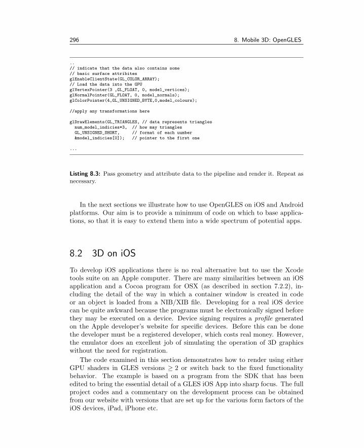
296 8. Mobile 3D: OpenGLES
..// indicate that the data also contains some// basic surface attribitesglEnableClientState(GL_COLOR_ARRAY);// Load the data into the GPUglVertexPointer(3 ,GL_FLOAT, 0, model_vertices);glNormalPointer(GL_FLOAT, 0, model_normals);glColorPointer(4,GL_UNSIGNED_BYTE,0,model_colours);
//apply any transformations here
glDrawElements(GL_TRIANGLES, // data represents trianglesnum_model_indicies*3, // how may trianglesGL_UNSIGNED_SHORT, // format of each uumber&model_indicies[0]); // pointer to the first one
...
Listing 8.3: Pass geometry and attribute data to the pipeline and render it. Repeat asnecessary.
In the next sections we illustrate how to use OpenGLES on iOS and Androidplatforms. Our aim is to provide a minimum of code on which to base applica-tions, so that it is easy to extend them into a wide spectrum of potential apps.
8.2 3D on iOS
To develop iOS applications there is no real alternative but to use the Xcodetools suite on an Apple computer. There are many similarities between an iOSapplication and a Cocoa program for OSX (as described in section 7.2.2), in-cluding the detail of the way in which a container window is created in codeor an object is loaded from a NIB/XIB file. Developing for a real iOS devicecan be quite awkward because the programs must be electronically signed beforethey may be executed on a device. Device signing requires a profile generatedon the Apple developer’s website for specific devices. Before this can be donethe developer must be a registered developer, which costs real money. However,the emulator does an excellent job of simulating the operation of 3D graphicswithout the need for registration.
The code examined in this section demonstrates how to render using eitherGPU shaders in GLES versions ≥ 2 or switch back to the fixed functionalitybehavior. The example is based on a program from the SDK that has beenedited to bring the essential detail of a GLES iOS App into sharp focus. The fullproject codes and a commentary on the development process can be obtainedfrom our website with versions that are set up for the various form factors of theiOS devices, iPad, iPhone etc.

8.2. 3D on iOS 297
One of the nice things about a program that uses OpenGL is that once adrawing surface has been established the need to interact with the host systemcan be kept to a minimum.
Any iOS App that is going to use GLES may be built by extending on codeassociated with the following basic steps:
1. Create the code for a class, derived from the UIView API class (e.g., calledEAGLView), to represent the View.
2. Add an object of this class to the XIB file using interface builder (Xcode).
3. Provide code in the AppDelegate class for the delegated functions.
4. Provide code for the class that will represent the OpenGL view. Since anobject of this class has been defined in the XIB file, an instance of it willbe created and its method called automatically:(id)initWithCoder:(NSCoder*)coder.It is within initWithCoder that the properties of the OpenGL displayshould be established. Also, since the EAGLView class is derived from theUIView class the delegated method (void)drawView:(id)sender willbe called automatically when the display needs to be refreshed. It is indrawView that we can place all our OpenGL drawing code.
Once these iOS specific tasks have been completed the addition of two (non-iOSspecific) functions that
1. do anything that can be done as a one-off set up and
2. draw whatever is needed (this function is called in response to a regulartimer)
will give a complete template for any App that wants to present itself on a 3Dcanvas. Listings 8.4 to 8.14 fill in a little more of the detail.
The AppDelegateClass of listings 8.4 and 8.5 provides overridden meth-ods that are called when the application object is created and when it is de-stroyed. This gives us the opportunity to control the behavior of the Viewobject which is defined in the XIB and linked to the glView member variable ofthe AppDelegateClass.
Our View object is an instance of the EAGLView class, which is derived fromthe standard iOS class UIView. To endow the EAGLView class with an OpenGLrendering surface a standard documented process has to be followed. In thisexample we are going to enhance the basic properties by offering the potentialto use either the OpenGLES version 1 or version 2 approach. (Remember thatthe GLES version 2 does not have a fixed functionality pipeline and all programsmust render through a pair of GPU shader codes.)
The derived View class is specified in listing 8.6 with its most relevantmembers and methods highlighted in listing 8.7. Since the View object is

298 8. Mobile 3D: OpenGLES
#import <UIKit/UIKit.h>
// forward class reference to main application class@class EAGLView;
@interface glesIosAppDelegate : NSObject <UIApplicationDelegate> {UIWindow *window;EAGLView *glView; // will point to the OpenGL View object}
// connect to object in XIB file@property (nonatomic, retain) IBOutlet UIWindow *window;@property (nonatomic, retain) IBOutlet EAGLView *glView;
@end
Listing 8.4: The application delegate header file defines sub-class with its applicationspecific members.
defined in the XIB (resource) file the standard approach of iOS is to call itsinitWithCoder: method during creation. It is in this method that all the hardwork of configuring the View is done.
Before looking at the configuration of the rendering surface for either GLESv1(version 1, fixed functionality) or GLESv2 (version 2 GPU shader) we shallconsider the methods in the EGALView class that start and stop the timed displayupdate. In listing 8.8 the startAnimation: method starts a timer that callsthe drawView: method, when the timer fires. The timer function then instructsthe appropriate renderer (for GLESv1 or GLESv2) to draw the scene.
Returning to consider the drawing code, the objects that perform either fixedfunction or programmable rendering are of classes that have similar form; theversion 2 class is presented in listing 8.9. The difference between a class repre-senting a version 1 (fixed function) drawing surface and one to be used withthe programmable version 2 pipeline lies not in their members but in whatcommands the initialization and rendering method have to issue. Under iOS,rendering is done into a framebuffer object (FBO) with attached renderbuffer.FBOs and renderbuffers were discussed in section 7.4 for desktop platforms andtheir use in the mobile context is no different, except that the actual presen-tation of the rendered output is done by calling the display context’s methodpresentRenderBuffer; as in:
// GLES version 1[context presentRenderbuffer:GL_RENDERBUFFER_OES];// GLES version 2[context presentRenderbuffer:GL_RENDERBUFFER];
In listing 8.10 the preparation of a drawing surface to receive output renderedthrough the programmable pipeline is shown. It includes a call to a method to

8.2. 3D on iOS 299
#import "glesIosAppDelegate.h" // class definition#import "EAGLView.h" // main class definition
@implementation glesIosAppDelegate // over-ridden methods
@synthesize window; // link pointer to object in XIB@synthesize glView; // link pointer to object in XIB
// This method is called by system when object is created- (BOOL)application:(UIApplication *)application
didFinishLaunchingWithOptions:(NSDictionary *)launchOptions {// Apply any launch specific code here.[window makeKeyAndVisible];// Start the timer associated with the view, to refresh// the display[glView startAnimation];return YES;
}// The class also delegates method that are called by the system// when other events occur, such as activation of another app.// They are omitted here for brevity.
// IOS programs call this method on exit to allow for clean-up.// We release the resources in the usual way.- (void)dealloc {[window release];[glView release];[super dealloc];
}
@end // end of the class
Listing 8.5: The application delegate source.
load, compile and install the shader programs. (The code for a loadShaders;
method would be similar to those used on a desktop with the exception that thesource will either be explicitly given in a text string in the code or a file withinthe application bundle.)
If the drawing window’s dimensions change then the View’s dimensions haveto be change. On mobile devices with their small screens a change of window sizeis much less likely to occur than in a desktop program; however, the possibilitymust still be serviced, not least because a change of size always happens when awindow is first created. As one would expect there are slight variations betweenresizing a FBO for fixed-function and for GPU-programmable rendering. Sincethe output surface is represented as a FBO, it and its attached renderbuffers haveto be resized accordingly. Fortunately, the same code can be used for every app,so the brief template, taken from the iOS API reference examples and shown inlisting 8.11, is sufficient to handle all re-sizing eventualities.
It is always good programming practice to perform a smooth shutdown andrelease of resources; listing 8.12 shows the way.
And now, after all the preamble we come to the actual drawing. Everythingthat you draw using OpenGLES—geometry, transformations, texture maps—can

300 8. Mobile 3D: OpenGLES
#import <UIKit/UIKit.h>#import <QuartzCore/QuartzCore.h>#import <OpenGLES/EAGL.h>#import <OpenGLES/EAGLDrawable.h>
// methods that are implemented by the rendering class@protocol ESRenderer <NSObject>- (void)render;- (BOOL)resizeFromLayer:(CAEAGLLayer *)layer;@end
// This class wraps the CoreAnimation CAEAGLLayer@interface EAGLView : UIView{@privateid <ESRenderer> renderer; // will point at renderer objectBOOL displayLinkSupported;NSInteger animationFrameInterval;id displayLink;NSTimer *animationTimer;// add any other members would go here}
@property (readonly,nonatomic,getter=isAnimating) BOOL animating;@property (nonatomic) NSInteger animationFrameInterval;
// overridden methods- (void)startAnimation;- (void)stopAnimation;- (void)drawView:(id)sender;
@end
Listing 8.6: The GLES derived class EGALView. The listing presented here follows theinstructions set out in the developer’s documentation and Apple’s distributed examples.
be done with the same code that you would use in a desktop application; eventhe GPU shaders are identical. Rendering is done in the render: method of therespective GLES version classes, ES1Renderer and ES2Renderer. Remember,render: is called via the timer created during initialization; see listing 8.8. Thecode required for rendering, apart from drawing the application specific compo-nents, only requires that the display context is first set, the framebuffer object isbound, and the renderbuffer content is presented to the user. Listing 8.13 exem-plifies these salient points in the case of a version 2 rendering context. GLES 2has no fixed-function capability and therefore a pair of GLSL shaders must beactivated and used. Listing 8.14 presents a short pair of shaders that perform thebare minimum of transforming the vertices into position. The color assignmenthighlights the process of passing attributes on a per vertex basis to the vertexshader, which then passes the vertex colors on through the rasterizer which in-terpolates them for the fragment shader. (Note: There is usually a one-to-onecorrespondence between fragments and pixels.)

8.2. 3D on iOS 301
#import "EAGLView.h" // class definition#import "ES1Renderer.h" // GLES version 1 renderer class#import "ES2Renderer.h" // GLES version 2 renderer class
@implementation EAGLView
@synthesize animating;@dynamic animationFrameInterval;
+ (Class)layerClass{ // class method must be implementedreturn [CAEAGLLayer class];
}
// The EAGL view is stored in the XIB file.// When it’s loaded -initWithCoder: is called- (id)initWithCoder:(NSCoder*)coder {if ((self = [super initWithCoder:coder])){// Get the layer and set its propertiesCAEAGLLayer *eaglLayer = (CAEAGLLayer *)self.layer;eaglLayer.opaque = TRUE;eaglLayer.drawableProperties = [...] // properties// try to allocate a GLES version 2 rendererrenderer = [[ES2Renderer alloc] init]; // call the init methodif(!renderer){ // no version 2 renderer// try to allocate a version 1 rendererrenderer = [[ES1Renderer alloc] init]; // and call "init"if(!renderer){ // no renderer available
[self release]; return nil;}
}... // any other code for this method}return self;
}// other overridden methods- (void)drawView:(id)sender { // draw the view[renderer render]; // call the chosen drawing method
}- (void)layoutSubviews { // resize the view[renderer resizeFromLayer:(CAEAGLLayer*)self.layer];[self drawView:nil]; // and draw again
}... // other methods}@end
Listing 8.7: Initialising the GLES view and preparing the surface for OpenGLES ren-dering using either GLES version 1 or version 2.
8.2.1 Some example iOS 3D projects
The iOS application we have described is very basic. It does not use any texturemaps or elaborate shaders; however it is readily extended. The View class andthe appDelegate class afford opportunities to access the device’s internal sensors,accelerometers, compass etc., and to make use of the multi-touch screen. Inthis book we don’t have the space to work through a number of interestingapplications, but there is no page limit on the website, and there you will find

302 8. Mobile 3D: OpenGLES
- (void)startAnimation {if (!animating){
animationTimer =[NSTimer scheduledTimerWithTimeInterval:(NSTimeInterval)((1.0/60.0) * animationFrameInterval)target:self selector:@selector(drawView:)userInfo:nil repeats:TRUE];
}.. // call any "execute once" OpenGL configuration from hereanimating = TRUE;
}}
- (void)stopAnimation {if (animating){ // remove the timer
[animationTimer invalidate];animationTimer = nil;
}animating = FALSE;
}}
- (void)drawView:(id)sender {// call the render function in the active GLES class object[renderer render];}
Listing 8.8: A system timer mechanism is used to re-draw the display at regular inter-vals, thus achieving an animated view.
the code for a few projects that elaborate on the basics covered in this sectionand use a few more of the features of the iDevices.
Two of the examples are:
• Porting the SanAngles city: The SanAngles program (figure 8.1) is a widelyavailable OpenGL program which uses no external data, no image mapsand a pre-programmed set of camera changes and object movement. It alsohas a high polygon count and no unusual aspects of OpenGL renderingare used. For these reasons the program is a good benchmarking exampleacross platforms. The SanAngles examples was one of the first applicationsused to demonstrate how to use native code on the Android platforms. Onthe book’s website you will find projects and code for our implementationsof the program for iOS (as well as for Nokia’s Symbian Smartphone OSand Windows, Mac OSX and Ubuntu Linux).
• The 3D map: This example demonstrates how to render a 3D map usingterrain data and textured with a satellite image. The challenge in this ex-ample does not come from the OpenGL rendering of a polygonal mesh andtexture map. It comes from the combination of a 3D display with standardon-screen dialog buttons and edit boxes, how to change the viewpoint and

8.2. 3D on iOS 303
// File ES1Renderer.h // for GLES version 2#import "EAGLView.h"
#import <OpenGLES/ES2/gl.h>#import <OpenGLES/ES2/glext.h>
@interface ES2Renderer : NSObject <ESRenderer>{@privateEAGLContext *context; // the device context// The pixel dimensions of the CAEAGLLayerGLint backingWidth,backingHeight;// The OpenGL ES names for the framebuffer and// renderbuffer used to render to this viewGLuint defaultFramebuffer, colorRenderbuffer;// The identity of the GPU shader program// required by GLES version 2 (or greater)GLuint program;
}
s- (void)render; // srawing method- (BOOL)resizeFromLayer:(CAEAGLLayer *)layer;
@end
Listing 8.9: The classes that encapsulate the rendering process are very similar forboth GLES versions 1 and 2. This listing presents the specification of the version 2classes.
Figure 8.1: The SanAngles application rendered on iPad.
view direction using the touch screen interface, and how to load the mapand 3D data from the application bundle. The application’s code, which isavailable from the website, should be readily followed and will build into aproduct (see figure 8.2) for either the emulator or any of the iOS devices.

304 8. Mobile 3D: OpenGLES
- (id)init { // (class ES1Renderer) called from the initWithCoder:if ((self = [super init])) {context = [[EAGLContext alloc] initWithAPI:kEAGLRenderingAPIOpenGLES2];if (!context ||
![EAGLContext setCurrentContext:context] ||![self loadShaders]) { // NOTE: Call to load shaders
[self release]; // If this point is reached then somethingreturn nil; // went wrong - no renderer available.
}// Create default framebuffer object.// The backing will be allocated for the current// layer in method "-resizeFromLayer"glGenFramebuffers(1, &defaultFramebuffer);glGenRenderbuffers(1, &colorRenderbuffer);glBindFramebuffer(GL_FRAMEBUFFER, defaultFramebuffer);glBindRenderbuffer(GL_RENDERBUFFER, colorRenderbuffer);glFramebufferRenderbuffer(GL_FRAMEBUFFER,
GL_COLOR_ATTACHMENT0,GL_RENDERBUFFER,colorRenderbuffer);
}return self;}
Listing 8.10: Initializing the display surface to receive output rendered using GLESversion 2 or greater (with programmable shaders).
// Code for resizing a GLES version 2 layer- (BOOL)resizeFromLayer:(CAEAGLLayer *)layer {// Allocate color buffer backing based on the current layer sizeglBindRenderbuffer(GL_RENDERBUFFER, colorRenderbuffer);[context renderbufferStorage:GL_RENDERBUFFER fromDrawable:layer];glGetRenderbufferParameteriv(GL_RENDERBUFFER,
GL_RENDERBUFFER_WIDTH, &backingWidth);glGetRenderbufferParameteriv(GL_RENDERBUFFER,GL_RENDERBUFFER_HEIGHT, &backingHeight);
if (glCheckFramebufferStatus(GL_FRAMEBUFFER)!= GL_FRAMEBUFFER_COMPLETE){ ... } // fail
return YES;}
Listing 8.11: Resize the display window, code taken from the GLES version 2 renderingclasses.
8.3 3D on Android
Android has proved very popular as a smart-phone operating system, and thereare a wide variety of tablet devices that use the Android OS. Android is anopen-source project and therefore development is not handicapped by needingto pay to run your program on your devices as it is on the iOS platforms. Theprinciple environment in which apps are executed is a JAVA virtual machine(VM) called Dalvik. In the devices themselves, the VM executes on top of a

8.3. 3D on Android 305
// Code to smoothly release the GL buffers and drawing contexts// for GLES version >= 2
- (void)dealloc {// Delete GL buffersif (defaultFramebuffer) {glDeleteFramebuffers(1, &defaultFramebuffer);defaultFramebuffer = 0;}if (colorRenderbuffer) {glDeleteRenderbuffers(1, &colorRenderbuffer);colorRenderbuffer = 0;}if (program){glDeleteProgram(program);program = 0;}// Release contextif ([EAGLContext currentContext] == context)[EAGLContext setCurrentContext:nil];[context release];context = nil;[super dealloc];
}
Listing 8.12: Closing down: Before an iOS application terminates, the framebuffersand any GPU shader programs should be deleted so that no resources are lost for otherapps.
Figure 8.2: A mapping application.
UNIX/Linux kernel; thus it is also possible to write Android applications in anative language, and execute them outside the VM. The Native DevelopmentKit (the NDK) provides all the information the developer needs to write andexecute apps written in C. Writing an app that uses some JAVA code runningin the VM and some C code compiled and used natively is also possible. Whilstthe Android API provides a rich collection of JAVA classes for making use of any

306 8. Mobile 3D: OpenGLES
- (void)render{// bind the frame buffers[EAGLContext setCurrentContext:context];glBindFramebuffer(GL_FRAMEBUFFER, defaultFramebuffer);
// Set up the display - this code could be ued in "init"glViewport(0, 0, backingWidth, backingHeight);glClearColor(0.5f, 0.5f, 0.5f, 1.0f);glClear(GL_COLOR_BUFFER_BIT);
// Choose the vertex and fragment programs to runglUseProgram(program);
/* DRAW USING OPENGL FUNCTION CALLS **/
glUseProgram(0); // Release GPU shader program// bind the buffer that has been rendered and display it in the ViewglBindRenderbuffer(GL_RENDERBUFFER, colorRenderbuffer);[context presentRenderbuffer:GL_RENDERBUFFER];}
Listing 8.13: Render function of class ES2Renderer. Note the function call used tospecify which GLSL program to run.
specialized device hardware, it is also possible to write native apps that accessthe underlying hardware, e.g., the accelerometers, the wireless and bluetoothnetworks, but this is undesirable. Accessing the hardware natively is complexand often depends on the specific hardware. One thing that is easy to do natively,however, is to render to the screen using OpenGL; thus if you are developing agame app for say both iOS and Android doing everything using OpenGL youshould be able to maximize the amount of common code used.
Three-dimensional graphics is a very small corner of the Android realm andapps that depend on it may not be so well known. Getting started with Androidapplication development is a little harder than with iOS and Cocoa touch becausedocumentation and example programs are not so centrally controlled and devicesavailable from a wide range of suppliers tend to have their little quirks. A goodbook that covers the basics is worth looking for if you have not written anAndroid app before. Which one to choose can be a matter of personal taste.Darcy [18] worked for me. Any others that become available after we go to presswill get a mention on the website.
One unfortunate consequence of the unbelievably rapid change in the mobile-phone/tablet arena (from zero to sophisticated multi-sensor image processingcomputer in less than four years) is that the developer’s tools and the SDKs canchange unrecognizably in less than a year. Every few months there is a new iOSor Android version. However in both cases, the fundamentals that are of interestto us have been established and when you look beyond the superficial changes indeveloper’s tool appearance, everything we discuss in this chapter should remainrelevant so long as there is an iPhone or Android tablet still on sale.

8.3. 3D on Android 307
// Vertex Shader ////#version 150 core// passed in from App to shader on a per-vertex basislayout(location = 0) in vec3 vertexPosition;layout(location = 1) in vec4 color;
uniform mat4 MVP; // vie and projecton transformation
//pass this to fragmet shaderout vec4 colorVarying;
void main() {// set the built in variablegl_Position = MVP * vec4(vertexPosition_modelspace,1);colorVarying = color;
}
// Fragment shader ////#version 150 core
in vec4 colorVarying;layout out (location = 0)gl_FragColor;
void main(){// set the outputgl_FragColor = colorVarying;
}
Listing 8.14: The minimal code needed for a pair of shaders to render scene geometry.
We have two choices when it comes to using OpenGLES on an Androidplatform: use the JAVA class wrappers for OpenGL, or go native and write in Cusing the native development kit (NDK). In this section the key stages of codedevelopment for both approaches will be outlined. As with all our examples inthe book, the listings will identify significant fragments whilst the full programswill be are available with added commentary on the website.
8.3.1 Rendering with the GLSurfaceView class
Android apps are based around the activity and possibly several activities. Often,each activity is associated with a specific task with a specific screen layout,showing buttons, text boxes and other user interface elements. As the userswitches from activity to activity, the display switches from screen to screen.
The screen layout is defined as an XML script located in one of the project’sresource folders. Apps can contain several activities and it is possible to put the3D elements in their own activity with their own full screen display. A GLESactivity can access hardware (e.g., accelerometers) and use the touch screeninterface in the same way as any other activity. To make the developer’s workeasier, the Android SDK provides a JAVA wrapper class for OpenGL functionsand a straightforward way of defining the drawing surface.

308 8. Mobile 3D: OpenGLES
No special permissions are required to draw on the display and a defaultmanifest file covers all necessary application settings.
For an activity to make use of OpenGL the additional API imports requiredare:
import javax.microedition.khronos.egl.EGLConfig;import javax.microedition.khronos.opengles.GL10;import android.opengl.GLSurfaceView;
Setting up the activity to use the programmable shader pipeline, availablein GLES version 2 or later, is not that different from setting up for a GLESversion 1.x output.1 A few method changes are required, but perhaps the mostsignificant addition is the need to compile, link and install the shader programs.
For an activity that makes use of OpenGLES 2 a couple of extra API importsare needed:
import android.opengl.GLES20; // additional includeimport android.opengl.Matrix; // for matrix operations
A pair of very basic shaders need be defined. The easiest way to do this isas a couple of JAVA strings:
public final String vertexShaderCode = " ";"uniform mat4 uMVPMatrix;" +"attribute vec4 vPosition;" +"void main() {" +" gl_Position = vPosition * uMVPMatrix;" +"}";
public final String fragmentShaderCode ="precision mediump float;" +"uniform vec4 vColor;" +"void main() {" +" gl_FragColor = vColor;" +"}";
Transformation matrices must be built in the application and passed to theshaders because OpenGL is phasing out the use of the built-in matrix stack.Listings 8.15 and 8.16 show how to implement the three most important methodsof the GLSurfaceView interface.
Listings 8.17 and 8.18 provide a few lines of code to exemplify how a user-defined class might define a mesh that can be rendered using the glDrawEle-ments(..) function. Note that in Android the glXXX() functions are wrapped asmethods of the gl.glXXX() and GLES20.glXXX classes.
At the time of writing GLES version 3.01 has been released. Whilst it addssome features, the basic principles described here remain valid.
8.3.2 3D rendering with the NDK
Using OpenGL through the Android SDK wrapper class is fine for most appli-cations but if you have an app that is only based around 3D graphics and you
1A document describing setting up a GLES version 1 display can be found on the website.

8.3. 3D on Android 309
class PA3DRenderer implements GLSurfaceView.Renderer {
private MyMesh mMesh; // the mesh// the projection matricesprivate final float[] mProjMatrix = new float[16];private final float[] mVMatrix = new float[16];private final float[] mMVPMatrix = new float[16];
private final int mProgram; // the shader program// define a pair of simple shaders as stringspublic final String vertexShaderCode = " ... ";public final String fragmentShaderCode = "... ";
public void onSurfaceCreated(GL10 gl, EGLConfig config) {// defnine the GLES surface backgroundGLES20.glClearColor(0.0f, 0.0f, 0.0f, 1.0f);// load and compile the shadersint vertexShader = loadShader(GLES20.GL_VERTEX_SHADER,vertexShaderCode);int fragmentShader = loadShader(GLES20.GL_FRAGMENT_SHADER,fragmentShaderCode);// create/attach/link the shader programmProgram = GLES20.glCreateProgram();GLES20.glAttachShader(mProgram, vertexShader);GLES20.glAttachShader(mProgram, fragmentShader);GLES20.glLinkProgram(mProgram);// load a meshmMesh = new MyMesh();// put any other initialization code HERE}
public static int loadShader(int type, String shaderCode){// create a vertex shader type (GLES20.GL_VERTEX_SHADER)// or a fragment shader type (GLES20.GL_FRAGMENT_SHADER)int shader = GLES20.glCreateShader(type);// add the source code to the shader and compile itGLES20.glShaderSource(shader, shaderCode);GLES20.glCompileShader(shader);return shader;}
}
Listing 8.15: The rendering class and its method create the OpenGL output surfaceand define a couple of very simple shaders.
want to execute on several platforms then avoiding as much use of the Java VMas possible is a worthy alternative. It is possible to build an app based entirelyon OpenGL and that makes no connection with a JAVA Activity class. Howeverthere may be occasions where it will be necessary to make use of some standardJAVA activity type classes. For this type of app, it is still possible to performall the major tasks in a native library with its functions accessed from a JAVAactivity. Such an app is readily organized so that the native code provides threefunctions to perform the tasks of initialization, drawing (in response to a timer)and release of resources.
All Android native code is compiled into a shared object library (a .SO li-brary) using the Android NDK tools and libraries. The functions that are re-

310 8. Mobile 3D: OpenGLES
public void onSurfaceChanged(GL10 gl, int w, int h) {// Adjust the viewport based on geometry changes,// such as screen rotationGLES20.glViewport(0, 0, width, height);float ratio = (float) width / height;// this projection matrix is applied to object coordinates// in the onDrawFrame() methodMatrix.frustumM(mProjMatrix, 0, -ratio, ratio, -1, 1, 3, 7);// put any view dependent code HERE
}
public void onDrawFrame(GL10 gl) {// Draw background colorGLES20.glClear(GLES20.GL_COLOR_BUFFER_BIT);// Set the camera position (View matrix)Matrix.setLookAtM(mVMatrix, 0, 0, 0, -3, 0f, 0f, 0f, 0f, 1.0f, 0.0f);// Calculate the projection and view transformationMatrix.multiplyMM(mMVPMatrix, 0, mProjMatrix, 0, mVMatrix, 0);// Draw the meshmMesh.draw(mMVPMatrix,mProgram);
}
Listing 8.16: The rendering class and its method create the OpenGL output surfaceand define a couple of very simple shaders.
quired to be externally visible have special wrapper methods written for themusing the notation of the Java Native Interface (the JNI) that makes them ex-ecutable within any Java program where they are declared as private static
native void MethodName(...) ... class methods.Our NDK example project is based on a slightly modified version of the
SanAngeles program that ships with the NDK. (The SanAngles example is awell-known benchmark program for OpenGLES. It has already been referencedin section 8.2.1 and multiple platform versions may be found on our website.)
Full details on the development process and code descriptions are given inthe commentary that accompanies the project’s downloadable archive but it isworth highlighting the details of the function naming and argument referencingthat must be adopted when linking Android JAVA VM code with code compiledinto a native shared object library. This is the JNI.
JNI nomenclature and NDK naming conventions The Java Native Interface (JNI)is not an Android-specific specification. It applies to any situation where Javacode running in a VM wishes to access native code written in a native language,typically C. The NDK uses the JNI as its definition of how to define functionnames and arguments in native code so that they can be used with the methodnames and calling conventions in the Java code. Because Java uses very differentstorage conventions for its variables (for example, Java strings are not simplybyte character arrays,) the matching of parameters passed back and forth willneed to undergo translation and use a highly structured naming convention. Thisis well documented in the JNI specification [55].

8.3. 3D on Android 311
class MyMesh {
private final FloatBuffer vertexBuffer;private final ShortBuffer drawListBuffer;
private int mPositionHandle;private int mColorHandle;private int mMVPMatrixHandle;
// some mesh data;// number of coordinates per vertex in this arraystatic final int COORDS_PER_VERTEX = 3;static float Coords[] = { ...};// order of the vertex dataprivate final short drawOrder[] = { ....};// 4 bytes per vertexprivate final int vertexStride = COORDS_PER_VERTEX * 4;
// Set color & alphafloat color[] = { .. };
public MyMesh() { // set up the mesh// initialize vertex byte bufferByteBuffer bb = ByteBuffer.allocateDirect(
// (# of coordinate values * 4 bytes per float)Coords.length * 4);
bb.order(ByteOrder.nativeOrder());vertexBuffer = bb.asFloatBuffer();vertexBuffer.put(Coords);vertexBuffer.position(0);// initialize byte buffer for the draw listByteBuffer dlb = ByteBuffer.allocateDirect(// (# of coordinate values * 2 bytes per short)
drawOrder.length * 2);dlb.order(ByteOrder.nativeOrder());drawListBuffer = dlb.asShortBuffer();drawListBuffer.put(drawOrder);drawListBuffer.position(0);
}
}
Listing 8.17: The geometry of a 3D scene is typically rendered with the use ofglDrawArrays() or glDrawElements().
One of the trickiest things to do with the NDK is to pass data and makefunction calls back and forth between the native functions and the Android API.The rules of the JNI describe how to interpret data passed to the native functions,and how to package data to be returned to the JAVA code. In terms of functioncalls it is also likely that one would want to:
• Call native functions from JAVA class methods
• Call JAVA class methods from the native code
• Create JAVA objects from the native code

312 8. Mobile 3D: OpenGLES
public void draw(float[] mvpMatrix, int mProgram) {// Use our shader to renderGLES20.glUseProgram(mProgram);// get handle to vertex shader’s membermPositionHandle = GLES20.glGetAttribLocation(mProgram, "vPosition");// Enable a handle to the verticesGLES20.glEnableVertexAttribArray(mPositionHandle);// Prepare the coordinate dataGLES20.glVertexAttribPointer(mPositionHandle, COORDS_PER_VERTEX,
GLES20.GL_FLOAT, false,vertexStride, vertexBuffer);
// get handle to fragment shader’s vColor membermColorHandle = GLES20.glGetUniformLocation(mProgram, "vColor");// Set color for drawing the meshGLES20.glUniform4fv(mColorHandle, 1, color, 0);// get handle to mesh’s transformation matrixmMVPMatrixHandle = GLES20.glGetUniformLocation(mProgram, "uMVPMatrix");MyGLRenderer.checkGlError("glGetUniformLocation");// Apply the projection and view transformationGLES20.glUniformMatrix4fv(mMVPMatrixHandle, 1, false, mvpMatrix, 0);// Draw the meshGLES20.glDrawElements(GLES20.GL_TRIANGLES, drawOrder.length,
GLES20.GL_UNSIGNED_SHORT, drawListBuffer);// Disable vertex arrayGLES20.glDisableVertexAttribArray(mPositionHandle);
}
Listing 8.18: The geometry of a 3D scene is typically rendered with the use ofglDrawArrays() or glDrawElements().
The best way to see the steps involved is to look at a minimalist examplethat does the things needed and that can provide template code snippets thatwe can call on when we ask how can I do that.
This example illustrates how to do some of the things you might wish to dousing the NDK. The code has been kept to a minimum but it illustrates howto call a native method, and how to call object and static class methods from anative function.
We do not have space to explain the full JNI notation and refer you tothe specification [55]; however the example we have chosen to describe includespassing integers, floats, and text strings, so with a bit of intelligent guessing youshould be able to work out how to use two, three, or more arguments in thefunctions.
Using the JNI notation Listings 8.19 and 8.20 present an example of how to usethe JNI in an Android activity. Listing 8.20 defines a class with a static methodthat will be called from the native functions. The main activity indicates thatthree native functions in a shared object library called libndk1 will be used. TheAndroidNDK1SampleActivity has four methods. The first three are attached tothree buttons on the screen and they execute when one of the buttons is pressed.The fourth method is used to illustrate how to call an object method from a

8.4. Summing up 313
function in the native library. The method in class CRsf; (listing 8.21) is usedto illustrate how to call a static method in a class that has not been instantiatedwith any objects. Method onCallNative1 passes a text string to the nativefunction helloLog. Method onCallNative2 passes two integers to the nativefunction getString that returns a string. Method onCallNative3 calls thenative function setup that calls back to the two JAVA methods: onRSFinstanceand onRSFstatic.
Listing 8.22 contains two functions. The first JNI OnLoad() is called when-ever the native library is loaded and affords the developer the opportunity toperform any tasks that must be done before any of the exported functions arecalled. The second function getString() serves two purposes. First it illus-trates the rather odd naming convention that must be used for functions thatare to be called from the JAVA code. The naming convention is relatively easyto work out because it is made up by using these instructions:
Start with Java , then append the name of package that is to con-tain the functions (but replace the “.” with an “ ”) then appendthe name of the activity (with “ ”s pre-pended and appended,) andfinally add the name of the function. Thus, for example, to calla native function using the method name setup from an activitycalled AndroidNDK1SampleActivity contained in a package calledorg.openfx.sample.ndk1 , the native code function name will needto be:
Java_org_openfx_sample_ndk1_AndroidNDK1SampleActivity_setup (...)
Quite a mouthful.
The second function in listing 8.22 (getString) demonstrates how to converta C language string into the form required by JAVA and pass that back to themethod that called it.
Listing 8.23 completes the code for this short demonstration. Here setup()
uses the NDK’s API functions to demonstrate how to get access to a method ina JAVA class and call that method with appropriate parameters. For examplethe AndroidNDK1SampleActivity class’ method onRSFinstance(...) requiresone integer argument passed by reference. The JNI code for a single integerargument is “(I)I”.
8.4 Summing up
This chapter has lifted the lid and peeped into the future of 3D graphics becausemobile computing is almost certainly going to be where the future is for mostpeople’s use of computers. By being there at the start, OpenGL is likely todominate the 3D mobile app market for the foreseeable future. And the reasonthat OpenGL can be delivered on these platforms is down to the skillful, efficient

314 8. Mobile 3D: OpenGLES
// the app will be packaged herepackage org.openfx.sample.ndk1;
import android.os.Bundle;import android.util.Log;import android.view.View;import android.widget.Toast;
public class AndroidNDK1SampleActivity extends Activity {private static final String DEBUG_TAG = "RSF-NDK1";/** Called when the activity is first created. */
@Overridepublic void onCreate(Bundle savedInstanceState) {super.onCreate(savedInstanceState);setContentView(R.layout.main);}
// class methods go here
// Native fuctions that will be called are listed// here with their return and argument data types.private native void helloLog(String logThis);private native String getString(int value1, int value2);private native void setup();
// the NDK library to load isstatic {
System.loadLibrary("ndk1");}
} // end of class
Listing 8.19: The main activity code.
design and implementation of the GLES. Our single chapter can only scratch thesurface of everything that can be done with the OpenGL for embedded systems.Check out Munshi et al. [63] to delve in more deeply. The significant changeof approach that has been seen in moving from GLES version 1 to version 2points to quite a bit of work in re-coding application programs. Fortunately inmoving from version 2 to version 3 (the latest at time of writing) there are nosignificant changes and version 2 programs should update without a problem(because version 3 adds rather than deprecates functionality).
However, just because you can draw in 3D on a mobile device doesn’t meanthat you should. Directly porting a successful 3D app from a desktop to adifferent media rarely works. While a tablet device may be forgiving, the muchsmaller screen on a phone or media player is so different that any app that hasbuttons, controls or displays text should be re-thought. Touch and multi-touch,and an exciting range of sensors are also likely to revolutionize the way the userinteracts with their device and its applications.
Of critical importance in the mobile world is the awareness of battery life,and the the need for an application to give way, for example when receiving aphone call.

8.4. Summing up 315
// methods to be included in main Activity class
public void onCallNative1(View view) {//Act on button// call to the native methodhelloLog("This string will go to the log");}
public void onCallNative2(View view) {// Act on buttonString result = getString(5,2); // native methodlongLog.v(DEBUG_TAG, "Result: new "+result);result = getString(105, 1232);}
public void onCallNative3(View view) {// act on button// call to the native methodLog.v(DEBUG_TAG, "Calling Setup new");setup();}
public int onRSFinstance(int i) { // called from NATIVEString d=String.format("%d",i);Log.v("RSF-C new", "Result:"+d);// creturn i+8; // return something}
Listing 8.20: The main activity’s methods.
package org.openfx.sample.rsf1;
import android.os.Bundle;import android.util.Log;
// a second class with a "static" method// to be called from the native code
public class CRsf {// called from ntive functionstatic public int onRSFstatic(int i) {Log.v("RSF-CA new", "Result: ");return i+8; // return something}
}
Listing 8.21: A class with a static method declared in a second JAVA file.
Like all 3D apps this chapter has, I hope, shown that the coding is the easypart. In reality the appeal of any 3D app is going to be in its models, artwork andanimation. Good programming only helps by delivering high-speed performanceto make the models dance.

316 8. Mobile 3D: OpenGLES
#include <jni.h>#include <string.h>#include <stdio.h>#include <android/log.h>#define DEBUG_TAG "NDK_AndroidNDK1SampleActivity"
// pointers and references used in the native codeJavaVM *vm;JNIEnv *env;jclass manager_class;jclass rsf_class;jobject self;
// Always called on library loadjint JNI_OnLoad(JavaVM *curVM, void *reserved) {return JNI_VERSION_1_4;}
//function name and return value (helloLog)void Java_org_openfx_sample_ndk1_AndroidNDK1SampleActivity_helloLog// arguments(JNIEnv * env, jobject this, jstring logThis) {jboolean isCopy;const char *szLogThis;
*szLogThis = (*env)->GetStringUTFChars(env, logThis, &isCopy);(*env)->ReleaseStringUTFChars(env, logThis, szLogThis);__android_log_print(ANDROID_LOG_DEBUG,DEBUG_TAG,"NDK:LC: [%s]",
szLogThis);}
//function name and return value (getString)jstring Java_org_openfx_sample_ndk1_AndroidNDK1SampleActivity_getString// arguments(JNIEnv * env, jobject this, jint value1, jint value2) {char *szFormat = "The sum of the two numbers is: %i";char *szResult;// add the two valuesjlong sum = value1+value2;// malloc room for the resulting stringszResult = malloc(sizeof(szFormat) + 20);// standard sprintfsprintf(szResult, szFormat, sum);// get an object stringjstring result = (*env)->NewStringUTF(env, szResult);// cleanupfree(szResult);return result;}
Listing 8.22: The native code: Loading function and examples of sending and receivinga text string.
Tablet and mobile devices do open up a brave new world because they give the3D app developer access to unique features like the accelerometers and compassthat have no real meaning for the desktop. Location-based services, GPS sensors,3D maps etc. can be the progenitor of many novel 3D-enabled applications.

8.4. Summing up 317
//function name and return valuevoid Java_org_openfx_sample_ndk1_AndroidNDK1SampleActivity_setup// arguments(JNIEnv * env, jobject this){int id = 88; // test value to be passed to JAVA methods..// call instance method// get pointer to classmanager_class = (*env)->FindClass
(env,"org/openfx/sample/ndk1/AndroidNDK1SampleActivity");// get the methodjmethodID mid = (*env)->GetMethodID
(env, manager_class, "onRSFinstance", "(I)I");// call the method (the "this" parameter is used here because// we are calling a method in the object that called this funciton)id=(*env)->CallIntMethod(env, this, mid, id);..// calling class static method// get pointer to classrsf_class = (*env)->FindClass
(env,"org/openfx/sample/rsf1/CRsf");// get the methodjmethodID mids = (*env)->GetStaticMethodID
(env, rsf_class, "onRSFstatic", "(I)I");// call the methodid=(*env)->CallStaticIntMethod(env, rsf_class, mids, id);..
}
Listing 8.23: The native code: Example of native code calling static and instancemethods in a JAVA class.

This page intentionally left blankThis page intentionally left blank

9The complete package:
OpenFX
The aim of this book is to put the algorithms of computer graphics into a prac-tical setting and make them usable. There can be no better way to do this thanby showing how this is done in a comprehensive application program with all thefeatures that one expects to find in a mainstream 3D animation tool. I have cho-sen to do this by examining the open source application suite called OpenFX.1
It is mature software, having been in continual development for over 10 years. Ithas a reputation of being robust and very comprehensive, and it has wide rangeof support materials available on its OpenFX.org website. The code is docu-mented extensively and there are many briefing notes on the OpenFX website,so this chapter aims to act as a description of how all the parts of OpenFX fittogether to turn it into a practical modeling, animation and rendering program.
There are two advantages of using OpenFX. First it covers almost every-thing one needs to consider in a book such as this. It has modules for buildingpolygonal 3D models, animating them and rendering images of the scenes us-ing conventional software algorithms and a near-real-time GPU engine. Second,despite an immediate reaction you might have that an application written byone man and a dog will be a big disadvantage, we disagree! Precisely becauseit is the product of a small team working part time, the code is short (enough),the implementation efficient and it will be much easier for you to follow than itwould otherwise be if it was the product of hundreds of person years of program-mer time. So that’s the rationale for shifting the focus in the second edition toexamine the code of a really useful 3D authoring tool. We will be able to seehow all the theory and algorithms that you’ve been reading about can be madepractical.
It’s not unreasonable to expect that after reading this chapter you will beable to take the code and adapt it for your own specific needs, for example toread, modify and write an editor for almost any polygon based 3D data.
1I designed the software architecture and engineered most of the code.
319

320 9. The complete package: OpenFX
OpenFX is written in ANSI C and uses the Windows native API and theOpenGL API. No other libraries, APIs or third-party software are required inorder to build it. It has been compatible with all version of Windows sinceWindows NT version 3.1 and is just at home on Windows 8. We originallybuilt the code using the Watcom C compiler and had DOS batch and makefilesto bring everything together.2 However, as the industry standard for Windowsapplications development is now Visual Studio, that’s what we use. Our preferredIDE is Visual Studio 2003. (We much prefer this to the later versions, but theVS2003 solution and project files can all be easily upgraded for use with thelater editions of Visual Studio. OpenFX builds just as happily with an upgradedsolution file in Visual Studio 2012 as it did in VS2003.)
OpenFX is not a single program. It is based around three executable pro-grams, a collection of dynamic link libraries, and a number of other stand-aloneutility programs. The three core applications behave (and appear to the user)as if they are one single application program. They are:
1. The Animator is where animations are staged and directed. Every elementon the stage is called an actor. Polygonal models move and turn in frontof a camera. Lights, backgrounds, non-mesh actors, for example a particlesystem, and even several cameras are also scripted in the Animator. Theaction is rehearsed and previewed in real-time, using wireframe visualiza-tion and when the director is satisfied with the clip, a script is written forthe Renderer to turn into a shaded image or movie. The Animator is theprogram that the user first sees. It loads the Designer and other programsas needed.
2. The Designer is used to design and build the polygonal mesh models thatwill be used as costumes for the Animator’s main actors. The models useconventional triangular polygons to represent the surfaces of the object.The Designer uses three main lists to record the geometry and its topol-ogy: (1) the polygonal faces, (2) the network of vertices that the faces areattached to, and (3) the edges in the model. The edges are not borderson the polygonal faces; any two vertices can be connected by an edge evenif they are not part of a face. The Designer is also used to build a list ofmaterials and texture maps and apply them to the polygonal surfaces.
3. The Renderer is the module that creates the photographic images of modelsbuilt in the Designer and animated in the Animator. The Renderer per-forms most of its work in the background using either a software scanlineZ-buffer hidden surface algorithm with an optional hybrid ray-tracing al-gorithm, or the GPU accelerated hardware accessed through the OpenGLlibrary. The Renderer is used by both the Animator and Designer and willcontinue to execute in the background while activity continues in the other
2Yes! The program actually ran under DOS (in its first version).

9.1. Using OpenFX 321
modules. The Renderer module can be used in a mode (called the ScriptRenderer) that does not need either the Animator or Designer modules tobe loaded. The Script Renderer may also be run on several other platformsat the same time.
OpenFX can be said to conform to the Document-View architecture of manyapplication programs. Word, Excel and Photoshop are all applications of thistype. The Microsoft Foundation Class (MFC) discussed in section 7.2.1 uses theDocument View design as one of its core concepts.
In the case of the Animator, the document is a description of a scene and theaction in the scene. The document is represented in memory as a collection ofobjects arranged as a tree structure held together using doubly-linked list datastructures. The view comes in two forms: a diagrammatic view of the tree anda three-dimensional map of the scene with a director’s camera view. The usercan use either view to alter the scene’s data and its inter-relationships.
In the case of the Designer the document is a description of a polygon meshmodel, its spatial design and the appearance of its surfaces. This document isrepresented in memory by lists of vertex positions, mesh topologies and surfacematerials. The view does just what it says; it allows the user to see the meshand alter it through a three-dimensional plan and oblique view.
This chapter begins with a brief review how OpenFX works from the user’sperspective. Then we will focus on the three main modules in turn, examiningtheir key data structures, how the plug-in modules work and how the code isconstructed. The whole book could have been devoted to exploring the OpenFXcode, and in a way it is. The theory on which computer graphics is based, therendering, modeling and shading algorithms, the structures used for describing3D models and the hardware visualization using OpenGL that preceded thischapter are OpenFX. Of course, we don’t have space to forensically examineevery one of the lines of code in the program but we can look at the mostimportant components of the data structures, the core program variables andthe flow of execution through the algorithms. The story that this tells is notavailable on the OpenFX website, but to make the most of this chapter it shouldbe read in conjunction with the code itself and especially the links providedon the book’s website which hook into the OpenFX developers’ web pages andDoxygen-generated reference documentation.
9.1 Using OpenFX
For reasons of space, we will say only a very little about the usage of OpenFX.There is no substitute for trying things yourself, so before we explore the code,why not download and install OpenFX and grab a copy of the source code too.
The best way to set up a development environment and explore the sourcecode is to start by installing the binary release and then superimpose the sourcecode onto the same folder structure.

322 9. The complete package: OpenFX
(c)
(b)(a)
Figure 9.1: The OpenFX user interfaces. (a) Animation, (b) Design and Modeling, (c)Timelines and Keyframes.
9.1.1 The OpenFX approach to animation and modeling
The program observes the standard conventions of:
• Click on an item to select it.
• Double click for extended information.
• Click and drag to move the item.
All the user actions take place in a cubic volume called the working-volume. A3D cursor may be placed anywhere inside the working-volume by moving it inone or more of the view windows.
The Animator and Designer modules have two main user interface compo-nents, (1) tools and (2) actions. Tools are appropriate for repeated use and ac-tions are usually applied one at a time. When a tool is activated it stays activeuntil another tool is selected. In the Designer, actions are normally prohibitedunless the default tool is in use.

9.1. Using OpenFX 323
The language of animation and modeling Amesh of triangular polygons representsthe objects that are to be animated. Objects can be anything, a car, a plane, adog or a human figure. Deciding how many triangles to use in the model is notan exact science. The triangular faces can be given additional attributes suchas color and texture. They can also have a picture or movie painted onto theirsurface.
The triangular facets (faces of the model) are positioned using a vertex ateach corner. Each triangular face is surrounded by three edges. The edges makeup a “wireframe” description of the model. The mouse (or stylus) is used to movethe vertices of the model in 3D space and thus change the shape of the model.Models are built inside a cubic region of space know as the working-volume. Thesize and position of the “working-volume” is easily changed.
Animation takes place over a number of frames. A Keyframer tool specifiescostume, movement, orientation and scale in keyframes. In an animation theterm actor is used to describe each directable element. An actor can be: a starthat performs in front of the camera, or a camera from which the animation isfilmed, or one of a number of lights, or a path along which other actors can move.The actors wear a costume which is a model created in the Designer. Actors canchange costume during the animation; this allows model morphing (changes ofshape). For example, a fish can turn into a bird.
Actors fulfill all the roles in an animation and as a consequence they take anumber of specific forms. The most common actor is a normal actor that canwear any mesh model as its costume. These actors will be the principal visibleelements in the rendered movies. Actors also represent other key elements: TheCamera actor does what its name implies. The Sky actor represents the back-ground. The Ground is a flat plane that extends to the horizon in all directions.A Director coordinates camera switching. The Post-process applies an imagefilter to the output. The last type of actor, and possibly the most interesting,is called a Robot. It is a special form of the Normal actor specifically used forcharacter animation.
Animating The Animator module is where animations are set up. Three orthog-onal views and a camera view show the world where the action takes place. Thevisible region of the world, the working-volume, may be moved through spaceand changed in size. A major component of the Animator is the Keyframer. TheKeyframer shows the timelines and keyframes for all the actors in a spreadsheet-like format.
Keyframer To direct the activity of an actor during an animation requires theuse of timelines and keyframes. The Keyframer is a module where the timelinesand keyframes of all actors can be viewed and edited in one display. Normallytimelines and keyframes are created implicitly as actors are added and the toolsare used to move them into position and tell them what to do. In the Keyframerwindow, time runs in the horizontal direction and for each actor the extent

324 9. The complete package: OpenFX
of timelines and position of keyframes is displayed. The timelines are the redhorizontal lines and the colored dots at the end of the timelines are the keyframes.
Designing The Designer module is where polygonal models are built. Threeorthogonal views give working access to the working-volume, where vertices,edges and faces may be placed. The mesh of polygons and vertices gives atriangular faceted model for real or imagined objects. The orthogonal view inthe upper right corner of the screen displays a rendered preview of the contentsof the working volume.
9.2 The OpenFX files and folders structure
Figure 9.2 shows a list of the sub-folders within the OpenFX main folder in whichthe source code is located. It is very important when building the applicationthat these folders retain their names and relative path locations. Preferably theOpenFX main folder should be located in the root on drive C:; however all thebuild files use relative path specifications and therefore building OpenFX on analternative drive or in a sub-folder of some other path should only throw upminor issues.
There are a number of other folders used during the execution of the program,and to hold sample models, animations, images, movies etc. However, these donot contain code and they have been omitted in figure 9.2.
As mentioned in the chapter’s opening remarks, although OpenFX appears tothe user as one application it is in fact structured as three main .EXE programs,plus a number of other utility programs that play movies, display images orconvert from one data format to another. The appearance of an integratedapplication is achieved by launching one application from another using theWinExec() API function. Using the knowledge that each application is basedaround a window of a unique Windows Class and that when an application isloaded it will respond to messages sent to its window. For example, the designermodule (main window class name of OFX:ModelerClass) can be instructed tobecome active using the code:
..if((hWnd=FindWindow("OFX:ModelerClass",NULL)) != NULL){
SetForegroundWindow(hWnd);BringWindowToTop(hWnd);
}else{
strcpy(modulename,gszHomeDir);strcat(modulename,"design.exe");result=WinExec(modulename,SW_SHOW);if(result < 32){ ... /* error */ }if((hWnd=FindWindow("OFX:ModelerClass",NULL)) != NULL){
SetForegroundWindow(hWnd);BringWindowToTop(hWnd);
}else .. // eror did not start
}...
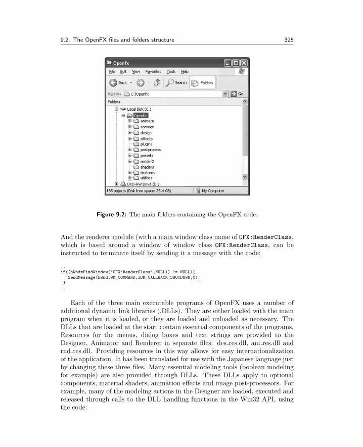
9.2. The OpenFX files and folders structure 325
Figure 9.2: The main folders containing the OpenFX code.
And the renderer module (with a main window class name of OFX:RenderClass,which is based around a window of window class OFX:RenderClass, can beinstructed to terminate itself by sending it a message with the code:
..if((hWnd=FindWindow("OFX:RenderClass",NULL)) != NULL){
SendMessage(hWnd,WM_COMMAND,IDM_CALLBACK_SHUTDOWN,0);}
..
Each of the three main executable programs of OpenFX uses a number ofadditional dynamic link libraries (.DLLs). They are either loaded with the mainprogram when it is loaded, or they are loaded and unloaded as necessary. TheDLLs that are loaded at the start contain essential components of the programs.Resources for the menus, dialog boxes and text strings are provided to theDesigner, Animator and Renderer in separate files: des res.dll, ani res.dll andrnd res.dll. Providing resources in this way allows for easy internationalizationof the application. It has been translated for use with the Japanese language justby changing these three files. Many essential modeling tools (boolean modelingfor example) are also provided through DLLs. These DLLs apply to optionalcomponents, material shaders, animation effects and image post-processors. Forexample, many of the modeling actions in the Designer are loaded, executed andreleased through calls to the DLL handling functions in the Win32 API, usingthe code:

326 9. The complete package: OpenFX
.BMP .GIF .TGA Image file formats supported
.JPG .PNG .TIF for input and output
.AV I Movies for input and output
.STL Stereo lithography data
.3DS Mesh objects in 3D Studio format
.DXF Autocad drawing format.
.WRL VRML formats.
Table 9.1: Well-known file types that OpenFX supports.
BOOL LoadInternalAction(char *library){..HMODULE hLib;FARPROC fpFun;X__STRUCTURE *Evs;BOOL (*fpFun1)(HWND, HWND, X__STRUCTURE *);Evs=&EviStructure;strcpy(lname,gszHomeDir); strcat(lname,library);if((hLib=LoadLibrary(lname)) != NULL){
if((fpFun=GetProcAddress(hLib,"_Xmodeler")) != NULL){fpFun1 = (void *)fpFun;status=(*fpFun1)(ghwnd_main,ghwnd_info,Evs);
}else return FALSE;FreeLibrary(hLib);
}else return FALSE;return TRUE;}
OpenFX uses a special structure, in this case an X STRUCTURE, to pass point-ers that give access to most of its global variables and functions to the attachingDLL. This is discussed in detail in section 9.8 on building plug-ins.
9.2.1 Filename extensions
Like all application programs OpenFX uses filename extensions to hint at thetype of information a file contains. A number of file extensions are used inaddition to the well-known file types that the program supports. The well-known filenames are mainly used to contain images and movies. Tables 9.1 and9.2 show the list of filename extensions used and supported by OpenFX. Therendering module uses a temporary script file (filename extension .SCR) that iscreated by the Animator. It is not normally of any concern to the user becauseit is written automatically and removed when the program terminates. Howeverit can be created for off-line rendering on multiple hosts.

9.3. Coordinate system and units 327
.OFX An animation.
.MFX A mesh model.
.SCR Intermediate Renderer’s file.
.EFX An animation plug-in effect.
.AFX A Designer action plug-in.
.DFX A Designer tool plug-in.
.XFX An image post processor.
.PFX An Animator’s preset animation.
.TFX A plug-in-shader.
.RSQ A robot actor sequence.
.PTH A path for actors to move along.
Table 9.2: OpenFX specific file formats.
9.3 Coordinate system and units
Before one can make sense of the code of OpenFX it is essential to know howOpenFX represents its data in three-dimensional space. The most significantfeature of the coordinate system is that it is integer based. Floating point (ei-ther float or double type) numbers are used in intermediate calculations andduring final transformations in the renderer and depth buffer. The reasons thatthe mesh models have their vertex coordinates recorded as integers is becausecomparisons can be done exactly. Many geometric algorithms can be done morerobustly when using integers for coordinates and the optimizing step made priorto ray-tracing can be made much more efficient.
Given these advantages there is the disadvantage that the scale of objectsis limited to the maximum size of a 32-bit integer, about 4 × 10⁹. Since theanimator can scale models up by many orders of magnitude a compromise hasto be accepted and the models built in the Designer are limited to sizes between±2048 and ±33554432 integer units. The zoom function is limited to work withinthese limits. In the Animator the limits are ±2048 and ±1073741824. The lowerlimit allows for some detail to be presented at higher detail than maximum zoompermits and the upper limit gives space for movement at maximum zoom out.These restrictions really only limit the level of detail that can be recorded in ascene, and pose no practical limitations on the scope of animations or modelsthat can be used.
The coordinates used by OpenFX differ from those used in OpenGL. InOpenFX the Z axis is vertical; models are built so that they face forward alongthe +Y axis. In the animator, when models move forward they move in thedirection of their local +Y axis. The coordinate system is right handed and thisdefines the direction of the X axis as lying toward the right.

328 9. The complete package: OpenFX
Figure 9.3 illustrates how the 2D screen is arranged so that the user canwork in a 3D volume, and how the windows into to the working-volume relateto the coordinate system. There are two important reference points highlightedin figure 9.3. First, the coordinate axis has to be defined. This is called thecenter point and it is the point by which the model is positioned and moved inthe animator. Second, because it is necessary to use a 2D computer screen, viamouse or pen, a way must be found to move and work at a 3D location in theworking-volume. This can be done by defining a 3D cursor. To move the 3Dcursor to a 3D location, the user has to position it using at least two of the viewwindows. The program variables NpointerX, NpointerY and NpointerZ holdthis value.
9.4 User interface implementation
To build 3D models and set up animated scenes, an application program requiresa fairly comprehensive user interface. The Animator and Designer programspresent a very similar similar appearance to the user, but there are minor differ-ences. The Animator’s fourth view window presents a wireframe representationof the scene as visualized by a camera. The Designer’s fourth window showsthe object as seen from an arbitrary view pointer. The Designer’s fourth win-dow may be optionally rendered using the OpenGL shading library (the otherwireframe views are rendered using Win32 GDI3 functions) and most of theinteractive tools can be used in this window. The Animator’s camera view ispurely passive. However, the renderer, which is a completely separate program,can be commanded to draw a 3D shaded view into the Animator’s camera viewwindows (demonstrating the power of the inter-process communication outlinedin section 9.2).
The Renderer does not need a sophisticated user interface, so its presentationis simply that of a tabbed Windows dialog box. The Renderer’s dialog layoutis loaded from a resource file. The majority of the Renderer’s code is platformindependent, and porting this module to other hosts would be a fairly simpletask.
The user interfaces of the Animator and Designer modules is based on a collec-tion of hierarchical windows. The application’s main windows has a blank clientarea and a menu. The three rectangular view windows and the perspective/cam-era windows are created as child windows. The toolbar buttons are implementedas child windows of another window representing the toolbar, which itself is achild window of the main window. The main window receives and processesmessages from the application’s menu bar.
The window class names and their message processing functions are given intable 9.3 for the Animator, and in table 9.4 for the Designer.
3Future versions of OpenFX will render all views using OpenGL at some point.

9.4. User interface implementation 329
Menu bar
Top view
+y
3
2
33
+x
+z
+y+x
+z
Side viewRear view
Status bar
View window
Toolbar
1
Figure 9.3: The OpenFX screen layout depicts three main user windows showing viewsinto the working volume. The views show a view from the top looking down, a viewfrom the rear looking forward and a view from the right side looking to the left. Inthe coordinate system used by OpenFX the Z axis is vertical and the X axis points tothe right. This figure also shows the other main screen elements and identifies threeimportant markers. (1) The center (hold) point, (2) an offset point, and (3) the 3Dcursor used to move the work position in 3D space.
The Animator’s menu commands are handled by the function calledAnimatorMenuCmd(... LOWORD(wparam), hwnd, lparam);, and the Designer’smenu commands are processed in DesignMenuCommand(LOWORD(wparam), hwnd,
lparam);. These functions take the standard Windows message parameters asarguments, and dispatch actions, tools and all the major tasks undertaken bythe program.
Other window messages are handled in the window functions for each classof windows, for example the mouse button, mouse move and keyboard messages.

330 9. The complete package: OpenFX
Class Name Message Handling Function Window
OFX:AnimatorClass MainAnimatorWndProc Main appli-cation
OFX:AnimatorViewClass AnimatorViewWndProc CameraOFX:AnimatorTriViewClass AnimatorTriViewWndProc Working
volume viewOFX:AnimatorQuicktimeClass QuicktimeWndProc Frames
progressbar.
OFX:AnimatorToolboxClass ToolboxWndProc Tool panelcontainer
OFX:AnimatorToolBtnClass ToolBtnWndProc Button intool panel
Table 9.3: Window class names, message handling functions in the Animator.
Class Name Message Handling Function Window
OFX:ModelerClass MainModelerWndProc Main applica-tion
OFX:ModelerViewClass ModelerViewWndProc Oblique viewOFX:ModelerTrivViewClass ModelerTriViewWndProc Each working
volumeOFX:ModelerToolboxClass ToolboxWndProc Tool panel
containerOFX:ModelerToolBtnClass ToolBtnWndProc Button in tool
panel
Table 9.4: Window class names, message handling functions in the Designer.
The three windows that show the top, rear and side views are all handled by thesame window function.
Rendering of the client areas of all the windows is not done directly in re-sponse to a WM PAINT message because for very large meshes this would betoo slow, especially when re-sizing a window. Instead, only when a tool is usedor an action is performed rendering takes place using the GDI API functionsinto an off-screen bitmap. The off-screen bitmap is rendered to the display usingPatBlt() when a WM PAINT message occurs, or is generated internally.
The Designer’s optional shaded perspective/orthographic view, rendered us-ing OpenGL, is created in a DLL (built with project “gldesign”) loaded at run-time. The OpenGL window replaces the OFX:ModelerViewClass window withone of class OFX:OpenGL. All its messages are processed by the handler func-tion OpenGLWndProc(), whose source code can be found in the file “gldesign.c”,that is one of the build files for the DLL gldesign.dll.

9.5. The Animation module 331
In addition to the program’s main windows there are a small number ofmodeless dialogs used for defining user-specified units, some of the tools, and inthe Designer for working with materials and image maps.
A few other window classes are used to handle some floating tool panel win-dows, for example the coordinates dialog box.
9.5 The Animation module
The Animator program is the launching point for all the other applications ofOpenFX. It provides a window into a four-dimensional world where the actionsof the actors are directed in space and time. The Animator’s interface imple-mentation is described in section 9.4. This section provides a commentary onthe way the Animator organizes its data structures and a tour of the main routein the path of execution.
9.5.1 The data structures
The numerical description of the action and the scene is recorded externally inthe .OFX file, and stored internally in a series of data objects for the variouscomponents. These are arranged in a series of doubly linked lists that are in-terconnected via object pointers that topologically resemble a tree. Figure 9.4illustrates how the data is organized. Each actor in a scene is represented byan instance of a node object whose data structure is presented in listing 9.1.The key program variable FirstNp points to the first node in the doubly linkedlist of nodes and may be used to gain access to every piece of data used in theAnimator. There must always be at least one actor in a scene; this must be acamera actor. In figure 9.4 the list of nodes can be see at the left-hand side.
For each node, the behavior of the actor is fully specified by providing up tofour additional linked lists for the key events. The list of key events map ontoa timeline with each event being described to the user as a key frame. The fourtypes of key events are:
• Costume: This type of event is defined by the variables in an object (orsky or director) data structure and the first item is pointed to by thevariable fobj / fsky/ fposition in the actor’s node structure.
• Position: This list of events, stating that the actor will be located at(x, y, z) in frame i, is pointed to by the variable fpos in the actor’s nodestructure.
• Alignment: This list of events, stating that the actor’s local y axis will berotated by angles (φ, θ, ρ) around the global (world) (x, y, z) axes in framek, is pointed to by the variable fali in the actor’s node structure.
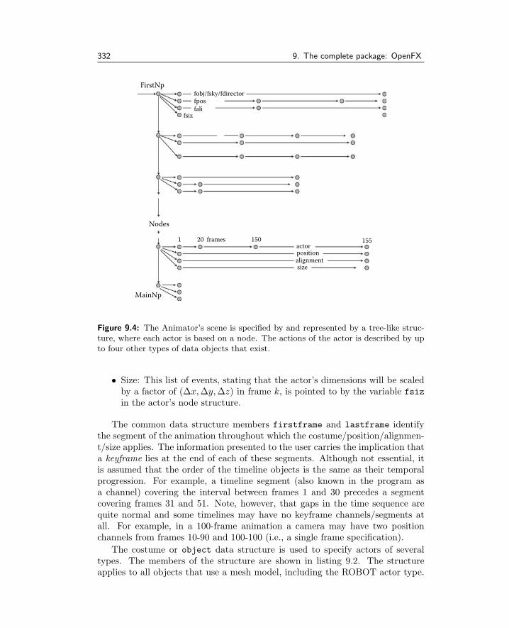
332 9. The complete package: OpenFX
FirstNp
Nodes
MainNp
fobj/fsky/fdirectorfposfali
fsiz
1 20 150framesactorposition
sizealignment
155
Figure 9.4: The Animator’s scene is specified by and represented by a tree-like struc-ture, where each actor is based on a node. The actions of the actor is described by upto four other types of data objects that exist.
• Size: This list of events, stating that the actor’s dimensions will be scaledby a factor of (∆x,∆y,∆z) in frame k, is pointed to by the variable fsizin the actor’s node structure.
The common data structure members firstframe and lastframe identifythe segment of the animation throughout which the costume/position/alignmen-t/size applies. The information presented to the user carries the implication thata keyframe lies at the end of each of these segments. Although not essential, itis assumed that the order of the timeline objects is the same as their temporalprogression. For example, a timeline segment (also known in the program asa channel) covering the interval between frames 1 and 30 precedes a segmentcovering frames 31 and 51. Note, however, that gaps in the time sequence arequite normal and some timelines may have no keyframe channels/segments atall. For example, in a 100-frame animation a camera may have two positionchannels from frames 10-90 and 100-100 (i.e., a single frame specification).
The costume or object data structure is used to specify actors of severaltypes. The members of the structure are shown in listing 9.2. The structureapplies to all objects that use a mesh model, including the ROBOT actor type.

9.5. The Animation module 333
typedef struct Animator_NODE {struct Animator_NODE *last; /* pointer to previous object */struct Animator_NODE *next; /* pointer to next object */struct Animator_SKY *fsky; /* pointer to the first sky object
for SKY actors otherwise NULL */struct Animator_DIRECTOR_tag
*fdirector; /* pointer to the first directorif not DIRECTOR then NULL */
struct Animator_OBJECT *fobj; /* pointer to the first OBJECT objectrepresents all other actor */
struct Animator_POSITION *fpos; /* pointer ot the first POSITIONtimeline segment for this actor */
struct Animator_ALIGN *fali; /* pointer ot the first ALIGNMENTsegment for this actor */
struct Animator_SIZE *fsiz; /* pointer ot the first SCALINGsegment for this actor */
short type, /* Identifies the type of actore.g. NORMAL CAMERA etc. */
ID; /* Unique identifier given byAnimator to represent the actor*/
char actorname[128]; /* Text string for the Actor’s name */} node;
Listing 9.1: The node data structure is a doubly linked list of actors in the scene. Itcontains pointers to the other objects that describe what the actor is doing, where itis doing it and when it is doing it.
The ROBOT actor type, PATH actors and even the PostProcessor actor use thisstructure. Any member variable that is not used for a particular actor is set toNULL.
The costume object is the largest object in OpenFX because it has to encom-pass such a disparate range of data. Listing 9.2 highlights the most importantdata pointers. Two of the pointers and two long structure members requirefurther consideration. These are npoints, nedges, *points and *edges. Thesemembers are significant because they are associated with the wireframe datafor costumes based on mesh models that have been built in the Designer andloaded from an .MFX type file (points are equivalent to vertices). The arraysthese pointer address can be large (perhaps > 100, 000 vertices) and will oc-cupy a large block of RAM memory. Some animations might need to instancethousands of these meshes and so, to save memory, if different actors use thesame mesh only one instance of each model (loaded from an MFX file) is heldin memory. Since the same memory might be used by several costumes carefulreference counting is required to ensure that this memory is only released whenthe last costume, that was using it, is deleted. Care also needs to be takenwhen costumes are being changed (i.e., a different mesh is being loaded into thecostume). There is also the question of when a costume is being changed doesthe change only apply to the selected actor, or does it apply to all actors usingthis mesh. The functions CreateCostume() and DeleteCostume() handle thisreference counting.

334 9. The complete package: OpenFX
typedef struct Animator_OBJECT {// for all actor typesstruct Animator_OBJECT *last; // Doubly-linked lsit of timelinestruct Animator_OBJECT *next; // segments (last and next pointers)short type; /* Actor type NORMAL ROBOT GROUND PATH etc */short firstframe, /* The first frame of this segment of the timeline */
lastframe; /* The last frame of this segment of the timeline */short morph; /* Indicates Actor’s costume is morphing */// Followed by actor type specific members..// Selected other memberslong nNurbs; /* Number of NURBS patches inNORMAL actor */nurbs *Nurbs; /* NURBS patch data for any NURBS in OBJECT *//* If this is a particle system actor then thi smember is valid */ParticleSystem particles;/* for IMAGEPROCESS actors the name of the effect*/char *xip;object;
Listing 9.2: The Costume (object) data structure. Some members have been removedfrom this listing to help highlight the most important items. (Consult the web referencesfor a link to a full list of member variables.) Listings 9.3, 9.4 and 9.5 contain details ofthe actor-specific structure members.
// NORMAL AND SKELETON specific memberspoint origin, /* origin of a mesh object */
offset; /* offset point */long npoints; /* Number of vertices in the model */long nedges; /* Number of edges in the model */long nskeleton; /* For ROBOT actors number of skelton bones */point *points; /* Array of vertices MAIN DATA FOR MESH OBJECT */Sedge *edges; /* Array of edges MAIN DATA FOR MESH OBJECT */long *skid; /* Vertx -> skeleton node it is attached to*/skel *skeleton; /* pointer to skeleton structure */char name[255]; /* The name of the MFX file for NORMAL and ROBOT */awire w_frame; /* A wireframe for use a bounding box */point outline[8]; /* Corners of the bounding box of the object */// external effectchar *effect; /* The name of any Animation effect */HMODULE hEffect; /* Handle to any animation effect DLL */
Listing 9.3: Members of the costume (object) structure specifically for NORMAL andROBOT actors.
Two types of actors have customized costume objects, the Sky and the Direc-tor. Neither of these actors have any connection with a mesh or extended data,whereas, a Path for example uses extended data to define its control points. Thekey members of the Sky and Director actors are highlighted in listing 9.6.
Looking back at the object (costume) data structure (listing 9.2), it can beseen that some members use instances of other data structures. The Robotactor uses an array of skel (see listing 9.7) types to specify the location and

9.5. The Animation module 335
// light and ground specific membersunsigned char colour[3], /* colour */acolour[3]; /* secondary colour */short groundtype; /* Type (PLAIN/TEXTURED etc.) */short lighttype; /* OMNIDIRECTION SPOTLIGHT NOSHADOW etc. */double light_intensity; /* light intensity [0 - 1] */short depth_cue; /* Is the light intgensity to fall off */..short self_shadow, /* This actor self shadows */cast_shadow, /* This actor does or does not cast a shadow. */show_shadow; /* Show or do not show shadows */RAMIMAGE image; /* Any image that is needed by a GROUND */
Listing 9.4: Members of the costume (object) structure specifically for LIGHT andGROUND actors.
// Path specific membersshort pathtype, /* type of path OPEN CLOSED etc. */double *v; /* pointer to velocity profile array */npathpoints; /* this holds the number of pathpoints. */pathpoint *firstpathpoint; /* pointer to their first pathpoint */double pathlength; /* path length (in internal units) */int npec; /* Number of pathedit control points */PATHEDITCONTROL *pec; /* Pointer pathedit control points */
Listing 9.5: Members of the costume (object) structure specifically for PATH actors.
orientation of the bones in the skeleton. It also uses a list to identify which meshvertex is attached to which bone. A ground actor might require an image mapand this is defined in a RAMIMAGE structure. Path type actors require a listof path control points (data type pathpoint, see listing 9.8) and a further set ofspline control points (data type patheditcontrol) are used to determine howfast objects following the path travel along the path, where they accelerate ordecelerate etc. Particle system actors have their own special structure to holdthe parameters and settings that define that particle system’s behavior.
The particle system implemented within OpenFX follows very closely theprinciples set out in section 6.7 but some special circumstances need to be takeninto account. These are the position, orientation and scale of the system, as wellas the time interval over which the effect takes place. No temporal scaling isapplied. The effect plays out in absolute time, but it may be curtailed if thetimeline segments are too short, or have finished completely if the segments aretoo long. Each costume timeline segment is designated as one performance of theparticle system. The behavior starts in frame one of the segment and continuesfor the duration of the segment. Some particle systems may have the appearanceof a flow that continues until the end of the segment. Some may burn themselvesout and have to be reignited with another segment.
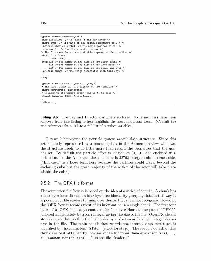
336 9. The complete package: OpenFX
typedef struct Animator_SKY {char name[128]; /* The name of the Sky actor */short type; /* The type of sky (simple Backdrop etc. ) */unsigned char colour[3], /* The sky’s horizon colour */zcolour[3]; /* The Sky’s zenith colour */
/* The first and last frames of this segment of the timeline */short firstframe,
lastframe;long aff,/* For animated Sky this is the first frame */
alf,/* For animated Sky this is the last frame */ast;/* For animated Sky this is the frame interval */
RAMIMAGE image; /* the image associated with this sky. */..} sky;
typedef struct Animator_DIRECTOR_tag {/* The first frame of this segment of the timeline */short firstframe, lastframe;/* Pointer to the Camera actor that is to be used */struct Animator_NODE *ActiveCamera;..} director;
Listing 9.6: The Sky and Director costume structures. Some members have beenremoved from this listing to help highlight the most important items. (Consult theweb references for a link to a full list of member variables.)
Listing 9.9 presents the particle system actor’s data structure. Since thisactor is only represented by a bounding box in the Animator’s view windows,the structure needs to do little more than record the properties that the userhas set. By default the particle effect is located at (0, 0, 0) and enclosed in aunit cube. In the Animator the unit cube is 32768 integer units on each side.(“Enclosed” is a loose term here because the particles could travel beyond theenclosing cube but the great majority of the action of the actor will take placewithin the cube.)
9.5.2 The OFX file format
The animation file format is based on the idea of a series of chunks. A chunk hasa four byte identifier and a four byte size block. By grouping data in this way itis possible for file readers to jump over chunks that it cannot recognize. However,the .OFX format records most of its information in a single chunk. The first fourbytes of a .OFX file always contains the four byte character sequence “OFXA”followed immediately by a long integer giving the size of the file. OpenFX alwaysstores integer data so that the high order byte of a two or four byte integer occursfirst in the file. The main chunk that records the internal data structures isidentified by the characters “STAG” (short for stage). The specific details of thischunk are best obtained by looking at the functions SaveAnimationFile(...)and LoadAnimationFile(...) in the file “loader.c”.

9.5. The Animation module 337
typedef struct Animator_SKELETON {long id; /* index of parent node in skeleton */char name[16]; /* name for skeleton element */vector u,v,w, /* u,v,w are original axes */
uu,vv,ww; /* transformed axes directions */double R[4][4], /* R is the rotational matrix */
Q[4][4], /* Q quaternion tweened R matrix */T[4][4]; /* T is the transformation matrix */
point p, /* p is original skeleton vertex */pp, /* transformed point */pt, /* pp after Actor’s transformation */wk, /* work point */bx[8]; /* bx is original bounding box */
double weight; /* bone weight */double wrange; /* bone weight range in % of length */double wzone ; /* bone weight falloff zone % */...
}skel;
Listing 9.7: The Robot actor data structure. Some members have been removed fromthis listing to help highlight the most important items. (Consult the web references fora link to a full list of member variables.)
typedef struct Animator_PATHPOINT {struct Animator_PATHPOINT *last; /* previous item */struct Animator_PATHPOINT *next; /* to next item */short status;point p; /* The coordinates of the path point.*/double distance; /* The distance of the point from path start */double ptheta, /* Tension related parameter - not used */
pfi; /* Tension related parameter - not used *//* Between path points the path curve is drawn as a spline
under tension these parameters holds the tension parameterto both sides of the point*/
double tension_p,tension_n;
} pathpoint
Listing 9.8: The pathpoint data structure. Some members have been removed fromthis listing to help highlight the most important items. (Consult the web references fora link to a full list of member variables.)
9.5.3 Program execution
The program begins at the usual Windows WinMain(..) entry point (file Ani-mate.c) where the classes for the user interface windows are registered and themessage processing loop executes. In this respect, OpenFX is nothing more thana standard Win32 API program. Messages from the main window menu are pro-cessed as described in section 9.4 by function MainAnimatorWndProc(..). Whenthe user engages a tool from the tool menu a command is passed up throughits hierarchical windows to the function AnimatorMenuCmd(...). Tools and ac-
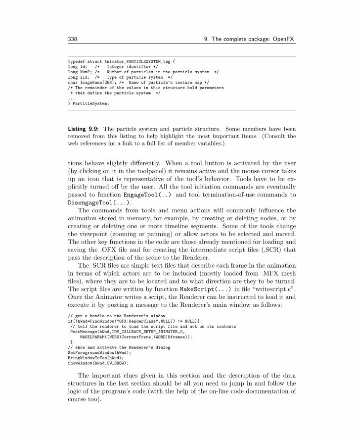
338 9. The complete package: OpenFX
typedef struct Animator_PARTICLESYSTEM_tag {long id; /* Integer identifier */long NumP; /* Number of particles in the particle system */long iid; /* Type of particle system */char ImageName[256]; /* Name of particle’s texture map *//* The remainder of the values in this structure hold parameters* that define the particle system. */...} ParticleSystem;
Listing 9.9: The particle system and particle structure. Some members have beenremoved from this listing to help highlight the most important items. (Consult theweb references for a link to a full list of member variables.)
tions behave slightly differently. When a tool button is activated by the user(by clicking on it in the toolpanel) it remains active and the mouse cursor takesup an icon that is representative of the tool’s behavior. Tools have to be ex-plicitly turned off by the user. All the tool initiation commands are eventuallypassed to function EngageTool(..) and tool termination-of-use commands toDisengageTool(...).
The commands from tools and menu actions will commonly influence theanimation stored in memory, for example, by creating or deleting nodes, or bycreating or deleting one or more timeline segments. Some of the tools changethe viewpoint (zooming or panning) or allow actors to be selected and moved.The other key functions in the code are those already mentioned for loading andsaving the .OFX file and for creating the intermediate script files (.SCR) thatpass the description of the scene to the Renderer.
The .SCR files are simple text files that describe each frame in the animationin terms of which actors are to be included (mostly loaded from .MFX meshfiles), where they are to be located and to what direction are they to be turned.The script files are written by function MakeScript(...) in file “writescript.c”.Once the Animator writes a script, the Renderer can be instructed to load it andexecute it by posting a message to the Renderer’s main window as follows:
// get a handle to the Renderer’s windowif((hWnd=FindWindow("OFX:RenderClass",NULL)) != NULL){// tell the renderer to load the script file and act on its contentsPostMessage(hWnd,IDM_CALLBACK_SETUP_ANIMATOR,0,
MAKELPARAM((WORD)CurrentFrame,(WORD)Nframes));}// show and activate the Renderer’s dialogSetForegroundWindow(hWnd);BringWindowToTop(hWnd);ShowWindow(hWnd,SW_SHOW);
The important clues given in this section and the description of the datastructures in the last section should be all you need to jump in and follow thelogic of the program’s code (with the help of the on-line code documentation ofcourse too).

9.5. The Animation module 339
typedef struct Animator_POSITION {/* First frame of the ’bar’ of this segment of the timeline
for specified actor. */short firstframe,
/* Last frame (at the time of keyframe) of bar in timeline */lastframe;
short type; /* Linear or Quadratic tweening */point finish; /* Position of actor in keyframe */struct Animator_NODE *onpath; /* This actor is following a path *//* When following a path this is the name of the followed object */char pnodename[128];/* When positions are being determined using spline tweening
these set hhe Spline parameter at start/end of the timeline */double tension_s,
tension_e,..
} position;
typedef struct Animator_ALIGN {short firstframe,lastframe; /* same as position */short type, /* Linearly or Quadratic interpolion */
im; /* Internal rotation (=0) or about an axis (= 1/2/3 ) */double theta, /* Banking (angles are in degrees) */
phi, /* Direction (around) 0 along +x X to rightrange is (-180 to +180 ) degrees */
alpha, /* Elevation */ima; /* Internal rotation 0=none 1=clock 2=anti-clock */
/* When aligned to a path this points to the path object */struct Animator_NODE *topath;
/* When aligned to another actor this string is the name of theactor this one uses for alignment */
char anodename[128];..} align;
typedef struct Animator_SIZE {/* The scaling values in X Y Z (local coordinates) */double Sx,Sy,Sz;
/* Type of interpolation - linear to last keyframe, orquadratic back to last two keyframes */
short firstframe, lastframe; /* same as position */short tweentype; /* Linear or Quadratic tweening */..
} size;
Listing 9.10: The Position Orientation and Size data structure. Some members havebeen removed from this listing to help highlight the most important items. (Consultthe web references for a link to a full list of member variables.)
9.5.4 Character animation
The Robot is a type of actor introduced in version 2 specifically to facilitatecharacter animation. Because it is based on a mesh model it uses the samebasic costume structure (listing 9.2 with the skel pointer playing an importantrole). Each bone in the skeleton is specified by the structure given in listing 9.7.The member variables R[4][4], Q[4][4] and T[4][4] play the pivotal role ofrepresenting the rotational transformation of the bone in its parent’s frame of
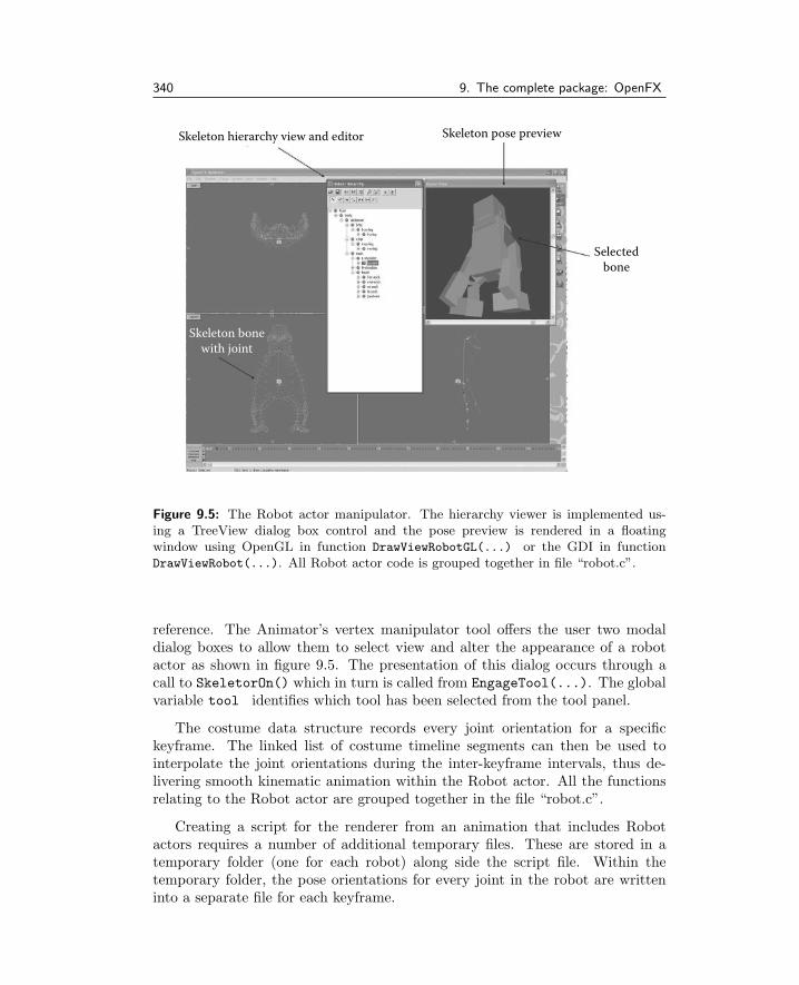
340 9. The complete package: OpenFX
Skeleton hierarchy view and editor Skeleton pose preview
Selectedbone
Skeleton bonewith joint
Figure 9.5: The Robot actor manipulator. The hierarchy viewer is implemented us-ing a TreeView dialog box control and the pose preview is rendered in a floatingwindow using OpenGL in function DrawViewRobotGL(...) or the GDI in functionDrawViewRobot(...). All Robot actor code is grouped together in file “robot.c”.
reference. The Animator’s vertex manipulator tool offers the user two modaldialog boxes to allow them to select view and alter the appearance of a robotactor as shown in figure 9.5. The presentation of this dialog occurs through acall to SkeletorOn() which in turn is called from EngageTool(...). The globalvariable tool identifies which tool has been selected from the tool panel.
The costume data structure records every joint orientation for a specifickeyframe. The linked list of costume timeline segments can then be used tointerpolate the joint orientations during the inter-keyframe intervals, thus de-livering smooth kinematic animation within the Robot actor. All the functionsrelating to the Robot actor are grouped together in the file “robot.c”.
Creating a script for the renderer from an animation that includes Robotactors requires a number of additional temporary files. These are stored in atemporary folder (one for each robot) along side the script file. Within thetemporary folder, the pose orientations for every joint in the robot are writteninto a separate file for each keyframe.

9.6. The Designer module 341
9.5.5 Extending the animation module
When the desire to add new functionality cannot be satisfied through the pro-duction of new plug-ins as discussed in section 9.8 then it is necessary to modifythe Animator’s source code directly. How this is done would of course dependon what that task is. The most likely additions might be the inclusion of a newtool or command action, or possibly a new type of actor.
Adding a command action is probably the least complex modification, notbecause the action itself is less complex but because the changes to the codewould be minimal. Adding a menu item and handler is relatively simple, thesteps involved being: (1) create identifiers for a menu item and text string hint tothe resource header files, (2) add the menu and string themselves to the resourceDLL (project “ani res”), (3) add a case in the function AnimatorMenuCmd(...),(4) add a new function (possibly in a new file) to perform the action, (5) call itfrom the added case block and when it returns and (6) call the functions thatupdate the display and status information by:
ReDrawStageDisplay(TRUE); // Update the view windowsPerspectiveView(0,1); // Update the camera windowUPDATETIMELINES(IDC_TIMEL_UPDATE) // Update the keyframe window.
Adding a tool would require an extra tool button to be inserted into thetool panel. Bitmaps to represent the tool would need to be added to the toolimages (located in the resource folder, e.g., tools-b.bmp), but it would not bedifficult to extend the number of number of tools in the tool panel. Modifyingthe N ICONS define statement, adding to the aTools[ ] array and providing adefined command message (e.g., IDM ACTOR TOOL MYTOOL will augment the userinterface. The new message should be handled in the AnimatorMenuCmd(...)
function and the actual tool code executed via the EngageTool(...0 function.Of course the tool will need to know what to do with the particular type of actorthat is selected and how to respond to mouse messages in the view windows(handled in the AnimatorTriViewWndProc(...) function.
9.6 The Designer module
The Designer program is normally launched from the Animator but can operateindependently. It provides a window into the three-dimensional world where itstools are used to build mesh models of almost any complexity. The Designer’suser interface is implemented using similar coding to that described in section 9.4and differs from the Animator’s user interface only because the idea of a cameraviewing a scene makes no sense and there is no aspect that needs to be a functionof time.
In the Designer the fourth window is used to provide a view, from any direc-tion, of the contents of the working-volume. The fourth view is normally pre-sented using a hidden surface and shaded drawing implemented using OpenGL.

342 9. The complete package: OpenFX
The functions that deliver the shaded view have been implemented within a self-contained DLL (called glview.dll) that also gives the user a real-time indicationof the alignment of any image maps or material shaders.
Like the Animator, the Designer uses integer coordinates for its vertex loca-tions and other key points. Each vertex is assigned a selection state from thelist: selected, deselected, hidden or ineditor. This status is recorded in the vertexobject and is used by the tools and actions, and the drawing functions. Toolsand actions only apply to selected vertices, or faces or edges. An edge is deemedto be selected if the vertices at both ends are selected. Faces are deemed selectedif all three face vertices are selected.
9.6.1 The main data structures
The data that describes the mesh models in OpenFX mirrors almost exactlythe structures discussed in chapter 3. The model data fall into two classes.First, the geometry is specified using lists of vertices, edges, faces and skeletonbones. Second, the appearance of the visible surfaces are defined by assigningthe polygons an identifier for either a material, or an image map. The material’sproperties and the image map’s images are recorded in two lists.
In other software from which OpenFX evolved the lists of vertices etc., werebuilt as doubly linked lists of individual objects. This data arrangement makesit much easier to add, delete and re-order the data but the Windows implemen-tation of the memory management functions were not fast enough to use thisapproach in models that might contain in excess of 100,000 vertices and 500,000faces. Chapter 3 showed how such limitations could be overcome with a littleeffort, thus the OpenFX Designer uses dynamically allocated arrays of objectsto store the data. The structures that represent the objects are described in thissection. The global variables that give access to the data are listed in table 9.5.Note that the skeleton bone structure is a much shorter list and therefore theskeleton bone data is represented as a doubly linked list of objects each one ofwhich represents a single bone.
Geometry data structures Whilst there are a few data structures used for minorpurposes the essentials of the geometry are described by lists of vertices, edgesand faces. The most important members of these structures are presented inlistings 9.11, 9.12 and 9.13. Consult the online references for a link to a full listof member variables.
The Skeleton data serves two purposes. First, because it describes a hier-archical relationship that allows groups of vertices in a model to be associatedwith a node (or bone) in the hierarchy it can make the process of vertex selec-tion significantly more convenient for the user. Vertex selection (and the impliededge and face selection that goes with it) is the first step the program user hasto do before applying tools or actions. Anything that eases this task for theuser is useful in itself. Second, because the skeleton’s nodes can also be given a3D position that is meaningful to the vertices attached to that node, it is pos-

9.6. The Designer module 343
Name Data type Function
Nvert int Number of verticesNedge int Number of edgesNface int Number of facesNskel int Number of skeleton bonesMainVp vertex * Pointer to array of verticesMainEp edge * Pointer to array of edgesMainFp face * Pointer to array of facesiMap[] IMAGEMAP Array of image mapsiMat[] SURFACEMATERIAL Array of surface materialsnImaps int Number of image/texture mapsnMats int Number of materialsMainSp skel * Pointer to the end of skeleton bone listFirstSp skel * Pointer to start of skeleton bone list
Table 9.5: The global variables that give access to the Designer’s main data most ofwhich is represented as user-defined data types.
typedef struct Designer_VERTEX_tag {/* This vertex belongs to this Skeleton node */struct Designer_SKELETON_tag *sp;/* The status of the vertex SELECTED DESELECTED HIDDEN etc.*/char status,status_undo;float x,y; /* Vertex texture coords */long xyz[3]; /* vertex coordinates */
} vertex;
Listing 9.11: The vertex data structure. Some members have been omitted to helphighlight the most important items.
sible to apply rotational transformations to those vertices using a local frame ofreference attached to that bone. The hierarchical (parent–child etc.) skeletonarrangement also allows the same rotation transformations to be applied to anydescendant nodes and their associated vertices. The same effect of these trans-formation would be exceptionally difficult to obtain using only rotations aboutone of the coordinate axes or even any about any arbitrary axis. Building ahierarchical skeleton into a model gives it the potential to be articulated. Thisforms the basis of the manipulation of a Robot actor in the Animator.
Having a hierarchical data relationship facilitates the potential for futuredevelopments, for example allowing the Skeleton to become part of an IK chain(see section 6.4) or be part of a muscle/skin deformation model where verticesrepresenting the surface of a limb of an animal moves as the skeletal bones changetheir relative orientations.

344 9. The complete package: OpenFX
typedef struct Designer_EDGE_tag {long V[2]; /* List of vertices at the end of the edge. */} edge;
Listing 9.12: The edge data structure. Some members have been omitted to helphighlight the most important items.
typedef struct Designer_FACE_tag {long V[3]; /* The vertices around the face. *//* Which material is to be applied to this face */short material;/* Which Image/Texture map is to be applied to this face*/short imagemap;/* These are the Image/Texture coordinates for the vertics
of the face, they are done on a PER FACE basis so thatadjacent faces cna have a different mapping*/
float x[3],y[3];BOOL gp; /* The mapping coordinates are valid for this face*/..} face;
Listing 9.13: The face data structure. Some members have been omitted to helphighlight the most important items.
Looking at the Skeleton’s data structure in listing 9.14 one should especiallynote the local frame of reference vectors u,v,w and the rotational transformationmatrix t. The axis vector u is always aligned with the bone (from the node atthe end toward the parent node to which it is attached). The other axes areorthogonal to u and are also mutually orthogonal. The user can change therotation orientation of the v and w axes relative to u. Once the nodes at theends of the bones have been positioned and the bone’s local frame of referencehas been defined, then this is considered as the rest pose of the skeleton. Therest pose is used in the animator when a Robot actor is animated.
The Designer’s Skeleton can also fulfill a third function, when no vertices areassigned to a specific bone. This phenomenon is known as rubber-bones and it isbased on the idea of a potential field surrounding the bones. When the rubber-bones tool is in use, the vertices are said to be influenced by their proximity tothe bones. If a bone is moved, it appears to pull the vertices with a strengththat is proportional to their distance from the bone. Of course, all the bonesinfluence the vertex and any bones that are not moved opposes this pull effect.How this effect works out depends on the weights and range parameters that theuser can assign to each bone. Member variables that record this information arealso present in the Skeleton node data structure (listing 9.14).
The functions in the Designer’s code that provide all the Skeleton manipula-tion and data management are located in the file “skeleton.c”.

9.6. The Designer module 345
typedef struct Designer_SKELETON_tag {struct Designer_SKELETON_tag *at, /* The parent of this bone */
*next,*last; /* Doubly linked list items *//* The bone’s frame of reference at the end of the bone */vector u,v,w;
/* Transformation and Inverse Transformation applied to the Bone */double t[4][4],tr[4][4];point xyz; // coordinate of endpointpoint bx[8]; // bounding boxchar name[16]; //name..// bone attributesdouble wrange,wzone; // range(in % of length of bone influence)double weight,r_scale; // bone influence weight..
} skel;
Listing 9.14: The Skeleton/Hierarchy data structure. Some members have been omit-ted to help highlight the most important items.
Material and image map data structures The geometry of a mesh model only tellshalf the story. The surface’s appearance is just as important. This could beas simple as a basic color, but to achieve any form of realism something moresophisticated is required. OpenFX provided two ways to describe the appearanceof a surface: its materials and image maps. Each polygonal face carries twointegers that identify the index into the two lists of surface materials and imagemaps. If these integers in the face data structure are set to −1 then no materialor image map is applied. For legacy reasons each face also carries values forsurface color and a couple of other attributes but it is uncommon for these tohave much usage in any model.
In OpenFX the materials cover basic settings properties, transparency etc.The image maps provide a way of layering up to four images over the surface.The materials also provide the mechanism for assigning procedural shaders tothe surface. Up to four shaders (implemented as external plug-in DLLs or GLSLprograms) can be combined in a single material. All image maps and some ma-terials require texture coordinates. OpenFX records texture coordinates on aper-vertex and a per-face basis. The reason for the per-face storage is becausetwo faces that may share common vertices could require different texture coordi-nates at a common vertex. Materials do not use a 2D texture coordinate systembased on vertices or faces. They use a 3D system based on a unit cell defined bya MATERIALAXIS structure that is part of the material. The ax member of theSURFACEMATERIAL structure (listing 9.15) holds the details of the reference cell.The concept of a texture is explained in section 11.1.1.
Listing 9.15 identifies the main members of the material data structure. Wor-thy of note is the four element array of shader objects. The shader objects areimplemented as external DLLs that are loaded when required. The persistentinformation that is needed for each shader is the name of the DLL and its user-

346 9. The complete package: OpenFX
typedef struct Designer_SURFACEMATERIAL_tag {char name[32]; /* Name of the material */// material colors Integer in [0 - 255]unsigned char mcolour1[3],mcolour2[3];// other properties integer [0 - 255]unsigned char gloss; // specularityunsigned char refl; // reflectivityunsigned char transp; // transparencylong refractive_index;/* The axis in use for this material */struct Designer_MATERIALAXIS_tag ax;/* The list of up to 4 external shaders per material */struct Designer_XSHADER_tag Shader[4];// On/Off switchesBOOL bSmooth,bShiny,bClear,bGlassEdge,bUseSurfaceMapping;..} SURFACEMATERIAL;
Listing 9.15: The material and shader data structures. Some members have beenomitted to help highlight the most important items.
typedef struct Designer_IMAGEMAP_tag {..char N[32],*S,*R,*B,*T;/* ImageMap name and filenames */RAMIMAGE si,ri,bi,ti; /* Image Is stored in RAM */short sp,rp,bp,tp; /* Fraction of map mxsed with material*/char TypeR,TypeB,TypeT,/* Is it an Amim/Still map */
Map, /* Planar/Cylindrical/Spherical */point P,X,Y; /* Map position */long Vlock[3]; /* control point locked to vertex */..} IMAGEMAP;
Listing 9.16: The image map data structure. Some members have been omitted tohelp highlight the most important items.
defined parameters. The user’s parameters are stored as a text string becausethis method allows external developers to choose the format of the parameters(for their plug-ins) but still permit them to be recorded in the Designer’s memoryspace and data file.
The image map structure, of listing 9.16, provides up to four classes of map.Starting with OpenFX version 2, the image source files are stored in memoryand also in the .OFX file so that there is no danger of the user losing them orhaving path location problems if they send models to another use. The imagesare stored as a byte-for-byte copy of the original file and thus there is no needto decode them in the Designer.
The oblique shaded view window has the option to display the model superim-posed with its surface image maps. To achieve this, small thumbnail images aremade whenever the image maps are updated. The thumbnail images are stored

9.6. The Designer module 347
in a list of GLMAP structures. The global pointer variable GLMAP *glMapList;
locates this list and it is updated in the “gldesign.dll” function BuildMapList();
called from GluCommands(..), which in turn is driven by sending a WM LOAD MAPS
message to the OpenGLWndProc(..) window message handler for window classOFX:OpenGL.
9.6.2 The MFX file format
The format used for the file to record the mesh models is based on the idea ofa chunk of data. In this it behaves in a similar way to the animation .OFX file,described in section 9.5.2. The file itself begins with a four character header“FORM” followed by a long integer giving the size of the file. The integeris stored with the high byte stored first. (This is not the natural order forWindows platforms and so an internal function is used for reading and writinglong integers.) The fact that the file contains an OpenFX mesh model is evidentby another four character sequence “OFXM” following immediately. After that,the file contains a number of chunks holding the appropriate data to describethe mesh geometry, the materials and image maps, and a few other essentials,like the coordinate origin point and the coordinate scaling between internal anduser units.
Each chunk of data begins with a four byte identifier and a long integer thatgives the length of the chunk. The code functions that handle reading and writingof the .OFX files is located in file “loader.c” with SaveObject(..) writing thedata and LoadObject(...) reading it.
Other functions in file “loader.c” support the undo functionality. Some opera-tions that only involve moving vertices are easily undone by simply copying theirposition before the action and replacing the current location with the backup ifthe operation is to be undone. Operations that increase the number of verticescan be easily undone by discarding the extra data that is always added to theend of the data lists. Other operations, those that involve the deletion of parts ofthe data, cannot be so easily undone. For those, the saving and loading functionsmake, and restore, temporary copies of the data.
9.6.3 Program execution
The Designer program is very similar in many respects to the Animator. Thetool panel and its buttons, the menu commands, status bar and orthogonal viewwindows are all created using very similar code in both programs. Executionof the Designer begins at the usual Windows WinMain(..) entry point (file de-sign.c) where the classes for the user interface windows are registered and themessage processing loop executes. Messages from the main window menu are pro-cessed as described in section 9.4 by function MainModelerWndProc(..). Whenthe user engages a tool from the tool menu a command is passed up throughits hierarchical windows to the function DesignMenuCommand(...). Tools and

348 9. The complete package: OpenFX
actions behave differently. When a tool button is activated by the user (byclicking on it in the toolpanel) it remains active and the mouse cursor takes upthe representative of the tool’s behavior. Tools have to be explicitly turned offby the user. All the tool initiation commands are eventually passed to func-tion EngageDesignerTool(..). The Skeleton tools are engaged from a menucommand and they call EngageSkeletonTool(..) to commence execution.The one-shot actions are initiated in function ExecuteDesignerAction(..).Some of the actions are built as external DLLs and their action is performedin LoadExternalAction(...).
The commands from tools and menu actions will commonly influence themodel geometry data stored in memory. Some of the tools change the viewpoint(zooming or panning) or allow vertices to be selected and moved. When tools areengaged, the mouse and keyboard messages sent to the message handler functionhave to be interpreted and appropriate actions taken. For example, when thepan-view tool is engaged (the global variable tool takes the value PAN) and ifthe user left-clicks the mouse in the client area of one of the view windows, aWM LBUTTONDOWN message is sent to the handler ModelerTriViewWndProc(..),where the code:
else if(tool == PAN){SetCapture(hwnd); // capture mouse messages to this windowClipCursor(...); // keep the mouse within the windowPanToolDown( ... ); // start the tool actionbTrackPan=TRUE; // flag that tool is in working
is executed. Now, when the mouse is moved and the WM MOUSEMOVE message isreceived, the code checks for the bTrackPan flag and executes:
else if(bTrackPan){ // using the pan toolPanToolMove(...); // change the working volume reference point..
}
When the user releases the mouse button the WM LBUTTONUP message results inthe capture being released and the bTrackPan flag lowered:
else if(bTrackPan){ClipCursor(NULL); // release the cursorReleaseCapture(); // stop capturing messagesPanToolUp( ); // fully re-drawbTrackPan=FALSE; // flag that tool is no longer working
}
The response to receipt of mouse messages for the other tools is handled inother branches of the if (...) then ... else if (..) else ... codegroups.

9.6. The Designer module 349
9.6.4 GLdesign
The provision of a window into the working-volume that provides an orthographicview from a user-defined direction is provided in the external DLL “gldesign”.This DLL is built with its own project in the design solution. The DLL’s exportedfunction AttachViewOpenGL() is called by the Designer to create an OpenGLwindow as a child of the main applications window and although implementedin its own DLL it has access to all the Designer’s global variables and mainfunctions through the mechanism to be discussed in section 9.8. Rendering anetwork of triangular polygons using OpenGL was discussed in section 7.2.1 andthe “gldesign” module follows those basic principles. The window’s messages arehandled in OpenGLWndProc(...) where the Designer’s tools can perform theirfunctions in response to the mouse move and button messages in the same waythat they do for the rectangular view windows. The shaded view is drawn infunction drawScene(...) which provides the option for stereoscopic rendering.To maintain as high a refresh rate as possible, the geometry, material and imagemaps are written into a display list which only needs to be updated if the contentsof the working-volume change. A basic change of viewing direction does notrequire the display list to be re-created.
The display lists are rebuilt in response to a WM UPDATE message being sentfrom the Designer’s refresh functions:
case WM_UPDATE:if(!bCanUseShaders)Make3dDisplayList(); // Fixed functionality versionelse Make3dDisplayListProg(); // Programmable shader versionInvalidateRect(hWnd, NULL, FALSE);break;
This code fragment initiates the shaded rendering which is done using eitherthe OpenGL fixed functionality or programmable pipeline. By supporting bothOpenGL pipelines OpenFX maintains the widest applicability possible. Buildingthe display list is simply a matter of looping through all the Nfaces faces in theMainFp list. Since the Designer does not record vertex normals these have to becreated and stored in a temporary array.
9.6.5 Extending the Designer module
Unless a tightly integrated tool is required, the best approach to extending theDesigner module is through an external tool or action. The material shaderslibrary can also be extended through the use of the plug-ins. In this case theDesigner is only peripherally involved. All it has to do is to load and display amodal dialog box for the user to define parameters. Writing plug-ins is discussedin section 9.8.

350 9. The complete package: OpenFX
9.7 The Renderer module
The Renderer application program is a Windows Win32 application controlledby the user through a dialog box from which the output image/movie file, imagesize and format can be set. Normally the Renderer is loaded implicitly fromeither the Animator or Designer by executing the .EXE file using the Wind32API function WinExec(..).
The Renderer program uses DLL library files loaded as necessary to:
• Unpack texture maps
• Render specific texture effects (shaders)
• Generate animation effects (such as flapping, morphing)
• Write output image or movie files in a number of formats
• Post-process the image, e.g., to add blurring, lens/optical effects and 3Dfog
Within the renderer there are actually two renderers:
1. A software scan-line, Phong shading, hidden surface renderer with a ray-tracing extension.
2. A hardware-based engine for use with graphics cards that have a pro-grammable OpenGL pipeline.
The GPU renderer is implemented using the OpenGL techniques introducedin chapter 7. It relies on an off-screen P-buffer or renderbuffer and framebufferobject (FBO) in order to render at a resolution that is larger than the outputwindow. The GPU renderer renders in near real-time because there are stilla number of steps that need to be executed in the CPU, things like loadingthe data files and the need to read back from the GPU the rendered images sothat they can be written to a file using a well known image/movie file format.However, even at resolutions in excess of 2048 by 2048 it still takes a fractionof a second to render a frame, even when an accumulation buffer is used eighttimes per frame for the purposes of anti-aliasing.
Most of the work of the Renderer is done without the need for any visiblepresentation and user interaction. Although written as a Windows application allthe Windows platform dependent functions are located in one file “winmain.c”.The user interface is implemented as a dialog-based application, two buttons onthe dialog run either the GPU or CPU renderer by calling render(...) witha list of arguments that mimic the way a C or C++ main(int argc, char **
rgv); is passed its command line arguments by the system. The reason forthis unusual way of passing data is that the Renderer used to be a completelyplatform independent command line application program only. The path ofexecution through the application will be explored in section 9.7.2 after the datastructures needed for the application are introduced.

9.7. The Renderer module 351
Stepping from frame to frame The Renderer is driven from a script file created inthe Animator. The script lists all the actors that are to appear in a scene on aframe-by-frame basis. The Renderer reads the scene description, loads the meshactors from their OFX file, positions them according to the instructions in thescript, renders the frame, then discards the scene data and returns to read againfrom the script file to process the next frame. Often a single frame is all thatis required; however in an animated sequence the Renderer may have to re-loadmesh models and texture map images, if they are needed in subsequent frames.Re-loading models and images from disk is a slow process and it could take upto 99% of the rendering time when using the GPU. To alleviate this inefficiency,the Renderer does not discard mesh models and image maps when working onan animation of more than one frame; instead it caches the models, and beforeloading data from a file it checks the cache to see whether there is a copy alreadythere. The mechanism by which the cache is implemented can be found in file“loadscpt.c”. When the script calls for a mesh object to be loaded a call is madeto CheckForExistingObject(..) . If it returns a non-negative identifier thenthat identifies the object (see listing 9.17) in the object list that has alreadybeen used and is cached. If a model is loaded, it is added to the cache by callingCopyObjectToBackup(ObjectID); The object cache does not exist in a separatelist. Each object maintains a copy of the original vertex and face list. When theRenderer has finished rendering the script it calls FreeAllObjects() to emptythe cache and release the memory buffers.
9.7.1 The main data structures
The Renderer does not need to use such a rich set of data structures as areneeded in the Designer or Animator modules. All the mesh models used in ascene give rise to the addition of an object to the object list which is pointed toby the global variable object *Object. The number of mesh models that areheld in the cache is given by the global variable ObjectCount. When a scene isbeing rendered, the member variable in use.of the object structure is used toindicate whether that particular object is needed in that particular frame. Usinga flag in this way avoids including mesh models when rendering a frame in whichthat mesh is not required. Listing 9.17 presents the mesh object data structure.In any frame there will only be one active camera, and up to one ground plane,and one background sky, so the specifications of these actors is recorded as singleinstances of ground and sky objects, in global variables Ground and Sky. Theedge data in a .MFX file is not used in the Renderer so the edge chunks in the.MFX file are bypassed.
Listing 9.18 highlights the most significant members in the principle geomet-ric data needed in the Renderer.
The Renderer also needs to load and store the material properties and imagemaps associated with the mesh objects. Structures similar to those used inthe Designer are used in the Renderer. Each object identifies its material list

352 9. The complete package: OpenFX
typedef struct Renderer_OBJECT_tag {BOOL in_use; /* Used to indicate object already loaded */// position informationvector Centre; /* Coordinate of centre */axis Abase; /* The object’s base axis */// Counts of each type of datalong NoFaces,NoVertices,NoNurbs, NoMaps,NoMats, NoSkeleton;long NoTraceVertices,NoTraceFaces;long NoFbackup,NoVbackup,NoTbackup;..// Pointers to key object datavertex *Vbase,*Vbackup; /* Pointers to the vertices*/face *Fbase,*Fbackup; /* List of faces with back up */long *Skids; /* Points vertices at their skeleton bone */skel *Skeleton; /* The object’s skeleton */imap *Mbase; /* Materials used in object */matl *Tbase,*Tbackup; /* Image (Texture) maps */nurbs *Nbase; /* Nurbs in model */..// Vertices and faces used in ray-tracing to traverse the octreetvertex *Vtracebase;tface *Ftracebase;../* Bounds for this object when projected onto framebuffer */long xmin,xmax,ymin,ymax;/* Transformation applied to this object and its inverse */double trpos[4][4],trinv[4][4];double fi,theta,alpha,ima; /* Orientation */double sx,sy,sz; /* Scaling */...} object;
Listing 9.17: The mesh object data structure. Some members have been omitted tohelp highlight the most important items.
typedef struct Renderer_VERTEX{/* structure for each vertex */vector p; /* real position 3D space */ivector ip; /* integer vertex coordinates */double u,v; /* texture coordinates */double x,y; /* screen location pixel space */...} vertex;
Listing 9.18: The vertex structure as used during rendering.
through the pointer *Tbase, and its image map list via *Mbase. Loading anduncompressing image data from files of type JPG, PNG and GIF can also slowthe rendering process significantly and so the Renderer caches the image datain a list called ImageStoreList which is a pointer to a dynamically allocatedarray of ImageStoreEntry structures that store the uncompressed image datain a raw 24 bit format. The functions and variables that relate to image mapmanagement are located in code file “loadmaps.c”.

9.7. The Renderer module 353
typedef struct Renderer_FACE {UNSIGNED V[3]; /* Vertex identifier */..short ffmap; /* identifies which image map is in use. */short ffmat; /* identifies which material is in use. *//* screen bounds for projected face 0 -> XMAX 0 -> YMAX */short top,bottom,left,right;vector n; /* normal to face */vector pn[3]; /* The phong normals */double uu[3],vv[3];/* mat/map coordinates of face vertices */double ww[3]; /* volume material coordinate */
} face;
Listing 9.19: The face structure as used during rendering.
The image cache is built up as each model’s image maps are created. Itis emptied by calling ReleaseImageStore(); when rendering of the script iscomplete. The task of reading and decoding an image file format is carried outin an external DLL and so it would not require a major code revision to add anadditional type of image to the supported list.
The scanline software renderer is multi-threaded. The way OpenFX uses thefull power of the processor is to dispatch rendering of all pixels in a scanline to athread of execution. Normally the Renderer determines how many processors/-cores are available and breaks up the number of rows in the output image inton = H/Nc threads, where H is the output image height and Nc is the numberof processors or cores. The operating system is then responsible for schedulingthread execution. The Renderer groups the scanlines in an interlaced pattern sothat alternate lines are sent to different cores. This usually helps in balancingthe rendering load without any additional scheduling. (There is an argument fororganizing the rendering into a tile based rasterization as that might be morecache friendly, but this does not fit in well with the scanline rendering approach.)
Of course there are some stages in the rendering process that are not prac-tical to carry out concurrently, (reading the script and loading the mesh andimage data are good examples,) so the Renderer performs all loading and trans-formation stages in a single thread. It then dispatches Nc threads to render agroup of n scanlines each. The dispatching thread waits until all the threadshave completed. It then runs the post-processors and cleans up.
To render a scanline, a number of temporary buffers are needed: a Z depthbuffer, and object and face lists. The buffers are sized to the width of theoutput image. If several scanlines are going to be rendered concurrently it willbe necessary to use different temporary storage locations for each thread. TheRenderer does this by setting aside memory blocks, breaking them up into thenecessary buffers, assigning pointers to appropriate locations, recording thesepointer values in a special object (its structure is shown in listing 9.20) andpassing a pointer to copies of these objects to each worker thread.
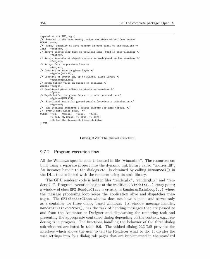
354 9. The complete package: OpenFX
typedef struct THD_tag {/* Pointer to the base memory, other variables offset from here*/UCHAR *ram;/* Array: identity of face visible in each pixel on the scanline */long *Zbuffer,/* Array: identifying face on previous line. Used in anti-aliasing */
*Xbuffer,/* Array: identity of object visible in each pixel on the scanline */
*Zobject,/* Array: face on previous line */
*Xobject,/* Identity of face in glass layer */
*Zglass[NGLASS],/* Identity of object in, up to NGLASS, glass layers */
*ZglassO[NGLASS];/* Depth buffer value in pixels on scanline */double *Zdepth,/* fractional pixel offset in pixels on scanline */
*Zposn,/* Depth buffer for glass faces in pixels on scanline */
*Zglassd[NGLASS],/* Fractional ratio for ground pixels (accelerate calculation */
*Zground;/* The scanline renderer’s output buffers for THIS thread. *//* over 3 anti-alias rows. */UCHAR *Red, *Green, *Blue, *Alfa,
*L_Red, *L_Green, *L_Blue, *L_Alfa,*LL_Red,*LL_Green,*LL_Blue,*LL_Alfa;
} THD;
Listing 9.20: The thread structure.
9.7.2 Program execution flow
All the Windows specific code is located in file “winmain.c”. The resources arebuilt using a separate project into the dynamic link library called “rnd res.dll”.An instance handle to the dialogs etc., is obtained by calling ResourceX() inthe DLL that is linked with the renderer using its stub library.
The GPU renderer code is held in files “rendergl.c”, “rendergl1.c” and “ren-dergl2.c”. Program execution begins at the traditional WinMain(..) entry point;a window of class OFX:RenderClass is created in RendererMainLoop(..) wherethe message processing loop keeps the application alive and dispatches mes-sages. The OFX:RenderClass window does not have a menu and serves onlyas a container for three dialog based windows. Its window message handler,RendererMainWndProc(), has the task of handing messages that are passed toand from the Animator or Designer and dispatching the rendering task andpresenting the appropriate contained dialog depending on the context, e.g., ren-dering is in progress. The functions handling the behavior of the three dialogsub-windows are listed in table 9.6. The tabbed dialog DLG TAB provides theinterface which allows the user to tell the Renderer what to do. It divides theuser settings into four dialog tab pages that are implemented in the standard

9.7. The Renderer module 355
Window Handle Resource ID Dialog Function Comment
hwndcontrol DLG TAB TabbedDlgProc Tabbed dialoghwndupdate RD UPDATE UpdateDlgProc Progress barshwndupdageX RD UPDATEX UpdateXDlgProc Progresswith preview
Table 9.6: The embedded dialog windows used by the Renderer to present its userinterface.
way described in the Win32 API documentation. The user settings are recordedin an instance of the PARAMLIST structure. These settings are passed to thefunction render(...) when it is called to commence the rendering process.
The tabbed dialog container has two large buttons that pass the commandmessage MENU FILE RENDERN to RendererMainLoop() to initiate the renderingprocess. It is at this point that there is an exchange of messages with the Ani-mator: The Renderer sends a message IDM CALLBACK ASCRIPT to the Animatorto instruct it to write a .SCR script file. When the Animator has written thescript file, it sends back a message to the Renderer IDM CALLBACK SETUP tellingit (the Renderer) that the script is written and rendering should commence. Onreceipt of the callback message the Renderer sends itself the go-code via messageIDM CALLBACK SETUP and function render(...) is called.
This seemingly convoluted message exchange allows the Renderer to appearto the user as if it is seamlessly integrated with the Animator. It can even renderits output image into the camera window within the Animator without appearingto have any user involvement at all.
Once render(...) gets started the rendering process needs no further in-tervention. The script is written and the remainder of the code is pretty muchindependent of the platform on which it operates. Inside render(..) the com-mand parameters are processed, variables are initialized, the script is read frameby frame, mesh data loaded, and either the software or hardware renderer exe-cuted. Listing 9.21 presents the key steps of function render(..).
9.7.3 The software renderer
This was the first renderer written for OpenFX and it has evolved over the yearsto include hybrid ray-tracing and concurrent rendering.
The arguments of the render() function are in the form of a list of textstrings (a legacy from the non-Windows entry point). These arguments specifythings like: image resolution, output format, controlling script file name, andray-tracer parameters. In function render() the script file is opened, and itsdescription of each frame in an animation or the objects in a specific scene areloaded. Then for each frame (or a single scene) the following steps are performed:
• GetCommand() (file loadscpt.c) reads all the .MFX files and assembles the

356 9. The complete package: OpenFX
int render(int argc, char **argv){..while(i < argc) /* process arguments */ .. i++; }}..if(AllocateRamBuffers() == FAIL)return FAIL // Allocate memory buffers}// open script fileif((CF=fopen((char *)scriptfile,"r")) == NULL)goto EXITPOINT;..NEXTFRAME:.. // process the script, load meshes etc.GetCommand( ... );SetPerspectiveView(); /* build view transformations */TransformSceneForRendering(..); /* move objects */// Rrender the scene using either the GPU or Softwareif(bRenderOpenGL){
RenderGL( ...); // GPU renderer..
}else{ // Software Renderer
if(RenderHide() == FAIL)failure=FAIL;..
}// store image in output buffer and output files..FREEPOINT:.. // end of frameFreeFrameObjects();if(Lights != NULL){X__Free(Lights); Lights = NULL;}if(trace_reflections || trace_refractions || trace_shadows)freeBST();goto NEXTFRAME;EXITPOINT:.. // clean upFreeAllObjects();FreeRamBuffers();free_render_discarded_list();ReleaseImageStore();if(CF != NULL)fclose(CF);return (int)failure;}
Listing 9.21: The render(..) function’s key steps.
data that describes the 3D models into the Renderer’s data structures (seelater). Objects are loaded in function R LoadObject() (file loadmesh.c).
• Once the objects have been loaded their vertex coordinates are transformedinto the coordinate system used by the Renderer. This is done in functionTransformSceneForRendering(). The coordinate system places the view-point at (0,0,0) with the direction of view (0,1,0) and the up vector (0,0,1).After this, the scene is rendered into the image memory buffer. This isdone by function RenderHide() (file render.c).
• The RenderHide() function is responsible for breaking up the scene intoscanline groups and dispatching them to each processor for rendering. It

9.7. The Renderer module 357
also applies some tricks to try and speed up the rendering process byswitching between two versions of the actual rendering algorithm: one foruse when anti-aliasing is to be applied, and one for use when anti-aliasingis not to be used.
Each scanline is passed to a function that does the actual rendering of thepixels in that scanline. Ultimately, the outcome of the calculations at apixel level are combined to form the final image.
• The function that carries out the rendering of a single scanline isRenderMultiThreaded().
Function RenderMultiThreaded() (file Render.c) is responsible for work-ing through the pixels on the given scanline. RenderMultiThreaded()
begins by obtaining any background value (e.g., from the sky or groundplane). It then loops through each object determining first strike polygons,and writing into the scanline buffer the identity of the polygon and objectthat are visible at each pixel on the scanline. (This process implementsthe hidden surface algorithm).
• Once the hidden surface algorithm determines what is visible, the ren-dering process can begin to determine the color values for the pixels onthe scanline. On completion of the rendering task the pixel image val-ues are stored temporarily so that anti-aliasing can be applied; they arethen written into the output buffer. (Functions AntiAliasLine() andScanlineToZbuffer() and ScanlineToZobject() carry out this task.)
• The core of the rendering process takes place in function ShadedScanLine()and its anti-aliasing equivalent FastAntiAliasedSchadedScanLine().ShadedScanLine() uses the information abut which object and polygonare visible in a pixel to commence the pixel rendering process.
• For every pixel on the scanline, the function GetRowPixelValue() is called.The arguments passed to this function contains all the information neces-sary to render what is visible in this pixel. GetRowPixelValue() is a thinwrapper for GetPixelValue() which renders each individual pixel. Thearguments to GetPixelValue() are:
1. the (i,j) image coordinates (of the pixel),
2. an identifier of the surface material properties of the polygon that isvisible in pixel (i,j),
3. the surface normal vector, and
4. the Z depth of that point.
It returns the (RGB) value to be written into the final output image.

358 9. The complete package: OpenFX
• GetPixelValue() (file Material.c) applies the lighting model and deter-mines the surface properties using information recorded about the surfacematerials data.
The pixel lighting model used in OpenFX is a simple diffuse illumina-tion model like that described in chapter 4 with the surface color beingdetermined from either a material specification (possibly including an al-gorithmic shader) or an image map that has been painted over the surface.Surface image maps, reflection maps, bump maps or transparency mapsare other possible options.
• When ray tracing is turned on, any surface with a material that has re-flectivity > 0 or transmissivity > 0 is further processed by calling one ofthe functions: trace transmission ray() or trace reflection ray()
to complete the rendering process. The trace xxx ray() (file Raytrace.c)functions are recursive. They call the function GetSurfaceValue() whichin turn calls GetPixelValue() to obtain the surface values.
An additional ray tracing function is used to determine shadows by tracingshadow rays from the surface point to each light source.
This brief tour through the Renderer’s code should give you all the cluesyou need to augment the software or to see how the algorithms described inchapters 4 and 5 can be applied in practice.
9.7.4 The hardware renderer
The GPU renderer is called into action after all the scene descriptions of a framein an animation have been read, the mesh models and picture maps loaded,material settings configured and geometric transformations applied. Thus, thecoordinates of all polygon vertices, and even the ground and sky, are positionedrelative to a frame of reference with the viewpoint located at (0, 0, 0) an up axisvertical along the z axis and the direction of view along the y axis. Of courseOpenGL uses a different arrangement of a right-handed coordinate system so inorder to maintain the same sense an additional axis mapping has to be included:x → x, y → −z and z → y.
The GPU renderer can target its output to an on-screen window, but sincethis limits the resolution it also offers an option to target its output to either ap-buffer or a renderbuffer attached to a FBO. It uses code based on the ideasexplained in section 7.4. In order to achieve an image quality to match the soft-ware renderer only hardware that supports a programmable pipeline can be usedfor this renderer. The choice of output is made in the function RenderGL(..)
which then dispatches execution to configure the output buffers. Again, most ofthe code required to prepare the output media has been discussed in chapter 7and it will not be discussed here again. Since OpenFX offers the simultaneoususe of four textures, surface, reflection, transparency and bump, a larger num-ber of two-dimensional textures have to be initialized. When rendering has been

9.7. The Renderer module 359
completed the OpenGL color buffers (and the depth buffer) have to be copiedinto the CPU buffers for writing to the output files. This done in two of thefunctions in the file “renergl.c”, CopyGLtoFSB() and CopyGLtoZdepth().
Irrespective of which output target is chosen, the scene is rendered from thecamera view in function RenderCameraView(...) in file “rendergl1.c”. As allthe vertices were transformed to match a camera located at (0, 0, 0) the scenecan be rendered without the need for any further transformations. However,to be able to deliver an anti-aliased result, the scene is drawn using a functionDraw3dScene() so that its output can be captured in an OpenGL display listthat is run several times with appropriate viewpoint pixel jitter. This approachto performing anti-aliasing on OpenGL generated images is discussed in the RedBook [82].
Function Draw3dScene(...) is the heart of the GLSL rendering engine. Itrelies on a number of sub-functions to render the mesh models: the ground andthe sky backdrop. The ground is presented as a flat quadrilateral. Using the firstlight and a reflection transformation, a shadow and reflection of the mesh modelsmay be rendered on the ground. By switching to an orthographic projection, aquadrilateral that fills the viewport is rendered into the background to representthe sky.
The rendering of the mesh models is achieved by partitioning their faces intothose that use (1) materials, (2) image maps or (3) neither materials nor maps.Faces exhibiting materials are further subdivided into those that are opaque andthose that are transparent or semi-transparent, with those that are opaque beingrendered first. Within this subdivision the polygons are rendered in the order oftheir material or image map. This allows external textures or image maps to beset up only once per frame. The small overhead of looping through all the facesin the mesh for every map and material is a small overhead when compared toswitching images in a 2D texture. The vertex and fragment shader codes thatare needed for the GPU renderer are located in the shaders folder. They areread and compiled as part of the initialization process (at the same time as therenderbuffer or p-buffer are created, function SetupRenderOpenGL()) by callingShadersInit(..) which may be found in file “shaders.c”.
This brief tour of the code of the GPU renderer has brought into focus howOpenFX deploys the GLSL and off-screen rendering to deliver a renderer thatalmost matches for quality, and exceeds for speed its software renderer. Hopefullyit will help you drill down into the code and follow it in detail so that you seehow the GLSL can be used in a real practical program.
9.7.5 The particle systems
The particle-system actors in OpenFX behave in a very similar way to the generalprinciple described in section 6.7 but with the extension that they are positioned,scaled and orientated using values obtained from the position, alignment andscaling timelines. If the script file, written by the Animator, directs a particle
360 9. The complete package: OpenFX
system to be present in a scene it will also define the properties of the system.However, a particle system actor is not like a normal actor because its appearancein a frame also depends on the time difference between the time of the frame andthe time at which the effect was initiated (e.g., in a burst of fireworks, where eachparticle of fire is located, during frame k depends on what frame the fireworkswere set off). Particle systems evolve; the position of the particles at frame n areusually determined from their positions during frame n− 1 often with a randomelement thrown in. Thus, in order to work out the appearance of a particlesystem for frame n, even when only rendering frame n, it is necessary to followthe evolution of the particle system, frame by frame, from its creation, right upto, and including frame n, even to the extent of making sure that the sequenceof any random numbers used gives the same result. This makes the task for theRenderer much harder.
The Renderer resolves the difficulties, outlined in the previous paragraph,by performing a full particle system evolution for every particle system thatexists during the rendering of frame n. Thus, for example, suppose a particlesystem has a costume that spans frames 10 to 20. When the renderer is workingon frame 12 it starts by working out the particle positions in frame 10 (at thestart). It then uses the frame 10 positions as the starting point for working outthe positions in frame 11. Then it uses the frame 11 particle states to workout the positions in frame 12. Having calculated what particles are where, whatthey look like, even if if they still exist (in frame 12), it will render them intothe output image buffer.
In any animation there could be many particle systems, these are recorded ina dynamically allocated list of ParticleSystem objects pointed to by the globalpointer variable *ParticleS . The global variable Nparticles gives a count ofthe total number of particle systems. The ParticleSystem and particle objectstructures are summarized in listing 9.22.
As each frame is loaded and while the objects are being moved into theirglobal position the particle systems are initialized by calling SetupParticles(..)from within the TransformSceneForRendering(..) function. Particle imagesare also loaded before rendering starts and if the OpenGL renderer is used,the images are converted into 2D textures. The set-up functions also performthe task of moving the state of the particle systems (and their particles) intothe state that they should be in during the frame being rendered, by callingUpdateParticleSystem(..);. (This step will take an increasing calculationtime as the animation progresses.)
All the code related to particle systems can be found in the file “particles.c”.Whilst there are a significant number of lines of code needed to deliver OpenFX’sparticle system’s behavior, it is basically repetition of the steps set out in theOpenGL example presented in section 7.5. The GPU and CPU renderers usecommon code to initialize and update the particle systems but they have to calltheir different functions to draw in their respective image buffers. The drawingfunctions are named RenderParticlesGL(...) and RenderParticles(..) and

9.7. The Renderer module 361
typedef struct Renderer_PARTICLE_tag{vector p,pl; /* position */vector v,g,dg;/* velocity and gravity */vector c; /* colour ( 0 - 1) */double fAlpha, ... ;/* Transparency */..
} Particle;
typedef struct Renderer_PARTICLESYSTEM_tag {vector pin; /* Base Position */../* Transformation of particle system object */double particle_object_transformation[4][4];long Rate; /* rate of creation per second */long NumP; /* number of particles */char ImageName[256]; /* Image filename */.../* Pointer to the particles in this particle system */Particle *particles;...
} ParticleSystem;
Listing 9.22: The particle system and particle data structures. Some of the membervariables have been omitted from this listing to force focus onto the Renderer significantmember variables.
they are called after the rendering of all the other elements in the scene havebeen completed.
9.7.6 Loading plug-ins
The Renderer uses three types of plug-ins: the Animator’s motion effect, thesurface material shaders and the image post-processors. All of these plug-ins areloaded as needed and released after rendering is complete. All are implementedas DLL libraries. The surface material shader differs from the other two typesof plug-ins because it has to remain active during the rendering process, andfunctions in the DLL will need to be called on a per-pixel basis. The motioneffect only need to be accessible during the preprocessing stage when the verticesof the mesh models are moved into their positions in the global frame of reference.By their very name, the image post-processors are only needed once renderinghas been completed and just before the image buffer is dumped into a picture ormovie file. Within the Renderer’s code all the plug-in modules are handled in thefile “plugins.c”. The mechanism of loading, accessing functions and unloadingDLL modules mimics that for the Animator and Designer.
The External material shader DLLs are loaded at the same time as the meshmodels are loaded by calling (LoadExternalTexture(...). At the same time asthe DLLs are attached, pointers to the external functions that render the shaderduring pixel calculations are obtained and stored in a shader structure so thatrendering of pixel is not penalized by having to find the function’s address every
362 9. The complete package: OpenFX
time it is needed. The shader structures are stored in a list that is pointedto by the global variable *Shader. If an external shader needs to be appliedto a polygon’s surface while rendering a pixel, the Shader list provides a directlookup for a pointer to the right function in the right library. Rendering of a pixelthat requires an external shader is done through RenderExternalTexture(...)
called from the core rendering function GetPixelValue(...).The animation motion effect is loaded and executed in ExternalFX(...) is
called from EffectObjectVertices(..) which executes as part of the set upphase. Image post-processing is done from within ExternalImageProcess(..)
which is called after all rendering has finished (at the end of function render(...)).Any DLL loaded by the Renderer remains attached until all frames have
been rendered. The number of loaded libraries is recorded by static variablenLibraryHandleListItems in file “allocmen.c”. Each library handle is recordedin a list of objects containing information about all the loaded DLLs. The list isaddressed by the static pointer LibraryHandleList. All external DLLs remainattached until the Renderer terminates, at which time they are released by callingFreeLibraryHandleList().
9.8 Adding to the software
To enhance the the range of modeling tools, imaging and animation effects, it isnot necessary to work directly with OpenFX’s Animator, Designer or Renderercodes. The software is designed in such a way that most of its functionalitycan be enhanced by writing plug-in modules. It is relatively easy to provide thefollowing additional components. The plug-in components are:
1. Modeling tools, used exclusively by the Designer.
2. Modeling actions, used exclusively by the Designer.
3. Animation templates, used exclusively by the Animator.
4. Material surface shaders, used by the Designer and the Renderer.
5. Animation motion effects, used by the Renderer and the Animator.
6. Image processors, used by the Designer and the Animator.
All instances of these plug-ins are created as Window’s DLLs that are loadedat runtime. Some may remain attached until the parent program terminates;others may complete their task and then be unloaded.
Full details of how to write these plug-ins are given on the OpenFX website,but it is worth explaining a couple of the important principles of this process.The most important thing to be able to do in a plug-in module is to gain accessto the data that the parent program is holding. It is also important to be able

9.8. Adding to the software 363
to use some of the functions that exist within the main program. Sometimesthis is called an API or library. In the case of OpenFX there is a mechanism inplace that provides access to most global variables and functions of the parentprograms, without the need to link any of the DLLs with an API or other library.
9.8.1 Accessing global variables and main program functions
OpenFX uses a pointer mechanism for granting the plug-ins access functionsin the parent program and the parent program’s global variables. Since allOpenFX plug-ins are DLLs that are loaded into the main application’s addressspace, all global functions and variables can be accessed by any loaded DLL. Itis only a matter of knowing where they reside in memory. OpenFX facilitatesthis by providing a collection of C/C++ pointers. The plug-in DLLs are notloaded when the main application starts.4 They are loaded when required andunloaded when the user is finished using them. In the case of plug-ins thatare used in the Designer or Animator and are needed by the Renderer (e.g.,procedural textures) then the Renderer loads all the needed plug-ins when itreads the script file during initialization. The Renderer unloads the plug-inswhen it is finished with the script.
In the case of an external animation template plug-in, when the Animatorwishes to use the template it calls the ExternalPreset(..) function with twoarguments: (HWND parent, and ANI STRUCTURE *lpevi). The first argument isa handle to the container’s window that is used in the generation of the modelessdialog box that allows the user to enter the template’s parameters. The third pa-rameter, the lpevi parameter, is a pointer to the instance of the ANI STRUCTURE
data structure. This instance contains pointers to the Animator’s global vari-ables and its most useful functions. Part of this structure is shown in listing 9.23.
Full details of the members of the ANI STRUCTURE structure can be foundin the code documentation; here we mention the most important. The globalvariables and functions referenced in this structure allow the developer to pro-grammatically generate animations of any complexity and length. Some of thevariables and function arguments refer to other OpenFX specific data types. Def-initions for these as well as many useful constants are included in the “struct.h”file. The Animator keeps only one copy of this structure. It is initialized atstart-up, and passed to the preset plug-in. By using the members of this struc-ture any plug-in can access the functions used internally by the Animator. Thismethod is a very simple and a very flexible method of allowing plug-ins to accessglobal data and functions in the calling programs.
In order that the contents of structures like ANI STRUCTURE can be madeavailable to all functions and files in a plug-in the pointers passed to the func-tions are normally transferred to a global variable. The global variable is then
4Many of the built-in actions are also implemented as DLLs that are loaded when theprogram starts.
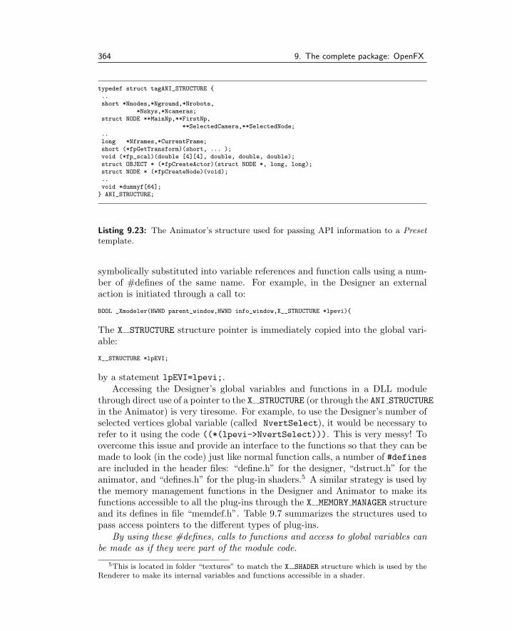
364 9. The complete package: OpenFX
typedef struct tagANI_STRUCTURE {..short *Nnodes,*Nground,*Nrobots,
*Nskys,*Ncameras;struct NODE **MainNp,**FirstNp,
**SelectedCamera,**SelectedNode;..long *Nframes,*CurrentFrame;short (*fpGetTransform)(short, ... );void (*fp_scal)(double [4][4], double, double, double);struct OBJECT * (*fpCreateActor)(struct NODE *, long, long);struct NODE * (*fpCreateNode)(void);..void *dummyf[64];} ANI_STRUCTURE;
Listing 9.23: The Animator’s structure used for passing API information to a Presettemplate.
symbolically substituted into variable references and function calls using a num-ber of #defines of the same name. For example, in the Designer an externalaction is initiated through a call to:
BOOL _Xmodeler(HWND parent_window,HWND info_window,X__STRUCTURE *lpevi){
The X STRUCTURE structure pointer is immediately copied into the global vari-able:
X__STRUCTURE *lpEVI;
by a statement lpEVI=lpevi;.Accessing the Designer’s global variables and functions in a DLL module
through direct use of a pointer to the X STRUCTURE (or through the ANI STRUCTURE
in the Animator) is very tiresome. For example, to use the Designer’s number ofselected vertices global variable (called NvertSelect), it would be necessary torefer to it using the code ((*(lpevi->NvertSelect))). This is very messy! Toovercome this issue and provide an interface to the functions so that they can bemade to look (in the code) just like normal function calls, a number of #definesare included in the header files: “define.h” for the designer, “dstruct.h” for theanimator, and “defines.h” for the plug-in shaders.5 A similar strategy is used bythe memory management functions in the Designer and Animator to make itsfunctions accessible to all the plug-ins through the X MEMORY MANAGER structureand its defines in file “memdef.h”. Table 9.7 summarizes the structures used topass access pointers to the different types of plug-ins.
By using these #defines, calls to functions and access to global variables canbe made as if they were part of the module code.
5This is located in folder “textures” to match the X SHADER structure which is used by theRenderer to make its internal variables and functions accessible in a shader.
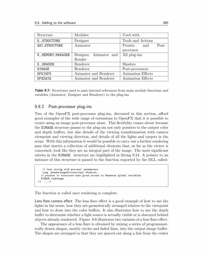
9.8. Adding to the software 365
Structure Modules Used with
X STRUCTURE Designer Tools and ActionsANI STRUCTURE Animator Presets and Post-
processorX MEMORY MANAGER Designer, Animator and
RenderAll plug-ins
X SHADER Renderer ShadersXIMAGE Renderer Post-processorsSFXINFO Animator and Renderer Animation EffectsSFXDATA Animator and Renderer Animation Effects
Table 9.7: Structures used to pass internal references from main module functions andvariables (Animator, Designer and Renderer) to the plug-ins.
9.8.2 Post-processor plug-ins
Two of the OpenFX post-processor plug-ins, discussed in this section, affordgood examples of the wide range of extensions to OpenFX that it is possible tocreate using an image post-processor alone. This flexibility comes about becausethe XIMAGE structure passes to the plug-ins not only pointers to the output colorand depth buffers, but also details of the viewing transformation with cameraviewpoint and viewing direction, and details of all the lights and targets in thescene. With this information it would be possible to carry out a further renderingpass that inserts a collection of additional elements that, as far as the viewer isconcerned, look like they are an integral part of the image. The most significantentries in the XIMAGE structure are highlighted in listing 9.24. A pointer to aninstance of this structure is passed to the function exported by the DLL called:
// text string with process’ parameterslong _RenderImageProcess(char *PrmList,
// pointer to structure that gives access to Renderer global variablesXIMAGE *lpXimage
){ ....}
The function is called once rendering is complete.
Lens flare camera effect The lens flare effect is a good example of how to use thelights in the scene, how they are geometrically arranged relative to the viewpointand how to draw into the color buffers. It also illustrates how to use the depthbuffer to determine whether a light source is actually visible or is obscured behindobjects already rendererd. Figure 9.6 illustrates two variants of a lens flare effect.
The appearance of a lens flare is obtained by mixing a series of programmat-ically drawn shapes, mostly circles and faded lines, into the output image buffer.The shapes are arranged so that they are spaced out along a line from the center

366 9. The complete package: OpenFX
typedef struct Renderer_XIMAGE_tag {double ViewTransform[4][4]; /* viewing transformation matrix */double Xscale,Yscale; /* scaling for camera field of view */long Frame; /* frame being rendered */long Xmax,Ymax; /* dimensions of the image */long Nlights; /* number of lights present */light *Lights; /* pointer to array of light structures*/long Ntargets; /* not used yet */vector *Targets; /* not used yet */fullscreenbuffer *Screen; /* pointer to screen buffer */double *Zbuffer; /* pointer to Z depth buffer */.... (omitted)double *ViewPoint; /* Camera viewpoint (vector) */double CamPhi; /* Camera setting */double CamTheta; /* " */double CamAlpha; /* " */double CamSx; /* " */double CamSy; /* " */double CamSz; /* " */char *aParameters; /* parameter list for current effect */char *mParameters; /* morph parameters (morphing from) */long version; /* version LITE / PRO /DEMO */short (*fp_Terminate)(void);/* test for termination */void (*fp_Yield)(void); /* yield for app messages */.. (omitted)} XIMAGE;
Listing 9.24: The structure used to pass references for the Renderer’s data to thepost-processor plug-ins.
of the image to the location of the light that is giving rise to the effect. Drawingshapes is probably not the best way to render the visual elements of a lens flare;a better approach would be to design the lens effect in an art program, divideit up into a number of elements, save these as individual images and then scaleand blend the images into the output buffer.
The lens flare effect is delivered in two source files: “lens.c” and “lens1.c”.The effect’s entry point in is “lens1.c”. Three types of flare are simulated andmost of the code is contained within the entry function RenderImageProcess(..).In a case where the position of a light is specified as a parameter of the effect, itscoordinates have to be transformed to match the camera view point and orienta-tion. This is done using the viewing transformation made available through theXIMAGE structure. It is applied in the utility function TransformIntoView(..)
which performs a straightforward 4 × 4 matrix multiplication. Any lights inthe scene will have already been moved by the Renderer and if one of thoseis involved in the effect then its identity will have been stored as part of theparameter settings.
Most of the remainder of the code is associated with (1) drawing the parts ofthe effect into the framebuffer which is referenced through the XIMAGE pointerlpXimage->Screen, or (2) providing a modal dialog for use by the Animatorto define the parameters of the effect. The user’s configuration dialog is cre-

9.8. Adding to the software 367
ated and used in response to a call from the Animator to the exported function:SetExternalParameters(...). This effect’s dialog is relatively complex be-cause it offers tabbed pages in which the user can set multiple parameters. Italso offers a small window in which the appearance of the lens flare can be sim-ulated. Despite these complexities, the dialog coding conforms very closely tothat of a standard Win32 API tabbed dialog.
An example atmospheric effect The atmospheric effect is a good example of howan additional rendering step can be added in post-production. Post-productioncan add a volume rendering step, in which the depth buffer and the spotlightshadow buffers can be used to provide the appearance of a dusty atmosphere.To render the volume effect, a ray originating at the viewpoint is traced throughthe scene until it passes beyond the rear-clipping plane. Each ray is traced insmall incremental steps gradually accumulating a small (and randomly gener-ated) increase in the proportion of scattered light seen in that pixel. This is avery approximate model, to be physically accurate, a real model for scatteringwould need to be made. However, tracing a ray in small steps even with only afew steps, for every pixel is a considerable computational burden, and thereforethis approximation is made.
Figure 9.6 illustrates a couple of examples of the use of this effect where aspotlight shines into a dusty (highly scattering) environment. The effect offers afew variants. This section will only discuss the model in the case of spotlights.Spotlights are the only type of light that can usefully be used in OpenFX be-cause in order to simulate the appearance of the shadowing one sees in a dustyenvironment it is necessary to determine the shadow state that applies at eachpoint along the line that is traced out into the scene. Using the shadow state,the fraction of the scattered light to be mixed into the image from dust/parti-cles/water vapor etc., in the environment may be determined. The shadow stateof any point along a ray may be determined by working out where that segmentlies in 3D space and (for spotlights) looking up their shadow depth buffer to seeif that point is in the shadow of some object or not.
Using this explanation of the concept that underlies the method ofrendering the effect, it is not difficult to follow the logic of the code.RenderImageProcess(..) is the entry point. Each light is then consideredin turn, followed by execution of the nested loops to work through every pixelin the image. In the case of spotlights, the tracing ray is checked to see if itpasses through the cone of illumination. When it does not, there is no need toproceed further as the viewing ray is not illuminated and therefore does not scat-ter any light. When the viewing ray does pass through the spotlight cone, it isnecessary to integrate along the ray summing up the scattering component overthose stretches in which it is not obscured from the light source by any interven-ing objects. Any point that falls within a spotlight’s shadow volume can haveits shadowing state determined without tracing a shadow ray through the scene.
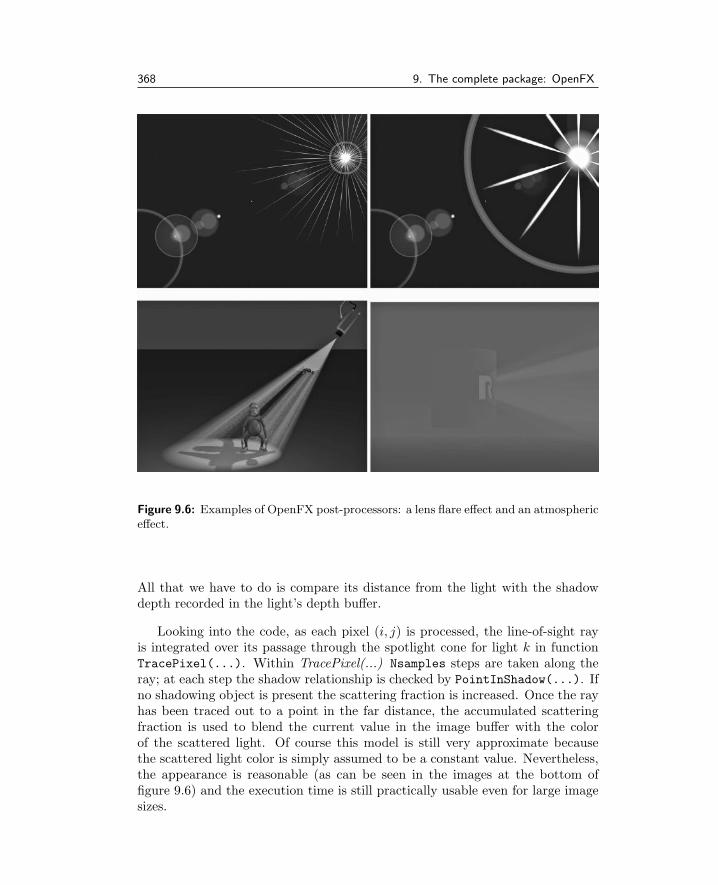
368 9. The complete package: OpenFX
Figure 9.6: Examples of OpenFX post-processors: a lens flare effect and an atmosphericeffect.
All that we have to do is compare its distance from the light with the shadowdepth recorded in the light’s depth buffer.
Looking into the code, as each pixel (i, j) is processed, the line-of-sight rayis integrated over its passage through the spotlight cone for light k in functionTracePixel(...). Within TracePixel(...) Nsamples steps are taken along theray; at each step the shadow relationship is checked by PointInShadow(...). Ifno shadowing object is present the scattering fraction is increased. Once the rayhas been traced out to a point in the far distance, the accumulated scatteringfraction is used to blend the current value in the image buffer with the colorof the scattered light. Of course this model is still very approximate becausethe scattered light color is simply assumed to be a constant value. Nevertheless,the appearance is reasonable (as can be seen in the images at the bottom offigure 9.6) and the execution time is still practically usable even for large imagesizes.

9.9. Continuing to dissect OpenFX 369
9.9 Continuing to dissect OpenFX
This chapter has provided the major clues that should let you get to grips withthe OpenFX program code and follow the fine detail of algorithm implemen-tation that we don’t have the space to cover here in great, or even modest,detail. OpenFX is a fully practical code and implements most of the algorithmsdiscussed in the rest of this book. It even uses the OpenGL coding concepts ofchapter 7. The code presents a complete picture of how to do it in practice—andremember, this 3D package probably has the shortest and most compact code ofany 3D application program of comparable power.
I hope that this chapter and the preceding ones in part II will provide youwith a good reference on how to do what you want to do with 3D graphicsand gives you some practical code that you can plug and adapt in your ownapplications.

This page intentionally left blankThis page intentionally left blank

Part III
Practical algorithms for modeling
and procedural textures

This page intentionally left blankThis page intentionally left blank

Introduction to part IIIThe two chapters in part III leave behind basic principles and introduce somespecific and more sophisticated, yet still practically useful, topics.
The modeling algorithms described in chapter 10 were chosen because theyconstitute some of the most essential tools for constructing polygonal modelsalgorithmically (as opposed to a simple tool that allows a program’s user todraw a curve in 3D); for example, triangulating an arbitrary polygon (that mightcontain holes) is a very tedious job when done manually. As another example, theboolean operations that are easy to perform on a model made up from a collectionof procedurally defined primitives are very difficult to create in an arbitrarynetwork of triangular polygons. But since many shapes are very difficult tobuild using any other method, it is something that we must be able to do.6 Thesealgorithms pose an interesting technical challenge (due mainly to the inabilityof any computer to perform arithmetic to arbitrary precision) as opposed tosomething simple, but still useful, like duplicating parts of a model.
The textures developed in chapter 11 have been chosen, first, because theyare visually appealing and have some novelty. But they are presented primarilybecause they cover a comprehensive range of classes of textures:
• Geometric: with well defined shapes and patterns, e.g., dots.
• Periodic: based on oscillatory functions, sinusoids, or combinations of si-nusoids, e.g., water waves.
• Random: based on pseudo random numbers, the famous fractal texturesare a form of these. However in chapter 11 the textures show how to extendthe Perlin noise based textures by mixing in some regularity.
And of course all these classes can be subdivided into those that perturb thesurface color, those that perturb (bump) the surface normal vector, or thosethat do both. Equipped with the code for these classes of shader it should beeasy for you to combine them, or adapt them to build your own unique designs.
Note: Consult the website to obtain the annotated code listings for thesealgorithms and both C and GLSL code versions of the shaders. Examining theOpenFX package source code is also a good way to see how these algorithms fitinto a fully equipped practical package.
6Even deciding whether a polygonated 3D model has a hole in it or not is considerablechallenge in practice—something that is necessary for boolean operation.
373

This page intentionally left blankThis page intentionally left blank

10Modeling with polygonal
datasets
In creating models of objects for use in computer animation and visualizationprograms the most popular and versatile approach is to build them from a largenumber of very simple primitive planar polygons. Highly successful professional3D animation programs and most computer games use this approach. It wouldbe quite impractical to build polygonated models by entering lists of facets andvertex positions on a keyboard. In all useful programs the computer providespre-built collections of flat triangular or rectangular polygons to represent prim-itive shapes such as cylinders, spheres and torii. It is rarely sufficient to limitthe modeling process to a simple combination of primitive shapes and thereforeapplication programs must provide a wide variety of algorithmic procedures tohelp the user combine and manipulate the basic shapes as well as creating othermore complex ones.
It is within this context that we may state: The primary goal of a modelingalgorithm is to construct medium to high complexity shapes automatically frombasic planar polygons. For example the helical tube illustrated in figure 4.27 andthe ribbon in figure 4.38 were both constructed algorithmically by creating andcombining many triangular polygons.
Any algorithm which builds models by combining polygonal shapes (trian-gles or quadrilaterals) must do so within a framework imposed by the way thespecification of the model is recorded. Chapter 3 investigated a number of com-monly used recording strategies and data structures to hold the specificationof the model. Those components of a model’s specification that are essentialfor the procedures described in this chapter are: the vertex, the edge and the(planar polygonal) facet. Since any planar polygonal facet can be reduced to aset of triangular facets (by the first algorithm to be discussed) all the remainingalgorithms we will consider use triangular polygons.
Even the longest and most involved procedures can be broken down into anumber of steps which themselves can usually be further subdivided. All ofthem will be written as a sequence of logical steps that are readily translatedinto whatever computer language happens to be currently in favor. Most callupon the geometric mathematics discussed in chapter 2.
375

376 10. Modeling with polygonal datasets
In order to keep the length of each algorithm as short as possible it is appro-priate to define a few procedures that perform basic tasks. The most fundamentalof these create new elements in the description of a model, a vertex, an edge, ora facet (polygon). These procedures which we call:
newV (x, y, z) Create a new vertex at coordinates (x, y, z).newE(v0, v1) Create a new edge joining vertices v0 and v1.newF (v0, v1, v2) Create a new facet with v0, v1 and v2 as its vertices.
belong to a group that manages data structures of the type described in chapter 3.Each function returns an index for the new item in the array of items. In analternative implementation the same functions might instead return a pointer toa new item at the end of a linked list. We will assume that in practice theseprocedures handle any internal failure, possibly as a result of shortage of storagespace. In the same class of function, procedures to remove one or more objects ofeach type from the database will be needed. A neat way to do this is to use a flagin the data structure for each element which if set will cause that element to bedeleted during the execution of a deleting procedure (for that type of element).This is discussed in section 3.3 and figure 3.7.
deleteV () Remove all flagged vertex objects from the description database.deleteE() Remove all flagged edge objects from the description database.deleteF () Remove all flagged facet objects from the description database.
Other helper procedures will be called upon to make lists, for example, makea list holding the identity of a group of vertices connected together, or make apath among a list of connected edges as illustrated in figure 10.1.
10.1 Triangulating polygons
This is one of the longer algorithms to be considered in this chapter, but itplays a key role in a number of others too. It is used not only to reduce ann sided polygon to a combination of triangular polygons but also to add facetsthat cover or cap the inside of a curve recorded as a set of edges. Capping isa vital step in building 3D models of text characters, such as those shown infigure 2.30. TrueType or postscript font systems describe their characters as aset of outlines. For a 3D model of a text character to be of any use the interiorof the characters must be filled with facets so that they can be colored, texturedand interact with the lighting. Incidentally, reducing an n sided polygon to a setof triangles to all intents and purposes requires the same algorithm as one thatcaps a closed path of n line segments. So we really only need to consider onealgorithm.

10.1. Triangulating polygons 377
List of vertices in path
10
10
15
15
23
23
1111
22
7
7
6
6
9
9 4
4
Figure 10.1: The action of a helper function GetPath(sid) to build a list (shown onthe right) which sequentially identifies each vertex starting at sid and is connected byedges forming a path. The procedure will stop when the path can go no further or aloop back to the start occurs.
One final comment in the preamble to this chapter: an enormous simplifica-tion can be made in cases where a polygon to be triangulated is convex. However,a significant complication is introduced if the polygon has a hole in it, so muchso that a discussion about capping of polygons with holes is postponed untilsection 10.2.
10.1.1 The case of convex polygons
Let’s look at the simple case first: Section 4.2 gave a definition of a convexpolygon, say called P , the implication of which is that a triangulation maybe simply obtained by adding a vertex V anywhere inside the polygon, edgesjoining V to all vertices of P , and facets between V and two adjacent vertices ofP . This forms a structure known as a triangle fan, one of which is illustrated infigure 10.2. The algorithm given in listing 10.1 creates a triangle fan.
10.1.2 Non-convex polygons
When it comes to filling non-convex (concave) polygons the approach describedin section 10.1.1 will not work. Figure 10.3 illustrates the problem. Some of thenew edges fall outside the polygon and some of the new facets overlap each other.A strategy must be devised that does not let new edges or facets fall outside theoriginal boundary of the polygon. It does not really matter whether additionalvertices are added or not.
Before developing an algorithm for a capping procedure that applies to non-convex polygons consider the following tentative procedure for capping the 8sided polygon shown in figure 10.4. Start with the 8 sided polygon, then: (a) Addan edge between vertices 0−2. This makes a facet with vertices 0−1−2. (b) Add

378 10. Modeling with polygonal datasets
3
n–2
n–2
n–1
V
Vn–1n–2
n–1
2
3
2
1
1
V
0
0
0
1
2
3
Figure 10.2: Triangulating a convex n sided polygon. Once additional vertex V iscreated, edges and facets are added linking V to the original n vertices.
Find a point (xc, yc, zc) that lies inside the polygon.
(Possibly, a point halfway between vertices 0 andn
2)
Add a vertex: newV (xc, yc, zc)(This is vertex number n.)Repeat for 0 ≤ i < n {
Add edge between vertices n and i: newE(n, i)}
Repeat for 0 ≤ i < n− 1Add facet: newF (n, i, (i+ 1))}
Add facet (linking back to the start): newF (n, (n− 1), 0)
Listing 10.1: Algorithm to replace an n > 2 sided convex polygon with n triangularfacets. The vertices are labeled 0, 1, 2, . . . , (n− 1).
another edge, 2− 4. Again a facet is made between vertices 2− 3− 4. Similarlyadd edges 4 − 6 and 6 − 0. (c) Having returned to vertex 0 this completes thefirst pass through the algorithm. The original 8 sided polygon has been partiallycapped but a hole is left in the center.
Suppose we now consider the edges joining vertices 0− 2 − 4 − 6 − 0 as a 4sided polygon. To cap this all we would have to do is go back and repeat theprocess. Joining vertices 0− 4 adds a facet with vertices 0 − 2− 4. This leavesa single three sided polygon 0 − 4 − 6 which can be immediately turned into afacet to complete the capping procedure as shown in figure 10.4(d).
With a little refinement this simple idea can be automated to give an algo-rithm that will cap (triangulate) any nearly planar (convex or concave) outline(polygon boundary) provided that there are no holes in it. The ‘little’ refinementmentioned is necessary because it is not always possible to join vertices like 0−2
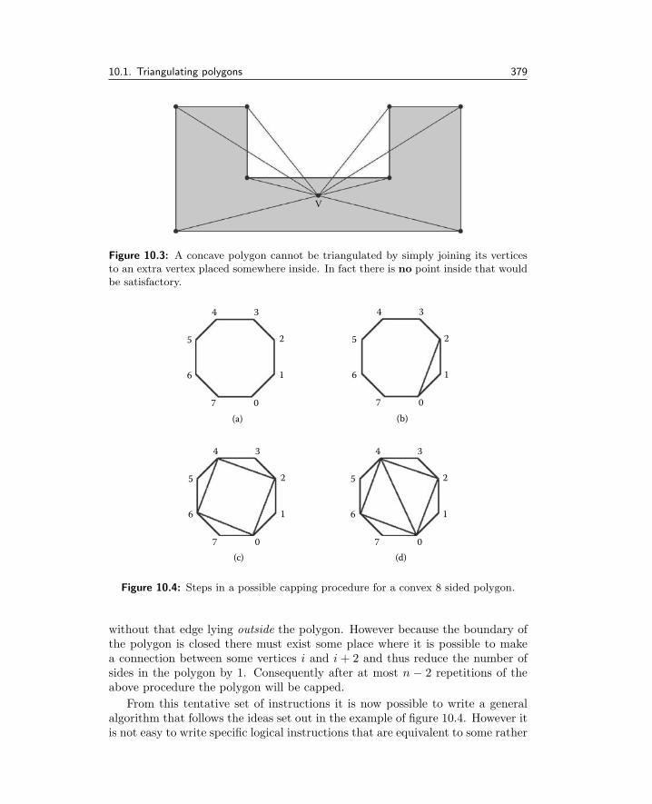
10.1. Triangulating polygons 379
V
Figure 10.3: A concave polygon cannot be triangulated by simply joining its verticesto an extra vertex placed somewhere inside. In fact there is no point inside that wouldbe satisfactory.
4 3
25
6
7 0
(d)
1
4 3
25
6
7 0
(c)
1
4 3
25
6
7 0
(b)
1
4 3
25
6
7 0
(a)
1
Figure 10.4: Steps in a possible capping procedure for a convex 8 sided polygon.
without that edge lying outside the polygon. However because the boundary ofthe polygon is closed there must exist some place where it is possible to makea connection between some vertices i and i + 2 and thus reduce the number ofsides in the polygon by 1. Consequently after at most n − 2 repetitions of theabove procedure the polygon will be capped.
From this tentative set of instructions it is now possible to write a generalalgorithm that follows the ideas set out in the example of figure 10.4. However itis not easy to write specific logical instructions that are equivalent to some rather

380 10. Modeling with polygonal datasets
vague statements. For example, to comply with the wishes of the instruction “...this reduces the number of sides by one, repeat the procedure with the remainingsides ...” some way of logically recognizing that an edge has been removed fromthe polygon must be found. Probably the best approach to resolve this specificissue is to design and use temporary data structures. The temporary structureswill be used only during the execution of a particular algorithm. When it finishesresources allocated temporarily will be released.
The advantage of using temporary structures is that the primary vertex, edgeand facet structures that record the description of a model don’t have to changeto facilitate specific needs of the procedure.
A suitable format for recording the temporary information is a list of n struc-tures, List(i). Each structure (List(i)) will correspond to one of the vertex/edgepairs that constitute the border of the outline to be capped and it will recordthe following information:
Vid A pointer to (identifier for) the vertex associated with this item.Ll An index into the list indicating the previous vertex that has not yet
been eliminated.Ln An index into the list indicating the next vertex that has not yet been
eliminated.ff A flag to indicate whether this item needs no further consideration.p The position vector recording the location of the vertex Vid.n The normal to the edge associated with this item.
The n items in List(i) will be ordered sequentially round the border of thepolygon (a border which must form a closed loop). The edge associated withitem i in the list joins the vertex for item i to the vertex for item i+1. The edgeassociated with item n− 1 joins the vertex for item n− 1 to the vertex for item0. For the example illustrated by figure 10.4 the initial state of the list is shownin figure 10.5.
The purpose of the entries Ll and Ln are to allow the algorithm to skip overthose edges that have been eliminated as the reduction continues. The membersni and pi are important in determining whether it is possible to join vertex iwith vertex i + 2 (i.e., determining whether the candidate edge lies inside theborder). The normal to the plane in which the polygon lies, n, is also necessaryfor this determination.
At first sight it would appear that it should be obvious whether an edgejoining vertices i and i+2 lies inside or outside a closed polygon (see figure 10.4)but there are two problems:
1. In three dimensions what does it mean to say: Inside of a polygon? Theanswer is: There is no meaning, unless we assume that the curve is planarand the concept of inside and outside is applied in the two-dimensionalsense to the plane in which the polygon lies.

10.1. Triangulating polygons 381
List Vid
0
1
2
3
4
5
6
7
1 (105)
0(103)
2 (143)
3 (121)4
5
6
7
p0
103
105
143
121
171
192
201
111
LI
7
0
1
2
3
4
5
6
Ll
1
2
3
4
5
6
7
0
ff
1
n
n0
n0
Edge 0
p
p0
1
1
1
1
1
1
1
Figure 10.5: The contents of the temporary vertex/edge list before the first step of theexample given in figure 10.4. The numbers shown in brackets beside the list of indicesare vertex identifies; for example the first vertex in the list is vertex number 103.
2. Even in two dimensions how does one algorithmically tell if a point liesinside or outside a curve? A human observer seems to find this a simplething to do provided the curve is not too convoluted.
To test whether an edge joining vertices i and i+ 2 lies inside the boundaryor not it is sufficient to test the mid-point, given by:
pm =1
2(List(i).p+ List(i+ 2).p)
lies inside the boundary. A test should be made to see if this new edge intersectsother edges in the boundary. The latter requirement need only be satisfied byedges not adjacent to either vertices i or i+ 2. Edges adjacent to vertices i andi+ 2 cannot possibly intersect an edge joining vertices i and i+ 2.
Thus, referred to a two-dimensional plane containing a closed curve C, thetest of whether a point P lies inside C is a three-step process:
1. From P draw a line in any direction until it is far away from C. (Say outto a circle which is large enough so that it encloses all of C and containsP .)
2. Move along the line from P counting the number of times C crosses theline.
3. If the count is an odd number then P is inside C; otherwise P is outsidethe curve.
This is called the Jordan curve theorem (see Haines [33]). Figure 10.6 illustratessome examples of the use of this test. This simple procedure works because: Togo from being inside to being outside C (or vice versa), C must be crossed. Togo from inside to outside and back to inside, or outside to inside to outside Chas to be crossed an even number of times.

382 10. Modeling with polygonal datasets
(d)
L
Pc
(e) (f )
(a) (b) (c)
Figure 10.6: Some examples of testing whether the point P lies inside the curve C.(a) 0 crossings outside. (b) 3 crossings inside. (c) 0 crossings outside. (d) 1 crossinginside. (e) 4 crossings outside. (f) 2 crossings outside.
It is important to keep in mind that in all the algorithms described in thischapter curves are represented by a finite number of straight line segments. Thusto test how many times the line L, from P , crosses C we have to only to checkL against each segment of C. There is no need to worry about going far enoughalong L because we are essentially checking every point on C. Since L can intheory be any line at all it is appropriate to choose something simple, say a lineat right angles to the edge for which pm is the mid-point.
Unfortunately, the accuracy of computer calculations can cause even thissimple test to go wrong. To see this look at the example in figure 10.7(a). Doesthe test line cross C within edge i or edge i+1? The answer is critically importantbecause if the calculation shows that it crosses both then the test will deliver anerroneous result. The only way to ensure a correct answer is to be very carefulin determining intersections that occur near the ends of the edges that make upC. For example one might say that if L intersects edge i within a very smalldistance of the end joined to edge i+ 1 the test for intersection with edge i+ 1would not be done. This would work for cases like figure 10.7(a) but in 10.7(b),alas, another mistake would occur.
To avoid all these problems the following action can be taken: If the inter-section between L and C is near the end of edge i don’t check edge i+1, insteadcheck to see if vertices Vi and Vi+2 are on the same side of L. If they are, thenL does not cross C, otherwise it does. One final complication: If a piece of C isparallel to L ignore it, e.g., as in Figure 10.7(c), but don’t forget that the vertexcomparison now applies to Vi and Vi+3.
In the preceding discussion it was assumed that containment was tested for intwo dimensions. The capping algorithm requires that the polygon be planar but

10.1. Triangulating polygons 383
(b)
(a)
(c)
L
Vi+1
Vi
Vi+2
i+1
i+1
i+2L
Vi+2
Vi+3
Vi+1Vi
P
P L
i
Edgei
P
Figure 10.7: The tricky question: Does line L cross C in segment i or segment i+1 ornot at all?
Fence
ni^
n
Figure 10.8: Fencing in a polygon prior to testing whether or not an edge lies inside apolygon’s boundary.
not necessarily lying in the (x, y) plane, i.e., that all the vertices lie in some planeso that it is possible to determine a single n for the plane of the polygon. Theplane may however be orientated in any direction. Therefore, all the calculationsfor containment must be performed in the plane of the polygon. One couldimagine finding an inverse transform that brings n in line with say the z axis,apply it to the vertices around the polygon and make the edge crossing tests inthe xy plane. The alternative is to make the edges take on a three-dimensionalcharacter by placing small rectangular planes parallel to n and lying along eachedge of the polygon, what might be described as fencing it in; see figure 10.8. Itdoesn’t really matter how the test is done; both approaches are subject to thesame problems of accuracy and the result they deliver is the same.
Once allowance is made for these complications we can set out an algorithmfor capping any closed polygon C, given that it is recorded as n straight edgesin an array of structures List(i). The algorithm is presented in listing 10.2.

384 10. Modeling with polygonal datasets
For the n edges making up C build the array holdingList(i), the temporary data discussed in the text.
Set the current index indicator i = 0.Set the number of edges remaining to be eliminated: m = n.
Repeat the following while m > 3 {Get the next two entries in the list. j = List(i).Ln and k = List(j).Ln
Test whether an edge joining vertices List(i).Vid and List(k).Vid
lies inside the polygon. If it does then: {Add an edge: newE(List(i).Vid, List(k).Vid)Add a facet: newF (List(i).Vid, List(j).Vid, List(k).Vid)Flag list entry j as begin invalid: List(j).ff = 0Switch it out of the list: List(i).Ln = k and List(k).Ll = iReduce the number of valid entries in the list: m = m− 1
Update the normal List(i).n to take account of the fact thatedge i replaces edges i and j and thereforejoins vertices List(i).Vid and List(k).Vid.
Move on to the next edge. Set i = k}
Otherwise {Move on to the next edge to try again. Set i = j
}}
Make a facet with the remaining three valid edges.(with the vertices for those entries for which List().ff = 1)
Listing 10.2: An algorithm to cap a planar polygon. It can also be used to cap a singleclosed piecewise linear curve, one that does not loop or consist of several pieces.
Revisiting the inside outside question Associated with the decision as to whetheran edge falls inside or outside the bounding outline are two problems that warrantadditional comment. They are illustrated in figure 10.9.
1. In the case of the polygon illustrated in figure 10.9(a) an edge e, joiningvertices i and i + 2, lies along the border of the polygon C. If insertedit would create a triangle with zero area. To prevent the need to ask thequestion whether the mid-point of e is inside or outside C (which is not aneasy question to answer) a preemptive test for co-linearity between linesjoining vertices i to i+ 1 and i to i+ 2 should be performed. This can bedone by creating vectors for the direction of these lines and testing that thedot product > (1− ǫ) where ǫ is of the order of magnitude of the precisionof the calculation.

10.2. Triangulating polygons with holes 385
(a)
i
i+1i–1
i+2
i+1
Pm
i+2C
C
(b)
i
Figure 10.9: Additional tests will need to be added to the procedure for determiningwhether a point lies inside an polygon. In (a) an edge joining vertices i with i+2 wouldform a triangle with zero area. In (b) the edge joining vertices i with i+ 2 is partiallyoutside the polygon.
2. In the situation illustrated in figure 10.9(b) the mid-point of the edgejoining vertices i and i+2, pm is inside C but other edges of C intersect it.In this case vertex i should not be joined to vertex i+2. To prevent edgesbeing falsely labeled as internal an additional test should be performed tocheck whether any edge in C crosses the proposed edge (the one betweenvertices i and i + 2). In making this test all the edges in C should bechecked except those linked to vertices i and i+ 2, i.e., the edges i− 1, i,i+ 1 and i+ 2.
Notes:
1. For a polygon that is planar any three vertices which are not co-linear canbe used to determine the normal n of the plane in which the polygon lies.
2. No matter how careful one is in making the calculation there will alwaysbe the potential for the algorithm to make a mistake. So in any practicalimplementation care should be taken to build in an escape mechanism.
O’Rourke [65] and De Berg [19] offer a rich source of algorithms for computationalgeometry problems like capping.
10.2 Triangulating polygons with holes
The algorithm developed in section 10.1 was restricted to capping an area en-closed by a single curve. It would very useful if it were possible to extend it toautomatically cope with more elaborate situations. Three typical examples aredepicted in figure 10.10. The first labeled (a) shows three simple closed curves.

386 10. Modeling with polygonal datasets
(a) (b) (c)
Figure 10.10: Some examples of more elaborate shapes that commonly arise and needto be capped. The shaded areas are the parts of the figures that should be coveredwith triangular polygons.
A fairly straightforward extension of the basic procedure could cope with this. Inthe second, diagram (b), a closed outline is shown containing three holes. Thisis a much more difficult case to cap satisfactorily and a procedure to accomplishthis is the subject we will turn to now. The third, illustration (c), shows an-other potentially troublesome situation with three separate pieces to be cappedone of which lies inside the hole in another. In fact it turns out that once analgorithm capable of capping separate pieces which have holes is developed anyof the examples in figure 10.10 can be capped successfully.
Most of the steps described in section 10.1 can be used again here by care-fully preprocessing the set of outlines to be capped. Consider the example infigure 10.11 where the shaded area represents the interior of the outlines that areto be capped. The example shows two separate shapes, labeled A and B, whichif they could be treated separately would be directly amenable to capping withthe algorithm of section 10.1. Note that piece B lies inside a hole, and that theholes themselves could be described as an outline associated with the boundaryof the shape that contains the hole.
Using these ideas as a guide we can write down three preprocessing steps thatwill prepare almost any combination of shapes for capping with the algorithmwe have just discussed:
1. Make a list of all separate pieces in the outline; call these Ci. Check thateach piece forms a closed curve. Checks could also be done to make surethat the curve does not cross itself or bifurcate, but these are probablyless necessary. Record the information about each piece in an array, sayList(i), of the data structures described in section 10.1.
2. After step 1 each piece in the outline will either be the outline of a holeor the outline of part of the shape. Determine into which category all the

10.2. Triangulating polygons with holes 387
A
B
Figure 10.11: Example of a complex outline to be capped. The shaded area representsthe interior. Curves labeled A and B are referred to in the text.
pieces fall. Deciding whether a curve Ci is the outline of a hole or theoutline of a shape or indeed the outline of a shape lying within a hole isessentially the same as determining whether a point P (any point on Ci)lies inside a curve.
3. If the piece Ck is the outline of a hole determine which of the curves Ci
is holed by Ck. Then amalgamate curves Ck with Ci and any other holesinside Ci to form a single curve. Order the structures in the list List(i) sothat a continuous path occurs round the augmented outline.
After preprocessing each separate piece of the outline can be passed to the algo-rithm given in figure 10.2 for capping.
(1)(2)
(3)
4
Figure 10.12: Preprocessing the example in figure 10.11 to eliminate holes and preparefor capping each piece of the outline by using the algorithm of figure 10.2.
Taking the outlines shown in figure 10.11 as an example the preprocessingsteps will reduce 7 discrete pieces to the 4 outlines shown in figure 10.12. Thepieces labeled A and B in figure 10.11 become the outlines labeled 2 and 4.

388 10. Modeling with polygonal datasets
The holes lying inside outline 1 have been joined to it. A consistent directionhas been assigned to the outline and at the joins a small gap has been insertedto emphasize the fact that there are no holes. The small gap does not reallyexist but it is essential to include it in the position vectors that are part of theList(i) structures. This is so that the inside/outside test does not get confusedby coincident edge segments.
Well, that’s the theory, we should now consider the preprocessing steps in alittle more detail.
Listing the pieces of the outline The simplest way to do this is to define an array ofList() structures. Let’s call it ListOfLists(). Each entry records the following:
List(i) Array of List structures. The List structure is defined in sec-tion 10.1.
n The number of List structures in this piece of the outline.fi Identity of closest enclosing piece if this is the outline of a hole.fd A flag to indicate whether this piece has been processed.n A normal vector for the plane in which this piece lies.
Determining the status of a piece of the outline This procedure follows closelythe arguments used to determine whether a point lies inside or outside a closedpolygon. For this situation the test does not have to be quite so rigorous becausewe can assume that the pieces of the outline don’t overlap. The test can takethe coordinates of the vertex at the start of the first edge in each piece (i.e.,ListOfLists(i).List(0).p) as the point to determine whether or not it lies insidethe other outlines (i.e., those which are 6= i).
If the point ListOfLists(i).List(0).p lies inside an odd number of piecesthen it is the boundary of a hole and the identity of the piece 6= i closest to it isrecorded in the variable ListOfLists(i).fi.
Joining holes to make a single outline to be capped Each hole H should be joinedto the piece of the outline B, surrounding it by linking the vertices Vh and Vb ineach that are closest together. These vertices are found by comparing distancesbetween every pair and choosing the smallest, provided the following conditionsare satisfied:
1. An edge joining Vh to Vb does not cross H.
2. An edge joining Vh to Vb does not cross B.
3. An edge joining Vh to Vb does not cross any other hole inside B.
Once a valid Vh and Vb have been found a new outline B′ that combines B and His constructed by building a replacement for the ListOfLists() entries holdingcurves H and B. The combined list will contain two additional edges in the

10.2. Triangulating polygons with holes 389
outline. These link Vb to Vh as the path goes from B to H and Vh to Vb as thepath rejoins B.
After that, as hinted earlier, the vertices at the ends of the two additionaledges are pulled back by a small displacement to prevent numerical problemsin the capping stage. The distance to pull back can be a small fraction of thelength of the edges. This perturbs some of the ListOfLists(i).List(j).p vectorsbut because they are copies of vertex positions the vertices themselves will notbe moved.
Completing the jigsaw A C language code for this algorithm is included withthe book. It takes as input an array of n of the ListOfLists data structuresdescribed earlier and uses the functions newE and newF to create the edgesand facets that complete a triangulation of the outlines described by the Listmembers of each structure in the ListOfLists array.
The code uses the approach of bounding the outline with a series of planesparallel to the normal n as illustrated in figure 10.8. This means that the cal-culations to determine whether or not a piece of the outline is part of a hole, orif an edge joining two vertices lies inside or outside, must find the intersectionbetween a line L and a bounded plane P :
L is a feeler ray designed to detect the number of times it crossesa boundary. It starts at the point to be tested for containment,pm, which is usually the mid-point of an edge between two ver-tices. L is directed at right angles to the edge and to n. P (thepiece of the fence) is a plane perpendicular to the plane in whichthe curves lie. For any edge i it is given by the equation:(p− List(i).p) · List(i).n = 0.
The piece of the fence along edge i is bounded by two lines parallelto n (perpendicular to the plane of the curve) and passing throughList(i).p and List(i + 1).p, respectively. The geometry is picturedin figure 10.13.
The test is divided into two parts:
1. Find pi the point of intersection between L and P .
2. Establish whether pi lies between the vertices i and i+1. Specif-ically in this case we know that pi will lie on the line throughthe points pa = List(i).p and pb = List(i + 1).p. Therefore aparameter µ may be determined from:
(pi − pa) = µ(pb − pa) (10.1)

390 10. Modeling with polygonal datasets
Test whether an edgejoining these two verticesof C lies inside C
pm
pi i
i+1N
C
P
Figure 10.13: Part of the test for containment of a point pm inside a piecewise linearcurve C. The test line L is checked for intersection with a piece P of the fence boundingthe curve.
After cappingBefore capping
Figure 10.14: Triangulating the shape shown on the left gives the result on the right.The shape contains nested holes.
If 0 ≤ µ ≤ 1 then C is crossed by L in C’s edge segment betweenvertices i and i + 1. Note that in equation 10.1 any one of thecomponents of the vectors could be used to determine µ. Toprevent division by zero, we choose the component of (pi − pa)with the largest magnitude. To determine pi use the expressionsgiven in section 2.6.
When all the preceding steps are combined the algorithm is complete. Theresults of its action when presented with an outline containing multiple nestedshapes and holes is shown in figure 10.14.

10.3. Subdividing polygonal facets 391
Basic 20 facetapproximation
Subdiving each facet in4 produces a betterlooking sphere.(phone shading included)
�ree subdivisions of thebasic 20 facet shape.
Figure 10.15: Approximating a sphere by repeated subdivision of the facets of whichit is composed.
10.3 Subdividing polygonal facets
The major reason to subdivide a polygon is to provide additional mesh elementsso that finer detail in a model may be included. For example: A sphere mightbe represented by 20 carefully arranged triangular polygons. However such anapproximation is very coarse and if rendered from a nearby viewpoint it wouldbe hard to convince any observer that it actually represented a sphere. Dividingeach edge of the 20 polygons will produce an approximation to the sphere with80 triangular facets. After moving the additional vertices at the mid-point of theedges to the surface of a sphere a much better, but still faceted, approximationis produced. Subdividing these 80 facets in the same way and repeating theoperation once more produces an excellent approximation to a sphere which afterrendering is hard to distinguish from a mathematically perfect CSG sphere.
CSG: Constructive solid geometry, is a method of building modelsfrom the functional description of a number of simple primitives. ACSG sphere is represented by its mathematical equation and thus willappear perfectly spherical when rendered at all resolutions and fromall viewpoints.
The example of constructing better and better approximations to a sphereby repeated subdivision of a faceted model is illustrated in figure 10.15.
Interior subdivision places a vertex at the center of each triangular facet andthus divides it into three. The important thing to note about this is that noedges in the model are divided. Thus in this form of subdivision, changes madeto one facet has no effect on facets sharing a common edge. Interior subdivisionis illustrated in figure 10.16.

392 10. Modeling with polygonal datasets
(a)
(b)
Figure 10.16: (a) Subdividing the interior of a triangular facet. In (b) it may beseen that a subdivision in one facet does not affect the vertex network of other facets.Compare this to the subdivision shown in figure 10.17.
(3)
(2)
(1)
2
3
4
1
(b)
(a)
A
B
A
Figure 10.17: Subdividing a facet: (a) Vertices are added along the mid-points of theedges of the facet. This necessarily effects adjacent facets if a triangulated polygonalnetwork is to be maintained. Part (b) shows the effect of subdividing a facet on itsneighbors; either the facet labeled B is subdivided or it becomes a quadrilateral (whichmay not be planar). The cases labeled (1), (2) and (3) are the outcomes discussed inthe text.
Subdividing internally a triangular polygon is straightforward since (as il-lustrated in figure 10.16) there are no knock on effects in adjacent facets. It issimply a matter of modifying the data structure for the facet being subdivided(to re-vector its vertex entries). Two additional facets with appropriate vertexdata are created and if an edge list is required then three new entries go intothat too.

10.3. Subdividing polygonal facets 393
(a)
5
4
0
3
28
7
61
(b) (c)
Figure 10.18: The knock on effect of subdividing one facet at a time.
A subdivision that involves the insertion of a vertex at the mid-point of theedges of a facet is more difficult to accomplish since we want to avoid creatinga polygon with more than three vertices. The case shown in figure 10.17(b)illustrates one aspect of the problem. For the facet labeled B there are threepossible outcomes:
1. Only the edge common with facet A is divided.
2. All its edges are divided.
3. It is not divided but is modified to become a quadrilateral with four ver-tices.
The last outcome is undesirable because if the vertex labeled 3 is moved then thequadrilateral facet B will no longer be planar and it is possible to open up a gapin the previously closed network of facets. The first two outcomes will ensurethat the subdivisions of B are triangular and planar but the second case hasknock on implications for any facets attached to B along the edges not commonto A.
Before the algorithm can be declared complete there is another practicalproblem that needs to be addressed. To see what this is look at figure 10.18(a).It shows a connected network of 8 triangular facets each one of which is to besubdivided. They have to be processed in order, but subdividing facet 0 alsoaffects facets 1, 3 and 4. It would not be a good idea to modify facets 1, 3 and4 as illustrated in (b) because when it comes time to subdivide them it wouldthen not be possible to obtain the optimal subdivision shown in (c). Yet anotherminor annoyance is that every facet must know the identity of its neighbors (e.g.,facet 0 is a neighbor of facets 1, 3 and 4). If this information is not availablethen every facet will have to be tested against every other facet to see if theyshare a common edge, or equivalently, have two vertices in common.
The algorithm given in listings 10.3 and 10.4 builds a subdivision by usingan auxiliary list to record the identity of vertices which divide the edges of the
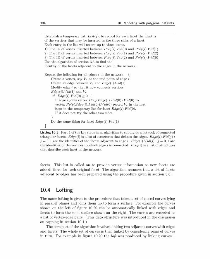
394 10. Modeling with polygonal datasets
Establish a temporary list, List(j), to record for each facet the identityof the vertices that may be inserted in the three sides of a facet.Each entry in the list will record up to three items.1) The ID of vertex inserted between Poly(i).V id(0) and Poly(i).V id(1)2) The ID of vertex inserted between Poly(i).V id(1) and Poly(i).V id(2)3) The ID of vertex inserted between Poly(i).V id(2) and Poly(i).V id(0)Use the algorithm of section 3.6 to find theidentity of the facets adjacent to the edges in the network.
Repeat the following for all edges i in the network {Create a vertex, say Vn at the mid point of edge iCreate an edge between Vn and Edge(i).V id(1)Modify edge i so that it now connects verticesEdge(i).V id(1) and Vn
i f Edge(i).F id(0) ≥ 0 {If edge i joins vertex Poly(Edge(i).F id(0)).V id(0) tovertex Poly(Edge(i).F id(0)).V id(0) record Vn in the firstitem in the temporary list for facet Edge(i).F id(0).If it does not try the other two sides.
}Do the same thing for facet Edge(i).F id(1)
}
Listing 10.3: Part 1 of the key steps in an algorithm to subdivide a network of connectedtriangular facets. Edge(i) is a list of structures that defines the edges. Edge(i).F id(j) :j = 0, 1 are the identities of the facets adjacent to edge i. Edge(i).V id(j) : j = 0, 1 arethe identities of the vertices to which edge i is connected. Poly(i) is a list of structuresthat describe each facet in the network.
facets. This list is called on to provide vertex information as new facets areadded; three for each original facet. The algorithm assumes that a list of facetsadjacent to edges has been prepared using the procedure given in section 3.6.
10.4 Lofting
The name lofting is given to the procedure that takes a set of closed curves lyingin parallel planes and joins them up to form a surface. For example the curvesshown on the left of figure 10.20 can be automatically linked with edges andfacets to form the solid surface shown on the right. The curves are recorded asa list of vertex-edge pairs. (This data structure was introduced in the discussionon capping in section 10.1.)
The core part of the algorithm involves linking two adjacent curves with edgesand facets. The whole set of curves is then linked by considering pairs of curvesin turn. For example in figure 10.20 the loft was produced by linking curves 1

10.4. Lofting 395
Repeat the following for all facets j in the network {[ Note that at this stage the list List(j) will have a[ vertex identity for all three items in each element because[ every side of all facets will have been subdivided.[ Note also that it is very important that a consistent ordering[ of vertices for new facets is maintained so that the surface[ normal vectors will point in the outward direction for all facets.Add three facets between the vertices below:Facet 1) List(j).V01, List(j).V12, List(j).V20
Facet 2) List(j).V01, Poly(j).V id(1), List(j).V12
Facet 3) List(j).V12, Poly(j).V id(2), List(j).V20
And three edges between the vertices below:Edge 1) List(j).V01, List(j).V12
Edge 2) List(j).V12, List(j).V20
Edge 3) List(j).V20, List(j).V01
[ These are illustrated in figure 10.19Modify facet j and so that it is attached to verticesPoly(j).V id(0), List(j).V01 and List(j).V20.
}
Listing 10.4: Part 2 of the key steps in an algorithm given in listing 10.3 that subdividea network of connected triangular facets.
With additional edge,facets and vertices.
Original
Vid(0)
Vid(1)
Facet(j)
Vid(2) Vid(2)
Vid(1)
Vid(0)
V01
(j)
V12
V20
Figure 10.19: Labeling of vertices for the subdivision algorithm given in Figure 10.3.
and 2, then curves 2 and 3, then curves 3 and 4, followed by curves 4 and 5 andfinally curves 5 and 6.
For any two planar closed curves with n and m vertex/edge pairs respectivelyit is essential that the join is made with triangular facets and that vertices neareach other are connected together. In other words: vertices from one side of thefirst curve must not be connected to the far side of the second. It would alsobe desirable to make the connections so that the triangular facets are as nearequilateral as possible. For some curves it is almost impossible to automatically

396 10. Modeling with polygonal datasets
After lofting
Piecewiselinear curves
6
5
4
3
21
x
y
z
Figure 10.20: Lofting involves joining a set of closed curves to form a solid surface. Inthis example the curves lie in xy planes and are displaced from one another in the zdirection.
decide what form the join should take. Even by eye it can sometimes be nonetoo easy either. Figure 10.21 illustrates how the simple act of displacing twocurves can lead to very different arrangements of edges and facets in a join.
Given the above caveats the following procedure will loft a set of k planarcurves recorded in an array of lists identifying the vertex/edge pairs that makeup each closed curve. For example the two curves depicted in figure 10.21 arecomposed of 11 and 20 vertex/edge pairs in the upper and lower curves respec-tively.
The algorithm consisting of 8 main steps is:
1. Pick the curves in pairs, 0 and 1, 1 and 2 etc., and repeat the followingsteps to join them. We will think of these curves as paths with a startingpoint that may or may not be the first vertex/edge in the list. The pathswill be labeled Pn and Pm with n elements (vertex/edge pairs) in Pn andm in Pm.
2. Find the elements in Pn and Pm that are closest together. Label these fnand fm.
3. Re-make the lists for Pn and Pm so that fn and fm are the first elementsin each list. This is the step that requires the curves to be closed. (It ispossible to modify this algorithm to loft a set of open curves by arrangingthe elements in the list so that the first ones are fn and fm.)
4. The procedure requires that Pn has fewer elements than Pm so if m > nswap the curves.
This completes the preparation, but before we can build the join which in-volves simultaneously moving along the paths stitching together elementsthat are “close”, we must decide in which directions to move.
5. To decide in which direction to move compare the distance lx between thesecond vertices in Pn and Pm with the distance ly between the second

10.4. Lofting 397
Original curves Joined curves
Plan
Elevation
Elevation
Displacing the curvesafter the join has been
effected results in avery different network
of edges and faces.
Plan
Figure 10.21: The effect on the join between two curves when one is displaced fromthe other before the join is executed. The curves are shown in plan and elevation view.
vertex in Pn and the last vertex in Pm. If lx > ly then the curves areoriented the wrong way round so one of them must be reversed; reversePm. This is illustrated in figure 10.22.
Getting the curves the right way round allows us to follow both curves inascending vertex order and basically join them up, vertices 1 to 1, 2 to 2etc. Because Pm may have more vertices than Pn a protocol will have tobe adopted to allow the extra ones to join in. These actions occur in thenext two steps.
6. For every element i, in Pn, find the element j in Pm so that vertex j isclosest to the vertex for i. Element j must be chosen so that no vertexfurther along Pm is already connected to any vertex in Pn. (This is veryimportant.) While this step is proceeding record in the data structure forthe elements of Pn the identity of the element in Pm to which each one isattached.

398 10. Modeling with polygonal datasets
Curves orientated correctly to link 1 to 1 etc.
m–1 m–1
0
0
n–1
n–1
3
2 1
0
0
13
4
3
2
2
1 1
43
2
Linking 1 to 1, 2 to 2 etc. will not work correctly
Figure 10.22: If curves are not orientated appropriately then the join will not work.
1
2
10
64
2
33
Pm
45
4
5
6
0
1
2
3
24
0Pn
1
3
Figure 10.23: An example of joining two curves before and after the execution of step 6in the algorithm.
After this step every vertex in Pn will be connected to a vertex in Pm. Theremay be some vertices in Pm not connected and triangular facets need to becreated but we have achieved a framework that has a reasonable geometryand no overlapping edges. Figure 10.23 illustrates an example of the stateof the join after this step.
7. Make a second pass along path Pn to join in the unconnected vertices ofPm and build the facets. For each element i in Pn do the following:
(a) Set an index, i0, to the identity of the element in Pm to which thevertex i is attached. If i is not at the end of Pn set another index, i1,to the element in Pm to which vertex i + 1 in Pn is attached. If i isat the end of Pn set i1 to some value > m.

10.4. Lofting 399
Pm
Add one edge and two facets
(a)
(b)
Add one facet herePm
Pm
Pn
Pn
Pn
Figure 10.24: Inserting one or two facets to make up the join. (a) Adding one facet.(b) Adding two facets requires an edge too.
Pm
Pn
PnBefore
After
Pm
Figure 10.25: Linking a longer gap in Pm to two adjacent vertices in Pn.
(b) If i1 = i0 then vertices i and i + 1 in Pn are attached to the samevertex in Pm and it is only necessary to add one facet as illustratedin figure 10.24(a).
(c) If i1 = i0+1 then two facets are required as shown in figure 10.24(b).
(d) If i1 > i0 + 1 then a variable number of facets and edges need to linki and i + 1 in Pn to j in Pm such that i0 + 1 ≤ j < i1. There area number of arrangements that can accomplish this. In the exampleshown in figure 10.25 the vertices in Pm are joined to vertex i untilone of them gets closer to vertex i+ 1. After that they are linked tovertex i+ 1.
8. The final step is to add the facets where the ends of Pn and Pm link backto the start.
This procedure will work in the vast majority of cases but it may run intoproblems where one oriented curve has a very large number of points whilst theone next to it has only a few.

400 10. Modeling with polygonal datasets
A
C
Figure 10.26: The surface of revolution on the right was produced by revolving thecurve C around the axis A, shown on the left.
10.5 Surfaces of revolution
A surface of revolution is the formal way to describe the shape produced in aworkshop with a lathe. It has an axis around which some curve is rotated tobuild a network of vertices and facets. The curve could be expressed analyticallyor it could be a piecewise linear approximation to a smooth curve. An analyticdescription is often used in constructive solid geometry applications but in thecontext of the polygon faceted description of surfaces used in this chapter it isappropriate to use a piecewise linear description of the curve.
A typical example of a model built with a single surface of revolution is thetorus illustrated in figure 10.26.
Typically the axis of revolution will be parallel to one of the Cartesian axes.Other parameters required are:
1. The angle through which the revolution occurs. A positive angle will resultin a counter-clockwise direction of rotation. A full revolution of 360◦ willproduced a closed surface; in this case the direction of rotation is irrelevant.
2. Because the surface is to be approximated by a finite number of polygonalpieces the number of steps (sections) in the rotation must be specified.For a 360◦ rotation more steps will result in a better approximation to asmooth surface of revolution. (The example of figure 10.26 used a sectionplaced every 15◦ which is about the minimum acceptable.)
Producing a surface of revolution is one of the most fundamental actions inconstructing 3D models because some of the most commonly used primitiveshapes are surfaces of revolution. The sphere, ellipse and torus may all beconstructed by revolving the appropriate curve.
An algorithm that builds a 3D surface of revolution will need to constructa network of connected facets and edges from vertices placed at the position ofthe sections. The algorithm proceeds one section at a time and if the revolutionis for a full 360◦ a final step will add facets to connect the last section back tothe first. Care will also be needed to account for the revolution of a curve whichis closed (such as that in figure 10.26) because in those cases the last vertex inthe piecewise representation is assumed to be connected to the first.
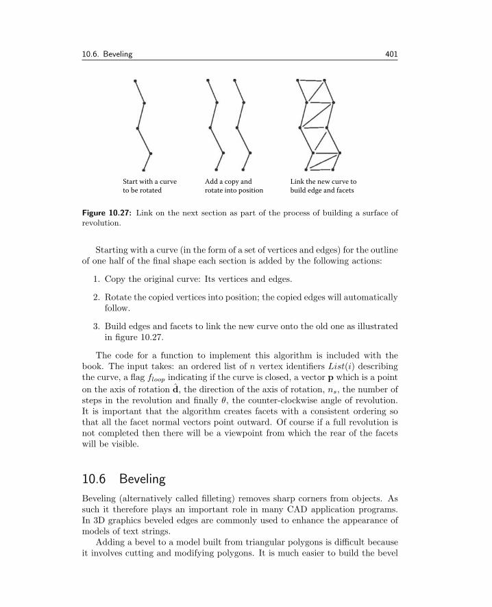
10.6. Beveling 401
Start with a curveto be rotated
Add a copy androtate into position
Link the new curve tobuild edge and facets
Figure 10.27: Link on the next section as part of the process of building a surface ofrevolution.
Starting with a curve (in the form of a set of vertices and edges) for the outlineof one half of the final shape each section is added by the following actions:
1. Copy the original curve: Its vertices and edges.
2. Rotate the copied vertices into position; the copied edges will automaticallyfollow.
3. Build edges and facets to link the new curve onto the old one as illustratedin figure 10.27.
The code for a function to implement this algorithm is included with thebook. The input takes: an ordered list of n vertex identifiers List(i) describingthe curve, a flag floop indicating if the curve is closed, a vector p which is a point
on the axis of rotation d, the direction of the axis of rotation, ns, the number ofsteps in the revolution and finally θ, the counter-clockwise angle of revolution.It is important that the algorithm creates facets with a consistent ordering sothat all the facet normal vectors point outward. Of course if a full revolution isnot completed then there will be a viewpoint from which the rear of the facetswill be visible.
10.6 Beveling
Beveling (alternatively called filleting) removes sharp corners from objects. Assuch it therefore plays an important role in many CAD application programs.In 3D graphics beveled edges are commonly used to enhance the appearance ofmodels of text strings.
Adding a bevel to a model built from triangular polygons is difficult becauseit involves cutting and modifying polygons. It is much easier to build the bevel

402 10. Modeling with polygonal datasets
Bevel
Hidden surfaceHidden line
Figure 10.28: Models for the letters A and S showing a bevel on the front face.
After capping
After bevel is added
Outline curve
Figure 10.29: Beveling an outline.
into the model as it is constructed. This is the way the model of the lettersshown in figure 10.28 was constructed.
The generation of a beveled shape can begin with a set of closed curves usinga modified version of the triangulation algorithm described in section 10.1. Oncethe curve has been beveled it can be capped with the triangulation algorithm toproduce a closed shape; see figure 10.29 for an example.
To create a bevel from a series of closed outlines there are two issues to beaddressed:
1. To which side of the curve is the bevel formed? This is tied in with theidea of a curve with a hole in it because the bevel round a hole should slantin the opposite direction to the bevel round the outside of the curve. Thecurves shown in figure 10.29 contain both a series of outside outlines anda hole; you should be able to see how the bevel is made accordingly.
2. How does the bevel behave as it goes round a bend? This will depend onwhether:
(a) The bevel is to appear on the inside of the bend as you go round(shorter path).

10.6. Beveling 403
(d)(c)(b)(a)
Bevel
Bevel
Bevel
BevelC C
C
C
Figure 10.30: Beveling a curve that goes round a bend. (a) The bevel is on the insideof the curve C. (b) The bevel is on the outside of C. (c) On the outside of a hairpinbend. (d) On the inside of a hairpin bend.
(b) The bevel is to appear on the outside of the bend as you go round(longer path).
These cases are shown in figure 10.30(a and b). Since all the curves usedin this chapter are built from straight edges (piecewise linear) the problemof how to arrange the facets in the bevel is accentuated when the curvesgo round a bend that is greater than about 270◦. The question thereforeis: How to how to build the bevel?
A first guess for a procedure might be: Add one edge lying parallel to eachedge in the original curves, offset it by the depth of the bevel and link it tothe main curve with edges and facets. However, this won’t work for curveswith hairpin bends, Figure 10.30(c and d), because the repositioned edgesoverlap or leave a gap as shown in Figure 10.31. Even though this first ideamay not work immediately it is a good starting point for a better procedurebecause an edge can be inserted to fill any gap and edges that would overlapcan be shortened. This approach leads to satisfactory looking bevels; seefigure 10.32.
A reasonable algorithm that produces such a bevel round a set of outlinecurves requires the following three steps:
1. Given a list of closed curves (closed curves are needed so that the bevelcan be placed to the inside) determine whether each curve represents theoutline of a hole or an outside edge.
2. For each vertex/edge pair Vi, determine a normal to the edge; call it ni.Choose ni so that it lies in the plane of the curve and points in the directionin which the bevel is to be made. In addition, for each Vi obtain the average
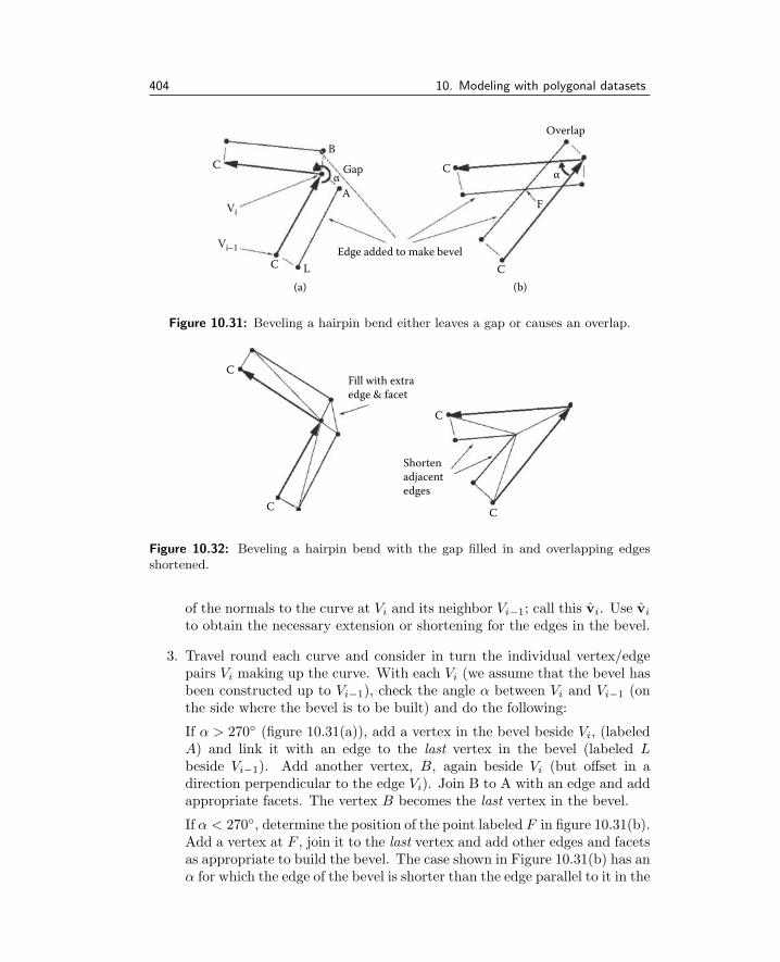
404 10. Modeling with polygonal datasets
Edge added to make bevel
(b)(a)
Vi–1
Vi
C C
Overlap
C C
F
L
B
A
Gapα α
Figure 10.31: Beveling a hairpin bend either leaves a gap or causes an overlap.
Shortenadjacentedges
Fill with extraedge & facet
C
CC
C
Figure 10.32: Beveling a hairpin bend with the gap filled in and overlapping edgesshortened.
of the normals to the curve at Vi and its neighbor Vi−1; call this vi. Use vi
to obtain the necessary extension or shortening for the edges in the bevel.
3. Travel round each curve and consider in turn the individual vertex/edgepairs Vi making up the curve. With each Vi (we assume that the bevel hasbeen constructed up to Vi−1), check the angle α between Vi and Vi−1 (onthe side where the bevel is to be built) and do the following:
If α > 270◦ (figure 10.31(a)), add a vertex in the bevel beside Vi, (labeledA) and link it with an edge to the last vertex in the bevel (labeled Lbeside Vi−1). Add another vertex, B, again beside Vi (but offset in adirection perpendicular to the edge Vi). Join B to A with an edge and addappropriate facets. The vertex B becomes the last vertex in the bevel.
If α < 270◦, determine the position of the point labeled F in figure 10.31(b).Add a vertex at F , join it to the last vertex and add other edges and facetsas appropriate to build the bevel. The case shown in Figure 10.31(b) has anα for which the edge of the bevel is shorter than the edge parallel to it in the

10.7. Orienting surface normals 405
Curve
(a) (b)
E
Bevel
Overlap
Figure 10.33: Resolving the problem that can occur if the curvature is too great toaccommodate the required bevel depth. In (a) the edges in the bevel overlap. Bypreventing the creation of a vertex and edge associated with edge E in the originalcurve, the overlap is avoided (b).
curve C. This will be true for cases where α < 180◦. If 180◦ < α < 270◦
the edge in the bevel will be longer than the one it is parallel to in thecurve C.
Figure 10.32 illustrates the result of applying this procedure to the curvefragments of figure 10.31.
There is one irritating complication when beveling part of a curve like thatshown in figure 10.31(b). What happens if the edge segments are shorter than thedepth of the bevel? In such cases the location of the point F (figure 10.31(b)),determined from two consecutive edges would cause an overlap as shown infigure 10.33(a). To avoid this a test should be inserted before creating a vertexat F to see if an overlap is going to occur. If the result of the test is positive thenF should not be created and the algorithm will just skip forward to consider thenext edge.
10.7 Orienting surface normals
Sometimes the order in which the vertices to which a polygon is attached isnot listed in a consistent order. That is, if you look at a plan of a networkof facets, some facets have their vertices listed in a clockwise sense and somehave their vertices listed in a counter-clockwise sense. An example is illustratedin figure 10.34. If this happens a renderer cannot determine if the front orback of a polygonal is the one facing the camera. Thus it is not possible toperform a back-face cull (see section 4.2.7) because this might lead to holesappearing in the model. Consequently all facets have to be rendered and thisslows the rendering procedure. A further complication of inconsistent orientation

406 10. Modeling with polygonal datasets
Note the directionin the two faces on
either side ofedges like these
An inconsistent network A consistent network
Figure 10.34: The order in which the vertices bordering a polygon are recorded canproduce a consistent or an inconsistent network. A consistent network is one in whichthe surface normals (formed by a vector cross product between two non co-linear edges)of connected polygons are directed toward the same side of the network.
in surface patches is that it is very difficult to calculate appropriate normalvectors and as a consequence unpleasant artifacts can appear when the Phongor Gouraud shading procedures are used to simulate curved surfaces.
This section presents a procedure that will orientate a network of connectedtriangular facets by making the order in which the vertices of any facet arerecorded consistently counter-clockwise when looking at the facets from the “out-side” of the model. Although some models do not have a definite inside or outside(a flat sheet of facets for example) one side can be arbitrarily designated the out-side. Models that consist of several pieces can be orientated simply by treatingeach piece as a separate network.
For the purposes of this algorithm a facet is part of a network only if it isconnected to other facets along at least one of its edges. Facets that meet onlyat a vertex are considered as separate networks.
The algorithm which is recursive can be summarized in the following fivesteps:
1. Add an integer identifier sid to the data structure describing each polygon.This will be used to identity separate pieces in the model.
2. Flag every polygon as being unidentified, i.e., set sid = −1.
3. For every polygon work out the identity of the polygons adjacent to it, i.e.,those that have a common edge will have two of their vertices the same asthe polygon being checked. A suitable procedure is given in section 3.5.
4. For each polygon k, check if it is unidentified. If it is, then call the recursivefunction IdentifyConnected(LastOneSet, SetThisOne) to assign it and
10.8. Delaunay triangulation 407
all facets connected to it. The function also makes all connected facetsadopt the same counter-clockwise vertex ordering scheme.
The function will be called with the identity of the polygon to be checked(the parameter SetThisOne), and the identity of the last one that hasbeen checked (parameter LastOneSet). Since 0 ≤ k we can use −1as the starting value for LastOneSet. The initial call then takes theform IdentifyConnected(−1, k). A counter c is initialized c = 0 whichwill count the number of discrete pieces in the model. On executionIdentifyConnected() performs the following functions:
(a) For polygon SetThisOne check if its flag sid ≥ 0. If it is then returnfrom the functions because facet SetThisOne has already been setand therefore this test stops further recursion.
(b) If LastOneSet ≥ 0 make the orientation of polygon SetThisOne thesame as LastOneSet by swapping two vertices in the vertex list ifnecessary. However if LastOneSet < 0 then increment the count cbecause as yet there are no adjacent facets.
(c) Assign the flag sid = c for polygon SetThisOne.
(d) Call IdentifyConnected() once for the polygons adjacent to polygonSetThisOne, with of course the LastOneSet parameter now specify-ing the polygon identified by SetThisOne.
5. With each individual piece, i.e., all those facets having the same values ofsid, do the following:
(a) Find a bounding box.
(b) Choose an arbitrary point P outside the bounding box. (If renderingis taking place the best choice for P is the viewpoint.)
(c) Find the polygon closest to P , say k. If k’s normal is directed sothat the back of k is visible from P reverse all the normal vectors andvertex orderings of polygons identified with the same sid as k.
10.8 Delaunay triangulation
Sometimes an arbitrary collection of points is encountered without any details aswhat happens between them. Perhaps they represent samples from a scientificexperiment for example. To be able to visualize them (by rendering) they mustbe connected together by a network of polygons. This specific problem occursfrequently in engineering design and analysis. If the number of points is large,then doing it by hand, say in an interactive design application, is out of thequestion and an automated procedure must be sought.

408 10. Modeling with polygonal datasets
For any set of more than three points building a network of triangular poly-gons is always possible. Grouping more than three points to form the basicpolygonal unit has the advantage that fewer polygons will need to be rendered.However there are many drawbacks, not the least of which is the complexity ofthe procedure to determine the polygonization.
Invariably the triangulated mesh used in a mathematical analysis requiresthat it should be as regular as possible, that is: The triangles should be approx-imately equiangular (or to put it another way: No long thin triangles). Thisrequirement is exactly the one we strive to attain in producing models for 3Dvisualization because it makes the writing of a good quality renderer so much eas-ier. All the numerical pitfalls that occur because of long thin facets are avoidedwhen the triangles are nearly equiangular. A method that guarantees to delivera locally equiangular arrangement of edges and facets has been devised. It goesby the name of Delaunay triangulation.
The Delaunay triangulation technique is particularly helpful in visualizingfunctions of two variables: z = f(x, y), especially when the sample points (x, y)are arranged randomly. A very good example of this is: Geographic InformationSystems (GIS) which record topographic data. The height z is sampled at aset of (x, y) coordinates. A triangulation based on the (x, y) coordinates withthe z coordinate derived from the height value at each point gives a 3D surfacethat can be sent to a standard renderer to produce informative images suchas that illustrated in figure 10.35. The locations of the data points for thescene in figure 10.35 and mesh created by Delaunay triangulation are shownin figure 10.36. A GIS therefore does not need to record any edge or facetinformation.
Many other scientific and engineering disciplines find this approach to visu-alizing information very useful and it is one use for 3D graphics. Another reasonfor us to consider the Delaunay procedure for triangulating a set of points isthat it forms an important step in the construction of faceted models using thetechnique of Boolean operations to be discussed in section 10.9.
The algorithm presented in this section will follow the approach of Sloan [83]with the exception that we will allow the plane in which the triangulation is builtto lie in any orientation rather than a horizontal xy plane. (An arbitrary planeof triangulation is essential for the Boolean procedure of section 10.9.) Delaunaytriangulations are produced on a flat plane. The third dimension is irrelevantbecause a surface cannot be assigned to an arbitrary collection of points in threedimensions.
The essence of the Delaunay triangulation algorithm is relatively straightfor-ward. The basic premise is:
Take one point from the data set at a time and insert it into apre-existing triangulation making any necessary adjustments to theedge/facet information so that all the facets remain as equiangularas possible.

10.8. Delaunay triangulation 409
Figure 10.35: Making a Delaunay triangulation from a collection of geographic dataallows a 3D renderer to produce a visualization of the landscape that the data repre-sents. An animation of the fly by type is readily generated over a model of a landscapefrom earth or some other world.
(a) (b)
Figure 10.36: The data points and mesh from which the image in figure 10.35 wasgenerated. (a) The location of the sample points. (b) The mesh generated by Delaunaytriangulation.
The process is started by making a dummy facet big enough to enclose all thepoints. After completing the Delaunay triangulation the vertices of this enclosingtriangle are removed and consequently any edges or facets attached to themdisappear too. The basic idea of the algorithm is illustrated in figure 10.37.

410 10. Modeling with polygonal datasets
(a) (b) (c) (d)
Figure 10.37: The triangulation of a set of points. (a) The points, (b) enclosed by asupertriangle, (c) triangulated and (d) with the supertriangle removed (enlarged view).
The basic steps are:
1. Add a triangular facet in the same plane in which the points lie. Make itlarge enough so that all points are inside it. Thus the initial triangulationcontains just a single triangle. Call this the supertriangle.
2. With each point P in the list of points to be inserted, do the following:
(a) Find an existing triangle that encloses P , say it is triangle k.
(b) Form three new triangles by connecting P to the vertices of k. Thenet gain of triangles is two and three new edges are created.
(c) The new triangulation is updated so that the properties of a Delaunaytriangulation again apply to the whole network of edges and facets.This is the main step in the algorithm and it will be discussed below.
3. Once all the points have been inserted in the triangulation the vertices thatform the supertriangle are removed. Any edge or facet attached to one ofthese supertriangle vertices must also be removed. Figure 10.37 illustratesthe outcome after the main steps in the algorithm.
In step 2 above it was stated that: After a point P is inserted in the triangu-lation the triangulation is updated so that the properties of a Delaunay networkare re-established. This is accomplished by the following three steps:
1. All the triangles that have a common edge with one of the three trianglesadjacent to P are placed on a last-in, first-out stack. The facets labeledX, Y , and Z in figure 10.38 are adjacent to P and the facets A, B and Care opposite to P .
2. If the stack is empty this phase of the algorithm is complete. Otherwise, atriangle is popped off the stack and a test made to see if the edge commonto it and its neighbor with P as a vertex should be switched, e.g., pairsA and X, B and Y etc. (See figure 10.38.) This test effectively decides

10.8. Delaunay triangulation 411
PA
XZ
Y
C
B
Figure 10.38: The triangles A, B and C, share a common edge with the (three) trianglesX, Y and Z, which have P as one of their vertices. A,B and C are said to be oppositeP .
(b)(a)
XX
A
A
U U
V V
P P
Figure 10.39: Should the edge common to triangles A and X shown in (a) be swappedto give the configuration shown in (b)? If configuration (b) is adopted then the triangleslabeled U and V will need to be reconsidered because they will now be opposite P andwe need to check whether their common edge needs to be swapped.
whether the internal angles of the triangles X and A in figure 10.39 arecloser to being equiangular in configuration (a) or configuration (b).
If a swap from configuration (a) to configuration (b) is made then twotriangles replace two triangles so no new edges or facets are created. How-ever the action of making such a swap will have implications for the othertriangles adjacent to that labeled A in figure 10.39(a) and this must beaccounted for in the next step.
3. If a swap is made any triangles that become opposite P are pushed ontothe stack. There will be at most two; see those labeled U and V in theexample of figure 10.39.
Execution then loops back to step 2 to continue processing the (possiblyextended) stack.

412 10. Modeling with polygonal datasets
Don’t swap
P
P
Swap
A
A
Figure 10.40: Swap the common edge if P lies inside the circumcircle of the triangle,A, opposite P .
Finally, to complete the description of the algorithm we must discuss the testthat determines whether to swap the common edge. In two dimensions thisis equivalent to deciding whether P lies inside the circumcircle of the triangleopposite P . If it does the edge is swapped, if it does not then no change isnecessary; see figure 10.40.
The point P (in figure 10.41) lies on the circumcircle of the triangle V1, V2,V3 if α + β = π. It lies inside the circumcircle if α + β > π and outside ifα + β < π. To calculate α and β directly would involve inverse trigonometricfunctions (which is always undesirable) but since α + β < 2π the point P willlie inside the circumcircle if sin(α + β) < 0. Using this formulation avoids theinverse trigonometric function but there are some numerical difficulties due toround off errors when α + β ≈ π; however the four-step algorithm due to Clineand Renka [16] can solve such problems. We can extend their two-dimensionalprocedure to apply to any plane where the points P , V1 etc., in figure 10.41are given by position vectors v1, v2, v3, and p. This algorithm is presented inlisting 10.5.
In the coding of the Delaunay algorithm that accompanies the book thefollowing points should be noted:
1. For this implementation the plane in which the points to be triangulatedlie may be selected to be parallel to the xy, yz or zx planes.
2. The supertriangle, which may be specified arbitrarily, is chosen by firstfinding the rectangle enclosing all the points in the plane. Let the centerof this rectangle be (xc, yc) and d its longest dimension. An equilateraltriangle with the circle, radius d center (xc, yc), inscribed inside it willalso enclose all the points. The vertices of the supertriangle are thereforelocated at (xc, yc + 2d), (xc −
√3d, yc − d) and (xc +
√3d, yc − d).
3. In order to swap an edge the data structure representing the facets needs tokeep a record of which facets are adjacent to which facets; and which edge

10.9. Boolean modeling 413
V3
V2
V1
P βα
Figure 10.41: The geometry used to test whether P lies inside the circumcircle of thetriangle V1 - V2 - V3.
is adjacent to which facet. When an edge is swapped it is not only vital toupdate the adjacency information in the facets directly affected but alsoto update the information in those adjacent to the modified facets bothbefore and after the swap. For example: Swapping the edge E shown infigure 10.42 will affect the adjacency information not only in the triangleslabeled A and B but also in triangles X and Y . The triangle Z is notaffected because it remains adjacent to A.
4. Care must be taken when swapping edges so that the order in which thevertex data is recorded remains consistent. We don’t want some of thenormal vectors pointing to one side of the plane and the remainder pointingto the other.
5. The code for this algorithm will generate a mesh from 10,000 points in afew seconds on a standard personal computer.
10.9 Boolean modeling
Boolean modeling is the name given to a procedure for building models from acombination of primitive shapes or indeed from other models. The name is takenfrom the algebra of mathematical logic devised by George Boole in 1847 becauseits operations provide a very useful analogy to describe the way in which shapesmay be combined.
The simplest way to combine two models is to add them together. This canbe represented by a Boolean operation called an or operation which is writtenusing the + symbol. For example if we let the symbol A represent an eight sided

414 10. Modeling with polygonal datasets
Start by calculating the vectors below:
v13 =v1 − v3 |v1 − v3|
v23 =v2 − v3 |v2 − v3|
v1p =v1 − p |v1 − p|
v2p =v2 − p |v2 − p|
Then make the scalar products:cosα = v13 · v23
cosβ = v1p · v2p
Now apply the test:i f ( cosα ≥ 0 and cosβ ≥ 0) Do not swap.else i f (cosα < 0 and cosβ < 0) Do swap.else {
Calculate:sinα = |v13 × v23|sinβ = |v2p × v1p|Then : i f (sinα cosβ + sinβ cosα < 0) Do swap.else Do not swap.
}
Listing 10.5: Algorithm to test whether the edge of the triangle between v1 and v2
should be swapped to join p to v3; see figure 10.41.
After swapping EBefore swapping E
P
BX
E E
X
B
AZ Z
A
Y YP
Figure 10.42: Swapping the edge E will alter which triangles are adjacent to whichother triangles not only in those directly affected, those labeled A and B, but also thoselabeled X and Y . However triangle Z is not affected because it remains adjacent to Airrespective of the orientation of edge E.
polygonal cube then a model made from two cubes can be described symbolicallyas A+ TA (where T represents a translation). If you need a model of a cylinderC with a sphere S sitting on top of it you can build a model for C and a modelfor S and then or them together, result C + S.
Suppose however you want a model where C pokes through S; something likethe illustration of figure 10.43(a). It would be quite difficult to design by hand a

10.9. Boolean modeling 415
(a) (b) (c)
Figure 10.43: (a) OR-ing a sphere and cylinder, expressed in Boolean algebra S + C.(b) AND-ing a sphere and cylinder, Boolean notation: S · C. (c) The result of theBoolean expression SC. We can think of this as subtracting a cylinder from a sphere.Notice that the cylinder, which is not visible, appears to cut a hole in the sphere.
mesh of facets to cover such a surface. However since this shape is just anothermanifestation of S +C if there was an automatic way to go from the meshes forS and C to one for S + C a very useful modeling procedure would result.
Incidentally: To generate an image of the combination S + C with a hiddensurface renderer there is no need to work out a mesh for S + C. The twocomponents can be used in their original form and the renderer will avoid drawingthose parts of the facets of C that lie inside S because they are obscured by S.
If S +C was the only Boolean combination then (from a 3D modeling pointof view) there would be no advantage in using it. However S+C is not the onlypossibility that Boolean algebra allows. The other relevant Boolean operationsare:
• not, written as A. It’s not possible to show a picture of S or C becausesuch a solid fills the whole universe except that small volume occupied byS or C. You might argue that not is not a very useful operation; on itsown that’s true but when it is used in conjunction with the next operationthe true power of “Booleans” as a 3D modeling tool is evident.
• and, written as S · C or simply SC. Again and is an unfortunate name.The symbols +, and . are much more revealing as to the actual effect ofoperations if you liken them to the add and multiply operations of basicalgebra. So what of SC (S AND C): This is a solid that occupies thespace where S and C overlap; an example is illustrated in figure 10.43(b).
The real power of a Boolean operation as a modeling idiom is that it allowsshapes like that shown in figure 10.43(c) to be produced from simple primitives,S and C in that example. We can think of the shape Figure 10.43(c) being theresult of the removal of that part of S where S and C overlap. One might call it

416 10. Modeling with polygonal datasets
a subtractive operation but strictly speaking it is SC (that part of the universeoccupied by the sphere and not by the cylinder). This subtractive operation isexceptionally useful. A number of very important constructional methods arebased on the principles of drilling a hole or cutting a bit off.
In theory it should be possible to build a model of any shape by emulatingsome combination of Boolean operations on a very small subset of primitiveshapes. Indeed this topic is so important it is given the name constructive solidgeometry. Most CAD applications use some CSG. A number of ray tracingprograms are based on the CSG concept because it can reduce the number ofelements that need to be rendered in any one scene whilst not restricting themodels to a few textured spheres or cubes.
One way to model an object using boolean primitives is to use Boole’s no-tation for combination of primitives and build the model out of primitives. Aray-tracing algorithm is just at home tracing rays through a model describedwith functional primitives (spheres, cylinders etc.) as it is tracing rays througha set of planar polygonal faces. Alternatively, the surface of a model describedby a Boolean combination of primitives can be readily turned into a network ofpolygonal faces using the marching cubes algorithm described in section 10.10.2.
In the context of a model made with polygonal faces it is more difficult touse the Boolean concept on the mesh because:
1. The models are not based on a relatively small number of primitive shapesbut on a large number of flat planar pieces. Therefore there are many morepossible configurations that need to be considered and this can take a longtime.
2. CSG objects always have a very well defined sense of inside and outside.Faceted models do not necessarily have that sense. Suppose we build afaceted model for a sphere but decide to remove a few facets from one sideof it. How could we then use this open sphere in Boolean operations?
3. Whereas a CSG representation of say a sphere and a cylinder will producean intersection that is smooth, if we try the same thing with faceted modelsthe line of intersection will be a jagged edge. This is especially noticeablewhen the faceted approximation is a coarse one. There is nothing muchcan be done about this except increase the resolution of the mesh.
4. The facets that result from a Boolean cutting operation tend to be poorlyshaped, long thin facets. These often occur and tend not to render verywell and preclude a lot of additional processing.
5. The algebra of the intersections of bounded planes in three dimensions isvery sensitive to the round off errors that occur in computer calculations.
Despite these difficulties some shapes are much more easily modeled usinga Boolean subtraction operation; for example, the holes in a Swiss cheese. It

10.9. Boolean modeling 417
Delete these pieces
to producea sphere with
a hole
Combine theremaining
pieces
Keep thesepiecesCylinder overlaps
sphere
Figure 10.44: The intersection of the faceted models for a sphere S and a cylinderC cuts them into three pieces each. By discarding unwanted pieces a model of theBoolean subtraction SC is obtained.
is therefore essential to devise an algorithm that can provide Boolean-like func-tionality to as good an approximation as possible.
Such an algorithm is presented in this section. The algorithm takes care toproduce a triangulation that minimizes the number of small and thin facets andto avoid (where possible) the problems due to round off errors. The algorithm isquite long but it is possible to break it up into a number of sections that can beconsidered separately and a relatively simple overview of the strategy it uses canalso be given. The procedure owes some of its heritage to the ideas of Laidlawet al. [52].
Before presenting the strategy of the procedure there are a few points thatare worth considering:
1. For a computer graphics application we do not need to consider an opera-tion equivalent to Boolean addition. Indeed because a polygonated modelmight not have a definite inside subtraction is also meaningless in somecases. A better way to think of the process is of a model being cut intopieces, some of which will be discarded to leave the appropriate shape; seefigure 10.44.
2. With a model made from a collection of triangular facets we must knowwhich facets are doing the cutting and which are being cut. This can beaccomplished by making a list of facets that fall into these two groups, wewill call these lists:
(a) The Work list
(b) The Tool list
For the example shown in figure 10.44 the facets that make up the sphere Sare placed in Work list while those in the cylinder C belong to the Tool list.

418 10. Modeling with polygonal datasets
Polygon A is triangulated(but not split) by Bso than an edgeoccurs along theline of intersectionwith B
Neither polygon A nor Bis split (because thereis no clean cut) but bothare triangulated so thatboth have edges alongthe line of intersection.
Polygon B issplit in twoby polygon A
A
AB
B
B
A
A
(b)(a)
Figure 10.45: An intersection between two triangular polygons. In (a) the polygonlabeled B is split in two by polygon A. In (b) neither polygon is split.
3. Breaks in the model occur where the facets from these two lists intersecteach other and both sets need to be divided. We can achieve this by firstbreaking the facets in the Work list along the line of intersection with thefacets in the Tool list. When that has been done the lists may be swappedand the algorithm repeated.
4. The intersection occurs along one or more piecewise linear sections whichform a path across the surface. Each linear segment occurs as the resultof the intersection of two planes. Some of these paths might form closedloops. For example the line of intersection between cylinder and sphere infigure 10.44 will consist of two circles on the sphere and two circles on thecylinder.
5. The SC operation depicted in figure 10.44 results in both S and C beingcompletely cut into 3 pieces each. However, any Boolean modeling proce-dure that is based on a network of planar polygons must be able to copewith the possibility that some shapes may not be completely dissected.For example an intersection between two triangular facets might not spliteither or might split just one of them; see figure 10.45.
Taking these observations into account we can propose a possible algorithmto cut two sets of facets along their line(s) of their intersection as follows:
1. With all facets in the model make two lists: (1) the Work list and (2) theTool list.

10.9. Boolean modeling 419
2. Find the line of intersection through the facets of the Work list due to in-tersection with the facets in the Tool list. Since all the facets are planar theline of intersection will consist of a finite number of straight line segments.
3. Build the line of intersection into the facets of the Work list.
4. Split the facets in the Work list along the line of intersection.
5. Swap the facets in the Tool and Work list and repeat the previous threesteps.
Steps 2, 3 and 4 above cover the main actions of the algorithm. However,adding a series of edges into a network of facets is very difficult and so it ispreferable to carry out the actions of creating and inserting (steps 2 and 3) atthe same time. Thus the line intersection is built into the facets from the Worklist at the same time as it is determined.
If we are able to implement these ideas we will have an acceptable procedurefor creating separated pieces that are the best approximation to Boolean prod-ucts one can obtain from a network of polygonal facets. The next sections willexpand on the detail of the two main stages (2 and 3).
10.9.1 Determining and incorporating the line of intersection
The first main action of the algorithm is to determine the line of intersectionbetween facets in the Tool and Work lists and to make sure that this is built intothe network of Work facets. To see how this works consider the small networkshown in plan view in figure 10.46. In (b) the line of intersection is shown andfor ease of illustration we will assume that facets in the Work list lie in the planeof the page and facets in the Tool list lie perpendicular to it. Hence they appearas a line in the diagram. Note that the intersection line appears as a number ofstraight line segments.
Consider now how the line of intersection is determined: It is made up froma number of line segments. So finding the points where these segments beginand end determines the line of intersection. Thus the algorithm is based on theidea that:
The segments that go to make up the line of intersection have theirend points at the locations where either an edge of a facet in the Worklist intersects a facet in the Tool list or where an edge of a facet inthe Tool list intersects a facet in the Work list.
Once we know where these points are everything else follows fairly readily fromthat; we proceed in two phases:
• Phase 1: For every edge of a facet in the Tool list find its point(s) ofintersection with a facet in the Work list.

420 10. Modeling with polygonal datasets
Points ofintersection
Work facet Line of intersection
(c)(b)(a)
Figure 10.46: (a) A plan view of some facets in the Work list. (b) Adding the (edge on)view of facets in the Tool list shows the line of intersection. (c) The line of intersectionwill pass through the points of intersection between edges of facets in the Tool list andfacets in the Work list and vice versa. There are no other places where it can changedirection.
• Phase 2: For every edge of a facet in the Work list find its point(s) ofintersection with a facet in the Tool list.
Figure 10.46(c) highlights where these points are for that particular example.Now consider another question: How is the line of intersection built into the
triangular polygon network given we know the points through which it mustpass? And the answer:
The line of intersection emerges automatically if we insist that asvertices are inserted at the points where edges meet facets the networkis constantly updated to make sure that all the facets in it remaintriangular.
Figure 10.47 illustrates the progress of these phases of the algorithm forthe example of figure 10.46 and shows how the line of intersection becomesevident with edges along it. In figure 10.47(a) is the initial network; the line ofintersection is shown dotted. (b) and (c) insert the two points where the edgeof the facets in the Tool list intersect facets in the Work list. In (d), (e), (f),(g) and (h) five points are inserted where the edges of facets in the Work listintersect facets in the Tool list. By the time all points have been inserted, at(h), edges along the full length of the intersection have been created. Diagram(i) highlights the resultant line of intersection along these edges.
All of this looks quite straightforward and for the example shown it is. Un-fortunately however both phases can be plagued by the creation of too manyedges and facets. To see how this might occur consider again the example shownin figure 10.47. After Phase 1 is complete, in diagram (c), six new edges are as-sociated with facets in the Work list; there are four additional facets too. Theseedges must themselves be used during Phase 2 to check for intersection with the

10.9. Boolean modeling 421
(a) (b) (c)
(d) (e) (f )
(g) (h) (i)
Figure 10.47: Inserting the points of intersection between the edges of facets in theWork and Tool lists one at a time into the network of Work facets produces edges lyingalong the line of intersection. Illustrations (a) to (i) are discussed in the text.
Tool facets. In the example of figure 10.47 they don’t intersect any of the toolfacets but that’s just the case in this particular example.
There is another problem that is manifest in Phase 1 itself. Look at theexample in figure 10.48. The Work list consists of one facet only and all thefacets in the Tool list intersect it. Inserting the points of intersection in the order1, 2, 3, 4 gives configuration (d) at the end of Phase 1. Phase 2 completes thetriangulation but at the price of the inclusion of another point P as shown in (e).
To be specific: In (a) the single facet is cut by facets in the Tool list (shownedge on, this is equivalent to the line of intersection too). This gives rise to fourintersection points as shown in (b) and labeled in the order in which they are tobe inserted. After the first point is inserted the Work facet is shown divided inthree (c). When Phase 1 is completed the triangulation (d) is the result. Afterchecking all the edges in the work facet for intersection with facets in the Tool listthe final triangulation with edges along the full length of the intersection line is

422 10. Modeling with polygonal datasets
(f )
(c)(b)(a)
2 4
31
(e)(d)
EP
Facet in work list
Edge on view of facets in tool list Points to be inserted
Figure 10.48: Triangulating an insertion in the Boolean algorithm. Details of illustra-tions (a) to (f) are discussed in the text.
produced (e). However, if the edge E in (d) had been “flipped” the triangulation(f) would have been produced. None of the edges in (f) intersect any of the Toolfacets and the full length of the line of intersection is completely covered withoutthe need for the extra point P .
Configuration (e) is unsatisfactory because the extra point P is unnecessary.Configuration (f) is much more acceptable but to achieve it the edge labeledE had to be flipped so that it joined points 3 and 4. Fortunately we havealready discussed an algorithm that does just this (Delaunay triangulation) insection 10.8. To apply the Delaunay procedure to Phase 1 of this stage in theBoolean algorithm we consider each facet in the Work list separately. Everyfacet in the Work list is considered as a Delaunay supertriangle and is used toproduce a best triangulation with any intersection points that fall inside it. Afterall the intersection points are inserted however the supertriangle is not deleted.Figure 10.49 illustrates the result of performing two Delaunay triangulations intwo work facets A and B.
Thus the algorithm for Phase 1 may be summarized as follows:
Repeat the following with all the edges i of the facets in the Tool list {Repeat the following with all the facets j in the Work list {
if edge i intersects facet j at point P {Add P into a Delaunay triangulation withfacet j as the original supertriangle.
}}
}

10.9. Boolean modeling 423
Build Delaunay triangulationin both triangles A and B
Facets in the work list
B
A
Edge on view of facets in the tool list
Figure 10.49: Delaunay triangulations are built (independently) in facets A and Bwhich are the entries in the Work list at the start of the algorithm.
There are a couple of observations that we will need to consider carefullywhen implementing the algorithm for Phase 1:
1. If it turns out that a point to be inserted just happens to hit an edge e ofthe growing Delaunay triangulation it must be left out. We do this becausein Phase 2 the intersection of e with a facet in the Tool list will create apoint at the same place and if it were inserted in Phase 1 it would createan infinitesimally thin facet which might not be removed by the Delaunayprocedure.
2. We must also be careful to use not only edges from Tool facets that crossWork facets but also edges where the vertex at one end actually lies in theplane of the Work facet.
These two observations are made because they are significantly influencedby round-off error in calculations. Numerical problems caused by the limitedaccuracy to which computers calculate implies that there are always going to bea few configurations of Work and Tool facets that result in a Boolean operationfailing.
Now consider the actions of Phase 2:
Take each edge of the facets in the Work list (including the edgesand facets added in Phase 1), find their point of intersection with thefacets in the Tool list and build these points into the network of Workfacets.
We cannot use a Delaunay procedure in this phase because the intersectionsare occurring at the edge of a facet rather than in its interior. This will affectfacets on both sides of the edge and they will have to be divided so that bothremain triangular. We will also have to be careful because when an edge iscreated in Phase 2 it has the potential to intersect other facets in the Tool list,indeed possibly one that has already been checked.

424 10. Modeling with polygonal datasets
Edge on view of facets in the tool list
Points thatwill need to beinserted
Facets in thework list
(a) (b) (c)
(f )(e)(d)
Figure 10.50: The first part of Phase 2 finds the point of intersection between Toolfacets and the edges of Work facets. If an intersection occurs then the edge is dividedin two and the facets on both sides are split.
It turns out that by a careful re-arrangement, somewhat analogous to theDelaunay triangle flipping procedure, it is possible to ensure that edges createdin Phase 2 will not intersect any facet. They will either:
1. stop short of a facet, or
2. lie in the plane of a Tool facet and thus be part of the line of intersection.
In Phase 2 the edges associated with facets in the Work list are processedtwice. In the first pass those edges arising from facets in the Work list as itstands after Phase 1 are tested. If an intersection occurs a vertex is added atthe point of intersection and the facets on both sides of the edges are split. Notethat the four facets and two edges created by the split are considered to be inthe Work list but they play no role in the first pass. This process is illustratedin figure 10.50.
In the first pass any edges that lie in the plane of a Tool facet are markedbecause they contribute a segment to the line of intersection. The second passuses an iterative procedure to rearrange the edges added in the first pass and itterminates when no edges of a Work facet cross any of the Tool facets.
To see what the iterative procedure does consider the example shown inFigure 10.51. In (a) a single facet is held in the Work list and the facets inthe Tool list form two separate pieces. In this example no edge of any facets inthe Tool list intersects a facet in the Work list and therefore the only points ofintersection arise in Phase 2 at the four points indicated in (b). The points areto be inserted in the order 1, 2, 3, 4. The triangulations shown in (c), (d), (e)and (f) illustrate the network as each point is built in.

10.9. Boolean modeling 425
Edge on view of facets in the tool list
Facetin thework list
4
4
4 4
3 31 1
3
3
AB
E E´ X
3
4
3
4
3
4
C
2
1
2
1
2
1
1
1
2
2
2 2
(a)
(e) (f ) (g) (h)
(b) (c) (d)
Figure 10.51: This example is discussed in the text.
On comparing triangulation (f) (figure 10.51) with the view (a) it can be seenthat the edge joining points (2−4) lies in the plane of one of the Tool facets andis therefore part of the line of intersection. Of the other internal edges createdin Phase 2 it is only the edge E, joining point 2 to vertex B (B is a vertex ofthe original triangle), which still intersects a facet in the Tool list. All the otheredges do not cross a facet in the Tool list. For the next step the edge labeledE will either have to be split, as in diagram (h), or flipped, as in diagram (g)so that E′ joins vertices (1 − 3). Triangulation (h) with its extra vertex X isobviously less desirable than triangulation (g) and it is the job of the iterativeprocedure to seek out edges like E and flip them.
Unfortunately, simply looking for internal edges created in the first part ofPhase 2 which intersect a Tool facet and then flipping them is not satisfactoryin some cases. The example shown in figure 10.52 illustrates the problem. Bothedges, e1 and e2, intersect a facet in the Tool list. However if edge e1 is flipped theresulting triangulation will have overlapping facets and this is most undesirable.The reason that facets overlap is that after flipping, the edge e1 no longer liesinside the quadrilateral formed by facets f1 and f2. In fact a flip will result inoverlapping facets if either of the angles α or β are ≥ π. Thus we must not allowedges such as e1 to be flipped if α ≥ π or β ≥ π.
Of course it is unacceptable to leave e1 so that it crosses a Tool facet. Fortu-nately the edge e2 can be flipped and when that is done it becomes possible toalso flip edge e1. As a result an appropriate triangulation is created with edgesalong all parts of the line of intersection. This is illustrated in figure 10.53.

426 10. Modeling with polygonal datasets
Flipping edge e1 results in two facesoverlapping here which has unsatisfactoryconsequences.
f2
e2
e1
f1β
�ese sections of the line of intersectionare completed. �ey should be joined butedges e1 and e2 are in the way.
α
Figure 10.52: A configuration in which the edges e1 and e2 intersect a facet in theTool list. Flipping e1 will result, at best, in a triangulation with overlapping facets orat worst cause subsequent steps to get stuck in an infinite loop!
Swap e2 first(this permits e1 to be swapped later) �en swap e1
e1
α
e2
e1f2
f1β
Figure 10.53: Flipping edge e2 first allows edge e1 to be flipped without creating anoverlap and produce a triangulation with edges covering the line of intersection.
Because an algorithmic procedure can only consider edges in the order inwhich they are stored and cannot know which edge to flip first, it must iterate.All candidate edges are tested for intersection with a Tool facet. If they intersectbut can’t be flipped a flag is raised and the process continues trying to flip theremainder. After all the edges have been tested and if the flag is raised the testsare repeated (iterated) until no edges intersect a Tool facet. This process relies onthe fact that if an edge to be flipped does not currently satisfy the interior angle
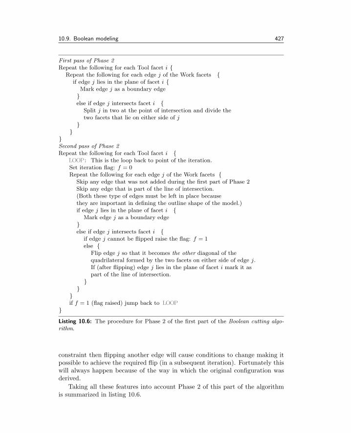
10.9. Boolean modeling 427
First pass of Phase 2Repeat the following for each Tool facet i {
Repeat the following for each edge j of the Work facets {if edge j lies in the plane of facet i {
Mark edge j as a boundary edge}else if edge j intersects facet i {
Split j in two at the point of intersection and divide thetwo facets that lie on either side of j
}}
}Second pass of Phase 2Repeat the following for each Tool facet i {
LOOP: This is the loop back to point of the iteration.Set iteration flag: f = 0Repeat the following for each edge j of the Work facets {
Skip any edge that was not added during the first part of Phase 2Skip any edge that is part of the line of intersection.(Both these type of edges must be left in place becausethey are important in defining the outline shape of the model.)if edge j lies in the plane of facet i {
Mark edge j as a boundary edge}else if edge j intersects facet i {
if edge j cannot be flipped raise the flag: f = 1else {
Flip edge j so that it becomes the other diagonal of thequadrilateral formed by the two facets on either side of edge j.If (after flipping) edge j lies in the plane of facet i mark it aspart of the line of intersection.
}}
}if f = 1 (flag raised) jump back to LOOP
}
Listing 10.6: The procedure for Phase 2 of the first part of the Boolean cutting algo-rithm.
constraint then flipping another edge will cause conditions to change making itpossible to achieve the required flip (in a subsequent iteration). Fortunately thiswill always happen because of the way in which the original configuration wasderived.
Taking all these features into account Phase 2 of this part of the algorithmis summarized in listing 10.6.

428 10. Modeling with polygonal datasets
Split
Lines ofintersec-tion
Figure 10.54: Lines of intersection that split a network of facets. Note that the partof the line of intersection labeled X does not cause a split.
10.9.2 Splitting facets along the line of intersection
Having built the line of intersection into the facets in the Work list it onlyremains to split them along it. Of course the network or Work facets will not besplit unless segments of the line of intersection form a complete cut, either byforming loops or crossing from one outside edge to another. This is illustratedin figure 10.54.
This stage of the algorithm is quite straightforward because the procedureof section 10.9.1 has already marked which edges in the model are part of theline of intersection. With this knowledge the following steps will cut the facetsin the work list along the line(s) of intersection if they split the network:
1. Set a counter l (initially to: l = −1). This will be used to count the numberof pieces and identify to which piece each facet belongs. Label all facets inthe work list as unidentified. This can be done by assigning a member ofthe facet data structure Facet(i).l = l.
2. Repeat steps (a) and (b) below until all Work facets are identified. (Thisprocedure is very similar to the “orienting” algorithm of section 10.7.)
(a) Increment l and pick an unidentified facet, say it is k. We could chooseit to be the first one for which Facet(k).l = −1. Assign Facet(k).l = l.
(b) Find the neighboring facets to facet k; this information is recordedin the Fid(j) member variables for the facet data structure. Letn = Facet(k).F id(j) with 0 ≤ j < 3 in turn. If the edge common tofacets n and k (given by Facet(k).Eid(j)) is not part of the line ofintersection then n is in the same piece as k and we repeat (recursively)this step in facet n and in n’s neighboring facets until progress isblocked either by the line of intersection or the edge of the model.

10.10. Metaball modeling and marching cubes 429
Note that the Eid and Fid can be determined by the algorithm givenin section 3.5 and that they are also kept up to date by the Delaunayalgorithm, as it flips edges and facets around.
3. Once all facets have been identified as belonging to one of the l piecesrepeat step (a) below for each i : 0 ≤ i < l.
(a) Make a copy of all the facets with Facet(k).l = i.
When copying facet k remember that the vertices it is attached to andthe edges which bound it must also be copied. Care will be neededto make sure that no edge or vertex is copied twice, for example fromadjacent facets with a common edge.
4. Remove from the database all the facets, edges and vertices recorded inthe Work list.Note: It may be easier to make copies of all the relevant bits and removethe originals rather than to try and copy the structure along the line ofintersection.
Figure 10.55 illustrates the identification of facets up to a boundary or lineof intersection. Note that if the edge of intersection does not completely splitthe network of facets then they will be identified as part of the same piece; thisis desirable. To be specific: In figure 10.55: (a) The edges that form the line ofintersection are highlighted. (b) Choose any facet at random and label this asbeing part of the first piece. (c) Label the facets adjacent to the first one chosenunless that facet is on the other side of the outline. (d) Finish labeling all facetsadjacent to those identified with a 0; remember a boundary may not be crossed.When there are no facets adjacent to 0 remaining choose another at random andlabel this 1. (e) Label with a 1 the facets adjacent to the facet labeled 1 in (d).(f) Label with a 1 the facets adjacent to the facets labeled 1 in (e). (g) Finishlabeling all possible facets adjacent to those facets labeled 1 in (f). Pick anotherat random and label this 2. (h) Label all possible facets adjacent to the onelabeled 2 in (f). Since there are no unidentified facets left the identification iscomplete. (i) Copy all the facets labeled 1, 2 and 3 as separate pieces and deletethe originals. This gives us the three pieces formed by the cutting operation.
10.10 Metaball modeling and marching cubes
There are shapes that do not lend themselves to modeling with any of the algo-rithms considered in this chapter, or even with an interactive design tool in whichthe user has a free hand. This is especially true of many organic shapes. Anothersource of three-dimensional data, laser scanners and stereoscopic imaging sys-tems produce a point cloud of data that represents the shape of the object. Beforea point cloud of 3D data can be visualized the surface needs to be meshed into

430 10. Modeling with polygonal datasets
First facet chosenat random
Lines of intersection
(a)(b) (c)
(f )(e)(d)
(g) (h)(i)
0 00
0
000
0
00
0
0
0
00
0
0
00
0
002
2
22 2
22
22
00
0
00
0
0
111
1
1 1
11
11 111
1111
11 1
11
11 1 1
11
11
11 1 1
1 1 11
11
1 1 1
11
1
11
1
1
1
11
1
11
11
1
11
1
1
1 1
1 11
11
1
1 1
1
1 1 1
11
111
11
1
1
Figure 10.55: Identifying the pieces to be split up. Illustrations (a) - (i) are discussedin the text.
a network of polygonal faces. This is not a trivial task, and a mesh generated inthis way can be very messy. Some manual tidying up is often inevitable. A thirdsource of data that is often visualized as a 3D model is a potential field, where thevisualization takes the form of a triangular mesh built across an equi-potentialsurface. Several layers may be superimposed with transparency. Medical imagedata and the results of scientific experiments are excellent examples of this sortof problem.
This section will dive into the concept and the algorithms of two techniquesthat allow us to visualize volume data and build mesh models through a combi-nation of potential fields. Some of the plug-in modules of OpenFX (chapter 9)
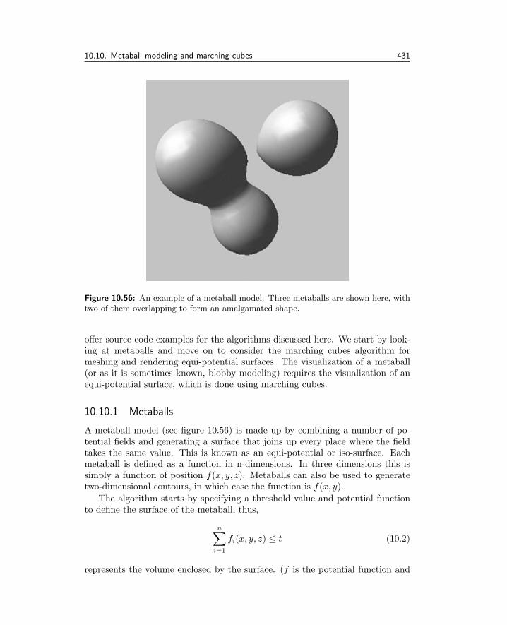
10.10. Metaball modeling and marching cubes 431
Figure 10.56: An example of a metaball model. Three metaballs are shown here, withtwo of them overlapping to form an amalgamated shape.
offer source code examples for the algorithms discussed here. We start by look-ing at metaballs and move on to consider the marching cubes algorithm formeshing and rendering equi-potential surfaces. The visualization of a metaball(or as it is sometimes known, blobby modeling) requires the visualization of anequi-potential surface, which is done using marching cubes.
10.10.1 Metaballs
A metaball model (see figure 10.56) is made up by combining a number of po-tential fields and generating a surface that joins up every place where the fieldtakes the same value. This is known as an equi-potential or iso-surface. Eachmetaball is defined as a function in n-dimensions. In three dimensions this issimply a function of position f(x, y, z). Metaballs can also be used to generatetwo-dimensional contours, in which case the function is f(x, y).
The algorithm starts by specifying a threshold value and potential functionto define the surface of the metaball, thus,
n∑
i=1
fi(x, y, z) ≤ t (10.2)
represents the volume enclosed by the surface. (f is the potential function and

432 10. Modeling with polygonal datasets
(a) (b) (c) (d)
(e) (f ) (g) (h)
Figure 10.57: Metaballs form by amalgamating potential fields.
t is the threshold value.) A typical function chosen for metaballs is:
f(x, y, z) =1
((x− x0)2 + (y − y0)2 + (z − z0)2)(10.3)
where (x0, y0, z0) is the center of the metaball. The fall-off function should goto zero at a maximum distance. When evaluating the metaball field, any pointsbeyond the maximum distance from the center point are ignored. Because theiso-surface is the result of adding the fields together, its smoothness is dependenton the smoothness of the fall-off curves. When metaball fields start to interactthe result is shown in figure 10.57.
The arrangement of metaballs shown in figure 10.56 was created by threemetaballs using the field function p(x,y,z) given by:
(
n∑
i=1
r2i|d2
i |
)
− t = 0 (10.4)
where: ri is the radius of the metaball, and di is the vector between P(x,y,z) andthe center of the metaball.
Metaballs do not have to be based on spherical fields surrounding a point.They can be based on a cylindrical field surrounding a line, or even lie around anplanar polygon, or any 3D shape, and they can be very effective when animated.Figures 10.58 and 10.59 illustrate how a set of metaballs can be visualized; thisis taken from OpenFX.
10.10.2 Marching cubes
At the core of the visualization of metaball generated equi-potential surfacesis the marching cubes algorithm. The same algorithm will render any equi-potential surface in a potential field, and can be used to render a non-convexhull around a point cloud, such as that shown in figure 10.59.

10.10. Metaball modeling and marching cubes 433
Figure 10.58: Three spherical metaballs are triangulated using the marching cubesalgorithm of section 10.10.2.
The marching cubes algorithm is a natural extension of the two-dimensionalmarching squares algorithm that is used to draw a contour at a specific value of a2D potential field. Marching squares has great utility in drawing height contourson a map or isobars on a weather map. It is much easier to understand thealgorithm’s concept in two dimensions and there are many fewer configurationsthat have to considered.
To appreciate the marching squares algorithm consider the grid shown infigure 10.60. Each point of this grid is given a weight (a potential value), and inthis example the reference potential value is 5. To draw a curve whose value isconstant and equal to the reference value, each square in the grid is individuallyconsidered. Those grid squares where every one of its four vertices is eitherbelow the reference value, or every one of its four vertices have a value above thereference value, will have no segments of the contour passing through them.
Where some corner potential values lie above and below the reference valuethen the contour will pass through that square. Careful consideration of allpossible combinations (above/below) indicates there are only 16 possible con-figurations required to represent all possible ways the contour can pass throughthe 2D squares. There are some possible combinations illustrated in figure 10.61that are ambiguous; these are labeled A. The ambiguity, which is illustrated infigure 10.62, does not imply any real error because the contours remain closed.

434 10. Modeling with polygonal datasets
Figure 10.59: A point cloud of vertices gives rise to a meta-surface by placing a metaballat each vertex and meshing the equi-potential surface.
The concept of the marching squares algorithm can be naturally extended tothree dimensions where the squares become cubes that have 8 vertices per cubeand the line segments that made up the contour become polygonal faces thatmake up the equi-potential surface (iso-surface). Each cube will either lie insidethe iso-surface, or outside the iso-surface, or it will straddle the iso-surface. Witheach cube having 8 vertices there are 256 (i.e., 28) possible arrangements of itscorners being inside or outside the volume enclosed by the iso-surface. However,taking into account symmetries (rotation, mirroring and re-labeling) this reducesto only 16 possibilities. Figure 10.63 depicts the possible combinations and thetriangulations that have to be constructed to produce the closed surface for thatpart of the iso-surface that lies inside the cube.
In order to be able to determine which of the 16 cases apply to a specific setof vertex potential values, each of the 16 cases is assigned an index formed froma binary interpretation of whether a corner (vertex) potential value is above orbelow the equi-potential surface; see figure 10.64.
In this way, vertices from 1 to 8 are weighted from 1 to 128 (v1 = 1, v2 = 2,v3 = 4, etc.); for example, the case 3 (figure 10.63) corresponds to the number5 (v1 and v3 are outside, 1 + 4 = 5). By using the corner weights in this way afast look-up table can be constructed to define how many polygons need to becreated for each of the 16 possible configurations and along which edges of the

10.10. Metaball modeling and marching cubes 435
33
3 7 8 6 2
8 9 7 3
2 6 6 1
3
1
1 12 20
1 42
Figure 10.60: A square grid with potential field values (of some nominal unit) at eachgrid point. A contour with the value of 5 is shown after interpolation. The shaded areaequates to the area where the potential field’s value is greater than 5.
A
A
InsideOutside
Figure 10.61: The 16 combinations of grid square crossings that depend on the valuesof the field at the corner vertices relative to the contour.
(b)(a)
Outside
Inside
Figure 10.62: In the ambiguous cases the contours could be connected in two differentways for the same pattern of vertex potential field values.

436 10. Modeling with polygonal datasets
0
1
1 2 2
2 2 3 3
4 4 4 4
4 4 4 8
15
40
3
76
2
5
40
3
76
2
Figure 10.63: The 16 possible combinations of in/out cube vertices and their associatedtriangulation.
cube, and where their surface vertices have to be positioned. Thus the algorithmcan be expressed in a few simple steps:
1. Break up space into small cubes ( > 1,000,000,000 ).
2. Consider each cube in turn.
3. Calculate an index by comparing the 8 corner density values with the iso-surface value.
4. Using this index look up the list of edges from a pre-calculated table (theedges around each triangle).
5. Interpolate the position of the intersection along the edge using the densityvalues at the vertices at each end of the edge.
6. Calculate a normal at each vertex.

10.10. Metaball modeling and marching cubes 437
id = v8|v7|v6|v5|v4|v3|v2|v1
v1 v2
e10
v6v5
v3
e1
e5
e9
e4
e8
v4
e2
e6
e12
e7
e3
e11
v8v7
x
y
z
Figure 10.64: Weights assigned to each cube’s vertices.
7. Output the triangle vertices and normals.
To implement this algorithm in practice we need to define some data struc-tures, first a 3D vector. There are many ways to do this, for this example wechoose:
typedef struct {f loat x ;f loat y ;f loat z ;
} VECTOR3D;
Next, a structure is needed for each grid point in the cubic lattice. Thisstructure might include other data that is interpolated across the cell.
// cube g r i d v e r t e xtypedef struct {VECTOR3D po s i t i o n ; // po s i t i o n o f the g r i d v e r t e xf loat value ; // the va lue o f the s c a l a r f i e l d. . // o ther data
} CUBE GRID VERTEX;
New vertices will be inserted along edges where the potential values at eitherend of the edge bracket the iso-surface value. This structure might include theidentity of the CUBE GRID VERTICES that it separates.
// v e r t e x crea t ed from the l i n e a r i n t e r p o l a t i o n a long edgetypedef struct {VECTOR3D p ; // po s i t i o n. . . . o ther data
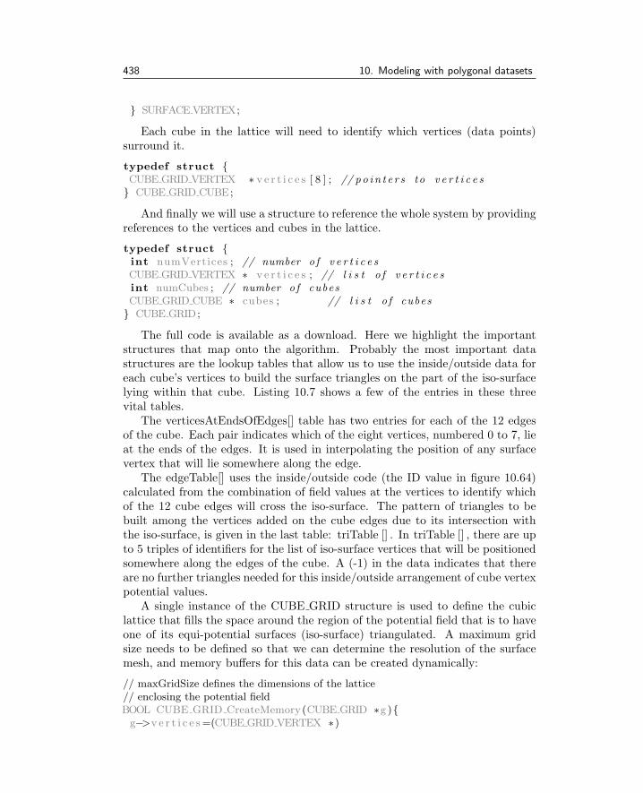
438 10. Modeling with polygonal datasets
} SURFACEVERTEX;
Each cube in the lattice will need to identify which vertices (data points)surround it.
typedef struct {CUBE GRID VERTEX ∗ v e r t i c e s [ 8 ] ; // po in t e r s to v e r t i c e s
} CUBE GRID CUBE;
And finally we will use a structure to reference the whole system by providingreferences to the vertices and cubes in the lattice.
typedef struct {int numVertices ; // number o f v e r t i c e sCUBE GRID VERTEX ∗ v e r t i c e s ; // l i s t o f v e r t i c e sint numCubes ; // number o f cubesCUBE GRID CUBE ∗ cubes ; // l i s t o f cubes
} CUBE GRID;
The full code is available as a download. Here we highlight the importantstructures that map onto the algorithm. Probably the most important datastructures are the lookup tables that allow us to use the inside/outside data foreach cube’s vertices to build the surface triangles on the part of the iso-surfacelying within that cube. Listing 10.7 shows a few of the entries in these threevital tables.
The verticesAtEndsOfEdges[] table has two entries for each of the 12 edgesof the cube. Each pair indicates which of the eight vertices, numbered 0 to 7, lieat the ends of the edges. It is used in interpolating the position of any surfacevertex that will lie somewhere along the edge.
The edgeTable[] uses the inside/outside code (the ID value in figure 10.64)calculated from the combination of field values at the vertices to identify whichof the 12 cube edges will cross the iso-surface. The pattern of triangles to bebuilt among the vertices added on the cube edges due to its intersection withthe iso-surface, is given in the last table: triTable [] . In triTable [] , there are upto 5 triples of identifiers for the list of iso-surface vertices that will be positionedsomewhere along the edges of the cube. A (-1) in the data indicates that thereare no further triangles needed for this inside/outside arrangement of cube vertexpotential values.
A single instance of the CUBE GRID structure is used to define the cubiclattice that fills the space around the region of the potential field that is to haveone of its equi-potential surfaces (iso-surface) triangulated. A maximum gridsize needs to be defined so that we can determine the resolution of the surfacemesh, and memory buffers for this data can be created dynamically:
// maxGridSize defines the dimensions of the lattice// enclosing the potential fieldBOOL CUBE GRID CreateMemory(CUBE GRID ∗g ){g−>v e r t i c e s=(CUBE GRID VERTEX ∗)

10.10. Metaball modeling and marching cubes 439
//Table gives the vertices at the end of each edgeint vert icesAtEndsOfEdges [24 ]={0 , 1 ,. . ,3 , 7} ;
// Table identifies which of 12 cude edges will cross the iso-surface.// Each entry is a bit pattern corresponding with an edge either crossing// or not crossing the threshold value. There is one entry for each of// the 256 possible arrangements of the 8 vertex states (in/out)int edgeTable [256]={0x0 , 0x109 , 0x203 , 0x30a , 0x406 , 0 x50f , 0x605 , 0x70c ,0x80c , 0x905 , 0 xa0f , 0xb06 , 0xc0a , 0xd03 , 0xe09 , 0 xf00 ,. .0x70c , 0x605 , 0 x50f , 0x406 , 0x30a , 0x203 , 0x109 , 0x0 } ;
//This table gives which of the vertices, added along the cube edges where//they cross the iso-surface, to join to form triangles for the surface//(-1) indicates no more groups of 3 (max of 5 triangles per cubeint t r iTab l e [ 2 5 6 ] [ 1 6 ] ={{−1,−1,−1,−1,−1,−1,−1,−1,−1,−1,−1,−1,−1,−1,−1,−1} ,{0 ,1 ,9 ,−1 ,−1 ,−1 ,−1 ,−1 ,−1 ,−1 ,−1 ,−1 ,−1 ,−1 ,−1 ,−1} ,. .{1 ,8 ,3 ,9 ,8 ,1 ,−1 ,−1 ,−1 ,−1 ,−1 ,−1 ,−1 ,−1 ,−1 ,−1} ,. .{2 ,8 ,3 ,2 ,10 ,8 ,10 ,9 ,8 ,−1 ,−1 ,−1 ,−1 ,−1 ,−1 ,−1} ,. .{−1,−1,−1,−1,−1,−1,−1,−1,−1,−1,−1,−1,−1,−1,−1,−1}} ;
Listing 10.7: The lookup tables for the marching cubes algorithm.
mal loc ( s izeof (CUBE GRID VERTEX)∗( maxGridSize+1)∗(maxGridSize+1)∗(maxGridSize +1)) ;i f ( ! g−>v e r t i c e s ) { return FALSE; }g−>cubes=(CUBE GRID CUBE∗) mal loc ( s izeof (CUBE GRID CUBE)∗maxGridSize∗maxGridSize∗maxGridSize ) ;
i f ( ! g−>cubes ) { return FALSE; }return TRUE;
}
The instances of the structure representing the cubes need to be initialized,the vertices at the lattice points within each cube need to be positioned andgiven a value or the potential field, and each cube needs to have its list of cornervertices assigned. This is done in listing 10.8.

440 10. Modeling with polygonal datasets
BOOL CUBE GRID Init (CUBE GRID ∗g , int g r i dS i z e ){int i , j , k ;
int currentCube ;int currentVertex=0;g−>numVertices=( g r i dS i z e +1)∗( g r i d S i z e +1)∗( g r i d S i z e +1);// assign lattice vertex positions, this example is based on a cubic// lattice centred on (0,0,0) and filling the cube [-10,10]for ( i =0; i<g r i dS i z e +1; i++) {for ( j =0; j<g r i dS i z e +1; j++){for ( k=0; k<g r i dS i z e +1; k++){g−>v e r t i c e s [ currentVertex ] . p . x=
( i ∗20 .0 f )/ ( g r i d S i z e )−10.0 f ;. . // other positionscurrentVertex++;
}}
}g−>numCubes=( g r i dS i z e )∗ ( g r i d S i z e )∗ ( g r i d S i z e ) ;currentCube=0;// assign the vertices around each cubefor ( i =0; i<g r i dS i z e ; i++) {for ( j =0; j<g r i dS i z e ; j++) {
for ( k=0; k<g r i dS i z e ; k++) {g−>cubes [ currentCube ] . v e r t i c e s [0 ]=&g−>v e r t i c e s [ ( i ∗( g r i d S i z e+1)+ j )∗ ( g r i d S i z e+1)+k ] ;g−>cubes [ currentCube ] . v e r t i c e s [1 ]=
&g−>v e r t i c e s [ ( i ∗( g r i d S i z e+1)+ j )∗ ( g r i d S i z e+1)+k+1] ;. . . // other vertex assignments
currentCube++;}
}}return TRUE;
}
Listing 10.8: Setting up the lattice coordinates with their field values.
Once the lookup tables are established and the preparatory work done inlistings 10.7 and 10.8 completed, the implementation of the marching cubesalgorithm in listing 10.9 can be executed.
The implementation of the algorithm proceeds by considering each cube inturn as a individual entity. The code in listing 10.9 fulfills the following logic:
1. Work out which of the patterns (using the ID value of figure 10.64) of iso-surface faces is required for the cube, based on the value of the field at thecube’s vertices. This is the variable cubeIndex.

10.10. Metaball modeling and marching cubes 441
void CUBE GRID DrawSurface (CUBE GRID ∗g , f loat th r e sho ld ){//local storage up to 12 possible vertices for any iso-surface in cubestat ic SURFACEVERTEX edgeVer t i c e s [ 1 2 ] ;for ( i =0; i<g−>numCubes ; i++){//loop through cubes//calculate which vertex pattern to apply//based on cube vertex valuesi f ( g−>cubes [ i ] . v e r t i c e s [0]−> value < th r e sho ld )
cubeIndex |= 1 ;i f ( g−>cubes [ i ] . v e r t i c e s [1]−> value < th r e sho ld )
cubeIndex |= 2 ;. . . // set indices for the other vertices//look-up this value in edge table to see which edges to interpolate alongusedEdges=edgeTable [ cubeIndex ] ;//if the cube is entirely within/outside surface, or has no facesi f ( usedEdges==0 | | usedEdges==255)continue ;//check each edge to see if it should have an iso-surface vertexfor ( currentEdge=0; currentEdge <12; currentEdge++) {i f ( usedEdges & 1<<currentEdge ) {CUBE GRID VERTEX ∗v1 ,∗ v2 ; // get the cube edge’s verticesve1=vert icesAtEndsOfEdges [ currentEdge ∗ 2 ] ;ve2=vert icesAtEndsOfEdges [ currentEdge ∗2+1] ;v1=g−>cubes [ i ] . v e r t i c e s [ ve1 ] ;v2=g−>cubes [ i ] . v e r t i c e s [ ve2 ] ;// intepolate to put iso-surface vertex along cube edgede l t a=( th r e sho ld − v1−>value )/ ( v2−>value − v1−>value ) ;edgeVer t i c e s [ currentEdge ] . p o s i t i o n . x= . . . .
}}//make the triangular faces in this cube 3 vertices per facefor ( k=0; t r iTab l e [ cubeIndex ] [ k ]!=−1; k+=3){MakeTriangleFaceAt (
&edgeVer t i c e s [ t r iTab l e [ cubeIndex ] [ k +0 ] ] . p ,&edgeVer t i c e s [ t r iTab l e [ cubeIndex ] [ k +1 ] ] . p ,&edgeVer t i c e s [ t r iTab l e [ cubeIndex ] [ k +2 ] ] . p )
}}
}
Listing 10.9: Executing the marching cubes algorithm.
2. Using cubeIndex, look up the edge table to identify which of the cube’sedges will cross the iso-surface.
3. Consider each edge of the current cube in turn: If it crosses the iso-surfacedetermine where, and record this in the edgeVertices [] list. If none of thecube’s edges cross the iso-surface just ignore this cube.

442 10. Modeling with polygonal datasets
2, 20, 2
0, 0 2, 0
3d R
Figure 10.65: The result of assigning texture coordinates to the vertices of two trian-gular facets.
4. Finally, build the triangular mesh by using the pattern of faces appropriatefor the cube’s ID. Table triTable [] holds the triangular face information byindexing the edgeVertices [] list. The coordinates of the triangles’ verticeswill be found in the edgeVertices [] list.
In this implementation of the marching cubes algorithm each polygon is cre-ated as a separate face. The network is not connected and each face’s verticesare independent of all the other vertices. To be useful in a 3D modeling packagewhere vertices from neighboring faces occur at the same point, the faces shouldreally share the same vertices, and where the edges of a face are common to otherfaces then only one edge should be inserted into the data structures. This couldbe done in a post-creation sorting stage, but it would be preferable if the codepresented here were modified to do this as the face data is being created. To dothis would require that each cube keeps a record of its 26 immediate neighborsso that when a new face is added a check is made to see whether any of its edgesor vertices have been created before in a neighboring cube. The use of an integerbased coordinate system for vertices makes this step very much more robust.
10.11 Texture coordinate generation
In section 4.6 the use of texture coordinates was discussed. It was not stated therehow texture coordinates are generated. It was stated that images were appliedto a two-dimensional texture coordinate system (X,Y ) (commonly referred to as(u, v) coordinates) and that a single copy of the image occupied the region inwhich the coordinates satisfied: 0 ≤ X < 1.0, 0 ≤ Y < 1.0.
One obvious way to assign texture coordinates is by hand. The example inFigure 10.65 shows two triangular facets with texture coordinates and a renderedpicture with the image shown mapped across the facets.
Manual assignment is however only satisfactory if very few facets are involved.An automatic procedure that assigns mapping coordinates according to some

10.11. Texture coordinate generation 443
(a) (b) (c)
Figure 10.66: Projected image texture mapping: (a) A planar map. (b) A cylindricalmap. (c) A spherical map.
more usable scheme is essential if we are to apply maps to models with manyfacets and non-planar geometry. It turns out that three basic formats providemap coverage for almost all situations. They are:
1. Planar mapping
2. Cylindrical mapping
3. Spherical mapping
These are illustrated in figure 10.66.Planar mapping is the most appropriate method of application when the sur-
face to be covered is approximately flat. Cylindrical and spherical mapping aremost appropriate when the surfaces to be painted are approximately cylindricalor spherical. Since it is impossible to achieve an undistorted mapping from aplane to a cylinder or plane to a sphere it is obvious that at least these threetypes of mapping must be available. Most potential uses for an image map arecovered by one of these three cases.
From a usability point of view each of these mapping methods requires onlya few parameters for their specification. Texture coordinates for each vertex arereadily calculated from one of these mapping methods.
10.11.1 Planar mapping
Figure 10.67(a) illustrates the mapping relationship. A network of triangularfacets is shown overlapped by a rectangle R, which is assumed to bound theimage being mapped. The question then is: What are the mapping coordinatesof any vertex, V , in the network of facets?
The case shown in figure 10.67(a) doesn’t tell the whole story because thefacets are located in three dimensions and whilst ideally they should be planarso that the map is not distorted, they don’t have to be. Neither do they have to

444 10. Modeling with polygonal datasets
(a)
V
V
RR
P0
n
Pi
Pα
Pβ
(b) (c)
Figure 10.67: (a) A rectangle bounding the image to be mapped is shown overlappinga network of facets. (b) A three-dimensional view of the same situation that showshow the mapping rectangle R is projected on to the surface at right angles to R.(c) Rendering the facets after assignment with mapping coordinates.
lie in the plane of R and therefore to obtain mapping coordinates for V we mustassume that the mapping coordinates are determined by a projection in threedimensions from R to V ; this is illustrated in figure 10.67(b).
The procedure for determining mapping coordinates at V is as follows: Astraight line through V (given by position vector Pv) is constructed in the di-rection of the normal to the plane of R, i.e., parallel to the normal to R (say n).It intersects the plane in which R lies at the point Pi. Since Pi is in the planeof R it can be expressed as a linear combination of the two vectors along thesides of R. Thus if R is defined by the three points P0, Pα and Pβ , the vectorsalong the edges are: Pβ −P0 and Pα −P0. The algorithm from section 2.11.1will allow us to find an α and β which satisfy:
Pi = P0 + α(Pα −P0) + β(Pβ −P0)
Pi is obtained by calculating the intersection point in the plane of R: (p−P0) ·n = 0 and the line: p = Pv + αn. (See Section 2.6.)
The mapping coordinates of V follow by assuming that at P0 the mappingcoordinates are (0, 0), atPα they are (1, 0) and atPβ they are (0, 1) and thereforeat V the (Xv, Yv) are simply:
Xv = α
Yv = β
If this procedure to assign texture coordinates to all vertices is followed, animage will be painted on the facets so that it lies inside the projection of R in aperpendicular direction to the plane in which R lies. The top left corner of theimage will occur at P0, the top right corner of the image at Pα and the bottomleft corner of the image at Pβ .

10.11. Texture coordinate generation 445
Note that the planar mapping described here uses three points to define thelocation of the map and therefore the opposite sides are always parallel eventhough the angle between Pα and Pβ does not have to be 90◦.
It would be possible to define a map using four points, one at each cornerof the rectangle but it is considerably more complex to determine the mappingcoordinates from such a map because the opposite sides would not necessar-ily be parallel. Haines [33] gives expressions (without derivation) for a convexquadrilateral mapping that could form the basis of the necessary procedure.
10.11.2 Cylindrical mapping
In cylindrical mapping one imagines that the picture is wrapped around a cylin-der enclosing the surface to be textured (see figure 10.66(b)). The texture co-ordinates are assigned to a vertex V by finding the point on the cylinder wherea line from the axis of the cylindrical map passing through V (at Pv) intersectsthe cylindrical surface, at Pi. This is illustrated in figure 10.68. Since Pi lieson the cylinder its position in a frame of reference associated with the cylindercan be specified as a fraction of the distance between the top and bottom of thecylinder d and a fraction of a full rotation round the cylinder θ. The angle ofrotation is specified relative to a line where the left hand edge of the image isstuck to the cylinder.
To define a cylindrical map the radius of the cylinder used to define the mapis not important. We can assume r = 1, but the following must be specified:
• The axis of the cylinder. The best way to do this is with a point on theaxis at the top of the cylinder P1 and a point at the bottom of the cylinderP2. We will assume that the Y mapping coordinate is zero at the top ofthe cylinder and unity at the bottom.
• The location of the left-hand edge of the map on the curved surface of thecylinder. An easy way to do this is by specifying some point PL whichmay be any point that is not on the axis of the cylinder.
The left-hand edge is a line running parallel to the axis of the cylinderthrough a point unit distance from the cylinder’s axis in the direction ofPL.
• The angle of rotation, φ, from the left-hand edge of the map round thecylindrical axis which is to be equivalent to one copy of the image. Thisis the location where the X mapping coordinate is unity. When φ = 2π it
takes one copy of the map to go all the way round the cylinder. If φ =π
4the map occupies one eighth of the cylinder, or to put it another way, ittakes eight copies to paint all around it.
This geometry is illustrated in figure 10.68.

446 10. Modeling with polygonal datasets
Axis of cylindrical map
Left edge here
Vertex to bemapped Plan view
r
r
q
n
Pi
P1
P2
Pv
PL
d θ
θ
φ
�e map rolls round thecylinder in this direction
Figure 10.68: Cylindrical mapping.
In view of the discussion above the assignment of mapping coordinates atany vertex is made using the following procedure:
Given that φ is the angle round the cylinder equivalent to an Xmapping coordinate of unity and the distance between the top andbottom of the cylinder is assumed to cover one unit of the Y mappingcoordinate, vertex V will be assigned texture coordinates accordingto:
Xv =θ
φ
Yv = d
d and θ are illustrated in figure 10.68. They may be calculated interms of P1, P2 and PL using the algorithm given in listing 10.10.Here Pv is the position vector for vertex V .
10.11.3 Spherical mapping
A spherical mapping can be described in a very similar way to a cylindricalmapping except that the central axis serves only to define the position of thenorth or south poles of the sphere. One can imagine the image being squeezedonto the sphere as illustrated in figure 10.66.
To map the image to the sphere we use the angular components (φ, θ) ofspherical polar coordinates (defined in section 2.1.2) where θ and φ satisfy: 0 ≤θ < π and −π < φ ≤ π. The parameters θ and φ will need to be equated tomapping coordinates (X,Y ) in the range 0 ≤ Y < 1 and 0 ≤ X < 1. For anyvertex V a φ and θ are obtained by drawing a line from V (with position vectorPv) to a point at the center of the spherical map, and calculating the pointwhere this line intersects the unit sphere.

10.11. Texture coordinate generation 447
Firstly find d:Let y = P2 −P1 ( the axis of the cylinder)Thus d is the projection of (PV −P1) onto the axis of the cylinder.
d =(PV −P1) · y
y · y
Secondly find θ:Let x = PL −P1 (a direction towards the ‘seam’)Let q = (PV −P1)− dy(q is the direction of PV from the cylinder’s axis)
Set q =q
|q|We need a direction perpendicular to the cylinder’s axis that is towards
the seam: Let l =(PL −P1) · y
y · yand r = (PL −P1)− ly(r is the direction of PL from the cylinder’s axis)
Set r =r
|r|Then θ = arccos(q · r)
This only specifies θ in the range: 0 ≤ θ < π we need to knowwhether θ lies in quadrant 3 or 4. Determine this by formingthe vector n which is perpendicular to the plane in whichP1, P2 and PL lie.
n =x× y
|x× y|
if q · n < 0 then θ = −θ
This algorithm gives θ in the range −π < θ ≤ π other rangescan be obtained by appropriate scaling.
Listing 10.10: Algorithm to determine the cylindrical mapping parameters d and θ forthe geometry illustrated in figure 10.68.
Once the point where this line intersects a unit sphere is known in terms ofangle θ (from the north pole) and φ (longitude) the mapping coordinates forvertex V , (Xv, Yv), are given by:
Yv =θ
π
Xv =
φ
2π: 0 ≤ φ ≤ π
2π + φ
2π: − π < φ < 0

448 10. Modeling with polygonal datasets
P2
P1x
y
zθ
φ
PL
North pole Pv
Figure 10.69: Spherical mapping.
This maps a picture with its top located at the north pole and its bottom atthe south pole. Angles θ and φ are obtained by following an argument similarto the one used to derive the cylindrical mapping coordinates. This geometry isillustrated in figure 10.68.
In the geometric specification illustrated in figure 10.69 the center of themapping sphere is at P1. We will assume that the south pole is located at P2
and that PL is an arbitrary point, not on the polar axis. In an analogous wayto the way it was used for cylindrical mapping PL specifies where the “seam”of the map lies. Given this information the algorithm presented in Figure 10.11will determine the θ and φ.
10.11.4 Automatic map coordinate generation
Generating image map coordinates is not always easy in a modeling tool. Pro-jections such as those just discussed can provide a great starting point becausemany objects have a high degree of topological similarity with the plane or cylin-der. When it is possible to start with a basic surface texture coordinate system,an interactive design tool that unrolls the mapping coordinates onto a 2D displaycan be written so that its user may interactively tweak the 2D texture coordi-nates corresponding to a 3D vertex so that it is positioned at the place in theimage map that they desire. The OpenFX software has such a tool; figure 10.70illustrates it in action. For this tool to be successful a good initial guess of themapping coordinates is essential, otherwise many 2D coordinates will overlapand it will be impossible for the artist to separate them.
Sometimes however it is not possible to get a good initial texture coordinatemapping, and another approach is worth exploring. When a surface is modeledby a mesh of polygons that are connected together in a coherent way, that is,there are no gaps in the mesh, and it does not twist back on itself, or bifurcatein a strange way, then it is possible to use the 2D mapping coordinates of justone polygon to establish a mapping over the whole surface of an object.
Of course there are going to be cases where this will not work very well; forexample trying to texture-map a cube made up from six quadrilaterals, when

10.11. Texture coordinate generation 449
First a right handed frame of reference relative to the givenspherical map must be established.Let:z = P1 −P2
y = z× (PL −P1)x = y × z
normalize:
x =x
|x|y =
y
|y|z =
z
|z|
Now determine φ:Let: r = Pv −P1
and : r =r
|r|then: φ = ATAN2((r · x), (r · y))
To determine θ use:θ = arccos(r · z)
Listing 10.11: Determining θ and φ relative to a specification of the spherical map fora vertex at Pv.
just one of them is initially mapped, is unlikely to produce a pleasing result. Inthis case a spherical map centered within the cube is likely to come much closerto the desired result.
In principle the automatic generation of a 2D coordinate system over a curvedsurface is relatively simple if we make the assumption that two adjacent faces canbe unrolled, by rotating the second face around the common edge so they theylie in a plane. Once unrolled the coordinate system can be mapped out acrossthe adjacent face and mapping coordinates assigned to the non-common vertex.Figure 10.71 illustrates the idea: (a) shows a flat mesh of triangular polygons inwhich vertices 1, 2 and 3 of triangle A have been assigned mapping coordinatesusing a frame of reference with the x axis lying along the edge from vertices 1to 3 and the y axis lying along the edge from 1 to 2. Since triangles B and Eare adjacent to A their non-common vertices 4 and 7 can have their mappingcoordinates assigned using the local frame of reference in triangle A. Now, astriangle B has a full 2D frame of reference its vertices’ mapping coordinates canbe used to establish a frame of reference relative to triangle B, which in turncan then be used to assign mapping coordinates to the non-common vertices inthe triangular faces adjacent to B.
Once triangle B has been mapped, the algorithm can simply recurse acrossthe connected mesh establishing mapping coordinates at every vertex until the

450 10. Modeling with polygonal datasets
(a) (b)
Figure 10.70: Interactively moving the texture map coordinates by superimposing the2D texture coordinates mesh over an image. (a) The 3D mesh model. (b) The 2Dtexture coordinates and image to be wrapped around the mesh.
whole mesh is triangulated. When the mesh represents a non-planar surface,the faces adjacent to the reference frame will need to be temporarily rotatedaround the common edge with the reference face, so that both faces lie in aplane. Once aligned in a plane, a 2D mapping coordinate can be generatedat their non-common vertex. A suitable transformation can be obtained byrecognizing that it has to align the faces’ normal vectors by a rotation aroundthe vector joining the vertices at the ends of the common edge. For example, infigure 10.71(b) the vectors nA and nB should be aligned by rotation around thevector d; section 2.12.5 describes suitable algorithms to achieve this.
In figure 10.71(a) the surface triangulation is totally consistent, because eachtriangle is only adjacent to a maximum of three other triangles and the surface isflat. This algorithm would not work for the case shown in figure 10.71(c) becauseof the single vertex joining the two pieces.
If we now imagine folding the mesh in figure 10.71(a) around a surface totake the shape, shown in cross-section in (b), there is no reason why the verticescannot carry the same texture coordinates. Indeed there is no reason why thetexture coordinate generation has to start with a flat mesh because the connec-tions among the faces remains the same. For example faces A and B virtuallylie in the same plane and it is easy to see that an assumption of continuing toapply the frame of reference from A into B is not a bad one.
The cross-section in figure 10.71(b) illustrates a mapping on to a spiral objectin which the map (defined in just one triangular face) winds round the spiral,something that could not be achieved with the use of a cylindrical map forexample. There are, of course, some cases where this algorithm will not workvery well. A triangle that is joined to two others along a common edge could leadto inconsistencies, figure 10.71(d). Applying the algorithm, starting at face A, tothe three sides of a cube shown in (e) could lead to different mapping coordinates

10.12. Building polygonal primitives 451
(e)
v
A
A
A
B
C
DA
B
C
DG
F
E
nA nB
3
4
6
1, 2
2, 3
5
1
2
(1, 0)
(0, 0) (1, 0)
A
(d)
(a)
GF
E
(b)
(c)
Figure 10.71: Recursively generating texture coordinates using the local frame of ref-erence established in an adjacent polygon. (a) Flat mesh, (b) rapping mesh around acurved surface, (c) a mesh that cannot be mapped, (d) and (e) cases that could resultin an inconsistent mapping.
assigned to vertex V , depending on the order in which the adjacency is processedby the recursive algorithm.
But, all-in-all, the algorithm can provide a very useful tool to the 3D artistwhen it comes to painting 2D mapping coordinates onto their 3D models, or atleast starting to assign a model’s vertices with 2D mapping coordinates.
10.12 Building polygonal primitives
Most primitive shapes are readily constructed using one or more of the algorithmswe have now considered.
In general it is therefore only necessary to specify a very small amount ofstructural information because the automatic procedures will do the bulk of thework. For example we saw that a torus can be constructed by specifying a circleof edges and vertices followed by the generation of a surface of revolution.
The following list suggests how the most basic primitives might be con-structed:
• CubeStart with a square, 4 vertices, 5 edges, 2 facets, copy it, move the copyand loft the two outlines.

452 10. Modeling with polygonal datasets
• PyramidStart with a square, add the rest by hand, one vertex, 4 edges and 4triangular facets.
• ConeStart with an angled line, 2 vertices, 1 edge. Construct a surface of revo-lution about an axis that passes through one of the vertices. If necessary,cap the base of the cone (which is a convex polygon).
• TubeStart with a line (2 vertices, 1 edge). Construct a surface of revolutionabout an axis parallel to, but offset from, the line.
• CylinderBuild a tube as above then proceed to cap the top and bottom; both areconvex polygons.
• SphereTwo possible methods:
1. Start with a set of vertices and edges describing a semi-circle. Thenbuild a surface of revolution around an axis passing through both endsof the semi-circle.
2. Start with a very basic approximation to a sphere. Subdivide theedges and facets and move the additional vertices radially until theylie on a sphere. If necessary repeat this process until the facetedappearance is reduced to an acceptable degree.
• DiskStart with a set of vertices and edges describing a circle, then cap the circle.
• TorusStart with a set of vertices and edges describing a circle, construct a surfaceof revolution about an axis outside the circle.

11Algorithms for procedural
textures
In chapter 4 the basic idea of the procedural (or algorithmic) texture was in-troduced. In this chapter we will look at some examples that take advantage ofthose ideas to produce a collection of interesting surface textures. We will con-centrate on what one might describe as following the basic principles of mixinggeometric and noise patterns.
It is important to realize that the procedural textures described in this chapterdo not have any basis in physical or biological principles; they are essentially just“computer hacks” that look good and do the job.
All the textures considered in this chapter have been implemented as eitherDLL plug-ins or as GLSL shaders for OpenFX. After reading this chapter andchapter 9 you should be able to follow the finer details of a practical imple-mentation of the algorithms in the OpenFX code. Since the first edition of thisbook was printed it has become routinely possible to make use of the hardwareacceleration offered by the GPU, so algorithmic textures can now be generatedin real-time and with increasing sophistication. Despite their programmability,GPUs are still specialized processors that are nowhere near as flexible as theCPU of a traditional general purpose processor. They also have quite a limitedmemory, especially for storing the shader codes. Despite the C like form of theGLSL it is usually necessary to re-engineer an algorithm’s implementation, fromthe way it would be written in a standard high level language, to the way itmust be structured as a pair of GLSL shader programs. For example, ratherthan generate a noise value using the Perlin algorithm an image map is used asa lookup table.
Another reason for adopting a different approach to texture implementationis the fact that the GPU is expected to render textures repeatedly in real-time,and therefore, moving as many operations as possible into a execute once set-upstep becomes essential. For these reasons we offer two versions of the proceduraltexture algorithms in this chapter, one that is usable within the limits imposedby the GPU hardware and another for the general software approach where thereare no limits.
453

454 11. Algorithms for procedural textures
Almost any natural pattern can be simulated with a procedural texture.Perlin has greatly extended his original work and others have developed theprocedural texture so that now almost any surface appearance can be simulated.For example: Turk [84] and Witkin and Kass [91] have shown that reactiondiffusion is a very successful technique for developing fascinating proceduraltextures including many animal skin patterns (giraffe, zebra), coral and weavedsurfaces. Other useful sources of information may be found in the book by Ebertet al. [23].
The range of possible uses of algorithmic is not limited to painting patternson 2D surfaces. Perlin and Hoffert [68] and Kajiya and Kay [48] introducedthe concept of the hypertexture which one could describe as a three-dimensionalequivalent of the procedural texture. Rather than applying a texture to a meshedsurface a volume of some sort is specified and calculations proceed to determinethe opacity at points within that volume. To determine what is visible whenlooking at a hypertexture the opacity must be calculated at a number of samplepoints along the viewing direction (or ray as it passes through the hypertexturevolume). As a result hypertextures are extremely slow to compute and thereforevery careful thought is needed before embarking on their use. In this chapterwe do not discuss hypertextures but for more information the aforementionedreferences are a good place to look.
11.1 A standard interface
It is a good idea to arrange that procedural textures interface to their hostrenderer with a few standard parameters. All those rendering applications thatoffer their users the ability to write plug-in textures communicate with theirplug-ins through a standard interface. It is also useful to design a standard setof variables to communicate with the GPU shader programs so that differentshaders can be called into action without having to call on a whole collection ofspecial cases.
11.1.1 An interface for procedural textures
For a renderer that uses textures through shared object libraries or DLLs, a com-prehensive interface can be achieved with the function prototype and argumentset given in listing 11.1.
The function returns the Boolean value FALSE if the function fails for anyreason, otherwise TRUE is returned. The function’s parameters fall into fivegroups:
1. (Vectors: p, n)p is a position vector of the spot on the textured surface for which we wishto calculate the texture value, i.e., the surface color.

11.1. A standard interface 455
BOOL TextureProcedure (VECTOR p , // coordinate of surface pointVECTOR n , // surface normal at ”p” (unit length)VECTOR P, // position vector to origin of texture parallelepipedVECTOR U, // normalized basis vectors of texture parallelepipedVECTOR V,VECTOR W,f loat u , // relation between ”p” and texture parallelepipedf loat v , // i.e. p = P + uU + vV + wWf loat w,
MATRIX3 T, //Transform vector from (x,y,z) to (U,V,W) coordinatesf loat ∗ opacity , //Opacity of surfacef loat ∗ r e f l e c t i v i t y , // Reflectivity of the surfaceVECTOR co l o r // return the surface RGB color (0.0 - 1.0)){. . Body of the texturing procedure. .//Return FALSE if function fails, otherwise return TRUEreturn TRUE;
}
Listing 11.1: A prototype for a wide variety of texturing functions.
n is a unit direction vector normal to the surface being textured at p.Many textures redirect n away from its input direction. Some bend itin combination with a color variation but a number of the most effectivetextures involve shifts in the direction of n alone.
2. (Vectors: P,U,V,W, and scalars: u,v,w)These important parameters allow a texture to be applied in a way thatis relative to a coordinate system that may move, be non-orthogonal ordifferentially scaled. Perhaps this frame of reference follows an object inan animation so that we don’t get the unpleasant appearance of the objectmoving through a sea of texture! Many textures are repetitive. A regularcheckerboard or wallpaper pattern for example is readily simulated with anappropriate use of u, v and w. Section 11.1.1 discusses these parametersfurther.
3. (Matrix: [T ])A 3 × 3 transformation matrix that allows direction vectors (such as thesurface normal n) which are specified in a global (x, y, z), frame of referenceto be used in the (U,V,W) frame. Whilst it is possible to calculate [T ] inthe body of a texture function from U, V and W it is much more efficient

456 11. Algorithms for procedural textures
to do this only once, before rendering the image, rather than every time apixel is rendered.
If the components of U etc., are (Ux, Uy, Uz) etc., then [T ] is given by:
[T ] =
Ux Vx Wx
Uy Vy Wy
Uz Vz Wz
−1
In those cases whereU, V andW form an orthogonal basis there is no needto calculate an inverse matrix because [T ] may be written immediately as:
[T ] =
Ux Uy Uz
Vx Vy Vz
Wx Wy Wz
4. (Scalars: *opacity and *reflectivity)If the client renderer is a ray tracer then modifications to the opacity orreflectivity of the surface by a procedural texture might have interestingpractical use. For example a texture simulating “clouds” would have zeroopacity in the gaps between the clouds, a rapid transition to a unit valueat the edge and unit opacity in the cloudy areas. Passing a pointer to thesefloating point values allows the texture function to modify the value or justleave it alone (in C++ a reference could be used). Both parameters lie inthe range [0, 1].
5. (Vector: color)This is a floating point triple (specified as a vector purely for convenience)that returns the red, green and blue (RGB) components of the texturecolor observed at p. Each component is scaled into the range [0, 1]. WhenTextureProcedure() is called this parameter should hold a basic underlyingsurface color that for certain textures (e.g. bumpy) will remain unchanged.
Also consult the OpenFX code in the “textures” folder (see chapter 9) whichimplements all the algorithms described in this chapter.
A reference frame The vector parameters P, U, V and W, introduced in sec-tion 11.1, are illustrated in figure 11.1. They define a unit texture cell (or paral-lelepiped) that we regard as being a bounding volume inside which the essentialfeatures of the texture will be created. The basis vectors U, V and W do nothave to be orthogonal and this allows skewed or sheared texture patterns to bereadily simulated. The base vectors have an origin at P and if U, V, W andP are transformed in the same way as any object the texture is applied to thenthe texture will look as if it is fixed to the object and not like some field throughwhich the object is moving; see figure 11.2.
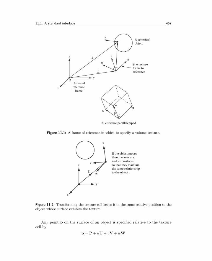
11.1. A standard interface 457
�e texture parallelepiped
Universalreference
frame
y
w
vu
β
x
z
O
P
w
vu
�e textureframe toreference
A sphericalobject
n
p
α
Figure 11.1: A frame of reference in which to specify a volume texture.
If the object movesthen the axes u, vand w transformso that they maintainthe same relationshipto the object
u
v
Pw
y
x
z
Figure 11.2: Transforming the texture cell keeps it in the same relative position to theobject whose surface exhibits the texture.
Any point p on the surface of an object is specified relative to the texturecell by:
p = P+ uU+ vV + wW

458 11. Algorithms for procedural textures
Step
Step
Ramp
Hermitex
x
x
Ramp
Figure 11.3: Applying a ramp transition between the colored dot and the backgroundremoves the unpleasant aliasing effects that are very noticeable when a step transitionis used.
The coefficients u, v and w are used as texture coordinates in calculating thesurface shading. To make the texture appear larger or smaller or be distorted,they can be scaled before calling the texture function.
As we have seen, if U, V and W form an orthogonal basis then u, v and wmay be easily calculated. For a non-orthogonal basis a set of three simultaneousequations must be solved every time the u, v and w are needed.
Color blending Textures that include color changes exhibit unpleasant aliasingeffects when change is abrupt. On the other hand if the change is blended overa small distance the aliasing effect is much less noticeable. Several blendingfunctions have been proposed but a simple ramp is often acceptable althoughsome texture developers recommend using Hermite interpolation. Figure 11.3illustrates alternative ramp shapes and the effect of a simple ramp on the edgesof a large colored dot.
Noise functions Many textures make use of the Perlin noise generators whichwere introduced in chapter 4, section 4.5.2. Four fundamental functions wereintroduced there. In the algorithms described in this chapter and the code thataccompanies them single and vector valued Noise and Turbulence functions arespecified in listing 11.2.
Note that in this case the position coordinates x,y,z are specified as threeseparate values rather than as a VECTOR data type.
The implementations of fNoise() etc., used in producing the textures illus-trated in this chapter were written to return single values in the range [0, 1] orvectors that are of unit length. There are many other codes that could be usedto generate noise with the necessary statistical properties.
It is important to appreciate that these noises are adjusted so that theygive a reasonable correlation between returned values when the input pointsare spaced one unit apart. That is v1 (given by v1 = fNoise (0.0,0.0.0) ) willbe fairly close to v2 (given by v2 = fNoise (1.0,0.0.0) ) whereas v3 (given by

11.1. A standard interface 459
Return a ”Noise” value in the range [ 0.0 - 1.0]f loat fNo i s e (f loat x , //Coordinates of the point at which the Noise valuef loat y , //is to be calculated.f loat z ) ;
Return a ” 1/f Noise” value in the range [ 0.0 - 1.0]f loat fTurbulence (f loat x , //Same as for fNoise function. Note that eachf loat y , //function will return the same number if calledf loat z // with the same ”x y z” values.
) ;
Return a normalized random vector with thevoid vNoise (VECTOR v , //Returned vectorf loat x , //Coordinates of the point at which the vectorf loat y , //is to be calculated.f loat z ) ;
Return a ” 1/f” random vectorvoid vTurbulence (VECTOR v , //Returned vectorf loat x , //Same as for fNoise function.f loat y , // ””f loat z // ””
) ;
Listing 11.2: Noise function definitions.
100
1001
010
Figure 11.4: (a) Noise texture at a resolution of one unit. (b) The same noise textureat a resolution of 100 units.
v3 = fNoise (100.0,0.0.0) ) will be virtually independent of v1. This point is il-lustrated in figure 11.4 which shows a texture based on the same noise functionviewed at two different scales.

460 11. Algorithms for procedural textures
Texture unit cell 3D tiledtexture
Figure 11.5: Tiling a texture by repeating the unit texture cell shown on the leftproduces a wallpaper effect.
Repetitive patterns To repeat a texture pattern the idea of the texture unit cellis a useful one. The unit cell depicted in figure 11.1 can be tiled to fill space.Three of the sides of the cell lie in planes formed by pairs of the vectors U,V and W with the others lying in parallel planes. Thus the texture cell is aparallelepiped with edges of unit length. Any point p with texture coordinates(u, v, w) may be tiled by first calculating:
u′ = u− floor(u)
v′ = v − floor(v)
w′ = w − floor(w)
where floor(x) returns the nearest lowest integer to x. The (u′, v′, w′) are thensubstituted in the remainder of the texture calculation in place of (u, v, w).
This technique of modifying p through its (u, v, w) coordinates before cal-culating a texture can also be used to differentially scale the appearance of atexture. For example the dots illustrated in figure 11.3 can appear flattened
along one or two of their axes if the values of u and v are prescaled by1
2.
Figure 11.5 illustrates a repetitive array of elliptical dots produced using thefunction given in listing 11.3.
Tiling a texture in this way makes it applicable for filling 3D space andnot just covering a two-dimensional surface. On those surfaces where mappingcoordinates (section 4.6) are available at p they can be used to determine thevalue returned by a procedural texture, however since there are only two mappingcoordinates we must choose to set the third to some arbitrary value, say zero.
As you have probably guessed, the example dot texture is generated by plac-ing a colored sphere at the center of the texture cell and making the calculationsin three dimensions. As a result the dots on the surface appear because thevisible surfaces cut through the array of texture cells, the voxels.
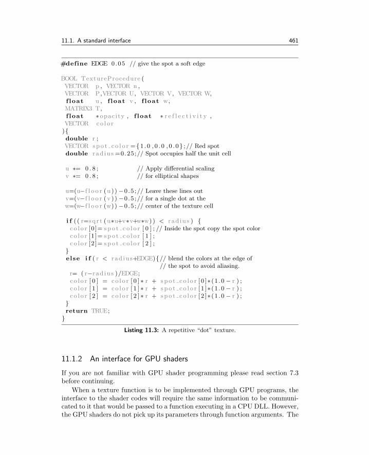
11.1. A standard interface 461
#define EDGE 0.05 // give the spot a soft edge
BOOL TextureProcedure (VECTOR p , VECTOR n ,VECTOR P,VECTOR U, VECTOR V, VECTOR W,f loat u , f loat v , f loat w,MATRIX3 T,f loat ∗ opacity , f loat ∗ r e f l e c t i v i t y ,VECTOR co l o r){double r ;VECTOR spo t c o l o r ={1 . 0 , 0 . 0 , 0 . 0} ; // Red spotdouble rad iu s =0.25;// Spot occupies half the unit cell
u ∗= 0 . 8 ; // Apply differential scalingv ∗= 0 . 8 ; // for elliptical shapes
u=(u−f l o o r (u )) −0 .5 ;// Leave these lines outv=(v−f l o o r ( v )) −0 .5 ;// for a single dot at thew=(w−f l o o r (w)) −0 .5 ;// center of the texture cell
i f ( ( r=sq r t (u∗u+v∗v+w∗w)) < rad iu s ) {c o l o r [0 ]= sp o t c o l o r [ 0 ] ; // Inside the spot copy the spot colorc o l o r [1 ]= sp o t c o l o r [ 1 ] ;c o l o r [2 ]= sp o t c o l o r [ 2 ] ;
}else i f ( r < rad iu s+EDGE){// blend the colors at the edge of
// the spot to avoid aliasing.r= ( r−rad iu s )/EDGE;c o l o r [ 0 ] = co l o r [ 0 ] ∗ r + sp o t c o l o r [ 0 ]∗ (1 .0 − r ) ;c o l o r [ 1 ] = co l o r [ 1 ] ∗ r + sp o t c o l o r [ 1 ]∗ (1 .0 − r ) ;c o l o r [ 2 ] = co l o r [ 2 ] ∗ r + sp o t c o l o r [ 2 ]∗ (1 .0 − r ) ;
}return TRUE;
}
Listing 11.3: A repetitive “dot” texture.
11.1.2 An interface for GPU shaders
If you are not familiar with GPU shader programming please read section 7.3before continuing.
When a texture function is to be implemented through GPU programs, theinterface to the shader codes will require the same information to be communi-cated to it that would be passed to a function executing in a CPU DLL. However,the GPU shaders do not pick up its parameters through function arguments. The

462 11. Algorithms for procedural textures
shader’s parameters are passed by using memory locations in the GPU that theapplication program can write into. All our shader examples will use GLSLuniform qualified variables that can be referenced through their names by theapplication program.
The main geometric data (vertex positions and normal vectors) are passed tothe shader through GLSL built-in variables, 2D or 3D texture maps are passedthough a small collection of samplers, a texture’s frame of reference is passedas three uniform variables and the texture coordinate of each vertex is passedthrough a buffer attached to a vertex array object.
The other major differences in using a GPU texture are (1) the need to usea texture map as a lookup table for the self-similar noise function, and (2) theneed to also implement other aspects of the rendering process, e.g., lighting.
In all the GLSL code examples the following GLSL code is included in thevertex shader:
//Input of the vertex position relative to the texture base axeslayout ( l o c a t i o n = 4) in vec3 ShaderPos i t ion ;
// Input of material base axes for the texture unit celluniform vec3 Uvector ;uniform vec3 Vvector ;uniform vec3 Wvector ;
In the fragment shader, the map that will be used as a noise lookup needs tobe made available:
uniform sampler3D NoiseMap ; // Map for 3D noise
It is also necessary to declare several variables that are assigned values in thevertex shaders and are used (after interpolation in the rasterizer) in the fragmentshader:
out vec3 tnorm ; //normal vectorout vec4 PP; //positionout vec3 texpos ; //texture position
out vec3 uvec ; //the three texture cell axesout vec3 vvec ;out vec3 wvec ;
Note: These in/out variables are assigned on a per-vertex basis in the vertexprogram, but when used in the fragment shader they apply to the location on thesurface visible in the fragment being rendered.
The GPU is highly efficient at carrying out interpolation and generating re-peating patterns. GLSL functions floor (..) , roof (..) , mix(..) and clamp(..)are provided to facilitate the tasks of blending color and determining fractionalpositions within a texture’s unit cell.

11.2. CPU textures 463
11.2 CPU textures
In this section we will examine algorithms to generate seven classes of proceduraltextures built using three principles: regular patterns, irregular patterns, per-turbation to surface normal vectors or a combination all three. The algorithmsdo not assume any particular restriction on their implementation. Versions ofsome of them for GPU use will be examined further in section 11.3.
11.2.1 Regular dots
In section 11.1.1 we saw how to produce a repetitive pattern of dots by embeddinga sphere in the basic texture cell. It would take only a small modification to placecubes or other patterns at the center of the cell. We can think of an analogywith the crystallographic arrangement of atoms in a solid. A dot at the centerof the texture cell corresponds to a body centered cubic (BCC) structure. Thereare other crystallographic arrangements that produce regular patterns of dots.In fact an hexagonal close packing (HCP) arrangement has proved to be veryuseful because quite a few of the textures to be described later are based on it.
On their own neither the HCP nor the face centered cubic (FCC) are partic-ularly exciting but they do raise an interesting and important issue:
Neither the FCC or HCP packaging arrangements can be tiled ina way so that all the spheres making up the basic repeat unit liecompletely within the unit cell.
This complicates the task of producing repetitive patterns because when we needto determine what texture feature occurs at some coordinate (u, v, w) we musttake account of adjacent texture cells so that the patterns match along theirborders. If the patterns from neighboring cells don’t match exactly some dotsin the pattern might look like they have been cut in half. (A problem analogousto aligning the wallpaper pattern when hanging adjacent strips.)
11.2.2 FCC dots
In an FCC pattern there is one spherical dot at the center of each face of thetexture cell. Thus to determine the color at (u, v, w) six spherical intersectiontests must be performed for each cell. In addition we must remember that eachsphere is shared with an adjacent texture cell. To make sure that no discontinuityoccurs the dots on opposite faces of the texture cell need to be the same size andcolor.
This introduces another important point that we should remember as othertextures are developed:
We are determining the texture at one given point (either p or equiva-lently (u, v, w)) on each function call, not the texture of many pointsthat satisfy some given property of the texture.

464 11. Algorithms for procedural textures
(a) (b) (c)
Figure 11.6: The unit cell for an FCC dots texture and an example of its application toa solid object. (a) Solid cell showing spheres protruding into adjacent cells. (b) Semi-transparent unit cell showing the 6 spheres. (c) Soft edged dots applied to a sphere.
For example we cannot set the color of all points inside a dot in onecall to the texturing function. This may seem like a trivial point but itis very significant in practice and for many textures, especially thosebased on random dots. It can significantly complicate the coding.
Figure 11.6 illustrates the relation of the FCC dots to the texture cell andpictures an example of the texture applied to a solid object. Details of thealgorithm which consists of a simple test as to whether a point lies inside one ofsix spheres can be found by following the code that accompanies the book.
11.2.3 HCP dots
In contrast to BCC and FCC dots an hexagonal close packed (HCP) arrangementof spheres forms the closest packing that it is possible to obtain. This pattern isof particular interest mainly because the hexagonal mesh, leopard, amphibian,honeycomb and vein textures are derived from it.
Like the FCC dots we must be careful to remember that spheres from onecell will overlap into adjacent texture cells. In this case to obtain a repeatabletexture cell we require 22 spheres. Compare this to the single test required for aBCC dot pattern. Figure 11.7 visualizes the arrangement of the spheres in theunit HCP cell. Because of the regularity, any spheres that lie partly outside thetexture cell exactly overlap spheres in adjacent cells and thus when working inadjacent cells they are automatically considered. That is, a sphere on the rightof cell i overlaps one from the left of cell i+ 1.
The HCP unit cell is not rectilinear. For a cell of unit width its length and
height are both
√3
2. Three layers of spheres are needed to fill the texture cell;
the middle layer is an offset copy of layer one and the top layer is a repeat of thebottom one. This arrangement of spheres in the layers is depicted in figure 11.8

11.2. CPU textures 465
Layer 2Layer 1Layer 3
Unit cell
Figure 11.7: Visualizing the spherical units that make up the HCP unit texture cell.
where the dimensions are also presented. Note that this illustration depicts thecase where the spheres just touch (as would be the case in a real HCP crystal).As we will see later some very interesting textures arise when the sphere radiivary from this nominal value, a situation that is of course impossible in a realcrystal. Seven spheres are needed for layers 1 and 3; eight spheres must be usedin layer 2.
In the HCP texture (as with those considered earlier) the actual pattern seenon any given surface is that which appears as the surface cuts through an infinitelattice of texture cells. This is depicted in figure 11.9 where an angled plane isshown cutting through a single texture cell.
The implementation of the algorithm for an HCP dot pattern follows closelythe same principles used in the FCC procedure. It basically tests to see if thepoint p lies inside (or on the edge of soft edges) any of the 22 spheres in the unitcell. If the test proves positive then the color or other surface attribute assignedto the dot is returned.
11.2.4 Regular bumps
The BCC, FCC or HCP dot pattern can be used to generate regular arrays ofraised bumps or sunken dimples if the surface normal vector is pushed off thevertical at points lying inside the dots. For example the bumps illustrated infigure 11.10 were produced from a basic BCC dot pattern but instead of changingthe color of the surface inside the dot the surface normal was perturbed in the wayillustrated in the cross-sections. It is relatively straightforward to make bumpson a surface when the bumps are derived from a two-dimensional function thatcovers the surface. However, more thought is necessary when the bumpy surfaceis to be derived from a texture that fills a 3D volume. In this case the surfacebumps are formed at those locations where the surface intersects spheres in thetexture cell. We must ensure that not only is the normal bent in the desireddirection (bump or pimple) but also that the direction is consistent for adjacentpoints on the surface. For example the bumps on the left, right, top and bottom
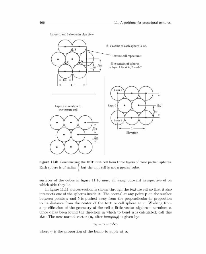
466 11. Algorithms for procedural textures
Layers 1 and 3 shown in plan view
�e radius of each sphere is 1/4
Texture cell repeat unit
�e centers of spheresin layer 2 lie at A, B and C
Layer 2 in relation tothe texture cell
1
1
Elevation
B
AC
1/2
1/2
Layer 3
Layer 1
Layer 2
3
1/2 3
3/4
3/4
3/4
3/2
Figure 11.8: Constructing the HCP unit cell from three layers of close packed spheres.
Each sphere is of radius1
4but the unit cell is not a precise cube.
surfaces of the cubes in figure 11.10 must all bump outward irrespective of onwhich side they lie.
In figure 11.11 a cross-section is shown through the texture cell so that it alsointersects one of the spheres inside it. The normal at any point p on the surfacebetween points a and b is pushed away from the perpendicular in proportionto its distance from the center of the texture cell sphere at c. Working froma specification of the geometry of the cell a little vector algebra determines c.Once c has been found the direction in which to bend n is calculated; call this∆n. The new normal vector (nb after bumping) is given by:
nb = n+ γ∆n
where γ is the proportion of the bump to apply at p.

11.2. CPU textures 467
(a) (b) (c)
Figure 11.9: (a) The texture cell with the planar surface cut through. (b) A cut awayview. (c) The pattern as it appears in the surface.
Since the surface normal n is determined with respect to a global frame ofreference but the texturing algorithms require that all calculations are done inthe (U,V,W) reference frame we must transform n and p so that they can beused relative to the (U,V,W) frame. The surface normal n in the (U,V,W)frame of reference is obtained by applying:
n′ = [T ]n
To obtain an equivalent for p, say p′ we use the known texture coordinates(u, v, w) at p and by letting p = (u′, v′, w′) with:
u′ = u− floor(u)
v′ = v − floor(v)
w′ = w − floor(w)
Account is taken of the fact that the texture cells repeat ad infinitum.After transformation, p′, like n′, can be manipulated relative to the texture
cell coordinate system. If calculation for the bumped surface normal proceedswith respect to the texture cell axes then the repetition of the texture cell willoccur automatically.
To determine the change in surface normal due to the bumps we proceed asfollows: Let r < 0.5 be the radius of a sphere at the center of the texture cell, i.e.,at: C = (0.5, 0.5, 0.5). Find the point p′
c (at c in figure 11.11(a); c is the pointon the surface closest to C) using p′ = (u′, v′, w′) (the position vector relativeto the texture cell for the point p). We can write:
p′c = C− ((p′ −C) · n′)n′
and therefore the direction in which we must bend the surface normal, relative

468 11. Algorithms for procedural textures
Normals Normals DepressionsRaised bumps
Figure 11.10: Regular bumps and depressions formed by modulating the surface normalof a solid object. The amplitude and direction of the modulation at a point p isdetermined by its distance from a sphere placed at the center of a texture cell. Thefigure illustrates how the surface normal behaves in a cross-section through one of thebumps. Bumps are shown on the left and depressions on the right.
to the texture cell axes, is given by:
∆n′ =p′ − p′
c
|p′ − p′c|
If |C− p′| < r then the point of interest lies inside the sphere and thenormal will be pushed in the direction of ∆n′ by an amount that depends onthe proportion of the distance γ, at which p′ lies between the points labeled aand c in figure 11.11(a). γ is given by:
γ = 1− |p′ − p′c|
√
r2 − (|C− p′c|)2
γ = 1 when p is at c and γ = 0 when p is at either a or b.The form of the rule used to mix ∆n′ with n determines the apparent shape
of the bump, but before it is added to n it must be transformed back to a global

11.2. CPU textures 469
Texture cellreference frame
Global referenceframe
p
(a)
(c)
(b)
Inside
a c b
∆nn
n
Inside
bc
a
n
Cp´
Figure 11.11: A cross-section through a surface intersecting one of the spheres in thetexture cell. (a) Case where the inside of the surface is on the left and (b) when it ison the right. (c) Shows a plane view and again ∆n is the direction in which n is bentat p.
frame of reference using:
∆n = ∆n′uU+∆n′
vV +∆n′wW
11.2.5 Pimples
The raised bump (or pimple) textures illustrated on the left of figure 11.10 wereproduced by adding ∆n with n when γ < 1 according to the equation:
n = αn+ (1− α)∆n
The parameter α is determined as follows for the three cases illustrated in thefigure with the rules:
1. Rounded pimples
α = sinπ
2γ

470 11. Algorithms for procedural textures
2. Buttons
α =
{
1 : γ < 0.512 (1− cos 4πγ) : γ ≥ 0.5
3. Studs
α =
{
0.5 : γ < 0.51 : γ ≥ 0.5
11.2.6 Dimples
The depression (or dimple) textures illustrated on the right of figure 11.10 wereproduced by adding ∆n with n when γ < 1 using:
n = αn− (1− α)∆n
Again α is determined as follows for the three cases:
1. Rounded dimples, the same as for rounded pimples above: α = sin π2 γ
2. Flat dimples, the same as for buttons above:
α =
{
1 : γ < 0.512 (1− cos 4πγ) : γ ≥ 0.5
3. Conical pitsα = 0.5
In all cases if γ ≥ 1 no modulation is applied to n.
11.2.7 A hexagonal mesh
Producing an hexagonal ridge pattern such as that illustrated in figure 11.12is relatively straightforward on a flat two-dimensional plane. To construct anequivalent pattern that fills three-dimensional space and at the same time sat-isfies the repetitive requirements of a procedural texture is a bit harder. Oneinteresting method that leads to the 3D hexagonal honeycomb texture of fig-ure 11.12 and has potential as a technique for further development (e.g., thetextures of section 11.2.23) arises from the same ideas that produced the dim-pled texture.
In essence the procedure is: Spheres used to produce the bumps of an HCPdimple pattern are expanded until they start to overlap. If the overlap is pre-vented the rounded edges of the dimples flatten out so that hexagons start toappear. A Z buffer (which only needs one value) may be used to prevent spheresoverlapping. This process is illustrated in figure 11.13.

11.2. CPU textures 471
Figure 11.12: An hexagonal ridge pattern produced by overlapping the HCP texturespheres.
Overlapping spheresgive a network of
hexagons
Spheres slightlyoverlapping
Spheres justtouching
Figure 11.13: A 3D hexagonal mesh produced by growing spheres.
In the case of the unit texture cell illustrated in figure 11.7 spheres of radius0.25 give maximum space filling, i.e., they just touch. If the radius is increased
to√32 perfect hexagonal shapes are the result. The algorithm presented in list-
ing 11.4 uses a Z buffer to determine inside which of the texture cell’s 22 spheres(one sphere equates to one hexagon) any point p lies.
To produce the ridges along the edges of the hexagonal cells we need todetermine whether a point lies within a small distance from the edge of the cell,i.e., inside the ridge. We can do this by considering the value in the Z buffer.When p lies near the edges of the hexagon its Z buffer value (call it Zp) will beof similar magnitude to the values in the Z buffers of adjacent spheres. Thus ifthe difference in value for two adjacent spheres is within some small tolerancethen p is said to be on the ridge between hexagons.
To bend the normal on the beveled sides of the hexagon the change in normaldirection is approximated with a vector ∆n derived in a manner analogous to

472 11. Algorithms for procedural textures
Set the depth buffer Z = 0
Given point of intersection p check each of the 22 spheres (i),to see if it lies inside. i.e. is (δi = |p− ci|) < r?If it does and δi > Z then {Set Z = δi and record the identity of sphere i : id = i(after all the sphere have been checked this reveals whichsphere has its center closest to p)
}
Set another depth buffer Zb = 0
To determine how close to the edge of the hexagon p is work throughall spheres (i) again.i f ( i 6= id) {i f (δi > 0 and (r − δi) > Zb ) {Set Zb = (r − δi)
}}i f ( |Zb − Z| < a1 ) {
p lies on the hexagonal ridge.}
else i f ( |Zb − Z| < a2 ) {p lies on beveled side.
}else {
p lies in the hexagonal depression.}
Listing 11.4: Algorithm to generate the basic elements of an hexagonal mesh pattern.a1 and a2 are parameters that determine the width of the ridges and their sloping sides.
that used for the regular dimples. Strictly speaking this will not exhibit a creaseat the point where two edges of the hexagon meet but this will hardly be noticed.The ridges in figure 11.13 do not have such a crease.
11.2.8 Textures derived from the noise functions
Apart from the basic bozo texture (section 4.5.2) and those simply derived fromit by color blending and added turbulence (e.g., wood, marble etc.) a number ofinteresting patterns can be produced by passing the output from Perlin’s noisegenerators through a number of functions.

11.2. CPU textures 473
Figure 11.14: A contour pattern which with some added turbulence and appropriateblend of color could resemble a three-dimensional wood grain pattern.
11.2.9 Contours
The contour pattern illustrated in figure 11.14 is derived from the basic bozotexture by passing it through a periodic function, in this case a sinusoid, andthen thresholding the result as follows:
Given the point of interest as a (u, v, w) coordinate.
nu,v,w = 1
2(1 + sin(2πfq fNoise(u, v, w))
i f (nu,v,w > (1.0− t)) {return the color of the contour
}else return the background
The parameter t governs how thick the contours appear and fq is a measurethat can be most accurately described as a sort of frequency of the contours.Values of about 0.1 for t and 20 for fq usually give good results, as illustrated infigure 11.14.
11.2.10 Plasma
The texture illustrated in figure 11.15 resembles the appearance of a brightlycolored plasma field. It is produced by adding differently scaled noises and pass-ing the result through a sinusoidal function to generate red, green and blue colorcomponents with different frequencies and phases. If the phases and frequenciesare the same for each color a monochrome pattern will be observed.
Red, green and blue (r, g, b) values of the plasma at coordinate (u, v, w) aredetermined by the algorithm in listing 11.5.

474 11. Algorithms for procedural textures
Figure 11.15: A texture that gives the illusion of a plasma field.
//Given the point of interest as a (u, v, w) coordinate.//the r, g, b color values are obtained as follows:
n1 = fNoise(u, v, w)n2 = fNoise( 1
2u, 1
2v, 1
2w)
n3 = fNoise( 14u, 1
4v, 1
4w)
N = n1 + n2 + n3
r = 1
2(1 + cos(2πfrN + φr))
g = 1
2(1 + cos(2πfgN + φg))
b = 1
2(1 + cos(2πfbN + φb))
Listing 11.5: Algorithm to generate a plasma texture.
11.2.11 Underwater (caustics)
The caustic pattern that appears on the bottom and sides of swimming pools andunderwater surfaces can be simulated by another modification of the basic noisepattern with appropriate color mixing. In the underwater pattern the noise ispassed to a function that folds high values down to lower values and then scalesand mixes the color of the caustic with a background shade. Two parametersgovern the appearance of the caustics: the sharpness (s) controls the rapidity ofcolor transitions, and the coverage (c) gives an overall increase in the percentageof the surface area covered by the caustic. The algorithm used to produce thecaustic pattern in figure 11.16 and return an RGB triple on the interval [0, 1] isgiven in listing 11.6.

11.2. CPU textures 475
Figure 11.16: A caustic pattern gives the appearance of the patterns of light that playon underwater surfaces. The features have a sharpness of 0 and a coverage of 0.8.
//Given the point of interest as a (u, v, w) coordinate.
n = fNoise(u, v, w)//Use a triangular function on the noise value:i f (n > 0.5)n = 2(1− n)else n = 2n//Rescale the noise as follows:n = 0.3 + 0.9n//Mix the caustic color with the background:i f (n > c) {
n =n− c
1.2− cn = n(1 + s)i f (n > 1) n = 1r = nRc + (1− n)Rb
g = nGc + (1− n)Gb
b = nBc + (1− n)Bb
}
Listing 11.6: Algorithm to generate a caustic texture.
11.2.12 Other worlds
A simple combination of the basic noise and turbulence functions with differentialscaling can give a very good approximation to the appearance of a gas planet,like Jupiter. It is especially effective when applied to a spherical object such asthat depicted in figure 11.17.
The algorithm in listing 11.7 (where n, β, ff and fs are parameters that affectvisual appearance) outlines the main steps in producing the textured surface offigure 11.17.

476 11. Algorithms for procedural textures
Figure 11.17: Simulating the appearance of the banding in the atmosphere of a largegaseous planet by differentially scaling the basic noise function.
//Given the point of interest as a (u, v, w) coordinate.//Note the differential scaling applied to the w coordinate.
t = fTurbulence(20u, 20v, 10w)w′ = w + ff ts = fNoise( u
1000, v1000
, βw′)s′ = s+ n( fNoise(50u, 50v, 25w′)− 0.5)//Limit s′ to lie in range [0, 1]s = 0.5 + (s′ − 0.5) ∗ fs//Finally blend the banding color with the background:r = sBr + (1− s)Cr
g = sBg + (1− s)Cg
b = sBb + (1− s)Cb
Listing 11.7: Procedure to create the texture illustrated in figure 11.17. If ff > 0eddies and vortices appear in the atmosphere. If b = 10 then approximately 10 bandsof gas lie in the unit cell. If n > 0 local perturbations in the atmospheric color appear.As fs → 0 the bands tend to fade. The input point is at coordinate (u, v, w) and theRGB triple r, g, b is the result of mixing the background color (Br, Bg, Bb) with theband color (Cr, Cg, Cb).
11.2.13 Clouds
Another simple use of the noise function is to simulate a cloudy sky. Appropriatecolor mixing gives the clouds white edges and dark gray centers. Wispy cloudscan be produced by differential scaling and the degree of shearing (a blustery day)is simulated by adding some turbulence. A point of interest is the way in whichthe turbulence is put into effect. Given a (u, v, w) coordinate at which a color isto be determined the turbulence is added to the position (u+∆u, v+∆v, w+∆w)before it is passed to the position dependent noise generator. This approach tomodifying a texture, i.e., pre-modulating the position, is a useful one with utility

11.2. CPU textures 477
Figure 11.18: A cloudy day.
for generating other interesting textures. Figure 11.18 illustrates the cloudytexture.
The algorithm in listing 11.8 outlines the main steps in producing the tex-tured surface of figure 11.18.
11.2.14 Regular dots perturbed by noise
In the discussion of the cloud texture it was pointed out that perturbing theposition coordinate before passing it to the noise function was a useful way ofproducing textures. The following sections look at three textures produced byperturbing the (u, v, w) coordinate before passing it to an HCP dot or bumpgenerator.
11.2.15 Leopard
The pattern illustrated in figure 11.19 was generated from a regular cell of HCPspheres by perturbing the position (u, v, w) with a number of sinusoids prior totesting for containment within one of the 22 HCP spheres.
The algorithm in listing 11.9 outlines the main steps in producing the tex-tured surface of figure 11.19.
11.2.16 Reptile
If the regular bump pattern (of section 11.2.4) is changed to an HCP arrange-ment and the radius of each bump is increased and allowed to overlap, then atexture resembling a “scaly” skin is the result. Modulating the pattern with acombination of sinusoids adds to the realistic appearance which can be furtherenhanced by color blending near the edges of the bumps as shown in figure 11.20.The algorithm used to produce the texture is given in listing 11.10.

478 11. Algorithms for procedural textures
//Given the point of interest as a (u, v, w) coordinate.
//Displace the sampling point (u, v, w) by obtaining a turbulence vector ∆p
vTurbulence(∆p, u, v, w, )u′ = u+ t∆puv′ = v + t∆pvw′ = w + t∆pw//Sample the noise function at (u′, v′, w′) and blend colors:n = fNoise(u′, v′, w′)i f (n < 0.5) //return the background colorelse i f (n < 0.6) {
//Blend to white from background: Bf = 10(n− 0.5)r = r + f(1−Br)g = g + f(1−Bg)b = b+ f(1−Bb)
}else {
//Blend to gray:f = 1− 5(n− 0.6)r = frg = fgb = fb
}
Listing 11.8: Procedure to create the texture illustrated in figure 11.18. The parametert governs the wispiness of the clouds.
11.2.17 Veins
The regular honeycomb pattern of section 11.2.7 is readily transformed into theveined pattern of figure 11.21 if the point of interest, (u, v, w), is perturbed bya noise value before executing the algorithm of listing 11.4. The beveled sidesof the hexagonal ridges are organized so that they form a trough rather than aridge.
The changes shown in listing 11.11 transform the regular hexagonal mesh offigure 11.12 into the veined surface of figure 11.21.
11.2.18 Random dots and crystals
One might think that producing random dots would be one of the easier texturesto create. After all one is just laying out a few spheres randomly in spaceand then determining whether a point p or (u, v, w) lies inside one of them.Unfortunately however because the texture must extend throughout an infinitevolume we would need to make an infinite number of tests to see whether p liesinside one of the random dots or not. Clearly this is not a practical propositionand another method will have to be found.
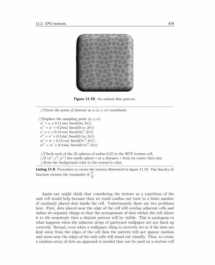
11.2. CPU textures 479
Figure 11.19: An animal skin pattern.
//Given the point of interest as a (u, v, w) coordinate.
//Displace the sampling point (u, v, w)u′ = u+ 0.11 sin( fmod(3u, 2π))u′′ = u′ + 0.2 sin( fmod(0.1v, 2π))v′ = v + 0.15 cos( fmod(4u′′, 2π))v′′ = v′ + 0.2 sin( fmod(0.1w, 2π))w′ = w + 0.15 cos( fmod(5v′′, 2π))w′′ = w′ + 0.2 sin( fmod(0.1u′′, 2π))
//Check each of the 22 spheres of radius 0.25 in the HCP texture cell,//if (u′′, v′′, w′′) lies inside sphere i at a distance r from its center then mix//from the background color to the texture’s color.
Listing 11.9: Procedure to create the texture illustrated in figure 11.19. The fmod(a, b)
function returns the remainder ofa
b.
Again one might think that considering the texture as a repetition of theunit cell would help because then we could confine our tests to a finite numberof randomly placed dots inside the cell. Unfortunately there are two problemshere. First, dots placed near the edge of the cell will overlap adjacent cells andunless we organize things so that the arrangement of dots within the cell allowsit to tile seamlessly then a disjoint pattern will be visible. This is analogous towhat happens when the adjacent strips of patterned wallpaper are not lined upcorrectly. Second, even when a wallpaper tiling is correctly set or if the dots arekept away from the edges of the cell then the pattern will not appear randomand areas near the edges of the unit cells will stand out visually. Thus, to createa random array of dots an approach is needed that can be used on a texture cell

480 11. Algorithms for procedural textures
Figure 11.20: A perturbed regular array of overlapping HCP bumps can resemble ascaly skin.
//Given the sampling point as the (u, v, w) coordinate.
//Displace the sampling point: (u, v, w)u′ = u+ 0.16 sin( fmod(2w, 2π))v′ = v + 0.16 cos( fmod(3u, 2π))w′ = v + 0.16 cos( fmod(4v, 2π))
//Check each of the 22 spheres of radius 0.5 in the HCP texture cell stopping//when (u′, v′, w′) lies inside one of them, say at a distance r from its center.//Bend the surface normal in proportion to r.
I f (r > 0.15) //blend from the background color to the texture color.
Listing 11.10: Procedure to create the scaly texture illustrated in figure 11.20.
basis whilst still allowing the random placement of dots, at least to the toleranceof a visual inspection.
Consider a single dot of radius r ≤ 0.5 placed randomly in a unit cell, sayas that shown in figure 11.22. Unless it is placed dead center it will overlapinto adjacent cells. However at most it will only intrude into the immediateneighbors. Therefore if we construct a random dot texture by placing one spheresomewhere in every unit cell when the time comes to check whether a point at(u, v, w) lies inside the sphere (which forms the dot) only the spheres from thecell in which (u, v, w) lies and its 26 immediate neighbors need be considered.Since one dot is put somewhere in each texture cell the pattern will be quitepleasing to the eye because there will be no large gaps between dots nor will thedots tend to cluster. Each dot in the texture cell is readily drawn with differentcolors or radii to add to the effect.

11.2. CPU textures 481
Figure 11.21: This veined texture could be used to represent leaded glass when thesurface is partially transparent.
//Given the point of interest is the coordinate (u, v, w).
//Get the random vector d from the noise function: vNoise(d, u, v, w)//Disturb the input point:u = u+ 0.7duv = v + 0.7dvw = w + 0.7dw//Proceed with the honeycomb pattern.//Note: d = (du, dv, dw) is a vector in the texture cell’s frame of reference.
Listing 11.11: Procedure to create a veined texture.
There are two apparent difficulties in implementing the algorithm suggestedin the previous paragraph. These are:
1. The first is that the random placement of dots must be done in a repro-ducible manner. To put it another way: If points (u, v, w) and (u′, v′, w′)both lie in cell i, j, k the set of spheres used throughout the algorithm(which will basically be the same as that discussed in section 11.2.14) mustbe consistent. We must also remember that in practice points will not bepassed to a texture generating function in any particular order (this wasone of the criteria under which Perlin’s noise function was developed).
2. Our second difficulty is that in considering points lying in texture cell i, j, kwe must consider the effect of cells i− 1, j, k etc., and therefore we need tobe able to reproduce the random placements of the dots in these cells aswell.

482 11. Algorithms for procedural textures
i – 1.j i, j i + 1, j
Figure 11.22: A random dot in texture cell i, j will overlap into at most cell i, j’snearest neighbors. (In this two-dimensional example the dot in cell i, j could lie in atmost 9 cells.)
The solution to both of these problems is straightforward in practice becausethe numbers that emerge from a pseudo random number generator are a repro-ducible sequence based on some seed value. Therefore if a seed is derived fromthe identity (the i, j, k) of the cell under test the random position of the spherewithin it may be reproduced exactly. Two alternative ways to generate such aseed are:
1. Use fNoise(i, j, k).
2. Use i, j, k and a hashing function to generate a pointer to an entry in atable of random numbers.
The first way is easier to implement but the second is faster and can be used incases where we need more than one dot per unit cell.
11.2.19 Random dots
The random dots illustrated in figure 11.23 are the results of the implementationof the method described above with an index into a table of 2000 random vectorsobtained by the hashing functions:
#define IMOD( z , a ) ( ( z ) − ( ( z )/ ( a ) )∗ ( a ) )#define PATTERN(x , y , z ) ( ( ( z )+16384L)∗64536L + \
( ( y)+16384L)∗32768L + \( ( x)+16384L) )
index=IMOD(PATTERN( i , j , k ) , 1 9 9 9 ) ;
Once selected a random vector is used to place each sphere at some point inthe texture cell. Random vectors from the same table are also used to vary thecolor and radius of the dot. Blending dot and background color near the dotedge helps to alleviate aliasing artifacts.

11.2. CPU textures 483
Figure 11.23: Variably sized random colored dots.
Figure 11.24: Random colored crystals. (Basically a random dot texture but with adot radius that exceeds the size of the unit cell.)
11.2.20 Crystals
By allowing the dot radius to increase until adjacent dots overlap and thenbringing into effect a Z buffer as used in section 11.2.7 the dots will appear tolock together into a matrix of colored crystals. Figure 11.24 illustrates a basicone sphere per unit cell texture after crystallization with the color of each dotchosen at random.
11.2.21 Blisters
Blisters are another example of the extension of the random dots texture. In thiscase the surface normal inside the dots is perturbed in much the same way as wasdone for the case of the regular bumps. Blisters are flatter than bumps but this

484 11. Algorithms for procedural textures
Figure 11.25: Random blisters: Raised random dots.
Figure 11.26: Peas: Rounded high density blisters.
is readily produced by using a slightly different mix of normal and perturbingvectors. Points that lie near the center of the dots can be colored differently foradded effect.
11.2.22 Peas
The pea texture is yet again another version of the blisters texture. A greaterdensity of random bumps is produced by placing 3 spheres in each unit cell. Noflattening of the bumps is used, but by changing the sphere radius, the surfacecan be covered to a lesser or greater extent; see figure 11.26.
11.2.23 Sharply edged features
These textures are constructed by a combination of the ideas already derivedand include the honeycomb and paving stones.

11.2. CPU textures 485
Figure 11.27: Honeycomb: a hexagonal mesh.
Figure 11.28: Paving stones and chipped fragments.
Honeycombs The honeycomb cube shown in figure 11.27 uses the steps from thehexagonal mesh algorithm (section 11.2.7), but without applying an inner limitto the extent of the beveled edge.
Paving stones The paving stone and fractured texture (figure 11.28) are derivedfrom the crystal texture (section 11.2.20). By simply beveling the edges of thecrystals the cracks between the paving stones appear. Points near the crystaledges are identified using the same calculation that identified whether pointswere on the ridges of a regular hexagonal mesh. In the case of the crackedtexture very wide ridges were used.
A neat trick is to make the interior of the paving stones look dirty or weath-ered by mixing in a dark color modulated by fNoise(u, v, w). Additionally, ifeach stone is given a slight color variation (a toned down multi-colored crystal)the whole surface looks more natural.

486 11. Algorithms for procedural textures
Figure 11.29: Some examples of basic undulating textures.
11.2.24 Rough surfaces
Rough surfaces fall into two categories:
1. Those with smooth changes to the direction of the surface normal, whichare derived from combinations of vector noises.
2. Those with sharp changes to the surface normal direction vector. Oftensome smooth undulations are mixed with the more pronounced sharp fea-tures.
A basic rough surface is a straightforward mix of surface normal n and outputfrom vNoise(∆n, u, v, w). Many different appearances are achieved by:
1. Scaling: calculate ∆n from vNoise(∆n, su, sv, sw) after scaling the inputcoordinate (u, v, w) by s.
2. Amplification: vary the bumpiness through the parameter α and perturbn by:
n = n+ α∆n
The bumpy cubes shown in figure 11.29 represent examples of different s andα values.
An almost infinite variety of other continuous rough and bumpy surfaces canbe achieved by adding vNoise() and vTurbulence() vectors in different propor-tions and at different scales. Experimentation is very often the best way offinding pleasing effects.
The remaining three rough textures discussed next are primarily based on thealgorithm for the Pea (section 11.2.22), which is a discontinuous bumpy surface.Each adds a new component to ∆n either a vNoise() or a scaled version of thePea itself with minor features superimposed on it.

11.2. CPU textures 487
Figure 11.30: Crusted surfaces.
11.2.25 Crusts
The crusted texture shown in figure 11.30 is the result of the following modifi-cations to the Pea texture algorithm:
1. Add a vector noise displacement to (u, v, w) before applying the Pea algo-rithm.
2. The radius of the peas are chosen from a random distribution in the range[0.6− 1.8] (relative to the size of the unit texture cell).
3. A power law, (a′ = a2), is applied to the fraction of ∆n mixed with n by:
n = a′n+ (1− a′)∆n
4. A continuous noise at a magnified scale is added to the final result. Thisadds a little fine detail to the gnarled look of the crusted texture.
The overall appearance will change depending on the resolution at which thetexture is rendered as is evident from the examples illustrated in figure 11.30.
11.2.26 Crumpled
A crumpled surface that can resemble used aluminum foil is an example of anangular texture and is produced by adding inverted Pea textures at smallerand smaller scales and with different amplitudes. Usually there is no need togo beyond about three overlapping textures. The illustration in figure 11.31was produced by perturbing (u, v, w) prior to computing the second and thirdcomponents. Each component is calculated at a scale which is twice as small asthe previous one and added in the proportions: 1.0, 0.8 and 0.95.

488 11. Algorithms for procedural textures
Figure 11.31: Scaly skin surface showing ridge features at decreasing scales.
11.2.27 Faceted
Crumpled surfaces exhibit features of a combination of basic rough surfaceswith decreasing amplitudes and reducing scales. A faceted texture uses thesame idea of summing effects at decreasing scales but without changing theamplitudes. Flat surfaces (which give the texture the appearance of some sortof naturally occurring mineral) are produced by quantizing ∆n using integerarithmetic before mixing it with the surface normal.
The Pea texture (11.2.22) forms the basis for this texture. This time thehemispherical peas are inverted so that they appear to be pushed into the sur-face. The normal vector is quantized as shown in the following C/C++ codefragment. This example gives approximately 16 flat quadrilaterals per hemi-spherical depression:
dn //is the vector that bends the surface normal.Normalize (dn ) ;dn [ 0 ]=0 . 5∗ (double ) ( ( int ) ( dn [ 0 ] ∗ 2 . 0 ) ) ; //Quantize the 3 componentsdn [ 1 ]=0 . 5∗ (double ) ( ( int ) ( dn [ 1 ] ∗ 2 . 0 ) ) ; //components of ”dn” usingdn [ 2 ]=0 . 5∗ (double ) ( ( int ) ( dn [ 2 ] ∗ 2 . 0 ) ) ; //integer arithmetic.Normalize (dn ) ;
Faceted rectangular surfaces are illustrated in figure 11.32. The sample on theright depicts an alternative version in which three unquantized faceted texturesare mixed by offsetting their position and only making a slight change of scale.The following code fragment documents the offset and scale change made duringeach of the 3 steps in the original version:
//offset the (u,v,w) coordinate and scale//it before adding the next ’inverted Peas’u += 20 . 0 ; v += 21 . 0 ; w += 22 . 0 ;u ∗= 1 . 2 ; v ∗= 1 . 2 ; w ∗=1.2;

11.2. CPU textures 489
Figure 11.32: Two example of a faceted surface with angular and rounded features.
Canyons RidgesPlateau
Figure 11.33: Stucco surfaces.
11.2.28 Stucco surfaces
Stucco textures are very useful in situations where rich surface detail is desirablebut without it becoming the center of attention. All the stucco textures involvebending the surface normal to form ridges, troughs or raised plateau-like features.Figure 11.33 illustrates three typical variations. The curved edges of the featuresmay themselves twist gently, tightly or be very ragged indeed.
Stucco surfaces are simulated by thresholding the noise function:
n = fNoise(u, v, w)
For example: In the plateau effect, illustrated in figure 11.33, points on thesurface where n > 0.5 are on the plateau and points where 0.55 < n < 0.6 areon the slope. The ridge effect requires points satisfying 0.4 < n < 0.45 to be onthe up slope and points where 0.55 < n < 0.6 to be on the down slope.
Determining the direction in which to bend the normal on the slopes requiresthe calculation of the gradient of fNoise() at the point (u, v, w), i.e., ∆n =−∇fu,v,w or:
∆n = −(
∂f
∂uu+
∂f
∂vv +
∂f
∂ww
)

490 11. Algorithms for procedural textures
Figure 11.34: Leather: (a) A derivative of Stucco textures and (b) Truncated Peas.
In practical terms this means using finite differences to determine the partialdifferentials. Thus the change in surface normal ∆n = (∆nu,∆nv,∆nw) isgiven by:
∆nu = − (fNoise(u+ δ, v, w)− fNoise(u− δ, v, w))
∆nv = − (fNoise(u, v + δ, w)− fNoise(u, v − δ, w))
∆nw = − (fNoise(u, v, w + δ)− fNoise(u, v, w − δ))
δ is a small increment in the coordinates of magnitude about 0.01. This valueis chosen because the texture cell is of unit size and we are only interested infeatures whose sizes are of the order of about 0.05 units on this scale.
The steepness of the slopes of the features are governed by a parameter αwhich scales ∆n before adding it to n:
n = n+ α∆n
Applying a turbulent perturbation to (u, v, w) before proceeding with the stuccoalgorithm will give very ragged and irregular boundaries and mixing the stuccosurface with other bumpy textures also makes interesting surfaces.
11.2.29 Leather and cauliflower
In this section we will look at a couple of interesting combination textures.Leather is a natural material in common use and it would be nice to have acomputer-generated texture that approximates to it. There is no one correctleather pattern so we will look at two variations. The first is produced by mixingstucco textures and the second is yet another variant of the ubiquitous Pea. Insome circumstances the cauliflower pattern, so called because it resembles theflorets of that vegetable, could even be used as a leather texture. The leathertextures are illustrated in figure 11.34 and the cauliflower in figure 11.35.
The stucco leather is composed with the sum of 4 stucco (canyon) tex-tures (using thresholds of 0.48, 0.54, 0.60 and 0.66) preprocessed by perturbing(u, v, w) with a little turbulence, viz.:

11.2. CPU textures 491
Figure 11.35: A Cauliflower.
vTurbulence (D, u , v , w) ;u += D[ 0 ] ∗ 0 . 4 ;v += D[ 1 ] ∗ 0 . 4 ;w += D[ 2 ] ∗ 0 . 4 ;
As each of the texture layers are added they are scaled and offset by:
u += 30 ; v += 40 ; w += 50 ; // offsetu ∗= 1 . 0 1 ; v ∗= 1 . 0 2 ; w ∗= 1 . 0 3 ; // scale
The only slight complication in this texture compared with a basic stuccois that special consideration must be given to those points where the canyonsoverlap. A canyon within a canyon must not be allowed to develop. One way toachieve this is by using a flag to indicate if point (u, v, w) is on the floor or sideof a canyon; the floor takes precedence. After all 4 patterns have been processedthe flag is used to select the correct ∆n.
The second potential leather pattern follows the Pea algorithm until theslope α of the pea at (u, v, w) is determined. Then α is modified as follows:
1. Thresholded: (if α < 0.4 do not bend n).
2. Subjected to a functional transformation α = α0.25.
3. Perturbed by an attenuated standard noise vector vNoise() at 15 scale.
For the cauliflower surface the Crumpled algorithm is followed with the fol-lowing exceptions:
1. The point (u, v, w) (input coordinate) is not perturbed after the additionto ∆n.
2. The “bumps” are inverted so that they bump out.
3. The amplitude of ∆n is not attenuated during the phase in which the Peaprocedure is repeated 3 times.
4. The feature size is reduced much more rapidly; 4 times on each loop.

492 11. Algorithms for procedural textures
Vertex position, normal and color (input)layout ( l o c a t i o n = 0) in vec3 VertexPos i t i on ;layout ( l o c a t i o n = 1) in vec3 VertexNormal ;layout ( l o c a t i o n = 2) in vec4 VertexColour ;Vertex position relative to the texture base axeslayout ( l o c a t i o n = 3) in vec3 ShaderPos i t ion ;
Material base axes for the texture unit celluniform vec3 Uvector ;uniform vec3 Vvector ;uniform vec3 Wvector ;
geometric Transformationsuniform mat4 NormalMatrix ;uniform mat4 ModelViewMatrix ;uniform mat4 ModelViewProjectionMatrix ;
Variables to pass to fragment shaderout vec3 tnorm ; Vertex normal vectorout vec4 PP; Vertex positionout vec3 texpos ; Texture positionout vec3 Color ; Vertex colorThe three texture cell axesout vec3 uvec ;out vec3 vvec ;out vec3 wvec ;
Listing 11.12: The global variables used for input and output to a GLSL vertex shaderfor all algorithmic and procedural textures.
11.3 GPU textures
The texture algorithms described in section 11.2 can, for the most part, beadapted to execute as part of a pair of GPU shader codes. Like the CPU pro-cedural textures the GPU textures make use of a repeating unit cell, and someother attributes that are passed to the GPU from the CPU application programs.In this section, the GPU specific features of an algorithm that has already beendiscussed in section 11.2 will be elaborated.
Most of the work in surface texturing which has to be done on a per-pixelbasis takes place in the GPU’s pixel (or fragment) program. The vertex programhas usually to do little more than pass on the texture cell coordinates, vertexposition, and surface normal vector. Listings 11.12 and 11.13 gives a GLSLvertex shader that is sufficient to work for all the textures in this chapter.
Note: The code that follows from the fragment programs makes use of theoutput variables defined in listing 11.12.

11.3. GPU textures 493
void main (void ){Compute the transformed normaltnorm = NormalMatrix∗VertexNormal ;Set the built in variable with the vertex positiong l P o s i t i o n = ModelViewProjectionMatrix ∗VertexPos i t i on ;Copy the vertex positionPP= ModelViewMatrix ∗ VertexPos i t i on ;Pass the vertex position in the texture cell andthe texture cell edge vectors to fragment programtexpos = ShaderPos i t ion ;vvec = normal ize ( NormalMatrix ∗ Vvector ) ;wvec = normal ize ( NormalMatrix ∗ Wvector ) ;uvec = normal ize ( NormalMatrix ∗ Uvector ) ;Set color ouptut variableColor = VertexColor ;
}
Listing 11.13: The code for the GLSL vertex shader that is used for all the algorithmicand procedural textures.
11.3.1 Regular patterns
Dots and checks and many other regular patterns are easily generated in a fewlines of fragment shader code, for example, a 3D space filling checker texturethat repeats once per unit cell can be coded as:
//Assign interpolated input to a shader variablevec4 s u r f a c e c o l o u r=g l Co l o r ;//Offset into cell (from varying variable)vec3 p=f l o o r ( texpos ) ;int id = int (p . x)+ int (p . y)+ int (p . z ) ; which octet ?//Override shader color valuei f ( ( ( id /2)∗2) != id ) {s u r f a c e c o l o u r=vec4 ( s econd co lo r , 1 . 0 ) ;
}//other code and pass on value of s u r f a c e c o l o u r
The FCC dots pattern of section 11.2.2 requires a static array of six vectorsvec3 ppp[6]. During execution each vector is tested against the texture cellcoordinate. When the texture coordinate of the pixel lies within a sphericalvolume centered on one of the list of vectors (ppp[] ) it is colored according tothe code in listing 11.14.
11.3.2 Regular bumps
Equivalent GPU textures for the bumps, pimples and dimples (section 11.2.4)require an array of 35 cell relative positions for the center of the bumps, and

494 11. Algorithms for procedural textures
vec3 p = texpos ; p=f r a c t (p ) ;vec4 s u r f a c e c o l o u r=g l Co l o r ;f loat e= // the edge fractionfor ( i =0; i<6 ; i++){ // for each spherei f ( ( a=length (p−ppp [ i ] ) ) < S i z e ){ // built in length functioni f ( ( S ize−a ) > zb ){zb=(Size−a ) ;i f ( i == 0 | | i == 2){s u r f a c e c o l o u r=vec4 ( Colour1 , 1 . 0 ) ; // alternative colors
}else i f ( i == 1 | | i == 3){s u r f a c e c o l o u r=vec4 ( Colour2 , 1 . 0 ) ; // for the crystal layers
}else {
s u r f a c e c o l o u r=vec4 ( Colour3 , 1 . 0 ) ;}i f ( a > e ){ // use mix function to blend sphere edges
s u r f a c e c o l o u r=mix ( su r f a c e c o l ou r , g l Co lo r ,( a−e )/ ( Size−e ) ) ;
}}
}}
Listing 11.14: Generating a volume dot pattern.
a procedure for bending the surface normal. The perturbation of the normalvector can follow closely the form of the code in the non-GPU C code whilsttaking advantage of the GLSL’s vector operations and built in functions. A fewkey lines in the shader are shown in listing 11.15.
11.3.3 Textures involving noise
Noise-based textures in a GPU require the use of a texture lookup. A 3D texturecan be thought of as a large table of random numbers that will give a reproducibleand periodic random number when looked-up for a 3D texture coordinate. Ournoise texture array contains 64× 64× 64 entries; the OpenFX code in file “glde-sign noise.c” that can be found in folder “render2” shows how to build a suitablenoise texture for shaders using Perlin’s algorithm.
In the case of the contour texture of section 11.2.9 the noise value from the3D noise texture lookup at the texture cell coordinate is passed through a cyclicsmoothing function to amplify/attenuate the underlying surface color as givenin listing 11.16.
This texture lookup will naturally repeat for any input coordinate outside therange [0, 1]. Other textures like clouds and caustics follow this approach closelyin their GPU implementations.

11.3. GPU textures 495
vec3 vnorm = normal ize ( tnorm ) ; // use built in function. .p = texpos ; // texture cell relative positionfor ( i i =0; i i <35 ; i i ++){// find which sphere is holding the bumpi f ( l ength (p−ppp [ i i ] ) < BumpSize )pnn=ppp [ i i ] ;
}. .
nw=abs ( dot (vnorm , wvec ) ) ; // get normal vector’s directionnu=abs ( dot (vnorm , uvec ) ) ; // relative to the texture cellnv=abs ( dot (vnorm , vvec ) ) ; // axes and assume surface local frame// Calculate the direction to bend the normal vector// relative to the cells base axes.vec2 c=p . xy ;nDelta = nw∗( c . x∗uvec + c . y∗vvec ) ;c=p . yz ;nDelta = nDelta + nu∗( c . x∗vvec + c . y∗wvec ) ;c=p . zx ;nDelta = nDelta + nv∗( c . x∗wvec + c . y∗uvec ) ;// bend the normal vectorvnorm += nDelta∗ s f a c t o r ; // add normal displacement
Listing 11.15: Generating regular bumps in a GPU fragment shader.
f loat s in tab ( in f loat value ){// periodic smoothing functionreturn 0 .5∗ (1 .0+ s i n ( ( value−f l o o r ( va lue ) )
∗3 . 141592657∗2 . 0 ) ) ;}. .vec4 s u r f a c e c o l o u r ;// look up the 3D texturevec4 Ns=texture3D (NoiseMap , texpos ) ;f loat noiseH=(Ns [ 0 ] ∗ 2 . 0 ) ; // just use the first valuenoiseH = s in tab ( noiseH ∗ 1 0 . 0 ) ;i f ( noiseH > 1.0−Thickness ){
s u r f a c e c o l o u r=vec4 ( noiseH∗C1 , 1 . 0 ) ;}. .
Listing 11.16: A contour texture shader.
11.3.4 Perturbation of regular textures
The leopard and reptile textures are obtained by perturbing a regular pattern,such as that set up in section 11.3.1. The GPU implementation can then followthe logic given in figures 11.9 and 11.10.

496 11. Algorithms for procedural textures
#define PATTERN(x , y , z ) ( ( ( z )+127 .0)∗511 .0 + \( ( x )+127 .0)∗255 .0 + \( ( y )+127 .0))
. . .f loat zb = 4 ; // maximum value of texture Z buffervec3 pf = texpos ; // texture position from varying variablevec p=f r a c t ( pf ) ; // fractional partpf=f l o o r ( pf ) ;// 27 cell patterns are needed to fill the texture cellint i i ; for ( i i =0; i i <27; i i ++){// choose a random pattern using hashing functions..// ppp[] is the centre of pattern cellf loat pat=PATTERN(ppp [ i i ] . x+
pf . x , ppp [ i i ] . y+pf . y , ppp [ i i ] . z+pf . z ) ;. . .
// NoiseData is a 2D table of random numbers to make different// crystal sizes using uniform variables ”bradius” and ”lradius”// that define the user’s choice texture propertiesvec3 v c l r i=texture2D (NoiseData , pat ) . rgb ;rad iu s=brad ius+l r a d i u s ∗( v c l r i [ 1 ] −0 . 5 ) ;p l=ppp [ i i ]+ v c l r i ; // offset the pattern entryp l=p−pl ;i f ( ( d l=length ( p l ) ) < rad iu s ){ // inside the cell// is this a larger value ?i f ( d l < zb ){ // zb is the Z-bufferz l=zb ;zb=dl ; // update cell Z bufferid=f loat ( i i ) ; // which patternc l r=v c l r i ;pnn=ppp [ i i ] ; // which pattern cell center
}}
}
Listing 11.17: A crystal texture.
The crystal-like textures of figure 11.24 are obtained by randomizing thepattern of cell positions and using a random number from a lookup table to givea variability to the size of the crystals in the pattern. Listing 11.17 highlightsthe main steps in a suitable shader implementation.
By also varying the direction of the surface normal vector throughout thecell, as was done in section 11.3.2, textures based on the peas of figure 11.26 areobtained.
Having now written GPU programs for the the crystal and pea texturesthen the other texture discussed in section 11.2 (the paving stones, the cracked,

11.4. Fur and short hair 497
Surfacenormals
Shells
Figure 11.36: A fur texture. Shells around the surface of the object are displaced alongthe surface normal (a part of the shell is shown with exaggerated displacement). Theshell is transparency mapped using a noise texture to give random regions of dense andlight fur.
crusted, crumpled and faceted surfaces, and the cauliflower) may be generatedby extension of the GPU codes for the crystal and pea, as was done for theCPU code.
In this section only the key feature of the fragment program have been high-lighted. To gain a full appreciation of the details of the code, and see how todeploy them in a powerful rendering engine, the GPU programs on the website(and those of the OpenFX program) should be studied.
11.4 Fur and short hair
The challenge in rendering a texture like animal fur and short stubbly hair arisesbecause the boundary silhouette of an object cannot be changed by simply alter-ing the appearance of the faces, or the surface normal vector, and unfortunatelythis is the most significant visual cue used by an observer to tell that the surfaceis furry. When viewing a furry material back down the local surface normal thereis also a perception of depth with some places on the surface being farther away;however this is a second-order effect. Despite these difficulties, and providedthat the fur or hair does not have any dynamic properties, a very reasonable ap-proximation to a furry texture can be created using the a combination of surface

498 11. Algorithms for procedural textures
displacement and transparency mapping. An example of a furry texture can beseen in figure 11.36 where the edge silhouette has become streaked and blurredand the normal view gives a depth perception that is only really discernible in astereoscopic rendering.
The combination of surface displacement and transparency mapping is gen-erally referred to as the Shells algorithm because the idea is to build a series ofsurface layers, shells, around the object by moving the vertices a small distancealong the direction of the normal vector at each vertex. Typically 10 to 20 shellsmay be needed and each one is transparency mapped with a noise texture thatalters the alpha across the displaced surface polygons. As the additional surfaceattenuations build up, the fur takes on the appearance of growing out of the orig-inal surface with a random orientation. Since the vertices are being moved foreach shell, the object’s silhouette loses its uniform appearance and looks blurry.The realism of fur generated in this way could be improved by adding a fewpolygons extending in the normal direction from the object’s surface and imagemapped with side views of the fur.

Bibliography
[1] T. Akenine-Moller and E. Haines. Real-Time Rendering. Natick MA: A. K. Peters,1999.
[2] V. B. Anand. Computer Graphics and Geometric Modeling for Engineers. NewYork NY: John Wiley and Sons, 1993.
[3] E. Angel. Computer Graphics. Reading MA: Addison Wesley, 1990.
[4] A. A. Apodaca and L. Gritz. Advanced Renderman: Creating CGI for MotionPictures. San Francisco CA: Morgan Kaufmann, 1999.
[5] Ian Ashdown. Radiosity: A Programmer’s Perspective. New York NY: John Wileyand Sons, 1994.
[6] J. Avro (Ed.). Graphics Gems II. Cambridge MA: Academic Press, 1991.
[7] F. Ayres. Theory and Problems of Matrices (Schaum’s Outline Series). New YorkNY: McGraw-Hill, 1975.
[8] R. H. Bartles, J. C. Beatty, and B. A. Barsky. Introduction to Splines for Use inComputer Graphics and Geometric Modeling. Los Altos CA: Morgan Kaufmann,1987.
[9] J. Bertails. “Realistic Hair Simulation, Animation and Rendering.” In SIGGRAPHCourse Notes, SIGGRAPH Course Notes. Los Angeles CA: SIGGRAPH, 2008.
[10] J. Blinn and M. E. Newell. “Texture and reflection in computer generated images.”Communications of the ACM 19:10.
[11] J. Blinn. “Simulation of wrinkled surfaces.” Computer Graphics 12.
[12] J. Blinn. Jim Blinn’s Corner: A Trip Down the Graphics Pipeline. San FranciscoCA: Morgan Kaufmann, 1996.
[13] T. Boullion and P. Odell. Generalized Inverse Matrices. New York NY: JohnWiley and Sons, 1971.
[14] J. E. Bresenham. “Algorithm for computer control of a digital plotter.” IBM SystJ. 4:1 (1965), 25 – 30.
[15] P. Burger and D. Gillies. Interactive Computer Graphics. Reading MA: AddisonWesley, 1989.
[16] A. K. Cline and R. L. Renka. “A storage efficient method for construction of aThiessen triangulation.” Journal of Mathematics 14.
499

500 Bibliography
[17] R. H. Crowell and R. E. Williamson. Calculus of Vector Functions. EnglewoodCliffs NJ: Prentice Hall, 1962.
[18] L. Darcey. Android Wireless Application Development. Upper Saddle River, NJ:Addison-Wesley, 2010.
[19] M. De Berg. Computational Geometry: Algorithms and Applications. Germany:Springer Verlag, 2000.
[20] M. DeLoura (Ed.). Game Programming Gems. Rockland MA: Charles RiverMedia, 2000.
[21] D. H. Eberly. 3D Game Engine Design. San Francisco CA: Morgan Kaufmann,2000.
[22] D.S. Ebert and S. Worley. Texturing and Modeling a Procedural Approach. Cam-bridge MA: Academic Press, 1994.
[23] D. Ebert, F. Musgrave, D. Peachey, K. Perlin, and S. Worley. Texturing andModeling a Procedural Approach. Cambridge MA: Academic Press, 1994.
[24] W. Engel (Ed.). Shader X3: Advanced Rendering Techniques with DirectX andOpenGL. Hingham MA: Charles River Media, 2005.
[25] W. Engel (Ed.). Shader X4: Advanced Rendering Techniques. Hingham MA:Charles River Media, 2006.
[26] W. Engel (Ed.). Shader X5: Advanced Rendering Techniques. Boston MA: CharlesRiver Media, 2007.
[27] W. Engel (Ed.). GPU Pro. Natick MA: A. K. Peters, 2010.
[28] W. Engel. Programming Vertex and Pixel Shaders. Boston MA: Charles RiversMedia, 2004.
[29] G. Farin, D. Hansford, and G. E. Farin. The Essentials of CAGD. Natick MA: A.K. Peters, 2000.
[30] R. Fernando (Ed.). GPU Gems. Boston MA: Addison Wesley, 2004.
[31] A. Foley, S. Van Dam, S. Feiner, and J. Hughes. Computer Graphics: Principlesand Practice, Second Edition. Reading MA: Addison-Wesley,, 1990.
[32] C. F. Gerald. Applied Numerical Analysis. Reading MA: Addison Wesley, 1978.
[33] A. S. Glassner (Ed.). An Introduction to Ray Tracing. London U.K.: AcademicPress, 1989.
[34] A. Glassner (Ed.). Graphics Gems. Cambridge MA: Academic Press, 1990.
[35] N. Greene. “Environment mapping and other applications of world projections.”IEEE Computer Graphics and Applications 6:11.
[36] J. Gregory. Game Engine Architecture. Natick MA: A. K. Peters, 2009.
[37] W. R. Hamilton. “On quaternions: Or on a new system of imaginaries in algebra.”Philosophical Magazine 25 (1844), 10–14.
[38] A. Hanson. Visualizing Quaternions. San Francisco CA: Morgan Kaufmann, 2006.
[39] R. Hartley and A. Zisserman. Multiple View Geometry in Computer Vision. Cam-bridge U.K.: Cambridge University Press, 2011.

Bibliography 501
[40] J. Hartman and J. Wernecke. The VRML 2.0 Handbook: Building Moving Worldson the Web. Reading MA: Addison Wesley, 1996.
[41] P. Heckbert (Ed.). Graphics Gems IV. Cambridge MA: Academic Press, 1994.
[42] A. Hillegass and A. Preble. Cocoa Programming for Mac OS X. Upper SaddleRiver NJ: Pearson Education, Inc., 2012.
[43] D. H. House and D. E. Breen (Ed.). Cloth Modeling and Animation. Natick, MA:A. K. Peters, 2000.
[44] Adobe Systems Inc. Postscript Language Reference Manual. Reading MA: AddisonWesley, 1990.
[45] T. L. Janssen. “A simple efficient hidden line algorithm.” Computers and Struc-tures 17:4 (1983), 563 – 571.
[46] H. W. Jensen. Realistic Image Synthesis Using Photon Mapping. Natick, MA: A.K. Peters, 2001.
[47] F. June. An Introduction to Video Compression in C/C++. On Demand Publish-ing LLC: Create Space, 2010.
[48] J. T. Kajiya and T. L. Kay. “Rendering fur with three-dimensional textures.”Computer Graphics 23:3.
[49] J. H. Kindle. Plane and Solid Geometry (Schaum’s Outline Series). New YorkNY: McGraw-Hill, 1950.
[50] D. Kirk (Ed.). Graphics Gems III. Cambridge MA: Academic Press, 1992.
[51] R. P. Kuehne and J. D. Sullivan. OpenGL Programming on Mac OS X. UpperSaddle River NJ: Addision Wesley, 2008.
[52] D. H. Laidlaw, W. B. Trumbore, and J. F. Hughes. “Constructive solid geometryfor polyhedral objects.” Computer Graphics 20:4.
[53] S. St Laurent. Shaders for Game Programmers and Artists. Boston MA: ThompsonCourse Technology, 2004.
[54] E. Lengyel. Mathematics for 3D Game Programming and Computer Graphics.Boston MA: Course Technology (Cengage), 2012.
[55] S. Liang. The Java Native Interface: Programmer’s Guide and Specification. PaloAlto CA: Sun Microsystems Inc., 1999.
[56] C. Lindley. Practical Ray Tracing in C. New York NY: John Wiley and Sons,1993.
[57] S. Lipschutz. Linear Algebra (Schaum’s Outline Series). New York NY: McGraw-Hill, 1975.
[58] T. R. McCalla. Introduction to Numerical Methods and FORTRAN Programming.New York NY: John Wiley and Sons, 1967.
[59] K. McMenemy and S. Ferguson. A Hitchhiker’s Guide to Virtual Reality. WellesleyMA: A. K. Peters, 2007.
[60] Moller and Trumbore. “Journal of Graphics Tools.” www.acm.org/jgt, 1990.
[61] M. E. Mortenson. Mathematics for Computer Graphics Applications: An Intro-duction to the Mathematics and Geometry of CAD/CAM, Geometric Modeling,Scientific Visualization. New York NY: Industrial Press Inc., 1999.

502 Bibliography
[62] M. E. Mortenson. Geometric Modelling. New York NY: Industrial Press Inc.,2006.
[63] A. Munshi, D. Ginsburg, and D. Shreiner. OpenGL ES 2.0. Upper Saddle RiverNJ: Addision Wesley, 2009.
[64] H. Nguyen (Ed.). GPU Gems 3. Upper Saddle River NJ: Addison Wesley, 2005.
[65] J. O’Rourke. Computational Geometry in C. Cambridge U.K.: Cambridge Uni-versity Press, 1993.
[66] A. Paeth (Ed.). Graphics Gems V. Cambridge MA: Academic Press, 1995.
[67] H.-O. Peitgen, H. Jurgens, and D. Saupe. Chaos and Fractals New Frontiers ofScience. New York NY: Springer-Verlag, 2011.
[68] K. Perlin and E. M. Hoffert. “Hypertexture.” Computer Graphics 23.
[69] K. Perlin. “An image synthesizer.” ACM SIGGRAPH Computer Graphics 19:3(1985), 287 – 296.
[70] M. Pharr and G. Humphreys. Physically Based Rendering from Theory to Imple-mentation. Burlington MA: Morgan Kaufmann, 2010.
[71] M. Pharr (Ed.). GPU Gems 2. Upper Saddle River NJ: Addison Wesley, 2005.
[72] B. T. Phong. “Illumination for computer generated pictures.” CACM 18:6.
[73] Majenta PLM. “Solid Edge.” www.majentaplm.com/solidedge/, 2012.
[74] W. H. Press, S. A. Teukolsky, W. T. Vetterling, and B. P. Flannery. NumericalRecipies in C++. Cambridge U.K.: Cambridge University Press, 2002.
[75] J. Prosise. Programming Windows with MFC. Redmond WA: Microsoft Press,1999.
[76] D. F. Rogers and J. A. Adams. Mathematical Elements for Computer Graphics.New York NY: McGraw-Hill, 1990.
[77] W. Schroeder, K. Martin, and B. Lorensen. The Visualization Toolkit and Object-Orientated Approach to 3D Graphics. New Jersey: Prentice Hall PTR, 1996.
[78] G. Sellers, R. S. Wright Jr., and N. Haemel. OpenGL SuperBible, sixth edition.Upper Saddle River NJ: Addison Wesley, 2013.
[79] A. Sherrod and W. Jones. Beginning DirectX 11 Game Programming. BostonMA: Course Technology (Cengage), 2012.
[80] P. Shirley. Realistic Ray Tracing. Natick MA: A. K. Peters, 2000.
[81] K. Shoemake. “Animating rotation with quaternion curves.” In Proceedings ofSIGGRAPH-85, pp. 245–254. ACM, 1985.
[82] D. Shreiner, G. Sellers, J. Kessenich, and B. Licea-Kane. OpenGL ProgrammingGuide: The Official Guide to Learning OpenGL Version 4.3 eighth edition. UpperSaddle River NJ: Addision Wesley, 2013.
[83] S. W. Sloan. “A fast algorithm for constructing Delaunay triangulations in theplane.” Advances in Engineering Software 1.
[84] G. Turk. “Generating textures on arbitrary surfaces using reaction-diffusion.”Computer Graphics 25:4.

Bibliography 503
[85] L. Vertlet. “Computer experiments on classical fluids.” Physics Review 159:6(1967), 98–103.
[86] A. Watt and M. Watt. Advanced Animation and Rendering Techniques: Theoryand Practice. Reading MA: Addison Wesley, 1992.
[87] A. Watt and M. Watt. 3D Computer Graphics. London U.K.: Longman HigherEducation, 1999.
[88] A. Watt. Fundamentals of Three-Dimensional Computer Graphics. Reading MA:Addison Wesley, 1989.
[89] A. Watt. 3D Computer Graphics. London U.K.: Longman Higher Education,1999.
[90] C. Welman. “Inverse Kinematics and Geometric Constraints for Articulated FigureManipulation.” MSc Thesis, Simon Frazer University.
[91] A. Witkin and M. Kass. “Reaction-diffusion textures.” Computer Graphics 25:4.
[92] D. Wolff. OpenGL 4.0 Shading Language Cookbook. Birmingham U.K.: PACKTPublishing, 2011.