(powerpoint presentation) ‏

The coupling of the lower atmosphere to the thermosphere

via gravity wave excitation, propagation and dissipation

Sharon VadasNWRA/CoRA division

CEDAR Prize Lecture, June 17, 2008

Big thank you to NSF Aeronomy (and program managers Bob Robinson and Bob Kerr)

for my 2002 and 2005 Aeronomy grants----without these grants, I likely would not have had the

resources and freedom to pursue this research.

Big thank you to Dave Fritts for many years of support and encouragement!

Papers for which this CEDAR Prize Lecture was awarded:

Vadas and Fritts, 2004, “Thermospheric responses to gravity waves arising from mesoscale convective complexes”, JASTP, 66, 781-804.

Vadas and Fritts, 2005, “ Thermospheric responses togravity waves: Influences of increasing viscosity and thermal

diffusivity”, JGR, 110, doi:10.1029/2004JD005574.

Vadas and Fritts, 2006, “ Influence of solar variability on gravity wave structure and dissipation in the thermosphere from tropospheric convection”, JGR, 111, doi:10.1029/2005JA011510.

Vadas, 2007, “Horizontal and vertical propagation and dissipation of gravity waves in the thermosphere from lower atmospheric and thermospheric sources”, JGR, 112, doi:10.1029/2006JA011845.

Vadas and Nicolls, 2008, “Using PFISR measurements and gravity wave dissipative theory to determine the neutral, background thermospheric winds”, GRL, 35, doi:10.1029/2007GL031522.

Rothera Base, Adelaide Island, Antartica (looking towards Antartic Penisula)‏

Adelaide Island, Antartica

The Earth's Atmosphere:

Temperature|

300 K|

900 K

Troposphere, z~0-12 km

Stratospherez~12-50 km

Thermosphere (neutrals) ‏z~90-1000 km

Mesospherez~50-90 km

Ionosphere (plasma, strongly ionized)‏

z~90-1000 km

Fluid stable

(if you push an

air parcel up, it falls back down

from gravity) ‏

Fluid may be unstable

z

In the stable part of the atmosphere, there are only 2 linear responses to a

“small” disturbance:(e.g., wind flow over mountains,

convective overshoot)‏

Sound Waves - generally not important energetically since typical disturbance velocities are much slower than the sound speed, which is ∼300 m/s in the lower atmosphere

Gravity Waves - these waves carry nearly ALL of the momentum flux and energy (from the linear response) away from typical lower-atmospheric disturbances

Hines, CJP, 1960

3 May, 1999, near Oklahoma City, Oklahoma

Note the wave-like circular ripples that move out from the overshooting convective plumes

Gravity Waves move upwards and away from the source region, carrying energy and momentum flux

Yucca Ridge OH imager, Colorado 8 Sept, 2005

(Coutesy of Jia Yue, Colorado State) ‏

Original question posed by Dave Fritts in 2002:

Can we show via modelling that gravity waves from convection with the right

scales and amplitudes are at the bottomside of the F region when plasma

instabilities are seeded?

It was well-known that GWs dissipate in the thermosphere

(Midgley and Liemohn, JGR, 1966) ‏

Numerical solutions of GWs dissipating in the thermosphere

Multi-layer approach

(Yeh etal, AG, 1975) ‏

Vertical distance over which amplitude is attenuated by 1/e.

Due to wave dispersion, a GW packet

spreads out to a large volume

in thermosphere

Not possible to simulate both excitation of GWs from convection and

propagation/dissipation in thermosphere, with single numerical model

Spatial extent of wave packet at z=200-250 km is∼500-1000 km

Convective plume envelope20 km x 20 km x 10 km

Our solution: 1) Calculate the spectrum of gravity waves using a small-

scale, linear model which simulates the updraft of air within a convective plume as a vertical body force,

and

2) Ray-trace these small and medium-scale GWs through realistic winds and temperatures into the thermosphere

using a different (ray-trace) model

Why ray-tracing? Because the results from ray-tracing are binned in 4 dimensions (in space and time), the dynamics and

influences from both small and large-scale gravity waves can be determined at any altitude of interest

IMPORTANT: Ray-Tracing requires an analytic gravity wave dispersion relation

which takes into account thermospheric dissipation.

(For gravity waves with periods less than an hour, kinematic viscosity and thermal diffusivity are extremely important, whereas ion drag can be neglected.)‏

At the time, only approximate analytic dispersion relations were available which break down when dissipation is strong. Therefore, none of these expressions could be utilized to ray-trace gravity waves.

(e.g., Pitteway and Hines,1963) ‏

Easier said than done...

(Pitteway and Hines,1963) ‏

The air in our atmosphere is a fluid. The Navier Stokes compressible, viscous

fluid equations are

ρ: mean mass density of fluidp: pressv: velocityF: body forceJ: heating

T: temperatureg: gravityΩ: Earth's rotationμ: molecular viscosityPr: Prandtl number

kinematic viscosity

Thermal diffusivity

conservation of momentum

conservation of mass

conservation of heat

Linearize the fluid variables,

Assume the background temperature is constant with altitude (i.e., isothermal) ‏

Density decreases exponentially with

altitude

wave solutions(k,l,m) is the wavenumber

NOTE: Wave amplitude grows exponentially with altitude

attributable to sound waves

(neglect if only want GWs)‏

gravity waves

Substitute these wave solutions into the Navier Stokes fluid equations.

The resulting complex gravity wave dispersion relation is:

Here,

In all previous studies, m was assumed complex(representing the decay of a wave's amplitude with altitude from dissipation). This makes sense if studying steady-state solutions, but results in an analytic mess. In this case, one only obtains a dispersion relation where dissipation is weak via performing a perturbation expansion to lowest order.

Instead, Vadas and Fritts (2005) assumed that a wave decays explicitly in time (and implicitly in altitude) by assuming a complex wave frequency ω and a real m. Although these scenarios are equivalent, this assumption results in a real gravity wave dispersion relation and a real decay rate in time accurate when dissipation is strong.

How does one solve this complex dispersion relation???

FINAL Anelastic, viscous GW dispersion relation:

(Vadas and Fritts, JGR, 2005) ‏

Wave amplitude decay rate in time:1/ , where

Note: δ depends on the intrinsic frequency and the vertical wavenumber!

A gravity wave dissipates rapidly above the altitude wherecg,z/ωIi ∼ H

LHS: vertical distance travelled by the wave over the decay time scale.

Since cg,z α λz ωIr, and |1/ωIi| ∼ 2/νm2 α λz

2,

LHS α λz3 ωIr

RHS: density scale

height

Therefore, dissipative filtering removes gravity waves with small λz and ωI at lower altitudes and

gravity waves with large λz and ωI at higher altitudes in the thermosphere

When T,U,V are constant, and Pr=1, an exact solution arises:

can be thought of as a generalized intrinsic frequency.

When winds are zero, ωIr =ωr=constant.m is negative for an upward-propagating GW. Therefore, LHS decreases with altitude.Analogous to moving in the direction of the background wind (prior to reaching a critical level, for exp.), this can only occur if λz decreases with altitude while dissipating.

(Vadas and Fritts, JGR, 2005) ‏

(In our atmosphere,

Pr=0.7) ‏

λz=50 km

Pr=0.7

Pr=1.0

Pr=infinity

Dissipation altitudes

(Thome, JGR, 1964) ‏ (Hines, JATP, 1968‏) ‏

Hines (1968) used the Pitteway and Hines (1963) dispersion relation to show that these constant ionization perturbation contours from 2 TIDs are the result of GW dissipation, since this dispersion relation predicts that m=0 (or λz=infinity) when a GW dissipates.

However, the Pitteway and Hines dispersion relation is the solution of a perturbation expansion in the kinematic viscosity and thermal diffusivity to lowest order. Therefore, this dispersion relation cannot be used when dissipation is strong.

The Vadas and Fritts dispersion relation is exact when T,U,V are constant, and λz<2πH when dissipation is strong. When a GW dissipates and T and U,V are nearly constant, λz decreases with altitude when it dissipates

What is ray-tracing?Propagate a gravity wave upwards and/or downwards in the

atmosphere by calculating its changing group-velocity.Calculate the location, wavenumber k=(k1,k1,k1), intrinsic frequency

ωIr = ωr - k1V1-k2V2, and phase φ. The ground-based frequency, ωr , is approximately constant.

Change of wave phase

Wave group velocity,

Mean background wind (V1,V2)‏

Location and wavenumber depends on

group velocity, winds, and intrinsic frequency

Lighthill,1978

Analytic derivatives of the GW dispersion relation are REQUIRED for ray-tracing

Anelastic, viscous GW dispersion relation:

Take derivatives of the dispersion relation with respect to ki and xi, then separate out all pieces on the LHS, and

solve for cg= and

(Vadas and Fritts, JGR,2005) ‏(...please memorize these formulas for the final exam)‏

Zonal group velocity

Meridional group velocity

Vertical group velocity

This new dispersion relation opened the door for coupling studies via ray-tracing

GWs excited from lower atmospheric sources into the thermosphere .

Applications of this dissipative dispersion relation briefly reviewed here:

1. Ray-trace white-noise GWs into the thermosphere---how does dissipative filtering affect GWs?

2. Ray-trace convectively-generated gravity waves into the thermosphere---do the vertically-dependent wave scales agree with observed GW scales?

3. Ray-trace convectively-generated gravity waves to the OH airglow layer, and compare with Yucca Ridge data---is the normalization of the convective plume model OK? (i.e., can we trust it to higher altitudes?)‏

4. Determine the neutral response to wave dissipation in the thermosphere from gravity waves from convection

5. Extract the vertically-varying, neutral horizontal winds from Poker Flat ISR (AMISR) electron density profiles

1. Ray-trace white-noise GWs into the thermosphere---how does dissipative filtering affect GWs?

“The atmosphere seems to behave like a frequency and height dependent selective

filter with respect to gravity waves”, in reference to the filtering of gravity waves in the

thermosphere ---Volland, JASTP, 491,1969.

(Vadas, JGR, 2007) ‏

Altitudes where GW amplitudes are maximum

T=600K

T=1000K

T=1500K

λH λH

GWs with λH ~100-600 km, λz~100-125 km and τ ~20-60 minutes propagate well into the F region to z~250 km before

dissipating

Dissipation altitudes for “white noise” GWsDissipative filtering causes λz (for the gravity waves remaining in the

spectrum) to increase nearly exponentially with altitudeλH also increases rapidly with altitude, and the wave periods

asymptote to 10 - 60 minutes

(Vadas, JGR,2007) ‏

“Satellite-based measurements of gravity wave-induced midlatitude plasma

perturbations”Correlated neutral and plasma density perturbations observed

at midlatitudes with the DE2 satellite.Only observed

the last month of the satellite's life, when the satellite was

below 300 km.Horizontal

wavelengths were 100 km or

greater

(Earle etal, JGR, 2008)‏

Theory agrees

with data quite well.

White noise GW spectra from

wind, temperature, and

dissipative filtering

Those GWs propagating against the wind (west in this example) propagate

to the highest altitudes in the

thermosphere with λH∼100-400 km,

λz∼100-300 km, and observed periods of

10-40 minObserved τ=10,20(bold),30,

and 60 min

(Fritts and Vadas, 2008, submitted to Annal. Geoph)‏

(Waldock and Jones, JATP, 1986) ‏

Periods of 15-40 minPhase speeds of 100-250 m/s

Propagate in all directions, subject to neutral wind

TIDs tend to propagate opposite to the thermospheric winds

Properties of mediun-scale TIDs observed at Leicester, U.K.

2. Ray-trace convectively-generated gravity waves into the thermosphere---do the vertically-dependent wave scales agree with observed GW scales?

(Lane etal, JAS, 2003) ‏

20 km envelope contains lots of smaller convective

updrafts (plumes)‏

Full non-linear 2D convection model

20 km on reflectivity map

Potential temperature

10 July, 1997, North Dakota

Convective plume

w'=0ground

Convective plume model: updraft of air is modelled as a vertical body forceneglect small-scale structureretain large-scale envelope of updrafts

image force forwave reflection

(Vadas and Fritts 2004, 2008, submitted to Annal. Geoph) ‏

Fourier-Laplace solutionsSecondary gravity waves are excited from a modelled

convective plume via a vertical body force

(Assumes an isothermal, windless environment with constant background density) ‏

compressible

Boussinesq

(Vadas and Fritts, 2008b, in preparation) ‏

(Vadas and Fritts, JAS, 2001) ‏

(Vadas and Fritts, 2008) ,‏submitted to Annal. Geoph)‏

Horizontal wavelengths

Horizontal wavelengths

Ver

tical

wav

elen

gths

GW spectra excited from single and multiple convective plumes:

Modeled GWs from mesoscale convective complexes (MCCs)

X (km) ‏ X (km) ‏ X (km) ‏

z=90 km (mesopause)‏

Gravity wave modelling (Piani etal, 2000; Lane etal, 2001, 2003, Horinouchi etal, 2002) ‏

Observations of concentric GWs (Taylor and Hapgood, 1988; Dewan etal, 1998; Sentman etal, 2003; Suzuki etal, 2006) ‏

(Vadas and Fritts, JASTP, 2004) ‏

Full non-linear 3D convection model

(Lane etal, JAS, 2001) ‏

z=40 km

Horinouchi et al, GRL, 2002

Horinouchi et al, GRL, 2002

Vertical velocity z=92 km

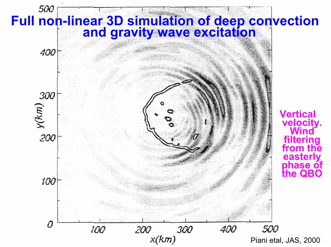
Piani etal, JAS, 2000

Full non-linear 3D simulation of deep convection and gravity wave excitation

Vertical velocity.

Wind filtering from the easterly phase of the QBO

Advantage of Vadas and Fritts (2004) convective plume model and ray

tracing over nonlinear simulations:

It is much faster (takes only days to run a thunderstorm on a standard desktop machine

(versus weeks or months on a super computer for a nonlinear simulation)‏

Medium-scale GWs with tiny initial amplitudes (but which are the only GWs left in the F region after dissipative filtering) can be accurately simulated

There is no need for an upper radiation condition or sponge layer, allowing for computations up to

z=500 km

1) Calculate the wave amplitudes and scales that are excited via convective plumes using this Fourier-Laplace idealistic model,

2) Embed these excited GWs into the frame of the wind at the tropopause,

3) Ray-trace these GWs into the mesosphere and thermosphere through variable winds and temperatures using the anelastic gravity wave dispersion relation

Our strategy:

λz λH

cH

Djuth et al and

Oliver et alresults

Theory agrees

with data quite well.

Application #1: compare wave scales from convection with measured wave scales

Altitude dependence of GWs from a single convective plume which propagate through a lower thermospheric shear

(Vadas, JGR,2007) ‏

At the highest

altitudes, only those medium-

scale GWs remain

τr

3. Ray-trace convectively-generated gravity waves to the OH airglow layer, and compare with Yucca Ridge data---is the normalization of the convective plume model OK? (i.e., can we trust it to higher altitudes?)‏

Yucca Ridge OH imager, Colorado 11 May, 2004

(Yue et al, 2008, in preparation) ‏

These concentric rings were centered on 2 convective plumes separated

by ∼ 100 km

NOAA NEXRAD Doppler radar at 3:05 UT: identify regions of convective overshoot

Winds were relatively small

(Yue et al, 2008, in preparation) ‏

Ray-tracing through

HAMMONIA mean zonal

windsassumptions: winds

and temperatures are slowly-varying

Jan JulApr

(Vadas et al, 2008, in preparation) ‏

APRIL mean zonal winds:Eastward GWs initially strong, then vanish at later times because of reflection of waves with small horizontal wavelengths (large k) ‏At later times, westward waves dominate

JAN and JUL windsCenters of concentric rings shift with time during April and Jul due to strong mean wind filtering on waves with slower phase speeds

t=70 min

t=90 min

t=120 min

t=50 min

Intensity at 4:02 UT

Yucca Ridge OH imager, Colorado 11 May, 2004Concentric rings of GWs observed in the OH airglow

layer during the equinox

Courtesy of Jia Yue

Temperature perturbations

Horizontal wavelength

Ray trace through mean zonal April HAMMONIA winds

t=55 min ____(theory)‏

4:02 UT - - - (data)‏

3:50 UT: diamonds

4:00 UT: triangles

4:30 UT: squares

t=45 min: ____

t=55 min: - - - - -

t=85 min: __ __

Intensities agree well with the convective plume

model results(Vadas et al, 2008, in preparation) ‏

4. Determine the neutral response to wave dissipation in the thermosphere from gravity waves from convection

When GWs dissipate in the thermosphere, they accelerate the neutral fluid in the direction they

were propagating prior to dissipating

(Hines, Space Res, 1972) ‏

Thermospheric body forces are 500-1000 km x 1000-1500 km x 50-100 km deepBody forces last for ½ hr for a single convective plumeBody force amplitudes are strong~ 1-10 m/s2

(Vadas andFritts, JGR2006) ‏

Horizontal thermospheric body forces are generated from dissipating GWs

Horizontal slices

x

y

(Zhu and Holton, JAS, 1987) ‏

Horizontal body forcings excite GWs

Study examined instantaneous

and step function forcings

(Vadas etal, JAS, 2003)‏

Mesosphere:Horizontal body forcings

generate neutral windsexcite secondary gravity waves

Study examined a horizontal forcing with sin2 in time

Reverse ray-tracing of a medium-scale GW observed in the OH imager above Brasilia, Brazil,

during the SpreadFEx campaignOct 1, 23:06 UT

λΗ~71.4 km

τ ~ 20.6 min

Propagating eastward

Reverse ray-traced to a strong, localized, convective plume with 40 m/s updraft, and 20 km horizontal extentVadas etal, 2008, submitted to Annal. Geoph)‏

Vertical profile of the created thermospheric body force on 01 Oct, 2005, in Brazil:

Body force is southeastward, with a very large amplitude

of 9 m/s2!Duration is 1.2 hrs,

horizontal extent is ∼5-8o

Maximum occurs at z∼177 km,

vertical extent is ∼50 km

These southeastward-propagating GWs created southeastward-propagating body forces where they dissipate in the thermosphereConvective

plume

Neutral temperature perturbations:Southeastward-propagating large-scale secondary GWs are

excited by this thermospheric body force.

z=250 km,times measured from 22:00 UT.

λH ~3000 km,

cH~700 m/s,

τ ~1.2 hrs

01 Oct, 2005, in Brazil

Courtesy of H-Li Liu

Perturbation amplitudes of short (40-400 km) and

long (400-4000 km) wavelengths GWs

are virtually independent of the Ap index below 60o

magnetic latitude

z~300 km

Hedin and Mayr, JGR,1987

5. Extract the vertically-varying, neutral horizontal winds from Poker Flat ISR (AMISR) electron density profiles

Observed Gravity Waves in Thermosphere using AMISR) system in Poker Flat, Alaska (Dec. 13, 2006)‏

Vertically-pointed beam

Relative electron density

perturbations

electron density

Ion velocity perturbations

Band-pass filtered ion

velocity perturbations

(Vadas and Nicolls, GRL, 2008) ‏

Intrinsic frequency

observed frequency Zonal

wind UMeridional

wind V

Solve for ωIr, then UH

Wind along direction of propagation

If one knows λΗ, λz, and the ground-based wave period,then the wind in the direction of propagation of the gravity wave can be determined iterativelyfrom the anelastic dissipative, GW dispersion relation.

(this includes the change in m from dissipation)‏

δ and δ+ depend on m and ωIr

Vertically-pointed beam

Conditions fairly quiet geomagnetically (ion

velocities only 10-20 m/s)‏assume a single ion species of O+ (a good approximation

above 200 km) Assume that ion drag causes vion=w, since magnetic field is

nearly vertically-pointed at PFISR

electron density continuity equation shows that the wave

phase is same for GW and electron density perturbation

λz can be computed by taking a vertical derivative of the relative electron density

perturbation along the “lines”of constant phases

(Vadas and Nicolls, GRL, 2008) ‏

Wind along propagation

direction

Computed vertically-varying intrinsic

period

Calculated vertically-varying

λz from data

(Vadas and Nicolls, GRL, 2008) ‏

Vap is mean component of the anti-parallel ion velocity, Umis neutral

wind along magnetic meridian (neglecting diffusion, which may be

important) ‏

Using simple geometry, calculated vertically-varying zonal and meridional winds

over PFISR

Can extract the total neutral, background wind from 180-250

km using this dissipative, anelastic dispersion relation if can calculate neutral wind along magnetic

meridian

Observed Gravity Waves in all 10 beams using PFISR

(Vadas and Nicolls, 2007) ‏

Relative electron density

perturbations

GW1: λH=180 km, τr=20 min,

propagating SEward

GW2: λH=200 km, τr=24 min,

propagating SEward

(Vadas and Nicolls, 2008, submitted to JASTP) ‏

Beam # 6

Beam # 7

Beam # 8

Beam # 9

Beam # 10

Extract the neutral, background wind profile for each constant wave

phase line.Then know how the winds evolve in time.

Extracted a 4.5-6 hr large-scale wave with λz=80 km

A third medium-scale wave with a 22 min period propagating

SEward

(Vadas and Nicolls, 2008, submitted to JASTP) ‏

SEward thermospheric

accelerations at the same times in

nearby beams of 0.1-0.2 m/s2

These accelerations are likely caused by

the dissipation of gravity waves from a source NW of Poker

Flat.

(Vadas and Nicolls, 2008, submitted to JASTP) ‏

z=180 and 190 km

Conclusions

The dissipative anelastic gravity wave dispersion relation is useful forUnderstanding the effects of dissipative filtering on wave scales and altitudesRay-trace studies coupling the lower atmosphere with the mesosphere and thermosphereExploring the role convection plays in the thermospheric dynamicsExtracting the vertically-varying neutral thermospheric wind profiles (and inferring neutral dynamics) from PFISR electron density profiles