Signal and Image Processing for Remote Sensing

Prof. C.H. Chen

Univ. of Massachusetts Dartmouth

Electrical and Computer Engineering Dept.

N. Dartmouth, MA 02747 USA cchen@umassd.edu

IGARSS2008 Tutorial, July 6, 2008 in Boston

Introduction:

• Objective of the Tutorial: to introduce the image and signal processing as

well as pattern recognition algorithms in remote sensing.

* Some useful references for this tutorial:

(1) “Signal and Image Processing for Remote Sensing”, edited by

C.H. Chen, CRC Press, 2006. (0-8453-5091-3). Referred to as the Book. This tutorial is based mainly on this book.

Split volume books 2007: Signal Processing for Remote Sensing (ISBN 1-4200-

6666-8), Image Processing for Remote Sensing (ISBN1-4200-6664-1)

(2) “Information Processing for Remote Sensing”, edited by C.H. Chen

World Scientific Publishing, 1999. (981-02-3737-5)

(3) “Frontiers of Remote Sensing Information Processing”, edited by

C.H. Chen, World Scientific Publishing 2003. (981-238-344-10-1)

3

Acknowledgement:

I thank all authors of the book chapters of the

three books listed above for the use of

their materials in this tutorial.

My special thanks go to Dr. Blackwell,

Dr. Escalante, Dr. Long, Dr. Moser,

Dr. Nasrabadi and Dr. Serpico for the use of

their power points in this tutorial.

Outline: * Part 1: PCA, ICA and Related Transforms

* Part 2: Change Detection for SAR Imagery

* Part 3a: The Classification Problems

* Part 3b: The Classification Problems continued

* Part 4: Contextual Classification in Remote Sensing

* Part 5: Other topics

5

Part 1: PCA, ICA and Related Transforms

* Definition: y = Vx; V = [ v1, v2 , …, vn ]

V is usually an orthogonal matrix for linear transforms.

The reconstruction error is minimized such as in PCA.

Data reconstruction (m<n):

• Let yi be an element of y. In a non-linear transform,

replace yi by a function of yi, gi (yi).

i

m

i

ivyx

1

6

• The Principal Component (PC) transform: The traditional

PCA attempts to maximize the data variances in the directions (components) of eigenvectors. The components are statistically uncorrelated and the reduced rank reconstruction error is minimized. It does not guarantee however maximizing the signal to noise ratio (SNR).

• The Noise-adjusted PC (NAPC) transform attempts to make noise covariance to be identical in all directions, thus maximizing the SNR.

• The Projected PC transform: The Wiener filtered data are projected onto the r-dimensional subspace of m eigenvectors of a modified covariance matrix (r<m).

Reference: Chapter 11 of the Book.

7

Comments on PCA and related transforms * PC Transform relies on the covariance matrix estimated from

data available. In the presence of noise, the covariance matrix

is the sum of the noise free covariance and the noise covariance.

The coefficients of the PC transform components are statistically

uncorrelated. The reduced rank reconstruction error is minimized

with respect to the data.

* NAPC Transform requires a good knowledge of the noise

statistics which often cannot be estimated accurately.

* PPC reconstruction of noise free data yields lower distortion

(i.e. reconstruction error) than the PC and NAPC Transforms.

The next slide on PC transforms performance comparison is from

Dr. Balckwell in his talk at the Univ. of Pittsburgh.

8

Performance Comparison of Principal Components Transforms

“Radiance

Reconstruction”

“Temperature

Profile

Estimation”

9

Some references on PCA in remote sensing

1. J.B. Lee, A.S. Woodyatt and M. Berman, “Enhancement of high

spectral resolution remote sensing data by a noise adjusted principal

component transform”, IEEE Trans. on Geoscience and Remote

Sensing, vol. 28, pp. 295-304, May 1990.

2. W.J. Blackwell, “Retrieval of cloud-cleared atmospheric temperature

profiles for hyperspectral infrared and microwave observations”, Ph.D.

dissertation, EECS Dept., MIT, June 2002.

3. W.J. Blackwell, “Retrieval of atmospheric profiles form hyperspectral

sounding data using PCA and a neural network”, Technical talk given

at University of Pittsburgh ECE Seminar, Feb. 27, 2008.

10

(Left) AVIRIS RGB image for the Linden, CA scene

collected on 20-Aug-1992, denoting location of various

features of interest and (Right) a plot of the spectral

distribution of the apparent reflectance for those features.

(Hsu, et al. in Frontiers of Remote Sensing Information Processing, WSP 2003)

400 700 1000 1300 1600 1900 2200 2500

Wavelength (nm)

0.1

1.0

10.0

Appar

ent R

efle

ctan

ce

Cloud

Fire

Hot Area

Grass

Lake

Bare Soil

Smoke (sm. part.)

Smoke (lg. part.)

ShadowSmoke - large part.

Cloud Hot Area

Smoke -

small part.

Fire

Shadow

Grass Lake

Soil

11

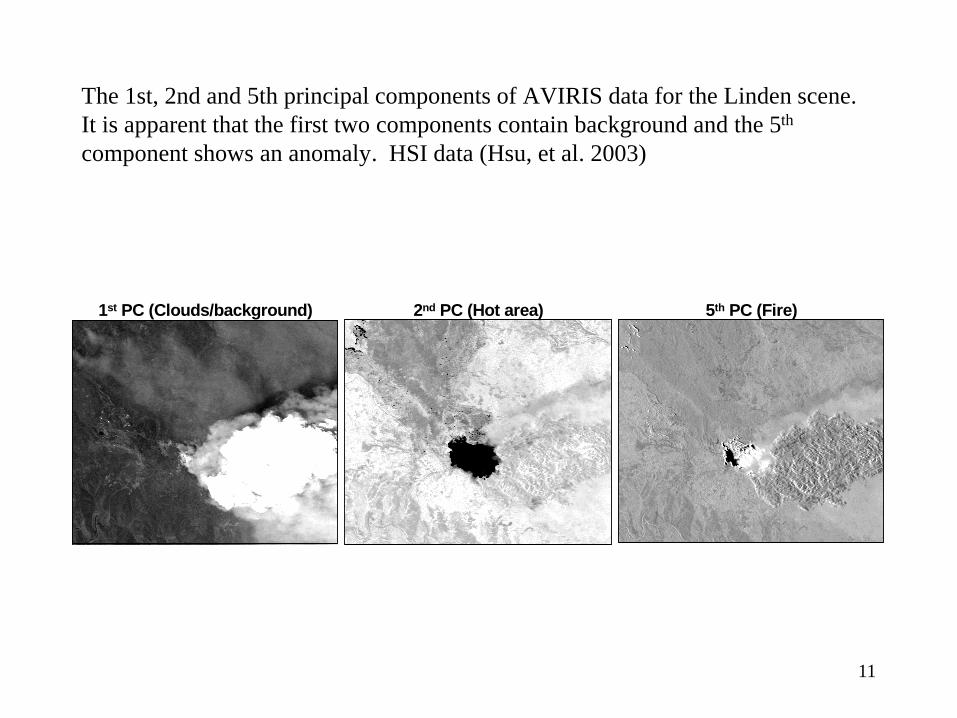
The 1st, 2nd and 5th principal components of AVIRIS data for the Linden scene.

It is apparent that the first two components contain background and the 5th

component shows an anomaly. HSI data (Hsu, et al. 2003)

1st PC (Clouds/background) 2nd PC (Hot area) 5th PC (Fire)

12

Cloud

Smokesmall particle

Clear

Shadow

Smokelarge particle

Hot

Fire

Cloud

Smokesmall particle

Clear

Shadow

Smokelarge particle

Hot

Fire

Cloud

Smokesmall particle

Clear

Shadow

Smokelarge particle

Hot

Fire

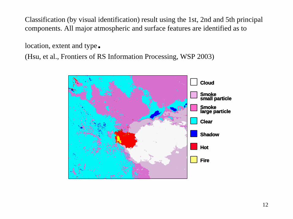
Classification (by visual identification) result using the 1st, 2nd and 5th principal

components. All major atmospheric and surface features are identified as to

location, extent and type. (Hsu, et al., Frontiers of RS Information Processing, WSP 2003)

13

Component Analysis * PCA, ICA, CCA, etc. are useful to extract essential information from the

large amount of remote sensing image data.

Component Analysis

* PCA only decorrelates the components of a vector.

* CCA (curvilinear component analysis) is for lower dimensional

reconstruction.

* CCA (canonical correlation analysis) jointly analyzes two sets of

variables. The desired linear combinations of the two sets of zero

mean variable X and Y are obtained by maximizing the

normalized correlation between them.

* ICA (independent component analysis) seeks for independent

components which provide complimentary information of the

data. ICA may use high-order statistical information.

* Nonlinear PCA attempts to use high-order statistics in PCA

analysis.

14

Component Analysis (continued)

* The Hermite Transform (HT) is an image representation model that mimics some important aspects of human visual perception, namely the local orientation analysis and the Gaussian derivative model of early vision. HT provides an efficient tool for image noise reduction and data fusion (Escalante, et al. SPIE2007). The Gaussian derivative family exhibits special kind of symmetries related to translation, rotation, and magnification and is particularly suitable for integration into Hermite transform for local orientation analysis. SAR image noise reduction and fusion for multispectral and SAR images clearly demonstrated the important applications of this unique approach

* An algorithm is presented by Escalante, et al. for integrating MS and PAN images, which employs the Hermite transform. Such a fusion method was designed and tested in the context of maintaining the information content of the original images.

• HT method can better characterize land-cover change than WT.

15

Hermite transform (Escalante, et al. 2007)

,

1, , ,

, p q S

L x y L x y V x p y qW x y

•The Hermite transform is a special case of polynomial

transform.

The image L(x,y) is located by multiplying it by a window

function V(x-p,y-q),

,p q S

2 2

2

1, exp

2

x yV x y

0

It uses overlapping Gaussian windows and projects

images locally onto a basis of orthogonal polynomials.

16

17

Comments on Gabor Transform

*Motivated by biological vision, schemes of signal and image representation by localized Gabor-type functions have been introduced and analyzed. *Its emphasis on different orientations of texture features makes it particularly suitable for classification of images which are rich in textures. The features extracted can be nearly rotation invariant, less sensitive to noise, and thus providing good classification results. (Chapter 22).

18

Current ICA Algorithms

ICA has been used mainly in source separation problems.

ICA algorithms try to obtain as independent components as

possible. Of course the results of different algorithms are not

identical. Algorithms developed include:

• Nonlinear PCA (Oja 1997)

• Bi-Gradient learning rule (Wang and Karhunen 1996)

• Fixed-point learning rule (Hyvarinen 1997)

• Informax method (Bell and Senjnowski 1999)

• Extended-Informax method (Lee and Sejnowski 1999)

• Equivalent Adaptive Separation via Independent (EASI) algorithm

(Cardoso 1996)

• Jointly and Approximately diagonalization (JADE) algorithm (Cardoso 1996)

• Noisy ICA and FastICA algorithms (see e.g. book by Oja et al. )

• Particle filtering for noisy ICA problems (2005 or later)

Etc.

19

ICA in remote sensing

• Szu (2000) employed ICA neural net to refine remote sensing with

multiple labels

• Chang, et al. (2000) employed ICA in demixing problems with mixed

pixels.

• Tu (2000) employed fast ICA in unsupervised signal extraction from

mixed pixels.

• Zhang and Chen (2002) developed a new ICA method that makes use

of the high-order statistics (HOS), i.e. ICA components which are

independent in the sense of 3rd and 4th order joint cumulants. The

method is called JC-ICA. HOS information provides better transform.

* ICA methods provide speckle reduction in SAR images

• ICA methods provide better features in pixel classification

* ICA methods provide significant data reduction in hyperspectral

images

20

The next 3 slides show the use of JC-ICA

approach in SAR images. The images now

available from IEEE GRS society data base

were acquired by NASA on an agricultural

area near the village of Feltwell, UK, with

Thematic Mapper (ATM) scanner and a PLC

Bands fully polarimetric SAR sensor. The

first few channels of ICA have much less

speckle noise.

21

Original: row 1, the-c-hh, th-c-hv, th-c-vv; row 2, th-l-hh, th-l-hv, th-l-vv; row 3: th-p-hh; th-p-hv, th-p-vv

22

PCA

23

ICA

24

Subspace Approach of Speckle Reduction

in SAR Images Using ICA (Chapter 20)

• Estimating ICA bases from the image: The image

patches of window size say 16x16 can be reduced, by

PCA for example, and inputted to a fastICA algorithm.

• Basis image classification: to classify the basis images

to “true signal source” and “speckle noise source”, a

binary decision using threshold.

• Feature emphasis by generalized adaptive gain (GAG)

• Nonlinear filtering (transform) for each component

25

Linear Representation and Independent Component

Analysis (ICA)

An image demoted by I(x,y) can be partitioned into a

number of image patches IP(x,y), i.e. I(x,y) ={IP(x,y)}.

I(x,y) can be expressed as a linear superposition of some

basis functions,

where a i(x,y) is the ith basis image, si is the

corresponding coefficient. It would be most useful to

estimate the linear transformation from the data itself, so

the transform could be ideally adapted to the data being

processed. Here ai(x,y) is estimated from the original

image, while si is estimated from image patches. ICA is to make the coefficients in the superposition independent,

at least approximately. For simplicity, we use vector-matrix notation

instead of the sums.

1

( , ) ( , ) (1)n

i i

i

I x y a x y s

26

Linear Representation and Independent Component

Analysis (ICA)-- continued

Arrange all the pixel values in a single vector, and denote by the vector of

the transformed component variables, the weight matrix, and the mixing

matrix, then we can obtain the mixing model:

x = As (2)

and the demixing model: y = Wx (3)

where W is the pseudoinverse of A. We will concentrate mainly on

estimating matrix A and use the transform to remove speckle noise. The

novel method we developed was to consider desired signal and the speckle

as coming from independent sources. A fastICA algorithm is used to

determine the transformed component variables.

27

ICA Basis images of the 9-channel POLSAR images;

S1 for edge images, S2 for texture images

28

19 Basis images belonging to signal sources (upper)45 Basis images belonging to speckle noises (lower)

29

Nonlinear filtering for each component

The nonlinear filtering is realized as follows. For the components that

belong to S2, we simply set them to zero, but for components that belong

to S1, we apply our GAG (nonlinear gain f) operator to enhance the image

feature. Then the recovered Si can be calculated by:

Finally the restored image can be obtained after a mixing transform

Note: sij above should be replaced by si.

^ 0 component S2

( ) component S1 ijij

iths f s ith

^ ^

x A s

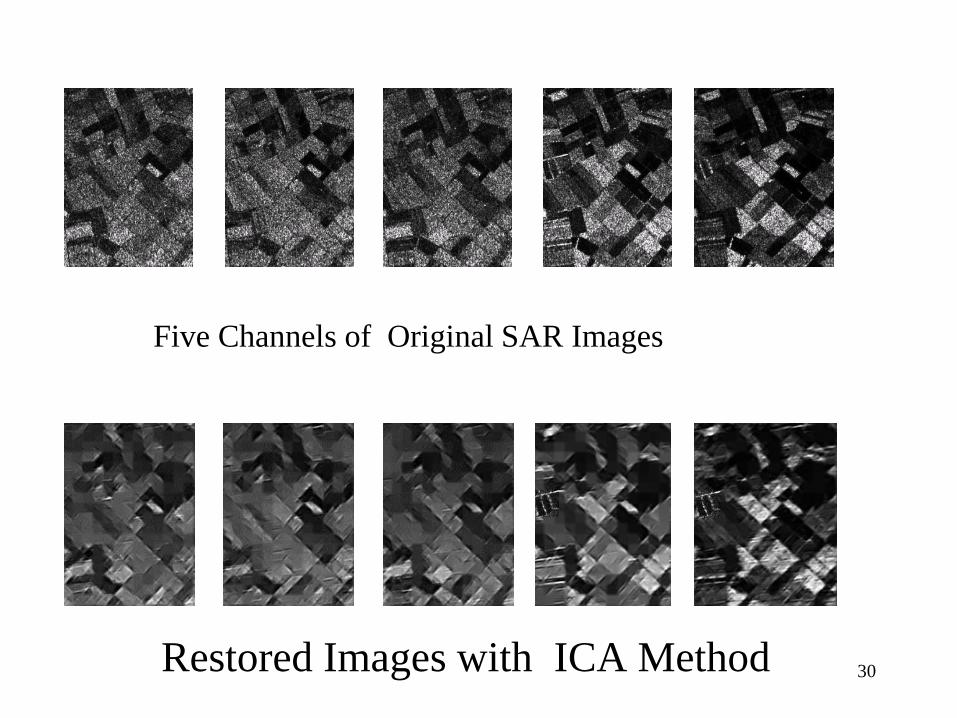
30 Restored Images with ICA Method

Five Channels of Original SAR Images

31

The same five channel images

recovered by Lee’s method

32

Performance comparison with ratio of SD/Mean

Original Our method Wiener filter Lee’s filter Kuan’s filter

Channel 1 0.1298 0.1086 0.1273 0.1191 0.1141

Channel 2 0.1009 0.0526 0.0852 0.1133 0.0770

Channel 3 0.1446 0.0938 0.1042 0.1277 0.1016

Channel 4 0.1259 0.0371 0.0531 0.0983 0.0515

Channel 5 0.1263 0.1010 0.0858 0.1933 0.0685

Table 1 Ratio Comparison

(The ratio is determined as the average of ratios of local standard deviation to mean

(SD/Mean) from deferent sections of an image)

33

RX filtering

RX filtering originally developed by Reed and Yu is a spatial-spectral processing algorithm for anomaly detection. A spatially moving window is used to calculate local background mean and covariance. The RX filtered value at the center of the window is detected on differences from the local background. The RX filtered value is calculated as the following:

RX = (x – m)’ S-1 (x – m)

x: Data spectrum

m: Local background mean

S: Local background covariance

34

Anomaly detection example. The left panel shows the RGB image of a forest

scene. The right panel shows detection of the vehicles with RX filtering. The

vehicles are approximately 5-pixel x 11-pixel in size. The RX filtering is

implemented using a 21x21 spatial window on four principal components. (Hsu, et

al. in Frontiers of Remote Sensing Information Processing, WSP 2003) HSI HYDICE data.

FRI Run 5 Anomaly Detection