Power Law Tails in the Italian Personal Income

Distribution∗

F. Clementia,c, M. Gallegatib,c

aDepartment of Public Economics, University of Rome “La Sapienza”, Via del Castro Laurenziano 9, 00161 Rome,Italy. E-mail address: fabio.clementi@uniroma1.it.

bDepartment of Economics, Universita Politecnica delle Marche, Piazzale Martelli 8, 60121 Ancona, Italy. E-mailaddress: gallegati@dea.unian.it.

cS.I.E.C., Universita Politecnica delle Marche, Piazzale Martelli 8, 60121 Ancona, Italy. Web address:http://www.dea.unian.it/wehia/.

May 11, 2005

Abstract

We investigate the shape of the Italian personal income distribution using microdata from the Survey onHousehold Income and Wealth, made publicly available by the Bank of Italy for the years 1977–2002.We find that the upper tail of the distribution is consistent with a Pareto power-law type distribution,while the rest follows a two-parameter lognormal distribution. The results of our analysis show a shiftof the distribution and a change of the indexes specifying it over time. As regards the first issue, wetest the hypothesis that the evolution of both gross domestic product and personal income is governed bysimilar mechanisms, pointing to the existence of correlation between these quantities. The fluctuations ofthe shape of income distribution are instead quantified by establishing some links with the business cyclephases experienced by the Italian economy over the years covered by our dataset.

Keywords: Personal income; Pareto law; Lognormal distribution; Income growth rate; Business cycle

JEL Classifications: C16; D31; E32

1 Introduction. In the last decades, extensive lit-erature has shown that the size of a large number

of phenomena can be well described by a power-lawtype distribution.

The modeling of income distribution originatedmore than a century ago with the work of VilfredoPareto, who observed in his Cours d’Economie Poli-tique (1897) that a plot of the logarithm of the num-ber of income-receiving units above a certain thresh-

∗Paper prepared for the International Conference inMemory of Two Eminent Social Scientists: C. Gini andM.O. Lorenz. Their Impact in the XXth Century De-velopment of Probability, Statistics and Economics, tobe held Siena (Italy) on May 23–26, 2005. The authors wouldlike to thank Corrado Di Guilmi and Yoshi Fujiwara for helpfulcomments and suggestions.

old against the logarithm of the income yields pointsclose to a straight line. This power-law behaviour isnowadays known as Pareto law.

Recent empirical work seems to confirm the valid-ity of Pareto (power) law. For example, [1] show thatthe distribution of income and income tax of individ-uals in Japan for the year 1998 is very well fitted bya power-law, even if it gradually deviates as the in-come approaches lower ranges. The applicability ofPareto distribution only to high incomes is actuallyacknowledged; therefore, other kinds of distributionshas been proposed by researchers for the low-middleincome region. According to [2], US personal incomedata for the years 1935–36 suggest a power-law dis-tribution for the high-income range and a lognormal

F. Clementi, M. Gallegati 2

distribution for the rest; a similar shape is found by[3] investigating the Japanese income and income taxdata for the high-income range over the 112 years1887–1998, and for the middle-income range over the44 years 1955–98.1 Reference [4] confirms the power-law decay for top taxpayers in the US and Japan from1960 to 1999, but find that the middle portion of theincome distribution has rather an exponential form;the same is proposed by [5] for the UK during theperiod 1994–99 and for the US in 1998.

The aim of this paper is to look at the shape of thepersonal income distribution in Italy by using cross-sectional data samples from the population of Italianhouseholds during the years 1977–2002. We find thatthe personal income distribution follows the Paretolaw in the high-income range, while the lognormalpattern is more appropriate in the central body ofthe distribution. From this analysis we get the resultthat the indexes specifying the distribution change intime; therefore, we try to look for some factors whichmight be the potential reasons for this behaviour.

The rest of the paper is organized as follows. Sec-tion 2 reports the data utilized in the analysis anddescribes the shape of the Italian personal incomedistribution. Section 3 explains the shift of the dis-tribution and the change of the indexes specifying itover the years covered by our dataset. Section 4 con-cludes the paper.

2 Lognormal Pattern with Power Law Tail.We use microdata from the Historical Archive

(HA) of the Survey on Household Income and Wealth(SHIW) made publicly available by the Bank of Italyfor the period 1977–2002 [7].2 All amounts are ex-pressed in thousands of lire. Since we are comparingincomes across years, to get rid of inflation data are

1Reference [6] suggests that a Pareto law may hold alsofor lower incomes, yielding a so-called double Pareto-lognormaldistribution, that is a distribution with a lognormal body anda double Pareto tail.

2The data for the years preceding 1977 are no longer avail-able. The survey was carried out yearly until 1987 (except for1985) and every two years thereafter (the survey for 1997 wasshifted to 1998). In 1989 a panel section consisting of unitsalready interviewed in the previous survey was introduced inorder to allow for better comparison over time. The basic def-inition of income provided by the SHIW is net of taxation andsocial security contributions. It is the sum of four main compo-nents: compensation of employees; pensions and net transfers;net income from self-employment; property income (includingincome from buildings and income from financial assets). In-come from financial assets started to be recorded only in 1987.See [8] for details on source description, data quality, and mainchanges in the sample design and income definition.

−4

−2

02

Cum

ulat

ive

prob

abili

ty

1 2 3 4 5Income (thousand £)

Income dataLognormalPower law

Fig. 1: The cumulative probability distribution ofthe Italian personal income in 1998. We take thehorizontal axis as the logarithm of the personal in-come in thousands of lire and the vertical axis as thelogarithm of the cumulative probability. The greensolid line is the lognormal fit with µ = 3.48 (0.004)and σ = 0.34 (0.006). Gibrat index is β = 2.10.

reported in 1976 prices using the Consumer PricesIndex (CPI) issued by the National Institute of Sta-tistics [9]. The average number of income-earners sur-veyed from the SHIW-HA is about 10,000.

Figure 1 shows the profile of the personal incomedistribution for the year 1998. We take the horizon-tal axis as the logarithm of the income in thousandsof lire and the vertical axis as the logarithm of thecumulative probability. The cumulative probabilityis the probability to find a person with an incomegreater than or equal to x:

P (X ≥ x) =

∞∫x

p(t)dt

Two facts emerge from this figure. Firstly, the cen-tral body of the distribution (almost all of it belowthe 99th percentile) follows a two-parameter lognor-mal distribution (green solid line). The probabilitydensity function is:

p (x) =1

xσ√

2πexp

[−1

2

(logx− µ

σ

)2]

with 0 < x < ∞, and where µ and σ are the meanand the standard deviation of the normal distribu-tion. The value of the fraction β = 1/

(σ√

2)

returnsthe so-called Gibrat index; if β has low values (large

3 Power Law Tails in the Italian Personal Income Distribution−

2−

10

1C

umul

ativ

e pr

obab

ility

3.5 4 4.5 5Income (thousand £)

Income dataPower law

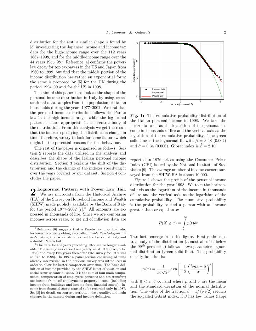
Fig. 2: The fit to the power-law distribution for theyear 1998. The red solid line is the best-fit func-tion. Pareto index, obtained by least-square-fit, isα = 2.76 (0.002); the estimated minimum income isx0 = 17, 141 thousand lire. The goodness of fit ofOLS estimate in terms of R2 index is 0.9993.

variance of the global distribution), the personal in-come is unevenly distributed. From our dataset weobtain the following maximum-likelihood estimates:3

µ = 3.48 (0.004) and σ = 0.34 (0.006);4 Gibrat indexis β = 2.10. Secondly, about the top 1% of the dis-tribution follows a Pareto (power-law) distribution.This power-law behaviour of the tail of the distribu-tion is more evident from Fig. 2, where the red solidline is the best-fit linear function. We extract thepower-law slope (Pareto index) by running a simpleOLS regression of the logarithm of the cumulativeprobability on a constant and the logarithm of per-sonal income, obtaining a point estimate of α = 2.76(0.002). Given this value for α, our estimate of x0

(the income level below which the Pareto distribu-tion would not apply) is 17,141 thousand lire. Thefit of linear regression is extremely good, as one canappreciate by noting that the value of R2 index is0.9993.

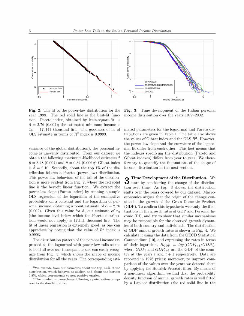
The distribution pattern of the personal income ex-pressed as the lognormal with power-law tails seemsto hold all over our time span, as one can easily recog-nize from Fig. 3, which shows the shape of incomedistribution for all the years. The corresponding esti-

3We exclude from our estimates about the top 1.4% of thedistribution, which behaves as outlier, and about the bottom0.8%, which corresponds to non positive entries.

4The number in parentheses following a point estimate rep-resents its standard error.

−2

−1

01

2C

umul

ativ

e pr

obab

ility

2.4 33 4 5Income (thousand £)

1977/78/791980/81/82/83/84/86/87/891991/93/95/982000/02

Fig. 3: Time development of the Italian personalincome distribution over the years 1977–2002.

mated parameters for the lognormal and Pareto dis-tributions are given in Table 1. The table also showsthe values of Gibrat index and the OLS R2. However,the power-law slope and the curvature of the lognor-mal fit differ from each other. This fact means thatthe indexes specifying the distribution (Pareto andGibrat indexes) differs from year to year. We there-fore try to quantify the fluctuations of the shape ofincome distribution in the next section.

3 Time Development of the Distribution. Westart by considering the change of the distribu-

tion over time. As Fig. 3 shows, the distributionshifts over the years covered by our dataset. Macro-economics argues that the origin of the change con-sists in the growth of the Gross Domestic Product(GDP). To confirm this hypothesis we study the fluc-tuations in the growth rates of GDP and Personal In-come (PI), and try to show that similar mechanismsmay be responsible for the observed growth dynam-ics of both country and individuals. The distributionof GDP annual growth rates is shown in Fig. 4. Wecalculate it using the data from the OECD StatisticalCompendium [10], and expressing the rates in termsof their logarithm, RGDP ≡ log (GDPt+1/GDPt),where GDPt and GDPt+1 are the GDP of the coun-try at the years t and t + 1 respectively. Data arereported in 1976 prices; moreover, to improve com-parison of the values over the years we detrend themby applying the Hodrick-Prescott filter. By means ofa non-linear algorithm, we find that the probabilitydensity function of annual growth rates is well fittedby a Laplace distribution (the red solid line in the

F. Clementi, M. Gallegati 4

Table 1: Estimated lognormal and Pareto distribution parameters for all the years (standard errors are inparentheses). Calculations are conducted using data and methods described in the text. For the lognormaldistribution and the Pareto distribution also shown are the values of Gibrat index and R2 index respectively.

Year µ σ β α x0 R2

1977 3.31 (0.005) 0.34 (0.004) 2.08 3.00 (0.008) 10,876 0.99211978 3.33 (0.005) 0.34 (0.004) 2.09 3.01 (0.008) 11,217 0.99331979 3.34 (0.005) 0.34 (0.005) 2.08 2.91 (0.009) 11,740 0.99081980 3.36 (0.005) 0.33 (0.005) 2.15 3.06 (0.008) 11,453 0.99151981 3.36 (0.005) 0.32 (0.005) 2.23 3.30 (0.008) 10,284 0.99391982 3.38 (0.004) 0.31 (0.005) 2.27 3.08 (0.005) 11,456 0.99521983 3.38 (0.005) 0.30 (0.005) 2.32 3.11 (0.006) 11,147 0.99451984 3.39 (0.004) 0.32 (0.005) 2.24 3.05 (0.007) 11,596 0.99371986 3.40 (0.004) 0.29 (0.006) 2.40 3.04 (0.005) 11,597 0.99501987 3.49 (0.004) 0.30 (0.004) 2.38 2.09 (0.002) 24,120 0.99931989 3.53 (0.003) 0.26 (0.003) 2.70 2.91 (0.002) 15,788 0.99951991 3.52 (0.004) 0.27 (0.004) 2.58 3.45 (0.008) 14,281 0.99881993 3.47 (0.004) 0.33 (0.004) 2.15 2.74 (0.002) 16,625 0.99971995 3.46 (0.004) 0.32 (0.003) 2.19 2.72 (0.002) 16,587 0.99961998 3.48 (0.004) 0.34 (0.006) 2.10 2.76 (0.002) 17,141 0.99932000 3.50 (0.004) 0.32 (0.004) 2.20 2.76 (0.002) 17,470 0.99942002 3.52 (0.004) 0.31 (0.005) 2.25 2.71 (0.002) 17,664 0.9997

0.2

.4.6

.81

Pro

babi

lity

dens

ity

−.04 −.02 0 .02 .04Growth rate

GDP data (1977−2002)Laplace fit

Fig. 4: Probability density function of Italian GDPannual growth rates for the period 1977–2002 to-gether with the Laplace fit (red solid line). Thedata have been detrended by applying the Hodrick-Prescott filter.

figure), which is expressed as:

p (x) =1

σ√

2exp

(−|x− µ|

σ

)with −∞ < x < +∞, and where µ and σ are the

mean value and the standard deviation. This resultseems to be in agreement with the growth dynamicsof PI, as shown in Fig. 5 for two randomly selecteddistributions. We calculate them using the panel sec-tion of the SHIW-HA, which covers the period 1987–2002. As one can easily recognize, the same func-tional form describing the probability distribution ofGDP annual growth rates is also valid in the case ofPI growth rates. These findings lead us to check thepossibility that the growth rates of both GDP andPI are drawn from the same distribution. To thisend, we perform a two-sample Kolmogorov-Smirnovtest and check the null hypothesis that both GDPand PI growth rate data are samples from the samedistribution. Before applying this test, to consider al-most the same number of data points relating to unitswith different sizes we draw a 2% random samplesof the data we have for individuals, and normalizethem together with the data for GDP annual growthrate using the transformations

(RPI −RPI

)/σPI and(

RGDP −RGDP

)/σGDP. As shown in Table 2, which

reports the p-values for all the cases we studied, thenull hypothesis of equality of the two distributionscan not be rejected at the usual 5% marginal sig-nificance level. Therefore, the data are consistentwith the assumption that a common empirical law

5 Power Law Tails in the Italian Personal Income Distribution

Table 2: Estimated Kolmogorov-Smirnov test p-values for both GDP and PI growth rate data. The nullhypothesis that the two distributions are the same at the 5% marginal significance level is not rejected in allthe cases.

Growth rate R89/87 R91/89 R93/91 R95/93 R98/95 R00/98 R02/00

RGDP 0.872 0.919 0.998 0.696 0.337 0.480 0.955R89/87 0.998 0.984 0.431 0.689 0.860 0.840R91/89 0.970 0.979 0.995 0.994 0.997R93/91 0.839 0.459 0.750 1.000R95/93 0.172 0.459 0.560R98/95 0.703 0.378R00/98 0.658

might describe the growth dynamics of both GDPand PI, as shown in Fig. 6, where all the curves forboth GDP and PI growth rate normalized data al-most collapse onto the red solid line representing thenon-linear Laplace fit.5

We next turn on the fluctuations of the indexesspecifying the income distribution, i.e. the Paretoand Gibrat indexes, whose yearly estimates are re-ported in Fig. 7. Figure 7(a) shows the fluctuationsof Pareto index over the years 1977–2002. The blackconnected solid line is the time series obtained by ex-cluding income from financial assets, while the redconnected solid line refers to the yearly estimates ob-tained by the inclusion of the above-stated income,which was regularly recorded only since 1987 (seenote 2). The course of the two series is similar,with the more complete definition of income showinga greater inequality because of the strongly concen-trated distribution of returns on capital. The samecan be said for the time series of Gibrat index (Fig.7(b)). Although the frequency of data (initially an-nual and then biennial from 1987) makes it difficultto establish a link with the business cycle, it seemspossible to find a (negative) relationship between theabove-stated indexes and the fluctuations of economicactivity. For example, Italy experienced a period ofeconomic growth until the late 1980s, but with alter-nating phases of the internal business cycle: of slow-down of production up to the 1983 stagnation; of re-covery in 1984; again of slowdown in 1986. As one canrecognize from the figure, the values of Pareto andGibrat indexes, inferred from the numerical fitting,tend to decrease in the periods of economic expan-sion (concentration goes up) and increase during the

5See [11] for similar findings about GDP and companygrowth rates.

recessions (income is more evenly distributed). Thetime pattern of inequality is shown in Fig. 8, whichreports the temporal change of Gini coefficient for theconsidered years.6 In Italy the level of inequality de-creased significantly during the 1980s and rised in theearly 1990s; it was substantially stable in the follow-ing years. In particular, a sharp rise of Gini coefficient(i.e., of inequality) is encountered in 1987 and 1993,corresponding to a sharp decline of Pareto index inthe former case and of both Pareto and Gibrat in-dexes in the latter case. We consider that the declineof Pareto exponent in 1987 corresponds with the peakof the speculative “bubble” begun in the early 1980s,and the rebounce of the index follows its burst on Oc-tober 19, when the Dow Jones index lost more than20% of its value dragging into disaster the other worldmarkets. This assumption seems confirmed by themovement of asset price in the Italian Stock Exchange(see Fig. 9(a)).7 As regards the sharp decline of bothindexes in 1993, the level and growth of personal in-come (especially in the middle-upper income range)were notably influenced by the bad results of the realeconomy in that year, following the September 1992lira exchange rate crisis. The effects of recession (vis-ible in Fig. 9(b)) produced a leftwards shift of thedistribution and widened its range; this, combinedwith a concentration of individuals towards middleincome range, induced an increase in inequality.8 It

6Unlike the Pareto and Gibrat indexes, which provide twodifferent measures corresponding to the tail and the rest, theGini coefficient is a measure of (in)equality of the income forthe overall distribution taking values from zero (completelyequal) to one (completely inequal).

7See [3] for a study of the correlation between Pareto indexand asset price in Japan.

8In particular, in this year there was a significant reductionof the number of self-employees, whose incomes are much moredependent from the business cycle. See [12] for further details

F. Clementi, M. Gallegati 60

.2.4

.6.8

1P

roba

bilit

y de

nsity

−2 −1 0 1 2Growth rate

PI data (1989/1987)Laplace fit

(a)

0.2

.4.6

.81

Pro

babi

lity

dens

ity

−2 −1 0 1 2Growth rate

PI data (1993/1991)Laplace fit

(b)

Fig. 5: Probability distribution of Italian PI growthrates RPI ≡ log (PIt+i/PIt) for the years 1989/1987(a) and 1993/1991 (b). The red solid line is the fitto the Laplace distribution. The data are taken fromthe panel section of the SHIW-HA, which covers theyears 1987–2002.

would be expected that these facts cause the invalid-ity of Pareto law for high incomes. This was well thecase of Italian economy during the mentioned years.Fig. 10 shows the power-law region in 1987 and 1993.Compared to other years, one can observe that thedata can not be fitted by the Pareto law in the entirerange of high-income.

on this issue.

0.2

.4.6

.81

Pro

babi

lity

dens

ity

−4 −2 0 2 4Growth rate

GDP (1977−2002)PI (1989/1987)PI (1991/1989)PI (1993/1991)PI (1995/1993)PI (1998/1995)PI (2000/1998)PI (2002/2000)Laplace fit

Fig. 6: Probability distribution of Italian GDP andPI growth rates. All data collapse onto a single curverepresenting the fit to the Laplace distribution (redsolid line), showing that the distributions are welldescribed by the same functional form.

4 Concluding Remarks. In this paper we findthat the Italian personal income microdata are

consistent with a Pareto (power-law) behaviour in thehigh-income range, and with a two-parameter lognor-mal pattern in the low-middle income region.

The numerical fitting over the time span coveredby our dataset show a shift of the distribution, whichis claimed to be a consequence of the growth of thecountry. This assumption is confirmed by testingthe hypothesis that the growth dynamics of bothgross domestic product of the country and personalincome of individuals is the same; the two-sampleKolmogorov-Smirnov test we perform on this sub-ject lead us to accept the null hypothesis that thegrowth rates of both the quantities are samples fromthe same probability distribution in all the cases westudied, pointing to the existence of correlation be-tween them.

Moreover, by calculating the yearly estimates ofPareto and Gibrat indexes, we quantify the fluctu-ations of the shape of the distribution over time byestablishing some links with the business cycle phaseswhich Italian economy experienced over the years ofour concern. We find that there exists a negative re-lationship between the above-stated indexes and thefluctuations of economic activity at least until thelate 1980s. In particular, we show that in two circum-stances (the 1987 burst of the asset-inflation “bubble”begun in the early 1980s and the 1993 recession year)the data can not be fitted by a power-law in the en-

7 Power Law Tails in the Italian Personal Income Distribution

22.

53

3.5

Par

eto

inde

x

1977 19801980 1985 1990 1995 20002000 2002Year

Excluding financial assets

Including financial assets

(a)

22.

22.

42.

62.

8G

ibra

t ind

ex

1977 19801980 1985 1990 1995 20002000 2002Year

Excluding financial assets

Including financial assets

(b)

Fig. 7: The temporal change of Pareto index (a)and Gibrat index (b) over the years 1977–2002. Theblack connected solid line is the time series of the twoindexes obtained by excluding income from financialassets, while the red connected solid line refers tothe yearly estimates obtained by the inclusion of theabove-stated income.

tire high-income range, causing breakdown of Paretolaw.

References

[1] H. Aoyama, Y. Nagahara, M.P. Okazaki, W.Souma, H. Takayasu, and M. Takayasu (2000),Pareto’s Law for Income of Individuals and Debtof Bankrupt Companies, Fractals, 8, 3, 293–300.

.28

.3.3

2.3

4.3

6G

ini c

oeffi

cien

t

1977 19801980 1985 1990 1995 20002000 2002Year

Excluding financial assets

Including financial assets

Fig. 8: Gini coefficient for Italian personal incomeduring the period 1977–2002. The black connectedsolid line excludes income from financial assets, whilethe red connected solid line includes it.

[2] E.W. Montroll, and M.F. Shlesinger (1983),Maximum Entropy Formalism, Fractals, ScalingPhenomena, and 1/f Noise: A Tale of Tails,Journal of Statistical Physics, 32, 2, 209–230.

[3] W. Souma (2001), Universal Structure of thePersonal Income Distribution, Fractals, 9, 4,463–470.

[4] M. Nirei, and W. Souma (2004), TwoFactors Model of Income Distribu-tion Dynamics, SFI Working Paper,http://www.santafe.edu/research/publications/workingpapers/04-10-029.pdf.

[5] A.A. Dragulescu, and V.M. Yakovenko (2001),Exponential and Power-Law Probability Distrib-utions of Wealth and Income in the United King-dom and the United States, Physica A, 299, 1–2,213–221.

[6] W.J. Reed (2003), The Pareto Law of Incomes– An Explanation and an Extension, Physica A,319, 469–486.

[7] Bank of Italy, Survey on Household Income andWealth, http://www.bancaditalia.it.

[8] A. Brandolini (1999), The Distribution of Per-sonal Income in Post-War Italy: Source De-scription, Data Quality, and the Time Patternof Income Inequality, Temi di discussione n. 350,Bank of Italy, Rome.

F. Clementi, M. Gallegati 8−

1−

.50

.5M

IB

1977 19801980 1985 1990 1995 20002000 2002Year

(a)

5.8

5.85

5.9

5.95

6G

ross

Dom

estic

Pro

duct

1977 19801980 1985 1990 1995 20002000 2002Year

(b)

Fig. 9: Temporal change of Italian Stock ExchangeMIB Index (a) and Italian GDP (b) during the period1977–2002. Shown are the logarithmic values of thevariables. The GDP is with the unit of million EURat 1995 prices. The data source is [10].

[9] National Institute of Statistics, ConIstat,http://www.istat.it.

[10] Organisation for Economic Co-operation andDevelopment, OECD Statistical Compendium,ed. 02#2003.

[11] Y. Lee, L.A.N. Amaral, D. Canning, M. Meyer,and H.E. Stanley (1998), Universal Features inthe Growth Dynamics of Complex Organizations,Physical Review Letters, 81, 15, 3275–3278.

−2

−1

01

2C

umul

ativ

e pr

obab

ility

3.5 4 4.5 5Income (thousand £)

Income dataPower law

(a)

−2

−1

01

Cum

ulat

ive

prob

abili

ty

3.5 4 4.5 5Income (thousand £)

Income dataPower law

(b)

Fig. 10: The power-law region in 1987 (a) and 1993(b). The red solid line is the fit to the power-law dis-tribution. The Pareto index for 1987 data is α = 2.09(0.002), while for 1993 data we have α = 2.74 (0.002).These estimates were obtained by least-square-fit ex-cluding about top and bottom 1.2% for 1987 data,and about top 1.4% and bottom 1.3% for 1993 data.OLS R2 values are 0.9993 and 0.9997 respectively.As one can note, a large deviation from Pareto law isseen in both the years.

[12] Bank of Italy (1993), Italian Household Budgetsin 1993, Supplements to the Statistical Bullet-tin, n. 44, Rome.