Pre

lim

inar

y D

raft

- D

IME

Confe

rence

Apri

l 2008

Power law tails in the inventive productivity:

their implications for growth∗

Mauro Rota†, Francesco Schettino‡, Luca Spinesi§

March 25, 2008

Abstract

This paper inquires on the inventors’ productivity with regard topatents. The statistical methodology relies on the “Power Law” frame-work. We apply the Lotka’s law and the usual instruments of “ParetoLaw” on NBER Patent Citations Data File, finding that patents perinventor distribution is highly uneven. In depth, we can divide thewhole inventors’ population in subsets of “normal” and “important”inventors, in each period and country we considered. We also pro-vide a theoretical interpretation of our outcomes. In particular, theresults about different individual productivity in creating new ideasare shown to be tied both to updating with new ideas and to techno-logical spillovers. Finally, both the theoretical interpretation and theempirical findings about a highly heterogeneous individual productiv-ity could be a further candidate to explain a divergence in growth rateand income level between countries.

Keywords: Inventive Productivity, Power Law, Divergence.JEL: O31, O33, C16.

∗With the usual disclaimers, we thank Carolina Castaldi and Fabio Clementi for helpfulcomments and suggestions.

†University of Rome, ‘La Sapienza’ - mauro.rota@uniroma1.it;‡Polytechnic University of Marche - f.schettino@univpm.it; Corresponding author§University of Macerata - luca.spinesi@unimc.it;

1

Pre

lim

inar

y D

raft

- D

IME

Confe

rence

Apri

l 2008 1 Introduction

Looking at chemistry publications, Lotka (1926) discovered an inverse squarelaw of academic productivity: the number of people producing n papers isproportional to 1/n2, i.e. for every 100 researchers with one paper, there are100/22, with two papers, 100/32 with three, and so on. Shifting the analysisfrom academic to industrial research, Narin and Breitzman (1995) fitted theabove law into the patents distribution of inventors. Such a parallelism isjustified by the same concept of power law, i.e. a mathematical representationof a natural law, which simply states that most of the brightest ideas arethe products of a few outstanding brains1. This may be due to differentmotives such as experience and prestige, although the main reason underpinsthe normal distribution of intelligence (Ernst et al., 2000). However, withthe partial exception of experience, many of these explanatory factors canbe hardly quantified. Moreover, while for academics the role of individualprestige can be very important, the same cannot be assumed for inventorssince, to be patented, an invention must fulfill a set of objective requirementsestablished by the patent law. This is not to say that, especially nowadays,to publish an article in a highly ranked journal is easier than to have a patentgranted by the USPTO or the EPO.

Thus, the idea pushed forward by Ernst et al. (2000), according to whichthe distribution of patenting output should be even more concentrated thanscientific publications one is hardly acceptable. Narin and Breitzman (ibid.)examined how the patents held by four large companies active in semiconduc-tor technology (namely, AT&T, Matsushita, Fuji and Xerox) were distributedamong the inventors occupied by them. Looking at the inventors productiv-ity, they found that, in each company, the top 1% of them was from 5 to 10times more productive than the average.

For each company, Narin and Breitzman’s findings were consistent withthe above prediction, suggesting that the overall patenting performances oflarge firms are strongly dependent on the ingenuity and creativity of a fewkey inventors. Accordingly, companies should make every effort to retain andnurture them as a sort of golden eggs gooses.

The crucial role played by a narrow set of very productive inventors has

1With a view to find an (albeit partial) explanation, de Solla Price (1976) developed aprobabilistic model of academic publications the so-called square root of elitism in which,for a researcher, the probability to publish an article increases with the number of papersshe/he has already published (a sort of learning by doing or Matthews effect ).

2

Pre

lim

inar

y D

raft

- D

IME

Confe

rence

Apri

l 2008 been restated by Ernst at al. (2000) who, by estimating the law, for the

patents of 43 German companies, find that the coefficients are very closeLokta’s predictions. However, they also find that patenting activity (mea-sured by the raw number of patent applications) is more highly concentratedthan patenting performance (measured by adjusting the number of applica-tions for their quality). Accordingly, these authors contend that patentingquality tends to increase when the total number of patent applications de-creases so that a higher patent quality can compensate for an inventor’s lowpatenting activity (ibid., p. 190). Since not all the patented inventions havethe same value, this casts some doubts on the effectiveness of the Lotka’s lawin capturing an important dimension of the inventive process.

Except the two mentioned contribution, few studies (often based on sin-gle companies) have examined the distribution of patents among individualinventors. Moreover, the functioning of the Lotkas distribution has beenalmost exclusively tested at company level. However, because such a distri-bution should capture a natural law, it should works also in other contexts.For instance, some authors have considered the scientists of different coun-tries and found that Lotka’s law is suitable for representing the distributionof their per-capita publications. The estimation methodology of Lotka’s lawcould be adequate to depicts the uneven feature of the inventors productivitydistribution in terms of patenting activity.

Anyway this is not the only Zipf’s law used to evaluate patenting activ-ity. Indeed, since the pioneeristic work of Vilfredo Pareto (1897), a significantnumber of researchers have tried to confirm the validity of its (power) lawin many fields. These applications have been particularly used in incomedistribution topic, deriving that, generally, the high-income range follows aPower law distribution, and the rest a lognormal (see in particular Clementiand Gallegati [7],[8]), confirming the basic assumption that, in the capi-talist economy “the rich get richer and the poor get poorer”. Yet, someauthors inquiring on international differences in productivity and innovativeperformance, tried to apply this statistical evidence in particular to patent“quality” in order to sketch out a method overcoming the patent homogene-ity that comes out from a normal analysis of patent count data. Inquiringon “forward citations”, as the proxy for patent quality (see Jaffe and Tra-jtenberg [23]), Silveberg and Verspagen [35] divide the total set of patents(provided by NBER Patent-Citations data File) in two groups: the “normal”and the “important” ones, patents whose forward citations frequency followsa lognormal distribution belong to the former, while patents whose forward

3

Pre

lim

inar

y D

raft

- D

IME

Confe

rence

Apri

l 2008 citations frequency follows a power-law distribution belong to the latter.

All the following applications and improvements of this statistical proce-dure (see Castaldi and Los [5],[6]) inquire on patent quality. In this paperwe want to principally inquire on the quantity feature of patenting activity.Indeed, we employ this methodology to break up the set of inventors in “nor-mal” and “important” ones, in order to give an empirical evaluation of thepatent production dynamics.

Furthermore we try to give a theoretical interpretation of these empiricalfindings. So, we develop a model of technology production in which thefocus is on inventors that produce patents. The flow of new ideas (patents)an individual is able to introduce depends on her own labor effort and onspillovers she gains from the existing stock of knowledge, that are describedwith a very general law. Yet, the labor effort can be spent both in updatingwith other researchers’ new ideas and in creating a new idea. The distinctionbetween the time spent either in creating or in updating with new knowledgeis crucial to explain the empirical evidence bout individual productivity.

The updating function sketched in our model is similar to the idea of ab-sorptive capacity proposed by Cohen and Levinthal (1989). In their originalidea, the knowledge’s absorptive capacity by a R&D firm positively dependson its own R&D effort (expenditure) and negatively depends on the exter-nal knowledge complexity. Our idea of an individual’s updating flow cost issimilar, yet we suppose that the higher the human capital an individual hasthe lower the cost of remaining updated, and the greater her own naturaltalent the smaller the updating cost. Natural talent is supposed to be nor-mally distributed into the population, while accumulated human capital canbe thought both as education (higher, graduated and post-graduated) andas on the job learning process. One more step is made allowing for a weightthat completes the flow cost function. We first weight for the overall stockof patents granted, and then for individual inventor’s stock of patents.

It is shown that, as long as the overall stock of patents grows at a positiverate, the individual patenting productivity can either grow or remain con-stant over time. The different dynamics in individual’s productivity dependson the updating flow cost and on the degree of knowledge spillovers. In par-ticular, by deflating the updating flow cost for each inventors’ patent stock,we guess that the updating function tend to zero at a slower pace than whenit is deflated for the overall stock of knowledge. In either formulation we findthe existence of top researchers whose productivity is higher and higher overtime, and a larger mass of researchers whose number of new ideas per unit

4

Pre

lim

inar

y D

raft

- D

IME

Confe

rence

Apri

l 2008 of time remains constant.

These results determine quite different results once aggregate productivityis analyzed. Indeed, by aggregating the flow of new patents for the mass ofinventors provide us with different growth perspective for an economy. Onceknowledge spillovers are large and diffuse in the economy, even if they arecostly, the economy can grow at a higher pace than with localized knowledgespillovers.

The paper is organized as follows: in Section 2 we describe data andmethodology we apply. Then, in Subsection 2.1 we present methodology andprincipal outcomes of fitting NBER Patent Data (1975-1999) by Lotka’s law,while in next Subsection, going deeper, we confirm the existence of two sub-sets of inventors, providing and interpreting the results. Thus, in Section 3 wegive a theoretical interpretation of empirical results and, then, we conclude.

2 The Inventive Productivity

2 Let us define as homogenous such a market where each firm, institutionor personal inventor could have the same opportunity and convenience of fillown patent application/s. The typical inventive product, patents, are linkedto a special type of labour involved in patenting, inventors. The methodsproposed in this section is essentially based on the the Zipf’s law princi-pally used in scientometric literature, the Lotka law (as in Lotka 1926 andNarin and Breizman 1995). In the subsection 2.2 we offer another methodrelied on the power law, or Pareto law, distribution as in the recent litera-ture (Clementi and Gallegati, 2005, Castaldi and Los 2007, Silverberg andVerspagen 2007). Both methodologies display that population of inventorsdistribution is uneven. The first one produces in time the same number ofpatents; the second one produces patents at a positive rate in time. Theinventor with more skills, ability endowment, an higher stock of patents hasmore chances to patenting in future. They grant an higher fraction of overallpatent. On contrast a large number of inventors producing the same numberof patent are granted for a smaller fraction over time. Let us to go in depthshowing results from data.

2In this, and in the following Sections and Subsections, we work on data provided byNBER Patent Citation Data File (1963-1999) as in Hall et alt. [19]

5

Pre

lim

inar

y D

raft

- D

IME

Confe

rence

Apri

l 2008 Table 1: USPTO Granted Patents by Applicant’s Country - 1975-1999

Freq. Percent Cum.

Austria 10,260 0.93 0.93Australia 11,386 1.03 1.96Belgium 10,972 0.99 2.95Canada 53,872 4.87 7.82Switzerland 43,313 3.92 11.74Germany 221,095 19.99 31.73Denmark 6,479 0.59 32.32Finland 6,984 0.63 32.95France 85,398 7.72 40.67Great Britain 98,012 8.86 49.54Israel 7,378 0.67 50.2Italy 32,433 2.93 53.14Japan 421,441 38.11 91.25South Korea 14,855 1.34 92.59Netherlands 26,687 2.41 95Sweden 28,286 2.56 97.56Russia 6,992 0.63 98.19Taiwan 19,979 1.81 100

Total 1,105,822 100

2.1 Evaluating Lotka’s Law

To proceed in our investigation, we used NBER patent database (1975-1999)to inquire on productivity of inventors employed in firms or institutions resi-dent in OECDs countries, excluding those from US. This, because our inten-tion is to compare the inventive productivity into a common and homoge-neous market, the American one, in which each firm, institution or personalinventor could have the same opportunity and convenience of fill its/theirpatent application/s. As a consequence, since the USPTO is the ‘national’office for American applicants, they have certainly different opportunities andscopes in filling their applications in that patent office. Following this selec-tion criteria, we select the country whose applicants have more than 0.5%of the whole granted patents, in order to homogenize our sample. Thus, wedevelop our analysis on 1,105,822 USPTO granted patents, and 2,084,813corresponding inventors (see table 2.1).

Before we proceed it is worthy to recall the generic Lotka’s law as:

Y = C/Xα (1)

where X is the number of patents, Y denotes the number of inventors withX patents, C is a constant and α is the coefficient that, according to Lotka’slaw, should be equal to 2.

6

Pre

lim

inar

y D

raft

- D

IME

Confe

rence

Apri

l 2008 Thus, once we have selected our granted patents sample, before we test

the fit’s goodness of Lotka’s law to our data, next to the “Whole patentcounts” we needed to construct “Fractional patent counts”. In fact, in thefirst case, for each inventor, whose name appears on a patent application, isgiven credit for the whole invention. But, that could generate the problemof over counting the inventive activity, because an inventor who is singlepatent authorship is counted as another that produced an idea (co-invented)with other n researchers. Thus, we proceed to make our estimates also onfractional data, giving to each co-inventor an equal part of the patent. Asa consequence, if 5 inventors co-developed a patented idea, they bring 1/5credit each one, instead of 1 credit each one. As [28] notes, this was not aproblem in 1926, when Lotka generates its law, because single authorship wasthe norm. On the contrary, since in last years multi-authorship in patentshas grown rapidly, we first fractioned the whole patent counts and, after werounded that data3, we proceed on estimations on not over-counted data.

Figure 1 depicts the regression for the whole dataset (1975-1999) with theexception of inventors from US. From there we can observe how the differencebetween ‘theoretical’ Lotka’s law and our estimation is almost insignificant.At this point of our investigations, we go further by estimating the parametersof equation 1 by country (see table 2.1).

As table 2.1 shows, α parameters are significant at 0.01 level for eachregression, and its level is always about 2 as in Lotka’s law, and the R −squared is always higher than 80, denoting the goodness of fit for each singlecountry. Moreover, the robustness of the regression is confirmed by theoutcomes of Germany, Great Britain, Japan and France that are the topUSPTO applicants. In fact, while α score is significantly not dissimilar than24, the adjusted R − squared is higher than 93%, confirming the goodnesslevel of the Lotka’s model estimations.

2.2 Power Law Tails

The estimation methodology of Lotka’s law, showed in section 2.1, could beadequate to depicts the uneven feature of the inventors productivity distri-bution in terms of patenting activity. Anyway, since we have patent databy single inventors (2,084,813), we can go deeper in the investigation on

3The fractional assignation of credits made no-sense to apply the Lotka’s law, as aninverse square law, so we need to round the data, see [28].

4As we confirm applying Wald test on these parameters.

7

Pre

lim

inar

y D

raft

- D

IME

Confe

rence

Apri

l 2008

Figure 1: Lotka’s fit - Whole Data Count - 1975-1999

−5

05

1015

1 2 3 4 5 6ln_pat

95% CI Fitted valuesln_freq ln_lotka

Our calculation on USPTO-NBER database

Table 2: Regression output (OLS) Fractional Data CountsDependent Variable: Number of Inventors

No.Patents Constant Obs. Adjusted R-squared

Austria -1.625*** (0.134) 6.241*** (0.388) 31 0.83Australia -2.443*** (0.196) 7.454*** (0.464) 19 0.90Belgium -2.449*** (0.134) 7.722*** (0.327) 22 0.94Canada -2.341*** (0.140) 8.693*** (0.416) 37 0.89Switzerland -2.047*** (0.104) 8.347*** (0.341) 53 0.88Germany -2.379*** (0.078) 10.671*** (0.281) 75 0.93Denmark -2.491*** (0.155) 7.315*** (0.318) 15 0.95Finland -2.308*** (0.160) 7.214*** (0.378) 20 0.92France -2.528*** (0.086) 9.915*** (0.266) 46 0.95Great Britain -2.702*** (0.073) 10.104*** (0.217) 42 0.97Israel -2.011*** (0.153) 6.708*** (0.401) 24 0.88Italy -2.249*** (0.101) 8.583*** (0.306) 42 0.92Japan -2.565*** (0.068) 12.159*** (0.264) 105 0.93South Korea -2.611*** (0.139) 8.267*** (0.344) 24 0.94Netherlands -2.300*** (0.162) 8.042*** (0.445) 30 0.87Sweden -2.452*** (0.179) 8.422*** (0.457) 25 0.89Russia -3.007*** (0.162) 6.366*** (0.239) 8 0.98Taiwan -1.825*** (0.147) 7.070*** (0.453) 38 0.81

Significance: ***0.01,**0.05, *0.1

8

Pre

lim

inar

y D

raft

- D

IME

Confe

rence

Apri

l 2008

Figure 2: Quantile to Quantile plot (normal and lognormal distributions) -Patent per Inventor (Fractioned) 1975-1999

10−2

10−1

100

101

102

103

0.0001

0.050.1

0.25

0.5

0.75

0.90.95

0.99

0.999

0.9999

Data

Pro

babi

lity

Probability plot for Lognormal distribution

0 50 100 150 200 250 300 350

0.0010.0030.01 0.02 0.05 0.10

0.25

0.50

0.75

0.90 0.95 0.98 0.99

0.9970.999

Data

Pro

babi

lity

Normal Probability Plot

Our calculation on USPTO-NBER database

9

Pre

lim

inar

y D

raft

- D

IME

Confe

rence

Apri

l 2008 patents distribution form, trying to find its best approximation. In figure 2

we compare, by a quantile to quantile plot, our empirical data with theoret-ical normal (and lognormal) distribution.

Once we exclude that the number of patents per inventor is well describedby a normal distribution (i.e. the inventing probability is not randomly dis-tributed between inventors) we follow Clementi and Gallegati [7], transform-ing the original distribution, as we take the horizontal axis as the numberof (fractioned and rounded) patents per inventor, and the vertical as thelogarithm of the cumulate probability (figure 3), that is the probability offinding an inventor able to discover a number of new patentable idea greateror equal to x (see equation 2).

P (X ≥ x) =

∞∫

x

p(t)dt (2)

According to the literature, while the first part of the distribution (theone that include the “normal” inventors) follows a two-parameters lognormaldistribution (eq. 3), the second part follows a typical Power law distribution(see red line in figure 3 and upper tail 2.2).

p(x) =1

xσ√

2π

[

1

2

(

log(x) − µ

σ

)2]

(3)

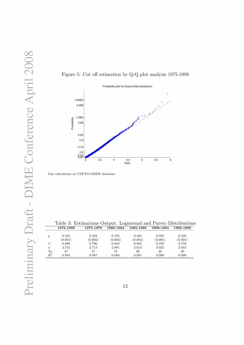
To select a suitable threshold or cutoff (X0)value separating the lognormalpart from the Pareto power law tail of the empirical patents distribution perinventor - i.e. normal to “superior” inventors -, we use visually oriented sta-tistical techniques such as the quantile-quantile plot. Since a log-transformedPareto random variable is exponentially distributed, we conduct experimen-tal analysis on the log-transformed data in order to obtain a fit closer to thestraight line (see figure 5 for our sample).

Once we have determined the cut-off point, we go further. First, applyingMLE methodology, we estimate parameters of lognormal observing and an-alyzing its dynamic (figure 2.2). Synthesizing the information coming fromlognormal distribution, we observe Gibrat index calculated as: β = 1/

(

σ√

2)

.The lower is β the more uneven is the whole distribution, since it representsa large variance of the sample. For what concerns power law distributionindicators, we run an OLS of the logarithm of the cumulative probability ona constant and the logarithm of patents per inventor, obtaining α = 2.752

10

Pre

lim

inar

y D

raft

- D

IME

Confe

rence

Apri

l 2008

Figure 3: Cumulative Probability Distribution - Patent per Inventor (Frac-tioned) 1975-1999

−3 −2 −1 0 1 2 3 4 5−14

−12

−10

−8

−6

−4

−2

0

Patent per Inventor (1975−1999)

Cum

ulat

ive

Pro

babi

lity

y vs. x linear

Our calculation on USPTO-NBER database

Figure 4: Upper tail - Patent per Inventor (Fractioned) 1975-1999

Pro

babi

lity

> p

atxi

nv

patxinv47.0205 300.084

.003922

.996078

Our calculation on USPTO-NBER database

11

Pre

lim

inar

y D

raft

- D

IME

Confe

rence

Apri

l 2008

Figure 5: Cut off estimation by Q-Q plot analysis 1975-1999

3 3.5 4 4.5 5 5.5 60.050.25

0.5

0.75

0.9

0.95

0.99

0.995

0.999

0.9995

Data

Pro

babi

lity

Probability plot for Exponential distribution

Our calculation on USPTO-NBER database

Table 3: Estimations Output: Lognormal and Pareto Distributions1975-1999 1975-1979 1980-1984 1985-1989 1990-1994 1995-1999

µ 0.323 0.494 0.476 0.465 0.505 0.529(0.001) (0.002) (0.002) (0.002) (0.001) (0.001)

β 0.689 0.796 0.804 0.805 0.783 0.776α 2.752 2.713 2.881 2.613 3.025 2.843X0 47 17 18 30 28 40R2 0.993 0.987 0.989 0.991 0.998 0.998

12

Pre

lim

inar

y D

raft

- D

IME

Confe

rence

Apri

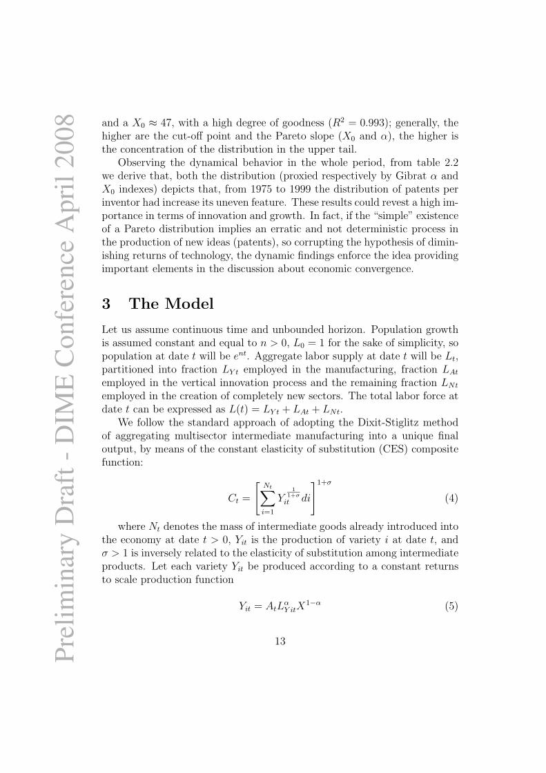
l 2008 and a X0 ≈ 47, with a high degree of goodness (R2 = 0.993); generally, the

higher are the cut-off point and the Pareto slope (X0 and α), the higher isthe concentration of the distribution in the upper tail.

Observing the dynamical behavior in the whole period, from table 2.2we derive that, both the distribution (proxied respectively by Gibrat α andX0 indexes) depicts that, from 1975 to 1999 the distribution of patents perinventor had increase its uneven feature. These results could revest a high im-portance in terms of innovation and growth. In fact, if the “simple” existenceof a Pareto distribution implies an erratic and not deterministic process inthe production of new ideas (patents), so corrupting the hypothesis of dimin-ishing returns of technology, the dynamic findings enforce the idea providingimportant elements in the discussion about economic convergence.

3 The Model

Let us assume continuous time and unbounded horizon. Population growthis assumed constant and equal to n > 0, L0 = 1 for the sake of simplicity, sopopulation at date t will be ent. Aggregate labor supply at date t will be Lt,partitioned into fraction LY t employed in the manufacturing, fraction LAt

employed in the vertical innovation process and the remaining fraction LNt

employed in the creation of completely new sectors. The total labor force atdate t can be expressed as L(t) = LY t + LAt + LNt.

We follow the standard approach of adopting the Dixit-Stiglitz methodof aggregating multisector intermediate manufacturing into a unique finaloutput, by means of the constant elasticity of substitution (CES) compositefunction:

Ct =

[

Nt∑

i=1

Y1

1+σ

it di

]1+σ

(4)

where Nt denotes the mass of intermediate goods already introduced intothe economy at date t > 0, Yit is the production of variety i at date t, andσ > 1 is inversely related to the elasticity of substitution among intermediateproducts. Let each variety Yit be produced according to a constant returnsto scale production function

Yit = AtLαY itX

1−α (5)

13

Pre

lim

inar

y D

raft

- D

IME

Confe

rence

Apri

l 2008 with X denoting the fixed factor (land) whose total supply is normalized

to 1, LY it is labor engaged in the production of the variety i at date t, andtotal factor productivity index At captures in a synthetic way the stock ofvertical innovations accumulated up to date t. Concentrating on symmetrywe assume LY it=LY t, Xi = X, and hence Yit = Yt, ∀i. Therefore we canwrite the aggregate final output as

Ct = Yt = AtLαY tX

1−αNσt = At (Lt − LNt − LAt)

α X1−αNσt (6)

To simplify matters, as in Howitt (2000), the mass of intermediate prod-ucts grows as a result of serendipitous imitation, not deliberate innovation.Each person has the same propensity to imitate β > 0, thus the aggregateflow of new products is

Nt = βLNt (7)

Since population grows at the constant rate n, also the number of productlines evolves at a relative pace of n.

Therefore, the per capita growth rate is equal to

gY t = gAt + σn − (1 − α) n = gAt + (σ + 1 − α) n (8)

New ideas are produced using as inputs labor and the stock of ideas –summarized by the per variety productivity level and the number of productlines – which are accumulated over time with the first being paid for and thesecond being common property.

In the existing literature the innovative activity benefits from the knowl-edge spillover so that each researcher gets immediately informed, withoutany effort (or “waste of time”), about the evolution of the general knowl-edge frontier. As remarked by Aghion and Howitt (1998) and Howitt (1999),and Segerstrom (2000) innovation in one productive line is better viewed asthe successful adoption of general knowledge advancement produced as a by-product of the whole economy’s innovative efforts. We adopt this view of theinnovative process, but we postulate that R&D units need to keep updatedabout the ongoing recent advances by spending a proportional labor cost.5

5See Cozzi and Spinesi (2004) about this point and the related references. In particular,we adopt the macroeconomic framework as in Cozzi and Spinesi (2004), and we providea microfoundation of their updating sunk cost that allows the empirical findings of ourcontribution to be explained.

14

Pre

lim

inar

y D

raft

- D

IME

Confe

rence

Apri

l 2008 Our model’s updating labor cost is proportional to gathered information,

but is inversely proportional to the economy-wide total factor productivitylevel. More specifically, at the date t > 0, the dynamic evolution of the stockof knowledge - i.e. the number of patents in this framework - for a researcherendowed with an exogenous ability θj and with a skill level hj follows the law

Ajt =At

LAt

= ϕ (At, Nt) Max

{

1 − fj (θj, hj)

At

At

LAt

(LAt − ε) , 0

}

(9)

where the flow of new patents for a generic researcher j - i.e. Ajt - can

be approximated by the per researcher flow of new ideas At

LAt. The term

ϕ (At, Nt) is any real and positive function that captures the productivity ofthe accumulated knowledge stock At over the mass of the existing productlines Nt at time t > 0 in the improvement of productivity, LAt is the fractionof total labor force Lt working in R&D. In equation (9) what allows us todiscriminate between the researchers’ productivity in introducing new ideasin the long term is the function fj (θj, hj). Indeed, at a given time t > 0,the individual productivity is assumed to be not much different betweenresearchers, so that the individual productivity can be approximated by theper researcher productivity. Over time, the flow of new ideas a researcherwill be able to introduce can follow a quite different dynamic between theresearchers, with a quite different long term behavior of a personal numberof new patents granted to each researcher, as the data show to be in practice.The function fj (θj, hj) represents the individual’s j updating flow cost, whichis tied to both her personal ability endowment θj and her skill ability hj.

To fix ideas,fj(θj ,hj)

Atis a positive flow labor unit cost of keeping oneself

updated about the latest innovations. In fact – in a discrete approximationinterpretation -

fj(θj ,hj)

At> 0 labor units have to be sunk in order to try to

adopt each general technological improvement to the product/industry line inwhich the researcher operates.6 Every time new technological improvementsoccur at the economy-wide level, Howitt’s (1999) and Segerstrom’s (2000)sectoral adoption problem becomes a new one, which means that a second

6As Garicano (2000, p. 878) maintains: “Workers can learn the solutions to the prob-lems they confront at a cost. I assume that the cost of learning an interval A of problemsis proportional to the size of this interval, µ(A) (its Lebesgue measure), and call the con-stantper period unit learning cost c. For example the cost of learning all problems in theinterval [0, Z] is cZ.”

15

Pre

lim

inar

y D

raft

- D

IME

Confe

rence

Apri

l 2008 vertical R&D labor sunk cost has to be incurred. The sequence of successive

sunk R&D labor costs per unit time is equal to the number of such sunk laborcosts times the number of general technological improvements being aimed atper unit time, i.e. At

LAt(LAt − ε). This becomes a quasi-fixed flow cost for each

researcher’s vertical R&D. Indeed, in order to introduce new patentable ideas,an individual should be updated of at least a fraction of other researchers’ flowof new ideas, which is captured by the term At

LAt(LAt − ε) in the equation (9).

The term At

LAtindicates the per researcher flow of new patents, and (LAt − ε)

indicates the number/mass of researchers but her own research effort time,which is assumed to be an infinitesimal amount ε of the whole research effort.It is important to remark that we are not even assuming that R&D workersneed to know all relevant innovations in their field in order to have a positiveprobability of innovating. The function fj (θj, hj) can capture any fractionof the flow of innovations that it is necessary to know. It may well be thatsuch a fraction is as small as one thousandth or less.

It is worthwhile noting that equation (9) captures the notion that thefaster the technological frontier expands, the more flow labor effort is neces-sary to assimilate it, but at the same time the higher the already acquiredgeneral knowledge the easier the acquisition of new information. In fact,given the already reached level of the transmission technology, monitoring adouble information flow imposes a higher monitoring time, but advances ininformation and communication technologies make it easier to transmit andto scan a larger mass of information per-unit time. Hence it seems quite nat-ural to assume that quasi-fixed R&D input requirements in the informationtransmission process decrease in the same proportion as do the manufactur-ing input requirements.

The function fj (·) is assumed to be bounded below for any researcher,with f

¯j (·) > 0 being the greatest lower bound of researcher’s j updating flow

cost. Morever, let us define the parameter c > 0 as the minimum greatestlower bound for all researchers, i.e. c = min

{

f¯j (·)

}

. The ability endowmentθj can be interpreted as the individual’s j talent in finding new ideas, and inupdating with the other researchers’ ideas. The skill ability hj can be inter-preted as the both the quantity and quality of human capital accumulatedthrough schooling by the researcher j and as on the job learning process,and it represents her personal skill ability when she undertake the researchactivity. The individual updating function is assumed to be a decreasingfunction in both ability endowment and skill, i.e.

∂fj(·)

∂θj≡ fjθj

(·) < 0 and

16

Pre

lim

inar

y D

raft

- D

IME

Confe

rence

Apri

l 2008 ∂fj(·)

∂hj≡ fjhj

(·) < 0.

The “purely innovative activity” in developing countries often – thoughnot always - consists in the learning and adaptation to local conditions oftechnologies invented elsewhere. In such a case it is very natural to assumethat the intertemporal learning spillover might be different from that of theleading-edge countries, because the researchers are doing qualitatively dif-ferent kinds of activities. Therefore we believe that a positive feature ofour formulation is the high degree of generality of function ϕ (At, Nt). Theinspiration that local researchers get from foreign knowledge stocks is po-tentially complicated and heterogeneous from culture to culture, whereasthe mechanical information transmission of new knowledge or new adoptionflows respond in the same way to general industrial productivity nearly ev-erywhere. Hence we believe that our formulation of R&D seems to fit also adevelopment context in a flexible enough way as to include several differentapplications.

By solving equation (9) for At

LAt, the following dynamic law is obtained:

At

LAt

=1

1ϕ(At,Nt)

+fj(θj ,hj)

At(LAt − ε)

(10)

The long term behavior of equation (10) can be quite different dependingon the behavior of the second term in the denominator of the right handside of the same equation (10). Indeed, the first term in the denominatortends to zero in the long run. Instead the second term can have a differentdynamic depending on the relative strength of its components. Both thestock of knowledge At and the population size tend to infinity in the longrun, as long as the growth rate of At is positive and population grows overtime. Therefore, in determining the long run behavior of equation (10), acrucial role is assumed by both the evolution and weight of the functionfj (θj, hj). As long as the updating function allowed the growth rate of the

numerator in the termfj(θj ,hj)

At(LAt − ε) to be low enough relatively to the

stock of knowledge growth rate, the flow of new patents would be higher andhigher over time, i.e. At

LAt→ ∞ as t → ∞. On the contrary, as long as

the updating function did not allow the growth rate of the numerator in theterm

fj(θj ,hj)

At(LAt − ε) to be low enough relatively to the stock of knowledge

growth rate, the flow of new patents would tend to zero, and therefore aresearcher would be able to introduce a constant number of patents overtime, i.e. At

LAt→ 0 as t → ∞. This last result is more plausible whenever a

17

Pre

lim

inar

y D

raft

- D

IME

Confe

rence

Apri

l 2008 researcher is endowed with a low talent θj, and whenever she has accumulated

a lower quantity and quality of skills in schooling, i.e. for a low hj. Moreover,whenever hj represents also some learning process - such as on the job training- the evolution of such skill ability allows the updating flow cost to be reducedover time, so that an individual productivity in introducing new valuableideas becomes higher and higher over time.

By aggregating equation (9) over the number/mass of researchers at timet, the following is obtained

At = ϕ (At, Nt) max

{

LAt −At

LAt

(LAt − ε)F (·) LAt

At

, 0

}

(11)

where F (·)LAt

At=

∫

LAt

fj(θj ,hj)

Atdj, with F (·) being the per researcher cumu-

lative updating function, which can be written as proportional to the researchlabor size LAt at time t. Because the weight of a researcher over the num-ber/mass of researchers is assumed to be infinitesimal - being LAt the worldresearch labor size - the other researcher’s size (LAt − ε) at time t is wellapproximated by LAt, i.e. (LAt − ε) ≃ LAt. Therefore, equation (11) reducesto

At = ϕ (At, Nt) LAt max

{

1 − F (·)At

At, 0

}

(12)

where, because c = min{

f¯j (·)

}

, we have that[

1 − F (·)At

At

]

<[

1 − cAt

At

]

.

Therefore, by soling equation (12) for the growth rate of the stock of knowl-edge, the following inequalities are obtained

At

At

≡ gAt =1

At

ϕ(At,Nt)LAt+ F (·)

<1

F (·)<

1

c(13)

This holds regardless of the degrees of intertemporal spillover and re-gardless of the economy’s being at a steady state or out of it. Moreover,since the economy’s growth rate is always lower than 1

F (·)in principle our

result allows both for endogenous and for exogenous growth depending onthe microeconomic foundations adopted in a more complete model.

So far we have assumed that researchers’ updating flow cost benefits ofspillovers from all the world-wide stock of knowledge At, or however from thestock of knowledge for which this economy is specified for.

18

Pre

lim

inar

y D

raft

- D

IME

Confe

rence

Apri

l 2008 However, some empirical evidence shows the existence of localized knowl-

edge spillovers. Studies from Jaffe (1993), Coe and Helpman (1995, 1997),Keller (2002) show the importance of the spatial proximity for knowledgediffusion and utilization. As Baldwin and Martin (2004) maintain: “Thediffusion of knowledge across regions and countries does exist but diminishesstrongly with physical distance which confirms the role that social inter-actions between individuals, dependent on spatial proximity, have in suchdiffusion.” A similar argument, and some empirical evidence, can be foundin cities. For example Black and Henderson (1999) maintain: “An urban-ized economy has different type of cities specialized in different traded goods,with city size and educational attainments varying by city type.” Moreover,specialization in some product lines can be due to the exogenous first naturalcharacteristics of each country.

Once these empirical facts are inserted in the above modeling specifica-tion, a different result about the growth performance of the economy arises.Indeed, let us suppose that in equation (9) a researcher updating cost benefitof only very limited knowledge spillovers:

Ajt =At

LAt

= ϕ (αAt, Nt) Max

{

1 − fj (θj, hj)

Ajt

At

LAt

(LAt − ε) , 0

}

(14)

where the differences with equation (9) concerns the spillovers term. Infunction ϕ (αAt, Nt), a researcher benefits of only a fraction α ∈ (0, 1) ofthe stock of the existing knowledge spillovers, and the updating flow costis reduced according to her own knowledge accumulated over time7. Byfollowing the same steps as before, the following dynamic law for an averageresearcher flow of new ideas is obtained

Ajt =At

LAt

=1

1ϕ(αAt,Nt)

+fj(θj ,hj)

Ajt(LAt − ε)

(15)

In such a case the dynamic evolution of a researcher’s flow of new ideasstrongly depends on her personal ability and productivity. Indeed, as abovethe first term in the denominator tends to zero in the long run. Instead, the

7This is a drastic specification for the flow updating cost adopted to render the newresult more evident. Yet, also assuming that the updating cost benefits of a limitedknowledge spillovers does not alter the qualitative results

19

Pre

lim

inar

y D

raft

- D

IME

Confe

rence

Apri

l 2008 second term can have a different dynamic depending on the relative strength

of its components. Both the stock of knowledge Ajt and the populationsize tend to infinity in the long run, as long as the growth rate of Ajt ispositive. Therefore, in determining the long run behavior of equation (15)a crucial role is assumed by both the evolution and weight of the functionfj (θj, hj). As long as the updating function allowed the growth rate of the

numerator in the termfj(θj ,hj)

Ajt(LAt − ε) to be low enough relatively to her

own stock of knowledge growth rate, the flow of new patents would be higherand higher over time, i.e. At

LAt→ ∞ as t → ∞. This is the case whenever

her own stock of knowledge is higher over time. On the contrary, as long asthe updating function did not allow the growth rate of the numerator in theterm

fj(θj ,hj)

Ajt(LAt − ε) to be low enough relatively to own stock of knowledge

growth rate, the flow of new patents would tend to zero, and therefore aresearcher would be able to introduce a constant number of patents overtime, i.e. At

LAt→ 0 as t → ∞.

However, the growth performance of an economy with localized spilloverscan be quite different in the very long run than an economy with economy-wide knowledge spillovers. Indeed, by aggregating equation (14) over thenumber/mass of researchers at time t, the following is obtained

At = ϕ (αAt, Nt) max

{

LAt −At

LAt

(LAt − ε)cLAt

Ajt

, 0

}

(16)

where we assume that fj (θj, hj) = c ∀j, and Ajt = max {Ajt}LAt

j=0, so thatwe pose the economy in the condition to have the highest growth perfor-mance, because the updating cost has a value as low as possible. In such acase

∫

LA

fj(θj ,hj)

Ajtdj reduces to cLAt

Ajt. Because the weight of a researcher over

the number/mass of researchers is assumed to be infinitesimal - being LAt

the world research labor size - the other researcher’s size (LAt − ε) at time tis well approximated by LAt, i.e. (LAt − ε) ≃ LAt. Therefore, equation (16)reduces to

At = ϕ (αAt, Nt) LAt max

{

1 − c

Ajt

At, 0

}

(17)

The stock of knowledge growth rate can be written as

20

Pre

lim

inar

y D

raft

- D

IME

Confe

rence

Apri

l 2008

At

At

≡ gAt =1

At

ϕ(αAt,Nt)LAt+ cAt

Ajt

(18)

in this case the first term in the denominator tends to zero or infinityfor any positive function ϕ (αAt, Nt) depending on the relative strength ofits terms. The second term tends to infinity because the term Ajt is alsoincluded in the term At, so that At grows at a pace not lower than Ajt.Therefore, in the case of localized spillovers the knowledge growth rate willtend to zero in the very long run.

Concluding Remarks

This paper inquire on the inventive productivity distributions of inventorsemployed in firms or institutions resident in OECDs countries, excludingthose from US using NBER patent citations database (1975-1999). Consid-ering the number of patents granted to individual inventor on the USPTO,the researchers’ population is divided into two well defined groups. The firstone involves inventors with very low productivity, at least constant; whilethe second one includes researchers with increasing productivity over time.More formal we have found that the inventive productivity is distributed inthe population as a log normal probability function with highly skewed tail.The last is governed by a power law or Pareto law. The skewed tail of distri-bution indicates that a sample of inventors in the population accounts for avery large amount of patents. In this way knowledge is concentrated in fewresearcher, while the largest group of inventors grants a constant number ofpatents over time. These results is verified at a country level over 1975-1999.

The theoretical model describes the flow of new ideas (patents) an indi-vidual is able to introduce as depending on labor effort and on spillovers onegains from the existing stock of knowledge. In articular, the labor effort canbe spent both in updating with other researchers’ new ideas and in creatinga own new idea.

It is shown that, as long as the overall stock of patents grows at a pos-itive rate, the individual patenting productivity can either grow or remainconstant over time. The different dynamics in individual’s productivity de-pends on the updating flow cost and on the degree of knowledge spillovers.In particular, by deflating the updating flow cost for each inventors’ patentstock, the updating function tend to zero at a slower pace than when it is

21

Pre

lim

inar

y D

raft

- D

IME

Confe

rence

Apri

l 2008 deflated for the overall stock of knowledge. In either formulation we find

the existence of top researchers whose productivity is higher and higher overtime, and a larger mass of researchers whose number of new ideas per unitof time remains constant.

These results determine quite different results once aggregate productiv-ity is analyzed. Indeed, by aggregating the flow of new patents for the mass ofinventors provide us with different growth perspectives for an economy. Onceknowledge spillovers are large and diffuse in the economy, even if they arecostly, the economy can grow at a higher pace in respect of localized knowl-edge spillovers. These results could be a further candidate to explain boththe per capita output growth rate and income differences between countries.In particular, a central question looked to be that several nations were notable to “rapidly assimilate industrial technology” (DeLong 1988, p. 1148).Furthermore, the seminal papers by Lucas (1988) and Romer (1986, 1990)concern a widening in the relative income distances between rich and poordue to the nontrivial questions that technology is the key element for growthand its transfer is not inevitable and not costless as well. Moreover, Easterlyand Levine (2001) have shown that technology and its spillovers matter forconvergence of real per capita incomes. If spillovers are local, diffusion oftechnology is limited in the neighbors of innovator firm/country and its ef-fects do not expand over the world economy. That leads to economic clusterswith persistent income differences. If spillovers are large and diffuse, tech-nology is better disposable for a larger number of agents and differences tendto diminish over time. Keller (2002) has recently estimated that technologyspillovers from the most innovative countries are local, but the localizationdegree has fallen on 1982-1998, when within industries spillovers are con-sidered. The theoretical results of this paper about individual productivityin creating new ideas tied to technology spillovers could be a further can-didate to explain these empirical findings about divergences in growth rateand income level between countries.

22

Pre

lim

inar

y D

raft

- D

IME

Confe

rence

Apri

l 2008 References

[1] Aghion, P., and Howitt, P. (1992) “A Model of Growth ThroughCreative Destruction.” Econometrica 60, 323-351.

[2] Baldwin R., Forslid R., Martin P., Ottaviano G., and Robert-Nicoud (2003) Economic Geography and Public Policy, Prince-ton University Press.

[3] Baldwin R. E. and Martin P. (2004), Agglomeration and re-gional growth, Handbook of Regional and Urban Economics, inHenderson J. V. and Thisse J. F. (eds.), Handbook of Regional

and Urban Economics, edition 1, volume 4, chapter 60, pages2671-2711.

[4] Black D. and Henderson J.V. (1997), Urban Growth, NBER

Working Papers 6008, National Bureau of Economic Research.

[5] Castaldi C, Los B (2007), International Technological Special-ization in Important Innovations: Some Industry-Level Explo-rations, Working Paper University of Groningen.

[6] Castaldi C, Los B (2007), The Identification of Important Inno-vations Using tail Estimators, Working Paper Innovation Stud-ies Utrecht (ISU).

[7] Clementi F, Gallegati M (2005), Power Law Tails in the ItalianPersonal Income Distribution. Physica A 350:427–438

[8] Clementi F, Gallegati M (2007), Pareto’s Law of Income Dis-tribution: Evidence for Germany, the United Kingdom, andthe United States, in Econophysics of Wealth Distributions

A.Chatterjee, S.Yarlagadda and B.K. Chakrabarti eds.; ed.Springer

23

Pre

lim

inar

y D

raft

- D

IME

Confe

rence

Apri

l 2008 [9] Coe D., and Helpman E. (1995) “International R&D Spillovers”

European Economic Review 39, 859-887.

[10] Coe D. T, Helpman E. and Hoffmaister A. W., (1997). North-South R&D Spillovers, Economic Journal, 107 (440), pp. 134-49.

[11] Cohen W. M. and Levinthal D. A. (1989), The Two Faces ofR&D, The Economic Journal, 99 (397), pp 569-596

[12] Cozzi G and Spinesi L, (2004), Information Transmission andthe Bounds to Growth, Topics in Economic Analysis & Policy,Berkeley Electronic Press, 4 (1), pp.1168-1168.

[13] David T. C. and Helpman E. (1995), International R&DSpillovers, European Economic Review, Elsevier 39 (5), pp. 859-887.

[14] De Long J. B. (1988) Productivity Growth, Convergence, andWelfare: Comment, American Economic Review 78 (5), pp.1138-1154.

[15] Duranton G., and Puga D. (2001) “Nursery Cities: Urban Diver-sity, Process Innovation and the Life Cycle of Products” Amer-

ican Economic Review 5, 1454-1477.

[16] Easterly W. and R. Levine (2001), It’s Not Factor Accumu-lation: Stylized Facts and Growth Model,World Banking Eco-

nomic Review, 15, pp 177-229.

[17] Garicano L. (2000), Hierarchies and the Organization of Knowl-edge in Production, Journal of Political Economy, 108 (5), pp.874-904.

[18] Grossman, G.M., and Helpman, E. (1991) Innovation andGrowth in the Global Economy. Cambridge, MA: MIT Press.

24

Pre

lim

inar

y D

raft

- D

IME

Confe

rence

Apri

l 2008 [19] Hall, B. H., A. B. Jaffe, and M. Tratjenberg (2001). The NBER

Patent Citation Data File: Lessons, Insights and MethodologicalTools. NBER Working Paper 8498.

[20] Heston A, Summers R. and Aten B., Penn World Table Version6.2, Center for International Comparisons of Production, Incomeand Prices at the University of Pennsylvania, September 2000.

[21] Howitt P. (1999) Steady Endogenous Growth with Populationand R&D Inputs Growing, Journal of Political Economy 107 pp.715-30.

[22] Howitt, P. (2000) “Endogenous growth and Cross Country In-come Differences.” American Economic Review, 90: 829-846.

[23] Jaffe and Trajtenberg (2002), Patents, Citations & Innovations:

A Window on the Knowledge Economy (Cambridge MA: MITpress)

[24] Jones, C. (1995) “R&D-Based Models of Economic Growth.”Journal of Political Economy, 103: 759-784.

[25] Jones C. (2005) Growth and Ideas, in Aghion P. and Durlauf S.N. eds. Handbook of Economic Growth, North-Holland.

[26] Keller W. (2002) Geographic Localization of International Tech-nology Diffusion, American Economic Review 92 (1), pp. 120-142.

[27] Lucas J. R. (1988) On the Mechanism of Economic Develop-ment, Journal of Monetary Economics, 22, pp. 3-42.

[28] Narin, F., Breitzman, A. (1995), Inventive Productivity, Re-

search Policy , 24 (1995) 507-519

25

Pre

lim

inar

y D

raft

- D

IME

Confe

rence

Apri

l 2008 [29] Romer P. (1986) Increasing Returns and Long-Run Growth,

Journal of Political Economy, 94 (5), pp. 1002-1037

[30] Romer P. (1990) Endogenous Technological Change, Journal of

Political Economy, 98 (5), Part 2: The Problem of Development:A Conference on the Institute for the Study of Free EnterpriseSystems, pp. S71-102

[31] Schumpeter, J. A. (1934) The Theory of Economic Develop-ment. Cambridge, MA: Harvard University Press.

[32] Schumpeter, J. A. (1939) Business Cycles. A Theoretical, His-torical and Statistical Analysis of the Capitalist Process. NewYork: Mc Graw Hill.

[33] Segerstrom, P. (1998). “Endogenous Growth Without Scale Ef-fects.” American Economic Review 88, 1290-1310.

[34] Segerstrom, P. S (2000) The Long-Run Growth Effects of R&DSubsidies, Journal of Economic Growth, 5 (3), pages 277-305.

[35] Silveberg G. and Verspagen B. (2007), The Size of Distribu-tion of Innovations Revisited: An Application of Extreme ValueStatistics to Citation and Value Measures of Patent Signifi-cance”, Journal of Econometrics, 139, pp. 318-339

26