arX

iv:h

ep-p

h/98

1023

5v2

14

Apr

199

9

hep-ph/9810235NT@UW-98-22

1st October 1998Revised 14th April 1999

Power Counting and β Function in NRQCD

Harald W. Grießhammer1

Nuclear Theory Group, Department of Physics, University of Washington,

Box 351 560, Seattle, WA 98195-1560, USA

Abstract

A computation of the NRQCD β function both in the Lorentz gauge family andin the Coulomb gauge to one loop order endorses a velocity power counting schemefor dimensionally regularised NRQCD. In addition to the ultrasoft scale representedby bremsstrahlung gluons and the potential scale with Coulomb gluons and on-shellquarks, a soft regime is identified in which energies and momenta are of order Mv,gluons are on shell and the quark propagator becomes static. The instantaneousgluon propagator has a non-zero vacuum polarisation only because of contributionsfrom this regime, irrespective of the gauge chosen. Rules are derived which allowone to read up from a given graph whether it is zero because of the homogeneıtyof dimensional regularisation. They also apply to threshold expansion and are usedto prove that ultrasoft quarks with energy and momentum of order Mv2 decouplefrom the theory.

Suggested PACS numbers: 12.38.Bx, 12.39.Hg, 12.39.Jh, 11.10.Gh.

Suggested Keywords: Non-Relativistic QCD, Heavy Quark Effective Theory,effective field theory, threshold expansion, renormalisa-tion, β function, dimensional regularisation.

1Email: hgrie@phys.washington.edu

1 Introduction

Non-Relativistic QCD [1, 2] takes advantage of the fact that when a heavy quark is nearlyon shell and its energy is dominated by its mass M , the resulting non-relativistic systemexhibits two small expansion parameters: the coupling constant g and the particle velocityv. The Coulomb interaction rules the level spacing in Charmonium and Bottomiumbecause αs is small enough for perturbative calculations and the relative velocity of thequarks is v ∼ αs(Mv) by virtue of the virial theorem, where the scale of g is set by theinverse Bohr radius Mv of the system. Albeit αs increases with decreasing Q2 ∼ (Mv)2,a window between the relativistic perturbative and the confinement regime remains inwhich both αs and v is small (e.g. for Bottomium, αs(Mbv) ≈ 0.35). Therefore, wavefunctions and potentials obtained by re-summation of ladder diagrams involving relevantcouplings as v → 0 may be used to account for bound state physics, and calculationsof production cross sections, hyperfine splittings, lifetimes, threshold properties etc. aremuch facilitated. The Abelian analogue, NRQED, to which all considerations in thisarticle apply equally well, has also simplified precision calculations in Positronium. Anincomplete list of recent references may include [3]-[12].

The NRQCD Lagrangean in terms of the heavy quark (anti-quark) bi-spinors Q (Q)and gluons (Dµ = ∂µ + igAµ) reads

LNRQCD = Q†(

i∂0 − gA0

)

Q +c1

2MQ† ~D2Q +

c28M3

Q† ~D4Q + . . .

+gc32M

Q†~σ · ~BQ + . . . − g2d1

4M2

(

CQ†~σQ)

·(

Q†~σCQ)

+ . . . (1.1)

− e14F a

µνFµν, a +

g3e2480π2M2

F aµνD

2F µν, a + . . .+ LGFix ,

where the coefficients ci, di, ei, . . . encode the ultraviolet physics: All excitations withfour-momenta of the order of M and higher are integrated out and give rise e.g. to four-point interactions between quarks (d1 6= 0). The perturbative part of the coefficientscan be determined by matching NRQCD matrix elements to their QCD counterpartsin the regime where both theories are perturbative in the coupling constant. This hasbeen performed to O(M−3) [13]. At tree level, a Foldy-Wouthuysen transformation givesci = 1, e1 = 1, and loop corrections are down by powers of g, the most famous examplebeing the coefficient for the Fermi term related to the anomalous magnetic moment of theelectron, c3 = 1 + αs

2π+ . . .. Further coefficients to enter at one loop level are d1 = e2 = 1.

Lorentz invariance demands c1 = c2 = 1 to all orders.The Lagrangean (1.1) consists of infinitely many terms constrained only by the symme-

tries of the theory and is non-renormalisable. Predictive power is nonetheless establishedwhen only a finite number of terms contribute to a given order in the two expansionparameters1, g and v. Besides the heavy quark mass M , the typical binding energy andmomentum scales in NRQCD are the non-relativistic kinetic energy Mv2 and the mo-mentum Mv of the quark, which in Quarkonia appear as the energy and inverse size of

1For clarity, the two will be distinguished in the following, although v ∼ αs, as noted above.

2

the bound state [1, 2]. Since for the smallest of the three scales αs(Mv2) 6< 1 in Bot-tomium and Charmonium, an expansion in g is justified only for the interactions takingplace on scales Mv and higher in the real world, but one can imagine a world in whichMv2 ≫ ΛQCD. Toponium fulfils this requirement but decays mainly weakly and very fastso that QCD effects do not dominate.

Because the effective Lagrangean does not exhibit the non-relativistic expansion pa-rameter v explicitly, a power counting scheme has to be established which determinesuniquely which terms in the Lagrangean must be taken into account to render consistentcalculations and predictive power to a given accuracy in v. It is at this point that NRQCDcan serve as a “toy model” for nuclear physics [14] (although this grossly understates itsvalue2): It will establish what the relevant kinematic regimes and infrared variables arein a theory with three (or more) separate scales, and it will demonstrate how to countpowers of the non-relativistic expansion parameter, v. Recently, velocity power count-ing rules were established for a toy model [15] following Beneke and Smirnov’s thresholdexpansion [16], which has become very useful for understanding non-relativistic effectivetheories. The relevant energy and momentum regimes and low energy degrees of freedomwere found for dimensionally regularised non-relativistic theories. This article presentsthe extension to NRQCD and as an application the calculation of the NRQCD β function.It will also be argued that the diagrammatic approach advocated here sheds a new lighton threshold expansion [16] and helps simplify calculations.

Both from a conceptual and a technical point of view the calculation of the NRQCDβ function proves interesting. NRQCD is a well-defined field theory of quarks and gluons.One can therefore investigate its renormalisation group equations under the assumptionthat perturbation theory is applicable at all scales. For example, the running and mixingof the dimension six operators has been investigated to one loop order by Bauer andManohar [17]. On the other hand, as NRQCD is the low energy limit of QCD, it mustreproduce the QCD β function with NF light quarks below the scale M , but this has notbeen demonstrated so far. The problem with the power counting developed until now [14,18, 19] was that gluons mediating the Coulomb interaction (“potential gluons”) seemedto have a vanishing vacuum polarisation and hence a β function which was neither gaugeinvariant nor agreed with the QCD result, while the coupling of gluons on a much lowerscale which mediate bremsstrahlung processes ran as expected. The apparent impassewhich results is resolved in this article.

Straightforward as the computation may thus seem with its outcome already antic-ipated, the prime goal of this article is not the result for the NRQCD β function; theobjective is rather to shed more light on power counting in NRQCD and to provide acomparison between calculations in the effective and the full theory. It will show thatthe Lorentz gauge family (and indeed any standard gauge) is a legitimate gauge choicein NRQCD, not only the Coulomb gauge. It will prove that the recently discussed softregime [15, 16, 20] with quarks and gluons of four-momenta of order Mv is indispensablefor NRQCD to describe the correct infrared limit of QCD. It will also test the validity

2The most striking difference to nuclear physics is that NRQCD has no exceptionally large scatteringlength to accommodate.

3

of the power counting proposed. In the Coulomb gauge, it will demonstrate that therenormalisation of the quark propagator and of the leading order quark gluon vertex aretrivial, so that for the β function in this gauge, only a computation of the gluon vacuumpolarisation is necessary. From a technical point of view, dimensional regularisation fornon-covariant loop integrals proves to be a simple regulator choice. It allows to develop aset of simple diagrammatic rules to determine which graphs yield non-zero contributionsin perturbation theory. This reduces the computational effort considerably as comparedto other regularisation schemes in which power divergences are present like e.g. when us-ing a lattice cut-off. Because of the association of threshold expansion and NRQCD, suchrules can be applied to the former, too. Finally, the calculation of the NRQCD β functionpresented here is – especially in the Feynman gauge – simpler than its QCD counterpartand shows some pedagogically intriguing aspects.

The article is organised as follows: In Sect. 2, the velocity power counting of NRQCDis presented. The relevant regimes of NRQCD are identified (Sect. 2.1), extending theformalism of Luke and Savage [18] by the soft regime of Beneke and Smirnov [16]. Thesection then proposes the rescaling rules necessary for a Lagrangean with manifest veloc-ity power counting (Sect. 2.2) and gives the vertex (Sect. 2.3) and loop velocity powercounting rules (Sect. 2.4). Gauge invariance of the power counting is addressed in Sect.2.5. The calculation of the NRQCD β function in the Lorentz gauges in Sect. 3 starts byhighlighting the intimate relation between threshold expansion and the proposed NRQCDpower counting, which will additionally be summarised in the Conclusions. Diagrammaticrules developed in Sect. 3.2 help to facilitate the calculation considerably and are usedin Sect. 3.3 to prove the absence of ultrasoft heavy quarks. As a tilly, the β functionis computed in the Coulomb gauge in Sect. 3.7. Summary and outlook conclude thearticle, together with an appendix containing exemplary calculations in non-covariantdimensional regularisation.

2 Velocity Power Counting

2.1 Regimes of NRQCD

The first power counting rules for NRQCD were derived by Lepage et al. [21] in theCoulomb gauge using the consistency of the equations of motion and a momentum cut-off. Only Coulomb gluons with typical momenta of order Mv were considered, takinginto account retardation, but neglecting bremsstrahlung effects. The power counting alsoheld to all orders only after all power divergences were subtracted.

Simpler counting rules were proposed by Luke and Manohar for Coulomb interac-tions [14], and by Grinstein and Rothstein for bremsstrahlung processes [19]. Luke andSavage [18] united these schemes using dimensional regularisation, so that the tree levelpower counting is automatically preserved to all orders in perturbation theory up to log-arithmic corrections. They also extended the formalism to include the Lorentz gauges.Labelle [22] proposed a similar scheme in time ordered perturbation theory. Beneke and

4

Smirnov [16] observed that the collinear divergence of the two gluon exchange contributionto Coulomb scattering between non-relativistic particles near threshold is not reproducedin this version of NRQCD because the soft low energy regime is not taken into account.A recent article [15] has shown that an extension of the work in [14, 18, 19] using dimen-sional regularisation, as motivated from threshold expansion [16], resolves this conflict ina toy model. The complete power counting scheme of NRQCD is presented briefly in thefollowing (see also [20]). In Sect. 3.1, the intimate relation between NRQCD as developedin recent years [14, 15, 18, 19] and threshold expansion is addressed in more detail.

The NRQCD propagators are read up from the Lagrangean (1.1) as

Q :i Num

T − ~p2

2M+ iǫ

, Aµ :i Num

k2 + iǫ, (2.1)

where T = p0 −M = ~p2

2M+ . . . is the kinetic energy of the quark. “Num” are numerators

containing the appropriate colour, Dirac and flavour indices, all of which are unimportantfor the considerations in this section and will be suppressed throughout this article. Gaugedependence of the gluon propagator for the power counting is addressed in Sect. 2.5.

Cuts and poles in scattering amplitudes close to threshold stem from saddle points ofthe loop integrand, corresponding to bound states and on-shell propagation of particlesin intermediate states. They give rise to infrared divergences and in general dominatecontributions to scattering amplitudes. With the two low energy scales at hand, andenergies and momenta being of either scale, three regimes are identified in which eitherthe quark or the gluon in (2.1) is on shell, as noted by Beneke and Smirnov [16]:

soft regime: Aµs : k0 ∼ |~k| ∼Mv ,

potential regime: Qp : T ∼Mv2 , |~p| ∼Mv , (2.2)

ultrasoft regime: Aµu : k0 ∼ |~k| ∼Mv2

Note that the scale M has been integrated out when deriving the non-relativistic La-grangean (1.1), so that a “hard” regime with on shell gluons and quarks of four-momentumof order M cannot be considered.

What is the particle content of each of the three regimes? Ultrasoft gluons Aµu are

emitted as bremsstrahlung or from excited states in the bound system, and hence arephysical. Soft gluons Aµ

s do not describe bremsstrahlung: Because in- and outgoingquarks Qp are close to their mass shell, they have an energy of order Mv2. Therefore,overall energy conservation forbids all processes with outgoing soft gluons but withoutingoing ones, and vice versa, as their energy is of order Mv. Finally, gluons which changethe quark momenta but keep them close to their mass shell relate the (instantaneous)Coulomb interaction:

Aµp : k0 ∼Mv2 , |~k| ∼ Mv (2.3)

When a soft gluon Aµs couples to a potential quark Qp, the outgoing quark is far off

its mass shell and carries energy and momentum of order Mv. Therefore, consistencyrequires the existence of quarks in the soft regime as well,

Qs : T ∼ |~p| ∼ Mv . (2.4)

5

With these five fields Qs, Qp, Aµs , A

µp, A

µu representing quarks and gluons in the three differ-

ent non-relativistic regimes, soft, potential and ultrasoft, NRQCD becomes self-consistent.These fields are the infrared-relevant degrees of freedom representing one and the samenon-relativistic particle in the respective kinematic regimes and came naturally by identi-fying all possible particle poles in the non-relativistic propagators. Their interactions arefixed by the non-relativistic Lagrangean (1.1). Section 3.3 will prove that a hypotheticalultrasoft quark, created e.g. by the radiation of a potential gluon off a potential quark,decouples completely from the theory. On the other hand, Sect. 3 will demonstrate thatin order to obtain the correct result for the NRQCD β function, all fields listed abovein the three regimes have to be accounted for. Therefore, the particle content presentedabove is not only consistent but both minimal and complete.

In order to guarantee that there is no overlap between interactions and particles indifferent regimes, the regularisation scheme must finally be chosen such that the expan-sion around one saddle point in the loop integral as performed above does not obtainany contribution from other regimes, represented by other saddle points in the loop in-tegrals. One might use an energy and momentum cut-off separating the soft from thepotential, and the potential from the ultrasoft regime, but the integrals encountered canin general not be performed analytically and in closed form. Furthermore, by introducinganother, artificial scale, cut-off regularisation jeopardises power counting and symmetries(gauge, chiral, . . . ). Power divergences occur when the (un-physical) cut-off is removedin intermediate steps but not in the final, physical result, complicating the computation.In contradistinction, using dimensional regularisation after the saddle point expansionpreserves power counting because its homogeneity guarantees that contributions from dif-ferent saddle points and regimes do not overlap. (A simple example is given in Ref. [15].)Homogeneıty will also be essential when developing diagrammatic rules to classify graphsas zero in Sect. 3.2 and when showing the decoupling of the ultrasoft quark in Sect. 3.3.

2.2 Rescaling Rules and Propagators

In order to establish explicit velocity power counting in the NRQCD Lagrangean, onerescales the space-time coordinates such that typical momenta in either regime are di-mensionless, as proposed by Luke and Manohar [14] for the potential regime and byGrinstein and Rothstein [19] for the ultrasoft one:

soft: t = (Mv)−1 Ts , ~x = (Mv)−1 ~Xs ,

potential: t = (Mv2)−1 Tu , ~x = (Mv)−1 ~Xs ,

ultrasoft: t = (Mv2)−1 Tu , ~x = (Mv2)−1 ~Xu .

(2.5)

For the propagator terms in the NRQCD Lagrangean to be normalised as order v0, onesets for the representatives of the gluons in the three regimes [15, 20]

soft: Aµs (~x, t) = (Mv) Aµ

s (~Xs, Ts) ,

potential: Aµp(~x, t) = (Mv

32 ) Aµ

p( ~Xs, Tu) , (2.6)

ultrasoft: Aµu(~x, t) = (Mv2) Aµ

u( ~Xu, Tu) ,

6

and for the quark representatives

soft: Qs(~x, t) = (Mv)32 Qs( ~Xs, Ts) , (2.7)

potential: Qp(~x, t) = (Mv)32 Qp( ~Xs, Tu) .

The rescaled free quark Lagrangean reads then

soft: d3Xs dTs Qs†(

i∂0 +v

2~∂2)

Qs , (2.8)

potential: d3Xs dTu Qp†(

i∂0 +1

2~∂2)

Qp . (2.9)

Here, as in the following, the positions of the fields have been left out whenever theycoincide with the rescaled variables of the volume element. Derivatives are to be takenwith respect to the rescaled variables of the volume element unless otherwise stated. Inorder to maintain velocity power counting, corrections of order v or higher must be treatedas insertions, so that one reads up the (un-rescaled) quark propagators and insertion as

soft: Qs :(T,~p)

:i

T + iǫ,

(T,~p)

: −i~p2

2M= P.C.(v1) ,(2.10)

potential: Qp :(T,~p)

:i

T − ~p2

2M+ iǫ

. (2.11)

The soft quark becomes static because T ∼ Mv ≫ ~p2

2M∼ Mv2 allows one to expand the

non-relativistic propagator (2.1) and to treat the momentum term as an insertion.Throughout this article, the symbol P.C.(vn) denotes at which order in the velocity

power counting a certain term or diagram contributes. In the approach presented, eachline in a loop diagram counts as P.C.(v0) because the strength of the propagator has beenset to unity in the rescaled Lagrangean (2.8/2.9). The rescaled Lagrangean measures thestrength of the insertion relative to the propagator. Therefore, the soft quark insertion(2.10) does not count as ~p2

2Mwhich scales like v2, but as ~p2

2M/T = P.C.(v). In contradis-

tinction to the approach in [16], one will therefore not obtain the absolute order in v atwhich a given graph contributes, but the relative order in v between graphs or vertices isread off more easily and asserted correctly.

The gauge fixing term was included in the NRQCD Lagrangean (1.1) since the decompo-sition of the Lagrangean into a free and an interacting part is gauge dependent. Becauseof the difference between canonical and physical momentum, it is important to specifythe gauge before identifying to which order in v a certain regime in the Lagrangean con-tributes, as will be seen shortly. In the following, the Feynman rules for the Lorentzgauges and for the Coulomb gauge are derived explicitly. Sect. 2.5 will comment on thegauge invariance of the procedure.

The rescaled free gluon Lagrangean in the Lorentz gauges reads

soft: d3Xs dTs1

2Aµ

s

[

∂2gµν − (1 − 1

α)∂µ∂ν

]

Aνs , (2.12)

7

potential: d3Xs dTu1

2Aµ

p

[

gµν(v2∂2

0 − ~∂2) − (2.13)

− (1 − 1

α)(vδµ0∂0 + δµi∂i)(vδν0∂0 + δνi∂i)

]

Aνu ,

ultrasoft: d3Xu dTu1

2Aµ

u

[

∂2gµν − (1 − 1

α)∂µ∂ν

]

Aνu , (2.14)

while in the Coulomb gauge

soft: d3Xs dTs1

2Ai,s

[

(~∂2 − ∂20)δij − ∂i∂j

]

Aj,s , (2.15)

potential: d3Xs dTu1

2

[

A0,p~∂2A0,p + Ai,p(~∂

2δij − ∂i∂j − v2∂20δij)Aj,p

]

, (2.16)

ultrasoft: d3Xs dTs1

2Ai,u

[

(~∂2 − ∂20)δij − ∂i∂j

]

Aj,u . (2.17)

The (un-rescaled) Coulomb and Lorentz gauge propagators are therefore given as (δijtr(~k) =

δij − kikj

~k2, Gµν(k) = −(gµν − (1 − α) kµkν

k2+iǫ))

Coulomb gauge Lorentz gauges

soft: Aµs :

kµ ν:

i δijtr(~k)

k2 + iǫ

i Gµν(k)

k2 + iǫ,

potential: Ap,0 :k,A00 0

:−i

−~k2 + iǫ

−i

−~k2 + iǫ,

~Ap :k, ~Ai j

:i δij

tr(~k)

−~k2 + iǫ

i [δij + (1 − α)kikj

−~k2+iǫ]

−~k2 + iǫ,

ultrasoft: Aµu :

kµ ν:

i δijtr(~k)

k2 + iǫ

i Gµν(k)

k2 + iǫ.

(2.18)

The potential gluon becomes instantaneous in both gauges as expected for the particlemediating the Coulomb interaction. Insertions are necessary only in the potential regime:

Coulomb gauge Lorentz gauges

0 0k,A0

: none −ik2

0

α= P.C.(v2) ,

i jk, ~A

: i k20 δij = P.C.(v2) i k2

0 δij = P.C.(v2) ,

i 0k,Aµ

: none −i (1 − 1

α) kik0 = P.C.(v)

(2.19)

The Lorentz gauge propagators and insertions for the potential and ultrasoft regimes werefirst given in [18]. Especially for the Feynman gauge α = 1 (Gµν(k) = gµν), Lorentz andCoulomb gauges in the potential regime differ only by insertions, i.e. at higher order in v.

8

As seen from (2.15–2.17), the choice of the Coulomb gauge makes A0 instantaneousto all orders in v, and hence it contributes in the potential regime, only. Since in thisgauge, A0 solely mediates the instantaneous Coulomb potential (physical fields are trans-

verse by virtue of Gauß’ law), this result was to be expected. The field ~Ap is associatedwith retardation effects like spin-orbit coupling and the Darwin term in (1.1). In theCoulomb gauge, the advantages of A0 only contributing in the potential regime and of itspropagator having no insertions or admixtures with the vector components of the gaugefield, are balanced by the fact that a more lengthy and cumbersome renormalisation seemsnecessary. The calculation of the NRQCD β function will prove that the Lorentz gaugesare a legitimate gauge choice in NRQCD, although the number of diagrams appears tobe larger because of a larger number of vertices, as will be seen now.

2.3 Vertex Rules

By experience, particles in the various regimes couple: On-shell (potential) quarks radiatebremsstrahlung (ultrasoft) gluons. In general, one must allow all couplings between thevarious regimes which obey “scale conservation”: Both energies and momenta must beconserved within each regime to the order in v one works. This will exclude for examplethe coupling of two potential quarks (T ∼ Mv2) to one soft gluon (q0 ∼ Mv), but not

to two soft gluons via the Q† ~A · ~AQ term of the Lagrangean (1.1). For a more rigorousderivation of this rule see Sect. 3.3.

As an example, consider a bremsstrahlung-like process: the radiation of a soft scalargluon As ,0 off a soft quark, resulting in a potential quark with four momentum (T ′

p,~p′).

The rescaled interaction Lagrangean with its Hermitean conjugate reads

d3Xs dTs

[

− g v0 Qs†( ~Xs, Ts)As,0( ~Xs, Ts)Qp( ~Xs, vTs) + H.c.

]

. (2.20)

Note that the scaling regime of the volume element is set by the particle with the highestmomentum and energy. Therefore, one obtains the power counting of a given vertex ina specific regime. As the external quarks are on shell, i.e. in the potential regime, thepower counting rules of subgraphs whose scaling rules have been determined in the softregime have to be transferred to the potential regime. This step is postponed to the nextsection. The strength of the example vertex above is read up as v0 in the soft regime.This is clearly also the strength of the Hermitean conjugate vertex.

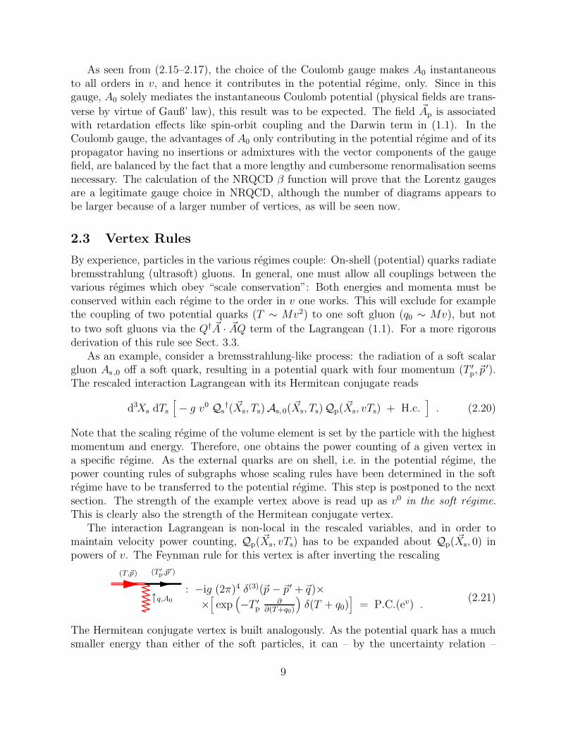
The interaction Lagrangean is non-local in the rescaled variables, and in order tomaintain velocity power counting, Qp( ~Xs, vTs) has to be expanded about Qp( ~Xs, 0) inpowers of v. The Feynman rule for this vertex is after inverting the rescaling

(T,~p)

↑q,A0

(T ′

p,~p′)

: −ig (2π)4 δ(3)(~p −~p ′ +~q)××[

exp(

−T ′p

∂∂(T+q0)

)

δ(T + q0)]

= P.C.(ev) .(2.21)

The Hermitean conjugate vertex is built analogously. As the potential quark has a muchsmaller energy than either of the soft particles, it can – by the uncertainty relation –

9

not resolve the precise time at which the soft quark emits or absorbs the soft gluon.This “temporal” multipole expansion comes technically from the different scaling of ~xand t in the three regimes. The multipole expansion symbolised in the power countingby ev corresponds term by term to an expansion in v and should be truncated at thedesired order. In general, the coupling between particles of different regimes will notbe point-like but contain multipole expansions for the particle belonging to the weakerkinematic regime. That the coupling of potential quarks to ultrasoft gluons requires amomentum multipole expansion as in atomic physics has been observed by Grinstein andRothstein [19], and by Labelle [22].

Amongst the fields introduced, six scale conserving interactions are allowed within andbetween the various regimes for any coupling of one gluon to two quarks. Because only inthe Coulomb gauge, A0 is a field in the potential regime only, its propagator always beinginstantaneous, only the first two interactions exist for the scalar coupling −gQ†A0Q oftable 1 in this gauge choice. The v counting for the lowest order quark-gluon interactionsfrom this vertex is presented in table 1.

Table 1: Velocity power counting and vertices for the interaction Lagrangean −gQ†A0Q.In the Coulomb gauge, only the first two diagrams exist. The last line indicates the fieldfor which an energy or momentum multipole expansion has to be performed.

Vertex A0

P.C. 1√

vv

1

2 v0 v0 v0 v

multipole none A0p(~x) A0

u(~x) none Qp(t) A0u(~x, t)

Note that – although both describing interactions with physical gluons – soft andultrasoft couplings occur at different orders in v. On the level of the vertex rules, anoverlap of different regimes resulting in double counting is prevented by the fact that inaddition to most of the propagators, all vertices are distinct because of different multipoleexpansion rules.

This approach may be compared to power counting in loop diagrams as proposed inBeneke and Smirnov’s threshold expansion [16] where the strength of all scalar gluoninteractions is v0 because the scalar vertex Q†A0Q of table 1 does not contain derivatives.Here, one can easily see that the Coulomb interaction is the only relevant coupling asv → 0 and that it scales like v−1/2. This follows immediately from the rescaling rulesproposed. Also, the suppression of bremsstrahlung processes relative to the Coulombinteraction is evident from table 1. In threshold expansion, these features are establishedby considering scattering processes with an arbitrary number of loops.

Velocity power counting for other vertices is again obtained by rescaling and multipole

10

expansion. For later reference, the counting rules for the coupling of one and two gluons,either minimally or via the Fermi term, and the rules for the three gluon interaction aredisplayed in tables 2, 3 and 4. In the second, couplings between on shell gluons in thesame regime are all of order v0 = c = 1 as expected for relativistic particles.

In the minimal coupling term − igMQ†~∂ · ~AQ, the derivative acts on both the gluon

and the quark field. Because the quark is either soft or potential, its derivative fromQ† ~A · ~∂Q is rescaled as ~∂ → (Mv) ~∂s. The same holds when the derivative acts on a soft

or potential gluon. But both for the one gluon part of the Fermi interaction Q†~σ · ~BQand for the term Q†(~∂ · ~A)Q of the minimal coupling, the derivative acts on an ultrasoft

gluon field and must hence be rescaled as ~∂ → (Mv2) ~∂u. That this part of the vertexcoupling is one power in v weaker than the part where the derivative acts on the quark,is recorded in parentheses in table 2. The v rules for the coupling of one gluon to thequark via the Fermi term are identical to those sub-dominant contributions to the minimalcoupling vertex for ultrasoft gluons, and to the dominant contributions in the other cases.A similar provision is made in table 3, but is not necessary in table 4.

Table 2: Velocity power counting and vertices for the interaction − igMQ†~∂ · ~AQ. When

the spatial derivative acts on an ultrasoft gluon field, the power counting in parenthesesis the sub-dominant contribution as explained in the text. It coincides with the powercounting for the one gluon component of the Fermi vertex.

Vertex ~A

P.C. v1

2 v (v2) v v v3

2 v2 (v3)

Table 3: Velocity power counting and vertices for the gluonic interaction Lagrangeang2fabc(∂µA

aν − ∂νA

aµ)Ab, µAc, ν . Sub-dominant contributions in parentheses.

Vertex

P.C. v1

2 (v3

2 ) v (v2) v0 v1

2 (v3

2 ) v (v2) v0

2.4 Loop Rules

As hinted upon above, the velocity power counting is not yet complete. The propagatorswere constructed such that they count as order v0 in each regime in a Feynman diagram.

11

Table 4: Velocity power counting and vertices for the coupling of two gluons to a quarkfrom the minimal coupling or the Fermi term in the NRQCD Lagrangean (1.1).

Vertex~A ~A

P.C. v v3

2 v2 v v v3

2

v3

2 v2 v v2 v3 v2 v5

2

As one sees from the volume element used in (2.20), the vertex rules for the soft regimecount powers of v with respect to the soft regime. There, one hence retrieves the velocitypower counting of Heavy Quark Effective Theory [23, 24] (HQET), in which the interac-tions between one heavy (and hence static) and one or several light quarks are described.HQET counts inverse powers of mass in the Lagrangean, but because in the soft regimeMv ∼ const., the two approaches are actually equivalent. Now, HQET becomes a sub-setof NRQCD, complemented by interactions between soft (HQET) and potential or ultra-soft particles. This has already been used by Manohar [13] to facilitate and unify thematching of the NRQCD/HQET Lagrangean to QCD.

In NRQCD with on-shell quarks as initial and final states, the soft regime can occuronly inside loops. Let us define as a “soft blob” each connected graph containing (soft)loops which is obtained when all potential and ultrasoft lines are cut. If the diagramcontains even one soft particle, scale conservation ensures that there is at least one loopwhich consists of only soft particles, be they quarks or gluons, and that it is part of thesoft blob. Inside the soft blob, the power counting for the vertices is performed in thesoft regime and has therefore to be transfered to the potential regime. Since soft loopmomenta scale like [d4ks] ∼ v4 while potential ones like [d4kp] ∼ v5, each soft blob isenhanced by an additional factor 1

v.

Consider for example the graphs of Fig. 1: Using the Lorentz gauges, vertex powercounting gives that the leading contribution is from the exchange of two potential gluons,coupled via Q†A0Q. There are four such vertices, so the diagram is O(g4) P.C.(v−2) fromtable 1. The next two diagrams are O(g6) P.C.(v0) and O(g2) P.C.(v1) from the vertexpower counting in the soft regime, but another factor 1

vmust be included because there

is one soft blob in each diagram. This way, the v counting of the soft regime is movedto the potential one. The intermediate couplings in the second diagram take place in the

12

Figure 1: Power counting with soft loops. The loops in the second and third diagramobtain an inverse power of v, the last diagram of v2 in addition to the power countingfollowing from the vertex rules.

soft regime and hence are counted in that regime. After cutting all potential and ultrasoftlines in the last diagram, two soft blobs are separated by the propagation of two potentialquarks. The graph is O(g14) P.C.(v0) from the vertices, and the loop counting gives afactor 1

v2 . Each soft blob contributes at least four powers of g, but only one inverse powerof v ∼ g2. Power counting is preserved. These velocity power counting rules in loops arealso verified in explicit calculations of exemplary graphs, [15] and App. A.2.

There is no similar rule for ultrasoft loops: In the absence of ultrasoft quarks (see Sect.3.3), the internal ultrasoft gluon couples ultimately to a particle in the potential or softregime. Those vertices are automatically counted in this stronger regime, while couplingsbetween ultrasoft particles are counted in the weakest regime. No “ultrasoft blobs” cantherefore be isolated by cutting all potential and soft lines. It is hence ultimately scaleconservation which forbids a non-trivial loop counting rule for the ultrasoft regime.

Irrespective of the gauge chosen, there is only one relevant quark-gluon coupling attree level in the renormalisation group approach (i.e. only one which dominates at zerovelocity): As expected, it is the Q†

pAp,0Qp coupling providing the binding (table 1). Thepotential gluon ladders must therefore be re-summed to all orders to yield the 1

rCoulomb

potential. Diagrams higher order in v are corrections. In the Coulomb gauge, all othercouplings and insertions are irrelevant, while in general, there are three marginal couplings:Q†

pAu,0Qp, Q†sAs,0Qs and Q†

sAs,0Qp. Because of the additional factor v−1 per soft blob,graphs containing the latter two couplings can indeed be relevant and contribute as v → 0(e.g. the second graph in Fig. 1). Eventually, retardation effects from Aµ

p will becomeweaker than contributions from the soft regime.

One finally turns to the inclusion of other relativistic particles. In the same way asNRQCD replaces the physical gluon with one representative per regime, any light (rel-ativistic) particle has to be tripled. There are therefore three ghost fields ηs, ηp, ηu withthe same rescaling rules as the gluon fields (2.6). Fermions require more thought: Inthe real world, the kinetic energy of the b quark in Bottomium is compatible to thestrange quark mass, Mbv

2 ∼ ms. For the sake of simplicity, this article assumes all lightparticles to have masses very much smaller than any other scale, mq ≪ Mv2, so thatthe relativistic particles can be treated as massless to lowest order and the denominatorsof the light particle propagators are identical to the ones of the gluon in the respec-

13

tive regimes. The Dirac spinors representing light quarks scale in the three regimes asψs ∼ (Mv)

32 ∼ ψp, ψu ∼ (Mv2)

32 , i.e. similar to the heavy quark but including its ul-

trasoft counterpart (see also Sect. 3.3). The number of vertices per term in the rescaledinteraction Lagrangean increases as shown above. Quark-ghost couplings and heavy-lightquark couplings will appear in the Lagrangean (1.1) at O(g4) to restore unitarity and canbe obtained by matching NRQCD to QCD.

With rescaling, multipole expansion and loop counting, the velocity power counting rulesare established. To witness, the rescaling rules (2.5/2.6/2.7) provide an efficient andwell-defined way to arrive at an NRQCD power counting: After rescaling, one reads upthe order in v at which any term in the Lagrangean contributes in each of the threekinematic regimes and performs the appropriate multipole expansions. This establishesthe Feynman rules for NRQCD and HQET simultaneously, and classifies the strength ofthe vertices in the regime of the particle with highest energy and momentum. Finally, therescaling is inverted, introducing one un-rescaled gluon and quark field as the infrared-relevant degrees of freedom for each kinematic regime. To obtain the power countingfor a certain graph, loop counting is taken into account to transfer the strength of asoft blob into the potential regime. Computations are performed most naturally in theoriginal, dimensionful variables. The rescaling rules are only needed to establish the powercounting, but in order to maintain it, one is of course not allowed to re-sum the multipoleexpansions in the un-rescaled variables. It is also interesting to note that there is nochoice but to assign one and the same coupling strength g to each interaction. Differentcouplings for one vertex in different regimes are not allowed. This is to be expected, asthe fields in the various regimes are representatives of one and the same non-relativisticparticle, whose interactions are fixed by the non-relativistic Lagrangean (1.1).

2.5 Gauge Invariance

The Coulomb gauge ~∂ · ~A = 0 is a natural choice in NRQED because in it, static chargesdo not radiate. In NRQCD, gluons carry colour and hence the Coulomb gauge doesnot have this advantage. Luke and Savage [18] showed how to establish explicit velocitypower counting in the Lorentz gauges of NRQCD, too. The set of gauges applicable toNRQCD can be extended further: The classification of the three kinematic regimes (2.2)itself relied only on the typical excitation energy and momentum, and hence on gaugeinvariant quantities, and on the form of the denominator in the propagators (2.1) whichis unchanged in any order of perturbation theory3. The perturbative quark propagatoris gauge independent. Gauge fixing will introduce gauge dependent denominators mul-tiplying the gauge independent denominators in the perturbative gluon propagators. Asan example that this will in general not change the identification of the soft and ultra-soft regimes from poles in the gluon propagators, consider the generalised axial gauge

3Non-perturbatively, the propagators are not of the form (2.1) because of confinement and the absenceof coloured states, so that the power counting presented here may break down.

14

(n2 = −1, α arbitrary), in which

Aµ :−i

k2 + iǫ

[

gµν −kµnν + nµkν

k · n +1 + αk2

(n · k)2

]

. (2.22)

The additional denominators n·k introduce no new combinations of the two infrared scalesMv and Mv2 for which the gluon propagator has a pole. Therefore, the decompositioninto the three regimes (2.2) remains unchanged, as do the rescaling properties of the fieldsand interactions, (2.5/2.6/2.7) and tables 1 to 4.

The standard gauges (axial, Weyl, Lorentz, Coulomb) will therefore all show the samepower counting and vertex rules quoted above. Details of the gluon propagator andits insertions look different in different regimes and gauges, and some gauges will notexhibit certain vertices, insertions and representatives, e.g. the Coulomb gauge is uniquein having A0 contribute only in the potential regime. Only when the gauge dependentdenominator introduces a new regime has the power counting to be modified. This is forexample the case in a gauge with denominator k4

0 −M2~k2, in which an exceptional regime

(k0 ∼Mv , |~k| ∼Mv2) enters. Rescaling is then performed including the new regime.As is well known, the Weyl gauge A0 = 0 wants a constraint quantisation: Gauß’

law ~D · ~E = gQ†Q, generating local gauge transformations, is the equation of motionderived by varying the Lagrangean with respect to A0. When A0 = 0, Gauß’ law willnot be recovered as an equation of motion. In order to restore local gauge invariance,a projector onto states obeying Gauß’ law has therefore to be inserted into the pathintegral. Resolving Gauß’ law explicitly, the Lagrangean of the Coulomb interaction hasthe structure

LCoulomb =∫

d3y g2 Q†Q(~x) G(~x− ~y) Q†Q(~y) , (2.23)

where G(~x−~y) is an appropriate instantaneous Green’s function to Gauß’ law with dimen-sion [mass]1, e.g. in QED 1

|~x−~y|. Using the rescaling rules (2.5/2.6/2.7), one derives the

Coulomb interaction between two quarks to be P.C.(v−1) as in the other gauges. Withoutconstraint quantisation, the longitudinal component of the vector gauge field mediatingthe Coulomb interaction in Weyl gauge QED, ~Al , has a static propagator i

k20

.

3 The NRQCD β Function

This chapter presents the computation of the perturbative part of the NRQCD β functionto order g3, v0 in the MS scheme using the vertex and rescaling rules derived in theprevious section. Initially, the Lorentz gauges are not only chosen because they allow aless cumbersome renormalisation than e.g. the Coulomb gauge, but also to demonstratethat in the final result, the gauge parameter α drops out. The Slavnov–Taylor identitieswill be shown to be fulfilled, and the Lorentz gauges are a legitimate gauge choice inNRQCD. As a by-product, Sect. 3.7 will calculate the NRQCD β function to lowest orderin the Coulomb gauge.

By construction, NRQCD and QCD must agree in the infrared limit, and especiallyin the structure of collinear (infrared) divergences. Matching proved that both the soft

15

quark and the soft gluon are indispensable to reproduce the correct structure of collineardivergences in a toy model given by Beneke and Smirnov [16] and confirmed the proposedcounting rules [15]. The calculation of the NRQCD β function will manifest the relevanceof the soft regime beyond infrared divergences, and it will endorse the power countingfurther. Deriving the lowest order β function in the following, the relation between thispower counting and threshold expansion [16] will be exemplified, and rules will be devel-oped which allow one to determine from the structure of a diagram whether it is zero ornot to all orders in v.

NRQCD with NF light quarks must reproduce the β function of QCD below the scale M ,

βQCD = − g3R

(4π)2

[11

3N − 2

3NF

]

(3.1)

to lowest order for the gauge group SU(N) and renormalised coupling gR. This meansespecially that the renormalised coupling strengths of all interactions steming from ex-panding the same term in the Lagrangean in the various regimes are the same, except thatthey have to be taken at different scales: For the interaction Lagrangean −gQ†A0Q, thesix vertices of table 1 all couple with the same un-renormalised strength. Although thenumber of vertices is increased in the approach presented here, the number of independentcouplings is not. Indeed, one major result of this chapter will be that renormalisation willnot destroy this symmetry because the renormalisation constants agree in all regimes.

One can obtain the β function from the ghost-gluon coupling, and the ghost and gluonself energy. Because the relativistic sector of NRQCD is identical to the one of QCD asseen in Sect. 2.3, the calculation proceeds in that case like in QCD and yields the sameresult. In this article, the β function is calculated by studying the heavy quark sector,namely the renormalised coupling Q†

RA0,RQR between the heavy quark and the scalargluon. This term yields immediately the coupling renormalisation. All other vertices aresuppressed by at least one power of v.

Because the integrals to be performed are not Lorentz invariant, standard formulae fordimensional regularisation often do not apply. Therefore, Ref. [15] used split dimensionalregularisation, which was introduced by Leibbrandt and Williams [25] to cure the problemsarising from pinch singularities in non-covariant gauges. It treats the temporal and spatialcomponents of the loop integrations on an equal footing by regularising the energy and

momentum integration separately,∫ ddk

(2π)d =∫ dσk0

(2π)σdd−σ~k

(2π)d−σ , σ → 1, d → 4 [26, Chap.

4.1]. Useful formulae for the computation of the β function are given in App. A.1.

3.1 NRQCD and Threshold Expansion: Potential Quark Self-

Energy

Threshold expansion [16] and NRQCD make use of very similar basic techniques butdifferent formulations, as this Section outlines. In order to clarify the relation, considerthe quark self-energy diagram lowest order in g which couples the scalar gluon and thequark in NRQCD. To facilitate the presentation initially, the Feynman gauge α = 1 is

16

chosen in which scalar and vector gauge fields do not mix when propagating. Withoutthe scaling rules for the various regimes, one obtains

A0,q

: iΣp(T,~p) = (−ig)2 CF

∫ddq

(2π)d

−i

q20 −~q2 + iǫ

i

T + q0 − (~p+~q)2

2M+ iǫ

, (3.2)

with CFδij = (tata)ij = N2−12N

δij the Casimir operator of the fundamental representation ofSU(N). Threshold expansion identifies the loop momentum of QCD to belong to a hardregime q ∼M or to either of the three regimes (2.2) and expands the integrand about thevarious saddle points, i.e. about the values of the loop-momentum q where poles occur, likethe NRQCD classification in Sect. 2.1. The hard regime subsumes the relativistic effectscontained in the coefficients ci, di, ei of the NRQCD Lagrangean (1.1) and hence providesthe matching between NRQCD and QCD [16]. In deriving the NRQCD Lagrangean (1.1),hard momenta have been integrated out, so that the ultraviolet behaviour of the aboveloop integral is arbitrary and it is not necessary to take the poles at q ∼ M in (3.2) intoaccount. Indeed, to be consistent, they should rather be discarded.

Let the incident quark be on shell, i.e. have a four-momentum (Tp,~p) in the potentialregime. The integral decomposes then into approximations about three saddle points:When q is soft, the gluon propagator has a pole, and one can expand the quark propagator

in powers of Tp/q0 ∼ v and (~p+~q)2

2M/q0 ∼ v. The quark becomes static:

i

q0 + Tp − (~p+~q)2

2M

−→ i

q0+

i

q0i(

Tp −(~p +~q)2

2M

)i

q0+ . . . (3.3)

=⇒ iΣp(T,~p)∣∣∣soft

= (−ig)2 CF

∫ddq

(2π)d

−i

q20 −~q2 + iǫ

i

q0 + iǫ

∞∑

n=0

(~p+~q)2

2M− Tp

q0 + iǫ

n

(3.4)

The NRQCD power counting proceeds on the level of the Lagrangean instead of theFeynman diagrams with corresponding diagrams for loop momenta in the soft regime,

q

+ + . . . : (3.5)

(−ig)2 CF

∫ddq

(2π)d

−i

q20 −~q2 + iǫ

i

q0 + iǫ

(

1 − i(~p +~q)2

2M

i

q0 + iǫ+ iTp

i

q0 + iǫ+ . . .

)

,

and recovers order by order in v the result of threshold expansion. The intermediatesoft quark is static, and the higher order terms in threshold expansion are interpretedas insertions into the soft quark propagator or as resulting from the energy multipoleexpansion at the QsA

µsQp vertex. In fact, using the equations of motion, a temporal

multipole expansion may be re-written such that the energy becomes conserved at thevertex. Now, both soft and potential or ultrasoft energies are present in the propagators,

17

making it necessary to expand it in ultrasoft and potential energies. An example wouldbe to restate the vertex (2.21) as

: −ig (2π)4 δ(T − T ′p + q0) δ

(3)(~p −~p ′ +~q) , (3.6)

and the soft propagator to contain insertions P.C.(v) for potential energies T ′p

(T=q0+T ′

p,~p)

:i

q0 + iǫ

∞∑

n=0

(−T ′p

q0

)n

. (3.7)

The same can be shown for the momentum-non-conserving vertices, too.When the loop momentum q is potential, threshold expansion picks the pole of the

quark propagator, and the gluon propagator is expanded as if q0 ≪ |~q|, corresponding toNRQCD diagrams with insertions in the gluon propagator:

q

+ + . . . : (3.8)

iΣp(T,~p)∣∣∣potential

= (−ig)2 CF

∫ddq

(2π)d

−i

−~q2 + iǫ

∞∑

n=0

(

q20

~q2

)ni

T + q0 − (~p+~q)2

2M+ iǫ

The correspondence is again complete for ultrasoft q, and the higher order terms of thresh-old expansion come from the spatial multipole expansion in NRQCD:

q

: iΣp(T,~p)∣∣∣ultrasoft

= (3.9)

= (−ig)2 CF

∫ ddq

(2π)d

−i

q20 −~q2 + iǫ

i

T + q0 − ~p2

2M+ iǫ

∞∑

n=0

2~p·~q+~q2

2M

T + q0 − ~p2

2M+ iǫ

n

.

Threshold expansion and NRQCD concur indeed in all diagrams to be calculated for theβ function. Further comparison of the two approaches is postponed to the Conclusions.

3.2 Some Diagrammatic Rules

In general, the number of possible diagrams in power counted NRQCD is considerablylarger than in the original theory because there are at least six vertices per interactionallowed by scale conservation, cf. tables 1 to 4 for interactions between three and fourparticles. In the preceding sub-section, three diagrams were drawn for the lowest ordercontribution to the potential quark self energy. The analogue problem in threshold ex-pansion is that each loop momentum can lie in either of the three regimes, so that thenumber of expansions for an n loop diagram grows like 3n.

18

The important step to cut down the computational effort in either approach is to notethat as an immediate consequence of the axioms of dimensional regularisation (e.g. [26,Chap. 4.1 and 4.2]), integrals without scales set by external momenta or energies in thedenominator vanish because of homogeneity,

∫ddq

(2π)dqα = 0 . (3.10)

For example, applying this theorem to the potential quark self energy diagrams, contri-butions from soft (3.4) and potential (3.8) loop momenta are zero to all orders in thevelocity expansion. For the potential gluon contribution (3.8), this is seen by shifting the

regularised loop integral T + q0 − (~p+~q)2

2M→ q0 before using (3.10) for the energy integral.

The importance of (3.10) has already been alluded to in threshold expansion [16], andhere a more thorough and formal treatment is presented.

It is this theorem (3.10) which renders most of the diagrams in NRQCD and thresholdexpansion calculations zero, and it is usually not even necessary to consider the wholediagram but only a sub-set of it. The following set of rules is helpful for reducing thenumbers of diagrams to be dealt with in the calculation of the β function.

In order to establish these rules, recall that all graphs vanish which contain a sub-graphzero by the rules developed. The routing of the loop four-momentum inside a diagramis arbitrary as always in dimensional regularisation so that having regularised the loopintegration, all loop four-momenta can be shifted at will like in ordinary integration.Since they have identical denominators (Sect. 2.3), gluon lines in any rule can be replacedby any relativistic particle, e.g. ghosts and light quarks. Finally and most importantly,numerators are unimportant to determine whether an integral is scale-less following (3.10).As multipole expansion and insertions do not change the denominators of the propagators,a diagram is therefore zero to all orders when it is zero because of (3.10) at leading orderin v. This result is also insensitive to the gauge chosen and to the specific vertex involved.For example, because the numerators play no role in rendering (3.4/3.8) zero using (3.10),the same will hold for any graph with the same diagrammatic representation but differentinteractions, e.g. also for graphs in which one or both vertices are replaced with theminimal coupled vector fields Q†~∂ · ~AQ or the Fermi interaction Q†~σ · ~BQ.

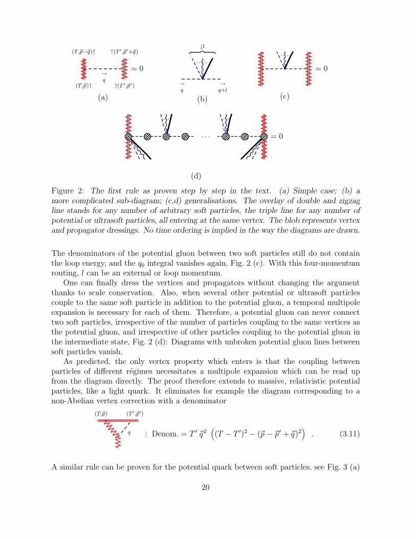
As a first rule, consider a potential gluon between two soft particles, represented by theoverlay of double and zigzag lines in Fig. 2 (a). This sub-diagram is zero when the loopenergy q0 is integrated over: Assign the potential loop momentum q to the instantaneousgluon with a propagator denominator −~q 2 (2.18). As the coupling of soft particles topotential ones is energy non-conserving, the denominators of the soft particles coupling toAµ

p do not contain q0 ∼Mv2, either. Therefore, q0 does not occur in any denominator, andthe dimensionally regularised loop integral over q0 is zero from (3.10). The rule is extendedby noting (Fig. 2 (b)) that overall energy conservation allows for the potential gluon lineto be attached with an arbitrary number of vertices into which an arbitrary number ofpotential or ultrasoft gluons or quarks with collective (potential) four-momentum l enters.

19

→q

(T,~p)↑

(T,~p−~q)↑

↑(T ′,~p′)

↑(T ′,~p′+~q)

(a)

= 0

↓l︷ ︸︸ ︷

→q

→q+l

(b) (c)

= 0

(d)

= 0

Figure 2: The first rule as proven step by step in the text. (a) Simple case; (b) amore complicated sub-diagram; (c,d) generalisations. The overlay of double and zigzagline stands for any number of arbitrary soft particles, the triple line for any number ofpotential or ultrasoft particles, all entering at the same vertex. The blob represents vertexand propagator dressings. No time ordering is implied in the way the diagrams are drawn.

The denominators of the potential gluon between two soft particles still do not containthe loop energy, and the q0 integral vanishes again, Fig. 2 (c). With this four-momentumrouting, l can be an external or loop momentum.

One can finally dress the vertices and propagators without changing the argumentthanks to scale conservation. Also, when several other potential or ultrasoft particlescouple to the same soft particle in addition to the potential gluon, a temporal multipoleexpansion is necessary for each of them. Therefore, a potential gluon can never connecttwo soft particles, irrespective of the number of particles coupling to the same vertices asthe potential gluon, and irrespective of other particles coupling to the potential gluon inthe intermediate state, Fig. 2 (d): Diagrams with unbroken potential gluon lines betweensoft particles vanish.

As predicted, the only vertex property which enters is that the coupling betweenparticles of different regimes necessitates a multipole expansion which can be read upfrom the diagram directly. The proof therefore extends to massive, relativistic potentialparticles, like a light quark. It eliminates for example the diagram corresponding to anon-Abelian vertex correction with a denominator

(T,~p) (T ′,~p′)

q : Denom. = T ′ ~q2(

(T − T ′)2 − (~p −~p′ +~q)2)

. (3.11)

A similar rule can be proven for the potential quark between soft particles, see Fig. 3 (a)

20

for its bare and (b) for its dressed form. The vertices are again energy non-conserving, so

(a)

= 0

(b)

= 0q (q0+l0,~q)

l

(c)

6= 0

Figure 3: The second rule in its bare (a) and dressed (b) version; (c) the generalisationanalogous to Fig. 2 (c) fails. Conventions as in Fig. 2.

that q0 enters only in the denominator of the potential quark in the combination q0 − ~q2

2M.

Shifting q0− ~q2

2M→ q0, the q0 integral again does not contain a scale in the denominator. In

contradistinction to the previous case, this rule cannot be extended to include potential orultrasoft momenta coupling to the blob, Fig. 3 (c). For example, a bremsstrahlung gluonwith external, ultrasoft four-momentum l renders the potential quark denominators inthe propagators as (q0 − ~q2

2M)(q0 + l0− ~q2

2M). Now, l0 provides the necessary scale for the q0

integration. As an example of the rule, the Abelian vertex contribution with denominator

(T,~p) (T ′,~p′)

q : Denom. =

(

q0 −~q2

2M

)

(T − T ′)(

T ′2 − (~p′ −~q)2)

(3.12)

is zero, but the last of the graphs in Fig. 1 is not.

As the coupling of an ultrasoft gluon to a soft particle conserves neither energy normomentum, one may disconnect the ultrasoft gluon from such a vertex, Fig. 4 (a). If after

(a)

−→

(b)

−→ = 0

Figure 4: (a) Soft-to-ultrasoft vertices are cut off in a third rule; (b) an example. Con-ventions as in Fig. 2.

cutting, a line with loop momenta to be integrated over becomes completely disconnectedfrom the graph, the resulting tadpole makes the graph vanish, Fig. 4 (b). If only one ofthe Aµ

u legs becomes dis-attached, the diagram can be non-zero, as the following diagramfor the Abelian vertex correction to the QsAs 0Qp coupling demonstrates:

q

(T,~p) (T ′,~p′)

−→ 6= 0 : Denom. = T q2

(

T ′ − q0 −~p2

2M

)

(3.13)

21

See also Sect. 3.6 and the computation of this graph in App. A.2.When several ultrasoft gluons couple to a soft particle at the same point, cutting does

usually not result in a tadpole, either. For example, the gluon-gluon vertex obtained bycutting the two-gluon two-quark vertex

q

k

−→ 6= 0 : Denom. = (k − q)2 q2 6= 0 (3.14)

might be represented by a small blob as a reminder that it is neither energy nor momentumconserving. In the “tadpole”, a scale is set by the external ultrasoft four-momentum k.

Loops made out of one soft quark and one soft gluon are restricted by another rule. In

q

(a)

= 0

q

(b)

= 0

Figure 5: The fourth rule in its (a) bare and (b) extended version, where the rule in Fig.4 (a) was used for attaching ultrasoft gluons to the soft gluon. Conventions as in Fig. 2.

Fig. 5 (a), the denominators are q20 − ~q 2 for the soft gluon and q0 for the soft quark.

Therefore, the diagram is without scale. The generalisation, Fig. 5 (b), eliminates all softcontributions to the potential quark self energy (3.5) and to Abelian vertex correctionsbetween potential and ultrasoft particles. Note that the light particle exchanged is mass-less or has a mass considerably smaller than Mv2. A relativistic particle mass of orderMv2 or bigger provides a scale in the relativistic propagator, invalidating this rule. Also,as soon as a potential particle couples to the soft gluon, the diagram is non-zero. Anexample is the non-Abelian vertex correction to the Q†

pAµpQp coupling with denominator

(T,~p) (T ′,~p′)

6= 0 : Denom. = q0 q2(

q20 − (~p −~p ′ +~q)2

)

. (3.15)

To summarise, the principle underlying the rules is simple: One identifies a potentiallyvanishing sub-set of the entire diagram and assigns the external and loop momenta to it,taking into account multipole expansions. Then, the denominators (i.e. inverse propaga-tors) are written out at lowest order in v. If by shifting integration variables, one arrives

22

at an energy or momentum integral without scale, the diagram vanishes to all orders.Along this line, further rules are easily established.

Two more rules are more straightforwardly derived from the propagator properties ofNRQCD directly. The first one cuts down the number of diagrams including potentialgluons. For the heavy quarks, there is no distinction between Feynman and retardedpropagators in NRQCD (2.10/2.11) because antiparticle propagation has been eliminatedby the field transformation from the relativistic to the non-relativistic Lagrangean. Thefields Qs and Qp propagate hence only time-like into the forward light cone. Still, Feyn-man’s perturbation theory becomes more convenient than the time-ordered formalism, asless diagrams have to be calculated. Soft and ultrasoft gluons propagate light-like, andpotential gluons instantaneously. Therefore, any diagram which – when time ordered –involves quarks propagating outside the forward light cone are zero, as are diagrams whichcannot be drawn with both ends of a potential gluon being space-like separated. This“forwardness” excludes all non-zero contributions from the potential gluon contributionto the quark self energy in any regime, e.g. (3.8).

Another rule is that there must at least be one pole on each side of the real q0 axisfor a diagram to be non-zero. This will e.g. not be the case when the loop momentum qonly occurs in one quark propagator besides potential gluon propagators. Likewise, thecontribution to the Abelian vertex correction

(T,~p) (T ′,~p′)

q : Denom. =

(

q0 −~q2

2M+ iǫ

)(

q0 −(~q + ~p ′ −~p)2

2M+ iǫ

)(

T 2 − (~p −~q)2)

(3.16)has only poles below the real axis. Closing the contour of the q0 integration above it, thediagram is zero. This can also be proven using dimensional regularisation.

In order to demonstrate that the rules established above are useful in reducing the numberof graphs, Fig. 6 shows that only one of the four scale-conserving graphs contributing tothe one loop soft quark self-energy survives their filter. The classification of the only

(a)

6= 0

(b)

= 0

(c)

= 0

(d)

= 0

Figure 6: Out of the four scale-conserving one loop contributions to the soft quark selfenergy, only the first one, (a), survives. (b) is zero because it contains a sub-graph zero byFig. 3 (a); (c) vanishes because of Fig. 2 (c) or because of forwardness; (d) is eliminatedby cutting off the ultrasoft gluons (Fig. 4 (a)). The resulting tadpole is zero.

non-zero diagrams for Abelian and non-Abelian one-loop corrections to one gluon verticesaddressed later, Figs. 8, 9 and 10, may serve as another example.

23

In conclusion, the homogeneıty of dimensional regularisation (3.10) can be translatedinto diagrammatic rules to systematically identify graphs which vanish to all orders inthreshold expansion or velocity expansion in NRQCD. The concept is sensitive only tothe multipole expansion of the vertices involved, not to their precise nature. It is alsoindependent of insertions and gauge chosen. Only the denominators of the graph lowestorder in v have to be looked at.

3.3 Theorems from Diagrammatic Rules

Diagrammatic rules are quite effective to prove decoupling theorems to all orders in per-turbation theory. “Scale conservation” entered in Sect. 2.3 as a constraint on both theoverall energy and momentum of a vertex because both have to be conserved order byorder in v. Now, one may resort to a more formal argument: If one rescales the fieldsin the Lagrangean in all possible combinations, diagrams containing scale non-conservingvertices are eliminated because they correspond to temporal or spatial tadpoles. As anexample, consider a soft particle coupling to two potential ones. The dashed-solid linerepresenting any potential particle, the multipole expansion is

(T,~p)

↑q,A0

(T ′,~p′)

∝ (2π)4 δ(3)(~p −~p′ +~q)[

exp(

(T − T ′)∂

∂q0

)

δ(q0)]

. (3.17)

The temporal tadpole of the q0 integration makes all diagrams vanish in which this vertexis embedded such that q is a loop momentum. If q0 is an external energy, its being zerocontradicts the assumption that it is of order Mv. Therefore, diagrams containing scalenon-conserving vertices are zero. In threshold expansion, this follows automatically fromthe observation that not the individual vertices but the loop momentum as a whole isexpanded, see Sect. 3.1.

Another application is the decoupling of an ultrasoft heavy quark from NRQCD. Whenthe particle content of NRQCD in the three different regimes was outlined in Sect. 2.1,the bremsstrahlung gluon was assumed to be the only ultrasoft field, and an ultrasoftquark Qu was not necessary to make the theory self-consistent. An ultrasoft quark mightstill be produced by the radiation of a potential gluon off a potential quark, but it is notunavoidable. In contradistinction, a soft quark is indispensable because a soft, on shellgluon excites a potential quark to a kinetic energy of order Mv: The potential quarkcoupling to a soft gluon becomes necessarily soft. Taking advantage of the homogeneıty(3.10) of dimensional regularisation, one can show that a hypothetical ultrasoft heavyquark decouples completely from the theory: All graphs containing it are zero. This factwas already remarked upon by Beneke and Smirnov [16], and the formal proof using theNRQCD techniques proceeds as follows.

Of all properties of the ultrasoft quark, the only ones needed are that its propagator

24

(denoted by a dotted line) is static because T ∼ Mv2, |~p| ∼ Mv2,

Qu :(T,~p)

:i

T + iǫ; (3.18)

and that it couples momentum non-conserving to all but ultrasoft particles. These fea-tures can of course be derived from the rescaling rules of an ultrasoft quark, Qu(~x, t) =

(Mv2)32Qu( ~Xu, Tu), in full analogy to Sect. 2.2. If it exists, Qu can only enter in internal

lines. Fermion number conservation dictates that it is produced and annihilated in avertex into which at least one soft or potential quark enters.

The simplest sub-diagram containing an ultrasoft quark is depicted in Fig. 7 (a) andvanishes because there is no loop momentum ~q in any denominator. This is still true

→q

(T,~p)↑

(T−q0,~p)↑

↑(T ′,~p′)

↑(T ′+q0,~p′)

(a)

= 0q q+l

↓l︷ ︸︸ ︷

(b)

= 0q l

(c)

(d)

= 0

Figure 7: Decoupling of the heavy, ultrasoft quark. (a) primitive diagram; (b) extensionto the case of ultrasoft particles coupling to Qu; (c) general vertex involving potential andultrasoft particles; (d) ultrasoft quarks decouple from any graph containing potential andultrasoft particles. Conventions as in Fig. 2.

when an arbitrary number of ultrasoft particles couple to Qu, Fig. 7 (b), and when such acoupling occurs repetitively. Now one considers couplings to potential particles like in Fig.7 (c). The momentum multipole expansion necessary for all ultrasoft particles separatelyin such a vertex disallows ~q to be transferred to a denominator. Therefore, any diagramcontaining an ultrasoft quark coupled to potential or ultrasoft particles is zero because ofthe spatial tadpole in the q integration, Fig. 7 (d). Because couplings of ultrasoft particlesto soft ones involve the same momentum multipole expansion as couplings to potentialones, the proof extends to all graphs containing ultrasoft quarks: Every diagram withultrasoft quarks is zero. Recursive application dresses all vertices and propagators.

25

3.4 The Quark Self-Energy

The rules cover the lowest order contributions to the potential quark self energy as dis-cussed in Sect. 3.1. The graph in (3.5) is zero because of Fig. 5, the one in (3.8) becauseof forwardness. The only remaining graph is (3.9), whose lowest order contribution isP.C.(v0) by the power counting of table 1. Indeed, corrections to particle propagators,quark or gluon, must count as v0 since the power counting was constructed such that freeparticle propagators in each regime scale like v0 (2.6/2.7) and renormalisation correctionsto propagators must be of the same order. Using the integral (A.4) of App. A.1, the polein four dimensions is extracted as

: iΣp(T,~p)|pole =−ig2

R µ2ε

8π2CF

3 − α

2Γ[ε]

(

T − ~p2

2M

)

+ P.C.(v) , (3.19)

where ε = 2− d2

and µ is the renormalisation parameter. The potential quark propagatoris recovered, confirming that different regimes do not mix under renormalisation. Thenon-relativistic quark propagator does not need renormalisation of the heavy quark mass.The quark wave function renormalisation is hence in the MS scheme

Z2 = 1 +g2R µ

2ε

8π2CF

3 − α

2Γ[ε] . (3.20)

For the soft quark self energy, the only diagram surviving the diagrammatic filter (Fig.6) is at lowest order in the power counting using the Feynman rules and (A.4)

: iΣs(T,~p)|pole =−ig2

R µ2ε

8π2CF

3 − α

2Γ[ε] T . (3.21)

That the soft quark renormalisation is the same as for the potential quark is not surprisingas both stem from the same un-expanded NRQCD diagram (3.2).

3.5 The Vacuum Polarisation

In contradistinction to the self energy for Qp which does not receive contributions fromsoft particles, the vacuum polarisation of the potential gluon is non-zero only because ofthe presence of soft gluons, independent of the gauge chosen. The scale-conserving graphswith gluon loops are

. (3.22)

The integral in the second graph does not contain q0 in the denominator and henceis zero; the third diagram vanishes because it couples a potential gluon to a light-likeparticle twice. Soft gluons are therefore indispensable to provide the gluons mediating

26

the Coulomb interaction with a non-zero vacuum polarisation, and hence to have a runningβ function. As the gluons in the soft and ultrasoft regimes are on-shell particles and mustrun in NRQCD as in QCD, there is no reason to expect the potential gluons to freezeout in perturbation theory. The only non-zero ghost and light quark contributions comeanalogously from soft ghost and soft light quark propagation in the loop.

The rescaling rules of table 3 give the three gluon vertex to count as v12 , and an

additional v−1 from the loop power counting makes the graph count as v0 at leadingorder. Again, this is expected not only because gluons are relativistic particles, but alsobecause one wants to renormalise a propagator which is P.C.(v0) in the power counting.Without the loop rule of Sect. 2.4, the graph would be of order v1, and the power countingwould predict that its contribution would vanish as v → 0 so that the potential gluonpropagator at rest would reduce to the bare one, a clearly unacceptable conclusion. Theexplicit computation (3.24) will also show that this graph is P.C.(v0).

The soft and ultrasoft gluon receive their vacuum polarisations from loops with on shellgluons, P.C.(v0):

(3.23)

All other diagrams vanish by the rules developed above. Both contributions are identicalto the ordinary QCD result, as no insertions or expansions enter. The gluon vacuumpolarisation from gluon, ghost and light fermion contributions is therefore in the soft andultrasoft regime [27, eq. (2.5.132)]

Πabµν(k) = δab (kµkν − k2gµν) Π(k2) with (3.24)

Π(k2) =g2R µ

2ε

(4π)2

[2

3NF − 1

2N(

13

3− α

)]

Γ[ε] + finite.

Because the potential gluon vacuum polarisation does not contain insertions or multipoleexpansions in the internal lines, either, the QCD result can be taken and expanded inpowers of the external energy k0 ≪ |~k|. As the infinite part of Π(k2) does not contain k,the only change will be that to lowest order in v, the part guaranteeing transversality ofthe gluon becomes

(kµkν − k2gµν) → (δµiδνjkikj + ~k2gµν) + P.C.(v) . (3.25)

Renormalisation therefore keeps the contributions from the three regimes separate andthe potential gluon propagator transversal up to higher order in v. For all three regimes,the gluon wave function renormalisation is in the end the one of QCD [27, eq. (2.5.135)],

Z3 = 1 − g2R µ

2ε

(4π)2

[2

3NF − 1

2N(

13

3− α

)]

Γ[ε] = ZQCD3 . (3.26)

27

3.6 The Vertex Correction and NRQCD β Function

Since they probe only the relativistic sector of the theory, the renormalisation constantsfor gluons, ghosts and other light particles are the same in QCD and NRQCD. The quarkwave function renormalisation is computed in the non-relativistic sector and for a non-relativistic bi-spinor rather than a relativistic Dirac spinor, so that it is not surprising

that the result (3.20) differs from its QCD counterpart ZQCD2 = 1 − g2

Rµ2ε

(4π)2CF α Γ[ε] [27,

eq. (2.5.139)] even in the dependence on α, although the MS scheme was used in bothcases. As both Lagrangeans are gauge invariant and agree in the light particle sector,the Slavnov–Taylor identities of QCD must also hold in NRQCD. Therefore, the renor-malisation Z1 of the quark-gluon vertex Q†A0Q can be inferred from Z2, Z3 and thethree-gluon renormalisation Z1, g of QCD (and NRQCD) not to be the same as in QCD

where ZQCD1 = 1 − g2

Rµ2ε

8π2 (CF α+N 3+α4

) Γ[ε] [27, eq. (2.5.145)]:

Z1 =Z2 Z1, g

Z3= 1 +

g2R µ

2ε

(4π)2

(

CF (3 − α) − N3 + α

4

)

Γ[ε] 6= ZQCD1 . (3.27)

In the following, one will identify as the cause that all non-zero contributions from bothAbelian and non-Abelian vertex corrections to the scalar gluon vertex in NRQCD aredifferent from their QCD values: Most notably, the non-Abelian vertex only providesgauge parameter corrections. As a by-product, the topologies of all one loop correctionsto interactions of one gluon with a quark will be found and their leading order velocitypower counting determined.

Which vertices may be encountered in the graphs leading in v? For every vertex, theQ†A0Q coupling is at least one order stronger in v than any other coupling (tables 1and 2). Any contribution is therefore suppressed in which scalar gluons in a vertex are

replaced with vector gluons, coupled either minimally or via the Fermi term gc32MQ†~σ · ~BQ

in (1.1). Moreover, the Fermi term couples one or two gluons to the quark spin. Whenonly one Fermi interaction is found in any vertex correction, parity conservation requiresthe strongest possible correction involving A0 as outgoing particle to be of the form ofthe spin-orbit term, i.e. proportional to Q†~σ · ( ~D× ~E)Q. This cannot correct the leadingscalar gluon vertex. Two Fermi interactions are even more suppressed because vectorcouplings are weaker than scalar couplings.

Each Abelian correction graph (Fig. 8) starts off at the same order as the bare graphwhose vertex correction it presents (table 1) when only scalar gluons couple to the quark.The only exception is the last diagram in the first row of Fig. 8, which by the powercounting is P.C.(v1) while the bare Q†

sAs 0Qp vertex is P.C.(v0) from table 1, as confirmedby an explicit computation of this graph in App. A.2. This diagram does therefore notenter in the computation of the vertex correction at lowest order.

The non-Abelian corrections to the Q†A0Q vertex at order g3 fall into two categories:The topology of the first class of diagrams, Fig. 9, is analogous to the one of the non-Abelian vertex correction in QCD. In the Feynman gauge α = 1, its leading order con-tribution involves two scalar gluons and one vector gluon because in that gauge, differentcomponents of the gluon field do not mix when propagating, (2.18), and the coupling of

28

P.C.(v0) P.C.(v12 ) P.C.(v0) P.C.(v)

P.C.(v) P.C.(v−12 ) P.C.(v0)

Figure 8: The Abelian vertex corrections of order g3 from the interactions Q†A0Q whichsurvive the diagrammatic filter. The leading order power counting is obtained when allvertices are the leading order scalar gluon interactions. After applying the rules of Sect.3.2, the seven diagrams drawn are the only survivors of 22 scale conserving graphs.

three scalar gluons is forbidden at order g by the Lorentz structure. Again because for

P.C.(v) P.C.(v32 ) P.C.(v) P.C.(v2)

P.C.(v2) P.C.(v12 ) P.C.(v

32 ) P.C.(v)

Figure 9: The non-Abelian vertex corrections of order g3 which survive the diagrammaticfilter. The soft blob in the second diagram in the second row provides an additional factor1v

by loop power counting. The power counting indicated is the leading contribution in theFeynman gauge, when the three gluon vertex is the standard QCD one and both one vectorand one scalar gluon couples minimally to the quark. In the Lorentz gauges, two scalargluons couple to the quark, making all diagrams a factor 1

vstronger and hence contribute

at the same order as the Abelian corrections in Fig. 8. Out of 25 scale-conserving diagrams,only eight survive the diagrammatic filter.

every vertex, the Q†A0Q coupling is stronger in v than any other coupling, the NRQCDanalogue to the non-Abelian QCD vertex correction to the scalar gluon vertex is sub-leading in the Feynman gauge. The resulting power counting is reported in Fig. 9. In thegeneralised Lorentz gauges, the scalar and vector components of the gauge field mix inthe gluon propagation, with the amount of mixing proportional to (1−α) (2.18). A scalargluon emitted from a quark will therefore partially turn into a vector gluon, which thenenters a three gluon vertex. The non-Abelian vertex corrections now have a non-trivialLorentz structure and evaluate to be proportional to (1−α) and (1−α)2, as is confirmed

29

in App. A.2, (A.15). A factor 1v

is gained with respect to the power counting with onevector gluon coupling as given in Fig. 9, making the diagrams of the same, leading orderas the Abelian vertex corrections. The non-Abelian graphs can consequently be seen asmerely providing gauge corrections to the Abelian vertex result. The last diagram in thefirst row and the next-to-last in the second row of Fig. 9 are sub-leading and vanish usingthe equations of motion at lowest order for the outgoing potential quark, see App. A.2.

There is no comparable graph in QCD to the second category of non-Abelian vertexcorrections in NRQCD at order g3. Figure 10 lists the topologies of all non-zero correctionsto one gluon vertices involving one gluon loop. Again, one convinces oneself easily from

~A~A

Aµ P.C.(v) P.C.(v32 ) P.C.(v)

P.C.(v3) P.C.(v12 ) P.C.(v2)

Figure 10: The only non-zero diagrams of the vertex corrections of order g3 from the Fermiterm proportional to c3 in the NRQCD Lagrangean (1.1). The soft blob in the next-to-lastdiagram provides an additional factor 1

vby loop power counting. The leading order power

counting is obtained when the three gluon vertex is the standard QCD one and the gluonscouple to the quark via the Fermi term. Out of 24 scale-conserving diagrams, only sixsurvive the diagrammatic filter.

tables 3 and 4 that these diagrams are at least one order in v weaker than the Abelianvertex corrections, even before the precise vertex structure is specified. In NRQED, thistype of diagrams occurs first at order g5 from the e2 term in the Lagrangean (1.1) becausea three photon coupling does not occur earlier. In QCD, the lowest order three gluoncoupling is totally antisymmetric in colour space, so that its contraction with the totallysymmetric expression in colour space from the vertex g2

2MQ† ~A2Q vanishes. The Fermi

interaction has a colour antisymmetric two gluon part because Bai = 1

2ǫijk(∂jA

ak − ∂kA

aj +

gfabcAbjA

ck), but is not a possible source of an order g3 vertex correction in Fig. 10 to the

minimal coupling of scalar gluons and quarks because the spin structures do not match.

Hence, the non-Abelian nature of the gauge field enters into the NRQCD β functiononly via the gluon vacuum polarisation and as what may be called gauge correctionrepresented by non-Abelian vertex corrections. Each of the six quark gluon couplingsbetween the various regimes is renormalised by one and only one non-zero Abelian andnon-Abelian vertex correction.

Since the classification of diagrams following the rules of Sect. 3.2 is insensitive to theprecise nature of the vertex coupling, the list leads as a by-product to a classification of

30

all non-zero one loop graphs in which two quarks and one gluon couple. The same is truefor the quark self energy and vacuum polarisation graphs. The v power counting of thediagrams in Figs. 8, 9 and 10 is specific to the interactions chosen, but the fact that allother graphs with the same topology are zero is not.

All Abelian graphs lead to the same vertex vertex correction, as demonstrated in App.A.2 at exemplary graphs:

− i gR µε ta ΓAbelian|pole =

i g3R µ

3ε

8π2

(

CF − N

2

)

ta3 − α

2Γ[ε] (3.28)

Likewise for the non-Abelian vertex corrections:

− i gR µε ta Γnon−Abelian|pole =

−i g3R µ

3ε

(4π)2

N

2ta

3(1 − α)

2Γ[ε] (3.29)

The vertex renormalisation in the MS scheme,

Z1 = 1 − ΓAbelian|pole − Γnon−Abelian|pole , (3.30)

coincides therefore with the one expected from the Slavnov–Taylor identities (3.27).The NRQCD β function is computed from the scale invariance of the bare coupling

g = gR µε Z1

Z2

√Z3

(3.31)

and agrees with the anticipated result (3.1),

βNRQCD = − g3R

(4π)2

[11

3N − 2

3NF

]

= βQCD . (3.32)

To the order calculated, one may “match” the relativistic and non-relativistic β functionsto infer that indeed to lowest order in g and v,

gQCDR = gNRQCD

R . (3.33)

To match NRQCD to QCD via the renormalisation group behaviour of its couplings andoperators is of course considerably more complicated than to match matrix elements.Nonetheless, it demonstrates that matching relations survive renormalisation. The renor-malised NRQCD coupling is as expected the same in all regimes, gauge invariant, andruns simultaneously in all regimes. The NRQCD β function is independent of the gaugeparameter α. The Lorentz gauges are a legitimate gauge choice in NRQCD, obeying theSlavnov–Taylor identities. Wave function and vertex renormalisations differ in QCD andNRQCD, while the β functions do not.

In dimensionally regularised NRQCD, the vacuum polarisation receives its sole con-tribution from the propagation of on-shell relativistic particles, i.e. of physical soft orultrasoft gluons and soft or ultrasoft ghosts and light quarks. Potential gluons, i.e. suchmediating the Coulomb interaction, do not give rise to a gluon renormalisation, nor do

31

they contribute to any other renormalisation at lowest order in v, (3.19) and Figs. 6, 8and 9. This observation applies to all standard gauges, including physical ones like theCoulomb gauge. It is traced back to the homogeneıty of dimensional regularisation (3.10),which in turn is well known to be connected to a cancellation of ultraviolet and infrareddivergences in scale-less integrals, e.g. [27, p. 172 f.]. In a cut-off regularisation, the situ-ation is different as massless tadpoles require both infrared and ultraviolet regularisationresulting in logarithms, invalidating (3.10) and all diagrammatic rules, e.g. [28, Chap.18.5]. In such a regularisation, the Coulomb gluon vacuum polarisation can thereforeindeed receive its main contribution from Coulomb gluons in the intermediate state.

To close this section, mind that this derivation of the NRQCD β function is slightlysimpler than its QCD counterpart but may be applied with equal generality. Except in thedetermination of the gluon vacuum polarisation, the Lorentz structure of the vertices andpropagators did not enter. The Dirac algebra is not needed except when light fermionsare included, and then the manipulations are straightforward. The vertex corrections inthe Feynman gauge reduce to the computation of one graph: the Abelian vertex whichinvolves neither Lorentz nor Dirac indices. Non-Abelian vertex corrections are easilyextracted, see App. A.2. The presentation demonstrates also intuitively that quarks withmass M higher than the scale at which the β function is computed freeze out and are notto be included in the light quark number NF of (3.32). In a world with Nf quarks, theQCD β function can hence be found from NRQCD with Nf = NF “light” quarks and onefictitious quark with a mass much bigger than any real quark mass.

3.7 The Coulomb Gauge β Function

With the gauge independent classification of all one-loop self-energy, vacuum polarisationand vertex correction diagrams completed, it is straightforward to calculate the β functionin the Coulomb gauge from the renormalisation of the scalar gluon field. In order toclassify the contributing diagrams, one combines the notion that in the Coulomb gauge,A0 is only potential (Sect. 2.2) with the knowledge of the topology of the non-zero oneloop diagrams as reported in (3.19/3.21/3.22) and Figs. 8 to 10. As noted in the previoussection, the leading order contribution in each self energy, vacuum polarisation or vertexcorrection graph is obtained when only scalar gluons couple to quarks, and when all gluonsare on shell, i.e. either soft or ultrasoft. Because for the Coulomb gauge, this eliminatesany correction which is of the same order as the quark propagator or the Q†A0Q vertex(table 1), the soft and potential quark self energy and all vertex corrections, Abelian ornon-Abelian, are therefore zero to all orders in g and v:

ZCoulomb1 = 1 , ZCoulomb

2 = 1 . (3.34)

The coupling constant is hence renormalised only because the potential gluon vacuumpolarisation in the Coulomb gauge is non-zero. A computation of the gluonic part which

32

makes again use of split dimensional regularisation can be found in [25, eq. (41)]:~A

~A

A0 A0

: Πab, Coulomb00 (k) =

i g2R µ

2ε

(4π)2δab ~k2 11

3N Γ[ε] + finite (3.35)

The ghost part is zero because ghosts do not propagate. The contribution for lightfermions is gauge independent and can hence be extracted from the Lorentz gauge result(3.26). One arrives finally at

ZCoulomb3 = 1 − g2

R µ2ε

(4π)2

[2

3NF − 11

3N]

Γ[ε] . (3.36)

Not surprisingly, the NRQCD β function is extracted as (3.32) using (3.31). This par-ticular part of renormalising NRQCD in the Coulomb gauge may appear simpler thanin the Lorentz gauges, but other parts suffer severely from technical problems like thenon-transversality of the gluon propagator.

4 Conclusions and Outlook

After presenting the extension to NRQCD of a recently proposed explicit velocity powercounting scheme for a non-relativistic toy field theory [15] following Beneke and Smirnov’sthreshold expansion [16], this article presented the computation of the NRQCD β functionto lowest order in g and v in the Lorentz gauges and in the Coulomb gauge. It endorsedthe relevance of a new quark representative and a new gluon representative in the softscaling regime E ∼ |~p | ∼ Mv in which quarks are static and gluons on shell. HQETbecomes a sub-set of NRQCD. The identification of three different regimes of scale foron-shell particles from the poles of the NRQCD propagators leads in a natural way to thisregime, in addition to the well known potential one with on-shell quarks and instantaneousgluons mediating the Coulomb binding [14] and the ultrasoft one with bremsstrahlung glu-ons [19]. Neither of the five fields in the three regimes should be thought of as “physicalparticles”. Rather, they represent the “true” quark and gluon in the respective regimesas the infrared-relevant degrees of freedom. None of the regimes overlap. Using a rescal-ing technique [14, 18, 19], Sect. 2 proposed an NRQCD Lagrangean which leads to thecorrect behaviour of scattering and production amplitudes [15]. It establishes explicitvelocity power counting, preserved to all orders in perturbation theory once dimensionalregularisation is chosen to complete the theory. The reason is the non-commutativityof the expansion in small parameters with dimensionally regularised integrals and thehomogeneıty of dimensional regularisation.

There is an intimate relation between the recently discovered threshold expansion [16]and this version of NRQCD which uses dimensional regularisation and has been developedover the past years [14, 15, 18, 19]. This was demonstrated at the outset of the compu-tation of the β function in Sect. 3.1 and has already led to fruitful exchange. As notedby Beneke and Smirnov [16], threshold expansion provides an efficient way to derive the

33

NRQCD Lagrangean (1.1) from QCD, deepening our understanding of effective field theo-ries: The coefficients ci, di, ei are obtained by computing QCD diagrams and sub-diagramsin the hard regime, q ∼ M . Threshold expansion also shows how to systematise identify-ing the different kinematic regimes of NRQCD. Indeed, NRQCD was incomplete withoutthe soft regime and its corresponding degrees of freedom as pointed out by Beneke andSmirnov [16]. One might therefore see threshold expansion and NRQCD as two sides ofthe same coin. The one expands loop integrals to establish a power counting for Feynmandiagrams, while the other uses rescaling properties to classify the relative strengths of allvertices, allowing for intuitive interpretations of the derived vertex power counting ruleson the level of the Lagrangean (see the end of Sect. 2.3). An effective field theory formu-lation can also be applied more easily to bound state problems. Finally, while thresholdexpansion has not yet been proven to be valid on a formal level, the existence of NRQCDas an effective field theory is guaranteed by the renormalisation group, e.g. [26, Chap. 8].

The calculation of the NRQCD β function in the Lorentz gauges to one loop orderin Sect. 3 – albeit its result was easily anticipated – was non-trivial as it demonstratedthat the power counting proposed is consistent also after renormalisation. Because of thesplitting of quark and gluon fields in different representatives in the various regimes, thismight be thought not to be straightforward. It also resolved a puzzle about the runningof the coupling of gluons mediating the Coulomb interaction. The rescaling and powercounting rules are gauge independent for a wide class of gauges including all standardgauges. Bare graphs and their corrections are of the same power in v. The soft regime isnecessary not only to render the same β function as in QCD, but even to attain a resultwhich is independent of the gauge parameter α at all and in which the renormalisationconstants obey the Slavnov–Taylor identities. In the Coulomb gauge calculation of the βfunction, the quark self energy and the vertex correction of the vertex coupling a quarkminimally to a scalar gluon is easily shown to be zero to all orders in g and v. In theCoulomb gauge, the vacuum polarisation is therefore the only non-trivial renormalisationnecessary for the β function.

The derivation was greatly simplified by diagrammatic rules (Sect. 3.2) which followfrom the homogeneıty property of dimensional regularisation and allow one to systemat-ically recognise the majority of NRQCD graphs as zero to all orders in v just by drawingthem, independently of the gauge and of details of the vertices involved. The rules applyequally well to threshold expansion and will prove fruitful in more rigorous investigations,also into NRQCD. Here, they were already used to prove scale conservation and the de-coupling of the ultrasoft, heavy quark in Sect. 3.3. All topologies of one loop correctionsto vertices involving one gluon and one quark were also classified, and the power countingof the leading order contributions determined.

Dimensional regularisation in NRQCD has many advantages over other regularisationschemes in which scale-less integrals are non-zero. It preserves the symmetries and guar-antees the tree level power counting to be corrected at most by logarithms. It is wellknown that cut-off regularisation violates gauge symmetry and wants removal of powerdivergences in the renormalisation process in order to conserve the tree level power count-ing to all orders. When massless tadpoles do not vanish, the number of diagrams to be

34

computed in order to obtain even a simple vertex correction was seen to increase fromone in dimensional regularisation to three or more. In general, it is not clear whetherscale conservation holds in cut-off regularisation: The three different regimes require theintroduction of at least three artificial cut-off scales to separate them and to cure ultra-violent divergences. Furthermore, the ultrasoft quark does not decouple, adding furtherdiagrams. In the end, the answers of all well-defined regularisation schemes do agree,but dimensional regularisation provides an elegant way which furthermore often leads toanalytic expressions. A disadvantage of dimensional regularisation is that in its standardformulation, it cannot be used to explore the non-perturbative sector of NRQCD.

Finally, NRQCD with dimensional regularisation shows how to establish a powercounting in any effective field theory with several low energy scales: The theory is firstdivided into one sector containing the particles relativistic at a given heavy scale andanother sector containing the non-relativistic particles. In NRQCD, the former are lightquarks, gluons and ghosts, the latter the heavy quark. The effect of all physics at largerscales is absorbed into the coefficients of the Lagrangean. Then, one identifies the combi-nations of scales in which particles become on shell by looking at the denominators of thevarious propagators. This gives the scaling regimes. Finally, the Lagrangean is rescaledto dimensionless fields in each regime to exhibit the vertex and loop power counting rules.A priori, all couplings obeying scale conservation are allowed. The diagrammatic rulesdeveloped in Sect. 3.2 still hold. Non-relativistic effective nuclear field theory is one ob-vious application with three low energy scales: the pion mass and production threshold,and the anomalously large scattering length of the two body system 4.

Among the points to be addressed further is an extension of the diagrammatic rules.An investigation of the influence of soft quarks and gluons on bound state calculationsin NRQED and NRQCD is also important because – as seen at the end of Sect. 2.4 –their contribution at O(g4) and higher becomes stronger than retardation effects. Toinvestigate the non-perturbative sector of NRQCD and to establish its equivalence toQCD in the continuum is another formidable task.

Acknowledgements

I am indebted to M. Luke for initial discussions about the problem of the β function inpower counted NRQCD out of which this article grew, and to M. Burkardt, J. Gasser,G. P. Lepage, H. Reinhardt, A. Pineda, M. J. Savage and J. Soto for valuable furtherexchanges and discussions. The work was supported in part by a Department of Energygrant DE-FG03-97ER41014.

4Following this article, Mehen and Stewart investigated the soft regime in effective nuclear theory [29].

35

A Some Details on Split Dimensional Regularisation

A.1 Useful Split Dimensionally Regularised Integrals

This appendix presents some useful formulae for non-covariant loop integrals using splitdimensional regularisation as introduced by Leibbrandt and Williams [25], see also theAppendix in [15]. In its results, split dimensional regularisation agrees with other meth-ods to compute loop integrals in non-covariant gauges, such as the non-principal valueprescription [30], but two features make it especially attractive: It treats the temporaland spatial components of the loop integrations on an equal footing, and no recipes arenecessary to deal with e.g. pinch singularities. Rather, it uses the fact that, like in ordi-nary integration, the axioms of dimensional regularisation [26, Chap. 4.1] allow to splitthe integration into two separate integrals:

∫ddk

(2π)d=∫

dσk0

(2π)σ

dd−σ~k

(2π)d−σ(A.1)

Where applicable, split and ordinary dimensional regularisation of covariant integralsmust hence agree once the limit σ → 1 is taken with d still arbitrary.

For the quark self energy, the integral

∫ddq

(2π)d

1

(q2 + iǫ)α

1

q0 + a+ iǫ(A.2)

is most easily computed by combining denominators as in HQET,

2α

∞∫

0

dλ∫ ddq

(2π)d

[

q2 + 2λ(q0 + a) + iǫ]−(α+1)

. (A.3)

Now, the integrand is in a standard covariant form and can be computed using Minkowskispace methods with the result

∫ddq

(2π)d

1

(q2 + iǫ)α

1

q0 + a+ iǫ=

2 i Γ[d2− α] Γ[2α + 1 − d]

(4π)d2 Γ[α]

(2a+ iǫ)d−(2α+1) eiπ(d2−α) .

(A.4)By differentiating with respect to a, the following formula useful for the computation ofthe vertex corrections is derived:

∫ddq

(2π)d

1

(q2 + iǫ)α

1

(q0 + a+ iǫ)β=

2 i Γ[d2− α] Γ[2α + β − d]

(4π)d2 Γ[α] Γ[β]

(2a+ iǫ)d−2α−β eiπ(d2−α)

(A.5)Another generalisation is easiest computed by first combining the denominators linear inq0 using Feynman parameters,

1

q0 + a+ iǫ

1

q0 + b+ iǫ=

1∫

0

dx1

[q0 + xa + (1 − x)b+ iǫ]2, (A.6)

36

and employing (A.5):

∫ ddq

(2π)d

1

(q2 + iǫ)α

1

q0 + a+ iǫ

1

q0 + b+ iǫ= (A.7)

=−2 i Γ[d

2− α] Γ[2α + 1 − d]

(4π)d2 Γ[α]

(2a+ iǫ)d−2α−1 − (2b+ iǫ)d−2α−1

a− beiπ(d

2−α)

Note that in all three integrals (A.4/A.5/A.7), a shift of ~q by an arbitrary value leavesthe result unaffected. A scale in the momentum integration is only induced by the scalesa, b of the energy integration.

A.2 Computation of Exemplary Vertex Corrections

In order to illustrate the NRQCD power counting scheme further, this appendix outlinesthe computation of characteristic Abelian and non-Abelian vertex corrections in Sect. 3.6.

The Feynman rules give for the Abelian correction to the Q†sAs,0Qs

q

(T,~p) (T ′,~p′)

(T−T ′,~p−~p′)

: (−i gR)3 µ3ε tbtatc∫

ddq

(2π)d

−iδbc

q2

[

1 − (1 − α)q20

q2

]

i

T + q0

i

T ′ + q0.

(A.8)As usual, tbtatb = (CF − N

2)ta. The integral containing q2

0 in the numerator is simplifiedby re-writing it as

q20

(T + q0)(T ′ + q0)= 1 +

T T ′

(T + q0)(T ′ + q0)− T

(T + q0)− T ′

(T ′ + q0)(A.9)

and noting that the first integral is zero as it is without scale (3.10). The remainingintegrals are using (A.4/A.7)

i g3Rµ

3ε

8π2

(

CF − N

2

)

ta3 − α

2Γ[ε] + finite, (A.10)

from which (3.28) is read up. The Abelian correction to Q†pAp,0Qp,

q

(T,~p) (T ′,~p′)

(T−T ′,~p−~p′)

: (A.11)

(−i gR)3 µ3ε tbtatc∫

ddq

(2π)d

−iδbc

q2

[

1 − (1 − α)q20

q2

]

i

T + q0 − ~p2

2M

i

T ′ + q0 − ~p′ 2

2M

,

is inferred by replacing T → T − ~p2

2Mand T ′ → T ′ − ~p2 ′

2Min (A.10). Again, ΓAbelian is

extracted as quoted in (3.28). Note that – if one were to employ the equations of motion

37

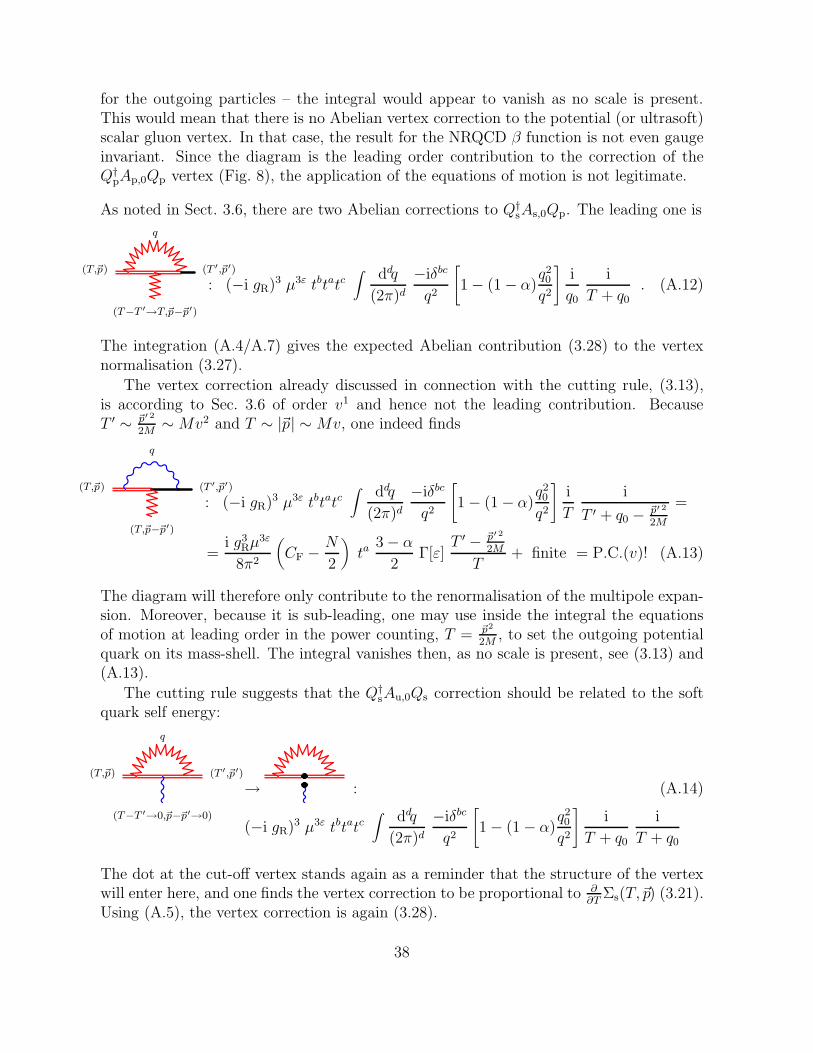
for the outgoing particles – the integral would appear to vanish as no scale is present.This would mean that there is no Abelian vertex correction to the potential (or ultrasoft)scalar gluon vertex. In that case, the result for the NRQCD β function is not even gaugeinvariant. Since the diagram is the leading order contribution to the correction of theQ†

pAp,0Qp vertex (Fig. 8), the application of the equations of motion is not legitimate.

As noted in Sect. 3.6, there are two Abelian corrections to Q†sAs,0Qp. The leading one is

q

(T,~p) (T ′,~p′)

(T−T ′→T,~p−~p′)

: (−i gR)3 µ3ε tbtatc∫ ddq

(2π)d

−iδbc

q2

[

1 − (1 − α)q20

q2

]

i

q0

i

T + q0. (A.12)

The integration (A.4/A.7) gives the expected Abelian contribution (3.28) to the vertexnormalisation (3.27).

The vertex correction already discussed in connection with the cutting rule, (3.13),is according to Sec. 3.6 of order v1 and hence not the leading contribution. BecauseT ′ ∼ ~p′ 2

2M∼Mv2 and T ∼ |~p| ∼ Mv, one indeed finds

q

(T,~p) (T ′,~p′)

(T,~p−~p′)

: (−i gR)3 µ3ε tbtatc∫

ddq

(2π)d

−iδbc

q2

[

1 − (1 − α)q20

q2

]

i

T

i

T ′ + q0 − ~p′ 2

2M

=

=i g3

Rµ3ε

8π2

(

CF − N

2

)

ta3 − α

2Γ[ε]

T ′ − ~p′ 2

2M

T+ finite = P.C.(v)! (A.13)

The diagram will therefore only contribute to the renormalisation of the multipole expan-sion. Moreover, because it is sub-leading, one may use inside the integral the equationsof motion at leading order in the power counting, T = ~p2

2M, to set the outgoing potential

quark on its mass-shell. The integral vanishes then, as no scale is present, see (3.13) and(A.13).

The cutting rule suggests that the Q†sAu,0Qs correction should be related to the soft

quark self energy:

q

(T,~p) (T ′,~p′)

(T−T ′→0,~p−~p′→0)

→ : (A.14)

(−i gR)3 µ3ε tbtatc∫

ddq

(2π)d

−iδbc

q2

[

1 − (1 − α)q20

q2

]

i

T + q0

i

T + q0

The dot at the cut-off vertex stands again as a reminder that the structure of the vertexwill enter here, and one finds the vertex correction to be proportional to ∂

∂TΣs(T,~p) (3.21).

Using (A.5), the vertex correction is again (3.28).

38

Finally, two examples for the straightforward but tedious non-Abelian vertex correctionsof Fig. 9 are given. First, one may calculate the non-Abelian correction to Q†

sAu,0Qs

(T,~p) (T ′,~p′)

(T−T ′→0,~p−~p′→0)

: (−i gR)2 gR µ3ε fabctbtc

∫ddq

(2π)d

i

T + q0

iG0µ(q)

q2

iG0ν(q)

q2×

× [−2q0gµν + qµgν0 + qνgµ0] . (A.15)

The Feynman gauge term, being independent of (1 − α), is zero as expected. For thisdiagram, even the terms proportional to (1−α)2 vanish, which can be shown to be finitein general and hence not to contribute to the vertex normalisation. In (A.15), only thecontribution leading in v is considered. Using the well known relation ifabctatb = −N

2ta

for SU(N), this can be collapsed down by re-writing numerators analogously to (A.9) to

g3R µ

3ε N ta (1 − α) T∫

ddq

(2π)d

1

T + q0

1

q4

[

T 2

q2− 1

]

. (A.16)

One extracts the pole part of the non-Abelian vertex correction as (3.29) from the resultobtained using (A.4):

−i g3R µ

3ε

(4π)2

N

2ta

3(1 − α)

2Γ[ε] + finite. (A.17)

The leading piece of the non-Abelian correction to Q†pAp,0Qp is extracted as

(T,~p) (T ′,~p′)

(T−T ′,~p−~p′)

: (−i gR)2 gR µ3ε fabctbtc

∫ddq

(2π)d

i

q0

iG0µ(q)

q2

iG0ν(q + ∆E)

(q + ∆E)2×

× [2q0gµν + (∆E − q)µgν0 − (q + 2∆E)νgµ0] , (A.18)

where ∆E = (0,~p ′ − ~p ). The term proportional to (1 − α) contains the ultravioletsingularity and can be written as

− g3R µ

3ε N ta (1 − α)∫

ddq

(2π)d

1

q4

1

(q + ∆E)2

(

q20 − q2 − 2E · q

)

. (A.19)

Standard formulae for dimensional regularisation yield as divergent part (3.29). The termproportional to (1 − α)2 is ultraviolet finite and can be reduced to the integral

g3R µ

3ε N

2ta (1 − α)2 ∆E2

∫ddq

(2π)d

q20

q4

1

(q + ∆E)4=

i g3R µ

3ε

(4π)2

N

2ta

(1 − α)2

2. (A.20)

39

References

[1] W. E. Caswell and G. P. Lepage: Phys. Lett. B 167, 437 (1986).

[2] G. T. Bodwin, E. Braaten and G. P. Lepage: Phys. Rev. D 51, 1125 (1995); Phys.

Rev. D 55, 5853 (1997).

[3] M. Nio and T. Kinoshita: Phys. Rev. D 55, 7267 (1997).

[4] A. H. Hoang, P. Labelle and S. M. Zebarjad: Phys. Rev. Lett. 79, 3387 (1997).

[5] A. H. Hoang and T. Teubner: Top Quark Pair Production at Threshold: Complete

Next-to-next-to-leading Order Relativistic Corrections; hep-ph/9801397, 1998 (to bepublished).

[6] A. Pineda and J. Soto: Potential NRQED: The Positronium Case; UB-ECM-PF98/11, KFA-IKP(TH)-98-9, hep-ph/9805424, 1998 (to be published).

[7] C. T. H. Davies for the NRQCD Collaboration: Nucl. Phys. (Proc. Suppl.) 63, 320(1998).

[8] H. Matsufuru et al.: Nucl. Phys. (Proc. Suppl.) 63, 368 (1998).

[9] A. Czarnecki and K. Melnikov: Phys. Rev. Lett. 80, 2531 (1998).

[10] M. Jezabek et al.: Phys. Rev. D 58, 14006 (1998).

[11] E. Braaten: Introduction to the NRQCD Factorization Approach to Heavy Quarko-

nium; hep-ph/9702225, 1997 (talk given at the third International Workshop onParticle Physics Phenomenology, Taipei, Taiwan, 14–17 Nov 1996).

[12] N. Brambilla and A. Vairo: Some Aspects of the Quark-Antiquark Wilson Loop For-

malism in the NRQCD Framework ; hep-ph/9809230, 1998 (to be published in theProceedings of the Euroconference QCD’98 at Montpellier, 2nd – 8th July 1998,Nucl. Phys. B(Proc. Suppl.)).

[13] A. V. Manohar: Phys. Rev. D 56, 230 (1997).

[14] M. Luke and A. V. Manohar: Phys. Rev. D 55, 4129 (1997).

[15] H. W. Grießhammer: Phys. Rev. D 58, 094027 (1998).

[16] M. Beneke and V. A. Smirnov: Nucl. Phys. B 522, 321 (1998).

[17] C. Bauer and A. V. Manohar: Phys. Rev. D 57, 337 (1998).

[18] M. Luke and M. J. Savage: Phys. Rev. D 57, 413 (1998).

[19] B. Grinstein and I. Z. Rothstein: Phys. Rev. D 57, 78 (1998).

40

[20] H. W. Grießhammer: The Soft Regime in NRQCD ; NT@UW-98-12, hep-ph/9804251,1998 (Proceedings of the Workshop “Nuclear Physics With Effective Field Theories”at Caltech, 26th – 27th February 1998, eds. R. Seki, U. van Kolck and M. J. Savage,World Scientific, p. 229).

[21] G. P. Lepage et al.: Phys. Rev. D 46, 4052 (1992).

[22] P. Labelle: Phys. Rev. D 58, 093013 (1998).

[23] N. Isgur and M. B. Wise: Phys. Lett. B 232, 113 (1989).

[24] N. Isgur and M. B. Wise: Phys. Lett. B 237, 527 (1990).

[25] G. Leibbrandt and J. Williams: Nucl. Phys. B 475, 469 (1996).

[26] J. Collins: Renormalization; Cambridge Monographs on Mathematical Physics, CUP(1984).

[27] T. Muta: Foundations of Quantum Chromodynamics ; Lecture Notes in Physics Vol.5, World Scientific (1987).

[28] T. D. Lee: Particle Physics and Introduction to Field Theory ; revised and updatedfirst edition, Contemporary Concepts in Physics Vol. 1, Harwood Academic Publish-ers (1988).

[29] T. Mehen and I. W. Stewart: Radiation Pions in Two-Nucleon Effective Field The-

ory ; CALT-68-2210, nucl-th/9901064, 1999 (to be published).

[30] K.-C. Lee and S.-L. Nyeo: J. Math. Phys. 35, 2210 (1994).

[31] P. Ramond: Field Theory: A Modern Primer ; Frontiers in Physics Vol. 74, AddisonWesley (1990).

41