Power Aware Simulation Framework for

Wireless Sensor Networks and NodesJohann Glaser, Daniel Weber, Sajjad A. Madani, and Stefan Mahlknecht

Abstract—The constrained resources of sensor nodes limitanalytical techniques as well as cost-time factors limit testbeds to study wireless sensor networks (WSNs). Consequently,simulation becomes an essential tool to evaluate such systems. Wepresent the PAWiS (Power Aware Wireless Sensors) simulationframework that supports design and simulation of wireless sensornetworks and nodes. The framework emphasizes power consump-tion capturing and hence the identification of inefficiencies invarious hardware and software modules of the systems. Thesemodules include all layers of the communication system, thetargeted class of application itself, the power supply and energymanagement, the central processing unit (CPU), and the sensor-actuator interface. The modular design makes it possible tosimulate heterogeneous systems. PAWiS is an OMNeT++ baseddiscrete event simulator written in C++. It captures the nodeinternals (modules) as well as the node surroundings (network,environment) and provides specific features critical to WSNs likecapturing power consumption at various levels of granularity,support for mobility and environmental dynamics as well as thesimulation of timing effects. A module library with standardizedinterfaces and a power analysis tool have been developed tosupport the design and analysis of simulation models. Theperformance of the PAWiS simulator is comparable with othersimulation environments.

I. INTRODUCTION

The advances in distributed computing and Micro-Electro-

Mechanical Systems (MEMS) has fueled the development

of smart environments powered by wireless sensor networks

(WSNs). WSNs face challenges like limited energy, memory,

and processing power and requires detailed study before

deploying them in the real world. Analytical techniques,

simulations, and test beds can be used to study WSNs.

Though analytical modeling provides a quick insight to study

WSNs, it fails to give realistic results because of WSN-specific

constraints like limited energy and the sheer number of sensor

nodes. Real world implementations and test beds are the most

accurate method to verify the concepts but are restricted by

costs, effort, and time factors. Simulations provide a good

approximation to verify different schemes and applications

developed for WSNs at low cost and in less time. The

available simulation frameworks are either general purpose

or WSN specific. The general purpose network simulators do

not address WSN specific unique characteristics while WSN

specific simulators mostly lack the capability of capturing and

analyzing the power consumption and timing issues at the

desired level of granularity.

The proposed PAWiS simulation framework [WGM07],

[GW07] assists in developing, modeling, simulating, and op-

Institute of Computer Technology, Technical University of Vienna

Email: {glaser,weber,madani,mahlknecht}@ict.tuwien.ac.at

timizing WSN nodes and networking protocols. It particularly

supports detailed power reporting and modeling of wireless

environments. A typical WSN node may comprise various

types of sensors (e.g., temperature, humidity, strain gage,

pressure), a processing unit (CPU) with peripherals, and a

radio transceiver. The simulation covers the internal structure

of these nodes as well as communication among them. Sensor

nodes forming a network communicate with each other via

an ad-hoc multi-hop network. The range of applications that

can be simulated covers many domains such as building

automation, car interior devices, car-to-car communication

systems, container monitoring and tracking, and environmental

surveillance.

The PAWiS simulation framework provides a way to reduce

the overall power consumption by carefully optimizing various

design aspects within the context of the application. Enhanc-

ing energy performance could propel many new applications

since the lack of sufficient battery lifetime or limited energy

scavenging systems are still the main causes for the slowly

spreading number of WSN applications.

In previous research performed at the Vienna University of

Technology [MGH05], several weaknesses of current WSN

nodes were identified. These include the wakeup problem

(i.e., how to wakeup a sleeping node), the voltage matching

and power supply problem, the fairly long oscillator start-

up time, and other hardware related problems. However,

overall efficiency also strongly depends upon the application

and its interaction with other nodes and the environment.

Here, communication protocols play an important role, but

considering the different layers of protocols independently and

not taking into account adjacent layers as well as the hard-

ware and environment, improvements can only be sub-optimal

[MMG07b]. PAWiS explicitly supports cross layer design to

exploit the synergy between layers. Several aspects regarding

power aware wireless sensors are emphasized and directly

supported by the PAWiS framework. The PAWiS framework

hence helps to capture the whole system in one simulation

and extracts power consumption figures from software and

hardware modules uncovering leakages in early design stages.

The main contributions of this work are

• to equip the user to program models of a wide variety of

abstraction,

• to model the internals of WSN nodes as well as the com-

munication between them. The framework distinguishes

between software and hardware tasks, yet it is easy to

change the hardware/software partitioning,

• An elaborate power simulation with any level of accu-

racy which can still be balanced with complexity. The

simulated power consumption can depend on the supply

voltage, e.g., for a nearly empty battery when supplying

a microcontroller that operates at very low voltages. In

WSN nodes components with different supply voltages

are combined resulting in the need for LDOs (low dropout

regulators) and DC/DC converters. The PAWiS Frame-

work allows to model this hierarchical supply structure

as well as the efficiency factor of the converters.

• Powerful analysis and visualization techniques are pro-

vided to evaluate the simulation results and derive a path

to optimization.

• The RF communication is modeled according to real-

world wave propagation phenomena while still main-

taining an efficient simulation. It includes interferers,

noise, and attenuation due to distance to influence the bit

error ratio of communication links. No preset topology is

required because the packets are transmitted to all nodes

within reach. The topology of network communication

itself originates from the link quality and the routing algo-

rithm. With this approach any routing protocol, especially

ad-hoc protocols, can be implemented. The transmission

model implementation is entirely independent of the

underlying modulation format enabling the simulation of

any type of modulation. Multiple participants can utilize

the RF channel by multiple access schemes and are

separated by space, time, frequency, and code.

II. RELATED WORK

To have credible results through simulation, the choice of

models and the simulation environment is very important.

Key properties for WSN simulators must include: a way to

capture energy consumption at any level of abstraction, a

powerful scripting language, graphical user interface (GUI)

support to animate, trace, and debug, and the ease to integrate

new modules. Some of these key properties are discussed in

[LAS+05].

NS-21 is a discrete event, object oriented, general purpose

network simulator written in C++. According to [KCC05], it

is the most widely used simulator and has a rich library of

protocols but focuses mainly on IP networks. OTcl [WL95]

is used as scripting language to control and configure simula-

tions. It provides a GUI support with the Network Animator

(Nam) which is not so good and only reproduces NS-2

trace [LAS+05]. For WSN, NS-2 does not scale well, and

it is difficult to simulate 100+ nodes [NG03]. NS-2 lacks

detailed support to measure the energy utilization of different

hardware, software, and firmware components of a WSN node.

“One of the problems of ns2 is its object-oriented design

that introduces much unnecessary inter-dependence between

modules. Such interdependence sometimes makes the addition

of new protocol models extremely difficult, which can only

be mastered by those who have intimate familiarity with the

simulator” [CBP+06].

SensorSim [PSS00] is a NS-2 based simulator for modeling

sensor networks. The authors have provided a power model,

a battery model, and a CPU model to address sensor network

1http://www.isi.edu/nsnam/ns/

specific constraints but because of the “unfinished nature of

the software”2, the simulator is no longer available.

OMNeT++3 [Var01] is a discrete event, component based,

general purpose, public source, modular simulation frame-

work written in C++. It provides a strong GUI support for

animation and debugging. The mobility framework (MF) (

[DSH+03]) for OMNeT++ is a specific purpose add-on to

simulate ad-hoc networks. In the MF, the links between pairs

of neighbor nodes are specified with OMNeT++ gates with the

help of an additional global module called Channel Control.

Unlike “visible communication paths” which are created and

freed in bulk, the Air module of the PAWiS framework (see

Sec. III-C7) decides about connection between pairs of nodes

dynamically based solely on their position information and

other radio transmission effects. Another difference is the

capturing of power consumption with the Power Meter (see

Sec. III-C8) that helps to identify major energy consuming

modules. OMNeT++/MF does not provide a WSN specific

module library [LAS+06] which can help expedite the design

process.

SenSim [MSK+05] is an OMNeT++ based simulation

framework for WSN. Some protocol layers and hardware

units are implemented as simple OMNeT++ modules. They

have provided implementations for different WSN specific

protocols, battery, a simple CPU implementation, a simple

radio, and a wireless channel. A coordinator module is im-

plemented to assist in inter-communication between hardware

and software modules. It does not add additional functionality

to OMNeT++ other than a simulation template with a small

number implemented modules.

NesCT4 is an add-on for OMNeT++ which allows the

simulation of TinyOS5 based sensor networks in OMNeT++.

It does not come with any additional functionality but acts

as a language translator between two different environments

(TinyOS and OMNeT++).

Global Mobile Information System Simulator (GlomoSim)

[ZBG98] is a library based general purpose, parallel simulator

for wired and wireless networks written in Parsec6 (C-based

discrete event simulation language for parallel programming).

Being parallel, it is highly scalable and can simulate up to

10,000 nodes [LAS+05]. Using GlomoSim requires learning

the new language Parsec. GlomoSim is superseded by Qual-

Net7, a commercial network simulator and is not released with

updated versions since 2000. However, sQualNet [VXSB07],

an evaluation framework for sensor networks, built on the top

of QualNet has been released recently.

OPNet Modeler8 is a commercial, well-established (1986),

general purpose, object oriented simulation environment writ-

ten in C++. It supports discrete event, hybrid, and analytical

simulation. It provides a very rich set of modules for all layers

of protocol stacks including the IEEE 802.11 family, IEEE

2http://nesl.ee.ucla.edu/projects/sensorsim/3http://www.omnetpp.org/4http://nesct.sourceforge.net/5http://www.tinyos.net/6http://pcl.cs.ucla.edu/projects/parsec/7http://www.scalable-networks.com/8http://www.opnet.com/

802.15.4, and routing protocols like AODV [PR99] and DSR

[JM96]. Each level of the protocol stack has to be implemented

as a state machine but it is “difficult to abstract such a

state machine from a pseudo-coded algorithm” [CSS02]. The

authors in [CSS02] compared OPNet Modeler, GlomoSim, and

NS-2 with a broadcast protocol. The results show that the

performance of NS-2 and GlomoSim, and OPNet are barely

comparable.

SENSE [CBP+06] is a sensor network specific, component

based simulator written in C++ built on the top of COST

[CS02]. To address the issue of scalability, SENSE provides an

optional way for parallel simulation as is done in GlomoSim.

It provides a small library of module implementations like

AODV and DSR, with simplistic battery and power models

but unlike PAWiS it does not provide a detailed structure

to capture energy consumption of different hardware and

software components. It also lacks a visualization tool which

is helpful in debugging and visual inspection.

Ptolemy II [LLL01] is a component assembly based soft-

ware package to study concurrent, real time, and heteroge-

neous embedded systems and is written in Java. Ptolemy

II provides a rich support to model, simulate and design

components in different domains (e.g., discrete time or com-

ponent interaction), but according to recent Ptolemy II 7.0.beta

release notes9, its wireless domain is still in experimental

phase. VisualSense [PBLLZ04] is an open source WSN visual

simulation framework built on Ptolemy II.

J-Sim [MNZZ97] is a general purpose, component based,

open source simulation framework written in Java. It is glued

to different scripting languages with TCL/Java and hence is

a dual language framework like NS-2. Initially, designed for

wired networks, its WSN specific package provision supports

only 802.11 MAC scheme and some high level models e.g.,

battery, CPU, wireless channel, and sensor channel.

Various WSN specific simulation and emulation tools

have been released in the previous years. These tools in-

clude TOSSIM [LNWD03], EmStar [GSR+04], and ATEMU

[PBM+04]. The advantage of using such tools is that the

code that is used for simulation/emulation also runs on the

real node (with minor modifications) reducing the effort to

re-write the code for the sensor node and giving detailed

information about resource utilization. The main problem with

such frameworks is that “the user is tied to a single platform

either software or hardware (typically MICA motes), and

to a single programming language (typically TinyOS/NesC)”

[LAS+05]. Tython [DLJ+05] and PowerTossim [SHC+04]

are extensions of Tossim to capture the dynamic behavior of

environment and power consumption respectively.

In contrast to many of the above frameworks, the PAWiS

Simulation Framework meets all the key properties outlined in

[LAS+05]. It utilizes the powerful GUI support of OMNeT++,

it utilizes the widely used scripting language Lua10 to include

environmental dynamics and mobility, and to reduce the test-

debug cycle. It focuses on capturing energy consumption at

hardware and software level, it provides a visualization tool

9http://ptolemy.berkeley.edu/ptolemyII/10http://www.lua.org/

to analyze energy consumption, a rich library of modules to

get an optimized protocol stack, standardized interfaces to

improve re-usability, and it provides a simulation template for

the user to jump start any simulation study.

III. SIMULATION FRAMEWORK

A Wireless Sensor Network is built of independent nodes

which communicate via an ad-hoc wireless network. The

PAWiS Simulation Framework is designed to model, simulate

and optimize both, the wireless communication protocols as

well as the interior of the nodes. Each node is built as a

virtual prototype in a way that its function, timing, and power

consumption as well as system failures are simulated at any

level of detailedness.

A. Methodology

The design of a WSN and its nodes follows a top-down

approach embedded in a cyclic process. The functional speci-

fication defines requirements of the WSN which apply to the

architecture as well as to the implementation. The implementa-

tion on the other hand imposes constraints on the architecture

and the functional specifications in a bottom-up manner. For

example, the functional specification of a tire pressure mon-

itoring system (TPMS, see also Sec. VI-B) may require the

sensors to measure the current pressure every 20 seconds. Due

to the power consumption of the current sensor technology and

the available battery capacity the implementation of a TPMS

sensor node imposes the constraint that this function can only

be maintained for 2 months, which is rather short compared

to the lifetime of a tire.

1) Work flow: To design a WSN and its nodes the functional

specification is defined. For a full optimization the work flow

is a cyclic application of the following steps.

a) Every node typically consists of multiple sub-modules.

In this step the node structure is defined and for ev-

ery module type a certain implementation is chosen

(composition). Initially, the modules only need to meet

minimum functional requirements. For instance, for the

aforementioned TPMS node, the user chooses a CPU,

a pressure sensor, an AD converter, a timer, an RF

transmitter and memory. Additionally, software modules

like the network stack and sensor handling are required.

b) The modules chosen in the previous step are integrated.

Their interfaces have to be adopted and their functions

must be coordinated. For example the chosen pressure

sensor might require special treatment for its power-on

sequence, which must be implemented accordingly in

the module which operates it.

c) The modules are configured, that includes setting values

for the clock frequency of the CPU, the resolution of

analog-to-digital converters (ADCs), etc.

d) In the previous steps a fully functional model of a node

and the network was setup and is simulated in the current

step.

e) The simulation results are evaluated. This includes

the verification of the function, analysis of the power

consumption and timing, and detection of potential for

further optimization (see Sec. V).

f) The issues identified in the previous step are consid-

ered for a refinement of the models as well as the

design. Examples are increasing the detailedness and

accuracy of power consumption and timing, dividing the

functionality into more elaborate modules, configuration

changes and even a modification of the node com-

position by exchanging module implementations. The

chosen pressure sensor might consume too much energy

in every measure cycle due to its long lasting power up

sequence and hence should be exchanged by a sensor

with faster startup. Another example is the physical layer

model (including the RF transceiver) which might need

a refinement of the power consumption reporting during

intermediate states (e.g., when switching from transmit

to receive mode) (see Sec. III-C8). With the refined node

implementation the procedure is started over again, until

the optimization goal is achieved.

These refinement cycles are the main track to enhance the

development and design [MGH05]. After completing the op-

timization process the final outcome comprises the verified

function, the architecture of the node, the implementation

details, and the power specification of every module.

The module library (see Sec. IV) is particularly intended

for the composition and integration of modules to a node. It

provides a collection of multiple module implementations for

every module type which can be combined in numerous ways.

The integration effort is minimized because these modules

conform to the interface specification (Sec. IV-B).2) Optimization: Several strategies for the optimization of

WSN nodes are proposed in [MGH05]. The PAWiS simulation

framework is especially constructed to assist the designer in

applying these strategies.

• System level optimization involves a modification of the

whole system behavior like choosing a different network

layout or application patterns.

• Exchanging the module implementation by selecting a

different module from the library. For example choose a

dual-slope, a Σ∆ or an successive approximation ADC.

Another example is to change a communication layer

implementation (e.g., use another medium access (MAC)

protocol).

• Exchanging multiple module implementations for adja-

cent modules that tightly work together. While modifying

a single module might degrade the node performance, the

interaction of the changes of multiple modules potentially

leads to an overall improvement.

• Cross-layer optimization works on more than one net-

work layer where e.g., modifying the routing protocol

benefits from a different physical layer.

• Partitioning of modules and/or functions by dividing the

task between hardware and software, digital and analog,

or RF and baseband. For example, a specific MAC

protocol could be implemented in software, as dedicated

hardware acceleration unit, or a combination of both.

• Scaling a module, e.g., the resolution of an ADC or the

register count of a CPU.

• Parameterization of modules, e.g., the timing, transmis-

sion power and bit rate of a radio transceiver.

B. Structure

The PAWiS simulation framework is based on the

OMNeT++ discrete event simulator [Var01] which is written

in the C++ programming language (Fig. 1). A discrete event

simulation system operates on the basis of chronological

consecutive events to change a system’s state. These events

are processed by the simulation kernel. The simulation time

itself does not progress continuously but is advanced with

each occurring event (hence it is not possible to issue events

that are scheduled before the current simulation time). The

proposed framework handles timing related issues according

to this discrete event mechanism.

User defined models are implemented as C++ classes and

mostly utilize framework concepts. The user of the frame-

work is only confronted with OMNeT++ to comprehend the

simulation process. Node composition and network layout

along with environmental and setup parameters are specified

in configuration files as well as script files (see Sec. III-D).

The modules are compiled and linked with the simulation

kernel and result in the simulation application. This offers a

GUI based frontend which enables visual debugging of the

communication processes of the model on a per-event basis at

simulation runtime. An optional command line based frontend

can be utilized for increased simulation performance.

Model

PAWiS Framework

Air

C++

OMNeT++

CPU PowerManagement

Misc Radio

Executeable Simulator

Programmer

SystemC

GUI

Sensors

Fig. 1. Structure of the PAWiS simulation framework.

The framework is primarily focused on simulating inter- and

intra-node communication. Additionally, fine grained aspects

(e.g., CPU instruction set emulation as used by [PBM+04])

can be easily modeled with user extensions. However a trade-

off between simulation details and execution performance (as

discussed in [HBE+01]) has to be considered with increasing

quantity of network nodes.

A promising feature is the possibility to use SystemC11 in

combination with OMNeT++. This is achieved by combining

the OMNeT++ simulation kernel and the SystemC simulation

kernel in a way that events from OMNeT++ and SystemC are

being processed together. This also allows the communication

11http://www.systemc.org/

between both domains. OMNeT++ allows the use of a custom

scheduler which is the central point to merge the messages and

events of OMNeT++ and SystemC, respectively. Unfortunately

the OSCI SystemC kernel does not offer such an interface, so

slight modifications in the source code were necessary.

Simulation results comprise timing and power consumption

profiles as well as event records. The completed model itself

contains information regarding the functional description and

architecture specifications along with low level implementa-

tion details.

C. Basic Concepts

1) Modularization: A wireless sensor node is typically

composed of multiple modules (e.g., CPU, timer, radio, net-

work layers). Internally every module is based on one or more

tasks. The framework defines two types of tasks: One type

models a hardware component (e.g., a timer, an ADC) whereas

the second type is a software task, e.g., application, routing,

MAC, and physical layer. Every module is implemented as

a C++ class derived from a framework base class. Tasks

are implemented as methods within a module class. The

execution of a single task is sequential but all active tasks are

running in parallel. This form of concurrency is implemented

as cooperative multi-threading, where the program flow is

suspended within a method when certain framework calls are

made (e.g., to wait for some condition to be satisfied) and

will continue execution after being dispatched again. This

process is transparent for the user and entirely handled by

the framework.

Basically the detailedness and granularity of the sensor

node model strongly depends on the design and simulation

requirements for hardware and software modules and is not

restricted by the PAWiS framework.

2) Functional Interfaces: Control flow transitions between

two modules are specified by so called Functional Interfaces

(FI). They can be thought of as subroutines with well known

names and parameter specifications. An invocation of an

FI is similar to a blocking subroutine call but may exceed

the module boundary. The framework allows the passing of

arguments to and from FIs. In the model, FIs are implemented

as class methods (similar to tasks).

A collection of FIs grouped together under a well known

name can be thought of as a functional module type de-

scription. This introduces a level of abstraction in the func-

tional design process and hence enables reusability of func-

tional design. Two modules that are completely satisfying the

specification regarding their FIs can said to be functionally

equivalent (although they might have entirely different power

consumption and timing profiles). This approach is utilized in

the Module Library (see Sec. IV).

3) CPU: As already mentioned in Sec. III-C1 tasks can

either model hardware or software. Software tasks of sensor

nodes are executed by a CPU. It is important to note that

multiple software tasks can not run in parallel, since typically

only one CPU is available and supported by the framework.

The CPU module of the framework ensures that only one

task’s code simulation is executed at a time.

To model the power consumption and timing behavior of

software tasks the PAWiS simulation framework splits the

simulation into two parts. The functional part is implemented

in the C++ method of the task. The timing and power

consumption part, on the other hand, is delegated to the CPU

module which maintains its power consumption and delays

execution of the software task for the calculated processing

time (the time that the code execution on the CPU would

take). This means that the whole functional part is executed at

the very same simulation time instant. The model programmer

has to insert special framework requests to the CPU module

to simulate the execution time and power consumption.

These requests include the estimated execution time of the

firmware code on the CPU. Now think that the CPU of a

given node should be replaced during the optimization process.

This would also require to modify all execution time estimates

in all modules of the node. To allows for a CPU exchange

without the need to adapt other modules the execution time

estimates are referred to the so called norm CPU. This is an

imaginary but well defined CPU implementation (regarding

its performance). The actual CPU model scales its processing

time and power consumption according to its individual prop-

erties. For higher accuracy the CPU request also supplies the

percentage of integer, floating point, memory access and flow

control operations.

Many microcontrollers used for WSN nodes have CPUs

which offer special low-power modes. The PAWiS Simulation

Framework also supports modeling of these states. This is done

by pausing code execution and setting the power consumption

of the CPU module to a lower value. To exit the low-power

mode an interrupt can be issued.

4) Timing: Modeling time delays differ whether they occur

in firmware or hardware modules. For hardware modules

the framework provides a simple wait method to suspend

execution for a certain amount of time. Several distinct im-

plementations of the wait method are available with support

for fixed and conditional timeouts.

Using wait is not valid for software tasks because it is not

possible to wait and do nothing in software (even for an infinite

loop without body the CPU does something). In fact, if delays

are needed in software, the corresponding module has to use

a loop (or a similar construct) to wait for a certain time and

therefore utilize the CPU to achieve the delay. The framework

offers a variety of methods to utilize the CPU for timing and

flow control purposes. Alternatively the CPU can be put to

a low-power mode which stops execution too and therefore

delays until an external or timer event occurs.

An important consequence of this timing model is that

consecutive user code lines without a wait call or a CPU

utilization request take place in the same simulation time

instant (i.e., no simulation time elapses during that code

execution). Simulation time only advances when these special

methods are invoked.

5) Interrupts: The framework provides a basic mechanism

to model interrupt handling in a two-step process that maps

• interrupt sources to interrupt vectors and

• interrupt vectors to interrupt service routines.

Whenever an interrupt request is issued, the framework han-

dles the necessary task scheduling according to the interrupt

priorities and the currently running task.

The implemented interrupt model supports several user

configurable interrupt sources (potentially coming from differ-

ent modules, e.g., a timer, an analog-digital-converter, etc.).

Each of these sources are mapped to an interrupt vector.

Additionally, it is possible to map multiple sources to one

specific interrupt vector. Furthermore, every vector maintains

a priority and an interrupt service routine (ISR). As the model

allows multiple vectors to share one ISR, the framework

provides means to identify the triggering vector from the ISR.

The framework’s CPU module entirely handles the interrupt

processing except for prioritizing of interrupt vectors that

needs to be provided in the user model by overriding the CPU

base class.

The user can register ISRs for interrupt vectors within

software modules. When interrupt sources trigger interrupt

requests, the CPU module determines the appropriate interrupt

vector, checks its priority and if appropriate transfers control to

the ISR (which is always a software task). In case of a control

transfer, the currently executed CPU task is preempted and

continues execution after the ISR has finished.

6) Environment: All sensor nodes are placed at 3D posi-

tions within the Environment. This is a representation of the

outer world and surroundings of all nodes including the RF

channel.

SensorNode

VibrationTemperature

Light Source

User Interactivity

RF - Channel

Energy

Sink

VelocityDirection

Dynamics

Environment

Environment Properties

Node Properties

PositionThicknessMaterial

Obstacle

Fig. 2. The Environment with properties, objects and sensor nodes.

Besides the nodes themselves, additional objects like walls,

floors, trees, interferers, heaters, light sources, global prop-

erties (e.g., the attenuation exponent b (see Sec. III-C7)),

and more the like are defined within the environment. The

entire Environment can be configured with configuration and

scripting files.

7) Air: The Air is an essential part of the Environment

to handle the RF channels, which are defined by 3D node

placement in space and obstacles between the nodes. A real RF

signal is subject to wave propagation phenomenons like attenu-

ation, reflection, refraction and fading (multi-path propagation)

from the transmitter to the receiver. In the PAWiS simulation

framework these effects can be modeled but currently we use

a distance based path loss radio model, which only consider

the distance between transmitter and receiver.

The packet transmission is modeled without the definition of

a predefined topology (similar to a wired network). Instead of

that, every RF message is transmitted to all other nodes and the

received RF power is calculated from the transmitter power,

antenna properties and especially the distance and obstacles

between the transmitter and the receiver. The topology of the

network results from the reachability between nodes which is

limited by the minimum received signal quality.

a) Signal Power: The received signal power of a node

is proportional to the transmitter power, only scaled by wave

propagation effects and node properties. These constant at-

tenuation factors between all nodes can be conflated to a

matrix which is referred to as Adjacency Matrix within the

framework. A simple row multiplication is used to calculate

the received signal power for all nodes. The matrix is a pre-

cisely defined interface from the Environment setup (i.e., node

positions, obstacles) to the data communication. Therefore, it

can also be calculated by an external RF channel simulation

tool.

The current implementation of the Air supports only

isotropic antennas with uniform antenna gain. Obstacles are

considered for the adjacency matrix by explicitly given ad-

ditional attenuation factors between pairs of nodes in the

Environment configuration.

b) Packet Transmission: Whenever a data packet is trans-

mitted by a node, the Air calculates the received signal power

for all other nodes and notifies every node (above a certain

threshold) about the start of the transmission. All nodes,

with a receiver currently in listen mode and which expect a

reasonable signal quality, confirm. During the transmission,

the receiving nodes calculate the signal to noise ratio (SNR)

between the received signal power Psignal and the received

and internal noise power Pnoise: SNR = PsignalPnoise

.

From this SNR, the bit error ratio (BER) is calculated, which

is a function of the SNR depending on the (fixed) modulation

format (the formula can be provided by the user). From the

BER and the bit length of the transmission, the bit error count

is calculated. Consequently, the user’s module decides whether

the received packet is valid or treat it as corrupted.

From the size of the transmitted data packet and the bit

rate, the Air calculates the duration for the transmission. At

the time when the transmission is finished, the Air notifies all

receiving nodes again. This notification contains the user data,

its length and the number of bit errors. Additionally, as some

protocols decide whether to process an incoming packet after

the arrival of some header fields, the framework provides a

mechanism to stop listening to a transmission after a specified

number of bits have arrived.

c) Collisions: If a node starts to send a packet while

another packet is already being transmitted, this second signal

is uncorrelated to the first sender. The framework models this

signal as noise and therefore decreases the SNR at the receiver

of the first packet. Such events can happen several times during

the reception of a data packet, therefore, the receiver has

to deal with changing SNR throughout the packet receiving

process. The final count of bit errors thus results from this

sequence of different SNR values and is assembled from the

portions of constant SNR. So the bit errors are accumulated

for all portions of the packet with constant SNR. The user

has to provide the method to calculate the bit error count for

a constant portion of SNR, everything else is handled by the

framework.

d) Multiple Access: To utilize the RF communication

by multiple participants, three multiple access methods are

supported. For separate services it is likely to utilize different

frequency bands (e.g., the 2.4 GHz ISM band and the 868 MHz

ISM band). Within these bands a separation using dedi-

cated frequency channels (frequency division multiple access,

FDMA) is typically implemented to increase the number of

nodes sending in parallel. The same purpose is served by

overlaying the RF signals in time and frequency domain but

coding these with different keys (code division multiple access,

CDMA). These three multiple access schemes are generalized

by the framework. The user provides a function to implement

the adjacent channel interference which handles the filter

suppression ratio or the coding gain. This is incorporated by

the Air to calculate signal and noise power and consequently

the SNR. The other two common multiple access formats,

space and time division multiple access (SDMA, TDMA) are

supported trivially due to the principle of the Air.

8) Power Simulation: A key feature of the framework

(regarding PAWiS requirements) is given by the power con-

sumption simulation of tasks. Therefore, a central Power Meter

object logs the power consumption values that are reported by

all modules of all nodes. Only tasks that simulate dedicated

hardware directly report power consumption. Software tasks

report their CPU utilization and the CPU module calculates its

power consumption and reports it on behalf of the requesting

task.

Every hardware task that consumes power reports this to

the central reporting facility. It can have different electrical

behavior, i.e., the current I depends in different ways on the

supply voltage U . The current can be constant and therefore

independent of the supply voltage. A resistive behavior (I =UR ) and a combination (I = Iconst + U

R ) can be modeled.

Additionally a user defined, e.g., non-linear characteristic can

be implemented and is supported by the framework. The power

consumption as well as the electrical behavior can be updated

by a task at any point in time.

The reporting of power consumption is accomplished by

calls to special methods offered by PAWiS framework classes.

The model programmer has to provide the appropriate fig-

ures (current, equivalent resistance). These numbers can be

determined in several ways. The most accurate numbers result

from measurements of real-world devices (e.g., a test chip or

prototype PCB) which should be modeled with the PAWiS

framework (though this requires the device to be already

available). Alternatively the user can obtain the consumption

parameters by electrical simulations of the circuitry using,

e.g., Spice. This is particularly interesting if the model is

programmed in parallel to designing the chip of the planned

module. For commercially available components (e.g., a mi-

crocontroller or RF transceiver) the data sheet provides the

appropriate power consumption values.

It is important to mention that modules of a sensor node

don’t consume constant power throughout their lifetime. On

the contrary, the power consumption varies with the operating

state. For example, the CPU consumes less power when being

in sleep mode (and hence doesn’t execute instructions), the

power consumption of the radio differs whether in transmit,

in receive, in PLL-locked or in idle mode. The model pro-

grammer has to report new power consumption figures every

time the state of the module changes.

The framework supports the modeling of a supply hierarchy

where the power input of a module (e.g., an ADC) is supplied

by the power output of another module (e.g., an LDO). Since

a power supply has varying efficiency according to load and

input voltage as well as non-zero output resistance, its output

voltage and internal consumption are calculated from its output

current. This output current is the sum of all supply currents

of the supplied modules. Additionally, the framework provides

a mechanism to specify different power supply behaviors

(particularly the output resistance). This power consumption

model results in a simple electrical network.

During the simulation, a task calculates its current, reports

this to its power supply and is notified about the actual

input voltage by the power supply in return. Most of this

is handled automatically by the framework. This mechanism

recursively propagates up the supply tree (breadth-first) and is

finally reported to the central Power Meter which stores this

values to an external data file. In this way for every module

and task of every node in the simulated WSN, the power

consumption is calculated and logged. With this approach the

power consumption of the whole node is covered and the

simulation results plausibly reflect the reality. These results

are analyzed and visualized by the Data Post Processing Tool

(see Sec. V). So the power simulation values are not actively

evaluated during the simulation run but analyzed after the

simulation is finished.

D. Dynamic Behavior

The PAWiS framework supports dynamic behavior (e.g.,

mobility, environmental dynamics) via an embedded scripting

language. Generally, scripting languages are platform inde-

pendent and need a virtual machine for execution. Although,

it degrades execution time compared to compiled languages,

it enables code adjustments and algorithm tweaks even at

runtime. Scripting languages can be considered as high level

languages as they usually feature dynamic typing, implicit

memory management (garbage collection), and often multi-

threading or support for coroutines intrinsically. An application

utilizing an embedded scripting engine needs to provide glue

code12 in order to make internals accessible via scripts. For

the PAWiS framework, the scripting language LUA13 [RI96]

has been chosen due to its simplicity, extensibility, widespread

usage, large community, fast execution, and maturity.

A large portion of the PAWiS framework’s basic function-

ality is glued to the scripting engine. A main part comprises

12Glue code is code that does not provide additional functionality but

“glues” application specific objects or functions to the scripting engine.13http://www.lua.org/

the module’s flow control and power consumption function-

ality which enables the user to provide Functional Interfaces

entirely in the scripting language. This is intended to serve

as a rapid prototype development scheme without the need

to re-compile the entire simulation. Scripts can be hooked to

various events fired by the framework, e.g., for setup purposes

scripts can be hooked to node or network creation events.

Usually simple topologies can be setup with the OMNeT++

intrinsic Ned language but more complex topologies can be

created utilizing these initialization scripts with less effort.

PAWiS scripts can be used to interface with the framework

on network-wide and intra-node levels during runtime or in

the network setup phase.

A real-world scenario for the necessity of introducing dy-

namic behavior of sensor nodes is shown in Fig. 3 where

two cars are passing each other. Each car is equipped with

a WSN and both networks affect each other when they come

close. In order to simulate and observe this simple yet realistic

Fig. 3. Two cars equipped with wireless sensor networks passing each other.

scenario, it is necessary that the two networks can be moved at

a certain velocity and in some direction during runtime. This

is achieved by grouping the nodes in two distinct networks and

then moving these groups via a script in opposite directions.

When sensor nodes change their position in space, the PAWiS

framework automatically handles the respective change in the

network connectivity and the signal strengths without the need

of user intervention (i.e., no method needs to be called to

update the adjacency matrix). Accordingly, the radio model is

rendered dirty and recalculated when the next activity on the

air occurs.

Besides mobility, scripting is useful to handle dynamic and

reproducible effects that occur within the sensor network’s

environment [DLJ+05]. Generally, sensors (even simulated

ones) need to monitor a certain phenomenon. Although the

PAWiS simulation framework does not provide a detailed

model to capture phenomena (e.g., humidity, and luminance) it

defines an abstract interface for sensors and the environment.

This sensor/phenomenon pair is handled like a typical sub-

scriber/producer pattern. Sensors subscribe to a phenomenon

to get it’s current value and will be notified of changes instead

of frequently polling the phenomenon thus reducing the com-

putational load. The timing behavior of the notification can

be setup (e.g., an update frequency or whenever a significant

change of a phenomenon’s value occurs) for each sensor

individually. Sensor properties maintained by the framework

are the position of the sensor and its orientation in 3D space.

Whenever a sensor reads its associated phenomenon’s value,

these properties affect the reading as they define the distance

and whether the sensor is facing the value’s source.

The semantic of the environmental values has to be intro-

duced by the user of the framework. Though this can be done

with C++, it is recommended to use scripts for the environment

model as it is more portable and can be exchanged easily

for a simulation run. With the help of scripts, even complex

environmental scenarios can be easily modeled and simulated.

Additionally, the framework supports the usage of pre-logged

data that can be used as values for phenomena. Currently,

effects of interest within the intended field of application

for the framework comprise day and night cycles, season

changes, weather conditions, and phenomena that support

energy scavenging mechanisms.

Utilizing scripting for environment and phenomena as men-

tioned above introduces reproducible pseudo realistic (opposed

to pseudo-random) values to the simulation. While further

methods to support more accurate and realistic values exist

some of them come up with inherent drawbacks (at least

for the targeted field of application). The EmStar [GSR+04]

framework has the ability to use a hybrid simulation scheme to

provide realistic sensor readings. This means that it uses real

sensor readings as input for the simulation. While this brings

real-world values into the simulation, it can not be reproduced

over multiple simulation runs. Furthermore, it is not possible to

simulate large time spans, e.g., when season dependent effects

need to be considered or the intended network lifetime is up

to a year or more.

IV. MODULE LIBRARY

The implementation within a module has to meet the specifi-

cation of the Functional Interfaces according to the type of the

module. This forms another key idea of the modeling process,

i.e., to provide a library with various distinct implementations

for a specific module type. The resulting library can be used

to evaluate, refine, and test architectural issues of the user’s

model. We provide a module library for the proposed protocol

architecture (see Sec. IV-A). These modules can be used in any

combination to get an optimized protocol stack for a particular

application. Protocol architecture and standardized interfaces

(discussed below) make it easy to integrate new modules or

interchange different implementations to get optimized results.

A. Protocol Architecture

The wireless communication characteristics (mobility,

rapidly changing link quality, limited resources, and environ-

mental obstructions) and new design paradigms (e.g., wake-

up radio) motivates to divert from traditional layered archi-

tectures. At the same time “plug and play” like features of

the layered architecture are important for extensibility and

interchangeability.

Physical Layer

Network Layer

Transport Layer

Application Layer

Link Layer

Secu

rity

Man

agem

ent

Cro

ss L

ayer

Man

agem

ent

Ener

gy M

anag

emen

tK

ey M

gmt.

Serv

ices

Dat

abas

eSe

rvic

es

Sche

dulin

gA

lgor

ithm

s

Applications

Nod

e M

anag

emen

t

Fig. 4. WSN protocol architecture.

We define a protocol architecture [MMG07a] which pro-

vides the benefits of traditional layered architectures [KK05]

and focuses on exploiting synergy across layers (e.g, to extend

network life time) [SL06]. The proposed architecture (see

Fig. 4) comprises traditional layers (application, transport,

network, link, and physical layer) with management planes

(cross layer, energy, security, and node). All layers and planes

are connected through well defined interfaces.

The Cross LAyer Management Plane (CLAMP) [MMG07b]

provides a mechanism to exchange cross layer information

but in an optional way that the concept of modularity of

layered architectures is still maintained. The CLAMP provides

a rich set of parameters available to all the modules of the

protocol stack by a publish-notify-update-query mechanism.

A discussion of benefits when using cross layer information

can be found in [RI04] and [MMG07b].

Limited energy sources (e.g., AA battery), insufficient en-

ergy from scavenging techniques [RSF+04], and the difficulty

to replace batteries (cost and geographic reasons) motivated

the introduction of an Energy Management Plane (EMP).

The EMP can be used to implement algorithms (for instance

[RVW03]) to compute remaining battery capacity or to sched-

ule different events (e.g., updating timers, periodic listening)

in order to save energy.

Generally, security is not considered as integrated compo-

nent of the system architecture (at the start) which affects

network security adversely [PSW04]. A Security Management

Plane (SMP) is included so that security related issues (key

management algorithms, light-weight encryption and decryp-

tion etc.) can easily be integrated into every component as

discussed in [PSW04]. Additionally, Network diagnosis and

Management (NM) used for resetting nodes, remote firmware

deployment, address assignment, querying the availability of

the node etc., is introduced.

B. Interfaces

Standardized interfaces (see Fig. 5) between different pro-

tocol layers and management planes expedites the process of

new module integration and module interchangeability and

hence reduces the overall design time. We kept the interfaces

small in number and simple to reduce the communication

overhead between layers and avoid complexity. Each interface

has its own syntax and semantics. The user-defined interfaces

can also be used if required. Fig. 5 shows the unified view of

the protocol layers, management planes, and interfaces among

them. The advantage of such interfaces is that it makes the

development of protocol layers independent from one another

and at the same time provides the functionality to exploit

synergy between different layers for cross layer optimization

benefits. Detailed information about the interfaces can be

found in [MMG07a].

V. DATA POST PROCESSING

A Data Post Processing Tool (DPPT) was developed to

analyze and visualize the information (power consumption,

timing, events, and module interaction) logged during the

simulation run. The DPPT (see Fig. 6 for a screenshot) along

with the PAWiS framework runs on Linux as well as Windows

platforms. The DPPT visualizes the simulation results in a

hierarchical way by network nodes, modules, submodules, and

user defined categories (e.g., the user can visualize energy

consumed by the whole node or by one of its modules like

routing or MAC). Each of these elements can be shown or

hidden. Elements can be presented in different display colors

to be distinguished in the graph. Several navigational helpers

(e.g., panning, zooming, scrolling, and snapping) are provided

to navigate the simulation data. The DTTP also provides

operations on data rows like integration of power consumption

etc.

Fig. 6. Data post processing tool.

The functions of the DPPT are divided into two categories,

analysis and visualization of the data. The analysis techniques

include

• power consumption,

• energy consumption (integral of power consumption over

time),

• reveal network topology from routing tables,

• calculate remaining battery capacity from power con-

sumption,

• sum of power consumption of a certain module type of

all nodes,

AL

sendreceive

RL

sendreceive

receive send

ML

send

receive send

listen carrierSense setPowerMode

send listen carrierSense setPowerMode

CLAMP

update

subscribe

notifyonChange

publish

query

CLAMPDatabase

CLAMPServices

EMP

SMP

Key Mgmt. EncryptionDecryption

MandatoryUser-defined

Functional CallFunctional Interface

Node Management

PL

Fig. 5. Interfaces between different layers and management planes.

• statistical analysis of end-to-end packet delay, number of

retransmissions, unnecessary CPU wakeups, and more,

• power and/or energy consumption distribution across

several nodes

The analysis results are visualized by

• chart (pie, bar, stack, etc.)

• tables (showing numbers)

• 3D maps (power and/or energy consumption distribution)

• vectors (network topology, routing decisions)

The main display as shown in Fig. 6 is the power consumption

of the modules of a node plotted over time. The individual

power values are stacked and colored according to the module.

As the user moves the mouse, an overlay shows the power

values at the cursor.

One major difficulty for displaying the data is the high

dynamic range of values and times. For WSN nodes, it is

typical that within a very short time interval many events

(and therefore changes in power consumption) occur followed

by a long period of no actions. The user would have to

constantly zoom in and out to inspect the points of interest.

The same problem applies to power consumption values, e.g.,

the power consumption of the RF transceiver is higher than

the consumption of the AD converter by a factor of several

hundreds. We tackle this visualization problem by applying a

non-linear monotonic concave function (e.g., the logarithm) to

the time and/or value differences.14 This reduces the dynamic

range of the differences while equal time intervals and power

values are displayed equally at every absolute point.

14We don’t transform the absolute time and sum of power values (as for

logarithmic plots) but the differences from one discrete event to the next.

VI. RESULTS

In this section we present a performance evaluation of the

PAWiS framework as well as a case study to show its benefit

in designing, simulating and optimizing real world scenarios.

A. Performance Evaluation

To get performance figures, we abstracted an application

layer by probabilistic sampling based on uniformly distributed

intervals (a node waits between 20 to 70 seconds and then

sends data with a probability of 20%). A position based

routing (a scheme which forwards data based on location of

the immediate source, the node itself and that of the destination

node) scheme which maximizes progress (minimizes distance)

towards the destination node was implemented on the routing

layer. At the MAC layer, a simple CSMA/CD (carrier sense

multiple access with colision detection) scheme was imple-

mented. A linear battery discharge model and a first order radio

model was used. Many to one communication was considered

where all the nodes send data to the sink node located at the

center of the network area. Multiple simulation runs with vari-

ous network sizes and approximately equal node density were

made for the performance evaluation. The network nodes were

distributed on a grid with a jitter around the grid positions.

Scripting was only used to setup the network and simulation

environment but no dynamic effects during simulation runtime

have been implemented. The used simulation model put more

emphasis on higher level effects (on protocol level) than on

intra-node communication or instruction set simulation. For

the execution of each simulation run a common desktop PC

equipped with an AMD Athlon 64 3000 CPU (2.0 GHz) and

1.5 GB of RAM has been used.

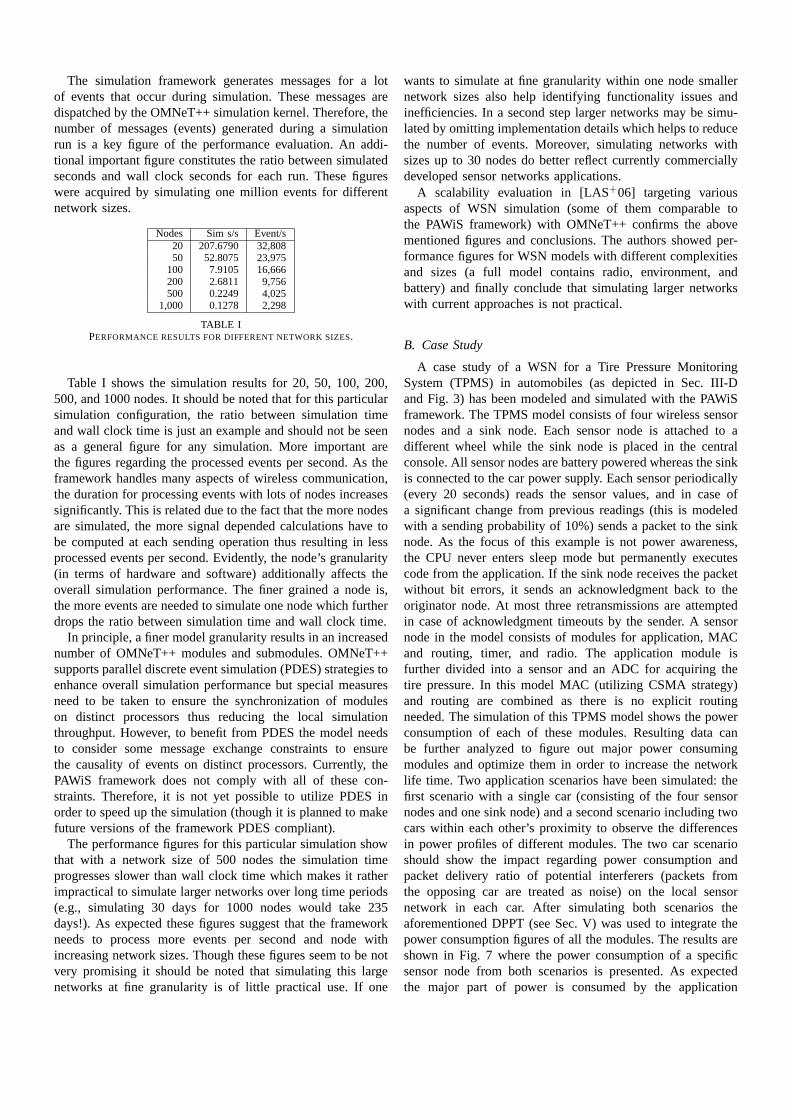
The simulation framework generates messages for a lot

of events that occur during simulation. These messages are

dispatched by the OMNeT++ simulation kernel. Therefore, the

number of messages (events) generated during a simulation

run is a key figure of the performance evaluation. An addi-

tional important figure constitutes the ratio between simulated

seconds and wall clock seconds for each run. These figures

were acquired by simulating one million events for different

network sizes.

Nodes Sim s/s Event/s

20 207.6790 32,808

50 52.8075 23,975

100 7.9105 16,666

200 2.6811 9,756

500 0.2249 4,025

1,000 0.1278 2,298

TABLE I

PERFORMANCE RESULTS FOR DIFFERENT NETWORK SIZES.

Table I shows the simulation results for 20, 50, 100, 200,

500, and 1000 nodes. It should be noted that for this particular

simulation configuration, the ratio between simulation time

and wall clock time is just an example and should not be seen

as a general figure for any simulation. More important are

the figures regarding the processed events per second. As the

framework handles many aspects of wireless communication,

the duration for processing events with lots of nodes increases

significantly. This is related due to the fact that the more nodes

are simulated, the more signal depended calculations have to

be computed at each sending operation thus resulting in less

processed events per second. Evidently, the node’s granularity

(in terms of hardware and software) additionally affects the

overall simulation performance. The finer grained a node is,

the more events are needed to simulate one node which further

drops the ratio between simulation time and wall clock time.

In principle, a finer model granularity results in an increased

number of OMNeT++ modules and submodules. OMNeT++

supports parallel discrete event simulation (PDES) strategies to

enhance overall simulation performance but special measures

need to be taken to ensure the synchronization of modules

on distinct processors thus reducing the local simulation

throughput. However, to benefit from PDES the model needs

to consider some message exchange constraints to ensure

the causality of events on distinct processors. Currently, the

PAWiS framework does not comply with all of these con-

straints. Therefore, it is not yet possible to utilize PDES in

order to speed up the simulation (though it is planned to make

future versions of the framework PDES compliant).

The performance figures for this particular simulation show

that with a network size of 500 nodes the simulation time

progresses slower than wall clock time which makes it rather

impractical to simulate larger networks over long time periods

(e.g., simulating 30 days for 1000 nodes would take 235

days!). As expected these figures suggest that the framework

needs to process more events per second and node with

increasing network sizes. Though these figures seem to be not

very promising it should be noted that simulating this large

networks at fine granularity is of little practical use. If one

wants to simulate at fine granularity within one node smaller

network sizes also help identifying functionality issues and

inefficiencies. In a second step larger networks may be simu-

lated by omitting implementation details which helps to reduce

the number of events. Moreover, simulating networks with

sizes up to 30 nodes do better reflect currently commercially

developed sensor networks applications.

A scalability evaluation in [LAS+06] targeting various

aspects of WSN simulation (some of them comparable to

the PAWiS framework) with OMNeT++ confirms the above

mentioned figures and conclusions. The authors showed per-

formance figures for WSN models with different complexities

and sizes (a full model contains radio, environment, and

battery) and finally conclude that simulating larger networks

with current approaches is not practical.

B. Case Study

A case study of a WSN for a Tire Pressure Monitoring

System (TPMS) in automobiles (as depicted in Sec. III-D

and Fig. 3) has been modeled and simulated with the PAWiS

framework. The TPMS model consists of four wireless sensor

nodes and a sink node. Each sensor node is attached to a

different wheel while the sink node is placed in the central

console. All sensor nodes are battery powered whereas the sink

is connected to the car power supply. Each sensor periodically

(every 20 seconds) reads the sensor values, and in case of

a significant change from previous readings (this is modeled

with a sending probability of 10%) sends a packet to the sink

node. As the focus of this example is not power awareness,

the CPU never enters sleep mode but permanently executes

code from the application. If the sink node receives the packet

without bit errors, it sends an acknowledgment back to the

originator node. At most three retransmissions are attempted

in case of acknowledgment timeouts by the sender. A sensor

node in the model consists of modules for application, MAC

and routing, timer, and radio. The application module is

further divided into a sensor and an ADC for acquiring the

tire pressure. In this model MAC (utilizing CSMA strategy)

and routing are combined as there is no explicit routing

needed. The simulation of this TPMS model shows the power

consumption of each of these modules. Resulting data can

be further analyzed to figure out major power consuming

modules and optimize them in order to increase the network

life time. Two application scenarios have been simulated: the

first scenario with a single car (consisting of the four sensor

nodes and one sink node) and a second scenario including two

cars within each other’s proximity to observe the differences

in power profiles of different modules. The two car scenario

should show the impact regarding power consumption and

packet delivery ratio of potential interferers (packets from

the opposing car are treated as noise) on the local sensor

network in each car. After simulating both scenarios the

aforementioned DPPT (see Sec. V) was used to integrate the

power consumption figures of all the modules. The results are

shown in Fig. 7 where the power consumption of a specific

sensor node from both scenarios is presented. As expected

the major part of power is consumed by the application

0.0

2.0

4.0

6.0

8.0

10.0

12.0[µ

W]

One CarTwo Cars

One Car 0.007 0.583 0.077 11.422 0.028

Two Cars 0.007 6.107 0.212 11.422 4.603

Sensor/ADC Radio Timer App MAC/Routing

0.0 5.0 10.0 15.0 20.0 25.0

Two Cars

One Car

[µW]

Sensor/ADC RadioTimer AppMAC/Routing

Fig. 7. Power consumption results of the TPMS simulation for one node.

module (indirectly as the CPU is actually consuming the power

for software modules) with almost the same value for both

scenarios. The sensor/ADC and timer modules contribute only

very small amounts to the overall power consumption since

they are inactive a significant portion of time. In the single car

scenario the radio and MAC/routing consumed significantly

less power than in the two car scenario. This happens due to

the fact that an increased number of sensor nodes within the

vicinity of each other results in more network collisions which

raises the bit error probability. Furthermore, bit errors result in

packet retransmissions which additionally keeps the radio in

listen state for a longer time to wait for acknowledgments. The

same applies for the MAC as more occurrences of timeouts

and retransmits have to be processed.

We simulated this simple and straightforward case study of

a TPMS on purpose. It took only about 20 man-hours to model

and simulate the real world scenario from scratch. Different

scenarios were simulated (e.g., without acknowledgments,

moving cars, static single car etc.) with minor adjustments in

the configuration file in less time. With the framework, module

inefficiencies can easily be identified (the absolute figures

may not be entirely accurate, although relative information

may provide a deep insight) and corrected in very short

development cycles.

C. Optimization Study

In this case study, we discuss the optimization methodology

for the development of a routing protocol with the PAWiS

framework. This study was aimed to develop and optimize a

table less position based routing protocol. Initially, we created

a skeleton model (the same as used for the study in Sec. VI-A)

for a simple node consisting of application layer (probabilistic

sampling), MAC layer (CSMA), and physical layer (simple

radio) as well as an implementation of the initial version of a

table less routing scheme which we call Progress Aware (PA).

As the composition of the protocol stack is easily managed

with the configuration file without the need to recompile

the particular simulation, we executed many trials with nu-

merous node compositions. After analyzing the simulation

results, we identified several enhancements and alternatives

for various aspects of the routing protocol. Consequently,

multiple refinement cycles with distinct implementations of the

position based routing strategy were applied. These strategies

include PA, Energy Aware (EA), PA and EA with Rts/Cts

packet exchanges, PA and EA with state of charge (Soc)

packet exchanges, and even hybrid approaches (to dynamically

change between progress aware and energy aware routing)

to route packets. First the performance figures acquired in

each refinement iteration were analyzed to identify the main

contributors to power consumption in the routing layers. In the

next step, the gained insights were reapplied to the routing

implementations resulting in additional refinement/analysis

cycles until the results met the targeted power consumption

constraints. The chart in Fig. 8 depicts the network lifetime for

0.0

0.2

0.4

0.6

0.8

1.0

1.2

1.4

PA EA PA Rts/Cts EA Rts/Cts PA Soc EA Soc Hybrid

Net

wor

k Li

fetim

e

Fig. 8. Network life time for various position based routing implementations.

various implementations of position based routing compared

to our initial version of a protocol that utilized a PA scheme

(with network lifetime scaled to 1 in the chart). The chart

shows that the EA scheme exhibits lower lifetime compared

to the PA scheme which can be perceived as a contradiction.

The reason for this is that in this scheme packet forwarding

is based on timers. For example, assume a four node network

comprising a source node S, a destination node D and two

potential forwarders A and B. If S has some data to transmit,

it sends them blindly. A and B being within transmission range

of S receive them and start their respective timers. The timer

of the node which provides maximum progress expires first

(i.e., the timer of the node with more remaining energy), and

further forwards the data while the other node upon listening

to that data kills its timer and drops that data. EA scheme

always try to balance energy consumption across nodes by

routing through nodes with more remaining energy, therefore,

once energy balance (all nodes having almost equal remaining

energy) across the network is achieved, duplicate packets occur

as timers of potential forwarders expire at the same time. These

duplicate packets cause the routing layer to utilize the radio

more often and hence drain the battery quicker which results

in reduced network lifetimes.

VII. CONCLUSIONS AND FUTURE WORK

In this paper we presented a power aware discrete event

simulation framework for wireless sensor networks and nodes.

Based on OMNeT++, it provides additional features to capture

energy consumption (at any desired level), introducing a model

for the RF communication (enabling complex topologies) and

environmental effects with scripting capabilities. It provides

a visualization tool to analyze and visualize energy usage.

The framework focuses on extensibility and re-usability by

outlining a protocol architecture and provides module library.

The results show that the performance (execution time) of

the PAWiS Simulation Framework is comparable with other

frameworks and appropriate for the targeted field of appli-

cation. The case studies showed that the modularization of

OMNeT++ models combined with the abstract component

concept of the PAWiS framework generally result in a reduced

design-debug cycle.

The framework in its current version handles already much

of the functionality and effects that are important for simu-

lating wireless sensor networks. However, there are still some

extensions and features that need to be enhanced or included.

Performance of the simulation framework needs to be further

enhanced, as the current results show scalability issues for

larger networks (see Sec. VI-A).

Furthermore, an important aspect of the simulation frame-

work is the post-processing tool chain. The visualization tool

will be extended by additional functions for analyzing the

output of the simulation application. Currently, the output

comprises power consumption, fired events, and module occu-

pation. Additionally, analysis tools will be included to allow

the comparison of nodes regarding various properties gained

from the simulation and features like significant power peak

detection, min-max over sliding window, integration features.

Additional and updated information regarding the PAWiS

project and the simulation framework is available at http://

www.ict.tuwien.ac.at/pawis/.

REFERENCES

[CBP+06] Gilbert Chen, Joel Branch, Michael Pflug, Lijuan Zhu, and

Boleslaw Szymanski2. Advances in Pervasive Computing and

Networking, chapter Sense: A Wireless Sensor Network Simu-

lator, pages 249–267. Springer US, 2006.

[CS02] G. Chen and B.K Szymanski. COST: a component-oriented

discrete event simulator. In Proceedings of the Winter Simulation

Conference, 2002.

[CSS02] David Cavin, Yoav Sasson, and Andre Schiper. On the accuracy

of MANET simulators. In POMC ’02: Proceedings of the second

ACM international workshop on Principles of mobile computing,

2002.

[DLJ+05] M. Demmer, P. Levi, A. Joki, E. Brewer, and D. Culler. Tython:

A Dynamic Simulation Environment for Sensor Networks. Tech-

nical Report Technical Report UCB/CSD-05-1372, Electical

Eng. and Computer Science Dept., Univ. of California, Berkeley,

2005.

[DSH+03] W. Drytkiewicz, S. Sroka, V. Handziski, A. Koepke, and H. Karl.

A Mobility Framework for OMNeT++. In 3rd International

OMNeT++ Workshop, 2003.

[GSR+04] L. Girod, T. Stathopoulos, N. Ramanathan, J. Elson, D. Estrin,

E. Osterweil, and T. Schoellhammer. A system for simulation,

emulation, and deployment of heterogeneous sensor networks. In

2nd international Conference on Embedded Networked Sensor

Systems, 2004.

[GW07] Johann Glaser and Daniel Weber. Simulation Framework for

Power Aware Wireless Sensors. In Koen Langendoen and

Thiemo Voigt, editors, 4th European Conference, EWSN 2007,

Adjunct poster/demo proceedings, Parallel and Distributed Sys-

tems Report Series, report number PDS-2007-001, pages 19–20,

Delft, The Netherlands, 29-31 January 2007.

[HBE+01] John Heidemann, Nirupama Bulusu, Jeremy Elson, Chalermek

Intanagonwiwat, Kun chan Lan, Ya Xu, Wei Ye, Deborah Estrin,

and Ramesh Govindan. Effects of Detail in Wireless Network

Simulation. In Proceedings of the SCS Multiconference on

Distributed Simulation, pages 3–11, Phoenix, Arizona, USA,

January 2001. USC/Information Sciences Institute, Society for

Computer Simulation.

[JM96] D. B. Johnson and D. A. Maltz. Dynamic source routing in ad

hoc wireless networks. 1996.

[KCC05] Stuart Kurkowski, Tracy Camp, and Michael Colagrosso.

MANET simulation studies: the incredibles. Mobile Computing

and Communications Review, 9(4):50–61, 2005.

[KK05] Vikas Kawadia and P. R. Kumar. A Cautionary Perspective on

Cross-Layer Design. IEEE wireless communication, 2005.

[LAS+05] Esteban Egea Lpez, Javier Vales Alonso, Alejandro Martnez

Sala, Pablo Pavn Mario, and Joan Garca Haro. Simulation tools

for wireless sensor networks. In International Symposium on

Performance Evaluation of Computer and Telecommunication

Systems (SPECTS05), Philadelphia, USA, 2005.

[LAS+06] Egea Lopez, Vales Alonso, Martinez Sala, Pavon Mario, and

Garcia Haro. Simulation scalability issues in wireless sensor

networks. IEEE Communications Magazine, 44(7):64–73, 2006.

[LLL01] He Liu, Xiaojun Liu, and E.A. Lee. Modeling distributed

hybrid systems in Ptolemy II. In American Control Conference,

volume 6, 2001.

[LNWD03] P. Levis, N.Lee, M. Welsh, and D.Culler. TOSSIM: accurate and

scalable simulation of entire tinyOS applications. In 1st inter-

national Conference on Embedded Networked Sensor Systems,

pages 126–137, 2003.

[MGH05] Stefan Mahlknecht, Johann Glaser, and Thomas Herndl. PAWIS:

Towards a Power Aware System Architecture for a SoC/SiP

Wireless Sensor and Actor Node Implementation. In Proceedings

of 6th IFAC International Conference on Fieldbus Systems and

their Applications, pages 129 – 134, Puebla, Mexiko, 14.-

15. November 2005.

[MMG07a] Sajjad Ahmad Madani, Stefan Mahlknecht, and Johann Glaser.

A step towards standardization of wireless sensor networks:

a layered protocol architecture perspective. In International

Conference on Sensor Technologies and Applications, 2007.

[MMG07b] Sajjad Ahmad Madani, Stefan Mahlknecht, and Johann Glaser.

CLAMP: Cross LAyer Management Plane for low power wire-

less sensor networks. In Fifth international workshop on frontiers

of information technology, 2007.

[MNZZ97] J.A. Miller, R.S. Nair, Z. Zhang, and H. Zhao. JSIM: A Java-

based simulation and animation environment. In 30th Annual

Simulation Symposium, pages 31–42, 1997.

[MSK+05] C. Mallanda, A. Suri, V. Kunchakarra, S.S. Iyengar, R. Kannan,

and A. Durresi. Simulating Wireless Sensor Networks with

Omnet++. [submitted to IEEE Computers], 2005.

[NG03] V. Naoumov and T. Gross. Simulation of large ad hoc networks.

In 6th ACM international Workshop on Modeling Analysis and

Simulation of Wireless and Mobile Systems, San Diego, CA,

USA, 2003.

[PBLLZ04] Sanjeev Kohli Philip Baldwin, Edward A. Lee, Xiaojun Liu,

and Yang Zhao. Modeling of Sensor Nets in Ptolemy II. In

Information Processing in Sensor Networks, 2004.

[PBM+04] J. Polley, D. Blazakis, J. McGee, D. Rusk, and J.S. Baras.

ATEMU: a fine-grained sensor network simulator. In First

Annual IEEE Communications Society Conference on Sensor and

Ad Hoc Communications and Networks (SECON), pages 145–

152, 4.-7. October 2004.

[PR99] C. Perkins and E. Royer. Ad hoc On demand distance vector

routing. In Proc. 2nd IEEE Wksp Mobile Comp. Sys. & Apps,

1999.

[PSS00] S. Park, A. Savvides, and M. B. Srivastava. SensorSim: a

simulation framework for sensor networks. In International

Workshop on Modeling Analysis and Simulation of Wireless and

Mobile Systems, 2000.

[PSW04] A. Perrig, J. Stankovic, and D. Wagner. Security in wireless

sensor networks. ACM Communications, 27(6), 2004.

[RI96] Waldemar Celes Filho Roberto Ierusalimschy, Luiz Henrique

de Figueiredo. Lua-An Extensible Extension Language. Soft-

ware: Practice and Experience, 26(6):635–652, 1996.

[RI04] Vijay T. Raisinghani and Sridhar Iyer. Cross-Layer Design

Optimizations in wireless protocol stacks. Computer Commu-

nications, 27(8):720–724, 2004.

[RSF+04] Shad Roundy, Dan Steingart, Luc Frechette, Paul Wright, and

Jan Rabaey. Power Sources for Wireless Sensor Networks. In

First EuropeanWorkshop on Wireless Sensor Networks, pages 1–

17. Springer Berlin / Heidelberg, 2004.

[RVW03] D. Rakhmatov, S. Vrudhula, and D.A. Wallach. A model for

battery lifetime analysis for organizing applications on a pocket

computer. IEEE Transactions on Very Large Scale Integration

(VLSI) Systems, 11(6), 2003.

[SHC+04] V. Shnayder, M. Hempstead, B. Chen, G. W. Allen, and M Welsh.

Simulating the power consumption of large-scale sensor network

applications. In Proceedings of the 2nd international Conference

on Embedded Networked Sensor Systems, 2004.

[SL06] W. Su and T. L. Lim. Cross-Layer Design and Optimization for-

Wireless Sensor Networks. In Proceedings of the Seventh ACIS

international Conference on Software Engineering, Artificial

intelligence, Networking, and Parallel/Distributed Computing,

2006.

[Var01] Andrs Varga. ’The OMNeT++ Discrete Event Simulation

System. In In the Proceedings of the European Simulation

Multiconference, 2001.

[VXSB07] Maneesh Varshney, Defeng Xu, Mani B Srivastava, and Rajive L

Bagrodia. sQualNet: An Accurate and Scalable Evaluation

Framework for Sensor Networks. In International Conference

on Information Processing in Sensor Networks, 2007.

[WGM07] Daniel Weber, Johann Glaser, and Stefan Mahlknecht. Discrete

Event Simulation Framework for Power Aware Wireless Sensor

Networks. In Proceedings of the 5th International Conference on

Industrial Informatics, INDIN 2007, volume 1, pages 335–340,

Vienna, Austria, 23-26 July 2007.

[WL95] D. Wetherall and C. J. Lindblad. Extending Tcl for Dynamic

Object-Oriented Programming. In Proceedings of the Tck/Tk

Workshop 95, 1995.

[ZBG98] X. Zeng, R Bagrodia, and M. Gerla. GloMoSim: a library for

parallel simulation of large-scale wireless networks. In Twelfth

Workshop on Parallel and Distributed Simulation, 1998.