Poverty-environmental links: The impact of soil and water conservation and tenure security on...
13
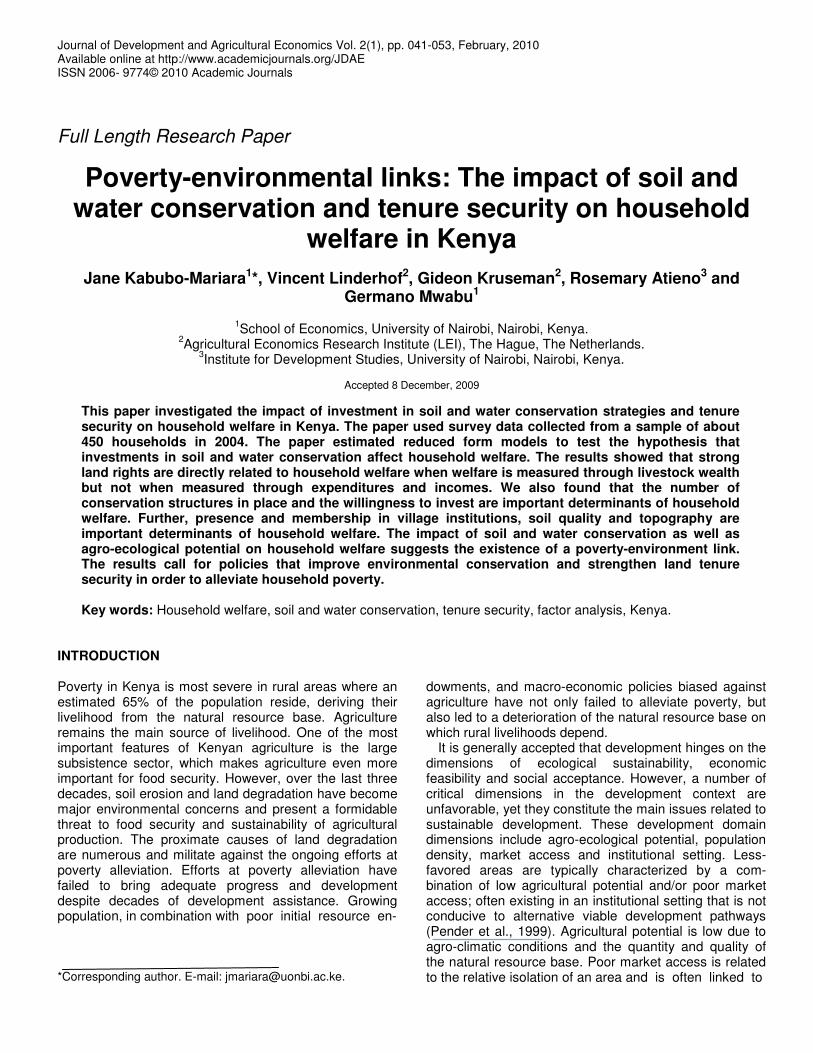
Journal of Development and Agricultural Economics Vol. 2(1), pp. 041-053, February, 2010 Available online at http://www.academicjournals.org/JDAE ISSN 2006- 9774© 2010 Academic Journals Full Length Research Paper Poverty-environmental links: The impact of soil and water conservation and tenure security on household welfare in Kenya Jane Kabubo-Mariara 1 *, Vincent Linderhof 2 , Gideon Kruseman 2 , Rosemary Atieno 3 and Germano Mwabu 1 1 School of Economics, University of Nairobi, Nairobi, Kenya. 2 Agricultural Economics Research Institute (LEI), The Hague, The Netherlands. 3 Institute for Development Studies, University of Nairobi, Nairobi, Kenya. Accepted 8 December, 2009 This paper investigated the impact of investment in soil and water conservation strategies and tenure security on household welfare in Kenya. The paper used survey data collected from a sample of about 450 households in 2004. The paper estimated reduced form models to test the hypothesis that investments in soil and water conservation affect household welfare. The results showed that strong land rights are directly related to household welfare when welfare is measured through livestock wealth but not when measured through expenditures and incomes. We also found that the number of conservation structures in place and the willingness to invest are important determinants of household welfare. Further, presence and membership in village institutions, soil quality and topography are important determinants of household welfare. The impact of soil and water conservation as well as agro-ecological potential on household welfare suggests the existence of a poverty-environment link. The results call for policies that improve environmental conservation and strengthen land tenure security in order to alleviate household poverty. Key words: Household welfare, soil and water conservation, tenure security, factor analysis, Kenya. INTRODUCTION Poverty in Kenya is most severe in rural areas where an estimated 65% of the population reside, deriving their livelihood from the natural resource base. Agriculture remains the main source of livelihood. One of the most important features of Kenyan agriculture is the large subsistence sector, which makes agriculture even more important for food security. However, over the last three decades, soil erosion and land degradation have become major environmental concerns and present a formidable threat to food security and sustainability of agricultural production. The proximate causes of land degradation are numerous and militate against the ongoing efforts at poverty alleviation. Efforts at poverty alleviation have failed to bring adequate progress and development despite decades of development assistance. Growing population, in combination with poor initial resource en- *Corresponding author. E-mail: [email protected]. dowments, and macro-economic policies biased against agriculture have not only failed to alleviate poverty, but also led to a deterioration of the natural resource base on which rural livelihoods depend. It is generally accepted that development hinges on the dimensions of ecological sustainability, economic feasibility and social acceptance. However, a number of critical dimensions in the development context are unfavorable, yet they constitute the main issues related to sustainable development. These development domain dimensions include agro-ecological potential, population density, market access and institutional setting. Less- favored areas are typically characterized by a com- bination of low agricultural potential and/or poor market access; often existing in an institutional setting that is not conducive to alternative viable development pathways (Pender et al., 1999). Agricultural potential is low due to agro-climatic conditions and the quantity and quality of the natural resource base. Poor market access is related to the relative isolation of an area and is often linked to
-
Upload
wageningen-ur -
Category
Documents
-
view
0 -
download
0
Transcript of Poverty-environmental links: The impact of soil and water conservation and tenure security on...
Journal of Development and Agricultural Economics Vol. 2(1), pp. 041-053, February, 2010 Available online at http://www.academicjournals.org/JDAE ISSN 2006- 9774© 2010 Academic Journals Full Length Research Paper
Poverty-environmental links: The impact of soil and water conservation and tenure security on household
welfare in Kenya
Jane Kabubo-Mariara1*, Vincent Linderhof2, Gideon Kruseman2, Rosemary Atieno3 and Germano Mwabu1
1School of Economics, University of Nairobi, Nairobi, Kenya. 2Agricultural Economics Research Institute (LEI), The Hague, The Netherlands.
3Institute for Development Studies, University of Nairobi, Nairobi, Kenya.
Accepted 8 December, 2009
This paper investigated the impact of investment in soil and water conservation strategies and tenure security on household welfare in Kenya. The paper used survey data collected from a sample of about 450 households in 2004. The paper estimated reduced form models to test the hypothesis that investments in soil and water conservation affect household welfare. The results showed that strong land rights are directly related to household welfare when welfare is measured through livestock wealth but not when measured through expenditures and incomes. We also found that the number of conservation structures in place and the willingness to invest are important determinants of household welfare. Further, presence and membership in village institutions, soil quality and topography are important determinants of household welfare. The impact of soil and water conservation as well as agro-ecological potential on household welfare suggests the existence of a poverty-environment link. The results call for policies that improve environmental conservation and strengthen land tenure security in order to alleviate household poverty. Key words: Household welfare, soil and water conservation, tenure security, factor analysis, Kenya.
INTRODUCTION Poverty in Kenya is most severe in rural areas where an estimated 65% of the population reside, deriving their livelihood from the natural resource base. Agriculture remains the main source of livelihood. One of the most important features of Kenyan agriculture is the large subsistence sector, which makes agriculture even more important for food security. However, over the last three decades, soil erosion and land degradation have become major environmental concerns and present a formidable threat to food security and sustainability of agricultural production. The proximate causes of land degradation are numerous and militate against the ongoing efforts at poverty alleviation. Efforts at poverty alleviation have failed to bring adequate progress and development despite decades of development assistance. Growing population, in combination with poor initial resource en- *Corresponding author. E-mail: [email protected].
dowments, and macro-economic policies biased against agriculture have not only failed to alleviate poverty, but also led to a deterioration of the natural resource base on which rural livelihoods depend.
It is generally accepted that development hinges on the dimensions of ecological sustainability, economic feasibility and social acceptance. However, a number of critical dimensions in the development context are unfavorable, yet they constitute the main issues related to sustainable development. These development domain dimensions include agro-ecological potential, population density, market access and institutional setting. Less-favored areas are typically characterized by a com-bination of low agricultural potential and/or poor market access; often existing in an institutional setting that is not conducive to alternative viable development pathways (Pender et al., 1999). Agricultural potential is low due to agro-climatic conditions and the quantity and quality of the natural resource base. Poor market access is related to the relative isolation of an area and is often linked to
042 J. Dev. Agric. Econ. poor physical infrastructure. High population density depends critically on the carrying capacity of the land since in many parts of Africa this is reached at low levels of population in absolute terms. The institutional setting refers to the set of rules governing natural resources and their use. Although land tenure can be hypothesized to play an important role, it is not the only factor, and is often subordinate to market access and relative resource endowments in general (Bruce et al., 1994). Soil and water conservation (SWC) investments cannot also be seen in isolation from development domain dimensions that frame the livelihood strategies of households in a specific area.
There is a no easy solution for the complex situation of less-favored areas. To improve the lot of the poor, there is need for a combination of appropriate technology, an institutional setting that helps households to cope with existing market and government failures, and a set of policy measures that induce behavior leading to both higher levels of household welfare and improved management of the natural resource base (World Bank, 1997).
Previous research concurs that poverty; agricultural stagnation and resource degradation are interlinked. The literature has shown that natural resource degradation contributes to declining agricultural productivity and reduced livelihoods options, while poverty and food insecurity in turn contribute to worsening resource degradation by households (see Kabubo-Mariara et al., 2006 for a review of the poverty-environment literature). Livelihoods in many resource poor farming and pastoral systems have been sustained by land use practices that have tended to perpetuate poverty, soil erosion and other land degradation phenomena. Available evidence further indicates that there are two overall aspects of poverty-environment nexus at the rural household level both of which are critical to a better understanding of the land degradation process in developing countries (Barbier, 1999). First, poverty is not a direct cause of land degra-dation, but is a constraining factor on rural households’ ability to avoid land degradation or to invest in mitigating strategies. Second, poor households are unable to compete for resources, including high-quality and productive land, such that they are often confined to unproductive areas, a situation that further perpetuates poverty. There are also both exogenous and endogenous factors whose feedback effects lead to a vicious circle of low productivity, poverty and land degradation (Shiferaw and Holden, 2001; Barbier, 1999; Reardon and Vosti, 1995; World Bank, 1997).
In Kenya, conservation and sustainable utilization of the environment and natural resources now form an integral part of national planning and poverty reduction efforts. The Economic Recovery Strategy Paper (ERS) recognizes that weak environmental management, unsu-stainable land use practices and depletion of the natural resource base have resulted in severe land degradation. This seriously impedes increases in agricultural produc-
tivity and must be addressed in order to check its adverse impact on poverty. This study examines some of the ERS concerns on conservation, sustainable utilization and management of the environment and natural resources and attempts to fill in research and policy gaps identified by the ERS. It aims at gaining insights in tenure security issues, providing guidelines for poverty reducing land conservation practices.
The present study builds on earlier works on the poverty-environment nexus in Kenya (see Tiffen et al., 1994; Kabubo-Mariara, 2004, 2005; Kabubo-Mariara, Mwabu and Kimuyu, 2006). The study contributes to the literature by analyzing the impact of tenure security, soil and water conservation investments and development domain dimensions on household welfare in Kenya. The study focuses on both income and non-income measures of poverty, analyzing the direct and indirect impacts of all exogenous variables.
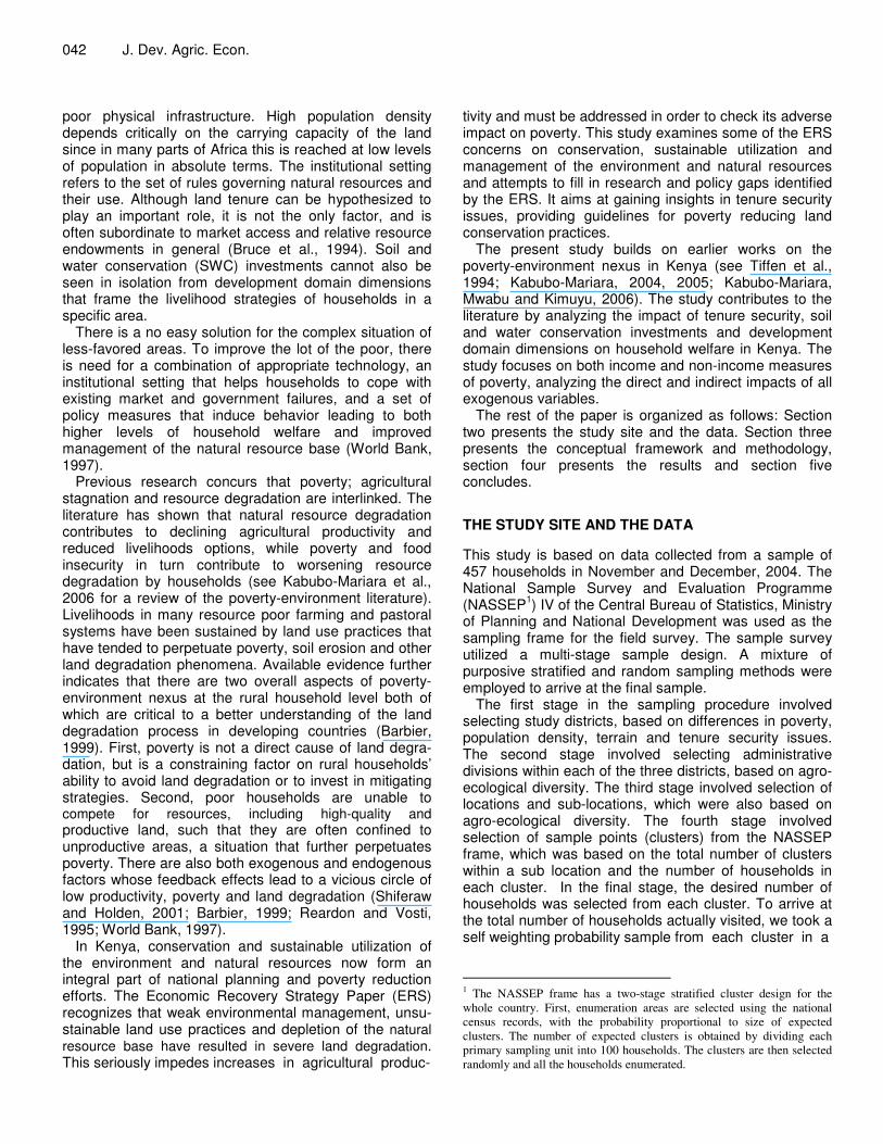
The rest of the paper is organized as follows: Section two presents the study site and the data. Section three presents the conceptual framework and methodology, section four presents the results and section five concludes. THE STUDY SITE AND THE DATA This study is based on data collected from a sample of 457 households in November and December, 2004. The National Sample Survey and Evaluation Programme (NASSEP1) IV of the Central Bureau of Statistics, Ministry of Planning and National Development was used as the sampling frame for the field survey. The sample survey utilized a multi-stage sample design. A mixture of purposive stratified and random sampling methods were employed to arrive at the final sample.
The first stage in the sampling procedure involved selecting study districts, based on differences in poverty, population density, terrain and tenure security issues. The second stage involved selecting administrative divisions within each of the three districts, based on agro-ecological diversity. The third stage involved selection of locations and sub-locations, which were also based on agro-ecological diversity. The fourth stage involved selection of sample points (clusters) from the NASSEP frame, which was based on the total number of clusters within a sub location and the number of households in each cluster. In the final stage, the desired number of households was selected from each cluster. To arrive at the total number of households actually visited, we took a self weighting probability sample from each cluster in a
1 The NASSEP frame has a two-stage stratified cluster design for the whole country. First, enumeration areas are selected using the national census records, with the probability proportional to size of expected clusters. The number of expected clusters is obtained by dividing each primary sampling unit into 100 households. The clusters are then selected randomly and all the households enumerated.
district making a total of 457 households from the three districts (151, 188 and 151 from Murang’a, Maragua and Narok districts respectively). In addition to the household survey, a community questionnaire was administered to selected key informants in each cluster (village). The village survey collected information on product and input prices, market access and village infrastructure and was meant to supplement information collected from house-holds. Full details on sampling, data and all descriptive statistics are presented in Kabubo-Mariara et al. (2006). CONCEPTUAL FRAMEWORK AND METHODOLOGY The impact of tenure security and investment in soil and water conservation is based on the agricultural household model. The model, assumes that households engage in activities using their scarce resources in order to attain their goals and aspirations taking into account that they are constrained by external environmental and socio-economic circumstances. The model can be summarized in a number of basic equations that are a slight expansion of the original model (Singh et al., 1986). The first equation is the utility function where u denotes utility and c a vector of consumption goods and l denotes leisure, ξ denotes household characteristics, Fn denotes the cumulative distribution function of states of nature that captures the inherent risk and uncertainty of rural livelihood systems in terms of prices, weather and in some cases tenure (see for instance Kruseman, 2000; 2001). The inclusion of SWC technology implies a longer time horizon which requires the inclusion of a subjective time preference as discount rate r comparable to the general formulation of optimal control models (Bulte and van Soest, 1999). Suppressing as in all following equations time and nature subscripts, the utility function is:
( , , ) rtc l e dtdFµ µ ξ −= �� (1)
Utility is maximized subject to a cash income constraint where cm and ca are vectors of market purchased and household produced consumption commodities, q is a vector of commodities produced by the household, pm and pa are vectors of market and farm-gate commodity prices respectively, pb is a vector of input prices related to material inputs x, w i and w o are vectors of factor prices (including wage rates and land rents) for hiring in or renting out production factors (f i and f o respectively), and y* is exogenous income:
( ) *m m a a b i i o op c p q c p x w f w f y= − − − + + (2)
The household faces a set of resource constraints that specify that the household cannot allocate more resources to activities than is available in terms of total stock f T:
factors allfor Tao fff ≤+ (3)
For labour there is an additional component of leisure which can be expressed as:
TL
aL
oL flff =++ (3a)
The household faces a production constraint reflected by a technology function that depicts the relationship between inputs (x, fi, fa) and outputs (q) conditional on farm characteristics ζ , soil
Kabubo-Mariara et al. 043 quality s and technology level τ :
( , , , , )i aq q x f f sζ τ= + (4) Solving the agricultural household model can be done in a number of ways: the first is to estimate the full structure of the model, by estimating each equation separately and then using the quantified model to simulate responses as commonly done in bio-economic modeling (Kruseman, 2000).
The alternative is to estimate reduced form equations of the household model. Using reduced form equations is traditionally considered the most appropriate way of dealing with these types of complexities. The coefficients in the reduced form equations capture the sum of both direct and indirect effects. Because of this characteristic it is imperative to include all relevant explanatory variables in the analysis, even if their coefficients are insignificant for the analysis being undertaken. This approach however deserves some attention. If we derive the first-order conditions for the agri-cultural household model and meticulously combine and collapse the resulting equations the end result is a system of equations where the dependent variables consist of the choice variables of the household (production structure, investment, consumption, resource allocation) and on the right-hand side all the exogenous factors (household characteristics, farm characteristics, institutional characteristics). However, we have to be very careful about causality and attribution in the inter-temporal context.
The equations that capture these decision processes include quasi-fixed inputs and determinants of wealth. The problem is however, that past decisions that lead to current wealth and already available SWC structures are based, in principle, on the same set of independent variables. Total cumulative investment and wealth are part of a set of inter-temporal dependent variables. This inter-temporal aspect is something that is often not fully taken into account.
Standard farm household theory, however, postulates that farm households in developing countries often show behaviour that indicates that consumption and production decisions are non-separable. The difficulty of estimating the underlying structural relationships and the complexity of the interacting components of the farm household, and the problem of unobservable or non mea-surable key variables, imply that there are serious consequences for econometric estimation of empirical models (Kruseman, 2001).
In addition to the farm household, household welfare analysis is also founded on the standard economic theory of consumer behaviour (Deaton and Muellbauer, 1980; Glewwe, 1991). Because household welfare is unobservable, consumption expenditure can be used as a proxy for welfare. The expenditure variable can however be scaled down as desired to take into consideration differences such as household size, so that the dependent variable collapses into per capita rather than absolute expenditure. This allows for comparison of welfare levels across households with different composition and across regions with different prices.
To explain household welfare, we can therefore estimate a reduced form model of per capita expenditure or income combining all the various structural relationships, which affect welfare. For policy analysis it is important to include variables influenced by government actions. We therefore include a vector of standard explanatory variables (Glewwe, 1991). These include household characteristics, farm characteristics and institutional variables. Using the survey data we examine the correlation that exists between welfare, resource conservation, land tenure security and land quality. To find out if there is a relationship between the endogenous variables related to welfare and resource conservation beyond the relationship between the exogenous variables that determine both issues, we use analysis of the regression model re-siduals. The residuals enter into the final model as error correction terms (ECM) and eliminate any bias that could arise from inter-
044 J. Dev. Agric. Econ. relationship between these endogenous variables and welfare. The basic model that we want to estimate is a generalized reduced form equation expressed as: Y = f(ζ,ξ,υ ) + � (5) Where; Y is per capita expenditure or any other measure of welfare, � �is a vector of farm characteristics, including land tenure arrange-ments surrounding the arable land and the asset base of the household, � �is a vector of household characteristics and υ �is a vector of village characteristics, including development domain dimensions and quantifiable institutional arrangements at village level. The regression coefficients capture the direct and indirect effects of the truly independent variables on household choice variables. Our deviation from standard poverty analysis is to introduce institutional factors and SWC investment variables into the welfare model. The institutional factors such as the presence of special interest groups and extension agencies, and the choice of SWC investments are (partly) endogenous determinants and have to be explained themselves. In particular, the presence of interest groups and the willingness to listen to extension agents affect the willingness to invest. In order to disentangle partly endogenous effects we use a step-wise estimation approach.
Institutional factors are indicators of how well households/villages organize themselves to enhance household welfare. To capture the impact of the membership of the household in special interest groups/village institutions, we use the following model.
igrpmigrpm vfp __ ),,( εξζ += (6)
We specify equation (6) for three (i=3) different interest groups: membership in income generating groups, loans groups and benevolent groups. By definition, the expected probability for membership if there is no organization present is zero. We therefore estimate a series of probit models on membership based on equation (6).
In addition, we are interested in analyzing the impact of extension services on household welfare. However, we do not have direct information on the presence of natural resource management (NRM) extension possibilities at village level. What we do have is information on whether households use extension for a variety of purposes. Even though we have information on specific NRM extension, information may have been supplied through other extension sources without the household realizing this.
The expected willingness to listen to extension services pex_yn is estimated with a probit model.
ynexynex vfp __ ),,( εξζ += (7)
The willingness to listen to extension in NRM, pex_NRM, is also a probit model, which can be specified as:
NRMexNRMex vfp __ ),,( εξζ += 8)
The willingness to invest in NRM at household level depends on household, farm and village characteristics. The willingness to invest is taken for investments made up to five years ago. If the household made no investments in the past 5 years the investment
is set to zero. Past investments ( EvNRMξδ ) are SWC investments
made more than 5 years ago. Next to the common determinant, the willingness to invest depends on the willingness to listen to NRM extension, and the willingness to listen to extension in general as well as the awareness of the presence and membership of NRM and other special interest groups. However, since these variables are endogenous, we need to apply a nested methodology for cap-
turing these variables. We can then use the residual terms of each of the equations (membership in each of the three interest groups, probability of listening to extension services and probability of listening to extension in NRM) as explanatory variables in the willingness to invest equation. The reason for using these residual terms for estimating the endogenous variables is that the terms are orthogonal to the other independent variables in the equation at hand2. The truly independent variables still capture both the direct and indirect effects, while the residual terms capture the effect of the endogenous variable.
The willingness to invest at household level then becomes:
hhIEvNRMNRMexynexgrpimhhI pppvfp ___,__ ),,,,,( εδξζ ξεεε += (9)
Where the superscript � over a variable denotes that the variable is a residual. However, we note that the equations deriving the residuals are a set of identical equations. In principal membership in special interest groups and willingness to listen to extension services (including extension in NRM) are related and therefore we should correct for correlation of variances. However methods such as seemingly unrelated regression (SUR) cannot be applied with probit models. We can however find a common variance factor by applying a factor analysis on the residuals of each of the probit results of each of the equations. Since all observations are present in all equations and the set of exogenous explanatory variables of each model is identical, the residuals are uncorrelated with the set of explanatory variables. The un-rotated factors with eigenvalues greater than 1.0 provide us with a measure of common variance. This can be included in the final estimation model of the willingness to invest in SWC. In the empirical analysis, the factor analysis loads on two factors, willingness to listen to extension in general and membership in special interest groups in general3. These two factors are then used in the final estimating model of the willingness to invest at the household level. Equation (9) therefore becomes:
hhgrpmexthhI vfp ___ ),,,,( ϕεϕϕξζ += (10)
To capture the effect of membership in interest groups, willingness to listen to extension and the willingness to invest in SWC on household welfare, we enter the residual terms of equations (6, 7 and 10) into the welfare equation (5). This way we are able to capture the direct and indirect effects of both the exogenous and potentially endogenous variables. The final estimating welfare equation becomes:
yhhIynexgrpim pppvfY εξζ εεε += ),,,,( __,_ (11)
Where; ε
hhIp _ is the residual of the willingness to invest in soil and
water conservation (predicted from equation 11). RESEARCH FINDINGS Descriptive statistics
In this section, we present a brief description of the key 2Note that the predicted residuals are not necessarily independent from the error term of the equation in which the endogenous variable appears as explanatory variable. Particularly, if they are dependent this estimation approach will yield biased estimators, although the bias will be small. 3 The results of the stepwise regression and factor analysis are not presented in this paper to save on space, but are available from the authors on request.
Kabubo-Mariara et al. 045
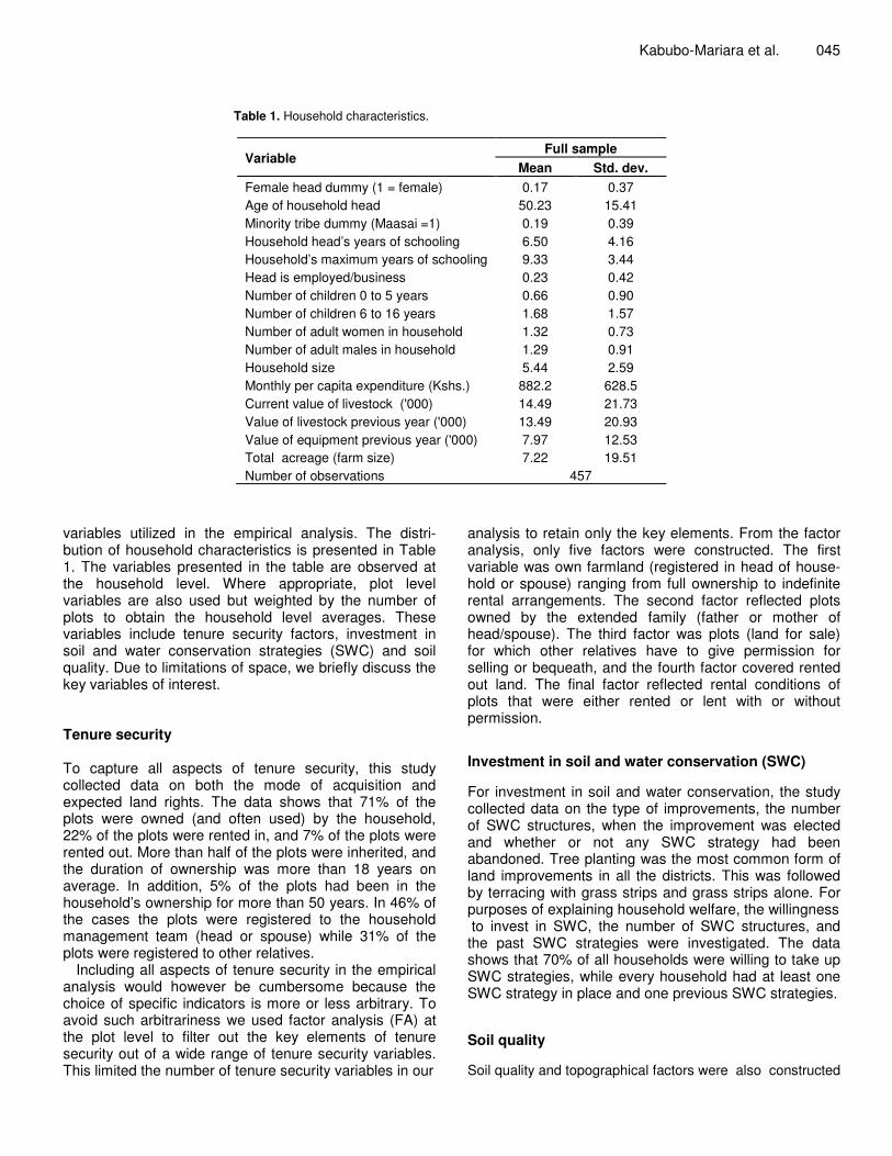
Table 1. Household characteristics.
Variable Full sample
Mean Std. dev. Female head dummy (1 = female) 0.17 0.37 Age of household head 50.23 15.41 Minority tribe dummy (Maasai =1) 0.19 0.39 Household head’s years of schooling 6.50 4.16 Household’s maximum years of schooling 9.33 3.44 Head is employed/business 0.23 0.42 Number of children 0 to 5 years 0.66 0.90 Number of children 6 to 16 years 1.68 1.57 Number of adult women in household 1.32 0.73 Number of adult males in household 1.29 0.91 Household size 5.44 2.59 Monthly per capita expenditure (Kshs.) 882.2 628.5 Current value of livestock ('000) 14.49 21.73 Value of livestock previous year ('000) 13.49 20.93 Value of equipment previous year ('000) 7.97 12.53 Total acreage (farm size) 7.22 19.51 Number of observations 457
variables utilized in the empirical analysis. The distri-bution of household characteristics is presented in Table 1. The variables presented in the table are observed at the household level. Where appropriate, plot level variables are also used but weighted by the number of plots to obtain the household level averages. These variables include tenure security factors, investment in soil and water conservation strategies (SWC) and soil quality. Due to limitations of space, we briefly discuss the key variables of interest. Tenure security To capture all aspects of tenure security, this study collected data on both the mode of acquisition and expected land rights. The data shows that 71% of the plots were owned (and often used) by the household, 22% of the plots were rented in, and 7% of the plots were rented out. More than half of the plots were inherited, and the duration of ownership was more than 18 years on average. In addition, 5% of the plots had been in the household’s ownership for more than 50 years. In 46% of the cases the plots were registered to the household management team (head or spouse) while 31% of the plots were registered to other relatives.
Including all aspects of tenure security in the empirical analysis would however be cumbersome because the choice of specific indicators is more or less arbitrary. To avoid such arbitrariness we used factor analysis (FA) at the plot level to filter out the key elements of tenure security out of a wide range of tenure security variables. This limited the number of tenure security variables in our
analysis to retain only the key elements. From the factor analysis, only five factors were constructed. The first variable was own farmland (registered in head of house-hold or spouse) ranging from full ownership to indefinite rental arrangements. The second factor reflected plots owned by the extended family (father or mother of head/spouse). The third factor was plots (land for sale) for which other relatives have to give permission for selling or bequeath, and the fourth factor covered rented out land. The final factor reflected rental conditions of plots that were either rented or lent with or without permission. Investment in soil and water conservation (SWC) For investment in soil and water conservation, the study collected data on the type of improvements, the number of SWC structures, when the improvement was elected and whether or not any SWC strategy had been abandoned. Tree planting was the most common form of land improvements in all the districts. This was followed by terracing with grass strips and grass strips alone. For purposes of explaining household welfare, the willingness to invest in SWC, the number of SWC structures, and the past SWC strategies were investigated. The data shows that 70% of all households were willing to take up SWC strategies, while every household had at least one SWC strategy in place and one previous SWC strategies. Soil quality Soil quality and topographical factors were also constructed
046 J. Dev. Agric. Econ. using factor analysis. The data on soil quality on all plots included type, workability, texture, depth of soil, as well as the perceptions regarding fertility of the soil. Except for depth of soil, all categories of soil quality variables were retained in the factor analysis and were therefore used as explanatory variables for welfare. Topography was measured through the terrain (whether sloped, flat or undulating). Three topographical factors were obtained from the factor analysis: flatness, moderate slope and undulating terrain. Village characteristics Village level variables were also determined using factor analysis. Market access was based on information on distance, mode, travel time and expenses from the village to particular destinations like markets and roads amongst others collected using a community questionnaire. For institutional variables, data was collected on type (village, men’s groups, women groups and other) and purpose of organization (loans, benevolent, incomes and other village groups including natural resource management). In addition to the type and purpose, we counted the number of institutions in each of the villages and applied factor analysis to shed light on the issue. Five factors were retained as key institutional factors, explaining 96% of variance in the factor loadings. These included the number of institutions present in each village, men’s groups, household investment and income generation groups, village groups and safety nets and natural resource management investment groups. RESULTS AND DISCUSSION In this section we present the regression results linking household welfare, tenure security and investment in water and soil conservation. To explain household wel-fare empirically, we use both the expenditure and income approaches to poverty on one hand and asset approach (livestock) on the other. We specify per capita values of these measures as a function of household, farm and village level characteristics including development domain dimensions and quantifiable institutional arrange-ments at village level as specified in equation (11) in the conceptual framework and methodology section. Household characteristics include gender and age of the household head, household composition and years of schooling of the household head. Farm characteristics are primarily related to the production factors: land, labour, capital and knowledge. Land is defined as the interplay of plot area, soil, topography, and the insti-tutional arrangements in terms of quantity and quality. In addition, investment in environmental conservation has an important bearing on land quality. Village charac-teristics consist of socio-economic conditions, institutional aspects and ecological potential proxied by district dummies.
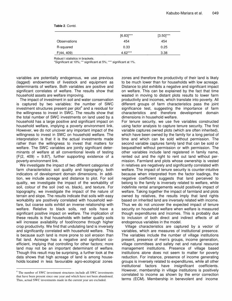
District dummies also capture the impact of other unaccounted for factors such as agro-ecological zones and climate which differ across districts. This controls for the community fixed effects, eliminating any bias from unobserved community level heterogeneity, provided such heterogeneity enters the welfare function linearly. Market access, population density and village institutions are the key village variables utilized in the empirical analysis. Determinants of per capita expenditures and incomes The results for per capita expenditure and incomes are presented in Table 2. A quick overall picture shows that vector of determinants used to explain welfare have a significant joint impact on per capita expenditure and incomes. In particular, the models fit the data better than the intercept only model at all levels of significance as shown by the F statistic. In addition, the variables explain 33% of the total variation in per capita expenditure but only 24% of the total variation in per capita income. Since expenditure is argued to be a better measure of welfare than incomes, we base the discussion on the per capita expenditure function. However, a quick overview indi-cates that some variables differ in their impact on the two measures of welfare, in terms of the magnitude, signs and significance of the coefficients.
The results show that household characteristics are important correlates of welfare. The dummy for female heads of households show that female headed house-holds are poorer than male headed household. Though this is consistent with studies on poverty in Kenya, the impact is insignificant. Age of the household head exhi-bits a U shape relationship with expenditure per capita implying that household welfare declines with the age of the household but after some age starts to increase. This point at family life cycle effects on welfare. Young households may not accumulate wealth in the formative years due to increased expenditure to cater for a growing family. After some threshold, the households are able to diversify their income base and even to save and thus increase per capita expenditure. The coefficient for age squared is not statistically different from zero.
Family composition variables are included to capture differential impact of different gender-age groups on household consumption. The gender-age categories of interest are number of children up to 5 years, number of children 6 to 16 years and number of adult males and females. Except for number of adult males, all the house-hold composition variables are negative and statistically significant implying that larger households are worse off than smaller households. We uncover no impact of education of household head on welfare. Household cha-racteristics are jointly significant at all conventional levels of testing {F(9,409) = 8.26}.
Other characteristics of interest are household assets (livestock and equipment ownership). Because these two
Kabubo-Mariara et al. 047
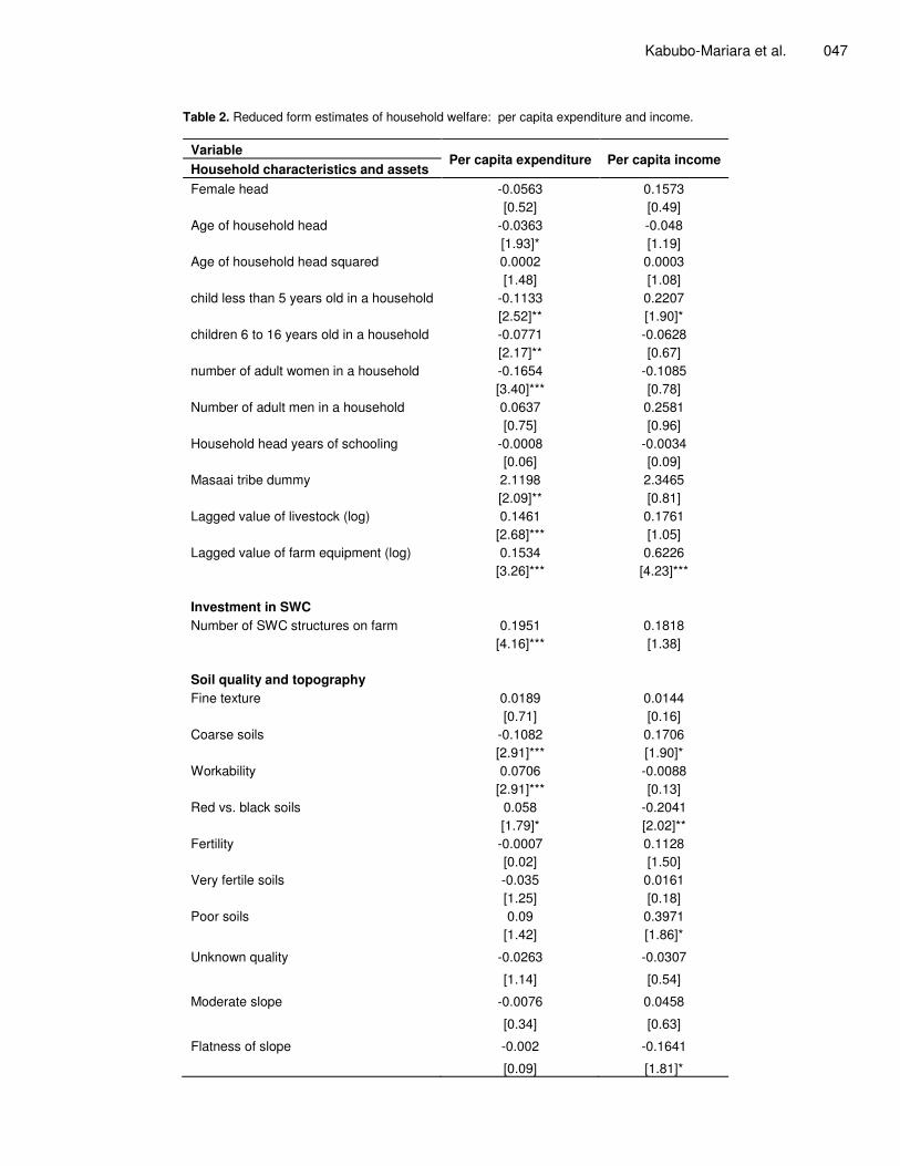
Table 2. Reduced form estimates of household welfare: per capita expenditure and income.
Variable Per capita expenditure Per capita income
Household characteristics and assets Female head -0.0563 0.1573 [0.52] [0.49] Age of household head -0.0363 -0.048 [1.93]* [1.19] Age of household head squared 0.0002 0.0003 [1.48] [1.08] child less than 5 years old in a household -0.1133 0.2207 [2.52]** [1.90]* children 6 to 16 years old in a household -0.0771 -0.0628 [2.17]** [0.67] number of adult women in a household -0.1654 -0.1085 [3.40]*** [0.78] Number of adult men in a household 0.0637 0.2581 [0.75] [0.96] Household head years of schooling -0.0008 -0.0034 [0.06] [0.09] Masaai tribe dummy 2.1198 2.3465 [2.09]** [0.81] Lagged value of livestock (log) 0.1461 0.1761 [2.68]*** [1.05] Lagged value of farm equipment (log) 0.1534 0.6226 [3.26]*** [4.23]*** Investment in SWC Number of SWC structures on farm 0.1951 0.1818 [4.16]*** [1.38] Soil quality and topography Fine texture 0.0189 0.0144 [0.71] [0.16] Coarse soils -0.1082 0.1706 [2.91]*** [1.90]* Workability 0.0706 -0.0088 [2.91]*** [0.13] Red vs. black soils 0.058 -0.2041 [1.79]* [2.02]** Fertility -0.0007 0.1128 [0.02] [1.50] Very fertile soils -0.035 0.0161 [1.25] [0.18] Poor soils 0.09 0.3971 [1.42] [1.86]*
Unknown quality -0.0263 -0.0307
[1.14] [0.54]
Moderate slope -0.0076 0.0458
[0.34] [0.63]
Flatness of slope -0.002 -0.1641 [0.09] [1.81]*
048 J. Dev. Agric. Econ.
Table 2. Contd.
Undulating terrain -0.0776 -0.0578 [3.14]*** [0.96] Tenure security and related factors Land registered in household head or spouse -0.0704 -0.281 [1.68]* [2.20]** Family land (registered in extended family) 0.0456 0.114 [1.34] [1.17] Right to sell family land with permission -0.1368 -0.122 [3.44]*** [0.99] Rented out land -0.0455 -0.2714 [0.63] [1.11] Lent out land 0.0043 0.0293 [0.21] [0.44] Plot area (farm size) -0.0587 0.0647 [2.29]** [0.76] Distance to plot -0.0044 -0.0022 [2.82]*** [0.45] Village characteristics Number of institutions present -0.2077 0.3957 [0.86] [0.50] Presence of men’s groups 0.095 -0.1454 [1.47] [0.83] Presence of income generating groups -0.557 -0.5268 [2.27]** [0.73] Presence of village committees/groups 0.4025 1.2383 [1.45] [1.37] Presence of safety net and NRM groups 0.3363 0.2107 [1.44] [0.28] Population density -0.0016 -0.0022 [3.54]*** [1.42] Market access -1.0539 -2.1673 [2.02]** [1.46] Murang’a district dummy -0.2965 -0.9338 [1.85]* [2.16]** Narok district dummy -4.4717 -4.3405 [2.46]** [0.82] Error correction terms (residuals) Listened to extension services 0.1316 -0.0531 [1.85]* [0.23] Membership in income generating groups 0.1933 0.52 [1.57] [1.35] Membership in loans generating groups 0.0222 0.382 Membership in benevolent groups 0.1988 -0.1932 [2.20]** [0.64] Willingness to invest in SWC -0.1411 -0.3127 [1.77]* [1.67]* [0.32] [2.03]**
Constant 5.7948 8.0008
Kabubo-Mariara et al. 049
Table 2. Contd.
[6.83]*** [3.50]***
Observations 454 454
R-squared 0.33 0.25
F(44, 409) 4.62*** 3.38
Robust t statistics in brackets. *Significant at 10%; ** significant at 5%; *** significant at 1%.
variables are potentially endogenous, we use previous (lagged) endowments of livestock and equipment as determinants of welfare. Both variables are positive and significant correlates of welfare. The results show that household assets are welfare improving.
The impact of investment in soil and water conservation is captured by two variables: the number of SWC investment structures present per plot4 and a residual for the willingness to invest in SWC. The results show that the total number of SWC investments on land used by a household has a large positive and significant impact on household welfare, implying a poverty environment link. However, we do not uncover any important impact of the willingness to invest in SWC on household welfare. The interpretation is that it is the actual investments made rather than the willingness to invest that matters for welfare. The SWC variables are jointly significant deter-minants of welfare at all conventional levels of testing {F(2, 409) = 9.87}, further supporting existence of a poverty-environment link.
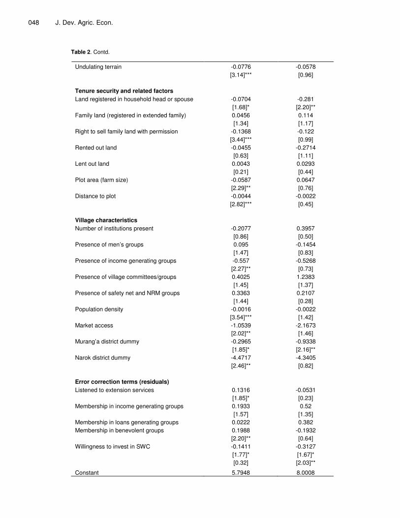
We investigate the impact of two different categories of farm characteristics: soil quality and topography, both indicators of development domain dimensions. In addi-tion, we include acreage and distance to plot. For soil quality, we investigate the impact of the workability of soil, colour of the soil (red vs. black), and texture. For topography, we investigate the impact of the nature of terrain and slope. The results indicate that soils with easy workability are positively correlated with household wel-fare, but coarse soils exhibit an inverse relationship with welfare. Relative to black soils, red soils have a significant positive impact on welfare. The implication of these results is that households with better quality soils will increase availability of food/income through higher crop productivity. We find that undulating land is inversely and significantly correlated with household welfare. This is because such land is more prone to soil erosion than flat land. Acreage has a negative and significant co-efficient, implying that controlling for other factors; more land may not be an important determinant of welfare. Though this result may be surprising, a further look at the data shows that high acreage of land is among house-holds located in less favourable agro-ecological zones
4 The number of SWC investment structures include all SWC investments that have been present since one year and which have not been abandoned. Thus, actual SWC investments made in the current year are excluded.
zones and therefore the productivity of their land is likely to be much lower than for households with low acreage. Distance to plot exhibits a negative and significant impact on welfare. This can be explained by the fact that time wasted in moving to distant plots results to lower farm productivity and incomes, which translate into poverty. All different groups of farm characteristics pass the joint significance test, suggesting the importance of farm characteristics and therefore development domain dimensions in household welfare. For tenure security, we use five variables constructed using factor analysis to capture tenure security. The first variable captures owned plots (which are often inherited), which have been owned by the family for a long period of time and which can be sold without permission. The second variable captures family land that can be sold or bequeathed without permission or with permission. The other variables include land registered in family name, rented out and the right to rent out land without per-mission. Farmland and plots whose ownership is vested in relatives are negatively and significantly correlated with welfare. The impact of tenure security is counter-intuitive because when interpreted from the factor loadings, the negative coefficient suggests that land perceived to belong to the family is inversely related to welfare, while indefinite rental arrangements would positively impact of welfare. Taking together the impact of farmland and plots owned by relatives, the results imply that land rights based on inherited land are inversely related with income. Thus we do not uncover the expected impact of tenure security on household welfare when welfare is measured though expenditures and incomes. This is probably due to inclusion of both direct and indirect effects of all endogenous variables in the model.
Village characteristics are captured by a vector of variables, which are measures of institutional presence. The variables include the number of village institutions present, presence of men’s groups, income generation, village committees and safety net and natural resource management institutions. Presence of village based institutions alone does not seem to matter for poverty reduction. For instance, presence of income generating groups is inversely related to expenditures, while all other institutional factors have insignificant coefficients. However, membership in village institutions is positively correlated to income as shown by the error correction terms (ECM). Membership in benevolent and income
050 J. Dev. Agric. Econ. generation groups is positively and significantly related to expenditure, confirming the importance of institutional factors in poverty reduction. Furthermore, the ECM var-iables are jointly significant at the 5% level of significance {F(3,409) = 2.45}. Households that listened to land conservation extension services are also less poor than their counterparts who never listened.
We also investigate the impact of population density and market access. Population density is inversely rela-ted to expenditure, implying that poverty is concentrated in regions of high population density. Market access has the unexpected negative and significant sign, making it difficult to explain. The expected correlation between po-pulation density and market access and also the testing of both direct and indirect effects probably explain these results. The significance of population density shows the importance of development domain dimensions in poverty alleviation.
The two district dummies included in the model (Murang’a and Narok), in reference to Maragua district exhibit negative and significant coefficients implying that households located in Murang’a and Narok are likely to be poorer than households located in Maragua district. This result is not unexpected given the distribution of per capita expenditure across the three districts. Determinants of asset poverty Assets are a measure of the structural income of the household and vary in importance among households can therefore be good indicators of whether households (Barrett et al., 2006)5. Assets (and changes in assets) can therefore be good indicators of whether households suffer the risk of remaining poor or whether they are likely to move out of poverty. In addition, asset measures of poverty overcome the limitations of standard poverty measurement (such as being defined over the wrong space to measure economic policies directly and the difficulties of distinguishing between transitory and chro-nic poverty even where panel data is available). An asset based approach therefore makes it easier to address the key questions surrounding household’s longer-term prospects of being non-poor (Carter and Barrett, 2006)6.
In this paper, we use livestock wealth as a proxy for asset poverty. This is because one of the districts of study has livestock production as a major economic activity. Income measures may therefore not be good indicators of the levels and characteristics of poverty in
5 Structural approach to poverty alleviation is based on enhancing the returns that poor households earn on their household endowments (assets) and facilitating accumulation of productive assets (Carter and Barrett, 2006). 6 See Carter and Barrett (2006) for detailed discussion on the value of asset-based approach to poverty measurement over other approaches.
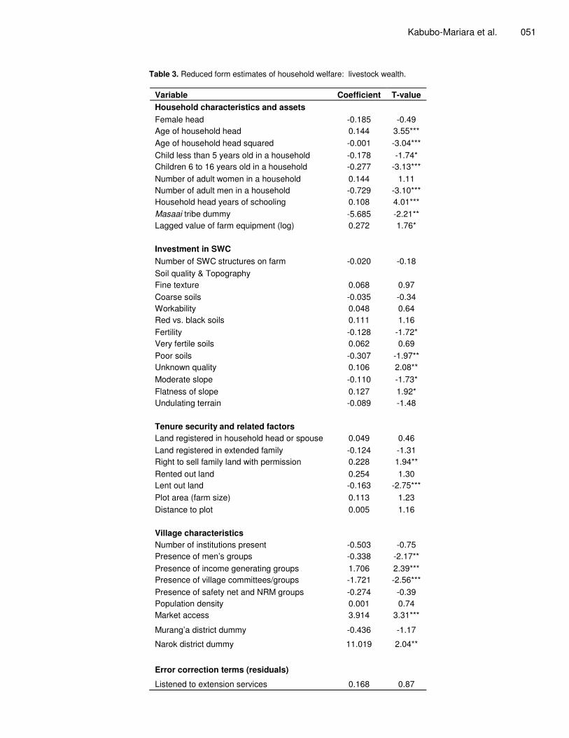
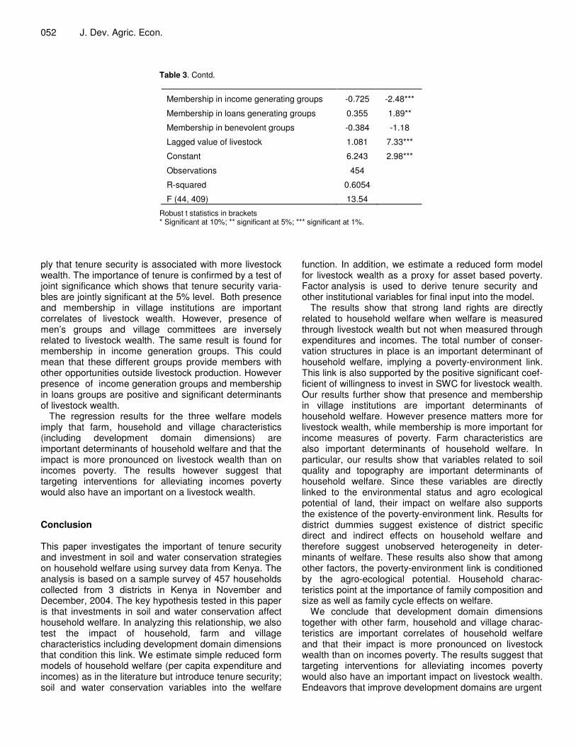
that district7. We model livestock wealth using the same determinants as the other measures of welfare. However, we use a two stage process to explain livestock wealth; first explaining livestock wealth a year prior to the survey. Previous livestock wealth is determined by the same characteristics that determine wealth today. This there-fore means that there is a correlation between livestock now and livestock owned a year ago. To solve for this endogeneity, we need to use two stage least squares. In the first stage, we explain lagged livestock and predict residuals which we use to correct for the correlation between current wealth and previous wealth. Though the coefficients of variables do not change dramatically by including the residual of past wealth, this residual act as an error correction variable and the results are therefore more efficient than without this correction. The results for the second stage are presented in Table 3. The livestock wealth model fits the data better than the per capita ex-penditure and income models, with the model explaining 60% of the total variation in livestock wealth.
The results suggest that household characteristics affect livestock wealth. Age exhibits an inverted U-shaped relationship with livestock wealth implying life cycle effects of age on wealth. Consistent with the results for per capita expenditure and incomes, larger house-holds are poorer than smaller households. We uncover no impact of female headship and number of adult females on livestock wealth. We uncover no important impact of the existing soil and water conservation assets on livestock wealth, but we find that the willingness to invest in soil and water conservation investments is a positive and significant determinant of livestock wealth. Other assets, namely education of the household head, equipment and the initial level of livestock wealth are positive and significant correlates of livestock wealth. Topography and soil quality factors also affect livestock wealth. Flat terrain is associated with higher livestock wealth. On the other hand, moderately sloped land, poor soils and general fertility of soil are inversely related to livestock wealth. Farm size and distance to plot do not seem to matter. Market access is a positive correlate of livestock wealth. Households in Narok are better off in livestock wealth terms than households in the other districts.
Some aspects of land tenure are important determi-nants of livestock wealth. In particular, land in the family rather than land titles has a positive impact on livestock wealth. However, rented land is inversely correlated with livestock wealth. Taken together, these two variables im-
7 Barrett et al. (2006) use a similar approach for herders in Northern Kenya, but use total livestock units rather than total value of livestock as in this paper.
Kabubo-Mariara et al. 051
Table 3. Reduced form estimates of household welfare: livestock wealth.
Variable Coefficient T-value Household characteristics and assets Female head -0.185 -0.49 Age of household head 0.144 3.55*** Age of household head squared -0.001 -3.04*** Child less than 5 years old in a household -0.178 -1.74* Children 6 to 16 years old in a household -0.277 -3.13*** Number of adult women in a household 0.144 1.11 Number of adult men in a household -0.729 -3.10*** Household head years of schooling 0.108 4.01*** Masaai tribe dummy -5.685 -2.21** Lagged value of farm equipment (log) 0.272 1.76* Investment in SWC Number of SWC structures on farm -0.020 -0.18 Soil quality & Topography Fine texture 0.068 0.97 Coarse soils -0.035 -0.34 Workability 0.048 0.64 Red vs. black soils 0.111 1.16 Fertility -0.128 -1.72* Very fertile soils 0.062 0.69 Poor soils -0.307 -1.97** Unknown quality 0.106 2.08** Moderate slope -0.110 -1.73* Flatness of slope 0.127 1.92* Undulating terrain -0.089 -1.48 Tenure security and related factors Land registered in household head or spouse 0.049 0.46 Land registered in extended family -0.124 -1.31 Right to sell family land with permission 0.228 1.94** Rented out land 0.254 1.30 Lent out land -0.163 -2.75*** Plot area (farm size) 0.113 1.23 Distance to plot 0.005 1.16 Village characteristics Number of institutions present -0.503 -0.75 Presence of men’s groups -0.338 -2.17** Presence of income generating groups 1.706 2.39*** Presence of village committees/groups -1.721 -2.56*** Presence of safety net and NRM groups -0.274 -0.39 Population density 0.001 0.74 Market access 3.914 3.31***
Murang’a district dummy -0.436 -1.17
Narok district dummy 11.019 2.04**
Error correction terms (residuals)
Listened to extension services 0.168 0.87
052 J. Dev. Agric. Econ.
Table 3. Contd.
Membership in income generating groups -0.725 -2.48***
Membership in loans generating groups 0.355 1.89**
Membership in benevolent groups -0.384 -1.18
Lagged value of livestock 1.081 7.33***
Constant 6.243 2.98***
Observations 454
R-squared 0.6054
F (44, 409) 13.54
Robust t statistics in brackets * Significant at 10%; ** significant at 5%; *** significant at 1%.
ply that tenure security is associated with more livestock wealth. The importance of tenure is confirmed by a test of joint significance which shows that tenure security varia-bles are jointly significant at the 5% level. Both presence and membership in village institutions are important correlates of livestock wealth. However, presence of men’s groups and village committees are inversely related to livestock wealth. The same result is found for membership in income generation groups. This could mean that these different groups provide members with other opportunities outside livestock production. However presence of income generation groups and membership in loans groups are positive and significant determinants of livestock wealth.
The regression results for the three welfare models imply that farm, household and village characteristics (including development domain dimensions) are important determinants of household welfare and that the impact is more pronounced on livestock wealth than on incomes poverty. The results however suggest that targeting interventions for alleviating incomes poverty would also have an important on a livestock wealth. Conclusion This paper investigates the important of tenure security and investment in soil and water conservation strategies on household welfare using survey data from Kenya. The analysis is based on a sample survey of 457 households collected from 3 districts in Kenya in November and December, 2004. The key hypothesis tested in this paper is that investments in soil and water conservation affect household welfare. In analyzing this relationship, we also test the impact of household, farm and village characteristics including development domain dimensions that condition this link. We estimate simple reduced form models of household welfare (per capita expenditure and incomes) as in the literature but introduce tenure security; soil and water conservation variables into the welfare
function. In addition, we estimate a reduced form model for livestock wealth as a proxy for asset based poverty. Factor analysis is used to derive tenure security and other institutional variables for final input into the model.
The results show that strong land rights are directly related to household welfare when welfare is measured through livestock wealth but not when measured through expenditures and incomes. The total number of conser-vation structures in place is an important determinant of household welfare, implying a poverty-environment link. This link is also supported by the positive significant coef-ficient of willingness to invest in SWC for livestock wealth. Our results further show that presence and membership in village institutions are important determinants of household welfare. However presence matters more for livestock wealth, while membership is more important for income measures of poverty. Farm characteristics are also important determinants of household welfare. In particular, our results show that variables related to soil quality and topography are important determinants of household welfare. Since these variables are directly linked to the environmental status and agro ecological potential of land, their impact on welfare also supports the existence of the poverty-environment link. Results for district dummies suggest existence of district specific direct and indirect effects on household welfare and therefore suggest unobserved heterogeneity in deter-minants of welfare. These results also show that among other factors, the poverty-environment link is conditioned by the agro-ecological potential. Household charac-teristics point at the importance of family composition and size as well as family cycle effects on welfare.
We conclude that development domain dimensions together with other farm, household and village charac-teristics are important correlates of household welfare and that their impact is more pronounced on livestock wealth than on incomes poverty. The results suggest that targeting interventions for alleviating incomes poverty would also have an important impact on livestock wealth. Endeavors that improve development domains are urgent
in the fight against poverty in Kenya. ACKNOWLEDGEMENTS The authors are grateful to Poverty Reduction and Envi-ronment Management (PREM) of the Institute for Environmental studies, Vrije Universiteit for financial sup- port. The authors are also grateful to participants of the International Conference on Economics of Poverty, Envi-ronment and Natural Resource Use held at Wageningen, May, 2006 and participants of the 9th Biennual Conference of the International Society for Ecological Economics on Ecological Sustainability and Human Well-being held at New Delhi, December 2006 for comments on earlier versions of this paper. The usual disclaimer applies. REFERENCES Barbier EB (1999), The Economics of Land Degradation and Rural
Poverty linkages in Africa: UNU/INRA Annual Lectures on Natural Resource Conservation and Management in Africa. Nov. 1998, Accra Ghana (Edited by J.J. Baibu-Forson).
Barrett CB, Marenya PP, McPeak J, Minten B, Murithi F, Oluoch-Kosura W, Place F, Randrianarisoa JC, Rasambainarivo J, Wangila J (2006). Welfare Dynamics in Rural Kenya and Madagascar. J. Dev Stud. 42(2): 248-277.
Bulte EH, van Soest DP (2001). “Environmental Degradation in Developing Countries: Explaining the Environmental Kuznets Curve.” J. Dev. Econ. 65(1): 225–36.
Carter MR, Barrett CB (2006). The Economics of Poverty Traps and Persistent Poverty: An Asset-Based Approach. J. Dev. Stud. 42(2):178-1999.
Deaton A, Muellbauer J, (1980). Economics and Consumer Behavior. Cambridge University Press.
Glewwe P (1991), Investigating the Determinants of Household Welfare in Cote d’Ivoire. J. Dev. Econ. 35: 307-337
Kabubo-Mariara J (2005), Herders Response to Acute Land Pressure under Changing Property Rights: Some Insights from Kenya. Environ Dev. Econ. 10: 167-85
Kabubo-Mariara J (2004), Poverty, Property Rights and Socio-economic incentives for Land Conservation: The case for Kenya. African J. Econ Policy 11(1): 35-68
Kabubo-Mariara et al 053 Kabubo-Mariara J, Linderhof V, Kruseman G, Atieno R, Mwabu G
(2006). Household Welfare, Investment in Soil and Water Conser-vation and Tenure Security: Evidence From Kenya. PREM Working Paper 06-06. Poverty Reduction and Environmental Management; Vrije Universiteit. www.prem-online.org.
Kabubo-Mariara J, Mwabu G, Kimuyu P (2006). Farm Productivity and Poverty in Kenya: The Effect of Soil Conservation. J. Food Agric. Environ. (4)2: 291-297
Kruseman G, (2001). Household technology choice and sustainable land use. In: Heerink NBM, van Keulen H, Kuiper M (Editors). Economic policy reforms and sustainable land use in LDCs: Recent advances in quantitative analysis. Physica-Verlag, Heidelberg pp. 135- 150.
Kruseman G (2000). Bio-economic Household Modeling for Agricultural Intensification. PhD Thesis. Wageningen University. Mansholt Studies No. 20, Wageningen Pender J, Place F, Ehui S (1999). Strategies for Sustainable Agricultural Development in the East African Highlands. Environ Production Technological Division working paper 41. IFPPRI, Washington DC.
Reardon T, Vosti SA (1995), Links Between Rural Poverty and the Environment in Developing Countries: Asset Categories and Investment Poverty. World Dev. 23(9): 1495-1506.
Shiferaw B, Holden S (2001), Farm-level Benefits to Investment for Mitigating land Degradation: Empirical Evidence from Ethiopia. Environ. Dev. Econ. 6: 335-358.
Singh I, Squire L, Strauss J (1986) Agricultural household models: extensions, applications, and policy. Baltimore: The Johns Hopkins University Press.
Tiffen M, Mortimore M, Gichuki F (1994), More People, Less Erosion: Environmental Recovery in Kenya. Chichester: John Wiley and Sons.
World Bank (1997), Taking Action to Reduce Poverty in Sub-Saharan Africa. World Bank Washington D.C.