CALCULATING ABANDONMENT VALUE

USING OPTION PRICING THEORY

Stewart C. Myers

Saman Majd

#1462-83May 1983

Revised: August 1983

DRAFT: PLEASE DO NOT QUOTE OR DISTRIBUTE WITHOUT THE

n--- a Cw -- .1 ---- IrotT AT U> rLrKMIlbluN r ne auinuvA.

� __ �

DRAFT: PLEASE DO NOT QUOTE OR DISTRIBUTE WITHOUT THE

PERMISSION OF THE AUTHORS.

Calculating Abandonment Value Using Option Pricing Theory

Stewart C. Myers*

and

Saman Majd**

Sloan School of Management, M.I.T.

May 1983

(revised: August 1983)

- 11^1_-_1___1_1__ _��_ ���.

Calculating Abandonment Value Using Option Pricing Theory

ABSTRACT

Conventional capital budgeting procedure values investment

projects as if they will be undertaken for a given economic

life, and assigns a prespecified salvage value to the assets at

the end of the life. This ignores the value of the option to

abandon the project early.

This paper models the abandonment option as an American

put option on a dividend paying stock, with varying dividend

yield and exercise price. A general procedure for calculating

the abandonment value is presented, along with some numerical

examples illustrating its practical importance.

1

Calculating Abandonment Value Using Option Pricing Theory

Modern finance advocates the use of net present value in

evaluating capital investments. The net present value (NPV) of

a capital investment project is the present value of its

expected after-tax cash flows. Most of the work on capital

budgeting has concentrated on the difficult problem of

specifying the appropriate discount rate. Modelling the cash

flows to the project is equally important, however.

Consider the choice between two production technologies.

Technology A employs standard machine tools which have an active

second hand market. Technology B uses custom designed,

specialized equipment for which there is no second hand market.

The two technologies produce an identical product and identical

revenues, but technology B is more efficient and has lower

operating costs. Production continues until the machines are

worn out and scrapped. If the two alternatives' cash flows are

projected under these assumptions and discounted at the same

rates, then the NPV of B is greater than that of A. These

calculations would presume that the duration of production is

known. But it is not known: if production may be halted

"early" (before the machines are worn out) then technology A's

�11111_ .1 .__��

greater salvage value makes it relatively more attractive.

Technology A's value in the second-hand market increases the net

present value of using it.

Standard capital budgeting procedure assigns an expected

salvage value to assets at the end of their (pre-determined)

project life. However, salvage value also affects the value of

an investment because of the option to abandon the project

early. The project will be abandoned if the value of continuing

is less than the salvage value at that time. Conventional

capital budgeting fails to take this option into account.

The true value of a project includes its abandonment

value, which depends on the salvage value and the optimal time

to abandon. The optimal time to abandon is of course not known

when the project is undertaken, but will depend on subsequent

performance.

Robichek and Van Horne [16] provide an early analysis of

abandonment value. They recognise that the option to abandon a

project early can be valuable, and illustrate the option's

practical importance. Their examples, however, assume that the

project will be abandoned as soon as the salvage value exceeds

the present value of the remaining expected cash flows. Dyl and

Long [4] emphasise that the optimal time to abandon the project

3

will not, in general, be the first instance where salvage value

exceeds the present value of the remaining expected cash flows.

Rather, the abandonment decision at each point in time must

recognize that, if the project is not abandoned, the firm

retains the option to abandon in the future.

Unfortunately, Robichek and Van Horne's solution procedure

(as corrected by Dyl and Long) is not practical when applied to

realistic situations. The subsequent finance literature has not

provided a practical approach to solving for the value of the

abandonment option and the optimal time for abandonment.

The option to abandon a project is formally equivalent to

an American put option and can be valued by applying the

1/techniques developed to value options on stocks . However, it

is not a simple put option: the project yields uncertain cash

flows and has an uncertain salvage value. These factors

significantly complicate the solution procedure. 2

This paper presents a general procedure for estimating the

abandonment value of a capital investment project. The next

section specifies the abandonment option as a contingent claim,

and discusses some of the important factors that affect its

value. Section II describes our simplifying assumptions and

valuation procedure, and section III presents some numerical

___l___l_______rs__l__I______� 1__1_1_

examples of the calculations. Section IV discusses how

uncertainty in the salvage value can be incorporated in the

analysis. Section V offers some concluding comments.

I. Problem Specification

The option to abandon a project is formally equivalent to

an American put option on a dividend-paying stock: the exercise

price of the put is the salvage value of the project; the cash

flows from the project are equivalent to the dividend payments

on the stock. Also, the project can be abandoned at any time

during its life.

Each of these factors affects the abandonment value of the

project, and to solve for the abandonment value, each must be

explicitly modelled. This section discusses how these factors

affect the abandonment value. The specific assumptions we make

to implement the solution technique are described in section II.

A. Cash Flows and Payout Ratios

In the classical model of stock valuation, the value of a

stock is the present value of its expected dividends.

Similarly, the value of a project is determined by the present

value of its expected cash flows. Since expectations about

future cash flows are revised as new information randomly

arrives, the value of the project varies randomly about its

--------- �------�I-'x�� --------^-- --�-----�-�-- ----------�P- ---

6

expected value. The uncertainty in the value of the project is

therefore related to that of the cash flows, although the

relationship is generally complex.

To apply the contingent claim valuation techniques to our

problem we must specify the stochastic process generating the

value of the project. However, in capital budgeting we normally

focus on the process generating the cash flows. Project cash

flow, rather than project value, is the natural state variable.

However, we can express cash flow as a function of asset value:

t = Ct/Vt . These "payout ratios" ( y ) can be functions of

time and project value.

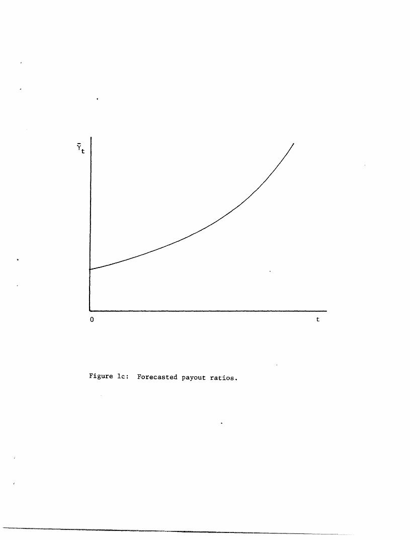
The following simple example shows how we restate the

forecasts of cash flows in terms of payout ratios. Suppose that

cash flows are forecasted to be constant over the life of the

project, so that it resembles a simple annuity (Figure la).

Since the value of the project at any time is the present value

of the remaining cash flows, we can derive the expected path of

the project value over time from the forecasted cash flows. The

project value will decline over time as in Figure lb. From

these two sets of forecasts we can forecast the payout ratios

implied by the expected path of project value: in this example

the payout ratios will increase over time (Figure c).

7

Suppose there is a forecast error in the cash flow. What

happens to the conditional forecast of the payout ratio? A

simple assumption is that the payout ratio is constant. That

is, the percent forecast error in the cash flow,

=[c(- Etl(Ct)] /Et 1(Ct) , causes the same percentaget t t-1 ( ]

change in project value: Vt= Et-1(Vt) [1+Et] . Hence the

forecasted payout ratio is unchanged.

If the assumption that payout ratios are independent of

project value seems unduly restrictive, note that it is

necessary for using a single risk-adjusted rate to discount

future cash flows, which is standard procedure in capital

3/budgeting .

Other assumptions about the effect of forecast errors in

the cash flows on forecasted payout ratios are possible. A

mean-reverting cash flow, for example, causes forecasted payout

ratios to be functions of both time and project value. More

complex specifications of payout ratios as functions of time and

project value are also possible.

The payout ratios used in the numerical valuations below

are constant or functions of time only.

___ ��__11_1_1______1_11_1�-----__11 ---_1___ I�

B. Asset Life and Salvage Value

Conventional capital budgeting treats salvage by assigning

a prespecified salvage value to the asset at the end of some

predetermined life. But what determines the 'life' of a

project?

The physical life of an asset depends on the time at which

it will wear out and must be replaced. This is the maximum life

of the asset. Physical life could be infinite or very long.

4/For example, think of land or a hydroelectric facility .

The economic life of the asset is the length of time

during which the asset is being used. Thus even if the project

is terminated, if the asset is still being employed in an

alternative use, its economic life continues.

The project life is not fixed, but is determined by the

decision to abandon. It is solved for simultaneously with the

value of the option to abandon. The determinants of the

abandonment value will therefore also determine the project

life.

I,-'--- - ---- -----~~~' ~~'" ~I'~`~'- ~~~c~~~--~-~-~--- ·---

111

9

A project may never be abandoned. In that case the

project life, the economic life and the physical life will all

be equal. Generally, however, the project life is less than the

economic life, which is less than the physical life.

If the decision to abandon determines project life, what

determines the life of the abandonment option? In principle,

the project can be abandoned at any time during the asset's

physical life, therefore this is the appropriate maturity for

the abandonment option.

The salvage value of an asset can vary over time and may

not be known in advance. Standardized assets, for which there

is an active second-hand market and which experience little

technological change, may have a relatively stable and

predictable salvage schedule. Assets subject to rapid

technological change may have unpredictable salvage values.

The salvage value at any time is the market value of the

asset in its next most productive use. It is net of any costs

of converting from one use to the other, and incorporates the

value of any subsequent options to abandon. Some assets with

several possible uses may be abandoned several times during

their physical life. Most land, for example, has many different

productive uses and infinite physical life. In such cases, the

1�·_1_11� ill ._

10

option to abandon (i.e., to switch from one use to another) is

like an 'option on an option': if the project is abandoned

before its economic life is over, its salvage value includes the

value of terminating its next tour of duty, and the next user

gets another abandonment option. Therefore a complete

specification of the stochastic properties of salvage value,

including its relation to project value, is not an easy thing to

write down or analyze. However, we can cope with uncertain

salvage values under the assumptions described in section IV.

11

II. Solution Procedure

Valuing an option requires solving a partial differential

equation whose boundary conditions define the nature of the

5/contingent claim . Sometimes the equation and boundary

conditions allow for a closed-form solution, as in the classic

Black-Scholes equation for the value of a European call option.

More generally, however, a closed-form solution does not exist,

forcing us to seek a numerical approximation.

The partial differential equation for the abandonment

value is: ½ o2App + [rP-y(P,t)] A -rA + A = 0,

where P is the value of the underlying project, o is the

standard deviation of the rate of return on the project, r is

the riskless interest rate, Y(P,t) is the payout ratio, and A is

the abandonment value.

Two boundary conditions specifying the nature of the

abandonment option are: (1) if the value of the project is

zero, the value of the option is the salvage value at that time:

A(P=O,t) = S(t); (2) as the value of the project becomes

infinitely large, the value of the option tends to zero:

lim A(P,t) = 0.

P-+oo

12

A third condition applies when the option is exercised:

the value of the project is the greater of the salvage value or

the value of continuing (but with optimal future abandonment).

This condition is invoked at each point in time, and thus the

optimal abandonment schedule is solved for implicitly.

Finally, a terminal boundary must be assigned, where the

value of the project is taken as zero. This boundary is the

physical life of the asset, and the boundary condition at

maturity of the option is: A(P,t=T) = max[S(T)-P(T),O].

The most general specification of the abandonment option

does not allow a closed-form solution because: (1) the future

salvage values are uncertain and are related to the project

value in a (generally) complex manner; (2) the future payout

ratios, as defined in the previous section, are uncertain and

can depend on time and project value in a (generally) complex

6/manner; (3) the abandonment option is an American option for

which early exercise will generally be optimal, and the timing

of early exercise must be jointly determined with the

abandonment value.

We focus first on the uncertainty regarding future cash

flows and project values by assuming a deterministic salvage

value. Specifically, we assume that the initial salvage value

13

is known and subsequently declines at a known constant rate. We

also assume that the payout ratios are constant over the entire

physical life of the asset. This allows the cash flows to be

uncertain but couples their uncertainty to that of the

7/project 7/

Since there is no closed-form solution to even this simple

formulation of the abandonment problem, we must use a numerical

approximation technique. Several techniques for such

approximations are available. We employ an explicit form of the

finite difference technique .

This numerical approximation results in a relationship

between the value of the abandonment option in any period and

its values in the next period. We can employ this relationship

recursively, starting with the values at the terminal boundary,

and working back to the abandonment values at the start of the

project. In addition, the procedure dictates the optimal

abandonment decision. Since the project present value (PV) is a

sufficient statistic for the value of the future cash flows,

optimal abandonment is expressed as a schedule of project PVs

over time. Should the project PV fall below this schedule at

any time the project will be abandoned. This schedule will not

be equal to the present value of remaining cash flows (as in

Robichek and Van Horne) because our recursive procedure includes

14

the value of optimal future abandonment at each point. Thus the

current abandonment decision implicitly accounts for optimal

future abandonment.

15

III. Numerical Examples for the Simplified Abandonment Problem

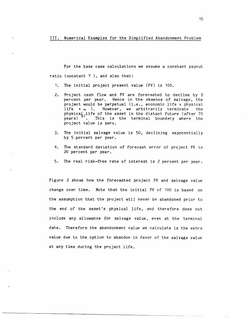
For the base case calculations we assume a constant payout

ratio (constant Y ), and also that:

1. The initial project present value (PV) is 100.

2. Project cash flow and PV are forecasted to decline by 8percent per year. Hence in the absence of salvage, theproject would be perpetual (i.e., economic life = physicallife = m ). However, we arbitrarily terminate thephysical/life of the asset in the distant future (after 70years) . This is the terminal boundary where theproject value is zero.

3. The initial salvage value is 50, declining exponentiallyby 5 percent per year.

4. The standard deviation of forecast error of project PV is20 percent per year.

5. The real risk-free rate of interest is 2 percent per year.

Figure 2 shows how the forecasted project PV and salvage value

change over time. Note that the initial PV of 100 is based on

the assumption that the project will never be abandoned prior to

the end of the asset's physical life, and therefore does not

include any allowance for salvage value, even at the terminal

date. Therefore the abandonment value we calculate is the extra

value due to the option to abandon in favor of the salvage value

at any time during the project life.

--·------- ---

III

16

Table I shows the results of the base case calculations.

Each entry in the table is the abandonment value given project

value. The first column gives the abandonment value at the

start of the project for different initial project values.

Thus, since the initial forecasted PV is 100, the abandonment

value is 5.63, or approximately 6 percent of project value. If

this project required an initial investment of 100, making its

NPV (without any salvage) zero, the abandonment value would make

the project worthwhile.

The optimal abandonment decision is also indicated in

Table I: if at any time the project value falls below the PV

corresponding to the line drawn in the table, the project should

be abandoned. In our base case, for example, if the project

value in year 2 is less than 24.53, the project should be

abandoned. Similarly, if the project value is less than 20.09

in year 9, the project should be abandoned.

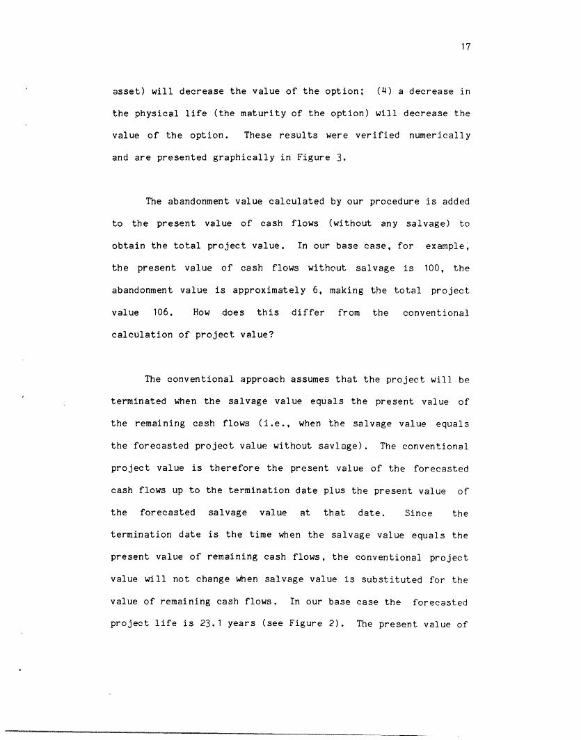
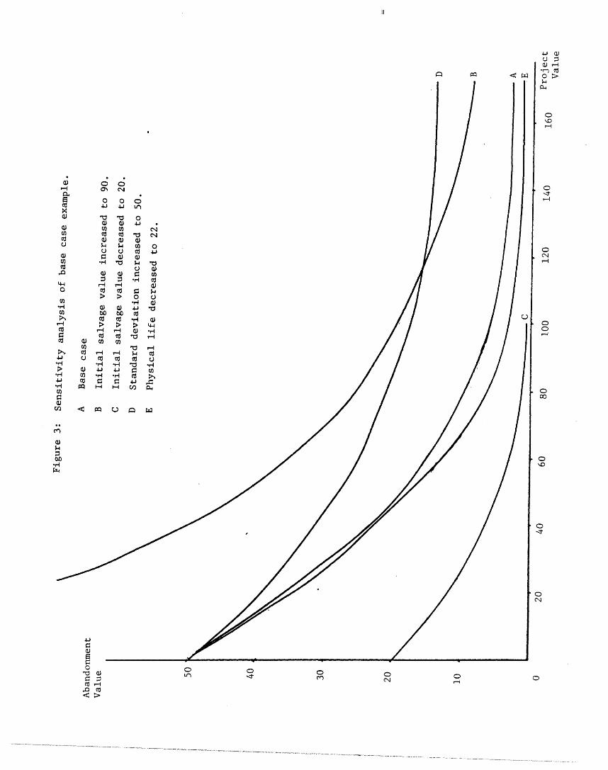
The direction of the change in abandonment value can be

predicted from standard option pricing theory: (1) an increase

in the salvage value (exercise price) will increase the value of

the abandonment option (put option); (2) an increase in the

volatility of the value of the project (the underlying asset)

will increase the value of the option; (3) an increase in the

forecasted project PV (the current value of the underlying

_X ·____1_____1·_ �lll^-__·_._tlll-l_ ·)·.._ .�1-·---174--11--1�--_·_-�-1--1-�--�111- ..-_...

17

asset) will decrease the value of the option; (4) a decrease in

the physical life (the maturity of the option) will decrease the

value of the option. These results were verified numerically

and are presented graphically in Figure 3.

The abandonment value calculated by our procedure is added

to the present value of cash flows (without any salvage) to

obtain the total project value. In our base case, for example,

the present value of cash flows without salvage is 100, the

abandonment value is approximately 6, making the total project

value 106. How does this differ from the conventional

calculation of project value?

The conventional approach assumes that the project will be

terminated when the salvage value equals the present value of

the remaining cash flows (i.e., when the salvage value equals

the forecasted project value without savlage). The conventional

project value is therefore the present value of the forecasted

cash flows up to the termination date plus the present value of

the forecasted salvage value at that date. Since the

termination date is the time when the salvage value equals the

present value of remaining cash flows, the conventional project

value will not change when salvage value is substituted for the

value of remaining cash flows. In our base case the forecasted

project life is 23.1 years (see Figure 2). The present value of

_�

18

cash flows up to this termination date is 96, and the present

value of salvage at this date is 4, making the total project

present value 100. This is also the project present value

without any salvage.

The forecasted project life can be changed by varying the

initial salvage value. The smaller the initial salvage value,

the longer the forecasted project life, the larger the present

value of cash flows up to termination, and the smaller the

present value of salvage. The total project value, including

salvage, remains constant at 100, as described above. These

results are shown in Table II for a range of forecasted project

lives.

Also shown in Table II is the corresponding abandonment

value calculation. The project present value without early

abandonment or salvage is 100. The abandonment value is the

extra value due to the option to terminate the project early,

and this is added to the present value of cash flows to get the

total project value. The results show that the project value

with conventional allowance for salvage can be very different

from the project value with allowance for the abandonment

option.

19

We also performed an illustrative calculation assuming

varying payout ratios. Specifically, we assumed that the

project payout ratio is zero in the first five years, 2 percent

in the next ten years, and 20 percent per year thereafter. This

implies the pattern for the forecasted project value shown in

Figure 4. In this example, if the initial forecasted PV is 100,

the abandonment value is 3.54, or approximately 4 percent of

project value.

�_�___�____�___�_______ 1___11_1___�_�__�1____�_ ____ ____��_

20

IV. Modelling Uncertain Salvage Values

Abandonment can occur more than once during an asset's

physical life: the asset may be switched from one use to

another several times. Included in the salvage value each time

abandonment occurs is the option to abandon again. Hence the

abandonment option is an option on a sequence of options.

Unfortunately, this makes complete specification of the

stochastic properties of the salvage value extremely difficult.

As a first step towards introducing uncertainty in the

salvage value we make two simplifying assumptions. The first is

that identical assets are being used elsewhere, and that these

assets are traded. Thus the salvage value is a market price.

Second, we assume that the stochastic processes for the project

value and the salvage value are:

dP/P = (a - Yp) dt+ a dZ ,p p P p

and,

dS/S = ( - Y) dt = s dZsS S S S

Here P is the project value, a the expected rate of change ofP

P, Y the project payout ratio, the standard deviation of the

rate of change of P, and dz the standard Weiner processP

11/generating the unexpected changes in P . The parameters for

the salvage value, S, are similarly defined. The project and

21

salvage values are correlated, with instantaneous correlation

coefficient P .

Margrabe [9] has valued an option to exchange one risky

asset for another. The assumptions above make our framework

similar to his, where the stochastic salvage value can be

interpreted as one of his risky assets. However, since his

analysis assumes no payouts from the assets, it would not

12/strictly apply to the abandonment option

However, we can use the valuation procedure developed

earlier to value the abandonment option with uncertain salvage

value. The appendix derives the differential equation for this

option, and shows that after suitable transformation, the

option's value obeys the same differential equation as applies

in the case of deterministic salvage. This transformation is as

follows: (1) Redefine the state variable as the ratio of

project to salvage value (X=P/S). (2) The standard deviation of

2 2 2this new state variable is a = a -2po a +o (3) Set the

X P ps s

exercise price equal to unity. (4) Substitute Y for the

riskless interest rate. With these four adjustments,

abandonment with uncertain salvage is reduced to an equivalent

option with known and constant exercise price.

XII__

22

Table III presents results of abandonment calculations

when salvage value is uncertain. As the results indicate, the

abandonment value is sensitive to changes in both the

correlation between salvage and project values and the standard

deviation of salvage value.

23

V. Conclusions

It is easy to think of the abandonment option as an

American put option, and somewhat more difficult to put that

insight to practical use. This paper discusses problems of

application in some detail and presents numerical estimates of

abandonment value for halfway realistic examples. The obvious

next step is to expand the numerical valuation program to allow

project payout ratios (i.e., cash flow to value ratios) to

depend on project value as well as time.

Such a program could help solve a variety of other

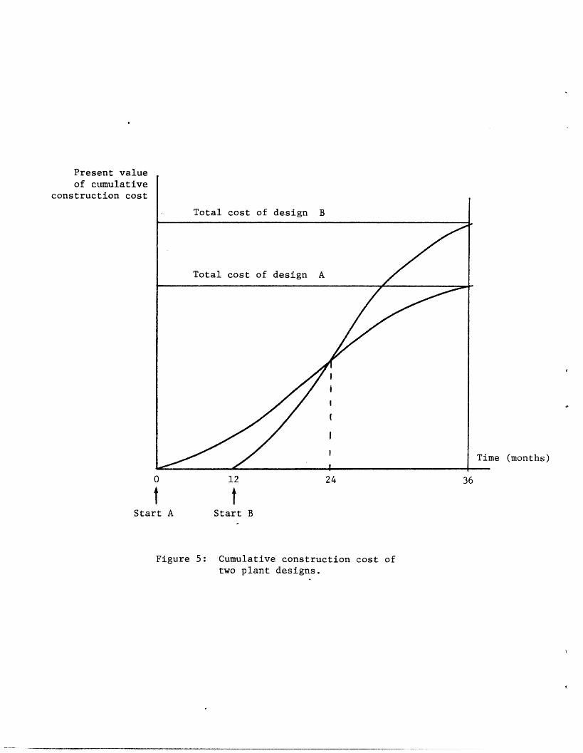
problems. Here is one example. Suppose you expect to need a

new plant ready to produce turbo-encabulators in 36 months. If

design A is chosen construction must begin immediately. Design

B is more expensive, but you can wait 12 months before breaking

ground. Figure 5 shows the cumulative present value of

construction costs for the two designs up to the 36-month

deadline. Assume the designs, once built, are equally efficient

and have equal production capacity.

A standard discounted cash flow analysis would rank design

A ahead of B. But suppose the demand for turbo-encabulators

falls and the new factory is not needed: then, as Figure 5

_ ����__�

III

24

shows, the firm would be better off with design B provided the

project is abandoned before month 24 13/

This is also an abandonment value problem. The underlying

asset is the present value of the turbo-encabulator project

assuming the firm must complete construction of the plant.

Think of putting the present value of required construction

expenditure in an escrow account. The account would of course

be larger for design B than design A. If either design is

abandoned before month 36, however, its 'salvage value' is the

unspent balance in the escrow account. This is the exercise

price at which the firm can 'put' the turbo-encabulator project

between month zero and month 36.

We are back to a standard abandonment option, where the

exercise price is determined by the pattern of cumulative

investment in the design being valued. Project net present

value is equal to (1) project present value assuming a

14/commitment to complete construction , less (2) the present

value of construction costs assuming this commitment, plus (3)

the present value of the option to abandon before construction

is completed. The value of (3) reflects the option to recover

part of the construction costs comprising (2).

25

Design B could be more valuable than A, if B's abandonment

value outweighed its higher cost.

It would be interesting to analyse the choice between gas

turbines, coal, and nuclear power plants using this option

pricing framework.

_��_ ��·�___�___I _I��_�_�_�_�_�

26

APPENDIX

This appendix derives the partial differential equation

(PDE) for the abandonment option when the salvage value is

stochastic, and shows that with suitable transformation, the

option value is also a solution to the PDE for deterministic

salvage.

The derivation follows the methodology of Merton [12] and

the reader is referred to his references for the supporting

literature. For simplicity, the derivation that follows assumes

a European type abandonment option; the extension to an

American type option is straightforward. (The numerical results

reported in section IV of the text refer, of course, to the

American abandonment option.)

The stochastic processes describing the project value

without salvage, P, and the salvage value, S, are:

dP/P = ( - yp)dt + a dZ ,

and,

dS/S = ( - Ys)dt + dZs

The rate of change of P has expectation Ua and standardP

deviation ac , the project payout ratio is yp, and dz is the

standard Weiner process generating the unexpected changes in P.

-1- ____ ____.... ... --___X-~-lll~~-

III

27

The parameters for S are similarly defined. The project and

salvage values are correlated with instantaneous correlation

coefficient P.

Let F(P,S,t) be the solution to the PDE:

2 P2 F pp+pap a PSFp+2S2 F SS+(r-p)PFp+(r- ) SFrF+Ft =OPP P PSS PP S

subject to the boundary conditions:

F(P=O,S,t) = S(t),

lim F(P,S,t) = 0,Pi*W

and F(P,S,t=T) = max[S(T)-P(T), 0].

From Ito's lemma,

2 2

dF:[F + (a -Yp)PFp+(as-Y)SFs+ ½ o P F + pa a PSFt p p p S S p pp ps

+½ o S2 F ] dt+ [pPFp] dz + [SFs] dz s P P P 5 5 S

Substituting from the PDE above, we have,

dF = FpdP + FdS + [rF-(r-yp)PFp-(r-YS)SFs]dt.

Consider the portfolio formed by investing the fractions x in P,

y in S, and the remainder in riskless Treasury bills. The

dynamics for the portfolio are,

dY = xY (dP + ypPdt)/P +yY (dS + ysSdt)/S + (-x-y)Yrdt.

Choose the investment proportions according to the rules:

x=FpP/Y and y=FsS/Y. Then,

dY = F (dP + ypPdt) + F (dS + YSdt) + (Y-F -F S)rdt

= dF + (Y-F)rdt.

_�_��II�__

28

If the amount initially invested in the portfolio is

Y(t=O) = F(P,S,t=O), then it is clear that Y(t) = F(P,S,t) at

all subsequent times. Further, the value of the portfolio, Y,

is equal to the function F(P,S,t) at the boundaries given above,

which by construction are identical to the boundaries for the

abandonment option. Since the portfolio has the same payoffs as

the abandonment option, then to avoid dominance, the value of

the abandonment option must be given by A(P,S,t) = Y(t) =

F(P,S,t).

The PDE for the abandonment option above can be simplified

by the transformation: G(X,t) = A(P,S,t)/S, where X=P/S. This

leads to the PDE:

2 ½2x XC2G + ( - Yp) XG - Y G + G = 0,

where x = Up -2p2p + The new boundary conditions are:

G(X=O,t) = 1,

lim G(X,t) = 0,X-tCO

and G(X,t=T) = max[1-X(T), 0].

This is identical to a formulation of the abandonment option

with deterministic exercise price (equal to unity), and with the

riskless rate replaced by Ys .

The intuition behind this transformation is clear: think

of the salvage value as the numeraire. In these units, the

project value is P/S (=X), and its variance is

II

---- -11-1-1-1-1-1- 1--------- ---- ---- ---" - -1- - . --I-..--- 1-------- --.I-- -.- � -111~~~~~~"

29

2 2 2ax = ap -2Paps +os. The exercise price is now known and

constant.

To see why Ys replaces the riskless rate, consider the

portfolio that is used to replicate the option. When the

salvage value is uncertain and is represented by a traded asset,

this asset is used to hedge against changes in the exercise

price. The salvage asset earns a fair total rate of return

which includes the cash flows to the asset. However the

exercise price changes only as the price of the salvage asset.

The difference between the total return to the salvage asset and

the rate of change of exercise price is the opportunity cost of

holding an option on the salvage asset rather than holding it

directly. This difference is the payout ratio Y which enters

the PDE instead of the riskless rate.

·r^s� I -- - 1 111 �-----

30

FOOTNOTES

* Professor of Finance, Sloan School of Management, MIT.

** Doctoral candidate, Sloan School of Management, MIT.

1.

Scholes

article,

For the seminal works on option pricing, see Black and

[1] and Merton [11]. For a comprehensive review

see Smith [18].

2. Kensinger [8] analyses project abandonment as a put

option. However, his analysis assumes that the option is of the

'European' type with a non-stochastic exercise price. This is

equivalent to assuming that the project can only be abandoned at

one time, and that the salvage value is known with certainty.

This misses important features of the option.

·---- ·-- ··------ ·-- --·--·----··-·----- ·-- ------·-· -·----·---·-·--·-··--·------·- -·-·----· ---- ·---·-·-·-- ··- ,,----------- ---- ----------- ·- --- ------------ ·------

31

3. For a discussion of the assumptions necessary for

using a single risk-adjusted discount rate, see Myers and

Turnbull [14].

4. Here is another example of an asset with very long

physical life. Consider a fleet of trucks of different

vintages. There is a program of maintenance and replacement

which maintains the fleet's productive capacity. The fleet

could live indefinitely. However, it has abandonment value:

its owner may decide to get out of the trucking business.

5. Black and Scholes [1] and Merton [11] were the first

to derive such partial differential equations for financial

options. Much of the subsequent literature on option pricing

has followed their methodology and assumptions.

6. Options on stocks with uncertain dividend payouts can

be valued given specific assumptions about the joint

distribution of stock price and dividend payout ratio. See

Geske [6].

____III_�_I_____^L___I___· ___

32

7. Note that this is not a causal relationship between

the value of the project and the cash flows. The causality runs

the other way, from cash flows to value.

8. For a discussion of numerical methods for solving

partial differential equations and examples of their application

to problems in financial economics, see Brennan and Schwartz [2]

and 3], Mason [10], Parkinson [15], and Schwartz [17]. Geske

and Shastri [7] provide a useful summary of the major numerical

methods.

9. Because our solution procedure starts at a terminal

boundary and works back recursively, we need a finite horizon

for our calculations. Since the base case has an infinite

horizon, we approximate this by setting the boundary far in the

future, at 70 years. Sensitivity analysis shows that this does

not induce a significant error in the initial abandonment value.

10. This implicitly assumes that there is no abandonment

option for the salvage asset. If there is, then the market

value of the salvage asset includes the value of this option,

and the simple dynamics posited for S will no longer be

33

appropriate. In particular, as will no longer be constant and

may depend on S in a complex manner.

11. For

underlying the

Merton 131.

option pricing

[11]).

a detailed discussion of the assumptions

use of such processes in financial economics see

The use of these processes is standard in the

literature (see Black and Scholes [1] and Merton

12. Fischer 5] also values a European call option with

stochastic exercise price. He also describes how the Capital

Asset Pricing Model can be used to infer the equilibrium

expected return on a security perfectly correlated with the

salvage asset if this security is not traded. Stultz [19]

extends Margrabe's results to more general European options on

the maximum or minimum of two risky assets.

13. We assume for simplicity that construction outlays are

totally lost if the project is abandoned before construction is

complete. Our story is easily adapted if some of the outlays

can be recovered.

~~~~~ ~~~~_1_11~~~~~~~~~____~~~~~~~~~~~_~~~~-- -

34

14. This present value would include the present value of

abandoning after month 36.

35

REFERENCES

1. Black, F., and M. Scholes, "The Pricing of Options and

Corporate Liabilities", Journal of Political Economy, May/June

1973, 637-659.

2. Brennan, M., and E.Schwartz, "Finite Difference

Methods and Jump Processes Arising in the Pricing of Contingent

Claims: A Synthesis", Journal of Financial and Quantitative

Analysis, September 1978, 461-474.

3. Brennan, M., and E.Schwartz, "Savings Bonds,

Retractable Bonds and Callable Bonds", Journal of Financial

Economics, August 1977, 67-88.

4. Dyl, E., and H. Long, "Abandonment Value and Capital

Budgeting: Comment", Journal of Finance, March 1969, 88-95.

5. Fischer, S., "Call Option Pricing When The Exercise

Price Is Uncertain, And The Valuation of Index Bonds", Journal

� �

36

of Finance, March 1978, 169-176.

6. Geske, R., "The Pricing of Options With Stochastic

Dividend Yield", Journal of Finance, May 1978, 617-625.

7. Geske, R., and K. Shastri, "Valuation By

Approximation: A Comparison of Alternative Option Valuation

Techniques", Working Paper 13-82, Graduate School of Management,

U.C.L.A., 1982.

8. Kensinger, J., "Project Abandonment as a Put Option:

Dealing With the Capital Investment Decision and Operating Risk

Using Option Pricing Theory", Working Paper 80-121, Edwin L.

Cox School of Business, Southern Methodist University, 1980.

9. Margrabe, W., "The Valuation of an Option to Exchange

One Asset for Another", Journal of Finance, March 1978, 177-186.

10. Mason, S., "The Theory of the Numerical Analysis of

Certain Free Boundary Problems Arising in Financial Economics",

37

unpublished Ph.D. dissertation, chapter 3, Sloan School of

Management, M.I.T., 1979.

11. Merton, R.C., "Theory of Rational Option Pricing",

Bell Journal of Economics and Management Science, Spring 1973,

141-183.

12. Merton, R.C., "On the Pricing of Contingent Claims and

the Modigliani-Miller Theorem", Journal of Financial Economics,

November 1977, 2 41-249.

13. Merton, R.C., "On The Mathematics and Economics

Assumptions of Continuous Time Models", in "Financial Economics:

Essays in Honor of Paul Cootner", edited by W. Sharpe and C.

Cootner, Prentice-Hall, 1982.

14. Myers, S.C., and S.Turnbull, "Capital Budgeting and

the Capital Asset Pricing Model: Good News and Bad News",

Journal of Finance, May 1977, 321-333.

^�-����~-"Y~"~~~"""�"~"I""� ------------------

III

38

15. Parkinson, M., "Option Pricing: The American Put",

The Journal of Business, January 1977, 21-36.

16. Robichek, A., and J. Van Horne, "Abandonment Value and

Capital Budgeting", Journal of Finance, December 1967, 577-590.

17. Schwartz, E.S., "The Valuation of Warrants:

Implementing a New Approach", Journal of Financial Economics,

January 1977, 79-93.

18. Smith, C., "Option Pricing: A Review", Journal of

Financial Economics, January/March 1976, 1-51.

19. Stulz, R., "Options on the Minimum or Maximum of Two

Risky Assets: Analysis and Applications", Journal of Financial

Economics, July 1982, 161-185.

Ct

t

Figure la: Forecasted cash flows.

___

~~D R~~~r~~~lu(~~~~~~rrsll~~~~~ -·-_ _~~~~~~~ ~~_~~~____ ~ ~ ~ ~ ----

-

Vt

F

Figure b: Forecasted project value.

t

__~____~______1~__~I__ __~__ ___~^ ------- ~i ·,a··-···-------- ---- ·- ·--·-------------

0 t

Figure c: Forecasted payout ratios.

�_��a� � I �___

III

100

50

0 23.1

Forecastedproject life

Figure 2: Forecasted project value and salvage value(base case example, constant payout ratio).

t

.1-· --,- -- .--- ·--,,,.. ... -1 - -- 1 .- -

o - M 0' 0 t C)- e ' CO ' CO N U1 1D C O 0 t- MD N O

O O - '- M -':I-J Ln -

O O >C. '- J * t - - FJ- Co b M F J -e N C\ J Lc O O a

O O tC- N i' ) J N 0 O 0 0

ON 0D UN Ln O CN N N L -O O 1 C O t CO- 0CO 0- cO

O '' _- N ; Li _ - OD ;

0 00O -- ,-

-- N CM 00 C 0\ - N- J- T t--- M - J O OJ M

n N C; U LC IC o 0O C' C li

o ar C- - N I'\ .o M .0 oM MC0 OT 0 -0 .0-- O

O - O IZ'CO -t - - C O -

O fO O ,- -- -T O -00 CJ --

o ' NJ N y J L- 0 t C N

C M O C N N - N

o -' 0 C C -c L t J)

O 0".0 O N N 0o %D Ln t - M

o .- . *;, L* C

O ) -I \O L( 0'0 0

O '-N M s In LC O-O w- V M mt L2 P

O C Ln oD -

oo,;-o Lo'1D

M t \Oo u co

o I

CO cO -t- LnoO t- - O D

*_: *o *N l

Ln \0 00 CMC COr \0o

c C y;

tJ t U' CY) fN~-Lc;;C

t-C-N -CO-o - -f

0 - 0' 0 M' O C o0 O I t-O M .; in O 0 ,~ M Ln

*~ ~ ~ ~ ~ ~ ~~1- *,- *1-** - '* *

0TI)

OC;0~

C-t-C;

c0 O0 ;N LC- -

~. N ' N N

JZ -, 0) =f M \ 00* .. *~ * .

LSE f O MCT vD 0N CEJ g M N M

t-o

t-

LC

Ccj

C-N --

· --

N CY) o0 0 N-T - U) 00 L)

.- '-C oL iVN oo M M

Un 00 C M,

00 O CU UcJ t_ m (m )N'.COMC(Y

I0 0 01 '0 o =oo0O L O O )O

0 N N) ogl N

-O N LfC C' ( rMM CO

I) C C- - f) W =:rLn (3 pc 08 Ln O^\ aJ ro. * L* * * -o =r OUL CT N C' NN NU mmm_

L 0 C - Ln O N t0\ UI U' 0 U 0 a\oo o q)o

N N N mm M' = o

N) O CO NJ L\ cr :T

lSN C ) C Y) O rf LC__cJ ~1 m (< )~ Jj JJ

CY) 0 C O t--rN - U- C) J

N N t- ICcr C\j M M M -

t- c O-C 0 - Ln 0C OJ aN L('1 n 0 % 0 O

U 0y; 1 Cm fJD AJ C N M M M vz U J J J

0 1 M N _-Z kDoD I Co ; ( Cr

U') - M C

C C -- O

: 9 : 5 C\ O

O

0C

In

-,

*,-)

C 4

0.

0

3)CO O

O0*4O

Uc

ogul

ss:* .

Hl

CJ

O

E

EH

'-4.0(UH-

4OC) *-0 a)

0 r-

cO L' (0, x w \

ON 00 C\--oJ -oN1 O .:Nc

____1_111___11�_1__1__I___�-_s____-�----

r-

L~

o C,

a a) 400

O) a)rt cn c s*I-4 '* W -r

> >0 U

bo 60 coa) a0

) ) 4U H Fl U) b0) w coi

C)2 -~~~1 ,H

Uq c cn H 6rci 4- 4~-J e

rlr 4- ,a II -4 Cf

Q u g

~o 5C a¢ :

0 >P4

0-

0

i-H

OC')

O0

OC)

"I

O

U ja

o O 0C O

C'

t

0

------' ---' -I ---r -, .-._ _ _ _ , , _ _ _ _ ., _ _ _ _ ._ _ _ _ , , , ----- ·_ _ _ --I. ----r. ....._

H £0 a H unI C 0 H H

H4 H4 H4 H

H %, 0 H LnSf4

0 0 0 0 00o o 0 0

o o 0 0 00 o 0 0 0

o < -i a% H _. cn

00,.

. '. _ ^QIoOC· o

,, V1V0

144

0 00

wC 30 r14

00 0.

0 0

c o t O

Ai c oO co0 C

.

H 0 no H CO

o co O0 H i 0 0)

H 0.00o XO 0 4.H4 * o1 v0a 0ia~03 '.0 000 0JOHl 0.44~00a 1400

0 4

0 1.0 *H

0. 00.

U C, H H

o 0 n o o

U

a

P4 00

2Ai .r.

4) 44100

c o ·

> 0

c >H0 C0 H

o

P4

0I

0 $4c.) 00

fil0041 0.00 000l .0

3P4

ad

410

0

4c0¢

0

"Io

O00

0

0

o

Ac

c

o4

00H41

0

,4p-'0

tolO

0)004.0

14to

H0

00C:H410

0

U

H@ X410

O 0 i14 H

w H14.10 >1.4H> a)cccoO

a

p U

Vi 4

o)

0 &.P B14 -A.u1

0 .1I0 Ii

40P0

00)O

4

00

a0.-4Cl4.o0

0

0

0C.0

0,a

-H

-H0-

00444i Ai0 C) 0 0 4'

P w0 0444

14 4)C1o bo to

V >

H 0 H 0n 0

--hr�b�i·····BPCB·O�1111�··1111·1�18�·11 .·.·�-�l�-�P� ·III 11�

Vt

100

0 5

Figure 4: Forecasted project value(varying payout ratio).

15 t

I

I

III

I

I

~~~~~`-"-~~~~~~~"~~~~~~~~~~~'~- -1 1- , ,- -1 T- - - -- -- -, - --- -- .. -· - -----· - -

Present valueof cumulative

construction cost

Total cost of design B

ne (months)

0

Start A

Figure

12 24 36

tStart B

Cumulative construction cost oftwo plant designs.

�_�����_ � I -�--^---- _�_1�1�___

Table III. Abandoment value with stochastic salvage value a

variance

of salvage

value ( 2):S

0.00

0.04

0.08

0.12

+0.9

5.55c

2.18

3.75

3.88

correlation coefficient

+0.5 0.00 -0.5

5.55

5.55

7.80

9.85

5.55 5.55

b

(0)

-0.9

5.55

8.83 11.45 13.13

11.45 14.63 16.18

13.50 16.53 19.63

a. For these calculations, we assume Ys = 0.07.

Otherwise the assumptions are those of the base

case with deterministic salvage.

b. The variance of the rate of change of project value in

units of salvage value,

x=P/S, is 02 2 - 2 + 2

x P ps s

c. When the uncertainty in salvage value is zero, the problem

reduces to our base case with deterministic salvage. The

difference between the abandonment value when = 0 ins

this table and our base case solution is due to round-off

error.

NOTES: