Physical Modelling of Brass Instruments using Finite ...

Physical Modelling of BrassInstruments using

Finite-Difference Time-DomainMethods

Reginald Langford Harrison-Harsley

Doctor of Philosophy

University of Edinburgh

2018

Abstract

This work considers the synthesis of brass instrument sounds using time-domain numerical

methods. The operation of such a brass instrument is as follows. The player’s lips are set

into motion by forcing air through them, which in turn creates a pressure disturbance in the

instrument mouthpiece. These disturbances produce waves that propagate along the air column,

here described using one spatial dimension, to set up a series of resonances that interact with the

vibrating lips of the player. Accurate description of these resonances requires the inclusion of

attenuation of the wave during propagation, due to the boundary layer effects in the tube, along

with how sound radiates from the instrument. A musically interesting instrument must also be

flexible in the control of the available resonances, achieved, for example, by the manipulation

of valves in trumpet-like instruments.

These features are incorporated into a synthesis framework that allows the user to design and

play a virtual instrument. This is all achieved using the finite-difference time-domain method.

Robustness of simulations is vital, so a global energy measure is employed, where possible, to

ensure numerical stability of the algorithms.

A new passive model of viscothermal losses is proposed using tools from electrical network

theory. An embedded system is also presented that couples a one-dimensional tube to the three-

dimensional wave equation to model sound radiation. Additional control of the instrument using

a simple lip model as well a time varying valve model to modify the instrument resonances is

presented and the range of the virtual instrument is explored. Looking towards extensions of

this tool, three nonlinear propagation models are compared, and differences related to distortion

and response to changing bore profiles are highlighted. A preliminary experimental investigation

into the effects of partially open valve configurations is also performed.

Declaration

I do hereby declare that the following thesis was composed by myself and that the work described

within is my own work, except where explicitly stated otherwise.

Reginald Langford Harrison-Harsley

March 2018

i

Acknowledgements

Throughout the course of my Ph.D. studies I have received support from various sources.

First I would like to thank my main supervisor, Stefan Bilbao, for his constant support with

all aspects of this research. Thanks also to my second supervisor, Michael Newton, for various

discussions on all things acoustics over the years.

I would like to thank my other colleagues in the Acoustics and Audio Group for their support

throughout my studies: John Chick, Murray Campbell, Charlotte Desvages, Brian Hamilton,

Amaya Lopez-Carromero, Alberto Torin, and Craig Webb. Additional thanks go to

collaborating researchers whose discussions have been vital to the development of this

research: Joel Gilbert, Jonathan Kemp, Bruno Lombard, and Christophe Vergez.

Thanks to the members of the Edinburgh Parallel Computing Centre who worked on the

NESS project: Paul Grahame, Alan Gray, Kostas Kavoussanakis, and James Perry.

Additional thanks to James Perry who ported the brass instrument environment from

MATLAB to C, allowing for use by composers including: Chris Chafe, Gordon Delap, Gadi

Sassoon, and Trevor Wishart.

Funding was gratefully received from the European Research Council under grant number

ERC-2011- StG-279068-NESS.

I’d like to thank my parents for their support throughout the various stages of my life.

Finally, I’d like to thank my wife, Kim, who has supported me in so many ways during the

period of this research.

ii

List of publications

[A] S. Bilbao and B. Hamilton and R. Harrison and A. Torin. Finite Difference Schemes in

Musical Acoustics: A Tutorial. For Inclusion in Handbook of Systematic Musicology, Editor:

R. Bader, Springer, Heidelberg, 2017.

[B] R. Harrison and B. Hamilton and A. Lopez-Carromero. Finite Difference Time Domain

Simulation of Hybrid 1D/3D Brass Instrument Model and Comparison to Measured

Radiation Data. In 24th International Congress on Sound and Vibration, 2017.

[C] S. Bilbao and R. Harrison. Optimisation techniques for finite order viscothermal loss

modelling in acoustic tubes. In Proceedings of the International Symposium on Musical and

Room Acoustics, 2016.

[D] Stefan Bilbao and Reginald Harrison. Passive time-domain numerical models of

viscothermal wave propagation in acoustic tubes of variable cross section. The Journal of

the Acoustical Society of America, 140(1), 2016.

[E] R. Harrison and S. Bilbao. Comments on travelling wave solutions in nonlinear acoustic

tubes: Application to musical acoustics. In Proceedings of the 22nd International Congress

on Acoustics, Buenos Aires, Argentina,, 2016.

[F] R. Harrison and S. Bilbao. Coupling of a one-dimensional acoustic tube to a

three-dimensional acoustic space using finite-difference time-domain methods. In

Proceedings of the International Symposium on Musical and Room Acoustics, La Plata,

Argentina,, 2016.

[G] Stefan Bilbao, Reginald Harrison, Jean Kergomard, Bruno Lombard, and Christophe

Vergez. Passive models of viscothermal wave propagation in acoustic tubes. The Journal of

the Acoustical Society of America, 138(2), 2015.

[H] R. Harrison, S. Bilbao, and J. Perry. An algorithm for a valved brass instrument synthesis

environment using finite-difference time-domain methods with performance optimisation. In

Proceedings of the 18th International Conference on Digital Audio Effects, Trondheim,

Norway, 2015.

[I] R. L. Harrison, S. Bilbao, J. Perry, and T. Wishart. An environment for physical modeling

of articulated brass instruments. Computer Music Journal, 29(4):80–95, 2015.

[J] R. L. Harrison and J. Chick. A single valve brass instrument model using finite-difference

time-domain methods. In Proceedings of the International Symposium on Musical

Acoustics., Le Mans, France, 2014.

iii

Contents

Abstract i

Declaration i

Acknowledgements ii

List of publications iii

List of Figures xviii

List of Tables xx

1 Introduction 1

1.1 Acoustics of brass wind instruments . . . . . . . . . . . . . . . . . . . . . . . . . 1

1.2 A brief history of physical modelling . . . . . . . . . . . . . . . . . . . . . . . . . 2

1.3 Passive time-domain modelling . . . . . . . . . . . . . . . . . . . . . . . . . . . . 2

1.4 Accuracy and efficiency . . . . . . . . . . . . . . . . . . . . . . . . . . . . . . . . 3

1.5 Thesis objectives . . . . . . . . . . . . . . . . . . . . . . . . . . . . . . . . . . . . 4

1.6 Thesis outline . . . . . . . . . . . . . . . . . . . . . . . . . . . . . . . . . . . . . . 4

1.7 Main contributions . . . . . . . . . . . . . . . . . . . . . . . . . . . . . . . . . . . 7

I Linear Acoustics 8

2 Wave propagation in acoustic tubes 9

2.1 Introducing notation: Etude I . . . . . . . . . . . . . . . . . . . . . . . . . . . . . 10

2.1.1 Partial differential equations and differential operators . . . . . . . . . . . 10

2.1.2 Integral relations and identities . . . . . . . . . . . . . . . . . . . . . . . . 10

2.1.3 The Laplace transform and the frequency domain . . . . . . . . . . . . . . 11

2.2 The wave equation . . . . . . . . . . . . . . . . . . . . . . . . . . . . . . . . . . . 12

2.2.1 Dispersion analysis . . . . . . . . . . . . . . . . . . . . . . . . . . . . . . . 14

2.2.2 Energy analysis: A conserved quantity . . . . . . . . . . . . . . . . . . . . 15

2.2.3 Boundary conditions . . . . . . . . . . . . . . . . . . . . . . . . . . . . . . 16

2.2.4 Modes of the system . . . . . . . . . . . . . . . . . . . . . . . . . . . . . . 17

2.2.5 Input impedance . . . . . . . . . . . . . . . . . . . . . . . . . . . . . . . . 18

2.3 The horn equation . . . . . . . . . . . . . . . . . . . . . . . . . . . . . . . . . . . 19


iv

2.3.2 Energy analysis . . . . . . . . . . . . . . . . . . . . . . . . . . . . . . . . . 23


2.3.4 Input impedance . . . . . . . . . . . . . . . . . . . . . . . . . . . . . . . . 26

2.3.5 The Transmission Matrix Method . . . . . . . . . . . . . . . . . . . . . . 26

2.4 Viscous and thermal losses . . . . . . . . . . . . . . . . . . . . . . . . . . . . . . . 29

2.4.1 The Zwikker and Kosten model . . . . . . . . . . . . . . . . . . . . . . . . 29

2.4.2 Approximations of the model and positive real functions . . . . . . . . . . 30

2.4.3 Circuit representation of the Zwikker and Kosten model . . . . . . . . . . 34

2.4.4 Cauer and Foster forms of RL and RC circuits . . . . . . . . . . . . . . . 34

2.4.5 Cauer structure representation of loss model . . . . . . . . . . . . . . . . 37

2.4.6 Foster structure representation of loss model . . . . . . . . . . . . . . . . 38

2.4.7 Time domain system of the Foster structure . . . . . . . . . . . . . . . . . 40

2.4.8 Energy analysis of Foster structure . . . . . . . . . . . . . . . . . . . . . . 41

2.4.9 Numerical optimisation procedures . . . . . . . . . . . . . . . . . . . . . . 42

2.4.10 Reusing Zv coefficients for Yt . . . . . . . . . . . . . . . . . . . . . . . . . 46

2.4.11 Generalising for different tube radii and temperatures . . . . . . . . . . . 47

2.4.12 Restricting optimisation ranges . . . . . . . . . . . . . . . . . . . . . . . . 49

2.4.13 Comparisons of viscothermal models . . . . . . . . . . . . . . . . . . . . . 50

3 Finite-difference time-domain methods: Applications to acoustic tubes 52

3.1 Numerical methods for solving PDEs . . . . . . . . . . . . . . . . . . . . . . . . . 53

3.1.1 Previous numerical methods applied to the horn equation . . . . . . . . . 53

3.1.2 Passive numerical methods . . . . . . . . . . . . . . . . . . . . . . . . . . 54

3.1.3 The finite-difference time-domain method . . . . . . . . . . . . . . . . . . 55

3.2 Basics of FDTD methods: Etude II . . . . . . . . . . . . . . . . . . . . . . . . . . 55

3.2.1 Grids . . . . . . . . . . . . . . . . . . . . . . . . . . . . . . . . . . . . . . 55

3.2.2 Finite-difference operators . . . . . . . . . . . . . . . . . . . . . . . . . . . 57

3.2.3 Accuracy of discrete operators . . . . . . . . . . . . . . . . . . . . . . . . 59

3.2.4 Inner products and useful identities . . . . . . . . . . . . . . . . . . . . . 60

3.2.5 Discrete frequency transforms . . . . . . . . . . . . . . . . . . . . . . . . . 62

3.2.6 The bilinear transform . . . . . . . . . . . . . . . . . . . . . . . . . . . . . 64

3.3 Scheme design: The wave equation . . . . . . . . . . . . . . . . . . . . . . . . . . 64

3.3.1 An explicit scheme . . . . . . . . . . . . . . . . . . . . . . . . . . . . . . . 65

3.3.2 Numerical dispersion . . . . . . . . . . . . . . . . . . . . . . . . . . . . . . 65

3.3.3 Stability and von Neumann analysis . . . . . . . . . . . . . . . . . . . . . 66

3.3.4 Bandwidth of scheme . . . . . . . . . . . . . . . . . . . . . . . . . . . . . 66

3.3.5 Energy analysis . . . . . . . . . . . . . . . . . . . . . . . . . . . . . . . . . 67



3.3.8 Implementation . . . . . . . . . . . . . . . . . . . . . . . . . . . . . . . . . 70

3.3.9 An implicit scheme: Variation on a scheme . . . . . . . . . . . . . . . . . 72

3.3.10 Numerical dispersion analysis . . . . . . . . . . . . . . . . . . . . . . . . . 73

3.3.11 Energy analysis . . . . . . . . . . . . . . . . . . . . . . . . . . . . . . . . . 73

3.3.12 Implementation . . . . . . . . . . . . . . . . . . . . . . . . . . . . . . . . . 74

3.3.13 Explicit vs implicit schemes . . . . . . . . . . . . . . . . . . . . . . . . . . 75

v

3.3.14 Schemes for PDEs using first vs. second derivatives . . . . . . . . . . . . 78

3.4 Scheme design: the horn equation . . . . . . . . . . . . . . . . . . . . . . . . . . . 79

3.4.1 An explicit scheme . . . . . . . . . . . . . . . . . . . . . . . . . . . . . . . 79


3.4.3 Implementation . . . . . . . . . . . . . . . . . . . . . . . . . . . . . . . . . 81

3.4.4 An implicit scheme . . . . . . . . . . . . . . . . . . . . . . . . . . . . . . . 82

3.4.5 Implementation . . . . . . . . . . . . . . . . . . . . . . . . . . . . . . . . . 83

3.4.6 Explicit vs. implicit scheme . . . . . . . . . . . . . . . . . . . . . . . . . . 84

3.4.7 A note in defence of the bilinear transform . . . . . . . . . . . . . . . . . 85

3.5 Scheme design: the horn equation with losses . . . . . . . . . . . . . . . . . . . . 86

3.5.1 Model with fractional derivatives . . . . . . . . . . . . . . . . . . . . . . . 86

3.5.2 Complete models for Zwikker and Kosten: Foster structure . . . . . . . . 92

3.5.3 Frequency warping in Foster structure . . . . . . . . . . . . . . . . . . . . 96

3.5.4 Comparison of loss models . . . . . . . . . . . . . . . . . . . . . . . . . . . 99

3.6 Conclusions . . . . . . . . . . . . . . . . . . . . . . . . . . . . . . . . . . . . . . . 103

4 Modelling radiation of sound from an acoustic tube 105

4.1 Radiation impedance models . . . . . . . . . . . . . . . . . . . . . . . . . . . . . 105

4.1.1 Network representation of radiation model . . . . . . . . . . . . . . . . . . 107

4.1.2 Energy analysis . . . . . . . . . . . . . . . . . . . . . . . . . . . . . . . . . 108

4.1.3 Numerical scheme . . . . . . . . . . . . . . . . . . . . . . . . . . . . . . . 109

4.1.4 Discrete energy analysis . . . . . . . . . . . . . . . . . . . . . . . . . . . . 111

4.1.5 Simulation results . . . . . . . . . . . . . . . . . . . . . . . . . . . . . . . 112

4.2 Coupling to a 3D acoustic field . . . . . . . . . . . . . . . . . . . . . . . . . . . . 113

4.2.1 Partial differential equations and integrals in higher dimensions: Etude IIIa115

4.2.2 The 3D wave equation . . . . . . . . . . . . . . . . . . . . . . . . . . . . . 116

4.2.3 Energy analysis . . . . . . . . . . . . . . . . . . . . . . . . . . . . . . . . . 116


4.2.5 Coupling the systems: Continuous case . . . . . . . . . . . . . . . . . . . 118

4.2.6 Finite-difference operators and inner products in higher dimensions: Etude

IIIb . . . . . . . . . . . . . . . . . . . . . . . . . . . . . . . . . . . . . . . 119

4.2.7 The simple scheme for the 3D wave equation . . . . . . . . . . . . . . . . 121


4.2.9 Matrix implementation . . . . . . . . . . . . . . . . . . . . . . . . . . . . 124

4.2.10 Coupling the systems: Discrete case . . . . . . . . . . . . . . . . . . . . . 125



4.3 Modelling a full instrument . . . . . . . . . . . . . . . . . . . . . . . . . . . . . . 130

4.4 Conclusions . . . . . . . . . . . . . . . . . . . . . . . . . . . . . . . . . . . . . . . 132

II Virtual Instrument 134

5 Towards a complete instrument 135

5.1 The lip reed model . . . . . . . . . . . . . . . . . . . . . . . . . . . . . . . . . . . 136

5.1.1 A simple model . . . . . . . . . . . . . . . . . . . . . . . . . . . . . . . . . 137

vi

5.1.2 Energy analysis . . . . . . . . . . . . . . . . . . . . . . . . . . . . . . . . . 138


5.1.4 Simulation . . . . . . . . . . . . . . . . . . . . . . . . . . . . . . . . . . . 141

5.2 Valves . . . . . . . . . . . . . . . . . . . . . . . . . . . . . . . . . . . . . . . . . . 142


5.2.2 Update for coupling . . . . . . . . . . . . . . . . . . . . . . . . . . . . . . 147

5.2.3 Recombining tubes . . . . . . . . . . . . . . . . . . . . . . . . . . . . . . . 148

5.2.4 Junction coupling using lossy propagation . . . . . . . . . . . . . . . . . . 150


5.2.6 Time varying valves . . . . . . . . . . . . . . . . . . . . . . . . . . . . . . 153

5.3 Conclusions . . . . . . . . . . . . . . . . . . . . . . . . . . . . . . . . . . . . . . . 156

6 A brass instrument synthesis environment 157

6.1 Structure of code . . . . . . . . . . . . . . . . . . . . . . . . . . . . . . . . . . . . 157

6.1.1 Input files . . . . . . . . . . . . . . . . . . . . . . . . . . . . . . . . . . . . 158

6.1.2 Precomputation . . . . . . . . . . . . . . . . . . . . . . . . . . . . . . . . 158

6.1.3 Main loop . . . . . . . . . . . . . . . . . . . . . . . . . . . . . . . . . . . . 159

6.1.4 Output sounds . . . . . . . . . . . . . . . . . . . . . . . . . . . . . . . . . 160

6.2 Control of instrument . . . . . . . . . . . . . . . . . . . . . . . . . . . . . . . . . 160

6.2.1 The instrument file . . . . . . . . . . . . . . . . . . . . . . . . . . . . . . . 160

6.2.2 The score file . . . . . . . . . . . . . . . . . . . . . . . . . . . . . . . . . . 161

6.2.3 Sound examples . . . . . . . . . . . . . . . . . . . . . . . . . . . . . . . . 162

6.2.4 Playability space . . . . . . . . . . . . . . . . . . . . . . . . . . . . . . . . 166

6.3 Conclusions . . . . . . . . . . . . . . . . . . . . . . . . . . . . . . . . . . . . . . . 168

III Nonlinear Acoustics 169

7 Comparison of nonlinear propagation models 170

7.1 History of nonlinear propagation and brassiness . . . . . . . . . . . . . . . . . . . 171

7.2 The Euler equations . . . . . . . . . . . . . . . . . . . . . . . . . . . . . . . . . . 172

7.2.1 Adiabatic approximation . . . . . . . . . . . . . . . . . . . . . . . . . . . 173

7.2.2 Riemann invariants . . . . . . . . . . . . . . . . . . . . . . . . . . . . . . . 173

7.3 Uni-directional models . . . . . . . . . . . . . . . . . . . . . . . . . . . . . . . . . 175

7.3.1 Burgers model . . . . . . . . . . . . . . . . . . . . . . . . . . . . . . . . . 175

7.3.2 Generalised Burgers model . . . . . . . . . . . . . . . . . . . . . . . . . . 175

7.4 Propagation behaviour in different models . . . . . . . . . . . . . . . . . . . . . . 177

7.4.1 Numerical methods . . . . . . . . . . . . . . . . . . . . . . . . . . . . . . . 177


7.5 Effect of varying bore profile on linearised models . . . . . . . . . . . . . . . . . . 181


7.5.2 Input impedances . . . . . . . . . . . . . . . . . . . . . . . . . . . . . . . 184

7.6 Effect of coupling of forwards and backwards waves in a cylinder . . . . . . . . . 185


7.7 Conclusions . . . . . . . . . . . . . . . . . . . . . . . . . . . . . . . . . . . . . . . 191

vii

IV Finale 193

8 Conclusions and future work 194

8.1 Summary . . . . . . . . . . . . . . . . . . . . . . . . . . . . . . . . . . . . . . . . 194

8.2 Future work . . . . . . . . . . . . . . . . . . . . . . . . . . . . . . . . . . . . . . . 195

A Circuit elements 197

B Foster network element values 201

B.1 Element values for continuous case . . . . . . . . . . . . . . . . . . . . . . . . . . 201

B.2 Element values for discrete case . . . . . . . . . . . . . . . . . . . . . . . . . . . . 203

C Experiments on brass instrument valves 206

C.1 Experimental set up . . . . . . . . . . . . . . . . . . . . . . . . . . . . . . . . . . 206

C.1.1 Results . . . . . . . . . . . . . . . . . . . . . . . . . . . . . . . . . . . . . 207

viii

List of Figures

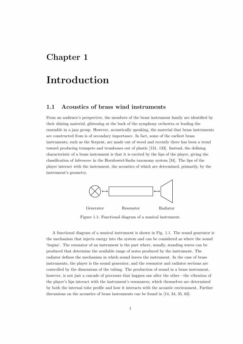
1.1 Functional diagram of a musical instrument. . . . . . . . . . . . . . . . . . . . . . 1

1.2 Schematic of how energy is transferred between different elements in the system.

Over time, all of the energy must be accounted for to determine stability. . . . . 3

2.1 Left: Undisturbed volume of air of length dz. Right: Air has been disturbed,

changing its overall length to dz′. The shaded area denotes the previous volume

the air occupied. . . . . . . . . . . . . . . . . . . . . . . . . . . . . . . . . . . . . 12

2.2 Left: Initial conditions to the wave equation. Forwards wave, ψ+(t − z/c0),

(dashed red); backwards wave, ψ−(t + z/c0), (dotted yellow); sum of forwards

and backwards solutions (solid blue). Right: Solution to the wave equation at a

later time. The waves now occupy different domains but preserve the shape they

had at t = t0. . . . . . . . . . . . . . . . . . . . . . . . . . . . . . . . . . . . . . . 13

2.3 Top: Input impedance for the wave equation with Dirichlet termination. Bottom:

Input impedance for the wave equation with Neumann termination. The cylinder

has a length L = 1 m, and radius r0 = 0.005 m. The values for air density and

speed of sound are ρ0 = 1.1769 kg ·m−3 and c0 = 347.23 m · s−1 corresponding

to a temperature of 26.85C. . . . . . . . . . . . . . . . . . . . . . . . . . . . . . 19

2.4 Profile of an acoustic tube with variable cross-sectional area, S(z), that changes

along the axial length, z. . . . . . . . . . . . . . . . . . . . . . . . . . . . . . . . . 20

2.5 Plots of the real part of the spatial solution to the horn equation, Re(ejβz

)at different frequencies. Left: ω is less than the cutoff frequency goes to zero.

Middle: ω is at the cutoff frequency and the solution still goes to zero but less

severely. Right: ω is above cutoff frequency and waves can propagate. . . . . . . 23

2.6 Top: Profile of an exponential horn of length 1 m, opening radius r(0) = 0.005 m

and flare parameter α = 5 m−1. Bottom: Input impedance for this horn with an

open end. c0 = 347.23 m · s−1 and ρ0 = 1.1769 kg ·m−3. Dashed vertical lines

show the resonances of a cylindrical tube with corresponding boundary conditions. 26

2.7 Top: A general acoustic tube. Bottom: An approximation of an acoustic tube

using a series of concatenated cylinders. . . . . . . . . . . . . . . . . . . . . . . . 27

2.8 Schematic of an element in the TMM. . . . . . . . . . . . . . . . . . . . . . . . . 28

2.9 Top: Real (left) and imaginary (right) parts of Γ calculated using the Zwikker

and Kosten Model for a tube of radius 0.005 m. Bottom: Fractional error of the

real and imaginary parts of Γ from the expansions given by Benade (blue), Keefe

(red), Causse et al. (yellow), Bilbao and Chick (purple) and Webster-Lokshin

(green). Note that the small and large expansions have been connected around

rv = 1 and rt = ν. . . . . . . . . . . . . . . . . . . . . . . . . . . . . . . . . . . . 33

ix

2.10 Left: Magnitude of Z in the complex plane. Right: Magnitude of Y in the

complex plane. Poles are bright yellow and zeros are green/blue. Note that

surfaces have been plotted using a logarithmic plot to accentuate the poles and

zeros. A tube of radius 0.03 m has been used to highlight the poles and zeros in

a reasonable range. . . . . . . . . . . . . . . . . . . . . . . . . . . . . . . . . . . . 35

2.11 Top: First form of Cauer RL circuit. Bottom: Second form of Cauer RC circuit. 35

2.12 Top: First form of Foster RL structure. Bottom: Second form of Foster RC.

Both structures have M branches. . . . . . . . . . . . . . . . . . . . . . . . . . . 36

2.13 Cauer structures. Top: Impedance structure. Bottom: Admittance structure. . . 38

2.14 Fractional error of impedance calculated using the Cauer structure for a tube of

radius 0.005 m. Left: Error in real part of impedance. Right: Error in imaginary

part of impedance. . . . . . . . . . . . . . . . . . . . . . . . . . . . . . . . . . . . 38

2.15 Fractional error of admittance calculated using the Cauer structure for a tube of

radius 0.005 m. Left: Error in real part of admittance. Right: Error in imaginary

part of admittance. . . . . . . . . . . . . . . . . . . . . . . . . . . . . . . . . . . . 39

2.16 Left: Magnitude of Zv in the complex plane. Right: Magnitude of Yt in the

complex plane. Poles are yellow and zeros are dark blue. Note that surfaces

have been plotted using a logarithmic plot to accentuate the poles and zeros.

The tube radius is 0.03 m . . . . . . . . . . . . . . . . . . . . . . . . . . . . . . . 39

2.17 Top: Zv Foster structure. Bottom: Yt Foster structure. . . . . . . . . . . . . . . . 40

2.18 Fractional error of Foster model optimised to Zv using ER for a tube of 0.005 m

over a frequency range 0 Hz to 10 kHz. Left: Error in real part. Right: Error in

imaginary part. . . . . . . . . . . . . . . . . . . . . . . . . . . . . . . . . . . . . . 45

2.19 Fractional error of Foster model optimised to Zv using EM for a tube of 0.005

m over a frequency range 0 Hz to 10 kHz. Left: Error in real part. Right: Error

in imaginary part. . . . . . . . . . . . . . . . . . . . . . . . . . . . . . . . . . . . 45


over a frequency range 0 Hz to 10 kHz when it is applied to admittance Yt. Left:

Error in real part. Right: Error in imaginary part. . . . . . . . . . . . . . . . . . 47

2.21 Fractional error of Foster model optimised to Zv using EM for a tube of 0.005

m over a frequency range 0 Hz to 10 kHz when it is applied to admittance Yt.

Left: Error in real part. Right: Error in imaginary part. . . . . . . . . . . . . . . 47

2.22 Fractional error of the impedance using the element values in (2.142) for a fourth

order filter. The original impedance was optimised using EM for a tube radius

of 0.005 m and a temperature of 26.85C. Left: Error in real part. Right: Error


2.23 Fractional error of the impedance using the element values in (2.143) for a fourth

order filter. The original impedance was optimised using EM for a tube radius

of 0.005 m and a temperature of 26.85C. Left: Error in real part. Right: Error




imaginary part. The shaded area shows the frequency range that optimisation

was performed over. . . . . . . . . . . . . . . . . . . . . . . . . . . . . . . . . . . 49

x

2.25 Fractional error of Foster model optimised to Zv using EM for a tube of 0.005 m


imaginary part. The shaded area shows the frequency range that optimisation

was performed over. . . . . . . . . . . . . . . . . . . . . . . . . . . . . . . . . . . 50

2.26 Fractional error of the impedance for the Foster model, optimised using ER (solid

lines) over a frequency range 0 Hz to 10 kHz, and for Cauer model (dashed lines)

for a tube of 0.005. Left: Error in real part. Right: Error in imaginary part. . . . 51

2.27 Fractional error of the impedance for the Foster model, optimised using EM

(solid lines) over a frequency range 0 Hz to 10 kHz, and for Cauer model (dashed

lines) for a tube of 0.005. Left: Error in real part. Right: Error in imaginary part. 51

3.1 Discretised domain for a finite-difference scheme. The temporal domain is sam-

pled at intervals of time k s and labelled using integers n. The spatial domain

is sampled at intervals of length h m and labelled using integers l. Black circles

denote the grid function f at each temporal and spatial point. . . . . . . . . . . . 56

3.2 Left: Grids that are interleaved only in space. Right: Grids that are interleaved

in time and space. Dashed lines show the original grid labelled by the integers n

and l. Dotted lines show the interleaved grid. Black circles denote the locations

of the grid function, f , on the integer field. White circles denote the locations

grid function, g, on the interleaved grids. . . . . . . . . . . . . . . . . . . . . . . . 57

3.3 Stencils of temporal difference operators, labelled at top, when applied to a grid

function at time step n (highlighted in green). Black circle denotes the grid

functions that are used, white circles are unused by the operator. . . . . . . . . . 58

3.4 Stencils of temporal difference operators, labelled at left, when applied to a grid

function at spatial step l (highlighted in red). Black circle denotes the grid

functions that are used, white circles are unused by the operator. . . . . . . . . . 59

3.5 Left: Geometric visualisation of inner product. Right: Geometric visualisation

of weighted inner product. At the boundaries of the domain, the weighted inner

product uses only half a spatial step. Black circles denote the values of f on the

spatial grid. . . . . . . . . . . . . . . . . . . . . . . . . . . . . . . . . . . . . . . . 61

3.6 Effect of bilinear transform on frequency mapping at different sample rates. At

high frequencies, the bilinear transform warps the frequency away from where it

is supposed to be represented. This is improved with a higher sample rate but

never truly goes away. . . . . . . . . . . . . . . . . . . . . . . . . . . . . . . . . . 64

3.7 Left: Dispersion for scheme (3.40) for different values of λ at a sample rate of 20

kHz. As λ moves away from the CFL condition, frequencies are warped. Right:

Bandwidth as a function of λ for the explicit scheme. The dashed line shows the

Nyquist frequency. . . . . . . . . . . . . . . . . . . . . . . . . . . . . . . . . . . . 67

3.8 Solutions calculated using scheme (3.42) at two time instants. The sample rate

is 20 kHz and λ = 1. The acoustic velocity potential has been initialised with an

Hann pulse of width 21 steps. . . . . . . . . . . . . . . . . . . . . . . . . . . . . . 71

3.9 Plot of hsum for the system in Fig. 3.8. The energy is calculated using the

weighted inner product form (3.64). . . . . . . . . . . . . . . . . . . . . . . . . . 72

xi

3.10 Left: Dispersion for scheme (3.78) for different values of λ at a sample rate of 20

kHz. Even for λ = 1, the dispersion deviates from the exact dispersion relation.

Right: Bandwidth of implicit scheme as a function of λ. The dashed line shows

the Nyquist frequency which this scheme can never fully achieve. . . . . . . . . . 73

3.11 Solutions calculated using scheme (3.89) at two time instances. The sample rate

is 20 kHz and λ = 1. The acoustic velocity potential has been initialised with

an Hann pulse of width 21 steps. Both sides of the domain are terminated using

the centred Neumann conditions. . . . . . . . . . . . . . . . . . . . . . . . . . . . 75

3.12 Plot of hsum for the system in Fig. 3.11. The energy is calculated using the

weighted inner product form (3.87). . . . . . . . . . . . . . . . . . . . . . . . . . 75

3.13 Input impedances calculated for a cylinder of length 0.3 m and radius 0.01 m

using the explicit (blue) and implicit (green) schemes. Top: Input impedance

calculated using λ = 1. Bottom: Input impedance calculated using λ = 0.7972.

Dashed vertical line show the exact resonances. Sample rate is 20 kHz. . . . . . . 76

3.14 Bore profile and surface areas on different girds. Solid line shows the bore profile.

Dashed line shows the spatial grid that S is calculated on and dotted line shows

the grid that S is sampled on. . . . . . . . . . . . . . . . . . . . . . . . . . . . . . 79

3.15 Input impedances for an exponential horn of length L = 0.3 m, flaring param-

eter α = 5 m−1, and opening radius r0 = 0.005 m calculated using the exact

expression (black), and explicit finite-difference scheme (blue), and an implicit

finite-difference scheme (green). Sample rate is 20 kHz and simulations were run

for 10 s. . . . . . . . . . . . . . . . . . . . . . . . . . . . . . . . . . . . . . . . . . 85

3.16 Left: Real part of (jω)1/2. Right: Imaginary part of (jω)1/2. Black line shows

the exact value. Coloured lines show approximations to the fractional derivative

using the IIR filter of differing orders constructed from the CFE of the bilinear

transform at 50 kHz. . . . . . . . . . . . . . . . . . . . . . . . . . . . . . . . . . . 89

3.17 Pole-zero plots for fractional derivative filter at 50 kHz. Left: Filter order of

20. Right: Filter order of 33. Poles are marked as red crosses and zeros as blue

circles. Dashed vertical and horizontal lines show where the real and imaginary

axes lie. Dashed circle is the unit circle. . . . . . . . . . . . . . . . . . . . . . . . 90

3.18 Left: Real part of (jω)1/2. Right: Imaginary part of (jω)1/2. Black line shows the

exact value. Blue, red and orange lines show approximations to the fractional

derivative using the IIR filter of order 4 (blue), 8 (red), 16 (orange), and 20

(purple) constructed from the CFE of the bilinear transform at 50 kHz. . . . . . 90

3.19 Errors in impedance when calculated using the bilinear transform at a sample

rate of 50 kHz (solid lines) and the exact frequency (dashed) for the Foster

network optimised using EM over 0 Hz to 10 kHz. Left: Error in real part.

Right: Error in imaginary part. . . . . . . . . . . . . . . . . . . . . . . . . . . . . 97

3.20 Errors in impedance when calculated using the bilinear transform at a sample

rate of 50 kHz (solid lines) and the exact frequency (dashed) for the Foster

network optimised using EM over 20 Hz to 3 kHz. Left: Error in real part.

Right: Error in imaginary part. Grey box shows optimisation range. . . . . . . . 97

3.21 Errors in impedance calculated using the bilinear transform at 50 kHz for the

Foster network optimised using E′M over 0 Hz to 10 kHz with pre-warped fre-

quencies. Left: Error in real part. Right: Error in imaginary part. . . . . . . . . 98

xii

3.22 Errors in impedance calculated using the bilinear transform at 50 kHz for the

Foster network optimised using E′M over 20 Hz to 3 kHz with pre-warped fre-

quencies. Left: Error in real part. Right: Error in imaginary part. Grey box

shows optimisation range. . . . . . . . . . . . . . . . . . . . . . . . . . . . . . . . 98

3.23 Input impedance calculated using the loss model of Bilbao and Chick for dif-

ferent filter orders. Top left: Input impedance magnitude. Bottom left: Input

impedance phase. Top right: Absolute percentage error in input impedance

peak position relative to TMM. Bottom right: Absolute percentage error in in-

put impedance peak magnitude. . . . . . . . . . . . . . . . . . . . . . . . . . . . . 100

3.24 Input impedance calculated using the Foster network with coefficients acquired

by optimising of E′M from 0 Hz to 10 kHz. Top left: Input impedance magnitude.

Bottom left: Input impedance phase. Top right: Absolute percentage error

in input impedance peak position relative to TMM. Bottom right: Absolute

percentage error in input impedance peak magnitude. . . . . . . . . . . . . . . . 100

3.25 Input impedance calculated using the Foster network with coefficients acquired

by optimising of E′M from 20 Hz to 3 kHz. Top left: Input impedance magnitude.




3.26 Input impedance of an exponential horn calculated using the Bilbao and Chick

loss model using different filter orders. Top left: Input impedance magnitude.




3.27 Input impedance of an exponential horn calculated using the Foster network

with coefficients acquired by optimising of E′M from 0 Hz to 10 kHz. Top left:

Input impedance magnitude. Bottom left: Input impedance phase. Top right:

Absolute percentage error in input impedance peak position relative to TMM.

Bottom right: Absolute percentage error in input impedance peak magnitude. . . 102

3.28 Input impedance of an exponential horn calculated using the Foster network

with coefficients acquired by optimising of E′M from 20 Hz to 3 kHz. Top left:

Input impedance magnitude. Bottom left: Input impedance phase. Top right:

Absolute percentage error in input impedance peak position relative to TMM.

Bottom right: Absolute percentage error in input impedance peak magnitude. . . 103

4.1 Circuit representation of approximation to the Levine and Schwinger radiation

model. . . . . . . . . . . . . . . . . . . . . . . . . . . . . . . . . . . . . . . . . . . 107

4.2 Left: Radiation reflection magnitude for a tube of radius 0.05 m calculated using

the Levine and Schwinger model (blue) and the network approximation. Right:

Radiation length correction. . . . . . . . . . . . . . . . . . . . . . . . . . . . . . . 108

4.3 Left: Error in reflection magnitude of network when using the bilinear transform

(dashed red) at 50 kHz. Right: Error in length correction. . . . . . . . . . . . . . 110

4.4 Top: Total stored energy (blue), stored energy in the tube (red), stored energy

in the radiation model (yellow), and energy lost by the radiation model (purple).

Bottom: Energy balance showing numerical precision of machine. . . . . . . . . . 112

xiii

4.5 Top: Input impedance of a lossless cylinder of radius 0.05 m and length 1 m

calculated using an FDTD simulation with lossy radiating end (solid black) and

a frequency domain calculation terminated with the Levine and Schwinger radia-

tion impedance (dashed red). Bottom: Absolute error in peak position of FDTD

simulation relative to frequency domain calculation. . . . . . . . . . . . . . . . . 113

4.6 Top: Input impedance of a lossless cylinder of radius 0.1 m and length 1 m cal-

culated using an FDTD simulation with lossy radiating end (solid black) and a

frequency domain calculation terminated with the Levine and Schwinger radia-

tion impedance (dashed red). Bottom: Absolute error in peak position of FDTD

simulation relative to frequency domain calculation. . . . . . . . . . . . . . . . . 114

4.7 Schematic of an embedded system. The cylindrical, or slowly varying, portion

of the instrument bore is modelled using a one-dimensional wave propagation

model. In the flaring portions of the instrument, a three-dimensional wave prop-

agation model is used. The dashed line shows the boundary between the two

sections of the instrument. . . . . . . . . . . . . . . . . . . . . . . . . . . . . . . . 114

4.8 Schematic of embedded system. Energy is transferred between the cylinder, at

left, and the enclosed volume of air, at right, via the point at the end of the tube

and the surface Ω. . . . . . . . . . . . . . . . . . . . . . . . . . . . . . . . . . . . 118

4.9 Illustration of the vectorisation of the three-dimensional grid function. . . . . . . 124

4.10 Staircased fitting applied to the interior of a circle, indicated by a blue line.

Dots indicate grid points and black lines denote the area they approximate. Red

centres denote grid points that lie within the circle, empty centres are those

that lie without. The perimeter of the staircased approximation to the circle is

indicated by a green line. . . . . . . . . . . . . . . . . . . . . . . . . . . . . . . . 125

4.11 Layout of simulations. Left: Wave propagation in one-dimensional model of

cylinder. Right: Cross-section of volume of air for the two simulation scenarios.

Top: Only the surface Ωd is positioned in the air box. Bottom: A cylindrical

profile is positioned behind the surface Ωd. Curved lines are a representation of

sound leaving Ωd. . . . . . . . . . . . . . . . . . . . . . . . . . . . . . . . . . . . . 128

4.12 Input impedance magnitudes of two cylinders calculated using the frequency do-

main expression terminated with the Levine and Schwinger radiation impedance

(solid blue) and using the embedded FDTD system with only the plane in the

air box (dashed red) and the cylinder in the air box (dotted yellow). Top: Tube

radius of 0.05 m. Bottom: Tube radius of 0.1 m. . . . . . . . . . . . . . . . . . . 129

4.13 Fractional differences in peak frequency of embedded system using just a plane

(red) and with a cylinder in the enclosed volume (yellow) relative to the exact

solution terminated with the Levine and Schwinger radiation impedance. Top:

Results for a tube of radius 0.05 m. Bottom: Results for a tube of radius 0.1 m. 129

4.14 Top: Energy evolution of the embedded FDTD system with only the plane Ωd

in the enclosed volume of air. Bottom: Deviation in the total stored and lost

energy over time. . . . . . . . . . . . . . . . . . . . . . . . . . . . . . . . . . . . . 130

4.15 Bore profile of Smith Watkins trumpet. . . . . . . . . . . . . . . . . . . . . . . . 130

xiv

4.16 Input impedances of the Smith Watkins trumpet with Kelly Screamer mouth-

piece; measured (black), simulation terminated with network approximation to

Levine and Schwinger radiation impedance (blue), simulation of embedded sys-

tem (red). . . . . . . . . . . . . . . . . . . . . . . . . . . . . . . . . . . . . . . . . 131

4.17 Top: Fractional error in peak position of input impedance of simulations relative

to experimental measurement. Bottom: Fractional error in peak magnitude of

impedance impedance of simulations relative to experiments. Error in simulation

terminated with network approximation shown in blue, error in embedded system

shown in red. . . . . . . . . . . . . . . . . . . . . . . . . . . . . . . . . . . . . . . 132

5.1 Schematic of lip reed. . . . . . . . . . . . . . . . . . . . . . . . . . . . . . . . . . 137

5.2 Displacement of the lip reed from equilibrium when no self sustained oscillation

occurs. . . . . . . . . . . . . . . . . . . . . . . . . . . . . . . . . . . . . . . . . . . 141

5.3 Energy balance of the system when no oscillation occurs. . . . . . . . . . . . . . 142

5.4 Displacement of the lip reed from equilibrium in the case of self sustained oscillation.142

5.5 Energy evolution of the system when self sustained oscillation occurs. Stored

energy in the reed (blue) and tube (red), summed power dissipation in reed

(orange) and summed power input at reed (purple). . . . . . . . . . . . . . . . . 143

5.6 Energy evolution of the system when self sustained oscillation occurs. Stored

energy in the reed (blue) and tube (red), summed power dissipation in reed

(orange) and summed power input at reed (purple). . . . . . . . . . . . . . . . . 143

5.7 Energy balance for self sustained oscillating system. . . . . . . . . . . . . . . . . 143

5.8 Schematic of a brass instrument valve. Three pieces of tubing are combined at

J . The pressure at the junction is the same in each piece of tubing and the total

volume velocity flow over the junction is conserved. . . . . . . . . . . . . . . . . . 144

5.9 Overlapping circles representing the junction of a valve. The default (green) and

bypass (red) tubes overlap the main tube (blue). However, it is clear that that

the total area of the main tube is not covered by the other tubes. . . . . . . . . . 145

5.10 Schematic of the valve junction on the discrete grids. The pressure at the valve

junctions is the same in each tube. There are velocities outside the domain, but

these can be removed using continuity of volume velocity over the junction. . . . 148

5.11 Schematic of a tube system that splits into two and then recombines back into

one tube. Note that modelling of the bypass tube is done by assuming it is

straight, its bent appearance in the figure is to show how the default and bypass

tubes reconnect. . . . . . . . . . . . . . . . . . . . . . . . . . . . . . . . . . . . . 149

5.12 Profile of the default tube. Black dotted lines show the pressure spatial grid,

grey dotted lines show the particle velocity grid, solid black lines show the bore

profile. . . . . . . . . . . . . . . . . . . . . . . . . . . . . . . . . . . . . . . . . . . 149

5.13 Top: Energy evolution of the system with q(d) = 0.5: total energy (blue), main

tube energy (red), default tube energy (yellow), bypass tube (purple), recombined

tube (green). Bottom: energy balance for the whole system. . . . . . . . . . . . . 151

5.14 Input impedance calculations for the lossy valved tube system for different open-

ing configurations. Top to bottom: Decreasing value of q(d) from 1 to 0 in

increments of 0.25. . . . . . . . . . . . . . . . . . . . . . . . . . . . . . . . . . . . 152

xv

5.15 Top: Energy evolution of the valved system with time varying openings. Bottom:

Energy balance of the system. . . . . . . . . . . . . . . . . . . . . . . . . . . . . . 156

6.1 Structure of the brass instrument synthesis environment. Users specify instru-

ment and score files (in blue rectangle) that are inputs to the code. These input

files are then used in the precomputation stage (green rectangle) to calculate

system parameters and control streams used in the main loop (red rectangle)

where the system variables (acoustic pressure, particle velocity, lip position) are

computed. The output (purple rectangle) is generated as a WAV file from the

pressure at the end of the instrument. . . . . . . . . . . . . . . . . . . . . . . . . 158

6.2 Example of an instrument constructed using the custom instrument function.

Section (a) is the mouthpiece defined using a cosine, (b) a cylindrical segment,

(c) is a bulge defined using the square of a sinusoid, (d) a converging conical

section, and (e) is the flaring section defined using a power of the axial position. 160

6.3 Top: Spectrogram of output sound when the lip frequency linearly changes from

220 Hz to 1000 Hz over 3 s. Bottom: The lip frequency as a function of time. . . 163

6.4 Top: Time series of output when two separate notes are played. Bottom: Cor-

responding mouth pressure as a function of time. . . . . . . . . . . . . . . . . . . 163

6.5 Top: Spectrogram of output sound when vibrato is added to the note after 1 s.

Bottom: Lip frequency as a function of time. Lip frequency is constant for first

second then modulation is added. . . . . . . . . . . . . . . . . . . . . . . . . . . . 164

6.6 Top: Time series of output sound when tremolo is added. Bottom: Mouth

pressure as a function of time. After the initial increase, the mouth pressure

remains constant for the first second, after which the tremolo is added. . . . . . . 164

6.7 Top: Spectrogram of output sound when noise is added after 1 s. Bottom:

Corresponding mouth pressure signal, with noise added after 1 s. . . . . . . . . . 165

6.8 Spectrogram of output for repeated lip frequency sweeps from 300 Hz to 700 Hz

over 2 s whilst changing valve configurations. At 2 s intervals, the next valve is

depressed. This corresponds to a reduction in the lowest peak frequency shown

in the spectrogram. . . . . . . . . . . . . . . . . . . . . . . . . . . . . . . . . . . . 165

6.9 Spectrum of sounds produced with valves in open configuration (blue) and par-

tially open configuration (red). . . . . . . . . . . . . . . . . . . . . . . . . . . . . 166

6.10 Top: Spectrogram of sound produced when first valve is modulated. Bottom:

Time series of the first valve opening. . . . . . . . . . . . . . . . . . . . . . . . . 167

6.11 Example of a sound that fits the acceptance criteria. It is clear that the appear-

ance of the repeated cycle that makes up the sustained part of the note occurs

before 0.07 s. . . . . . . . . . . . . . . . . . . . . . . . . . . . . . . . . . . . . . . 167

6.12 Playability space for Smith Watkins trumpet bore used in brass instrument en-

vironment. Points denote areas where a note is produced whose sustained part

occurs in 0.07 s or less. Dashed vertical lines show where the instrument reso-

nances lie. . . . . . . . . . . . . . . . . . . . . . . . . . . . . . . . . . . . . . . . . 168

xvi

7.1 Left: A simple wave. Right: An example of distortion applied to the wave (solid

line) with the original wave profile shown as reference (dotted line). Arrows show

how the wave has been distorted, with positive values sped up, and negative

values slowed down. . . . . . . . . . . . . . . . . . . . . . . . . . . . . . . . . . . 174

7.2 Propagation of a Hann pressure pulse of width 1/300 s and amplitude 3 % of

atmospheric pressure in a cylindrical tube modelled using the Euler equations

(blue), Burgers equation (dashed red), generalised Burgers equation (dash-dot

yellow), and the linear horn equation (dotted purple). Labels above peaks denote

corresponding time steps. . . . . . . . . . . . . . . . . . . . . . . . . . . . . . . . 180


atmospheric pressure in a cylindrical tube modelled using the Euler equations

(blue), Burgers equation (dashed red), generalised Burgers equation (dash-dot

yellow), and the linear horn equation (dotted purple). Labels above peaks denote

corresponding time steps. . . . . . . . . . . . . . . . . . . . . . . . . . . . . . . . 180


atmospheric pressure in an exponential horn with flaring parameter α = 0.5

m−1 modelled using the Euler equations (blue), Burgers equation (dashed red),

generalised Burgers equation (dash-dot yellow), and the linear horn equation

(dotted purple). Labels above peaks denote corresponding time steps. . . . . . . 181


atmospheric pressure in an exponential horn with flaring parameter α = 1 m−1

modelled using the Euler equations (blue), Burgers equation (dashed red), gener-

alised Burgers equation (dash-dot yellow), and the linear horn equation (dotted

purple). Labels above peaks denote corresponding time steps. . . . . . . . . . . . 181

7.6 Input impedances calculated using models 1-3 for an exponential horn of length 1

m and flaring parameter 1 m−1 terminated with a Dirichlet boundary condition.

Dashed black lines show the resonance frequencies of a cylinder of similar length. 185

7.7 Top: Test case where the tube is excited with the same signal at both ends.

Bottom: Test case where the tube is excited with signals of opposite signs at

both ends. Dashed line shows where the output is taken. . . . . . . . . . . . . . . 185

7.8 Pressure signals recorded 75 % along a tube of length 3 m when excited at both

ends with Hann pulses of amplitude 5 % of atmospheric pressure, with the same

sign, Test 1 (blue), and opposite sign, Test 2 (red). Top: Pulse width 1/300 s.

Middle: Pulse width 1/500 s. Bottom: Pulse width 1/700 s. . . . . . . . . . . . . 186

7.9 Percentage differences in magnitude of output relative to a single input. Top:

Test 1 difference. Bottom: Test 2 difference. . . . . . . . . . . . . . . . . . . . . . 187

7.10 Percentage differences in angle of output relative to a single input. Top: Test 1

difference. Bottom: Test 2 difference. . . . . . . . . . . . . . . . . . . . . . . . . . 188

7.11 Percentage differences in magnitude of output relative to a single input for a

pulse of width 1/500 s for tubes of different lengths. Top: Test 1 difference.

Bottom: Test 2 difference. . . . . . . . . . . . . . . . . . . . . . . . . . . . . . . . 189

7.12 Percentage differences in angle of output relative to a single input for a pulse

of width 1/500 s for tubes of different lengths. Top: Test 1 difference. Bottom:

Test 2 difference. . . . . . . . . . . . . . . . . . . . . . . . . . . . . . . . . . . . . 189

xvii

7.13 Percentage differences in magnitude of output relative to a single input for a

pulse of width 1/300 s for tubes of different lengths. Top: Test 1 difference.

Bottom: Test 2 difference. For L = 6 m the differences go to 25 % for Test 1

and −25 % for test 2. . . . . . . . . . . . . . . . . . . . . . . . . . . . . . . . . . 190

7.14 Percentage differences in angle of output relative to a single input for a pulse

of width 1/300 s for tubes of different lengths. Top: Test 1 difference. Bottom:

Test 2 difference. For L = 6 m the differences go to 25 % for Test 1 and −25 %

for test 2. . . . . . . . . . . . . . . . . . . . . . . . . . . . . . . . . . . . . . . . . 190

A.1 One-port networks. Left: Resistor network. Middle: Inductor network. Right:

Capacitor network. . . . . . . . . . . . . . . . . . . . . . . . . . . . . . . . . . . . 197

A.2 Left: Currents into and out of a node. Right: The looped sum of voltages. . . . . 198

A.3 Top: Circuit with elements connected in series. Bottom: Circuit with elements

connected in parallel. . . . . . . . . . . . . . . . . . . . . . . . . . . . . . . . . . . 199

A.4 An RLC circuit which has the same response as a simple harmonic oscillator

with damping. . . . . . . . . . . . . . . . . . . . . . . . . . . . . . . . . . . . . . 199

C.1 A trumpet valve in isolation. . . . . . . . . . . . . . . . . . . . . . . . . . . . . . 207

C.2 Schematic of valve experiment . . . . . . . . . . . . . . . . . . . . . . . . . . . . . 207

C.3 Simulated and measured input impedance with the valve fully open. . . . . . . . 208

C.4 Simulated and measured input impedance where 9 washers are used to keep the

valve partially open. . . . . . . . . . . . . . . . . . . . . . . . . . . . . . . . . . . 208







C.8 Simulated and measured input impedance with the valve fully closed. . . . . . . 210


valve partially open. The value of q(b) has been modified in the simulation to

better match the results of experiment. . . . . . . . . . . . . . . . . . . . . . . . . 210

xviii

List of Tables

2.1 Modal solutions and modal frequencies of the wave equation for different combi-

nations of boundary conditions. . . . . . . . . . . . . . . . . . . . . . . . . . . . . 18

2.2 Resonance frequencies of 1 m horns of cylindrical and exponential profile, flaring

constant being 5 m−1, and percentage difference of horn resonances relative to

cylinder resonances. c0 = 325 m · s−1. . . . . . . . . . . . . . . . . . . . . . . . . 25

2.3 Angular frequencies of resonances of 1 m long exponential horn with flaring con-

stant being 5 m−1 calculated using the exact expression (2.76) and the Transmis-

sion Matrix Method with element lengths of 0.1 m and 0.01 m. c0 = 325 m · s−1.

. . . . . . . . . . . . . . . . . . . . . . . . . . . . . . . . . . . . . . . . . . . . . . 29

2.4 List of thermodynamic constants and their calculation as a function of ∆T which

is the temperature deviation from 26.85 C. Originally presented by Benade [13]

and reprinted by Keefe [94] . . . . . . . . . . . . . . . . . . . . . . . . . . . . . . 30

2.5 Frequency domain impedance and admittances that include viscous and thermal

losses in acoustic tubes . . . . . . . . . . . . . . . . . . . . . . . . . . . . . . . . . 31

2.6 Propagation constants that include viscous and thermal losses in acoustic tubes. 32

3.1 Differential operators and the expansion point that gives second order accuracy

in time or space. . . . . . . . . . . . . . . . . . . . . . . . . . . . . . . . . . . . . 60

3.2 Modal solutions and modal frequencies for the wave equation solved with the

explicit scheme (3.40) using the uncentred and centred Neumann boundary con-

ditions at l = 0 and l = N . . . . . . . . . . . . . . . . . . . . . . . . . . . . . . . 69

6.1 Parameters and typical values used in score file that plays a trumpet. . . . . . . 161

B.1 Foster element values when optimising using ER for a tube of radius 0.005 m at

26.85 C over the frequency range 0.1− 10 kHz. . . . . . . . . . . . . . . . . . . . 201

B.2 Foster element values when optimising using EM for a tube of radius 0.005 m at

26.85 C over the frequency range 0.1− 10 kHz. . . . . . . . . . . . . . . . . . . . 202

B.3 Foster element values when optimising using ER over a smaller frequency range

for a tube of radius 0.005 m at 26.85 C over the reduced frequency range 20 Hz

- 3 kHz. . . . . . . . . . . . . . . . . . . . . . . . . . . . . . . . . . . . . . . . . . 202

B.4 Foster element values when optimising using EM for a tube of radius 0.005 m at

26.85 C over the reduced frequency range 20 Hz - 3 kHz. . . . . . . . . . . . . . 203

B.5 Foster element values when optimising using E′M for a tube of radius 0.005 m at

26.85 C over the pre-warped frequency range 0.1 − 10 kHz at a sample rate of

50 kHz. . . . . . . . . . . . . . . . . . . . . . . . . . . . . . . . . . . . . . . . . . 204

xix


26.85 C over the pre-warped frequency range 20 Hz - 3 kHz at a sample rate of

50 kHz. . . . . . . . . . . . . . . . . . . . . . . . . . . . . . . . . . . . . . . . . . 204



50 kHz. . . . . . . . . . . . . . . . . . . . . . . . . . . . . . . . . . . . . . . . . . 205



100 kHz. . . . . . . . . . . . . . . . . . . . . . . . . . . . . . . . . . . . . . . . . . 205

xx

Chapter 1

Introduction

1.1 Acoustics of brass wind instruments

From an audience’s perspective, the members of the brass instrument family are identified by

their shining material, glistening at the back of the symphony orchestra or leading the

ensemble in a jazz group. However, acoustically speaking, the material that brass instruments

are constructed from is of secondary importance. In fact, some of the earliest brass

instruments, such as the Serpent, are made out of wood and recently there has been a trend

toward producing trumpets and trombones out of plastic [131, 133]. Instead, the defining

characteristic of a brass instrument is that it is excited by the lips of the player, giving the

classification of labrosone in the Hornbostel-Sachs taxonomy system [34]. The lips of the

player interact with the instrument, the acoustics of which are determined, primarily, by the

instrument’s geometry.

Generator Resonator Radiator

Figure 1.1: Functional diagram of a musical instrument.

A functional diagram of a musical instrument is shown in Fig. 1.1. The sound generator is

the mechanism that injects energy into the system and can be considered as where the sound

‘begins’. The resonator of an instrument is the part where, usually, standing waves can be

produced that determine the available range of notes produced by the instrument. The

radiator defines the mechanism in which sound leaves the instrument. In the case of brass

instruments, the player is the sound generator, and the resonator and radiator sections are

controlled by the dimensions of the tubing. The production of sound in a brass instrument,

however, is not just a cascade of processes that happen one after the other—the vibration of

the player’s lips interact with the instrument’s resonances, which themselves are determined

by both the internal tube profile and how it interacts with the acoustic environment. Further

discussions on the acoustics of brass instruments can be found in [14, 34, 35, 63].

1

The conventional modelling picture of a musical instrument is that of steady state

oscillations to produce a single note at a fixed pitch. In this work we intend to be more

general and extend this picture beyond single tones.

1.2 A brief history of physical modelling

The history of sound synthesis and the field of physical modelling are intimately linked with

developments in electronics and computing that occurred during the 20th Century. Methods

such as additive, subtractive, and FM synthesis involve the manipulation of periodic signals to

control the timbre of the sound. Wavetable synthesis involves the use of lookup tables to store

waveforms that are then repeated at different speeds to change the pitch. Amplitude

modulation can then be used to modify these sounds. These early synthesis methods are

described by Roads in [141] and were applied to trumpet synthesis by Morrill [119]. These

methods allow for a wide variety of sounds with minimal computational effort, but require a

large and non-intuitive parameter space that is difficult to map to the perceived sounds.

As understanding of the musical instrument systems improved, researchers began using the

physics of the systems to produce sounds—the beginning of physical modelling. Constructing

virtual instruments using these methods gives the user an intuition over their control.

The work of Kelly and Lochbaum on vocal tract modelling [96] is considered the first

physical modelling framework, and its influence is still seen today in acoustic tube modelling

as an efficient simulation tool; see [81] for example. The Kelly-Lochbaum structure uses the

knowledge of the physical system, mainly the scattering of waves from changes in

cross-sectional area, to produce a filter that behaves in a similar manner to the vocal tract.

Other methods based on travelling wave formulations have followed from this earlier work,

particularly the Digitial Waveguide Framework used in string [149] and brass [47] instrument

synthesis. This method saw later commercial success in the Yamaha VL1 synthesiser [144].

Modal methods can be applied to simulate the individual modes of vibration present

within the instrument and were applied to brass instrument synthesis in the MoReeSC

framework [148] and to general synthesis in the MOSAIC system [120].

With improvements in computing hardware, it became possible to directly simulate

musical instrument systems using discrete numerical methods, such as finite-difference

time-domain (FDTD) methods, to solve the partial differential equations. Although

applications to string modelling dates back to the 1970’s [87], and even earlier to solve

problems in electromagnetism [179], these methods have seen regular application in the last

twenty years, spurred on by the work of Botteldooren [31, 32] and Savioja [145] in room

acoustics and Chaigne [38] in musical acoustics. Recently these methods have been extended

by Bilbao and colleagues [21, 74, 163], with specific applications to brass instruments shown in

[22, 23]. It is these methods that will be the focus of this thesis.

1.3 Passive time-domain modelling

The steady state solutions to instrument systems show only part of the possible soundscape

that virtual instruments can produce. To extend the region of possible sounds we must look

to time varying systems. This is not a trivial task as time domain problems can suffer from

stability issues. The modular approach to describing a brass instrument through sound

2

generator, resonator, and radiator also introduces problems as the connections between each

section must be stable. To approach this problem, we therefore look to passive methods of

time domain modelling that guarantee this type of growth does not occur in the global system

and its connecting parts.

As we are examining a physical system, it is sensible to consider the overall energy of the

system. This includes the energy stored within the propagating parts of the system and at the

boundaries along with any dissipation or forcing terms; see Fig. 1.2.

Energy storedin domain

Energy storedat boundaries

Energy lostover domain

Energy lostat boundaries

Energy injectedinto system

Total energyover time

Figure 1.2: Schematic of how energy is transferred between different elements in the system.Over time, all of the energy must be accounted for to determine stability.

Energy methods [71] are constructed by taking appropriate norms over the continuous

system equations to define an upper limit to the energy as the system evolves in time. This

idea is related to the Port-Hamiltonian framework [164] which uses a general energy picture to

construct the synthesis procedure; this will be discussed in Chap. 3. Additional non-negativity

constraints on the energy bound the norms of the solution which suggests stable behaviour.

These energy methods can then be transferred into the discrete domain to determine if the

numerical scheme is going to be stable. The reader may reasonably ask ‘Why not apply these

methods to the discrete case immediately?’. As will become apparent in Chap. 3, there are

multiple approaches to discretising schemes along with multiple approaches to constructing

numerical energies for them. By already constructing an energy in the continuous time

domain, we know what to aim for in the discrete case.

The discrete energy methods offer additional advantages for the algorithm designer.

Discrete forms of boundary conditions are naturally suggested from the construction of the

numerical energy, aiding in scheme design. In addition, a computation of the discrete energy

of the system serves as a debugging tool, where deviations in the energy beyond that of

machine precision would suggest incorrect implementation.

1.4 Accuracy and efficiency

Applications of numerical methods introduce inaccuracies into simulations, typically

highlighted through examining the truncation order [156], which displays how accurate the

scheme is with relation to how it is discretised. For audio applications, we do not require an

infinite accuracy as there is an upper limit to the frequencies a human can hear. However,

3

additional artefacts can be introduced by the numerical method, such as inharmonicity due to

frequency warping and aliasing, which must be removed.

In general, accuracy of a numerical method can be improved by increasing the resolution

of the domain over which simulations are performed over. This, however, creates its own

issues from a user standpoint: a finer resolution simulation requires more computational

operations and therefore takes longer to complete. An ideal simulation would at best be

real-time: a user would have to wait one second for a single second of sound to be produced.

However, if this fast output displays significant artefacts, a user will not be satisfied with the

sound. As a result, the algorithm designer must be aware of this balance between creating the

correct solution within a reasonable amount of time.

1.5 Thesis objectives

The main objective of this thesis is to develop a framework for the synthesis of brass

instrument sounds. This broad objective can be broken down into several smaller objectives:

• Model wave propagation in an acoustic tube, with the inclusion of boundary layer effects

and those due to changes in cross-sectional area of the tube

• Inclusion of boundary conditions at the entrance and exit of the tube for accurate

excitation and radiation modelling

• Enabling the changing of the instrument’s resonances through the use of valves

• Incorporation of nonlinearities in the propagation models

These goals will be achieved through the application of FDTD methods. Geometric

integration methods focussing on the energy of the system will be used to guarantee that the

formulations are passive.

The framework described in this work has been applied in a virtual instrument

environment that has been used by several musicians during the course of this Ph.D. project.

The specifics of the design of the environment is outwith the scope of this work, but some

discussion on how the code is structured and how such a virtual instrument is controlled is

presented in Chap. 6.

1.6 Thesis outline

The outline of this thesis is as follows:

Chapter 2 - Wave propagation in acoustic tubes

We begin with an outline of the linear acoustic tube system that describes low-amplitude

wave propagation in brass instruments. The wave equation is derived for disturbances within

a fluid filled cylindrical tube followed by the introduction of dispersion and energy analysis of

the system. Simple boundary conditions are discussed along with the concept of an input

impedance, a common experimentally measured quantity. The system is then extended to a

lossless acoustic tube whose cross-sectional area varies along the axial coordinate. The

4

Transmission Matrix Method is introduced as a ‘ground truth’ that later FDTD simulations

will be compared against.

The second half of this chapter concerns losses restricted to the boundary layers of

acoustic tubes—of particular interest is the model of Zwikker and Kosten. A survey of

previous approximations to this model is presented, along with a discussion of positive real

functions (a requirement for passivity). This then leads into a novel approximation using

electrical network representations. These networks are fully explored so that a minimal choice

of parameters can be applied to tubes of different radii and systems at different temperatures.

The accuracy of these structures can also be improved by reducing the frequency range over

which they are optimised.

Chapter 3 - Finite-difference time-domain methods: Applications to

acoustic tubes

This chapter concerns the numerical problem of simulating wave propagation in acoustic

tubes. The fundamentals of FDTD methods are introduced and then applied to the equations

introduced in Chap. 2. Comparisons are made using explicit and implicit numerical schemes

(the latter employing the bilinear transform) to simulate wave propagation in the lossless

system, with focus on the construction of a numerical energy as well as frequency domain

effects related to bandwidth reduction and warping.

FDTD methods are then applied to the system that includes boundary layer losses. A

method for constructing an approximation to the fractional derivatives seen in the literature is

presented, although stability is not proven. A numerical scheme for the network model is also

presented which is proven to be stable. Frequency warping effects can be addressed in this

approximation by ‘pre-warping’ the frequency variable during the optimisation procedure.

The numerical schemes for the loss models are compared for the cases of a cylinder and an

exponential horn.

Chapter 4 - Modelling radiation of sound from an acoustic tube

The problem of modelling the sound radiation behaviour of an acoustic tube is the subject of

this chapter. The first section looks at first approximating the Levine and Schwinger radiation

impedance of an unflanged cylinder using a simple equivalent electrical network and how this

is translated into an FDTD scheme that is coupled to the acoustic tube.

The remainder of the chapter looks to embedding the instrument in a three-dimensional

sound field. This is done by coupling the one dimensional acoustic tube model to the

three-dimensional wave equation via energy conserving principles. The problem is stated in

the continuous domain and then translated to the discrete domain. Comparisons against

experimental measurements show greater agreement for the embedded system than the

simpler equivalent network model.

Chapter 5 - Towards a complete instrument

This chapter introduces the remaining elements required to produce a virtual instrument. A

review of lip reed modelling is presented and a simple model is chosen as the excitation

5

mechanism for the instrument. The discretisation procedure and some simple results using

this model are presented.

To modify the resonances of the instrument, a valve model is presented that introduces

additional paths that waves may propagate through. The model presented here is derived

from energy and momentum conservation and allows for the interaction between the two

paths when the valve is partially depressed, resulting in complex resonance phenomena. The

scheme for the lossless system is presented, along with extensions to those where losses are

included in the wave propagation model and when the valves are allowed to vary with time.

Chapter 6 - A brass instrument synthesis environment

The elements described in the previous chapters are combined to create a virtual instrument

that allows the user to construct and control the instrument. The basic structure of the code

is presented along with a discussion on how the user interacts with it. Examples of gestures

are presented, displaying such effects as time varying modulation of parameters along with the

production of ‘multiphonic’ sounds from partially open valves. A simple playability space

study highlights some of issues related to control of an instrument.

Chapter 7 - Comparison of nonlinear propagation models

This chapter looks to the extension of the propagation model by including nonlinear effects

that contribute to the ‘brassy’ timbre of brass-wind instruments played at high dynamic

levels. A review of current models highlights the use of separable wave solutions—the effect of

this assumption is explored in this chapter. Simple numerical experiments are performed to

show the effect of coupling between forwards and backwards waves in an acoustic tube and

linearised forms of the models help explain why such models do not accurately represent the

behaviour due to changes in cross-sectional area.

Chapter 8 - Conclusions and future work

This chapter provides a summary of the work performed in this thesis and how it can be

extended in the future.

Appendix A - Circuit elements

A brief introduction to the use of passive circuit representations is presented here for those

unacquainted with the method. Although not extensive, this should help the unfamiliar

reader with the discussions in chapters 2-4.

Appendix B - Foster network element values

This appendix presents a list of tables containing the network element values used in the

Foster network apporoximation to the boundary layer loss model.

Appendix C - Experiments on brass instrument valves

Preliminary experiments are presented relating to the effect of partially open valve systems. A

simple experimental set up is described and experimental measurements are compared to

6

simulations.

1.7 Main contributions

The main contributions of this thesis are

• Development of an approximation to the boundary layer loss model of Zwikker and

Kosten using passive circuit representations whose parameters can be modified for use in

both the impedance and admittance models, different tube radii, and simulations at

different temperatures. This approximation is presented in Secs. 2.4.3 to 2.4.12

• Construction of an explicit, passive, and guaranteed stable numerical scheme for the

boundary layer loss model including modification to counter frequency warping effects.

This scheme is presented in Secs. 3.5.2 to 3.5.3.

• Modelling an embedded instrument system by coupling the one-dimensional model to

the three-dimensional wave equation. This is presented in Secs. 4.2 to 4.2.12.

• Development of a time-varying valve model to modify the instrument’s resonances that

allow for production of multiphonic tones. This model is presented in Sec. 5.2

• Investigation of wave separation in nonlinear propagation models. This is presented in

Chap. 7.

All results, with the exception of the nonlinear propagation models, are tied together with

strict passive realisations to create explicit schemes.

7

Act I

Linear Acoustics

8

Chapter 2

Wave propagation in acoustic

tubes

“Essentially, all models are wrong, but some are useful.”

— George Box

The construction of a brass instrument creates an enclosure of air within the instrument’s

tubing. The diameter of the instrument is significantly less than its overall length—we can

describe this as an acoustic tube. Although, strictly speaking, a brass instrument is defined in

a three-dimensional space, its behaviour can be well described using a one-dimensional

approximation. There are some caveats to this simplification, namely that the wavelengths of

interest are longer than the diameter of the instrument bore and that the bore profile changes

slowly along the length of the instrument [63, 132]. The input of the instrument is closed off

by the lips of the player (or by a loudspeaker in experimental settings) and its radiating end is

left open. When excited, e.g. by buzzing the lips to inject pulses of air into the system, waves

are created that travel along the length of the tube. At the open end, the wave is partially

transmitted out of the instrument (which becomes the sound an observer hears) and partially

reflected back into it. This reflected wave combines with the other incoming waves to set up a

series of resonances within the instrument—these resonances are what determine the range of

available notes that can be played.

In the linear approximation, the profile of the instrument bore and associated viscous and

thermal effects in air dominate the locations and widths of these resonances [63]—the

dynamics of the acoustic tube in isolation are the subject of this chapter. Another attribute is

that of radiation, but discussion of this is postponed until Chap. 4. See Chap. 7 for models

that include nonlinear propagation—the mechanism which creates the ‘brassy’ sound at high

dynamic levels [88].

This chapter is concerned with the model problem. Numerical simulation techniques will

be introduced in the next chapter. To begin, the notation used for partial differential

equations is introduced along with identities that will be used frequently in the analysis of the

systems. Frequency domain transformations will also be covered in this section.

The rest of this chapter is then split into two parts. First the lossless problem is discussed

in the case of a cylindrical tube and then with a tube of varying cross-section. The discussion

of these two systems follows in a parallel manner. Dispersion analysis is discussed followed by

9

energy analysis on the infinite, then bounded domains. Passivity of the system is a constant

theme throughout this work and the energy analysis presented here is a suitable method to

show stability that later translates into the discrete case. In addition, this also allows for a

convenient analysis of boundary conditions which are used to calculate the modes of the

system. The concept of the input impedance is then introduced which is related to the modes

of the system. A small step is taken into numerical methods at this point to cover the

Transmission Matrix Method as this will be used as our “ground truth” when comparing the

numerical models in later chapters.

The last section of this chapter concerns viscous and thermal mechanisms that lead to the

dissipation of energy within an acoustic tube. The standard model of Zwikker and Kosten

[182] is introduced; in general, this model is expressed in the frequency domain so further

approximations must be made for it to be used in a time domain model, several of which are

presented from the literature. The concept of positive realness [165, 174] is introduced as this

is important for the construction of equivalent circuits to approximate the Zwikker and

Kosten model. Two such structures are presented: Cauer and Foster [165, 174]. A brief

discussion of these structures is presented before application to attenuation modelling, in

which the Foster model is selected as a suitable candidate. The time domain representation of

the Foster structure is introduced, along with energy analysis to show that the network is

passive. Implementation of the Foster structure requires appropriate circuit element values

which are found through a numerical optimisation procedure. This is briefly discussed, along

with how the values can be manipulated to use for different tubes. Finally, an overall

comparison of the different approximations is made.

2.1 Introducing notation: Etude I

Before discussing the model for wave propagation, some notation must first be introduced.

2.1.1 Partial differential equations and differential operators

In many branches of science, the system under examination can be described by partial

differential equations (PDEs). These equations describe how some function varies with respect

to its independent variables, e.g. space or time. For the majority of this work we will only

consider variation in time over the positive real axis, t ∈ R+ = 0 ≤ t ≤ ∞, and axial

coordinate over the real axis, z ∈ R = −∞ ≤ z ≤ ∞. A finite spatial domain of an acoustic

tube is defined by D = z ∈ R | 0 ≤ z ≤ L], where L is the finite length of the acoustic tube.

∂t and ∂z represent differentiation with respect to t and z respectively. Higher derivatives are

denoted as powers of the operators mentioned previously, e.g. ∂2t , ∂3

z . PDEs will be labelled

according to their highest derivative, e.g. second derivative PDE, first derivative PDE. This

strays from the normal labelling using ‘order’ so as to avoid confusion when discussing

accuracy of simulations in later chapters. In order to describe a complete physical system, a

PDE must be complemented by boundary conditions and initial conditions.

2.1.2 Integral relations and identities

It is useful to define inner products along with other identities that can be used to determine

passivity of the system through energy analysis. The one-dimensional L2 inner product

10

between two continuous functions f and g over the generic domain z ∈ W is

〈f, g〉W =

∫Wfgdz (2.1)

The L2 norm comes from this inner product

‖f‖W =√〈f, f〉W (2.2)

Integration by parts will be used repeatedly in the work that follows:∫Wf∂zgdz = |fg|W+

W−−∫W

(∂zf) gdz =⇒ 〈f, ∂zg〉W = fg|z=W+−fg|z=W−−〈∂zf, g〉W (2.3)

where W+ and W− denote the boundaries of the domain.

Another useful identity is:

f∂tf =1

2∂t(f2)

=⇒ 〈f, ∂tf〉D =1

2

d

dt‖f‖2D (2.4)

where the d/dt is the total derivative operator1.

2.1.3 The Laplace transform and the frequency domain

In acoustics and signal processing, it is often of use to analyse the system using the Laplace

transform. This maps the function f(t) of time to the complex plane f(s), where s = σ + jω,

σ is the real frequency, ω is the imaginary or angular frequency, and j = +√−1. Frequency

domain functions will be notated with theˆoperator.

Neglecting initial conditions2 the two sided Laplace transformation is defined as [39]

f(s) = Lf(t) =

∫ ∞−∞

e−stf(t)dt (2.5)

The Laplace transform of the time derivative of a function is

L∂tf(t) = sf(s) (2.6)

The two sided Laplace transform is equivalent to the ansatz

f = est (2.7)

For multivariable functions of time and space, the Laplace transform is easily extended as the

spatial coordinate is independent of time.

The Fourier transform is related to the Laplace transform. It considers only the imaginary

part of the complex domain so that s = jω. This is denoted as

f(ω) = Ff(t) =

∫ ∞−∞

e−jωtf(t)dt (2.8)

1Here the coordinate z is independent of t so that the norm of f is only a function of t. We can therefore gofrom the partial derivative with respect to time to the total derivative with respect to time.

2This is valid as we will consider only the steady state in this type of analysis.

11

The same properties hold for the Fourier transform of the time derivative as for the Laplace

transform.

2.2 The wave equation

Here, we derive the one-dimensional wave equation that describes the dynamics of air

contained in a cylindrical tube of cross-sectional area S0. The derivation here follows that of

Morse [121].

z z + dz

dz

ξ (t, z) ξ (t, z + dz)

dz′

Figure 2.1: Left: Undisturbed volume of air of length dz. Right: Air has been disturbed,changing its overall length to dz′. The shaded area denotes the previous volume the air occupied.

Consider a small element of air within the tube that lies between z and z + dz, where dz is

the length of the element; see at left in Fig. 2.1. The total volume of air is given by V = S0dz

with a total mass m = ρ0V , where ρ0 is the static air density. As a disturbance passes

through the tube, the end points of this element are displaced a distance ξ(t, z) as shown at

right in Fig. 2.1. This changes the total length to be

dz′ = dz + ξ(t, z + dz)− ξ(t, z) (2.9)

For small dz, the Taylor expansion of this expression reduces to

dz′ = (1 + ∂zξ) dz (2.10)

so that the new volume is

V ′ = S0 (1 + ∂zξ) dz (2.11)

The change in volume is given by

dV = S∂zξdz (2.12)

Assuming there is no change in temperature over the element, the pressure, p(t, z), generated

due to the change in volume is given by

p = −KdV

V=⇒ p = −K∂zξ (2.13)

where K is the bulk modulus of air.

If we now examine the forces acting on the element of air, we see that the acceleration of

the element is given by the pressure gradient over the two sides

ρ0S0dz∂2t ξ = −S0 (p(t, z + dz)− p(t, z)) (2.14)

12

For small dz this becomes

ρ0S0∂2t ξ = −S0∂zp (2.15)

Taking the spatial derivative of this expression and combining with the second time derivative

of (2.13) produces the one-dimensional wave equation in terms of pressure

S0∂2t p− S0c

20∂

2zp = 0 (2.16)

where c0 =√K/ρ0 is the speed of sound in air.

Alternatively, the wave equation can be defined in terms of the acoustic velocity potential

ψ(t, z) [122]

ρ0S0∂ttψ − ρ0S0c20∂zzψ = 0 (2.17)

where

ρ0∂tψ = p, ∂zψ = −v (2.18)

and v(t, z) is the velocity of the element. The acoustic velocity potential allows for simple

treatment of boundary conditions, presented later in this chapter, and will be used in

discussions on the wave equation.

The wave equation can be factored into

S0ρ0 (∂t + c0∂z) (∂t − c0∂z)ψ = 0 (2.19)

In this form, it is clear that the solution is made up of travelling waves

ψ(t, z) = ψ+(t− z/c0) + ψ−(t+ z/c0) (2.20)

where ψ+(t− z/c0) and ψ−(t+ z/c0) are wave solutions that travel in the positive and

negative axial directions respectively. The arguments signify some translation in space as time

progresses, without distortion of the initial disturbance; see Fig. 2.2.

Figure 2.2: Left: Initial conditions to the wave equation. Forwards wave, ψ+(t−z/c0), (dashedred); backwards wave, ψ−(t+ z/c0), (dotted yellow); sum of forwards and backwards solutions(solid blue). Right: Solution to the wave equation at a later time. The waves now occupydifferent domains but preserve the shape they had at t = t0.

13

Digital waveguides

Although the main discussion on numerical methods is postponed until the next chapter, it is

worthwhile to take a small stop here to mention digital waveguides (DWG) without disrupting

the flow of the overall topic; see the reference of Julius Smith for a thorough description of the

method [151].

The use of DWGs follows from the idea of travelling wave solutions—from some set of

initial conditions, the forwards and backwards waves can be found and then propagated

without their overall form being changed. This can be implemented computationally by

moving pointers around a circular buffer—a very small computational cost which makes the

method so efficient compared to methods discussed later in this work (at the cost of

generality). Of course, as models of wave propagation are improved this travelling wave

solution is no longer exact, so modifications, such as scattering junctions [19] to include the

effect of varying the cross-sectional area of the tube, must be made which complicate the

construction of the scheme. An example of this is the Kelly-Lochbaum scheme [96] but this

method is a specific case of a finite-difference scheme [21].

2.2.1 Dispersion analysis

The behaviour of the wave equation can be analysed by first assuming that the temporal and

spatial parts of the solution can be separated. Assuming a time harmonic dependence over an

infinite spatial domain, the solution can be written in the form [140]

ψ (t, z) = ejωtejβz (2.21)

where β is the spatial wavenumber and is considered real at this point as we are considering

bounded solutions. In this case ψ can be complex—the observed quantity is therefore Re(ψ).

Substituting (2.21) into (2.17) gives gives the characteristic equation

− ω2

c20+ β2 = 0 (2.22)

Solving for the angular frequency gives the dispersion relation

ω = ±c0β (2.23)

From this, we can define a phase velocity, vp, and group velocity, vg, as [63]

vp =ω

β, vg =

dω

dβ=

(dβ

dω

)−1

(2.24)

It is clear that the phase and group velocity have the same value for the wave equation

vp = vg = ±c0 (2.25)

Alternatively we can solve the dispersion relationship for the spatial wavenumber

β = ± ωc0

(2.26)

14

This will be used when solving for the modes of the system. It is clear from the dispersion

analysis that the harmonic solutions are bounded over time.

2.2.2 Energy analysis: A conserved quantity

The wave equation describes a lossless system—as such it must be energy conserving; we will

come back to the lossy system later in this chapter. This is an extremely useful way to analyse

a system, both in terms of boundary conditions and later for numerical implementation.

Let us first examine the wave equation over the infinite domain z ∈ R. First, we take the

inner product of (2.17) with ∂tψ

S0ρ0

c20〈∂tψ, ∂2

t ψ〉R − S0ρ0〈∂tψ, ∂2zψ〉R = 0 (2.27)

Using integration by parts, (2.3), on the second term gives

S0ρ0

c20〈∂tψ, ∂2

t ψ〉R + S0ρ0〈∂t∂zψ, ∂zψ〉R = 0 (2.28)

where it is assumed that ψ = 0 at z = ±∞. This assumption is valid as we can say that any

disturbances will not have travelled to z = ±∞ due to the finite phase and group velocities of

the system. Using (2.4) gives

d

dt

(S0ρ0

2c20‖∂tψ‖2R +

S0ρ0

2‖∂zψ‖2R

)= 0 (2.29)

This can be rewritten asdHwedt

= 0 (2.30)

where Hwe is the energy in the system described by the wave equation

Hwe =S0ρ0

2c20‖∂tψ‖2R +

S0ρ0

2‖∂zψ‖2R (2.31)

Equation (2.30) describes the rate of change of energy of the system. It is clear that this

system is lossless and that

Hwe(t) = Hwe(0) ≥ 0, t ∈ R+ (2.32)

As the energy does not grow with time, the system can be considered passive [19]; there are

no energy generating components within it. This is important in the construction of

numerical schemes, which we shall return to in Chap. 3.

The energy, Hwe, is a Lyapunov function of the system [45]. The methods used in this

thesis will utilise energy conserving principles as well as taking into account dissipation

processes as systems become more complex, similar to the Port-Hamiltonian framework

[59, 164].

15

Bounds on the solution

It is clear from (2.30) and (2.31) that Hwe is a) constant throughout time and b) is always a

non-negative, real quantity. The phase space of this system can be defined as

||∂tψ||2R + c20||∂zψ||2R =2c20S0ρ0

Hwe (0) (2.33)

which describes an ellipse whose dimensions are constant in time. We can consider the values

‖∂tψ‖R and ‖∂zψ‖R as travelling around this ellipse, the starting point being determined by

the initial conditions of the system. This implies that the norms of the derivatives of the

solution are bounded by

‖∂tψ‖R ≤ c0

√2Hwe(0)

S0ρ0, ‖∂zψ‖R ≤

√2Hwe(0)

S0ρ0(2.34)

although we cannot say the same about the norms of the solutions themselves3. At best, we

can say that the growth of the solutions can be no more than linear. If we were to perform

the same analysis in terms of the acoustic pressure and velocity so that the energy is given by

Hwe =S0

2ρ0c20‖p‖2R +

S0ρ0

2‖v‖2R (2.35)

we can say that there are bounds on the norms of the solutions to p and v—there will be no

linear drift in the norm of these values.

‖p‖R ≤ c0

√2ρ0Hwe(0)

S0, ‖v‖R ≤

√2Hwe(0)

S0ρ0(2.36)

If there were loss terms in the PDE describing the system, the trajectory of the norms would

no longer be bound on an ellipse, instead they would travel on an elliptical spiral that

concentrates on the origin.

2.2.3 Boundary conditions

Let us now consider the wave equation, (2.17), over the finite domain D. Using the same

method as in the previous subsection, (2.30) is now

dHwedt

+ Bwe = 0 (2.37)

where the energy is now defined over D

Hwe =S0ρ0

2c20‖∂tψ‖2D +

S0ρ0

2‖∂zψ‖2D (2.38)

and the power transfer at the tube boundaries is

Bwe = S0ρ0 (∂tψ) (∂zψ)|z=0 − S0ρ0 (∂tψ) (∂zψ)|z=L

= − pS0v|z=0 + pS0v|z=L (2.39)

3These solutions are described in a Sobolev space.

16

Two simple boundary conditions that preserve the energy of the system are [63]

∂tψ(t, 0) =p(t, 0)

ρ0= 0, ∂tψ(t, L) =

p(t, L)

ρ0= 0 (Dirichlet) (2.40a)

∂zψ(t, 0) = −v(t, 0) = 0, ∂zψ(t, L) = −v(t, L) = 0 (Neumann) (2.40b)

Both of these boundary conditions reflect waves that are incident upon them and it is clear

that Bwe = 0. The physical interpretation of these boundary conditions in an acoustic tube

are as follows. For the Neumann boundary conditions, the particle velocity is zero at the

boundaries and this corresponds to a closed tube. For the Dirichlet condition, the acoustic

pressure is zero; this is a crude first order approximation to an open tube. See Chap. 4 for

more realistic modelling of boundary conditions in acoustic tubes.

Lossy boundary conditions

Boundary conditions do not have have to be lossless; in the case of lossy boundary conditions

the energy is no longer constant over time. Integrating (2.37) with respect to time gives

Hwe(t)−Hwe(0) +

∫ t

0

Bwe(t′)dt′ = 0 (2.41)

where we are now taking into account the energy transfer at the boundaries of the system.

Energy storing boundary conditions

The boundary conditions mentioned above are considered to be ‘memoryless’, that is there is

no mechanism for them to store energy. When boundary conditions do have this property, the

power transfer at the boundary can be considered as

Bwe =dHbdt

+Qb (2.42)

where the energy stored and the power dissipated by the boundary condition are denoted by

Hb and Qb respectively. The energy of the system is then given by

dHtdt

+Qb = 0 =⇒ Ht(t) +

∫ t

0

Qb(t′)dt′ = 0 (2.43)

where the combined energy stored in the wave equation and the boundary condition is given

by Ht = Hwe +Hb. This form will be returned to in later sections.

2.2.4 Modes of the system

The selection of boundary conditions determines the overall behaviour of the solution to the

wave equation.

Since the dispersion relation gives two solutions for β, the spatial part of the wave

equation can be given as a combination of sine and cosine terms. This is modified by a

harmonic time component so that the solution is of the form

ψ = ejωt(A sin

(ωz

c0

)+B cos

(ωz

c0

))(2.44)

17

where A and B are constants.

A relationship between A and B, along with constraints on the angular frequencies, can be

found from the boundary conditions set at z = 0 and z = L. The angular frequencies, ωm, are

the modal frequencies of the system; see Tab. 2.1 for a list of solutions and possible

frequencies.

Boundary conditions Solution Mode frequenciesDirichlet z = 0

ψm = Amejωmt sin

(ωmzc0

)ωm =

mπc0L

, m = 1, 2, 3, ...Dirichlet z = LDirichlet z = 0,

ψm = Amejωmt sin

(ωmzc0

)ωm =

(2m− 1)πc02L

, m = 1, 2, 3, ...Neumann z = LNeumann z = 0,

ψm = Bmejωmt cos

(ωmzc0

)ωm =

(2m− 1)πc02L

m = 1, 2, 3, ...Dirichlet z = LNeumann z = 0,

ψm = Bmejωmt cos

(ωmzc0

)ωm =

mπc0L

, m = 0, 1, 2, ...Neumann z = L

Table 2.1: Modal solutions and modal frequencies of the wave equation for different combina-tions of boundary conditions.

Since there are multiple modal frequencies, the total solution is a combination of all the

modal shapes. This is the principle behind modal synthesis methods such as those used in the

Modalys [52], MoReeSC [148], and Mosaic [120] frameworks.

2.2.5 Input impedance

The input/output behaviour of a brass instrument can be characterised by the input

impedance [63] which describes the frequency response of the system to some volume flow

injected at the input. The input impedance of a cylinder is given by the ratio of the acoustic

pressure and volume velocity at the input of the tube

Zin (ω) =p (ω, 0)

S0v (ω, 0)(2.45)

where p(ω, z) and v(ω, z) are the Fourier transforms of the pressure and velocity. The input

impedance gives information about how waves propagate through the domain and how they

are reflected at the far boundary.

The characteristic impedance of air in a cylindrical tube is defined as

Zc =ρ0c0S0

(2.46)

which is the input impedance of an infinitely long tube. A wave travelling in an infinitely long

cylinder does not have a chance to be reflected, so the input does not see any returning waves

and it ‘appears’ as if the wave has been dissipated—this is highlighted in the purely real value

of the characteristic impedance.

A finite cylinder behaves in a different manner. For a Dirichlet boundary condition at

z = L, the input impedance is

Zin = jZctan

(ωL

c0

)(2.47)

18

For Neumann boundary conditions at z = L, the input impedance is

Zin = −jZccot

(ωL

c0

)(2.48)

Both cases exhibit resonances and antiresonances, the phases of which depend on the

boundary conditions. The resonances occur at frequencies where Zin =∞; these are the same

frequencies calculated using the modal analysis. See Fig. 2.3 for plots of these impedances.

Figure 2.3: Top: Input impedance for the wave equation with Dirichlet termination. Bottom:Input impedance for the wave equation with Neumann termination. The cylinder has a lengthL = 1 m, and radius r0 = 0.005 m. The values for air density and speed of sound are ρ0 =1.1769 kg ·m−3 and c0 = 347.23 m · s−1 corresponding to a temperature of 26.85C.

2.3 The horn equation

The wave equation is a suitable description of the dynamics of a cylindrical tube system.

However, if we are to describe the behaviour of brass instruments, we need to include the

effect of a variable cross-sectional area, S(z); see Fig. 2.4.

A suitable first derivative PDE system describing the dynamics of an acoustic tube system

isS

ρ0c20∂tp+ ∂z (Sv) = 0, ρ0∂tv + ∂zp = 0 (2.49)

This can be written in a second derivative form in terms of the acoustic velocity potential

S∂ttψ − c20∂z (S∂zψ) = 0 (2.50)

which is traditionally called Webster’s [173] or the horn equation. This equation can also be

written in terms of pressure, but the acoustic velocity potential lends itself to simpler

applications of boundary conditions.

Combining (2.49) gives

(∂t ± c0∂z)

p

ρ0c0± v

= −c0vS

dS

dz(2.51)

19

Figure 2.4: Profile of an acoustic tube with variable cross-sectional area, S(z), that changesalong the axial length, z.

When S(z) is constant, (2.50) reduces to the wave equation and (2.51) allows for separable

waves; the wave variables being the terms in . However, for general bore profiles this

equation does not allow for separable solutions as waves are scattered by the change in

cross-sectional area; the right hand side of the equation can only be written in terms of the

forwards and backwards waves. We will return to this type of analysis in Chap. 7 when

looking at nonlinear propagation models.

A note on one-dimensional models of brass instruments

The reader might wonder whether it is correct to use a one-dimensional model to describe

three-dimensional phenomena. For the wavelengths of interest in audio applications, the

one-dimensional model is suitable and has been tested in the works cited below. Although a

complete model includes losses in the air, a topic that will be covered later in this chapter, the

following citations do show that the one-dimensional model is suitable.

Recent work by Eveno et al. [56] and Helie et al. [80] show good agreement between

one-dimensional models and experiments on real brass instruments.

In this work, the shape of the wavefronts is assumed to be planar—the pressure and

velocity fields are assumed constant over a circular cross-section of the instrument that is

perpendicular to the axial coordinate. Other choices of wavefront shape are available. Benade

and Jansson [15] used spherical wave fronts in their model of wave propagation. A curved, but

not spherical, wavefront shape was proposed by Helie that uses the walls of the instrument as

the coordinate system [79].

Modes beyond the planar mode have been included in multimodal studies by, e.g., Amir et

al. [6] and Kemp [99].

20


For an acoustic tube with varying cross-sectional area, dispersion analysis is not, in general,

illuminating because the PDE does not have constant coefficients. Approximations, such as

the WKB method [95], can be applied but require additional assumptions. However, in

certain special cases, the PDE can be rendered constant coefficient. A particular example is

the exponential horn of cross-section defined by

S(z) = S0eαz (2.52)

where S0 is now the opening cross-sectional area of the tube and α is a flaring constant.

This results in the following form of the horn equation in terms of acoustic velocity

potential

1

c20∂2t ψ − ∂2

zψ − α∂zψ = 0 (2.53)

Even though the bore profile is spatially varying, the PDE has constant coefficients.

Again we can assume the solution is of the form

ψ = ejωtejβz (2.54)

which results in the following dispersion relation

− ω2

c20+ β2 − jαβ = 0 (2.55)

Solving for ω gives

ω = ±c0√β2 − jαβ (2.56)

We define ω as being real from its relation to s therefore the expression β2 − jαβ must be real

and non-negative. The wavenumber β must be complex to satisfy this, although in other

contexts β is restricted to be real [65, 124]. The real and imaginary parts of this expression

must satisfy

Re(β)2 − Im(β)2 + αIm(β) ≥ 0 (2.57a)

Re(β) (2Im(β)− α) = 0 (2.57b)

There are two solutions that satisfy (2.57b). When Re(β) = 0 then Im(β) lies within 0 and α

for (2.57a) to hold. When Im(β) = α/2 then (2.57a) always holds.

This is more succinctly shown if we solve the dispersion relation for β

β =jα±

√4ω

2

c20− α2

2(2.58)

where for ω ≤ c0α/2, β is imaginary with 0 < Im(β) < α and for ω > c0α/2, Im(β) = α/2 and

Re(β) > 0. As in the case of the wave equation, the dispersion relation shows that the

solutions are bounded in time.

21

The phase and group velocities for waves in an exponential horn are

vp =ω

Re(β)= ± 2ω√

4ω2

c20− α2

, vg = ±c20

√4ω

2

c20− α2

2ω(2.59)

where the phase velocity is defined using the real part of the wavenumber [63]. The phase and

group velocities are different in the exponential horn, whereas they are equal for the free space

wave equation. These velocities are also functions of frequency meaning that waves of

different frequency travel at different velocities, indicating dispersion.

Cutoff frequency

Clearly the solutions of the horn equation behave differently to the those of the wave

equation, as shown by the relationship between ω and β. For the wave equation, a real β

always produces a real ω, therefore waves of all frequencies can propagate over the entire

domain. For the horn equation, β is now complex (and sometimes imaginary) restricting wave

propagation at certain frequencies. This means that waves must have a frequency above a

certain cutoff if they are to propagate.

As previously stated, for ω ≤ αc02 , β is a positive, imaginary number. In this case, the

spatial part of the solution is determined by an exponential function whose argument is

always negative over the positive side of the spatial domain. This means that waves of

frequencies below this value have a spatial envelope that goes to zero exponentially. This is

also reflected in the group and phase velocities which are imaginary numbers so waves have no

real propagation speed.

When ω > αc02 , then β is complex so that the spatial solution can instead be described by

sine and cosine functions, with some exponential envelope that corresponds to the spreading

of the wave over the increasing surface area of the horn. In this case, waves are allowed to

propagate—again reflected in the phase and group velocities as they now have real parts. The

value αc02 is the cutoff frequency [132], above which waves can propagate4. Fig. 2.5 shows the

spatial solution of the horn equation for three different cases.

Alternate forms

The horn equation can be transformed into an alternate PDE [63] by using the scaling

φ =√Sψ (2.60)

which gives

1

c20∂2t φ− ∂2

zφ+

(1

2

∂2zS

S− 1

4

(∂zS

S

)2)φ = 0 (2.61)

Using the case of the exponential horn and assuming solutions of the form

φ = ejωtejβz (2.62)

4Really it makes more sense to think of this as a cuton frequency since the waves can propagate as we increasethe frequency. However, the literature refers to this as a cutoff so this convention has been chosen.

22

Figure 2.5: Plots of the real part of the spatial solution to the horn equation, Re(ejβz

)at

different frequencies. Left: ω is less than the cutoff frequency goes to zero. Middle: ω is at thecutoff frequency and the solution still goes to zero but less severely. Right: ω is above cutofffrequency and waves can propagate.

the alternate form of the horn equation becomes

− ω2

c20+ β2 +

α2

4= 0 (2.63)

Solving for the wavenumber gives

β = ±1

2

√4ω2

c20− α2 (2.64)

The wave number in this case is the same as that of the square root term in the

untransformed system. The cutoff behaviour is still present but because the transformed

variable has been scaled by the cross section, there is no frequency independent imaginary

part. The behaviour is recovered when transforming back to the original variable, but the

mathematics has been simplified somewhat in this case.

2.3.2 Energy analysis

Energy analysis can be performed on the horn equation, with a general bore profile, to show

that it is well behaved. Considering first the infinite domain z ∈ R and taking the inner

product of the first of (2.49) with p gives

1

ρ0c20〈p, S∂tp〉R + 〈p, ∂z (Sv)〉R = 0 (2.65)

Following the same procedure as in Sec. 2.2.2 results in

dHhedt

= 0 (2.66)

where Hhe is the energy in the acoustic tube given by

Hhe =1

2ρ0c20‖√Sp‖2R +

ρ0

2‖√Sv‖2R (2.67)

23

This describes a lossless system so that

Hhe(t) = Hhe(0) ≥ 0, t ∈ R+ (2.68)

A similar expression can be found using the velocity potential and the scaled velocity

potential

Hhe =ρ0

2c20‖√S∂tψ‖2R +

ρ0

2‖√S∂zψ‖2R (2.69a)

Hhe =ρ0

2c20‖∂tφ‖2R +

ρ0

2‖∂zφ‖2R +

ρ0

2‖

√∂zzS

2S−(∂zS

S

)2

φ‖2R (2.69b)

Bounds on the solution

Once again, it is clear that the energy of the system is a non-negative, real constant and the

solutions to the system are bounded by the equation

||√Sp||2R + ρ2

0c20||√Sv||2R = 2ρ0c

20Hhe (0) (2.70)

which, as in the case of the wave equation, describes an ellipse in the phase space. At any

given time, the solution must lie on the level curve given by (2.70). This implies that

‖√Sp‖R ≤ c0

√2ρ0Hhe(0), ‖

√Sv‖R ≤

√2Hhe(0)

ρ0(2.71)

Whereas dispersion analysis could only be performed for the case of an exponential horn (or a

geometry that allows for constant coefficient) the energy analysis presented here shows that

the system is bounded for a general class of bore profiles.

Energy over a finite domain

Now consider the Equations (2.49) over the finite domain z ∈ D. The energy analysis over this

domain changes (2.66) todHhedt

+ Bhe = 0 (2.72)

where Hhe is now defined over D and the power gain or lost at the end of the horn is

Bhe = −pSv|z=0 + pSv|z=L (2.73)


In general, it is not possible to give analytic expressions for the modes of system (2.49) except

for special cases. Here, we present the modes of an exponential horn with boundary

conditions relevant to brass musical instruments: Neumann at z = 0 and Dirichlet at z = L.

Solutions to (2.49) can be written in terms of the acoustic velocity potential as

ψ = ejωte−α2 z (A sin (βaz) +B cos (βaz)) (2.74)

where the wavenumber has been split into β = − jα2 ± βa. This solution is suitable providing

the angular frequencies are above cutoff.

24

For a Neumann condition at z = 0, the solutions are of the form

ψ = Bejωte−α2 z

(α

2βasin (βaz) + cos (βaz)

)(2.75)

Setting boundary conditions at z = L constrains the possible values of βa, and therefore the

possible modal frequencies. For a Dirichlet termination this is given by the implicit expression

tan (βaL) = −2βaα

(2.76)

For α = 0, the expression is the same as for the cylindrical tube5. As βa →∞, the constraint

is also similar to that of the cylinder

βamL→(2m− 1)π

2, m ∈ Z+,m→∞ (2.77)

or

ωm →c02

√((2m− 1)π

L

)2

+ α2 (2.78)

Tab. 2.2 shows the angular frequencies of the resonances of a cylindrical tube and exponential

horn terminated with these boundary conditions.

Cylinder Resonances [rad · s−1] Horn Resonances [rad · s−1] Percentage Difference [%]511 1122 119.771532 1864 21.742553 2771 8.563574 3734 4.504595 4721 2.765617 5720 1.866637 6725 1.347658 7735 1.0018679 8747 0.789700 9761 0.63

Table 2.2: Resonance frequencies of 1 m horns of cylindrical and exponential profile, flaring con-stant being 5 m−1, and percentage difference of horn resonances relative to cylinder resonances.c0 = 325 m · s−1.

Comparison of exponential horn to cylindrical tube

It is clear from the previous section that the exponential horn does behave similarly to a

cylindrical tube with the same boundary conditions, producing a distinct sets of resonances.

These resonance frequencies exhibit a shift as a function of the flaring parameter α. The shift

is more apparent at lower frequencies. At high frequencies, the resonances approach that of a

cylinder. This means that the effect of positively flaring the tube walls is to increase the

frequency of the lower resonances relative to the higher frequencies and highlights the

importance of the instrument bell in its overall tuning.

5A useful sanity check when looking at these systems is that they reduce to systems we already know.

25

2.3.4 Input impedance

As for the modes of the acoustic tube, it is not always possible to write an analytical

expression for the input impedance. An analytical expression is available for the input

impedance of an exponential horn, which shall be discussed here; other methods for

calculating the input impedance will be discussed in the next subsection.

For an exponential horn open at the far end—but using a simple Dirichlet condition, not a

radiation condition—the input impedance is

Zin = −jρ0ω

S0

tan (βaL)

βa + α2 tan (βaL)

(2.79)

See Fig. 2.6 for the impedance of an exponential horn open at the far end with comparisons

to the resonances of a cylinder.

Figure 2.6: Top: Profile of an exponential horn of length 1 m, opening radius r(0) = 0.005 mand flare parameter α = 5 m−1. Bottom: Input impedance for this horn with an open end.c0 = 347.23 m · s−1 and ρ0 = 1.1769 kg ·m−3. Dashed vertical lines show the resonances of acylindrical tube with corresponding boundary conditions.

2.3.5 The Transmission Matrix Method

The Transmission Matrix Method (TMM) can be used to determine a ‘ground truth’ for the

calculation of input impedances when no analytical solution exists and is regularly used in

predicting impedances of real musical instruments [37, 56]. The TMM is a frequency domain

method that approximates the bore profile as a series of concatenated cylindrical or conical

tubes. In this work, concatenated cylinders will be used; see Fig. 2.7 for a representation of

this approximation.

Here, the TMM will be used as a reference point to test the numerical methods presented

in the next chapter. To begin, the first derivative form of the horn equation can be expressed

in the frequency domain as

SY p+ ∂z (Sv) = 0, Zv + ∂z p = 0 (2.80)

26

Figure 2.7: Top: A general acoustic tube. Bottom: An approximation of an acoustic tube usinga series of concatenated cylinders.

where p (ω, z) and v (ω, z) are the Fourier transforms of the acoustic pressure and particle

velocity. For a lossless acoustic tube

Y = Y0(ω) =jω

ρ0c20, Z = Z0(ω) = ρ0jω (2.81)

are the lossless shunt admittance and series impedance6 of the system—these expressions will

later be modified to include losses in Sec. 2.4.

The bore profile is then approximated by a series of cylinders of length ∆L. Each cylinder

has a corresponding surface area Sl, where l ∈ Z+ is used to index the position of the

cylinder, and pressure and velocity at the opening of the cylinder, pl and vl; see Fig. 2.8. In

general, the series impedance, Zl, and shunt admittance, Yl, will be different in each cylinder.

The transmission matrix is then used to show the relationship between the pressure and

velocity at both ends of the cylindrical section[pl

vl

]=

[cosh (Γl∆L) Zclsinh (Γl∆L)1Zcl

sinh (Γl∆L) cosh (Γl∆L)

]︸︷︷︸

Tl

[pl+1

vl+1

](2.82)

where Γl = (ZlYl)0.5

is the propagation constant7, and Zcl = 1Sl

(Zl/Yl)0.5

is the characteristic

impedance.

The pressure and velocity at the input of the tube can then be related to those at the end

of the tube by [p0

v0

]= T

[pN

vN

](2.83)

6Not to be confused with the input impedance.7Although not technically a constant as it depends on frequency and tube radius, both of which vary, this

terminology has been left so as to fit with the literature. This is also the same as the spatial wavenumber β butagain has been left in this form to match the literature in the TMM.

27

pl

vl

pl+1

vl+1Sl

∆L

Figure 2.8: Schematic of an element in the TMM.

where

T =

N∏l=0

Tl (2.84)

is the transmission matrix of the system. For a given radiation impedance, Zr = pN/SN vN ,

the output pressure and velocity can be written as[pN

vN

]=

[SNZr

1

]vN or

[1

1/SNZr

]pN (2.85)

so that the input variables are both proportional to either pN or vN . The following algorithm

can then be implemented to calculate an input impedance for the system:

• Discretize the cross-sectional area into N = L/∆L cylindrical elements

• For a given frequency calculate T

• Take the product of T with (2.85)8 to give[p0

v0

]= T

[SNZr

1

]vN =⇒

[p0/vN

v0/vN

]= T

[Zr

1

](2.86)

• Calculate the input impedance at that frequency from

Zin =p0/vNS0v0/vN

(2.87)

• Repeat for other frequencies

Tab. 2.3 shows the resonances for an exponential horn open at one end calculated using

the modal frequencies (2.76) and by finding the maxima of the absolute value of the input

impedance peaks calculated using the TMM with two values of ∆L. It shows that for a

sufficiently fine resolution, the TMM is a good method for solving the equations. However,

this leads to long computation times that make the method unsuitable for synthesis purposes.

It is also not possible to incorporate time varying gestures using the TMM as the results refer

to the steady state solutions of the system, limiting its applicability as an interesting musical

instrument.

8For the case of Zr = ∞ then use the second of (2.85).

28

Exact [rad · s−1] TMM ∆L = 0.1 m TMM ∆L = 0.01 m1122 1107 11221864 1834 18642771 2721 27713734 3661 37344721 4622 47205720 5588 57196725 6549 67247735 7489 77338747 8377 87459761 9103 9759

Table 2.3: Angular frequencies of resonances of 1 m long exponential horn with flaring constantbeing 5 m−1 calculated using the exact expression (2.76) and the Transmission Matrix Methodwith element lengths of 0.1 m and 0.01 m. c0 = 325 m · s−1.

2.4 Viscous and thermal losses

So far, only lossless wave propagation has been considered in this work. In reality, wave

propagation in acoustic tubes is far from lossless: effects due to viscosity and heat transfer

need to be included in our model. Before extending our acoustic tube model, let us first

re-examine the lossless shunt admittance and series impedance of the horn equation. Under

transformation in the complex frequency domain, jω → s these become

Y0(s) =s

ρ0c20, Z0(s) = ρ0s (2.88)

There are two important properties to note. The first is that when s is real, the admittance

and impedance are both real. The second is that for when the real part of s is positive, the

real parts of the admittance and impedance are positive. This property is known as positive

realness and is useful as it is another way of classifying systems as passive; we shall define

positive realness in Sec. 2.4.2. As we look to extend our models, we shall look for this

property in the functions to ensure that the system is passive.

For musical applications the viscothermal losses are confined to a thin boundary layer

along the tube walls rather than in the main volume of air in the tube [115].

Dimensionless viscous and thermal boundary layer thicknesses, respectively, are [63]

rv = r

√ρ0ω

η, rt = νr

√ρ0ω

η(2.89)

These quantities are given in terms of thermodynamic gas constants including the shear

viscosity, η, and Prandtl number, Pr = ν2. See Tab. 2.4 for a list of thermodynamic constants

and associated values. In this work, thermodynamic constants will be defined at a

temperature T = 26.85 C.

2.4.1 The Zwikker and Kosten model

A model that will be at the focus of this work is the one proposed by Zwikker and Kosten

[182], although the form presented by Benade [13] will be used here. The Zwikker and Kosten

model treats the viscous and thermal effects separately, putting the viscous effects into a

29

Name Symbol DefinitionSpeed of sound c0 3.4723× 102 (1 + 0.00166∆T ) m · s−1

Air density ρ0 1.1769 (1− 0.00335∆T ) kg ·m−3

Shear viscosity η 1.846× (1 + 0.0025∆T ) kg · s−1 ·m−1

Root of Prandtl number ν 0.8410 (1− 0.0002∆T )Ratio of specific heats γ 1.4017 (1− 0.00002∆T )

Table 2.4: List of thermodynamic constants and their calculation as a function of ∆T which isthe temperature deviation from 26.85 C. Originally presented by Benade [13] and reprintedby Keefe [94]

series impedance and the thermal effects into a shunt admittance. Recalling the first

derivative form of the horn equation over the domain z ∈ D to give the frequency response of

the pressure and particle velocity in a tube

SY p+ ∂z (Sv) = 0, Zv + ∂z p = 0 (2.90)

the viscous and thermal losses can be incorporated into the system by using

Y =jω

ρ0c20(1 + (γ − 1)Ft) , Z =

ρ0jω

1− Fv(2.91)

where γ is the ratio of specific heats and

Ft = φ(√−jrt

), Fv = φ

(√−jrv

), φ (ξ) =

2

ξ

J1 (ξ)

J0 (ξ)(2.92)

The functions J0 and J1 are Bessel functions of zeroth and first order.

This model is suitable for cylindrical tubes; see the work of Stinson [154], Stinson and

Champoux [155], and Christensen [46] for viscothermal models using different tube

cross-section geometries.

2.4.2 Approximations of the model and positive real functions

Despite the Zwikker and Kosten model being a good match for experiments [53], this model is

difficult to implement in the time domain due to the lack of representation of the ratio of

Bessel functions in Ft and Fv. As a result, approximations must be made for time domain

applications.

Approximations of the Zwikker and Kosten model

Multiple approximations in terms of a power series expansion in rv and rt exist for the

Zwikker and Kosten model. Benade [13] and Keefe9 [94] give expansions for large and small

values of the boundary layers. Benade approached this by evaluating the impedance and

admittance as the frequencies approached zero and infinity, whereas Keefe used truncated

power series and asymptotic expansions. Keefe also focused on matching the small and large

expressions over a particular transition region, something missing in Benade’s original work.

9In Keefe’s original publication [94] there appears to be an error in the values of G and ωL for the smallexpansion for the powers of the tube radius. This has been corrected in this work.

30

Although it is not clear if Benade and Keefe used the same methods, Benade’s expressions can

be obtained through simplification of those presented by Keefe.

The large term expansions corresponds to a high frequency (or large tube radius) limit and

are suitable for most applications in brass instruments. Causse et al. [37] used this argument

to come up with their own expression that goes up to the second power of rv,t, which is also a

truncation of Keefe’s large frequency limit10. Bilbao and Chick [24] presented another form of

Keefe and Causse et al.’s models for use in the time domain. Kemp et al. [97]used simplified

version that neglected the frequency independent loss term in the impedance.

An alternative to approximating impedances and admittances is to approximate the

propagation constant Γ. This is how the Webster-Lokshin model [79] is presented, although

Benade [13] attributes it to Rayleigh [157]. In this case, the loss is applied to the second

derivative form of the wave equation in pressure, leaving the temporal behaviour of the

velocity as the lossless momentum conservation equation. This is different to the treatment in

the other approximations as the thermal and viscous effects are mixed. Tab. 2.5 shows the

expansions of the Zwikker and Kosten impedance and admittance attributed to Benade,

Keefe, Causse et al., and Bilbao and Chick, and Tab. 2.6 shows the propagation constants of

these expressions along with the Webster-Lokshin model. From these tables it is clear that the

all of the approximations presented can be deduced from Keefe’s forms through

simplifications—the expressions of Benade, Causse et al., and Bilbao and Chick are simplified

impedances and admittances and Webster-Lokshin is a simplified propagation constant.

Model rv, rt 1 rv, rt 1

Zwikker & Z = ρ0jω1−Fv

Kosten Y = jωρ0c20

(1 + (γ − 1)Ft)

Benade Z = ρ0jω(

43 −

8jr2v

)Z = ρ0jω

(1− 2j3/2

rv

)Y = jω

ρ0c20

(γ − (γ − 1)

jr2t

8

)Y = jω

ρ0c20

(1− (γ − 1) 2j3/2

rt

)Keefe Z = ρ0jω

(43 −

8jr2v

)Z = ρ0jω

(1− 2j3/2

rv− 3j

r2v− (4 + 15j)

√2

8r3v

)Y = jω

ρ0c20

[γ − (γ − 1)

jr2t

8

(1− 13r4

t

384

)]Y = jω

ρ0c20

(1− (γ − 1)

(2j3/2

rt− j

r2t− j1/2

4r3t

))Causse Not provided Z = ρ0jω

(1− 2j3/2

rv− 3j

r2v

)et al. Y = jω

ρ0c20

(1− (γ − 1)

(2j3/2

rt− j

r2t

))Bilbao Not provided Z = ρ0jω

(1− 2j3/2

rv− 3j

r2v

)and Chick Y = jω

ρ0c20

(1− (γ − 1) 2j3/2

rt

)Table 2.5: Frequency domain impedance and admittances that include viscous and thermallosses in acoustic tubes

The exact form of Γ =√ZY for the Zwikker and Kosten model is shown in Fig. 2.9 along

with the associated errors of the expansions in Tab. 2.6. Note that the small and large

expansions have been joined in these plots and that the Causse et al., Bilbao and Chick, and

Webster-Lokshin models have been plotted in the small boundary layer region, despite being

defined in the large limit. All models tend toward the Zwikker and Kosten model at high

frequencies but only the expressions of Benade and Keefe match at low frequencies (since the

10There is also a typographical error in Causse et al.’s original paper which has been corrected here: in theexpression for Z, there should be a

√2 not a 2.

31

Propagation ConstantZwikker & Kosten ∀rv, rt

Γ =jω

c0

(1 + (γ − 1)Ft

1− Fv

)1/2

Benaderv, rt 1

Γ =jω

c0

(γ

4

3− (γ − 1)ν2 − j

(γ

8

r2v

+ (γ − 1)r2t

6

))1/2

rv, rt 1

Γ =jω

c0

(1− 2j3/2

(1

rv+γ − 1

rt

)− (γ − 1)

4j

rvrt

)1/2

Keeferv, rt 1

Γ =jω

c0

(γ

4

3− (γ − 1)ν2

(1− 13r4

t

48

)− j

(γ

8

r2v

+ (γ − 1)r2t

6− 13r6

t

2304

))1/2

rv, rt 1

Γ =jω

c0

(1− 2j3/2

(1

rv+γ − 1

rt

)− j

(3

r2v

− (γ − 1)

(1

r2t

− 4

rvrt

))−√

2(4 + 15j)

8r3v

+ (γ − 1)j1/2

(2

rvr2t

− 6

r2vrt

+1

4r3t

)+(γ − 1)

(1

2rvr3t

+3

r2vr

2t

+

√2(4j3/2 − 15j1/2)

4r3vrt

)

−(γ − 1)

(3j3/2

4r2vr

3t

+

√2(4j − 15)

8r3vr

2t

−√

2(4j1/2 + 15j3/2)

32r3vr

3t

))1/2

Causse et al.rv, rt 1

Γ =jω

c0

(1− 2j3/2

(1

rv+γ − 1

rt

)− j

(3

r2v

− (γ − 1)

(1

r2t

− 4

rvrt

))+(γ − 1)j1/2

(2

rvr2t

− 6

rtr2v

)− (γ − 1)

3

r2vr

2t

)1/2

Bilbao and Chickrv, rt 1

Γ = jωc0

(1− 2j3/2

(1rv

+ γ−1rt

)− j

(3r2v

+ 4(γ−1)rvrt

)− j1/26(γ−1)

r2vrt

)1/2

Webster-Lokshinrv, rt 1

Γ = jωc0

(1− 2j3/2

(1rv

+ γ−1rt

))1/2

Table 2.6: Propagation constants that include viscous and thermal losses in acoustic tubes.

32

other three models do not have low frequency forms). The real part of Γ is best approximated

by Keefe but this is not the case for the imaginary part, with the models of Benade, Causse et

al. and Bilbao and Chick having a smaller error around the transition region. However, the

discontinuity at the transition is smaller for Keefe than for Benade which is a feature of

Keefe’s model.

Figure 2.9: Top: Real (left) and imaginary (right) parts of Γ calculated using the Zwikkerand Kosten Model for a tube of radius 0.005 m. Bottom: Fractional error of the real andimaginary parts of Γ from the expansions given by Benade (blue), Keefe (red), Causse et al.(yellow), Bilbao and Chick (purple) and Webster-Lokshin (green). Note that the small andlarge expansions have been connected around rv = 1 and rt = ν.

In all of the approximations above, fractional powers of jω are present. This creates some

nontrivial problems from a time domain modelling perspective; upon transforming from the

frequency domain to the time domain, these operators become fractional derivatives with

respect to time that require their own discrete approximation [41, 42, 171]. Helie and

Matignon [81], Mignot et al. [118] and Lombard and Mercier [106], to name a few, have

presented methods to approximate fractional derivatives with applications to acoustic tubes;

see Chap. 3 for a method applied in finite-difference schemes.

Positive real functions

So far, the loss model has only been discussed in the frequency domain yet we intend to

construct a time domain system. The expansions provided can be transformed to the time

domain but we cannot, at first, know if this will result in a passive system. It is therefore of

use to introduce the concept of a positive real function.

A complex function f(s) is defined as positive real if [165, 174]

Re(f(s)) ≥ 0 if Re(s) ≥ 0

f is real when Im(s) = 0

33

The importance of this classification is that if f(s) is positive real, then it can be realised

by a passive one-port structure meaning that, from a simulation perspective, the energy of the

modelled system will not grow beyond the amount of energy that is supplied to it.

Some useful properties of positive real functions are:

1. The poles and zeros of the function lie in the left hand half of the complex plane.

2. If f(s) is positive real then (1/f(s)) is positive real—this applies to admittance

realisations.

3. The sum of two positive real functions is positive real—we can make a large positive real

structure from smaller positive real elements.

In their current form, the large r models of Keefe and Causse et al. are not positive

real—at low frequencies the admittance approaches a negative value. The Benade, Bilbao and

Chick, and the Webster-Lokshin models are positive real and can therefore by realised in the

time-domain. We chose the model of Bilbao and Chick for this work as it offers the greatest

accuracy to the original Zwikker and Kosten model of the suitable expansions. Transforming

the Bilbao and Chick model to the time domain gives

S

ρ0c20∂tp+ ∂z (Sv) + q∂

1/2t p = 0 (2.94a)

ρ0∂tv + ∂zp+ fv + g∂1/2t v = 0 (2.94b)

where

f = 3ηπ

S, g = 2

√ρ0ηπ

S, q =

2(γ − 1)

νc20

√ηπ

S

ρ30

(2.95)

2.4.3 Circuit representation of the Zwikker and Kosten model

Although the power series expansions produce usable expressions to approximate the Zwikker

and Kosten model, they are not guaranteed to be passive when modelled in the time domain.

Instead, we can draw on work from electrical network theory to construct equivalent circuits;

see App. A for an introduction to the concepts used here. We have already discussed that if

an impedance or admittance can be classified as a positive real function, then the process it

describes is passive. Network synthesis investigates how such a passive impedance can be

described through connections of smaller, passive elements—the fundamental elements being

the capacitor, inductor, and resistor.

Analysing the model of Zwikker and Kosten in the complex plane shows that the poles and

zeros are interlaced on the negative real axis; see Fig. 2.10.

This particular arrangement of poles and zeros means that the function can be described

by structures containing only two types of elements, either RC (resistor and capacitor) or RL

(resistor and inductor) [165].

2.4.4 Cauer and Foster forms of RL and RC circuits

Two element structures are of particular use as they allow for simple canonical realisations of

an impedance or admittance. Two particular types of circuit will be considered here: Cauer

34

Figure 2.10: Left: Magnitude of Z in the complex plane. Right: Magnitude of Y in the complexplane. Poles are bright yellow and zeros are green/blue. Note that surfaces have been plottedusing a logarithmic plot to accentuate the poles and zeros. A tube of radius 0.03 m has beenused to highlight the poles and zeros in a reasonable range.

and Foster. Canonical realisations also exist for general impedances but the realisations are

not simple, e.g., Brune synthesis[165, 174].

Cauer form

The Cauer forms are derived from a continued fraction expansion of the impedance or

admittance that is to be approximated. If the expansion is around infinity, the first Cauer

form is used; if the expansion is around zero, the second Cauer form is used. Fig. 2.11 shows

the first form for an RL circuit and the second form for an RC circuit. Note that for

admittances, the conductivity G = 1/R is used to describe the behaviour of the resistor.

R1

L1

. . .RM

LM

. . .

Z

C1

G1

. . .

CM

GM

. . .

Y

Figure 2.11: Top: First form of Cauer RL circuit. Bottom: Second form of Cauer RC circuit.

The impedance of the first form RL circuit is given by the continued fraction expansion

Z = R1 +1

1

L1jω+

.. .1

RM +1

LM jω

(2.96)

35

The admittance of the RC circuit is given by

Y =1

1

C1jω+

1

G1 +.. .

1

1

CM jω+

1

GM

(2.97)

Foster form

Another type of RL and RC circuit are the first and second Foster forms. The first form

consists of a series connection of parallel elements; the second form is the reverse, parallel

connection of series elements. The first and second Foster forms are illustrated in Fig. 2.12.

R1

L1

. . .RM

LM. . .

Z

G1

C1

. . .

GM

CM. . .

Y

Figure 2.12: Top: First form of Foster RL structure. Bottom: Second form of Foster RC. Bothstructures have M branches.

The impedances of the qth branches of the first form are

Zq =RqLqjω

Rq + Lqjω(2.98)

The admittances of the qth branches in the second form are

Yq =GqCqjω

Gq + Cqjω(2.99)

For structures constructed entirely of either first or second Foster forms with M branches, it

is easy to obtain the total impedance and admittance, respectively, as

Z =

M∑q=1

RqLqjω

Rq + Lqjω(2.100a)

Y =

M∑q=1

GqCqjω

Gq + Cqjω(2.100b)

36

This kind of structure is of particular use when using optimisation procedures to find

appropriate element values in the final expression for the immittance, as each branch is

independent of the others, minimising the amount of mathematics required.

Providing all of the circuit elements have positive values, the total impedance and

admittance of these structures will be positive real. This means that these structures are

suitable for modelling physical, passive mechanisms such as viscous and thermal losses in

acoustic tubes.

2.4.5 Cauer structure representation of loss model

Thompson et al. [162] use Cauer structures to model viscous and thermal losses in acoustic

tubes11. First the impedance and admittance are written as

Z = ρ0jω − ρ0jω1

1−(

2J1(√−jrv)

√−jrvJ0(

√−jrv)

)−1 (2.101a)

Y =jω

ρ0c20+jω (γ − 1)

ρ0c20

2J1

(√−jrt

)√−jrtJ0

(√−jrt

) (2.101b)

and continued fraction expansions (CFE) are used on the second term in each expression to

give

Z = L0jω +R1 +1

1

L1jω+

.. .1

RM +1

1

LM jω

(2.102a)

Y = C0jω +1

1

C1jω+

1

G1 +.. .

1

1

CM jω+

1

GM

(2.102b)

where

Rq = qRν , Lq =L0

2q + 1, q = 1, ...,M (2.103a)

Gq = qGt, Cq = (γ − 1)C0

2q − 1, q = 1, ..,M (2.103b)

and L0 = ρ0, Rν = 8ρ0η/r2, C0 = 1/ρ0c

20, Gt = 8η(γ − 1)C0/(ρ0r

2ν2). See Fig. 2.13 for the

circuit structures.

In principle the model of Thompson et al. approximates the model of Zwikker and Kosten

to arbitrary accuracy, see Figs. 2.14 and 2.15. However, it requires many branches for it to be

useful over the musical frequency range for a given radius—at least 16 branches are required

for a tube of radius 0.005 m to reach 1% accuracy over the 0− 1 kHz band.

Looking forward to designing numerical schemes that include attenuation processes, it is

11In Thompson et al.’s original paper, the surface area is included in the expressions. Here it has beenfactorised.

37

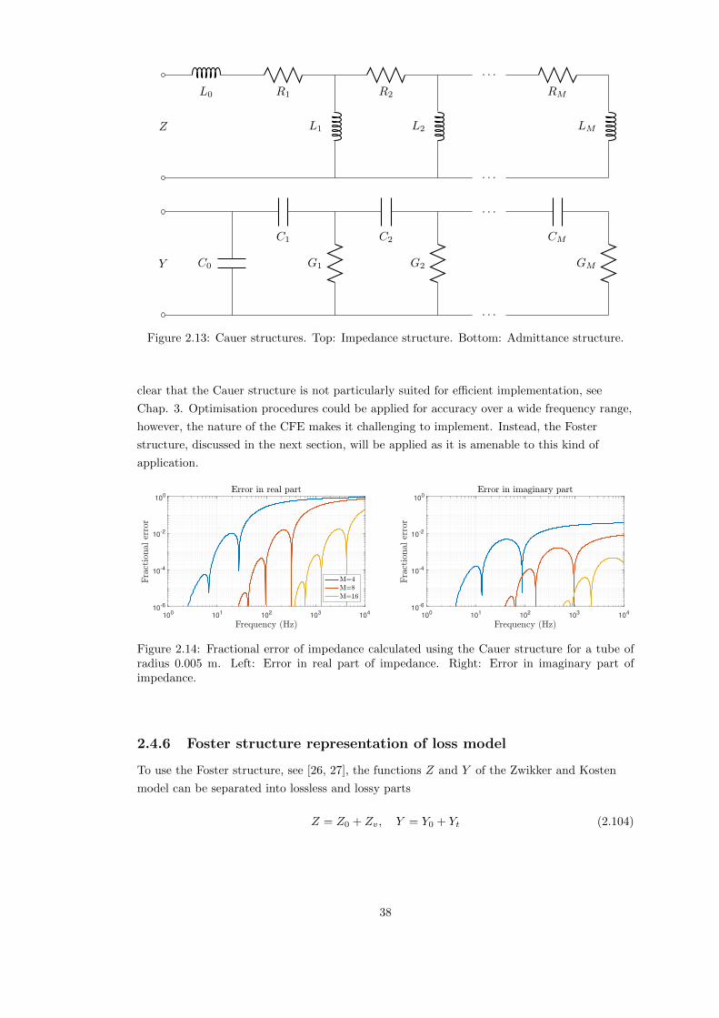
L0 R1

L1

R2

L2

. . .

RM

LM

. . .

Z

C0

C1

G1

C2

G2

. . .

CM

GM

. . .

Y

Figure 2.13: Cauer structures. Top: Impedance structure. Bottom: Admittance structure.

clear that the Cauer structure is not particularly suited for efficient implementation, see

Chap. 3. Optimisation procedures could be applied for accuracy over a wide frequency range,

however, the nature of the CFE makes it challenging to implement. Instead, the Foster

structure, discussed in the next section, will be applied as it is amenable to this kind of

application.

100

101

102

103

104

10-6

10-4

10-2

100

100

101

102

103

104

10-6

10-4

10-2

100

Figure 2.14: Fractional error of impedance calculated using the Cauer structure for a tube ofradius 0.005 m. Left: Error in real part of impedance. Right: Error in imaginary part ofimpedance.

2.4.6 Foster structure representation of loss model

To use the Foster structure, see [26, 27], the functions Z and Y of the Zwikker and Kosten

model can be separated into lossless and lossy parts

Z = Z0 + Zv, Y = Y0 + Yt (2.104)

38

100

101

102

103

104

10-6

10-4

10-2

100

100

101

102

103

104

10-6

10-4

10-2

100

Figure 2.15: Fractional error of admittance calculated using the Cauer structure for a tubeof radius 0.005 m. Left: Error in real part of admittance. Right: Error in imaginary part ofadmittance.

where the lossless propagation parts, Z0 and Y0, are the same as (2.81) and the lossy parts are

Zv = jωρ0Fv

1− Fv, Yt =

jω

ρ0c20(γ − 1)Ft (2.105)

Fig. 2.16 shows the absolute value Zv and Yt in the complex plane. This again shows

interlaced poles and zeros. For numerical reasons it is important to treat the lossless and lossy

parts separately, this will become clear in the next chapter.

Figure 2.16: Left: Magnitude of Zv in the complex plane. Right: Magnitude of Yt in thecomplex plane. Poles are yellow and zeros are dark blue. Note that surfaces have been plottedusing a logarithmic plot to accentuate the poles and zeros. The tube radius is 0.03 m

We can modify the admittance of this model by removing an equivalent capacitor of

capacitance C = (γ − 1)/ρ0c20 leaving the modified admittance

Yt = jωCFt

1− Ft(2.106)

It is clear that Zv and Yt are of the same form, and therefore element values for one of the

immitances can be reused for the other after applying some scaling. Whereas the Cauer

structure in the previous section is a direct expansion of the model of Zwikker and Kosten, a

Foster structure can be used in an optimisation procedure to calculate element values that fit

to the impedances of Zwikker and Kosten curves. The approximations to these immitances

39

are

ZMv = R0 +

M∑q=1

RqLqjω

Rq + Lqjω(2.107a)

YMt = G0 +

M∑q=1

GqCqjω

Gq + Cqjω(2.107b)

The structures representing Zv and Yt using the Foster form are presented in Fig. 2.17.

R0

∆0

R1

v1

∆1

v′1

L1

. . .∆M

RMvM

v′M

LM. . .

v

∆

C

p0

G0 p

m0 C1 p′1

m1

G1 p1

. . .

CM p′M

mM

GM pM

. . .m

p

Figure 2.17: Top: Zv Foster structure. Bottom: Yt Foster structure.

2.4.7 Time domain system of the Foster structure

The Foster structure can be incorporated into the acoustic tube equations by using the

following PDE system

S

ρ0c20∂tp+ ∂z (Sv) + Sm = 0 (2.108a)

ρ0∂tv + ∂zp+ ∆ = 0 (2.108b)

where m is the current going into the RC circuit for Yt and ∆ is the voltage over the RL

circuit. Using Kirchoff’s current laws, the following relations for these values are

p = p0 + p, m =

M∑q=0

mq, p = pq + p′q, q = 1 . . . ,M (2.109a)

m = C∂tp0, m0 = G0p, mq = Gqpq = Cq∂tp′q, q = 1, . . . ,M (2.109b)

40

∆ =

M∑q=0

∆q, v = vq + v′q, q = 1, . . . ,M (2.110a)

∆0 = R0v, ∆q = Rqvq = Lq∂tv′q, q = 1, . . . ,M (2.110b)

where p0, p, pq, p′q and ∆q are interpreted as partial voltages over the circuit elements and

mq, vq and v′q are interpreted as partial currents from each node.

2.4.8 Energy analysis of Foster structure

Foster structures correspond to positive real impedances and admittances and are therefore

passive systems. We can also show this in the time domain using energy methods.

Taking the inner product of the first of (2.108) with p over the domain D then employing

integration by parts and substituting the second of (2.108) gives

dHhedt

+ Bhe + 〈Sv,∆〉D + 〈p, Sm〉D = 0 (2.111)

The final two terms can be approached separately using (2.109) and (2.110). The velocity

term becomes

〈Sv,∆〉D(2.110a)

=

M∑q=0

〈Sv,∆q〉D

(2.110a)= 〈Sv,∆0〉D +

M∑q=1

〈S(vq + v′q),∆q〉D

(2.110b)= 〈Sv,R0v〉D +

M∑q=1

〈Svq, Rqvq〉D + 〈Sv′q, Lq∂tv′q〉D

(2.4)=

dHvdt

+Qv (2.112)

where

Hv =

M∑q=1

1

2‖√SLqv

′q‖2D ≥ 0 (2.113a)

Qv = ‖√SR0v‖2D +

M∑q=1

‖√SRqvq‖2D ≥ 0 (2.113b)

41

Similarly, the pressure term of the energy analysis becomes

〈p, Sm〉D(2.109a)

= 〈p0 + p, Sm〉D(2.109a)

= 〈p0, Sm〉D +

M∑q=0

〈p, Smq〉D

(2.109a)= 〈p0, Sm〉D + 〈p, Sm0〉D +

M∑q=1

〈pq + p′q, Smq〉D

(2.109b)= 〈p0, SC∂tp0〉D + 〈p, SG0p〉D +

M∑q=1

〈pq, SGqpq〉D + 〈p′q, SCq∂tp′q〉D

(2.4)=

dHtdt

+Qt (2.114)

where

Ht =1

2‖√SCp0‖2D +

1

2

M∑q=1

‖√SCqp

′q‖2D ≥ 0 (2.115a)

Qt = ‖√SG0p‖2D +

M∑q=1

‖√SGqpq‖2D ≥ 0 (2.115b)

Incorporating these terms into the energy balance gives

d

dt(Hhe +Hv +Ht) + Bhe +Qv +Qt = 0 (2.116)

It is clear that the energy and dissipation terms are non-negative and the solutions of the

system are therefore bounded.

2.4.9 Numerical optimisation procedures

One approach to setting the circuit elements for the Foster structure would be to determine

the location of the poles of the Zwikker and Kosten model numerically and truncate the

expression to the first M poles; this is how the Cauer structure is applied [162]. However, this

method does not provide the most optimal results in every application. Numerical

optimisation procedures are then of use to find element values [25].

To guarantee a passive realisation of the structure, the impedance can be rewritten in

terms of the free parameters x = [a0, ...aM , b1, ..., bM ]T

ZMv (ω,x) = ea0 +

M∑q=1

eaqjω

ebq + jω, aq, bq ∈ R (2.117)

so that

R0 = ea0 , Rq = eaq , Lq = eaq−bq (2.118)

Use of the exponential function simplifies some of the mathematics used in optimisation

procedures12. It also removes limits on aq and bq as the exponential function produces

positive real values for any real input.

12Online searches describe this reparametrisation as the ‘log trick’, see https://justindomke.wordpress.com/

log-gradient-descent/, last accessed on 30th January 2017, for a brief description of this.

42

https://justindomke.wordpress.com/log-gradient-descent/

https://justindomke.wordpress.com/log-gradient-descent/

A cost function E(x) is then defined which is used to determine how far our approximated

function deviates from the exact function over a finite set of frequencies w = [ω0, ..., ωR]T ,

where R is an integer. We shall uses ωr to denote the rth element of w. Here we investigate

two such cost functions. One looks at the deviation over the real part of the impedance

ER =1

2

R∑r=0

(Re (Zvr)− Re

(ZMvr

)Re (Zvr)

)2

(2.119)

where ZMvr = ZMv (ωr,x) and Zvr = Zv(ωr). The other looks over the magnitude of the

impedance

EM =1

2

R∑r=0

(|Zvr − ZMvr ||Zvr|

)2

(2.120)

where |.| denotes the absolute value. Both ER and EM are always non-negative, real numbers,

which are necessary conditions for this optimisation problem. We expect that using ER

should produce results that approximate the losses of the model, determined by the real part

of the admittance/impedance, better than optimising over the magnitude of the impedances.

However, as the real and imaginary parts are combined in the absolute operation, the results

produced using EM should approximate the overall behaviour of viscous and thermal effects

in air better than optimising over only the real part.

To find the minimum of a function F (x) of multiple variables contained in vector x, we

begin with an initial guess, x0, and then use an iterative procedure to find a new point so that

xi+1 = xi − εdi(F ), i = 0, 1, . . . (2.121)

where di(F ) is a descent direction at the ith iteration, and ε is the step size, the distance that

the direction is followed. We now look at two such ways to determine the descent direction.

Steepest descent

A simple optimisation procedure is the steepest descent algorithm [30, 153]. This is an

iterative method that follows the negative gradient of the function we are trying to

approximate towards a local minimum. The descent direction for the steepest descent

algorithm is given by

di =∇F (xi)

|∇F (xi)|, i = 0, 1, . . . (2.122)

where ∇ denotes the multidimensional gradient operator.

The step size is very important for the efficiency of this algorithm; too small and it will

take a long time to reach a minimum, too large and it will overshoot the minimum and

potentially position xi+1 so that it increases the function F . Since this procedure only finds

local minima, the algorithm must be run multiple times with different initial guesses that are

randomly placed in the domain in an attempt to find a global minimum.

Newton’s method

Steepest descent is useful in that it can approach a minimum with relatively little

computational effort at each iteration. However, convergence is slow. It is therefore useful to

use a method that approaches the minimum in a more efficient manner.

43

Newton’s method [30, 153] is a second order method that locally approximates a function

as a quadratic and moves towards the minimum faster than the steepest descent method. The

descent direction for this algorithm is

di =[H(F (xi)

)]−1∇F (xi) (2.123)

where H is the Hessian matrix of F given by

H(F ) =

∂2F∂x2

1

∂2F∂x1∂x2

. . . ∂2F∂x1∂xm

∂2F∂x2∂x1

∂2F∂x2

2. . . ∂2F

∂x2∂xm...

.... . .

...∂2F

∂xm∂x1

∂2F∂xm∂x1

. . . ∂2F∂x2m

(2.124)

In practice, Newton’s method is used with a trust region set by εT so that the descent

direction is modified to

di = [H(F (xi)) + εT I]−1∇F (xi) (2.125)

Optimisation procedure for the Foster structure

To optimise the Foster structure, we aim to minimise the functions ER(x) and EM (x). The

elements of the gradient and Hessian of the cost functions13 are

∂ER∂xq

= −R∑r=0

Re(Zvr − ZMvr )

Re(Zvr)Re

(∂ZMvr∂xq

)(2.126a)

∂2ER∂xp∂xq

=

R∑r=0

[1

(Re(Zvr))2Re

(∂ZMvr∂xp

)(∂ZMvr∂xq

)− Re(Zvr − ZMvr )

(Re(Zvr))2Re

(∂2ZMvr∂xp∂xq

)](2.126b)

∂EM∂xq

= −R∑r=0

(1

|Zvr|2Re

((Zvr − ZMvr )∗

∂ZMvr∂xq

))(2.127a)

∂2EM∂xp∂xq

=

R∑r=0

[1

|ZMvr |2Re

(∂ZM∗vr

∂xp

∂ZMvr∂xq

)− 1

|Zvr|2Re

((Zvr − ZMvr )∗

∂2ZMvr∂xp∂xq

)](2.127b)

where ∗ denotes complex conjugation and

∂ZMv∂a0

= ea0 ,∂ZMv∂aq

=eaqjω

ebq + jω,

∂ZMv∂bq

= − eaq+bqjω

(ebq + jω)2 , q = 1, . . . ,M (2.128)

∂2ZMv∂a2

0

= ea0 ,∂2ZMv∂a0∂aq

= 0,∂2ZMv∂a0∂bq

= 0,∂2ZMv∂aq∂bp

= 0, p 6= q (2.129a)

13It is fine to take the gradient operator within the real function. First, define f(ξ) = Re(z(ξ)) and z(ξ) =x(ξ) + jy(ξ) =⇒ f(ξ) = x(ξ). The derivatives are df/dξ = dx/dξ and dz/dξ = dx/dξ + jdy/dξ so thatRe (dz/dξ) = dx/dξ = df/dξ =⇒ dRe(z)/dξ = Re(dz/dξ)

44

∂2ZMv∂a2

q

=eaqjω

ebq + jω,

∂2ZMv∂aq∂bq

= − eaq+bqjω

(ebq + jω)2 ,

∂2ZMv∂b2q

=2jωeaq+2bq

(ebq + jω)3−

jωeaq+bq

(ebq + jω)2 (2.129b)

For this system we also have∂ZM∗vr

∂xq=

(∂ZMvr∂xq

)∗(2.130)

The Foster structure allows for reasonably straightforward calculations of the derivatives of

the cost functions—for the Cauer structure the procedure is much more involved.

App. B presents tables of coefficient values for different filter orders using both ER and

EM as the cost functions over the logarithmically spaced frequency range between 0.1 Hz and

10 kHz so that the elements of the frequency vector w are

ωr = 2π

(0.1e

(rR log

(104

0.1

))), r = 0, 1, ..., R (2.131)

Figs. 2.18 and 2.19 show the accuracy of these approximations when they are optimised using

ER and EM respectively.

10-1

100

101

102

103

104

10-5

100

10-1

100

101

102

103

104

10-5

100

Figure 2.18: Fractional error of Foster model optimised to Zv using ER for a tube of 0.005 mover a frequency range 0 Hz to 10 kHz. Left: Error in real part. Right: Error in imaginarypart.

10-1

100

101

102

103

104

10-8

10-6

10-4

10-2

100

10-1

100

101

102

103

104

10-8

10-6

10-4

10-2

100

Figure 2.19: Fractional error of Foster model optimised to Zv using EM for a tube of 0.005 mover a frequency range 0 Hz to 10 kHz. Left: Error in real part. Right: Error in imaginarypart.

Both cost functions allow for improved accuracy as the order of the structure is increased.

Using ER gives an error in the real part : less than 10 % for M = 4, less than 0.1 % for

M = 8, and around 0.001 % for M = 16. However, since the cost function focuses on the real

45

part of the function, the imaginary part is not taken into account which allows for larger

errors. Using EM gives an error in the real part : less than 10 % for M = 4, around 0.1 % for

M = 8, and around 0.001 % for M = 16. The accuracy is similar for the imaginary part.

It should be noted that the poles and zeros of this new impedance do not necessarily

match those of the original function. This is to be expected as we are not directly expanding

the function. Instead we are trying to find another function that matches the target over a

particular frequency range.

It is also important to note that although we have performed an optimisation for one

particular tube radius and temperature for the impedance, we can show in the following

sections that small changes can be made so that these parameters can be reused for the

admittance as well as for changes to the tube radius and air temperature.

2.4.10 Reusing Zv coefficients for Yt

The coefficient values for Zv can be reused for the filter Yt since they both have the same

functional form. Recall that

Zv = jωρ0Fv

1− Fv, Yt =

jω(γ − 1)

ρ0c20

Ft1− Ft

(2.132)

Substituting the angular frequencies in terms of the respective dimensionless characteristic

parameters gives

Zv =

[jηr2

v

r2

Fv(rv)

1− Fv(rv)

](2.133)

Yt =γ − 1

ρ20c

20ν

2

[jηr2

t

r2

Ft(rt)

1− Ft(rt)

]=

γ − 1

ρ20c

20ν

2Zv (rt)

=γ − 1

ρ20c

20ν

2Zv (νrv) (2.134)

The function Yt is then the same as Zv except for a multiplicative factor of C0/ρ0ν2 and a

change of variables from rv → νrv. The Foster structure can then be modified using a

multiplicative factor and changing the angular frequency using ω → ν2ω.

Yt ≈γ − 1

ρ20c

20ν

2ea0 +

M∑q=1

γ − 1

ρ20c

20ν

2

eaqν2jω

ebq + ν2jω(2.135)

The same element values for ZMv can be used for YMt using

G0 =γ − 1

ρ20c

20ν

2ea0 , Gq =

γ − 1

ρ20c

20ν

2eaq , Cq =

γ − 1

ρ20c

20

eaq−bq (2.136)

or

G0 =γ − 1

ρ20c

20ν

2R0, Gq =

γ − 1

ρ20c

20ν

2Rq, Cq =

γ − 1

ρ20c

20

Lq (2.137)

For typical room temperatures ν < 1, so the domain of Yt falls within that of Zv. Figs. 2.20

and 2.21 show the admittances calculated using the element values calculated by optimising

46

over the real part and the magnitude of Zv. These show similar order errors to those of the

original impedance.

10-1

100

101

102

103

104

10-5

100

10-1

100

101

102

103

104

10-5

100

Figure 2.20: Fractional error of Foster model optimised to Zv using ER for a tube of 0.005 mover a frequency range 0 Hz to 10 kHz when it is applied to admittance Yt. Left: Error in realpart. Right: Error in imaginary part.

10-1

100

101

102

103

104

10-8

10-6

10-4

10-2

100

10-1

100

101

102

103

104

10-8

10-6

10-4

10-2

100

Figure 2.21: Fractional error of Foster model optimised to Zv using EM for a tube of 0.005 mover a frequency range 0 Hz to 10 kHz when it is applied to admittance Yt. Left: Error in realpart. Right: Error in imaginary part.

2.4.11 Generalising for different tube radii and temperatures

The method of finding the coefficients so far is designed to be used on tubes of one particular

radius—the accuracy of the results would decrease if we were to use the same coefficients for a

tube of different radius. It is therefore useful to be able to transform these coefficients so that

they can be applied to tubes of differing radius. Again returning to the expression for the

impedance at one particular radius r1, with dimensionless parameter rv1 and impedance

Zv1 =jηr2

v1

r21

Fv(rv1)

1− Fv(rv1)(2.138)

Another impedance for a tube of radius r2 with dimensionless parameter rv2 is

Zv2 =jηr2

v2

r22

Fv(rv2)

1− Fv(rv2)(2.139)

47

The variables rv1 and rv2 lie over different ranges because they correspond to different tube

radii. They can be related as

rv2 =r2

r1rv1 (2.140)

So the second impedance can be written as

Zv2 =

(r1

r2

)2ηjr21

(r2

r1rv1

)2 Fv

(r2r1rv1

)1− Fv

(r2r1rv1

)

=

(r1

r2

)2

Zv1

(r2

r1rv1

)(2.141)

We can therefore reuse the impedance calculated for a tube of radius r for tubes of different

radii r by scaling the impedance and using the transform ω →(rr

)2ω. The element values

then become

R0 =( rr

)2

ea0 , Rq =( rr

)2

eaq , Lq = eaq−bq (2.142)

Note that the inductor values do not change in this case. Fig. 2.22 shows the error in the

impedance when the element values are modified in this way for two different tube radii.

10-1

100

101

102

103

104

10-4

10-3

10-2

10-1

100

10-1

100

101

102

103

104

10-4

10-3

10-2

10-1

100

Figure 2.22: Fractional error of the impedance using the element values in (2.142) for a fourthorder filter. The original impedance was optimised using EM for a tube radius of 0.005 m anda temperature of 26.85C. Left: Error in real part. Right: Error in imaginary part.

When the r < r, the error remains at the same magnitude. When the r > r, the error is

larger at high frequencies. This is not surprising as the smaller magnitude will be included

within the original range that was optimised over, whereas the larger magnitude will lie

outside the original range. It is therefore useful to make sure that optimisation is performed

for reasonably large tube radius. A typical range for the radii of a trumpet is between 0.004 m

and 0.15 m. This is reasonably large so in practice it is worthwhile to optimise the parameter

values for several radii which are used over different ranges.

A similar method can be used for different temperatures. In this case the element values

become

R0 =η

ηea0 , Rq =

η

ηeaq , Lq =

ρ0

ρ0eaq−bq (2.143)

where η and ρ0 are the values of viscosity and density that are used in the original

optimisation procedure. Fig. 2.23 shows the error in the impedance calculated at different

temperatures using the values. The impedance is not as sensitive to changes in temperature

as it is to changing the radii so the error remains roughly the same.

48

10-1

100

101

102

103

104

10-4

10-3

10-2

10-1

100

10-1

100

101

102

103

104

10-4

10-3

10-2

10-1

100

Figure 2.23: Fractional error of the impedance using the element values in (2.143) for a fourthorder filter. The original impedance was optimised using EM for a tube radius of 0.005 m anda temperature of 26.85C. Left: Error in real part. Right: Error in imaginary part.

2.4.12 Restricting optimisation ranges

The accuracy of the Foster structure can be improved by limiting the frequency range over

which they are optimised [25]. The previous results used a wide range from 0 Hz to 10 kHz.

However, the dynamics of brass instruments are dominated by effects over a smaller range.

Figs. 2.24 and 2.25 show the errors in the Foster approximations when optimised over the

range 20 Hz to 3 kHz.

Figure 2.24: Fractional error of Foster model optimised to Zv using ER for a tube of 0.005 mover a frequency range 20 Hz to 3 kHz. Left: Error in real part. Right: Error in imaginarypart. The shaded area shows the frequency range that optimisation was performed over.

49

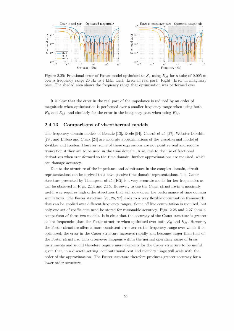
Figure 2.25: Fractional error of Foster model optimised to Zv using EM for a tube of 0.005 mover a frequency range 20 Hz to 3 kHz. Left: Error in real part. Right: Error in imaginarypart. The shaded area shows the frequency range that optimisation was performed over.

It is clear that the error in the real part of the impedance is reduced by an order of

magnitude when optimisation is performed over a smaller frequency range when using both

ER and EM , and similarly for the error in the imaginary part when using EM .

2.4.13 Comparisons of viscothermal models

The frequency domain models of Benade [13], Keefe [94], Causse et al. [37], Webster-Lokshin

[79], and Bilbao and Chick [24] are accurate approximations of the viscothermal model of

Zwikker and Kosten. However, some of these expressions are not positive real and require

truncation if they are to be used in the time domain. Also, due to the use of fractional

derivatives when transformed to the time domain, further approximations are required, which

can damage accuracy.

Due to the structure of the impedance and admittance in the complex domain, circuit

representations can be derived that have passive time-domain representations. The Cauer

structure presented by Thompson et al. [162] is a very accurate model for low frequencies as

can be observed in Figs. 2.14 and 2.15. However, to use the Cauer structure in a musically

useful way requires high order structures that will slow down the performance of time domain

simulations. The Foster structure [25, 26, 27] leads to a very flexible optimisation framework

that can be applied over different frequency ranges. Some off line computation is required, but

only one set of coefficients need be stored for reasonable accuracy. Figs. 2.26 and 2.27 show a

comparison of these two models. It is clear that the accuracy of the Cauer structure is greater

at low frequencies than the Foster structure when optimised over both ER and EM . However,

the Foster structure offers a more consistent error across the frequency range over which it is

optimised; the error in the Cauer structure increases rapidly and becomes larger than that of

the Foster structure. This cross-over happens within the normal operating range of brass

instruments and would therefore require more elements for the Cauer structure to be useful

given that, in a discrete setting, computational cost and memory usage will scale with the

order of the approximation. The Foster structure therefore produces greater accuracy for a

lower order structure.

50

10-1

100

101

102

103

104

10-6

10-4

10-2

100

10-1

100

101

102

103

104

10-6

10-4

10-2

100

Figure 2.26: Fractional error of the impedance for the Foster model, optimised using ER (solidlines) over a frequency range 0 Hz to 10 kHz, and for Cauer model (dashed lines) for a tube of0.005. Left: Error in real part. Right: Error in imaginary part.

10-1

100

101

102

103

104

10-8

10-6

10-4

10-2

100

10-1

100

101

102

103

104

10-8

10-6

10-4

10-2

100

Figure 2.27: Fractional error of the impedance for the Foster model, optimised using EM (solidlines) over a frequency range 0 Hz to 10 kHz, and for Cauer model (dashed lines) for a tube of0.005. Left: Error in real part. Right: Error in imaginary part.

The Foster model can be optimised over a smaller frequency range, which improves

accuracy. However, some care must be taken when reducing the range. For example, the

mechanism for extreme high note playing is still unclear [105], so viscous and thermal effects

may need to be included in the upper frequency ranges.

There are some extra complexities when using the Foster structure. Although using ER as

the cost function allows for better accuracy on the real part of the impedance, the error in the

imaginary part is not taken into account. The cost function EM does take into account errors

in both the real and imaginary parts of the impedance, but, in general, the error in the real

part is higher than that calculated using ER.

51

Chapter 3

Finite-difference time-domain

methods: Applications to

acoustic tubes

“The worthwhile problems are the ones you can really

solve or help solve, the ones you can really contribute

something to... No problem is too small or too trivial if

we can really do something about it.”

— Richard P. Feynman

The models described in the previous chapter yield a good description of the dynamics of

acoustic tubes in the linear regime. Because of the spatially varying character of the bore,

analytic solutions are not available in general. We must therefore look to numerical methods

to solve the PDEs.

In the construction of numerical schemes, particularly for synthesis applications, we must

consider the following:

1. Stability

2. Accuracy

3. Efficiency

Stability concerns how the solutions develop over time. The simulations should at most

display bounded growth which does not interfere with the computation of the solutions. This

is particularly important for combined systems where care must be taken at their interfaces,

e.g., at the domain boundaries. The user should expect usable results for any configuration

selected.

In a mathematical sense, accuracy relates to how well our numerical method approximates

the original equations in terms of a deviation from the original result or how the scheme

converges. Additional accuracy concerns arise in audio applications as numerical methods can

impose frequency dependent errors such as numerical dispersion and bandwidth limitation.

Care must be taken in this setting as such errors are audible and would make the method

useless if too extreme.

52

Efficiency relates to how much time is required to process the algorithm. In a scientific

setting, the user will sacrifice long run times on a computer processor if it produces very

accurate results. In a creative setting, the user may wish for a faster application so as to

quickly explore and refine the sounds being constructed. As such there is an intimate link

between accuracy and efficiency.

This chapter is concerned with the numerical problem and finite-difference time-domain

(FDTD) methods will be applied to the systems discussed in the previous chapter. To begin,

a summary of previous numerical methods used for solving the spatially varying horn

equation are presented, and justification for using FDTD methods is given. This is followed

by an introduction to the FDTD method. The grids on which the domains are represented are

introduced along with shifting operators that are used to make the discrete approximations to

derivatives. Accuracy and convergence of the discrete operators are discussed. This section

will also cover discrete identities and frequency transformations.

The remainder then follows parallel treatment to that of Chap. 2, splitting into lossless

and lossy problems. In the lossless section there is an investigation into numerical schemes for

the wave and horn equations. There are multiple choices of FDTD schemes for an individual

problem so time is taken to explore two different schemes, one explicit and the other implicit.

Numerical dispersion analysis is performed on the schemes and is followed by energy analysis

which allows for a discussion on numerical boundary conditions. Although the implicit

scheme, which utilises the bilinear transform, lends itself to simpler energy analysis than the

explicit scheme, frequency warping effects are more prominent given equal grid spacings and

there is a higher computational cost. However, the bilinear transform can be used to

guarantee passivity in the lossy problem, whilst leaving the lossless part in explicit form; this

is exploited in later sections.

The final section focusses on discrete modelling of viscous and thermal losses. Simulations

are performed using the loss models from the previous chapter. A fractional derivative

operator is derived for use in the Bilbao and Chick approximation of the Zwikker and Kosten

model. Finally the discrete form of the Foster network is presented. The Foster network lends

itself well to numerical simulation as the individual branches can be updated independently of

each other. Frequency warping effects reduce the accuracy of the higher order structures but

can be taken into account when searching for element values. All of the models are then

compared in the final discussion.

3.1 Numerical methods for solving PDEs

Here we cover the previous methods used to solve the spatially varying horn equation and give

justification for using the finite-difference time-domain method.

3.1.1 Previous numerical methods applied to the horn equation

The transmission matrix method (TMM) described in Sec. 2.3.5 is commonly used in musical

acoustics research as it offers a high degree of accuracy to the user [37, 56]. However, this

technique is constrained to steady state solutions, which limits its applications in constructing

a flexible virtual musical instrument.

Modal methods have been applied to the time domain case of an acoustic tube in the

53

MoReeSC framework [148] but these methods are difficult to apply if the resonances of the

system vary with time, as in the case of time varying valves we wish to study in Chap. 5.

Wave based methods have seen much success in physical modelling. The earliest

application of travelling wave solutions was to voice synthesis using the Kelly-Lochbaum (KL)

framework [96]. This time domain synthesis method is similar to the frequency domain TMM

as the cross-sectional area of a tube is approximated by a series concatenated cylinders, and

scattering of waves is performed at the junction between each cylinder. As with the TMM,

the bore profile can be approximated using concatenated cones with spherical wavefronts, but

convex profiles can lead to non-causal and unstable behaviour due to a pole positioned in the

right hand side of the complex plane [18]. To avoid this, a frequency domain mapping that

cuts around this unstable pole must applied [117].

Digital waveguides (DWG) [151] operate in a similar fashion to the KL framework and

have been applied to acoustic tube systems for brass [18, 47, 82, 92, 116] and woodwind

[146, 152] instrument modelling. Discrete spatial samples of the forwards and backwards wave

solutions are stored in delay lines. The solutions are then propagated by ‘shifting’ the

elements of the delay lines. For finite domains, boundary conditions are derived that reflect

one delay line into the other. In addition, the scattering behaviour present over the interior of

the domain can be consolidated into one digital filter that is applied at a termination. This

consolidation can aid in the stability of the framework; Scavone [146] showed that the

instabilities present in the modelling of convex tube profiles using a spherical wave KL

framework were effectively cancelled out as they were lumped together in the DWG

framework.

The shifting of delay line elements produces efficient simulations. However, as the order of

the terminating filter increases, for example, by requiring more scattering elements to describe

a complex bore profile, the computational advantage of DWGs decreases. In addition,

including time-varying phenomena, such as moving valves, makes implementation difficult.

Digital waveguide filters are an extension to DWG and have been applied to simulations of

acoustic tubes [7, 166, 167].

3.1.2 Passive numerical methods

As with the continuous time domain problems, numerical methods can also display issues with

growth, even if the original system is bounded. For the wave based methods, passivity is

ensured through examination of the reflection and transmission properties of the scattering

junctions [19]. An alternative method is to extend the energy methods described in Chap. 2

to the discrete domain.

One such extension is used in the Port-Hamiltonian (PH) framework [59, 164] which has

been applied to systems such as analogue circuits [57, 60], lossy wave systems [111], an

electro-mechanical piano [58], vocal folds [54] and a simplified brass instrument system

[108, 109]. This method focuses on the conserved energy of the system, including the energy

stored and dissipated within the system, along with the energy injected into the system

through driving terms. Discretisation of the problem is then applied using guaranteed stable

methods, such as the bilinear transform which is discussed later in Sec. 3.2.6. This, however,

results in implicit schemes that display a high level of numerical dispersion and require

solutions to systems of linear equations.

54

3.1.3 The finite-difference time-domain method

Finite-difference time-domain (FDTD) methods offer a flexible means of modelling physical

systems. The derivative of a function is defined to be the limit of

df

dz= limh→0

f(z + h)− f(z)

h(3.1)

Instead of taking the limit of the step size h to approach zero, we can fix it to be a small, but

non-zero, value. Substituting this into differential equations changes a calculus problem into

an algebraic problem that can be solved in a loop over the dimensions of interest. The

analysis of these schemes, however, requires some higher level mathematical skill. See the

texts of Gustafsson et al. [71] and Strikwerda [156] for overviews of FDTD methods and that

of Bilbao for applications to musical acoustics [21]. Finite-volume methods are an extension of

finite-difference methods, see the text of Leveque [103], and have been applied in, e.g., room

acoustics simulations by Botteldooren [31, 32] and more recently by Hamilton [74]. These

methods are of use when boundaries have complex geometries—since the boundaries of the

one-dimensional brass system are relatively simple we will stick to FDTD methods.

Although the computational load is higher for FDTD methods than that of DWGs, the

compute time is more than reasonable on modern home computers (at least for the case of

one-dimensional systems). In addition, modifications to the internal geometry of the system

modelled with a FDTD scheme does not significantly change the computation time, as

opposed to the DWG framework.

The passivity of FDTD methods can be shown through the extension of the energy

methods previously described in this work. The form of these discrete energies bear

resemblance to their continuous counterparts, so analysis in the continuous case is beneficial

before applying the numerical method.

3.2 Basics of FDTD methods: Etude II

This section introduces the fundamental concepts of FDTD scheme design.

3.2.1 Grids

The first step in using FDTD methods is to discretise the domain of interest. All of the

independent variables of interest, which in this work are space and time, are approximated on

grids that are equally spaced in each dimension—although the spacings for each dimension are

generally different.

For time domain problems, it is sensible to set the temporal grid size, k, by the sample

rate, Fs, so that k = 1/Fs. This is useful as we immediately know the maximum frequency

bandwidth of the simulation given by the Nyquist limit [151]. For sound synthesis purposes,

we are primarily concerned with the range of human hearing, namely between 20 Hz and 20

kHz [63]. However, discrete numerical methods can introduce unwanted audible dispersion.

This can be rectified through the use of oversampling, which extends the frequency bandwidth

of the simulations and improves the dispersion characteristics over the audible frequency

range, but with the cost of increased computation times. The balance between accuracy and

performance is an important theme in synthesis methods.

55

The spatial domain is sampled on a grid of step size h. Some FDTD schemes allow for

independent control over the spatial and temporal grid spacings but others place some limit on

these sizes if the scheme is to be stable, this will be discussed later for specific FDTD schemes.

The temporal grid will be labelled by integers n and the spatial grid by l; see Fig. 3.1.

These labels correspond to actual times tn = nk and positions zl = lh, where h is the spatial

grid size. The temporal index will lie over the non-negative integers n ∈ Z+ = 0, 1, ...,∞and the spatial index will lie over all of the integers l ∈ Z = −∞, ...,−1, 0, 1, ...∞. A discrete

domain corresponding to D in the previous chapter is given by d = l ∈ Z | 0 ≤ l ≤ N, where

N = floor (L/h) is the number of discrete points in the spatial domain.

t

z

n

n+ 1

n− 1

l l + 1l − 1

h

k

Figure 3.1: Discretised domain for a finite-difference scheme. The temporal domain is sampledat intervals of time k s and labelled using integers n. The spatial domain is sampled at intervalsof length h m and labelled using integers l. Black circles denote the grid function f at eachtemporal and spatial point.

The variables of interest in simulations will be approximated on these grids. A compact

notation of subscripts and superscripts will be used to define a grid function

fnl ≈ f(tn = nk, zl = lh) (3.2)

where the superscript denotes the temporal index and the subscript the spatial index. The

grid function, fnl , is not a sample of the original function, f(t, z), but is an approximation; it

is worth highlighting this subtlety.

Interleaved grids

For first derivative PDE systems, we will employ interleaved grids as presented by Yee in

electromagnetism [179]. In this case, one of the dependent variables will be approximated on

the integer grid mentioned above, and the other on the in-between grids in either space, see

Fig. 3.2 at left, or space/time, see Fig. 3.2 at right.

A function g(t, z) approximated on a spatially interleaved grid is denoted by

gnl+1/2 ≈ g (nk, (l + 1/2)h) (3.3)

56

t

z

t

z

n+ 1

n

n− 1

l + 12

ll − 12

n+ 12

n

n− 12

l + 12

ll − 12

h

k

Figure 3.2: Left: Grids that are interleaved only in space. Right: Grids that are interleaved intime and space. Dashed lines show the original grid labelled by the integers n and l. Dottedlines show the interleaved grid. Black circles denote the locations of the grid function, f , onthe integer field. White circles denote the locations grid function, g, on the interleaved grids.

If it is approximated on a spatially and temporally interleaved grid then it is denoted by

gn+1/2l+1/2 ≈ g ((n+ 1/2)k, (l + 1/2)h) (3.4)

For spatially interleaved grids another domain is defined d ∈ l ∈ Z | 0 ≤ l ≤ N − 1 which lies

between the points represented by d.

The discrete domains mentioned above label sampled points of the continuous domains.

For example, the finite discrete domains d and d correspond to points that lie within the

continuous domain D. However, because d is used for functions that are indexed using half

integers, this domain represents the points between those of d.

3.2.2 Finite-difference operators

In this section we consider the infinite temporal and spatial domains. To construct

approximations to derivatives we must first define temporal and spatial shifting operators,

wt± and wz±, whose action is to advance the function by one grid point forwards or

backwards in the chosen dimension so that

wt+fnl = fn+1

l , wt−fnl = fn−1

l (3.5a)

wz+fnl = fnl+1, wz−f

nl = fnl−1 (3.5b)

A selection of discrete approximations to the first time derivative, ∂t, is as follows

δt+ =wt+ − 1

k, δt· =

wt+ − wt−2k

, δt− =1− wt−

k(3.6)

In this work, the lower case delta symbol, δ, will be used for discrete approximations to

differential operators. The three operators above are called, respectively, the ‘forwards’,

‘centred’ and ‘backwards’ difference operators due to which time steps they utilise.

An approximation to the second time derivative can be constructed from the forwards and

57

backwards difference operators

δtt = δt+δt− =wt+ − 2 + wt−

k2≈ ∂tt (3.7)

Note that the second difference operator is no longer a square of one operator but a product

of two different ones.

Our operators are, in general, acting on functions of two variables. If these operators are

applied to a time series then they reduce to approximating ordinary differentiation. Fig. 3.3

shows the stencils of the temporal difference operators.

n

n+ 1

n+ 2

n− 1

n− 2

δt−, µt− δt+, µt+ δt·, µt· δtt

Figure 3.3: Stencils of temporal difference operators, labelled at top, when applied to a gridfunction at time step n (highlighted in green). Black circle denotes the grid functions that areused, white circles are unused by the operator.

Similarly, the discrete first operators for the spatial derivative, ∂z, are

δz+ =wz+ − 1

h, δz· =

wz+ − wz−2h

, δz− =1− wz−

h(3.8)

and the discrete second spatial derivative

δzz = δz+δz− =wz+ − 2 + wz−

h2≈ ∂zz (3.9)

The stencils of the spatial difference operators are presented in Fig. 3.4.

Averaging operators are used to centre schemes. Temporal averaging operators are

µt+ =wt+ + 1

2, µt· =

wt+ + wt−2

, µt− =1 + wt−

2(3.10)

Spatial averaging operators are

µz+ =wz+ + 1

2, µz· =

wz+ + wz−2

, µz− =1 + wz−

2(3.11)

The centred difference operators can be constructed using difference and averaging operators

δt· = δt+µt− = µt+δt− (3.12a)

δz· = δz+µz− = µz+δz− (3.12b)

All of the operators mentioned in this section can be applied to functions that are

58

l − 2 l − 1 l l + 1 l + 2

δz−, µz−

δz+, µz+

δz·, µz·

δzz

Figure 3.4: Stencils of temporal difference operators, labelled at left, when applied to a gridfunction at spatial step l (highlighted in red). Black circle denotes the grid functions that areused, white circles are unused by the operator.

approximated on the interleaved grids, e.g.,

wt+gn+1/2l+1/2 = g

n+3/2l+1/2 , wz−g

n+1/2l+1/2 = g

n+1/2l−1/2 (3.13)

3.2.3 Accuracy of discrete operators

Let us now look at the behaviour of the difference operators on continuous functions of one

variable. Accuracy of individual operators can be determined by performing a suitable Taylor

expansion [156]. Examining the centred time difference operator on the continuous time

dependent function f(t) and performing a Taylor expansion around t = nk gives

δt·f(nk) =f ((n+ 1) k)− f ((n− 1) k)

2k

=1

2k

(f(nk) + k

df

dt

∣∣∣∣t=nk

+k2

2

d2f

dt2

∣∣∣∣t=nk

+k3

6

d3f

dt3

∣∣∣∣t=nk

+ · · · (3.14)

− f(nk) + kdf

dt

∣∣∣∣t=nk

− k2

2

d2f

dt2

∣∣∣∣t=nk

+k3

6

d3f

dt3

∣∣∣∣t=nk

− · · ·)

=df

dt

∣∣∣∣t=nk

+O(k2)

(3.15)

where O (·) denotes the truncation error; in this case the operator is second order accurate.

This tells us that the centred difference operator is a reasonable approximation to the first

time derivative at t = nk and deviates from the exact value on the order of the square of the

time step.

Performing the same expansion on the forwards difference operator gives

δt+f(nk) =1

k(f ((n+ 1) k)− f(nk)) (3.16)

=1

k

(f(nk) + k

df

dt

∣∣∣∣t=nk

+k2

2

d2f

dt2

∣∣∣∣t=nk

+ · · · − f(nk)

)(3.17)

=df

dt

∣∣∣∣t=nk

+O(k) (3.18)

At first glance, it would appear that the forwards difference operator is less accurate than the

centred one, since the forwards operator deviates from the exact solution by the order of the

time step rather than the square of the time step. However, if we instead take the Taylor

59

expansion around t =(n+ 1

2

)k this results in

δt+f(nk) =df

dt

∣∣∣∣t=(n+ 1

2 )k+O

(k2)

(3.19)

In this case the forwards difference operator is second order accurate when expanded

in-between the two grid points it uses—this is why interleaved grids are useful for PDE

systems using first derivatives (see Section 3.4). Improved accuracy can also be found by

using different operators in the scheme—this is not a trivial task and requires effort and

intuition to develop the most accurate schemes. Tab. 3.1 shows the expansion points that give

second order accuracy for different discrete operators.

Temporal SpatialOperators Expansion point Operators Expansion pointδtt, δt·, µt· t = nk δzz, δt·, µt· z = lh

δt+, µt+ t =(n+ 1

2

)k δz+, µz+ z =

(l + 1

2

)h

δt−, µt− t =(n− 1

2

)k δz−, µz− z =

(l − 1

2

)h

Table 3.1: Differential operators and the expansion point that gives second order accuracy intime or space.

The type of analysis discussed in this section can be extended to combinations of operators

used to approximate a PDE system. In this case, the accuracy is given by the truncation error

[156] that determines how well the overall scheme approximates the original PDE. Additional

forms of determining the accuracy of schemes will be discussed in this work with regards to

numerical dispersion.

In general the FDTD operators will be applied to grid functions in the rest of this work.

3.2.4 Inner products and useful identities

To determine the passivity of a numerical scheme, we look to extending the energy methods

used throughout Chap. 2 in the discrete setting. As such we require discrete forms of the

identities presented in Sec. 2.1.2.

The discrete counterpart to the inner product (2.1) is the discrete inner product. The

discrete inner product [71] of two functions, fl and gl, that lie over the same spatial domain d

is given by

〈f, g〉d =

N∑l=0

hflgl (3.20)

The inner product in the discrete domain is therefore the Reimann sum and taking the limit

of h→ 0 would produce an integral (as in the continuous case). Other inner products can also

be defined such as the weighted inner product

〈f, g〉χd =

N∑l=0

hχlflgl (3.21)

60

where

χl =

12 , l = 0, N

1, 0 < l < N(3.22)

For the most part, the weighted inner product is the same as the inner product except that

the values at the boundary are weighted in a different manner. We can think of these two

inner products as different ways of setting the Riemann sums; see Fig. 3.5 for a geometric

visualisation of this. The weighted inner product uses the values at the ends of the domain

and therefore uses only half rectangles for these points. The inner product has the end points

defined part way into the domain and therefore uses full rectangles.

. . . . . .

h h h h h2 h h h

2z

z

f f

Figure 3.5: Left: Geometric visualisation of inner product. Right: Geometric visualisation ofweighted inner product. At the boundaries of the domain, the weighted inner product uses onlyhalf a spatial step. Black circles denote the values of f on the spatial grid.

As in the continuous case, the discrete l2 norm is defined as

‖f‖d =√〈f, f〉d, ‖f‖χd =

√〈f, f〉χd (3.23)

Similarly, the inner product of two functions fl+1/2 and gl+1/2 that lie on the interleaved

grids on the domain d is

〈f, g〉d =

N−1∑l=0

hfl+1/2gl+1/2 (3.24)

‖f‖d =√〈f, f〉d (3.25)

The weighted inner product will not be used on this domain.

The following identities (point-wise and summed over the domain since this is independent

of time) will be utilised in this work

(δt·f)(δttf) = δt+

(1

2(δt−f)2

)=⇒ 〈δt·f, δttf〉d = δt+

(1

2‖δt−f‖d

)(3.26a)

(δt·f)f = δt+

(1

2fwt−f

)=⇒ 〈δt·f, f〉d = δt+

(1

2〈f, wt−f〉2d

)(3.26b)

(δt+f)µt+f = δt+

(1

2f2

)=⇒ 〈δt+f, µt+f〉d = δt+

(1

2‖f‖2d

)(3.26c)

(µt·f)f = µt+(fwt−f) =⇒ 〈µt·f, f〉d = µt+ (〈f, wt−f〉d) (3.26d)

(µt·f)(δt·f) = δt·

(1

2f2

)=⇒ 〈µt·f, δt·f〉d = δt·

(1

2‖f‖2d

)(3.26e)

fwt−f = (µt−f)2 − k2

4(δt−f)2 =⇒ 〈f, wt−f〉d = ‖µt−f‖2d −

k2

4‖δt−f‖2d (3.26f)

61

δt+(fg) = (δt+f)(µt+g) + (µt+f)(δt+g)

=⇒ δt+ (〈f, g〉d) = 〈δt+f, µt+g〉d + 〈µt+f, δt+g〉d (3.26g)

f (µt+µt−f) = µt−((µt+f)2

)− k2

8δtt(f

2)

=⇒ 〈f, µt+µt−f〉d = µt−(‖µt+f‖2d

)− k2

8δtt(‖f‖2d

)(3.26h)

These identities hold for all inner products regardless of the domain they are taken over.

The discrete form of integration by parts is summation by parts and in this work we will

use forms for the inner product and weighted inner product. Consider two functions fl and

gl+1/2 defined over d and d respectively. Define another function g′l over d that is the

backwards derivative of gl+1/2 so that g′l = δz−gl+1/2. Taking the inner product of fl with g′lover d gives

〈f, g′〉d = 〈f, δz−g〉d =

N∑l=0

hfl

(gl+1/2 − gl−1/2

h

)

= −N−1∑l=0

h

(fl+1 − fl

h

)gl+1/2 − f0g−1/2 + fNgN+1/2

= −〈δz+f, g〉d − f0g−1/2 + fNgN+1/2 (3.27)

Using summation by parts over interleaved grids, it is natural to change the domains over

which the inner product is taken. We can think of this as moving from the normal spatial

grid, d, to the interleaved one, d. This process also introduces terms that lie outside of the

domain—these additional terms must be set through the application of boundary conditions.

A similar process results in the summation by parts identity for the weighted inner product

〈f, δz−g〉χd = −〈δz+f, g〉d − f0µz−g1/2 + fNµz−gN+1/2 (3.28)

Again, the domain of summation is changed from d to d but in this case, the type of inner

product changes and the terms at the extremes of the domain are centred at the boundary.

The identities (3.27) and (3.28) bear resemblance to those used in the Summation-by-Parts

Finite Difference Methods, see, e.g., [158, 172].

The following inequalities will also be used

‖δz+f‖d ≤2

h‖f‖χd ≤

2

h‖f‖d (3.29a)

‖√gδz+f‖d ≤2

h‖√µz−gf‖d (3.29b)

which come from summation by parts.

3.2.5 Discrete frequency transforms

The discrete form of the Laplace transform is the Z transform which allows us to analyse

discrete time functions in the frequency domain. This should not be confused with the use of

z as the axial coordinate; the choice of transform name has been left so as to match with the

rest of the literature. In this section we apply them to the infinite domain. The Z transform

62

of a discrete time series fn is defined as

f(esk) =

∞∑n=−∞

e−sknfn (3.30)

where it is recalled that s is the complex frequency. If s is restricted to s = jω then the Z

transform becomes the Discrete time Fourier Transform (DFT)

f(ejωk

)= F(f) =

∞∑n=−∞

e−jωknfn (3.31)

For both the discrete Laplace and Fourier transforms the angular frequency is limited so that

−π/k ≤ ω ≤ π/k.

Under discrete Laplace transformation, the time shifting operators can be interpreted as a

multiplication

wt±fn →

(esk)±1

f =⇒ wt± →(esk)±1

(3.32)

From this, we can write the discrete difference operators in the frequency domain as

δt+ →esk − 1

k, δt− →

1− e−sk

k, δt· →

esk − e−sk

2k(3.33a)

δtt →esk − 2 + e−sk

k2(3.33b)

µt+ →esk + 1

2, µt− →

1 + e−sk

2(3.33c)

Similarly a discrete spatial Fourier transform can be defined as

g(ejβh) =

∞∑l=−∞

e−jβhlgl (3.34)

where the wavenumber is limited between −π/h ≤ β ≤ π/h. The spatial shifting operators

can also be interpreted as a multiplication in the discrete spatial frequency domain

wz±gl →(ejβh

)±1g =⇒ wz± →

(ejβh

)±1(3.35)

This leads to spatial difference operators being represented in the spatial frequency domain as

δz+ →ejβh − 1

h, δz− →

1− e−jhβh

h, δz· →

ejβh − e−jβh

2h(3.36a)

δzz →ejβh − 2 + e−jβh

h2(3.36b)

µz+ →ejβh + 1

2, µz− →

1 + e−jβh

2(3.36c)

Over the infinite domain the discrete wavenumber must be real, which results in the

following expressions

δz+ →2je

jβh2

hsin

(βh

2

), δz− →

2je−jβh

2

hsin

(βh

2

), δz· →

j

hsin(βh) (3.37a)

63

δzz → −4 sin2(βh2 )

h2(3.37b)

µz+ → ejβh2 cos

(βh

2

), µz− → e−j

βh2 cos

(βh

2

)(3.37c)

3.2.6 The bilinear transform

The bilinear transform, also known as the Tustin transform or the trapezoid rule, [180] is a

discrete frequency mapping

jω → 2

k

1− e−jωk

1 + e−jωk(3.38)

This maps the continuous frequency ω to the discrete frequency ω and is used, for example, in

the wave digital filter [62] and port-Hamiltonian frameworks [60]. This transform is useful as

it preserves the passivity of the continuous system. It does, however, introduce frequency

warping effects which are highlighted in Fig. 3.6, and will be further investigated in later

sections. At low frequencies, the bilinear transform behaves the same way as ordinary

frequencies but exhibits increasing deviation with increasing frequency. This is important for

synthesis purposes as audible dispersion is produced that requires oversampling to rectify. An

additional problem with the use of the bilinear transform is that it can result in implicit

numerical schemes for distributed systems that require additional computations to solve.

0 1 2 3 4 5 6

104

0

1

2

3

4

5

6

104

Figure 3.6: Effect of bilinear transform on frequency mapping at different sample rates. Athigh frequencies, the bilinear transform warps the frequency away from where it is supposed tobe represented. This is improved with a higher sample rate but never truly goes away.

The time domain interpretation is

∂t → µ−1t+ δt+ or µ−1

t− δt− (3.39)

where the −1 denotes the inverse of the averaging function.

The bilinear transform can be seen as a specific application of a Mobius transformation

that maps the complex plane onto a circle [91]. A similar process, known as the Cayley

transform, maps the upper half of the complex domain onto the unit circle [29].

3.3 Scheme design: The wave equation

Now we look at two FDTD schemes that solve the wave equation. This gives an example of

how different schemes can be selected, along with highlighting the advantages, and

64

disadvantages, of using such schemes.

3.3.1 An explicit scheme

First we look at the following scheme that produces an explicit update to model the wave

equation (2.17)ρ0

c20δttψ

nl − ρ0δzzψ

nl = 0 (3.40)

Here the variables ψnl are grid functions. We can check the accuracy of scheme (3.40) by

applying this combination of operators onto the continuous functions ψ(t, z) and performing a

Taylor expansion around t = nk and z = lh. This gives

ρ0

c20δttψ − ρ0δzzψ =

ρ0

c20∂ttψ − ρ0∂zzψ +O

(k2, h2

)(3.41)

The truncation error is O(k2, h2

), so scheme (3.40) is therefore nominally second order

accurate in time and space. When c0k/h = 1, this scheme gives an exact solution to the wave

equation and is therefore of infinite accuracy. This exact accuracy at c0k/h = 1 is also

exploited in the DWG framework.

Expanding (3.40) and rearranging for time step n+ 1, which is assumed to be unknown,

gives

ψn+1l = 2

(1−

(c0k

h

)2)ψnl +

(c0k

h

)2 (ψnl+1 + ψnl−1

)− ψn−1

l (3.42)

3.3.2 Numerical dispersion

Numerical dispersion analysis can be performed on (3.40). Using the frequency domain ansatz

ψnl = ejωnkejβlh (3.43)

and substituting into (3.40) gives the numerical characteristic equation

sin2

(ωk

2

)=

(c0k

h

)2

sin2

(βh

2

)(3.44)

Rearranging for ω gives the numerical dispersion relation

ω = ±2

ksin−1

(c0k

hsin

(βh

2

))(3.45)

which is to be compared to the frequency independent dispersion relation for the continuous

case (2.23).

The numerical dispersion relation gives information on how the discrete scheme affects the

propagation behaviour of the system. In general, discretisation leads to dispersion—wave

speed is frequency (or wavenumber) dependent. This is evident in the phase and group

velocities

vp = ±2

k

sin−1(c0kh sin

(βh2

))β

, vg = ±c0cos(βh2

)√

1−(c0kh sin

(βh2

))2(3.46)

65

3.3.3 Stability and von Neumann analysis

Although the solutions to the wave equation are bounded in the continuous domain, this is

not guaranteed for the discrete case. A method of checking whether the scheme will be stable

is von Neumann analysis [156]. The steps in this method are similar to those in the previous

section on numerical dispersion but extended to complex frequencies, in order to examine

conditions under which exponential growth, or instability can occur. The utility of this

technique is limited to the case of constant coefficient PDE systems defined over infinite

domains, with some extensions to the analysis of simple boundary conditions available under

so-called GKS analysis [71]. In this work we will focus on energy methods to prove stability.

However, it is worth briefly covering von Neumann analysis for completeness.

The discrete frequency domain ansatz, this time with complex temporal frequency, is

ψnl = esnkejβlh (3.47)

where we recall that s = σ + jω. Substituting into scheme (3.40) gives the characteristic

equation

esk + 2

(2

(c0k

h

)2

sin2

(βh

2

)− 1

)+ e−sk = 0 (3.48)

Solving for esk gives

esk = 1− 2

(c0k

h

)2

sin2

(βh

2

)± 2

√√√√(1− 2

(c0k

h

)2

sin2

(βh

2

))2

− 1 (3.49)

For stable solutions—that is solutions with no exponential growth—then |esk| ≤ 1 which

means that ∣∣∣∣1− 2λ2 sin2

(βh

2

)∣∣∣∣ ≤ 1 (3.50)

where λ = c0k/h is the Courant number [103]. The inequality holds if λ ≤ 1, known as the

Courant-Friedrichs-Lewy (CFL) condition [48]. This means there is a bound on the

relationship between the temporal grid size and spatial grid size. This can also be determined

from inspection of the numerical dispersion relation (3.45); the argument of the arcsine

function must lie between −1 and +1 which can only be satisfied if the CFL condition is

satisfied.

3.3.4 Bandwidth of scheme

Returning to the dispersion relation, we can see that (3.45) can be rewritten as

ω = ±2

ksin−1

(λ sin

(βh

2

))(3.51)

The Courant number therefore gives us information about how much bandwidth is

available in the scheme; see Fig. 3.7.

It is clear that the maximum angular frequency is given by

ωmax =2

ksin−1(λ) (3.52)

66

0 50 100 150 200

0

1

2

3

4

5

6

710

4

0 0.2 0.4 0.6 0.8 1

0

2000

4000

6000

8000

10000

Figure 3.7: Left: Dispersion for scheme (3.40) for different values of λ at a sample rate of 20kHz. As λ moves away from the CFL condition, frequencies are warped. Right: Bandwidth asa function of λ for the explicit scheme. The dashed line shows the Nyquist frequency.

For the case of λ = 1, the Nyquist frequency is the highest possible frequency that can be

represented by the scheme and the numerical dispersion relation and phase and group

velocities are the same as for the continuous case

ω = ±βc0, vp = vg = ±c0 (3.53)

and the scheme is thus exact. When λ < 1, so that the h is increased for fixed k, the

bandwidth is reduced and frequency warping occurs. The latter is highlighted in Fig. 3.7 as

the dispersion relation deviates from the exact form.


As in the continuous case, we can define a numerical energy for our finite-difference schemes

[71]. Henceforth, the time and spatial indices of ψ are suppressed and assumed to be n and l

unless otherwise stated. Taking the inner product of δt·ψ with scheme (3.40) over d gives

ρ0

c20〈δt·ψ, δttψ〉d − ρ0〈δt·ψ, δzzψ〉d = 0 (3.54)

Using summation by parts, (3.27), gives

ρ0

c20〈δt·ψ, δttψ〉d + ρ0〈δt·δz+ψ, δz+ψ〉d − ρ0δt·ψ0δz+ψ−1 + ρ0δt·ψNδz+ψN = 0 (3.55)

Employing (3.26a) and (3.26b) gives

δt+hwe + bwe = 0 (3.56)

where

hwe =ρ0

2c20‖δt−ψ‖2d +

ρ0

2〈δz+ψ,wt−δz+ψ〉d (3.57)

is the discrete energy of the system and

bwe = −ρ0δt·ψ0δz+ψ−1 + ρ0δt·ψNδz+ψN (3.58)

67

is the power gain or loss at the tube boundaries. The power loss term is useful as it suggests

strategies for setting numerical boundary conditions.

Unlike in the continuous case, we cannot immediately say that the energy of the system is

always non-negative—and therefore cannot say that the solutions are bounded; some further

mathematical legwork is required. Using (3.26f), the second term in the discrete energy

becomes

ρ0

2〈δz+ψ,wt−δz+ψ〉d =

ρ0

2

(‖µt−δz+ψ‖2d −

k2

4‖δt−δz+ψ‖2d

)≥ −ρ0k

2

8‖δt−δz+ψ‖2d (3.59)

From inequality (3.29a) we can then say that

ρ0k2

8‖δt−δz+ψ‖2d ≤

ρ0k2

2h2||δt−ψ||2d (3.60)

which means that the total discrete energy satisfies

hwe ≥ρ0

2c20‖δt−ψ‖2d −

ρ0k2

2h2‖δt−ψ‖2d =

(1− λ2

) ρ0

2c20‖δt−ψ‖2d (3.61)

The discrete energy is always non-negative provided that

1− λ2 ≥ 0 (3.62)

which is the same result we get from von Neumann analysis.

The power in using energy analysis rather than von Neumann analysis is that energy

methods can be extended to handle variable coefficient PDE systems as well as boundary

conditions. This will be demonstrated in Sec. 3.4. On the other hand, von Neumann analysis,

when it applies, yields additional useful information regarding numerical dispersion.


The boundary terms generated from the energy analysis gives some guidance as to the choice

of appropriate difference operators that terminate the system at the boundaries. In this case

an obvious choice is

δt·ψ0 = 0, δt·ψN = 0 (Dirichlet) (3.63a)

δz+ψ−1 = 0, δz+ψN = 0 (Neumann) (3.63b)

However, from Sec. 3.2.3 we can see that the Neumann boundary conditions are not centred

about the domain boundary, and thus some degradation in accuracy is to be expected.

The expression for the discrete energy given in (3.57) is consistent with the expression for

the continuous energy in the limit as grid spacing becomes small. It is not, however, unique;

other choices of inner product are available that result in different choices of boundary

conditions, giving more power to this type of approach. If we use the weighted inner product

68

in the energy analysis we end up with

hwe =1

2(‖δt−ψ‖χd )

2+c202〈δz−ψ,wt−δz−ψ〉d, bwe = c20 (δt·ψ0δz·ψ0 − δt·ψNδz·ψN ) (3.64)

In this case the Neumann boundary conditions would be

δz·ψ0 = 0, δz·ψN = 0 (3.65)

which do offer second order accuracy at l = 0 and l = N . These Neumann conditions will be

called centred.

DWG interpretation of boundary conditions

For the case of λ = 1, these boundary conditions reduce to DWG terminations [21]. The

uncentered FDTD Neumann boundary condition at l = 0 is the same as feeding a leftward

going wave, ψ−(nk, lh), into the rightward going wave, ψ+(nk, lh), with a single time step

delay so that

δz−ψn0 = 0 ≡ ψ+(nk, 0) = ψ− ((n− 1)k, 0) (3.66)

The centred FDTD Neumann boundary condition is the same application but without the

delay

δz·ψn0 = 0 ≡ ψ+(nk, 0) = ψ−(nk, 0) (3.67)


We can investigate the effect of these two boundary conditions on the modes of the system in

a similar fashion to the continuous case. For simplicity we will operate at the stability limit

λ = 1 so that β = ω/c0, giving a best case scenario. From the dispersion analysis we can write

the solutions as

ψnl = ejωkn(A sin

(ωhl

c0

)+B cos

(ωhl

c0

))(3.68)

where A and B are constants determined by boundary conditions. Tab. 3.2 shows the modal

solutions and frequencies for the two types of Neumann boundary conditions applied at both

ends of the tube.

Boundary condition Solution Mode frequenciesUncentred

ψnl(m) = Bmejωmnk

(sin

(ωmh(l+1)

c0

)−sin

(ωmhlc0

)sin

(ωmhc0

) )ωm = mπc0

h(N+1) ,

Neumann m = 1, 2, ...

Centredψnl(m) = Bme

jωmnk cos(ωmhlc0

) ωm = mπc0hN ,

Neumann m = 1, 2, ...

Table 3.2: Modal solutions and modal frequencies for the wave equation solved with the explicitscheme (3.40) using the uncentred and centred Neumann boundary conditions at l = 0 andl = N .

The centred boundary conditions yield the modal frequencies that are derived from the

exact case shown in Tab. 2.1. The uncentred boundary conditions, when used in the same

way, have modal frequencies lower than they should be—the tube appears to be of length

L+ h rather than L. This, however, corresponds to boundaries of the domain set at l = 0 and

69

l = N with l lying over the integers. If, instead, we set l to lie over a half integer domain and

use the uncentered boundary conditions, then this will correspond to the correct length1. If

we were to use the centred boundary conditions, the tube will appear to be shorter. This

highlights how important it is to think about how we set up our FDTD schemes and how the

boundary conditions are selected.

3.3.8 Implementation

Scheme (3.40) can be implemented by either looping over the spatial domain at each time step

or, alternatively, using a matrix formulation [21]. As the code generated in this thesis is

primarily produced using MATLAB, which is well suited for problems involving matrices, we

discuss this implementation here. In addition, explicit schemes have sparse representations,

operations which have been optimised in MATLAB.

To implement the matrix formulation, we first define the vector

Ψn = [ψn0 , ..., ψnN ]T (3.69)

then (3.40) can be represented as

Ψn+1 = BΨn −Ψn−1 (3.70)

where B is a sparse square matrix of size N + 1. The elements of this matrix, Bq,r, are

defined for the qth row and rth column, where q and r run from 0 to N

Bl,l = 2(1− λ2), l = 0, ..., N (3.71a)

Bl,l+1 = λ2, l = 0, ..., N − 1 (3.71b)

Bl,l−1 = λ2, l = 1, ..., N (3.71c)

It should be noted that this indexing makes references to zeroth columns and vectors; this has

been done so as to match with the original labelling of the scheme. Pseudocode for such an

implementation is shown in Alg. 1.

Algorithm 1 Pseudocode for implementation of explicit FDTD scheme for the wave equation.

Define simulation parametersConstruct BInitialise Ψn+1, Ψn, and Ψn−1

for n = 1→ no. timesteps doΨn+1 ← BΨn −Ψn−1

Ψn−1 ← Ψn

Ψn ← Ψn+1

end for

Fig. 3.8 shows solutions to the wave equation calculated using scheme (3.42) after

initialising with a Hann pulse.

1We can use a finite-volume interpretation [103] to understand why different energy analysis allows fordifferent position of the boundaries. For the weighted inner product, we can think of the boundary cells as beinghalf the size of the interior cells which is linked to the factors of a half in the weighted inner product definition.As a result, the flux over the exterior wall of that cell is aligned with the cell centre. In the other case of theinner product, the cell at the boundary is a full cell, hence the extra length. This is linked to Fig. 3.5.

70

0 0.1 0.2 0.3 0.4 0.5 0.6 0.7 0.8 0.9 1

-0.1

0

0.1

0.2

0.3

0.4

0.5

0.6

0.7

0.8

0.9

0 0.1 0.2 0.3 0.4 0.5 0.6 0.7 0.8 0.9 1

-0.1

0

0.1

0.2

0.3

0.4

0.5

0.6

0.7

0.8

0.9

Figure 3.8: Solutions calculated using scheme (3.42) at two time instants. The sample rate is20 kHz and λ = 1. The acoustic velocity potential has been initialised with an Hann pulse ofwidth 21 steps.

Boundary conditions can be implemented by modifying the elements of B. For the

uncentred Neumann conditions

B0,0 = 2− λ2, BN,N = 2− λ2 (3.72)

For the centred Neumann conditions

B0,1 = 2λ2, BN,N−1 = 2λ2 (3.73)

Dirichlet boundary conditions can be implemented by only updating the interior points so

that Ψ = [ψ1, ..., ψN−1]T and B being a square matrix of size N − 1.

Bl,l = 2(1− λ2), l = 0, ..., N − 2 (3.74a)

Bl,l+1 = λ2, l = 0, ..., N − 3 (3.74b)

Bl,l−1 = λ2, l = 1, ..., N − 1 (3.74c)

Calculating energy

The energy of the system can be monitored using the summed form [163]

hn+1sum =

hn+1we − h0

we + k∑nq=0 b

n+1/2we

bh0wec2

= 0 (3.75)

which is the discrete form of the integrated energy2 (2.41). The operator b.c2 denotes

rounding to the nearest power of two towards zero so that

bh0wec2 = 2fix(log2(h0

we)) (3.76)

where fix(·) denotes rounding towards zero.

2Note that in this chapter we shall be considering lossless boundary conditions so bwe = 0.

71

In practice, the value of hsum is never exactly zero due to finite machine precision. We

can, however, see bit wise deviations of size 2.2204× 10−16 which corresponds to machine

epsilon in double precision floating point arithmetic; see Fig. 3.9.

0 50 100 150 200 250 300 350 400 450 500

-1

-0.5

0

0.5

1

1.5

210

-15

Figure 3.9: Plot of hsum for the system in Fig. 3.8. The energy is calculated using the weightedinner product form (3.64).

Monitoring the energy is useful as a debugging tool when creating discrete schemes. Any

unexplained deviations beyond machine precision would suggest that there are problems with

implementation.

3.3.9 An implicit scheme: Variation on a scheme

An alternative finite-difference scheme can be constructed using the bilinear transform

ρ0

c20

(µ−1t+ δt+

) (µ−1t− δt−

)ψnl − ρ0δzzψ

nl = 0 (3.77)

orρ0

c20δttψ

nl − ρ0µt+µt−δzzψ

nl = 0 (3.78)

The method of construction of scheme (3.78) is also known as the Crank-Nicolson method

[160]. A similar approach can be applied in the PH framework [60].

The truncation error for the implicit scheme (3.78) is the same as the truncation error of

the explicit scheme (3.40): O(k2, h2).

The update for this scheme is given by(1 +

λ2

2

)ψn+1l − λ2

4

(ψn+1l+1 + ψn+1

l−1

)=(2− λ2

)ψnl −

(1 +

λ2

2

)ψn−1l

+λ2

2

(ψnl+1 + ψnl−1

)+λ2

4

(ψn−1l+1 + ψn−1

l−1

)(3.79)

It is clear that this scheme is implicit, as there are three unknowns at time step n+ 1.

72

3.3.10 Numerical dispersion analysis

Using the discrete frequency domain ansatz, (3.43), the numerical dispersion of scheme (3.78)

is given by

tan2

(ωk

2

)= λ2 sin2

(βh

2

)(3.80)

or

ω = ±2

ktan−1

(λ sin

(βh

2

))(3.81)

Fig. 3.10 at left shows the dispersion of the implicit scheme for different values of λ. The

maximum frequency of this scheme is given by

ωmax =2

ktan−1(λ) (3.82)

When λ = 1, ωmax = π/(2k) which is half of the total possible frequency bandwidth allowed

by the Nyquist theorem for a given time step k, see Fig. 3.10 at right. In fact, it is only in the

limit of λ→∞ that the maximum frequency of the scheme coincides with the Nyquist

frequency. As a result, the sample rate must be set sufficiently high, either temporally or

spatially, to correctly represent the frequency range of interest.

0 50 100 150 200

0

1

2

3

4

5

6

710

4

0 1 2 3 4 5

0

2000

4000

6000

8000

10000

Figure 3.10: Left: Dispersion for scheme (3.78) for different values of λ at a sample rate of20 kHz. Even for λ = 1, the dispersion deviates from the exact dispersion relation. Right:Bandwidth of implicit scheme as a function of λ. The dashed line shows the Nyquist frequencywhich this scheme can never fully achieve.


Energy analysis for scheme (3.78) can be performed in the same way as in the explicit case by

taking the inner product with δt·ψ over d

ρ0

c20〈δt·ψ, δttψ〉d − ρ0〈δt·ψ, µt+µt−δzzψ〉d = 0 (3.83)

Using summation by parts and identities (3.26a) and (3.26c)3 gives

δt+h(imp)we + b(imp)

we = 0 (3.84)

3Recall that δt· = δt+µt− = δt−µt+

73

where

h(imp)we =

ρ0

2c20‖δt−ψ‖2d +

ρ0

2‖µt−δz+ψ‖2d ≥ 0 (3.85)

and

b(imp)we = ρ0 (−δt·ψ0µt+µt−δz+ψ−1 + δt·ψNµt+µt−δz+ψN ) (3.86)

It is clear in this case that the discrete energy, h(imp), is always non-negative and thus there

are no constraints on the grid spacing h or time step k—this scheme is said to be

unconditionally stable.

The same procedure can be performed using the weighted inner product to yield centred

boundary conditions

h(imp)we =

ρ0

2c20(‖δt−ψ‖χd )

2+ρ0

2‖µt−δz+ψ‖2d ≥ 0 (3.87)

and

b(imp)we = ρ0 (−δt·ψ0µt+µt−δz·ψ0 + δt·ψNµt+µt−δz·ψN ) (3.88)


The implicit scheme is implemented using the matrix-vector form as follows

AΨn+1 = BΨn −AΨn−1 =⇒ Ψn+1 = A−1BΨn −Ψn−1 (3.89)

where A and B are sparse N ×N matrices with elements

Al,l = 1 +λ2

2, Bl,l = 2− λ2, l = 0, ..., N (3.90a)

Al,l+1 = −λ2

4, Bl,l+1 =

λ2

2, l = 0, ..., N − 1 (3.90b)

Al,l−1 = −λ2

4, Bl,l−1 =

λ2

2, l = 1, ..., N (3.90c)

Noncentred Neumann conditions can be applied using

A0,0 = 1 +λ2

4, B0,0 = 2− λ2

2(3.91a)

AN,N = −λ2

4, BN,N = 2− λ2

2(3.91b)

Centred Neumann conditions can be applied using

A0,1 = −λ2

2, B0,1 = λ2 (3.92a)

AN,N−1 = −λ2

2, BN,N−1 = λ2 (3.92b)

Fig. 3.11 shows solutions to the wave equation initialised with a Hann pulse solved using the

implicit scheme, as was done previously for the explicit scheme. It is clear that dispersion is

present in this scheme as there are ripples that lie behind each of the wave fronts—compare to

Fig. 3.8 where there are no ripples and the solutions are exact. Fig. 3.12 shows the energy for

this system.

74

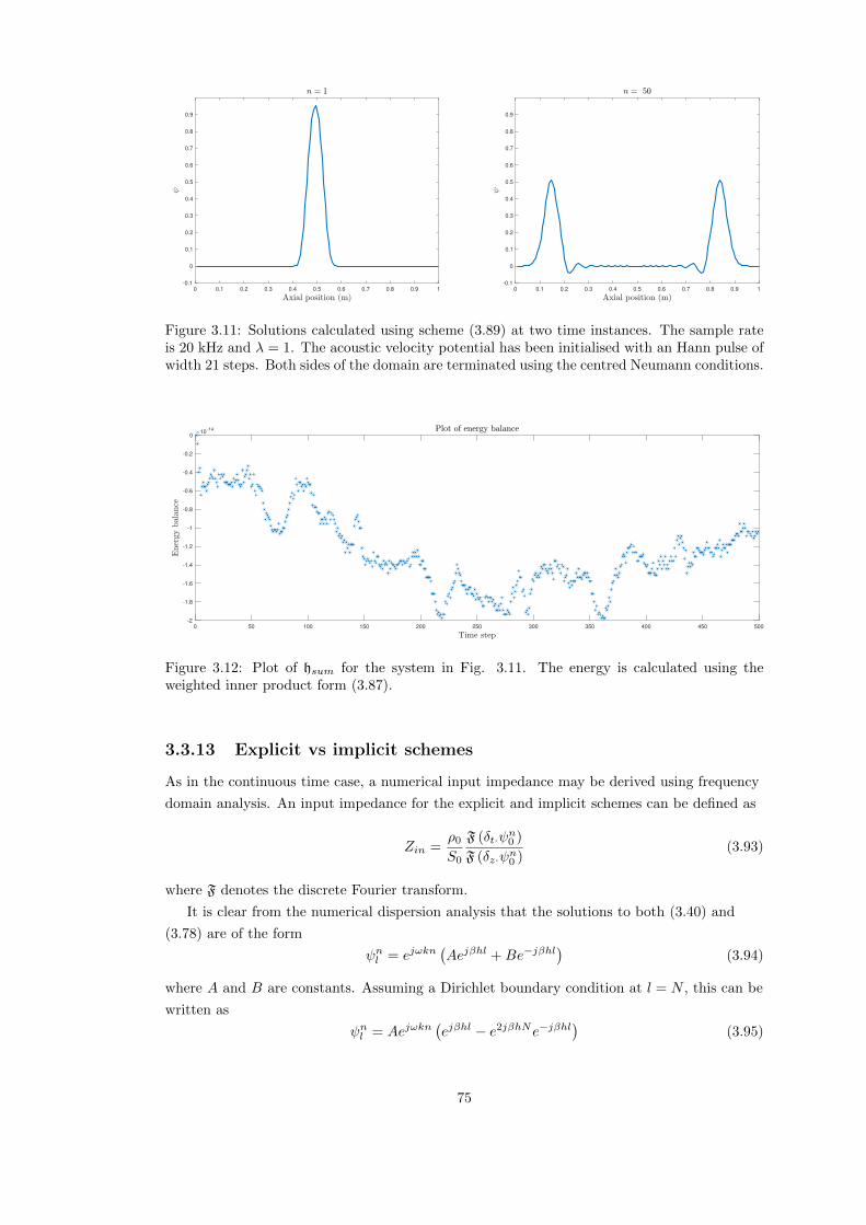
0 0.1 0.2 0.3 0.4 0.5 0.6 0.7 0.8 0.9 1

-0.1

0

0.1

0.2

0.3

0.4

0.5

0.6

0.7

0.8

0.9

0 0.1 0.2 0.3 0.4 0.5 0.6 0.7 0.8 0.9 1

-0.1

0

0.1

0.2

0.3

0.4

0.5

0.6

0.7

0.8

0.9

Figure 3.11: Solutions calculated using scheme (3.89) at two time instances. The sample rateis 20 kHz and λ = 1. The acoustic velocity potential has been initialised with an Hann pulse ofwidth 21 steps. Both sides of the domain are terminated using the centred Neumann conditions.

0 50 100 150 200 250 300 350 400 450 500

-2

-1.8

-1.6

-1.4

-1.2

-1

-0.8

-0.6

-0.4

-0.2

010

-14

Figure 3.12: Plot of hsum for the system in Fig. 3.11. The energy is calculated using theweighted inner product form (3.87).

3.3.13 Explicit vs implicit schemes

As in the continuous time case, a numerical input impedance may be derived using frequency

domain analysis. An input impedance for the explicit and implicit schemes can be defined as

Zin =ρ0

S0

F (δt·ψn0 )

F (δz·ψn0 )(3.93)

where F denotes the discrete Fourier transform.

It is clear from the numerical dispersion analysis that the solutions to both (3.40) and

(3.78) are of the form

ψnl = ejωkn(Aejβhl +Be−jβhl

)(3.94)

where A and B are constants. Assuming a Dirichlet boundary condition at l = N , this can be

written as

ψnl = Aejωkn(ejβhl − e2jβhNe−jβhl

)(3.95)

75

so that Zin becomes

Zin = − ρ0

S0

h

k

j sin (ωk)

sin (βh)tan (βhN) (3.96)

We can then substitute the suitable numerical dispersion relations between β and ω for the

explicit and implicit schemes to calculate an input impedance. In this case the dispersion

relation is given by specifying a velocity at l = 0 as an impulse. In practice, δz·ψn0 is impulsive

in the time domain leading to a unity frequency response with zero phase meaning that the

input impedance is related to the Fourier transform of the pressure signal.

0 200 400 600 800 1000 1200 1400 1600 1800 2000

105

0 200 400 600 800 1000 1200 1400 1600 1800 2000

105

Figure 3.13: Input impedances calculated for a cylinder of length 0.3 m and radius 0.01 m usingthe explicit (blue) and implicit (green) schemes. Top: Input impedance calculated using λ = 1.Bottom: Input impedance calculated using λ = 0.7972. Dashed vertical line show the exactresonances. Sample rate is 20 kHz.

Fig. 3.13 shows the input impedance calculated from the two schemes with reference to the

exact calculation. For λ = 1, the explicit scheme gives the same result as the exact expression

whereas the implicit scheme starts to deviate at higher frequencies. For lower values of λ,

frequency warping is present in both schemes but is more severe for the implicit scheme.

It is worthwhile to take a moment to compare these explicit and implicit schemes in the

context of the desirable properties of a numerical method, outlined at the beginning of this

chapter.

Stability

The implicit scheme (3.78) is shown to be unconditionally stable and therefore there are no

limits set on the temporal and spatial step sizes. The explicit scheme can also be shown to be

stable, but this is conditional on the ratio of the spatial step size to the temporal step size4. A

lower bound is placed on the spatial step size, therefore, investigations that require a fine

spatial resolution require a high temporal sample rate.

4This is stated in Theorem 1.6.2 in the text of Strikwerda [156]: There are no explicit, unconditionally stable,consistent finite-difference schemes for hyperbolic systems of partial differential equations.

76

Accuracy

Use of the implicit scheme introduces severe numerical dispersion which, in practice, cannot

be fully removed. As a result, frequency warping is present accompanied by reduction of

bandwidth. The explicit scheme, on the other hand, displays no numerical dispersion when

operating at the stability limit, λ = 1, allowing for bandwidth up to the Nyquist frequency.

When operating away from the stability limit (λ < 1), some numerical dispersion is

introduced but it is not as severe as in the implicit scheme for the same temporal and spatial

step sizes. These effects of numerical dispersion are highlighted in the input impedances

shown in Fig. 3.13.

Efficiency

Matrix implementation of the implicit scheme uses dense matrices, whereas sparse matrices

define the update for the explicit scheme. As such, the computational time differs between the

two methods. Using the same relation between temporal and spatial step size (λ = 1,

T = 26.85C), the temporal loop for a 1 s duration simulation at a temporal sample rate of 20

kHz of a 1 m long tube takes around 0.02 s using the explicit scheme and 0.06 s using the

implicit scheme. Simulations were performed in MATLAB R2016b on a 2013 MacBook Pro

with 2.8 GHz Intel Core i7 processor. The schemes were implemented in their most optimal

manner: the implicit scheme used a full matrix representation5, the explicit used a sparse

matrix implementation.

Numerical energy and passive numerical methods

In both the explicit and implicit FDTD schemes for the wave equation presented in this

chapter, a numerical energy can be defined that is similar in form to that derived from the

continuous system. However, the energies for each scheme are distinct from each other and

the amount of analysis required to show non-negativity varies—the energy of the implicit

scheme is shown to be non-negative immediately, whereas the explicit scheme requires several

steps to determine passivity. In addition, the choice of inner product used to define the

numerical energy determines how passive boundary conditions are implemented, which, in

turn, can have implications on the size of the domain.

Such implicit schemes are employed to guarantee stability for schemes used in the

modelling nonlinear wave propagation or collisions [40]. However, implementation of these

methods results in longer simulation times. In addition, to achieve a high level of accuracy

using theses implicit schemes requires using either a finer spatial resolution or a higher

temporal sample rate to overcome numerical dispersion, further increasing computational

requirements.

Energy balance methods, such as the PH framework, typically employ temporal

discretisations that preserve the passivity of the system [57, 109]. An N element PH system is

presented in terms of a state vector x = [x0, x1, ..., xN ]T and the associated Hamiltonian

H =∑Ni=0Hi(xi), where Hi gives the energy corresponding to the ith state variable. The

temporal behaviour is given by

∂tx = J∇xH (3.97)

5Use of sparse representation increases the computational time of the implicit scheme to 0.12 s

77

where J is a state matrix that describes the interactions between individual elements of the

system and ∇x is the multi-dimensional gradient with respect to the state variable. For linear

storage elements Hi ∝ 12 (xi)

2, therefore (3.97) becomes

∂tx = J′x (3.98)

where J′ ∝ J takes into account any constants of proportionality in the definition Hi.

A guaranteed stable discretisation of of (3.97) involves using the forwards time difference

operator to approximate ∂t and the following approximation for each element of the

multi-dimensional gradient

[∇xH]i ≈Hi(x

n+1i )−Hi(x

ni )

xn+1i − xn+1

i

(3.99)

which for linear storage elements becomes

[∇xH]i ≈1

2

(xn+1i )2 − (xni )2

xn+1i − xn+1

i

(3.100)

≈ 1

2

(xn+1i + xni

)(3.101)

≈ µt+xni (3.102)

The discrete form of (3.97) is therefore

δt+x = J′µt+x (3.103)

which is clearly an application of the bilinear transform to (3.98) and will therefore suffer

from frequency warping effects.

3.3.14 Schemes for PDEs using first vs. second derivatives

The wave equation does not have to be solved in the form using second derivatives. An

equivalent description of the system can be given using differential equations for the acoustic

pressure and particle velocity variables. In Torin’s thesis [163], a small investigation was made

into the differences in results between first and second derivative forms of FDTD schemes for

the simple harmonic oscillator. In that study, it was shown that the first derivative forms

showed a smaller deviation in the numerical energy calculations than the second derivative

forms; the latter was shown to be more sensitive to rounding effects caused by implementation

of the scheme.

In the previous chapter, it was shown that the second derivative equation solutions were

bounded by their first derivatives of the solutions, whereas the actual solutions were bounded

to the first derivative system equations. In this case, the explicit scheme for the wave

equation, (3.40) can be recast using pressure, pnl , and velocity, vn+1/2l+1/2 , as

ρ0δt−v − ∂z+p = 0, l ∈ d (3.104a)

1

ρ0c20∂tp+ ∂z−v = 0, l ∈ d (3.104b)

78

with corresponding energy balance

hwe + bwe = 0 (3.105)

hwe =1

2ρ0c20(‖p‖χd )

2+ρ0

2〈v, wt−v〉d ≥ 0, λ ≤ 1 (3.106)

bwe = −µt+pn0µz−v1/2 + µ5+pnNµz−vN+1/2 (3.107)

In general, in this thesis, we will consider the first derivative PDE system equations for the

horn equation although will use the second derivative form for simple discussion of boundary

conditions. We shall use the acoustic velocity potential when modelling wave propagation in

three-dimensions later in Chap. 4.

3.4 Scheme design: the horn equation

Now, we look at ways of discretising the horn equation. In this case, we are trying to

discretise PDE systems with spatially varying coefficients, so the typical frequency domain

analysis tools are no longer available for use.

3.4.1 An explicit scheme

An explicit scheme for the transmission line form of the horn equation (2.49) is given by

Slρ0c20

δt+pnl + δz−

(Sl+1/2v

n+1/2l+1/2

)= 0, ρ0δt−v

n+1/2l+1/2 + δz+p

nl = 0 (3.108)

In this case an interleaved scheme has been used, where the spatial and temporal grid points

for the velocity field lie between those of the pressure field, see Fig. 3.2. Of course, this could

be presented with the grids for pressure and velocity interchanged; (3.108) is just one way to

create an explicit scheme. The values Sl and Sl+1/2 are approximations to the surface area on

the different grids; see Fig. 3.14.

Figure 3.14: Bore profile and surface areas on different girds. Solid line shows the bore profile.Dashed line shows the spatial grid that S is calculated on and dotted line shows the grid thatS is sampled on.

The update for scheme (3.108) is given by

pn+1l = pnl −

ρ0c0λ

Sl

(Sl+1/2v

n+1/2l+1/2 − Sl−1/2v

n+1/2l−1/2

), l ∈ d (3.109a)

79

vn+1/2l+1/2 = v

n−1/2l+1/2 −

λ

ρ0c0

(pnl+1 − pnl

), l ∈ d (3.109b)

The update for the pressure will require boundary conditions to be chosen at l = 0 and

l = N—the scheme will require values for v−1/2 and vN+1/2, respectively, which lie outside the

domain. This is not the case for the velocity update, which is entirely determined by values

internal to the domain.

Energy analysis

As in the case of dispersion analysis for the continuous horn equation, the spatial

inhomogeneity in the system due to the change in cross sectional area means that it is not, in

general, possible to perform von Neumann analysis on the scheme for the horn equation. As

standard frequency domain analysis cannot be used to determine stability of (3.108) we look

for a discrete energy to find bounds on the solutions. Temporal and spatial indices are

suppressed and assumed to be n and l for p, and n+ 1/2 and l + 1/2 for v, unless otherwise

stated. Spatial indices are also suppressed for the surface areas and assumed to be l for S, and

l + 1/2 for S. Taking the weighted inner product of µt+p with the first of (3.108) over d gives

1

ρ0c20〈µt+p, Sδt+p〉χd + 〈µt+p, δz− (Sv)〉χd = 0 (3.110)

Summation by parts, (3.28), results in

1

ρ0c20〈µt+p, Sδt+p〉χd + 〈µt+δz+p, (Sv)〉d + bhe = 0 (3.111)

where

bhe = −µt+p0µz−(S1/2v1/2

)+ µt+pNµz−

(SN+1/2vN+1/2

)(3.112)

Substituting the second of (3.108) gives

1

ρ0c20〈µt+p, Sδt+p〉χd + ρ0〈δt·v, (Sv)〉d + bhe = 0 (3.113)

Using (3.26b) and (3.26c) results in

δt+hhe + bhe = 0 (3.114)

where

hhe =1

2ρ0c20

(‖√Slp‖χd

)2

+ρ0

2〈Sv,wt−v〉d (3.115)

As for the explicit scheme for the wave equation, it is not immediately obvious that the

energy analysis of (3.108) results in a non-negative energy; further work must be done to

prove that the solutions are bounded and the scheme is therefore stable.

Using (3.26f) and the second of (3.108), the second term of the numerical energy can be

80

rewritten as

ρ0

2〈Sv,wt−v〉d

(3.26f)=

ρ0

2

(‖√Sµt−v‖2d −

k2

4‖√Sδt−v‖2d

)≥ −ρ0k

2

8‖√Sδt−v‖2d

(3.108)

≥ − k2

8ρ0‖√Sδz+p‖2d (3.116)

Using (3.29b) and (3.29a), this can be reinserted into the numerical energy expression so that

hhe(3.29b)

≥ 1

2ρ0c20

(‖√Sp‖χd

)2

− k2

2ρ0h2‖√µz−Sp‖2d

(3.29a)

≥ 1

2ρ0c20

(‖√Sp‖χd

)2

− k2

2ρ0h2

(‖√µz−Sp‖χd

)2

≥ 1

2ρ0c20〈(S − λ2µz−S)p, p〉χd (3.117)

If

Sl = µz−Sl+1/2 (3.118)

then the CFL bound

λ ≤ 1 (3.119)

is satisfactory for the energy to be non-negative and therefore the scheme produces bounded

solutions. Note in particular that this condition is convenient to use as it is independent of

the continuous bore profile.


We can see from the definition of bhe that we can define our boundary conditions from µt+p0,

µt+pN , µz−(S1/2v1/2) and µz−(SN+1/2vN+1/2). Since the weighted inner product has been

used in calculating an energy these boundary conditions are centred. Lossless boundary

conditions are therefore defined by

p0 = 0, pN = 0, (Dirichlet) (3.120a)

µz−(S1/2v1/2

)= 0, µz−

(SN+1/2vN+1/2

)= 0, (Neumann) (3.120b)


Scheme (3.109) can be implemented in matrix form. Defining the vectors for pressure and

velocity as p = [p0, ..., pN ]T and v = [v1/2, ..., vN−1/2]T , the scheme can be written as

vn+1/2 = vn−1/2 + Bpn, pn+1 = pn + Dvn+1/2 (3.121)

81

where B and D are sparse matrices of size N × (N + 1) and (N + 1)×N respectively. The

elements of these matrices are given by

Bl,l =λ

ρ0c0, Bl,l+1 = − λ

ρ0c0, l = 0, ..., N − 1 (3.122a)

Dl,l = −ρ0c0λSl+1/2

Sl, l = 0, ..., N (3.122b)

Dl,l−1 = ρ0c0λSl−1/2

Sl, l = 1, ..., N (3.122c)

At the boundaries of the domain, it is sufficient to set the values of S0 and SN to be those

given by the continuous case at z = 0 and z = L, rather than trying to assign a value to S−1/2

and SN+1/2 outside of the domain for averaging purposes.

For Neumann boundary conditions, elements of D are modified to

D0,0 = −2ρ0c0λS1/2

S0, DN,N−1 = 2ρ0c0λ

SN−1/2

SN(3.123)

Rather than redefining our matrix notation to correctly index surface areas, Dirichlet

boundary conditions can be implemented by assigning the boundary entries of B and D to

zero

B0,0 = 0, BN−1,N = 0 (3.124a)

D0,0 = 0, DN,N−1 = 0 (3.124b)

This is equivalent to pn0 , pnN = 0.

3.4.4 An implicit scheme

An implicit scheme to model the horn equation is given by

Slρ0c20

δt+pnl = −δz−µt+

(Sl+1/2v

nl+1/2

), ρ0δt+v

nl+1/2 = −δz+µt+pnl (3.125)

where the pressure and velocity fields are temporally aligned but interleaved with respect to

space. Scheme (3.125) results in the update

pn+1l +

ρ0c0λ

2Sl

(Sl+1/2v

n+1l+1/2 − Sl−1/2v

n+1l−1/2

)= pnl −

ρ0c0λ

2Sl

(Sl+1/2v

nl+1/2 − Sl−1/2v

nl−1/2

)(3.126a)

l ∈ d

vn+1l+1/2 +

λ

2ρ0c0

(pn+1l+1 − p

n+1l

)= vnl+1/2 −

λ

2ρ0c0

(pnl+1 − pnl

), l ∈ d (3.126b)

Energy analysis

We again look to produce a discrete energy for (3.125). In this case, the temporal index for v

is assumed to be n. Taking the weighted inner product of µt+p with the first of (3.125) over d

82

results in1

ρ0c20〈µt+p, Sδt+p〉χd + 〈µt+p, δz−µt+ (Sv)〉χd = 0 (3.127)

Employing summation by parts, (3.28), results in

1

ρ0c20〈µt+p, Sδt+p〉χd − 〈δz+µt+p, µt+ (Sv)〉d + b

(imp)he = 0 (3.128)

where

b(imp)he = −µt+p0µt+µz−

(S1/2v1/2

)+ µt+pNµt+µz−

(S1/2vN+1/2

)(3.129)

Then substituting the second of (3.125) and using (3.26c) gives

δt+h(imp)he + b

(imp)he = 0 (3.130)

where

h(imp)he =

1

2ρ0c20

(‖√Sp‖χd

)2

+ρ0

2‖√Sv‖2d ≥ 0 (3.131)

It is clear that the numerical energy for scheme (3.125) is always non-negative, regardless of

how the cross sectional area is defined or the choice of spatial step size.


Scheme (3.126) can be represented in matrix vector form

A

[pn+1

vn+1

]= B

[pn

vn

]=⇒

[pn+1

vn+1

]= A−1B

[pn

vn

](3.132)

where A and B are square matrices of size 2N + 1. These matrices can be decomposed in

block form as

A =

[I(N+1) C

D I(N)

], B =

[I(N+1) −C

−D I(N)

](3.133)

where I(N+1) and I(N) are identity matrices of size N + 1 and N , and C and D are sparse

matrices of size N + 1×N and N ×N + 1 respectively with element values

Cl,l =ρ0c0λ

2

Sl+1/2

Sl, l = 0, ..., N (3.134a)

Cl,l−1 = −ρ0c0λ

2

Sl−1/2

Sl, l = 1, ..., N (3.134b)

Dl,l = − λ

2ρ0c0, Dl,l+1 =

λ

2ρ0c0, l = 0, ..., N − 1 (3.134c)

Neumann boundary conditions can be applied by modifying the elements of C to

C0,0 = ρ0c0λS1/2

S0, CN,N−1 = −ρ0c0λ

SN−1/2

SN(3.135)

Dirichlet boundary conditions can be implemented in a similar fashion to the explicit

83

scheme by assigning elements of the system matrices to zero

A0,0 = 0, AN,N = 0 (3.136a)

C0,0 = 0, CN,N−1 = 0 (3.136b)

D0,0 = 0, DN−1,N = 0 (3.136c)

3.4.6 Explicit vs. implicit scheme

Unlike the schemes for the wave equation, it is not possible to derive a closed form expression

that describes the behaviour of schemes (3.108) and (3.125). This is because they cannot be

written in a spatially homogenous way for a changing bore profile. Instead, the simulations

must be run for a significant period of time to offer a suitable resolution or a state space

solution can be found in the frequency domain.

To calculate an input impedance, a volume velocity is imposed at the input. This leads to

system matrices that include a Neumann boundary condition at l = 0. The volume velocity

injected into the acoustic tube is

Un+1/2 = µz−

(S1/2v

n+1/21/2

)(3.137)

We can then rewrite the spatial difference operator in terms of the averaging operator

δz− =2

h(1− µz−) =⇒ δz−

(S1/2v

n+1/21/2

)=

2

h

(S1/2v

n+1/21/2 − Un+1/2

)(3.138)

which adds a driving term to the update scheme. For the explicit scheme, this become

pn+1 = pn + Dvn+1/2 + Un+1/2 (3.139)

where Un+1/2 = [2ρ0c0λUn+1/2/S0, 0, ..., 0]T is the input volume velocity which is the same

size as the pressure vector. A similar approach can be taken for the implicit scheme, where

the volume velocity is now centred at integer time steps

Un = µz−

(S1/2v

n1/2

)(3.140)

The update for the implicit scheme is now[pn+1

vn+1

]= A−1B

[pn

vn

]+ Un+1/2 (3.141)

where the volume velocity vector is now Un+1/2 = A−1[2ρ0c0λµt+Un/S0, 0, ..., 0]T .

Fig. 3.15 shows the impedances for an exponential horn with a Dirichlet boundary

condition at l = N , calculated using the explicit and implicit horn equation schemes. These

are compared to the exact solution for the horn’s input impedance. The simulations were

performed at 20 kHz and were run for a duration of 10 s. A value of λ = 0.9838 was used for

both the explicit and implicit simulations. The volume velocities Un+1/2 and µt+Un were

initialised with a value of unity at n = 0 and zero for all other n. The output of the

simulations was the pressure at l = 0 and these values were temporally averaged with their

84

previous value to centre the results with the volume velocity6. The Discrete Fourier

Transform of the output was then taken to give the input impedance7. For lossless systems,

simulations of the input impedance do not exactly match those of the exact case as we would

require extremely long simulation times. We can, however, make comparisons with the

position of the maxima of the impedances. The peaks calculated with the explicit scheme

show good agreement with the exact case up to 2000 Hz. The implicit scheme begins to

display some frequency warping at the second peak. The performance of the implicit scheme

could be improved by using a finer grid resolution, which is not possible for the explicit

scheme for a fixed sample rate, but this would increase computation time. As stated in the

Sec. 3.3.13 for the wave equation, the implicit scheme already takes a longer time to run

relative to the explicit scheme (for the same grid spacing); to get the same accuracy as that

provided by the explicit scheme would require significantly more computation time.

0 200 400 600 800 1000 1200 1400 1600 1800 200010

3

104

105

106

107

108

109

1010

1011

Figure 3.15: Input impedances for an exponential horn of length L = 0.3 m, flaring parameterα = 5 m−1, and opening radius r0 = 0.005 m calculated using the exact expression (black), andexplicit finite-difference scheme (blue), and an implicit finite-difference scheme (green). Samplerate is 20 kHz and simulations were run for 10 s.

3.4.7 A note in defence of the bilinear transform

So far it would seem that the bilinear transform is not an appropriate tool for any application

in physical modelling, due to its severe frequency warping effects and increased computational

load due to implicit solving of equations. However, suitable applications can be found in the

next section where its stability preserving property can be taken advantage of. It is even

possible to counteract the frequency warping effects when designing numerical filters.

When blindly applied the problems of the bilinear transform outweigh its benefit, but with

subtle use its strengths can truly be realised. In the remainder of this work, the explicit

scheme will be applied to the lossless part of the problem, the implicit scheme has only been

shown to highlight the issues with a blanket application of the bilinear transform [90].

6We can treat the injected volume velocity of the implicit scheme, µt+Un as its own individual time seriesUn+1/2 for simplicity. This means, however, that the pressure must be averaged.

7The DFT of the volume velocity, in this case, has a magnitude of unity and a phase of zero, hence the DFTof the output gives the input impedance.

85

3.5 Scheme design: the horn equation with losses

We now consider schemes that model the viscous and thermal effects in acoustic tubes using

the approximations presented in the previous chapter. These new schemes will be slight

modifications to the explicit scheme used to model the horn equation, with the bilinear

transform used to preserve passivity of the models. Unless otherwise stated, the temporal and

spatial indices of the pressure variable, p, are n and l, and the indices for the velocity variable,

v, are n+ 1/2 and l + 1/2. The spatial indices for the surface areas S and S are assumed to

be l and l + 1/2 respectively.

3.5.1 Model with fractional derivatives

In this section, we consider the Bilbao and Chick model [24] given by (2.94). Immediately it is

obvious that something is missing from our current library of FDTD operators—an operator

must be created that approximates fractional temporal derivatives.

Approximation to fractional derivatives

Approximations to fractional derivatives have seen much work in the field of control theory.

Vinagre et al. [171] present a collection of approximations that can be used in both the

continuous and discrete time domains. The approximations are generated in the frequency

domain and then transformed to the time domain to become either differential equations (in

the continuous case) or difference equations (in the discrete case). These approximations

include rational functions derived from polynomial series expansions (PSE), continued

fractions expansions (CFE), or numerical fitting procedures. One can interpret these

approximations as Finite Impulse Response (FIR) or Infinite Impulse Response (IIR) filters,

where a PSE will usually generate an FIR filter and a CFE an IIR filter.

For discrete approximations, a generating function, Ω, is chosen to map the continuous

frequencies, ω, to the discrete frequencies, ω so that

jω → Ω(e−jωk

)(3.142)

Expansion methods are then used to arrive at a discrete approximation. We are already

familiar with one such generating function: the bilinear transform

Ωbt =2

k

1− e−jωk

1 + e−jωk(3.143)

Another mapping we have encountered, although not explicitly as a mapping, corresponds to

the backwards temporal difference operator

Ωδt− =1

k

(1− e−jωk

)(3.144)

Vinagre et al. constructed a fractional derivative operator using a CFE on the bilinear

transform and CFE and PSE on the backwards time difference operator. Using the PSE on

the backwards time difference operator produces the Gruwald-Leitnikov operator, an instance

of an FIR filter. Step responses showed that the approximation using the CFE on the bilinear

transform best matched the exact response for the discrete case.

86

Chen and Moore [41] also used the bilinear transform as a generating function but used

the Muir-recursion to generate the rational function. They also presented another

approximation from the Al-Alaoui operator [3], a weighted mix of backwards time difference

operator and bilinear transform, using a CFE.

ΩAA =8

7k

1− e−jωk

1 + e−jωk/7(3.145)

The Al-Alaoui operator was a better fit but this study used a low sample rate relative to that

used in musical acoustics. A later review by Chen et al. [42] used the CFE on the bilinear

transform along with other mixed generating functions.

These methods have been applied in time-domain brass instrument modelling: fitting

procedures were used by Bilbao [22, 23] to construct FIR filters, the Grunwald-Leitnikov

operator was used by Kemp et al. [97], and the CFE of the bilinear transform was used by

Bilbao and Chick [24]. For these works, FIR type approximations required more terms than

IIR type for a given accuracy, although, in general, FIR types have preferable stability

properties.

Haddar et al. [72] provide an alternative to direct expansions of fractional order derivatives

by replacing them with a diffusive system of differential equations. A quadrature rule must be

applied to find appropriate weights for the states of the system, either from expansions or

numerical fitting procedures. This method has been applied in works on acoustic tubes by, for

example, Lombard et al. [107], Lombard and Mercier [106] and Berjamin et al. [17].

In this work we follow that of Bilbao and Chick [24] to arrive at a fractional order

differentiator by using a CFE on the bilinear transform. In the frequency domain we have

(jω)1/2 ≈(

Ωbt

)1/2

=

√2

k

(1− e−jωk1 + e−jωk

)(3.146)

Setting aside the factor√

2/k for the moment, a general power series form of the expansion is√(1− e−jωk1 + e−jωk

)≈ f (0)

g(0)(3.147)

where f (0)(e−jωk

)and g(0)

(e−jωk

)are infinite power series of e−jωk. We denote the rth term

of these functions using subscripts f(0)r and g

(0)r . The CFE is then constructed by using

Viscovatov’s algorithm [49]. This algorithm proceeds as follows:√(1− e−jωk1 + e−jωk

)≈ f (0)

g(0)︸︷︷︸Expression

+f

(0)0

g(0)0

− f(0)0

g(0)0︸︷︷︸

+0

=f

(0)0

g(0)0

+f (0) − f

(0)0

g(0)0

g(0)

g(0)

The constant term in the numerator of the second term cancels out meaning that the

87

expression can be written √(1− e−jωk1 + e−jωk

)≈ f

(0)0

g(0)0

+e−jωkg(1)

g(0)

= ξ(0) +e−jωk

f (1)

g(1)

where ξ(0) = f(0)0 /g

(0)0 , f (1) = g(0) and g(1) =

f(0)−f(0)0 g(0)/g

(0)0

e−jωk. This process can then be

repeated on the lowest fraction term. For the ith iteration, the new functions are given as

ξ(i) =f

(i)0

g(i)0

, f (i) = g(i−1), g(i) =f (i−1) − f (i−1)

0 g(i−1)/g(i−1)0

e−jωk(3.148)

A CFE for the original expression is then of the form√(1− e−jωk1 + e−jωk

)≈ ξ(0) +

e−jωk

ξ(1) +e−jωk

+.. .

(3.149)

At this point, the expansion is still infinite and therefore must be truncated for it to be used in

a numerical scheme. Truncating after 2M terms, where M is the final order of the filter, gives√(1− e−jωk1 + e−jωk

)≈ ξ(0) +

e−jωk

ξ(1) +e−jωk

+.. .

e−jωk

ξ(2M−1) +e−jωk

ξ(2M)

(3.150)

≈ ξ(0) +e−jωk

ξ(1) +e−jωk

+.. .

ξ(2M−1)ξ(2M) + e−jωk

ξ(2M)

(3.151)

The lowest level of the truncated CFE can be rewritten as

b(1)0 + b

(1)1 e−jωk

a(1)0

(3.152)

where

b(1)0 = ξ(2M−1)ξ(2M), b

(1)1 = 1, a

(1)0 = ξ(2M) (3.153)

We can then rewrite the entire CFE as a series expansion using the coefficients b(i)r and a

(i)r .

For each iteration, the lowest level can be rewritten in a similar form to (3.153) using

b(i)0 = ξ(2M−i)b

(i−1)0 , b(i)r = a

(i−1)r−1 + ξ(2M−i)b(i−1)

r , r = 1, ..., i (3.154a)

a(i)r = b(i−1)

r , r = 0, ..., i (3.154b)

88

This leads to a discrete frequency domain approximation to the square root of the imaginary

part of the Laplace variable

(jω)1/2 ≈√

2

k

∑Mr=0 br(e

−jωk)−r∑Mr=0 ar(e

−jωk)−r(3.155)

where br and ar are given by the final iteration of the CFE inversion and they have been

normalised so that a0 = 1. This leads to a discrete operator that approximates the fractional

derivative

δt1/2 ≈√

2

k

(M∑r=0

arw−rt−

)−1( M∑r=0

brw−rt−

)(3.156)

To summarise, the procedure that arrives at an M th order IIR filter that models fractional

derivatives is as follows:

1. Construct two infinite power series expansions to the numerator and denominator of the

bilinear transform, neglecting the factor√

2/k

2. Use (3.148) to find the coefficients, ξ, of the CFE up to the 2M th term

3. Rearrange the truncated CFE to create a rational expansion using (3.153) and (3.154)

to acquire coefficients ar and br

4. Normalise these coefficients so that a0 = 1

Fig. 3.16 shows the real and imaginary parts of (jω)1/2, and the approximations

constructed from this algorithm for different filter orders. In this case, the power series

expansions are arrived at through Taylor’s method. For a sample rate of 50 kHz, a filter order

Figure 3.16: Left: Real part of (jω)1/2. Right: Imaginary part of (jω)1/2. Black line showsthe exact value. Coloured lines show approximations to the fractional derivative using the IIRfilter of differing orders constructed from the CFE of the bilinear transform at 50 kHz.

of M = 20 is suitable for the frequency range of 20 Hz to 10 kHz. This increases the number

of points that need to be stored per update—over the interior of the domain, the lossless

scheme requires only the previous values to be stored for both the pressure and velocity

updates. A scheme using the fractional derivative would therefore require 40 points per

pressure and velocity update when M = 20.

The accuracy at lower frequencies would improve if we were to use a higher order filter.

However, as the order M of the approximation grows, effects of numerical precision begin to

89

amount. Fig. 3.17 shows two pole-zero plots. For M = 20, all the poles lie within the unit

circle. For M = 33, we see that a spurious pole has appeared outside of the unit circle,

meaning that exponential growth will occur if such a design is used in a simulation routine.

-1.5 -1 -0.5 0 0.5 1 1.5

-1

-0.8

-0.6

-0.4

-0.2

0

0.2

0.4

0.6

0.8

1

-4 -3 -2 -1 0 1 2 3 4

-2.5

-2

-1.5

-1

-0.5

0

0.5

1

1.5

2

2.5

Figure 3.17: Pole-zero plots for fractional derivative filter at 50 kHz. Left: Filter order of 20.Right: Filter order of 33. Poles are marked as red crosses and zeros as blue circles. Dashedvertical and horizontal lines show where the real and imaginary axes lie. Dashed circle is theunit circle.

When the same algorithm is performed with single precision, poles outside of the unit

circle are produced at M = 16, suggesting that rounding error during the construction of the

CFE is the cause of the spurious poles.

Fig. 3.18 shows the frequency response of the CFE applied to the Al-Alaoui operator at 50

kHz. Although the M = 20 order filter is better at low frequencies than the one constructed

using the bilinear transform, in general the Al-Alaoui operator is worse at higher frequencies.

This contradicts what Chen et al. [41, 42] said about this operator but they were interested in

a lower frequency range than here. We will therefore use the filter constructed using the

bilinear transform for the approximation to the fractional derivative.

Figure 3.18: Left: Real part of (jω)1/2. Right: Imaginary part of (jω)1/2. Black line shows theexact value. Blue, red and orange lines show approximations to the fractional derivative usingthe IIR filter of order 4 (blue), 8 (red), 16 (orange), and 20 (purple) constructed from the CFEof the bilinear transform at 50 kHz.

90

Scheme with fractional derivative

A suitable scheme that uses the approximation to the fractional derivative in Eq. (2.94) is

S

ρ0c20δt+p+ δz− (Sv) + qδt1/2µt+p = 0 (3.157a)

ρ0δt−v + δz+p+ fµt−v + gδt1/2µt−v = 0 (3.157b)

where

fl+1/2 = 3ηπ

Sl+1/2, gl+1/2 = 2

√ρ0ηπ

Sl+1/2, ql =

2(γ − 1)

νc20

√ηπSlρ3

0

(3.158)

In constructing this scheme, we hope to preserve some of the properties of the explicit lossless

model, namely the good dispersion characteristics, whilst preserving the passivity of the

system by applying the bilinear transform to the lossy part of the model. However, passivity

via energy analysis has not been shown for this scheme.

Multiplying (3.157) by∑Mr=0 arw

rt− and rearranging gives the following update

pn+1l =

M∑r=0

Q(r)pp w

(r)t− p

nl −Q(r)

pv wrt−δz−

(Sl+1/2v

n+1/2l+1/2

), l = 0, ..., N (3.159a)

vn+1/2l+1/2 =

M∑t=0

Q(r)vv w

rt−v

n−1/2l+1/2 −Q

(r)vp w

rt− (δz+p

nl ) , l = 0, ..., N − 1 (3.159b)

where, for r = 0, ...,M ,

Q(r)pp =

2Sl (ar − ar+1)− ρ0c20kql (br + br+1)

2Sla0 + ρ0c20kqlb0(3.160a)

Q(r)pv =

2ρ0c20kar

2Sla0 + ρ0c20kqlb0(3.160b)

Q(r)vv =

2ρ0 (ar − ar+1)− k(fl+1/2 (ar + ar+1) + gl+1/2 (br + br+1)

)(2ρ0 + kfl+1/2

)a0 + kgl+1/2b0

(3.160c)

Q(r)vp =

2kar(2ρ0 + kfl+1/2

)a0 + kgl+1/2b0

(3.160d)

The values of aM+1 and bM+1 are set to zero. Simulation results produced using scheme

(3.160) are presented later in Sec. 3.5.4.

Increase in computational load

Introducing the approximation to the fractional derivative to the scheme increases the number

of time instances which must be stored: whilst the lossless, explicit horn equation, (3.108),

required only the previous values for the pressure and particle velocity, the scheme with the

fractional derivative approximation now requires the previous M values to be stored. Ideally,

we would choose a value of M = 20, increasing the number of previous values tenfold. This in

turn increases the amount of calculations required at each spatial sample: the lossless scheme

only required three multiplications to update the pressure and velocity; the lossy scheme now

requires 3× 20 = 60 multiplications for each sample.

91

3.5.2 Complete models for Zwikker and Kosten: Foster structure

A discrete form of the Foster network representation, (2.108) - (2.110), is

S

ρ0c20δt+p+ δz− (Sv) + Sm = 0 (3.161a)

ρ0δt−v + δz+p+ ∆ = 0 (3.161b)

p = p0 + p, m =

M∑q=0

mq, p = pq + p′q, q = 1, ...,M (3.162a)

m = Cδt+p0, m0 = G0µt+p, mq = Gqµt+pq = Cqδt+p′q, q = 1, ...,M (3.162b)

∆ =

M∑q=0

∆q, v = vq + v′q, q = 1, ...,M (3.163a)

∆0 = R0µt−v, ∆q = Rqµt−vq = Lqδt−v′q, q = 1, ...,M (3.163b)

Again this scheme uses the explicit form for the propagation part and the bilinear transform

for the losses. The updates for pressure equations are given by

pn+1l = α

(p)l pnl + β

(p)l

(Sl+1/2v

n+1/2l+1/2 − Sl−1/2v

n+1/2l−1/2

)+ α

(p)0,l p

n0,l +

M∑q=1

α(p)q,l p

′nq,l (3.164a)

l ∈ d

pn+10,l = ε

(p)l pn0,l + ν

(p)l

(pn+1l + pnl

)+

M∑q=1

v(p)q,l p

′nq,l, l ∈ d (3.164b)

p′n+1q,l = τ

(p)q,l p

′nq,l + ξ

(p)q,l

(pn+1l + pnl − pn+1

0,l − pn0,l

), l ∈ d (3.164c)

where

α(p)l =

1− ElGl1 + ElGl

, β(p)l = − ρ0c

20k

Slh(1 + ElGl

) , α(p)0,l =

2ElGl1 + ElGl

, α(p)q,l =

2ElGq,l1 + ElGl

(3.165a)

ε(p)l =

2Cl − Glk2Cl + Glk

, ν(p)l =

Glk

2Cl + Glk, v

(p)q,l = − 2Gq,lk

2Cl + Glk(3.165b)

τ(p)q,l =

2Cq,l −Gq,lk2Cq,l +Gq,lk

, ξ(p)q,l =

Gq,lk

2Cq,l +Gq,lk(3.165c)

Gq,l =2Cq,lGq,l

2Cq,l + kGq,l, Gl = G0,l +

M∑q=1

Gq,l, El =ρ0c

20kCl

2Cl + Glk(3.165d)

The velocity update is

vn+1/2l+1/2 = α

(v)l+1/2v

n+1/2l+1/2 + β

(v)l+1/2

(pnl+1 − pnl

)+

M∑q=1

α(v)q,l+1/2v

′n−1/2q,l+1/2, l ∈ d (3.166a)

v′n+1/2q,l+1/2 = τ

(v)q,l+1/2v

′n−1/2q,l+1/2 + ξ

(v)q,l+1/2

(vn+1/2l+1/2 + v

n−1/2l+1/2

), l ∈ d (3.166b)

92

where

α(v)l+1/2 =

2ρ0 − kRl+1/2

2ρ0 + kRl+1/2

, β(v)l+1/2 = − 2k/h

2ρ0 + kRl+1/2

, α(v)q,l+1/2 =

2kRq,l+1/2

2ρ0 + kRl+1/2

(3.167a)

τ(v)q,l+1/2 =

2Lq,l+1/2 − kRq,l+1/2

2Lq,l+1/2 + kRq,l+1/2, ξ

(v)q,l+1/2 =

kRq,l+1/2

2Lq,l+1/2 + kRq,l+1/2(3.167b)

Rq,l+1/2 =2Lq,l+1/2Rq,l+1/2

2Lq,l+1/2 + kRq,l+1/2, Rl+1/2 = R0,l+1/2 +

M∑q=1

Rq,l+1/2 (3.167c)

Discrete energy analysis

Energy analysis of system (3.161)-(3.163) is as follows. Taking the weighted inner product of

(3.161) with µt+p over d and using summation by parts gives

δt+hhe + bhe + 〈Sv, µt+∆〉d + 〈µt+p, Sm〉χd = 0 (3.168)

It is not clear whether at this point the system is stable, further work must be done to show

this.

〈Sv, µt+∆〉d(3.163a)

=

M∑q=0

〈Sv, µt+∆q〉d

(3.163a)= 〈Sv, µt+∆0〉d +

M∑q=1

〈S(vq + v′q), µt+∆q〉d

(3.163b)= 〈Sv,R0µt+v〉d +

M∑q=1

〈Svq, Rqµt+µt−vq〉d + 〈Sv′q, Lqδt·v′q〉d

(3.26b)= δt+hv + qv (3.169)

where

hv =1

2

M∑q=1

〈v′q, SLqwt−v′q〉d (3.170a)

qv = 〈v, SR0µt+µt−v〉d +

M∑q=1

〈vq, SRqµt+µt−vq〉d (3.170b)

93

〈µt+p, Sm〉χd(3.162a)

= 〈µt+(p0 + p), Sm〉χd

(3.162a)= 〈µt+p0, Sm〉χd +

M∑q=0

〈µt+p, Smq〉χd

(3.162b)= 〈µt+p0, Sm〉χd + 〈µt+p, Sm0〉χd +

M∑q=1

〈µt+(pq + p′q), Smq〉χd

(3.162b)= 〈µt+p0, SCδt+p0〉χd + 〈µt+p, SG0µt+p〉χd

+

M∑q=1

〈µt+pq, SGqµt+pq〉χd + 〈µt+p′q, SCqδt+p′q〉χd

(3.26c)= δt+ht + qt (3.171)

where

ht =1

2

(‖√SCp0‖χd

)2

+1

2

M∑q=1

(‖√SCqp

′q‖χd

)2

≥ 0 (3.172a)

qt =(‖√SG0µt+p‖χd

)2

+M∑q=1

(‖√SGqµt+pq‖χd

)2

≥ 0 (3.172b)

So that the total energy balance of the system is

δt+ (hhe + hv + ht) + bhe + qv + qt = 0 (3.173)

In this form, it is not clear that the energy of the system is non-negative and we cannot

yet say that the solutions are bounded. To prove this, the energy balance must be modified to

prove stability.

Modified energy balance

We can rewrite qv using (3.26h) to give

qv =µt−

(‖√SR0µt+v‖2d +

M∑q=1

‖√SRqµt+vq‖2d

)− k2

8δtt

(‖√SR0v‖2d +

M∑q=1

‖√SRqvq‖2d

)=δt+hmod + qmod (3.174)

where

hmod = −k2

8δt−

(‖√SR0v‖2d +

M∑q=1

‖√SRqvq‖2d

)(3.175a)

qmod = µt−

(‖√SR0µt+v‖2d +

M∑q=1

‖√SRqµt+vq‖2d

)≥ 0 (3.175b)

The change in energy of the system is now given by

δt+(hwe + hv + hmod + ht) + qmod + qt = 0 (3.176)

94

Rewriting hhe using (3.26f) gives

hhe =1

2ρ0c20

(‖√Sp‖χd

)2

+ρ0

2‖√Sv‖2d −

ρ0k2

8‖√Sδt−v‖d (3.177)

Substituting (3.161b) gives

hhe =1

2ρ0c20

(‖√Sp‖χd

)2

+ρ0

2‖√Sv‖2d −

k2

8ρ0‖√Sδz+p‖2d −

k2

8ρ0‖√S∆‖2d −

k2

4ρ0〈Sδz+p,∆〉d

(3.178)

Similarly, hv can be rewritten using (3.26f)

hv =1

2

M∑q=1

‖√SLqµt−v

′q‖2d −

k2

4‖√SLqδt−v

′q‖2d (3.179)

Using (3.26g) on the expression for hmod gives

hmod = −k2

4

(〈SR0µt−v, δt−v〉d +

M∑q=1

〈SRqµt−vq, δt−vq〉d

)(3.180)

Using (3.163) and (3.161b) gives

hmod =− k2

4

(− 1

ρ0〈S∆0, δz+p+ ∆〉d +

M∑q=1

〈S∆q, δt−v − δt−v′q〉d

)

=k2

4

(1

ρ0〈S∆, δz+p+ ∆〉d +

M∑q=1

‖√SLqδt−v

′q‖2d

)(3.181)

Combining the new expressions for hwe, hv and hmod gives

hwe + hv + hmod =1

2ρ0c20

(‖√Sp‖χd

)2

+ρ0

2‖√Sv‖2d −

k2

8ρ0‖√Sδz+p‖2d

+k2

8ρ0‖√S∆‖2d +

1

2

M∑q=1

‖√SLqµt−v

′q‖2d (3.182)

The same reasoning can be applied as for the lossless horn equation to show that

hwe + hv + hmod ≥ 0, when λ ≤ 1, Sl = µz−Sl+1/2 (3.183)

which is the same condition as for the lossless horn equation. Summarising, this means that

hwe + hv + hmod + ht ≥ 0 when λ ≤ 1, Sl = µz−Sl+1/2 (3.184a)

qmod + qt ≥ 0 (3.184b)

The solutions are therefore bounded.

95

3.5.3 Frequency warping in Foster structure

We can show that the chosen discretisation of the Foster network is the same as applying the

bilinear transform to the lossy part of the impedance. As such, it is a hybrid discretisation

rule: the wave-like behaviour of the system is approximated using a low-dispersion explicit

method, and losses using the bilinear transform, thus maintaining an explicit algorithm and

avoiding the dispersive effects of a globally applied trapezoid rule.

Recall that the total impedance of the system, Z, can be split into lossless, Z0, and lossy,

Zv, parts

Z = Z0 + Zv (3.185)

For the scheme using the Foster network, the lossless part is given in the discrete frequency

domain by

Z0 = ρ01− e−jωk

k(3.186)

Transforming to the discrete frequency domain, and noting that the velocity variable is

indexed at n+ 1/2, gives

Z0(ω) =2j

ksin

(ωk

2

)(3.187)

In this case the frequency mapping of the lossless part of propagation is given by

ω → 2k sin

(ωk2

).

The qth branch of the lossy part is given in the continuous frequency domain by

ZMvq (ω) =RqLqjω

Rq + Lqjω(3.188)

Using the bilinear transform so that ω → 2k tan

(ωk2

)produces

ZMvq (ω) =RqLq

2jk tan

(ωk2

)Rq + Lq

2k tan

(ωk2

) (3.189)

for the discrete lossy impedance.

Returning to the time domain network and transforming (3.163a) and (3.163b) of the

velocity update scheme to the discrete frequency domain gives

v = vq + v′q, ∆q = cos

(ωk

2

)Rq vq =

2j

ksin

(ωk

2

)Lq v

′q (3.190)

where v, vq, v′q, and ∆q are the discrete Fourier transforms of the particle velocity and qth

branch currents and voltages of the Foster network. The factor ejωk2 , resulting in the cos and

sin terms, occurs because the time series ∆n is aligned with the integer labelled time series

but the currents are aligned at the half integer time series. Combining these equations gives

v =

(1

cos(ωk2

)Rq

+k

2j sin(ωk2

)Lq

)∆q

=

(2j sin

(ωk2

)Lq + k cos

(ωk2

)Rq

2j cos(ωk2

)sin(ωk2

)LqRq

)∆q

=⇒ ∆q =RqLq

2jk tan

(ωk2

)Rq + Lq

2jk tan

(ωk2

) v = ZMvq (ω)v (3.191)

96

From this we can see that the voltage, ∆q, is given by the qth branch of the impedance

ZMv where the angular frequency has been mapped to the discrete frequency domain using the

bilinear transform. However, the lossless part of the scheme uses a different frequency mapping

that results in the explicit scheme. The same process can be shown for the pressure scheme.

The use of the bilinear transform in the discretisation of the Foster network results in

frequency warping that reduces the accuracy of the optimised network at high frequencies.

This effect is shown in Figs. 3.19 and 3.20 where the errors for the networks calculated in the

previous chapter using EM are calculated using the warped frequency ω and compared to the

exact.

Figure 3.19: Errors in impedance when calculated using the bilinear transform at a sample rateof 50 kHz (solid lines) and the exact frequency (dashed) for the Foster network optimised usingEM over 0 Hz to 10 kHz. Left: Error in real part. Right: Error in imaginary part.

Figure 3.20: Errors in impedance when calculated using the bilinear transform at a sample rateof 50 kHz (solid lines) and the exact frequency (dashed) for the Foster network optimised usingEM over 20 Hz to 3 kHz. Left: Error in real part. Right: Error in imaginary part. Grey boxshows optimisation range.

For M = 4, there is little impact on the accuracy of the networks when the bilinear

transform is applied. However, for M = 8 and M = 16, there is a clear reduction in accuracy

at higher frequencies.

To rectify this, the frequencies can be ‘pre-warped’ [25] in the optimisation procedure by

using

ω′ =2

ktan−1

(ωk

2

)(3.192)

The network impedances are then given as functions of these pre-warped frequencies ZMv (ω′),

97

whilst the original impedance we are approximating is left as a function of the continuous

frequency. The cost function to optimise over the magnitude function becomes

E′M =1

2

R∑r=0

(|Zv(ωr)− ZMv (ω′r)|

|Zv(ωr)|

)2

(3.193)

Using the new cost function will maintain the accuracy when applied in the discrete domain

as shown in Figs. 3.21 and 3.22. Here the error remains relatively flat over the optimisation

range.

10-1

100

101

102

103

104

10-8

10-6

10-4

10-2

100

10-1

100

101

102

103

104

10-8

10-6

10-4

10-2

100

Figure 3.21: Errors in impedance calculated using the bilinear transform at 50 kHz for theFoster network optimised using E′M over 0 Hz to 10 kHz with pre-warped frequencies. Left:Error in real part. Right: Error in imaginary part.

Figure 3.22: Errors in impedance calculated using the bilinear transform at 50 kHz for theFoster network optimised using E′M over 20 Hz to 3 kHz with pre-warped frequencies. Left:Error in real part. Right: Error in imaginary part. Grey box shows optimisation range.

Increase in computational load

For each pressure update for the Foster structure there are:

• 4 +M multiplications to update the pressure pl

• 3 +M multiplications to update the equivalent voltage p0

• M × 5 to update all of the equivalent voltages p′q

To update the pressure therefore requires 7 + 7M multiplications. For M = 16, a total of 116

multiplications are required, more than twice the amount required for the scheme using the

98

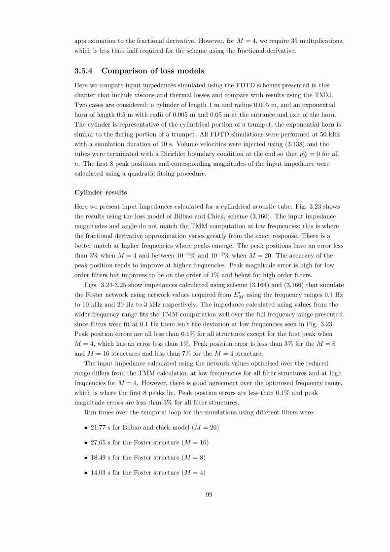
approximation to the fractional derivative. However, for M = 4, we require 35 multiplications,

which is less than half required for the scheme using the fractional derivative.

3.5.4 Comparison of loss models

Here we compare input impedances simulated using the FDTD schemes presented in this

chapter that include viscous and thermal losses and compare with results using the TMM.

Two cases are considered: a cylinder of length 1 m and radius 0.005 m, and an exponential

horn of length 0.5 m with radii of 0.005 m and 0.05 m at the entrance and exit of the horn.

The cylinder is representative of the cylindrical portion of a trumpet, the exponential horn is

similar to the flaring portion of a trumpet. All FDTD simulations were performed at 50 kHz

with a simulation duration of 10 s. Volume velocities were injected using (3.138) and the

tubes were terminated with a Dirichlet boundary condition at the end so that pnN = 0 for all

n. The first 8 peak positions and corresponding magnitudes of the input impedance were

calculated using a quadratic fitting procedure.

Cylinder results

Here we present input impedances calculated for a cylindrical acoustic tube. Fig. 3.23 shows

the results using the loss model of Bilbao and Chick, scheme (3.160). The input impedance

magnitudes and angle do not match the TMM computation at low frequencies; this is where

the fractional derivative approximation varies greatly from the exact response. There is a

better match at higher frequencies where peaks emerge. The peak positions have an error less

than 3% when M = 4 and between 10−4% and 10−2% when M = 20. The accuracy of the

peak position tends to improve at higher frequencies. Peak magnitude error is high for low

order filters but improves to be on the order of 1% and below for high order filters.

Figs. 3.24-3.25 show impedances calculated using scheme (3.164) and (3.166) that simulate

the Foster network using network values acquired from E′M using the frequency ranges 0.1 Hz

to 10 kHz and 20 Hz to 3 kHz respectively. The impedance calculated using values from the

wider frequency range fits the TMM computation well over the full frequency range presented;

since filters were fit at 0.1 Hz there isn’t the deviation at low frequencies seen in Fig. 3.23.

Peak position errors are all less than 0.1% for all structures except for the first peak when

M = 4, which has an error less than 1%. Peak position error is less than 3% for the M = 8

and M = 16 structures and less than 7% for the M = 4 structure.

The input impedance calculated using the network values optimised over the reduced

range differs from the TMM calculation at low frequencies for all filter structures and at high

frequencies for M = 4. However, there is good agreement over the optimised frequency range,

which is where the first 8 peaks lie. Peak position errors are less than 0.1% and peak

magnitude errors are less than 3% for all filter structures.

Run times over the temporal loop for the simulations using different filters were:

• 21.77 s for Bilbao and chick model (M = 20)

• 27.65 s for the Foster structure (M = 16)



99

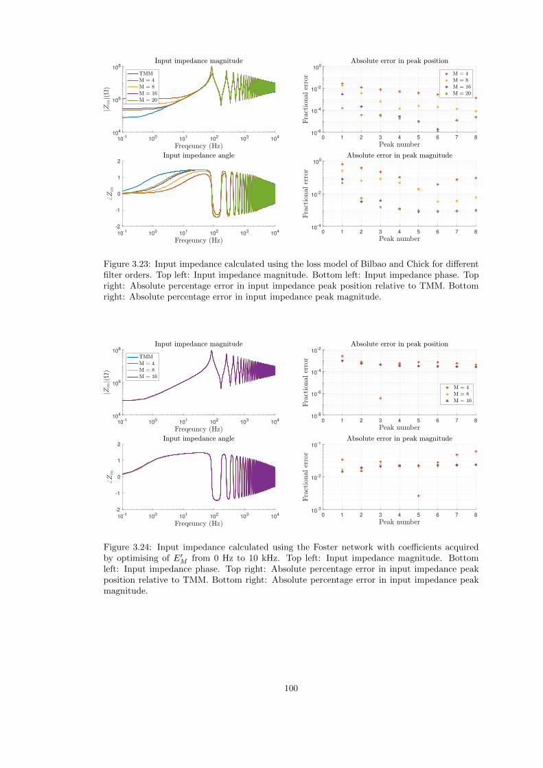
10-1

100

101

102

103

104

104

106

108

10-1

100

101

102

103

104

-2

-1

0

1

2

0 1 2 3 4 5 6 7 810

-6

10-4

10-2

100

0 1 2 3 4 5 6 7 810

-4

10-2

100

Figure 3.23: Input impedance calculated using the loss model of Bilbao and Chick for differentfilter orders. Top left: Input impedance magnitude. Bottom left: Input impedance phase. Topright: Absolute percentage error in input impedance peak position relative to TMM. Bottomright: Absolute percentage error in input impedance peak magnitude.

10-1

100

101

102

103

104

104

106

108

10-1

100

101

102

103

104

-2

-1

0

1

2

0 1 2 3 4 5 6 7 810

-8

10-6

10-4

10-2

0 1 2 3 4 5 6 7 810

-3

10-2

10-1

Figure 3.24: Input impedance calculated using the Foster network with coefficients acquiredby optimising of E′M from 0 Hz to 10 kHz. Top left: Input impedance magnitude. Bottomleft: Input impedance phase. Top right: Absolute percentage error in input impedance peakposition relative to TMM. Bottom right: Absolute percentage error in input impedance peakmagnitude.

100

10-1

100

101

102

103

104

104

106

108

10-1

100

101

102

103

104

-2

-1

0

1

2

0 1 2 3 4 5 6 7 8

4

6

8

10-4

0 1 2 3 4 5 6 7 810

-3

10-2

10-1

Figure 3.25: Input impedance calculated using the Foster network with coefficients acquiredby optimising of E′M from 20 Hz to 3 kHz. Top left: Input impedance magnitude. Bottomleft: Input impedance phase. Top right: Absolute percentage error in input impedance peakposition relative to TMM. Bottom right: Absolute percentage error in input impedance peakmagnitude.

Exponential horn results

Here we present input impedances calculated for an exponential horn. Fig. 3.26 shows the

input impedance calculated using the scheme with the Bilbao and Chick loss model. The

absolute errors in the positions of the input impedance peaks are less than 3 % for M = 4 and

less than 0.02% for M = 20. The error in the peak magnitude is less than 3% for M = 4 and

less than 1% for M = 20. The error in the first peak magnitude is better for the exponential

horn than for the cylinder since this first peak has a higher frequency (the fractional

derivative approximation deviates from the exact result at low frequencies).

Figs. 3.27 and 3.28 show the input impedances of an exponential horn simulated using the

Foster network. Element values were calculated by optimising for a tube radius of 0.05 m, the

maximum radius of this horn, using E′M . Fig. 3.27 shows the input impedance using values

optimised over 0.1 Hz to 10 kHz. Peak position error is less than 0.1% for M = 4 and less

than 0.02% for M = 16. Peak magnitude error is less than 11% for M = 4 and less than 4%

for M = 16.

Fig. 3.28 uses element values optimised over the freqeuncy range 20 Hz to 3 kHz. Peak

position error is less than 0.1% for M = 4 and less than 0.02% for M = 16. Peak magnitude

error is less than 20% for M = 4 and less than 4% for M = 16.

Run times over the temporal loop for the simulations using different filters were:

• 12.19 s for Bilbao and chick model (M = 20)




101

10-1

100

101

102

103

104

100

105

1010

10-1

100

101

102

103

104

-2

-1

0

1

2

0 1 2 3 4 5 6 7 810

-5

10-4

10-3

10-2

0 1 2 3 4 5 6 7 810

-3

10-2

10-1

100

Figure 3.26: Input impedance of an exponential horn calculated using the Bilbao and Chickloss model using different filter orders. Top left: Input impedance magnitude. Bottom left:Input impedance phase. Top right: Absolute percentage error in input impedance peak positionrelative to TMM. Bottom right: Absolute percentage error in input impedance peak magnitude.

10-1

100

101

102

103

104

100

105

1010

10-1

100

101

102

103

104

-2

-1

0

1

2

0 1 2 3 4 5 6 7 810

-5

10-4

10-3

0 1 2 3 4 5 6 7 810

-3

10-2

10-1

Figure 3.27: Input impedance of an exponential horn calculated using the Foster network withcoefficients acquired by optimising of E′M from 0 Hz to 10 kHz. Top left: Input impedancemagnitude. Bottom left: Input impedance phase. Top right: Absolute percentage error ininput impedance peak position relative to TMM. Bottom right: Absolute percentage error ininput impedance peak magnitude.

102

10-1

100

101

102

103

104

100

105

1010

10-1

100

101

102

103

104

-2

-1

0

1

2

0 1 2 3 4 5 6 7 810

-5

10-4

10-3

10-2

0 1 2 3 4 5 6 7 810

-4

10-2

100

Figure 3.28: Input impedance of an exponential horn calculated using the Foster network withcoefficients acquired by optimising of E′M from 20 Hz to 3 kHz. Top left: Input impedancemagnitude. Bottom left: Input impedance phase. Top right: Absolute percentage error ininput impedance peak position relative to TMM. Bottom right: Absolute percentage error ininput impedance peak magnitude.

3.6 Conclusions

This chapter has focussed on how FDTD methods can be used in problems relating to

acoustic tubes. Simple boundary conditions have been chosen so as to focus on the properties

of various schemes over the domain interior.

We began with the simplest system, a lossless cylindrical tube, and the effect of FDTD

scheme on the simulations. This was then extended to an acoustic tube of variable

cross-sectional area. For a cylindrical tube, the explicit scheme on an interleaved time and

space grid was able to produce exact results whereas the implicit scheme, where only the

spatial grids are interleaved, produced frequency warping and was never able to match the

exact solutions. The frequency warping is due to the application of the bilinear transform in

these schemes. Similar performance occurs in a tube of varying cross-sectional area, although

the explicit scheme cannot give exact solutions due to discretisation of the bore. Of course, in

practice, the explicit scheme is not infallible as the spatial domain requires

truncation—resulting in either an incorrect domain size if the spatial step is not modified or

some small degree of frequency warping if it is. However, this is a very small effect relative to

the frequency warping present in the implicit scheme.

The bilinear transform does have its uses, namely the guaranteed passivity of the discrete

schemes if the continuous system is known to be passive; this is motivation behinds its use in

the Port-Hamiltonian framework [164] and in nonlinear schemes [40]. This makes it an ideal

partner to use in tandem with the explicit scheme as the foundation of our system solver. The

effects of viscous and thermal losses are relatively small compared to the main propagation

elements of the system but are important enough to modify resonances and increase the

complexity of the simulations. As a result, the mathematical simplicity of the bilinear

103

transform is a useful property in the analysis of these systems but its frequency warping

nature is less apparent when used in the lossy part.

Modelling of the lossy part has been tackled using two approaches: using a truncated

model of the immittances that require an extra approximation to fractional derivatives, and

by constructing equivalent electrical networks that directly approximate the immittances.

Before considering the numerics applied to the simulation of these models, it is worth pointing

out that the models themselves are different approaches to approximating the Zwikker and

Kosten loss model (as shown in Chap. 2). The truncated model is described for a high

frequency/large tube radius limit, whereas the Foster network can be optimised over different

ranges.

The truncated expansion model is useful as it does not require any offline computation for

changes in cross-sectional area. However, approximating the fractional order derivatives

requires high order recursions to be of use and even then the approximation fails for low

frequencies. It is also affected by numerical rounding errors meaning that the stability of the

system is compromised when trying to improve accuracy. Although the development of the

fractional order derivative approximation starts from the bilinear transform, the final operator

deviates due to truncation of the CFE.

The use of numerical fitting procedures in the Foster network allows for great accuracy

with a relatively low computational cost. One can even modify the optimised parameters so

that they can be applied to systems of different radii and temperatures, although with a slight

loss of accuracy. Simulating this model in the time domain requires some care since the

current formulation is equivalent to applying the bilinear transform to the continuous model.

This reduces the accuracy of the filter structures when the element values are applied straight

to the discrete system. The frequency warping can be taken into account by ‘pre-warping’ the

frequency vector in the optimisation procedure. When this is performed, the filters maintain

their accuracy over the optmised frequency range.

104

Chapter 4

Modelling radiation of sound

from an acoustic tube

“Life is like a trumpet—if you don’t put anything into

it, you don’t get anything out of it.”

— William Christopher Handy

So far, we have considered the brass instrument as a confined system; waves have been

fully reflected by the lossless boundary conditions of an ideally open or closed tube. Although

these models are useful for a preliminary treatment of the brass instrument system, the reality

is more complicated (and interesting). For a listener to hear a sound produced by the

instrument, the instrument system must transfer energy into the listening space and therefore

lose energy. This energy loss is frequency dependent in a non-trivial way. It also turns out

that there are length correction effects present that modify the position of the instrument’s

resonances [63]. In this chapter we begin to refine our brass instrument model to include a

more realistic open tube condition.

Two methods of modelling sound radiation are considered and treatment of both will

follow in a parallel manner. The first model treats the behaviour of sound radiation through a

lumped radiation impedance. As with the case of the tube wall losses, this model is not

immediately useable in the time domain but can be approximated by an equivalent electrical

network leading, ultimately, to a recursible algorithm. The second model directly models the

transfer of energy from the one-dimensional tube system to the three-dimensional air system.

Although this system is more computationally expensive, it does allow for extensions that

include realistic acoustic environment and hearing models (something which is beyond the

scope of this work).

For both models the problem is stated in the continuous domain first and then discretised.

Energy conservation shows that these systems are passive. Results produced using the

algorithms developed in this chapter are presented.

4.1 Radiation impedance models

Rayleigh [157] and Morse [121] consider radiation from a cylindrical tube with an infinite

flange; this system being modelled as a tube within a large wall. In this case, the interface

105

between the cylinder and the free space was considered as a vibrating piston. Whereas

Rayleigh only considered a rigid piston, Morse considered the effect of nonuniform motion on

the piston but did not apply it to the case of an open cylinder. Zorumski [181] extended the

rigid piston model in an infinite flange to include an admittance at the tube walls and the

effect this has on conversion between the planar and higher modes. Amir et al. [5] also

investigated mode conversion in the lossless cylinder with an infinite flange and used ‘edge

functions’ that converged faster than normal mode solutions.

The radiating portion of a brass instrument, however, is far from an infinite flange. A

treatment for plane waves exiting an unflanged cylindrical pipe was given by Levine and

Schwinger [104]. This model is arrived at by matching the plane waves from a cylindrical tube

to the spherical waves of the free field through manipulation of Green’s theorem. Causse et. al

[37] modified the planar radiation model to better represent spherical waves by using a ratio

of the area of the spherical wavefront to that of the planar wavefront at the end of the horn.

Helie and Rodet [83] provide a spherical model of radiation from a horn. Instead of using a

vibrating piston, the radiating part of the horn is considered to be an area of a sphere that

vibrates. Averaging over the surface allowed for the model to be incorporated into

one-dimensional models. However, averaging introduces errors that are significant at small

flaring angles.

As planar wave propagation is considered in the interior of the acoustic tube, the Levine

and Schwinger model was chosen as a radiation condition for this work. The model is given in

terms of a complex reflection function

R = −|R|e2j ω∆lc0 (4.1)

where the reflection magnitude and length correction are, respectively,

|R| = exp

−2rLω

πc0

∫ rLωc0

0

tan−1 (−J1(x)/N1(x))

x[(rL

ωc0

)2 − x2]1/2 dx

(4.2a)

∆l =rLπ

∫ rL

ωc0

0

log(πJ1(x)

[J1(x)2 +N1(x)2

]1/2)x

[(rL

ωc0

)2

− x2

]1/2dx

+

∫ ∞0

log [1/ (2I1(x)K1(x))]

x

[x2 +

(rL

ωc0

)2]1/2

dx

(4.2b)

where rL is the radius at the end of the tube, J1 and N1 are Bessel functions of first and

second kind, I1 and K1 are the modified Bessel functions of first and second kind1. The exp(·)notation, rather than e·, has been used in the reflection magnitude for clarity.

1In Levine and Schwinger’s original manuscript, these functions are described as the cylindrical functions.

106

The radiation impedance is given by

ZR = ρ0c01 +R

1−R(4.3)

4.1.1 Network representation of radiation model

The form of (4.1) is expressed in the frequency domain. To be used in a time domain model,

some further approximations must be made.

Causse et al. [37] provide some approximations that could be used in the time domain, but

they are only valid over a limited frequency range. Silva et al. [147] used fitting procedures to

match Pade approximations to the Levine and Schwinger model. These approximations can

be applied over a wider frequency range than that presented by Causse et al., and were later

used by Bilbao and Chick [24] in the form of a passive network, see Fig. 4.1, for modelling

acoustic tubes, and by Harrison et al. [75, 76] for a full brass instrument synthesis

environment. A similar method was presented by Helie and Rodet [83] to model the spherical

radiation model in the time domain.

The radiation impedance is associated with a one-port circuit element, with pressure, p,

associated with a voltage and particle velocity, v, associated with a current. Additional state

variables of the circuit are associated currents v(1), v(2), v(3), and v(4), and voltage p(1). The

internal state variables are distinguished from those used for the pressure and velocity inside

an acoustic tube through the use of brackets in the subscripts.

p

v

Lr

v(1)

R1 v(2)

R2

v(3)

v(4)

Crp(1)

Figure 4.1: Circuit representation of approximation to the Levine and Schwinger radiationmodel.

The radiation impedance given by this network is

Zrad =Lr(R1 +R2)jω + LrR1R2Cr(jω)2

R1 +R2 + (Lr +R1R2Cr)jω + LrR2Cr(jω)2(4.4)

with element values

R1 = ρ0c0, Lr = 0.613ρ0rL, R2 = 0.505ρ0c0, Cr = 1.111rLρ0c20

(4.5)

The voltage and current at the open terminal are related to the pressure and velocity at

the end of the acoustic tube by

p = p(t, L), v = v(t, L) (4.6)

107

and the internal state variables are given by

v = v(1) + v(2), p = Lrdv(1)

dt, p = R1v(2) + p(1) (4.7a)

v(2) = v(3) + v(4), p(1) = R2v(3), v(4) = Crdp(1)

dt(4.7b)

We do not need to solve for all of these state variables; (4.7) can be reduced to

v = v(1) +

(1

R2+ Cr

d

dt

)p(1) (4.8a)

p = Lrdv(1)

dt(4.8b)

p =

(1 +

R1

R2+R1Cr

d

dt

)p(1) (4.8c)

Fig. 4.2 shows the radiation reflection magnitude and length correction calculated using

the Levine and Schwinger expression (4.2) and the network approximation (4.4) for a tube

radius of 0.05 m, typical of the end of a trumpet. The Levine and Schwinger model is defined

only for planar propagation; in this case the upper frequency limit is 2661 Hz at a

temperature of 26.85 C and was calculated using the integral function in MATLAB.

0 0.5 1 1.5 2 2.5 3 3.5 4

0

0.2

0.4

0.6

0.8

1

0 0.5 1 1.5 2 2.5 3 3.5 4

0.1

0.2

0.3

0.4

0.5

0.6

0.7

Figure 4.2: Left: Radiation reflection magnitude for a tube of radius 0.05 m calculated using theLevine and Schwinger model (blue) and the network approximation. Right: Radiation lengthcorrection.

The network approximation is a good match at low frequencies but deviates at high

frequencies.


Although it is known that this network is passive, it is useful to derive an energy for the

system when it is used in tandem with the horn equation. Recalling the power transfer at the

boundary from the energy analysis of the horn equation (2.49) over the domain D is

Bhe = − pSv|z=0 + pSv|z=L (4.9)

108

Replacing the boundary term at z = L with the associated voltage and current in our

radiation network allows for the following manipulation

pSv|z=L(4.6)= S(L)pv

(4.7a)= S(L)p

(v(1) + v(2)

)(4.7a)

= S(L)

(Lrv(1)

dv(1)

dt+ pv(2)

)(4.7a)

= S(L)

(Lrv(1)

dv(1)

dt+(R1v(2) + p(1)

)v(2)

)(4.7b)

= S(L)

(Lrv(1)

dv(1)

dt+R1v

2(2) + p(1)

(v(3) + v(4)

))(4.7b)

= S(L)

(Lrv(1)

dv(1)

dt+R1v

2(2) +R2v

2(3) + Crp(1)

dp(1)

dt

)(2.4)=

dHraddt

+Qrad (4.10)

where

Hrad =S(L)

2

(Lrv

2(1) + Crp

2(1)

)≥ 0 (4.11a)

Qrad = S(L)(R1v

2(2) +R2v

2(3)

)≥ 0 (4.11b)

In this case, the boundary condition contains a storage component, along with dissipation as

discussed in Sec. 2.2.3. Combining this with the energy for the whole system gives

d

dt(Hhe +Hrad) +Qrad + B′he = 0 (4.12)

where B′he = − pSv|z=0. The total energy of the system and the power loss from the radiation

model are non-negative values and the solutions to the system are therefore bounded.

4.1.3 Numerical scheme

We now look to discretising the network structure approximating the Levine and Schwinger

radiation impedance presented in Sec. 4.1.1. The pressure and velocity at the end of the horn

are related to the voltage and current of the network by

p = µt+pN , SN v = µz−(SN+1/2vN+1/2

)(4.13)

where pn+1/2 and vn+1/2 lie on the interleaved temporal grid. The internal state variables are

given by

v = µt+v(1) + µt+v(2), p = Lrδt+v(1), p = R1µt+v(2) + µt+p(1) (4.14a)

v(2) = v(3) + v(4), p(1) = R2v(3), µt+v(4) = Crδt+p(1) (4.14b)

109

where currents vn(1), vn(2), v

n(3), and vn(4), and voltage pn(1) are aligned on the integer temporal

grid. We can reduce system (4.14) to

v = µt+v(1) +1

R2µt+p(1) + Crδt+p(1) (4.15a)

p = Lrδt+v(1) (4.15b)

p =

(1 +

R1

R2

)µt+p(1) +R1Crδt+p(1) (4.15c)

This choice of discretisation is equivalent to applying the bilinear transform in (4.4). Fig. 4.3

shows the effect of using the bilinear transform on this system compared to the continuous

case. For this system, the discretisation has little effect over the frequency domain of interest.

0 0.5 1 1.5 2 2.5 3 3.5 4

-0.035

-0.03

-0.025

-0.02

-0.015

-0.01

-0.005

0

0 0.5 1 1.5 2 2.5 3 3.5 4

-0.025

-0.02

-0.015

-0.01

-0.005

0

Figure 4.3: Left: Error in reflection magnitude of network when using the bilinear transform(dashed red) at 50 kHz. Right: Error in length correction.

To couple this model to the horn equation, we look at the pressure equations of (3.108) at

l = NSNρ0c20

δt+pN = −δz−(SN+1/2vN+1/2

)(4.16)

Using the identity δz− = 2h (µz− − wz−) results in

SNρ0c20

δt+pN = − 2

h

(µz−

(SN+1/2vN+1/2

)− SN−1/2vN−1/2

)= − 2

h

(SN v − SN−1/2vN−1/2

)(4.17)

We then look to writing v in terms of known values of v(1), p(1) and pnN as well as the unknown

pn+1N . We do this by first expressing the current and voltage in terms of their previous values

and the unknown pressure, and then substitute these into our expression for v. This results in

pn+1N = α(R)pnN + β(R)SN−1/2vN−1/2 + ε(R)vn(1) + ν(R)pn(1) (4.18a)

vn+1(1) = vn(1) +

k

Lrµt+pN (4.18b)

pn+1(1) = τ (R)pn(1) + χ(R)µt+pN (4.18c)

where

110

α(R) =1− E(R)

1 + E(R)(4.18d)

β(R) =2ρ0c

20k

SNh(1 + E(R)

) (4.18e)

ε(R) = − 2ρ0c20k

h(1 + E(R)

) (4.18f)

ν(R) = ε(R)

(1

2R2(τ (R) + 1) +

Crk

(τ (R) − 1)

)(4.18g)

τ (R) =R1Cr −H(R)

R1Cr +H(R)(4.18h)

χ(R) =k

R1Cr +H(R)(4.18i)

E(R) =ρ0c

20k

h

(k

2Lr+

(1

2R2+Crk

)χ(R)

)(4.18j)

H(R) =k

2

(1 +

R1

R2

)(4.18k)

4.1.4 Discrete energy analysis

Recalling that the discrete power transfer at the boundaries for the explicit scheme for the

horn equation (3.108) is

bhe = −µt+p0µz−(S1/2v1/2

)+ µt+pNµz−

(SN+1/2vN+1/2

)(4.19)

we can find a discrete energy for our coupled system. We can rewrite the term at l = N using

(4.13) as µt+pNµz−(SN+1/2vN+1/2

)= SN pv which can then be manipulated as follows

SN pv(4.15a)

= SN p

(µt+v(1) +

1

R2µt+p(1) + Crδt+p(1)

)(4.14a)

= SN(Lrµt+v(1)δt+v(1) + pµt+v(2)

)(4.14a)

= SN(Lrµt+v(1)δt+v(1) +

(R1µt+v(2) + µt+p(1)

)µt+v(2)

)(4.14b)

= SN

(Lrµt+v(1)δt+v(1) +R1

(µt+v(2)

)2+ µt+p(1)

(µt+v(3) + µt+v(4)

))(4.14b)

= SN

(Lrµt+v(1)δt+v(1) +R1

(µt+v(2)

)2+R1

(µt+v(3)

)2+ Crµt+p(1)δt+p(1)

)(3.26c)

= δt+hrad + qrad (4.20)

where

hrad =SN2

(Lrv

2(1) + Crp

2(1)

)≥ 0 (4.21a)

qrad = SN

(R1

(µt+v(2)

)2+R2

(µt+v(3)

)2) ≥ 0 (4.21b)

Combining this with the total energy of the system gives

δt+ (hhe + hrad) + qrad + b′he = 0 (4.22)

111

where b′he = −µt+p0µz−(S1/2v1/2

). It is clear that the combined energy and the losses due to

radiation are non-negative and therefore the solutions to the system are bounded.

4.1.5 Simulation results

Simulations were performed for a cylindrical tube of length 1 m and radius of 0.05 m at a

temperature of 26.85 C. The sample rate was 50 kHz, simulation duration 10 s, and Courant

number λ = 0.9861. Losses were neglected over the interior of the acoustic tube.

Fig. 4.4 shows the energy evolution of the FDTD simulation and its total energy balance

(3.75). At the 142nd time step, corresponding to the time taken for a disturbance to travel the

length of the tube, energy is transferred from the end of tube to the radiation model; there is

a reduction in the energy stored in the cylinder and an increase in the energy stored in the

radiation model. The subsequent variations in energy of the tube and radiation model are not

monotonically decreasing and increasing—oscillations in stored energy of the tube and the

radiation model are observed. This is because there is additonal exchange of energy between

the two models after the pulse has initially interacted at the boundary. The energy of the

overall system decreases over time due to the lossy processes in the radiation model. The total

energy balance shows bit-wise deviations in the energy on the order of the machine precision.

Figure 4.4: Top: Total stored energy (blue), stored energy in the tube (red), stored energy inthe radiation model (yellow), and energy lost by the radiation model (purple). Bottom: Energybalance showing numerical precision of machine.

Input impedances were calculated from simulations using the procedure described in Sec.

3.4.3. Simulation results were compared to the exact expression [63] for the input impedance

of a cylinder terminated with the Levine and Schwinger radiation impedance

Z(exact) =jρ0c0S0

jρ0c0 sin(ωLc0

)+ ZR cos

(ωLc0

)jρ0c0 cos

(ωLc0

)− ZR sin

(ωLc0

) (4.23)

Fig. 4.5 shows the input impedance calculated from simulations and Z(exact) along with

the error in the frequency of the first ten peaks produced by the FDTD model. The error in

112

0 200 400 600 800 1000 1200 1400 1600 1800 200010

0

105

1010

1 2 3 4 5 6 7 8 9 1010

-5

10-4

10-3

10-2

Figure 4.5: Top: Input impedance of a lossless cylinder of radius 0.05 m and length 1 mcalculated using an FDTD simulation with lossy radiating end (solid black) and a frequencydomain calculation terminated with the Levine and Schwinger radiation impedance (dashedred). Bottom: Absolute error in peak position of FDTD simulation relative to frequencydomain calculation.

the position for the first five peaks is less than 0.02 % and increases to 0.1 % over the sixth to

tenth peaks.

Fig. 4.6 shows the input impedance calculated for a cylinder of radius 0.1 m. The error in

the peak position given by the FDTD model is slightly larger than for the smaller tube, but

still lies under 0.4 % for the first ten peaks.

These results extend the comparison of the network approximation and the Levine and

Schwinger radiation model. The errors in the FDTD simulation can be described in terms of

the errors of the network model as opposed to numerical errors. We are therefore justified in

our use of the bilinear transform to model the network radiation model, taking advantage of

its passive behaviour. This is the same procedure employed for incorporating viscous and

thermal losses in Chap. 3—using an explicit scheme for efficient and accurate modelling of

wave propagation and the bilinear transform to preserve passivity of connected processes.

4.2 Coupling to a 3D acoustic field

An alternative to modelling a radiation impedance is to directly model the interaction of the

tube with the three-dimensional space it occupies. There are multiple publications presenting

simulations of the three-dimensional field in an acoustic tube; see [68, 69, 70] for

three-dimensional modelling of woodwind instruments and [4, 137, 138] for two and

three-dimensional modelling of brass instruments2. However, there are several disadvantages

to this approach. The most obvious in terms of developing a synthesis tool is computational

cost—if we increase the size of the domain of interest, more computations are required at each

time step, resulting in longer computation times. In addition, incorporation of the viscous and

thermal boundary layer losses in higher dimensions requires an extremely high spatial

resolution for accurate modelling. In contrast, the one-dimensional model presented in this

2Note that these works used a nonlinear propagation model.

113

0 200 400 600 800 1000 1200 1400 1600 1800 200010

0

105

1010

1 2 3 4 5 6 7 8 9 1010

-5

10-4

10-3

10-2

Figure 4.6: Top: Input impedance of a lossless cylinder of radius 0.1 m and length 1 m calculatedusing an FDTD simulation with lossy radiating end (solid black) and a frequency domain calcu-lation terminated with the Levine and Schwinger radiation impedance (dashed red). Bottom:Absolute error in peak position of FDTD simulation relative to frequency domain calculation.

thesis requires little in terms of computing power and accurately models boundary layer

losses. However, it does not allow for non-planar modes to be excited in the flaring portions of

the instrument.

We can exploit the strengths of the one- and three- dimensional approaches: a

one-dimensional acoustic tube model that encorporates the viscous and thermal losses in an

efficient manner, and a model of the three-dimensional acoustic field that includes effects due

to the flaring of the instrument bell and the radiation of sound away from the instrument.

These two models are then coupled at a chosen point along the length of the instrument; we

name this an embedded instrument system, see Fig. 4.7.

1D propagation 3D propagation

Couplingpoint

Figure 4.7: Schematic of an embedded system. The cylindrical, or slowly varying, portion of theinstrument bore is modelled using a one-dimensional wave propagation model. In the flaringportions of the instrument, a three-dimensional wave propagation model is used. The dashedline shows the boundary between the two sections of the instrument.

This is somewhat similar to the method approached by Noreland [127], albeit in the time

domain rather than the frequency domain. In Noreland’s paper, a radiation impedance was

calculated using a FDTD scheme in the flaring portion of the instrument. This radiation

114

impedance was used to terminate a TMM calculation over the remainder of the instrument

where the bore profile was considered to be slowly varying. In a later paper by Noreland et al.

[129], radiation behaviour was calculated using the Finite Element method and used in a bore

optmisation procedure.

In [127] a two-dimensional curvilinear coordinate system was chosen to best represent the

geometry of the walls of the instrument. However, as an observer moves further away from the

instrument the grid spacing increases, which drastically reduces the available bandwidth of

the simulated sounds. To avoid this, we instead use a scheme on a regular Cartesian grid.

4.2.1 Partial differential equations and integrals in higher

dimensions: Etude IIIa

In this section, we retain the dimension of time t ∈ R but must extend our spatial domain to

the Euclidean space R3. Vectors will be identified using bold typeface. Coordinates are

defined using the triple (x′, y′, z′) ∈ R3. We will consider a cubic region of side length L(3)

centred at the origin defined by D(3) = (x′, y′, z′) ∈ R3 | −L(3)/2 ≤ x′, y′, z′ ≤ L(3)/2. This

region encloses a volume defined by V = (x′, y′, z′) ∈ R3 | −L(3)/2 < x′, y′, z′ < L(3)/2 and

is enclosed by a surface given by ∂V = D(3) \ V.

For a multidimensional scalar function, f(t, x′, y′, z′), the gradient of the function is

∇f = [∂x′f, ∂y′f, ∂z′f ]T

(4.24)

For a vector function g(t, x′, y′, z′) = [gx′(t, x′, y′, z′), gy′(t, x

′, y′, z′), gz′(t, x′, y′, z′)]

T, the

divergence is given by

∇ · g = ∂x′gx′ + ∂y′gy′ + ∂z′gz′ (4.25)

The extension to higher dimensions of the second spatial derivative of a scalar function is the

Laplacian operator given by

∇2f = ∇ · ∇f = ∂x′x′f + ∂y′y′f + ∂z′z′f (4.26)

We define the inner product of two scalar functions, f and g, over a three-dimensional

cubic region D(3) as

〈f, g〉D(3) =

∫D(3)

fgdV =

∫ L(3)/2

−L(3)/2

∫ L(3)/2

−L(3)/2

∫ L(3)/

−L(3)/2

fg dx′ dy′ dz′ (4.27)

Similarly the inner product of two vector functions, f and g, over the region D(3) is

〈f ,g〉D(3) =

∫D(3)

f · gdV (4.28)

The three-dimensional L2 norm is given by

‖f‖D(3) =√〈f, f〉D(3) , ‖g‖D(3) =

√〈g,g〉 (4.29)

The continuous temporal identity (2.4) in the one-dimensional case extends to the

three-dimensional case.

115

We shall also use the inner product and norm over the closed surface of a domain

f, g∂V =

∮∂Vfg dA, ‖f‖∂V =

√f, f∂V (4.30)

here dA denotes integration over the surface of the domain.

Integration by parts extends to the three-dimensional case. An example using the

derivative in the z′ dimension over the cubic domain is∫D(3)

f∂z′gdV = −∫D(3)

(∂z′f) gdV +

∫ L(3)/2

−L(3)/2

∫ L(3)/2

−L(3)/2

fg|z′=L(3)

2

− fg|z′=L(3)

2

dx′dy′ (4.31)

Notice that the boundary terms are integrations over surfaces of the domain. For this work,

we use integration by parts in three-dimensions solely for problems concerning the Laplacian

operator ∫D(3)

f∇2gdV = −∫D(3)

(∇f) · (∇g) dV +

∮∂Vfn · ∇g dA (4.32)

where n denotes the outward normal of the surface ∂V. This is a specific application of the

Divergence theorem [140]. Using the norm notation, Eq. (4.32) is given as

〈f,∇2g〉D(3) = −〈∇f,∇g〉D(3) + f,n · ∇g∂V (4.33)

4.2.2 The 3D wave equation

The three-dimensional wave equation is given by [122]

ρ0

c20∂ttψ − ρ0∇2ψ = 0 (4.34)

where ψ(t, x′, y′, z′) is the acoustic velocity potential in three dimensions. The scalar pressure,

p3D(t, x′, y′, z′), and vector particle velocity, v3D(t, x′, y′, z′), fields are given by

p3D = ρ0∂tψ, v3D = −∇ψ (4.35)


Taking the inner product of (4.34) with ∂tψ over the cubic domain D(3) results in

ρ0

c20〈∂tψ, ∂ttψ〉D(3) − ρ0〈∂tψ,∇2ψ〉D(3) = 0 (4.36)

Applying integration by parts, (4.33), results in

ρ0

c20〈∂tψ, ∂ttψ〉D3 + ρ0〈∂t∇ψ,∇ψ〉D3 + B3we = 0 (4.37)

where

B3we = ρ0∂tψ,n · ∇ψ∂V (4.38)

is the power transferred at the boundaries of the domain.

116

Using (2.4) results in the energy balance

dH3we

dt+ B3we = 0 (4.39)

where

H3we(t) =ρ0

2c20‖∂tψ‖2D(3) +

ρ0

2‖∇ψ‖2D(3) ≥ 0 (4.40)

is the energy stored in the three-dimensional wave equation. This quantity is non-negative,

therefore solutions are bounded.


A lossless Neumann condition at a boundary is given by

n · ∇ψ = 0 (4.41)

This boundary condition is used to model rigid walls in the acoustic field, such as the walls of

a brass instrument.

Ideally, we wish to perform simulations in an infinite domain, so as not to have any

resonances from the three-dimensional space interfering with the response of the instrument;

the case of performing in a reverberant space is beyond the scope of this work. In practice,

this is not possible, so we wish to define a smaller computational domain that absorbs waves

at the domain boundaries, thus behaving as if in an infinite domain.

One such manner of achieving this is the application of Perfectly Matched Layers [16],

where gradually increasing damping is introduced at the computational domain boundaries.

This requires additional points on the domain boundaries, we would wish to minimise this.

An alternative is to use the absorbing boundary conditions of Engquist and Majda [55]. On

the surfaces perpendicular to the z′ axis, perfectly absorbing boundary conditions are given by

−ψ∣∣z′=−L(3)

2

= 0, +ψ∣∣z′=L(3)

2

= 0 ± = ∂z′ ±∂tc0

√1−

(∂x′

∂t/c0

)2

−(

∂y′

∂t/c0

)2

(4.42)

By symmetry, this can be extended to other boundary surfaces. However, the square root

term in the operators prevents implementation. This is resolved by using a low order Taylor

expansion, resulting in the first order approximation [55]

1

c0∂tψ + n · ∇ψ = 0, (x′, y′, z′) ∈ ∂V (4.43)

Examples at the boundaries in the z′ direction in D(3) are

1

c0∂tψ − ∂z′ψ = 0, z′ = −L

(3)

2(4.44a)

1

c0∂tψ + ∂z′ψ = 0, z′ =

L(3)

2(4.44b)

By symmetry, similar conditions hold at the domain boundaries in the x′ and y′ dimensions.

These boundary conditions were successfully applied by Torin [163] for embedding of

percussion instruments.

117

For boundary conditions of the first-order Enquist-Majda type, the power transfer at the

domain boundaries, (4.38), becomes

B3we =ρ0

c0‖∂tψ‖2∂V ≥ 0 (4.45)

This is non-negative and therefore the absorbing boundary conditions are passive. Additional

work was performed by Higdon [84, 85] on developing discrete absorbing boundary conditions

that are equivalent to those presented by Engquist and Majda; we use the first order

approximation (4.43) in this work due to their simple application and determination of

passivity.

4.2.5 Coupling the systems: Continuous case

To begin this study of embedding instruments, let us first consider a lossless cylinder placed in

an enclosed volume of air. Propagation within the cylinder will be modelled using the

one-dimensional horn equation (2.49). Propagation of sound in the enclosed volume of air will

be described using the three-dimensional wave equation (4.34). These two models will be

coupled so that energy can be transferred from the end point on the one-dimensional model at

z = L, and one side of a disc Ω in the three-dimensional model; see Fig. 4.8. The disc has a

radius rL (the same as the radius the end of the acoustic tube), centred at the origin, and is

orientated perpendicular to the z′ axis. The surface of the disc is given by

Ω = (x′, y′, z′) ∈ R3 |√x′2 + y′2 ≤ rL, z′ = 0. We label the sides of the disc directly in

front, z′ = 0+, and behind, z′ = 0−, as Ω+ and Ω− respectively.

L(3)

L(3)

L(3)

Ω

L

S(L)

Energy transfer

z

z′

x′

y′

Figure 4.8: Schematic of embedded system. Energy is transferred between the cylinder, at left,and the enclosed volume of air, at right, via the point at the end of the tube and the surface Ω.

The energy balance for the three-dimensional system now becomes

dH3we

dt+ B3we = − ρ0

∫Ω+

∂tψ∂z′ψdA︸︷︷︸Power transfer on Ω+

+ ρ0

∫Ω−

∂tψ∂z′ψdA︸︷︷︸Power transfer on Ω−

(4.46)

The energy balance shows power transfer on the two surfaces Ω+ and Ω−. However, we wish

for sound to only be radiated from one side of Ω, and must set a suitable boundary condition

on the other. In this case, we assume energy transfer only occurs on Ω+ and a Neumann

118

boundary condition is considered on Ω−. The energy balance becomes

dH3we

dt+ B3we = −ρ0

∫Ω+

∂tψ∂z′ψdA (4.47)

Recall the energy balance (2.72) for the horn equation

dHhedt

+ B′he = −pSv|z=L (4.48)

This allows us to couple the two systems using power conservation across the interface. A

disturbance leaving the acoustic tube will inject energy into the acoustic space; likewise, any

energy within the acoustic space that is incident on the surface Ω+ will (partially) transfer

into the tube. This means that the power transferred out of the end of the tube is equal to

power transferred into the air box on the surface Ω+ so that

pSv|z=L = −ρ0

∫Ω+

∂tψ∂z′ψdA (4.49)

For the one-dimensional model, we assume that our variables lie on a planar cross-section of

the tube, which, for practical purposes, is considered as an isophase surface. It is therefore

suitable to assign the pressure on the surface Ω+ to the value given at the end of the tube

ρ0∂tψ = p(t, L), (x′, y′, z′) ∈ Ω+ (4.50)

which, when substituted into (4.49), leads to

S(L)v(t, L) = −∫

Ω+

∂z′ψdA (4.51)

4.2.6 Finite-difference operators and inner products in higher

dimensions: Etude IIIb

We now discuss the discretisation of the three dimensional domain using finite-difference

methods. A point on the grid is indexed using l = (lx′ , ly′ , lz′) ∈ Z3 so that a grid function is

defined by

fnl = fnlx′ ,ly′ ,lz′ ≈ f(nk, lx′h3, ly′h3, lz′h3) (4.52)

where h3 is the three-dimensional grid spacing that, in general, is not equal to the grid

spacing for the one-dimensional model, h. The spatial indices lie in the domain

d(3) =l ∈ Z3 | −N3

2 ≤ lx′ , ly′ , lz′ ≤N3

2

where N3 = floor(L(3)/h3) is the number of points in

each dimension on the spatial grid. For simplicity, let us assume that N3 is an even number.

The discrete domain d(3) corresponds to points in the continuous cubic domain D(3). We must

also consider points that lie on the surfaces of the domain. For example, the surfaces of the

domain perpendicular to the x′ axis are

b(x′−) =

l ∈ Z3 | lx′ = −N3

2,−N3

2≤ ly′ , lz′ ≤

N3

2

(4.53)

b(x′+) =

l ∈ Z3 | lx′ =

N3

2,−N3

2≤ ly′ , lz′ ≤

N3

2

(4.54)

119

The notation used above can be extended to the other surfaces.

The spatial shifting operators for higher dimensions are

wx′±fnl = fnlx′±1,ly′ ,lz′

, wy′±fnl = fnlx′ ,ly′±1,lz′

, wz′±fnl = fnlx′ ,ly′ ,lz′±1 (4.55)

Discrete approximations to the first spatial derivatives ∂x′ , ∂y′ , and ∂z′ are, respectively,

δx′+ =wx′+ − 1

h3δx′− =

1− wx′−h3

(4.56a)

δy′+ =wy′+ − 1

h3δy′− =

1− wy′−h3

(4.56b)

δz′+ =wz′+ − 1

h3δz′− =

1− wz′−h3

(4.56c)

Approximations to the second derivatives, ∂x′x′ , ∂y′y′ , and ∂z′z′ , are given by

δx′x′ = δx′+δx′− =wx′+ − 2 + wx′−

h23

(4.57a)

δy′y′ = δy′+δy′− =wy′+ − 2 + wy′−

h23

(4.57b)

δz′z′ = δz′+δz′− =wz′+ − 2 + wz′−

h23

(4.57c)

so that a simple approximation to the Laplacian is

δ∇2 = δx′x′ + δy′y′ + δz′z′ (4.58)

The discrete three-dimensional inner product between functions fl and gl over d(3) is given

by

〈f, g〉d(3) =∑l∈d(3)

h33 flgl (4.59)

The weighted inner product is given by

〈f, g〉χd(3) =

∑l∈d(3)

h33 χlflgl (4.60)

where χl is a weighting function so that

χl =

1, over the interior of the domain

12 , on the surfaces of the domain

14 , on the edges of the domain

18 , on the corners of the domain

(4.61)

The discrete three-dimensional weighted inner product is similar to the one-dimensional

weighted inner product in that boundary points are scaled.

Norms are again denoted by

‖f‖d(3) =√〈f, f〉d(3) , ‖f‖χ

d(3) =√〈f, f〉χ

d(3) (4.62)

We will use the bracket notation to signify the inner products over smaller domains.

120

We will only consider the weighted inner product and norm over a surface

f, gχb(x′+) =

∑l∈b(x′+)

h23 χlflgl, ‖f‖χ

b(x′+) =√f, f′

b(x′+) (4.63)

Summation by parts is extended to three dimensions. For example, using the weighted

inner product, summation by parts for discrete difference operator in the z′ direction is

〈f, δz′+g〉χd(3) = −〈δz′−f, g〉d′(3)

z′− f, µz′−gχb(z′−) + f, µz′+gχb(z′+) (4.64)

where d(3)z′ =

(lx′ , ly′ , lz′) ∈ Z3 | −N3

2 ≤ lx′ , ly′ ≤N3

2 ,−N3

2 ≤ lz′ ≤N3

2 − 1

. By symmetry

(4.64) applies to other dimensions.

As in the one-dimensional case, the domain of the inner product changes when summation

by parts is performed. This occurs only in the direction of the difference operator—the

domain dimensions perpendicular to this remain unchanged and the weightings of the

weighted inner product are not affected. For example, the weighted inner product over the

domain d(3)x′ is weighted at ly′ , lz′ = ±N3

2 , but not for lx′ = −N3

2 ,N3

2 − 1.

4.2.7 The simple scheme for the 3D wave equation

A discrete approximation to the three-dimensional wave equation (4.34) is

ρ0

c20δttψ

nlx′ ,ly′ ,lz′

− ρ0δ∇2ψnlx′ ,ly′ ,lz′ = 0 (4.65)

which, over the domain interior, has the update

ψn+1l =2

(1− 3λ2

)ψnlx′ ,ly′ ,lz′ − ψ

n−1lx′ ,ly′ ,lz′

+ λ2(ψnlx′+1,ly′ ,lz′

+ ψnlx′−1,ly′ ,lz′+ ψnlx′ ,ly′+1,lz′

+ ψnlx′ ,ly′−1,lz′+ ψnlx′ ,ly′ ,lz′+1 + ψnlx′ ,ly′ ,lz′−1

)(4.66)

This particular scheme, and its generalisations, has been used in [31, 32]. Taking the weighted

inner product of (4.65) with δt·ψnl over d(3) gives

ρ0

c20〈δt·ψ, δttψ〉χd(3) − ρ0〈δt·ψ, δ∇2ψ〉χ

d(3) = 0 (4.67)

Using summation by parts, (4.64), gives

ρ0

c20〈δt·ψ, δttψ〉χd(3) + ρ0

(〈δt·δx′−ψ, δx′−ψ〉χ

d(3)

x′

+ 〈δt·δy′−ψ, δy′−ψ〉χd

(3)

y′+ 〈δt·δz′−ψ, δz′−ψ〉χ

d(3)

z′

)+ b3we = 0 (4.68)

where

b3we =ρ0

c20

(−δt·ψ, δx′·ψχb(x−) + δt·ψ, δx′·ψχb(x+) − δt·ψ, δy′·ψχb(y′−)

+ δt·ψ, δy′·ψχb(y′−) − δt·ψ, δz′·ψχ

b(z′−) + δt·ψ, δz′·ψχb(z′+)

)(4.69)

121

is the power transfer at the domain boundaries. Using (3.26a) and (3.26b) gives

δt+h3we + b3we = 0 (4.70)

where

h3we =ρ0

2c20

(‖δt−ψ‖χd(3)

)2+ρ0

2

(〈δx′−ψ,wt−δx′−ψ〉χ

d(3)

x′+ 〈δy′−ψ,wt−δy′−ψ〉χ

d(3)

y′

+ 〈δz′−ψ,wt−δz′−ψ〉χd

(3)

z′

)(4.71)

is the discrete energy in the domain. As in the discussion of the explicit scheme (3.40) for the

one-dimensional wave equation in Chap. 3, we wish to find conditions for which h3we is

non-negative, so that the solutions are bounded. Using (3.26f) and (3.29a) produces

ρ0

2〈δx′−ψ,wt−ψ〉χ

d(3)

x′

(3.26f)

≥ −ρ0k2

8

(‖δt−δx′−ψ‖χ

d(3)

x′

)2

(3.29a)

≥ −ρ0k2

2h23


)2(4.72)

and likewise for the δy′− and δz′− terms. This leads to

h3we ≥ρ0

2

(1

c20− 3k2

h23

)(‖δt−ψ‖χd(3)

)2(4.73)

The discrete energy, h3we, is non-negative provided that the three-dimensional Courant

number satisfies

λ3 =c0k

h3≤ 1√

3(4.74)

For this case, solutions will be bounded. Note that the bound on the Courant number in three

dimensions is different to that in one dimension. As a result, different spacings are used for

the two systems. It is clear that for the three-dimensional case, the spatial grid spacing is

larger than that used for the one-dimensional case, thus the bandwidth of the

three-dimensional system is less than that of the one-dimensional system. The

one-dimensional spatial step size could be set to be equal to the three-dimensional spatial step

size, however, this would result in poor dispersion behaviour in the one-dimensional part of

the problem. This extends from the discussion of numerical dispersion in Sec. 3.3.2.

In addition, scheme (4.65) suffers from direction-dependent numerical dispersion, which is

not present in the one-dimensional models. On axis, that is in directions parallel to the x′, y′,

and z′ axes, the effects of numerical dispersion are strongest. However, on cube diagonals,

there is no numerical dispersion. It is much simpler, mathematically, to align a horn with the

z′ axis so this is the chosen orientation. This may seem contradictory to the criticism

regarding numerical dispersion in the scheme used by Noreland [127]. However, scheme (4.65)

displays anisotropic numerical dispersion whereas the numerical dispersion of the scheme used

by Noreland is inhomogenous—the dispersion characteristics change with distance from the

horn. The work presented here could be extended to use other three-dimensional FDTD

schemes with better on-axis dispersion properties, such as those studied in [74].

122


Discrete Neumann conditions at the boundaries perpendicular to the x′ coordinate are given

by

δx′·ψ = 0, (lx′ , ly′ , lz′) ∈ b(x′−), b(x

′+) (4.75)

Absorbing boundary conditions are given by

1

c0δt·ψ − δx′·ψ = 0, (lx′ , ly′ , lz′) ∈ b(x

′−) (4.76)

1

c0δt·ψ + δx′·ψ = 0, (lx′ , ly′ , lz′) ∈ b(x

′+) (4.77)

Both the Neumann and absorbing boundary conditions can be applied to the boundaries

perpendicular to the y′ and z′ coordinates by symmetry.

Using the absorbing boundary conditions results in a non-negative power transfer term

b3we =ρ0

c20

∑i∈

x′±,y′±,z′±

‖δt·ψ‖2b(i) ≥ 0 (4.78)

The discrete absorbing boundary conditions modify the scheme at the boundaries. First,

consider a point on the interior on the surface b(x′−) so that lx′ = −N3

2 ,−N3

2 < ly′ , lz′ <N3

2 .

The update (4.66) becomes

(1 + λ)ψn+1

−N32 ,ly′ ,lz′

=2(1− 3λ2

)ψn−N3

2 ,ly′ ,lz′+ (λ− 1)ψn−1

−N32 ,ly′ ,lz′

+ λ2(

2ψn−N32 +1,ly′ ,lz′

+ ψn−N32 ,ly′+1,lz′

+ ψn−N32 ,ly′−1,lz′

+ψn−N32 ,ly′ ,lz′+1

+ ψn−N32 ,ly′ ,lz′−1

)(4.79)

On the edge lx′ , ly′ = −N3

2 , −N3

2 < lz′ <N3

2

(1 + 2λ)ψn+1

−N32 ,−N3

2 ,lz′=2(1− 3λ2

)ψn−N3

2 ,−N32 ,lz′

+ (2λ− 1)ψn−1

−N32 ,−N3

2 ,lz′

+ λ2(

2ψn−N32 +1,−N3

2 ,lz′+ 2ψn−N3

2 ,−N32 +1,lz′

+ ψn−N32 ,−N3

2 ,lz′+1+ ψn−N3

2 ,−N32 ,lz′−1

)(4.80)

On the corner lx′ , ly′ , lz′ = −N3

2

(1 + 3λ)ψn+1

−N32 ,−N3

2 ,−N32

=2(1− 3λ2

)ψn−N3

2 ,−N32 ,−N3

2

+ (3λ− 1)ψn−1

−N32 ,−N3

2 ,−N32

+ 2λ2(ψn−N3

2 +1,−N32 ,−N3

2

+ ψn−N32 ,−N3

2 +1,−N32

+ ψn−N32 ,−N3

2 ,−N32 +1

)(4.81)

These boundary conditions can be extended to other surfaces, edges, and corners.

123

4.2.9 Matrix implementation

We look to extend the matrix implementation presented in Sec. 3.3.8 for the one-dimensional

wave equation to three-dimensions for scheme (4.65), so as to take advantage of the

performance of sparse matrix procedures in MATLAB. The values of the acoustic velocity

potential, ψn+1/2lx′ ,ly′ ,lz′

are stored in the vector, Ψn+1/2, by concatenating all of the values in the

domain into a single vector, as in [20, 163]; see Fig. 4.9 for an illustration of this.

ly′ = 0, 1, 2, 3,

lx′ = 0,

1,

2,

3,

lz′ = 0

lz′ = 1

ly′ = 0

ly′ = 1

ly′ = 2

ly′ = 3

lz′ = 0

lz′ = 1

Figure 4.9: Illustration of the vectorisation of the three-dimensional grid function.

We can then construct matrices that represent the discrete spatial operators. Consider the

general second difference matrix D of size (N3 + 1)× (N3 + 1) whose elements are given by

Dl,l = − 2

h23

, 0 ≤ l ≤ N3 (4.82a)

Dl,l+1 =1

h23

, 0 ≤ l ≤ N3 − 1 (4.82b)

Dl+1,l =1

h23

, 1 ≤ l ≤ N3 (4.82c)

The matrices for the difference operators in each direction are then given as

D(3)x′x′ = D⊗

(I(N3+1) ⊗ I(N3+1)

)(4.83a)

D(3)y′y′ = I(N3+1) ⊗

(D⊗ I(N3+1)

)(4.83b)

D(3)z′z′ = I(N3+1) ⊗

(I(N3+1) ⊗D

)(4.83c)

where I(N3+1) is the identity matrix of size (N3 + 1)× (N3 + 1) and ⊗ denotes the Kronecker

product [89]. The update (4.66) can be written in matrix form as

Ψn+3/2 =(

2I(N3+1)3

+ k2c20

(D

(3)x′x′ + D

(3)y′y′ + D

(3)z′z′

))Ψn+1/2 −Ψn−1/2 (4.84)

where I(N3+1)3

is the identity matrix of size (N3 + 1)3.

Boundary conditions are incorporated into this formulation through modification of the

elements of the system matrices.

124

4.2.10 Coupling the systems: Discrete case

We now look to couple the discrete one-dimensional horn equation (3.108) (described using

the pressure and particle velocity variables, pnl and vn+1/2l+1/2 ) with the three-dimensional wave

equation (4.65) (described using the acoustic velocity potential ψn+1/2lx′ ,ly′ ,lz′

). Recall that

different grid spacings are being used: h for the one-dimensional system, and h3 for the

three-dimensional system. The time step, k, is the same for both systems.

To begin, we must first define the surface Ωd that is a discrete representation of the

surface Ω. One such case is to use a so-called ‘staircased’ approximation [21, 74, 163] given by

Ωd = (lx′ , ly′ , lz′) ∈ Z3 |√l2x′ + l2y′ ≤

rNh3, lz′ = 0

where the surface is centred at the origin and rN is the radius at the end of the acoustic tube.

The number of grid points that lie on Ωd is NΩ. Fig. 4.10 illustrates such a staircased

approximation in the case of a circular region over a Cartesian grid.

Figure 4.10: Staircased fitting applied to the interior of a circle, indicated by a blue line. Dotsindicate grid points and black lines denote the area they approximate. Red centres denote gridpoints that lie within the circle, empty centres are those that lie without. The perimeter of thestaircased approximation to the circle is indicated by a green line.

Considering Ωd as a boundary results in the following energy balance

δt+h3we + b3we = −ρ0

∑l∈Ωd

h23δt·ψlδz′−ψl

+ρ0

∑l∈Ω−d

h23δt·ψlδz′+ψl (4.85)

where the surface Ω−d is defined by

Ω−d = (lx′ , ly′ , lz′) ∈ Z3 |√l2x′ + l2y′ ≤

rNh3, lz′ = −1 (4.86)

125

The numerical energy is now defined using

h3we =ρ0

2c20


)2+ρ0

2

(〈δx′−ψ,wt−δx′−ψ〉χ

d(3)

x′+ 〈δy′−ψ,wt−δy′−ψ〉χ

d(3)

y′

+〈δz′−ψ,wt−δz′−ψ〉χd

(3)

z′ \Ωd

)(4.87)

which is again non-negative provided λ3 ≤ 1/√

3. The domain d(3)z′ \ Ωd denotes the

three-dimensional discrete domain that does not include Ωd.

The terms in the right hand side of (4.85) appear to cancel out if left untreated. However,

we wish to treat each surface, Ωd and Ω−d , in a different manner, as in the continuous case:

energy is transferred between the acoustic tube and the three-dimensional space over Ωd and

a Neumann boundary condition is applied on Ω−d using

δz′+ψl = 0, l ∈ Ω−d (4.88)

so that (4.85) becomes

δt+h3we + b3we = −ρ0

∑l∈Ωd

h23δt·ψlδz′−ψl (4.89)

The summation over Ωd on the right hand side of (4.89) can be written in a vector form so

that

δt+h3we + b3we = −ρ0h23(δt·ΨΩd)T (δz′−ΨΩd) (4.90)

where Ψn+1/2Ωd

is a column vector of length NΩ whose elements are the values of the acoustic

velocity potential grid function that lie on Ωd.

We now look to coupling the energy of the acoustic tube to the three-dimensional field.

Recalling from (3.114) that the discrete power transfer at the end of the acoustic tube is given

by µt+pNµz−(SN+1/2vN+1/2

)we have

µt+pNµz−(SN+1/2vN+1/2

)= −ρ0h

23(δt·ΨΩd)T (δz′−ΨΩd) (4.91)

Using this expression to combine the energies gives

δt+ (hhe + h3we) + b′he + b3we = 0 (4.92)

We have shown, separately, that solutions to each system are bounded and combining them in

the way presented here does not affect this.

Returning to the power balance (4.91), we can set

ρ0δt·ΨΩd = µt+pN q (4.93)

where q = [1, ..., 1]T is a column vector of length NΩ that assigns the pressure at the end of

the acoustic tube to a point on the surface Ωd. Substituting back into our power balance gives

µt+pNµz−(SN+1/2vN+1/2

)= −h2

3µt+pNqT δz′−ΨΩd

=⇒ µz−(SN+1/2vN+1/2

)= −h2

3qT δz′−ΨΩd (4.94)

These conditions are discrete forms of the continuous coupling conditions (4.50) and (4.51).

126


We now determine the discrete implementation of the coupling between the one-dimensional

horn equation and three-dimensional wave equation. First, we rewrite the horn equation at

l = N as2SNρ0c20k

(µt+ − 1) pN +2

h(µz− − wz−)SN+1/2vN+1/2 = 0 (4.95)

and the wave equation on Ωd to give

2ρ0

c20k(δt· − δt−) ΨΩd − ρ0

(δx′x′ + δy′y′ +

(δz′+ − δz′−

h3

))ΨΩd = 0 (4.96)

where we have used δz′z′ = (δz′+ − δz′−) /h3. Multiplying by qT and rearranging gives

qT((

2ρ0

c20kδt· +

ρ0

h3δz′−

)ΨΩd

)= qT

((2ρ0

c20kδt− + ρ0

(δx′x′ + δy′y′ +

1

h3δz′+

))ΨΩd

)(4.97)

Using (4.93) and (4.94) yields

2NΩd

c20kp− ρ0

h33

SN v = ρ0qT

((2

c20kδt− + δx′x′ + δy′y′ +

1

h3δz′+

)ΨΩd

)(4.98)

where pn+1/2 = µt+pnN and SN v

n+1/2 = µz′−

(SN+1/2v

n+1/2N+1/2

).

Combining this equation with that of the altered form of the horn equation (4.95) results

in the system of equations

A

[p

SN v

]= b (4.99)

where

A =

[2SNρ0c20k

2h

2NΩd

c20k− ρ0

h33

], b =

2SNρ0c20k

pnN + 2hSN−1/2v

n+1/2N−1/2

ρ0qT(

2c20k

δt− + δx′x′ + δy′y′ + 1h3δz′+

)Ψn+1/2Ωd

(4.100)

Note that the update (4.99) requires the calculation of the inverse of the 2× 2 matrix A,

which, for typical playing conditions, remains constant over time and can be computed

outside of the temporal loop.


Simulations were performed at 50 kHz over a duration of 10 s. Two cylinders, both with a

length of 1 m, were considered with radii 0.05 m and 0.1 m. In each case, the interior was

modelled using the one dimensional horn equation (3.108). The enclosed volume of air

representing the radiation field had a side length of 0.5 m and was terminated with first-order

Enquist-Majda absorbing boundary conditions. The one-dimensional model was connected to

the volume of air through the surface Ωd which was aligned perpendicularly to the z′ axis.

The centre point of Ωd coincided with the centre of the enclosed volume.

This simulation framework allows us to consider some non-physical configurations. Two

scenarios were considered for each tube radius. In one case only the radiating surface is

considered, and in the other a cylinder is connected to Ωd; see Fig. 4.11. In both cases,

propagation within the cylinder is modelled in the one-dimensional parts. The difference

127

between the two is whether enclosed volume of air is affected by the cylinder. The bounding

surface of the cylinder is an extension of the perimeter of Ωd on the z′ axis and defined using

Neumann boundary conditions.

Ωd

Ωd

Ω−d

Ω−d

1D model 3D model

z = L

Figure 4.11: Layout of simulations. Left: Wave propagation in one-dimensional model ofcylinder. Right: Cross-section of volume of air for the two simulation scenarios. Top: Only thesurface Ωd is positioned in the air box. Bottom: A cylindrical profile is positioned behind thesurface Ωd. Curved lines are a representation of sound leaving Ωd.

Input impedances were calculated from the simulations and compared to the frequency

domain expression terminated with the Levine and Schwinger radiation impedance, (4.23), for

cylinders of two different radii; see Fig. 4.12. It is clear from the input impedance magnitude

plots that the embedded systems behave differently from the model terminated with the

Levine and Schwinger radiation impedance. These frequency shifts are shown in Fig. 4.13.

When only the plane Ωd is present in the enclosed volume of air, the frequencies of the

impedance peaks are, in general, higher than the Levine and Schwinger model. Introducing

the cylinder adjoining Ωd shifts the peak frequencies down relative to those of the Levine and

Schwinger model. In general, the peak positions for the plane only simulation display a

smaller magnitude deviation than when the cylinder is included in the three-dimensional part

of the problem.

Fig. 4.14 shows the energy evolution of the embedded FDTD system of radius 0.1 m with

only the plane Ωd in the box. It is clear that energy is exchanged between the acoustic tube

and the air box and vice versa—this model also displays energy storing behaviour as seen in

128

0 200 400 600 800 1000 1200 1400 1600 1800 200010

2

104

106

108

0 200 400 600 800 1000 1200 1400 1600 1800 200010

2

104

106

108

Figure 4.12: Input impedance magnitudes of two cylinders calculated using the frequency do-main expression terminated with the Levine and Schwinger radiation impedance (solid blue)and using the embedded FDTD system with only the plane in the air box (dashed red) and thecylinder in the air box (dotted yellow). Top: Tube radius of 0.05 m. Bottom: Tube radius of0.1 m.

1 2 3 4 5 6 7 8 9 10

-0.04

-0.03

-0.02

-0.01

0

0.01

1 2 3 4 5 6 7 8 9 10

-0.04

-0.02

0

0.02

Figure 4.13: Fractional differences in peak frequency of embedded system using just a plane(red) and with a cylinder in the enclosed volume (yellow) relative to the exact solution termi-nated with the Levine and Schwinger radiation impedance. Top: Results for a tube of radius0.05 m. Bottom: Results for a tube of radius 0.1 m.

129

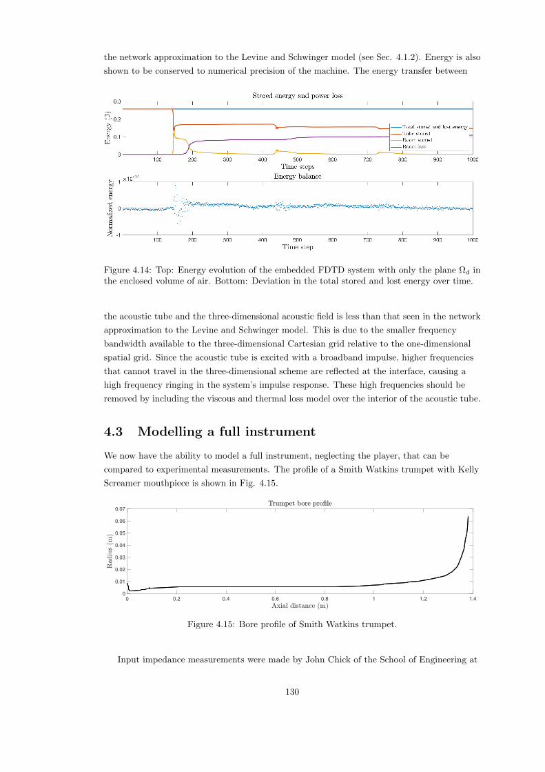
the network approximation to the Levine and Schwinger model (see Sec. 4.1.2). Energy is also

shown to be conserved to numerical precision of the machine. The energy transfer between

Figure 4.14: Top: Energy evolution of the embedded FDTD system with only the plane Ωd inthe enclosed volume of air. Bottom: Deviation in the total stored and lost energy over time.

the acoustic tube and the three-dimensional acoustic field is less than that seen in the network

approximation to the Levine and Schwinger model. This is due to the smaller frequency

bandwidth available to the three-dimensional Cartesian grid relative to the one-dimensional

spatial grid. Since the acoustic tube is excited with a broadband impulse, higher frequencies

that cannot travel in the three-dimensional scheme are reflected at the interface, causing a

high frequency ringing in the system’s impulse response. These high frequencies should be

removed by including the viscous and thermal loss model over the interior of the acoustic tube.

4.3 Modelling a full instrument

We now have the ability to model a full instrument, neglecting the player, that can be

compared to experimental measurements. The profile of a Smith Watkins trumpet with Kelly

Screamer mouthpiece is shown in Fig. 4.15.

0 0.2 0.4 0.6 0.8 1 1.2 1.4

0

0.01

0.02

0.03

0.04

0.05

0.06

0.07

Figure 4.15: Bore profile of Smith Watkins trumpet.

Input impedance measurements were made by John Chick of the School of Engineering at

130

the University of Edinburgh, and compared against simulations. The one-dimensional part of

the acoustic tube was simulated using (3.164) and (3.166), with a fourth order Foster

structure. Two cases were simulated. The first used the approximation to the Levine and

Schwinger radiation impedance presented in Sec. 4.1.3 to terminate the acoustic tube. The

second case used the embedded system from Sec. 4.2.11. The final 0.08 m of the instrument

bore, where ∂zS is reasonably large, was modelled using the three-dimensional wave equation,

with the majority of the instrument modelled using the same one-dimensional model [78]. In

the three-dimensional system, the walls of the instrument were described using a staircased

approximation and were modelled as rigid boundaries using discrete Neumann boundary

conditions. It should be noted, in general, that at typical audio rates, the staircased

approximation does not reasonably approximate a cylinder if the radius is too small, so care

must be taken when selecting the position at which the embedded system is connected.

Simulations3 were performed at 100 kHz for a duration of 1 s. Input impedances are

presented in Fig. 4.16, with corresponding peak position and magnitude errors of the

simulations shown in Fig. 4.17. Both models produce similar results at low frequencies.

Above the fifth resonance peak the response of the models changes, with the approximation to

the Levine and Schwinger radiation model producing peaks that are higher in frequency than

those measured. The position of the higher peaks of the embedded system remain close to

those measured experimentally, with an error less than 1 %, whereas the network radiation

model gives a larger error of around 2 %. This matches with the comparison between the

Levine and Schwinger model and the embedded system when applied to a cylinder; the

embedded system always produces peaks of a lower frequency.

0 200 400 600 800 1000 1200 1400 1600 1800 200010

5

106

107

108

109

Figure 4.16: Input impedances of the Smith Watkins trumpet with Kelly Screamer mouthpiece;measured (black), simulation terminated with network approximation to Levine and Schwingerradiation impedance (blue), simulation of embedded system (red).

At high frequencies, above the twelfth resonance, the sharpness of the peaks seen in the

experimental measurements reduces. This is also displayed in the embedded system but less

so in the network radiation impedance model. This is most likely due to the plane wave

approximation in the one-dimensional propagation model. In the embedded system, curved

3The mouthpiece for this instrument was particularly shallow, so a high spatial, and therefore temporal,resolution was required.

131

wavefronts are permitted in the three-dimensional part of the simulation. As the peaks of the

experimental input impedance and that calculated from the embedded system become less

defined at high frequencies, the network radiation model still displays sharp peaks. Although

the error in magnitude of the embedded system appears to be greater than that produced by

the network model, the overall behaviour of the system seems to match experiment better.

The run times over the temporal update loop for each simulation are:

• 5.70 s for the RLC termination model

• 1271.56 s for the embedded model

The embedded simulation takes over 200 times longer to perform the temporal update

compared to the lumped RLC model. Note that these times do not take in the additional

time required to construct the matrices that are used in the temporal update loop.

2 4 6 8 10 12 14

0

0.02

0.04

0.06

2 4 6 8 10 12 14

-0.2

0

0.2

0.4

Figure 4.17: Top: Fractional error in peak position of input impedance of simulations relativeto experimental measurement. Bottom: Fractional error in peak magnitude of impedanceimpedance of simulations relative to experiments. Error in simulation terminated with networkapproximation shown in blue, error in embedded system shown in red.

4.4 Conclusions

This chapter has focussed on the boundary condition at the far end of the acoustic tube that

radiates sound into the instrument’s environment. Two approaches to modelling this problem

have been presented. One uses a passive network approximation to the classic Levine and

Schwinger radiation model, the other directly simulates the three-dimensional acoustic field in

the flaring portion of the instrument, whilst the slowly varying part of the system is modelled

in one-dimension.

Both models have stable implementations, as shown through energy analysis of the

numerical schemes. The network model has the advantage of computational speed, requiring

little in terms of storage and computation. The high frequency behaviour of this model,

however, begins to diverge from experiments. It also does not give information about how

132

disturbances behave outside the instrument, requiring additional modelling to determine how

the performance space interacts with the instrument.

The embedded system is of a different character. The high frequency resonance behaviour

is more similar to that seen in experiments and it is possible to observe the sound field outside

of the instrument. The disadvantage is significantly longer computation times.

Higher order structures could be used to improve the accuracy of the network

approximation to the Levine and Schwinger radiation model. Alternatively, multiple

simulations of propagation in cylinders could be performed using the embedded system and

the radiation impedance can be extracted. The parameters of the network model could then

be optimised to best fit these radiation impedance models, combining the accuracy of the

embedded model with the efficiency of the network model.

133

Act II

Virtual Instrument

134

Chapter 5

Towards a complete instrument

“When scientists are asked what they are working on,

their response is seldom ‘Finding the origin of the

universe’ or ‘Seeking to cure cancer.’ Usually, they will

claim to be tackling a very specific problem - a small

piece of the jigsaw that builds up the big picture.”

— Martin Rees

The previous chapters of this work have focussed on the fundamental acoustics of the

resonator of a brass instrument. We now move on from a static resonator to an instrument

that a) is driven by a pressure source supplied by the user and b) whose resonances can be

manipulated over time by the user.

The excitation mechanism of an acoustic tube can be described as a reed, regardless of the

material it is constructed from. The instruments of the flute family, and certain organ pipes,

are excited by an air reed, whilst the rest of the wind instruments use a mechanical reed.

There are three main types of mechanical reed exciter [34, 63]: the single reed present in

clarinets and saxophones; the double reed present in oboes and bassoons; and the lip reed

employed by brass instruments. The lip reed shall be the focus of this work. The reed

mechanism excites the air column within the instrument, producing a note near one of the

instrument’s resonances. However, for a static bore profile this means there are several gaps in

the instrument’s range.

Woodwind instruments (and also some early brass instruments such as the Serpent) have

tone holes that modify the effective length of the instrument, thus allowing for additional

pitches to be produced by the instrument. As metal working techniques improved, alternative

methods to widen the pitch range of brass instruments were developed. Slides, seen in the

modern trombone, allowed the player to lengthen the instrument by extending a section of

cylindrical tubing. Another technique, which will be investigated in this work, uses valves to

divert air flow into a different piece of tubing on the instrument which either lengthens or

shortens the air column [35]. This is the most common feature in modern day brass

instruments, seen in trumpets, French horns and tubas, to name a few. As well as introducing

new notes to the instrument, partial depressing of the valves allows for multiple paths to be

present in the instrument that creates some new timbral possibilities.

In this chapter, we introduce the remaining components required for a playable instrument

which are used in the environment described in [75, 76]; the next chapter will introduce how

135

the instrument code is structured as well as how the user designs and controls the instrument.

The first section will introduce the lip model used to excite the instrument. This is an

active area of research, so many models of varying complexity are available. Here, we discuss

a simple outward striking reed model that creates suitable results. The model is presented in

the continuous time domain first and then discretised using FDTD methods, followed by a

discussion on energy analysis. The subsequent section describes how the instrument’s

resonances can be modified using a valve. This model, previously described in [22, 77], is

developed from continuity of pressure and volume velocity between three connecting pieces of

tubing and is shown to be passive in both the continuous and discrete time domains. The

lossless, static system is first discussed followed by the inclusion of boundary layer losses as

well as time-varying valve openings.

5.1 The lip reed model

The literature of wind instrument excitation mechanisms refers to the exciter as a pressure

controlled valve [63]. Since we shall later be discussing the valves that modify the length of

the air column, we shall not use this conflicting description, instead calling the exciter a reed.

Reed excitation mechanisms are primarily based on lumped masses. The simplest model

involves a single mass that is constrained to movement in one-dimension—a damped, simple

harmonic oscillator driven by the pressure difference over the lip. In some cases, such as the

clarinet reed, the mass of the oscillator can be neglected [149, 151], but work using the full

simple harmonic oscillator model can be seen, for example, in [20, 61, 86] in relation to single

reed instruments and [1, 17, 47, 142] for applications to brass instruments. Extensions to the

reed models include increasing the number of degrees of freedom of the individual mass [2]

and modelling the reed as a series of connected masses [139]. Distributed models have been

proposed where the reed is modelled as a one-dimensional bar [8]. Changes in the dynamics of

the reed upon closure can be included through increasing the reed stiffness [168] or developing

more complex models using penalty methods [28]. Many of these extensions have been applied

to the clarinet reed; here we shall focus on the lip reed.

As well as the dynamics of the independent reed, the interaction between the reed and the

instrument affects the overall output. Three classifications of reed exist, each with their own

oscillatory behaviour [63]. An inward striking reed closes as the pressure difference increases

slowly and plays below both the reed and instrument resonances. An outward striking reed

opens as the pressure increases and plays above the instrument and reed resonances. The

sliding door reed closes as the pressure difference is increased and plays below the instrument

and reed resonances. The single reed exciter of the clarinet can be classified as an inward

striking reed. The lip reed, when modelled using a single degree of freedom, varies between

the outward striking and sliding door models depending on the pitch of the note.

Although features of a lip reed, such as the transition between outward striking and sliding

door behaviour, require extra degrees of freedom for a full description, they also require

additional control parameters that the user must select. As we look towards creating a usable

musical instrument, we select the simplest model as our excitation mechanism.

136

5.1.1 A simple model

Here, we use the outward striking door model of the lip reed; see Fig. 5.1. This model is

similar to the clarinet reed model in [20] without the collisions.

pm p(t, 0)µr, Sr

∆pH0

y

Figure 5.1: Schematic of lip reed.

The dynamics of a reed exciter are described by

µrd2y

dt2+ µrσ

dy

dt+ µrω

20y = Sr∆p (5.1)

where y(t) is the displacement of the reed from equilibrium, σ is a damping parameter, ω0 is

the natural angular frequency of the reed, Sr and µr are the effective surface area and mass of

the lip and

∆p = pm − p(t, 0) (5.2)

is the pressure difference between the pressure in the mouth, pm, and the pressure in the

instrument mouthpiece, p(t, 0).

Additional expressions are required to couple the reed to the instrument. McIntyre et. al.

[113] coupled excitation mechanisms to instruments by convolving the instrument reflection

function with the flow that passes through the reed. This was later employed by Adachi and

Sato for a trumpet player model [1, 2], among others. Here, we also use the flow passing

through the reed to couple to the instrument but without the use of convolution, similar to

applications using DWGs [149, 151]. The two approaches can be considered to be doing the

same thing, but the method presented here can be considered as an IIR implementation,

whereas the convolution would require an infinitely long FIR implementation. The pressure

difference over the reed generates a volume velocity given by the Bernoulli equation

Ub = w[y +H0]+sign(∆p)

√2|∆p|ρ0

(5.3)

where w is an effective width of the reed, H0 is the static equilibrium separation, sign(·) is the

sign operator, and [·]+ = max(·, 0) which removes any flow when the lips are closed1. A

volume flow is also generated by the motion of the reed

Ur = Srdy

dt(5.4)

We assume volume velocity is conserved so the total volume of air injected into the

1It is interesting to note some conflict in the early literature on reeds where the experimental data showeddifferent power laws relating the volume flow to the area and pressure difference [9]

137

instrument from the player is

Sv|z=0 = Ub + Ur (5.5)


Multiplying (5.1) by the first derivative of y and rearranging gives

µrdy

dt

d2y

dt2+ µrσ

(dy

dt

)2

+ µrω20

dy

dty − dy

dtSr∆p = 0 (5.6)

Substituting (5.4) into this expression and using (5.5) gives

µrdy

dt

d2y

dt2+ µrσ

(dy

dt

)2

+ µrω20

dy

dty + (Ub − Sv|z=0) ∆p = 0 (5.7)

Using (5.2) gives

µrdy

dt

d2y

dt2+ µrσ

(dy

dt

)2

+ µrω20

dy

dty + Ub∆p− Sv|z=0(pm − p(t, 0)) = 0 (5.8)

Recalling that the power at the input of an acoustic tube is given by

B′he = −pSv|z=0 (5.9)

and neglecting any losses within the acoustic tube or additional boundary conditions gives

µrdy

dt

d2y

dt2+ µrσ

(dy

dt

)2

+ µrω20

dy

dty +

dHhedt− Sv|z=0pm + Ub∆p = 0 (5.10)

Using (2.4) and rearranging produces

d

dt(Hhe +Hreed) +Qreed + Preed = 0 (5.11)

where

Hreed =µr2

((dy

dt

)2

+ ω20y

2

)≥ 0 (5.12a)

Qreed = µr

(dy

dt

)2

+ w[y +H0]+

√2

ρ0|∆p|3/2 ≥ 0 (5.12b)

Preed = −(Ub + Ur)pm (5.12c)

The energy stored in the reed, Hreed, and the power dissipated, Qreed, are non-negative.

Energy is injected into the system by the player, shown in the term Preed, but there is loss due

to damping in the oscillator and due to the coupling between the reed and the instrument.

138


Discrete forms of (5.1)-(5.5) are [20]

µrδtty + µrσδt·y + µrω20µt·y = Sr∆p (5.13a)

∆p = pm − µt+p0 (5.13b)

Ub = w[y +H0]+sign (∆p)

√2|∆p|ρ0

(5.13c)

Ur = Srδt·y (5.13d)

µz−(S1/2v1/2

)= Ub + Ur (5.13e)

where yn+1/2, ∆pn+1/2, Un+1/2b , and U

n+1/2r are all sampled on the half integer temporal grid.

This superscript will be supressed and assumed to be n+ 1/2 unless otherwise stated for these

variables.

Energy analysis

Multiplying (5.13a) by δt·y and rearranging gives

µrδt·yδtty + µrσ (δt·y)2

+ µrω20δt·yµt·y − Srδt·y∆p = 0 (5.14)

Using (5.13d) and (5.13e) gives


+ µrω20δt·yµt·y +

(Ub − µz−

(S1/2v1/2

))∆p = 0 (5.15)

and using (5.13b) and (5.13c)


+ µrω20δt·yµt·y + Ub∆p− µz−

(S1/2v1/2

)(pm − µt+p0) = 0 (5.16)

Recalling that the discrete power transfer at the entrance of the acoustic tube is given by

b′he = −µt+p0µz−(S1/2v1/2

)(5.17)

gives


+ µrω20δt·yµt·y + Ub∆p− µz−

(S1/2v1/2

)pm + δt+hhe = 0 (5.18)

Using (3.26a) and (3.26e) gives

δt+ (hhe + hreed) + Qreed + preed = 0 (5.19)

where

hreed =µr2

((δt−y)

2+ ω2

0µt−(y2))≥ 0 (5.20a)

Qreed = µrσ (δt·y)2

+ w[y +H0]+

√2

ρ0|∆p|3/2 ≥ 0 (5.20b)

preed = − (Ub + Ur) pm (5.20c)

139

Again, the stored energy in the reed and power dissipation are non-negative.

Update for reed coupling

The update for the reed position is given by

yn+3/2 = αryn+1/2 + βry

n−1/2 + ξr∆pn+1/2 (5.21)

where

αr =4

2 + kσ + k2ω20

(5.22a)

βr =kσ − 2− k2ω2

0

2 + kσ + k2ω20

(5.22b)

ξr =2k2Sr

µr(2 + kσ + k2ω20)

(5.22c)

To get the pressure difference across the reed (5.13a)-(5.13e) need to be combined, along

with appropriate manipulations of the discrete operators. Using

δtt =2

k(δt· − δt−) , µt· = kδt· + wt− (5.23)

allows us to rewrite (5.13a) as

a1δt·y − a2∆p− an3 = 0 (5.24)

where

a1 =2

k+ σ + kω2

0 ≥ 0, a2 =Srµr≥ 0, an3 =

(2

kδt− − ω2

0wt−

)y (5.25)

Substituting (5.13d) followed by (5.13e) gives

a1

Sr

(µz−

(S1/2v1/2

)− Ub

)− a2∆p− an3 = 0 (5.26)

Recall that the lossless horn equation, (3.108), at l = 0 can be written as

S0

ρ0c20δt+p0 = − 2

h

(S1/2v1/2 − µz−

(S1/2v1/2

))(5.27)

Using δt+ = 2k (µt+ − 1) and using (5.13b) gives

µz−(S1/2v1/2

)= bn1 − b2∆p (5.28)

where

bn1 = S1/2v1/2 +hS0

ρ0c20k(pm − p0) , b2 =

hS0

ρ0c20k≥ 0 (5.29)

Using this expression in (5.26) and substituting (5.13c) gives

− cn1 sign (∆p) |∆p|1/2 − c2∆p+ cn3 = 0 (5.30)

where

cn1 = w[y +H0]+

√2

ρ0≥ 0, c2 = b2 +

Sra2

a1≥ 0, cn3 = bn1 −

Sran3

a1(5.31)

140

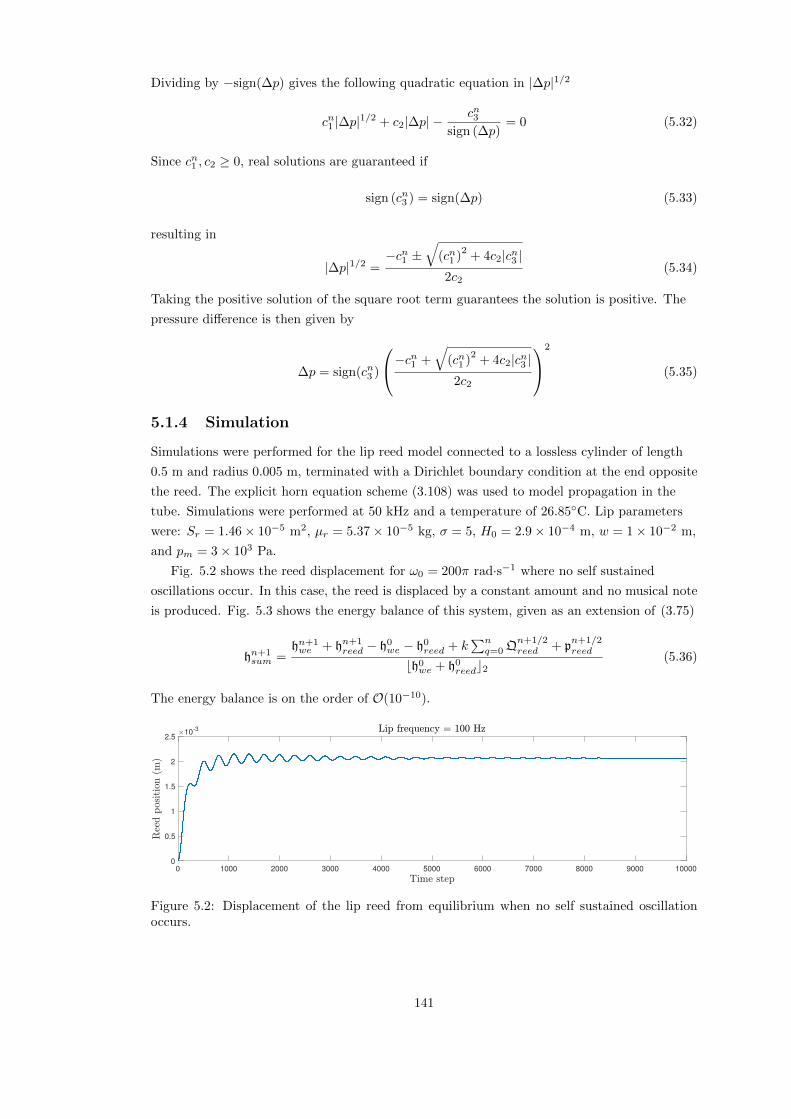
Dividing by −sign(∆p) gives the following quadratic equation in |∆p|1/2

cn1 |∆p|1/2 + c2|∆p| −cn3

sign (∆p)= 0 (5.32)

Since cn1 , c2 ≥ 0, real solutions are guaranteed if

sign (cn3 ) = sign(∆p) (5.33)

resulting in

|∆p|1/2 =−cn1 ±

√(cn1 )

2+ 4c2|cn3 |

2c2(5.34)

Taking the positive solution of the square root term guarantees the solution is positive. The

pressure difference is then given by

∆p = sign(cn3 )

−cn1 +√

(cn1 )2

+ 4c2|cn3 |2c2

2

(5.35)

5.1.4 Simulation

Simulations were performed for the lip reed model connected to a lossless cylinder of length

0.5 m and radius 0.005 m, terminated with a Dirichlet boundary condition at the end opposite

the reed. The explicit horn equation scheme (3.108) was used to model propagation in the

tube. Simulations were performed at 50 kHz and a temperature of 26.85C. Lip parameters

were: Sr = 1.46× 10−5 m2, µr = 5.37× 10−5 kg, σ = 5, H0 = 2.9× 10−4 m, w = 1× 10−2 m,

and pm = 3× 103 Pa.

Fig. 5.2 shows the reed displacement for ω0 = 200π rad·s−1 where no self sustained

oscillations occur. In this case, the reed is displaced by a constant amount and no musical note

is produced. Fig. 5.3 shows the energy balance of this system, given as an extension of (3.75)

hn+1sum =

hn+1we + hn+1

reed − h0we − h0

reed + k∑nq=0 Q

n+1/2reed + p

n+1/2reed

bh0we + h0

reedc2(5.36)

The energy balance is on the order of O(10−10).

0 1000 2000 3000 4000 5000 6000 7000 8000 9000 10000

0

0.5

1

1.5

2

2.510

-3

Figure 5.2: Displacement of the lip reed from equilibrium when no self sustained oscillationoccurs.

141

0 1000 2000 3000 4000 5000 6000 7000 8000 9000 10000

-20

-15

-10

-5

0

510

-10

Figure 5.3: Energy balance of the system when no oscillation occurs.

Fig. 5.4 shows the reed displacement for ω0 = 340π rad·s−1 where, after a transient stage,

self sustained oscillations occur. Fig. 5.5 shows the corresponding energy evolution of the

system; Fig. 5.6 shows the same plot but enlarged so as to see the variations in stored energy.

Most of the energy is dissipated by the coupling between the reed and the acoustic tube,

however, there is a clear periodic exchange of energy between the acoustic tube and the reed.

The energy balance is shown in Fig. 5.7 for this configuration. The variation in the

normalised energy balance is also on the order of 10−10.

Both examples presented here display variations in energy that are above machine

precision. This could be a result of rounding errors in the update scheme for the lip reed:

there are several orders of magnitude difference between the energy stored in the tube and the

reed. Torin [163] showed variations in the discrete energy of a simple harmonic oscillator were

caused by floating point rounding errors when dividing by terms in the FDTD scheme; similar

operations are seen in the lip coupling scheme. Such issues are interesting but are beyond the

scope of this work.

0 1000 2000 3000 4000 5000 6000 7000 8000 9000 10000

-2

-1

0

1

2

310

-3

Figure 5.4: Displacement of the lip reed from equilibrium in the case of self sustained oscillation.

5.2 Valves

As previously mentioned in the introduction to this chapter, the pitch of a note produced by a

brass instrument is determined by the coupling between the reed and the instrument’s

resonances. The lower resonances of an instrument are separated by large intervals, spanning

several musical notes, meaning that the instrument bore profile must be modified to fill in

142

1000 2000 3000 4000 5000 6000 7000 8000 9000 10000

-0.1

-0.05

0

0.05

0.1

Figure 5.5: Energy evolution of the system when self sustained oscillation occurs. Stored energyin the reed (blue) and tube (red), summed power dissipation in reed (orange) and summed powerinput at reed (purple).

1000 2000 3000 4000 5000 6000 7000 8000 9000 10000

-4

-2

0

2

4

6

810

-3

Figure 5.6: Energy evolution of the system when self sustained oscillation occurs. Stored energyin the reed (blue) and tube (red), summed power dissipation in reed (orange) and summed powerinput at reed (purple).

0 1000 2000 3000 4000 5000 6000 7000 8000 9000 10000

-0.5

0

0.5

1

1.5

2

2.510

-10

Figure 5.7: Energy balance for self sustained oscillating system.

these gaps. This can be done by changing the length of the air column. In woodwind

instruments, tone holes are used to disrupt the pressure field in the tube and change the

internal mode shapes. Trombones (and to some extent instruments with tuning slides) adjust

the length of the air column by extending a moveable slide to make the instrument longer.

Another method of lengthening the air column in a brass instrument is through the use of

valves that divert air into longer, or shorter, pieces of tubing.

Simple treatment of changing notes using DWG methods involves storing the individual

tube lengths corresponding to different pitches in separate delay lines [47]. However, this

143

approach does not allow for interactions between tube branches or include transient effects as

the system in modified with time. Kemp et. al. [98] presented a time-domain model of an

extending trombone slide that included doppler shift, although this was not used for sound

synthesis purposes. Models for a single tone hole were presented by Keefe [93] and Dubos et.

al. [50]; these have been extended to model the effect of several open tone holes in an

instrument in the frequency domain [100, 101, 128] and time domain [20]. Modelling of tone

holes has also been performed in three-dimensions by Giordano [68] and in two-dimensions by

Allen and Raghuvanshi [4]. The latter team also used their system to model valves, but did

not include interactions between the tubes that make up the valve system. Bilbao [22]

presented a model that does allow for this interaction and is presented here.

A simplified schematic of a brass instrument valve is shown in Fig. 5.8. Three pieces of

tubing are connected at a junction J : a main tube feeds into a default tube and a bypass

tube. The default tube is the path that airflow can take when the valve is left in the neutral

position; the bypass tube is the route air takes when the valve is depressed. This description

extracts the most important behaviour but neglects the additional complexity of the bore

profile in such valve sections.

S(m)v(m)

S(b)v(b)

S(d)v(d)

Main tube

Bypass tube

Default tube

J

Figure 5.8: Schematic of a brass instrument valve. Three pieces of tubing are combined at J .The pressure at the junction is the same in each piece of tubing and the total volume velocityflow over the junction is conserved.

It is useful to consider each piece of tubing in its own spatial domain. The superscripts

(m), (d), and (b) will refer to variables concerned with the main, default, and bypass tubes.

The main tube lies over the spatial interval Dm = z ∈ R | 0 ≤ z ≤ Lm, the default tube over

Dd = z ∈ R | 0 ≤ z ≤ Ld, and the bypass tube over Db = z ∈ R | 0 ≤ z ≤ Lb. The values

Lm, Ld, and Lb are the lengths of the respective pieces of tubing. The junction, J , is

positioned at z = Lm in Dm for the main tube and z = 0 in Dd and Db for the default and

bypass tubes.

At the junction, the pressure is the same in each tube

p(m)(t, Lm) = p(d)(t, 0) = p(b)(t, 0) = p(J)(t) (5.37)

Volume flow is also conserved across the junction so that

S(m)(Lm)v(m)(t, Lm) = S(d)(0)v(d)(t, 0) + S(b)(0)v(b)(t, 0) (5.38)

144

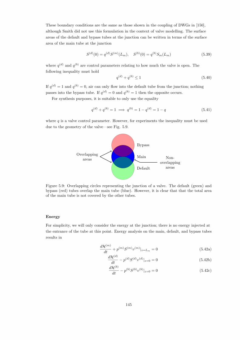
These boundary conditions are the same as those shown in the coupling of DWGs in [150],

although Smith did not use this formulation in the context of valve modelling. The surface

areas of the default and bypass tubes at the junction can be written in terms of the surface

area of the main tube at the junction

S(d)(0) = q(d)S(m)(Lm), S(b)(0) = q(b)Sm(Lm) (5.39)

where q(d) and q(b) are control parameters relating to how much the valve is open. The

following inequality must hold

q(d) + q(b) ≤ 1 (5.40)

If q(d) = 1 and q(b) = 0, air can only flow into the default tube from the junction; nothing

passes into the bypass tube. If q(d) = 0 and q(b) = 1 then the opposite occurs.

For synthesis purposes, it is suitable to only use the equality

q(d) + q(b) = 1 =⇒ q(b) = 1− q(d) = 1− q (5.41)

where q is a valve control parameter. However, for experiments the inequality must be used

due to the geometry of the valve—see Fig. 5.9.

Main

Bypass

Default

Overlappingareas Non-

overlappingareas

Figure 5.9: Overlapping circles representing the junction of a valve. The default (green) andbypass (red) tubes overlap the main tube (blue). However, it is clear that that the total areaof the main tube is not covered by the other tubes.

Energy

For simplicity, we will only consider the energy at the junction; there is no energy injected at

the entrance of the tube at this point. Energy analysis on the main, default, and bypass tubes

results in

dH(m)

dt+ p(m)S(m)v(m)|z=Lm = 0 (5.42a)

dH(d)

dt− p(d)S(d)v(d)|z=0 = 0 (5.42b)

dH(b)

dt− p(b)S(b)v(b)|z=0 = 0 (5.42c)

145

where

H(m) =1

2ρ0c20‖√S(m)p(m)‖2Dm +

ρ0

2‖√S(m)v(m)‖2Dm ≥ 0 (5.43a)

H(d) =1

2ρ0c20‖√S(d)p(d)‖2Dd +

ρ0

2‖√S(d)v(d)‖2Dd ≥ 0 (5.43b)

H(b) =1

2ρ0c20‖√S(b)p(b)‖2Db +

ρ0

2‖√S(b)v(b)‖2Db ≥ 0 (5.43c)

(5.43d)

and only the power transfer at the tube junction has been taken into account. Using the

pressure condition (5.37) gives

dH(m)

dt+ p(J)S(m)v(m)|z=Lm = 0 (5.44a)

dH(d)

dt− p(J)S(d)v(d)|z=0 = 0 (5.44b)

dH(b)

dt− p(J)S(b)v(b)|z=0 = 0 (5.44c)

Utilising conservation of volume velocity over the junction, (5.38), gives

dH(m)

dt+ p(J)

(S(d)v(d)|z=0 + S(m)v(m)|z=0

)= 0 (5.45)

Using (5.44b) and (5.44c) gives

d

dt

(H(m) +H(d) +H(b)

)= 0 (5.46)

It is clear that the expression H(m) +H(d) +H(b) is non-negative so coupling of the system in

this way results in bounded solutions.


We now discretise the spatial domains for each tube section. The pressure lies over the spatial

grids defined by: dm = l ∈ Z | 0 ≤ l ≤ Nm in the main tube, dd = l ∈ Z | 0 ≤ l ≤ Nd in

the default tube, and db = l ∈ Z | 0 ≤ l ≤ Nb in the bypass tube. The velocity lies over the

spatial grids defined by: dm = l ∈ Z | 0 ≤ l ≤ Nm − 1 in the main tube,

dd = l ∈ Z | 0 ≤ l ≤ Nd − 1 in the default tube, and db = l ∈ Z | 0 ≤ l ≤ Nb − 1 in the

bypass tube. The number of points in each tube are given, respectively, by

Nm = floor(Lm/hm), Nd = floor(Ld/hd), and Nb = floor(Lb/hb), where the spacings hm, hd,

and hb all satisfy the Courant condition but are not necessarily of equal lengths. Temporal

indices will be suppressed and are assumed to be at n for pressure variables and n+ 1/2 for

velocity variables, unless otherwise stated. The junction between the tubes lies at l = Nm in

dm in the main tube and l = 0 in dd and db for the default and bypass tubes.

The discrete forms of (5.37) - (5.39) are

p(m)Nm

= p(d)0 = p

(b)0 = p(J) (5.47a)

146

µz−SNm+1/2v(m)Nm+1/2 = µz−S

(d)1/2v

(d)1/2 + µz−S

(d)1/2v

(b)1/2 (5.47b)

S(d)0 = q(d)S

(m)Nm

, S(b)0 = q(b)S

(m)Nm

(5.47c)

The discrete energy in each of the tubes is given by

δt+h(m) + p

(m)Nm

µz−S(m)Nm+1/2v

(m)Nm+1/2 = 0 (5.48a)

δt+h(d) − p(d)

0 µz−S(d)1/2v

(d)1/2 = 0 (5.48b)

δt+h(b) − p(b)

0 µz−S(b)1/2v

(b)1/2 = 0 (5.48c)

where

h(m) =1

2ρ0c20

(‖√S(m)p(m)‖χ

)2

dm+ρ0

2〈S(m)v(m), wt−v

(m)〉dm ≥ 0 if λm ≥ 1 (5.49a)

h(d) =1

2ρ0c20

(‖√S(d)p(d)‖χ

)2

dd+ρ0

2〈S(d)v(d), wt−v

(d)〉dd ≥ 0 if λd ≥ 1 (5.49b)

h(b) =1

2ρ0c20

(‖√S(b)p(b)‖χ

)2

db+ρ0

2〈S(b)v(b), wt−v

(b)〉db ≥ 0 if λb ≥ 1 (5.49c)

Note that we only consider the energy at the junction and neglect any power changes at the

far ends.

Using (5.47a) and (5.47b) allows us to combine all of the energies so that

δt+

(h(m) + h(d) + h(b)

)= 0 (5.50)

The total energy of the system is non-negative, so solutions are bounded.

5.2.2 Update for coupling

We have shown that the specific discretisation of the coupling condition between tubes is

stable, we now look at how to actually implement this scheme. Consider lossless wave

propagation to begin with. We can write the pressure FDTD scheme of the horn equation,

(3.108), of each tube at the junction as

S(m)Nm

ρ0c20δt+p

(m)Nm

+2

hm

(µz−S

(m)Nm+1/2v

(m)Nm+1/2 − S

(m)Nm−1/2v

(m)Nm−1/2

)= 0 (5.51a)

S(d)0

ρ0c20δt+p

(d)0 +

2

hd

(S

(d)1/2v

(d)1/2 − µz−S

(d)1/2v

(d)1/2

)= 0 (5.51b)

S(b)0

ρ0c20δt+p

(b)0 +

2

hb

(S

(b)1/2v

(b)1/2 − µz−S

(b)1/2v

(b)1/2

)= 0 (5.51c)

It is clear that this form uses points outside of the domain of the tubes; see Fig. 5.10 for a

representation of this. The boundary conditions previously specified allow us to couple the

tubes. Using (5.47b) allows us to combine these equations, which, after rearranging, gives

hmS(m)Nm

2ρ0c20δt+p

(m)Nj

+hdS

(d)0

2ρ0c20δt+p

(d)0 +

hbS(b)0

2ρ0c20δt+p

(b)0 =S

(m)Nm−1/2v

(m)Nm−1/2 − S

(d)1/2v

(d)1/2

− S(b)1/2v

(b)1/2 (5.52)

147

· · ·l = Nm

n+ 1

n+ 1/2

n

n+ 1

n+ 1/2

n

n+ 1

n+ 1/2

n

l = 0

l = 0

Valvejunction

Main tube

Bypass tube

Default tube

Knownpressure

Unknownpressure

Knownvelocity

Velocityoutsidedomain

Figure 5.10: Schematic of the valve junction on the discrete grids. The pressure at the valvejunctions is the same in each tube. There are velocities outside the domain, but these can beremoved using continuity of volume velocity over the junction.

Rewriting this expression in terms of the pressure and main tube surface area at the junction

using (5.47a) and (5.47c) produces

(hm + hdq

(d) + hbq(b)) S

(m)Nm

2ρ0c20δt+p

(J) = S(m)Nm−1/2v

(m)Nm−1/2 − S

(d)1/2v

(d)1/2 − S

(b)1/2v

(b)1/2 (5.53)

Rearranging to give the value of p(J),n+1 gives

p(J),n+1 = p(J),n +2ρ0c

20k

S(m)Nm

(hm + hdq(d) + hbq(b)

) (S(m)Nm−1/2v

(m)Nm−1/2 − S

(d)1/2v

(d)1/2

−S(b)1/2v

(b)1/2

)(5.54)

5.2.3 Recombining tubes

In brass instruments the tubes in the valve sections must recombine to form a single air

column, see Fig. 5.11. We define the new variables in the recombined tube using the

superscript (m′) and go straight into application in the discrete domain. The pressure in this

new tube is defined over the discrete domain dm′ = l ∈ Z | 0 ≤ l ≤ Nm′, where

Nm′ = floor(Lm′/hm′), Lm′ is the length of the tube, and hm′ is the step size used in the new

domain. The velocity is defined over dm′ = l ∈ Z | 0 ≤ l ≤ Nm′ − 1. The new junction, J ′,

combines the default and bypass tubes at l = Nd in dd and l = Nb in db, respectively, to the

recombined tube at l = 0 in dm′ .

The boundary conditions concerning pressure and volume velocity, (5.47a) and (5.47b),

remain the same. However, implementation is modified since the side of the domain where the

unknown points changes, resulting in a change of sign for the volume velocities. The pressure

148

J J ′

Main tube Recombined tubeDefault

Bypass

Figure 5.11: Schematic of a tube system that splits into two and then recombines back intoone tube. Note that modelling of the bypass tube is done by assuming it is straight, its bentappearance in the figure is to show how the default and bypass tubes reconnect.

update at the recombining junction is given by

p(J′),n+1 = p(J′),n − 2ρ0c20k

S(m′)0

(hm′ + hdq(d) + hbq(b)

) (S(m′)1/2 v

(m′)1/2 − S

(d)Nd−1/2v

(d)Nd−1/2

−S(b)Nb−1/2v

(b)Nb−1/2

)(5.55)

Profile for default and bypass tubes

The cross-sectional area of the default and bypass tubes require modification at the tube ends

on both the pressure and velocity grids. We state examples for the default tube but the

discussion extends in the same way for the bypass tube.

On the pressure grid, (5.47c) holds for S(d) at l = 0 and l = Nd. This is also the case the

points on the particle velocity grid so that

S(d)1/2 = S

(d)0 , S

(d)Nd−1/2 = S

(d)Nd

(5.56)

The remainder of the bore profile on the velocity grid is then sampled directly from the bore.

The bore profile on the pressure grid is averaged from the neighbouring points on the velocity

grid; see Fig. 5.12.

S(d) S(d) S(d) S(d)

Figure 5.12: Profile of the default tube. Black dotted lines show the pressure spatial grid, greydotted lines show the particle velocity grid, solid black lines show the bore profile.

For a real instrument geometry there are extra complications that should be noted. For

typical audio sample rates, the length of the default tube section can only contain the

149

pressures at the junctions and one internal velocity field point. This results in a cylindrical

profile with area q(d)S(m). Due to the construction of the real instrument valve, the bypass

tube has a section at either end that is a similar geometry to the default tube. This part is

also cylindrical with areas that are scaled by the bypass tube opening but expand to the

actual tube diameter over the interior of the tube.

5.2.4 Junction coupling using lossy propagation

The same boundary conditions can be applied to joining tubes modelled with lossy

propagation. For example, the pressure update (3.164) that uses the Foster network

approximation becomes

p(J),n+1 =α(p)Nm

p(J),n + β(J),(p)(S

(d)1/2v

(d)1/2 + S

(b)1/2v

(b)1/2 − S

(m)Nm−1/2v

(m)Nm−1/2

)+ α

(p)0,Nm

p(J),n0 +

M∑q=1

α(p)q,Nm

p′(J),nq (5.57)

where only the volume velocity constant is modified

β(J),(p) = − ρ0c20k

S(J)(hm + q(d)hd + q(b)hb

) (1 + ElGl

) (5.58)

The updates of the network variables, p(J)0 and p

′(J)q , at the junction remain the same as

those defined in Chap. 3. At first it seems counter-intuitive that the inclusion of a branching

tube to the visctherm model only requires modification of one term. However, for the Zwikker

and Kosten model the attenuation processes are essentially local and would not be modified

by neighbouring points.


Simulations were performed for the lossless system with tube lengths of Lm = 1.3 m,

Ld = 0.016 m, Lb = 0.2 m, and Lm′ = 1 m. The radii of each tube were 0.05 m. Simulations

were performed at a sample rate of 50 kHz and for a duration of 10 s.

Fig. 5.13 shows the energy evolution of the lossless valve system when q(d) = 0.5. Energy

is transferred from one tube to the next as the wave propagates along the tube system and

energy is conserved to numerical precision of the machine.

Fig. 5.14 shows simulation results for the lossy system2 using the Foster loss model with

M = 4. Input impedances were calculated for different values of q(d) using the procedure

described in Sec. 3.4.3. The equality q(b) = 1− q(d) was used to set the bypass tube opening.

There is a reduction in the frequency of the input impedance peaks as q(d) reduces. For

partially open configurations the input impedance peaks lie between the fully open and fully

closed configurations and are unevenly spaced. Comparing to the fully open or fully closed

configurations, the partially open systems appear to add some additional resonances either by

introducing a new impedance peak, shown by the peak around 700 Hz, or by splitting the

impedance peaks, such as those below 900 Hz. Modifying the valve opening changes the

magnitude and position of these peaks, although the effect is more noticeable above 600 Hz.

2The results for the lossless system are similar to those presented here. However, using the lossy model givesa clearer indication on the effect of partial valve openings on the input impedance.

150

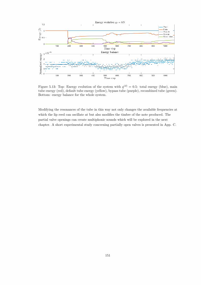
Figure 5.13: Top: Energy evolution of the system with q(d) = 0.5: total energy (blue), maintube energy (red), default tube energy (yellow), bypass tube (purple), recombined tube (green).Bottom: energy balance for the whole system.

Modifying the resonances of the tube in this way not only changes the available frequencies at

which the lip reed can oscillate at but also modifies the timbre of the note produced. The

partial valve openings can create multiphonic sounds which will be explored in the next

chapter. A short experimental study concerning partially open valves is presented in App. C.

151

0 100 200 300 400 500 600 700 800 900 100010

2

103

104

105

106

107

0 100 200 300 400 500 600 700 800 900 100010

2

103

104

105

106

107

0 100 200 300 400 500 600 700 800 900 100010

2

103

104

105

106

107

0 100 200 300 400 500 600 700 800 900 100010

2

103

104

105

106

107

0 100 200 300 400 500 600 700 800 900 100010

2

103

104

105

106

107

Figure 5.14: Input impedance calculations for the lossy valved tube system for different openingconfigurations. Top to bottom: Decreasing value of q(d) from 1 to 0 in increments of 0.25.

152

5.2.6 Time varying valves

We now look to the action of dynamic valves whose openings vary with time. We return to

the single acoustic tube that lies over D, whose cross-sectional area, S(t, z), now varies with

time. A suitable model taken from the literature on vocal tract modelling [134] is

1

ρ0c20∂t (Sp) + ∂tS + ∂z (Sv) = 0, ρ0∂tv + ∂zp = 0 (5.59)

which reduces to the normal horn equation, (2.49), when the cross-sectional area is constant

over time. Taking the inner product of the first of (5.59) with p over the domain D gives

1

ρ0c20〈p, ∂t (Sp)〉D + 〈p, ∂tS〉D + 〈p, ∂z (Sv)〉D = 0 (5.60)

Employing integration by parts (2.3) and using the second of (5.59) gives

1

ρ0c20〈p, ∂t (Sp)〉D + 〈p, ∂tS〉D + ρ0〈∂tv, Sv〉D + Bhe = 0 (5.61)

where Bhe is the same boundary term that is present for the static horn equation. This is

important as it means that the same boundary conditions discussed in the previous sections

can be applied when joining tubes together in valves.

We know that this system reduces to the horn equation when there is no time variation in

the surface area so we should expect terms ∂t‖√Sp‖2D and ∂t‖

√Sv‖2D to appear; this makes

the derivations slightly easier if we already know what form to expect. Expanding these

expressions for the time varying surface area case gives

∂t‖√Sv‖2D = 〈∂tS, v2〉D + 2〈Sv, ∂tv〉D (5.62a)

∂t‖√Sp‖2D = 〈∂tS, p2〉D + 2〈Sp, ∂tp〉D

= 〈∂tS, p2〉D + 2〈p, ∂t(Sp)− p∂tS〉D= 2〈p, ∂t (Sp)〉D − 〈∂tS, p2〉D (5.62b)

Substituting these back into our main energy expression gives

dHhedt

+ Pmov + Bhe = 0 (5.63)

where Hhe is the normal expression for energy stored in the acoustic tube but now with time

varying S(t)

Hhe =1

2ρ0c20‖√Sp‖2D +

ρ0

2‖√Sv‖2D (5.64)

and

Pmov = 〈∂tS, p〉D +1

2ρ0c20〈∂tS, p2〉D −

ρ0

2〈∂tS, v2〉D (5.65)

Discrete implementation

A discrete form of (5.59) is

1

ρ0c20δt+(Sp)

+ δt+S + δz− (Sv) = 0, ρ0δt−v + δz+p = 0 (5.66)

153

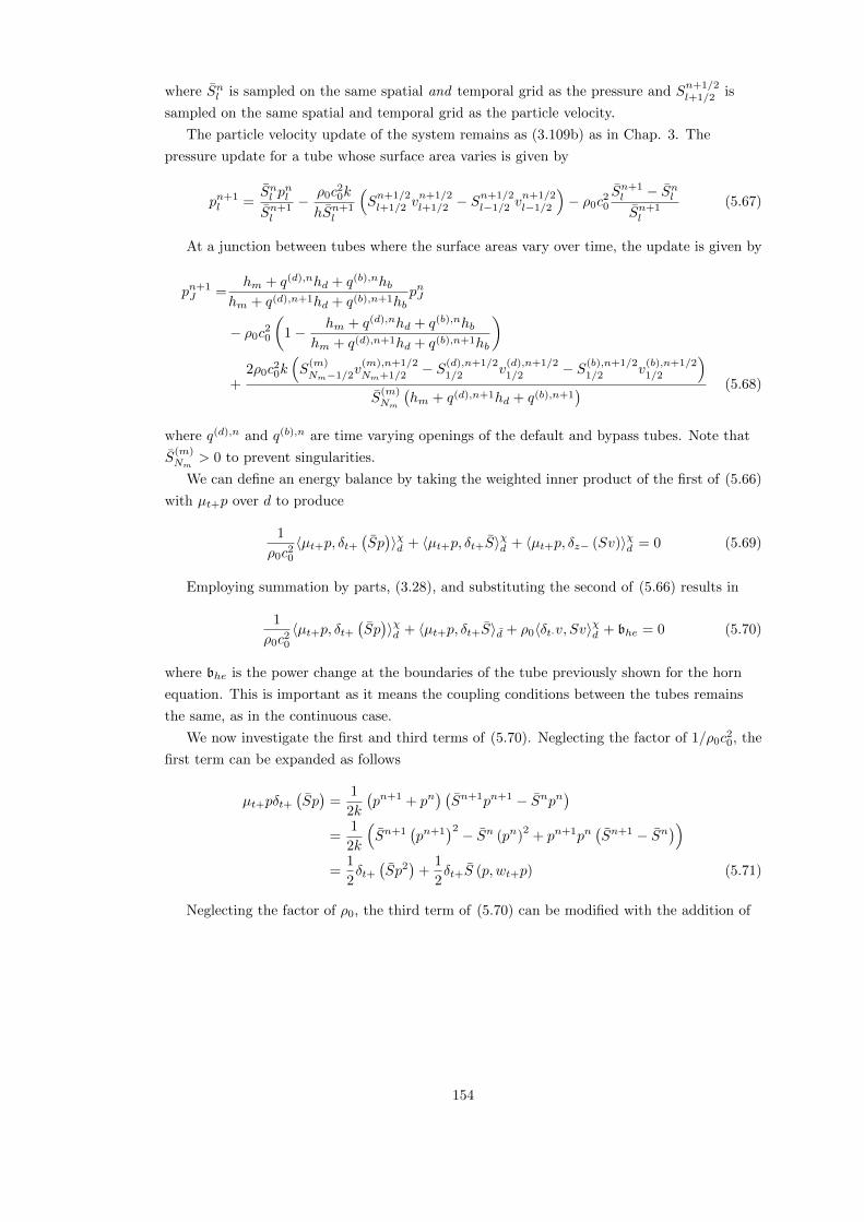
where Snl is sampled on the same spatial and temporal grid as the pressure and Sn+1/2l+1/2 is

sampled on the same spatial and temporal grid as the particle velocity.

The particle velocity update of the system remains as (3.109b) as in Chap. 3. The

pressure update for a tube whose surface area varies is given by

pn+1l =

Snl pnl

Sn+1l

− ρ0c20k

hSn+1l

(Sn+1/2l+1/2 v

n+1/2l+1/2 − S

n+1/2l−1/2 v

n+1/2l−1/2

)− ρ0c

20

Sn+1l − SnlSn+1l

(5.67)

At a junction between tubes where the surface areas vary over time, the update is given by

pn+1J =

hm + q(d),nhd + q(b),nhbhm + q(d),n+1hd + q(b),n+1hb

pnJ

− ρ0c20

(1− hm + q(d),nhd + q(b),nhb

hm + q(d),n+1hd + q(b),n+1hb

)

+2ρ0c

20k(S

(m)Nm−1/2v

(m),n+1/2Nm+1/2 − S(d),n+1/2

1/2 v(d),n+1/21/2 − S(b),n+1/2

1/2 v(b),n+1/21/2

)S

(m)Nm

(hm + q(d),n+1hd + q(b),n+1

) (5.68)

where q(d),n and q(b),n are time varying openings of the default and bypass tubes. Note that

S(m)Nm

> 0 to prevent singularities.

We can define an energy balance by taking the weighted inner product of the first of (5.66)

with µt+p over d to produce

1

ρ0c20〈µt+p, δt+

(Sp)〉χd + 〈µt+p, δt+S〉χd + 〈µt+p, δz− (Sv)〉χd = 0 (5.69)

Employing summation by parts, (3.28), and substituting the second of (5.66) results in

1

ρ0c20〈µt+p, δt+

(Sp)〉χd + 〈µt+p, δt+S〉d + ρ0〈δt·v, Sv〉χd + bhe = 0 (5.70)

where bhe is the power change at the boundaries of the tube previously shown for the horn

equation. This is important as it means the coupling conditions between the tubes remains

the same, as in the continuous case.

We now investigate the first and third terms of (5.70). Neglecting the factor of 1/ρ0c20, the

first term can be expanded as follows

µt+pδt+(Sp)

=1

2k

(pn+1 + pn

) (Sn+1pn+1 − Snpn

)=

1

2k

(Sn+1

(pn+1

)2 − Sn (pn)2

+ pn+1pn(Sn+1 − Sn

))=

1

2δt+(Sp2

)+

1

2δt+S (p, wt+p) (5.71)

Neglecting the factor of ρ0, the third term of (5.70) can be modified with the addition of

154

zero

δt·vSv =Sn+1/2

2k

(vn+3/2vn+1/2 − vn+1/2vn−1/2

)±S

n−1/2

2kvn+1/2vn−1/2︸︷︷︸+0

=1

2k

(vn+3/2Sn+1/2vn+1/2 − vn+1/2Sn−1/2vn−1/2 + vn+1/2vn−1/2

(−Sn+1/2 + Sn−1/2

))=

1

2δt+ (vwt− (Sv))− 1

2δt−Svwt−v (5.72)

Using these expressions in our energy derivation results in

δt+hhe + pmov + bhe = 0 (5.73)

where hhe is the normal expression for the energy stored in the horn equation but with time

varying S and S

hnwe =1

2ρ0c20

(‖√Snpn‖χd

)2

+ρ0

2〈vn+1/2, wt−

(Sn+1/2vn+1/2

)〉d (5.74)

and

pmov = 〈δt+S, µt+p〉χd +1

2ρ0c20〈δt+S, pwt+p〉χd −

ρ0

2〈δt−S, vwt−v〉d (5.75)

We choose to use

λ ≤ 1 (5.76)

and

Snl = µz−Sn+1/2l+1/2 (5.77)

Although we can define an energy balance, which is useful as a debugging tool, determining

stability of this numerical scheme is still an open problem.

Simulation results

Fig. 5.15 shows the energy for the moving valve system with q(d) linearly changing from 1 to 0

over 0.1 s, this time with no volume velocity injected into the instrument. It is clear that

moving the valves injects energy into the system—the motion of the valve acts as a volume

velocity source. However, the energy balance of the system is shown to be conserved.

155

100 200 300 400 500 600 700 800 900 1000

-5

0

5

100 200 300 400 500 600 700 800 900 1000

-2

0

2

410

-15

Figure 5.15: Top: Energy evolution of the valved system with time varying openings. Bottom:Energy balance of the system.

5.3 Conclusions

This chapter has presented the additional models required to make a virtual brass instrument.

A lumped one degree of freedom reed model with outward striking behaviour is chosen as

the excitation mechanism for the virtual instrument. This model allows for a relatively small

parameter space to produce sounds, whilst maintaining complex coupling behaviour with an

acoustic tube. A numerical update is presented for this model along with discrete energy

analysis. Simulations are performed that give examples of when the model produces, and also

does not produce, self sustained oscillations. The numerical energy appears to vary above

machine precision, but this could be a result of rounding errors previously discussed by Torin

[163].

Whilst this simple lip reed model restricts the ability to shift whether the instrument plays

above or below the instrument resonance, the motion of the reed is still, essentially, sinusoidal.

The majority of harmonic generation occurs through the Bernoulli equation, given in (5.3). In

terms of the resulting sound, adding additional degrees of freedom will not have much of a

perceptible impact on the resulting sound, and will only add to overload the user with

additional parameters.

Introducing valves allows for the resonances of the tube to be modified. A static model for

a branching and recombining tube is presented with and without viscothermal losses.

Boundary conditions that couple the sections of the valve together are derived from

conservation of numerical energy, and the schemes are shown to be passive. Examples of input

impedances for partially open valve configurations are then presented. The additional paths

introduce resonances to the system which modify the timbre of the produced sound. The valve

model is then extended to the case of time-varying valves. A numerical update and energy

balance is presented, although the determination of stability is left as an open problem.

156

Chapter 6

A brass instrument synthesis

environment

“I dream of instruments obedient to my thought and

which with their contribution of a whole new world of

unsuspected sounds, will lend themselves to the

exigencies of my inner rhythm.”

— Edgard Varese

We now have the individual components required to model a brass instrument: a

generator, the lip reed; a variable resonator, the acoustic tube with time-varying valve

sections; and a radiator, the radiation model. The next step is to forge these elements

together to create a virtual instrument and determine how such an instrument is controlled;

this is the subject of this chapter.

In this work brass instrument synthesis is performed using FDTD methods although

several other approaches have been used historically to create virtual brass instruments. DWG

methods were employed by Cook [47] in the ‘TBone’ workbench and were later implemented

in the Yamaha VL1 synthesiser [144]. Modal methods were used in the MoReeSC framework

[148], although this is intended for musical acoustics research rather than as a composer’s

tool. A convolution modelling method was used in the BRASS project [170], which also

included some nonlinear propagation effects. Allen and Raghuvanshi [4] used FDTD methods

in a two-dimensional wave simulator to produce woodwind and brass instrument sounds, but

they did not present any results for partially open valve configurations.

In this chapter, the structure of the synthesis code is presented. This is followed by a

detailed discussion of the input files used to control the instrument along with examples of

gestures that can be produced with the environment. A short playability study concludes the

chapter. The synthesis environment described here has previously been discussed in [76], with

details of the algorithm and code optimisation procedures in [75].

6.1 Structure of code

The synthesis environment was developed in MATLAB by the author and then optimised by

James Perry of Edinburgh Parallel Computing Centre at the University of Edinburgh. The

157

original version used the loss model of Bilbao and Chick along with the RLC radiation

impedance [24]. However, the discussion here will be general enough to apply to all of the

models presented in this thesis. The general structure of the code is similar to that of Torin

[163]; see Fig. 6.1 for a flow chart of this.

Instrument File Score File

System parameters Control streams

Instrument geometry

Finite difference matrices

Initialisation

Main loop

Sounds

User input

Precomputation

Computation

Output

Figure 6.1: Structure of the brass instrument synthesis environment. Users specify instrumentand score files (in blue rectangle) that are inputs to the code. These input files are then used inthe precomputation stage (green rectangle) to calculate system parameters and control streamsused in the main loop (red rectangle) where the system variables (acoustic pressure, particlevelocity, lip position) are computed. The output (purple rectangle) is generated as a WAV filefrom the pressure at the end of the instrument.

6.1.1 Input files

The synthesis environment is controlled through separate instrument and score files described

in detail in Sec. 6.2. The instrument file defines the instrument bore either from

measurements of a real instrument or through a parameterised description of a synthetic bore.

The score file indicates how the instrument is played by giving time varying parameters that

control the lip dynamics and valve openings.

6.1.2 Precomputation

After selection of the input files, the brass environment precomputes the necessary matrices

used in the main loop. This can be separated into several sections.

System parameters

Temporal step size is calculated from the sample rate. Thermodynamic constants are

computed from a user selected temperature. Temporal step size and speed of sound are used

158

to compute a minimum spatial step size that satisfies the Courant condition. The spatial step

size is modified so that an integer number of points define the tubes of the instrument.

Control streams

The control parameters, e.g. lip frequencies and valve openings, are given as break point

functions in the score files (see Sec. 6.2). Interpolation is therefore required to sample these

control parameters on the discrete temporal grid. Modulation of the control streams, if

specified by the user, is applied here. The valve opening control stream is examined at this

point to restrict values between 0 and 1. If the valve openings lie outside this range they are

forced to the nearest limit.

Instrument geometry

If the custom instrument function is selected, the bore profile must be generated at this stage.

For a valved instrument, there are multiple pieces of tubing that make up the entire

instrument each requiring, in general, a distinct spatial step size for correct representation of

the tube length. Using these spatial step sizes, discrete axial distance vectors can be

constructed that the instrument bore is sampled on.

Finite-difference matrices

Matrices are constructed that approximate the operators in the PDE system and include

effects due to boundary conditions and the shape of the instrument bore. These are used in

the temporal loop.

Initialisation

The variables of the system are assigned memory prior to the start of the main temporal loop.

Variables associated to propagation are stored in vectors of length equal to the discrete

number of points in that domain. Boundary condition terms (lip position and network

variables of the radiation model) are stored as single variables, one for each time step required

in the individual update expressions.

6.1.3 Main loop

A temporal loop is performed to evolve the state variables at each time step. First, the

pressure difference between the mouth and the instrument mouthpiece is computed. This is

used to update the lip position and and the pressure in the instrument mouthpiece. The

pressure along the instrument bore is then updated, either by a loop over the spatial index or

by matrix multiplication1. The pressure at the radiating end of the instrument is computed

and the network variables updated. Finally the particle velocity is updated along the length

of the instrument. This process is repeated for the appropriate number of time steps.

1In this work, software generated from the C programming language used a loop implementation. MATLABallows both loop and matrix implementation, and is optimised for the latter.

159

6.1.4 Output sounds

For sound generation, the output signal is taken as the pressure at the end of the instrument,

where the radiation model is applied. The output is normalised by the maximum absolute

value of the time series, to avoid any distortion from clipping during playback, and saved as a

WAV format file.

6.2 Control of instrument

We now look to how the virtual brass instrument can be controlled through the use of the

input files. Users can describe the geometry of the instrument, through the use of the

instrument file, and how the instrument is played, though the score file.

6.2.1 The instrument file

The instrument file allows the user to define the instrument geometry along with the sample

rate the simulations are performed at and the temperature which defines the thermodynamic

constants. Users can either input the profile of a real instrument using position-diameter pairs,

or set the parameters that are used to create a custom instrument, discussed below. Positions

of the valves are specified along with corresponding lengths of the default and bypass tubes.

Custom instrument function

The custom instrument function allows the user to design an instrument through

parametrisation of the bore profile. The instrument as a whole can be split into three main

sections: the mouthpiece, the central bore, and a flaring section. The mouthpiece is defined

using half a period of a cosine function where the user specifies the length and diameter at the

two ends of the mouthpiece. The bell is defined using a power of the axial distance; the user

sets this power along with the final tube diameter. The central section of the instrument is

defined by a series of concatenated tubes with differing profile set by the user. The choice of

profiles is: cylindrical, conical, cosinusoidal ramp (similar to mouthpiece definition), and a

sinusoidal bulge. Users specify the length of these sections along with the diameter of the end

points. Fig. 6.2 shows three types of profiles in this middle section but in practice users can

set as many as required, provided the length of all the sections fits the full length of the

instrument.

(a) (b) (c) (d) (e)

Figure 6.2: Example of an instrument constructed using the custom instrument function. Sec-tion (a) is the mouthpiece defined using a cosine, (b) a cylindrical segment, (c) is a bulge definedusing the square of a sinusoid, (d) a converging conical section, and (e) is the flaring sectiondefined using a power of the axial position.

160

6.2.2 The score file

The score file determines the overall duration of the simulation along with the time varying

parameters used in the control of the instrument. The time varying parameters include the lip

parameters (surface area, mass, damping, equilibrium separation, width, oscillation

frequency), mouth pressure, and valve openings. Tab. 6.1 shows some example ranges of these

control parameters to produce sound for a trumpet, found through a process of trial and

error. The control parameters are given as time-value pairs that define a breakpoint function.

Valve parameters specify the valve openings at each time instance.

Score parameter Typical values for trumpet simulationsLength of simulation [s] ≥ 1Effective lip area [m2] 1.46× 10−5

Effective lip mass [kg] 5.37× 10−5

Lip damping 5Lip equilibrium position [m] 2.9× 10−4

Effective lip width [m] 10−2

Lip frequency [Hz] 400− 1000Mouth pressure [Pa] 2.5× 103 − 5.0× 103

Vibrato amplitude 0− 0.05Vibrato frequency [Hz] 0− 7Tremolo amplitude 0− 0.2Tremolo frequency [Hz] 0− 7Noise amplitude 0− 0.05Valve opening 0− 1Valve modulation frequency [Hz] 0− 5Valve modulation amplitude 0− 0.5

Table 6.1: Parameters and typical values used in score file that plays a trumpet.

Modulation functions are also available for lip frequency, mouth pressure and valve

openings.

Vibrato (lip frequency modulation) and tremolo (mouth pressure modulation)2 are

controlled by specifying an amplitude and rate of the modulation so that

fnlip :→ fnlip (1 +Anv sin(2πfnv nk)) , pnm :→ pnm (1 +Ant sin(2πfnt nk)) (6.1)

where Anv and Ant are the amplitudes of the vibrato and tremolo, given as fractions of the

static values, and fnv and fnt are the respective modulation frequencies. Noise can be added to

the mouth pressure using

pnm :→ pnm (1 +Annoiseθn) (6.2)

where Annoise is the amplitude of the noise signal given as a fraction of the mouth pressure and

θn generates a time series of numbers randomly generated between −1 and 1.

Valve modulation is performed in a different manner—if the valve opening is set to zero,

no modulation would occur using the modulation procedure for vibrato and tremolo. Instead,

2Here, tremolo denotes a loudness modulation rather than the performance direction to play a series ofunmetered, repeating notes.

161

valve modulation is performed by using

q(d),n :→ q(d),n +Anvalve sin (2πfnvalvenk) (6.3)

where fnvalve is the valve modulation frequency and Anvalve is the modulation amplitude given

in terms of an actual valve opening.

All of the control parameters in the score files can be varied in time. However, in practice

the lip area, mass, damping, equilibrium position and width remain constant.

6.2.3 Sound examples

We now give some examples of what types of gestures can be performed using the brass

instrument synthesis tool. The instrument file was generated from measurements of a Smith

Watkins trumpet provided by Dr. John Chick of the School of Engineering at the University

of Edinburgh. Valves are positioned at 0.6 m, 0.63 m, and 0.69 m. Default tubes are all of

length 0.02 m and bypass tubes are all of length 0.2 m.

Simulations were performed at a sample rate of 50 kHz. Lip parameters (area, mass,

damping, equilibrium position, and width) are set to those in Tab. 6.1. Unless otherwise

stated, the following parameter choice was used:

• A constant natural lip frequency of 550 Hz

• Pressure in the mouth increased from 0 Pa to 5× 103 Pa over 10−4 s.

• Valves are assumed to be open, so the air column does not pass into the bypass tubes.

• No modulation of control parameters.

Peaks in spectrogram plots have been clipped to aid in viewing frequencies that are present in

the sound. Yellow colours in the spectrogram denote regions where frequency content is

strong, blue regions show where it is weak.

Simple gestures

Simple gestures can be performed by modifying the lip frequency to change note pitch or

changing the mouth pressure to articulate notes. A linear sweep in lip frequency allows for an

assessment of which lip frequencies produce notes when the instrument is in a static

configuration. Fig. 6.3 shows the results of a simulation where the lip frequency begins at 220

Hz and linearly increases up to 1000 Hz over a duration of 3 s.

162

Figure 6.3: Top: Spectrogram of output sound when the lip frequency linearly changes from220 Hz to 1000 Hz over 3 s. Bottom: The lip frequency as a function of time.

As the lip frequency increases, there is a gradual increase in the frequency of the

spectrogram peaks of the produced sound. The spectrogram shows regions where the lips

destabilise and then couple to a different instrument resonance; see just after 0.5 s, 1 s and 1.5

s. It should be noted that due to the nonlinear coupling between the reed and the instrument

the lip frequency does not equal the fundamental frequency of the produced sound.

Separate notes can be produced through control of the mouth pressure. Fig. 6.4 shows an

example where separate notes have been produced by linearly decreasing the end of the note

from 5× 103 Pa to 0 Pa over 0.1 s. Decreasing the mouth pressure stops the lips from being

driven, which in turn stops the instrument producing sound.

0 0.2 0.4 0.6 0.8 1 1.2 1.4 1.6 1.8 2

-0.5

0

0.5

0 0.2 0.4 0.6 0.8 1 1.2 1.4 1.6 1.8 2

0

2000

4000

Figure 6.4: Top: Time series of output when two separate notes are played. Bottom: Corre-sponding mouth pressure as a function of time.

163

Modulating parameters

Fig. 6.5 shows results from a simulation where a vibrato of amplitude 0.05 and frequency of 7

Hz is applied to the lip frequency after 1 s. The peaks of the spectrogram of the output show

modulation when vibrato is added to the note.

Figure 6.5: Top: Spectrogram of output sound when vibrato is added to the note after 1 s.Bottom: Lip frequency as a function of time. Lip frequency is constant for first second thenmodulation is added.

Fig. 6.6 shows simulation results where a tremolo of amplitude 0.2 and frequency of 7 Hz

is applied to the mouth pressure after 1 s, with corresponding variations in the note’s loudness

shown in the output sound.

0 0.2 0.4 0.6 0.8 1 1.2 1.4 1.6 1.8 2

-0.5

0

0.5

0 0.2 0.4 0.6 0.8 1 1.2 1.4 1.6 1.8 2

0

2000

4000

6000

Figure 6.6: Top: Time series of output sound when tremolo is added. Bottom: Mouth pressureas a function of time. After the initial increase, the mouth pressure remains constant for thefirst second, after which the tremolo is added.

Fig. 6.7 shows the effect of adding noise of amplitude 0.05 to the mouth pressure after 1 s.

An increase in non-harmonic frequency content is displayed in the spectrogram once noise is

added.

164

Figure 6.7: Top: Spectrogram of output sound when noise is added after 1 s. Bottom: Corre-sponding mouth pressure signal, with noise added after 1 s.

These specific examples lie to the more extreme effects of modulation. Simple treatment of

these modulating parameters can result in ‘synthetic’ sounds as patterns in the sound are

regularly repeated. This is not necessarily a negative result as users may wish to produce

these types of sound. However, if the intended result requires something more ‘realistic’, then

small variations must be carried out to make the sound constantly evolve. It is easier to do

this with the modulating functions than to type out the individual lip frequency and pressure

breakpoint functions.

Valve effects

Valves can be opened and closed over time to modify the resonances of the instrument. Fig.

6.8 shows the effect of changing the valve openings over time by closing sucessive valves at 2 s

intervals whilst varying the lip frequency from 300 Hz to 700 Hz. Each time a valve is

depressed, an additional piece of tubing is added to the air column that lowers the resonances

of the instrument. This changes the available frequencies at which the lips couple to the

instrument.

Figure 6.8: Spectrogram of output for repeated lip frequency sweeps from 300 Hz to 700 Hzover 2 s whilst changing valve configurations. At 2 s intervals, the next valve is depressed. Thiscorresponds to a reduction in the lowest peak frequency shown in the spectrogram.

165

Setting the valves in a partially open configuration allows for the production of notes with

a multiphonic timbre. Fig. 6.9 shows a comparison of the spectrum of a simulated note played

using a fixed lip frequency and a) with all valves open and b) by using the partially open

configuration of: q(d) = 0.7 for the first valve, q(d) = 0.5 for the second valve, and q(d) = 0.2

for the third valve.

It is clear from the spectrum plot that the frequency content of the sound is modified

when partial valve configurations are used. As the instrument resonances are different for the

two valve configurations, the frequencies at which the lip oscillates at are different, despite

using the same natural frequency. The magnitude of the spectrum is different for the two

configurations, particularly between 2000 Hz and 2500 Hz where the partially open

configuration has a lower value. This corresponds to the slightly muted characteristic of the

sound produced in the partially open configuration, where there is a low presence of high

frequency content.

0 500 1000 1500 2000 2500 300010

-2

100

102

104

106

Figure 6.9: Spectrum of sounds produced with valves in open configuration (blue) and partiallyopen configuration (red).

Valves can also be modulated over time. Fig. 6.10 shows the result of applying a

modulation to the first valve of amplitude 0.25 and frequency 5 Hz, where all valve openings

are set to a value of q(d) = 0.5. As the valve is modulated, small variations in the frequency of

the peaks of the spectrogram of the sound are observed.

6.2.4 Playability space

We have shown some of the capabilities of the brass instrument environment as a useable

instrument. It is worth highlighting some issues to do with playability here.

A simple playability test can be performed by examining combinations of lip frequency

and mouth pressure that produce a sustained note from the instrument, whilst keeping the

other parameters in the score file constant. The space investigated consisted of lip frequencies

between 50 Hz and 1 kHz, spaced at 10 Hz intervals, and mouth pressures between 2.5 kPa

and 5.5 kPa, spaced at intervals of 0.5 kPa. The other score parameters were the same as

those in Tab. 6.1. Additional inclusion criteria need to be specified as production of a

sustained note can take over 1 s for some combinations of lip frequency and mouth pressure.

Luce and Clark [110] measured the average transient responses in brass instruments as

0.05± 0.02 s. Experiments by Chick et. al. [43] showed that the variations in pitch in an

instrument mouthpiece significantly reduce over a period of 0.04 s for a horn of length 1.8 m

long. From these suggestions, the inclusion criteria for this test is that the sustained part of

166

Figure 6.10: Top: Spectrogram of sound produced when first valve is modulated. Bottom:Time series of the first valve opening.

the note occurs in 0.07 s or less; see Fig. 6.11.

0 0.01 0.02 0.03 0.04 0.05 0.06 0.07 0.08 0.09 0.1

-1

-0.5

0

0.5

1

Figure 6.11: Example of a sound that fits the acceptance criteria. It is clear that the appearanceof the repeated cycle that makes up the sustained part of the note occurs before 0.07 s.

Fig. 6.12 shows the playability space using the Smith Watkins trumpet bore. It is clear

that there are regions in this space where sounds are not produced. As the mouth pressure

increases, the number of lip frequencies that produce notes that fall within the selection

criteria increases.

Although this type of study suggest possible combinations of lip frequency and mouth

pressure that produce a sustained note, it does not give any information about the pitch of

the produced note or its timbre. The particular choice of inclusion criteria eliminates many lip

frequency/mouth pressure combinations that can produce a sustained note that takes longer

to develop than 0.07 s. These omitted examples could have their note onsets digitally

manipulated so that the timing would work in an electronic composition. However, the use of

the shorter onset time allows for an objective inclusion criteria that is based on real systems.

167

400 500 600 700 800 900 1000 1100

2000

3000

4000

5000

6000

Figure 6.12: Playability space for Smith Watkins trumpet bore used in brass instrument envi-ronment. Points denote areas where a note is produced whose sustained part occurs in 0.07 sor less. Dashed vertical lines show where the instrument resonances lie.

6.3 Conclusions

Here we have presented the structure of the synthesis code along with descriptions of the

input files. The synthesis code is controlled by an instrument and score file. Real instrument

geometries can be specified but users also have the option to create their own custom

instruments. All control parameters in the score file can be varied over time to produce a wide

variety of gestures.

168

Act III

Nonlinear Acoustics

169

Chapter 7

Comparison of nonlinear

propagation models

“All science is based on models, and every scientific

model comprises three distinct stages: statement of

well-defined hypotheses; deduction of all the

consequences of these hypotheses, and nothing but these

consequences; confrontation of these consequences with

observed data.”— Maurice Allais

A key playing feature of a brass instrument whose bore profile is predominantly cylindrical,

such as the trombone, is the change in timbral quality between a note played at piano and

forte dynamic levels. This change to what is labelled the ‘brassy’ regime is characterised by

the generation of high frequency content in the sound spectrum of a loud note.

The environment presented in Chap. 6 uses a nonlinear coupling between the reed and the

instrument; the Bernoulli flow generates additional harmonics beyond the sinusoidal motion of

the reed opening. However, the propagation model is linear with frequency dependent losses.

It was originally believed the coupling between the reed and the instrument was solely

repsonsible for harmonic generation in brass instruments [10], but Beauchamp [11, 12]

suggested that there were additional nonlinearities in the system. The work of Hirschberg et

al. [88] discovered the presence of shock waves in trombones which could only be produced by

nonlinear propagation within the instrument bore.

Such nonlinear effects allow for classification of brass instruments using an objective

brassiness parameter [66, 67] that relates the nonlinear propagation behaviour of the

instrument to that of a cylinder. Predictions of the brassiness parameter, however, are

dependent on the model used to describe nonlinear propagation. The analysis of such models

is inherently difficult, and simplifications have been applied to produce results. These

simplifications, however, neglect some important behaviour—this is the subject of this

chapter, the outline is as follows.

First, a review of nonlinear wave propagation is performed in the context of brass

instrument acoustics. Then the Euler equations for a tube of varying cross-sectional area are

presented followed by a discussion on common simplifications used in modelling applications.

Two such models from the literature are presented and compared to the Euler equations.

170

Specific examples are then investigated: the scattering of waves due to changes in

cross-sectional area and the interaction between forwards and backwards waves in a cylinder.

7.1 History of nonlinear propagation and brassiness

Beauchamp [11, 12] is often credited as the first to investigate the change in timbre when a

brass instrument plays at high dynamic levels. He described this using a volume flow

dependent low pass filter, whose cutoff frequency increased with dynamic level. However, the

mechanism for this process was not described.

Hirschberg et al. [88] presented the first measurements showing a developing nonlinearity

within the bore of a trombone, and similar results were later presented by Pandya et al. for

the trumpet [130]. At high dynamic levels, a shock wave—a wave with a discontinuity in its

profile—was seen to develop as disturbances travelled along the instrument. Importantly, the

shock wave was seen to develop in the cylindrical portions of the instrument, indicating that

trumpets and trombones, instruments with predominantly cylindrical bore profiles, would

experience a developing brassiness as the dynamic level was increased. Instruments with a

predominantly conical bore, such as the Saxhorns and Flugelhorns, do not have a developing

brassiness as the increasing cross-section reduces the pressure, and therefore the overall

nonlinearity in the system. A theoretical value for the distance over which a sinusoidal source

develops into a shock in a lossless cylinder is [88]

Lshock ≈2γP0ctot

(γ + 1)max (dpin/dt)(7.1)

where P0 is atmospheric pressure, ctot is the speed of sound in air, and max (dpin/dt) denotes

the maximum value of the temporal derivative of the driving pressure function.

Since brass instruments behave as radiators at high frequencies, Hirschberg et al.

suggested that only the sound heard by the listener was affected by the nonlinearity; the

player’s lips only interacted with the linear behaviour of the instrument. This led to several

synthesis applications that used a mix of linear and nonlinear propagation models. Thompson

and Strong [161] used a linear model of the instrument to simulate its reflection function.

This was then used to separate forwards and backwards waves from experimentally measured

mouthpiece pressures. The forward wave was then used to excite a nonlinear frequency

domain propagation model based on the Burgers equation. A similar approach was adopted

by Vergez and Rodet using the Burgers equation [169] and with an artificial distortion

parameter [168]. In both cases this system was excited using a simple lip reed model.

Msallam et al. [123] used a nonlinear delay line representation in their synthesis work. As

well as applying the nonlinearity to the output produced by a linear model, they also

investigated the effect of using a nonlinear propagation model in the cylindrical portions of

the resonator which produced more spectral enrichment than applying to only the forwards

wave. This work still assumed that forwards and backwards waves were independent of each

other. Kausel and Geyer [92] used a similar delay line approach but modified the wave speed

based on the local pressure in DWGs to simulate nonlinear wave propagation, thus including

some coupling between the waves. Allen and Raghuvanshi [4] used FDTD methods to directly

simulate the two-dimensional wave equation to model wind instruments, but the local speed

of sound had to be artificially limited to maintain the stability of simulations.

171

Additional models have been developed to describe nonlinear wave propagation in acoustic

tubes. A common thread in these models is the use of separable, or uni-directional, waves. In

this work, we will define separable waves as the solutions who travel in one direction only and

who do not interact with waves travelling in the opposite direction. Of particular interest are

the Burgers model, used, for example, by Lombard et al. [17, 107], and the generalised

Burgers model developed by Menguy and Gilbert [114, 115]. Both of these models will be

discussed in more detail in Sec. 7.3.1 and 7.3.2 respectively.

An application of these uni-directional theories is the classification of brass instruments in

terms of their ‘Brassiness’, defined by an objective Brassiness parameter; see

[33, 36, 44, 66, 67]. Experiments in brassiness look at how the spectral centroid, a measure of

frequency content, of the wave changes as it propagates through the instrument. The

brassiness parameter has been shown to correlate with this spectral enrichment, how the

spectral centroid changes during propagation through the instrument, so a higher brassiness

parameter will classify an instrument as having a brighter sound.

The calculation of the brassiness parameter requires defining an equivalent cylinder length

over which the same amount distortion occurs as in the real instrument. The brassiness

parameter is then given as the ratio of this cylinder length to an equivalent cone length that

fits the instrument’s resonances. To determine the correct cylinder length requires accurate

modelling of the nonlinear processes.

Of course, the development of shock waves is dependent on the shape of the original

signal; recent work has returned to investigating this [135].

7.2 The Euler equations

A suitable model of nonlinear propagation in acoustic tubes is given by the Euler equations,

which are derived from conservation laws. In one-dimension, the Euler equations are given as1

[103]

∂tρtot + ∂z (ρtotv) = 0 (7.2a)

∂t (ρtotv) + ∂z(ρtotv

2)

+ ∂zptot = 0 (7.2b)

where the total density and pressure can be decomposed into static and oscillatory

contributions so that ρtot = ρ0 + ρ and ptot = P0 + p, where ρ0 and P0 are the static

components and ρ and p are the oscillatory parts. Note that the particle velocity is purely

oscillatory; we assume no mean flow.

In this chapter, we shall again consider the finite spatial domain

z ∈ D = z ∈ R | 0 ≤ z ≤ L, where the length of the tube L is considered to be shorter than

the shock distance Lshock. The temporal domain shall be limited so that 0 ≤ t < c0L so as

not to include any reflections.

For a tube of varying cross-sectional area, the Euler equations are given by [102]

S∂tρtot + ∂z (Sρtotv) = 0 (7.3a)

∂t (Sρtotv) + ∂z(Sρtotv

2)

+ S∂zptot = 0 (7.3b)

1The Euler equations are usually accompanied by an energy evolution equation. We neglect that here as wewill later relate pressure and density, therefore requiring only two PDEs to describe the system.

172

7.2.1 Adiabatic approximation

If we assume there is no heat transfer in the gas we can use the adiabatic gas law2 to relate

pressure and density [64]

ptot = κργtot, κ =P0

ργ0(7.4)

This allows us to rewrite (7.3) in terms of the acoustic pressure and velocity

∂tp+ v∂zp+ γ (P0 + p) ∂zv + γv (P0 + p)S′

S= 0 (7.5a)

∂tv + v∂zv +1

ρ0

(1 +

p

P0

)− 1γ

∂zp = 0 (7.5b)

It is clear that linearising these equations results in the horn equation, (2.49), since the linear

speed of sound is given by [63]

c0 =

√γP0

ρ0(7.6)

This is an important feature to point out as the horn equation has been tested against

experiments in the linear regime of playing. The Euler equations will therefore behave in a

similar manner in the low amplitude limit.

7.2.2 Riemann invariants

The speed of sound in the nonlinear regime is given by [64]

ctot =

√γptotρtot

(7.7)

When using the adiabatic approximation, (7.4), this results in a speed of sound given in terms

of the pressure

ctot =

√γκp

γ−1γ

tot (7.8)

Replacing the total pressure in (7.5) with this definition of the speed of sound and combining

the equations results in

(∂t + (v ± ctot) ∂z)v ± 2

γ − 1c

︸︷︷︸

φ±

= ∓ctotvS

dS

dz(7.9)

where c is the deviation in the speed of sound so that ctot = c0 + c. In Chap. 2, similar

analysis of the horn equation resulted in (2.51). The terms within of (7.9) are the

Riemann invariants of the system. In the method of characteristics [103], these invariants

remain constant as they travel along the characteristic curves defined by the PDE system. In

2The adiabatic gas law is typically used in the literature of brass instrument modelling. This describes alossless process, however, when shocks develop the system is no longer lossless [143].

173

this case there are two invariants given by

φ± = v ± 2

γ − 1c (7.10)

that travel in individual directions with speeds v + ctot and v − ctot.Let us first consider a cylinder, so that S is constant. The system is initialised so that φ+

is zero and φ− is a continuous, smooth function. This means that only the forwards

propagating wave exists, simplifying the system to

(∂t + (v − ctot)∂z)φ− = 0 (7.11)

This describes a propagating wave whose velocity depends on its own initial conditions. This

means that different parts of the wave travel at different speeds, distorting the wave profile;

see Fig. 7.1 for an example with an initial sinusoidal profile.

Figure 7.1: Left: A simple wave. Right: An example of distortion applied to the wave (solidline) with the original wave profile shown as reference (dotted line). Arrows show how the wavehas been distorted, with positive values sped up, and negative values slowed down.

If this wave is allowed to travel for a sufficiently long period of time, the parts of the wave

travelling at a higher velocity will catch up to those that were originally ahead of it. When

this occurs, the solution becomes multivalued at the point of overlap and a shock develops.

This creates issues when applying numerical methods to solving the systems both in terms of

numerical stability and accuracy, as the shocks cannot be reasonably resolved on any grid; see

the text of LeVeque for more on this subject [103].

Now consider the case when both invariants are initialised with smooth functions

(∂t + (v ± ctot))φ± = 0 (7.12)

When φ± are defined to be non-zero in separate regions then we can consider them in the

same way as (7.11). However, once they overlap they interact with each other because the

particle velocity and deviation in speed of sound are dependent on both invariants

v =1

2(φ+ + φ−) , c =

γ − 1

4(φ+ − φ−) (7.13)

There is now a coupling between the forwards and backwards waves. In the case of a tube

with spatially varying bore profile, there is also an additional coupling due to the spatial

derivative of the cross-sectional area in (7.9).

174

7.3 Uni-directional models

We now present two uni-directional nonlinear wave propagation models used in brass

instrument modelling: the Burgers model and the generalised Burgers model. Typically these

models are presented with terms associated with attenuation due to boundary layer effects,

but these have been neglected here so as to focus only on the nonlinear behaviour.

7.3.1 Burgers model

The Burgers model is presented as(∂t +

(γ + 1

2v± ± c0

)∂z

)v± = ∓c0v

±

S

dS

dz(7.14)

where v±(t, z) are the forwards and backwards velocity waves, the sum of which gives the

total particle velocity [17, 107]. The forwards and backwards pressure waves, p±(t, z), in this

model are assumed to be locally dependent on the particle velocity and given by the linear

relationship

p± = ±ρ0c0v± (7.15)

resulting in (∂t ±

(γ + 1

2ρ0c0p± + c0

)∂z

)p± = ∓c0p

±

S

dS

dz(7.16)

The model can be seen as a simplification to the Riemann invariants, (7.9), of the Euler

equations (in fact, for a single travelling wave solution in a cylindrical tube, this is the result

given by the Euler equations). The wave velocity is modified using the method of

characteristics

v ± ctot →γ + 1

2v± ± c0 (7.17)

see [51]. The cross-sectional area term on the right hand side of (7.14) can then be seen as

neglecting higher order values of Mach number (see Sec. 7.3.2).

In [17] and [107] the travelling wave equation (7.14) is described as the Menguy-Gilbert

model, discussed in the next section as the generalised Burgers model. This is not exactly the

case: there are differences between the propagation terms of the two models and they are

identified as distinct from each other in [112]. There is a similar presentation of the Burgers

model in [66] to (7.16), but this citation includes a multiple of 1/2 on the right hand side of

the equation. This is not present in [17, 106], therefore the models are considered as distinct.

7.3.2 Generalised Burgers model

The generalised Burgers model for propagation in acoustic tubes was first presented in [115]

for cylindrical tubes and was extended in [114] for tubes with a varying cross-sectional area.

This model is constructed by nondimensionalising the Euler equations using the Mach number

M =|v|maxc0

(7.18)

where |v|max represents the maximum absolute value of the particle velocity. The Mach

number is a measure of the nonlinearity of the system. For musical acoustics applications it is

175

assumed that M 1 so that the system can be described as weakly nonlinear.

Nondimensionalising the system using this parameter allows for simplifications, usually that

terms of O(M2) and above are neglected. This has the equivalent effect of linearising the right

hand side (7.9) to be

(∂t + (v ± c)∂z)v ± 2

γ − 1c

= ∓c0v

S

dS

dz(7.19)

The waves are still coupled via the propagation speed and the change in cross-sectional area,

but the scattering occurs in a linear fashion.

After normalising the system, the Method of Multiple Scales (MMS) perturbation method

is applied to develop a series of PDEs in a transformed coordinate system. The specific details

of this perturbation method are out with the scope of this work but a brief discussion is

required here; for more information on MMS see the text of Nayfeh [126] and the publications

of Menguy and Gilbert [114, 115].

Perturbation methods assume that nonlinear behaviour can be included by introducing a

small modification to known solutions to a similar linear system. For a nonlinear equation

that does not have analytical solutions, we begin with a linear equation with similar

properties and that has a known solution fl(t, z). The solution to the linear equation is

modified by adding an additional perturbation function, fp(t, z), so that an approximation to

the solution of the nonlinear system is

fnl ≈ fl +Mfp (7.20)

where it is common practice in fluid mechanics problems to use the Mach number as a

weighting for the perturbation function. This combined solution can then be substituted into

the nonlinear PDE system, which, by gathering like terms of powers of M , can be reduced to

a simpler ODE system.

As well as introducing a perturbation to the solution, MMS uses transformed coordinates

to separate the behaviour of the system into slow and fast scale processes. The fast scale

processes are those that happen locally, such as the main propagation of waves within the

fluid. The slow scale processes require larger time scales to become noticeable, such as the

gradual distortion of the wave profile. As the change in cross-sectional area is assumed to be

small, this effect is also treated as a slow scale process in the generalised Burgers model for

wave propagation in acoustic tubes. By making this assumption, we are left with just the

wave equation as the linear part of the problem, not the horn equation, which always results

in separable wave solutions. The perturbed part of the solution then shows how these waves

are distorted and how the magnitude is scaled by the cross-sectional area. This means that

the wave coupling is completely neglected and no scattering is included in the model. In the

normalised, modified coordinate system, the generalised Burgers model is presented as

∂σq± = ±q±∂θ±q± ∓

q±

2S

dS

dσ(7.21)

where q±(σ, θ±) are the forwards and backwards travelling wave variables, treated as

non-dimensionalised pressure waves, σ = ω γ+12c0

z is a scaled length coordinate and

θ± = ω(t∓ x

c0

)are the characteristic variables of the waves. It should be noted that in

[114, 115], the angular frequency is is used as a normalisation parameter to describe effects

176

related to boundary layer losses that are neglected in this chapter; in practice, ω appears as a

multiple of each term in the equation so can be factorised. To return to the normal time and

space coordinates we use

∂σ =2

ω(γ + 1)(c0∂z ± ∂t) , ∂θ± =

∂tω

(7.22)

which gives ((1− γ − 1

2q±)∂t ± c0∂z

)q± = −c0q

±

2S

dS

dz(7.23)

The form of this wave equation is again different to the Euler equations. The nonlinearity is

now a multiple of the temporal derivative, whereas it appears as a multiple of the spatial

derivative in the Euler equations and the Burgers model. The sign of the cross-sectional area

term on the right hand side is always negative, whereas it changes sign depending on the

direction of wave propagation in the Euler and Burgers equations.

The wave variables, q±, are related to the pressure and velocity by

p± = ρ0c20q±, v± = ±c0q± (7.24)

The generalised Burgers equations can then be written in terms of pressure waves as((1− γ − 1

2ρ0c20p±)∂t ± c0∂z

)p± = −c0p

±

2S

dS

dz(7.25)

7.4 Propagation behaviour in different models

It is clear there are differences between the Euler, Burgers, and generalised Burgers equations

described in the previous section. The primary difference is that the Burgers and generalised

Burgers models permit separable travelling wave solutions in all cases, whereas the Euler

equations only permit these solutions under specific configurations.

It is clear that the Euler equations reduce to the Burgers equations for the case of a single

travelling wave in a cylinder. However, when two travelling waves exist the two models differ

as the Burgers model neglects the coupling of the two waves through the local wave speed.

The generalised Burgers model is significantly different from the Euler equations for a

single travelling wave in a cylindrical tube as the nonlinearity is present in the time derivative

instead of the spatial derivative.

In tubes of varying cross-section, both the Burgers and generalised Burgers equations

differ from the Euler equations as they neglect any wave scattering in the tube. Ultimately,

we must utilise numerical methods to study the difference between each model.

7.4.1 Numerical methods

We can compare the individual nonlinear acoustic tube models by using FDTD methods.

For the Euler equations we use the interleaved grids for pressure and velocity presented in

177

Chap. 3. We recall that the pressure and velocity are approximated by the grid functions

pnl ≈ p(nk, lh), l ∈ d = l ∈ Z | 0 ≤ l ≤ N (7.26)

vn+1/2l+1/2 ≈ v((n+ 1/2)k, (l + 1/2)h), l ∈ d = l ∈ Z | 0 ≤ l ≤ N − 1 (7.27)

We shall only consider temporal indices so that 0 ≤ n < N . A discrete form of the Euler

equations, (7.5), is

δt·p+ δz·pµz−µt−v + γ (P0 + p)µt−δz−v + γ (P0 + p)µt−µz−vδz−S

S= 0 (7.28a)

δt·v + vδz·v +1

ρ0

(1 +

µt+µz + p

P0

)− 1γ

µt+δz+p = 0 (7.28b)

which results in the following update equations

pn+1l = pn−1

l − k

4h

(pnl+1 − pnl−1

) (vn+1/2l+1/2 + v

n+1/2l−1/2 + v

n−1/2l+1/2 + v

n−1/2l−1/2

)− γk

h(P0 + pnl )

(vn+1/2l+1/2 − v

n+1/2l−1/2 + v

n−1/2l+1/2 − v

n−1/2l−1/2

)− γk

2h(P0 + pnl )

(vn+1/2l+1/2 + v

n+1/2l−1/2 + v

n−1/2l+1/2 + v

n−1/2l−1/2

) Sl+1/2 − Sl−1/2

Sl(7.29a)

vn+3/2l+1/2 =v

n−1/2l+1/2 −

k

hvn+1/2l+1/2

(vn+1/2l+3/2 − v

n+1/2l−1/2

)− k

ρ0h

(1 +

pn+1l+1 + pn+1

l + pnl+1 + pnl4P0

)− 1γ (pn+1l+1 − p

n+1l + pnl+1 − pnl

)(7.29b)

At present, it is not possible to show that this scheme is stable. However, when linearised,

scheme (7.28) can be seen as the temporal average of the explicit scheme for the horn

equation, (3.108). We therefore use the same relationship between the length spacing and the

time step, λ = c0k/h. Convergence tests show consistency of scheme (7.28) over regions where

a shock has yet to develop.

At l = 0 and l = N , the update for the velocity, (7.28b), requires points that lie outside of

the domain. Rather than constructing additional boundary conditions, we use the linearised

form of (7.28b) at these points in space

vn+3/2l+1/2 = v

n−1/2l+1/2 −

k

ρ0h

(pn+1l+1 − p

n+1l + pnl+1 − pnl

)(7.30)

The Burgers and generalised Burgers equations will use the following grid function to

approximate the forwards pressure wave

p+,nl ≈ p+(nk, lh) (7.31)

Typically, one-way advection equations would be implemented using upwind methods

[103]. However, these schemes are uncentered; we wish to use centred schemes to match the

form used for (7.28). The discrete form of the forwards Burgers pressure wave equation,

178

(7.16), is given by

δt·p+ +

(γ + 1

2ρ0c0p+ + c0

)δz·p

+ = −c0p+ δz−S

S(7.32)

resulting in the following update

p+,n+1l = p+,n−1

l − k

h

(γ + 1

2ρ0c0p+,n + c0

)(p+,nl+1 − p

+,nl−1

)− 2c0k

hp+,nl

Sl+1/2 − Sl−1/2

Sl(7.33)

The generalised Burgers equation is discretised using(1− γ − 1

2ρ0c20p+

)δt·p

+ + c0δt·p+ = −c0p

+

2

δz−S

S(7.34)

resulting in the update

p+,n+1l = p+,n−1

l − c0k

h

(1− γ − 1

2ρ0c20p+,nl

)−1(p+,nl+1 − p

+,nl−1 + p+,n

l

(Sl+1/2 − Sl−1/2

Sl

))(7.35)

Again, at l = 0 and l = N , the schemes for the Burgers equation, (7.32), and the

generalised Burgers equation, (7.35), require points outside of the domain. However, in this

work the systems will always be excited by a pressure source at the boundaries, so we need

not consider additional numerical boundary conditions.


Simulations were performed at a sample rate of 100 kHz in a tube of length 4 m. At l = 0, the

pressure in each model was excited using a Hann pulse of width THann = 1/300 s.

pn0 = AinpnHann, pnHann =

0.5(

1− cos(

2πnKHann

)), 0 ≤ n ≤ KHann

0, n > KHann

(7.36)

where Ain is the maximum excitation of the input signal and KHann = floor(THann/k) is the

number of time steps corresponding to the width, THann, of each pulse.

Each model used the same spatial step size calculated using a Courant number of λ = 0.9.

This choice of Courant number was used to reduce the risk of instability in the simulations. A

linear simulation using the explicit FDTD scheme for the horn equation, (3.108), was also

performed under the same conditions for comparison.

Figs. 7.2-7.5 show snapshots of wave propagation simulated using the models described

above under different configurations. Fig. 7.2 shows propagation in a cylinder using

Ain = 0.03P0. This corresponds to the upper pressures used in the spectral enrichment and

brassiness investigations by Campbell et al. [33, 36, 67, 125]. The Euler and Burgers models

behave identically, showing some wave steepening as the disturbance propagates along the

tube. The generalised Burgers model shows little steepening relative to the linear propagation

model.

179

0 0.5 1 1.5 2 2.5 3 3.5 4

0

500

1000

1500

2000

2500

3000

3500

Figure 7.2: Propagation of a Hann pressure pulse of width 1/300 s and amplitude 3 % ofatmospheric pressure in a cylindrical tube modelled using the Euler equations (blue), Burgersequation (dashed red), generalised Burgers equation (dash-dot yellow), and the linear hornequation (dotted purple). Labels above peaks denote corresponding time steps.

Higher excitation pressures up to 4 % of atmospheric pressure are used in the

investigations of Hirschberg et al. [88] and Rendon et al. [136]. Fig. 7.3, shows simulations of

wave propagation in a cylinder excited with a signal whose maximum amplitude is

Ain = 0.05P0. This excitation amplitude is used in subsequent simulations. Again, the Euler

and Burgers models behave identically. The generalised Burgers model displays some wave

steepening but not to the same extent as the other nonlinear models.

0 0.5 1 1.5 2 2.5 3 3.5 4

0

1000

2000

3000

4000

5000

6000

Figure 7.3: Propagation of a Hann pressure pulse of width 1/300 s and amplitude 5 % ofatmospheric pressure in a cylindrical tube modelled using the Euler equations (blue), Burgersequation (dashed red), generalised Burgers equation (dash-dot yellow), and the linear hornequation (dotted purple). Labels above peaks denote corresponding time steps.

Simulations using an exponential horn profile with flaring parameter α = 0.5 m−1 and

opening radius of r0 = 0.01 m are shown in Fig. 7.4. We recall the surface area of an

exponential horn is given by

S = S0eαz (7.37)

There is more variation between the models when there is a change in cross-sectional area.

The simulation using the Burgers model shows a larger reduction in the value of the pressure

as it propagates along the horn. The generalised Burgers model appears to have reduced a

similar amount as the Euler and linear horn equations, but again does not show a great deal

of distortion. There is a small amount of scattering present in the simulations using the Euler

and linear horn equations caused by the change in cross-sectional area. This isn’t present in

180

the simulations using the Burgers and generalised Burgers models as these models are

uni-directional and don’t include any transfer of energy between the forwards and backwards

waves.

0 0.5 1 1.5 2 2.5 3 3.5 4

0

1000

2000

3000

4000

5000

Figure 7.4: Propagation of a Hann pressure pulse of width 1/300 s and amplitude 5 % ofatmospheric pressure in an exponential horn with flaring parameter α = 0.5 m−1 modelledusing the Euler equations (blue), Burgers equation (dashed red), generalised Burgers equation(dash-dot yellow), and the linear horn equation (dotted purple). Labels above peaks denotecorresponding time steps.

Simulations for an exponential horn with a larger flaring parameter, α = 1 m−1, are shown

in Fig. 7.5. The reduction in pressure profile of the Burgers model is greater in this

configuration than in the previous case. The wave simulated using the generalised Burgers

model is slightly larger in amplitude than the Euler and horn equation simulations, which are

of similar magnitude and display the same scattering behaviour.

0 0.5 1 1.5 2 2.5 3 3.5 4

0

1000

2000

3000

4000

5000

Figure 7.5: Propagation of a Hann pressure pulse of width 1/300 s and amplitude 5 % ofatmospheric pressure in an exponential horn with flaring parameter α = 1 m−1 modelledusing the Euler equations (blue), Burgers equation (dashed red), generalised Burgers equation(dash-dot yellow), and the linear horn equation (dotted purple). Labels above peaks denotecorresponding time steps.

7.5 Effect of varying bore profile on linearised models

The simulation results presented in Figs. 7.4 and 7.5 show significant differences between the

models when there is a change in cross-sectional area. We can investigate these effects further

by performing dispersion analysis on the linearised forms of the Euler, Burgers, and

generalised Burgers equations. We return to the domain of positive real numbers for time so

181

that t ∈ R+.

As noted earlier, the Euler equations, (7.5), reduce to the horn equation, which, we recall

is given in transmission line form as

Model 1 : ∂tp+ ρ0c20∂zv +

ρ0c20v

S

dS

dz= 0, ∂tv +

1

ρ0∂zp = 0 (7.38)

Linearising the Burgers model, (7.14), and using the linear relation between pressure and

velocity, (7.15), results in


ρ0c20v

S

dS

dz= 0, ∂tv +

1

ρ0∂zp+

p

ρ0S

dS

dz= 0 (7.39)

Linearising the generalised Burgers model, (7.23), and using the relation between the

forwards and backwards wave variables to pressure and velocity, (7.24), produces


c0p

2S

dS

dz= 0, ∂tv +

1

ρ0∂zp+

c0v

2S

dS

dz= 0 (7.40)

We have already shown in Chap. 2 that Model 1 does not permit separable wave solutions

when there is a change in cross-sectional area. Model 2 can be rewritten in the form of a wave

equation with wave variable Sp

∂tt (Sp)− c20∂zz (Sp) = 0 (7.41)

The effect of the surface area for this model is to scale the pressure (or particle velocity) but

does not create any scattering effects. This is clear when using the scaled pressure.

p = Sp =⇒ ∂ttp− c20∂zz p = 0 (7.42)

where p is the conserved quantity.

Model 3 can be rewritten in two separate advection equations using the variables q+ and

q−

∂t

(√Sq+

)+ c20∂z

(√Sq+

)= 0, ∂t

(q−√S

)− c20∂z

(q−√S

)= 0 (7.43)

Again, there is no scattering due to the a change in cross-sectional area which only has the

effect of scaling the wave variables. However, this scaling is different depending on which

direction the wave is travelling in. Defining new scaled wave variables

q+ =√Sq+, q− =

q−√S

(7.44)

182

we can construct another wave equation

∂ttq − c20∂zz q = 0 (7.45)

where q = q+ + q− is the conserved quantity. In this case, the process to retrieve the original

wave variables is different for the forwards and backwards waves.

Immediately it is clear that the effect of scattering due to changes in the tube cross-section

are neglected in models 2 and 3.


Dispersion analysis can be performed on models 1-3 using an exponential horn. The system

equations become:

Model 1

∂tp+ ρ0c20∂zv + ρ0c

20αv = 0, ∂tv +

1

ρ0∂zp = 0 (7.46)

Model 2

∂tp+ ρ0c20∂zv + ρ0c

20αv = 0, ∂tv +

1

ρ0∂zp+

αp

ρ0= 0 (7.47)

Model 3

∂tp+ ρ0c20∂zv +

c0αp

2= 0, ∂tv +

1

ρ0∂zp+

c0αv

2= 0 (7.48)

Assuming harmonic solutions of the form

p = ejωtejβz (7.49)

allows for the determination of the dispersion relations.

The dispersion relation for Model 1, which we recall from Chap. 2, Sec. 2.3.1, is

β1 =jα±

√4(ωc0

)2

− α2

2(7.50)

with phase and group velocities

vp1 = ± 2ω√4 (ω/c0)

2 − α2

, vg1 = ±c20

√4 (ω/c0)

2 − α2

2ω(7.51)

We recall that for Model 1, dispersion analysis shows that a) there is a cutoff frequency,

αc0/2, below which waves cannot propagate, and b) that different frequency waves travel at

different velocities due to the flaring parameter.

The dispersion relation for Model 2 is given by

β2 = jα± ω

c0(7.52)

with phase and group velocities given by

vp2 = vg2 = ±c0 (7.53)

183

A similar dispersion relation is found for Model 3

β3 = ∓jα2± ω

c0(7.54)

with phase and group velocities given by

vp3 = vg3 = ±c0 (7.55)

It is clear that wave solutions to models 2 and 3 do not display any dispersion due to the

change in cross-sectional area3. There is also no cutoff frequency in these models, meaning

that the low frequency behaviour of models 2 and 3 is very different to that of Model 1.

The imaginary part of β2 is twice the value in β1 meaning that waves modelled using

Model 2 will see a greater reduction in amplitude due to the increase in tube cross-section, as

shown in the simulations in Figs. 7.4 and 7.5.

The magnitude of the imaginary part of β3 is the same as in β1, but there is a change in

sign for the first solution, corresponding to a solution travelling in the negative z direction.

Considering α > 0, this means that the backwards solution is travelling into a contracting

tube. For Model 1, we would expect the pressure to increase as it is concentrated over a

smaller surface area. However, for Model 3, the opposite happens and the acoustic pressure

reduces.

7.5.2 Input impedances

The input impedances predicted by the linear models 1-3 can be calculated using their

corresponding dispersion relations, in the same manner as presented in Chap. 2, Sec. 2.3.4.

Fig. 7.6 shows the input impedances calculated using each model for an exponential horn of

length 1 m and flaring parameter 1 m−1 terminated with a Dirichlet boundary condition.

The input impedance calculated using Model 1 has already been discussed in Chap. 2; we

recall that the lower resonance peaks are raised in frequency relative to those of a cylinder of

the same length. Models 2 and 3 do not exhibit this shift in lower resonances, in fact they are

the same frequency as those of a cylinder. Whereas Model 2 still shows well defined peaks, the

resonances of Model 3 are not sharply defined and tend to flatten out as the flaring parameter

is increased.

3Note that we are discussing actual dispersion in the model, not any numerical dispersion created by a FDTDscheme.

184

Figure 7.6: Input impedances calculated using models 1-3 for an exponential horn of length 1m and flaring parameter 1 m−1 terminated with a Dirichlet boundary condition. Dashed blacklines show the resonance frequencies of a cylinder of similar length.

7.6 Effect of coupling of forwards and backwards waves

in a cylinder

We now look to investigate the importance of two waves interacting with each other in a

cylinder caused by the nonlinearity in the Euler model. Consider a cylinder of length

L < Lshock that is excited at both ends by a pressure signal. We assume a finite time so that

0 ≤ t < c0L. At either end, the excitations can either have the same sign, a configuration we

label ‘Test 1’, or the opposite sign, ‘Test 2’; see Fig. 7.7. Taking a pressure measurement at

some point along the tube after the waves have crossed over each other allows for comparison

between the two scenarios. If there is little or no difference between the measurements, then

the coupling between the two waves can be neglected.

0 0.5 1 1.5 2 2.5 3 3.5 4

-1000

-500

0

500

1000

0 0.5 1 1.5 2 2.5 3 3.5 4

-1000

-500

0

500

1000

Figure 7.7: Top: Test case where the tube is excited with the same signal at both ends. Bottom:Test case where the tube is excited with signals of opposite signs at both ends. Dashed lineshows where the output is taken.

185


Simulations are performed using the FDTD scheme (7.28) to solve the Euler equations at a

sample rate of 100 kHz and Courant number of λ = 0.9 for several excitation signals and tube

lengths. The measurement position is set to be 75 % along the tube length, with a simple

linear interpolation performed if this position lies between grid points. Signals are truncated

so that only the rightward travelling component is presented, with the signal length being 501

samples long, resulting in a frequency resolution of around 200 Hz. At the end points, the

pressure is set by the driving pressures

pn0 = AinpnHann (7.56)

pnN =

AinpnHann, Test 1

−AinpnHann, Test 2(7.57)

Fig. 7.8 show simulations for a 3 m long tube using Ain = 0.05P0 and widths, THann, of

1/300 s, 1/500 s, and 1/700 s, respectively. There is a clear shift in arrival time between the

two test scenarios; pressure pulses of the same sign, shown in Test 1, arrive later than when

they are of the opposite sign, shown in Test 2. However, the overall shape of the final pulse is

similar in both cases. These results show that there is some effect due to the coupling of wave

speeds in the cylinder.

6.5 7 7.5 8 8.5 9 9.5 10

10-3

0

2000

4000

6000

6.5 7 7.5 8 8.5 9 9.5 10

10-3

0

2000

4000

6000

6.5 7 7.5 8 8.5 9 9.5 10

10-3

0

2000

4000

6000

Figure 7.8: Pressure signals recorded 75 % along a tube of length 3 m when excited at bothends with Hann pulses of amplitude 5 % of atmospheric pressure, with the same sign, Test 1(blue), and opposite sign, Test 2 (red). Top: Pulse width 1/300 s. Middle: Pulse width 1/500s. Bottom: Pulse width 1/700 s.

To quantify these results, we compare them to the case where only the left hand side of

the tube is excited; this mimics the effect of using a uni-directional model without introducing

assumptions that modify the behaviour of the model. Let us label the output of this result yn0 ,

186

and use yn1 and yn2 to denote the results from Tests 1 and 2 respectively. The percentage

difference in the change of spectral content is given by

∆A1 = 100

(|F(y1)| − |F(y0)|

|F(y0)|

), ∆A2 = 100

(|F(y2)| − |F(y0)|

|F(y0)|

)(7.58)

where we recall that F() denotes the DFT of a signal. The percentage difference in phase, or

angle, of these signals is given by

∆θ1 = 100

(∠F(y1)− ∠F(y0)

∠F(y0)

), ∆θ2 = 100

(∠F(y2)− ∠F(y0)

∠F(y0)

)(7.59)

The change in spectral content for the simulations presented in Fig. 7.8 is shown in Fig.

7.9. For the shorter duration pulses of length 1/700 s and 1/500 s, ∆A1 is positive—there is

an increase in harmonic content in Test 1, where the interacting pressure pulses have the same

sign, relative to the single wave. The value of ∆A2, on the other hand, is negative for this

case. The absolute change in spectral content is less than 1 % for the 1/700 s pulse. There is

a larger change in spectral content for the 1/500 s pulse of up to 5 %. For the widest pulse of

duration 1/300 s, the change in harmonic content is less symmetric between tests 1 and 2

than for the shorter duration pulses. For ∆A1, the difference changes by up ±2 % whereas

∆A2 has a maximum value of 4 % and a minimum of −11 %.

0 500 1000 1500 2000 2500 3000 3500 4000 4500 5000

-2

0

2

4

6

0 500 1000 1500 2000 2500 3000 3500 4000 4500 5000

-15

-10

-5

0

5

Figure 7.9: Percentage differences in magnitude of output relative to a single input. Top: Test1 difference. Bottom: Test 2 difference.

The percentage difference in the angle of the DFT is shown in Fig. 7.10. ∆θ1 is always

negative, ∆θ2 is always positive. This reflects what is shown in the time signals as the Test 2

results appear to arrive before the Test 1 results. As the pulse width is reduced, the values of

∆θ1 and ∆θ2 both approach zero.

187

0 500 1000 1500 2000 2500 3000 3500 4000 4500 5000

-6

-4

-2

0

0 500 1000 1500 2000 2500 3000 3500 4000 4500 5000

0

2

4

6

Figure 7.10: Percentage differences in angle of output relative to a single input. Top: Test 1difference. Bottom: Test 2 difference.

We can describe these results in the following way. The narrowest pulse exhibits the

smallest change due to interaction of waves because there is a shorter interaction time as the

pulses pass over each other. The pulse of duration 1/500 s has a longer time to overlap, so the

change in spectral behaviour is greater. In Test 1, the pulses add together to create a larger

local pressure and therefore a larger local speed of sound. This in turn increases the

nonlinearity and would explain why there is an increase in harmonic content. For Test 2, the

pulses cancel each other out, effectively reducing the nonlinearity in the region where the

pulses overlap. This would explain why the harmonic content reduces for this case. This

argument does not easily explain why the longest pulse of 1/300 s does not present a

systematic increase or decrease in harmonic content. This could be due to the low gradient of

the pulse meaning that not enough distortion has occurred. There is a noticeable increase in

the difference of the phase for this pulse in both test cases, corresponding to a longer overlap

time.

Similar numerical experiments were performed for tubes of different lengths to investigate

whether the amount that the pulse has distorted affects the interaction between the two

waves. The spectrum magnitude and angle differences are shown in Figs. 7.11 and 7.12,

respectively, for a pulse of width 1/500 s. These results are similar to those shown in Figs. 7.9

and 7.10: ∆A1 is generally positive and ∆θ1 is negative; ∆A2 is generally negative and ∆θ2 is

positive. However, these differences reduce as the tube length, and therefore the

corresponding amount of distortion that occurs to the pulses, increases.

The smaller differences for larger tube lengths can be explained in a similar manner to the

discussion above regarding pulse widths. As the pulse propagates along the tube, the

maximum value of the pulse shifts towards the front of the wave. This means that when

opposing waves overlap, the overall pressure profile is going to have a sharper peak than waves

whose maxima lie more to their centre. The corresponding increase in local pressure occurs

over a shorter period of time, meaning the increased (or decreased) nonlinearity occurs over a

shorter period of time.

Magnitude differences for pulses of width 1/300 s propagating in tubes of different length

are shown in Fig. 7.13. There appears to be some symmetric behaviour between tests 1 and 2;

188

0 500 1000 1500 2000 2500 3000 3500 4000 4500 5000

-2

0

2

4

6

0 500 1000 1500 2000 2500 3000 3500 4000 4500 5000

-6

-4

-2

0

2

Figure 7.11: Percentage differences in magnitude of output relative to a single input for apulse of width 1/500 s for tubes of different lengths. Top: Test 1 difference. Bottom: Test 2difference.

0 500 1000 1500 2000 2500 3000 3500 4000 4500 5000

-2

-1.5

-1

-0.5

0

0 500 1000 1500 2000 2500 3000 3500 4000 4500 5000

0

0.5

1

1.5

2

Figure 7.12: Percentage differences in angle of output relative to a single input for a pulse ofwidth 1/500 s for tubes of different lengths. Top: Test 1 difference. Bottom: Test 2 difference.

189

where results for Test 1 show a positive magnitude difference, results for Test 2 show a

negative magnitude difference of similar magnitude and vice-versa. However, the difference in

magnitude between the interacting and non-interacting waves does not decrease as the tube

length increases. There appears to be a reduction in magnitude difference from a maximum of

4 % to just under 2 % as the tube length increases from 3 m to 5 m but results from the 6 m

tube show an increased magnitude difference with a maximum of 25 % around 4200 Hz.

0 500 1000 1500 2000 2500 3000 3500 4000 4500 5000

-2

0

2

4

0 500 1000 1500 2000 2500 3000 3500 4000 4500 5000

-4

-2

0

2

4

Figure 7.13: Percentage differences in magnitude of output relative to a single input for apulse of width 1/300 s for tubes of different lengths. Top: Test 1 difference. Bottom: Test 2difference. For L = 6 m the differences go to 25 % for Test 1 and −25 % for test 2.

The angle differences for the pulses of width 1/300 s are shown in Fig. 7.14. In general,

∆θ1 and ∆θ2 tend towards zero for the two test cases as the length of the tube increases. The

notable exceptions are for the 4 m long tube above 3000 Hz, which increases the absolute

values of these angle differences with frequency, and for the 5 and 6 m long tubes around 400

Hz, where a spike in angle difference is present but reduces as frequency increases.

0 500 1000 1500 2000 2500 3000 3500 4000 4500 5000

-25

-20

-15

-10

-5

0

0 500 1000 1500 2000 2500 3000 3500 4000 4500 5000

0

5

10

15

20

25

Figure 7.14: Percentage differences in angle of output relative to a single input for a pulse ofwidth 1/300 s for tubes of different lengths. Top: Test 1 difference. Bottom: Test 2 difference.For L = 6 m the differences go to 25 % for Test 1 and −25 % for test 2.

190

7.7 Conclusions

In this chapter we have investigated some of the models used to describe nonlinear

propagation within acoustic tubes. In musical acoustics, this nonlinearity is important in

describing the change in timbre when brass instruments are played at high dynamic levels.

The models in the literature stem from the Euler equations, with assumptions made that

allow for separable solutions. However, it is clear from looking at the Riemann invariants of

the Euler equations that separable solutions are not, in general, possible; there is a coupling

between forwards and backwards waves through the wave speed and due to the change in

cross-sectional area. To the author’s knowledge, no one has investigated what effect neglecting

this coupling has on wave propagation.

To investigate the differences in models, simulations were performed using simple finite

difference schemes. It was shown that for a cylinder, the Burgers model distorts the same as

for the Euler equations, whereas the generalised Burgers model shows significantly less

distortion. For an exponential horn, the Burgers model shows a greater reduction in the

pressure amplitude than that shown in the Euler model. The pressure amplitude produced by

the generalised Burgers model is slightly larger than observed in the Euler model.

By linearising the models and performing dispersion analysis, it is clear that the extra

reduction of the pressure amplitude observed in the Burgers model results from the linear

effect of changing the cross-sectional area. This argument cannot be used to explain why the

generalised Burgers model shows less reduction in amplitude as the imaginary part of the

wave number is the same as for the horn equation. Instead, this effect could be described by

the scattering that occurs in the Euler model. Since the peak amplitude of the Euler and horn

equation simulations appear to be of a similar value, it could be that the extra reduction is

caused by waves being scattered backwards, an effect that is not included in the

uni-directional models.

Finally, the effect of coupling between forwards and backwards waves in a cylinder was

investigated. This was done using simulations of a cylindrical tube excited at both ends with

the same signal, but with inverted sign for one test case. Simulations for this study were done

using just the Euler equations and results were compared against the case of a single

propagating pulse. This removed any effects introduced by the other models to ensure a fair

comparison when the waves interacted. It is clear that there is a small modification in the

wave speed when waves interact with each other; if the pressure disturbances have the same

sign they slow each other down, if the sign is opposite they speed each other up. The

interaction also affects the amount of distortion that occurs—the same signs increase the

nonlinearity whereas opposite signs can cancel each other out and reduce the nonlinearity.

The overall effect on wave propagation is related to the amount of time that the disturbances

interact with each other. The amount of distortion that has already occurred also appears to

have an impact on the interaction.

The implications of this wave interaction are as follows. The scattering behaviour caused

by changes in cross-sectional area is different between the models, leading to different

resonance behaviour; the uni-directional models always produce the resonances of a cylinder.

This is important from a physical modelling perspective as the virtual instruments synthesised

using these methods will not have the same playable notes as a real tube with spatially varying

cross-section. It should be noted, however, that other work using the uni-directional models

191

has often focussed on high frequency experiments where the scattering is less pronounced.

The amount of distortion between the propagation models is also different. Results from

the Burgers model are identical to those of Euler model for the case of a cylinder when waves

do not overlap. However, there is a deviation for non-cylindrical bore profiles, with the

amplitude of the pressure in the Burgers model being reduced by a greater amount due to

scaling over the cross-sectional area. It is clear that for an exponential horn the Euler

equations still produce some distortion of the profile of the wave; this distortion will be

weaker in Burgers model due to the lower pressure. The generalised Burgers model displays a

significantly weaker distortion of waves than the Euler model for a cylindrical and exponential

horn tube profile.

The simulations performed in this study did not include losses due to boundary layer

effects, see Chap. 2. Since the strength of this loss mechanism increases with frequency, we

would expect that at some point this will start to reduce the nonlinearity, and reduce the

effect of the nonlinear interactions, provided the loss mechanism remains linear.

192

Act IV

Finale

193

Chapter 8

Conclusions and future work

The main objective of this thesis has been to develop a synthesis framework for the

production of brass instrument sounds. This objective has been achieved; the algorithms

presented in this work are stable, accurate, and efficient. In addition, the algorithms have

been implemented in a virtual instrument environment, with the help of colleagues in

Edinburgh Parallel Computing Centre, and used in several compositions by international

musicians. In this chapter, we first summarise the contents of this thesis before moving onto

how this research can be advanced.

8.1 Summary

In Chap. 2, the acoustic tube system was introduced in the continuous domain. The lossless

system was first considered with the example of cylindrical tubes and then extended to tubes

of varying cross-sectional area. Attenuation processes were included using approximations to

the boundary layer loss model of Zwikker and Kosten—a review of frequency domain

approximations was presented followed by the construction of an equivalent network model.

This chapter introduced dispersion analysis as a method to characterise the behaviour of

systems along with measures of the energy of the system. The dispersion analysis allows for a

measure of accuracy of the numerical scheme and is also used in determining behaviour of the

nonlinear models studied in Chap. 7. Energy analysis allows for the determination of system

passivity and constitutes the first step in determining stability of numerical schemes.

In Chap. 3, the finite-difference time-domain method was introduced in the context of

acoustic tube modelling. The energy methods described in the previous chapter were

extended to the discrete case, and the passivity of a numerical scheme was used to show

numerical stability. In addition, these energy methods also suggest strategies for

implementing numerical boundary conditions. A conditionally stable explicit scheme with

good dispersion characteristics and efficient implementation was compared to an

unconditionally stable scheme constructed using the bilinear transform, a standard

discretisation tool. The bilinear transform is unsuitable for the lossless part of the acoustic

tube system due to the severity of numerical dispersion. However, its guaranteed passivity

property was exploited for modelling attenuation processes, whilst the explicit scheme is used

for accurate modelling of wave propagation. Schemes using both fractional derivatives and

network approximations were presented for attenuation modelling, with the network

194

approaches requiring significantly less processing power.

The problem of radiation of sound from an acoustic tube was considered in Chap. 4.

Modelling of sound radiation was approached in two separate manners: an approximation to

the Levine and Schwinger radiation impedance using an equivalent electrical network,

discretised using the bilinear transform, and direct simulation of the acoustic field outside the

instrument. The network approximation is suitable for synthesis purposes due to its efficient

implementation, but modelling the acoustic field outside of the instrument allows for the

inclusion of mode conversion and additional effects concerning the acoustics of the

performance space.

The remaining elements required for instrument emulation, the exciter and valve model,

were presented in Chap. 5. The numerical energy analysis of an acoustic tube presented in

Chap. 3 was used to determine suitable strategies to couple both the reed model to the

acoustic tube and to connect three tubes together to form a valve. A single degree of freedom

outward striking reed model was selected as the instrument sound generator, and an

appropriate discretisation method was presented. The valve model was constructed using

conservation of energy and momentum over the valve boundary and schemes were presented

for the static lossless and lossy cases, as well as the time varying case.

Chap. 6 explored the possible uses of the virtual instrument. Simple gestures were

presented that included time-varying parameters. A short playability study was performed to

highlight the sensitivity of the performance parameter space.

Finally, a comparison of some commonly used nonlinear propagation models was

performed in Chap. 7. Analysis of these models was performed using simulation frameworks

based on schemes presented in Chap. 3 and using the dispersion analysis presented in Chap.

2. The effect of using unidirectional models was shown to be significant when a change in

cross-sectional area was present. Changes in wave speed and distortion of solutions are

observable due to interactions between forwards and backwards waves but it is not yet clear

how important this is for the purposes of brass instrument synthesis.

8.2 Future work

There are several problems that could not be fully addressed in this work, a discussion of

some future work follows.

Passivity of fractional derivative model

Throughout the course of this work there has been a focus on proving the passivity of the

presented algorithms using energy methods, the one exception being the fractional derivative

model derived in Sec. 3.5.1. Although we can determine stability properties for this model

from frequency domain behaviour, that of positive realness and where the poles lie on the unit

circle, we cannot derive this from the energy methods discussed in this thesis. One would

expect that there would be a network representation of this model, for example a Cauer

structure, for which it would be relatively straightforward to prove passivity using energy

methods.

195

Approximating radiation models with electrical networks

The radiation impedance approximation used in this work was originally presented by Silva et

al. [147], who used this model due to its amenability to numerical optimisation procedures. A

similar form was used by Helie and Rodet [83] to approximate their spherical radiation model.

This would suggest some connection between these radiation models, and potentially others

such as the plane piston [121] and those of Zorumski [181], where the RLC structure used in

this work could be a low order expansion of a positive real network; higher order expansions

would therefore improve the accuracy of simulations. These structures could then be

optimised to fit the results gathered from the embedded system, improving the accuracy of the

one-dimensional system with a smaller computational cost than the three-dimensional one.

Validating the valve model

The valve model presented in Chap. 5 allows for the production of interesting resonance

behaviour in the virtual instrument. However, despite valves being an important feature of

brass instruments, there is surprisingly little literature on the topic. Some preliminary

experiments are described in App. C that investigate the behaviour of partially open valve

configurations. A detailed study of wave propagation through the interior of the valve

(potentially from a fluid dynamics perspective) in both static and time varying applications

would be beneficial.

Other methods of changing instrument resonances

The valve is not the only method of modifying the internal geometry of a brass instrument.

Trombones use a sliding tube to adjust the total length of the instrument, whilst many

woodwind instruments employ tone holes to change pitch. The slide mechanism requires

modification of the tube domain, either by introducing new grid points or extending spatial

step sizes. However, it is not clear how to incorporate these processes in a stable manner and

the extension of step sizes would reduce the available bandwidth of the simulations. Models

for tone holes exist in the literature but often incorporate reactive (non-passive) elements

which require careful numerical treatment. The incorporation of these additional features

would make for a more flexible instrument.

Stable modelling of nonlinear propagation models

The numerical scheme used to model the Euler equations in Chap. 7 was suitable for the

study of interacting waves in acoustic tubes. However, to the author’s knowledge, this scheme

cannot be shown to be stable using the energy methods used throughout this thesis. As such,

we cannot determine stability conditions that would make the method suitable for synthesis

purposes. Alternative geometric integration methods could be applied to other conserved

quantities, such as the entropy of the system [159], but again issues arise as the nonlinearity

develops. Of course, the introduction of boundary layer losses removes energy from the system

but, as shown by Hirschberg et al. [88], shocks still develop in brass instruments. Along with

stability issues, there are also problems with correctly representing the shock on a discrete grid

as some numerical methods produce numerical dispersion that smears the shock front—useful

in terms of simulation stability but detrimental for giving accurate solutions [103].

196

Appendix A

Circuit elements

In this short appendix, we highlight some fundamentals of circuit analysis that have been used

in this work.

The three core elements of an electrical circuit are the resistor, inductor and capacitor

[165, 174]; see Fig. A.1.

i

v R

i

v L

i

v C

Figure A.1: One-port networks. Left: Resistor network. Middle: Inductor network. Right:Capacitor network.

A resistor, of resistance R, reduces the electric current flowing through it for a given

potential difference and therefore takes energy out of the circuit as heat. A resistor can also

be classified in terms of its gain, G = 1/R. A capacitor, of capacitance C, and inductor, of

inductance L, store energy within them and in this work do not dissipate energy1. The

capacitor stores energy by holding charge on two adjacent plates whereas the inductor stores

energy in the magnetic field surrounding the coil of wire it is constructed from.

The defining equations between the current, i(t), and voltage, v(t), over these network

elements are given by [165]

v = Ri︸︷︷︸Resistor

, v = Ldi

dt,︸︷︷︸

Inductor

v =1

C

∫idt︸︷︷︸

Capacitor

(A.1)

In the frequency domain these relations are

v = Ri, v = jωLi, v =1

jωCi (A.2)

where v(ω) and i(ω) are the Fourier transforms of the voltage and current. The impedances of

1In the real world of non-spherical chickens outside of the vacuum these circuit elements do contain a finiteresistance.

197

these elements, that is the ratio of current to voltage over the elements, are given by

ZR = R, ZL = jωL, ZC =1

jωC(A.3)

The admittance of each element is the inverse of the impedance

YR =1

R= G, YL =

1

jωL, YC = jωC (A.4)

It is useful to use the Kirchoff’s circuit laws for the analysis of more complex arrangements

of network elements [73]. Kirchoff’s current law is that at any junction in a circuit, the sum of

currents flowing into and out of the junction equals zero or

M∑m=0

im = 0 (A.5)

Kirchoff’s voltage law is that the sum of voltages over a closed loop must equal zero

M∑m=0

vm = 0 (A.6)

See Fig. A.2 for a representation of these laws.

i1

i2

iM

...

v1 v2

vM

. . .

Figure A.2: Left: Currents into and out of a node. Right: The looped sum of voltages.

We can use Kirchoff’s laws to determine the impedance and admittance of series and

parallel networks; see Fig. A.3. For a network made up of M elements connected in series, the

total impedance of the circuit is

Z = Z1 + Z2 + · · ·+ ZM (A.7)

Similarly, for M elements connected in parallel, the total admittance of the circuit is

Y = Y1 + Y2 + · · ·+ YM (A.8)

We can label networks made up of particular elements by using the symbols in their name:

RL networks contain only resistors and inductors, RC are made up of resistors and capacitors,

LC are constructed from inductors and capacitors, and RLC contain all three elements.

198

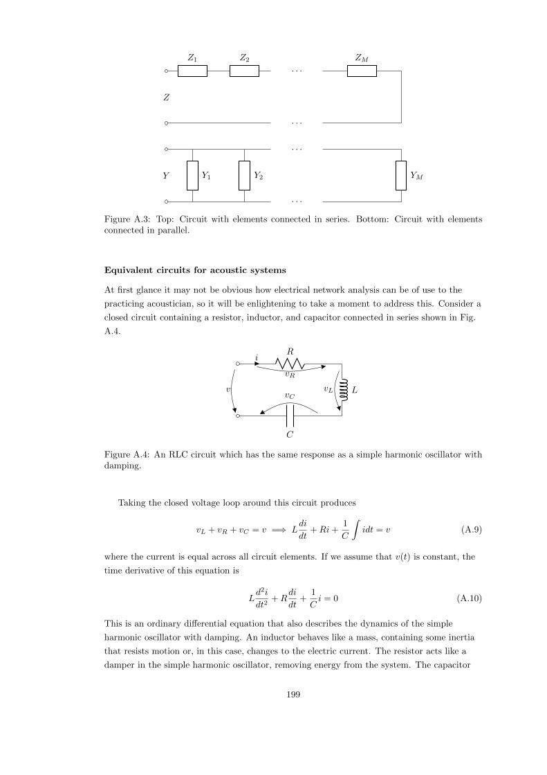
Z1 Z2 ZM

Z

. . .

. . .

Y1 Y2 YM

. . .

. . .

Y

Figure A.3: Top: Circuit with elements connected in series. Bottom: Circuit with elementsconnected in parallel.

Equivalent circuits for acoustic systems

At first glance it may not be obvious how electrical network analysis can be of use to the

practicing acoustician, so it will be enlightening to take a moment to address this. Consider a

closed circuit containing a resistor, inductor, and capacitor connected in series shown in Fig.

A.4.

R

vR

i

LvL

C

vCv

Figure A.4: An RLC circuit which has the same response as a simple harmonic oscillator withdamping.

Taking the closed voltage loop around this circuit produces

vL + vR + vC = v =⇒ Ldi

dt+Ri+

1

C

∫idt = v (A.9)

where the current is equal across all circuit elements. If we assume that v(t) is constant, the

time derivative of this equation is

Ld2i

dt2+R

di

dt+

1

Ci = 0 (A.10)

This is an ordinary differential equation that also describes the dynamics of the simple

harmonic oscillator with damping. An inductor behaves like a mass, containing some inertia

that resists motion or, in this case, changes to the electric current. The resistor acts like a

damper in the simple harmonic oscillator, removing energy from the system. The capacitor

199

behaves like a spring, pushing the current in the opposite direction when it gains a charge.

We can also use network analogies for acoustic tubes [63]. Consider air in a small section

of tubing of length ∆L and constant cross-sectional area S. The mass of the air is equal to

∆LSρ0 meaning that the force acting on the air is

ρ0S∆Ldv

dt= −S∆p (A.11)

where ∆p is the difference in acoustic pressure between the two sides of the air and v is the

particle velocity. Rearranging this equation and using the volume velocity, U = Sv gives

−∆p =ρ0∆L

S

dU

dt(A.12)

It is apparent that this description is similar to that of the voltage over an inductor, where

the minus of the pressure difference across the tube is equivalent to the electric potential

difference and the volume velocity is equivalent to the electric current. This means that an

acoustic tube behaves like an inductor of inductance ρ0∆L/S. This analogy is only equivalent

for low frequencies relative to the length of the tube but is a useful tool in acoustics.

200

Appendix B

Foster network element values

Recall the impedance of the Foster network is given by

ZMv = ea0 +

M∑q=1

eaqjω

ebq + jω(B.1)

B.1 Element values for continuous case

Here we present elements for the Foster network used to model viscous and thermal losses in

the continuous domain.

M = 4ER 0.0234494664073590a0 1.78673332377038aq 2.00382931898420, 3.14804951042440, 4.26150413518742, 5.50971380536713bq 3.39879310458637, 5.71032238039009, 7.95854733511626, 10.2448811301000M = 8ER 5.07851108448002× 10−06

a0 1.77626921138020aq 1.16947203816779, 1.63455222619591, 2.22808996187010, 2.80868696959160,

3.38432152205144, 3.96412484168712, 4.59313872296893, 5.69321545319216bq 2.83622816669839, 4.06100811397873, 5.21824406563471, 6.37563229181463,

7.52951817958072, 8.68261962284996, 9.85466844512209, 11.2408213780434M = 16ER 1.88335259896002× 10−09

a0 1.77617055460705aq 1.07101111930346,−0.191137256934357,−2.22953634694106, 1.16757650362629,

1.66903973571218, 2.07340818247316, 2.45430225714201, 2.82326302711027,3.20075853542216, 3.58778174627400, 3.97118596901446, 3.31992288500898,3.92720986887682, 2.30723002141302, 5.20175600836121, 13.2880886930482

bq 2.80368863323309, 3.58176534709911, 3.58176534709918, 3.99610463720205,4.80277903673739, 5.61822018775434, 6.42065124229265, 7.20347156389189,7.97353741515494, 8.74240977325489, 9.51243176421373, 10.1896361251182,10.3802224475833, 10.3802224475834, 11.2511443129779, 16.1294168496902

Table B.1: Foster element values when optimising using ER for a tube of radius 0.005 m at26.85 C over the frequency range 0.1− 10 kHz.

201

M = 4EM 0.0715786353463127a0 1.78951546246885aq 2.16943661559377, 3.45849867528497, 4.72224630727469, 6.56083118728158bq 3.54230512771505, 6.10613832356612, 8.63503593028419, 11.4369230510207M = 8EM 3.02574820340624× 10−05

a0 1.77634594834302aq 1.21795689259388, 1.79065106148618, 2.44955980938622, 3.09168299006462,

3.72826439347756, 4.37542420032459, 5.16877952981315, 7.21687325848349bq 2.85582406620587, 4.17355773792651, 5.45409713324216, 6.73606613886749,

8.01371812473195, 9.29168545594392, 10.6300369143409, 12.7756407005101M = 16EM 5.18445861030921× 10−09

a0 1.77617202016723aq 1.08365861138349, 1.12477948750744, 1.40845944720948, 1.85942844554413,

2.29454995017727, 2.66834447630448, 2.68811937341307, 2.84251699918943,3.59998948569483, 4.08100455035118, 4.58449010348442, 5.32313671277967,4.43502083478810, 6.98152719509852, 8.08233840300017, 11.8382444340280

bq 2.80638898398790, 3.80345071146270, 4.53921311487309, 5.28632327535363,6.07789421939354, 6.87599343819387, 7.57735113785327, 8.04471614010159,8.72499399382516, 9.54537236402782, 10.4137737821984, 11.4133949247559,12.3647128781383, 13.2694199447204, 16.0705166705316, 19.9800369207571

Table B.2: Foster element values when optimising using EM for a tube of radius 0.005 m at26.85 C over the frequency range 0.1− 10 kHz.

M = 4ER = 0.000141542510562678a0 2.56895852024480aq 2.64949367699711, 3.22982054694367, 3.93587280446617, 5.02394562987361bq 5.36449351366720, 6.83407959595604, 8.22900585988905, 9.78167541147680M = 8ER 3.99781337238800× 10−08

a0 2.39072893487651aq 2.15102947324571, 2.36815257481046, 2.75545270609303, 3.14972376266256,

3.53533745702292, 4.03733314014764, 5.18520009303550, 6.28892616777464bq 4.76875954807544, 5.86184446803226, 6.78331533424035, 7.65707903669578,

8.49572411718712, 9.33986959979712, 10.4669497561953, 13.1573441638063M = 16ER 8.12541058964733× 10−12

a0 2.26365426784080aq 1.83997418435759, 0.920452943638728, 1.49311893808675, 2.03637769782586,

2.17577282856170, 2.22897034234053, 2.63834315056954, 3.02500312860672,3.33449922896188, 3.55097521394667, 3.64683211177011, 4.29760437361149,4.30490487567676, 4.29059837456845, 3.98103941392489, 3.95880481718749

bq 4.36612882657212, 5.16602396489476, 5.40775762815384, 6.03684009382674,6.62885728933031, 7.11199723654211, 7.59243922608423, 8.15738597081932,8.75139201571871, 9.33231489577200, 9.83318188398057, 10.3945896153586,11.3316694308202, 11.3316694357558, 11.3316695631162, 11.3316695740028

Table B.3: Foster element values when optimising using ER over a smaller frequency range fora tube of radius 0.005 m at 26.85 C over the reduced frequency range 20 Hz - 3 kHz.

202

M = 4EM 0.00292405569458211a0 2.34766307840886aq 2.75636235102840, 3.49113805269408, 4.39152888271209, 6.31303994619724bq 5.11148131891873, 6.93271213517213, 8.66939248628015, 10.9760400605784M = 8EM 2.92901975654115× 10−06

a0 2.05492378788811aq 2.15796320342803, 2.42769393302163, 2.92603347210292, 3.46620375991204,

4.05373572096265, 4.94793064525109, 7.14033510305905, 0.425390103699538bq 4.20235209252206, 5.58875042436207, 6.71184100642302, 7.80374400862574,

8.90649235577635, 10.1562576278865, 12.4898544544823, 16.0338293462206M = 16EM 5.13467272533272× 10−10

a0 1.84523042820203aq 0.978598570821724, 0.610390905902404, 1.41269379178733, 1.71408606755416,

2.02246238922607, 2.30736365261612, 2.61757068069792, 2.98880213909959,3.38663816791189, 3.76729088509325, 3.91813370682619, 4.83401760385133,0.138658341528488, 6.65093866036470, 5.76744064476961, 5.17425387924675

bq 3.29284207979976, 3.29288403065929, 4.35202258319201, 5.10456449178987,5.82056267776754, 6.49684324910576, 7.14697466045120, 7.80680431173218,8.50034240269842, 9.22234460481371, 9.89643622819650, 10.6211438212465,11.5480572028912, 12.6217948634956, 12.6218124886916, 12.6218313956849

Table B.4: Foster element values when optimising using EM for a tube of radius 0.005 m at26.85 C over the reduced frequency range 20 Hz - 3 kHz.

B.2 Element values for discrete case

Here we present element values for the Foster network for viscous and thermal losses to be

used in the discrete case. The functions have been optimised by pre-warping the angular

frequency at a sample rate of 50 kHz. Recall that the pre-warped frequency is given by

ω′ =2

ktan−1

(ωk

2

)(B.2)

203

M = 4E′M 0.0949462118367476a0 1.79093241217392aq 2.21774119544845, 3.53504355037690, 4.83185854842939, 6.64025932147926bq 3.58977483976854, 6.21359662754855, 8.80260096873909, 11.6431597743201M = 8E′M 0.000641573586939728a0 1.77683207696528aq 1.36531177499111, 2.12114439455379, 2.89185539361509, 3.65093958860183,

4.42226341209098, 5.42645465366763, 3.90091429236591, 12.7743460756721bq 2.92770775765477, 4.47004911143952, 5.99369478960792, 7.51277808432381,

9.03348730169642, 10.6448301293608, 15.2214508864753, 18.5455246297529M = 16E′M 0.000349802524735779a0 1.77615317539466aq 1.10633531463411, 1.36236941583819, 1.83223005953335, 2.26436038812417,

2.54385001973642, 2.91163891261644, 3.60176303629582, 2.26051339836179,4.20846521595365, 4.56589829859680, 4.81572728306258, 1.66279414507306,3.46818783238449, 4.65013925527772, 6.00859131506436, 17.7759740465847

bq 2.81315365903336, 3.89742994877119, 4.84400746181209, 5.77465110428627,6.62622199124618, 7.37671923901475, 8.25914862942342, 9.35530147420441,9.35530291195798, 10.7304632732496, 10.7304632757414, 16.6684144163614,17.5730136833208, 18.1607921130290, 18.8327009237834, 23.5612132844038

Table B.5: Foster element values when optimising using E′M for a tube of radius 0.005 m at26.85 C over the pre-warped frequency range 0.1− 10 kHz at a sample rate of 50 kHz.

M = 4E′M 0.00929084924724041a0 2.44236974312547aq 2.93857509943753, 3.80626415894440, 4.92319050461018, 16.5624516922382bq 5.37218475536302, 7.35442924111783, 9.33154028303281, 21.7089231966319M = 8E′M 3.52008223183838× 10−06

a0 2.06645888670347aq 2.17841480671394, 2.45048715454489, 2.94835415197161, 3.49319854222213,

4.10348922337212, 5.16755939809455, 4.00430000497253, 15.3795286202532bq 4.23931674709201, 5.62870995450119, 6.75380891854883, 7.84836703302100,

8.96271626101145, 10.2919724072509, 13.1946488108175, 20.9549152866118M = 16E′M 7.62125439714811× 10−08

a0 1.90985046368390aq 1.81663954068205, 0.536368601929249, 0.436980756110944, 1.10335637104465,

2.00170278316213, 2.33253144555721, 2.68906252875716, 2.92931151549284,3.26653718262055, 3.92836624630039, 3.70092722168874, 3.93142979868540,3.99044225686261, 6.31113629994617, 6.43649290780868, 7.16006917490418

bq 3.65958533096794, 4.84545510629187, 4.87459206592095, 4.91508859428561,5.69023740044383, 6.40117613253956, 7.11316668007365, 7.79308097200874,8.42114254390272, 9.17419515658121, 10.2560791756143, 10.2561415456023,10.2561549651551, 13.2371018161500, 13.2378488945643, 13.2405893531275

Table B.6: Foster element values when optimising using E′M for a tube of radius 0.005 m at26.85 C over the pre-warped frequency range 20 Hz - 3 kHz at a sample rate of 50 kHz.

204

M = 4E′M 1.22593380574525a0 −2.41998781013108aq −0.849649872840543, 0.979862667053578, 2.82555593535784, 18.5427131525947bq 1.33447857934923, 5.03978465891827, 8.71835966169953, 26.0615486637585M = 8E′M 0.00490523564648042a0 −2.82447898096001aq −2.33820672045830,−1.57840081667709,−0.671448908145540, 0.241673098913610,

1.15486750407413, 2.07293392472161, 3.14480055969493, 15.4829361443098bq −0.790680087648193, 1.25128501779993, 3.09468026097488, 4.92522841659633,

6.75300303522660, 8.58160927832192, 10.4674610830690, 23.5090324114909M = 16E′M 0.000386692886726619a0 −2.82890826539225aq −2.81212376884297,−2.36172064486213,−1.75942461079875,−1.12313365312854,

−0.483746903294402, 0.154039963204909, 0.786922616903839, 1.41704831339022,2.09037210174763, 3.09707034249958,−11.3725763984025, 0.962211184700942,10.1089657554913, 17.5597311227531, 23.7025207935390, 34.9049244703962

bq −1.29194645855069, 0.312416743320408, 1.62753069876081, 2.91021502232840,4.18951462489131, 5.46776181216450, 6.74234861658821, 8.01037714784997,9.28887316962720, 10.7212417030777, 13.3876978872944, 17.7285990762499,22.4661852641953, 28.4487717742128, 32.0582863389304, 44.8074401218128

Table B.7: Foster element values when optimising using E′M for a tube of radius 0.05 m at26.85 C over the pre-warped frequency range 0.1− 10 kHz at a sample rate of 50 kHz.

M = 4E′M 0.819929246258164a0 −4.06539981031461aq −2.05283660403148,−0.402423555580136, 1.31194754722074, 3.28208410822298bq 0.285603342794180, 3.78650421679124, 7.21862529778111, 10.7613276998334

Table B.8: Foster element values when optimising using E′M for a tube of radius 0.1 m at 26.85

C over the pre-warped frequency range 0.1− 10 kHz at a sample rate of 100 kHz.

205

Appendix C

Experiments on brass instrument

valves

The valves in instruments such as the trumpet allow for extensions in the range of notes

available to the player. Despite their importance in performance, there is little in the way of

either theoretical or experimental work on brass instrument valves. The main discussions of

valves often revolve around the tuning concerns when multiple valves are depressed [34, 63].

To the author’s knowledge, the only experimental investigation on brass instrument valves

was performed by Widholm, who investigated the use of the Viennese action in French horns

in relation to slurred notes [176, 177].

This short appendix presents a simple experiment to investigate the effect of a brass

instrument valve when it is set in a partially open configuration and comparisons are made to

simulations. This work was first described in [77], although simulations were performed using

scheme (3.157), the discrete form of the attenuation model of Bilbao and Chick.

C.1 Experimental set up

A simplified valved brass instrument was constructed to investigate the effects of partial

openings. The third valve of a standard B[ trumpet was removed from the original instrument

and two cylindrical tubes were attached to either end. The valve in isolation is shown in Fig.

C.1 and a schematic of the experimental set up is shown in Fig. C.2.

206

Figure C.1: A trumpet valve in isolation.

Valve

Cylindrical tubing Cylindrical tubing

BIAS head

Figure C.2: Schematic of valve experiment

With the valve in an open configuration (so only air can flow through the default path),

the total length of the instrument was 2492 mm. Fully depressing the valve extends the

instrument length by 217 mm. The diameter of the tubing was 11.6 mm, which is close to the

radius of the valve openings. Machined spacers were used to control the depression of the

piston in 2 mm increments.

C.1.1 Results

Input impedance measurements were made using the BIAS capillary-based impedance

measurement device [175, 178] for different configurations of the valve openings. Comparisons

were made to simulations performed at 50 kHz for a duration of 1 s. In each tube, the explicit

scheme using a fourth order Foster network approximation for attenuation, (3.161), was used

to model propagation, and the lossy valve update (5.57) was used at the valve junctions. The

system was terminated using scheme (4.14) to approximate the Levine and Schwinger

radiation impedance. Simulated input impedances were gathered using the method described

in Sec. 3.4.6.

207

For partially open configurations, the parameters q(d) and q(b) were were given as the ratio

of the area of the intersecting circles between the main tube and default and bypass tubes,

respectively, to the area of the main tube. This also takes into account the separation between

the default and bypass paths in the valve housing.

Figs. C.3 - C.8 show simulated and experimentally measured input impedances as the

valve changes from a fully open configuration to a fully closed configuration. As the valve is

closed, additional peaks are introduced to the input impedance as waves can travel through

the system via a new path. The simulations show similar behaviour to the experimental

measurements, but there is a large deviation in magnitude. There are several reasons for this.

For the fully open and closed configurations, the simulations consistently over predict the

input impedance peak magnitude compared to the experiment. As it was difficult to attach

the valve to the main tubing, this could suggest that the seal was not secure, and leaks were

present in the experimental set-up. There could also be some errors relating to measuring the

geometry of the experiment. When the valve is fully closed, the simulation predicts peak

positions at higher frequencies than those seen in the experiment whereas there is a better

agreement between simulation and experiment for the fully open case. This suggests some

error in measuring the bypass section of the valve.

0 200 400 600 800 1000 1200 1400 1600 1800 200010

5

106

107

108

Figure C.3: Simulated and measured input impedance with the valve fully open.

0 200 400 600 800 1000 1200 1400 1600 1800 200010

5

106

107

108

Figure C.4: Simulated and measured input impedance where 9 washers are used to keep thevalve partially open.

208

0 200 400 600 800 1000 1200 1400 1600 1800 200010

5

106

107

108


0 200 400 600 800 1000 1200 1400 1600 1800 200010

5

106

107

108


0 200 400 600 800 1000 1200 1400 1600 1800 200010

5

106

107

108


209

0 200 400 600 800 1000 1200 1400 1600 1800 200010

5

106

107

108

Figure C.8: Simulated and measured input impedance with the valve fully closed.

The shape of the valve junctions also introduces some error to the geometry of the system.

Where the two tubes overlap, the area is no longer circular so the symmetry in the system

breaks down. There are also uncertainties in calculating the values of q(d) and q(b). For

example, Fig. C.9 shows the input impedance when 7 washers are used to open the the valve

but q(b) is multiplied by a factor of 0.45, so it is less than half the value used in Fig. C.5. This

shows an improved agreement between simulated and experimental data and would suggest

problems in determining the cross-sectional area at the valve junctions.

0 200 400 600 800 1000 1200 1400 1600 1800 200010

5

106

107

108

Figure C.9: Simulated and measured input impedance where 7 washers are used to keep thevalve partially open. The value of q(b) has been modified in the simulation to better match theresults of experiment.

210

Bibliography

[1] S. Adachi and M. Sato. Time-domain simulation of sound production in the brass

instrument. Journal of the Acoustical Society of America, 97(6):3850–3861, 1995.

[2] S. Adachi and M. Sato. Trumpet sound simulation using a two-dimensional lip vibration

model. Journal of the Acoustical Society of America, 99(2):1200–1209, 1996.

[3] M. A. Al-Alaoui. Novel digital integrator and differentiator. Electronics Letters,

29(4):376–378, 1993.

[4] A. Allen and N. Raghuvanshi. Aerophones in flatland: Interactive wave simulation of

wind instruments. ACM Trans. Graph., 34(4):134:1–134:11, July 2015.

[5] N. Amir, H. Matzner, and S. Shtrikman. Acoustics of a flanged cylindrical pipe using

singular basis functions. Journal of the Acoustical Society of America, 107(2):714–724,

2000.

[6] N. Amir, V. Pagneux, and J. Kergomard. A study of wave propagation in varying

cross-section waveguides by modal decomposition. part ii. results. Journal of the

Acoustical Society of America, 101(5):2504–2517, 1997.

[7] N. Amir, U. Shimony, and G. Rosenhouse. A discrete model for tubular acoustic

systems with varying cross section - the direct and inverse problems. part 1: Theory.

Acustica, 81(5):450–462, 1995.

[8] F. Avanzini and M. van Walstijn. Modelling the mechanical response of the

reed-mouthpiece-lip system of a clarinet. part i. a one-dimensional distributed model.

Acta Acustica united with Acustica, 90:537–547, 2004.

[9] J. Backus. Small-vibration theory of the clarinet. Journal of the Acoustical Society of

America, 33(3):305–313, 1963.

[10] J. Backus and T. C. Hundley. Harmonic generation in the trumpet. Journal of the


[11] J. W. Beauchamp. Analysis of simultaneous mouthpiece and output waveforms of wind

instruments. In Audio Engineering Society Convention 66, Los Angeles, United States

of America, May 1980.

[12] J. W. Beauchamp. Wind instrument transfer responses. In The 115th Meeting of the

Acoustical Society of America, Washington, United States of America, May 1988.

211

[13] A. H. Benade. On the propagation of sound waves in a cylindrical conduit. Journal of

the Acoustical Society of America, 44(2):616–623, 1968.

[14] A. H. Benade. Fundamentals of Musical Acoustics. Dover, New York, second, revised

edition, 1990.

[15] A. H. Benade and E. V. Jansson. On plane and spherical waves in horns with

nonuniform flare i. theory of radiation, resonance frequencies and mode conversion.

Acustica, 31:79–98, 1974.

[16] J.-P. Berenger. Three-dimensional perfectly matched layer for the absorption of

electromagnetic waves. Journal of Computational Physics, 127(2):363–379, 1996.

[17] H. Berjamin, B. Lombard, C. Vergez, and E. Cottanceau. Time-domain numerical

modeling of brass instruments including nonlinear wave propagation, viscothermal

losses, and lips vibration. Acta Acustica united with Acustica, 103:117–131, 2017.

[18] D. P. Berners. Acoustics and Signal Processing Techniques for Physical Modelling of

Brass Instruments. PhD thesis, Stanford University, 1999.

[19] S. Bilbao. Wave and Scattering Methods for Numerical Simulation. John Wiley & Sons,

Chichester, 2004.

[20] S. Bilbao. Direct simulation of reed wind instruments. Computer Music Journal,

33(4):43–55, 2009.

[21] S. Bilbao. Numerical Sound Synthesis: Finite Difference Schemes and Simulation in

Musical Acoustics. John Wiley & Sons, Chichester, 2009.

[22] S. Bilbao. Modelling of brass instrument valves. In Proceedings of the 14th International

Conference on Digital Audio Effects, pages 337–343, Paris, France, September 2011.

[23] S. Bilbao. Time domain simulation of brass instruments. In Forum Acusticum, Aalborg,

Denmark, June 2011.

[24] S. Bilbao and J. Chick. Finite difference time domain simulation for the brass

instrument bore. Journal of the Acoustical Society of America, 134(5):3860–3871, 2013.

[25] S. Bilbao and R. Harrison. Optimisation techniques for finite order viscothermal loss

modelling in acoustic tubes. In Proceedings of the International Symposium on Musical

and Room Acoustics, La Plata, Argentina,, September 2016.

[26] S. Bilbao and R. Harrison. Passive time-domain numerical models of viscothermal wave

propagation in acoustic tubes of variable cross section. The Journal of the Acoustical

Society of America, 140(1), 2016.

[27] S. Bilbao, R. Harrison, J. Kergomard, B. Lombard, and C. Vergez. Passive models of

viscothermal wave propagation in acoustic tubes. The Journal of the Acoustical Society

of America, 138(2), 2015.

[28] S. Bilbao, A. Torin, and V. Chatziioannou. Numerical modeling of collisions in musical

instruments. Acta Acustica united with Acustica, 101:292–299, 2015.

212

[29] B. Blackadar. Operator Algebras: Theory of C-Algebras and von Neumann Algebras,

volume 122 of Encyclopaedia of Mathematical Sciences. Springer, Berlin, 2006.

[30] J. F. Bonnans, J. C. Gilbert, C. Lemaechal, and C. A. Sagastizabal. Numerical

Optimization: Theoretical and Practical Aspects. Springer-Verlag, Berlin, second edition,

2006.

[31] D. Botteldooren. Acoustical finite-difference time-domain simulation in a quasi-cartesian

grid. Journal of the Acoustical Society of America, 95(5):2313–2319, 1994.

[32] D. Botteldooren. Finite-difference time-domain simulation of low-frequency room

acoustic problems. Journal of the Acoustical Society of America, 98(6):3302–3308, 1995.

[33] M. Campbell, J. Chick, J. Gilbert, J. Kemp, A. Myers, and M. Newton. Spectral

enrichment in brass instruments due to nonlinear sound propagation: a comparison of

measurements and predictions. In Proceedings of the International Symposium on

Musical Acoustics 2014, Le Mans, France, July 2014.

[34] M. Campbell and C. Greated. The Musician’s Guide to Acoustics. Oxford, Oxford,

1987. Reprint 2001.

[35] M. Campbell, C. Greated, and A. Myers. Musical Instruments: History, Technology, &

Performance of Instruments of Western Music. Oxford, New York, 2004.

[36] M. Campbell, M. Newton, J. Chick, A. Lopez-Carromero, and A. Myers. The influence

of bore profile on spectral enrichment due to nonlinear sound propagation in brass

instruments. In Proc. of the International Symposium on Musical and Room Acoustics,

La Plata, Argentina, September 2016.

[37] R. Causse, J. Kergomard, and X. Lurton. Input impedance of brass musical instruments

- comparison between experiment and numerical models. Journal of the Acoustical

Society of America, 75(1):241–254, 1984.

[38] A. Chaigne and A. Askenfelt. Numerical simulations of piano strings. i. a physical

model for a struck string using finite difference methods. Journal of the Acoustical

Society of America, 95(2):1112–1118, 1994.

[39] L. Chaparro. Signals and Systems Using MATLAB. Academic Press, Oxford, second

edition, 2015.

[40] V. Chatziioannou and M. van Walstijn. Energy conserving schemes for the simulation of

musical instrument contact dynamics. Journal of Sound and Vibration, 339:262–279,

2013.

[41] Y. Chen and K. Moore. Discretization schemes for fractional-order differentiators and

integrators. IEEE Trans. Circuits Syst., 49(3):363–367, 2002.

[42] Y. Chen, B. M Vinagre, and I. Podlubny. Continued fraction expansion approaches to

discretizing fractional order derivatives - an expository review. Nonlinear Dynamics,

38:115–170, 2004.

213

[43] J. Chick, S. Bromage, and M. Campbell. Transient behaviour in the motion of the brass

player’s lips. In Forum Acusticum, Budapest, Hungary, August/September 2005.

[44] J. P. Chick, S. M. Logie, M. Campbell, and J. Gilbert. Spectral enrichment and wall

losses in trombones played at high dynamic levels. In Proceedings of the Acoustics 2012

Nantes Conference, Nantes, France, April 2012.

[45] C. Chicone. Ordinary Differential Equations with Applications. Springer, New York,

2006.

[46] R. Christensen. Modeling the effects of viscosity and thermal conduction on acoustic

propagation in rigid tubes with various cross-sectional shapes. Acta Acustica united with

Acustica, 97:193–201, 2011.

[47] P. Cook. Tbone: An interactive waveguide brass instrument synthesis workbench for the

next machine. In Proceedings of the 1991 International Computer Music Conference,

pages 297–299, Montreal, Canada, October 1991.

[48] R. Courant, K. Friedrichs, and H. Lewy. On the partial differential equations of

mathematical physics. IBM Journal of Research and Development, 11(2):215–234, 1967.

Originally published in 1928 as “Uber die partiellen Differenzengleichungen der

mathematischen Physik.” Mathematissche Annalen 100(1):32-74.

[49] Annie Cuyt. Handbook of continued fractions for special functions. [electronic resource].

Springer, Dordrecht, 2008.

[50] V. Dubos, J. Kergomard, A. Kettabi, J. P. Dalmont, D. H. Keefe, and C. J. Nederveen.

Theory of sound propagation in a duct with a branched tube using modal

decomposition. Acustica - Acta Acustica, 85:153–169, 1999.

[51] S. Earnshaw. On the mathematical theory of sound. Philosophical Transactions of the

Royal Society of London, 150:133–148, 1860.

[52] G. Eckel, F. Iovino, and R. Causse. Sound synthesis by physical modelling with

modalys. In Proceedings of the International Symposium on Musical Acoustics, pages

479–482, Dourdan, France, July 1995.

[53] S. Elliot, J. Bowsher, and P. Watkinson. Input and transfer response of brass wind

instruments. Journal of the Acoustical Society of America, 72:1747–1760, 1982.

[54] M. Encina, J. Yuz, M. Zanartu, and G. Galindo. Vocal fold modeling through the

port-hamiltonian systems approach. In IEEE Conference on Control Applications,

Sydney, Australia, September 2015.

[55] B. Engquist and A. Majda. Absorbing boundary conditions for the numerical simulation

of waves. Mathematics of Computation, 31(139):629–651, 1977.

[56] P. Eveno, J. P. Dalmont, R. Causse, and J. Gilbert. Wave propagation and radiation in

a horn: Comparisons between models and measurements. Acta Acustica united with

Acustica, 98:158–165, 2012.

214

[57] A. Falaize and T. Helie. Passive simulation of electrodynamic loudspeakers for guitar

amplifiers: a port - hamiltonian approach. In Proceedings of the International

Symposium on Musical Acoustics 2014, Le Mans, France, July 2014.

[58] A. Falaize and T. Helie. Guaranteed-passive simulation of an electro-mechanical piano:

A port-hamiltonian approach. In Proc. of the 18th Int. Conference on Digital Audio

Effects, Trondheim, Norway, December 2015.

[59] A. Falaize, N. Lopes, T. Helie, D. Matignon, and B. Maschke. Energy-balanced models

for acoustic and audio systems: a port - hamiltonian approach. In Unfold Mechanics

Colloquium, Paris, France, September 2014.

[60] A. Falaize-Skrzek and T. Helie. Simulation of an analog circuit of a wah pedal: a

port-hamiltonian approach. In Audio Engineering Society Convention 135, New York,

USA, October 2013.

[61] S. Farner, C. Vergez, J. Kergomard, and A. Lizee. Contribution to harmonic balance

calculations of self-sustained periodic oscillations with focus on single-reed instruments.

Journal of the Acoustical Society of America, 119(3):1794–1804, 2006.

[62] A. Fettweis. Wave digital filters: Theory and practice. Proceedings of the IEEE,

74(2):270–327, 1986.

[63] N. H. Fletcher and T. D. Rossing. The Physics of Musical Instruments. Springer, New

York, second edition, 1998. Reprint 2005.

[64] B. H. Flowers and E. Mendoza. Properties of Matter. John Wiley & Sons Ltd.,

Chichester, 1970. Reprint 1989.

[65] V. Gerasik and M. Stastna. Complex group velocity and energy transport in absorbing

media. Pysical Review E, 81(5):056602, 2010.

[66] J. Gilbert, D. M. Campbell, A. Myers, and R. W. Pyle. Differences between brass

instruments arising from variations in brassiness due to nonlinear propagation. In

Proceedings of the International Symposium on Musical Acoustics, Barcelona, Spain,

September 2007.

[67] J. Gilbert, L. Menguy, and M. Campbell. A simulation tool for brassiness studies(l).


[68] N. Giordano. Nonlinear effects at woodwind toneholes. In Proceedings of the

International Symposium on Musical Acoustics 2014, Le Mans, France, July 2014.

[69] N. Giordano. Chaotic behaviour of the piccolo. In Proc. of the 22ndInternational

Congress on Acoustics, Buenos Aires, Argentina, September 2016.

[70] N. Giordano. Mode switching in an air-jet instrument. In Proc. of the International

Symposium on Musical and Room Acoustics, La Plata, Argentina, September 2016.

[71] B. Gustafsson, H-O. Kreiss, and J. Oliger. Time Dependent Problems and Difference

Methods. John Wiley & Sons, Inc., New York, 1995.

215

[72] H. Haddar, J. R. Li, and D. Matignon. Efficient solution of a wave equation with

fractional-order dissipative terms. Journal of Computational and Applied Mathematics,

234(6):2003–2010, 2009.

[73] D. Halliday, R. Resnick, and J. Walker. Fundamentals of Physics. John Wiley & Sons,

Inc., New Jersey, United States, eighth edition, 2008.

[74] B. Hamilton. Finite Difference and Finite Volume Methods for Wave-Based Modelling

of Room Acoustics. PhD thesis, The University of Edinburgh, 2016.

[75] R. Harrison, S. Bilbao, and J. Perry. An algorithm for a valved brass instrument

synthesis environment using finite-difference time-domain methods with performance

optimisation. In Proceedings of the 18th International Conference on Digital Audio

Effects, Trondheim, Norway, November/December 2015.

[76] R. L. Harrison, S. Bilbao, J. Perry, and T. Wishart. An environment for physical

modeling of articulated brass instruments. Computer Music Journal, 29(4):80–95, 2015.

[77] R. L. Harrison and J. Chick. A single valve brass instrument model using

finite-difference time-domain methods. In Proceedings of the International Symposium

on Musical Acoustics., Le Mans, France, July 2014.

[78] R. L. Harrison, B. Hamilton, and A. Lopez-Carromero. Finite difference time domain

simulation of a hybrid 1d/3d brass instrument model and comparison to measured

radiation data. In 24th International Congress on Sound and Vibration, July 2017.

[79] T. Helie. Unidimensional models of acoustic propagation in axisymmetric waveguides.


[80] T. Helie, T. Hezard, R. Mignot, and D. Matignon. One-dimensional acoustic models of

horns and comparison with measurements. Acta Acustica united with Acustica,

99:960–974, 2013.

[81] T. Helie and D. Matignon. Diffusive representations for the analysis and simulation of

flared acoustic pipes with visco-thermal losses. Mathematical Models and Methods in

Applied Sciences, 16(4):503–536, 2006.

[82] T. Helie, R. Mignot, and D. Matignon. Waveguide modeling of lossy flared acoustic

pipes: Derivation of a kelly-lochbaum structure for real-time simulations. In IEEE

Workshop on Applications of Signal Processing to Audio and Acoustics, New Paltz, NY,

October 2007.

[83] T. Helie and X. Rodet. Radiation of a pulsating portion of a sphere: Application to

horn radiation. Acta Acustica united with Acustica, 89:565–577, 2003.

[84] R. L. Higdon. Absorbing boundary condition for difference approximations to the

multi-dimensional wave equation. Mathematics of Computation, 47(176):437–459, 1986.

[85] R. L. Higdon. Numerical absorbing boundary condition for the wave equation.

Mathematics of Computation, 49(179):65–90, 1987.

216

[86] T. Hikichi, N. Osaka, and F. Itakura. Time-domain simulation of sound production of

the sho. Journal of the Acoustical Society of America, 113(2):1092–1101, 2003.

[87] L. Hiller and P. Ruiz. Synthesizing musical sounds by solving the wave equation for

vibrating objects: Part i. Journal of the Audio Engineering Society, 17(1):462–470, 1971.

[88] A. Hirschberg, J. Gilbert, R. Msallam, and A. P. J. Wijnands. Shock waves in

trombones. Journal of the Acoustical Society of America, 99(3):1754–1758, 1996.

[89] Roger A. Horn and Charles R. Johnson. Topics in Matrix Analysis. Cambridge

University Press, Cambridge, 1991.

[90] C. S. Jog and A. Nandy. Conservation properties of the trapezoidal rule in linear time

domain analysis of acoustics and structures. Journal of Vibration and Acoustics,

137:1189–1198, 2015.

[91] Gareth A. Jones and David Singerman. Complex Functions: An Algebraic and

Geometric Viewpoint. Cambridge University Press, 1987.

[92] W. Kausel and C. B. Geyer. Time domain simulation of standing waves in brass wind

instruments taking non-linear wave steepening into account. In Proceedings of the

Stockholm Music Acoustics Conference, Stockholm, Sweden, July/August 2013.

[93] D. H. Keefe. Theory of the single woodwind tone hole. Journal of the Acoustical Society

of America, 72:676–687, 1982.

[94] D. H. Keefe. Acoustical wave propagation in cylindrical ducts: Transmission line

parameter approximations for isothermal and nonisothermal boundary conditions.


[95] D. H. Keefe and A. Barjau. Acoustic propagation in flaring, axisymmetric horns: Ii.

numerical results, wkb theory, and viscothermal effects. Acustica - Acta Acustica,

85:285–293, 1999.

[96] J. Kelly and C. Lochbaum. Speech synthesis. In Proceedings of the Fourth International

Congress on Acoustics, Copenhagen, Denmark, September 1962.

[97] J. Kemp, S. Bilbao, J. McMaster, and R. Smith. Wave separation in the trumpet under

playing conditions and comparison with time domain finite difference simulations.


[98] J. Kemp, A. Lopez-Carromero, A. Wooley, and M. Campbell. Experimental

investigation of doppler shift and infrasound generation during wave propagation within

the bore of the trombone during slide movement. In Proc. of the Third Vienna Talk on

Music Acoustics, Vienna, Austria, September 2015.

[99] J. A. Kemp. Theoretical and experimental study of wave propagation in brass musical

instruments. PhD thesis, The University of Edinburgh, 2002.

[100] J. Kergomard. Regularity and irregularity in wind instruments with tone holes or bells.

In Proceedings of the International Symposium on Musical Acoustics 2014, Le Mans,

France, July 2014.

217

[101] J. Kergomard and M. Pachebat. Low frequency coupling and mode interference in an in

homogenous lattice of finite length. In Forum Acusticum 2014, Krakow, Poland,

September 2014.

[102] P. G. LeFloch and M. Westdickenberg. Finite energy solutions to the isentropic euler

equations with geometric effects. Journal de Mathematiques Pures et Appliquees,

88(2):389–429, 2007.

[103] R. J. LeVeque. Finite Volume Methods for Hyperbolic Problems. Cambridge University

Press, New York, 2002.

[104] H. Levine and J. Schwinger. On the radiation of sound from an unflanged circular pipe.

Physical Review, 73(4):383–406, 1948.

[105] S. M. Logie. An Acoustical Study of the Playing Characteristics of Brass Wind

Instruments. PhD thesis, The University of Edinburgh, 2012.

[106] B. Lombard and J-F Mercier. Numerical modelling of nonlinear acoustic waves in a

tube connected with helmholtz resonators. Journal of Computational Physics,

259:421–443, 2014.

[107] B. Lombard, C. Vergez, and E. Cottenceau. Modelibation de la propagation non lineaire

avec pertes viscothermiques: application a la famill des cuivres. In Proceedings of the

Congres Francais d’Acoustique (CFA), Poitiers, France, April 2014.

[108] N. Lopes and T. Helie. A power-balanced model of a valve exciter including shocks and

based on a conservative jet for brass instruments: Simulations and comparison with

standard models. In Proceedings of the International Symposium on Musical Acoustics

2014, Le Mans, France, July 2014.

[109] N. Lopes and T. Helie. Energy balanced model of a jet interacting with a brass player’s

lip. Acta Acustica united with Acustica, 102:141–154, 2016.

[110] D. Luce and M. Clark. Physical correlates of brass-instrument tones. Journal of the


[111] D. Matignon and T. Helie. A calss of damping models preserving eigenspaces for linear

conservative port-hamiltonian systems. European Journal of Control, 19:486–494, 2013.

[112] S. Maugeais and J. Gilbert. Nonlinear acoustic propagation applied to brassiness

studies, a new simulation tool in the time domain. Acta Acustica united with Acustica,

103:67–79, 2017.

[113] M. E. McIntyre, R. T. Schumacher, and J. Woodhouse. On the oscillations of musical

instruments. Journal of the Acoustical Society of America, 74(5):1325–1345, 1983.

[114] L. Menguy. Propagation Acoustique Non Lineaire Dans Les Guides Monodimensionnels.

PhD thesis, Universite du Maine, 2001.

[115] L. Menguy and J. Gilbert. Weakly nonlinear gas oscillations in air-filled tubes; solutions

and experiments. Acustica - Acta Acustica, 86:798–810, 2000.

218

[116] R. Mignot, T. Helie, and D. Matignon. Stable realization of a delay system modeling a

convergent acoustic cone. In 16th Mediterranean Conference on Control and

Automation, Ajaccio, France, June 2008.

[117] R. Mignot, T. Helie, and D. Matignon. Acoustic modelling of a convex pipe adapted for

digital waveguide simulation. In Proceedings of the 13th International Conference on

Digital Audio Effects, Graz, Austria, September 2010.

[118] R. Mignot, T. Helie, and D. Matignon. Digital waveguide modeling for wind

instruments: Building a state-space representation based on webster-lokshin model.

IEEE Transactions on Audio, Speech, and Language Processing, 18(4):843–854, 2010.

[119] D. Morrill. Trumpet algorithms for computer composition. Computer Music Journal,

1(1):46–52, 1977.

[120] J. D. Morrison and J-M. Adrien. Mosaic: A framework for modal synthesis. Computer

Music Journal, 17(1):45–56, 1993.

[121] P. M. Morse. Vibration and Sound. Acoustical Society of America, New York, second

edition, 1981. Reprint 1995.

[122] P. M. Morse and K. U. Ingard. Theoretical acoustics. International series in pure and

applied physics. McGraw-Hill, New York, 1968.

[123] R. Msallam, S. Dequidt, R. Causse, and S. Tassart. Physical model of the trombone

including nonlinear effects. application to the sound synthesis of loud tones. Acustica -

Acta Acustica, 86:725–736, 2000.

[124] L .Muschiettie and C. T. Dum. Real group velocity in a media with dissipation. Physics

of Fluids B, 5(5):1383–1397, 1993.

[125] A. Myers, R. W. Pyle, J. Gilbert, M. Campbell, J. P. Chick, and S. Logie. Effects of

nonlinear sound propagation on the characteristic timbres of brass instruments. Journal

of the Acoustical Society of America, 131(1):678–688, 2012.

[126] A. H. Nayfeh. Perturbation Methods. John Wiley & Sons Inc, New York, 1973.

[127] D. Noreland. A numerical method for acoustic waves in horns. Acta Acustica united

with Acustica, 88:576–586, 2002.

[128] D. Noreland, J. Kergomard, F. Laloo, C. Vergez, P. Guillemain, and A. Guilloteau. The

logical clarinet: numerical optimisation of the geometry of woodwind instruments. Acta

Acustica united with Acustica, 99(4):615–628, 2013.

[129] J. O. D. Noreland, M. R. Udawalpola, and O. M. Berggren. A hybrid scheme for bore

design optimization of a brass instrument. Journal of the Acoustical Society of America,

128(3):1391–1400, 2010.

[130] B. H. Pandya, G. S. Settles, and J. D. Miller. Schlieren imaging of shock waves from a

trumpet. Journal of the Acoustical Society of America, 114(6):3363–3367, 2003.

[131] pBone. pbone plastic trombone: The worlds best selling trombone, July 2017. Last

accessed July 2017.

219

[132] A. D. Pierce. Acoustics: An Introduction to Its Physical Principles and Applications.

Acoustical Society of America, New York, 1981. Reprint 1994.

[133] pTrumpet. ptrumpet: World’s first all plastic trumpet, July 2017. Last accessed July

2017.

[134] L. R. Rabiner and R. W. Schafer. Digital processing of speech signals. Prentice-Hall

Inc., New Jersey, 1978.

[135] P. L. Rendon, C. G. Malanche, and F. Oruna-Bustamente. Effect of input signal shape

on the nonlinear steepening of transient acoustic waves in a cylindrical tube. In Proc. of

the 22ndInternational Congress on Acoustics, Buenos Aires, Argentina, September 2016.

[136] P. L. Rendon, F. Ordu na Bustamente, D. Narezo, and A. Perez-Lopez. Nonlinear

progressive waves in a slide trombone resonator. Journal of the Acoustical Society of

America, 127(2):1096–1103, 2010.

[137] J. Resch. Nonlinear Wave Propagation in Brass Instruments. PhD thesis, The

University of Waterloo, 2012.

[138] J. Resch, L. Krivodonova, and J. Vanderkooy. A two-dimensional study of finite

amplitude sound waves in a trumpet using the discontinuous galerkin method. Journal

of Computational Acoustics, 22(3):145007, 2014.

[139] O. Richards. Investigation of the Lip Reed Using Computational Modelling and

Experimental Studies with an Artificial Mouth. PhD thesis, The University of

Edinburgh, 2003.

[140] K. F. Riley, M. P. Hobson, and S. J. Bence. Mathematical Methods for Physics and

Engineering. Cambridge, Cambridge, third edition, 2006.

[141] C. Roads. The Computer Music Tutorial. MIT Press, Cambridge, Massachusetts, 1996.

[142] X. Rodet and C. Vergez. Nonlinear dynamics: From basic models to true

musical-instrument models. Computer Music Journal, 23(3):35–49, 1999.

[143] O. V. Rudenko and S. I. Soluyan. Theoretical Foundations of Nonlinear Acoustics.

Nauka Press, Moscow, 1975. Trans. by R. T. Beyer, Consultants Bureau, New York,

1977.

[144] M. Russ. Yamaha vl1 virtual acoustic synthesizer. Sound on Sound, 1994. Available

online https://web.archive.org/web/20150608005838/http:

//www.soundonsound.com/sos/1994_articles/jul94/yamahavl1.html, Last accessed

August 2017.

[145] L. Savioja, T. J. Rinne, and T. Takala. Simulation of room acoustics with a 3-d finite

difference mesh. In Proceedings of the 1994 International Computer Music Conference,

Arhus, Denmark, September 1994.

[146] G. P. Scavone. An Acoustic Analysis of Single-Reed Woodwind Instruments with an

Emphasis on Design and Performance Issues and Digital Waveguide Modeling

Techniques. PhD thesis, Stanford University, 1997.

220

https://web.archive.org/web/20150608005838/http://www.soundonsound.com/sos/1994_articles/jul94/yamahavl1.html

https://web.archive.org/web/20150608005838/http://www.soundonsound.com/sos/1994_articles/jul94/yamahavl1.html

[147] F. Silva, Ph. Guillemain, J. Kergomard, B. Mallaroni, and A. N. Norris. Approximation

formulae for the acoustic radiation impedance of a cylindrical pipe. Journal of Sound

and Vibration, 322:255–263, 2009.

[148] F. Silva, C. Vergez, P. Guillemain, J. Kergomard, and V. Debut. Moreesc: A framework

for the simulation and analysis of sound production in reed and brass instruments. Acta

Acustica united with Acustica, 100:126–138, 2014.

[149] J. O. Smith. Efficient simulation of the reed-bore and bow-string mechanisms. In

Proceedings of the 1986 International Computer Music Conference, pages 275–280, The

Hague, Netherlands, October 1986.

[150] J. O. Smith III. Musical applications of digital waveguides. Technical Report

STAN-M-39, Center for Computer Research in Music and Acoustics, 1987.

[151] J. O. Smith III. Physical Audio Signal Procesing. Stanford, CA, 2004. Draft version.

Available online at http://ccrma.stanford.edu/~jos/pasp04/, Last accessed August

2017.

[152] T. Smyth and M. Rouhipour. Saxophone modelling and system identification. In

Proceedings of Meeting on Acoustics, Montreal, Canada, June 2013.

[153] Jan A. Snyman. Practical Mathematical Optimization: An Introduction to Basic

Optimization Theory and Classical and New Gradient-Based Algorithms. Springer, New

York, 2005.

[154] M. R. Stinson. The propagation of plane sound waves in narrow and wide circular

tubes, and generalisation to uniform tubes of arbitrary cross-sectional shape. Journal of

the Acoustical Society of America, 89(2):550–558, 1991.

[155] M. R. Stinson and Y. Champoux. Propagation of sound and the assignment of shape

factors in model porous materials having simple pore geometries. Journal of the


[156] J. C. Strikwerda. Finite Difference Schemes and Partial Differential Equations. Society

for Industrial and Applied Mathematics, Philadelphia, second edition, 2004.

[157] J. W. Strutt. The Theory of Sound Volume II. Dover, New York, second edition, 1896.

Reprint 1945.

[158] M. Svard and J. Nordstrom. Review of summation-by-parts schemes for

initial-boundary-value problems. Journal of Computational Physics, 268:17–38, 2014.

[159] E. Tadmor. Entropy stability for difference approximations of nonlinear conservation

laws and related time-dependent problems. Acta Numerica, (12):451–512, 2003.

[160] J. W. Thomas. Numerical Partial Differential Equations: Finite Difference Methods.

Springer, New York, 1995.

[161] M. W. Thompson and W. J. Strong. Inclusion of wave steepening in a frequency-domain

model of trombone sound production. Journal of the Acoustical Society of America,

110(1):556–562, 2001.

221

[162] S. C. Thompson, T. B. Gabrielson, and D. M. Warren. Analog model for thermoviscous

propagation in a cylindrical tube. Journal of the Acoustical Society of America,

135(2):585–590, 2014.

[163] A. Torin. Percussion Instrument Modelling in 3D: Sound Synthesis Through Time

Domain Numerical Simulation. PhD thesis, The University of Edinburgh, 2015.

[164] A. van der Schaft. Port-hamiltonian systems: an introductory survey. In Proceedings of

the International Congress of Mathematicians, Madrid, Spain, August 2006.

[165] M. E. van Valkenburg. Introduction to Modern Network Synthesis. John Wiley & Sons

Inc, New York, 1960.

[166] M. van Walstijn. Wave-based simulation of wind instrument resonators. IEEE Signal

Processing Magazine, 21:21–31, 2007.

[167] M. van Walstijn and M. Campbell. Discrete-time modelling of woodwind instrument

bores using wave variables. Journal of the Acoustical Society of America,

113(1):575–585, 2003.

[168] C. Vergez and X. Rodet. Dynamical systems and physical models of trumpet-like

instruments. analytical study and asymptotical properties. Acustica - Acta Acustica,

86:147–162, 2000.

[169] C. Vergez and X. Rodet. Trumpet and trumpet player: Model and simulation in a

musical context. In Proceedings of the 2001 International Computer Music Conference,

La Habana, Cuba, September 2001.

[170] C. Vergez and P. Tisserand. The brass project, from physical models to virtual musical

instruments: Playability issues. In R. Kronland-Martinet, T. Voinier, and S. Ystad,

editors, Lecture Notes in Computer Science: Computer Music Modeling and Retrieval,

volume 3902, pages 24–33. Springer, Berlin, September 2006.

[171] B. Vinagre, I. Podlubny, A. Hernandez, and V. Feliu. Some approximations of fractional

order operators used in control theory and applications. Fractional Calculus and Applied

Analysis, 3(3):231–248, 2000.

[172] S. Wang and G. Kreiss. Convergence of summation-by-parts finite difference methods

for the wave equation. Journal of Scientific Computing, 71(1):219–245, 2017.

[173] A. G. Webster. Acoustical impedance, and the theory of horns and of the phonograph.

Proceedings of the National Academy of Sciences of the United States of America,

5(7):275–282, 1919.

[174] L. Weinberg. Network Analysis and Synthesis. McGraw-Hill Book Company, Inc, New

York, 1962.

[175] G. Widholm. Brass wind instrument quality measured and evaluated by a new

computer system. In Proceedings of the 15th International Congress on Acoustics,

Trondheim, Norway, June 1995.

222

[176] G. Widholm. The influence of valve mechanisms on the microstructure of slurs played

with brass wind instruments. In Proceedings of the International Symposium on Musical

Acoustics, Edinbugrh, United Kingdom, August 1997.

[177] G. Widholm. The vienna horn - a historic relict successfully used by top orchestras of

the 21 century. In Forum Acusticum, Budapest, Hungary, August/September 2005.

[178] G. Widholm, H. Pichler, and T. Ossmann. Bias: A computer-aided test system for brass

wind instruments. In Audio Engineering Society Convention 87, New York, United

States of America, October 1989.

[179] K. S. Yee. Numerical solution of initial boundary value problems involving maxwell’s

equations in isotropic media. IEEE Transactions on Antennas and Propagation,

14(3):302–307, 1966.

[180] U. Zolzer. Digital Audio Signal Processing. John Wiley & Sons Ltd, Chichester, second

edition, 2008.

[181] W. E. Zorumski. Generalized radiation impedances and reflection coefficients of circular

and annular ducts. Journal of the Acoustical Society of America, 54(6):1667–1673, 1973.

[182] C. Zwikker and C.W. Kosten. Sound absorbing materials. Elsevier Pub. Co., 1949.

223

Physical Modelling of Brass Instruments using Finite ...

Documents

Transcript of Physical Modelling of Brass Instruments using Finite ...