physical distribution analysis for the traffic manager - Open ...

PHYSICAL DISTRIBUTION ANALYSIS FOR THE TRAFFIC MANAGER

A Thesis

Presented to

the Faculty of Commerce and Business Administration

University of B r i t i s h Columbia

In P a r t i a l F u l f i l l m e n t

of the Requirements f o r the Degree

Master of Business Administration

by

David Joseph Schmirler

May 1964

ACCEPTANCE

This Thesis has been accepted i n p a r t i a l

f u l f i l l m e n t of the requirements for the Degree of

Master of Business Administration i n the Faculty of

Commerce and Business Administration of the University

of B r i t i s h Columbia.

Date

Dean, Faculty of Commerce and Business Administration

Chairman

In presenting this thesis in partial fulfilment of

the requirements for an advanced degree at the University of

Bri t i sh Columbia, I agree that the Library shall make i t freely

available for reference and study, I further agree that per

mission for extensive copying of this thesis for scholarly

purposes may be granted by the Head of my Department or by

his representatives. It is understood that, copying or publi

cation of this thesis for financial gain shall not be allowed

without my written permission*

Department of ^o-iv^MiMJLy &s~^JL

The University of Brit ish Columbia, Vancouver 8, Canada

Date / W l /f*4. .

ABSTRACT

The physical d i s t r i b u t i o n concept recognizes the

int e r r e l a t i o n s h i p s between transportation, materials

handling, warehousing and the other processes that are

involved i n the physical flow of t r a f f i c from the source

of raw materials, through production and d i s t r i b u t i o n

f a c i l i t i e s , t o the firm's customers. The essence of the

concept i s that i t i s the t o t a l cost of the several

processes, rather than the cost of i n d i v i d u a l processes,

that must be taken into account i n decisions i n which

there are alternatives for the physical movement of

materials and products. Physical d i s t r i b u t i o n analysis

involves the formulation and comparison of the alternatives

f o r t r a f f i c flow.

This thesis i s concerned primarily with the develop

ment of a procedure for physical d i s t r i b u t i o n analysis that

may be useful i n the formulation of decisions that are

within the T r a f f i c Manager's sphere of r e s p o n s i b i l i t y . In

order to i d e n t i f y the nature of these decisions and i n

order to develop a suitable framework f o r the T r a f f i c

Manager's analyses, the second chapter describes the major

decisions i n which physical d i s t r i b u t i o n p r i n c i p l e s should

be applied; relates these applications to successive

2

planning i n t e r v a l s ; and considers the scope of these

decisions i n terms of the authority that i s necessary

for t h e i r implementation.

The author suggests that the major applications of

the physical d i s t r i b u t i o n concept include long-term

decisions related to the s p a t i a l a l l o c a t i o n of production

capacities, intermediate-term decisions involving changes

i n the f i x e d f a c i l i t i e s for physical d i s t r i b u t i o n , and

short-term decisions concerning the u t i l i z a t i o n of

e x i s t i n g production and physical d i s t r i b u t i o n f a c i l i t i e s .

Of these applications, i t i s only the short-term

decisions that are l i k e l y to be made by the T r a f f i c

Manager. Chapters three to f i v e , therefore, are concerned

with the procedures f o r formulating and comparing short-

term a l t e r n a t i v e s .

To f a c i l i t a t e presentation, the author deals

s p e c i f i c a l l y with the development of a procedure for

analysis for two of the short-term physical d i s t r i b u t i o n

problems -- the day-to-day problem of meeting customer

orders out of inventories that are on hand at d i s t r i

bution warehouses; and the problem of a l l o c a t i n g short-

term output among the firm's plants.

The author recommends the l i n e a r programming

technique as the method for selecting the optimum

3 alternative for each of these problems. The application

of t h i s technique i s described i n d e t a i l i n Chapter V.

The major determinants of physical d i s t r i b u t i o n

alternatives, the i d e n t i f i c a t i o n of feasible alternatives,

and the development of unit variable costs required by

the l i n e a r programming models are dealt with i n Chapters

III and IV.

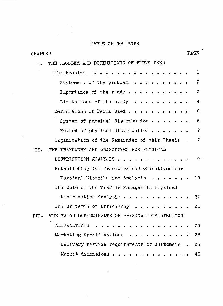
TABLE OF CONTENTS

CHAPTER PAGE

I. THE PROBLEM AND DEFINITIONS OF TERMS USED

The Problem 1

Statement of the problem 3

Importance of the study 3

Limitations of the study 4

De f i n i t i o n s of Terms Used 6

System of physical d i s t r i b u t i o n 6

Method of physical d i s t r i b u t i o n 7

Organization of the Remainder of t h i s Thesis . 7

I I . THE FRAMEWORK AND OBJECTIVES FOR PHYSICAL

DISTRIBUTION ANALYSIS . 9

Est a b l i s h i n g the Framework and Objectives f o r

Physical D i s t r i b u t i o n Analysis 10

The Role of the T r a f f i c Manager i n Physical

D i s t r i b u t i o n Analysis 24

The C r i t e r i a of E f f i c i e n c y . . . . 30 I I I . THE MAJOR DETERMINANTS OF PHYSICAL DISTRIBUTION

ALTERNATIVES . . . . . 34

Marketing Specifications . . 38

Delivery service requirements of customers • 38

Market dimensions . 40

iv

CHAPTER PAGE

Sales forecasts 57

F l e x i b i l i t y i n Production and Physical

D i s t r i b u t i o n F a c i l i t i e s 58

Production f a c i l i t i e s . . . 58

D i s t r i b u t i o n warehouses . . . . . 62

Transportation and handling 62

Order-processing and communications . . . . 64

IV. COLLECTION AND PREPARATION OF DATA 66

Flow Diagrams . . . . . . 66

Cost Schedules and Other Data 71

Raw materials data 72

Transportation data 73

Production data . . . . . . . . 74

Warehousing data 78

Inventory data 80

Order-processing and communications data . 81

Total Route Cost 82

Estimating the cost of physical

d i s t r i b u t i o n from plant to warehouse . • 84

Estimating the cost f o r the f i r s t h a l f of

a t r a f f i c route 106

V

CHAPTER PAGE

V. DETERMINING THE OPTIMUM ALTERNATIVE • 112

Linear Programming Model f o r Output

A l l o c a t i o n Decisions . . . . 114

Demands, constraints and costs 116

The Simplex formulation . . . . . 118

Conversion of the Simplex matrix . . . . . 125

Solution through the transportation

procedure . . . . . . . . . 132

Interpretation of the optimum . . . . . . . 146

Solution implications . . . . 150

Linear Programming Model f o r Day-to-day

Physical D i s t r i b u t i o n Decisions 153

VI. SUMMARY AND CONCLUSIONS 162

Summary 162

Major applications of the physical

d i s t r i b u t i o n concept . . . . 163

The t r a f f i c manager's role 167

The day-to-day problem . . . . . 169

The output a l l o c a t i o n problem . . . . . . . 171

Conclusions 178

BIBLIOGRAPHY 189

LIST OF TABLES

TABLE PAGE

I. Raw Materials Data 73

I I . Transportation Data 74

I I I . Processing Cost Data 75

IV. Plant Capacity Data 78

V. Warehousing Data 79

VI. Order-Processing and Communications Data . • • 82

VII. Inventory Value Per Unit 87

VIII. Volume and Value of Transit Inventory . . . . 89

IX. Volume and Value of Cycle Inventory 94

X. Lead Time 98

XI. Volume and Value of Safety Stock 102

XII. Cost of Carrying Inventory . . . . . 103

XIII. T o t a l Variable Cost of Physical

D i s t r i b u t i o n Plant to Warehouse 104

XIV. Simplex Matrix 122

XV. Simplex Matrix a f t e r Step 1 12 7

XVI. Simplex Matrix a f t e r Step 2 129

XVII. Simplex Matrix a f t e r Step 3 130

XVIII. Transportation Matrix 133

XIX. Transportation Matrix - I n i t i a l Assignment . . 135

XX. Transportation Matrix - F i r s t Adjustment . . . 143

v i i

TABLE PAGE

XXI. Transportation Matrix - Optimum Solution . . . 145

XXII. Plant Capacity Absorbed i n the

Transportation Solution . . . 148

XXIII. Inventory A v a i l a b i l i t y and D i s t r i b u t i o n

Record 156

XXIV. Inventory A v a i l a b i l i t y and D i s t r i b u t i o n

Record 157

XXV. Customer Orders 158

XXVI. Shipping and Transportation Cost . . . . . . . 159

XXVII. Transportation Matrix 160

LIST OF FIGURES

FIGURE PAGE

1. Delivery Range of Warehouses A, B and C 42

2. Delivery Range of Warehouses A and B 46

3. The Reduction i n Delivery Range of

D i s t r i b u t i o n Points A and B to t h e i r

Handling Capacity . . . . . . . . 47

4. Transportation Rate Areas Within the

Overlapping Delivery Range of Warehouses

A and B 52

5. Shipping and Transportation Cost Per Unit . . . . 53

6. Optimum A l l o c a t i o n of D i s t r i b u t i o n Point A's

Available Capacity 55

7. Flow Diagram 69

8. Flow Diagram 70

9. Average Cycle, Transit and Safety Inventories . • 88

10. D i s t r i b u t i o n of Demand over Twelve Day Intervals. 97

11. D i s t r i b u t i o n of Demand over Indicated Lead

Time 99

12. Determining the Cost of an Unused T r a f f i c Route 139

13. Determining the Cost of an Unused T r a f f i c

Route 140

CHAPTER I

THE PROBLEM AND DEFINITIONS OF TERMS USED

In the not too distant past, the business f i r m was

required to adapt i t s d i s t r i b u t i o n f a c i l i t i e s and opera

tions to the railway monopoly on inland transportation.

The railways opened new markets by providing r e l a t i v e l y

rapid and inexpensive transportation for materials and

products. Business firms expanded their production

operations to accommodate these markets and established

warehouses and other d i s t r i b u t i o n f a c i l i t i e s that were

complimentary to the railway method of transportation.

The basic function of the t r a f f i c manager i n th i s

environment was to negotiate with the railways f o r

suitable freight rates and services. The right to route

t r a f f i c — that i s to select the c a r r i e r — was an

ef f e c t i v e bargaining t o o l i n t e r r i t o r i e s that were served

by two or more railways. Negotiation with transportation

agencies i s s t i l l a basic function of the t r a f f i c

department and the effectiveness of t h i s a c t i v i t y has

been considerably enhanced i n recent years as alternative

transportation agencies s t r i v e to improve t h e i r

i n d i v i d u a l competitive p o s i t i o n .

2

The alternative methods of transportation that are

available i n today's environment, however, provide

opportunities that are far greater i n scope than a mere

reduction i n freight rates. New markets and new sources

of raw materials have become available that could not

previously be reached through railway f a c i l i t i e s ; s p a t i a l

a l l o c a t i o n s for production capacities and d i s t r i b u t i o n

f a c i l i t i e s are now free of the constraining influenoe of

railway a v a i l a b i l i t y , rates and service; inventory l e v e l s

at plants and at d i s t r i b u t i o n points have become more

f l e x i b l e with the range of delivery service that i s

offered through alternative c a r r i e r s ; and packaging

demands as well as the equipment for loading and unloading

materials and products are no longer diotated by the

requirements of a single c a r r i e r . These and other

opportunities that have emerged with competition i n the

transportation industry demand a new approach to the

problems that are associated d i r e c t l y and i n d i r e c t l y with

the physical movement of materials and products. The new

approach must recognize the i n t e r r e l a t i o n s h i p between

transportation and the other processes that are involved

i n the flow of t r a f f i c to plants and through d i s t r i b u t i o n

points to customers. Dr. Plowman, vice-president, t r a f f i c ,

3 of the United States Steel Corporation of Delaware has

s a i d :

T r a f f i c management ... has become a complex problem, a transport control problem, of selection of the best combination, In t h i s selection process, which involves not only the best form of transportation but also the most desirable among the numerous competing c a r r i e r s , there i s need for careful and accurate c a l c u l a t i o n of transportation cost and of i t s r e l a t i o n or balance with other factors such as inventory and warehousing oosts and oustomer service requirements.!

Physical d i s t r i b u t i o n i s the nomenclature that i s

most frequently used i n r e f e r r i n g to t h i s complex of

i n t e r r e l a t e d variables.

I. THE PROBLEM

Statement of the Problem. The purpose of t h i s

study i s to indicate the e s s e n t i a l considerations i n an

analysis of the physical d i s t r i b u t i o n function; and to

develop a model that may be used by a business f i r m to

e s t a b l i s h i t s optimum method of physical d i s t r i b u t i o n .

More s p e c i f i c a l l y , the objectives are t o :

1) Determine the considerations necessary i n the

1 Edward W, Smykay (ed. ) Essays on Physical

D i s t r i b u t i o n Management (New York: The T r a f f i c Services Corporation, 1961), p. 59.

development of a plan for physical

d i s t r i b u t i o n analysis,

Z) Determine, examine and relate the cost

components of the physical d i s t r i b u t i o n

function, and

3) Incorporate these components int o a

mathematical model capable of indicating the

optimum method of phy s i c a l d i s t r i b u t i o n .

It i s the hope of the writer that t h i s study w i l l

strengthen the trend toward physical d i s t r i b u t i o n ,

analysis and a s s i s t management i n the evaluation of i t s

physical d i s t r i b u t i o n operations.

Importance of the Study. The lack of attention i n

the area of physical d i s t r i b u t i o n i s apparent when one

considers that few business firms are able to i s o l a t e the

cost of moving t h e i r materials and products to the factory

and from the factory to consumer. Dr. Smykay states:

In those companies that are not presently applying the p r i n c i p l e s of p h y s i c a l - d i s t r i b u t i o n analysis and planning, a cost reduction of at least 10 per cent can generally be attained quite easily.2

^Edward W. Smykay, "P h y s i c a l - D i s t r i b u t i o n Management: Concepts, Methods, and Organizational Approaches", New Concepts i n Manufacturing Management, AMA Management Report Number 60, Manufacturing D i v i s i o n , American Management Association Inc., New York: 1960, p. 43.

5

This reduction must be r e a l i z e d i f the business f i r m

i s to maintain i t s competitive p o s i t i o n , and i f the

economic resources that are available to the enterprise

are to be allocated e f f i c i e n t l y . Management must become

aware of the po t e n t i a l i n t h i s area and must be given

the tools with which d i s t r i b u t i o n alternatives can be

measured.

Recent managerial l i t e r a t u r e has indicated an

interest i n the physical d i s t r i b u t i o n function. The

majority of writings have successfully i d e n t i f i e d the

cost components and have stressed the need to consider

the i n t e r r e l a t i o n s h i p s between these factors.

It appears, however, that the types of problems to

whioh the physical d i s t r i b u t i o n concept should be applied

have not been c l e a r l y defined; and that the procedures or

techniques that w i l l be useful i n an analysis of physical

d i s t r i b u t i o n a l t e r n a t i v e s have not received adequate

attention. An attempt i s made i n this t h e s i s to i s o l a t e

the major applications of the physical d i s t r i b u t i o n

concept; and one of the objectives of t h i s study i s to

6

outline a technique that may he of use to a business f i r m

i n s electing i t s optimum method of physical d i s t r i b u t i o n .

Limitations of the Study. A substantial volume of

l i t e r a t u r e that describes the physical c h a r a c t e r i s t i c s of

the various transportation, materials handling, ware

housing, and communications f a c i l i t i e s are available i n

writings s p e c i f i c a l l y related to these areas. For t h i s

reason, a review of these considerations w i l l not be

included i n t h i s study.

Procedures f o r forecasting sales have been excluded

for the same reason, although a well developed sales

forecast i s e s s e n t i a l to physical d i s t r i b u t i o n analysis.

The procedures that are suggested for comparing

physioal d i s t r i b u t i o n alternatives include the technique

commonly referred to as l i n e a r programming. This thesis

does not include the mathematical theory upon which t h i s

technique i s based.

I I . DEFINITIONS OF TERMS USED

System of Physi c a l D i s t r i b u t i o n . A system of

physical d i s t r i b u t i o n may be defined f o r purposes of t h i s

thesis as the fix e d f a c i l i t i e s that are associated with a

s p e c i f i c alternative f o r materials and product movement,

7

eg., warehouses, materials handling equipment, order-

processing and communications f a c i l i t i e s , etc.

Method of Physical D i s t r i b u t i o n . A method of

physical d i s t r i b u t i o n may be defined as one of the ways i n

which the f a c i l i t i e s that comprise a system of physical

d i s t r i b u t i o n may be u t i l i z e d . Several methods of physical

d i s t r i b u t i o n w i l l generally be available with each system

of f a c i l i t i e s .

I I I . ORGANIZATION OF THE REMAINDER OF THIS THESIS

This thesis i s divided into six chapters. Chapters

two to four deal progressively with the problem of

establishing a framework f o r analysis, and the problem of

i d e n t i f y i n g physical d i s t r i b u t i o n alternatives and

quantifying these into a form that i s suitable f o r use i n

the l i n e a r programming application described i n chapter

f i v e .

Chapter two examines the nature of the major

opportunities that are available to the business firm

through application of the physical d i s t r i b u t i o n concept

and considers the objectives and framework for an analysis

of each of these opportunities. This chapter emphasizes

the importance of r e l a t i n g d i s t r i b u t i o n opportunities to

8

successive i n t e r v a l s of the firm's future time period i n

order to develop an appropriate framework f o r each analysis.

The role of the t r a f f i c manager i n physical d i s t r i b u t i o n

analysis and the c r i t e r i a to be used i n a comparison of

alternative courses of action are also discussed i n t h i s

chapter.

Chapters three to f i v e are ooncerned s p e c i f i c a l l y

with the short-term a p p l i c a t i o n of the physical d i s t r i

bution ooncept since i t i s i n t h i s area that decisions

f a l l within the scope of the t r a f f i c manager's authority

and r e s p o n s i b i l i t y . The major determinants of short-term

physioal d i s t r i b u t i o n a l t e r n a t i v e s are i d e n t i f i e d i n

chapter three. Chapter four deals with the problems of

c o l l e c t i n g , preparing and r e l a t i n g cost data for alternative

methods of materials and products movement and chapter f i v e

outlines the l i n e a r programming technique i n selecting the

optimum of these alternatives. A summary of the findings

of t h i s study i s included i n chapter s i x .

CHAPTER II

THE FRAMEWORK AND OBJECTIVES FOR

PHYSICAL DISTRIBUTION ANALYSIS

"The objective of physical d i s t r i b u t i o n i s to have

the right quantity of goods i n the right place at the right

time." To ensure that t h i s objective is achieved, i t i s

necessary to define the physical d i s t r i b u t i o n requirements

of the firm; to formulate the alternatives for physical

d i s t r i b u t i o n that w i l l meet these requirements; and to

compare the alternatives with a view to selecting the

optimum according to the c r i t e r i a of e f f i c i e n c y that i s

acceptable to the firm.

The f i r s t step i n physical d i s t r i b u t i o n analysis

i s to est a b l i s h objectives and a framework f o r the study

that w i l l serve as a basis f o r the formulation and

comparison of alternatives. This task, i s complicated by

the need to develop a framework that w i l l permit

evaluation of phy s i c a l d i s t r i b u t i o n opportunities that are

s i g n i f i c a n t l y d i f f e r e n t i n scope and that emerge at

Edward W. Smykay, Donald J . Bowersox, Frank H. Mossman, Phy si c a l D i s t r i b u t i o n Management (New York: The MacMillan Company, 1961), p. 86 7.

successive i n t e r v a l s i n the firm's future. The nature of

the several opportunities that are associated with the

physical d i s t r i b u t i o n concept, and the types of objectives

and framework that are necessary to an evaluation of each

of these opportunities are discussed i n the f i r s t section of

t h i s chapter. The role of the T r a f f i c Manager i n physical

d i s t r i b u t i o n analysis i s discussed i n the second section,

and the c r i t e r i a f o r the comparison of alternatives i s

included i n the l a s t part of the chapter.

Establishing the Framework and Objectives f o r Physical D i s t r i b u t i o n Analysis^

The alternatives for physical d i s t r i b u t i o n are

adequate or inadequate depending upon the volumes of

t r a f f i c , the locations of materials, plants and markets,

and the standards of d e l i v e r y service. These s p e c i f i

cations are the basic framework fo r physical d i s t r i b u t i o n

analyses and must be defined i n s p e c i f i c terms before

alternatives can be i s o l a t e d and compared.

An i n i t i a l problem i n establishing t h i s framework i s

that the volume, place and service p o s s i b i l i t i e s change

over time with the implementation of production and

marketing plans and with market growth or deterioration,

s h i f t s i n the location of materials or markets, changes i n the competitive environment, technological innovation and

11

other environmental changes. It i s necessary, therefore, to

define the time period f o r analysis i n order to i s o l a t e the

physical d i s t r i b u t i o n p o s s i b i l i t i e s that are available i n

that p a r t i c u l a r period.

It i s possible to select any time period f o r analysis

purposes; to i s o l a t e the volume place and service require

ments, or the alternatives of these s p e c i f i c a t i o n s over t h i s

period; to develop the alternatives for physical d i s t r i b u t i o n

for each of the relevant set of s p e c i f i c a t i o n s ; and to

select the optimum course of action according to the

c r i t e r i a of e f f i c i e n c y that i s acceptable to the firm. This

procedure, however, w i l l not ensure physical d i s t r i b u t i o n

e f f i c i e n c y . I f the period i s too long, the alternatives

w i l l be required to embrace too broad a range of

sp e c i f i c a t i o n s . As a r e s u l t , the fi r m may overlook

opportunities to improve physical d i s t r i b u t i o n e f f i c i e n c y

through changes i n methods or systems that are adequate f o r

shorter periods of time. In other words, the alternative

that i s selected on t h i s basis w i l l be optimum when compared

with other alternatives covering the same period, but not

necessarily optimum over the whole time period. Conversely,

i f the selected period i s too short, the analysis may over

look alternatives that would prove more e f f i c i e n t over a

longer time period than the series of adjustments indicated

12

on the basis of successive short-term analyses.

The appropriate time periods f o r physical

d i s t r i b u t i o n analyses are those that r e f l e c t differences

i n the nature of the opportunities that are available to

the firm. In general, there are three d i s t i n c t

opportunities f o r physical d i s t r i b u t i o n and these are

related to separate and successive inte r v a l s i n the firm's

time period. These opportunities are:

1. A more e f f i c i e n t u t i l i z a t i o n of e x i s t i n g

physical d i s t r i b u t i o n f a c i l i t i e s .

2. A more e f f i c i e n t system of physical

d i s t r i b u t i o n .

3. A more e f f i c i e n t s p a t i a l arrangement of

production f a c i l i t i e s .

These three opportunities are related i n the sense that

the e x i s t i n g system of production and physical

d i s t r i b u t i o n f a c i l i t i e s i s one of the alternatives to be

taken into account i n a comparison of systems of physical

d i s t r i b u t i o n , and i n a comparison of the alternative

s p a t i a l allocations for production capacities. It is only

the optimum u t i l i z a t i o n of the e x i s t i n g system, however,

that i s relevant i n a study of alternative physical

d i s t r i b u t i o n systems. S i m i l a r l y , i t i s only the optimum

system of physical d i s t r i b u t i o n with e x i s t i n g plant

13

locations that i s relevant i n a study of alternative

s p a t i a l arrangements f o r production capacities. I t

follows, therefore, that a study of the physical d i s t r i

bution function may be divided into three parts. A f i r s t

analysis to e s t a b l i s h the optimum u t i l i z a t i o n of e x i s t i n g

f a c i l i t i e s ; a second to determine the system of physical

d i s t r i b u t i o n that i s optimum with given plant locations;

and a t h i r d to e s t a b l i s h the optimum s p a t i a l a l l o c a t i o n

for production capacities.

There are two steps that may be followed i n

defining the time period for the three analyses. The f i r s t

step i s to define the period during which the e x i s t i n g

f a c i l i t i e s can e f f i c i e n t l y handle the anticipated range of

volume, markets and delivery service and the period during

which changes i n these requirements are s u f f i c i e n t to

j u s t i f y changes i n the system of physical d i s t r i b u t i o n , but

not s i g n i f i c a n t enough to warrant a s p a t i a l rearrangement

of production f a c i l i t i e s . This step requires a

preliminary survey of the e x i s t i n g system of physical

d i s t r i b u t i o n and alternative systems at successive i n t e r

vals i n the future u n t i l the point i s reached where the

present system i s inadequate or i n e f f i c i e n t . S i m i l a r l y ,

14

the point i n time i s reached where an alternative s p a t i a l

arrangement of production f a c i l i t i e s becomes superior to

the changes that can be made i n the system of physical

d i s t r i b u t i o n alone.

This step i d e n t i f i e s the points i n time at' which i t

becomes desirable to adopt a new system of physical

d i s t r i b u t i o n or to change the s p a t i a l a l l o c a t i o n of

production f a c i l i t i e s . This step alone i s d e f i c i e n t ,

however, i n that there may be s i g n i f i c a n t differences

between what i s desirable and what i s feasible f o r the

firm. It i s conceivable, f o r example, that the changes i n

physical d i s t r i b u t i o n requirements within the next few

years w i l l suggest a s p a t i a l r e l o c a t i o n of production

f a c i l i t i e s . This Information i s of l i t t l e p r a c t i c a l value

to the firm, however, i f the c a p i t a l and f l e x i b i l i t y that

i s necessary f o r such a change Is not available.

In considering the problem of defining time periods

for operations analyses, Baumol points out that decision

f l e x i b i l i t y within the f i r m i s circumscribed by present

p o l i c y , contracts and other commitments, and that

f l e x i b i l i t y increases with the time period as these

15

commitments expire. This fact suggests that the second

step i n defining the time periods f o r physical d i s t r i

bution analysis i s to re l a t e these to decision f l e x i b i l i t y

within the firm. The goal is to determine the time i n the

future at which i t becomes p r a c t i c a l for the f i r m to adopt

an alternative system of physical d i s t r i b u t i o n ; and the

point i n the distant future at which the f i r m i s free to

consider the alternative s p a t i a l a l l o c a t i o n of production

f a c i l i t i e s .

The f i r s t i n t e r v a l of time f o r analysis can be

defined as the short-term period during which alternatives

are l i m i t e d to the f l e x i b i l i t y of the e x i s t i n g physical

d i s t r i b u t i o n f a c i l i t i e s . While i t i s possible that short-

run volume market and service requirements can be

accommodated more e f f i c i e n t l y through an alternative

combination of handling, transportation, inventory, order-

processing and communication f a c i l i t i e s , a change i n

system i n the short-term i s impractical. The time that i s

required to e s t a b l i s h one or more of the f a c i l i t i e s that

are a part of an alternative system; the i n f l e x i b i l i t y of

short-term p o l i c y , contracts and other commitments; and

William J . Baumol, Economic Theory and Operations Analysis (Englewood C l i f f s , N.J.: Prentice H a l l Inc., 1961), p. 187.

16

the r i g i d i t y of established routine with suppliers and

consumers and i n the methods of physical d i s t r i b u t i o n do

not permit a rapid change from one system to another.

The f l e x i b i l i t y that i s required to introduce a

change i n the system of physical d i s t r i b u t i o n w i l l , of

course, vary with the nature of the a l t e r n a t i v e s . There

i s a s p e c i f i c i n t e r v a l of time, however, before i t becomes

p r a c t i c a l to introduce any of the alternatives to the

present system. To define t h i s i n t e r v a l of time i t i s

necessary to review the p o t e n t i a l systems of physical

d i s t r i b u t i o n i n the l i g h t of the c a p i t a l and f l e x i b i l i t y

that would be required with t h e i r adoption. A survey of

c a p i t a l a v a i l a b i l i t y within the firm, and other short-term

constraints mentioned above, w i l l then indicate the point

i n time at which a change i n system becomes f e a s i b l e .

Opportunities up to t h i s point include alternative

allocations of output among productive units; adjustments

i n inventory l e v e l s ; changes i n transportation rates and

service; greater e f f i c i e n c y i n the handling and ware

housing of goods and i n the u t i l i z a t i o n of order-processing

and communications f a c i l i t i e s ; and other alternatives that

do not involve changes i n system f a c i l i t i e s , i e . , ware

houses, handling and transporting equipment, order-

17

processing and communications f a c i l i t i e s , etc.

The point i n time at which c a p i t a l and f l e x i b i l i t y

i s s u f f i c i e n t to permit the adoption of alt e r n a t i v e

physical d i s t r i b u t i o n f a c i l i t i e s , should such action prove

desirable, marks the end of the short-term period and the

beginning of the second period for physical d i s t r i b u t i o n

analysis. At t h i s point i n time, the opportunity s h i f t s

from methods to systems of physical d i s t r i b u t i o n . The

short-term analysis seeks to e s t a b l i s h the optimum method

of physical d i s t r i b u t i o n with given f a c i l i t i e s and

s p e c i f i c a t i o n s , while analysis i n the second period i s

concerned with the formulation and comparison of the

optimum methods of system alternatives. In other words i t

is only the most e f f i c i e n t u t i l i z a t i o n of the present

system and each of the alternative systems of physical

d i s t r i b u t i o n that are relevant i n the intermediate period

analysis.

It i s important to recognize that alternative

systems of physioal d i s t r i b u t i o n emerge at successive

points i n the intermediate period as more and more of the

shorter term constraints expire and as changes i n physical

d i s t r i b u t i o n requirements become more s i g n i f i c a n t .

18

I f a l l of the costs associated with a system of

physical d i s t r i b u t i o n were variable, the successive

alternatives would be independent and i t would be possible

to l i m i t the intermediate-term analysis to a comparison of

alternatives as they emerge over time. A system of physical

d i s t r i b u t i o n , however, consists of a s p e c i f i c set of f i x e d

f a c i l i t i e s f o r the handling, transporting or storing of

materials and products and f o r order-processing and

communications services. It i s a change i n one or more of

these f a c i l i t i e s that constitute a change i n the system of

physical d i s t r i b u t i o n . Hence, alternative systems involve

c a p i t a l investment i n one or more of the fixed f a c i l i t i e s

and these costs, as well as the variable operating costs,

must be taken into account i n the intermediate-term

analysis.

The problem i n comparing i n d i v i d u a l systems of

physical d i s t r i b u t i o n i s that the economic l i f e of the

incremental investment costs may or may not correspond with

the l i f e of the alternative system with which they are

i n i t i a l l y associated. An i n i t i a l a l t e r n a t i v e , for example,

may include an investment i n warehouses that are also a

part of the f a c i l i t y requirements of a l a t e r a l t e r n a t i v e .

I f the economic l i f e of these warehouses i s assumed to be

19

equal to the l i f e of the i n i t i a l a lternative, this system

w i l l be less a t t r a c t i v e from a cost standpoint than other

alternatives with a lower investment content. The l a t e r

alternative w i l l be more or less a t t r a c t i v e depending upon

whether or not the i n i t i a l alternative, which included the

warehouse investment, was adopted by the firm. It i s

impractical to assume that the useful l i f e of physical

d i s t r i b u t i o n f a c i l i t i e s w i l l or w i l l not extend beyond the

system with which they are associated u n t i l the require

ments of future systems have been ascertained. The

incremental investment oost of a future alternative on the

other hand, i s dependent upon the nature of fixed f a c i l i t i e s

that are available from the preceding system. Hence, It i s

incorrect to evaluate two or more successive alternatives

independently when these are related through common


The approach to intermediate-term analysis must be

to formulate and compare alternative plans that include

one or more successive systems of physical d i s t r i b u t i o n .

In other words, each of the alternative plans w i l l include

an a l t e r n a t i v e system that is available at the beginning

of the intermediate period and may also include one or

more' bh'anges i n system over the period as f l e x i b i l i t y

permits and as physical d i s t r i b u t i o n requirements demand.

80

In p r a c t i c e , many of the plans w i l l consist of successive

modifications of the i n i t i a l system, eg., additional ware

houses or the consolidation of d i s t r i b u t i o n outlets; new

f a c i l i t i e s for handling or transporting materials and

products; new order-processing or communications

f a c i l i t i e s , etc.

The second period for analysis terminates when

there i s s u f f i c i e n t c a p i t a l and f l e x i b i l i t y to permit

changes i n the s p a t i a l a l l o c a t i o n of production f a c i l i t i e s ,

should such action prove desirable. U n t i l t h i s time, the

systems of physical d i s t r i b u t i o n that are available to the

firm are l i m i t e d to those that can accommodate the volume,

market and service requirements of the firm from e x i s t i n g

production locations. The framework for the second period

analysis i s the t o t a l range of volume, markets and service

p o s s i b i l i t i e s between the time at which a change i n system

becomes feasible to the time at which the opportunity

inoludes a change i n the s p a t i a l arrangement of production

f a c i l i t i e s . The objective of analysis i s to determine the

optimum physical d i s t r i b u t i o n plan f o r the period.

Alternative plans may include a single system that i s

capable of meeting t o t a l requirements over the period; a

series of physical d i s t r i b u t i o n systems; or a series of

21

system modifications.

The t h i r d time period for analysis occurs when there

i s maximum decision f l e x i b i l i t y . This point i n time i s

usually referred to as the firm's long-term or very long-

run.

The very-long run i s a period over which the firm's present contracts w i l l have run out, i t s present plant and equipment w i l l have been worn out or rendered obsolete and w i l l therefore need replacement, etc. In other words, the long-run i s a period of s u f f i c i e n t duration f o r the company to become completely free i n i t s decisions from Its present p o l i c i e s , possessions and commitments. Thus the long-run i s a s u f f i c i e n t l y distant period i n which the firm i s free to reconsider a l l of i t s p o l i c i e s . For example, i f the company finds that the demand f o r i t s product has increased subs t a n t i a l l y , i t may be ten years before i t can afford to redesign i t s plant and equipment completely i n accord with the requirements of t h i s development.3

The major difference between intermediate and long-

term f l e x i b i l i t y i s that the f i r m i s free i n the long-term

to consider alternative locations f o r production

f a c i l i t i e s . The geographical l i m i t s of the firm's

operations i n the intermediate-term are those markets that

can be accommodated by the physical d i s t r i b u t i o n function

from fi x e d plant locations. In the long-term, markets are

s i m i l a r l y l i m i t e d for each s p e c i f i c combination of plant

locations and systems of physical d i s t r i b u t i o n , but are

William J . Baumol, op_. c i t . . p. 187.

variable i n that the firm i s free to select a l t e r n a t i v e

locations for production.

The o v e r a l l task i n the long-term i s to formulate

and oompare the alternative combinations of markets, plant

locations and systems of physical d i s t r i b u t i o n . The

objective i s to select the optimum combination of these

three i n t e r r e l a t e d variables.

The volume, market and service p o s s i b i l i t i e s f o r

physical d i s t r i b u t i o n i n the long-term are undefined u n t i l

the s p a t i a l a l l o c a t i o n of production f a c i l i t i e s has been

decided. This decision, however, can be made only i f the

capacity and e f f i c i e n c y of alternative systems of

physioal d i s t r i b u t i o n are taken into account. Henoe, the

se l e c t i o n of the long-term system w i l l be simultaneous

with the se l e c t i o n of long-term markets and the s p a t i a l

a l l o c a t i o n of production f a c i l i t i e s .

Physical d i s t r i b u t i o n analysis i n the long-term

context i s only a part of the ov e r a l l analysis. The task

i s to provide information r e l a t e d to the capacity and

e f f i c i e n c y of systems of physical d i s t r i b u t i o n for each of

the p o t e n t i a l combinations of plant locations. The

objective i s to ensure that a l l of the altern a t i v e s f o r

physical d i s t r i b u t i o n i n the long-term are i d e n t i f i e d and

made available f or in c l u s i o n i n the formulation and

23

comparison of alternative combinations of markets and plant

locations.

In summary, the t o t a l benefits that are available

to the firm through the physical d i s t r i b u t i o n concept w i l l

be r e a l i z e d i f there i s an e f f i c i e n t u t i l i z a t i o n of

physical d i s t r i b u t i o n f a c i l i t i e s over the short-run period

of time during which changes i n system are impractical; i f

changes i n the system of physical d i s t r i b u t i o n are

optimized f o r the period p r i o r to a s p a t i a l r e l o c a t i o n of

production f a c i l i t i e s ; and i f the p r i n c i p l e s of physical

d i s t r i b u t i o n are taken into account i n plans f o r the

future s p a t i a l a l l o c a t i o n of production c a p a c i t i e s .

Decision f l e x i b i l i t y determines the points i n time

at which i t i s p r a c t i c a l f o r the f i r m to adopt changes i n

the system of physical d i s t r i b u t i o n , or to Introduce

changes i n the s p a t i a l a l l o c a t i o n of plants. I f these

points i n time are i d e n t i f i e d i t Is possible to define the

range of volume, market and service requirements, or the

alter n a t i v e s of these s p e c i f i c a t i o n s , f o r each of the

short-term, intermediate-term and long-term planning

periods.

.• 24

The Role of the T r a f f i c Manager In Physioal D i s t r i b u t i o n Analysis

Physical d i s t r i b u t i o n analysis i s a part of the

planning process and as such should be undertaken at the

proper administrative l e v e l of the organization. In the

t y p i c a l organization structure the various a c t i v i t i e s of

the business are divided among functional departments,

eg., sales, production, t r a f f i c , e t c , with provision f o r

co-ordination at headquarters l e v e l . Planning by

ind i v i d u a l department heads i s then li m i t e d to a c t i v i t i e s

that are within t h e i r specialized sphere of operations,

while plans that are beyond the scope of a single depart

ment are developed at a higher l e v e l . Granger l i s t s three

l e v e l s i n the organizational structure at which planning

takes place:

( l ) Planning by the heads of ex i s t i n g operating units for future earnings i n t h e i r own area. (2) Headquarters l e v e l planning for generating future sources of earnings from areas beyond the normal scope of the ex i s t i n g units (including p r o f i t improvement by possible withdrawal from some of the present operations); and (3) Planning by heads of headquarters s t a f f units, such as f i n a n c i a l planning, marketing planning, research and development planning, etc. (to the extent that such a c t i v i t i e s exist at the headquarters-staff level).4

4Charles H. Granger, "Best Laid Plans", The Controller (August 1962), p. 44.

The T r a f f i c Manager, as the head of an operating

unit of the firm, plays a major role i n a l l three physical

d i s t r i b u t i o n analyses because of his specialized knowledge

of the alternatives f o r handling, moving and storing the

firm's materials and products. His role i s advisory,

however, whenever the decisions i n physical d i s t r i b u t i o n

are l i k e l y to affect operations i n other functional

departments. Of the three analyses suggested i n the

foregoing i t i s only the short-term analysis that the

T r a f f i c Manager i s i n a p o s i t i o n to direct and co-ordinate.

In the intermediate and long-term periods, production,

marketing, f i n a n c i a l and other factors that are beyond the

scope of the t r a f f i c department's operations must be taken

into account i n the analysis.

In the intermediate-term, some of the system

alternatives w i l l enable the f i r m to serve additional

markets or to increase the volume of sales i n e x i s t i n g

markets — up to the l i m i t s of productive capacity.

Moreover, differences i n the cost of system alternatives

affect the margin of p r o f i t on unit sales so that

opportunities exist f o r improving the firm's o v e r a l l

f i n a n c i a l results through adjustments i n the t o t a l volume

of operations. Hence, the intermediate-term alternatives

affect operations i n the marketing and production depart-

86

ments as well as i n the t r a f f i c department. Physical

d i s t r i b u t i o n analysis f o r t h i s period requires top-level

d i r e c t i o n and co-ordination with the p a r t i c i p a t i o n of the

marketing, production, t r a f f i c and other interested

departments. A study of the long-term s p a t i a l a l l o c a t i o n

of f a c i l i t i e s should also be undertaken at an upper-level

i n the organization since no one of the operating depart

ments are i n a p o s i t i o n to i d e n t i f y the i n t e r r e l a t i o n s h i p

between markets and production locations with each of the

alternatives for physical d i s t r i b u t i o n .

The short-term alternatives for physical

d i s t r i b u t i o n are l i m i t e d to the f l e x i b i l i t y of given

f a c i l i t i e s . Moreover, the volume, markets and delivery

service s p e c i f i c a t i o n s f o r physical d i s t r i b u t i o n are

i n f l e x i b l e during t h i s period of time. Markets are

l i m i t e d to the geographical t e r r i t o r y that can be served

with e x i s t i n g f a c i l i t i e s and are further limited to that

portion of the t e r r i t o r y i n which the firm has established

the necessary marketing channels, eg., dealers,

d i s t r i b u t o r s , agents, wholesalers, or other channels

through which output i s d i s t r i b u t e d . Short-term volume

may be sensitive to the standard of delivery service that

i s offered. It w i l l be explained i n the following chapter,

27

however, that the short-term delivery standard should be

one that the firm w i l l wish to maintain on a longer-term

basis. In other words, while a change i n volume may be

possible through a temporary adjustment i n delivery

standard, the need to maintain a consistent and r e l i a b l e

standard of service to customers on a longer-term basis

w i l l generally preclude t h i s type of interim action.

Given the markets and the delivery standard to be offered

i n these markets, i t i s clear that the choice of short-term

physical d i s t r i b u t i o n alternative w i l l not affect marketing

plans or operations.

The e f f i c i e n c y with which marketing s p e c i f i c a t i o n s

can be s a t i s f i e d i n the short-term depends upon the

l o c a t i o n of output i n r e l a t i o n to markets and the

alt e r n a t i v e methods f o r physical d i s t r i b u t i o n . Once

production i s completed the locations of output are f i x e d

and alternatives are l i m i t e d to methods of physical

d i s t r i b u t i o n . The choice of method i n t h i s case does not

affect production operations.

The objective i n the short-term, however, i s not

only to optimize the physical d i s t r i b u t i o n of available

output, but also to optimize the l o c a t i o n of output

according to combined production and physical d i s t r i b u t i o n

28

e f f i c i e n c y . In other words, there i s a second application

of the physical d i s t r i b u t i o n concept i n the short-term

period i n that t o t a l operating e f f i c i e n c y can be improved

through an integration of production and physical

d i s t r i b u t i o n planning. I f cost i s the c r i t e r i a , f o r

example, the objective i s to allocate output among

productive units i n such a way as to achieve minimum t o t a l

delivered product cost rather than minimum t o t a l production

cost.

In the t y p i c a l business organization, the

Production Manager allocates output among productive units

on the basis of t o t a l production cost — subject to various

short-term constraints including p o l i c y related to

employment s t a b i l i z a t i o n , equipment u t i l i z a t i o n , the use

of overtime, employee and public r e l a t i o n s , etc. The

T r a f f i c Manager's direct r e s p o n s i b i l i t y i s generally

considered to be the e f f i c i e n t movement of materials and

products to plants and to markets. "The major functions

or r e s p o n s i b i l i t i e s of the t r a f f i c department are those

concerned with freight movements".^ The T r a f f i c Manager,

"Charles A. Taff, T r a f f i c Management P r i n c i p l e s and Practices (Homewood, I l l i n o i s : Richard D. Irwin, Inc., 1959), p. 11.

29

however, i s f a m i l i a r with the physical d i s t r i b u t i o n

alternatives that should be taken into account i n

determining the optimum a l l o c a t i o n of output among plants.

The problem i s i n bringing together the spec i a l i z e d

knowledge of the two departments i n the output a l l o c a t i o n

decision. This can be done through co-ordination at an

upper l e v e l or through co-operation at the departmental

l e v e l . It i s suggested that the l a t t e r i s the most

desirable since the integration that i s required i s

continuous rather than periodic. Output plans must be

geared to marketing expectations over the production cycle.

Better estimates become available over the cycle, however,

and i t i s desirable to adjust output at s p e c i f i c plants i f

f l e x i b i l i t y permits. Hence, a continuous review of demand

i n r e l a t i o n to production f l e x i b i l i t y is necessary to

achieve the optimum locations f o r output.

In summary, the T r a f f i c Manager may be c a l l e d upon

to provide information related to the cost and e f f i c i e n c y

of alternative systems of physical d i s t r i b u t i o n i n the

intermediate-term and long-term analysis. His role i s

advisory i n both analyses since marketing, production,

f i n a n c i a l and other factors with which the t r a f f i c depart

ment i s unfamiliar must be taken into account. Moreover,

the effect of decisions that become necessary as a result

30 of these analyses extend beyond the T r a f f i c Managers sphere

of r e s p o n s i b i l i t y and cannot, therefore, be considered a

part of his authority.

Physical d i s t r i b u t i o n analysis for the short-term

period insofar as the movement of available output i s

concerned, i s within the T r a f f i c Manager's area of

operations. The a l l o c a t i o n of output among productive

units i s a co-operative function to be handled j o i n t l y by

the t r a f f i c and production departments.

Since the T r a f f i c Manager i s d i r e c t l y responsible

only f o r the short-term physical d i s t r i b u t i o n analyses and

decisions, the balance of t h i s thesis w i l l be related to

the methods for formulating a l t e r n a t i v e s and sele c t i n g the

optimum alternatives for t h i s period. i

The C r i t e r i a of E f f i c i e n c y

The d e s i r a b i l i t y of one alternative over another

depends upon the purpose to be served by analysis. I f

p r o f i t maximization i s the purpose of analysis, for

example, p r o f i t i s the c r i t e r i a to be used i n comparing

al t e r n a t i v e s . A l t e r n a t i v e l y , maximum customer service i s

the standard i f t h i s i s the purpose for analysis. Bowersox

suggests that maximum service, maximum p r o f i t and minimum

31

cost are alternative standards f o r physical d i s t r i b u t i o n

a n a l y s i s . 6

A maximum service c r i t e r i a implies the use of

delivery service as a marketing strategy i n that such an

objective would be intended to increase sales volume, to

maintain customer l o y a l t y , to improve customer r e l a t i o n s ,

etc. While these objectives may be v a l i d , i t i s

incorrect to assume that maximum delivery service i s the

most e f f i c i e n t strategy f o r t h e i r achievement.

Advertising, increased sales e f f o r t , and other marketing

alternatives may. well accomplish the desired result at

less economic cost. For t h i s reason the estimated cost

and r e s u l t of alternative service standards should be

compared with other strategy i n the formulation of

marketing plans. The T r a f f i c Manager i s i n a p o s i t i o n to

advise the marketing department with respect to the range

of available service standards and the incremental cost

of adopting successively higher standards. Once the

marketing department has determined the standard of

zz

delivery service that i s optimum i n r e l a t i o n to other

strategy, t h i s standard becomes one of the s p e c i f i c a t i o n s

to be s a t i s f i e d by physical d i s t r i b u t i o n a l t e r n a t i v e s . In

other words, delivery service i s more appropriate as a

guide i n the formulation of p h y s i c a l d i s t r i b u t i o n

alternatives than as a c r i t e r i a f o r selecting the optimum.

A minimum cost c r i t e r i a would be applicable only i n

the s p e c i a l case where demand f o r the firm's products i s

i n s e n s i t i v e to v a r i a t i o n s i n delivery service. The

minimum cost c r i t e r i a i s also applicable, however, when i t

is associated with f i x e d product prices and given volume,

market and service s p e c i f i c a t i o n s . In t h i s case minimum

cost physical d i s t r i b u t i o n i s equivalent to the maximum

p r o f i t alternative — which i s the goal that most firms

wish to achieve. "In contrast to much academic

speculation, with very few exceptions, firms seek to

maximize p r o f i t s i n d i s t r i b u t i o n decision making". 7 The

minimum cost standard within the framework of given prices

and given volume, market and service requirements has at

least two additional advantages:

1. Minimum cost i s a generally understood and

commonly used c r i t e r i a of e f f i c i e n c y .

Ibid*

33 2. The need to define the marketing s p e c i f i c a t i o n s

of the f i r m — including delivery service —

places the proper emphasis on service as a

marketing strategy. I f the marketing

department i s required to j u s t i f y the defined

standards of service, the cost and result of

t h i s alternative w i l l be taken i n t o account i n

the marketing plans of the firm.

CHAPTER III

THE MAJOR DETERMINANTS OF

PHYSICAL DISTRIBUTION ALTERNATIVES

In r e l a t i n g the problems of production and

inventory control, Magee states: "A r e a l i s t i c system

must recognize l i m i t a t i o n s i n f l e x i b i l i t y but take

advantage of elements of f l e x i b i l i t y that do e x i s t . n l

This statement i s p a r t i c u l a r l y relevant i n the

formulation of short-term physical d i s t r i b u t i o n

a l t e r n a t i v e s . Opportunities i n t h i s area emerge with

elements of f l e x i b i l i t y i n the production, handling,

transportation and warehousing of materials and products,

but action i s limited to the alternatives that w i l l

s a t i s f y given marketing requirements and that are within

the f l e x i b i l i t y of given p o l i c y , commitments and physical

f a c i l i t i e s .

F l e x i b i l i t y i s a meaningless term unless i t i s

related to a s p e c i f i c point i n time. In the day-to-day

problem of moving materials and products to plants, stock

John F. Magee, Production Planning and Inventory Control (New York, N.Y.: McGraw H i l l Book Company, 1958) p. 22.

35

points and customers, f l e x i b i l i t y i s l i m i t e d to

alternatives f o r shipping and transportation. I f we are

speaking of next month's operations, however, there may be

s u f f i c i e n t time to adapt f a c i l i t i e s to a broader range of

transportation alternatives; to adjust the rate of output at

some of the plants; to adjust the rate of handling and the

l e v e l of inventories at oertain warehouses; etc. It i s

important to i d e n t i f y the points i n time at which the

various elements of f l e x i b i l i t y become available so that

decisions that are related to these opportunities can be

made i n time f o r t h e i r implementation. F i n a l l y , the

period of time can be taken f a r enough into the short-term

future to permit a review of the a l l o c a t i o n of anticipated

demand among the firm's productive units — subject to

various p o l i c y and commitments, but free from the

constraining influence of e x i s t i n g production schedules

and the current l e v e l of a o t i v i t y at d i s t r i b u t i o n points.

lo recapitulate, the extremes of short-term

physioal d i s t r i b u t i o n decisions deal with the day-to-day

transportation problem and the future a l l o c a t i o n of output

among plants. During the i n t e r v a l between these extremes,

elements of f l e x i b i l i t y i n the various processes that are

involved i n t r a f f i c flow permit decisions that are greater

36

i n scope than the d a i l y deoisions, but le s s e r i n scope than

the output a l l o c a t i o n decision. This thesis w i l l be li m i t e d

to consideration of the two extremes since the methods of

analysis f o r other short-term i n t e r v a l s w i l l be a

modification of those f o r day-to-day and f o r output

a l l o c a t i o n decisions.

In the day-to-day problem, given customer orders

are to be f i l l e d from the given quantities of products

that are available for d i s t r i b u t i o n at f i n a l stock points.

The determinants of physical d i s t r i b u t i o n alternatives i n

t h i s s i t u a t i o n are simply the delivery service require

ments of customer orders, and the a v a i l a b i l i t y of

alternative methods of shipping and transportation.

The short-term planning problem i s e s s e n t i a l l y to

determine the optimum a l l o c a t i o n of anticipated demand

among the firm's plants according to the combined costs

of production and physioal d i s t r i b u t i o n . The pattern of

t r a f f i c flow that i s i m p l i c i t i n the solution to t h i s

problem w i l l indicate the mix and volume of t r a f f i c that

each of the production and physical d i s t r i b u t i o n f a c i l i t i e s

w i l l be required to accommodate. The objective i s not to

provide a detailed plan of operations, but rather to

indicate the optimum flow of t r a f f i c s u f f i c i e n t l y i n

3.7 advance to permit production and physical d i s t r i b u t i o n

f a c i l i t i e s to be geared to t h i s requirement. Changes i n

plant and warehouse layout, production schedules,

agreements with transportation agencies, employment

adjustments and other detailed planning that may be

required to adapt f a c i l i t i e s to the optimum flow can be

l e f t to the i n d i v i d u a l plant managers, purchasing agents,

warehouse managers and other personnel who are

responsible f o r the various segments of operations that

are involved i n the processing and movement of materials

and products. It i s necessary only that the al t e r n a t i v e s

that are considered i n analysis be f e a s i b l e i n terms of

the required changes i n operations. The optimum of these

alternatives, broken down into i t s component parts w i l l

then provide the necessary d i r e c t i o n and co-ordination f o r

detailed operating plans.

Alternatives for short-term t r a f f i c flow are

determined by:

1. Market, service and volume s p e c i f i c a t i o n s .

2. F l e x i b i l i t y i n the u t i l i z a t i o n of given

production and physical d i s t r i b u t i o n f a c i l i t i e s .

Marketing s p e c i f i c a t i o n s and the r e l a t i v e

Importance of i n d i v i d u a l customers i n analysis i s

38

discussed i n the f i r s t half of th i s chapter. The l a s t

half deals with the nature and f l e x i b i l i t y of production

and physical d i s t r i b u t i o n f a c i l i t i e s .

I. MARKETING SPECIFICATIONS

Delivery Service Requirements of Customers

The alternative methods of physical d i s t r i b u t i o n

are relevant only i f they w i l l s a t i s f y the delivery

service requirements of customers. The f i r s t step i n

defining the delivery standard is to i d e n t i f y the e x p l i c i t

or apparent policy of the firm toward customer service.

Some of the more common p o l i c i e s include:

1. Service equivalent to that of competitors.

2. A sim i l a r standard for a l l of the firm's

customers.

3 . A s i m i l a r standard for a l l customers ?dthin

defined geographical areas.

4. Consumer oriented delivery service, i e . ,

service as sp e c i f i e d by some or a l l of the

firm's customers.

In the absence of s p e c i f i c a l l y defined delivery

requirements, the t r a f f i c manager may use the present

l e v e l of delivery service as a standard i n formulating

39

alternatives — provided policy constraints are s a t i s f i e d .

It i s possible, however, that present delivery standards

r e f l e c t the method of transportation that has been used i n

the past rather than the minimum delivery service that i s

acceptable to the firm's customers. It i s suggested,

therefore, that the e x i s t i n g delivery service be used as

a guide i n the formulation of alternatives, but that

judgement be employed i n accepting or rejecting

alternatives that f a i l to meet this assumed standard.

Some of the factors that w i l l be important i n deciding

whether the deviation from the present standard i s

s i g n i f i c a n t include the sales volume of the affected

customers, the nature of the product, the competitive

environment, and customer reaction i n the past to delivery

delays.

I f the optimum alternative i s one i n which service

to c e r t a i n customers or areas i s substandard, i t s adoption

should be subject to approval by the marketing department.

This procedure i s a necessary safeguard against improper

evaluation of customer reaction by the t r a f f i c department.

In addition to the l i m i t on substandard d e l i v e r y

service, i t i s also desirable to l i m i t short-term

improvements i n the standard of service. Onoe the firm's

4 0

customers have adjusted to a l e v e l of delivery service, i t

may be d i f f i c u l t to reduce the standard without serious

consequences. For t h i s reason, the short-term standard

of service should not he s i g n i f i c a n t l y higher than can be

economically maintained on a longer-term basis. Ideally,

the longer-term plan w i l l be developed p r i o r to short-term

analysis and the delivery standards from t h i s plan can be

used as the upper l i m i t for short-term delivery service.

The delivery standards of the f i r m should be

expressed i n terms of delivery delay, eg., the number of

days delay from receipt of orders to delivery at customer's

establishments.

Market Dimensions

An i n i t i a l problem i n establishing the framework

for short-term analysis i s that of d i v i d i n g the firm's

t o t a l sales forecast into the market areas that w i l l

determine the pattern of t r a f f i c flow through plants and


Many firms divide t h e i r t o t a l market into defined

geographical regions and adopt the practice of serving the

customers within each of these t e r r i t o r i e s from s p e c i f i c

d i s t r i b u t i o n points. A four d i v i s i o n system f o r national

d i s t r i b u t i o n i n Canada, for example, may include defined

A t l a n t i c , Central, P r a i r i e and P a c i f i c regions with

d i s t r i b u t i o n warehouses located i n Montreal, Toronto,

Winnipeg and Edmonton. The forecasting task as well as

the whole analysis i s much simpler i f pre-defined service

areas f o r warehouses are used as the basis f o r short-term

production and physical d i s t r i b u t i o n planning. This

procedure, however, may overlook s i g n i f i c a n t savings i f

some of the firm's customers can be served from more than

one of the d i s t r i b u t i o n warehouses.

To avoid the exclusion of relevant a l t e r n a t i v e s ,

the firm that s e l l s i t s products to a small number of

large customers may be j u s t i f i e d i n t r e a t i n g each customer

as a separate demand unit i n analysis. The more common

sit u a t i o n , however, i s where the firm's products are sold

to a large number of various size customers. In t h i s case

i t i s desirable to simplify forecasting and analysis

procedures through a preliminary grouping of i n d i v i d u a l

customers. A combination of short-term constraints —

including the delivery service requirements of customers,

and the f i x e d l o c a t i o n and capacity of d i s t r i b u t i o n ware

houses f a c i l i t a t e customer groupings that do. not

eliminate the relevant alternatives f o r t r a f f i c flow.

42

The f i r s t of these groupings can be achieved by-

id e n t i f y i n g the customers or oustomer areas that are with

i n the exolusive delivery range of each d i s t r i b u t i o n

warehouse. Given the delivery service speoifioations and

the alternative transportation f a c i l i t i e s and schedules

between stock points and customers, i t is possible to

define the outer l i m i t s of the geographical area that can

be served from eaoh of the f i n a l d i s t r i b u t i o n warehouses.

To I l l u s t r a t e , assume that the firm's products are sold

within the geographical area indicated i n Figure 1.

FIGURE 1

DELIVERY RANGE OF WAREHOUSES A, B, AND C

45.

This t o t a l area i s served by three warehouses A, B, and C,

whose service areas, based on delivery standards, are

within the boundaries indicated by the s o l i d l i n e , broken

l i n e and dotted l i n e respectively. The cross-hatched

sections represent the market areas that are exclusive

to one or the other stock point. Since these areas can

only be served from one or the other warehouse, the t o t a l

customers within each can be grouped into single demand

units f o r planning purposes.

I f the t o t a l demand that i s generated by oustomers

within these exclusive t e r r i t o r e s represents the bulk of

the firm's sales i t i s reasonable to assume that t h i s

demand w i l l dictate the pattern of flow through plants and

between plants and d i s t r i b u t i o n points; and that the

demand of other oustomers, i e . , customers within delivery

range of two or more d i s t r i b u t i o n points, w i l l merely

increase the volume v i a alternative routes of t h i s basic

pattern. In other words, the pattern of t r a f f i c flow w i l l

be the same whether or not the non-exclusive delivery

areas are included i n analysis, provided demand within

these areas i s a s u f f i c i e n t l y small proportion of the

t o t a l .

To include the overlapping delivery areas i n

44

analysis, one cannot simply treat each of these as a

single demand unit, unless the transportation rate i s the

same to a l l oustomers within the area. The alternative

oost of serving one of these customers includes the

delivered product cost at alternative d i s t r i b u t i o n points

plus the f i n a l transportation cost. Where the

transportation rate d i f f e r s among customers within the

t e r r i t o r y , i t i s possible that the t o t a l delivered

product cost to some of these customers w i l l favor

delivery through one warehouse, while other customers w i l l

be optimally served through an alternative stock point.

Since a great deal of additional work may be involved i f

each of the customers within overlaps are to be included

i n analysis, i t i s desirable to l i m i t the analysis to the

exclusive t e r r i t o r i e s whenever demand within these areas

i s s u f f i c i e n t to dictate the pattern of t r a f f i c flow; and

whenever the volumes through the channels of this pattern

are a s u f f i c i e n t proportion of the t o t a l to provide a

reasonable basis for short-term operating plans. These

conditions w i l l usually be s a t i s f i e d i f the exclusive

delivery areas as defined above include a l l of the firm's

major market areas.

I f there are a few large customers outside of the

46

exclusive areas, t h e i r i n c l u s i o n i n analysis as separate

demand units may provide the desired l e v e l of confidence

and precision. I f not, i t i s desirable to aohieve a

further grouping rather than to treat a great number of

small customers as separate demand un i t s .

The l i m i t e d capacity of stock points serves as a

basis f o r a further grouping. Assuming that t o t a l

capacity at f i n a l d i s t r i b u t i o n points i s s u f f i c i e n t , but

not s i g n i f i c a n t l y i n excess of t o t a l anticipated demand,

a reduction i n the delivery, range of f i n a l d i s t r i b u t i o n

points to t h e i r handling capacity w i l l result i n an

increase i n the groups of customers that are to be

accommodated exclusively through one or the other

d i s t r i b u t i o n warehouse. To i l l u s t r a t e , assume the service

areas of warehouses A and B, based on delivery standards,

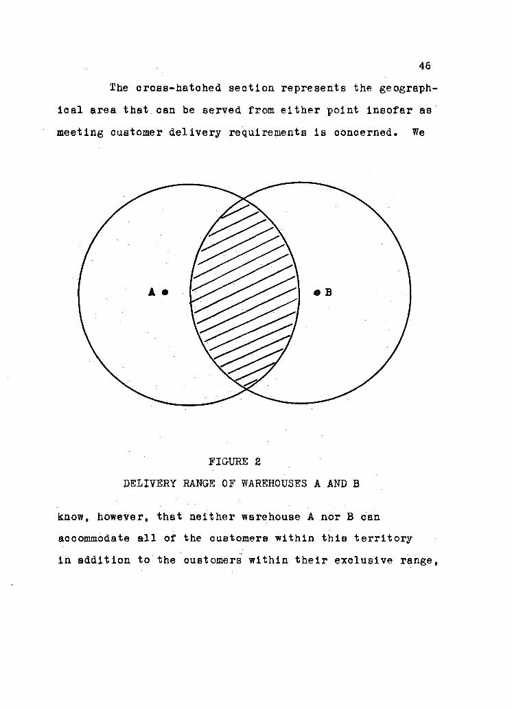
are as shown i n Figure 2.

46

The cross-hatohed section represents the geograph

i c a l area that can be served from either point insofar as

meeting customer delivery requirements is concerned. We

FIGURE 2

DELIVERY RANGE OF WAREHOUSES A AND B

know, however, that neither warehouse A nor B can

accommodate a l l of the customers within this terri tory

in addition to the oustomers within their exclusive range,

47

i e . , the clear area i n Figure 2. The clear area i n the

oentre of Figure 3 represents the remaining overlap i n the

service t e r r i t o r y of warehouses A and B af t e r a reduotion

i n the delivery range of these two stock points to t h e i r

handling capaoity.

FIGURE 3

THE REDUCTION IN DELIVERY RANGE OF DISTRIBUTION POINTS A AND B TO

THEIR HANDLING CAPACITY

48

The cross-hatched section on the right i s now a

part of the t o t a l market area to be served exclusively

from warehouse B. The same section on the l e f t i s now a

part of the t o t a l market area to be served exclusively

from warehouse A.

The extent of the remaining overlap i n service

areas depends upon the anticipated volume of t r a f f i c i n

r e l a t i o n to d i s t r i b u t i o n point capacities. In general,

the t o t a l handling capacity of a l l of the f i n a l

d i s t r i b u t i o n points within a system w i l l not be

s i g n i f i c a n t l y greater than the t o t a l flow of t r a f f i c —

except where warehouse capacity has been established on

the basis of overly optimistic forecasts. Hence, only a

minor portion of the t o t a l volume of t r a f f i c i s l i k e l y to

be within range of alternative d i s t r i b u t i o n points a f t e r

the service areas of stock points have been reduced to

t h e i r handling c a p a c i t i e s . In t h i s case i t i s reasonable

to assume that the bulk of the firm's volume which has now

been assigned to one or another d i s t r i b u t i o n point w i l l

determine the optimum pattern of t r a f f i c flow. Once t h i s

pattern has been established, the marginal cost of

increasing the flow through alternative production-

d i s t r i b u t i o n channels of the pattern can be used to

49

determine which of the d i s t r i b u t i o n points should serve

customers within the remaining overlaps.

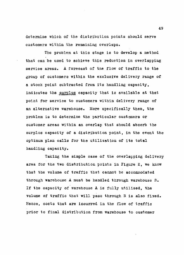
The problem at t h i s stage i s to develop a method

that can be used to achieve t h i s reduction i n overlapping

service areas. A forecast of the flow of t r a f f i c to the

group of customers within the exclusive delivery range of

a stock point subtracted from i t s handling capacity,

indicates the surplus capacity that i s available at that

point for service to customers within delivery range of

an alternative warehouse. More s p e c i f i c a l l y then, the

problem i s to determine the p a r t i c u l a r customers or

customer areas within an overlap that should absorb the

surplus capacity of a d i s t r i b u t i o n point, In the event the

optimum plan c a l l s f o r the u t i l i z a t i o n of i t s t o t a l

handling capacity.

Taking the simple case of the overlapping delivery

area for the two d i s t r i b u t i o n points i n Figure 2, we know

that the volume of t r a f f i c that cannot be accommodated

through warehouse A must be handled through warehouse B.

I f the capacity of warehouse A i s f u l l y u t i l i z e d , the

volume of t r a f f i c that w i l l pass through B i s also f i x e d .

Hence, costs that are incurred i n the flow of t r a f f i c

p r i o r to f i n a l d i s t r i b u t i o n from warehouse to customer

w i l l be the same regardless of the combination of

customers within the overlap that are serviced from the

f u l l y u t i l i z e d warehouse. These costs may be ignored,

therefore, i n determining the oapaeity servioe area of

d i s t r i b u t i o n points.

Since shipping and transportation costs are the only

additional costs between f i n a l stock points and customers,

the t o t a l of these costs may be used as the basis f o r

a l l o c a t i n g the surplus capacity of a d i s t r i b u t i o n ware

house among customers or customer areas within the over

lapping t e r r i t o r y . The objective i s to minimize the t o t a l

shipping and transportation cost to customers within the

overlap — given that the warehouse i n question i s to be

f u l l y u t i l i z e d . Referring again to Figure 2, we would

f i r s t e s t a b l i s h the capacity service area of warehouse A

by minimizing t o t a l shipping and transportation cost to

a l l customers within the overlap-~ given that the t o t a l

capacity of A i s to be u t i l i z e d . The next step would be

to determine the capacity service area of warehouse B i n

the same way and assuming that B, and not A, w i l l be

f u l l y u t i l i z e d .

Where a large number of customers are included i n

the overlap, i t i s desirable to avoid a forecast of

t r a f f i c f or each by dividing the t e r r i t o r y into

transportation rate areas. Each of these areas should

include the group of customers with the same r e l a t i v e

f r e i g h t rate from the alternative d i s t r i b u t i o n points.

For example, i f one hundred customers can be served from

warehouse A at the same freight rate, but only f i f t y of

these have the same rate from warehouse B, the rate area

would consist of the f i f t y customers with the same

r e l a t i v e rate from the two warehouses.

A forecast of demand within each of these rate

t e r r i t o r i e s oan now be related to the capacity that i s

available to the overlap from the alternative


In Figure 4, the overlapping delivery range of

warehouses A and B has been divided into transportation

rate areas. The forecast of sales to customers within

each segment i s shown as well as the capacity that i s

available to the t o t a l overlap from d i s t r i b u t i o n points

A and B.

The problem, then, i s to determine which of these

segments would be served from A i f A i s used to capacity

i n the optimum plan; and, s i m i l a r l y the segments t

would be served from B, i f B i s used to oapacity.

FIGURE 4

TRANSPORTATION RATE AREAS WITHIN THE OVERLAPPING DELIVERY RANGE

OF WAREHOUSES A AND B

Assuming the sum of shipping and transportation

costs between warehouses and customers are as shown i n

Figure 5, we can es t a b l i s h an order of service preference

from each d i s t r i b u t i o n point.

Market Areas U V W X Y Z

Warehouse A 1.00 1.70 1.70 1.80 2.20 1.90

Warehouse B 1.50 1.30 2.30 1.80 1.40 1.80

A - B -.50 .40 -.60 0 .80 .10

FIGURE 5

SHIPPING AND TRANSPORTATION COST

PER UNIT (D0ILARS)

The r e l a t i v e cost of serving the various t e r r i t o r i e s

from warehouse A, indicates that the cost to t e r r i t o r y W

i s seventy cents per unit higher than to t e r r i t o r y U. We

know, however, that i f warehouse A has s u f f i c i e n t capacity

to serve only one of these t e r r i t o r i e s that the other must

54

be served from the alternative d i s t r i b u t i o n point. Hence,

the r e l a t i v e cost, of serving the two customers from ware

house B must also be taken into account. It i s cle a r

that the per unit saving from A to U (seventy cents) i s

offset by the higher oost of serving W from B (eighty

cents). T e r r i t o r y W, therefore, must be served from

point A i n preference to t e r r i t o r y U.

The simpler comparison i s the r e l a t i v e cost of

serving each t e r r i t o r y from the two d i s t r i b u t i o n points.

The saving of sixt y cents per unit by serving t e r r i t o r y

W from A instead of B i s greater than the saving of f i f t y

cents per unit i n serving U from A. Both methods lead to

the same net r e s u l t . The order of preference, therefore,

can be established for each d i s t r i b u t i o n point on the

basis of the difference i n shipping and transportation

cost to the same customers. The order of preference for

warehouse A i s t e r r i t o r i e s W, U, X, Z, V and Y as

indicated by the t h i r d row i n Figure 5.

I f the optimum pattern of t r a f f i c flow c a l l s f o r

the capacity u t i l i z a t i o n of d i s t r i b u t i o n point A, the

1000 units of capacity available at A must be allocated

as shown i n Figure 6. No other a l l o c a t i o n w i l l result

i n a lower t o t a l cost.

55

fe may conclude, therefore, that while t e r r i t o r y

V, X, Y and Z are within delivery range of d i s t r i b u t i o n

point A, the capacity of A w i l l not permit delivery to

V, Y or Z, and, i f f u l l y u t i l i z e d w i l l meet only f i v e -

sixths of the volume required i n t e r r i t o r y X. Hence,

t e r r i t o r i e s V, Y, Z and one-sixth of X may be excluded

from the capacity service area of warehouse A without

eliminating the relevant alternatives for product flow.

Market Areas U - V W X Y Z

Warehouse A 100 400 500

Warehouse B 500 100 E00 300

Market Demand 100 600 400 1

600 200 300

FIGURE 6

OPTIMUM AlLOCATION OF DISTRIBUTION POINT A'S AVAILABLE CAPACITY

The order of preference for warehouse B i s , of

course, the opposite of A, and the same analysis w i l l

indicate that t e r r i t o r i e s U, W, and one-sixth of X may be

excluded from the capacity service area of warehouse B.

T e r r i t o r i e s excluded from the capacity service area

of one warehouse automatically become part of the t o t a l

market area to be served from the alt e r n a t i v e stock point.

The result i n the above example i s a reduction i n the

56

overlap of the service area of warehouses A and B to two-

thirds of the anticipated volume within t e r r i t o r y X.

The volumes of t r a f f i c to t e r r i t o r i e s that are

excluded from A's capacity area can be added to the t o t a l

volume within B's exclusive delivery range. S i m i l a r l y ,

volumes excluded from B's capacity area can be added to

the t o t a l volume within A's exclusive delivery range.

Analysis to determine the optimum flow of t r a f f i c through

production and physical d i s t r i b u t i o n f a c i l i t i e s i s thus

s i m p l i f i e d by reducing the number of demand units to the

number of d i s t r i b u t i o n points (assuming the volumes within

the remaining overlaps are r e l a t i v e l y i n s i g n i f i c a n t and can

be ignored i n formulating t r a f f i c flow alternatives.) I f a

s i g n i f i c a n t proportion of forecasted volume i s to customers

within the remaining overlaps., the number of demand units

f o r analysis can be increased to include some or a l l of the

transportation rate areas that are within these market

segments.

It should be noted that the above procedure f o r

i d e n t i f y i n g segments of the overlap with s p e c i f i c d i s t r i

bution points can be used only for the d i s t r i b u t i o n of a

single product. Transportation rates, however, tend to be

geographically d i s t r i b u t e d and there w i l l be a s i m i l a r

relat i o n s h i p , therefore, between the cost from two ware-

houses to the same customer areas f o r various commodities.

Hence, the same transportation rate areas are l i k e l y to

apply f o r several of the firm's products and s u f f i c i e n t of

these can be included i n analysis to provide the desired

l e v e l of confidence and pr e c i s i o n .

Sales Forecasts

According to a study sponsored by the Controllers

I n s t i t u t e Research Foundation, almost a l l manufacturing

firms use sales forecasts as a primary basis for short-o

term planning i n the various functions of the business.

The short-term forecast generally originates i n the

marketing department. Following approval by upper manage

ment, i t i s passed on to operating d i v i s i o n s to guide and

co-ordinate planning and budgeting. The anticipated

volumes of sales are commonly expressed i n d o l l a r figures

which are then converted by the various departments into

units that are appropriate to planning i n t h e i r respective

areas.

It i s desirable that the approved sales forecast be

used as the basis for production and physical d i s t r i b u t i o n

Burnard H. Sord, Glenn A. Welsch, Business Budgeting (New York: Controllers I n s t i t u t e Research Foundation, 1958), p. 133.

58

planning to ensure that the l e v e l of planned a c t i v i t y i n

t h i s area i s geared to marketing requirements. This

forecast, however, w i l l require refinement before i t can be

used fo r t h i s purpose. In p a r t i c u l a r , the t o t a l volume of

sales w i l l have to be divided among the t e r r i t o r i e s , and into

the product groups that are relevant f o r physical d i s t r i

bution planning.

. It i s suggested that the t r a f f i c manager's role i n

forecasting should be limited to defining the market

dimensions and the product groups that are relevant f o r his

purposes. The marketing department should then assume the

task of a l l o c a t i n g the anticipated sales among the defined

t e r r i t o r i e s according to the various assumptions that

underlie the approved forecast.

I I . FLEXIBILITY IN PRODUCTION AND

PHYSICAL DISTRIBUTION FACILITIES

Production F a c i l i t i e s

The alternatives f o r product flow are l i m i t e d i n

the short-term by the f i x e d l o c a t i o n of the firm's

productive units and by the l i m i t e d capacity of each of

these units.

"Production i s the result of the flow of work that

59

goes from one to another of the fundamental s t r u c t u r a l

elements, each o f which includes man, machine, t o o l s ,

material, and s p e c i f i c a t i o n s . " 3 The maohines and tools

at a plant with which materials can be transformed into

products of the desired s p e c i f i c a t i o n s are given i n the

short-term. The output at a plant, therefore, i s lim i t e d

f i r s t of a l l to the volume that can be achieved through

the maximum u t i l i z a t i o n of i t s machines and t o o l s .

Expansion of output to t h i s l e v e l , however, may be

impossible i n the short-term for several reasons.

Additional manpower of the type that i s required may not

be r e a d i l y a v a i l a b l e , or i t may be impossible to

adequately t r a i n the additional personnel i n the time that

i s a v a i l a b l e . I f increased output c a l l s for the use of

overtime, t h i s may c o n f l i c t with e x i s t i n g labor agreements

or management p o l i c y . The period may be too short to

organize and introduoe the new operations and maintenance

procedures that are required with a higher u t i l i z a t i o n .

These and other constraints must be considered i n

determining the maximum l e v e l of output that i s r e a l i s t i c

f o r each plant i n the short-term.

Raymond V i l l e r s , Dynamic Management i n Industry (Englewood C l i f f s , N.J.: Prentice-Hall, Inc., I960), p. 222.

60

Reinfeld and "Vogel employ what i s referred to as

the bottleneck concept i n determining alternative

production mix f o r a p l a n t . 4 This concept may also be

used to simplify a study of output f l e x i b i l i t y . The

procedure i s t o i d e n t i f y the least f l e x i b l e of the

manufacturing processes within the plant. This may be a

s p e c i f i c machine operation, a process requiring special

labor s k i l l , etc. A thorough study of t h i s p a r t i c u l a r

segment of the t o t a l manufacturing operation w i l l reveal

the maximum output that can be achieved, regardless of

f l e x i b i l i t y i n other processes.

Elements of short-term i n f l e x i b i l i t y including

technical problems, policy and commitments, may also l i m i t

the extent to which output at in d i v i d u a l plants can be

reduced. A decrease i n the l e v e l of output at a plant w i l l

generally involve a reduction i n the labor force and a

r e d i s t r i b u t i o n of work among remaining employees and

among machines. The technical implications of t h i s action

may include a change i n plant layout; new operations and

maintenance plans; and employee t r a i n i n g where the

r e d i s t r i b u t i o n of work requires the remaining employees

*Nyles V. Reinfeld, William R. Yogel, Mathematical Programming (Englewood C l i f f s , N.J.: Prentice-Hall, Inc., 1958), p. 210,

to handle new or additional tasks. The solution to these

problems may well require more time than i s available i n

the short-term. Commitments that l i m i t a reduction i n

plant output may include r e s t r i c t i v e clauses i n labor

contracts, eg., guaranteed annual wage clauses, minimum

work crews, etc. The f i r m may have entered into longer

term purchase agreements with suppliers or transportation

contracts f o r minimum quantities of materials to be

shipped to s p e c i f i c plants. P o l i c y w i l l often govern the

more intangible factors that are involved i n reducing the

l e v e l of plant operation. Employment s t a b i l i z a t i o n p o l i c y ,

fo r example, may be e x p l i c i t i n order to avoid adverse

public or employee reaction. P o l i c y may also apply where

output reductions are l i k e l y to affect the welfare of

employees, dependent suppliers or the community i n which

the plant i s located.

In summary, the relevant alternatives for product

flow are those that c a l l f o r a l e v e l of output at each

plant that i s within the feasible minimum and maximum

range. This range should be defined by responsible

production personnel who are f a m i l i a r with the various

constraints that l i m i t f l e x i b i l i t y i n t h i s function of

the business.

62 D i s t r i b u t i o n Warehouses

The constraints that l i m i t f l e x i b i l i t y i n the rate

of flow through each of the firm's stock points are

s i m i l a r to those that l i m i t the range of output at plants.

Limited storage capacity and given packing and

materials handling f a c i l i t i e s ; i n f l e x i b i l i t y i n the

u t i l i z a t i o n of f a c i l i t i e s due to labor agreements, p o l i c y ,

s k i l l s ; and shortages of the types of labor that are

required to increase handling, are some of the constraints

that must be taken into account l n determining the range

of t r a f f i c volumes that can be accommodated through


Concentration on the least f l e x i b l e of the handling

procedures at a warehouse w i l l s implify the problem of

establishing i t s feasible handling capacity. Materials

handling equipment, f o r example, may l i m i t the volume

that can be accommodated regardless of f l e x i b i l i t y i n

other warehousing operations.

Transportation and Handling

Although there may be a great number of available

modes of transportation between stock points and customers,

the alternatives that are acceptable i n the short-term

63

are l i m i t e d to those that w i l l meet the following

conditions:

1. A minimum delivery service to customers. This

may be the ex i s t i n g standard; an approved lower

standard; or a l e v e l of service requested by the

customer or the marketing department.

2. A maximum delivery standard. This constraint

is necessary to prevent the adoption of a l e v e l

of service that cannot be maintained on a longer

term basis. The maximum should be the standard

c a l l e d for i n the longer-term d i s t r i b u t i o n plans.

3. Transportation methods that are suitable f o r the

firm's products and that can be used i n

conjunction with loading and unloading f a c i l i t i e s

at plants and warehouses. It may be impossible

i n the short-term, f o r example, to adapt the

physi c a l layout of a plant to truck loading i f

the e x i s t i n g arrangement is intended for r a i l

loading. Freight handling or paokaging equip

ment at a plant or warehouse may be l i m i t e d to

use with a s p e c i f i c method of transportation.

4. Transportation methods that are acceptable to

customers. I f customers specify the method, a l l

other forms of transportation are irrelevant i n

64

analysis.

Transportation alternatives to plants and between

plants and warehouses are lim i t e d to those that are

suitable f o r the firm's materials and products; and to

those that can be used i n conjunction with e x i s t i n g

loading and unloading f a c i l i t i e s at plants and warehouses.

Order-Processing and Communications

In addition to s a t i s f y i n g physical movement require

ments, alternatives i n the short-term must be feasible i n

terms of the changes that are necessary i n order-

processing and communications procedures.

A flow of t r a f f i c i s preceded by the flow of paper

work associated with the preparation and dispatch of

customer orders and supply r e q u i s i t i o n s . F l e x i b i l i t y i n

the u t i l i z a t i o n of c l e r i c a l s t a f f s and o f f i c e equipment

must be adequate for the patterns of d i s t r i b u t i o n being

considered i n analysis. The constraints on short-term

changes i n s t a f f that were discussed i n the production

and warehousing sections also apply i n t h i s area.

Communications f a c i l i t i e s i n the form of mail,

telephone and telegraph are generally available f o r any

of the ohanges that may be considered for t r a f f i c flow.

Some firms, however, employ electronic systems for

processing and communicating orders from d i s t r i b u t i o n

points to plants and i n some cases from customers to

d i s t r i b u t i o n points. I f , i n t h i s case, the firm has

abandoned the conventional s t a f f , equipment and paper

procedures that can be used as an alternative to the

system, i t may be impractical to consider alternatives

fo r t r a f f i c flow that do not conform with established

channels of the communications network.

CHAPTER IV

COLLECTION AND PREPARATION OF DATA

The method of analysis suggested i n Chapter V to

determine the optimum a l l o c a t i o n of output among the firm's

plants involves a comparison of the variable cost of the

alternative routes that t r a f f i c may take through the

production-physical d i s t r i b u t i o n system. It i s necessary,

therefore, to determine the alternative t r a f f i c routes that

are available to the f i r m i n the short-term and to i d e n t i f y

and relate the elements of variable cost that are associated

with each of these routes.

Flow diagrams may be useful i n i d e n t i f y i n g

alternative routes and the major processes that are

involved i n t r a f f i c flow. The preparation of these

diagrams i s dealt with i n the f i r s t section of t h i s chapter.

The variable costs of the various processes involved i n

t r a f f i c flow and the types of information that are required

i n order to relate adjacent processes are discussed i n a

l a t e r section.

I. FLOW DIAGRAMS

Magee states that w,.. an organization, whatever i t

may be can be viewed as consisting of a number of stock

points and a number of operations, together with a control

system. In p r i n c i p l e a flow chart can be constructed

showing the course of the flow from the sources of raw

materials through the intermediate stock points to

customers." 1 Transportation i s the connecting l i n k

between adjacent stages i n the flow of materials and

products and i t s a v a i l a b i l i t y and s u i t a b i l i t y , therefore,

w i l l determine the p o t e n t i a l routes that t r a f f i c may take

to plants, between plants and warehouses and from f i n a l

d i s t r i b u t i o n warehouses to customers.

A chart of alternative t r a f f i c routes should begin

by defining the locations of raw materials, plants and

stock points. An evaluation of transportation f a c i l i t i e s

between adjacent stages w i l l then indicate the f e a s i b i l i t y

of l i n k i n g a given plant with a p a r t i c u l a r souroe of raw

materials, a given warehouse with a p a r t i c u l a r plant, etc.

Delivery service i s a prime consideration i n

determining the f e a s i b i l i t y of l i n k i n g a f i n a l d i s t r i b u t i o n

point and a customer through a p a r t i c u l a r mode of trans

portation. Delivery service, however, i s undefined i n the

ohn F. Magee, Production Planning and Inventory Control (New York, N.Y.: McGraw H i l l Book Company, 1958), p. 16.

68

movement of t r a f f i c to. plants and between plants and stock

points -- except where product p e r i s h a b i l i t y or obsolescence

i s involved. I f transportation f a c i l i t i e s are available

and are t e c h n i c a l l y suitable f o r the movement of the firm's

t r a f f i c through to a d i s t r i b u t i o n warehouse, the route i s

feasible regardless of movement time. While successively

longer delivery time increases the inventory carrying cost,

t h i s additional cost may well be offset by savings In one

or more of purchasing, production, warehousing and

transportation costs.

The technical s u i t a b i l i t y of a method of trans

portation must be evaluated i n terms of the nature of

materials or products as well as the handling requirements

at plants and warehouses. The c a r r i e r , for example, must

be capable of accommodating the dimensional size and

weight of the firm's materials or products and must be able

to provide r e f r i g e r a t e d , heated or other s p e c i a l i z e d

equipment where t h i s i s required. loading and unloading

f a c i l i t i e s at plants and warehouses must be adaptable to

the requirements of the c a r r i e r . A stock-pile of

materials or products on a railway spur, f o r example, may

be inaccessible to motor vehicles. Specialized loading

equipment such as oranes and conveyors, and the physioal

l o c a t i o n and layout of the firm's plants and warehouses

69

may also l i m i t i t s a b i l i t y to adapt to a p a r t i c u l a r mode

of available transportation. These and other

considerations must be taken into account before the route

i s accepted as te c h n i c a l l y feas i b l e .

Figure 7 i s a flow diagram of a hypothetical three

plant, fiv e warehouse system. Raw materials are available

from four locations. The l i n e s l i n k i n g raw materials

supply points with plants, and plants with warehouses,

indicate the feasible t r a f f i c routes insofar as trans

portation a v a i l a b i l i t y and s u i t a b i l i t y i s concerned.

Raw materials Locations Warehouses

FIGURE 7

FLOW DIAGRAM

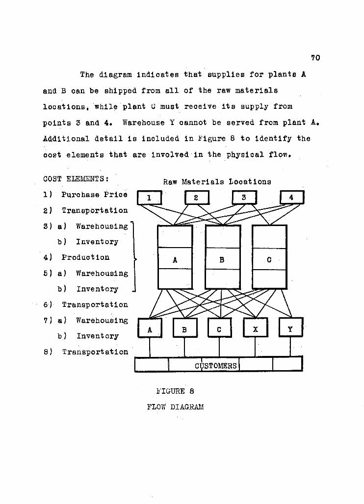
The diagram indicates that supplies f o r plants A

and B can be shipped from a l l of the raw materials

locations, while plant U must receive i t s supply from

points 3 and 4. Warehouse Y cannot be served from plant A ,

Additional d e t a i l i s included i n Figure 8 to i d e n t i f y the

cost elements that are involved i n the physical flow.

COST ELEMENTS:

1) Purchase Prioe

2) Transportation

3) a) Warehousing

b) Inventory

4) Production

5 ) a) Warehousing

b) Inventory

6) Transportation

7 ) a) Warehousing

b) Inventory

8) Transportation

Raw Materials Locations

A B C X Y

CUSTOMERS

FIGURE 8

FLOW DIAGRAM

71

The diagram assumes that customers have been

divided among the f i v e warehouses according to the

procedure described i n the previous chapter.

The advantage of a flow diagram i s that i t s

preparation a s s i s t s the analyst i n his understanding of

the e x i s t i n g system by requiring preliminary studies of

the various processes and t h e i r t e c h n i c a l r e l a t i o n s h i p s .

This background information i s useful i n i d e n t i f y i n g the

feas i b l e t r a f f i c routes and the alternatives for moving

t r a f f i c through each of these routes.

I I . COST SCHEDULES AND OTHER DATA

The cost elements shown i n Figure 8 are not

independent. The delivered cost of raw materials at plants

varies with the sources from which they are received and

the method of transportation that i s used f o r t h e i r

delivery. Moreover, the volume of inventory that must be

carri e d at stock points, as well as the volumes i n t r a n s i t ,

vary with differences i n the delivery time of alternative

c a r r i e r s . Handling costs at warehouses may also d i f f e r

with the alternative methods of receiving and forwarding

materials and products.

Hence, i n addition to estimates of cost f o r each

78

segment of the alternative t r a f f i c routes, the data f o r

analysis must include the key parameters that permit a

l i n k i n g of i n d i v i d u a l cost elements into t o t a l route costs.

These costs and parameters are discussed i n the following

sections. The preparation of data into t o t a l route eosts

i s dealt with i n the la s t part of the chapter.

It i s assumed f o r purposes of t h i s thesis that a l l

raw materials are purchased; that these are transported by

public c a r r i e r to processing plants; that f a c i l i t i e s at

the plant include storage space for materials and fi n i s h e d

produots; and that products are transported by public

c a r r i e r to company owned f i e l d warehouses for d i s t r i b u t i o n

to customers.

Raw Materials Data

The purchase price of raw materials should be

l i s t e d f o r each point at which these are available to the

firm. Alternative prices should be shown i f the price

varies with the size of the order.

A review of the locations and price of raw

materials should be undertaken by the firm's Purchasing

Agent. The results of t h i s survey may be prepared i n a

form such as shown i n Table 1.

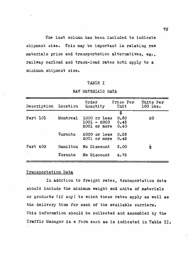
73 The l a s t column has been included to indicate

shipment si z e . This may be important i n r e l a t i n g raw

materials price and transportation a l t e r n a t i v e s , eg.,

railway carload and truok-load rates both apply to a

minimum shipment size.

TABLE I

PAW MATERIALS DATA

Order Price Per Units Per Description Location Quantity Unit 100 Lbs.

Part 101 Montreal 1000 or less 1001 - 2000 2001 or more

1 0.50 20 0.45 0.40

Toronto 2000 or less 2001 or more

0.55 0.45

Part 403 Hamilton No Discount 5.00 £

Toronto No Discount 4.75

Transportation Data

In addition to freight rates , transportation data

should include the minimum weight and units of materials

or products ( i f any) to which these rates apply as well as

the delivery time f o r each of the available c a r r i e r s .

This information should be co l l e c t e d and assembled by the

T r a f f i c Manager i n a form such as i s indicated i n Table I I .

74

The delivery time includes time f o r f i l l i n g the order at

the supply point.

TABLE II

TRANSPORTATION DATA

Commodity: Raw Material - Part 101

Car r i e r From Rate Per

To 100 Lbs. Minimum Weight

Minimum Units

Delivery Time

CNR Mtl. Wpg. 2.50 None - 4 Days

CNR Mtl. Wpg. 1.70 20,000 l b s . 4000 6 Days

Midland Mtl. Wpg. 2.80 None - 3 Days

Midland Mtl. Wpg. 2.00 10,000 l b s . 2000 3 Days

Delivery time has been included i n Table II

because of i t s direct relationship to t r a n s i t and safety

inventories. Minimum shipment volumes to which oertain

rates apply may also require larger than normal cycle

inventories. The nature of these relationships w i l l be

discussed i n d e t a i l i n a l a t e r section of t h i s chapter.

Production Data

The variable processing eost f o r each product that

i s manufactured at a plant should be estimated by the

Production Manager. These estimates w i l l consist l a r g e l y

75

of the wages of some or a l l of the plant employees and the

cost of operating machines and equipment. The cost of raw

materials w i l l he handled separately and should not,

therefore, be included, but information from the production

department should include the types and quantities of raw

materials that are required f o r each product.

Given the period of time to be covered i n the

analysis, the Production Manager w i l l be i n the p o s i t i o n to

ascertain the v a r i a b i l i t y i n cost of the various plant

operations. The determination of costs may be r e l a t i v e l y

simple i f the firm's cost accounting system provides a

l o g i c a l a l l o c a t i o n of variable costs among products.

Processing cost may be presented i n the following form:

TABLE I I I

PROCESSING COST DATA

Location of Plant : Montreal

Variable Cost Per Unit of Product Product Labor ' Machines Other Total

10D

<fe <fe

0.50 0.33 0.08 1

0.91

6F 0.82 0.54 0.15 1.51

76

In addition to cost information, the Production

Manager should determine the output capacity f o r each

plant over the planning period.

Where only one product i s manufactured, or when

manufacturing processes f o r each product are independent,

capacity can he expressed i n "units of product". The more

general problem, however, i s where a plant manufactures

several products, each of whieh pass through one or more

of the same processes. In t h i s case, the mix of output

that w i l l absorb plant capacity cannot be predetermined

and i t becomes necessary to define capacity i n man-hours,

machine-hours or other appropriate common measurement.

The oapacity measurement that should be used depends upon

the nature of the manufacturing process that l i m i t s t o t a l

output. Production at a furniture plant, f o r example, may

be li m i t e d to the rate at which i t s carpenters can assemble

the basic frames. In t h i s oase, available man-hours i n the

frame assembly d i v i s i o n i s an appropriate measurement of

capacity• The output of a pipe m i l l , on the other hand,

may be li m i t e d to the capacity of i t s welding equipment.

In t h i s event, available processing time on welding

machines i s the capacity measurement that should be used

i n analysis.

77

Defining maximum capacity i n t h i s way, i e . , i n

terms of the bottleneck operation, 2 implies that the out

put of other manufacturing processes at the plant can be

adjusted to whatever mix of production i s c a l l e d f o r i n

the optimum plan. This assumption may or may not be v a l i d .

A necessary concluding step i n analysis, therefore, i s to

compare the proposed output of a product with the

capacity of i t s exclusive manufacturing processes; and to

compare combined product outputs against the capacity of

the appropriate eommon manufacturing processes.

Information related to plant capacities should

include a l i s t of the manufacturing processes i n the plant;

the short-term oapaeity for each process In man-hours,

machine-hours or other appropriate measurement; the

products that pass through each of the processes; and the

quantity of process capacity that i s required f o r each

unit of product. Table IV i s an example of the form i n

which t h i s information may be presented.

6Nyles V. Heinfeld, William R. Vogel, Mathematical Programming (Englewood C l i f f s , tf.J.: P rentice-Hall Inc., 1958), p. 210.

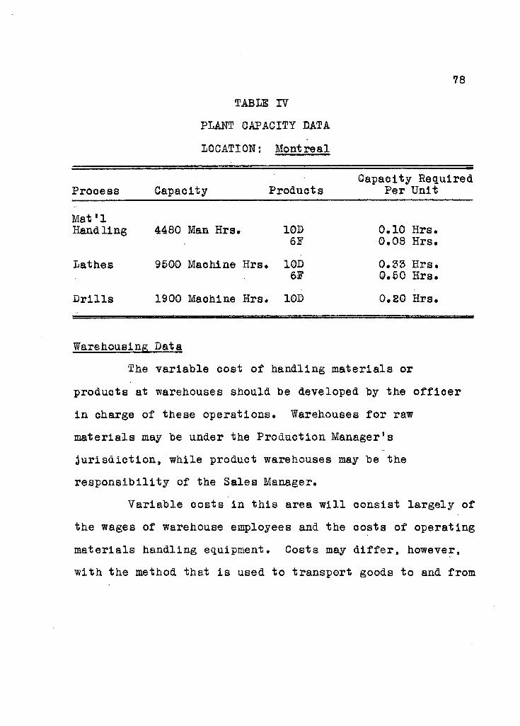
78

TABLE IV

PLANT CAPACITY DATA

LOCATION: Montreal

Capacity Required Process Capacity Products Per Unit

Mat'1 Handling 4480 Man Hrs, 10D 0.10 Hrs. Handling

6F 0,08 Hrs,

Lathes 9500 Machine Hrs, 10D 0.35 Hrs. 6F 0.50 Hrs.

D r i l l s 1900 Machine Hrs. 10D 0.E0 Hrs.

Warehousing Data

The variable cost of handling materials or

products at warehouses should be developed by the o f f i c e r

i n charge of these operations. Warehouses f o r raw

materials may be under the Production Manager's

j u r i s d i c t i o n , while product warehouses may be the

r e s p o n s i b i l i t y of the Sales Manager.

Variable costs i n t h i s area w i l l consist largely of

the wages of warehouse employees and the costs of operating

materials handling equipment. Costs may d i f f e r , however,

with the method that i s used to transport goods to and from

these points. The transportation schedule i l l u s t r a t e d i n

a previous section of t h i s chapter indicates the po t e n t i a l

methods f o r the movement of raw materials and products to

plant warehouses and to d i s t r i b u t i o n warehouses. Using

th i s schedule as a guide, the handling cost per unit of

material or product should be developed f o r each of the

potent i a l modes of transportation. This information may

be presented i n a form such as i s indicated i n Table 7.

TABLE V

WAREHOUSING DATA

LOCATION: Winnipeg

Method of Handling Cost Product Transport ation Per Unit

10D R a i l CL f

0.025 R a i l - LCL 0.015 Truck 0.010

6F R a i l - CL 0.100 R a i l - LCL 0.125 Truck 0.125

The capacity of d i s t r i b u t i o n warehouses w i l l have

been taken into account i n determining t h e i r geographical 2

service areas. Warehousing space f o r raw materials and

See Chapter I I I , pp. 41-57.

80

f i n i s h e d product inventories at plants w i l l not be

considered d i r e c t l y i n the production a l l o c a t i o n analysis.

Provision should be made, however, to check the space

capacity of those points at which the volume of inventories

(as suggested i n the a l l o c a t i o n solution) i s s i g n i f i c a n t l y

greater than i n the past.

Inventory Bata

The cost of carrying Inventory i n the short-term

inoludes the r i s k of obsolesoenee and deterioration, as

well as the opportunity cost of having funds invested i n

inventories. A cost i s involved i n the use of storage

space at warehouses only i f the space has alternative

productive use.

It i s assumed for purposes of t h i s thesis that the

cost of carrying inventory i s l a r g e l y the opportunity cost

involved i n having funds t i e d up i n materials and products.

This cost should represent n...the return that would be

obtained i f the c a p i t a l were invested otherwise. In

making t h i s estimate, account should be taken of the

l i q u i d i t y and r i s k involved."^

^Charles C. Holt, Franco Modigliani, John F. Muth, Herbert A. Simon, Planning Production. Inventories and Work Force (Englewood G l i f f s , N.J.: Pren t i c e - H a l l Inc., 19"60), p. 71.

81

Trie quantity and value of inventory that w i l l he

required for each of the t r a f f i c routes i s dealt with i n

the l a t t e r part of t h i s chapter. At t h i s stage i t i s

s u f f i c i e n t to define the cost of carrying inventory i n

terms of the percentage return that i s required on

inventory investment.

Order-processing and Communication Data

The cost of placing an order includes the c l e r i c a l

time involved i n preparing the r e q u i s i t i o n , the cost of

stationary, and the variable cost of using o f f i c e

machines and equipment. Transmitting the order to the

supply point includes the cost of postal, telephone,

telegraph and other f a c i l i t i e s that may be used f o r t h i s

purpose. The cost of processing an order received at a

plant from a d i s t r i b u t i o n point w i l l include the variable

c l e r i c a l , stationary and machine costs of issuing shipment

req u i s i t i o n s or other i n s t r u c t i o n s to the shipping

department.

The variable cost of order placement and trans

mission should be developed for each of the relevant

combinations of raw materials supply points and plants.

The variable cost of order placement, transmission and

8E

receipt should be developed for each of the plant to

warehouse alt e r n a t i v e s . This information may be prepared

as shown i n Table VI.

TABLE VI

ORDER PROCESSING AND COMMUNICATION COSTS

Variable Cost Per Order

Placing Receiving Order From To Order Order Transmission T o t a l Cost

I t $ I M t l . Wpg. 10.00 10.00 5.00 25.00

Mtl. Edmtn. 10.00 7.00 7.00 24.00

The fourth column w i l l be l e f t blank: f o r orders placed by

the plant since i t i s assumed that a l l raw materials are

purohased from outside suppliers.

I I I . TOTAL ROUTE COST

The method of comparing alternatives suggested i n

Chapter V requires an estimate of the t o t a l unit variable

cost incurred i n the manufacture and p h y s i c a l ' d i s t r i b u t i o n

of each product to each d i s t r i b u t i o n warehouse and through

each of the routes that the product may take through the

8 3

production-distribution system.

The f i r s t section of t h i s chapter indicated that

the p o t e n t i a l t r a f f i c routes and t h e i r major component

processes can he i d e n t i f i e d through the preparation of a

flow diagram. Each of the alternative routes consist of

a source of raw materials, a plant and a d i s t r i b u t i o n

warehouse linked together by one or more methods of

transportation. The second section discussed the variable

cost of the Individual processes involved i n the flow of

t r a f f i c and the types of other information that may be

required to l i n k successive processes into route

alternatives. At t h i s stage i t i s necessary to examine

some of the implications of adding together the related

costs of adjacent processes.

The f i r s t part of t h i s section deals with the

problems of r e l a t i n g the variable costs of physical

d i s t r i b u t i o n between a plant and a f i n a l d i s t r i b u t i o n

warehouse. It i s assumed f o r purposes of t h i s discussion

that the accumulated variable cost of the product up to the

point at which i t i s available for d i s t r i b u t i o n at the

plant has been determined. The f i r s t h a l f of the t r a f f i c

route, i e . , the purchase and d i s t r i b u t i o n of raw materials

and the manufacturing process, i s discussed i n the l a t t e r

84

half of t h i s section.

Estimating the Costs of Physical D i s t r i b u t i o n from Plant to Warehouse

The problem at t h i s stage i n analysis i s to

determine the minimum cost method of u t i l i z i n g each of the

feasible plant to warehouse routes. Taking one route at a

time, we may proceed by r e l a t i n g each of the cost elements

to each of the alternative methods of transportation f o r

the route. A comparison of the t o t a l costs associated with

each of the alternatives f o r transportation w i l l then

indicate the minimum cost method of physical d i s t r i b u t i o n

for the route.

To I l l u s t r a t e the procedure, we w i l l assume that

the planning period has been defined as "the year ending

December 31, 1965" and that the following information

r e l a t i n g to t h i s period has been developed:

1. Product value at the Plant (PV) = $10.00 per

unit.

2. Transportation alternatives between the plant

and warehouse and t h e i r respective per unit

costs:

85

Transpor- Minimum Transit Time ta t i o n Cost Shipping Plant to

Alternative Per Unit Quantity Warehouse | (Unit .8) (Days)

1) Rail-CL 0.10 1,200 7

2) Rail-ICL 0.17 - 5

3) Truck-TL 0.14 600 4

4) Truek-LTl 0.20 - 3

Handling costs per unit at the plant and ware

house, assuming a direct r e l a t i o n s h i p to the

method of transportation that i s used.

Method of Transport at i o n

Handling Cost Per Plant Warehouse

* *

Unit T o t a l $

1) Rail-CL 0.015 0.025 0.040

2) Rail-LCL 0.015 0.015 0.030

3) Truck-TL 0.010 0.010 0.020

4) Truck-LTL 0.010 0.010 0.020

Order-processing and communication costs (S):

Cost of placing an order at the warehouse #10.00

Cost of receiving and d i s t r i b u t i n g the

order at the plant 10.00

Cost of expediting the order 5.00

To t a l per order $25.00

Cost of carrying inventory ( I ) : 25 percent of

the inventory value.

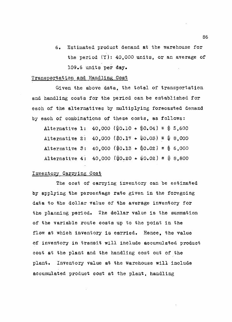
86

6, Estimated product demand at the warehouse f o r

the period (Y): 40,000 units, or an average of

109.6 units per day.

Transportation and Handling Cost

Given the above data, the t o t a l of transportation

and handling costs f o r the period can be established f o r

each of the alternatives by multiplying forecasted demand

by each of combinations of these costs, as follows:

Alternative 1: 40,000 (#0.10 + $0.04) = $ 5,600

Alternative E: 40,000 ($0.17 + $0.03) = $ 8,000

Alternative 3: 40,000 ($0.13 + $0.02) = $ 6,000

Alternative 4: 40,000 ($0.20 + $0.02) = $ 8,800

Inventory Carrying Cost

The cost of carrying inventory can be estimated

by applying the percentage rate given i n the foregoing

data to the d o l l a r value of the average inventory f o r

the planning period. The d o l l a r value i s the summation

of the variable route costs up to the point In the

flow at which inventory i s ca r r i e d . Hence, the value

of inventory i n t r a n s i t w i l l include accumulated product

cost at the plant and the handling cost out of the

plant. Inventory value at the warehouse w i l l include

accumulated product cost at the plant, handling

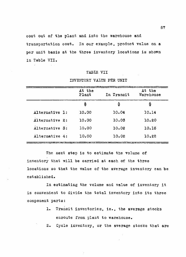
87

cost out of the plant and into the warehouse and

transportation cost. In our example, product value on a

per unit basis at the three inventory locations i s shown

in Table VII.

TABLE VII

INVENTORY VALUE PER UNIT

At the At the Plant In Transit Warehouse

4fe <lfe

* * * Alternative 1: 10.00 10.04 10.14

Alternative 2: 10.00 10.03 10.20

Alternative 3: 10.00 10.02 10.15

Alternative 4: 10.00 10.02 10.22

The next step i s to estimate the volume of

inventory that w i l l be car r i e d at each of the three

locations so that the value of the average inventory can be

established.

In estimating the volume and value of inventory i t

i s convenient to divide the t o t a l inventory into i t s three

component parts:

1. Transit Inventories, i e . , the average stocks

enroute from plant to warehouse.

2. Cycle Inventory, or the average stocks that are

88

carried at the plant and warehouse to meet

normal demand,,

3. Safety inventory, l e . , stocks that are held at

the warehouse to protect against unanticipated

lnoreases i n demand between the time orders

are placed and received.

These three inventories are shown graphically l n

Figure 9.

Normal rate of demand

Maximum reasonable demand over the lead time

V " | "rv—

Transit Lead Time Time

T I M E—= •

FIGURE 9

AVERAGE CYCLE, TRANSIT AND SAFETY INVENTORIES

89

The average volume of inventory i n tr a n s i t f o r the

planning period i s simply the normal rate of demand per day

multip l i e d by the number of days i t takes to transport the

product from plant to warehouse. The volume and value of

tra n s i t inventory i n our example, therefore, may be

computed as follows:

TABLE VIII

VOLUME AND VALUE OF TRANSIT INVENTORY

Normal Average Per Value of Avge. Demand Transit Transit Unit Inventory i n Per Day Time Inventory Value Transit

Alternative 1: (Units) 109.6

(Days) 7

(Units) 767 10.04

$ 7701

Alternative £: 109.6 5 547 10.03 5496

Alternative 3: 109.6 4 436 10.02 4393

Alternative 4: 109.6 3 328 10.02 3295

In estimating the average volume of cycle stock that

w i l l be carried with each of the four alternatives, we may

employ a modification of the equation that i s used by

Magee, op., c i t . t p. 17. Note that the result of t h i s c a l c u l a t i o n represents the average inventory i n t r a n s i t over the planning period rather than the average over the t r a n s i t Intervals of the period.

90

Whitin to determine the optimum purchase quantity.

The equation, before modification, i s as follows:

Y = expected yearly sales i n units'

Q, = economic purchase quantity i n units

C = unit cost

S = procurement expense i n making one

order ( i n d o l l a r s )

I = cost of carrying a d o l l a r s worth of

inventory over the planning period.

This equation recognizes that the t o t a l variable

cost associated with cycle stock includes the cost of

procuring the inventory as well as the cost of carrying

the inventory. Expressed i n equation form, procurement

cost f o r the period becomes Y g and carrying cost becomes

0,0 _ . The d i v i s i o n by two i n the l a t t e r equation

suggests that, on the average, one-half of the order

quantity w i l l be on hand at the stock point. This

assumption i s reasonable when i t i s expected, as i n our

6Thornson M. Whitin, The Theory of Inventory Management (Princeton, New Jersey: Princeton University Press, 1957). p. 33.

where,

2

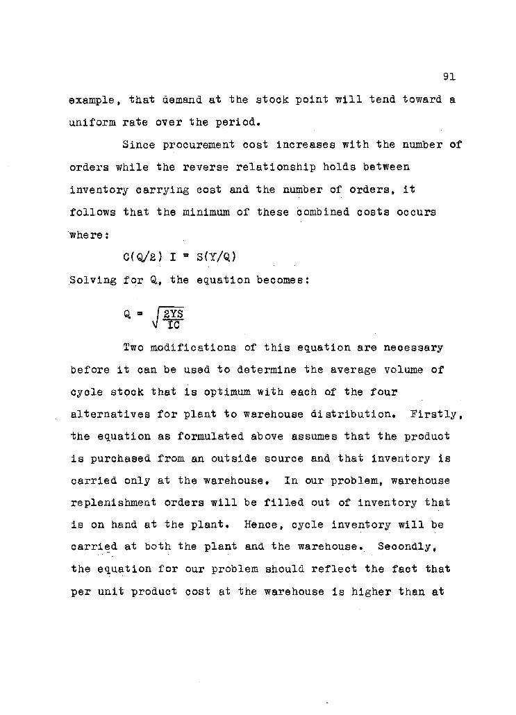
91

example, that demand at the stock point w i l l tend toward a

uniform rate over the period.

Since procurement cost increases with the number of

orders while the reverse r e l a t i o n s h i p holds between

inventory carrying cost and the number of orders, i t

follows that the minimum of these oombined costs occurs

where:

C(Q/E) I a S(Y/Q)

Solving f o r 0,, the equation becomes:

Q, » / EYS V IC

Two modifications of t h i s equation are neoessary

before i t can be used to determine the average volume of

cyole stock that i s optimum with eaeh of the four

alternatives f o r plant to warehouse d i s t r i b u t i o n . F i r s t l y ,

the equation as formulated above assumes that the product

i s purchased from an outside source and that inventory i s

carried only at the warehouse. In our problem, warehouse

replenishment orders w i l l be f i l l e d out of inventory that

i s on hand at the plant. Hence, cycle inventory w i l l be

carr i e d at both the plant and the warehouse. Seoondly,

the equation f o r our problem should r e f l e c t the fact that

per unit product cost at the warehouse i s higher than at

92

the plant by the per unit handling and transportation

costs.

Assuming f o r our purpose that the rate of

production at the plant w i l l be geared to the normal rate

of demand at the warehouse, output at the plant w i l l

accumulate at the same rate as inventory at the warehouse

i s depleted. Total cycle stock, therefore, w i l l be equal

to the size of the warehouse replenishment order — an

average of one-half of t h i s quantity being on hand at eaoh

of the plant and the d i s t r i b u t i o n warehouse. I f we l e t

G denote the unit cost of the product at the plant and

G w the unit cost of the product at the warehouse, the cost

of carrying cycle stock can be written as?

1(0/2) C p + KQ/2) , or 1(072) (G p + C w) Then the t o t a l of procurement costs (order-processing and

oommunioations) and inventory carrying costs i s at a

minimum where:

K Q / 2 ) (G p + G w) = S(Y/QJ

Solving f o r Q,, t h i s equation becomes;

Q, = / 2YS

See Table VII, p. 87.

This equation may now be applied to determine the

optimum volume of cycle stock f o r each of the four

alternatives f o r physical d i s t r i b u t i o n between the plant

and warehouse. Using the sales volume (Y), the order-

processing and communications cost (S), and the carrying

cost per d o l l a r of inventory (I) given i n the data at

the beginning of the section; and the per unit product

costs at the plant and the warehouse as shown i n Table VII,

the optimum cycle stocks (Q,) f o r each of the alternatives

are as follows:

Alternative 1: Q = / ,2 (125.00) (40.000) = 6 3 0 u n i t s

\/0.25 (flO.OO + $10.14)

Alternative 2: Q = / 2 (125.00) (40,000) = &Z9 units JO.25 (§10.00 + flO.20)

Alternative 3: Q = fz ($25.00) (40,000) = 6 2 0 units s/o.r --- -,25 ($10.00 + 110.15)

Alternative 4: Q = / 2 ($25.00) (40.000) = 6 2 9 u n i + a

VO.25 ($10.00 +. 110.22) Referring back to the data presented at the

beginning of th i s chapter, however, we see that there i s

a minimum shipping quantity of 1,200 units associated with

the oarload transportation a l t e r n a t i v e . Hence, although

the above formula suggests an order quantity of 630 units

for alternative one, i t i s clear that the order quantity

8 See pp. 85-86.

94

w i l l have to he 1,200 units for t h i s alternative i n order

to obtain the carload freight rate.

Since, on the average, one-half of the order

quantity w i l l be on hand at each of the plant and warehouse,,

the d o l l a r value of cycle stock may be expressed as

follows:

Q/2 (C p) + Q/2 (C w)

The result of t h i s c a l c u l a t i o n i s shown i n Table IX for

each of the alternatives i n our example.

TABLE IX

VOLUME AND VALUE OF CYCLE INVENTORY

Volume Value

(units) I

Alternative 1: 1200 12,084




Safety inventory at a d i s t r i b u t i o n warehouse i s

necessary to protect against unpredictable increases i n

demand over the lead time, i e . , over the i n t e r v a l between

the time a replenishment order i s placed and received.

But the cost of carrying additional inventory to protect

95

against maximum possible demand over these i n t e r v a l s i s

usually p r o h i b i t i v e . It becomes necessary, therefore, to

es t a b l i s h "...a reasonable balance between the amount of

extra inventory (and i t s o a p i t a l , storage and other costs)

and the protection obtained against stock exhaustion."

To estimate the volume of safety stock at which

t h i s balance i s achieved, Magee states that two pieces of

information are required:

1. A d i s t r i b u t i o n of differences between foreoast

and actual demand over a lead time.

2. An agreement as to how often run-outs may be

allowed to o c c u r . ^

The f i r s t part of th i s information indicates the

frequency with which stock shortages are l i k e l y to occur

at various l e v e l s of safety Inventory. The permissable

frequency of stook run-outs given i n the second part the n

indicates the l e v e l of safety inventory that i s necessary.

The d i s t r i b u t i o n of differences between forecast

and actual demand can be estimated from h i s t o r i c a l

experience. Assume, for example, that the lead time i s

Magee, op_. c i t . , p. 69.

'ibid., p. 7£.

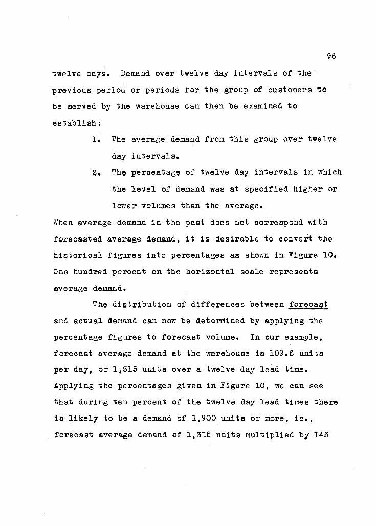
96

twelve days. Demand over twelve day i n t e r v a l s of the

previous period or periods for the group of customers to

he served hy the warehouse can then be examined to

es t a b l i s h :

1. The average demand from t h i s group over twelve

day i n t e r v a l s .

2. The percentage of twelve day in t e r v a l s i n which

the l e v e l of demand was at spec i f i e d higher or

lower volumes than the average.

When average demand i n the past does not correspond with

forecasted average demand, i t i s desirable to convert the

h i s t o r i c a l figures into percentages as shown i n Figure 10.

One hundred percent on the horizontal scale represents

average demand.

The d i s t r i b u t i o n of differences between forecast

and actual demand can now be determined by applying the

percentage figures to forecast volume. In our example,

forecast average demand at the warehouse i s 109.6 units

per day, or 1,315 units over a twelve day lead time.

Applying the percentages given i n Figure 10, we can see

that during ten percent of the twelve day lead times there

i s l i k e l y to be a demand of 1,900 units or more, i e . ,

forecast average demand of 1,315 units m u l t i p l i e d by 145

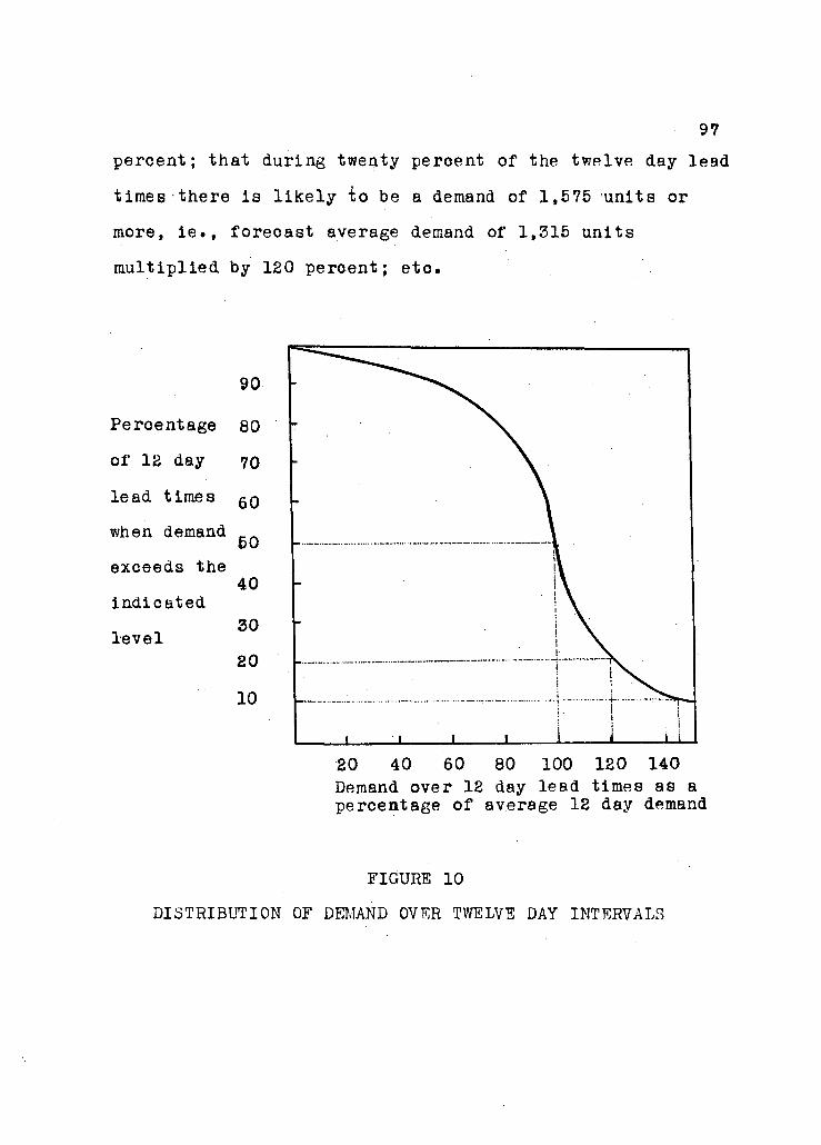
97 percent; that during twenty peroent of the twelve day lead

times there i s l i k e l y i o be a demand of 1,575 units or

more, i e . , foreoast average demand of 1,315 units

multiplied by 120 peroent; etc.

i • 1 J L i _ 20 40 60 80 100 120 140 Demand over 12 day lead times as a percentage of average 12 day demand

FIGURE 10

DISTRIBUTION OF DEMAND OVER TWELVE DAY INTERVALS

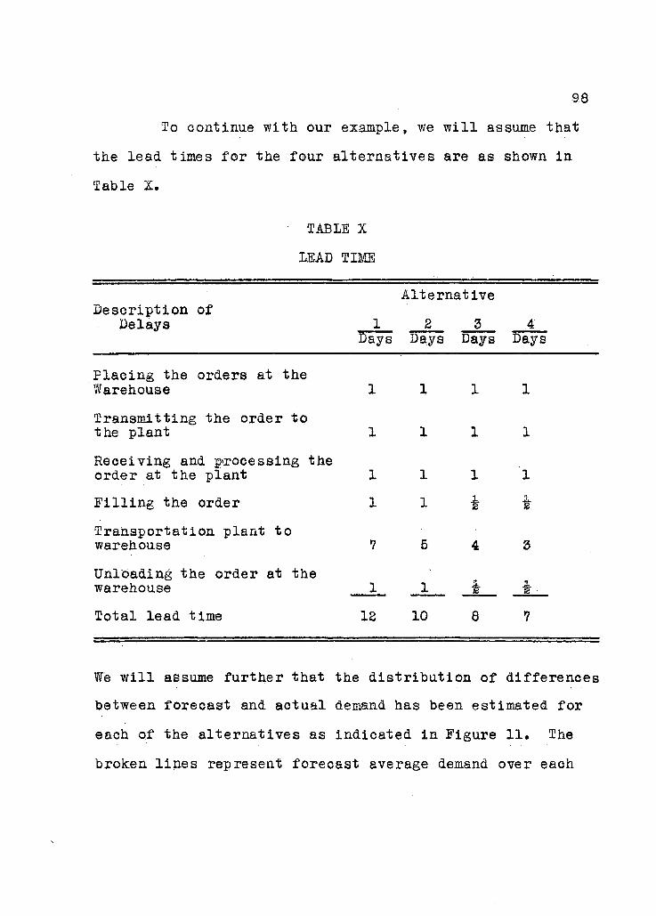
98

To continue with our example, we w i l l assume that

the lead times f o r the four alternatives are as shown i n

Table X.

TABLE X

LEAD TIME

Description of Delays

Alternative

Days Days Days Days

Placing the orders at the Warehouse

Transmitting the order to the plant

Receiving and processing the order at the plant

F i l l i n g the order

Transportation plant to warehouse

Unloading the order at the warehouse

1

1

1

1

7

1

1

1

1

1

5

1

1

1

4

1

1

Total lead time 12 10 8

We w i l l assume further that the d i s t r i b u t i o n of differences

between forecast and actual demand has been estimated f o r

each of the alternatives as indicated i n Figure 11. The

broken l i n e s represent forecast average demand over each

of the lead times. Since cycle inventory i s intended to

s a t i s f y average demand, safety inventory w i l l be the

volume i n excess of t h i s quantity. Hence i f the protection

that i s required against stock shortages i s set at a l e v e l

equivalent to ten percent of the lead times, I t i s apparent

that a safety stook of 585 units w i l l be necessary with a

lead time of twelve days (1,900 units as shown i n Figure 11

at the ten percent l e v e l l e s s average demand over the lead

time of 1,315 u n i t s ) .

90 lead Times

80 12 Days 70 10 Days

Percentage 70

8 Days of lead times 60 -7 Days when demand 50 exoeeds the

50 ft \ A

Indicated 40 \ i\ '\ I \ i \ ! \ level 30 \ \ \ 20

10 I I » ' * . I • I

600 1000 1500 2000 Demand over lead times

FIGURE 11

DISTRIBUTION OF DEMAND OVER INDICATED LEAD TIME

100

The next step i n estimating the volume of safety

inventory i s to determine the l e v e l of protection that i s

required against stock shortage. This w i l l depend i n part

upon the cost of carrying successively larger volumes of

safety stock and i n part upon opposing factors such as

possible losses i n sales due to stock shortages,

deterioration i n r e l a t i o n s with customers as a result of

delivery delays, etc.

The cost of carrying safety inventory f o r

alternative l e v e l s of protection can be estimated by

multiplying the appropriate volumes, as calculated from

Figure 11, by the cost of oarrying a unit of inventory

over the defined planning period. The extent and cost of

sales losses and deteriorated r e l a t i o n s with customers as

a result of stock shortages, however, i s d i f f i c u l t to

i d e n t i f y and to quantify. In the t y p i o a l case, therefore,

the judgement of experienced management personnel i s l i k e l y

to play an important role In estimating these costs, and i n

balancing the sum of these factors against the costs of

carrying safety inventory to arrive at an agreement as to

the permissible frequency of stock run-outs.

Continuing with our example, we w i l l assume that an

agreement has been reached to the ef f e c t that stock short-

101

ages should not occur more frequently than six times during

the planning period. This i s equivalent to saying that i t

is permissible to have a stock shortage at the warehouse

during s i x of the t o t a l lead times, since i t i s only during

a lead time that the r i s k of run-out occurs. There w i l l be

a t o t a l of thirty-three lead times over the period i f

alternative one i s used ( t o t a l demand of 40,000 units f o r

the year divided by the order quantity of 1,200 u n i t s ) .

Alternatives two, three and four each require a t o t a l of

sixty-four lead times over the period. Hence, the l e v e l

of protection expressed as a percentage-of-lead-time w i l l

be eighteen percent f o r alternative one and nine percent

for each of alternatives two, three and four (permissible

stock-outs divided by the t o t a l number of lead times).

The volume of safety stock can now be determined from

Figure 11 by taking the difference between the quantities

indicated i n t h i s chart at the eighteen percent and f i f t y

percent l e v e l s f o r alternative one and at the nine percent

and f i f t y percent l e v e l s for alternatives two, three and

four. Figure 11 has been used i n estimating the volumes

of safety stock shown i n Table XI.

102

TABLE XI

VOLUME AND VALUE OF SAFETY STOCK

ALTERNATIVE 1 2 3 4

Maximum demand over the lead time at the 18$ l e v e l of protection (units) 1650

Maximum demand over the lead time at the 9% l e v e l of protection (units) 1625 1200 1080

Average demand over the lead time (units) 1315 1096 877 767

Safety stock (units) 335 529 323 313

Unit produet value at the warehouse §10.14 110.20 $10.16 $10*22

D o l l a r value of safety stock: |3397 #5396 #3282 $3199

Having estimated the value of t r a n s i t , cycle and

safety stocks, the cost of carrying inventory can now he

estimated f o r each of the four alternatives by applying the

carrying cost per d o l l a r of inventory to the sum of these

three inventory amounts. Inventory values given i n Tables

VIII, IX and XI have been t o t a l l e d i n Table XII and the

percentage rate has been applied to produce an estimate

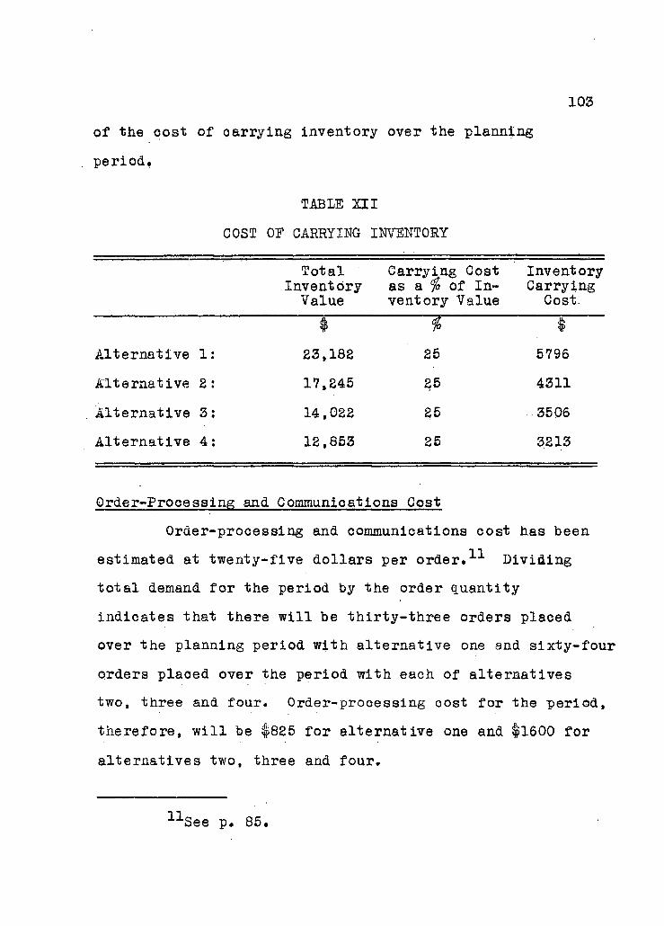
103

of the cost of oarrying inventory over the planning

period.

TABLE XII

COST OE CARRYING INVENTORY

Total Inventory

Value

Carrying Cost as a fo of Inventory Value

T 25

25

25

25

Inventory Carrying

Cost.

Alternative 1:

Alternative 2:

Alternative 3:

Alternative 4:

23,182

17,245

14,022

12,853

5796

4311

3506

3213

Order-Processing and Communications Cost

Order-processing and communications cost has been

estimated at twenty-five d o l l a r s per o r d e r . 1 1 Dividing

t o t a l demand f o r the period by the order quantity

indicates that there w i l l be thir t y - t h r e e orders placed

over the planning period with alternative one and sixty-four

orders plaoed over the period with each of alternatives

two, three and four. Order-processing oost for the period,

therefore, w i l l be |825 f o r alternative one and |l600 for

alternatives two, three and four.

See p. 85

104

Tota l Variable Cost

To complete the example that we are using f o r

i l l u s t r a t i o n purposes, i t remains to t o t a l the i n d i v i d u a l

cost elements developed i n the preceding section. Table

XIII i s a summary of these costs and shows the t o t a l and

the per unit cost of physical d i s t r i b u t i o n from the plant

to the d i s t r i b u t i o n warehouse f o r each of the four

a l t e r n a t i v e s .

TABLE XIII

TOTAL VARIABLE COST OF PHYSICAL DISTRIBUTION

PLANT TO WAREHOUSE

ALTERNATIVE

Cost Elements 1 2 3 4

Transportation and

Handling $ 5,600 | 8,000 #6,000 $ 8,800

Inventory 5,796 4,311 3,506 3,213

Order-processing and

Communication 825 1.600 1,600 1.600

Total Cost 12,221 13,911 11,106 13,613

Per Unit Cost 0.306 0.348 0.278 0.341 It i s clear that the t h i r d alternative i s the

optimum method f o r physical d i s t r i b u t i o n from the plant to

the d i s t r i b u t i o n warehouse used i n t h i s example.

105

To produce an estimate of the t o t a l variable cost

for the whole route we must now add the |0.278 per unit for

plant to warehouse d i s t r i b u t i o n to the variable cost per

unit for the f i r s t h a l f of the route, i e . , to the accumulated

variable eost of the product up to the point at which i t

becomes available f o r d i s t r i b u t i o n at the plant. In

developing inventory carrying costs f o r the plant to ware

house portion of the route, we assumed that the accumulated

variable cost for the f i r s t half of the route had already

been estimated at $10.00 per unit. Total variable cost

for the whole route, therefore, would be flO.88 per unit.

This figure w i l l be the one that i s compared with

s i m i l a r l y developed unit costs representing alternative

routes to determine the optimum a l l o c a t i o n of output among

the firm's plants. This comparison w i l l be dealt with i n

chapter V.

Returning now to the procedure for determining

t o t a l variable cost f o r the f i r s t half of the route, the

problem i s to r e l a t e the processes that are Involved i n

the physical d i s t r i b u t i o n of raw materials and i n t h e i r

manufacture into the f i n i s h e d product. The objective

i s to determine the minimum per unit product cost at each

of the plants for each of the points from which raw

106

materials may be reoeived.

Estimating trie Cost for the F i r s t Half of a T r a f f i c Route

Dealing with one plant at a time, the f i r s t

problem i s to specify the products that the plant i s

equipped to manufacture and the raw materials requirement

fo r each of these products. At thi s point i t should be

decided i f i t w i l l be worthwhile to investigate the

physical d i s t r i b u t i o n of a l l of the materials that are

used i n the manufacturing prooess. I f the product consists

of one or two basic materials and only minimal amounts of

several other r e l a t i v e l y low cost items, an inv e s t i g a t i o n

of the physical d i s t r i b u t i o n of the l a t t e r group i s not

l i k e l y to bring about a s i g n i f i c a n t change i n produot cost.

The quantity, purchase price and transportation cost of

each of the raw materials that are used f o r a product are

the major factors that should be considered i n deciding

which of these should be included i n the study of raw

materials d i s t r i b u t i o n .

It may be assumed, for purposes of estimating the

per unit cost of the excluded group, that these materials

w i l l be received from the same source as i n the past; that

the transportation and handling cost w i l l be the same and

that the same l e v e l of inventory per unit of material w i l l

107

apply. In other words, an approximation based upon

h i s t o r i c a l records should be adequate f o r an estimate of

the per unit delivered cost f o r t h i s group of materials.

The second step i s to investigate the physical

d i s t r i b u t i o n of each of the raw materials that have been

selected f o r further i n v e s t i g a t i o n . The objective i s to

determine the minimum cost method of physical d i s t r i b u t i o n

to the plant from each of the available sources of supply.

The available sources are those from which there are

suitable methods of transportation.

The costs that are involved i n the physical

d i s t r i b u t i o n of raw materials include the purchase p r i c e ,

transportation, handling, order-processing and inventory

carrying costs. The purchase price can be obtained from

the purchasing department. The,alternatives f o r

transportation and handling and t h e i r respective costs w i l l

be available i f the schedules discussed i n the previous

section of t h i s chapter have been prepared.

Inventory and order-prooessing costs f o r t h i s

portion of the route cannot be established with the same

degree of p r e c i s i o n as f o r plant to warehouse d i s t r i b u t i o n .

It has been shown that the volume of inventory that i s

required i s c l o s e l y related to the rate of demand. The

108

demand for a product at a s p e c i f i c plant, however, i s

c l e a r l y unknown at t h i s stage since i t i s the objective of

analysis to determine how t o t a l demand should be allocated

among the firm's plants.

For purposes of a preliminary estimate of order-

processing and inventory carrying costs, i t may be assumed

that demand f o r raw material at the plant over the planning

period w i l l be the same as i n the past. The procedure as

described above f o r plant to warehouse d i s t r i b u t i o n may now

be used to estimate the t o t a l inventory and order-processing

cost for the period for each of the alternatives f o r

transportation and handling between a source of raw

materials and the plant. Since i t i s assumed that raw

materials are purchased, there w i l l be no stocks held at

the source. Cycle inventory, therefore, w i l l be equal to

one-half of the order quantity, as compared with a cycle

inventory equivalent to t o t a l order quantity f o r plant to

warehouse d i s t r i b u t i o n . It should be noted that the

percentage of inventory value representing the cost of

carrying inventory w i l l , i n t h i s case, be applied to the

sum of the purchase price and the cost of transporting and

handling the material between i t s source and the plant.

The estimate of inventory and order-processing cost

109

may now be added to the related purchase p r i c e ,

transportation and handling costs to determine the t o t a l

variable cost of the raw material at the plant. A

comparison of the t o t a l variable cost associated with each

of the methods of transportation and handling w i l l then

indicate the alternative that offers minimum materials

cost from a given source.

It i s assumed i n t h i s thesis that there i s no l i m i t

to the volume of a raw material that can be purchased from

a single source. Hence, where there are two or more

available sources of supply f o r a s p e c i f i c plant, the cost

of material used i n determining product cost w i l l be the

minimum of a l l of the al t e r n a t i v e s . In other words, a

f i n a l comparison of the minimum material cost at the plant

from each of the sources of supply w i l l have to be made to

ensure that the material cost used i n analysis i s the

minimum of the alternatives from a l l available sources of

supply.

Given the minimum t o t a l variable cost of raw

materials at the plant, i t remains to add the cost of the

quantities required by a product to the processing cost to

determine the variable cost of the product at the plant.

The types and quantities of raw material that are used i n

110

the manufacture of a product, as well as the processing

cost per unit of product, w i l l be available from the

information provided by the production department.

The per unit product cost at the plants as

determined through the above procedure may now be used as

the basis for establishing delivered product cost at each

of the firm's d i s t r i b u t i o n points. The method f o r

determining t o t a l cost f o r the plant to d i s t r i b u t i o n ware

house portion of the route has been outlined i n the f i r s t

part of t h i s section. Although plant to warehouse

d i s t r i b u t i o n was considered f i r s t i n the foregoing

discussion, i t i s necessary, of course, to develop

estimates of product cost at the plants before the t o t a l

cost of the product at f i n a l d i s t r i b u t i o n warehouses can

be ascertained.

In summarizing t h i s chapter i t i s suggested that

a preliminary study of transportation and handling

a l t e r n a t i v e s w i l l be useful i n i d e n t i f y i n g available route

alternatives between the source of raw materials and

plants and between plants and d i s t r i b u t i o n warehouses.

Given t h i s framework, e f f o r t can be concentrated i n the

development of costs f o r the various processes involved i n

the relevant alternatives f o r t r a f f i c flow. These

I l l processes and t h e i r respective costs were discussed i n the

second section of the chapter.

The objective of the l a t t e r section of the chapter

was to outline a procedure f o r r e l a t i n g the elements of

route cost i n order to produce unit product costs at each

d i s t r i b u t i o n warehouse for each of the alternative routes

that t r a f f i c may take to these points. The way i n which

these unit costs w i l l be used to determine the optimum

a l l o c a t i o n of output among the firm's plants w i l l be the

subject of the following chapter.

CHAPTER V

DETERMINING THE OPTIMUM ALTERNATIVE

It was indicated i n Chapter III that t h i s thesis

w i l l deal with two of short-term physical d i s t r i b u t i o n

problems. These two problems were defined as:

1. The day-to-day alternatives f o r s a t i s f y i n g

customer orders from output that i s available

at d i s t r i b u t i o n warehouses, and

2. The alternatives f o r a l l o c a t i n g short-term

production among the firms plants.

Having discussed the determinants of the

alternatives that are associated with each of these

problems and the prooedure that may be used to i d e n t i f y

alternatives and t h e i r cost, i t remains to outline the

method f o r selecting the optimum i n each case.

The number of alternatives that must be taken into

account i n the t y p i c a l physical d i s t r i b u t i o n problem

precludes analysis through conventional methods. Henderson

and S c h l a i f e r make the following comment to i l l u s t r a t e the

need f o r improved methods f o r day-to-day physical

d i s t r i b u t i o n decisions:

113

When there are only a few possible courses of action — for example, when a company with only two plants wants to supply three or four customers at the lowest possible freight cost — any competent scheduler can quickly f i n d the right answer. However, when the number of variables becomes larger — when a company has a dozen fa c t o r i e s and 200 or 300 customers scattered a l l over the country — the man with the job of finding the best shipping pattern may well spend many days only to end up with a frustrated f e e l i n g ; though he thinks he i s close to the right answer, he i s not at a l l sure that he has i t . What i s worse, he does not even know how f a r o f f he i s , or whether i t i s worth spending s t i l l more time tr y i n g to improve his schedule. 1

The solution to a physical d i s t r i b u t i o n problem

requires an a l l o c a t i o n of l i m i t e d resources among

competing demands. In the case of the day-to-day problem,

there i s usually s u f f i c i e n t inventory to meet t o t a l

customer orders, but there are competing orders f o r the

li m i t e d quantity of products that are available at

i n d i v i d u a l d i s t r i b u t i o n warehouses. S i m i l a r l y , there are

competing ways i n which the li m i t e d capacity of each

production and physical d i s t r i b u t i o n f a c i l i t y may be

u t i l i z e d i n the short-term planning problem. The l i m i t e d

resources, competing demands c h a r a c t e r i s t i c s place these

problems within the realm of mathematical solution that

•'•Alexander Henderson and Robert S c h l a i f e r , "Mathematical Programming," Harvard Business Review. May - June, 1954, p. 118.

114 i s generally referred to as l i n e a r programming.

The chief advantage of the l i n e a r programming

technique i s the ease with which i t provides the right

answer to a problem that may involve a multitude of

interdependent alternatives.

What "mathematical" programming does i s to reduce the whole procedure to a simple, d e f i n i t e routine. There i s a rule for f i n d i n g a program to start with, there i s a rule for f i n d i n g the successive changes that w i l l increase the p r o f i t s or lower the costs, and there i s a rule for following through a l l the repercussions of each change. What i s more, i t i s absolutely c e r t a i n that i f these rules are followed, they w i l l lead to the best possible program; and i t w i l l be p e r f e c t l y clear when the best possible program has been found. 2

The f i r s t section of t h i s chapter w i l l i l l u s t r a t e

the use of the l i n e a r programming technique i n selecting

the optimum alternative for output a l l o c a t i o n decisions.

The l a t t e r part of the chapter w i l l outline the application

of the technique to the day-to-day physical d i s t r i b u t i o n

problem.

I. LINEAR PROGRAMMING MODEL

FOR OUTPUT ALLOCATION DECISIONS

Several methods are available for solving l i n e a r

programming problems. Most of these have been developed

2 I b i d . , p. 119,

115

as alternatives to the general procedure — sometimes

referred to as the Simplex. g The general procedure w i l l

solve any l i n e a r programming problem, but the work that

i s required i n the application of t h i s method i s tedious.

One of the alternative methods that can be used f o r

ce r t a i n types of problems and "...by f a r the most frequently

useful of the shorter procedures i s the one known as the

Transportation Problem Procedure". 4

Problems that can be solved through the Transpor

t a t i o n Procedure must meet c e r t a i n conditions — one of

which i s that demands and constraints be expressed i n the

same units. The output a l l o c a t i o n problem with which we

are concerned i n t h i s section does not meet t h i s condition

and cannot, therefore, be formulated d i r e c t l y f o r solution

through the Transportation Method. The problem must be

formulated f o r the Simplex, but i n c e r t a i n circumstances

i t i s possible to convert the Simplex tableau into a

Transportation matrix so that the Transportation Method of

solution can be used.

3 F o r a description of the general procedure see: A. Charnes, W.W. Cooper, and A. Henderson, An Introduction to Linear Programming. (New York, John Wiley and Sons, Inc., 19517)

Alexander Henderson and Robert S c h l a i f e r , op_. c i t . , p. 138.

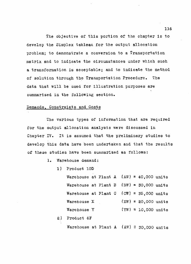
116 The objective of t h i s portion of the chapter i s to

develop the Simplex tableau f o r the output a l l o c a t i o n

problem; to demonstrate a conversion to a Transportation

matrix and to indicate the circumstances under which such

a transformation i s acceptable; and to indicate the method

of solution through the Transportation Procedure. The

data that w i l l be used f o r i l l u s t r a t i o n purposes are

summarized i n the following section.

Demands, Constraints and Costs

The various types of information that are required

for the output a l l o c a t i o n analysis were discussed i n

Chapter IV. It i s assumed that the preliminary studies to

develop th i s data have been undertaken and that the r e s u l t s

of these studies have been summarized as follows:

1. Warehouse demand:

1) Product 10D

Warehouse at Plant A (AW) = 40,000 units

Warehouse at Plant B (BW) * 30,000 units

Warehouse at Plant C (CW) = 35,000 units

Warehouse X (XW) 20,000 units

Warehouse Y (YW) 10,000 units

Product 6F

Warehouse at Plant A (AW) 30,000 units

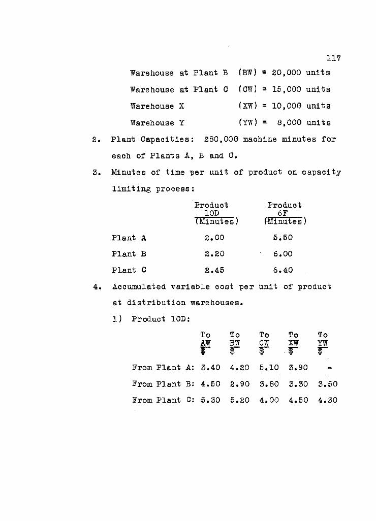
117 Warehouse at Plant B (BW) = 20,000 units

Warehouse at Plant C (CW) = 15,000 units

Warehouse X (XW) = 10,000 units

Warehouse Y (YW) = 8,000 units

Plant Capacities: 280,000 machine minutes for

each of Plants A, B and C.

Minutes of time per unit of product on capacity

l i m i t i n g process:

Product Product 10D 6F

(Minutes) (Minut e s) Plant A 2.00 5.50

Plant B 2.20 6.00

Plant C 2.45 6.40

Accumulated variable cost per unit of product

at d i s t r i b u t i o n warehouses.

1) Product 10D:

To To To To To AW BW CW XW YW r F F •F F

From Plant A: 3.40 4.20 5.10 3.90 -From Plant B: 4.50 2.90 3.80 3.30 3.50

From Plant C: 5.30 5.20 4.00 4.50 4.30

118

2) Product 6?:

To To To To To AW BW CW XW YW T T T T T

From Plant A: 8 , i d 10.50 11.20 9.20

From Plant B: 10.20 8.70 9.50 9.00 9.30

From Plant G: 12.20 11.80 8.90 9.60 9.20

The figures shown above represent the minimum cost

methods of u t i l i z i n g each of the p o t e n t i a l t r a f f i c routes.

A preliminary comparison of alternatives f o r d i s t r i b u t i n g

product 10D from Plant A to warehouse G, for example, has

shown that the minimum delivered product cost v i a t h i s

route w i l l be #5.10.

The Simplex Formulation

Given the data i n the preceding section, the f i r s t

step i n setting up the Simplex i s to express the demands

and constraints a l g e b r a i c a l l y . Standard mathematical

notation may be used as follows:

1. Number the plants one through three.

2. Number the d i s t r i b u t i o n warehouses one through

119

f i v e f o r product 10D; and six through ten f o r

product 6F. (Numbers one and six both r e f e r

to warehouse A, two and seven both r e f e r to

warehouse B, etc.)

3. Let X j j equal the number of units of product

supplied by plant i to warehouse j . Then the

quantities of product required at warehouses

can be stated as follows:

1) *11 X81 X31 o-4 = 40,000

8) x12 X22 X32 *• U5 " 30,000

3) X l 3 X23 • X33 35,000

4) *14 X24 + X34 + u 7 = 20,000

5) X25 X35 + U8 = 10,000

6) X16 X26 X36 30,000

7) X17 X27 x37 1̂0= 20,000

8) X18 + ^8 x38 Ull= 15,000

9) x19 + X29 + X39 U12- 10,000

10) X2,10 + X 3,10 * %3 = 8,000

The U variable i s added to each equation i n order

to eliminate the i n e q u a l i t i e s .

The capacity constraints at each plant are given

by the following equations:

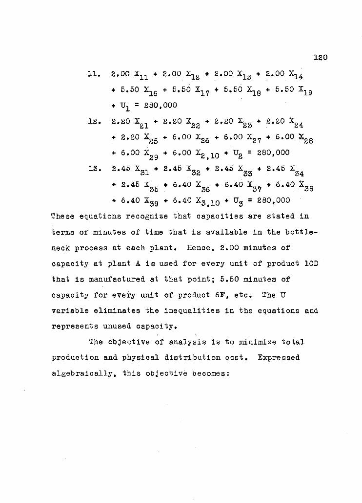
120

11. 2.00 X i ; l + 2.00 X l g + 2.00 X 1 3 + 2.00 X 1 4

+ 5.50 X 1 6 + 5.50 X 1 ? + 5*50 X 1 8 + 5.50 X 1 9

t U x = 280,000

12. 2.20 X g l + 2.20 X 2 g + 2.20 X g g + 2.20 X g 4

+ 2.20 X-2g • 6.00 X 2 6 + 6.00 X g 7 + 6.00 Xg 8

+ 6.00 X g g + 6.00 X g t l 0 * U 2 = 280,000

13. 2.45 X „ T • 2.45 X „ 0 + 2.45 X„„ + 2.45 ZrtA

ox oc, 33 34 * 2.45 X „ c • 6.40 X„^ + 6.40 X^„ • 6.40 X„_

CO OD o" oo

• 6.40 X g 9 + 6.40 X 3 > 1 0 • U 3 = 280,000

These equations recognize that capacities are stated i n

terras of minutes of time that i s available i n the b o t t l e

neck process at each plant. Henoe, 2.00 minutes of

capacity at plant A i s used f o r every unit of product 10D

that i s manufactured at that point; 5.50 minutes of

capacity for every unit of product 6F, etc. The U

variable eliminates the i n e q u a l i t i e s i n the equations and

represents unused capacity.

The objective of analysis i s to minimize t o t a l

production and physical d i s t r i b u t i o n cost. Expressed

a l g e b r a i c a l l y , t h i s objective becomes:

121

3.40 X l : L + 4.50 X 2 1 + 5.30 X 3 1 + 4.20 X 1 2

+ 2.90 X 22 * 5.20 X 3 2 + 5.10 X 1 3 + 3.80 X g 3

• 4.00 X 3 3 * 3.90 X 1 4 + 3.30 X 2 4 + 4.50 X 3 4

+ 3.50 X 2 5 + 4.30 X 3 6 «r 8.10 X 1 6 + 10.20 X 2 6

+ 12.20 X 3 6 + 10.50 X 1 ? + 8.70 X g 7 + 11.80 X 3 ?

+ 11.20 X 1 8 4. 9.50 X 2 8 + 8.90 X 3 8 + 9.20 X 1 9

+ 9.00 X 2 9 * 9.60 X 3 9 + 9.30 X 2 ^ 1 0 * 9.20 Xg 1 Q

+ U-L * Ug +> Ug +• U 4 + Ug + U 6 + U 7 + U Q + U 9

f U 1 0 + U 1 X + U 1 2 f U 1 3 = MINIMUM

The next step l n the formulation of the Simplex i s

to set up the variables and c o e f f i c i e n t s from the above

equations i n matrix form. 5 This has been done i n Table

XIV on page 122.

The c o e f f i c i e n t s of the objective equation have

been placed i n the second row from the top. The f i r s t

f i f t e e n spaces i n th i s row indicate the unit variable cost

of product 10D at each warehouse from each of the a l t e r

native plants. Spaces sixteen through t h i r t y i n t h i s row

5 For a description of the Simplex matrix see Nyles

V. Rienfeld, William R. Vogel, Mathematical Programming, (Englewood C l i f f s , N.J., Prentice H a l l , Inc., 1958), p. 81.

TABLE XIV

SIMPLEX MATRIX

1 2 3 4 6 7 - 6 9 .10 11 . .12 13 14 15 16 17 18 19 20 . .21 22' £3 24 £5 26 27. 28 29' 30 31 32 33 34 36 36 37 36 39 40 41 42 43

COST » 3.40 4.50 5.30 4.20 £.9( 5.20 J_ -

5.10 aso 4.00 3.90 3.30 4.50 if 3^0 4.30 8.10 10.20 12.20 10.50 5.70 LL£0 2120 9.50 6.90 9.20 9.00 9.60 U 9.31 3.20 0 0 0 0 0 6 0 0 0 0 0 0 0

103 t o AW 10D t o BI • i o D J t o cvr 10D t o 10B t o IW 6F t o AX 6F t o BS- 6F to . CW 6F t o T R 6F t o W

.A £60 ,000 £.00 2.00 2.00 £.00 E.OO S.60 E.60 5.50 S.50 5.'50 1

B £80.000 2.20 2.20 2.20 £.£0 2.20 6.CO 5.00 6.00 5.00 6.0O 1

0 S60.000 2.45 2.4 5 £.45 2.45 2.45 6.40 6.40 6.40 6.40 6.40 1

Alt 40,000 1 • 1 1. 1

B« 30.000 1 1 1

CW 35,000 - 1 1 1 1

I B £ 0 , 0 0 0 - -1 1 3 - 1

YS 10.000 K . 1 1 1

AH 30,000 1 1 1 1

B B 20,000 1 . 1 1 1

IS.000 1 . 1. 1 1

'Xt 10.000 1 1 i 1

T» 8,000 1 .1 1 1

1

1.

5 2.

H ro

123 show the same Information f o r product 6F. Spaoes t h i r t y -

one through forty-three indicate that there i s no vari able

cost involved i n unused plant capacity or u n f i l l e d demand.

Note that the l e t t e r M has been entered i n the thi r t e e n t h

and twenty-eighth spaces. Since i t i s impossible to ship

output from plant A to warehouse Y the M may be interpreted

as a s u f f i c i e n t l y high cost to preclude the in c l u s i o n of

t h i s route i n the solution to the problem.

Plant capacities i n minutes are shown i n the

second column at the l e f t i n rows numbered one through

three. Warehouse demands for product 10D are shown i n

units of product i n rows four through eight and warehouse

demand for product 6F i n rows nine through t h i r t e e n .

The body of the matrix ( i e . column one through

t h i r t y ) includes the c o e f f i c i e n t s of the plant capacity

equations and the c o e f f i c i e n t s of the warehouse demand

equations. The figure one i n rows numbered four through

t h i r t e e n s i g n i f y that t o t a l production f o r eaoh warehouse

i s not to exceed i t s demand, but that demand may be

s a t i s f i e d from any one or more of the plants.

The c o e f f i c i e n t s of the U variable from each of the

aforementioned equations are shown i n the Identity portion

of the matrix ( i e . , column thirty-one through forty-three).

These c o e f f i c i e n t s consist of the figure one i n each case

and i t i s a requirement of the Simplex matrix that these he

diagonally arranged as shown i n the table.

It i s possible to f i n d the minimum cost solution to

t h i s problem by applying Simplex rules to the matrix as

formulated i n Table XIV, page 122. It i s generally

impractical, however, to attempt a solution through hand

c a l c u a l t i o n . It has been assumed f o r s i m p l i c i t y sake i n

our example that there are only three plants, f i v e ware

houses and two products. These assumptions have produced

a matrix with 539 spaces. A more t y p i c a l example would

probably involve a considerably broader product l i n e and

perhaps additional plants and warehouses to produce a

matrix of several thousand spaces. Rienfeld and Vogel

suggest that i t would perhaps take from two to three

months to solve a Simplex matrix with from 800 to 1200

spaces. Bearing i n mind that the model i s to be used for

short-term planning purposes and that a great deal of time

w i l l have already been spent i n developing the data to be

included i n the analysis, a rapid solution i s desirable.

6 I b i d , p. 132.

125

Many of the larger computers have been programmed f o r the

Simplex and t h i s i s the preferred method of solu t i o n f o r

the size of matrix that w i l l usually be involved i n t h i s

type of problem.

In c e r t a i n circumstances, however, the Simplex

method of solu t i o n can be avoided by reducing the matrix

to one that i s suitable for solution through the Transpor

t a t i o n Method. The procedure for reduction and the

circumstances under which t h i s s i m p l i f i c a t i o n w i l l produce

an adequate solut i o n are described i n the following

section and have been adapted from the writings of

Rienfeld and Vogel. 7

Conversion of the Simplex Matrix

A Simplex tableau can be reduced to a form suitable

for conversion into a transportation model provided each of

the figures contained i n the body of t h i s matrix can be

transformed to the figure one. The body of the matrix i n

Table XIV consists of rows numbered one through thirteen,

up to and including column number t h i r t y . The following

matrix algebra rules w i l l be used for the required Simplex

7 I b i d . , p. 137 - 141

transformation:

1. You can divide or multiply any row i n the

matrix by any number other than zero*

8. You can divide or multiply any column i n the

matrix by any number other than zero.

In either case, every number i n the row (or column) must

be mu l t i p l i e d (or divided) by the number.

The transformation with the use of these rules can

be achieved i n four steps, as follows:

1. Divide rows numbered one through three by 8.00,

.j 8.20, and 8.45 respectively. A l l of the

figures i n the body up to and including column

number f i f t e e n become l ' s . The tableau a f t e r

completion of t h i s step i s shown i n Table XV,

page 187.

8. Divide column number sixteen and every t h i r d

column thereafter up to and including column

twenty-eight by 8.75.

Divide column number seventeen and every t h i r d


twenty-nine by 8.73.

Divide column number eighteen and every t h i r d


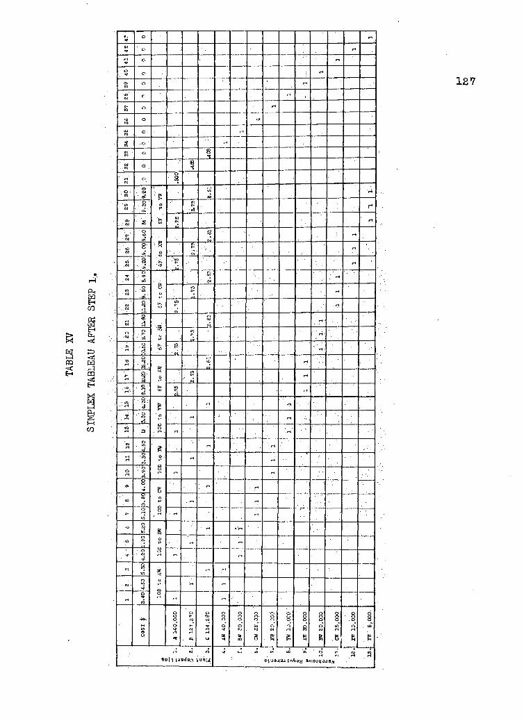
o r-l

O) *r o H

i-i o

o o r-l

o> o •

O) w

c- r

« o

o 17*

tO KJ o • .-1

35 •.. o '

Vi o 8 OJ o ifl

. » o

0

8 O

' to

' o • w

Ol ' p

>o

W r i

' (71 «

O ' . M cn

o CO t> *J

H

to •' <V ' 2 •

> ta r-i

w O

m . 5

o

3 CM

r-t

e\i

o o . 5 o

CO 0

cw rt

•CO . 8 " . C T »

fit ' t> cu

ri

*r O

.' cn u5 a

o O

U ) r-i

• W • CM

o in

• m "

a o O

to

cu • .•. «

« • rt

•o iO 0

•

r-t 8 ! i

O CM

o to

in u

to t\t

j> ' r-l

.8 d

>o

- • OJ ri

CD i-i

o.

' « . rH

,B-9

O lO c-CM

i-l

<£>' r-i*

o Pu, 1 0

C-Y rH

• -• m • i-i

•••8: fc rt

, i • • s . «

" r t r-t

CO r-i 0 r-i • ri

01 i-i

o to •V

1-1 • i-i

r-t ri

o to pj'

0 . r-H

o r-1

' ' o ' 1̂

0 r-i r-i

. a> o o

B

CO o aj co

a •*-» . 1-* r-i

£-o

to

0 • rH -

>D o <H Ui S

Hi o o> 0

+•

a O •r-i r-t

- '3 to X

-<

• CM •

o in M*

O

O

r-t -a CO

O n r-i

E-t

O o

O O

Q

O ' «* r-i

O

CM

. at

O G ) ( M

O 0 0

0

BE

O O O

O fj B= rfl

O O O

to to

5

O O

r> CM

0 0 0

0

a §

EX

cl O O

O

CW 15

,000

O O

. O

O rH

R

b 8 (O

•H W f) . . 0 L - al cn O r-a

128

t h i r t y hy 2.61.

These d i v i s i o n s also apply to the figure i n the

cost row. Table XVI on page 129 shows the

result of t h i s transformation. •

Divide rows nine through t h i r t e e n by 0.371, i e . ,

by the average of the three figures i n each of

these rows. The result of t h i s step i s shown

i n Table XVII on page 130.

Note i n Table XVII that the figures i n the body

of the matrix i n each of rows nine through

th i r t e e n now approximate the figure one. Since

t h i s i s the l a s t of the steps that can be taken

to transform the body of the matrix, i t must be

decided whether or not each of these figures

are s u f f i c i e n t l y close to the figure one to

consider the matrix as transformed s u f f i c i e n t l y

to apply the Transportation Method of solution.

In t h i s p a r t i c u l a r example, the converted

figures indicate that there w i l l be a maximum

error of 3.2 percent i n the solution that i s

suggested f o r product 6F through the use of the

Transportation Method. But there w i l l be no

error i n the solu t i o n suggested f o r the

production and physical d i s t r i b u t i o n of

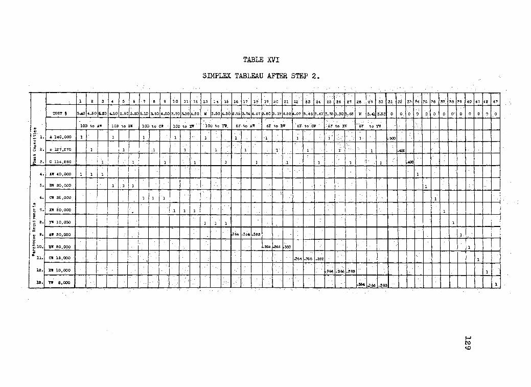
TABLE XVI

SIMPLEX TABLEAU AFTER STEP 2.

1 z 3 4 6 6 7 8 9 10 11 IS 13 14 16 16 17 19 19 20 21 22 23 ?4 26. 26 27 28 . 29 30 3.1 32 33 34 '£ 36 S7 38 79 40 41 42 43

COST.$ 340 4.60 5.20 4.20 2.90 6. SO 6.10 3.80 4.00 3.90 MO 4;50 V 2.80 4.30 £ . 3 6 3.74 4.67 3.60 5.19 4.E2 4.07 3.45 3.41 3.36 3.30 3.68 V. 3.41 3.53 0 0. 0 0 0/ 0 0 0' 0 0 0 0 0

IOC to AW l O B to BW 102 to CW . IOC to IW lot to VS. 6r to kV 6F to BW .'tr. to .CW -67 to- r B ' 6F to YR

A 140,000 1 1 1 1. 1 1 1 1 1 . 1 .600

S 127,270 1 1 .1 1 1 1 1

1

1 ' 1' '.'-'• - 1 .456

C 114,260 1. 1 l" . 1 1 1 1 1 1 1 406

AW 40,000 1 1 1 1

B* 30,000 1 . 1 1 1

CW 36,000 1 1 1 1

xw 20.000 .1 1 1

y* IO.OOO 1 1 1. 1 i

AW 30,000 364 . 3 5 6 .383 1.

BW £ 0 . 0 0 0 .364 .366 .383 1

CW 15,000 • .364 .366 .3S3 1

ZW 10,000 .364. .366 .583 1

T» 8,000 .364 .2 66 .383 1

_ 1.

ILL

c 7 .

& V a Ii 3 •>

; i o . s

' 11.

12.

13.

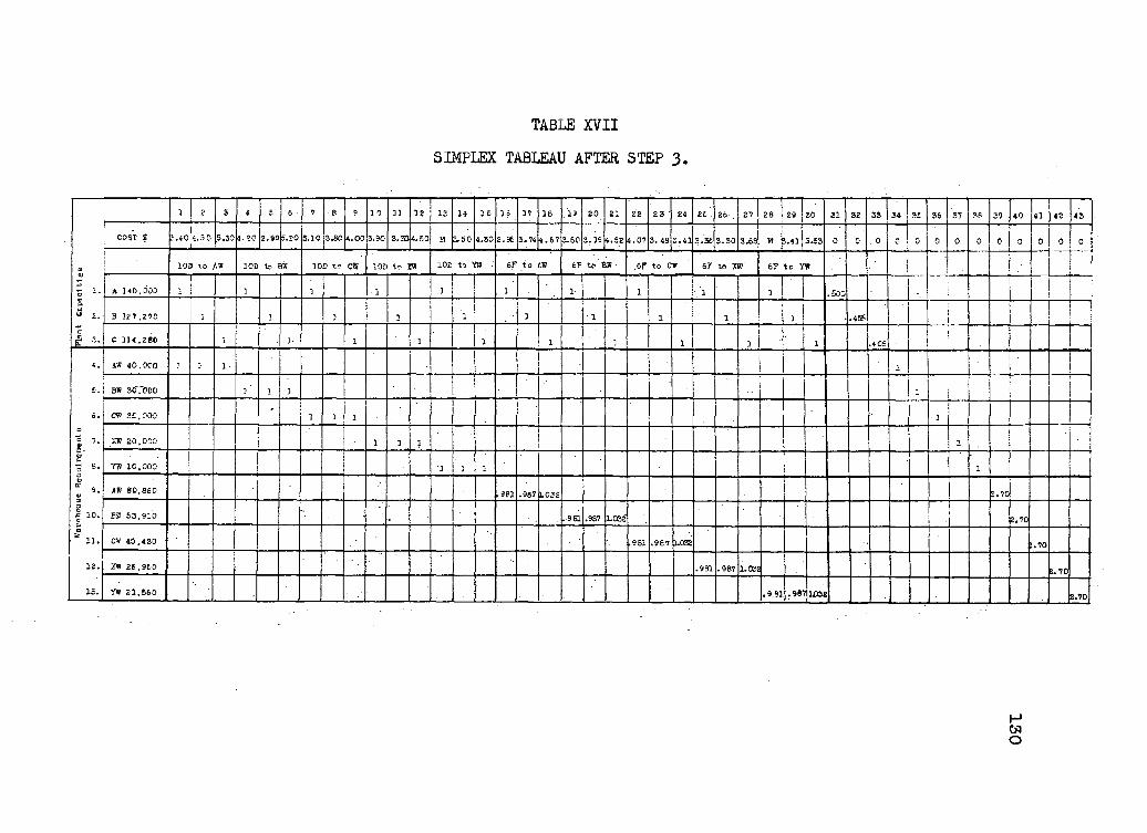
TABLE XVII SIMPLEX TABLEAU AFTER STEP 3.

l | 2 3 < 6 • 7 8 9 1 0 13 I

i t ; i= 14 16 i s 17 16 .19 . 20 21 22 23 ' 24 26 26 . £ 7 29

i 29 30 31 32 33 34 3£ 36 37 39 40 41 42 43

COST t 1

? . « O 4 . 5 0 _ i . . .

5.30 i.?o z.so 5.20 5.10 3.SO 4.00 3.90 3.3D 4.60 M S.50 4.30 2.96 3.74 4.67 3.60 3.19 4.52 4.07 3 .49 3.41 3.36 3 .30 3.68 M fe.4lb.63 l 1

0 0 : 0 0 0 0 0 0 0 0 0 0 0

a m u 2.

C

10D t o AW 10D to BW 30D tr C(B 10D t r 151 10B t 5 TO ' 6F t o if t o B.W 6F t o C F 6F t o 73 6F t o YW

a m u 2.

C

A H O , 000 I

J j 3 1 1 • 3 1 3 i l : . i

1 " . 1 1 .500 i

a m u 2.

C 3 32 7.2 70 I 1 1 1 1 1 • 1 1 j 1 3 .455

i i

a m u 2.

C C 114.280 1 J- 1 1 1 1 3 i 1 1 .406

!

4. AW 40.000 1 1 l 1 1

£ BW 307000 3 1

6.

1. '• 01 u ~* a. 3 " a t>

K 9 . V l i e . s a

= 11.

12.

CB 26.000 •

1 1 1 - 3 6.

1. '• 01 u ~* a. 3 " a t>

K 9 . V l i e . s a

= 11.

12.

X» 20,000 1 1 1 | 1

6.

1. '• 01 u ~* a. 3 " a t>

K 9 . V l i e . s a

= 11.

12.

YW 10,000 1 1 1

6.

1. '• 01 u ~* a. 3 " a t>

K 9 . V l i e . s a

= 11.

12.

jtSI 80,860 .sei .987 L032 2.70

6.

1. '• 01 u ~* a. 3 " a t>

K 9 . V l i e . s a

= 11.

12.

BUT 63,910 .961 .987 3-038" 2.70

6.

1. '• 01 u ~* a. 3 " a t>

K 9 . V l i e . s a

= 11.

12.

CW 40.430 .981 .967 1.032 J.70

6.

1. '• 01 u ~* a. 3 " a t>

K 9 . V l i e . s a

= 11.

12.

ZW 26,960 .991 .987 1.032 1. 70

1 3 . YW 21,660 .9.81 .98* 103! 2.70

03 O

http://fe.4lb.63

131

product 10D since a l l of the figures i n t h i s

portion of the matrix are exactly ones. Hence,

the maximum t o t a l error r e s u l t i n g from the use

of the Transportation Method i s l i k e l y to

produce an error of less than two percent,

considering the relationships between oonverted

costs and demands of the two products. A

p o t e n t i a l error of t h i s size w i l l usually be

i n s i g n i f i c a n t — p a r t i c u l a r l y since the

estimates that are necessary i n the formulation

of forecasts and product costs are l i k e l y to

contain errors of t h i s size or larger. In any

case, the size of error that i s acceptable must

be considered i n the l i g h t of the saving i n

time and e f f o r t that i s available through the

use of the Transportation Method.

4. The f i n a l step i s to convert the id e n t i t y

portion of the matrix. This can be

accomplished by multiplying each of the figures

contained therein by the appropriate integer to

produce the figure one.

The Simplex matrix has now been converted into the

form suitable f o r setting up the Transportation matrix.

138

The circumstances i n which the reduction to the Transpor

t a t i o n Method i s desirable i s , of course, related to the

size of the error discussed under step three. The size

of t h i s error w i l l increase with l a r g e r differences i n the

units of capacity u t i l i z e d i n the manufacture of products

at alternative plants. It i s clear, however, that a few

calculations can be made to determine the d e s i r a b i l i t y of

the Transportation Method without performing the complete

conversion as discussed above.

Solution Through the Transportation Procedure

To set up the Transportation matrix, the warehouse

requirement figures shown i n Table XVII are treated as

product demands; the converted available minutes are taken

as the plant capacities; and the converted cost figures

are inserted i n the small squares of the Transportation

matrix (see Table XVIII). Plant capacity In t h i s example

exceeds demand for the period and a dummy warehouse has

been added to the matrix to eliminate t h i s inequality.

There i s no variable cost associated with unused capacity

as indicated by the zeros i n the small squares of the

dummy warehouse eolumn.

The f i r s t step i n solution i s to inspect the cost

figures i n t h i s matrix and to take a guess at the best

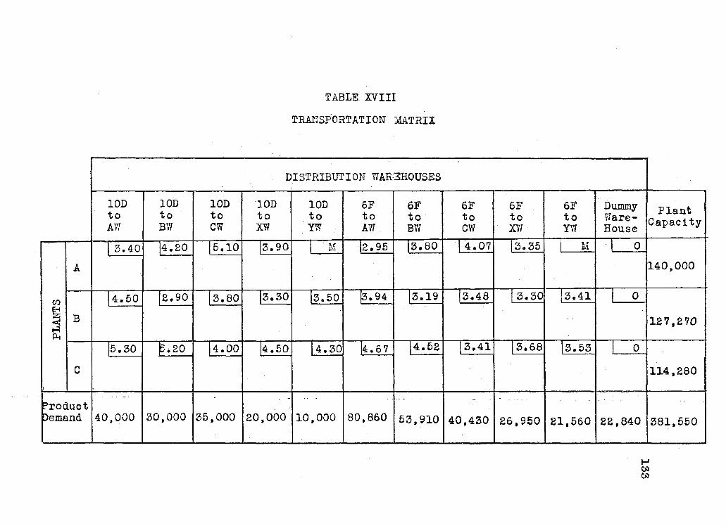
TABLE X V I I I

TRANSPORTATION- MATRIX

DISTRIBUTION WAREHOUSES

10D to AW

10D to BW

10D to CW

10D to XW

10D to YW

6F to AW

6F to BW

6F to CW

6F to XW

6F to YW

Dummy Ware-House

Plant Capacity

3.40 4.20 5.10 3.90 M 2.95 3.80 4.07 3.35 M 0

A 140,000

ro 4.50 2.90 3.80 3.30 3.50 3.94 3.19 3.48 3.30 3.41 0

PLANT:

B 127,270

5.30 5.20 4.00 4.50 4.30 4.67 4.52 3.41 3.68 3.53 0

C 114,280

Product Demand 40,000 30,000 35,000 20,000 10,000 80,860 53,910 40,430 26,950 21,560 22,840 381,550

H

134

assignment of demands according to the capacities available

at each plant. S t a r t i n g with the f i r s t column, for example,

i t appears l i k e l y that the demand for product 10D at ware

house A should be met from plant A since t h i s i s the lowest

cost frame i n the column. Product demand of 40,000 units

may be entered i n t h i s frame, therefore, and s i m i l a r l y f o r

each succeeding guess u n t i l a l l demands have been s a t i s f i e d .

The c i r c l e d figures i n Table XIX represent a completed

guess at the optimum solu t i o n . Note that the assignment

must be made i n such a way that the c i r c l e d figures i n each

row add up to the figures shown i n that row for plant

capacity. S i m i l a r l y , the c i r c l e d figures i n each column

must add up to the corresponding product demand f i g u r e .

The problem at thi s stage i s to determine whether

or not t h i s assignment i s the minimum cost s o l u t i o n . The

test of optimality requires an inv e s t i g a t i o n of the change

i n t o t a l cost that would result i f the assignment were to

include any one of the excluded routes, Ie., the frames i n

Table XIX i n which there are no c i r c l e d figures. These

routes must be analyzed one at a time. It i s s u f f i c i e n t to

appraise the cost of moving one unit v i a an unused route to

determine whether or not i t s u t i l i z a t i o n w i l l improve the

assignment.

TABLE XIX

TRANSPORTATION MATRIX - INITIAL -ASSIGNMENT


lOD to AW

10D to BW

10D to CW

10D to XW

10D to YW

6F to AW

6F to BW

6F to CW

6F to XW

6F to YW

Dummy Warehouse

Plaat Capacity

3.40 4.20 5.10 3.90 M 2.95 3.80 4.07 3.35 M 0

A d tooog) 1.25 1.10 0.55 M (|0860) 0.56 0.66 (^3590) M (5550) 140000

4.50 2.90 3.80 3.30 3.50 3.94 3.19 3.48 3.30 3.41 0

W B ] ..15 (30000) -0.15 (20000) (̂ OOOO) 1.04 (5391^) 0.12 (13360) -0.07 0.05 127270

5.30 5.20 4.00 4.50 4.30 4.67 4.52 3.41 3.68 3.53 0

C .1.90 2.25 (350^) 1.15 0.75 1.72 1.28 (4043B) 0.33 (21560) L729^ 114280

Product Demand 40000 30000 35000 20000 10000 80860 53910 40430 26950 21560 22840 381550

136

Bearing i n mind that the assignment must always

s a t i s f y demand and capacity constraints, i t i s clear that

to place a unit i n an empty frame requires at least three

adjustments i n the ex i s t i n g assignment. Assume, f o r

example, that one unit l s placed i n the second frame of

the f i r s t row of Table XIX. To reduce the t o t a l assignment

i n the second column to the required 30,000 units i t i s now

necessary to subtract one unit from the second frame of the

second row. But t h i s w i l l result i n an unassigned unit of

capacity f o r plant B, while at the same time the t o t a l

assignment i n row one now exceeds plant A's capacity by

one unit as a result of the i n i t i a l step. The next

adjustment, therefore, must correct the assignments i n

rows one and two without v i o l a t i n g demand requirements.

This can only be done by subtracting one unit from the

assignment i n the ninth frame of the f i r s t row and adding

thi s unit to the assignment i n the ninth frame of the

second row. These adjustments, expressed i n terms of cost

indicate that an additional $4.20 would be involved i n

assigning one unit to the second frame of the f i r s t row,

a saving of $2.90 by reducing the assignment i n the second

frame of the second row by one unit; an additional $3.30

for increasing the assignment i n the ninth frame of the

13.7

second row; and a saving of $3.35 by reducing the assign

ment i n the ninth frame of the f i r s t row. In t o t a l , the

use of this route would involve an additional cost of

$1.25 per unit ($4.20 - $2.90 + $3.30 - $3.35). This

figure has been shown i n the second frame of the f i r s t row

i n Table XIX . Since the t o t a l cost would be increased,

i t i s clear that the u t i l i z a t i o n of t h i s route w i l l not

improve the assignment.

A few simple rules can be used to quickly evaluate

each of the empty frames. These rules are as follows:

1. Start from an empty frame and record i t s unit

c os t .

2. Proceed to a frame i n the same row or column i n

which there i s a c i r c l e d number and record i t s

unit cost as a minus fi g u r e .

3. Make a right angle turn and proceed to the

second c i r c l e d number. Record i t s unit cost.

(The second move must, of course, be to a

c i r c l e d number from which the t h i r d move i s

possible)•

4. Make another right angle turn and proceed to

the t h i r d c i r c l e d number. Record i t s cost as

a minus figure. (The t h i r d move must be made

138

i n such a way that the fourth move i s po s s i b l e ) .

I f t h i s c i r c l e d number i s i n the same column or

row as the empty frame, the loop i s oomplete.

I f not, continue the series of right angle

moves to successive frames i n which there are

c i r c l e d numbers (recording the unit cost

a l t e r n a t i v e l y as positive and negative) u n t i l

the c i r c l e d figure to which a move i s made i s

i n the same column or row as the s t a r t i n g

point.

5. Total the unit costs and enter the figure i n

the empty frame.

Examples of the ap p l i c a t i o n of these rules are

shown i n Figures 12 and 13. Both figures are sections of

the body of the matrix shown i n Table XIX,

139

FIGURE 12

DETERMINING THE COST OF AN

UNUSED TRAFFIC ROUTE

Following the arrows; costs would he recorded as follows:

Start ^3.48 Step 1 -#3.41

2 0 3 0 4 3.35 5 - 3.30

6.83 - 6.71

The net ohange i n t o t a l oost, i f the f i r s t frame of the

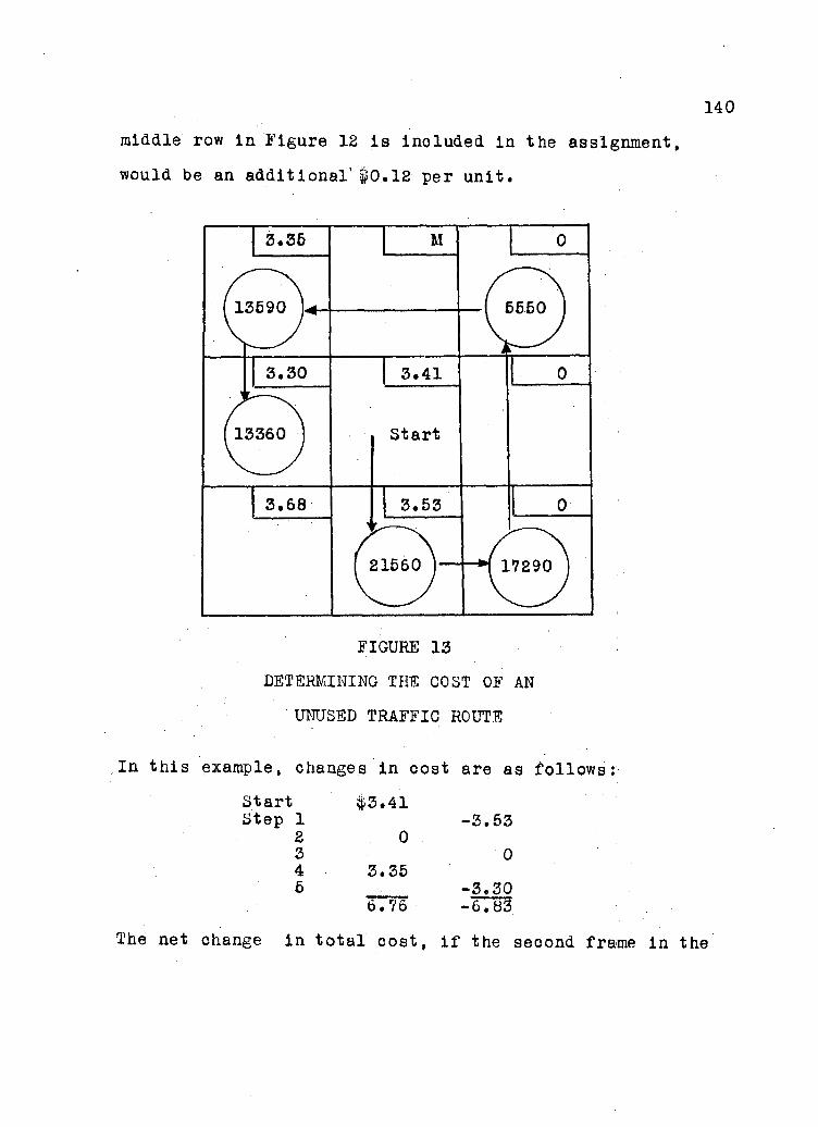
middle row i n Figure 12 i s included i n the assignment,

would be an additional' $0.12 per unit.

FIGURE 13

DETERMINING THE COST OF AN

UNUSED TRAFFIC ROUTE

In t h i s example, changes i n cost are as follows:

Start $3.41 Step 1 -3.53

2 0 3 0 4 3.35 5 -3.30

6.76 -6.83

The net change i n t o t a l cost, i f the second frame i n tr

141

middle row of Figure 13 i s included i n the assignment,

would be a saving of $0.07 per u n i t . .

The above procedure has been c a r r i e d out i n

evaluating the per unit cost associated with the

u t i l i z a t i o n of each of the routes that have been excluded

from the assignment. The numbers i n each of the unused

frames i n Table XIX are the result of these evaluations.

The negative figures appearing i n the t h i r d and tenth

frames of the second row indicate that the assignment, as

o r i g i n a l l y formulated, i s not optimum. There i s a

p o t e n t i a l reduction i n t o t a l assignment cost of $0.15 per

unit f o r every unit that can be placed i n the t h i r d frame,

and $0.07 f o r every unit that can be placed i n the tenth

frame* The next step, therefore, i s to change the

assignment to include these routes.

The procedure for t h i s step i s to follow the same

path that was used to evaluate the frame i n which the

negative number appears. The path that was used,to

evaluate frame ten of the second row i s shown i n Figure 13

and w i l l be used, therefore, to i l l u s t r a t e t h i s step.

Normally, however, the f i r s t change would be to include

the frame i n which the largest negative number appears.

148

Referring to Figure 13, the f i r s t step i n

adjusting the assignment i s to determine the maximum

number of units that can he placed i n the s t a r t i n g frame.

Following the arrows, we see that we w i l l have to subtract

the units that are placed i n t h i s frame from three of the

c i r c l e d numbers — 21,560, 5,550 and 13,360. Since the

d i s t r i b u t i o n from plant to warehouse must be eith e r zero

or a pos i t i v e quantity, i t i s clear that 5,560 i s the

maximum number of units that can be placed i n the s t a r t i n g

frame. The t o t a l adjustment through the i n c l u s i o n of

5,550 units i n the s t a r t i n g frame and successive

subtractions and additions of the same amount to the

c i r c l e d numbers i n Figure 13, i s shown i n Table XX.

The next step i s to recompute the cost of

u t i l i z i n g each of the routes that have not "been included

i n the new assignment. The result of t h i s c a l c u l a t i o n i s

shown i n each of the frames of Table XX l n which c i r c l e d

numbers do not appear. The negative number i n the t h i r d

frame of the second row indicates that the solution i s

s t i l l not optimum. The same procedure as outlined above

w i l l Indicate that the 5,550 units that has just been

placed i n the tenth frame of the second row, must now be

placed i n the t h i r d frame of that row, with a

TABLE XX

TRANSPORTATION MATRIX - FIRST ADJUSTMENT


10D to AW

10D to BW

10D to CW

10D to XW

10D to YW

6F to AW

6F to BW

6F to CW

6F to XW

6F to YW

Dummy Warehouse

Plant Capacity

3.40 4.20 5.1C 3.90 M 2.95 3 . 80 4.07 !3.35 M 0

A (^oooS) 1.85 1.17 0.55 M <|086(^ 0.56 ( ),73 (^9149) U 0.07 140000

co E-I

ih

4.50 2.90 3.8C 3.30 3.50 3.94 3.19 3.48 3.30 3.41 0 co E-I

ih B 1 ..15 (3000^) -0.08 <2000§) C^OOOO) 1.04 <^391§) 0.19 < 7810) (^555^) 0.12 127270

co E-I

ih 5.30 5.20 4.0C 4.50 4.30 4.67 4.52 3.41 (3.68 3.53 0

C 1.83 2.18 (3500^ 1.08 0.68 1 e 65 1.21 <£043^ 0.26 <^601§} ^2284^ 114280

Product Demand 40000 30000 35000 20000 10000 80860 53910 40430 26950 21560 22840 381550

H

corresponding subtraction and addition respectively i n the

t h i r d and tenth frames of the t h i r d row. The ehange i n

assignment as a result of th i s adjustment i s shown i n

Table XXI.

The recomputed cost of u t i l i z i n g each of the routes

that have been excluded from the new•assignment are also

shown i n Table XXI. Note that a l l of these figures are

now p o s i t i v e . This means that i t i s impossible to

rearrange the assignment to produce a lower t o t a l cost.

The solution, therefore, i s optimum.

As a point of interest, the t o t a l cost of the

assignments i n each of Tables XIX, XX and XXI has been

established by summing the product of each of the c i r c l e d

figures and t h e i r appropriate unit cost (eg., 40,000 x

#3.40 + 80,860 x $2.95 + , e t c . ) . The r e s u l t of these

calculations are as follows:

Table XIX fl,178,098

Table XX 1,177,709 (Improvement $389,)

Table XXI 1,177,265 (improvement $444.)

The saving through re-assignment In Table XX can be

established by simply multiplying the saving per unit that

was shown to be available i n frame ten of the second row

i n Table XIX by the number of units assigned to that frame

i n Table XX, i e . , $0.07 x 5,550 = $389. S i m i l a r l y , the

TABLE XXI

TRANSPORTATION MATRIX - OPTIMUM SOLUTION


lOD to AW

10D to BW

10D to CW

10D to XW

10D to YW

6F to AW

6F to BW

6F to CW

6F to XW

6F to YW

Dummy Warehouse

Plant Capacity

3.40 4.20 5.10 3.90 M 2.95 3.80 4.07 3.35 K 0

A (40000). 1.25 1.25 0.55 M (§0860) 0.56 0.81 (19143) M 0.15 140000

PL

AN

TS

4.50 2.90 3.80 3.30 3.50 3.94 3.19 3.48 3.30 3.41 0

PL

AN

TS

B 1.15 (3OOO9) (Wo) (20000) (lOOO^) 1.04 (53910) 0.27 (7810) 0.08 0.20 127270

PL

AN

TS

5.30 5.20 4.00 4.50 4.30 4.67 4.52 3.41 3.68 3.53 0

C 1.75 2.10 (Slio) 1.00 O06Q 1«£7 1.13 (40430) 0.18 (2156^) (22840) 114280

Produot Demand 40000 30000 35000 20000 10000 80860 53910 40430 2 5950 21560 22840 381550

146

saving through re-assignment i n Table XXI can be computed

by multiplying the saving per unit shown i n the t h i r d frame

of the second row of Table XX by the number of units

assigned to that frame i n Table XXI, i e . , $0.08 x 5,550 =

$444. These savings are r e l a t i v e l y small i n comparison to

the t o t a l cost. It should be remembered, however, that we

have limited the number of plants, warehouses and products

i n these i l l u s t r a t i o n s i n order to simplify the discussion.

As a r e s u l t , we were able to come closer to the optimum

solution on the f i r s t t r y than would usually be possible

i n the p r a c t i c a l s i t u a t i o n where the analyst would be

working with a matrix that i s made up of a substantially

l a r g e r product l i n e and perhaps additional plants and

warehouses. It i s clear, however, that the organization

of data into a Transportation matrix i n i t s e l f provides

the basis for a more i n t e l l i g e n t guess at the optimum

solution.

Interpretation of the Optimum

The reduction of the Simplex to a form suitable

for the formulation of the Transportation matrix resulted

i n a transformation of some of the o r i g i n a l data. The

solution that has been provided through the Transportation

Method i s , of course, i n terms of t h i s transformation and

147

must now be converted back to the o r i g i n a l data.

Product costs, demand forecasts and plant

capacities are given i n the o r i g i n a l data and there i s no

need, therefore, to convert these figures. Furthermore,

the warehouse requirements of product 10D were not changed

i n the transformation process and are stated, therefore, i n

actual physical quantities i n the Transportation solution.

The only conversion that i s necessary i s that required to

establish the physical quantity of product 6F that has been

assigned to each plant i n the optimum solution.

In transforming the Simplex, the warehouse require

ments of product 6F were divided by the number 0.371 (see

step 3 of the conversion process on page 128). These

converted or normalized figures were then transferred to

the Transportation matrix. The physical quantities of

product 6F, therefore, w i l l be 37.1 percent of the figures

shown i n the Transportation solution.

Taking 37.1 percent of the sum of the c i r c l e d

figures f o r product 6F i n each row of Table XXI, we see

that the output of t h i s product that w i l l be required at

each plant i s as follows:

Plant A = 37*100 units (37.1$ of 80,860 + 19,140)

Plant B • 22,900 units (37.1$ of 53,910 + 7,810)

Plant C = 23,000 units '(37.1$ of 40,430 + 21,560)

148

The output of product 10D that w i l l he required at each

plant — taken d i r e c t l y from Table XXI — i s as follows:

Plant A - 40,000 units

Plant B - 65i550 units

Plant 0 = 39,450 units

The t o t a l capacity that w i l l he absorbed by the above

combination of output at each plant i s shown i n Table XXII.

TABLE XXII

PLANT CAPACITY ABSORBED IN THE

TRANSPORTATION SOLUTION

Plant Product Units

Production Time

Per Unit

Total Production

Time

A 10D 40,000 61 37,100

2.00 5.50

80,000 204.000

Absorbed Capacity at A 284,000

B 10D 65,550 6F 22,900

2.20 6.00

144,200 137,400

Absorbed Capacity at B 281,600

C 10D 29,450 6F 23,000

2.45 6.40

72,200 147*200

Absorbed Capacity at C 219,400

We have stated i n the o r i g i n a l data that there w i l l

be 280,000 minutes of capacity time available at each plant*

Absorbed time at plant C i s , of course, below t h i s

149

constraint because the solution has provided that the

firm's excess productive capacity be concentrated at t h i s

point. Absorbed time at plants A and B i s s l i g h t l y above

the capacity constraint. This has occurred as a result of

the assumption that each of the converted figures i n the

Simplex matrix were s u f f i c i e n t l y close to the figure one to 8

permit the formulation of a Transportation model. It was

recognized, however, that there would be a p o t e n t i a l error

of less than two percent i n the Transportation solution as

a result of t h i s assumption. It i s not surprising,

therefore, that the solution suggests a combination of

output that exceeds the' capacity constraint at plant A by

1.4 percent and at plant B by 0 . 6 percent. An adjustment

i n the assignment to conform with appropriate reductions

i n the capacity constraints of both plants A and B w i l l , of

course, be necessary i f i t i s impossible to accommodate the

increase i n output that would be required with the solution

as given i n Table XXI. In general, however, there w i l l be

some f l e x i b i l i t y i n the capacity estimates that are used i n

analysis. It w i l l be advisable, therefore, to re-evaluate

these estimates i n the l i g h t of the solution that has been

provided. The solution should be rejected only when t h i s

re-evaluation has shown that one or more plants w i l l be

See pp. 128 and 131.

150

unable to adapt to the suggested l e v e l of output.

Demand constraints f o r product 10D have, of course,

been met by the solution since there was no conversion i n

transferring these figures to the.Transportation matrix.

To show that these constraints have also been s a t i s f i e d

f o r product 6F, the c i r c l e d figures i n the appropriate

columns of Table XXI should be mult i p l i e d by 37.1 percent,

as follows:

Warehouse A - 80,860 x 37,1$ = 30,000 units

Warehouse B = 53,910 x 37.1$ = 20,000 units

Warehouse G = 40,430 x 37.1$ = 15,000 units

Warehouse X = 26,950 x 37.1$ = 10,000 units

Warehouse Y = 21,560 x 37.1$ = 8,000 units"

The r e s u l t s of these calculations correspond with demand

figures shown i n the o r i g i n a l data.

Solution Implications

The method that has been described i n the foregoing

was based upon bottleneck: capacity at each plant, and a

predetermined product cost at d i s t r i b u t i o n warehouses v i a

alternative t r a f f i c routes. The v a l i d i t y of the

assumptions that underlie these two parameters must now

be evaluated i n the l i g h t of the t r a f f i c flow that i s

i m p l i c i t i n the output a l l o c a t i o n solution.

151

Plant capacity* It was indicated i n Chapter IV

that plant capacity defined i n terms of the bottleneck

operation implies that the output of other manufacturing

processes at the plant can be adjusted to whatever mix

of production i s c a l l e d f o r i n the optimum plan. In other

words, while the output a l l o c a t i o n solution w i l l be within

the capacity l i m i t s of the assumed bottleneck operation,

i t i s possible that the p a r t i c u l a r mix of output that

would be required by t h i s solution w i l l cause an unforeseen

bottleneck i n other plant operations.

It i s necessary, therefore, to check the capacity

of each of the manufacturing processes i n the plant i n

the l i g h t of the mix of output that i s c a l l e d f o r i n the

solution. The so l u t i o n w i l l be an adequate basis f o r

short-term planning only i f the mix i s within the capacity

l i m i t s of a l l of the production processes i n each plant.

Product Cost Estimates. In estimating product

oosts at d i s t r i b u t i o n warehouses, i t was necessary to

assume a certain flow of t r a f f i c through a route i n order

to approximate c e r t a i n of the cost elements.

The method and cost of transportation, f o r example,

assumed that t o t a l demand at a warehouse would be met

through one or another t r a f f i c routes. I f we look at the

152

optimum solution as shown i n Table XXI, we see. that the

demand f o r product 6F at warehouse X i s to be s a t i s f i e d

through two routes. The question then arises as to

whether or not the s p l i t i n demand among the two routes

w i l l affect the method of transportation that w i l l be used.

If the r a i l carload rate was used i n costing the plant B

to warehouse X movement, for example, w i l l the much lower

volume through t h i s route preclude a r a i l carload movement?

If so, Is the change i n transportation rate s i g n i f i c a n t ?

Inventory carrying costs and order processing costs

at d i s t r i b u t i o n warehouses were based i n part upon the

assumed method of transportation. It i s possible,

therefore, that these costs w i l l change i f the transportation

method d i f f e r s from that assumed i n the cost estimates.

The transportation and inventory cost estimates for raw

materials also assumed a certain minimum flow. The

v a l i d i t y of th i s assumption may also be questionable i n the

l i g h t of the mix of output that i s suggested i n the optimum

solution.

It i s desirable, therefore, to ensure that the

pattern of t r a f f i c flow that i s i m p l i c i t i n the output

a l l o c a t i o n solution w i l l not result i n s i g n i f i c a n t l y

d i f f e r e n t unit costs from those that were used i n the

analysis. This may be done by re-computing the unit costs

153

for each of the t r a f f i c routes that are included i n the

solution — using the t r a f f i c flow from t h i s solution as

the basis f o r the new estimates. I f i t i s found that there

i s a difference between the o r i g i n a l and the new estimate

fo r a p a r t i c u l a r route, put the new estimate through the

Simplex conversion and transfer the result to the

appropriate frame i n the Transportation matrix. It w i l l

then be apparent whether or not the difference i s

si g n i f i c a n t enough to require an adjustment i n the output

a l l o c a t i o n solution.

I I . LINEAR PROGRAMMING MODEL FOR DAY-TO-DAY

PHYSICAL DISTRIBUTION DECISIONS

It was suggested i n Chapter III that shipping and

transportation from d i s t r i b u t i o n warehouses to customers

i s the only additional cost i n the physical d i s t r i b u t i o n

process, once the firm's output becomes available at i t s

f i n a l stock points. One of the t r a f f i c manager's tasks,

therefore, i s to minimize the shipping and transportation

cost i n f i l l i n g customers orders out of the given quantities

of products that are available f o r d i s t r i b u t i o n at f i n a l

warehouses- It i s assumed that customer orders are

received at a central location and that the t r a f f i c manager

allocates these among d i s t r i b u t i o n warehouses on a d a i l y

basis.

154

The quantity of products that are available f o r

d i s t r i b u t i o n on any p a r t i c u l a r day requires some

c l a r i f i c a t i o n . I f i t i s assumed that a l l of the inventory

that i s on hand at a stock point may be used for immediate

customer orders, there i s a danger of sub-optimization.

To i l l u s t r a t e , consider the simple case of two warehouses,

A and B, and two customers, Y and Z. There are only 500

units of product on hand at warehouse A. Shipping and

transportation cost per unit to Y and Z are as follows:

A to Y $1.00 and A to Z $3.00

B to Y $4.00 and B to Z $5.00

On the f i r s t day an order i s received from Z f o r 500 units.

Since the shipping and transportation cost from A i s less

than from B, the order i s f i l l e d from A at a cost of $1500.

On the following day, and before inventory at A can be re

plenished,, an order i s received from Y f o r 500 units. This

order must be f i l l e d from warehouse B at a cost of $2000.

Total cost for the two orders i s $3500. Had both orders

been received on the same day, or i n reverse order, Y

would have been supplied from A and Z from B at a t o t a l

cost for the two orders of only $3000.

To avoid t h i s kind of sub-optimization i t i s

desirable to l i m i t the day-to-day d i s t r i b u t i o n from each

warehouse to what may be termed surplus Inventory. A

155

portion of the t o t a l inventory at each warehouse i s intended

to protect against a maximum demand from a s p e c i f i c group

of customers over a lead time, l e . , between the time a

replenishment order i s placed and received. I f day-to-day

d i s t r i b u t i o n is lim i t e d to the inventory i n excess of t h i s

portion, sub-optimization i s not l i k e l y to occur. This

l i m i t may change from one day to the next — depending

upon whether or not a replenishment order has been placed

and, i f so, the time that w i l l elapse before receipt of

the order. To i l l u s t r a t e , consider a si t u a t i o n i n which

the l e v e l of inventory at a warehouse is based upon a group

of customers with a maximum demand of ten units per day.

I f i t takes ten days to receive a replenishment order from

the plant, d i s t r i b u t i o n from the warehouse on any day

before an order Is placed should be li m i t e d to the quantity

on hand i n excess of one hundred units. I f a replenishment

order has been placed, however, any quantity i n excess of

ten units multiplied by the remaining days of lead time

should be considered as available f o r d i s t r i b u t i o n .

A perpetual record of inventory a v a i l a b i l i t y and

d i s t r i b u t i o n at each warehouse w i l l simplify the

formulation of a day-to-day physical d i s t r i b u t i o n model.

Table XXIII i s an example of the way i n which t h i s

information may be recorded.

156

TABLE XXIII

INVENTORY AVAILABILITY AND DISTRIBUTION RECORD

PRODUCT: lOD DATE: June 1

Warehouse On Hand To be

Retained A v a i l able Shipped

Balance On Hand

A 1,000 400 600 100 900

B 200 100 100 70 130

C 400 200 200 120 280

X 1*000 400 600 80 920

Y 800 300 500 80 720

The balance on hand a f t e r shipments have been made on June

f i r s t are shown i n the la s t column. The figures from t h i s

column may now be transferred to a second copy of the form

to record inventory transactions for the following day*

This has been done i n Table XXIV.

Note that the quantity to be retained at warehouse

B has been reduced to 50 units i n Table XXIV. This

reduction shows that a replenishment order has been placed

and that the order w i l l be received at B on June 3*

(Units t o be retained at B on June 2 divided by a maximum

demand per day of f i f t y u n i t s ) . It i s also apparent from

Table XXIV that a replenishment order has been plaoed f o r

warehouse C.

157

TABLE XXIV

INVENTORY AVAILABILITY AND DISTRIBUTION RECORD

PRODUCT: 10D DATE: June 2

To be A v a i l Balance Ware ho us e On Hand Retained able Shipped On Hand

A 900 400 500

B ISO 50 80

C £80 150 130

X 9£0 400 5£0

Y 7£0 300 420

The figures i n the available column of Table XXIV

may now be used as the capacity constraints In a l i n e a r

programming model to determine the minimum cost method of

meeting customer orders on June 2*

In addition t o product a v a i l a b i l i t y , the model f o r

day-to-day physical d i s t r i b u t i o n decisions must inolude

customer demands and the shipping and transportation cost

to each customer from alternative warehouses.

It i s assumed f o r i l l u s t r a t i o n purposes that

customer orders f o r June 2 are as shown i n Table XXV.

158

TABLE XX?

CUSTOMER ORDERS

Gust omer Location Order

Quantity To he

Delivered by

1. Adams Ottawa 30 Wednesday A.M.

2. Wilson Montreal 50 Wednesday A.M.

3. Brown Toronto 140 Wednesday A.M.

4. White Hamilton 100 Thursday A.M.

5. Smith Winnipeg 60 Friday A.M. ,

6. Jones Edmont on 20 Friday A.M.

Shipping and transportation cost per unit of

product between each warehouse and customer is shown In

Table XXVI. It i s assumed that a comparison of the

alternative methods of transportation to each customer

from each warehouse has been made and that the costs shown

represent the minimum cost alternative f o r each warehouse-

customer combination -- given the size of the orders and

the delivery requirements. The l e t t e r M indicates an

impossible shipping route.

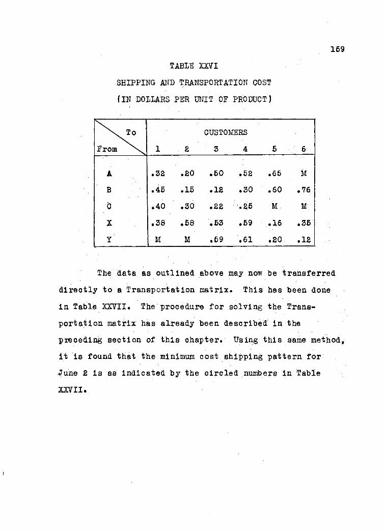
169

TABLE XXVI

SHIPPING AND TRANSPORTATION COST

(IN DOLLARS PER UNIT OF PRODUCT)

\ v To CUSTOMERS

From 1 2 3 4 5 6

A .32 .20 .60 .52 .65 M

B .45 .15 .12 .30 .60 .76

G .40 .30 .22 .25 M M

X .38 .58 .53 .69 .16 .36

y M. M .59 .61 .20 .12

The data as outlined above may now be transferred

d i r e o t l y to a Transportation matrix. This has been done

i n Table XXVII. The procedure f o r solving the Trans

portation matrix has already been described' l n the

preceding section of t h i s chapter. Using t h i s same method,

i t i s found that the minimum cost shipping pattern for

June 2 i s as indicated by the o i r c l e d numbers i n Table

XXVII.

160

TABLE XXVII

TRANSPORTATION MATRIX

To CUSTOMERS A v a i l

From \. 1 2 3 4 5 6 Dummy able Quantity

32 20 50 52 65 M 0 A © © © (390) 500

45 15 12 30 60 76 0

CO CO

B ^8oJ) 80 CO CO 40 30 22 25 . M M 0 o W C (6cT) © 130

38 58 53 59 16 35 0 X © (̂ 60) 520

M M 59 61 20 12 0 Y © (400) 420

Customer Demand 30 50 140 100 60 20 1250 1650

Once again, the. minimum cost solution i s rather

obvious i n this case through an inspection of th« Trans

portation matrix., In the p r a c t i c a l s i t u a t i o n , however,

the selection of the optimum w i l l usually be complicated

by a f a r greater number of customer orders than has been

used i n t h i s i l l u s t r a t i o n . But even then, the Trans

portation Method w i l l provide the optimum solution i n

few simple steps.

CHAPTER. VI

SUMMARY AND CONCLUSIONS

I. SUMMARY

The physical d i s t r i b u t i o n concept i s concerned

with the group of i n t e r r e l a t e d processes that are involved

i n the physical flow of t r a f f i c from the source of raw

materials to production and from production through

d i s t r i b u t i o n f a c i l i t i e s to customers. These processes

include transportation, materials handling, warehousing,

order-processing and communications.

There i s an increasing volume of l i t e r a t u r e

emphasizing the fact that i t i s the t o t a l oost of the

physical d i s t r i b u t i o n processes rather than cost of

ind i v i d u a l processes that must be taken into account i n

problems related d i r e o t l y or i n d i r e c t l y to the physical

movement of materials and products. This l i t e r a t u r e ,

however, tends to concentrate on one or the other of the

several problems to which the physical d i s t r i b u t i o n

concept may be applied. There also tends to be a lack of

attention i n the area of procedures that can be followed

by the f i r m i n the formulation and comparison of physical

d i s t r i b u t i o n a l t e rnatives.

Chapter two of this thesis attempted to i d e n t i f y

163

the major applications of the p h y s i c a l d i s t r i b u t i o n

concept and to i s o l a t e those applications that are within

the scope of the t r a f f i c manager's sphere of r e s p o n s i b i l i t y .

Chapters three to f i v e developed the step-by-step

procedures that may be useful to the t r a f f i c manager i n

applying the physical d i s t r i b u t i o n concept to decisions

that f a l l within his j u r i s d i c t i o n a l area.

Maj.or Applications of the Physical D i s t r i b u t i o n Concept

The scope of the problem to which the physical

d i s t r i b u t i o n concept should be applied tends to increase

with the time period. In day-to-day operations, demand

must be met out of inventories that are on hand at

d i s t r i b u t i o n points. The application i n t h i s case i s

limited to the determination of which customer orders

should be f i l l e d from which d i s t r i b u t i o n point, and the

methods of transportation that should be used between

stock points and customers. Considering the problem over

successively longer planning i n t e r v a l s , however, i t

becomes clear that alternatives of progressively greater

scope emerge with the expiration of present constraints i n

the form of c a p i t a l shortage, contracts and other current

commitments. T y p i c a l l y , the alternatives for physical

d i s t r i b u t i o n w i l l increase i n scope i n the following order

164

as the planning period i s extended further into the future:

1. Alternative u t i l i z a t i o n of e x i s t i n g physical

d i s t r i b u t i o n f a c i l i t i e s .

2. Alternative systems of physical d i s t r i b u t i o n

f a c i l i t i e s with present production locations

and capacities.

3. Alternative systems of physical d i s t r i b u t i o n

i n combination with alternative s p a t i a l

allocations f o r production capacities.

A study of the physical d i s t r i b u t i o n function,

should provide f o r an evaluation of each of these groups

of alternatives i f the t o t a l benefit that i s envisaged i n

the concept i s to be r e a l i z e d .

Since the three groups of alternatives l i s t e d above

emerge at successive Intervals i n the future, the study can

be divided into three separate analysis. Care must be

exercised, however, In defining the time period f o r each

analysis i n order to avoid sub-optimization i n physical

d i s t r i b u t i o n planning. Sub-optimization w i l l occur, f o r

example, i f plans f o r the u t i l i z a t i o n of present

f a c i l i t i e s are developed fo r a period during which i t i s

feasible to introduce a more e f f i c i e n t system of physical

d i s t r i b u t i o n f a c i l i t i e s . S i m i l a r l y , planned changes i n

165

system f a c i l i t i e s w i l l be sub-optimum i f the time i n t e r v a l

that has been used i n the development of t h i s plan extends

beyond the point i n time at which a change i n the s p a t i a l

a l l o c a t i o n of plants should be introduced.

Increasing f l e x i b i l i t y over time i n the form of

c a p i t a l a v a i l a b i l i t y and freedom from present p o l i c y ,

contracts and other commitments w i l l determine,

successively, the points i n time at which i t becomes

p r a c t i c a l to consider changes i n system f a c i l i t i e s and

changes i n plant locations. An analysis of long-term

alternatives w i l l then determine the point at which i t

becomes desirable to adopt a change i n plant locations.

This point i n time marks the end of the period during which

alternatives are l i m i t e d by e x i s t i n g plant locations and,

hence, defines the shorter-term i n t e r v a l of time over which

analysis should be concerned with p o t e n t i a l changes i n the

system of physical d i s t r i b u t i o n f a c i l i t i e s . S i m i l a r l y , an

analysis of changes i n physical d i s t r i b u t i o n f a c i l i t i e s

(assuming present plant locations) w i l l i d e n t i f y the point

i n time at which the f i r s t change i n system becomes

desirable. The period p r i o r to t h i s date i s the appropriate

i n t e r v a l f o r an analysis of the alternatives f o r u t i l i z i n g

the present system of physical d i s t r i b u t i o n f a c i l i t i e s .

166

In addition to the need to avoid sub-optimization,

properly defined time periods are necessary to the

formulation of relevant physical d i s t r i b u t i o n a l t e r n a t i v e s .

Physical d i s t r i b u t i o n alternatives are adequate or

inadequate depending upon the volumes of t r a f f i c , the

location of raw materials, plants and markets and the

standards of delivery service, or the alternatives of

these s p e c i f i c a t i o n s . Alternatives are feasible only i f

they are within the confines of operating constraints,

including c a p i t a l shortages, unexpired contracts and other

commitments, and the capacity and other operating l i m i t a t i o n s

of fixed f a c i l i t i e s ( i f any). Physical d i s t r i b u t i o n

requirements and operating constraints are both subject to

change over time and i t i s only when the time period i s

c l e a r l y defined that these elements of the framework can

be i d e n t i f i e d .

It i s apparent, therefore, that a study of the

physical d i s t r i b u t i o n function should progress from a long-

term analysis to an Investigation of the alternatives f o r

successively shorter-term i n t e r v a l s of the future time

period. This procedure w i l l avoid sub-optimization In

physical d i s t r i b u t i o n planning and w i l l f a c i l i t a t e the

development of an appropriate framework fo r each of the

167

three applications of the physical d i s t r i b u t i o n ooncept.

The T r a f f i c Manager's Role

The t r a f f i c manager plays an important role i n each

of the three applications of the physical d i s t r i b u t i o n

concept. His role i s usually advisory, however, i n

decisions related to a change i n plant l o c a t i o n or a

change i n physical d i s t r i b u t i o n f a c i l i t i e s . These

decisions generally affect operations i n several functional

departments, eg., marketing, production and finance, and

cannot, therefore, be properly evaluated by any one of the

functional department heads. Decisions of t h i s nature

require top l e v e l d i r e c t i o n and co-ordination with the

p a r t i c i p a t i o n of the t r a f f i c , marketing, production and

other interested departments.

Shorter-term applications are defined i n t h i s

thesis as those In which alternatives are l i m i t e d to the

u t i l i z a t i o n of e x i s t i n g f a c i l i t i e s . These applications

range from the day-to-day problem of d i s t r i b u t i o n to

customers from available inventories, to the problem of

planning the short-term a l l o c a t i o n of output among the

firm's plants. The day-to-day decision i s e n t i r e l y within

the t r a f f i c manager's sphere of r e s p o n s i b i l i t y since

alternatives i n t h i s case are limited to the methods fo r

shipping and transportation — operations that are

t r a d i t i o n a l t r a f f i c department r e s p o n s i b i l i t i e s .

The output a l l o c a t i o n decision has been

t r a d i t i o n a l l y associated with the production manager's

r e s p o n s i b i l i t y . It i s clear, however, that physical

d i s t r i b u t i o n p r i n c i p l e s should be used i n making t h i s

decision to ensure that the product i s delivered to the

market at minimum t o t a l cost. This decision, therefore,

should be a joint undertaking by the t r a f f i c and the

production managers who are f a m i l i a r respectively with

physical movement and production alternatives. (It should

be pointed out that marketing sp e c i f i c a t i o n s i n the short-

term are usually f i x e d by longer-term plans and p o l i c y .

Short-term physical d i s t r i b u t i o n alternatives must meet

these requirements and there i s no danger, therefore, that

marketing a c t i v i t y w i l l be adversely affected by the

short-term production a l l o c a t i o n decision).

Since i t i s only the short-term applications of

the physical d i s t r i b u t i o n concept i n which physical

d i s t r i b u t i o n decisions w i l l be made by the t r a f f i c manager,

th i s thesis has been l i m i t e d t o the development of a

method of analysis f o r two of the physical d i s t r i b u t i o n

applications for t h i s period — the day-to-day problem

and the output a l l o c a t i o n problem.

169

The solution to both of these problems requires an

a l l o c a t i o n of limited resources among competing demands.

In the day-to-day problem, there are competing customer

orders f o r the limited quantity of inventory that i s

available at i n d i v i d u a l d i s t r i b u t i o n warehouses. In the

output a l l o c a t i o n problem, there are competing ways l n

which the l i m i t e d capacity of each production and physical

d i s t r i b u t i o n f a c i l i t y can be u t i l i z e d . The l i m i t e d

resources, competing demands c h a r a c t e r i s t i c s place the

solution to these problems within the scope of the l i n e a r

programming technique. This thesis attempts to set down

the step-by-step procedures that can be followed i n

developing the physical d i s t r i b u t i o n alternatives into a

form suitable f o r s o l u t i o n through t h i s technique.

The Day-to-day Problem

In the day-to-day problem, customer orders must be

s a t i s f i e d out of inventories that are on hand at f i n a l

d i s t r i b u t i o n warehouses. The objective of analysis i s to

determine which customer orders should be f i l l e d from

which warehouse i n order to minimize the t o t a l cost of

f i l l i n g the day's orders. Shipping and transportation i s

the only additional physioal d i s t r i b u t i o n cost, once the

product becomes available f o r d i s t r i b u t i o n at the f i n a l

170

d i s t r i b u t i o n points. The optimum solution to the day-to

day problem, therefore, w i l l be the one that minimizes the

t o t a l of these costs f o r the day's orders.

The l i n e a r programming model i n t h i s case requires

a l i s t of the customers from whom orders have been received

and the size of t h e i r respective orders; a l i s t of the

d i s t r i b u t i o n warehouses and the units of product that are

available for d i s t r i b u t i o n at each of these points; and

the minimum shipping and transportation cost per unit of

product to each customer from alternative d i s t r i b u t i o n

points.

The l i s t of customers and t h e i r order quantities

can be taken d i r e c t l y from the day's sales orders, or

from shipping r e q u i s i t i o n s received from the sales

department. The units of product that are available f o r

d i s t r i b u t i o n at each warehouse can be calculated from

warehouse inventory records — the available inventory

at a warehouse being the difference between the quantity

on hand and the quantity that i s expected to be required

over the period p r i o r to receipt of a replenishment order

to s a t i s f y a predetermined maximum reasonable demand from

customers that are normally served from that point.

The minimum shipping and transportation costs per

171

unit of product w i l l have to he established through a

comparison of the alternatives of these processes f o r each

of the feasible warehouse-customer combinations. A ware

house-customer combination i s f e a s i b l e i f there i s a s u i t

able method or suitable methods of transportation that w i l l

s a t i s f y delivery service s p e c i f i c a t i o n s . The required

delivery service f o r each order may be specified i n the

shipping r e q u i s i t i o n , or by the marketing department. In

other instances, the analyst may assume that the l e v e l of

service that has been provided i n the past i s adequate.

Having established the minimum per unit cost for

shipping and transportation between each of the f e a s i b l e

warehouse-customer combinations, t h i s information together

with i n d i v i d u a l customer orders and the quantity of

inventory that i s available f o r d i s t r i b u t i o n at each ware

house, oan be Inserted i n a l i n e a r programming matrix. The

optimum method of physical d i s t r i b u t i o n can now be

established from t h i s matrix by applying the l i n e a r

programming method of solution commonly referred to as the

Transportation Method. This method i s described i n d e t a i l

i n Chapter V.

The Output A l l o c a t i o n Problem

In the output a l l o c a t i o n problem, the objective of

172

analysis i s to determine the optimum a l l o c a t i o n of forecast

short-term demand among the firm's plants. The optimum is

the alternative that w i l l minimize the t o t a l of short-term

production and physical d i s t r i b u t i o n costs.

The l i n e a r programming model f o r t h i s problem

requires a forecast of product demand at each of the

d i s t r i b u t i o n warehouses; a d e f i n i t i o n of the production

capacity of each plant; and an estimate of the t o t a l unit

variable cost that would be incurred i n the manufacture

and physical d i s t r i b u t i o n of each product to each

d i s t r i b u t i o n warehouse and through each of the routes that

t r a f f i c may take through the production-distribution

system.

In forecasting the units of product that w i l l pass

through each warehouse during the period, the f i r s t step

i s to define the market areas that w i l l be served from

each point. This can be accomplished i n two steps. The

f i r s t step i s to i d e n t i f y the geographical segments of the

t o t a l market that can be served from each d i s t r i b u t i o n

warehouse. The procedure i s to relate delivery service

requirements i n the various customer areas with transpor

t a t i o n a v a i l a b i l i t y to determine whether or not i t i s

feasib l e to serve a s p e c i f i c customer location from a

173

given warehouse. The seoond step i s to reduce the size of

the market area that can he served from a warehouse to i t s

handling capacity by eliminating the demand of those

customers that can be served from an alternative warehouse

at a lower shipping and transportation cost.

Sales forecasts and defined delivery standards are

necessary i n the above procedures. Since the marketing

department Is l i k e l y to be f a m i l i a r with the t e r r i t o r i a l

breakdown of the t o t a l sales forecast, t h i s department

should be c a l l e d upon to allocate forecast demand i n units

of product among geographical areas as defined by the

t r a f f i c manager. Delivery service s p e c i f i c a t i o n s f o r the

various customer areas may be defined e x p l i c i t l y by the

marketing department, or may have to be developed by the

t r a f f i c manager through a review of p o l i c y , longer-term

plans or h i s t o r i c a l service records. The delivery

standards used i n analysis should not be higher than those

that w i l l be provided i n the longer-term and should not be

lower than i n the past, unless approval has been obtained

from the marketing department.

Having established the forecast of demand at each

d i s t r i b u t i o n warehouse, the next step i n analysis i s to

define the output capacity of each of the firm's plants

174

over the short-term period. The output of a plant during

. t h i s period i s limited by technical considerations i n the

u t i l i z a t i o n of f a c i l i t i e s , p o l i c y , organizational problems

and other constraints that contribute toward production

i n f l e x i b i l i t y . The production manager should examine

these constraints with a view to defining the minimum and

maximum output that i s feasible f o r each plant over the

defined i n t e r v a l . The maximum output figures w i l l be used

i n the l i n e a r programming model. Minimum output figures

w i l l not be used d i r e c t l y i n the model but rather as a

check on the solution to ensure that the output that i s

oalled f o r at each plant i s not below the feasi b l e minimum.

When two or more of the products that are

manufactured at a plant pass through one or more of the

same processes, the mix of output that w i l l absorb capacity

cannot be predetermined and i t becomes necessary to express

capacity i n terms of man-hours, machine-hours or other

common measurement. In t h i s case, the various manufacturing

operations i n the plant should be examined to determine the

common process that l i m i t s t o t a l output. I f t h i s bottleneck

process i s a manual operation, plant capacity should be

defined i n terms of available man-hours i n t h i s process f o r

the period. S i m i l a r l y , i f the bottleneck process i s a

machine operation, t o t a l available hours i n t h i s process

175

for the period would he the appropriate capacity measure

ment. The production manager should also define the

portion of bottleneck: capacity that w i l l be absorbed i n

the manufacture of a unit of each of the firm's products

so that the combinations of product volumes that w i l l

absorb t o t a l capacity at the plant can be i d e n t i f i e d .

Given the demand forecast f o r each warehouse, and

the output capacity of each plant, i t remains to complete

the data f o r the l i n e a r programming model by estimating

the t o t a l per unit variable cost of each product at each

of the d i s t r i b u t i o n warehouses and through each of the

routes that t r a f f i c may take through the production-

physical d i s t r i b u t i o n system.

A t r a f f i c route consists of a source or sources

of raw materials for the, product, a plant at which the

product can be manufactured and a d i s t r i b u t i o n warehouse,

linked together by one or more methods of transportation.

The f i r s t step i s to define the feasible t r a f f i c routes

by determining whether or not there i s a suitable and

available method of transportation between each source of

raw materials and each plant, and between each plant and

each d i s t r i b u t i o n warehouse. The r e s u l t of t h i s

investigation can be shown i n a flow diagram.

176

The second step i s to i d e n t i f y the variable cost

of each of the production and physical d i s t r i b u t i o n

processes and the key parameters that w i l l permit a

l i n k i n g of the i n d i v i d u a l process costs into t o t a l route

cost* The unit variable cost f o r a route w i l l include

the purchase price of raw materials used i n the produot,

the cost of shipping and transportation between the

source of raw materials and the plant, the cost of

manufacturing, the cost of shipping and transportation

between the plant and .distribution warehouse, the cost of

carrying raw materials and f i n i s h e d product inventories

at the plant, the cost of carrying product inventory at

the warehouse and the cost of order-processing and

communication procedures.

Schedules for each of these costs and the

procedures to be followed i n estimating and r e l a t i n g

i n dividual process costs into t o t a l route costs are

described i n d e t a i l i n Chapter IV.

When there are alternatives for transportation

between the source of raw materials and the plant or

between the plant and warehouse portions of a route, the

t o t a l variable cost that would be incurred with each

method of transportation must be developed. A comparison

of the t o t a l variable costs associated with alternative

177

methods of transportation must then be made i n order to

i d e n t i f y the alternative that offers minimum per unit

product cost for the route. This cost figure w i l l be the

one that i s used i n the l i n e a r programming model'.

Having established the minimum variable cost per

unit f o r each product and f o r each of the f e a s i b l e

t r a f f i c routes, t h i s information, together with the

demand at each d i s t r i b u t i o n warehouse; the capacity of

each plant and the capacity that w i l l be absorbed at

each plant by a unit of each product, should be inserted

i n a l i n e a r programming matrix of the type that i s

commonly referred to as the Simplex Matrix. The minimum

cost solution to the production a l l o c a t i o n problem can be

determined by applying prescribed Simplex rules to t h i s

matrix. It i s generally impractical, however, to.attempt

a solution through hand c a l c u l a t i o n because of the volume

of work that i s involved i n applying these rules. Many

of the larger computers have been programmed for the

Simplex and t h i s i s the preferred method of solution when

th i s equipment i s available.

In c e r t a i n circumstances, however, the Simplex

matrix can be transformed into a matrix that i s suitable

for s olution through the r e l a t i v e l y simple Transporta-

178

t i o n Method. The p a r t i c u l a r circumstances i n which t h i s

transformation i s acceptable and the step-by-step

procedure to be followed i n converting from a Simplex to

a Transportation Matrix i s described i n d e t a i l i n Chapter

V of t h i s thesis.

I I . CONCLUSIONS

The physical d i s t r i b u t i o n concept emphasizes the

int e r r e l a t i o n s h i p between transportation, handling, order-

processing, warehousing and the other processes that are

involved i n the physical flow of t r a f f i c from the source

of raw materials to plants and from plants through

d i s t r i b u t i o n f a c i l i t i e s to customers. The essence of the

concept i s that i t i s the t o t a l cost of the several

processes rather than the cost of i n d i v i d u a l processes

that should be taken into account i n decisions that are

related d i r e c t l y or i n d i r e c t l y to the physical movement of

materials and products.

( The business decisions i n which physical

d i s t r i b u t i o n cost i s an important element include the long-

term s p a t i a l a l l o c a t i o n of production f a c i l i t i e s ; the

intermediate-term changes i n the system of physical

d i s t r i b u t i o n f a c i l i t i e s ; the short-term u t i l i z a t i o n of

exi s t i n g production and physical d i s t r i b u t i o n f a c i l i t i e s ;

179

and the day-to-day d i s t r i b u t i o n of available output.

In making these decisions, i t i s important to

recognize that physical d i s t r i b u t i o n alternatives (except

day-to-day alternatives) are usually i n t e r r e l a t e d with

alternatives i n one or more of the purchasing, production

and marketing functions of the enterprise. This i n t e r

relationship i s not surprising since physical d i s t r i b u t i o n

i s the connecting l i n k between purchasing and production

and between production and marketing operations. The cost

of raw materials input at a plant, f o r example, includes

the price of raw materials as well as the cost of physical

d i s t r i b u t i o n from t h e i r source to the plant. Hence, when

there are alternative sources of raw materials, the

purchase decision and the physical d i s t r i b u t i o n decision

cannot be made independently. S i m i l a r l y , the cost of the

product at a d i s t r i b u t i o n point includes the cost of the

manufactured product at a plant as well as the cost of

physical d i s t r i b u t i o n from plant to warehouse. Hence,

when d i s t r i b u t i o n warehouses can receive the product from

alternative plants and when future demand i s not expected

to absorb t o t a l production capacity, there must be an

integration of the decisions that w i l l govern the rate of

output at each of the firm's plants and the methods of

180

physical d i s t r i b u t i o n between plants and d i s t r i b u t i o n

warehouses.

Considered i n the longer-term, there w i l l be

s u f f i c i e n t c a p i t a l and operating f l e x i b i l i t y to introduce

changes i n the system of physical d i s t r i b u t i o n f a c i l i t i e s ,

some of which w i l l e i t h e r extend the geographical

t e r r i t o r y that the f i r m w i l l be able to accommodate,

increase the e f f i c i e n c y i n terms of cost or delivery service

with which the exi s t i n g markets can be served or change the

r e l a t i v e e f f i c i e n c y with which the product can be delivered

to s p e c i f i c segments of the present market. In other

words, marketing implications are associated with physical

d i s t r i b u t i o n alternatives and decisions i n the .two areas

are therefore interdependent. In the very long-term,

f l e x i b i l i t y w i l l be s u f f i c i e n t to permit the fi r m to

consider a relocation of production capacities together

with a change i n the system of physical d i s t r i b u t i o n . It

i s imperative, of course, that each of the alternative

combinations of markets that are available to the fi r m i n

the very long-term be evaluated i n the l i g h t of t o t a l

delivered product cost through alternative s p a t i a l

allocations of production capacities and alternative

systems of physical d i s t r i b u t i o n f a c i l i t i e s .

181

In view of these i n t e r r e l a t i o n s h i p s , i t i s clear

that physical d i s t r i b u t i o n analysis, i e . , the formulation

and comparison of physical d i s t r i b u t i o n a l t e r n a t i v e s , i s

usually only a part of the o v e r a l l analysis i n which

physioal d i s t r i b u t i o n alternatives are integrated with

alternatives i n other areas of operations to determine

the optimum course of action for the firm. An exception

i s the day-to-day problem of s a t i s f y i n g customer orders

from output that i s available at f i n a l d i s t r i b u t i o n points*

Physical d i s t r i b u t i o n alternatives In t h i s case must

s a t i s f y i n f l e x i b l e marketing requirements (given customer

orders and delivery service). Purchasing and production

operations are unaffected by the day-to-day warehouse to

customer physical movement decisions.

Day-to-day decisions i n physical d i s t r i b u t i o n

appear to f a l l within the sphere of r e s p o n s i b i l i t y that i s

usually assigned to the t r a f f i c manager. It i s clear,

however, that longer-term decisions i n which i t i s

necessary to integrate alternatives for physical d i s t r i

bution with alternatives i n other areas of operations, are

beyond the soope of the decisions that can be made by the

t r a f f i c manager of the t y p i c a l organization structure. A

few firm's have appointed physical d i s t r i b u t i o n managers.

This t i t l e , however, appears to he functionally oriented

i f i t i s intended that these o f f i c e r s are to integrate

marketing, production and physical d i s t r i b u t i o n

alternatives.

In the author's opinion, physical d i s t r i b u t i o n

decisions for the longer-term, i e . , changes i n the system

of physical d i s t r i b u t i o n f a c i l i t i e s and i n the s p a t i a l

a l l o c a t i o n of production capacities, i s an i n t e g r a l part

of the development of o v e r a l l corporate plans. The

corporate planning function i s usually undertaken by a

planning unit that reports d i r e c t l y to the chief

executive, or by a research and development department.

It would seem that t h i s i s where the i n t e r r e l a t i o n s h i p

between the longer-term physical d i s t r i b u t i o n alternatives

and other operations can be properly evaluated. The role

of the t r a f f i c department and other operating departments

should be to contribute to the o v e r a l l planning process by

providing cost and other information related to

alternatives within t h e i r respective f i e l d s .

While the t r a f f i c manager's role i s advisory i n

planning for the longer-term, i t would seem that t h i s

o f f i c e r i s i n a p o s i t i o n to direct and co-ordinate the

analysis that i s necessary for short-term operating plans

183

i n which materials and product d i s t r i b u t i o n i s involved*

Marketing requirements during t h i s period are usually

fixed since the firm w i l l have committed i t s e l f , through

longer-term plans and p o l i c y , to certain markets and to

a c e r t a i n standard of service within each of these

markets. Production and d i s t r i b u t i o n f a c i l i t i e s are also

fi x e d during t h i s period, but there w i l l usually be some

f l e x i b i l i t y i n the mix and the rate of output that can be

achieved at each plant, and i n the methods of physical

d i s t r i b u t i o n that can be employed with given f a c i l i t i e s .

Marketing requirements, the l o c a t i o n and price of

raw materials, and the cost and f l e x i b i l i t y of production

at each plant can be defined f o r analysis purposes by the

marketing, purchasing and production departments. This

framework w i l l permit the t r a f f i c manager to develop the

alternatives f o r short-term t r a f f i c flow through the

production-distribution system; to determine the t o t a l

cost of production and physical d i s t r i b u t i o n for each of

the flow alternatives; and to select the alternative that

offers minimum t o t a l delivered product cost f o r the

period. The' pattern of t r a f f i c flow that i s i m p l i c i t i n

the solution to t h i s problem w i l l indicate the locations

from which materials are to be purchased and the mix and

184

volume of t r a f f i c that each of the production and physical

d i s t r i b u t i o n f a c i l i t i e s w i l l be required to accommodate.

The solution, then, w i l l provide the basis f o r detailed

operating plans within each of the purchasing, production

and physical d i s t r i b u t i o n areas of business operations.

Mathematical programming i n general and l i n e a r

programming i n p a r t i c u l a r appear to have promise as the

methods i n which the complex in t e r r e l a t i o n s h i p s that are

usually associated with physical d i s t r i b u t i o n applications

can be resolved. The problems f o r which mathematical

programming is i d e a l l y suited are those i n which there are

several possible courses of action; c e r t a i n conditions

that must be met (demands); and c e r t a i n l i m i t a t i o n s that

must not be exceeded (constraints). Physical d i s t r i b u t i o n

applications f a l l within t h i s group of problems. In the

short-term planning problem, for example, there are

several ways in which future demand may be allocated among

the firm's plants, but alternative allocations must

s a t i s f y warehouse demands and must not exceed the capacity

of production and physical d i s t r i b u t i o n f a c i l i t i e s . The

advantages of the mathematical programming technique are

that i t requires a mathematical formulation of the problem

and, hence, requires an organized procedure f o r the

185

formulation of a l t e r n a t i v e s ; i t permits a l l of the

quantifiable deciands and constraints that are relevant to

the problem to be taken into account; and i t provides the

best solution out of the several possible solutions

through a simple and a d e f i n i t e routine.

In view of these imposing advantages and the fact

that the c h a r a c t e r i s t i c s of physical d i s t r i b u t i o n

applications place these problems within the realm of t h i s

technique, i t i s surprising that few of the proponents of

the physical d i s t r i b u t i o n concept have emphasized the

potential of mathematical programming i n physical d i s t r i

bution analyses. There i s a need f o r further research

into the development of l i n e a r programming, non-linear

programming and other mathematical models as the tools f o r

physical d i s t r i b u t i o n analysis.

This thesis has not dealt i n d e t a i l with some of

the obvious problems that are l i k e l y to arise i n the

development of data f o r the planning model. The per unit

handling costs and order-processing and communications

costs per order, f o r example, are not l i k e l y to be readily

available from accounting and other records that are

maintained by the firm — p a r t i c u l a r l y for the alterna

tives to present methods. It may be necessary, therefore,

186

to employ work study procedures, regression analysis,

engineering studies or other methods to develop suitable

estimates of i n d i v i d u a l process costs. A second short

coming of t h i s thesis i s that the assumed relationships

between physical d i s t r i b u t i o n processes that have been

used i n the i l l u s t r a t e d example may be overly s i m p l i f i e d .

Handling costs, f o r example, may vary with the degree of

congestion at the stock point as well as with the method

of transportation that i s used. Order-processing and

communication costs, which include the cost of expediting

an order through the system, may vary with the point from

which materials are received or with the method of

transportation that i s used. It i s e s s e n t i a l , of course,

that a l l of the relationships between physical d i s t r i b u t i o n

processes be i d e n t i f i e d i n order to produce r e l i a b l e

estimates of route costs.

In practice, the planning problem may be

complicated by several factors that have not been taken

into account i n the hypothetical problem that has been

described i n t h i s t h e s i s . The purchase price of raw

materials, f o r example, may vary with order size; i t may be

possible to combine various materials or products for

shipping purposes; i t may be possible to achieve higher

output at plants through the use of overtime; etc.

187

A procedure fo r the formulation and comparison of

alternative systems of physical d i s t r i b u t i o n f a c i l i t i e s

and alternative s p a t i a l a l l o c a t i o n s f o r plant capacities

was beyond the scope of t h i s thesis. These applications

of the physical d i s t r i b u t i o n concept have been discussed

i n some of the published l i t e r a t u r e , most of which has

dwelt upon the development of alternatives within the

framework of given marketing s p e c i f i c a t i o n s . It should

be emphasized however, that the markets that can be served

and the standards of service that can be offered may vary

with alternative systems of physical d i s t r i b u t i o n

f a c i l i t i e s and with alternative s p a t i a l allocations for

production capacities. I f marketing s p e c i f i c a t i o n s are

predefined, i t i s possible that an opportunity to serve a

more pr o f i t a b l e combination of markets, or an opportunity

to improve the net contribution from existing markets,

w i l l be overlooked.

A review of the l i t e r a t u r e dealing with the

physical d i s t r i b u t i o n concept suggests the need f o r

additional case h i s t o r i e s of successful applications*

These case studies should be s u f f i c i e n t l y detailed to

permit the readers to evaluate:

1. The factors that have been taken into account

188

i n establishing the objectives and the frame

work for analyses.

E i The procedures that have been used i n the

development of physical d i s t r i b u t i o n

alternatives.

3. The procedures that have been employed i n

establishing the i n t e r r e l a t i o n s h i p between the

cost of i n d i v i d u a l physical d i s t r i b u t i o n

processes.

4. The provision that has been made for r e l a t i n g

physical d i s t r i b u t i o n alternatives with

alternatives i n other areas of operations.

5. The method that has been used i n s e l e c t i n g

the optimum altern a t i v e .

In conclusion, i t appears that there i s a need at

t h i s time for a bridge between physical d i s t r i b u t i o n

theory and physical d i s t r i b u t i o n practice. More empirical

studies are necessary before management w i l l be able to

grasp the essentials of physical d i s t r i b u t i o n analysis and

the procedures for analysis that w i l l s a t i s f y t h e i r

i n d i v i d u a l requirements.

189

BIBLIOGRAPHY

1. BOOKS

Aminer, Dean S. Materials Management. Homewood, I l l i n o i s : Richard D. Irwin Inc., 1962.

Baumol, William J . Economic Theory and Operations Analysis. Englewood C l i f f s , New Jersey: Prentice-H a l l Inc., 1961.

Bock, Robert H., and William K. Holstein. Production Planning and Control: Text and Readings. Columbus, Ohio: Charles E. M e r r i l l Books Inc., 1963.

Bowman, Edward H., and Robert B. Fetter. Analysis f o r Production Management. Homewood, I l l i n o i s : Richard D. Irwin Inc., 1957*

Brown, R.G. S t a t i s t i c a l Forecasting for Inventory Control. New York: McGraw-Hill Book Company Inc., 1959.

Charnes, A., W.W. Cooper, and A. Henderson. An Introduction to Linear Programming. New York: John Wiley and Sons Inc., 1953.

Churchman, C. West, Russell L. Ackoff, and Leonard E. Arnoff. Introduction to Operations Research. New York: John Wiley and Sons Inc., 1957.

Dorfman, R., P.A. Samuelson, and R.M* Solow. Linear Programming and Economic Analysis.' New York: McGraw-Hill Book Company Inc., 1958.

Frederick, John F. Using Public Warehouses. Philadelphia: Chilton Company Inc., 1957.

Greenhut, Melvin L. Plant Location i n Theory and i n Practi c e . Chapel H i l l , North Carolina: The University of North Carolina Press, 1956.

Holt, Charles C., et a l . Planning Production, Inventories. and Work Force. Englewood C l i f f s , New Jersey: Prentice-Hall Inc., 1960.

190

Isard, Walter. Location and Space-Economy. New York: John Wiley and Sons Inc., 1956.

Lewis, Howard T., and James W. C u l l i t o n . The Role of A i r Freight i n Physical D i s t r i b u t i o n . Boston: The Alpine Press Inc., 1956.

Magee, John F. Production Planning and Inventory Control.- New York: McGraw-Hill Book Company Inc., 1958.

Reinfeld, V., and William R. Vogel. Mathematical Programming. Englewood C l i f f s , New Jersey: Prentice-Hall Inc., 1958.

Sasieni, Maurice, Arthur Yaspan, and Lawrence Friedman. Operations Research-Methods and Problems. New York: John Wiley and Sons Inc., 1959.

Smykay, Edward ¥., Donald J . Bowersox, and Frank H. Mossman. Physical D i s t r i b u t i o n Management. New York: The MacMillan Company, 1961.

Sord, Burnard H., and Glenn A. f/elsch. Business Budgeting. New York: Controllers Institute Research Foundation, 1958.

Taff, Charles A., T r a f f i c Management P r i n c i p l e s and Practices.. Homewood, I l l i n o i s : Richard D. Irwin Inc., 1959.

Yazsonyi, Andrew. S c i e n t i f i c Programming In Business and Industry* New York: John Wiley and Sons Inc., 1958.

V i l l e r s , Raymond. Dynamic Management i n Industry. Englewood C l i f f s , New Jersey: Prentice-Hall Inc., 1960.

Welch, W. Evert. Tested S c i e n t i f i c Inventory Control. Greenwich, Connecticut: Management Publishing Corporation, 1956.

Whit In j Thomson M. The Theory of Inventory Management. Princeton, New Jersey: Princeton University Press, 1957.

191

2. PERIODICALS

Baer, John W. "Pinpointing Transport's Hidden Costs," D i s t r i b u t i o n Age, LIX, No. 7 (July, 1960), pp. 36, 37 and 70..

Baumol, William J . , and P h i l i p Wolfe. "A Warehouse Location Problem," -Operations Research. VI, 1958, pp. 25S-63.

D i l l o n , John D. "Geographical D i s t r i b u t i o n of Production in,Multiple Plant Operations," Management Science, I I , No. 1 (October, 1955), pp. 353-65. .

Eneborg, C.G. "How to Plot the Ideal Location for a Warehouse,"- Management Methods, XIII (January* 1958), pp..52-55.

Forrester, Jay W. " I n d u s t r i a l Dynamics: A Major Breakthrough f o r Decision Makers," Harvard Business Review, XXXVI, No. 4 (July-August, 1958), pp. 37-66.

Granger, Charles H. "Best Laid Plans," The Controller. (August, 1962), pp. 42-45.

Greene, A.W. "The DM, New Man On Industry's Top Team," D i s t r i b u t i o n Age, LIX, No. 3 (March, 1960), pp. 37-38.

Henderson, Alexander, and Robert S c h l a i f e r . "Mathematical Programming, Better Information f o r Better Decision Making," Harvard Business Review, XXXII, No. 3 (May-June,.. 1954), pp. 117^44.

Heskett, J.L. "Ferment i n Marketing's Oldest Area, n

Journal of Marketing, XXVI, No. 4 (October, 1962), pp. 40-45.

Holt, C.C., F. Modigliani, and H.A. Simon. "A Linear Decision Rule for Production and Employment Scheduling," Management Science, I I , No. 1 (October, 1955), pp. 1-30.

192

"Keys to Warehouse Selection," D i s t r i b u t i o n Age, IX, No. 2 (February, 1961), pp. 30-31.

Landis, Eugene. " D i s t r i b u t i o n Management. How to Set Up Your Department," D i s t r i b u t i o n Age. LX, No. 11 (November, 1961), pp. 34-36.

Lazer, William. " D i s t r i b u t i o n and Marketing Mix," Transportation and D i s t r i b u t i o n Management. I I , No. 12 (December, 1962), pp. 12-17.

Magee, John F. "Guides to Inventory P o l i c y , " Harvard Business Review, XXXIV, No. 1 (January-February, 1956), pp. 49-60; XXXIV, No. 2 (March-April, 1956), pp. 103-16.

. "The l o g i s t l o s of D i s t r i b u t i o n , " Harvard Business Review. XXXVIII, No. 4 (July-^ August, 1960), pp. 89-101.

"Mathematics i n Management," Plant Administration and Engineering, XXII* No. 11 (November, 1962), pp. 53-72.

Modigliani, F., and F.E. Hohn. "Planning over Time, with Some Conclusions About the Nature of the Expectation and Planning Horizon," Econometrica. XXIII (January, 1955), pp. 46-66..

" P i t t Seminar Analyses Total Costs i n D i s t r i b u t i o n Management," Railway Age, CL, No. 9 (February 27, 1961), pp. 40-41.

Rapoport, Leo A., and William P. Drews. "Mathematical Approach to Long-Range Planning," Harvard Business Review. XL, No. 3 (May-June, 1962), pp. 75-87.

Schorr, Jerry. "Product Glut and Start-Up Inventory," Transportation and D i s t r i b u t i o n Management. I l l , . No. 4 ( A p r i l , 1963), pp. 24-26.

Shycon, Harvey N., and Richard B. Maffie. "Simulation: Tool f o r Better D i s t r i b u t i o n , " Harvard- Bus ine s s Review. XXXVIII, No. 6 (November-December, I960)-, pp. 65-75.

193

Smykay, Edward W. "Physical D i s t r i b u t i o n Management," T r a f f i c World. CVII, No. 7 (February 18. 1961), pp. 75-81; CVII, No. 15 ( A p r i l 15, 1961), pp. 64-6

Snyder, Richard E. "Physical D i s t r i b u t i o n Costs," D i s t r i b u t i o n Age. LXI, No. 1 (January/ 1962),

(March, 1962), p. 35; LXI, No. 4 T A p r i l , 1962), p. 37.

Sweeney, Richard J . "How to Determine the Number and Location of Warehouses," Modern Materials Handling, XVII* No. 1 (January, 1962). pp. 76-79.

"Warehouse X - Its P r o f i t a b l e Shipping Area," D i s t r i b u t i o n Age. IX, No. 2 (February, 1961), pp. 32-33.

PUBLICATIONS OF THE GOVERNMENT AID OTHER ORGANISATIONS

Beckmann, M., and T. Marschak. "An A c t i v i t y Analysis Approach to Location Theory," Proceedings of the Second Symposium i n Linear Programming* pp. 331-79. Washington: National Bureau of Standards, U.S. Department of Commerce, 1955.

Flaks, Marvin. Total Cost Approach to Physical D i s t r i b u t i o n . BMC Report Number 3. Greenwich, Connecticut: Business Management Council Inc., 1963.

Physical D i s t r i b u t i o n Management. AMA Management Report No. 49. New York: American Management Association Inc., 1960.

Smykay, Edward W. (Ed). Essays on Physical D i s t r i b u t i o n Management. Washington: The T r a f f i c Service -Corporation, 1961.

pp. 44-51.

.".Putting the Physical D i s t r i b u t i o n Cost Survey

UNPUBLISHED MATERIALS

Robertsj M e r r i l l J . "Transport Dynamics and D i s t r i b u t i o n Management." Paper read at the Physical D i s t r i b u t i o n Management Seminar, University of Pittsburgh, February 3, 1961.

Thompson, John T. "Unimarket, An Integrated D i s t r i b u t i o n System." Paper read at the D i s t r i b u t i o n Management Conference sponsored by the American Management Association Inc., San Francisco, C a l i f o r n i a , A p r i l 13, 1960.

physical distribution analysis for the traffic manager - Open ...

Documents

Transcript of physical distribution analysis for the traffic manager - Open ...