PHY 122 Lab Manual - Thomas More Physics
62
-
Upload
khangminh22 -
Category
Documents
-
view
0 -
download
0
Transcript of PHY 122 Lab Manual - Thomas More Physics

PHY 122 Lab Manual
Thomas More College, Algebra-based Introductory Physics

PHY 122 Lab Manual
Thomas More College, Algebra-based Introductory Physics
Joe Christensen
Thomas More College
Jack Wells
Thomas More College
Wes Ryle
Thomas More College
Latest update: January 9, 2018
About the Authors
Joe Christensen:
B.S. Mathematics and Physics, Bradley University, IL (1990)
Ph.D. Physics, University of Kentucky, KY (1997)
�rst came to Thomas More College in 2007
Wes Ryle:
B.S. Mathematics and Physics, Western Kentucky University, KY (2003)
M.S. Physics, Georgia State University, GA (2006)
Ph.D. Astronomy, Georgia State University, GA (2008)
�rst came to Thomas More College in 2008
Jack Wells:
B.S. Physics, State University of New York at Oneonta, Oneonta, NY (1975)
M.S. Physics, University of Toledo, Toledo, OH (1978)
�rst came to Thomas More College in 1980
Edition: Annual Edition 2017-2018
Website: TMC Physics
© 2017�2018 J. Christensen, J. Wells, W. Ryle
PHY122 Lab Manual: Thomas More College by Joe Christensen, Jack Wells, and Wes Ryleis licensed under a Creative Commons Attribution-ShareAlike 4.0 International License.
Permissions beyond the scope of this license may be available by contacting one of the authors listed athttp://www.thomasmore.edu/physics/faculty.cfm.

Acknowledgements
We would like to acknowledge the following reviewers and users for their helpful comments and suggestions.
� Tom Neal, Physics Adjunct
� Dr. Jeremy Huber, Physics Sabbatical Replacement
I would also like to thank Robert A. Beezer and David Farmer for their hard work and guidance with theMathBookXML / PreTeXt format.
v

vi

Preface
This text is intended for a one or two-semester undergraduate course in introductory algebra-based physics.
vii

viii

Download the PDF here
A full PDF version of this document can be found at spring-lab-manual.pdf (638 kB).
ix

x
Contents
Acknowledgements v
Preface vii
Download the PDF here ix
1 Review the Skills of PHY 121 Lab 1
2 Archimedes' Principle 3
3 Standing Waves on a String 7
4 Speed of Sound in a Cardboard Tube 11
5 Speci�c and Latent Heats of Solids 13
6 Thermal Expansion 17
7 Re�ection and Refraction at a Plane Surface 19
8 Simple Lenses 25
9 Electric Field Lines 29
10 Internal Resistance of Batteries 31
11 Using Ohm's Law to Determine Equivalent Resistance 33
12 Magnetic Field Demonstrations - An Exercise 37
A Managing Uncertainties 43
xi

xii CONTENTS

Lab 1
Review the Skills of PHY 121 Lab
In this lab, you will be provided a worksheet of some straightforward exercises that require you to use thefollowing skills that you should have learned in the �rst term (PHY 121).
� measurement uncertainty
� propagation of uncertainty
� accuracy versus precision
� %-error and %-di�erence
� Using DataStudio and the Capstone software
� Tabulate data in excel
� Graph data in excel
� Linear Regression
� How to write a Lab Report
The point of this to provide you with an opportunity to ask questions and develop any skills you may havelost track of between then and now.
1

2 LAB 1. REVIEW THE SKILLS OF PHY 121 LAB
Lab 2
Archimedes' Principle
Experimental Objectives
� After verifying some properties of the buoyant force using Archimedes' principle, each group will predictthe maximum amount of cargo (the number of pennies) that a ship (glass beaker) will hold withoutsinking.
Archimedes was a Greek scientist who lived from 287-212 BCE. As the story goes, the king thought thathis crown was not pure gold and asked Archimedes to determine if this was true. Archimedes had previouslyobserved that a totally submerged object displaces a volume of �uid which is equal to the volume of the object,and deduced what is now called Archimedes' principle: that the buoyant force on the submerged object isequal to the weight of the displaced �uid. Knowing the weight and density of gold, Archimedes measuredthe weight of the crown and the weight and volume of the water displaced by the crown, enabling him todetermine that the crown was not pure gold.
As any swimmer who has had their head more than about 8 feet deep can tell you, the pressure exertedon the diver by the water increases as the diver swims deeper into the water. We can express this as: thepressure within a �uid is dependent on the depth at which the object sits (h), the gravitational accelerationof the earth (g), and the density of the �uid (ρf ): P = ρfgh. Because of this, the bottom surface of anyobject in a �uid will have more pressure on it than the top surface. This ∆P gives rise to a net upward forceacting on the submerged object: the buoyant force (FB). The magnitude of the upward force depends on thedensity of the �uid and the size of the object: FB = ρfgVo, where Vo is the submerged portion of the volumeof the object. A partially submerged object has a smaller buoyant force than a completely submerged object.Interestingly, unless the �uid density depends on the depth of the �uid, the FB is independent of the depth ofthe object.
Knowing the buoyant force will help you determine if an object will �oat or sink. To determine whetheran object will sink or �oat one should use Newton's second law to determine the direction of the net force.Assuming the simplest case of a submerged object feeling only its weight (Fg = mog = ρogVo) and the buoyantforce (FB = ρfgVo), if the weight of the object is greater than FB then the net force on the object is down andit will sink. If FB is larger than the weight then the net force on the object is up and then it will accelerateup. However, when an object is �oating, it is in equilibrium and the object's weight is equal to FB , whichdepends on the submerged volume. While �oating, not all of the object is submerged.
2.1 Pre-Lab Work
� Using the de�nitions of force as pressure times area, F = PA, and pressure, P = ρfgh, derive theequations for the buoyant force FB = ρfgVo (if totally submerged) and for the object's weight Fg = ρogVo,where ρo is the object's density.
3
4 LAB 2. ARCHIMEDES' PRINCIPLE
� Show that although the pressure on an object does depend on depth within the �uid, the ∆P = Pbottom−Ptop (and therefore FB) is independent of the depth within the �uid.
� Draw a force diagram for a completely submerged object:
case 1 object's density is greater than that of the �uid's,
case 2 object's density is less than that of the �uid's.
� Using Newton's Second Law show that the object in case 1 will sink, and that the object in case 2 willaccelerate up.
� Draw a force diagram for a partially submerged object which is �oating.
� Using Newton's Second Law show that if an object has a density ρo = .5ρf that only 0.5 of the object'svolume is submerged.
� Look up the density of water.
2.2 Procedure
2.2.1 Develop Your Understanding
� Select an object for which you can easily measure the volume using a caliper.
� Measure the dimensions and calculate the volume.
� Measure the mass using the triple beam balance at your table.
� Calculate the density with uncertainty.
� Predict (with uncertainty) what buoyant force this object would have if it were completely submerged.
� Predict (with uncertainty) what a scale would read if this object were completely submerged.
2.2.2 Verify Your Understanding
� Place a balance on top of a support rod so that the side with the string dangling can drop into a containerof water.
� Find the mass of your catch beaker � this should be a graduated cylinder because you will be using thisbeaker to measure both the volume and the mass of the �uid that over�ows from the over�ow container.
� Place an over�ow container under the scale so that the string can dip into the container if the lab jackis raised or lowered.
� Place a catch beaker next to the over�ow container and slowly �ll the over�ow container until it juststarts dripping. Gently tap the over�ow container once. Be very careful not to bump your table afterthis.
� As thoroughly as possible, dry o� your catch beaker and put it back in place. If you cannot dry it o�completely, you will not be able to accurately complete all of the necessary steps.
� Attach your object to the string, measure the mass of the object, mo, in air while the object dangles.
� Raise the lab jack until the object is completely submerged. Be sure to catch all of the water that
over�ows from the container!
� The scale should now read a reduced mass, ms, for the submerged object. Record this value.
� You now have three ways of calculating the buoyant force: (Pay attention to which is the most preciseand why.)
2.2. PROCEDURE 5
1. The water (via the buoyant force) supports the di�erence in weights between not submerged andtotally submerged. Calculate the buoyant force, with uncertainty, as the di�erence in these weights.Does it agree with your prediction?
2. Measure the volume of the over�ow water. This is equal to the volume of the object submerged,Vf = Vo. Calculate (with uncertainty) the buoyant force from this volume, FB = ρfgVo. Does thisagree with your prediction?
3. Note that ρfVf = mf , so instead of measuring Vf , we can measure the mass of the over�ow water.The buoyant force can also be found from: FB = mfg, the weight of the �uid. Does this agree withyour prediction?
You should ensure that you understand these results with uncertainty before continuing. If this doesn'tmake sense, then check your numbers, check your units, remeasure quantities that you thought you were sureof, and ask your instructor.
2.2.3 Consider How the Buoyant Force Changes as an Object is Submerged
For this part, you are going to repeat the previous procedure, with three modi�cations. First, you won't beable to measure the volume with a caliper. Second, based on the previous procedure, we now know whichmeasurement provides the best estimate (smallest uncertainty) for the buoyant force, so you should only needto do one of Item , Item , or Item from the previous section. Finally, we will consider an object in air, partiallysubmerged, and fully submerged.
� Select a fairly large object for which you cannot easily measure the volume using a caliper. This must�t within the over�ow container without touching the sides.
� Re�ll the over�ow container, as before, until is just starts to over�ow.
� As thoroughly as possible, dry o� your catch beaker. If you cannot dry it o�, you will have to measureits mass with whatever water is in it and you will not be able to use the previous section technique Itembecause you cannot accurately measure the volume of new water.
� Attach it to the string hanging from the balance and �nd the mass in air, mo.
� You will need to do the rest of this very carefully. Go slowly and do not bump the table.
� Raise the lab jack until the object is about half submerged. Catch the over�ow water.
� Measure the apparent mass of the object and the mass or volume of the over�ow water, as appropriate
◦ Calculate the buoyant force with uncertainty.
◦ Calculate the volume (with uncertainty) of the object that is submerged.
� Without removing any of the water from the catch beaker, continue to submerge the object and catchthe over�ow water until the object is completely submerged.
� Measure the new apparent mass of the object and the mass or volume of the over�ow water, as appro-priate.
◦ Calculate the buoyant force with uncertainty.
◦ Calculate the volume (with uncertainty) of the object that is submerged.
◦ Calculate the density (with uncertainty) of the object.
2.2.4 Fill the Cargo-Hold
You have been provided with a beaker and some pennies. Use the information in the previous sections topredict the maximum number of pennies that can be gently placed into the beaker without allowing it to sink.You should measure the mass of the beaker and the dimensions of the beaker. The volume of a cylinder isV = πr2h. You should also measure about 30 pennies (all at once) to �nd an average mass for the pennies.
After you have calculated your prediction with uncertainty, prepare the over�ow canister with water anddry the catch beaker. Invite the instructor to your table and allow the instructor to test your prediction.
6 LAB 2. ARCHIMEDES' PRINCIPLE
2.3 Questions
1. Why does an object weigh a di�erent amount when in air and when submerged in water?
2. If the string was cut on your �rst object (while submerged), what would be the acceleration of the object?
3. Why is it important to make certain that no air bubbles adhere to the object during the submerged weighingprocedures?
4. What would the buoyant force be for an object that was immersed in a �uid with the same density as theobject?
5. A �oating barge �lled with coal is in a lock along the Ohio River. If the barge accidentally dumps its loadinto the water, will the water level in the lock rise or fall?
6. Does the mass of displaced water depend on the mass of the totally submerged object or on the volume ofthe submerged object?
7. There are two identical cargo ships. One has a cargo of 5 tons of steel and the other has a cargo of 5 tonsof styrofoam. Which ship �oats lower in the water?
Last revised: Nov. 23, 2008A PDF version might be found at Archimedes.pdf (123 kB)Copyright and license information can be found here.
Lab 3
Standing Waves on a String
Experimental Objectives
In this experiment, the conditions required for the production of standing waves in a string will be inves-tigated in order to
� empirically verify the relationship between the frequency (f), wavelength (λ), and speed of a standingwave (v), for a series of normal modes of oscillation, and
� use the two relationships of the speed of the wave
v =
√FT
m/L(3.1)
v = λf (3.2)
to empirically relate the string tension (FT ) and the wave velocity (v), for one mode of oscillation,speci�cally the fundamental mode.
A wave is the propagation of a disturbance in a medium. In a transverse wave, the disturbance of themedium is perpendicular to the direction of the propagation of the wave. In this experiment, transverse waveswill be propagated along a taut �exible string. The frequency of the waves is determined by the source, thewave generator, which is driving one end of the string. The speed of the waves, v, is determined by themedium itself; namely the linear mass density of the string, (m/L), and the tension in the string which isdetermined by the static force of a mass suspended from the other end of the string, FT . This is expressed byEquation (3.1) above.
Upon hitting at the �xed end of the string, the transverse waves will re�ect back along the string. If theend of the string is rigidly held then the re�ected waves will be inverted 180◦. The initial propagated wavesand the re�ected waves will interfere constructively and destructively. At particular string tensions and/orwave frequencies, this wave superposition will give rise to waves called standing waves or stationary waves.There are many di�erent standing waves patterns (normal modes) possible which have di�erent wavelengths.The di�erent modes are characterized by the number of nodes or antinodes in the wave. At one of the normalmodes of oscillation, the amplitude of oscillation can become rather large, much larger than the amplitudeof the original propagated wave. This phenomenon is called resonance. In this experiment, each end of thestring will be close to a node position. The fundamental frequency (mode n=1) exhibits a wave pattern withone antinode. The second harmonic (mode n=2) exhibits a wave pattern with two antinodes, and so forth.
3.1 Pre-Lab Work
� De�ne the following terms: standing wave, node, and antinode.
7
8 LAB 3. STANDING WAVES ON A STRING
� Draw a set of pictures of a standing wave on a string with two �xed ends showing the fundamentalfrequency (n = 1), and the harmonics n = 2, 3, 4, and 5. Label a wavelength, the nodes, and theantinodes on each picture.
� Given Equation (3.1), predict what will happen to the velocity of the wave as the static hanging mass(providing the tension) increases, decreases, or stays the same.
� Given Equation (3.2), how can measurements of λ and f be plotted to determine the wave velocity fromthe graph? (There is more than one way to do this; one way in particular produces a line.) How shouldthe axes of the graph be labeled? Explain your reasoning.
3.2 Fixed Tension
In order to verify Equation (3.2), you can �x FT and compare multiple f to the corresponding λ.
3.2.1 Procedure
� If you have not already done so, measure the mass and length of the string in order to calculate thelinear mass density (m/L). You might note Question 3.4.3.
� A mechanical vibrator, driven with a (variable frequency) function generator, will be the wave source.Use a string slightly greater than the length of the table. Connect one end of the string to a post suchthat the vibrator can wiggle the string near that end. Hang the other end over a pulley. Keeping thestring horizontal by adjusting the height of the pulley and the location of connection at the other end.The height of the vibrator will determine the height you need the ends to be.
� Set up the system with some particular string tension (like 450 grams). This tension will be kept constantfor this entire part.
� Produce 5 di�erent normal modes by changing the frequency of the vibrator. Adjust the standing waveamplitude until it is at its maximum. Record the corresponding frequency for each normal mode.
� Measure the corresponding wavelengths for each normal mode, directly from the string with a meterstick. The vibrator end of the string is not a true node because the string is vibrating a small amount.Take this into account when measuring the wavelengths.
� Try touching the string at a node and at an antinode. What happens to the wave in each case?
� Optional: Try measuring the frequency of the vibrator with a strobe lamp.
3.2.2 Analysis
� Determine the mathematical relation between the wavelength of the standing wave and the frequency ofthe vibrator that will produce a straight line (y = mx+ b) when graphed.
� Comment on the signi�cance (and units) of the slope and intercept of this graph. Determine both theprecision and the accuracy of the slope and of the intercept; are they consistent with what you expect?(Your expectation should be based on the �other� equation which we are not testing here.)
� Use one or both of these (slope and intercept) to determine the velocity (with uncertainty) of the standingwave. Relate this (%-error) to the expected value based on the tension you chose for your speci�c string.
3.3 Fixed Wavelength
In order to verify Equation (3.1), you can �x λ and compare multiple FT to the corresponding v.
3.4. QUESTIONS 9
3.3.1 Procedure
� If you have not already done so, measure the mass and length of the string in order to calculate thelinear mass density (m/L). You might note Question 3.4.3.
� A mechanical vibrator, driven with a (variable frequency) function generator, will be the wave source.Use a string slightly greater than the length of the table. Connect one end of the string to a post suchthat the vibrator can wiggle the string near that end. Hang the other end over a pulley. Keeping thestring horizontal by adjusting the height of the pulley and the location of connection at the other end.The height of the vibrator will determine the height you need the ends to be.
� Place 150 grams (including the hanger) on the end of the string. (If you start with too little mass, thestring stretches di�erent amounts � changing the string's e�ective density � during the experiment,causing unaccounted for curving in the graph.)
� Adjust the frequency of the generator until the n = 2 mode is observed and is at its maximum amplitude.Record the frequency and corresponding wave velocity.
� Repeat the previous step for 6 hanging masses up to about 1200 grams.
3.3.2 Analysis
� Determine the mathematical relation between the hanging mass (FT ) and the wave velocity (v) that willproduce a straight line (y = mx+ b) when graphed.
� Determine which variables the slope and intercept of this graph should be related to. Determine both theprecision and the accuracy of the slope and of the intercept; are they consistent with what you expect?(The equation we are testing should imply what to expect.)
3.4 Questions
1. What are the necessary and su�cient conditions for the production of standing waves?
2. Is it valid to consider the tightening of the string to be the same as a change of medium? (Does tighteningthe string change the way waves move or the way standing waves are produced on the string?) Why or whynot?
3. When you measure the length of string, remember that the string will be under tension (pulled on) andmay have some �give� to it. It may be possible for it to stretch by nearly 10%. If you don't account for this (ifyou measure the unstretched length) will your value of density be incorrect too large or incorrect too small?Can you account for this either in the value of the length or in the uncertainty of the length. Will this a�ectcomparison to either of your graphs?
4. Consider the Fixed Tension graph. We noted that the vibrator end of the string should not be consideredto be a node. This means that the node might be a little in front of the post or a little behind the postand therefore your wavelength values might be a little wrong, but your error bars should already include theamount the values could be o�. Based on the error bars on your Fixed Tension graph, would shifting thewavelength data a little larger or a little smaller have made a di�erence to the values of slope or intercept thatyou calculated? If so, would it have increased the value or decreased the value? If not, why not?
5. If the tension and the linear density of the string remain constant, but the pulley is shifted further fromthe post (so that the region which is vibrating lengthens), how is the resonant wavelength a�ected? How isthe velocity of the wave a�ected?
6. What was the experimental velocity (and uncertainty) of the waves in part I of the experiment?
7. What will happen to the velocity of the wave if the tension is �xed but the frequency is changed.

10 LAB 3. STANDING WAVES ON A STRING
Last revised: (Jan, 2013)A PDF version might be found at standingwaves.pdf (103 kB)Copyright and license information can be found here.
Lab 4
Speed of Sound in a Cardboard Tube
Experimental Objectives
� The purpose of this experiment is to determine the speed of sound in an air column, both from an openand a closed tube. Data should be taken at a number of di�erent resonant frequencies.
Longitudinal sound waves can be produced by any vibrating source. The frequency of these waves isdetermined solely by this vibrating source. There must also be a medium (solid, liquid, or gas) in order forthe sound wave to be propagated. These waves do not travel through the medium instantaneously. There is a�nite wave speed which is determined by the characteristics of the medium. The wave speed is not dependenton the source. If the medium is changed, then the speed of sound also changes. For example, the pressure ofa gas, the temperature of a gas, and the gas composition are all factors which a�ect the speed of sound in thegas.
Sound waves can experience interference just like waves on a string, especially when the waves are insidea tube, like an organ pipe. Traveling waves can reach the end of the tube, then they can be re�ected back inthe direction in which they came. There are now two sets of waves which can interfere, that is the two setsof amplitudes are added together. At certain frequencies this interference gives rise to a special wave called astanding wave. This is a resonance e�ect. Standing waves can occur in tubes which have only one end open, orin tubes that have both ends open. The derivation of the equation for these special resonant frequencies willbe slightly di�erent for these open or closed tubes. See your text book for the needed pictures and equations.
4.1 Pre-Lab Work
Show a set of pictures and equations for the �rst �ve harmonics, for both an open and for a closed tube. Showand explain what nodes and antinodes are. Show and explain what a standing wave is.
4.2 Experimental Procedure
Initial set-up:
� The source of the waves will be a stereo type speaker, powered by a frequency oscillator. The waves willmove through the normal room air inside of a cardboard tube. The speaker will be placed at one end ofthe pipe.
� A microphone (Pasco) will be placed to receive the waves at the same end of the pipe.
� The Pasco Interface and the software Data Studio in the oscilloscope mode will be used to determinewhich frequencies give the maximum sound intensity for resonance.
� Measure the length of the tube.
11
12 LAB 4. SPEED OF SOUND IN A CARDBOARD TUBE
� Calculate the resonant frequency for the n=3 harmonic, using an approximate value for the speed ofsound.
� Set the generator frequency near this calculated value.
Doing the experiment:
� Adjust the sound intensity amplitude on the generator (not too loud).
� Adjust the frequency (on the generator) until the amplitude (on the scope) is actually at the maximum.This is called the resonance condition. Record the small range of frequencies which keep the amplitudeat a maximum.
� Repeat this procedure to determine 4 additional resonance frequency points.
� Repeat this for both an open tube and for the closed end tube. (Five points for each type of tube.)
� Make a graph of the resonant frequency versus the harmonic number, for each tube type.
� Determine the speed of sound from each graph.
� Calculate a speed of sound value at 20◦C.
� Determine the precision and accuracy for this experiment.
4.3 Questions
1. Does the speed of the wave depend on the frequency of the oscillator?
2. How does the speed of sound in air vary with the air temperature? By how much would the results of yourexperiment change if you conducted the experiment outside today?
3. What is meant by resonant condition?
4. In interference, at least 2 sets of waves are added together. What 2 sets of waves are added together inthis experiment?
5. Why does the closed tube only show resonance for the odd harmonics?
6. Demonstrate how sound waves can be re�ected by the open end of a tube.
7. What random errors might be in this experiment? And show any evidence of them.
8. What systematic errors might be in this experiment? And show any evidence of them.
Last revised: (Jan, 2007)A PDF version might be found at sound-cardboard-tube.pdf (66 kB)Copyright and license information can be found here.
Lab 5
Speci�c and Latent Heats of Solids
Experimental Objectives
� By measuring properties such as the �nal temperature of an isolated system that consists of hot andcool materials, you can compute the speci�c heat of an unknown material and, if this is veri�able, thenyou will have proven the equations related to the speci�c heat.
� By measuring properties of an isolated system such as the mass of ice that melts in the presence of othermaterials, you can compute the latent heat of water and, if this is veri�able, then you will have proventhe equations related to the latent heat.
When multiple substances at di�erent temperatures are placed in thermal contact, the hotter substanceslose energy (heat) while the colder ones gain energy (heat) until thermal equilibrium is reached. It is assumedthat the sum of the heat lost by the warmer objects is equal to the sum of the heat gained by the others:
−Qlost = Qgained (5.1)
Notice that Equation (5.2) says that when you heat the shot, it not only �gets warmer� (increases temper-ature), but it also �heats up� (gains energy). These are not the same, but they are very closely related. Therelation between the heat content (or internal energy) and the change of temperature is
Q = mc∆T (5.2)
where m is the mass of the substance, ∆T is the change in the temperature, and c is the speci�c heat. (Theproduct mc is also known as the �water equivalent.�) The speci�c heat of a substance is a measure of themolecular activity within the material. Measurements of speci�c heats have played an important role in helpingus to understand the nature of matter.
Furthermore, the relation between the heat content and a change of phase is
Q = mL (5.3)
where L is called the latent heat. There is a latent heat associated with each phase change.
� Latent heat of fusion, Lf , refers to the heat associated with the liquid/solid phase change.
� Latent heat of vaporization, Lv, refers to the heat associated with the vapor/liquid phase change.
For example, given one ice cube (5 g) at −10◦ C, which is to be warmed to 30◦ C, we must warm the iceto the melting point, melt it, and then warm the melted ice some more. (There are three separate terms.)The heat required to do so is
Q = mcice ∆T +mLf +mcwater ∆T
Q = (5 g)(cice)[(0◦ C)− (−10◦C)] + (5 g)Lf
+ (5 g)(cwater)[(30◦C)− (0◦C)]
This expression gives the amount of heat required (Qgained) regardless of how the ice is warmed. It doesaddress the heat lost (Qlost) by whatever warmed the ice.
13
14 LAB 5. SPECIFIC AND LATENT HEATS OF SOLIDS
5.1 Speci�c Heat Pre-Lab Exercise
A few days before doing this lab, you should download the pre-lab worksheet and do the math to remindyourself how the propagation of uncertainty works. If you did not learn this last semester, then this is youropportunity! A PDF version of the pre-lab worksheet alone can be downloaded from SHprelab.pdf (29 kB).A PDF version of the pre-lab with room for your data can be downloaded from SHprelab-data.pdf (37 kB).
The point of this worksheet is to walk you through the measurements and calculations for the Speci�c Heatlab in order to help you decide how to analyze the data and develop a thoughtful report. When you calculatethe speci�c heat based on measurements from the lab, you will use Equation (5.1):
−Qbrass = QAlcup +Qwater
−mbcb∆Tb = maca∆Ta +mwcw∆Tw
solving this for cb, we get:
cb =maca (Tf − Tia) +mwcw (Tf − Tiw)
−mb (Tf − Tib)
The �error analysis� for this lab is somewhat more involved than most of the previous labs. In order toensure your familiarity with the process, there is a Pre-Lab worksheet appended to the end of the labmanual. It is the last page so that you can tear it o� without ruining the rest of the manual. Pleaseuse the formula above and the worksheet as a guide to calculate the speci�c heat, c of brass based onthe measurements provided on the worksheet.After you have completed the calculations, you should answer the pre-lab questions below in your labnotebook. These are written speci�cally to point out the comparisons that you will need to make whenyou write up your analysis of the data.
5.1.1 Pre-Lab Questions
1. When calculating Qw, does one of the terms, ∆Tw, mw, or cw, have a signi�cantly larger relative uncer-tainty? If so, what is it about that measurement that made that uncertainty large while the others were small?Is this uncertainty improvable?
2. When calculating Qa, does one of the terms, ∆Ta, ma, or ca, have a signi�cantly larger relative uncertainty?If so, what is it about that measurement that made that uncertainty large while the others were small? Is thisuncertainty improvable?
3. When calculating the numerator, does one of the terms, Qw or Qa, have a signi�cantly larger uncertainty?If so, which measurement caused that uncertainty to be large? (See questions 1 and 2.)
4. When calculating the denominator, does one of the terms, ∆Tb or mb, have a signi�cantly larger relativeuncertainty? If so, which measurement caused that uncertainty to be large? Is this uncertainty improvable?
5. Which term, (Qw+Qa) ormb∆Tb, had the largest relative uncertainty? What is it about that measurementthat made that uncertainty large while the others were small? Is this uncertainty improvable?
6. Which measurement ultimately caused the size of δc to be as large as it was? Is there a way to reduce therelative uncertainty by planning the experiment di�erently? For example, should you use a di�erent mass ofwater or of metal? Should you start at a di�erent temperature? Should the �nal temperature be higher orlower? How might one accomplish this?
7. When you do any experiment, a signi�cant component of the analysis should be devoted to the question:For each measurement, if you measured the value to be higher than the true value, then how does this a�ectthe �nal result? To that end, for this case, answer the following:
(a) If all masses are skewed high by the scale, then is c a�ected?
(b) If all temperatures are skewed high by the thermometer, then is c a�ected?
(c) If some heat escaped into the atmosphere, lost to the experiment, then how does this a�ect the �naltemperature of the mixture and how does this a�ect the �nal value of c?
5.2. THE SPECIFIC HEAT CAPACITY OF AN UNKNOWN METAL 15
5.2 The Speci�c Heat Capacity of an Unknown Metal
The following considerations should allow you to experimentally determine (with uncertainty) the speci�c heatof the metal and, from that, the composition of the metal. Use these questions to determine your procedure,with notes about where to be careful. Verify the procedure with the professor before beginning the experiment.
1. We would like the metal to be at some warm, stable, and uniform temperature. Can you imagine whatconvenient temperature we can warm the metal to which satis�es these three conditions? Hint: In orderfor the cylinder to be at a uniform temperature, it must sit in this environment for some short time;since we don't know the temperature of a burner, we can't just place the metal on the burner itself.
2. We would like the water to be at some cool, stable, and uniform temperature. Can you imagine whatconvenient temperature we can maintain for the water which satis�es these three conditions? HINT:The container for the water must also be in thermal equilibrium with the water before the unknownmetal is added.
Note 5.2.1 (Assumption). The aluminum cup is always at the same temperature as the water.
1. The speci�c heat is an inherent property of a material. Since the cup is aluminum, you can easily �ndit's speci�c heat with a CRC, or a textbook, or it may also be stamped onto your equipment.
2. When the metal and water (with container) are placed in thermal contact, they must be isolated fromthe external environment. With what equipment will this be done? (See your lab table.)
3. If some hot metal is held in the air, it cools down. What happens to the heat when hot metal is exposedto the air? Can we easily measure the heat lost to the air? How will this a�ect your experimentaltechnique?
4. Think about Equation (5.2) and the likely values of c for the water and for the unknown metal. If thereare equal masses of water and metal, then where (roughly) do you expect the �nal temperature to be(closer to Ti for water or Ti for metal)? What if you have more water?
5. If the �nal temperature is far from room temperature and the calorimeter is not well insulated, thenwhere will the actual �nal temperature be? If the �nal temperature value is wrong in this way, then willyour calculated c for the metal be wrong too high or wrong too low?
5.3 The Latent Heat of Fusion for Water
The following considerations should allow you to experimentally determine (with uncertainty) the latent heatof water. Use these questions to determine your procedure, with notes about where to be careful. Verify theprocedure with the professor before beginning the experiment.
1. We would like the water to be at some warm, stable, and uniform temperature. Can you imagine whatconvenient temperature we can maintain for the water which satis�es these three conditions?
2. We would like the ice to be at some cool, stable, uniform, and known temperature. Can you imaginewhat convenient temperature we can maintain for the ice which satis�es these three conditions? HINT:Most freezers are colder than freezing.
Note 5.3.1 (Assumption). The aluminum cup is always at the same temperature as the water.
1. When the ice and water (with container) are placed in thermal contact, they must be isolated from theexternal environment. With what equipment will this be done? (See your lab table.)
2. You will need to know the mass of the ice added. If you take the time to weigh it on a scale, it will melt.How can we determine the mass of the ice added without explicitly placing it on the scale before addingto the water?
16 LAB 5. SPECIFIC AND LATENT HEATS OF SOLIDS
3. Based on the expected value of the latent heat of fusion for water, how much ice should you use comparedto the amount of water that you have?
4. When you add the ice, the mL term should only include the mass of the ice that will melt in the water.If you add water with your ice, then this value of m will not be accurate. How does this fact a�ect yourprocedure for adding ice?
5. If the �nal temperature is far from room temperature and the calorimeter is not well insulated, thenwhere will the actual �nal temperature be? If the �nal temperature value is wrong in this way, then willyour calculated L be wrong too high or wrong too low?
Last revised: Jan, 2010A PDF version might be found at spheat.pdf (125 kB)Copyright and license information can be found here.
Lab 6
Thermal Expansion
Experimental Objectives
� In this lab, we will use the equation for thermal expansion to identify the composition of three di�erentrods.
You may have noticed that most materials expand as they are heated. This can be seen in a wide varietyof situations: Your front door doesn't seal out the colder air, bridges have a gap of a few inches at each end,stuck jars are easier to open when hot water is run over them, etc.
6.1 Pre-Lab Questions
Consider the following situations:
1. If a single rod, 1 m in length, expands by 1 mm when heated a speci�ed amount, how much does a 2 mrod (made of the same material) expand when heated by the same amount as the 1 m rod?
2. If I have a glass jar with a metal lid and heat up both glass and lid by the same amount, do they expandthe same amount? If not, which one expands more? Why is it possible to open the heated jar?
3. If my single, 1 m metal rod is heated some amount and expands 1 mm, how much does that same rodexpand when heated by twice the original amount?
The answers to these questions show that the expansion of a material depends on it's original size, it's ma-terial composition, and the amount that the temperature changes. The equation for linear thermal expansionis
∆L = L0α∆T (6.1)
and α (lower-case Greek-symbol alpha) is the coe�cient of linear expansion, which is di�erent for each material.
Please note, ∆L is the absolute expansion,(
∆LL0
)is the relative expansion (the expansion relative
to the original length), and(
∆LL0× 100%
)is the percent expansion (the relative expansion written as a
percentage).In order to experimentally measure the value of α, you must measure the relative expansion and the change
in temperature.
1. Based on Equation (6.1), what are the units of α?
2. For reliable temperature measurements, the entire rod should be at the same temperature. This requiresa stable temperature environment. List three temperatures that can be conveniently maintained.
17
18 LAB 6. THERMAL EXPANSION
3. Ice can be colder than 0 ◦C and steam can be warmer than 100 ◦C. How can we use either (speci�callysteam) to ensure a stable temperature environment?
4. If we immerse our meter stick into the steam bath with the rod to measure the expansion, then wecannot trust the reading of the meter stick to accurately determine the new length of the rod. . . WHYNOT? What does this require of our measuring device?
5. We have an apparatus which will allow steam to enter at one end and water to drain at the other. Atwhat temperature do you expect the rod to be when it is immersed in this steam-water mixture?
6. With several groups creating steam in the same room, why should we worry about the value of �RoomTemperature� when we make a second or third measurement?
6.2 The Experiment
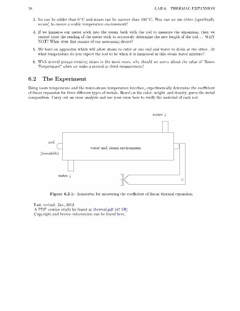
Using room temperature and the water-steam temperature interface, experimentally determine the coe�cientof linear expansion for three di�erent types of metals. Based on the color, weight, and density, guess the metalcomposition. Carry out an error analysis and use your error-bars to verify the material of each rod.
water and steam environment
rod
(immobile)
� �
water ↓
steam ↓
c��@@
Figure 6.2.1: Apparatus for measuring the coe�cient of linear thermal expansion.
Last revised: Jan, 2012A PDF version might be found at thermal.pdf (87 kB)Copyright and license information can be found here.
Lab 7
Re�ection and Refraction at a Plane
Surface
Experimental Objectives
� Experimentally verify the law of re�ection from a plane surface by tracing the paths of the incident andthe re�ected light rays.
� Experimentally verify the law of refraction from a plane surface by tracing the paths of the incident andthe refracted light rays to calculate n for the glass,
� Experimentally verify the law of refraction from a plane surface by predicting the path a ray of light willemerge from a prism for a given incident angle, and
� Experimentally determine the critical angle for a piece of glass.
Sir Isaac Newton developed a particle theory of light (essentially photons) in order to use geometry toexplain two commonly observed optical properties of light: re�ection and refraction. Those interested inoptics in Newton's time had observed that whenever light is incident upon any surface, some of the light isre�ected o� from the surface and some of the light is transmitted through the surface. When the incident lightapproaches along a line normal to the surface, it continues along its straight-line path. However, when theincident light approaches at an angle as in Figure 7.0.1, then the light changes direction. The transmitted lightis said to refract. The property that determines the amount of the refraction is called the index of refraction
and is denoted by n. By convention, the angles for the incident, the re�ected, and the refracted light are allmeasured from the line normal to the surface.
Since the re�ected light never sees the material with a di�erent index of refraction, the re�ection followsthe law of re�ection, which states that the angle of the incident ray is equal to the angle of the re�ected ray:
θincident = θreflected.
The transmitted light, on the other hand, enters the material, which has a di�erent index of refraction andfollows the law of refraction or Snell's Law, named for Willebrord Snell (1591-1626). This law is expressed interms of the sine of the incident and refracted angles, θi and θr:
ni sin θi = nr sin θr
where ni is the index of refraction for the incident medium, and nr is the index of refraction for the refractedmaterial.
19
20 LAB 7. REFLECTION AND REFRACTION AT A PLANE SURFACE
JJJJJJJJJ
CCCCCC
θrefract
θi θre�ect
nr
ni
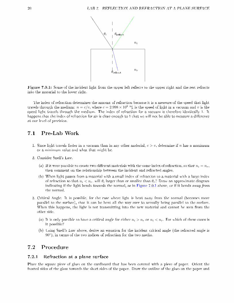
Figure 7.0.1: Some of the incident light from the upper left re�ects to the upper right and the rest refractsinto the material to the lower right.
The index of refraction determines the amount of refraction because it is a measure of the speed that lighttravels through the medium: n = c/v, where c = 2.998× 10⁸ m/s is the speed of light in a vacuum and v is thespeed light travels through the medium. The index of refraction for a vacuum is therefore identically 1. Ithappens that the index of refraction for air is close enough to 1 that we will not be able to measure a di�erenceat our level of precision.
7.1 Pre-Lab Work
1. Since light travels faster in a vacuum than in any other material, c > v, determine if n has a maximumor a minimum value and what that might be.
2. Consider Snell's Law.
(a) If it were possible to create two di�erent materials with the same index of refraction, so that ni = nr,then comment on the relationship between the incident and refracted angles.
(b) When light passes from a material with a small index of refraction to a material with a large indexof refraction so that ni < nr, will θi larger than or smaller than θr? Draw an approximate diagramindicating if the light bends towards the normal, as in Figure 7.0.1 above, or if it bends away from
the normal.
3. Critical Angle: It is possible, for the case where light is bent away from the normal (becomes moreparallel to the surface), that it can be bent all the way over to actually being parallel to the surface.When this happens, the light is not transmitting into the new material and cannot be seen from theother side.
(a) It is only possible to have a critical angle for either ni > nr or ni < nr. For which of these cases isit possible?
(b) Using Snell's Law above, derive an equation for the incident critical angle (the refracted angle is90◦), in terms of the two indices of refraction for the two media.
7.2 Procedure
7.2.1 Refraction at a plane surface
Place the square piece of glass on the cardboard that has been covered with a piece of paper. Orient thefrosted sides of the glass towards the short sides of the paper. Draw the outline of the glass on the paper and
7.2. PROCEDURE 21
be careful to not move the glass. (You may want to use a pair of pins at the corners to �x the glass in place.)
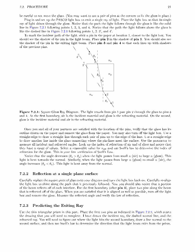
Plug in and set up the PASCO light box to emit a single ray of light. Place the light box so that its singleray of light shines through the glass. Notice that the path the light follows through the glass is like the solidline in Figure 7.2.1 following points 1, 2, 3, and 4. Notice that the path the light follows above the glass islike the dashed line in Figure 7.2.1 following points 1, 2, 3′, and 4′.
To mark the incident path of the light, stick a pin in the paper at location 1, closest to the light box. Youshould see the shadow of the pin in the light beam. Place pin 2 in the shadow of pin 1. You should also seethe shadow of the pin in the exiting light beam. Place pin 3 and pin 4 so that each lines up with shadowsof the previous pins.
JJJJJJ
DDDDDDDDDJJJJJJ
rr
rr
JJ
JJ
JJ
JJ
JJ
bb
θa
θg
θg
θa
ng
na
na
3
4
2
1
3′
4′
Figure 7.2.1: Square Glass Ray Diagram. The light travels from pin 1 past pin 2 through the glass to pins 3and 4. At the �rst boundary, air is the incident material and glass is the refracting material. On the second,glass is the incident material and air is the refracting material.
Once you and all of your partners are satis�ed with the location of the pins, verify that the glass has itsoutline drawn on the paper and remove the glass from the paper. You may also turn o� the light box. Use astraight-edge to draw a straight line through each pair of pins up to the edge of the lens. Use a straight-edgeto draw another line inside the glass connecting where the pin-lines meet the surface. Use the protractor tomeasure all incident and refracted angles. Look up the index of refraction of air and of glass and notice thatthey have a range of values. Select a reasonable value for nair and use Snell's law to determine the index ofrefraction for the glass. This is your �rst veri�cation of Snell's Law.
Notice that the angle decreases (θa > θg) when the light passes from small n (air) to large n (glass). Thislight is bent towards the normal. Similarly, when the light passes from large n (glass) to small n (air), theangle increases (θg < θa). This light is bent away from the normal.
7.2.2 Re�ection at a single plane surface
Carefully replace the square piece of glass onto your diagram and turn the light box back on. Carefully re-alignthe light box to shine along the path that it previously followed. Now you should also notice that a portionof the beam re�ects o� of each interface. For the �rst boundary (after pin 3), place two pins along the beamthat is re�ected o� of the glass. When you are satis�ed that it is aligned as well as possible, turn o� the lightbox and remove the glass. Measure the re�ected angle and verify the law of re�ection.
7.2.3 Predicting the Exiting Ray
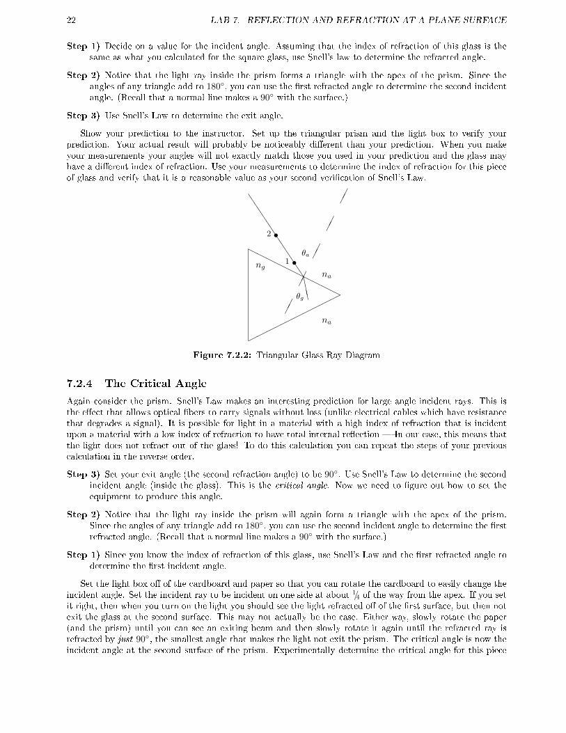
Use the thin triangular prism in this part. Place the �rst two pins as indicated in Figure 7.2.2, which startsthe drawing that you will need to complete. I have drawn the incident ray, the dashed normal line, and therefracted ray. You will need to �gure out where the light hits the second boundary, draw a line normal to thesecond surface, and then use Snell's law to determine the direction that the light beam exits from the prism.
22 LAB 7. REFLECTION AND REFRACTION AT A PLANE SURFACE
Step 1) Decide on a value for the incident angle. Assuming that the index of refraction of this glass is thesame as what you calculated for the square glass, use Snell's law to determine the refracted angle.
Step 2) Notice that the light ray inside the prism forms a triangle with the apex of the prism. Since theangles of any triangle add to 180◦, you can use the �rst refracted angle to determine the second incidentangle. (Recall that a normal line makes a 90◦ with the surface.)
Step 3) Use Snell's Law to determine the exit angle.
Show your prediction to the instructor. Set up the triangular prism and the light box to verify yourprediction. Your actual result will probably be noticeably di�erent than your prediction. When you makeyour measurements your angles will not exactly match those you used in your prediction and the glass mayhave a di�erent index of refraction. Use your measurements to determine the index of refraction for this pieceof glass and verify that it is a reasonable value as your second veri�cation of Snell's Law.
HHH
HHH
HHH
H
�����
�����
JJJJJJJJJ
DDD
��
��
��
��
��
ss
θa
θg
ngna
na
1
2
Figure 7.2.2: Triangular Glass Ray Diagram
7.2.4 The Critical Angle
Again consider the prism. Snell's Law makes an interesting prediction for large angle incident rays. This isthe e�ect that allows optical �bers to carry signals without loss (unlike electrical cables which have resistancethat degrades a signal). It is possible for light in a material with a high index of refraction that is incidentupon a material with a low index of refraction to have total internal re�ection � In our case, this means thatthe light does not refract out of the glass! To do this calculation you can repeat the steps of your previouscalculation in the reverse order.
Step 3) Set your exit angle (the second refraction angle) to be 90◦. Use Snell's Law to determine the secondincident angle (inside the glass). This is the critical angle. Now we need to �gure out how to set theequipment to produce this angle.
Step 2) Notice that the light ray inside the prism will again form a triangle with the apex of the prism.Since the angles of any triangle add to 180◦, you can use the second incident angle to determine the �rstrefracted angle. (Recall that a normal line makes a 90◦ with the surface.)
Step 1) Since you know the index of refraction of this glass, use Snell's Law and the �rst refracted angle todetermine the �rst incident angle.
Set the light box o� of the cardboard and paper so that you can rotate the cardboard to easily change theincident angle. Set the incident ray to be incident on one side at about 1/4 of the way from the apex. If you setit right, then when you turn on the light you should see the light refracted o� of the �rst surface, but then notexit the glass at the second surface. This may not actually be the case. Either way, slowly rotate the paper(and the prism) until you can see an exiting beam and then slowly rotate it again until the refracted ray isrefracted by just 90◦, the smallest angle that makes the light not exit the prism. The critical angle is now theincident angle at the second surface of the prism. Experimentally determine the critical angle for this piece
7.3. QUESTIONS 23
of glass. Compare the predicted value of the critical angle to the measured value of the critical angle as yourthird and �nal veri�cation of Snell's Law.
7.3 Questions
1. Explain why a plane mirror reverse left and right. It will help to draw a ray diagram that replaces a thepins with a wider object that has a clear left side and right side.
2. What happens to the speed that light travels through a medium a greater index of refraction?
Last revised: Spring, 2012A PDF version might be found at refraction.pdf (139 kB)Copyright and license information can be found here.

24 LAB 7. REFLECTION AND REFRACTION AT A PLANE SURFACE
Lab 8
Simple Lenses
Experimental Objectives
Through the various arrangements suggested below, you should be able to. . .
� . . . �gure out the de�nition of the following terms based on the images you observe
◦ magni�ed versus mini�ed
◦ upright versus inverted
◦ real versus virtual
� . . . �gure out the relationships between the measurable quantities:
◦ the magni�cation, de�ned in terms of the image height and the object height: M =hiho
◦ the image distance (from the lens) q
◦ the object distance (from the lens) p
◦ the focal length, f .
Anybody who has looked through glasses, microscopes, telescopes, a magnifying glass, or even a windowhas experienced a lens. We see images through lenses.
8.1 Procedure with Questions for the Analysis
Warning 8.1.1. The data you take in Subsection 8.1.2 will also be used in Subsection 8.1.3, so tabulate it ina coherent and clear format.
8.1.1 De�ning Your Terms
As a group, take one of the three lenses and your white screen into a dark room so that you can see a brighterroom through a doorway. Have one person in the group go stand in the bright room and move around whileanother person looks through the lens. Then trade places until everybody has a chance to look through thelens.
Exercise 8.1.2.
1. As a group, decide how to describe the image in the terms above: Magni�ed or mini�ed? upright orinverted? real or virtual?
25
26 LAB 8. SIMPLE LENSES
2. While still in the darker room, notice that if you hold up your lens in front of a white screen (or a teeshirt) so that the lens is between the screen and the person in the other room, the image of the brighterroom appears on the screen. (Have somebody dance and jump in the bright room while you watch theimage on the screen.)
Take that same lens back into the room and have each person view this text through the lens.
Exercise 8.1.3.
1. As a group, decide how to describe the image in the terms above: Magni�ed or mini�ed? upright orinverted? real or virtual?
2. Notice this time that the text appears to be on the same side of the lens as the actual text is. There isno place that you can put your white screen to have the words from the page appear on the screen.
Compare and contrast the image of the room to the image of the text.
Exercise 8.1.4.
1. If you had to choose between the names real and virtual, which image would you call real? which wouldyou call virtual? why?
2. Decide if either of the images change based on the location of the lens relative to the object being viewed.
8.1.2 Quantify the Magni�cation
In order to make precise measurements, attach the screen to one end of the optical bench and the light source tothe other side. The illuminated cross-hairs on the light source will be the object observed. Place a converginglens1 on the optical bench between the object and the screen. Keep the screen and the light source fairly farapart (the convenient distance will depend on which lens you are using). Adjust the position of the lens untila clear image is formed on the screen.
Exercise 8.1.5.
1. Describe the image formed in the terms de�ned above.
Measure the distances between the lens and the image (image distance, q), and between the lens and theobject (object distance, p). Measure the height of the image on the screen hi and the height of the object onthe light source ho. (If the image is inverted, then hi is a negative value.) Calculate the magni�cation factor
of the image, M =hiho
.
For this same lens, without changing the position of the screen or the light source, �nd a second imagethat has a di�erent description using the de�ned terms above. Again, measure p, q, hi, and ho and calculateM .
Exercise 8.1.6.
1. Describe this second image in the terms de�ned above.
Repeat this for each of the other two lenses.
Exercise 8.1.7.
1. Determine the relationship between M , q, and/or p. Verify that your relationship works (to about twosigni�cant �gures) for all six data sets separately.
1Converging lenses, also called convex lenses, bulge in the middle. Diverging lenses, also called concave lenses, bulge at the
edges.
8.1. PROCEDURE WITH QUESTIONS FOR THE ANALYSIS 27
8.1.3 Quantify the Focal Length
The lens equation,1
p+
1
q=
1
f, shows the relationship between the image distance, q, object distance, p, and
the focal length of the lens, f . Using your data from Subsection 8.1.2, determine the focal length of each lens.Each lens should have two values for f (one for each image).
Exercise 8.1.8.
1. For each lens separately, compare the average of these numbers to the accepted value.
The focal length of a lens may also be determined by forming the image of a very distant object on ascreen. In this case, the object distance, p, becomes very large and therefore 1/p becomes very small. Whenthis is the case, the lens equation may be written as 1/q = 1/f , or more conveniently, q = f . Using a distantobject in an adjacent room, measure the image distance and thereby determine the focal length for each lens.
Exercise 8.1.9.
1. Compare this with your results for f from the data in Subsection 8.1.2.
2. Describe the image formed by this distant object.
In principle, an object needs to be in�nitely far away for this second method to be true. In practice, theobject only needs to be �far enough.� Determine, theoretically or experimentally, how far an object needsto be to get an accurate measurement of the focal length in this manner. If the day is sunny, under strict
instructor supervision take a lens outside and, using the sun as �an in�nitely far away object,� measurethe focal length by forming an image of the sun on your lab notebook. Take a minute or so to really visualizethe sun on your paper. Predict the results.
Last revised: Aug, 2011A PDF version might be found at simplens.pdf (108 kB)Copyright and license information can be found here.

28 LAB 8. SIMPLE LENSES
Lab 9
Electric Field Lines
Experimental Objectives: Experimental Objectives
� In this experiment, you will map out the equipotential lines for a couple of given electric �eld con�gura-tions and determine the pattern of the electric lines of force for these con�gurations. You will then givea physical explanation of the terms �electric �eld� and �electric potential� and their relationship.
The e�ects of electric charges (positive and negative) can be seen in many electronic devices, like the radio.The e�ects of static electricity can be seen when clothing is pulled out of a dryer on a winter day. There isa force exerted on one charge by another charge and this can be either attractive or repulsive. This force iscalled the Coulomb force and is named after Charles Coulomb (1736-1806).
Physics relies on abstractions (new quantities and new names), with pictures to help convey informationand ideas. The English scientist Michael Faraday (1791-1867) introduced the concept of lines of force, a force�eld, as an aid in visualizing the interactions of charges. These lines of force are a mental abstraction, butthey can be visualized with the use of iron �lings placed near a charge or a group of charges. These lines offorce convey a picture of the interaction between one charge and another. The iron �lings will align themselveswhen in the presence of a single charge. This conceptualizes the idea of the electric �eld strength E (electricforce per unit charge) because it is convenient to know the electric force per unit charge at any point in spacedue to a nearby set of electric charges. The electric �eld strength though can not be easily measured with ameter.
It requires work to move a charge against an electric �eld. The ratio of the work done to the chargestrength is called the potential di�erence (voltage) and it is measured in units of joules/coulomb and is calleda volt. This potential di�erence is easily measured with a voltmeter. If the charge is moved along a pathperpendicular to the electric �eld lines then there is no work done, it takes zero energy. This is because thereis no force component in the direction of the path. The potential (voltage) is then constant along paths whichare perpendicular to the �eld lines. Such paths are called equipotential lines. These equipotential lines canbe measured with a simple voltmeter, and then from these the electric �eld lines can be deduced.
9.1 Pre-Lab Work
� De�ne Coulomb's law.
� Give a de�nition of electric �eld, both mathematical and pictorial.
� Show a picture of the electric �eld near:
a) a point charge,
b) two equal and opposite point charges, and
c) two equal positive point charges.
29
30 LAB 9. ELECTRIC FIELD LINES
� Show from the above three cases (pictures), places where the electric �eld is zero.
� Show in a picture, the electric �eld inside and outside of a positively charged conductor (show thatelectric �eld lines will start from the surface of the charged conductor).
� Give an argument why two electric �eld lines can never cross.
� Give an argument why an electric �eld line is perpendicular to the equipotential line.
9.2 Procedure
� A special conducting plate with metal terminals will serve as the charge con�guration. This plate shouldbe fastened beneath the �eld-mapping board, without observing the speci�c charge con�guration.
� An electric �eld is produced when a power supply (battery) is connected between the two terminals(points X and Y). Set the power supply at 10 volts.
� Points of equal potential (voltage) are found using a movable U-shaped probe which is connected toa voltmeter. Plot a series of points on your own graph paper which are at a constant potential (anequipotential line). Then repeat this for di�erent potentials in steps of one volt. In this way the entire�eld is explored.
� Obtain an equipotential map and the electric �eld lines map (on graph paper) for three di�erent chargecon�gurations. Be sure to indicate the direction of the electric �eld lines on your maps.
9.3 Analysis
� Discuss the relationships between the voltage measurements and the electric �eld lines, and between theelectric �eld lines and the charge con�guration. Estimate the magnitude of the electric �eld at a fewpoints on each map. Please write the electric �eld intensities in units of volts/meter.
� Discuss any irregularities in the �eld patterns which you have found.
� Discuss the spacing and what it represents, for the equipotential lines, and for the electric �eld lines.
� Indicate on your maps the location of the positive and negative charge distributions and their approxi-mate shapes.
9.4 Questions
1. Can equipotential lines cross? Can electric �eld lines cross? Explain.
2. Why are there direction arrows on electric �eld lines but not on equipotential lines?
3. Why are the lines of force always perpendicular to the equipotential lines?
4. How is the electric potential a�ected by an insulator, and by a conductor, when they are placed in theelectric �eld?
5. How is the electric �eld a�ected inside an insulator, and inside a conductor, when they are placed in the�eld?
Last revised: (March, 1997)A PDF version might be found at EField.pdf (67 kB)Copyright and license information can be found here.
Lab 10
Internal Resistance of Batteries
Experimental Objectives
� In this experiment, we would like to consider the characteristics of a voltage source.
A voltage source, V , is anything that has a potential di�erence across two terminals: A liquid battery(such as in a car), a dry cell battery, a power plant (accessible through the wall socket), etc. An ideal voltagesource, E , will provide the same amount of voltage regardless of how much current is drawn from it. Physicalvoltage sources will approximate this to various degrees.
In order to determine how ideal a voltage source is, we will draw more and more current and measure howmuch voltage it is able to supply. If we attach a large resistance to the voltage source, then it will resist thecurrent and we will only draw o� a small current. If we attach a small resistance to the voltage source, thenit will draw a large current.
Next week, you will consider the details of that relationship. Your resistors should already be orderedlargest to smallest; don't worry about their actual values, but please try to keep them in order. Each of theresistors has multiple color bands on it. Please be diligent about recording the colors in order on each resistor.When you are �nished with the lab, you should be able to sort them largest to smallest.
10.1 The Equipment
In the diagrams, Amis an ammeter, which measures the current in amps (A), milliamps (mA), or microamps(µA). These measure the current through a wire and must be placed in series with the circuit element. Twocircuit elements are �in series� if all of the current which goes through one also goes through the other. Currentis the �ow of charge (an amount of material); it does not diminish as it passes through the circuit elements.
In the diagrams, Vmis a voltmeter, which measures the voltage in volts (V). These measure the voltage
across (the potential di�erence from before to after) a circuit element and must be placed in parallel withthe circuit element. Two circuit elements are �in parallel� if the current gets split between one and the other.Voltage is related to the energy of the charges; it does diminish (or increase) as it passes through the circuitelements.
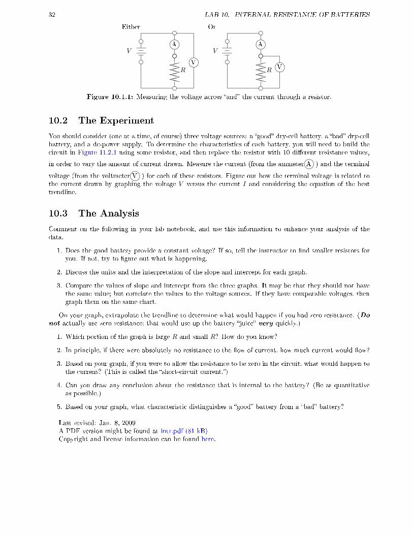
Figure 10.1.1 shows two con�gurations of ammeter and voltmeter. The small circles are the connectionsfor the wires. In this lab, we are trying to measure the current drawn from the battery and the voltage outputby the battery. On the left, the voltmeter is in parallel with the battery, but the ammeter is not in series withthe battery. (V is correct, but I is too small.) On the right, the ammeter is in series with the battery, but thevoltmeter is not in parallel with the battery. (I is correct, but V is too small.) You will be making a mistakeeither way, but hopefully neither is too wrong. For only your largest and smallest resistors, measure this bothways and see how large the e�ect is. (It is incorrect to use the voltage from one circuit and the current fromthe other.)
31
32 LAB 10. INTERNAL RESISTANCE OF BATTERIES
Either
eV
e
eR
��������
XXXXXXXX
eemAemV
Or
eV
e
eR
��������
XXXXXXXX
eemAe
mVFigure 10.1.1: Measuring the voltage across �and� the current through a resistor.
10.2 The Experiment
You should consider (one at a time, of course) three voltage sources: a �good� dry-cell battery, a �bad� dry-cellbattery, and a dc-power supply. To determine the characteristics of each battery, you will need to build thecircuit in Figure 11.2.1 using some resistor, and then replace the resistor with 10 di�erent resistance values,
in order to vary the amount of current drawn. Measure the current (from the ammeter Am) and the terminal
voltage (from the voltmeter Vm) for each of these resistors. Figure out how the terminal voltage is related tothe current drawn by graphing the voltage V versus the current I and considering the equation of the besttrendline.
10.3 The Analysis
Comment on the following in your lab notebook, and use this information to enhance your analysis of thedata.
1. Does the good battery provide a constant voltage? If so, tell the instructor to �nd smaller resistors foryou. If not, try to �gure out what is happening.
2. Discuss the units and the interpretation of the slope and intercept for each graph.
3. Compare the values of slope and intercept from the three graphs. It may be that they should not havethe same value; but correlate the values to the voltage sources. If they have comparable voltages, thengraph them on the same chart.
On your graph, extrapolate the trendline to determine what would happen if you had zero resistance. (Do
not actually use zero resistance; that would use up the battery �juice� very quickly.)
1. Which portion of the graph is large R and small R? How do you know?
2. In principle, if there were absolutely no resistance to the �ow of current, how much current would �ow?
3. Based on your graph, if you were to allow the resistance to be zero in the circuit, what would happen tothe current? (This is called the �short-circuit current.�)
4. Can you draw any conclusion about the resistance that is internal to the battery? (Be as quantitativeas possible.)
5. Based on your graph, what characteristic distinguishes a �good� battery from a �bad� battery?
Last revised: Jan. 8, 2009A PDF version might be found at intr.pdf (81 kB)Copyright and license information can be found here.
Lab 11
Using Ohm's Law to Determine
Equivalent Resistance
Experimental Objectives
� In this lab, after empirically verifying Ohm's Law, you would like to empirically determine the equivalentresistance of two resistors in series and of those two resistors in parallel.
When current moves through a wire due to an electrical potential di�erence (a voltage), it is literally electriccharges falling through the wire due to an electrical �eld. This is completely analogous to gravitational charges(masses) falling through the air due to a gravitational �eld. Di�erent types and sizes (gauges) of wire resistthis current by di�erent amounts. Ohm's Law describes (for some materials) just how this resistance a�ectsa current for a speci�ed voltage, i.e., it relates the current to the voltage. Using the equipment in the lab,you too will be able to discover Ohm's law! Hooray! Furthermore, we can investigate the e�ect of multiple
resistors on a current in some voltage.For each of the cases outlined below, we will measure at least eight voltage values (from a dc-power supply)
and the corresponding current for a speci�c resistor or combination of resistors.
11.1 Pre-Lab
Answer the following questions before you come into lab.
1. Look up Ohm's Law. If you plot V versus I, what do you expect the graph to look like?
2. What units should the slope and intercept have?
3. What values do you expect the slope and intercept to have?
4. Draw one circuit diagram each for resistors in series and for resistors in parallel.
5. Look up the resistor color code in your textbook.
11.2 The Equipment
In the diagrams, Amis an ammeter, which measures the current in amps (A), milliamps (mA), or microamps(µA). These measure the current through a wire and must be placed in series with the circuit element. Twocircuit elements are �in series� if all of the current which goes through one also goes through the other. Currentis the �ow of charge (an amount of material); it does not diminish as it passes through the circuit elements.
In the diagrams, Vmis a voltmeter, which measures the voltage in volts (V). These measure the voltage
across (the potential di�erence from before to after) a circuit element and must be placed in parallel with
33
34 LAB 11. USING OHM'S LAW TO DETERMINE EQUIVALENT RESISTANCE
the circuit element. Two circuit elements are �in parallel� if the current gets split between one and the other.Voltage is related to the energy of the charges; it does diminish (or increase) as it passes through the circuitelements.
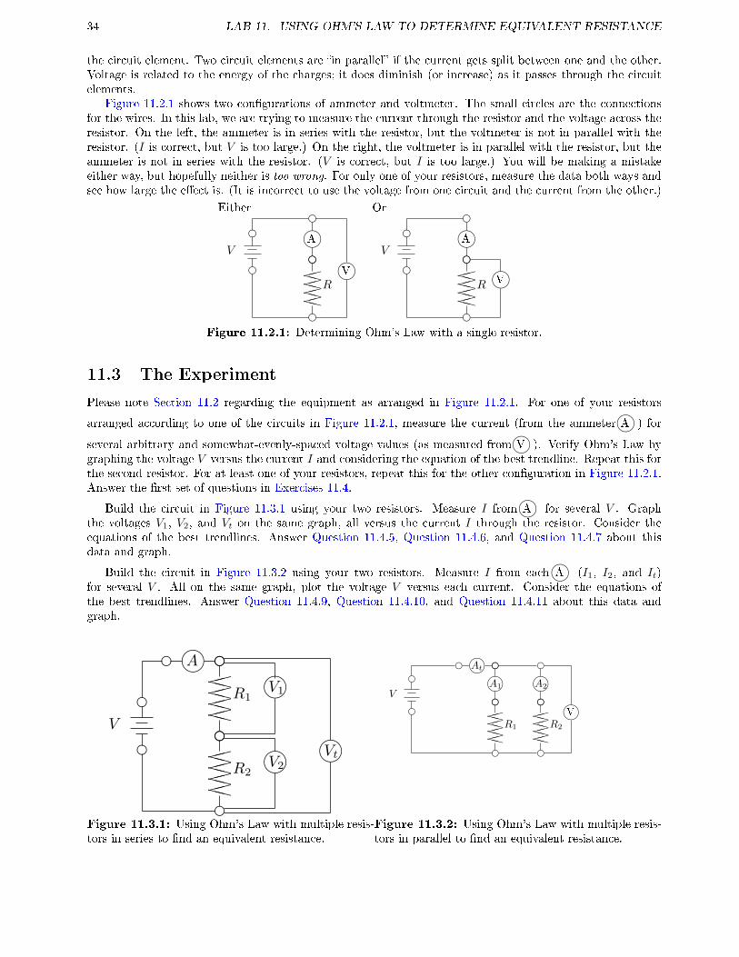
Figure 11.2.1 shows two con�gurations of ammeter and voltmeter. The small circles are the connectionsfor the wires. In this lab, we are trying to measure the current through the resistor and the voltage across theresistor. On the left, the ammeter is in series with the resistor, but the voltmeter is not in parallel with theresistor. (I is correct, but V is too large.) On the right, the voltmeter is in parallel with the resistor, but theammeter is not in series with the resistor. (V is correct, but I is too large.) You will be making a mistakeeither way, but hopefully neither is too wrong. For only one of your resistors, measure the data both ways andsee how large the e�ect is. (It is incorrect to use the voltage from one circuit and the current from the other.)
Either
eV
e
eR
��������
XXXXXXXX
eemAemV
Or
eV
e
eR
��������
XXXXXXXX
eemAe
mVFigure 11.2.1: Determining Ohm's Law with a single resistor.
11.3 The Experiment
Please note Section 11.2 regarding the equipment as arranged in Figure 11.2.1. For one of your resistors
arranged according to one of the circuits in Figure 11.2.1, measure the current (from the ammeter Am) forseveral arbitrary and somewhat-evenly-spaced voltage values (as measured from Vm). Verify Ohm's Law bygraphing the voltage V versus the current I and considering the equation of the best trendline. Repeat this forthe second resistor. For at least one of your resistors, repeat this for the other con�guration in Figure 11.2.1.Answer the �rst set of questions in Exercises 11.4.
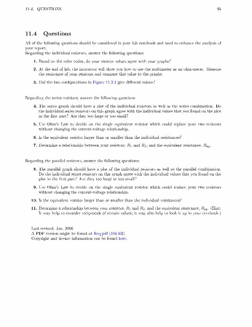
Build the circuit in Figure 11.3.1 using your two resistors. Measure I from Amfor several V . Graphthe voltages V1, V2, and Vt on the same graph, all versus the current I through the resistor. Consider theequations of the best trendlines. Answer Question 11.4.5, Question 11.4.6, and Question 11.4.7 about thisdata and graph.
Build the circuit in Figure 11.3.2 using your two resistors. Measure I from each Am(I1, I2, and It)for several V . All on the same graph, plot the voltage V versus each current. Consider the equations ofthe best trendlines. Answer Question 11.4.9, Question 11.4.10, and Question 11.4.11 about this data andgraph.
eV
eeR1
��������
XXXXXXXX
e
eR2
��������
XXXXXXXX
ee mA e
mVtmV1
mV2
eV
e
eR1
��������
XXXXXXXX
eemA1
ee mAte
eR2
��������
XXXXXXXX
eemA2
emV
Figure 11.3.1: Using Ohm's Law with multiple resis-tors in series to �nd an equivalent resistance.
Figure 11.3.2: Using Ohm's Law with multiple resis-tors in parallel to �nd an equivalent resistance.
11.4. QUESTIONS 35
11.4 Questions
All of the following questions should be considered in your lab notebook and used to enhance the analysis ofyour report.Regarding the individual resistors, answer the following questions:
Based on the color codes, do your resistor values agree with your graphs?1.
At the end of lab, the instructor will show you how to use the multimeter as an ohm-meter. Measurethe resistance of your resistors and compare this value to the graphs.
2.
Did the two con�gurations in Figure 11.2.1 give di�erent values?3.
Regarding the series resistors, answer the following questions:
The series graph should have a plot of the individual resistors as well as the series combination. Dothe individual series resistors on this graph agree with the individual values that you found on the plotin the �rst part? Are they too large or too small?
4.
Use Ohm's Law to decide on the single equivalent resistor which could replace your two resistorswithout changing the current-voltage relationship.
5.
Is the equivalent resistor larger than or smaller than the individual resistances?6.
Determine a relationship between your resistors, R1 and R2, and the equivalent resistance, Req.7.
Regarding the parallel resistors, answer the following questions:
The parallel graph should have a plot of the individual resistors as well as the parallel combination.Do the individual series resistors on this graph agree with the individual values that you found on theplot in the �rst part? Are they too large or too small?
8.
Use Ohm's Law to decide on the single equivalent resistor which could replace your two resistorswithout changing the current-voltage relationship.
9.
Is the equivalent resistor larger than or smaller than the individual resistances?10.
Determine a relationship between your resistors, R1 and R2, and the equivalent resistance, Req. (Hint:It may help to consider reciprocals of certain values; it may also help to look it up in your textbook.)
11.
Last revised: Jan, 2006A PDF version might be found at Req.pdf (104 kB)Copyright and license information can be found here.

36 LAB 11. USING OHM'S LAW TO DETERMINE EQUIVALENT RESISTANCE
Lab 12
Magnetic Field Demonstrations - An
Exercise
The lab room has been set up with �ve lab stations; each involves a short experiment designed to demonstratethe characteristics of the magnetic �eld for various objects. Your group will move from table to table andcarry out each of these experiments, making observations and collecting data as necessary. Listed below arequestions which you should attempt to answer at each station. Instead of a lab report, you will need to writea half-page summary on each station. It should be thorough enough to explain the phenomenon to a colleaguewho missed today's lab.
You should form into four groups so that there is always an empty station. Take notes in your lab notebook,but then write up and turn in a formal document that discusses the relevant ideas for each station.
Warning 12.0.1. In all experiments, note that electronic equipment such as power supplies and computersproduce magnetic �elds that might impact your experiment. You should not measure your magnetic �eldsnear other electronic devices. You should also be aware that strong magnetic �elds can erase credit cards andother magnetic storage devices.
12.1 Data Studio's Magnetic Field Sensor (for reference, not an ex-periment)
To use the magnetic �eld sensor, turn on Data Studio, plug in the sensor, and activate the sensor in the usualmanner. At the tip of the arm on the sensor are two white dots, one on the end of the tip and one on theside of the tip. Notice also the control buttons on the handle of the sensor. The �rst button has two settings:marked →→ and ↑↑ and these are labeled [Radial/Axial]. The Radial setting measures magnetic �eld pointinginto the side of the arm of the sensor, at the location of the white dot. The Axial setting measures magnetic�eld pointing into the end of the sensor, at the location of the white dot. Negative means that the magnetic�eld is out of the sensor instead of into the sensor.
When changing between Axial and Radial, the sensor must be tared. If you tare it while it is pointing inthe direction of some magnetic �eld, then it cannot1 measure that magnetic �eld.
12.1.1 Measuring the B of a Permanent Magnet
Determine the expected direction of the magnetic �eld. Set the sensor to either Radial or Axial, accordingto how you expect to hold it, and tare it. Verify that the scale is set to [1×] and plot in Gauss or Tesla, asappropriate. Place the tip of the sensor such that the white dot on the side (or top as necessary) is near themagnet pointing in the direction of the expected magnetic �eld.
1This is exactly analogous to tarring a scale with a cup on it; the scale only reads the mass of the material added to the cup
after the tarring, not the mass of the cup itself.
37
38 LAB 12. MAGNETIC FIELD DEMONSTRATIONS - AN EXERCISE
12.1.2 Measuring the B of a Wire Loop
Use the right-hand rule to determine the expected direction of the magnetic �eld. Set the sensor to Axial andtare it. Verify that the scale is set to [1×] and plot in Gauss or Tesla, as appropriate. Place the tip of thesensor such that the white dot on the end is as close to the center of the wire loop as possible and points asperpendicular as possible to the plane of the coil.
If there is a cross-�eld (a �eld perpendicular to the �eld of the coil), then you might also try to measurethat by removing the sensor from the vicinity of the coil, setting it to Radial, re-taring it, and then replacingthe sensor into the center of the coil with the white dot on the side pointing in the direction of the cross �eld.
12.1.3 Measuring the B of a Solenoid
Use the right-hand rule to determine the expected direction of the magnetic �eld. Set the sensor to Axial andtare it. Verify that the scale is set to [1×] and plot in Gauss or Tesla, as appropriate. Place the tip of thesensor such that the white dot on the end is as close to the center of the solenoid as possible and points asclose as possible along the axis of the solenoid.
You might also try to measure the radial component to the �eld by removing the sensor from the vicinityof the coil, setting it to Radial, re-taring it, and then replacing the sensor into the center of the solenoid withthe white dot on the side pointing outwards towards the coil.
12.1.4 Measuring the B of a Long Straight Wire
Use the right-hand rule to determine the expected direction of the magnetic �eld. Set the sensor to Radialand tare it. Verify that the scale is set to [1×] and plot in Gauss or Tesla, as appropriate. Place the tip ofthe sensor such that the white dot on the side is in the vicinity of the wire pointing in the direction of theexpected magnetic �eld.
If there is a cross-�eld (a �eld perpendicular to the �eld of the wire), then you might also try to measurethat by removing the sensor from the vicinity of the wire, setting it to Radial, re-taring it, and then replacingthe sensor into the center of the coil with the white dot on the side pointing in the direction of the cross �eld.
12.2 Magnetic Field of a Permanent Magnet - Iron Filings
You should have two cylindrical magnets, a co�ee �lter, a sti� plastic plate, some paper clips and nails, anda salt shaker of iron �lings available at this station. Each magnet is labeled with either �N� or �S� to indicatethe north or south pole of the magnet, respectively.
12.2.1 Magnets and Paper Clips
Consider how magnets and paper clips interact. In each of the following, you may replace the paper clips withnails if you like.
Exercise 12.2.1.
1. Describe any interaction you experience when you touch any pair of the paper clips together in thevarious possible orientations.
2. Describe any interaction you experience when you touch the magnets together in the various possibleorientations.
(a) Describe how you can pick one magnet up with the other.
(b) Describe how you can knock one magnet over with the other (without making contact).
3. Describe any interaction you experience when you touch one of the magnets together with any one ofthe paper clips in the various possible orientations.
12.3. MAGNETIC FIELD OF A PERMANENT MAGNET - FIELD SENSOR 39
(a) Pick up one paper clip with the narrow end of one of the magnets so that the clip hangs straightout from the magnet. Then, while these are still in contact, touch a second paper clip with the endof the �rst clip. Now, while carefully holding the �rst clip near the magnet, carefully remove themagnet from the �rst clip. After showing the result to your instructor, describe and explain theresult on the two paper clips.
(b) Predict what will happen if you brought either end of the magnet slowly towards the lower end ofthe dangling paper clip. Verify your predictions and provide an explanation for how and why yourpredictions were correct or incorrect. (Be sure to include comments about the orientation of thepoles of the magnets as well as the poles of the paper clips.)
4. Explain why it is possible to stick either end of a paper clip to either end of a magnet, but you cannotstick one end of a magnet to either end of another magnet.
12.2.2 Magnets and Iron Filings
Iron �lings act similarly to the paper clips. The iron �lings are small enough that they allow us to �map� themagnetic �eld of an object. Each individual �ling will align itself with the magnetic �eld.
Place the co�ee �lter on top of the clear, plastic plate. Sprinkle some iron �lings on the co�ee �lter. Note:We are using a co�ee �lter because its shape allows us to minimize spilling the �lings on the table, or worse,the �oor. Be very careful not to spill the �lings. Have one person hold the plate up with both handshigh enough for another person to move one of the cylindrical magnets beneath it while you all watch whathappens to the iron �lings. Meanwhile, somebody else should place one of the cylindrical magnets underneaththe sheet of paper so that everybody can observe the patterned displayed by the �lings.
Exercise 12.2.2.
1. Determine if you can make any interesting patterns in the �lings by placing or moving the magnet underthe �lings. When you think you have a good sense of the patterns, try to draw or describe some of whatyou found.
2. Without the magnet, try to smooth out the �lings. (If you can't smooth them out well, then carefullyhold the salt-shaker over the co�ee �lter and unscrew the cap, pour the �lings back in, replace the cap,and re-sprinkle more �lings onto the �lter.) Predict what you should see if you had two magnets underthe �lings each with the North pole facing the other magnet. What if both South poles were facing eachother? What if one North and one South pole faced the other?
3. While one person holds the plate with the �lter and �lings, have two people each hold a magnet underthe �lings as described in the previous question. Verify your predictions and provide an explanation forhow and why your predictions were correct or incorrect.
12.3 Magnetic Field of a Permanent Magnet - Field Sensor
You should have a small, four-post, wooden stand with a hole in the top and a wooden cylinder taped to a ruleron a lab-jack. The wooden equipment was hand-made and is delicate; please be careful when handling
the apparatus.
Exercise 12.3.1.
1. Use the �eld sensor (as described in Section 12.1) set to Axial to measure (and record) the strength ofthe magnetic �eld due to the permanent magnet at various positions from the magnet. It will be usefulto set the sensor 10.0 cm from the magnet and make a measurement at each 1.0 cm interval as you movetowards the magnet.
2. Repeat this for the Radial setting.
3. Tabulate your results (you may also graph it if you like) and discuss the manner in which the �elddepends on distance. Is it linear? Polynomial? something else?
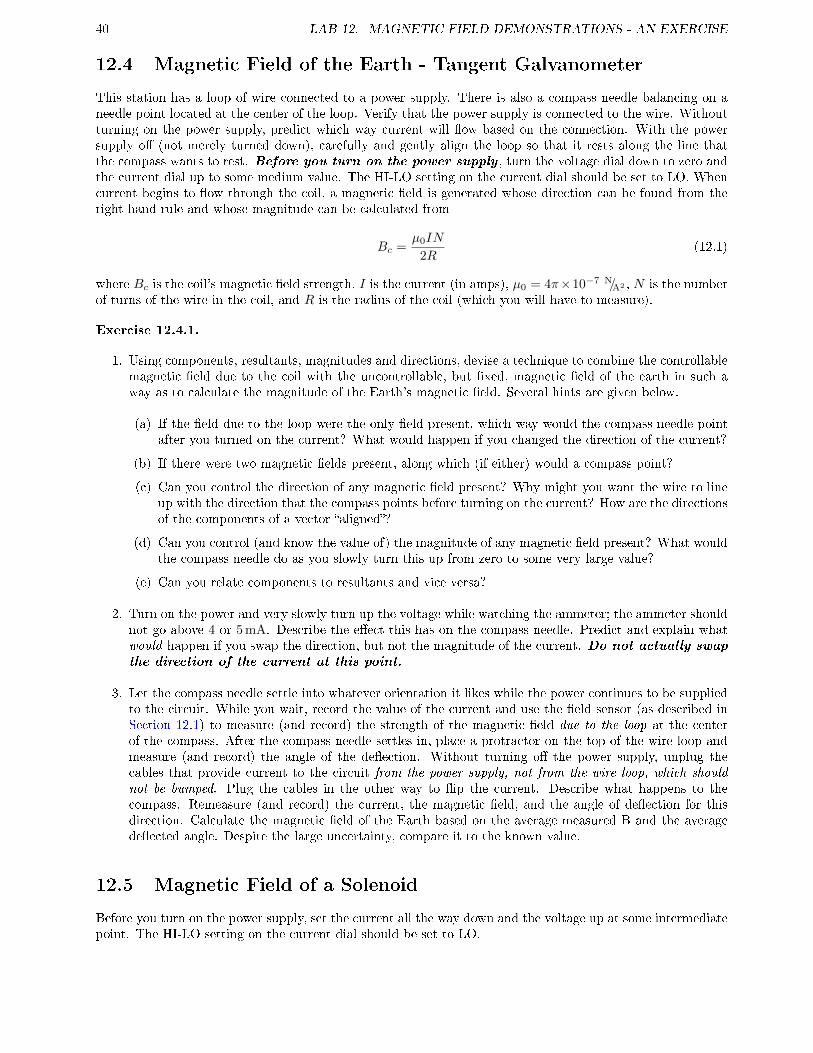
40 LAB 12. MAGNETIC FIELD DEMONSTRATIONS - AN EXERCISE
12.4 Magnetic Field of the Earth - Tangent Galvanometer
This station has a loop of wire connected to a power supply. There is also a compass needle balancing on aneedle point located at the center of the loop. Verify that the power supply is connected to the wire. Withoutturning on the power supply, predict which way current will �ow based on the connection. With the powersupply o� (not merely turned down), carefully and gently align the loop so that it rests along the line thatthe compass wants to rest. Before you turn on the power supply , turn the voltage dial down to zero andthe current dial up to some medium value. The HI-LO setting on the current dial should be set to LO. Whencurrent begins to �ow through the coil, a magnetic �eld is generated whose direction can be found from theright-hand rule and whose magnitude can be calculated from
Bc =µ0IN
2R(12.1)
where Bc is the coil's magnetic �eld strength, I is the current (in amps), µ0 = 4π×10−7 N/A2 , N is the numberof turns of the wire in the coil, and R is the radius of the coil (which you will have to measure).
Exercise 12.4.1.
1. Using components, resultants, magnitudes and directions, devise a technique to combine the controllablemagnetic �eld due to the coil with the uncontrollable, but �xed, magnetic �eld of the earth in such away as to calculate the magnitude of the Earth's magnetic �eld. Several hints are given below.
(a) If the �eld due to the loop were the only �eld present, which way would the compass needle pointafter you turned on the current? What would happen if you changed the direction of the current?
(b) If there were two magnetic �elds present, along which (if either) would a compass point?
(c) Can you control the direction of any magnetic �eld present? Why might you want the wire to lineup with the direction that the compass points before turning on the current? How are the directionsof the components of a vector �aligned�?
(d) Can you control (and know the value of) the magnitude of any magnetic �eld present? What wouldthe compass needle do as you slowly turn this up from zero to some very large value?
(e) Can you relate components to resultants and vice versa?
2. Turn on the power and very slowly turn up the voltage while watching the ammeter; the ammeter shouldnot go above 4 or 5 mA. Describe the e�ect this has on the compass needle. Predict and explain whatwould happen if you swap the direction, but not the magnitude of the current. Do not actually swap
the direction of the current at this point.
3. Let the compass needle settle into whatever orientation it likes while the power continues to be suppliedto the circuit. While you wait, record the value of the current and use the �eld sensor (as described inSection 12.1) to measure (and record) the strength of the magnetic �eld due to the loop at the centerof the compass. After the compass needle settles in, place a protractor on the top of the wire loop andmeasure (and record) the angle of the de�ection. Without turning o� the power supply, unplug thecables that provide current to the circuit from the power supply, not from the wire loop, which should
not be bumped. Plug the cables in the other way to �ip the current. Describe what happens to thecompass. Remeasure (and record) the current, the magnetic �eld, and the angle of de�ection for thisdirection. Calculate the magnetic �eld of the Earth based on the average measured B and the averagede�ected angle. Despite the large uncertainty, compare it to the known value.
12.5 Magnetic Field of a Solenoid
Before you turn on the power supply, set the current all the way down and the voltage up at some intermediatepoint. The HI-LO setting on the current dial should be set to LO.
12.6. MAGNETIC FIELD OF A WIRE 41
12.5.1 The Small Solenoid
Exercise 12.5.1.
1. Without turning on the power supply, connect the positive and negative terminals of the power supplyto the terminals of the smaller solenoid. Note the direction of current �ow and predict the direction ofthe magnetic �eld.
2. Use the �eld sensor (as described in Section 12.1) set to Axial to measure (and record) the strength ofthe magnetic �eld due to the solenoid. Insert the sensor as far along the axis of the solenoid as possibleand try to keep your hand as steady as possible. Turn on the power supply and slowly turn up thecurrent to some intermediate value. Move the sensor around a little inside the solenoid and discuss theresults.
3. Repeat the previous step with the sensor set to Radial. What variables does the magnetic �eld due toa solenoid depend on? Does it follow the predicted equation for a solenoid?
Turn the power supply o�. Disconnect the wire from the solenoid.
12.5.2 Measurements with the Large Solenoid
Before connecting the large solenoid, measure the number of turns per length, n =N
L. Do not measure the
full number of loops nor the full length. Find some portion of the coil and measure the number of coils andthe length in that small sample size. When you calculate n, notice that the solenoid is wrapped four coilsdeep, so multiply your N by 4. In this problem, you can measure B and I in order to �nd µ0 to verify theequation of a solenoid.
Exercise 12.5.2.
1. Connect the power supply in series with an ammeter and then the solenoid before completing the circuitback to the power supply. Be sure that the ammeter reads several amps. Insert the �eld sensor set tothe appropriate settings as close as possible to the axis of the solenoid. Predict what you will measurefor the Radial and Axial measurements above.
2. Measure the current from the ammeter, the magnetic �eld from the sensor and calculate a value forµ0 based on the equation for a solenoid. Compare this to the accepted value in your book. Draw aconclusion about the equation of a solenoid.
12.6 Magnetic Field of a Wire
Before you turn on the power supply, set the current all the way down and the voltage up at some intermediatepoint. The HI-LO setting on the current dial should be set to HI. (You will be using a current of about 8 A.)
Notice that the wire connects are exposed. Be careful not to touch the connections when the current is on.
Exercise 12.6.1.
1. Without turning on the power supply, connect the positive and negative terminals of the power supplyto opposite ends of one of the three wires inside the Romex� cable. Be sure, based on color, to connectthem to the same wire. Straighten a long section of the wire as well as possible. Note the direction ofcurrent �ow and predict the direction of the magnetic �eld.
2. Use the �eld sensor (as described in Section 12.1) set to Radial to measure (and record) the strengthof the magnetic �eld due to the long straight wire. The sensor should lie along the direction of the wireand must be touching the wire to make any measurement. Turn on the power supply and turn up thecurrent to about 8 A. (You may change the current in order to see the e�ect of current on the size ofthe magnetic �eld.) Move the sensor to di�erent radii and discuss the results. Place the sensor close tothe wire and slowly vary the strength of the current using the knob on the power supply. Discuss theresults.
42 LAB 12. MAGNETIC FIELD DEMONSTRATIONS - AN EXERCISE
3. Repeat the previous step with the sensor set to Axial.
4. Turn the power supply o�. Disconnect the wire from the power supply. Connect the red terminal to oneside of the white wire and the black terminal to the black wire so that both connections are at the sameend. On the far end, connect the black and white wires (this is where the lamp goes and you should notactually do this at home where there is signi�cantly more current able to �ow! Really !). Predict whatyou will measure for the Radial and Axial measurements above.
5. Repeat Questions Question 12.6.1.2 and Question 12.6.1.3 for the two wire case. Verify your predictionsand provide an explanation for how and why your predictions were correct or incorrect.
Last revised: Apr 6, 2009A PDF version might be found at Magneticdemo.pdf (173 kB)Copyright and license information can be found here.
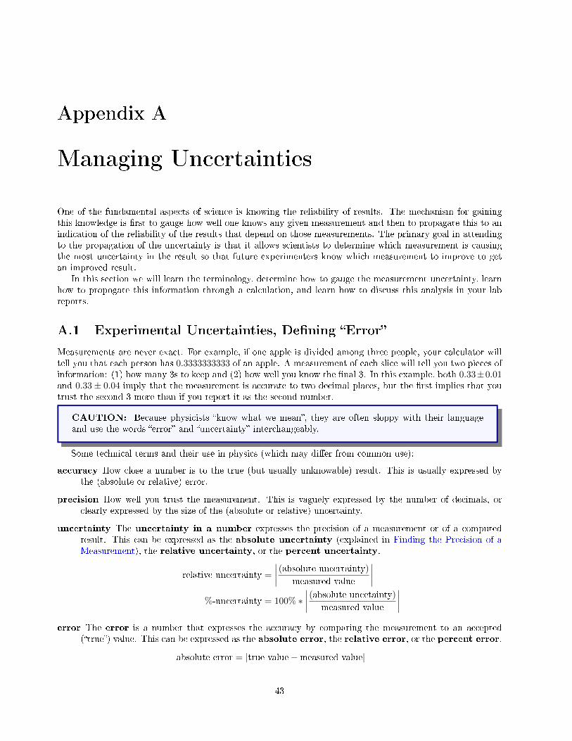
Appendix A
Managing Uncertainties
One of the fundamental aspects of science is knowing the reliability of results. The mechanism for gainingthis knowledge is �rst to gauge how well one knows any given measurement and then to propagate this to anindication of the reliability of the results that depend on those measurements. The primary goal in attendingto the propagation of the uncertainty is that it allows scientists to determine which measurement is causingthe most uncertainty in the result so that future experimenters know which measurement to improve to getan improved result.
In this section we will learn the terminology, determine how to gauge the measurement uncertainty, learnhow to propogate this information through a calculation, and learn how to discuss this analysis in your labreports.
A.1 Experimental Uncertainties, De�ning �Error�
Measurements are never exact. For example, if one apple is divided among three people, your calculator willtell you that each person has 0.3333333333 of an apple. A measurement of each slice will tell you two pieces ofinformation: (1) how many 3s to keep and (2) how well you know the �nal 3. In this example, both 0.33±0.01and 0.33± 0.04 imply that the measurement is accurate to two decimal places, but the �rst implies that youtrust the second 3 more than if you report it as the second number.
CAUTION: Because physicists �know what we mean�, they are often sloppy with their languageand use the words �error� and �uncertainty� interchangeably.
Some technical terms and their use in physics (which may di�er from common use):
accuracy How close a number is to the true (but usually unknowable) result. This is usually expressed bythe (absolute or relative) error.
precision How well you trust the measurement. This is vaguely expressed by the number of decimals, orclearly expressed by the size of the (absolute or relative) uncertainty.
uncertainty The uncertainty in a number expresses the precision of a measurement or of a computedresult. This can be expressed as the absolute uncertainty (explained in Finding the Precision of aMeasurement), the relative uncertainty, or the percent uncertainty.
relative uncertainty =
∣∣∣∣ (absolute uncertainty)
measured value
∣∣∣∣%-uncertainty = 100% ∗
∣∣∣∣ (absolute uncetainty)
measured value
∣∣∣∣error The error is a number that expresses the accuracy by comparing the measurement to an accepted
(�true�) value. This can be expressed as the absolute error, the relative error, or the percent error.
absolute error = |true value−measured value|
43
44 APPENDIX A. MANAGING UNCERTAINTIES
relative error =
∣∣∣∣ (true value−measured value)
true value
∣∣∣∣%-error = 100% ∗
∣∣∣∣ (true value−measured value)
true value
∣∣∣∣di�erence The di�erence is a number that expresses the consistency of a multiple measurements by com-
paring one measurement to another. This can be expressed as the absolute di�erence, the relativedi�erence, or the percent di�erence. You should notice that since we don't know which measure-ment to trust, we take the absolute di�erence relative to the average of the measurements (rather thanchoosing one measurement as �true�).
absolute di�erence = (measurement1 −measurement2)
relative di�erence =(measurement1 −measurement2)[(measurement1)+(measurement2)
2
]%-di�erence = 100% ∗ (measurement1 −measurement2)[
(measurement1)+(measurement2)2
]Note A.1.1 (compare). Whenever you are asked to �compare� values, it is expected that you will not onlycompute a %-error or %-di�erence (as appropriate, according to the above considerations); but will alsocomment on if the uncertainty of the values overlap. Recall that the uncertainty means that your measurementdoes not distinguish between values within that range, so if the uncertainties overlap, then the values are �thesame to within your ability to measure them.�
A.2 Writing an Analysis of Error
The conclusion of your lab report should be based on an analysis of the error in the experiment. The analysisof error is one of the most certain gauges available to the instructor by which the student's scienti�c insightcan be evaluated. To be done well, this analysis calls for comments about the factors that impacted the extentto which the experimental results agree with the theoretical value (what factors impact the percent error), thelimitations and restrictions of the instruments used (what factors impact the uncertainty), and the legitimacyof the assumptions.
Physicists usually use the phrase �sources of error� (or �sources of uncertainty�) to describe how the limits ofmeasurement propagate through a calculation (see Propagation of Uncertainties) to impact the uncertaintyin the �nal result. This type of �error analysis� gives insight into the accuracy of the result. Considerationsfor the Error Analysis provides questions that can help you describe which of several measurements can moste�ectively improve the precision of the result so that you can gain insight into the accuracy of the result.The accuracy allows one to gauge the veracity (truth) of an underlying relationship, but precision allows youto gauge accuracy. Said another way, a small percent di�erence usually is used to imply a small percenterror. Said another way, imprecise measurements always seem accurate.
A.2.1 Technically, Errors are not Mistakes
Your report should not list �human error� because most students misunderstand this term to mean �places Imight have made a mistake� rather than �the limiting factor when using the equipment correctly.� Findingthe Precision of a Measurement discusses measurement uncertainties as de�ned above.
In the example of the apple above, the fact that one person has 0.33± 0.04 of an apple does not re�ect a�mistake� in the cutting, but rather re�ects that the cutter is limited in their precision. What is important is touse the uncertainty to express how well one can repeated cut the apple into thirds. The absolute uncertainty of0.04 is generally interpreted to say that most instances (roughly 68%, as explained in Uncertainty of multiple,repeated measurements) of the cutting of an apple in this way will result in having between 0.29 to 0.37 of anapple for any given slice.
When describing the cause of an error (di�erence from the theoretical value) or of an uncertainty (theextent you trust a number), you can usually categorize this source of error as a random error (a cause that
A.2. WRITING AN ANALYSIS OF ERROR 45
could skew the result too large or too small) or as a systematic error (a cause that tends to skew the result inone particular direction).
Random Error An environmental circumstances, generally uncontrollable, that sometimes makes the mea-sured result too high and sometimes make it too low in an unpredictable fashion. Random errors mayhave a statistical origin � that is, they are due to chance. For example, if one hundred pennies aredumped on a table, on average we expect that �fty would land heads up. But we should not be surprisedif �fty-three or forty-seven actually landed heads-up. This deviation is statistical in nature becausethe way in which a penny lands is due to chance. Random errors can sometimes be reduced by eithercollecting more data and averaging the readings, or by using instruments with greater precision.
Systematic Error A systematic error can be ascribed to a factor which would tend to push the resultin a certain direction away from the theory value. The error would make all of the results eithersystematically too high or systematically to low. One key idea here is that systematic errors can beeliminated or reduced if the factor causing the error can be eliminated or controlled. This is sometimesa big �if�, because not all factors can be controlled. Systematic errors can be caused by instrumentswhich are not calibrated correctly, maybe a zero-point error (an error with the zero reading of theinstrument). This type of error can usually be found and corrected. Systematic errors also often arisebecause the experimental setup is somehow di�erent from that assumed in the theory. If the accelerationdue to gravity was measured to be 9.52 m/s2 with an experimental uncertainty (precision) of 0.05 m/s2 ,rather than the textbook value of 9.81 m/s2 , then we should be concerned with why the accuracy is notas good as the precision. This is most likely to mean that there is a signi�cant systematic error in theexperiment, where one of the initial assumptions may not be valid. The textbook value does not considerthe e�ects of the air. The e�ects of the air may or may not be controllable, and the di�erence betweenthe theory and the data may be (within appropriate limits or tests) considered a correction factor forthe systematic error.
A.2.2 Considerations for the Error Analysis
In order to help you get started on your discussion of error, the following list of questions is provided. It isnot an exhaustive list. You need not answer all of these questions in a single report.
1. Is the error large or small? Is it random or systematic? . . . statistical? . . . cumulative?
(a) What accuracy (precision) was expected? Why? What accuracy (precision) was attained? Ifdi�erent, why?
(b) Was the experimental technique sensitive enough? Was the e�ect masked by noise?
2. Is it possible to determine which measurements are responsible for greater percent error by checkingitems measured and reasoning from the physical principles, the nature of the measuring instrument, andusing the rules for propagation of error?
(a) Is the error partly attributable to the fact that the experimental set-up did not approximate theideal that was required by the physical theory closely enough? How did it fail?
(b) If a systematic error skews high (low), then is your result too high (low)? Is this a reasonableexplanation? Is the size of the skew enough to explain the result?
(c) What can be done to improve the equipment and eliminate error? How can the in�uence of envi-ronmental factors be diminished? Why is this so?
3. Is the error (deviation) in the experiment reasonable?
Note A.2.1 (compare). Whenever you are asked to �compare� values, it is expected that you will not onlycompute a %-error or %-di�erence (as appropriate); but will also comment on if the uncertainty of the valuesoverlap. Recall that the uncertainty means that your measurement does not distinguish between values withinthat range, so if the uncertainties overlap, then the values are �the same to within your ability to measurethem.�
46 APPENDIX A. MANAGING UNCERTAINTIES
A.3 Finding the Precision of a Measurement
A.3.1 Uncertainty of a single measurement
All equipment has a �nite precision. For example, if you are stepping o� the length of a room by placing onefoot in front of the other and counting steps, then you are measuring in �shoe-lengths�. You can likely estimatea half-show length or a third-of-a-shoe-length, but it might be di�cult to accurately gauge smaller intervalsof a shoe-length. Conveniently for me, my size 11 shoe is 12 in long. So, I can replace a shoe-length with a�foot�. Furthermore, I could replace my measurement technique with a yard-stick (or better yet a meterstick).Since a meter-stick has increments of millimeters on it, it is straightforward to measure the distance to thenearest millimeter. In fact, you can probably guess the nearest half-millimeter. The uncertainty in yourshoe-measurement is about 4 in (or about 10 cm = 100 mm). The uncertainty in the meter-stick measurementis about 0.5 mm, signi�cantly better than your shoe.
In addition, to how well the equipment can make a measurement, there is also how well you can gauge themeasurement with that piece of equipment. If you measure the length of the room using 12 in rulers, then youwill need quite a few of them. It is possible that with so many individual rulers, you will either not measure inexactly a straight line or you might not be able to keep the rulers exactly parallel to each other. Both of these(inappropriate but di�cult to control) uses of the rulers will introduce error and, since you can't necessarilyjudge if you are doing this (especially since you are trying to not do so), you are introducing uncertainty. Youdo not necessarily know what errors are actually happening when they are so small. Nonetheless, you need toaccount for the possibility of such errors in your uncertainty. (Recall the types of error in Technically, Errorsare not Mistakes.) In each of the cases mentioned here, the error would necessarily increase the measurementvalue to a number larger than the actual value. There are other instances (perhaps using a string to measuredistance and mis-gauging the tautness of the string) where the value might be systematically small or perhapsrandomly distributed.
To get a sense of how large the possible variations are due to this measurement uncertainty, it is advisableto always take more data. Having more data is always better (statistically). If you measure a quantity manytimes and you do not see any variation, then the precision of the instrument dominates the uncertainty; thatis, your instrument is less precise than your technique. If you measure a quantity many times and see somevariation, then your measurement technique dominates the uncertainty; that is, your technique is less precisethan your instrument. Usually the actual uncertainty will be a combination of both. For our purposes, wewill consider 10-20 measurements to be �many�, and hope it is su�cient. If you are asked to do a lab exerciseon �Standard Deviation�, then you will explore what a �su�cient number of measurements� means.
In the next subsection (Uncertainty of multiple, repeated measurements), we will discuss how to do thestatistics to account for multiple measurements.
A.3.2 Uncertainty of multiple, repeated measurements
Calculate or estimate the precision of a measurement by one or more of the following methods:
1. by the precision of the measuring instrument, and take into account any uncertainties that are intrinsicto the object itself;
2. by the range of values obtained, the minimum and/or maximum deviation (d);
di = |Xi −Xave|
3. by the standard deviation, which is the square root of the sum of the squares of the individual deviations(d) divided by the number of readings (N) minus one;
σ =
√1
(N − 1)
∑d2 =
√1
(N − 1)
∑i
|Xi −Xave|2
4. by the standard deviation of the mean, which is the standard deviation divided by the square root ofthe number of readings;
5. by the square root of the number of readings (√N), if N is considered large;
A.4. PROPAGATION OF UNCERTAINTIES 47
If many data points were taken and plotted on a histogram, it would smooth out and approach thesymmetrical graph typical of the binomial distribution (Recall the histogram in the Standard Deviation Lab ofPHY121 ). This distribution and many others in statistics may be approximated by the gaussian distribution.
The standard deviation, σ, can be estimated from the above graph. It is a measure of the �width� ofthe distribution. For the case shown, the standard deviation has the value of �ve. The greater the standarddeviation, the wider the distribution and the less likely that an individual reading will be close to the averagevalue. About 68% of the individual readings fall within one standard deviation (between 45 and 55 in thiscase). About 96% of the readings fall within two standard deviations (between 40 and 60 in this case).
As more and more readings are taken, the e�ect of the random error is gradually eliminated. In the absenceof systematic error, the average value of the readings should gradually approach the true value. The smoothcurve above was drawn assuming that there was no systematic error. If there were, the graph would merelybe displaced sideways. The average value for the number would then be say 55.
The distribution of many average (mean) readings is also gaussian in shape. Comparing this to thedistribution for individual readings, it is much narrower. We would expect this, since each reading on thisgraph is an average of individual readings and has much less random error. By taking an average of readings,a considerable portion of the random error has been canceled. The standard deviation for this distributionis called the standard deviation of the mean (σm). For this distribution, 68% of the averages of the readingsare within one standard deviation of the mean, and 98% of the average readings fall within two standarddeviations of the mean.
The standard deviation of the mean tells how close a particular average of several readings is likely to beto an overall average when many readings are taken. The standard deviation tells how close an individual
reading is likely to be to the average.There is one case for which the standard deviation can be estimated from one reading. In counting
experiments (radioactivity, for example), the distribution is a Poisson distribution. For this distribution, thestandard deviation is just the square root of the average reading. One reading can give an estimate of theaverage, and therefore, give an estimate of-the standard deviation.
A.4 Propagation of Uncertainties
The previous sections discussed the uncertainties of directly measured quantities. Now we need to considerhow these uncertainties a�ect the rest of the analysis. In most experiments, the analysis or �nal results areobtained by adding, subtracting, multiplying, or dividing the primary data. The uncertainty in the �nal resultis therefore a combination of the errors in the primary data. The way in which the error propagates from theprimary data through the calculations to the �nal result may be summarized as follows:
1. The error to be assigned to the sum or di�erence of two quantities is equal to the sum of their absoluteerrors.
2. Relative error is the ratio of the absolute error to the quantity itself. The relative error to be assignedto the product or quotient of two quantities is the sum of their relative errors.
3. The relative error to be assigned to the power of a quantity is the power times the relative error of thequantity itself.
These rules are not arbitrary, but rather they follow directly from the nature of the mathematical operations.These rules may be derived using calculus.
Exercise A.4.1 (Try Propagating the Uncertainty When Adding Numbers). Compute the perimeter of atable that is measured to be 176.7 cm± 0.2 cm along one side and 148.3 cm± 0.3 cm along the other side.
Hint 1. To �nd the perimeter, add the four sides of the rectangle. Use the values, but not the uncertainty.
Hint 2. To �nd the uncertainty, use Rule 1.
Answer. The perimeter is P = 650 cm± 1 cm.
Solution. The perimeter can be found as:
P = (176.7 cm) + (148.3 cm) + (176.7 cm) + (148.3 cm)
P = 650.0 cm
48 APPENDIX A. MANAGING UNCERTAINTIES
but we do not know the precision (appropriate number of decimals) until we compute the uncertainty, whichis
∆P = (0.2 cm) + (0.3 cm) + (0.2 cm) + (0.3 cm)
∆P = 1.0 cm
The value of the uncertainty determines where you round the result. Because the �rst digit of the uncertaintyis in the �one's place�, we round both the value and the uncertainty to that place.
The perimeter is P = 650 cm± 1 cm.
Exercise A.4.2 (Try Propagating the Uncertainty When Multiplying Numbers). Compute the area of a tablethat is measured to be 176.7 cm± 0.2 cm along one side and 148.3 cm± 0.3 cm along the other side.
Hint 1. To �nd the area, multiple the length and width of the rectangle. Use the values, but not theuncertainty.
Hint 2. Because the area of the table is calculated using multiplication, use Rule 2to �nd the uncertainty.
Answer. The area is A = (2.620× 10⁴)± (0.008× 10⁴)cm2.
Solution. The area is found to be (signi�cant digits are underlined)
A = (176.7cm)× (148.3cm)
A = 26204.61cm2
The rules for signi�cant �gures gives a guide for the precision (appropriate number of decimals), that isonly an approximation. To know with certainty, we need to compute the uncertainty, which is
%-uncertainty =
(.2cm
176.7cm100%
)+
(0.3cm
148.3cm100%
)%-uncertainty = (.11%) + (.20%) = (.31%)
Insigni�cant Please be aware that the reason some digits are called insigni�cant is that they areinsigni�cant :
(.31548%)× (26204.61) = 82.67
(.31%)× (26204.61) = 81.23
(.31%)× (26200) = 81.22
(.3%)× (26204.61) = 78.61
(.3%)× (26200) = 78.60
All of these round to an uncertainty of 80 cm2.
To �nd the uncertainty, we calculate
(.31%)× (26204.61cm2) = 81.23cm2
This tells us that we need to round at the �ten's place�. We can write the area in a variety of ways:
A = (2.620× 104 cm2)± 0.3%
= (2.620× 10⁴)± (0.008× 10⁴) cm2
= 2.620(8)× 104 cm2
A.5 Signi�cant Figures only approximates Uncertainty
The precision/accuracy of any measurement or number is approximated by writing the number with a conven-tion called using signi�cant �gures. Every measuring instrument can be read with only so much precision
A.5. SIGNIFICANT FIGURES ONLY APPROXIMATES UNCERTAINTY 49
and no more. For example, a meter stick can be used to measure the length of a small metal rod to one-tenthof a millimeter, whereas a micrometer can be used to measure the length to one-thousandth of a millimeter.When reporting these two measurements, the precision is indicated by the number of digits used to expressthe result. You should always record your data and results using the convention of signi�cant �gures.
To give a speci�c example, suppose that the rod mentioned above was 52.430 mm long. When making thismeasurement with the meter stick, you would count o� the total number of millimeters in the length of therod and then add your best guess that the rod was four-tenths of a millimeter longer than that. Using themicrometer, you would count o� the hundredths of a millimeter and then add your best guess of the numberof thousandths of a millimeter, to complete the measurement. How would you communicate the fact that onemeasurement is more precise than the other? If you wrote both quantities in the same way, you could not tellwhich was which.
The rules for signi�cant �gures:
1. Signi�cant �gures include all certain digits plus the �rst of the doubtful digits. (Note Convention A.5.1.)
2. Zeros to the right of the number are signi�cant; zeros on the left are not. (Note Convention A.5.2 andExample A.5.3.)
3. Round the number, increasing by one the last digit retained if the following digit is greater than �ve.(Note Convention A.5.4.)
4. In addition and subtraction, carry the result only up to the �rst doubtful decimal place of any of thestarting numbers.
5. In multiplication and division, retain as many signi�cant �gures in the answer as there are in the startingnumber with the smallest number of signi�cant �gures.
Convention A.5.1 (One doubtful digit). (Note Rule 1.) The reading obtained from the meter stick would bewritten as 52.4 mm; all digits up to and including the �rst doubtful digit. The reading from the micrometerwould be written as 52.430 mm. The �rst doubtful digit in the case of the meter stick is .4 mm. The �rstdoubtful digit in the case of the micrometer is zero-thousandths of a millimeter. Note that the number ofsigni�cant �gures is related to the precision of the measuring instrument � it is not an abstraction about thenumber.
Sometimes the character zero is confusing. See Rule 2.
Convention A.5.2 (Dealing with Zero). (Note Rule 2 and Example A.5.3.) In the example above, the readingof the micrometer was given as 52.430 mm. The zero is a signi�cant �gure, it communicates the fact that themicrometer measurement is good to a thousandth of a millimeter. Zeros used to the left of signi�cant digits toposition the decimal point are not signi�cant. They are not communicating the precision of the measurement.For example, if the measurement from the meter stick were written as 0.0524 meter, the zeros would not besigni�cant digits. Because of the units (meters instead of millimeters), the decimal point had to be moved tothe left. This measurement still has only three signi�cant �gures.
Example A.5.3 (Handling Zero). Suppose that you wished to give the meter stick measurement in terms ofmicrons (µ) (1 micron = 1 millionth of a meter). We determined that the meter stick reading has 3 sig. �gs.,one good way to write this is to use scienti�c notation. Write the number as 5.24× 10⁴ microns. The factor of104 shows the order of magnitude, while the 5.24 retains the proper number of signi�cant �gures. Study thefollowing examples:
5.24 cm 3 signi�cant �gures
52.4 mm 3 signi�cant �gures
0.0524 m 3 signi�cant �gures
5.24× 104 µm 3 signi�cant �gures
52.430 mm 5 signi�cant �gures
0.052430 m 5 signi�cant �gures
5.2430× 104 µm 5 signi�cant �gures
52430µm 4 signi�cant �gures
52430. µm 5 signi�cant �gures
Because all measurements are limited in their precision, then all results derived from these measurements
50 APPENDIX A. MANAGING UNCERTAINTIES
are also limited in their precision. Many students get carried away with the number of digits produced bya calculator and mislead the reader by reporting their results with more signi�cant �gures than their datapermits. Form the habit of rejecting all �gures which will have no in�uence in the �nal result and report theresult with only the number of signi�cant digits allowed by the data. The following rules will help you do thissuccessfully.
Convention A.5.4 (Rounding). (Note Rule 3.) Because the use of signi�cant digits is meant to be anapproximation to the more precise use of measurement uncertainty, the convention for the rounding of the�nal digit is not critical and is treated a little di�erently by di�erent scientists. Some round-up anything�ve-or-more. Some round-down anything �ve-or-less. Some round the �ve up or down based on whether thenext digit is even or odd. This third choice is intended to express that we don't actually know which wayto round it and letting the randomness of the next digit make the determination is like �ipping a coin. Youshould ask your instructor, which approach they prefer.
When determining or estimating the experimental uncertainty, the precision of the measuring instrumentis important, as shown in the above examples. But you must also be aware of other experimental factors.For example, a good stopwatch may have a precision of 0.01 seconds. Is this the total uncertainty of themeasurement? You must remember that our physical reaction time maybe another 0.3 seconds. This is morethan 10 times larger than the precision of the timer. This is very signi�cant. Another example is trying tomeasure the diameter of a fuzzy cotton ball with a micrometer. Why is this not a very productive procedure?There are major uncertainties here that are intrinsic to the object itself and are unrelated to the measuringinstrument. One must use common sense when estimating these uncertainties.
The actual uncertainty written in the units of the measurement, may not convey a sense of how goodthe precision is. A better measure of the precision is given by the relative uncertainty. This is de�ned as theactual uncertainty divided by the measurement itself and multiplied by 100, the relative uncertainty doesnot carry any units, just a %.