Phonon spectra and thermal properties of some fcc metals ...

mmmm$mmmmmw^

BROCK UNIVERSITY LIBRARY

39 57 00834754 7

Phonon Spectra And Thermal Properties Of Some fee

Metals Using Embedded-Atom Potentials

by

Qiuping Bian

A THESIS SUBMITTED IN PARTIAL FULFILMENT OFTHE REQUIREMENTS FOR THE DEGREE OF

MASTER OF SCIENCE

in

The Faculty of Mathematics and Sciences

Department of Physics

BROCK UNIVERSITY

September 2, 2005

2005 © Qiuping Bian X^MESAGffiSONLIBRARfBROCK UNIVERSITYST. CATHARINES Oti

In presenting this thesis in partial fulfilment of the requirements for an advanced degree

at the Brock University, I agree that the Library shall make it freely available for reference

and study. I further agree that permission for extensive copying of this thesis for scholarly

purposes may be granted by the head of my department or by his or her representatives.

It is understood that copying or publication of this thesis for financial gain shall not be

allowed without my written permission.

(Signature)

Depaxtment of Physics

Brock University

St.Catharines, Canada

Date

Abstract

Abstract

By employing the embedded-atom potentials of Mei et ai.[l], we have calculated the dy-

namical matrices and phonon dispersion curves for six fee metals (Cu,Ag,Au,Ni,Pd and

Pt). We have also investigated, within the quasiharmonic approximation, some other ther-

mal properties of these metals which depend on the phonon density of states, such as the

temperature dependence of lattice constant, coefficient of linear thermal expansion, isother-

mal and adiabatic bulk moduli, heat capacities at constant volume and constant pressure,

Griineisen parameter and Debye temperature. The computed results are compared with

the experimental findings wherever possible. The comparison shows a generally good agree-

ment between the theoretical values and experimental data for all properties except the

discrepancies of phonon frequencies and Debye temperature for Pd, Pt and Au. Further,

we modify the parameters of this model for Pd and Pt and obtain the phonon dispersion

curves which is in good agreement with experimental data.

Contents iii

Contents

Abstract ii

Contents iii

List of Tables v

List of Figures vi

Acknowledgements xiv

1 Introduction 1

1.1 Embedded Atom Theory 1

1.2 The EAM Potentials of Mei et ai 5

2 Theory And Calculations 12

2.1 Phonon Dispersion Curves 12

2.1.1 Theory of Phonon Vibration 12

2.1.2 Phonon Frequencies 16

2.2 Thermodynamical Properties 23

2.2.1 Zero-Point Energy 23

2.2.2 Linear Thermal Expansion 25

2.2.3 Isothermal Bulk Modulus 31

Contents iv

2.2.4 Heat Capacity C^ and Cp 38

2.2.5 Griineisen Parameter 39

2.2.6 Debye Temperature 46

2.2.7 Adiabatic Bulk Modulus 47

3 Discussions and Conclusions 55

A Proofs of some Equations 64

A.l Theproof of Eq.(2.31) 64

A.2 The proof of Eq. (2.36) 66

A.3 theproof of Eqs.(2.39-2.44) 71

Bibliography 74

List of Tables

List of Tables

1.1 Coefficients c^ of function f{R) and the model parameters for the six fee

metals, (pe is in units of eV. Other parameters are dimensionless 8

1.2 Input and output data for the elastic constants Cii,Ci2 and C44,which are

in units of lO^^N/m^ 9

2.1 Zero-Point Energy in Rydberg per atom at 300 K 25

3.1 Modified Parameters In Mei's Model 57

3.2 The elastic constants Cu , C12 and C44 calculated from the modified paramters,which

are in units of lO^^N/m^ 58

3.3 The Linear Thermal Expansion of Ni, Cu, Ag, and Au as a Function of

Temperature 60

3.4 Comparison of Griineisen parameter 7 with experimental and other theoret-

ical values 61

List of Figures vi

List of Figures

1.1 Embedding functional F{p) against electron density p 4

1.2 The energy per atom as a function of lattice parameter for Cu. a:contribution

from the first shell. 6:contribution from the first two shells. c:contribution

from the first three shells 10

1.3 Embedding function against lattice parameter for Cu. axontribution from

the first shell. 6:contribution from the first two shell, crcontribution from

the first three shells, (/contribution from the first four shells. e:contributioin

from the first six shells 10

2.1 Phonon dispersion curves for Ag. The solid lines are the calculated phonon

dispersion curves at the lattice parameter corresponding to static equilib-

rium. The square and round points are the experimental data from[34] at

room temperature. L and T represent transverse modes and longitudinal

modes respectively. 20

2.2 Phonon dispersion curves for Cu. The sohd lines are the calculated phonon


rium. The square and round points are the experimental data from [35] at

296K. L and T represent transverse modes and longitudinal modes respec-

tively. 21

List of Figures vii

2.3 Phonon dispersion curves for Pd. The solid lines are the calculated phonon




tively. 21

2.4 Phonon dispersion ciurves for Pt. The solid lines are the calculated phonon



90K. L and T represent transverse modes and longitudinal modes respectively. 22

2.5 Phonon dispersion curves for Ni. the soUd lines are the calculated phonon




tively 22

2.6 Phonon dispersion curves for Au. The solid lines are the calculated phonon


rium, the square and round points are the experimental data from [39] at


tively 23

2.7 Lattice Constant Against Temperature for the fee Metals. Line a is for Ag,

b is for Au, c is for Pt, d is for Pd, e is for Cu, and f is for Ni. line g is the

results of the MD simulation from Ref.[l] for Cu 28

2.8 Temperature dependence of linear thermal expansion e(T) for Ag. the solid

line is the calculated values, and the square points are the experimental

values from Ref.[45] 28

List of Figures viii

2.9 Temperature dependence of linear thermal expansion e{T) for Cu. the solid



2.10 Temperature dependence of hnear thermal expansion e(T) for Ni. the solid



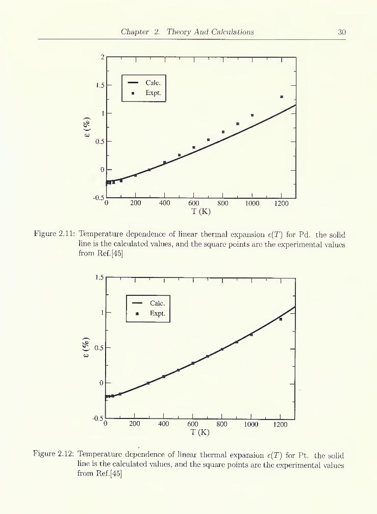
2.11 Temperature dependence of linear thermal expansion e(T) for Pd. the solid



2.12 Temperature dependence of linear thermal expansion e(T) for Pt. the solid

Une is the calculated values, and the square points are the experimental


2.13 Temperature dependence of hnear thermal expansion e{T) for Au. the solid

hne is the calculated values, and the square points are the experimental


2.14 Coefficient of hnear thermal expansion a{T) as a function of temperature

for Ag. the solid line is the calculated values, and the square points are the

experimental values from Ref.[45] 32


for Cu. the solid line is the calculated values, the square points are the

experimental values from Ref.[45], and the dash line is the results of the MD

simulation from Ref.[l] 32

2.16 Coefficient of linear thermal expansion a{T) as a function of temperature

for Ni. the solid line is the calculated values, and the square points are the


List of Figures ix


for Pd. the sohd hne is the calculated values, and the square points are the



for Pt. the solid line is the calculated values, and the square points are the



for Au. the solid line is the calculated values, and the square points are the


2.20 Isothermal bulk modulus B{T) as a function of temperature for Ag. the

solid line is the calculated values, the square points are the experimental

values from Ref.[47] and the round point is the experimental value from [48]. 35

2.21 Isothermal bulk modulus B{T) as a function of temperature for Cu. the


values from Ref.[47]and the round point is the experimental value from [48]. 36

2.22 Isothermal bulk modulus B{T) as a function of temperature for Ni. the solid

line is the calculated values, and the round point is the experimental value

from Ref. [48] 36

2.23 Isothermal bulk modulus B{T) as a function of temperature for Pd. the

solid line is the calculated values, and the round point is the experimental

value from Ref. [48] 37

2.24 Isothermal bulk modulus B{T) as a function of temperature for Pt. the solid


fromRef.[48] 37

List of Figures x

2.25 Isothermal bulk modulus B{T) as a function of temperature for Au. the


values from Ref.[47] and the round point is experimental value from Ref.[48]. 38

2.26 Calculated temperature dependence of heat capacity of Ag at constant vol-

ume Cy , at constant pressure Cp and electronical contribution Cy^. The

square points are the experimental data of heat capacitiy at constant pres-

sure from Ref.[50] 40

2.27 Calculated temperature dependence of heat capacity of Cu at constant vol-

ume Cy , at constant pressure Cp and electronical contribution Cy". The

square points are the experimental data heat capacitiy at constant pressure

from Ref.[50]. The point hne is the results from Ref.[l] 40

2.28 Calculated temperature dependence of heat capacity of Ni at constant vol-

ume Cy , at constant pressure Cp and electronical contribution Cy". The


fromRef.[50] 41

2.29 Calculated temperature dependence of heat capacity of Pd at constant vol-

ume Cy , at constant pressure Cp and electronical contribution Cy'. The


fromRef.[50] 41

2.30 Calculated temperature dependence of heat capacity of Pt at constant vol-

ume Cy,at constant pressure Cp and electronical contribution Cy'. The


from Ref.[50] 42

List of Figures xi

2.31 Calculated temperature dependence of heat capacity of Au at constant vol-

ume Cy , at constant pressure Cp and electronical contribution Cy . The


fromRef.[50] 42

2.32 Overall Griineisen Parameter 7 as a function of temperature for Ag. The

solid line is the calculated values and the square point is the experimental

values taken from Ref.[44] 43

2.33 Overall Griineisen Parameter 7 as a function of temperature for Cu. The

solid line is the calculated values and the square points are the experimental


2.34 Overall Griineisen Parameter 7 as a function of temperature for Ni. The



2.35 Overall Griineisen Parameter 7 as a function of temperature for Pd. The



2.36 Overall Griineisen Parameter 7 as a function of temperature for Pt. The



2.37 Overall Griineisen Parameter 7 as a function of temperature for Au. The

solid line is the calculated values and the square point is the experimental


List of Figures xii

2.38 Debye temperature Qd as a function of temperature T for Ag. The solid

line is the calculated results, the square points are the experimental values

from Ref. [53] , the round point is the experimental value at the temperature

r = 298/5rfromRef.[54] 47

2.39 Debye temperature 0/j as a function of temperature T for Cu. The sohd line

is the calculated results, the up triangle points are the experimental values

from Ref. [53] , the round point is the experimental values at the temperature

T = '298K from Ref. [54] , the square points are experimental values from [55] . 48

2.40 Debye temperature Qjj as a function of temperature T for Ni. The solid

line is the calculated results, the round point is the experimental values at

very low temperature from Ref. [48], the square points are the experimental

values at T = Oi^ and T = 298K from Ref.[54] 48

2.41 Debye temperature Qd as a function of temperature T for Pd. The solid

line is the calculated results, the round points are the experimental values

at the temperature T = 298K and T = OK respectively from Ref. [54]. . . 49

2.42 Debye temperature 6^ as a function of temperature T for Pt. The solid line

is the calculated results, the round points are the experimental values at the

temperature 7^ = 298/^ and r = 0/C respectively from Ref. [54] 49

2.43 Debye temperature O^ as a function of temperature T for Au. The solid


from Ref. [53], the round points (a and b) are the experimental values at the

temperature T = 298K from Ref.[54] 50

2.44 Adiabatic bulk modulus B{T) as a function of temperature for Ag. The sohd

lines are the calculated values and the square points are the experimental

values from Ref. [56] 50

List of Figures xiii

2.45 Adiabatic bulk modulus B{T) as a function of temperature for Cu. The solid



2.46 Adiabatic bulk modulus B{T) as a function of temperature for Ni. The solid

lines axe the calculated values and square points are the experimental values

from Ref.[48] 51

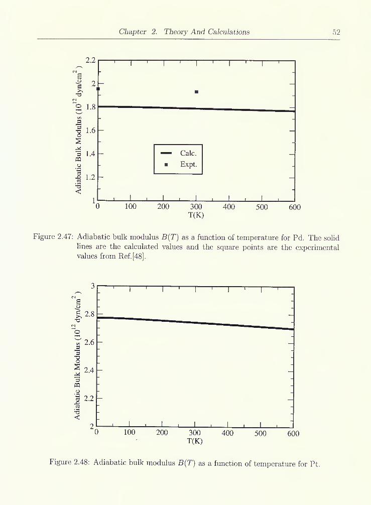
2.47 Adiabatic bulk modulus B{T) as a function of temperature for Pd. The solid



2.48 Adiabatic bulk modulus B{T) as a function of temperature for Pt 52

2.49 Adiabatic bulk modulus B{T) as a function of temperature for Au. The solid



3.1 Phonon dispersion curves for Pd. the dash lines are the calculated values

from Mei's parameter, the solid lines are the calculated results from the

modified parameters, and the round and squre points are the experimental

data 59

3.2 Phonon dispersion curves for Pt. The dash lines are the calculated values

from Mei's parameter, the solid lines are the calculated results from the

modified parameters, and the round and squre points are the experimental

data 59

Acknowledgements xiv

Acknowledgements

I would like to extend my heartfelt thanks to Dr. Bose and Dr. Shukla for their patience in

supervising me, for their kindness in helping my life in St. Catharines and for their financial

support received from the NSERC grant. I also want to express my sincere gratitude to

Dr. Reedyk for her generous donation to Department of Physics Graduate Scholarship and

to Ms. Brown for her donation to Ronald Brown Graduate Award. In addition, I wish to

acknowledge all professors in the department of physics who taught and helped me before.

Finally, a thousand thanks will be given to the department of physics for supplying me

with the very pleasant environment of research.

Chapter 1 . Introduction

Chapter 1

Introduction

1.1 Embedded Atom Theory

The embedded-atom method (EAM) was first porposed in 1983 by Daw and Baskes[2,

3] as an approach to calculate the energy of a multi-atom system. In this method, the

energy of the metal is viewed as the energy to embed an atom into the local electron

density provided by the remaining atoms of the system, plus an electrostatic pair interaction

potential between the atoms. The ansatz which Daw and Baskes used is

£^tot = 5]F,(p,,) + ^E^(^^)' (1-1)

i i,j

Ph,i = Yl /?(^j)' (1-2)

where Etot is the total internal energy, ph,i is the host electron density at atom i due to all

other atoms, fj is the electron density of atom j as a function of distance from its center,

Rij is the separation distance between atoms i and j. The function Fi(p;i_i), called the

embedding energy, is the energy to embed atom i in an electron density ph,i. $ij is two body

central repulsive potential between atoms i and j representing the electrostatic interaction

plus the interaction related to Pauli-principle due to the overlap of the charge clouds. The

host electron density ph^i is assumed to be a linear superposition of contributions from all

individual atoms except atom i, which in turn are assumed to be spherically symmetrical.

Chapter 1. Introduction

The embedding energy is assumed to be independent of the gradients of the electron charge

density [4].

The EAM is an empirical or semiempirical method. The concrete forms of the embed-

ding functions are determined to describe the bulk equilibrium solid. In particular, they

axe determined by comparing the simulation results with experimental ones and minimiz-

ing the differences to fit to the equilibrium lattice constant, heat of sublimation, elastic

constants, vacancy-formation energy, etc[5]. Over the years, many efforts have been made

in this area. Daw and Baskes[3] used the form of F{p) which was proposed by Puska et al.

[6] and given by

F{p) = ap-bp'/\ (1.3)

to calculate the hydrogen embrittlement in metals. In equation (1.3), a and h are the

positive constants. Foiles, Baskes, and Daw[7] developed the EAM functions for the fee

metals ( Ag, Au, Cu, Ni, Pd and Pt ) and their alloys by numerically fitting the functions to

the bulk lattice constants, cohesive energy, elastic constants, vacancy-formation energy, and

alloy heats of mixing. These EAM functions have been fairly successful in a wide range of

applications [8]. Baskes[9] calculated the properties of metastable phases and point defects

for siUcon by taking the embdedding funtion as

np) p_

LPe

InP_

Pe(1.4)

where Eo is the sublimation energy, and pe is the density an atom sees at equilibrium in

the initial reference structure. Recently Johnson[4, 10], by using an exponentially decaying

function instead of the spherically averaged free-atom densities calculated from Hartree-

Fock theory, suggested a nearest-neighbor model for fee metals. In this model, the EAM


potentials are simplified and expressed as the following analytic functions:

Fip) = -E,[->


0.6

0.41/2

F(p) = p - p

F(p) = [l-0.51n(p)]p"'-p"'

0.25 0.5 0.75 1

Electron density p

1.25 1.5

Figure 1.1: Embedding functional F{p) against electron density p.

The EAM has been widely developed over the past two decades. Finnis and Sinclair[13]

proposed a model in which the total energy of an assembly of atoms consists of a binding

term proportional to the square-root of the local density and a repulsive pairwise potential

term. This model is mathematically equivalent to the EAM. Manninen[14], Jacobsen,

N0rskov, and Puska[15] also derived the functional form of the energy of the EAM by

using density functional theory. Presently the EMB has become a very popular method

for computing the energetics of metallic systems for use with various computer simulation

techniques, because it overcomes some inherent or practical limitations which often plague

the other theories. For example, Band theories[16] are generally limited by basis-set size and

the requirement of periodicity[17, 18]. Cluster theories are also limited by the size of clusters

or basis sets permitted by computers. The early pair-potential methods, while including

corrections due to many body interactions and yielding the total energy directly, require


the use of an accompanying volume-dependent energy to describe the elastic properties of

a metal[19]. This volume-dependent term makes it difficult to simulate the surfaces and

the extended crystal defects, where the volume of the sample is ambiguous [2]. In addition,

ab initio methods require large computing resource to study large-scale structures [20].

Because of its computational simplicity and effectiveness, the EAM has been used in study

of condensed matter in many areas. Daw and Hatcher [21] successfully applied the EAM to

discuss the bulk phonons of some transition metals and Nelson et al. [22] calculated surface

phonons for copper by using embedded-atom parameters fit to bulk properties. Foiles[5]

suggested a set of EAM functions fitted to bulk solid properties to study the structure

and pressure of various liquid metals. Daw and Baskes[2] obtained the embedding energy

and pair potential for some metals and used them to treat the problem of the defects in

metals. Foiles et al. [7] determined a set of the EAM functions for some fee metals and

their alloys by fitting to the sublimation energy, equilibrium latttice and elastic constants

of the pure metals and the heats of solution of the binary alloys to study the properties

of the metals and their alloys. Johnson [23] investigated the phase stability of fee alloys.

Daw and Baskes[2, 3, 20] used the analytical EAM functions to study the properties of

impurities for some fee and bcc materials. The appUcation in other fields, such as fracture,

surface structure, surface adsorbate ordering, surface segregation and surface ordered, can

be found in Ref.[4, 24-30].

1.2 The EAM Potentials of Mei et al

For a perfect monatomic crystal, Eqs.(l.l) and (1.2) can be simplified to

Etot = NE, (1.8)


E = F{p) + 1/2 J2sA<f>{RA), (1.9)

A

A

where A^ is the number of atoms in the crystal, E the energy per atom, i?A the distance of

the Ath-neighbor shell with respect to a given atom, and Sa the number of atoms in that

shell.

For a perfect crystal, we have

Ra=PaRi,A = 1,2,..., (1.11)

here the constants p\ depend on the type of the crystal structure and pa = \/A for a fee

crystal.

Rose et ai.[31] has shown that, for most metals, the energy is well approximated by the

relation

E{Ri) = -E,[l + a{RjRu - l)]exp[-a{R,/Ru - 1)], (1.12)

with

a = (g^efie/^c)'/', (1.13)

where Q is the atomic volume and B the bulk modulus. The subscript e indicates the

evaluation at equilibrium.

Plotting the electron densities calculated from Hartree-Fock method, Johnson[4] found

they are quite well approximated by a single exponential term in the range of distances of

interest in EAM calculation:

p = Peexp[-/5(/?i/i?ie - 1)], (1.14)

where parameters pe and f3 are determinded from fitting the calculated electron density.

Mei et ai.[l] also did some calculations of the electron density for many metals and proved


p{Ri) is really well described by the exponential decay of Eq.(1.14) when Ri is not far from

Rie. Mei et al. assumed function f{R) in Eq.(l.lO) to have a form

f{R) = feY,^r{Ru/Rr, (1.15)

T=0

where the parameters Cr are determined by using least-squares fitting to fit the equation

J2 ^a/(^a) = Peexp[-P{Ri/Ru - 1)], (1.16)

A

or the equivalent equation

K

Y,9r{RllRleV = exp[-/?(i?i/i?ie " 1)], (1-17)

r=0

with

Qr = Cr{fe/Pe)^ SaP^' '^ = 0, 1, -, «, (1.18)

A

provided k is given and fe = Pe/12.0. The coefficients c^ with specifying k = 5 for some

fee metals (Ag, Cu, Ni, Pd, Pt and Au) are listed in Table(l.l).

By taking into consideration of Eqs.(1.12) and (1.14), Mei et ai.[l] took the EAM

potentials as the following forms

0(i?) = -0e[l + 5{R/R^, - l)]exp[-7(i?/i?i, - 1)], (1.19)

np) ErH-

Chapter 1. Introduction 8

these parameters for those fee metals are also listed in Table 1.1. The calculated values of

the three elastic constants Cu,Ci2 and C44 are compared with the experimental values to

which they were fitted in Table 1.2

Table 1.1: Coefficients Cr of function f{R) and the model parameters for the six fee metals.

0e is in units of eV. Other parameters are dimensionless.

Chapter 1 . Introduction

Table 1.2: Input and output data for the elastic constants C\\,C12 and C44,which are in

units of lO^^N/m^


-3.3

-3.35

>u

Bo

A'a.

00

w-3.45 -

— - Rose Model

Mei Model

3.75

Lattice Parameter (10 m )

Figure 1.2: The energy per atom as a function of lattice parameter for Cu. arcontribution

from the first shell. 6:contribution from the first two shells, c:contribution from

the first three shells.

-0.45

><L>

CO

s

-0.75 -

-1.05

Lattice Parameter a (10 m)

Figure 1.3: Embedding function against lattice parameter for Cu. a:contribution from the

first shell. 6:contribution from the first two shell, c:contribution from the first

three shells, d:contribution from the first four shells. e:contributioin from the

first six shells.


contribution to the embedding potential which can be ignored. So it is reasonable that in

later calculations we will consider all summations up to the sixth shell of the neighbors

with respect to a given atom.

Mei et ai.[l] has extended the nearest-neighbor model of Johnson and suggested the

analytic forms of the embedded-atom potentials valid for any choice of cutoff distance.

Our present work is based on the model of Mei et al. . By using these relatively simple

analytic EAM potentials, we have calculated the phonon frequencies for six fee metals

(Ag, Cu, Ni, Pd, Pt and Au ). To investigate the applicability of this model further, we

focus on the other thermodynamic properties of these metals and have computed the zero

point free energy at room temperature and temperature dependence of the lattice constant,

the coefficient of thermal expansion, the isothermal and adiabatic bulk moduli, Griineisen

parameters, Debye temperature and phonon contributions to the heat capacities at constant

volume Cv and at constant pressure Cp. Then we compare the calculated values with the

experimental findings and give some conclusions.

Chapter 2. Theory And Calculations 12

Chapter 2

Theory And Calculations

2.1 Phonon Dispersion Curves

2.1.1 Theory of Phonon Vibration

Here we just take into consideration of primitive crystal without losing any generality. For

an infinitely extended primitive crystal, if each atom / located instantaneously at positon

R(/) is displaced from its equihbrium position Re(0 by u(/), which means we have

R(/) = Re(0 + u(0, (2.1)

and

R'{l)^Ri{l) + Ui{l), (2.2)

the total kinetic energy of the crystal can be written as

T = ^^M^^(/), (2.3)

i,i

where M/ is the mass of the atom / and the sum runs over all atoms in crystal. R\l), Ri{l)

and Ui{l) are the z-cartesian components of R(/), Re(0 ^^^ u(/) respectively with i — x,y, z.

According to the theory of phonon vibration [32, 33], the total potential energy ^ of the

crystal, which is assumed to be a function of the instantaneous positions of all atoms, can

be expanded into a Taylor's series in powers of the atomic displacements u(/) and has the


form

l,i l,m

+ — X $ijfc(/, m, n)ui{l)uj{m)uk{m) H . (2.4)

l,m,n

In this expansion, ê is the potential energy of the static lattice which means all atoms are

at rest at their equilibrium positions, while obviously

*«(0 =

îj{l,m) =

îjk{l, m, n) =

5*dui{l)

dui{l)duj{m)

^3^,etc.

(2.5)

(2.6)

(2.7)dui {l)duj {m)duk (n)

where the subscript e means that the derivatives are evaluated with all atoms at the equi-

lirium configuration, and the coefficients #j(Z), ^,j(/,m), #ijfc(/, m,n), • • are known as

atomic force constants of the first, second, third,- • •, order, respectivly.

It is clear that a mixed partial derivative is independent of the order in which the

differentiations are carried out. The coefficients in the expansion (2.4) are completely

symmetrical in the indices, such as

îj{l,m) = ^ji{m,l), (2.8)

îjk{l, m, n) = ^jki{m, n, /) = ^jik{m, I, n) = îkj{l, n, m)

= ^kji{n,m,l) = ^kij{n,l,m),etc. (2.9)

From the definition fo Eqs.(2.4) and (2.5), we can see the physical interpretation in

them. The first order force constant î{l) is that it is the negative of the force acting in


the i direction on the atom at R(/) in the equihbrium configuration. It must vanish because

in equihbrium configuration the net force on any atom must be zero, so we have the result

*,(/) = -F(0|e = 0. (2.10)

Here F'(/) denotes the i cartisian component of the force F(/) acted on atom /. The second

order force constant *ij(/, m) is the negative of the force exerted in the i direction on the

atom / when the atom m displaced a unit distance in the j direction, all other atoms staying

at their equilibrium positions. It can be expressed as

dF'{l)îj{l,m) = (2.11)

duj{m)

If the lattice as a whole is subjected to an infinitesimal rigid body displacement v, the

lattice potential and its derivatives must remain unchanged. This property of the lattice

imposes some conditions on the atomic force constants which can be expressed as

J2MI)^0, (2.12)

J2 îj ii^rn) = Y^ îj {l,m) = 0, (2.13)

I m

^îjk{l,m,n) = ^#ijfc(Z,m,n) = ^îjk{l,m,n) = 0,etc. (2.14)

I m n

The vibrational hamiltonian for the crystal can be written £is

H = T + ^. (2.15)

If we use the harmonic approximation, namely neglect all terms whose orders are higher

more than two in Eq(2.4), we can rewrite the vibrational hamiltonian as

H = ê + -J^Miii-îl) + ^J2îjil,m)ui{l)uj{m). (2.16)


Denoting by pi{l) the z-cartesian componet of the momentum of the /th atom, we can

change Eq.(2.16) into

i/ = #e + ^p^(/)/2M, +^^ $,,(/, m)«,(/)w,(m). (2.17)

i,l l,m

Prom this Hamiltonian, we can immediately obtain the equation of motion of the crystal

dui{l)MiUi{l) - —K—ff. = - XI *'j(^' "^)"j(^)- (2-18)

The equation of motion Eq(2.18) with different / and i labels forms an infinite set of

simultaneous Unear differential equations. Their solutions are simplified by the periodicity

of the lattice and the restrictions on atomic force constants which follow from the symmetry

and structure of a crystal. Therefore we can choose as a solution of this set of coupled

equations a function of the form

mil) = M~'/^ei(/|Ks)exp[-ic^,(K)i + iK • R(/)]. (2.19)

Here the vector K in the exponent is called wave vector, and its magnitude is equal to 27r

times the reciprocal of the wavelength of an elastic wave propagation through the medium,

and its direction is the direction of propagation of the wave. The coefficient ej(/|Ks) satisfies

the equation

ul{K.)ei{l\Ks) = Y^ Dij{l, m|K)e,(m|Ks), (2.20)

m,j

where

Dij{l, m|K) = (MiM^)-i/2 Y^ ^..(^i^ m)exp[-zK • (R(/) - R(m))]. (2.21)

m

Usually, the matrix Dij{l, m|K) is called dynamical matrix of the crystal. It is a hermitian

matrix and has the properties

Dij{l,m\K) = D*i{mJ\K) (2.22)


Dij{l, m\-K) = D*^{1, m\K). (2.23)

The condition that the set of Eq.(2.20) have a nontrivial solution is that the determinant

of coefficients vanish

\Dij{l, m|K) - uj^^{K)Sij5im\ = 0. (2.24)

Eq.(2.24) is a 3 X 3 matrix equation. For each given vector K, the allowed values of the

frequency u) have three branches denoted by Us{K.),s = 1,2,3, and their square are the

eigenvalues of dynamical matrix. Furthermore, Eq.(2.20) defines the eigenvectors ei(/|Ks)

only to within an arbitrarily chosen constant, so they are assumed to satisfy the orthonor-

mality and closure conditions:

Y^e*il\Ks)e,{l\Ks')=5ss', (2.25)

i

Y, e*(/|Ks)e,(m|Ks) = SijSim- (2.26)

s

It is clear that R(/) and u(/) are related linarly, so the derivative with respect to u(/)

makes no difference from the derivative with respect to R(/). In following sections, we more

often use the expression (9/(9R(/) instead of d/du{l).

2.1.2 Phonon Frequencies

The application of the theory of phonon vibration to the model of Mei et ai[l] is straightfor-

ward. Keeping the notations used in section (2.1.1), we substitue Eq.(1.15) into Eq.(l.lO),

and write the electron density at the position of atom / as

T=5

Pl = f-J2Y1 CriRle/RlmY, (2.27)

m T=0

where Rim is the distance between atom I and atom m which can be written as

i?;^ = |R(/)-R(m)|, (2.28)


the sum m runs over the all neighbors of the reference atom /.

Considering Eqs.(1.19) and (1.20), the embedded atom potentials of Mei et al, we can

obtain the total energy of the crystal

Etot = 5] |f,(p/) + 1/2 J] $(/t:/^)|

l,Tn

Pel

PL

PeI

+ 2^e Yl ^M-iPlm - 1)7] X

a/13

l + (P/m- l)5-p;^-ln/3 Lp.

Pi Pi

Pe

Pin

-UeY, [1 + S{Rim/Ru - l)]exp[-7(i?,^/i?ie - 1)], (2.29)

with pi-m having the form

Plm — Rlm/Rle, (2.30)

here the first summation / runs over all atoms in the crystal, and the second one m runs

over all neighbors of a given atom /.

Using the expression of the total energy Eq.(2.29), we can calculate the net force ex-

certing on the atom / which is of the form(see details in Appendix A.l)

F(/) = -V,F,„, = -J2 [F'MfmiRlm) + F'^{pm)n{Rlm) + <i>'lm{Rlm)]^ . (2.31)

m(yil}

here V/ means to do derivative with respect to the three components of the position vector

R(/) of atom /, namely

^' = mrf' + dWf' + dW)''^(2.32)

xo, yo and Zq are the unit vectors in the directions of x, y and z respectively. The prime in

the function of Eq.(2.31) donetes the derivative of the function with respect to its argument,


îm/Rim is a unit vector which points from atom / to atom m, it has the form

R,^ R(0 - R(m)

with the three components

(2.33)

The second force constant can be obtained in the same straightforward way as it was

deduced in Ref.[13, 22]

The result for / 7^ m is (see details in Appendix A. 2)

Îm^lm T?l ( ^ \f"fD \RlmR\m if^'l f u \ Îm^lIm Im•2

Im

It.

*,,(/,m) = -F/(p,)/;(i?;^)-^^-F;(p^)//'(i?,^)^^-$"(i?,^)^

-[F'l{pl)fm{Rlm) + F'^{pm)n{Rlm) + ^'(^"")]{|^ " ^^j+ E K{Pn)fl{Rln)nRmn)-^^. (2.36)

Using Eq.(2.13), we can obtain the second force constant for / = m.

îj{hl)^-^^r,{Um). (2.37)

m(^/)

Noticing Eq.(2.37), we can rewrite Eq.(2.21) as

A,(/,mlK) = (MM^)-i/2^ *,,(/, m)expHK-(R(/)-R(m))]m

= {MiMm)-^/Hîj{l,l) + E *^J(^m)exp[-^K • (R(/) - R(m))]|

= {MiMm)--^''' E *i,(/,m)|exp[-zK • (R(/) - R(m))] - 1 j. (2.38)

m(#/)


Combining Eq.(2.36) with the following equations(see appendix A.3 in details),

F'iPi) =dpi PeP'

:ln El

PeJ

El

Pe

a/13-1

+ :j-^^(^M-ipit-'^h]ti^i)

5 7x<; -pit-3+pit-g l + iPit - l)S-pit-ln El

Pe

El

iPe(?.39)

F"ipi) =dpi

,al + (--l)ln El

pe

El

pe

a *•

HP.j -1)

5 7-Plt-3+Plt^ 1 + {pit - l)5-pit-\n El]

.Pel.


X W r A—' L

oB(03p


W A— L

^

o

1

7 -/^

1


C (K=[00a27r/a) C (K=[0Cl]27i/a) ^ (K=[0^Q2n/a) C (K=[CCa27i/a)

Figure 2.4: Phonon dispersion curves for Pt. The solid lines are the calculated phonondispersion curves at the lattice parameter corresponding to static equilibrium.

The square and round points are the experimental data from [37] at 90K. Land T represent transverse modes and longitudinal modes respectively.

oB

r A— X


Pi(l) = y(^)^ E^^'''(K)e.(/|K.)e'^-^W(6K. - t^^J, (2.49)

Ks

and the inverses to these expansions

bKs = (2A^/i)-'/'X]<(^l^^)^'''''''^'M[^'^^(K)]'/'wi(0 + i[Mu;,(K)]-i/2p.(^)|^ ^2.50)

li

where h is Planck's constant, A'' is the number of primitive unit cells in a parallelepiped

all of which fill of crystal space without gaps and overlap, both K and K' are restricted to

he inside the first Brillouin zone, we can obtain the Hamiltonian in the forms of these new

operators

H = J2^s{K)[b^^bKs + l/2]. (2.52)

Ks

The ground state |0 > is defined by

bKs\0 >= 0, for aU (Ks). (2.53)

Therefore, the eigensolutions of the Hamiltonian (2.52) read

\ns,{Ki),--- ,ns3(Ki),--- ,n,j(Kiv), • • • ,n,3(K7v) >/- AT 3

,^ -1/2 N 3

= nn("K.)! nn(^K.rio>. (2.54)•^ K s=l J K s=l

N 3

E{{nKs}) = ^ J]/ia;,(K)[nK. + -], (2.55)

K s=l

where

nKs = 0,1,2,- (2.56)

denotes the number of phonons of frequency u!s{K) present in the state (2.54).


Table 2.1: Zero-Point Energy in Rydberg per atom at 300 K.

Elements


where H is Hamiltonian in the harmonic approximation, P = l/Zc^T, ks is Boltzmann's

constant, and T is the absolute temperature. It is convenient to evaluate the trace in

Eq.(2.58) in the space in which H is diagonal. Therefore, if taking the forms of Eq.(2.52)

and Eq.(2.54) and submitting in Eq.(2.58), we can find

^ = E •• E exp|-/3^^.(K)[nK. + -]["Kisi=0 nKNS3=0 ^ Ks J

lll_exp[-/3^,(K)]- ^^-^^^

The Helmholtz free energy which comes from the contribution of phonon vibration is

given by

F,ib = -keTlnZ = A;^V ln{2sm/i^^ }

.

(2.60)

The entropy S , the internal energy E and the specific heat at constant volume Cy of

the crystal become

Ks

^BE{-^ooth^ - H^srnh^)

I(2.61)

E = F + TS = Y, ^^'^^^^^'^^^^^ (2.62)

C - \^^^

= Y^^viKs)K,5

^^ I 2kBT ] sinh^[hujs{K)/2kBTy^^-SS)

Ka


In the quasiharmonic approximation, the total Helmholtz free energy of crystal at tem-

perature T and volume V or lattice constant o is [43]

F{a,T) = Etotia) + F,i,{a,T) = EUa) + fcs y;in{2sm/i^^^^^^} (2.64)

where Etot is static total energy at a given volume V or lattice constant a which is defined

by Eq.(l.l). We use u;s{K,a) instead of uJs{K) in Eq.(2.64) to specify that frequency is

also a function of lattice parameter a.

At a given temperature T and zero pressure, the equilibrium geometry is determined

by the minmum of the Helmhotz free energy [43], that is

(^^).^^+(^^^). = 0. ,2.65)

In application of Eq.(2.65), we use the free energy per atom instead of the free energy

of the crystal by evaluating F^ib on a 20 x 20 x 20 K-points mesh in the Brillouin Zone and

plus the static energy per atom which is defined in Eq.(1.9). First, we set up an array for

the lattice parameter a, and then we change the temperature T value at a step equal to

2K from OK to lAOOK to calculate the free energy per atom at different lattice parameter.

The equilibrium lattice constant ae{T) at the given temperature T is the one corresponding

to the minimun of the free energy per atom at that temperature. In Fig. (2.7), we plot the

lattice parameter against temperature.

Using the results obtained for the lattice constant as a function of temperature, we can

determine the linear thermal expansion [43]

,(r)^ "'(^)-°'W, (2.66)

^eX-l- c)

where we have chosen lattice constant ae{Tc) at T^ = 293K to be the reference length as

[44] did. Figs. (2.8-2. 13) give the calculated results and experimental data.


4.2

\ "^

ac 3.9

BC

(J^°

oa 3.7

3.6

3.5

'1 ' 1


CO

200 400 600 800 1000 1200

T(K)

Figure 2.9: Temperature dependence of linear thermal expansion e{T) for Cu. the sohd

line is the calculated values, and the square points are the experimental values

fromRef.[45]

1.5 -

1-

^CO

0.5

-0.5


CO

z


^u

Z.J


3.5x10

3.0x10

2.5x10

-5

7 2.0x10

S 1.5x10"'

1.0x10"'

5.0x10"^

0.0

-


200 400 600 800 1000 1200

T(K)

Figure 2.16: Coefficient of linear thermal expansion a{T) as a function of temperature

for Ni. the solid line is the calculated values, and the square points are the

experimental values from Ref.[45].

2.0x10I

—

I

1—

I

1

1 r

1.5x10"

T

0.0 *f L

200 400 600 800 1000 1200

T(K)

Figure 2.17: Coefficient of hnear thermal expansion a{T) as a function of temperature for

Pd. the solid line is the calculated values, and the square points are the

experimental values from Ref.[45]


200 400 600 800 1000 1200

T(K)

Figure 2.18: Coefficient of linear thermal expansion a{T) as a function of temperature

for Pt. the solid line is the calculated values, and the square points are the

experimental values from Ref.[45]

^a

5.UX10


200 300T(K)

400 500

Figure 2.20: Isothermal bulk modulus B{T) as a function of temperature for Ag. the solid

line is the calculated values, the square points are the experimental values

from Ref.[47] and the round point is the experimental value from[48].

derivative of the free energy [46]

:

The temperature dependence of the isothermal bulk modulus is defined by [46]

(2.69)

(2.70)

or

B{T) \Qy2lT

V;^T/2/ "^V PT/2 )t'^dV^' dV^

(2.71)

We use the numerical method to evaluate the Eq.(2.71) and plot the results with ex-

perimental data in Figs.(2.20 - 2.25).


e

•a

»3

T5Oe

1.5 -

J2 0.5

o1/1

1

—


200 300T(K)

400 500

Figure 2.23: Isothermal bulk modulus B{T) as a function of temperature for Pd. the solid


from Ref.[48].

3.5

1.5

o


Z.J


and submitting Eq.(2.69) into Eq.(2.73), we can obtain

Cp{T) - Cv{T) = al{T)B{T)VT. (2.75)

It is clear that the Unear thermal expansion coefficient and the volume thermal expansion

coefficient are related by the following equation

av{T) = Za{T). (2.76)

Noticing the volume of each atom in fee structure is V = ag(T)/4, we rewrite Eq.(2.75) as

Cp{T) - Cv{T) - â\T)B{T)al{T)T (2.77)

or

Cp{T) = Cf (T) + C^{T) + â\T)B{T)al{T)T. (2.78)

We use Eq.(2.63) to calculate the first term Cl!'{T) in Eq.(2.78) at different tempera-

ture by evaluating it on a 20 x 20 x 20 K-point mesh in the Brillouin Zone, and then we

apply the STUTGART TB-LMTO-ASA program to compute the electronical contribution

to heat capacity C^{T). We take the results a{T), B{T) and ae{T) from the above to cal-

culate the third term in Eq.(2.78) and plus three terms together to obtain the temperature

dependant Cp{T). Figs.(2.26 - 2.31) show the temperature dependence of heat capacity at

constant volume C^, at constant pressure Cp and electronical contribution Cy with the

experimental data.

2.2.5 Griineisen Parameter

Submitting Eq.(2.64) into Eq.(2.69), we can write the equation of state as

dV ^ dV 't

= ^^ + Ê^^(K)<-.(K)), (2.79)


Figure 2.26: Calculated temperature dependence of heat capacity of Ag at constant volume

Cy ,at constant pressure Cp and electronical contribution Cy^. The square

points are the experimental data of heat capacitiy at constant pressure from

Ref.[50].

o

U•a

>

Figure 2.27: Calculated temperature dependence of heat capacity of Cu at constant volumeC^

,at constant pressure Cp and electronical contribution C^^. The square

points are the experimental data heat capacitiy at constant pressure fromRef.[50]. The point line is the results from Ref.[l].


Ho

U

>

Figure 2.28: Calculated temperature dependence of heat capacity of Ni at constant volume

Cy , at constant pressure Cp and electronical contribution Cy . The square

points are the experimental data heat capacitiy at constant pressure from

Ref.[50].

4 -

So

09

o.

U 2\-T3C>

U

200 400

'1 '

1


4 -

Eoa

m

o.

U 2T3CC3

U1 -,

1


3


2.5 1—

I

1—

1

1 11—I—I—I—I—

r

I I I

Calc.

Expt.

0'—1—I—I—1—1—I—I—I—

I

I I I I I I I II I

200 400 600 800 1000 1200

T(K)

Figure 2.33: Overall Griineisen Parameter 7 as a function of temperature for Cu. The solid

line is the calculated values and the squaxe points are the experimental values

taken from Ref.[44].

B 1.5

6

Oh

c 1

c5O 0.5

1i.

200 400 600 800

T(K)1000 1200

Figure 2.34: Overall Griineisen Parameter 7 as a function of temperature for Ni. The solid

line is the calculated values and the square points are the experimental values

taken from Ref.[51].


-4—

»

0)

03;-!

cj

Oh

C

'53

c2O

J


5 -

CLh 3

c<u1/1

so

'

1'


150 200

T(K)250 300 350

Figure 2.38: Debye temperature Qd as a function of temperature T for Ag. The solid line is

the calculated results, the square points are the experimental values from Ref.

[53] , the round point is the experimental value at the temperature T = 298Kfrom Ref. [54].

Qd is called Debye temperature. Prom the results of temperature dependent Cv{T) calcu-

lated in the above subsection, we can obtain the temperature dependent Debye temperature

Od{T) by numerically evaluating the integral in the right side of Eq.(2.83) and matching it

with Cv(r) in the left side. The results are plotted in Figs. (2.38 - 2.43)

2.2.7 Adiabatic Bulk IModulus

The adiabatic compressibihty ks{T) is [47]

Mr) = -^(|^)^. (2.86)

The adiabatic bulk modulus Bs{T) is the inverse of the adiabatic compressibility:


375 r~I—I—I—r-|—I I I I

350

g"c 325

i3 300

<u

i 275

u^250

Q

I I

II I I I 1 I I I I

II I I I

225

200 I'll 1 L_l 1 I I I I l_l_J I I I I I I I I r I I I I I I

50 100 150 200 250 300

T(K)

Figure 2.39: Debye temperature Qd as a function of temperature T for Cu. The solid line

is the calculated results, the up triangle points are the experimental values

from Ref. [53], the round point is the experimental values at the temperature

T = 298K from Ref. [54], the square points are experimental values from [55].

500

50 100 150 200

T(K)250 300 350

Figure 2.40: Debye temperature Go as a function of temperature T for Ni. The soUd line

is the calculated results, the round point is the experimental values at verylow temperature from Ref. [48], the square points are the experimental values

at T = Ois: and T = 298K from Ref. [54].


325

3001-

gS 275 h

I 250

i 225

u>^200<u

Q1751-

150

1 '1

'1

' 1


150 200

T(K)250 300 350

Figure 2.43: Debye temperature G^ as a function of temperature T for Au. The solid


from Ref. [53], the round points (a and b) are the experimental values at the

temperature T = 29SK from Ref. [54].

.r 1.5


1.8

I

_3

O

CQoa

2

<

1.6 -

1.4

1.2

0.8

'

1'


100 200 300 400 500 600T(K)

Figure 2.47: Adiabatic bulk modulus B{T) as a function of temperature for Pd. The solid


values from Ref.[48].

J


-a

CO

T3OS

^.J


We calculate the adiabatic bulk modulus for the fee metals and plot them as the func-

tions of temperature in Figs. (2.44 - 2.49).

Chapter 3. Discussions and Conclusions 55

Chapter 3

Discussions and Conclusions

We apply the analytic embedding functions of Mei et ai.[l] to calculate the phonon disper-

sion curves and some other dynamical properties of fee metals. From Figs. (2.1 - 2.6), it

is clear that the calculated phonon dispersion curves for Cu and Ag agree quite well with

experimental data. The relative error, which is defined as the absolute difference between

the theoretical value and experimental value divided by the experimental value, when wave

vector K is at F, Xand L points, is not more than 5.0% for Ag and 7.0% for Cu. Xie[46]

used density functional theory(DFT) and density functional perturbation theroy(DFPT)

to perform first-principles calculation of thermal properties for Ag. Narasimhan[43] has

used local density approximation(LDA) and generalized gradient approximations(GGA) to

carry out ab initio calculation of the thermal properties for Cu. From the phonon dispersion

curves in these works, it appears that their results are no better than the present results.

Daw[21] used different embedded atom potentials[2] to calculate phonon dispersion curves

for Ni and Pd. For Ni, present results axe close to the ones in Ref.[21], which agree with

experimental values very well at small wave vector K. However, for Pd, present longitu-

dinal mode results are worse than those in Ref.[21] at small wave vector K in comparion

with experimental values. The parameters in the embedding functions of Mei et al.[l] are

obtained from fitting the total energy of the crystal and elastic constants to the exper-

imeantal values, not from fitting the force constants as has been done by Miller [36]. The

approach of Mei et al.[l], thus, is more fundamental than that of Miller, even though it is


not a completely first-principles method.

In an attempt to improve the computed results of phonon frequencies, we made small

changes in parameters in the model of Mei et al.[l] for Pd and Pt, which are listed in

the following table (3.1). Using these modified parameters we computed the phonon fre-

quencies again. The interesting thing is that, with the modified parameters, the calculated

phonon dispersion curves agree with experimental values very well (see Fig. 3.1 and Fig.3.2).

However, we apply the same formula[2] as used by Mei to calculate the elastic constants

Cii,Ci2 and C44 and find that the calculated results have large deviation from the ones

obtained in Ref.[l] and Ref.[5]. We list the results in table (3.2). This interesting result

suggests that there is room for imrovement in the parameters. This can be the subject of

future research. For example, how are the parameters improved in this model to make the

theoretically calculated values get closer and closer to the experimental values for all other

dynamical properties.

We have studied the temperature dependent thermodynamical properties. First, we

obtain the variation of lattice constants with temperature(see Fig.2.7). It is easy to see

that present calculation based on the theory of lattice dynamics is very close to the results

obtained by Mei et al. from the molecular dynamics simulation. To check the results, we

calculate the linear thermal expansions. From the Figs. (2.8 - 2.13), we can say that the

model of Mei et ai.[l] works very well. T.Qagin[58] also use molecular dynamics(MD) to

study the thermal and mechanical properties of some fee transition metals: As a com-

parison, we list the linear thermal expansion results in table 3.3. Obviously, the results

calculated from the model of Mei et ai.[l] are much better than Ref.[58].

For the coefficient of linear thermal expansion, it is clear to see in Figs. (2. 14 - 2.19) that

the values calculated from the model of Mei et ai.[l] give a good prediction for each metal,

especailly at low temperatures, although they are slightly underestimated for Cu, Ag, Pd


Table 3.1: Modified Parameters In Mei's Model


Table 3.2: The elastic constants Cn,Ci2 and C44 calculated from the modified

paramters,which are in units of lO^^N/m^


>> 4oca

r A—> X w X <—I ]


Table 3.3: The Linear Thermal Expansion of Ni, Cu, Ag, and Au as a Function of Tem-

perature

Elements


Table 3.4: Compaxison of Griineisen parameter 7 with experimental and other theoretical

values.

Elements


and Ni, and overestimated for Au and Pt at very high temperatures. MacDonald et al. in

Ref. [44] also calculated the coefficient of linear thermal expansion using a kind of the volume

dependent free energy. However, their results are not satisfatory: there are deviations from

the experimental values both ant high and low temperature regions. For Cu, we also plot

the results from Ref.[l] as a comparison (see Fig.2.15). At room temperature, Mei et al.

gave a value of 1.5 x \Q~^K~^ better than present value of 1.35 x 10"^/C~^ , while at lower

temperature the MD simulation fails.

The lattice contributions to the isothermal and adiabatic bulk moduli are shown in

Figs. (2.20 - 2.25) and in Figs. (2.44 - 2.49). For all cases our calculations give a remarkably

successful prediction, as they agree with experimental data very well.

Heat capacity is an important thermal property of solids. The calculated Cp and Cy

are displayed in Figs. (2.26 - 2.31). As we can see that the calculated curves for Cp are all

in very good agreement with experimental data, except for Ni. Curie temperature of Nickel

is Q21K. Below this temperature Nickel is ferromagnetic. Above this temperature. Nickel

becomes paramagnetic. However, the embedded atom method, as used by Mei et al, does

not have the necessary degrees of freedom (i.e., treating spin up and spin down eletrons

separately) required to describe the magnetic state. The heat capacity C^ for all cases

approches the value of 3A;b per atom at very high temperatures, the classical harmonic

limit. In Fig.2.27, we also give the results of Cp for copper calculated by Mei et ai.[l].

Their results agree quite well with experimental values in a range from SOOA' to lOOOA',

but at low temperatures there is a big discrepancy with experimental data.

Another important thermodynamic quantity is Griineisen parameter. The overall Griineisen

parameter is the average of mode Griineisen parameter relative to the volume derivative of

frequency with the weight of the heat capacity at each mode. Due to the shortage of direct

way to measure, there is a large variation with experimental results as shown in table 3.4.


Compared to the indirect measured values of this quantity, the agreement between theory

and experiment is poor for Cu and Ag.

Debye temperature as a function of temperature is calculated and plotted in Figs. (2.38 -

2.43). Obviously, the calculated Debye temperature for Cu and Ag is in excellent agreement

with experimental values. In fact, it is easy for us to predict this result by noticing the very

good agreement between the calculated values and experimental ones in phonon dispersion

curves. For Pd, Ft and Ni, the Debye temperature are slightly underestimated, but for Au,

the Debye temperature is underestimated too much, close to 20 percent.

We have applied the analytical embedded atom potentials of Mei et al.[l] to investi-

gate the dynamical properties of some fee metals. Under the harmonic aprroximation, we

have calculated the phonon frequencies, lattice parameter as a function of temperature,

zero-point energy of phonon vibration at room temperature. We have also calculated the

temperature dependence of linear thermal expansion, coefficient of linear thermal expan-

sion, isothermal bulk modulus, adiabatic bulk modulus, heat capacity at constant volume

and at constant pressure, Griineisen parameter and Debye temperature. After comparing

the theoretically calculated values with experimental data, we have found that our cal-

culations give good predictions for most of the dynamical properties of all these metals.

Therefore, this model should be useful and might be one of good choices in the investigation

of pure crystal properties.

Appendix A. Proofs of some Equations 64

Appendix A

Proofs of some Equations

A.l The proof of Eq.(2.31)

We can write the derivative of Etot with respect to the position vector of atom / in i-cartecian

component as

dEitot d

dRi{l) dRi{l)J2FniPn) + 1/2 Y^HRnm)

n^m

dRi{iy

RecaUing the following equations,

ILm = ^J{Ri{n) - R,im))^ + {R,{n) - Rj{m)y + (i2,(n) - Rk{m))^

and

dRnm ^ Rijn) - Ri{m)

dRi{l) ~ Rnm

we can write the first term in Eq.(A.l) as

{Sin — Sim),

dRi{iy

(A.l)

(A.2)

(A.3)

= EKiPn)J^[ E fi^rn))

(A.4)


Simplifing it, we have

= E lFliPl)fniRln) + F-(Pn)//(/?/„)]^^^^~^^^^

(A.5)

The second term as

d

n,m ^^i\'') n,m ^"iml J

(A.6)

= 1/2 Y, nR.„)M>^3MTn(^l)

-1/2 y: i>'(fl.,)'^'"'"^"'

Substituting Eqs.(A.5) and (A.6) in Eq.(A.l), we can obtain

#^ = E [FliPl)fniRln) + F:,{pn)fl{Rln) + $'(/?,„)]Ml^M^. (A.7)

In the same way, we can write the derivative of Etot with respect to the position vector of

atom / in j and A;-cartesian component respectively as

dEtot= E lP'liPl)fniRln) + i^;(Pn)//(/?/„) + $'(i?;„)]M1_^M (A.8)

and

#7K = E [^/(P')/n.(^M) + KiPn)fKRln) + $'(i?,„)]Ml^J^^. (A.Q)


Combining Eqs.(A.7, (A.8 and (A. 9) together, we have

F(/)= - V.£;.. = -|^^z + ^^j + ^^-^fc|

- E \Fl{pi)aRln) + F^(Pn)//(i2.n) + $'(i?/n)] ^^^^^^^^^j

- E [^/(P/)/n(^/n) + F:,{pr.)fliRlr.) + $'(i?,„)]Ml^M^l A;

- - E [P^MfniRln) + F'SPn)ri{Rln) + $^(i^^n)]^^^^ I

^^''^(A.IO)

This is exactly the Eq.(2.31).

A.2 The proof of Eq.(2.36)

To verify Eq.(2.36), we substitute Eq.(2.29) into Eq.(2.11) and then we get

''^' ' dRi{l)dRjim) dRjim)

^^ E [Fl{pi)f:,{Rin) + F:(p„)//(i?/n) + $'(/?,„)]Ml^M!)

+

Rln

4;^)ait:,(m) t Ri^ J

+ E iFliPl)fL{Rln) + K(p„)//(i?,„) + $'(i?,„)]—^(MlZj^iM |.(A.ll)


As did in Appendix A.l, we can write

dp

Wi ~ 2^ /<?(^'9) B (^'m - VJ' (A. 12)

If noticing the following equations,

dRin _ d

dRj{m) dRj{m)

R,{l)-Rj{n)

^{R,{1) - R,{n)Y + {R^{1) - Rj{n)y + {Rk{l) - Rk{n)Y

D {Îm-^nm), (A. 14)

d \ R,{1) - R,{n) \ {d\mj)-_R^ ^ ^ ^^ dRin \ 1

dRM)\ R^n / = 1 dR,{m) ^'"-f^(^)-^(")J9^RJ^

= { [Îmîj — ^nm5ij\Rln

-[i?,(/)-i?,(n)]MIz_M^(5^^_5_)|^ (A.15)

we can write Eq.(A.ll) as

aR,{l)dRj{m) dRj(m)

n{#Z) l- ^' J ^'"


Now we simplify the above equation by using the symmtrey of fee structure.The first

term of double summation can be rewritten as

, Rln

From the symmetry of fee crystal, we have

9(#0

therefore, we can get

E ^"(«){ E 4(fi.,)^'"'~^''^\

^<.~ - ^,..)|/:W..)^"':^'"' = 0. (A.20)

Similarly, for the second term of double summation, we can write

.Ri{l)-Ri{n)In)-

= E FMm.MUR^nf'^'^l-^''"' «")-«(")

. (A.21)


Accounting for Eqs.(A.20)and (A. 21), we write Eq.(A.16) as

d-'Etot dFiil)^ij{l,m) =

dRi{l)dRj{m) dRj{m)

[RS)- Ri{m)][Ik{l) - IU{m)]

n(^l)

-FiiPdnRim)Rl l^m

+ Z^ ^nKPn)Jl {Rln) ^ dim

n{^l)

-F'm{Pm)n\Rlm)

Rl

[R,{1) - Rj{m)][R,{l) - R,{m)]

Rl

n/^n In

l^m

n{^l)

-^"{Rlm)[Rj{l) - Ri{m)][R,{l) - R,{m)]

RL l^m

[Rijl) - Ri{n)][R^{l) - R^{n)]

/?3 \Hm

-[F'l{pi)L{Rlm) + F:^{pm)n{Rlm) + ^\Rlm)]{^ynin

[Rijl) - Ri{m)][Rj{l) - Rj{m)]

R^l^m

(A.22)

If we do summation over m to Eq.(A.22)and notice summation label is just a dumb

label which has the property

j2 F!MaRj-Mi^3,i^}msi^RMn(#0 Rfn

- E^/(pom^) ^^-^^^-^-^y(^^-^^-)J,

(A.23)

2(#0 i?L

we can obtain


or clearly we have

n{^l)

+ E ^n(p.)/,--w„)'^-"'-^-'y"-^'"'i

n(#/)i??.

[i?,(/)-i?,(n)][fi,(0-i?,(n)]l

[fi,(/)-i?,(m)][.R,(0-i?,(m)]|

+ E op.)/;(b...)^"'-^''''

X {£/;(ft„„)Mriz^} (A.24)

E*u(i.m) = (A.25)

This is the direct result of Eq.(2.13).


lil ^ m, finally we can get

dÊ,tot dFS)

= -Fi{pi)nRim)

-F'^{Pm)n'{Rlm)

dRi{l)dRj{m) dRj{m)

[Rj{l) - Rj{m)][Ri{l) - Rijm)]

RL[Ri{l) - Rj{m)][Ri{l) - Rijm)]

Rim.

-^"{Rlm)[Rj{l) - Rj{m)][R,{l) - R,{m)]

RL

-[F'l{pi)fURlm) + F^{prn)n{Rlm) + $'(i?/^)] ^[Ri{l) - Ri{m)][Rj{l) - Rj{m)]

Rfm

(A.26)

A.3 the proof of Eqs. (2.39-2.44)

Prom the definition

F{P)= - E,P IPe.

P_

Pe

a/0

+ 9</'eE^^P[~(PA-l)7]

X 1 + (Pa- l)5-p(,-\n P_

Pe

P_

PeJ

PA 7

(A.27)

we have

F\p) = ^^(^)_.Udp dp -i'"

P_

Pe

P_

Pe

«//?

Er-i'"

P_

Pe dp

d+ 2êêxp[-{p;, - 1)7] X

I

— 1 + (Pa- l)5-p^-\n P_

Pe

P_

.Pe

'

p_

.pe

a//?

PA

X 1 + (Pa- 1)5 -Pa -InP_

PeX

d_

dp

P_

Pe

PA-,

(A.28)


or

F'{p) = a a

-i'"p_

Pe

P_

Pe\

a/13-1

+ -^ê^(iM-{P^ - ^)l]

5 1

0Pe

Eca\ \p

Pe P^ IPe

P_

Pe

P^

iPe}

paS-i

+ 1 + (Pa - 1)S -p^-\nP [Pe\

PaPPe

p_

pe

PA 3-1

a//3-l10e

+ ;5-r5Zexp[-(pA-l)7]^ Pe A

X {-'4 + Pa 1 + (Pa- 1)5 -Pa -InP [P

P_

VPe

PAi-1

(A.29)

Then from Eq.(A.27), we can further obtain

dF'{p)F'\P) =

dp

10e

PeP'X

P_

Pe

" 10-^ d

dpIn

P_

Pe+ ln

d_

Pe\dp

P_

Pe\

2-1B ^

Xi-PA^+PA^ 1 + (pa- l)5-pA^lnP d

10e

2p+9t5]«^p[-(pa -1)^'] ^ 1 "^^â^^"'

/? LPeJ J j5p

Pe ]

P_

.Pe

P_

Pe

lPA^-1

1PA^-1

£;. aM 1

Pe P"^ I P,

10e

Pe\

'J ^ 1 .a+ -(--l)ln

Pe P

+^^S^^p[~(p^~i)t'] ^{ 'P^^'^p^'b 1 + (Pa- l)(5-pA^ln

^;^S-^'p_

Pe

nPAi-2l<ê

+ 9-^Xlexp[-(pA-l)7] X

Pe'/3'

,a1 + (- - l)ln

P

PeJJ LP,

P

A

2^7PA/52

1

Pe

P_

Pe

_P"

Pe.

)

PAi-2

10e

^ Pe A

Pa5 + (Pa^-1)^^2

7 5 7-PA^+PA^ 1 + (Pa- l)(^-pA^lnP_

Pe

P_

Pe

nPA^-2

(A.30)

Prom the pair potential

$(/?) = -0e[l + 5(i?//2le - l)]exp[-7(/?/i?ie - 1)], (A.31)


we have

and

$'(i?)dR Rie R\e

R

1)]

-U^ + Si^- l)](-^)exp[-7([^ - 1)]Uie tile -n-le

R\e I7 }exp[-7(^ - 1)] (A.32)

$"(i?) = d^^R)

dR^

r.{'-

-^-^exp[-7(-— -1)]

rile rile rile

7 l + 5(-^-l)rCle

—-)exp[-7(—

-

rile -rtje

0,

Rl25 7 l + (5( 1) |exp[-7(— -

1)] (A.33)

Bibliography 74

Bibliography

[1] J.Mei, J.W.Davenport, and G.W.Fernando. Analytic embedded-atom potentials for

fee metals: Application to liquid and solid copper. Phys.Rev.B, 43:4653-4685, 1991.

[2] Murray S. Daw and M. I. Baskes. Embedded-atom method: Derivation and application

to impurities, surfaces, and other defects in metals. Phys. Rev. B, 29:6443-6453, 1984.

[3] Murray S. Daw and M. I. Baskes. Semiempirical, quantum mechanical calculation of

hydrogen embrittlement in metals. Phys. Rev. Lett, 50:1285-1288, 1983.

[4] R. A. Johnson. Analytic nearest-neighbor model for fee metals. Phys. Rev. B, 37:3924-

3931, 1988.

[5] S. M. Foiles. Application of the embedded-atom method to hquid transition metals.

Phys.Rev. B, 32:3409-3415, 1985.

[6] M.J.Puska, R.M.Nieminen, and M.Manninen. Atoms embedded in an electron gas:

Immersion energies. Phys. Rev. B, 24:3037-3047, 1981.

[7] M. I. Baskes S. M. Foiles and M. S. Daw. Embedded-atom-method functions for the

fee metals cu, ag, au, ni, pd, pt, and their alloys. Phys.Rev. B, 33:7983-7991, 1986.

[8] S.M. Foiles and J.B.Adams. Thermodynamic properties of fee transition metals as

calculated with the embedded-atom method. Phys. Rev. B, 40:5909-5915, 1989.

Bibliography 75

[9] M.I.Baskes. Application of the embedded-atom method to covalent materials: A

semiempirical potential for silicon. Phys.Rev.Latt, 59:2666-2669, 1987.

[10] R. A. Johnson. Alloy models with the embedded-atom method. Phys.Rev.B, 39:12554-

12559, 1989.

[11] J. Mei and J. W. Davenport. Molecular-dynamics study of self-diffusion in liquid

transition metals. Phys.Rev.B, 42:9682-9684, 1990.

[12] D.J.Oh and R.A.Johnson. Simple embedded atom method model for fee and hep

metals. J. Mater. Res., 3:471-478, 1988.

[13] M.W.Finnis and J.E. Sinclair. A simple empirical n-body potential for transition

metals. Philos. Mag., A50:45-55, 1984.

[14] M.Manninen. Interatomic interactions in solids: An effective-medium approach.

Phys.Rev.B, 34:8486-8495, 1986.

[15] J.K.N^rskove K. W. Jacobsen and M.J.Puska. Interatomic interactions in the effective-

medium theory. Phys.Rev.B, 35:7423-7442, 1987.

[16] J.C. Slater. Quantum Theory of Matter, 2nd ed. McGraw-Hill, New York, 1990.

[17] C. D.Gelatt, H. Ehrenreich, and J.A.Weiss. Transition-metal hydrides: Electronic

structure and the heats of formation. Phys.Rev.B, 17:1940-1957, 1978.

[18] A. C. Switendick. Electronic band structures of metal hydrides. Solid State Commun.,

8:1463f-1467, 1970.

[19] R. A. Johnson. Relationship between two-body interatomic potentials in a lattice

model and elastic constants. Phys.Rev.B, 6:2094-2100, 1972.

Bibliography 76

[20] M. I. Baskes. Modified embedded-atom potentials for cubic materials and impurities.

Phys.Rev.B, 46:2727-2742, 1992.

[21] Murray S. Daw and R. D. Hatcher. Application of the embedded atom method to

phonons in transition metals. Solid State Commun., 56:693-696, 1985.

[22] J.S.Nelson and and M.S.Daw E.C.Sowa. Calculation of phonons on the cu(lOO) surface

by the embedded-atom method. Phys. Rev. Lett, 61:1977-1980, 1988.

[23] R.A.Johnson. Phase stability of fee alloys with the embedded-atom method.

Phys.Rev.B, 41:9717-9720, 1990.

[24] S.M.Foiles. Surf. Sci, 191:329-, 1987.

[25] M.S.Daw and S.M. Foiles. Order-disorder transition of au and pt (110) surfaces: The

significance of relaxations and vibrations. Phys. Rev. Lett, 59:2756-2759, 1987.

[26] M.S.Daw and S.M. Foiles. Theory of subsurface occupation, ordered structures, and

order-disorder transitions for hydrogen on pd(lll). Phys.Rev.B, 35:2128-2136, 1987.

[27] M. S.Daw T.E.Felter, S.M.Foiles and R.H. Stulen. Order-disorder transitions and

subsurface occupation for hydrogen on pd(lll). Surf. Sci, 171:L379-L386, 1986.

[28] M.S Daw, M.I.Baskes, C.L.Bisson, and W.G.Wolfer. Modeling Environmental Effects

on Crack Growth Processes. The Metallurgical Society, Warrendale,PA, 1986.

[29] S.M.Foiles. Surf. Sci., 191:L779-L791, 1987.

[30] Murray S. Daw and Stephen M. Foiles. Calculations of the energetics and structure of

pt(llO) using the embedded atom method. J.Vac.Sci.Technol. A, 4:1412-1413, 1986.

Bibliography 77

[31] J.H. Rose, J.R.Smith, F.Guinea, and J.Ferrante. Universal features of the equation of

state of metals. Phys.Rev.B, 29:2963-2969, 1984.

[32] Max Born and Keun Huang. Dynamical Theory of Crystal Lattices. Oxford University

Press, Oxford, 1954.

[33] A.A.Maradudin, E.W.Montroll, G.H. Weiss, and I.RIpatova. Theory of lattice dynam-

ics in the harmonic approximation. In Kerry Ehrenreich, Frederick Seitz, and David

TurnbuU, editors, Solid State Physics, volume supplement 3, New York and London,

1971. ACADEMIC PRESS.

[34] W. A. Kamitakahara and B. N. Brockhouse. Crystal dynamics of silver. Phys. Lett,

29A:639-640, 1969.

[35] E.C.Svensson, B.N.Brockhouse, and J.M.Rowe. Crystal dynamics of copper.

Phys. Rev., 155:619-632, 1967.

[36] A.P.Miiller and B.N. Brockhouse. Crystal dynamics and electronic specific heats of

palladium and copper. Can. J. Phys., 49:704-723, 1971.

[37] D.H.Dutton and B.N.Brocihouse. Crystal dynamics of platinum by inelastic neutron

scattering. Can.J.Phys., 50:2915-2923, 1972.

[38] R.J.Birgeneau, J.Cordes, G. Dolling, and A.D.B.woods. Normal modes of vibration in

nickel. Phys.Rev., 136:A1359-A1365, 1964.

[39] J.W.Lynn, H.G.Smith, and R.M.Nicklow. Lattice dynamics of gold. Phys.Rev.B,

8:3493-3499, 1973.

[40] J. K. Baria. Themperature dependent lattice mechanical properties of some fee tran-

sition metals. Chin. J. Phys., 42:287-306, 2004.

Bibliography 78

[41] M. Singh and J. Pure. Relationship between two-body interatomic potentials in a

lattice model and elastic constants. App. Phys., 22:741 2100, 1984.

[42] C. Domb and Slater. Relationship between two-body interatomic potentials in a lattice

model and elastic constants. Phil. Mag., 43:1083-2100, 1952.

[43] S.Narasimhan and S.D.Gironcoh. ab initio calculation of the thermal properties of cu:

Performance of the Ida and gga. Phys.Rev.B, 65:064302-1-064302-7, 2002.

[44] Rosemary A. MacDonald and william M. MacDonald. Thermodynamic properties of

fee metals at high temperatures. Phys.Rev.B, 15:1715-1724, 1981.

[45] Y.S.Touloukian, R. K. Kirby, R.E.Taylor, and P.D.Desai. Thermophysical properties

of matter, the tprc data series. In Y.S.Touloukian and C.Y.Ho, editors. Thermal

Expansion, Metallic Elements and alloys, volume 12, New York, 1977. Plenum DAta

Company.

[46] Jianjun Xie, Stefano de Gironocoli, Stefano Baroni, and Matthias Scheffler. Frist-

principles calculation of the thermal properties of silver. Phys.Rev.B, 59:965-969,

1999-11.

[47] Duane C. Wallace. Thermodynamics of Crystals. John Wiley and Sons, Inc., Canada,

Toronto, 1972.

[48] Charles Kittel. Introduction to Solid State Physics. John Wiley and Sons, Inc., New

York, Chichester, 1996.

[49] Jianjun Xie and S.P. Chen. Thermodynamic properties and lattice dynamics of silver

at high pressure: A first-principles study. Philosophical Magazine B, 79(6):911-919,

1999.

Bibliography 79

[50] Y.S.Touloukian and E. H.Buyco. Thermophysical properties of matter, the tprc data

series. In Y.S.Touloukian and C.Y.Ho, editors, Specific Heat, Metallic Elements and

alloys, volume 4, New York, 1970. Plenum DAta Company.

[51] C.V.Pandya, P.R.Vyas, T.C.Pandya, and V. B.Gohel. Volume variation of gruneisen

parameters of fee transition metals. Bull. Mater. Sci., 25:63-67, 2002.

[52] Gerald Burns. Solid State Physics. Academic Pres, Inc. (London) Ltd., Orlando,

Florida, 1985.

[53] D.L. Martin. Specific heat of copper, silver, and gold below 30°A:. Phys.Rev., 141:576-

582, 1966.

[54] W.D.Compton, K.A.Gschneidner, M.T.Hutchings, Herbert Rabin, and Mario P.Tosi.

Solid states physics. In R.Seitz and D.TurnbuU, editors. Advances in Research and

Applications, volume 16, New York and London, 1964. Academic Press.

[55] D.L.Martin. Relationship between two-body interatomic potentials in a lattice model

and elastic constants. Can. J. Phys., 38:2094-2100, 1960.

[56] J.R.Neighbours and G.A.Llers. Elastic constants of silver and gold. Phys.Rev.,

111:707-712, 1958.

[57] W. C. Overton, Jr., and John Gaffney. Temperature variation of the elastic constants

of cubic elements, i. copper. Phys. Rev., 98:969-977, 1955.

[58] T.Qagin, G.Derli, M.Uludogan, and M.Tomak. Thermal and mechanical properties of

some fee transition metals; Phys.Rev. B, 59:3486-3473, 1999-1.

[59] K.A.Gschneidner. Solid state phys. advances in research and applications (eds). Aca-

demic Press, New York, 1964.

Bibliography 80

[60] W.B.Daniels and C.S.Smith. Pressure derivatives of the elastic constants of copper,

silver, and gold to 10 000 bars. Phys. Rev., 111:713-721, 1958.

[61] John M. Wills and Walter A. Harrison. Interionic interactions in transition metals.

Phys. Rev. B, 28:4363-4373, 1983.

[62] G.D.Barrera and A. Batana. Phys. Status Solidi (b), 179:59-70, 1993.

[63] G.D.Barrera and A. Batana. Quasiharmonic lattice dynamics of noble metals. Phys.

Rev. B, 47:8588-8593, 1993.

Phonon spectra and thermal properties of some fcc metals ...

Documents

Transcript of Phonon spectra and thermal properties of some fcc metals ...