Phase shifting technique using generalization of Carre algorithm with many images

Phase Shifting Technique Using Generalizationof Carre Algorithm with Many ImagesPedro Americo Almeida MAGALHAES, Jr.�, Perrin Smith NETO, and Clovis Sperb DE BARCELLOS1

Pontificia Universidade Catolica de Minas Gerais, Av. Dom Jose Gaspar 500, CEP 30535-610,Belo Horizonte, Minas Gerai, Brazil1Universidade Federal de Santa Catarina, Florianopolis, Campus Universitario Reitor Joao David Ferreira Lima,Trindade, CEP 88.040-900, Florianopolis, Santa Catarina, Brazil

(Received January 25, 2009; Revised April 24, 2009; Accepted April 24, 2009)

The present work offers new algorithms for phase evaluation in optics measurements. Several phase-shifting algorithmswith an arbitrary but constant phase-shift between captured intensity frames are proposed. The algorithms are derivedsimilarly to the so called Carre algorithm. The idea is to develop a generalization of Carre that is not restricted to fourimages. Errors and random noise in the images cannot be eliminated, but the uncertainty due to its effects can bereduced by increasing the number of observations. The advantages of the proposed algorithm are its precision in themeasures taken and immunity to noise in images. # 2009 The Optical Society of Japan

Keywords: phase shifting technique, carre algorithm, phase calculation algorithms, measurement

1. Introduction

Phase shifting is an important technique in engineer-ing.1–3) Conventional phase shifting algorithms require phaseshift amounts to be known; however, errors on phase shiftsare common for the phase shift modulators in realapplications, and such errors can further cause substantialerrors on the determinations of phase distributions. There aremany potential error sources, which may affect the accuracyof the practical measurement, e.g., the phase shifting errors,detector nonlinearities, quantization errors, source stability,vibrations and air turbulence, and so on.4)

Currently, the phase shifting technique is the most widelyused technique for evaluation of interference fields in manyareas of science and engineering. The principle of themethod is based on the evaluation of the phase values fromseveral phase modulated measurements of the intensity ofthe interference field. It is necessary to carry out at leastthree phase shifted intensity measurements in order todetermine unambiguously and very accurately the phase atevery point of the detector plane. The phase shiftingtechnique offers fully automatic calculation of the phasedifference between two coherent wave fields that interferein the process. There are various phase shifting algorithmsfor phase calculation that differ on the number of phasesteps, on phase shift values between captured intensityframes, and on their sensitivity to the influencing factorsduring practical measurements.5)

2. Theory of Phase Shifting Technique

The fringe pattern is assumed to be a sinusoidal functionand it is represented by intensity distribution Iðx; yÞ. Thisfunction can be written in general form as

Iðx; yÞ ¼ Imðx; yÞ þ Iaðx; yÞ cos½�ðx; yÞ þ ��; ð1Þ

where Im is the background intensity variation, Ia is the

modulation strength, �ðx; yÞ is the phase at origin and � is thephase shift related to the origin.6)

The general theory of synchronous detection can beapplied to discrete sampling procedure, with only a fewsample points. At least four signal measurements are neededto determine the phase � and the term �. Phase Shifting is thepreferred technique whenever the external turbulence andmechanical conditions of the images remain constant overthe time required to obtain the four phase-shifted frames.Typically, the technique used in this experiment is called theCarre method.7) By solving eq. (1) above, the phase � can bedetermined. The intensity distribution of fringe pattern in apixel may be represented by the gray level, which variesfrom 0 to 255. With the Carre method, the phase shift (�)amount is treated as an unknown value. The method usesfour phase-shifted images as

I1ðx; yÞ ¼ Imðx; yÞ þ Iaðx; yÞ cos½�ðx; yÞ � 3�=2�I2ðx; yÞ ¼ Imðx; yÞ þ Iaðx; yÞ cos½�ðx; yÞ � �=2�I3ðx; yÞ ¼ Imðx; yÞ þ Iaðx; yÞ cos½�ðx; yÞ þ �=2�I4ðx; yÞ ¼ Imðx; yÞ þ Iaðx; yÞ cos½�ðx; yÞ þ 3�=2�

8>>><>>>:

: ð2Þ

Assuming the phase shift is linear and does not changeduring the measurements, the phase at each point isdetermined as

� ¼ arctan

ffiffiffiffiffiffiffiffiffiffiffiffiffiffiffiffiffiffiffiffiffiffiffiffiffiffiffiffiffiffiffiffiffiffiffiffiffiffiffiffiffiffiffiffiffiffiffiffiffiffiffiffiffiffiffiffiffiffiffiffiffiffiffiffiffiffiffiffiffiffiffiffiffiffiffiffiffiffiffiffiffiffiffiffiffiffi½ðI1 � I4Þ þ ðI2 � I3Þ�½3ðI2 � I3Þ � ðI1 � I4Þ�

p

ðI2 þ I3Þ � ðI1 þ I4Þ

� �:

ð3ÞExpanding eq. (3), we obtain the Carre method as

tanð�Þ ¼

ffiffiffiffiffiffiffiffiffiffiffiffiffiffiffiffiffiffiffiffiffiffiffiffiffiffiffiffiffiffiffiffiffiffiffiffiffiffiffiffiffiffiffiffiffiffiffiffiffiffiffiffiffiffiffiffiffiffiffiffiffiffiffiffiffiffiffi�I21 þ2I1I2 �2I1I3 þ2I1I4

þ3I22 �6I2I3 �2I2I4

þ3I23 þ2I3I4

�I24

��

��

vuuuuuuutj�I1 þ I2 þ I3 � I4j

: ð4Þ

or in a matrix form:�E-mail address: [email protected]

OPTICAL REVIEW Vol. 16, No. 4 (2009) 432–441

432

tanð�Þ ¼

ffiffiffiffiffiffiffiffiffiffiffiffiffiffiffiffiffiffiffiffiffiffiffiffiffiffiffiffiffiffiffi��X4r¼1

X4s¼r

nr;sIrIs

��vuut

��X4r¼1

drIr

��

Num ¼

n1;1 n1;2 n1;3 n1;4

n2;2 n2;3 n2;4

n3;3 n3;4

n4;4

26664

37775; Dem ¼ ½d1 d2 d3 d4�

Num ¼

�1 2 �2 2

3 �6 �2

3 2

�1

26664

37775; Dem ¼ ½�1 1 1 �1�

8>>>>>>>>>>>>><>>>>>>>>>>>>>:

: ð5Þ

Almost all the existing phase-shifting algorithms arebased on the assumption that the phase-shift at all pixels ofthe intensity frame is equal and known. However, it may bevery difficult to achieve this in practice. Phase measuringalgorithms are more or less sensitive to some types of errorsthat can occur during measurements with images. The phase-shift value is assumed to be unknown but constant in phasecalculation algorithms, which are derived in this article.Consider now the constant but unknown phase shift value �between recorded images of the intensity of the observedinterference field.

Considering N phase shifted intensity measurements, wecan write for the intensity distribution Ik at every point of krecorded phase shifted interference patterns

Ikðx; yÞ ¼ Imðx; yÞ þ Iaðx; yÞ cos �ðx; yÞ þ2k � N � 1

2

� ��

� �;

ð6Þwhere k ¼ 1; . . . ;N and N being the number of frames.In Novak,4) several five-step phase-shifting algorithms

insensitive to phase shift calibration are described, and a

complex error analysis of these phase calculation algorithmsis performed. The best five-step algorithm, eq. (7), seems tobe a very accurate and stable phase shifting algorithm withthe unknown phase step for a wide range of phase stepvalues

ajk ¼ Ij � Ik

bjk ¼ Ij þ Ik

�;

tanð�Þ ¼ffiffiffiffiffiffiffiffiffiffiffiffiffiffiffiffiffiffiffiffiffi4a224 � a215

p2I3 � b15

¼

ffiffiffiffiffiffiffiffiffiffiffiffiffiffiffiffiffiffiffiffiffiffiffiffiffiffiffiffiffiffiffiffiffiffiffiffiffiffiffiffiffiffiffiffiffi4ðI2 � I4Þ2 � ðI1 � I5Þ2

p2I3 � I1 � I5

: ð7Þ

Expanding eq. (7), we obtain the Novak method as

tanð�Þ ¼

ffiffiffiffiffiffiffiffiffiffiffiffiffiffiffiffiffiffiffiffiffiffiffiffiffiffiffiffiffiffiffiffiffiffiffiffiffiffiffiffiffiffiffiffiffiffiffiffiffiffiffiffiffiffiffiffiffiffiffiffiffiffiffiffiffiffiffiffi�I21 þ2I1I5

þ4I22 �8I2I4

þ4I24

�I25

��

��

vuuuuuuuuuutj�I1 þ 2I3 � I5j

; ð8Þ

or in matrix of coefficient:

tanð�Þ ¼

ffiffiffiffiffiffiffiffiffiffiffiffiffiffiffiffiffiffiffiffiffiffiffiffiffiffiffiffiffiffiffi��X5r¼1

X5s¼r

nr;sIrIs

��vuut

��X5r¼1

drIr

��

Num ¼

n1;1 n1;2 n1;3 n1;4 n1;5

n2;2 n2;3 n2;4 n2;5

n3;3 n3;4 n3;5

n4;4 n4;5

n5;5

26666664

37777775; Dem ¼ ½d1 d2 d3 d4 d5�

Num ¼

�1 0 0 0 2

4 0 �8 0

0 0 0

4 0

�1

26666664

37777775; Dem ¼ ½�1 0 2 0 �1�

8>>>>>>>>>>>>>>>>>>><>>>>>>>>>>>>>>>>>>>:

: ð9Þ

3. Proposed Algorithms

Presently proposed is a general equation for calculatingthe phase for any number, N, of images tanð�Þ ¼ffiffiffiffiffiffiffiffiffiffiffiffijNumj

p=jDemj where

tanð�Þ ¼ffiffiffiffiffiffiffiffiffiffiffiffijNumj

p

jDemj¼

ffiffiffiffiffiffiffiffiffiffiffiffiffiffiffiffiffiffiffiffiffiffiffiffiffiffiffiffiffiffi��XNr¼1

XNs¼r

nrsIrIs

��vuut

��XNr¼1

drIr

��; ð10Þ

or expanding the summations and allowing an arbitrarynumber of lines

OPTICAL REVIEW Vol. 16, No. 4 (2009) P. A. A. MAGALHAES, Jr. et al. 433

tanð�Þ ¼

ffiffiffiffiffiffiffiffiffiffiffiffiffiffiffiffiffiffiffiffiffiffiffiffiffiffiffiffiffiffiffiffiffiffiffiffiffiffiffiffiffiffiffiffiffiffiffiffiffiffiffiffiffiffiffiffiffiffiffiffiffiffiffiffiffiffiffiffiffiffiffiffiffiffiffiffiffiffiffiffiffiffiffiffiffiffiffiffiffiffiffiffiffiffiffiffiffiffiffiffiffiffiffiffiffiffiffiffiffiffiffiffiffiffiffiffiffin1;1I

21 þn1;2I1I2 þn1;3I1I3 þn1;4I1I4 � � � þn1;NI1IN

þn2;2I22 þn2;3I2I3 þn2;4I2I4 � � � þn2;NI2IN

þn3;3I23 þn3;4I3I4 � � � þn3;NI3IN

þn4;4I24 � � � þn4;NI4IN

� � � � � �þnN;NI

2N

��

��

vuuuuuuuuuuuutjd1I1 þ d2I2 þ d3I3 þ d4I4 þ � � � þ dN�1IN�1 þ dNIN j

; ð11Þ

or emphasizing only the matrix of coefficients of thenumerator and the denominator

tanð�Þ ¼ffiffiffiffiffiffiffiffiffiffiffiffijNumj

p

jDemj;

Num ¼

n1;1 n1;2 n1;3 n1;4 � � � n1;N

n2;2 n2;3 n2;4 � � � n2;N

n3;3 n3;4 � � � n3;N

n4;4 � � � n4;N

� � � � � �nN;N

2666666664

3777777775

Dem ¼ ½d1 d2 d3 d4 � � � dN�1 dN�

8>>>>>>>>>><>>>>>>>>>>:

: ð12Þ

To display the phase calculation equation in this waypermits the viewing of symmetries and plans of a sparsematrix. The use of the absolute value in the numerator and inthe denominator restricts the angle between 0 and 90� butavoids negative roots, and, in addition, eliminates the finding

of false angles. Subsequent considerations will later removethis restriction.4–6)

In the tested practical applications, an increase of 20%was noticed in the processing time when 16 images wereused instead of 4 when processing the standard Carrealgorithm, due to many zero coefficients. But if one changesthe coefficients from integer type to real, the processing timefor the evaluation of phase practically duplicates becausereal numbers use more memory and more processing time toevaluate floating point additions and multiplications, whichare numerous in the equations with a large quantity ofimages.

The shift on the problem focus of obtaining algorithms forcalculating the phase of an analytical problem of a numericalvision is a great innovation and breaks a paradigm that washitherto used by several authors. After several attempts innumerical modeling the problem, the following mathemat-ical problem was identified

MinimalXNr¼1

XNs¼r

jnr;sj þXNr¼1

jdrj;

subject

tanð�Þ ¼ SqrtðjNumjÞ=jDemj number of variables

i) tan2ð�vÞXNr¼1

drIvr

!2

¼XNr¼1

XNs¼r

nr;sIvr I

vs ; v ¼ 1; . . . ;

ðN þ 1ÞN2

þ N

� �

ii)XNs¼r

jns;rj þ jdrj � 1; r ¼ 1; . . . ;N, enter all frames

iii)XNs¼r

jnr;sj þ jdrj � 1; r ¼ 1; . . . ;N, enter all frames

iv) �2N � nr;s � 2N; r ¼ 1; . . . ;N; s ¼ r; . . . ;N

v) �2N � dr � 2N; r ¼ 1; . . . ;N

vi) nr;s are integer; r ¼ 1; . . . ;N; s ¼ r; . . . ;N

vii) dr are integer; r ¼ 1; . . . ;N

8>>>>>>>>>>>>>>>>>>>>>>><>>>>>>>>>>>>>>>>>>>>>>>:

;

where for each v:

Ivk ðx; yÞ ¼ Ivmðx; yÞ þ Iva ðx; yÞ cos �vðx; yÞ þ

2k � N � 1

2

� ��v

� �; k ¼ 1; . . . ;N

Ivm 2 ½0; 128� random and real

Iva 2 ½0; 127� random and real

�v 2 ½��;�� random and real

�v 2 ½�2�; 2�� random and real

8>>>>>>>><>>>>>>>>:

: ð13Þ

434 OPTICAL REVIEW Vol. 16, No. 4 (2009) P. A. A. MAGALHAES, Jr. et al.

The coefficients of matrices of the numerator (nrs) anddenominator (dr) must be an integer in order to increase theperformance of the computer algorithm, as the values of theintensity of the images (Ik) are also integers ranging from 0to 255. Modern computers perform integer computations(additions and multiplications) much faster than floatingpoint ones. It should be noted that the commercial digitalphotographic cameras already present graphics resolutionabove 12 mega pixels and that the evaluation of phase (�)should be done pixel to pixel. Another motivation is the useof memory: integer values can be stored on a single bytewhile real values use at least 4 bytes. The present schemeonly uses real numbers in the square root of the numerator,the division by denominator, and the arc-tangent over theentire operation.

The idea of obtaining a minimum sum of the values of anabsolute or a module of the coefficients of matrices of thenumerator (nrs) and denominator (dr) comes from theattempt to force these factors to zero, for computationalspeed up and for reducing the required memory, since zeroterms in sparse matrices do not need to be stored. It is alsoimportant that those ratios are not very large so that thevalues of the sum of the numerator and of the denominatordo not have very high value in order fit into an integervariable. For a precise phase evaluation, these factors willincrease the values of the intensity of the images (Ik) thatcontains errors due to noise in the image, in its discretizationin pixels and in shades of gray.

The first restriction of the problem (13) is eq. (10) whichis squared to the form of the relation that one is seeking.Note that the results of solving the mathematical problem ofthe coefficients are matrices on the numerator (nrs) anddenominator (dr), so the number of unknowns is given by �.To ensure that one has a hyper-restricted problem, thenumber of restrictions must be greater or at least equal to thenumber of variables. The � restrictions of the model areobtained through random choice of values for Im, Ia, �, and �and using eq. (6) to compute Ik. Tests showed that for evenlow numbers for other values of �, the mathematical problemleads only to one optimal solution, while it becomes moretime consuming. Indeed, the values of Im, Ia, �, and � can beany real number, but to maintain compatibility with theproblem images, it was decided to limit Im from 0 to 128 andIa between 0 and 127 so that Ik is between 0 and 255.

The restrictions ii and iii of the problem are based on theidea that all image luminous intensities, Ik, must be presentin the equation. This increases the amounts of samples toreduce the noise of random images and requires that all thesampling images enter the algorithm for phase calculation.This is achieved by prescribing that the sum of absolutevalues of the coefficients of each row or column of thematrix of both the numerator (nrs), plus the module at therate corresponding to that image in the denominator (dr) begreater than or equal to 1. Thus the coefficients on thealgorithm to calculate the phase for a given image Ik will notbe all zeros, ensuring their participation in the equation.

Restrictions iv and v of the problem are used to acceleratethe solution of this mathematical model. This limitation in

the value of the coefficients of matrices of the numerator(nrs) and denominator (dr) presents a significant reduction inthe universe of search and in the search for a solution of themodel optimization. Whenever N is greater than 16, thecoefficients of matrices of the numerator (nrs) and denom-inator (dr) can be limited to the interval ½�4; 4�. The searchis restricted to coefficients of matrices of the numerator (nrs)and denominator (dr) which are integers of small value, andsince it meets the restrictions of the model, it does not needto be minimized (desirable but not necessary).

Once a solution to the problem is found, it can become arestriction. Therefore, solving the problem again leads to anew and different solution. This allows the problem (13) tolead to many different algorithms for a given value of N,making it very flexible and the numerical problem compre-hensive. The following multi-step algorithms for phasecalculation use well known trigonometric relations and thebranch-and-bound algorithm8) for pure integer nonlinearprogramming with the mathematic problem (13). Thefollowing, tables show some algorithms (Tables 1, 2, and 3).

Following the model presented of uncertainty analysis in½4; 14�, these new equations have excellent results with theapplication of Monte Carlo-based technique of uncertaintypropagation. The Monte Carlo-based technique requires firstassigning probability density functions (PDFs) to each inputquantity. A computer algorithm is set up to generate an inputvector P ¼ ðp1; . . . ; pnÞT; each element pj of this vector isgenerated according to the specific PDF assigned to thecorresponding quantity pj. By applying the generated vectorP to the model Q ¼ MðPÞ, the corresponding output valueQ can be computed. If the simulating process is repeatedn times (n � 1), the outcome is a series of indications(q1; . . . ; qn) whose frequency distribution allows us toidentify the PDF of Q. Then, irrespective of the form ofthis PDF, the estimate qe and its associated standarduncertainty uðqeÞ can be calculated by

qe ¼1

n

Xnl¼1

ql ð14Þ

and

uðqeÞ ¼

ffiffiffiffiffiffiffiffiffiffiffiffiffiffiffiffiffiffiffiffiffiffiffiffiffiffiffiffiffiffiffiffiffiffiffiffiffiffiffiffiffi1

ðn� 1Þ

Xnl¼1

ðql � qeÞ2s

: ð15Þ

The influence of the error sources affecting the phasevalues is considered in these models through the values ofthe intensity Ik. This is done by modifying eq. (6):

Table 1. Matrix of coefficient for N ¼ 4 and 5, with typetanð�Þ ¼

ffiffiffiffiffiffiffiffiffiffiffiffijNumj

p=jDemj.


Table 2. Matrix of coefficient for N ¼ 6; . . . ; 12, with type tanð�Þ ¼ffiffiffiffiffiffiffiffiffiffiffiffijNumj

p=jDemj.


Ikðx; yÞ ¼ Imðx; yÞ þ Iaðx; yÞ

cos �ðx; yÞ þ2k � N � 1

2

� �ð�þ �Þ þ "k

� �þ �k:

ð16ÞComparing eqs. (6) and (16), it can be observed that three

input quantities, (�; "k; �k), were included. � allows us toconsider that in the uncertainty propagation the systematicerror used to induce the phase shift is not adequatelycalibrated. The error bound allowed us to assign to � arectangular PDF over the interval (��=10 rad, þ�=10 rad)."k allows us to account for the influence of environmentalperturbations. The error bound allowed us to assign to "k arectangular PDF over the interval (��=20 rad, þ�=20 rad).�k allows us to account for the nearly random effect of theoptical noise. The rectangular PDFs assigned to �k should bein the interval (�10;þ10).

The values of � were considered to be given in the range(0; �=2). A computer algorithm was set up to generate singlevalues of (�; "k; �k) according to the corresponding PDFs.With the generated values of the input quantities, weevaluated the phase �0 by using the new algorithms. Since

this simulating process and the corresponding phase evalua-tion were repeated n ¼ 104 ¼ 10;000 times, we were able toform the series (�01; . . . ; �

010000) with the outcomes.

Table 3. Matrix of coefficient for N ¼ 13; . . . ; 16, with type tanð�Þ ¼ffiffiffiffiffiffiffiffiffiffiffiffijNumj

p=jDemj.

000

020

040

060

080

100

120

000 031 062 093 124 155 186 217 248 279 310

Algorithm 4a

Algorithm 5a

Algorithm 6a

Algorithm 7a

Algorithm 8a

Algorithm 10a

Algorithm 12a

Algorithm 15a

Algorithm 16a

Phase shift(δ) x10–2 rad

The

sta

ndar

d un

cert

aint

y of

the

phas

e va

lues

u(φ

) x1

0–3 ra

d

Fig. 1. Mean phase error of uð�0Þ for each algorithm withvariation of phase shift (�). Note that the error is smaller near� ¼ �=2 and decreases with increase in the number of images.


The algorithms with letters (a) are better, more accurate,more robust and more stable for the random noise. The testsshow that the optimum phase-shift interval with which thealgorithm gives minimum errors for the noise is near �=2radians (Fig. 1).

4. Change � 2 ½0; �=2� to �� 2 ½��; ��

Because of the character of the evaluation algorithms,only phase values � 2 ½0; �=2� were calculated. For un-equivocal determination of the wrapped phase values � it

was necessary to test four values, �, ��, �� , and ��þ �,using values of Ik and small systems. With this, the value�� 2 ½��; �� was obtained.3–6) In case N ¼ 5, with I1, I2, I3,I4, and I5, � was found in the first equation and the values, �,��, �� , and ��þ � were attributed to �� in order to testthe other equation; Ia was found using a second equation. Asan example, for each ðx; yÞ the four values, �, ��, �� and��þ � were tested in (addition and subtraction of first,last and middle frames, the Ik)

even N ¼ 4

cosð�=2Þ ¼

ffiffiffiffiffiffiffiffiffiffiffiffiffiffiffiffiffiffiffiffiI1 � I4

4ðI2 � I3Þ

s

I1 � I4 ¼ 2Ia sinð��Þ sinð3�=2ÞI2 � I3 ¼ 2Ia sinð��Þ sinð�=2ÞðI1 þ I4Þ � ðI2 þ I3Þ ¼ 2Ia cosð��Þ½cosð3�=2Þ � cosð�=2Þ�I1 � I3 ¼ Ia½cosð�� 3�=2Þ � cosð�� þ �=2Þ�

8>>>>>>>>><>>>>>>>>>:

; ð17Þ

odd N ¼ 5

cosð�Þ ¼I1 � I5

2ðI2 � I4ÞI1 � I5 ¼ 2Ia sinð��Þ sinð2�ÞI2 � I4 ¼ 2Ia sinð��Þ sinð�ÞI1 þ I5 � 2I3 ¼ 2Ia cosð��Þ½cosð2�Þ � 1�I2 þ I4 � 2I3 ¼ 2Ia cosð��Þ½cosð�Þ � 1�

8>>>>>>>><>>>>>>>>:

: ð18Þ

In a different approach, for unambiguous determination ofthe wrapped phase values, it is necessary to test four values,�, ��, �� , and ��þ �, using values of Ik and to solvesmall nonlinear systems (Newton–Raphson method). Foreach angle, �, ��, �� , and ��þ �, the nonlinear systemby Newton–Raphson in eq. (19) can be solved, getting thevalues of Im, Ia, and �.

I1 � Im þ Ia cos �� þ

2:1� N � 1

2

� ��

� �� ¼ 0


2:2� N � 1

2

� ��

� �� ¼ 0


2:3� N � 1

2

� ��

� �� ¼ 0

8>>>>>>><>>>>>>>:

ð19Þ

Test the values of Im, Ia and �, in eq. (20) and find the correctangle �� 2 ½��; ��.


2:4� N � 1

2

� ��

� �� ¼ 0

� � �

IN � Im þ Ia cos �� þ

2N � N � 1

2

� ��

� �� ¼ 0

8>>>><>>>>:

ð20Þ

5. Testing and Analysis of Error

The phase �� obtained from the Phase Shifting Algorithmabove is a wrapped phase, which varies from ��=2 to �=2.The relationship between the wrapped phase and theunwrapped phase may thus be stated as

�ðx; yÞ ¼ ��ðx; yÞ þ 2� jðx; yÞ; ð21Þ

where j is an integer number, �� is a wrapped phase and isan unwrapped phase.

The next step is to unwrap the wrapped phase map.13)

When unwrapping, several of the phase values should beshifted by an integer multiple of 2�. Unwrapping is thusadding or subtracting 2� offsets at each discontinuityencountered in phase data. The unwrapping procedureconsists of finding the correct field number for each phasemeasurement.9–11)

The modulation phase obtained by unwrapping physi-cally represents the fractional fringe order numbers in theMoire images. The shape can be determined by applyingthe out-of-plane deformation equation for Shadow Moire:

Zðx; yÞ ¼pð�ðx; yÞ=2�Þtan�þ tan �

; ð22Þ

where Zðx; yÞ = elevation difference between two pointslocated at the body surface to be analyzed; p = frameperiod; � = light angle; � = observation angle.

The experiments were carried out using a square wavegrating with 1mm frame grid period, light source wascommon white of 300W with no use of plane waves, lightangle (�) and observation angle (�) were 45�, the objectsurface was white and smooth and the resolution of photowas one mega pixel. The phase stepping was made bydisplacing the grid in the horizontal direction in fractionsof millimetres (Fig. 2).

To test the new equations for phase calculation, they wereused with the technique of Shadow Moire12) for an objectwith known dimensions and the average error evaluated by


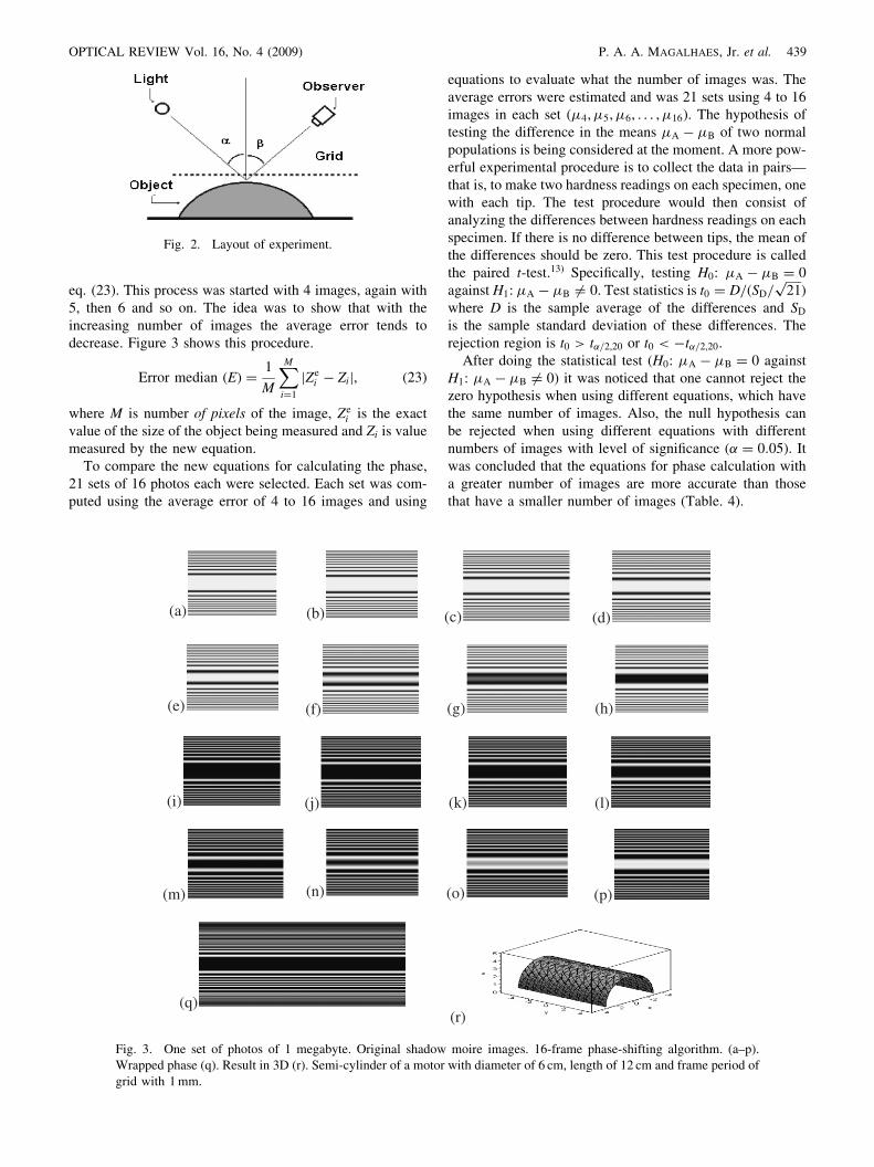
eq. (23). This process was started with 4 images, again with5, then 6 and so on. The idea was to show that with theincreasing number of images the average error tends todecrease. Figure 3 shows this procedure.

Error median (E) ¼1

M

XMi¼1

jZei � Zij; ð23Þ

where M is number of pixels of the image, Zei is the exact

value of the size of the object being measured and Zi is valuemeasured by the new equation.

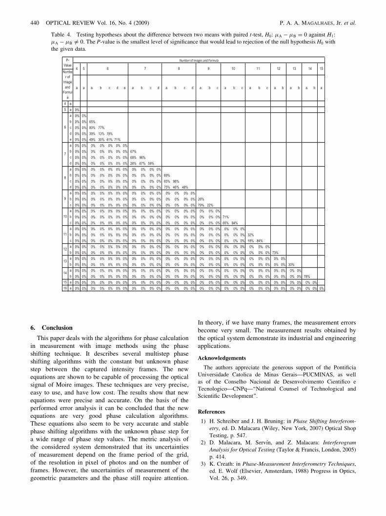
To compare the new equations for calculating the phase,21 sets of 16 photos each were selected. Each set was com-puted using the average error of 4 to 16 images and using

equations to evaluate what the number of images was. Theaverage errors were estimated and was 21 sets using 4 to 16images in each set (4; 5; 6; . . . ; 16). The hypothesis oftesting the difference in the means A � B of two normalpopulations is being considered at the moment. A more pow-erful experimental procedure is to collect the data in pairs—that is, to make two hardness readings on each specimen, onewith each tip. The test procedure would then consist ofanalyzing the differences between hardness readings on eachspecimen. If there is no difference between tips, the mean ofthe differences should be zero. This test procedure is calledthe paired t-test.13) Specifically, testing H0: A � B ¼ 0

against H1: A � B 6¼ 0. Test statistics is t0 ¼ D=ðSD=ffiffiffiffiffi21

pÞ

where D is the sample average of the differences and SDis the sample standard deviation of these differences. Therejection region is t0 > t�=2;20 or t0 < �t�=2;20.

After doing the statistical test (H0: A � B ¼ 0 againstH1: A � B 6¼ 0) it was noticed that one cannot reject thezero hypothesis when using different equations, which havethe same number of images. Also, the null hypothesis canbe rejected when using different equations with differentnumbers of images with level of significance (� ¼ 0:05). Itwas concluded that the equations for phase calculation witha greater number of images are more accurate than thosethat have a smaller number of images (Table. 4).

(a) (b) (c) (d)

(e) (f) (g) (h)

(i) (j) (k) (l)

(m) (n) (o) (p)

(q)(r)

Fig. 3. One set of photos of 1 megabyte. Original shadow moire images. 16-frame phase-shifting algorithm. (a–p).Wrapped phase (q). Result in 3D (r). Semi-cylinder of a motor with diameter of 6 cm, length of 12 cm and frame period ofgrid with 1mm.

Fig. 2. Layout of experiment.


6. Conclusion

This paper deals with the algorithms for phase calculationin measurement with image methods using the phaseshifting technique. It describes several multistep phaseshifting algorithms with the constant but unknown phasestep between the captured intensity frames. The newequations are shown to be capable of processing the opticalsignal of Moire images. These techniques are very precise,easy to use, and have low cost. The results show that newequations were precise and accurate. On the basis of theperformed error analysis it can be concluded that the newequations are very good phase calculation algorithms.These equations also seem to be very accurate and stablephase shifting algorithms with the unknown phase step fora wide range of phase step values. The metric analysis ofthe considered system demonstrated that its uncertaintiesof measurement depend on the frame period of the grid,of the resolution in pixel of photos and on the number offrames. However, the uncertainties of measurement of thegeometric parameters and the phase still require attention.

In theory, if we have many frames, the measurement errorsbecome very small. The measurement results obtained bythe optical system demonstrate its industrial and engineeringapplications.

Acknowledgements

The authors appreciate the generous support of the PontificiaUniversidade Catolica de Minas Gerais—PUCMINAS, as wellas of the Conselho Nacional de Desenvolvimento Cientifico eTecnologico—CNPq—‘‘National Counsel of Technological andScientific Development’’.

References

1) H. Schreiber and J. H. Bruning: in Phase Shifting Interferom-etry, ed. D. Malacara (Wiley, New York, 2007) Optical ShopTesting, p. 547.

2) D. Malacara, M. Servın, and Z. Malacara: InterferogramAnalysis for Optical Testing (Taylor & Francis, London, 2005)p. 414.

3) K. Creath: in Phase-Measurement Interferometry Techniques,ed. E. Wolf (Elsevier, Amsterdam, 1988) Progress in Optics,Vol. 26, p. 349.

Table 4. Testing hypotheses about the difference between two means with paired t-test, H0: A � B ¼ 0 against H1:A � B 6¼ 0. The P-value is the smallest level of significance that would lead to rejection of the null hypothesis H0 withthe given data.


4) J. Novak: Optik 114 (2003) 63.5) J. Novak, P. Novak, and A. Miks: Opt. Commun. 281 (2008)

5302.6) P. S. Huang and H. Guo: Proc. SPIE 7066 (2008) 70660B.7) Optical Shop Testing, ed. D. Malacara (Wiley, New York,

1992).8) F. S. Hillier and G. J. Lieberman: Introduction to Operations

Research (McGraw-Hill, New York, 2005) 8th ed.9) D. C. Ghiglia and M. D. Pritt: Two-Dimensional Phase

Unwrapping: Theory, Algorithms and Software (Wiley, NewYork, 1998).

10) J. M. Huntley: Appl. Opt. 28 (1989) 3268.11) E. Zappa and G. Busca: Opt. Lasers Eng. 46 (2008) 106.12) C. Han and B. Han: Appl. Opt. 45 (2006) 1124.13) M. F. Triola: Elementary Statistics (Addison-Wesley, Read-

ing, MA, 2007) 10th ed.14) R. R. Cordero, J. Molimard, A. Martinez, and F. Labbe: Opt.

Commun. 275 (2007) 144.


Phase shifting technique using generalization of Carre algorithm with many images

Documents

Transcript of Phase shifting technique using generalization of Carre algorithm with many images