PetroGraph: A new software to visualize, model, and presentgeochemical data in igneous petrology

M. Petrelli, G. Poli, D. Perugini, and A. PeccerilloDepartment of Earth Sciences, University of Perugia, Piazza Universita, 1, 06100 Perugia, Italy (maurip@unipg.it)

[1] A new software, PetroGraph, has been developed to visualize, elaborate, and model geochemical datafor igneous petrology purposes. The software is able to plot data on several different diagrams, including alarge number of classification and ‘‘petrotectonic’’ plots. PetroGraph gives the opportunity to handle largegeochemical data sets in a single program without the need of passing from one software to the other asusually happens in petrologic data handling. Along with these basic functions, PetroGraph contains a widechoice of modeling possibilities, from major element mass balance calculations to the most common partialmelting and magma evolution models based on trace element and isotopic data. Results and graphs can beexported as vector graphics in publication-quality form, or they can be copied and pasted within the mostcommon graphics programs for further modifications. All these features make PetroGraph one of the mostcomplete software presently available for igneous petrology research.

Components: 4646 words, 10 figures, 4 tables.

Keywords: data management; data plotting; geochemical modeling; petrology; software.

Index Terms: 3610 Mineralogy and Petrology: Geochemical modeling (1009, 8410); 1065 Geochemistry: Major and trace

element geochemistry; 1094 Geochemistry: Instruments and techniques.

Received 3 February 2005; Revised 5 May 2005; Accepted 11 May 2005; Published 26 July 2005.

Petrelli, M., G. Poli, D. Perugini, and A. Peccerillo (2005), PetroGraph: A new software to visualize, model, and present

geochemical data in igneous petrology, Geochem. Geophys. Geosyst., 6, Q07011, doi:10.1029/2005GC000932.

1. Introduction

[2] Handling, visualization, and modeling of geo-chemical data are of fundamental importance inigneous petrology. Most of these operations canbe performed using a variety of software pack-ages such as spreadsheet programs (e.g., MSExcel1 or Microcal Origin1), interpreted scien-tific computer languages (e.g., R1 or Matlab1),or software specifically developed for igneouspetrology such as MinPet1 (MinPet1 GeologicalSoftware Inc. Web site: http://www.minpet.com/),GCDKit [Janousek et al., 2003], IgPet1 (IgPet1

RockWare Web site: http://www.rockware.com/)and PetroPlot [Su et al., 2003]. Moreover, a largenumber of codes have been developed [e.g.,Wright and Doherty, 1970; Stormer and Nicholls,1978; Woussen and Cote, 1987; Conrad, 1987;

Holm, 1988, 1990; Nielsen, 1988; Defant andNielsen, 1990; Harnois, 1991; Benito and Lopez-Ruiz, 1992; D’Orazio, 1993; Verma et al., 1998;Keskin, 2002; Spera and Bohrson, 2001] to helpresearchers in performing specific geochemicalmodels. All these software allowed users togreatly speed up modeling of geochemical data,but some of them are designed for old MS-DOSoperating systems and cause problems whenloaded into modern MS Windows systems.Other programs have limited possibility ofgeochemical modeling (e.g., MinPet, GCDKitand PetroPlot). Moreover, problems can arisewhen trying to run algorithms available only assource codes; for example, the mass balancealgorithm by Stormer and Nicholls [1978]requires a FORTRAN compiler to be loaded,and this may cause difficulties for the user if

G3G3GeochemistryGeophysics

Geosystems

Published by AGU and the Geochemical Society

AN ELECTRONIC JOURNAL OF THE EARTH SCIENCES

GeochemistryGeophysics

Geosystems

Technical Brief

Volume 6, Number 7

26 July 2005

Q07011, doi:10.1029/2005GC000932

ISSN: 1525-2027

Copyright 2005 by the American Geophysical Union 1 of 15

compared to modern object-oriented, user-friendlysoftware.

[3] In this contribution we present a new pro-gram, PetroGraph (Figure 1), developed with theaim of giving a complete platform to handle,visualize and model geochemical data in a userfriendly environment. The program runs underWindows 98/2000/XP1 platforms as a stand-alone application. The source code is written inMS Visual Basic 6.01 and is distributed togetherwith the program. The code is open source andwe invite all users to contribute to the develop-ment of the software by proposing improvementor developing new codes. To download the soft-ware and the tutorial, please go to http://www.unipg.it/�maurip/SOFTWARE.htm (see also ancil-lary material).

[4] In the following sections we present the mainfeatures and potentialities of PetroGraph. The pa-per is divided into five main sections (Figure 2),including (1) input of geochemical data, (2) data

visualization, (3) development of geochemicalmodels, (4) data management, and (5) additionalfeatures.

2. Data Input

[5] Geochemical data can be imported into Petro-Graph in three file formats (Figure 2a): (1) MSExcel1 worksheets, (2) IgPetWin1 formatted files,and (3) PetroGraph (.peg) files.

[6] MS Excel1 worksheets need little formattingbefore imported to PetroGraph, as reported inFigure 2. The arrangement of the worksheet, how-ever, is not much different from common analyticaloutputs. In particular, the first column must containthe sample name, whereas the following threecolumns are dedicated to symbol and color man-agement and to the choice to show (1) or not toshow (0) the sample in the diagrams (see thetutorial for a detailed explanation of the arrange-ment of the MS Excel1 file).

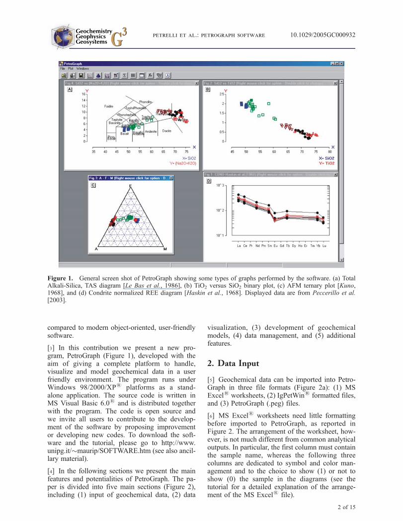
Figure 1. General screen shot of PetroGraph showing some types of graphs performed by the software. (a) TotalAlkali-Silica, TAS diagram [Le Bas et al., 1986], (b) TiO2 versus SiO2 binary plot, (c) AFM ternary plot [Kuno,1968], and (d) Condrite normalized REE diagram [Haskin et al., 1968]. Displayed data are from Peccerillo et al.[2003].

GeochemistryGeophysicsGeosystems G3G3

petrelli et al.: petrograph software 10.1029/2005GC000932

2 of 15

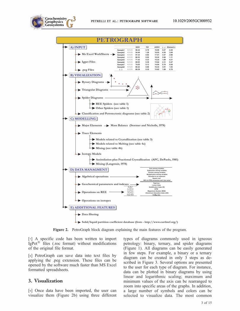
[7] A specific code has been written to importIgPet1 files (.roc format) without modificationsof the original file format.

[8] PetroGraph can save data into text files byapplying the .peg extension. These files can beopened by the software much faster than MS Excelformatted spreadsheets.

3. Visualization

[9] Once data have been imported, the user canvisualize them (Figure 2b) using three different

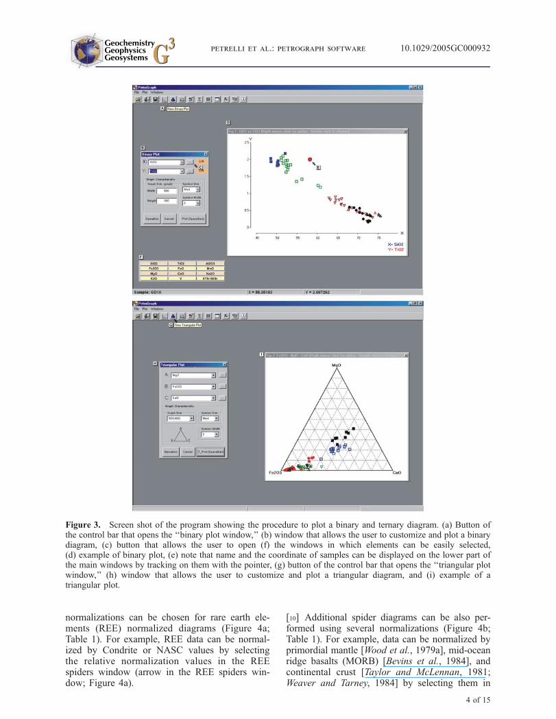
types of diagrams commonly used in igneouspetrology: binary, ternary, and spider diagrams(Figure 1). All diagrams can be easily generatedin few steps. For example, a binary or a ternarydiagram can be created in only 3 steps as de-scribed in Figure 3. Several options are presentedto the user for each type of diagram. For instance,data can be plotted in binary diagrams by usinglinear and logarithmic scaling; maximum andminimum values of the axis can be rearranged tozoom into specific areas of the graphs. In addition,a large number of symbols and colors can beselected to visualize data. The most common

Figure 2. PetroGraph block diagram explaining the main features of the program.

GeochemistryGeophysicsGeosystems G3G3

petrelli et al.: petrograph software 10.1029/2005GC000932petrelli et al.: petrograph software 10.1029/2005GC000932

3 of 15

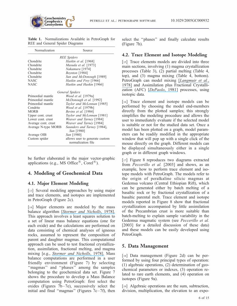
normalizations can be chosen for rare earth ele-ments (REE) normalized diagrams (Figure 4a;Table 1). For example, REE data can be normal-ized by Condrite or NASC values by selectingthe relative normalization values in the REEspiders window (arrow in the REE spiders win-dow; Figure 4a).

[10] Additional spider diagrams can be also per-formed using several normalizations (Figure 4b;Table 1). For example, data can be normalized byprimordial mantle [Wood et al., 1979a], mid-oceanridge basalts (MORB) [Bevins et al., 1984], andcontinental crust [Taylor and McLennan, 1981;Weaver and Tarney, 1984] by selecting them in

Figure 3. Screen shot of the program showing the procedure to plot a binary and ternary diagram. (a) Button ofthe control bar that opens the ‘‘binary plot window,’’ (b) window that allows the user to customize and plot a binarydiagram, (c) button that allows the user to open (f) the windows in which elements can be easily selected,(d) example of binary plot, (e) note that name and the coordinate of samples can be displayed on the lower part ofthe main windows by tracking on them with the pointer, (g) button of the control bar that opens the ‘‘triangular plotwindow,’’ (h) window that allows the user to customize and plot a triangular diagram, and (i) example of atriangular plot.

GeochemistryGeophysicsGeosystems G3G3

petrelli et al.: petrograph software 10.1029/2005GC000932

4 of 15

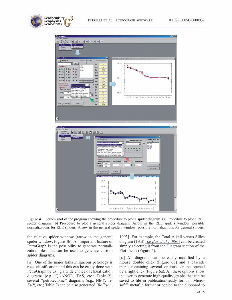
the relative spider window (arrow in the generalspider window; Figure 4b). An important feature ofPetroGraph is the possibility to generate normali-zation files that can be used to generate customspider diagrams.

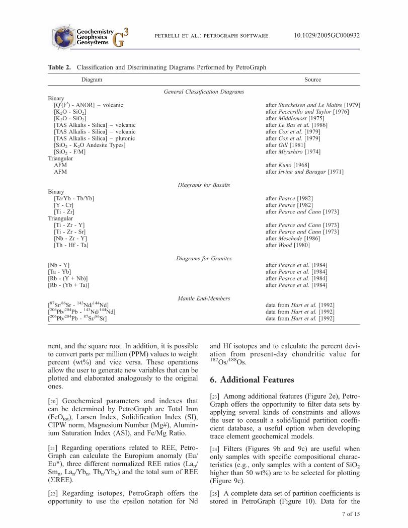
[11] One of the major tasks in igneous petrology isrock classification and this can be easily done withPetroGraph by using a wide choice of classificationdiagrams (e.g., Q’-ANOR, TAS, etc.; Table 2);several ‘‘petrotectonic’’ diagrams (e.g., Nb-Y, Ti-Zr-Y, etc.; Table 2) can be also generated [Rollison,

1993]. For example, the Total Alkali versus Silicadiagram (TAS) [Le Bas et al., 1986] can be createdsimply selecting it from the Diagram section of thePlot menu (Figure 5).

[12] All diagrams can be easily modified by amouse double click (Figure 6b) and a cascademenu containing several options can be openedby a right click (Figure 6a). All these options allowthe user to generate high-quality graphs that can besaved to file in publication-ready form in Micro-soft1 metafile format or copied to the clipboard to

Figure 4. Screen shot of the program showing the procedure to plot a spider diagram. (a) Procedure to plot a REEspider diagram. (b) Procedure to plot a general spider diagram. Arrow in the REE spiders window: possiblenormalizations for REE spiders. Arrow in the general spiders window: possible normalizations for general spiders.

GeochemistryGeophysicsGeosystems G3G3

petrelli et al.: petrograph software 10.1029/2005GC000932

5 of 15

be further elaborated in the major vector-graphicapplications (e.g., MS Office1, Corel1).

4. Modeling of Geochemical Data

4.1. Major Element Modeling

[13] Several modeling approaches by using majorand trace elements, and isotopes are implementedin PetroGraph (Figure 2c).

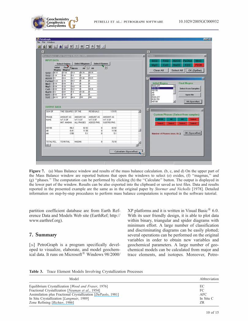
[14] Major elements are modeled by the massbalance algorithm [Stormer and Nicholls, 1978].This approach involves a least squares solution toa set of linear mass balance equations (one foreach oxide) and the calculations are performed ondata consisting of chemical analyses of igneousrocks, assumed to represent the composition ofparent and daughter magmas. This computationalapproach can be used to test fractional crystalliza-tion, assimilation, fractional melting, and magmamixing [e.g., Stormer and Nicholls, 1978]. Massbalance computations are performed in a userfriendly environment (Figure 7) by selecting‘‘magmas’’ and ‘‘phases’’ among the samplesbelonging to the geochemical data set. Figure 7shows the procedure to develop a Mass Balancecomputation using PetroGraph: first select theoxides (Figures 7b–7e), successively select theinitial and final ‘‘magmas’’ (Figures 7c–7f), then

select the ‘‘phases’’ and finally calculate results(Figure 7h).

4.2. Trace Element and Isotope Modeling

[15] Trace elements models are divided into threemain sections, involving (1) magma crystallizationprocesses (Table 3), (2) partial melting (Table 4,top), and (3) magma mixing (Table 4, bottom).PetroGraph can model mixing [Langmuir et al.,1978] and Assimilation plus Fractional Crystalli-zation (AFC) [DePaolo, 1981] processes, usingisotopic data.

[16] Trace element and isotope models can beperformed by choosing the model end-membersdirectly from the plotted samples; this stronglysimplifies the modeling procedure and allows theuser to immediately evaluate if the selected modelis suitable or not for the studied data set. Once amodel has been plotted on a graph, model param-eters can be readily modified in the appropriatewindow that will pop up with a single click of themouse directly on the graph. Different models canbe displayed simultaneously either in a singlegraph or in different graph windows.

[17] Figure 8 reproduces two diagrams extractedfrom Peccerillo et al. [2003] and shows, as anexample, how to perform trace element and iso-tope models with PetroGraph. The models refer tothe origin of peralkaline silicic magmas atGedemsa volcano (Central Ethiopian Rift), whichcan be generated either by batch melting of abasaltic rock or by fractional crystallization of abasaltic parental melt. Trace element and isotopemodels reported in Figure 8 show that fractionalcrystallization accompanied by little assimilationof the Precambrian crust is more suitable thanbatch-melting to explain sample variability in theGedemsa magmatic system (see Peccerillo et al.[2003] for a detailed discussion of these data)and these models can be easily developed usingPetroGraph.

5. Data Management

[18] Data management (Figure 2d) can be per-formed by using four principal types of operation:(1) algebraic operations, (2) determination of geo-chemical parameters or indexes, (3) operation re-lated to rare earth elements, and (4) operation onisotopes (Figure 9a).

[19] Algebraic operations are the sum, subtraction,division, multiplication, the elevation to an expo-

Table 1. Normalizations Available in PetroGraph forREE and General Spider Diagrams

Normalization Source

REE SpidersChondrite Haskin et al. [1968]Chondrite Masuda et al. [1973]Chondrite Nakamura [1974]Chondrite Boynton [1984]Chondrite Sun and McDonough [1989]NASC Haskin and Frey [1966]NASC Haskin and Haskin [1966]

General SpidersPrimordial mantle Wood et al. [1979a]Primordial mantle McDonough et al. [1992]Primordial mantle Taylor and McLennan [1985]Condrite Wood et al. [1979b]MORB Bevins et al. [1984]Upper cont. crust Taylor and McLennan [1981]Lower cont. crust Weaver and Tarney [1984]Average cont. crust Weaver and Tarney [1984]Average N-type MORB Saunders and Tarney [1984],

Sun [1980]Average OIB Sun [1980]Custom spider allows user to generate custom

normalization file

GeochemistryGeophysicsGeosystems G3G3

petrelli et al.: petrograph software 10.1029/2005GC000932

6 of 15

nent, and the square root. In addition, it is possibleto convert parts per million (PPM) values to weightpercent (wt%) and vice versa. These operationsallow the user to generate new variables that can beplotted and elaborated analogously to the originalones.

[20] Geochemical parameters and indexes thatcan be determined by PetroGraph are Total Iron(FeOtot), Larsen Index, Solidification Index (SI),CIPW norm, Magnesium Number (Mg#), Alumin-ium Saturation Index (ASI), and Fe/Mg Ratio.

[21] Regarding operations related to REE, Petro-Graph can calculate the Europium anomaly (Eu/Eu*), three different normalized REE ratios (Lan/Smn, Lan/Ybn, Tbn/Ybn) and the total sum of REE(SREE).

[22] Regarding isotopes, PetroGraph offers theopportunity to use the epsilon notation for Nd

and Hf isotopes and to calculate the percent devi-ation from present-day chondritic value for187Os/188Os.

6. Additional Features

[23] Among additional features (Figure 2e), Petro-Graph offers the opportunity to filter data sets byapplying several kinds of constraints and allowsthe user to consult a solid/liquid partition coeffi-cient database, a useful option when developingtrace element geochemical models.

[24] Filters (Figures 9b and 9c) are useful whenonly samples with specific compositional charac-teristics (e.g., only samples with a content of SiO2

higher than 50 wt%) are to be selected for plotting(Figure 9c).

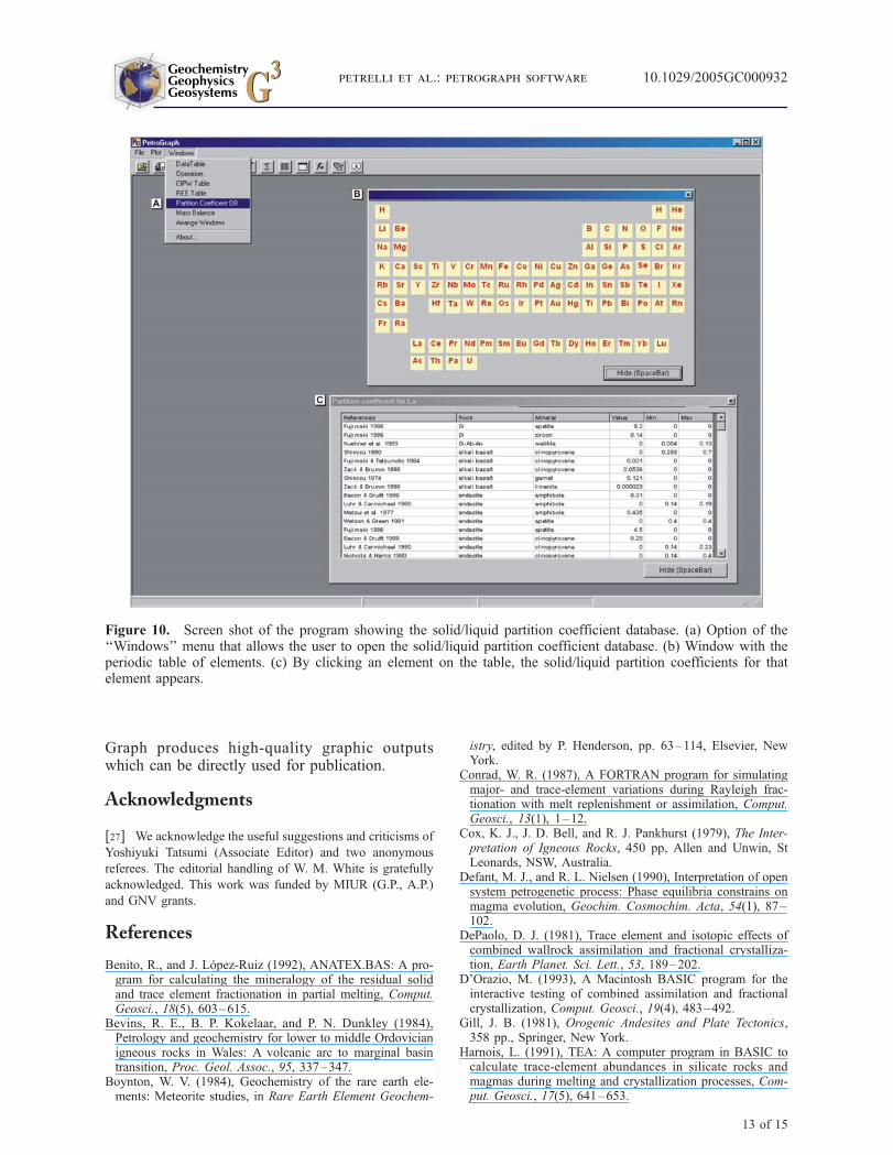
[25] A complete data set of partition coefficients isstored in PetroGraph (Figure 10). Data for the

Table 2. Classification and Discriminating Diagrams Performed by PetroGraph

Diagram Source

General Classification DiagramsBinary[Q0(F0) - ANOR] – volcanic after Streckeisen and Le Maitre [1979][K2O - SiO2] after Peccerillo and Taylor [1976][K2O - SiO2] after Middlemost [1975][TAS Alkalis - Silica] – volcanic after Le Bas et al. [1986][TAS Alkalis - Silica] – volcanic after Cox et al. [1979][TAS Alkalis - Silica] – plutonic after Cox et al. [1979][SiO2 - K2O Andesite Types] after Gill [1981][SiO2 - F/M] after Miyashiro [1974]

TriangularAFM after Kuno [1968]AFM after Irvine and Baragar [1971]

Diagrams for BasaltsBinary[Ta/Yb - Tb/Yb] after Pearce [1982][Y - Cr] after Pearce [1982][Ti - Zr] after Pearce and Cann [1973]

Triangular[Ti - Zr - Y] after Pearce and Cann [1973][Ti - Zr - Sr] after Pearce and Cann [1973][Nb - Zr - Y] after Meschede [1986][Th - Hf - Ta] after Wood [1980]

Diagrams for Granites[Nb - Y] after Pearce et al. [1984][Ta - Yb] after Pearce et al. [1984][Rb - (Y + Nb)] after Pearce et al. [1984][Rb - (Yb + Ta)] after Pearce et al. [1984]

Mantle End-Members[87Sr/86Sr - 143Nd/144Nd] data from Hart et al. [1992][206Pb/204Pb - 143Nd/144Nd] data from Hart et al. [1992][206Pb/204Pb - 87Sr/86Sr] data from Hart et al. [1992]

GeochemistryGeophysicsGeosystems G3G3

petrelli et al.: petrograph software 10.1029/2005GC000932

7 of 15

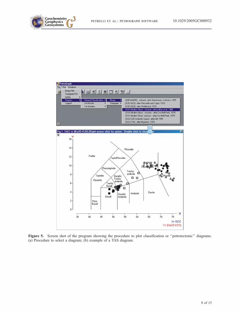
Figure 5. Screen shot of the program showing the procedure to plot classification or ‘‘petrotectonic’’ diagrams.(a) Procedure to select a diagram; (b) example of a TAS diagram.

GeochemistryGeophysicsGeosystems G3G3

petrelli et al.: petrograph software 10.1029/2005GC000932

8 of 15

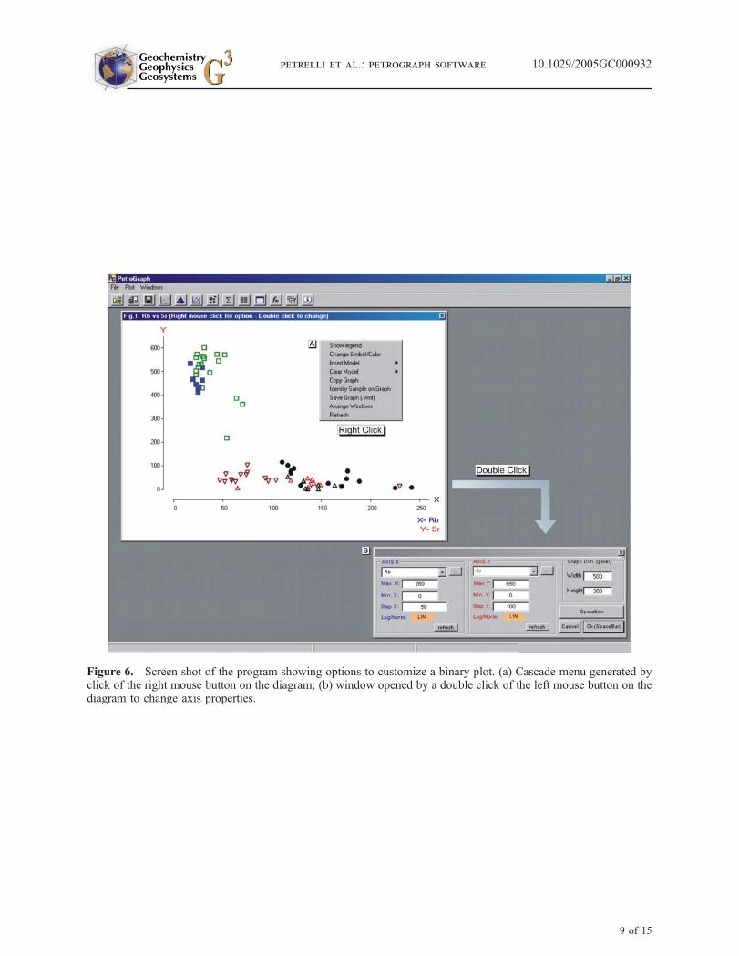
Figure 6. Screen shot of the program showing options to customize a binary plot. (a) Cascade menu generated byclick of the right mouse button on the diagram; (b) window opened by a double click of the left mouse button on thediagram to change axis properties.

GeochemistryGeophysicsGeosystems G3G3

petrelli et al.: petrograph software 10.1029/2005GC000932

9 of 15

partition coefficient database are from Earth Ref-erence Data and Models Web site (EarthRef; http://www.earthref.org).

7. Summary

[26] PetroGraph is a program specifically devel-oped to visualize, elaborate, and model geochem-ical data. It runs on Microsoft1 Windows 98/2000/

XP platforms and it is written in Visual Basic1 6.0.With its user friendly design, it is able to plot datawithin binary, triangular and spider diagrams withminimum effort. A large number of classificationand discriminating diagrams can be easily plotted;several operations can be performed on the originalvariables in order to obtain new variables andgeochemical parameters. A large number of geo-chemical models can be calculated from major andtrace elements, and isotopes. Moreover, Petro-

Figure 7. (a) Mass Balance window and results of the mass balance calculation. (b, c, and d) On the upper part ofthe Mass Balance window are reported buttons that open the windows to select (e) oxides, (f) ‘‘magmas,’’ and(g) ‘‘phases.’’ The computation can be performed by clicking (h) the ‘‘Calculate’’ button. The output is displayed inthe lower part of the window. Results can be also exported into the clipboard or saved as text files. Data and resultsreported in the presented example are the same as in the original paper by Stormer and Nicholls [1978]. Detailedinformation on step-by-step procedures to perform mass balance computations is reported in the software tutorial.

Table 3. Trace Element Models Involving Crystallization Processes

Model Abbreviation

Equilibrium Crystallization [Wood and Fraser, 1976] ECFractional Crystallization [Neuman et al., 1954] FCAssimilation plus Fractional Crystallization [DePaolo, 1981] AFCIn Situ Crystallization [Langmuir, 1989] In Situ CZone Refining [Richter, 1986] ZR

GeochemistryGeophysicsGeosystems G3G3

petrelli et al.: petrograph software 10.1029/2005GC000932

10 of 15

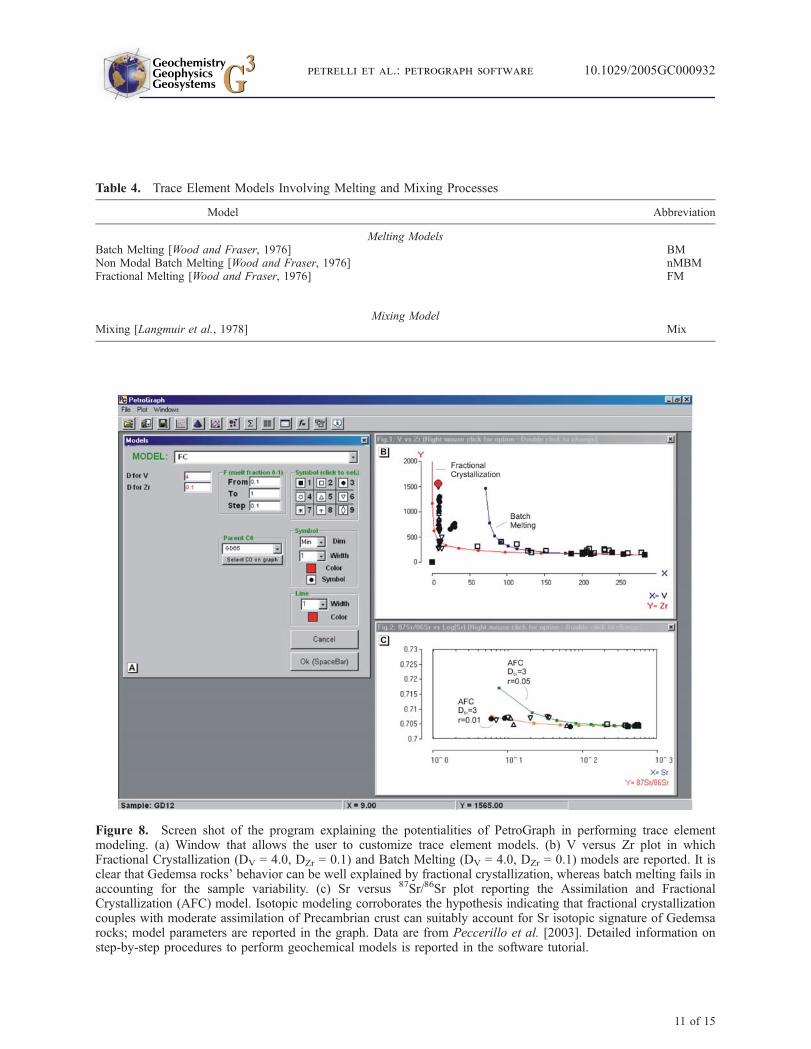
Table 4. Trace Element Models Involving Melting and Mixing Processes

Model Abbreviation

Melting ModelsBatch Melting [Wood and Fraser, 1976] BMNon Modal Batch Melting [Wood and Fraser, 1976] nMBMFractional Melting [Wood and Fraser, 1976] FM

Mixing ModelMixing [Langmuir et al., 1978] Mix

Figure 8. Screen shot of the program explaining the potentialities of PetroGraph in performing trace elementmodeling. (a) Window that allows the user to customize trace element models. (b) V versus Zr plot in whichFractional Crystallization (DV = 4.0, DZr = 0.1) and Batch Melting (DV = 4.0, DZr = 0.1) models are reported. It isclear that Gedemsa rocks’ behavior can be well explained by fractional crystallization, whereas batch melting fails inaccounting for the sample variability. (c) Sr versus 87Sr/86Sr plot reporting the Assimilation and FractionalCrystallization (AFC) model. Isotopic modeling corroborates the hypothesis indicating that fractional crystallizationcouples with moderate assimilation of Precambrian crust can suitably account for Sr isotopic signature of Gedemsarocks; model parameters are reported in the graph. Data are from Peccerillo et al. [2003]. Detailed information onstep-by-step procedures to perform geochemical models is reported in the software tutorial.

GeochemistryGeophysicsGeosystems G3G3

petrelli et al.: petrograph software 10.1029/2005GC000932

11 of 15

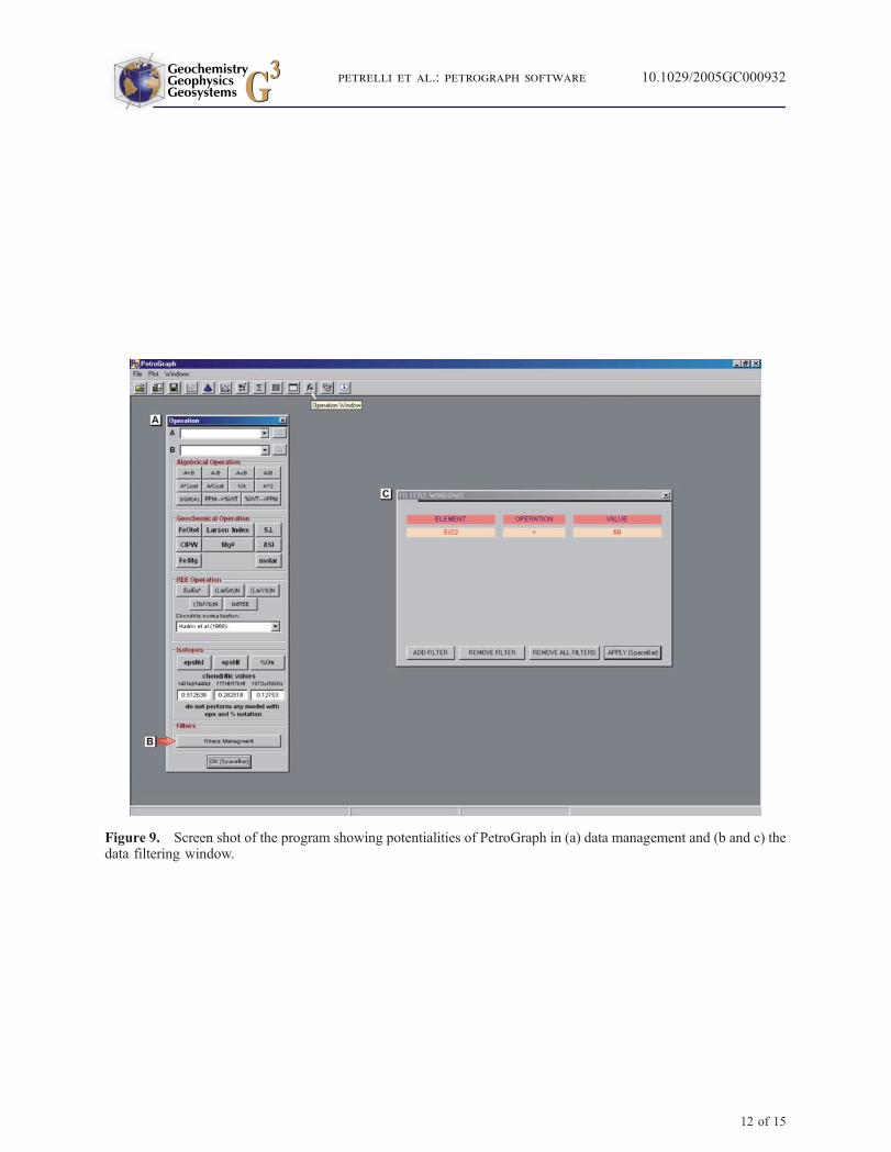
Figure 9. Screen shot of the program showing potentialities of PetroGraph in (a) data management and (b and c) thedata filtering window.

GeochemistryGeophysicsGeosystems G3G3

petrelli et al.: petrograph software 10.1029/2005GC000932

12 of 15

Graph produces high-quality graphic outputswhich can be directly used for publication.

Acknowledgments

[27] We acknowledge the useful suggestions and criticisms of

Yoshiyuki Tatsumi (Associate Editor) and two anonymous

referees. The editorial handling of W. M. White is gratefully

acknowledged. This work was funded by MIUR (G.P., A.P.)

and GNV grants.

References

Benito, R., and J. Lopez-Ruiz (1992), ANATEX.BAS: A pro-gram for calculating the mineralogy of the residual solidand trace element fractionation in partial melting, Comput.Geosci., 18(5), 603–615.

Bevins, R. E., B. P. Kokelaar, and P. N. Dunkley (1984),Petrology and geochemistry for lower to middle Ordovicianigneous rocks in Wales: A volcanic arc to marginal basintransition, Proc. Geol. Assoc., 95, 337–347.

Boynton, W. V. (1984), Geochemistry of the rare earth ele-ments: Meteorite studies, in Rare Earth Element Geochem-

istry, edited by P. Henderson, pp. 63–114, Elsevier, NewYork.

Conrad, W. R. (1987), A FORTRAN program for simulatingmajor- and trace-element variations during Rayleigh frac-tionation with melt replenishment or assimilation, Comput.Geosci., 13(1), 1–12.

Cox, K. J., J. D. Bell, and R. J. Pankhurst (1979), The Inter-pretation of Igneous Rocks, 450 pp, Allen and Unwin, StLeonards, NSW, Australia.

Defant, M. J., and R. L. Nielsen (1990), Interpretation of opensystem petrogenetic process: Phase equilibria constrains onmagma evolution, Geochim. Cosmochim. Acta, 54(1), 87–102.

DePaolo, D. J. (1981), Trace element and isotopic effects ofcombined wallrock assimilation and fractional crystalliza-tion, Earth Planet. Sci. Lett., 53, 189–202.

D’Orazio, M. (1993), A Macintosh BASIC program for theinteractive testing of combined assimilation and fractionalcrystallization, Comput. Geosci., 19(4), 483–492.

Gill, J. B. (1981), Orogenic Andesites and Plate Tectonics,358 pp., Springer, New York.

Harnois, L. (1991), TEA: A computer program in BASIC tocalculate trace-element abundances in silicate rocks andmagmas during melting and crystallization processes, Com-put. Geosci., 17(5), 641–653.

Figure 10. Screen shot of the program showing the solid/liquid partition coefficient database. (a) Option of the‘‘Windows’’ menu that allows the user to open the solid/liquid partition coefficient database. (b) Window with theperiodic table of elements. (c) By clicking an element on the table, the solid/liquid partition coefficients for thatelement appears.

GeochemistryGeophysicsGeosystems G3G3

petrelli et al.: petrograph software 10.1029/2005GC000932

13 of 15

Hart, S. R., E. H. Hauri, L. A. Oschmann, and J. A. Whitehead(1992), Mantle plumes and entrainment: Isotopic evidence,Science, 256, 515–519.

Haskin, L. A., M. A. Haskin, F. A. Frey, and T. R. Wildman(1968), Relative and absolute terrestrial abundances of the rareearths, in Origin and Distribution of the Elements, vol. 1,edited by L. H. Ahrens, pp. 889–911, Elsevier, New York.

Haskin, M. A., and F. A. Frey (1966), Dispersed and not-so-rare earths, Science, 152, 299–314.

Haskin, M. A., and L. A. Haskin (1966), Rare earths in Euro-pean shales: A redetermination, Science, 154, 507–509.

Holm, P. E. (1988), Petrogenetic modeling with a spreadsheetprogram, J. Geol. Educ., 36(3), 155–156.

Holm, P. E. (1990), Complex petrogenetic modelling usingspreadsheet software, Comput. Geosci., 16(8), 1117–1122.

Irvine, T. N., and W. R. A. Baragar (1971), A guide to thechemical classification of the common volcanic rocks, Can.J. Earth Sci., 8, 523–548.

Janousek, V., C. M. Farrow, and V. Erban (2003), GCDKit:New PC software for interpretation of whole-rock geochem-ical data from igneous rocks, Geochim. Cosmochim. Acta,67, A186.

Keskin, M. (2002), FC-modeler: A Microsoft1 Excel#

spreadsheet program for modeling Rayleigh fractionationvectors in closed magmatic systemsComput. Geosci.,28(8), 919–928.

Kuno, H. (1968), Differentiation of basalt magmas, in Basalts:The Poldervaart Treatise on Rocks of Basaltic Composition,vol. 2, edited by H. H. Hess and A. Poldervaart, pp. 623–688, Wiley-Interscience, Hoboken, N. J.

Langmuir, C. H. (1989), Geochemical consequences of in situcrystallization, Nature, 340, 199–205.

Langmuir, C. H., R. D. Vocke, Jr., N. H. Gilbert, and R. H.Stanley (1978), A general mixing equation with applicationsto Icelandic basalts, Earth Planet. Sci. Lett., 37, 380–392.

Le Bas, M. J., R. W. Le Maitre, A. Streckeisen, and B. Zanettin(1986), A chemical classification of volcanic rocks based onthe total alkali-silica diagram, J. Petrol., 27, 745–750.

Masuda, A., N. Nakamura, and T. Tanaka (1973), Fine struc-ture of mutually normalised rare-earth patterns of chondrites,Geochim. Cosmochim. Acta, 37, 239–248.

McDonough, W. F., S. Sun, A. E. Ringwood, E. Jagoutz, andA. W. Hofmann (1992), K, Rb, and Cs in the earth and moonand the evolution of the Earth mantle, Geochim. Cosmochim.Acta, S. R. Taylor Symposium volume, 1001–1012.

Meschede, M. (1986), A method of discriminating betweendifferent type of mid-ocean ridge basalts and continentaltholeiites with the Nb-Zr-Y diagram, Chem. Geol., 56,207–218.

Middlemost, E. A. K. (1975), The basalt clan, Earth Sci. Rev.,11, 337–364.

Miyashiro, A. (1974), Volcanic rock series in island arcs andactive continental margins, Am. J. Sci., 274, 321–355.

Nakamura, N. (1974), Determination of REE, Ba, Fe, Mg, Naand K in carbonaceous and ordinary chondrites, Geochim.Cosmochim. Acta, 38, 757–775.

Neuman, H., J. Mead, and C. J. Vitaliano (1954), Trace-element variation during fractional crystallization as calcu-lated from the distribution law, Geochim. Cosmochim. Acta,6, 90–100.

Nielsen, R. L. (1988), TRACE.FOR: A program for the calcu-lation of combined major and trace element liquid line ofdescent for natural magmatic systemsComput. Geosci.,14(1), 15–35.

Pearce, J. A. (1982), Trace element characteristics of lavasfrom destructive plate boundaries, in Andesites: Orogenic

Andesites and Related Rocks, edited by R. S. Thorpe,pp. 525–548, John Wiley, Hoboken, N. J.

Pearce, J. A., and J. R. Cann (1973), Tectonic setting of basicvolcanic rocks determined using trace element analyses,Earth Planet. Sci. Lett., 19, 290–300.

Pearce, J. A., N. B. W. Harris, and A. G. Tindle (1984), Traceelement discrimination diagrams for the tectonic interpreta-tion of granitic rocks, J. Petrol., 25, 956–983.

Peccerillo, A., and S. R. Taylor (1976), Geochemistry of Eo-cene calc-alkaline rocks from Kastamonu area, Northern Tur-key, Contrib. Mineral. Petrol., 58, 63–81.

Peccerillo, A.,M.R.Barberio, G.Yirgu,D.Ayalew,M.Barbieri,and T. W. Wu (2003), Relationships between mafic and per-alcaline silicic magmatism in continental rift settings: A pet-rological, geochemical and isotopic study of the Gedemsavolcano, central Ethiopian rift, J. Petrol., 44, 2003–2032.

Richter, F. M. (1986), Simple models for trace-element frac-tionation during melt segregation, Earth Planet. Sci. Lett.,77, 333–344.

Rollison, H. (1993), Using Geochemical Data: Evaluation,Presentation, Interpretation, 352 pp., Longman Sci. andTech., Harlow, UK.

Saunders, A. D., and J. Tarney (1984), Geochemical character-istics of basaltic volcanism within back-arc basin, inMarginalBasin Geology, edited by B. P. Kokelaar and M. F. Howells,Geol. Soc. Spec. Publ., 16, 59–76.

Spera, F. J., and W. A. Bohrson (2001), Energy-constrainedopen-system magmatic processes I: General model and en-ergy-constrained, J. Petrol., 42, 999–1018.

Stormer, J. C., and J. Nicholls (1978), XLFRAC: A programfor the interactive testing of magmatic differentiation mod-els, Comput. Geosci., 4, 143–159.

Streckeisen, A., and R. W. Le Maitre (1979), A chemicalapproximation to the modal QAPF classification of igneousrocks, Neues Jahrb. Mineral. Abh., 136, 169–206.

Su, Y., C. H. Langmuir, and P. D. Asimow (2003), PetroPlot: Aplotting and data management tool set for Microsoft Excel,Geochem. Geophys. Geosyst., 4(3), 1030, doi:10.1029/2002GC000323.

Sun, S. S. (1980), Lead isotopic study of young volcanic rocksfrom mid-ocean ridges, ocean islands and island arcs, Philos.Trans. R. Soc. London, Ser. A, 297, 409–445.

Sun, S. S., and W. F. McDonough (1989), Chemical and iso-topic systematics of ocean basalts: Implications for mantlecomposition and processes, in Magmatism in Ocean Basins,edited by A. D. Saunders and M. J. Norry, Geol. Soc. Spec.Publ., 42, 313–345.

Taylor, S. R., and S. M. McLennan (1981), The compositionand evolution of the continental crust: Rare earth elementevidence from sedimentary rocks, Philos. Trans. R. Soc.London, Ser. A, 301, 381–399.

Taylor, S. R., and S. M. McLennan (1985), The ContinentalCrust: Its Composition and Evolution, 312 pp., BlackwellSci., Malden, Mass.

Verma, S. P., R. Ciriaco-Villanueva, and I. S. Torres-Alvarado(1998), SIMOCF: Modeling fractional crystallization using aMonte Carlo approach, Comput. Geosci., 24(10), 1021–1027.

Weaver, B., and J. Tarney (1984), Empirical approach to esti-mating the composition of the continental crust, Nature, 310,575–577.

Wood, B. J., and D. G. Fraser (1976), Elementary Thermody-namics for Geologists, 303 pp., Oxford Univ. Press, NewYork.

Wood, D. A. (1980), The application of a Th-Hf-Ta diagram toproblems of tecnomagmatic classification and to establishing

GeochemistryGeophysicsGeosystems G3G3

petrelli et al.: petrograph software 10.1029/2005GC000932

14 of 15

the nature of crustal contamination of basaltic lavas of theBritish Tertiary volcanic province, Earth Planet. Sci. Lett.,50, 11–30.

Wood, D. A., J. L. Joron, M. Treuil, M. Norry, and J. Tarney(1979a), Elemental and Sr isotope variations in basic lavasfrom Iceland and the surrounding ocean floor, Contrib.Mineral. Petrol., 70, 3219–3239.

Wood, D. A., J. Tarney, J. Varet, A. D. Saunders, Y. Bougault,J. L. Joron, M. Treuil, and J. R. Cann (1979b), Geochemistry

of basalts drilled in the North Atlantic by IPOD Leg 49:Implications for mantle heterogeneity, Earth Planet. Sci.Lett., 42, 77–97.

Woussen, G., and D. Cote (1987), HYPERFUNC: BASICprogram to calculate hyperbolic magna-mixing curves forgeochemical data, Comput. Geosci., 13(4), 421–431.

Wright, T. L., and P. C. Doherty (1970), A linear programmingand least squares computer method for solving petrologicmixing problems, Bull. Geol. Soc. Am., 81, 1995–2008.

GeochemistryGeophysicsGeosystems G3G3

petrelli et al.: petrograph software 10.1029/2005GC000932

15 of 15