Clim. Past, 8, 483–507, 2012www.clim-past.net/8/483/2012/doi:10.5194/cp-8-483-2012© Author(s) 2012. CC Attribution 3.0 License.

Climateof the Past

Persistent influence of ice sheet melting on high northern latitudeclimate during the early Last Interglacial

A. Govin1,*, P. Braconnot1, E. Capron1,** , E. Cortijo 1, J.-C. Duplessy1, E. Jansen2, L. Labeyrie1, A. Landais1,O. Marti 1, E. Michel1, E. Mosquet1, B. Risebrobakken2, D. Swingedouw1, and C. Waelbroeck1

1LSCE/IPSL Laboratoire des Sciences du Climat et de l’Environnement, CEA-CNRS-UVSQ – UMR8212,Gif sur Yvette, France2Bjerknes Centre for Climate Research, University of Bergen, Bergen, Norway* now at: MARUM/Center for Marine Environmental Sciences, University of Bremen, Leobener Strasse, Bremen, Germany** now at: British Antarctic Survey, High Cross, Madingley Road, Cambridge, CB3 0ET, UK

Correspondence to:A. Govin (aline.govin@uni-bremen.de)

Received: 3 October 2011 – Published in Clim. Past Discuss.: 11 October 2011Revised: 6 February 2012 – Accepted: 7 February 2012 – Published: 14 March 2012

Abstract. Although the Last Interglacial (LIG) is often con-sidered as a possible analogue for future climate in high lat-itudes, its precise climate evolution and associated causesremain uncertain. Here we compile high-resolution marinesediment records from the North Atlantic, Labrador Sea,Norwegian Sea and the Southern Ocean. We document a de-lay in the establishment of peak interglacial conditions in theNorth Atlantic, Labrador and Norwegian Seas as comparedto the Southern Ocean. In particular, we observe a persistenticeberg melting at high northern latitudes at the beginning ofthe LIG. It is associated with (1) colder and fresher surface-water conditions in the North Atlantic, Labrador and Nor-wegian Seas, and (2) a weaker ventilation of North Atlanticdeep waters during the early LIG (129–125 ka) comparedto the late LIG. Results from an ocean-atmosphere coupledmodel with insolation as a sole forcing for three key periodsof the LIG show warmer North Atlantic surface waters andstronger Atlantic overturning during the early LIG (126 ka)than the late LIG (122 ka). Hence, insolation variations alonedo not explain the delay in peak interglacial conditions ob-served at high northern latitudes. Additionally, we consideran idealized meltwater scenario at 126 ka where the freshwa-ter input is interactively computed in response to the high bo-real summer insolation. The model simulates colder, fresherNorth Atlantic surface waters and weaker Atlantic overturn-ing during the early LIG (126 ka) compared to the late LIG(122 ka). This result suggests that both insolation and icesheet melting have to be considered to reproduce the climatic

pattern that we identify during the early LIG. Our model-data comparison also reveals a number of limitations andreinforces the need for further detailed investigations usingcoupled climate-ice sheet models and transient simulations.

1 Introduction

The Last Interglacial (LIG) period (129–118 ka,1 ka = 1000 years) is also termed Marine Isotope Stage 5.5(MIS 5.5) in marine sediment cores or Eemian in Europeancontinental records (e.g. Kukla et al., 1997, 2002). Thisperiod is characterized by a high-latitude climate warmerby several degrees than today (North Greenland Ice CoreProject members, 2004; Cape Last Interglacial Projectmembers, 2006; EPICA Community members, 2006; Clarkand Huybers, 2009). Sea level was at least 6 m above thepresent level (Kopp et al., 2009) due to smaller glacier icevolume (e.g. Koerner, 1989; Otto-Bliesner et al., 2006) in re-sponse to the high boreal summer insolation (e.g. Berger andLoutre, 1991). Given its high insolation forcing, the LIG isgenerally regarded as a potential analogue for future climateevolution (e.g. Kukla et al., 2002; Jansen et al., 2007).

Characterized by extreme seasonal variations intemperature-sensitive processes (e.g. sea ice extent)and large-scale feedbacks mechanisms, polar regions areparticularly sensitive to variations in climate forcing and areexpected to experience large environmental changes in the

Published by Copernicus Publications on behalf of the European Geosciences Union.

484 A. Govin et al.: Early Last Interglacial climate and ice sheet melting

near future (Meehl et al., 2007). The sequence of variationsin the surface and deep oceans is well documented at highnorthern and southern latitudes during the last deglaciation(Termination I, see Denton et al., 2010 for a review). Mostmarine records from the North Atlantic and the Nordic Seasindicate an early to mid-Holocene (∼10–8 ka) oceanic ther-mal optimum (e.g. Birks and Koc, 2002; Calvo et al., 2002;Hald et al., 2007; Bauch and Erlenkeuser, 2008; Anderssonet al., 2010; Risebrobakken et al., 2011), in agreement withmaximum boreal summer insolation values recorded at 11 ka(e.g. Berger and Loutre, 1991). Similarly, high southernlatitudes exhibit high temperatures as early as 11.7 ka in theSouthern Ocean (e.g. Calvo et al., 2007; Skinner et al., 2010)and over Antarctica (e.g. EPICA Community members,2006; Stenni et al., 2011). In contrast, sea level rose ca. 60 mduring the early Holocene until 7 ka when the Holocene sealevel highstand was reached (e.g. Smith et al., 2011 for areview).

The deglacial history of the penultimate deglaciation (Ter-mination II) is less documented. For example, discrepanciesexist between marine records on the existence of a northerntemperature reversal during Termination II (Sarnthein andTiedemann, 1990; Adkins et al., 1997; Chapman and Shack-leton, 1998; Oppo et al., 2001; Kelly et al., 2006; Desprat etal., 2007; Weldeab et al., 2007). The establishment of thepeak interglacial warmth at high northern latitudes duringthe LIG also remains controversial. Some studies showedevidence for an early LIG development of peak interglacialconditions in the Norwegian Sea and a later climatic opti-mum at mid latitudes in the North Atlantic (Cortijo et al.,1994, 1999). In contrast, other studies highlighted an earlywarming phase in the North Atlantic during the LIG (Ras-mussen et al., 2003b; Bauch and Kandiano, 2007) and a latewarming phase in the Norwegian Sea (Fronval and Jansen,1997; Fronval et al., 1998; Rasmussen et al., 2003b). Partof these discrepancies arise from the difficulty of (1) collect-ing marine sediment cores from the Nordic Seas with highsedimentation rates during the LIG, and (2) defining reliablestratigraphical time frames between the North Atlantic andthe Nordic Seas during the LIG (e.g. Fronval and Jansen,1997; Cortijo et al., 1999; Rasmussen et al., 2003b; Rise-brobakken et al., 2005, 2006; Bauch and Erlenkeuser, 2008).

Recent high-resolution Norwegian Sea records suggestthat the LIG thermal optimum in the Norwegian Sea occurredrelatively late after the penultimate deglaciation (Bauch andErlenkeuser, 2008; Bauch et al., 2011; Van Nieuwenhoveet al., 2011), at a time when the boreal summer insolationwas already significantly reduced (e.g. Berger and Loutre,1991). They also show that the LIG peak warmth in theNorwegian Sea never reached the high warmth level of theearly Holocene (Bauch and Erlenkeuser, 2008; Bauch et al.,2011), although the boreal summer insolation at the begin-ning of the LIG was higher by 20 W m−2 than during theearly Holocene. This weakened LIG warmth in comparisonto the early Holocene suggests that the temperature evolu-

tion in the Nordic Seas does not solely respond to insolationvariations during the LIG (Bauch et al., 2011).

The Late Saalian glacial period (160–140 ka) precedingthe LIG was a prolonged cold period in Europe character-ized by a large Eurasian ice sheet that extended from theNorwegian shelf to the Barents-Kara Sea further south thanany subsequent glacial episode (e.g. Svendsen et al., 2004).The Eurasian Saalian ice sheet retreated relatively quicklyduring Termination II. For example, grounded ice remainedonly on northern Scandinavia, the present Kara Sea and Arc-tic islands at ca. 134 ka (Lambeck et al., 2006). High bo-real summer insolation explains the rapidity of northern icesheet retreat during the penultimate deglaciation (Ruddimanet al., 1980). This fast ice sheet melting, which inducedhigh meltwater discharge (Carlson, 2008) and reduced At-lantic Meridional Overturning Circulation (AMOC) through-out the deglaciation (Oppo et al., 1997), also likely explainsthe absence of a Younger Dryas-like event during Termina-tion II (Ruddiman et al., 1980; Carlson, 2008). Uncertaintieshowever remain on the timing of the LIG sea level highstandranging from around 129 ka to around 124 ka (Cutler et al.,2003; Siddall et al., 2003; Thompson and Goldstein, 2006;Rohling et al., 2008; Waelbroeck et al., 2008; Blanchon et al.,2009). Hence, continued melting from the Eurasian Saalianice sheet at the beginning of the LIG may have contributedto the delay in peak interglacial warmth recently documentedin the Norwegian Sea (Bauch et al., 2011; Van Nieuwenhoveet al., 2011).

The objectives of this study are twofold. First we inves-tigate the geographical polar extension of the late thermaloptimum recorded in Norwegian Sea surface waters duringthe LIG and its potential counterpart in deep waters. For thatpurpose, we compiled five high-resolution marine sedimentrecords from the North Atlantic, Labrador Sea and Norwe-gian Sea that we compare with a sediment record from theSouthern Ocean, taken as a reference for high southern lat-itude climate. We define a consistent time frame betweenthe Norwegian Sea, Labrador Sea, the North Atlantic andSouthern Ocean during the LIG and compare the timing ofestablishment of high-latitude peak interglacial conditionsrecorded by surface and deep waters. Second, we use a cou-pled ocean-atmosphere general circulation model to inves-tigate the plausible causes (insolation changes versus melt-water input) responsible for the late oceanic climate opti-mum observed at high northern latitudes during the LIG. Wediscuss the results of the model simulations performed forthree key periods of the LIG and the limits of the model-dataintercomparison.

Clim. Past, 8, 483–507, 2012 www.clim-past.net/8/483/2012/

A. Govin et al.: Early Last Interglacial climate and ice sheet melting 485

Table 1. Cores considered in this study (the location of cores from the North Atlantic, Labrador and Norwegian Seas is shown in Fig. 9).

Ocean Core Latitude Longitude Depth Reference

Norwegian Sea MD95-2010 66.68◦ N 4.57◦ E 1226 m Risebrobakken et al. (2005, 2006)

Labrador Sea EW9302-JPC2 48.80◦ N 45.09◦ W 1251 m Rasmussen et al. (2003b)

North Atlantic ODP 980 55.49◦ N 14.70◦ W 2168 m McManus et al. (1999); Oppo et al. (2006)CH69-K09 41.76◦ N 47.35◦ W 4100 m Cortijo et al. (1999); Labeyrie et al. (1999)MD95-2042 37.80◦ N 10.17◦ W 3146 m Shackleton et al. (2000, 2002)

Southern Ocean MD02-2488 46.47◦ S 88.02◦ E 3420 m Govin et al. (2009)

2 Material and methods

2.1 Marine sediment cores and analyses

2.1.1 Sediment cores

We selected six marine sediment cores with a relatively highsedimentation rate (ranging from∼5 to 17 cm ka−1) duringthe LIG (see Table 1 for the name and references of thecores). We chose three cores in the North Atlantic locatedat increasing water-depths from 2000 m to 4000 m (Table 1).The core locations presently lie in North Atlantic Deep Wa-ters (NADW). We completed this dataset with two sedimentcores collected from basins of modern deep-water forma-tion: one in the Norwegian Sea and one in the LabradorSea (Table 1). Finally, we chose one sediment core fromthe Indian sector of the Southern Ocean as a reference forthe LIG climate evolution in southern subpolar regions (Ta-ble 1). Complementary proxies (foraminiferal stable isotopeanalyses, sea surface temperature and ice-rafted detritus re-constructions) are available in these cores during our periodof interest (132–115 ka).

2.1.2 Stable isotopes

All discussed cores present high-resolution oxygen and car-bon isotopic (δ18O and δ13C) records obtained on bothplanktic and benthic foraminifera. Foraminiferalδ18Oand δ13C analyses are expressed in ‰ versus ViennaPDB, defined with respect to NBS 19 calcite standard(δ18O =−2.20 ‰ andδ13C = +1.95 ‰). We present the ben-thic δ18O data on theUvigerina scale and showδ13C datameasured on the epibenthicCibicidesgenus only. We in-creased the resolution of the benthic foraminiferal isotopicrecord from the Southern Ocean core reported by Govin etal. (2009) and generated a benthic record with a resolutionbetter than 0.5 ka over the entire period 130–115 ka.

2.1.3 Sea surface temperatures

Reconstructions of summer sea surface temperatures (SST)are exclusively based on faunal assemblages of foraminiferain the North Atlantic and Southern Ocean cores for higher

consistency. We increased the resolution of SST data fromthe Southern Ocean core to an averaged resolution of 0.4 kaduring the LIG, following the methodology described inGovin et al. (2009). In the Norwegian and Labrador Seacores, SST estimates are originally based on the percentageof the polar foraminifera speciesNeogloboquadrina pachy-dermasinistral. In order to indicate the range of temperaturechange in the Norwegian and Labrador Seas, we convertedthe percentages ofN. pachydermasinistral into summer SST.The calibration is derived from the MARGO dataset com-prising 862 sites in the North Atlantic and the Nordic Seas(Kucera et al., 2005). We calculated the linear relation-ship linking the percentage ofN. pachydermasinistral athigh northern latitudes and the summer SST (averaged July-August-September temperatures taken at 10 m water-depthfrom the World Ocean Atlas 2001; Stephens et al., 2002,following Kucera et al., 2005) (Fig. 1). Based on the sitescharacterized by summer SST below 15◦C and percentagesof N. pachydermasinistral ranging from 10 to 94 %, we de-fined the regression in the 6 to 12◦C range (Fig. 1). Theroot mean square deviation of the relationship is±1.8◦C(1σ ). Modifying the calibration interval (e.g. 10–94 % or13–84 %) produces similar linear relationships within un-certainties. The change in reconstructed SST ranges from<0.1◦C to 0.7◦C for respectively high and low percentagesof N. pachyderma. The effect of the calibration interval onreconstructed SST remains small. The calibration provides areliable range of temperature change in the Norwegian andLabrador Seas. The uncertainty onN. pachydermasinis-tral percentages (<5 %) results in small SST uncertainties(ranging from 0.3◦C to 0.7◦C for respectively low and highN. pachydermapercentages). The error on the calibration(1.8◦C) hence dominates the total error (1.9◦C) on SST re-constructed fromN. pachydermasinistral percentages.

2.1.4 Ice rafted detritus

IRD data are expressed as the number of lithic grains pergram of dry sediment. IRD> 150 µm were counted in theNorth Atlantic cores, whereas IRD> 500 µm were countedin the Norwegian Sea core.

www.clim-past.net/8/483/2012/ Clim. Past, 8, 483–507, 2012

486 A. Govin et al.: Early Last Interglacial climate and ice sheet melting

46

Figures 1

2

3

Figure 1: Linear relationship defined between summer SST and the percentage of the polar 4 planktic species Neogloboquadrina pachyderma sinistral (NPS) in the North Atlantic. We 5 used the MARGO database from the North Atlantic (Kucera et al., 2005). The relationship 6 (thick black line) is defined for summer SST below 15°C and percentages of N. pachyderma 7 sinistral between 10 % and 94 % (black diamonds). The grey circles represent the other sites 8 of the database characterized by SST values above 15°C or by percentages of N. pachyderma 9 sinistral above 94% or below 10%. The root mean square deviation (RMSD) of the 10 relationship is ± 1.8°C (1!). 11

12

Fig. 1. Linear relationship defined between summer SST and thepercentage of the polar planktic speciesNeogloboquadrina pachy-dermasinistral (NPS) in the North Atlantic. We used the MARGOdatabase from the North Atlantic (Kucera et al., 2005). The rela-tionship (thick black line) is defined for summer SST below 15◦Cand percentages ofN. pachydermasinistral between 10 % and 94 %(black diamonds). The grey circles represent the other sites of thedatabase characterized by SST values above 15◦C or by percent-ages ofN. pachydermasinistral above 94 % or below 10 %. Theroot mean square deviation (RMSD) of the relationship is±1.8◦C(1σ ).

2.1.5 Seawaterδ18O

Finally, we reconstructed seawaterδ18O (δ18Osw) variationsin the North Atlantic cores CH69-K09 and ODP 980. Wecalculatedδ18Osw values as the residual (e.g. Duplessy et al.,1991) between the plankticδ18O records (fromGlobigerinabulloidesin core CH69-K09 andN. pachydermadextral incore ODP 980) and SST records using the following pale-otemperature equation (Shackleton, 1974):

Tiso = 16.9 − 4.38 ·

(δ18Oc + 0.27 − δ18Osw

)+ 0.10 ·

(δ18Oc + 0.27 − δ18Osw

)2.

Tiso is the isotopic or calcification temperature (◦C); δ18Oc,the isotopic composition of the calcite (‰ PDB);δ18Osw,the isotopic composition of seawater (‰ SMOW). The fac-tor “0.27” is added for calibration against internationalstandards.

In order to determine how much the calcification tempera-ture ofG. bulloidesandN. pachydermadextral deviates fromthe summer SST (e.g. Duplessy et al., 1991), we comparedin both cores the averaged coretop (0–3.5 ka) summer SSTand the modern isotopic temperature that we calculated fromthe in situδ18Osw value and the averaged coretop (0–3.5 ka)plankticδ18O value (see Table 2 for details). This approachaccounts for the different calcification depths ofG. bulloidesandN. pachydermadextral (Table 2). The calcification tem-peratures ofG. bulloidesand N. pachydermadextral are

47

1

Figure 2: Reconstruction of seawater "18O ("18Osw) in cores ODP 980 (left panel) and CH69-2 K09 (right panel). For higher clarity, the records are shown versus age over the interval 115-3 132 ka (see section 3.1.1 and Figure 5 for the definition of age models). (a) Planktic "18O 4 records from N. pachyderma dextral in core ODP 980 (Oppo et al., 2006) and G. bulloides in 5 core CH69-K09 (Labeyrie et al., 1999). (b) Summer SST records (Labeyrie et al., 1999; Oppo 6 et al., 2006). (c) Reconstructed seawater "18O. The arrows along the Y-axis highlight the 7 modern "18Osw value at the site of core ODP 980 (0.38 ‰) and CH69-K09 (0.75 ‰) (Schmidt 8 et al., 1999) (see Table 2). Grey lines show the raw data. Thick black lines are 3-point 9 smoothing average for the planktic "18O and SST records, and 5-point smoothing average for 10 the "18Osw records. 11

Fig. 2. Reconstruction of seawaterδ18O (δ18Osw) in coresODP 980 (left panel) and CH69-K09 (right panel). For higherclarity, the records are shown versus age over the interval 115–132 ka (see Sect. 3.1.1 and Fig. 5 for the definition of age mod-els). (a) Plankticδ18O records fromN. pachydermadextral in coreODP 980 (Oppo et al., 2006) andG. bulloidesin core CH69-K09(Labeyrie et al., 1999).(b) Summer SST records (Labeyrie et al.,1999; Oppo et al., 2006).(c) Reconstructed seawaterδ18O. The ar-rows along the Y-axis highlight the modernδ18Osw value at the siteof core ODP 980 (0.38 ‰) and CH69-K09 (0.75 ‰) (Schmidt etal., 1999) (see Table 2). Grey lines show the raw data. Thick blacklines are 3-point smoothing average for the plankticδ18O and SSTrecords, and 5-point smoothing average for theδ18Osw records.

hence lower by respectively 2◦C and 1.5◦C than the sum-mer SST (Table 2). This deviation is identical to the mostrecent calibration forG. bulloides(Chapman et al., 2000).No such study exists so far forN. pachydermadextral. Usingthese factors, we corrected the summer SST records fromcores CH69-K09 and ODP 980 to reconstruct pastδ18Oswvariations (Fig. 2). Given the uncertainties on the timing ofthe LIG sea level highstand and the relatively small ampli-tude of sea level variations (<10 m) over the interval 130–115 ka (e.g. Waelbroeck et al., 2002; Thompson and Gold-stein, 2006; Rohling et al., 2008; Blanchon et al., 2009),we did not correct here theδ18Osw values for ice volumevariations. The uncertainty onδ18Osw estimates is around±0.5 ‰ (e.g. Duplessy et al., 1991; Chapman et al., 2000;Malaize and Caley, 2009). The SST andδ18Osw records fromcore CH69-K09, which is located at the boundary betweenthe North Atlantic and Labrador currents (Labeyrie et al.,1999), show higher variability (Fig. 2) than core ODP 980 lo-cated along the pathway of the North Atlantic current (Oppoet al., 2006).

Clim. Past, 8, 483–507, 2012 www.clim-past.net/8/483/2012/

A. Govin et al.: Early Last Interglacial climate and ice sheet melting 487

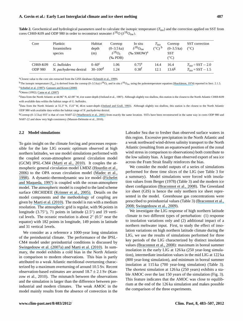
Table 2. Geochemical and hydrological parameters used to calculate the isotopic temperature (Tiso) and the correction applied on SST fromcores CH69-K09 and ODP 980 in order to reconstruct seawaterδ18O (δ18Osw).

Core Planktic Habitat Coretop In situ Tiso Coretop SST correctionforaminifera depth (0–3.5 ka) δ18Osw (◦C) b (0–3.5 ka) (◦C)species (m) δ18Oc (‰ SMOW)a SST

(‰ PDB) (◦C)

CH69-K09 G. bulloides 0–60c 1.06 0.75e 14.4 16.4 Tiso= SST− 2.0ODP 980 N. pachydermadextral 30–100d 1.24 0.38f 12.1 13.6g Tiso= SST− 1.5

aClosest value to the core site extracted from the GISS database (Schmidt et al., 1999).bThe isotopic temperature (Tiso) is derived from the coretop (0–3.5 ka)δ18Oc and in situδ18Osw using the paleotemperature equation (Shackleton, 1974) reported in Sect. 2.1.5.cSchiebel et al. (1997); Ganssen and Kroon (2000)dOttens (1992); Came et al. (2007)eData from the North Atlantic at 44.96◦ N, 42.08◦ W, 4 m water-depth (Ostlund et al., 1987). Although slightly too shallow, this station is the closest to the North Atlantic CH69-K09

with available data within the habitat range ofG. bulloides.fData from the North Atlantic at 55.3◦ N, 15.6◦ W, 46 m water-depth (Ostlund and Grall, 1993). Although slightly too shallow, this station is the closest to the North Atlantic

ODP 980 with available data within the habitat range ofN. pachydermadextral.gCoretop (0–3.5 ka) SST is that of core NA87-22 (Waelbroeck et al., 2001) from exactly the same location. SSTs have been reconstructed in the same way in cores ODP 980 and

NA87-22 and show very high consistency (Masson-Delmotte et al., 2010).

2.2 Model simulations

To gain insight on the climate forcing and processes respon-sible for the late LIG oceanic optimum observed at highnorthern latitudes, we use model simulations performed withthe coupled ocean-atmosphere general circulation model(GCM) IPSL-CM4 (Marti et al., 2010). It couples the at-mospheric general circulation model LMDZ (Hourdin et al.,2006) to the OPA ocean circulation model (Madec et al.,1998). A dynamic-thermodynamic sea ice model (Fichefetand Maqueda, 1997) is coupled with the ocean-atmospheremodel. The atmospheric model is coupled to the land schemesurface ORCHIDEE (Krinner et al., 2005). Details on themodel components and the methodology of coupling aregiven by Marti et al. (2010). The model is run with a mediumresolution. The atmospheric grid is regular, with 96 points inlongitude (3.75◦), 71 points in latitude (2.5◦) and 19 verti-cal levels. The oceanic resolution is about 2◦ (0.5◦ near theequator) with 182 points in longitude, 149 points in latitudeand 31 vertical 1evels.

We consider as a reference a 1000-year long simulationof the preindustrial climate. The performance of the IPSL-CM4 model under preindustrial conditions is discussed bySwingedouw et al. (2007a) and Marti et al. (2010). In sum-mary, the model exhibits a cold bias in the North Atlanticin comparison to modern observations. This bias is partlyattributed to a weak Atlantic meridional overturning charac-terized by a maximum overturning of around 10.5 Sv. Recentobservation-based estimates are around 18.7± 2.1 Sv (Kan-zow et al., 2010). The mismatch between the observationsand the simulation is larger than the difference between pre-industrial and modern climates. The weak AMOC in themodel mainly results from the absence of convection in the

Labrador Sea due to fresher than observed surface waters inthis region. Excessive precipitation in the North Atlantic anda weak northward wind-driven salinity transport to the NorthAtlantic (resulting from an equatorward position of the zonalwind stress in comparison to observations) both contribute tothe low salinity bias. A larger than observed export of sea iceacross the Fram Strait finally reinforces the bias.

We consider the model outputs of a series of simulationsperformed for three time slices of the LIG (see Table 3 fora summary). Model simulations were forced with insola-tion values from Berger (1978) (Table 3) and the modern icesheet configuration (Braconnot et al., 2008). The Greenlandice sheet (GIS) is hence the only northern ice sheet repre-sented in the model. Greenhouse gas concentrations wereprescribed to preindustrial values (Table 3) (Braconnot et al.,2008; Swingedouw et al., 2009).

We investigate the LIG response of high northern latitudeclimate to two different types of perturbation: (1) responseto insolation variations only and (2) additional impact of anorthern meltwater input. First, to study the effect of inso-lation variations on high northern latitude climate during theLIG, we use the results of simulations performed for threekey periods of the LIG characterized by distinct insolationvalues (Braconnot et al., 2008): maximum in boreal summerinsolation in the early LIG at 126 ka (250 year-long simula-tion), intermediate insolation values in the mid LIG at 122 ka(800 year-long simulation), and minimum in boreal summerinsolation at 115 ka (700 year-long simulation) (Table 3).The shortest simulation at 126 ka (250 years) exhibits a sta-ble AMOC over the last 150 years of the simulation (Fig. 3).This feature indicates that the AMOC was close to equilib-rium at the end of the 126 ka simulation and makes possiblethe comparison of the three experiments.

www.clim-past.net/8/483/2012/ Clim. Past, 8, 483–507, 2012

488 A. Govin et al.: Early Last Interglacial climate and ice sheet melting

Table 3. Characteristics of the four IPSL-CM4 model simulations considered in this study. The simulations are forced with the modern icesheet configuration.

126 ka 122 ka 115 ka 126 ka meltwater

Eccentricity (◦) 0.0397 0.0407 0.0414 0.0397Obliquity (◦) 23.9 23.2 22.4 23.9Precession (ω − 180◦) 201 356 111 201CO2 (ppmv) 280 280 280 280CH4 (ppbv) 650 650 650 650N2O (ppbv) 270 270 270 270Interactive meltwater ∗ 0.17input (Sv)Reference Braconnot et al. (2008) Braconnot et al. (2008) Braconnot et al. (2008) Swingedouw et al. (2007b, 2009)

∗The simulation at 122 ka contains a small input of freshwater (0.03 Sv), which has a very limited impact on deep-water formation.

48

1 Figure 3: Maximum of the Atlantic meridional overturning streamfunction (1 Sv = 106 m3/s) 2 taken from 500 m to the bottom for all simulations: preindustrial (black), 126 ka (red), 126 ka 3 meltwater (blue), 122 ka (green) and 115 ka (turquoise). 4

5

Fig. 3. Maximum of the Atlantic meridional overturning stream-function (1 Sv = 106 m3 s−1) taken from 500 m to the bottom for allsimulations: preindustrial (black), 126 ka (red), 126 ka meltwater(blue), 122 ka (green) and 115 ka (turquoise).

Second, to investigate the influence of a northern meltwa-ter input on high-latitude climate during the early LIG, weconsider two simulations at 126 ka. In addition to the 126 kasimulation described above, which integrates the direct cli-matic response to insolation forcing at 126 ka (Braconnot etal., 2008), we add the response of ice caps (here the meltingof Greenland) in a second simulation called “126 ka meltwa-ter” (250 year-long simulation) (Table 3). We used the simpleparameterization developed for future climate (Swingedouwet al., 2007b, 2009). The novelty here, when compared toclassical freshwater experiments, is that (1) the influence ofthe specific 126 ka insolation values on the LIG climate istaken into account, and (2) the meltwater flux is interactivewith climate (Swingedouw et al., 2007b, 2009). In responseto the high boreal summer insolation at 126 ka, about 0.17 Svfreshwater flux is redistributed in the North Atlantic northof 40◦ N. Because this number is high as compared to other

estimates (Otto-Bliesner et al., 2006), the “126 ka meltwa-ter” simulation represents the highest effect that a meltwaterpulse could have on high northern latitude climate during theearly LIG and does not pretend to represent the real climateat 126 ka (see Sect. 4.3.2).

3 Marine records: evolution of the LIG climate

3.1 Establishment of the interhemispheric time frame

The definition of reliable chronologies is critical to comparethe LIG climate evolution indicated by records from dif-ferent water depths and oceanic basins. Direct correlationof the plateau of benthicδ18O minimum values (hereaftercalled benthic O-plateau) is commonly applied during theLIG (e.g. Cortijo et al., 1999). Benthicδ18O data however donot only reflect global ice volume variations because they arealso affected by deep-water temperature changes (e.g. Skin-ner and Shackleton, 2005), the presence of18O-depleteddeep waters in the Nordic Seas (e.g. Dokken and Jansen,1999; Risebrobakken et al., 2006; Bauch and Erlenkeuser,2008), that may reach the deep North Atlantic (Labeyrie etal., 2005; Waelbroeck et al., 2006, 2011), and/or the injectionof 18O-depleted meltwater (Ganopolski and Roche, 2009).We prefer to develop here a common time frame betweensediment cores from the Labrador and Norwegian Seas, theNorth Atlantic and Southern Ocean during the LIG that is in-dependent from benthic isotope stratigraphy (e.g. Skinner etal., 2010; Waelbroeck et al., 2011). We transfer the marinesediment records on one single time scale, and use the mostrecent (EDC3) chronology available for the Antarctic EPICADome C (EDC) and Dronning Maud Land (EDML) ice coresduring the LIG (Loulergue et al., 2007; Parrenin et al., 2007;Ruth et al., 2007). This chronology has been extended tothe Greenland ice core at NorthGRIP (North Greenland IceCore Project members, 2004) during the LIG, using globalatmospheric markers (Capron et al., 2010).

Clim. Past, 8, 483–507, 2012 www.clim-past.net/8/483/2012/

A. Govin et al.: Early Last Interglacial climate and ice sheet melting 489

3.1.1 Age models of the Southern Ocean and NorthAtlantic cores

To transfer the Southern Ocean and North Atlantic recordson this timescale, we assume that surface-water tempera-ture changes in the subantarctic zone of the Southern Ocean(respectively in the North Atlantic) occurred simultaneouslywith air temperature variations over inland Antarctica (re-spectively Greenland). This has in particular been observedduring the last glacial period and Termination I (e.g. Bond etal., 1993; Calvo et al., 2007).

Southern Ocean core

We tied the SST record from core MD02-2488 to the deu-terium record from the EDC ice core (Jouzel et al., 2007).Because the SST resolution of the Southern Ocean core hasbeen increased since the publication by Govin et al. (2009),we adjusted the original age model by up to 2 ka during theLIG period. Figure 4 presents the new age model. Thetie-points defined and associated age uncertainties are givenin Table 4. Tie-points are defined as follows. We syn-chronized the first increase in SST and deuterium recordedin the marine and ice cores at the beginning of Termina-tion II (Fig. 4). The accelerated temperature increases ob-served between small “temperature plateaux” in EDC deu-terium record during Termination II are tied to similar eventsrecorded in core MD02-2488 (Fig. 4). We synchronized theSST and deuterium maxima from the marine and ice cores atthe beginning of the LIG, and the beginning of the SST anddeuterium decrease from both cores at the end of the LIG(Fig. 4). Finally, the age model during the last glacial incep-tion relies on three tie-points: at the midpoint, by the tem-perature minimum preceding the warm phase of Dansgaard-Oeschger (D/O) event 25, and by the temperature minimumdefined between the warm phases of D/O 25 and 24 (Fig. 4).

North Atlantic cores

We synchronized the SST proxy records from the North At-lantic cores ODP 980, MD95-2042 and CH69-K09 to the iceδ18O record from the NGRIP Greenland ice core during thelast glacial inception (Fig. 5). Note that the plankticGlobige-rina bulloidesδ18O record is a good proxy of SST in coreMD95-2042 (Shackleton et al., 2000). However, the Green-land ice core starts at 122 ka and does not cover the early LIG(North Greenland Ice Core Project members, 2004). Pastrecords from the Greenland ice cores indicate that abruptGreenland warming phases during the glacial millennial-scale Dansgaard-Oeschger events and Termination I are inphase with sharp methane increases (e.g. Chappellaz et al.,1993; Severinghaus and Brook, 1999; Fluckiger et al., 2004;Huber et al., 2006). Here we assume that similarly, theabrupt warming of the air above Greenland during Termi-nation II is synchronous with the global abrupt methane in-

49

1

Figure 4: Definition of the age model of core MD02-2488 from the Southern Ocean. (a) Sea 2 Surface Temperature (3-point smoothing curve, black line) from core MD02-2488 (Govin et 3 al., 2009). Diamonds and vertical dotted lines highlight the tie-points. (b) Antarctic EDC !D 4 record (EPICA Community members, 2004; Jouzel et al., 2007) (5-point smoothing curve, 5 grey line). (c) Sedimentation rate variations in core MD02-2488. (d) Age uncertainty of the 6 tie-points defined between core MD02-2488 and EDC ice core (see Table 4 for details). 7 8

9

Fig. 4. Definition of the age model of core MD02-2488 from theSouthern Ocean.(a) Sea surface temperature (3-point smoothingcurve, black line) from core MD02-2488 (Govin et al., 2009). Dia-monds and vertical dotted lines highlight the tie-points.(b) Antarc-tic EDC δD record (EPICA Community members, 2004; Jouzel etal., 2007) (5-point smoothing curve, grey line).(c) Sedimentationrate variations in core MD02-2488.(d) Age uncertainty of the tie-points defined between core MD02-2488 and EDC ice core (seeTable 4 for details).

crease recorded in the Antarctic ice core (Loulergue et al.,2008). This hypothesis reflects the major methane emissionsby boreal wetlands that resulted from Northern Hemispherewarming and ice sheet retreat associated with the termina-tions of the last 800 ka (Loulergue et al., 2008). Therefore,we tied (1) the North Atlantic warming indicated by SSTproxy records to the EDC methane increase during Termi-nation II, and (2) North Atlantic SST variations to NGRIPice δ18O record at the end of the LIG (Fig. 5). We definedall tie-points as follows (Table 4). At the beginning of theLIG, the final SST increase recorded in the marine cores

www.clim-past.net/8/483/2012/ Clim. Past, 8, 483–507, 2012

490 A. Govin et al.: Early Last Interglacial climate and ice sheet melting

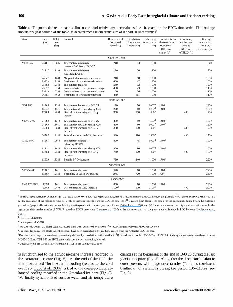
Table 4. Tie-points defined in each sediment core and relative age uncertainties (1σ , in years) on the EDC3 time scale. The total ageuncertainty (last column of the table) is derived from the quadratic sum of individual uncertaintiesa.

Core Depth EDC3 Rational Resolution of Resolution Matching Uncertainty on Uncertainty Total age(cm) age correlated of reference uncertainty the transfer of on the gas- uncertainty

(ka) record (y) record (y) (y) NGRIP on ice age on EDC3EDC3 time difference time scale (y)scaleb (y) of EDCc (y)

Southern Ocean

MD02-2488 2346.1 108.6 Temperature minimum 240 73 800 840between D/O 24 and D/O 25

2431.3 111.9 Temperature minimum 150 70 800 820preceding D/O 25

2494.3 116.8 Midpoint of temperature decrease 210 58 1200 13002522.4 121.4 Beginning of temperature decrease 400 47 1200 13002549.0 128.8 Temperature maxima 560 32 1000 12002553.7 131.4 Enhanced rate of temperature change 450 43 1000 11002571.6 132.4 Enhanced rate of temperature change 100 56 1000 11002658.1 136.2 Beginning of temperature increase 440 101 1000 1100

North Atlantic

ODP 980 1436.9 112.4 Temperature increase of D/O 25 130 50 1000d 1400b 18001504.1 116.1 Temperature decrease during C26 220 80 1000d 1400b 18001726.8 128.8 Final abrupt warming and CH4 350 170 400e 400 700

increase

MD95-2042 2438.9 112.4 Temperature increase of D/O 25 450 50 500d 1400b 16002486.0 116.1 Temperature decrease during C26 460 80 1000d 1400b 18002570.0 128.8 Final abrupt warming and CH4 380 170 400e 400 700

increase

2650.5 131.8 Start of warming and CH4 increase 360 280 1500e 400 1700

CH69-K09 1138.7 109.4 Temperature decrease 800 45 1000d 1400b 1900following D/O 25

1181.1 116.2 Temperature decrease during C26 800 80 1000d 1400b 19001268.8 128.8 Final abrupt warming and CH4 750 170 400e 400 1000

increase

1293.6 132.5 Benthicδ18O decrease 750 340 1000 1700f 2200

Norwegian Sea

MD95-2010 1246.1 116.1 Temperature decrease 520 80 1500 1400b 22001260.4 128.8 Beginning of benthic O-plateau 2000 720 1000 700f 2500

Labrador Sea

EW9302-JPC2 782.8 116.1 Temperature decrease 800 80 1500 1400b 2300839.3 128.8 Diatom mat and CH4 increase 1500g 170 1500e 400 2200

aThe total age uncertainty combines: (1) the resolution of correlated record (for example, the SST record from core MD02-2488, or the plankticδ18O record from core MD95-2042);

(2) the resolution of the reference record (e.g.δD or methane records from the EDC ice core, iceδ18O record from NGRIP ice core); (3) the uncertainty derived from the matching

procedure (graphically estimated when defining the tie-points with the Analyseries software, Paillard et al., 1996); and (4) for sediment cores from high northern latitudes only, the

age uncertainty on the transfer of NGRIP record on EDC3 time scale (Capron et al., 2010) or the age uncertainty on the gas-ice age difference in EDC ice core (Loulergue et al.,

2007).bCapron et al. (2010)cLoulergue et al. (2008)dFor these tie-points, the North Atlantic records have been correlated to the iceδ18O record from the Greenland NGRIP ice core.eFor these tie-points, the North Atlantic records have been correlated to the methane record from the Antarctic EDC ice core.fBecause these tie-points have been respectively defined by correlation to the benthicδ18O record from core MD95-2042 and ODP 980, their age uncertainties are those of cores

MD95-2042 and ODP 980 on EDC3 time scale over the corresponding intervals.gUncertainty on the upper limit of the diatom layer in the Labrador Sea core.

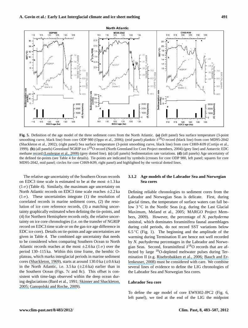
is synchronized to the abrupt methane increase recorded inthe Antarctic ice core (Fig. 5). At the end of the LIG, thefirst pronounced North Atlantic cooling (related to the coldevent 26, Oppo et al., 2006) is tied to the corresponding en-hanced cooling recorded in the Greenland ice core (Fig. 5).We finally synchronized surface-water and air temperature

changes at the beginning or the end of D/O 25 during the lastglacial inception (Fig. 5). Altogether the three North Atlanticcores present, within age uncertainties (Table 4), consistentbenthicδ18O variations during the period 135–110 ka (seeFig. 8).

Clim. Past, 8, 483–507, 2012 www.clim-past.net/8/483/2012/

A. Govin et al.: Early Last Interglacial climate and ice sheet melting 491

50

1

Figure 5: Definition of the age model of the three sediment cores from the North Atlantic. (a) (left panel) Sea Surface Temperature (3-point 2 smoothing curve, black line) from core ODP 980 (Oppo et al., 2006); (mid panel) planktic !18O record (black line) from core MD95-2042 3 (Shackleton et al., 2002); (right panel) Sea Surface Temperature (3-point smoothing curve, black line) from core CH69-K09 (Cortijo et al., 4 1999). (b) (all panels) Greenland NGRIP ice !18O record (North Greenland Ice Core Project members, 2004) (grey line) and Antarctic EDC 5 methane record (Loulergue et al., 2008) (grey dotted line). (c) (all panels) Sedimentation rate variations. (d) (all panels) Age uncertainty of the 6 defined tie-points (see Table 4 for details). Tie-points are indicated by symbols (crosses for core ODP 980, left panel; squares for core MD95-7 2042, mid panel; circles for core CH69-K09, right panel) and highlighted by the vertical dotted lines. 8

Fig. 5. Definition of the age model of the three sediment cores from the North Atlantic.(a) (left panel) Sea surface temperature (3-pointsmoothing curve, black line) from core ODP 980 (Oppo et al., 2006); (mid panel) plankticδ18O record (black line) from core MD95-2042(Shackleton et al., 2002); (right panel) Sea surface temperature (3-point smoothing curve, black line) from core CH69-K09 (Cortijo et al.,1999).(b) (all panels) Greenland NGRIP iceδ18O record (North Greenland Ice Core Project members, 2004) (grey line) and Antarctic EDCmethane record (Loulergue et al., 2008) (grey dotted line).(c) (all panels) Sedimentation rate variations.(d) (all panels) Age uncertainty ofthe defined tie-points (see Table 4 for details). Tie-points are indicated by symbols (crosses for core ODP 980, left panel; squares for coreMD95-2042, mid panel; circles for core CH69-K09, right panel) and highlighted by the vertical dotted lines.

The relative age uncertainty of the Southern Ocean recordson EDC3 time scale is estimated to be at the most±1.3 ka(1σ ) (Table 4). Similarly, the maximum age uncertainty onNorth Atlantic records on EDC3 time scale reaches±2.2 ka(1σ ). These uncertainties integrate (1) the resolution ofcorrelated records in marine sediment cores, (2) the reso-lution of ice core reference records, (3) a matching uncer-tainty graphically estimated when defining the tie-points, and(4) for Northern Hemisphere records only, the relative uncer-tainty on ice core chronologies (i.e. on the transfer of NGRIPrecord on EDC3 time scale or on the gas-ice age difference inEDC ice core). Details on tie-points and age uncertainties aregiven in Table 4. The combined age uncertainty that needsto be considered when comparing Southern Ocean to NorthAtlantic records reaches at the most±2.6 ka (1σ ) over theperiod 130–115 ka. Within this time frame, the benthic O-plateau, which marks interglacial periods in marine sedimentcores (Shackleton, 1969), starts at around 130.0 ka (±0.6 ka)in the North Atlantic, i.e. 3.5 ka (±2.6 ka) earlier than inthe Southern Ocean (Figs. 7c and 8c). This offset is con-sistent with time-lags observed within the deep ocean dur-ing deglaciations (Bard et al., 1991; Skinner and Shackleton,2005; Ganopolski and Roche, 2009).

3.1.2 Age models of the Labrador Sea and NorwegianSea cores

Defining reliable chronologies to sediment cores from theLabrador and Norwegian Seas is delicate. First, duringglacial times, the temperature of surface waters can fall be-low 3◦C in the Nordic Seas (e.g. during the Last GlacialMaximum, Meland et al., 2005; MARGO Project Mem-bers, 2009). However, the percentage ofN. pachydermasinistral, which dominates foraminifera faunal assemblagesduring cold periods, do not record SST variations below6.5◦C (Fig. 1). The beginning and the amplitude of thewarming during Termination II are hence not well recordedby N. pachydermapercentages in the Labrador and Norwe-gian Seas. Second, foraminiferalδ18O records that are af-fected by large18O-depleted meltwater pulses during Ter-mination II (e.g. Risebrobakken et al., 2006; Bauch and Er-lenkeuser, 2008) must be considered with care. We combineseveral lines of evidence to define the LIG chronologies ofthe Labrador Sea and Norwegian Sea cores.

Labrador Sea core

To define the age model of core EW9302-JPC2 (Fig. 6,left panel), we tied at the end of the LIG the midpoint

www.clim-past.net/8/483/2012/ Clim. Past, 8, 483–507, 2012

492 A. Govin et al.: Early Last Interglacial climate and ice sheet melting

51

1

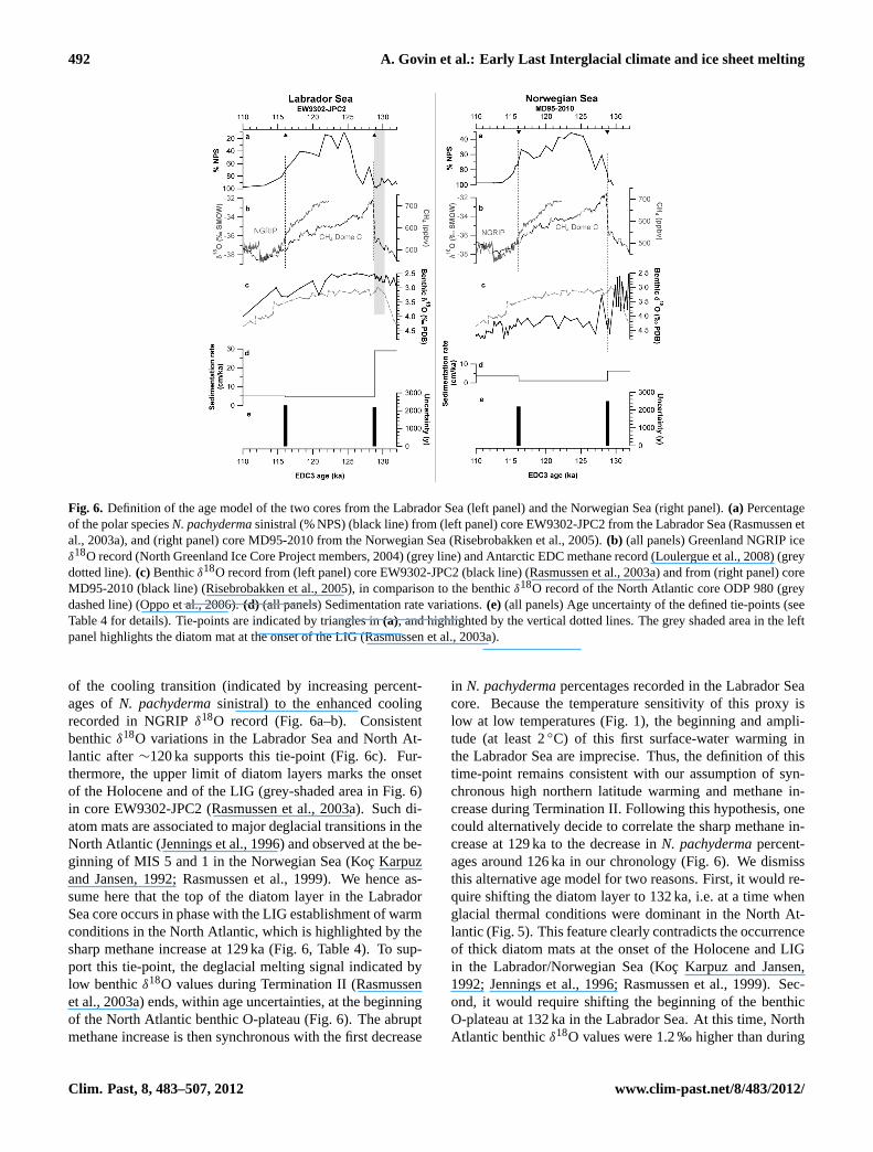
Figure 6: Definition of the age model of the two cores from the Labrador Sea (left panel) and 2 the Norwegian Sea (right panel). (a) Percentage of the polar species N. pachyderma sinistral 3 (% NPS) (black line) from (left panel) core EW9302-JPC2 from the Labrador Sea 4 (Rasmussen et al., 2003a), and (right panel) core MD95-2010 from the Norwegian Sea 5 (Risebrobakken et al., 2005). (b) (all panels) Greenland NGRIP ice !18O record (North 6 Greenland Ice Core Project members, 2004) (grey line) and Antarctic EDC methane record 7 (Loulergue et al., 2008) (grey dotted line). (c) Benthic !18O record from (left panel) core 8 EW9302-JPC2 (black line) (Rasmussen et al., 2003a) and from (right panel) core MD95-2010 9 (black line) (Risebrobakken et al., 2005), in comparison to the benthic !18O record of the 10 North Atlantic core ODP 980 (grey dashed line) (Oppo et al., 2006). (d) (all panels) 11 Sedimentation rate variations. (e) (all panels) Age uncertainty of the defined tie-points (see 12 Table 4 for details). Tie-points are indicated by triangles in (a), and highlighted by the vertical 13 dotted lines. The grey shaded area in the left panel highlights the diatom mat at the onset of 14 the LIG (Rasmussen et al., 2003a). 15 16

17

Fig. 6. Definition of the age model of the two cores from the Labrador Sea (left panel) and the Norwegian Sea (right panel).(a) Percentageof the polar speciesN. pachydermasinistral (% NPS) (black line) from (left panel) core EW9302-JPC2 from the Labrador Sea (Rasmussen etal., 2003a), and (right panel) core MD95-2010 from the Norwegian Sea (Risebrobakken et al., 2005).(b) (all panels) Greenland NGRIP iceδ18O record (North Greenland Ice Core Project members, 2004) (grey line) and Antarctic EDC methane record (Loulergue et al., 2008) (greydotted line).(c) Benthicδ18O record from (left panel) core EW9302-JPC2 (black line) (Rasmussen et al., 2003a) and from (right panel) coreMD95-2010 (black line) (Risebrobakken et al., 2005), in comparison to the benthicδ18O record of the North Atlantic core ODP 980 (greydashed line) (Oppo et al., 2006).(d) (all panels) Sedimentation rate variations.(e) (all panels) Age uncertainty of the defined tie-points (seeTable 4 for details). Tie-points are indicated by triangles in(a), and highlighted by the vertical dotted lines. The grey shaded area in the leftpanel highlights the diatom mat at the onset of the LIG (Rasmussen et al., 2003a).

of the cooling transition (indicated by increasing percent-ages ofN. pachydermasinistral) to the enhanced coolingrecorded in NGRIPδ18O record (Fig. 6a–b). Consistentbenthicδ18O variations in the Labrador Sea and North At-lantic after∼120 ka supports this tie-point (Fig. 6c). Fur-thermore, the upper limit of diatom layers marks the onsetof the Holocene and of the LIG (grey-shaded area in Fig. 6)in core EW9302-JPC2 (Rasmussen et al., 2003a). Such di-atom mats are associated to major deglacial transitions in theNorth Atlantic (Jennings et al., 1996) and observed at the be-ginning of MIS 5 and 1 in the Norwegian Sea (Koc Karpuzand Jansen, 1992; Rasmussen et al., 1999). We hence as-sume here that the top of the diatom layer in the LabradorSea core occurs in phase with the LIG establishment of warmconditions in the North Atlantic, which is highlighted by thesharp methane increase at 129 ka (Fig. 6, Table 4). To sup-port this tie-point, the deglacial melting signal indicated bylow benthicδ18O values during Termination II (Rasmussenet al., 2003a) ends, within age uncertainties, at the beginningof the North Atlantic benthic O-plateau (Fig. 6). The abruptmethane increase is then synchronous with the first decrease

in N. pachydermapercentages recorded in the Labrador Seacore. Because the temperature sensitivity of this proxy islow at low temperatures (Fig. 1), the beginning and ampli-tude (at least 2◦C) of this first surface-water warming inthe Labrador Sea are imprecise. Thus, the definition of thistime-point remains consistent with our assumption of syn-chronous high northern latitude warming and methane in-crease during Termination II. Following this hypothesis, onecould alternatively decide to correlate the sharp methane in-crease at 129 ka to the decrease inN. pachydermapercent-ages around 126 ka in our chronology (Fig. 6). We dismissthis alternative age model for two reasons. First, it would re-quire shifting the diatom layer to 132 ka, i.e. at a time whenglacial thermal conditions were dominant in the North At-lantic (Fig. 5). This feature clearly contradicts the occurrenceof thick diatom mats at the onset of the Holocene and LIGin the Labrador/Norwegian Sea (Koc Karpuz and Jansen,1992; Jennings et al., 1996; Rasmussen et al., 1999). Sec-ond, it would require shifting the beginning of the benthicO-plateau at 132 ka in the Labrador Sea. At this time, NorthAtlantic benthicδ18O values were 1.2 ‰ higher than during

Clim. Past, 8, 483–507, 2012 www.clim-past.net/8/483/2012/

A. Govin et al.: Early Last Interglacial climate and ice sheet melting 493

the LIG plateau. Even integrating deep-water temperaturechanges, thisδ18O difference implies a significant sea levelincrease (several dozen meters). Stable benthicδ18O valuesin the Labrador Sea from 132 ka on would require a verylarge amount of freshwater to compensate for this remainingsea level increase. IRD data however indicate that the melt-water supply was already significantly reduced at the begin-ning of the benthic O-plateau in the Labrador/Norwegian Sea(Fig. 7a). Altogether, these arguments make this alternativechronology very unlikely.

3.1.3 Norwegian Sea core

Similarly to the Labrador Sea core, we tied at the end ofthe LIG the midpoint of the cooling recorded by increas-ing percentages ofN. pachydermasinistral in the Norwe-gian Sea core MD95-2010 to the enhanced cooling recordedin NGRIP δ18O record (Fig. 6, right panel). A simulta-neous increase (within age uncertainties) in benthicδ18Orecords from the Norwegian Sea and the North Atlantic af-ter ∼120 ka (Fig. 6c) supports this tie-point. At the begin-ning of the LIG, we defined the tie-point so that the deglacialmelting signal indicated by low Norwegian Sea benthicδ18Ovalues during Termination II (Risebrobakken et al., 2006;Bauch and Erlenkeuser, 2008) ended when the benthic O-plateau started in the North Atlantic (Fig. 6).δ18O values ofthe LIG benthic plateau are about 1 ‰ higher in the Norwe-gian Sea than in the North Atlantic (Fig. 6, Table 4). Thisfeature is consistent with Norwegian Sea deep waters beingcolder by 3 to 4◦C than North Atlantic deep waters duringinterglacials (Labeyrie et al., 1987). The abrupt methane in-crease at 129 ka then occurred in phase with the first Nor-wegian Sea surface-water warming indicated by the decreasein N. pachydermapercentages. We just reported this fea-ture in the Labrador Sea. It highlights our assumption ofsimultaneous methane increase and high northern latitudewarming during Termination II and supports the definitionof this tie-point. As a result, surface waters from the Nor-wegian Sea and the Labrador Sea show a similar thermalevolution throughout the LIG (Fig. 7b). The warming in-dicated by the large decrease inN. pachydermapercentagesin the Norwegian/Labrador Sea lags by 3–4 ka the North At-lantic deglacial warming (Fig. 7d). Based on the identifica-tion of a common ash layer (at 127 ka) in two cores northand south of Iceland, Rasmussen et al. (2003b) document thesame late LIG warming in the Norwegian Sea in compari-son to the North Atlantic. The poor plankticδ18O resolutionand lack of benthic foraminifera for stable isotope analysesin the North Atlantic core used by Rasmussen et al. (2003b)prevent us from providing here additional constraints on thechronology of the Norwegian Sea core MD95-2010. Thestudy by Rasmussen et al. (2003b) nevertheless supports witha robust tephra tie-point the chronostratigraphical approachthat we developed here in the Norwegian Sea and LabradorSea cores.

52

1

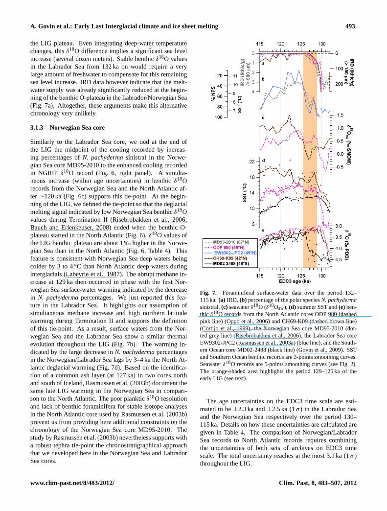
Figure 7: Foraminiferal surface-water data over the period 131-115 ka. (a) IRD, (b) 2 percentage of the polar species N. pachyderma sinistral, (c) seawater !18O (!18Osw), (d) 3 summer SST and (e) benthic !18O records from the North Atlantic cores ODP 980 (dashed 4 pink line) (Oppo et al., 2006) and CH69-K09 (dashed brown line) (Cortijo et al., 1999), the 5 Norwegian Sea core MD95-2010 (dotted grey line) (Risebrobakken et al., 2006), the Labrador 6 Sea core EW9302-JPC2 (Rasmussen et al., 2003a) (blue line), and the Southern Ocean core 7 MD02-2488 (black line) (Govin et al., 2009). SST and Southern Ocean benthic records are 3-8 points smoothing curves. Seawater !18O records are 5-points smoothing curves (see Figure 2). 9 The orange-shaded area highlights the period 129-125 ka of the early LIG (see text). 10

11

Fig. 7. Foraminiferal surface-water data over the period 132–115 ka.(a) IRD, (b) percentage of the polar speciesN. pachydermasinistral,(c) seawaterδ18O (δ18Osw), (d) summer SST and(e)ben-thic δ18O records from the North Atlantic cores ODP 980 (dashedpink line) (Oppo et al., 2006) and CH69-K09 (dashed brown line)(Cortijo et al., 1999), the Norwegian Sea core MD95-2010 (dot-ted grey line) (Risebrobakken et al., 2006), the Labrador Sea coreEW9302-JPC2 (Rasmussen et al., 2003a) (blue line), and the South-ern Ocean core MD02-2488 (black line) (Govin et al., 2009). SSTand Southern Ocean benthic records are 3-points smoothing curves.Seawaterδ18O records are 5-points smoothing curves (see Fig. 2).The orange-shaded area highlights the period 129–125 ka of theearly LIG (see text).

The age uncertainties on the EDC3 time scale are esti-mated to be±2.3 ka and±2.5 ka (1σ ) in the Labrador Seaand the Norwegian Sea respectively over the period 130–115 ka. Details on how these uncertainties are calculated aregiven in Table 4. The comparison of Norwegian/LabradorSea records to North Atlantic records requires combiningthe uncertainties of both sets of archives on EDC3 timescale. The total uncertainty reaches at the most 3.1 ka (1σ )throughout the LIG.

www.clim-past.net/8/483/2012/ Clim. Past, 8, 483–507, 2012

494 A. Govin et al.: Early Last Interglacial climate and ice sheet melting

3.2 Evidence for a global late LIG climatic optimum athigh northern latitudes

3.2.1 Evolution of surface waters during the LIG

The evolution of northern and southern surface-water con-ditions is reported in Fig. 7. The Southern Ocean corerecord indicates the establishment of peak interglacial SSTsat 130 ka at high southern latitudes (Fig. 7b), i.e. immedi-ately at the end of the deglacial warming recorded in south-ern subpolar waters during Termination II. In contrast, theSST reconstructions from subpolar regions show that peakinterglacial SSTs occur at 125 ka in the Labrador Sea and theNorwegian Sea (Fig. 7b). In the North Atlantic at 55◦ N, thelarge deglacial surface-water warming associated with Ter-mination II ends at 129 ka (Fig. 7d). It is followed by rel-atively stable SSTs during around 3–4 ka and an additionalwarming of 2◦C, which leads to maximal North Atlantic SSTat 125 ka (Fig. 7d). We finally observe a gradual increasein surface-water temperature at mid-latitudes (42◦ N) in theNorth Atlantic during the LIG (Cortijo et al., 1999) (Fig. 7d).Therefore, SST records from the Labrador Sea, NorwegianSea and high-latitude North Atlantic indicate the establish-ment of optimal thermal conditions at 125 ka at high north-ern latitudes, i.e. 5 ka (±2.6 ka) after the beginning of peakinterglacial SSTs in the Southern Ocean.

We hence identify at the beginning of the LIG benthicO-plateau, an interval lasting three to four thousands years(period 129–125 ka, hereafter called “early LIG”) charac-terized by: (1) peak interglacial conditions in the SouthernHemisphere, and (2) high northern latitude surface waterscolder than in the later part of the benthic O-plateau (pe-riod 125–119 ka, hereafter called “late LIG”). The late es-tablishment of oceanic thermal conditions that we documentat high northern latitudes seems a consistent feature of theLIG climatic evolution in the Norwegian Sea (Rasmussen etal., 2003b; Bauch and Erlenkeuser, 2008; Bauch et al., 2011;Van Nieuwenhove et al., 2011). Our results suggest that theLIG delay in peak interglacial warmth is not restricted to theNorwegian Sea and extended to the Labrador Sea and high-latitude North Atlantic. The establishment of warm surface-water conditions at 125 ka in the North Atlantic (55◦ N) takesplace in two phases. The high-amplitude (9◦C) deglacialwarming between 131 and 129 ka precedes a second warm-ing of 2◦C leading to optimal thermal conditions at 125 ka(Fig. 7d). The relatively small amplitude of this additionalwarming probably explains why the LIG delay in peak in-terglacial warmth is not visible in lower-resolution recordsfrom the North Atlantic (Oppo et al., 2001; Rasmussen et al.,2003b; Kandiano et al., 2004; Bauch and Kandiano, 2007).

The late North Atlantic thermal optimum is associatedwith a delay in peak interglacial salinities in North Atlanticsurface waters. Reconstructions of seawaterδ18O (Fig. 7c)show peak surface-waterδ18O values at around 122 ka at42◦ N in the North Atlantic. At 55◦ N, high surface-water

δ18O values similar to Holocene values mark the begin-ning of the LIG at 129 ka (Fig. 7c). An additional increasein seawaterδ18O of 0.5 ‰ however leads to the establish-ment of peak surface-waterδ18O values at 55◦ N at 125 kaonly (Fig. 7c). North Atlantic surface waters are thus rela-tively fresher during the early LIG than during the late LIG(Fig. 7c). This feature is consistent with lower salinitiesrecorded during the early LIG in the Norwegian Sea (VanNieuwenhove and Bauch, 2008; Bauch et al., 2011).

Finally, IRD data indicate the persistence of iceberg melt-ing until around 126 ka in the North Atlantic and in the Nor-wegian Sea (Fig. 7a). This result is consistent with persistentIRD documented after Termination II on the Vøring Plateauin the Norwegian Sea (Van Nieuwenhove and Bauch, 2008).The disappearance of iceberg melting at 126 ka coincides,within age uncertainties, with the latest estimates of the LIGsea level highstand registered by corals (Waelbroeck et al.,2008; Blanchon et al., 2009). Iceberg melting hence per-sists at high northern latitudes within the LIG benthic O-plateau recorded in North Atlantic and Southern Ocean cores(Fig. 7e). Available data do not allow us to assign the spe-cific geographical origin of the icebergs. However, icebergsare probably released by the remnant melting of the Northernice sheets (NIS), in particular the Eurasian Saalian ice sheet(Svendsen et al., 2004; Lambeck et al., 2006). Iceberg melt-ing likely contributes to maintain the relatively colder andfresher surface-water conditions observed at high northernlatitudes during the early LIG compared to the late LIG.

3.2.2 Evolution of deep waters during the LIG

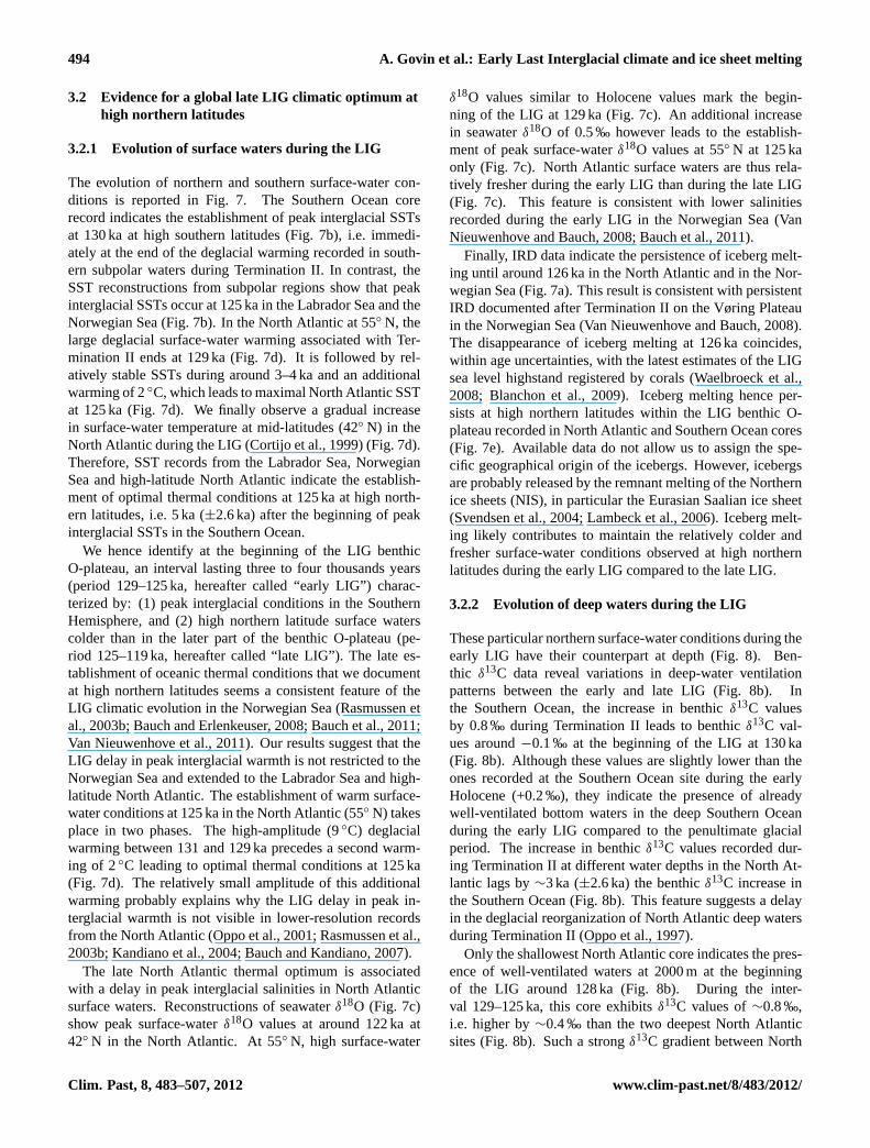
These particular northern surface-water conditions during theearly LIG have their counterpart at depth (Fig. 8). Ben-thic δ13C data reveal variations in deep-water ventilationpatterns between the early and late LIG (Fig. 8b). Inthe Southern Ocean, the increase in benthicδ13C valuesby 0.8 ‰ during Termination II leads to benthicδ13C val-ues around−0.1 ‰ at the beginning of the LIG at 130 ka(Fig. 8b). Although these values are slightly lower than theones recorded at the Southern Ocean site during the earlyHolocene (+0.2 ‰), they indicate the presence of alreadywell-ventilated bottom waters in the deep Southern Oceanduring the early LIG compared to the penultimate glacialperiod. The increase in benthicδ13C values recorded dur-ing Termination II at different water depths in the North At-lantic lags by∼3 ka (±2.6 ka) the benthicδ13C increase inthe Southern Ocean (Fig. 8b). This feature suggests a delayin the deglacial reorganization of North Atlantic deep watersduring Termination II (Oppo et al., 1997).

Only the shallowest North Atlantic core indicates the pres-ence of well-ventilated waters at 2000 m at the beginningof the LIG around 128 ka (Fig. 8b). During the inter-val 129–125 ka, this core exhibitsδ13C values of∼0.8 ‰,i.e. higher by∼0.4 ‰ than the two deepest North Atlanticsites (Fig. 8b). Such a strongδ13C gradient between North

Clim. Past, 8, 483–507, 2012 www.clim-past.net/8/483/2012/

A. Govin et al.: Early Last Interglacial climate and ice sheet melting 495

53

1

Figure 8: Foraminiferal deep-water data over the period 134-115 ka. (a) 21 June insolation at 2 65°N (black line, Berger, 1978). Corresponding rate of insolation change (dashed grey line, 3 right Y-axis) plotted for the period 127-115 ka only. The star along the left Y-axis indicates 4 the insolation maximum at 11 ka. Benthic (b) !13C (Cibicides) and (c) !18O records from the 5 North Atlantic cores ODP 980 (dashed pink line) (Oppo et al., 2006), MD95-2042 (green 6 line) (Shackleton et al., 2002), CH69-K09 (dashed brown line) (Cortijo et al., 1999), and from 7 the Southern Ocean core MD02-2488 (black line, 3-point smoothing curves) (Govin et al., 8 2009). The orange-shaded area highlights the period 129-125 ka of the early LIG (see text). 9

10

Fig. 8. Foraminiferal deep-water data over the period 134–115 ka.(a) 21 June insolation at 65◦ N (black line, Berger, 1978). Corre-sponding rate of insolation change (dashed grey line, right y-axis)plotted for the period 127–115 ka only. The star along the left y-axisindicates the insolation maximum at 11 ka. Benthic(b) δ13C (Cibi-cides) and(c) δ18O records from the North Atlantic cores ODP 980(dashed pink line) (Oppo et al., 2006), MD95-2042 (green line)(Shackleton et al., 2002), CH69-K09 (dashed brown line) (Cortijoet al., 1999), and from the Southern Ocean core MD02-2488 (blackline, 3-point smoothing curves) (Govin et al., 2009). The orange-shaded area highlights the period 129–125 ka of the early LIG (seetext).

Atlantic intermediate and deep waters during the early LIGis supported by further data from the North Atlantic (Keig-win et al., 1994; Oppo et al., 1997; Hodell et al., 2009).This δ13C gradient reflects the persistent influence of bot-tom waters of southern origin in the deep North Atlantic dur-ing the early LIG (Oppo et al., 1997), i.e. the formation ofa well-ventilated NADW that is less dense than during thelate LIG. This feature is consistent with a weak North At-lantic deep-water circulation persistent at the beginning ofthe LIG on Gardar Drift (Iceland Basin) (Hodell et al., 2009).It is only during the late LIG, when the delivery of icebergshas ended and when northern surface waters are warm andsaline (Fig. 7), that the deep ocean circulation becomes sim-ilar to the modern one. During that period, all North At-lantic cores between 2200 and 4100 m water depth exhibithigh δ13C values around 0.8 ‰ (Fig. 8b). Theseδ13C val-ues indicate the presence of the same water-mass, similar tothe present-day high-ventilated NADW, between 2000 and4000 m in the North Atlantic.

Our compilation of LIG data from the high northern andsouthern latitudes shows evidence for a persistent iceberg de-livery at high northern latitudes during the early LIG. It isassociated with relatively low salinity and temperature val-ues in North Atlantic surface waters (Fig. 7), as well asa relatively weak ventilation of North Atlantic deep waters(Fig. 8) during the early LIG (129–125 ka) compared to thelate LIG. The delay in peak interglacial warmth documentedin the Norwegian Sea (Bauch and Erlenkeuser, 2008; Bauchet al., 2011; Van Nieuwenhove et al., 2011) hence affectsthe Labrador Sea and high-latitude North Atlantic regionsand has its counterpart at depth. Oceanic conditions at highnorthern latitudes are hence intermediate between glacialand full interglacial conditions at the beginning of the LIG.They are in contrast with the Southern Ocean climate evolu-tion, which exhibits maximum interglacial warmth and well-ventilated bottom waters from the beginning of the LIG at∼130 ka.

4 Model-data comparison: possible climate processesresponsible for the LIG climate evolution

Delays in peak warmth conditions between the northern andsouthern high latitudes, similar to what we observe at the be-ginning of the LIG, are attributed to “bipolar seesaw” mech-anisms during the last glacial period (e.g. Blunier and Brook,2001). During Termination II, rapid northern ice sheet melt-ing however suppressed the imprint of “bipolar seesaw” sig-nals (northern temperature reversal) in climate records fromthe penultimate deglaciation (Ruddiman et al., 1980; Carl-son, 2008). Boreal summer insolation values of the LIGexceed the early Holocene maximum value during 7 ka atthe beginning of the LIG (period 131–124 ka, Fig. 8a). Inthis section, we propose potential climate forcing and mech-anisms responsible for the late LIG establishment of peakinterglacial warmth and North Atlantic deep-water circula-tion. From the results of the model simulations, we investi-gate (1) to which extent high northern latitude climate solelyresponds to insolation variations during the LIG and (2) whatthe signature of a massive ice sheet melting would be duringthe early LIG.

4.1 Oceanic response to insolation changes during theLIG

We consider here the simulations performed with insolationas a sole forcing (Table 3): at 126 ka (high boreal summerinsolation) and 122 ka (intermediate insolation values), incomparison to 115 ka (minimum in boreal summer insola-tion) (Fig. 8a). Figure 9 presents changes in surface and deepwaters in the North Atlantic and Nordic Seas between thesethree time slices.

Northern high-latitude surface waters are warmer by 1.5 to3◦C at 126 ka than at 122 ka, and by around 1◦C at 122 ka

www.clim-past.net/8/483/2012/ Clim. Past, 8, 483–507, 2012

496 A. Govin et al.: Early Last Interglacial climate and ice sheet melting

54

1

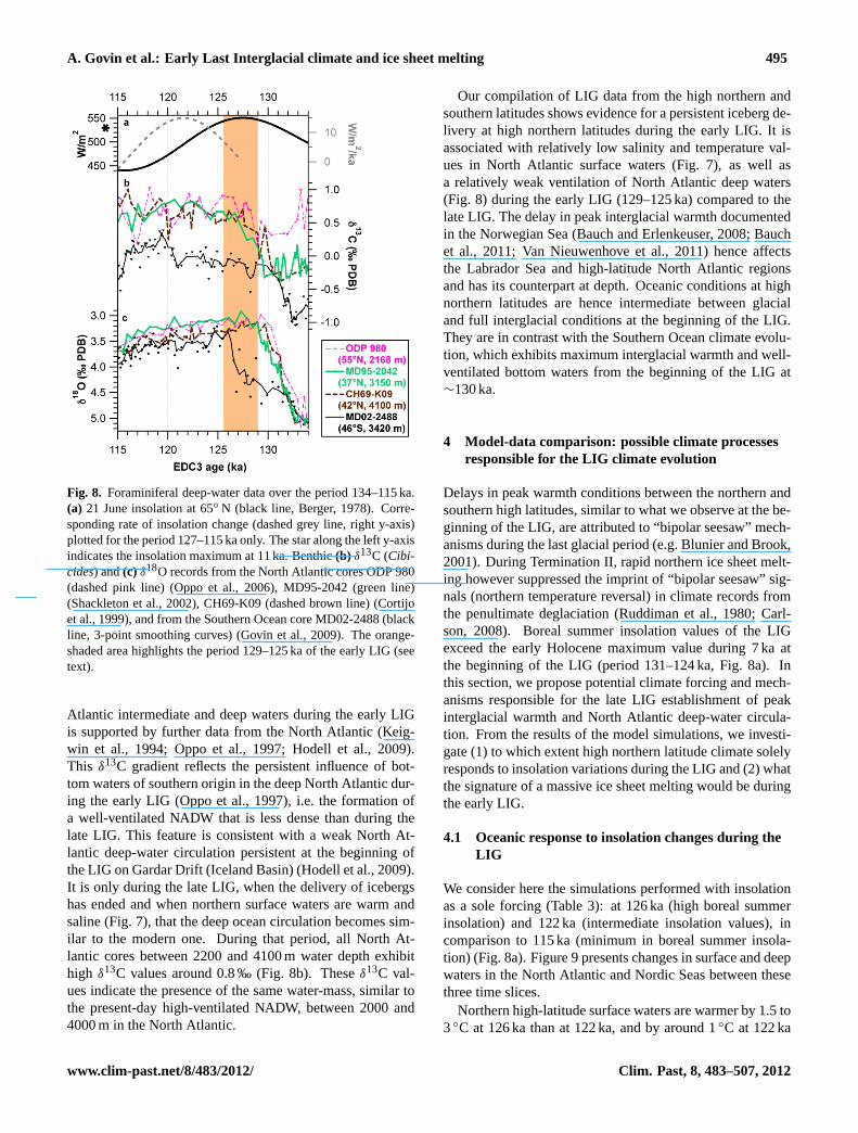
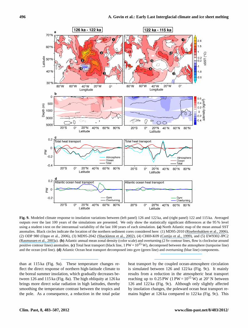
Figure 9: Modeled climate response to insolation variations between (left panel) 126 and 2 122 ka, and (right panel) 122 and 115 ka. Averaged outputs over the last 100 years of the 3 simulations are presented. We only show the statistically significant differences at the 95% 4 level using a student t-test on the interannual variability of the last 100 years of each 5 simulation. (a) North Atlantic map of the mean annual SST anomalies. Black circles indicate 6 the location of the northern sediment cores considered here: (1) MD95-2010 (Risebrobakken 7 et al., 2006), (2) ODP 980 (Oppo et al., 2006), (3) MD95-2042 (Shackleton et al., 2002), (4) 8 CH69-K09 (Cortijo et al., 1999), and (5) EW9302-JPC2 (Rasmussen et al., 2003a). (b) 9 Atlantic annual mean zonal density (color scale) and overturning (2 Sv contour lines, flow is 10 clockwise around positive contour lines) anomalies. (c) Total heat transport (black line, 1 PW 11 = 1015 W), decomposed between the atmosphere (turquoise line) and the ocean (red line). (d) 12 Atlantic Ocean heat transport decomposed into gyre (green line) and overturning (blue line) 13 components.14

Fig. 9. Modeled climate response to insolation variations between (left panel) 126 and 122 ka, and (right panel) 122 and 115 ka. Averagedoutputs over the last 100 years of the simulations are presented. We only show the statistically significant differences at the 95 % levelusing a student t-test on the interannual variability of the last 100 years of each simulation.(a) North Atlantic map of the mean annual SSTanomalies. Black circles indicate the location of the northern sediment cores considered here: (1) MD95-2010 (Risebrobakken et al., 2006),(2) ODP 980 (Oppo et al., 2006), (3) MD95-2042 (Shackleton et al., 2002), (4) CH69-K09 (Cortijo et al., 1999), and (5) EW9302-JPC2(Rasmussen et al., 2003a).(b) Atlantic annual mean zonal density (color scale) and overturning (2 Sv contour lines, flow is clockwise aroundpositive contour lines) anomalies.(c) Total heat transport (black line, 1 PW = 1015W), decomposed between the atmosphere (turquoise line)and the ocean (red line).(d) Atlantic Ocean heat transport decomposed into gyre (green line) and overturning (blue line) components.

than at 115 ka (Fig. 9a). These temperature changes re-flect the direct response of northern high-latitude climate tothe boreal summer insolation, which gradually decreases be-tween 126 and 115 ka (Fig. 8a). The high obliquity at 126 kabrings more direct solar radiation in high latitudes, therebysmoothing the temperature contrast between the tropics andthe pole. As a consequence, a reduction in the total polar

heat transport by the coupled ocean-atmosphere circulationis simulated between 126 and 122 ka (Fig. 9c). It mainlyresults from a reduction in the atmospheric heat transportreaching up to 0.25 PW (1 PW = 1015 W) at 20◦ N between126 and 122 ka (Fig. 9c). Although only slightly affectedby insolation changes, the poleward ocean heat transport re-mains higher at 126 ka compared to 122 ka (Fig. 9c). This

Clim. Past, 8, 483–507, 2012 www.clim-past.net/8/483/2012/

A. Govin et al.: Early Last Interglacial climate and ice sheet melting 497

increase is mainly due to changes in the North Atlantic sec-tor (up to 0.10 PW). Therefore, higher North Atlantic SSTsat 126 ka compared to 122 ka reflects the increase in the At-lantic poleward heat transport. Figure 9d indicates that thisincrease in Atlantic heat transport at 126 ka is mainly due to astronger Atlantic overturning between the equator and 40◦ Nand a stronger subpolar gyre around 50◦ N (see Born et al.,2010).

Future climate simulations with increasing atmosphericcarbon dioxide concentrations show that increased North At-lantic SSTs stratify the upper water, thereby limiting the deepconvection that feeds the AMOC (Gregory et al., 2005). Themodel however simulates here a stronger AMOC at 126 kathan at 122 ka (Fig. 9b), due to the sinking of denser NADW(Fig. 9b). The reasons for a stronger AMOC at 126 ka com-pared to at 122 ka are twofold. (1) SST in late winter, whenconvection mostly occurs in the North Atlantic, is not differ-ent between the two periods, limiting the upper layer sta-bilizing effect. (2) The mechanism identified here bringsthe export of Arctic sea ice towards the Nordic Seas (wheresea ice melts) into play. In the warmer climate at 126 ka,the production of sea ice in the Arctic is reduced, so thatthe export of sea ice through the Fram Strait is reduced by0.04 Sv at 126 ka compared to 122 ka. This reduced exportof sea ice from the Arctic to the Atlantic Ocean tends to de-crease the sea surface salinity (SSS) in the Arctic at 126 kacompared to 122 ka. Furthermore less sea ice melts in theNordic Seas, which increases the SSS in the Nordic Seas(not shown), sustains deep-water convection in the North At-lantic and a stronger AMOC at 126 ka compared to 122 ka.A similar mechanism has been proposed for simulations offuture climate (Hu et al., 2004; Swingedouw et al., 2007b).At the demise of the LIG, Born et al. (2010) also documentedwith the same climate model a weaker AMOC at 115 ka thanat 126 ka due to this enhanced advection of Arctic sea iceinto the North Atlantic. We observe here very little changein the Atlantic overturning (<0.5 Sv, 1 Sv = 106 m3 s−1) be-tween 122 ka and 115 ka (Fig. 9b). Similarly, changes in theAtlantic oceanic heat transport (in particular in the overturn-ing component) remain low (<0.05 PW) between 122 ka and115 ka (Fig. 9d), while the globally decreased atmosphericheat transport in the Northern Hemisphere account for thereduction in total heat transport (Fig. 9c). Therefore, mostof the AMOC reduction identified between 126 and 115 kaduring the last glacial inception (Born et al., 2010) occurswithin the LIG between 126 and 122 ka. We attribute thismajor change in AMOC during the LIG to the increasing rateof high-latitude insolation change (Fig. 8a) that results froma rapid obliquity decrease and has a major climatic impact athigh latitudes between 126 and 122 ka.

In summary, the climate model simulates a warmer climateat high northern latitudes and more intense AMOC during theearly LIG (126 ka) compared to the later LIG (122 ka) in re-sponse to insolation changes. These modeling results are incontradiction with proxy data, which indicate colder surface

waters at high northern latitudes and a shallower NADW cellduring the early LIG compared to the late LIG. Insolationvariations are hence not the sole factors regulating the cli-mate at high northern latitudes at the beginning of the LIG.

4.2 Additional impact of ice sheet melting on NorthAtlantic climate

To evaluate the contribution of a persistent ice sheet meltingon the LIG climate at high northern latitudes, we consider inaddition the simulation performed at 126 ka with interactivefreshwater input (“126 ka meltwater”).

When comparing the two simulations at 126 ka (“126 ka”and “126 ka meltwater”, Fig. 10), we observe colder surfacewaters of up to 3◦C in the North Atlantic and the NordicSeas (up to 65◦ N) when the meltwater is active at 126 ka(Fig. 10a). The warming observed at higher latitudes in theNorwegian Sea (Fig. 10a) is a common feature simulated infreshwater experiments by coupled ocean-atmosphere GCM(e.g. Stouffer et al., 2006, see discussion in Sect. 4.3.3 be-low). In addition, the model simulates a freshening of sur-face waters (not shown) at high northern latitudes, which isdirectly linked to the freshwater input. The supply of fresh-water also stratifies the upper ocean and lowers the densityof NADW (Fig. 10b). The strength of the AMOC decreasesby 6 Sv (Fig. 10b), which corresponds to a 50 % reduction ofthe AMOC intensity at 126 ka. The weakening of the AMOCin the “126 ka meltwater” simulation induces a strong reduc-tion in the poleward heat transport by the Atlantic overturn-ing (Fig. 10d), which explains the cooling simulated in NorthAtlantic surface waters (Fig. 10a).

The climatic patterns described above at 126 ka cor-respond to classical North Atlantic climate responsescomputed in freshwater experiments by coupled models(e.g. Stouffer et al., 2006; Swingedouw et al., 2009). We alsoobserve similar climate features simulated at high northernlatitudes when considering the LIG climate evolution high-lighted by the simulation at 126 ka with interactive freshwa-ter input and the one at 122 ka. Surface waters in the NorthAtlantic (south of 60◦ N) are colder by up to 2◦C (Fig. 10a)and fresher (not shown) at 126 ka when the meltwater is ac-tive compared to at 122 ka. These characteristics are consis-tent with proxy-data SST andδ18Osw variations, which indi-cate colder and fresher conditions at high northern latitudesduring the early LIG compared to the late LIG (Sect. 3.2.1).The simulated AMOC is also reduced by 4 Sv at 126 ka com-pared to 122 ka (Fig. 10b). The AMOC weakening is due tothe reduction of NADW production in response to the sur-face freshwater input at 126 ka (Fig. 10b). The AMOC re-duction simulated between 126 ka and 122 ka also results ina decrease in the poleward Atlantic heat transport (Fig. 10d),which explains the cooling of North Atlantic surface waters(Fig. 10a). This AMOC weakening is consistent with a shal-low NADW cell indicated by North Atlantic proxy data atthe beginning of the LIG (Sect. 3.2.2). The North Atlantic

www.clim-past.net/8/483/2012/ Clim. Past, 8, 483–507, 2012

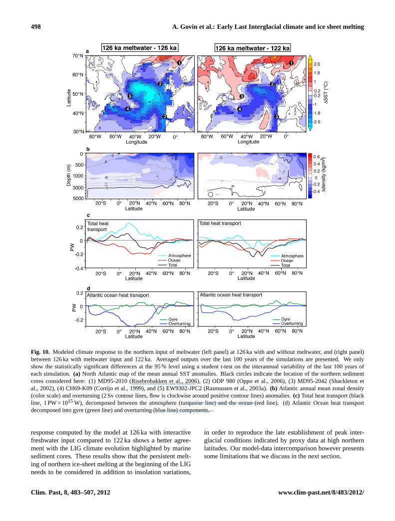
498 A. Govin et al.: Early Last Interglacial climate and ice sheet melting

55

1 Figure 10: Modeled climate response to the northern input of meltwater (left panel) at 126 ka 2 with and without meltwater, and (right panel) between 126 ka with meltwater input and 3 122 ka. Averaged outputs over the last 100 years of the simulations are presented. We only 4 show the statistically significant differences at the 95% level using a student t-test on the 5 interannual variability of the last 100 years of each simulation. (a) North Atlantic map of the 6 mean annual SST anomalies. Black circles indicate the location of the northern sediment 7 cores considered here: (1) MD95-2010 (Risebrobakken et al., 2006), (2) ODP 980 (Oppo et 8 al., 2006), (3) MD95-2042 (Shackleton et al., 2002), (4) CH69-K09 (Cortijo et al., 1999), and 9 (5) EW9302-JPC2 (Rasmussen et al., 2003a). (b) Atlantic annual mean zonal density (color 10 scale) and overturning (2 Sv contour lines, flow is clockwise around positive contour lines) 11 anomalies. (c) Total heat transport (black line, 1 PW = 1015 W), decomposed between the 12 atmosphere (turquoise line) and the ocean (red line). (d) Atlantic Ocean heat transport 13 decomposed into gyre (green line) and overturning (blue line) components. 14

Fig. 10. Modeled climate response to the northern input of meltwater (left panel) at 126 ka with and without meltwater, and (right panel)between 126 ka with meltwater input and 122 ka. Averaged outputs over the last 100 years of the simulations are presented. We onlyshow the statistically significant differences at the 95 % level using a student t-test on the interannual variability of the last 100 years ofeach simulation.(a) North Atlantic map of the mean annual SST anomalies. Black circles indicate the location of the northern sedimentcores considered here: (1) MD95-2010 (Risebrobakken et al., 2006), (2) ODP 980 (Oppo et al., 2006), (3) MD95-2042 (Shackleton etal., 2002), (4) CH69-K09 (Cortijo et al., 1999), and (5) EW9302-JPC2 (Rasmussen et al., 2003a).(b) Atlantic annual mean zonal density(color scale) and overturning (2 Sv contour lines, flow is clockwise around positive contour lines) anomalies.(c) Total heat transport (blackline, 1 PW = 1015W), decomposed between the atmosphere (turquoise line) and the ocean (red line). (d) Atlantic Ocean heat transportdecomposed into gyre (green line) and overturning (blue line) components.

response computed by the model at 126 ka with interactivefreshwater input compared to 122 ka shows a better agree-ment with the LIG climate evolution highlighted by marinesediment cores. These results show that the persistent melt-ing of northern ice-sheet melting at the beginning of the LIGneeds to be considered in addition to insolation variations,

in order to reproduce the late establishment of peak inter-glacial conditions indicated by proxy data at high northernlatitudes. Our model-data intercomparison however presentssome limitations that we discuss in the next section.

Clim. Past, 8, 483–507, 2012 www.clim-past.net/8/483/2012/

A. Govin et al.: Early Last Interglacial climate and ice sheet melting 499

4.3 Discussion on the limitations of the model-datacomparison

4.3.1 Origin of the icebergs and melting water

In the model simulation, the meltwater input originates fromthe Greenland ice sheet, which is the only northern ice sheetrepresented in the model configuration. The freshwater fluxcomputed is then redistributed in the Atlantic to the north of40◦ N (Marti et al., 2010). The model simulations can hencerepresent the ocean and climate responses to the melting ofunspecified northern ice sheets. Available data do not allowidentifying the specific northern origin of ice-rafted detritusthat are found in marine sediment cores from the North At-lantic and the Norwegian Sea at the beginning of the LIG(Fig. 7a). IRD are recorded at high northern latitudes ata time during the early LIG when North Atlantic benthicδ18O values remain low and when benthicδ18O variationssmaller than 0.2 ‰ indicate sea level fluctuations smallerthan 20 m (Fig. 7). This feature suggests that most glacialice sheets have already melted away during the early LIG. Arecent study indicates that ice persisted on southern Green-land throughout the LIG (Colville et al., 2011). The contri-bution of Greenland melting to the LIG sea level highstandhas been reevaluated to 1.6 m to 2.2 m (compared to moderntimes) (Colville et al., 2011). This estimate agrees with thelower end inferred from model simulations (Otto-Bliesner etal., 2006). It suggests a limited contribution of the Green-land retreat to the meltwater input at the beginning of theLIG. Therefore, a significant proportion of icebergs meltingin the North Atlantic during the early LIG likely originatefrom remnants of glacial northern ice sheets. The EurasianSaalian ice sheet, which extended during MIS 6 further souththan during any subsequent glacial episode (e.g. Svendsen etal., 2004), constitutes a very likely source for the icebergs.The influence of the melting Laurentide ice sheet can alsonot be excluded. Evaluating the respective contribution ofnorthern ice sheets to the early LIG meltwater input wouldconstitute an interesting challenge for new climate modelingstudies.

4.3.2 Magnitude of the computed freshwater flux andNorth Atlantic response

The magnitude of the AMOC in the IPSL-CM4 model usedhere is known to be too low under preindustrial conditionscompared to estimates based on observations (Swingedouwet al., 2007a). Nevertheless, the AMOC sensitivity to stan-dard freshwater inputs (e.g. Stouffer et al., 2006) remainswithin the sensitivity of most coupled GCMs (Swingedouwet al., 2009).

Previous work on future climate with coupled climate icesheet models (e.g. Ridley et al., 2005) indicates (1) the melt-ing of the Greenland ice sheet (additional freshwater in-put reaching at most 0.06 Sv) under warm conditions, (2) a

small AMOC weakening (1–2 Sv, i.e.<10 % of the simu-lation without ice sheet melting) caused by the meltwaterinput and (3) an AMOC recovery∼400 years later, whenmost of the additional freshwater input ceases. In our study,the freshwater input is still present at the end of the “126 kameltwater” simulation (250-year long) and stabilized around0.17 Sv. This feature explains the large AMOC reduction atthat time (6 Sv, i.e. 50 % of the AMOC overturning at 126 ka,Fig. 3). The long-term evolution of the AMOC remains un-certain in our study. Future work should include longer simu-lations of the LIG climate with interactive ice sheets in orderto determine the long-term impact of ice sheet melting on theAMOC.

The freshwater flux computed in response to the meltingof the Greenland ice sheet under the strong insolation forcingat 126 ka is very large (0.17 Sv). It explains the strong reduc-tion in the Atlantic overturning circulation (4 Sv, i.e. 38 % ofthe preindustrial simulation) observed between the simula-tions at 126 ka with interactive freshwater flux and at 122 ka(Fig. 10b). The large input of freshwater computed hereis unrealistic for the LIG. For example, such a meltwaterflux would imply the disappearance of the modern Green-land ice sheet (volume of 2.93× 106 km3, Bamber et al.,2001) in around 550 years. This value contradicts the re-duction (not disappearance) of the Greenland ice sheet re-constructed for the LIG (e.g. Koerner, 1989; North Green-land Ice Core Project members, 2004; Otto-Bliesner et al.,2006; Willerslev et al., 2007). The simulation performed at126 ka with the interactive freshwater flux should hence beconsidered as a maximum perturbation of the North Atlanticclimate during the LIG induced by an extreme input of melt-water. Melting with such a magnitude could have only oc-curred on a very limited time scale. The climate conditionscomputed in the “126 ka meltwater” simulation are probablyrepresentative of climate conditions at the very beginning ofthe LIG (e.g.∼130–129 ka), when intense iceberg dischargetook place at high northern latitudes. The “real” ocean andclimate responses to insolation variations and meltwater in-put during the early LIG are likely to be intermediate be-tween the two simulations at 126 ka, with and without theinteractive freshwater input.

Using an ensemble of sensitivity experiments with a modelof intermediate complexity, Bakker et al. (2011) investigatedthe range of Greenland melting rate at the beginning ofthe LIG. They indicate a possible range between 0.052 and0.13 Sv of the meltwater flux that resulted in decreased deepconvection and reduced air temperatures over the North At-lantic and the Labrador Sea (Bakker et al., 2011). This studyconfirms the extremely high freshwater flux computed in ourstudy. It also shows with “more realistic” freshwater valuesthe similar impact of northern ice sheet melting on North At-lantic climate that we report at the beginning of the LIG. Inaddition, relatively stable North Atlantic benthicδ18O dataduring the early LIG (Fig. 8c) suggest sea level fluctuationssmaller than 20 m. Assuming a sea level rise of maximum

www.clim-past.net/8/483/2012/ Clim. Past, 8, 483–507, 2012

500 A. Govin et al.: Early Last Interglacial climate and ice sheet melting

20 m during the 3–4 ka of persistent IRD deposition at the be-ginning of the LIG implies a mean freshwater flux of 0.06 to0.08 Sv (that was probably irregular and higher at 130 ka than126 ka). Although highly uncertain, these values fall withinthe range of meltwater flux inferred by Bakker et al. (2011).

Nevertheless, all these elements highlight the critical needin the near future to couple ice sheet and climate models inorder to improve the computation of freshwater fluxes andrealistically estimate their impact on North Atlantic climate.

4.3.3 Climatic response in the Norwegian Sea

Model results and proxy data disagree on the climatic re-sponse during the early LIG in the Norwegian Sea. Ma-rine sediment cores record a late thermal optimum during theLIG, i.e. colder SST during the early LIG than the late LIG.The delay in the establishment of peak interglacial warmthindicated by marine records during the LIG appears to bea robust feature of the LIG climate evolution in the en-tire Norwegian Sea (Fronval and Jansen, 1997; Fronval etal., 1998; Rasmussen et al., 2003b; Bauch and Erlenkeuser,2008; Bauch et al., 2011; Van Nieuwenhove et al., 2011). Al-though uncertainties on the chronologies of sediment coresfrom the Norwegian Sea remain relatively high for the LIG,independent age models of Norwegian Sea cores based ontephra layers support the late thermal optimum in the NordicSeas (Wastegaard and Rasmussen, 2001; Rasmussen et al.,2003b).

In contrast, the IPSL-CM4 model simulates a warmingof several degrees in the Norwegian Sea between the earlyLIG (“126 ka meltwater” simulation) and late LIG (“122 ka”simulation) (Fig. 10a). Given the large amount of freshwa-ter redistributed at high northern latitudes in the model (seeSect. 4.3.2), the magnitude of this warming is probably over-estimated in comparison to a potential “real” surface-waterwarming signal in the Norwegian Sea. This warming pat-tern, which is observed in response to freshwater input underdifferent climate conditions, is a common feature of fresh-water experiments in this model (Swingedouw et al., 2009).It is due to the adjustment of atmospheric dynamics in re-sponse to the initial global cooling. The changes in atmo-spheric dynamics increases the surface currents and the con-tribution of the gyre to the Atlantic heat transport north of60◦ N (Fig. 10d). These two effects (wind and ocean) reducethe sea ice cover along the eastern coast of Greenland, whichleads to a warming in the Norwegian Sea (see Swingedouw etal., 2009 for further details). This warming pattern is not onlya characteristic of the IPSL-CM4 model. Most atmosphere-ocean coupled models simulate this warming signal in theNordic Seas in response to freshwater input (e.g. Stouffer etal., 2006; Saenko et al., 2007). Further studies on the reasonsfor such adjustments of the atmospheric circulation appearto be necessary to reconcile the LIG climate history seen bymodel simulations and proxy data in the Norwegian Sea.

4.3.4 Alternative mechanisms to the early LIG climaticpattern?

Although the presence of IRD in North Atlantic and Norwe-gian Sea cores (Fig. 7a) strongly argues in favour of ice sheetmelting during the early LIG, other modelling studies exhibita similar cold North Atlantic climate (Felis et al., 2004; Kas-par and Cubasch, 2007) or weakened AMOC (Khodri et al.,2003; Groger et al., 2007) during the LIG insolation peakwithout meltwater forcing. Felis et al. (2004) and Kasparet al. (2007) simulate with the same GCM colder air tem-peratures (up to 2◦C) above the Labrador Sea, the southernNordic Seas and the North Atlantic (north of 40◦ N) duringthe early LIG (at 124 ka and 125 ka respectively) comparedto preindustrial times. They simulate by contrast a warmingover Europe, North America and the tropical North Atlantic(Felis et al., 2004; Kaspar and Cubasch, 2007). These au-thors attribute this LIG temperature pattern to a high positiveindex of the North Atlantic Oscillation (NAO) (Felis et al.,2004). The increased pressure difference between the NorthAtlantic high and Icelandic low results from a reduced pole-to-equator temperature gradient and weakened Hadley cell inresponse to the reduced boreal winter insolation in the tropics(Felis et al., 2004). In our study, we observe no such temper-ature pattern, neither between 126 and 122 ka (Fig. 9a) norbetween 126 ka and preindustrial times (not shown). The dis-crepancy between these two GMCs certainly calls for furtherdetailed investigations of the LIG climate with other models.These authors however did not discuss the change in oceancirculation (Felis et al., 2004; Kaspar and Cubasch, 2007).

Few modelling studies investigated the climate evolutionthroughout the LIG (e.g. Crucifix and Loutre, 2002; Kho-dri et al., 2003; Calov et al., 2005; Groger et al., 2007). Atthe beginning of the LIG, they simulate an enhanced (thisstudy, Crucifix and Loutre, 2002; Calov et al., 2005) orweakened AMOC (Khodri et al., 2003; Groger et al., 2007)in response to insolation variations. This feature highlightsthe difference in overturning sensitivity in the models duringthe LIG, as already outlined for future climate simulations(Schmittner et al., 2005; Schneider et al., 2007). In par-ticular, two transient studies indicate a decrease in AMOCduring the early LIG (e.g. 125 ka) compared to the late LIG(e.g. 120 ka) without meltwater forcing (Khodri et al., 2003;Groger et al., 2007). The mechanisms involved differ. Theslight AMOC weakening (by 1 Sv, i.e.∼5 %) simulated byKhodri et al. (2003) results from higher freshwater input inthe Arctic (+0.01 Sv) that decreases the SSS in the Arcticand hence the Nordic Seas, thereby limiting the deep convec-tion. The AMOC weakening (by 3 Sv, i.e. up to 20 %) simu-lated by Groger et al. (2007) results from (1) warmer NorthAtlantic surface waters that stratify the upper water columnand (2) a 0.027 Sv increase in freshwater input in the Arc-tic/North Atlantic drainage basin. In their model, no decreasein sea ice transport through the Fram Strait is reported, whichdiffers from our study. The processes related to the export of

Clim. Past, 8, 483–507, 2012 www.clim-past.net/8/483/2012/

A. Govin et al.: Early Last Interglacial climate and ice sheet melting 501

Arctic sea ice that we identify here (Sect. 4.1) are not spe-cific to the IPSL-CM4 model. In future climate projections,Hu et al. (2004) showed that similar sea ice processes con-tributed to the future evolution of the AMOC simulated withthe Parallel Climate Model. In addition, the model used byGroger et al. (2007) comprises flux corrections for freshwa-ter and wind stress, which can largely affect its sensitivityto different climatic conditions and explain the difference insensitivity between the two models. Finally, both transientstudies exhibit higher North Atlantic SST and SSS duringthe early LIG compared to the late LIG (Khodri et al., 2003;Groger et al., 2007). This pattern is in contradiction with ourcompilation of proxy data (Fig. 7).

The evolution of the Arctic freshwater budget and its im-pact on North Atlantic climate during the LIG remain un-clear. Past changes in precipitation are difficult to estimatefrom proxy data. Qualitative estimates suggest wetter con-ditions in most Arctic sectors during the LIG compared tothe Holocene (Cape Last Interglacial Project members, 2006;Miller et al., 2010). The response of the Arctic freshwa-ter budget to the sole insolation forcing differs in modellingstudies. Whereas it is slightly reduced at 126 ka comparedto 122 ka in our study (not shown), it is slightly increasedin other LIG simulations due to increased Arctic precipita-tion during the early LIG (Khodri et al., 2003; Groger etal., 2007). Depending on the simulations, Arctic freshwa-ter variations can have an impact on the AMOC (Khodri etal., 2003), be overprinted by the warming of surface waters(Groger et al., 2007) or by changes in Arctic sea ice export tothe Nordic Seas (our study, Sect. 4.1). Therefore, the impactof insolation changes on the AMOC remains under debate.Mechanisms with opposite effect on the AMOC come intoplay. Depending on their relative magnitude in the models,these mechanisms can lead to different AMOC responses, asalready illustrated in future climate projections (Gregory etal., 2005).

In summary, our simulations are so far the only ones thatreproduce both the cooling/freshening in high northern lat-itudes and AMOC weakening documented during the earlyLIG by proxy data. This characteristic tends to support ourassumption of persistent ice sheet melting at the beginning ofthe LIG. However, other models are able to simulate part ofthe LIG climatic pattern (North Atlantic cooling or AMOCreduction) identified here without freshwater input. The va-riety of mechanisms involved (e.g. high NAO index, Arcticfreshwater budget, temperature effect on density) leaves thequestion open to alternative explanations. Further investi-gation with different models is clearly required to disentan-gle the climatic forcing and mechanisms regulating the LIGclimate.

5 Conclusions

Our compilation of proxy data for the LIG documents a delayin the establishment of peak interglacial conditions at highnorthern latitudes compared to high southern latitudes. Weobserve a persistent northern freshwater supply at the be-ginning of the LIG. It is associated with (1) relatively lowsalinity and temperature values in surface waters from theNorth Atlantic, Labrador and Norwegian Seas, and (2) a rel-atively weak ventilation of North Atlantic deep waters dur-ing the early LIG (129–125 ka) compared to the late LIG.These results indicate that the late thermal optimum docu-mented in the Norwegian Sea (Bauch and Erlenkeuser, 2008;Bauch et al., 2011; Van Nieuwenhove et al., 2011) also takesplace in the Labrador Sea and high-latitude North Atlanticregions. It also has its counterpart at depth, with a shal-lower North Atlantic deep-water cell during the early LIG(Hodell et al., 2009). At the beginning of the LIG, oceanicconditions at high northern latitudes are hence intermediatebetween glacial and full interglacial conditions.

The comparison with model results indicates that the delayin peak interglacial conditions at high northern latitudes can-not be a direct response to insolation variations. In responseto the sole insolation forcing, North Atlantic surface watersare warmer and more saline during the early LIG (126 ka)compared to the late LIG (122 ka). In that case, the Atlanticthermohaline circulation is also stronger at 126 ka than at122 ka. The modelled climate response to insolation varia-tions is in contradiction to the LIG climate evolution indi-cated by proxy data. The model better reproduces the LIGclimate history when the melting of northern ice sheets isconsidered during the early LIG (126 ka). North Atlanticsurface waters are indeed colder and fresher, and the At-lantic meridional overturning weaker, at 126 ka with inter-active freshwater flux compared to 122 ka. Insolation varia-tions and persistent northern meltwater input hence need tobe both considered in order to reproduce the late establish-ment of peak interglacial conditions during the LIG. This re-sult emphasizes the sensitivity of North Atlantic climate tothe melting of northern ice sheets in a warm climate and thenecessity to consider ice-sheet melting in the simulations ofwarm climates.

Our model-data comparison also reveals the limits of ourset of simulations performed with one ocean-atmospherecoupled model to reproduce the LIG climate evolution. Thefreshwater flux computed in this study is extremely high andcannot represent the real climate of the early LIG. In addi-tion, other models can reproduce part of the climatic pattern(North Atlantic cooling or AMOC reduction) that we identifyhere at the beginning of the LIG without freshwater input.They bring a variety of processes into play (e.g. Arctic fresh-water budget, NAO, temperature/salinity effect on density).These results highlight the critical need in the near future to(1) develop ice sheet-climate coupled models to improve thecomputation of freshwater fluxes and realistically simulate

www.clim-past.net/8/483/2012/ Clim. Past, 8, 483–507, 2012

502 A. Govin et al.: Early Last Interglacial climate and ice sheet melting

the magnitude of freshwater input and climatic responses,(2) perform transient experiments lasting few thousand yearsto investigate the long-term impact of ice sheet melting onthe AMOC and North Atlantic climate, and (3) comparesimulations performed with a variety of models to evaluatethe climatic forcing and mechanisms that are most likely toinfluence the LIG climate.

Acknowledgements.We thank Gulay Isguder (LSCE) and FabienDewilde (LSCE) for increasing the resolution of respectivelythe SST and benthic isotopic records from core MD02-2488.Discussions with Dominique Raynaud and Didier Paillard helpedto improve an early version of the manuscript. We gratefullyacknowledge the constructive comments of three anonymousreferees and the editor (M. Siddall). We also thank the crew ofthe research vessel Marion-Dufresne and the French Paul EmileVictor Institute (IPEV) for collecting most of the cores studiedhere. Funding of the cruises has been facilitated by IMAGESscientific collaborations. Part of this study has been performedwithin the framework of the French National Research AgencyANR PICC project. The research leading to these results hasreceived funding from the European Union’s Seventh Frameworkprogramme (FP7/2007-2013) under grant agreement no. 243908,“Past4Future. Climate change – Learning from the past climate”.This is LSCE publication no. 4754.

Edited by: M. Siddall

The publication of this article is financed by CNRS-INSU.

References

Adkins, J. F., Boyle, E. A., Keigwin, L. D., and Cortijo, E.: Vari-ability of the North Atlantic thermohaline circulation during thelast interglacial period, Nature, 390, 154–156, 1997.

Andersson, C., Pausata, F. S. R., Jansen, E., Risebrobakken, B., andTelford, R. J.: Holocene trends in the foraminifer record fromthe Norwegian Sea and the North Atlantic Ocean, Clim. Past, 6,179–193,doi:10.5194/cp-6-179-2010, 2010.

Bakker, P., Van Meerbeeck, C. J., and Renssen, H.: Sensitivityof the North Atlantic climate to Greenland Ice Sheet meltingduring the Last Interglacial, Clim. Past Discuss., 7, 2763–2801,doi:10.5194/cpd-7-2763-2011, 2011.

Bamber, J. L., Layberry, R. L., and Gogineni, S. P.: A new ice thick-ness and bed data set for the Greenland ice sheet 1. Measurement,data reduction, and errors, J. Geophys. Res., 106, 33773–33780,doi:10.1029/2001jd900054, 2001.

Bard, E., Arnold, M., and Duplessy, J. C.: Reconciling the sea levelrecord of the last deglaciation with the d18O spectra from deepsea cores, in: Radiocarbon dating: recent applications and fu-

ture potential, edited by: Lowe, J. J., Quaternary Proceedings,Quaternary Research Association, Cambridge, 67–73, 1991.

Bauch, H. A. and Erlenkeuser, H.: A “critical” climatic evaluationof last interglacial (MIS 5e) records from the Norwegian Sea,Polar Res., 27, 135–151, 2008.

Bauch, H. A. and Kandiano, E. S.: Evidence for earlywarming and cooling in North Atlantic surface waters dur-ing the last interglacial, Paleoceanography, 22, PA1201,doi:10.1029/2005pa001252, 2007.

Bauch, H. A., Kandiano, E. S., Helmke, J., Andersen, N., Rosell-Mele, A., and Erlenkeuser, H.: Climatic bisection of the last in-terglacial warm period in the Polar North Atlantic, QuaternarySci. Rev., 30, 1813–1818,doi:10.1016/j.quascirev.2011.05.012,2011.

Berger, A. and Loutre, M. F.: Insolation values for the climate of thelast 10 million years, Quaternary Sci. Rev., 10, 297–317, 1991.

Berger, A. L.: Long-Term Variations of Daily Insolation and Qua-ternary Climatic Changes, J. Atmos. Sci., 35, 2362–2367, 1978.

Birks, C. J. A. and Koc, N.: A high-resolution diatom record of late-Quaternary sea-surface temperatures and oceanographic condi-tions from the eastern Norwegian Sea, Boreas, 31, 323–344,doi:10.1111/j.1502-3885.2002.tb01077.x, 2002.

Blanchon, P., Eisenhauer, A., Fietzke, J., and Liebetrau, V.: Rapidsea-level rise and reef back-stepping at the close of the last inter-glacial highstand, Nature, 458, 881–884, 2009.

Blunier, T. and Brook, E. J.: Timing of millenial-scale climatechange in Antarctica and Greenland during the Last Glacial Pe-riod, Science, 291, 109–112, 2001.

Bond, G. C., Broecker, W., Johnsen, S., McManus, J., Labeyrie, L.,Jouzel, J., and Bonani, G.: Correlations between climate recordsfrom the North Atlantic sediments and Greenland Ice, Nature,365, 143–147, 1993.

Born, A., Nisancioglu, K., and Braconnot, P.: Sea ice inducedchanges in ocean circulation during the Eemian, Clim. Dynam.,35, 1361–1371,doi:10.1007/s00382-009-0709-2, 2010.

Braconnot, P., Marzin, C., Gregoire, L., Mosquet, E., and Marti,O.: Monsoon response to changes in Earth’s orbital parame-ters: comparisons between simulations of the Eemian and of theHolocene, Clim. Past, 4, 281–294,doi:10.5194/cp-4-281-2008,2008.

Calov, R., Ganopolski, A., Petoukhov, V., Claussen, M., Brovkin,V., and Kubatski, C.: Transient simulation of the last glacial in-ception, Part II: sensitivity and feedback analysis, Clim. Dynam.,24, 563–576, 2005.

Calvo, E., Grimalt, J., and Jansen, E.: High resolution U37K seasurface temperature reconstruction in the Norwegian Sea dur-ing the Holocene, Quaternary Science Reviews, 21, 1385–1394,doi:10.1016/S0277-3791(01)00096-8, 2002.

Calvo, E., Pelejero, C., de Deckker, P., and Logan, G. A.: Antarc-tic deglacial pattern in a 30 kyr record of sea surface tempera-ture offshore South Australia, Geophys. Res. Lett., 34, L13707,doi:10.1029/2007GL029937, 2007.

Came, R. E., Oppo, D. W., and McManus, J. F.: Amplitudeand timing of temperature and salinity variability in the subpo-lar North Atlantic over the past 10 k.y, Geology, 35, 315–318,doi:10.1130/g23455a.1, 2007.

Cape Last Interglacial Project members: Last Interglacial Arcticwarmth confirms polar amplification of climate change, Quater-nary Sci. Rev., 25, 1383–1400, 2006.

Clim. Past, 8, 483–507, 2012 www.clim-past.net/8/483/2012/

A. Govin et al.: Early Last Interglacial climate and ice sheet melting 503

Capron, E., Landais, A., Lemieux-Dudon, B., Schilt, A., Masson-Delmotte, V., Buiron, D., Chappellaz, J., Dahl-Jensen, D.,Johnsen, S., Leuenberger, M., Loulergue, L., and Oerter,H.: Synchronising EDML and NorthGRIP ice cores usingδ18O of atmospheric oxygen (δ18Oatm) and CH4 measurementsover MIS5 (80–123 kyr), Quaternary Sci. Rev., 29, 222–234,doi:10.1016/j.quascirev.2009.07.014, 2010.

Carlson, A. E.: Why there was not a Younger Dryas-like event dur-ing the Penultimate Deglaciation, Quaternary Sci. Rev., 27, 882–887, 2008.

Chapman, M. R. and Shackleton, N. J.: Millennial-scale fluctua-tions in North Atlantic heat flux during the last 150,000 years,Earth Planet. Sci. Lett., 159, 57–70, 1998.

Chapman, M. R., Shackleton, N. J., and Duplessy, J.-C.: Sea sur-face temperature variability during the last glacial-interglacialcycle: assessing the magnitude and pattern of climate changein the North Atlantic, Palaeogeogr. Palaeocli., 157, 1–25,doi:10.1016/S0031-0182(99)00168-6, 2000.

Chappellaz, J., Bluniert, T., Raynaud, D., Barnola, J. M., Schwan-der, J., and Stauffert, B.: Synchronous changes in atmosphericCH4 and Greenland climate between 40 and 8 kyr BP, Nature,366, 443–445,doi:10.1038/366443a0, 1993.

Clark, P. U. and Huybers, P.: Global change: Interglacial and futuresea level, Nature, 462, 856–857,doi:10.1038/462856a, 2009.

Colville, E. J., Carlson, A. E., Beard, B. L., Hatfield, R. G.,Stoner, J. S., Reyes, A. V., and Ullman, D. J.: Sr-Nd-PbIsotope Evidence for Ice-Sheet Presence on Southern Green-land During the Last Interglacial, Science, 333, 620–623,doi:10.1126/science.1204673, 2011.

Cortijo, E., Duplessy, J. C., Labeyrie, L., Leclaire, H., Duprat, J.,and van Weering, T. C. E.: Eemian cooling in the Norwegian Seaand North Atlantic ocean preceding continental ice-sheet growth,Nature, 372, 446–449, 1994.

Cortijo, E., Lehman, S., Keigwin, L., Chapman, M., Paillard, D.,and Labeyrie, L.: Changes in meridional temperature and salinitygradients in the North Atlantic Ocean (30–72◦ N) during the lastinterglacial period, Paleoceanography, 14, 23–33, 1999.

Crucifix, M. and Loutre, F.: Transient simulations over the last in-terglacial period (126–115 kyr BP): feedback and forcing analy-sis, Clim. Dynam., 19, 417–433,doi:10.1007/s00382-002-0234-z, 2002.

Cutler, K. B., Edwards, R. L., Taylor, F. W., Cheng, H., Adkins,J., Gallups, C. D., Cutler, P. M., Burr, G. S., and Bloom, A. L.:Rapid sea-level fall and deep-ocean temperature change since thelast interglacial period, Earth Planet. Sc. Lett., 206, 253–271,2003.

Denton, G. H., Anderson, R. F., Toggweiler, J. R., Edwards, R. L.,Schaefer, J. M., and Putnam, A. E.: The Last Glacial Termi-nation, Science, 328, 1652–1656,doi:10.1126/science.1184119,2010.

Desprat, S., Sanchez Goni, M. F., Naughton, F., Turon, J.-L.,Duprat, J., Malaize, B., Cortijo, E., and Peypouquet, J.-P.: Cli-mate variability of the last five isotopic interglacials: directland-sea-ice correlation from the multiproxy analysis of North-Western Iberian margin deep-sea cores, in: The Climate of PastInterglacials, edited by: Sirocko, F., Claussen, M., Sanchez Goni,M. F., and Litt, T., Developments in Quaternary Science, Vol. 7,Elsevier, Amsterdam, 375–386, 2007.

Dokken, T. and Jansen, E.: Rapid changes in the mechanism of

ocean convection during the last glacial period, Nature, 401,458–461, 1999.

Duplessy, J. C., Labeyrie, L., Juillet-Leclerc, A., Maitre, F., Duprat,J., and Sarnthein, M.: Surface salinity reconstruction of the NorthAtlantic Ocean during the last glacial maximum, Oceanol. Acta,14, 311–324, 1991.

EPICA Community members: Eight glacial cycles from an Antarc-tic ice core, Nature, 429, 623–628, 2004.

EPICA Community members: One-to-one coupling of glacial cli-mate variability in Greenland and Antarctica, Nature, 444, 195–198, 2006.

Felis, T., Lohmann, G., Kuhnert, H., Lorenz, S. J., Scholz, D.,Patzold, J., Al-Rousan, S. A., and Al-Moghrabi, S. M.: Increasedseasonality in Middle East temperatures during the last inter-glacial period, Nature, 429, 164–168,doi:10.1038/nature02546,2004.

Fichefet, T. and Maqueda, M. A. M.: Sensitivity of a global seaice model to the treatment of ice thermodynamics and dynamics,J. Geophys. Res., 102, 12609–12646,doi:10.1029/97jc00480,1997.

Fluckiger, J., Blunier, T., Stauffer, B., Chappellaz, J., Spahni, R.,Kawamura, K., Schwander, J., Stocker, T., and Dahl-Jensen, D.:N2O and CH4 variations during the last glacial epoch: insightinto global processes, Global Biogeochem. Cy., 18, GB1020,doi:10.1029/2003gb002122, 2004.

Fronval, T. and Jansen, E.: Eemian and Early Weichselian (140–60 ka) Paleoceanography and Paleoclimate in the Nordic SeasWith Comparisons to Holocene Conditions, Paleoceanography,12, 443–462,doi:10.1029/97pa00322, 1997.

Fronval, T., Jansen, E., Haflidason, H., and Sejrup, H. P.: Variabilityin surface and deep water conditions in the Nordic Seas duringthe last interglacial period, Quaternary Sci. Rev., 17, 963–985,1998.

Ganopolski, A. and Roche, D. M.: On the nature oflead-lag relationships during glacial-interglacial cli-mate transitions, Quaternary Sci. Rev., 28, 3361–3378,doi:10.1016/j.quascirev.2009.09.019, 2009.

Ganssen, G. M. and Kroon, D.: The isotopic signature of planktonicforaminifera from NE Atlantic surface sediments: implicationsfor the reconstruction of past oceanic conditions, J. Geol. Soc.,157, 693–699,doi:10.1144/jgs.157.3.693, 2000.

Govin, A., Michel, E., Labeyrie, L., Waelbroeck, C., Dewilde,F., and Jansen, E.: Evidence for northward expansion ofAntarctic Bottom Water mass in the Southern Ocean dur-ing the last glacial inception, Paleoceanography, 24, PA1202,doi:10.1029/2008PA001603, 2009.

Gregory, J. M., Stouffer, K. W. D. R. J., Weaver, A. J., Driess-chaert, E., Eby, M., Fichefet, T., Hasumi, H., Hu, A., Jung-claus, J. H., Kamenkovich, I. V., Levermann, A., Montoya,M., Murakami, S., Nawrath, S., Oka, A., Sokolov, A. P., andThorpe, R. B.: A model intercomparison of changes in the At-lantic thermohaline circulation in response to increasing atmo-spheric CO2 concentration, Geophys. Res. Lett., 32, L12703,doi:10.1029/2005GL023209, 2005.

Groger, M., Maier-Reimer, E., Mikolajewicz, U., Schurgers, G.,Vizcaıno, M., and Winguth, A.: Changes in the hydrologicalcycle, ocean circulation, and carbon/nutrient cycling during thelast interglacial and glacial transition, Paleoceanography, 22,PA4205,doi:10.1029/2006pa001375, 2007.

www.clim-past.net/8/483/2012/ Clim. Past, 8, 483–507, 2012

504 A. Govin et al.: Early Last Interglacial climate and ice sheet melting

Hald, M., Andersson, C., Ebbesen, H., Jansen, E., Klitgaard-Kristensen, D., Risebrobakken, B., Salomonsen, G. R., Sarn-thein, M., Sejrup, H. P., and Telford, R. J.: Variations in tem-perature and extent of Atlantic Water in the northern North At-lantic during the Holocene, Quaternary Sci. Rev., 26, 3423–3440,doi:10.1016/j.quascirev.2007.10.005, 2007.

Hodell, D. A., Minth, E. K., Curtis, J. H., McCave, I. N., Hall,I. R., Channell, J. E. T., and Xuan, C.: Surface and deep-water hydrography on Gardar Drift (Iceland Basin) during thelast interglacial period, Earth Planet. Sc. Lett., 288, 10–19,doi:10.1016/j.epsl.2009.08.040, 2009.

Hourdin, F., Musat, I., Bony, S., Braconnot, P., Codron, F.,Dufresne, J.-L., Fairhead, L., Filiberti, M.-A., Friedlingstein, P.,Grandpeix, J.-Y., Krinner, G., LeVan, P., Li, Z.-X., and Lott,F.: The LMDZ4 general circulation model: climate performanceand sensitivity to parametrized physics with emphasis on tropicalconvection, Clim. Dynam., 27, 787–813,doi:10.1007/s00382-006-0158-0, 2006.

Hu, A., Meehl, G. A., Washington, W. M., and Dai, A.: Responseof the Atlantic Thermohaline Circulation to Increased Atmo-spheric CO2 in a Coupled Model, J. Climate, 17, 4267–4279,doi:10.1175/jcli3208.1, 2004.

Huber, C., Leuenberger, M., Spahni, R., Fluckiger, J., Schwander,J., Stocker, T. F., Johnsen, S., Landais, A., and Jouzel, J.: Iso-tope calibrated Greenland temperature record over Marine Iso-tope Stage 3 and its relation to CH4, Earth Planet. Sc. Lett., 243,504–519, 2006.

Jansen, E., Overpeck, J. T., Briffa, K. R., Duplessy, J. C., Joos, F.,Masson-Delmotte, V., Olago, D., Otto-Bliesner, B., Peltier, W.R., Rahmstorf, S., Ramesh, R., Raynaud, D., Rind, D., Solom-ina, O., Villalba, R., and Zhang, D.: Palaeoclimate, in: Cli-mate Change 2007: The Physical Science Basis, Contributionof Working Group I to the Four Assessment Report of the In-tergovernmental Panel on Climate Change, edited by: Solomon,S., Qin, D., Manning, M., Chen, Z., Marquis, M., Averyt, K.B., Tignor, M., and Miller, H. L., Cambridge University Press,Cambridge, UK and New York, NY, USA, 2007.

Jennings, A. E., Tedesco, K. A., Andrews, J. T., and Kirby, M.E.: Shelf erosion and glacial ice proximity in the Labrador Seaduring and after Heinrich events (H-3 or 4 to H-0) as shown byforaminifera, in: Late Quaternary Paleoceanography of the NorthAtlantic Margins edited by: Andrews, J. T., Austin, W. E. N.,Bergsten, H., and Jennings, A. E., 1, Geological Society, Lon-don, 29–49, 1996.

Jouzel, J., Masson-Delmotte, V., Cattani, O., Dreyfus, G., Falourd,S., Hoffmann, G., Minster, B., Nouet, J., Barnola, J. M., Chap-pellaz, J., Fischer, H., Gallet, J. C., Johnsen, S., Leuenberger, M.,Loulergue, L., Luethi, D., Oerter, H., Parrenin, F., Raisbeck, G.,Raynaud, D., Schilt, A., Schwander, J., Selmo, E., Souchez, R.,Spahni, R., Stauffer, B., Steffensen, J. P., Stenni, B., Stocker, T.F., Tison, J. L., Werner, M., and Wolff, E. W.: Orbital and Mil-lennial Antarctic Climate Variability over the Past 800,000 Years,Science, 317, 793–796,doi:10.1126/science.1141038, 2007.

Kandiano, E. S., Bauch, H. A., and Muller, A.: Sea Surface temper-ature variability in the North Atlantic during the last two glacial-interglacial cycles: comparison of faunal, oxygen isotopic, andMg/Ca-derived records, Palaeogeogr. Palaeocl., 204, 145–164,2004.

Kanzow, T., Cunningham, S. A., Johns, W. E., Hirschi, J. J. M.,

Marotzke, J., Baringer, M. O., Meinen, C. S., Chidichimo, M.P., Atkinson, C., Beal, L. M., Bryden, H. L., and Collins,J.: Seasonal Variability of the Atlantic Meridional Over-turning Circulation at 26.5◦ N, J. Climate, 23, 5678–5698,doi:10.1175/2010jcli3389.1, 2010.

Kaspar, F. and Cubasch, U.: 33. Simulations of the Eemian in-terglacial and the subsequent glacial inception with a coupledocean-atmosphere general circulation model, in: Developmentsin Quaternary Sciences, edited by: Sirocko, F., Claussen, M.,Sanchez Goni, M. F., and Litt, T., Elsevier, 499–515, 2007.

Keigwin, L. D., Curry, W. B., Lehman, S. J., and Johnsen, S.: Therole of the deep ocean in North Atlantic climate change between70 and 130 kyr ago, Nature, 371, 323–326, 1994.

Kelly, M. J., Edwards, R. L., Cheng, H., Yuan, D., Cai, Y., Zhang,M., Lin, Y., and An, Z.: High resolution characterization ofthe Asian Monsoon between 146,000 and 99,000 years B.P. fromDongge Cave, China and global correlation of events sur-rounding Termination II, Palaeogeogr. Palaeocl., 236, 20–38,doi:10.1016/j.palaeo.2005.11.042, 2006.

Khodri, M., Ramstein, G., Paillard, D., Duplessy, J. C., Kageyama,M., and Ganopolski, A.: Modelling the climate evolution fromthe last interglacial to the start of the last glaciation: The role ofArctic Ocean freshwater budget, Geophys. Res. Lett., 30, 1606,doi:10.1029/2003gl017108, 2003.

Koc Karpuz, N., and Jansen, E.: A High-Resolution Diatom Recordof the Last Deglaciation from the SE Norwegian Sea: Documen-tation of Rapid Climatic Changes, Paleoceanography, 7, 499–520,doi:10.1029/92pa01651, 1992.

Koerner, R. M.: Ice Core Evidence for Extensive Melting of theGreenland Ice Sheet in the Last Interglacial, Science, 244, 964–968,doi:10.1126/science.244.4907.964, 1989.

Kopp, R. E., Simons, F. J., Mitrovica, J. X., Maloof, A.C., and Oppenheimer, M.: Probabilistic assessment of sealevel during the last interglacial stage, Nature, 462, 863–867,doi:10.1038/nature08686, 2009.

Krinner, G., Viovy, N., de Noblet-Ducoudre, N., Ogee, J., Polcher,J., Friedlingstein, P., Ciais, P., Sitch, S., and Prentice, I. C.:A dynamic global vegetation model for studies of the cou-pled atmosphere-biosphere system, Global Biogeochem. Cy., 19,GB1015,doi:10.1029/2003gb002199, 2005.

Kucera, M., Weinelt, M., Kiefer, T., Pflaumann, U., Hayes,A., Chen, M. T., Mix, A. C., Barrows, T. T., Cortijo, E.,Duprat, J., Juggins, S., and Waelbroeck, C.: Reconstructionof sea-surface temperatures from assemblages of planktonicforaminifera: multi-technique approach based on geographicallyconstrained calibration data sets and its application to glacial At-lantic and Pacific Oceans, Quaternary Sci. Rev., 24, 951–998,2005.

Kukla, G., McManus, J. F., Rousseau, D. D., and Chuine, I.: Howlong and how stable was the last interglacial?, Quaternary Sci.Rev., 16, 605–612, 1997.

Kukla, G. J., Bender, M. L., de Beaulieu, J. L., Bond, G. C.,Broecker, W., Cleveringa, P., Gavin, J. E., Herbert, T. D., Im-brie, J., Jouzel, J., Keigwin, L. D., Knudsen, K. L., McManus,J. F., Merkt, J., Muhs, D. R., Muller, H., Poore, R. Z., Porter, S.C., Seret, G., Shackleton, N. J., Turner, C., Tzedakis, P. C., andWinograd, I. J.: Last interglacial climates, Quaternary Res., 58,2–13, 2002.

Labeyrie, L., Duplessy, J. C., and Blanc, P. L.: Variations in mode

Clim. Past, 8, 483–507, 2012 www.clim-past.net/8/483/2012/

A. Govin et al.: Early Last Interglacial climate and ice sheet melting 505

of formation and temperature of oceanic deep waters over thepast 125,000 years, Nature, 327, 477–482, 1987.

Labeyrie, L., Leclaire, H., Waelbroeck, C., Cortijo, E., Duplessy, J.C., Vidal, L., Elliot, M., and Le Coat, B.: Temporal variabilityof the surface and deep waters of the North West Atlantic Oceanat orbital and millenial scales, Geophys. Monogr., 112, 77–98,1999.

Labeyrie, L., Waelbroeck, C., Cortijo, E., Michel, E., and Duplessy,J. C.: Changes in deep water hydrology during the last deglacia-tion, C. R. Geosci., 337, 919–927, 2005.

Lambeck, K., Purcell, A., Funder, S., Kjær, K. H., Larsen,E., and Moller, P. E. R.: Constraints on the Late Saalianto early Middle Weichselian ice sheet of Eurasia fromfield data and rebound modelling, Boreas, 35, 539–575,doi:10.1080/03009480600781875, 2006.

Loulergue, L., Parrenin, F., Blunier, T., Barnola, J.-M., Spahni, R.,Schilt, A., Raisbeck, G., and Chappellaz, J.: New constraintson the gas age-ice age difference along the EPICA ice cores,0–50 kyr, Clim. Past, 3, 527–540,doi:10.5194/cp-3-527-2007,2007.

Loulergue, L., Schilt, A., Spahni, R., Masson-Delmotte, V., Blu-nier, T., Lemieux, B., Barnola, J. M., Raynaud, D., Stocker, T.F., and Chappellaz, J.: Orbital and millennial-scale features ofatmospheric CH4 over the past 800,000 years, Nature, 453, 383–386, 2008.

Madec, G., Delecluse, P., Imbard, M., and Levy, C.: OPA 8.1 oceangeneral circulation model reference manual, Institut Pierre-Simon Laplace (IPSL)– Note du Pole de modelisation 11, 91 pp.,1998.

Malaize, B. and Caley, T.: Sea surface salinity reconstruction asseen with foraminifera shells: Methods and cases studies, Eur.Phys. J. Conf. 1, 177–188,doi:10.1140/epjconf/e2009-00919-6,2009.

MARGO Project Members: Constraints on the magnitude and pat-terns of ocean cooling at the Last Glacial Maximum, Nature Geo-science, 2, 127–132,doi:10.1038/ngeo411, 2009.

Marti, O., Braconnot, P., Dufresne, J. L., Bellier, J., Benshila, R.,Bony, S., Brockmann, P., Cadule, P., Caubel, A., Codron, F., deNoblet, N., Denvil, S., Fairhead, L., Fichefet, T., Foujols, M. A.,Friedlingstein, P., Goosse, H., Grandpeix, J. Y., Guilyardi, E.,Hourdin, F., Idelkadi, A., Kageyama, M., Krinner, G., Levy, C.,Madec, G., Mignot, J., Musat, I., Swingedouw, D., and Talandier,C.: Key features of the IPSL ocean atmosphere model and itssensitivity to atmospheric resolution, Clim. Dynam., 34, 1–26,doi:10.1007/s00382-009-0640-6, 2010.

Masson-Delmotte, V., Stenni, B., Blunier, T., Cattani, O., Chap-pellaz, J., Cheng, H., Dreyfus, G., Edwards, R. L., Falourd, S.,Govin, A., Kawamura, K., Johnsen, S. J., Jouzel, J., Landais, A.,Lemieux-Dudon, B., Lourantou, A., Marshall, G., Minster, B.,Mudelsee, M., Pol, K., Rothlisberger, R., Selmo, E., and Wael-broeck, C.: Abrupt change of Antarctic moisture origin at theend of Termination II, P. Natl. Acad. Sci., 107, 12091–12094,doi:10.1073/pnas.0914536107, 2010.

McManus, J. F., Oppo, D. W., and Cullen, J.: A 0.5-million-yearrecord of millenial-scale climate variability in the North Atlantic,Science, 283, 971–975, 1999.

Meehl, G., Stocker, T. F., Collins, W. D., Friedlingstein, P., Gaye, A.T., Gregory, J. M., Kitoh, A., Knutti, R., Murphy, J. M., Noda,A., Raper, S. C. B., Watterson, I. G., Weaver, A. J., and Zhao,

Z.-C.: Global Climate Projections, in: Climate change 2007:The Physical Science Basis. Contribution of Working Group I tothe Fourth Assessment Report of the Intergovernmental Panel onClimate Change, edited by: Solomon, S., Qin, D., Manning, M.,Chen, Z., Marquis, M., Averyt, K. B., Tignor, M., and Miller, H.L., Cambridge University Press, Cambridge, UK and New York,NY, USA, 2007.

Meland, M. Y., Jansen, E., and Elderfield, H.: Constraintson SST estimates for the northern North Atlantic/NordicSeas during the LGM, Quaternary Sci. Rev., 24, 835–852,doi:10.1016/j.quascirev.2004.05.011, 2005.

Miller, G. H., Brigham-Grette, J., Alley, R. B., Anderson, L.,Bauch, H. A., Douglas, M. S. V., Edwards, M. E., Elias, S. A.,Finney, B. P., Fitzpatrick, J. J., Funder, S. V., Herbert, T. D.,Hinzman, L. D., Kaufman, D. S., MacDonald, G. M., Polyak, L.,Robock, A., Serreze, M. C., Smol, J. P., Spielhagen, R., White, J.W. C., Wolfe, A. P., and Wolff, E. W.: Temperature and precipita-tion history of the Arctic, Quaternary Sci. Rev., 29, 1679–1715,doi:10.1016/j.quascirev.2010.03.001, 2010.

North Greenland Ice Core Project members: High-resolution cli-mate record of Northern Hemisphere climate extending into thelast interglacial period, Nature, 431, 147–151, 2004.

Oppo, D. W., Horowitz, M., and Lehman, S. J.: Marine core evi-dence for reduced deep water production during Termination IIfollowed by a relatively stable substage 5e (Eemian), Paleo-ceanography, 12, 51–63, 1997.

Oppo, D. W., Keigwin, L. D., McManus, J. F., and Cullen, J. L.:Persistent suborbital climate variability in marine isotope stage 5and Termination II, Paleoceanography, 16, 280–292, 2001.

Oppo, D. W., McManus, J. F., and Cullen, J.: Evolution and demiseof the last interglacial warmth in the subpolar North Atlantic,Quaternary Sci. Rev., 25, 3268–3277, 2006.

Ostlund, H. G. and Grall, C.: Arctic tritium: 1973–1991, Data Re-port 19, University of Miami, Rosenstiel School of Marine andAtmospheric Science, 1993.

Ostlund, H. G., Craig, H., Broecker, W. S., and Spenser, D.:GEOSECS Atlantic, Pacific and Indian Ocean expeditions:Shorebased data and graphics, Nat. Sci. Found., Washington,DC, 7, 1987.

Ottens, J. J.: Planktic foraminifera as indicators of ocean environ-ments in the northeast Atlantic, PhD thesis, Vrije UniversiteitAmsterdam, Amsterdam, 189 pp., 1992.

Otto-Bliesner, B. L., Marshall, S. J., Overpeck, J. T., Miller, G.H., Hu, A., and members, C. L. I. P.: Simulating arctic climatewarmth and icefield retreat in the Last Interglacial, Science, 311,1751–1753, 2006.

Paillard, D., Labeyrie, L., and Yiou, P.: Macintosh programperforms time-series analyses, Eos Trans. AGU, 77, 379,doi:10.1029/96EO00259, 1996.

Parrenin, F., Barnola, J.-M., Beer, J., Blunier, T., Castellano, E.,Chappellaz, J., Dreyfus, G., Fischer, H., Fujita, S., Jouzel, J.,Kawamura, K., Lemieux-Dudon, B., Loulergue, L., Masson-Delmotte, V., Narcisi, B., Petit, J.-R., Raisbeck, G., Raynaud,D., Ruth, U., Schwander, J., Severi, M., Spahni, R., Steffensen,J. P., Svensson, A., Udisti, R., Waelbroeck, C., and Wolff, E.:The EDC3 chronology for the EPICA Dome C ice core, Clim.Past, 3, 485–497,doi:10.5194/cp-3-485-2007, 2007.

Rasmussen, T. L., Balbon, E., Thomsen, E., Labeyrie, L., and VanWeering, T. C. E.: Climate records and changes in deep outflow

www.clim-past.net/8/483/2012/ Clim. Past, 8, 483–507, 2012

506 A. Govin et al.: Early Last Interglacial climate and ice sheet melting

from the Norwegian Sea<150–55 ka, Terra Nova, 11, 61–66,doi:10.1046/j.1365-3121.1999.00226.x, 1999.

Rasmussen, T. L., Oppo, D. W., Thomsen, E., and Lehman,S. J.: Deep sea records from the southeast LabradorSea: ocean circulation changes and ice-rafting events dur-ing the last 160,000 years, Paleoceanography, 18, 1018,doi:10.1029/2001PA000736, 2003a.

Rasmussen, T. L., Thomsen, E., Kuijpers, A., and Wastegard, S.:Late warming and early cooling of the sea surface in the Nordicseas during MIS 5e (Eemian Interglacial), Quaternary Sci. Rev.,22, 809–821, 2003b.

Ridley, J. K., Huybrechts, P., Gregory, J. M., and Lowe, J. A.: Elim-ination of the Greenland Ice Sheet in a High CO2 Climate, J.Climate, 18, 3409–3427,doi:10.1175/jcli3482.1, 2005.

Risebrobakken, B., Dokken, T., and Jansen, E.: Extent and variabil-ity of the Meridional Atlantic Circulation in the Eastern NordicSeas during Marine Isotope Stage 5 and its influence on the in-ception of the last Glacial, in: The Nordic Seas: an integratedperspective, edited by: Drange, H., Dokken, T., Furevik, T.,Gerdes, R., and Berger, W. H., AGU Geophysical Monograph,323–339, 2005.

Risebrobakken, B., Balbon, E., Dokken, T., Jansen, E., Kissel, C.,Labeyrie, L., Richter, T., and Senneset, L.: The penultimatedeglaciation: high-resolution paleoceanographic evidence from anorth-south transect along the eastern Nordic Seas, Earth Planet.Sc. Lett., 241, 505–516, 2006.

Risebrobakken, B., Dokken, T., Smedsrud, L. H., Andersson, C.,Jansen, E., Moros, M., and Ivanova, E. V.: Early Holocene tem-perature variability in the Nordic Seas: The role of oceanic heatadvection versus changes in orbital forcing, Paleoceanography,26, PA4206,doi:10.1029/2011pa002117, 2011.

Rohling, E. J., Grant, K., Hemleben, C., Siddall, M., Hoogakker,B. A. A., Bolshaw, M., and Kucera, M.: High rates of sea-levelrise during the last interglacial period, Nat. Geosci., 1, 38–42,doi:10.1038/ngeo.2007.28, 2008.

Ruddiman, W. F., Molfino, B., Esmay, A., and Pokras, E.: Evi-dence bearing on the mechanism of rapid deglaciation, ClimaticChange, 3, 65–87, 1980.

Ruth, U., Barnola, J.-M., Beer, J., Bigler, M., Blunier, T., Castel-lano, E., Fischer, H., Fundel, F., Huybrechts, P., Kaufmann, P.,Kipfstuhl, S., Lambrecht, A., Morganti, A., Oerter, H., Parrenin,F., Rybak, O., Severi, M., Udisti, R., Wilhelms, F., and Wolff,E.: “EDML1”: a chronology for the EPICA deep ice core fromDronning Maud Land, Antarctica, over the last 150 000 years,Clim. Past, 3, 475–484,doi:10.5194/cp-3-475-2007, 2007.

Saenko, O. A., Weaver, A. J., Robitaille, D. Y., and Flato, G.M.: Warming of the subpolar Atlantic triggered by freshwaterdischarge at the continental boundary, Geophys. Res. Lett., 34,15604,doi:10.1029/2007GL030674, 2007.

Sarnthein, M. and Tiedemann, R.: Younger Dryas-Style CoolingEvents at Glacial Terminations I–VI at ODP Site 658: Associ-ated benthicδ13C anomalies constrain meltwater hypothesis, Pa-leoceanography, 5, 1041–1055, 1990.

Schiebel, R., Bijma, J., and Hemleben, C.: Population dynam-ics of the planktic foraminifer Globigerina bulloides from theeastern North Atlantic, Deep Sea Research Part I: Oceano-graphic Research Papers, 44, 1701–1713,doi:10.1016/S0967-0637(97)00036-8, 1997.

Schmidt, G. A., Bigg, G. R., and Rohling, E. J.: Global Seawater

Oxygen-18 Database – v1.21,http://data.giss.nasa.gov/o18data/,1999.

Schmittner, A., Latif, M., and Schneider, B.: Model projectionsof the North Atlantic thermohaline circulation for the 21st cen-tury assessed by observations, Geophys. Res. Lett., 32, L23710,doi:10.1029/2005gl024368, 2005.

Schneider, B., Latif, M., and Schmittner, A.: Evaluation of Differ-ent Methods to Assess Model Projections of the Future Evolutionof the Atlantic Meridional Overturning Circulation, J. Climate,20, 2121–2132,doi:10.1175/JCLI4128.1, 2007.

Severinghaus, J. P. and Brook, E. J.: Abrupt Climate Change at theEnd of the Last Glacial Period Inferred from Trapped Air in PolarIce, Science, 286, 930–934, 1999.

Shackleton, N. J.: The last interglacial in the marine and terrestrialrecords, P. Roy. Soc. Lond. B, 174, 135–154, 1969.

Shackleton, N. J.: Attainment of isotopic equilibrium betweenocean water and the benthonic foraminifera genus Uvigerina:isotopic changes in the ocean during the last glacial, Colloquesinternationaux du CNRS, 219, 1974.

Shackleton, N. J., Hall, M. A., and Vincent, E.: Phase relationshipsbetween millenial-scale events 64,000–24,000 years ago, Paleo-ceanography, 15, 565–569, 2000.

Shackleton, N. J., Chapman, M. R., Sanchez-Goni, M. F., Pailler,D., and Lancelot, Y.: The classic Marine Isotope Substage 5e,Quaternary Res., 58, 14–16, 2002.

Siddall, M., Rohling, E. J., Almogi-Labin, A., Hemleben, C., Meis-chner, D., Schmelzer, I., and Smeed, D. A.: Sea-level fluc-tuations during the last glacial cycle, Nature, 423, 853–858,doi:10.1038/nature01690, 2003.

Skinner, L. C. and Shackleton, N. J.: An Atlantic lead over Pa-cific deep-water change across Termination I: implications forthe application of the marine isotope stage stratigraphy, Quater-nary Sci. Rev., 24, 571–580, 2005.

Skinner, L. C., Fallon, S., Waelbroeck, C., Michel, E., and Barker,S.: Ventilation of the Deep Southern Ocean and Deglacial CO2Rise, Science, 328, 1147–1151,doi:10.1126/science.1183627,2010.

Smith, D. E., Harrison, S., Firth, C. R., and Jordan, J. T.: The earlyHolocene sea level rise, Quaternary Sci. Rev., 30, 1846–1860,doi:10.1016/j.quascirev.2011.04.019, 2011.

Stenni, B., Buiron, D., Frezzotti, M., Albani, S., Barbante, C.,Bard, E., Barnola, J. M., Baroni, M., Baumgartner, M., Bonazza,M., Capron, E., Castellano, E., Chappellaz, J., Delmonte, B.,Falourd, S., Genoni, L., Iacumin, P., Jouzel, J., Kipfstuhl, S.,Landais, A., Lemieux-Dudon, B., Maggi, V., Masson-Delmotte,V., Mazzola, C., Minster, B., Montagnat, M., Mulvaney, R., Nar-cisi, B., Oerter, H., Parrenin, F., Petit, J. R., Ritz, C., Scarchilli,C., Schilt, A., Schupbach, S., Schwander, J., Selmo, E., Severi,M., Stocker, T. F., and Udisti, R.: Expression of the bipolar see-saw in Antarctic climate records during the last deglaciation, Nat.Geosci., 4, 46–49,doi:10.1038/ngeo1026, 2011.

Stephens, C., Antonov, J. I., Boyer, T. P., Conkright, M. E., Lo-carnini, R. A., O’Brien, T. D., and Garcia, H. E.: World OceanAtlas 2001, Volume 1: Temperature, in: NOAA Atlas NES-DIS 49, edited by: Levitus, S., U.S. Government Printing Office,Washington, DC, 167, 2002.

Stouffer, R. J., Yin, J., Gregory, J. M., Dixon, K. W., Spelman, M. J.,Hurlin, W., Weaver, A. J., Eby, M., Flato, G. M., and Hasumi, H.:Investigating the Causes of the Response of the Thermohaline

Clim. Past, 8, 483–507, 2012 www.clim-past.net/8/483/2012/

A. Govin et al.: Early Last Interglacial climate and ice sheet melting 507

Circulation to Past and Future Climate Changes, J. Climate, 19,1365–1387, 2006.

Svendsen, J. I., Alexanderson, H., Astakhov, V. I., Demidov, I.,Dowdeswell, J. A., Funder, S., Gataullin, V., Henriksen, M.,Hjort, C., Houmark-Nielsen, M., Hubberten, H. W., Ingolfs-son, O., Jakobsson, M., Kjær, K. H., Larsen, E., Lokrantz,H., Lunkka, J. P., Lysaa, A., Mangerud, J., Matiouchkov,A., Murray, A., Moller, P., Niessen, F., Nikolskaya, O.,Polyak, L., Saarnisto, M., Siegert, C., Siegert, M. J., Spiel-hagen, R. F., and Stein, R.: Late Quaternary ice sheet his-tory of northern Eurasia, Quaternary Sci. Rev., 23, 1229–1271,doi:10.1016/j.quascirev.2003.12.008, 2004.

Swingedouw, D., Braconnot, P., Delecluse, P., Guilyardi, E., andMarti, O.: The impact of global freshwater forcing on the ther-mohaline circulation: adjustment of North Atlantic convectionsites in a CGCM, Clim. Dynam., 28, 291–305, 2007a.

Swingedouw, D., Braconnot, P., Delecluse, P., Guilyardi, E., andMarti, O.: Quantifying the AMOC feedbacks during a 2× CO2stabilization experiment with land-ice melting, Clim. Dynam.,29, 521–534, 2007b.

Swingedouw, D., Mignot, J., Braconnot, P., Mosquet, E.,Kageyama, M., and Alkama, R.: Impact of Freshwater Releasein the North Atlantic under Different Climate Conditions in anOAGCM, J. Climate, 22, 6377–6403, 2009.

Thompson, W. G. and Goldstein, S. L.: A radiometric calibration ofthe SPECMAP timescale, Quaternary Sci. Rev., 25, 3207–3215,doi:10.1016/j.quascirev.2006.02.007, 2006.

Van Nieuwenhove, N. and Bauch, H. A.: Last interglacial (MIS 5e)surface water conditions at the Vøring Plateau (NorwegianSea), based on dinoflagellate cysts, Polar Res., 27, 175–186,doi:10.1111/j.1751-8369.2008.00062.x, 2008.

Van Nieuwenhove, N., Bauch, H. A., Eynaud, F., Kandiano,E., Cortijo, E., and Turon, J.-L.: Evidence for delayed pole-ward expansion of North Atlantic surface waters during thelast interglacial (MIS 5e), Quaternary Sci. Rev., 30, 934–946,doi:10.1016/j.quascirev.2011.01.013, 2011.

Waelbroeck, C., Duplessy, J. C., Michel, E., Labeyrie, L., Paillard,D., and Duprat, J.: The timing of the last deglaciation in NorthAtlantic climate records, Nature, 412, 724–727, 2001.

Waelbroeck, C., Labeyrie, L., Michel, E., Duplessy, J. C., Mc-Manus, J. F., Lambeck, K., Balbon, E., and Labracherie, M.:Sea-level and deep water temperature changes derived from ben-thic foraminifera isotopic records, Quaternary Sci. Rev., 21, 295–305, 2002.

Waelbroeck, C., Levi, C., Duplessy, J. C., Labeyrie, L., Michel, E.,Cortijo, E., Bassinot, F., and Guichard, F.: Distant origin of cir-culation changes in the Indian Ocean during the last deglaciation,Earth Planet. Sc. Lett., 243, 244–251, 2006.

Waelbroeck, C., Frank, N., Jouzel, J., Parrenin, F., Masson-Delmotte, V., and Genty, D.: Transferring radiometric dating ofthe last interglacial sea level high stand to marine and ice corerecords, Earth Planet. Sc. Lett., 265, 183–194, 2008.

Waelbroeck, C., Skinner, L. C., Labeyrie, L., Duplessy, J. C.,Michel, E., Vazquez Riveiros, N., Gherardi, J. M., and Dewilde,F.: The timing of deglacial circulation changes in the Atlantic,Paleoceanography, 26, PA3213, 10.1029/2010pa002007, 2011.

Wastegaard, S. and Rasmussen, T. L.: New tephra horizons fromOxygen Isotope Stage 5 in the North Atlantic: correlation po-tential for terrestrial, marine and ice-core archives, QuaternarySci. Rev., 20, 1587–1593,doi:10.1016/S0277-3791(01)00055-5,2001.

Weldeab, S., Lea, D. W., Schneider, R. R., and An-dersen, N.: 155,000 Years of West African Monsoonand Ocean Thermal Evolution, Science, 316, 1303–1307,doi:10.1126/science.1140461, 2007.

Willerslev, E., Cappellini, E., Boomsma, W., Nielsen, R., Hebs-gaard, M. B., Brand, T. B., Hofreiter, M., Bunce, M., Poinar,H. N., Dahl-Jensen, D., Johnsen, S., Steffensen, J. P., Ben-nike, O., Schwenninger, J.-L., Nathan, R., Armitage, S., deHoog, C.-J., Alfimov, V., Christl, M., Beer, J., Muscheler,R., Barker, J., Sharp, M., Penkman, K. E. H., Haile, J.,Taberlet, P., Gilbert, M. T. P., Casoli, A., Campani, E., andCollins, M. J.: Ancient Biomolecules from Deep Ice Cores Re-veal a Forested Southern Greenland, Science, 317, 111–114,doi:10.1126/science.1141758, 2007.

www.clim-past.net/8/483/2012/ Clim. Past, 8, 483–507, 2012