Performance of a finite element procedure for hyperelastic–viscoplastic large deformation problems

Finite Elements in Analysis and Design 34 (2000) 89}112

Performance of a "nite element procedure forhyperelastic}viscoplastic large deformation problems

Abul Fazal M. Arif !,*, Tasneem Pervez", M. Pervez Mughal#

!King Fahd University of Petroleum & Minerals, Saudi Arabia"International Islamic University Malaysia, Malaysia

#GIK Institute of Engineering Science and Technology, Pakistan

Abstract

In this paper, the details of implementation of a formulation for hyperelastic}viscoplastic solids arediscussed. The formulation employs the constitutive equation based on multiplicative decomposition ofdeformation gradient, incrementally objective integration, and closed-form tangent operator consistent withthe constitutive evaluation. The standard updated Lagrangian framework for the virtual work equation isused. Di!erent measures, taken to make computation e$cient and stable, are discussed such as the solutionof scalar nonlinear equations for rate-dependent plasticity using a hybrid method. The proposed method isnumerically implemented and the computational aspects are examined in detail. A number of numericalexamples are presented that illustrate the excellent performance of the proposed method, even with very largestrain increments. The performance of the current implementation is compared with other closed-formelasto-viscoplastic tangent operators having hypoelastic or hyperelastic assumption reported in the litera-ture. ( 2000 Elsevier Science B.V. All rights reserved.

Keywords: Large deformation; Numerical integration; Constitutive equation; Hyperelastic

1. Introduction

In the "rst part of this paper, the formulation and constitutive evaluation for "nite strainhyperelastic}viscoplasticity, employing multiplicative decomposition, is reported. The second partof this paper, which is the primary objective of this work, is concerned with the algorithmic

*Corresponding author.

0168-874X/00/$ - see front matter ( 2000 Elsevier Science B.V. All rights reserved.PII: S 0 1 6 8 - 8 7 4 X ( 9 9 ) 0 0 0 3 1 - 1

treatment and numerical implementation of the formulation developed in the "rst part. To put inperspective the proposed approach, main features of formulation and computational treatments of"nite strain problems are "rst outlined.

A substantial body of research work on the development of physically realistic and com-putationally e$cient large strain "nite element formulation has appeared in the literature.This development is particularly di$cult in inelastic analysis, where the material character-izations are very complex and the computations may not be tractable. Most of thisreported research e!ort dealt with the numerical implementation of rate-independent plasticitywith hypoelastic form of the constitutive equation for stress. To uncouple the elasticand plastic deformation an additive decomposition of the spatial rate of total deformationwas used.

For metals with small elastic strains, the hypoelastic form is a good approximation. However, asemphasized by a number of authors [1}3], in the absence of plastic #ow hypoelastic equation forstress lead to dissipation. Hence, as suggested by Weber [4], it is better to retain the totalhyperelastic relation for the stress to avoid dissipation and to handle large elastic dilatationalchanges in metal under high pressure.

The plastic behavior of metals is usually modeled as rate-independent. It is well knownthat the plastic #ow in metals as well as geo-materials is inherently rate-dependent, even atmoderate temperatures as discussed by Gillman [5]. Therefore, the assumption of rate-indepen-dency is a matter of convenience rather than a physical reality. On the other hand, for certainmaterials and at suitably low temperatures, a great deal can be learned by the assumption ofa rate-dependent elsto-plastic response. The current work is mainly focused on rate-dependentplasticity. However, the extension to rate-independent models is also given in order to evaluate theperformance of the present numerical procedure by comparing with other results available in theliterature.

The representation of inelastic material behaviour under "nite strains and rotations has been thesubject of signi"cant discussion in the plasticity literature, which includes Onat [6], Loret [7],Dafalias [8], Anand [9] Agah-Tehrani et al. [10], Lee [11], Green and Naghdi [12] and others.The multiplicative decomposition of the deformation gradient into elastic and plastic parts was"rst proposed by Lee [11], thereby introducing the concept of the relaxed intermediate con"gura-tion. Recently, the physical signi"cance of such an intermediate con"guration has been debated.Hill and Rice [13], Asaro [14], Havner [15] have proposed a convenient frame work for therepresentation of single crystal plasticity. Loret [7] and Anand [9] extended this to polycrystallinematerials. Boyce et al. [16] showed that the choice of relaxed con"guration is not essential in theproblem solution. Weber and Anand [4] prescribed a constitutive model using this theory and thestress response in their work was formulated as a hyperelastic relation between an elastic strainmeasure and its conjugate stress. Agah-Tehrani et al. [10] used the multiplicative decomposition ofthe deformation gradient to develop constitutive relations involving induced anisotropy at "nitestrain.

The evolution equation for the stress is usually expressed in a rate form through an objectivehypoelastic form of elasticity. The stresses are found by integrating stress rates. Several di!erentmethods have been discussed by Owen and Hinton [17], Krieg and Krieg [18], Schreyer et al. [19],Cris"eld [20] and Nyssen [21] for the integration of constitutive equations in small deformationplasticity. Most of these algorithms are based on an explicit integration of the constitutive relation.

90 A.F.M. Arif et al. / Finite Elements in Analysis and Design 34 (2000) 89}112

Integration of constitutive models with large deformations requires that the numerically calculatedstresses satisfy the same objectivity requirements as the stresses themselves, this is known in theliterature as incremental objectivity. Various implicit incrementally objective integration schemesare given by Hughes and Winget [22], Rubinstein and Atluri [23], Reed and Atluri [24], Nagtegaaland Veldpaus [25], Hughes [26], Nagtegaal and Rebelo [27], Weber et al. [28], Lush et al. [29],Runnesson et al. [30], Hutchinson [31], Wang and Budiansky [32], Pinsky et al. [33] and others.A family of two parameter numerically objective integration schemes was developed by Zabarasand Arif [34], whose all members were incrementally objective. The schemes reported in the earlierliterature were incrementally objective only for a particular member of the family. The previouswork [34] employed a Jaumann type of integral to avoid the rotational e!ects. An additivedecomposition of the total spatial rate of deformation was used to replace the elastic rate ofdeformation in the hypoelastic model. In this paper, the previous computational procedure isextended for a hyperelastic model using a similar approach as reported by Weber and Anand [4].The plastic #ow rule is derived referring to a stress-free con"guration, which is de"ned by themultiplicative decomposition of the deformation gradient.

Due to the extreme non-linearity associated with the PVW for large quasi-static deforma-tion of inelastic bodies, in most of the algorithms an updated Lagrangian description isemployed [24,35]. Newton}Raphson type of method is commonly used to solve the set ofnonlinear equations for the incremental displacement "eld and it requires the linearization of thegoverning equations about the present guess of the solution. In order to obtain the linearized form,PVW must be written referring to a "xed state so that all integrations are carried out and allgradients are taken in this state. Based on the choice of the reference state for successive iterationstwo di!erent methods are described and their performances are compared by Arif and Zabaras[36]. In Method 1, the reference state is updated to the solution con"guration only whenequilibrium is achieved at the end of the step. Method 2 is the commonly used Newton}Raphsonmethod where the reference con"guration is updated after each iteration whether it is in equilib-rium with the prescribed loading or not. It is reported by the authors [36] that the Method 1 canhandle very large incremental steps with high accuracy and without any convergence or stabilityproblems. However, when for a speci"c time step both methods 1 and 2 converage, it has beenshown that Method 2 requires less computing time for the same accuracy as compared to Method1. Because of the convergence and stability characteristics, Method 1 is employed in the currentwork.

An outline of the paper is as follows. In Section 2 the constitutive model is described. Section 3 isconcerned with the development of the integration algorithm for constitutive evaluation and theglobal Jacobian for iterative method. Important issues related to the use of the global Jacobian arealso discussed. Section 4 is concerned with the "nite element implementation of the proposedformulation. Numerical examples are presented in Section 5.

2. Constitutive model

In this section, a mathematical description of the material behaviour is described. The elastic andplastic material responses are postulated separately and then combined using decomposition of thedeformation gradient into elastic and plastic parts.

A.F.M. Arif et al. / Finite Elements in Analysis and Design 34 (2000) 89}112 91

2.1. Kinematic decomposition

Elastic and plastic phenomena in solids are completely in contrast to each other. Elasticdeformations consist of reversible movements of atoms, molecules, or cells corresponding to strainsnot exceeding certain value for metals, composites, concrete and wood. The elastic behavior haszero dissipation and it is independent of the history of stressing or straining. Therefore, a functionalrelationship exists between the elastic deformation and stress. On the other hand, experimentsshow that plastic deformation is the result of relative motion, or slip, on speci"c crystallographicplanes. This process involves permanent deformation and is history dependent having an in-cremental or #ow-type relation in terms of plastic strain rate, stress, stress rate and state variables.This suggests an uncoupling between the elastic and plastic deformations.

A precise uncoupling of this contrasting behaviour of the elastic and plastic responses of solidshas been achieved by Lee [11] through the multiplicative decomposition of the total deformationgradient F, as

F"F%F1, (1)

where F% is the part of the deformation gradient due to elastic strains and F1 is the part due toplastic deformations. The decomposition is shown schematically in Fig. 1, where X, x and f are theposition vectors in the reference, current and intermediate stress-free con"gurations, respectively.The elastic and plastic part of the total deformation gradient can be expressed as follows:

F1"LfLX

, (2a)

F%"LXLf

. (2b)

Thus, the plastic deformation gradient, F1, represents the con"guration obtained by completeelastic destressing to the stress-free state and physically indicates the permanent deformationexisting in the material. It should be noted that there is no need for Z (stress-free intermediatecon"guration) to be physically achieved. Its purpose is solely to aid in the formulation ofappropriate variables with which to express the elastic and plastic behavior of the material in thedeformed con"guration B

t.

The deformation gradient may also be expressed by using the polar decomposition theorem forF% and F1 as

F"R%U%F1"R%U%V1R1. (3)

2.2. Elastic material behavior

On the contrary to hypo-elasticity, the reversibility of elastic deformation and the path indepen-dence of elastic deformation lead to assume the existence of a di!erentiable function of strains fromwhich the stress can be derived. The material is then called hyperelastic having a functional relationbetween appropriate stress and strain measures.


Fig. 1. Multiplicative decompositin of the total deformation gradient.

In the present work, a hyper-elastic model with a "nite elastic range [37] will be used. Thestress}strain relation is

ki"J%t

i"

LtLe

i

, (4)

where J%"e%1e%2e%3, and t

iand k

iare, respectively, the principal components of the Cauchy, T, and

Kirchho!, K, stress tensor.The classical strain-energy function, t, of in"nitesimal isotropic elasticity is given by

t"k(e8 e21#e8 e2

2#e8 e2

3)#

j2

(e8 %1#e8 %

2#e8 %

3)2, (5)

where e8 %i

are the principal strains of the in"nitesimal strain tensor, and k, and j are the Lamemoduli. It has been shown [37] that replacing the e8 %

iwith the principal Hencky or logarithm strains

e%i"ln(j%

i), i"1, 2, 3, (6)

where j%i

are the principal stretches, the predictions of Eq. (1) are in reasonable accord with theexperimental data available in the literature for moderately large strains. Although, using manyvariable parameters it is possible to get a better agreement between a theory and experimentalresults. For the theory discussed in [37], it is emphasized that there are only two constants. j and k,that are determined from the experimental data at small strains. Still, the above hyper-elastic linearrelation for isotropic elastic solids is an excellent generalization of the classical Hooke's law forin"nitesimal isotropic elasticity to moderately large elastic strains involving principal stretches inthe range 0.7 and 1.3. All moderate nonlinearities are incorporated in the logarithmic strainmeasure. The above stress}strain relation is found to be very useful for metals, when undergoinglarge elastic dilatational changes under high pressure due to high-velocity impact or in explosionphenomenon or to avoid elastic dissipation in the absence of plastic deformation, polyurethanefoam rubbers, vulcanized natural rubber and glassy polymers. It is noted that isotropic elasticity is


taken to hold for all times since the magnitude e!ects of developing elastic anisotropy is small,especially in the overall solution of a problem involving large strain plasticity.

Finally, the above Hencky's constitutive Eq. (4) can be written in the following spatial tensorialform with respect to the stress-free state:

KM "J%TM "L[EM %], (7)

where

EM %"ln(U%), (8a)

TM "R%TTR%, (8b)

KM "ReTKR%, (8c)

J%"det (U %). (8d)

U% and R% are the elastic right stretch and elastic rotation tensors, respectively, in the polardecomposition of the elastic deformation gradient, F%. L is the fourth-order elastic moduli tensor.

2.3. Plastic yow based on exact kinematics

To characterize the material behavior during rate-dependent plastic deformation, we need:

(a) a yow rule, which relates the increment in some plastic deformation measure to the currentvalues of stress and initial state. The #ow rule may be derived in the current loaded, rotation-neutralized loaded or intermediate con"guration.

(b) the evolution equations for internal state variables.

It must be noted that for rate-dependent plasticity we have no yield surface or yielding conditionto initiate plastic deformation, but in the case of rate-independent plasticity, we need to have a yieldcondition. In addition, the hardening rule for rate-independent plasticity speci"es how the yieldsurface grows with plastic deformation. In this section, a plastic #ow rule is described using thekinematic decomposition of Eq. (1).

The velocity gradient is found as

L"FQ F~1"L%#L1 (9)

with

L%"FQ %F%~1, (10a)

L1"F%LI 1F%~1, (10b)

LI p"FQ 1F1~1. (10c)

If Q1 is de"ned as the plastic rotation due to plastic spin in the intermediate con"guration, thenusing the de"nition of rotation-neutralized quantities [34], we can write Eq. (10c) as

LI 1"DI 1#WI 1, (11)


where

DI 1"Q1FMQ 1FM 1~1Q1T, (12a)

WI 1"QQ 1Q1T, (12b)

FM 1"Q1TF1. (12c)

For a long time, one of the main issues regarding the use of multiplicative decomposition was thechoice of a unique relaxed con"guration. However, Boyce et al. [16] demonstrated that thekinematic decomposition of elastic}plastic deformation does not e!ect the problem solution and,therefore, the choice of the relaxed con"guration is a matter of convenience to best analyse thematerial response. Three di!erent ways for obtaining the relaxed con"guration have been em-ployed: one way is to prescribe constitutive constraints on the plastic spin, the second approach isto elastically destress to a stress-free con"guration without any rotation (F%"FeT), and anotherway to get the relaxed con"guration is to lump all the rotation in the elastic deformation makingR1"1.

In the current work, the "rst approach is adopted and the simplest possible form for the spin ofthe relaxed con"guration is chosen, i.e.,

WI 1"0. (13)

In other words, a relaxed con"guration which is not spinning is chosen throughout the history ofplastic deformation. In general, this results in elastic and plastic deformation gradients with bothcontaining rotations. The solution at any time t of the initial value problem given by Eq. (12b) is

Q1(t)"Q1(t0)"I. (14)

As a result of the above assumption, Eqs. (11) and (12a) are reduced to

LI 1"DI 1, (15a)

DI 1"FMQ 1FM 1~1, (15b)

FM 1"F1. (15c)

Now, the rate of plastic deformation in the current deformed con"guration is de"ned as thesymmetric part of L1 i.e.

D1"sym (L1). (16)

Using Eqs. (10b) and (15a) and together with right polar decomposition of F% Eq. (16) and doingpull back with respect to R%, we have

D1"sym (U%DI 1U%~1). (17)

For the present model, it is assumed that the material behaviour is isotropic and remains isotropicafter plastic deformation. For the case of isotropic plasticity combined with isotropic elasticity the


principal directions of U%, KM and DI 1 coincide. Thus, the three, matrices in Eq. (17) all have the sameprincipal axes, the multiplication is, therefore, commutative and the "rst and last factors cancel.Thus, Eq. (17) reduces to

DI 1"DM 1. (18)

A rate of plastic deformation must be constitutively prescribed for the material either in the loaded,rotation-neutralized loaded or unloaded con"guration. For the present model, it will prescribed atthe rotation-neutralized (with respect to R%) loaded. Using Eq. (18), we have the following #ow rule,which is the same as given by Weber et al. [4],

DI 1"S32

e65 1NM 1, (19)

where NM 1 and e65 1 are the direction of plastic strain and the equivalent plastic strain rate, respective-ly. It must be noted that the above #ow rule is true only when material behavior in elastic as well asin plastic deformation remains isotropic with the plastic spin in the stress-free con"guration (WI 1) iszero. The resulting constitutive model is summarized in Table 1.

At this moment, it seems reasonable to mention that the bar form of F1 is the neutralized form ofF1 with respect to the rotation as a result of plastic spin. Because of the kinematic constraints onthe plastic spin in the relaxed con"gurations, the rotation (Q1) as a result of the plastic spin isidentity and the two F1s coincide (see Eq. (15c)). It must be noted that all other bar quantities areneutralized with respect to the elastic material rotation R%.

Table 1Constitutive model for isotropic, hyperelastic}plastic solids

1. Evolution equation for the stress, KKM "L[EM %],whereEM %"ln(U%),KM "R%TKR%,

2. Flow rule for plastic deformation

DM 1"FQ 1Fp~1"S

3

2e65 p NM 1~1

with

NM 1(KM @, p8 )"KM @

DDKM @DD"S

3

2

KM @p8

,

where KM @ is the deviatoric part of the Kirchho! stress and the equivalent stress is de"end as p8 "J32KM @ )KM @

3. For rate-dependent model, the equivalent tensile plastic strain rate is prescribed by a constitutive function asbefore e65 1"f (p8 , s)

4. For rate-independent model, the von-Mises yield condition is u"p8 !s)05. Evolution equation for the internal state variable (s) is prescribed as s5"g(p8 , s)"h(s)e65 1


3. Computational procedure

3.1. Constitutive evaluation

For plastic deformation, an intermediate stress-free con"guration is used to obtain #ow rule.Fig. 2 shows di!erent con"gurations of a body in its path of deformation from B

nto B

n`1with the

involved kinematic decompositions. All the quantities have the same meaning as de"ned in theprevious sections except that the subscript u stands for the incremental value over the time interval*t"t

n`1!t

n, and the superscript f is used to indicate that the deformation gradient is taken with

respect to Zn. The physical quantities F

n`1, R

n`1and U

n`1are de"ned with respect to the

undeformed con"guration B0.

From Fig. 2, one can write

F fn`1

"Fn`1

F1~1

n"F%

n`1F1

u, (20a)

U%n`1

"FM fn`1

F1~1

u, (20b)

F1n`1

"F1uF1

n. (20c)

Following the same arguments as given in Section 2.2 for isotropic materials, we get

EM fn`1

"EM %n`1

#EM 1u, (21a)

where

EM fn`1

"ln(;fn`1

), (21b)

EM 1u"ln(F1

u). (21c)

To calculate the incremental plastic strain, we assume that the rotation-neutralized plasticdeformation rate (DM 1) is constant over the increment *t("t

n`1!t

n). The solution of the

Fig. 2. Di!erent con"guration of a body during its path of deformation over an incremental step from Bn

to Bn`1

.


Table 2Hyperelastic extension of the radial return method

Step 1 Calculate F fn`1

using Eq. (20a).Step 2 Compute R%

n`1and Uf

n`1using the polar decomposition of F f

n`1(Ff

n`1"R%

n`1U f

n`1) and then set

FM fn`1

"Ufn`1

.Step 3 Compute EM f

n`1using Eq. (26).

Step 4 Calculate the trial stress and mean normal pressure

KM 53*!-n`1

"L[EM fn`1

],

PM 53*!-n`1

"!13

tr(KM 53*!-n`1

).

Step 5 Calculate the deviatoric trial elastic stress and equivalent tensile stress

KM 53*!-n`1

"KM 53*!-n`1

#p6 53*!-n`1

I and p8 53*!-n`1

"J32

KM 53*!-n`1

)KM 53*!-n`1

.

Step 6 (Optional: only if rate-independent):

if p8 53*!-n`1

(sn

then

elastic deformation

sn`1

"sn

Kn`1

"KM 53*!-n`1

"Rn`1

KM 53*!-n`1

RTn`1

else

deformaiton is elastic}plastic and go to next step.

Step 7 Update stress and internal state variable(i) solve iteratively for s

n`1and p8

n`1Case 1: Rate-dependent model

Sn`1

!sn!*tg(p8

n`1, s

n`1)"0,

p8n`1

!p8 53*!-n`1

#*t3Gf (p8n`1

, sn`1

)"0.

Case 2: Rate-independent model.

Sn`1

!sn!h(s

n`1Mp8 53*!-

n`1!s

n`1N/3G"0,

p8n`1

"sn`1

.

(ii) calculate the radial return factor

gn`1

"(p8n`1

)/(p8 53*!-n`1

)

(iii) update stress

KMn`1

"gn`1

KM @ 53*!-n`1

#p6 53*!-n`1

I,

Kn`1

"Rn`1

KMn`1

RTn`1

.

di!erential equation describing the plastic #ow (see Table 1) with the initial condition F1(tn)"F1

nis

F1n`1

"exp(DM 1*t)F1n. (22)


It is easy to observe that the above equation preserves the incompressibility characteristic of theplastic deformation with tr(DM 1)"0 and det (F1)"1 using the identity

det(exp (DM 1))"exp (tr(DM 1)).

Comparing Eqs. (22) and (20c) we have

F1u"exp(DM 1*t), (23)

substituting Eq. (23) in Eq. (21c) we get

EM 1u"DM 1*t. (24)

Finally, Eqs. (7), (21a) and (24) give

KMn`1

"KM 53*!-n`1

!L[DM 1*t], (25a)

where

KM 53*!-n`1

"L[EM fn`1

]. (25b)

It can easily be proved that for Euler backward scheme, Eq. (25a) reduces to the radial returnmethod [34]. Since Ef

n`1is the logarithm of Uf

n`1, it can be approximated by using its "rst PadeH

approximation [38] as

EM fn`1

"2(Ufn`1

!I)(Ufn`1

#I)~1. (26)

The algorithm to update the material state (Tn`1

, sn`1

) is summarized in Table 2 for which at timetn, the following are assumed known.

1. History of plastic deformation through the plastic deformation gradient F1n, of the intermediate

con"guration at tn

and the material state (Kn, s

n).

2. The deformation gradient (Fn`1

) of the body at t"tn`1

with respect to reference con"gurationBo.

The numerical algorithm adopted to solve the resulting non-linear scalar equations of step 7(i) ofTable 2 is discussed in Appendix A.

3.2. Global iterative method

Using Bn

as the reference, the PVW can be written in terms of incremental virtual displacement"eld u8 (x

n) in updated Lagrangian form [36] as follows:

Z(un`1

, u8 (xn))"P

Bn

Sn`1

)Lu8Lx

n

dV!P/Bn`1

tI )u8 ds!PBn`1

bK ) u8 dV"0, (27)

where the "rst Piola}Kirchho! stress is de"ned as

Sn`1

"Kn`1

F~Tu

(28a)

"(det Fu)T

n`1F~T

u. (28b)


To derive the linearized form we proceed exactly in the same manner as in [36] but, now Fu

playsthe role of F

n`1. We get

dSn`1

"(dKn`1

!Kn`1

F~Tu

dFTu)F~T

u, (29)

dKn`1

"dRuRT

uK

n`1#R

udKI

n`1RT

u#K

n`1R

udRT

n, (30)

dRuRT

u"!dRT

uR

u

"dFuF~1

u!R

usym[U~1

usym MFT

udF

uN]U~1

uRT

u#O((EB

u)2), (31)

dEIu"4(U

u#I)~1 dU

u(U

u#I)~1. (32)

Finally, substituting Eq. (28a) and (b) to Eq. (32) in the linearized form of PVW, we get

dZ"PBn

MRu(MM %1[dEM 6])RT

u#K

n`1R

udU6F~1

u!R

udU~1

uF~1u

Kn`1

#dFuF~1

uK

n`1!2K

n`1sym(dF

uF~1

u)N ) G

Lu8Lx

n

F~1u Hd<

!d (forcing terms)"0. (33)

If we update the reference con"guration after each iteration making Fu"I with B

3%&equal to the

current guess of Bn`1

then we have

dZ@"PB3%&

MM%1[dEu]) ) (dEI

u)!2(dE

uK

n`1) )dEI

u#K

n`1) (dFT

udFI

u)N d<

!d (forcing terms)"0. (34)

Some of the important issues related to the use of the above global jacobians are discussed below:(1) Calculation of the linearized moduli: Stress update algorithm enters into the tangent operator

for implicit methods, and it is important to preserve quadratic convergence characteristics of theNewton}Raphson method. The integration of the spatial rate form of hypoelastic model gives theincrement in stress due to an increment in the strain. Therefore, the linearization of the integrationscheme directly relates the di!erential change in the stress (dTM ) to the di!erential change in theincrement of total strain (dEM

u). Since these increments are de"ned with respect to B

n, the above

linearization does not give any problem. However, the hyperelastic model relates the total stress tothe total strain. It is Lagrangian (material) type of mathematical description of the materialresponse with respect to the stress-free con"guration. Although the linearized moduli, M%1, in thiscase remain the same as given in [36], it is di$cult to derive a relation between dKM and dEM

uby

linearizing any hyperelastic model. Also, there is no direct transformation between the rotation-neutralized con"guration BM extracting total rotation e!ect and the one extracting the incrementalrotation e!ects.

However, if the elastic deformation is small, then by using proper rotation transformation it ispossible to relate the linearized moduli (M%1) between dKM and dEM f

n`1to the one MK %1 between dKM

and dEMu. To make the current implementation cost e!ective MM %1 is assumed to be equal to M%1.


(2) Update of the intermediate conxguration: After each incremental step, the intermediatecon"guration is updated through the total plastic deformation gradient. For this purpose, we needto calculate F1

uand it involves the calculation of the exponential of a symmetric tensor (see Eqs. (22)

and (23)). To do this, one way is to compute the spectral decomposition of DM 1 to get F1u:

F1u"

3+i/1

j1u(i)

e1(i)

?e1(i)

,

where j1u(i)

are the eigenvalues and e1(i)

are the eigenvectors of DM 1*t. Another approach is tointegrate plastic deformation gradient using Euler backward scheme. In this case

F1u"(I!*tDM 1

n`1)~1.

Both of the above procedures may require signi"cant computational e!ort. A more e$cientapproach is to compute in the following way (for axisymmetric case):

F1u"C

IIc!I

c*tDM 1

11!I

c*tDM 1

120

!Ic*tDM 1

12II

c!I

c*tDM 1

220

0 0 exp(*tDM 133

)D , (35a)

where

Ic"

exp(j1u1

)j1u2!j1

u1

#

exp(j1u2

)j1u1!j1

u2

, (35b)

IIc"

exp(j1u1

)j1u2!j1

u1

j1u2#

exp(j1u2

)j1u1!j1

u2

j1u1

. (35c)

The above approach is based on a theorem for power series of matrices and tensors and is given in[39] and the details are described in Appendix C.

4. Numerical examples

In this section several numerical examples are presented to assess the computational e!orts andaccuracy involved in the proposed algorithm and comparisons made with similar formulationsavailable in the literature.

4.1. Elastic behaviour under homogeneous cycle of deformation

In this example a square piece of material of sides h is stretched by ;f, sheared by S

fand

unloaded by !;f

until the element attains it's original height, and "nally release shear !Sf

sothat the body returns to its original underformed con"guration as shown in Fig. 3.

Mathematically, the above motion can be described using a dimensionless time (u) as follows:

0)u)1 : x1"X

1, x

2"X

2A1#;

fu

h B,


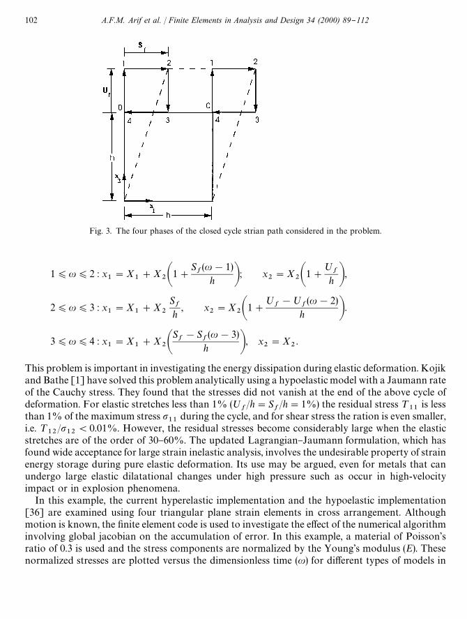
Fig. 3. The four phases of the closed cycle strian path considered in the problem.

1)u)2 : x1"X

1#X

2A1#Sf(u!1)

h B; x2"X

2A1#;

fh B,

2)u)3 : x1"X

1#X

2

Sfh

, x2"X

2A1#;

f!;

f(u!2)

h B.

3)u)4 : x1"X

1#X

2ASf!S

f(u!3)

h B, x2"X

2.

This problem is important in investigating the energy dissipation during elastic deformation. Kojikand Bathe [1] have solved this problem analytically using a hypoelastic model with a Jaumann rateof the Cauchy stress. They found that the stresses did not vanish at the end of the above cycle ofdeformation. For elastic stretches less than 1% (;

f/h"S

f/h"1%) the residual stress ¹

11is less

than 1% of the maximum stress p11

during the cycle, and for shear stress the ration is even smaller,i.e. ¹

12/p

12(0.01%. However, the residual stresses become considerably large when the elastic

stretches are of the order of 30}60%. The updated Lagrangian}Jaumann formulation, which hasfound wide acceptance for large strain inelastic analysis, involves the undesirable property of strainenergy storage during pure elastic deformation. Its use may be argued, even for metals that canundergo large elastic dilatational changes under high pressure such as occur in high-velocityimpact or in explosion phenomena.

In this example, the current hyperelastic implementation and the hypoelastic implementation[36] are examined using four triangular plane strain elements in cross arrangement. Althoughmotion is known, the "nite element code is used to investigate the e!ect of the numerical algorithminvolving global jacobian on the accumulation of error. In this example, a material of Poisson'sratio of 0.3 is used and the stress components are normalized by the Young's modulus (E). Thesenormalized stresses are plotted versus the dimensionless time (u) for di!erent types of models in


Fig. 4. Hypoelastic stress response with ;f/h"S

f/h"1%.

Fig. 5. Hypoelastic stress response for ;f/h"S

f/h"60%.

Fig. 6. Hyperelastic stress response for ;f/h"S

f/h"60% with small steps.

Fig. 7. Hyperelastic stress response for ;f/h"S

f/h"60% with large step size.

Figs. 4}7. Table 3 summarizes for both hypoelastic as well as hyperelastic models the relative errorin the Cauchy stress components (T

ij) at the end of the cycle with respect to the maximum value of

the corresponding stress component (pij) achieved during the cycle. It can be observed that for the

hypoelastic case, very large error occurs (11.7% for ¹22

) for a 60% extension, while for smallextension (for instance, 1% extension) the error is negligible. On the other hand, hyperelastic modeldoes not have undesirable property. The present results agree well with those reported in [1,4].


Table 3Relative error for homogeneous cycle of elastic deformation

Model ;f/h & s

f/h No. of steps Relative error (%)

for each phase¹

11/p

11¹

12/p

12¹

22/p

22¹

33/p

33

Hypoelastic 1% 1 3.3(E-3) 1.4(E-3) 5.0(E-3) 2.56(E-14)60% 1 5.30 2.54 11.7 1.07(E-14)

Hyperelastic 60% 10 2.80(E-28) 5.90(E-28) 4.33(E-13) 3.20(E-28)60% 1 6.00(E-28) 1.20(E-27) 6.40(E-13) 6.76(E-28)

Fig. 8. Load vs displacement curve using nine equal steps for 60% upset. In hyperelastic case deformation continued to67% reduction in height.

This example also demonstrates that the current "nite element implementation for hyperelasticmodel using updated Lagrangian description to solve the incremental displacements "eld preservesthe path-independent character of the hyperelasticity, even at very large steps.

4.2. Elastic}plastic upsetting of an axisymmetric billet

The upsetting problem is solved here with the hyperelastic algorithm, "rst in order to examine itse$ciency of with respect to the hypoelastic algorithm [36] and secondly to evaluate it's perfor-mance as compared to other hyperelastic formulations. This upsetting problem, which has beenproposed as severe test problem [35], is also considered by Simo [40] suing their hyperelasticformulation. Simo [40] achieved 64% upsetting in 120 equal load steps with an average of "veiterations per step using di!erent material properties. With the current procedure, the sameupsetting is attained with a minimum of four equal increments with an average of eight iterations.


Fig. 9. (a) Undeformed mesh of the billet. Due to symmetry, only quarter of this is used for analysis. (b) Deformedcon"guration after 60% upset using nine equal steps. (c) Deformed con"guration after about 67% upset with 10 equalsteps.

Fig. 8 shows the die force plotted against die displacement when 67% reduction of height isachieved in 10 equal steps. This "gure also include the results of the hypoelastic algorithm [36]with nine equal increments to get 60% reduction, and also Ref. [35] solution with 150 equal steps.Although due to symmetry only quarter of the billet is analysed, Fig. 9a}c show the undeformedmesh for the whole billet, the deformed shape after 60% reduction and the deformed mesh after67% upset is achieved in 10 steps, respectively. It can be seen from these "gures that the modeldepicts fold over at the corners and the predicted die forces agree very well with the range for dieforces found by a group of other workers [35] for this problem.


Fig. 10. Load vs displacement curve using four equal steps for 60% upset.

Fig. 11. Deformed shape of the quarter of the billet depicting fold over at corner when the 60% reduction is achieved infour equal steps.

Figs. 10 and 11 shows the load versus displacement curves when 60% upsetting is simulated inonly four equal steps. It is interesting to note that although the die force predicted by the currenthyperelastic model is larger than that of the hypoelastic algorithm [36], the current model depictsthe fold over at the corners more accurately. The hypoelastic model with number of steps less than9, was unable to predict this important phenomenon at the corner of the die and workpieceinterface [36].

5. Concluding remarks

In this paper, a computational procedure of elasto-plasticity employing hyperelastic stress}strain relation and #ow rule emanating from exact kinematics for "nite deformation is presented.The numerical simulations presented demonstrate it's ability to handle very large increments ofloading without losing accuracy and e$ciency, thus, making the proposed hyperelastic extension ofthe algorithm presented in [36] well suited for large-scale computations.

Appendix A. Solution of non-linear scalar equations

A.1. Rate-dependent case

To update the material state for rate-dependent model using the radial return method, one mustimplicity solve scalar equations of step 7 for p8

n`1and s

n`1. Using an iterative process, one can


write these equations for a generic iteration k as

F(k)1"p8 (k)

n`1!p8 53*!-

n`1#3*tGf (p8 (k)

n`1, s(k)

n`1)"0, (A.1)

F(k)2"s(k)

n`1!s

n!*t g(p8 (k)

n`1, s(k)

n`1)"0. (A.2)

The hybrid method presented by Powell [41] has been found to work well for di!erent f andg functions and is brie#y summerized here.

To begin the kth generic iteration we require an initial estimate, which is described at the end ofthis appendix, of the solution vector x(k)"Mp8 (k)

n`1, s(k)

n`1NT, a step-length D(k), and two "xed positive

numbers TOLER and BOUND which govern the conditions for "nishing the iterative process. Thestep length can be changed on each iteration and its purpose is to restrict the length of thecorrection (x(k#1)!x(k)) in order that the iteration decrease the sum of the square of residualsgiven by R(x)"F2

1#F2

2.

TOLER is set to a very small value and the iteration converges if R(x)(TOLER. BOUND isusually set to an over-estimate of the distance from x(1) to the solution in order that the otheralgorithm termination condition is obtained only when x is close to a stationary point (usuallya local minimum) of R(x).

The following steps are followed for a generic iteration k:Step 1. Calculate the Jacobian matrix

J(k)ij,C

LFi

LXjDx/x

(k)

. (A.3)

Step 2. Evaluate the Newton}Raphson correction d(k) by solving the following linear system:

Fi(x(k))#

2+j/1

J(k)ij

d(k)j"0, i"1, 2. (A.4)

Step 3. Evaluate the gradient p(k) of R(x) at x(k) as follows:

p(k)j"C

LR(x)LXjDx/x

(k)

"22+i/1CF

i(x)

LFi(x)

LXjDx/x

(k)

. (A.5)

Step 4. Test if

R(x(k))* (BOUND) DD p(k)DD2

(A.6)

If the above constraint holds, we "nish iterating because of the likelihood that the sequence ofestimates x(k) is converging not to a solution of the equation, but to a local minimum of R(x).

Step 5. If condition (A.6) does not hold, then calculate a correction dM (k) to add to the vector x(k).This correction is just the classical Newton}Raphson correction d(k) if D(k))DDd(k)DD

2. But if

D(k)'DDd(k)DD2

(A.7)

then we make the length of dM (k) equal to D(k). In this case, the correction has the form

dM (k)"!D(k)p(k)/DDp(k)DD2, (A.8)


if it does not go beyond the predicted minimum of R(x) along the steepest descent vector from x(k).This predicted minimum is at the point

x(k)!M1/2DDp(k)DD2/DDJ(k)p(k)DD2Np(k), (A.9)

so we try the condition

D(k))12DDp(k)DD3

2/DDJ(k)p(k)DD2

2. (A.10)

If both conditions (A.7) and (A.8) hold then dM (k) is de"ned by Eq. (A.8). In that case condition (A.7)holds but (A.10) is not satis"ed, we let the point Mx(k)#dM (k)N be on the straight line joining the point(A.9) to the point Mx(k)#d(k)N, the actual components of dM (k) being determined using the extracondition DDdM (k)DD

2"D(k).

Step 6. Now, try the test

R(x(k)#dM (k))(R(x(k)) (A.11)

and if it holds then the iteration de"nes x(k`1)"x(k)#dM (k), and we try the following convergencetest at x(k`1):

R(x(k`1))(TOLER.

However, if condition (A.11) fails we let x(k`1)"x(k) and reduce D(k) as described in the next step.Step 7. To revise the step length determine the sum of the squares of residuals at x(k)#dM (k),

namely

U(k)"2+i/1GFi

(x(k))#2+j/1

J(k)ij

dM (k)j H

2, (A.12)

which is less than R(x(k)). If we "nd that this procedure is so bad that the actual value of R(x)satis"es the inequality

R(x(k)#dM (k))'(1!e)R(x(k))#e/(k), (A.13)

where e is a constant from the open interval (0, 1), then we judge that the linear approximation tothe function F

i(x), derived from the jacobian elements, is not adequate over the length DDdM (k)DD.

Therefore, we reduce D(k) by a factor k. Ref. [41] recommends the values of e and k equal to 0.1 and0.5, respectively. However, if inequality (A.13) fails then we may increase D(k) according to somestrategy.

Rate-independent case: For rate-independent case, we have only one non-linear equation (2.47) asgiven below

H(k)"s(k)n`1

!sn!h(s(k)

n`1)(p8 53*!-

n`1!s(k)

n`1)/3G"0, (A.14a)

ds(k)n`1

"!H(i)NALH

Lsn`1B

(k), (A.14b)

s(k`1)n`1

"s(k)n`1

#ds(k)n`1

. (A.14c)

In order to bound the iterative scheme, bisection or interval halving method is employed togetherwith the Newton}Raphson method.


Initialization technique: With a reasonable initial guess for p8n`1

and sn`1

for rate-dependent caseand p8

n`1for rate-independent case, the iteration loops are rapidly convergent. For rate-indepen-

dent models, a purely elastic initial guess for p8n`1

works e$ciently. However, for the rate-dependent case it proved to be slowly convergent as did an initial guess of zero. The algorithmwhich is used in this work is a forward gradient approximate solution of the governing equations. Ithas been found to be both rapidly convergent and inexpensive. The Taylor series expansions of thefunctions F

1and F

2about the state at t"t

nare

F1(p8

n`1, s

n`1)"F

1(p8

n, s

n)#

LF1

Lp8 Ktn

(p8n`1

!p8n)#

LF1

Ls Ktn

(sn`1

!sn),

F2(p8

n`1, s

n`1)"F

1(p8

n, s

n)#

LF2

Lp8 Ktn

(p8n`1

!p8n)#

LF2

Ls Ktn

(sn`1

!sn).

Solving the pair of equations one can obtain

p8n`1

"p8n#b

2Z/>,

sn`1

"sn#(b

2Z#a

1*tX(p8

n, s

n))/>,

where

Z"p8 53*!-n`1

!p8n!3*tGf (p8

n, s

n), >"b

2a1#a

2b1

with

a1"1#3G*t

LfLp8 K

n

, a2"3G*t

LfLs K

n

.

b1"*t

LfLp8 K

n

, b2"1!*t

LfLs K

n

. (A.15)

The constants a1, a

2, b

1and b

2are evaluated at time t"t

n.

Appendix B. Linearized tangent modulus for hyperelastic model

We de"ne the linearized moduli relating the di!erential change is stress to the di!erential changein the total strain and the incremental strain as follows:

dKM n`1"MM %1[dEM fn`1

], (B.1)

dKM n`1"MK %1[dEMu], (B.2)

The di!erential strain increments are can be written as

dEM fn`1

"4(Ufn`1

#I )~1 dUfn`1

(Ufn`1

#I )~1, (B.3)

dEM fu"4(U

u#I)~1 dU

u(U

u#I)~1. (B.4)

Using Fig. 2 and polar decomposition theorem for Fu

and F%n, we have

(Ufn`1

#I)~1"ReT

n(U

uV %

n#I)~1R%

n(B.5)


with the approximation that

R%T

n"R%

T

n`1Ru.

Substituting Eq. (B.5) in Eq. (B.3) and doing some algebra, we get

dEM fn`1

"R%T

n[4(U

uV%

n#I)~1 dU

uV%

n(U

uV%

n#I)~1]R%

n(B.6)

if V%n"I then Eq. (B.6) reduces to

dEM fn`1

"R%T

ndEM

uR%

n(B.7)

substituting Eq. (B.7) in Eq. (B.1) gives

MK %1"R%T

nMM %1R%

n. (B.8)

Appendix C. Calculation of exp (*tDM 1)

To calculate the exponential of a symmetric tensor the following theorem is used from [39]:

Theorem. If F(j) is a power series that converges for all j, then the matrice power series F(A) can becomputed by the expansion

F(A)"n+i/1

F(ji)G

i, (C.1)

where A is an n-rowed square matrix with n distinct characteristic roots j1, j

2, j

3, j

n, and

G1, G

2, G

3, G

n 2, are n matrices de"ned by

Gi"

+jE1

(jjI!A)

+jE1

(jj!j

i). (C.2)

The above theorem yields

exp(A)"n+i/1

exp(ji)G

i. (C.3)

Now, in our case matrix *tDM 1 has the following form:

*tDM 1"C*tDM 1

11*tDM 1

120

*tDM 112

*tDM 122

0

0 0 *tDM 133D

The exponential of the above matrix for axisymmetric problems can be written as

exp(*tDM 1)"Cexp(B) 0

0 exp(*tDM 133

)D (C.4)


Using Eq. (C.3), the exp (B) is given by

exp(B)"exp(j1)j2

I!Bj2!j

1

#exp(j2)j1

I!Bj1!j

2

, (C.5)

after doing some algebra, we get

exp(B)"CII

c!I

c*tDM 1

11!I

c*tDM 1

12!I

c*tDM 1

12II

c!I

c*tDM 1

22D (C.6)

with

Ic"

exp(j1u1

)j1u2!j1

u1

#

exp(j1u2

)j1u1!j1

u2

, (C.7a)

IIc"

exp(j1u1

)j1u2!j1

u1

j1u2#

exp(j1u2

)j1u1!j1

u2

j1u1

. (C.7b)

Substitution of Eq. (C.6) in (C.4) gives "nal form for the exp (*tDM 1).

References

[1] M. Kojic, K. Bathe, Studies of "nite element procedures * Stress solution of a closed elastic strain path withstretching and shearing using the updated Lagrangian Jaumann formulation, Comput. Stuct. 26 (1987) 175}179.

[2] J.C. Simo, M. Ortiz, A uni"ed approach to "nite deformation elastoplastic analysis based on the use of hyperelasticconstitutive equations, Comput. Methods Appl. Mech. Eng. 49 (1985) 221}245.

[3] B. Moran, M. Ortiz, C.F. Shih, Constitutive and computational aspects of "nite deformation elastoplasticity,Brown University Technical Report, 1987.

[4] G. Weber, L. Anand, Finite deformation constitutive equations and a time integration procedure for isotropic,hyperelastic}viscoplastic solids, Comput. Methods Appl. Mech. Eng. 79 (1990) 173}202.

[5] J.J. Gilman, Progress in the microdynamical theory of plasticity, Proceedings of the Fifth National Congress ofApplied Mechanics, ASME, New York, pp. 385}403.

[6] E.T. Onat, Recent Advances in Creep and Fracture of Engineering Materials and Structures, Pineridge Press,Swansea U.K, 1982 (Chapter 5).

[7] B. Loret, On the e!ects of plastic rotation in the "nite deformation of anisotropic elastoplastic materials, Mech.Mater. 2 (1983) 287}304.

[8] Y.F. Dafalias, The plastic spin, J, Appl. Mech. 52 (1985) 865}873.[9] L. Anand, Consitutive equations for hot working of metals, Int. J. Plasticity 1 (1985) 213}231.

[10] A. Agah-Tehrani, E.H. Lee, R.L. Mallet, E.T. Onat, The theory of elastic-plastic deformation at "nite strain withinduced anisotropy modelled as combined isotropic-kinematic hardening, J. Mech. Phys. Solids 35 (1987) 519}539.

[11] E.H. Lee, Elastic-plastic deformation at "nite strains, J. Appl. Mech. 36 (1969) 1}6.[12] A.E. Green, P.M. Naghdi, Some remarks on elastic-plastic deformation at "nite strain, Int. J. Eng. Sci. 9 (1971)

1219}1229.[13] R. Hill, J.R. Rice, Constitutive analysis of elastic-plastic crystals at arbitrary strain, J. Mech. Phys. Solids 20 (1972)

401}413.[14] R.J. Asaro, Micromechanics of crystals and polycrystals, Adv. Appl. Mech. 23 (1983) 1}115.[15] K.S. Havner, The theory of "nite plastic deformation of crystalline solids, in: H.G. Hopkins, M.J. Sewell (Eds.),

Pergamon Press, Oxford, 1982, pp. 262}302.[16] M.C. Boyce, G.C. Weber, D.M. Parks, On the kinematics of "nite strain plasticity, J. Mech. Phys. Solids 37 (1989)

647}665.


[17] D.R.J. Owen, E. Hinton, Finite Element in Plasticity: Theory and Practice, Pineridge Press, Swansea, UK, 1986.[18] R.D. Krieg, B.D. Krieg, Accuracies of numerical solution methods for the elastic-perfectly plastic model, J. Press.

Vessel Technol. 99 (1977) 510}515.[19] H.L. Schreyer, R.F. Kulak, J.M. Kramer, Accurate numerical solutions for elastic-plastic models, J. Press. Vessels

Technol. 101 (1979) 226}234.[20] M.A. Cris"eld, A fast incremental iterative solution procedure that handles snap-through, Comput. Struct. 13

(1981) 55}62.[21] C. Nyssen, An e!ective and accurate iterative method allowing large incremental steps to solve elastic-plastic

problem, Comput. Struct. 13 (1981) 63}71.[22] T.J.R. Hughes, J. Winget, Finite rotation e!ects in numerical integration of rate constitutive equations arising in

large-deformation analysis, Int. J. Numer. Methods Eng. 15 (1980) 1862}1867.[23] R. Rubenstein, S.N. Atluri, Objectivity of incremental constitutive relations over "nite time steps in computational

"nite deformation analysis, Comput. Methods Appl. Mech. Eng. 36 (1983) 277}290.[24] K.W. Reed, S.N. Atluri, Constitutive modelling and computational implementation for "nite strain plasticity, Int. J.

Plasticity 1 (1985) 63}87.[25] J.C. Nagtegaal, F.E. Veldpaus, On the implementation of "nite strain plasticity equations in a numerical model, in:

J.F.T. Pittman, O.C. Zienkiewicz, R.D. Wood, J.M. Alexander (Eds.), Numerical Analysis of Forming Processes,Wiley, New York, 1984, pp. 351}371.

[26] T.J.R. Hughes, Numerical implementation of constitutive models: rate independent deviatoric plasticity, in: S.Nemat-Nasser, R.J. Asaro, G.A. Hegemier (Eds.), Theoretical Foundation for Large-Scale Computations ofNonlinear Material Behaviour, 1984, pp. 29}57.

[27] J.C. Nagtegaal, N. Rebelo, On the development of a general purpose "nite element program for analysis of formingprocesses, in: K. Mattiason et al. (Eds.), Proceedings of the second International Conference on Numerical methodsin Industrial Forming Processes, NUMIFORM'86, 1986, pp. 41}49.

[28] G. Weber, A.M. Lush, L. Anand, A time integration procedure for a set of uni"ed elasto-viscoplastic constitutiveequation, Proceedings of International Conference on Computational Engineering Science, Atlanta, 1988.

[29] A.M. Lush, G. Weber, L. Anand, An implicit time integration procedure for a set of internal variable constitutiveequations for isotropic elastoviscoplasticity, Int. J. Plasticity 5 (1989) 521}549.

[30] K. Runnesson, L. Bernspang, K. Mattiason, Implicit integration in plasticity, in: Taylor et al. (Eds.), NumericalMethods for Nonlinear Problems, Vol. 3, Dubrovnik, 1986.

[31] J.W. Hutchison, Finite strain analysis of elastic-plastic solids and structures, in: Hartung (Ed.), Numer. Sol. ofNonlinear Struc. Problems, ADM-6, ASME, New York 1973, pp. 17}25.

[32] N.M. Wang, B. Budiansky, Analysis of sheet metal stamping by a "nite element method, J. Appl. Mech. 45 (1978)73}82.

[33] P.M. Pinsky, M. Ortiz, K.S. Pister, Numerical integration of rate constitutive equations in "nite deformationanalysis, Comput. Methods Appl. Mech. Eng. 40 (1983) 137}158.

[34] N. Zabaras, A.F.M. Arif, A family of integration algorithms for constitutive equations in "nite deformationelasto-viscoplasticity, Int. J. Numer. Methods Eng. 33 (1992) 59}84.

[35] L.M. Taylor, E.B. Becker, Some computational aspects of large deformation, rate-dependent plasticity problems,Comput. Methods. Appl. Mech. Eng. 41 (1983) 251}277.

[36] A.F.M. Arif, N. Zabaras, On the performance of two tangent operators for "nite element analysis of largedeformation inelastic problems, Int. J. Numer. Methods Eng. 35 (1992) 369}389.

[37] L. Anand, H. On, Hencky's approximate strain-energy function for moderate deformation, ASME J. Appl. Mech.46 (1979) 78}82.

[38] G. Weber, Computational procedures for some new rate constitutive equations for elasto-plasticity, Ph.D Thesis,MIT, 1988.

[39] A.D. Michal, Matrix and Tensor Calculus with Applications to Mechanics, Elasticity and Aeronautics, Wiley, New York.[40] J.C. Simo, A framework for "nite strain elastoplasticity based on maximum plastic dissipation and multiplicative

decomposition. Part II: computational aspects, Comput. Methods Appl. Mech. Eng. 68 (1988) 1}31.[41] M.J.D. Powell, A hybrid method for non-linear equations in: P. Rabinowitz (Ed.), Numerical methods for

non-linear algebraic equations, Gordon and Breach Sc. Pub., London, 1970, pp. 87}114.


Performance of a finite element procedure for hyperelastic–viscoplastic large deformation problems

Documents

Transcript of Performance of a finite element procedure for hyperelastic–viscoplastic large deformation problems