Performance and Policy Evaluation of Solar Energy Technologies for Domestic Application in Ireland

Dublin Institute of TechnologyARROW@DIT

Doctoral Engineering

2011-5

Performance and Policy Evaluation of Solar EnergyTechnologies for Domestic Application in IrelandLacour Ayompe (Thesis)Dublin Institute of Technology

Follow this and additional works at: http://arrow.dit.ie/engdoc

Part of the Civil and Environmental Engineering Commons

This Theses, Ph.D is brought to you for free and open access by theEngineering at ARROW@DIT. It has been accepted for inclusion inDoctoral by an authorized administrator of ARROW@DIT. For moreinformation, please contact [email protected], [email protected].

This work is licensed under a Creative Commons Attribution-Noncommercial-Share Alike 3.0 License

Recommended CitationAyompe, L.: Performance and Policy Evaluation of Solar Energy Technologies for Domestic Application in Ireland. Doctoral Thesis.Dublin Institute of Technology, 2011.

http://arrow.dit.ie?utm_source=arrow.dit.ie%2Fengdoc%2F37&utm_medium=PDF&utm_campaign=PDFCoverPages

http://arrow.dit.ie/engdoc?utm_source=arrow.dit.ie%2Fengdoc%2F37&utm_medium=PDF&utm_campaign=PDFCoverPages

http://arrow.dit.ie/engthe?utm_source=arrow.dit.ie%2Fengdoc%2F37&utm_medium=PDF&utm_campaign=PDFCoverPages

http://arrow.dit.ie/engdoc?utm_source=arrow.dit.ie%2Fengdoc%2F37&utm_medium=PDF&utm_campaign=PDFCoverPages

http://network.bepress.com/hgg/discipline/251?utm_source=arrow.dit.ie%2Fengdoc%2F37&utm_medium=PDF&utm_campaign=PDFCoverPages

mailto:[email protected],%[email protected]

http://creativecommons.org/licenses/by-nc-sa/3.0/




Performance and Policy Evaluation of Solar Energy Technologies for Domestic

Lacour Mody AYOMPESchool of Civil and Building Services

Dublin Institute of Technology, Bolton Street,

The thesis is submitted in fulfilment of the requirements for the degree of

Supervisors: Dr. A. Duffy (Dublin Institute of TechnologyDr. S. McCormack (Trinity College, Dublin)Dr. M. Conlon (Dublin Institute of

1


Application in Ireland

Lacour Mody AYOMPE (B.Engr, M.Engr., MSc)

School of Civil and Building Services EngineeringDublin Institute of Technology, Bolton Street, Ireland

The thesis is submitted in fulfilment of the requirements for the degree ofDoctor of Philosophy

Dublin Institute of Technology)

(Trinity College, Dublin) Dublin Institute of Technology)

May 2011 �

�


(B.Engr, M.Engr., MSc) Engineering

Ireland

The thesis is submitted in fulfilment of the requirements for the degree of

ii

DECLARATION PAGE

I certify that this thesis which I now submit for examination for the award of PhD, is

entirely my own work and has not been taken from the work of others, save and to the

extent that such work has been cited and acknowledged within the text of my work

This thesis was prepared according to the regulations for postgraduate study by research

of the Dublin Institute of Technology and has not been submitted in whole or in part for

another award in any Institute.

The work reported on in this thesis conforms to the principles and requirements of the

Institute's guidelines for ethics in research.

The Institute has permission to keep, lend or copy this thesis in whole or in part, on

condition that any such use of the material of the thesis be duly acknowledged.

Signature ________________________________Date ___________________

��

iii

ACKNOWLEDGEMENT

My sincere thanks go to my thesis supervisors Dr. A. Duffy, Dr. S.J.

McCormack and Dr. M. Conlon for their excellent guidance and unquantifiable

contributions to the completion of this project. I remain grateful to Dr. M. Mc

Keever for his support in designing and setting up the automated component of the

solar water heating system rigs. My thanks also go to J. Turner, Head of the School of

Civil and Building Services Engineering; J. Kindregan, Head of the Department of Civil

and Structural Engineering; Dr. M. Rebow for all the useful advice I received from

him; and all the researchers at Dublin Energy Lab.

I appreciate the kind contributions and support from my colleagues Dr. A.

Acquaye, F. McLoughlin, N. Shams, Dr. B. Cullen, K. O’Toole, D. Callaghan, M.

Wylie and C. Carey. I am also grateful to C. Byrne of Glas Renewable Energy Saving

Solutions for setting up the solar water heating systems.

I am thankful to my darling wife Emilia for her continued love and support

throughout the course of this project. I am also thankful to my daughter Maxmine

and mother in-law Monica for their love and encouragement. I am thankful to God

our creator for my wonderful parents Mr. and Mrs. G.T. Ayompe who have always

had a firm commitment in providing my basic needs since birth. I also appreciate the

continued moral and financial assistance provided by my brother Johnson, sister

Eyindo and her husband Kemajou. I am also appreciative of the care and love from

my nice Tanesha and cousins Ayompe Ayompe and Michael Njang. Many thanks to

the members of the Northern Virginia prayer cell of Omega Gospel Mission, USA

for their continuous prayers and MECA Dublin members.

All glory and honour goes to the Lord Almighty, our God (the best Engineer

and only perfect Designer) for offering me this unique scholarship opportunity and

also for keeping me alive and making good things possible in my life.

iv

TABLE OF CONTENTS

DECLARATION PAGE ................................................................................................... ii�

ACKNOWLEDGEMENT ............................................................................................... iii�

TABLE OF CONTENTS ................................................................................................. iv�

LIST OF FIGURES ....................................................................................................... xvi�

LIST OF TABLES ....................................................................................................... xxiii�

LIST OF ABBREVIATIONS ....................................................................................... xxx�

NOMENCLATURE .................................................................................................... xxxii�

GLOSSARY ................................................................................................................ xxxv�

ABSTRACT ............................................................................................................... xxxix�

CHAPTER 1: INTRODUCTION ..................................................................................... 1�

1.1� Background ............................................................................................................ 1�

1.2� Research Justification............................................................................................. 4�

1.2.1� Photovoltaics ................................................................................................... 5�

1.2.2� Solar Water Heaters ........................................................................................ 7�

1.3� Research Aim ....................................................................................................... 10�

1.4� Research Objectives ............................................................................................. 10�

1.5� Research Methodology......................................................................................... 11�

1.6� Contributions to Knowledge ................................................................................ 13�

1.7� Thesis structure .................................................................................................... 14�

v

1.8� Energy in Ireland .................................................................................................. 15�

1.9� Residential sector ................................................................................................. 17�

1.9.1� Energy Use .................................................................................................... 17�

1.9.2� Greenhouse Gas Emissions ........................................................................... 19�

1.10� Renewable Energy Sources (RES) ....................................................................... 19�

1.10.1� The Case for RES ......................................................................................... 20�

1.10.2� Micro-generation .......................................................................................... 21�

1.11� Irish Policies ......................................................................................................... 24�

1.11.1� Irish PV Support ........................................................................................... 25�

1.11.2� Irish Solar Thermal Support ......................................................................... 26�

CHAPTER 2: REVIEW OF PHOTOVOLTAIC SYSTEMS ......................................... 29�

2.1� Background .......................................................................................................... 29�

2.2� PV Benefits .......................................................................................................... 31�

2.3� PV History and Development .............................................................................. 33�

2.4� PV System ............................................................................................................ 35�

2.4.1� PV System Classification.............................................................................. 37�

2.4.2� PV Systems ................................................................................................... 37�

2.4.2.1� Grid-connected PV System ................................................................... 38�

2.5� Technology Status ................................................................................................ 41�

2.5.1� Crystalline Silicon......................................................................................... 41�

2.5.2� Thin Films ..................................................................................................... 42�

vi

2.6� Industry Trends .................................................................................................... 43�

2.7� Production Trends ................................................................................................ 43�

2.7.1� Solar Grade Silicon ....................................................................................... 44�

2.9� Global PV Market ................................................................................................ 45�

2.8� Performance Studies............................................................................................. 47�

2.8.1� Performance Evaluation and Assessments ................................................... 47�

2.8.2� PV Performance Prediction .......................................................................... 50�

2.8.3� PV Temperature ............................................................................................ 51�

2.8.4� Effect of Low Insolation ............................................................................... 53�

2.9� Summary .............................................................................................................. 54�

CHAPTER 3: FIELD TRIALS AND PERFORMANCE ANALYSIS .......................... 55�

3.1� PV System Sizing ................................................................................................. 56�

3.2� PV System Description ........................................................................................ 59�

3.3� Monitoring and Data Acquisition......................................................................... 61�

3.4� PV System Terminologies ................................................................................... 62�

Normal Operating Cell Temperature (NOCT) ............................................................ 62�

Standard Test Conditions (STC) ................................................................................. 62�

Standard Operating Conditions (SOC) ........................................................................ 63�

Fill Factor (FF) ............................................................................................................ 63�

Pack Factor .................................................................................................................. 64�

3.5� Monitoring Results ............................................................................................... 64�

vii

3.5.1� Weather Data ................................................................................................ 65�

3.5.2� PV Module Temperature .............................................................................. 68�

3.6� Energy Performance Analysis .............................................................................. 68�

3.6.1� Energy Output ............................................................................................... 69�

3.6.2� Array Yield ................................................................................................... 72�

3.6.3� Final Yield .................................................................................................... 73�

3.6.4� Reference Yield ............................................................................................ 74�

3.6.5� PV Module Efficiency .................................................................................. 75�

3.6.6� System Efficiency ......................................................................................... 75�

3.6.7� Inverter Efficiency ........................................................................................ 76�

3.6.8� Performance Ratio ........................................................................................ 79�

3.6.9� Capacity Factor ............................................................................................. 81�

3.6.10� Energy Losses ............................................................................................... 81�

Array Capture Losses............................................................................................... 83�

System Losses .......................................................................................................... 83�

Cell Temperature Losses ......................................................................................... 84�

3.6.11� Seasonal Performance ................................................................................... 85�

3.7� Comparative PV System Performance ................................................................. 88�

3.8� Summary .............................................................................................................. 90�

viii

CHAPTER 4: ENERGY PERFORMANCE MODELING OF�

GRID-CONNECTED PV SYSTEMS ............................................................................ 91�

4.1� Introduction .......................................................................................................... 91�

4.2� Lumped Modelling of PV System Energy Output ............................................... 93�

4.2.1� PV Array Energy Output .............................................................................. 93�

4.2.2� PV System Energy Output ............................................................................ 94�

4.3� Dynamic Modelling of PV System Energy Output.............................................. 99�

4.3.1� PV Cell Temperature .................................................................................... 99�

4.3.1.1� Explicit Correlations ............................................................................ 100�

4.3.1.2� Steady-State Analysis .......................................................................... 101�

4.3.1.3� Heat Transfer Coefficients .................................................................. 102�

4.3.2� PV Cell and Module Efficiency .................................................................. 103�

4.3.3� PV Array Power Output .............................................................................. 105�

4.3.4� Inverter Efficiency ...................................................................................... 106�

4.3.5� PV System Power Output ........................................................................... 107�

4.4� Proposed PV Energy Output Model ................................................................... 107�

4.4.1� Model Validation ........................................................................................ 107�

4.4.2� PV Cell Temperature .................................................................................. 108�

4.4.3� PV Array Output Power .............................................................................. 109�

4.4.4� PV System AC Output Power ..................................................................... 110�

4.5� Summary ............................................................................................................ 112�

ix

CHAPTER 5: REVIEW OF SOLAR WATER HEATING SYSTEMS ....................... 113�

5.1� Introduction ........................................................................................................ 113�

5.2� Solar Water Heating Systems............................................................................. 114�

5.3� Solar Energy Collectors ..................................................................................... 118�

5.3.1� Flat Plate Collectors .................................................................................... 119�

5.3.1.1� Glazing Materials ................................................................................ 121�

5.3.1.2� Absorbing Plates .................................................................................. 121�

5.3.2� Heat pipe evacuated tube collectors............................................................ 122�

5.5� Energy Performance Analysis ............................................................................ 124�

5.5.1� Useful Heat Gain ........................................................................................ 124�

5.5.2� Efficiency .................................................................................................... 125�

5.5.3� Optical Analysis .......................................................................................... 127�

5.5.3.1� Incidence Angle Modifier.................................................................... 128�

5.5.4� Daily Performance ...................................................................................... 129�

5.5.6� Performance of Heat Pipe Collectors .......................................................... 129�

5.6� Modelling ........................................................................................................... 131�

5.6.1� Optimization of SWH Systems ................................................................... 133�

5.7� Summary ............................................................................................................ 133�

CHAPTER 6: FIELD TRIALS AND PERFORMANCE ANALYSIS OF SOLAR

WATER HEATING SYSTEMS ................................................................................... 135�

6.1� Introduction ........................................................................................................ 135�

6.2� Methodology ...................................................................................................... 136�

x

6.3� System Description ............................................................................................ 137�

6.3.4� Hot Water Demand Profile ......................................................................... 138�

6.3.5� Auxiliary Heating and Hot Water Demand Management System .............. 138�

6.3.6� Data Measurement and Logging ................................................................. 140�

6.4� Energy Performance Analysis ............................................................................ 141�

6.4.1� Energy Collected......................................................................................... 141�

6.4.2� Energy Delivered and Supply Pipe Losses ................................................. 142�

6.4.3� Solar Fraction .............................................................................................. 142�

6.4.4� Collector Efficiency .................................................................................... 143�

6.4.5� System Efficiency ....................................................................................... 143�

6.5� Results and Discussions ..................................................................................... 143�

6.5.1� Energy Collected......................................................................................... 143�

6.5.2� Energy Delivered and Supply Pipe Losses ................................................. 145�

6.5.3� Energy Extracted and Auxiliary Energy ..................................................... 145�

6.5.5� Collector and System Efficiency ................................................................ 147�

6.5.6� System Temperatures .................................................................................. 147�

6.5.7� Daily Performance ...................................................................................... 150�

6.5.7.1� Environmental/Ambient Conditions .................................................... 150�

6.5.7.2� Solar Fluid Mass Flow Rate ................................................................ 151�

6.5.7.3� Energy Collected ................................................................................. 152�

6.5.7.4� System Temperatures .......................................................................... 154�

xi

6.5.7.5� Collector Efficiency ............................................................................ 157�

6.5.8� Seasonal Performance ................................................................................. 158�

6.6� Summary ............................................................................................................ 159�

CHAPTER 7: MODELLING SOLAR WATER HEATING SYSTEMS..................... 163�

7.1� Modelling ........................................................................................................... 163�

7.1.1� TRNSYS Model .......................................................................................... 163�

7.1.2� Weather Data .............................................................................................. 166�

7.1.3� Mass Flow Rate .......................................................................................... 167�

7.2� Results and Discussions ..................................................................................... 168�

7.2.1� Collector Outlet Temperature ..................................................................... 168�

7.2.2� Heat Collected............................................................................................. 169�

7.2.3� Heat Delivered to Load ............................................................................... 171�

7.3� Summary ............................................................................................................ 173�

CHAPTER 8: ECONOMIC AND ENVIRONMENTAL ANALYSIS OF GRID-

CONNECTED PV SYSTEMS ..................................................................................... 174�

8.1� Introduction ........................................................................................................ 174�

8.2� Investment Appraisal ......................................................................................... 175�

8.2.1� Simple Payback Period ............................................................................... 176�

8.2.2� Net Present Value ....................................................................................... 177�

8.2.3� Internal Rate of Return ............................................................................... 178�

8.3� Levelised Cost .................................................................................................... 178�

8.4� Economic and Environmental Scenarios ........................................................... 179�

xii

8.4.1� EU Energy Trends ...................................................................................... 179�

Baseline Scenario ................................................................................................... 179�

Reference Scenario ................................................................................................ 179�

8.4.2� International Oil Markets ............................................................................ 180�

8.5� Technology Learning Rates and Market Scenarios ........................................... 181�

8.5.1� PV Market Growth and Learning Rate ....................................................... 182�

Advanced Scenario ................................................................................................ 183�

Moderate Scenario ................................................................................................. 184�

8.6� PV System Costs ................................................................................................ 186�

8.6.1� Current Cost of Photovoltaic Systems ........................................................ 186�

8.6.2� Projected Cost ............................................................................................. 189�

8.7� Levelised Cost of Electricity .............................................................................. 190�

8.7.1� PV Generated Electricity ............................................................................ 192�

8.8� Domestic Electricity ........................................................................................... 193�

8.8.1� End-user Categories .................................................................................... 193�

8.8.2� Housing profile ........................................................................................... 193�

8.8.3� Domestic Electricity Demand Profiles ....................................................... 194�

8.8.4� Matching PV Electricity Generation and Domestic Electricity Profiles .... 197�

8.8.5� Domestic Sector Electricity Prices ............................................................. 199�

8.9� Wholesale Electricity Prices .............................................................................. 203�

8.10� Grid Parity Analysis ........................................................................................... 205�

xiii

8.11� Economic Viability Assessment ........................................................................ 208�

8.11.1� System (Final) Yield ................................................................................... 208�

8.11.2� Revenue ...................................................................................................... 208�



8.12� Emission Analysis .............................................................................................. 213�

8.12.1� All-Island Fuel-Mix 2009 ........................................................................... 213�

8.12.2� CO2 Intensity of Power Generation ............................................................ 214�

8.12.3� Life Cycle Emission Savings ...................................................................... 215�

8.13� FIT Design for Ireland ....................................................................................... 216�

8.14� Sensitivity Analysis on PV systems ................................................................... 221�

8.14.1� Effect of Discount Rate on FIT................................................................... 221�

8.14.2� Effect of FIT on NPV ................................................................................. 221�

8.14.3� Effect of FIT on SPP ................................................................................... 222�

8.15� PV System Marginal Abatement Costs .............................................................. 224�

8.13� Summary ............................................................................................................ 228�

CHAPTER 9: ECONOMIC AND ENVIRONMENTAL ANALYSIS OF SOLAR


9.0� Overview ............................................................................................................ 230�

9.1� Technology Learning Rates and Market Growth ............................................... 231�

Moderate Scenario ..................................................................................................... 232�

Advanced scenario .................................................................................................... 232�

xiv

9.2� Solar Water Heating System Cost ...................................................................... 233�

9.2.1� Projected SWHS Cost ................................................................................. 235�

9.3� Fuel Prices .......................................................................................................... 236�

9.4� Economic Viability Assessment ........................................................................ 237�

9.4.1� System Yield ............................................................................................... 237�

9.4.2� Revenue ...................................................................................................... 237�



9.4.5� Levelised Heating Cost ............................................................................... 241�

9.5� Emission Analysis .............................................................................................. 243�

9.5.1� Life Cycle Emission Savings ...................................................................... 243�

9.6� SWHS Marginal Abatement Costs .................................................................... 244�

9.7� Conclusion ......................................................................................................... 245�

CHAPTER 10: POLICY ANALYSIS OF GRID-CONNECTED PV AND SOLAR


10.1� Overview ............................................................................................................ 248�

10.2� European Policy Context.................................................................................... 249�

10.3� Global Solar Thermal Support Schemes ............................................................ 251�

10.4� PV Financial Support Schemes .......................................................................... 253�

10.4.1� Direct Capital Subsidies.............................................................................. 255�

10.4.2� Tax Credits .................................................................................................. 255�

10.4.3� Renewable Portfolio Standards (RPS) and Renewable Obligation (RO) ... 256�

xv

10.4.4� Net Metering ............................................................................................... 257�

10.4.5� Renewable Energy Certificates (RECs) ...................................................... 257�

10.4.6� Feed-in Tariff .............................................................................................. 258�

10.4.7� Carbon Tax ................................................................................................. 260�

10.4.8� Feed-in Tariffs in Different Countries ........................................................ 260�

10.5� Policy Findings .................................................................................................. 264�

10.6� Conclusion ......................................................................................................... 267�

CHAPTER 11: CONCLUSIONS AND RECOMMENDATIONS .............................. 268�

11.1� Conclusions ........................................................................................................ 268�

11.2� Policy Recommendations ................................................................................... 273�

11.3� Recommendations for Further Research ............................................................ 275�

REFERENCES .............................................................................................................. 277�

APPENDICES .............................................................................................................. 298�

LIST OF PUBLICATIONS .......................................................................................... 340�

xvi

LIST OF FIGURES

Figure 1.1: Solar energy use in domestic dwellings ......................................................... 4�

Figure 1.2: Annual installed and cumulative capacity of solar thermal systems in Ireland

........................................................................................................................................... 8�

Figure 1.3: Annual installation of solar thermal systems under the GHS ......................... 9�

Figure 1.4: All-Island fuel-mix 2009 .............................................................................. 16�

Figure 1.5: Share of fuels in residential energy use in 2007 ........................................... 18�

Figure 1.6: Annual ST market, capacity in operation and ST support policies in Ireland

(2001 to 2009) ................................................................................................................. 27�

Figure 1.7: Number of renewable heating systems installed under the GHS from 2006 to

2010 ................................................................................................................................. 28�

Figure 2.1: Composition of a PV array ........................................................................... 36�

Figure 2.3: The world of PV applications ....................................................................... 38�

Figure 2.4: Grid-connected photovoltaic system ............................................................ 39�

Figure 2.5: Yearly worldwide production of PV ............................................................ 44�

Figure 2.6: Historical development of cumulative installed global and EU PV capacity

......................................................................................................................................... 46�

Figure 3.1: The PV System Installation .......................................................................... 60�

Figure 3.2: Sunny WebBox, power injector and analog electricity meter ...................... 61�

Figure 3.3: Monthly average long-term in-plane average for Dublin airport [104],

measured average daily total in-plane solar insolation, wind speed ............................... 66�

Figure 3.4: Monthly average daily ambient air and PV module temperature over the

monitored period ............................................................................................................. 66�

Figure 3.5: Monthly total energy generated over the monitored period ......................... 70�

xvii

Figure 3.6: DC power output with solar radiation .......................................................... 71�

Figure 3.7: AC power output with solar radiation .......................................................... 72�

Figure 3.8: Monthly average daily PV system’s final yield, reference yield and array

yield over the monitoring period ..................................................................................... 75�

Figure 3.9: Monthly average daily PV module, system and inverter efficiencies .......... 77�

over the monitoring period .............................................................................................. 77�

Figure 3.10: Daily variation of PV module and inverter efficiencies ............................. 78�

Figure 3.11: Average inverter efficiency at different levels of solar radiation over the

monitoring period ............................................................................................................ 79�

Figure 3.12: Average PV module efficiency at different levels of solar radiation over the


Figure 3.13: Monthly average daily performance ratio and capacity factor over the


Figure 3.14: Monthly daily average capture, system and temperature losses over the

monitored period ............................................................................................................. 86�

Figure 4.1: Representative daily domestic scale PV system electricity generation and

demand ............................................................................................................................ 93�

Figure 4.2: Predicted and measured PV system energy output ....................................... 97�

Figure 4.3: Measured and modelled PV cell temperature ............................................. 108�

Figure 4.4: Measured and modelled PV array maximum DC power output ................ 110�

Figure 4.5: Measured and modelled PV system maximum AC power output ............. 111�

Figure 5.1: Classification of solar thermal systems ...................................................... 116�

Figure 5.2: Schematic diagram of an electricity boosted solar hot water system ......... 117�

Figure 5.3: Schematic diagram of a flat plate collector ................................................ 119�

Figure 5.4: Components of a flat plate collector ........................................................... 120�

xviii

Figure 5.5: Schematic diagram of a heat pipe evacuated tube collector ....................... 122�

Figure 5.6: Schematic diagram of a heat pipe with wick .............................................. 123�

Figure 5.7: Collector efficiency of various types of liquid collectors........................... 128�

Figure 6.1: Volume of hot water (60 oC) draw-off at different times of the day [150] 136�

Figure 6.2: Schematic diagram of the FPC and ETC systems ...................................... 139�

Figure 6.3: Evacuated tube and flat plate collectors ..................................................... 140�

Figure 6.4: In-door installation of the experimental rig ................................................ 140�

Figure 6.5: In-plane global solar radiation for three characteristic days....................... 151�

Figure 6.6: Ambient air temperature and wind speed for three characteristic days ...... 151�

Figure 6.7: Solar fluid mass flow rate for FPC ............................................................. 152�

Figure 6.8: Solar fluid mass flow rate for the ETC system ........................................... 153�

Figure 6.9: Energy collected by the FPC system .......................................................... 153�

Figure 6.10: Energy collected by the ETC system ........................................................ 154�

Figure 6.11: Collector outlet fluid temperature for the FPC and ETC systems ............ 155�

Figure 6.12: Hot water tank outlet temperature for the FPC and ETC systems............ 156�

Figure 6.13: Hot water tank bottom (T2) and middle (T3) temperatures for the FPC

system ............................................................................................................................ 157�

Figure 6.14: Hot water tank bottom (T2) and middle (T3) temperatures for the ETC

system ............................................................................................................................ 157�

Figure 6.15: Hourly global in-plane solar radiation, FPC and ETC efficiencies .......... 158�

Table 6.7: Seasonal values of solar insolation, energy collected, energy delivered,

supply pipe losses and energy collected per unit area for the FPC and ETC systems .. 160�

Table 6.8: Seasonal average daily collector and system efficiencies, energy extracted

and auxiliary energy for the FPC and ETC systems ..................................................... 161�

xix

Figure 7.1: TRNSYS information flow diagram for the forced circulation solar water

heating systems ............................................................................................................. 164�

Figure 7.2: Solar radiation, wind speed and ambient air temperature .......................... 167�

Figure 7.3: Solar fluid mass flow rate for the FPC and ETC systems .......................... 167�

Figure 7.4: Measured and modelled collector outlet temperature for FPC system ....... 169�

Figure 7.5: Measured and modelled collector outlet temperature for ETC system ...... 169�

Figure 7.6: Measured and predicted heat collected by the FPC system ....................... 170�

Figure 7.7: Measured and modelled heat collected by the ETC system ....................... 170�

Figure 7.8: Measured and modelled heat delivered to load by FPC system ................. 171�

Figure 7.9: Measured and modelled heat delivered to load by ETC system ................ 172�

Figure 8.1: Annual installed capacity projections for the advanced ............................. 183�

scenario 2008-2030 [13] .............................................................................................. 183�

Figure 8.2: Annual installed capacity projections for the moderate ............................. 184�

scenario 2008-2030 [13] .............................................................................................. 184�

Figure 8.3: PV learning rate and global market growth scenarios ................................ 185�

Figure 8.4: Average PV system, PV array and BOS cost for different PV system

capacities ....................................................................................................................... 187�

Figure 8.5: Normalised PV module cost band and PV module annual installed capacity

under different scenarios ............................................................................................... 189�

Figure 8.6: Average normalised life cycle cost for different PV system sizes from 2010

to 2030 ........................................................................................................................... 190�

Figure 8.7: Average electricity generation cost for different PV system sizes ............. 193�

(2010-2030) ................................................................................................................... 193�

Figure 8.8: Frequency distribution of average annual electricity demand for the sampled

households [174] ........................................................................................................... 195�

xx

Figure 8.9: Average weekly summer electricity demand profiles (13-19 July, 2009)

[174] .............................................................................................................................. 196�

Figure 8.10: Average weekly winter electricity demand profiles ................................. 196�

(14-20 December, 2009) [174] ...................................................................................... 196�

Figure 8.11: Average daily electricity demand [174] and electricity generation by

different PV systems ..................................................................................................... 197�

Figure 8.12: Percentage on-site household electricity use against average annual

electricity demand ......................................................................................................... 199�

Figure 8.13: Historic household electricity prices were obtained from the EU

Commission’s energy portal ......................................................................................... 200�

Figure 8.14: Historic and projected nominal household electricity prices (band DC) in

Ireland ........................................................................................................................... 201�

Figure 8.15: Natural gas, crude oil and electricity prices from 1996 to 2009............... 205�

Figure 8.16: Household, PV generated and BNE electricity price projections from 2010

to 2030 in Ireland .......................................................................................................... 206�

Figure 8.17: Average PV generation and household electricity cost from 2010 to 2030

for different PV sizes .................................................................................................... 207�

Figure 8.18: Frequency distribution of simple payback periods for different PV systems

installed by ESBCS customers in 2010. ........................................................................ 212�

Figure 8.19: Simple payback periods for different PV systems installed by non-ESBCS

customers in 2010 ......................................................................................................... 212�

Figure 8.20: All-Island fuel-mix 2009 .......................................................................... 213�

Figure 8.21: Fuel mix for electricity generation in Ireland (2005-2009) [162] ............ 214�

Figure 8.22: Carbon intensity of power generation under the baseline and reference

scenario (tCO2/MWh) ................................................................................................... 215�

xxi

Figure 8.23: PV system life cycle CO2 emission savings for different years of

installation ..................................................................................................................... 216�

Figure 8.24: Cumulative frequency of NPV for different PV system sizes and

recommended FIT to achieve 8% IRR and at least 50% market penetration ............... 218�

Figure 8.25: Required FITs for different PV system sizes against year of installation 219�

Figure 8.26: Feed-in tariff for different PV system capacities and year of installation 220�

Figure 8.27: Cumulative frequency distribution of SPPs for different PV systems using

FITs that target 50% market penetration in 2011.......................................................... 220�

Figure 8.28: Required FIT for different PV system capacities for 6-10% discount rates

in 2011 ........................................................................................................................... 221�

Figure 8.29: Cumulative frequency of NPVs for different PV system capacities in 2011

(0.31 �/kWh FIT) .......................................................................................................... 222�

Figure 8.30: Cumulative frequency of NPVs for different PV system capacities in 2011

(0.45 �/kWh FIT) .......................................................................................................... 223�

Figure 10.10: Cumulative frequency of SPPs for different PV system capacities in 2011

(0.31 kWp FIT) .............................................................................................................. 223�

Figure 8.31: Cumulative frequency of SPPs for different PV system capacities in 2011

(0.45 kWp FIT) .............................................................................................................. 224�

Figure 8.32: MACs for domestic scale PV systems in Ireland and projected CO2 price

for the baseline scenario (2011-2030) ........................................................................... 227�

Figure 8.33: MACs for domestic scale PV systems in Ireland and projected CO2 price

for the reference scenario (2011-2030) ......................................................................... 228�

Figure 9.1: Projected annual installed capacity of solar thermal systems in Europe (2010

to 2030) ......................................................................................................................... 233�

Figure 9.2: Solar water heating system costs ................................................................ 234�

xxii

Figure 9.3: Projected costs and installed capacity of solar water heating systems in

Ireland (2010-2030) ...................................................................................................... 236�

Figure 9.4: Projected life cycle system cost under different scenarios (2010 to 2030) 236�

Figure 9.5: Projected fuel prices for SWHS auxiliary heaters from 2010 to 2030 ....... 237�

Figure 9.6: NPVs for SWHSs with different auxiliary heaters in 2010 ........................ 238�

Figure 9.7: Projected average net present value for SWHSs with different auxiliary

heaters ........................................................................................................................... 239�

Figure 9.8: SPP for SWHS with different auxiliary heaters in 2010 ............................ 240�

Figure 9.9: Projected simple payback periods for SWHSs with different auxiliary

heaters from 2010 to 2030............................................................................................. 240�

Figure 9.10: LHC for SWHSs with different types of auxiliary heaters in 2010.......... 242�

Figure 9.11: Average Levelised heating cost for SWHSs with different auxiliary heaters

....................................................................................................................................... 243�

Figure 9.12: Marginal abatement cost curves (�/tCO2) for SWHSs with different

auxiliary heaters and carbon prices ............................................................................... 245�

Figure 10.1: Number of new domestic scale PV systems participating in the UK FIT

scheme against different commissioning periods ......................................................... 263�

Figure 10.2: Frequency distribution of commissioned domestic scale PV systems in the

UK at the end of December 2010 .................................................................................. 263�

Figure 10.3: Levelised energy generation costs for domestic scale PV and SWHSs

between 2010 and 2030 ................................................................................................. 266�

Figure 10.4: Marginal abatement costs for domestic scale solar water heating systems

and grid connected PV systems .................................................................................... 266�

xxiii

LIST OF TABLES

Table 1.1: Total final energy consumption by sector in Ireland from 1990 to 2007 kilo

tonnes of oil equivalent (ktoe)......................................................................................... 17�

Table 1.2: Residential energy use in Ireland from 1990 to 2007 (ktoe) ......................... 17�

Table 1.3: Percentage of dwellings with central heating from 1987 to 2005 ................. 19�

Table 1.4: Residential energy use and applicable technologies for micro-generation in

Ireland ............................................................................................................................. 23�

Table 2.1: Solar PV module type and efficiency ............................................................ 41�

Table 2.2: Projected production capacities by the end of 2010 ...................................... 44�

Table 3.1: PV module and array specifications .............................................................. 60�

Table 3.2: Sunny Boy 1700 inverter specifications ........................................................ 60�

Table 3.3: The principal parameters of solar cells .......................................................... 62�

Table 3.4: Monthly average daily solar insolation, ambient air temperature, PV module

temperature and wind speed between April 2009 and March 2010. ............................... 65�

Table 3.5:� Average ambient air temperature, PV module temperature and wind speed

for different levels of solar radiation ............................................................................... 67�

Table 3.6: Monthly variation of ambient air temperature, PV module temperature and

wind speed ....................................................................................................................... 68�

Table 3.7: Normalised total DC and AC energy output and percentage conversion loss

......................................................................................................................................... 70�

Table 3.8: Array, final and reference yields of the PV system ....................................... 74�

Table 3.9: PV module, PV system and inverter efficiencies........................................... 77�

Table 3.10. PV module and system performance ratio and capacity factor .................... 82�

Table 3.11: PV array and system losses .......................................................................... 85�

xxiv

Table 3.12: Seasonal average daily in-plane solar insolation, ambient temperature,

module temperature, wind speed, PV module efficiency, system efficiency and inverter

efficiency over the monitored period. ............................................................................. 86�

Table 3.13: Seasonal energy generated, final yield, reference yield, array yield, capture

losses, system losses, capacity factor and performance ratio over the monitored period.

......................................................................................................................................... 87�

Table 3.14:� Performance parameters for different building mounted PV systems ...... 89�

Table 3.15: Summary of field trial findings .................................................................... 90�

Table 4.1: Monthly average daily and monthly total solar insolation in Dublin on a PV

module inclined at 53o to the horizontal ......................................................................... 94�

Table 4.2: Estimated annual energy generation using monthly average data ................. 98�

Table 4.3: Percentage mean absolute error for PV cell temperature predictions .......... 108�

Table 4.4: Percentage mean absolute error for predicted PV array power output ........ 109�

Table 4.4: Percentage cumulative error for predicted PV array output energy ............ 110�

Table 4.5: Percentage mean absolute error for predicted PV system AC output power

....................................................................................................................................... 111�

Table 4.6: Percentage cumulative error for predicted PV system AC output energy ... 112�

Table 6.1:� Average daily solar insolation, energy collected, energy delivered and

supply pipe losses for the FPC and ETC systems ......................................................... 144�

Table 6.2: Energy extracted from the hot water tanks and auxiliary energy supplied to

the FPC and ETC systems ............................................................................................. 146�

Table 6.3: FP and ET collector and system efficiencies ............................................... 147�

Table 6.4: Monthly average and maximum daily FPC and ETC inlet (T1) and outlet (T6)

temperatures .................................................................................................................. 148�

xxv

Table 6.5: Monthly average and maximum daily water temperature at the bottom (T2)

and middle (T3) of the hot water tank for the FPC and ETC systems ........................... 149�

Table 6.6: Monthly average and maximum daily water temperature at the tank inlet (T7)

and outlet (T8) for the FPC and ETC systems ............................................................... 150�

Table 6.9: Summary of energy performance analysis results ....................................... 162�

Table 7.1: Hot water cylinder parameters ..................................................................... 165�

Table 7.2: Solar collector parameters............................................................................ 166�

Table 7.3: Pump parameters .......................................................................................... 166�

Table 7.4: PMEA and PME for collector outlet temperature (Tco), heat collected by the

collector (Qcoll) and heat delivered to the load (Qload) ................................................... 172�

Table 8.1: Solar generation scenario for PV market development based on annual

installed capacity up to 2010 ......................................................................................... 183�

Table 8.2: Detailed breakdown of domestic scale PV system installed cost in Ireland

(2010) ............................................................................................................................ 187�

Table 8.3: Categories for domestic end-use of electricity [173] ................................... 193�

Table 8.4: Percentage composition of electricity cost for ............................................. 202�

different customer types ................................................................................................ 202�

Table 8.5: Population density and length of distribution lines in Ireland and Britain .. 202�

Table 8.5: Projected ETS carbon prices �’ 08/tCO2 ...................................................... 205�

Table 9.1: Technical parameters ................................................................................... 231�

Table 9.2: Economic parameters ................................................................................... 232�

Table 10.1: National overall target for the share of energy from renewable sources in

gross final consumption of energy in 2005 and 2020 ................................................... 251�

Table 10.2: Solar Thermal policy types ........................................................................ 252�

Table 10.3: Purchase conditions for PV electricity in some EU countries ................... 261�

xxvi

Table 10.4: UK Feed-in tariff structure......................................................................... 262�

Table 10.5: Period when parity between PV generated electricity and retail and

wholesale electricity prices ........................................................................................... 264�

Table 10.6: Periods when CO2 parity occurs between the energy displaced by PV and

SWH systems ................................................................................................................ 265�

Table 10.7: Comparative assessment of FIT policies ................................................... 267�

Appendix 8.1: Average annual percentage change in world oil prices for LOP and HOP

(2010-2035) ................................................................................................................... 298�

Appendix 8.2a: Normalised PV module cost under different scenarios for 0.47 kWp,

1.41 kWp and 1.72 kWp PV systems (2010-2030) ....................................................... 299�

Appendix 8.2b: Normalised PV module cost under different scenarios for 2.82 kWp,

4.23 kWp and 5.64 kWp PV systems (2010-2030) ........................................................ 300�

Appendix 8.3a: Normalised PV system cost under different scenarios for 2.82 kWp,

4.23 kWp and 5.64 kWp PV systems (2010-2030) ....................................................... 301�

Appendix 8.3b: Normalised PV system cost under different scenarios for 2.82 kWp,

4.23 kWp and 5.64 kWp PV systems (2010-2030) ........................................................ 302�

Appendix 8.3c: Average normalised PV system cost for different PV systems (2010-

2030) ............................................................................................................................. 303�

Appendix 8.4: Average levelised electricity generation costs for different PV system

sizes (2010-2030) .......................................................................................................... 304�

Appendix 8.5: Results of average annual electricity demand, average percentage of on-

site electricity consumption and annual total electricity generated by the PV systems 305�

Appendix 8.6: Projected average EU and Irish household after tax electricity prices

(�/MWh) ........................................................................................................................ 306�

xxvii

Appendix 8.7: Historic and projected household electricity prices (band DC) in Ireland

(�cents/kWh incl. taxes) ................................................................................................ 307�

Appendix 8.8a: BNE price for 2010 and projections from 2011 to 2020 ..................... 308�

Appendix 8.8b: BNE price projection from 2021 to 2030 ............................................ 309�

Appendix 8.9: BNE price component summary for 2003-2006 ................................... 310�

Appendix 8.10: Household, PV generated and BNE electricity price (�/kWh)

projections from 2010 to 2030 in Ireland ...................................................................... 311�

Appendix 8.11: Average PV generation and household electricity cost from 2010 to

2030 for different PV sizes ........................................................................................... 312�

Appendix 8.12: Percentage fuel-mix and average carbon dioxide emissions in Ireland

(2005-2009) ................................................................................................................... 313�

Appendix 8.13: Historic and projected carbon intensity of power generation under the

baseline and reference scenario (tCO2/MWh)............................................................... 314�

Appendix 8.14: PV system life cycle CO2 emission savings (tCO2/kWp) under the

Baseline and Reference scenarios ................................................................................. 315�

Appendix 8.15: Net present value and cumulative frequency for different PV system

capacities under the proposed FITs for 2011 ................................................................ 316�

Appendix 8.16: Proposed FIT (�/kWh) for different PV system sizes and different year

(8% discount rate) ......................................................................................................... 317�

Appendix 8.17: Simple payback period and cumulative frequency for different PV

system capacities under the proposed FIT for 2011 ..................................................... 318�

Appendix 8.18: Required FIT (�/kWh) for different PV system sizes that targets 50%

market penetration in 2011............................................................................................ 319�

Appendix 8.19: NPV and CF for different PV system capacities in 2011 (0.31 �/kWp

FIT) ............................................................................................................................... 320�

xxviii

Appendix 8.20: NPV and CF for different PV system capacities in 2011(0.45 �/kWp)

....................................................................................................................................... 321�

Appendix 8.21: SPP and CF for different PV system capacities in 2011 (0.31 �/kWp

FIT) ............................................................................................................................... 322�

Appendix 8.22: SPP and CF for different PV system capacities in 2011 (0.45 �/kWp

FIT) ............................................................................................................................... 323�

Appendix 8.23: MAC for domestic scale PV systems in Ireland and projected CO2

prices for the baseline scenario (2011-2030) ................................................................ 324�

Appendix 8.24: MAC for domestic scale PV systems in Ireland and projected CO2

prices for the reference scenario (2011-2030) .............................................................. 325�

Appendix 9.1: Detailed costs of the FPC and ETC systems ......................................... 326�

Appendix 9.2: Projected costs of solar water heating systems in Ireland (2010-2030) 327�

Appendix 9.3: Projected life cycle system cost under different scenarios .................... 328�

Appendix 9.4: Projected fuel prices (�/kWh) in Ireland from 2010 to 2030 ................ 329�

Appendix 9.5: Projected average NPVs for SWHSs with different auxiliary heaters .. 330�

Appendix 9.6: Projected simple payback period for SWHSs with different auxiliary

heaters in Ireland (2010 to 2030) .................................................................................. 331�

Appendix 9.7: Average levelised heating cost (�/kWh) for SWHSs with different

auxiliary heaters ............................................................................................................ 332�

Appendix 9.8: Average emission factors for grid electricity, residual oil, natural gas and

life cycle emission savings (tCO2) for FPC and ETC SWHSs with different auxiliary

heaters ........................................................................................................................... 333�

Appendix 9.9: Marginal abatement costs (�/tCO2) for SWHSs with different auxiliary

heaters ........................................................................................................................... 334�

Appendix 10.1: Characteristics of some key support measures .................................... 335�

xxix

Appendix 10.2: National 2020 target and estimated trajectory of energy from renewable

sources in heating and cooling, electricity and transport .............................................. 336�

Appendix 10.3: Expected gross final energy consumption of Ireland in heating and

cooling, electricity and transport up to 2020 taking into account the effects of energy

efficiency and energy saving measures 2010-2020 (ktoe) ............................................ 337�

Appendix 10.4: Calculation table for the renewable energy contribution of each sector

to final energy consumption (ktoe) ............................................................................... 338�

Appendix 10.5: Overview of micro-generation policies and measures in Ireland ........ 339�

xxx

LIST OF ABBREVIATIONS

AC Alternating Current AM air mass BER Building Energy Rating BIPV Building Integrated Photovoltaic BL Baseline BNE Best New Entrant BOS Balance of System CCGT Combined Cycle Gas Turbine CCS Carbon Capture and Storage CdTe Cadmium Telluride CEC Commission for European Communities CES Conventional Energy Sources CER Commission for Energy Regulation CF Capacity Factor CHP Combined Heat and Power CIGS Copper-Indium-Gallium-Diselenide CO2 carbon dioxide DC Direct Current DCENR Department of Communication Energy and Natural Resources DEAP Dwelling Energy Assessment Procedure DEHLG Department of Environment Heritage and Local Government DUoS Distributed Use of System DVD Digital Video Display EC European Commission EEA European Energy Agency EIA Energy Information Agency EPA Environmental Protection Agency EPIA European Photovoltaic Industry Association EREC European Renewable Energy Council ESB Electricity Supply Board ESBCS Electricity Supply Board Customer Supply EST Energy Saving Trust ET Evacuated Tube ETC Evacuated Tube Collector ETS Emissions Trading Scheme EU European Union FF Fill Factor FIT Feed-in Tariff FP Flat Plate FPC Flat Plate Collector GHG Greenhouse Gas GHS Greener Homes Scheme HOP high oil price HVAC Heating ventilation and air conditioning IEA International Energy Agency IRR Internal rate of return

xxxi

LOP low oil price MAC Marginal Abatement Cost MPE Mean Percentage Error MPP Maximum Power Point MPPT Maximum Power Point Tracking NMBE Normalised Mean Bias Error NOCT normal operating cell temperature (45 oC) NPV Net present value NREAP National Renewable Energy Action Plan OFGEM Office of the Gas and Electricity Markets OPEC Organisation of the Petroleum Exporting Countries PCM Phase Change Material PES Public Electricity Supplier PF Pack Factor PMAE Percentage Mean Absolute Error PPSP Photovoltaic Power Systems Programme PR Performance Ratio PSH Peak Sun Hours PSO Public Service Obligation PV Photovoltaic PV/T Photovoltaic Thermal PW Present Worth REC Renewable Energy Certificate REF Reference RES Renewable Energy System RET Renewable Energy Technology ROC Renewable Obligation Certificate RPS Renewable Portfolio Standard SDC Sustainable Development Council SEAI Sustainable Energy Authority Ireland SEI Sustainable Energy Ireland SEM Single Electricity Market SOC Standard Operating Condition SPP Simple Payback Period STC Standard Test Condition SWH Solar Water Heater SWHS Solar Water Heating System TUoS transmission use of system TV Television UK United Kingdom USA United States of America

xxxii

NOMENCLATURE

A area (m2) Aa Array area (m2) Ac PV cell or collector area (m2) Am PV module area (m2) Ap absorber plate area (m2) C heat capacity (J/K) Cp Specific heat capacity (J/kgK) CE specific energy cost (�/kWh) CF Capacity Factor (%) d discount rate (%) EAC AC energy output (kWh) EDC,d total daily total DC energy output (kWh) EAC,d total daily total AC energy output (kWh) EAC,m total monthly AC energy output (kWh) EAC,a total annual AC energy output (kWh)

dAC,E monthly average daily total AC output (kWh)

dDC,E monthly average daily total DC output (kWh) Eideal energy generated at rated power (kWh) Ereal energy generated during operation (kWh) F ′ collector efficiency factor (dimensionless) FR heat removal factor (dimensionless) Gm in-plane solar radiation (W/m2) Gt total in-plane solar radiation (W/m2) GSTC total solar radiation under standard test conditions (W/m2) hc forced convective heat transfer coefficient (W/m2K) hca combined (convection and radiation) heat transfer coefficient from solar cell to ambient air (W/m2K) hc,w convective heat transfer coefficient due to wind (W/m2K) hps,d peak sun hours in a day (@ 1-sun) hr radiative heat transfer coefficient (W/m2K) hw heat transfer coefficient due to wind (W/m2K) Hd global daily in-plane solar insolation (kWh/d) Ht total in-plane solar insolation (kWh/m2) i interest rate (%) Im maximum current (A) IT total solar radiation intensity (W/m2) Lc capture losses (h/d) Ls system losses (h/d) LT cell temperature losses (h/d) m� mass flow rate (kg/s) nm number of modules (dimensionless) Pel electrical power (W) ns number of PV cells in series (dimensionless) np number of PV cells in parallel (dimensionless) Nd number of days (dimensionless) Pm maximum power (W)

xxxiii

Pp nominal power (W) Pn,m nominal PV module power (W) PAC AC power (kW) PDC DC power (kW) PDC,STC DC power under standard test conditions (kW) PPV,rated PV rated power (kWp) PR Performance Ratio (%) Q heat transfer rate (W) Qaux auxiliary heating requirement (W) Qc useful heat collected (W) Qd useful heat delivered (W) Ql supply pipe heat loss (W) Qs solar yield (W) Qu useful heat gain (W)

cQ�

thermal losses by convection (W)

GQ�

absorbed solar radiation (W)

rQ�

thermal losses by radiation (W) S absorbed solar radiation flux (W/m2) SE avoided energy (kWh) SF solar fraction (%) SPP simple payback period (years) T temperature (oC, K) Ta ambient air temperature (oC, K) Tc cell temperature (K) UL overall heat transfer coefficient (W/m2K) Vm maximum voltage (V) Vw wind speed (m/s) YA array yield (kWh/kWp) YF final yield (kWh/kWp) YR reference yield (kWh/kWp) Greek symbols � absorptivity � temperature coefficient of Pm of the PV panel (0.3%/oC) � emissivity � transmisivity � efficiency (%) �PV,d average daily PV module energy efficiency (dimensionless) �PV,m average monthly PV module energy efficiency (dimensionless) �c solar cell efficiency (dimensionless) �pc power conversion or electrical efficiency (dimensionless) �t coefficient that includes all factors that lead to the actual energy produced by a

module/array with respect to the energy that would be produced if it were operating at STC (dimensionless)

�temp Temperature loss coefficient (dimensionless) � Stefan-Boltzman’ s constant (5.67x10-8 W/m2K4)

xxxiv

Subscripts

a ambient c cell con conversion d daily deg degradation e electrical f fluid in inlet inv inverter m module, monthly n,c nominal cell oc open circuit out outlet p absorber plate r reference s sun soil soiling sys system temp temperature w wind

xxxv

GLOSSARY

Allowance: One allowance is defined as permission to emit to the atmosphere, one

tonne of carbon dioxide equivalent during a specified trading period.

Capacity Factor: It is the ratio of the actual energy produced to the energy which

would be produced if operating at rated output over the same period.

Capital cost: This is the total initial cost of buying and installing and commissioning

the PV system.

Carbon capture and storage (CCS): Carbon capture and geological storage is a

technique for trapping carbon dioxide emitted from large point sources, compressing it,

and transporting it to a suitable storage site where it is injected into the ground.

Carbon intensity: The amount of CO2 emitted per unit of energy consumed or

produced (tCO2/tonne of oil equivalent (toe) or MWh).

CO2 Emissions to GDP: The amount of CO2 emitted per unit of GDP (carbon intensity

of GDP - tCO2/M Euro).

Combined Cycle Gas Turbine (CCGT): A technology which combines gas turbines

and steam turbines, connected to one or more electrical generators at the same plant.

The gas turbine (usually fuelled by natural gas or oil) produces mechanical power,

which drives the generator, and heat in the form of hot exhaust gases. These gases are

fed to a boiler, where steam is raised at pressure to drive a conventional steam turbine,

xxxvi

which is also connected to an electrical generator. This has the effect of producing

additional electricity from the same fuel com-pared to an open cycle turbine.

Combined Heat and Power (CHP): This means co-generation of useful heat and

power (electricity) in a single process. In contrast to conventional power plants that

convert only a limited part of the primary energy into electricity with the remainder of

this energy being discharged as waste heat, CHP makes use of large parts of this energy

for e.g. industrial processes, district heating, and space heating. CHP therefore improves

energy efficiency.

Discount rate: This is the rate at which money would increase in value if invested.

Energy intensity: energy consumption/GDP or an-other indicator for economic

activity.

EU Emission Trading Scheme (EU-ETS): A scheme for greenhouse gas emission

allowance trading within the Community established by Directive 2003/87/EC in order

to promote reductions of greenhouse gas emissions in a cost-effective and economically

efficient manner. Installations included in the scheme are combustion plants, oil

refineries, coke ovens, iron and steel plants, and factories producing cement, glass, lime,

brick, ceramics, pulp and paper. Recent amendments (2008/101/EC and 2009/29/EC)

have enlarged its scope, including aviation and further process emissions.

Feed-in tariff: The price per unit of electricity that a utility or supplier has to pay for

renewable electricity.

xxxvii

Final energy demand: Energy finally consumed in the transport, industrial, household,

services and agriculture sectors; the latter two sectors are sometimes aggregated and

named "tertiary". It excludes deliveries to the energy transformation sector (e.g. power

plants) and to the energy branch. It includes electricity consumption in the above

mentioned final demand sectors.

Generation capacity: The maximum rated output of a generator, prime mover, or other

electric power production equipment under specific conditions designated by the

manufacturer.

Gross Inland Consumption (or primary energy consumption): Quantity of energy

consumed within the borders of a country. It is calculated as primary production +

recovered products + imports +/- stock changes – exports – bunkers (i.e. quantities

supplied to international sea-shipping).

Gross Inland Consumption/GDP: Energy intensity indicator calculated as the ratio of

total energy consumption to GDP – (toe/M Euro).

Import dependency: It shows the extent to which a country relies upon imports in

order to meet its energy needs.

Inflation: This is the rate of price increase of a component.

Life-cycle cost: This is the sum of all costs of a system over its lifetime discounted to

present value. Life-cycle costing consists of looking at not just the initial costs, but all

future costs for the entire operational life of the system. Future costs involve all

operating costs such as annual insurance costs, replacement cost as well as maintenance

costs.

xxxviii

Marginal Cost: Marginal cost is the change in total cost that arises when the quantity

produced changes by one unit i.e. the cost of producing one more unit of a good.

Non fossil fuels: Nuclear and renewable energy sources.

Operation and maintenance cost: The amount spent in keeping the system operational

throughout its lifespan.

Period of analysis: This is the lifetime of the longest-lived component of the system

being considered.

Prosumer: It is a blend of the words producer and consumer. It is used to describe an

energy producer who also consumes the energy he produces.

Renewable energy sources: Energy resources that are naturally replenishing but flow-

limited. They are virtually inexhaustible in duration but limited in the amount of energy

that is available per unit of time. Renewable energy resources include: biomass, waste

energy, hydro, wind, geothermal, solar, wave and tidal energy.

Replacement cost: This is the cost of replacing components before the lifetime of the

PV system.

Tonne of oil equivalent (toe): This is the amount of energy released by burning one

tonne of crude oil (approximately 42 GJ).

xxxix

ABSTRACT

The aim of this research is to investigate the techno-economic and environmental

performance of domestic scale grid-connected photovoltaic (PV) and forced circulation

solar water heating (SWH) systems in Ireland; and propose a new feed-in tariff designed

using a large sample of high resolution electricity demand data in order to provide credible

information for informed policy formulation.

Detailed field trials of experimental installations of a 1.72 kWp grid-connected PV

and two SWH systems (with 4 m2 flat plate and 3 m2 heat pipe evacuated tube collectors)

were undertaken to collect data. The energy, economic and environmental performances of

the systems was evaluated. Energy balance models for the systems were developed and

validated using performance data. Drawing upon system performance data, the implications

for policy formulation in Ireland were discussed.

Results from the economic analysis on six commercially available sizes of grid-

connected PV systems and the two SWH systems equipped with different types of auxiliary

heating systems revealed that they are not yet economically viable in Ireland under the

existing support policies and assumptions considered. However, projecting current system

costs into the future using technology learning rates and market data revealed that some of

the systems become economically viable at a later stage under different scenarios.

Alternative policies were explored and a new feed-in tariff was designed that

guarantees 50% market penetration for domestic scale PV system sizes. Grid parity between

retail and wholesale electricity prices was projected to occur in 2023 and 2025 respectively

under the best scenarios. A look at the marginal abatement costs for the PV and SWH

systems show that on a purely economic basis, it does not make sense to promote

investment in domestic-scale PV systems in Ireland now, since Ireland would have very

little impact on the technology learning curves and thus system costs being a small market.

However, existing policy support for solar thermal systems should be sustained since it

improves the economic viability of SWH systems.

1

CHAPTER 1

INTRODUCTION

1.1 Background

Reducing fossil fuel dependency is a central energy policy at a global level for

reasons of climate change, security of supply and future cost-competitiveness. In

industrialised countries, the residential sector contributes a significant portion of total

energy use; for example it accounts for 22% and 26% of final energy use in the US [1]

and EU-27 [2] respectively. Residential fossil fuel end-use can be significantly reduced

through energy efficiency (EE) and the use of renewable energy supply (RES)

technologies such as building-mounted photovoltaics (PV) to produce electricity for on-

site consumption and/or export to the grid and solar water heating systems for hot water

provision and space heating support. A large number of barriers to the uptake of

domestic-scale RES technologies exist. One of these is the lack of credible, dwelling-

specific information about their economic performances.

As a member of the United Nations Framework for the Convention on Climate

Change (UNFCCC), Ireland ratified the Kyoto Protocol in 2002 which committed the

country to limit its greenhouse gas emissions to 13 per cent above a 1990 baseline

estimate of 55,525 kilotonnes CO2 equivalent over the period 2008-2012 [3]. Also as a

European Union (EU) member state, Ireland must implement the EU’ s ambitious

energy policy objectives for 2020 outlined in the European Strategic Energy

Technology Plan [4]. The objectives are:

• to reduce EU greenhouse gas emissions by 30%, conditional to a global

agreement on climate change or 20% unilaterally;

• to achieve a 20% share of renewables in the overall energy supply mix;

2

• to reduce primary energy consumption by 20%; and

• to achieve 5% in 2010 or 10% of biofuels in 2020.

These commitments are enshrined as legally binding targets for each member

state in Directive 2009/28/EC in which Ireland is committed to achieve 16% of gross

national energy consumption from renewables by 2020. In the National Renewable

Energy Action Plan (NREAP); the government of Ireland has set targets of 40%, 12.5%

and 10% of electricity consumption, heating and cooling as well as transport

respectively from renewable energy sources by 2020 [5].

In order to meet its international commitments the Irish government has adopted

a number of measures to reduce energy consumption and greenhouse gas emissions.

Because different sectors of the economy have very different energy needs, it is

important that a sectoral approach to reducing greenhouse gas emissions be adopted

since policies limiting energy demand in one sector may not necessarily apply to the

others.

For example, a key policy tool within the residential sector is the 2008 Building

Regulations (Part L) which limits CO2 emissions from new domestic buildings through

the introduction of energy efficiency measures and renewable energy technologies [6].

This demands a 40% reduction in energy use for space heating, hot water provision and

lighting compared to preceding standards. New houses and apartments have to achieve a

B1 rating with annual energy consumption between 75-100 kWh/m2. In addition there is

a mandatory requirement for a renewable energy contribution of either 10 kWh/m2/y for

space heating, water heating or cooling, or 4 kWh/m2/y for electricity, or a combination

of the above with equivalent effect.

Ireland’ s heavy dependence on fossil fuels where imports reached 89% in 2008,

growing CO2 emissions coupled with rapidly fluctuating fossil fuel prices and lower

3

emissions’ limits mean that its economy and society are particularly vulnerable to the

international fossil fuel supply chain and market. In order to reduce its dependence on

fossil fuels and play its part in global warming mitigation, Ireland must develop viable

renewable energy technologies and policies which are sustainable in the long-term.

Adoption of cost-effective renewable energy technologies would help to

diversify the energy mix and could also help sustain economic growth because of the

long term availability and abundance of renewable energy sources. The effective

development and use of renewables will curb emissions of harmful greenhouse gases

and reduce Ireland’ s reliance on imported fossil fuels thereby improving security of

energy supply [7]. The cost-effectiveness of renewable energy technologies however

depends on relative future fossil fuel prices and government interventions to overcome

the burden of high up front capital cost.

There however has to be a basis that guides these proposed government

interventions. Policy makers and investors therefore turn to marginal abatement cost

(MAC) curves which are sets of financing options available to an economy to reduce

pollution. They are valuable tools in understanding emissions trading, driving forecasts

of carbon allowance prices, prioritizing investment opportunities, and shaping policy

discussions. MACs represent the marginal cost of achieving a certain emission target

given some level of output. Comhar Sustainable Development Council (SDC) [8] is an

advisory council that provides guidance to the Government through research on the best

ways to achieve sustainable development in Ireland. It recommends that as a matter of

urgency, MACs should be developed for energy efficient and renewable energy source

(EE/RES) technologies for all economic sectors in Ireland. These sectoral MAC curves

should be used to inform future national climate change policy.

4

1.2 Research Justification

In order for Ireland to reduce its dependence on fossil fuels where imports

reached 89% in 2008, and also to play its part in global warming mitigation, Ireland

must develop viable renewable energy and energy efficiency policies which are

sustainable in the long-term. Per capita emissions in the residential sector accounted for

26.5% of total emissions in 2008 in Ireland [9]. In 2007, the residential sector accounted

for 22% of total final energy consumption while 96.5% of that energy was derived from

fossil fuels [10].

Solar energy based technologies have enormous potential in delivering clean and

reliable energy compared to other forms of energy. The sun’ s total energy output is 3.8

x 1020 MW - equal to 63 MW/m2 of the sun’ s surface. This energy radiates outwards in

all directions. Only a tiny fraction, 1.7 x 1014 kW, of the total radiation emitted is

intercepted by the earth [11]. Despite the small fraction, it is estimated that 30 minutes

of solar radiation falling on earth is equal to the world energy demand for one year [12].

Energy from the sun can be used in three major ways to supply energy to

domestic dwellings. It can be used in the form of passive heat, photovoltaic energy and

solar thermal as shown in Figure 1.1.

Figure 1.1: Solar energy use in domestic dwellings

Solar Energy

Photovoltaics Solar thermalPassive heat

Natural heat from the sun is used to provide heat through

building design

Provides heat for hot water and space heating systems

Generates electricity to power appliances

5

The Irish residential sector is dominated by housing which offers ample roof

space for the installation of solar water heaters and PV systems. These two technologies

both make use of free fuel from the sun, resulting in low operating costs and eliminating

fuel price risk. They also offer significant potential for GHG emission reduction.

Although PV systems offer these benefits, they are not currently cost effective in most

countries including Ireland but have a high potential for cost reduction due to high

technology learning rates and future market growth making them a technology for the

future. In Northern European countries, it is projected that the cost of grid supplied

electricity will be at parity with PV-generated electricity around 2020 [13]. On the basis

of the issues highlighted above, solar water heating systems (with flat plate and

evacuated tubes) and grid-connected photovoltaic systems were chosen for this study.

1.2.1 Photovoltaics

It is widely accepted that PV may become one of the major future sources of

electricity generation considering the potential for cost reduction of PV systems and

grid-parity expected in Southern and Northern Europe between 2015 and 2020

respectively [13]. Global PV electricity generating technology has sustained an

impressive annual growth rate compared with other renewable energy generating

technologies. Total global installed capacity of grid-connected solar PV was 3.5 GWp,

5.1 GWp, 7.5 GWp and 13 GWp in 2005, 2006, 2007 and 2008 respectively [14].

Despite this impressive growth, Ireland still lags with virtually little or no installations.

In 2008, the cumulative installed PV capacity in Ireland was 0.4 MWp made up of 0.1

MWp and 0.3 MWp of grid-connected and off-grid capacity respectively. The installed

photovoltaic power per inhabitant in Ireland was 0.09 Wp/inhabitant while the EU-27

average was 19.2 Wp/inhabitant [15].

6

In April 2008, the Irish Government announced a new micro and small scale

electricity generation programme. 50 Pilot trial micro-generation installations were due

to be installed in 2009 including domestic-scale PV systems having an average plant

size of 1.25 kWp [16]. This initiative highlighted the Irish Government’ s desire to

implement a micro-generation support programme for electricity generation. As a

further measure to encourage the uptake of this technology, in February 2009 the

government announced the implementation of a feed-in tariff of 19 � cents per kWh for

electricity from micro-generation to Electricity Supply Board (ESB) customers [17].

For such a programme to be successfully implemented, it is imperative that both

field trials to provide information on the annual energy yield of typical installations and

studies to determine the economics as well as environmental benefits of PV systems in

Ireland are undertaken for informed policy implementation. The Irish Government’ s

pilot trial programme is due to run until mid-2011 and no results have been published.

A wide variety of barriers exist to the widespread uptake of PV grid-connected

micro-generation. Foremost is their poor economic performance - the avoided cost of

purchasing electricity (i.e. where the cost of grid electricity is treated as an income

stream) does not normally repay the capital cost of the PV system within the useful

lifetime. In addition to high manufacturing costs (relative to the value of electricity

produced), micro-generation PV system investment costs in Ireland and many other

countries (with the possible exception of countries where enhanced feed-in tariffs exist

such as Germany, Spain, Italy, Greece) are still high owing to the relatively small

number and scale of installations, a lack of installer experience and a relatively

uncompetitive environment. It is often argued that this latter point represents the most

important barrier to PV deployment [18-20].

7

Lack of government support, grid access, and the delayed implementation of

FITs have also contributed to the low adoption rate in Ireland. Lack of access to low

cost capital, high installed costs due to a very small market and the lack of credible

information on the performance of PV systems under typical Irish weather conditions

have also served as barriers to the uptake of this technology [21]. Findings of a study

carried out by Claudy et al. [22] in Ireland revealed that a major reason for the slow

uptake of PV within the domestic sector is partly due to home owners’ willingness to

pay (WTP), which is significantly below market prices.

1.2.2 Solar Water Heaters

Solar water heaters are fast becoming an established technology in Ireland and

are increasingly used for hot water provision and space heating support. In 2007, solar

thermal contributed 4% of total renewable energy used within the residential sector.

This figure will certainly rise given government grant aid support for installation in

existing dwellings as well as obligations from the 2008 Building Regulations (Part L)

for new buildings.

Hot water use within the Irish residential sector is fairly constant throughout the

year and solar water heaters have the potential to displace fossil fuels and electricity

during the several months when space heating requirements are low and electric

immersion heaters are commonly used. Solar water heaters therefore have significant

potential to reduce residential GHG emissions. This is evident in the dwelling energy

assessment procedure (DEAP) software developed by Sustainable Energy Authority of

Ireland for the Building Energy Rating (BER) assessment.

Most solar water heating systems installed in Ireland employ two basic types of

collectors: flat plates; and evacuated tubes. In single domestic dwellings with 3-6

inhabitants, industry practice is to install solar water heating systems with either 4m2 of

flat plate collectors or 3m2 of heat pipe evacuated tube collectors. According to the

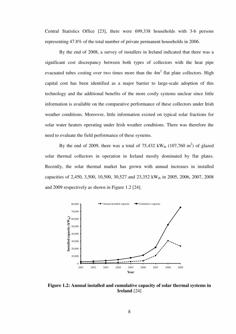
8

Central Statistics Office [23], there were 699,338 households with 3-6 persons

representing 47.8% of the total number of private permanent households in 2006.

By the end of 2008, a survey of installers in Ireland indicated that there was a

significant cost discrepancy between both types of collectors with the heat pipe

evacuated tubes costing over two times more than the 4m2 flat plate collectors. High

capital cost has been identified as a major barrier to large-scale adoption of this

technology and the additional benefits of the more costly systems unclear since little

information is available on the comparative performance of these collectors under Irish

weather conditions. Moreover, little information existed on typical solar fractions for

solar water heaters operating under Irish weather conditions. There was therefore the

need to evaluate the field performance of these systems.

By the end of 2009, there was a total of 75,432 kWth (107,760 m2) of glazed

solar thermal collectors in operation in Ireland mostly dominated by flat plates.

Recently, the solar thermal market has grown with annual increases in installed

capacities of 2,450, 3,500, 10,500, 30,527 and 23,352 kWth in 2005, 2006, 2007, 2008

and 2009 respectively as shown in Figure 1.2 [24].

Figure 1.2: Annual installed and cumulative capacity of solar thermal systems in Ireland [24]

0

10,000

20,000

30,000

40,000

50,000

60,000

70,000

80,000

2001 2002 2003 2004 2005 2006 2007 2008 2009

Inst

alle

d ca

paci

ty (k

Wth

)

Year

Annual installed capacity Cumulative capacity

9

A 191% rise between 2007 and 2008 was largely the result of government

support in the form of capital grant aid through the Greener Homes Scheme (GHS). The

drop of 24% between 2008 and 2009 can be attributed to a change in the GHS where

grants were offered only to retrofit installations, as well as a fall in the number of newly

built houses. Since July 2008, the third phase of the GHS offered capital subsidies of

250 and 300 �/m2 for flat plate collectors and evacuated tube collector systems to a

maximum of 6 m2 for a single domestic dwelling. By the end of 2010, there were about

19,611 solar thermal systems installed under this scheme as shown in Figure 1.3 [25].

Figure 1.3: Annual installation of solar thermal systems under the GHS [25]

There are several factors that have contributed to the poor deployment of solar

thermal technology in Ireland which have served as barriers to large-scale adoption.

Prominent among the barriers are: high initial investment costs compared to other heat

sources, historically low fuel prices, lack of financial incentives until 2006, lack of

attainment of critical mass, homeowner-tenant dilemma, lack of awareness and shortage

of skilled installers. Ireland is no exception since the full potential of solar thermal

434

2,97

9

6,04

1

5,71

5

4,44

2

0

1,000

2,000

3,000

4,000

5,000

6,000

7,000

2006 2007 2008 2009 2010

Num

ber o

f sys

tem

s

Year

10

systems has not been reached in most IEA countries due to relatively high capital costs

and long payback periods, compared with conventional water heating systems [19].

1.3 Research Aim

The aim of this research is to investigate the techno-economic and

environmental performance of domestic scale grid-connected photovoltaic (PV) and

forced circulation solar water heating (SWH) systems in Ireland; and propose a new

feed-in tariff designed using a large sample of high resolution electricity demand data in

order to provide credible information for informed policy formulation.

1.4 Research Objectives

Specific objectives of this project are to:

• install a PV system and two solar water heating systems (SWHSs) with flat

plates and evacuated tubes representative of systems installed in domestic

dwellings;

• test these PV system and SWHSs in field trials under typical Irish weather

conditions;

• evaluate the energy, economic and environmental performance of the

SWHSs and PV system;

• formulate dynamic energy balance, financial and environmental models

using the latest literature and validate these models using field trial data;

• use the validated models to test the suitability/impact of existing and

alternative policies to encourage large-scale uptake in the Irish residential

sector;

11

• rank the technologies in order of value to society as in achieving Kyoto and

EU 2020 goals; and

• investigate whether it is possible to draw up a set of recommendations which

will align incentives both for individuals and policymakers.

1.5 Research Methodology

1. A review of existing literature including:

o technology identification (technology, efficiency and cost trends

etc);

o state-of-the-art modelling of grid-connected and SWH systems

(theory, software, strengths, weaknesses etc); and

o performance assessment, policies and international comparisons.

2. The design and set up of test rigs and data collecting involving:

o design, install and commission SWHs and PV systems that mimic

actual domestic installations; and

o collect on-site weather data for wind speed, ambient temperature,

solar radiation (direct, diffuse) on 5 minutes basis.

3. The evaluation of energy, economic and environmental performances of the

two technologies using:

o field trial data and system parameters;

o system installed cost and cost projections based on production

learning rates and global annual installed capacities; and

o CO2 intensities of the displaced fuels.

12

4. The development/implementation of techno-economic and environmental

models for the systems and validating the models with field trial, cost and

other data by:

o formulating energy balance, economic and CO2 emission models for

SWHs and grid-connected PV systems and validating them with field

trial data; and

o computing and optimising economic performance parameters such

as: net present value (NPV); payback period; and internal rate of

return (IRR) using capital cost projections/trends, energy prices and

financial support mechanisms.

5. The evaluation of policy options using validated models by:

o using existing policy support measures such as capital cost grants,

feed-in tariff, obligation (Building Regulation Part L) to evaluate the

impact on incentives for individual investors and, consequently

technology deployment;

o developing Marginal Abatement Costs (MACs) for the two

technologies to inform policymakers; and

o exploring other policy support measures not yet applicable and

evaluate their impact on technology deployment.

In line with research based on case studies, the research methodology adopted in

this research has its strengths and weaknesses which are discussed here.

Some of the strengths of the research methodology include:

• it does provide reliable site specific data to analyse the micro-level

performance of the systems;

13

• data collected can be used to validate energy balance models for the systems.

The outputs from such models can be used as a tool for parametric studies to

optimise the systems;

• it provides an interdisciplinary approach to policy analysis; and

• it can be adapted to analyse the performance of other micro-generation

technologies.

Some of the weaknesses of the research methodology include:

• it could be expensive and cumbersome to implement; and

• it requires extensive knowledge from different fields of studies

1.6 Contributions to Knowledge

The contributions of this work to knowledge in the area of performance and

policy evaluation in order to support the uptake of micro-generation renewable energy

technologies in Ireland are outlined below:

• Provision of new performance data for the systems unique for Dublin.

• Using a system’ s approach, this study combined knowledge of the micro-level

energy, economic and environmental performance of solar water heating and

photovoltaic systems to inform policy formulation to encourage large-scale

uptake in Ireland.

• The design and implementation of an automated hot water dispensing unit which

extracted water from the hot water tanks and controlled the operation of the

electric immersion heaters in such a way as to mimic real life operation where

the users interact with the SWH systems.

14

• A comparative energy performance assessment of the energy generation of solar

water heating systems with flat plate and heat pipe evacuated tube collectors was

undertaken under the same weather and operating conditions.

• Development and validation of a dynamic energy balance models for the SWH

system test rigs that can accommodate different hot water demand profiles as

well as modification and validation of dynamic energy balance models for grid-

connected PV systems suitable for small time interval predictions.

• Computation of new feed-in tariffs (FITs) that guarantees an 8% internal rate of

return on investment and 50% market penetration for domestic scale PV systems

in Ireland using a large sample of high resolution household electricity demand

data.

• Assessment of a roadmap towards parity between domestic-scale PV generated

and grid electricity in Ireland.

• Evaluation of Marginal Abatement Costs (MACs) for domestic-scale solar water

heating systems and proposed (MACs) for photovoltaic systems using the

evaluated FITs.

1.7 Thesis structure

This thesis is divided into three sections made up of three chapters each. It starts

with an introduction chapter and ends with a conclusions and recommendations chapter.

• Section 1: Grid-connected PV systems.

A review of literature on the current state-of-the-art of PV systems is presented

in Chapter two. Chapter three presents the design, installation and field trial

performance results of a 1.72 kWp PV system in Dublin. In Chapter four, the

process of selecting and validating the parameters of an empirical model that can

15

be used to accurately determine the energy output from the grid-connected PV

system is presented.

• Section 2: Solar water heating systems

A review of the current state-of-the-art of solar water heating systems

with flat plate and heat pipe evacuated tube collectors is presented in Chapter

five. Chapter six presents the design, installation and comparative field trial

performance results from two domestic scale solar water heating systems

equipped with flat plate and evacuated tube collectors and the same

configuration of non-collector components. Chapter seven presents validated

TRNSYS models for solar water heating systems with flat plate and heat pipe

evacuated tube collectors.

• Section 3: Economic, environmental and policy analysis of PV and solar water

heating systems in Ireland.

Chapters eight and nine assess the economic and environmental performance of

grid-connected PV systems and solar water heating systems under current

economic and policy support measures as well as carbon intensity of electricity

generation in Ireland. Chapter ten reviews existing policy support measures for

PV and solar water heating systems world-wide. It then proposes alternative

policy options and discusses their implications in promoting large-scale

deployment of the technologies in Ireland.

1.8 Energy in Ireland

Ireland remains heavily dependent on fossil fuels which accounted for 95% of

all energy used in 2009. Oil was the dominant fuel, making up some 52% of total

16

primary energy used in the same year. Renewables satisfied 4.9% of gross final energy

use in 2009 and their contribution grew by 14% during 2009. Wind energy and biomass

were the main sources of renewable energy in total primary energy consumption while

wind and hydro were the major renewables used in electricity generation in 2009. The

growth rate in use of fuels in Ireland over the period 2005 to 2009 indicates fuel

switching away from carbon-intensive coal and oil towards natural gas and renewable

energy. The average annual growth in the five-year period was 5.5% for natural gas and

15% for renewable energy, while coal and oil decreased by 10.4% and 4% respectively

[26].

In 2009, the electricity generation mix comprised of coal, natural gas, oil, peat,

renewables and other fuels in proportions of 14.2%, 61.8%, 2.5%, 6.7%, 14.2% and

0.4% respectively. Figure 1.4 shows the All-Island fuel-mix for 2009. It is seen that gas

made the largest contribution to the island’ s electricity supply of 61.8% while

renewable energy made up 14.2% of the total. Renewables consisted of 11% wind,

2.6% hydro, 0.6% biomass and >0% photovoltaic. CO2 emissions from electricity

generation were 533 g/kWh in the same year [27]. Energy imports increased from 50%

in 1990 to 89% in 2009 due to a growth in demand combined with a decrease in

domestic production.

Figure 1.4: All-Island fuel-mix 2009 [28]

Gas 61.8%Coal 14.2%

Renewables 14.2%

Peat 6.7%

Oil 2.5% Other 0.4%

17

In 2009 the Irish residential sector was the second highest energy consumer after

the transport sector representing 22% of total final energy consumption as shown in

Table 1.1. Between 1991 and 2006 the Irish population grew from 3,525,719 to

4,239,848 - an average annual growth of 44,633 [23].

Table 1.1: Total final energy consumption by sector in Ireland from 1990 to 2007 kilo tonnes of oil equivalent (ktoe) [29]

Sector 1990 1995 2000 2005 2006 2007 2008 2009 Industry 1,720 1,971 2,529 2,673 2,721 2,685 2,536 2,215 Transport 2,022 2,384 4,080 5,031 5,390 5,685 5,612 5,075 Residential 2,259 2,214 2,520 2,961 2,997 2,928 3,185 3,099 Commercial/Public services 1,007 1,090 1,368 1,684 1,623 1,690 1,807 1,586 Agriculture 252 340 317 336 322 301 300 272 Total 7,260 7,998 10,814 12,684 13,053 13,289 13,440 12,247

1.9 Residential sector

1.9.1 Energy Use

Direct use of micro-generation renewables in domestic dwellings decreased

from 45 ktoe in 1990 to 15 ktoe in 2004 and then increased to 25 ktoe in 2007 as shown

in Table 1.2. Solar energy and biomass were the main sources of renewables with

biomass supplying the larger share of energy. Given that renewables contributed 11% of

the fuel supply mix for electricity generation in 2007, the net contribution of renewables

in residential energy use was therefore 80.6 ktoe or 2.7% of the total energy demand.

Figure 1.5 shows the share of fuels in residential energy use in 2007.

Table 1.2: Residential energy use in Ireland from 1990 to 2007 (ktoe) [10]

Fuel 1990 1995 2000 2001 2002 2003 2004 2005 2006 2007 Coal 626 246 286 264 252 239 231 246 219 208 Peat 725 606 299 288 290 270 266 273 284 271 Oil 392 656 935 1,035 1,033 1,076 1,117 1,166 1,142 1,127 Natural Gas 117 252 439 482 476 539 601 607 632 593 Renewables 45 30 17 16 16 15 15 16 18 25 Electricity 356 427 548 579 566 599 632 646 695 693 Total 2,261 2,216 2,524 2,664 2,633 2,738 2,862 2,954 2,990 2,918

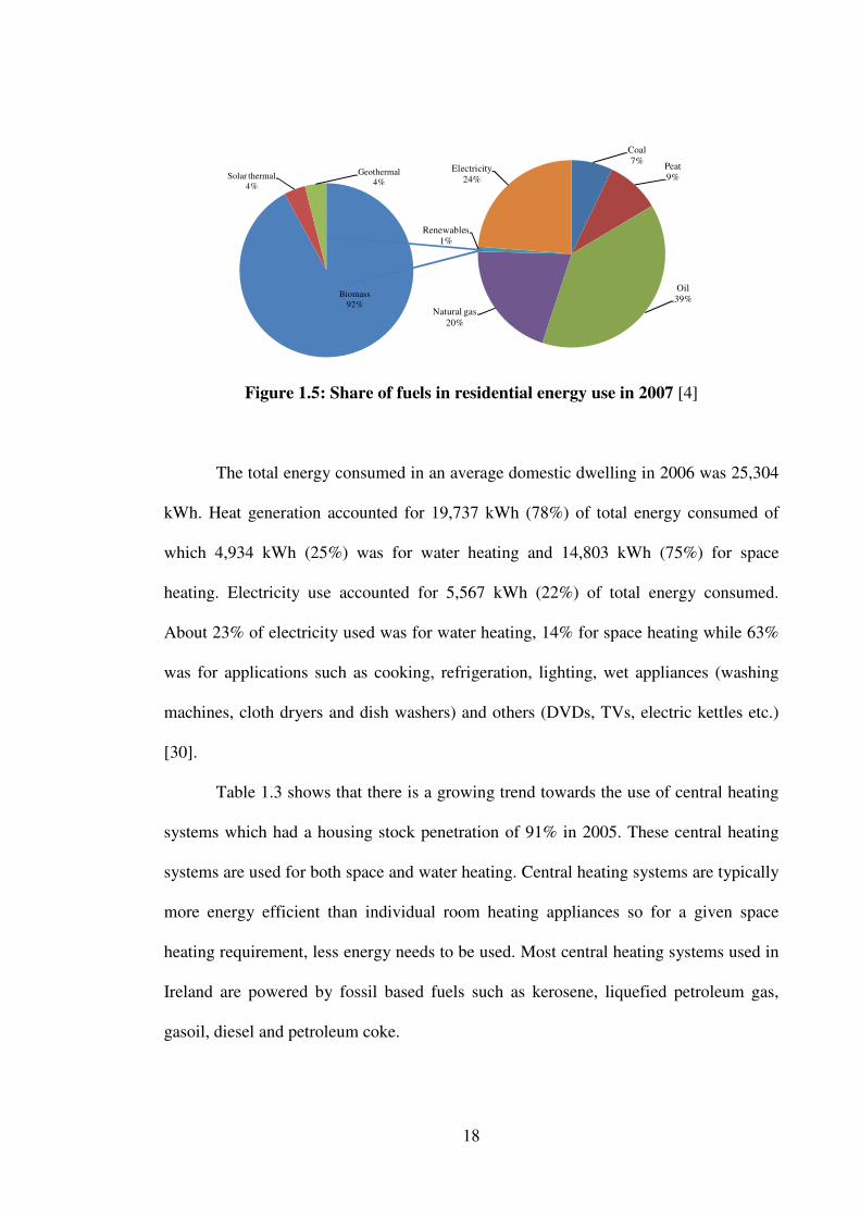
18

Figure 1.5: Share of fuels in residential energy use in 2007 [4]

The total energy consumed in an average domestic dwelling in 2006 was 25,304

kWh. Heat generation accounted for 19,737 kWh (78%) of total energy consumed of

which 4,934 kWh (25%) was for water heating and 14,803 kWh (75%) for space

heating. Electricity use accounted for 5,567 kWh (22%) of total energy consumed.

About 23% of electricity used was for water heating, 14% for space heating while 63%

was for applications such as cooking, refrigeration, lighting, wet appliances (washing

machines, cloth dryers and dish washers) and others (DVDs, TVs, electric kettles etc.)

[30].

Table 1.3 shows that there is a growing trend towards the use of central heating

systems which had a housing stock penetration of 91% in 2005. These central heating

systems are used for both space and water heating. Central heating systems are typically

more energy efficient than individual room heating appliances so for a given space

heating requirement, less energy needs to be used. Most central heating systems used in

Ireland are powered by fossil based fuels such as kerosene, liquefied petroleum gas,

gasoil, diesel and petroleum coke.

Biomass92%

Solar thermal4%

Geothermal4%

Coal7% Peat

9%

Oil39%

Natural gas20%

Renewables1%

Electricity24%

19

Table 1.3: Percentage of dwellings with central heating from 1987 to 2005 [8]

Fuel Type 1987 1995 2000 2005 Solid Fuel 31 21 9 8 Electricity 1 2 4 3 Oil Fired 12 25 39 46 Natural Gas Fired 4 14 25 28 Dual System 4 6 7 5 Total Central Heating 52 68 83 91

1.9.2 Greenhouse Gas Emissions

The expansion of the Irish economy by over 150% between 1992 and 2006 and

a population growth of 20.3% between 1991 and 2006 contributed to a 25% increase in

national greenhouse gas emissions between 1992 and 2006 [31]. In 2007, the residential

sector emitted 7,062 kilo tonnes of carbon dioxide (ktCO2) equivalent or 10.2% of

energy-related CO2 emissions [3]. The average dwelling was responsible for emitting

approximately 8.1 tonnes of CO2. A total of 4.8 tonnes of CO2 (59%) was from direct

fuel use, the remainder being the result of upstream emissions from electricity usage

[30]. The average Irish dwelling in 2005 emitted 47% more CO2 than the average

dwelling in the UK. Emissions were 92% and 104% higher than the average for the EU-

15 and EU-27 respectively. This high emission rate has been attributed to: inefficient

housing stock; a lack of many district heating systems in Ireland; and emissions from

district heating systems being included in the services sector of other countries [32].

1.10 Renewable Energy Sources (RES)

All energy, with the exception of geothermal resources, is derived from the sun.

Fossil fuels are solar energy stored in organic materials converted to hydrocarbon fuels

by pressure and temperature over geologic time. Unlike hydrocarbon fuels, solar energy

is pollution free and for all practical purposes, inexhaustible since the sun will continue

to shine for the next four billion years or so. RES are among the oldest sources of

20

energy used and new technologies have enhanced the use of this energy for the

production of electricity as well as thermal and mechanical energy [33].

Renewable energy is energy obtained from natural and persistent flows that are

compatible with the environment such as the sun and can be renewed within a

reasonable timeframe. The energy is later returned to the environment, so no thermal

pollution can occur on anything but a small scale. An exception is air pollution from

incomplete combustion of biomass or refuse. Environmental pollution does however

occur when fossil fuels are used to extract and process materials used to produce

renewable energy devices, although modern manufacturing processes have led to a

reduction in the embodied energy required to produce some of these devices. The

environmental impact of RES depends on the particular technology and circumstances

[34]. There are five principal RES that are applicable to the domestic sector namely: the

sun, the wind, flowing water, biomass and heat from within the earth.

1.10.1 The Case for RES

Today, the world’ s energy supply is largely based on fossil fuels which are finite

in nature (within a human timeframe) and have proven to be among the main causes of

global warming. The use of RES are in line with an overall strategy of sustainable

development [7] and according to the International Energy Agency [35] can help

address some of the challenges faced by today’ s societies by:

• contributing to climate change mitigation and general environmental

protection;

• fostering technological innovation, market creation and employment creation

leading to economic growth;

21

• enhancing energy supply security through diversification, preventing

conflicts over source natural resources;

• reducing poverty through better energy access and gender equality; and

• improving public health through reduced local air pollution and indoor air

pollution.

The most important benefit of renewable energy systems is the decrease of

environmental pollution. This is achieved by the reduction of air emissions due to the

substitution of electricity generated from fossil fuel and conventional fuels. The most

important effects of air pollutants on the human and natural environment are their

impact on public health, agriculture and on ecosystems. In contrast with other air

pollutants, the social cost of CO2 does not vary with the geographical characteristics of

the source as each unit of CO2 contributes equally to the climate change threat and the

resulting cost [12].

Governments around the world are placing considerable faith in renewable

energy for reducing energy related environmental problems, particularly CO2 emissions.

There is no doubt that the potential scale of their contribution is very large, but

sustained growth will be needed, in the face of the lower cost and often more convenient

alternatives [36].

1.10.2 Micro-generation

Micro-generation is small-scale heat or electricity generation in or around

individual or groups of buildings. Unlike other generating technologies, micro-

generation gives households the opportunity to generate energy to partly or totally

sustain their homes or buildings [37, 38].

22

In the urban built environment, micro-generation has the potential for

decentralized generation which is used to satisfy local electricity demand, curb fuel

poverty and reduce greenhouse gas emissions [36]. Within the Irish domestic sector,

micro-generation technologies have the potential to help tackle climate change while at

the same time ensuring security of supply, environmental sustainability and economic

competitiveness. Micro-generation gives occupants the responsibility to produce energy

to partly sustain their homes or buildings and raises energy consciousness.

One of the most notable features of renewable forms of energy is the diversity of

technologies and resources [36]. Domestic sector energy end use includes: space

heating; water heating; lighting; cooking; and refrigeration. Suitable micro-generation

renewable energy technologies that can provide energy with comparatively low- or

zero-carbon intensities include: photovoltaic systems; solar water heaters; solar passive

heating; micro-wind systems; biomass boilers and stoves; heat pumps; and micro-hydro

systems [39-41].

Table 1.4 shows how renewable energy technologies can be used to satisfy

domestic energy demands for heat and electricity; space cooling is omitted since it is

not currently common in Irish domestic dwellings.

Renewable energy systems (RESs) use, and are at the same time limited by, the

various forces of nature to produce energy. The sun does not shine all day, the wind

does not always blow, and droughts occur. Combining renewable technologies can

increase the reliability and efficiency of energy production and is referred to as a

‘hybrid system’ . In hybrid systems, the technologies are chosen such that they

compensate for energy generation gaps, physical limitations or poor economic

performances of the other technologies in the mix. Hybrid systems are used whenever

large amounts of reliable energy are needed continuously. They are more costly and

23

complex, but make up for this disadvantage by their reliability [33]. Since the 1990’ s,

hybrid systems have become viable alternatives for energy production because they

allow system designers to take advantage of the strengths of both conventional and

renewable energy sources [42].

Table 1.4: Residential energy use and applicable technologies for micro-generation in Ireland

Description Form of energy End use Medium Technology Energy source

Residential energy

Heat

Space heating

Under floor

Biomass stove/boiler

Wood chips, logs and pellets

Heat pump Air, ground and water

Solar water heater Solar radiation

Micro wind turbine Wind

Radiator


Wood logs, chips and pellets




Direct space

Heat pump Air Heat recovery system Air

Passive solar Solar radiation Biomass stove/boiler

Charcoal, wood logs, chips and pellets

Water heating

Hot water tank


Wood logs, chips and pellets




Electricity

Lighting, cooking, refrigeration, powering equipment etc.

Electric cables Micro wind turbine Wind

Photovoltaic system Solar radiation

RES can form part of a hybrid system when employed in combination with

conventional energy sources (CESs) or other RES. Some possible exclusive RES are:

• PV + micro-wind for electricity generation;

24

• solar thermal + heat pumps, solar thermal + wood pellet boiler, heat pumps +

wood pellet boiler for heat generation; and

• photovoltaic and thermal panels for electricity and heat generation.

1.11 Irish Policies

The development of renewable energy is central to overall energy policy in

Ireland. Renewable energy reduces dependence on fossil fuels, improves security of

supply, and reduces greenhouse gas emissions creating environmental benefits, while

delivering green jobs to the economy. They can contribute to national competitiveness if

they are cost effective. The Irish government’ s commitment to accelerating the

development of renewable energy is set out in the documents: ‘Delivering a sustainable

energy future for Ireland – The Energy Policy Framework 2007-2020’[43]; and

‘Building Ireland’s Smart Economy – A Framework for Sustainable Economic

Renewal’ [44].

In NREAP [5], the Irish government identified climate change, energy security

and competitiveness as challenges that will be addressed through transforming its

economy from one based on fossil fuel dependence to a low carbon economy based

around energy efficiency, renewable energy and smart networks. Two areas of interest

to the domestic sector are electricity and heat generation.

In NREAP [5] the Irish government highlighted the potential contribution of

micro-generation to create employment and enable participation by a wide section of the

community in achieving its energy policy goals. It acknowledged that the introduction

of a robust framework for the development of a vibrant micro-generation sector is an

important component of building societal acceptance of energy infrastructure and

ownership of the national renewable energy targets. The government believes that this

25

has the potential to complement the contribution of large scale renewable energy

generation.

Very few policies and measures have been put in place to encourage widespread

deployment of micro-generation RETs in Ireland. This is evident in the fact that the first

direct support measure for micro-generation was implemented as recently as 2006.

Existing support measures include: financial support through the Greener Homes

Scheme (GHS) and the small and micro scale generation pilot programme; regulatory

measures such as the Part L of the building regulations and statutory instruments; and

technical measures notably the smart metering pilot programme. Appendix 10.5 shows

an overview of micro-generation policies and measures in Ireland.

1.11.1 Irish PV Support

In 2007, the Commission for Energy Regulation (CER) encouraged electricity

suppliers to develop payment arrangements for micro-generators. Consequently, in

February 2009 the CER through its decision paper [45] announced the introduction of a

domestic micro-generator export tariff of 9.00 cents/kWh for Electricity Supply Board

Customer Supply (ESBCS) customers. ESBCS as the Public Electricity Supplier (PES)

with the highest market share of electricity customers, also committed to pay a

supplementary payment of 10 cents/kWh resulting in a total FIT of 19 cents/kWh for

the first 3,000 kWh exported annually until the end of 2010. This is currently the only

existing FIT for PV systems in Ireland.

As an interim measure in the absence of a long term government policy, the

ESBCS export tariff was extended in December 2010 and is due to expire at the end of

2011. By the end of November 2010 almost 300 customers had signed up to the tariff

[46]. To date, the uptake of PV in the Irish domestic sector has been very small, and the

26

low level of adoption of this technology provides enough evidence of the inadequacy of

the existing policy to provide sufficient incentives for households to invest in the

technology.

The existing FIT does not attract widespread adoption due to a number of flaws

notably it:

• does not guarantee financial viability although it does improve on the no export

payment case which applies to non ESBCS customers; and

• was originally scheduled for only 23 months and has been currently extended

for an additional 12 months as an interim measure. The short duration of the

support measure does not provide long term stability for investment in the

technology.

A long-term/enduring solution would therefore be required if micro PV is to

contribute to the Irish government’ s efforts in meeting its European obligations and

adhering to targets put forward under the White Paper and National Renewable Energy

Action Plan (NREAP). This decision requires an understanding of the present and future

MACs and payback periods for PV systems.

1.11.2 Irish Solar Thermal Support

Very few government support policies for solar thermal (ST) systems have been

implemented in Ireland. The House of Tomorrow programme which, although not

explicitly focused on ST systems, aimed at supporting installer training, provided

technology guides as well as funding research and development projects between 2001

and 2006. This programme however had very little impact on the uptake of ST systems

in Ireland. This is illustrated in Figure 1.6 which shows annual ST market, capacity in

operation and ST support policies in Ireland from 2001 to 2010.

27

Figure 1.6: Annual ST market, capacity in operation and ST support policies in Ireland (2001 to 2009)

The second ST support policy, which was established at the end of 2005 by a

number of Irish local authorities, introduced building energy standards as part of

planning requirements for their jurisdiction. These building energy standards required a

substantial increase in the energy performance of new buildings (between 40 and 60%

reduction in energy usage) as well as a mandatory contribution of renewable energy to

their thermal energy requirement. The energy standard requirements that all new

buildings had to achieve as a prerequisite to receiving planning approval were [47]:

• annual heating requirement was to be lower than 50 kWh/m2 per year and;

• at least 30% of the building space and water heating requirements to be

supplied by a renewable energy system.

The third ST support policy was the Greener Homes Scheme (GHS) which was

implemented in March 2006. The GHS had the following objectives [25]:

• to increase the number of households in Ireland that use renewable energy;

0.2

0.4

0.8

1.4 2.5 3.5

10.5

30.5

23.4

2.5

2.9 3.7 5.1 7.

6 11.1

21.6

52.1

75.4

0

10

20

30

40

50

60

70

80

2001 2002 2003 2004 2005 2006 2007 2008 2009

Inst

alle

d ca

paci

ty (M

Wth

)

Year

Annual market In operation

House of tomorrowprogramme

(September, 2001to 2006)

Greener HomesScheme Phase I(March 2006 to September 2007)

Greener HomesScheme Phase III(July, 2008 to date)

Greener HomesScheme Phase II(October 2007 to

July 2008)

Energy Performance of Building Directive

( Part L Amendment, 2008)

Solar Obligationby Local Councils

(End of 2005)

28

• to guide consumers towards discerning choices of renewable energy heating;

• to ensure that the market for the products, services and fuels continues to

develop in a robust manner;

• to decrease Ireland’ s reliance on imports of fossil fuels; and

• to benefit the environment by reducing carbon dioxide emissions.

The GHS has so far proven to be effective in stimulating the ST market in

Ireland. Although other renewable energy heating technologies were targeted by the

scheme, ST systems have had the highest level of uptake as shown in Figure 1.7. The

third phase of the GHS was implemented in July 2008 with grand aid of 250 �/m2 of

FPC and 300 �/m2 of ETC being offered to retrofit installations. Newly constructed

houses are subject to regulatory measures notably Part L of the building regulations.

Figure 1.7: Number of renewable heating systems installed under the GHS from 2006 to 2010

854

2,70

5

1,53

5

620

26543

4

2,97

9

6,04

1

5,71

5

4,44

2

450

2,14

5

2,06

7

976

176

0

1,000

2,000

3,000

4,000

5,000

6,000

7,000

2006 2007 2008 2009 2010

Num

ber o

f sys

tem

s

Year

Biomass Solar thermal Heat pump

29

CHAPTER 2

REVIEW OF PHOTOVOLTAIC SYSTEMS

2.1 Background

Renewable energy systems (RESs) for producing electricity have received

greater attention in recent years due to increase in fossil fuel prices, concerns over

increasing levels of greenhouse gas emissions and global climate change. There is an

urgent need to develop and implement RESs that can make substantial contributions

towards curtailing the impact of increasing energy demand. The European Commission

[48] has identified photovoltaic (PV) as one such technology.

Life cycle PV electricity costs remain higher than electricity generated using

fossil fuels. However, the conventional economic comparison is distorted by hidden

environmental and health costs associated with fossil fuels which are not generally

included in energy prices together with the fact that many conventional energy carriers

are subsidized [49].

Environmental concerns are growing, interest in environmental issues is

increasing and the idea of generating electricity with less pollution is becoming more

and more attractive. Unlike conventional generation systems, fuel for PV systems is

available at no cost. PV systems generate electricity pollution-free and can easily be

installed on the roof of residential buildings as well as on the walls of commercial

buildings for grid-connected application [50].

A more widespread use of grid-connected PV systems is hindered by a number

of reasons which include; the declining, but still high costs of PV generated electricity

and lack of knowledge about the benefits of distributed generation with PV in the urban

environment. When strategically sited, PV generators integrated into building façades

30

and rooftops in urban areas at limited penetration levels can benefit local distribution

networks.

A number of studies have been published [51-55], with learning curves

demonstrating the cost-reduction potential of large-scale PV production, and in some

markets the cost of PV electricity is approaching residential tariffs, the so-called grid

parity [56]. Due to the intermittent nature of solar radiation resource, PV is considered

non-despatchable power, but under some conditions, in sunny urban areas with

electricity load curves dominated by air-conditioning loads, there is a high correlation

between PV generation and feeder loads. In these situations, a considerable fraction of a

given PV generator can be considered as a firm source of power supply [57].

In recent years the PV industry has been experiencing a dramatic growth at a

global level. Continuous increase of conventional fuel costs as well as growing pressure

to turn towards RES have been identified as the main drivers behind this rapidly

expanding industry which, since 2000 has achieved consistent annual growth rates of

around 30%. At a global energy output level, the PV industry is still lagging behind

other RES technologies, such as, hydropower and wind energy [58]. This is attributed to

the high costs associated with the manufacturing of PV modules, costs that should

however steadily diminish as a result of continuous advancements in technology [59].

Since the mid-1980s, PV has developed into a mature technology and become

acceptable worldwide. As a promising renewable energy resource, PV technology

enjoys substantial government supports in research and application in several major

industrial countries such as Germany, Italy, Spain. International competition, along with

years of experience in manufacturing, research and development, has resulted in

improved PV module efficiency, cost reduction and productivity increases [60].

31

Despite a significant decrease in PV module costs, the cost of entire PV systems

remains relatively high compared with traditional power generation technologies. The

high cost necessitates that the design parameters, such as surface tilt angle and array

size, should be optimized [60].

PV electricity is widely considered as one of the more promising renewable

energy technologies which produces electricity without moving parts, emissions or

noise and all this by converting abundant sunlight [61]. This has led to growing support

from governments for photovoltaic research, development programmes and market

introduction schemes [62].

2.2 PV Benefits

The principal advantages associated with PV systems are that they have no

moving parts, require little maintenance, and work quite satisfactorily with beam or

diffuse radiation. Also they are readily adapted to varying power requirements because

a PV cell is like a ‘building block’ which can be scaled up easily to match load

requirements. The main factors limiting their use are that they are costly and that there

is very little economy of scale associated with the magnitude of power generation in an

installation [63].

PV systems provide direct energy benefits in terms of sustainable electrical

power generation. Indirect benefits include: CO2 mitigation; grid strengthening through

demand reduction. When these are combined with occupier perception and behaviour,

further environmental benefits can be achieved. Other benefits that can be derived from

installing PV systems in domestic buildings are listed below [38, 64]:

• Solar energy used as fuel is free. Silicon, which is the most commonly used

material for PV cell manufacture is an abundant and non-toxic material.

32

• PV systems are very safe and highly reliable. They have an estimated lifespan

above 25 years with over 80%, achieving their original performance after this

period.

• The modules are almost maintenance free and easy to install.

• Some PV modules can be aesthetically integrated into buildings to replace

building elements such as roofs, facades etc to replace building elements.

• The sector creates jobs and current high annual growth rates have contributed

immensely.

• The energy payback times of PV modules are decreasing making them more

viable energy producing sources.

• They contribute to improve security of energy supply by reducing reliance on

imported energy sources.

• Their ‘greenness’ and an associated feel-good factor for the owner.

• They produce no harmful emissions or polluting gases during operation and

therefore contribute positively towards avoiding greenhouse gas emissions.

PV arrays mounted on roof tops and facades offer the possibility of large-scale

power generation in decentralised medium-sized grid connected units. The PV system

may supply the electricity needs of the building, feed surplus electricity into the grid to

earn revenue, and draw electricity from the grid at low insolation or feed all the

electricity into the grid. Small distributed PV systems offer some advantages over large

centralized PV plants due to the following:

• the avoidance of additional costs associated with buying and preparing large

sites for installation; and

• lower transmission losses because the load is on the same site as the supply.

33

2.3 PV History and Development

The word ‘photovoltaic’ is an amalgamation of two words ‘photo’ and ‘volt’ .

‘Photo’ in Greek means ‘light’ while volt is a measure of electric potential at a point.

The PV effect is the process by which a PV cell converts sunlight into electricity. When

sunlight shines on a PV cell, it may be reflected, absorbed, or pass through it. The

absorbed light is what generates electricity.

Although the PV effect was first discovered by Edmund Becquerel in 1839, an

understanding of this effect was only gained around the early part of the 1950’ s when it

was used as a source of power for space applications. PV has its origins in the US space

programme and were first utilised in the 1960s to power satellites [33]. Global concerns

over the effects of the 1973 oil crisis triggered funding for research and development

programmes which led to a rapid development of PV for energy conversion. Since then

until the early 1990s research in the area has focused on improving the efficiency of

light conversion into electricity. Conversion efficiencies are typically in the 12-20%

range without, and 22-28% with concentrators [33].

PV systems have progressively come down in price making them increasingly

affordable to power homes and businesses. PV is emerging as a major power resource,

increasingly becoming more affordable and proving to be more reliable than

conventional power utilities in some areas. Ideal conditions for generating electricity

using photovoltaic cells are long, clear, cold, sunny days.

In the early 1990s, the concept of integrating PV arrays into a building’ s fabric

and connecting the system to the grid so that the cost of power generation and demand

can be negotiated between the PV owner and the electrical supplier was introduced.

This concept has provided a major boost for the technology resulting in an annual

growth of 15-30% during the 1990s [65].

34

The early driver of market expansion was niche applications for very small

amounts of power such as calculators, and remote small-scale applications such as

telecommunications. However, supportive policies in several countries have played an

important role in expanding markets for PV for both grid and off-grid electricity supply

in recent years [36]. In 2009 global installed PV power was in excess of 7.2 GWp and

by the end of 2009 the global cumulative capacity exceeded 22.8 GWp. The EU

contributed around 70% of the global cumulative capacity [66].

The PV industry is experiencing rapid growth as concerns over security of fuel

supplies and carbon emissions mean that governments and individuals are increasingly

prepared to ignore its current high costs. It is envisaged that PV will become a

mainstream electricity generation technology when its costs are comparable to other

energy sources [56]. At the moment, it is still more expensive than grid supplied

electricity in most parts of the world.

Growing recognition of the environmental impact of non-renewable energy

sources and the economic volatility that comes from the reliance on oil and gas has

contributed to current expansion of the PV industry [67]. Most of the growth in the late

1990s in Japan and Germany was triggered by subsidy-based market strategies.

At country level, many governments (Austria, Germany, Greece, Italy, France,

Czech Republic, Spain, Portugal) have already included different PV promotion

programmes (e.g. subsidies, feed-in tariff, etc.) in their national electrification plans. At

industrial level, efforts aimed at promoting PV systems worldwide have focused on

increasing the technical and economic performances of PV modules and systems,

developing new technologies, and enacting effective government regulations and

policies [48].

35

PV modules are being architecturally integrated into low-energy buildings

designed with multifunctional outer skins that offer protection, electricity generation

and aesthetics. These buildings have the potential to become an important part of the

built environment, and can serve as independent power stations that generate electricity

for local use as well as social, economic and environmental benefits.

The multifunctional feature of PV modules integrates well with other sustainable

technologies in a building’ s energy strategy. Some of these sustainable technologies

include active solar thermal water heating, energy efficient appliances, good thermal

insulation, efficient heating, heating ventilation and air conditioning (HVAC)

equipment, and advanced glazing.

As the market for PV in the built environment has evolved, PV products have

been developed to create more attractive aesthetics in modules without significantly

reducing their efficiency. The different types of PV modules for example,

monocrystalline, polycrystalline or amorphous silicon have different aesthetic and

functional properties. Roof tiles, laminates, glass-glass skin of buildings have shapes

and sizes to match architectural design specifications. PV cell components, including

contact grids and anti-reflection coatings, have been modified to change the visual

appearance, colour and texture of the cells to achieve better aesthetics.

2.4 PV System

A PV system comprises several components among which are the PV cells

(generator), batteries or electricity grid (storage), power conditioning units and

sometimes supplementary or backup generator (in stand-alone systems) to form a hybrid

system. Power conditioning is essential since PV cells produce direct current (DC)

while most appliances use alternating current (AC) [68].

36

PV systems use cells to convert solar radiation into electricity. The cell consists

of one or two layers of a semi-conducting material. When light shines on the cell it

creates an electric field across the layers, causing electricity to flow. The greater the

intensity of the light, the greater the flow of electricity. A PV system therefore does not

only need beam (direct) radiation in order to operate but can also generate electricity on

cloudy days. Due to the reflection of sunlight, slightly cloudy days can even result in

higher energy yields than days with a completely cloudless sky [64].

The most common semiconductor material used in PV cells is silicon, an

element most commonly found in sand. There is no limitation to its availability as a raw

material and it is the second most abundant material in the earth’ s mass [64, 69]. The

heart of a PV system is the generator which consists of PV modules interconnected to

form a DC power generating unit. A physical assembly of modules and their support

forms an array as shown in Figure 2.1.

Figure 2.1: Composition of a PV array [68]

A PV array is the complete power-generating unit, consisting of any number of

PV modules. It consists of a number of individual PV modules or panels wired together

37

in series and/or parallel to deliver the voltage and amperage required. An array can be as

small as a single pair of modules, or large enough to cover wide areas.

2.4.1 PV System Classification

PV systems can be broadly classified into two types based on their use and

applications namely: photovoltaic (PV) systems and photovoltaic thermal (PV/T)

systems. PV systems can further be classified into space applications, stand-alone PV

systems, grid connected PV systems, photovoltaic hydrogen production systems and

miscellaneous small scale applications. PV/T systems are not discussed further because

they are not relevant to this research. Figure 2.2 shows the classification of photovoltaic

systems according to their applications.

Figure 2.2: Classification of PV systems based on their applications [70]

2.4.2 PV Systems

PV systems can be divided into grid-connected and stand-alone systems. A

summary of the ‘world of PV applications’ is shown in Figure 2.3. Only grid-connected

PV systems would be discussed further because they are the main focus of this research.

38

Figure 2.3: The world of PV applications [71]

2.4.2.1 Grid-connected PV System

A grid-connected PV system is a type of installation where three major

components are used i.e. the PV generator (comprising a number of PV modules

connected in series or parallel), the inverter, DC and AC cabling and a conventional

power line [71, 72]. The inverter plays a key role in energy efficiency and reliability

since it operates the PV array at the Maximum Power Point (MPP). Moreover, inverters

convert the DC power generated by PV modules into AC of the desired voltage and

frequency (e.g. 230 V/50 Hz).

Grid-connected PV systems do not include batteries [73, 74]. Since the public

electricity network serves as storage for grid-connected PV systems. Over 99% of the

installed PV systems in Europe in 2009 were grid-connected [75]. This is due to the

extensive coverage of electricity grids where a PV plant equipped with suitable power

��

��

� ��

� ��

� ��

� ��

��

��

� � ��

� � ��

� ��

� ��

� ��

��

��

� ��

� ��

� ��

� ��

��

��

� � ��

� � ��

� ��

� ��

� ��

39

conditioning units can supply power to these grids. Figure 2.4 shows the main

components of a grid-connected PV system. The metered output of the PV system

should be capable of measuring in both directions (i.e. import and export), and where

this is not the case, an incoming meter should be included between the outgoing meter

and the mains circuit breaker. The electrical energy invoiced to the utility (where this

occurs) will be the difference between the metered output and input energy taking into

consideration the applicable feed-in tariffs (FITs).

Figure 2.4: Grid-connected photovoltaic system [74]

Grid-connected PV systems have a variety of manifestations including: large

centralised power stations; and building mounted or integrated on commercial buildings

and individual houses. Worldwide, the application of grid connected PV power systems

is expanding rapidly. Prices of both PV modules and balance of system (BOS)

components are decreasing following a trend of increased production and improved

technology which will lead to further increase in use [72]. Grid-connected solar

photovoltaic electricity has not reached competitiveness yet but it has considerable long

term potential.

��

��

� ��

� ��

��

��

��

��

��

��

40

Grid-connected distributed PV systems are installed to provide power to a grid-

connected customer or directly to the electricity network (specifically where that part of

the electricity network is configured to supply power to a number of customers rather

than to provide a bulk transport function). Such systems may be on or integrated into

the customer’ s premises, often on the demand side of the electricity meter, on public

and commercial buildings [76].

A grid-connected photovoltaic system eliminates the need for a battery storage

bank resulting in a considerable reduction in the initial and maintenance costs. The

photovoltaic system instead uses the grid as a storage bank where the excess electrical

power can be deposited to, and when necessary withdrawn from. When the photovoltaic

system is applied in buildings, the PV modules are mounted either on rooftops or

façades, which can reduce the size and cost of mounting structures and land

requirements [60]. Since PV is dependent on intermittent solar irradiation, during

daytime only and centred around noon, it is generally not fit for base or intermittent

load electricity production [77].

Building integrated roof or façade PV systems have been promoted by industry-

political programs such as the 100,000 roof program of Germany, the 70,000 roof

program of Japan, and the million solar roofs initiative of the United States [61].

Grid-connected centralised PV systems perform the functions of centralized

power stations. The power supplied by such a system is not associated with a particular

electricity customer, and the system is not located to perform specific functions on the

electricity network other than the supply of bulk power. These systems are typically

ground-mounted and function independently of any nearby development [76].

41

2.5 Technology Status

The current PV market consists of a range of technologies including wafer-based

silicon and a variety of thin-film technologies [78]. There are four major types of PV

modules commercially available namely single (mono-) crystalline, polycrystalline,

amorphous and thin film. Single crystalline cells are the oldest and most expensive

production technique but they are the most efficient conversion technology available.

Polycrystalline cells are less efficient than single crystalline cells but their

manufacturing costs are lower. Amorphous and thin film cells have the lowest cost but

their efficiencies are lower than those for single and polycrystalline cells. Table 2.1

shows different PV modules and their associated efficiencies.

Table 2.1: Solar PV module type and efficiency [79]

Cell type Efficiency (%) Single crystalline 17 Polycrystalline 15 Amorphous 10 Thin film 9-12

2.5.1 Crystalline Silicon

PV modules currently use crystalline silicon in one of two main forms: single

crystalline silicon or multi crystalline silicon. Single crystalline silicon PV modules are

more expensive than their multi crystalline counterparts. New device technologies are

pushing commercial single-crystal wafer silicon efficiencies to the 18-21% range

offering the potential for lower peak output costs (�/Wp) as a result of increased

efficiencies. However, in 2007 multi-crystalline silicon accounted for 63% of the world

market, including manufacturers with PV cell efficiencies around 13-14% but at overall

lower �/Wp cost [67].

42

More than 90% of PV modules are made from wafer-based crystalline silicon

and this is expected to remain the main PV technology until at least 2020. It is a well-

established and reliable technology that uses significant silicon resources as a primary

feedstock material [19].

2.5.2 Thin Films

Thin films are produced by depositing extremely thin layers of photo-sensitive

materials on a low-cost substrate such as glass, stainless steel or plastic. Thin film

technologies are based on amorphous silicon, cadmium telluride (CdTe) and copper-

indium-gallium-diselenide (CIGS). The main advantages of thin films are their

relatively low consumption of raw materials, high manufacturing automation, suitability

for building integration, good visual appearance and reduced sensitivity to overheating.

The current drawbacks are lower efficiencies, limited experience of lifetime

performance and, so far, small production units. Commercial CIGS modules have

however reached 11% efficiency [19].

Thin films are expected to increase their market share significantly by 2020. In

the medium term, it is likely that PV modules that combine crystalline and thin film

technology will appear on the market. These devices will take advantage of the best of

both technologies in that they will combine high efficiencies with lower material

consumption, larger deposition areas, and continuous automatic manufacturing

processes. Such Si thin film modules are expected to reach an efficiency of 18% by

2030 [61].

43

2.6 Industry Trends

The solar PV industry had a production of 12.3 GW of solar cell in 2009, up

55.7% from 7.9 GW in 2008. For the first time in its history, the photovoltaic industry

entered an era of overproduction. Silicon, wafer and polycrystalline module prices

dropped by unprecedented levels in 2009. The price of crystalline modules fell by an

average of 37.8%, wafers by 50% and silicon by 80% in 2009. Thin film cells

constituted 17.7% of the market while crystalline silicon had a market share of 82.3%

[75]. The top five global producers in 2009 were First Solar (USA), Suntech Power

(China), Sharp (Japan), Q-cells (Germany), and Yingli Green Energy (China). Together,

these five accounted for almost half of global production. Investment in new solar PV

manufacturing facilities was strong in Europe, Japan, China, Chinese Taipei, and the

United States, with many new ventures reported.

The solar PV industry also saw a boom in silicon production facilities around the

world, responding to silicon feedstock shortages of recent years. Solar PV

manufacturers signed long-term contracts to ensure a growing supply, and silicon

manufacturers have consistently announced plans to build new plants. By the end of

2007, more than 70 silicon manufacturing facilities were being constructed or planned

[79].

2.7 Production Trends

Silicon is the second most abundant raw material on earth. For some years the

supply of processed silicon was the major bottleneck of the PV industry. Figure 2.5

shows yearly worldwide production of PV from 1993 to 2007. Due to the vast

expansion of production capacities and the introduction of new capacities, silicon

capacity was expected to reach 8-10 GWp by 2010 as shown in Table 2.2. As silicon is a

44

major raw material for c-Si technologies (93% in 2006), silicon capacities predefine the

upper production limit for the industry. In addition to the established c-Si capacity,

approximately 4 GWp of thin film capacity is expected to be available by the end of

2010. Although all technologies face high expansion rates, thin film capacities are

currently expanding at a faster rate than capacities for other technologies [80].

Figure 2.5: Yearly worldwide production of PV [81]

Table 2.2: Projected production capacities by the end of 2010 [80]

Material Capacity (GWp) Silicon 8-10 Wafer 10-12 Cells 11-14 c-Si Modules 14-16 Thin Film 4

2.7.1 Solar Grade Silicon

Silicon is the basic material required for the production of solar cells based on

crystalline technology which makes up over 90% of the world market. The availability

of sufficient silicon at reasonable prices is therefore an essential precondition for a

dynamic PV industry [13].

69 69 78 89 126

155

200 28

9 401 55

8 759

1196

1771

2474

3733

0

500

1000

1500

2000

2500

3000

3500

4000

1993

1994

1995

1996

1997

1998

1999

2000

2001

2002

2003

2004

2005

2006

2007

Phot

ovol

taic

cel

l pro

duct

ion

(MW

p)

Year

45

Until recently, the silicon industry produced electronic grade silicon exclusively

for the semi-conductor industry, mainly for use in computers. Only a small fraction was

delivered to the PV industry, which represented a good way for the suppliers to level

out demand fluctuations from the semi-conductor industry. With the dynamic growth of

the PV industry in recent years, however, the situation has changed. In 2007, more than

half of the worldwide production of electronic grade silicon was used to produce solar

cells [13].

2.9 Global PV Market

Promotion of renewable energy sources has been adopted as a top priority in the

energy strategies of many countries world-wide. Global PV electricity generating

technology has sustained an impressive annual growth rate compared with other

renewable energy generating technologies.

Photovoltaic modules have proven to be the most reliable power source for

remote unattended applications - particularly communications - throughout the world.

Crystalline silicon solar cells will continue to serve this important sector owing to its

proven reliability. The annual global market has developed from less than 1 GWp in

2003 to more than 7.2 GWp in 2009 in spite of the difficult financial and economic

circumstances. After a 160% compound annual growth rate (CAGR) growth from 2007

to 2008, the PV market grew by a further 15% in 2009 [66].

46

Figure 2.6 shows historical cumulative installed global and EU PV capacity.

With a cumulative PV power installed of almost 10 GWp, including around 3.8 GWp

installed in 2009, Germany remains the world’ s largest PV market.

Figure 2.6: Historical development of cumulative installed global and EU PV capacity [66]

Continuous political support is however needed to sustain this market growth in

some countries while expanding support is also needed in countries which have not

been active supporters of PV so far. In the long-run, it is expected that the cost of PV

generated electricity will become equal to that of conventionally generated electricity.

This is referred to as grid parity and is expected to then trigger a significant increase or

step change in demand. PV generated electricity will therefore become increasingly

competitive as a result of a continuous decrease in PV technology prices and expected

price increases of fossil energy sources [79].

This growth in PV production capacity is attributed to the fact that many

countries have recognised the future potential of PV in energy supply, exports and

employment. Many countries such as Germany, Japan and the USA have implemented

189

286

429

628 1,33

4

2,34

1

3,30

9 5,27

9

10,3

38

15,9

43

1,42

8

1,76

2

2,23

6

2,81

8

3,93

9 5,36

1 6,95

6

9,55

0

15,6

75

22,8

78

0

5,000

10,000

15,000

20,000

25,000

2000 2001 2002 2003 2004 2005 2006 2007 2008 2009

PV cu

mul

ativ

e ins

talle

d ca

paci

ty (M

Wp)

Year

EU Global

47

national programmes to promote the use of PV, resulting in an expansion of

manufacturing capacity and cost reductions [65]. The existence of international

standards has served to build consumer confidence, reduce costs and contribute to the

expansion of PV development.

The most significant increases have been in the grid-connected applications,

particularly in buildings. This market sector is gaining government assistance in a

number of industrialized countries, notably Japan, Germany, Spain, Italy, France, The

Netherlands and USA [79].

2.8 Performance Studies

This section reviews different studies on grid-connected PV system performance

reported in literature. It is divided into sub sections grouping together related topics for

clarity purposes.

2.8.1 Performance Evaluation and Assessments

Evaluation and assessment of PV cell performance requires the measurement of

current as a function of voltage, temperature, intensity of solar radiation, wind speed

and radiation spectrum. Most noticeable of these parameters is the PV conversion

efficiency, which is measured under standard test condition (STC) [82].

Monitoring PV performance provides data to demonstrate the performance of

system components, energy production, loss mechanisms associated with system

operation, reliability and causes of system failures, validity of theoretical models using

measured data, and long term system performance [83].

Although PV cell temperature affects module performance, there exists other

mechanisms such as spectral effects, low-light level behaviour and any long-term

48

variations in efficiency that are also significant. Crystalline silicon modules perform

better in winter than summer (10% better for m-Si) while the reverse is true for

amorphous -Si because crystalline -Si has larger negative temperature coefficients [84].

The hourly energy generation by a grid-connected PV system depends on many

parameters such as: PV array peak power, in-plane solar radiation, PV cell temperature,

inverter efficiency and size, and maximum power point tracking losses [85, 86].

Mondol et al. [87] carried out long-term performance analysis of a 13 kWp roof

mounted grid-connected PV system in Northern Ireland over a period of three years.

They analysed the measured data on hourly, daily and monthly bases and evaluated

performance parameters which include: reference yield, array yield, final yield, array

capture losses, system losses, PV and inverter efficiencies and performance ratio. They

investigated the effects of insolation and inverter operation on system performance.

Their results showed that the monthly average daily PV module, system and inverter

efficiencies varied from 4.5% to 9.2%, 3.6% to 7.8% and 50% to 87% respectively,

while the annual average PV module, system and inverter efficiencies were 7.6%, 6.4%

and 75%, respectively. The monthly average daily PV array and system performance

ratios ranged from 35% to 74% and 29% to 66%, respectively, while the annual average

monthly PV system performance ratios were 60%, 61% and 62%, respectively during

the monitoring period.

Kymakis et al. [88] also monitored the performance of a 171.4 kWp photovoltaic

park in the island of Crete, Greece over a year using data collected at 10 minute

intervals. They evaluated the performance ratio and computed different power losses

(temperature, soiling, internal, network, power electronics, grid availability and

interconnection). The PV park supplied 229 MWh of electricity to the grid in 2007, with

daily output ranging from 335.5 to 869.7 kWh. The average annual energy output in the

49

same year was 1,336.4 kWh/kWp. The final yield ranged from 1.96 to 5.07 h/d, the

performance ratio ranged from 58 to 73%, with an annual average of 67.4% while the

average annual capacity factor was 15.2%.

Decker and Jahn [89] analysed the performance of 170 grid-connected PV plants

in Northern Germany. The annual final yields of the PV plants ranged between 430 and

875 kWh/kWp with a mean value of 680 kWh/kWp. The annual performance ratios -

determined using annual in-plane irradiation - ranged between 47.5 - 81% with a mean

of 66.5%.

Cardona and López [86] analysed the performance of a 2.0 kWp grid-connected

photovoltaic system installed in Málaga (Spain) between January and December 1997.

The total energy output from their PV system was 2,678 kWh with mean daily output of

7.4 kWh/d. The annual performance ratio was 64.5% while the monthly average daily

system efficiency varied between 6.1 and 8.0%.

Drif et al. [90] analysed the performance of a 200 kWp grid-connected PV

system installed in Jaén (Spain) after four years of operation between 2000 and 2003.

Average daily annual values obtained were 65%, 2.74 h/d, 9.6%, 84.2% and 8.1% for

performance ratio, final yield, module efficiency, inverter efficiency and system

efficiency respectively.

Benatiallah et al. [91] presented performance evaluation results of a 1.5 kWp

photovoltaic system with nominal PV module efficiency of 12% installed in southern

Algeria. Between January and December 2001 the average solar insolation was 7.2

kWh/m2/d. The DC power output varied from 3,512 kWh in December to 7,983 kWh in

August. The annual average daily PV module and inverter efficiencies were 10.1% and

80.7% respectively during the same period. They reported that low insolation led to a

decrease in PV module efficiency. The efficiency decreased at low incident solar

50

radiation and was higher in summer than winter because of longer days. The system

generated 2.5 kWh during the period January 2000 to August 2000.

Cucumo et al. [92] presented the performance analysis of a 2.7 kWp grid-

connected photovoltaic plant installed at the University of Calabria (Italy). The

polycrystalline silicon modules had a reference efficiency of 11.11%. The mean daily

energy supplied by the PV system was 9.1 kWh or 3.37 kWh/kWp/d.

Chokmaviroj et al. [93] presented results for the first eight months of monitoring

a 500 kWp photovoltaic pilot plant in Mae Hong Son province, Thailand. Their PV

system consisted of a PV array of 1680 modules (140 strings, 12 modules/string; 300

Wp), power conditioning units and battery converter system. During the first eight

months of operation, the PV system generated about 383,274 kWh. The average daily

electricity generation was 1,695 kWh ranging from 1,452 to 2,042 kWh. The system

efficiency ranged from 9 to 12% while the inverter efficiency ranged from 92 to 98%.

The final yield ranged from 2.91 to 3.98 h/d and the performance ratio ranged from 0.7

to 0.9.

2.8.2 PV Performance Prediction

Alamsyah et al. [94] presented a simplified method for predicting long-term

average conventional energy conversion or performance of a PV system in Malaysia.

They reported that their approach was suitable for hand calculations using only one day

for each month. The method is however, limited to initial evaluation of the average

performance of PV systems with a more rigorous techno-economic analysis being

required for more accurate predictions.

Mavromatakis et al. [95] presented a methodology for modelling the

photovoltaic potential of a site. They modelled the energy produced by a PV system

using its nominal power, incoming irradiance and major energy loss mechanisms. They

51

found that energy loss mechanisms involve the temperature of the PV cells, the

response of PV cells to low intensity light, the spectrum and polarization of light, the

deviation from maximum power point tracking, module mismatch and ohmic losses.

The model proposed by Mavromatakis et al. [95] is based on the nominal power

of the PV array, the temperature coefficient of the modules, in-plane solar irradiance,

the air temperature and wind speed. Measured field performance data is required to

analytically calculate the factors that cause reduction in power output from STC. Their

model can however, be improved if empirical formulae based on PV array specific data

are used. Their proposed model is given as:

STC

mtpm G

G�PP ⋅⋅=

(2.1)

Where:

Pm maximum power (W)

Pp nominal power (W)

�t coefficient that includes all factors that lead to the actual energy produced by a

module/array with respect to the energy that would be produced if it were

operating at STC (dimensionless).

Gm in-plane solar radiation (W/m2)

GSTC solar radiation under standard test conditions (W/m2)

2.8.3 PV Temperature

The important role of PV cell operating temperature on the electrical

performance of silicon based photovoltaic installations has attracted much attention

from the scientific community and led to the development of several models which can

be used for its estimation [96, 97].

52

The temperature of PV cells is one of the most important variables used in

assessing the performance of PV systems and their electrical energy production. This

temperature depends on parameters such as the thermal properties of materials used in

PV module encapsulation, types of PV cells, configuration of PV modules’ installation

and local climatic conditions [98].

With an increase in ambient temperature, there is a deficiency in the electrical

energy that the PV cells can supply. This situation is especially important in hot

climates. Outdoor exposure tests of PV cells carried out by Malik et al. [82] showed that

the efficiency of single crystal silicon PV cells strongly depends on its operating

temperature. They observed that at an operating temperature of 64 °C, there was a

decrease of 69% in the efficiency of the PV cell compared to that measured under

standard test conditions.

Skoplaki and Palyvos [97] discussed the importance of PV cell/module

operating temperature on the electrical performance of silicon based photovoltaic

installations. They presented existing explicit and implicit correlations for PV cell

temperature with standard weather variables notably ambient air temperature, wind

speed, solar radiation flux and material/system-dependent properties such as glazing-

cover transmittance, plate absorptance etc. They reported that mathematical correlations

for PV cell operating temperature (Tc) are either explicit in form, thus giving Tc directly,

or are implicit, i.e. involve variables which themselves depend on Tc with an iteration

procedure being required in the latter situation.

Malik et al. [82] concluded that cold temperatures produce more efficient photo

conversion for single-crystalline PV cells since the efficiency of mono-crystalline solar

cell decreases as the operating temperature of cells increases. For the same irradiance

level, the output power, and therefore the efficiency, decreases with increasing cell

temperature. In order to reduce the cell temperature to get near the rated value for

maximum efficiency, a cost effective solution is required.

53

Skoplaki and Palyvos [97] noted that the operating cell temperature is a key

variable of the photovoltaic conversion process. Numerous correlations for Tc exist in

literature, which apply to freely mounted PV arrays, PV/T collectors, and BIPV

installations. These correlations involve basic environmental variables and material or

system dependent parameters. They recommended that modellers must be cautious

when applying particular expressions for Tc because the available correlations have

been developed with specific mounting geometry or building integration levels. It is

therefore necessary that suitable correlations be identified that suit a particular

application.

In practice, PV cell temperature is very difficult to measure since the cells are

tightly encapsulated for moisture protection. The temperature at the back surface of PV

modules are therefore measured and it is generally assumed that the temperatures of the

cells are the same as that at the back surface [96].

Jones and Underwood [99] studied variation of the temperature profile of PV

modules under transient conditions. They conducted experiments for a clear sky and

cloudy day and their results showed that the PV module temperature varied between

300 and 325 K (27-52oC) when the ambient temperature was 297.5 K (24.5oC).

2.8.4 Effect of Low Insolation

Under low solar insolation, a PV array generates power at only part of its rated

capacity and the inverter thus operates under part load conditions with lower system

efficiency [100]. PV efficiency is also affected adversely when an inverter’ s rated

capacity is much lower than the PV peak power, since it would be operating at overload

conditions [84].

54

2.9 Summary

A review of literature on grid-connected PV systems revealed a continuous

increase in global installed capacity with growth sustained by policy support in some

countries. Technology trends in 2009 showed that PV modules with crystalline silicon

cells had over 80% of the market share with thin film cells covering the other portion.

Literature also revealed that energy output prediction of PV cells is dependent

on accurate determination of their efficiency. However, PV cell efficiencies quoted by

manufacturers are measured under standard test conditions which are different from

operating weather conditions. The efficiency of crystalline silicon PV cells is strongly

dependent on their operating temperature which varies with ambient conditions notably

ambient air temperature, wind speed and solar radiation.

Accurate prediction of PV cell efficiency therefore requires determining the PV

cell temperature with reduced errors. Although several correlations to determine PV cell

temperature exist in literature, caution must be applied in their use since they were

developed using systems operating under different weather conditions, specific

mounting geometry or building integration levels. In order to develop accurate

parameters for the correlations of PV cell temperature, it is therefore important to have

site specific measured data on the performance of the PV system.

Lack of such system specific data for Ireland’ s weather conditions prompted the

setting up of the field trial in Chapter 3. Energy performance evaluation of the PV

system provided data for detailed techno-economic and environmental analysis as

described in Chapter 8. In order to assess the techno-economic and environmental

performance of different sizes of commercially available PV systems, a model to predict

the energy output from the PV systems was developed in Chapter 4 and validated using

field trial data collected in Chapter 3.

55

CHAPTER 3

FIELD TRIALS AND PERFORMANCE ANALYSIS

The goal of this chapter is to design, install, monitor, and evaluate the energy

performance of the grid-connected PV system under Irish weather conditions.

Monitoring of the test rig, data collection, performance analysis and reporting were in

line with IEC 61724 standards [101]. Specific objectives are to:

• present the design procedure;

• describe the experimental setup and data monitoring process;

• present collected field trial data;

• present equations used to analyse the system’ s energy performance indices and

report the results; and

• compare the system’ s performance with that of other systems reported in

literature.

Energy performance analysis of a grid-connected PV system involves collecting

and analysing field trial data in order to evaluate its energy output; PV array, system,

reference yields and losses; PV module, system and inverter efficiencies; PV array and

system performance ratios; and capacity factor. The results obtained from the analysis

are summarized for different seasons of the year and a comparative energy performance

analysis against other PV systems reported in literature is also presented.

56

3.1 PV System Sizing

Sizing domestic scale grid-connected PV systems has traditionally been based

more on the area available for the PV installation and the budget of the buyer, than on

any economic rationale. After the daily electrical demand has been determined, the

correct size of the PV generator needs to be determined. The most sensible procedure to

determine the yield of different PV module types is to base this on their nominal power.

Pertinent questions for PV system design include [102]:

• How many kWh/y are required?

• How many peak watts of DC power are needed to provide that amount?

• How much area will the system require?

• What component sizes are available?

• What rooftop areas and orientations are available?

• What is the cost of system components?

• What budget is available?

In this study, it was assumed that the PV system would be installed in a house to

generate 1,500 kWh/y of electricity. It was therefore important to determine the number

of kWp of DC at STC of panels and the roof area required. It was assumed that the roof

is south-facing with a tilt angle equal to the local latitude of Dublin (53o) corresponding

to a global long-term annual average daily in-plane solar insolation of 2.83 kWh/m2/d.

The annual energy output (EAC) from a grid-connected PV system is given as

[102]:

EAC = PAC x hd,ps x Nd (3.1)

where,

EAC annual energy output (kWh)

PAC AC power output (kW)

57

hd,ps peak sun hours in a day at 1-sun (2.83 hrs)

Nd number of days in a year (365)

Therefore, the annual AC power output (PAC) is calculated from Equation 3.1 as

1.45 kW. Taking into account the impacts of temperature, inverter efficiency, module

mismatch and dirt, we consider a derating of about 15% or an efficiency of 85% for DC

to AC conversion [102]. The DC power under standard test conditions (PDC,STC) is

calculated as 1.71kWp using Equation 3.2

inv

ACDC,STC

�

PP =

(3.2)

where, �inv is the inverter efficiency.

With a nominal PV module efficiency of 17.2%, we can calculate the PV array

area. The DC power under STC is given as:

maSTCSTCDC, �AGP ××= (3.3)

where,

GSTC total solar radiation under standard test conditions (kW/m2)

Aa array area (m2)

�m PV module efficiency (%)

The PV array area (Aa) is computed as 9.94 m2. The number of modules (Nm)

required is calculated as 8 using Equation 3.4:

mn,

STCDC,m P

P N =

(3.4)

where, Pn,m is the nominal (rated) PV module power.

To decide on the number of modules we have to consider how they will be

arranged in an array. With 8 modules in a string, the STC rated voltage would be 8 x 42

= 336 V (42V is the PV voltage at maximum power). The Sunny Boy 1700 inverter

58

input PV voltage range at MPPT is 139-400 V. This fits very well with the voltage from

8 PV modules at maximum power. It therefore suggests that we use an array with a

single string of 8 modules.

It is important to estimate the maximum open circuit voltage of the array to be

sure that it does not violate the highest DC voltage that the inverter can accept, which in

this case is 400 V. We should remember that the VOC increases when cell temperature is

below 25 oC. Therefore on a cold morning, with a strong cold wind and low sunlight,

cell temperature might be close to ambient that might be well below 25 oC. With VOC

increasing by 0.129 V/oC below 25 oC, the VOC could then be well above its STC value.

Considering a PV cell temperature of -5 oC the maximum open circuit voltage (VOC,max)

would then be:

[ ] 349V5)0.00129(251336V maxOC, =++=

which, is lower than the upper limit of the voltage at MPPT of 400V.

Since each PV module has an area of 1.25 m2, the total roof area required is 10

m2. The rated DC power of the array under STC (PDC,STC) is given as 1,720 W using

Equation 3.4.

Again, assuming a 15% derating for AC power and using the 2.83 kWh/m2/d

average insolation, the annual AC power output from a PV system is given as 1,510.2

kWh/y using Equation 3.5:

dpsd,invratedPV,AC Nh�PE ×××= (3.5)

where, PPV,rated is the rated PV array power (kWp)

So the goal of 1,500 kWh/y would be met with 8 PV modules each having a

capacity of 215 W and efficiency of 17.2%. Using meteorological data for Bulgaria and

France (Corsica), Notton et al. [84] showed that the main parameter affecting the sizing

59

of such systems is the inverter efficiency curve. They reported that the influence of the

PV module technology seems less important except for amorphous PV modules. They

also reported that PV module inclination influences system performance particularly

when the inverter is undersized compared to the PV peak power. A 1700 W inverter was

therefore chosen for the PV system.

3.2 PV System Description

The PV system has an installed capacity of 1.72 kWp, consists of 8 modules

covering a total area of 10 m2. It was installed on a flat roof at the Focas Institute

building, Dublin Institute of Technology, Dublin 8, Ireland. The 215 Wp Sanyo HIP-

215NHE5 PV modules were made of thin monocrystalline silicon wafer surrounded by

ultra-thin amorphous silicon layers with anti-reflective coatings that maximise sunlight

absorption [103]. The unshaded modules were installed facing south and inclined at 53o

to the horizontal corresponding to the local latitude of Dublin. The roof was

approximately 12 m high and the PV modules were mounted on metal frames that were

1m high.

The PV modules were left uncleaned throughout the monitoring period to mimic

operation in a domestic dwelling. A single phase Sunny Boy SB 1700 inverter was used

to convert DC to AC which was fed directly into the Focas Institute building’ s 220

VAC electrical network. The inverter had a rated maximum efficiency of 93.5% and

maximum AC power output of 1700 W. The characteristic parameters of the PV

modules and the complete array are shown in Table 3.1 while the inverter specifications

are given in Table 3.2. Figure 3.1 shows pictures of the PV system installation.

60

Table 3.1: PV module and array specifications

PV module/array Specification Type Monocrystalline silicon Cell efficiency 19.3% Module efficiency 17.2% Maximum power (Pmax) 215 W Maximum power voltage (Vpm) 42.0 V Maximum power current (Ipm) 5.13A Open circuit voltage (Voc) 51.6 V Short circuit current (Isc) 5.61 A Warranted minimum power (Pmin) 204.3 W Output power tolerance +10/-5% Maximum system voltage (Vdc) 1000 Temperature coefficient of Pmax -0.3%/oC Module area 1.25m2

No. of modules 8 NOCT 47oC

Table 3.2: Sunny Boy 1700 inverter specifications

Inverter Specification Input Maximum dc power 1850 W Maximum dc voltage 400 V PV – voltage range at MPPT 139-400 V Output Maximum ac power 1700 W Nominal ac power 1550 W Efficiency Maximum efficiency 93.5% Euro-eta 91.8% Weight 25 kg

Figure 3.1: The PV System Installation

Front view ofPV array Rear view of PV array

Sunny Boy inverter

61

3.3 Monitoring and Data Acquisition

The data acquisition system consisted of a Sunny Boy 1700 inverter, Sunny

SensorBox and Sunny WebBox. The Sunny SensorBox was used to measure in-plane

global solar radiation on the PV modules. Additional sensors for measuring ambient

temperature, wind speed and temperature at the back of the PV module were connected

to the SensorBox.

A solar radiation sensor with accuracy of ±8% and resolution of 1 W/m2

installed on the PV module plane was used to measure incident solar radiation. The

temperature at the back of one of the PV modules was measured using a PT 100-M type

sensor with accuracy of ±0.5 oC. Ambient air temperature was measured using a JUMO

PT 100 U type sensor with accuracy of ±0.5 oC. A Thies small wind transmitter

anemometer with accuracy of ±5% was used to measure wind speed. The SensorBox

and inverter were connected to the Sunny WebBox via a serial RS485 link and Power

Injector. Data recorded at 5-minute intervals in the WebBox was extracted via a secure

digital card and read directly into a computer. Figure 3.2 shows the Sunny WebBox,

power injector and an analog electricity meter.

Figure 3.2: Sunny WebBox, power injector and analog electricity meter

��

� ��

Powerinjector

��

� ��

62

3.4 PV System Terminologies

Power is the rate at which energy is generated or used and is measured in Joules

per second (watts). Energy is the ability to do work and is measured in Joules. Electrical

energy is watts multiplied by time and is measured in Watt-hr. Table 3.3 shows the

principal parameters of solar cells, their commonly used symbols, units of measurement

and description.

Table 3.3: The principal parameters of solar cells [71]

Parameter Formula

sign Unit Description

MPP power PMPP Wp Maximum power under STC (nominal power) Efficiency � % Ratio of the power delivered by the cell and the solar

irradiance Fill factor FF - Quality yardstick for solar cells, generally between 0.5 and

0.85 MPP voltage VMPP V PV voltage at MPP (nominal voltage) Open-circuit voltage Voc V Open circuit voltage, generally specified for STC: voltage that

the solar cell supplies when both terminals are directly connected

MPP current IMPP A PV current, generally specified for STC: Short-circuit current Isc A Short-circuit current, generally specified for STC: current that

the solar cell supplies when both terminals are directly connected

Normal Operating Cell Temperature (NOCT)

This is the temperature a PV cell reaches when it operates under standard

operating conditions (SOC). Usually NOCT is 20-40oC above ambient temperature.

Standard Test Conditions (STC)

These are environmental conditions specified for testing PV cells. They are

usually specified as:

• Solar intensity on the PV cell: GSTC = 1000 W/m2

• Temperature of the PV cell: Tc = 25 oC and

• Solar spectrum air mass, AM0 1.5

63

Standard Operating Conditions (SOC)

These conditions have been proposed to determine the peak power (Pm) since

these conditions are closer to real operating conditions. The conditions are [68]:

• Solar radiation (GSOC) on the PV cell of 800 W/m2, ambient temperature of

20 oC and wind speed below 1 m/s

• The PV modules have to be south facing and the measurements must be

carried out at solar noon (hour angle, =0)

• All measurements should be taken under open circuit conditions

Fill Factor (FF)

It describes the quality of solar cells. It is defined as the quotient of maximum

power point (MPP) power and the theoretical maximum power that results at the

product of short-circuit current and open-circuit voltage. For crystalline solar cells, the

fill factor is around 0.75-0.85, and for amorphous solar cells around 0.5-0.7. The fill

factor is given as [71] [68]:

scoc

m

scoc

mm

iVP

iViV

FF×

=××

= (3.6)

where,

Vm maximum voltage (V)

im maximum current (A)

Voc open circuit voltage (V)

isc short circuit current (A)

Pm maximum power (W)

64

Pack Factor

The pack factor (PF) is the ratio of the total area of PV cells (Ac) over the area of

the PV module (Am) and is given as [68]:

m

cps

A

AnnPF =

(3.7)

where,

ns number of PV cells in series

np number of PV cells in parallel

3.5 Monitoring Results

Monitoring of the test rig, data collection, performance analysis and reporting

were in line with IEC 61724 standards [104]. Data was collected at 5-minute intervals

but subsequently aggregated by summing the energy output over 30-minute intervals for

the analysis. The interval was deemed suitable since it corresponds to current billing

intervals prevalent with smart metering. Table 3.4 shows monthly average daily solar

insolation, ambient air temperature, PV module temperature and wind speed during the

monitoring period. Annual average daily measured solar insolation, long-term solar

insolation, ambient air temperature, PV module temperature and wind speed were 2.86

kWh/m2/d, 2.83 kWh/m2/d, 12.7 oC, 16.7 oC and 3.9 m/s respectively.

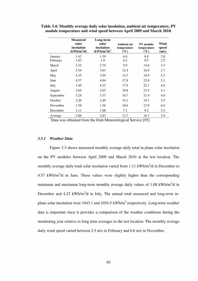
65

Table 3.4: Monthly average daily solar insolation, ambient air temperature, PV module temperature and wind speed between April 2009 and March 2010.

Measured solar

insolation (kWh/m2/d)

Long-term solar

insolation (kWh/m2/d)*

Ambient air temperature

(oC)

PV module temperature

(oC)

Wind speed (m/s)

January 1.42 1.39 6.0 8.8 2.8 February 1.83 1.9 6.5 9.5 2.5 March 3.32 2.79 9.9 14.8 3.3 April 3.54 3.63 12.4 16.9 2.7 May 4.35 3.84 14.3 18.9 5.3 June 4.57 4.04 17.8 23.8 3.1 July 3.49 4.22 17.9 22.1 4.6 August 3.64 3.65 18.8 23.5 5.1 September 3.24 3.37 16.7 21.4 4.0 October 2.20 2.49 15.1 19.1 3.5 November 1.58 1.56 10.6 12.8 6.6 December 1.11 1.08 7.1 9.2 3.3

Average 2.86 2.83 12.7 16.7 3.9 *Data was obtained from the Irish Meteorological Service [95]

3.5.1 Weather Data

Figure 3.3 shows measured monthly average daily total in-plane solar insolation

on the PV modules between April 2009 and March 2010 at the test location. The

monthly average daily total solar insolation varied from 1.11 kWh/m2/d in December to

4.57 kWh/m2/d in June. These values were slightly higher than the corresponding

minimum and maximum long-term monthly average daily values of 1.08 kWh/m2/d in

December and 4.22 kWh/m2/d in July. The annual total measured and long-term in-

plane solar insolation were 1043.1 and 1034.5 kWh/m2 respectively. Long-term weather

data is important since it provides a comparison of the weather conditions during the

monitoring year relative to long term averages in the test location. The monthly average

daily wind speed varied between 2.5 m/s in February and 6.6 m/s in November.

66

Figure 3.3: Monthly average long-term in-plane average for Dublin airport [104],

measured average daily total in-plane solar insolation, wind speed

Figure 3.4 shows monthly average daily ambient temperature and temperature at

the back of one of the PV modules over the monitored period. The monthly average

ambient temperature varied between 6.0 oC in January and 18.8 oC in August while the

PV module temperature varied between 8.8 oC in January and 23.8 oC in June.

Maximum recorded values for solar radiation, ambient air temperature, PV module

temperature and wind speed were 1031.0 W/m2, 27.0 oC, 45.8 oC and 16.3 m/s in

August, June, September and November respectively.

Figure 3.4: Monthly average daily ambient air and PV module temperature over the monitored period

0.0

1.0

2.0

3.0

4.0

5.0

6.0

7.0

0.0

1.0

2.0

3.0

4.0

5.0

Jan

10

Feb

10

Mar

10

Apr

09

may

09

Jun

09

Jul 0

9

Aug

09

Sep

09

Oct

09

Nov

09

Dec

09

Win

d sp

eed

(ms-1

)

Sola

r ins

olat

ion

(kW

hm-2

d-1)

Month

Solar insolation Long-term solar insolation Wind speed

0

2

4

6

8

10

12

14

16

18

20

22

24

26

Jan

10

Feb

10

Mar

10

Apr

09

may

09

Jun

09

Jul 0

9

Aug

09

Sep

09

Oct

09

Nov

09

Dec

09

Tem

pera

ture

(o C)

Month

Ambient air PV module

67

Table 3.5 shows the fraction of solar radiation, average ambient air temperature,

PV module temperature, and wind speed for different levels of solar radiation between

April 2009 and March 2010. The average ambient air temperature varied between 11.0

oC at 5-49 W/m2 and 17.3 oC at 800-899 W/m2. The average PV module temperature

varied between 10.6 oC at 5-49 W/m2 and 34.6 oC at 900-999 W/m2. 95.7% of total in-

plane solar radiation was below 800 W/m2 with an average PV module temperature of

23.8 oC in this solar radiation range. Also, 70.9% of in-plane solar radiation was below

300 W/m2. This indicates low influence of high PV module temperature on the PV

system’ s performance and shows the prevalence of low levels of solar radiation at the

test site. Low average ambient air temperatures and high wind speeds provided good

operating conditions for the PV system by keeping the average PV module operating

temperature lower than the SOC temperature of 20 oC.

Table 3.5: Average ambient air temperature, PV module temperature and wind

speed for different levels of solar radiation

In-plane solar radiation (W/m2)

Fraction of solar radiation (%)

Ambient air temperature (oC)

PV module temperature (oC)

Wind speed (m/s)

5-49 25.5 11.0 10.6 3.0

50-99 16.0 12.6 13.4 3.5

100-199 18.4 13.7 16.0 3.9

200-299 11.0 14.7 19.1 4.2

300-399 7.9 14.6 21.1 4.2

400-499 5.7 14.9 22.9 4.4

500-599 5.0 14.7 24.5 4.6

600-699 3.4 15.4 27.0 4.8

700-799 2.9 16.2 30.0 4.6

800-899 2.6 17.3 33.5 4.3

900-999 1.6 17.0 34.6 4.5

1000-1099 0.1 15.5 32.5 4.6

68

3.5.2 PV Module Temperature

Table 3.6 shows monthly ranges for variation of ambient air temperature, PV

module temperature and wind speed. It is seen that the minimum ambient air

temperature was -6.0 oC in January while the maximum was 27.0 oC in June. PV

module temperature varied between -7.8 oC in January and 45.8 oC in June/September

respectively. Wind speed varied from 0.0 m/s to 16.2 m/s in May/November.

Table 3.6: Monthly variation of ambient air temperature, PV module temperature and wind speed

Ambient air

temperature (oC) PV module

temperature (oC) Wind speed (m/s)

Month Min Max Min Max Min Max

January -6.0 13.0 -7.8 28.2 0.0 13.3

February 0.0 12.0 -3.9 31.3 0.0 8.0

March -0.5 16.2 -4.9 36.4 0.0 9.2

April 5.3 19.2 1.6 38.2 0.0 14.5

May 6.2 22.6 3.8 43.7 0.0 16.2

June 7.6 27.0 7.0 45.8 0.0 10.1

July 11.6 23.7 9.5 39.6 0.0 10.7

August 10.8 25.0 9.1 44.5 0.0 12.2

September 8.6 23.1 5.4 45.8 0.0 10.1

October 5.4 20.4 2.5 42.0 0.0 12.9

November 0.0 16.5 -1.6 28.1 0.0 16.2

December -2.8 15.5 -5.2 28.4 0.0 12.9

3.6 Energy Performance Analysis

In order to analyse the energy related performance of a grid-connected PV

system, some important parameters are to be computed using data collected during its

operation in a given location. These parameters include: the total AC energy generated

by the PV system (EAC); array yield (YA); final yield (YF); reference yield (YR);

performance ratio (PR); and capacity factor (CF). These normalized performance

indicators are relevant since they provide a basis under which PV systems can be

compared under various operating conditions.

69

3.6.1 Energy Output

Energy yield is one of the most important parameters for characterising a PV

system and it is of great interest to end users who can be either a home owner or an

investor. The former is concerned about the maximum energy (kWh) produced per kWp

of installed power, while the latter is interested in the maximum possible profit from the

system [95].

The total daily (EAC,d) and monthly (EAC,m) AC energy generated by the PV

system were obtained as:

�=

=

=48t

1ttAC,dAC, EE (3.8)

�=

=N

1ddAC,mAC, EE

(3.9)

where N is the number of days in the month and t is the number of 30 minute

time intervals in a day.

Similarly, the total daily (EDC,d) and monthly (EDC,m) DC energy generated by

the PV array were obtained as:

�=

=

=48t

1ttDC,dDC, EE (3.10)

�=

=N

1ddDC,mDC, EE

(3.11)

Table 3.7 shows normalised total DC and AC energy generated by the PV

system. The normalised total annual DC and AC energy generated by the PV system

was 963.2 and 881.9 kWh/kWp respectively. The minimum and maximum monthly total

DC energy generated was 39.7 and 121.3 kWh/kWp while the minimum and maximum

monthly total AC energy generated was 36.3 and 111.5 kWh/kWp in December and

June respectively.

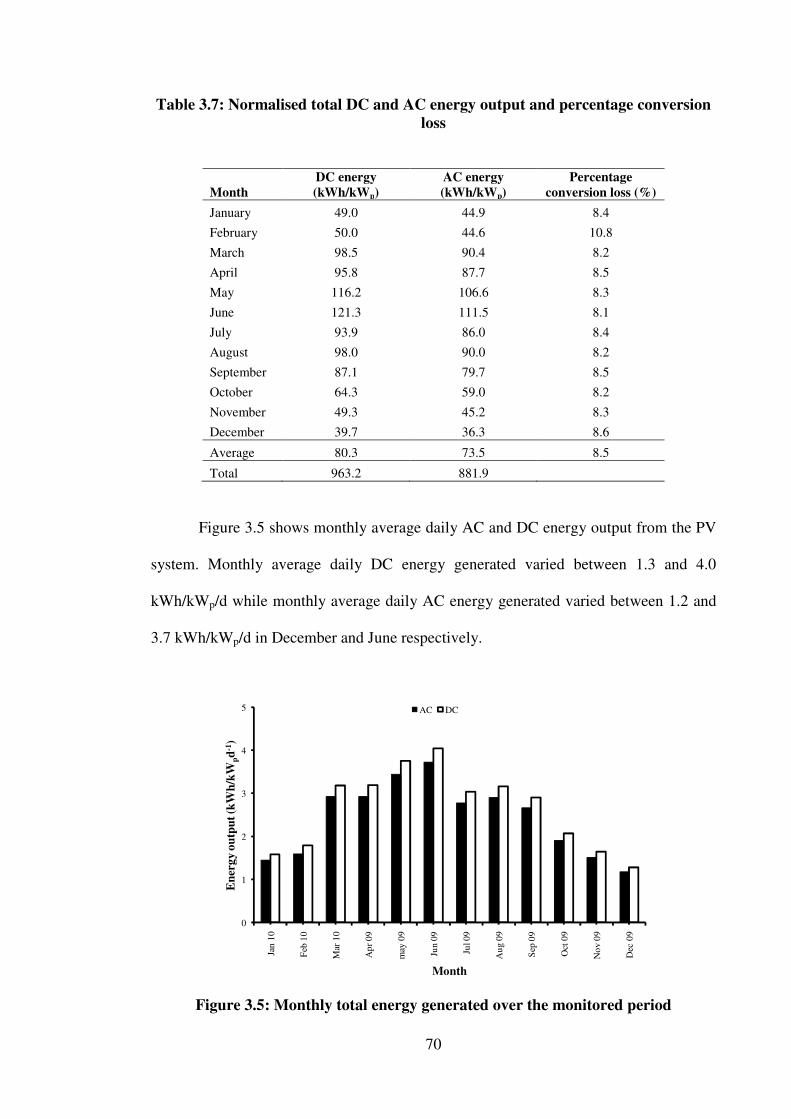
70

Table 3.7: Normalised total DC and AC energy output and percentage conversion loss

Month DC energy (kWh/kWp)

AC energy (kWh/kWp)

Percentage conversion loss (%)

January 49.0 44.9 8.4 February 50.0 44.6 10.8 March 98.5 90.4 8.2 April 95.8 87.7 8.5 May 116.2 106.6 8.3 June 121.3 111.5 8.1 July 93.9 86.0 8.4 August 98.0 90.0 8.2 September 87.1 79.7 8.5 October 64.3 59.0 8.2 November 49.3 45.2 8.3 December 39.7 36.3 8.6

Average 80.3 73.5 8.5

Total 963.2 881.9

Figure 3.5 shows monthly average daily AC and DC energy output from the PV

system. Monthly average daily DC energy generated varied between 1.3 and 4.0

kWh/kWp/d while monthly average daily AC energy generated varied between 1.2 and

3.7 kWh/kWp/d in December and June respectively.

Figure 3.5: Monthly total energy generated over the monitored period

0

1

2

3

4

5

Jan

10

Feb

10

Mar

10

Apr

09

may

09

Jun

09

Jul 0

9

Aug

09

Sep

09

Oct

09

Nov

09

Dec

09

Ene

rgy

outp

ut (k

Wh/

kWpd

-1)

Month

AC DC

71

Figures 3.6 and 3.7 show variation of DC and AC power output against solar

radiation. It is seen that both DC and AC power output from the PV array and inverter

have a linear relationship with solar radiation with correlation coefficients (R2) of

0.9868 and 0.9861 respectively. The high correlation coefficient shows that both DC

and AC power output from the PV array and inverter can be predicted at any instant

with known solar radiation using equations 3.5 and 3.6 given as:

6.94881.6246GP mDC −= (3.12)

5889.81.5072GP mAC −= (3.13)

where,

Gm total in-plane solar radiation (W/m2)

PDC DC power (kW)

PAC AC power (kW)

Figure 3.6: DC power output with solar radiation

y = 1.6246x - 6.9488R² = 0.9868

0

200

400

600

800

1000

1200

1400

1600

1800

0 200 400 600 800 1000 1200

DC

pow

er o

utpu

t (W

)

Solar radiation (Wm-2)

72

Figure 3.7: AC power output with solar radiation

3.6.2 Array Yield

The array yield (YA) is defined as the energy output from a PV array over a

defined period (day, month or year) divided by its rated power and is given as [88]:

ratedPV,

DCA P

EY = (3.14)

YA array yield (kWh/kWp)

EDC DC energy (kWh)

PPV,rated PV rated power (kWp)

The daily array yield (YA,d) and monthly average daily array yield (YA,m) are

given as [29]:

ratedPV,

dDC,dA, P

EY = (3.15)

�=

=N

1ddA,mA, Y

N1

Y (3.16)

where,

YA,d daily array yield (kWh/kWp)

y = 1.5072x - 8.5889R² = 0.9861

0

200

400

600

800

1000

1200

1400

1600

1800

0 200 400 600 800 1000 1200

AC

pow

er o

utpu

t (W

)


73

EDC,d total daily DC energy output (kWh)

YA,m monthly average daily array yield (kWh/kWp)

N number of days in the month

3.6.3 Final Yield

The final yield is defined as the annual, monthly or daily net AC energy output

of the system divided by the rated or nominal power of the installed PV array at STC.

This is a representative figure that enables comparison of similar PV systems in a

specific geographic region. It is dependent on the type of mounting, vertical on a façade

or inclined on a roof and also on the location [105]. The annual final yield is given as

[87, 88]:

ratedPV,

aAC,aF, P

EY = (3.17)

YF,a annual final yield (kWh/kWp)

EAC,a total annual AC energy output (kWh)

The daily final yield (YF,d) and the monthly average daily final yield (YF,m) are

given as:

ratedPV,

dAC,dF, P

EY =

(3.18)

�=

=N

1ddF,mF, Y

N1

Y (3.19)

YF,d daily final yield (kWh/kWp)

EAC,d total daily AC energy output (kWh)

YF,m monthly average daily final yield (kWh/kWp)

74

3.6.4 Reference Yield

The reference yield is the ratio of total in-plane solar insolation (Gm) divided by

the total solar radiation on the PV array at STC (GSTC). It is the number of peak sun-

hours and is given as [88]:

STC

mR G

GY =

(3.20)

YR reference yield (kWh/kWp)

Table 3.8 shows average daily array, final and reference yields of the PV system

during the monitoring period. The monthly average daily final, reference and array

yields varied between 1.17 to 3.72 h/d, 1.11 to 4.57 h/d and 1.28 to 4.04 h/d in

December and June respectively. The annual average daily final, reference and array

yields were 2.43 h/d, 2.86 h/d and 2.65 h/d respectively. Figure 3.8 shows the monthly

average daily PV system’ s final, reference and array yields over the monitored period.

Table 3.8: Array, final and reference yields of the PV system

Month Array yield

(h/d) Final yield

(h/d) Reference yield (h/d)

January 1.58 1.45 1.42 February 1.79 1.63 1.83 March 3.18 2.92 3.32 April 3.19 2.92 3.54 May 3.89 3.57 4.35 June 4.04 3.72 4.57 July 3.03 2.77 3.49 August 3.16 2.90 3.64 September 2.90 2.66 3.24 October 2.07 1.90 2.20 November 1.64 1.51 1.58 December 1.28 1.17 1.11 Average 2.65 2.43 2.86

75

Figure 3.8: Monthly average daily PV system’s final yield, reference yield and

array yield over the monitoring period

3.6.5 PV Module Efficiency

The instantaneous PV module conversion efficiency is calculated as [106]:

mm

DCPV AG

P� = (3.21)

�PV instantaneous PV module conversion efficiency (dimensionless)

The monthly PV module efficiency (�PV,m) is calculated as [107]:

100%AG

E�

mm

dDC,mPV, ×��

�

��

�= (3.22)

�PV,m average monthly PV module conversion efficiency (dimensionless)

dDC,E monthly average daily total DC output (kWh)

3.6.6 System Efficiency

The instantaneous PV system efficiency is calculated as [106]:

am

ACsys AG

P� = (3.23)

�sys PV system efficiency (dimensionless)

0

1

2

3

4

5

Jan

10

Feb

10

Mar

10

Apr

09

may

09

Jun

09

Jul 0

9

Aug

09

Sep

09

Oct

09

Nov

09

Dec

09

Yie

ld (h

d-1)

Month

Array yield Reference yield Final yield

76

The monthly PV system efficiency (�sys,m) is calculated as [107]:

%100AG

E�

am

dAC,msys, ×��

�

��

�= (3.24)

dAC,E monthly average daily total AC output (kWh)

�sys,m monthly PV system efficiency (dimensionless)

3.6.7 Inverter Efficiency

The instantaneous inverter efficiency is calculated as:

DC

ACPV P

P� = (3.25)

The monthly inverter efficiency (�inv,m) is calculated as follows [107]:

100%EE

�dDC,

dAC,minv, ×��

�

��

�= (3.26)

�inv,m monthly inverter efficiency (dimensionless)

Table 3.9 presents monthly average daily PV module, PV system and inverter

efficiencies during the monitoring period. The PV module efficiency varied between

13.7% in April and 15.4 in January while the PV system efficiency varied between

11.8% in April and 13.1% in January and March respectively. The monthly average

daily inverter efficiency varied between 73.9% in December and 86.3% in August. The

annual average daily PV module, PV system and inverter efficiencies were 14.4%,

12.5% and 82.6% respectively. Figure 3.9 shows the monthly average daily PV module,

system and inverter efficiency over the monitored period.

The inverter efficiency was lowest in December and January because of the

prevalence of low levels of solar insolation as shown in Table 3.4. Figure 3.11 also

shows that the average inverter efficiency was affected by solar radiation levels below

77

100 W/m2. Optimal efficiency from technical specification is 93.5% and the efficiency

depends mainly on the input voltage of the connected PV strings. The efficiency

increases as the input voltage decreases [89, 108]

Table 3.9: PV module, PV system and inverter efficiencies

Efficiency (%) Month PV module PV system Inverter January 15.4 13.1 77.3 February 14.7 12.4 81.3 March 15.0 13.1 85.1 April 13.7 11.8 82.8 May 14.0 12.2 85.3 June 13.9 12.2 85.9 July 14.0 12.2 86.1 August 13.8 12.2 86.3 September 14.3 12.3 85.5 October 13.9 12.1 81.1 November 14.8 12.9 80.5 December 15.3 12.9 73.9

Average 14.4 12.5 82.6

Figure 3.9: Monthly average daily PV module, system and inverter efficiencies

over the monitoring period

0

10

20

30

40

50

60

70

80

90

100

Jan

10

Feb

10

Mar

10

Apr

09

may

09

Jun

09

Jul 0

9

Aug

09

Sep

09

Oct

09

Nov

09

Dec

09

Eff

icie

ncy

(%)

Month

PV module PV system Inverter

78

Figure 3.10 shows daily variation of PV module and inverter efficiencies during

three days characterized by clear (01/06/10), intermittent cloud covered (25/11/09) and

heavily overcast skies (20/01/10). During the clear sky day, the PV module and inverter

efficiencies peaked during the early hours after sunrise and late hours during sunset. The

lowest efficiencies occur at the peak of solar radiation showing the effect of PV cell

temperature increase on cell efficiency. During the day with heavily overcast sky and

intermittent cloud covered sky the PV module and inverter efficiencies showed an

irregular profile.

Figure 3.10: Daily variation of PV module and inverter efficiencies

Figure 3.11 shows a plot of inverter efficiency with in-plane solar radiation. The

inverter efficiency is seen to increase as the level of solar radiation increases from 0-200

W/m2 and then remains fairly constant between 91 and 93%. The maximum recorded

inverter efficiency was 93% at a solar radiation range of 400-499 W/m2.

Figure 3.12 shows variation of PV module efficiency with in-plane solar

radiation. The PV module efficiency is seen to increase as the level of solar radiation

0

100

200

300

400

500

600

700

800

900

1000

0

10

20

30

40

50

60

70

80

90

100

0 2 4 6 8 10 12 14 16 18 20 22 0 2 4 6 8 10 12 14 16 18 20 22 0 2 4 6 8 10 12 14 16 18 20 22

Sola

r rad

iatio

n (W

m-2

)

Eff

icie

ncy

(%)

Time

Inverter efficiency PV module efficiency Solar radiation

01/0

6/20

09

25/1

1/20

09

20/0

1/20

10

79

increases from 0-200 W/m2 and then remains fairly constant between 15 and 17% at

higher levels of solar radiation.

Figure 3.11: Average inverter efficiency at different levels of solar radiation over the monitoring period

Figure 3.12: Average PV module efficiency at different levels of solar radiation over the monitoring period

3.6.8 Performance Ratio

The performance ratio (PR) indicates the overall effect of losses on a PV array’ s

normal power output and depends on its temperature, incomplete utilization of incident

solar radiation and system component inefficiencies or failures. The PR of a PV system

indicates how close it approaches ideal performance during real operation and allows

0

10

20

30

40

50

60

70

80

90

100

0-4

5-49

50-9

9

100-

199

200-

299

300-

399

400-

499

500-

599

600-

699

700-

799

800-

899

900-

999

1000

-109

9

Inve

rter

effic

ienc

y (%

)


0

2

4

6

8

10

12

14

16

18

0-4

5-49

50-9

9

100-

199

200-

299

300-

399

400-

499

500-

599

600-

699

700-

799

800-

899

900-

999

1000

-109

9

PV m

odul

e eff

icie

ncy

(%)


80

comparison of PV systems independent of location, tilt angle, orientation and their

nominal rated power capacity [89, 108]. The PV system efficiency is compared with the

nominal efficiency of the photovoltaic generator under standard test conditions.

Performance ratio is defined by the following equations [109, 110]:

STCm

AC

STCDC,

STC

m

AC

STC

sys

�GE

PG

GE

�

�PR === (3.27)

where,

ma

ACsys GA

E� = and

STCa

STCDC,STC GA

P� =

PR performance ratio (dimensionless)

Performance ratio is also defined as a ratio of the final yield divided by the

reference yield and it represents the total losses in the PV system when converting from

DC to AC. Performance ratio is also expressed as [71, 88, 105]:

invsoiltemdegideal

real

R

F ��EE

YY

PR === (3.28)

�deg efficiency loss due to degradation (dimensionless)

�temp efficiency loss due to temperature (dimensionless)

�soil efficiency loss due to soiling (dimensionless)

�inv inverter efficiency (dimensionless)

PR is influenced by solar insolation, shading, operating temperature of the PV

module, relative sizing ratio of inverter and PV array, type of PV module, inverter

characteristics and system layout [111]. The PR for grid connected PV systems varies

from 40-80% [87].

81

3.6.9 Capacity Factor

The capacity factor (CF) is a means used to present the energy delivered by an

electric power generating system. If the system delivers full rated power continuously,

its CF would be unity. CF is defined as the ratio of the actual annual energy output to

the amount of energy the PV system would generate if it operated at full rated power

(PPV,rated) for 24 hours per day for a year and is given as [88]:

8760PPRG

8760PE

36524Y

CFratedPV,

m

ratedPV,

aAC,aF,

××=

×=

×= (3.29)

CF capacity factor (dimensionless)

The CF for a grid-connected PV system is also given as [102]:

24h

CF dps,= (3.30)

Table 3.10 presents monthly average daily PV module and system performance

ratios and capacity factors during the monitoring period. The PV module performance

ratio varied between 79.9% in April and 89.8% in January with an annual average of

83.7%, while the PV system performance ratio varied between 68.3% in April and

76.4% in March with an annual average of 72.4%. The monthly average daily capacity

factor varied between 7.8% in December and 12.5% in March with an annual average of

10.3%. Figure 3.13 shows monthly average daily PV module performance ratio, PV

system performance ratio and PV system capacity factor over the monitored period.

3.6.10 Energy Losses

PV system losses include: array capture losses; system losses; cell temperature

losses; soiling losses; and degradation losses. Soiling and degradation losses are more

difficult to evaluate because they are small effects that occur over large fluctuations in

operating conditions and are not discussed here.

82

Table 3.10. PV module and system performance ratio and capacity factor

Month PV module

PR (%) PV system

PR (%) Capacity

factor (%) January 89.8 76.1 9.0 February 85.2 72.2 8.3 March 87.0 76.4 12.5 April 79.9 68.3 10.8 May 81.5 71.1 12.0 June 80.9 71.1 12.1 July 81.1 70.9 9.6 August 80.4 70.8 10.9 September 83.0 71.7 11.0 October 81.1 70.3 9.7 November 86.1 74.9 9.2 December 88.8 75.1 7.8 Average 83.7 72.4 10.3

Figure 3.13: Monthly average daily performance ratio and capacity factor over the monitoring period

Under real operating conditions the following additional losses can be observed

[112]:

• Optical reflection losses due to non-perpendicular irradiance

• Losses due to low irradiance levels (reduction of form factor and voltage)

• Thermal losses as voltage reduction due to elevated cell temperatures

0

2

4

6

8

10

12

14

0

10

20

30

40

50

60

70

80

90

100

Jan

10

Feb

10

Mar

10

Apr

09

may

09

Jun

09

Jul 0

9

Aug

09

Sep

09

Oct

09

Nov

09

Dec

09

Cap

acity

fact

or (%

)

Perf

orm

ance

ratio

(%)

Month

PV module PV system Capacity factor

83

• Reduction of output current for irradiance sun spectra with an air mass lower

than AM 1.5

• Shadowing: if a cell is shadowed in a serial string, the output current is

limited by the reduced current of the shadowed cell.

• Power conditioning units are very often located in a small building some

distance away from the generator. According to literature, the wiring (ohmic)

losses from the PV panels to the converters are in the vicinity of 3% for most

applications

• Inverters often have high conversion efficiencies at the rated power input,

but for low irradiance levels and low power input the conversion efficiency

decreases. Therefore, the average conversion efficiency over a whole day

could be considerably lower than the rated one.

Array Capture Losses

Array capture losses (Lc) are due to losses within the PV array and are given as

[88]:

ARc YYL −= (3.31)

Lc array capture losses (h/d)

System Losses

System losses (Ls) are as a result of the inverter and are given as [88]:

FAs YYL −= (3.32)

Ls system losses (h/d)

84

Cell Temperature Losses

As a general rule of thumb, the PV module peak power (Pm) decreases by 0.3-

0.4% for every 1 oC increase in the PV cell temperature above STC. Losses resulting

due to the operating cell temperature varying about the temperature at STC (LT), are

calculated as [113]:

ACATT EEL −= (3.33)

where,

tem

ACAT

�

EE =

LT cell temperature losses (h/d)

�tem temperature loss coefficient (dimensionless)

The temperature loss coefficient (�tem) is calculated as [88]:

)T�(T1� rctem −−= (3.34)

� temperature coefficient of Pm of the PV panel (%/oC)

Tc PV cell temperature (oC)

Tr PV cell reference temperature (oC)

Table 3.11 presents results of the PV array and system losses. The system losses

varied between 0.11 h/d in December to 0.33 h/d in May. In November, December and

January the PV modules experienced improvements in capture of 0.06, 0.17 and 0.16

h/d respectively while capture losses varied between 0.04 h/d in February to 0.52 h/d in

June. These improvements in capture are in line with findings from Malik et al. [82] that

showed that mono-crystalline solar cells show higher photo conversion efficiency in

cold climates. Figure 3.14 shows the monthly average daily capture and system losses

over the monitored period.

85

Table 3.11: PV array and system losses

Month Array losses

(h/d) System losses

(h/d) Jan 10 -0.16 0.13 Feb 10 0.04 0.16 Mar 10 0.14 0.26 Apr 09 0.34 0.27 May 09 0.46 0.32 Jun 09 0.52 0.33 Jul 09 0.46 0.26 Aug 09 0.48 0.26 Sep 09 0.34 0.25 Oct 09 0.13 0.17 Nov 09 -0.06 0.14 Dec 09 -0.17 0.11

Average 0.21 0.22

3.6.11 Seasonal Performance

Seasonal average daily in-plane solar insolation, ambient air temperature, PV

module temperature, wind speed, PV module efficiency, PV system efficiency and

inverter efficiency over the monitored period are shown in Table 3.12. The results show

that the maximum seasonal average in-plane solar insolation, ambient air temperature,

PV module temperature and inverter efficiency were 3.9 kWh/m2/d, 18.2 oC, 23.1 oC

and 86.1% respectively in summer while the maximum wind speed, PV module

efficiency and system efficiency were 4.7 m/s (in autumn), 15.1% and 12.8% (both in

winter) respectively. The minimum seasonal average in-plane solar insolation, ambient

air temperature, PV module temperature and inverter efficiency were 1.45 kWh/m2/d,

6.5 oC, 9.2 oC and 77.5% respectively in winter while the minimum wind speed was 4.0

m/s in Autumn and the minimum PV module and system efficiencies were 13.9% and

12.2% respectively in summer. PV module efficiency varies seasonally due to the

monthly variation of the incident solar irradiance angle, cell temperature and shading

[71].

86

Figure 3.14: Monthly daily average capture, system and temperature losses over the monitored period

Table 3.12: Seasonal average daily in-plane solar insolation, ambient temperature, module temperature, wind speed, PV module efficiency, system efficiency and

inverter efficiency over the monitored period.

Season

In-plane solar

insolation (kWh/m2/d)

Ambient temperature

(oC)

PV module temperature

(oC)

Wind speed (m/s)

PV module

efficiency (%)

System efficiency

(%)

Inverter efficiency

(%) Winter 1.45 6.5 9.2 2.9 15.1 12.8 77.5 Spring 3.74 12.2 16.9 3.7 14.2 12.4 84.4 Summer 3.90 18.2 23.1 4.3 13.9 12.2 86.1 Autumn 2.34 14.1 17.8 4.7 14.3 12.4 82.4 Average 2.86 12.7 16.7 3.9 14.4 12.5 82.6

The seasonal energy generated, final yield, reference yield, array yield, capture

losses, system losses, capacity factor and performance ratio over the monitored period

are shown in Table 3.13.

-0.2

0.0

0.2

0.4

0.6

Jan

10

Feb

10

Mar

10

Apr

09

may

09

Jun

09

Jul 0

9

Aug

09

Sep

09

Oct

09

Nov

09

Dec

09

Los

ses (

hd-1

)

Month

Array losses System losses

87

Table 3.13: Seasonal energy generated, final yield, reference yield, array yield, capture losses, system losses, capacity factor and performance ratio over the monitored period.

Season

Energy generated

(kWh/kWp) Final yield

(KWh/kWp/d)

Reference yield

(KWh/kWp/d) Array yield

(KWh/kWp/d)

Capture losses (h/d)

System losses (h/d)

Capacity factor (%)

PV module performance

ratio (%)

PV system performance

ratio (%) Winter 125.8 1.42 1.45 1.55 -0.10* 0.13 8.4 87.9 74.5 Spring 284.7 3.14 3.74 3.42 0.32 0.28 11.8 82.8 71.9 Summer 287.5 3.13 3.90 3.41 0.49 0.28 10.9 80.8 71.0 Autumn 183.9 2.02 2.34 2.21 0.14 0.19 10.0 83.4 72.3

Average 220.5 2.43 2.86 2.65 0.21 0.22 10.3 83.7 72.4 *values represent capture gains

88

3.7 Comparative PV System Performance

To be able to compare operating results from different PV systems, the specific

yield in kWh/kWp/y is calculated as well as the performance ratio. The full-load hours

or the final yield (YF) is also a very important factor for comparing PV systems. The

full load hours is the ratio of the yield over a particular time period to the nominal

power of the generator. The reference time-frame can be a day, week, month or year and

the final yield is given as [71]:

ratedPV,

realF P

EY = (3.35)

Ereal energy generated during operation (kWh)

The annual average daily final yield of other monitored PV systems previously

reported include: Germany, 1.8 kWh/kWp/d; the Netherlands, 1.8 kWh/kWp/d; Italy, 2.0

kWh/kWp/d; Japan, 2.7 kWh/kWp/d and Israel, 3.5 kWh/kWp/d [114]. Table 3.14 shows

performance parameters for different building mounted PV systems. The annual average

daily final yield of the PV system in this study was 2.4 kWh/kWp/d which was higher

than those reported in Germany, Poland and Northern Ireland. It is comparable to results

from some parts of Spain but it was lower than the reported yields in Italy and southern

parts of Spain. The PV system had the highest PV module efficiency, system efficiency

and performance ratio compared to the other systems. High wind speeds and low

ambient temperature at the test location provided suitable conditions for PV systems.

89

Table 3.14: Performance parameters for different building mounted PV systems [88]

Location PV type

Energy output

(kWh/kWp)

Final yield

(kWh/kWp/d)

PV module efficiency

(%)

System efficiency

(%)

Inverter efficiency

(%)

PV system Performance

ratio (%)

Reference

Crete, Greece PC-Si 1336.4 2.0-5.1 - - - 67.4 [88] Germany 680 1.9 - - - 66.5 [89] Málaga, Spain 1339 3.7 8.8-10.3 6.1-8.0 85-88 64.5 [86] Jaén, Spain 892.1 2.4 8.9 7.8 88.1 62.7 [90] Algeria MC-Si 10.1 9.3 80.7 - [91] Calabria, Italy PC-Si 1230 3.4 7.6 - 84.8 - [92] Germany 700-1000 1.9-2.7 - - - - [110] Ballymena, Northern Ireland

MC-Si 616.9 1.7 7.5-10.0 6.0-9.0 87 60-62 [87]

Warsaw, Poland

A-Si 830 2.3 4.5-5.5 4.0-5.0 92-93 60-80 [115]

Castile & Leon, Spain

MC-Si 1180 1.4-4.8 13.7 12.2 89.5 69.8 [116]

Umbertide, Italy

PC-Si - - 4.0-7.0 6.2-6.7 - - [117]

UK 744 - - - - 69 [105] Liverpool, UK Tiles 777 - - - - 72 [105] Dublin, Ireland

HIT 881.9 2.4 14.4 12.5 82.6 72.4 Present study

UK A-Si - - 3.7 3.2 64.5 42.0 [87] UK PC-Si - - - 7.5 - 68.0 [87] UK - - - - 8.4 90-91 59-61 [87] Italy A-Si - - - - - 66 [87] Germany - - - - - - 50-81 [87] Brazil A-Si - - - 5 91 - [87] Thailand - - 2.9-4.0 - - 92-98 70-90 [93]

PC-Si: poly-crystalline silicon, MC-Si: mono-crystalline silicon, A-Si: amorphous silicon,

HIT: Heterojunction with intrinsic thin layer

90

3.8 Summary

A 1.72 kWp grid connected PV system installed in Dublin, Ireland was

monitored between April 2009 and March 2010 and its energy performance was

evaluated on monthly, seasonal and annual basis. Table 3.15 shows a summary of

parameters from the field trial findings.

Table 3.15: Summary of field trial findings

Parameter Minimum Maximum Average Solar insolation (kWh/m2/d) 1.11 4.57 2.86 PV module temperature (oC) 8.8 23.8 16.7 Ambient air temperature (oC) 6.0 18.8 12.7 Wind speed (m/s) 2.5 6.6 3.9 Energy generated (kWh/kWp/d) 1.17 3.72 2.42 Reference yield (h/d) 1.11 4.57 2.86 Array yield (h/d) 1.28 4.04 2.65 Final yield (h/d) 1.17 3.72 2.43 PV module efficiency (%) 13.7 15.4 14.4 PV system efficiency (%) 12.1 13.1 12.5 Inverter efficiency (%) 73.9 86.3 82.6 PV system performance ratio (%) 68.3 76.1 72.4 Capacity factor (%) 7.8 12.5 10.3 System losses (h/d) 0.11 0.33 0.22

Comparison of results from this study with those obtained from other internal

studies (see Table 3.14) revealed that the PV system’ s annual average daily final yield

of 2.4 kWh/kWp/d is higher than those reported in Germany, Poland and Northern

Ireland. It is comparable to results from some parts of northern Spain but it is lower than

the reported yields in most parts of Italy and Spain. The PV system has the highest PV

module efficiency, system efficiency and performance ratio compared to the other

reported systems. Despite low insolation levels, high average wind speeds and low

ambient temperature improve Ireland’ s suitability. The final yield was normalised to

allow for differences in PV system size but it however does not take into consideration

differences in PV cell technology.

91

CHAPTER 4

ENERGY PERFORMANCE MODELING OF GRID-CONNECTED PV SYSTEMS

The goal of this chapter is to investigate the validity of existing models for PC

cell efficiency prediction and to modify the applicable correlation parameters using

measured performance data from Chapter 3 in order to accurately predict PV cell energy

output. Specific objectives are to:

• modify a lumped energy balance model and validate it using field trial data;

• use measured data and statistical parameters to test the validity of different

explicit models to predict PV cell temperature;

• modify implicit models for PV cell temperature based on measured data;

• use measured data to test the validity of different PV cell efficiency models;

and

• select a validated model to predict the energy output from the grid-connected

PV system

4.1 Introduction

Predicting the performance of a PV system is a matter of combining the

characteristics of the major components, that is, the PV array and the inverter with local

insolation and temperature data.

Most existing generic models for assessing the energy output of grid-connected

PV systems are lumped since they determine average daily, monthly or annual energy

output. These models are adapted to support policies such as net metering (applicable in

Japan and some States in America) where electricity is sold to the grid at the same price

92

at which it is bought. Lumped models are also useful in countries where enhanced feed-

in tariffs (high buy-back rates) apply such as in Germany, Spain, Italy, Greece and

France. Lumped models are, however, not adapted to analyse the real-time or dynamic

performances of grid-connected PV systems such as those where support policies are

based on paying for the excess electricity generated, which is fed into the utility grid

(such as in Ireland and other countries). Moreover, they cannot cope with variable

electricity prices based on time of use, which is likely to become more common as

smart metering becomes widely deployed.

Smart meters provide much more precise information on electricity consumed as

well as the time of use. They are two-way communication devices with digital real time

power measurement. They offer the opportunity for remote operation and remote meter

reading as well as the potential for real time pricing, new tariff options and demand side

management [118].

During the day when solar radiation is available, a grid-connected PV system

generates AC power. If the PV system is installed in a domestic dwelling, the AC power

is fed into the main electrical distribution panel of the house, from which it can provide

power to the house for on-site consumption, the excess is supplied to the utility grid.

Figure 4.1 shows representative measured electricity generated from a 1.72 kWp PV

system located in Dublin, Ireland; average electricity consumption of a representative

domestic dwelling in Ireland; the quantity of electricity exported; and spilled to the grid

on the 1st of June 2009.

93

Figure 4.1: Representative daily domestic scale PV system electricity generation and demand

It is seen in Figure 4.1 that domestic energy demand and energy generation from

PV systems are both dynamic in nature varying over the day and different days of the

year. Varying electricity prices based on time-of-day requires that PV system economics

be evaluated based on instantaneous energy demand and generation to account for cost

variation and quantity spilled and imported in order to optimise such systems. This

therefore requires robust dynamic models that predict PV energy output within short

time intervals with minimal errors.

4.2 Lumped Modelling of PV System Energy Output

4.2.1 PV Array Energy Output

The daily, monthly or annual total energy generated by a PV generator (EPV) is

calculated as:

mmmtPV �nAHE = (4.1)

-0.4

-0.3

-0.2

-0.1

0.0

0.1

0.2

0.3

0.4

0.5

00:0

0

01:0

0

02:0

0

03:0

0

04:0

0

05:0

0

06:0

0

07:0

0

08:0

0

09:0

0

10:0

0

11:0

0

12:0

0

13:0

0

14:0

0

15:0

0

16:0

0

17:0

0

18:0

0

19:0

0

20:0

0

21:0

0

22:0

0

23:0

0

Ene

rgy

(kW

h)

Time of day

Electricity demand PV generated electricity Difference

Energy spilled to grid

Energy imported from grid

(h)

94

where,

Ht total in-plane solar insolation (kWh/m2)

Am PV module area (m2)

nm number of PV modules

�m PV module efficiency (%)

For the installed PV array with a capacity of 1.72 kWp composed of 8 PV

modules each with rated output of 215 W inclined at 53o the theoretical annual energy

generated can be calculated using global in-plane solar insolation values shown in Table

4.1.

Ignoring energy losses, the estimated amount of electricity generated annually

by the PV array in this study can be calculated using equation 4.1 as 1,775.9 kWh/y and

long-term average global solar insolation data for Dublin shown in Table 4.1 as:

Table 4.1: Monthly average daily and monthly total solar insolation in Dublin on a PV module inclined at 53o to the horizontal

Month Average daily global

solar insolation (kWh/m2/d)

Monthly global solar insolation (kWh/m2)

January 1.39 43.1 February 1.90 53.2 March 2.79 84.5 April 3.63 108.9 May 3.84 119 June 4.04 121.2 July 4.22 130.8 August 3.65 113.2 September 3.37 101.1 October 2.49 77.2 November 1.56 46.8 December 1.08 33.5 2.83 1,032.5

4.2.2 PV System Energy Output

Since 1-sun of insolation is defined as 1 kW/m2, an insolation of 2.83 kWh/m2/d

can be interpreted as being the same as 2.83 h/d of 1-sun, or 2.83 h of “Peak sun”. So, if

95

the AC power delivered by an array under 1-sun insolation (PAC) is known, that rated

power can be multiplied by the number of hours of peak sun to get the daily energy

(kWh) delivered. Energy delivered in a day can be written as [102]:

� AHE atd ××= (4.2)

where,

� average system efficiency over the day (%)

Aa PV array area (m2)

When exposed to 1-sun of insolation, the AC power output (PAC in KW) from

the PV system can be expressed as:

sun1aSTCAC �AG P −××= (4.3)

where,

sun1� − PV system’ s efficiency at 1-sun (dimensionless)

The average daily energy delivered (Ed) is therefore given as:

��

��

�×�

��

×=

−sun1STC

tACd

�

�

GH

P E (4.4)

Ed average daily energy delivered (kWh)

� average daily PV system efficiency (dimensionless)

If we assume that the average efficiency of the PV system over a day’ s time is

the same as the efficiency when it is exposed to 1-sun, then the energy collected is given

as:

PSHP E ACd ×= (4.5)

PSH peak sun hours (h)

The key assumption of Equation 4.5 is that the system efficiency remains almost

constant throughout the day. The main justification is that these grid-connected systems

96

have maximum power point trackers that keep the operating point near the peak of the I-

V curve throughout the day. Since power at the maximum point is nearly directly

proportional to insolation, system efficiency should be reasonably constant. Cell

temperature plays a role but it is less important. Efficiency might be a bit higher than

average in the morning, when it is cooler and there is less insolation, but all that will do

is make Equation 4.5 slightly conservative [102].

As an illustration of the peak sun hour approach, considering a PV system with

array loss due to mismatched modules and dirt of 4%, inverter efficiency of 93.5%, PV

rating of 1.72 kW under STC, nominal operating cell temperature (NOCT) of 47oC,

mean measured annual ambient temperature of 12.7oC and the PV module temperature

coefficient (�) of 0.3%/oC. The cell temperature is calculated as [68, 88]:

mac G0.8

20NOCTTT �

�

��

� −+= (4.6)

Ta ambient temperature (oC)

The power output from the array is given as 1.61 kW using Equation 4.7 [102]:

25)]�(T[1PP crDC −−= (4.7)

Pr rated PV array power (kW)

Including mismatch, dirt and inverter efficiency gives an annual estimated AC

power output 1.44 kW was obtained using Equation 4.3.

It is important to note that the choice of a value for array losses is important

since a low value will tend to overestimate energy production while a high value will

have the opposite effect. The annual energy output was calculated as 1,503.2 kWh using

Equation 4.8.

dacAC nPSHP E ××= (4.8)

where,

97

EAC annual energy output (kWh)

nd number of days in year

This value can be compared with that obtained if the calculations were done

using monthly average values as shown in Table 4.2. The estimate for annual energy

using annual average values of temperature and solar insolation was 1,503.2 kWh/y

while the monthly calculation yielded 1,502.2 kWh/y. The difference is negligible that it

would appear that using the simpler approach with annual average values rather than

monthly is quite reasonable under a wide range of temperature conditions.

A comparison of measured and modelled monthly energy output yielded an

annual PMAE of 6%. The model predicted fairly accurately in February, April, June and

September with PMAE less than 2%. The model however, predicted poorly in January,

November and December with PMAE of 15.9%, 11.2% and 19.1% respectively. Figure

4.2 shows modelled and measured PV system energy output.

Figure 4.2: Predicted and measured PV system energy output

0

50

100

150

200

Jan 10 Feb 10 Mar 10 Apr 09 may 09 Jun 09 Jul 09 Aug 09 Sep 09 Oct 09 Nov 09 Dec 09

Ene

rgy

outp

ut (k

Wh)

Month

Modelled Measured

98

Table 4.2: Estimated annual energy generation using monthly average data

Number of days

Solar insolation

(kWh/m2/d)

Ambient temperature

(oC)

PV cell temperature

(oC)

DC power output (kW)

AC power output (kW)

Modelled energy output

(kWh/m)

Measured energy output

(kWh/m) PMAE

(%) Jan 10 31 1.42 6.0 39.7 1.6 1.5 65.0 77.3 15.9 Feb 10 28 1.83 6.5 40.3 1.6 1.5 75.5 76.8 1.7 Mar 10 31 3.32 9.9 43.6 1.6 1.5 150.0 155.5 3.6 Apr 09 30 3.54 12.4 46.2 1.6 1.4 153.4 150.8 1.7 may 09 31 4.35 14.3 48.0 1.6 1.4 194.0 183.4 5.8 Jun 09 30 4.57 17.8 51.5 1.6 1.4 194.7 191.8 1.5 Jul 09 31 3.49 17.9 51.6 1.6 1.4 153.9 147.9 4.1 Aug 09 31 3.64 18.8 52.5 1.6 1.4 159.7 154.8 3.1 Sep 09 30 3.24 16.7 50.4 1.6 1.4 138.8 137.1 1.2 Oct 09 31 2.20 15.1 48.8 1.6 1.4 97.9 101.4 3.4 Nov 09 30 1.58 10.6 44.3 1.6 1.5 69.0 77.7 11.2 Dec 09 31 1.11 7.1 40.8 1.6 1.5 50.5 62.4 19.1

Average 2.86 12.7 46.5 1.61 1.44 125.19 126.41 6.0

Total 365 1502.2 1516.9

99

4.3 Dynamic Modelling of PV System Energy Output

Dynamic modelling of PV system energy output involves identifying all

independent variables and establishing their mathematical relationships with power

output. The variables identified from literature include: solar radiation; wind speed;

ambient temperature; cell efficiency; cell temperature; and module area.

Given that current smart metering practice is based on 30-minute intervals, the

mathematical representation of the PV system was simulated at 30-minute intervals

daily using measured data between April 2009 and March 2010. In order to achieve this,

it was necessary to accurately predict the PV cell temperature, which influences the cell

efficiency. Once the cell efficiency and inverter efficiency at any given instant are

accurately predicted, the PV power equation is then used to calculate the power output

from the PV system.

4.3.1 PV Cell Temperature

Temperature of PV cells is one of the most important parameters used in

assessing the performance of PV systems and their electricity output. Cell temperature

depends on several parameters such as the thermal properties of the materials used, type

of cells, module configuration and local climate conditions [98, 99].

PV module’ s efficiency strongly depends on its cells’ operating temperature. PV

cell temperatures are very difficult to measure since the cells are tightly encapsulated in

order to protect them from environmental degradation. The temperature of the back

surface of PV modules is commonly measured and used in place of the cell temperature

with the assumption that these temperatures closely match [96].

From a mathematical point of view, correlations for PV cell operating

temperature (Tc) are either explicit in form, thus giving Tc directly, or implicit, i.e.

100

involve variables such as cell efficiency or heat transfer coefficients, which themselves

depend on Tc. In the latter case, an iteration procedure is necessary to calculate the cell

temperature [97]. Six models for PV cell temperature evaluation were identified from

literature. They include five explicit and one implicit model, the latter a steady state

model.

4.3.1.1 Explicit Correlations

Explicit correlation models express the PV cell temperature as a function of

ambient temperature, solar radiation, wind speed and other system parameters ignoring

heat exchange dynamics between the PV module and its environment. The first

correlation expresses the cell temperature of a PV module (Tc) in Equation 4.9 as [119]:

��

��

� −−+=��

�120)(NOCT

GG

TT c

SOC

mac

(4.9)

where, �� = 0.9 [120]

�c PV cell efficiency (dimensionless)

GSOC solar radiation under standard operating conditions (800 W/m2)

A simplified model of Equation 4.9 is given in Equation 4.10 as [68, 88]:

20)(NOCT800G

TT mac −+=

(4.10)

Equation 4.11 gives the simplest explicit correlation for the operating

temperature of a PV cell with the ambient temperature and incident solar radiation flux

[97]. Earlier reported values for hw were in the range 0.02–0.04 W/m2K [121]. In this

study, the heat transfer coefficient due to wind, hw was determined to be 0.018 W/m2K

using nonlinear regression analysis on measured data.

wmac hGTT += (4.11)

101

where, Tc and Ta are in degrees Kelvin.

The PV module temperature can also be determined using Equation 4.12

proposed by TamizhMani et al. in [122] given as:

wamc dVcTbGaT +++= (4.12)

where, a, b, c and d are system-specific regression coefficients with values of -1.987,

0.02, 1.102 and -0.097, respectively, and R2 of 0.97 determined using measured data

from the Dublin site. Vw is the wind speed in m/s.

King in [97] proposed an expression for PV cell temperature given by Equation

4.13 as:

[ ]cbVaVGG

TT w2w

STC

mac +++=

(4.13)

where, a, b, and c are coefficients with values of 0.043, -1.652 and 24.382, respectively,

and R2 of 0.96, again determined using measured data.

Other explicit correlations reported in literature [97] are based on field

performance data, which are site specific and, therefore, not applicable in this case.

4.3.1.2 Steady-State Analysis

In this approach it is assumed that, within a short-time period (normally less

than 1 h), the intensity of the incoming solar irradiance and other parameters affecting

the PV module’ s behaviour are constant. If the variation in the overall heat loss rates of

the PV module is small, then it can be assumed that the rate of heat transfer from the PV

module to the environment is steady and the temperatures at each point of the PV

module are constant over a short-time period [96].

The equation for the PV cell temperature operating under steady state is derived

assuming that the incident energy on a solar cell is equal to the electrical energy output

102

of the cell plus the sum of the energy losses due to convection and radiation. The

resulting energy balance equation is given as [113, 123]:

0QQPQ crelG =−−− ��

(4.14)

GQ� absorbed solar radiation (W)

elP electrical power (W)

rQ� thermal losses by radiation (W)

cQ� thermal losses by convection (W)

Substituting the relevant terms in Equation 4.14 results in Equation 4.15 given

as [110]:

0)T(TA2h)T(TA2hAG�A��G acccaccrcmccm =−−−−− (4.15)

Ac PV cell area (m2)

hc forced convective heat transfer coefficient (W/m2K)

hr radiative heat transfer coefficient due to wind (W/m2K)

� transmisivity (dimensionless)

� absorptivity (dimensionless)

From Equation 4.15, the PV module temperature is given as:

acr

mPVc T

)h2(h)G�(�

T ++

−= α

(4.16)

where, Tc and Ta are in degrees Kelvin

4.3.1.3 Heat Transfer Coefficients

The radiative heat transfer coefficient between the module front and the sky, and

the module rear and the ground (hr) is given as [106]:

103

)T)(TT��(Th ac2a

2cr ++=

(4.17)

� Stefan-Boltzmann’ s constant (5.67x10-8 W/m2/K4)

� emissivity (dimensionless)

The convective heat flow is dominated at the module front by forced convection

driven by wind forces and at the module rear, depending on the installation situation, by

free laminar or turbulent convection. The convective heat transfer coefficient is given as

[110]:

3 3freec,

3wc,c hhh +=

(4.18)

wwc, 3.575V4.214h += (4.19)

1/3

acfreec, )T1.78(Th −= (4.20)

hc,w convective heat transfer coefficient due to wind (W/m2K)

Because of the wide discrepancies in the value for hc, it is difficult to choose a

particular value. Duffie and Beckman [106] suggested the use of the expression for hc,w

proposed by McAdams [124] for flat plates exposed to outside winds:

wwc, 3.86V5.67h += (4.21)

Nolay in [120] uses the following relationship:

wwc, 4.07V5.82h += (4.22)

4.3.2 PV Cell and Module Efficiency

The most widely-known model to predict the efficiency of a PV cell (�c) is given

as [92, 120] :

)]/G�Log(G)T�(T[1�� STCmrccn,c +−−= (4.23)

where, Tr = 25oC, � = 0.12, �n,c is the nominal cell efficiency (dimensionless).

104

Most often Equation 4.23 is given with � = 0 and it reduces to a linear

dependence of �c on temperature given as [120, 123]:

)]T�(T[1�� rccn,c −−= (4.24)

The efficiency of solar cells can also be expressed as being dependent on the

incident solar radiation and cell temperature. The efficiency at a particular irradiance or

temperature is the result of the nominal efficiency minus the change in efficiency given

as [71]:

�

��

−−��

�

��

�+= )T�(T

GG

ln �1�� rcSTC

mcn,c (4.25)

Another expression for the cell efficiency assuming that the transmittance-

absorptance losses (��/UL) are constant over the relevant operating temperature range is

given as [125]:

�

��

−−−−= )T�(T)T(NOCT

GG

0.9�1�� raSOCSOC

mcn,c

(4.26)

Durisch et al. [126] developed a semi-empirical PV cell efficiency model given

as:

��

��

�

��

��

�+++

��

��

�

��

��

�+=

g

00r

c

c

STC

m

STC

mcn,c AM

AMAMAM

fTT

edGG

GG

ba��

(4.27)

AM air mass (dimensionless)

AM0 absolute air mass (1.5)

The parameters a, b, c, d, e, f and g are regression coefficients with values of

1.249, -0.241, 0.193, 0.244, -0.179, -0.037 and 0.073, respectively, and R2 of 0.99

which were determined using measured data from the Dublin site. Air mass (AM) is the

ratio of the mass of air that the direct radiation has to traverse at any given time and

105

location to the mass of air that it would traverse if the sun were at the zenith [127]. The

air mass is calculated for any time of day at any day of the year from the sun’ s altitude

� (in degrees) using the equation given as [128]:

�)1/Cos(90AM −=

(4.28)

The nominal efficiency (�n,c) of PV cells is given as [71]:

STCc

MPP(STC)cn, GA

P�

×=

(4.29)

PMPP(STC) power at maximum power point under standard test conditions (W)

The nominal efficiency of a PV module is given as:

PF�� cn,mn, ×= (4.30)

PF pack factor (dimensionless) defined in section 3.4

The measured PV module efficiency is given as [106]:

mm

DCDCexp AG

IV� =

(4.31)

�exp measures PV module efficiency (dimensionless)

4.3.3 PV Array Power Output

The DC power output from a PV array is given as:

mmLcn,mDC AGPF��nP ×××××= (4.32)

�L accounts for losses that reduce power output from STC. These losses include:

the difference of the operating PV cell temperature from the reference temperature of 25

oC, the deviation from the maximum power point, the ohmic losses of the conductors,

how clean the PV module surface is, the deviation of the solar irradiance from an ideal

path in order to produce a photoelectron in the cell (optical path deviation), the aging of

106

the PV material [95]. Due to the complexity of modelling the individual losses, �L is

often modelled using Equations 4.23-4.26 representing the terms that are multiplied by

the nominal PV cell efficiency (�n,c). Equation 4.32 therefore reduces to

mmcmDC AGPF�nP ××××= (4.33)

4.3.4 Inverter Efficiency

The inverter efficiency is given as [119]:

nPV,

ninv,inv P

P� = (4.34)

Pinv,n normalised inverter power output (W)

PPV,n normalised PV array output (W)

The normalised inverter output Pinv,n is given as a second-order polynomial by

Peippo and Lund in [119] as:

2nPV,2nPV,10ninv, PkPkkP ++= (4.35)

where

ratedinv,

PVnPV, P

PP = (4.36)

and

ratedinv,

invninv, P

PP = (4.37)

k0 is the normalized self-consumption loss, k1 is the linear efficiency coefficient

and k2 is the coefficient for losses proportional to input power squared as defined by

Peippo and Lund in [119]. PPV,n and Pinv,n are the normalised inverter input and output

power, respectively. PPV and Pinv are the PV array DC input and AC output from the

inverter at any instant of time respectively while Pinv,rated is the rated inverter input

107

capacity. A regression analysis carried out at the Dublin site on normalised inverter

input and output power yielded values for the constants k0, k1 and k2 of -0.001, 0.926

and 0.004, respectively with R2 of 1.

4.3.5 PV System Power Output

The PV system AC power output is given as:

DCinvAC P�P = (4.38)

4.4 Proposed PV Energy Output Model

MatLab software was used to develop a programme to predict the energy output

from a trial PV installation using measured weather data at 30 minute intervals between

April 2009 and March 2010. At 30 minute intervals, the PV cell temperature was

modelled using Equations 4.9-4.13 and Equation 4.16. PV array DC power and PV

system AC power outputs were modelled using Equations 4.33 and 4.38 respectively.

4.4.1 Model Validation

Model validation was carried out using two statistical parameters percentage

mean absolute error and percentage mean error.

One year’ s data collected at 5-minute intervals between April 2009 and March

2010 at the test site was aggregated to 30 minutes and used for model validation. The

data set included the following variables: solar radiation; ambient temperature; PV

module temperature; wind speed; PV array DC current; PV array DC voltage; and PV

system AC power output. A detailed description of the weather data is given in section

3.5.1.

108

4.4.2 PV Cell Temperature

Table 4.3 presents percentage mean absolute error for PV cell temperature

predictions for a model based on Equations 4.9-4.13 and 4.16. The results show that the

empirical models in Equations 4.12 and 4.13 produce the least PMAE of 7.3% and 7.1%

respectively. Where field trial data is not available to derive the empirical coefficients,

Equation 4.9 can be used to predict the PV cell temperature with a higher PMAE of

14.4%. Figure 4.4 shows measured and modelled PV cell temperature using Equations

4.12 and 4.13. It can be seen from Figure 4.3 that the predicted PV cell temperatures

show good correlation with the measured data.

Table 4.3: Percentage mean absolute error for PV cell temperature predictions

Equation

4.9 Equation

4.10 Equation

4.11 Equation

4.12 Equation

4.13 Equation

4.16

PMAE 14.4 23.3 8.2 7.3 7.1 8.8

Figure 4.3: Measured and modelled PV cell temperature

0

10

20

30

40

50

PV ce

ll te

mpe

ratu

re (o C

)

Time

Measured Modelled using Eq. 4.10 Modelled using Eq. 4.11

03/06/2009 04/06/2009 05/06/2009

4.12 4.13

109

4.4.3 PV Array Output Power

Percentage mean absolute error for predicted PV array DC power output using

PV cell temperature models (Equations 4.9-4.13 and 4.16) and modified PV cell

efficiency models (Equations 4.23-4.27) are presented in Table 4.4. The results show

that when field trial data is available to obtain regression coefficients, the empirical

models for PV cell temperature (Equations 4.11 and 4.12) and PV cell efficiency

(Equation 4.27) yield the lowest PMAE of 7.3%. Where only weather data is available,

Equations 4.9 and 4.23 can be used to predict PV array output power with PMAE of

9.1%. Figure 4.4 shows measured and modelled PV array maximum DC output power.

It can be seen that the predicted PV array maximum output power shows good

correlation with the measured data.

Table 4.4: Percentage mean absolute error for predicted PV array power output

Equation

4.9 Equation

4.10 Equation

4.11 Equation

4.12 Equation

4.13 Equation

4.16 Equation 4.23 9.1 11.6 9.8 9.7 9.9 10.2 Equation 4.24 12.5 15.4 13.4 13.3 13.4 13.8 Equation 4.25 12.3 15.2 13.2 13.1 13.2 13.5 Equation 4.26 11.4 12.0 11.2 11.3 11.3 11.5 Equation 4.27 7.8 11.0 7.3 7.3 7.7 8.3

Table 4.5 shows percentage cumulative errors for predicted PV array output

energy against the measured power output of 1,661.4 kWh. The empirical models in

Equations 4.11-4.13 and 4.27 have percentage cumulative errors of 0.6-0.7% while the

non-empirical models using Equations 4.9 and 4.23 have an error of 2.5%. Both models

however tend to over-estimate PV array power output during sunrise.

110

Figure 4.4: Measured and modelled PV array maximum DC power output

Table 4.4: Percentage cumulative error for predicted PV array output energy

Equation

4.9 Equation

4.10 Equation

4.11 Equation

4.12 Equation

4.13 Equation

4.16 Equation 4.23 2.5 6.5 3.8 3.8 3.8 4.2 Equation 4.24 8.0 12.1 9.4 9.4 9.4 9.7 Equation 4.25 7.7 11.8 9.1 9.0 9.0 9.4 Equation 4.26 3.3 7.3 4.6 4.6 4.6 5.0 Equation 4.27 2.3 6.7 0.7 0.6 0.6 1.4

4.4.4 PV System AC Output Power

Percentage mean absolute error for PV system AC power prediction using

modelled PV cell temperatures (Equations 4.9-4.13 and 4.16) and PV cell efficiency

(Equations 4.23-4.27) are shown in Table 4.5. The empirical models (Equations 4.11-

4.13 and 4.27) give the lowest PMAE of 7.9% while the non-empirical models

(Equations 4.9 and 4.23) yield a PMAE of 10%. Again the results show that more

accurate predictions are obtained when measured PV system performance data are used

to generate empirical models. Figure 4.5 shows measured and modelled PV system AC

0

200

400

600

800

1000

1200

1400

1600

PV a

rray

max

imum

pow

er (W

)

Time

Measured Modelled using Eqs. 4.7 & 4.21 Modelled using Eqs. 4.9 & 4.25

03/06/2009 04/06/2009 05/06/2009

4.9 & 4.23 4.11 & 4.27

111

output power. It is seen in Figure 4.5 that both the empirical and non-empirical models

show good agreement with measured data

Table 4.5: Percentage mean absolute error for predicted PV system AC output power

Equation

4.9 Equation

4.10 Equation

4.11 Equation

4.12 Equation

4.13 Equation

4.16 Equation

4.23 10.0 12.4 10.7 10.6 10.7 11.1 Equation

4.27 8.4 11.7 7.9 7.9 8.3 9.0

Figure 4.5: Measured and modelled PV system maximum AC power output

Table 4.6 presents percentage cumulative errors for PV system AC energy

output prediction using PV cell temperature models (Equations 4.9-4.13 and 4.16) and

PV cell efficiency models (Equations 4.23 and 4.27) against the measured PV system

AC energy output of 1,522.5 kWh. The empirical models (Equations 4.11-4.13 and

4.27) result in over-estimations of 1.3-1.4% while the non-empirical models (Equations

4.9 and 4.23) have an over-estimation error of 3.3%.

0

200

400

600

800

1000

1200

1400

1600

PV sy

stem

max

imum

pow

er (W

)

Time

Measured Modelled using Eqs. 4.7 & 4.21 Modelled using Eqs. 4.9 & 4.25

03/06/2009 04/06/2009 05/06/2009

4.9 & 4.23 4.11 & 4.27

112

Table 4.6: Percentage cumulative error for predicted PV system AC output energy

Equation

4.9 Equation

4.10 Equation

4.11 Equation

4.12 Equation

4.13 Equation

4.16 Equation 4.23 3.3 7.4 4.6 4.6 4.6 5.0 Equation 4.27 -1.6 7.5 1.4 1.3 1.4 2.2

4.5 Summary

The introduction of smart meters in countries such as Ireland, Belgium and the UK,

which are currently trailing this technology with a view of its widespread deployment,

necessitates more accurate prediction of PV system power output within short time intervals

such as 30 minutes. In this study, measured field performance data for a domestic-scale

grid-connected PV installation was used to validate some of the widely quoted correlations

in literature employed to model PV cell temperature and efficiency for power output

prediction. The best prediction of PV system AC output power was obtained using Equation

4.12 for PV cell temperature and Equation 4.27 for PV cell efficiency with percentage mean

absolute and cumulative errors of 7.9% and 1.3% respectively. Results show that for short-

term PV array power output prediction as is applicable to smart metering, two options are

available:

• Where field performance data of the PV system is available, empirical models for

PV cell temperature (Equations 4.11 and 4.12) and PV cell efficiency (Equation

4.27) are to be used.

• Where field performance data of the PV system is not available, the non-empirical

models for PV cell temperature (Equation 4.9) and PV cell efficiency (Equation

4.23) are to be used.

However, if field performance data is not available parameters obtained in this

research can be used subject to similarity of weather conditions. In both cases, inverter

performance data is required to model the PV system AC power output. The proposed

models can help to establish the dynamic performance of PV systems when combined with

time-of-day billing systems.

113

CHAPTER 5

REVIEW OF SOLAR WATER HEATING SYSTEMS

The goal of this chapter is to review the current status of forced circulation solar

water heating systems appropriate to Irish households and studies on such systems

reported in literature. Specific objectives are to:

• review forced circulation SWH systems and their main components;

• present the main parameters used in energy performance analysis of SWH

systems;

• review reported studies on the performance and modelling of SWH systems

and their components; and

• get the technical specifications for the most appropriate forced circulation

SWH for Irish households.

5.1 Introduction

In developed countries, energy consumption in the building sector accounts for

40% of energy end use. Most of this consumption is used for heating, cooling,

ventilation and sanitary hot water; in two-thirds of households, heating alone accounts

for more than 50% of all energy use [129]. Water is generally heated by burning fuels

such as firewood, kerosene, oil, liquid petroleum gas (LPG), coal and electricity (either

by geysers or immersion heaters) in urban areas [130]. In this regard, utilization of solar

energy through solar water heating (SWH) systems plays a big role in offsetting the

quantity of conventional energy required [131]. Solar water heaters therefore have

114

significant potential to reduce environmental emissions arising from the use of fossil

fuels [132].

Solar water heaters are the most popular means of solar energy utilization since

they are a relatively mature technology and are perceived as economically attractive

compared with other kinds of solar energy utilization. Solar water heater technology has

been well developed and can be easily implemented at low cost [133]. In a solar

domestic hot water system, the solar collector is the main component of the system,

hence, its optimal performance is important [134].

Flat plate and evacuated tube collectors are the main type of collectors used in

solar water heating systems for domestic applications in Ireland [24]. These collectors

absorb both diffuse and direct solar radiation and would therefore function even under

overcast skies. Water is heated in the collectors and a pump is used to circulate a water

glycol mixture used as the heat transfer fluid. A solar controller triggers the pump when

the solar fluid outlet temperature from the collector is above a set value of the water

temperature at the bottom of the storage tank. A solar coil at the bottom of the hot water

tank is used to heat water. The solar fluid should have some desirable properties such as

low freezing and high boiling points [63]. The ease of operation and low cost of solar

energy collectors makes them suitable for low temperature applications below 80oC. An

auxiliary heating system is used to raise the water temperature during periods when

there is less heat available from the solar collector [106].

5.2 Solar Water Heating Systems

There are several main types of solar water heaters (SWH) for single-family

houses [135]:

115

1. Thermosyphon and forced circulation systems: Thermosyphon systems do not

require pumps, as in this case gravity is used for liquid transport, whereas

systems with forced circulation require circulating pumps for this purpose.

2. Open and closed systems: Open systems have an open container at the highest

point of the solar circuit, which absorbs the volumetric expansion of the liquid

caused by the temperature changes. The pressure in open systems thereby

corresponds at its maximum to the static pressure of the liquid column. Closed

(sealed) systems operate with a higher pressure (1.5-10 bar), which influences

the physical properties (such as the evaporation temperature) of the solar liquid.

Closed systems require special safety devices.

3. Single-circuit (direct) and twin-circuit (indirect) systems: In direct systems the

domestic water circulates from the storage vessel to the collector and back again.

Indirect systems have two separate circuits, the solar circuit and domestic water

circuit. The solar circuit includes the collectors, the ascending pipes, the solar

pump with safety equipment and a heat exchanger. A mixture of water and

antifreeze agent can be used as the heat transfer fluid. The domestic water circuit

includes the storage vessel as well as the cold water and hot water installations

of the house.

4. Filled and drainback systems: Indirect systems can have a collector circuit that is

either completely filled or only partly filled. In the latter systems, which are

called drainback systems, the collector drains completely when the collector

pump is switched off.

Systems with forced circulation are predominant in temperate climates, such as

in central and northern Europe. In southern Europe, Australia, Israel and other mostly

116

sunny countries, thermosiphon systems are the most common type. Figure 5.1 shows a

classification of solar thermal systems.

Figure 5.1: Classification of solar thermal systems [135]

Solar domestic hot water systems typically used in Ireland employ a solar

collector that converts both direct and diffuse solar radiation to heat. A solar fluid

comprising a mixture of water and glycol is circulated through the collector using a

pump operated by a controller. This enables the solar fluid to collect heat when it is

available and transfer it to a hot water tank via a solar coil. This cycle continues as long

as there is a sufficient temperature difference between the inlet and outlet temperature

of the collector. The system’ s auxiliary heating system takes over when more hot water

is needed than can be supplied by the solar collector. Figure 5.2 shows the basic

components of an electricity boosted SWH system used in Ireland.

Over the years, solar water heating systems have witnessed significant increases

in performance and production volumes as well as installed cost reductions due to

economies of scale, learning and technological developments. For example, improved

methods of production and the use of surfaces with increased absorptivities and lower

Solar thermal systems

Forced circulation systems

Thermosyphonsystems

Open systems Closed systems

Single-circuitsystems

Twin-circuitsystems

117

emissivities have increased efficiencies. Modularization has facilitated production

optimisation while improved pump designs have been adapted to suit different flow

regimes. Development in control devices have also contributed to system

improvements. Furthermore, reductions in collector and hot water tank heat losses have

been achieved due to improvements in insulating materials. Different auxiliary heating

systems have also been integrated into storage tanks while new tank designs with

enhanced stratification mechanisms have been developed, thus reducing system losses

[106].

Figure 5.2: Schematic diagram of an electricity boosted solar hot water system

Promising new designs include ‘combi-systems’ that combine water and space

heating. This extends the operation period, thus improving economic performance.

Active solar space and water heating systems usually need a back-up system that uses

electricity, bioenergy or fossil fuels. Other designs integrate a solar-assisted heating

system with a heat pump resulting in ultra-high efficiencies of 125% to 145% compared

to a condensing boiler at around 107% [19].

Pump

Hot water out to demand

Hot watertank

Immersion heater

Solar coil

Solar controller

Solar fluidCold water in

Thermostat

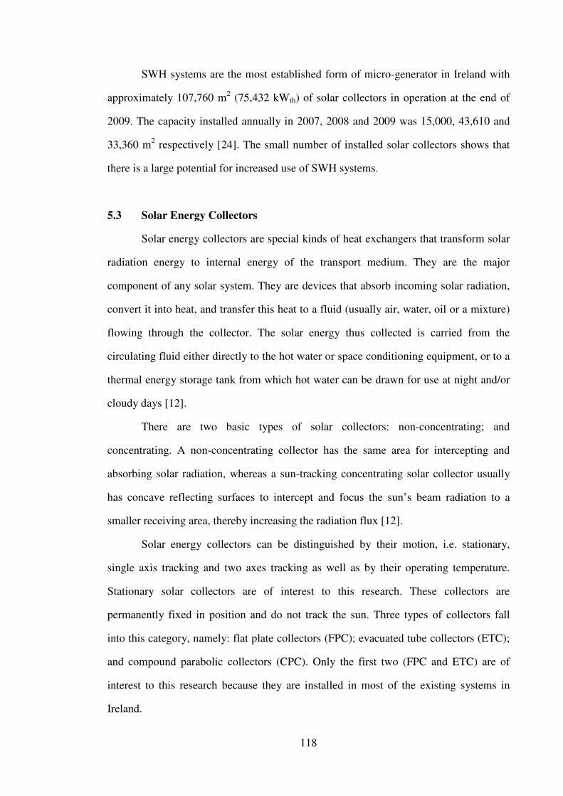
118

SWH systems are the most established form of micro-generator in Ireland with

approximately 107,760 m2 (75,432 kWth) of solar collectors in operation at the end of

2009. The capacity installed annually in 2007, 2008 and 2009 was 15,000, 43,610 and

33,360 m2 respectively [24]. The small number of installed solar collectors shows that

there is a large potential for increased use of SWH systems.

5.3 Solar Energy Collectors

Solar energy collectors are special kinds of heat exchangers that transform solar

radiation energy to internal energy of the transport medium. They are the major

component of any solar system. They are devices that absorb incoming solar radiation,

convert it into heat, and transfer this heat to a fluid (usually air, water, oil or a mixture)

flowing through the collector. The solar energy thus collected is carried from the

circulating fluid either directly to the hot water or space conditioning equipment, or to a

thermal energy storage tank from which hot water can be drawn for use at night and/or

cloudy days [12].

There are two basic types of solar collectors: non-concentrating; and

concentrating. A non-concentrating collector has the same area for intercepting and

absorbing solar radiation, whereas a sun-tracking concentrating solar collector usually

has concave reflecting surfaces to intercept and focus the sun’ s beam radiation to a

smaller receiving area, thereby increasing the radiation flux [12].

Solar energy collectors can be distinguished by their motion, i.e. stationary,

single axis tracking and two axes tracking as well as by their operating temperature.

Stationary solar collectors are of interest to this research. These collectors are

permanently fixed in position and do not track the sun. Three types of collectors fall

into this category, namely: flat plate collectors (FPC); evacuated tube collectors (ETC);

and compound parabolic collectors (CPC). Only the first two (FPC and ETC) are of

interest to this research because they are installed in most of the existing systems in

Ireland.

119

Efficiency is typically around 30-35% for flat plate collector systems and 45-

50% for evacuated tube collector systems [135]. Under Irish weather conditions, the

industry norm for sizing solar water systems is to allow 1-1.3 m2 of collector area per

dwelling occupant. Cylinder requirements are typically 50-60 litres capacity per m2

collector area.

5.3.1 Flat Plate Collectors

A schematic diagram of a flat plate collector is shown in Figure 5.3 while Figure

5.4 shows the components of a flat plate collector. When solar radiation passes through

a transparent cover and impinges on the blackened absorber surface of high

absorptivity, a large portion of this energy is absorbed by the plate and then transferred

to the transport medium in the fluid tubes to be carried away for storage or use. The

underside of the absorber plate and the side of the casing are well insulated to reduce

conduction losses. The liquid tubes can be welded to the absorbing plate, or they can be

an integral part of the plate. The liquid tubes are connected at both ends by large

diameter header tubes [12].

Figure 5.3: Schematic diagram of a flat plate collector [12]

120

Figure 5.4: Components of a flat plate collector [12]

The transparent cover is used to reduce convection losses from the absorber

plate through the restraint of the stagnant air layer between the absorber plate and the

glass. It also reduces radiation losses from the collector as the glass is transparent to

short wave radiation received by the sun but it is nearly opaque to long-wave thermal

radiation emitted by the absorber plate [12].

FPCs should be oriented directly towards the equator, facing south in the

northern hemisphere and north in the southern. The optimum tilt angle of the collector is

equal to the latitude of the location with angle variations of 10-15o more or less

depending on the application [136]. Conventional simple flat plate solar collectors were

developed for use in sunny and warm climates. Their benefits however are greatly

reduced when conditions become unfavourable during cold, cloudy and windy days.

Furthermore, weathering influences such as condensation and moisture can cause early

deterioration of internal materials resulting in reduced performance and system failure.

FPCs have been built in a wide variety of designs and from many different

materials. They have been used to heat fluids such as water, water plus antifreeze

121

additive, or air. Their major purpose is to collect as much solar energy as possible at the

lower possible total cost. The collector should also have a long effective life, despite the

adverse effects of the sun’ s ultraviolet radiation, corrosion and clogging because of

acidity, alkalinity or hardness of the heat transfer fluid, freezing of water, or deposition

of dust or moisture on the glazing, and breakage of the glazing because of thermal

expansion, hail, vandalism or other causes. These causes can be minimised by the use of

tempered glass [12].

5.3.1.1 Glazing Materials

Glass has been widely used to glaze solar collectors because it can transmit as

much as 90% of the incoming shortwave solar irradiation while transmitting virtually

none of the longwave radiation emitted outward by the absorber plate. Glass with low

iron content has a relatively high transmittance for solar radiation (approximately 0.85-

0.90 at normal incidence), but its transmittance is essentially zero for long wave thermal

radiation (5.0-50 mm) emitted by sun-heated surfaces [12].

5.3.1.2 Absorbing Plates

The collector plate absorbs as much of the irradiation as possible through the

glazing, while loosing as little heat as possible upward to the atmosphere and downward

through the back of the casing. The collector plates transfer the retained heat to the

transport fluid. The absorptance of the collector surface for shortwave solar radiation

depends on the nature and colour of the coating and on the incident angle. Usually black

is used, however various colour coatings have been proposed by Tripanagnostopoulos et

al. [137] mainly for aesthetic reasons.

122

By suitable electrolytic or chemical treatments, surfaces can be produced with

high values of solar radiation absorptance (�) and low values of longwave emittance (�).

Essentially, typical selective surfaces consist of a thin upper layer, which is highly

absorbent to shortwave solar radiation but relatively transparent to longwave thermal

radiation, deposited on a surface that has a high reflectance and a low emittance for

longwave radiation. Selective surfaces are particularly important when the collector

surface temperature is much higher than ambient air temperature [12].

5.3.2 Heat pipe evacuated tube collectors

These solar collectors consist of a heat pipe inside a vacuum-sealed tube, as

shown in Figure 5.5. The vacuum envelope reduces convection and conduction losses,

so the collectors can operate at higher temperatures than FPC. Like FPC, they collect

both direct and diffuse radiation. However, their efficiency is higher at low incidence

angles. This effect tends to give ETC an advantage over FPC in day-long performance

[12].

Figure 5.5: Schematic diagram of a heat pipe evacuated tube collector [12] (a) (b)

123

Heat pipes are structures of very high thermal conductance. They permit the

transport of heat with a temperature drop, which are several orders of magnitude smaller

than that for any solid conductor of the same size. Heat pipes consist of a sealed

container with a small amount of working fluid. The heat is transferred as latent heat

energy by evaporating the working fluid in a heating zone and condensing the vapour in

a cooling zone, the circulation is completed by return flow of the condensate to the

heating zone through the capillary structure which lines the inner wall of the container

[138, 139]. These tubes are mounted, the metal tips up, into a heat exchanger (manifold)

as shown in Figure 5.5b. Water or water/glycol mixture flows through the manifold and

picks up the heat from the tubes.

The condenser of a heat pipe can be fitted with a wick as shown in Figure 5.6.

The wick is required for circumferential distribution of liquid in the evaporator. When

the condenser of the heat pipe is elevated so that the condensate returns to the

evaporator with the assistance of gravity, a high heat transfer capability can be

achieved. No wick is therefore required in the condenser since gravity drains the

condensate from the wall to the paddle [140].

Figure 5.6: Schematic diagram of a heat pipe with wick [140]

Wickless heat pipe flat plate solar collectors are essentially a two phase closed

thermosiphon tube with high efficiency for heat transmission [139]. Using wickless heat

124

pipes in flat plate solar collectors do not need moving parts or external pumping power

and act as a thermal diode, preventing the reverse circulation problem in conventional

solar collectors. This minimizes heat loss from the transporting fluid, e.g., water, when

incident radiation is low. Furthermore, when the maximum design temperature of the

collector is reached, additional heat transfer can be prevented. This would prevent over-

heating of the circulating fluid, a common problem in many applications of solar

collectors [141].

The basic difference in thermal performance between a heat-pipe solar collector

and a conventional collector lies in the heat-transfer processes from the absorber tube

wall to the energy-transporting fluid. In the heat pipe collector the processes involved

are evaporation-condensation-convection, while for conventional solar collectors, heat

transfer occurs only in the absorber plate. Solar collectors with heat pipes have a lower

thermal mass, resulting in a shorter start-up time than their flat plate counterparts [142].


5.5.1 Useful Heat Gain

The basic method of measuring collector performance is to expose the operating

collector to solar radiation and measure the fluid flow rate. The useful heat gain (Qu) by

the solar fluid is given as [63]:

)T(TCmQ inoutpfu −= � (5.1)

Cp heat capacity of the solar fluid (kJ/kgK)

fm� solar fluid mass flow rate (kg/s)

Qu useful heat gain (W)

Tout solar fluid outlet temperature (oC)

Tin solar fluid inlet temperature (oC)

125

The Hottel-Whillier equation for the useful heat gain (Qu) of a flat plate solar

collector system, considering the heat losses from the solar collector to the atmosphere

is given as [63]:

)]T(TU)([GFAQ ainLtRcu −−= τα (5.2)

Qu useful heat gain (W)

Ac collector area (m2)

FR heat removal factor (dimensionless)

Gt total in-plane solar radiation (W/m2)

Ta ambient temperature (oC)

UL collector overall loss coefficient (W/m2K)

�� transmittance-absorptance product (dimensionless)

The heat removal factor (FR) is defined as [106]:

��

��

��

��

��

�� ′

−−=pf

cL

cL

pfR Cm

AUFexp1

AUCm

F�

�

(5.3)

F' efficiency factor (dimensionless)

In addition, radiation on the collector, ambient temperature and wind speed are

also recorded. Thus two types of information are available: data on the thermal output,

and data on the conditions producing that thermal performance. These data permit the

characterization of a collector by parameters that indicate how the collector absorbs

energy and how it loses energy to the surroundings [106].

5.5.2 Efficiency

The performance of a solar collector is usually evaluated using its efficiency (�)

which is defined as the ratio of heat taken from the manifold by the cooling liquid and

the incident irradiation striking the collector absorber. � varies with a number of

126

external parameters, including global in-plane solar irradiation (Gt), ambient

temperature (Ta), as well as cooling fluid inlet temperature (Ti) and mass flow rate

).m( f� The collector efficiency is given as [142]:

��

��

� −−=t

am10 G

TT��

(5.4)

where, �0 and �1 are characteristic collector parameters and ��

��

� +=2

TTT oi

m

The low efficiency of flat plate collectors is mainly due to heat loss via the cover

surface due to conduction and convection. Standard flat plate collectors have typical

efficiencies of 50% or less while evacuated devices have efficiencies of about 50-80%

[142].

The instantaneous collection efficiency is given by [63]:

tp

ui GA

Q� =

(5.5)

The collector efficiency can be obtained by dividing Qu by (GtAc) to obtain

[106]

�

��

−−=t

aiLR G

)T(TU��F� (5.6)

For incidence angles below about 35o, the product �� is essentially constant and

Equations (5.2) and (5.6) are linear with respect to the parameter (Ti – Ta)/Gt, as long as

UL remains constant. In reality the heat loss coefficient UL in Equation (5.2) is not

constant but is a function of the collector inlet and ambient temperatures. Therefore,

)T(TccUF ai21LR −+= (5.7)

Applying Equation 5.7 in Equation 5.2 we have [106]:

[ ]2ai2ai1tRcu )T(Tc)T(Tc��GFAQ −−−−= (5.8)

127

The efficiency can then be written as [106]

t

2ai

2t

ai1R G

)T(Tc

G)T(T

c��F�−−−−= (5.9)

Usually the second-order terms are neglected i.e. c2 = 0, in which case Equation 5.9

plots as a straight line on a graph of efficiency versus the heat loss parameter (Ti –

Ta)/Gt. The intercept (intersection of the line with the vertical efficiency axis) equals to

FR��. The slope of the line, that is, the efficiency difference divided by the

corresponding horizontal scale difference, equals -FRUL. If experimental data on

collector heat delivery at various temperatures and solar conditions are plotted, with

efficiency as the vertical axis and T/Gt as the horizontal axis, the best straight line

through the data points correlates collector performance with solar and temperature

conditions. The intersection of the line with the vertical axis is where the temperature of

the fluid entering the collector equals the ambient temperature and collector efficiency

is at its maximum. At the intersection of the line with the horizontal axis, collector

efficiency is zero. This condition corresponds to such a low radiation level, or to such a

high temperature of the fluid into the collector, that heat losses equal solar absorption,

and the collector delivers no useful heat. This condition is normally called stagnation,

and it occurs when no fluid flows in the collector [12]. Figure 5.7 shows plots of

collector efficiencies for various types of liquid collectors.

5.5.3 Optical Analysis

Absorbed solar radiation flux (S) is defined as [63]:

t)G(S τα= (5.10)

128

where (��) is the transmittance-absorptance product which is equal to the optical

efficiency (�o).

The overall transmittance-absorptance product (��) is determined as [106]:

t

gtddbb

G

(��

�G(��

G(�G)(�

)2cos1

)2cos1

) αααα

��

��

� −+��

��

� ++= (5.11)

Figure 5.7: Collector efficiency of various types of liquid collectors [12]

5.5.3.1 Incidence Angle Modifier

The performance Equation 5.7 assumes that the sun is perpendicular to the plane

of the collector, which rarely occurs. For the glass cover plates of a flat plate collector,

specular reflection of radiation occurs thereby reducing the (��) product. The incidence

angle modifier k��, defined as the ratio of �� at some incident angle � to �� at normal

radiation (��)n, is described by the following expression

2

10�� 1� cos

1b1

� cos1

b1k ��

��

� −−��

��

� −−= (5.12)

129

For single glass cover, a single-order equation can be used with b0 = -0.1 and b1

= 0. With the incidence angle modifier, the collector efficiency Equation 5.8 can be

modified as [106]:

t

2ai

2t

ai1��R G

)T(Tc

G)T(T

c)k(F�−−−−= nτα (5.13)

5.5.4 Daily Performance

The solar fluid flow rate, inlet temperature to the collector and outlet

temperature from the collector are used to compute the useful heat gained. The useful

heat gain and efficiency are strongly dependent on solar radiation. The daily efficiency

is calculated as [63]:

�

�

=

== 24

1ttp

24

1tu

i

GA

Q�

(5.14)

5.5.6 Performance of Heat Pipe Collectors

Azad [140] carried out an experimental study and investigated the thermal

behaviour of a forced circulation SWH with flat plate heat pipe collector and 200 litres

storage tank in Tehran (latitude 35.7 oN; longitude 52.3 oE altitude 1190 m). Using a

water flow rate of 0.03-0.032 kg/s, he determined the collector efficiency using the

ASHRAE standard 93-1986 procedure.

Hussein [143] undertook an experimental investigation of a wickless heat pipe

flat plate solar collector with a cross flow heat exchanger under meteorological

conditions of Cairo, Egypt. His experiments on the collector were conducted at different

cooling water flow rates. During each experiment, the mass flow rate of the cooling

130

water was kept constant, and the other physical quantities were recorded. Results

obtained showed that the instantaneous efficiencies of the collector were optimum at the

cooling water mass flow rate of 0.0292 kg/s which is very close to the ASHRAE

standard mass flow rate of 0.02Acoll kg/s for testing conventional flat plate solar water

collectors.

Hammad [144] carried out an experimental study of the performance of a flat

plate solar collector cooled by a set of heat pipes, designed and manufactured locally to

work at low temperature conditions equal to that of flat plate solar collectors.

Efficiencies and quantities of energy transferred to a water storage tank were calculated

and found to be comparable to those obtained by using water cooled solar collector. The

efficiency of such a collector depends on the time of day, solar radiation intensity,

ambient temperature and flat plate mean temperature. He studied the efficiency, as the

dependent variable on the above mentioned parameters, and then compared it with that

of a commonly used water cooled collector.

Mathioulakis [145] carried out a theoretical and experimental investigation of

the performance of a new solar hot water system with an integrated heat-pipe. His solar

water heating system used a wickless gravity assisted loop heat-pipe for the heat

transfer from the collector–evaporator to the tank through a heat exchanger–condenser.

A detailed heat transfer experimental study which focused on the thermal behaviour of

the different parts of the system was performed. The results obtained showed that the

system could reach satisfactory efficiencies which, in combination with manufacturing

simplicity, absence of moving parts and good behaviour under freeze conditions, make

it an interesting technological solution. Furthermore, a theoretical model for the

collector was developed and validated with experimental results was also performed.

Mathioulakis concluded that his model could be used to optimize the system’ s design.

131

5.6 Modelling

Azad [140] investigated the thermal behaviour of a gravity assisted heat pipe

solar collector theoretically and experimentally. He developed a theoretical model based

on the effectiveness-NTU method for evaluating the thermal efficiency of the collector,

the inlet, outlet water temperatures and heat pipe temperature. He determined an

optimum value for the evaporator length to condenser length ratio.

Hussein [143] developed a simulation model for a wickless heat pipe flat plate

solar collector with a cross flow heat exchanger. He validated his model using field

performance data under different meteorological conditions for Cairo, Egypt and

collector operating parameters.

Riffat et al. [142] constructed a novel flat plate called thin membrane heat pipe

solar collector. They developed an analytical model that was used to simulate heat

transfer processes occurring in the collector, calculate its efficiency and determine the

relation between efficiency and general external parameters, (Tmean-Ta)/Gt. Their model

applied the heat balance and heat resistance network method, which is a new approach

in collector thermal performance analyses.

Bong et al. [146] presented a theoretical model to determine the efficiency, heat

removal factor, and outlet water temperature of a single collector and an array of flat

plate heat-pipe collectors. Their model was validated using field trial data for 16 heat-

pipe collectors under typical weather conditions in Singapore. Their results showed that

the proposed model was sufficient to describe the steady-state performance of the

collector array within the operational range of hot water temperatures.

Ezekwe [147] analysed the thermal behaviour of solar energy systems using heat

pipe absorbers and compared them with systems using conventional solar collectors.

132

The mathematical model he used was based on the Hottel-Whillier-Bliss equation for

solar collectors. His results showed that the heat transfer ratio (�) is a very useful

parameter in predicting the thermal performance of a heat pipe absorber. He concluded

that for solar heating applications, the heat removal factor (Fr) of the heat pipe system is

apparently lower than that of an equivalent conventional system because of the extra

heat transfer surface in the heat pipe system. This penalty, however, can be minimized

by proper design of the heat pipe condenser and system manifold.

Traditional solar collector modelling methods consider the system as a whole

entity lumping all parameters as a group of non-dimensional scale-factors. This has a

disadvantage as it may obscure the fundamentals of heat transfer processes, which are

apparent in the heat circuit analysis [34]. This therefore highlights the advantage of

using the heat circuit analysis to model solar water heating collectors.

Boji� et al. [148] modelled and simulated a forced circulation solar water

heating system using a time marching model. They evaluated the annual variation of

solar fraction with respect to the volume of the storage tank, demand hot water

temperature required, difference of this temperature and preset storage tank water

temperature, and consumption profile of the domestic hot water demand. Their results

for a number of designs with different storage tank volumes indicate that the systems

with greater volume yield higher solar fraction values. Their results also showed that the

solar fraction of the system increases with lower hot water demand temperature and

higher differences between the mean storage water and the demand temperatures. They

concluded that when a larger storage tank volume is used, the solar fraction is less

sensitive to a variation of these operating parameters.

133

5.6.1 Optimization of SWH Systems

Lima et al. [149] developed an optimization model using water heating system

design parameters, using a numerical simulation routine, in a long-term transient

regime. Their optimized design gives the slope and area of the flat plate collector, which

results in the minimum cost over the equipment life cycle. Using TRNSYS they

simulated the performance of a thermosyphon solar water heating system with flat-plate

collector using climate data for Sao Paulo, Brazil. They carried out an economic

analysis to investigate if it is more attractive to increase the gain of solar energy in the

winter period, with the consequence of reducing the solar energy gain along the year, or

to adopt the adequate slope, which improves the yearly solar energy gain. Their results

showed that it is possible to maximize the annual total energy so that the system has a

low initial cost, although the cost of auxiliary energy during use of the system is higher

than the other system.

5.7 Summary

A review of literature showed that although SWH systems are an established

technology, so there has been significant increase in performance and production

volumes as well as installed cost reductions due to economies of scale, learning and

technological developments. However, the SWH system market is still in its infancy in

Ireland despite being the most established micro-generation technology.

A review of literature also revealed that some studies have been carried out to

determine the technical specifications and performance of different designs of collectors

integrated within solar water heating systems. However, no suitable published data was

found in literature that was representative of the performance of the SWH systems being

investigated in this research. It was therefore imperative that field trials were necessary

134

to provide data for energy performance analysis of the SWH systems as described in

Chapter 6 as well as economic and environmental analysis as in Chapter 9.

Collectors are the main components with flat plate and evacuated tube collectors

being the most widely deployed in forced circulation systems installed in Ireland.

Collector efficiencies are typically around 30-35% for flat plates and 45-50% for

evacuated tubes. Typical systems installed in Irish domestic dwellings employ either 4

m2 flat plate or 3 m2 heat pipe evacuated tube collectors. Given that the collectors have

different efficiencies and costs, while using the same balance of system components, a

comparative techno-economic and environmental performance assessment of the two

systems was undertaken in Chapters 6 and 9.

It was evident that there was lack of credible data on the performance of SWH

systems with variable and fully controlled hot water demand. A sub-system was

therefore designed and incorporated into the two conventional forced circulation SWH

systems presented in Chapter 6. The sub-system consisted of a unit that automatically

dispensed a defined hot water demand profile and also controlled the switching of the

auxiliary heaters thereby mimicking interaction between a user and the SWH systems.

It was also seen in literature that several researchers have developed theoretical

models to study the thermal behaviour of different designs of flat plate and evacuated

tube collectors. Most of these models were derived from first principles and are

component or system specific. Also, their solution procedures and programming could

be quite cumbersome. No dynamic energy balance models for forced circulation SWH

systems using proprietary software such as TRNSYS was found.

This therefore highlighted the need for validated dynamic energy balance

models for the SWH systems that could be used to predict their energy performance

under different weather and operating conditions. TRNSYS models for the modified

FPC and ETC systems were developed and presented in Chapter 7.

135

CHAPTER 6

FIELD TRIALS AND PERFORMANCE ANALYSIS OF SOLAR WATER HEATING SYSTEMS

The goal of this chapter is to compare the energy performance of forced

circulation SWH systems with 4 m2 FPC and 3 m2 heat pipe ETC equipped with a sub-

system that automatically dispenses a predefined hot water demand profile and controls

the operation of the auxiliary heaters. Specific objectives are to:

• describe the methodology used in the field trials;

• design, construct and implement the SWH systems and the automated sub-

system;

• outline the equations used in the energy performance analysis;

• to provide data for system model validation;

• present performance results of different system components; and

• compare the energy performance of the two SWH systems using indices

such as energy output from the collectors; energy delivered to the hot water

tanks; collector and system efficiencies; heat loss in the pipes between the

collectors; and solar coils and solar fraction.

6.1 Introduction

This chapter presents the results of energy performance monitoring over a one

year period of two solar water heating systems - one with 4 m2 flat plate and one with 3

m2 heat pipe evacuated tube collectors - operating under the same weather conditions in

Dublin, Ireland. The solar water heaters are standard systems currently installed in

average sized single domestic dwellings in Ireland. An automated system was

136

developed and incorporated to control the hot water draw-offs and electric immersion

heaters to mimic the operation of solar water heating systems in domestic dwellings.

The energy performance of the two systems was compared on daily, monthly and yearly

basis.

6.2 Methodology

Two complete forced circulation solar water heating systems with 4 m2 FPC and

3 m2 ETC were installed side by side on a flat rooftop and subjected to the same

weather and operating conditions in the Focas Institute, Dublin, Ireland. The two water

heating systems each had a 300 litre hot water tank equipped with an electrical auxiliary

immersion heater which was used to top up the tank temperature to 60 oC in the

morning and evening whenever the solar coil fell short of doing so. An automated hot

water draw off system was developed which mimicked domestic hot water use; exactly

the same hot water demand profile was applied to both SWH systems (shown in Figure

6.1). System performance data were collected every minute.

Figure 6.1: Volume of hot water (60 oC) draw-off at different times of the day [150]

2

24

2 2

62

52 2 2 2 2 2

62 2 2 2 2 2 2

13

62

2

0

10

20

30

40

50

60

70

07:0

5

07:0

5

07:3

0

07:4

5

08:0

5

08:3

0

08:4

5

09:0

0

09:3

0

10:3

0

11:3

0

11:4

5

12:4

5

14:3

0

15:3

0

16:3

0

18:0

0

18:1

5

18:3

0

19:0

0

20:3

0

21:0

0

21:3

0

Vol

ume (

litre

s)

Time

137

6.3 System Description

Typical solar water heating systems used in temperate climates consist of a hot

water storage tank, control unit, pump station and either flat plate or evacuated tube

collectors. The collectors used in this study were south facing and inclined at 53o equal

to the local latitude of the location. The hot water cylinders were installed nearby in the

building’ s plant room. The solar circuits consisted of 12 mm diameter copper pipes

insulated with 22 mm thick Class O Armaflex. All pipe fittings were insulated to reduce

heat losses. The solar circuit pipe length for the ETC supply and return were 14 m and

15.4 m respectively while they were 14 m and 15.6 m respectively for the FPC. Detailed

specifications of the two collectors are shown in Table 7.2.

ETC was a Thermomax HP200 consisting of a heat pipe solar collector with a

row of 30 evacuated tubes and an insulated water manifold. It had two separate circuits,

one in each individual tube inside the heat pipe and one in the manifold through which

the solar fluid circulates. The collector had an absorber surface of 3 m2 and the tubes

had a vacuum level of 10-5 mbar.

FPC consisted of two K420-EM2L flat plate collectors each with a gross area

of 2.18 m2 and aperture area of 2 m2 connected in series giving a total area of 4 m2.

Each collector had maximum operating and stagnation temperatures of 120 oC and 191

oC respectively, a maximum operating pressure of 10 bar and a fluid content of 1.73

litres.

Stainless steel hot water cylinders (model HM 300L D/coil U44332) were

used of height 1680 mm and diameter 580 mm and an operating pressure of 3 bar. Each

cylinder was equipped with two electric immersion heaters of 2.75/3.0 kW capacity

located at the bottom and middle of the tank. The cylinders each had two heating coils

with surface areas of 1.4 m2 and a rating of 21 kW.

138

6.3.4 Hot Water Demand Profile

The hot water demand profile employed was the EU reference tapping cycle

number 3 presented in Figure 6.1, equivalent to a daily energy output of 11.7 kWh

representing 199.8 litres of water at 60 oC. It is based on hot water use of the average

European household described in the European Union mandate for the elaboration and

adoption of measurement standards for household appliances EU M324EN [150].

6.3.5 Auxiliary Heating and Hot Water Demand Management System

A key innovation of the SWH systems field performance test was the

introduction of an automated hot water dispensing unit which extracted water from the

hot water tanks in such a way as to mimic real life operation where the users interact

with the SWH systems. It consists of a programmable logic controller (PLC),

contactors, relays, electrical fittings, solenoid valves, thermostats, impulse flow meters,

etc. A software code was written to control the auxiliary heating system as well as

opening and shutting of the solenoid valves. The operation was synchronised for the

two SWH systems to ensure they operated identically.

The PLC turned on the immersion heaters between 5-8 am and 6-9 pm daily just

before the two peak hot water draw-offs. Analogue thermostats placed at the top of the

hot water tanks were set to turn-off the electricity supply to the immersion heaters when

the temperature of water at the top of the tank exceeded 60 oC. Hot water was dispensed

using solenoid valves that were opened and closed using signals from the PLC. Pulse

flow meters (1 pulse per litre) installed at the end of the solenoid valves were used to

count the number of litres of water extracted from the hot water tanks. The solenoid

valves were closed when the required volume of water was dispensed based on the

water demand profile (Figure 6.1).

139

Figure 6.2 shows a schematic diagram of the experimental setup of the two

SWH systems. It shows the location of the SWH system components as well as the

position of the thermocouple sensors. Parameters measured include the following: solar

fluid temperature at the collector outlet (T1), water temperature at the bottom of the hot

water tank (T2), water temperature at the middle of the hot water tank (T3), solar fluid

temperature at inlet to the solar coil (T4), solar fluid temperature at the outlet from the

solar coil (T5), solar fluid temperature at inlet to the collector (T6), cold water inlet

temperature (T7), hot water supply temperature (T8) and the volume flow rate of the

solar fluid. Figure 6.3 shows the evacuated tube and flat plate collectors while Figure

6.4 in-door installation of the experimental rig.

Figure 6.2: Schematic diagram of the FPC and ETC systems

Pump

Hot water out to demand

Hot watertank

Immersion heater

Solar coil

Solar controller

Solar fluidCold water in

Pulse flow meter

Pulse flow meter

T6

T1

T2

T3

T8

T7

T4

T5

Hot water demand &

auxiliary heating control systemThermostat

Pulse flow meter

Solenoid valve

140

Figure 6.3: Evacuated tube and flat plate collectors

Figure 6.4: In-door installation of the experimental rig

6.3.6 Data Measurement and Logging

Each SWH system was equipped with a RESOL DeltaSol M solar controller

which had relay inputs to control the operation of the solar pump station. It also had

temperature sensor inputs onto which PT1000 platinum resistance temperature sensors

were connected to measure water and solar fluid temperatures (T1-T8) shown in Figure

6.2. The volumetric flow rate of the solar fluid was measured using RESOL V40-06

Evacuated tube collector Flat plate collectors

Hot watercylinder

Pumpstation

Controller

Thermostat

Immersion heater

141

impulse flow meters which react at 10 litres per pulse. RESOL DL2 data loggers were

used to store data every minute from the RESOL DeltaSol M solar controllers via

RESOL VBus cables. DL2 data loggers were equipped with a secure digital (SD) drive

and a local area network (LAN) port for direct connection to a personal computer (PC).

Data from the loggers was extracted using a Web browser or an SD card and then

converted to text format using the RESOL Service Centre Software.

In-plane global solar radiation, ambient temperature and wind speed data were

measured using a weather station consisting of an SMA Sunny Sensor Box equipped

with an ambient temperature sensor and an anemometer. The solar radiation sensor had

an accuracy of ±8% and a resolution of 1 W/m2. The PT1000 platinum temperature

sensors had an accuracy of ±0.5 oC while the ambient temperature sensor was a JUMO

PT 100 U type with accuracy of ±0.5 oC. The anemometer was a Thies small wind

transmitter with accuracy of ±5%. Weather data was logged at 5 minute intervals using

a Sunny Box WebBox.


The energy performance indices evaluated in this study include: energy

collected, energy delivered and supply pipe losses, solar fraction, collector efficiency

and system efficiency.

6.4.1 Energy Collected

The useful energy collected by the solar energy collector is given as [127]:

)T(TCmQ 61pc −= � (6.1)

Qc useful energy collected (W)

T1 solar fluid temperature at collector outlet (oC)

142

T6 solar fluid temperature at collector inlet (oC)

m� Solar fluid mass flow rate (kg/s)

Cp specific heat capacity (kJ/kgK)

6.4.2 Energy Delivered and Supply Pipe Losses

The useful energy delivered by the solar coil to the hot water tank is given as

)T(TCmQ 54pd −= � (6.2)

Qd useful energy delivered (W)

T4 solar fluid temperature at solar coil inlet (oC)

T5 solar fluid temperature at solar coil outlet (oC)

Supply pipe losses were as a result of temperature drop as the solar fluid flowed

between the collector outlet and the solar coil inlet to the hot water tank. These losses

were calculated as:

)T(TCmQ 41pl −= � (6.3)

Ql supply pipe heat loss (W)

6.4.3 Solar Fraction

The solar fraction (SF) is the ratio of solar heat yield to the total energy

requirement for water heating and is given as [135]:

auxs

s

QQQ

SF+

= (6.4)

SF solar fraction (dimensionless)

Qs solar heat yield (W)

Qaux auxiliary heat (W)

143

6.4.4 Collector Efficiency

The efficiency of the collectors were calculated as [63, 106]:

tc

61pcol GA

)T(TCm�

−=

�

(6.5)

�col collector efficiency (dimensionless)

Ac collector area (m2)

Gt total in-plane solar radiation (W/m2)

6.4.5 System Efficiency

The efficiency of the collectors were calculated as [63, 106]:

tc

54psys GA

)T(TCm�

−=

�

(6.6)

�sys system efficiency (dimensionless)

6.5 Results and Discussions

6.5.1 Energy Collected

Table 6.1 shows average daily solar insolation, energy collected, energy

delivered and supply pipe losses from the FPC and ETC systems. The average daily

energy collected by the FPC was 2.0 and 9.2 kWh/d in December and April

respectively, and 1.7 and 9.5 kWh/d in June respectively for the ETC. Annual total

energy collected by the 4 m2 FPC and 3 m2 ETC was 1,984 and 2,056 kWh/y

respectively. Annually, the 3 m2 ETC system therefore generated 3.5% more energy

than the 4 m2 FPC system. The results also show that over the year a unit area of FPC

and ETC generated 496 and 681 kWh/m2/y of heat energy respectively.

144

Tab

le 6

.1:

Ave

rage

dai

ly so

lar

inso

latio

n, e

nerg

y co

llect

ed, e

nerg

y de

liver

ed a

nd su

pply

pip

e lo

sses

for

the

FPC

and

ET

C sy

stem

s

In-p

lane

So

lar

inso

latio

n (k

Wh/

m2 /d

) T

otal

ene

rgy

colle

cted

(KW

h/d)

E

nerg

y de

liver

ed

(KW

h/d)

Su

pply

pip

e lo

sses

(KW

h/d)

Ene

rgy

colle

cted

pe

r un

it ar

ea

(kW

h/m

2 /d)

Mon

th

FP

C

(4m

2 ) E

TC

(3

m2 )

FPC

(4

m2 )

ET

C

(3m

2 ) FP

C

(4m

2 ) E

TC

(3

m2 )

FPC

E

TC

Ja

n-10

1.

5 3.

0 2.

4 2.

5 2.

0 0.

5 0.

4 0.

8 0.

8 Fe

b-10

1.

9 4.

1 3.

0 3.

4 2.

4 0.

7 0.

5 1.

0 1.

0 M

ar-1

0 3.

3 6.

7 6.

2 5.

4 5.

4 1.

0 0.

9 1.

7 2.

1 A

pr-1

0 4.

5 9.

2 8.

5 7.

5 7.

4 1.

4 1.

3 2.

3 2.

8 M

ay-1

0 4.

2 7.

7 9.

0 6.

4 7.

4 1.

3 1.

6 1.

9 3.

0 Ju

n-09

4.

6 8.

2 9.

5 7.

1 7.

7 1.

1 1.

8 2.

1 3.

2 Ju

l-09

3.6

5.5

6.7

4.5

5.3

1.0

1.4

1.4

2.2

Aug

-09

3.7

5.9

7.1

5.0

5.7

1.0

1.5

1.5

2.4

Sep-

09

3.3

5.8

6.5

4.9

5.2

0.9

1.2

1.4

2.2

Oct

-09

2.2

3.9

4.1

3.2

3.4

0.7

0.7

1.0

1.4

Nov

-09

1.8

3.3

3.0

2.6

2.5

0.7

0.5

0.8

1.0

Dec

-09

1.2

2.0

1.7

1.6

1.5

0.4

0.2

0.5

0.6

Ann

ual

aver

age

3.0

5.4

5.6

4.5

4.6

0.9

1.0

1.4

1.9

Ann

ual

tota

l 1,

087

1,98

4 2,

056

1,63

9 1,

699

326

366

496

681

145

6.5.2 Energy Delivered and Supply Pipe Losses

It is seen in Table 6.1 that the FPC system delivered a daily average of 1.6 and

7.5 kWh/d of heat energy in December and April respectively while the ETC system

delivered a daily average of 1.5 and 7.7 kWh/d of heat energy in December and June

respectively.

Heat losses occur along the supply side of the solar circuit especially at high

collector outlet temperatures. The FPC and ETC systems had annual supply pipe heat

losses of 326 and 366 kWh/y respectively corresponding to 16.4% and 17.8% of energy

collected. These losses are quite significant representing 65.7% and 53.7% of the energy

generated by a unit area of FPC and ETC respectively annually. The supply pipe length

should therefore be kept as short as possible and all joints insulated to reduce heat

losses. Large heat losses could also be attributed to a problem with the critical radius of

the pipe’ s insulation. Using insulation materials with thicknesses below the critical

radius would lead to increased heat loss.

6.5.3 Energy Extracted and Auxiliary Energy

Table 6.2 shows monthly average, daily, annual average and annual total energy

extracted from the hot water tanks and auxiliary energy supplied to the FPC and ETC

systems. During the monitoring period a total of 4,591.2 and 4,455.6 kWh of heat

energy were extracted from the hot water tanks of the FPC and ETC systems

respectively. The results also show that the monthly average quantity of auxiliary

energy added varied between 5.4 and 4.9 kWh/d in June and 11.8 and 11.6 kWh in

December for the FPC and ETC systems respectively.

146

6.5.4 Solar Fraction

Table 6.2 shows the monthly and annual solar fraction (SF) for the FPC and

ETC systems. SF of the FPC system range between 14.6% and 60.4% in December and

June respectively while SF for the ETC ranged between 12.7% and 66.1% in December

and June respectively. It is seen that the FPC system had higher SF between January

and April as well as November and December while the ETC system had higher SF

between May and October. FPC and ETC systems had annual average SFs of 38.6%

and 40.2% respectively. It is also seen that the quantity of energy required for auxiliary

heating decreases with increase in SF.

Table 6.2: Energy extracted from the hot water tanks and auxiliary energy supplied to the FPC and ETC systems

Norton [151] reported that a solar water heater in Ireland can satisfy about 40%

of a typical annual domestic hot water demand. Studies carried out by Allen et al. [152]

Energy extracted

(kWh/d) Auxiliary energy

(kWh/d) Solar fraction

(%)

Month FPC (4m2)

ETC (3m2)

FPC (4m2)

ETC (3m2)

FPC (4m2)

ETC (3m2)

Jan-10 13.2 12.9 11.6 11.4 20.7 17.2 Feb-10 13.4 13.1 11.1 11.1 26.8 21.0 Mar-10 12.0 11.8 8.3 8.0 44.5 43.7 Apr-10 14.3 14.2 6.6 6.9 58.2 56.2 May-10 14.9 14.3 7.4 7.2 51.0 55.4 Jun-09 14.8 14.2 5.4 4.9 60.4 66.1 Jul-09 14.9 14.3 7.3 6.7 42.9 49.8 Aug-09 14.7 14.3 6.9 6.4 46.4 52.7 Sep-09 14.3 14.0 7.6 7.3 43.2 47.1 Oct-09 14.0 13.7 9.2 9.0 29.7 31.2 Nov-09 13.9 13.4 10.5 10.3 23.8 22.2 Dec-09 13.4 13.1 11.8 11.6 14.6 12.7 Annual average 14.0 13.6 8.6 8.4 38.6 40.2 Annual total (kWh) 4,591.2 4,455.6 3,149.7 3,053.6

147

showed that the maximum achievable solar fraction achievable across the UK ranges

between 28% and 52% for a range of installations.

6.5.5 Collector and System Efficiency

Table 6.3 shows results of collector and system efficiencies for the FPC and

ETC systems. The respective minimum and maximum efficiencies of the FPCs was

38.5% in July and 54.5% in February while those of the ETCs were 48.3% in December

and 71.4% in May. Similarly, the range of efficiencies of the overall FPC system varied

from 31.6% in July to 45.6% in February and from 42.8% in December to 58.8% in

May for the ETC system.

Table 6.3: FP and ET collector and system efficiencies

Collector

efficiency (%) System efficiency

(%) Month FPC ETC FPC ETC Jan-10 51.5 53.5 42.2 44.1 Feb-10 54.5 52.6 45.6 43.2 Mar-10 50.0 62.3 40.3 54.4 Apr-10 51.6 63.2 41.7 55.0 May-10 45.7 71.4 37.8 58.8 Jun-09 44.5 68.7 38.4 55.8 Jul-09 38.5 62.5 31.6 49.3 Aug-09 39.6 63.4 33.2 50.5 Sep-09 43.8 65.6 36.9 53.0 Oct-09 44.3 62.2 36.2 51.3 Nov-09 45.5 54.6 36.4 45.5 Dec-09 43.7 48.3 34.9 42.8 Annual average 46.1 60.7 37.9 50.3

6.5.6 System Temperatures

Table 6.4 shows monthly average and maximum daily collector inlet and outlet

solar fluid temperatures for the FPC and ETC systems. Monthly average daily collector

solar fluid inlet temperatures for the FPC ranged from 9.0 oC to 27.7 oC in January and

148

June while and from 8.7 oC and 27.7 oC during the same months for the ETC system.

Maximum recorded collector solar fluid inlet temperatures were 66.8 oC and 65.6 oC for

FPC and ETC systems respectively in June. Monthly average daily collector outlet

temperatures for the FPC system ranged from 7.2 oC to 27.9 oC in January and June and

from 7.9 oC to 29.1 oC during the same months for the ETC system. It is worth noting

that the low temperatures of the collectors at night time and winter tend to reduce the

monthly average daily solar fluid temperatures at the collector outlet. Maximum

recorded collector outlet solar fluid temperatures were 70.4 oC and 70.3 oC for the FPC

and ETC systems in June and April respectively.

Table 6.4: Monthly average and maximum daily FPC and ETC inlet (T1) and

outlet (T6) temperatures

T1 avg T1 max T6 avg T6 max

Month FPC (4m2)

ETC (3m2)

FPC (4m2)

ETC (3m2)

FPC (4m2)

ETC (3m2)

FPC (4m2)

ETC (3m2)

Jan-10 7.2 7.9 45.6 43.9 9.0 8.7 39.5 39.2 Feb-10 9.2 9.5 57.6 48.3 10.5 10.0 44.5 43.3 Mar-10 14.6 15.7 62.9 53.7 15.4 15.4 49.7 47.9 Apr-10 22.4 23.2 63.1 70.3 22.1 22.8 59.3 64.0 May-10 23.2 24.1 65.7 62.6 23.0 23.2 59.6 57.2 Jun-09 27.9 29.1 70.4 69.4 27.7 27.7 66.8 65.6 Jul-09 25.8 26.7 67.4 60.8 25.7 25.4 57.5 55.6 Aug-09 26.1 26.7 67.2 66.5 26.2 25.7 61.6 60.2 Sep-09 22.5 23.0 66.2 66.2 23.3 22.7 62.3 61.3 Oct-09 18.4 18.9 64.3 57.4 19.8 19.3 54.6 52.5 Nov-09 12.8 13.5 56.9 46.6 14.6 14.1 42.7 41.0 Dec-09 7.8 8.6 42.9 35.9 10.0 9.8 29.8 29.9

Table 6.5 shows monthly average and maximum daily water temperatures at the

bottom (T2) and middle (T3) of the hot water tank for the FPC and ETC systems.

Monthly average daily temperatures at the bottom of the hot water tank for the FPC

system ranged between 11.2 oC to 28.4 oC in January and June and from 11.5 oC and

28.4 oC during the same months for the ETC system. Maximum recorded temperatures

149

at the bottom of the tank were 59.9 oC and 59.5 oC for the FPC and ETC systems in

June respectively. Monthly average daily temperatures at the middle of the hot water

tank for the FPC ranged from 22.1 oC to 42.2 oC in January and June and from 22.4 oC

to 42.4 oC during the same months for the ETC system. Maximum recorded

temperatures at the middle of the hot water tank were 60.5 oC and 60.0 oC for the FPC

and ETC systems respectively.

Table 6.5: Monthly average and maximum daily water temperature at the bottom (T2) and middle (T3) of the hot water tank for the FPC and ETC systems


Month FPC (4m2)

ETC (3m2)

FPC (4m2)

ETC (3m2)

FPC (4m2)

ETC (3m2)

FPC (4m2)

ETC (3m2)


Table 6.6 shows monthly average and maximum daily water temperatures at the

inlet (T7) and outlet (T8) of the hot water tank for the FPC and ETC systems. Monthly

average daily tank inlet temperatures for FPC ranged from 10.2 oC to 21.6 oC in January

and August and from 9.7 oC to 21.1 oC during the same months for ETC. Maximum

recorded temperatures at the inlet to the hot water tank were 28.0 oC and 28.2 oC for the

FPC and ETC systems in June respectively. Monthly average temperatures at the outlet

from the hot water tank for the FPC ranged between 46.3 oC and 56.9 oC in January and

June and from 44.7 oC to 55.2 oC in January and August for the ETC system. Maximum

150

recorded temperatures at the outlet from the hot water tank were 69.0 oC and 65.8 oC for

the FPC and ETC systems respectively.

Table 6.6: Monthly average and maximum daily water temperature at the tank inlet (T7) and outlet (T8) for the FPC and ETC systems


Month FPC (4m2)

ETC (3m2)

FPC (4m2)

ETC (3m2)

FPC (4m2)

ETC (3m2)

FPC (4m2)

ETC (3m2)


6.5.7 Daily Performance

6.5.7.1 Environmental/Ambient Conditions

Figure 6.5 shows in-plane global solar radiation for three ‘typical’ days

characterised by heavily overcast sky (20/01/2010), clear sky (1/06/2009) and

intermittent cloud covered sky (25/11/09) measured at five minute intervals. Maximum

solar radiation was 398.8, 932.1 and 692.5 W/m2 on the heavily overcast, clear and

intermittent cloud covered sky days respectively.

Figure 6.6 shows ambient air temperature and wind speed for the three days

measured at five minute intervals. Maximum ambient air temperatures were 8.8, 23.6

and 10.3 oC while the maximum wind speeds were 10.2, 6.2 and 16.3 m/s on the heavily

overcast, clear and intermittent cloud covered sky days respectively.

151

Figure 6.5: In-plane global solar radiation for three characteristic days

Figure 6.6: Ambient air temperature and wind speed for three characteristic days

6.5.7.2 Solar Fluid Mass Flow Rate

Both systems had variable speed pumps controlled by the Resol DeltaSol M

controller. Figure 6.7 shows the solar fluid mass flow rate for the FPC. During the

heavily overcast day the mass flow rate was largely below 0.02 kg/s and only

occasionally reached 0.04 kg/s. During the clear sky day the mass flow rate showed a

more regular pattern at sun rise and sun set peaking at 0.068 kg/s. During the day with

0

5

10

15

20

25

0

5

10

15

20

25

00:0

002

:30

05:0

007

:30

10:0

012

:30

15:0

017

:30

20:0

022

:30

01:0

003

:30

06:0

008

:30

11:0

013

:30

16:0

018

:30

21:0

023

:30

01:5

504

:30

07:0

009

:30

12:0

014

:30

17:0

019

:30

22:0

0

Win

d sp

eed

(ms-1

)

Am

bien

t tem

pera

ture

(o C)

Time of day

Ambient temperature Wind speed

20/01/2010

01/06/2009

25/11/2009

0

100

200

300

400

500

600

700

800

900

1,000

00:0

002

:30

05:0

007

:30

10:0

012

:30

15:0

017

:30

20:0

022

:30

01:0

003

:30

06:0

008

:30

11:0

013

:30

16:0

018

:30

21:0

023

:30

01:5

504

:30

07:0

009

:30

12:0

014

:30

17:0

019

:30

22:0

0

Sola

r rad

iatio

n (W

m-2

)

Time of day

20/01/2010 01/06/2009 25/11/2009

152

intermittent cloud cover, the mass flow rate peaked at 0.088 kg/s and was occasionally

zero.

Figure 6.7: Solar fluid mass flow rate for FPC

Figure 6.8 shows the solar fluid mass flow rate for ETC. During the heavily

overcast day the pump cycled on and off regularly to peaks of 0.045 kg/s. During the

clear sky day the pump operated largely continuously between 0.045 kg/s and 0.098

kg/s, peaking intermittently at 0.168 kg/s during early morning. During the day with

intermittent cloud cover the mass flow rate occasional peaked at 0.17 kg/s but was

typically 0.056 kg/s. Again explain what this means as opposed to just listing figures

6.5.7.3 Energy Collected

Figure 6.9 shows the energy collected by the FPC at 1 min intervals. It can be

seen that the total energy collected during the days with heavily overcast and

intermittent cloud cover was very low with intermittent spikes as a result of the pump

turning on and off as the intensity of solar radiation varied. The energy collected during

the clear sky day peaked at around solar noon.

0.00

0.02

0.04

0.06

0.08

0.10

0.12

0.14

0.16

0.18

00:0

002

:00

04:0

006

:00

08:0

010

:00

12:0

014

:00

16:0

018

:00

20:0

022

:00

00:0

002

:00

04:0

006

:00

08:0

010

:00

12:0

014

:00

16:0

018

:00

20:0

022

:00

00:0

002

:00

04:0

006

:00

08:0

010

:00

12:0

014

:00

16:0

018

:00

20:0

022

:00

Mas

s flo

w ra

te (k

gs-1

)

Time of day

20/01/2010 01/06/2009 25/11/2009

153

Figure 6.8: Solar fluid mass flow rate for the ETC system

Figure 6.9: Energy collected by the FPC system

Figure 6.10 shows the energy collected by the ETC system. Unlike the FPC

system, the ETC system tends to operate during low levels of solar insolation at sunrise

and sunset. This has an impact on the quantity of energy collected since short

-0.02

0.00

0.02

0.04

0.06

0.08

0.10

0.12

00:0

002

:00

04:0

006

:00

08:0

010

:00

12:0

014

:00

16:0

018

:00

20:0

022

:00

00:0

002

:00

04:0

006

:00

08:0

010

:00

12:0

014

:00

16:0

018

:00

20:0

022

:00

00:0

002

:00

04:0

006

:00

08:0

010

:00

12:0

014

:00

16:0

018

:00

20:0

022

:00

Ene

rgy

colle

cted

(kW

h/m

in)

Time of day

20/01/2010 01/06/2009 25/11/2009

0.00

0.02

0.04

0.06

0.08

0.10

0.12

0.14

0.16

0.18

00:0

002

:00

04:0

006

:00

08:0

010

:00

12:0

014

:00

16:0

018

:00

20:0

022

:00

00:0

002

:00

04:0

006

:00

08:0

010

:00

12:0

014

:00

16:0

018

:00

20:0

022

:00

00:0

002

:00

04:0

006

:00

08:0

010

:00

12:0

014

:00

16:0

018

:00

20:0

022

:00

Mas

s flo

w ra

te (k

gs-1

)

Time of day

20/01/2010 01/06/2009 25/11/2009

154

intermittent flows of the solar fluid tends to carry heat away from the hot water tank and

dump it into the collector leading to energy losses as seen on the 20/01/2010 and

25/11/2009. This results in a reduction in the energy collected and, in some periods

during the cold winter months to net negative energy balances. This shows that there is

scope for improvement in the operation of ETC systems equipped with heat pipe

collectors.

Figure 6.10: Energy collected by the ETC system

6.5.7.4 System Temperatures

Figure 6.11 shows collector outlet solar fluid temperatures for the FPC and ETC

systems for the three days at 1 min intervals. It can be seen that the FPC system had

slightly higher collector outlet solar fluid temperatures than the ETC system. This can

be attributed to the lower mass flow rates of the FPC system. FPC outlet solar fluid

temperature had a lag over the ETC system temperature and this lag was evident during

the clear sky day. This lag was as a result of the high mass flow rates of the ETC.

-0.04

-0.02

0.00

0.02

0.04

0.06

0.08

0.10

0.12

00:0

002

:00

04:0

006

:00

08:0

010

:00

12:0

014

:00

16:0

018

:00

20:0

022

:00

00:0

002

:00

04:0

006

:00

08:0

010

:00

12:0

014

:00

16:0

018

:00

20:0

022

:00

00:0

002

:00

04:0

006

:00

08:0

010

:00

12:0

014

:00

16:0

018

:00

20:0

022

:00

Ene

rgy

colle

cted

(kW

h/m

in)

Time of day

20/01/2010 01/06/2009 25/11/2009

155

Figure 6.11: Collector outlet fluid temperature for the FPC and ETC systems

Figure 6.12 shows the hot water tank outlet fluid temperature for the FPC and

ETC systems measured along the hot water discharge pipe. The peaks show the outlet

fluid temperatures during water draw-offs. The temperatures in both FPC and ETC

systems were quite close since they were operated under similar conditions. It is seen

that during the heavily overcast and intermittently cloud covered days the tank outlet

fluid temperature dropped significantly during the daytime since little energy was

delivered by the solar coil and remained significantly below 50 oC for approximately 10

hours (8:30 am – 6:30 pm) . On the other hand during the clear sky day the tank outlet

fluid temperature stayed above 50 oC since energy was added to its content throughout

the day thereby raising its temperature.

0

10

20

30

40

50

60

70

00:0

002

:00

04:0

006

:00

08:0

010

:00

12:0

014

:00

16:0

018

:00

20:0

022

:00

00:0

002

:00

04:0

006

:00

08:0

010

:00

12:0

014

:00

16:0

018

:00

20:0

022

:00

00:0

002

:00

04:0

006

:00

08:0

010

:00

12:0

014

:00

16:0

018

:00

20:0

022

:00

Col

lect

or o

utle

t tem

pera

ture

(o C)

Time of day

FPC ETC

20/01/2010 01/06/2009 25/11/2009

156

Figure 6.12: Hot water tank outlet temperature for the FPC and ETC systems

Figure 6.13 shows the hot water tank bottom and middle temperatures for the

FPC system for the three days at 1 min intervals. It can be seen that during the heavily

overcast day the immersion heater was used to raise the temperature of the middle of the

tank (T3) from 12 oC to 52 oC in the morning and from 14 oC to 58 oC in the evening.

During the clear sky day, T2 increased to T3 and both temperatures increased until 14

hours when T2 peaked at 57.7 oC while T3 was 56.7 oC. This shows that the FPC system

can achieve 100% solar fraction during a clear sky day with total daily solar insolation

of 6.7 kWh/m2/d. During the day with intermittent cloud cover, T2 increased alongside

T3 and peaked at 25 oC. Auxiliary energy from the immersion heater was then used to

increase T3 to 58 oC. A similar trend in T2 and T3 increase was obtained with the ETC

system as shown in Figure 6.14.

0

10

20

30

40

50

60

70

00:0

002

:00

04:0

006

:00

08:0

010

:00

12:0

014

:00

16:0

018

:00

20:0

022

:00

00:0

002

:00

04:0

006

:00

08:0

010

:00

12:0

014

:00

16:0

018

:00

20:0

022

:00

00:0

002

:00

04:0

006

:00

08:0

010

:00

12:0

014

:00

16:0

018

:00

20:0

022

:00

Hot

wat

er ta

nk o

utle

t tem

pera

ture

(o C)

Time of day

FPC ETC

20/01/2010 01/06/2009 25/11/2009

157

Figure 6.13: Hot water tank bottom (T2) and middle (T3) temperatures for the

FPC system

Figure 6.14: Hot water tank bottom (T2) and middle (T3) temperatures for the ETC system

6.5.7.5 Collector Efficiency

Figure 6.15 shows hourly global in-plane solar radiation, FPC and ETC

efficiencies on the 20/01/2010, 01/06/2009 and 25/11/2009. It is seen that during the

0

10

20

30

40

50

60

70

00:0

002

:00

04:0

006

:00

08:0

010

:00

12:0

014

:00

16:0

018

:00

20:0

022

:00

00:0

002

:00

04:0

006

:00

08:0

010

:00

12:0

014

:00

16:0

018

:00

20:0

022

:00

00:0

002

:00

04:0

006

:00

08:0

010

:00

12:0

014

:00

16:0

018

:00

20:0

022

:00

Hot

wat

er ta

nk o

utle

t tem

pera

ture

(o C)

Time of day

T2 (FPC) T3 (FPC)

20/01/2010 01/06/2009 25/11/2009

0

10

20

30

40

50

60

70

00:0

002

:00

04:0

006

:00

08:0

010

:00

12:0

014

:00

16:0

018

:00

20:0

022

:00

00:0

002

:00

04:0

006

:00

08:0

010

:00

12:0

014

:00

16:0

018

:00

20:0

022

:00

00:0

002

:00

04:0

006

:00

08:0

010

:00

12:0

014

:00

16:0

018

:00

20:0

022

:00

Hot

wat

er ta

nk o

utle

t tem

pera

ture

(o C)

Time of day

T2 (ETC) T3 (ETC)

20/01/2010 01/06/2009 25/11/2009

158

heavily overcast day in winter (20/01/2010) with a maximum hourly solar radiation of

207 W/m2, the FPC and ETC had maximum hourly efficiencies of 84.7% and 48.0%

respectively. During the clear sky day in summer (01/06/2009) with a maximum hourly

solar radiation of 918 W/m2, the ETC was more efficient than the FPC with maximum

hourly efficiency of 88.1% compared to 73.7% for the FPC. During the intermittently

cloud-covered day in Autumn (25/11/2009) with a maximum hourly solar radiation of

407 W/m2, the ETC was again more efficient than the FPC with maximum hourly

efficiency of 88.2% compared to 61.1% for the FPC. The results show that the FPC was

more efficient than the ETC during days with low levels of solar radiation while the

ETC was more efficient during days with high levels of solar radiation and intermittent

cloud cover.

Figure 6.15: Hourly global in-plane solar radiation, FPC and ETC efficiencies

6.5.8 Seasonal Performance

Table 6.7 shows seasonal daily average values of solar insolation, energy

collected, energy delivered and supply pipe losses. It is seen that the 4 m2 FPC system

0

100

200

300

400

500

600

700

800

900

1000

0

10

20

30

40

50

60

70

80

90

100

1 5 9 13 17 21 1 5 9 13 17 21 1 5 9 13 17 21

Sola

r rad

iatio

n (W

m-2

)

Eff

icie

ncy

(%)

Time of day

FPC efficiency ETC efficiency Solar radiation

20/01/2010 01/06/2009 25/11/2009

159

collected and delivered more heat energy than the 3 m2 ETC system in winter. Both

systems collected 7.9 kWh/d of heat energy in Spring while the ETC system collected

and delivered more heat energy than the FPC system in Summer and Autumn. The

supply pipe losses for the FPC and ETC systems were highest in Spring and Summer

respectively.

Table 6.8 shows seasonal average daily collector and system efficiencies, energy

extracted and auxiliary energy for the FPC and ETC systems. The collector and system

efficiencies for the FPC ranged from 40.9% in summer to 49.9% in winter while those

for the ETC ranged from 51.5% in winter to 65.6% in spring. These results show that

the FPC system was most efficient in winter while the ETC was most efficient in

Spring. 6.5 kWh/d and 6.0 kWh/d of auxiliary energy was added to the FPC and ETC

system hot water tanks respectively using the electric immersion heaters in summer,

while 11.5 kWh/d and 11.3 kWh/d was added in winter.

6.6 Summary

The year round energy performance analysis of two selected and commonly

used forced circulation SWH systems has been carried out using trial installations in

Dublin, Ireland. An automated sub-system was designed and incorporated to the

conventional SWH systems to enable them operate in such a way as to mimic real life

operation taking into consideration the interactions between collectors, storage tanks

and users. Electric immersion heaters were used to supply auxiliary energy when the

solar coils were unable to raise the tank water temperature to the required temperature.

A summary of the energy performance analysis results is shown in Table 6.9.

160

Table 6.7: Seasonal values of solar insolation, energy collected, energy delivered, supply pipe losses and energy collected per unit area for the FPC and ETC systems

Solar insolation

(kWh/m2/d) Energy collected

(kWh/d) Energy delivered

(kWh/d) Supply pipe losses

(kWh/d)

Energy collected per

unit area (kWh/m2/d)

Season FPC

(4 m2) ETC (3m2)

FPC (4 m2)

ETC (3m2)

FPC (4 m2)

ETC (3m2) FPC ETC

Winter 1.5 3.0 2.3 2.5 2.0 0.5 0.4 0.8 0.8 Spring 4.0 7.9 7.9 6.4 6.7 1.2 1.3 2.0 2.6 Summer 4.0 6.5 7.8 5.5 6.2 1.0 1.5 1.6 2.6 Autumn 2.4 4.3 4.5 3.6 3.7 0.8 0.8 1.1 1.5

161

Table 6.8: Seasonal average daily collector and system efficiencies, energy extracted and auxiliary energy for the FPC and ETC systems

Collector efficiency (%)

System efficiency (%)

Energy extracted (kWh/d)

Auxiliary energy (kWh/d)

Season FPC

(4 m2) ETC

(3 m2) FPC

(4 m2) ETC

(3 m2) FPC

(4 m2) ETC

(3 m2) FPC

(4 m2) ETC

(3 m2) Winter 49.9 51.5 40.9 43.4 13.3 13.0 11.5 11.3 Spring 49.1 65.6 39.9 56.1 13.7 13.4 7.4 7.4 Summer 40.9 64.9 34.4 51.9 14.8 14.3 6.5 6.0 Autumn 44.6 60.8 36.5 49.9 14.1 13.7 9.1 8.9

162

Table 6.9: Summary of energy performance analysis results

Item description FPC (4 m2) ETC (3 m2) Total in-plane solar insolation (kWh/yr) 1,087 1,087 Total energy collected (kWh/yr) 1,984 2,056 (3.5%) Energy collected per unit area (kWh/m2) 496 681 Energy delivered to hot water tank (kWh/yr) 1,639 1,699 Supply pipe losses (kWh/yr) 326 (16.4%) 366 (17.8%) Solar fraction (%) 38.6 40.2 Collector efficiency (%) 46.1 60.7 System efficiency (%) 37.9 50.3 Reported system efficiency (%) 35-45* 45-50*

*Values obtained from The German Solar Energy Society [135]

Performance results showed that the 4 m2 FPC system compares quite

favourably with the 3 m2 ETC system when connected to a 300 litres hot water tank.

The higher efficiency of the ETC did not translate to additional energy collected that

justifies its additional cost over the FPC. It is therefore suggested that ETC should be

considered for installation where roof space constraints exist.

Measured field performance data collected was used for detailed economic and

environmental comparison of the two SWH systems in Chapter 9. The field

performance data was used to validate the TRNSYS models developed in Chapter 7.

The data will also provide valuable information to researchers, policymakers and

installers.

163

CHAPTER 7

MODELLING SOLAR WATER HEATING SYSTEMS

The aim of this chapter is to develop dynamic energy balance simulation models

using TRNSYS program for forced circulation solar water heating systems with flat

plate and heat pipe evacuated tube collectors and validate the model using measured

field performance data. Specific objectives are to:

• use TRNSYS to develop models for the solar water heating systems

investigated in Chapter 6;

• present the TRNSYS model information flow diagram;

• present detailed descriptions of the SWH systems’ components;

• present measured field performance data; and

• present results from the TRNSYS models and the validation procedure.

Although not used in the economic and environmental analysis of this research

due to the availability of field trial data, the validated TRNSYS models can be used as a

tool for long-term energy performance simulation. They can also be used to carryout

parametric studies for system optimisation under different weather and operating

conditions. Section 6.3 presents a description of the solar water heating systems and a

schematic diagram of the FPC and ETC systems is shown in Figure 6.2 while Figures

6.3 and 6.4 show pictures of the collectors and in-door installations.

7.1 Modelling

7.1.1 TRNSYS Model

The solar water heating system model was developed using transient simulation

(TRNSYS) software, which is a quasi-steady state simulation program. The program

164

consists of many subroutines that model subsystem components. The mathematical

models for the subsystem components are given in terms of their ordinary differential or

algebraic equations. With a program such as TRNSYS which has the capability of

interconnecting system components in any desired manner, solving differential

equations and facilitating information output, the entire problem of system simulation

reduces to a problem of identifying all the components that comprise the particular

system and formulating a general mathematical description of each [153].

TRNSYS enables system components represented as proformas to be selected

and interconnected in any desired manner to construct a system’ s model. In order to

facilitate the selection of the system components, it is important to develop an

information flow diagram. The information flow diagram for the models is shown in

Figure 7.1.

Figure 7.1: TRNSYS information flow diagram for the forced circulation solar water heating systems

165

The main component of the model is the solar energy collector which is either a

flat plate collector (Type 73) or evacuated tube collector (Type 538). Additional

components to the model include: Type 31 pipe duct, Type 60d hot water cylinder with

1 inlet and 1 outlet, Type 2b differential temperature controller, Type 110 variable

speed pump, Type 14 forcing functions, Type 65 online plotter and Type 28b simulation

summary. Type 14 forcing functions were used several times in the model to input

ambient air temperature and mains water supply temperature (Type 14e), wind speed

(Type 14g), hot water demand profile (Type 14b), immersion heater control signals and

in-plane solar radiation (Type 14h). Tables 7.1, 7.2 and 7.3 show values of parameters

for the hot water cylinder, solar collectors and pump respectively used in the TRNSYS

model.

Table 7.1: Hot water cylinder parameters

Parameter Value Unit User specified inlet positions 2 Tank volume 0.3 m3 Tank height 1.68 M Height of flow inlet 1 0.2 M Height of flow outlet 1 1.6 M Fluid specific heat 4.19 kJkg-1K-1

Fluid density 1000 kgm-3 Tank loss coefficient 0.3 Wm-2K-1

Fluid thermal conductivity 1.4 kJhr-1m-1K-1 Boiling temperature 100 oC Height of 1st auxiliary heater 1 m Height of 1st thermostat 1.5 m Set point temperature for element 1 60 oC Dead band for heating element 1 5 delta C Maximum heating rate of element 1 9900 kJhr-1 Fraction of glycol 0.4 Heat exchanger inside diameter 0.016 m Heat exchanger outside diameter 0.02 m Heat exchanger fin diameter 0.02 m Total surface area of heat exchanger 1.4 m2 Heat exchanger length 2.0 m Heat exchanger wall conductivity 1.8 kJhr-1m-1K-1 Heat exchanger material conductivity 1.8 kJhr-1mK-1 Height of heat exchanger inlet 0.4 m Height of heat exchanger outlet 0.3 m

166

Table 7.2: Solar collector parameters

Parameter Unit FPC (Value) ETC (Value) Number in series 2 1 Collector absorber area m2 3.95 3.021 Fluid specific heat kJkg-1K 3.708 3.708 Tested flow rate kghr-1m-2 80 Intercept efficiency 0.776 0.778 First order efficiency coefficient kJhr-1m-2K-1 14.22 3.276 Second order efficiency coefficient kJhr-1m-2K-2 0.0594 0.036 Maximum flow rate Kghr-1 212 330 Collector slope degrees 53 53 Absorber plate emmittance 0.7 Absorbance of absorber plate 0.8 Number of covers 1 Index of refraction of cover 1.526 Extinction coefficient thickness product 0.28

Table 7.3: Pump parameters

Parameter Value Unit Rated flow rate (FPC) 212 kghr-1 Rated flow rate (ETC) 330 kghr-1 Fluid specific heat capacity 3.708 kJkg-1K-1 Rated power 226.8 kJhr-1

7.1.2 Weather Data

Weather for three days, notably: clear sky in summer (02/06/2009); intermittent

cloud cover in autumn (25/11/2009); and heavily overcast in winter (20/01/2010), were

chosen to represent different weather conditions prevalent in Ireland. This data was used

as inputs of the TRNSYS model. Figure 7.2 shows mean hourly values of solar

radiation, ambient air temperature and wind speed. Maximum hourly values of in-plane

solar radiation were 3,234, 1,463 and 745 kJ/m2 during the three days. Maximum hourly

ambient air temperatures were 25.0 oC, 9.9 oC and 8.0 oC while the maximum wind

speeds were 3.1 m/s, 14.6 m/s and 8.7 m/s respectively.

167

Figure 7.2: Solar radiation, wind speed and ambient air temperature 7.1.3 Mass Flow Rate

Figure 7.3 shows the measured solar fluid mass flow rate for the FPC and ETC

systems. It is seen that the solar fluid mass flow rate was 212.4, 85.8 and 61.5 kg/hr for

the FPC system and 300.2, 151.5 and 54.9 kg/hr for the ETC system during the clear

sky, intermittent cloud covered and heavily overcast days respectively. For both systems

the solar fluid mass flow rate shows clear dependence on the level of solar radiation.

Figure 7.3: Solar fluid mass flow rate for the FPC and ETC systems

0

500

1,000

1,500

2,000

2,500

3,000

3,500

0

5

10

15

20

25

30

1 4 7 10 13 16 19 22 1 4 7 10 13 16 19 22 1 4 7 10 13 16 19 22

Sola

r rad

iatio

n (k

Jm-2

)

Am

bien

t tem

pera

ture

(o C

) and

win

d sp

eed

(ms-1

)

Time (h)

Wind speed Ambient air temperature Solar radiation

02/06/2009

25/11/2009

20/01/2010

0

50

100

150

200

250

300

350

1 4 7 10 13 16 19 22 1 4 7 10 13 16 19 22 1 4 7 10 13 16 19 22

Mas

s flo

w ra

te (k

g/s)

Time (h)

FPC ETC

02/06/2009

25/11/2009

20/01/2010

168

The variable speed pump (TRNSYS Type 110) operates on an ON/OFF

sequence running at the maximum rate flow rates of 212 and 330 kg/hr for the FPC and

ETC systems respectively when on. This does not take into account the variable nature

of the solar fluid mass flow rates shown in Figure 7.3. The solar fluid mass flow rate

was therefore modelled to reflect real-time operation of the actual pump. The fluid mass

flow rate was observed to vary linearly with in-plane solar radiation and was modelled

following the expression shown in Equation 7.1.

baGm tf +=� (7.1)

where, fm� is the fluid mass flow rate in kg/hr, Gt is the in-plane solar radiation in kJ/m2,

a and b are empirical coefficients with values of 0.0623 and -2.1394 for the FPC system

and 0.0976 and 2.059 for the ETC system determined using measured data. The

correlation coefficients (R2) for the FPC and ETC systems were 0.97 and 0.93

respectively.

7.2 Results and Discussions

7.2.1 Collector Outlet Temperature

Figure 7.4 shows measured and modelled collector outlet temperature (Tco) for

the FPC system. It is seen that the modelled values follow the same trend as the

measured values. The model however overestimated Tco during the bright sunny day

(02/06/2009) while it underestimated same during the other two days. Figure 7.5 shows

measured and modelled values of Tco for the ETC system. Again it is seen that the

modelled values follow the same trend as the measured values. The model however,

overestimated Tco during all three days.

169

Figure 7.4: Measured and modelled collector outlet temperature for FPC system

Figure 7.5: Measured and modelled collector outlet temperature for ETC system

7.2.2 Heat Collected

Figure 7.6 shows measured and modelled heat collected (Qcoll) by the FPC. It is

seen that the modelled values follow the same pattern as the measured values. The

model slightly overestimated Qcoll on the bright sunny day (02/06/2009) and

0

10

20

30

40

50

60

70

80

1 4 7 10 13 16 19 22 1 4 7 10 13 16 19 22 1 4 7 10 13 16 19 22

Col

lect

or o

utle

t tem

pera

ture

for

FPC

sys

tem

(o C

)

Time (h)

Measured Modelled

02/06/2009

25/11/2009

20/01/2010

0

10

20

30

40

50

60

70

80

1 4 7 10 13 16 19 22 1 4 7 10 13 16 19 22 1 4 7 10 13 16 19 22

Col

lect

or o

utle

t tem

pera

ture

for

ET

C s

yste

m (

o C)

Time (h)

Measured Modelled

02/06/2009

25/11/2009

20/01/2010

170

underestimated Qcoll during the other two days. Figure 7.7 shows measured and

modelled heat collected (Qcoll) by the ETC. It is seen that the modelled values follow the

same pattern as the measured values. The model slightly underestimated Qcoll on the

bright sunny day (02/06/2009) and overestimated Qcoll during the other two days.

Figure 7.6: Measured and predicted heat collected by the FPC system

Figure 7.7: Measured and modelled heat collected by the ETC system

0

500

1,000

1,500

2,000

2,500

3,000

1 4 7 10 13 16 19 22 1 4 7 10 13 16 19 22 1 4 7 10 13 16 19 22

Hea

t col

lect

ed b

y FP

C s

yste

m (k

J)

Time (h)

Measured Modelled

02/06/2009

25/11/2009

20/01/2010

0

500

1,000

1,500

2,000

2,500

3,000

1 4 7 10 13 16 19 22 1 4 7 10 13 16 19 22 1 4 7 10 13 16 19 22

Hea

t col

lect

ed b

y E

TC

syst

em (k

J)

Time (h)

Measured Modelled

02/06/2009

25/11/2009

20/01/2010

171

The high discrepancy between the modelled and measured Qcoll for the ETC

system was as a result of the nature of operation of the heat pipe evacuated collector

which has two different circuits. The evaporation and condensation cycle of the primary

heat transfer fluid in the primary circuit as well as heat removal through the secondary

circuit causes the pump to intermittently switch on and off in quick succession. This

sometimes results in energy loss from the hot water tank thereby reducing the net

energy collected.

7.2.3 Heat Delivered to Load

Figures 7.8 and 7.9 show measured and modelled heat delivered to the load for

the FPC and ETC systems. It is seen that the model predictions for both the FPC and

ETC systems closely followed the same trend as the measured heat delivered to the load

during the three days with the model slightly overestimating the quantity of heat

delivered to the load.

Figure 7.8: Measured and modelled heat delivered to load by FPC system

0

2,000

4,000

6,000

8,000

10,000

12,000

14,000

16,000

18,000

20,000

1 4 7 10 13 16 19 22 1 4 7 10 13 16 19 22 1 4 7 10 13 16 19 22

Hea

t del

iver

ed to

load

by

ET

C sy

stem

(kJ)

Time (h)

Measured Modelled

02/06/2009

25/11/2009

20/01/2010

172

Figure 7.9: Measured and modelled heat delivered to load by ETC system

Table 7.4 presents percentage mean absolute errors (PMAE) and mean

percentage error (MPE) for collector outlet temperature (Tco), heat collected by the

collector (Qcoll) and heat delivered to the load (Qload) for both the FPC and ETC systems.

The results show that the model performed slightly better in all six cases for the FPC

system. It however, predicted Qload for the FPC system with the least PMAE of 6.9%

while it predicted Tco for the ETC system with the highest PMAE of 18.4%. The

negative value of MPE for the FPC indicates an underestimation of Tco by the model.

Table 7.4: PMEA and PME for collector outlet temperature (Tco), heat collected by

the collector (Qcoll) and heat delivered to the load (Qload)

PMAE MPE Tco Qcoll Qload Tco Qcoll Qload FPC 16.9 14.1 6.9 -9.7 7.6 6.9 ETC 18.4 16.8 7.6 13.7 12.4 7.6

0

2,000

4,000

6,000

8,000

10,000

12,000

14,000

16,000

18,000

20,000

1 4 7 10 13 16 19 22 1 4 7 10 13 16 19 22 1 4 7 10 13 16 19 22

Hea

t del

iver

ed to

load

by

FPC

sys

tem

(kJ)

Time (h)

Measured Modelled

02/06/2009

25/11/2009

20/01/2010

173

7.3 Summary

TRNSYS models were developed for forced circulation solar water heating

systems with flat place and heat pipe evacuated tube collectors. The models were

validated using field trial data for systems installed in Dublin, Ireland. Results obtained

showed that the model predicted the collector outlet fluid temperature with percentage

mean absolute error (PMAE) of 16.9% and 18.4% for the FPC and ETC systems

respectively. Heat collected and delivered to the load was also predicted with PMAE of

14.1% and 6.9% for the FPC system and 16.9% and 7.6% for the ETC system

respectively. The model underestimated the collector outlet fluid temperature by -9.6%

and overestimated the heat collected and heat delivered to load by 7.6% and 6.9% for

the FPC system. The model overestimated all three parameters by 13.7%, 12.4% and

7.6% for the ETC system.

For the purpose of this thesis, measured system performance data was used to

evaluate the techno-economic and environmental performance of the SWH systems.

The validated TRNSYS models can however be used for further research as a tool to

obtain reliable data for policy analysis. The validated TRNSYS models can also be used

to:

• predict long-term performance of the solar water heating systems in different

locations;

• simulate system performances under different weather and operating

conditions; and

• optimise solar water heating system sizes to match different load profiles.

174

CHAPTER 8

ECONOMIC AND ENVIRONMENTAL ANALYSIS OF GRID-CONNECTED PV SYSTEMS

The aim of this chapter is to evaluate the economic and environmental

performance of six commercially available domestic scale grid-connected PV systems

in Ireland and propose a new feed-in tariff designed using a large sample of high

resolution electricity demand data. Specific objectives are to:

• review different investment appraisal techniques;

• present the economic and environmental scenarios used in the analyses;

• present details of the PV systems’ costs;

• compute the levelised costs of electricity generation;

• present characteristic electricity demand profiles for the Irish domestic

sector;

• evaluate when grid parity occurs;

• evaluate the current economic performance;

• design a new FIT for the Irish domestic sector; and

• evaluate the marginal abatement costs of the PV systems.

8.1 Introduction

The methodology adopted in this chapter consists of reviewing the basic

economic concepts that are used to evaluate the economic viability of grid-connected

PV and solar water heating system notably: simple payback period (SPP), net present

value (NPV), internal rate of return (IRR) and levelised cost (LC). The underlining

assumptions of future energy prices, technology learning rates and carbon intensities of

175

electricity generation used in the analysis are also presented. PV system costs were

collected from installers in Ireland and technology learning rates were used to project

future system costs.

Current system costs, tariffs, carbon intensities of electricity generation and

policies were used to evaluate cash flows which were further used to compute SPPs,

and NPVs.

However, there are many ways to evaluate the economic viability of a

distributed energy generation system. The capital cost of equipment, operation and

maintenance costs, and fuel costs must be combined so that a comparison can be made

with the cost of not undertaking the installation [102]. A number of different approaches

are therefore used. Unless otherwise stated, only prices obtained from installers were

used in the cost-benefit analyses.

From an investor’ s perspective, investment can be defined as any application of

funds, which is intended to provide a return by way of interest, dividend or capital

appreciation; whereas viewed from a business perspective, it is an outlay of cash now,

in return for cash inflows over future periods [154].

8.2 Investment Appraisal

Investment appraisal techniques are used to evaluate proposed projects.

Although several investment appraisal techniques exist, only simple payback period

(SPP), net present value (NPV) and internal rate of return (IRR) will be discussed in this

section. NPV and IRR are two of the most important measures of investment appraisal

using discounted cash flow techniques [155].

Static economic analysis compares only average yearly savings and costs but

does not consider the influence of the time value of money. As solar systems integrated

176

in buildings have long lifetimes (in the range between 15 and 25 years), year-by-year

analysis is preferable because it fully accounts for the importance of the time when

payments occur. Static analyses are commonly used because they require less

mathematical effort than dynamic methods [156].

8.2.1 Simple Payback Period

This is one of the most common ways to evaluate the economic value of a

project. SPP is the minimum amount of time (years) required for the positive cash flows

to surpass the initial investment, without regard to the time value of money. The main

drawbacks of this method are that the timing of cash flows is ignored and cash flows

beyond the payback period are not accounted for [157]. However, it has the advantage

of being the easiest for the public to understand of all economic measures. The payback

period is the ratio of the extra first cost �C0 (or capital cost) to the annual cost savings,

S and is given as [102]:

S�C

SPP 0= (8.1)

The extra first cost is the over and above cost of the solar system which does not include

costs that would have arisen for the installation of components which would have been

necessary had the solar system not been installed. Annual revenues are the averaged

energy cost avoided annually, which consists of the annual energy savings multiplied by

the cost per energy unit.

When deciding between two or more competing projects, the usual decision is to

accept the one with the shorter payback. Companies who have a target payback would

reject a project unless its payback period is less than a target number of years [155].

177

8.2.2 Net Present Value

The NPV method works on the simple, but fundamental principle that an

investment is worthwhile undertaking if the money got out of the investment is greater

than the money put in (assuming that our objective can be defined in financial terms)

[154]. The NPV method works out the present values of all cash inflows and outflows

of an investment at a given target rate of return or cost of capital, and then works out a

net total. Cost of capital is the opportunity cost of funds used to finance the project.

Projects with a positive NPV are deemed acceptable or viable while those that exhibit a

negative NPV are considered to be unacceptable [158]. In mathematical terms, NPV is

expressed as [154]:

NPV = present value of net cash inflows – present value of cash outflows (8.2)

The net present value method has been criticised on the basis that [154]:

• It is not as easily understood as payback; and

• The discount factor used. A company’ s cost of capital is normally used as a

basis for the discount factor which may be difficult to find and may change

over the life of the project.

Points in favour of the NPV are [102, 158]:

• It takes into account the time value of money and the level of risk associated

with the cash flows explicitly.

• It is expressed in today’ s money terms; and

• It uses cash flow rather than accounting profits over the entire life of the

project.

178

8.2.3 Internal Rate of Return

It can be regarded as another way of applying the discounted cash flow

principle. It requires the determination, by trial and error of a rate of discount which will

equate the returns promised by an investment to its cost, i.e. which will create a net

present value of nil [159]. The IRR decision rule is to accept all independent investment

projects with an IRR greater than the cost of capital or target rate of return [102, 160].

IRR is the most persuasive measure of the value of a distributed generation project. IRR

allows the energy investment to be directly compared with the return that might be

obtained for any other competing investment [161].

8.3 Levelised Cost

Levelised cost (LC) attempts to capture the full lifetime costs of an energy

generating installation, and allocate those costs over the lifetime energy output, with

both future costs and output discounted to present values. The result is expressed in cost

per unit of output (e.g. �/MWh) which has the appealing characteristic of allowing

ready comparison between different generation options. LCs can also provide a view of

the level of subsidy (if any) needed to promote individual technologies, or technology

types, such as renewable energy.

Gross et al. [161] reported that LCs provide parameters that can be used in

assessing the rationale for intervention and informing policy. They highlighted two

different levels of application of LCs notably for:

• high level comparison of generating technologies; and

• assessment of cost effectiveness to various policy goals.

179

8.4 Economic and Environmental Scenarios

8.4.1 EU Energy Trends

Two scenarios for EU energy trends were used to project future household

electricity prices notably: the Baseline scenario (December 2009) and the Reference

scenario (April 2010) developed by the European Commission Directorate-General for

Energy [162].

Baseline Scenario

The Baseline (BL) scenario determines the development of the EU energy

system under existing trends and policies. It includes current trends on population and

economic development including the 2008-2009 economic downturn and takes into

account the highly volatile energy import price environment of recent years. Economic

decisions are driven by market forces and technology progress in the framework of

concrete national and EU policies and measures implemented until April 2009. This

includes the emission trading scheme (ETS) and several energy efficiency measures but

excludes the renewable energy target and non-ETS targets.

Reference Scenario

The Reference (REF) scenario is based on the same macroeconomic, price,

technology and policy assumptions as the BL scenario. In addition to the measures

reflected in the BL scenario, it includes policies adopted between April 2009 and

December 2009 and assumes that national targets under the Renewables Directive

2009/28/EC and the GHG effort sharing decision 2009/406/EC are achieved in 2020.

180

8.4.2 International Oil Markets

Oil price scenarios depict uncertainty in world oil markets. World oil price

projections in the US Energy Information Agency’ s Annual Energy Outlook 2010

(AEO2010) [163] defined in terms of the average price of low-sulphur, light crude oil

delivered to Cushing, Oklahoma, span a broad range reflecting the inherent volatility

and uncertainty of world oil prices. The AEO2010 price paths are not intended to reflect

absolute bounds for future oil prices, but rather to allow analysis of the implications of

world oil markets.

The High Oil Price (HOP) scenario depicts a future world oil market in which

conventional production is restricted by political decisions and economic access to

resources: use of quotas, fiscal regimes, and various degrees of access restrictions by the

major producing countries decrease their oil production, and consuming countries turn

to high-cost unconventional liquids production to satisfy demand. The HOP case could

result from a more cohesive and market-assertive OPEC that reduces overall production

volumes while resource rich non-OPEC producers restrict economic access to their oil

reserves.

The Low Oil Price (LOP) scenario assumes that greater competition and

international cooperation will guide the development of political and fiscal regimes in

both consuming and producing nations, facilitating coordination and cooperation among

them. Non-OPEC producing countries are assumed to develop fiscal policies and

investment regimes that encourage private-sector participation in the development of

their domestic resources; and OPEC is assumed to increase its production levels,

providing 50 per cent of the world’ s liquids supply by 2035. Appendix 8.1 contains

historical average annual world oil prices from 1980-2010 and projected prices for the

HOP and LOP scenarios.

181

8.5 Technology Learning Rates and Market Scenarios

RETs vary in price and performance over time. Improved performance and

reduced cost have been achieved with the evolution of technologies and improvements

in the production, distribution and installation of products. Although improved designs

and economies of scale have been achieved in RETs, there still remains the challenge to

move the industry from an initial position of high unit costs and a marginal place in the

energy industry of many countries to lower unit costs and larger market shares [164].

Strategic deployment accelerates the installation process and continues until the

cost of a new RET becomes competitive with conventional technology, the familiar

‘learning-by-doing’ effect. When the break-even point is reached, new technologies

produce energy below the costs of established technologies, resulting in savings through

which the upfront subsidies can be recouped [165].

Evidence on cost reduction potential for different RET options is generally

based upon two approaches to the assessment of future costs notably: ‘engineering

assessment’ ; and ‘learning curve’ approach [36, 166].

Gross et al. [36] reported that learning or experience curves are the principal

alternative to the engineering assessment approach. They concluded that typical

learning rates for industrial products are in the range of 10 to 30%. The learning rates

used in this work for the grid-connected PV and SWH systems were in the same range.

The concept of learning-by-doing expresses that accumulating the deployment

or use of a technology increases the corresponding experience, which typically results in

the optimization of the processes involved. In particular, technology improvements are

often economic in nature and thus result in cost reductions, so that changes in cost or

price are usually used as a proxy for learning-by-doing [167]. Learning curves for PV

are usually expressed as [56, 77, 167]:

182

( )b0t0t /xx)C(x)C(x = (8.3)

where,

xt cumulative installed PV module capacity at year t

b learning parameter or learning elasticity parameter or rate of innovation

C(xt) PV module cost per kWp at year t

C(x0) PV module cost at an arbitrary starting year

x0 cumulative installed PV module capacity at an arbitrary starting point

With every doubling of cumulative production, costs decrease to a value

expressed as the initial cost multiplied by a factor called the progress ratio. The progress

ratio (PR) is given as [56, 77]:

0

t

0

t

xx

ln)C(x)C(x

lnb 22LR1PR ==−= (8.4)

PR progress ratio

LR learning rate

8.5.1 PV Market Growth and Learning Rate

The political framework of any given country has a great impact on the

deployment of the solar PV market. Support mechanisms are defined in national laws.

The introduction, modification or phasing out of such support schemes can have

profound consequences on PV industries. PV market forecasts therefore depend on an

understanding of the current and likely future political frameworks [80].

Greenpeace and EPIA [13] developed two scenarios to forecast the growth of

global installed PV capacity. The scenarios were built on the premise that if PV is to

have a promising future as a major energy source, it must build on the experiences of

those countries that have already led the way in stimulating the solar electricity market.

183

Table 8.1 shows the solar generation scenario for PV market development based on

annual installed capacity up to 2010.

Table 8.1: Solar generation scenario for PV market development based on annual installed capacity up to 2010 [13]

2007 2008 2009 2010 Advanced scenario 2,392 MW 4,175 MW 5,160 MW 6,950 MW Moderate scenario 2,392 MW 3,110 MW 4,043 MW 5,256 MW

Advanced Scenario

This scenario is based on the assumption that continuing and additional market

support mechanisms will lead to a dynamic expansion of worldwide PV installed

capacity. Market support programmes create economies of scale and PV prices will fall

faster as a result, leading to a further market pull. Although such market programmes

are designed to be only a temporary means of support, they are nonetheless crucial in

initiating a stable, favourable commercial environment. Under this scenario, average

growth rates of 40%, 28% and 18% were proposed for the periods of 2007-2010, 2011-

2020 and 2021-2030 respectively as shown in Figure 8.1.

Figure 8.1: Annual installed capacity projections for the advanced

scenario 2008-2030 [13]

3.9 5.4

6.9 11

.8 16.7 21.6 26.5 31.4 36.3 41.2 46.1 51 56

78

101

123

146

168

191

213

236

258

281

0.0

50.0

100.0

150.0

200.0

250.0

300.0

2008

2009

2010

2011

2012

2013

2014

2015

2016

2017

2018

2019

2020

2021

2022

2023

2024

2025

2026

2027

2028

2029

2030

PV in

stal

led

capa

city

(MW

)

Year

184

Moderate Scenario

This scenario envisages the development of PV against the background of a

lower level of political commitment. With insufficient additional global political

support, fast market deployment is difficult. Without the potential for economies of

scale, PV production costs and prices will fall at a slower rate than in the Advanced

Scenario, resulting in a lower level of PV deployment. Under this scenario, average

growth rates of 30%, 21% and 12% were proposed for the periods of 2007-2010, 2011-

2020 and 2021-2030 respectively as shown in Figure 8.2.

A learning rate of 20% with a sensitivity range of ±5% that accounts for

uncertainties of PV technologies and cost development as recommended by Neij [168]

was used in this study. Future PV module costs were evaluated using learning rates of

15% and 25% (progress ratios of 0.85 and 0.75 respectively). In order to extrapolate

future costs of PV modules, it is important to estimate future global installation of PV

systems. The advanced and moderate scenarios for future growth in global installed PV

capacity described above were therefore used.

Figure 8.2: Annual installed capacity projections for the moderate scenario 2008-2030 [13]

3.4 4.3 5.3 8.

3 11.2 14

.2 17.2 20

.2 23.1 26

.1 29.1 32

35

42

49

56

63

70

77

84

91

98

105

0.0

20.0

40.0

60.0

80.0

100.0

120.0

2008

2009

2010

2011

2012

2013

2014

2015

2016

2017

2018

2019

2020

2021

2022

2023

2024

2025

2026

2027

2028

2029

2030

PV in

stal

led

capa

city

(MW

)

Year

185

Four scenarios were developed to model the effect of PV module cost reduction

based on a moderate and advanced growth in annual installed global PV capacity and a

learning rate of either 15% or 25% (i.e. 20±5%). The scenarios are illustrated in Figure

8.3. System NPVs and life cycle electricity generation costs were calculated for the four

scenarios based on the PV system costs and a system lifespan of 25 years.

Figure 8.3: PV learning rate and global market growth scenarios

Learning at PV module level makes no distinction between global and local

learning, since most of the module manufacturing is done by international companies

and there is extensive exchange of scientific and technological information on module

technology [56]. Shum and Watanabe [54] argue that balance of system (BOS) learning

is mostly local in nature while module learning is relatively global. Therefore, BOS

learning can mostly be attributed to cumulative experience of system design, integration

and installation attained through greater system integration and a reduction in the

number of BOS parts.

The study carried out by Schaeffer and Moor [53] on small rooftop grid

connected PV systems in Germany and the Netherlands showed that PV module

learning rates also apply to BOS cost. This study therefore assumes that PV module

learning rates also apply to BOS component cost.

Global PV market growth Moderate Advanced

Learning Rate

25% ‘Mod 25’ ‘Adv 25’ 15% ‘Mod 15’ ‘Adv 15’

186

8.6 PV System Costs

The installed cost of a roof mounted, grid-connected PV system depends on its

capacity, type of PV modules, nature of the building on which it is to be installed and

cost of BOS components. BOS cost accounts for all other PV system components

except the modules and includes costs associated with mounting structures, installation,

commissioning, design, metering, inverter, cabling and wiring.

8.6.1 Current Cost of Photovoltaic Systems

Table 8.2 shows a detailed breakdown of the installed cost of six domestic scale

(0.47 to 5.64 kWp) commercially available sizes of monocrystalline PV systems

obtained in June 2010 from installers in Ireland. The total PV system costs are broken

down into their component parts notably: PV modules and BOS. The normalised

installed costs ranged from 4,917 to 6,249 �/kWp while the proportion of BOS cost

relative to total cost ranged from 43.8% to 54.1% for 4.23 and 0.47 kWp PV systems

respectively. The average PV module cost, PV system cost and BOS percentage of total

cost were 2,806±55 �/kWp, 5,428±501 �/kWp and 48±4% respectively. This represents

a significant drop in average PV module cost and PV system cost in Ireland which were

5,700±1,100 �/kWp and 8,750±1,700 �/kWp respectively in 2008 as reported by

Ayompe et al. [21]. Annual operation and maintenance costs mainly account for the

inverter replacement and has widely been quoted to be 1 per cent of the initial system

capital cost [56, 169, 170].

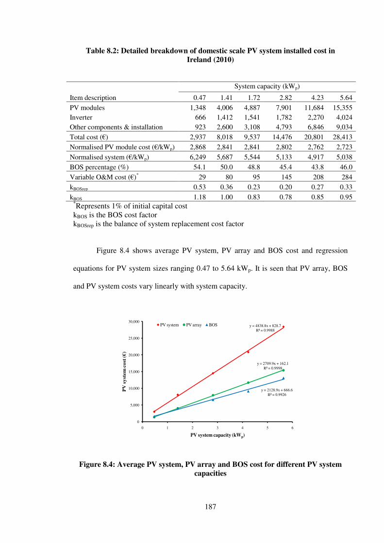
187

Table 8.2: Detailed breakdown of domestic scale PV system installed cost in Ireland (2010)

System capacity (kWp) Item description 0.47 1.41 1.72 2.82 4.23 5.64 PV modules 1,348 4,006 4,887 7,901 11,684 15,355 Inverter 666 1,412 1,541 1,782 2,270 4,024 Other components & installation 923 2,600 3,108 4,793 6,846 9,034 Total cost (�) 2,937 8,018 9,537 14,476 20,801 28,413 Normalised PV module cost (�/kWp) 2,868 2,841 2,841 2,802 2,762 2,723 Normalised system (�/kWp) 6,249 5,687 5,544 5,133 4,917 5,038 BOS percentage (%) 54.1 50.0 48.8 45.4 43.8 46.0 Variable O&M cost (�)* 29 80 95 145 208 284 kBOSrep 0.53 0.36 0.23 0.20 0.27 0.33 kBOS 1.18 1.00 0.83 0.78 0.85 0.95

*Represents 1% of initial capital cost kBOS is the BOS cost factor kBOSrep is the balance of system replacement cost factor

Figure 8.4 shows average PV system, PV array and BOS cost and regression

equations for PV system sizes ranging 0.47 to 5.64 kWp. It is seen that PV array, BOS

and PV system costs vary linearly with system capacity.

Figure 8.4: Average PV system, PV array and BOS cost for different PV system capacities

y = 4838.8x + 828.7R² = 0.9988

y = 2709.9x + 162.1R² = 0.9998

y = 2128.9x + 666.6R² = 0.9926

0

5,000

10,000

15,000

20,000

25,000

30,000

0 1 2 3 4 5 6

PV sy

stem

cost

(�)

PV system capacity (kWp)

PV system PV array BOS

188

The present value of total cost of the PV system is the sum of the present value

of costs associated with the PV module, initial BOS, replacement cost of BOS and

variable cost. The total life cycle cost of the PV system (Ct) is given as [56]:

vBOSrepBOSmtt CCCCC +++= (8.5)

and written as:

�

��

��

��

+−++

��

��

+++= ��

=

=

=

=

Nn

1nn

n

v

Nn

1n)(N

BOSrepBOSBOSpeakmt d)d(1

1d)(1k

d)(1

kkkk1PCC

r

r

(8.6)

The PV module price reduction factor (k) is given as:

m(n)

)Nm(n

C

Ck r+=

where,

Ct total PV system cost (�)

Cmt present value of cost associated with PV module (�2010)

CBOS present value of cost associated with the initial investment on BOS (�2010)

CBOSrep present value of BOS replacement cost (�2010)

Cv present value of total variable cost (�2010)

d discount rate (%)

kBOS BOS cost factor

kBOSrep balance of system replacement cost factor

N PV system life (years)

Nr BOS component life time (years)

Ppeak PV system peak power (kWp)

Cm normalise PV module cost (�/kWp)

189

8.6.2 Projected Cost

Using normalised PV module costs in Table 8.1, PV module learning rates and

market growth scenarios in section 8.3, Equation 8.15 was used to compute normalised

PV module costs beyond the 2010 base year. Figure 8.5 shows normalised PV module

cost and PV module annual installed capacity under different scenarios. The normalised

PV module cost is seen to decrease as the year of installation increases and also as the

PV system capacity increases for a given year.

The shaded band shows the range of normalised PV module cost over the range

of PV system capacities, market scenarios and year of installation. Normalised PV

module costs are projected to decrease from �2,868 to �1,424 for the 0.47 kWp PV

system under the Mod 15 scenario and from �2,723 to �585 for the 5.64 kWp PV system

under the Adv 25 scenario between 2010 and 2030. Detailed values for the normalised

PV module costs are shown in Appendices 8.2a and 8.2b.

Figure 8.5: Normalised PV module cost band and PV module annual installed capacity under different scenarios

The same methodology used to compute the projected normalised PV module cost

was employed to compute the normalised PV system life cycle costs. For each PV system

0

50

100

150

200

250

300

0

500

1,000

1,500

2,000

2,500

3,000

2010

2011

2012

2013

2014

2015

2016

2017

2018

2019

2020

2021

2022

2023

2024

2025

2026

2027

2028

2029

2030

PV m

odul

e an

nual

inst

alle

d ca

paci

ty (G

Wp)

Nor

mal

ised

PV

mod

ule c

ost (�

/kW

p)

Year of installation

0.47 kWp (Mod 15)5.64 kWp (Adv 25)Installed capacity (Moderate growth)Installed capacity (Advanced growth)

190

capacity the average normalised life cycle cost was obtained by calculating the mean cost

under the four market growth scenarios. Figure 8.6 shows average normalised life cycle cost

for different PV system sizes from 2010 to 2030. It is seen that the average normalised life

cycle costs vary from �7,331 to �2,630 for the 0.47 kWp PV system and from �5,250 to

�1,871 for the 2.82 kWp PV system. The normalised life cycle cost increases from the 2.82

kWp PV system up because of the higher BOS cost and variable O&M cost which is

evaluated as 1% of the capital cost. Detailed results are shown in Appendices 8.3a-c.

Figure 8.6: Average normalised life cycle cost for different PV system sizes from 2010 to 2030

8.7 Levelised Cost of Electricity

Levelised cost of electricity (LCOE) is the most transparent consensus measure

and remains a widely used tool for comparing the unit costs of different technologies

over their economic life in modelling and policy discussions. The calculation of LCOE

is based on the equivalence of the present value of the sum of discounted revenues and

the present value of the sum of discounted costs. LCOE corresponds to the cost of an

investor assuming the certainty of production costs and the stability of electricity prices.

The discount rate used in LCOE calculations reflects the return on capital for an

investor in the absence of specific market or technology risks. LCOE is equal to the

0

1,000

2,000

3,000

4,000

5,000

6,000

7,000

8,000

2010

2011

2012

2013

2014

2015

2016

2017

2018

2019

2020

2021

2022

2023

2024

2025

2026

2027

2028

2029

2030

Nor

mal

ised

life

cyc

le c

ost (�

/kW

p)


0.47 kWp 1.41 kWp 1.72 kWp 2.82 kWp 4.23 kWp 5.64 kWp

191

present value of the sum of discounted costs divided by total production adjusted for its

economic time value. Thus, if the electricity price is equal to the levelised average

lifetime costs, an investor would precisely break even on the project. This equivalence

of electricity prices and LCOE is based on two important assumptions [171]:

• the interest rate “d” used for discounting both costs and benefits is stable and

does not vary during the lifetime of the project under consideration; and

• the electricity price is stable and does not change during the lifetime of the

project. All output, once produced, is immediately sold at this price.

LCOE therefore represents a minimum breakeven tariff expressed in �/kWh,

based on the assumptions considered and the discount rate chosen. The levelised

average lifetime cost of electricity is given as [171]:

�=

−

−

+

+++++= N

1n

nn

nnnnnn

d)(1G

d))(1DecomCarbonFuelM&O(InvLCOE

(8.7)

where,

LCOE levelised cost of generation (�/kWh)

Invn investment costs in year “n” (�)

O&Mn operations and maintenance costs in year “n” (�)

Fueln fuel cost in year “n” (�)

Carbonn carbon cost in year “n” (�)

Decomn decommissioning cost in year “n” (�)

Gn net generation in operating year “n” (kWh)

n operating year

d annual discount rate (8% real)

N operating system life

192

The numerator in Equation 8.7 represents the net present value of total costs.

LCOE can therefore be defined as the ratio of the net present value of total capital and

operating costs to the net present value of the net electricity generated over the

operating life of the generating plant, i.e. [172]:

NPVGTOTC

LCOE = (8.8)

where,

TOTC net present value of total costs (capital and operating) (�)

NPVG net present value of net electricity generation (kWh)

8.7.1 PV Generated Electricity

Figure 8.7 shows average levelised electricity generation costs for the range of

PV system sizes considered in this study from 2010 to 2030. It is seen that the average

levelised electricity generation cost decreases with time. It varies from 0.85 �/kWh in

2010 to 0.31 �/kWh in 2030 for the 0.47 kWp PV system and from 0.61 �/kWh in 2010

to 0.22 �/kWh in 2030 for the 2.82 kWp PV system. The results show that the levelised

average cost of electricity generation decreases as the PV system size increases from

0.47 kWp to 2.82 kWp and then starts increasing from 2.8 kWp to 5.64 kWp PV systems.

Detailed values of average levelised electricity generation costs for different PV system

sizes from 2010 to 2030 are shown in Appendix 8.4. The non-linearity of the variable

O&M cost (caused by for example the inverter replacement cost, see Table 8.2) led to a

non-linear increase in the life cycle cost. For a given year, the minimum electricity

generation cost was for the 2.82 kWp PV system.

193

Figure 8.7: Average electricity generation cost for different PV system sizes (2010-2030)

8.8 Domestic Electricity

8.8.1 End-user Categories

In Ireland, households are classified by the electricity supply board (ESB) into

five categories based on their annual total quantity of electricity used as shown in Table

8.3. With regards to consumption bands, the most relevant for the majority of domestic

consumers are the DC band (45.5%) and the DD band (36.0%).

Table 8.3: Categories for domestic end-use of electricity [173]

Household end-user

Annual electricity consumption (kWh)

Frequency distribution

Lowest Highest (%)*

Very small (DA) < 1,000 2.0 Small ((DB) 1,000 2,500 17.5 Medium (DC) 2,500 5,000 45.5 Large (DD) 5,000 15,000 36.0 Very large (DE) � 15,000 0.0

*Values were obtained from smart metering data presented in section 8.6.2.

8.8.2 Housing profile

2006 census figures showed the Irish housing stock consisted of the following

house types: detached (43%), semi-detached (27%), terraced (18%), flat/apartment

0.0

0.1

0.2

0.3

0.4

0.5

0.6

0.7

0.8

0.9

2010

2011

2012

2013

2014

2015

2016

2017

2018

2019

2020

2021

2022

2023

2024

2025

2026

2027

2028

2029

2030

Aver

age

elec

tric

ity g

ener

atio

n co

st (�

/kW

h)



194

(10%), and other (3%) [23]. In April 2006 there were 1,462,296 private households

living in permanent housing units with an average occupancy of 2.81; a further 266,000

units were estimated to be vacant giving a total housing stock of 1,728,296 units and

vacancy rate of 15.4% [32]. Average floor areas of new houses grew from 130 m2 in

1990 to 159 m2 in 2006 while over the same period the ratio of planning permissions for

flats to houses rose from approximately 1:9 to approximately 1:3. In 1991, 6.5% of the

housing stock consisted of apartments or flats, whereas in 2006 the proportion was 10%

showing a growing trend towards apartments [30].

8.8.3 Domestic Electricity Demand Profiles

The electricity demand profiles used in this study were a sample of 3,889

households obtained from a smart metering survey of the ESB in Ireland [174].

Electricity demand was measured at 30-minute intervals for each domestic dwelling

over a six month period from July 1, 2009 to December 31, 2009. In the absence of data

from January to June, the data was mirrored with December and July representing

January and June respectively. Monthly total electricity consumption data from the

standard domestic dwelling electricity profiles supported this assumption. Total annual

electricity consumption varied between 196.0 kWh and 9,997.2 kWh with mean of

4,371.1 kWh and standard deviation of 2,000.9 kWh. The average daily electricity

consumption was 12.0 kWh.

Figure 8.8 shows the frequency distribution of average annual electricity

demand for the sampled households. It is seen that the consumption band with average

annual electricity demand between 4,000 and 5,000 kWh has the highest frequency

distribution of 18.1% while the band between 9,000 and 10,000 kWh has the lowest

frequency distribution of 1.5%. Households with annual electricity demands greater

than 10,000 kWh were excluded because they represented an insignificant part of the

sample.

195

Figure 8.8: Frequency distribution of average annual electricity demand for the sampled households [174]

Figure 8.9 shows average weekly summer electricity demand profiles from July

13-19, 2009. It is seen that the profiles vary between week days and weekends. During

weekdays, the demand peaks at 13:30 hrs and then 18:30 hrs. Saturday also has a double

peak as the weekdays but shows a higher demand in the morning and afternoon than the

weekdays. Sunday has a peak demand at 13:00 hrs with demand in the evening and

night being lower than the afternoon.

Figure 8.10 shows average weekly winter electricity demand profiles from

December 14-20, 2009. It is seen that the profiles vary between weekdays and

weekends. During weekdays, the demand peaks in the morning at 08:30 hrs and then

18:30 hrs with the maximum demand occurring in the evening. During weekends,

demand peaks at 13:30 hrs and the maximum demand occurs at 18:30 hrs coinciding

with the maximum demand during weekdays.

2.0

10.0

16.4

17.618.1

14.0

10.9

6.4

3.2

1.5

0

2

4

6

8

10

12

14

16

18

20

1,000 2,000 3,000 4,000 5,000 6,000 7,000 8,000 9,000 10,000

Freq

uenc

y di

stri

butio

n (%

)

Average annual electricity demand (kWh)

196

Figure 8.9: Average weekly summer electricity demand profiles (13-19 July, 2009) [174]

Figure 8.10: Average weekly winter electricity demand profiles (14-20 December, 2009) [174]

Based on a study on the electricity consumption patterns for 27 representative

dwellings in Northern Ireland carried out by Yohanis et al. [175], it was shown that the

factors that have significant impacts on electricity consumption include: type of

dwelling; location; ownership and size; household appliances; attributes of the

occupants including number of occupants; income; age; and occupancy patterns.

Figures 8.9 and 8.10 show that in addition to the factors highlighted above, household

electricity demand also varies between week days and weekends as well as between

seasons i.e. summer and winter.

0

0.05

0.1

0.15

0.2

0.25

0.3

0.35

0.4

00:3

0

01:3

0

02:3

0

03:3

0

04:3

0

05:3

0

06:3

0

07:3

0

08:3

0

09:3

0

10:3

0

11:3

0

12:3

0

13:3

0

14:3

0

15:3

0

16:3

0

17:3

0

18:3

0

19:3

0

20:3

0

21:3

0

22:3

0

23:3

0

Ele

ctri

city

dem

and

(kW

h)

Time

Monday Tuesday Wednesday Thursday Friday Saturday Sunday

0

0.1

0.2

0.3

0.4

0.5

0.6

0.7

00:3

0

01:3

0

02:3

0

03:3

0

04:3

0

05:3

0

06:3

0

07:3

0

08:3

0

09:3

0

10:3

0

11:3

0

12:3

0

13:3

0

14:3

0

15:3

0

16:3

0

17:3

0

18:3

0

19:3

0

20:3

0

21:3

0

22:3

0

23:3

0

Ele

ctri

city

dem

and

(kW

h)

Time

Monday Tuesday Wednesday Thursday Friday Saturday Sunday

197

8.8.4 Matching PV Electricity Generation and Domestic Electricity Profiles

Figure 8.11 shows average daily domestic dwelling electricity demand and

electricity generation by the six commercially available PV system sizes in Dublin,

Ireland. Measured PV performance data obtained from the field trials reported in

Chapter 3 for the 1.72 kWp PV system was scaled appropriately to obtain the

corresponding outputs from the other systems. This is deemed valid since power output

from a PV array is directly proportional to the array area as shown in Equation 3.2.

As seen in Figure 8.11, there exists a mismatch in peaks between average peak

household electricity demand and PV system electricity generation. This mismatch

would lead to a portion of the generated electricity to be exported, or “ spilled” to the

grid. The quantity of exported electricity depends on the PV system size and the

electricity demand profile. In order to minimise the quantity of exported electricity the

PV system has to be adequately sized taking into consideration the instantaneous match

between PV system output and the electricity load profile for a given household.

Figure 8.11: Average daily electricity demand [174] and electricity generation by different PV systems

0

0.2

0.4

0.6

0.8

1

1.2

00:3

0

01:3

0

02:3

0

03:3

0

04:3

0

05:3

0

06:3

0

07:3

0

08:3

0

09:3

0

10:3

0

11:3

0

12:3

0

13:3

0

14:3

0

15:3

0

16:3

0

17:3

0

18:3

0

19:3

0

20:3

0

21:3

0

22:3

0

23:3

0

Ele

ctri

city

(kW

h)

Time

0.47 kWp

1.41 kWp

1.72 kWp

2.82 kWp

4.23 kWp

5.64 kWp

Electricity demand

198

Following the work of Bahaj and James [38] who identified three export

scenarios for household-generated electricity as a function of different consumer

behaviours, the new classifications adopted were:

• low exporter with 25 per cent export;

• high exporter with 70 per cent export; and

• typical user with 50 percent export.

These three export scenarios were adopted in this work and used to classify

different consumer behaviours based on the quantity of PV generated electricity they

use on-site. The percentage of on-site household electricity use is given as:

�=

��

��

�=

N

1t t

ton,on PV

EN

100E (8.9)

For a given time, t, if Ed,t < PVt, then Eon,t = Ed,t while if Ed,t � PVt, then Eon,t = PVt.

Equation 8.21 is valid only when PVt > 0.

Eon percentage on-site household electricity use (%)

N number of 30-minute time intervals i.e. 17,520

Ed,t electricity demand at time, t (kWh)

Eon,t electricity used on-site at time, t (kWh)

PVt PV generated electricity at time, t (kWh)

Using half-hourly smart metering data for the 3,889 households and the 30-

minute interval electricity generated from the six commercially available PV system

sizes ranging from 0.47 kWp to 5.64 kWp, the percentage of on-site electricity use for

each of the households was determined over the 12-month period. Figure 8.14 shows

percentage on-site electricity use against average annual electricity demand for different

households under the three export scenarios. It is seen that for a given quantity of

annual electricity demand, the percentage of on-site electricity use decreases as the size

of the PV system increases. Figure 8.12 can be used as a design tool for sizing

domestic-scale PV systems when the average annual electricity demand is known and

199

detailed energy demand data for a household is not available. Appendix 8.5 shows

detailed results of average annual electricity demand, average percentage of on-site

electricity consumption and annual total electricity generated by the PV systems.

Figure 8.12: Percentage on-site household electricity use against average annual electricity demand

8.8.5 Domestic Sector Electricity Prices

For Irish households, electricity prices include all charges payable including:

energy consumed; network charges; other charges (capacity charges, commercialisation,

meter rental etc.) all netted for any rebates or premiums due but excluding initial

connection charges. In the lower consumption bands (shown in Table 8.3) the average

cost per kWh is higher because the standing charges and network charges form a larger

proportion of the annual costs. In the case of Ireland for instance, there are significant

numbers of holiday homes that may be unoccupied for most of the year yet standing

charges are still incurred with little or no electricity usage.

Figure 8.13 shows projected average EU and Irish household after tax electricity

prices under the Baseline and Reference scenarios. Projected average after tax

electricity price to EU households increases from 144 �/MWh in 2010 to 180 �/MWh in

0

10

20

30

40

50

60

70

80

90

100

0 1,000 2,000 3,000 4,000 5,000 6,000 7,000 8,000 9,000 10,000

Perc

enta

ge o

n-si

te el

ectr

icit

y us

e (%

)

Average annual electricity demand (kWh)


Low exporter

Typical user

High exporter

200

2020 and 192 �/MWh in 2030 under the Baseline scenario while it increases from 145

�/MWh in 2010 to 186 �/MWh in 2020 and remains constant at 186 �/MWh in 2030

under the Reference scenario. Projected average EU and Irish household after tax

electricity prices are shown in Appendix 8.6. This is a consistent rise compared to

current values due to higher capital and operation and maintenance (O&M) costs, and

higher fuel and variable costs. Taxes on fuels account for 9.4% of the average pre-tax

electricity price [162].

Electricity prices in Ireland are higher than the European average although the

price gap has been closing. The high price is heavily influenced by Ireland’ s reliance on

imported fossil fuels for electricity generation. Other key factors influencing the price of

electricity in Ireland are [176]:

• the need for essential network investment;

• low population density; and

• uncompetitive market.

Figure 8.13: Historic household electricity prices were obtained from the EU

Commission’s energy portal [177].

In the absence of domestic electricity price projections for Ireland, EU

household electricity price projections between 2010 and 2030 were used. Figure 8.14

0

50

100

150

200

250

300

2010 2015 2020 2025 2030

Hou

seho

ld el

ectr

icity

pri

ce (�

/MW

h)

Year

EU (Baseline scenario) EU (Reference scenario)Ireland (Baseline scenario) Ireland (Reference scenario)

201

shows historic and projected household electricity prices for band DC (see Table 8.3) in

Ireland. Projections show that Irish household electricity prices would increase from

203 �/MWh in 2010 to 274 �/MWh and 264 �/MWh under the Baseline and Reference

scenarios. Detailed historic and projected household electricity prices (band DC) in

Ireland are shown in Appendix 8.7.

Figure 8.14: Historic and projected nominal household electricity prices (band DC) in Ireland

Electricity comes from a variety of generation plants consisting of coal, oil, gas,

peat and renewables mostly wind and hydro. Gas is the dominant fuel in Ireland within

the region of 60% of electricity generated from imported gas. Therefore, international

fossil fuel prices are the key driver to Irish generation costs and, therefore, electricity

prices [176]. Thus it is fair to assume that fossil fuels will continue to dominate

electricity production. This relationship however weakens or at least gets more

complicated with the growth in large scale renewables (i.e. wind). Table 8.4 shows the

composition of electricity cost for different customer types.

0

5

10

15

20

25

3019

9819

9920

0020

0120

0220

0320

0420

0520

0620

0720

0820

0920

1020

1120

1220

1320

1420

1520

1620

1720

1820

1920

2020

2120

2220

2320

2420

2520

2620

2720

2820

2920

30

Ele

ctri

city

pri

ce (�

cent

s/kW

h)

Year

Baseline scenario Reference scenario

ProjectionsHistoric

202

Table 8.4: Percentage composition of electricity cost for different customer types [176]

Domestic customers Small and medium business customers

Generation cost 54 60 Distribution cost (DUoS) 29 28 Retail cost 12 6 Transmission cost (TUoS) 5 6 PSO levy 0 0

Generation costs for power plants are driven by the cost of imported fossil fuels

over which Ireland has no control. Network costs involve sending the electricity from

the generation plants through the transmission and distribution wires to customers. New

investment in network lines and infrastructure are a key cost driver. Over �5 billion was

invested over the last 10 years with more to be invested. Expansion is needed to

accommodate the introduction of new renewable energy production plants to meet the

40% target by 2020 to achieve the greening of electricity [176]. The dispersed nature of

the Irish population contributes to network costs and it means that more wires per

customer are needed than in other countries.

Table 8.5: Population density and length of distribution lines in Ireland and Britain [176]

Ireland Britain Population density 60 persons/km2 244 persons/km2 Length of distribution line 84 m/customer 49 m/customer

• Retail activity and costs for the supplier include the cost of procuring energy and

customer accounting

• Public service obligation (PSO) levy is a government related initiative related to

purchasing certain required forms of electricity generation such as wind power

or peat.

• Carbon tax

203

8.9 Wholesale Electricity Prices

In the marginal dispatching electricity model which is the dominant model in

Europe, the bidding price on the spot market includes only the variable costs. Variable

costs comprise: fuel prices; operational and maintenance costs; and CO2 emission

allowance costs. Cost of capital or any fixed costs are not included [178].

The Irish market includes a capacity payment (payment to generators based on

the availability of their plant). This means that whereas an energy-only market tends to

be characterized by price volatility, prices in markets with capacity payments are more

stable as peaking generators (open cycle gas turbines) are not relying on revenue from

the energy component only but also get a capacity payment [178].

Natural gas-fired technologies, mainly combined cycle gas turbines (CCGTs),

are often the marginal technologies which set the peak electricity price on the day-ahead

market. Consequently, developments in the gas markets have a direct impact on the

electricity market both in terms of the price level and price volatility [178]. Principal

uses for natural gas are for power generation, where it can be replaced by gas oil

(diesel) and for home-heating and industrial boilers which are also markets for low-

sulphur fuel oil. The price of gas is therefore linked to those two products over a period

of six to nine months to smooth volatility, and rebalanced by a factor to equate the

energy content of the three fuels [179].

According to the Commission for Energy Regulation (CER) [180] the best new

entrant (BNE) price is a calculation of the costs of generating electricity with a

generation plant using the best available technology. The BNE price is used to

determine wholesale electricity cost. Calculations of the BNE 2007 contain the

following:

204

• the cost of carbon (�/tonne) is converted to a carbon cost of generation (�/MWh)

assuming the carbon (C) content of natural gas is 1,501 grams per therm,

equivalent to 0.0055 tonnes of CO2

per therm;

• the lifetime net plant heat rate is 7,299 kJ per kWh (HHV) which yields a

specific CO2

production of 0.38 tonnes per MWh generated; and

• the cost of carbon credits is assumed to be �17.02 per tonne but the BNE

receives 73.7% free allocation of credits meaning that it is only charged the

shortfall of 26.3%. The overall carbon cost of generation is therefore �1.7/MWh.

The third phase of the ETS would introduce auctioning of CO2 emission

allowances with Irish allocations decreasing from 73.7% at the end of 2012 to 0% in

2020. Assuming a linear decrease in allocations and no further increase in the efficiency

of gas turbines, the specific CO2 production remains 0.38 tonnes per MWh generated of

electricity generated.

Emission Trading Scheme (ETS) carbon prices are modelled in such a way that

ETS emissions plus limited use of the Clean Development Mechanism (CDM) credits

just meet the cumulative ETS cap in 2008-2030. This gives rise to carbon prices

clearing the ETS market at 25 �/tCO2 in 2020 and 39 �/tCO2 in 2030 under the baseline

scenario. The increase in RES in the baseline scenario requires a higher amount of gas

fired power plants to cope with the higher amount of intermittent energy sources. This

leads to an increase in the share of gas fired power plants in fossil fuel power

generation. The above changes in the fuel mix of power generation with the penetration

of carbon free sources imply a steady decrease in carbon intensity of power generation:

the average emission of CO2 per MWh produced halves in 2030 compared to 2005.

Under the reference scenario ETS carbon prices reach 16.5 �/tCO2 in 2020 and 18.7

�/tCO2 in 2030 under the reference scenario as shown in Table 8.6 [162].

205

Table 8.5: Projected ETS carbon prices �’08/tCO2

Scenario 2020 2030 Baseline 25.0 39.0 Reference 16.5 18.7

In the absence of market prices, the BNE was used as a proxy for wholesale

prices. The low and high fuel cost scenarios described in section 8.2.2 were used to

model gas price projections beyond 2010. Figure 8.15 shows the link between gas,

crude oil and electricity prices. It is seen that electricity prices have generally followed

the same trend as gas and oil prices and gas price trends also show a good correlation

with crude oil prices although this might not always be the case in the long distant

future. BNE price for 2010 and projections from 2011 to 2030 are shown in Appendices

8.8a and 8.8b. Appendix 8.9 shows BNE price component summary from 2003 to 2006.

Figure 8.15: Natural gas, crude oil and electricity prices from 1996 to 2009 [181]

8.10 Grid Parity Analysis

Grid parity is the time point when the cost of generating a unit of electricity

using solar PV equals that produced and supplied through the grid [56]. Grid electricity

0

2

4

6

8

10

12

14

16

18

20

0

2

4

6

8

10

12

14

16

18

1996

1997

1998

1999

2000

2001

2002

2003

2004

2005

2006

2007

2008

2009

Ele

ctri

city

pri

ce (�

cent

s/kW

h)

Cru

de o

il an

d ga

s pri

ces (

US$

/mill

ion

Btu

)

Year

Gas (UK Heren NBP) Crude oil (OECD) Electricity

206

however has two different prices notably: a wholesale price; and a household consumer

price. The EPIA [182] defines grid parity as the time when the cost of PV generated

electricity equals the cost of retail electricity.

Figure 8.16 shows household, PV generated and BNE electricity price

projections from 2010 to 2030 in Ireland. The shaded band shows the upper and lower

bounds of PV generated electricity costs for the PV systems considered in the study

under different market growth scenarios. It is seen that the 0.47 kWp PV system under

the Mod 15 scenario has the highest electricity generation cost while the 2.8 kWp PV

system under the Advance 25 scenario has the lowest electricity generation cost.

Figure 8.19 also shows that while the projected costs of electricity generation

from all the PV systems decreases as the year of installation increases, the cost of

household and BNE (wholesale) electricity increases. The only exception is the BNE

price under the low fuel price and baseline scenario where the cost of electricity

generation remains fairly constant. Detailed values are shown in Appendix 8.10.

Figure 8.16: Household, PV generated and BNE electricity price projections from 2010 to 2030 in Ireland

0.0

0.1

0.2

0.3

0.4

0.5

0.6

0.7

0.8

0.9

1.0

2010

2011

2012

2013

2014

2015

2016

2017

2018

2019

2020

2021

2022

2023

2024

2025

2026

2027

2028

2029

2030

Ele

ctri

city

pri

ce (�

/kW

h)

Year

Household electricity price (baseline scenario)0.47 kWp PV system (Mod 15 scenario)2.82 kWp PV system (Adv 25 scenario)BNE price (low fuel & reference scenario)BNE price (high fuel & baseline scenario)

207

Thus, allowing for a modest increase in efficiency of PV modules and ignoring

further learning, with a 25 year lifetime and an 8% discount rate, the cost of PV

generated electricity in 2010 was between 0.60-0.89 �/kWh. Projections show that PV

could deliver electricity at around 0.25-0.57 �/kWh by 2020, falling to 0.13-0.44 �/kWh

by 2030 in Ireland. Grid parity between PV generated electricity from a 2.82 kWp plant

under the Adv 25 scenario and retail electricity prices (production for local

consumption) would occur in 2020 while parity with wholesale prices (production for

national consumption) would occur in 2025. The former represents the period after

which support for domestic scale PV systems would not be required.

Figure 8.17 shows average PV generation and household electricity costs from

2010 to 2030 for a range of different PV system sizes. It is seen that average PV

electricity generation costs would be at parity with household electricity costs in 2029,

2024, 2023, 2024 and 2026 for PV systems with capacities of 1.41 kWp, 1.72 kWp, 2.82

kWp, 4.23 kWp, and 5.64 kWp respectively.

Figure 8.17: Average PV generation and household electricity cost from 2010 to 2030 for different PV sizes

0.0

0.1

0.2

0.3

0.4

0.5

0.6

0.7

0.8

0.9

2010

2011

2012

2013

2014

2015

2016

2017

2018

2019

2020

2021

2022

2023

2024

2025

2026

2027

2028

2029

2030

Aver

age

elec

tric

ity g

ener

atio

n co

st (�

/kW

h)


0.47 kWp 1.41 kWp1.72 kWp 2.82 kWp4.23 kWp 5.64 kWpHousehold (Band DC)

208

8.11 Economic Viability Assessment

8.11.1 System (Final) Yield

The final yield is defined as the annual net AC energy output of the system

divided by the rated or nominal power of the installed PV array at standard test

conditions (STC) of 1 kW/m2 solar irradiance and 25 oC cell temperature. This is a

representative figure that enables comparison of similar PV systems in a specific

geographic region. It is dependent on the type of mounting, (vertical on a façade or

inclined on a roof) and location [105].

Lack of field performance data for different PV system types in Ireland has been

a limitation to expanding this study to other PV module technologies. However, field

performance monitoring data from Ayompe et al. [183] showed that the annual yield of

the mono-crystalline PV system in Dublin, Ireland was 885.1 kWh/kWp. The annual

total solar radiation intensity during the monitoring period was 0.83% higher than the

long-term average for the location so the annual yield was corrected to 877.5 kWh/kWp.

8.11.2 Revenue

Revenue depends primarily on the amount of electricity produced by the PV

system (system yield) and is a function of the electricity load profile of the PV owner,

import and export tariffs, as well as policy incentives. Revenues can be calculated as

[184]:

�EX�TG�AIRevenues ++= (8.10)

AI = avoided import as a share of total electricity generated

EX = electricity export as a share of total electricity generated

TG = total generation

� = electricity import tariff

209

� = unit value of a generation-based policy incentive (e.g. renewable obligation

certificate (ROC) price or FIT) or a generation-based reward to export tariff

� = electricity export tariff

�AI = value of avoided import. This depends on the import tariff and on the amount of

generated electricity that is consumed locally, which varies according to

different PV owners’ load profiles. Matching of the electricity production of the

PV system with the relative user load profile over time provides the measure of

the amount of self-consumption and peak saving versus electricity exported

�TG = value of the policy incentives considered, which applies to the total electricity

generated. Generation-based policy incentives include ROCs and FITs. � is the

generation-based reward to export tariff when this type of reward is included in

the analysis scenario.

�EX = value of exported electricity, which depends on the amount of electricity actually

exported to the grid (depending on the matching of PV generation with the end

user’ s electricity load profile). This term applies when export-based rewards are

included in the analysis.

A Renewables Obligation Certificate (ROC) is a green certificate issued to an

accredited generator for eligible renewable electricity generated within the United

Kingdom and supplied to customers within the United Kingdom by a licensed

electricity supplier. One ROC is issued for each megawatt hour (MWh) of eligible

renewable output generated [182].


In this section, the economic viabilities of the six domestic scale PV systems are

investigated under current market and policy support measures using net present value.

Two case studies were undertaken notably: a FIT of �19 c/kWh for exported electricity

210

offered by Electricity Supply Board Customer Supply (ESBCS) to its customers; and no

FIT for non ESBCS customers.

FIT Case Study: PV systems installed in 2010, FIT of 19 cents/kWh for exported

electricity and 8% discount rate.

This first analysis was conducted using PV system costs for June, 2010 and

considering that these systems were installed by ESBCS customers who receive a FIT

of 19 c/kWh for exported electricity. Further revenue accrues from the avoided cost of

displaced grid electricity. The EPIA [182] recommended discount rates of 6-10% to

ensure sustainable growth so a discount rate of 8% was used to obtain the present value

of revenues. It was assumed that the FIT remained unchanged throughout the service

life of the PV system. The analysis was run for each of the six PV system sizes

considered in this study matching their electricity generation with the electricity demand

for 3,889 households on 30-minute intervals.

The range of NPVs vary from -�3,372 to -�3,367, -�8,683 to -�8,669, -�9,260 to

-�9,243, -�14,363 to -�14,341, -�22,567 to -�22,538, and -�31,956 to -�31,922 for the

0.47 kWp, 1.41 kWp, 1.72 kWp, 2.82 kWp, 4.23 kWp, and 5.64 kWp PV systems

respectively. This shows that under current policies and supports, it is not economically

viable to invest in domestic scale PV systems in Ireland.

No FIT Case Study

This second analysis was conducted using PV system costs for June, 2010 and

considering that the PV systems were installed by non-ESBCS customers who receive

no reward for exported electricity. Their revenues accrue from the avoided cost of

displaced grid electricity discounted at 8% to obtain the present value of revenues. The

analysis was again run for each of the six PV system sizes matching their electricity

generation with the electricity demand for 3,889 households at 30-minute intervals.

211

The range of NPVs vary from -�3,438 to -�3,367, -�8,894 to -�8,679, -�9,519 to

-�9,268, -�14,795 to -�14,438, -�23,218 to -�22,757, and -�32,827 to -�32,286 for the

0.47 kWp, 1.41 kWp, 1.72 kWp, 2.82 kWp, 4.23 kWp, and 5.64 kWp PV systems

respectively. The results once again show that under current policies and supports, it is

not economically viable to invest in domestic scale PV systems in Ireland.


Simple payback period (SPP) was evaluated for the six domestic scale PV

systems under current and existing policy support measures. Two case studies were

undertaken notably: a FIT of �19 c/kWh for exported electricity offered by ESBCS to

its customers; and no FIT for non ESBCS customers.

FIT Case Study: PV systems installed in 2010 by ESBCS customers receiving a FIT

of 19 cents/kWh for exported electricity.

Results from SPP analysis showed that the distribution of SPP for all six PV

system sizes was above the assumed PV system life of 25 years. SPP varied from 34.7

to 36.8 years, 31.6 to 33.6 years, 30.9 to 32.8 years, 28.9 to 30.4 years, 27.9 to 29.1

years and 28.7 to 29.8 years for the 0.47 kWp, 1.41 kWp, 1.72 kWp, 2.82 kWp, 4.23 kWp

and 5.64 kWp PV systems respectively. Figure 8.18 shows the frequency distribution of

SPPs for the smart metering customer sample for different PV. The FIT had a small

effect of spreading the SPP frequency distribution over a few years compared to the no

FIT case.

212

Figure 8.18: Frequency distribution of simple payback periods for different PV systems installed by ESBCS customers in 2010.

No FIT Case Study: PV systems installed in 2010 by non-ESBCS customers receiving

no FIT for exported electricity.

Results from SPP analysis for PV systems installed in 2010 by non-ESBCS

customers receiving no FIT for exported electricity showed that the SPP for all six PV

system sizes was above the assumed PV system life of 25 years. SPP varied from 33.1

to 47.7 years for the 1.41 kWp and 5.64 kWp PV systems respectively as shown in

Figure 8.19.

Figure 8.19: Simple payback periods for different PV systems installed by non-ESBCS customers in 2010

0

10

20

30

40

50

60

70

80

90

100

110

27 28 29 30 31 32 33 34 35 36 37

Freq

uenc

y di

stri

butio

n (%

)

Simple payback period (Years)


34.733.1 33.8

36.5

40.9

47.7

0

5

10

15

20

25

30

35

40

45

50

0.47 1.41 1.72 2.82 4.23 5.64

Sim

ple p

ayba

ck p

erio

d (y

ears

)


213

8.12 Emission Analysis

8.12.1 All-Island Fuel-Mix 2009

Figure 8.20 shows the All-Island fuel-mix for

2009. It is seen that gas made the largest

contribution to the island’ s electricity

supply of 61.8% while renewable energy

made up 14.2% of the total. Renewables

consisted of 11% wind, 2.6% hydro, 0.6%

biomass and >0% photovoltaic. Figure

8.21 shows percentages of fuel-mix and

average carbon dioxide emissions for 2005-2009.

Figure 8.20: All-Island fuel-mix 2009 [28]

Gas 61.8%Coal 14.2%

Renewables 14.2%

Peat 6.7%

Oil 2.5% Other 0.4%

0%

10%

20%

30%

40%

50%

60%

70%

80%

90%

100%

2005 2006 2007 2008 2009

Perc

enta

ge co

ntri

butio

n

Year

Gas Coal Renewables Peat Oil Other

214

Figure 8.21: Fuel mix for electricity generation in Ireland (2005-2009) [162]

Comparing 2009 with 2008, gas, peat and renewables all contributed more to the

total than in 2008 at the expense of oil and coal. This confirms a trend that has been

evident since 2005. It is seen that the annual average carbon dioxide emissions per

MWh of electricity generated fell approximately 5% (0.029 t/MWh) in 2009 for Ireland.

This was mainly as a result of the increase in renewable energy generation and the

larger share of gas in the final mix at the expense of higher carbon intensive fuels such

as oil and coal. Figures from 2005-2007 relate to Ireland only and calculations are based

on pre-Single Electricity Market (SEM) methodology. Figures for 2008 and 2009 relate

to Ireland and Northern Ireland and are based on the Interim Arrangements

methodology. Values of the percentage fuel-mix and average carbon dioxide emissions

in Ireland between 2005 and 2009 are shown in Appendix 8.12.

8.12.2 CO2 Intensity of Power Generation

Historic and projected EU average CO2 intensity of power generation were

obtained from the EU Commission’ s Directorate-General for Energy’ s publication on

EU energy trends to 2030 [162]. Historic carbon intensity of power generation for

Ireland was obtained from the Commission of Energy Regulation’ s fuel mix disclosure

document for 2009 [28]. Ireland’ s average CO2 intensity of power generation was then

projected based on the percentage change of projected EU average CO2 intensity of

power generation. It was assumed that Ireland’ s average CO2 intensity of power

generation will decrease at the same rate as that of the EU under the Baseline and

Reference scenarios as shown in Figure 8.22. Detailed values of historic and projected

215

carbon intensity of power generation under the baseline and reference scenarios are

shown in Appendix 8.13.

Figure 8.22: Carbon intensity of power generation under the baseline and reference scenario (tCO2/MWh)

EU ETS involves the auctioning of emission allowances after 2013 (with some

exemption for new Member States until 2020); hence electricity prices increase in the

Baseline scenario reflecting the additional costs from auctioning, adding a price effect

on demand which favours less consumption and more emission reduction. Although the

achievement of RES targets is not imposed in the Baseline scenario, the on-going

investments, subsidy schemes and other facilitation infrastructures, which are being

developed in the Member States, are included in the scenario [162].

8.12.3 Life Cycle Emission Savings

Figure 8.23 shows life cycle CO2 emission savings by PV systems for different

years of installation. The life cycle CO2 emissions from the PV systems was evaluated

assuming negligible change in the annual energy output and using projected carbon

intensities of power generation under the baseline and reference scenarios developed in

0.000

0.100

0.200

0.300

0.400

0.500

0.600

0.700

0.800

2005

2006

2007

2008

2009

2010

2011

2012

2013

2014

2015

2016

2017

2018

2019

2020

2021

2022

2023

2024

2025

2026

2027

2028

2029

2030

Car

bon

inte

nsity

(tC

O2/M

Wh)

Year

Baseline scenario Reference scenario

ProjectionsHistoric

216

section 8.10.2. Life cycle CO2 emissions are seen to reduce from 8.8 tCO2/kWp in 2010

to 7.2 tCO2/kWp in 2020 and 6.5 tCO2/kWp in 2030 under the baseline scenario while

under the reference scenario, they reduce from 8.6 tCO2/kWp in 2010 to 7.6 tCO2/kWp

in 2020 and 7.4 tCO2/kWp in 2030. Detailed values are shown in Appendix 8.14.

Figure 8.23: PV system life cycle CO2 emission savings for different years of installation

8.13 FIT Design for Ireland

Analyses carried out in section 8.9 show that domestic scale PV systems are not

economically viable in Ireland under the current market and legislative conditions.

Lessons learnt from countries that have instituted FITs such as Germany, Spain, Italy,

Greece and recently the UK show that FITs can encourage increased deployment of PV

systems. Careful attention however has to be accorded to the design of FITs to avoid

them being too costly.

FITs policies that target the total quantity of electricity generated that is sold to

the grid are easy to design since it is straight forward to calculate expected revenues

required to achieve a desired rate of return on investment. Optimal PV system sizing is

6.0

6.5

7.0

7.5

8.0

8.5

9.020

10

2011

2012

2013

2014

2015

2016

2017

2018

2019

2020

2021

2022

2023

2024

2025

2026

2027

2028

2029

2030

Life

cycl

e CO

2sa

ving

s (tC

O2/k

Wp)


Baseline 2009 Reference 2009

217

based on available budget, roof space, and the prevailing FIT. These policies are

applicable to Germany, France, Italy, Spain, Greece and a host of other countries.

On the other hand, FIT policies that target the quantities of electricity generated,

and used on-site and exported are much more complicated to design. They, however,

have the advantage of targeting ‘prosumers’ providing maximum benefit for on-site

electricity use. Optimal PV system design would therefore be dependent not only on the

available budget, roof space and prevailing FIT but also on matching household

electricity demand with PV electricity generation/installed capacity. Perverse incentives

should therefore be avoided since they might have a negative effect of increasing local

consumption.

This section considers the design of a FIT for domestic scale ‘prosumers’ in

Ireland that rewards both electricity generation similar to that used in the UK. An export

tariff equal to the cost of electricity in the wholesale market determined by the BNE

price was used in the analyses. The rewards from displaced grid electricity used

modelled values from Section 8.6.4. The required FIT for PV generated electricity was

modelled to achieve an IRR of 8% (an IRR of 6-10% is recommended for a sustainable

policy) to the investor for the range of smart metering sample data.

Figure 8.24 shows the cumulative frequency (CF) of NPV for different PV

system sizes and recommended FIT to achieve the targeted minimum 8% IRR for at

least 50% market penetration. It is seen that the FIT to guarantee a targeted IRR varies

widely with PV system size. It highlights shortcomings that may arise from lumping PV

system sizes within the same FIT as is applicable to the UK where PV systems with up

to 4 kWp capacity are attribute a single tariff. In order to guarantee an IRR of 8% to at

least 50% of investors, the recommended FITs for PV generated electricity are 45

c/kWh, 39 c/kWh, 32 c/kWh, 31 c/kWh, 34 c/kWh, and 38 c/kWh for 0.47 kWp, 1.41

218

kWp, 1.72 kWp, 2.82 kWp, 4.23 kWp, and 5.64 kWp PV systems respectively for

systems installed in 2011. Detailed values of NPV and CF for different PV system

capacities under the proposed FITs for 2011 are shown in Appendix 8.15.

Figure 8.24: Cumulative frequency of NPV for different PV system sizes and recommended FIT to achieve 8% IRR and at least 50% market penetration

It is seen from Figure 8.24 that if a FIT of 0.32 �/kWh is adopted and all Irish

households install a 1.72 kWp PV system, at least 50% of them would have positive

NPVs considering an 8% rate of return on their investment. Similarly, a FIT of 0.39

�/kWh for the 1.41 kWp PV system would result in positive NPVs and an 8% return on

investment for at least 50% of households.

Figure 8.25 shows proposed FIT for different PV system sizes against year of

installation in Ireland from 2011 to 2030. It is seen that the required FIT to ensure an

IRR of 8% for 50% of the population decreases as the year of installation increases for

all PV system sizes. The proposed annual FITs guarantee positive NPVs for at least

50% of the sampled household electricity demand. Although long-term FIT projections

may not prove to be very accurate, they nevertheless provide an insight into possible

future FIT prices and provide a valuable resource for evidence-based policy

formulation. Detailed values of the proposed FITs for different PV system capacities

0

10

20

30

40

50

60

70

80

90

100

110

-1,500 -1,000 -500 0 500 1,000 1,500 2,000 2,500 3,000 3,500

Cum

ulat

ive f

requ

ency

(%)

Net present value (�)

0.47 kWp (0.45 �/kWh) 1.41 kWp (0.39 �/kWh) 1.72 kWp (0.32 �/kWh)2.82 kWp (0.31 �/kWh) 4.23 kWp (0.34 �/kWh) 5.64 kWp (0.38 �/kWh)

219

required to guarantee at least 50% market penetration and an IRR of 8% are shown in

Appendix 8.16.

The proposed FITs show significant variations between PV system sizes with

the 1.72 and 2.82 kWp systems having the lowest FITs for a given year of installation as

shown in Figure 8.26. Detailed results of the proposed FIT for domestic scale PV

systems in Ireland are shown in Appendix 8.17. The results show that for domestic scale

FITs there should be further disaggregation of the FIT for PV capacities ranging from 0-

1 kWp, 1-2 kWp, 2-3 kWp and 3-4 kWp.

Figure 8.25: Required FITs for different PV system sizes against year of installation

0

0.05

0.1

0.15

0.2

0.25

0.3

0.35

0.4

0.45

2011

2012

2013

2014

2015

2016

2017

2018

2019

2020

2021

2022

2023

2024

2025

2026

2027

2028

2029

2030

FIT

(�/k

Wh)



0.00

0.05

0.10

0.15

0.20

0.25

0.30

0.35

0.40

0.45

0.50

0 1 2 3 4 5 6

Feed

-in ta

riff

(�/k

Wh)


2011 2012 2013 2014 2015 2020 2025 2030

220

Figure 8.26: Feed-in tariff for different PV system capacities and year of installation

Figure 8.27 shows the cumulative frequency distribution of SPP for different PV

systems installed using FITs that target 50% market penetration in 2011. Results from

the SPP analysis under the proposed FIT scheme showed that the distribution of SPP for

all six PV system sizes ranged between 7 and 11 years which are shorter than the

assumed PV system life of 25 years. It is seen that for a FIT of 0.45 �/kWh the SPP

varied from 9.1 to 11.2 years for the 0.47 kWp system. Similarly, for a FIT of 0.39

�/kWh, the SPP varied from 9.2 to 11.7 years for the 1.41 kWp system. Detailed values

are shown in Appendix 8.18.

Figure 8.27: Cumulative frequency distribution of SPPs for different PV systems using FITs that target 50% market penetration in 2011

Between the years from 2012 and 2015, SPP for PV systems installed under the

proposed FIT scheme would decrease from 9.1 to 6.7 years, 9.5 to 6.8 years, 10.5 to 7.4

years, 10.2 to 7.5 years, 9.4 to 7.1 years and 8.9 to 7.2 years for the 0.47 kWp, 1.41 kWp,

1.72 kWp, 2.82 kWp, 4.23 kWp and 5.64 kWp PV systems respectively. SPP ranging

from 6.5 to 10.5 years are in line with SPPs from the empirical study on the willingness

to pay for micro-generation technologies carried out by Claudy et al. [22] where

respondent’ s proposed SPPs ranged from 8-13 years.

0

20

40

60

80

100

120

7 8 9 10 11 12 13 14 15 16

Cum

ulat

ive f

requ

ency

(%)

Payback period (years)

0.47 kWp (0.45 �/kWh) 1.41 kWp (0.39 �/kWh) 1.72 kWp (0.32 �/kWh)2.82 kWp (0.31 �/kWh) 4.23 kWp (0.34 �/kWh) 5.64 kWp (0.38 �/kWh)

221

8.14 Sensitivity Analysis on PV systems

8.14.1 Effect of Discount Rate on FIT

The discount rate chosen is seen to have a significant effect on the FIT required

to ensure 50% market penetration of the PV systems. Figure 8.28 shows the required

FIT to guarantee 50% market penetration of the PV systems considered in this study for

discount rates. It is seen that for 6-10% discount rates recommended by the EPIA [182]

to ensure sustainable growth, the required FITs increase with discount rate for a given

PV system size. For a given discount rate, the required FITs were highest for the 0.47

kWp and lowest for the 2.82 kWp PV systems. The results show that there is scope for

policy intervention to reduce the discount rate (discussed later) and consequently the

required FIT which is a burden to society. Detailed values are shown in Appendix 8.18.

Figure 8.28: Required FIT for different PV system capacities for 6-10% discount rates in 2011

8.14.2 Effect of FIT on NPV

The effect of FIT on NPV was investigated by applying the proposed minimum

and maximum FITs for 2011. Figure 8.29 shows cumulative frequency (CF) plots

against NPV for different PV system capacities for a FIT of 0.31 �/kWh. This FIT

guarantees positive NPVs for at least 50% and 30% of the population for the 2.8 kWp

0

0.1

0.2

0.3

0.4

0.5

0.6

0 1 2 3 4 5 6

Feed

-in ta

riff

(�/k

Wh)


6% 7% 8% 9% 10%

222

and 1.72 kWp PV systems respectively. The FIT results in negative NPVs for the other

PV systems with the 5.64 kWp PV system having the worst NPVs. This shows that a

single FIT is not suitable to ensure economic viability for the range of PV systems

applicable to the domestic sector. Detailed values of NPV and CF are shown in

Appendix 8.19.

Figure 8.29: Cumulative frequency of NPVs for different PV system capacities in 2011 (0.31 �/kWh FIT)

Figure 8.30 shows plots of cumulative frequency of net present value for

different PV system capacities for the proposed FIT of 0.45 �/kWp suitable to guarantee

at least 50% economic viability for the 0.47 kWp PV system. It is seen that a high FIT

guarantees 100% economic viability for the other five PV systems with windfall profits

which result in IRRs much higher than the envisaged 8%. This again shows that a single

FIT is not efficient to ensure economic viability for the range of PV systems applicable

to the domestic sector. Detailed values of NPV and CF are shown in Appendix 8.20.

8.14.3 Effect of FIT on SPP

The effect of FIT on SPP was investigated by applying the proposed minimum

and maximum FITs for 2011. Figure 8.31 is a CF of SPPs for different PV system

0

10

20

30

40

50

60

70

80

90

100

110

-5,000 -4,000 -3,000 -2,000 -1,000 0 1,000 2,000

Cum

ulat

ive f

requ

ency

(%)

NPV (�)


223

capacities for a FIT of 0.31 �/kWh. This FIT guarantees SPPs of 11.6 to 15.1 years,

10.7 to 14.0 years, 10.5 to 13.7 years, 10.1 to 12.8 years, 10.0 to 12.3 years and 10.5 to

12.6 years for the 0.47, 1.41, 1.72, 2.82, 4.23 and 5.64 kWp PV systems respectively.

Detailed values of CF and SPP are shown in Appendix 8.21.

Figure 8.30: Cumulative frequency of NPVs for different PV system capacities in 2011 (0.45 �/kWh FIT)

Figure 10.10: Cumulative frequency of SPPs for different PV system capacities in 2011 (0.31 kWp FIT)

0

20

40

60

80

100

120

-1,000 0 1,000 2,000 3,000 4,000 5,000 6,000 7,000

Cum

ulat

ive f

requ

ency

(%)

NPV (�)


0

20

40

60

80

100

120

7 8 9 10 11 12 13 14 15 16

Cum

ulat

ive f

requ

ency

(%)



224

Figure 8.31 is a CF of SPPs for different PV system capacities for a FIT of 0.45

�/kWh. This FIT guarantees SPPs of 9.1 to 11.2 years, 8.4 to 10.3 years, 8.2 to 10.1

years, 7.8 to 9.4 years, 7.7 to 9.0 years and 8.0 to 9.2 years for the 0.47, 1.41, 1.72, 2.82,

4.23 and 5.64 kWp PV systems respectively. Detailed values of CF and SPP are shown

in Appendix 8.22.

Figure 8.31: Cumulative frequency of SPPs for different PV system capacities in 2011 (0.45 kWp FIT)

8.15 PV System Marginal Abatement Costs

In section 8.11.3 it was shown that the existing FIT for PV systems does not

render them economically viable. The MACs for PV systems were therefore computed

using the FITs evaluated in Section 8.13. The MACs are therefore theoretical and

depend on policy decision to implement the proposed FITs.

The CO2 abatement cost of PV electricity generation is analysed. CO2 emission

factors for electricity generation in Ireland were used to evaluate the abatement cost of

domestic scale PV generated electricity. The CO2 abatement cost of PV electricity was

analysed using a dynamic grid fuel mix emissions factor that varies annually.

0

20

40

60

80

100

120

7 8 9 10 11 12 13 14 15 16

Cum

ulat

ive f

requ

ency

(%)



225

Greenhouse gas abatement costs are generally defined as the costs of a

greenhouse gas reduction measure divided by its greenhouse gas reduction potential,

and are expressed in � per ton of C or CO2 equivalents avoided. Greenhouse gas

abatement costs are a measure of the cost effectiveness of reduction options and are

used to compare and prioritise GHG reduction measures [185]. CO2 abatement cost can

be calculated from Equation 8.11 given as [186]:

abatement CObaseline CORevenuePW CostsPW

AC22 −

−= (8.11)

where, AC is the abatement cost (�/tCO2), PW Costs is the present worth of costs (�),

and PW Revenue is the present worth of revenue (from energy cost savings) (�). The

denominator represents the CO2 emission reduction by the abatement option over the

scenario period.

The marginal cost of energy production is the change in total cost that arises

when the quantity of energy produced increases by one unit. Costs include additional

investment costs relative to a baseline and may also include fuel cost savings and

additional costs or benefits. The marginal abatement cost is given as [186]:

option)abatement emissions 2CO(option) baseline from emissions 2(COoption) baseline ofcost Full(option)abatement ofcost (Full

MAC−−= (8.12)

where MAC is the marginal abatement cost (�/tCO2). The full cost of both abatement

and baseline options are expressed in Euro (�), while the CO2 emissions are expressed

in tonnes of CO2 (tCO2).

In most EU countries, the distribution of the costs emerging from the support of

renewable energy is distributed equally among all electricity consumers by including

them in the electricity price [186]. The introduction of domestic-scale PV systems into

226

the electricity generation mix results in a marginal price of electricity. The marginal

increase in costs (MIC) of delivering electricity from PV systems is given as:

ACPMETFITMIC −+= (8.13)

MIC marginal increase in costs (�/kWh)

FIT feed-in tariff (�/kWh)

MET marginal effects on tariffs (�/kWh)

ACP avoided costs and profit from spilled electricity (�/kWh)

Equation 8.12 is therefore modified to:

PV) from emissions CO(y)electricit grid from emissions (COMIC

MAC22 −

= (8.14)

For low penetration of PV systems, the quantity of PV generated electricity is

low so MET and ACP in Equation 8.13 can be neglected. The value of CO2 emissions

from PV is set to zero since PV systems do not generate any emissions at the margin.

CO2 emissions from grid electricity used in the analysis were calculated in section

8.10.2. The marginal abatement cost is therefore obtained as:

yelectricit grid from emissions COFIT

MAC2

= (8.15)

Considering that no dedicated FIT for PV generated electricity exists in Ireland

under current policies, the MACs are considered to be zero.

Figure 8.32 shows the evolution of MACs for domestic scale PV systems in

Ireland and projected CO2 prices for the baseline scenario from 2011 to 2030. The

MAC is seen to decrease from: 915.8 to 136.2 �/tCO2 for the 0.47 kWp; 793.7 to 102.1

�/tCO2 for the 1.41 kWp; 651.3 to 0.0 �/tCO2 for the 1.72 kWp; 630.9 to 34.0 �/tCO2 for

227

the 2.82 kWp; 692.0 to 68.1 �/tCO2; and 773.4 to 136.2 �/tCO2 for the 5.64 kWp PV

systems respectively. Detailed values for the MAC projections are shown in Appendix

8.23.

Figure 8.32: MACs for domestic scale PV systems in Ireland and projected CO2 price for the baseline scenario (2011-2030)

Figure 8.33 shows the evolution of MACs for domestic scale PV systems in

Ireland and projected CO2 prices for the reference scenario from 2011 to 2030. The

MAC is seen to decrease from: 922.7 to 119.4 �/tCO2 for the 0.47 kWp; 799.7 to 89.6

�/tCO2 for the 1.41 kWp; 656.2 to 0.0 �/tCO2 for the 1.72 kWp; 635.7 to 29.9 �/tCO2 for

the 2.82 kWp; 697.2 to 59.7 �/tCO2; and 779.2 to 119.4 �/tCO2 for the 5.64 kWp PV

systems respectively. Detailed values for the MAC projections are shown in Appendix

8.24.

0

100

200

300

400

500

600

700

800

900

1,000

2011

2012

2013

2014

2015

2016

2017

2018

2019

2020

2021

2022

2023

2024

2025

2026

2027

2028

2029

2030

Mar

gina

l aba

tem

ent c

ost (�

/tCO

2)


0.47 kWp 1.41 kWp 1.72 kWp 2.82 kWp4.23 kWp 5.64 kWp CO2 price (BL) CO2 price (REF)

0

100

200

300

400

500

600

700

800

900

1,000

2011

2012

2013

2014

2015

2016

2017

2018

2019

2020

2021

2022

2023

2024

2025

2026

2027

2028

2029

2030

Mar

gina

l aba

tem

ent c

ost (�

/tCO

2)


0.47 kWp 1.41 kWp 1.72 kWp2.82 kWp 4.23 kWp 5.64 kWpCO2 price (BL) CO2 price (REF)

228

Figure 8.33: MACs for domestic scale PV systems in Ireland and projected CO2 price for the reference scenario (2011-2030)

8.13 Summary

Investment appraisal techniques notably: simple payback period (SPP), net

present value (NPV), internal rate of return (IRR) and levelised cost of energy (LCOE)

were used to evaluate the economic viability of domestic scale grid connected PV

systems in Ireland. Current costs for 6 commercially available PV system sizes (0.47 to

5.64 kWp) were projected into the future using energy market growth scenarios and PV

technology learning rates.

Allowing for a modest increase in efficiency of PV modules and ignoring further

technology learning, with a 25 year lifetime and an 8% discount rate, the cost of PV

generated electricity in 2010 was between 0.6-0.89 �/kWh. Projections showed that PV

could deliver electricity at around 0.25-0.57 �/kWh by 2020, falling to 0.13-0.44 �/kWh

by 2030 in Ireland. Grid parity between PV generated electricity from a 2.82 kWp plant

under the Adv 25 scenario and retail electricity prices (production for local

consumption) would occur in 2020 while parity with wholesale prices (production for

national consumption) would occur in 2025. The former represents the period after

which support for domestic scale PV systems would not be required. Average PV

electricity generation costs would be at parity with household electricity costs in 2029,

2024, 2023, 2024 and 2026 for PV systems with capacities of 1.41 kWp, 1.72 kWp, 2.82

kWp, 4.23 kWp, and 5.64 kWp respectively. The results show that the 2.82 kWp PV

system is the most appropriate of the sizes considered.

Results from this study showed that existing support policies are inadequate. For

both the no FIT and a FIT of 0.19 �/kWh cases, PV systems are not yet economically

229

viable under the assumptions considered in this study. The NPVs for the no FIT case

varied between -�3,438 and -�32,827 for the various PV system sizes. For the 0.19

�/kWh FIT, the NPVs varied between -�3,372 and -�31,956 for the various PV system

sizes. These results showed that alternative support policies must be put in place to

make the technology economically viable. A new FIT policy was therefore designed

and proposed for the Irish domestic sector.

The life cycle CO2 emissions from the PV systems were evaluated assuming

negligible change in the annual energy output and using projected carbon intensities of

power generation under the baseline and reference scenarios developed in section

8.10.2. Life cycle CO2 emissions are seen to reduce from 8.8 tCO2/kWp in 2010 to 7.2

tCO2/kWp in 2020 and 6.5 tCO2/kWp under the baseline scenario while under the

reference scenario, they reduce from 8.6 tCO2/kWp in 2010 to 7.6 tCO2/kWp in 2020

and 7.4 tCO2/kWp.

Marginal abatement costs (MACs) for domestic scale PV systems in Ireland

under the baseline scenario from 2011 to 2030 decreased from: 915.8 to 136.2 �/tCO2

for the 0.47 kWp; to 651.3 to 0.0 �/tCO2 for the 1.72 kWp. Under the reference scenario,

MACs decreased from: 922.7 to 119.4 �/tCO2 for the 0.47 kWp to 635.7 to 29.9 �/tCO2

for the 2.82 kWp.

230

CHAPTER 9

ECONOMIC AND ENVIRONMENTAL ANALYSIS OF SOLAR WATER HEATING SYSTEMS

The aim of this chapter is to evaluate the economic and environmental

performance of forced circulation SWH systems with FPC and heat pipe ETC equipped

with different types of auxiliary heating systems. Specific objectives are to:

• present the economic scenarios used in the analysis;

• present the costs of the SWH systems;

• perform an economic viability assessment;

• evaluate the environmental performance of the SWH systems;

• compute the marginal abatement costs of the SWH systems.

9.0 Overview

The methodology adopted in this chapter consists of evaluating the economic

and environmental performance of domestic scale solar water heating systems (SWHSs)

in Ireland. Simple payback period (SPP), net present value (NPV) and levelised heating

cost (LHC) were used to evaluate the economic performance while the quantities of

avoided CO2 emissions were used to evaluate their environmental performances.

Calculations were based on potential savings compared to using an electric

immersion water heater, a condensing gas boiler and an oil fired boiler. Tables 9.1 and

9.2 show the technical and economic parameters used in the economic analysis of the

solar water heating systems. The quantities of heat delivered by the flat plate collector

231

(FPC) and evacuated tube collector (ETC) systems were obtained from field

performance data. The cost of electricity, natural gas and heating oil used were 2010

market prices in Ireland. The system life is assumed to be 20 years which is in line with

the duration quoted by most manufacturers of solar water heating collectors. The annual

operation and maintenance cost was estimated to be 1% of the initial capital cost as

described in Kalogirou [187]. It was assumed that all the energy delivered to the hot

water tanks was used with negligible tank losses.

9.1 Technology Learning Rates and Market Growth

For solar water heating systems, a relatively mature technology, the Energy

Saving Trust [170] indicates a learning rate of 10% (progress ratio of 0.9) and future

solar thermal system costs were evaluated using this value. In order to extrapolate future

costs of solar thermal systems, it is important to estimate the rate of future global

installations. A moderate and an advanced scenario for future growth in solar thermal

installed capacity were developed using historic annual average installed capacities in

the EU and projections by the European Solar Thermal Technology Platform [188].

Table 9.1: Technical parameters

Description Units Value Electric heater efficiency (%) 100 Oil boiler efficiency (%) 65 Condensing natural gas boiler efficiency (%) 90 Heat delivered by ETC kWh/yr 1,699 Heat delivered by FPC kWh/yr 1,639 FPC area for grant calculation m2 4.0 ETC area for grant calculation m2 3.2

232

Table 9.2: Economic parameters

Description Units Value

(inc. VAT)

Electricity cost �2010/kWh 0.20 Gas cost �2010/kWh 0.055 Heating oil cost �2010/kWh 0.064 Grant for FPC (�/m2) 250 Grant for ETC (�/m2) 300 Installed cost of FPC system �2010 4400 Installed cost of ETC system �2010 5000 System life Years 20 Discount rate % 8

Moderate Scenario

The moderate scenario was developed using the average annual rate of solar

thermal growth in Europe between 2001 and 2009 based on published data from ESTIF

which gives an average annual growth rate of installed capacity of 25.5% [24].

Advanced scenario

Without question, solar thermal technology is already a mature technology.

Solar thermal energy is an important alternative to fossil fuels with a huge potential. In

2005 approximately 10 GWth of solar thermal capacity was in operation in Europe. This

capacity could well be increased to at least 200 GWth by 2030, when regulations will

require that solar thermal energy will be used in the majority of European buildings.

The typical share of solar thermal energy in meeting the heating and cooling demands of

a single building will be increased dramatically to more than 50%, and up to 100%

[188]. Based on projections of 200 GWth in 2030 and an installed capacity of 22.1 GWth

in 2009, the advanced scenario was built with an average annual installation rate of

38.3%.

233

Two scenarios were developed to model the effect of solar thermal system cost

reduction based on the moderate and advanced scenarios and 10% learning rate. The

scenarios are described as: Mod 10 representing the moderate scenario and 10%

learning rate; and Adv 10 representing the advanced scenario and 10% learning rate.

Figure 9.1 shows projected annual installed capacity of solar thermal systems in Europe

from 2010 to 2030 for the moderate and advanced scenarios.

Figure 9.1: Projected annual installed capacity of solar thermal systems in Europe (2010 to 2030)

9.2 Solar Water Heating System Cost

The installed cost of a SWHS depends on its collector size and type, nature of

the building on which it will be installed and the cost of BOS components. The BOS

components comprise the hot water tanks, pipe work, anti-freeze, pump station,

controller, fitting pack etc.

Figure 9.2 shows the installed costs of the flat plate collector (FPC) and

evacuated tube collector (ETC) systems in 2008 and 2010. It shows that there has been

a significant decrease in the cost of SWHSs in Ireland between 2008 and 2010. A price

survey of 12 approved installers in 2010 showed the installed costs dropped from

�5,731 and �7,895 in 2008 to �4,400 and �5000 in 2010 for FPC and ETC systems

0

20

40

60

80

100

120

140

160

180

200

2010

2011

2012

2013

2014

2015

2016

2017

2018

2019

2020

2021

2022

2023

2024

2025

2026

2027

2028

2029

2030

Inst

alle

d ca

paci

ty (G

Wth

)

Year

Moderate Scenario Advanced scenario

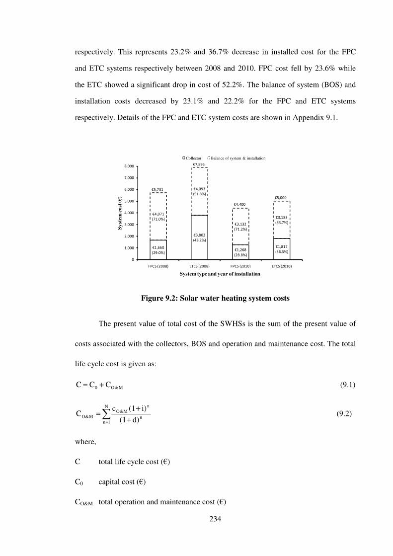
234

respectively. This represents 23.2% and 36.7% decrease in installed cost for the FPC

and ETC systems respectively between 2008 and 2010. FPC cost fell by 23.6% while

the ETC showed a significant drop in cost of 52.2%. The balance of system (BOS) and

installation costs decreased by 23.1% and 22.2% for the FPC and ETC systems

respectively. Details of the FPC and ETC system costs are shown in Appendix 9.1.

Figure 9.2: Solar water heating system costs

The present value of total cost of the SWHSs is the sum of the present value of

costs associated with the collectors, BOS and operation and maintenance cost. The total

life cycle cost is given as:

M&O0 CCC += (9.1)

�= +

+=N

1nn

nM&O

M&O d)(1i)(1c

C (9.2)

where,

C total life cycle cost (�)

C0 capital cost (�)

CO&M total operation and maintenance cost (�)

��

��

��

� ��

��

��

��!

��

� ��!�

�!��

� ��

�"��

��

�!��

��

��!� �

�

��

��

��

��

"��

��

!��

��

#$%�� &'%�� #$%�� &'%��

Syst

em co

st (�

)

System type and year of installation

Collector Balance of system & installation

�"�!��

�!��"

� � ��

�"��

235

cO&M annual operation and maintenance cost (�)

i inflation rate (%)

N service life (years)

d discount rate (%)

9.2.1 Projected SWHS Cost

Using SWHS costs for 2010, SWHS learning rate and market growth scenarios

in section 9.1, Equation 8.3 was used to compute SWHS costs beyond the 2010 base

year. Figure 9.3 shows projected costs of the SWHSs in Ireland from 2010 to 2030 for

the moderate and advanced scenarios. The cost of the FPC system decreases from

�4,400 in 2010 to �3,439 and �3,308 in 2030 under the Mod 10 and Adv 10 scenarios

while the cost of the ETC system decreases from �5,000 to �3,908 and �3,759 under the

Mod 10 and Adv 10 over the same period. Detailed values are shown in Appendix 9.2.

The same methodology used to compute the projected system capital cost was

employed to compute the SWHS life cycle cost. For both SWHS types, the projected

life cycle costs were calculated under the Mod 10 and Adv 10 scenarios. Figure 9.4

shows projected life cycle costs of the SWHSs under the two scenarios. It is seen that

the life cycle costs decrease from �4,913 to �3,952 and �3,820 for SWHSs with FPC

and from �5,583 to �4,491 and �4,341 for SWHSs with ETC under the Mod 10 and Adv

10 scenarios. Detailed values are shown in Appendix 9.3.

236

Figure 9.3: Projected costs and installed capacity of solar water heating systems in Ireland (2010-2030)

Figure 9.4: Projected life cycle system cost under different scenarios (2010 to 2030)

9.3 Fuel Prices

Using the HOP scenario in section 8.2.2, natural gas and oil prices in 2010 were

used to make future projections to 2030. Figure 9.5 shows projected fuel prices for

SWHS auxiliary heaters from 2010 to 2030. It is seen that electricity prices are highest

followed by oil and natural gas. Projected electricity, oil and natural gas prices increase

from 0.203 to 0.274 �/kWh, 0.064 to 0.184 � and 0.055 to 0.160 �/kWh respectively

from 2010 to 2030. Detailed values of fuel prices are shown in Appendix 9.4.

0

50

100

150

200

0

1,000

2,000

3,000

4,000

5,000

2010

2011

2012

2013

2014

2015

2016

2017

2018

2019

2020

2021

2022

2023

2024

2025

2026

2027

2028

2029

2030

Sola

r th

erm

al a

nnua

l ins

talle

d ca

paci

ty (G

Wth

)

Syst

em c

apita

l cos

t (�

)

Year

Installed capacity (Mod) Installed capacity (Adv) FPC (Mod 10)ETC (Mod 10) FPC (Adv 10) ETC (Adv 10)

3,000

3,500

4,000

4,500

5,000

5,500

6,000

2010

2011

2012

2013

2014

2015

2016

2017

2018

2019

2020

2021

2022

2023

2024

2025

2026

2027

2028

2029

2030

Life

cyc

le sy

stem

cos

t (�

)


FPC (Mod 10) ETC (Mod 10) FPC (Adv 10) ETC (Adv 10)

237

Figure 9.5: Projected fuel prices for SWHS auxiliary heaters from 2010 to 2030

9.4 Economic Viability Assessment

9.4.1 System Yield

The final yield is the annual net energy delivered by the solar water heating

system. Results of field performance studies carried out by Ayompe et al. [189] showed

that the annual total energy delivered by the FPC and ETC SWHSs were 1,639 and

1,699 kWh respectively.

9.4.2 Revenue

The total revenue (Rt) accrued over the service life of the solar water heating

system is given as:

�= +

+=N

1nn

n

h

uft d)(1

e)(1�

QCR (9.3)

where,

Rt total discounted revenue (�)

Cf displaced fuel cost (�/kWh)

Qu useful heat delivered (kWh/y)

e fuel annual escalation rate (%)

d discount rate (%)

0.00

0.05

0.10

0.15

0.20

0.25

0.30

2010

2011

2012

2013

2014

2015

2016

2017

2018

2019

2020

2021

2022

2023

2024

2025

2026

2027

2028

2029

2030

Fuel

pri

ce (�

/kW

h)

Year

Natural gas price Oil price Electricity price

238

�h heater efficiency (%)

n period considered (years)

N service life (years)


The net present value (NPV) of the solar water heating systems is given as:

CRNPV t −= (9.4)

where,

NPV net present value (�)

C total life cycle cost (�) in Equation 9.1

The NPVs for FPC and ETC SWHSs with condensing gas boilers, oil boilers

and electric immersion heaters were evaluated for systems installed in 2010 with and

without grant aid. Figure 9.6 shows NPVs for SWHSs with different auxiliary heaters in

2010. The results show that under prevailing system costs (2010), existing grant aid

structure and the assumed discount rate, solar water heating systems are not yet

economically viable in Ireland except for FPC systems with electric immersion heaters

being offered grant aid. SWHSs with condensing gas boilers had the worst NPVs while

SWHSs with electric immersion heaters had the best NPVs.

Figure 9.6: NPVs for SWHSs with different auxiliary heaters in 2010

-1,738

-409

-10

-2,365

-987

-574

-2,738

-1,409

-1,010

-3,328

-1,950

-1,537

-3,500

-3,000

-2,500

-2,000

-1,500

-1,000

-500

0Condensing gas boiler Oil boiler Electric immersion heater

Net

pre

sent

val

ue (�

)

Auxiliary heater type

FPC (with grant) ETC (with grant) FPC ETC

239

Figure 9.7 shows projected average NPVs for SWHSs with different auxiliary

heating systems from 2010 to 2030 without grant aid. It is seen that both SWHSs with

condensing gas boilers are not economically viable throughout the projected period. On

the other hand FPC SWHSs with oil boilers and electric immersion heaters will become

economically viable in 2017 and 2018 respectively under the assumptions made while

ETC SWHSs with oil boilers and electric immersion heaters will become economically

viable in 2021 and 2025 respectively. Detailed values are shown in Appendix 9.5.

Figure 9.7: Projected average net present value for SWHSs with different auxiliary

heaters


The simple payback period (SPP) for the SWHSs were calculated using

Equation 8.1. Figure 9.8 shows SPPs for SWHSs with different auxiliary heaters

installed in 2010. It is seen that systems fitted with electric immersion heaters had the

lowest SPPs while those fitted with condensing gas boilers had the highest SPPs. The

SPPs varied between 10.2 years and 48.2 years for grant aided FPC systems fitted with

electric immersion heaters and ETC systems without grant aid fitted with condensing

gas boilers respectively.

-3,500

-3,000

-2,500

-2,000

-1,500

-1,000

-500

0

500

2010

2011

2012

2013

2014

2015

2016

2017

2018

2019

2020

2021

2022

2023

2024

2025

2026

2027

2028

2029

2030

Net

pre

sent

val

ue (�

)


FPC (condensing gas boiler) FPC (oil boiler)FPC (electric immersion heater) ETC (condesing gas boiler)ETC (oil boiler) ETC (electric immersion heater)

240

Figure 9.8: SPP for SWHS with different auxiliary heaters in 2010

Figure 9.9 shows projected SPPs for SWHSs with different auxiliary heaters from

2010 to 2030. It is seen that the SPPs for SWHSs with condensing gas boilers and oil

boilers decrease sharply from 2010 to 2016 and then remain fairly constant until 2030. SPPs

for FPC SWHSs decrease from 43.9 to 15.1 years, 27.3 to 9.4 years and 13.2 to 9.8 years

for condensing gas boilers, oil boilers and electric immersion heaters respectively between

2010 and 2030. Similarly, SPPs for ETC SWHSs decrease from 48.2 to 16.6 years, 29.9 to

10.3 years and 14.5 to 10.7 years for condensing gas boilers, oil boilers and electric

immersion heaters respectively between 2010 and 2030. Detailed values are shown in

Appendix 9.6.

Figure 9.9: Projected simple payback periods for SWHSs with different auxiliary heaters from 2010 to 2030

0

5

10

15

20

25

30

35

40

45

50

2010

2011

2012

2013

2014

2015

2016

2017

2018

2019

2020

2021

2022

2023

2024

2025

2026

2027

2028

2029

2030

Payb

ack

peri

od (y

ears

)


FPC (condensing gas boiler) FPC (oil boiler)FPC (electric immersion heater) ETC (condesing gas boiler)ETC (oil boiler) ETC (electric immersion heater)

43.9

27.3

13.2

48.2

29.9

14.5

33.9

21.1

10.2

38.9

24.1

11.7

0

5

10

15

20

25

30

35

40

45

50

Condensing gas boiler Oil boiler Electric immersion heater

Sim

ple p

ayba

ck p

erio

d (y

ears

)


FPC ETC FPC (with grant) ETC (with grant)

241

9.4.5 Levelised Heating Cost

The levelised heating cost (LHC) is the cost per kWh of heat generated. LHC is

obtained by dividing the annuity of the life cycle cost (C) by the quantity of

conventional energy displaced annually (Ec) in Equation 9.6 and is given as:

1d)(1d)d(1

EC

LHC n

n

c −++=

(9.5)

LHC levelised heating cost (�/kWh)

C life cycle cost (�)

Ec quantity of conventional energy displaced (kWh)

d discount rate (%)

n number of years the annuity has to run (20 years)

The quantity of conventional energy displaced annually (Ec) is computed as:

huc /�QE = (9.6)

�h auxiliary heater efficiency (%)

Qu useful energy collected by the solar collector (kWh)

Annuity is defined as a constant amount, A, payable at the end of every ‘n’

interest period in years for which the sum of payments is equal to the future amount of

the initial capital value, C, after these ‘n’ years. The annuity is obtained as [190]:

C1d)(1

d)d(1A n

n

−++= (9.7)

Figure 9.10 shows the levelised heating cost (LHC) for SWHSs fitted with

different types of auxiliary heaters installed in 2010. It is seen that SWHSs fitted with

oil boilers had the lowest LHC while systems fitted with electric immersion heaters had

the highest LHC. The LHC varied between 0.158 �/kWh and 0.335 �/kWh for the FPC

system with grant aid fitted with an oil boiler and ETC system without grant aid fitted

242

with an electric immersion heater. SWHSs fitted with electric immersion heaters have

the highest LHC followed by natural gas and oil boilers. The difference in LHC being

attributed to the efficiency of the auxiliary heating system.

Figure 9.10: LHC for SWHSs with different types of auxiliary heaters in 2010

Figure 9.11 shows average levelised heating cost for SWHSs with different

auxiliary heaters from 2010 to 2030. It is seen that SWHSs with electric immersion

heaters have the highest LHC while those with oil boilers have the lowest LHC. This is

as a result of the high efficiency of immersion heaters and low efficiency of oil boilers.

The LHC for the FPC SWHS decreases from �0.305 to �0.241, �0.198 to �0.157 and

�0.275 to �0.217 for electric immersion, oil boilers and condensing gas boilers

respectively between 2010 and 2030. Similarly, the LHC for the ETC SWHS decreases

from �0.335 to �0.265, �0.218 to �0.172 and �0.301 to �0.238 for electric immersion,

oil boilers and condensing gas boilers respectively over the same period. Detailed

values of average LHCs are shown in Appendix 9.7.

0.27

5

0.19

8

0.30

5

0.30

1

0.21

8

0.33

5

0.21

9

0.15

8

0.24

3

0.24

9

0.18

0

0.27

7

0.00

0.05

0.10

0.15

0.20

0.25

0.30

0.35

0.40

Condensing gas boiler Oil boiler Electric immersion heater

Lev

elis

ed h

eatin

g co

st (�

/kW

h)


FPC ETC FPC (with grant) ETC (with grant)

243

Figure 9.11: Average Levelised heating cost for SWHSs with different auxiliary heaters

9.5 Emission Analysis

9.5.1 Life Cycle Emission Savings

The emission factors for grid electricity, residual oil and natural gas used to

evaluate life cycle emissions for the SWHSs were 533 gCO2/kWh, 273.6 gCO2/kWh

and 205.6 gCO2/kWh [191]. It was assumed that the emission factors for residual oil

and natural gas as well as the annual quantity of energy generated by the solar energy

system remained constant throughout the service life of the SWHSs. Grid electricity

emission factor projections were obtained from section 8.10.2. Life cycle emission

savings were calculated using Equation 9.8 given as:

�=

=N

1ii

h

u EF�

QLE (9.8)

where,

LE life cycle emission savings (tCO2)

Qu annual useful energy delivered by the solar energy system (kWh)

EFi fuel emission factor in year i (tCO2/kWh)

�h auxiliary heater efficiency (%)

0.15

0.20

0.25

0.30

0.35

2010

2011

2012

2013

2014

2015

2016

2017

2018

2019

2020

2021

2022

2023

2024

2025

2026

2027

2028

2029

2030

Lev

elis

ed h

eatin

g co

st (�

/kW

h)


FPC (Electric immersion) ETC (Electric immersion) FPC (oil boiler)ETC (oil boiler) FPC (condensing boiler) ETC (condensing boiler)

244

Life cycle emission savings for FPC SWHSs with condensing gas boilers, oil

boilers and electric immersion heaters were: 7.9 tCO2; 14.5 tCO2; and 15.4 to 13.6 tCO2

respectively between 2010 and 2030. Similarly, life cycle emission savings for ETC

SWHSs with condensing gas boilers, oil boilers and electric immersion heaters were:

8.2 tCO2; 15.0 tCO2; and 15.9 to 14.1 tCO2 respectively between 2010 and 2030.

Average emission factors for grid electricity, residual oil, natural gas and life cycle

emission savings (tCO2) for FPC and ETC SWHSs with different auxiliary heaters are

shown in Appendix 9.8.

9.6 SWHS Marginal Abatement Costs

Marginal abatement cost curves were constructed for the two SWHSs with

different auxiliary heaters. The MAC was calculated using Equation 8.15 modified to

give:

s

NPV

EMS

MAC = (9.9)

where,

MAC marginal abatement cost (�/tCO2)

SNPV solar water heater net present value (�)

EMs CO2 emission savings (or avoided CO2) (tCO2)

Figure 9.12 shows marginal abatement cost curves for SWHSs with different

auxiliary heaters and carbon prices. It is seen that SWHSs with condensing gas boilers

had the highest marginal abatement costs. MACs for FPC SWHSs decrease from 348 to

25 �/tCO2, 97 to 13 �/tCO2, and 66 to -9 �/tCO2 for condensing gas boilers, oil boilers

and electric immersion heaters between 2010 and 2030. Similarly, MACs for ETC

SWHSs decrease from 408 to 35 �/tCO2, 130 to -8 �/tCO2, and 97 to -3 �/tCO2 for

condensing gas boilers, oil boilers and electric immersion heaters between 2010 and

2030. Detailed values are shown in Appendix 9.9.

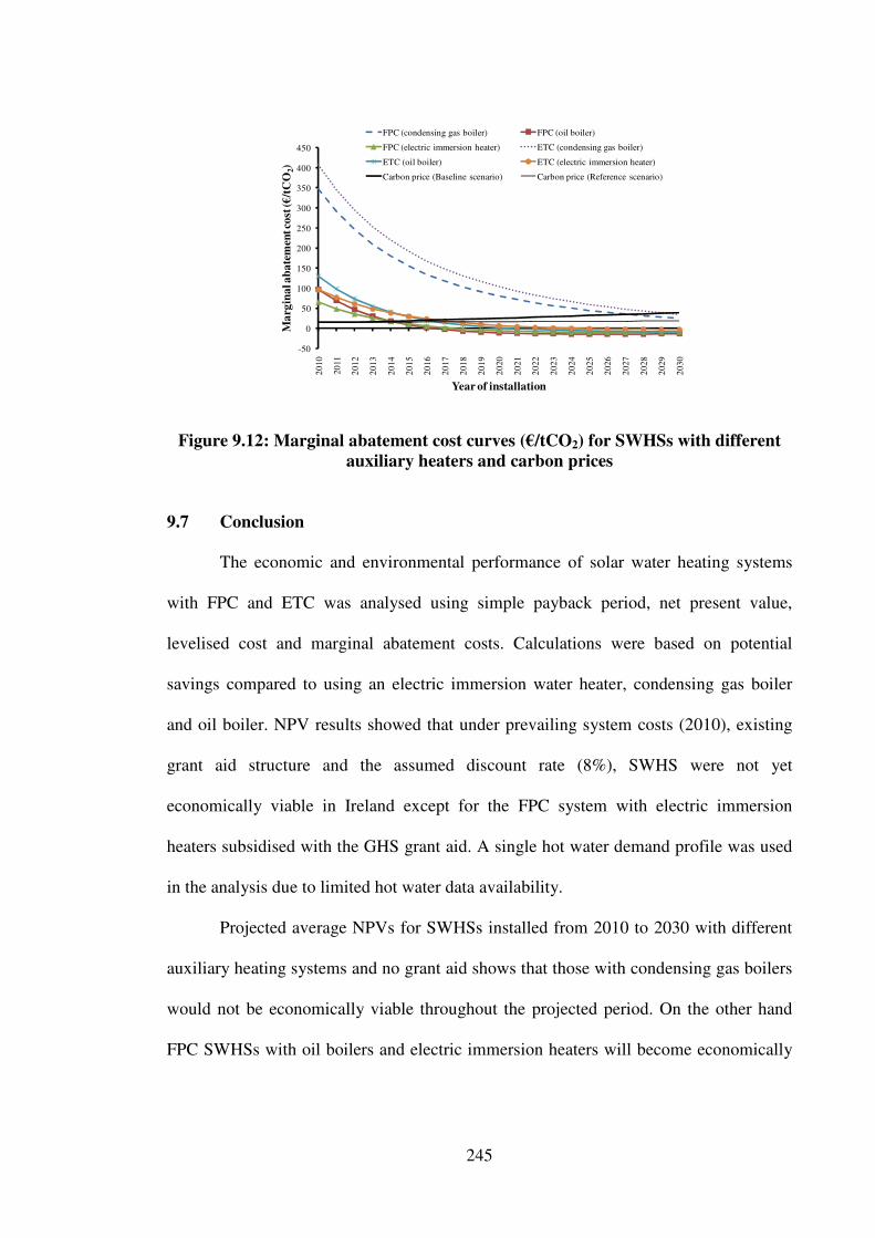
245

Figure 9.12: Marginal abatement cost curves (�/tCO2) for SWHSs with different auxiliary heaters and carbon prices

9.7 Conclusion

The economic and environmental performance of solar water heating systems

with FPC and ETC was analysed using simple payback period, net present value,

levelised cost and marginal abatement costs. Calculations were based on potential

savings compared to using an electric immersion water heater, condensing gas boiler

and oil boiler. NPV results showed that under prevailing system costs (2010), existing

grant aid structure and the assumed discount rate (8%), SWHS were not yet

economically viable in Ireland except for the FPC system with electric immersion

heaters subsidised with the GHS grant aid. A single hot water demand profile was used

in the analysis due to limited hot water data availability.

Projected average NPVs for SWHSs installed from 2010 to 2030 with different

auxiliary heating systems and no grant aid shows that those with condensing gas boilers

would not be economically viable throughout the projected period. On the other hand

FPC SWHSs with oil boilers and electric immersion heaters will become economically

-50

0

50

100

150

200

250

300

350

400

450

2010

2011

2012

2013

2014

2015

2016

2017

2018

2019

2020

2021

2022

2023

2024

2025

2026

2027

2028

2029

2030

Mar

gina

l aba

tem

ent c

ost (�

/tCO

2)


FPC (condensing gas boiler) FPC (oil boiler)

FPC (electric immersion heater) ETC (condensing gas boiler)

ETC (oil boiler) ETC (electric immersion heater)

Carbon price (Baseline scenario) Carbon price (Reference scenario)

246

viable in 2017 and 2018 respectively while ETC SWHSs with oil boilers and electric

immersion heaters will become economically viable in 2021 and 2025 respectively.

Simple payback period results showed that systems fitted with electric

immersion heaters had the lowest SPPs while those fitted with condensing gas boilers

had the highest SPPs. The SPPs varied between 10.2 years and 48.2 years for FPC

systems with grant aid fitted with electric immersion heaters and ETC systems without

grant aid fitted with condensing gas boilers respectively. Projected SPPs for FPC

SWHSs decreased from 43.9 to 15.1 years, 27.3 to 9.4 years and 13.2 to 9.8 years for

systems with condensing gas boilers, oil boilers and electric immersion heaters

respectively between 2010 and 2030. Similarly, SPPs for ETC SWHSs decreased from

48.2 to 16.6 years, 29.9 to 10.3 years and 14.5 to 10.7 years for systems with

condensing gas boilers, oil boilers and electric immersion heaters respectively between

2010 and 2030.

SWHSs fitted with oil boilers had the lowest levelised heating cost (LHC) while

systems fitted with electric immersion heaters had the highest LHC. The LHC varied

between 0.158 �/kWh and 0.335 �/kWh for the FPC system with grant aid fitted with an

oil boiler and ETC system without grant aid fitted with an electric immersion heater in

2010. Projections showed that the LHC for the FPC SWHS decreased from �0.305 to

�0.241, �0.198 to �0.157 and �0.275 to �0.217 for electric immersion, oil boilers and

condensing gas boilers respectively between 2010 and 2030. Similarly, the LHC for the

ETC SWHS decreased from �0.335 to �0.265, �0.218 to �0.172 and �0.301 to �0.238

for electric immersion, oil boilers and condensing gas boilers respectively over the same

period.

247

Results from emission analysis showed that life cycle emission savings for FPC

SWHSs with condensing gas boilers, oil boilers and electric immersion heaters were:

7.9 tCO2; 14.5 tCO2; and 15.4 to 13.6 tCO2 respectively between 2010 and 2030.

Similarly, life cycle emission savings for ETC SWHSs with condensing gas boilers, oil

boilers and electric immersion heaters were: 8.2 tCO2; 15.0 tCO2; and 15.9 to 14.1 tCO2

respectively between 2010 and 2030.

MACs for FPC SWHSs decrease from 348 to 25 �/tCO2, 97 to 13 �/tCO2, and

66 to -9 �/tCO2 for condensing gas boilers, oil boilers and electric immersion heaters

between 2010 and 2030. Similarly, MACs for ETC SWHSs decrease from 408 to 35

�/tCO2, 130 to -8 �/tCO2, and 97 to -3 �/tCO2 for condensing gas boilers, oil boilers and

electric immersion heaters between 2010 and 2030.

248

CHAPTER 10

POLICY ANALYSIS OF GRID-CONNECTED PV AND SOLAR WATER HEATING SYSTEMS

The aim of this chapter is to undertake a policy analysis of domestic scale grid-

connected PV and SWH systems. Specific objectives are to:

• review existing global policy support measures to support the two

technologies;

• present policy findings based on the techno-economic and environmental

analysis of the systems; and

• rank the technologies based on their levelised cost of energy generation and

marginal abatement costs.

10.1 Overview

Over the past decade there have been fluctuations in the price of crude oil

worldwide which has created the knock-on effect of increasing the cost of conventional

energy sources. There has also been an increase in international commitments to reduce

CO2 emissions. Governments worldwide have reacted by focusing their attention on

rebalancing their respective energy mixes to include greater quantities of renewable

energy technologies (RETs).

Significant resources are being applied worldwide to solve this problem by

supporting the deployment of RETs. The questions that arise are: is money being spent

efficiently and on the best technology?

Government support schemes have been used to accelerate the introduction of

appropriate RETs, often using the argument that external costs to society justify the

249

subsidy involved. These support schemes may take the form of direct subsidies for

individuals and companies, FITs, tax credits and loan guarantees. The policy intent is to

subsidize the appropriate technology for a limited time in the expectation that the

technology can continue to exist on its own in a mature stage [192]. Appendix 10.1

shows the characteristics of some key support measures.

One key concern in the deployment of RETs is the various types of barriers that

need to be overcome before they become a mainstream energy supply option. These

barriers can be categorised as technical, economic and regulatory. Their diverse natures

necessitate the development of a holistic, strategic approach to RET deployment.

Existing energy policies have mostly relied upon financial subsidies, market-based

instruments such as renewable portfolio standards, FITs and production tax credits to

stimulate the installation and use of equipment to generate electricity from renewable

sources [165]. The focus of this work is on economic barriers.

The underpinning objective of the strategic approach is predominantly

economic, using up-front subsidies to finance learning investments that will drive down

the costs of new technologies at the system level. Lower costs encourage more

adoption, which sustains more learning [165]. Subsidies can also be used to promote a

political agenda by giving money directly to the electorate. Moreover, governments are

poor at ‘picking winners’ due to lack of expertise, evidence-based policy making and

the unknown futures of markets and technologies. Market-based instruments are

therefore seen to be more economically efficient in guiding the choice of winners and

losers.

10.2 European Policy Context

European Directive 2001/77/EC imposes an obligation on EU Member States to

implement measures that facilitate the generation of electricity from renewable sources

250

in order to reduce greenhouse gas emissions, enhance security of supply and improve

economic competitiveness. A key component of the Directive is for the 27 EU Member

States to increase their share of electricity generated from renewable resources to 21%

[193].

In 2007, EU member states agreed a Climate Change Strategy which included a

commitment to achieve an overall target of 20% primary energy consumption from

renewable energy sources by 2020. These commitments are enshrined as legally binding

targets for each member state in Directive 2009/28/EC in which Ireland is committed to

achieve 16% of gross national energy consumption from renewables by 2020 as shown

in Table 10.1. In the National Renewable Energy Action Plan (NREAP) [5] the

government of Ireland has set targets of 42.5%, 12.5% and 10% for: electricity

production; heating and cooling; and transport respectively from renewable energy

sources by 2020, details of which are as shown in Appendix 10.2. Appendix 10.3 shows

expected gross final energy consumption of Ireland in heating and cooling, electricity

and transport up to 2020 taking into account the effects of energy efficiency and energy

saving measures from 2010 to 2020. For the reference scenario, expected gross final

energy consumption increases from 2,511 to 2,937 ktoe and from 5,184 to 5,724 ktoe

for electricity, heating and cooling respectively between 2010 and 2020. With additional

energy efficiency measures, expected gross final energy consumption increases from

2,473 to 2,813 ktoe for electricity and decreases from 5,160 to 4,931 ktoe for heating

and cooling between 2010 and 2020.

Appendix 10.4 shows the renewable energy contribution of each sector to final

energy consumption. It is seen that the expected gross final consumption of RES for

heating and cooling increases from 220 to 591 ktoe between 2010 and 2020 while the

251

expected gross final consumption of electricity from RES increases from 504 to 1,196

ktoe over the same period.

Table 10.1: National overall target for the share of energy from renewable sources in gross final consumption of energy in 2005 and 2020 [5]

Share of energy from renewable sources in gross final consumption of energy in 2005 (S2005) (%)

3.1%

Target of energy consumption from renewable sources in gross final consumption in 2020 (S2020) (%)

16%

Expected total adjusted annual energy consumption in 2020 (Ktoe)

14,142

Required annual amount of energy from renewable sources corresponding to the 2020 target (ktoe)

2,269

10.3 Global Solar Thermal Support Schemes

This section reviews international policies regarding solar water heating to see

which aspects have been effective in gaining an increased penetration of solar systems

for water heating. Throughout the world a wide range of policy types have been used to

increase the uptake of solar water heating including [194]:

• collector-area-based subsidies;

• performance-based subsidies;

• tax credits;

• tax reduction; and

• mandatory policies or obligation.

Table 10.2 shows different solar thermal policies and their characteristics as

applied to different countries.

252

Table 10.2: Solar Thermal policy types

Policy Type Countries Characteristics Positives Downside

Collector-area-based subsidies Austria, Germany, Ireland

Financial remunerations are offered for a given collector area sometimes differentiated by collector type

Most common type of policy to promote solar thermal systems. Successful in increasing penetration of SWH

Increases the number of systems but does not indicate whether an overall reduction in energy demand has been eventuated or that the systems have been either cost effective or have realised real energy savings over the lifespan of the systems with the embodied energy taken into account.

Performance-based subsidies The Netherlands, Australia, Sweden

Indicates whether the systems are working well or reducing overall national energy consumption

Difficult to get some proxy for system performance without actually monitoring individual systems.

Tax credits France

Reduction of the value added tax or a percentage of capital cost is deducted from taxes

Successful in increasing penetration of SWH

Increases the number of systems but does not indicate whether an overall reduction in energy demand has been eventuated or that the systems have been either cost effective or have realised real energy savings over the lifespan of the systems with the embodied energy taken into account.

Tax deduction Greece Related to the income tax of the investor

By off-setting investment costs against taxable income, the investor could reduce investment costs

Equity issue: people who pay the most tax (the richest part of the population) obtain maximum cost reduction

Mandatory policy (obligation)

Israel, Spain, Ireland, Germany, Italy

Applicable to new buildings and those undergoing major renovation

Very successful in promoting large-scale deployment

Fundamentally changes the market growth since investors often search for the cheapest available solution.

253

The EU RES Directive proposal requires EU member states to develop NREAPs

to encourage national, regional and local authorities to implement one or several

additional instruments to promote solar thermal notably [195]:

• Financial incentives to investment or fiscal reductions. These financial measures

should be stable and long-term oriented, in order to build up confidence with

investors.

• Awareness raising campaigns supported by public authorities and focused on

relevant target groups: end users (house owners, operators of high-potential

applications such as hotels, swimming pools, collective buildings), architects,

craftsmen (heating installers and roofers), building & construction industry

• Support specific training for solar thermal technologies, focused on key

professional actors: planners, architects, heating installers and roofers.

10.4 PV Financial Support Schemes

PV generated electricity is expected to become a major source of cheap

electricity in the decades to come. It is envisaged that it will do so by delivering clean,

safe and reliable electricity that is needed to face global environmental challenges [79].

With the current cost of PV generated electricity being higher than that of

conventionally generated electricity, the deployment of the PV market is greatly

influenced by the political framework and supports of any given country. The

introduction, modification or phasing out of such support schemes can have profound

consequences on the PV market [80]. Photovoltaic devices and systems already

represent a fast-growing and dynamic industry as a direct result of national support

programmes resulting in learning through research and demonstration [196].

254

A variety of policies have been used in different jurisdictions to promote the

adoption of new energy technologies and to initiate a transition from conventional

sources to renewable sources of energy. Several scholars have argued on the preferred

type of policy required at different stages of development of the PV industry. Rowlands

[197] and Lauber [198] advocate generous feed-in tariffs that include external costs

avoided by the technology leading to early-stage PV market growth. They also argue

that renewable portfolio standards (RPS) (described later in this section) are better

suited for a more established technology. Parker [164] postulates that FITs are regarded

by others as being better for middle stage market development where the technology has

reached a stage of maturity such as PV. Carbon taxes are however the most

economically efficient policy since the market can choose technologies with the lowest

MAC.

Local, national and international policies, as well as the presence of suitable

standards and codes and a positive perception by the general public and utilities, all

govern the rate of deployment of PV systems. There are two broad strategic categories

of financial policies to promote RETs [165]:

• those that aid installation of renewable energy equipment such as direct

capital subsidies and tax credits; and

• those that support the market price of electricity derived from renewable

sources and thus encourage the use of the installed equipment such as

renewable portfolio standards (RPS), net metering, renewable energy

certificates (RECs) and FITs.

255

10.4.1 Direct Capital Subsidies

Direct capital subsidies or capital cost grants can effectively tackle the up-front

cost barrier, which is often the most significant hurdle facing PV deployment even with

a FIT, and can be used in grid-connected markets. They can be very effective (as the

Japanese residential PV market has demonstrated) and are relatively simple to

implement. Criticisms include: they do not encourage the use of efficient PV systems;

they do not encourage broader consideration of customer’ s energy usage; and they do

not address the customer’ s willingness to pay for PV. Direct capital subsidies are also

more broadly criticized for inflating PV system prices [76].

Further drawback of the direct capital subsidy approach is the absence of

incentives to invest in high quality PV electricity systems and to ensure their efficient

operation and maintenance. If the customer receives a fixed payment per installed

capacity unit, there is no incentive to go for high-quality products, which usually mean

a higher price, or to optimally operate the PV system. In contrast, optimal PV

generation leading to the best return on investment is incentivised by FITs [199].

10.4.2 Tax Credits

Tax credits are a means of financing FITs where utilities are allowed to offset

their tax liabilities so that they can purchase renewable electricity. One advantage of

using utility tax credits to fund a FIT policy is that the added costs are not passed on to

electricity ratepayers but to society in general. The electricity price is not directly

impacted. The disadvantage of this approach is that it imposes an implicit cap on

program size based on the size of utilities’ tax liability. This could make it difficult to

fund large and sustained amounts of renewable energy (RE) deployment, except in the

256

case of the largest utilities. This approach can also erode state tax revenues, particularly

if large amounts of RE are developed [200].

Tax credits can tackle the up-front cost barrier and various forms of this measure

have emerged in a number of countries. However, it assumes that entities with a tax

liability are prime candidates for PV, which may or may not be the case depending on

the particular market. Tax credits are probably not as effective in the early stages of PV

market development when deployment targeted at specific end-users may produce the

best results [76].

In practice, public support can involve a combination of measures and will

usually function more effectively when this is the case. Funding issues are significant

and funding continuity is critical to the success of any mechanism.

10.4.3 Renewable Portfolio Standards (RPS) and Renewable Obligation (RO)

The renewable portfolio standard (RPS) is one of the most common state-level

renewable energy policies in the United States. It is designed to encourage new

renewable energy development by establishing a target or quota on the proportion of

electricity generation that must come from renewable energy sources by a certain date

[201, 202]. RPS policies often use a process of competitive solicitations to procure

supply and promote competition between project developers. RPS laws oblige electric

power companies to expand the use of electricity generated from new and renewable

energy sources.

The Renewables Obligation (RO) was designed to encourage generation of

electricity from eligible renewable sources in the United Kingdom. It was introduced in

England and Wales and in a different form (the Renewables Obligation (Scotland)) in

257

Scotland in April 2002 and in Northern Ireland in April 2005, replacing the Non-Fossil

Fuel Obligation which operated from 1990 [203].

10.4.4 Net Metering

Net metering describes the practice of metering the energy consumption of an

electricity consumer net of that generated on the premises (in particular from

photovoltaics). The net measurement is undertaken with a bi-directional meter or a pair

of unidirectional meters spinning in opposite directions. In the case that the electricity

production exceeds consumption at a particular time, the electricity-meter spins

backwards so the value at the end is smaller than at the beginning of a period. Although

net metering is most common in the USA, some EU countries like Italy, Denmark,

Germany and Malta apply net metering or similar measures [165, 204].

10.4.5 Renewable Energy Certificates (RECs)

Renewable energy certificates (RECs) represent the environmental attributes of

electricity generated from renewable energy sources, and represent a second commodity

in addition to the electricity itself. They are designed to offer additional revenues for

project developers; and, they are often traded or sold within bilateral contracts [200].

RECs are also known as Green tags, renewable energy credits, or tradable

environmental commodities in the United States. One REC constitutes proof that one

megawatt-hour (MWh) of electricity was generated from an eligible renewable energy

source. These certificates can be sold and traded, and the owner of the REC can claim to

have purchased renewable energy. RECs can encourage the use of renewable energy by

providing a production subsidy or production tax credits for electricity generated from

renewable sources [165].

258

10.4.6 Feed-in Tariff

A feed-in tariff (FIT) refers to an explicit monetary reward for producing PV

electricity, at a rate per kWh. In principle the measure encourages efficient production

of PV electricity with the output from the PV system being monitored and recorded, and

has consequently been promoted as the preferred micro PV support policy in most

countries based on the successes achieved in countries where it was initially

implemented, notably Germany.

The FIT scheme involves an obligation on the part of utilities to purchase the

electricity produced by renewable energy producers in their service area at a tariff

determined by the public authorities and guaranteed for a specified period of time [205].

Advocates of FITs [206-208] argue that they are the most cost effective means of

producing rapid deployment of renewable energy technologies at the least cost.

The principal drawback of FITs is that because they act as a cross subsidy

setting tariffs above current market prices, they distort the market structure. Customers

are credited for energy at a price higher (and sometimes considerably higher) than the

normal wholesale rate. That additional cost needs to be borne elsewhere in the industry.

This means that the retail price paid by other customers would increase. The amount by

which prices to other customers would increase depends on the rate and design of the

tariff structure, and the level of uptake. Again if tariffs are not monitored, there is the

potential that installers and manufacturers do not improve their technologies, or lower

costs, as whatever happens, the tariff is the same and all customers are satisfied.

The basic FIT is a mandated long-term premium price for renewable energy,

usually differentiated by the technology used and size of installation to account for

electricity generation cost variations. Such a payment is guaranteed over a long-term

period that usually covers a significant portion of the working life of the installation

259

[184]. Long-term tariff structures are needed so that an investor can calculate his return

on investment. The return on investment with FIT is heavily dependent on the

performance of the PV system as well as the “ prosumer’ s” electricity demand profile.

Prosumer is a portmanteau formed by contracting the word producer with the word

consumer.

Advanced feed-in tariffs pay higher fees for the electricity generated in

recognition of its time-of-use value (production at peak demand times associated with

air conditioning loads), its distributed benefits (avoiding investment in network

capacity) and the avoided environmental costs (associated with poor air quality and

greenhouse gas emissions) [164].

There are three main types of reward mechanisms to exported electricity

notably: metered offers; generation-based offers; and unmetered offers [184].

1. Metered offers: These include two distinct tariffs notably one for the total

quantity of electricity generated and one for exported electricity to the grid

as is applicable to the UK.

2. Generation based offers: The tariff offered is applied on the total electricity

generated by the system. Such type of tariff also include ROCs price, with

the suppliers acting as third agent for the PV system owner. Such tariffs are

applicable to countries such as Germany, Spain, Italy, Greece, Portugal etc.

3. Unmetered offers: These offers are independent of metered electricity flows.

In some cases, they are applied to exported electricity only, but on the basis

of export volume estimates; in other cases, an annual fixed amount is offered

per kWp installed.

260

10.4.7 Carbon Tax

Carbon tax is an incentive-based policy instrument for controlling the emissions

of carbon dioxide [209]. A carbon tax operates by providing an incentive for consumers

and firms to substitute away from those goods which have the highest carbon

intensities. Prices of more carbon intensive goods increase proportionately more than

those with lower intensities. These intensities in turn depend on the fossil fuels used in

the production of each good and the nature of inter-industry transactions. Such a tax is

obviously designed to correct a market failure (the absence of a market for carbon

dioxide) but it can also have unintended consequences. These include the fact that the

price changes induced by the tax may give rise to excess burdens. In addition, there may

be adverse impacts on the distribution of welfare [210].

10.4.8 Feed-in Tariffs in Different Countries

2007 saw a consolidation of FIT as the most popular international mechanism

for promoting grid-connected PV applications. This was reinforced by strong growth in

PV markets in France, Germany, Italy, Korea, Portugal and Spain [76]. Germany has

shown that micro-generation, in particular solar PV generation can contribute very

significant amounts of the nation’ s energy and that a feed-in tariff is the best way to

encourage this growth.

Most of the discussions about FIT have now shifted to its implementation on

issues such as payment for all PV electricity generated or only the portion exported to

the grid, how to control take-up rates without using a blunt ‘cap’ approach and how to

best reward different types of plants. It is argued that the FITs and the decisions made in

relatively few countries, to a large extent influence the evolution of world prices for PV

modules (in conjunction with supply-demand dynamics and competition in the PV

industry). Consequently a number of countries have looked at the structure of their

schemes for future years with the aim of making the payments more reflective of true

costs [76]..

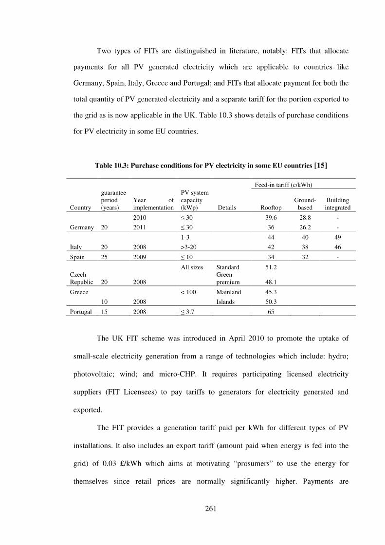
261

Two types of FITs are distinguished in literature, notably: FITs that allocate

payments for all PV generated electricity which are applicable to countries like

Germany, Spain, Italy, Greece and Portugal; and FITs that allocate payment for both the

total quantity of PV generated electricity and a separate tariff for the portion exported to

the grid as is now applicable in the UK. Table 10.3 shows details of purchase conditions

for PV electricity in some EU countries.

Table 10.3: Purchase conditions for PV electricity in some EU countries [15]

Feed-in tariff (c/kWh)

Country

guarantee period (years)

Year of implementation

PV system capacity (kWp) Details Rooftop

Ground-based

Building integrated

Germany 20 2010 � 30 39.6 28.8 - 2011 � 30 36 26.2 -

Italy 20 2008 1-3 44 40 49 >3-20 42 38 46

Spain 25 2009 � 10 34 32 -

Czech Republic 20 2008

All sizes Standard 51.2

Green premium 48.1

Greece 10 2008

< 100 Mainland 45.3 Islands 50.3

Portugal 15 2008 � 3.7 65

The UK FIT scheme was introduced in April 2010 to promote the uptake of

small-scale electricity generation from a range of technologies which include: hydro;

photovoltaic; wind; and micro-CHP. It requires participating licensed electricity

suppliers (FIT Licensees) to pay tariffs to generators for electricity generated and

exported.

The FIT provides a generation tariff paid per kWh for different types of PV

installations. It also includes an export tariff (amount paid when energy is fed into the

grid) of 0.03 £/kWh which aims at motivating “ prosumers” to use the energy for

themselves since retail prices are normally significantly higher. Payments are

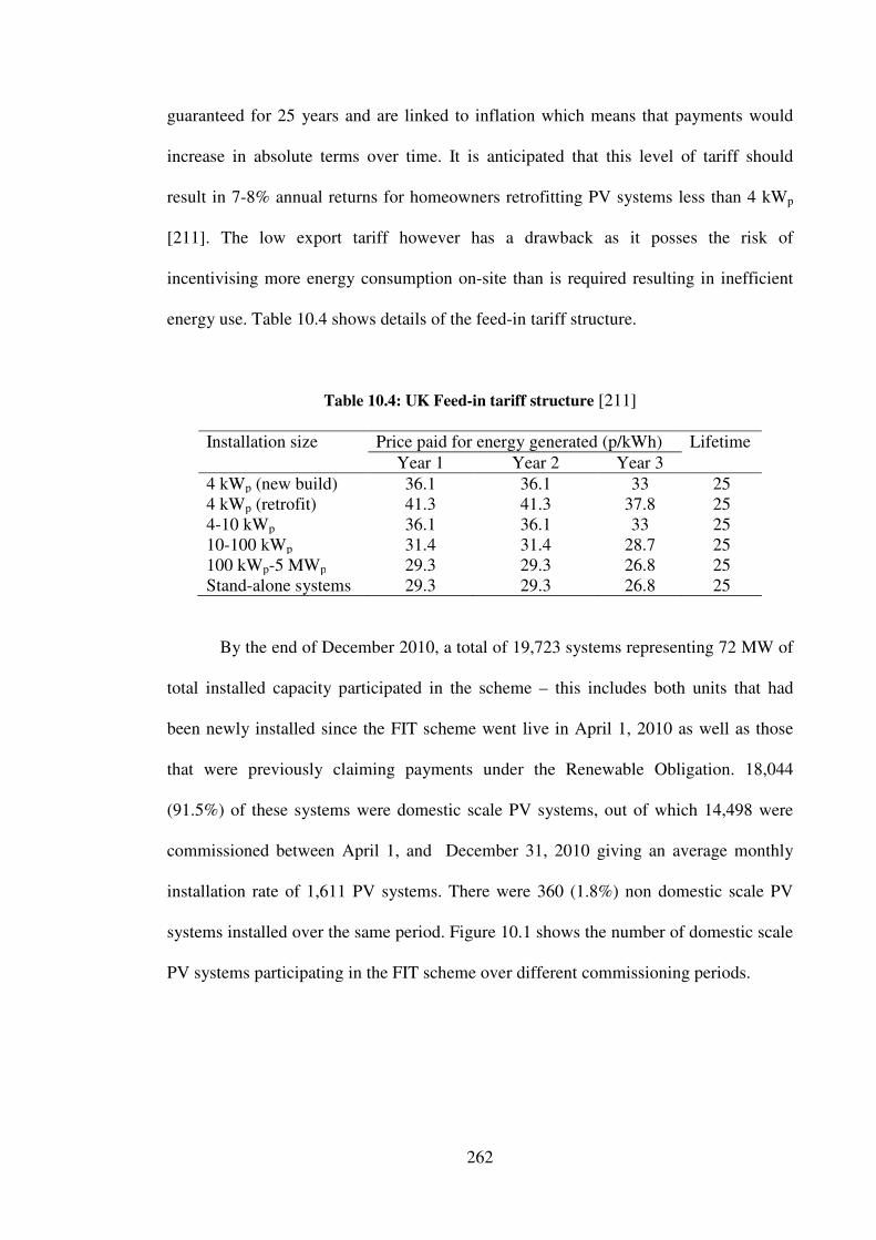
262

guaranteed for 25 years and are linked to inflation which means that payments would

increase in absolute terms over time. It is anticipated that this level of tariff should

result in 7-8% annual returns for homeowners retrofitting PV systems less than 4 kWp

[211]. The low export tariff however has a drawback as it posses the risk of

incentivising more energy consumption on-site than is required resulting in inefficient

energy use. Table 10.4 shows details of the feed-in tariff structure.

Table 10.4: UK Feed-in tariff structure [211]

Installation size Price paid for energy generated (p/kWh) Lifetime Year 1 Year 2 Year 3 4 kWp (new build) 36.1 36.1 33 25 4 kWp (retrofit) 41.3 41.3 37.8 25 4-10 kWp 36.1 36.1 33 25 10-100 kWp 31.4 31.4 28.7 25 100 kWp-5 MWp 29.3 29.3 26.8 25 Stand-alone systems 29.3 29.3 26.8 25

By the end of December 2010, a total of 19,723 systems representing 72 MW of

total installed capacity participated in the scheme – this includes both units that had

been newly installed since the FIT scheme went live in April 1, 2010 as well as those

that were previously claiming payments under the Renewable Obligation. 18,044

(91.5%) of these systems were domestic scale PV systems, out of which 14,498 were

commissioned between April 1, and December 31, 2010 giving an average monthly

installation rate of 1,611 PV systems. There were 360 (1.8%) non domestic scale PV

systems installed over the same period. Figure 10.1 shows the number of domestic scale

PV systems participating in the FIT scheme over different commissioning periods.

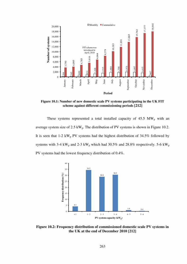
263

�

Figure 10.1: Number of new domestic scale PV systems participating in the UK FIT scheme against different commissioning periods [212]

These systems represented a total installed capacity of 45.5 MWp with an

average system size of 2.5 kWp. The distribution of PV systems is shown in Figure 10.2.

It is seen that 1-2 kWp PV systems had the highest distribution of 34.5% followed by

systems with 3-4 kWp and 2-3 kWp which had 30.5% and 28.8% respectively. 5-6 kWp

PV systems had the lowest frequency distribution of 0.4%.

Figure 10.2: Frequency distribution of commissioned domestic scale PV systems in

the UK at the end of December 2010 [212]

4.1

34.5

28.830.5

1.0 0.40

5

10

15

20

25

30

35

40

< 1 1 - 2 2 - 3 3 - 4 4 - 5 5 - 6

Freq

uenc

y di

stri

butio

n (%

)


204

345

690

831

1,24

8

1,51

5

1,80

4

1,70

8

1,97

4

1,89

7

1,61

5

667

3,75

0

4,09

5

4,78

5

5,61

6 6,86

4 8,37

9 10,1

83 11,8

91 13,8

65 15,7

62 17,3

77

18,0

44

0

2,000

4,000

6,000

8,000

10,000

12,000

14,000

16,000

18,000

20,000

Janu

ary

Febr

uary

Mar

ch

Apr

il

May

June

July

Aug

ust

Sept

embe

r

Oct

ober

Nov

embe

r

Dec

embe

r

Num

ber o

f sys

tem

s

Period

Monthly Cummulative

FIT scheme wasintroduced inApril, 2010

264

10.5 Policy Findings

This section presents policy findings and recommendations drawn as a result of

this research.

Roadmap towards grid parity

A roadmap towards grid parity was investigated in this study. Results in Table

10.5 show the periods when parity between PV generated electricity and retail as well as

wholesale electricity prices occur. It is seen that the earliest time when parity occurs is

2020 with retail prices and 2025 with wholesale prices from conventional generators.

Table 10.5: Period when parity between PV generated electricity and retail and wholesale electricity prices

Retail prices Wholesale

prices Soonest 2020 2025 Latest Post 2030 Post 2030

Roadmap towards CO2 parity

Table 10.6 shows the period when CO2 market prices and the cost of CO2

abatement for different technologies become equal (i.e. CO2 parity). It is seen that the

soonest periods when CO2 parity occurs for PV systems is 2023. For FPC SWHSs, CO2

parity occurs soonest in 2014 for systems with electric immersion heaters while at its

latest it occurs in 2027 for systems with condensing gas boilers. CO2 parity occurs

soonest in 2016 for ETC systems with oil boilers while it occurs latest in 2030 for ETC

systems with condensing gas boilers.

Results in Table 10.6 show that it is not rational to incentivise PV since grid

parity (2020) occurs before CO2 parity (2023). SWHSs should however be incentivised

since CO2 parity occurs as early as 2014 for FPC with electric immersion heaters.

265

Table 10.6: Periods when CO2 parity occurs between the energy displaced by PV and SWH systems

System type Soonest System type Latest 2.82 kWp PV 2023 0.47 kWp PV Post 2030 FPC with electric immersion heater

2014 FPC with condensing gas boiler

2027

ETC with oil boiler 2016 ETC with condensing gas boiler

2030

Comparison of Levelised Energy Generation Costs

Figure 10.3 shows levelised energy generation costs for domestic scale PV and

solar water heating systems between 2010 and 2030. Levelised electricity generation

costs using PV systems are higher than the cost of heat generation using SWHSs. The

levelised cost of energy generation using PV systems however decreases faster than the

levelised cost of heat generation using SWHSs due to the higher technology learning

rate for PV systems. The cost of electricity generation decreases from 0.853 to 0.306

�/kWh and from 0.611 to 0.218 �/kWh for 0.47 kWp and 2.82 kWp PV systems between

2010 and 2030 respectively. The cost of heat generation decreases from 0.335 to 0.265

�/kWh and from 0.198 to 0.157 �/kWh for ETC SWHSs with electric immersion heaters

and FPC SWHSs with oil boilers respectively over the same period. Parity in energy

generation cost between 2.82 kWp PV systems and ETC SWHSs with electric

immersion heaters occurs in 2022 at a cost of 0.28 �/kWh.

266

Figure 10.3: Levelised energy generation costs for domestic scale PV and SWHSs between 2010 and 2030

Marginal Abatement Costs

Figure 10.4 shows marginal abatement costs for domestic-scale solar water

heating systems and grid-connected PV systems in Ireland between 2011 and 2030. It is

seen that SWHSs have lower marginal abatement costs compared to PV systems. The

MACs for PV systems however decrease much more rapidly than those of SWHSs and

parity between the MACs for the best case scenario of PV systems (1.72 kWp PV

system under the reference scenario) and the worst case scenario of SWHSs (ETC with

condensing gas boiler) occurring in 2027.

Figure 10.4: Marginal abatement costs for domestic scale solar water heating systems and grid connected PV systems

0.0

0.1

0.2

0.3

0.4

0.5

0.6

0.7

0.8

0.9

2010

2011

2012

2013

2014

2015

2016

2017

2018

2019

2020

2021

2022

2023

2024

2025

2026

2027

2028

2029

2030

Lev

elis

ed en

ergy

gen

erat

ion

cost

(�/k

Wh)


ETC (Electric immersion) FPC (oil boiler)0.47 kWp PV system 2.82 kWp PV system

-200

0

200

400

600

800

1,000

2011

2012

2013

2014

2015

2016

2017

2018

2019

2020

2021

2022

2023

2024

2025

2026

2027

2028

2029

2030

Mar

gina

l aba

tem

ent c

ost (�

/tCO

2)

Year of Installation

0.47 kWp (reference scenario) 1.72 kWp (reference scenario)FPC (electric immersion heater) ETC (condensing gas boiler)

267

Comparative Assessment of FIT Policies

Table 10.7 shows a comparative assessment of the characteristics, advantages

and disadvantages of different PV support policies.

Table 10.7: Comparative assessment of FIT policies

Policy Characteristics Advantages Disadvantages Net metering Electricity is imported

and exported at the same cost.

Easy to implement Does not guarantee economic viability to investor.

Dedicated FIT High FIT offered for all electricity generated.

Easy to design and implement

No incentive for on-site electricity use.

UK (Generation FIT and low export FIT)

High FIT for total electricity generated and low FIT for spilled electricity

Ensures a predefined rate of return on investment for a targeted PV system size

Encourages electricity wastage. Can result in both low and windfall returns.

This study High base FIT for all electricity generated. Supplemental spill FIT at wholesale price. Supplemental FIT for on-site consumption at displaced price. Low cost to society.

Provides different tariffs for domestic-scale PV systems that guarantees a defined rate of return on investment.

Requires smart metering data. Difficult to design.

10.6 Conclusion

Global support policies for grid-connected PV and solar thermal systems were

reviewed. Policy findings from this study showed that under the best scenario, parity

between PV generated electricity and both retail and wholesale prices from

conventional generators occurs in 2020 and 2025 respectively.

CO2 parity between CO2 market prices and the cost of CO2 from energy

displaced by the PV and SWH systems occur soonest in 2023 and 2014 respectively.

The PV systems had higher levelised cost of energy generation than SWH systems. Due

to their higher learning rate, parity between the best case PV systems and worst cast

SWH systems occurs in 2023. Similarl, the MACs for PV systems was higher than

those for the SWH systems with parity occurring in 2027.

268

CHAPTER 11

CONCLUSIONS AND RECOMMENDATIONS

11.1 Conclusions

Under the European Commission’ s energy policy goals for 2020, Ireland is

committed to reduce both its primary energy consumption and GHG emissions by 20%

compared to 1990 levels. In order for these targets to be achieved, it is important to

implement sustainable policy support measures geared towards reducing its

consumption of fossil fuels and promote the use of renewable energy technologies.

Because different sectors of the economy have varying energy needs, it is important that

a sectoral approach to reducing greenhouse gas emissions be adopted since policies

limiting energy demand in one sector may not necessarily apply to the others.

In 2006 the Irish residential sector accounted for 25% of total primary energy

consumption and 25% of total CO2 emissions - second only to the transportation sector.

This sector therefore provides great potential to reduce overall energy demand and GHG

emissions. Previous studies have shown that investment in micro-generation renewable

energy technologies (MGRTs) can be an economically viable way to reduce energy

costs and CO2 emissions and can help trigger positive change [42]. Electricity and heat

can be generated at the point of use with MGRTs such as photovoltaic panels, solar

water heaters, wood pellet boilers, micro wind turbines, and heat pumps. MGRTs

therefore have great potential to assist Ireland in meeting its renewable energy and

emission targets as well as contributing towards a shift in energy consumption patterns

since they greatly raise awareness.

269

The high cost of MGRTs compared to other conventional energy technologies

has been a major barrier to their large-scale deployment worldwide. Economic

considerations such as system costs can easily be addressed through policy intervention.

Any policy aiming to promote MGRTs needs to tackle the high upfront investment cost,

thereby reducing the gap between consumer’ s willingness to pay and actual market

price. Public policy in the form of financial incentives such as grant aid, FITs or tax

incentives can however be very costly if not properly designed.

Given that the Irish government does not have unlimited resources, it is

important that information on the techno-economic and environmental performance of

MGRTs be made available for informed policy formulation. Such information would

guide policy makers in choosing what technologies to promote. The choice of winners

and losers by policy makers is guided by the cost of abating CO2 emissions by different

technologies. With limited or no information on the marginal abatement cost (MAC) of

different technologies in Ireland, Comhar SDC [8] an advisory council that provides

guidance to the Government through research on the best ways to achieve sustainable

development in Ireland recommended that as a matter of urgency, MACs should be

developed for energy efficienct and renewable energy source technologies for all

economic sectors in Ireland.

This research therefore investigated the techno-economic and environmental

performance of promising micro-generation technologies for domestic application in

order to inform policy formulation in Ireland. Although several micro-generation

technologies exist, this research focused on two solar energy technologies notably: grid-

connected photovoltaic systems for electricity generation and solar water heating

systems with flat plate and heat pipe evacuated tube collectors for hot water provision.

270

The overall methodology adopted consisted of setting up field trials with state-

of-the-art PV and solar water heating systems suitable for Irish domestic dwellings.

System performance and weather data were collected from the field trials and the

systems’ energy performances were evaluated. Dynamic energy performance models

were developed and validated using measured field trial data. Using system and weather

data, these models can be used to predict the energy generated.

The economic potential of the PV system and SWHSs were evaluated now and

in the future using system costs, current and future energy prices, technology learning

rates, discount rate, projected annual installed capacity, life cycle costs. It is worth

noting that the economic potential of the systems is largely theoretically dependent on

the choice of values for the above mentioned parameters. The environmental

performances of the systems were evaluated based on CO2 emission savings and

marginal abatement costs. Existing and alternative policy support measures were used

in the economic and environmental performance analysis.

Field trial results from this study revealed that the total annual energy generated

by the PV system was 882 kWh/kWp while a unit area of FPC and ETC each generated

496 kWh/m2 and 681 kWh/m2 respectively.

An assessment of the economic performance of six domestic-scale PV system

sizes (0.47 to 5.64 kWp) showed that the cost of electricity generation in 2010 was

between 0.6-0.89 c/kWh falling to 0.13-0.44 �/kWh in 2030. Under the best scenario

considered (Adv 25), grid parity occurs in 2020 and 2025 between the cost of electricity

generation using the 2.82 kWp PV system; and retail electricity and wholesale electricity

prices respectively. Under existing PV support policy notably feed-in tariff of 0.19

�/kWh, NPVs ranged between -�3,372 and -�31,956 showing that investing in all six

271

PV systems was not economically viable. Alternative support measures are therefore

required should policy makers decide to promote PV.

SWHSs also performed poorly under 2010 market conditions and existing policy

support (i.e. grant aid from the GHS for retrofits). Only SWHSs with electric immersion

heaters benefiting from grant aid had an NPV close to zero. NPVs for FPC systems

varied between -�1,738 and -�10 with grant aid and between -�2,738 and -1,010

without grant aid. The NPVs for ETC systems varied between -�2,365 and -�574, and

between -�3,328 and -�1,537 with and without grant aid respectively. NPV projections

showed that without policy support both SWHSs with condensing gas boilers will not

be economically viable by 2030. On the other hand FPC SWHSs with oil boilers and

electric immersion heaters will become economically viable in 2017 and 2018

respectively while ETC SWHSs with oil boilers and electric immersion heaters will

become economically viable in 2021 and 2025 respectively. These results show that the

level of support required depends on both the type of auxiliary heating system and

collector used.

Results from emission analysis revealed that life cycle CO2 emissions for PV

systems reduce from 8.8 tCO2/kWp in 2010 to 7.2 tCO2/kWp in 2020 and 6.5 tCO2/kWp

under the baseline scenario while under the reference scenario emissions decrease from

8.6 tCO2/kWp in 2010 to 7.6 tCO2/kWp in 2020 and 7.4 tCO2/kWpin 2030. Life cycle

emission savings for FPC SWHSs with condensing gas boilers, oil boilers and electric

immersion heaters were: 7.9 tCO2; 14.5 tCO2; and 15.4 to 13.6 tCO2 respectively

between 2010 and 2030. Similarly, life cycle emission savings for ETC SWHSs with

condensing gas boilers, oil boilers and electric immersion heaters were: 8.2 tCO2; 15.0

tCO2; and 15.9 to 14.1 tCO2 respectively between 2010 and 2030.

272

MACs for domestic scale PV systems in Ireland and projected CO2 prices under

the baseline scenario from 2011 to 2030 decrease from: 915.8 to 136.2 �/tCO2 for the

0.47 kWp and from 651.3 to 0.0 �/tCO2 for the 1.72 kWp system. Under the reference

scenario, the MACs decrease from 922.7 to 119.4 �/tCO2 for the 0.47 kWp system and

from 656.2 to 0.0 �/tCO2 for the 1.72 kWp system over the same period. MACs for FPC

SWHSs decrease from 348 to 25 �/tCO2, 97 to 13 �/tCO2, and 66 to -9 �/tCO2 for

condensing gas boilers, oil boilers and electric immersion heaters between 2010 and

2030. Similarly, MACs for ETC SWHSs decrease from 408 to 35 �/tCO2, 130 to -8

�/tCO2, and 97 to -3 �/tCO2 for condensing gas boilers, oil boilers and electric

immersion heaters between 2010 and 2030.

Analyses from this study has shown that PV and SWH systems have the

potential to reduce emissions from the use of fossil fuels. However, these technologies

are still expensive and are not yet economically viable to date in Ireland. Both

technologies however have cost reduction potential arising due to their technology

learning rates. SWH is a mature technology with lower technology learning rate in the

order of 10% while PV a less mature technology has higher learning rates of 20±5%

showing higher cost reduction potential.

Findings from this study show that both solar water heating (SWH) and

photovoltaic (PV) systems for domestic application would become viable technologies

in the future in Ireland provided global support policies are maintained. The

introduction of support policies worldwide has contributed towards stimulating local

markets. Continued and sustained growth is however required to enable the markets to

reach a critical mass that would enable cost reduction and self sustainability.

By the end of 2010, a few policy support measures had been put in place in

Ireland in favour of MGRTs notably: grant aid through the greener homes scheme and

273

the FIT for PV generated electricity. Yet despite these policies, the rate of adoption

among households remains very low. If support for MGRTs is a chosen policy, it will

therefore be important to implement sustainable support policies in order to make their

MACs compare favourably with those of other projects in order to facilitate increased

deployment of the technologies within the domestic sector.

A look at the MACs for SWHSs and PV show that on a purely economic basis,

it does not make sense to promote investment in domestic-scale PV systems in Ireland

now. Ireland, being a small market would have very little impact on the technology

learning curves and thus system costs. However, global market growth sustained by

support policies would certainly continue to drive down costs. Two options are

therefore available for Irish policy makers notably: wait for the global market to

develop and drive down cost and then invest at a time when the systems become

economically viable to the individual or the policy maker (i.e. MAC equal market cost);

or introduce and/or sustain policy support to stimulate the market and develop the

critical mass required as well as improve installer experience that would also drive

down installation costs. It is important to have the structures in place to capitalise on the

technology when they become economically viable. Should policy makers decide to

invest on PV then it is proposed that the FIT designed in this work be implemented.

11.2 Policy Recommendations

In order to help Ireland meet its commitments to fight climate change, ensure

security of energy supply, ensure economic competitiveness (providing value for tax

payer’ s money) and reduce its dependence on energy imports, sustainable policies have

to be formulated to support the use of renewable energy technologies. Considering that

different sectors of the economy have different energy needs, it is important that a

274

sectoral approach to reducing greenhouse gas emission be adopted. Based on the

findings of this study the policy recommendations outlined below are proposed:

• Although SWHSs are not yet economically viable, existing support policies

notably grant aid for systems installed in houses undergoing renovation and

obligations for newly built houses should be maintained in order to sustain

market growth.

• The emission reduction potential for SWHSs depends to a great extent on the

type of auxiliary heating systems displaced. Support policies should target

dwellings with oil boilers and electric immersion heaters which have high

emission reduction potential.

• Extensive field performance data for different PV system types collected under

the SEAI micro-generation field trials should be analysed and used to ascertain

the energy performance of PV systems in different areas in Ireland.

• PV systems, though not currently economically viable, have a high potential for

future cost reduction as well as CO2 emission reduction potential. If PV is to be

promoted, a more sustainable FIT scheme must be designed to promote adoption

of PV technology. A stepped approach should be adopted where the FIT

decreases over time reflecting the effect of cost reduction due to the technology

learning effect.

• The FIT should also be stepped based on system size since a single FIT has been

shown not to be suitable for domestic-scale PV systems. It results in very low

return on investment or windfall profits for some system sizes.

• The discount rate used in the analyses significantly influences the economic

viability of PV systems. Results showed that the expected return on investments

for a given household can be accurately determined. With guaranteed long term

275

FITs the risk in investing in domestic-scale PV systems can be significantly

reduced. If PV is to be promoted, it is recommended that a mortgage type of

product (20-25 years) be developed where low interest rate loans are offered to

facilitate the purchase/installation of PV systems.

• An integrated bottom-up multi-disciplinary approach to energy policy

formulation that incorporates a thorough understanding of the energy

performance, system cost dynamics and environmental performance of different

renewable energy technologies should be adopted.

11.3 Recommendations for Further Research

It is hoped that this work can form the basis for further research into providing

useful information for informed renewable energy technology support policy

formulation within the domestic sector.

Results from this study showed that significant loss in SWHS performance

occurs due to pipe losses and inadequate pump control strategies under rapidly changing

weather conditions. It is therefore recommended that further studies be carried out to

improve pump control strategies and sensor design optimisation.

Stratified hot water tanks installed in solar water heating systems for domestic

dwellings with 4-6 persons have a capacity of 200-300 litres and require 2-2.5 m height.

This poses a serious problem in retrofit installations were space constraints exist. Using

phase change materials (PCMs) to increase the density of the hot water storage can

contribute towards reducing tank height. It is therefore recommended that further

studies be carried out to investigate the techno-economic effect of introducing PCMs in

hot water tanks. Validated TRNSYS models can then be used to optimize tank heights

for different household hot water demand profiles.

276

The performance of solar water heating systems should be investigated under

different realistic hot water demand profiles using validated simulation models. Large

samples of high resolution hot water demand data are therefore required. It is

recommended that an extensive collection of hot water demand data be undertaken for

domestic dwellings.

This study did not take into consideration the social characteristics of the

households whose electricity and heat demand profiles were used in this study. Where

high resolution data such as the smart metering data is available, regression analysis can

be used to extrapolate household characteristics which can provide useful information

for policy formulation targeting the intended recipients. It is therefore recommended

that smart metering data be used to extend the methodology to other micro-generation

technologies.

277

REFERENCES

1 EIA, Energy consumption by sector overview. Available:

http://www.eia.doe.gov/aer/pdf/pages/sec2_4.pdf (Accessed 13th May, 2009).

2. EEA, Final energy consumption by sector in EU-27. Available:

http://dataservice.eea.europa.eu/atlas/viewdata/viewpub.asp?id=4292. (Accessed

13th May, 2009).

3. EPA. Ireland’ s greenhouse gas emissions in 2007. Available:

http://www.epa.ie/downloads/pubs/air/airemissions/GHG_UN_2007_

Final_150409.pdf (Accessed 14th May, 2009).

4. CEC, An energy policy for Europe, Brussels, January 2007.

5. DCENR, National Renewable Energy Action Plan, 2010.

6. DEHLG, Statutory Instrument S.I. No. 259 of 2008. Building Regulations (Part

L Amendment) Regulations 2008. Available:

http://www.environ.ie/en/Legislation/DevelopmentandHousing/BuildingStandar

ds/FileDownLoad,17840,en.pdf (Accessed 12th October, 2008).

7. EREC, Renewable heating: Action plan for Europe, Brussels, 2007.

8. Comhar Sustainable Development Council, Carbon pricing for central

government cost benefit analysis in Ireland, November 2008.

9. IEA, CO2 emissions from fuel combustion: Highlights, 2010.

10. M. Howley and B. Ó. Gallachóir, Energy statistics 1990-2007: 2008 report,

Energy Policy Statistical Support Unit, Sustainable Energy Ireland, December

2008.

11. B. Anderson, Solar energy: fundamentals in building design. McGraw-Hill, New

York, 1977.

278

12. S. A. Kalogirou, “ Solar thermal collectors and applications,” Progress in Energy

and Combustion Science, 30(3), pp. 231-295, 2004.

13. EPIA and Green Peace, Solar generation V., 2008. Available from:

http://www.epia.org (Accessed 13th December, 2008).

14. Renewable Energy Policy Framework (REN21), Renewables global status

report: 2009 update. Paris, 2009.

15. Eurobserv'er, Photovoltaic barometer, March 2009.

16. SEI, Micro and small scale-generation pilot trial consultation. 2008. Available:

http://www.sei.ie/index.asp?locID=1708&docID=-1 (Accessed 20th November,

2008).

17. DEHLG, People power. 2009. Available:

http://www.dcenr.gov.ie/Press+Releases/People+power+-

+Minister+Ryan+announces+incentives+for+micro-generation.htm (Accessed

20th March, 2009).

18. G. Boyle, ed., Renewable energy: Power for a sustainable future. Second ed.

Oxford University Press, Oxford, 2004.

19. OECD/IEA, Energy technology perspectives: Scenarios and strategies to 2050,

Paris, 2008.

21. L. M. Ayompe, et al., “ Projected costs of a grid-connected domestic PV system

under different scenarios in Ireland, using measured data from a trial

installation,” Energy Policy, 38(7), pp. 3731-3743, 2010.

22. M. C. Claudy, C. Michelsen, and A. O'Driscoll, “ The diffusion of

microgeneration technologies - assessing the influence of perceived product

characteristics on home owners' willingness to pay,” Energy Policy. 39(3), pp.

1459-1469, 2011.

279

23. Central Statistics Office Ireland. Available: www.cso.ie.

24. ESTIF, Solar Thermal Markets in Europe: Trends and Market Statistics 2009.

2010. Available:

http://www.estif.org/fileadmin/estif/content/market_data/downloads/2009%20so

lar_thermal_markets.pdf.

25. SEAI, Greener Homes Scheme Statistics. Available: www.seai.ie.

26. M. Howley, E. Dennehy and B. Ó. Gallachóir, Energy in Ireland 1990-2009:

2010 report, 2010.

27. ESB. Fuel mix disclosure. Available:

https://www.esb.ie/esbcustomersupply/business/your_account/fuel_mix.jsp.

28. CER, Fuel mix and CO2 emission disclosure 2009, 2010.

29. SEAI, 1990-2009 Irish energy balances: Statistics publications. Available:

www.seai.ie.

30. F. O’ Leary, M. Howley, and B. Ó. Gallachóir, Energy in the residential sector.

2008 Report: Energy Policy Statistical Support Unit, Sustainable Energy Ireland.

31. F. O’ Leary, M. Howley, and B. Ó. Gallachóir, Energy Statistics 1990-2006:

2007 report, Energy Policy Statistical Support Unit, Sustainable Energy Ireland,

December 2007.

32. DCENR. Delivering a sustainable energy future for Ireland: The energy policy

framework 2007-2020.

33. G. Owens, Best practices guide: Economic & financial evaluation of renewable

energy projects, June 2002. Available:

<http://www.iie.org/programs/energy/pdfs/Econ%20Finacial%20Eval%20of%2

0Renewable%20Energy%20Projects.pdf>.

280

34. J. Twidell and T. Weir. Renewable energy resources. Second ed., Taylor and

Francis, New York, 2006.

35. IEA, Deploying renewables: Principles for effective policies. Paris, France,

2008.

36. R. Gross, M. Leach and A. Bauen, “ Progress in renewable energy,” Environment

International, 29(1), pp. 105-122, 2003.

37. J. Watson, Co-provision in sustainable energy systems: the case of micro-generation, Energy Policy, 32(17), pp. 1981-1990, 2004.

38. A. S. Bahaj and P. A. B. James, “ Urban energy generation: The added value of

photovoltaics in social housing,” Renewable and Sustainable Energy Reviews,

11(9), pp. 2121-2136, 2007.

39. SEI, A renewable energy heat pump in your house. Available:

http://www.sei.ie/uploadedfiles/RenewableEnergy/ResidentialHPfactsheetforWeb.pdf.

40. SEI, Your guide to renewable energy in the home, Available:

http://www.sei.ie/Publications/Your_Home_Publications/SEIRenewablebookletfnl.pdf.

41. M. Hinnells, “ Technologies to achieve demand reduction and micro-generation

in buildings,” Energy Policy, 36(12), pp. 4427-4433, 2008.

42. S. R. Allen, G.P. Hammond and M.C. McManus, “ Prospects for and barriers to

domestic micro-generation: A United Kingdom perspective,” Applied Energy,

85(6): pp. 528-544, 2008.

43. DCMNR, Government White Paper: Delivering a sustainable energy future for

Ireland. The energy policy framework 2007-2020.

281

44. Department of the Taoiseach, Building Ireland’ s Smart Economy: A framework

for sustainable economic renewal, 2008. Available:

www.taoiseach.gov.ie/.../Building_Ireland's_Smart_Economy/Building_Ireland'

s_Smart_Economy_rtf.rtf.

45. CER, ESBCS domestic microgenerator export tarifff decision, CER/09/033, 2009.

46. CER, ESBCS domestic micro-generation export tariff: Information note,

CER/10/219, 2010.

47. ESTIF, Best practice regulations for solar thermal, Brussels, 2007.

48. EC, A Vision for Photovoltaic Technology, Publication Office, Luxemburg, 2005.

49. G. C. Bakos and M. Soursos, “ Technical feasibility and economic viability of a

grid-connected PV installation for low cost electricity production,” Energy and

Buildings, 34(7), pp. 753-758, 2002.

50. A. Zahedi, “ Solar photovoltaic (PV) energy; latest developments in the building

integrated and hybrid PV systems,” Renewable Energy, 31(5), pp. 711-718, 2006.

51. C. Beneking, Perspective for industrial development. In: Second Photovoltaic

Mediterranean Conference, 19–20 April 2007, Athens. 2007.

52. C. Harmon, Experience Curves of Photovoltaic Technology, International

Institute for Applied System Analysis, Laxenburg, Austria, 2000.

53. G. J. Schaeffer and H. H. C. de Moor, Learning in PV trends and future

prospects, In: 19th European PV Solar Energy Conference and Exhibition, Paris,

France, June 2004.

54. K. L. Shum and C. Watanabe, “ Towards a local learning (innovation) model of

solar photovoltaic deployment,” Energy Policy, 36(2), pp. 508-521, 2008.

282

55. R. Wiser, et al., “ Analyzing historical cost trends in California’ s market for

customer sited photovoltaic,” Progress in Photovoltaic: Research and

Applications, 15(1), pp. 69-85, 2007.

56. R. Bhandari and I. Stadler, “ Grid parity analysis of solar photovoltaic systems in

Germany using experience curves, Solar Energy, 83(9), pp. 1634-1644, 2009.

57. C. D. S. Jardim, et al., “ The strategic siting and the roofing area requirements of

building-integrated photovoltaic solar energy generators in urban areas in

Brazil,” Energy and Buildings, 40(3), pp. 365-370, 2008.

58. A. Poullikkas, “ Parametric cost-benefit analysis for the installation of photovoltaic

parks in the island of Cyprus,” Energy Policy, 37(9), pp. 3673-3680, 2009.

59. A. D. Compaan, “ Photovoltaics: Clean power for the 21st century,” Solar

Energy Materials and Solar Cells, 90(15), pp. 2170-2180, 2006.

60. X. Gong and M. Kulkarni, “ Design optimization of a large scale rooftop

photovoltaic system,” Solar Energy, 78(3), pp. 362-374, 2005.

61. W. Hoffmann, “ PV solar electricity industry: Market growth and perspective,”

Solar Energy Materials and Solar Cells, 90(18-19), pp. 3285-3311, 2006.

62. E. A. Alsema and E. Nieuwlaar, “ Energy viability of photovoltaic systems,”

Energy Policy, 28(14), pp. 999-1010, 2000.

63. S. P. Sukhatme, Solar energy: Principles of thermal collection and storage,

Second ed., Tata McGraw-Hill, New Delhi, 1998.

64. EPIA, Photovoltaic energy: Electricity from the sun, Available: www.epia.org.

65. A. S. Bahaj, “ Means of enhancing and promoting the use of solar energy,”

Renewable Energy, 27(1), pp. 97-105, 2002.

66. EPIA, Global market outlook for photovoltaic until 2014. May 2010.

283

67. D. M. Bagnall and M. Boreland, “ Photovoltaic technologies,” Energy Policy,

36(12), pp. 4390-4396, 2008.

68. T. Markvart, Solar electricity, Second ed., John Wiley and Sons, Chichester, 2000.

69. A. H. Marafia, “ Feasibility study of photovoltaic technology in Qatar,”

Renewable Energy, 24(3-4), pp. 565-567, 2001.

70. A. S. Joshi, I. Dincer and B. V. Reddy, “ Performance analysis of photovoltaic

systems: A review,” Renewable and Sustainable Energy Reviews, 13(8), pp.

1884-1897, 2009.

71. The German Solar Energy Society, Planning and installing photovoltaic systems:

A guide for installers, architects and engineers. James and James, UK, 2006.

72. E. D. Spooner and G. Harbidge, “ Review of international standards for grid

connected photovoltaic systems,” Renewable Energy, 22(1-3), pp. 235-239, 2001.

73. G. Cramer, M. Ibrahim and W. Keinkauf, “ PV system technologies: State-of-

the-art and trends in decentralized electrification,” Refocus, January/February 2004.

74. J. L. Bernal-Agustín, and R. Dufo-López, “ Economical and environmental

analysis of grid connected photovoltaic systems in Spain,” Renewable Energy,

31(8), pp. 1107-1128, 2006.

75. EurObserv’ ER, Photovoltaic barometer 2010.

Available: http://www.eurobserv-er.org/pdf/baro196.pdf.

76. PPSP, Trends in photovoltaic applications: Survey report of selected IEA

countries between 1992 and 2007, 2008.

77. B. van der Zwaan and A. Rabl, “ Prospects for PV: a learning curve analysis,”

Solar Energy, 74(1), pp. 19-31, 2003.

78. M. Green, Third-generation photovoltaics: Advanced solar energy conversion.

Springer, Berlin, 2006.

284

79. Renewable Energy Policy Framework (REN21), Renewables 2007 global status

report. Available: http://www.ren21.net/pdf/RE2007_Global_Status_Report.pdf.

80. EPIA, Global market outlook for photovoltaics until 2012: Facing a sunny

future. Available:

http://www.epia.org/fileadmin/EPIA_docs/publications/epia/EPIA__MarketPubl

ication_18feb.pdf.

81. EurObserv’ ER, Photovoltaic energy barometer 2008. Available:

http://ec.europa.eu/energy/res/publications/barometers_en.htm.

82. A. Q. Malik and S. J. B. H. Damit, “ Outdoor testing of single crystal silicon

solar cells,” Renewable Energy, 28(9), pp. 1433-1445, 2003.

83. S. C. Tripathy and A. K. Saxena, “ Performance evaluation of 20 kWp

photovoltaic system,” Energy Conversion and Management, 34(8), pp. 619-626, 1993.

84. G. Notton, V. Lazarov, and L. Stoyanov, “ Optimal sizing of a grid-connected

PV system for various PV module technologies and inclinations, inverter

efficiency characteristics and locations,” Renewable Energy. 35(2), pp. 541-554, 2010.

85. S. Ransome, How accurate can PV energy yield simulations be? In: PVSAT-4,

University of Bath, UK, 2-4 April, 2008. Available: http://steveransome.com.

86. M. Sidrach-de-Cardona and L. Mora López, “ Performance analysis of a grid-

connected photovoltaic system,” Energy, 24(2), pp. 93-102, 1999.

87. J. D. Mondol et al., “ Long term performance analysis of a grid connected

photovoltaic system in Northern Ireland,” Energy Conversion and Management,

47(18-19), pp. 2925-2947, 2006.

88. E. Kymakis, S. Kalykakis and T. M. Papazoglou, “ Performance analysis of a

grid connected photovoltaic park on the island of Crete,” Energy Conversion

and Management, 50(3), pp. 433-438, 2009.

285

89. B. Decker and U. Jahn, “ Performance of 170 grid connected PV plants in

Northern Germany -- Analysis of yields and optimization potentials,” Solar

Energy, 59(4-6), pp. 127-133, 1997.

90. M. Drif, et al., “ Univer Project. A grid connected photovoltaic system of at Jaén

University. Overview and performance analysis,” Solar Energy Materials and

Solar Cells, 91(8), pp. 670-683, 2007.

91. A. Benatiallah, R. Mostefaou and K. Bradja, “ Performance of photovoltaic solar

system in Algeria,” Desalination, 209(1-3), pp. 39-42, 2007.

92. M. Cucumo, et al., “ Performance analysis of a 3 kW grid-connected

photovoltaic plant,” Renewable Energy, 31(8), pp. 1129-1138, 2006.

93. S. Chokmaviroj, R. Wattanapong and Y. Suchart, “ Performance of a 500 kWp

grid connected photovoltaic system at Mae Hong Son Province, Thailand,”

Renewable Energy, 31, pp. 19-28, 2006.

94. T. M. I. Alamsyah, K. Sopian and A. Shahrir, “ Predicting average energy

conversion of photovoltaic system in Malaysia using a simplified method,”


95. F. Mavromatakis, et al., “ Modeling the photovoltaic potential of a site,”


96. P. Trinuruk, C. Sorapipatana, and D. Chenvidhya, “ Estimating operating cell

temperature of BIPV modules in Thailand,” Renewable Energy, 34(11), pp.

2515-2523, 2009.

97. E. Skoplaki and J. A. Palyvos, “ Operating temperature of photovoltaic modules:

A survey of pertinent correlations,” Renewable Energy, 34(1), pp. 23-29, 2009.

286

98. M. C. Alonso García and J. L. Balenzategui, “ Estimation of photovoltaic module

yearly temperature and performance based on Nominal Operation Cell

Temperature calculations,” Renewable Energy, 29(12), pp. 1997-2010, 2004.

99. A. D. Jones and C. P. Underwood, “ A thermal model for photovoltaic systems,”

Solar Energy, 70(4), pp. 349-359, 2001.

100. J. D. Mondol, Y. G. Yohanis and B. Norton, “ Optimal sizing of array and

inverter for grid-connected photovoltaic systems,” Solar Energy, 80(12), pp.

1517-1539, 2006.

101. S. Pless, et al., Procedure for Measuring and Reporting the Performance of

Photovoltaic Systems in Buildings, Technical Report NREL/TP-550-38603,

October, 2005.

102. G. M. Masters, Renewable and efficient electric power systems, John Wiley and

Sons, New Jersey, 2004.

103. Sanyo HIT photovoltaic module manual for HIP-215NHE5, HIP-210NHE5 and

HIP-205NHE5. Available: http://www.solarcentury.com/Residential-

developers/Specifying-Solar/PV-Catalogue/HIP-215-NHE5-NHE-Series.

104. The Irish Meteorological Service Online. Available: <http://www.met.ie>.

105. PPSP, Cost and performance trends in grid-connected photovoltaic systems and

case studies. IEA-PVPS T2-06:2007.

106. J. A. Duffie and W. A. Beckman, Solar engineering of thermal processes, Wiley,

New York 1991.

107. J. D. Mondol, Y.G. Yohanis, and B. Norton, “ The effect of low insolation

conditions and inverter oversizing on long-term performance of a grid-connected

photovoltaic system,” Prog. Photovolt. Res. Appl, 15, pp. 353-368, 2007.

287

108. G. Blaesser, “ PV system measurements and monitoring the European

experience,” Solar Energy Materials and Solar Cells, 47(1-4), pp. 167-176,

1997.

109. H. Nakagami, et al., “ Performance of residential PV system under actual field

conditions in wester part of Japan,” In: International Solar Energy Conference,

Hawaii, USA, 2003.

110. U. Eicker, Solar technologies for buildings, John Wiley and Sons, England, 2003.

111. K. Bücher, “ Site dependence of the energy collection of PV modules,” Solar

Energy Materials and Solar Cells, 47(1-4), pp. 85-94, 1997.

112. S. C. W. Krauter, Solar electric power generation: Photovoltaic energy systems,

Springer, Berlin, 2006.

113. Y. Ueda, et al., “ Performance analysis of various system configurations on grid-

connected residential PV systems,” Solar Energy Materials and Solar Cells,

93(6-7), pp. 945-949, 2009.

114. U. Jahn, et al., International Energy Agency TASK II database on photovoltaic

power systems: statistical and analytical evaluation of PV operational data, In:

2nd World Conference on Photovoltaic Solar Energy Conversion, Vienna,

Austria, 1998.

115. S. M. Pietruszko and M. Gradzki, “ Performance of a grid connected small PV

system in Poland,” Applied Energy, 74(1-2), pp. 177-184, 2003.

116. A. D. Miguel, et al., “ Performance analysis of a grid-connected PV system in a

rural site in the northwest of Spain,” In: World Renewable Energy Congress VII

2002, Cologne, Germany, 2002.

288

117. S. Ubertini and U. Desideri, “ Performance estimation and experimental

measurements of a photovoltaic roof,” Renewable Energy, 28(12), pp. 1833-

1850, 2003.

118. S. S. S. R. Depuru, L. Wang and V. Devabhaktuni, “ Smart meters for power

grid: Challenges, issues, advantages and status.” Renewable and Sustainable

Energy Reviews, 15(6), pp. 2736-2742, 2011.

119. J. D. Mondol, et al., “ Long-term validated simulation of a building integrated

photovoltaic system,” Solar Energy, 78(2), pp. 163-176, 2005.

120. M. Mattei, et al., “ Calculation of the polycrystalline PV module temperature

using a simple method of energy balance,” Renewable Energy, 31(4), pp. 553-

567, 2006.

121. M. Buresch, Photovoltaic energy systems, McGraw-Hill, New York, 1983.

122. R. Chenni, et al., “ A detailed modeling method for photovoltaic cells,” Energy,

32(9), pp. 1724-1730, 2007.

123. M. Kolhe, et al., “ Analytical model for predicting the performance of

photovoltaic array coupled with a wind turbine in a stand-alone renewable

energy system based on hydrogen,” Renewable Energy, 28(5), pp. 727-742, 2003.

124. W. C. McAdams, Heat transmission, Third ed., McGraw-Hill, New York, 1954.

125. T. Hove, “ A method for predicting long-term average performance of

photovoltaic systems,” Renewable Energy, 21(2), pp. 207-229, 2000.

126. W. Durisch, et al., “ Efficiency model for photovoltaic modules and

demonstration of its application to energy yield estimation,” Solar Energy

Materials and Solar Cells, 91(1), pp. 79-84, 2007.

127. S. A. Kalogirou, Solar energy engineering: Processes and systems, Elsevier,

London, 2009,

289

128. W. Durisch, K. H. Lam and J. Close, “ Efficiency and degradation of a copper

indium diselenide photovoltaic module and yearly output at a sunny site in

Jordan,” Applied Energy, 83(12), pp. 1339-1350, 2006.

129. IEA, Energy use in the new millenium: Trends in IEA countries, 2007.

Available: http://www.iea.org/textbase/nppdf/free/2007/millennium.pdf.

130. D. W. Lee and A. Sharma, “ Thermal performances of the active and passive

water heating systems based on annual operation,” Solar Energy, 81(2), pp. 207-

215, 2007.

131. H. Gunerhan and A. Hepbasli, “ Exergetic modeling and performance evaluation

of solar water heating systems for building applications,” Energy and Buildings,

39(5), pp. 509-516, 2007.

132. S. A. Kalogirou, “ Environmental benefits of domestic solar energy systems,”

Energy Conversion and Management, 45(18-19), pp. 3075-3092, 2004.

133. W. Xiaowu and H. Ben, “ Exergy analysis of domestic-scale solar water heaters,”

Renewable and Sustainable Energy Reviews, 9(6), pp. 638-645, 2005.

134. I. Luminosu and L. Fara, “ Determination of the optimal operation mode of a flat

solar collector by exergetic analysis and numerical simulation,” Energy, 30(5),

pp. 731-747, 2005.

135. The German Solar Energy Society, Planning and installing solar thermal systems:

A guide for installers, architects and engineers, James and James, UK, 2007.

136. S. Kalogirou, “ The potential of solar industrial process heat applications,”

Applied Energy, 76(4), pp. 337-361, 2003.

137. Y. Tripanagnostopoulos, M. Souliotis and T. Nousia, “ Solar collectors with

colored absorbers,” Solar Energy, 68(4), pp. 343-356, 2000.

138. P. D. Dunn and D. A. Reay, Heat pipe, Third ed., Pergamon, New York Press, 1982.

290

139. A. Faghri, Heat pipe science, Taylor & Francis, London, 1995.

140. E. Azad, “ Theoretical and experimental investigation of heat pipe solar

collector,” Experimental Thermal and Fluid Science, 32(8), pp. 1666-1672, 2008.

141. H. F. W. de Vries, W. Kamminga and J. C. Francken, “ Fluid circulation control

in conventional and heat pipe planar solar collectors,” Solar Energy, 24(2), pp.

209-213, 1980.

142. S. B. Riffat, X. Zhao and P. S. Doherty, “ Developing a theoretical model to

investigate thermal performance of a thin membrane heat-pipe solar collector,”

Applied Thermal Engineering, 25(5-6), pp. 899-915, 2005.

143. H. M. S. Hussein, “ Theoretical and experimental investigation of wickless heat

pipes flat plate solar collector with cross flow heat exchanger,” Energy

Conversion and Management, 48(4), pp. 1266-1272, 2007.

144. M. Hammad, “ Experimental study of the performance of a solar collector cooled

by heat pipes,” Energy Conversion and Management, 36(3), pp. 197-203, 1995.

145. E. Mathioulakis and V. Belessiotis, “ A new heat-pipe type solar domestic hot

water system,” Solar Energy, 72(1), pp. 13-20, 2002.

146. T.Y. Bong, K.C. Ng, and H. Bao, “ Thermal performance of a flat-plate heat-pipe

collector array” Solar Energy, 50(6), pp. 491-498, 1993.

147. C. I. Ezekwe, “ Thermal performance of heat pipe solar energy systems,” Solar

& Wind Technology, 7(4), pp. 349-354, 1990.

148. M. Bojic, S. Kalogirou and K. Petronijevic, “ Simulation of a solar domestic

water heating system using a time marching model,” Renewable Energy, 27(3),

pp. 441-452, 2002.

291

149. J. B. A. Lima, R. T. A. Prado and V. M. Taborianski, “ Optimization of tank and

flat-plate collector of solar water heating system for single-family households to

assure economic efficiency through the TRNSYS program” Renewable Energy,

31(10), pp. 1581-1595, 2006.

150. EC, Mandate to CEN and CENELEC for the elaboration and adoption of

measurement standards for household appliances: water heaters, hot water

storage appliances and water heating systems, Brussels, 2002.

151. B. Norton, Solar energy and the Irish climate. In: Proceedings of the Conference

on Energy and the Irish Climate: Harnessing the Irish Climate for Energy, The

National Botanic Gardens, 2008.

152. S. R. Allen, et al., “ Integrated appraisal of a Solar Hot Water system,” Energy,

35(3), pp. 1351-1362, 2010.

153. S. A. Kalogirou, “ Use of TRNSYS for modelling and simulation of a hybrid PV-

thermal solar system for Cyprus,” Renewable Energy, 23(2), pp. 247-260, 2001.

154. T. Power, S. Walsh and P. O'Meara, Financial management: An Irish context. Third ed., Gill & Mcmillan, Dublin, 2009.

155. S. Lumby and C. Jones, Investment appraisal and financial decisions. Sixth ed.,

International Thomson Business Press, London, 1999.

156. S. R. Hastings and O. Morck, eds., Solar air systems: A design handbook, James

and James, London, 2000.

157. S. Kaplan, Energy Economics: Quantitative methods for energy and

environmental decisions, McGraw-Hill, New York, 1983.

158. R. B. Brockington, Financial management. Sixth ed., DP Publications Ltd, London, 1993.

159. D. Watson and A. Head, Corporate finance: principles and practice. Third ed.,

Prentice Hall, London, 2004.

292

160. I. Odeh, Y.G. Yohanis and B. Norton, “ Economic viability of photovoltaic water

pumping systems,” Solar Energy, 80(7), pp. 850-860, 2006.

161. R. Gross, W. Blyth and P. Heptonstall, “ Risks, revenues and investment in

electricity generation: Why policy needs to look beyond costs,” Energy

Economics, 32(4), pp. 796-804, 2010.

162. European Commission Directorate-General for Energy, EU energy trends to

2030, Belgium, 2010.

163. EIA, Annual Energy Outlook 2010, 2010.

164. P. Parker, “ Residential solar photovoltaic market stimulation: Japanese and

Australian lessons for Canada,” Renewable and Sustainable Energy Reviews,

12(7), pp. 1944-1958, 2008.

165. K. L. Shum and C. Watanabe, “ An innovation management approach for

renewable energy deployment--the case of solar photovoltaic (PV) technology,”

Energy Policy, 37(9), pp. 3535-3544, 2009.

166. R. Beith, I. P. Burdon and M. Knowles, Micro energy systems: Review of

technology, issues of scale and integration, Professional Engineering Publishing,

London, 2004.

167. F. Ferioli, K. Schoots and B. C. C. van der Zwaan, “ Use and limitations of

learning curves for energy technology policy: A component-learning

hypothesis,” Energy Policy, 37(7), pp. 2525-2535, 2009.

168. L. Neij, “ Cost development of future technologies for power generation--A

study based on experience curves and complementary bottom-up assessments,”

Energy Policy, 36(6), pp. 2200-2211, 2008.

293

169. J. Watson, et al., Unlocking the power house: policy and system change for

domestic micro-generation in the UK, University of Sussex, University of

Southampton, Imperial College London, 2006.

170. EST, Econnect, and Elementenergy, Potential for microgeneration, study and

analysis, Final report, 2005.

171. OECD, IEA, and NEA, Projected costs of generating electricity, Paris, 2010.

172. M. MacDonald, UK electricity generation costs update, June 2010. Available:

http://www.decc.gov.uk/assets/decc/statistics/projections/71-uk-electricity-

generation-costs-update-.pdf.

173. SEAI, Electricity & Gas Prices in Ireland: 2nd Semester (July - December)

2009, Cork, 2010.

174. ESB, Smart metering data monitoring programme. Available: <www.esb.ie>.

175. Y. G. Yohanis, et al., “ Real-life energy use in the UK: How occupancy and

dwelling characteristics affect domestic electricity use,” Energy and Buildings,

40(6), pp. 1053-1059, 2008.

176. CER, Fact sheet: Electricity prices in Ireland.

177. EC, Eurostat energy statistics. Available:

http://epp.eurostat.ec.europa.eu/portal/page/portal/energy/data/main_tables.

178. IEA, CO2 allowance and electricity price interaction: Impact on industry's

electricity purchasing strategies in Europe, 2007.

179. IEA, Natural gas market review 2006: Towards a global gas market, Paris, 2006.

180. CER, Best new entrant price 2007: Decision paper. CER/06/148, August 2006.

294

181. British Petroleum, Natural gas prices. Available:

http://www.bp.com/liveassets/bp_internet/globalbp/globalbp_uk_english/reports

_and_publications/statistical_energy_review_2008/STAGING/local_assets/2010

_downloads/natural_gas_section_2010.pdf.

182. EPIA, PV observatory: Policy recommendations, 2010.

183. L.M. Ayompe, et al., “ Measured performance of a 1.72 kW rooftop grid

connected photovoltaic system in Ireland,” Energy Conversion and

Management, 52(2), pp. 816-825, 2011.

184. C. Candelise, R. Gross and M. A. Leach, “ Conditions for photovoltaics

deployment in the UK: the role of policy and technical developments,” Journal

of Power and Energy, 224(Part A), pp. 153-168, 2010.

185. R. Smokers, Ab de Buck and M. van Valkengoed, GHG reduction in transport:

an expensive option? Delft, CE Delft, May 2009.

186. A. Hasanbeigi, C. Menke, and L. Price, “ The CO2 abatement cost curve for the

Thailand cement industry,” Journal of Cleaner Production, 18(15), pp. 1509-

1518, 2010.

187. S. Kalogirou, “ Thermal performance, economic and environmental life cycle

analysis of thermosiphon solar water heaters,” Solar Energy, 83(1), pp. 39-48, 2009.

188. ESTTP, Solar thermal vision 2030, Brussels, 2006.

189. L. M. Ayompe, et al., “ Comparative field performance study of flat plate and

heat pipe evacuated tube collectors (ETCs) for domestic water heating systems

in a temperate climate, 36(5), pp. 3370-3378, 2011.

190. D. G. Newnan, J. P. Lavelle and T. G. Eschenbach, Essentials of engineering

economic analysis. 2nd ed., Oxford University Press, Oxford, 2002.

295

191. SEAI, Emission factors. Available:

http://www.seai.ie/Publications/Statistics_Publications/Emission_Factors/.

192. EPIA and Greenpeace, Solar Generation: Solar electricity for over one billion

people and two million jobs by 2020, 2006. Available:

http://www2.epia.org/documents/SG3.pdf.

193. EC, Directive 2001/77/EC on the promotion of electricity produced from

renewable energy sources in the internal electricity market, 2001.

194. T. Roulleau and C.R. Lloyd, “ International policy issues regarding solar water

heating, with a focus on New Zealand,” Energy Policy, 36(6), pp. 1843-1857, 2008.

195. EU, Directive 2009/28/EC of the European Parliament and of the Council of 23

April 2009 on the promotion of the use of energy from renewable sources and

amending and subsequently repealing Directives 2001/77/EC and 2003/30/EC.

196. EC, Photovoltaic solar energy: Development and current research, 2009.

197. I. H. Rowlands, “ Envisaging feed-in tariffs for solar photovoltaic electricity:

European lessons for Canada,” Renewable and Sustainable Energy Reviews,

9(1), pp. 51-68, 2005.

198. V. Lauber, “ REFIT and RPS: options for a harmonised Community framework,”

Energy Policy, 32(12), pp. 1405-1414, 2004.

199. EPIA, Supporting solar photovoltaic electricity: An argument for feed-in tariffs.

Available:

http://www.epia.org/fileadmin/EPIA_docs/documents/An_Argument_for_Feed-in_Tariffs.pdf.

200. T. D. Couture, et al., A policymaker's guide to feed-in tariff policy design.

Technical report NREL/TP-6A2-44849, July 2010. Available:

www.nrel.gov/docs/fy10osti/44849.pdf.

296

201. D. Hurlbut, State Clean Energy Policies Analysis: Renewable Portfolio

Standards, National Renewable Energy Laboratory, technical report, NREL/TP-

670-43512, July 2008. Available: http://www.nrel.gov/analysis/pdfs/43512.pdf.

202. R. Wiser and M. Bolinger, “ Can deployment of renewable energy put downward

pressure on natural gas prices?,” Energy Policy, 35(1), pp. 295-306, 2007.

203. OFGEM. Renewables Obligation. Available:

204. A. Klein, et al., Evaluation of different feed-in tariff design options: Best

practice paper for the International Feed-in Cooperation, Second ed., 2008.

205. P. Menanteau, D. Finon and M. L. Lamy, “ Prices versus quantities: choosing

policies for promoting the development of renewable energy,” Energy Policy,

31(8), pp. 799-812, 2003.

206. C. Mitchell, D. Bauknecht and P. M. Connor, “ Effectiveness through risk

reduction: a comparison of the renewable obligation in England and Wales and

the feed-in system in Germany,” Energy Policy, 34(3), pp. 297-305, 2006.

207. J. A. Lesser and X. Su, “ Design of an economically efficient feed-in tariff

structure for renewable energy development,” Energy Policy, 36(3), pp. 981-

990, 2008.

208. D. Toke, “ Renewable financial support systems and cost-effectiveness,” Journal

of Cleaner Production, 15(3), pp. 280-287, 2007.

209. C. Lu, Q. Tong and X. Liu, “ The impacts of carbon tax and complementary

policies on Chinese economy,” Energy Policy, 38(11), pp. 7278-7285, 2010.

210. J. Creedy and C. Sleeman, “ Carbon taxation, prices and welfare in New

Zealand,” Ecological Economics, 57(3), pp. 333-345, 2006.

211. Department of Energy and Climate Change, National renewable energy action

plan for the United Kingdom.

297

212. OFGEM, The feed-in tariff scheme. Available: www.ofgem.gov.co.uk.

213. CER, Best new entrant price 2004: Best new entrant price: CER/03/201. 2003:

Dublin.

214. CER, Best new entrant price 2006: Best new entrant price. CER/05/088. 2005:

Dublin.

298

APPENDICES

Appendix 8.1: Average annual percentage change in world oil prices for LOP and

HOP (2010-2035) [163, 213, 214]

Annual Percentage change

Year High Low Reference

2010 0 0 0 2011 19.33 -17.72 3.93 2012 19.68 -5.12 8.69 2013 15.09 -1.86 7.97 2014 14.98 -1.99 6.03 2015 8.97 -2.27 3.97 2016 7.99 0.27 3.93 2017 6.79 0.10 3.05 2018 5.04 0.08 3.14 2019 3.32 0.17 1.97 2020 2.44 -0.10 1.70 2021 1.48 -0.06 1.15 2022 1.22 -0.02 1.28 2023 1.09 -0.04 1.26 2024 0.67 -0.08 1.17 2025 1.00 -0.06 1.28 2026 0.81 -0.04 1.32 2027 0.62 0.00 1.47 2028 0.82 -0.10 1.53 2029 0.92 -0.08 1.59 2030 0.80 0.02 1.20 2031 0.69 -0.08 1.67 2032 0.69 -0.12 1.49 2033 0.51 -0.06 1.46 2034 0.44 -0.02 1.52 2035 0.43 -0.10 1.50

299

App

endi

x 8.

2a: N

orm

alis

ed P

V m

odul

e co

st u

nder

diff

eren

t sce

nari

os fo

r 0.

47 k

Wp,

1.4

1 kW

p an

d 1.

72 k

Wp

PV sy

stem

s (20

10-2

030)

0.47

kW

p 1.

41 k

Wp

1.72

kW

p

Yea

r

PV m

odul

e co

st

(Mod

erat

e)

(15%

)

PV m

odul

e co

st

(Adv

ance

d)

(15%

)

PV m

odul

e co

st

(Mod

erat

e)

(25%

)

PV m

odul

e co

st

(Adv

ance

d)

(25%

)

PV m

odul

e co

st

(Mod

erat

e)

(15%

)

PV m

odul

e co

st

(Adv

ance

d)

(15%

)

PV m

odul

e co

st

(Mod

erat

e)

(25%

)

PV m

odul

e co

st

(Adv

ance

d)

(25%

)

PV m

odul

e co

st

(Mod

erat

e)

(15%

)

PV m

odul

e co

st

(Adv

ance

d)

(15%

)

PV m

odul

e co

st

(Mod

erat

e)

(25%

)

PV m

odul

e co

st

(Adv

ance

d)

(25%

) 20

10

2868

28

68

2868

28

68

2841

28

41

2841

28

41

2841

28

41

2841

28

41

2011

25

82

2529

23

81

2295

25

58

2505

23

59

2274

25

58

2505

23

59

2274

20

12

2407

23

31

2102

19

87

2384

23

09

2083

19

69

2384

23

09

2083

19

69

2013

22

76

2195

19

05

1786

22

55

2174

18

87

1769

22

55

2174

18

87

1769

20

14

2176

20

92

1760

16

41

2156

20

72

1743

16

25

2156

20

72

1743

16

25

2015

20

96

2010

16

46

1529

20

76

1992

16

31

1515

20

76

1992

16

31

1515

20

16

2031

19

43

1557

14

40

2012

19

25

1542

14

26

2012

19

25

1542

14

26

2017

19

74

1886

14

80

1366

19

55

1869

14

66

1353

19

55

1869

14

66

1353

20

18

1924

18

37

1415

13

04

1906

18

20

1401

12

92

1906

18

20

1401

12

92

2019

18

81

1794

13

60

1250

18

64

1777

13

47

1239

18

64

1778

13

47

1239

20

20

1842

17

55

1310

12

03

1825

17

39

1298

11

91

1825

17

39

1298

11

92

2021

17

65

1639

12

15

1065

17

49

1624

12

03

1055

17

49

1624

12

03

1055

20

22

1703

15

29

1139

94

2 16

87

1514

11

29

933

1687

15

14

1129

93

3 20

23

1650

14

60

1078

86

8 16

35

1446

10

68

860

1635

14

46

1068

86

0 20

24

1605

14

02

1027

80

8 15

90

1389

10

17

800

1590

13

89

1017

80

1 20

25

1566

13

57

983

762

1551

13

44

973

755

1551

13

44

973

755

2026

15

31

1317

94

5 72

3 15

17

1304

93

6 71

6 15

17

1304

93

6 71

6 20

27

1500

12

83

911

691

1486

12

71

902

684

1486

12

71

903

684

2028

14

73

1253

88

1 66

2 14

59

1241

87

3 65

6 14

59

1241

87

3 65

6 20

29

1447

12

27

855

638

1434

12

15

847

632

1434

12

15

847

632

2030

14

24

1203

83

0 61

6 14

11

1191

82

3 61

0 14

11

1191

82

3 61

0

300

Appendix 8.2b: Normalised PV module cost under different scenarios for 2.82 kWp, 4.23 kWp and 5.64 kWp PV systems (2010-2030)

2.82 kWp 4.23 kWp 5.64 kWp

Year

PV module cost

(Moderate) (15%)

PV module cost

(Advanced) (15%)

PV module cost

(Moderate) (25%)

PV module cost

(Advanced) (25%)

PV module cost

(Moderate) (15%)

PV module cost

(Advanced) (15%)

PV module cost

(Moderate) (25%)

PV module cost

(Advanced) (25%)

PV module cost

(Moderate) (15%)

PV module cost

(Advanced) (15%)

PV module cost

(Moderate) (25%)

PV module cost

(Advanced) (25%)

2010 2802 2802 2802 2802 2762 2762 2762 2762 2723 2723 2723 2723 2011 2522 2471 2326 2242 2486 2436 2293 2211 2451 2401 2260 2179 2012 2351 2277 2054 1941 2318 2245 2025 1914 2284 2213 1996 1886 2013 2224 2144 1861 1745 2192 2114 1835 1720 2161 2083 1809 1695 2014 2126 2044 1719 1603 2096 2015 1695 1580 2066 1986 1670 1557 2015 2047 1964 1608 1494 2018 1936 1585 1473 1989 1908 1562 1452 2016 1984 1898 1521 1407 1956 1871 1499 1387 1928 1845 1478 1367 2017 1928 1843 1446 1335 1901 1817 1425 1316 1873 1791 1405 1297 2018 1879 1795 1382 1274 1853 1770 1362 1256 1826 1744 1343 1238 2019 1838 1753 1328 1221 1812 1728 1310 1204 1786 1703 1291 1187 2020 1800 1715 1280 1175 1774 1691 1262 1158 1749 1666 1244 1142 2021 1724 1601 1187 1041 1700 1579 1170 1026 1676 1556 1153 1011 2022 1663 1493 1113 920 1640 1472 1097 907 1616 1451 1082 894 2023 1612 1426 1053 848 1589 1406 1038 836 1566 1386 1023 824 2024 1568 1370 1003 789 1546 1350 989 778 1524 1331 974 767 2025 1530 1325 960 745 1508 1307 946 734 1487 1288 933 724 2026 1496 1286 923 706 1475 1268 910 696 1454 1250 897 686 2027 1466 1254 890 675 1445 1236 877 665 1424 1218 865 656 2028 1439 1224 861 647 1418 1207 849 638 1398 1189 837 628 2029 1414 1199 835 623 1394 1182 823 614 1374 1165 811 606 2030 1391 1175 811 602 1371 1158 800 593 1352 1142 788 585

301

Appendix 8.3a: Normalised PV system cost under different scenarios for 2.82 kWp, 4.23 kWp and 5.64 kWp PV systems (2010-2030)

2.82 kWp 4.23 kWp 5.64 kWp

Year

PV module cost

(Moderate) (15%)

PV module cost

(Advanced) (15%)

PV module cost

(Moderate) (25%)

PV module cost

(Advanced) (25%)

PV module cost

(Moderate) (15%)

PV module cost

(Advanced) (15%)

PV module cost

(Moderate) (25%)

PV module cost

(Advanced) (25%)

PV module cost

(Moderate) (15%)

PV module cost

(Advanced) (15%)

PV module cost

(Moderate) (25%)

PV module cost

(Advanced) (25%)

2010 7638 7505 7164 7018 6494 6416 6217 6131 5637 5595 5487 5441 2011 6876 6617 5947 5617 5846 5658 5161 4907 5074 4933 4555 4355 2012 6409 6100 5252 4863 5449 5215 4557 4248 4730 4547 4022 3770 2013 6062 5743 4759 4371 5155 4910 4130 3818 4474 4281 3645 3388 2014 5796 5474 4395 4015 4928 4680 3814 3507 4277 4081 3366 3113 2015 5582 5261 4111 3742 4746 4498 3568 3269 4119 3922 3149 2901 2016 5409 5085 3889 3523 4599 4347 3374 3078 3991 3791 2979 2732 2017 5256 4936 3697 3343 4469 4220 3208 2920 3879 3680 2831 2592 2018 5124 4808 3533 3191 4356 4110 3066 2787 3781 3584 2706 2474 2019 5011 4695 3397 3060 4260 4014 2948 2673 3698 3500 2602 2372 2020 4907 4593 3273 2943 4172 3927 2840 2571 3621 3424 2507 2282 2021 4701 4289 3034 2607 3997 3667 2633 2278 3469 3198 2324 2021 2022 4534 4000 2846 2304 3855 3420 2470 2013 3346 2982 2180 1786 2023 4395 3819 2693 2123 3737 3265 2337 1855 3243 2847 2062 1646 2024 4275 3669 2564 1977 3635 3137 2225 1727 3155 2735 1964 1533 2025 4171 3550 2455 1866 3546 3035 2130 1630 3078 2647 1880 1446 2026 4078 3445 2359 1769 3468 2945 2047 1545 3010 2568 1807 1371 2027 3996 3358 2276 1691 3398 2871 1975 1477 2949 2503 1743 1311 2028 3922 3278 2201 1620 3335 2803 1910 1415 2894 2444 1686 1256 2029 3854 3210 2135 1561 3277 2745 1852 1364 2844 2393 1635 1210 2030 3792 3147 2074 1507 3225 2690 1800 1316 2799 2346 1589 1168

302

Appendix 8.3b: Normalised PV system cost under different scenarios for 2.82 kWp, 4.23 kWp and 5.64 kWp PV systems (2010-2030)

2.82 kWp 4.23 kWp 5.64 kWp

Year

PV module cost

(Moderate) (15%)

PV module cost

(Advanced) (15%)

PV module cost

(Moderate) (25%)

PV module cost

(Advanced) (25%)

PV module cost

(Moderate) (15%)

PV module cost

(Advanced) (15%)

PV module cost

(Moderate) (25%)

PV module cost

(Advanced) (25%)

PV module cost

(Moderate) (15%)

PV module cost

(Advanced) (15%)

PV module cost

(Moderate) (25%)

PV module cost

(Advanced) (25%)

2010 5325 5292 5209 5174 5600 5553 5432 5381 5968 5905 5743 5673 2011 4793 4667 4324 4141 5041 4896 4510 4306 5373 5207 4767 4541 2012 4468 4302 3819 3585 4699 4513 3982 3728 5008 4799 4210 3931 2013 4226 4050 3461 3222 4444 4249 3609 3351 4737 4519 3815 3533 2014 4041 3860 3196 2960 4249 4050 3333 3078 4529 4307 3523 3246 2015 3891 3710 2990 2759 4092 3892 3118 2869 4361 4139 3296 3025 2016 3771 3586 2828 2597 3965 3762 2949 2701 4226 4001 3117 2848 2017 3664 3481 2688 2464 3853 3652 2803 2563 4107 3884 2963 2702 2018 3572 3390 2569 2352 3756 3557 2679 2446 4004 3783 2832 2579 2019 3493 3311 2470 2256 3674 3474 2576 2346 3915 3694 2723 2473 2020 3421 3239 2380 2170 3597 3398 2482 2256 3834 3614 2623 2379 2021 3277 3025 2206 1922 3447 3173 2301 1999 3673 3375 2432 2108 2022 3161 2821 2070 1699 3324 2960 2158 1767 3543 3147 2282 1863 2023 3064 2693 1958 1565 3222 2826 2042 1628 3434 3005 2159 1716 2024 2980 2587 1865 1458 3134 2715 1944 1516 3340 2887 2056 1598 2025 2907 2504 1785 1375 3058 2627 1861 1430 3259 2793 1968 1508 2026 2843 2429 1716 1304 2990 2549 1789 1356 3187 2711 1891 1430 2027 2786 2368 1655 1246 2930 2485 1726 1296 3122 2642 1824 1367 2028 2734 2312 1601 1194 2875 2426 1669 1242 3064 2579 1765 1310 2029 2687 2264 1552 1151 2826 2375 1619 1197 3012 2526 1711 1262 2030 2644 2219 1508 1111 2780 2328 1573 1155 2963 2476 1663 1218

303

Appendix 8.3c: Average normalised PV system cost for different PV systems (2010-2030)

Year 0.47 kWp 1.41 kWp 1.72 kWp 2.82 kWp 4.23 kWp 5.64 kWp 2010 7331 6315 5540 5250 5491 5822 2011 6264 5393 4729 4481 4688 4972 2012 5656 4868 4268 4043 4231 4487 2013 5234 4503 3947 3740 3913 4151 2014 4920 4232 3709 3514 3678 3901 2015 4674 4020 3523 3337 3493 3705 2016 4476 3850 3373 3195 3344 3548 2017 4308 3704 3245 3074 3218 3414 2018 4164 3580 3136 2971 3110 3299 2019 4041 3474 3043 2882 3017 3201 2020 3929 3377 2958 2802 2933 3113 2021 3658 3144 2753 2608 2730 2897 2022 3421 2939 2574 2438 2552 2709 2023 3258 2798 2450 2320 2429 2578 2024 3121 2681 2347 2222 2327 2470 2025 3010 2585 2263 2143 2244 2382 2026 2913 2501 2189 2073 2171 2305 2027 2830 2430 2127 2014 2109 2239 2028 2755 2366 2070 1960 2053 2179 2029 2690 2310 2021 1914 2004 2128 2030 2630 2258 1975 1871 1959 2080

304

Appendix 8.4: Average levelised electricity generation costs for different PV system sizes (2010-2030)


Year 0.47 1.41 1.72 2.82 4.23 5.64 2010 0.85 0.73 0.64 0.61 0.64 0.68 2011 0.73 0.63 0.55 0.52 0.55 0.58 2012 0.66 0.57 0.50 0.47 0.49 0.52 2013 0.61 0.52 0.46 0.43 0.46 0.48 2014 0.57 0.49 0.43 0.41 0.43 0.45 2015 0.54 0.47 0.41 0.39 0.41 0.43 2016 0.52 0.45 0.39 0.37 0.39 0.41 2017 0.50 0.43 0.38 0.36 0.37 0.40 2018 0.48 0.42 0.36 0.35 0.36 0.38 2019 0.47 0.40 0.35 0.34 0.35 0.37 2020 0.46 0.39 0.34 0.33 0.34 0.36 2021 0.43 0.37 0.32 0.30 0.32 0.34 2022 0.40 0.34 0.30 0.28 0.30 0.32 2023 0.38 0.33 0.28 0.27 0.28 0.30 2024 0.36 0.31 0.27 0.26 0.27 0.29 2025 0.35 0.30 0.27 0.26 0.26 0.28 2026 0.34 0.29 0.25 0.24 0.25 0.27 2027 0.33 0.28 0.25 0.23 0.25 0.26 2028 0.32 0.28 0.24 0.23 0.24 0.25 2029 0.31 0.27 0.24 0.22 0.23 0.25 2030 0.31 0.26 0.23 0.22 0.23 0.24

305

App

endi

x 8.

5: R

esul

ts o

f ave

rage

ann

ual e

lect

rici

ty d

eman

d, a

vera

ge p

erce

ntag

e of

on-

site

ele

ctri

city

con

sum

ptio

n an

d an

nual

tota

l el

ectr

icity

gen

erat

ed b

y th

e PV

syst

ems

T

otal

ann

ual e

lect

rici

ty g

ener

ated

(kW

h)

417.

2 12

51.5

15

26.6

25

02.9

37

54.4

50

05.9

0.47

kW

p 1.

41 k

Wp

1.72

kW

p 2.

82 k

Wp

4.23

kW

p 5.

64 k

Wp

Ave

rage

an

nual

el

ectr

icity

de

man

d (k

Wh)

Ave

rage

pe

rcen

tage

of

on-

site

en

ergy

co

nsum

ptio

n (%

)

Ave

rage

an

nual

el

ectr

icity

de

man

d (k

Wh)

Ave

rage

pe

rcen

tage

of

on-

site

en

ergy

co

nsum

ptio

n (%

)

Ave

rage

an

nual

el

ectr

icity

de

man

d (k

Wh)

Ave

rage

pe

rcen

tage

of

on-

site

en

ergy

co

nsum

ptio

n (%

)

Ave

rage

an

nual

el

ectr

icity

de

man

d (k

Wh)

Ave

rage

pe

rcen

tage

of

on-

site

en

ergy

co

nsum

ptio

n (%

)

Ave

rage

an

nual

el

ectr

icity

de

man

d (k

Wh)

Ave

rage

pe

rcen

tage

of

on-

site

en

ergy

co

nsum

ptio

n (%

)

Ave

rage

an

nual

el

ectr

icity

de

man

d (k

Wh)

Ave

rage

pe

rcen

tage

of

on-

site

en

ergy

co

nsum

ptio

n (%

)

353.

5 9.

8 44

5.7

7.5

505.

0 7.

6 61

3.8

6.6

930.

8 7.

4 11

97.5

7.

4 43

6.0

16.8

91

9.9

16.2

11

05.7

16

.5

1500

.2

15.8

19

61.6

15

.5

2411

.4

15.4

82

5.3

25.2

15

68.0

25

.7

1767

.2

25.4

24

16.5

25

.3

3288

.8

25.3

40

29.0

25

.0

1124

.6

35.8

22

16.1

35

.4

2505

.0

35.2

35

79.8

35

.2

4725

.2

34.8

58

06.8

34

.4

1560

.3

45.7

30

76.3

45

.3

3506

.5

45.3

48

18.3

44

.9

6350

.6

44.3

75

39.8

43

.8

1962

.2

55.2

39

85.5

55

.0

4507

.2

55.1

62

92.4

54

.6

7817

.7

53.7

89

26.7

52

.7

2657

.9

65.5

50

79.5

64

.9

5826

.2

64.6

75

79.4

64

.1

9039

.1

62.5

34

07.9

75

.0

6464

.5

74.5

73

16.1

75

.7

8899

.0

72.6

43

94.7

85

.1

7752

.4

83.8

84

09.0

83

.2

6133

.1

94.9

86

78.3

91

.6

9735

.6

90.9

306

Appendix 8.6: Projected average EU and Irish household after tax electricity prices (�/MWh)

*EU Baseline scenario

*EU Reference scenario

Ireland Baseline scenario

Ireland Reference scenario

Year Price

(�/MWh)

Annual change

(%) Price

(�/MWh)

Annual change

(%)

Price (�/MWh)

Price (�/MWh)

2010 144 145 203 203 2015 164 2.8 165 2.8 233 233 2020 180 2.0 186 2.5 256 264 2025 191 1.2 190 0.4 273 270 2030 192 0.1 186 -0.4 274 264

*Source: European Commission Directorate-General for Energy [162]

307

Appendix 8.7: Historic and projected household electricity prices (band DC) in Ireland (�cents/kWh incl. taxes)

Year 1998 1999 2000 2001 2002 2003 2004 Historic 9.02 9.02 9.02 9.02 10.02 11.42 11.97

Year 2005 2006 2007 2008 2009 2010 Historic 13.59 14.58 16.63 17.69 20.31 20.31

Year 2011 2012 2013 2014 2015 2016 2017 2018 2019 2020 Baseline scenario 20.87 21.45 22.04 22.66 23.29 23.74 24.20 24.68 25.16 25.65 Reference scenario 20.87 21.44 22.03 22.64 23.26 23.86 24.46 25.09 25.73 26.38

Year 2021 2022 2023 2024 2025 2026 2027 2028 2029 2030 Baseline scenario 25.96 26.28 26.60 26.93 27.25 27.28 27.31 27.34 27.37 27.40 Reference scenario 26.49 26.61 26.72 26.84 26.95 26.84 26.73 26.61 26.50 26.39

308

Appendix 8.8a: BNE price for 2010 and projections from 2011 to 2020

2010 2011 2012 2013 2014 2015 2016 2017 2018 2019 2020

ETS allocation (%) 73.7 73.7 73.7 64.5 55.3 46.1 36.9 27.6 18.4 9.2 0.0 CO2 cost baseline (�/tCO2) 15.00 15.00 15.00 16.25 17.50 18.75 20.00 21.25 22.50 23.75 25.00 CO2 cost reference (�/tCO2) 15.00 15.00 15.00 15.19 15.38 15.56 15.75 15.94 16.13 16.31 16.50 CO2 cost baseline (�cents/kWh) 0.15 0.15 0.15 0.22 0.30 0.38 0.48 0.58 0.70 0.82 0.95 CO2 cost reference (�cents/kWh) 0.15 0.15 0.15 0.20 0.26 0.32 0.38 0.44 0.50 0.56 0.63 Low fuel cost (�cents/kWh) 4.43 3.64 3.46 3.39 3.33 3.25 3.26 3.26 3.27 3.27 3.27 High fuel cost (�cents/kWh) 4.43 5.29 6.33 7.28 8.37 9.12 9.85 10.52 11.05 11.42 11.70

Capacity cost (�cents/kWh) 0.90 0.90 0.90 0.90 0.90 0.90 0.90 0.90 0.90 0.90 0.90 Fixed O&M, Rates, etc cost (�cents/kWh) 1.01 0.99 0.99 0.99 0.99 0.99 0.99 0.99 0.99 0.99 0.99 Variable O&M (�cents/kWh) 0.05 0.05 0.05 0.05 0.05 0.05 0.05 0.05 0.05 0.05 0.05

BNE price (low fuel & baseline scenario) 6.54 5.73 5.55 5.55 5.56 5.57 5.68 5.79 5.90 6.03 6.16 BNE price (low fuel & reference scenario) 6.54 5.73 5.55 5.54 5.53 5.51 5.58 5.64 5.70 5.77 5.84 BNE price (high fuel & baseline scenario) 6.54 7.38 8.42 9.44 10.61 11.45 12.27 13.05 13.69 14.18 14.59 BNE price (high fuel & reference scenario) 6.54 7.38 8.42 9.43 10.57 11.38 12.17 12.90 13.49 13.92 14.27

309

Appendix 8.8b: BNE price projection from 2021 to 2030

2021 2022 2023 2024 2025 2026 2027 2028 2029 2030

ETS allocation (%) 0.0 0.0 0.0 0.0 0.0 0.0 0.0 0.0 0.0 0.0

CO2 cost baseline (�/tCO2) 26.40 27.80 29.20 30.60 32.00 33.40 34.80 36.20 37.60 39.00

CO2 cost reference (�/tCO2) 16.72 16.94 17.16 17.38 17.60 17.82 18.04 18.26 18.48 18.70 CO2 cost baseline (�cents/kWh) 1.00 1.06 1.11 1.16 1.22 1.27 1.32 1.37 1.43 1.48 CO2 cost reference (�cents/kWh) 0.64 0.65 0.65 0.66 0.67 0.68 0.69 0.69 0.70 0.71 Low fuel cost (�cents/kWh) 3.27 3.27 3.26 3.26 3.26 3.26 3.26 3.26 3.25 3.25 High fuel cost (�cents/kWh) 11.87 12.02 12.15 12.23 12.35 12.45 12.53 12.63 12.75 12.85

Capacity cost (�cents/kWh) 0.90 0.90 0.90 0.90 0.90 0.90 0.90 0.90 0.90 0.90 Fixed O&M, Rates, etc cost (�cents/kWh) 0.99 0.99 0.99 0.99 0.99 0.99 0.99 0.99 0.99 0.99 Variable O&M (�cents/kWh) 0.05 0.05 0.05 0.05 0.05 0.05 0.05 0.05 0.05 0.05

BNE price (low fuel & baseline scenario) 6.21 6.26 6.31 6.36 6.41 6.47 6.52 6.57 6.62 6.67 BNE price (low fuel & reference scenario) 5.84 5.85 5.86 5.86 5.87 5.88 5.88 5.89 5.89 5.90 BNE price (high fuel & baseline scenario) 14.81 15.01 15.19 15.33 15.51 15.66 15.79 15.94 16.11 16.27 BNE price (high fuel & reference scenario) 14.45 14.60 14.74 14.83 14.96 15.07 15.15 15.26 15.39 15.50

310

Appendix 8.9: BNE price component summary for 2003-2006 [196, 215]

2003 2004 2005 2006 2007

Description Cost

(�cents/kWh) (%) Cost




(�cents/kWh) (%)

Capacity 1.02 21.7 1.03 21.5 0.95 17.7 0.9 12.4 1.02 11.8 Fixed O&M, Rates, etc 0.73 15.5 0.8 16.7 0.77 14.4 0.61 8.4 0.63 7.3 Variable O&M 0.04 0.9 0.05 1.0 0.05 0.9 0.05 0.7 0.05 0.6 Energy (fuel cost) 2.91 61.9 2.91 60.8 3.48 64.9 5.52 75.8 6.76 78.2 CO2 cost 0.00 0.0 0.00 0.0 0.11 2.1 0.20 2.7 .17 2.0

Total contribution (%) 100.0 100.0 100.0 100.0 100.0 Total BNE price (�cents/kWh) 4.7 4.79 5.36 7.28 8.64

311

Appendix 8.10: Household, PV generated and BNE electricity price (�/kWh) projections from 2010 to 2030 in Ireland

Year

0.47 KWp PV system (Mod 15 scenario)

2.82 kWp PV system (Adv 25 scenario)

Household electricity price (BL scenario)

Low fuel price (REF scenario)

High fuel price (BL scenario)

2010 0.89 0.60 0.20 0.07 0.07 2011 0.80 0.48 0.21 0.06 0.07 2012 0.75 0.42 0.21 0.06 0.08 2013 0.71 0.37 0.22 0.06 0.09 2014 0.67 0.34 0.23 0.06 0.11 2015 0.65 0.32 0.23 0.06 0.11 2016 0.63 0.30 0.24 0.06 0.12 2017 0.61 0.29 0.24 0.06 0.13 2018 0.60 0.27 0.25 0.06 0.14 2019 0.58 0.26 0.25 0.06 0.14 2020 0.57 0.25 0.26 0.06 0.15 2021 0.55 0.22 0.26 0.06 0.15 2022 0.53 0.20 0.26 0.06 0.15 2023 0.51 0.18 0.27 0.06 0.15 2024 0.50 0.17 0.27 0.06 0.15 2025 0.49 0.16 0.27 0.06 0.16 2026 0.47 0.15 0.27 0.06 0.16 2027 0.46 0.14 0.27 0.06 0.16 2028 0.46 0.14 0.27 0.06 0.16 2029 0.45 0.13 0.27 0.06 0.16 2030 0.44 0.13 0.27 0.06 0.16

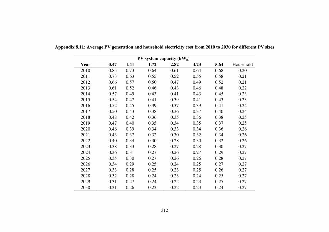
312

Appendix 8.11: Average PV generation and household electricity cost from 2010 to 2030 for different PV sizes

PV system capacity (kWp) Year 0.47 1.41 1.72 2.82 4.23 5.64 Household 2010 0.85 0.73 0.64 0.61 0.64 0.68 0.20 2011 0.73 0.63 0.55 0.52 0.55 0.58 0.21 2012 0.66 0.57 0.50 0.47 0.49 0.52 0.21 2013 0.61 0.52 0.46 0.43 0.46 0.48 0.22 2014 0.57 0.49 0.43 0.41 0.43 0.45 0.23 2015 0.54 0.47 0.41 0.39 0.41 0.43 0.23 2016 0.52 0.45 0.39 0.37 0.39 0.41 0.24 2017 0.50 0.43 0.38 0.36 0.37 0.40 0.24 2018 0.48 0.42 0.36 0.35 0.36 0.38 0.25 2019 0.47 0.40 0.35 0.34 0.35 0.37 0.25 2020 0.46 0.39 0.34 0.33 0.34 0.36 0.26 2021 0.43 0.37 0.32 0.30 0.32 0.34 0.26 2022 0.40 0.34 0.30 0.28 0.30 0.32 0.26 2023 0.38 0.33 0.28 0.27 0.28 0.30 0.27 2024 0.36 0.31 0.27 0.26 0.27 0.29 0.27 2025 0.35 0.30 0.27 0.26 0.26 0.28 0.27 2026 0.34 0.29 0.25 0.24 0.25 0.27 0.27 2027 0.33 0.28 0.25 0.23 0.25 0.26 0.27 2028 0.32 0.28 0.24 0.23 0.24 0.25 0.27 2029 0.31 0.27 0.24 0.22 0.23 0.25 0.27 2030 0.31 0.26 0.23 0.22 0.23 0.24 0.27

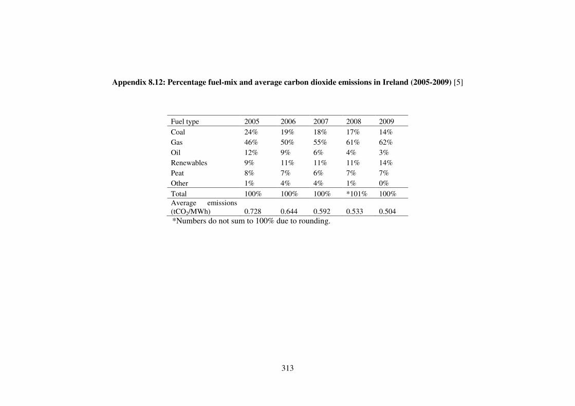
313

Appendix 8.12: Percentage fuel-mix and average carbon dioxide emissions in Ireland (2005-2009) [5]

Fuel type 2005 2006 2007 2008 2009 Coal 24% 19% 18% 17% 14% Gas 46% 50% 55% 61% 62% Oil 12% 9% 6% 4% 3% Renewables 9% 11% 11% 11% 14% Peat 8% 7% 6% 7% 7% Other 1% 4% 4% 1% 0% Total 100% 100% 100% *101% 100% Average emissions (tCO2/MWh) 0.728 0.644 0.592 0.533 0.504 *Numbers do not sum to 100% due to rounding.

314

Appendix 8.13: Historic and projected carbon intensity of power generation under the baseline and reference scenario (tCO2/MWh)

Year 2005 2006 2007 2008 2009 2010 2011 2012 2013 2014 2015 2016 2017

Baseline 2009 0.728 0.644 0.592 0.533 0.504 0.497 0.491 0.485 0.480 0.474 0.468 0.461 0.454

Reference 2009 0.728 0.644 0.592 0.533 0.504 0.500 0.488 0.475 0.464 0.452 0.441 0.428 0.416

Year 2018 2019 2020 2021 2022 2023 2024 2025 2026 2027 2028 2029 2030

Baseline 2009 0.447 0.440 0.433 0.421 0.409 0.398 0.387 0.376 0.358 0.341 0.324 0.309 0.294

Reference 2009 0.404 0.392 0.381 0.378 0.375 0.372 0.369 0.366 0.359 0.353 0.347 0.341 0.335

315

Appendix 8.14: PV system life cycle CO2 emission savings (tCO2/kWp) under the Baseline and Reference scenarios

Year Baseline Reference 2010 8.8 8.6 2011 8.6 8.5 2012 8.4 8.3 2013 8.2 8.2 2014 8.1 8.1 2015 7.9 8.0 2016 7.8 7.9 2017 7.6 7.8 2018 7.5 7.8 2019 7.3 7.7 2020 7.2 7.6 2021 7.1 7.6 2022 7.0 7.6 2023 6.9 7.5 2024 6.8 7.5 2025 6.7 7.5 2026 6.6 7.4 2027 6.6 7.4 2028 6.5 7.4 2029 6.5 7.4 2030 6.5 7.4

316

Appendix 8.15: Net present value and cumulative frequency for different PV system capacities under the proposed FITs for 2011

PV system

capacity 0.47 kWp 1.41 kWp 1.72 kWp 2.82 kWp 4.23 kWp 5.64 kWp FIT

(�/kWh) 0.45 0.39 0.32 0.31 0.34 0.38 CF

(%) NPV (�)

CF (%)

NPV (�)

CF (%)

NPV (�)

CF (%)

NPV (�)

CF (%)

NPV (�)

CF (%)

NPV (�)

0.2 -324 0.6 -633 0.7 -784 0.9 -889 1.5 -1,039 1.9 -869 0.7 -277 2.9 -490 3.8 -616 6.0 -651 8.7 -732 10.4 -508 1.6 -229 9.0 -347 10.8 -449 15.7 -414 20.2 -425 24.1 -148 3.6 -182 18.5 -203 21.6 -281 29.1 -176 36.7 -118 42.2 213 8.1 -135 32.3 -60 37.4 -113 48.1 62 57.1 189 62.4 574 14.6 -87 51.8 84 56.7 55 67.3 300 75.0 496 79.9 935 25.4 -40 72.7 227 76.8 222 84.2 538 88.8 803 91.2 1,295 42.2 7 89.8 370 92.1 390 94.4 776 96.3 1,110 97.4 1,656 68.3 54 98.3 514 98.5 558 98.9 1,014 99.4 1,417 99.5 2,017 99.9 102 100.0 657 100.0 725 100.0 1,252 100.0 1,724 100.0 2,378 100.0 149 100.0 801 100.0 893 100.0 1,490 100.0 2,031 100.0 2,738

NPV = net present value; CF = cumulative frequency

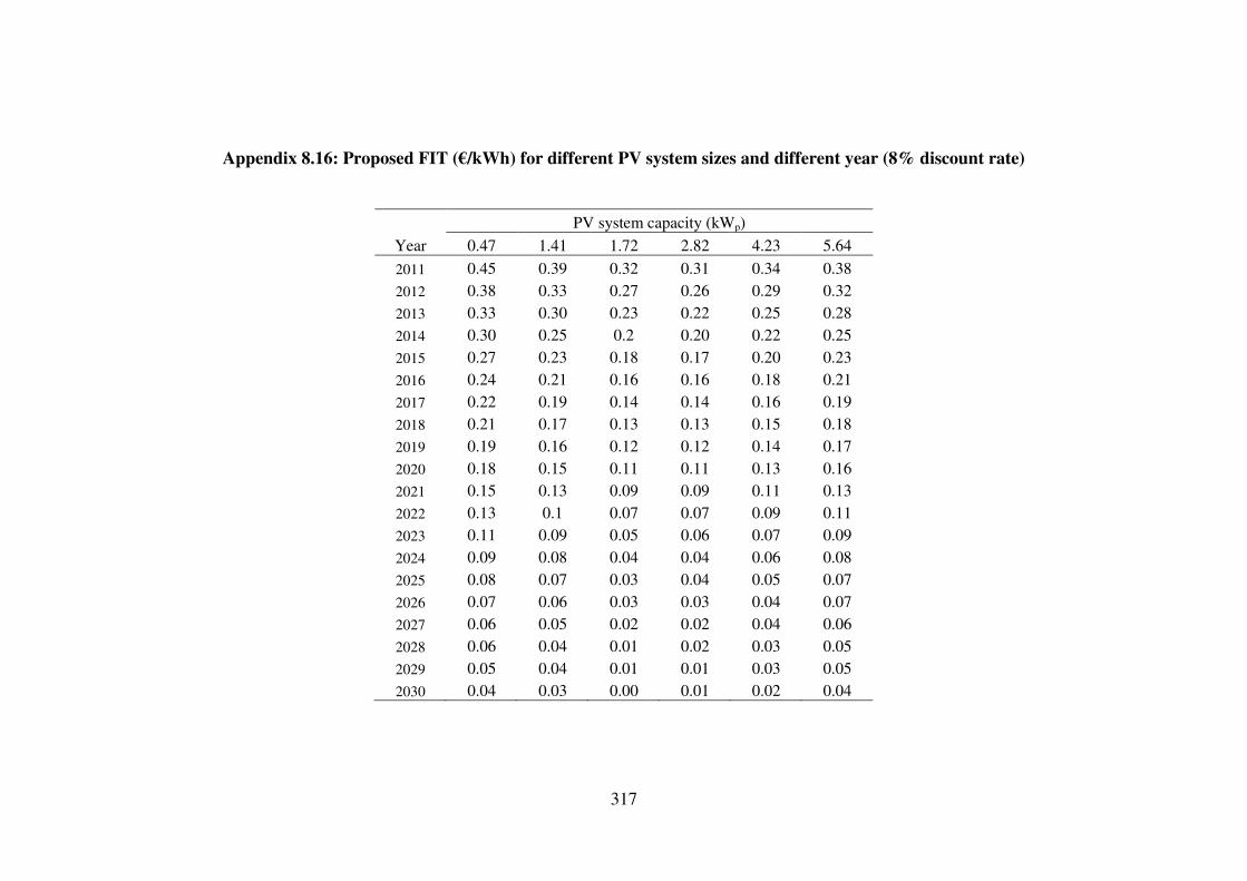
317

Appendix 8.16: Proposed FIT (�/kWh) for different PV system sizes and different year (8% discount rate)

Year PV system capacity (kWp)

0.47 1.41 1.72 2.82 4.23 5.64 2011 0.45 0.39 0.32 0.31 0.34 0.38 2012 0.38 0.33 0.27 0.26 0.29 0.32 2013 0.33 0.30 0.23 0.22 0.25 0.28 2014 0.30 0.25 0.2 0.20 0.22 0.25 2015 0.27 0.23 0.18 0.17 0.20 0.23 2016 0.24 0.21 0.16 0.16 0.18 0.21 2017 0.22 0.19 0.14 0.14 0.16 0.19 2018 0.21 0.17 0.13 0.13 0.15 0.18 2019 0.19 0.16 0.12 0.12 0.14 0.17 2020 0.18 0.15 0.11 0.11 0.13 0.16 2021 0.15 0.13 0.09 0.09 0.11 0.13 2022 0.13 0.1 0.07 0.07 0.09 0.11 2023 0.11 0.09 0.05 0.06 0.07 0.09 2024 0.09 0.08 0.04 0.04 0.06 0.08 2025 0.08 0.07 0.03 0.04 0.05 0.07 2026 0.07 0.06 0.03 0.03 0.04 0.07 2027 0.06 0.05 0.02 0.02 0.04 0.06 2028 0.06 0.04 0.01 0.02 0.03 0.05 2029 0.05 0.04 0.01 0.01 0.03 0.05 2030 0.04 0.03 0.00 0.01 0.02 0.04

318

Appendix 8.17: Simple payback period and cumulative frequency for different PV system capacities under the proposed FIT for 2011

PV system

capacity 0.47 kWp 1.41 kWp 1.72 kWp 2.82 kWp 4.23 kWp 5.64 kWp FIT

(�/kWh) 0.45 0.39 0.32 0.31 0.34 0.38 SPP

(years) CF (%) SPP

(years) CF (%) SPP

(years) CF (%) SPP

(years) CF (%) SPP

(years) CF (%) SPP

(years) CF (%) 9.1 37.7 9.2 3.1 10.3 2.5 10.1 1.7 9.4 1.0 9.1 0.6 9.3 64.7 9.5 16.2 10.6 14.0 10.4 8.5 9.6 5.5 9.2 3.7 9.5 80.3 9.7 38.3 10.9 34.0 10.6 23.9 9.8 16.0 9.4 11.7 9.7 89.0 10.0 59.5 11.2 56.0 10.9 43.2 10.0 33.2 9.6 26.6 9.9 94.6 10.2 76.5 11.5 73.6 11.2 63.2 10.2 53.2 9.7 45.2 10.2 97.5 10.4 87.0 11.9 85.5 11.4 78.6 10.4 71.7 9.9 65.0 10.4 98.8 10.7 94.3 12.2 93.3 11.7 89.3 10.6 84.6 10.0 80.9 10.6 99.4 10.9 98.2 12.5 97.9 12.0 96.3 10.8 94.0 10.2 91.8 10.8 99.9 11.2 99.4 12.8 99.4 12.2 99.3 11.0 99.1 10.3 98.8 11.0 100.0 11.4 100.0 13.1 100.0 12.5 100.0 11.2 100.0 10.5 100.0 11.2 100.0 11.7 100.0 13.4 100.0 12.8 100.0 11.4 100.0 10.6 100.0

SPP = simple payback period; CF = cumulative frequency

319

Appendix 8.18: Required FIT (�/kWh) for different PV system sizes that targets 50% market penetration in 2011

Discount rate (%)

PV system capacity (kWp) 0.47 1.41 1.72 2.82 4.23 5.64

6 0.34 0.29 0.24 0.23 0.26 0.29 7 0.39 0.34 0.28 0.27 0.29 0.33 8 0.45 0.39 0.32 0.31 0.34 0.38 9 0.50 0.44 0.37 0.35 0.38 0.42 10 0.56 0.49 0.41 0.39 0.43 0.47

320

Appendix 8.19: NPV and CF for different PV system capacities in 2011 (0.31 �/kWp FIT)

PV system

capacity 0.47 kWp 1.41 kWp 1.72 kWp 2.82 kWp 4.23 kWp 5.64 kWp CF

(%) NPV (�)

CF (%)

NPV (�)

CF (%)

NPV (�)

CF (%)

NPV (�)

CF (%)

NPV (�)

CF (%)

NPV (�)

0.2 -947 0.6 -1,702 0.7 -947 0.9 -889 1.5 -2,241 1.9 -4,610 0.7 -900 2.9 -1,559 3.8 -779 6.0 -651 8.7 -1,934 10.4 -4,249 1.6 -853 9.0 -1,415 10.8 -612 15.7 -414 20.2 -1,627 24.1 -3,888 3.6 -805 18.5 -1,272 21.6 -444 29.1 -176 36.7 -1,320 42.2 -3,527 8.1 -758 32.3 -1,128 37.4 -276 48.1 62 57.1 -1,013 62.4 -3,167 14.6 -711 51.8 -985 56.7 -108 67.3 300 75.0 -706 79.9 -2,806 25.4 -664 72.7 -842 76.8 59 84.2 538 88.8 -399 91.2 -2,445 42.2 -616 89.8 -698 92.1 227 94.4 776 96.3 -92 97.4 -2,084 68.3 -569 98.3 -555 98.5 395 98.9 1,014 99.4 215 99.5 -1,724 99.9 -522 100.0 -411 100.0 562 100.0 1,252 100.0 522 100.0 -1,363 100.0 -474 100.0 -268 100.0 730 100.0 1,490 100.0 829 100.0 -1,002


321

Appendix 8.20: NPV and CF for different PV system capacities in 2011(0.45 �/kWp)

PV system

capacity 0.47 kWp 1.41 kWp 1.72 kWp 2.82 kWp 4.23 kWp 5.64 kWp CF

(%) NPV (�)

CF (%)

NPV (�)

CF (%)

NPV (�)

CF (%)

NPV (�)

CF (%)

NPV (�)

CF (%)

NPV (�)

0.2 -324 0.6 168 0.7 1,335 0.9 2,851 1.5 3,370 1.9 2,871 0.7 -277 2.9 312 3.8 1,502 6.0 3,089 8.7 3,677 10.4 3,232 1.6 -229 9.0 455 10.8 1,670 15.7 3,327 20.2 3,984 24.1 3,593 3.6 -182 18.5 598 21.6 1,838 29.1 3,565 36.7 4,291 42.2 3,954 8.1 -135 32.3 742 37.4 2,005 48.1 3,803 57.1 4,598 62.4 4,314 14.6 -87 51.8 885 56.7 2,173 67.3 4,041 75.0 4,905 79.9 4,675 25.4 -40 72.7 1,029 76.8 2,341 84.2 4,279 88.8 5,212 91.2 5,036 42.2 7 89.8 1,172 92.1 2,508 94.4 4,517 96.3 5,519 97.4 5,397 68.3 54 98.3 1,315 98.5 2,676 98.9 4,755 99.4 5,826 99.5 5,757 99.9 102 100.0 1,459 100.0 2,844 100.0 4,993 100.0 6,132 100.0 6,118 100.0 149 100.0 1,602 100.0 3,012 100.0 5,231 100.0 6,439 100.0 6,479


322

Appendix 8.21: SPP and CF for different PV system capacities in 2011 (0.31 �/kWp FIT)

PV system

capacity 0.47 kWp 1.41 kWp 1.72 kWp 2.82 kWp 4.23 kWp 5.64 kWp SPP

(years) CF (%)

SPP (years)

CF (%)

SPP (years)

CF (%)

SPP (years)

CF (%)

SPP (years)

CF (%)

SPP (years)

CF (%)

11.6 39.4 10.7 3.3 10.5 2.5 10.1 1.7 10.0 1.0 10.5 0.6 11.9 66.5 11.0 17.3 10.8 14.2 10.4 8.5 10.2 5.7 10.7 4.0 12.3 81.9 11.3 40.5 11.2 34.3 10.6 23.9 10.4 16.5 10.9 12.5 12.7 89.9 11.7 61.3 11.5 56.2 10.9 43.2 10.7 33.9 11.1 27.5 13.0 95.1 12.0 77.6 11.8 73.8 11.2 63.2 10.9 53.8 11.3 46.8 13.4 97.8 12.4 88.0 12.1 85.7 11.4 78.6 11.1 72.0 11.5 66.1 13.7 98.9 12.7 94.8 12.4 93.3 11.7 89.3 11.3 84.9 11.7 81.6 14.1 99.4 13.0 98.4 12.8 97.9 12.0 96.3 11.6 94.2 11.9 92.2 14.4 99.9 13.4 99.5 13.1 99.4 12.2 99.3 11.8 99.1 12.1 98.8 14.8 100.0 13.7 100.0 13.4 100.0 12.5 100.0 12.0 100.0 12.4 100.0 15.1 100.0 14.0 100.0 13.7 100.0 12.8 100.0 12.3 100.0 12.6 100.0


323

Appendix 8.22: SPP and CF for different PV system capacities in 2011 (0.45 �/kWp FIT)

PV system

capacity 0.47 kWp 1.41 kWp 1.72 kWp 2.82 kWp 4.23 kWp 5.64 kWp SPP

(years) CF (%)

SPP (years)

CF (%)

SPP (years)

CF (%)

SPP (years)

CF (%)

SPP (years)

CF (%)

SPP (years)

CF (%)

9.1 37.7 8.4 2.9 8.2 2.0 7.8 1.5 7.7 0.9 8.0 0.6 9.3 64.7 8.6 15.5 8.4 12.9 8.0 7.7 7.8 5.1 8.2 3.5 9.5 80.3 8.8 37.0 8.6 31.7 8.1 21.8 8.0 14.8 8.3 11.3 9.7 89.0 9.0 58.7 8.8 53.0 8.3 40.8 8.1 31.6 8.4 25.8 9.9 94.6 9.2 75.6 9.0 71.6 8.5 60.4 8.2 51.5 8.5 44.2 10.2 97.5 9.4 86.6 9.2 84.0 8.6 76.8 8.3 70.3 8.6 64.2 10.4 98.8 9.5 94.1 9.4 92.5 8.8 88.1 8.5 83.6 8.7 80.4 10.6 99.4 9.7 98.1 9.5 97.9 8.9 95.7 8.6 93.4 8.9 91.5 10.8 99.9 9.9 99.4 9.7 99.4 9.1 99.3 8.7 99.0 9.0 98.7 11.0 100.0 10.1 100.0 9.9 100.0 9.2 100.0 8.9 100.0 9.1 100.0 11.2 100.0 10.3 100.0 10.1 100.0 9.4 100.0 9.0 100.0 9.2 100.0


324

Appendix 8.23: MAC for domestic scale PV systems in Ireland and projected CO2 prices for the baseline scenario (2011-2030)

Carbon price

(�/tCO2) CO2 abatement cost (�/tCO2)

Year Baseline scenario

Reference scenario

0.47 kWp

1.41 kWp

1.72 kWp

2.82 kWp

4.23 kWp

5.64 kWp

2011 15.0 15.0 915.8 793.7 651.3 630.9 692.0 773.4 2012 15.0 15.0 782.8 679.8 556.2 535.6 597.4 659.2 2013 16.3 15.2 688.1 625.5 479.6 458.7 521.3 583.8 2014 17.5 15.4 633.1 527.6 422.1 422.1 464.3 527.6 2015 18.8 15.6 576.7 491.3 384.5 363.1 427.2 491.3 2016 20.0 15.8 520.7 455.6 347.2 347.2 390.5 455.6 2017 21.3 15.9 484.8 418.7 308.5 308.5 352.6 418.7 2018 22.5 16.1 470.1 380.5 291.0 291.0 335.8 402.9 2019 23.8 16.3 432.0 363.8 272.8 272.8 318.3 386.5 2020 25.0 16.5 415.7 346.4 254.0 254.0 300.2 369.5 2021 26.4 16.7 356.3 308.8 213.8 213.8 261.3 308.8 2022 27.8 16.9 317.6 244.3 171.0 171.0 219.9 268.7 2023 29.2 17.2 276.4 226.2 125.6 150.8 175.9 226.2 2024 30.6 17.4 232.6 206.8 103.4 103.4 155.1 206.8 2025 32.0 17.6 212.7 186.1 79.7 106.3 132.9 186.1 2026 33.4 17.8 195.5 167.6 83.8 83.8 111.7 195.5 2027 34.8 18.0 176.1 146.7 58.7 58.7 117.4 176.1 2028 36.2 18.3 185.0 123.4 30.8 61.7 92.5 154.2 2029 37.6 18.5 162.0 129.6 32.4 32.4 97.2 162.0 2030 39.0 18.7 136.2 102.1 0.0 34.0 68.1 136.2

325

Appendix 8.24: MAC for domestic scale PV systems in Ireland and projected CO2 prices for the reference scenario (2011-2030)

Carbon price

(�/tCO2) CO2 abatement cost (�/tCO2)

Year Baseline scenario

Reference scenario

0.47 kWp

1.41 kWp

1.72 kWp

2.82 kWp

4.23 kWp

5.64 kWp

2011 15.0 15.0 922.7 799.7 656.2 635.7 697.2 779.2 2012 15.0 15.0 799.2 694.0 567.8 546.8 609.9 673.0 2013 16.3 15.2 711.8 647.1 496.1 474.5 539.3 604.0 2014 17.5 15.4 663.7 553.1 442.5 442.5 486.7 553.1 2015 18.8 15.6 612.6 521.9 408.4 385.7 453.8 521.9 2016 20.0 15.8 560.6 490.5 373.7 373.7 420.4 490.5 2017 21.3 15.9 529.0 456.8 336.6 336.6 384.7 456.8 2018 22.5 16.1 519.8 420.8 321.8 321.8 371.3 445.5 2019 23.8 16.3 484.1 407.7 305.8 305.8 356.7 433.2 2020 25.0 16.5 472.1 393.4 288.5 288.5 341.0 419.7 2021 26.4 16.7 396.7 343.8 238.0 238.0 290.9 343.8 2022 27.8 16.9 346.7 266.7 186.7 186.7 240.0 293.4 2023 29.2 17.2 295.9 242.1 134.5 161.4 188.3 242.1 2024 30.6 17.4 244.1 217.0 108.5 108.5 162.7 217.0 2025 32.0 17.6 218.8 191.5 82.1 109.4 136.8 191.5 2026 33.4 17.8 194.8 167.0 83.5 83.5 111.3 194.8 2027 34.8 18.0 170.0 141.6 56.7 56.7 113.3 170.0 2028 36.2 18.3 173.0 115.3 28.8 57.7 86.5 144.1 2029 37.6 18.5 146.7 117.4 29.3 29.3 88.0 146.7 2030 39.0 18.7 119.4 89.6 0.0 29.9 59.7 119.4

326

Appendix 9.1: Detailed costs of the FPC and ETC systems

FPC system ETC system

Item description Quantity Unit

cost (�) Total cost

inc. VAT (�) Total cost

inc. VAT (�) Solar pipe work (10 metres average) 1 250 250 250 Cylinder 300 litres 1 1100 1100 1100 Roof flashing 2 20 40 40 Anti-freeze 10 litres concentrate 1 65 65 65 Pump station 1 180 180 180 Controller 1 160 160 160 Expansion vessel and mounting kit 1 90 90 90 Mixing valve 1 60 60 60 Lightning arrestor 1 17 17 17 Fitting pack 1 50 50 50 2 flat plate collectors 1 968 968 - Mounting rails and connections (FPC) 1 300 300 - 30 vacuum tube collector 1 677 - 1777 06 solar bolts 1 40 - 40 Installation cost (FPC) 1 1120 1120 - Installation cost (ETC) 1 1171 - 1171 Total system cost �4,400 �5,000

327

Appendix 9.2: Projected costs of solar water heating systems in Ireland (2010-2030)

Annual installed capacity (GWth) SWHS costs (�)

Year Moderate Scenario

Advanced scenario

FPC (Mod 10)

ETC (Mod 10)

FPC (Adv 10)

ETC (Adv 10)

2010 27.8 30.6 4,400 5,000 4,400 5,000 2011 33.4 39.1 4,278 4,862 4,240 4,818 2012 39.0 47.5 4,178 4,748 4,115 4,676 2013 44.7 56.0 4,093 4,651 4,014 4,561 2014 50.3 64.5 4,020 4,568 3,929 4,465 2015 55.9 73.0 3,956 4,495 3,856 4,382 2016 61.6 81.4 3,898 4,430 3,792 4,309 2017 67.2 89.9 3,847 4,371 3,735 4,245 2018 72.8 98.4 3,800 4,318 3,685 4,187 2019 78.5 106.8 3,757 4,270 3,639 4,135 2020 84.1 115.3 3,718 4,225 3,597 4,087 2021 89.8 123.8 3,681 4,183 3,558 4,043 2022 95.4 132.2 3,648 4,145 3,522 4,003 2023 101.0 140.7 3,616 4,109 3,489 3,965 2024 106.7 149.2 3,586 4,075 3,459 3,930 2025 112.3 157.7 3,558 4,043 3,430 3,897 2026 117.9 166.1 3,532 4,013 3,402 3,866 2027 123.6 174.6 3,507 3,985 3,377 3,837 2028 129.2 183.1 3,483 3,958 3,353 3,810 2029 134.8 191.5 3,461 3,933 3,330 3,784 2030 140.5 200.0 3,439 3,908 3,308 3,759

328

Appendix 9.3: Projected life cycle system cost under different scenarios

Year FPC (Mod 10)

ETC (Mod 10)

FPC (Adv 10)

ETC (Adv 10)

2010 4913 5583 4913 5583 2011 4791 5444 4752 5400 2012 4691 5330 4628 5259 2013 4606 5234 4526 5144 2014 4533 5151 4441 5047 2015 4468 5078 4368 4964 2016 4411 5013 4305 4892 2017 4360 4954 4248 4827 2018 4313 4901 4197 4770 2019 4270 4852 4151 4717 2020 4231 4807 4109 4670 2021 4194 4766 4071 4626 2022 4160 4727 4035 4585 2023 4128 4691 4002 4548 2024 4099 4658 3971 4513 2025 4071 4626 3942 4480 2026 4044 4596 3915 4449 2027 4019 4568 3889 4420 2028 3996 4541 3865 4392 2029 3973 4515 3842 4366 2030 3952 4491 3820 4341

329

Appendix 9.4: Projected fuel prices (�/kWh) in Ireland from 2010 to 2030

Year Gas price Oil price Electricity

price 2010 0.055 0.064 0.203 2011 0.066 0.076 0.209 2012 0.079 0.091 0.215 2013 0.090 0.105 0.220 2014 0.104 0.121 0.227 2015 0.113 0.132 0.233 2016 0.122 0.142 0.237 2017 0.131 0.152 0.242 2018 0.137 0.160 0.247 2019 0.142 0.165 0.252 2020 0.145 0.169 0.257 2021 0.147 0.171 0.260 2022 0.149 0.174 0.263 2023 0.151 0.175 0.266 2024 0.152 0.177 0.269 2025 0.153 0.178 0.273 2026 0.155 0.180 0.273 2027 0.156 0.181 0.273 2028 0.157 0.182 0.273 2029 0.158 0.184 0.274 2030 0.160 0.186 0.274

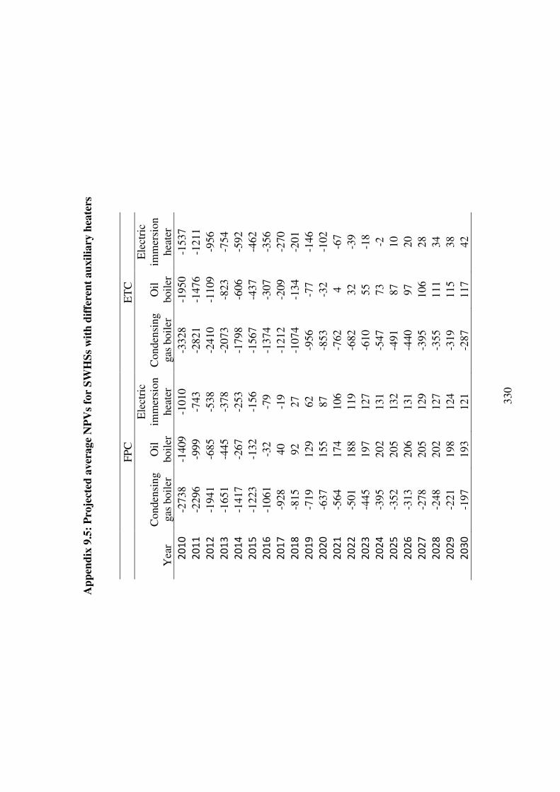
330

A

ppen

dix

9.5:

Pro

ject

ed a

vera

ge N

PVs f

or S

WH

Ss w

ith d

iffer

ent a

uxili

ary

heat

ers

FP

C

ET

C

Y

ear

Con

dens

ing

gas

boile

r O

il bo

iler

Ele

ctri

c im

mer

sion

he

ater

C

onde

nsin

g ga

s bo

iler

Oil

boile

r

Ele

ctri

c im

mer

sion

he

ater

��

-273

8 -1

409

-101

0 -3

328

-195

0 -1

537

��

-229

6 -9

99

-743

-2

821

-147

6 -1

211

��

-194

1 -6

85

-538

-2

410

-110

9 -9

56

��

-165

1 -4

45

-378

-2

073

-823

-7

54

��

-141

7 -2

67

-253

-1

798

-606

-5

92

��"�

-122

3 -1

32

-156

-1

567

-437

-4

62

��

-106

1 -3

2 -7

9 -1

374

-307

-3

56

��!�

-928

40

-1

9 -1

212

-209

-2

70

��

-815

92

27

-1

074

-134

-2

01

��

-719

12

9 62

-9

56

-77

-146

��

-637

15

5 87

-8

53

-32

-102

��

-564

17

4 10

6 -7

62

4 -6

7 ��

-501

18

8 11

9 -6

82

32

-39

��

-445

19

7 12

7 -6

10

55

-18

��

-395

20

2 13

1 -5

47

73

-2

��"�

-352

20

5 13

2 -4

91

87

10

��

-313

20

6 13

1 -4

40

97

20

��!�

-278

20

5 12

9 -3

95

106

28

��

-248

20

2 12

7 -3

55

111

34

��

-221

19

8 12

4 -3

19

115

38

��

-197

19

3 12

1 -2

87

117

42

331

Appendix 9.6: Projected simple payback period for SWHSs with different auxiliary heaters in Ireland (2010 to 2030)

FPC ETC

Year Condensing gas boiler

Oil boiler

Electric immersion

heater Condensing gas boiler

Oil boiler

Electric immersion

heater 2010 43.9 27.3 13.2 48.2 29.9 14.5 2011 36.8 22.8 12.9 40.4 25.0 14.1 2012 30.8 19.1 12.5 33.7 20.9 13.7 2013 26.7 16.6 12.2 29.3 18.2 13.4 2014 23.2 14.4 11.8 25.5 15.8 13.0 2015 21.3 13.2 11.5 23.4 14.5 12.6 2016 19.8 12.3 11.3 21.7 13.4 12.4 2017 18.5 11.5 11.1 20.3 12.6 12.2 2018 17.6 10.9 10.9 19.3 12.0 11.9 2019 17.0 10.6 10.7 18.7 11.6 11.7 2020 16.6 10.3 10.5 18.2 11.3 11.5 2021 16.4 10.2 10.3 18.0 11.2 11.3 2022 16.2 10.1 10.2 17.8 11.0 11.2 2023 16.0 9.9 10.1 17.6 10.9 11.1 2024 15.9 9.9 10.0 17.4 10.8 10.9 2025 15.8 9.8 9.9 17.3 10.7 10.8 2026 15.6 9.7 9.8 17.1 10.6 10.8 2027 15.5 9.6 9.8 17.0 10.6 10.8 2028 15.4 9.6 9.8 16.9 10.5 10.8 2029 15.3 9.5 9.8 16.7 10.4 10.8 2030 15.1 9.4 9.8 16.6 10.3 10.7

332

A

ppen

dix

9.7:

Ave

rage

leve

lised

hea

ting

cost

( �/k

Wh)

for

SWH

Ss w

ith d

iffer

ent a

uxili

ary

heat

ers

E

lect

ric

imm

ersi

on h

eate

r O

il bo

iler

Con

dens

ing

gas

boile

r Y

ear

FPC

E

TC

FP

C

ET

C

FPC

E

TC

20

10

0.30

5 0.

335

0.19

8 0.

218

0.27

5 0.

301

2011

0.

297

0.32

5 0.

193

0.21

1 0.

267

0.29

3 20

12

0.29

0 0.

317

0.18

8 0.

206

0.26

1 0.

286

2013

0.

284

0.31

1 0.

184

0.20

2 0.

255

0.28

0 20

14

0.27

9 0.

306

0.18

1 0.

199

0.25

1 0.

275

2015

0.

275

0.30

1 0.

178

0.19

6 0.

247

0.27

1 20

16

0.27

1 0.

297

0.17

6 0.

193

0.24

4 0.

267

2017

0.

267

0.29

3 0.

174

0.19

1 0.

241

0.26

4 20

18

0.26

4 0.

290

0.17

2 0.

188

0.23

8 0.

261

2019

0.

262

0.28

7 0.

170

0.18

6 0.

235

0.25

8 20

20

0.25

9 0.

284

0.16

8 0.

185

0.23

3 0.

256

2021

0.

257

0.28

2 0.

167

0.18

3 0.

231

0.25

3 20

22

0.25

5 0.

279

0.16

6 0.

181

0.22

9 0.

251

2023

0.

253

0.27

7 0.

164

0.18

0 0.

227

0.24

9 20

24

0.25

1 0.

275

0.16

3 0.

179

0.22

6 0.

247

2025

0.

249

0.27

3 0.

162

0.17

7 0.

224

0.24

6 20

26

0.24

7 0.

271

0.16

1 0.

176

0.22

3 0.

244

2027

0.

246

0.26

9 0.

160

0.17

5 0.

221

0.24

2 20

28

0.24

4 0.

268

0.15

9 0.

174

0.22

0 0.

241

2029

0.

243

0.26

6 0.

158

0.17

3 0.

219

0.24

0 20

30

0.24

1 0.

265

0.15

7 0.

172

0.21

7 0.

238

333

Appendix 9.8: Average emission factors for grid electricity, residual oil, natural gas and life cycle emission savings (tCO2) for FPC and

ETC SWHSs with different auxiliary heaters

Emission factors (kgCO2/kWh) FPC ETC

Year

Grid

electricity

Residual

oil

Natural

gas Condensing gas boiler

Oil boiler

Electric immersion

heater Condensing gas boiler

Oil boiler

Electric immersion

heater 2010 0.499 0.274 0.206 7.9 14.5 15.4 8.2 15.0 15.9 2011 0.494 0.274 0.206 7.9 14.5 15.2 8.2 15.0 15.7 2012 0.488 0.274 0.206 7.9 14.5 15.0 8.2 15.0 15.6 2013 0.483 0.274 0.206 7.9 14.5 14.9 8.2 15.0 15.4 2014 0.478 0.274 0.206 7.9 14.5 14.7 8.2 15.0 15.3 2015 0.473 0.274 0.206 7.9 14.5 14.6 8.2 15.0 15.1 2016 0.467 0.274 0.206 7.9 14.5 14.5 8.2 15.0 15.0 2017 0.462 0.274 0.206 7.9 14.5 14.3 8.2 15.0 14.9 2018 0.457 0.274 0.206 7.9 14.5 14.2 8.2 15.0 14.8 2019 0.452 0.274 0.206 7.9 14.5 14.1 8.2 15.0 14.6 2020 0.446 0.274 0.206 7.9 14.5 14.0 8.2 15.0 14.5 2021 0.441 0.274 0.206 7.9 14.5 13.9 8.2 15.0 14.5 2022 0.436 0.274 0.206 7.9 14.5 13.9 8.2 15.0 14.4 2023 0.431 0.274 0.206 7.9 14.5 13.8 8.2 15.0 14.3 2024 0.425 0.274 0.206 7.9 14.5 13.7 8.2 15.0 14.2 2025 0.420 0.274 0.206 7.9 14.5 13.7 8.2 15.0 14.2 2026 0.415 0.274 0.206 7.9 14.5 13.6 8.2 15.0 14.1 2027 0.410 0.274 0.206 7.9 14.5 13.6 8.2 15.0 14.1 2028 0.404 0.274 0.206 7.9 14.5 13.6 8.2 15.0 14.1 2029 0.399 0.274 0.206 7.9 14.5 13.6 8.2 15.0 14.1 2030 0.394 0.274 0.206 7.9 14.5 13.6 8.2 15.0 14.1

334

Appendix 9.9: Marginal abatement costs (�/tCO2) for SWHSs with different auxiliary heaters

FPC ETC Carbon price (�/tCO2)

Year Condensing gas

boiler Oil

boiler Electric

immersion heater Condensing gas

boiler Oil

boiler Electric

immersion heater Baseline scenario Reference

scenario 2010 348 97 66 408 130 97 15.0 15.0 2011 291 69 49 345 98 77 15.0 15.0 2012 246 47 36 295 74 61 15.0 15.0 2013 210 31 25 254 55 49 16.3 15.2 2014 180 18 17 220 40 39 17.5 15.4 2015 155 9 11 192 29 31 18.8 15.6 2016 135 2 5 168 20 24 20.0 15.8 2017 118 -3 1 148 14 18 21.3 15.9 2018 103 -6 -2 132 9 14 22.5 16.1 2019 91 -9 -4 117 5 10 23.8 16.3 2020 81 -11 -6 104 2 7 25.0 16.5 2021 72 -12 -8 93 0 5 26.4 16.7 2022 64 -13 -9 83 -2 3 27.8 16.9 2023 56 -14 -9 75 -4 1 29.2 17.2 2024 50 -14 -10 67 -5 0 30.6 17.4 2025 45 -14 -10 60 -6 -1 32.0 17.6 2026 40 -14 -10 54 -6 -1 33.4 17.8 2027 35 -14 -10 48 -7 -2 34.8 18.0 2028 31 -14 -9 43 -7 -2 36.2 18.3 2029 28 -14 -9 39 -8 -3 37.6 18.5 2030 25 -13 -9 35 -8 -3 39.0 18.7

335

Appendix 10.1: Characteristics of some key support measures

Enhanced feed-in tariffs

Direct capital subsidies

Green electricity schemes

Renewable portfolio standards

Tax credits Sustainable building requirements

Target audience

Grid-connected PV customers with business cash flow requirements e.g. housing developers, investors, commercial entities

PV customers with limited access to capital e.g. households, small businesses, public organizations

Residential and commercial electricity customers

Liable parties, typically the electricity retailing businesses

Any entity with a tax liability, such as salary earners and businesses. However, may not be relevant for may prime candidates for PV

New building developments (residential and commercial); also properties for sale

Countries reporting use of this support measure, or similar

Austria, Canada, Switzerland, Germany, Spain, France, Italy, Korea

Australia, Austria, Switzerland, Germany, Spain, France, Italy, Japan, Korea, Sweden, USA

Australia, Austria, Canada, Switzerland, Germany, UK, Italy, Japan, USA

Australia, UK, Japan, Sweden, USA

Canada, Switzerland, France, UK, Japan, Portugal, USA

Australia, Canada, Switzerland, Germany, Spain, Korea, Portugal, USA

Implementation Typically administered by the electricity industry billing entity

Requires considerable public administrative support to handle applications, approvals and disbursements

Commercial business operation of the electricity utility; some public administrative support for accreditation of projects

Public administrative support via a regulatory body

Administered by the existing taxation bodies

Typically administered by the local building consent authority

Economic and political considerations

Method of internalizing the externalities associated with traditional energy supply

Up-front capital cost is seen as the main economic barrier to the deployment of PV. Can be used for grid-connected support programmes

Government involvement in selective, customer-driven, electricity business commercial activities raises some interesting questions. However, utility projects may better realize the network benefits of PV

Can be seen as a distortion in the functioning of the electricity market, especially if overly prescriptive

Same benefits as the direct capital subsidies but without some of the negatives

Appeal largely depends upon the degree to which property prices are impacted and the cultural acceptance of prescriptive approaches

There are varying political perceptions regarding the use of public funds or funds generated by the electricity industry

336

Appendix 10.2: National 2020 target and estimated trajectory of energy from renewable sources in heating and cooling, electricity and transport

2005 2010 2011 2012 2013 2014 2015 2016 2017 2018 2019 2020

RES-H&C (%) 3.5% 4.3% 4.9% 6.1% 6.9% 7.7% 8.9% 9.7% 10.1% 10.5% 11.2% 12.0% RES-E (%) 6.9% 20.4% 24.6% 25.3% 30.5% 31.0% 32.4% 32.2% 33.8% 37.5% 37.3% 42.5% RES-T (%) 0.0% 3.0% 3.9% 4.6% 5.1% 5.5% 5.9% 6.6% 7.4% 8.1% 8.8% 10.0%

Overall RES share (%) 3.1% 6.6% 8.1% 9.0% 10.5% 11.0% 11.8% 12.2% 12.9% 14.0% 14.4% 16.0% Of which from cooperation mechanism (%) 0% 0% 0% 0% 0% 0% 0% 0% 0% 0% 0% Surplus for cooperation mechanism (%) 0% 1.4% 1.4% 1.9% 1.9% 1.6% 1.6% 1.0% 1.0% 0% 0%

As part B of Annex 1 of the Directive 2011-2012 2013-2014 2015-2016 2017-2018 2020

RES minimum trajectory (%) 5.69% 6.98% 8.92% 11.51% 16%

RES minimum trajectory (Ktoe) 739 930 1,217 1,599 2,263

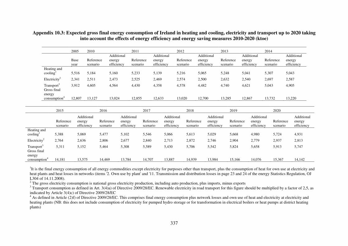
337

Appendix 10.3: Expected gross final energy consumption of Ireland in heating and cooling, electricity and transport up to 2020 taking into account the effects of energy efficiency and energy saving measures 2010-2020 (ktoe)

2005 2010 2011 2012 2013 2014

Base year

Reference scenario

Additional energy efficiency

Reference scenario


Reference scenario


Reference scenario


Reference scenario


Heating and cooling1 5,516 5,184 5,160 5,233 5,139 5,216 5,065 5,248 5,041 5,307 5,043

Electricity2 2,341 2,511 2,473 2,525 2,469 2,574 2,500 2,632 2,540 2,697 2,587

Transport3 3,912 4,605 4,564 4,430 4,358 4,578 4,482 4,740 4,621 5,043 4,905 Gross final energy consumption4 12,807 13,127 13,024 12,855 12,633 13,020 12,700 13,285 12,867 13,732 13,220

2015 2016 2017 2018 2019 2020

Reference scenario


Reference scenario


Reference scenario


Reference scenario


Reference scenario


Reference scenario


Heating and cooling1 5,388 5,069 5,477 5,102 5,546 5,066 5,613 5,029 5,668 4,980 5,724 4,931

Electricity2 2,764 2,636 2,806 2,677 2,840 2,713 2,872 2,746 2,904 2,779 2,937 2,813

Transport3 5,311 5,152 5,464 5,308 5,589 5,430 5,706 5,542 5,824 5,658 5,913 5,747 Gross final energy consumption4 14,181 13,575 14,469 13,784 14,707 13,887 14,939 13,984 15,166 14,076 15,367 14,142

1It is the final energy consumption of all energy commodities except electricity for purposes other than transport, plus the consumption of heat for own use at electricity and heat plants and heat losses in networks (items '2. Own use by plant' and '11. Transmission and distribution losses in page 23 and 24 of the energy Statistics Regulation, OJ L304 of 14.11.2008). 2 The gross electricity consumption is national gross electricity production, including auto production, plus imports, minus exports 3 Transport consumption as defined in Art. 3(4)a) of Directive 2009/28/EC. Renewable electricity in road transport for this figure should be multiplied by a factor of 2,5, as indicated by Article 3(4)c) of Directive 2009/28/EC 4 As defined in Article (2)f) of Directive 2009/28/EC. This comprises final energy consumption plus network losses and own use of heat and electricity at electricity and heating plants (NB: this does not include consumption of electricity for pumped hydro storage or for transformation in electrical boilers or heat pumps at district heating plants)

338

Appendix 10.4: Calculation table for the renewable energy contribution of each sector to final energy consumption (ktoe)

2005 2010 2011 2012 2013 2014 2015 2016 2017 2018 2019 2020 (A) Expected gross final consumption of RES for heating and cooling 193 220 253 311 348 387 451 493 509 527 559 591 (B) Expected gross final consumption of electricity from RES 180 504 607 634 775 803 855 862 917 1,030 1,037 1,196 (C) Expected final consumption of energy from RES in transport 1 135 168 201 234 267 300 333 366 399 432 482 (D) Expected total RES consumption 373 859 1,028 1,145 1,357 1,457 1,605 1,688 1,792 1,956 2,027 2,269 (E) Expected transfer of RES to other Member states 0 0 168 168 233 233 211 211 136 136 0 0 (F) Expected transfer of RES from other Member states and 3rd countries 0 0 0 0 0 0 0 0 0 0 0 0 (G) Expected RES consumption adjusted for target (D)-(E)+(D) 373 859 860 978 1,123 1,224 1,394 1,476 1,656 1,820 2,027 2,269

339

Appendix 10.5: Overview of micro-generation policies and measures in Ireland

Name and reference of the

measure

Type of measure

Expected result Targeted group and or activity

Existing or planned Start and end dates of the measure

Greener Homes Scheme (GHS)

Financial Facilitates the wider deployment of renewable-energy heating technologies in the residential sector and supports the development of of a sustainable market, resulting in reduced dependence on fossil fuel and lower CO2 emissions.

Homeowners Existing 2006 onwards

Small and Micro Scale Generation Pilot Programme

Financial The pilot is expected to inform on the technical, market and regulatory issues associated with the installation, network connection and operation of small and micro scale generation technologies.

Micro renewable generators

Existing (closed for new applications) Launched in February 2009. Initial results from the monitoring programme are expected within the 3rd quarter 2010, with monitoring continuing through 2011.

Part L of the Second Schedule of the Building Regulations 1997-2008

Regulatory In relation to Dwellings, Part L 3(b) requires that “ a reasonable proportion of the energy consumption to meet the energy performance of the dwellings is provided by renewable energy sources” . This provision is expected to increase use of renewable energy in dwellings

Domestic (dwellings) Existing The Department of Environment is developing a strategic framework to achieve a carbon neutral standard for dwellings by 2013. Increased use of onsite renewables will be a key element of the framework. Building Regulations Part L (Conservation of Fuel and Energy) for buildings other than dwellings are being reviewed in 2010.

2008

Statutory Instrument (SI) 83 of 2007 and SI 235 of 2008

Regulatory Conditional planning exemptions for renewable technologies that meet specified criteria are expected to encourage uptake of energy from renewable technologies

Domestic, business and agricultural sectors

Existing 2007 and 2008 Onwards

Smart metering pilot programme

Technical/Soft The results of the smart metering pilot will inform an analysis of the feasibility of implementing smart meters throughout Ireland. Electricity and gas smart meter trials are underway.

Electricity and Gas consumers policy makers

Existing 2007 onwards

340

LIST OF PUBLICATIONS

Journal Publication �

• L.M. Ayompe, A. Duffy, M. Mc Keever, M. Conlon and S.J. McCormack.

Comparative field performance study of flat plate and heat pipe evacuated tube

collectors for domestic water heating systems in a temperate climate. Energy

(2011): 36; 5, 3370-3378.

• L.M. Ayompe, A. Duffy, S.J. McCormack and M. Conlon. Validated TRNSYS

model for forced circulation solar water heating systems with flat plate and heat

pipe evacuated tube collectors. Applied Thermal Engineering (2011): 31; 1536-

1542.

• L.M. Ayompe, A. Duffy, S.J. McCormack and M. Conlon. Measured

performance of a 1.72 kilowatt rooftop grid connected photovoltaic system in

Ireland. Energy Conversion and Management (2011): 52; 2, 816-825.

• L.M. Ayompe, A. Duffy, S.J. McCormack and M. Conlon. Validated real-time

energy model for small-scale grid-connected PV systems. Energy (2010): 35;

10, 4086-4091.

• L.M. Ayompe, A. Duffy, S.J. McCormack and M. Conlon. Projected costs of a

grid-connected domestic PV system under different scenarios in Ireland, using

measured data from a trial installation. Energy Policy (2010): 38; 3731-3743.

Journal Submissions: Under Review �

• L.M. Ayompe, A. Duffy, S.J. McCormack and M. Conlon. Energy and exergy

analysis of a small-scale grid-connected PV system. Energy Conversion and

Management (Under review).

341

Conference Proceedings �

• L.M. Ayompe, A. Duffy, S.J. McCormack, M. Conlon. Field performance

evaluation of domestic-scale solar water heating systems with flat plate and heat

pipe evacuated tube collectors. Engineering Sustainability 2011 Conference,

David Lawrence Convention Center, Pittsburgh, Pa, USA, April 10-12, 2011.

• L.M. Ayompe, A. Duffy, S.J. McCormack, M. Conlon. Economic Analysis of

Domestic Solar Water Heating Systems in Ireland – Future Trends and Policy

Implications. The Challenge of Sustainability 2008 Conference, Dundalk

Institute of Technology, 20th June, 2008.

• L.M. Ayompe, A. Duffy, S.J. McCormack, M. Conlon. Economic and

environmental performance analysis of PV systems for domestic applications in

Ireland. Engineering Sustainability 2009 Conference, David Lawrence

Convention Center, Pittsburgh, Pa, USA, April 19-21, 2009.

Performance and Policy Evaluation of Solar Energy Technologies for Domestic Application in Ireland

Documents

Transcript of Performance and Policy Evaluation of Solar Energy Technologies for Domestic Application in Ireland