Guidelines to Develop Inhalation and Oral Cancer and Non-Cancer Toxicity Factors

Chapters 1-6

Draft June 7, 2011

DO NOT CITE OR QUOTE

Texas Commission on Environmental Quality Toxicology Division

Chief Engineer’s Office

Prepared by: Toxicology Division

Chief Engineer’s Office

i

Document Description and Intended Use 1

This is a technical guide written and used by the Texas Commission on Environmental Quality 2 (TCEQ) to develop the following health- and welfare-based inhalation toxicity values, and 3 health-based oral toxicity values: 4

• acute and chronic inhalation Effects Screening Levels (ESLs), 5

• acute and chronic inhalation Reference Values (ReVs), 6

• chronic inhalation Unit Risk Factor (URF) values 7

• chronic oral reference dose (RfD) and slope factor (SFo) values. 8

Although this document is primarily written as guidance for the TCEQ staff, it also documents 9 (largely by reference) the processes used to develop different toxicity values for any interested 10 person with training in inhalation and oral toxicology and risk assessment. 11

Inhalation ESLs are chemical-specific air concentrations set to protect human health and welfare. 12 ESLs are used in the air permitting program. Short-term ESLs are based on data concerning 13 acute health effects, the potential for odors to be a nuisance, and effects on vegetation, while 14 long-term ESLs are based on data concerning chronic health and vegetation effects. Welfare-15 based ESLs (odor and vegetation) are set based on effect threshold concentrations. Health-based 16 ESLs, however, are calculated from ReV and URF toxicity factors. ReVs and URFs are based on 17 the most sensitive adverse health effect relevant to humans. Derivation of a ReV or URF begins 18 with a toxicity assessment involving hazard identification and dose-response assessment based 19 on the chemical’s mode of action. The resulting ReV and URF values are then used to calculate 20 ESLs that correspond to no significant risk levels. Air Monitoring Comparison Values (AMCVs) 21 are used to evaluate ambient air monitoring data and are based on specific health-based ReV and 22 health- and welfare-based ESL values. 23

Chronic RfDs are chemical-specific oral doses set to protect human health for exposure via 24 ingestion and are based on data concerning chronic noncancer health effects. A SFo represents 25 the carcinogenic potency of a chemical and is based on data concerning chronic cancer effects. 26 RfD and SFo values are based on the most sensitive adverse health effect relevant to humans 27 from oral exposure. Derivation of RfD and SFo values begins with a toxicity assessment 28 involving hazard identification and dose-response assessment based on the chemical’s mode of 29 action. ReV, URF, RfD, and SFo values are used to calculate health-protective cleanup levels for 30 the TCEQ’s remediation program. 31

This guide is presented in seven chapters. In Chapter 1, several fundamental topics are addressed 32 including legal authority and regulatory use, consideration of cumulative risk, problem 33 formulation, and public participation opportunities. Chapter 1 also provides an introduction 34 to the different toxicity values and their use in calculating health-based inhalation ESLs, 35

ii

introduces and explains the use of Air Monitoring Comparison Values (AMCVs), and the use of 1 toxicity factors in remediation projects. Chapter 2 describes how welfare-based ESLs are 2 determined (i.e., odor- and vegetation-based values). Chapter 3 discusses common procedures 3 used to develop both acute and chronic toxicity values for the inhalation routes and chronic 4 toxicity factors for the oral routes of exposure. Chapter 4 addresses the procedures that are 5 unique to the derivation of acute inhalation ReVs, and Chapter 5 addresses the procedures that 6 are unique to the derivation of chronic toxicity factors. Chapter 6 provides procedures for the 7 treatment of chemical groups and mixtures and Chapter 7 discusses procedures for using 8 epidemiology studies to develop toxicity factors. 9

10 11

iii

TABLE OF CONTENTS 1

DOCUMENT DESCRIPTION AND INTENDED USE ........................................................................................... I 2 LIST OF TABLES ................................................................................................................................................. VIII 3 LIST OF FIGURES .................................................................................................................................................. IX 4 ACRONYMS AND ABBREVIATIONS ................................................................................................................... X 5 CHAPTER 1 INTRODUCTION TO INHALATION AND ORAL TOXICITY FACTORS .......................... 1 6

1.1 LEGAL AUTHORITY AND REGULATORY USE .................................................................................................... 1 7 1.1.1 Inhalation Toxicity Factors ................................................................................................................... 1 8 1.1.2 Oral Toxicity Factors............................................................................................................................. 2 9 1.1.3 Outline ................................................................................................................................................... 2 10

1.2 DEFINITION OF REV, URF, RFD, AND SFO VALUES ........................................................................................ 2 11 1.2.1 ReV and RfD Values for Threshold Dose-Response Effects .................................................................. 3 12 1.2.2 URF and SFo Values for Nonthreshold Dose-Response Effects ............................................................ 5 13 1.2.3 Margin of Exposure Approach............................................................................................................... 5 14

1.3 CONSIDERATION OF CUMULATIVE RISK ........................................................................................................... 5 15 1.3.1 Cumulative Risk for Air Emissions ........................................................................................................ 6 16 1.3.2 Cumulative Risk and Hazard in Remediation Projects .......................................................................... 7 17

1.4 GENERAL RISK MANAGEMENT OBJECTIVES .................................................................................................... 7 18 1.4.1 Health-Based Risk Management Objectives (No Significant Risk Levels) ............................................. 7 19 1.4.2 Air Permitting Risk Management Objectives ......................................................................................... 7 20 1.4.3 Air Monitoring Risk Management Objectives ........................................................................................ 8 21 1.4.4 Remediation Risk Management Objectives ............................................................................................ 9 22

1.5 ESLS FOR AIR PERMITTING .............................................................................................................................. 9 23 1.5.1 Problem Formulation ............................................................................................................................ 9 24 1.5.2 Health-Based ESLs .............................................................................................................................. 10 25

1.5.2.1 Calculation of ESLs for Threshold Effects ...................................................................................................... 10 26 1.5.2.2 Calculation of ESLs for Nonthreshold Effects ................................................................................................ 11 27

1.5.3 Determination of Short-Term and Long-Term ESLs for Air Permitting .............................................. 11 28 1.6 EXEMPTION OF SUBSTANCES FROM ESL DEVELOPMENT ............................................................................... 15 29 1.7 AMCVS FOR AIR MONITORING ..................................................................................................................... 16 30

1.7.1 Problem Formulation .......................................................................................................................... 16 31 1.7.2 How AMCVs Relate to ReVs and ESLs ................................................................................................ 17 32

1.8 SUMMARY OF TOXICITY FACTORS IN TCEQ PROGRAM AREAS ..................................................................... 19 33 1.9 TOXICITY FACTOR DEVELOPMENT SUPPORT DOCUMENT (DSD) ................................................................... 20 34 1.10 SELECTION OF CHEMICALS AND DATA SOLICITATION FOR AIR PROGRAMS .............................................. 20 35 1.11 SELECTION OF CHEMICALS AND DATA SOLICITATION FOR REMEDIATION ................................................ 20 36 1.12 PUBLIC COMMENT AND PEER-REVIEW OF DSDS ...................................................................................... 21 37

CHAPTER 2 WELFARE-BASED ESLS ........................................................................................................... 22 38 2.1 BACKGROUND INFORMATION REGARDING AIR QUALITY AND PROTECTION OF WELFARE ............................ 22 39 2.2 ODOR-BASED ESLS ....................................................................................................................................... 22 40

2.2.1 Background .......................................................................................................................................... 22 41 2.2.2 Evaluation ............................................................................................................................................ 24 42 2.2.3 Guidelines for Setting Odor-Based ESLs ............................................................................................. 25 43

2.2.3.1 Level 1 and 2 odor threshold values ................................................................................................................ 27 44 2.2.3.2 Level 3 odor threshold values determined from 1990 onward ........................................................................ 27 45 2.2.3.3 Level 3 odor threshold values determined before 1990 ................................................................................... 27 46

2.2.4 Calculation of Level 2 Corrected Odor Detection Threshold .............................................................. 27 47 2.2.5 Duration Adjustments and use of an acuteESLodor for Longer Exposure Durations ............................... 28 48 2.2.6 Odorous Compounds with Limited Odor Threshold Values ................................................................ 28 49

2.2.6.1 Chemical Groups and Correlation with Carbon Chain Length ........................................................................ 28 50

iv

2.2.6.2 Derivation of a Generic acuteESLodor for Chemicals with Limited Odor Data .................................................. 30 1 2.2.6.3 Examples of Derivation of odor-based ESL for chemicals without odor data ................................................. 32 2

2.2.6.3.1 Example 1: alcohol without odor data ................................................................................................. 32 3 2.2.6.3.2 Example 2: carboxylic acid without odor data ...................................................................................... 33 4

2.2.7 Odor Threshold Differences between Children and Adults ................................................................. 33 5 2.3 VEGETATION-BASED ESLS ............................................................................................................................ 33 6

CHAPTER 3 COMMON PROCEDURES USED TO DERIVE ACUTE AND CHRONIC TOXICITY 7 FACTORS 35 8

3.1 FEDERAL AND STATE GUIDANCE DOCUMENTS .............................................................................................. 35 9 3.1.1 USEPA Cancer Guidelines .................................................................................................................. 35 10 3.1.2 USEPA Risk Guidelines (Other than Cancer) ..................................................................................... 36 11 3.1.3 USEPA Science Policy Council Guidelines ......................................................................................... 36 12 3.1.4 NCEA Guidelines for Peer Review ...................................................................................................... 36 13 3.1.5 Other Guidance Documents and Technical Panel Reports ................................................................. 36 14 3.1.6 References Cited in Older Assessment Documents but Superseded by More Recent Guidance .......... 37 15 3.1.7 References from other State and Federal Agencies ............................................................................. 37 16

3.2 CHILD ADULT RISK DIFFERENCES ................................................................................................................. 37 17 3.2.1 Toxicokinetic Differences .................................................................................................................... 39 18 3.2.2 Toxicodynamic Differences .................................................................................................................. 41 19 3.2.3 Differences in the Inhalation and Oral Routes of Exposure. ............................................................... 42 20 3.2.4 Conclusions.......................................................................................................................................... 42 21

3.3 OVERVIEW FOR DEVELOPMENT OF TOXICITY VALUES .................................................................................. 44 22 3.4 REVIEW ESSENTIAL DATA AND SELECT KEY STUDIES ................................................................................... 45 23

3.4.1 Consideration of Physical and Chemical Properties ........................................................................... 45 24 3.4.1.1 Inhalation Exposure ........................................................................................................................................ 45 25 3.4.1.2 Oral Exposure ................................................................................................................................................. 46 26 3.4.1.3 Water Solubility Values (USEPA 2005c) ....................................................................................................... 46 27 3.4.1.4 Log Kow Rules of Thumb (USEPA 2005c) .................................................................................................... 46 28 3.4.1.5 Melting Point (USEPA 2005c) ........................................................................................................................ 47 29 3.4.1.6 Vapor Pressure ................................................................................................................................................ 47 30 3.4.1.7 Boiling Point (USEPA 2005c) ........................................................................................................................ 47 31

3.4.2 Review Essential Data ......................................................................................................................... 47 32 3.4.2.1 Examples of Databases.................................................................................................................................... 47 33 3.4.2.2 Examples of European databases .................................................................................................................... 48 34 3.4.2.3 Examples of published books and documents from the public and private sectors ......................................... 48 35

3.4.3 Select Key Studies ................................................................................................................................ 49 36 3.4.3.1 Overview ......................................................................................................................................................... 49 37 3.4.3.2 Sensitive Subpopulations ................................................................................................................................ 49 38 3.4.3.3 Human Studies ................................................................................................................................................ 49 39 3.4.3.4 Epidemiology .................................................................................................................................................. 50 40 3.4.3.5 Controlled Exposure Studies or Clinical Studies ............................................................................................. 50 41 3.4.3.6 Case Reports ................................................................................................................................................... 50 42

3.4.3.6.1 Field Studies ......................................................................................................................................... 50 43 3.4.3.6.2 Occupational Studies ............................................................................................................................ 50 44

3.4.3.7 Laboratory Animal Data .................................................................................................................................. 51 45 3.5 CONDUCT A MOA ANALYSIS ......................................................................................................................... 52 46 3.6 CHOOSE THE APPROPRIATE DOSE METRIC ..................................................................................................... 54 47 3.7 DETERMINE THE POD .................................................................................................................................... 54 48

3.7.1 Determination of Adverse Effects ........................................................................................................ 54 49 3.7.1.1 Recognition of Adverse and Non-Adverse Effect ........................................................................................... 55 50 3.7.1.2 Evaluation Process .......................................................................................................................................... 56 51 3.7.1.3 Nature and Severity of Adverse Effects .......................................................................................................... 58 52 3.7.1.4 Listing of Adverse Effects ............................................................................................................................... 59 53

3.7.1.4.1 Non-Adverse Effects ............................................................................................................................ 59 54 3.7.1.4.2 Less Serious Effects .............................................................................................................................. 59 55 3.7.1.4.3 Transitional Effects (Between Less Serious and Serious) ..................................................................... 60 56

v

3.7.1.4.4 Serious Effects ...................................................................................................................................... 60 1 3.7.2 Definitions of PODs ............................................................................................................................. 60 2 3.7.3 Benchmark Dose Modeling .................................................................................................................. 63 3

3.7.3.1 Dichotomous Data ........................................................................................................................................... 65 4 3.7.3.2 Continuous Data .............................................................................................................................................. 65 5

3.8 CONDUCT APPROPRIATE DOSIMETRIC MODELING ......................................................................................... 66 6 3.8.1 Physiologically-Based Pharmacokinetic Model .................................................................................. 67 7 3.8.2 Inhalation Models ................................................................................................................................ 68 8

3.8.2.1 Flow-Limited or Perfusion-Limited Model ..................................................................................................... 68 9 3.8.2.2 Membrane-Limited Transport Model .............................................................................................................. 68 10 3.8.2.3 Distributed Parameter Model .......................................................................................................................... 68 11 3.8.2.4 Gas-Phase Limited Transport Model ............................................................................................................... 68 12 3.8.2.5 Considerations of Hierarchy of Model Structures ........................................................................................... 69 13

3.9 DEFAULT EXPOSURE DURATION ADJUSTMENTS ............................................................................................ 70 14 3.9.1 Acute and Chronic Inhalation Exposures ............................................................................................ 70 15 3.9.2 Chronic Oral Exposures ...................................................................................................................... 73 16 3.9.3 Adjustments for a Free-Standing NOAEL ............................................................................................ 73 17

3.10 DEFAULT DOSIMETRY INHALATION ADJUSTMENTS FROM ANIMAL-TO-HUMAN EXPOSURE ..................... 73 18 3.10.1 Default Dosimetry Adjustments for Gases ...................................................................................... 74 19 3.10.2 Default Dosimetry Adjustments for Particulate Matter .................................................................. 76 20 3.10.3 Experimental and Ambient PM Exposures Differences .................................................................. 77 21 3.10.4 Child/Adult Risk Differences in Inhalation Dosimetry .................................................................... 77 22

3.10.4.1 Animal- to-Human Inhalation Dosimetry .................................................................................................. 77 23 3.10.4.2 Comparison of Child/Adult Differences .................................................................................................... 78 24

3.10.4.2.1 Ginsberg et al. (2008) ........................................................................................................................... 78 25 3.10.4.2.2 Haber et al. (2009) ................................................................................................................................ 78 26

3.11 SELECT CRITICAL EFFECT AND EXTRAPOLATE FROM THE POD TO LOWER EXPOSURES ........................... 80 27 3.12 APPLY APPROPRIATE UNCERTAINTY FACTORS FOR CHEMICALS WITH A THRESHOLD DOSE RESPONSE ... 83 28

3.12.1 Interspecies (UFH) and Intraspecies (UFA) Factors ....................................................................... 85 29 3.12.1.1 UFH or UFA Based on Scientific Data ........................................................................................................ 85 30

3.12.1.1.1 Factors Considered for UFA .................................................................................................................. 86 31 3.12.1.1.2 Factors Considered for UFH, Including Child/Adult Risk Differences ................................................. 86 32

3.12.1.2 Chemical-Specific Adjustment Factors ...................................................................................................... 87 33 3.12.2 LOAEL to NOAEL UF: UFL ........................................................................................................... 87 34

3.12.2.1 TCEQ Approach ........................................................................................................................................ 88 35 3.12.2.2 Other Federal and State Agency Approaches ............................................................................................. 88 36

3.12.3 Database Uncertainty Factor: UFD ................................................................................................ 89 37 3.12.3.1 Database Deficiency and Study Quality Uncertainty and Confidence Levels ............................................ 90 38 3.12.3.2 Relevant Questions and Considerations ..................................................................................................... 91 39

3.12.4 Rationale for Not Using a Modifying Factor .................................................................................. 93 40 3.12.5 Procedures for Combining Values of Different UFs ....................................................................... 93 41 3.12.6 Application of Appropriate Uncertainty Factors ............................................................................ 93 42

3.13 EVALUATING THE REASONABLENESS OF ALL RISK ASSESSMENT DECISIONS ............................................ 95 43 3.14 IDENTIFICATION OF INHALATION EFFECT LEVELS ..................................................................................... 95 44

3.14.1 Chemicals with a Threshold MOA .................................................................................................. 95 45 3.14.2 Application of UFs or Duration Adjustments ................................................................................. 96 46 3.14.3 Chemicals with a Nonthreshold MOA ............................................................................................. 96 47

3.15 EXPOSURE-RESPONSE OR REFERENCE VALUE ARRAYS ............................................................................ 97 48 3.16 CHEMICALS WITH LIMITED TOXICITY DATA ............................................................................................. 99 49

3.16.1 Route-to-Route Extrapolation ....................................................................................................... 100 50 3.16.2 Relative Toxicity/Relative Potency Approach ............................................................................... 102 51

3.16.2.1 Background .............................................................................................................................................. 102 52 3.16.2.2 Quantitative Structure Activity Relationships versus Structural Activity Relationships .......................... 103 53 3.16.2.3 Steps to Perform Relative Toxicity/Potency ............................................................................................ 103 54

3.17 SENSITIZATION ........................................................................................................................................ 106 55 3.18 SIGNIFICANT FIGURES AND ROUNDING PROCEDURES ............................................................................. 107 56

vi

3.18.1 General Procedures ...................................................................................................................... 107 1 3.18.2 Air Permitting ............................................................................................................................... 108 2

CHAPTER 4 DERIVATION OF ACUTE TOXICITY FACTORS .............................................................. 109 3 4.1 PUBLISHED TOXICITY FACTORS OR GUIDELINE LEVELS .............................................................................. 109 4

4.1.1 Federal and State Guideline Levels ................................................................................................... 109 5 4.1.2 Guideline Levels for Public Emergency Response Situations ............................................................ 109 6 4.1.3 Short-Term Occupational Exposure Limits ....................................................................................... 111 7 4.1.4 Summary of Acute Reference Values ................................................................................................. 112 8 4.1.5 Toxicologic Assessments from other Countries ................................................................................. 112 9

4.2 ACUTE EXPOSURE DURATION ADJUSTMENTS .............................................................................................. 113 10 4.2.1 Adjustments from a Shorter Exposure Duration to a Longer Exposure Duration ............................. 113 11 4.2.2 Adjustments from a Longer Exposure Duration to a Shorter Exposure Duration ............................. 114 12 4.2.3 Adjustments for Subacute Studies ...................................................................................................... 114 13

4.2.3.1 Adjustments for a 1-h ReV ............................................................................................................................ 114 14 4.2.3.2 Adjustments for a 24-h ReV .......................................................................................................................... 115 15

4.2.4 Adjustments for Reproductive/Developmental Effects ....................................................................... 115 16 4.2.4.1 Short-Term Reproductive Effects.................................................................................................................. 115 17 4.2.4.2 Short-Term Developmental Effects ............................................................................................................... 116 18

4.3 TWENTY-FOUR HOUR REV AND AMCV VALUES ........................................................................................ 116 19 4.3.1 Availability of Toxicity Studies .......................................................................................................... 117 20 4.3.2 Mode of Action and Dose Metric ....................................................................................................... 119 21 4.3.3 Toxicokinetics/Toxicodynamics ......................................................................................................... 119 22 4.3.4 Exposure Duration Adjustments ........................................................................................................ 119 23

4.3.4.1 Duration Adjustments for Acute Studies (< 24 h) ......................................................................................... 120 24 4.3.4.1.1 Concentration-Dependent Duration Adjustment ................................................................................. 122 25 4.3.4.1.2 Concentration and/or Duration-Dependent Defaults ........................................................................... 122 26

4.3.4.2 Duration Adjustments for a Subacute Multi-Day Study ................................................................................ 122 27 4.3.4.3 Duration Adjustments for a Subchronic Study (OEHHA 2008) .................................................................... 123 28

4.3.5 Critical Evaluation of Duration Adjustment Procedures ................................................................... 123 29 4.3.6 Conclusions........................................................................................................................................ 124 30

4.4 MINIMUM DATABASE REQUIREMENTS FOR DEVELOPMENT OF AN ACUTE REV .......................................... 124 31 4.5 CONSIDERATION OF UNCERTAINTY FACTORS SPECIFIC FOR THE DEVELOPMENT OF AN ACUTE REV .......... 126 32

4.5.1 Acute Intraspecies UF (UFH) ............................................................................................................. 126 33 4.5.1.1 General Procedures ....................................................................................................................................... 126 34 4.5.1.2 Child Adult Differences ................................................................................................................................ 126 35

4.5.2 Acute Database Uncertainty Factor: UFD ......................................................................................... 127 36 4.5.2.1 General Procedures ....................................................................................................................................... 127 37 4.5.2.2 Child Adult Differences ................................................................................................................................ 127 38

4.6 CHEMICALS WITH LIMITED TOXICITY DATA ................................................................................................ 127 39 4.6.1 Tier I Default ESL: Threshold of Regulation Approach .................................................................... 128 40 4.6.2 Tier II Generic ESL: NOAEL-to-LC50 Ratio Approach ..................................................................... 129 41

4.6.2.1 Criteria for Selection of Acute Lethality Data ............................................................................................... 129 42 4.6.2.2 N-L Ratio Approach ...................................................................................................................................... 131 43

4.6.3 Tier III Generic ESL: Relative Toxicity/Relative Potency Approach ................................................. 131 44 CHAPTER 5 DERIVATION OF CHRONIC TOXICITY FACTORS ......................................................... 133 45

5.1 PUBLISHED TOXICITY FACTORS ................................................................................................................... 133 46 5.1.1 IRIS Toxicity Factors ......................................................................................................................... 133 47 5.1.2 Cal EPA Toxicity Factors .................................................................................................................. 133 48 5.1.3 ATSDR MRLs ..................................................................................................................................... 133 49 5.1.4 Provisional Peer-Reviewed Toxicity Values ...................................................................................... 134 50 5.1.5 HEAST Toxicity Factors .................................................................................................................... 134 51 5.1.6 Occupational Data ............................................................................................................................. 134 52 5.1.7 Assessments from other Countries ..................................................................................................... 134 53

vii

5.2 DURATION ADJUSTMENTS ............................................................................................................................ 134 1 5.2.1 Inhalation Study Duration Adjustments ............................................................................................. 135 2

5.2.1.1 Duration Adjustment of Human Inhalation Data ........................................................................................... 135 3 5.2.1.2 Duration Adjustment of Animal Inhalation Data .......................................................................................... 136 4

5.2.2 Oral Study Dosimetric Adjustments ................................................................................................... 136 5 5.2.2.1 Adjustment of Human Oral Data to mg/kg-day ............................................................................................ 136 6 5.2.2.2 Adjustment of Animal Oral Data to mg/kg-day ............................................................................................ 137 7

5.3 ADJUSTMENT OF ANIMAL ORAL DATA TO HUMANS (ANIMAL-TO-HUMAN DOSIMETRIC ADJUSTMENTS) ... 138 8 5.3.1 Interspecies Scaling for Carcinogenic Effects ................................................................................... 138 9 5.3.2 Interspecies Scaling for Noncarcinogenic Effects ............................................................................. 139 10

5.4 MINIMUM DATABASE REQUIREMENTS FOR THE DEVELOPMENT OF A CHRONIC REV OR RFD ..................... 143 11 5.5 UNCERTAINTY FACTORS SPECIFIC FOR THE DEVELOPMENT OF A CHRONIC REV OR RFD ........................... 145 12

5.5.1 Chronic UFH ...................................................................................................................................... 145 13 5.5.2 Chronic UFD ...................................................................................................................................... 145 14 5.5.3 Use of the UFH and UFD to Account for Child-Adult Differences ..................................................... 146 15 5.5.4 Subchronic to Chronic UF ................................................................................................................. 146 16

5.6 RFDS FOR CHEMICALS WITH LIMITED TOXICITY DATA ............................................................................... 147 17 5.7 NONTHRESHOLD CARCINOGENS AND THRESHOLD CARCINOGENS ............................................................... 148 18

5.7.1 Hazard Assessment and Weight of Evidence ..................................................................................... 149 19 5.7.2 MOA................................................................................................................................................... 150 20 5.7.3 Dose-Response Assessment ................................................................................................................ 151 21

5.7.3.1 Derivation of a POD based on observed data ................................................................................................ 151 22 5.7.3.2 Dosimetric Adjustments to the POD ............................................................................................................. 153 23 5.7.3.3 Extrapolation to Lower Exposures ................................................................................................................ 153 24

5.7.4 Evaluating Susceptibility from Early-Life Exposure to Carcinogens ................................................ 155 25 5.7.4.1 Mutagenic MOA ........................................................................................................................................... 155 26

5.7.4.1.1 WOE Approach to Determine if the Chemical has Genotoxic and/or Mutagenic Potential ................ 156 27 5.7.4.1.2 WOE Approach to Determine if a Carcinogen is Operating via a Mutagenic MOA .......................... 159 28

5.7.4.2 Carcinogens Acting Through a Mutagenic MOA.......................................................................................... 162 29 5.7.4.3 Calculation of an ESL and SFos for Carcinogens Acting Through a Mutagenic MOA ................................ 162 30 5.7.4.4 Carcinogens Not Known to Act Through a Mutagenic MOA ....................................................................... 163 31

CHAPTER 6 ASSESSMENT OF CHEMICAL GROUPS AND MIXTURES ............................................. 165 32 6.1 OVERVIEW ................................................................................................................................................... 165 33 6.2 CARCINOGENIC POLYCYCLIC AROMATIC HYDROCARBONS ......................................................................... 165 34 6.3 DIOXINS/FURANS AND DIOXIN-LIKE POLYCHLORINATED BIPHENYLS ......................................................... 165 35 6.4 PRODUCT FORMULATIONS ........................................................................................................................... 166 36

REFERENCES FOR CHAPTERS 1-6 .................................................................................................................. 167 37 CHAPTER 7 CHAPTER 7 ................................................................... ERROR! BOOKMARK NOT DEFINED. 38 REFERENCES FOR CHAPTER 7........................................................... ERROR! BOOKMARK NOT DEFINED. 39

40 41

viii

1

List of Tables 2

Table 1-1 List of Chemicals with NAAQS and/or Texas State Standards 3 .................................................. 15Table 1-2 Examples of Substances Exempt from ESL Development 4 ......................................................... 15Table 1-3 Differences between Air Permitting and Air Monitoring 5 ........................................................... 17Table 1-4 How AMCVs Relate to ESLs 6 .................................................................................................... 18Table 1-5 Uses of ESLs and AMCVs in Air Permitting and Air Monitoring 7 ............................................. 19Table 2-1. Derivation of a Generic acuteESLodor Using Correlation Equations 8 ............................................. 31Table 2-2. Derivation of Generic acuteESLodor Using Geometric Mean 9 ........................................................ 31Table 3-1 Life Stages of Children and Physiological Characteristics * 10 ...................................................... 40Table 3-2 Evaluating Degree of Concern for Children's Toxicity - A WOE Approach (Health Canada 11 2008) ........................................................................................................................................................... 43 12 Table 3-3 Definitions of POD Terms 13 .......................................................................................................... 61Table 3-4 Gas Category Scheme Specifies Dosimetric Adjustments * 14 ...................................................... 75Table 3-5 The Use Of Uncertainty Factors In Deriving An RfC or RfD 15 .................................................... 84Table 3-6 Comparison of Uncertainty Factors Used by Different Health Organizations 16 ........................... 94Table 3-7 Example of How to Organize Endpoint Information for a Series of Chemicals 17 ...................... 106Table 4-1 Summary Table of Published Acute Reference Values 18 ............................................................ 112Table 4-2 Minimum Database for an Acute 1-h ReV and Assignment of Confidence Levels 19 ................. 125Table 5-1 Default DAFo (USEPA 2002a) 20 ................................................................................................ 143Table 5-2 Minimum Database for Both High- and Low-Confidence Chronic ReV and RfD d 21 ................ 144Table 5-3. Mutagenicity and Genotoxicity Assays and Endpoints 22 ........................................................... 157 23 24

ix

1

List of Figures 2

Figure 1-1 Short-Term ESL development for air permitting 3 ...................................................................... 13Figure 1-2 Long-Term ESL development for air permitting 4 ...................................................................... 14Figure 2-1 Flowchart for Setting Odor-Based Effects Screening Levels 5 .................................................... 26Figure 2-2 Good correlation of Log OT50 to carbon chain number for selected chemical groups 6 .............. 29Figure 2-3 Poor correlation of Log OT50 to carbon chain number for selected chemical groups 7 ............... 30Figure 2-4 Flowchart for Derivation and Application of Odor-Based ESLs for Chemicals with Limited 8 Data ............................................................................................................................................................. 32 9 Figure 3-1 Main steps in evaluating the human relevance of an animal MOA to humans. 10 ........................ 51Figure 3-2 Different steps or key events from exposure to a chemical to the development of adverse 11 effects. ......................................................................................................................................................... 53 12 Figure 3-3 Quantitative outcome of toxicity studies is dependent upon observation points 13 ...................... 56Figure 3-4 Structured approach to evaluating the outcome of toxicology studies 14 ...................................... 58Figure 3-5. Dose-response assessment for a chemical with a threshold MOA. 15 .......................................... 62Figure 3-6 Sample of a model fit to dichotomous data, with BMD and BMDL indicated. 16 ........................ 64Figure 3-7 Schematic characterization of the comprehensive exposure dose-response continuum. 17 .......... 67Figure 3-8. Cn x T = K for different values of “n”. 18 ..................................................................................... 71Figure 3-9. n Log C + Log T = K for different values of “n”. 19 .................................................................... 71Figure 3-10 Revised framework for evaluating the relative tissue dosimetry in adults and children for 20 inhaled gases ............................................................................................................................................... 80 21 Figure 3-11 A harmonized approach to extrapolate from the POD to lower exposures. 22 ............................ 81Figure 3-12 Example of a dose-response array based on a threshold dose response. 23 ................................. 82Figure 3-13 Exposure-Response Array for Ammonia, generated by the ATSDR 24 ...................................... 98Figure 3-14 Exposure-Reference Value Array for Ammonia, generated by USEPA 25 ................................. 99Figure 4-1 Illustration of different effect levels for Acute Exposure Guidelines Levels 26 .......................... 110Figure 4-2 Flowchart for Derivation of 24-h ReV 27 .................................................................................... 121Figure 4-3 A three-tiered approach to setting a default or a generic health-based ESL. 28 .......................... 128Figure 4-4 Criteria to select LC50 data. 29 ..................................................................................................... 130Figure 5-1 Hierarchy of Interspecies Dosimetric Extrapolation Approaches for RfD Derivation (USEPA 30 2011) ......................................................................................................................................................... 141 31 Figure 5-2 Example of a linear approach to extrapolate to lower exposures. 32 ........................................... 151 33

34

x

Acronyms and Abbreviations 1

Acronyms and Abbreviations

Definition

ACGIH American Conference of Governmental Industrial Hygienists

ADAF age-dependent default adjustment factors

ADI acceptable daily intake

AEGL Acute Exposure Guideline Level

AIHA American Industrial Hygiene Association

AMCV Air Monitoring Comparison Value

AMCV Odor

acuteESLodor

AMCV short-term vegetation

acuteESLveg

AMCV long-term vegetation

chronicESLveg

AMCV short-term health

Acute ReV or acuteESLgeneric or interim ESL

AMCV long-term health

lowest value of the chronic ReV [threshold(c)], chronic ReV [threshold(nc)], chronicESLnonthreshold(c), or chronicESLnonthreshold(nc), or interim ESL

ATSDR Agency for Toxic Substances and Disease Registry

BMC benchmark concentration

BMCL benchmark concentration lower confidence limit

BMD benchmark dose

BMDL benchmark dose lower confidence limit

BMDS benchmark dose software

BMR benchmark response

C concentration

Cal EPA California Environmental Protection Agency

CFR Code of Federal Regulations

xi

Acronyms and Abbreviations

Definition

CNS Central nervous system

COT Committee on Toxicology

CSAF chemical-specific adjustment factor

D exposure duration, hour per day

da dalton

DF deposition fraction in the target region of the respiratory tract

DAF dosimetric adjustment factor

DOE Department of Energy

DSD development support document

E exposure level or concentration

EC effective concentration

ET extrathoracic

ERPG Emergency Response Planning Guideline

ESL Effects Screening Level acuteESL acute health-based Effects Screening Level for chemicals meeting

minimum database requirements acuteESLgeneric acute health-based Effects Screening Level for chemicals not

meeting minimum database requirements acuteESLodor acute odor-based Effects Screening Level acuteESLveg acute vegetation-based Effects Screening Level chronicESL nonthreshold(c) chronic health-based Effects Screening Level for nonthreshold dose

response cancer effect chronicESL nonthreshold(nc) chronic health-based Effects Screening Level for nonthreshold dose

response noncancer effects chronicESLthreshold(c) chronic health-based Effects Screening Level for threshold dose

response cancer effects chronicESLthreshold(nc) chronic health-based Effects Screening Level for threshold dose

response noncancer effects chronicESLveg chronic vegetation-based Effects Screening Level

F exposure frequency, days per week

xii

Acronyms and Abbreviations

Definition

FDA Food and Drug administration

FEL frank effect level

GHS Globally Harmonized System

GLC ground-level concentration

GLCmax maximum ground-level concentration

h hour

Hb/g blood:gas partition coefficient

HEAST Health Effects Assessment Summary Tables

HEC human equivalent concentration

HED human equivalent dose

HQ hazard quotient

IARC International Agency for Research on Cancer

ICRP International Commission on Radiological Protection

IDLH Immediately Dangerous to Life or Health IPCS International Programme on Chemical Safety

IRIS Integrated Risk Information System K constant level or severity of response LC50 concentration producing lethality in 50% of experimental animals LCLo lowest concentration producing lethality LD50 dose producing lethality in 50% of experimental animals LEC lowest effective concentration LLNA local lymph node assay LOAEL lowest-observed-adverse-effect-level LTD limited toxicity data m meter MAK Federal Republic of Germany Maximum Concentration Values in

the Workplace MERA Modeling and Effects Review Applicability MF modifying factor MLA Mouse Lymphoma Assay

xiii

Acronyms and Abbreviations

Definition

MW molecular weight µg microgram min minute MPPD multiple pass particle dosimetry MOA mode of action MRL Minimal Risk Level

NAAQS National Ambient Air Quality Standards NAC National Advisory Committee NATA

National-Scale Air Toxics Assessment

NCEA National Center for Environmental Assessment NF normalizing factor NIOSH National Institute for Occupational Safety and Health N-L Ratio NOAEL-to LC50 Ratio NLM National Library of Medicine NOAEL no-observed-adverse-effect-level

NOEL no-observed-effect-level NRC National Research Council NTIS National Technical Information Service NTP National Toxicology Program OECD Organisation for Economic Co-operation and Development OEHHA Office of Environmental Health Hazard Assessment OEL Occupational Exposure Limit OPPTS Office of Prevention, Pesticides and Toxic Substances OSHA Occupational Safety and Health Administration PAH polycyclic aromatic hydrocarbon PBPK physiologically-based pharmacokinetic model PCBs polychlorinated biphenyls

PEL Permissible Exposure Limit PM particulate matter POD point of departure PODADJ point of departure adjusted for exposure duration

xiv

Acronyms and Abbreviations

Definition

PODHEC point of departure adjusted for human equivalent concentration POE portal of entry PU pulmonary ppbv parts per billion by volume ppm parts per million QSAR quantitative structure-activity relationship RDDR regional deposited dose ratio REL Reference Exposure Level (Cal EPA OEHHA) REL Recommended Exposure Limit (NIOSH)

ReV Reference Value RfC Reference Concentration RfD Reference dose RGDA regional gas dose in animal RGDH regional gas dose in human RGDR regional gas dose ratio RIVM Rijksinstituut voor Volksgezondheid en Milieu (Dutch National

Institute for Public Health and the Environment)

RGM geometric mean ratio RPF relative potency factor

RTECS Registry of Toxic Effects of Chemical Substances SAR structure activity relationship

SCAPA Subcommittee on Consequence Assessment and Protective Action SFo Oral Slope Factor STEL Short-term Exposure Level T time or exposure duration TB trachiobronchial

TC toxicity category TCEQ Texas Commission on Environmental Quality

2,3,7,8-TCDD 2,3,7,8-tetrachlorodibenzo-p-dioxin TEEL Temporary Emergency Exposure Limit

TEF toxicity equivalency factor

xv

Acronyms and Abbreviations

Definition

TH thoracic THSC Texas Health and Safety Code TLV Threshold Limit Value

TD Toxicology Division TOC threshold of concern TOXLINE Toxicology Literature Online TWA Time-Weighted Average TWA-TLV Time-Weighted Average Threshold Limit Value UF uncertainty factor UFH interindividual or intraspecies human uncertainty factor UFA animal to human uncertainty factor UFSub subchronic to chronic exposure uncertainty factor UFL LOAEL to NOAEL uncertainty factor UFD incomplete database uncertainty factor UN United Nations URF Unit Risk Factor USEPA United States Environmental Protection Agency VE minute ventilation VEho default occupational ventilation rate for an eight-hour day VEh default non-occupational ventilation rate for a 24-h day

WEEL Workplace Environmental Exposure Level WHO World Health Organization WOE weight of evidence

1

Chapter 1 Introduction to Inhalation and Oral Toxicity Factors 1

1.1 Legal Authority and Regulatory Use 2

1.1.1 Inhalation Toxicity Factors 3 The Texas Clean Air Act (Chapter 382 of the Texas Health and Safety Code (THSC)) authorizes 4 the Texas Commission on Environmental Quality (TCEQ) to prevent and remedy conditions of 5 air pollution. Section 382.003 of the THSC defines air pollution as 6

the presence in the atmosphere of one or more air contaminants or combination of air 7 contaminants in such concentration and of such duration that: 8

(a) are or may tend to be injurious to or to adversely affect human health or welfare, 9 animal life, vegetation, or property; or 10

(b) interfere with the normal use and enjoyment of animal life, vegetation, or property. 11

Sections 382.0518 and 382.085 of the THSC specifically mandate the TCEQ to conduct air 12 permit reviews of all new and modified facilities to ensure that the operation of a proposed 13 facility will not cause or contribute to a condition of air pollution. Air permit reviews typically 14 involve evaluations of best available control technology and predicted air concentrations related 15 to proposed emissions from the new or modified facility. In the review of proposed emissions, 16 federal/state standards and chemical-specific Effects Screening Levels (ESLs) are used, 17 respectively, for criteria and non-criteria pollutants. Because of the comprehensiveness of the 18 language in the THSC, ESLs are developed for as many air contaminants as possible, even for 19 chemicals with limited toxicity data. Health-based ESLs are calculated from reference value 20 (ReV) and unit risk factor (URF) toxicity factors. Welfare-based ESLs, however, are set based 21 on odor and vegetation effect threshold concentrations. 22

Air contaminants may cause both direct and indirect effects. Direct effects are those that result 23 from direct inhalation and dermal exposures to chemicals in air. Deposition of contaminants on 24 soil and water—and subsequent uptake by plants and animals—may cause indirect effects in 25 humans who consume those plants and animals. However, the THSC authorizes the prevention 26 and remedy of air pollution based on effects and interference from contaminants present in the 27 atmosphere, i.e., direct effects. Therefore, during the air permitting process, the TCEQ does not 28 set air emission limits to restrict, or perform analysis to determine, the impacts emissions may 29 have, by themselves or in combination with other contaminants or pathways, after being 30 deposited on land or water or incorporated into the food chain. However, indirect effects are 31 assessed during cleanup efforts under the Risk Reduction and Texas Risk Reduction Program 32 (TRRP) Rules, described below. 33

The TCEQ also relies upon this authority to evaluate air monitoring data. Texas has the largest 34 ambient air toxics monitoring network in the country. Air toxics are defined here as including 35 volatile organic compounds (VOCs), semivolatile organic compounds (SVOCs), carbonyls, and 36 metals. As of March 2011, TCEQ receives and analyzes monitoring data for more than 120 air 37

2

toxics at approximately 90 different locations throughout the state. An Air Monitoring 1 Comparison Value (AMCV) is used to evaluate measured air toxics concentrations for their 2 potential to cause health and welfare effects, as well as to help the agency prioritize its resources 3 in the areas of permitting, compliance, and enforcement. Health-based AMCVs are based on 4 ReV and URF toxicity factors whereas welfare-based AMCVs are equal to welfare-based ESLs. 5

1.1.2 Oral Toxicity Factors 6 The 2007 TRRP rule (30 Texas Administrative Code (TAC) §350) and the dated 1993 Risk 7 Reduction Rule (Subchapters A and S of 30 TAC §335) require the calculation of health-8 protective cleanup levels for the TCEQ’s remediation program. Oral reference dose (RfD) and 9 slope factor (SFo) values as well as inhalation ReV and URF values are used, in accordance with 10 rule requirements and guidance, to calculate media (e.g., soil and groundwater) cleanup levels 11 that are health-protective of long-term exposure to contaminants. Under TCEQ’s most current 12 remediation rule (TRRP), the need for the TCEQ to develop chronic toxicity factors is consistent 13 with §350.73. 14

1.1.3 Outline 15 With this legal authority as the starting point, the subsequent sections of this chapter will 16 introduce the following basic concepts: 17

• development of inhalation ReV and URF or oral RfD and SFo values based on the 18 chemical’s mode of action (MOA) and dose-response relationship, 19

• discuss consideration of cumulative risk and risk management objectives for toxicity 20 values used in air permitting, review of ambient air monitoring data, and remediation 21 projects, 22

• describe calculation of a health-based ESL from ReV and URF values, 23 • describe the use of AMCVs for review of ambient air monitoring data and discuss the 24

relationship between AMCVs and ESLs, 25 • describe the use of oral toxicity factors (e.g., RfD and SFo values) in remediation 26

projects. 27

Chapter 1 ends with sections describing the use of ReV, URF, RfD, SFo, ESL, and AMCV 28 values in various TCEQ program areas, instances when chemicals are exempt from ESL 29 development, the completion of individual Development Support Documents (DSDs), the 30 selection of chemicals for toxicity factor development, and opportunities for public participation 31 in the toxicity factor development process. Although welfare-based ESLs will be referred to in 32 this chapter, development of welfare-based ESLs for odor and vegetation effects will be 33 discussed in detail in Chapter 2. 34

1.2 Definition of ReV, URF, RfD, and SFo Values 35 Acute and chronic ReV and chronic URF toxicity factors are the health-based values used in the 36 evaluation of ambient air monitoring data and in the calculation of health-based ESLs. Chronic 37 ReVs and URFs are used in the inhalation component for calculations of environmental media 38 (e.g., soil) cleanup levels for remediation (e.g., TRRP). RfD and SFo toxicity factors are chronic 39 health-based values used in the oral exposure component for calculations of media cleanup 40

3

levels. This section introduces several toxicological concepts necessary for derivation of ReV, 1 URF, RfD, and SFo values. Subsequent chapters discuss the development of these toxicity 2 factors in detail. The method by which ReVs and URFs are used in the calculation of health-3 based ESLs is described in Section 1.5.2. Section 1.7 describes how they are used to calculate 4 health-based AMCVs. 5

Derivation of ReV, URF, RfD, and SFo values begins with a toxicity assessment involving 6 hazard identification and dose-response assessment based on a chemical’s MOA. For each 7 hazard (i.e., adverse health effect) this assessment determines whether the dose-response 8 relationship is (or is presumed to be) nonthreshold (typically a linear low-dose extrapolation) or 9 threshold (typically a nonlinear low-dose extrapolation) in the low-dose region, depending on the 10 MOA. The low-dose region is generally defined as the dose range below the experimental doses. 11 Nonlinear dose response, linear dose response, and threshold are defined as follows: 12

Nonlinear Dose Response: A pattern of frequency or severity of biological 13 response that does not vary directly with the dose of an agent. Noncarcinogenic 14 effects typically exhibit nonlinear dose-response relationships. In addition, when 15 MOA information indicates that carcinogenic effects may not follow a linear 16 pattern below the dose range of the observed data, nonlinear methods for 17 determining risk at low dose may be justified. If a chemical’s dose-response 18 relationship is nonlinear, it has an effects threshold, meaning that there exists a 19 concentration and resulting dose of that chemical below which exposure is not 20 expected to cause adverse effects. 21

Linear Dose Response: A pattern of frequency or severity of biological response 22 that varies directly with dose of an agent. Carcinogenic effects are typically 23 assumed to exhibit a linear dose-response relationship in the extrapolated low-24 dose range below the observed data. Conversely, if a chemical’s dose-response 25 relationship is linear, it is presumed to be non-threshold, meaning that any dose, 26 no matter how small, causes an effect. 27

Threshold: The dose or exposure below which no deleterious effect is expected 28 to occur. In addition to noncancer effects, this may also apply to cancer effects for 29 some chemicals (e.g., formaldehyde-induced respiratory tract cancers, dioxin). 30

Acute and chronic inhalation ReV and chronic oral RfD values are derived for human health 31 hazards associated with threshold dose-response relationships. Chronic inhalation URF and oral 32 SFo values are derived for hazards associated with nonthreshold dose-response relationships. In 33 other words, the derivation of a ReV, URF, RfD, or SFo is dependent on whether the adverse 34 effect is associated with (or assumed to have) a nonthreshold or threshold dose-response 35 relationship, not with the classification of the effect as carcinogenic or noncarcinogenic. 36

1.2.1 ReV and RfD Values for Threshold Dose-Response Effects 37 For adverse human health effects determined to be associated with threshold dose-response 38 relationships in the low-dose region, the TCEQ adopts or derives acute and chronic ReVs to 39 evaluate inhalation exposure and chronic RfDs for oral exposure. This determination is based on 40

4

data or science policy default assumptions. These effects have been shown or are assumed to 1 exhibit a threshold, a dose below which no effect is observed. Typically, the effects associated 2 with such threshold dose-response relationships are noncarcinogenic. However, some 3 carcinogenic effects, such as formaldehyde-induced respiratory tract cancers (TCEQ 2008) and 4 possibly cancers from other chemicals (e.g., dioxins), are understood to exhibit a threshold dose-5 response. The TCEQ derives or adopts inhalation ReVs and oral RfDs for both noncarcinogenic 6 and carcinogenic effects which are associated with threshold dose-response relationships based 7 on their MOAs (Chapters 3-6). 8

Acute ReVs are health-based exposure concentrations used in assessing health risks of short-term 9 chemical exposures. They are derived from acute or subacute human or animal studies, or from 10 short-term reproductive/developmental toxicity studies conducted on animals. Acute ReVs are 11 typically derived for a 1-hour (h) exposure duration, although those based on reproductive/ 12 developmental effects may be derived for exposure durations other than 1 h. Acute ReVs will 13 also be derived for a 24-h exposure duration for review of ambient air monitoring data if 14 sufficient data are available to derive defensible 24-h values (Chapters 3 and 4). Acute ReVs 15 may be adjusted to other averaging times using guidelines in Chapters 3 and 4 when other short-16 term exposure durations are needed to evaluate air monitoring data. 17

Chronic inhalation ReV and oral RfD values are health-based exposure concentrations and oral 18 doses, respectively, used in assessing health risks of long-term (i.e., lifetime) chemical 19 exposures. Chronic toxicity factors are derived from chronic human epidemiology studies, 20 chronic animal studies, or well-conducted subchronic human or animal studies. Chronic ReV and 21 oral RfD values are derived for a lifetime exposure duration. 22

An inhalation ReV or oral RfD is defined as an estimate of an inhalation exposure concentration 23 or oral exposure dose, respectively, for a given duration to the human population (including 24 susceptible subgroups) that is likely to be without an appreciable risk of adverse effects. ReV and 25 RfD values are based on the most sensitive adverse health effect relevant to humans reported in 26 the scientific literature. ReV and RfD values are derived by adjusting an appropriate point of 27 departure (POD) with uncertainty/variability factors (UFs) to reflect data limitations and to 28 derive a value that is below levels where health effects would be expected to occur. Examples of 29 PODs include the benchmark concentration lower confidence limit (BMCL) and the no-30 observed-adverse-effect-level (NOAEL). 31

ReV and RfD values are designed to protect the most sensitive individuals in a population, 32 including children, in part by inclusion of uncertainty/variability factors (UFs). However, ReVs 33 may not protect individuals who exhibit rare or idiosyncratic responses which cannot be 34 predicted based on typical animal toxicity studies or human health effects studies. While the 35 default UF for intrahuman variability is generally considered protective, the true range of 36 variability among the population for a response to a given chemical is often unknown. The 37 TCEQ attempts to identify specific sensitive subgroups for each substance from the literature, 38 but may not identify all conditions that result in adverse health effects following exposure to 39 chemicals. However, UFs account for differences between study animal and human species, 40 variability within the human species, and uncertainties related to the applicability and 41 completeness of the available data. Since UFs are incorporated to address data gaps, variability, 42

5

and other uncertainties, exceeding the ReV or RfD does not necessarily indicate that an adverse 1 health effect would occur. In addition, if a study in a sensitive population is available, that study 2 will be used to derive the ReV and RfD. 3

1.2.2 URF and SFo Values for Nonthreshold Dose-Response Effects 4 For chronic adverse effects determined to be associated with nonthreshold dose-response 5 relationships in the low-dose region, the TCEQ adopts or derives inhalation URF and oral SFo 6 values. This determination is based on data or science policy default assumptions. Typically, the 7 effects associated with nonthreshold dose-response relationships are carcinogenic and are from 8 chronic exposures. The TCEQ recognizes that the dose-response relationship for some 9 noncarcinogenic effects, such as those of lead, may also be best described as nonthreshold. 10

For adverse effects associated with a nonthreshold dose-response, it is assumed that an effects 11 threshold does not exist. Therefore, a linear extrapolation from the POD to the origin of the dose-12 response curve is performed to estimate excess lifetime risk at lower doses. The slope of the line 13 from this linear extrapolation is the URF or SFo. The URF is generally defined as the upper-14 bound excess risk estimated to result from continuous lifetime exposure to an agent at a 15 concentration of 1 μg/m3 in air (i.e., risk estimate per μg/m3). The SFo is generally defined as the 16 upper-bound excess risk estimated to result from continuous lifetime exposure to an agent at an 17 oral dose of 1 mg/kd-day. However, the central estimate as opposed to the upper-bound estimate 18 may be used in certain circumstances as discussed in Chapter 5. A biologically-based model, if 19 available, may be used. 20

While guidance for developing URF and SFo values has been explicit for carcinogenic effects 21 (USEPA 2005a), URF and SFo values could also be developed for chronic noncarcinogenic 22 effects which exhibit a nonthreshold dose-response relationship such as decreasing IQ due to 23 exposure to lead. 24

1.2.3 Margin of Exposure Approach 25 On rare occasions, instead of developing a ReV, RfD, URF, or SFo, the TCEQ may use a margin 26 of exposure approach to evaluate the health risk of a chemical concentration in air or other 27 environmental media. In a margin of exposure evaluation, the POD is compared with the level of 28 exposure observed in humans or surrogate species, and the distance between the two levels is 29 assessed with respect to the safety of human health. For example, a margin of exposure approach 30 has often been used for dioxins (USEPA 2000a). 31

1.3 Consideration of Cumulative Risk 32 The term “cumulative” has been used to describe various combinations of exposure or risk. In its 33 Framework for Cumulative Risk Assessment, USEPA (2003a) defined cumulative risk as “the 34 combined risks from aggregate exposures to multiple agents or stressors”, where aggregate 35 exposure is the “combined exposure of an individual (or defined population) to a specific agent 36 or stressor via relevant routes, pathways, and sources.” 37

6

1.3.1 Cumulative Risk for Air Emissions 1 In 2001, House Bill 2912 (77th Texas Legislature) Section 1.12 amended Subchapter D, Chapter 2 5 of the Texas Water Code by adding Section 5.130 Consideration of Cumulative Risk which 3 states: 4

The Commission shall: 5

(1) develop and implement policies, by specific environmental media, to protect the 6 public from cumulative risk in areas of concentrated operations; and 7

(2) give priority to monitoring and enforcement in areas in which regulated facilities are 8 concentrated. 9

In this document which describes the development of ESL, ReV and URF toxicity factors for 10 evaluation of pollutant concentrations in air, “cumulative” considerations are restricted to the air 11 medium. Cumulative exposure is exposure to multiple airborne chemicals. Aggregate exposure, 12 on the other hand, is exposure to a single airborne chemical multiple times or from multiple 13 sources. Cumulative risk combines consideration for both cumulative and aggregate exposure. 14

In addition to the Texas Water Code amendment quoted above, empirical evidence supports 15 consideration of cumulative risk. First, ambient air monitoring demonstrates the presence of 16 multiple chemicals present in air at a single location and time. Second, monitoring data indicate 17 that a single chemical can be detected intermittently over time. Third, multiple sources of the 18 same chemical can contribute to the concentration of that chemical detected at a single location. 19 Thus, exposure to chemicals in ambient air can be both cumulative across chemicals and 20 aggregate across sources and time. 21

Risk management objectives should take into account the statutory requirement for consideration 22 of cumulative risk as discussed in Section 1.3. However, other procedures are used by the TCEQ 23 to protect against cumulative risk as discussed in Cumulative Risk For Airborne Chemicals. 24 These procedures include review of air data for multiple chemicals from TCEQ’s extensive air 25 monitoring network and designation of an Air Pollutant Watch List (APWL) in areas exceeding 26 AMCVs 27 (http://tceq.com/assets/public/implementation/tox/faqs/cumulative%20risk%20assessment.pdf). 28

The public and TCEQ benefit from the largest stationary air toxics monitoring network in the 29 country. The TCEQ’s extensive air monitoring network helps verify that its permitting process 30 has been effective for multiple chemicals and emission sources even in the most industrialized 31 areas of Texas. Many of these monitors are placed in areas with densely located sources, such as 32 industrial areas, which represent a worst-case scenario of aggregate exposure—giving the agency 33 high confidence that policies and practices that work in those areas will work equally well in less 34 industrial areas. 35

Air monitors provide reliable data on aggregate and cumulative exposure as they measure the air 36 concentrations of many chemicals due to emissions from all sources (such as industrial sites, 37 mobile sources such as cars, and area sources such as gas stations). The vast majority of the 38

7

monitors in the state show annual average concentrations under the 1-in-100,000 screening level 1 for carcinogenic chemicals like benzene. Because actual monitoring data verify acceptable 2 exposure levels and the ESLs are inherently conservative and health-protective, the TCEQ is 3 confident that the potential for additional impacts from individual sources in an area is minimal. 4

The TCEQ also uses cumulative risk assessments from other organizations, such as USEPA’s 5 National-Scale Air Toxics Assessment (NATA), to identify areas with computer-modeled 6 concentrations above a level of concern. Although NATA is based on a theoretical model of 7 reported emissions rather than actual monitored concentrations, the assessment helps the TCEQ 8 identify other potential issues. 9

Finally, in the limited areas where actual monitored concentrations of chemicals indicate a 10 potential concern, the TCEQ uses the APWL to focus agency resources and efforts to reduce 11 ambient levels of chemicals of concern: the list considers all possible sources. More information 12 can be found online at www.tceq.state.tx.us/goto/apwl. 13

1.3.2 Cumulative Risk and Hazard in Remediation Projects 14 The TRRP rule (30 TAC §350) and the dated 1993 Risk Reduction Rule (Subchapters A and S of 15 30 TAC §335) consider and provide limits for cumulative risk and hazard. The details are 16 addressed within the rules, specific to remediation risk assessment, irrelevant to the derivation of 17 toxicity factors for use with remediation rules, and thus are beyond the scope of this document. 18 Please refer to the rules for information regarding how cumulative risk and hazard are addressed 19 in remediation programs. 20

1.4 General Risk Management Objectives 21

1.4.1 Health-Based Risk Management Objectives (No Significant Risk Levels) 22 In order to ensure consistent protection of human health, ReV and RfD values are based on a 23 defined risk management objective of no significant risk. The no significant risk level for an 24 individual chemical with a threshold dose-response assessment is defined as the concentration 25 associated with a hazard quotient (HQ) of 1 (Section 1.5.2.1). The no significant excess risk level 26 for a carcinogenic chemical with a nonthreshold assessment is defined as the concentration 27 associated with a theoretical excess lifetime cancer risk of one in 100,000 (1 x 10-5) (Section 28 1.5.2.2). This theoretical excess lifetime cancer risk level is consistent with the State of 29 California’s No Significant Risk Level (22 CCR §12703). These risk management goals were 30 approved by the Commissioners and Executive Director of the TCEQ and are consistent with 31 other TCEQ programs. 32

1.4.2 Air Permitting Risk Management Objectives 33 ESLs are intended to be screening levels used in the TCEQ’s air permitting process to help 34 ensure that authorized emissions of air contaminants do not cause or contribute to a condition of 35 air pollution. To help meet this objective, short-term and long-term ESLs are developed to 36 evaluate short-term and long-term emissions, respectively. A short-term ESL is specifically 37 defined as the lowest value of all acute health- and welfare-based ESLs (Section 1.5.3) so the 38 short-term ESL for a given chemical protects against short-term health effects, nuisance odor 39

8

conditions, and vegetation effects. They also consider that ambient exposure is dependent on 1 meteorology and source emission patterns, and that peak exposure could potentially occur 2 several times per day. A long-term ESL is specifically defined as the lowest value of all chronic 3 health- and vegetation-based ESLs (Section 1.5.3) so the long-term ESL for a given chemical 4 protects against chronic health effects and vegetation effects. Additional TCEQ guidance is 5 available that describes how short-term and long-term ESLs, which are specific regulatory terms, 6 are used in the air permitting process (TCEQ 1999; TCEQ 2009). 7

During the air permit review process, emissions of one chemical from one site are evaluated, not 8 emissions from multiple sites or multiple chemicals (i.e., chemicals are evaluated on a chemical-9 by-chemical basis). In consideration of cumulative and aggregate exposure, the TCEQ uses an 10 HQ of 0.3 to calculate acute and chronic health-based ESLs for chemicals with a threshold dose-11 response assessment (Section 1.5.2.1). The TCEQ uses an excess risk management goal of 1 x 12 10-5 to calculate ESLs for individual chemicals (e.g., carcinogens) with a nonthreshold dose-13 response assessment (Section 1.5.2.2). Further adjustment of this no significant excess risk level 14 is not necessary since few chemicals with a nonthreshold dose-response assessment are routinely 15 permitted in Texas for a given facility and the risk management goal of 1 x 10-5 is ten times 16 lower than the 1 x 10-4 level, defined by USEPA as an acceptable level of risk (USEPA 2000e). 17 Health-based ESLs developed in accordance with a HQ of 0.3 and an excess risk management 18 goal of 1 x 10-5 are intended to prevent adverse effects potentially associated with cumulative 19 and aggregate exposures (Section 1.3). Vegetation- and odor-based ESLs are not adjusted for 20 cumulative risk but are near effect threshold levels. 21

1.4.3 Air Monitor ing Risk Management Objectives 22 For air monitoring, acute health-based ReVs are developed to evaluate short-term sampling 23 results (e.g., grab samples and 1-h automated gas chromatograph data and 24-h canister 24 samples), and chronic health-based ReV and URF values are developed to evaluate long-term 25 sampling results (e.g., annual average concentrations). The ReV is used for air monitoring 26 whereas the corresponding health-based ESL, which is 70% lower than the ReV, is used in air 27 permitting. The reasons are as follows: 28

• Air concentrations of chemicals collected in air monitoring samples represent emissions 29 from multiple chemicals and from different sites and sources (i.e., are representative of 30 both cumulative exposure across chemicals and aggregate exposure across sources and 31 time). Thus, for review of air monitoring data, the health-based ReV is appropriate. The 32 acute or chronic ReV, which corresponds to a HQ of 1, is used for chemicals with a 33 threshold dose-response assessment. 34

• For review of air permit applications, site-wide modeled concentrations are evaluated one 35 chemical at a time. The impacts from multiple chemicals or from different sites are not 36 included. Therefore, for air permitting, an additional buffer which considers these impacts 37 is applied to the acute or chronic ReV to calculate the acute and chronic ESLs, 38 respectively (i.e., the final acute and chronic health-based ESLs are 70% lower than the 39 respective acute and chronic ReV). 40

9

• For chemicals with cancer-based long-term values, the same level of conservatism is used 1 in both air monitoring and air permitting because of the concern for cancer. The no 2 significant excess risk level of 1 x 10-5 risk (one in one hundred thousand) is ten times less 3 than the upper end of USEPA’s acceptable risk range (1 x 10-4) and is used to calculate 4 cancer-based air concentrations from URFs. 5

• If the Guidelines have not yet been used to develop a health-based ReV for a chemical, the 6 original short-term and long-term ESLs (i.e., interim ESLs) are used in both program 7 areas (i.e., air monitoring and air permitting). 8

• Welfare-based ESLs (odor and vegetation) are set based on effect threshold concentrations 9 so the same level or ESL is used in both air program areas (i.e., a higher value is not used 10 in air monitoring). 11

1.4.4 Remediation Risk Management Objectives 12 The TRRP rule (30 TAC §350) and the dated 1993 Risk Reduction Rule (Subchapters A and S of 13 30 TAC §335) provide the risk management objectives associated with calculation of 14 environmental media (e.g., soil, groundwater) cleanup levels. These objectives are addressed 15 within the rules, specific to remediation, and are not subject to this guidance. The only 16 remediation risk management objective of any significance within the context of this guidance is 17 that generic noncarcinogenic-based cleanup values are calculated at an HQ of 1. Therefore, the 18 chronic ReV (HQ of 1), as opposed to the chronic ESL (HQ of 0.3), is the relevant 19 noncarcinogenic air toxicity factor for use with remediation rules (e.g., TRRP). Please refer to 20 the rules for information regarding risk management objectives (both individual chemical and 21 cumulative) for remediation programs. 22

1.5 ESLs for Air Permitting 23

1.5.1 Problem Formulation 24 ESLs are chemical-specific air concentrations set to protect human health and welfare. Exposure 25 to an air concentration at or below the ESL is not likely to cause an adverse health effect in the 26 general public, including sensitive subgroups such as children, the elderly, pregnant women, and 27 people with preexisting health conditions. ESLs are developed for all chemicals, even if they 28 have limited toxicity information. ESLs are used in the air permitting process to assess the 29 protectiveness of substance-specific emission rate limits for facilities undergoing air permit 30 reviews. Evaluations of modeled worst-case ground-level air concentrations are conducted 31 to determine the potential for adverse effects to occur due to the operation of a proposed facility. 32 ESLs are screening levels, not ambient air standards. If predicted airborne levels of a chemical 33 exceed its ESL, adverse health or welfare effects would not necessarily be expected to result, but 34 a more in-depth review would be triggered, as described in Modeling and Effects Review 35 Applicability: How to Determine the Scope of Modeling and Effects Review for Air Permits 36 (TCEQ 2009) 37 (http://www.tceq.state.tx.us/assets/public/permitting/air/Guidance/NewSourceReview/mera.pdf). 38

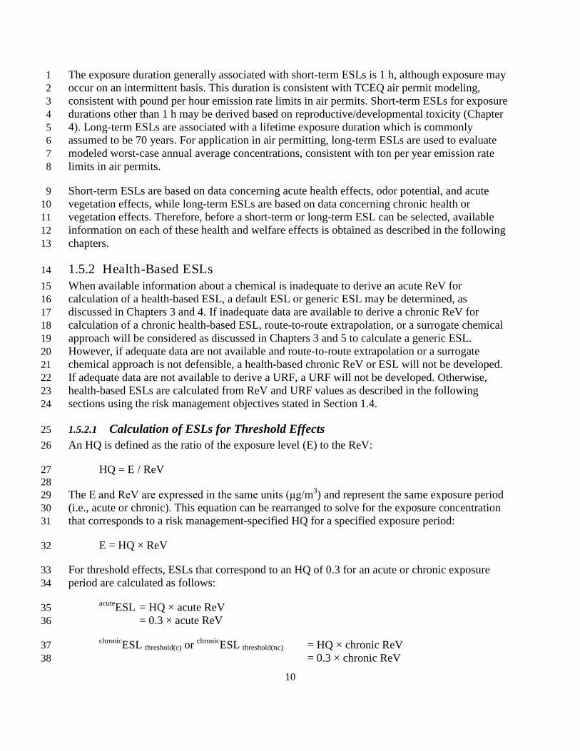
10

The exposure duration generally associated with short-term ESLs is 1 h, although exposure may 1 occur on an intermittent basis. This duration is consistent with TCEQ air permit modeling, 2 consistent with pound per hour emission rate limits in air permits. Short-term ESLs for exposure 3 durations other than 1 h may be derived based on reproductive/developmental toxicity (Chapter 4 4). Long-term ESLs are associated with a lifetime exposure duration which is commonly 5 assumed to be 70 years. For application in air permitting, long-term ESLs are used to evaluate 6 modeled worst-case annual average concentrations, consistent with ton per year emission rate 7 limits in air permits. 8

Short-term ESLs are based on data concerning acute health effects, odor potential, and acute 9 vegetation effects, while long-term ESLs are based on data concerning chronic health or 10 vegetation effects. Therefore, before a short-term or long-term ESL can be selected, available 11 information on each of these health and welfare effects is obtained as described in the following 12 chapters. 13

1.5.2 Health-Based ESLs 14 When available information about a chemical is inadequate to derive an acute ReV for 15 calculation of a health-based ESL, a default ESL or generic ESL may be determined, as 16 discussed in Chapters 3 and 4. If inadequate data are available to derive a chronic ReV for 17 calculation of a chronic health-based ESL, route-to-route extrapolation, or a surrogate chemical 18 approach will be considered as discussed in Chapters 3 and 5 to calculate a generic ESL. 19 However, if adequate data are not available and route-to-route extrapolation or a surrogate 20 chemical approach is not defensible, a health-based chronic ReV or ESL will not be developed. 21 If adequate data are not available to derive a URF, a URF will not be developed. Otherwise, 22 health-based ESLs are calculated from ReV and URF values as described in the following 23 sections using the risk management objectives stated in Section 1.4. 24

1.5.2.1 Calculation of ESLs for Threshold Effects 25 An HQ is defined as the ratio of the exposure level (E) to the ReV: 26

HQ = E / ReV 27 28

The E and ReV are expressed in the same units (μg/m3) and represent the same exposure period 29 (i.e., acute or chronic). This equation can be rearranged to solve for the exposure concentration 30 that corresponds to a risk management-specified HQ for a specified exposure period: 31

E = HQ × ReV 32

For threshold effects, ESLs that correspond to an HQ of 0.3 for an acute or chronic exposure 33 period are calculated as follows: 34

acuteESL = HQ × acute ReV 35 = 0.3 × acute ReV 36

chronicESL threshold(c) or chronicESL threshold(nc) = HQ × chronic ReV 37 = 0.3 × chronic ReV 38

11

1 The acuteESL, chronicESLthreshold(c) or chronicESLthreshold(nc) (HQ = 0.3) used for threshold effects are 2 not used to evaluate ambient air monitoring data. Acute and chronic ReVs are used as health-3 based AMCVs (Section 1.7). 4

1.5.2.2 Calculation of ESLs for Nonthreshold Effects 5 The URF is expressed in reciprocal units to E (i.e., μg/m3 and (μg/m3)-1, respectively) and both 6 represent a chronic exposure. This equation can be rearranged to solve for E (μg/m3) for a 7 chronic exposure period that corresponds to a specified no significant excess risk level: 8

Risk Level = E × URF 9 E = No Significant Risk Level / URF 10

For nonthreshold effects, the continuous lifetime exposure concentration of a chemical that 11 corresponds to TCEQ’s no significant excess risk level of 1 x 10-5 (chronicESLnonthreshold) is 12 calculated as follows: 13

chronicESLnonthreshold(c) and chronicESLnonthreshold(nc) = 1 x 10-5 / URF 14

However, when the nonthreshold effect is cancer mediated through a mutagenic MOA, 15 consideration of early-life exposure (Section 5.7.4) results in the following chronic ESL 16 calculation: 17

chronicESLnonthreshold(c) = 6 x 10-6 / URF

18

The chronicESLnonthreshold(c) and chronicESLnonthreshold(nc) are used in air permitting and as chronic 19 health-based AMCVs for evaluation of ambient air monitoring data. 20

1.5.3 Determination of Shor t-Term and Long-Term ESLs for Air Permitting 21 The preceding sections introduce the derivation of health-based ReVs and URFs. Chapter 2 22 describes the development of odor- and vegetation-based ESLs. A short-term ESL is determined 23 by choosing the lowest value of the following health- and welfare-based ESLs (as available): 24

acuteESL or acuteESLgeneric 25 acuteESLodor or generic acuteESLodor 26 acuteESLveg 27

A long-term ESL is determined by choosing the lowest value of the following health- and 28 welfare-based ESLs (as available): 29

chronicESLnonthreshold(c) 30 chronicESLnonthreshold(nc) 31 chronicESLthreshold(c) 32 chronicESLthreshold(nc) or generic chronicESLthreshold(nc) 33 chronicESLveg 34

12

If the Guidelines have not yet been used to develop a health-based ReV, original ESLs, termed 1 interim ESLs, are used. The processes whereby health- and welfare-based ESLs are developed 2 and then used to determine the short-term ESL (Figure 1-1) and long-term ESL (Figure 1-2) are 3 shown on the following pages. Go to 4 http://www.tceq.state.tx.us/implementation/tox/esl/list_main.html to download previous and 5 current ESL lists for Air Permitting. 6

7

13

1 Figure 1-1 Short-Term ESL development for air permitting 2

Conduct MOA analysis

Determine generichealth-based ESL

acuteESLgeneric

(Ch.3 & 4)

Calculate health-based ESLReV x 0.3 = acuteESL

Derive acuteReV

(Ch. 3 & 4)

Is chemicalodorous?

Determine acuteESLodoror generic acuteESLodor

(Ch.2)

Doeschemical

cause acutevegetativeeffects?

For health effects,is minimum

database met?

DetermineacuteESLveg

(Ch.2)

Conduct literature review and solicit informationfrom interested parties

Set the short-term ESLequal to the lowest of available:acuteESLgeneric,acuteESL,acuteESLodor,

generic acuteESLodor,acuteESLveg

No

No

No

Yes

Yes

Yes

14

1 Figure 1-2 Long-Term ESL development for air permitting2

Conduct literature review and solicit informationfrom interested parties

For cancereffects (based on

WOE*), isminimum

database met?

Based onMOA, is dose

responsenonthreshold?

Calculate cancer-based ESL10-5 / URF = chronicESLnonthreshold(c)ReV x 0.3 = chronicESLthreshold(c)

Derive URF(Ch. 3 & 5)

Derive chronicReV

(Ch. 3 & 5)

Fornoncancereffects, isminimumdatabase

met?

Based onMOA, is dose-

responsenonthreshold?

Derive URF(Ch. 3 & 5)

Derive chronicReV

(Ch. 3 & 5)

Calculate noncancer-based ESL10-5 / URF = chronicESLnonthreshold(c)ReV x 0.3 = chronicESLthreshold(nc)

Doeschemical

cause chronicvegetativeeffects?

DeterminechronicESLveg

(Ch.2)

Set the long-term ESLequal to the lowest of available**:chronicESLnonthreshold(c),chronicESLthreshold (c),chronicESLnonthreshold(nc),chronicESLthreshold(nc),chronicESLgeneric,

chronicESLveg

No

No

No

No

Yes

Yes

Yes

Yes orunknown

Yes

No orunknown

*WOE = weight of evidence**If no chronic ESLs can be derived, a long-term ESL will not be set.

Determine generichealth-based ESL

chronicESLgeneric

(Ch. 3 & 5)

15

1.6 Exemption of Substances from ESL Development 1 ESLs are developed for all substances determined by the TCEQ to be airborne toxicants. 2 Substances not considered to be airborne toxicants of significance are exempt from ESL 3 development. A substance is accorded exemption status by the TCEQ if the scientific evidence 4 or prior regulatory experience indicates that the substance should not be classified as an airborne 5 toxicant. In addition, the TCEQ does not develop ESLs for constituents with specific National 6 Ambient Air Quality Standards (NAAQS) or specific Texas state standards (Table 1-1). 7

Table 1-1 List of Chemicals with NAAQS and/or Texas State Standards 8 NAAQS State Standard Sulfur dioxide Sulfur dioxide Inhalable particulate matter (PM10) Hydrogen sulfide Fine particulate matter (PM2.5) Sulfuric acid Nitrogen dioxide Carbon monoxide Lead (elemental) Ozone

Substances may be added or removed from the exempt list if scientific evidence or regulatory 9 experience dictates a change in status. The TCEQ strongly encourages interested parties (e.g., 10 industry trade associations, individual companies, environmental groups, academia, etc.) to 11 submit technical information to aid in the categorization of substances as exempt or not. 12 Examples of substances currently exempt from ESL development are shown in Table 1-2 13

Table 1-2 Examples of Substances Exempt from ESL Development 14

Substance Comment

Argon major component of ambient air; simple asphyxiant

Carbon dioxide major component of ambient air

Ethane simple asphyxiant

Helium simple asphyxiant

Hydrogen simple asphyxiant

Methane simple asphyxiant

Neon simple asphyxiant

Nitrogen major component of ambient air; simple asphyxiant

Propane simple asphyxiant

Propylene simple asphyxiant

Fruit juices (apple, orange, etc.) generally considered as safe

Sweeteners (sugar, molasses, corn generally considered as safe

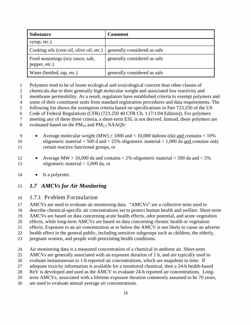
16

Substance Comment syrup, etc.)

Cooking oils (corn oil, olive oil, etc.) generally considered as safe

Food seasonings (soy sauce, salt, pepper, etc.)

generally considered as safe

Water (bottled, tap, etc.) generally considered as safe

Polymers tend to be of lesser ecological and toxicological concern than other classes of 1 chemicals due to their generally high molecular weight and associated low reactivity and 2 membrane permeability. As a result, regulators have established criteria to exempt polymers and 3 some of their constituent units from standard registration procedures and data requirements. The 4 following list shows the exemption criteria based on specifications in Part 723.250 of the US 5 Code of Federal Regulations (CFR) (723.250 40 CFR Ch. 1 (7/1/04 Edition)). For polymers 6 meeting any of these three criteria, a short-term ESL is not derived. Instead, these polymers are 7 evaluated based on the PM10 and PM2.5 NAAQS: 8

• Average molecular weight (MW) ≥ 1000 and < 10,000 daltons (da) and contains < 10% 9 oligomeric material < 500 d and < 25% oligomeric material < 1,000 da and

• Average MW > 10,000 da and contains < 2% oligomeric material < 500 da and < 5% 12 oligomeric material < 1,000 da, or 13

contains only 10 certain reactive functional groups, or 11

• Is a polyester. 14

1.7 AMCVs for Air Monitoring 15

1.7.1 Problem Formulation 16 AMCVs are used to evaluate air monitoring data. “AMCVs” are a collective term used to 17 describe chemical-specific air concentrations set to protect human health and welfare. Short-term 18 AMCVs are based on data concerning acute health effects, odor potential, and acute vegetation 19 effects, while long-term AMCVs are based on data concerning chronic health or vegetation 20 effects. Exposure to an air concentration at or below the AMCV is not likely to cause an adverse 21 health effect in the general public, including sensitive subgroups such as children, the elderly, 22 pregnant women, and people with preexisting health conditions. 23

Air monitoring data is a measured concentration of a chemical in ambient air. Short-term 24 AMCVs are generally associated with an exposure duration of 1 h, and are typically used to 25 evaluate instantaneous to 1-h reported air concentrations, which are snapshots in time. If 26 adequate toxicity information is available for a monitored chemical, then a 24-h health-based 27 ReV is developed and used as the AMCV to evaluate 24-h reported air concentrations. Long-28 term AMCVs, associated with a lifetime exposure duration commonly assumed to be 70 years, 29 are used to evaluate annual average air concentrations. 30

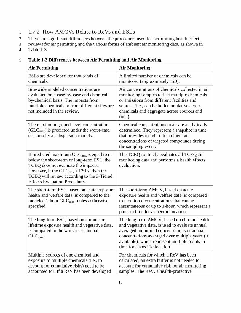
17

1.7.2 How AMCVs Relate to ReVs and ESLs 1 There are significant differences between the procedures used for performing health effect 2 reviews for air permitting and the various forms of ambient air monitoring data, as shown in 3 Table 1-3. 4

Table 1-3 Differences between Air Permitting and Air Monitoring 5

Air Permitting Air Monitoring

ESLs are developed for thousands of chemicals.

A limited number of chemicals can be monitored (approximately 120).

Site-wide modeled concentrations are evaluated on a case-by-case and chemical-by-chemical basis. The impacts from multiple chemicals or from different sites are not included in the review.

Air concentrations of chemicals collected in air monitoring samples reflect multiple chemicals or emissions from different facilities and sources (i.e., can be both cumulative across chemicals and aggregate across sources and time).

The maximum ground-level concentration (GLCmax) is predicted under the worst-case scenario by air dispersion models.

Chemical concentrations in air are analytically determined. They represent a snapshot in time that provides insight into ambient air concentrations of targeted compounds during the sampling event.

If predicted maximum GLCmax is equal to or below the short-term or long-term ESL, the TCEQ does not evaluate the impacts. However, if the GLCmax > ESLs, then the TCEQ will review according to the 3-Tiered Effects Evaluation Procedures.

The TCEQ routinely evaluates all TCEQ air monitoring data and performs a health effects evaluation.

The short-term ESL, based on acute exposure health and welfare data, is compared to the modeled 1-hour GLCmax, unless otherwise specified.

The short-term AMCV, based on acute exposure health and welfare data, is compared to monitored concentrations that can be instantaneous or up to 1-hour, which represent a point in time for a specific location.

The long-term ESL, based on chronic or lifetime exposure health and vegetative data, is compared to the worst-case annual GLCmax.

The long-term AMCV, based on chronic health and vegetative data, is used to evaluate annual averaged monitored concentrations or annual concentrations averaged over multiple years (if available), which represent multiple points in time for a specific location.

Multiple sources of one chemical and exposure to multiple chemicals (i.e., to account for cumulative risks) need to be accounted for. If a ReV has been developed

For chemicals for which a ReV has been calculated, an extra buffer is not needed to account for cumulative risk for air monitoring samples. The ReV, a health-protective

18

Air Permitting Air Monitoring for a chemical, an extra buffer is used to calculate health-based ESLs that are 70% lower than the ReV.

concentration, is appropriate.

The terms “short-term ESL” and “long-term ESL” have specific meanings and uses in the air permitting program and regulatory guidance.

TCEQ staff uses all comparison values (i.e., odor-, vegetative-, and health-based values).

ESLs are the terminology used for air permitting.

AMCVs are the terminology used for ambient air monitoring because of the significant differences from the air permitting program.

Because of these differences, different risk management objectives are used for air monitoring, 1 as discussed in Section 1.4.3 Air Monitoring Risk Management Objectives. The TCEQ has begun 2 using the term “AMCVs” in evaluations of air monitoring data. The term “AMCVs” is a 3 collective term and refers to all odor-, vegetative-, and health-based values used in reviewing air 4 monitoring data. The use of different values and different terminology is appropriate because the 5 air monitoring and air permitting programs perform different functions in the protection of 6 human health and welfare. The main difference between values used in air monitoring and air 7 permitting involve the use of the ReV. The ReV is used for air monitoring whereas the health-8 based ESL, which is 70% lower than the ReV, is used in air permitting. Table 1-4 show the 9 relationship between different types of AMCVs and ESLs. 10

Table 1-4 How AMCVs Relate to ESLs 11

AMCV Definition

Odor AMCV acuteESLodor

short-term vegetation AMCV acuteESLveg

long-term vegetation AMCV chronicESLveg

1-h short-term health AMCV 1-h Acute ReV or acuteESLgeneric or interim acute ESL1

24-h short-term health AMCV 24-h ReV

long-term health AMCV lowest value of the chronic ReV [threshold(c)], chronic ReV [threshold(nc)], chronicESLnonthreshold(c), chronicESLnonthreshold(nc) or interim chronic ESL 1

1 If the Guidelines have not yet been used to develop a health-based ReV, original ESLs, termed 12 interim ESLs, are used. 13

Go to http://www.tceq.state.tx.us/implementation/tox/AirToxics.html to download the list of the 14 odor-, vegetative-, and health-based AMCVs. 15

19

1.8 Summary of Toxicity Factors in TCEQ Program Areas 1 The TCEQ develops ReV, URF, RfD, SFo, and ESL values and designates AMCV values to 2 provide toxicological support to multiple program areas within the TCEQ. In the air permit 3 review process, the TCEQ utilizes short- and long-term ESLs to evaluate proposed emissions for 4 their potential to adversely affect human health and welfare (Table 1-5). For evaluation of 5 ambient air monitoring results, AMCVs are used to assess the potential for exposure to the 6 measured concentrations to adversely affect human health and welfare (Table 1-5). 7

Table 1-5 Uses of ESLs and AMCVs in Air Permitting and Air Monitoring 8

Air Permitting ESLs

Air Monitoring 1 AMCVs

Short-term Exposure

Short-Term ESLlowest value of:

is defined as the

acuteESLgeneric, acuteESL, acuteESLodor, generic acuteESLodor, or acuteESLveg (Figure 1-1)

Short-Term Health 2

Acute ReV, or =

acuteESLgeneric, or interim ESL3

Odor = acuteESLodor

Short-Term Vegetation

Long-term Exposure

= acuteESLveg

Long-Term ESLlowest value of:

is defined as the

chronicESLnonthreshold(c), chronicESLnonthreshold(nc), chronicESLthreshold(c), chronicESLthreshold(nc), or chronicESLveg chronicESLgeneric (Figure 1-2)

Long-Term Health

Chronic ReV [threshold(c)],

is the lowest value

of:

Chronic ReV [threshold(nc)], chronicESLnonthreshold(c), or chronicESLnonthreshold(nc)

Long-Term Vegetation

1 All values are used in the review of measured analytical concentrations for air monitoring data 9

= chronicESLveg

2 Short-Term health AMCVs are usually designated for 1 h exposure duration. A 24-h ReV may be 10 developed if adequate data is available 11

3 If the Guidelines have not yet been used to develop a health-based ReV, original ESLs, termed interim 12 ESLs, are used in both program areas 13

Lastly, in accordance with rule requirements and guidance, the TCEQ uses chronic ReV, URF, 14 RfD, and SFo values as toxicity factors for both the current TRRP rule (30 TAC §350) and the 15 dated 1993 Risk Reduction Rule (Subchapters A and S of 30 TAC §335) ) to derive health-16 protective environmental media (e.g., soil, groundwater) cleanup levels for the TCEQ’s 17 remediation program. Please refer to the current TRRP rule (30 TAC §350) and dated 1993 Risk 18 Reduction Rule (Subchapters A and S of 30 TAC §335) for information regarding how toxicity 19 factors are used to calculate media cleanup levels as this is beyond the scope of this document. 20

20

1.9 Toxicity Factor Development Support Document (DSD) 1 The purpose of the DSD is to provide a summary of information on the toxicity factor 2 development process and the key toxicity studies/information used to derive inhalation and oral 3 toxicity factors. First, several summary tables of key information are provided followed by a 4 brief summary of occurrence and use of the chemical. As discussed in Section 3.3, the following 5 analytical approach is used to derive toxicity factors for chemicals: review essential data 6 including physical/chemical properties and select key studies; conduct a MOA analysis; choose 7 the appropriate dose metric; determine the POD for each key study; conduct appropriate 8 dosimetric modeling; select critical effect; and extrapolate from the adjusted POD to lower 9 exposures based on MOA analysis. These key steps are discussed in the DSD for each chemical. 10 Finally, a section entitled “Other Relevant Information” may be included, if additional 11 information pertinent to an understanding of the toxicity of the compound is available. At the end 12 of the DSD, there are two separate reference sections: a list of the references of key studies 13 discussed in the DSD and a list of references of other studies that were reviewed and considered 14 by the TCEQ staff but were not discussed in the DSD. 15

Often, toxicity factors for a chemical without existing toxicity factors are needed on an expedited 16 basis (e.g., within weeks). Due to time limitations, DSDs are not developed for toxicity factors 17 developed in these situations. However, documentation is created which memorializes derivation 18 of the values consistent with these guidelines. In the absence of such time constraints, a DSD is 19 developed for toxicity factors. 20

1.10 Selection of Chemicals and Data Solicitation for Air Programs 21 On an approximately annual basis, the TCEQ selects about 10-15 chemicals for the development 22 of inhalation toxicity factors. Selection of the specific chemicals is made in consultation with 23 TCEQ upper management and considers the following: 24

• Mass of emissions reported 25

• Frequency with which the chemical is permitted 26

• Ambient monitoring data 27

• Public input 28

The TCEQ publishes the list of chemicals under consideration for ESL development on the 29 TCEQ website approximately once per year and encourages submission of relevant data from 30 interested parties (e.g., citizens, industry trade associations, individual companies, environmental 31 groups, academia, etc.). 32

1.11 Selection of Chemicals and Data Solicitation for Remediation 33 Toxicity factors are developed on an as-needed basis for remediation programs. For example, 34 some site contaminants may not have existing toxicity factors developed by other agencies (e.g., 35 USEPA, ATSDR). Requests for toxicity factors for such chemicals typically come from the 36 TCEQ project manager or an outside environmental consultant assessing a remediation site. 37

21

Additionally, the TCEQ may identify a chemical for toxicity factor development because the 1 existing factors are outdated. Having up-to-date oral toxicity factors (i.e., RfD, SFo) is of 2 particularly high importance because they are typically the drivers (i.e., the critical 3 concentration-limiting factors) in calculations of media cleanup values for remediation sites. 4

1.12 Public Comment and Peer-Review of DSDs 5 A Development Team composed of TCEQ toxicologists conducts the data evaluation, data 6 selection, and development for each chemical under review. The product of this effort is a Draft 7 DSD which is then circulated to other TCEQ toxicologists for review and comment. Suggested 8 changes/revisions are incorporated, resulting in a Proposed DSD. 9

The Proposed DSD is published on the TCEQ website for a 90-day public review and comment 10 period. For data-rich or controversial substances, additional time may be allowed so interested 11 parties will have adequate time to submit comments on the Proposed DSD. Following the review 12 and comment period, the Development Team reviews the comments that were received, 13 addresses and resolves relevant issues, and seeks internal consensus on the original or modified 14 values and the accompanying scientific rationale. Following resolution of relevant issues raised 15 through public review and comment, the ReV, ESL, URF, RfD and/or SFo values are classified 16 as final. The public comments, TCEQ response to public comments, and the final DSD are 17 posted on the TCEQ website. The chemical may be reviewed again if compelling new data 18 become available. 19

Individual DSDs are not routinely submitted for external scientific peer review, although 20 scientists are encouraged to comment on the DSDs during the public comment period. External 21 scientific peer reviews are expensive and the TCEQ does not have the resources to conduct peer 22 reviews for the approximately 10-15 chemicals for which it plans to develop toxicity values each 23 year. However, this regulatory guidance document did undergo external scientific peer review 24 and public comment. The TCEQ may occasionally decide to conduct an external scientific peer 25 review of an individual DSD if sufficient public interest is expressed and if resources are 26 available (e.g., 1-3 butadiene (TCEQ 2008), nickel and nickel compounds (TCEQ 2009), and 27 inorganic arsenic and arsenic compounds (TCEQ 2010)).28

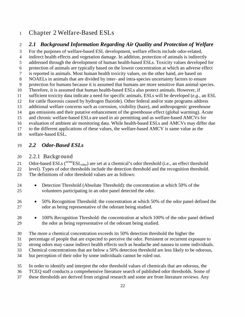
22

Chapter 2 Welfare-Based ESLs 1

2.1 Background Information Regarding Air Quality and Protection of Welfare 2 For the purposes of welfare-based ESL development, welfare effects include odor-related, 3 indirect health effects and vegetation damage. In addition, protection of animals is indirectly 4 addressed through the development of human health-based ESLs. Toxicity values developed for 5 protection of animals are typically based on the lowest concentration at which an adverse effect 6 is reported in animals. Most human health toxicity values, on the other hand, are based on 7 NOAELs in animals that are divided by inter- and intra-species uncertainty factors to ensure 8 protection for humans because it is assumed that humans are more sensitive than animal species. 9 Therefore, it is assumed that human health-based ESLs also protect animals. However, if 10 sufficient toxicity data indicate a need for specific animals, ESLs will be developed (e.g., an ESL 11 for cattle fluorosis caused by hydrogen fluoride). Other federal and/or state programs address 12 additional welfare concerns such as corrosion, visibility (haze), and anthropogenic greenhouse 13 gas emissions and their putative enhancement of the greenhouse effect (global warming). Acute 14 and chronic welfare-based ESLs are used in air permitting and as welfare-based AMCVs for 15 evaluation of ambient air monitoring data. While health-based ESLs and AMCVs may differ due 16 to the different applications of these values, the welfare-based AMCV is same value as the 17 welfare-based ESL. 18

2.2 Odor-Based ESLs 19

2.2.1 Background 20 Odor-based ESLs (acuteESLodor) are set at a chemical’s odor threshold (i.e., an effect threshold 21 level). Types of odor thresholds include the detection threshold and the recognition threshold. 22 The definitions of odor threshold values are as follows: 23

• Detection Threshold (Absolute Threshold): the concentration at which 50% of the 24 volunteers participating in an odor panel detected the odor. 25

• 50% Recognition Threshold: the concentration at which 50% of the odor panel defined the 26 odor as being representative of the odorant being studied. 27

• 100% Recognition Threshold: the concentration at which 100% of the odor panel defined 28 the odor as being representative of the odorant being studied. 29

The more a chemical concentration exceeds its 50% detection threshold the higher the 30 percentage of people that are expected to perceive the odor. Persistent or recurrent exposure to 31 strong odors may cause indirect health effects such as headache and nausea in some individuals. 32 Chemical concentrations that are below a 50% detection threshold are less likely to be odorous, 33 but perception of their odor by some individuals cannot be ruled out. 34

In order to identify and interpret the odor threshold values of chemicals that are odorous, the 35 TCEQ staff conducts a comprehensive literature search of published odor thresholds. Some of 36 these thresholds are derived from original research and some are from literature reviews. Any 37

23

updated study is considered when developing an odor-based ESL as discussed in the following 1 sections. It should be noted that reported odor threshold data often differ considerably. It is not 2 uncommon for reported odor threshold values to range over several orders of magnitude for the 3 same chemical. For example, 26 values were reported for hydrogen sulfide, ranging from 0.072 - 4 1,400 parts per billion by volume (ppbv), a factor of 10,000. Major sources of variability include 5 different types of data sources; differences in experimental methodology; and human olfactory 6 response characteristics, which exhibit a great deal of inter-individual variability. 7

In a report: “Odor Threshold for Chemicals with Established Occupational Health Standards”, 8 the American Industrial Hygiene Association (AIHA 1989) reviewed and critiqued odor 9 threshold data for 182 chemicals which have a threshold limit value (TLV). The project 10 developed a set of criteria for acceptability of odor threshold measurement techniques to evaluate 11 the experimental odor threshold determinations reported in the literature. The criteria are briefly 12 summarized below. 13 14

• Panel size of at least six people per group 15 • Panelist selection based on odor sensitivity 16 • Panel calibration 17 • Consideration of vapor modality (air or water) 18 • Diluent in accord with compound 19 • Presentation mode that minimizes additional dilution (ambient) air intake 20 • Analytical measurement of odorant concentration 21 • Calibration of flow rate and face velocity (olfactometers) 22 • Concentration presentation series that reduces olfactory fatigue 23 • Repeated trials 24 • Forced-choice procedure 25 • Concentration steps increasing by a factor of two or three 26

Of the 182 odorants with a TLV, the AIHA review resulted in 110 compounds, from 36 27 reference sources, that had odor threshold values that met evaluation criteria (AIHA 1989). The 28 AIHA approach was then used by the United States Environmental Protection Agency (USEPA 29 1992a) to conduct critical reviews of published odor threshold values for the chemicals listed as 30 hazardous air pollutants (HAPs) in the 1990 Clean Air Act Amendments. The review resulted in 31 57 odorous HAPs from 16 reference sources with acceptable odor threshold values (USEPA 32 1992a). 33

In the past, an acuteESLodor was generally set at the lowest acceptable odor threshold value that 34 met the evaluation criteria set by AIHA and USEPA. To set appropriate acuteESLodor values for 35 odorous air contaminants, the odor threshold values for chemicals that have been critiqued and 36 accepted by AIHA and USEPA or current odor studies that have been conducted in accordance 37 with criteria established by AIHA and USEPA were considered first. However, these primary 38 experimental odor threshold values established prior to 1989 may be outdated. Therefore, in 39 order to set appropriate acuteESLodor values for odorous air contaminants, an additional evaluation 40 is needed. 41

24

2.2.2 Evaluation 1 van Harreveld et al. (1999) reported that since the early 1990s, the introduction of improved 2 instrument calibration, improved panel screening procedures and the adoption of n-butanol as a 3 reference material, have enabled more objective odor measurements. Additionally, in a National 4 Advisory Committee for Acute Exposure Guideline Levels for Hazardous Substances 5 (NAC/AEGL Committee) meeting, van Doorn et al. (2002) stated that odor thresholds reported 6 more than several decades ago probably were not obtained under the same conditions of 7 methodological precision compared to today’s olfactometer methods. van Doorn et al. (2002) 8 further indicated that modern performance tests, such as using forced choice dynamic 9 olfactometry, has greatly improved the objectivity, sensitivity, repeatability, and reproducibility 10 of odor threshold determinations. Standardized odor measurement practices published by the 11 American Society of Testing and Materials (ASTM E679), Dutch Standard (NVN 2820), 12 Australia/New Zealand Standard (AS/NZS4323.3:2001), and European Committee for 13 Standardization (CEN) Standard (CEN 13725); as well as the Japanese Triangle Odor Bag 14 Method are considered the preferred olfactometry methods (Ruijten et al. 2009, van Doorn et al. 15 2002, McGinley 2002, Mahin 2003). These standard methods are considered objective, 16 quantitative, dependable, and reproducible (St. Croix Sensory 2005). The following are some of 17 the latest publications of these preferred standardized methods of measuring odor: 18

• The American Society of Testing and Materials (ASTM) Standard of Practice E679-04: 19 Standard Practice for Determination of Odor and Taste Threshold by a Forced-Choice 20 Ascending Concentration Series Method of Limits (ASTM 2004). 21

• The European Committee for Standardization (CEN) Standard CEN 13725:2003: Air 22 Quality – Determination of Odour Concentration by Dynamic Olfactometry (CEN 2003). 23

• The Australian/New Zealand Standard. AS/NZS4323.3:2001: Stationary source 24 emissions. Part 3: Determination of odour concentration by dynamic olfactometry. 25 Standard Australia, Sydney, Australia (AS/NZS 2003). 26

• The Dutch Standard NVN 2820: Air Quality, Sensory Odour Measurement Using an 27 Olfactometer (Netherlands 1995). The Japanese Triangle Odor Bag Method (Iwasaki 28 2003, Nagata 2003). 29

• An 8-station vapor delivery device (VDD8), ascending concentration approach. (Cain et 30 al. 2007; Cometto-Muñiz and Abraham 2008). 31

• Air and Waste Management Association (AWMA) EE-6 Subcommittee on the 32 Standardization of Odor Measurement. Guidelines for odor sampling and measurement by 33 dynamic dilution olfactometry (AWMA 2002). 34

• Others such as those reported by McGinley (2001), St. Croix Sensory (2005). 35

Several studies comparing results of odor thresholds for compounds determined by these 36 methods indicated that the detection thresholds obtained using the Japanese triangle method (e.g. 37 odor threshold values from Nagata (2003)) appear to be in close agreement with those obtained 38

25

using the European or Dutch standard methods. The differences between the methods are quite 1 small compared to those commonly reported for olfactometry. All these methods are considered 2 compatible and preferred methods for measuring odor (Ruijten et al. 2009, Hoshika et al. 1993, 3 van Doom et al. 2002, Nagata 2003, van Harreveld 2003, McGinley 2001). 4

The National Advisory Committee Acute Exposure Guideline Level (NAC/AEGL) Committee 5 (van Doom et al. 2002) and the Netherlands National Institute for Public Health and the 6 Environment (Ruijten et al. 2009) have also defined the following quality levels for all odor 7 thresholds reported in the literature: 8

• Level 1: the threshold of a compound determined according to the aforementioned 9 standardized methods. 10

• Level 2: thresholds from other sources other than the aforementioned standardized 11 methods that include an internal reference to an n-butanol standard. Level 2 odor 12 thresholds are corrected by the ratio of the reference value of 40 ppb threshold for n-13 butanol to the measured value for n-butanol determined in the test panel (refer to Section 14 2.2.4 for an example calculation for a Level 2 corrected odor threshold). 15

• Level 3: thresholds measured without an internal reference to an n-butanol standard that 16 meet the criteria (Code A) for odor studies established by AIHA and USEPA. Such 17 thresholds are often found in compilations by AIHA and USEPA. 18

2.2.3 Guidelines for Setting Odor -Based ESLs 19 In general, odor detection values defined as Level 1 by the NAC/AEGL Committee (van Doom 20 et al. 2002) and the Netherlands National Institute for Public Health and the Environment 21 (Ruijten et al. 2009) will be considered first in setting the acuteESLodor values. If no Level 1 values 22 are available, Level 2 quality data will be considered. If no Level 1 or 2 odor thresholds are 23 available, then Level 3 quality data that meet the criteria from the AIHA (1989) and USEPA 24 (1992) may be used, as discussed in the following sections and illustrated by the flow chart in 25 Figure 2.1. In the case of air permit reviews only, surrogate odor-ESLs may be extrapolated from 26 similar structure-activity relationship (SAR) chemicals with acceptable odor threshold values for 27 chemicals that belong to chemical groups with known unpleasant odor, yet have no odor 28 threshold values (i.e., acetates, alcohols, aldehydes, alkenes, aromatics, ketones, reduced sulfur 29 and carboxylic acids), see Section 2.2.6 below.30

26

Figure 2-1 Flowchart for Setting Odor-Based Effects Screening Levels

Set theacuteESLodor at the

lowest value

Set theacuteESLodor at

the lowest Level 3 value

Develop ageneric

acuteESLodor

Set theacuteESLodor at theavailable butanol-corrected Level 2

value

Determine thegeometric meanof Level 1 values

Set theacuteESLodor at theavailable Level 1

value

Determine thegeometric mean

of butanol-corrected Level 2

values

Set the acuteESLodorat the geometric

mean of the Level 1values

Set theacuteESLodor at thelowest reportedLevel 1 value

Set the acuteESLodorat the geometricmean of butanol-corrected Level 2

values

Set the acuteESLodorat the lowest

butanol-correctedLevel 2 value

AreLevel 1 a odor threshold values

available?

AreLevel 2 b odor threshold values

available?

AreLevel 3 c odor threshold valuesdetermined from 1990 or after

available?

AreLevel 3 c odor threshold

values determined before1990 available?

Is there more than oneLevel 2 value available?

Is there more than oneLevel 1 value available?

Have TCEQfield staff reported odors at

measured levels at or lower thanthe geometric mean?

Have TCEQfield staff reported odors at

measured levels at or lower thanthe geometric mean?

Yes

Yes

Yes

Yes

Yes

Yes

Yes

Yes

No

No

No

No

No

No

No

No

a Level 1: the threshold of a compound determined according to the listed standardized methods in Section 2.

b Level 2: thresholds from other sources other than the standardized methods that include an internal reference to an n-butanol standard. Level 2 odor thresholds are corrected by the ratio of the reference value of 40 ppb (121 µg/m3) threshold for n-butanol to the measured value for n-butanol determined in the test panel (refer to Appendix A).

c Level 3: thresholds measured without an internal reference to an n-butanol standard that meet the criteria (Code A) for odor studies established by AIHA and USEPA. Such thresholds are often found in compilations by AIHA and USEPA.

Are datasufficient to develop an

acuteESLodor for structurally-related chemicals?

Yes

Don’t develop anacuteESLodor

No

27

2.2.3.1 Level 1 and 2 odor threshold values 1 While the acuteESLodor is generally set at the lowest acceptable odor threshold (TCEQ 2006), 2 according to the NAC/AEGL Committee’s guidance for the application of odor in emergency 3 response and the Netherlands’ assessment of odor annoyance in chemical emergency 4 management, the geometric mean of all Level 1 or Level 2 odor thresholds, instead of the lowest 5 odor threshold, is determined to be the odor detection threshold (OT50) (van Doorn et al. 2002, 6 Ruijten et al. 2009). Considering that most standardized methods as those listed in Section 2.2.2 7 are the compatible and preferred methods for measuring odor, it would be more reasonable to use 8 the geometric mean of odor thresholds rather than selecting the lowest one. Level 1 and Level 2 9 odor thresholds will not be combined to arrive at a single geometric mean, because Level 1 odor 10 thresholds are preferred over Level 2 odor thresholds. 11

However, the TCEQ may set the acuteESLodor values at the lowest acceptable reported odor 12 thresholds rather than the geometric mean if available data indicate that TCEQ air mobile 13 monitoring staff members and/or field investigators have reported odors at measured levels at or 14 lower than the geometric mean. Examples of such odorous air contaminants include, but are not 15 limited to, styrene, alkyl amines, reduced sulfur compounds, or other sharp/pungent odorous 16 compounds. 17

2.2.3.2 Level 3 odor threshold values determined from 1990 onward 18 All experimental threshold detection values for an odorous air contaminant reported from 1990 19 and later that meet the criteria established by AIHA and USEPA will be preferentially used to set 20 an acuteESLodor (i.e., if acceptable odor threshold values for a chemical are reported before and 21 after 1990, only those reported after 1990 will be used for setting an acuteESLodor for that 22 chemical). The acuteESLodor is set at the lowest acceptable 50% detection threshold. 23

2.2.3.3 Level 3 odor threshold values determined before 1990 24 For odorous air contaminants with experimental odor threshold values that were determined 25 before 1990, e.g., those found in compilations by AIHA (1989) or USEPA (1992), the TD will 26 continue to set the acuteESLodor values at the lowest acceptable 50% detection threshold. To select 27 an appropriate odor threshold value from those that were reported before 1990, van Doorn et al. 28 (2002) and Ruijten et al. (2009) suggested that the best choice would be the lowest reported 29 value from all acceptable sources and not the geometric mean, because the bias introduced by 30 older inadequate testing methodology is always towards higher odor thresholds. 31

2.2.4 Calculation of Level 2 Corrected Odor Detection Threshold 32 As described by van Doom et al. (2002) in Section 2.2.2 for Level 2, the Level 2 corrected 50% 33 odor detection threshold (OT50) for a chemical (reported to be X ppb) is corrected by the ratio of 34 the internal reference value of 40 ppb threshold for n-butanol standard to the measured value for 35 n-butanol determined in the same test panel (reported as Y ppb). Thus, to calculate the corrected 36 OT50 for the chemical, the following equations are used: 37

corrected OT50 for chemical (ppb) = X ppb * 40 ppb / Y ppb 38

28

Where: 1

X = OT50 for chemical 2 Y = OT50 for n-butanol reported in same study as chemical X 3

2.2.5 Duration Adjustments and use of an acuteESLodor for Longer Exposure 4 Durations 5

The acuteESLodor is generally set based on exposure of humans to chemicals for periods 6 significantly less than 1 h. These short duration exposure periods are not adjusted to reflect a 1-h 7 exposure duration because the perception of odor is concentration dependent rather than duration 8 dependent (i.e., an enhanced response is not produced by prolonged exposure) (NRC 2001). 9 Since odor is concentration dependent, the 1-h acuteESLodor may be used to evaluate odor-potential 10 for longer averaging times (i.e., they can be used on a limited basis as odor-based 24-h AMCVs). 11 If the 24-h ambient air concentration is above the odor-based AMCV, then odors would be 12 expected to occur. However, if the 24-h concentration is below the odor-based AMCV, then it 13 does not indicate that odors did not occur, since it is possible that a peak 1-h ambient air 14 concentration above the 1-h odor-based ESL could have occurred. 15

2.2.6 Odorous Compounds with Limited Odor Threshold Values 16

2.2.6.1 Chemical Groups and Correlation with Carbon Chain Length 17 Certain chemical groups, such as mercaptans, sulfides, aldehydes, alcohols, and alkenes, are 18 known to be odorous, highlighting the need to derive an odor-based ESL for such chemicals even 19 in the absence of odor threshold data. Previous studies have demonstrated that chemical groups 20 have characteristic odors that are directly related to their molecular structure, including 21 functional groups, molecular weight, carbon chain length, steric hindrance and electronic effects 22 (Klopping 1971, Moncrieff 1967, Punter 1983, Verschueren 2001, Nagata 2003). In most cases, 23 there is the tendency for the odor threshold to decrease as the molecular weight or carbon chain 24 length increases within a specific chemical group. For some chemical groups, the relationship 25 between carbon chain length and odor threshold is so strong that it can be used to estimate the 26 odor threshold for compounds within that group that have limited odor data (Cometto-Muniz et 27 al. 1998, Cometto-Muniz and Cain 1993, Cometto-Muniz and Cain 1990, Cometto-Muniz and 28 Abraham 2008). The TCEQ conducted a correlation study using a list of approved, Level 1 29 reference OT50 values that were generated using the aforementioned guidance, to identify the 30 relationship between log OT50 and carbon chain length (Bredfeldt et al. 2011). 31

We found that for acetates, alcohols, alkenes, aldehydes, aromatic hydrocarbons, and ketones 32 there were strong to moderate correlations (i.e., R2 > 0.7and R2 > 0.3, respectively) between 33 carbon chain length and log OT50 values. (Figures 2-2 A-F). Amines, carboxylic acids, 34 mercaptans, and sulfides had a weak correlation (i.e., R2 < 0.3) between carbon chain and odor 35 threshold (Figures 2-3 A-D). However, these chemical groups could be expected to have very 36 unpleasant odors, highlighting the importance of derivation of an odor-based ESL for these 37 particular chemical groups. Figures 2-2 and 2-3 illustrate the relationship between log OT50 and 38 carbon chain length for specific chemical groups. 39

29

A

B

C

D

E

F

Figure 2-2 Good correlation of Log OT50 to carbon chain number for selected chemical 1 groups 2 Log OT50 correlates with carbon chain number for (A) acetates (R2 = 0.77); (B) alcohols (R2 = 0.75); (C) 3 alkenes (R2 = 0.8); (D) aldehydes (R2 = 0.46); (E) aromatic hydrocarbons (R2 = 0.63); and (F) ketones (R2 4 = 0.71). 5

30

A

B

C

D

Figure 2-3 Poor correlation of Log OT50 to carbon chain number for selected chemical 1 groups 2 Log OT50 does not have a strong correlation with carbon chain number for (A) amines (R2 = 3 0.05); (B) carboxylic acids (R2 = 0.28); (C) mercaptans (R2 = 0.28); or (D) sulfides (R2 = 0.11). 4

2.2.6.2 Derivation of a Generic acuteESLodor for Chemicals with Limited Odor Data 5 For air permit reviews only, the data from specific chemical groups may be used as a surrogate 6 for structurally-related chemicals with unavailable odor data based on professional judgment. For 7 example, to derive an odor-based ESL for a chemical with limited odor data, the chemical 8 structure of the compound in question is identified. For structurally-related chemicals that have a 9 good correlation between log OT50 and carbon chain length within a given chemical group 10 (Figures 2-2 A-F), the equation describing this relationship is used to derive the generic odor-11 based ESL. The correlation equations for acetates, alcohols, alkenes, aldehydes, aromatic 12 hydrocarbons and ketones that describe the relationship between carbon chain length (x) and log 13 OT50 (ppb) are summarized in Table 2-1. 14

15

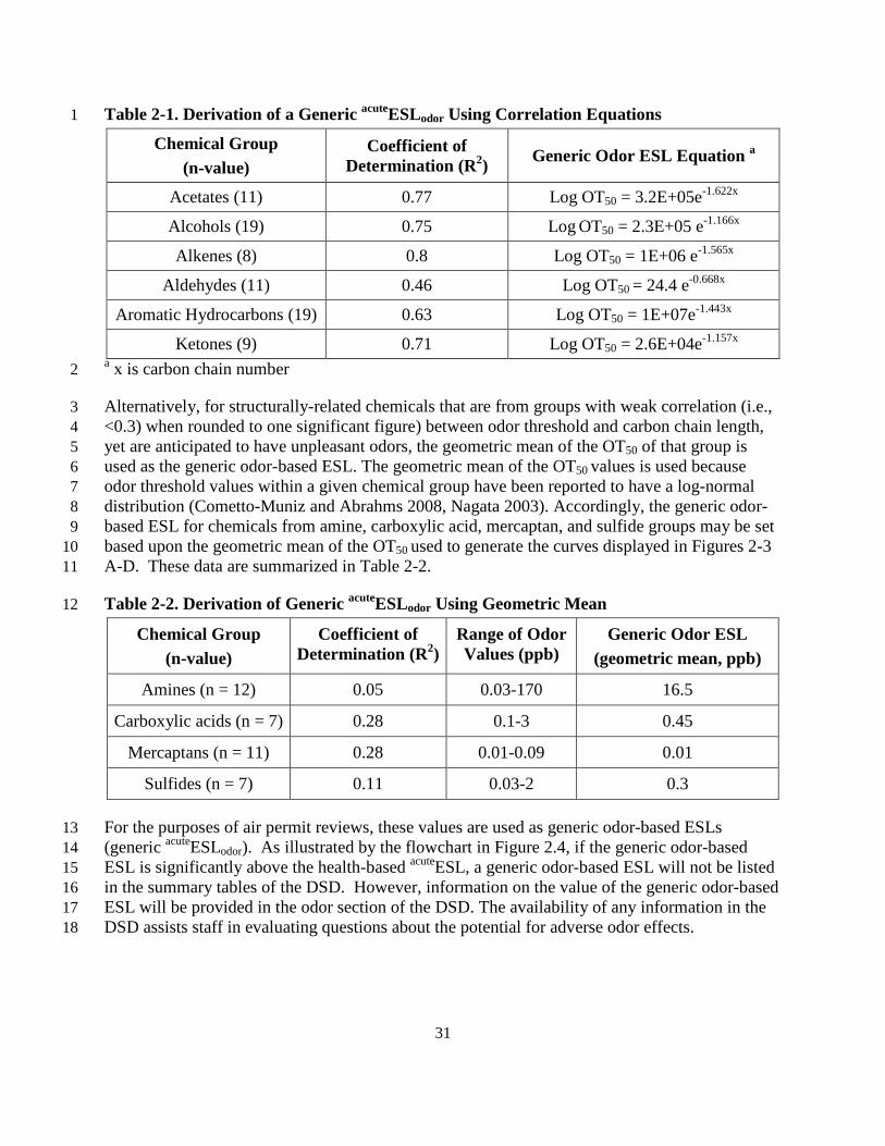
31

Table 2-1. Derivation of a Generic acuteESLodor Using Correlation Equations 1

Chemical Group (n-value)

Coefficient of Determination (R2) Generic Odor ESL Equation a

Acetates (11) 0.77 Log OT50 = 3.2E+05e-1.622x

Alcohols (19) 0.75 Log OT50 = 2.3E+05 e-1.166x

Alkenes (8) 0.8 Log OT50 = 1E+06 e-1.565x

Aldehydes (11) 0.46 Log OT50 = 24.4 e-0.668x

Aromatic Hydrocarbons (19) 0.63 Log OT50 = 1E+07e-1.443x

Ketones (9) 0.71 Log OT50 = 2.6E+04e-1.157x a x is carbon chain number 2

Alternatively, for structurally-related chemicals that are from groups with weak correlation (i.e., 3 <0.3) when rounded to one significant figure) between odor threshold and carbon chain length, 4 yet are anticipated to have unpleasant odors, the geometric mean of the OT50 of that group is 5 used as the generic odor-based ESL. The geometric mean of the OT50 values is used because 6 odor threshold values within a given chemical group have been reported to have a log-normal 7 distribution (Cometto-Muniz and Abrahms 2008, Nagata 2003). Accordingly, the generic odor- 8 based ESL for chemicals from amine, carboxylic acid, mercaptan, and sulfide groups may be set 9 based upon the geometric mean of the OT50 used to generate the curves displayed in Figures 2-3 10 A-D. These data are summarized in Table 2-2. 11

Table 2-2. Derivation of Generic acuteESLodor Using Geometric Mean 12

Chemical Group (n-value)

Coefficient of Determination (R2)

Range of Odor Values (ppb)

Generic Odor ESL (geometric mean, ppb)

Amines (n = 12) 0.05 0.03-170 16.5

Carboxylic acids (n = 7) 0.28 0.1-3 0.45

Mercaptans (n = 11) 0.28 0.01-0.09 0.01

Sulfides (n = 7) 0.11 0.03-2 0.3

For the purposes of air permit reviews, these values are used as generic odor-based ESLs 13 (generic acuteESLodor). As illustrated by the flowchart in Figure 2.4, if the generic odor-based 14 ESL is significantly above the health-based acuteESL, a generic odor-based ESL will not be listed 15 in the summary tables of the DSD. However, information on the value of the generic odor-based 16 ESL will be provided in the odor section of the DSD. The availability of any information in the 17 DSD assists staff in evaluating questions about the potential for adverse odor effects. 18

32

1 Figure 2-4 Flowchart for Derivation and Application of Odor-Based ESLs for Chemicals 2 with Limited Data 3

2.2.6.3 Examples of Derivation of odor-based ESL for chemicals without odor data 4

2.2.6.3.1 Example 1: alcohol without odor data 5 • Lookup graph in Figure 2-2B and Table 2-1 and see that there is a strong correlation 6

between odor threshold and carbon chain number (R2 = 0.75) 7

• Lookup the structure for the given alcohol to identify carbon number of chemical of 8 interest 9

• Lookup equation for alcohols in Table 2-1 and acquire the equation that describes the 10 Derivation of a generic acuteESLodor Using Correlation Equations 11

33

• Log OT50 = 2.3E+05 e-1.166x is the correct equation where x = carbon chain number and y 1 = estimated odor threshold (OT50) 2

• if x = 7 carbons, then y = 6.54 ppb 3

• Generic acuteESLodor for C7 alcohol is 6.5 ppb 4

2.2.6.3.2 Example 2: carboxylic acid without odor data 5 • Lookup Figure 2-3B and Table 2-2 and determine whether there is a correlation between 6

odor threshold and carbon chain number 7

• In this case, R2 is less than 0.3 and is not high enough to use the equation that describes 8 this relationship to estimate odor threshold 9

• Look up geometric mean for carboxylic acids odor threshold to determine a conservative 10 value for odor-based ESL (Table 2-2) 11

• Generic acuteESLodor = 0.45 ppb 12

2.2.7 Odor Threshold Differences between Children and Adults 13 Studies have found no difference in odor threshold between children and young adults, although, 14 the elderly have decreased olfactory functions (Lehrner et al. 1999). Infants are capable of 15 olfactory associative learning during the first day after birth (Sullivan et al. 1991). To investigate 16 age-related differences, Lehrner et al. (1999) conducted a study with 142 human subjects, split 17 into four age groups: children from 4 to 11 years old, young adults from 18 to 30 years, middle-18 aged adults from 31 to 57 years, and elderly subjects with an age range from 64 to 90 years. 19 Study participants were subjected to an odor detection threshold test, an odor identification task, 20 and an odor recognition memory task. Authors found that olfactory sensitivity was not impaired 21 in children, however, due to limitations in vocabulary and odor familiarity, odor naming and 22 odor memory were less developed in children. The elderly have decreased odor identification, 23 odor memory, and a loss of olfactory sensitivity (Lehrner et al. 1999). This may be due to 24 impaired cognitive abilities and/or physiological and neuropathological changes in the olfactory 25 system. Since there are no differences in odor thresholds between children and adults, a different 26 chronicESLodor to protect children does not need to be developed. 27

2.3 Vegetation-Based ESLs 28 Vegetation-based ESLs (acuteESLveg and chronicESLveg) are set at the lowest-observed-effects level 29 (LOEL) or critical level. The World Health Organization (WHO 2000) defines vegetation critical 30 level as the concentration of pollutants in the atmosphere above which direct adverse effects on 31 plants may occur according to present knowledge. Relatively few data exist to describe chemical 32 toxicity in plants. While vegetation effects of a few chemicals—such as ethylene, sulfur dioxide, 33 hydrogen fluoride, perchloroethylene, nitrogeneous pollutans (e.g., NOx, NH3 and NH4

+), and 34 ozone—have been studied, vegetation effect levels and no-effect levels of most chemicals are not 35 available. Any available vegetation toxicity data is identified during the data gathering phase for 36 each chemical’s ESL development. Identification of particular adverse effects (hazard 37

34

identification) and measurements of magnitude of effects at various exposure concentrations and 1 durations (dose-response assessment) are of particular interest. If available plant toxicity data 2 indicate that a chemical’s observed effects concentration in plants is substantially higher than its 3 odor threshold or adverse effect levels in humans, the plant toxicity information is presented in 4 the DSD, but a vegetation-based ESL is not developed. This approach is taken in such situations 5 for the following reasons: 6

• development of a vegetation-based ESL is not necessary for the protection of human 7 health and welfare, while the human health- and odor-based ESLs would also protect 8 vegetation; 9

• the amount and quality of the available plant toxicity information is likely to be low; and, 10

• the provision of any available information in the DSD assists staff in evaluating questions 11 about the potential for adverse vegetation effects. 12

If hazard identification and dose-response assessment of a chemical’s vegetation effects indicates 13 that the observed effects concentration is close to or below levels of odor or human health 14 concern, the following guidance is applied depending on data availability: an acuteESLveg and a 15 chronicESLveg are set to protect sensitive plant species from serious adverse effects associated with 16 short-term exposure and long-term exposure, respectively. Hazard identification focuses on: (1) 17 plant species that are native to Texas or known to be grown in the state; and (2) relatively 18 moderate adverse effects such as defoliation, abscission of flower buds, epinasty, failure of seed 19 filling and disproportionate leaf growth, rather than milder effects such as slight dry sepal injury. 20

Relevant toxicity information is obtained from published scientific literature and plant experts as 21 necessary. Several publications provide general information about air pollution and plant damage 22 and are available in the TCEQ State Library Collection (Air Pollution Control Association 1970; 23 American Chemical Society 1974; Bell 2002; Heck and Brandt 1977; University of California, 24 Irvine 1977; U.S. Department of Agriculture 1974). 25

26

35

Chapter 3 Common Procedures Used to Der ive Acute and Chronic 1

Toxicity Factors 2

3.1 Federal and State Guidance Documents 3 The procedures used to develop acute and chronic toxicity factors employ the four-step risk 4 assessment process formalized by the National Research Council (NRC) in Risk Assessment in 5 the Federal Government (NRC 1983) and Science and Judgment in Risk Assessment (NRC 1994) 6 as well as procedures recommended in numerous USEPA risk assessment guidance documents 7 and the scientific literature. The TCEQ also considered guidance in Science and Decisions 8 Advancing Risk Assessment (NRC 2009). There are similarities as well as unique differences in 9 the procedures used to derive acute versus chronic values. This chapter discusses common 10 procedures used to derive acute and chronic toxicity factors. Chapter 4 addresses the procedures 11 that are unique to the derivation of acute ReVs and ESLs and Chapter 5 addresses the procedures 12 that are unique to the derivation of chronic ReV, RfD, URF and SFo values. Acute and chronic 13 ReV values as well as chronic RfD, URF and SFo values are hereafter referred to as toxicity 14 factors. 15

The procedures for developing chronic toxicity values are fairly well established. The Integrated 16 Risk Information System (IRIS) and federal and state agencies have published numerous chronic 17 toxicity values for chemicals using these established guidelines. However, the procedures for 18 developing acute toxicity values other than those used for emergency response and planning 19 (NRC 2001) are still being formalized. The TCEQ reviewed numerous federal and state guidance 20 documents and scientific articles. The following guidance documents are used by USEPA to 21 perform IRIS assessments: 22

3.1.1 USEPA Cancer Guidelines 23 • USEPA 2007. Framework for Determining a Mutagenic Mode of Action for 24

Carcinogenicity. Review Draft. EPA 120/R-07/002-A, Sep 2007. 25

• USEPA. 2005. Guidelines for Carcinogen Risk Assessmenthttp://www.epa.gov/osa/mmoaframework/pdfs/MMOA-ERD-FINAL-83007.pdf 26

. EPA/630/P-03/001F, Mar 27 2005.

• USEPA. 2005. Supplemental Guidance for Assessing Susceptibility from Early-Life http://www.epa.gov/cancerguidelines/ 28

29 Exposure to Carcinogens. EPA/630/R-03/003F, Mar 2005. 30

• USEPA. 1999. Guidelines for Carcinogen Risk Assessmenthttp://www.epa.gov/cancerguidelines/guidelines-carcinogen-supplement.htm 31

Review draft. NCEA-F-0644, 32 Jul 1999.

• USEPA. 1996. Proposed Guidelines for Carcinogen Risk Assessment (PDF)http://www.epa.gov/cancerguidelines/draft-guidelines-carcinogen-ra-1999.htm 33

. EPA/600/P-34 92/003C, Apr 1996.

• USEPA. 1986. Guidelines for Carcinogen Risk Assessmenthttp://www.epa.gov/raf/publications/pdfs/propcra_1996.pdf 35

. EPA/630/R-00/004, Sep 36 1986. http://www.epa.gov/cancerguidelines/guidelines-carcinogen-risk-assessment-37 1986.htm 38

36

3.1.2 USEPA Risk Guidelines (Other than Cancer ) 1 • USEPA. 2000. Supplementary Guidance for Conducting Health Risk Assessment of 2

Chemical Mixtures. EPA/630/R-00/002, Aug 2000. 3

• USEPA. 1998. Guidelines for Neurotoxicity Risk Assessmenthttp://cfpub.epa.gov/ncea/cfm/recordisplay.cfm?deid=20533 4

. EPA/630/R-95/001F, Apr 5 1998.

• USEPA, 1996. Guidelines for Reproductive Toxicity Risk Assessmenthttp://www.epa.gov/raf/publications/guidelines-neurotoxicity-risk-assessment.htm 6

. EPA/630/R-7 96/009, Oct 1996.

• USEPA. 1991. Guidelines for Developmental Toxicity Risk Assessment

http://www.epa.gov/raf/publications/guidelines-reproductive-tox-risk-8 assessment.htm 9

. EPA/600/FR-10 91/001, Dec 1991.

• USEPA. 1986. Guidelines for Mutagenicity Risk Assessment

http://www.epa.gov/raf/publications/guidelines-dev-toxicity-risk-11 assessment.htm 12

. EPA/630/R-98/003, Sep 13 1986.

• USEPA. 1986. Guidelines for the Health Risk Assessment of Chemical Mixtures (PDF)http://www.epa.gov/raf/publications/guidelines-mutagenicityl-risk-assessment.htm 14

. 15 EPA/630/R-98/002, Sep 1986. 16

3.1.3 USEPA Science Policy Council Guidelines 18

http://cfpub.epa.gov/ncea/cfm/recordisplay.cfm?deid=22567 17

• USEPA. 2006. Science Policy Council Handbook: Peer Review. Third edition. Office of 19 Science Policy, Office of Research and Development, Washington, DC. EPA/100/B-20 06/002.

• USEPA. 2000. Science Policy Council Handbook: Risk Characterizationhttp://www.epa.gov/spc/2peerrev.htm 21

. Office of 22 Science Policy, Office of Research and Development, Washington, DC. EPA 100-B-00-23 002.

• USEPA. 2000. Science Policy Council Handbook: Peer Review (PDF)http://www.epa.gov/spc/2riskchr.htm 24

Second edition. 25 Office of Science Policy, Office of Research and Development, Washington, DC. EPA 26 100-B-00-001.

3.1.4 NCEA Guidelines for Peer Review 28

http://www.epa.gov/iris/pdfs/Policy_IRIS_Peer_Reviews.pdf 27

• NCEA 2009. Policy and Procedures for Conducting IRIS Peer Reviews (PDF). 29

3.1.5 Other Guidance Documents and Technical Panel Repor ts 31

http://www.epa.gov/iris/pdfs/Policy_IRIS_Peer_Reviews.pdf 30

• USEPA. 2002. A Review of the Reference Dose and Reference Concentration Processes. 32 EPA/630/P-02/002F, Dec 2002.

• USEPA. 2000. Benchmark Dose Technical Guidance Document (PDF)

http://www.epa.gov/raf/publications/review-reference-33 dose.htm 34

External Review 35 Draft. EPA/630/R-00/001, Oct 2000.

• USEPA. 1994. Methods for Derivation of Inhalation Reference Concentrations and

http://www.epa.gov/nceawww1/pdfs/bmds/BMD-36 External_10_13_2000.pdf 37

38 Application of Inhalation Dosimetry. EPA/600/8-90/066F, Oct 1994. 39 http://cfpub.epa.gov/ncea/cfm/recordisplay.cfm?deid=71993 40

37

• USEPA. 1994. Interim policy for particle size and limit concentration issues in inhalation 1 toxicity studies: Notice of availability. Federal Register Notice 59(206): 53799. 2

• USEPA. 1988. Recommendations for and Documentation of Biological Values for use in http://cfpub.epa.gov/ncea/cfm/recordisplay.cfm?deid=186068 3

4 Risk Assessment. EPA 600/6-87/008, Feb 1988. 5

3.1.6 References Cited in Older Assessment Documents but Superseded by 7 More Recent Guidance 8

http://cfpub.epa.gov/ncea/cfm/recordisplay.cfm?deid=34855 6

• USEPA. 1993. Reference Dose (RfD): Description and Use in Health Risk Assessments 9 Mar 1993.

• USEPA. 1992. EPA's Approach for Assessing the Risks Associated with Chronic http://www.epa.gov/iris/rfd.htm 10

11 Exposures to Carcinogens Jan 1992.

3.1.7 References from other State and Federal Agencies 13

http://www.epa.gov/iris/carcino.htm 12

• OEHHA. 2008. Technical Support Document for the Derivation of Noncancer 14 Reference Exposure Levels. 15 http://www.oehha.ca.gov/air/hot_spots/2008/NoncancerTSD_final.pdf 16

• ATSDR. 2007. Guidance for the Preparation of a Twenty First Set Toxicological 17 Profile. http://www.atsdr.cdc.gov/toxprofiles/guidance/set_21_guidance.pdf 18

• NRC 2001. Standing Operating Procedures (SOP) of the National Advisory Committee 19 on Acute Exposure Guideline Levels for Hazardous Substances (PDF). 20 http://www.epa.gov/opptintr/aegl/pubs/sop.pdf 21

• NRC. 2007. Scientific Review of the Proposed Risk Assessment Bulletin from the 22 Office of Management and Budget. http://www.nap.edu/catalog/11811.html 23

• FDA 2002 Guidance for Industry Immunotoxicology Evaluation of Investigational New 24 Drugs, 25 http://www.fda.gov/downloads/Drugs/GuidanceComplianceRegulatoryInformation/Guid26 ances/ucm079239.pdf 27

The TCEQ closely follows procedures provided in the above mentioned guidance documents so 28 a detailed discussion of procedures that are well established is not included here. Instead, a brief 29 summary describing these procedures is included with a reference to the appropriate guidance 30 document. However, if the procedures were not clearly defined in the guidance documents, if 31 there were differences between the procedures recommended in these guidance documents, or if 32 the TCEQ employed different procedures than those recommended in the guidance documents, 33 then a discussion is included to clarify the approaches that the TCEQ uses in deriving toxicity 34 factors. 35

3.2 Child Adult Risk Differences 36 These Guidelines include information to inform TCEQ staff about possible differences between 37 children and adults that are important to consider when developing acute and chronic toxicity 38 factors. In this document, children are defined as individuals from conception to 18 years of age. 39 Children are developing and growing and differ from adults in a number of ways, including rapid 40

38

growth of tissues and organs, metabolism, and physiological and biochemical processes (NRC 1 1993). A number of factors, including their rapidly developing tissues and biological systems, 2 detoxification processes, and exposure may be different from those of adults, and therefore, 3 children may be more or less sensitive to environmental toxicants (Ginsberg et al. 2002, Hines et 4 al. 2010). It is important that the TCEQ use the terms susceptible and sensitive consistently in 5 describing subpopulations. The TCEQ defines susceptible as a capacity characterized by 6 biological factors that can modify the effect of a specific exposure, leading to a higher health risk 7 at a given exposure level (Hines et al. 2010). The word sensitive describes the capacity for 8 higher risk due to combined effect of susceptibility and differences in exposure (Hines et al. 9 2010). 10

A number of physiologic and metabolic factors, toxicodynamics, and diet and behavior patterns 11 influence the increased or decreased susceptibility of children (Snodgrass 1992). For example, 12 children breathe more than adults on a per kg body weight. However, this difference might be 13 somewhat counterbalanced by their alveoli being less developed, which results in infants and 14 young children having a relatively small area for gas exchange. Children also eat and drink more 15 than adults on a per kg body weight basis. Thus, tissue doses of some chemicals can be higher in 16 children and the significance of the higher tissue doses varies depending on the mechanism of 17 toxicity (OEHHA 2008). There is also a large amount of variability in developing children, even 18 within a narrow age range. A number of recent references and guidance documents should be 19 consulted for further information on differences between adults and children and their effects on 20 risk assessment, including Daston et al. (2004), WHO (2006), OEHHA (2008), USEPA (2006), 21 Olin and Sonawane (2003), Anderson (2002), Dorne (2010), Clewell et al. (2004), and Hines et 22 al. (2010). 23

Regulatory initiatives including the 1996 Food Quality Protection Act, USEPA’s Cancer 24 Guidelines (USEPA 2005a), and USEPA’s Supplemental Guidance for Assessing Susceptibility 25 from Early-Life Exposure to Carcinogens (USEPA 2005b), have focused attention on specific 26 differences between adults and children. Children and adults may differ in their susceptibility to 27 chemicals and those differences should be evaluated on a case-by-case basis (Guzelian and 28 Henry 1992). Although it is often assumed that children are more susceptible to the potential 29 adverse health effects from environmental toxicants, data show that the susceptibility depends on 30 the chemical and the exposure scenario (Guzelian and Henry 1992). There may be no differences 31 in susceptibility between children and adults, although in some cases, children may be more or 32 less susceptible. 33

When toxicity factors are developed, if relevant endpoints that account for children’s potentially 34 increased susceptibility are chosen and uncertainty factors are applied properly, children should 35 be protected. However, in some instances, specific data may raise uncertainties about a high 36 concern for children. In those cases, the TCEQ will analyze the degree of concern and evaluate 37 the weight of evidence (WOE) for that chemical. This process will involve examining the level 38 of concern for sensitivity/susceptibility and assessing whether traditional uncertainty factors 39 already incorporated into the risk assessment are adequate to protect the safety of infants and 40 children. 41

39

The USEPA (2006) defines life stages as “temporal stages of life that have distinct anatomical, 1 physiological, and behavioral or functional characteristics that contribute to potential differences 2 in vulnerability to environmental exposures.” A life stage approach to risk characterization is 3 defined by USEPA (2006) as an approach considering relevant periods of exposure in 4 developmental life stages and it considers existing data as well as data gaps for exposure and 5 health outcomes at various life stages. The TCEQ will use life stage information to assess 6 toxicity data and data gaps in order to inform the toxicity assessment and selection of uncertainty 7 factors. Table 3-1 provides information on life stages of children and physiological 8 characteristics. Different organ systems develop at different rates, but it has been shown that for 9 each developmental stage, there are both broad windows of susceptibility and more specific 10 periods of susceptibility (Faustman et al. 2000 in WHO 2006). Certain systems and agents (e.g., 11 central nervous system development and radiation exposure) have been well studied; however, in 12 some cases the exact time when organ systems are susceptible to the actions of toxins is 13 unknown. 14

3.2.1 Toxicokinetic Differences 15 Toxicokinetic factors that may be important for assessing differences between adults and 16 children include information regarding the main pathways of absorption, distribution, chemical 17 biotransformation, and clearance that can be used to determine the child-specific toxicokinetics 18 that may alter chemical fate (Daston et al. 2004). Children differ from adults in several ways 19 including smaller body size; different ratios of fat, muscle, and water; higher breathing and 20 metabolic rates per body weight; and immaturity of clearance systems and enzymatic reactions 21 (Ginsberg et al. 2004). 22

Neonates (infants less than one month old) and young children may be better or less able than 23 adults to deal with toxicants because of differences in metabolic capacity (Spielberg 1992, NRC 24 1993, Dorne et al. 2005). Where the parent chemical is the toxic form as opposed to a 25 metabolite, the increased sensitivity of neonates may be related to their very low metabolizing 26 capacity. Hepatic clearance is also immature in neonates due to the presence of fewer enzymes 27 available for xenobiotic metabolism, that can lead to potentially slower clearance and higher 28 systemic dose due to less first pass metabolism (Ginsberg et al. 2004, USEPA 2006). Differences 29 in susceptibility between adults and children should be evaluated on a case-by-case basis. For 30 example, the fetal/infant kidney is vulnerable to renal toxicity of certain compounds because of its 31 morphological and functional characteristics. However, sometimes the fetal/infant kidney is more 32 tolerant to certain compounds compared to the adult kidney because of its reduced glomerular 33 filtration rate (GFR), concentrating capability, and active transportation (Suzuki 2009, Hines et al. 34 2010). Information on the developmental profiles of enzymes or organ systems can help identify 35 particularly susceptible age groups (USEPA 2006). 36

37

40

Table 3-1 Life Stages of Children and Physiological Characteristics * 1 Life Stages Age Groups Anatomy/Physiology Characteristics

Prenatal Conception to birth Fusion of gametes to form a new organism. Larger population of stem cells with a greater degree of genetic/epigenetic instability. Metabolic enzyme systems start to develop. Rapid growth and weight gain.

Infant Birth to <3 months Rapid growth and weight gain. Proportion of body fat increases. Deficiencies in hepatic enzyme activity. Immature immune system functions. High oxygen requirements (leading to higher inhalation rates). Stomach more alkaline. Increases in extracellular fluid. Renal function less than predicted by surface area.

3 to <6 months Rapid growth and weight gain. Proportion of body fat increases. Deficiencies in hepatic enzyme activity. Immature immune system functions. Increases in extracellular fluid. Renal function less than predicted by surface area.

6 to <12 months Rapid growth and weight gain. Body fat increase begins to level off. Deficiencies in hepatic enzyme activity. Immature immune system functions. Rapid decrease in extracellular fluid. Can begin predicting renal function by surface area.

1 to <3 years Some hepatic enzyme activities peaks, then falls back to adult range. Most immune system functions have matured. Extracellular fluid becomes more consistently related to body size.

Child 3 to <10 years Period of relatively stable weight gain and skeletal growth (as opposed to a period marked by growth spurts).

Adolescent 10 to <16/18 years Rapid skeletal growth. Epiphyseal closure may take until age 20. Rapid reproductive and endocrine system changes, inclusive of puberty.

* adapted from USEPA (2005, 2006) 2

3

41

Within the first few years of life, some metabolic pathways responsible for xenobiotic 1 biotransformation rapidly develop. For example, cytochrome P450 (CYP)-dependent metabolism 2 is low at birth; however, by 2-3 years enzymatic activity exceeds adult values, and by puberty, 3 CYP-dependent metabolism is at adult levels (Anderson 2002). Young children have an 4 increased ability to metabolize drugs or chemicals eliminated by CYP-dependent metabolism 5 (Anderson 2002). Children are more resistant to the hepatotoxicity of acetaminophen when 6 compared to adults because children metabolize the parent compound differently (children via 7 sulfation and adults primarily through glucuronidation). Many metabolic enzymes have distinct 8 developmental patterns. At various stages of growth and development, levels of particular 9 enzymes may be higher or lower than those of adults, and sometimes unique enzymes may exist 10 at particular developmental stages (Leeder and Kearns 1997, Komori et al. 1990, Vieira et al. 11 1996, NRC 1993). Whether differences in metabolism make the child more or less susceptible 12 depends on whether the relevant enzymes are involved in activation of the parent compound to 13 its toxic form or in detoxification. 14

The comparison of clearance (volume of blood from which chemical is eliminated per unit time) 15 and half-life (time taken to reduce the initial concentration by 50%) between adults and children 16 can be used to evaluate toxicokinetic differences (WHO 2006). Ginsberg et al. (2002) compiled 17 toxicokinetic parameters, including elimination half-lives and volumes of distribution, for 18 children and adults for 45 therapeutic drugs. Hattis et al. (2003) later analyzed the toxicokinetic 19 parameters to define mean differences between adults and children. They found that the half-20 lives of orally administered drugs in children 2 months to 18 years were within a factor of 3.2 of 21 the adult half-lives (i.e., the toxicokinetic intraspecies uncertainty factor (UFH-K) of 3.16 would 22 be expected to protect children – refer to Section 3.12.1). However, 27% of the zero- to one-23 week age group and 19% of the one-week to two-month age group had half-lives that exceeded 24 the adult mean half-lives by more than the 3-fold UFH-K. The authors pointed out that drugs are 25 not always ideally representative of environmental toxicants and they note that most of the drugs 26 evaluated have short half-lives (e.g., less than one day). In conclusion, differences between 27 adults and children affecting the toxicokinetic portion of the UFH discussed in more detail in 28 Section 3.12.1 should be evaluated on a chemical-by-chemical basis. 29

3.2.2 Toxicodynamic Differences 30 Quantitative data regarding toxicodynamic differences between adults and children are limited. 31 Systems, including the immune system, the respiratory system, the nervous system, the 32 reproductive system, the digestive system, and the blood-brain barrier, undergo qualitative and 33 quantitative changes with age (OEHHA 2008). While the specific mechanisms resulting in the 34 toxicodynamic responses are often not completely understood, data generally indicate 35 developing systems are more vulnerable than mature systems (OEHHA 2008). 36

Examples of toxicodynamic differences between adults and children involve specific organ 37 systems such as the respiratory, immune, and nervous systems. According to Daston et al. 38 (2004), 80% of the alveoli present in the adult lung are formed after birth and numerous 39 metabolic and biochemical functions of the lungs undergo development and maturation after 40 birth. Lung development continues for up to eight years after birth and lung function growth 41 continues through adolescence (OEHAA 2008). Particle deposition may be greater in children 42 due to smaller diameters of the airways compared to adults (OEHAA 2008). The immune system 43

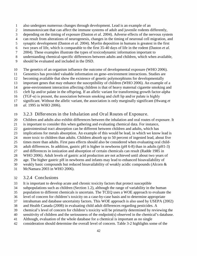
42

also undergoes numerous changes through development. Lead is an example of an 1 immunotoxicant that can affect the immune systems of adult and juvenile rodents differently, 2 depending on the timing of exposure (Daston et al. 2004). Adverse effects of the nervous system 3 can result from alterations of neurogenesis, changes in the timing of neuronal cell migration, and 4 synaptic development (Daston et al. 2004). Myelin deposition in humans is greatest in the first 5 two years of life, which is comparable to the first 35-40 days of life in the rodent (Daston et al. 6 2004). These examples illustrate the types of toxicodynamic information important to 7 understanding chemical-specific differences between adults and children, which when available, 8 should be evaluated and included in the DSD. 9

The genetics of an organism influence the outcome of developmental exposure (WHO 2006). 10 Genomics has provided valuable information on gene–environment interactions. Studies are 11 becoming available that show the existence of genetic polymorphisms for developmentally 12 important genes that may enhance the susceptibility of children (WHO 2006). An example of a 13 gene-environment interaction affecting children is that of heavy maternal cigarette smoking and 14 cleft lip and/or palate in the offspring. If an allelic variant for transforming growth factor-alpha 15 (TGF-α) is present, the association between smoking and cleft lip and/or palate is highly 16 significant. Without the allelic variant, the association is only marginally significant (Hwang et 17 al. 1995 in WHO 2006). 18

3.2.3 Differences in the Inhalation and Oral Routes of Exposure. 19 Children and adults also exhibit differences between the inhalation and oral routes of exposure. It 20 is important to consider this when gathering and evaluating chemical data. For instance, 21 gastrointestinal tract absorption can be different between children and adults, which has 22 implications for metals absorption. An example of this would be lead, in which we know lead is 23 more toxic to children than adults. Children absorb up to 50 percent of ingested lead, about five 24 times more than adults. First pass effects should also be considered when evaluating oral child-25 adult differences. In addition, gastric pH is higher in newborns (pH 6-8) than in adults (pH1-3) 26 and differences in ionization and absorption of certain chemicals can result (Radde 1985 in 27 WHO 2006). Adult levels of gastric acid production are not achieved until about two years of 28 age. The higher gastric pH in newborns and infants may lead to enhanced bioavailability of 29 weakly basic compounds but reduced bioavailability of weakly acidic compounds (Alcorn & 30 McNamara 2003 in WHO 2006). 31

3.2.4 Conclusions 32 It is important to develop acute and chronic toxicity factors that protect susceptible 33 subpopulations such as children (Section 1.2), although the range of variability in the human 34 population to different chemicals is uncertain. The TCEQ uses a WOE approach to evaluate the 35 level of concern for children’s toxicity on a case-by-case basis and to determine appropriate 36 intrahuman and database uncertainty factors. This WOE approach is also used by USEPA (2002) 37 and Health Canada (2008) in evaluating child adult differences regarding pesticides. A 38 chemical’s level of concern for children’s toxicity will be primarily determined by reviewing the 39 sensitivity of children and the seriousness of the endpoint(s) observed in the chemical’s database. 40 Although, evaluation of the whole database for a chemical is important as no single 41 consideration should determine the overall level of concern. Table 3-2 highlights some of the 42

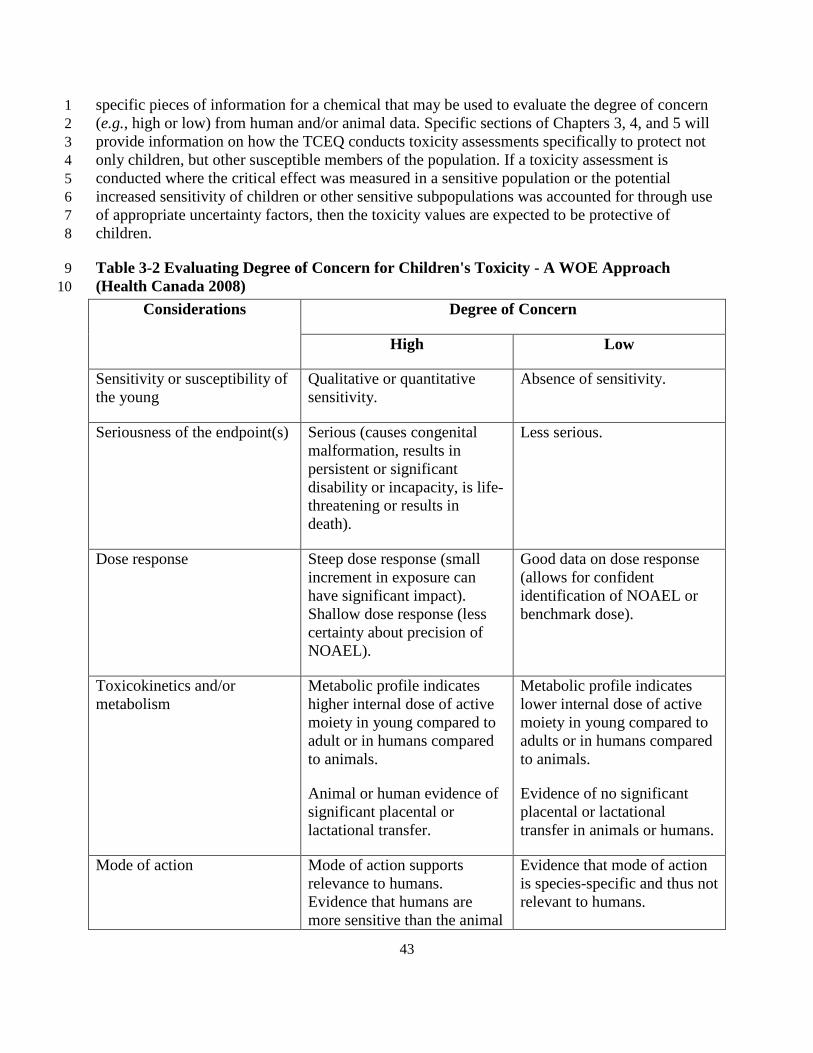
43

specific pieces of information for a chemical that may be used to evaluate the degree of concern 1 (e.g., high or low) from human and/or animal data. Specific sections of Chapters 3, 4, and 5 will 2 provide information on how the TCEQ conducts toxicity assessments specifically to protect not 3 only children, but other susceptible members of the population. If a toxicity assessment is 4 conducted where the critical effect was measured in a sensitive population or the potential 5 increased sensitivity of children or other sensitive subpopulations was accounted for through use 6 of appropriate uncertainty factors, then the toxicity values are expected to be protective of 7 children. 8

Table 3-2 Evaluating Degree of Concern for Children's Toxicity - A WOE Approach 9 (Health Canada 2008) 10

Considerations Degree of Concern

High Low

Sensitivity or susceptibility of the young

Qualitative or quantitative sensitivity.

Absence of sensitivity.

Seriousness of the endpoint(s) Serious (causes congenital malformation, results in persistent or significant disability or incapacity, is life-threatening or results in death).

Less serious.

Dose response Steep dose response (small increment in exposure can have significant impact). Shallow dose response (less certainty about precision of NOAEL).

Good data on dose response (allows for confident identification of NOAEL or benchmark dose).

Toxicokinetics and/or metabolism

Metabolic profile indicates higher internal dose of active moiety in young compared to adult or in humans compared to animals.

Animal or human evidence of significant placental or lactational transfer.

Metabolic profile indicates lower internal dose of active moiety in young compared to adults or in humans compared to animals.

Evidence of no significant placental or lactational transfer in animals or humans.

Mode of action Mode of action supports relevance to humans. Evidence that humans are more sensitive than the animal

Evidence that mode of action is species-specific and thus not relevant to humans.

44

Considerations Degree of Concern

High Low

model. Mode of action may lead to several developmental effects.

Evidence indicates that humans are less sensitive than the animal model.

Confidence in study and/or endpoint

Low quality database.

Study limitations.

Poorly defined NOAEL.

High quality database.

Well-conducted study.

Well-defined NOAEL.

Human information Effects found in humans related to exposure.

No adverse human effects associated with exposure.

1

3.3 Overview for Development of Toxicity Values 2 Animal toxicity studies generally fall into one of the following exposure duration categories: 3

• Acute - exposure to a chemical for less than or equal to 24 h 4 • Subacute - repeated or continuous exposure to a chemical > 1 day to 1 month or less 5 • Subchronic - repeated or continuous exposure for 1-3 months, usually a 90-day study 6 • Chronic - repeated or continuous exposure for longer than 3 months, most commonly 7

a 2-year bioassay in rodents. 8

Since the focus of a 1-h acute ReV is generally a 1-h exposure duration, acute exposure studies 9 are preferentially used to derive these acute ReVs. Acute as well as subacute studies may be used 10 to derive the 1-h ReV (i.e., if the only toxicity information for a chemical is from a well-11 conducted subacute study lasting from 1 day to 4 weeks, it is used to derive an acute 1-h ReV 12 corresponding to the desired exposure duration). For the development of 24-h acute ReV values 13 used for the evaluation of 24-h ambient air monitoring data, acute exposure studies for a 24-h 14 exposure duration are preferred. However, 24-h exposure duration studies are rarely available in 15 the scientific literature. Therefore, acute, subacute and subchronic studies may be used to derive 16 a 24-h acute ReV (Section 4.3). It is acceptable risk assessment practice to incorporate longer-17 term data from toxicity studies to develop acute toxicity values corresponding to shorter duration 18 exposures when it is justified by the MOA analysis (Section 4.2.3). Chronic experimental 19 exposure data is preferentially used to derive chronic toxicity dose-response estimates, although 20 subchronic data may be used with the application of an uncertainty factor to account for the 21 effect of exposure duration, as discussed in Chapter 5. Some studies (e.g., developmental, 22 immune, or reproductive parameter studies) have exposure durations that are neither acute nor 23 chronic but still may be appropriate for use as key studies in the development of acute or chronic 24 toxicity factors. For example, developmental toxicity studies can be used to develop both acute 25 and chronic toxicity factors. 26

45

Toxicity factors are derived from dose-response assessments of adverse health effects that have 1 been scientifically demonstrated to result from exposure to specific chemicals, or for which a 2 significant body of scientific evidence suggests that such a relationship exists. The following 3 analytical approach is used to derive toxicity factors for chemicals as well as to evaluate toxicity 4 factors derived by others: 5

1) Review essential data including physical/chemical properties and select key studies 6

2) Conduct a MOA analysis 7

3) Choose the appropriate dose metric considering toxicokinetics and MOA 8

4) Determine the POD for each key study 9

5) Conduct appropriate dosimetric modeling 10

6) Select critical effect based on human equivalent exposure after considering each key 11 study 12

7) Extrapolate from the adjusted POD to lower exposures based on MOA analysis. 13

3.4 Review Essential Data and Select Key Studies 14

3.4.1 Consideration of Physical and Chemical Proper ties 15 The following sections provide information on the importance of physical and chemical 16 properties for oral and inhalation exposure and provide definitions and meanings of 17 physical/chemical parameters provided by USEPA (2005c) and used by the TCEQ to describe 18 key physical/chemical parameters in the DSDs. 19

3.4.1.1 Inhalation Exposure 20 The physical and chemical characteristics of a chemical influence the nature of its toxic effect 21 since they influence deposition and retention within the respiratory tract, translocation within the 22 respiratory system, and distribution to other tissues (USEPA 1994). For a particle or aerosol, the 23 mean diameter and size distribution determine respiratory tract deposition and toxic potential. 24 For gases and vapors, water solubility and reactivity are major determinants of uptake and toxic 25 effect. Reactivity is defined to include both the propensity for dissociation as well as the ability 26 to serve as a substrate for metabolism in the respiratory tract. Gases that are water soluble and 27 reactive are likely to exhibit portal-of-entry effects. Gases that are not water soluble or reactive 28 are relatively inert to the airways and penetrate to the pulmonary region. Section 3.1.2 of the 29 Methods for Derivation of Inhalation Reference Concentrations and Application of Inhalation 30 Dosimetry (USEPA 1994), hereafter referred to as the RfC Methodology provides a detailed 31 discussion of the importance of physicochemical characteristics of an inhaled chemical and their 32 contribution to the toxic effect. 33

46

3.4.1.2 Oral Exposure 1 Physical/chemical parameters will affect the toxicokinetics and, therefore, the MOA of the 2 chemical when exposure is through the oral route. The physical and chemical characteristics are 3 also important for determining the environmental fate and transport of contaminants being 4 assessed under TCEQ remediation programs (e.g., TRRP). Although the Toxicology Division 5 (TD) develops toxicity factors (e.g., RfD, SFo) for use in TCEQ remediation programs, another 6 section at TCEQ is responsible for developing the physical/chemical parameters for specific 7 chemicals. Therefore, the TD does not gather physical/chemical parameters when developing 8 toxicity factors (e.g., RfD, SFo) exclusively for use in TCEQ remediation programs. 9

3.4.1.3 Water Solubility Values (USEPA 2005c) 10 Water solubility is the degree to which a chemical will dissolve in a liter of water. Water 11 solubility classifications (mg/L or ppm) have been defined by USEPA (2005) as follows: 12

• Very soluble > 10,000 mg/L 13 • Soluble > 1,000 -10,000 mg/L 14 • Moderately soluble > 100 -1,000 mg/L 15 • Slightly soluble > 0.1 -100 mg/L 16 • Insoluble < 0.1 mg/L 17

3.4.1.4 Log Kow Rules of Thumb (USEPA 2005c) 18 Kow is a partition coefficient at the equilibrium ratio of the concentration of a substance 19 dissolved in an organic solvent (octanol) to the concentration of the same substance dissolved in 20 water. Kow (also referred to as Pow) is often reported as a log due to the extremely wide range 21 of measured Kow values. A log Kow of zero indicates an equal affinity for lipids and for water. 22 There is a unique relationship between log Kow and the ability to bioconcentrate in organisms: 23 as log Kow increases, the solubility in lipids increases. This means an increase in the potential to 24 bioconcentrate in organisms is associated with an increase in log Kow (i.e., Kow >

• Log Kow <1 Highly soluble in water (hydrophilic) 29

4). This 25 relationship begins to change around log Kow of 6. For chemicals with log Kow exceeding 6 the 26 potential to bioconcentrate begins to drop and approaches zero at a log Kow of 12. A log Kow 27 indicates to the assessor: 28

• Log Kow >4 Not very soluble in water (hydrophobic) 30 • Log Kow >8 Not readily bioavailable 31 • Log Kow >10 Difficult to measure experimentally (essentially insoluble in water, not 32

bioavailable). 33 34

Kow affects absorption through biological membranes: 35

• Liquids with a log Kow of 2-4 tend to absorb well through the skin 36 • Chemicals with a log Kow > 4 tend to not absorb well 37 • Chemicals with a log Kow of 5-6 tend to bioconcentrate 38 • Chemicals with a log Kow of >6 tend to not bioconcentrate 39

47

3.4.1.5 Melting Point (USEPA 2005c) 1 Melting point (MP) is the temperature at which a chemical changes from solid to liquid. MP 2 indicates the state (solid-liquid-gas) of the chemical in the ambient environment and provides 3 clues to other chemical properties. 4

• MP <100 °C – increased volatility and higher potential exposures 5 • MP > 25 °C – solid 6 • MP < 25 °C – liquid 7 • High MP indicates low water solubility 8 • Low MP indicates increased absorption is possible through the skin, GI tract, or lungs 9 • The range of measured MPs indicates it purity: narrow = more pure, wide = less pure 10

3.4.1.6 Vapor Pressure 11 Vapor pressure (VP), the pressure at which a liquid and its vapor are in equilibrium at a given 12 temperature, gives clues to other chemical properties. For air permit reviews, the TCEQ 13 considers chemicals with VP < 0.01 mm Hg (at 25 °C room temperature) as PM and chemicals 14 with VP > 0.01 mm Hg as vapors. 15

3.4.1.7 Boiling Point (USEPA 2005c) 16 Boiling Point (BP), the temperature at which the VP of a chemical in a liquid state equals 17 atmospheric pressure, gives clues to other chemical properties. A high BP indicates low VP (e.g., 18 structurally large substances with molecular weight > 200, like polymers. A BP < 25 °C indicates 19 the chemical is a gas. For air permit reviews, the TCEQ considers chemicals with BP > 204 °C 20 (> 400 °F) particulate matter (PM). 21

3.4.2 Review Essential Data 22 The TCEQ uses scientifically defensible studies, identified through reviewing literature from 23 reputable sources, to review underlying data to develop toxicity factors (e.g., to demonstrate 24 adverse effects due to exposure and dose-response data). Sources of information include, but are 25 not limited to, the following: electronic databases, peer-reviewed journals, government 26 databases, published books and documents from the public and private sectors, and data from 27 private industry or other private organizations. 28

3.4.2.1 Examples of Databases 29 TOXNET (http://toxnet.nlm.nih.gov) is supported by the National Library of Medicine and 30 includes several searchable databases including: 31

ChemIDplus - Dictionary of over 370,000 chemicals 32 Hazardous Substances Data Bank 33 Toxicology Literature Online (TOXLINE) 34 Chemical Carcinogenesis Research Information System 35 Developmental and Reproductive Toxicology Database 36 Genetic Toxicology Data Bank 37

National Cancer Institute http://www.cancer.gov/ 38 Public Medicine (PUBMED) (http://www.ncbi.nlm.nih.gov/PubMed) 39

48

Registry of Toxic Effects of Chemical Substances (RTECS) 1 (http://www.cdc.gov/niosh/rtecs/) 2

National Technical Information Service (NTIS) (http://www.ntis.gov) 3 Integrated Risk Information System (IRIS) (http://www.epa.gov/iris) 4 Federal Research in Progress (http://www.ntis.gov/products/fedrip.aspx) 5 Defense Technical Information Center (http://www.dtic.mil) 6 Chemfinder (http://chemfinder.cambridgesoft.com/) 7 Toxicity and Exposure Assessment for Children’s Health (TEACH) 8 (http://www.epa.gov/teach/) 9

3.4.2.2 Examples of European databases 10 European Chemical Substances Information System (ESIS) 11 (http://ecb.jrc.ec.europa.eu/esis/) 12 Screening Information Datasets (SIDS) for High Volume Chemicals 13 (http://www.chem.unep.ch/irptc/sids/oecdsids/indexcasnumb.htm and 14 http://www.chem.unep.ch/irptc/sids/OECDSIDS/INDEXCHEMIC.htm) 15 eChemPortal (http://webnet3.oecd.org/echemportal/) 16 International Programme on Chemical Safety (IPCS) Inchem: Chemical Safety 17 Information from Intergovernmental Organizations (http://www.inchem.org/) 18

3.4.2.3 Examples of published books and documents from the public and private 19 sectors 20

General References for Toxicology and Chemical Information 21 Agency for Toxic Substances and Disease Registry (ATSDR) Toxicological Profiles 22

(http://www.atsdr.cdc.gov/) 23 Current Contents, Life Sciences edition 24 Health Effects Assessment Summary Tables (HEAST) (USEPA 1997) 25 Kirk-Othmer Encyclopedia of Chemical Technology 26 International Agency for Research on Cancer (IARC) 27

(http://www.iarc.frhttp://www.iarc.frhttp://www.iarc.frMerck Index 29

) 28

National Toxicology Program (NTP) (http://ntp-server.niehs.nih.gov) 30 Patty’s Industrial Hygiene and Toxicology 31 General References for Regulatory Information and Standards 32 American Industrial Hygiene Association (AIHA) (http://www.aiha.org) 33 American Conference of Government and Industrial Hygienists (ACGIH) 34

(http://www.acgih.org/home.htm) 35 National Ambient Air Quality Standards (NAAQS) (http://www.epa.gov/ttn/naaqs) 36 National Institute for Occupational Safety and Health (NIOSH) 37

(http://www.cdc.gov/niosh/homepage.html) 38 Occupational Safety and Health Administration (OSHA) (http://www.osha.gov) 39 Federal Republic of Germany Maximum Concentration Values in the Workplace (MAK) 40 EPA Health Effects Documents 41 California Environmental Protection Agency (Cal EPA) (http://www.calepa.ca.gov) 42

49

3.4.3 Select Key Studies 1

3.4.3.1 Overview 2 Evaluation and selection of key studies follows the guidelines detailed by USEPA (1994; 2005a) 3 and NRC (2001). Studies that contribute most significantly to the WOE and identify critical 4 effects relevant to humans are selected as key studies. For example, inhalation exposure studies 5 typically take precedence over oral exposure studies for determining inhalation toxicity factors 6 and oral exposure studies typically take precedence over inhalation studies for determining oral 7 toxicity factors. Key studies are used to estimate a threshold for adverse effects with thresholds 8 and to identify the critical adverse effect. These studies may involve a human population 9 evaluated in an epidemiological, clinical or experimental exposure setting, or they may involve 10 experimentation with laboratory animals. Several factors are considered in this process, such as 11 evidence of a dose-response relationship, reproducibility of findings, mechanism or MOA, and 12 consistency with other studies. Most importantly, a temporal association between exposure to the 13 compound and the adverse health effect and dose-response are verified. The strength, 14 consistency, and specificity of the association between chemical exposure and adverse effect are 15 also assessed. Section 2.2.1.7 of the 2005 Cancer Guidelines (USEPA 2005a) provides an in 16 depth discussion of these issues and the evidence for causality first developed by Sir Bradford 17 Hill 1965). As mentioned previously, some studies (e.g., developmental, immune, or 18 reproductive parameter studies) have exposure durations that are neither acute nor chronic but 19 still may be appropriate for use as key studies in the development of acute or chronic toxicity 20 factors. 21

3.4.3.2 Sensitive Subpopulations 22 In some cases, studies are available for children or juvenile laboratory animals (e.g., toxicity 23 studies showing infants are more susceptible to adverse effects after exposure to nitrates) or other 24 sensitive members of the population (e.g., studies in asthmatics after inhalation exposure to 25 irritants). Critical life stages or windows of susceptibility should be identified, if possible, for 26 chemicals. Studies based on sensitive members of the population are often used as key studies, 27 especially if the critical effect in sensitive subpopulations is observed at lower 28 concentrations/doses than in the general population. If a toxicity assessment is conducted where 29 the critical effect was measured in a sensitive population or the potential increased sensitivity of 30 children or other sensitive subpopulations was accounted for through use of appropriate 31 uncertainty factors, then these subpopulations are protected (Section 3.2). 32

3.4.3.3 Human Studies 33 Human data are preferred as the source on which to base toxicity factors. Several study types are 34 relied upon for human exposure data (i.e., epidemiology, controlled human inhalation 35 experiments, case reports, field studies, and occupational studies). Each of these study types has 36 limitations and advantages. One advantage common to all is the potential verification that 37 adverse effects demonstrated in animal studies is also likely to be observed in the human 38 population as well (i.e., the health effect observed in animal studies is relevant to humans). 39

50

3.4.3.4 Epidemiology 1 Epidemiology provides data about associations between exposure and effect that are useful in 2 hazard identification, and if accompanied by sufficiently accurate and reliable exposure data, 3 may be useful in the dose-response assessment for a toxicant. Use of epidemiological studies can 4 be limited by such issues as confounding factors (e.g., predisposing lifestyles, preexisting health 5 problems), reliability of the exposure data, and lack of a causal relationship between exposure 6 and effect. Data from epidemiological studies have been used by various organizations to 7 establish inhalation toxicity factors. The TD evaluates dose-response data from epidemiological 8 studies of acceptable quality which demonstrate a cause-and-effect relationship, and if 9 acceptable, those data are used to derive a toxicity factor. Chapter 7 provides guidelines for using 10 epidemiology studies to derive toxicity factors. 11

3.4.3.5 Controlled Exposure Studies or Clinical Studies 12 Human exposure studies or clinical studies involve well-controlled environments in which short-13 term effects of exposure to a toxicant may be documented. Moreover, they can provide data 14 about the disposition of the toxicant and may identify biomarkers of early exposure or effect. 15 Their short duration is useful in the derivation of acute toxicity factors, but limits their use in 16 chronic toxicity factor development, as do their small sample size and the noninvasive nature of 17 the post-exposure evaluations. IPCS (2005) provides the following guidance concerning small 18 sample size of human subjects: 19

The number of subjects within the population, or within the major subgroup if there are 20 two or more groups, should be sufficient to provide an accurate measure of the central 21 tendency. As a guide, the standard error (standard deviation [SD] of the sample divided 22 by the square root of the sample size) should be less than approximately 20% of the 23 mean. Based on available data, this would normally involve a minimum number of 24 approximately five subjects or samples from five individuals, unless the variability is 25 very low (i.e., small coefficient of variability). 26

3.4.3.6 Case Reports 27 Case reports can provide confirmation that effects seen in laboratory animal studies also occur in 28 exposed human populations and are useful in hazard identification. Since case reports frequently 29 involve exposure to high concentrations, they may be useful in the derivation of acute toxicity 30 factors if the exposure concentrations are estimated and reasonably reliable. However, their small 31 sample size, short exposure duration, and high exposure concentrations may limit their use in the 32 derivation of chronic toxicity factors. 33

3.4.3.6.1 Field Studies 34 Field studies involve the acquisition of data from monitoring of employees in facilities where 35 detectable ambient air concentrations exist, sampling of indoor air in public or private buildings, 36 and reporting of health effects that may be linked to these exposures. Well-designed and well-37 executed field studies can provide correlative information about exposures to a constituent and 38 the human health effects that may be linked to those exposures. 39

3.4.3.6.2 Occupational Studies 40

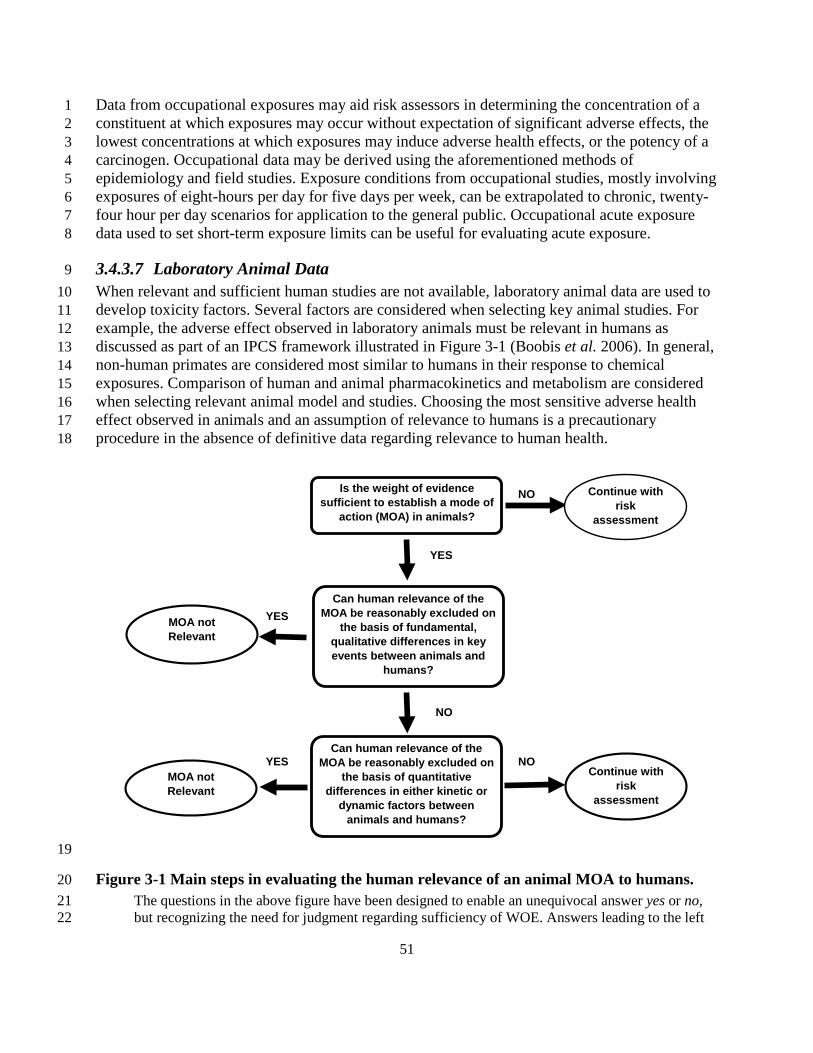
51

Data from occupational exposures may aid risk assessors in determining the concentration of a 1 constituent at which exposures may occur without expectation of significant adverse effects, the 2 lowest concentrations at which exposures may induce adverse health effects, or the potency of a 3 carcinogen. Occupational data may be derived using the aforementioned methods of 4 epidemiology and field studies. Exposure conditions from occupational studies, mostly involving 5 exposures of eight-hours per day for five days per week, can be extrapolated to chronic, twenty-6 four hour per day scenarios for application to the general public. Occupational acute exposure 7 data used to set short-term exposure limits can be useful for evaluating acute exposure. 8

3.4.3.7 Laboratory Animal Data 9 When relevant and sufficient human studies are not available, laboratory animal data are used to 10 develop toxicity factors. Several factors are considered when selecting key animal studies. For 11 example, the adverse effect observed in laboratory animals must be relevant in humans as 12 discussed as part of an IPCS framework illustrated in Figure 3-1 (Boobis et al. 2006). In general, 13 non-human primates are considered most similar to humans in their response to chemical 14 exposures. Comparison of human and animal pharmacokinetics and metabolism are considered 15 when selecting relevant animal model and studies. Choosing the most sensitive adverse health 16 effect observed in animals and an assumption of relevance to humans is a precautionary 17 procedure in the absence of definitive data regarding relevance to human health. 18

19

Figure 3-1 Main steps in evaluating the human relevance of an animal MOA to humans. 20 The questions in the above figure have been designed to enable an unequivocal answer yes or no, 21 but recognizing the need for judgment regarding sufficiency of WOE. Answers leading to the left 22

NO

YES

YES

NO

YES NO

Is the weight of evidence sufficient to establish a mode of

action (MOA) in animals?

Continue with risk

assessment

Can human relevance of the MOA be reasonably excluded on

the basis of fundamental, qualitative differences in key events between animals and

humans?

MOA not Relevant

Can human relevance of the MOA be reasonably excluded on

the basis of quantitative differences in either kinetic or

dynamic factors between animals and humans?

Continue with risk

assessment

MOA not Relevant

52

side of the diagram indicate that the WOE is such that the MOA is not considered relevant to 1 humans. Answers leading to the right side of the diagram indicate either that the WOE is such that 2 the MOA is likely to be relevant to humans or that it is not possible to reach a conclusion regarding 3 likely relevance to humans, due to uncertainties in the available information. In these cases, the 4 assessment would proceed to risk characterization. It should be noted that only at this stage would 5 human exposure be included in the evaluation. (from Boobis et al. 2006, reproduced with 6 permission from Informa Healthcare) 7

3.5 Conduct a MOA Analysis 8 MOA is the series of events leading to induction of the critical toxic endpoint (IPCS 2001; 9 Anderson et al. 2005). The key and obligatory steps that describe the alterations in cellular or 10 organ function leading to toxicity should be described (Figure 3-2). This is in contrast to 11 mechanism of action, which is a detailed understanding at the molecular level of all the steps 12 leading to an adverse effect (USEPA 2005a). It is important to conduct a MOA analysis that 13 describes in detail, to the extent possible, the potential for toxicity and the nature of the dose-14 response curve. This analysis involves consideration of a chemical’s toxicity based on physical 15 and chemical characteristics (e.g., does the chemical have properties that indicate it is likely to be 16 reactive in the portal of entry (POE)) as well as empirical data obtained from experimental 17 studies, as discussed above. MOA information can be used to make decisions about the relevance 18 of animal data to humans, assist in identifying potentially sensitive subpopulations, and model 19 health effects including tumor incidence and key precursor event data. Based on the chemical’s 20 MOA analysis: 21

• The most appropriate dose metric can be chosen to conduct a dose-response 22 assessment; 23

• A decision can be made on whether the chemical has a threshold or nonthreshold dose 24 response; 25

• An evaluation of whether the adverse effect is relevant to humans can be conducted; 26 and 27

• An assessment can be done on whether children (or another group) may be more 28 sensitive than adults to the relevant adverse effect. 29

.30

53

Figure 3-2 Different steps or key events from exposure to a chemical to the development of adverse effects. Adapted from Julien et al. (2009)

Biologicalinteraction or

process(absorption)

Interaction orprocess (in

target tissue)ULTIMATE EFFECT

OF CONCERN

Homeostaticcompensation,

adaptation,repair

Modificationof targettissue

exposure

Modificationof

absorption

Homeostaticcompensation,

adaptation,repair

Interaction orprocess

(e.g.,metabolism)

Interaction orprocess

(e.g., transport/distribution/excretion)

Initial Dose(intake orexposure)

54

3.6 Choose the Appropriate Dose Metric 1 It is important to clearly distinguish between exposure concentration and dose to the critical 2 target tissues since they are not always proportional to each other. The nature and the putative 3 MOA of the toxic response are used to choose an appropriate measure of “dose.” Potential dose 4 metrics are discussed by Jarabek (1995a) and include (from most commonly available to less 5 commonly available): 6

• Exposure dose or concentration of parent chemical 7 • Blood concentration of parent chemical 8 • Area under blood concentration curve of parent chemical 9 • Tissue concentration of parent chemical 10 • Area under tissue concentration curve 11 • Tissue concentration of metabolite 12 • Area under tissue concentration of stable metabolite 13 • Area under tissue concentration of reactive metabolite 14

Available dose metrics, including those which may be more closely related to the toxic effect 15 (e.g., toxic metabolite level at the target tissue), the MOA, and information on toxicokinetics 16 (i.e., absorption, distribution, metabolism, elimination) should be discussed and used to choose 17 the most appropriate dose metric. Toxicokinetic information is especially important to assess 18 whether children may be more sensitive than adults to the adverse effects produced after 19 chemical exposure. 20

The importance of choosing the appropriate dose metric to evaluate toxic response is illustrated 21 by the differences between acute and chronic exposure to benzene. When considering acute high-22 concentration benzene exposure, an appropriate dose metric to describe central nervous system 23 (CNS) depression would be the parent compound blood concentration, whereas for chronic low-24 level exposure that produces erythroid precursor perturbations, the appropriate dose metric 25 would be the area under the tissue concentration curve for toxic metabolites (Jarabek 1995a). 26

3.7 Determine the POD 27 The POD is the point on the dose-response curve that marks the beginning of a low-dose 28 extrapolation for an adverse effect. When choosing the critical adverse effect, it is important to 29 note that all effects reported for a substance are not necessarily considered adverse. For example, 30 exposure to a chemical may result in increases of protective enzymes in a tissue which would not 31 be considered an adverse effect. However, at higher concentrations, the chemical may cause 32 tissue necrosis, an adverse effect. 33

3.7.1 Determination of Adverse Effects 34 An adverse effect may be considered to be a change (biochemical, functional, or structural) that 35 may impair performance and generally has a detrimental effect on growth, development or life 36 span when observed in a non-clinical toxicology model (Dorat and Engelhardt 2005). The 37 USEPA defines an adverse effect as “any effect resulting in functional impairment and/or 38 pathological lesions that may affect the performance of the whole organism, or that reduce an 39 organism’s ability to respond to an additional challenge” (USEPA 1994). 40

55

Adversity typically implies some induction of functional impairment or generation of 1 pathological lesion(s) that affects the performance of the whole organism or reduces an 2 organism's ability to withstand or respond to additional environmental challenges. Consistent 3 with the goal of public health to control exposures before the occurrence of functional 4 impairment of the whole organism (NRC 2007), TCEQ calculates conservative health-based 5 toxicity factors to protect against adverse effects. The National Research Council (NRC) 6 recommended identifying measurable adverse effects or biologic changes that occur at a point in 7 which they are minor, reversible, or subclinical and that do not affect vulnerable or susceptible 8 individuals within the population. The California EPA follows NRC (2007) in recommending a 9 cautious and health-protective approach to the determination of whether a given biological 10 endpoint is appropriate to consider frankly “adverse,” or is a biologically significant precursor 11 lesion, in which case it would be a suitable endpoint for consideration in a toxicity assessment. 12 Alternatively, an effect may be a non-adverse adaptive or incidental change, which occurs 13 merely by chance and may in fact be unrelated to study treatment or exposure (OEHHA 2008). 14 15 3.7.1.1 Recognition of Adverse and Non-Adverse Effect 16 It is important to identify the highest exposure level in toxicity studies that does not cause 17 treatment-related effects that could be considered relevant to human health. Lewis et al. (2002) 18 stated “that toxicity studies are of necessity limited to a small number of quantitative observation 19 points (dose or concentration levels), although the biological response may represent a 20 continuum of change with changing dose.” As shown graphically in Figure 3-3, the outputs of 21 such tests in terms of quantitative indices (e.g., adverse effect and non-adverse effect levels), and 22 in the derived shape of the dose response curves, represent only an approximation of the true 23 dose- response relationship that is characteristic of the biological effect under investigation 24 (Lewis et al. 2002). 25

The judgment on the adverse nature of an observation in a toxicology study is often subject to 26 debate and reinterpretation. Decisions about the amount of change necessary to consider an 27 effect adverse must always be made using professional scientific judgment and must be viewed 28 in light of all the data available on the endpoint of concern. All available toxicological data on a 29 chemical must be reviewed before deciding whether an effect is biologically significant and 30 adverse, and how the results fit with what is known about the underlying MOA. Both the 31 biological and the statistical significance of the effects are considered when making these 32 judgments. Biological significance is the determination that the observed effect (a biochemical 33 change, functional impairment, or pathological lesion) is likely to impair the performance or 34 reduce the ability of an individual organism to function or to respond to additional challenge 35 from the agent even though there may be no statistically significant differences from control. 36 Biological significance is also attributed to effects that are consistent with the sequence of events 37 that occur in a known MOA. Statistical significance quantifies the likelihood that the observed 38 effect is not due to chance alone. Precedence is given to biological significance because a 39 statistically significant change that lacks biological significance is not considered an adverse 40 response (USEPA 2002a). 41

56

1 Figure 3-3 Quantitative outcome of toxicity studies is dependent upon observation points 2

(adapted from Lewis 2002) 3

For many discrete or quantal endpoints (e.g., birth defects, tumors, or some discrete pathological 4 changes), USEPA (2002) indicates that this judgment is more straightforward because criteria 5 have been established for deciding the magnitude, incidence, and types of effects that are 6 considered to be adverse. Importantly, the relevance of an increase of an effect above the 7 background rate can be evaluated using statistical tools. In the case of continuous measures (e.g., 8 body weight, enzyme changes, physiological measures), this tends to be more difficult, because 9 the amount of change to be considered adverse may not be defined by or agreed upon by 10 toxicologists or health scientists. Consequently, the question of adversity is often decided in the 11 context of the endpoint itself, the study methods, and the relationship of changes in that endpoint 12 to other effects of the chemical. Using a default cutoff value to define adversity for continuous 13 measures (e.g., 1 SD) may be necessary, but could result in an inappropriate interpretation of 14 data and less than optimum evaluation of a chemical’s effects (USEPA 2002a). If toxicity data 15 are modeled using benchmark dose modeling, USEPA (2002) has provided guidance for both 16 dichotomous and continuous endpoints to determine whether the benchmark response and 17 corresponding 95% confidence level of the benchmark dose is adverse or not. Please refer to 18 Section 3.7.3 for additional information. 19

3.7.1.2 Evaluation Process 20 The European Center for Ecotoxicology and Toxicology of Chemicals (ECETOC 2002) and 21 Lewis et al. (2002) have presented a structured approach to determine if a response in a 22

57

toxicology study is adverse or non-adverse. This approach includes an evaluation of the adaptive, 1 transient/persistent, and progressive nature of the response, its association with other effects, the 2 occurrence of functional impairment, and the primary or secondary nature of the response. 3

Briefly, the evaluation process, as shown in Figure 3-4, involves two main steps. In the first, the 4 toxicologist must decide whether differences from control values are treatment-related or if they 5 are chance deviations. In the second step, only those differences judged to be effects based on 6 statistical or biological significance are further evaluated in order to discriminate between those 7 that are adverse and those that are not. For each step, criteria are described that can be used to 8 make consistent judgments. In differentiating an effect from a chance finding, consideration is 9 given among other things to dose response, spurious measurements in individual parameters, the 10 precision of the measurement under evaluation, ranges of natural variation and the overall 11 biological plausibility of the observation. In discriminating between adverse and non-adverse 12 effects consideration is given to whether: 13

• the effect is an adaptive response; 14 • it is transient, the magnitude of the effect, its association with effects in other related 15

endpoints; 16 • it is a precursor to a more significant effect; 17 • it has an effect on the overall function of the organism; 18 • it is a specific effect on an organ or organ system or secondary to general toxicity; or 19 • the effect is a predictable consequence of the experimental model. 20

Finally, in interpreting complex studies, it is recognized that a WOE approach, combining the 21 criteria outlined here to reach an overall judgment, is the optimal way of applying the evaluation 22 process. 23

58

Is therea difference

compared to controlvalues?

Is thedifference an effect of

treatment?

Is the effect adverse?

NO

YESNO

NO

YES

YES

Effect isadverse

Effect is notadverse

STOP

STOP

1

Figure 3-4 Structured approach to evaluating the outcome of toxicology studies 2 (adapted from Lewis et al. 2002) 3

3.7.1.3 Nature and Severity of Adverse Effects 4 The toxic effects of chemicals are of varying types and degrees of severity. Following an acute 5 exposure to a toxicant, such as highly reactive and water soluble chemicals, effects on the upper 6 and lower respiratory tract may be observed as POE effects. Toxic effects from airborne 7 substances may also be due to exposure via the skin and eyes. Systemic effects may result from 8 absorption and distribution of toxicant (e.g., moderately water-soluble or relatively water-9 insoluble chemicals) to a site distant from its entry point. Certain chemicals, after a single 10 exposure, have the potential to produce delayed adverse effects. 11

Not all effects reported for a substance are necessarily considered adverse (e.g., adaptive 12 biochemical responses such as enzyme induction) (Sherwin 1983, ATS 2000). Reserve loss 13 involves both reversible and irreversible alterations of the cell population and includes metabolic 14 abnormalities and alterations of the intercellular milieu. Therefore, the earliest effect is an altered 15 ecology at the cellular level. 16

Adverse effects may occur with a range of severity from mild (sensory or subjective effects, 17 which are reversible) to severe (clinically significant pathological changes, disabling or strongly 18 objectionable sensory effects, persistent or irreversible histological or functional damage), or 19

59

even to life-threatening (OEHHA 2008). The OEHHA criteria for determining the severity of an 1 inhalation effect is presented in Appendix B (OEHHA 2008). Similar criteria for different 2 biological endpoints from available toxicity studies as NOAELs and less serious and serious 3 lowest-observed-adverse-effect-levels(LOAELs) have been provided by ATSDR (2007). Tables 4 3-1 to 3-17of ATSDR (2007) list 17 organ or system categories and classifies the degrees of 5 severity within the system categories. 6

It is noted that toxicity factors are set to protect the general public health and the biological 7 endpoint of choice for determination will generally be a mild effect. However, a more severe 8 effect may be used if it is in fact the most sensitive endpoint that occurs at the lowest exposure 9 level (for example irreversible developmental effects), or if no data on mild effects are available. 10 Under such circumstances, additional UFs may be used in order to provide adequate health 11 protection for the majority of the exposed population. This practice is consistent with those used 12 by other agencies (USEPA 2002a, ATSDR 2007, and OEHHA 2008). 13

3.7.1.4 Listing of Adverse Effects 14 Refer to Tables 3-1 to 3-17of the Guidance for the Preparation of a Twenty First Set 15 Toxicological Profile (ATSDR 2007) 16 (http://www.atsdr.cdc.gov/toxprofiles/guidance/set_21_guidance.pdf for more detailed 17 information. 18

3.7.1.4.1 Non-Adverse Effects 19 • Weight loss or decrease in body weight gain of less than 10% in adult animals 20 • Weight loss or decrease in body weight gain of less than 5% in fetuses 21 • Changes in organ weight of non-target organ tissues that are not associated with 22

abnormal morphologic or biochemical changes 23 • Increased mortality over controls that is not significant (p>0.05) 24 • Some adaptive responses 25 • Since the benchmark response (BMR) (1, 5, or 10%) or critical effect size at 1 SD (CES1 26

SD) should represent a response level of no significant concern, the corresponding 27 benchmark dose lower confidence limit (BMDL) should be comparable to the NOAEL 28 rather than the LOAEL (refer to Section 3.7.3 Benchmark Dose Modeling) 29

3.7.1.4.2 Less Ser ious Effects 30 • Reversible cellular alterations at the ultrastructural level (e.g., dilated endoplasmic 31

reticulum, loss of microvilli, myelin figures) and at the light-microscopy level (e.g., 32 cloudy swelling, hydropic degeneration, fatty change) 33

• Necrosis (dependent upon location, distribution, and magnitude), metaplasia, or atrophy 34 with no apparent decrement of organ function 35

• Moderate serum chemistry changes (e.g., moderate elevations of serum glutamic 36 oxaloacetic transaminase (SGOT), serum glutamic pyruvic transaminase (SGPT)) 37

• Organ weight change in known target organ tissue that is not associated with 38 morphologic or biochemical alterations 39

60

• Weight loss or decrease in body weight gain of 10-19% (assuming normal food 1 consumption and when weight loss is due to a systemic effect of toxicant) 2

• Some adaptive responses (e.g., hepatic CYP p-450 induction) 3

3.7.1.4.3 Transitional Effects (Between Less Ser ious and Ser ious) 4 Some effects (such as necrosis, atrophy, metaplasia, and serum chemistry alterations) could be 5 classified as less serious or serious based on their reversibility, the organ affected, or the degree 6 of associated dysfunction. 7

3.7.1.4.4 Ser ious Effects 8 • Death 9 • Clinical effects of significant organ impairment (e.g., convulsions, icterus, cyanosis) 10 • Morphologic changes in organ tissues that could result in severe dysfunction (e.g., 11

marked necrosis of hepatocytes or renal tubules) 12 • Weight loss or decrease in body weight gain of 20% or greater (assuming normal food 13

consumption) 14 • Major serum chemistry changes (e.g., major elevations of SGOT, SGPT, blood urea 15

nitrogen (BUN)) 16 • Major metabolic effects (e.g., ketosis, acidosis, alkalosis) 17 • Cancer effects 18

3.7.2 Definitions of PODs 19 A review of regulatory and other scientific literature and of current practices conducted by Lewis 20 et al. (2002) revealed a lack of consistency in definition and application of frequently used terms 21 such as adverse effect, no-observed-effect level (NOEL), NOAEL, LOAEL, biologically 22 significant effect or toxicologically significant effect. The USEPA (2002) has defined these 23 terms as shown in Table 3-3, which TCEQ will use to promote consistency. 24

25

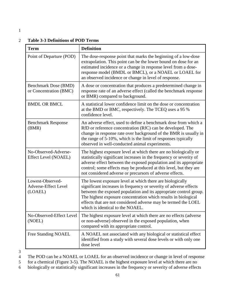
61

1

Table 3-3 Definitions of POD Terms 2

Term Definition

Point of Departure (POD) The dose-response point that marks the beginning of a low-dose extrapolation. This point can be the lower bound on dose for an estimated incidence or a change in response level from a dose-response model (BMDL or BMCL), or a NOAEL or LOAEL for an observed incidence or change in level of response.

Benchmark Dose (BMD) or Concentration (BMC)

A dose or concentration that produces a predetermined change in response rate of an adverse effect (called the benchmark response or BMR) compared to background.

BMDL OR BMCL A statistical lower confidence limit on the dose or concentration at the BMD or BMC, respectively. The TCEQ uses a 95 % confidence level.

Benchmark Response (BMR)

An adverse effect, used to define a benchmark dose from which a RfD or reference concentration (RfC) can be developed. The change in response rate over background of the BMR is usually in the range of 5-10%, which is the limit of responses typically observed in well-conducted animal experiments.

No-Observed-Adverse-Effect Level (NOAEL)

The highest exposure level at which there are no biologically or statistically significant increases in the frequency or severity of adverse effect between the exposed population and its appropriate control; some effects may be produced at this level, but they are not considered adverse or precursors of adverse effects.

Lowest-Observed-Adverse-Effect Level (LOAEL)

The lowest exposure level at which there are biologically significant increases in frequency or severity of adverse effects between the exposed population and its appropriate control group. The highest exposure concentration which results in biological effects that are not considered adverse may be termed the LOEL which is identical to the NOAEL.

No-Observed-Effect Level (NOEL)

The highest exposure level at which there are no effects (adverse or non-adverse) observed in the exposed population, when compared with its appropriate control.

Free Standing NOAEL A NOAEL not associated with any biological or statistical effect identified from a study with several dose levels or with only one dose level

3 The POD can be a NOAEL or LOAEL for an observed incidence or change in level of response 4 for a chemical (Figure 3-5). The NOAEL is the highest exposure level at which there are no 5 biologically or statistically significant increases in the frequency or severity of adverse effects 6

62

between the exposed population and its appropriate control. Some effects may be produced at the 1 NOAEL, but they are not considered adverse, as discussed in previous sections. The LOAEL is 2 the lowest exposure level at which there are biologically or statistically significant increases in 3 frequency or severity of adverse effects between the exposed population and its appropriate 4 control group. The NOAEL approach has been criticized because it does not use the full dataset 5 of the dose-response curve and is dependent on choice of dose for study (i.e., spacing between 6 doses). For studies with greater variation in endpoint measurement or smaller sample size, the 7 NOAEL approach tends to result in a higher NOAEL being determined based on statistical 8 comparison to the controls. In addition, some experimental studies only identify a LOAEL. 9

10 Figure 3-5. Dose-response assessment for a chemical with a threshold MOA. 11

A dose may exist below the minimum health effect level for which no adverse effects occur. The 12 USEPA typically assumes that at low doses the body's natural protective mechanisms prevent or 13 repair any damage caused by the pollutant, so there is no ill effect at low doses. Even long-term 14 (chronic) exposures below the threshold are not expected to have adverse effects. The dose-15 response relationship (the response occurring with increasing dose) varies with pollutant, 16 individual sensitivity, and type of health effect (adapted from Exhibit 12-3B of USEPA 2004a). 17

If there exist multiple, non-identical NOAELs and LOAELs for the same compound and critical 18 effect, the study of the best quality reporting the highest value for a NOAEL (preferred) or the 19 lowest value for the LOAEL is used for the development of toxicity values. Scientific data as 20 well as professional scientific judgment should be used to decide the most appropriate POD. 21

% o

f Sub

ject

s R

espo

ndin

g

Dose

NOEL NOAEL LOAEL

•

∆

•

•

••

∆∆

∆

∆

◊

◊

◊

Enzyme Change

Liver Toxicity(Critical Effect)

Nervous System Toxicity(Tremors)

Human RfC or RfD

Application of Uncertainty

Factors

63

A NOAEL not associated with any biological or statistical effect identified from a study with 1 several dose levels or with only one dose level (i.e., free-standing NOAEL) is typically 2 unsuitable for derivation of a toxicity value (USEPA 1994). However, the TCEQ must develop 3 toxicity values for many chemicals with limited toxicity data. In many cases, the chemical is not 4 very toxic, and even high doses or concentrations do not produce an adverse effect. A free-5 standing NOAEL without an associated LOAEL identified in the same study may be used in 6 deriving a toxicity value, but only if there are no other suitable studies, and so long as the overall 7 health hazard data (including any case reports or studies with shorter durations) for that 8 substance are consistent with the NOAEL study. For example, another study may have identified 9 a free-standing LOAEL just above the dose range tested in the study that identified a free-10 standing NOAEL and both evaluated similar endpoints. 11

Lewis et al. (2002) proposed a definition for biologically significant effect to assist in 12 differentiating between adverse and non-adverse effects consistently: 13

Biologically significant effect: A response (to a stimulus) in an organism or other 14 biological system that is considered to have substantial or noteworthy effect (positive or 15 negative) on the well-being of the biological system. The concept is to be distinguished 16 from statistically significant effects or changes, which may or may not be meaningful to 17 the general state of health of the system. 18

In general, there are two types of significant biological responses. First, there are the normal 19 biological responses, which will manifest in response to stress, such as sweating in exercise or 20 losing weight when caloric intake is restricted. These changes often represent normal 21 homeostatic reactions to stimuli. Second, there are the abnormal biological responses, which may 22 be caused by chemicals or other stresses. Either of these biological responses could be 23 significantly different from the normal baseline when analyzed by statistics or may show no 24 statistical differences from control. Therefore, one must be cautious in relating a statistical 25 finding to a true adverse biological effect (Lewis et al. 2002). 26

3.7.3 Benchmark Dose Modeling 27 As an alternative to the NOAEL/LOAEL approach for identifying a POD, a mathematical model 28 can be used to fit the entire dose-response data for a chemical with a threshold MOA so that the 29 concentration corresponding to an estimated incidence or change in level of response (i.e., BMD) 30 as well as the BMDL from a dose-response model can be determined (Figure 3-6). The 31 advantages of BMD modeling are it uses the full dataset of the dose-response curve, accounts for 32 the greater uncertainty due to smaller sample size or greater variation, and can estimate the 33 threshold concentration when a NOAEL cannot be established. However, BMD modeling also 34 has some disadvantages. Travis et al. (2005) discusses the advantages and disadvantages of both 35 the BMD and NOAEL approach. When possible, the TCEQ performs BMD modeling following 36 established guidelines because of the advantages of this approach over the NOAEL/LOAEL 37 approach (USEPA 1995; USEPA 2000b). 38

When performing benchmark modeling for oral exposure studies the terms BMD and BMDL are 39 used. The terms BMC and BMCL are use for benchmark modeling for inhalation exposures. 40 Throughout this chapter, the terms BMD and BMDL will be used to describe both oral and 41

64

inhalation exposures. Similar mathematical modeling procedures are followed for choosing a 1 POD for chemicals with a nonthreshold MOA including carcinogenic chemicals. Traditionally, 2 the terminology differs for carcinogenic chemicals. The term effective dose (ED) is the central 3 estimate and is analogous to the term “BMD” whereas the term lower bound of ED (LED) is the 4 lower 95% confidence limit and is analogous to the term “BMDL. Refer to Section 5.7.3 of 5 Chapter 5 for a discussion of choosing a POD for carcinogenic chemicals. 6

7 Figure 3-6 Sample of a model fit to dichotomous data, with BMD and BMDL indicated. 8

The fraction of animals affected in each dose group is indicated by filled circles. The error bars 9 indicate 95% confidence intervals for the fraction affected. The BMR for this example is an extra 10 risk of 10%. The dashed curve indicates the BMDL for a range of BMRs. The dose labeled 11 BMDL corresponds to the lower end of a one-sided 95% confidence interval for the BMD. 12 (adapted from Figure 1 from USEPA 2000b) 13

Certain toxicity data are not amenable to BMD modeling. The quality of the experimental study 14 as well as the nature of the data collected during the study determines whether the dose-response 15 data can be modeled using BMD modeling (USEPA 1995; 2000b) or whether a NOAEL/LOAEL 16 approach is used. For example, when there is a maximum response at all doses, there are 17 inadequate response data at the midpoint of the dose-response curve, then the data are not 18 amenable to BMD modeling. When BMD modeling cannot be performed, acceptable exposure 19 doses or concentrations are determined using the NOAEL or LOAEL as the POD. 20

Frac

tion

Aff

ecte

d

Dose

BMDL

•

•

•

•

•

◊

◊

◊◊

BMD

0

0.2

0

0.4

0.6

0.8

1.0

50 100 150 200

ModelBMD Lower Bound

65

3.7.3.1 Dichotomous Data 1 Dichotomous data are modeled using dichotomous models in the USEPA’s BMDS software 2 (Version 2.1.2) and guidance in USEPA (2000). Model updates are available from 3 http://www.epa.gov/ncea/bmds/index.html. 4

If there is an accepted level of change in the endpoint that is considered to be biologically 5 significant, then that amount of change is chosen for determination of the POD (USEPA 2000e). 6 For dichotomous data, this level is referred to as the BMR. The level of the BMR chosen for 7 BMD modeling is the lowest dose level that can be supported by the data. Typically, this lowest 8 dose level is either the BMR05 or BMR10, which are observable levels of effect in the standard 9 animal bioassay, as discussed by Barnes et al. (1995). For some epidemiological studies of 10 sufficient quality, a BMR01 or BMR001 (Grant et al. 2009) may be adequately modeled. 11

Several investigators have compared the BMDL (1, 5, or 10%) to the NOAEL or LOAEL 12 (Kimmel 1990; Farland and Dourson 1992; Gaylor 1992;Faustman 1996; Fowles et al. 1999; 13 Filipsson et al. 2003). It has been suggested that an additional UF be applied to a BMDL if there 14 is reason to believe it is comparable to a LOAEL (i.e., based on severity of the adverse effect or a 15 flat dose-response curve). Since the BMR (1, 5, or 10%) should represent a response level of no 16 significant concern, the corresponding BMDL should be comparable to the NOAEL rather than 17 the LOAEL. Therefore, the TCEQ does not routinely apply an additional UF. However, severity 18 of response is considered when determining the level of the BMR. If the endpoint of concern is 19 more severe or detrimental, then a lower level BMR (e.g., 1% or 5%) is modeled in order to be 20 health-protective. The steepness of the dose-response curve may also be considered in the choice 21 of BMR. However, unless information about the MOA through which the toxic agent causes the 22 particular effect is available, a level of the BMR should not be extrapolated to doses outside the 23 tested dose range (Filipsson et al. 2003). Large extrapolations (e.g., to a 1% response level from 24 a standard assay showing observable effect at the 10% level) are not appropriate. Additional 25 information concerning consideration of severity of response when selecting the BMR level is 26 provided by the CalEPA Department of Pesticide Regulation (DPR 2004a; 2004b). No matter 27 what BMR level is chosen to model the data, the BMD10 and BMDL10 should be calculated and 28 presented for comparison purposes as suggested by USEPA (2000). 29

3.7.3.2 Continuous Data 30 Continuous data are modeled using continuous models in USEPA’s BMDS software (Version 31 2.1.2) and guidance in USEPA (1995, 2000). Model updates are available from 32 http://www.epa.gov/ncea/bmds/index.html. The TCEQ does not attempt to change continuous 33 data into dichotomous data and model the resulting dose-response curve with dichotomous 34 models. USEPA (2000) noted that when continuous data are changed into dichotomous data, it 35 potentially results in loss of information about the magnitude of response. 36

In order to distinguish continuous data from dichotomous data, Dekkers et al. (2001) 37 recommended the term “critical effect size” (CES) be used instead of the term “BMR,” since for 38 continuous data, the effect measure is expressed on a continuous scale. A CES defines the 39 demarcation between non-adverse and adverse changes in toxicological effect parameters for 40 continuous data (Dekkers et al. 2001). For example, a CES of 10% or CES10 for continuous data 41

66

(i.e., a 10% change in the mean of a treated group compared to the control mean) is not the same 1 as a BMR of 10% or BMR10 (i.e., 10% of total animals responding for dichotomous data). 2

If there is an accepted level of change in a continuous endpoint that is considered to be 3 biologically significant and sub-adverse (e.g., 10% decrease in body weight), then that amount of 4 change is chosen for determination of the POD. Otherwise, the CES results for one SD (CES 1 5 SD) is considered to be nonadverse. A CES 1 SD from control mean corresponds to an 6 approximately 10% excess risk for individuals below the 2nd percentile or above the 95th 7 percentile of the control distribution for normally distributed effects (USEPA 2000e). No matter 8 what CES response level is chosen to model the data, the CES1 SD should be calculated and 9 presented for comparison purposes as suggested by USEPA (2000). 10

3.8 Conduct Appropriate Dosimetric Modeling 11 When the POD for each key study is determined, adjustments are made to account for 12 differences between experimental and desired exposure durations and/or differences in anatomy 13 and physiology in experimental animals and humans, (i.e., the respiratory systems for inhalation 14 exposure or gastrointestinal systems for oral exposures) including sensitive subpopulations such 15 as children. For example, different respiratory mathematical dosimetry models have been used to 16 account for chemical disposition, toxicant-target interactions, and tissue responses (USEPA 17 1994; Jarabek 1995b; Hanna et al. 2001). These models allow a more accurate characterization 18 of the different steps of the pathogenic process, although they depend on knowledge of model 19 parameters and their fidelity to the biological system. 20

A comprehensive biologically-based dose-response model links mechanistic determinants of 21 chemical disposition, toxicant-target interactions, and tissue responses into an overall model of 22 pathogenesis (Figure 3-7; most quantitative method). The proposed stages between exposure and 23 response include processes relating exposure to consequent tissue dose (i.e., toxicokinetics) and 24 processes that determine response to the tissue dose (i.e., toxicodynamics). If empirical data are 25 not available to construct a comprehensive biologically-based dose-response model for a 26 chemical (the vast majority of cases), then response can be related to exposure by incorporating 27 and integrating as much mechanistic data as possible to allow a more accurate characterization of 28 the pathogenic process. At the rudimentary level, response is related to exposure without 29 consideration of internal dose (Figure 3-7, qualitative method). 30

67

1 Figure 3-7 Schematic characterization of the comprehensive exposure dose-response 2 continuum. 3

This figure illustrates the evolution of protective to predictive dose-response estimates (Figure 1-4 2 from USEPA 1994). 5

3.8.1 Physiologically-Based Pharmacokinetic Model 6 Physiologically-based pharmacokinetic (PBPK) compartmental models are used to characterize 7 pharmacokinetic (a.k.a. toxicokinetic) behavior of a chemical. Available data on blood flow rates 8 and metabolic and other processes which the chemical undergoes within each compartment are 9 used to construct a mass-balance framework. The TCEQ will use verified PBPK models to 10 perform dosimetric adjustments for both oral and inhalation exposure following guidance 11 provided by USEPA (2006a). USEPA (2006b) provides guidance on assessing the impact of 12 human age and interindividual difference in physiology and biochemistry. 13

As with inhalation exposure, PBPK modeling is the preferred approach for dosimetric 14 adjustments when assessing oral exposure (USEPA 2011). For inhalation exposure, PBPK 15 models have principally been used to describe a chemical’s systemic distribution (i.e., gas 16 absorption (as opposed to particles) in the respiratory tract) and have focused on the limiting case 17 of gases with high lipid solubility where uptake is determined by perfusion (e.g., volatile organic 18 compounds). The respiratory tract is regarded as a conduit to pulmonary absorption and systemic 19 delivery of dose. Therefore, blood flow, not the diffusional mass transport across the blood-gas 20 barrier, is considered to be of prime importance. In addition to PBPK, there are several types of 21 inhalation dosimetry models. 22

68

3.8.2 Inhalation Models 1 In order to understand inhalation dosimetry models, a distinction must be made between the 2 equilibrium assumption in which transport is dependent on regional blood flow and dynamic 3 models in which transport occurs across a concentration gradient near the transport barrier. The 4 following sections which are based on information presented by Hanna et al. (2001) briefly 5 discuss the differences between basic inhalation dosimetry models and provide general 6 considerations for choosing model structures. 7

3.8.2.1 Flow-Limited or Perfusion-Limited Model 8 Flow-limited or perfusion-limited models are relevant to lipid-soluble gases that are absorbed in 9 the alveolar region of the lung. The permeability of the transport barrier (or membrane) is 10 significantly greater than the flow or perfusion to the transport barrier so the transport of 11 chemicals to the systemic circulation is dependent on the flow volume or perfusion rate. The 12 alveolar ventilation rate determines the alveolar gas-phase concentration, and the equilibrium 13 partition coefficient of the gas is used to establish the equilibrium between blood concentration 14 and the alveolar gas concentration. Blood flow, blood distribution, and the equilibrium condition 15 determines transport to systemic compartments. 16

3.8.2.2 Membrane-Limited Transport Model 17 In a membrane-limited transport model, the membrane or transport barrier itself limits the rate at 18 which the chemical permeates the barrier to enter the systemic circulation or to act on the tissue 19 itself. Perfusion rate does not limit intracellular or tissue concentrations. Equilibrium is not 20 established since it is assumed that a concentration gradient exists between the tissue and blood. 21 Diffusion within the blood is typically ignored because it is of minor significance compared to 22 the gradient in the tissue. Diffusion in the gas stream itself may result in the establishment of a 23 significant concentration gradient that also affects the rate of uptake. Therefore, this case 24 requires a model capable of describing the dynamic transport process both in the gas phase and 25 within the tissue. 26

3.8.2.3 Distributed Parameter Model 27 Distributed parameter models have been used to describe the uptake of gases that are water-28 soluble and/or reactive within the airway tissue. Since these gases distribute regionally within the 29 airways, models must differentiate between the various respiratory tract regions rather than focus 30 on the blood-gas exchange region alone. However, it is possible for a metabolite to be 31 sufficiently stable to distribute to the systemic circulation. The transport of these gases is 32 determined by the transport of the gas along the concentration gradient from within the gas 33 stream extending laterally to the liquid/tissue compartment. The equilibrium assumption used in 34 flow-limited or perfusion-limited models is inappropriate. In distributed parameter models it is 35 assumed that a quasi-steady-state concentration gradient exists. 36

3.8.2.4 Gas-Phase Limited Transport Model 37 The gas-phase limited transport model has been used for chemicals where the tissue is almost an 38 infinite sink so the gas-phase concentration gradient completely controls the rate of uptake (i.e., 39 highly water-soluble gases that are readily absorbed by the airway lining and gases that react 40

69

nearly completely within the airway lining). The rate at which the gas can cross the gas-phase 1 concentration gradient, or gas-phase transport barrier, to the tissue limits the rate of absorption. 2 As a consequence, equilibrium cannot be assumed between the gas-phase concentration and the 3 transport barrier of the airway surface because the gas-phase concentration gradient represents a 4 barrier to transport and requires the mass to diffuse across this barrier. 5

3.8.2.5 Considerations of Hierarchy of Model Structures 6 Any method used to extrapolate dose across species must be sufficiently robust to describe the 7 exposure-dose relationship in animal species and must also predict human dose to allow 8 dosimetric adjustment(s) to be made. A dosimetric model must be able to describe the anatomy, 9 physiology, and metabolism of the species of interest without introducing unnecessary 10 parameters that contribute to additional uncertainty especially when experimental data are used 11 to “fit” the model. In addition, model verification is essential to the modeling framework as 12 discussed in Section 3.2.3 of the RfC Methodology. Every effort should be made to obtain a 13 solution appropriate to the physicochemical properties of the specific gas. 14

The following are considerations of hierarchy of model structures for exposure-dose response 15 and interspecies extrapolation (USEPA 1994): 16

Optimal Model Structures 17 • Structure describes all significant mechanistic determinants of chemical disposition, 18

toxicant-target interaction, and tissue response 19 • Uses chemical-specific and species-specific parameters 20 • Dose metric(s) described at level of detail commensurate with toxicity data 21

Default Model structure 22 • Limited or default description of mechanistic determinants of chemical disposition, 23

toxicant-target interaction, and tissue response 24 • Uses categorical or default values for chemical and species parameters 25 • Dose metric(s) at generic level of detail 26

Optimal models are preferred to default models. The development of calibrated inhalation 27 optimal/preferred dosimetry models with predictive capability for hazard assessment is an active, 28 ongoing area of research (USEPA 2006). The TCEQ uses available results from calibrated, 29 predictive PBPK model or other inhalation dosimetry models, as discussed by Hanna et al. 30 (2001) and Jarabek (1995b), to perform dosimetric adjustments from laboratory animal data to a 31 human equivalent concentration (HEC) or to perform exposure duration adjustments for both 32 acute and chronic ReVs. Preference will be given to inhalation dosimetry models published in 33 the scientific literature. Default procedures discussed in Chapters 3, 4, and 5 are followed only if 34 information to perform PBPK or other optimal/preferred inhalation dosimetry models is not 35 available or if time and resource constraints do not allow for the development of a PBPK model. 36 Examples of inhalation dosimetry models developed after the RfC Methodology was published 37 (USEPA 1994) that are used by the TCEQ based on MOA, chemical-specific, and species-38 specific information are: 39

70

• The International Commission on Radiological Protection 66 Human Respiratory Tract 1 Model for Radiological Protection (ICRP 66 1994). Snipes et al. (1997) used the ICRP66 2 human respiratory tract dosimetry model to investigate lung burdens from exposures to 3 environmental aerosols. 4

• The Multiple Pass Particle Dosimetry (MPPD) Model, version 2, for performing 5 dosimetric adjustments from rat to human (CIIT 2004). Jarebek et al. (2005) used the 6 2004 MPPD model to investigate different aspects of dosimetric adjustments of inhaled 7 poorly soluble particles. 8

• A hybrid computational fluid dynamics and PBPK model as discussed by USEPA (2009). 9 10

3.9 Default Exposure Duration Adjustments 11

3.9.1 Acute and Chronic Inhalation Exposures 12 If an experimental study is available for the specific exposure period being evaluated, no 13 adjustment for exposure duration is required. However, experimental studies may involve 14 exposure durations in humans or experimental animals that are different than the desired 15 exposure duration (i.e., the POD from the original study should be adjusted to the desired 16 exposure duration (PODADJ)). For acute exposures, it may be necessary to adjust data from 17 experiments conducted at different short-term exposure durations to a 1-h or 24-h exposure 18 duration. Chapter 4 discusses exposure duration adjustments that are unique for specific types of 19 chemicals and health effects from acute exposures. For chronic exposure, it may be necessary to 20 adjust discontinuous human or animal exposure regimens to continuous exposure. Chapter 5 21 discusses exposure duration adjustments that are unique for chronic exposures. Common 22 procedures and principles for acute or chronic exposure durations adjustments are discussed in 23 the following subsections. 24 25 In the absence of a calibrated, predictive PBPK or other inhalation dosimetry model, duration 26 adjustments are based on the relationship of the product of concentration and time. However, 27 certain health effects such as irritation, narcosis, or asphyxia may be more dependent on 28 concentration than duration so exposure concentrations are not adjusted for these health effects. 29 For a chemical where concentration and duration both play a role in producing an adverse effect, 30 the magnitude of response to a chemical exposure can be correlated with both the duration of the 31 exposure and concentration since the internal dose of a chemical at the target tissue, and 32 therefore the response, is dependent on the combination of these components. Haber’s rule states 33 the product of the exposure concentration (C) and exposure duration (T) required to produce an 34 adverse effect is equal to a constant level or severity of response (K) (Rinehart and Hatch 1964): 35

C x T = K 36

The most commonly used “K” level of response used to relate C x T is an LC50 value, but other 37 constant biological endpoints could be the used. Exposure concentration and exposure duration 38 may be reciprocally adjusted to maintain a cumulative exposure constant K. This cumulative 39 exposure constant produces a specific quantitative and qualitative response. However, an 40 assessment by ten Berge et al. (1986) of LC50 data for certain chemicals revealed that there was 41 an exponential relationship between exposure concentration and exposure duration for specific 42

71

chemicals. Therefore, it is more appropriate to express the relationship as Cn x T = K, where “n” 1 represents a chemical- and endpoint-specific exponent (Figure 3-8). When the health endpoint 2 evaluated was lethality, ten Berge et al. (1986) showed that only one of 20 chemicals had a value 3 of “n” less than 1, whereas the other chemicals had values that ranged from 1 to 3.5. Haber’s rule 4 is the special case where n = 1 and both concentration and duration play an equal role in the 5 induction of a specific adverse health effect(s). 6

7 Figure 3-8. Cn x T = K for different values of “n”. 8

This figure illustrates the relationship of Cn x T = K for a 1-, 4-, 6-, 8-, and 24-h exposure 9 duration, for different values of “n” for a hypothetical case where experimental data are available 10 for a 2-h exposure duration to an air concentration of 200 ppm. When extrapolating from a 2-h 11 exposure to a 1-h exposure: if n = 1, the adjusted concentration is approximately 400 ppm; if n = 12 2, the adjusted concentration is approximately 300 ppm, whereas if n = 3, the adjusted 13 concentration is approximately 250 ppm. 14

15 Figure 3-9. n Log C + Log T = K for different values of “n”. 16

Figure 3-9 illustrates the linear relationship between log concentration versus log time for the data 17 from Figure 3-8. 18

050

100150200250300350400450

0 2 4 6 8 10 12 14 16 18 20 22 24

Time (hours)

Conc

entra

tion

(ppm

) n = 3 n = 2 n = 1

1

1.5

2

2.5

3

0.0 0.5 1.0 1.5Log Time (hours)

Log

Conc

entra

tion

(ppm

)

n = 3 n = 2 n = 1

72

Since the relationship between C and T is linear on a log-log scale (Figure 3-9) and could easily 1 be solved by simple calculations, toxicologists in the past have readily used this relationship to 2 perform duration adjustments. Recently, Miller et al. (2000) demonstrated that Haber’s rule is 3 simply a special case in a family of power law curves relating C and T to a fixed level of 4 response for a given endpoint. In order to examine the relative importance of C and T together, 5 both C and T can be raised to a power. The possibility of a threshold concentration for an effect 6 yields the following general family of power law curves where K is a constant associated with a 7 fixed level of response for a given endpoint and Co is a constant representing a threshold 8 concentration below which no response is measurable: 9

(C-Co)n x Tm = K 10

When a threshold does not exist, the above equation reduces to: 11

Cn x Tm = K 0 < n, m, K 12

If n = m = 1, then the equation becomes Haber’s rule. Otherwise, four cases are possible 13 depending on whether “n” and “m” are greater than or less than one (Miller et al. 2000). The 14 TCEQ uses the nomenclature of “n” and “m” as exponents, whereas Miller et al. (2000) used the 15 exponents “α” and “β”, respectively. 16

If chemical-specific, empirically-derived values for “n” and “m” can be determined based on the 17 suggested equations and procedures discussed by Miller et al. (2000), then these values and 18 procedures are used for exposure duration adjustments. However, data to derive chemical-19 specific, empirically-derived values for “n” and “m” are available for relatively few chemicals. If 20 a chemical-specific, empirically-derived values for “m” cannot be determined because 21 experimental data are not adequate but a chemical-specific, empirically-derived value for “n” for 22 the health effect endpoint is available from the scientific literature, then a value for “n” and 23 Haber’s rule as modified by ten Berge (1986) is used for exposure duration adjustment (i.e., “m” 24 is assumed to equal 1). However, values for “n” for specific health endpoints are available for 25 relatively few chemicals and those that are available use lethality as an endpoint (ten Berge et al. 26 1986). 27

If an acceptable “n” value is not available from the scientific literature, the TCEQ derives a 28 chemical- and endpoint-specific “n” value if adequate experimental data at different exposure 29 durations are available. C and T data are modeled using the ten Berge model in USEPA’s BMDS 30 software (Version 2.1.2) and procedures for curve fitting and statistical testing of the generated 31 curve recommended by the NRC (2001). The experimental data are deemed to be adequate if the 32 different exposure durations of the studies are similar to the desired exposure duration; the 33 studies evaluate the appropriate health effect endpoint; and the quality and quantity of the data 34 are adequate (NRC 2001). 35

Exposure duration adjustments using this procedure are only conducted over a limited time 36 extrapolation. For example, a subacute exposure study would not be extrapolated to a chronic 37 exposure nor would a 3-day continuous exposure duration study be extrapolated to a 1-h 38 exposure duration. A subacute study could be used to develop 1- and 24-h ReV values (Section 39

73

4.2.3 and 4.3). If a chemical- and endpoint- specific value of “n” cannot be determined, then 1 conservative default procedures specific to short-term duration adjustments as discussed in 2 Chapter 4 or long-term duration adjustments as discussed in Chapter 5 are used to perform 3 duration adjustments. 4

3.9.2 Chronic Oral Exposures 5 Duration adjustments for chronic oral exposures are discussed in Section 5.2. 6

3.9.3 Adjustments for a Free-Standing NOAEL 7 In some cases, only a free standing NOAEL is available for a chemical, so information on the 8 slope of the dose-response relationship for the chemical is unknown. When using a free-standing 9 NOAEL, duration adjustments from a shorter exposure duration to a longer exposure duration 10 will be conducted using “n” = 1, since it results in a more conservative value, but duration 11 adjustments will not be conducted from a longer duration study to a shorter duration study unless 12 there is scientific data at earlier exposure durations showing that an adjustment is scientifically 13 defensible. 14

3.10 Default Dosimetry Inhalation Adjustments from Animal-to-Human 15 Exposure 16

Dosimetric adjustments from animal-to-human exposure differ for inhalation and oral exposure 17 (USEPA 2002a). Therefore, these adjustments are discussed separately. The following sections 18 discuss default dosimetry adjustments from animal-to-human exposure for both acute and 19 chronic ReVs and chronic URFs for inhalation exposure. The default dosimetry adjustments 20 from animal-to-human exposure used to develop chronic RfD and SFo values for oral exposure 21 are discussed in Section 5.3. 22

Anatomy and physiology differ between the respiratory systems of experimental animals and 23 humans. Therefore, dose-response data obtained from animal studies should be adjusted to be 24 relevant for humans. Ideally, detailed MOA, chemical-specific, and species-specific data would 25 be available so that PBPK models or optimal/preferred inhalation dosimetry models (Section 3.8) 26 could be used to describe the disposition of the chemical in humans based on the experimental 27 animal species (Hanna et al. 2001). However, when such data are not available, simplified 28 mathematical models based on the generalized mass transport model can be used as discussed in 29 the RfC Methodology. These models in reduced form are used in conjunction with a category 30 scheme for gases based on an evaluation of a chemical’s physicochemical and toxicologic 31 properties to calculate default animal-to-human dosimetric adjustment factors (DAFs). A 32 framework for choosing model structure as well as calculating different default DAFs is based on 33 the fundamental knowledge that absorption rate is determined by water solubility and reactivity. 34 Chapter 3 and Appendices G-J of the RfC Methodology discuss issues relating to particles, the 35 categorization scheme of gases, and the simplified assumptions in the inhalation dosimetry 36 models that were adopted in order to calculate DAFs for the respiratory region. It is essential to 37 refer to the RfC Methodology (USEPA 1994) for a thorough understanding of these default 38 dosimetric adjustments. 39

74

Depending on whether the chemical is a gas or particle, PODs derived from animal studies are 1 adjusted using DAFs for respiratory tract regions to account for these differences as follows: 2

PODHEC = PODADJ x DAFr 3

where: 4

PODHEC = human equivalent concentration POD 5 PODADJ = POD from animal studies, adjusted for exposure duration 6 DAFr = dosimetric adjustment factor for respiratory tract region 7

Depending on the physical/chemical characteristics of gases, the DAFr is either the regional gas 8 dose ratio (RGDRr) or the ratio of the blood:gas partition coefficient in the experimental species 9 to the blood:gas partition coefficient in humans ((Hb/g)A/(Hb/g)H). For particles, the DAFr is the 10 regional deposited dose ratio (RDDRr). The DAFr accounts for the animal-to-human differences 11 in regional deposition and absorption within the respiratory tract (i.e., extrathoracic (ET), 12 trachiobronchial (TB), pulmonary (PU), thoracic (TH), or Total). The following sections briefly 13 discuss the DAFr for gases and particles. Although the selected dose metric may differ between 14 acute and chronic evaluations (e.g., peak concentration may be more appropriate than area-15 under-the-curve, or deposited dose may be more appropriate than retained dose (Jarabek 1995a; 16 Jarabek et al. 2005), application of these dosimetric adjustments is the same for acute and 17 chronic exposure. 18

3.10.1 Default Dosimetry Adjustments for Gases 19 The physico-chemical properties of a chemical, such as reactivity and lipid and water solubility, 20 influence whether gaseous toxicants affect the respiratory system (POE effects) or more distal 21 organ systems. These properties also determine the effective dose achieved in each respiratory 22 region (i.e., ET, TB, or PU). Table 3-4 lists the gas category scheme including physic-chemical 23 characteristics, toxicokinetic properties, and default model assumptions. 24

75

Table 3-4 Gas Category Scheme Specifies Dosimetric Adjustments * 1

Category Description

Category 1: Physicochemical characteristics: Toxicokinetic properties: Default model:

Highly “reactive” and water soluble Interact with the respiratory tract as the portal of entry Three respiratory-tract compartments Uptake defined by regional overall mass-transfer coefficient

Category 2: Physicochemical characteristics: Toxicokinetic properties: Default model:

Water soluble, but some blood accumulation can occur Both respiratory and remote effects Structure includes both respiratory-tract compartments and remote distribution Uptake defined by overall mass-transfer coefficient and flow-limited perfusion distribution

Category 3: Physicochemical characteristics: Toxicokinetic properties: Default model:

Poorly water soluble Remote effects Respiratory tract depicted as one compartment Uptake defined by partition coefficient and flow-limited perfusion

* Copyright 2001 from Mass Transport Analysis: Inhalation RfC Methods Framework for 2 Interspecies dosimetric Adjustment by Hanna et al. 2001. Reproduced by permission of Taylor & 3 Francis Group, LLC., http://www.taylorandfrancis.com 4

Category 1 includes gases that are highly water soluble and undergo rapid, irreversible reactions 5 in the respiratory tract (e.g., hydrogen fluoride, chlorine, formaldehyde, and volatile organic 6 acids and esters). Category 1 gases often exert POE effects. Category 2 includes moderately 7 water-soluble gases that may remain within the respiratory system and/or migrate within the 8 blood to distal organ systems (e.g., sulfur dioxide, xylene, propanol, and isoamyl alcohol). 9 Category 3 includes gases that are relatively insoluble in water (e.g., 1,3-butadiene and 10 dichloromethane). Inhaled Category 3 gases may be toxic to organ systems distal to the 11 respiratory system. 12

For Category 1 gases, the DAFr for inhaled gases is the RGDRr. This ratio is defined as the ratio 13 of regional gas dose in the experimental animal species to that of humans for the respiratory 14 region of interest (RGD)A/(RGD)H. The relevant dosimetric adjustment is provided by this gas 15 dose ratio in the respiratory region of interest (i.e., where the POE effects are observed). After 16 the appropriate RGDRr is determined, the PODHEC is calculated as follows: 17

PODHEC = PODADJ x RGDRr 18

where: 19

76

RGDRr = (RGD)A/(RGD)H, the ratio of regional gas dose in the experimental animal 1 species to that of humans for the region of interest. 2

For Category 3 gases, on the other hand, the adverse effect of interest is systemic, rather than 3 POE. In this situation, the regional gas doses are not the relevant basis for dosimetric adjustment. 4 Rather, movement of gas from the respiratory tract into the blood in the alveolar region is 5 important. For Category 3 gases the DAFr is the ratio of the blood:gas partition coefficient in the 6 experimental species to the blood:gas partition coefficient in humans (Hb/g)A/(Hb/g)H: 7

PODHEC = PODADJ x [(Hb/g)A / (Hb/g)H] 8

where: 9

Hb/g = ratio of the blood:gas partition coefficient 10 A = animal 11 H = human 12

More specific equations used to calculate the DAFsr are found in the RfC Methodology (USEPA 13 1994). Dosimetry for Category 2 gases is under review by USEPA. Until new findings suggest 14 otherwise, the TCEQ conducts dosimetric adjustments for Category 2 gases using either 15 Category 1 or 3 dosimetry equations, whichever is most relevant. The decision of which one to 16 use is based on whether the adverse effect occurs in the respiratory system or target organs distal 17 to the respiratory system. 18

3.10.2 Default Dosimetry Adjustments for Par ticulate Matter 19 Version 2.1, 2009 Multiple Pass Particle Dosimetry Model (Anjilvel and Asgharian 1995; RIVM 20 2002; CIIT 2004; ARA 2009) or the latest updated model is used for dosimetry adjustments for 21 PM if the experimental animal is the rat and the necessary MOA and chemical-specific 22 information is available. This model is appropriate for the derivation of both short- and long-23 term exposures if the proper dose metric is used. For example, normalized retained particle mass 24 is more applicable than normalized deposited particle mass for chronic exposure (Jarabek et al. 25 2005). 26

For other animal species or when the necessary MOA and chemical-specific information are not 27 available, the TCEQ uses the RDDR software for PM and procedures recommended in the RfC 28 Methodology (USEPA 1994). According to the RfC Methodology, the RDDR adjusts for the 29 effective dose in a particular region of the respiratory tract as follows (USEPA 1994): 30

A

H

H

A

HE

AEr

NFNF

DFDF

)(V)(VRDDR ××= 31

Where: 32

RDDRr = Regional Deposited Dose Ratio 33 VE = minute ventilation 34 DF = deposition fraction in the target region of the respiratory tract 35 NF = normalizing factor 36 A = animals 37

77

H = humans 1

This calculation accounts for breathing parameters and deposition of particles. The NF is often 2 assumed to be the surface area of the target respiratory region. However, the number of particles 3 can also be used as the NF of the inhaled dose. The RDDRr may be extrathoracic (RDDRET), 4 thoracic (RDDRTH), tracheobronchial (RDDRTB), pulmonary (RDDRPU), the total respiratory 5 tract or extrarespiratory. The RDDRET includes the region from the external nares to the 6 beginning of the trachea, and the RDDRTH includes the tracheobronchial (RDDRTB) and 7 pulmonary (RDDRPU) regions. When justified by available data, use of the RDDRTB and 8 RDDRPU in lieu of the RDDRTH can distinguish deposition and effects within the thoracic region. 9

3.10.3 Exper imental and Ambient PM Exposures Differences 10 There are a number of airborne chemical compounds that are present as PM ranging in size from 11 0.005-100 μm. Particles of concern for human health include coarse (2.5-10 μm) and fine (≤ 2.5 12 μm) particles. National Ambient Air Quality Standards (NAAQS) have been established by the 13 USEPA to protect human health from exposure to both coarse and fine PM (USEPA 2004b). The 14 TCEQ seeks to further protect human health by ensuring that chemicals comprising PM do not 15 exceed levels that might cause adverse effects. 16

DSDs developed for particulate chemicals will report the PM size(s) from the experimental 17 studies utilized to derive the inhalation toxicity factors in the main summary tables. In the event 18 that an exceedance of an AMCV or ESL occurs for monitored or modeled PM levels, 19 respectively, and significant differences in PM size, PM size distribution, and/or chemical form 20 exist, further evaluation is necessary to better assess public health risk. The RfC Methodology 21 (USEPA 1994) discusses procedures that may be followed to evaluate differences between 22 experimental and ambient exposures (Section 4.3.5.3 Additional Issues for Particle Dosimetry, 23 page 4-41). 24

3.10.4 Child/Adult Risk Differences in Inhalation Dosimetry 25

3.10.4.1 Animal- to-Human Inhalation Dosimetry 26 USEPA conducted a Workshop on Inhalation Risk Assessment in Children in 2006. A 27 presentation and analysis by Dr. John Stanek from USEPA evaluated whether the RfC 28 methodology defaults used to convert a PODAnimal to a PODHEC for gases and vapors (i.e., VE/SA 29 ratio defaults) are protective of children. Dr. Stanek compared the USEPA representative VE/SA 30 defaults for different regions of the respiratory tract to actual age-specific VE/SA ratios (obtained 31 from the International Commission on Radiological Protection (ICRP) for a 3-month, 1-, 5-, and 32 10-year human and, 15- and 35-year (male and female) human. His findings indicated that the 33 USEPA defaults to convert a PODAnimal to a PODHEC for gases and vapors were protective of 34 children: 35

• The current USEPA default VE/SA ratio for the ET region is higher (i.e., more 36 conservative) than any of the age-specific ratios based on ICRP data. Application of the 37 default USEPA ratio in a typical RGDRET will result in a lower PODHEC than for any age-38 specific value 39

78

• The current USEPA default VE/SA ratio for the TB region approximates the ICRP age-1 specific ratios. Application of the default ratio in a typical RGDRTB will result in a 2 PODHEC that is a close approximation to the age-specific ratios from ICRP. 3

• The current EPA default VE/SA ratio for the PU region is higher (i.e., more conservative) 4 than any of the age-specific ICRP ratios. Application of the default EPA ratio in a typical 5 RGDRPU will result in a PODHEC that is lower than any age-specific ratios from ICRP. 6 Although the ICRP data show a slightly higher VE/SA ratio in the PU region of the very 7 young compared to adults, application of the EPA representative default ratio is still more 8 conservative or “public health protective.” 9

3.10.4.2 Comparison of Child/Adult Differences 10

3.10.4.2.1 Ginsberg et al. (2008) 11 Based on information presented at the 2006 Workshop, Ginsberg et al. (2008) published a paper 12 discussing different modeling approaches for estimating the dosimetry of inhaled toxicants in 13 children. Some general findings from different modeling approaches indicate: 14

• For particle dosimetry, the difference in dose/surface between children and adults is less 15 than 2 for the ET region whereas for the TB region, children have a smaller dose/surface 16 ratio. For the PU region, children had greater than three times higher dose/surface area 17 for particles <1 micron. For retained particle dose (more important for chronic exposure 18 than acute exposure), 14-year olds had consistently less retained dose than those of 19 adults. Estimates for retained dose for 3-month olds are consistently higher than for 20 adults (by <2x), and 3-year olds are in the middle. 21

• The impact of differences in amount of oronasal breathing is an important uncertainty 22 • Dosimetry modeling for reactive gases did not show marked child-adult differences 23

although this was dependent on the ventilation rates used in the modeling exercise. 24 Garcia et al. (2009) using CFD nasal dosimetry modeling found that for formaldehyde 25 (representative of other reactive, water-soluble gases), there was only a 1.6-fold 26 difference between five adults and two children (age 7-8 years old). 27

• Internal dosimetry for Category 3 gases may be greater in children than adults with the 28 difference dependent on the chemical’s blood:air partition coefficient, rate of hepatic 29 metabolism, and whether the parent compound or metabolite is of most concern. 30

3.10.4.2.2 Haber et al. (2009) 31 Haber et al. (2009) (Appendix C White Paper on Child-Adult Differences in Inhalation 32 Dosimetry of Gases: Application to Selected Systemically-Acting Volatile Organic Chemicals) 33 presented a draft framework for evaluating age-related differences in inhalation dosimetry for 34 systemically-active volatile organic compounds and the resulting impact on internal dose (Figure 35 3-10). The framework provides an approach to thinking about relative dose to child and adult. 36 The broader framework and equations can be enhanced with additional chemical-specific 37 information when appropriate when there may be a window of increased susceptibility. The 38 White Paper was the result of three peer consultations and several Meeting Reports (TERA 2005 39 a,b,c; 2007; 2008). Case studies were conducted to demonstrate the potential quantitative 40 differences between children and adults for chemicals for which the parent, reactive metabolite, 41

79

or stable metabolite was the toxic moiety of concern (Figure 3-10). Generally, the primary 1 concern for toxicokinetic differences between children and adults is for the first year of life, 2 when metabolism and renal clearance is undeveloped. Other conclusions are: 3

• While differences can produce greater or lesser risks for children relative to adults, from 4 an applied perspective, the difference is most important when children are deemed to be 5 at greater risk. If the window of susceptibility falls during childhood, the internal dose 6 during that period of time is a key determinant of response, and it is important to consider 7 the relative internal dose to children and adults for a given air concentration, regardless of 8 the total exposure duration. 9

• For most chemicals, the ratio of mean child:mean adult was 2 or less, but the ratio can get 10 large if the active form is a stable metabolite that is cleared efficiently in adults, but not in 11 children 12

• Steady state equations provided in the White Paper provide estimates of relative dose for 13 common industrial chemicals similar to those obtained using sophisticated models. These 14 equations can provide rough estimates of relative dose for other chemicals with key data 15 (partition coefficient, active form, metabolic pathway) 16

• The second situation when differences in the child and adult dose would be of particular 17 interest is when the exposure duration is generally comparable to or shorter than the 18 duration of the age range of interest. 19

Please refer to Appendix C (Haber et al. 2009) for additional discussion. 20

80

1 Figure 3-10 Revised framework for evaluating the relative tissue dosimetry in adults and 2 children for inhaled gases 3

3.11 Select Critical Effect and Extrapolate from the POD to Lower Exposures 4 Dose-response assessments for each potential critical health effect are performed using the 5 following steps: (1) derivation of a POD based on observed data, (2) dosimetric adjustment of 6 the POD to a human equivalent concentration (POD[HEC] for inhalation concentration) or dose 7 (POD[HED] for oral dose), (3) selection of the critical effect as the lowest human equivalent 8 concentration or dose based on a toxicological or epidemiological study of acceptable quality 9 which demonstrates a cause-and-effect relationship for the effect, and (4) extrapolation to lower 10 exposures. 11

MOA information may support a nonthreshold or threshold approach for dose-response 12 extrapolations, as discussed previously in Chapter 1 and illustrated in Figure 3-11 (below). For 13 carcinogenic effects, when the MOA information supports a nonthreshold MOA (i.e., the case 14 for a carcinogen operating via a mutagenic MOA or when MOA is not understood), a linear 15 default approach is typically used (Figure 3-11) and a URF or SFo is derived or a margin of 16 exposure approach may be employed. A discussion of the procedures to perform carcinogenic 17 assessments and extrapolations from the POD to lower exposures is discussed in more detail in 18 Section 5.7. 19

Reactive

Exposure DurationMode of ActionNature of Effect

Steady StateApproach

(Eq. 2)

Parent

Steady StateApproach +Clearance

(Eq. 4)

Metabolite

Parent orMetabolite

PBPK Model

Parent

Steady StateApproach

(Eq. 2)

Metabolite

Parent orMetabolite

Acute,Window of

vulnerabilityChronic

Stable orReactive

Stable

SystemicPortal of

Entry Systemic

Reach SS

N Y

PBPK Model

Steady StateApproach

(Eq. 3)

Regional TissueConcentration

81

If sufficient evidence is available to support a threshold MOA for the general population and any 1 subpopulations of concern for either carcinogenic or noncarcinogenic effects, the default 2 approach changes to a determination of a POD as discussed in Section 3.7 and application of 3 UFs as discussed in Section 3.12 and a ReV or RfD is derived. 4

5

6

Figure 3-11 A harmonized approach to extrapolate from the POD to lower exposures. 7

After all supporting data have been reviewed and evaluated and necessary dosimetric 8 adjustments have been completed for the POD from each key study, the TCEQ identifies the 9 relevant, adverse health effect observed at the lowest POD[HEC] or POD[HED] in the most 10 appropriate, sensitive species. This is the critical adverse effect based on available dose-response 11 data and represents the lowest dose at which a corresponding effect may be expected to occur in 12 some humans. Then, extrapolation from the POD to lower exposures is performed. If more than 13 one key study is available, a data array evaluation may be useful to select the principal study that 14 reflects optimal data on the critical effect (Figure 3-12). 15

Nonthreshold MOABest method for

combining uncertainty &variability?

Extrapolation

Point of Departure (POD)[Modeling within the data]

Mode of Action (MOA)[Based on key event(s)]Hazard Identification

Dose-Response Assessment

Straight line through theorigin (URF, SFo)

Application of uncertaintyfactors for all endpoints

(ReV, RfD)

If cancer, nonthreshold default - typically a linear default (URF, SFo)

If noncancer, threshold default - typically application of UFs to the POD (ReV, RfD)

Unknown MOA

Threshold MOA

Various Toxic EndpointsRespiratory

Renal Birth Defects Neurotoxicity Immunotoxicity

Dermal/Occular

Irritancy Cancer Hepatic

82

1

Figure 3-12 Example of a dose-response array based on a threshold dose response. 2 The TCEQ does not use a MF to derive a ReV. FEL = frank effect level (Figure 4-11 from 3 USEPA (1994)) 4

If the critical adverse effect is prevented in the sensitive subpopulations, all other effects should 5 also be prevented. Dose-response data points for all reported effects are examined as a 6 component of this review, although a preference is given to choosing a mild adverse critical 7 effect as opposed to a severe effect. If the only toxicity information available for a chemical is 8 based on a severe effect and only a LOAEL is available, then the TCEQ considers using a greater 9 LOAEL to NOAEL uncertainty factor to account for the uncertainty involved in using a severe 10 effect as the critical effect or if the data are amenable to BMC modeling, a lower BMR or CES 11 may be chosen (see Table 3-5). Steps and examples of decisions involved in selecting the critical 12 effect are discussed in USEPA guidance (Section 4.3.8 and Table 4-7 of USEPA 1994; USEPA 13 2002a). Issues of particular significance are as follows (USEPA 1994): 14

• Delineation of all toxic effects and associated exposure levels; 15 • Determination, to the extent possible, of effect-specific experimental threshold regions 16

(e.g., the BMDL[HEC] - BMR[HEC] or NOAEL[HED] – LOAEL[HED] interface or bracket); 17 • Determination of the critical effect defined as the one associated with the lowest 18

BMDL[HEC] - BMR[HEC] or NOAEL[HEC] – LOAEL[HEC] interface or bracket (likewise for 19 oral exposures); 20

• Consideration of species, POE effects, and/or route-specific differences in 21 pharmacokinetic parameters and the slope of the dose-response curve 22

83

3.12 Apply Appropriate Uncertainty Factors for Chemicals with a Threshold 1 Dose Response 2

Most dose-response assessments have inherent uncertainty because the process requires some 3 scientific judgment, use of default assumptions, and data extrapolations. Therefore, the ReV or 4 RfD is derived from the POD[HEC/HED] for the critical effect with the application of UFs to 5 account for uncertainty (a lack of knowledge) and variability (true heterogeneity or diversity) 6 (USEPA 1994, 2002a): 7

ReV or RfD = POD [HEC or HED] / (UFH x UFA x UFSub x UFL x UFD) 8

where: 9

UFH = variation in susceptibility among the members of the human population (i.e., 10 interindividual or intraspecies variability) 11

UFA = uncertainty in extrapolating animal data to humans (i.e., interspecies uncertainty) 12 UFSub = uncertainty in extrapolating from data obtained in a subchronic study (e.g., less-13

than-lifetime exposure) to chronic exposure) 14 UFL = uncertainty in extrapolating from a LOAEL rather than from a NOAEL 15 UFD = uncertainty associated with an incomplete database. 16

Default factors of up to 10 have been commonly applied to account for each of these sources of 17 uncertainty and variability. The exact value of UFs selected may depend on the quality of the 18 studies available, the extent of the database, and scientific judgment (USEPA 1994, 2002a). It is 19 the goal of the TCEQ to allow default UFs to be replaced with actual data, if they are available. 20 Bogdanffy and Jarabek (1995) as well as USEPA (USEPA 1994, 2002a) discuss selection of UFs 21 and cases where default UFs can be replaced with chemical-specific data if the mode or 22 mechanism of action of toxicants are known. The following sections provide a discussion of data 23 considered by the TCEQ staff when selecting UFs and the rationale for making final chemical-24 specific determinations. Four of the five UFs (UFH, UFA, UFL, and UFD) are used to derive both 25 acute and chronic ReVs, and chronic RfDs, and are discussed in the following sections. The UFD 26 for acute ReVs and chronic ReVs/RfDs is discussed in more detail in Sections 4.5.2 and 5.5.2, 27 respectively, because acute and chronic minimum database requirements differ. Since UFSub only 28 applies to the derivation of chronic toxicity factors, it is discussed in Chapter 5. 29

The general approach the TCEQ uses in applying UFs during the ReV and RfD derivation 30 process is very similar to the approach discussed by USEPA (1994, 2002a). Table 3-5 discusses 31 the information and factors the TCEQ uses in considering whether a value other than a default 32 value is appropriate as a chemical-specific UF. Specifically, Table 3-5 lists the process that is 33 encompassed by each UF. Table 3-5 is taken from the RfC Methodology (Table 4-9 from 34 USEPA 1994) but is also applicable to UFs used to derive ReVs and RfDs. 35

36

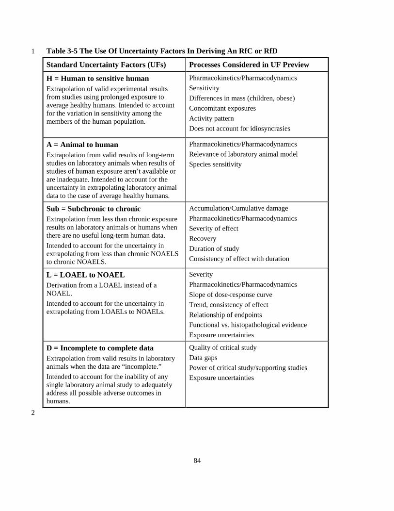
84

Table 3-5 The Use Of Uncertainty Factors In Deriving An RfC or RfD 1

Standard Uncertainty Factors (UFs) Processes Considered in UF Preview

H = Human to sensitive human Extrapolation of valid experimental results from studies using prolonged exposure to average healthy humans. Intended to account for the variation in sensitivity among the members of the human population.

Pharmacokinetics/Pharmacodynamics Sensitivity Differences in mass (children, obese) Concomitant exposures Activity pattern Does not account for idiosyncrasies

A = Animal to human Extrapolation from valid results of long-term studies on laboratory animals when results of studies of human exposure aren’t available or are inadequate. Intended to account for the uncertainty in extrapolating laboratory animal data to the case of average healthy humans.

Pharmacokinetics/Pharmacodynamics Relevance of laboratory animal model Species sensitivity

Sub = Subchronic to chronic Extrapolation from less than chronic exposure results on laboratory animals or humans when there are no useful long-term human data. Intended to account for the uncertainty in extrapolating from less than chronic NOAELS to chronic NOAELS.

Accumulation/Cumulative damage Pharmacokinetics/Pharmacodynamics Severity of effect Recovery Duration of study Consistency of effect with duration

L = LOAEL to NOAEL Derivation from a LOAEL instead of a NOAEL. Intended to account for the uncertainty in extrapolating from LOAELs to NOAELs.

Severity Pharmacokinetics/Pharmacodynamics Slope of dose-response curve Trend, consistency of effect Relationship of endpoints Functional vs. histopathological evidence Exposure uncertainties

D = Incomplete to complete data Extrapolation from valid results in laboratory animals when the data are “incomplete.” Intended to account for the inability of any single laboratory animal study to adequately address all possible adverse outcomes in humans.

Quality of critical study Data gaps Power of critical study/supporting studies Exposure uncertainties

2

85

Although the USEPA approach (1994, 2002a) addresses development of chronic toxicity factors, 1 many aspects of the approach are also applicable to the development of acute toxicity factors. 2 Typically, chronic toxicity values are not developed by USEPA for chemicals if all five areas of 3 uncertainty are present, or if there is an absence of data on potential respiratory tract toxicity 4 (relevant to TCEQ’s derivation of a chronic ReV) or oral toxicity (relevant to derivation of an 5 RfD). 6

However, due to State of Texas statutory requirements as discussed in Chapter 1, the TCEQ 7 develops acute and chronic inhalation or chronic oral toxicity values even when there is a greater 8 level of uncertainty (Section 3.16 Chemicals with Limited Toxicity Data). Potential methods 9 include using route-to-route extrapolation if specific criteria are met (Section 3.16.1) or a relative 10 toxicity/relative potency surrogate approach (Section 3.16.2). Alternate approaches for chemicals 11 with limited acute inhalation toxicity information to develop generic acute ESLs may be used 12 (Section 4.6) or alternate approaches for chemicals with limited chronic oral toxicity information 13 may be used to develop chronic RfDs (Section 5.6). 14

3.12.1 Interspecies (UFH) and Intraspecies (UFA) Factors 15

Toxicological responses may vary across species (interspecies variation) and among individuals 16 within the same species (intraspecies variation) (USEPA 1994). Therefore, the POD derived 17 from experimental data is adjusted by interspecies and intraspecies UFs to account for known 18 and unknown response variability. If toxicokinetic and toxicodynamic data are available, they 19 may be used to support the selection of UFs other than default values of 10 (Bogdanffy and 20 Jarabek 1995; IPCS 1999, 2005; ECETOC 2003). The primary approach to derive interspecies 21 and intraspecies UFs is to develop non-default UFs based on scientific data (i.e., data-based UFs) 22 (Renwick 1993; Renwick and Lazarus 1998; Dourson 1996; Dourson et al. 1996). Another 23 approach involves the use of chemical-specific adjustment factors (CSAFs) (IPCS 2001, 2005) 24 using available toxicokinetic and toxicodynamic data. Each of these approaches for dealing with 25 UFH or UFA is discussed below. 26

3.12.1.1 UFH or UFA Based on Scientific Data 27

Factors of 10 have been commonly applied by default to account for interspecies and intraspecies 28 sources of variability. The factor of 10 is considered to protect the majority of the human 29 population including children and the elderly. Renwick (1993) proposed that each of these UFs 30 can be described in terms of differences in toxicokinetics and toxicodynamics. He defines 31 toxicokinetics as all processes contributing to the concentration and duration of exposure of the 32 active chemical toxicant at the target tissue, and toxicodynamics as the mode or mechanism of 33 action of the active toxicant at the target tissue site. In regard to the UFH, there are differences 34 between children and adults in toxicokinetics (especially infants in their first months) and 35 toxicodynamics (especially at different stages of development), which may render children more 36 or less susceptible to the toxic effects of a substance. In situations where there are appropriate 37 chemical-specific toxicokinetic and/or toxicodynamic data relevant to the UFH or UFA, Renwick 38 (1993) suggested that the relevant default UF be replaced by a factor based on scientific data. If a 39 UF based on scientific data is introduced, then the commonly used 10-fold factor would be 40 replaced by the product of that factor and the remaining factor. 41

86

The UFA and the UFH of 10 can be divided into toxicokinetic and toxicodynamic components. If 1 credible information on toxicokinetics or toxicodynamics is available to support a lower UF than 2 the default of 10, a UF of 3, or even 1, may be used. Conversely, credible information may be 3 available to support a UF greater than 10, although in practice, an order of magnitude has 4 generally been used as a plausible upper bound for each UF (USEPA 1994). 5

USEPA (1994, 2002a) recommends dividing the UFH and UFA in half, one-geometric half (100.5 6 or 3.16 rounded to 3) each for toxicokinetic (UFH-k or UFA-k) and toxicodynamic (UFH-d or UFA-7 d) differences. For example, if an inhalation dosimetry adjustment from animal to human 8 exposure has been performed to account for toxicokinetic differences in calculating HEC, then 9 the full UFH of 10 may be reduced to 3 (a composite value obtained on multiplying 1 for UFA-k 10 and 3 for UFA-d) (Bogdanffy and Jarabek 1995; Jarabek 1995c; USEPA 1994). 11

A discussion of interspecies and intraspecies variability of response, as well as research and case 12 studies from the USEPA and the Health Canada risk assessments that demonstrate the use of 13 lower UFs are presented in papers by Bogdanffy and Jarabek (1995), Dourson et al. (1996), and 14 Jarabek (1995c). In addition, when BMD modeling is conducted and a BMDL is used as the 15 POD, Barnes et al. (1995) provide guidance on using data-based UFs rather than the default UF 16 of 10. NRC (2001) provides a list of questions that should be addressed to support the rationale 17 for the UF used. The TCEQ determines data-based UFs to account for interspecies and 18 intraspecies variation on a chemical-by-chemical basis, and the rationale for application of other 19 than default UFH or UFA values is provided in the DSD for each chemical. 20

3.12.1.1.1 Factors Considered for UFA 21 The factors considered when deciding on a specific value for the UFA include: (1) the relevance 22 and sensitivity of the laboratory animal model; (2) the animal species used in experimental 23 studies; (3) the likely mode/mechanism of action; (4) the range of response in the animal species 24 tested; (5) the variability of response among the species tested; and (6) 25 toxicokinetic/toxicodynamic differences among the species tested. 26

3.12.1.1.2 Factors Considered for UFH, Including Child/Adult Risk Differences 27 For the UFH, the factors considered in deciding on a specific value include: (1) the 28 mode/mechanism of action, (2) the toxicological endpoint observed, (3) what is known/unknown 29 about toxicokinetic/toxicodynamic differences among individuals, (3) the range of response 30 among humans and subpopulations (i.e., differences due to mass or activity pattern), (4) whether 31 toxicological (e.g., dose-response) data exist on effects in a susceptible human population, and 32 (5) sensitivity. 33

The potential sensitivity of children compared to adults is an important consideration for the 34 UFH. Section 3.2 discusses differences, including toxicokinetic and toxicodynamic differences, 35 between adults and children. Quantitative data regarding chemical-specific differences in 36 toxicokinetics between adults and children are limited. However, there are some studies that 37 have evaluated data to determine if the traditional uncertainty factors are protective of children 38 (Renwick 1998, Ginsberg 35 al. 2002, Rane 1992, Skowronski and Abdel-Rahman 2001, and 39 Calabrese 1986). Based on scientific data and an evaluation conducted on a chemical-by-40 chemical basis, the UFH may need to be greater than 10 in order to adequately protect children. 41

87

OEHHA (2008) concluded that differences between children and adults for relative minute 1 volume to surface area ratios are 4-fold or less and that those differences are accounted for in 2 many cases by the UFH to protect susceptible subpopulations. Nielsen et al. (2010) found that 3 young children frequently eliminate xenobiotics more rapidly by metabolism and excretion 4 compared with adults, suggesting that children would be adequately protected by a 3.16-fold 5 factor for toxicokinetics applied to the mean data for adults. Other analyses (Dorne et al. 2005 6 and Dorne and Renwick 2005 in Nielsen et al. 2010) found that neonates, if the parent chemical 7 is the toxic moiety, would be the most susceptible subgroup for all pathways of metabolism 8 because elimination processes are immature at birth up to 2 months of age. However, neonates 9 and infants less than two months old tend to stay indoors and are less likely to be exposed to 10 environmental pollutants. Refer to Section 3.10.4 for a discussion of differences in inhalation 11 dosimetry for children and adults. 12

Criteria to consider when evaluating any child/adult differences include indications or suspicions 13 of effects on organ systems and functions that are especially vulnerable during development and 14 maturation in early life (e.g., the nervous, reproductive, immune systems, and metabolic 15 pathways), and evaluating experimental data on such effects in young animals. Child/adult 16 differences will be discussed separately for acute exposures (Chapter 4) and chronic exposures 17 (Chapter 5). 18

3.12.1.2 Chemical-Specific Adjustment Factors 19 For a few chemicals, data are available to derive a CSAF to replace the default UF, thereby 20 reducing the overall uncertainty. A CSAF is based on ratios of kinetic or dynamic values 21 determined in animals and/or humans (e.g., ratio of peak concentration in animals divided by 22 peak concentration in humans, if the relevant dose metric is peak concentration). Therefore, 23 CSAFs are different than data-derived UFs (Section 3.12.1.1). For example, a data-derived UF 24 may be based on information that shows variability in different species is small, so a smaller 25 UFA could be used based on scientific judgment. IPCS (2001, 2005) published a guidance 26 document that details the data needed to develop CSAFs to account for interspecies differences 27 and human variability in toxicokinetics and toxicodynamics. Some of the data requirements 28 discussed by the IPCS (2001, 2005) include identification of the active chemical moiety, choice 29 of relevant toxicokinetic parameter, consideration of the experimental data, and consideration of 30 the endpoint. The TCEQ uses CSAFs to account for interspecies and intraspecies variation 31 depending on the availability of toxicity information and time and resource constraints. 32

3.12.2 LOAEL to NOAEL UF: UFL 33

Although the goal is to identify a POD that reflects the highest exposure level that does not cause 34 an adverse effect (NOAEL), in some cases, only a LOAEL is available from an experimental 35 study. Therefore, the LOAEL should be converted to a value analogous to a NOAEL. The 36 uncertainty in converting a LOAEL into a NOAEL can be addressed with a UF (UFL). Typically, 37 a default UFL of 10 is used to adjust the LOAEL to a NOAEL. However, multiple studies have 38 justified use of a UFL less than 10. It is important to consider the slope of the dose-response 39 curve in the range of the LOAEL in making the determination to reduce the size of the UFL 40 (USEPA 2002a). Several studies have reported that the LOAELs rarely exceed the NOAEL by 41 more than about 5-6 fold and are typically close to a value of 3 based on the ratios of LOAELs to 42

88

NOAELs for a range of different chemicals and different study durations (subacute, subchronic, 1 and chronic) (ECETOC 2003), although these findings are dependent on the dose spacing chosen 2 in toxicity studies. Dourson et al. (1996) state the choice of UFL should generally depend on the 3 severity of the effect at the LOAEL. If the effect at the LOAEL is severe, a larger UFL may be 4 needed. If the effect is mild, then these effects would not require a large UFL. 5

As described in Section 1.4, toxicity factors are set to protect the general public health, and the 6 biological endpoint of choice for determination (i.e., critical effect) will generally be a mild 7 effect. However, a more severe effect may be used if it is in fact the most sensitive endpoint that 8 occurs at the lowest exposure level (for example, irreversible developmental effects), or if no 9 data on mild effects are available. When the effect at the LOAEL is of low severity (e.g., mild local 10 effects by inhalation), the LOAEL is likely to be relatively nearer to the NOAEL, and thus a UFL of 11 1-3 may be sufficient. Conversely, more severe effects indicate the likelihood of a higher LOAEL to 12 NOAEL ratio. 13

3.12.2.1 TCEQ Approach 14

The TCEQ uses a UFL up to 10 or develops a chemical-specific UFL if data are sufficient based 15 on MOA analysis and/or severity of effect. The TCEQ uses professional scientific judgment in 16 determining the most scientifically-defensible UFL for a given chemical on a case-by-case basis, 17 considering all of the information discussed above. Pohl and Abadin (1995) provide examples of 18 chemicals where chemical-specific toxicity information was used to justify a UFL less than 10. 19

In general, the TCEQ uses the following default values of UFL, for acute and chronic ReV 20 derivations: 21

• Where the observed effect level is a NOAEL or equivalent benchmark (i.e., BMDL05 or 22 BMCL10), the value of UFL is 1. 23

• When the POD is based on a LOAEL and, the observed effect is minimal (< mild, 24 USEPA grade 3 or below), or where there is an indication that the LOAEL is close to the 25 NOAEL, the value of UFL may be 2 to 3. 26

• When the POD is based on a LOAEL and, the observed effect is mild/severe (USEPA 27 grade 4 to 5), the value of UFL is 6. 28

• When the POD is based on a LOAEL and, the observed effect is severe (USEPA grade 6 29 and above), the value of UFL is 10. 30

These default values are based on the criteria for determining the severity of adverse effects 31 (Section 3.7.1) and on Table B-1 in Appendix B and may be replaced by more specific values 32 where appropriate data are available (OEHHA 2008). USEPA (2002a) noted that data should be 33 carefully evaluated, taking into consideration the level of response at the LOAEL and the 34 NOAEL and the slope of the dose-response curve before reducing the size of the UF applied to 35 the LOAEL. 36

3.12.2.2 Other Federal and State Agency Approaches 37

When the less serious LOAEL approaches the threshold level (i.e., only minimal effects are observed 38 representing an early indication of toxicity), the ATSDR (Selene et al. 1998) and the ECETOC 39

89

(ECETOC 2003) recommend using a UFL of 3 and 2, respectively, for the “minimal” LOAEL. 1 When the effects observed at the LOAEL are not considered minimal but are less serious (mild 2 to moderate) or serious (severe), the ECETOC recommends a UFL of 6 be used. However, the 3 CalEPA (OEHHA 2008) recommends using a UFL of 6 and 10 for mild and severe effects, 4 respectively, to derive its acute REL, and using a UFL of 10 for any effect to derive its chronic 5 REL. In addition, IPCS (1999) recommends using UFs of 3, 5, or 10 to extrapolate from a 6 LOAEL to a NOAEL depending on the nature of the effect(s) and the dose-response relationship 7 (Table 3-6). 8

3.12.3 Database Uncer tainty Factor : UFD 9 Many important considerations relevant to the UFD are discussed in this section. However, issues 10 specifically related to the UFD used for the development of acute ReV and chronic ReV/RfD 11 values are discussed in Sections 4.5.2 and 5.5.2, respectively. Therefore, all relevant sections 12 should be referenced when selecting a UFD value for a particular toxicity factor. 13

Uncertainty introduced by database deficiencies, such as the inability of any single animal study 14 to adequately address all potential endpoints at various critical life stages or deficiencies in the 15 design or quality of an experimental study, can be addressed by the use of a UF (i.e., UFD) 16 (Dourson et al. 1996; USEPA 1994). The UFD is used to account for the fact that a potential 17 health effect may not be identified if the database is missing a particular type of study, and for 18 study quality deficiencies as well. The TCEQ also assigns a confidence level to the quality of the 19 key study and the database, not to the ReV or RfD. The TCEQ selects UFD values based on case-20 by-case determinations when deriving ReVs and RfDs, and generally uses a UFD of 1 for a 21 toxicological database with no substantial data and quality deficiencies and a UFD of up to 10 for 22 a database with substantial database and quality deficiencies. The areas of uncertainty considered 23 for the UFD are: 24

• Uncertainty associated with database deficiency (Section 3.12.3.1) including uncertainty 25 associated with potential child/adult differences (Section 3.2) 26

• Uncertainty associated with study quality (Section 3.12.3.2) 27

Prior to discussing these two areas of database uncertainty, it should be noted that there are 28 minimum database requirements for derivation of toxicity factors which are relevant to database 29 deficiency and the selection of a UFD value. The minimum database requirements, confidence 30 levels, and preliminary UFD values based on the number and types of studies available for 31 development of an acute ReV and chronic ReV/RfD are provided in Table 4-2 of Chapter 4 and 32 Table 5-2 of Chapter 5, respectively. However, the basic summary information given in Tables 33 4-2 and 5-2 may not accurately or adequately represent the completeness of the overall database 34 for a given chemical, as many important details and considerations are not addressed. Therefore, 35 use of these tables alone for this purpose would represent a significant oversimplification of 36 scientific judgment necessary for the UFD value selection process. Many of the important and 37 relevant details and considerations not addressed by these tables are discussed below and in 38 Section 3.12.3.2. 39

90

3.12.3.1 Database Deficiency and Study Quality Uncertainty and Confidence Levels 1

Database Uncertainty 2

As previously mentioned, the UFD is used to account for uncertainty resulting from an important 3 health effect potentially not being identified due to a particular type of study being missing from 4 the database. Uncertainty in such database gaps or other deficiencies includes completeness 5 (adequacy or limitations) and the size of the database. Unless a comprehensive array of 6 endpoints (e.g., tissues, organs, systems, life stages) is addressed by the database over the 7 exposure duration of interest, there is uncertainty as to whether the critical effect chosen for the 8 ReV or RfD is the most sensitive or appropriate. See Section 3.12.3.2 below for other relevant 9 considerations and questions regarding database (and study quality) uncertainty. 10

Of particular concern is the ability of some chemicals to affect the developing fetus or 11 development in infants and children. Consequently, the data available for various life stages 12 should be specifically considered. If appropriate studies to evaluate developmental effects or 13 effects in immature animals are lacking, it may not be possible to predict if effects on developing 14 organs and tissues occur at doses lower or higher than those which affect other endpoints. Refer 15 to Tables 4.2 and 5.2 for recommended reproductive/developmental studies. The ideal dataset for 16 evaluating developmental endpoints would include studies in two species in which exposure 17 occurs during gestation (relevant for development of acute ReVs) and a two-generation 18 reproductive study in two species (relevant to development of chronic ReVs and RfDs). When 19 reviewing a chemical’s database on developmental effects, it is important to assess (to the extent 20 possible) the potential for systemic toxicity in neonatal animals and evaluate whether an 21 immature metabolic system would result in increased or decreased sensitivity. In regard to the 22 lack of data for early life stages, Nielsen et al. (2010) noted the additional 10-fold factor for 23 infants and children called for in the 1996 Food Quality Protection Act (FQPA) is similar to the 24 UFD. It was concluded that an additional UF is not needed because the traditional factors were 25 considered sufficient to account for uncertainties in the database from which the toxicity factors 26 (e.g., reference values) are derived, including lack of data on children. The rationale for 27 application of the UFD selected will be presented in the individual toxicity summaries for each 28 chemical. 29

Study Quality Uncertainty 30

In addition to database deficiency, the UFD may also be used to account for less than desirable 31 study quality of the key study or other supporting toxicity studies. Factors relevant to study 32 quality include, but are not limited to, an appropriate number of animals per sex per group, 33 proper use of statistics, adequate analytical techniques and instrumentation, sufficiently sensitive 34 and objective measurement/ascertainment of adverse effects, general good laboratory practices, 35 sufficiently detailed documentation and results, etc. See Section 3.12.3.2 below for other relevant 36 considerations and questions regarding study quality (and database) uncertainty. 37

Database and Study Quality Confidence Levels 38

Confidence (reliability) levels are assigned to the overall database upon which ReVs or RfDs are 39 based. These confidence levels are assigned based on guidance in the RfC Methodology (USEPA 40

91

1994). A dataset confidence level of high, medium, or low is assigned to the overall database as 1 discussed in Section 4.5.2 for an acute database and Section 5.5.3 for a chronic database. 2

The TCEQ also assigns confidence levels to key studies. A key study of excellent quality likely 3 receives a high confidence rating, even if its duration is not ideal (e.g., a subchronic study for a 4 chronic ESL). A key study has a higher confidence rating if it is based on reliable human data 5 and supported by laboratory animal data. The level of confidence in an animal study is evaluated 6 through consideration of adequacy of study design, appropriate use of statistics, good laboratory 7 practices, spectrum of investigated endpoints, demonstration of dose-response relationships, 8 support from other studies, and other factors. Examples of low degree of confidence are: (1) low 9 number of animals used, (2) conflicting results between the key study and other studies, and (3) 10 uncertainty about the reliability of the route-to-route extrapolation (Nielsen et al. 2010). More 11 data, either on effects or on exposure, may be needed to increase the degree of confidence. 12

3.12.3.2 Relevant Questions and Considerations 13 It is important to consider the adequacy of the database (i.e., the overall confidence regarding the 14 quality, completeness, and consistency of the database) to help ensure derivation of health-15 protective toxicity factors. Some general questions that need to be considered in evaluating 16 database adequacy for toxicity factor (e.g., ReV, RfD) derivation are as follows (Nielsen et al. 17 2010): 18

• How extensive is the database? 19 • What is the quality of the studies? 20 • What are the data gaps (e.g., endpoints, life stages)? 21 • Are both human and animal data available, and are the results consistent? 22 • Are there data on more than one species, and are the results consistent? 23 • Are data available for the relevant route of exposure? 24 • What are the scientific uncertainties? 25 • What is the overall confidence in the database? 26

27

The TCEQ also considers more specific questions (adapted from USEPA 1994) that are useful in 28 the overall evaluation of database adequacy, which are grouped by subject below. As the relative 29 importance and relevance of some of these (and other) questions will vary from chemical to 30 chemical, ultimately, sound scientific judgment is used to decide on the value for the UFD on a 31 case-by-case basis. The primary aspect of database adequacy that each question addresses (e.g., 32 key/supporting study quality, relevance of study results for humans, database quality) has been 33 added in parenthesis to aid in separating study quality considerations (e.g., proper study design 34 and statistics) from those simply pertaining to the usefulness of a study for the purpose of 35 deriving a particular human toxicity factor (e.g., exposure route and duration, toxicokinetic 36 similarity of laboratory animal species to humans). While the utility of a study for deriving a 37 particular toxicity factor does not determine its quality (e.g., an intraperitoneal study may be of 38 high quality but not particularly useful for toxicity factor development), it should be noted that 39 the quality, number, and diversity (e.g., endpoints, life stages, and species evaluated) of studies 40

92

relevant to deriving a particular human toxicity factor does determine database quality for that 1 toxicity factor. 2

Adequacy and relevance of study design 3

• Is the route of exposure relevant to humans and the toxicity factor being developed 4 (relevance of study results to humans and toxicity factor development)? 5

• Were an appropriate number of animals and of both sexes used for determination of 6 statistical significance (key/supporting study quality)? 7

• Was the duration of exposure sufficient to allow results to be extrapolated to humans for 8 the exposure condition/duration of interest (relevance of study results to development of 9 the toxicity factor)? 10

• Were appropriate statistical techniques applied (key/supporting study quality)? 11 • Were the analytical techniques sufficient to adequately measure the level of the test 12

substance in the exposure protocol, including biological media (key/supporting study 13 quality)? 14

• Is the animal species and strain appropriate as a surrogate for humans (relevance of study 15 results to humans)? 16

• Are the techniques for measurement of the biological endpoints scientifically sound and 17 of sufficient sensitivity (key/supporting study quality)? 18

• To what degree may the biological endpoints be extrapolated (qualitatively or 19 quantitatively) to humans (relevance of study results to humans)? 20 21

Demonstration of dose-response relationships 22 23 • Were sufficient exposure levels used to demonstrate the highest NOAEL for the endpoint 24

of concern (key/supporting study and database quality)? 25 • Is the shape of the dose-response curve consistent with the known pharmacokinetics of 26

the test substance (key/supporting study quality)? 27 • Has the dose-response curve been replicated by or is it consistent with data from other 28

laboratories and other laboratory animal species (key/supporting study quality, human 29 relevance)? 30 31

Species differences 32 33 • Are the metabolism and pharmacokinetics in the laboratory animal species similar to 34

those for humans (relevance of study results for humans)? 35 • Is the species response consistent with that in other species (relevance of study results for 36

humans)? 37 • Is the species from which the threshold value was derived the most sensitive, relevant 38

species for humans (relevance of study results for humans)? 39 40

Other factors 41 42

93

• The number of biological endpoints evaluated and associated with dose-response 1 relationships (database and key/supporting study quality). 2

• Sufficient description of exposure protocol, statistical tests, and results to make an 3 evaluation (key/supporting study quality). 4

• Condition of animals used in the study (key/supporting study quality). 5 • The evaluation of effects of exposure in early life stages (database and key/supporting 6

study quality). 7 8

3.12.4 Rationale for Not Using a Modifying Factor 9 In the past, the USEPA (1994) recommended using a modifying factor (MF) to account for 10 scientific deficiencies in the quality of the critical study (i.e., the one used as the basis of the 11 POD) such as the number of animals tested or quality of exposure characterization. However, 12 based on recent USEPA (2002a) guidance that recommends the use of the MF be discontinued, 13 the TCEQ does not use a MF to develop toxicity factors. The USEPA (2002a) rationale for 14 discontinuing use of the MF centers on an examination of its infrequent application in IRIS and 15 the realization that all aspects of uncertainty considered for the MF are already explicitly 16 addressed in the UFD or in other UFs. Essentially, the purpose of the MF is “sufficiently 17 subsumed in the general database UF” (USEPA 2002a). 18

3.12.5 Procedures for Combining Values of Different UFs 19 USEPA (1994, 2002a) recommends dividing the UFH and UFA in half, one-geometric half (100.5 20 or 3.16 rounded to 3) each for toxicokinetic (UFH-k or UFA-k) and toxicodynamic (UFH-d or UFA-21 d) differences. When multiplying these factors (UFH-k or UFA-k or UFH-d or UFA-d) of “3” with 22 each other, the product would be 10, since one geometric half (100.5) multiplied by another 23 geometric half (100.5) is 10. 24

Since UFSub, UFL, and UFD are not based on geometric half values, the actual value for UFSub, 25 UFL, and UFD will be used to form the final product of all UFs. For example, if UFH = 3, UFA = 26 3, UFL = 2, UFD = 10, then UFH x UFA would be 3 x 3 = 10 (i.e., since they are one-geometric 27 half (100.5)), but the final product of all UFs would be 200 times the actual values of UFL = 2, 28 UFD = 10 (i.e., 10 x 2 x 10 = 200). 29

3.12.6 Application of Appropr iate Uncer tainty Factors 30

The exact values of the UFs chosen should depend on the quality of the studies available, the 31 extent of the database, and scientific judgment. For the purpose of comparison, the TCEQ lists 32 default UFs recommended by the USEPA and several other regulatory agencies and non-33 regulatory organizations in Table 3-6. 34

94

Table 3-6 Comparison of Uncertainty Factors Used by Different Health Organizations

Uncertainty Factors

TCEQ USEPA ATSDR OEHHA FDA ECETOC Netherlands

Health Canada/

IPCS Interspecies,

UFH

≤ 10 ≤ 10 1, 3 or 10 ≤ 100 10 2-7 (systemic effects)

1 (local effects) 3 10

Toxicokinetics UFH-K

Toxicodynamics,

UFH-d

3 3

3 3

--

--

1, 3 or 10

1, 3 or 10

--

--

--

--

--

--

2.5

4 Intraspecies,

UFA

≤ 10 ≤ 10 1, 3 or 10 ≤ 10 10 5 10 10

Toxicokinetics, UFA-K

Toxicodynamics,

UFA-d

3 3

3 3

--

--

1, 2 or 3

1, 2 or 3

--

--

--

--

--

--

2.5

4

Subchronic to chronic, UFSub

≤ 10 ≤ 10 1, 3 or 10 1, 3 or 10 10 2 (default)

1 (local effects) 1 to 10 1 to 100 for UFSub,

UFL & UFD

LOAEL to NOAEL, UFL

2-3 (≤ mild) 6 (mild/severe)

10 (severe) ≤ 10

--

3 (minimal effects)

10 ( serious effects)

6 (mild effects) 10 (severe effects)

NA --

3 (default) ± 3 (depends on severity)

1 to 10 -- See above

Incomplete database, UFD

≤ 10 = database deficiency and key

study quality, including child/adult

differences ≤ 10 NA 1 or 3 NA

1: high confidence level 1-2: medium

> 2: low NA See above Modifying factor,

UFM

N/A ≤ 10

(discontinued) 1 to 10 NA NA 1 to 10 1 to 10 1 to 10

95

3.13 Evaluating the Reasonableness of all Risk Assessment Decisions 1

When default factors of 10 are used to account for each area of uncertainty (e.g., interspecies, 2 intraspecies, LOAEL to NOAEL, incomplete database, subchronic to chronic), the product of the 3 UFs can be as high as 10,000-100,000, which may result in an overly conservative toxicity value 4 (Swartout et al. 1998). If four UFs are used and the cumulative UF exceeds 3,000, the TCEQ 5 uses a default of 3,000. This reduction from a higher cumulative UF is used in recognition of a 6 lack of independence of these factors (USEPA 1994) and to account for the interrelationships of 7 uncertainty categories for both acute and chronic toxicity factors (USEPA 2002a). Each 8 individual UF is generally conservative, and multiplying several areas of uncertainty (four or five 9 values of 10) likely yields unrealistically conservative toxicity factors (USEPA 1994). 10

In general, the more limited the toxicity information for a chemical, the higher the product of the 11 UFs will be in order to increase the expectation that the adjusted toxicity value is health-12 protective. In all cases, the DSD for each chemical discusses the basis for each component UF 13 and the conservatism of the resulting product. The TCEQ uses criteria from the latest reference 14 concentration/dose derivation guidance documents (USEPA 1994, 2002a), information on the 15 differential toxicity of chemical classes or isomers, as well as scientific judgment to determine 16 whether the aggregate impact of all risk assessment decisions results in a toxicity factor that is 17 unreasonable. An unreasonable toxicity factor is one that would incorporate a product of UFs 18 greater than 3000. 19

3.14 Identification of Inhalation Effect Levels 20 Toxicity factors and their corresponding risk-specific concentrations are considered “safe levels” 21 because they are set below levels where adverse health effects are expected to occur. Risk 22 managers as well as the general public may want information on the air concentrations where 23 health effects would be expected to occur (i.e., an air concentration effect level). Thus, when 24 adequate data exist for inhalation, the TCEQ will provide effect levels in DSDs for comparison 25 to safe levels. These effect levels are primarily for informational purposes. 26

3.14.1 Chemicals with a Threshold MOA 27 For noncarcinogens or carcinogens with a threshold MOA, the LOAELHEC from the study that 28 identified the critical effect can be considered the lowest documented level where effects in the 29 human population could be expected to occur in some members of the population. If BMC 30 modeling is conducted, the central estimate BMCHEC corresponding to a BMR of concern for 31 adverse effects (e.g., BMC10-HEC for decreased body weight) which does not require significant 32 extrapolation below the range of the data is used as the lowest level where effects in the human 33 population could be expected to occur. 34

More specifically, an LOAELHEC determined from human studies, where effects occurred in 35 some individuals, represents a concentration at which it is probable that similar effects could 36 occur in some individuals exposed to this level over the same duration as used in the study or 37 longer. Importantly, effects are not a certainty due to potential intraspecies differences in 38 sensitivity. Conversely, the NOAELHEC from a human study is the highest concentration known 39 (based on dose-response data) which may not be expected to result in adverse effects in humans 40 similar to the study-exposed population (e.g., workers, adult volunteers) exposed over the same 41

96

(or shorter) duration, although this is not a certainty (e.g., study power considerations). In 1 addition, other subpopulations could be more sensitive than the study-exposed population. 2

For an LOAELHEC determined from animal studies in the most sensitive species, as effects 3 occurred in some animals in the most sensitive species, the LOAELHEC represents a 4 concentration at which it is possible that similar effects could occur in some individuals exposed 5 to this level over the same duration as used in the study or longer, although effects are not a 6 certainty (e.g., potential species differences in sensitivity). If laboratory animal data are relied 7 upon and there is no information on the sensitivity of animals versus humans, the determination 8 of effect levels needs to be put into the context of a discussion of studies in other species which 9 did not show effects at similar or higher levels/durations. 10

3.14.2 Application of UFs or Duration Adjustments 11 Determinations of actual effect levels should have a reasonable degree of certainty associated 12 with them, and therefore should be based on what is known (i.e., be founded in actual dose-13 response data). Consequently, UFs are inapplicable because they are based in uncertainty and 14 applying a UF interjects uncertainty about (i.e., essentially negates) the expectation of a human 15 response occurring in some individuals based on the dose-response data. Additionally, if data are 16 not available for an exposure duration adjustment that is predictive of toxicity, exposure duration 17 adjustments will not be performed. For example, for an acute 1-h ReV, an “n” of 3 is used to 18 perform exposure duration adjustments from a longer exposure duration study to 1-h because it is 19 generally considered to be conservative, not because the duration adjustment accurately predicts 20 a 1-h level associated with the same probability of a response. Using UFs and duration 21 adjustments results in a value with an unknown ability to predict the probability of a response 22 and arguably some conservatism, which is contrary to the purpose of identifying a level where 23 with a reasonable degree of certainty, a response in some individuals may be expected. 24

3.14.3 Chemicals with a Nonthreshold MOA 25 For carcinogenic effects or noncarcinogens with a nonthreshold MOA, the risk-specific dose is 26 set at the no significant excess risk level associated with a theoretical excess lifetime cancer risk 27 of one in 100,000 (1 x 10-5 or simply 10-5). USEPA’s acceptable risk range is 10-6 to 10-4 28 (USEPA 2000e). When tumor data are used, a POD is obtained from the modeled tumor 29 incidences. Conventional cancer bioassays, with approximately 50 animals per group, generally 30 can support modeling down to an increased incidence of 1–10% (10-2 to 10-1 risk); epidemiologic 31 studies, with larger sample sizes, below 1% (10-2 risk) (USEPA 2005a). For a well-conducted 32 epidemiology study with adequate number of subjects and statistical power, it may be possible to 33 detect an increase in background cancer incidence/ mortality at the 10-3 risk level (Grant et al. 34 2007) or lower. Seiler and Alvarez (1994) determined that for radiation carcinogenesis, the 35 minimum significant risk for the model is considerable larger than 10-3 and for the usual 36 confidence limits, the minimum significant risk exceeds 10-2: 37

“Whereas a more careful error analysis may yield lower limits, it is unlikely that they will 38 lie below 1 x 10-3. Thus, even though risk values below this limit can be calculated, they 39 are not meaningful because they are smaller than their total standard errors, and are thus 40 not compatible with finite risks”. 41

97

An air concentration corresponding to the excess risk level detected by the key epidemiological 1 study (e.g., 10-3), preferably based on the statistical best estimate of the potency factor since this 2 may be most predictive (i.e., central estimate or maximum likelihood estimate), can be 3 considered the lowest level for which effects in some individuals in the human population would 4 be expected with reasonable certainty if exposed over a similar (or longer) exposure duration 5 than those in the epidemiological study. Alternatively, a range of values corresponding to air 6 risk-specific concentrations of around 10-3 (e.g., 10-4 to 10-3) could be used. 7

However, calculating these risk-specific values based on assumed lifetime environmental 8 exposure may be inappropriate for this purpose. For example, dose rate may have at least 9 enhanced carcinogenesis or the carcinogenic MOA in workers (e.g., the metabolic pathways 10 responsible for carcinogenesis in workers). That is, an exposure duration similar to that in the 11 epidemiological study may need to be used to calculate these risk-specific values so that the 12 predictiveness of the values is reasonably certain (e.g., dose rate effects and dose-related changes 13 in metabolic pathways are not potential issues). 14

For animal studies, air concentrations corresponding to the detected increase in cancer 15 incidence/mortality over background or the EC10 and converted to an HEC can be used. 16 Ultimately, the response level used to calculate an air concentration where adverse effects would 17 be expected to occur (based on dose-response data) in some individuals of the population will be 18 based on best scientific judgment on a case-by-case basis and justified in the DSD. 19

3.15 Exposure-Response or Reference Value Arrays 20 Exposure arrays are a valuable graphical tool to display toxicity data regarding a chemical across 21 toxic endpoints, species, and exposure durations (USEPA 2009). Often a chemical has many 22 studies that together describe the toxicity of that chemical based on duration and concentration of 23 exposure, so exposure arrays are valuable to both toxicologists and lay persons. Importantly, 24 exposure arrays may also provide a means by which the toxic effect caused by a given duration 25 exposure may be easily determined. 26

There are several ways that exposure arrays have been used by various regulatory agencies. The 27 ATSDR regularly uses exposure response arrays to summarize toxicity data for acute, 28 subchronic, or chronic exposure duration for chemicals. In general, the ATSDR plots exposure 29 concentration on the y-axis and duration on the x-axis. The x-axis, in these cases, is further 30 broken down by organ system. Symbols on these graphs represent LOAELs or NOAELs 31 identified in critical studies. This style of representation is particularly valuable because it not 32 only shows toxic effect or biological response by dose and duration of exposure, but also 33 conveys a sense of the margin of toxicity, in other words what is the margin between NOAEL 34 and LOAEL for a particular study (Figure 3-13). 35

98

1 Figure 3-13 Exposure-Response Array for Ammonia, generated by the ATSDR 2

Exposure concentration (on a log scale), duration for acute exposure and toxic effect are 3 specified. In addition, symbols represent whether the endpoint was a NOAEL or a LOAEL and in 4 what animal species that value was identified. Importantly, by displaying data in this way, 5 relationships between exposure duration and effect can be observed independent from test 6 organism. (Figure 3-1 from ATSDR 2004). 7

Similarly, the USEPA (2009) has recently written guidance for the generation of exposure- 8 response arrays, “Graphical Arrays of Chemical-Specific Health Effect Reference Values for 9 Inhalation Exposures”. That document presents duration-specific reference values developed by 10 different federal and state organizations for a chemical as a function of exposure duration (acute, 11 short-term, subchronic, and chronic). Thus, similar to the graphics routinely used by ATSDR, 12 data are displayed in a comprehensive manner that allows comparison across exposure duration, 13 species, and toxic effect. This approach does, however, display reference values rather than 14 NOAELs and LOAELs. Thus, to have a better understanding of the margin of exposure between 15 protective reference values and the concentrations where effects are observed would require 16 identifying the PODs for the reference values, how the PODHEC values were derived, and the 17 UFs applied (Figure 3.14). 18

Exposure-response arrays should be included in DSDs if sufficient data exist. Minimal data 19 requirements for the generation of an exposure response array include at least two acute, sub-20 acute, and chronic studies. The format for the exposure-response array may be limited by what 21 data are available for a chemical. However, for the evaluation of a basic toxicity assessment, data 22 displayed in the format of NOAELs and LOAELs may be more informative because of the lack 23

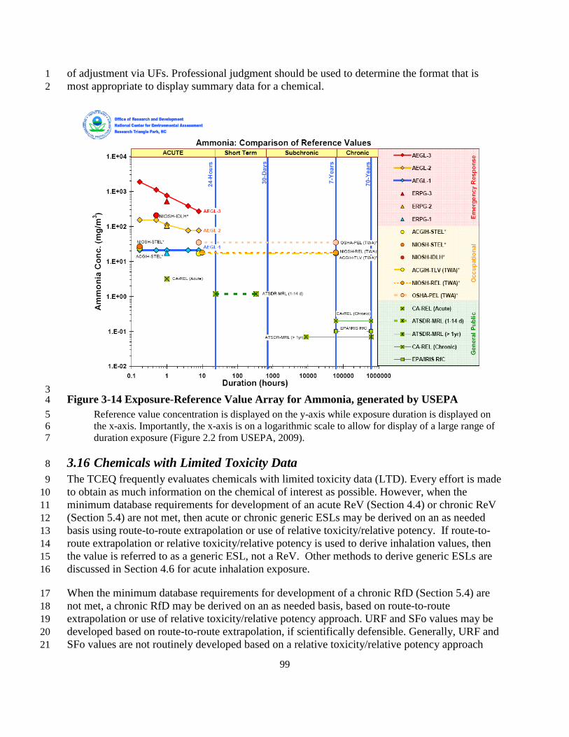
99

of adjustment via UFs. Professional judgment should be used to determine the format that is 1 most appropriate to display summary data for a chemical. 2

3 Figure 3-14 Exposure-Reference Value Array for Ammonia, generated by USEPA 4

Reference value concentration is displayed on the y-axis while exposure duration is displayed on 5 the x-axis. Importantly, the x-axis is on a logarithmic scale to allow for display of a large range of 6 duration exposure (Figure 2.2 from USEPA, 2009). 7

3.16 Chemicals with Limited Toxicity Data 8 The TCEQ frequently evaluates chemicals with limited toxicity data (LTD). Every effort is made 9 to obtain as much information on the chemical of interest as possible. However, when the 10 minimum database requirements for development of an acute ReV (Section 4.4) or chronic ReV 11 (Section 5.4) are not met, then acute or chronic generic ESLs may be derived on an as needed 12 basis using route-to-route extrapolation or use of relative toxicity/relative potency. If route-to-13 route extrapolation or relative toxicity/relative potency is used to derive inhalation values, then 14 the value is referred to as a generic ESL, not a ReV. Other methods to derive generic ESLs are 15 discussed in Section 4.6 for acute inhalation exposure. 16

When the minimum database requirements for development of a chronic RfD (Section 5.4) are 17 not met, a chronic RfD may be derived on an as needed basis, based on route-to-route 18 extrapolation or use of relative toxicity/relative potency approach. URF and SFo values may be 19 developed based on route-to-route extrapolation, if scientifically defensible. Generally, URF and 20 SFo values are not routinely developed based on a relative toxicity/relative potency approach 21

100

except in certain cases (e.g., relative potency factors for polycylic aromatic hydrocarbons 1 (Chapter 6)). Other methods to derive RfDs are discussed in Section 5.6 RfDs for Chemicals with 2 Limited Toxicity Data. 3

3.16.1 Route-to-Route Extrapolation 4 In the absence of human and animal dose-response data for either the oral or inhalation route of a 5 given agent, the TCEQ may derive toxicity factors or generic ESLs based on data from 6 inhalation or non-inhalation (e.g., most likely oral) exposure routes, respectively, only if strict 7 criteria are met. However, for TCEQ’s purposes it is anticipated that the most likely route-to-8 route extrapolation will be derivation of a generic ESL from oral data. Route-to-route 9 extrapolation for purposes of deriving a Generic ESL or RfD will be performed on the 10 PODHED/HEC of the critical study, not on the final toxicity factor so that appropriate UFs can be 11 applied. Most specifically, a UFD which considers and accounts for the uncertainty of deriving a 12 toxicity factor based on route-to-route extrapolation. Route-to-route extrapolation for purposes of 13 deriving a SFo or URF will be performed on the toxicity factor for the exposure route with 14 carcinogenicity data as UFs are not used in the derivation of carcinogenic toxicity factors. 15

Extrapolation of dose-response data from one exposure route to another is accompanied by 16 uncertainty, which is important to minimize as much as the available data and methods allow. 17 The major factors contributing to the uncertainties associated with route-to-route extrapolation 18 include: (1) the presence of POE effects in the lung or gastrointestinal tract and the potential for 19 such effects for the exposure route being extrapolated to; (2) liver first-pass effects following 20 oral dosing which would result in an expectation of adverse effects different than those due to 21 inhalation exposure; and (3) accurate dosimetry to normalize the internal dose and biologically 22 effective dose achieved by the compared exposure routes (i.e., pharmacokinetic differences) is 23 unknown. USEPA states that if either a first-pass effect or POE effect is present, route-to-route 24 extrapolation is not recommended for derivation of chronic health reference values such as the 25 RfC (USEPA 1994). 26

Oral ingestion is the most common exposure route from which toxicity is estimated for other 27 routes, including inhalation. Data from parenteral exposure may also be considered although 28 accurate dosimetry is still required to normalize internal and effective doses to those expected 29 from inhalation. Honma and Suda (1998) performed a correlation of lethal doses of industrial 30 chemicals between oral or intraperitoneal administrations and inhalation exposure and 31 demonstrated that the correlations between LC50 and LD50 data with intraperitoneal 32 administration were higher than those between LC50 and LD50 both in rats and mice. 33

Given the uncertainties associated with route-to-route extrapolation, the TCEQ does not perform 34 route-to-route extrapolation if any of the following circumstances would be expected based on 35 available data or information (refer to Figure 4-3 in Section 4.1.2 of USEPA 1994): 36

• Different critical adverse effects are expected to result from the compared exposure 37 routes; 38

• POE effects occur; 39 • Respiratory or hepatic first-pass effects are expected; 40

101

• A respiratory or oral effect is known to occur, but accurate dosimetry between the two 1 routes is not established; 2

• Referenced oral/inhalation studies do not include adequate assessment of respiratory tract 3 or gastrointestinal effects, respectively; or 4

• Studies are not of adequate quality to establish a toxicity factor for the exposure route 5 from which to extrapolate. 6

7 If the above mentioned route-to-route concerns are addressed, toxicity information from other 8 exposure routes may be used to add to the WOE, determine the MOA, or address other issues 9 when deriving a toxicity factor for another route of exposure. For example, if a 2-generation 10 study is available via the oral route showing no reproductive/developmental effects, and oral 11 absorption is known to occur, then this information may be used to support the likelihood that 12 the chemical is not a reproductive/developmental toxicant via the inhalation route (assuming no 13 POE effects, etc. are expected). 14

The preferred method for route-to-route extrapolation is the use of PBPK modeling, which 15 provides the best estimate of a toxicant’s internal and biologically effective dose as a function of 16 exposure. PBPK modeling accomplishes this by application of algorithms for physiologic factors 17 such as ventilation/perfusion ratios, renal clearance and metabolism, as well as properties of the 18 given toxicant (e.g., partition coefficients, reactivity). The combination of PBPK modeling and 19 supporting toxicity data allows route-to-route extrapolation with fewer uncertainties than other 20 methods, and the TCEQ utilizes this method whenever possible to derive toxicity factors for a 21 constituent. When the available data are inadequate for PBPK modeling, other available 22 mathematical dosimetry models can be used based on MOA of the chemical and whether 23 necessary physiologic factors are available. For extrapolation of oral to inhalation, the following 24 papers provide several case studies for different chemicals illustrating the use of mathematical 25 models and approaches for route-to-route extrapolation that are particularly informative (e.g. 26 chloroform, cadmium, carbon tetrachloride, and trichloroethylene) (Overton and Jarabek 27 1989a,b; Gerrity and Henry 1990; Overton 1990; USEPA 1994). 28

For deriving a generic ESL, if a more appropriate chemical-specific model is not available, the 29 PODHEC can be calculated from the corresponding PODHED as follows: 30

PODHEC = [(PODHED x BWH x (day/20 m3)] x (Aoral / Ainh) 31

where: 32

PODHEC = human equivalent concentration POD (mg/m3) 33 PODHED = human equivalent dose POD (mg/kg-day) 34 BWH = human body weight (70 kg) 35 Aoral = absorption via oral exposure (unitless) 36 Ainh = absorption via inhalation exposure (unitless) 37

For deriving a RfD, the PODHED can be calculated from the corresponding PODHEC as follows: 38

PODHED = [(PODHEC x 20 m3/day) / BWH] x (Ainh / Aoral) 39

102

For deriving a URF, assuming route-to-route extrapolation is considered scientifically defensible, 1 the following equation may be used to convert the SFo: 2

URF (risk per µg/m3) = (SFo/BWH) x 20 m3/day x (1 mg/1,000 µg) x (Ainh/Aoral) 3 where: 4

SFo = oral slope factor (risk per mg/kg-day) 5 BWH = human body weight (70 kg) 6 Aoral = absorption via oral exposure (unitless) 7 Ainh = absorption via inhalation exposure (unitless) 8 9

Rearranging the equation to derive a SFo from a URF yields: 10

SFo (risk per mg/kg-day) = (URF/20 m3/day) x BWH x (1,000 µg/1 mg) x (Aoral/Ainh) 11

Chemical-specific values for Ainh and Aoral should preferentially be used but Ainh and Aoral data 12 from a structurally-related chemical or chemical-class may be used if data indicates it is relevant 13 and scientifically defensible. Otherwise, a default absorption ratio (Ainh / Aoral or Aoral / Ainh) of 1 14 may be used. TCEQ utilizes best scientific judgment on a case-by-case basis in determining 15 whether to perform route-to-route extrapolation for derivation of a particular toxicity factor 16 (generic ESL, RfD, SFo, URF). 17

3.16.2 Relative Toxicity/Relative Potency Approach 18

3.16.2.1 Background 19 Relative potency can be defined as a procedure to estimate the “toxicity” of a LTD chemical in 20 relation to a reference or an index chemical(s) for which toxicity has been well defined. The 21 concept of relative potency has been used for polycyclic aromatic hydrocarbons (PAHs) (Collins 22 et al. 1998) and organophosphate pesticides (USEPA 2002b). PAHs are considered a class of 23 structurally and toxicologically similar chemicals. Therefore, the concept of relative toxicity has 24 been used to derive toxicity values for PAHs with limited toxicity information based on the 25 toxicity information of benzo[a]pyrene, for which there is a wealth of information (Collins et al. 26 1998). 27

Various government and regulatory agencies have adopted the relative potency approach or have 28 adopted comparable methodologies for the purpose of estimating toxicity values for chemicals 29 with limited information. The relative potency approach was used to determine Acute Exposure 30 Guideline Level (AEGL) values for some nerve agents based on the toxicity data of nerve gas 31 sarin. The rationale for the relative potency approach was that other nerve gases such as tabun, 32 soman, cyclosarin, and VX were similar in structure and toxicity to sarin gas (NRC 2003). The 33 emergency planning and safety analysis divisions within the US Department of Energy 34 (USDOE) complex often need to derive Temporary Emergency Exposure Levels (TEELs) for 35 chemicals with limited toxicological information until ERPGs are available (USDOE 2008). The 36 methodology for deriving TEELS for LTD chemicals involves comparing 50% lethality data of a 37 structurally-similar chemical with adequate inhalation reference values to the lethality data of the 38

103

LTD chemical in order to estimate values for the LTD chemical if that is the only available data 1 (USDOE 2008). 2

3.16.2.2 Quantitative Structure Activity Relationships versus Structural Activity 3 Relationships 4

Quantitative structure activity relationships (QSARs) use a mathematical relationship to 5 quantitatively link chemical structure and pharmacological activity for a series of compounds 6 (USEPA 1999a). While QSARs have proven to be very useful for predicting mutagenicity, their 7 use in risk assessment is limited as they require highly trained toxicologists who are proficient in 8 the use of the computer software to correlate complex molecular structures to varied health 9 effects (e.g., acute vs. chronic, in vitro vs. in vivo, mutagenicity vs. general toxicity vs 10 developmental toxicity). Therefore, QSARs can become time consuming, data-intensive, and 11 expensive tools in risk assessment. Therefore, the TCEQ does not directly perform QSAR to 12 predict acute inhalation toxicity endpoints but uses information from QSAR studies published in 13 the scientific literature. 14

Structural activity relationships (SARs) can be described as the relationship of the molecular 15 structure of a chemical with a physicochemical property, environmental fate, and/or specific 16 effect on human health or on environmental species (USEPA 1999a). Both the USEPA and 17 European Chemical Bureau have recognized the benefits of using SARs as a way to reduce the 18 amount of testing required for chemicals with limited information. USEPA and the European 19 Chemical Bureau define a category as a group of chemicals whose physicochemical and 20 toxicological properties are likely to be similar or follow a regular pattern as a result of structural 21 similarity. The underlying premise of SARs is that members of a chemical group or class share 22 similar physical and chemical properties and MOA, and therefore, they will tend to behave in a 23 similar toxicological manner (USEPA 1999a; USEPA 1999b). For example, the similarities 24 among the chemicals in the category can be based on a common functional group (e.g., aldehyde, 25 epoxide, ester, etc.) or an incremental and constant change across the category (e.g. the 26 dimethylene group difference between adjacent members of the alpha-olefins or the presence of 27 homologous series as in glycol ethers) (USEPA 1999b). 28

The TCEQ uses the principles of SAR to choose an appropriate analog chemical or to categorize 29 chemicals into groups or classes. An analog is defined as a chemical compound that is 30 structurally similar to another compound but differs slightly in composition (as in the 31 replacement of one atom by an atom of a different element or in the presence of a particular 32 functional group). In order to use the analog approach, there should be unambiguous structural 33 and metabolic relationships between the LTD chemical and the chemical with toxicity 34 information. A potential category can be formed by grouping a series of chemicals or using 35 chemical categories that have been defined by USEPA such as the high production volume 36 chemical classes (USEPA1999b). 37

3.16.2.3 Steps to Perform Relative Toxicity/Potency 38 The TCEQ uses the principles of SAR coupled with the knowledge of the MOA of an index 39 chemical or a class of chemicals in conjunction with expert judgment of trained staff to develop 40 generic toxicity factors for LTD chemicals. Procedures used previously by others are used by 41

104

TCEQ staff to estimate toxicity factors based on relative potency (USDOE 2008; Glass et al. 1 1991). The TCEQ maintains the generic toxicity factors on an interim basis until additional 2 toxicological information becomes available. The estimation process is especially valuable for 3 estimating toxicity factors for categories of chemicals that are known to be relatively less toxic 4 (Globally Harmonized System (GHS) Categories 3, 4 and 5; UN 2005) and for which traditional 5 testing may not occur. Use of scientifically-valid estimation tools for the relatively less toxic 6 chemicals allows more resources (time and resources) to be directed toward toxicity factor 7 development for the more toxic chemicals (GHS Categories 1 and 2) which warrant a higher 8 level of review. The following steps briefly describe the qualitative expert judgment approach 9 that the TCEQ uses to apply the concept of SAR and relative potency for estimating generic 10 ESLs or other toxicity factors for LTD chemicals. These steps can be employed when similar 11 chemical categories or an analog chemical approach is used: 12

Step 1: Identify potential index chemical(s) for which toxicity factors have been 13 developed. 14

Step 2: Gather data on physicochemical properties, toxicity, etc. for the potential index 15 chemical(s) and the LTD chemical. 16

Step 3: Construct a matrix of data for all chemicals. Table 3-7 is an example of how to 17 organize endpoint information for a series of potential index chemicals and the LTD 18 chemical. 19

Step 4: Evaluate the data to determine if there is a correlation among chemicals and the 20 endpoints by conducting a simple trend analysis to determine whether a predictable 21 pattern exists amongst the chemicals. 22

Step 5: Perform a MOA analysis and determine the relevant endpoints that can be used for 23 a relative potency approach. Relevant endpoints should be determined using similar 24 testing techniques, exposure durations, and species. 25

Step 6: Calculate the relative potency of the pertinent endpoint based on an MOA analysis 26 of the index chemical to the pertinent endpoint of the LTD chemical: 27

ChemicalIndex

Chemical LTD

EndpointRelevant Endpoint Relevant Potency Relative = 28

Step 7: Estimate the generic toxicity factor of the LTD chemical by adjusting the index 29 chemical’s value by the relative potency factor. The following equation shows this 30 adjustment for a generic ESL, but it could also be used for a chronic generic ESL or RfD: 31

Potency Relative x ESL ESL Generic ChemicalIndex Chemical LTD = 32

Relevant endpoint data used to ratio toxicity may be as straightforward as mortality 33 measurements (e.g., LC50 and LD50 data). In addition, MOA can be used to identity other 34 relevant endpoints whose ratio is expected to describe the difference in toxicity between the two 35 chemicals. For example, if one needs to estimate a generic RfD for a limited-data 36 organophosphate pesticide based on the RfD of another organophosphate pesticide, 37

105

measurements of brain cholinesterase inhibition could be the relevant endpoint. The RfD of the 1 index organophosphate pesticide would be multiplied by the ratio of cholinesterase inhibition of 2 the limited-data chemical to the cholinesterase inhibition of the index chemical. 3

If multiple values of relative potency based on the same or different relevant endpoint are 4 available, a geometric mean of the calculated relative potency ratios (RGM) is obtained. The 5 generic value for the LTD chemical can then be calculated by multiplying the RGM by the value 6 of the structurally-similar index chemical. This process may be repeated if more than one 7 chemical similar to the chemical of interest is identified. 8

Alternately, depending on data availability and time and resource constraints, the lowest, most 9 conservative toxicity factor for a series of structurally-similar compounds can be used as a 10 generic value for other structurally-similar compounds with limited toxicity information. For 11 example, OEHHA developed a reference exposure level (REL) for metallic mercury vapor, but 12 there was less information on mercury salts. However, OEHHA stated “Since mercury salts have 13 no significant vapor pressure under normal atmospheric conditions, they would only be of 14 concern as hazards if aerosolized in aqueous solution or burned. This REL is developed for 15 metallic mercury vapor and would be an overestimate of the REL for mercury salts.” (OEHHA 16 1999b) 17

18

106

Table 3-7 Example of How to Organize Endpoint Information for a Series of Chemicals 1

Endpoint Potential Index Chemical #1

Potential Index Chemical #2

LTD Chemical

Potential Index Chemical #3

Category

Molecular weight

Chemical Formula

Chemical Structure

Physical Form

Boiling Point

Melting Point

Vapor Pressure at 25o C

Partition Coefficient

Log Kow

Solubility

Odor

Health effects

Short-term ESL

LC50

LD50

RD50

NOAEL

LOAEL

Reproductive/ Developmental

2

3.17 Sensitization 3 Sensitization is an immune process by which individuals develop an exaggerated, pathological 4 immune response, or hypersensitivity, upon subsequent exposure to a particular antigen. 5 Sensitization occurs in two phases: (1) induction and (2) elicitation. Induction occurs when an 6 individual is initially exposed to an antigen. This antigen is presented in the local lymph node 7 and initiates clonal expansion of T lymphocytes, leading to the development of immunological 8

107

memory. Immunological memory supports elicitation, an abrupt and intense cell- or antibody-1 mediated allergic response, upon subsequent exposure to the primary antigen. 2

A sensitizer is defined by OSHA as “a chemical that causes a substantial proportion of exposed 3 people or animals to develop an allergic reaction in normal tissue after repeated exposure to the 4 chemical” (Appendix A of 29 CFR 1910.1200). A respiratory sensitizer is a chemical that causes 5 the development of an allergic reaction in the airways following inhalation. The TCEQ identifies 6 a chemical as a respiratory sensitizer if evidence exists that a chemical can induce specific 7 respiratory hypersensitivity in humans or appropriate animal models using established scientific 8 methods. Current established scientific methods include human epidemiology and occupational 9 exposure studies as well as animal local lymph node assay (LLNA), mouse IgE, and guinea pig 10 pulmonary response tests. The LLNA was originally developed to identify contact sensitizers 11 (Kimber 1992). However, this assay can be used to identify respiratory sensitizers if (1) 12 induction occurs via the inhalation route or (2) induction occurs via the dermal route and a 13 cytokine profile indicates primary elicitation of the T helper 2-cell response (Dearman 2000). 14

Through selection of the most sensitive endpoint and the application of UFs, short-term and 15 long-term ESLs are designed to protect the human population, including sensitive individuals, 16 against adverse health effects. Sensitization is typically caused by high initial doses of the 17 chemical antigen (USEPA 1994). Therefore, to protect against sensitization, exceedances of the 18 short-term or long-term ESLs should be discouraged during the air permit review for chemicals 19 identified as respiratory sensitizers. However, it should be noted that this precaution does not 20 necessarily protect individuals who were previously sensitized. The TCEQ specifically identifies 21 respiratory sensitizers in the DSD to inform the public and to allow previously sensitized 22 individuals to further reduce their individual exposure to these chemicals. 23

3.18 Significant Figures and Rounding Procedures 24

3.18.1 General Procedures 25 In order for the TCEQ to be consistent in the derivation process of toxicity factors, the 26 convention of retaining significant figures used throughout the calculation process should be 27 consistent. The TCEQ determined that it will not round numbers in intermediate equations (i.e., 28 no rounding of numerical results will occur between separate equations). When each calculation 29 is performed, original numerical data should be used, showing the unit conversions. 30

Once the toxicity factor is calculated, it will then be rounded to two significant figures. When 31 rounding, if the number next to the significant figure to be rounded is a 5 or less, the number will 32 be rounded down (e.g., 13563 rounded to two significant figures = 13000). If the number next to 33 the significant figure to be rounded is a 6 or more, the number will be rounded up (e.g., 13623 34 rounded to two significant figures = 14000). 35

When converting toxicity factors and ESL values from µg/m3 to ppb, or ppb to µg/m3, the 36 rounded value will be used. Once the conversion is complete, the converted number will then be 37 rounded to two significant figures. A statement will be added to the DSD document informing 38 readers of the method by which the final values were calculated. When the TCEQ shows 39

108

calculations in the DSD, it will be up to the judgment of the individual toxicologist as to how 1 many significant figures are represented in the intermediate calculations. 2

3.18.2 Air Permitting 3 For air permitting, the rounded toxicity factor will then be used to determine the ESL (i.e., the 4 ReV will be multiplied by 0.3 or the URF will be used to calculate a 1 in 100,000 extra cancer 5 risk). The ESL will also be rounded to two significant figures. 6

7

109

Chapter 4 Der ivation of Acute Toxicity Factor s 1

4.1 Published Toxicity Factors or Guideline Levels 2 The following sections discuss the database sources to which the TCEQ refers during its search 3 for published acute values and/or data. When acute toxicity factors or guideline levels are 4 identified in the scientific literature or databases, they are reviewed to determine whether the 5 approach used to develop these toxicity factors is similar to the procedures used by the TCEQ to 6 develop ReVs. If so, the TCEQ considers adoption of the published toxicity factor or guideline 7 level, with preference given to values that have undergone an external peer review and public 8 involvement process. Many published acute toxicity factors are not appropriate to be used as 9 ReVs because it is likely that procedures other than those recommended in this guidance 10 document were used to derive these values. Due to time and resource constraints, the TCEQ 11 considers the published values and their respective key studies as a starting place for gathering 12 toxicity information. However, because the toxicity factors or guideline levels may be outdated, 13 the TCEQ also evaluates peer-reviewed studies available after the date these toxicity factors or 14 guideline levels were published to ensure that the latest data are considered prior to developing 15 an acute toxicity factor. 16

The TCEQ also reviews other published toxicity factors and toxicity information from 17 organizations that specifically address susceptibility of children. Some of those organizations and 18 factors/levels are ATSDR toxicological profiles, USEPA TEACH chemical summaries, 19 CalEPA’s RELs, USEPA Voluntary Children's Chemical Evaluation Program (VCCEP), World 20 Health Organization (WHO), Health Canada, and ECETOC. 21

The following sections list the major database sources to which the TCEQ refers during its 22 search for published acute values and/or toxicity data, although Jarabek (1995a), USEPA 23 (2002a), and Woodall (2005) provide more extensive discussions of available acute toxicity 24 values. 25

4.1.1 Federal and State Guideline Levels 26 Cal EPA OEHHA publishes acute reference exposure levels (RELs) for chemicals identified in 27 the Air Toxics “Hot Spots” Act (http://www.oehha.ca.gov/air/acute_rels/index.html). The RELs 28 are no-effect levels used to evaluate exposures for 1 h and 8 h, except for 29 reproductive/developmental toxicants (OEHHA 2008). 30

The ATSDR publishes acute (1-14 days) inhalation minimal risk levels (MRLs) for noncancer 31 health effects for several chemicals (http://www.atsdr.cdc.gov/mrls/index.asp)

4.1.2 Guideline Levels for Public Emergency Response Situations 35

(ATSDR 2007). 32 However, for some MRLs, dosimetric modeling to convert the POD from experimental animal 33 concentrations to a PODHEC was not conducted. 34

Acute guideline levels for the general public have been developed for use in emergency response 36 situations involving accidental chemical releases. These guideline levels are concentrations that 37 may cause effects. These effects range from mild, transient irritation for Acute Exposure 38

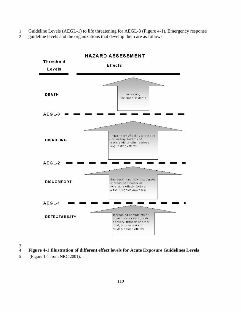
110

Guideline Levels (AEGL-1) to life threatening for AEGL-3 (Figure 4-1). Emergency response 1 guideline levels and the organizations that develop them are as follows: 2

3 Figure 4-1 Illustration of different effect levels for Acute Exposure Guidelines Levels 4 (Figure 1-1 from NRC 2001). 5

111

• Acute Exposure Guideline Levels (see Figure 4-1 for health effects at AEGL-1, AEGL-1 2, AEGL-3), National Advisory Committee (NAC) for AEGLs and Committee on 2 Toxicology (COT), part of the National Research Council of the National Academies of 3 Science (NRC 2001) (http://www.epa.gov/oppt/aegl/pubs/humanhealth.htm

• Emergency Response Planning Guidelines (ERPG-1, ERPG-2, ERPG-3), AIHA. The 5 health effects observed for ERPG-1, ERPG-2, ERPG-3 are similar to AEGL-1, AEGL-2, 6 AEGL-3, respectively; 7

); 4

• Temporary Emergency Exposure Limits (TEEL-0, TEEL-1, TEEL-2, TEEL-3), 8 Department of Energy (USDOE) Emergency Management Advisory Committee’s 9 Subcommittee on Consequence Assessment and Protective Action (SCAPA) (USDOE 10 2008). Table 2-2 of USDOE (2008) provides a comparison of the health effects observed 11 for different levels of AEGLs, ERPG, and TEELs. 12

4.1.3 Shor t-Term Occupational Exposure Limits 13 Data used in the establishment of the following short-term occupational exposure limits (OELs) 14 (i.e., ceiling limits, short-term exposure limits (STELs), and immediately dangerous to life or 15 health concentrations (IDLHs)) may also be considered; however, these values are developed for 16 healthy workers during an 8 h work day and not for the general public. 17

• Ceiling Limits - published by OSHA and ACGIH. The ceiling concentrations must not be 18 exceeded during any part of the workday; 19

• STELs - published by ACGIH, NIOSH and OSHA. The STEL is a 15-minute time-20 weighted average (TWA) exposure that should not be exceeded at any time during a 21 workday; 22

• IDLHs - published by NIOSH for use in assigning respiratory protection equipment as 23 part of the Standards Completion Program, a joint project by NIOSH and OSHA. IDLH 24 values, as well as the basis and references for current and original IDLH values, are 25 available in an online database maintained by NIOSH 26 (http://www.cdc.gov/niosh/idlh/idlh-1.html). 27

28

112

1

4.1.4 Summary of Acute Reference Values 2 Table 4-1 is a summary table of the acute reference values discussed above. General population 3 guideline levels are the most applicable for adoption by the TCEQ, if procedures similar to those 4 outlined in the Guidelines have been followed. 5

Table 4-1 Summary Table of Published Acute Reference Values 6

Acute reference value Exposure duration Organization

General population guideline levels

MRL – minimal risk level 1-14 day (acute) ATSDR

REL – reference exposure level 1 h and 8 h except for reproductive/developmental toxicants

OEHHA

ARE – acute reference exposure 1, 4, 8, and 24 h USEPA

Public emergency response guideline levels

AEGL – acute exposure guideline level 10 and 30 min; 1, 4, and 8 h NAC, COT

ERPG – emergency response planning guideline

1 h AIHA

TEEL – temporary emergency exposure level

15 min (TWA) DOE

Occupational exposure limits for healthy workers

Ceiling Limit Should not be exceeded during any part of the working exposure

OSHA; ACGIH

Occupational guideline levels for healthy workers

IDLH – immediately dangerous to life and health

Up to 30 min (immediate action)

NIOSH

STEL – short term exposure limit 15 min (TWA) NIOSH; OSHA; ACGIH

TLV-STEL – TLV short-term exposure limit

15 min (TWA) ACGIH

7

4.1.5 Toxicologic Assessments from other Countr ies 8 If acute toxicity values or toxicity assessments are available from international agencies they are 9 considered as sources of toxicity information and key studies (e.g., acute reference 10

113

concentrations from Organisation for Economic Co-Operation and Development (OECD 2010), 1 WHO, IARC, Health Canada or the Dutch government’s National Institute for Public Health and 2 the Environment (RIVM). 3

4.2 Acute Exposure Duration Adjustments 4 As discussed in Section 3.9, if an experimental study is available for the specific exposure period 5 being evaluated, no adjustment for exposure duration is required. If the MOA of a chemical 6 indicates the appropriate dose metric is concentration (i.e., an enhanced response is not produced 7 by prolonged exposure), a duration adjustment is not performed. For example, odor and other 8 mild sensory effects are typically concentration dependent (NRC 2001). Therefore, the TCEQ 9 does not perform exposure duration adjustments for odor or mild sensory effects unless 10 experimental data suggest odors or mild sensory effects increase in severity because of the 11 cumulative dose over time. 12

As discussed in Section 3.9, if a calibrated, predictive PBPK model or other mathematical 13 inhalation dosimetry model is available and validated for a given chemical or if chemical- and 14 endpoint-specific values of the exponents for C and T can be determined from experimental data, 15 then this information is used to adjust exposure concentrations. The latest version of USEPA’s 16 BMDS software (Version 2.1.2) can calculate chemical-specific values of “n” based on 17 chemical-specific data (Section 3.9.1). 18

In the absence of such information, duration adjustments are based on the relationship of the 19 product of concentration and time as discussed in the following sections. The following default 20 procedures are used to perform exposure duration adjustments for chemicals made over a limited 21 time period. Duration adjustments for data based on reproductive/developmental effects are 22 treated differently (Section 4.2.5). 23

4.2.1 Adjustments from a Shor ter Exposure Duration to a Longer Exposure 24 Duration 25

Duration adjustments are typically completed by applying Haber’s rule as modified by ten Berge 26 (1986) as discussed previously in Section 3.9. It is important to look at the mechanistic data for 27 each chemical and determine the appropriate duration adjustment on a case-by-case basis. As an 28 example of how to perform an adjustment for a 1-h ReV, if the experimental study was 29 conducted for a 30-min exposure duration, and concentration and duration both play a role in 30 toxicity, then the concentration for a 1-h exposure duration would be derived as follows using the 31 equation for Haber’s rule as modified by ten Berge (1986) using a default value of one for “n”: 32

Haber’s rule can be expressed as follows: 33

C1n x T1 = C2

n x T2 34

When adjusting from one concentration (C1) for a specific exposure duration of 30 min (T1) to 35 another concentration (C2) at the desired exposure duration of 60 min (T2), then the TCEQ 36 assumes that n = 1 and the equation simplifies to the following equation: 37

C1 x T1 = C2 x T2 38

114

Solving for C2: 1

C2 = C1 x (T1 / T2) or 2 C2 = C1 x (30 min / 60 min) 3

4.2.2 Adjustments from a Longer Exposure Duration to a Shor ter Exposure 4 Duration 5

For adjustment from an experimental study of less than or equal to 24 h to shorter durations for 6 the development of a 1-h ReV, the TCEQ uses MOA information as discussed in Jarabek (1995). 7 If it can be determined that concentration and duration both play a role, then Haber’s rule as 8 modified by ten Berge (1986) with a default value of “n” = 3 will be used to adjust the 9 concentration at a specific exposure duration of > 1 h to 1 h. This is generally thought to be a 10 conservative procedure since it results in a slow increase in concentration. If it can be determined 11 that concentration alone is the dominant determinant of toxicity or if sufficient MOA information 12 is not available for a chemical, the TCEQ conservatively assumes there is no change in 13 concentration (USEPA 1998; USEPA 2002a). For example, if concentration alone plays a role in 14 toxicity, the experimental study was conducted for a 4-h exposure duration and the POD was 30 15 ppm, then the POD for a 1-h exposure duration is assumed to be 30 ppm. 16

4.2.3 Adjustments for Subacute Studies 17

4.2.3.1 Adjustments for a 1-h ReV 18 In some cases, toxicity information is available for a chemical from a well-conducted subacute 19 study lasting from 1 day to 4 weeks. The TCEQ uses the experimental data from the subacute 20 study when it is justified by the MOA analysis. In addition, the TCEQ uses MOA information 21 (Jarabek 1995) to determine if concentration alone is the dominant determinant of toxicity or 22 whether concentration and duration both play a role. If it can be determined that concentration 23 and duration both play a role, then Haber’s rule as modified by ten Berge (1986) with a default 24 value of “n” = 3 will be used to adjust the concentration at a specific exposure duration of > 1 25 h/day to 1 h/day. If it can be determined that concentration alone is the dominant determinant of 26 toxicity or if MOA information is not available for a chemical, the TCEQ conservatively 27 assumes there is no change in concentration in order to derive the 1-h ReV. 28

As an example of how to perform an adjustment if concentration and duration both play a role in 29 toxicity, the experimental study was conducted for 4 h/day for 5 days, and the POD was 30 determined to be 100 ppm, then the POD for a 1-h exposure duration is calculated using the 31 procedures described below. 32

When adjusting from one concentration (C1) at a specific exposure duration of 4 h (T1) to another 33 concentration (C2) at the desired exposure duration of 1 h (T2 ), then the TCEQ assumes that “n” 34 = 3: 35

C13 x T1 = C2

3 x T2 36

Solving for C2: 37

115

C23 = (100 ppm)3 x (4 h /1 h) or 1

C2 = [(1 x 106 ppm) x 4] (1/3) 2 C2 = 160 ppm 3

4.2.3.2 Adjustments for a 24-h ReV 4 Please refer to Section 4.3.4 for procedures for duration adjustments used to develop a 24-h ReV 5 when a subacute study is used as the critical study. 6

4.2.4 Adjustments for Reproductive/Developmental Effects 7 Reproductive and developmental studies are usually conducted by exposing experimental 8 animals to repeated doses over several days (e.g., 6 h/day for gestational day 6-15). The TCEQ 9 uses a single day of exposure from the experimental study as the exposure duration (OEHHA 10 2008). In doing so, we recognize reproductive and developmental effects may have been caused 11 by only a single day’s exposure that occurred at a critical time during gestation. The averaging 12 time for ReV and ESL values based on reproductive or developmental effects is the number of 13 hours of the single day of exposure, not a 1-h averaging time as is typical for 1-h ReVs. For 24-h 14 ReVs, Section 4.3.4 provides procedures for duration adjustment using a subacute study if it is 15 used as the critical study. The following sections provide a more detailed discussion of short-16 term reproductive and developmental effects in order to evaluate “critical windows of exposure” 17 so child adult risks can be considered. 18

4.2.4.1 Short-Term Reproductive Effects 19 Reproductive toxicity is defined as a dysfunction induced by a chemical agent that affects the 20 process of gametogenesis, implantation of the embryo, or fetus prior to birth (ATSDR 2007). 21 The mother, father, or both may be affected by exposure to toxicants that could influence 22 reproductive outcome. Reproductive difficulties due to various causes are common. According to 23 the US Centers for Disease Control, about 10 percent of women in the United States ages 15–44 24 years have difficulty getting pregnant or staying pregnant. There are three main targets for 25 reproductive effects; direct acting toxicants on the central nervous system altering secretion of 26 hormones (e.g., the hypothalamus), direct acting toxicants on the reproductive organs (ovary and 27 testis), and those that inhibit or alter spermatogenesis, which can lead to sterility or decreased 28 fertility. Examples of adverse reproductive effects that can occur after short-term exposure 29 include decreased litters, ovary weight change, testicular atrophy, vaginal bleeding, spontaneous 30 abortions or miscarriage (loss of the embryo or fetus before full term), impaired 31 spermatogenesis, abnormal sperm, and decreased fertility (ATSDR 2007). 32

To determine the critical reproductive toxicity endpoint for short-term exposure, the endpoint 33 should be evaluated along with the MOA of the toxicant to evaluate the plausibility of the 34 adverse effect to result following short-term exposure. If there are not route-specific data 35 regarding short-term reproductive effects, pharmacokinetic data may be used to support the 36 toxicant’s potential to affect reproduction across routes of exposure. In those cases, it may be 37 possible to provide qualitative information regarding the potential for reproductive effects across 38 routes (ATSDR 2007). For more information on reproductive effects see WHO (2001), USEPA 39 (1996), and ATSDR (2007). 40

116

4.2.4.2 Short-Term Developmental Effects 1 Developmental toxicity is any adverse effect on the developing organism from implantation 2 through prenatal development. Developmental effects are distinguished from reproductive effects 3 by evaluation of the embryo or fetus after it is implanted (ATSDR 2007). There are many 4 developmental effects in humans with an unknown cause without links to exposure to 5 environmental agents. Roughly three percent of live births are found to have one or more 6 congenital malformations, and by the end of the first postnatal year, about three percent more are 7 found to have serious developmental defects (USEPA 1991). 8

Developmental toxicity can be difficult to distinguish between effects mediated through the 9 parents versus direct interaction with developmental processes. For example, developmental 10 toxicity may be influenced by the effects of toxic agents on the maternal system when exposure 11 occurs during pregnancy or lactation. In addition, exposure to the parents prior to conception can 12 result in developmental toxicity in their offspring and, potentially, in subsequent generations 13 (USEPA 1991). There are four manifestations of developmental toxicity: death, structural 14 abnormality, growth alteration, and/or functional deficit (e.g., neurobehavioral endpoints). 15 Examples of specific developmental effects that can occur after short-term exposure include 16 malformations, early postnatal mortality, reduced birth weight, mental retardation, sensory loss, 17 and other adverse functional or physical changes that are manifested after birth (USEPA 1991). 18 Teratogenicity is used to describe permanent structural abnormalities that may adversely affect 19 survival, development, or function (ATSDR 2007). 20

It is assumed that a toxicant that produces an adverse developmental effect in experimental 21 animals will potentially pose a hazard to humans following sufficient exposure during 22 development. Although the types of developmental effects seen in animal studies may not 23 necessarily be the same as those that may be produced in humans (USEPA 1991). This is 24 assumed because it is difficult to determine the most appropriate species in terms of predicting 25 the specific types of developmental effects seen in humans. Animal species differ in their critical 26 periods, differences in timing of exposure, metabolism, developmental patterns, placentation, or 27 mechanisms of action (USEPA 1991). Toxicokinetics and the MOA should be used to select the 28 most appropriate animal species and without that information, the most sensitive species should 29 be used, based on observations that humans are equal to or are more sensitive as the most 30 sensitive animal species tested for the majority of agents known to cause human developmental 31 toxicity (USEPA 1991). For more information on developmental effects see USEPA (1986, 32 1991), Carney and Kimmel (2007), and Rogers et al. (2004). 33

4.3 Twenty-Four Hour ReV and AMCV Values 34 Short-term AMCVs have generally been derived to evaluate 1-h reported concentrations of 35 chemicals of interest detected in the TCEQ ambient air monitoring network (Chapter 1). In 36 addition to 1-h ambient air samples, 5-min to 24-h ambient air samples may be collected. The 37 use of a 1-h AMCV to evaluate monitoring data collected for exposure durations less than 1 h is 38 likely to be conservative and risk may be overestimated. However, a significant amount of 39 ambient air data is collected over a 24-h duration, which is an acute exposure duration 40 significantly longer than 1-h. Therefore, it may not be appropriate to use a short-term, 1-h 41 AMCV or long-term AMCV to evaluate a 24-h ambient air sample. This is due to the fact that 42

117

while the 24-h data is an acute rather than a chronic exposure duration, toxic effects induced by 1 24-h exposure may be governed by modes of action somewhat different than those influencing 2 toxicity due to 1-h or chronic exposure . Therefore, the derivation of chemical-specific 24-h 3 AMCV values may be needed to evaluate ambient 24-h data. For some chemicals, particularly 4 those where the duration of exposure is a contributing factor in toxicity (e.g., chemicals with 5 long clearance times, cumulative or sensitizing effects), derivation of a 24-h AMCV is 6 appropriate for the evaluation of 24-h air monitoring data and is desired because the 1-h AMCV 7 may be much higher than the 24-h AMCV. For chemicals where concentration is the primary 8 contributing factor to toxicity, the 24-h AMCV may be similar to the 1-h AMCV, but the 9 determination of a 24-h AMCV is still needed. For ambient air monitoring, the 24-h AMCV is 10 equal to the 24-h ReV. 11

A 24-h ReV is derived for human health hazards associated with threshold dose-response 12 relationships (typically effects other than cancer) and is defined as an estimate of an inhalation 13 exposure concentration that is likely to be without an appreciable risk of adverse effects to the 14 human population (including susceptible subgroups) for a 24-h exposure. Exposure to chemicals 15 may occur on an intermittent basis, however. The 24-h ReV would be protective of intermittent 16 24-h exposures if the time period between intermittent exposures is sufficient for adequate 17 toxicokinetic and toxicodynamic clearance such that a toxicologically significant accumulation 18 of neither the particular causative agent nor effect is expected. 19

The same analytical steps used to derive acute 1-h ReVs and chronic ReVs are used to derive a 20 24-h ReV (Section 3.3).The critical step in deciding whether or not to derive a 24-h ReV is the 21 availability of appropriate toxicity studies that provide meaningful information to evaluate a 24-h 22 exposure duration. If there are inadequate data to derive a 24-h ReV, then a 24-h ReV will not be 23 developed. An evaluation of the mode of action, dose metric, and the toxicokinetics and 24 toxicodynamics of the chemical of concern as well as exposure duration adjustments that are 25 unique for the derivation of a 24-h ReV (Figure 4.2) will be discussed in the following sections. 26 However, animal-to-human dosimetric adjustments as well as application of UFs to the PODHEC 27 to calculate a ReV are similar to the development of acute 1-h ReV values (Chapter 3 and 28 Sections 4.5) and will not be discussed. 29

4.3.1 Availability of Toxicity Studies 30 Available literature should be researched to determine if data are available to guide the 31 derivation of a 24-h ReV. Ideally, an acute study with an exposure duration of 24-h would be 32 used to develop a 24-h ReV, but such toxicity studies are rare. Many chemicals have a poor 33 database, making the derivation of a 24-h ReV at best difficult. In these instances, professional, 34 scientific judgment must be used to decide whether sufficient data exist to support a 35 scientifically-defensible 24-h ReV. 36

For a data-rich chemical, it may be possible to perform PBPK modeling or categorical regression 37 from studies that are conducted at other durations than 24 h. For chemicals with data at different 38 exposure durations, a POD may need to be developed based on an acute study, subacute study or 39 subchronic study and appropriate duration adjustments used to develop a 24-h value. The best 40 approach for developing a 24-h ReV is to examine all available acute and subacute studies (and 41 possibly subchronic studies) and develop an exposure response array (Section 3.15). Then a 42

118

consideration of physical/chemical parameters, MOA, toxicokinetics/toxicodynamics, etc., 1 should be used to determine the most appropriate adverse effect relevant to humans for a 24-h 2 exposure duration. Development of several potential 24-h ReV values based on different studies 3 of different durations may be needed to aid in the decision-making process. 4

The acute key study used to develop the 1-h ReV may or may not be appropriate to develop a 24-5 h ReV based on the MOA, toxicodynamics, or toxicokinetics of a chemical, particularly if the 1-6 h ReV is based on a key study with a 1-h exposure duration or less. If data in the literature 7 indicate that a key study other than the one used to derive the 1-h ReV is the most appropriate 8 study to derive a 24-h ReV, which is expected to generally be the case, then a new PODHEC 24-h 9 should be identified and new UFs should be applied to this value. A literature search should 10 always be conducted to identify a key study and adverse effect that is most appropriate for a 24-h 11 exposure duration. The following are some examples of toxicity studies that may be appropriate 12 for derivation of a 24-h ReV: 13

• acute toxicity studies (exposure durations 6-24 h) where duration adjustments produce 14 appropriate or meaningful values (refer to Section 4.3.5 Critical Evaluation of Duration 15 Adjustment Procedures) 16

• acute or subacute toxicity studies may be used to derive a 24-h ReV, particularly when 17 data from subchronic and chronic studies indicate that longer exposure durations induce 18 adverse effects unrelated to those expected to be caused by a 24-h exposure duration 19

• studies using exposure durations of less than 6 h must be used cautiously, and may only be 20 appropriate when available data indicate that the primary toxic effect induced by a 21 chemical is irritation, the magnitude of which is generally determined by exposure 22 concentration, and an exposure for a 24-h duration would not be expected to have 23 additional adverse effects other than the irritation 24

• subacute toxicity studies (i.e., repeated or continuous exposure to a chemical > 1 day to 1 25 month or less) may be more appropriate than acute, single exposure studies because they 26 may be more predictive of the effects expected due to 24-h exposure 27

• subchronic toxicity studies may be appropriate when acute or subacute studies are 28 unavailable. Subchronic studies may be used for derivation of a 24-h ReV if MOA and 29 toxicokinetic/dynamic information support this application (e.g., chemicals with long 30 toxicokinetic or toxicodynamic half-lives). However, use of a subchronic study to derive a 31 24-h ReV may result in an unrealistic/unpredictive value. Section 4.3.4.3 provides 32 appropriate adjustments that may be applied to aid in the generation of more realistic 33 values 34

• chronic toxicity studies are usually not used for derivation of a 24-h ReV, since the MOA 35 for a chronic effect would generally be different than the one governing an effect induced 36 by a 24-h exposure duration 37

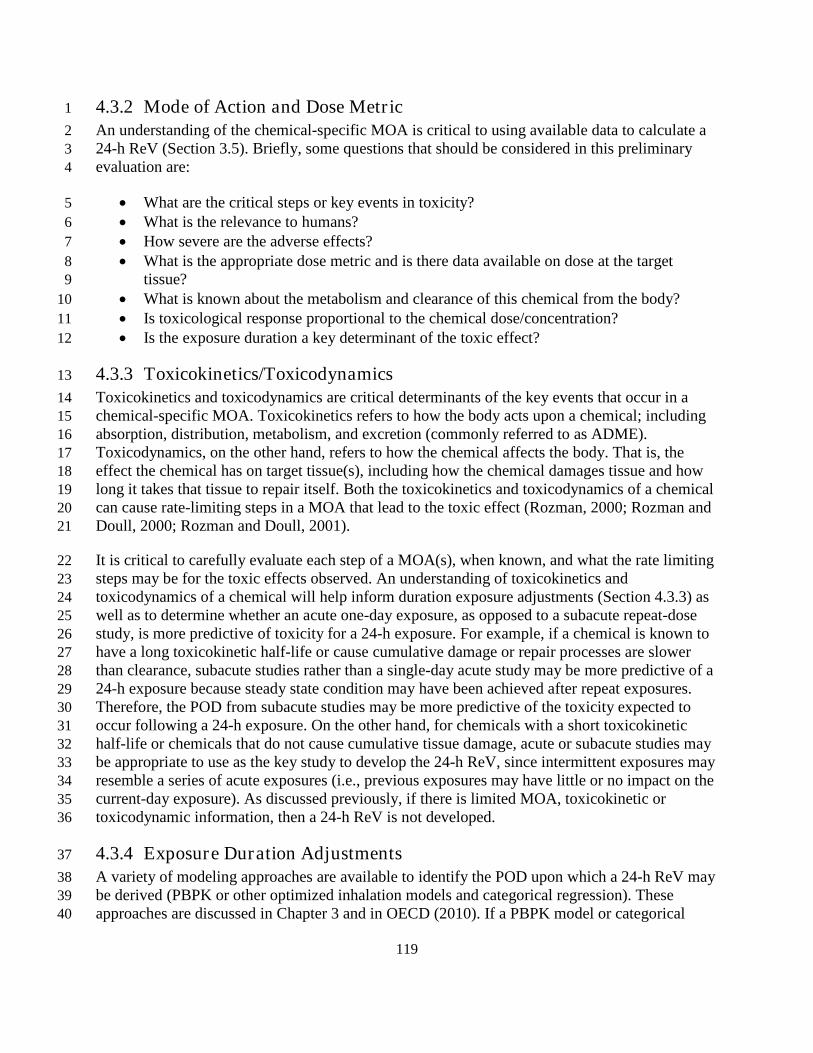
119

4.3.2 Mode of Action and Dose Metr ic 1 An understanding of the chemical-specific MOA is critical to using available data to calculate a 2 24-h ReV (Section 3.5). Briefly, some questions that should be considered in this preliminary 3 evaluation are: 4

• What are the critical steps or key events in toxicity? 5 • What is the relevance to humans? 6 • How severe are the adverse effects? 7 • What is the appropriate dose metric and is there data available on dose at the target 8

tissue? 9 • What is known about the metabolism and clearance of this chemical from the body? 10 • Is toxicological response proportional to the chemical dose/concentration? 11 • Is the exposure duration a key determinant of the toxic effect? 12

4.3.3 Toxicokinetics/Toxicodynamics 13 Toxicokinetics and toxicodynamics are critical determinants of the key events that occur in a 14 chemical-specific MOA. Toxicokinetics refers to how the body acts upon a chemical; including 15 absorption, distribution, metabolism, and excretion (commonly referred to as ADME). 16 Toxicodynamics, on the other hand, refers to how the chemical affects the body. That is, the 17 effect the chemical has on target tissue(s), including how the chemical damages tissue and how 18 long it takes that tissue to repair itself. Both the toxicokinetics and toxicodynamics of a chemical 19 can cause rate-limiting steps in a MOA that lead to the toxic effect (Rozman, 2000; Rozman and 20 Doull, 2000; Rozman and Doull, 2001). 21

It is critical to carefully evaluate each step of a MOA(s), when known, and what the rate limiting 22 steps may be for the toxic effects observed. An understanding of toxicokinetics and 23 toxicodynamics of a chemical will help inform duration exposure adjustments (Section 4.3.3) as 24 well as to determine whether an acute one-day exposure, as opposed to a subacute repeat-dose 25 study, is more predictive of toxicity for a 24-h exposure. For example, if a chemical is known to 26 have a long toxicokinetic half-life or cause cumulative damage or repair processes are slower 27 than clearance, subacute studies rather than a single-day acute study may be more predictive of a 28 24-h exposure because steady state condition may have been achieved after repeat exposures. 29 Therefore, the POD from subacute studies may be more predictive of the toxicity expected to 30 occur following a 24-h exposure. On the other hand, for chemicals with a short toxicokinetic 31 half-life or chemicals that do not cause cumulative tissue damage, acute or subacute studies may 32 be appropriate to use as the key study to develop the 24-h ReV, since intermittent exposures may 33 resemble a series of acute exposures (i.e., previous exposures may have little or no impact on the 34 current-day exposure). As discussed previously, if there is limited MOA, toxicokinetic or 35 toxicodynamic information, then a 24-h ReV is not developed. 36

4.3.4 Exposure Duration Adjustments 37 A variety of modeling approaches are available to identify the POD upon which a 24-h ReV may 38 be derived (PBPK or other optimized inhalation models and categorical regression). These 39 approaches are discussed in Chapter 3 and in OECD (2010). If a PBPK model or categorical 40

120

regression is used to derive a POD, these models can be used directly to perform exposure 1 duration adjustments. Briefly, the model that may be chosen to identify the POD from a key 2 study is dictated by the quantity and quality of the data available for a chemical of interest 3 (Figure 4.2): 4

• a PBPK model may be used to identify a PODADJ for a chemical based on an exposure 5 duration of interest when such a model is available; 6

• exposure-response arrays may be generated as a means of estimating what a logical POD 7 for a 24-h ReV might be (OECD 2010); 8

• categorical regression is a valuable tool to assess toxicity across studies and exposure 9 durations to identify an appropriate PODADJ, which may be used to derive a 24-h ReV 10 where duration adjustment is unnecessary (OECD 2010); and 11

• when data are insufficient to apply any of the aforementioned approaches, benchmark 12 concentration modeling or a NOAEL/LOAEL approach may be used to identify a POD. 13 In these cases, exposure duration adjustments may be needed to calculate a PODADJ for a 14 24-h ReV. 15

The approach used to identify the POD for a 24-h ReV is highly dependent on the data available 16 for a given chemical. While several approaches may be developed, the final approach used to 17 derive a 24-h ReV will be selected using best scientific judgment. 18

4.3.4.1 Duration Adjustments for Acute Studies (< 24 h) 19 If the above models are not available, there are several ways to perform exposure duration 20 adjustments. Studies evaluating 24-h chemical exposures are not often available and a key study 21 conducted for a different exposure duration may be the most appropriate key study used to derive 22 the 24 h ReV. In this case, Haber’s rule as modified by ten Berge (1986) can be used to calculate 23 a POD to be used for the 24-h ReV (Cn x Tm = K, Section 3.9). The same principles of 24 performing duration adjustments discussed in Sections 3.9 and 4.2 are generally applicable for 25 exposure duration adjustments for a 24-hr ReV. The chosen method for exposure duration 26 adjustments for the development of a 24-h ReV should be dictated by available data and 27 professional scientific judgment. 28

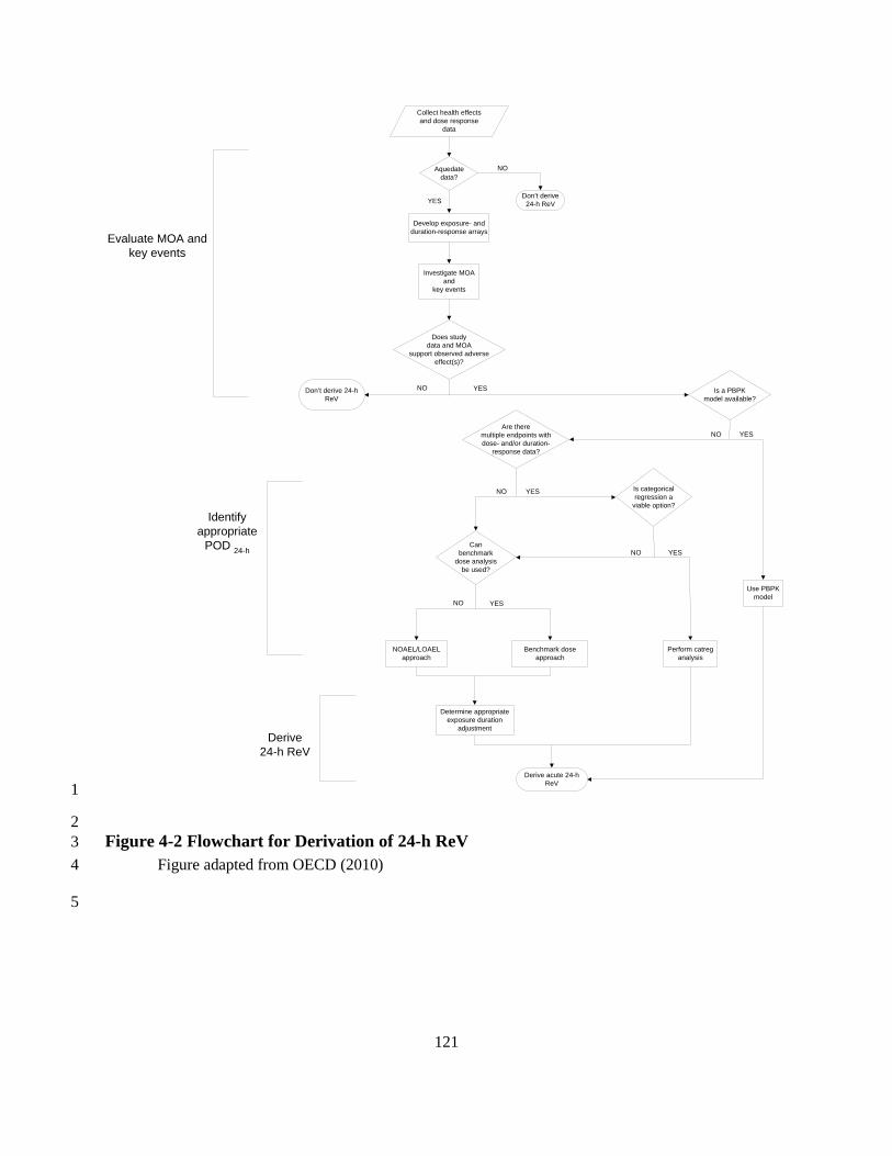
121

1

2 Figure 4-2 Flowchart for Derivation of 24-h ReV 3

Figure adapted from OECD (2010) 4

5

Collect health effectsand dose response

data

Develop exposure- andduration-response arrays

Investigate MOAand

key events

NOAEL/LOAELapproach

Benchmark doseapproach

Perform catreganalysis

Determine appropriateexposure duration

adjustment

Use PBPKmodel

Don’t derive 24-hReV

Evaluate MOA andkey events

Identifyappropriate

POD 24-h

Derive24-h ReV

Don’t derive24-h ReV

Derive acute 24-hReV

Does studydata and MOA

support observed adverseeffect(s)?

NO

YES

Aquedatedata?

NO YES

NO YES

Is categoricalregression a

viable option?

YESNO

YESNOCan

benchmarkdose analysis

be used?

NO YES

Is a PBPKmodel available?

Are theremultiple endpoints withdose- and/or duration-

response data?

122

Haber’s rule is dependent on the assumption that log concentration and log time have a linear 1 relationship or that a study employs experimental conditions wherein steady state toxicokinetics 2 or toxicodynamics are achieved. This assumption, however, does not apply to chemicals that 3 have rate-limiting critical steps in their MOA or experimental conditions that do not achieve 4 steady state (Rozman and Doull 2001). There are many ways that a chemical’s MOA may have 5 rate-limiting critical steps, including a very short or long toxicokinetic/dynamic half-life, zero 6 order toxicokinetics, reduced elimination due to high apparent volume of distribution caused by 7 compound or metabolite accumulation in the study organism’s body, or an MOA where tissue 8 damage is particularly severe or irreversible as is the case with certain neuropathies (Rozman 9 2000, Rozman and Doull 2001, Witschi 1999). 10

4.3.4.1.1 Concentration-Dependent Duration Adjustment 11 As discussed in Section 4.2, if the MOA of a chemical indicates the appropriate dose metric is 12 concentration (i.e., an enhanced response is not produced by prolonged exposure), a duration 13 adjustment is not performed. For example, odor and other mild sensory effects are typically 14 concentration dependent (NRC 2001). Therefore, the TCEQ does not perform exposure duration 15 adjustments for odor or mild sensory effects unless experimental data suggest odors or mild 16 sensory effects increase in severity because of the cumulative dose over time. OECD (2010) 17 refers to this method as “flat-lining” the exposure response array. For example, if the POD from 18 the key study is 3 ppm and the exposure duration is 8 h, then the POD24 h is 3 ppm. 19

4.3.4.1.2 Concentration and/or Duration-Dependent Defaults 20 When a chemical’s MOA is poorly characterized, C and T exponents, “n” and “m” (Section 3.9) 21 regarding Haber’s rule, Cn x Tm = K), are set equal to default values of 1, which are considered 22 to be conservative when performing a duration adjustment from a shorter exposure duration to a 23 longer one. 24

When adjusting from one concentration (C1) for a specific exposure duration of 6 h (T1) to 25 another concentration (C2) at the desired exposure duration of 24 h (T2), then the TCEQ assumes 26 that n = 1 and the equation simplifies to the following equation: 27

C1 x T1 = C2 x T2 28

Solving for C2: 29

C2 = C1 x (T1 / T2) or 30 C2 = C1 x (6 h / 24 h) 31

4.3.4.2 Duration Adjustments for a Subacute Multi-Day Study 32 Subacute studies (> 1 day) may be used to derive a 24-h ReV if an appropriate acute (i.e., < 24-33 h) study is not available. Typically, subacute studies are conducted for 6 h/day for up to 2 weeks. 34 In these cases, the following adjustments will be made to the subacute POD to calculate a 35 PODADJ appropriate for a 24-h exposure duration. 36

• If it is reasonable to assume that steady state has been achieved, or toxicodynamics 37 indicate that no additional toxic effect would be expected to occur with the subacute 38

123

exposure duration, the POD from the subacute study can be used as the 24-h POD. No 1 duration adjustments will be made. 2

• If the chemical has a short dynamic half-life and each new day represents a toxic effect 3 induced by recurring exposure, then a duration adjustment can be performed to derive the 4 24-h ReV. The duration adjustment can be the traditional approach where a POD is 5 derived from a key study or through an analytical method such as benchmark dose 6 modeling or categorical regression. 7

• Alternatively, the OEHHA (2008) method for subchronic studies, which is described 8 below, may be used to calculate a POD for a 24-h exposure duration based on a subacute 9 study. 10

4.3.4.3 Duration Adjustments for a Subchronic Study (OEHHA 2008) 11 Subchronic studies may also be used to derive a 24-h ReV if acceptable acute or subacute studies 12 are not available or if the toxicokinetic or toxicodynamic half-life of the chemical is long. In 13 those cases, the TCEQ uses the OEHHA (2008) default approach for a subchronic POD 14 (PODsubchronic) to calculate a POD appropriate for a 24-h exposure duration (POD24-h). Similar 15 procedures may be used to adjust a subacute study as discussed in Section 4.3.4.2. The default 16 approach to estimating an equivalent POD24-h from the PODsubchronic is summarized as: 17

POD24-h = PODsubchronic x (N h/24 h) x (D days per week) 18

where: 19

PODsubchronic = POD identified from key subchronic study 20

N = number of hours of exposure per day in the key subchronic study 21

D = number of days per week conducted in the key subchronic study 22

For example, if a subchonic study is available that identified a PODsubchronic of 40 ppm when 23 animals were treated for 4 h/day for 5 days/week, then the POD24-h is calculated as follows: 24

POD24-h = PODsubchronic x (N h/24 h) x (D days per week) 25

POD24-h = 40 ppm x (4 h/24 h) x 5 days 26

POD24-h = 33.3 ppm 27

4.3.5 Critical Evaluation of Duration Adjustment Procedures 28 When performing exposure duration adjustments using default procedures outlined in the above 29 sections, it is important to evaluate the reasonableness of the adjustment. Importantly, use of a 30 default value of 1 for “n”, where the exposure concentration and duration are thought to 31 contribute equally to the toxic effect of a chemical, may not result in a reasonable or predictive 32 24-h ReV, particularly when exposure durations of less than 6 h are used to calculate the 24-h 33 ReV. This is due to the fact that the product of this calculation may result in a number that is 34 lower than the chronic ReV. 35

124

In addition, MOA(s) governing the toxic response following a shorter exposure may be unrelated 1 to the MOA(s) that induces a toxic effect following a 24-h exposure. To evaluate whether a 24-h 2 ReV derived using a default value of 1 for “n” generates a realistic value, compare where the 3 potential 24-h ReV falls on the exposure array generated for the chemical of interest. If the value 4 for the 24-h ReV is less than or equal to the 1-h ReV and greater than the chronic ReV, it may be 5 a reasonable and predictive value. If the 24-h ReV appears to be an unreasonable value, a higher 6 value for n, such as n = 2 or 3, may result in a more reasonable POD for derivation of the 24-h 7 ReV given what is known about the toxicity of the chemical. The OECD (2010) refers to this 8 procedure as “interpolation.” Exposure-response arrays may be generated as a means of 9 interpolating the PODADJ for a 24-h ReV. Alternatively, an appropriate, chemical-specific “n” 10 value may be derived via curve fitting on a log Concentration versus log Time plot or using the 11 ten Berge program in USEPA’s BMD Modeling Program if adequate data is available. Thus, it is 12 always advisable to use scientific judgment to identify the most scientifically defensible 13 approach for exposure durations used to derive the 24-h ReV. 14

4.3.6 Conclusions 15 Section 4.3 describes a framework approach to derive a 24-h ReV to be used as a 24-h AMCV. 16 The steps involved in the derivation of the 24-h ReV are largely dictated by available, chemical-17 specific data, and include evaluation of the MOA, identification of rate limiting steps for the 18 resultant toxicity, selection of an approach to derive a POD24-h, and selection of UFs to apply to 19 that POD24-h (Figure 4.2 above). The OECD (2010) has proposed a similar approach for the 20 derivation of acute reference concentrations and has published a draft document wherein case 21 studies detailing this approach may be found. Since a similar approach will be used by the 22 TCEQ, these examples offer an illustration of how this approach can be successfully applied to 23 chemicals (OECD 2010). 24

4.4 Minimum Database Requirements for Development of an Acute ReV 25 The minimum toxicological database required for the development of an acute 1-h ReV is a well-26 conducted acute or subacute inhalation bioassay that evaluates a comprehensive array of 27 endpoints, including an adequate evaluation of POE respiratory tract effects, and establishes an 28 unequivocal NOAEL and/or LOAEL. Table 4-2 lists the minimum database needed to develop 29 an acute 1-h ReV and the confidence level assigned to databases consisting of various types of 30 studies. The TCEQ considers and evaluates developmental toxicity studies as possible key 31 studies when developing both acute and chronic toxicity factors. 32

Confidence in toxicological databases will vary depending on how much is known about each 33 chemical’s MOA and the quality of the experimental study (Section 3.12.3). The same 34 requirements needed for development of a 1-h ReV is generally applicable to a 24-h ReV. 35 However there are unique differences between 1-h ReVs and 24-h ReVs. Please refer to Section 36 4.3 for discussions of when a 24-h ReV may or may not be developed. 37

38

125

Table 4-2 Minimum Database for an Acute 1-h ReV and Assignment of Confidence Levels 1

Acute Mammalian Database a Database Confidence

Comments (potential UFD values)

1. A. Two inhalation bioassays in different species b

High Minimum database for high confidence (UFD of 1) B. Two prenatal developmental toxicity

studies in different species c

2. 1A and 3D (below) 1B and 3C (below)

Medium to high

(UFD of 3-6)

3. C. One inhalation bioassay in one species a

Medium D. One prenatal developmental toxicity study in one species c

4. One inhalation bioassay d, e or oral data for a chemical that met the criteria for route-to-route extrapolation

Low Minimum database for estimation of a ReV (UFD of 10)

a Composed of studies published in refereed journals, reports that adhered to good laboratory 2 practice and have undergone final QA/QC, or studies rated by the Office of Pesticide 3 Programs as “core-minimum”. It is understood that adequate acute or subacute toxicity data 4 in humans can form the basis of an acute ReV and yield high confidence in the ReV without 5 this database. 6

b Acute exposure data < 24 h 7 c Pharmacokinetic data that indicate insignificant distribution occurs remote to the respiratory 8

tract may decrease requirements for prenatal developmental data. 9 d Acute data < 24 h preferred but subacute studies up to 4 weeks in duration acceptable if 10

MOA analysis indicates this is applicable. 11 e If MOA analysis indicates insignificant distribution occurs remote to the respiratory tract or 12

the chemical does not cause developmental toxicity, the confidence in the database will be 13 upgraded from low to medium if data on multiple toxicological endpoints are provided. In 14 addition, reports must adhere to good laboratory practice, have undergone final QA/QC, or 15 the studies were rated by the Office of Pesticide Programs as “core-minimum”. 16

Studies where the data support BMCL modeling are preferred as well as studies that identify 17 both a LOAEL and a NOAEL. However, since inhalation exposure studies are more difficult to 18 conduct than oral exposure, inhalation studies frequently identify only a LOAEL, and these are 19 used to derive a ReV under certain conditions. For example, for chemicals that exhibit low 20 toxicity, some well-conducted studies only identify a NOAEL at the highest dose tested (i.e., 21 free-standing NOEAL). In these cases, the NOAEL is conservatively chosen as the highest dose 22 tested and a ReV is developed. In other instances, only a LOAEL is identified. A ReV is 23 developed based on this study if studies by other investigators support the use of the LOAEL. 24

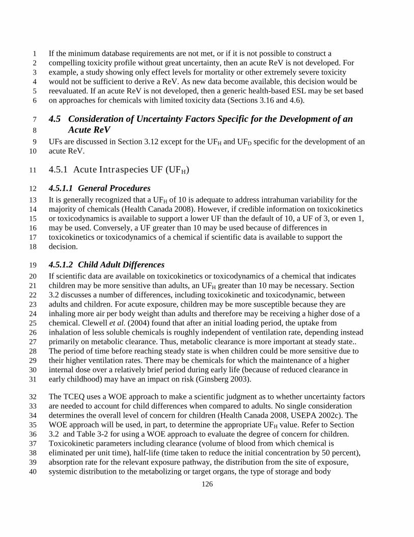
126

If the minimum database requirements are not met, or if it is not possible to construct a 1 compelling toxicity profile without great uncertainty, then an acute ReV is not developed. For 2 example, a study showing only effect levels for mortality or other extremely severe toxicity 3 would not be sufficient to derive a ReV. As new data become available, this decision would be 4 reevaluated. If an acute ReV is not developed, then a generic health-based ESL may be set based 5 on approaches for chemicals with limited toxicity data (Sections 3.16 and 4.6). 6

4.5 Consideration of Uncertainty Factors Specific for the Development of an 7 Acute ReV 8

UFs are discussed in Section 3.12 except for the UFH and UFD specific for the development of an 9 acute ReV. 10

4.5.1 Acute Intraspecies UF (UFH) 11

4.5.1.1 General Procedures 12 It is generally recognized that a UFH of 10 is adequate to address intrahuman variability for the 13 majority of chemicals (Health Canada 2008). However, if credible information on toxicokinetics 14 or toxicodynamics is available to support a lower UF than the default of 10, a UF of 3, or even 1, 15 may be used. Conversely, a UF greater than 10 may be used because of differences in 16 toxicokinetics or toxicodynamics of a chemical if scientific data is available to support the 17 decision. 18

4.5.1.2 Child Adult Differences 19 If scientific data are available on toxicokinetics or toxicodynamics of a chemical that indicates 20 children may be more sensitive than adults, an UFH greater than 10 may be necessary. Section 21 3.2 discusses a number of differences, including toxicokinetic and toxicodynamic, between 22 adults and children. For acute exposure, children may be more susceptible because they are 23 inhaling more air per body weight than adults and therefore may be receiving a higher dose of a 24 chemical. Clewell et al. (2004) found that after an initial loading period, the uptake from 25 inhalation of less soluble chemicals is roughly independent of ventilation rate, depending instead 26 primarily on metabolic clearance. Thus, metabolic clearance is more important at steady state.. 27 The period of time before reaching steady state is when children could be more sensitive due to 28 their higher ventilation rates. There may be chemicals for which the maintenance of a higher 29 internal dose over a relatively brief period during early life (because of reduced clearance in 30 early childhood) may have an impact on risk (Ginsberg 2003). 31

The TCEQ uses a WOE approach to make a scientific judgment as to whether uncertainty factors 32 are needed to account for child differences when compared to adults. No single consideration 33 determines the overall level of concern for children (Health Canada 2008, USEPA 2002c). The 34 WOE approach will be used, in part, to determine the appropriate UFH value. Refer to Section 35 3.2 and Table 3-2 for using a WOE approach to evaluate the degree of concern for children. 36 Toxicokinetic parameters including clearance (volume of blood from which chemical is 37 eliminated per unit time), half-life (time taken to reduce the initial concentration by 50 percent), 38 absorption rate for the relevant exposure pathway, the distribution from the site of exposure, 39 systemic distribution to the metabolizing or target organs, the type of storage and body 40

127

compartments of interest (in utero, this would include maternal, placental, and embryo/fetal 1 compartments), and the metabolic rates for both activation and detoxification pathways may be 2 useful in determining any child adult differences (WHO 2006, Ginsberg 2002). Refer to Section 3 3.10.4 for a discussion of differences in inhalation dosimetry for children and adults. 4

4.5.2 Acute Database Uncer tainty Factor : UFD 5

4.5.2.1 General Procedures 6 As discussed in Section 3.12.3, the TCEQ uses a database UF generally up to 10 to address 7 database deficiencies, especially uncertainties due to the lack of acute exposure studies during 8 sensitive life stages (e.g., prenatal developmental toxicants): 9

• Uncertainty associated with database deficiency, including uncertainty associated with 10 potential child/adult differences (Section 3.12.3.1) 11

• Uncertainty associated with study quality (Section 3.12.3.2) 12

4.5.2.2 Child Adult Differences 13 In most cases, the UF of up to 10 is adequate, if appropriately applied in combination with the 14 UFH, to account for deficiencies in the database regarding child adult differences in susceptibility 15 (Nielsen et al. 2010). If toxicokinetic data indicate significant distribution does not occur remote 16 to the respiratory tract, then the database UFD for lack of a prenatal developmental study is not 17 applied. Please refer to Section 4.4 and Table 4-2 for additional information. 18

Identifying any chemical-specific, critical life-stage or window of susceptibility may help 19 determine if any database deficiencies exist relevant for acute exposures (Ozkaynak et al. 2005). 20 Information to look for in evaluating any child adult differences regarding acute exposures 21 includes: 22

• indications or suspicions of effects on organ systems and functions that are especially 23 vulnerable during development and maturation in early life (in particular the nervous, 24 reproductive, and immune systems and also the metabolic pathways) and 25

• insufficent experimental data on such effects in young animals. 26

4.6 Chemicals with Limited Toxicity Data 27 On an interim basis during the air permit review process, the TCEQ frequently evaluates 28 chemicals with limited toxicity data (LTD chemicals). Every effort is made to obtain as much 29 information on the chemical of interest as possible, including requesting supporting information/ 30 documentation from the facility whose permit application is under review. However, when the 31 minimum database requirement (Section 4.4) is not met, an acute ReV is not developed. Instead, 32 a tiered approach is used to either set a default ESL or derive a generic health-based ESL 33 depending on the availability of toxicity information and time and resource constraints (Figure 34 4.3). 35

• Tier I – Threshold of Regulation (default ESL = 2 µg/m3) 36 • Tier II – Use of LC50 Data (generic ESL) 37

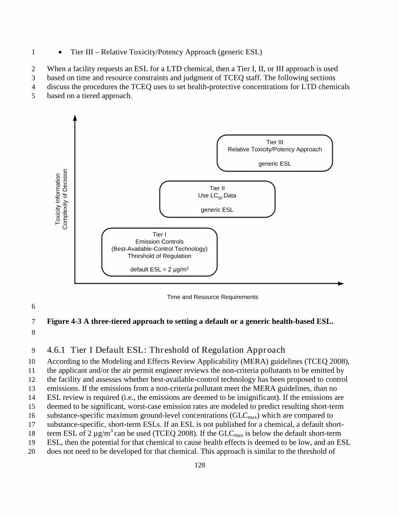
128

• Tier III – Relative Toxicity/Potency Approach (generic ESL) 1

When a facility requests an ESL for a LTD chemical, then a Tier I, II, or III approach is used 2 based on time and resource constraints and judgment of TCEQ staff. The following sections 3 discuss the procedures the TCEQ uses to set health-protective concentrations for LTD chemicals 4 based on a tiered approach. 5

6

Figure 4-3 A three-tiered approach to setting a default or a generic health-based ESL. 7 8

4.6.1 Tier I Default ESL: Threshold of Regulation Approach 9 According to the Modeling and Effects Review Applicability (MERA) guidelines (TCEQ 2008), 10 the applicant and/or the air permit engineer reviews the non-criteria pollutants to be emitted by 11 the facility and assesses whether best-available-control technology has been proposed to control 12 emissions. If the emissions from a non-criteria pollutant meet the MERA guidelines, than no 13 ESL review is required (i.e., the emissions are deemed to be insignificant). If the emissions are 14 deemed to be significant, worst-case emission rates are modeled to predict resulting short-term 15 substance-specific maximum ground-level concentrations (GLCmax) which are compared to 16 substance-specific, short-term ESLs. If an ESL is not published for a chemical, a default short-17 term ESL of 2 µg/m3 can be used (TCEQ 2008). If the GLCmax is below the default short-term 18 ESL, then the potential for that chemical to cause health effects is deemed to be low, and an ESL 19 does not need to be developed for that chemical. This approach is similar to the threshold of 20

Tier IEmission Controls

(Best-Available-Control Technology)Threshold of Regulation

default ESL = 2 μg/m3

Tier IIUse LC50 Data

generic ESL

Tier IIIRelative Toxicity/Potency Approach

generic ESL

Time and Resource Requirements

Toxi

city

Info

rmat

ion

Com

plex

ity o

f Dec

isio

n

129

regulation approach used by the Food and Drug Administration (FDA) for food contact articles 1 with limited toxicity information (FDA 1995). 2

If the default short-term ESL of 2 µg/m3 is not attainable for an applicant for a LTD chemical, a 3 Tier II or Tier III approach is used to estimate a generic short-term ESL. 4

4.6.2 Tier II Gener ic ESL: NOAEL-to-LC50 Ratio Approach 5 The evaluation of toxicity following short-term exposure to a chemical is an integral step in the 6 assessment of its toxic potential by regulatory agencies. The TCEQ uses the information from 7 standard acute LC50 toxicity tests and a NOAEL-to-LC50 (N-L) Ratio Approach to estimate a 8 Tier II generic ESL (Grant et al. 2007). In the past, a Threshold of Concern (TOC) Approach 9 was also used to estimate a Tier II generic ESL (Grant et al. 2007). However, a study by Phillips 10 et al. (2011) demonstrated that the N-L ratio approach was more predictive of toxicity whereas 11 the TOC Approach was overly conservative. Therefore, only the N-L Ratio Approach is 12 discussed. 13

4.6.2.1 Criteria for Selection of Acute Lethality Data 14 For the N-L ratio approach, acute inhalation lethality data are multiplied by a tenth percentile 15 composite factor N-L ratio to estimate health-protective air concentrations. The first step is 16 selection of scientifically-defensible acute lethality data using the following criteria. 17

For many substances, more than one LC50 may be identified from the literature, resulting from 18 the fact that many substances are tested in more than one species and sex and/or at different 19 exposure durations. This may lead, in some cases, to multiple LC50 values for individual 20 substances. Figure 4-4 illustrates the steps that are followed for selection of LC50 data used for 21 the N-L ratio approach. First, LC50 data for all species < 4 h are obtained (Step 1). Values are 22 adjusted to correspond to a 4-h exposure duration because a 4-h exposure duration for LC50 data 23 is more commonly available than other exposure durations. Duration adjustments for LC50 data 24 are made using Haber’s Law (Rinehart and Hatch 1964) as modified by ten Berge et al. (1986) as 25 discussed previously in Section 3.9 and 4.2. If all extrapolated values produce the same LC50 26 data, no further action is required. If the extrapolated values produce different LC50 data, then the 27 lowest value is chosen although the quality of the experimental study, physical/chemical 28 characteristics of the chemical, and other data such as eye/skin irritation, etc., can be used in the 29 decision process. If LC50 data < 4 h are not available, then LC50 data > 4 h but < 12 h are 30 obtained (Step 2). Duration adjustments are not performed on LC50 data > 4 h because of the 31 uncertainties involved with extrapolating exposure durations from longer exposure to shorter 32 exposure durations (Jarabek 1995). If all values produce the same LC50 data, no further action is 33 required. If the extrapolated values produce different LC50 data, then the lowest LC50 data is 34 chosen. The quality of the experimental study, physical/chemical characteristics of the chemical, 35 and other data such as eye/skin irritation, etc., are also used to decide the chemical’s LC50. If 36 LC50 data < 12 h are not available, then all other pertinent inhalation lethality data (i.e., LClow, 37 LC33, etc.) are used (Step 3). This is generally a conservative approach because these values are 38 lower than LC50 data. 39

Acute toxicity testing is generally performed by the most relevant route of exposure in order to 40 provide information on health hazards likely to arise from short-term exposure by that route. 41

130

Therefore, the inhalation route may not have been evaluated for a product or chemical if the most 1 relevant route of exposure is oral or dermal. Oral data may be used to extrapolate to LC50 values. 2 but only if the chemical meets the strict criteria discussed in Section 3.16.1 Route- to-Route 3 Extrapolation and is determined not to be corrosive and/or reactive (Step 4). 4

If inhalation or oral lethality data are not available, then information on whether a chemical is 5 corrosive or an eye or skin irritant can be used to categorize a chemical using the TOC Approach 6 (Grant et al. 2007) (Step 5). In order to determine whether a chemical is corrosive, available 7 empirical data are used. If a chemical is an oxidizer, an inorganic or organic acid or base, reacts 8 with water to form corrosive or reactive products, or is readily hydrolyzed by nasal 9 carboxylesterases, it is more likely to be corrosive or reactive or result in POE effects. The 10 European Union has devised a tiered testing strategy to determine whether or not compounds 11 cause skin irritation and corrosion based on the integrated use of physicochemical properties, 12 QSAR, and in vitro data (Cronin et al. 2003). If information on a chemical is derived using this 13 tiered testing strategy, then the TCEQ uses this information to evaluate whether or not a 14 chemical is corrosive. Information based on MOA for specific chemical classes, 15 physical/chemical parameters, reactivity and all other available information from acute toxicity 16 tests is used to categorize a chemical into the appropriate toxicity category if the TOC Approach 17 is used. In addition, the facility can be contacted and additional information can be obtained. 18

19 Figure 4-4 Criteria to select LC50 data. 20

1. Obtain LC50 data for all species for < 4 h

2. Obtain LC50 data for all species for > 4 h but < 12 h.

3. Obtain LClow data or any other pertinent inhalation lethality data.

4. Obtain oral LD50 data for all species if strict criteria for perfoming route to route extrapolation are met.

5. Consider other data: physical/chemical characteristics; corrosion or reactivity of the chemical; ocular toxicity, etc. Consider Threshold of Concern Approach.

Extrapolate all LC50 values < 4 h duration to 4 h using Haber’s Law using an empirically derived “n” value, if available. Otherwise, use a default value of “n” = 1. Do not perform duration adjustment for LC50 values > 4 h.

If all extrapolated values produce the same LC50 data no further action is required.

If the extrapolated values produce different LC50 values, conservatively choose the lowest value or consider the following to decide the LC50 value: - quality of experimental study - physical/chemical characteristics of the chemical and - other data such as eye/skin irritation, etc.

If there are different LD50 values, consider the following to decide what LD50 value is best: - quality of experimental study - physical/chemical characteristics of the chemical and - other data such as eye/skin irritation, etc.

Contact the facility and obtain additional information.

NO

NO

NO

NO

YES

YES

YES

YES

131

4.6.2.2 N-L Ratio Approach 1 After choosing an LC50 value for a LTD chemical as described in the previous section, an N-L 2 ratio-based Tier II generic ESL can be determined by multiplying the LC50 by 8.3 x 10-5. The 3 background of the N-L ratio approach is discussed in detail in Grant et al. (2007) and is briefly 4 discussed below. 5

Several investigators have suggested using readily-available acute toxicity data to estimate 6 chronic endpoints for LTD chemicals. This procedure was proposed by Layton et al. (1987) for 7 estimating acceptable daily intakes (ADI) for the evaluation of exposures to contaminants at 8 hazardous waste sites. Venman and Flaga (1985) used this procedure to establish provisional 9 ADIs for the evaluation of waste water contaminants. Both investigators calculated NOAEL-to-10 oral LD50 ratios from chronic animal studies for different chemicals and determined the fifth 11 percentile of the cumulative distributions of the ratios. The LD50 value for contaminants with 12 limited toxicity data was multiplied by the fifth percentile ratio to derive a surrogate NOAEL. 13 The surrogate NOAEL was divided by an uncertainty factor of 100 in order to establish a 14 conservative threshold dose below which no appreciable risk to human health would occur. 15

Grant et al. (2007) used the basic approach of Layton et al. (1987) and Venman and Flaga (1985) 16 to establish a procedure to estimate Tier II generic ESLs for LTD chemicals using available LC50 17 data. Grant et al. (2007) provides a detailed discussion of how an acute inhalation N-L ratio was 18 calculated for the evaluation of acute inhalation toxicity, so only a brief discussion is provided 19 here. A large reference database consisting of LC50 data and acute inhalation NOAELs for 55 20 chemicals was compiled. The database consisted of acute toxicity data tested for a variety of 21 acute inhalation endpoints where the exposure durations of the NOAEL studies were less than 24 22 h. The N-L ratio was calculated for each chemical and the tenth percentile of the cumulative 23 distribution of the ratios was calculated and divided by an uncertainty factor of 100. The tenth 24 percentile composite factor N-L ratio was 8.3 x 10-5. For a LTD chemical, this factor is 25 multiplied by LC50 values which have been adjusted to 4 h or other appropriate inhalation 26 lethality data based on criteria in Figure 4-4 to estimate a conservative generic ESL below which 27 no appreciable risk to human health would occur (Grant et al. 2007). 28

TCEQ has implemented the N-L ratio approach and the TOC approach to determine Tier II 29 generic ESLs for pentene isomers (TCEQ 2007a) and hexane (TCEQ 2007b). For both pentene 30 and hexane, the N-L ratio approach was deemed to be more applicable than the TOC approach. 31 Phillips et al. (2011) conducted a ground-truth exercise where health-based acuteESLs derived 32 using the guidelines were compared to Tier II generic ESLs using the N-L ratio approach and the 33 TOC approach. For 3 out of 19 chemicals, the generic ESLs derived using the N-L ratio 34 approach were slightly higher but were within a factor of two of the health-based acuteESLs. For 35 16 of the 19 chemicals, the generic ESLs using the N-L ratio approach were lower than the 36 health-based acuteESLs. Generally, the TOC method was more conservative than the N-L ratio 37 approach, especially for relatively nontoxic chemicals. 38

4.6.3 Tier III Gener ic ESL: Relative Toxicity/Relative Potency Approach 39 Conservative Tier I default ESLs and Tier II generic ESLs are developed on an interim basis 40 upon request. The TCEQ will consider development of a Tier III generic ESL based on a relative 41

132

toxicity/relative potency approach as discussed in Section 3.16.2. Development of a Tier III 1 generic ESL is more time- and labor-intensive (Figure 4.3). 2

3

133

Chapter 5 Der ivation of Chronic Toxicity Factors 1

5.1 Published Toxicity Factors 2 The following sections discuss the database sources to which the TCEQ refers during its search 3 for published chronic values and/or data. When chronic inhalation (e.g., RfC, URF) or oral (e.g., 4 RfD, SFo) toxicity factors or guideline levels are identified in the scientific literature or 5 databases, they are reviewed to determine whether the approach used to develop these toxicity 6 factors is similar to the procedures used by the TCEQ. If so, the TCEQ considers adoption of the 7 published chronic toxicity factor or guideline level, with preference given to values that have 8 undergone an external peer review and public involvement process. Many published chronic 9 toxicity factors are not appropriate for use by TCEQ because it is likely that procedures other 10 than those recommended in this guidance document were used to derive these values. Due to 11 time and resource constraints, the TCEQ considers the published values and their respective key 12 studies as a starting place for gathering toxicity information to develop a DSD. However, 13 because existing toxicity factors or guideline levels may be outdated, the TCEQ also evaluates 14 peer-reviewed studies available after the date these toxicity factors or guideline levels were 15 published to ensure that the latest data are considered prior to developing a chronic toxicity 16 factor. 17

The TCEQ also reviews other published toxicity factors and toxicity information from 18 organizations that specifically address susceptibility of children. Some of those organizations and 19 factors/levels are ATSDR toxicological profiles, USEPA TEACH chemical summaries, Cal 20 EPA’s RELs, USEPA VCCEP, WHO, and ECETOC. 21

5.1.1 IRIS Toxicity Factors 22 USEPA’s IRIS (http://www.epa.gov/iris/)

5.1.2 Cal EPA Toxicity Factors 30

is often the preferred database from which to obtain 23 existing inhalation and oral toxicity factors or to select key studies if the assessments are current. 24 IRIS toxicity factors address both carcinogenic (i.e., URF, SFo) and noncarcinogenic (i.e., RfC, 25 RfD) effects. The data on IRIS are accompanied by references to key and supportive studies, and 26 the methodology and guidance used to derive the toxicity factors are provided. USEPA reviews 27 the quality and reliability of the data and the key and supportive studies. IRIS assessments 28 undergo an external peer review. 29

Cal EPA OEHHA maintains a database of peer-reviewed chronic inhalation (i.e., REL) and oral 31 (e.g, SFo) toxicity factors, which address both carcinogenic and noncarcinogenic endpoints 32 (http://oehha.ca.gov/risk/chemicalDB/start.asp

5.1.3 ATSDR MRLs 34

). 33

ATSDR publishes chronic inhalation and oral MRLs as screening values for use in public health 35 assessments at hazardous waste sites. For a given substance, its MRL is “an estimate of daily 36 human exposure that is likely to be without appreciable risk of adverse noncancer health effects 37 over a specified duration of exposure” (http://www.atsdr.cdc.gov/mrls/index.asp). However, for 38 some ATSDR MRLs, dosimetric modeling to convert experimental animal concentrations to a 39

134

HEC was not conducted. Additionally, ATSDR does not include a UFD in their MRL 1 calculations in consideration of any database deficiencies. 2

5.1.4 Provisional Peer -Reviewed Toxicity Values 3 The USEPA Office of Research and Development/National Center for Environmental 4 Assessment (NCEA)/Superfund Health Risk Technical Support Center develops Provisional 5 Peer-Reviewed Toxicity Values (PPRTVs) in response to requests from regional USEPA offices 6 (USEPA 2003b), and is conducting a batch review of values listed in HEAST (USEPA 1997). 7 PPRTVs are derived for both inhalation and oral routes of exposure, and both carcinogenic and 8 noncarcinogenic endpoints. The TCEQ obtains the technical support documents for individual 9 chemicals to evaluate the key and supportive studies. PPRTVs are available at 10 http://hhpprtv.ornl.gov. 11

5.1.5 HEAST Toxicity Factors 12 USEPA’s Environmental Criteria and Assessment Office last updated HEAST in 1997 (USEPA 13 1997). The inhalation and oral values in HEAST (carcinogenic and noncarcinogenic) are 14 provisional but references of key studies are provided. 15

5.1.6 Occupational Data 16 Recommended OELs have been published for many chemicals. They include: time-weighted 17 average threshold limit values (TWA-TLVs) published by ACGIH; permissible exposure limits 18 (PELs) published by OSHA; recommended exposure limits published by the NIOSH; workplace 19 environmental exposure level guides (WEELs) published by AIHA; maximum concentration 20 values in the workplace (MAKs) published by Germany’s Commission for the Investigation of 21 Hazards of Chemical Compounds in the Work Area; and OELs published by the European Union 22 Subcommittee on Occupational Exposure Limits. Occupational values that are strictly health-23 based are likely the most relevant source for environmental risk assessment. Worker exposure 24 data used in the development of these OELs or unpublished industry worker studies may also be 25 evaluated. 26

5.1.7 Assessments from other Countr ies 27 If chronic toxicity values are available from international agencies (e.g. OECD, IARC, and 28 WHO) or other countries (e.g. Health Canada or RIVM), they are considered as sources of 29 toxicity assessment information. 30

5.2 Duration Adjustments 31 Duration adjustments are commonly required for human and animal inhalation study PODs 32 because such studies typically involve discontinuous exposure regimens, and the POD used to 33 derive a ReV or URF should reflect continuous chronic exposure for the general human 34 population. Such adjustments are usually not necessary for human and animal oral studies, which 35 typically express dose in terms of an average daily dose on a body weight basis (i.e., mg/kg-day) 36 over the chronic study duration. However, some oral studies may require other adjustments to the 37 POD to calculate dose in the units commonly used (i.e., mg/kg-day) to derive oral toxicity 38 factors (i.e., RfD, SFo). Therefore, as necessary, adjustments typically differ for inhalation and 39

135

oral studies. Study POD adjustments are addressed separately below for inhalation and oral 1 studies. 2

5.2.1 Inhalation Study Duration Adjustments 3 Human and animal inhalation studies usually involve discontinuous exposure regimens. The 4 inhalation data are adjusted to reflect continuous chronic exposure for the general human 5 population. Ideally, MOA, chemical-specific, and species-specific data would be available so 6 that PBPK models or optimal/preferred inhalation dosimetry models (Section 3.8) could be used 7 for duration adjustments (Jarabek 1995b; Hanna et al. 2001). Otherwise, the following published 8 default guidelines (USEPA 1994) are used for inhalation exposures, although the TCEQ 9 recognizes that the application of the default guidelines may not be appropriate in all cases. 10 11 According to the RfC Methodology, application of the default adjustment is appropriate only 12 when the dosing protocol generates steady-state blood levels and obeys first-order kinetics 13 (USEPA 1994). If detoxification or clearance occurs, then exposure duration may become 14 negligible and the product of concentration and exposure duration may not be valid (Bogdanffy 15 and Jarabek 1995). More specifically, the default adjustment should generally not be applied 16 when both the kinetic half-life of the putative causative chemical or metabolite and the dynamic 17 half-life of the effect are brief compared to the time period between doses since both the 18 causative agent and adverse effect are effectively cleared between doses. However, the default 19 adjustment is applicable if either the dynamic half-life of the chemical effect or the kinetic half-20 life is long relative to the dosing period. For example, the default adjustment is applicable if the 21 dynamic half-life of the chemical effect is long relative to the dosing period, despite a short 22 kinetic half-life. Sarin gas is an example of a chemical that obeys Haber’s rule despite a short 23 kinetic half-life (Rozman and Doull 2001). If data are unavailable to inform a chemical-specific 24 duration adjustment (e.g., no validated PBPK model), the following default adjustments are used. 25

5.2.1.1 Duration Adjustment of Human Inhalation Data 26 Data obtained from human occupational or controlled inhalation studies are adjusted to reflect 27 ventilation rates and exposure durations in the general human population. This adjustment yields 28 the HEC, as a NOAELHEC, LOAELHEC, or other relevant POD. The example that follows 29 concerns an occupational study when average daily concentration is used as the dose metric (i.e., 30 mg/m3 or ppm); however, application to data from controlled human studies may differ regarding 31 the ventilation factors and exposure regimen. 32 33

POD POD x VEVE

x days weekdays weekHEC OC

ho

h

oc

res=

//

34

where: 35 PODHEC = human equivalent concentration POD applicable to the general public 36 PODOC = occupational time-weighted average POD 37 VEho = default occupational ventilation rate for an eight-hour day (10 m3/day) 38 VEh = default non-occupational ventilation rate for a 24-hour day (20 m3/day) 39 days/weekoc = occupational exposure frequency, usually 5 days/week 40 days/weekres = residential exposure frequency; usually 7 days/week 41

136

If the exposure dose metric is cumulative exposure (e.g., mg/m3/year) from an epidemiology 1 study, the cumulative exposure dose metric is converted to an average daily exposure 2 concentration by averaging cumulative exposure over an averaging time of years workers were 3 exposed, unless MOA information is available that indicates another averaging time is more 4 defensible. An example of the latter can be found in the silica DSD (TCEQ 2009). 5

5.2.1.2 Duration Adjustment of Animal Inhalation Data 6 The adjustment of a discontinuous animal inhalation exposure regimen to continuous exposure is 7 similar to that used for data from human studies. 8

POD POD xDhours

xF

daysADJ =24 7

9

where: 10

PODADJ = POD from animal studies, adjusted to a continuous exposure scenario 11 POD = POD from animal studies, based on a discontinuous exposure scenario 12 D = exposure duration, hours per day 13 F = exposure frequency, days per week 14

USEPA recommends that this same adjustment to continuous exposure be used in calculating a 15 chronic toxicity factor from an animal developmental toxicity study. According to USEPA 16 (2002), duration adjustment is appropriate as the more health-protective procedure, unless there 17 are toxicokinetic data suggesting that the adjustment to a continuous exposure equivalent is 18 inappropriate, or MOA information suggests that a susceptible period of development is 19 specifically targeted (which would suggest that the peak dose may represent the effective dose). 20 For example, if a chemical is rapidly absorbed, distributed, and metabolized, duration adjustment 21 may be less appropriate than peak exposure. 22

5.2.2 Oral Study Dosimetr ic Adjustments 23 There is no single USEPA guidance document available for the development of oral toxicity 24 factors (i.e., RfD, SFo). As mentioned in Section 3.1, there are numerous guidance documents 25 available at http://www.epa.gov/iris/backgrd.html and other sites that are used to develop the oral 26 toxicity factors published in IRIS. 27

Human and animal chronic oral studies often express dose in terms of an average daily dose on a 28 body weight basis (i.e., mg/kg-day) over the study duration, which is the dose metric commonly 29 used to derive oral toxicity factors (e.g., RfD). However, some oral studies may express dose in 30 other units (e.g., mg/day, drinking water concentrations), requiring adjustments to the POD given 31 in the study to calculate dose in mg/kg-day. 32

5.2.2.1 Adjustment of Human Oral Data to mg/kg-day 33 If an oral human study does not provide an average daily dose on a body weight basis (i.e., 34 mg/kg-day) over the duration of the study, study-specific or default values (e.g., 70 kg adult 35 body weight (BW)) may be used to convert intake into units of average daily dose on a BW basis 36 to be used as the human equivalent dose point of departure (PODHED) in the derivation of the 37

137

RfD or SFo. The example that follows is a common calculation for oral studies to derive the 1 PODHED in mg/kg-day. 2

PODHED = DD/ BWH 3

where: 4

PODHED = human equivalent dose POD (mg/kg-day) 5 DD = daily dose (average) over the study duration (mg/kg) 6 BWH = human body weight (default of 70 kg) 7

5.2.2.2 Adjustment of Animal Oral Data to mg/kg-day 8 Similar to oral data from human exposure, data from animal chronic oral studies is often 9 expressed in average daily dose on a BW basis (i.e., mg/kg-day) over the study duration. If not, 10 study-specific or default values (e.g., animal BW, drinking water or food intake rates) may be 11 used to convert intake into units of average daily dose on a BW basis to be used as the animal 12 dose point of departure (PODAnimal) for derivation of the RfD or SFo. This section provides three 13 example calculations to derive the PODAnimal in mg/kg-day. The example that follows is a 14 common calculation for oral studies. 15

PODAnimal = DD/ BWA 16

where: 17

PODAnimal = animal dose POD (mg/kg-day) 18 DD = daily dose (average) over the study duration (mg/day) 19 BWA = animal body weight (kg) 20

Sometimes animal oral studies express dose in simple terms of chemical concentrations in 21 drinking water or food (e.g., 100 mg chemical per liter of drinking water). In this case, study-22 specific or default values for intake (drinking water or food) and animal BW must be used to 23 calculate the average daily dose on a body weight basis. While study-specific values are 24 preferred, USEPA (1988) may be used as a source of species-specific default values. 25

PODAnimal = (CC x IDaily)/ BWA 26

where: 27

PODAnimal = animal dose POD (mg/kg-day) 28 CC = chemical concentration in food (mg chemical/kg food) or 29

drinking water (mg chemical/L water) 30 IDaily = daily intake rate of food (kg food/day) or drinking water 31

(L water/day) 32 BWA = animal body weight (kg) 33

Any duration adjustment required for oral animal data will likely pertain to the days of exposure 34 per week (e.g., exposure regimen of 5 days per week). If this exposure duration adjustment is 35

138

necessary to reflect continuous chronic exposure, the following example equation may be used to 1 calculate the PODAnimal. 2

PODAnimal-ADJ = PODAnimal x [F (days per week) / 7 (total days in a week)] 3

where: 4

PODAnimal-ADJ = animal dose POD, adjusted to a continuous oral exposure scenario 5 (mg/kg-day) 6

PODAnimal = animal dose POD (mg/kg-day) 7 F = exposure frequency, days per week 8

As this document cannot provide equations for all possible and necessary adjustments, TCEQ 9 staff should consult the guidance documents and chemical assessments of others agencies (e.g., 10 USEPA) and the scientific peer-reviewed literature as needed in these cases. When chronic 11 animal study oral data are expressed in average daily dose on a BW basis (i.e., mg/kg-day), 12 animal-to-human dosimetric extrapolation must still be conducted. 13

5.3 Adjustment of Animal Oral Data to Humans (Animal-to-Human Dosimetric 14 Adjustments) 15

Dosimetric adjustment must be performed to convert a PODAnimal into a PODHED. The hierarchy 16 of preferred options for animal-to-human dosimetric adjustments is: (1) a validated, chemical-17 specific PBPK (or PBPK-TD) model parameterized for the species and target tissues of interest 18 so that internal target organ doses can be calculated; (2) use of species- and chemical-specific 19 data on toxicokinetic and toxicodynamic differences; or (3) a default procedure (USEPA 2006b, 20 2002a). 21

The most scientifically-sound approach for animal-to-human dosimetric adjustment involves use 22 of options (1) or (2) to estimate the human external dose (mg/kg-day) that would result in the 23 same internal dose at the target organ as in the laboratory animal, as internal dose at the target 24 organ is the most proximate dose metric determinant of risk. However, PBPK models and 25 sufficient species- and chemical-specific data on toxicokinetic and toxicodynamic differences 26 frequently do not exist for the chemical of interest. Therefore, absent an acceptable PBPK model 27 or species- and chemical-specific data that can be used, default procedures are needed to conduct 28 these adjustments based on the administered doses cited in the oral toxicity study (USEPA 29 2006b). 30

5.3.1 Interspecies Scaling for Carcinogenic Effects 31 USEPA (2005a) and TCEQ use body weight scaling to the ¾ power (BW3/4) for interspecies 32 extrapolation when deriving a carcinogenic oral toxicity factor (i.e., SFo). This animal-to-human 33 dosimetric adjustment can be performed on the animal doses used for carcinogenic dose-34 response modeling or on the SFo resulting from modeling unadjusted animal doses (SFoA), but 35 should not be performed on both. The equations discussed below in the context of deriving RfDs 36 can also be used to adjust the animal doses to be used in cancer dose-response modeling. 37 Alternatively, the following equation may be used to dosimetrically adjust the SFo resulting from 38 modeling the unadjusted animal doses (i.e., adjusting the SFoA) (USEPA 2010a). 39

139

SFoH = SFoA x (BWH/ BWA)1/4 1

where: 2

SFoH = oral slope factor applicable to humans (excess risk per mg/kg-day) 3 SFoA = animal oral slope factor based on unadjusted doses (excess risk per mg/kg-day) 4 BWH = human body weight (default of 70 kg) 5 BWA = animal body weight (kg) 6

See USEPA (2011) for details regarding the derivation of the (BWH/ BWA)1/4 relationship for 7 BW3/4 scaling. 8

5.3.2 Interspecies Scaling for Noncarcinogenic Effects 9 When deriving noncarcinogenic oral toxicity factors (i.e., RfDs), a UFA of 10 (3 each for 10 toxicokinetics and toxicodynamics) has historically been used in consideration of the 11 uncertainties associated with the extrapolation of animal data to humans (USEPA 2002a). Recent 12 USEPA assessments continue to use this UFA (e.g., USEPA 2010a, 2010b). However, USEPA 13 has endorsed using BW3/4 as a scientifically-based default procedure for animal-to-human 14 extrapolation of toxicologically equivalent doses of chronic orally administered chemicals when 15 deriving noncarcinogenic oral toxicity factors (i.e., RfDs) (USEPA 2011, 2006b). This 16 adjustment is most appropriate where the area under the concentration-time curve (AUC) of the 17 parent chemical or active metabolite is associated with toxicity, and is also recommended for 18 POE effects (i.e., gastrointestinal) until information is developed to specifically address animal-19 to-human dosimetric adjustment for oral POE effects. As opposed to chronic exposures 20 demonstrating sensitive effects where repair processes (toxicodynamics) are at work (as with 21 RfD derivation), scaling with BW3/4 is likely not appropriate for acute exposures causing 22 immediate and severe effects (USEPA 2011, 2006b). Using BW3/4 for interspecies dosimetric 23 adjustments for both carcinogenic and noncarcinogenic toxicity factors would harmonize the 24 interspecies scaling factor aspect of cancer and noncancer risk assessment. However, full 25 harmonization is prevented under current draft USEPA proposals as an additional UFA of 3 is 26 recommended for potential interspecies toxicodynamic differences (USEPA 2011, 2006b, 27 2002a). 28

While a great deal of emphasis has historically been placed on data that generally support BW3/4 29 for interspecies extrapolation of important physiological determinants of toxicokinetics and of 30 carcinogenic potency, there are also data that generally support BW3/4 for interspecies scaling of 31 toxicity (i.e., both toxicokinetics and toxicodynamics). For example, Schneider et al. (2004) 32 proposed BW3/4 for interspecies extrapolation of repeat dose toxicity evaluations in the absence 33 of species- and chemical-specific data based on the good agreement of toxicity data for six 34 species (including humans) with BW3/4 predictions for 63 anti-neoplastic chemicals (e.g., see 35 Table 6 of Schneider et al. 2004), and Figure 4B of that study shows that BW3/4 scaling 36 predicted the relative sensitivities of the species to toxicity relatively well. Schneider et al. 37 (2004) also found that BW3/4 scaling predicted reasonably well the toxicity of pesticides in long-38 term rat, mouse, and dog studies (Table 4 of Schneider et al. 2004). Across these species 39 comparisons, to use an additional factor of 3 to upwardly adjust the BW3/4 predicted sensitivity 40 of the larger species would result in a 3.5 fold (for anti-neoplastic agents) and 3.1 fold (for 41

140

pesticides) over-estimation of the actual central tendency (median) sensitivity of the larger 1 species. The overall predictiveness of BW3/4 shown in Schneider et al. (2004) for these 2 noncarcinogenic effects is consistent with the overall predictiveness and use of BW3/4 for animal-3 to-human dosimetric adjustment for carcinogenic potency without further adjustment (i.e., no 4 UFA is used). 5

Other studies of the application of allometric scaling to toxicity data also support BW3/4 (i.e., 6 exponent of 0.75) as a reasonably predictive coefficient for animal-to-human dosimetric 7 adjustment and toxicity. Krasovskii (1973, 1975, and 1976 as cited by Davidson et al. 1986) 8 found high correlations between toxicity and BW raised to exponents between 0.62 and 0.81 for 9 6 to 20 mammalian species and 278 compounds of seven chemical classes. Travis and White 10 (1988) found the best overall slope for the combined toxicity data set of 27 anti-cancer agents 11 across six species (i.e., the best exponent for BW) was 0.73, with 95% confidence bounds of 0.69 12 and 0.77, supporting BW3/4 for animal-to-human scaling of toxicity data. These results are not 13 surprising given that in general, important factors for interspecies correlation of toxicologic 14 parameters such as half-life (T1/2), AUC, clearance, hepatic enzyme activity (including the P-450 15 monooxygenase system), and others correlate with BW exponents of 0.67 to 0.75 (Davidson et 16 al. 1986). Data such as those described above suggest that an additional toxicodynamic UFA is 17 not necessary since using BW3/4 for cross-species dosimetric adjustment is generally predictive 18 of toxicity. This is not particularly surprising since BW3/4 scaling addresses aspects of 19 toxicodynamics such as many types of repair processes (e.g., cellular repair and regeneration) 20 (USEPA 2011). 21

Useful default procedures need to achieve wide applicability and generality. Therefore, it is 22 necessary to rely on general principles and simplified broad patterns in developing default 23 procedures predictive of overall trends while recognizing there is uncertainty with any default 24 procedure which may lead to under- or over-estimating human risk. No default procedure can 25 arrive at an accurate and true toxicologically equivalent dose in all circumstances, especially 26 considering that events at high doses in animal studies (e.g., metabolic saturation of a pathway 27 operable at environmental levels) may not be relevant to much lower human doses (i.e., the 28 problem of high-to-low-dose extrapolation). For this reason, species- and chemical-specific data 29 should be used for animal-to-human dosimetric adjustment when available (USEPA 1992b). 30 Default procedures are the last option on the hierarchal framework of approaches for interspecies 31 dosimetric extrapolation, which emphasizes the incorporation of as much species- and chemical-32 specific mechanistic data as feasible (see Figure 5-1 below, taken from USEPA 2011). 33

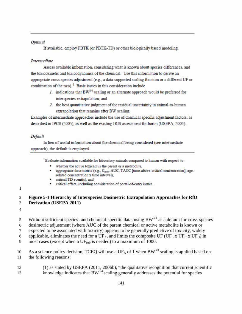
141

1

Figure 5-1 Hierarchy of Interspecies Dosimetric Extrapolation Approaches for RfD 2 Derivation (USEPA 2011) 3 4

Without sufficient species- and chemical-specific data, using BW3/4 as a default for cross-species 5 dosimetric adjustment (where AUC of the parent chemical or active metabolite is known or 6 expected to be associated with toxicity) appears to be generally predictive of toxicity, widely 7 applicable, eliminates the need for a UFA, and limits the composite UF (UFL x UFH x UFD) in 8 most cases (except when a UFsub is needed) to a maximum of 1000. 9

As a science policy decision, TCEQ will use a UFA of 1 when BW3/4 scaling is applied based on 10 the following reasons: 11

(1) as stated by USEPA (2011, 2006b), “the qualitative recognition that current scientific 12 knowledge indicates that BW3/4 scaling generally addresses the potential for species 13

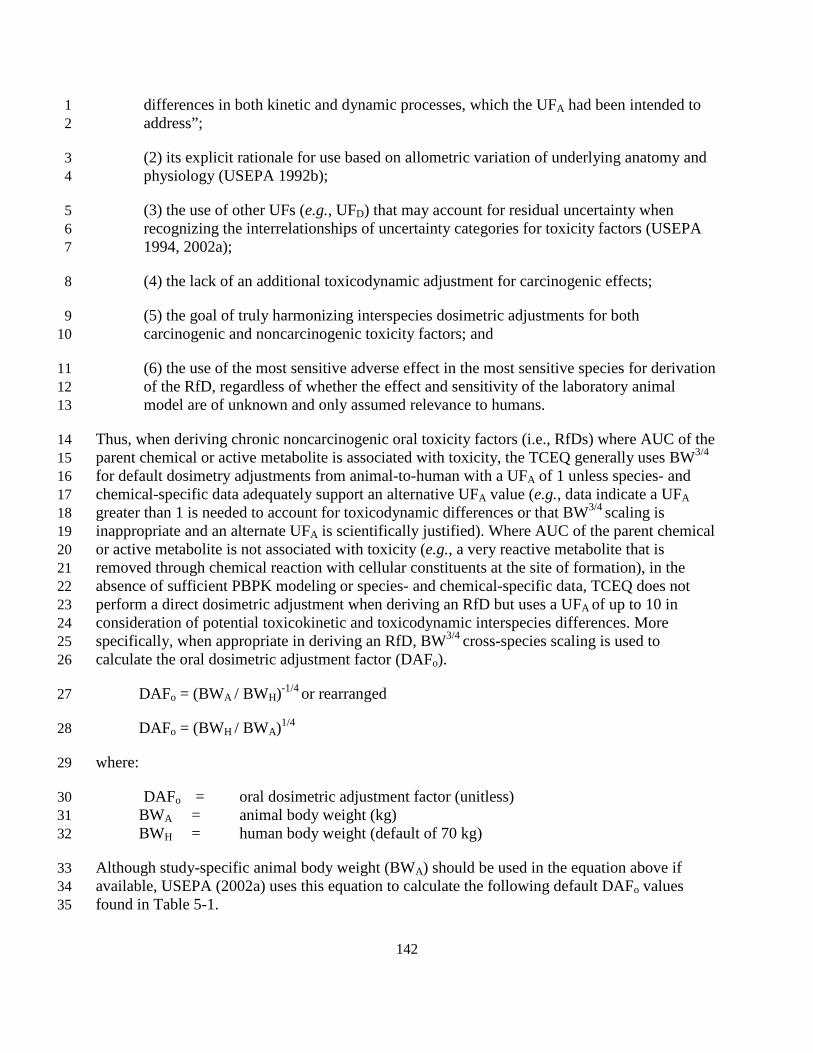
142

differences in both kinetic and dynamic processes, which the UFA had been intended to 1 address”; 2

(2) its explicit rationale for use based on allometric variation of underlying anatomy and 3 physiology (USEPA 1992b); 4

(3) the use of other UFs (e.g., UFD) that may account for residual uncertainty when 5 recognizing the interrelationships of uncertainty categories for toxicity factors (USEPA 6 1994, 2002a); 7

(4) the lack of an additional toxicodynamic adjustment for carcinogenic effects; 8

(5) the goal of truly harmonizing interspecies dosimetric adjustments for both 9 carcinogenic and noncarcinogenic toxicity factors; and 10

(6) the use of the most sensitive adverse effect in the most sensitive species for derivation 11 of the RfD, regardless of whether the effect and sensitivity of the laboratory animal 12 model are of unknown and only assumed relevance to humans. 13

Thus, when deriving chronic noncarcinogenic oral toxicity factors (i.e., RfDs) where AUC of the 14 parent chemical or active metabolite is associated with toxicity, the TCEQ generally uses BW3/4 15 for default dosimetry adjustments from animal-to-human with a UFA of 1 unless species- and 16 chemical-specific data adequately support an alternative UFA value (e.g., data indicate a UFA 17 greater than 1 is needed to account for toxicodynamic differences or that BW3/4 scaling is 18 inappropriate and an alternate UFA is scientifically justified). Where AUC of the parent chemical 19 or active metabolite is not associated with toxicity (e.g., a very reactive metabolite that is 20 removed through chemical reaction with cellular constituents at the site of formation), in the 21 absence of sufficient PBPK modeling or species- and chemical-specific data, TCEQ does not 22 perform a direct dosimetric adjustment when deriving an RfD but uses a UFA of up to 10 in 23 consideration of potential toxicokinetic and toxicodynamic interspecies differences. More 24 specifically, when appropriate in deriving an RfD, BW3/4 cross-species scaling is used to 25 calculate the oral dosimetric adjustment factor (DAFo). 26

DAFo = (BWA / BWH)-1/4 or rearranged 27

DAFo = (BWH / BWA)1/4 28

where: 29

DAFo = oral dosimetric adjustment factor (unitless) 30 BWA = animal body weight (kg) 31 BWH = human body weight (default of 70 kg) 32

Although study-specific animal body weight (BWA) should be used in the equation above if 33 available, USEPA (2002a) uses this equation to calculate the following default DAFo values 34 found in Table 5-1. 35

143

Table 5-1 Default DAFo (USEPA 2002a) 1 Species Default Body Weight (kg) Default DAFo Mouse 0.03 7 Rat 0.25 4 Guinea pig 0.5 3 Rabbit 2.5 2 Human 70 1

2 Once a DAFo has been determined, the following equation is used to calculate the PODHED. 3

PODHED = PODAnimal-ADJ / DAFo 4

where: 5

PODHED = human equivalent dose POD (mg/kg-day) 6 PODAnimal-ADJ = animal dose POD, adjusted to a continuous oral exposure scenario 7

(mg/kg-day) 8 DAFo = oral dosimetric adjustment factor (unitless) 9

See USEPA (2011) for additional information regarding use of BW3/4 animal-to-human 10 dosimetric scaling. 11

5.4 Minimum Database Requirements for the Development of a Chronic ReV 12 or RfD 13

USEPA (1994) states that the minimum toxicologic database requirement for the development of 14 an RfC with low confidence is “a well-conducted subchronic inhalation bioassay that evaluated a 15 comprehensive array of endpoints, including an adequate evaluation of portal-of-entry 16 (respiratory tract) effects, and established an unequivocal NOAEL and LOAEL.” Table 5-2 is an 17 adaptation from Table 4-1 in the RfC Methodology (USEPA 1994), which lists different studies 18 that should be available to establish a higher confidence RfC. 19

Since the confidence in the database should be based on an understanding of the putative MOA 20 for the observed effects, it varies on a case-by-case basis as discussed in the RfC Methodology. 21 The TCEQ assigns a confidence level to the study quality of the key study and the database, not 22 to the ReV or RfD. Although the TCEQ does not assign a confidence level to a ReV or RfD, 23 case-specific factors could affect the database confidence category as determined under Table 5-24 2 and Section 3.12.3 (e.g., the available chronic studies did not examine the likely most sensitive 25 toxic effects for a chemical, used a poor animal model or means of exposure (gavage) dissimilar 26 to environmental human exposure), the TCEQ generally uses the criteria in Table 5-2 for the 27 minimum database requirements used to develop a chronic ReV and the confidence level 28 assigned to the database. The minimum database that USEPA has defined for derivation of low- 29 and high-confidence RfDs is the same as for RfCs (USEPA 2002a). Thus, Table 5-2 also 30 represents the minimum database requirements for derivation of an RfD and the confidence level 31 assigned to the database. In order to properly consider chronic child adult differences, a two-32

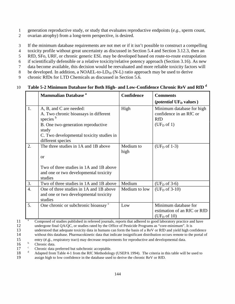
144

generation reproductive study, or study that evaluates reproductive endpoints (e.g., sperm count, 1 ovarian atrophy) from a long-term perspective, is desired. 2

If the minimum database requirements are not met or if it isn’t possible to construct a compelling 3 toxicity profile without great uncertainty as discussed in Section 5.4 and Section 3.12.3, then an 4 RfD, SFo, URF, or chronic generic ESL may be developed based on route-to-route extrapolation 5 if scientifically defensible or a relative toxicity/relative potency approach (Section 3.16). As new 6 data become available, this decision would be reevaluated and more reliable toxicity factors will 7 be developed. In addition, a NOAEL-to-LD50 (N-L) ratio approach may be used to derive 8 chronic RfDs for LTD Chemicals as discussed in Section 5.6. 9

Table 5-2 Minimum Database for Both High- and Low-Confidence Chronic ReV and RfD d 10

Mammalian Database a Confidence Comments (potential UFD values )

1. A, B, and C are needed: A. Two chronic bioassays in different species b

High Minimum database for high confidence in an RfC or RfD (UFD of 1) B. One two-generation reproductive

study C. Two developmental toxicity studies in different species

2. The three studies in 1A and 1B above or Two of three studies in 1A and 1B above and one or two developmental toxicity studies

Medium to high

(UFD of 1-3)

3. Two of three studies in 1A and 1B above Medium (UFD of 3-6) 4. One of three studies in 1A and 1B above

and one or two developmental toxicity studies

Medium to low (UFD of 3-10)

5. One chronic or subchronic bioassay c Low Minimum database for estimation of an RfC or RfD (UFD of 10)

a Composed of studies published in refereed journals, reports that adhered to good laboratory practice and have 11 undergone final QA/QC, or studies rated by the Office of Pesticide Programs as “core-minimum”. It is 12 understood that adequate toxicity data in humans can form the basis of a ReV or RfD and yield high confidence 13 without this database. Pharmacokinetic data that indicate insignificant distribution occurs remote to the portal of 14 entry (e.g., respiratory tract) may decrease requirements for reproductive and developmental data. 15

b Chronic data. 16 c Chronic data preferred but subchronic acceptable. 17 d Adapted from Table 4-1 from the RfC Methodology (USEPA 1994). The criteria in this table will be used to 18

assign high to low confidence in the database used to derive the chronic ReV or RfD. 19

145

5.5 Uncertainty Factors Specific for the Development of a Chronic ReV or RfD 1 UFs are discussed in Chapter 3 except for the following UFs specific to development of a 2 chronic ReV or RfD: UFH, UFD, and UFSub. Recognizing the interrelationships of uncertainty 3 categories (Section 3.13 and USEPA 2002a), if the cumulative UF exceeds 3000, the TCEQ uses 4 a default of 3000. 5

5.5.1 Chronic UFH 6 Developing organisms can be more sensitive than mature organisms (OEHHA 2008). However, 7 data are often not available to identify what toxicokinetic and/or toxicodynamic differences exist 8 within the human population (e.g., between children and adults) that may affect the toxicity of a 9 particular chemical. Likewise, data are often lacking to determine the extent to which any 10 differences will affect sensitivity to toxicity from exposure to a particular chemical (i.e., what 11 numerical adjustment is required to account for toxicokinetic and/or toxicodynamic differences 12 among humans that impact the toxicity of a particular chemical). The toxicokinetic UF (UFH-K) is 13 used in consideration of potential differences in humans in the absorption, distribution, 14 metabolism, and elimination of the chemical. The toxicodynamic UF (UFH-D) is used in 15 consideration of potential differences among humans in the mode or mechanism of action. 16 Typically, these values are up to 100.5 each. Studies have indicated that an overall UFH of 10 is 17 protective of intraspecies variability in humans, including children (Dourson et al. 1996). In 18 certain cases, a higher UF may be used to protect children because of differences in 19 toxicokinetics or toxicodynamics of a chemical between children and adults if scientific data is 20 available to support this decision. As discussed in Section 3.2, there are toxicokinetic differences 21 or exposure differences between children and adults which can affect the absorption, distribution, 22 metabolism, and elimination of a chemical. For example, children inhale more air per body 23 weight and respiratory tract surface area than adults (Ginserg et al. 2008), and ingest more food 24 and water per kg body weight than adults (CalEPA 2008). Children have less contribution from 25 nasal breathing and less efficient nasal filtering, resulting in reduced uptake of particles in the 26 nasal airways and greater deposition efficiency of particles and some vapor phase chemicals in 27 the lower respiratory tract (Foos et al. 2008). The TCEQ uses a WOE approach to make a 28 scientific judgment as to whether UFs are needed to account for child differences when 29 compared to adults. No single consideration determines the overall level of concern for children 30 (Health Canada 2008, USEPA 2002c). The WOE approach will be used, in part, to determine the 31 appropriate UFH value. Refer to Section 3.2 and Table 3-2 for using a WOE approach to evaluate 32 the degree of concern for children. 33

5.5.2 Chronic UFD 34 Uncertainty introduced by database deficiencies such as a limited number of experimental 35 studies, animal species, or bioassays, lack of data describing child-adult differences, or 36 deficiencies in the study design/quality can be addressed by the use of a UF (Dourson et al. 37 1996). The TCEQ generally uses a total UFD up to 10 to address different areas of uncertainty in 38 the database. 39

An important consideration for the UFD is whether or not child-adult differences have been 40 adequately investigated. In order to properly consider chronic child-adult differences, in the 41 absence of relevant human data, a two-generation reproductive study is preferred (Table 5-2). 42

146

Studies that evaluate reproductive endpoints (e.g., sperm count, testicular lesions, ovarian 1 atrophy) from a long-term perspective should also be present. The UFD is applied to take into 2 account the lack of child-adult difference information and other deficiencies in the database for a 3 particular chemical. 4

The minimum database confidence levels given in Table 5-2 for RfD/RfC derivation cannot 5 represent the completeness of the overall database for a given chemical as many important 6 details and considerations are not addressed, and use of Table 5-2 solely for this purpose would 7 represent a significant oversimplification of scientific judgment necessary for the UFD value 8 selection process. Therefore, Table 5-2 should not be the sole consideration in selecting a UFD 9 value for a chemical. Refer to Section 3.12.3 for additional information. 10

5.5.3 Use of the UFH and UFD to Account for Child-Adult Differences 11 Data from several studies indicate that in most cases, a UFD of up to 10 is adequate, if 12 appropriately applied in conjunction with the UFH of up to 10 to account for child-adult 13 differences in susceptibility (Nielsen et al. 2010; Dourson et al. 2002; USEPA 2002c). However, 14 in some cases, a UFH greater than 10 may be used to account for significant toxicokinetic and 15 toxicodynamic differences conferring increased sensitivity to children for a particular chemical 16 may not be adequately accounted for by a UFH of 10. The need for a UFH of greater than 10 will 17 be evaluated on a chemical-by-chemical basis, and scientific justification will be provided in the 18 chemical's DSD for the value of UFH. Please refer to Section 3.12 for additional information. 19

5.5.4 Subchronic to Chronic UF 20 If subchronic exposure studies are the only available studies for a given chemical, then they can 21 be extrapolated to derive chronic ReV or RfD values when the uncertainty resulting from using 22 data from subchronic exposure studies is accounted for through use of an appropriate UFSub. A 23 default UFSub of up to 10 is typically applied to account for this extrapolation. The scientific 24 defensibility of using a default UFSub of 10 is debatable. Studies have been published that support 25 a lower default UFSub (e.g., Beck et al. 1993), while others support a default UFSub of 10 (e.g., 26 Pieters et al. 1998). The TCEQ recognizes that the application of UFs should be evaluated on a 27 case-by-case basis. In cases where toxic metabolites or damage do not accumulate (Bogdanffy 28 and Jarabek 1995) or subchronic exposure studies indicate the chemical is relatively nontoxic, 29 chronic effects would not be expected to differ significantly from subchronic effects and an 30 UFSub of 10 would be unnecessary. However, if the putative causative chemical or metabolite 31 bioaccumulates and/or damage recovery (i.e., toxicodynamic half-life) is not rapid or this 32 information is unavailable, a default UFSub of up to 10 is applied. The UFSub is not applied when 33 a developmental or other shorter-duration study with a critical window of exposure is the key 34 study. Thus, the UFSub is determined and applied based on case-specific information. 35

ECETOC (2003) recommends that no adjustment for exposure duration is needed (i.e., UFSub = 36 1) for chemicals that have: (1) local effects (i.e., sensory irritation); or (2) a relatively short 37 toxicokinetic half-life, no toxic metabolite, no potential for bioaccumulation and/or cumulative 38 toxicity, and no reactivity to tissue components. OEHHA (2008) uses a default UFSub of 1 to 10 39 for extrapolating from subchronic to chronic exposures. Specifically, a UFSub of 1 is applied for 40 exposures longer than 12% of expected lifetime (chronic studies), a UFSub of 3 is applied for 41

147

exposures from 8 to 12% of expected lifetime (subchronic studies), and a UFSub of 10 is applied 1 for exposures less than 8% of expected lifetime. These values may be used in the absence of any 2 other informative data (e.g., toxicokinetic and toxicodynamic half-life information). 3

5.6 RfDs for Chemicals with Limited Toxicity Data 4 Occasionally, chemicals with limited toxicity data (LTD chemicals) are contaminants at 5 remediation sites being addressed under the TRRP rule (30TAC§350). Since a LTD chemical 6 may pose a potential health concern at a site that might otherwise require no remedial action due 7 to other contaminants, it is important to calculate an RfD for LTD chemical so that health-8 protective media (e.g., surface soil) concentrations may be calculated to determine if further 9 action may be needed. In remediation programs, an RfD is especially important since the 10 incidental ingestion of soil is the most important (i.e., media concentration limiting) exposure 11 pathway in calculating a health-protective concentration for the vast majority of chemicals. 12 Additionally, as exposure to site contaminants may be ongoing, it is not reasonable or prudent 13 for the protection of public health to await possible future toxicity testing prior to using available 14 data and procedures in the best possible effort to determine the need for remedial action. 15 Therefore, for the protection of public health, LTD chemicals associated with remediation sites 16 are an exception to the minimum database requirements for an RfD under Section 5.4 and the 17 TCEQ will calculate an RfD for LTD chemicals. As discussed in Section 3-16, the TCEQ may 18 develop an RfD based on route-to-route extrapolation or a relative toxicity/relative potency 19 approach, if scientifically defensible. 20

Another method to calculate an RfD for LTD chemicals is to use a NOAEL-to-LD50 (N-L) Ratio 21 Approach. On an as-needed basis, the TCEQ uses a NOAEL-to-LD50 (N-L) ratio approach to 22 estimate an RfD for an LTD chemical. After choosing the lowest LD50 value of acceptable 23 quality for a LTD chemical, an N-L ratio-based RfD can be calculated by multiplying the LD50 24 by 6.7 x 10-6. The background of the N-L ratio RfD approach is briefly discussed below. 25

Several investigators have suggested using readily available acute toxicity data to estimate 26 chronic endpoints for LTD chemicals. This procedure was proposed by Layton et al. (1987) for 27 estimating ADIs for the evaluation and management of exposures and health hazard from 28 contaminants at hazardous waste sites. Venman and Flaga (1985) also used this procedure to 29 establish provisional ADIs for the evaluation of waste water contaminants. Both investigators 30 calculated NOEL-to-oral LD50 ratios from chronic animal studies for different organic chemicals 31 and determined the fifth percentile of the cumulative distributions of the ratios. The LD50 value 32 for contaminants with limited toxicity data was multiplied by the fifth percentile ratio to derive a 33 surrogate NOEL. The surrogate NOEL was divided by an uncertainty factor of 100 (UFA = 10 34 and UFH = 10) in order to establish a conservative threshold dose (i.e., ADI) below which no 35 appreciable risk to human health would occur. 36

The TCEQ used results from Layton et al. (1987) to establish a procedure to estimate interim 37 RfDs (as needed) for LTD chemicals using available LD50 data. Layton et al. (1987) used a fairly 38 large dataset which included data from Venman and Flaga (1985), other prior studies, and data 39 that the study authors assimilated themselves. The suggested multiplicative factor necessary to 40 estimate an ADI from LD50 data ranged from 5.0 x 10-6 to 1.0 x 10-5. Again, these factors are 41 based on the fifth percentiles of various NOEL-to-LD50 ratio datasets divided by an uncertainty 42

148

factor of 100 to derive an ADI, which is similar to an RfD. The factor on the low end of the 1 range is that associated only with use of rat LD50 data, while that on the high end of the range is 2 based on data for rats and other small laboratory mammals. There is no clear scientific rationale 3 for selecting any specific value within this range. As a science policy decision, the TCEQ will 4 use the factor of 6.7 x 10-6. This value is conservative compared to central tendency factor 5 estimates (e.g., 22 times more conservative than the multiplicative factor associated with the 6 geometric mean of the chronic rat NOEL/LD50 ratio database (1.5 x 10-4) from three prior studies 7 and 27 times more conservative than the geometric mean of the chronic NOEL/LD50 ratio 8 database (1.8 x 10-4) for rats and other small laboratory mammals). Additionally, the selected 9 factor of 6.7 x 10-6 is: 10

• on the conservative end of the range of fifth percentile factors calculated from the datasets 11 of three prior studies used by Layton et al. (1987); 12

• likely to result in an adequately health-protective RfD since the lowest scientifically-13 acceptable LD50 value across species will be used by TCEQ and additional toxicity testing 14 would likely result in higher ADI values (Layton et al. 1987); and 15

• likely to result in health-protective media cleanup concentrations as it is combined with 16 conservative exposure assumptions (e.g., long-term, daily simultaneous exposure to 17 surface soil through incidental ingestion, dermal exposure, consumption of vegetables 18 homegrown in the soil, and the inhalation of vapor/particulate emanating from the soil). 19

For LTD chemicals needing an RfD, the LD50 value is multiplied by the factor of 6.7 x 10-6 to 20 calculate an RfD. This RfD will be used until toxicity information which is more informative of 21 potential chronic effects is available to derive an RfD. 22

RfD = LD50 x 6.7 x 10-6 23

where: 24

RfD = chronic oral reference dose (mg/kg-day) 25 LD50= lowest LD50 value of acceptable quality (mg/kg) 26

Similar to the discussion in Section 4.6.2.1 for the selection of LC50 data, the TCEQ may use 27 study quality considerations to select the LD50 value used for RfD derivation if significant 28 quality differences exist between experimental studies, or conservatively select the lowest LD50 29 value. An RfD calculated using this procedure will be replaced when and if sufficient toxicity 30 information becomes available to calculate a more scientifically-defensible RfD. 31

5.7 Nonthreshold Carcinogens and Threshold Carcinogens 32 This section describes the approach used by the TCEQ to determine whether a toxicant warrants 33 consideration for possible carcinogenic endpoints. The same analytical approach discussed in 34 Section 3.3 is used to derive toxicity factors for carcinogens as well as to evaluate carcinogenic 35 toxicity factors derived by other scientists or regulatory agencies (i.e., review essential data 36 including physical/chemical properties and select key studies; conduct a MOA analysis; choose 37

149

the appropriate dose metric; determine the POD for each key study; conduct appropriate 1 dosimetric modeling; select critical effect and extrapolate from the adjusted POD to lower 2 exposures based on MOA analysis). If the dose-response is determined to be nonthreshold in the 3 low-dose region (based on data or science policy default assumptions), inhalation URFs or oral 4 SFos are derived whereas if the dose-response is determined to be threshold, then inhalation 5 ReVs or oral RfDs are derived. 6

In March 2005, USEPA issued an updated version of the Guidelines for Carcinogen Risk 7 Assessment, hereafter referred to as the 2005 Cancer Guidelines (USEPA 2005a) as well as a 8 supplemental guidance document entitled Supplemental Guidance for Assessing Susceptibility 9 from Early-Life Exposure to Carcinogens (USEPA 2005b), hereafter referred to as the 2005 10 Supplemental Guidance. The purpose of the 2005 Supplemental Guidance is to address the 11 potential for an increased susceptibility to cancer due to early-life exposure to carcinogenic 12 compounds. The 2005 Cancer Guidelines and the 2005 Supplemental Guidance reflect 13 knowledge concerning the carcinogenic process gained in recent years and have undergone an 14 extensive peer-review and public comment process. Therefore, the TCEQ uses these guidance 15 documents as the main source of information to derive carcinogenic URFs/SFos and ReVs/RfDs. 16 However, if new information, scientific understanding, or science policy judgment become 17 available, the TCEQ may conduct cancer risk assessments differently than envisioned in the 18 cancer guidelines. The following sections briefly summarize key features of the 2005 Cancer 19 Guidelines and the 2005 Supplemental Guidance which are found at the following website: 20 http://www.epa.gov/iris/backgrd.html. 21

5.7.1 Hazard Assessment and Weight of Evidence 22 The 2005 Cancer Guidelines contain a detailed discussion of hazard identification based on a 23 chemical’s MOA using a WOE approach so a detailed discussion is not included here (Chapter 2 24 of USEPA 2005a). Briefly, hazard assessment determines whether a chemical may pose a 25 carcinogenic hazard to humans and under what circumstances an identified hazard may be 26 expressed (NRC 1994). A variety of data ranging from observations of tumor responses to 27 analysis of SARs are examined in order “to construct a total analysis examining what the 28 biological data reveal as a whole about carcinogenic effects and MOA of the agent, and their 29 implications for human hazard and dose-response evaluation” (USEPA 2005a). 30

The 2005 Cancer Guidelines recommend that a hazard narrative be used instead of the 31 classification system suggested in the 1986 Cancer Guidelines. The following standard hazard 32 descriptors are used as part of the hazard narrative to summarize the WOE for potential human 33 carcinogenicity: 34

• Carcinogenic to Humans 35 • Likely to Be Carcinogenic to Humans 36 • Suggestive Evidence of Carcinogenic Potential, but Not Sufficient to Assess Human 37

Carcinogenic Potential 38 • Data Are Inadequate for an Assessment of Human Carcinogenic Potential 39 • Not Likely to be Carcinogenic to Humans. 40

150

Additional information is included in the narrative, such as whether a chemical appears to be 1 carcinogenic by certain routes of exposure but not others, or whether exposure during potentially 2 sensitive life-stages of development may increase the carcinogenic potential of a chemical. The 3 narrative may also summarize uncertainties and key default options used in the assessment. The 4 entire range of information included in the narrative should be considered instead of simply 5 focusing on the descriptor. 6

Hazard identification for carcinogens by organizations other than USEPA is typically 7 approached using a WOE classification system. These systems may be numeric, alphabetic, or 8 alphanumeric, depending on the organization that publishes them. In the United States, 9 organizations that classify carcinogens by WOE classification systems include NTP, OSHA, 10 ACGIH, and NIOSH. In Europe, the German MAK classification scheme is used, and 11 internationally, IARC publishes a WOE classification. 12

The TCEQ uses all of the aforementioned sources as well as other peer-reviewed research when 13 considering the carcinogenic potential of a toxicant based on a WOE approach. Generally, the 14 TCEQ only performs carcinogenic dose-response assessments for chemicals considered 15 “Carcinogenic to Humans” and “Likely to Be Carcinogenic to Humans” and for which available 16 data adequately characterize the dose-response curve. Additionally, it should be known or 17 biologically plausible that the putative carcinogenic MOA operates at environmentally-relevant 18 exposure levels, and if based on laboratory animal data, the tumors observed must be of known 19 or biologically-plausible relevance to humans. 20

5.7.2 MOA 21 The 2005 Cancer Guidelines emphasize that a critical analysis of all relevant information be used 22 as a starting point to assess carcinogenic risk of a compound rather than using default options. In 23 fact, the use of MOA information is a main focus of the guidelines. Section 2.4 of the 2005 24 Cancer Guidelines discusses how to evaluate and accept a carcinogenic MOA. MOA information 25 can be used to make decisions about the relevance of animal data to humans, assist in identifying 26 sensitive subpopulations, model tumor incidence or key precursor event data (i.e., curve fitting), 27 and decide upon approaches of high-dose to low-dose extrapolation in dose-response assessment. 28 However, extensive experimentation is needed to support a hypothesis as to MOA for a specific 29 tumor response, or to decide whether other MOAs are plausible. 30

An initial process in the cancer dose-response assessment is to examine the MOA and dose-31 response for each tumor type with a significant increase in incidence. This includes an analysis 32 of the following information on all tumor types that are increased in incidence by the chemical: 33 the number of sites; their consistency across sexes, strains and species; the strength of the MOA 34 information for each tumor type; the anticipated relevance of each tumor type to humans; and the 35 consistency of the means of estimating risks across tumor types. For each tumor, the MOA and 36 other information may support one of the following dose-response extrapolations: 1) 37 nonthreshold (typically a linear extrapolation to zero); 2) threshold (typically choosing a POD 38 and applying UFs; or (3) both. 39

151

5.7.3 Dose-Response Assessment 1 Different dose-response assessments may be conducted when tumor data is based on animal 2 studies or whether human epidemiology studies are available. Dose-response assessment for each 3 tumor type is performed using the following steps: derivation of a POD based on observed data, 4 dosimetric adjustments to the POD, followed by extrapolation to lower concentrations. The 5 following sections discuss basic principles common to both. Chapter 7 will discuss dose-6 response modeling for data obtained from human epidemiology studies. 7

5.7.3.1 Derivation of a POD based on observed data 8 Derivation of a POD is discussed in Section 3.7, although the terminology used for a 9 carcinogenic assessment is different. For inhalation exposure, the term “effective concentration 10 (EC)” is the central estimate and is analogous to the term “BMC” and the term “lower bound of 11 EC (LEC)” is the lower 95% confidence limit and is analogous to the term “BMCL”. When the 12 POD is determined from an oral exposure study, the term “effective dose (ED)” is the central 13 estimate and is analogous to the term “benchmark dose “BMD” and the term “lower bound of 14 ED (LED)” is the lower 95% confidence limit and is analogous to the term “benchmark dose 15 level BMDL” as shown in Figure 5-2. 16

17 Figure 5-2 Example of a linear approach to extrapolate to lower exposures. 18 The terms “ED10 and LED10” refer to dose but are analogous to the terms “EC10 and LEC10”, 19 respectively (Exhibit 12-3A of USEPA 2004a). 20

Typically for animal studies, the EC or ED is at a 10% response level (EC10 or ED10) as the limit 21 of detection of studies of tumor effect in animal studies is about 10%. Since the POD alone does 22 not convey all the critical information present in the data from which it is derived, it is suggested 23 that a POD narrative be included in a cancer assessment. Section 3.2.5 of the 2005 Cancer 24 Guidelines discusses several key factors to consider for characterizing the POD. These factors 25 include: 26

152

• nature and level of the response, 1 • nature of the study population, 2 • slope of the observed dose-response curve at the POD, 3 • relationship of the POD with other cancers, and 4 • extent of the overall cancer database 5

For epidemiological studies, the type of study and how dose and response are measured in the 6 study determine how the data in the range of observation are modeled. The 2005 Cancer 7 Guidelines refers to the Science Advisory Board who stated "it may be appropriate to emphasize 8 lower statistical bounds in screening analyses and in activities designed to develop an 9 appropriate human exposure value, since such activities require accounting for various types of 10 uncertainties and a lower bound on the central estimate is a scientifically-based approach 11 accounting for the uncertainty in the true value of the ED10 [or central estimate].” The LEC/LED 12 or the EC10/ LED10 may be appropriate for certain datasets based on human epidemiological 13 data. When the TCEQ staff develop a toxicity value for a carcinogen based on a human 14 epidemiological study, the following types of uncertainties of the human study are considered in 15 order to determine whether to use the EC/ED or the LEC/LED as the POD (Section 3.2.1 of 16 USEPA 2005a): 17

• when estimates of mortality are available rather than incidence because survival rates for 18 different cancers vary; 19

• when the chemical has discernible competing or additive interactions with other agents 20 and epidemiologic studies cannot adequately estimate the contribution of each agent as a 21 risk factor for the effects of the other; 22

• when control groups have been exposed to the chemical, risk estimates may be biased 23 toward zero (analysis is improved if background exposures in the exposed and control 24 groups are taken into account); 25

• when a well-conducted meta-analysis based on several epidemiologic studies is 26 performed, the risk calculation can be done with greater precision thereby decreasing 27 uncertainty; 28

• when MOA analysis indicates that the carcinogen acts on multiple stages of the 29 carcinogenic process, all periods of exposure including study subjects who were exposed 30 near the end of the study should be considered. However, if MOA indicates there may be 31 a latency period, then study subjects who were exposed near the end of the study need to 32 be analyzed differently. Their data may be similar to analysis of data for those who were 33 not exposed; 34

• when studies investigate only one effect (typical of many case-control studies), include 35 only one population segment (e.g., male workers or workers of one socioeconomic class), 36 or include only one lifestage 37

USEPA (2005a) states “risk assessors should calculate, to the extent practicable, and present the 38 central estimate and the corresponding upper and lower statistical bounds (such as confidence 39 limits) to inform decision makers.” This applies for both animal studies and human studies. 40

153

In addition to using BMC/BMD modeling to derive an EC10/LEC10 or ED10/LED10 for 1 extrapolation to lower exposures as discussed in Section 3.7.3, specific dose-response modeling 2 and a BEIR IV life-table analysis (NRC 1988) may be used to calculate these values for use as 3 the POD for low-dose extrapolation as discussed in Chapter 7. Briefly, a BEIR IV analysis 4 accounts for age-specific noncancer mortality and cancer mortality for the cancer endpoint of 5 interest in estimating excess lifetime risk as a linear function of dose. Cancer potency factors (β 6 and 95% UCL β values) are estimated through fitting a linear model to study cancer data (e.g., 7 maximum likelihood estimates of β from Cox or Poisson regression of cancer mortality against 8 dose fit by maximum likelihood estimation). Then, a cancer potency factor is input into the BEIR 9 IV analysis and the lowest POD adequately supported by data (e.g., LEC10 or LED10) is 10 calculated for extrapolation to lower exposures. That is, the BEIR IV methodology is used to 11 calculate the lifetime daily inhalation or oral dose (mg/kg-day) corresponding to the lowest 12 excess cancer BMR supported by data (e.g., LEC10 or LED10) for use as the POD for low-dose 13 extrapolation, with the end result being a URF (risk per µg/m3) or a SFo (risk per mg/kg-day). 14 See Chapter 7 for additional information on using these types of analyses with data from 15 epidemiological studies to derive a POD. 16

5.7.3.2 Dosimetric Adjustments to the POD 17 All approaches for performing dosimetric adjustments to the POD to account for animal-to-18 human differences and exposure duration discussed in Chapter 3 and Sections 5.2 and 5.3 are 19 used to perform adjustments to the POD for both threshold and nonthreshold cancer assessment 20 when average daily concentration is used as the dose metric (i.e., mg/m3 or ppm). If the exposure 21 dose metric is from a worker epidemiology study to be used in a BEIR IV life-table analysis, the 22 dose metric is converted to an average daily environmental concentration for the general public 23 consistent with procedures in Chapter 7. 24

5.7.3.3 Extrapolation to Lower Exposures 25 After a PODADJ or PODHEC/HED has been determined, extrapolation to lower dose levels is 26 conducted. In a few cases, detailed MOA information may be available that allows the 27 formulation of a toxicodynamic or biologically-based model for extrapolation to lower exposures 28 (USEPA 2005a; Moolgavkar and Knudson 1981; Chen and Farland 1991; Portier 1987). If 29 substantial MOA information is available, the extrapolation is based on an extension of a 30 biologically-based model. If not, any information on the proposed MOA(s) of the chemical can 31 be used to decide whether the extrapolations should assume a nonthreshold or threshold response 32 for the dose-response relationship, or both. Examples of factors supporting a nonthreshold (i.e., 33 linear) approach, threshold approach, or both approaches are discussed in Section 3.3 of the 2005 34 Cancer Guidelines. 35

When the MOA information supports nonthreshold, as is the case for a carcinogen operating via 36 a mutagenic MOA, or when the MOA is not understood for a chemical, the default is to use a 37 nonthreshold (i.e., linear low-dose extrapolation) approach (Figure 5-2). This approach utilizes a 38 straight line extrapolation from the POD to the origin (zero incremental dose, zero incremental 39 response) (USEPA 2005a). For example, if the LEC10 is used as the POD, then the slope of the 40 line from the LEC10 to the origin of the dose-response curve yields the inhalation URF, the 41

154

upper-bound excess lifetime cancer risk estimated to result from continuous exposure to an agent 1 at a concentration of 1 μg/m3 in air: 2

URF = 0.10/ LEC10 3

See Section 1.5.2.2 for the equation to use this URF to calculate the air concentration at a 1 in 4 100,000 excess cancer risk (i.e., chronicESLnonthreshold (c)). 5

In regard to oral exposure, the same equation as above may be used to derive a SFo where the 6 ED10 or LED10 is in units of mg/kg-day (i.e., average daily dose over a lifetime). In this ED/LED 7 approach to low dose extrapolation and SFo derivation, the standard procedure is to calculate the 8 ED or LED (lower 95% confidence bound on the ED) with the BMR typically set at 10% extra 9 risk (i.e., calculate an ED10 or LED10). The SFo is then calculated by dividing the BMR by the 10 ED10 or LED10. Although the LED10 is typically used as the POD for both animal and 11 epidemiological carcinogenicity studies, see Section 5.7.3.1 for a discussion of the human study 12 uncertainties considered in determining whether to use the ED10 or LED10. For example, if the 13 LED10 is used as the POD, the resulting SFo represents upper-bound excess lifetime cancer risk 14 estimated to result from continuous exposure to an agent at an intake of 1 mg/kg-day (i.e., SFo 15 units are excess risk per mg/kg-day): 16

SFo = 0.10 / LED10 17

If based on animal carcinogenicity data, see Section 5.3 regarding the method to convert the 18 SFoA to a human equivalent SFoH. 19

If sufficient evidence is available to support a threshold MOA for the general population and any 20 subpopulations of concern, the default approach changes to a determination of a POD and 21 application of UFs in order to derive a ReV or RfD protective of carcinogenic effects. The POD 22 is generally the LEC (i.e., BMCL), LED (i.e., BMDL), NOAEL, or LOAEL depending on the 23 quality and nature of the data as discussed in Chapter 3 and illustrated in Figure 3-11. 24

Chloroform is an example of a carcinogen where available evidence indicates that the 25 carcinogenic response is secondary to another toxicity that has a threshold (USEPA 2001). 26 Chloroform-induced carcinogenicity appears to be secondary to cytotoxicity and regenerative 27 hyperplasia. Accordingly, doses below the RfD do not result in cytolethality and hence are 28 unlikely to result in increased risk of cancer. The RfD developed for protection against 29 noncancer effects (including cytolethality and regenerative hyperplasia) can also be considered 30 protective against increased risk of cancer. Formaldehyde-induced respiratory cancers and dioxin 31 carcinogenicity are also likely to be threshold phenomena. 32

The POD for threshold carcinogens can be based on precursor responses if MOA information 33 indicates that precursor responses are key events in the development of tumors or tumor 34 incidence. Precursor events can often be detected with greater sensitivity (i.e., prior to tumor 35 development and at lower doses). Thus, such a POD actually represents a “no effect level” with 36 respect to tumor formation. An example of a chemical where a consideration of precursor effects 37 is warranted is vinyl acetate (Bogdanffy and Jarabek 1995). Acetic acid produced within 38 sustentacular cells of olfactory epithelium due to exposure to vinyl acetate initiates cytotoxicity. 39

155

Tissue proton burdens that overwhelm the natural cellular buffering and proton transport 1 mechanisms leads to cell death. Based on this MOA analysis and the observation that nasal 2 tumors were observed at the highest concentration only, IRIS derived an RfC for vinyl acetate, 3 not a URF. 4

If the dose-response can be adequately described by both a linear and a nonlinear (e.g., 5 threshold) approach, then the default is to present both the linear and nonlinear analyses. The 6 results of both analyses are considered by the TCEQ. It is helpful to present the data on both the 7 linear or nonlinear assessment in a form that allows an informed decision to be made, such as a 8 data array mentioned in Chapter 3. Carcinogenic MOA data may ultimately suggest which 9 approach is likely more biologically plausible and predictive of human risk at environmentally-10 relevant exposure levels. 11

A list of options for presenting results when multiple estimates can be developed is presented in 12 Section 3.3.5 of the Cancer Guidelines (e.g., multiple risks estimated from several different 13 tumor types) (USEPA 2005a): 14

• Adding risk estimates derived from different tumor sites 15 • Combining data from different datasets in a joint analysis 16 • Combining responses that operate through a common MOA 17 • Representing the overall response in each experiment by counting animals with any 18

tumor showing a statistically significant increase 19 • Presenting a range of results from multiple datasets (in this case, the dose-response 20

assessment includes guidance on how to choose an appropriate value from the range) 21 • Choosing a single dataset if it can be justified as most representative of the overall 22

response in humans 23 • A combination of these options 24

5.7.4 Evaluating Susceptibility from Ear ly-Life Exposure to Carcinogens 25 USEPA issued a 2005 Supplemental Guidance document (USEPA 2005b) at the same time as 26 the 2005 Cancer Guidelines to address the potential for an increased susceptibility to cancer due 27 to early-life exposure to carcinogenic compounds compared with adult and whole-life exposure. 28 Additional supplements are expected to be issued in the future. The TCEQ closely monitors 29 emerging issues in evaluating susceptibility from early-life exposure to carcinogens and will 30 revise the ESL development guidance as appropriate. 31

If carcinogens act through a mutagenic MOA, the 2005 Supplemental Guidance provides 32 specific guidance on potency adjustment for early-life exposures. A mutagenic MOA is one that 33 produces cancer via irreversible changes to DNA, a determination that is to be reached by a 34 WOE approach as described below and in additional detail in Section 2.3.5 of the Cancer 35 Guidelines (USEPA 2005a). 36

5.7.4.1 Mutagenic MOA 37 A draft mutagenic MOA framework proposed by the USEPA considers all relevant evidence 38 (e.g., genotoxicity data, structural alert information, pharmacokinetic data) to determine if a 39

156

chemical or its metabolite causes cancer via a mutagenic MOA (USEPA 2007). The framework 1 outlines a multi-step process for assembling, characterizing, and evaluating data to judge whether 2 or not an agent has a mutagenic MOA for carcinogenicity. 3

In evaluating the carcinogenic MOA, USEPA (2007) emphasizes: 4

“The determination that a chemical carcinogen is capable of producing mutation is not 5 sufficient to conclude that it causes specific tumors by a mutagenic MOA or that mutation 6 is the only key event in the pathway to tumor induction.”“For a chemical to act by a 7 mutagenic MOA, either the chemical or its direct metabolite is the agent inducing the 8 mutations that initiate cancer. This is contrasted with a MOA wherein mutagenicity 9 occurs as an indirect effect of another key event in carcinogenesis occurring later in the 10 process.” 11

The TCEQ agrees with these statements and will use them as guiding principles in evaluating the 12 carcinogenic MOAs for chemical carcinogens. The TCEQ interprets these principles as setting a 13 reasonably scientifically-rigorous standard for demonstration of a mutagenic MOA. Most 14 specifically, the WOE of scientific information must sufficiently support that, “either the 15 chemical or its direct metabolite is the agent inducing the mutations that initiate cancer 16 [emphasis added].” This requires scientific judgment regarding the WOE of information relevant 17 to: (1) linking the chemical or a metabolite to mutations; and (2) linking those mutations induced 18 by the chemical to the initiation of cancer in target tissues. 19

Two key WOE determinations are involved in applying the USEPA (2007) framework 20 (McCarroll et. al. 2008, 2010). They concern the overall questions: 21

1. Does the carcinogen have genotoxic and/or mutagenic potential? 22

2. Is the carcinogen operating via a mutagenic MOA? 23

Considerations for each of these WOE determinations are discussed below. 24

5.7.4.1.1 WOE Approach to Determine if the Chemical has Genotoxic and/or 25 Mutagenic Potential 26

Genotoxicity assays are used to screen chemicals for their ability to cause mutations (i.e., 27 submicroscopic changes in the base sequence of DNA) and other types of genetic damage. 28 Genotoxicity and mutagenicity have not been defined in the draft mutagenic MOA framework 29 proposed by the USEPA (2007). However, McCarroll et al. (2010) provides the definitions 30 quoted below: 31

Genotoxicity—Refers to the ability of agents to interact with and damage DNA. 32

Mutagenicity—Refers to the ability of agents to cause gene mutations and/or 33 chromosome aberrations. 34

Within the context of these definitions, agents that are mutagenic are also genotoxic but not all 35 agents that are genotoxic are mutagenic. Examples of assays designed to detect genotoxicity 36

157

include: sister chromatid exchange, unscheduled DNA synthesis, DNA strand breaks, or DNA 1 adducts (McCarroll et al. 2010). For example, DNA adducts may result in mutations, but only if 2 DNA replication takes place before repair and replication results in an error. Mutations, at either 3 the gene or the chromosome level, are irreversible changes in DNA structure that alter its genetic 4 information content. Unlike DNA adducts, mutations cannot be repaired and are heritable in the 5 progeny of the originally mutated cell (Swenberg et al. 2008). Because of the wide variety of 6 possible genetic events that can occur, no single test is able to detect the entire spectrum of 7 chemically-induced genotoxicity and/or mutagenicity. Accordingly, assays and test batteries 8 have been developed to assess effects on three major endpoints of genetic damage associated 9 with human disease (Cimino 2006, USEPA 1986a): 10

• Gene mutation (i.e., point mutations that affect single genes or blocks of genes), 11 • Clastogenicity (i.e., structural chromosome aberrations such as deficiencies, duplications, 12

insertions, inversions, and translocations), and 13 • Aneuploidy (i.e., numerical chromosome aberrations as gains or losses of whole 14

chromosomes (e.g., trisomy, monosomy) or sets of chromosomes (i.e., haploidy, 15 polyploidy)). 16 17

Table 5-3 summarizes the common mutagenicity and genotoxicity tests and the endpoints they 18 evaluate based on information provided in USEPA (2007), Eastmond et al. (2009), and Dearfield 19 et al. (2011). Refer to the original articles for strengths and limitations for each assay. This 20 information may be useful in organizing and summarizing study results in a WOE approach. 21

Table 5-3. Mutagenicity and Genotoxicity Assays and Endpoints 22

Type of Assay Endpoint Evaluated

Bacterial reverse gene mutations

Point mutation, oligonucleotide insertion or deletion

In vitro mammalian gene mutations (e.g. MLA*)

Point mutation, oligonucleotide insertion or deletion, allele loss, small and large chromosome alteration, and aneuploidy (varies by the reporter genes and cell systems selected)

Chromosome aberrations Large chromosome alteration

Micronucleus Large chromosome alteration and aneuploidy

Comet or single cell gel electrophoresis

single strand breaks (strand breaks and incomplete excision repair sites), DNA adducts, crosslinks and oxidative damage

DNA adduct analysis DNA damage

Sister chromatid exchanges Inter-chromatid exchange

Unscheduled DNA synthesis

DNA synthesis occurs other than S-phase in the cell cycle (usually associated with DNA repairs in response to DNA damage)

158

Type of Assay Endpoint Evaluated

Transgenic animal models Gene mutation (mostly point mutation, deletions in some models), can be applied to many tissues and gene specific

The rodent dominant lethal assay (in vivo)

Dominant lethal mutation in germ cell

* Mouse Lymphoma Assay (MLA) uses L5178Y Mouse Lymphoma cell for thymidine kinase 1 gene forward mutation 2

Some important considerations for the mutagenic potential WOE include, but are not limited to, 3 the following (USEPA 2007, Nielsen et al. 2010): 4

• Positive effects in multiple test systems for different genetic endpoints, particularly gene 5 mutations and structural chromosome aberrations. 6

• Mutagenicity tests are generally of greater significance than genotoxicity tests when 7 results differ. 8

• Mammalian cell tests are generally of greater significance than nonmammalian cell tests 9 when results differ, although differences may be explained by differences in metabolism 10 or the organization of genetic material. 11

• In vivo tests are generally of greater significance than in vitro tests if results are 12 contradictory. 13

• Positive in vivo results (particularly for mutagenicity) in multiple organs/tissues, species, 14 and by multiple routes of exposure (for systemic mutagens). 15

• Positive in vivo results for highly reactive chemicals (or metabolites) at the POE or site of 16 metabolism. 17

• Positive in vitro tests are supporting data for positive in vivo tests. 18 19

Additionally, several guidelines (USEPA 1986a, 2007, ICH 2008) and scientific literature 20 articles (Dearfield et al.1991, Dearfield and Moore 2005, Elespuru et al. 2009, Kirkland et al. 21 2007, Thybaud et al. 2010) may be useful in using a WOE approach for determining the ability 22 of an agent to damage DNA and/or produce mutations or chromosomal alterations. 23

It is important to recognize that the in vitro assays were designed to optimize the possibility of 24 detecting a response. The bacterial reverse mutation test uses a series of different bacterial 25 strains, all altered in different ways to be very sensitive to genetic damage. The in vitro 26 mammalian assays (both for mutation and for cytogenetic analysis) are conducted in cell lines 27 well adapted for growth in culture (with the exception of cytogenetic analysis conducted in 28 primary human lymphocytes) and with exposure concentraions that cause considerable 29 cytotoxicity to the cells (Dearfield and Moore 2005). A number of recent analyses demonstrated 30 an extremely high false positive rate for in vitro genotoxicity tests (in particular, tests in 31 mammalian cell lines) when compared with rodent carcinogenicity results (Kirkland et al. 2007). 32

Positive in vivo data (especially in the carcinogenic target tissue) are of greater significance than 33 positive in vitro results. However, a negative in vivo assay does not automatically negate positive 34 in vitro assay results. Similarly, the WOE for genotoxicity and/or mutagenicity (much less the 35

159

WOE for a mutagenic MOA) is not determined simply by the number of positive or negative 1 study results. TCEQ uses best scientific judgment and considers applicable guidance and 2 scientific literature (e.g., USEPA 2007, 1986b) in determining the WOE that a chemical has 3 mutagenic potential. 4

5.7.4.1.2 WOE Approach to Determine if a Carcinogen is Operating via a 5 Mutagenic MOA 6

Because USEPA (2005) guidance on potency adjustment for early-life exposure only applies to 7 carcinogens which act through a mutagenic MOA, it is insufficient to simply conclude that a 8 carcinogen has genotoxic and/or mutagenic potential (i.e., carcinogens which exhibit some type 9 of genotoxicity and/or mutagenicity in some cells/tests do not necessarily induce cancer through 10 those same effects in target tissues in vivo). Whether the carcinogenic MOA is likely 11 mutagenicity must be determined. 12

The carcinogenic MOA encompasses a sequence of key events and processes, starting with the 13 interaction of a chemical with a cell, proceeding through functional and structural changes, and 14 resulting in cancer formation. See Table 1 of Preston and Williams (2005) for an example of key 15 events and processes leading to cancer formation for DNA-reactive carcinogens. For a mutagenic 16 MOA for cancer, mutagenicity induced by the chemical is an obligatory early action (i.e., 17 generally a very early key event for the MOA of the chemical or its metabolite). This is 18 contrasted with other MOAs wherein mutations are acquired subsequent to other key events 19 (e.g., cytotoxicity with regenerative cell proliferation). Consequently, for a mutagenic MOA for 20 carcinogenesis, the chemical is expected to interact with DNA early in the process and produce 21 changes in the DNA that are heritable (USEPA 2007). 22

It is well established that mutations in somatic cells play a key, early role in cancer initiation and 23 may also affect other stages of the carcinogenic process (e.g., promotion, progression). Since all 24 cancer cells acquire multiple mutations during carcinogenesis, mutation induction or acquisition 25 can be key events at some stage in all cancers. However, there are several important 26 considerations in assessing evidence for a mutagenic MOA for cancer once a carcinogenic has 27 been determined to have mutagenic potential: (1) whether there is evidence that the action of the 28 carcinogen as a mutagen is a key event in the sequence of key events in the chemical’s 29 carcinogenic process; (2) whether the chemical-induced mutation occurs prior to the initiation of 30 the carcinogenic process (i.e., early in relation to the key events that lead to cancer) in the target 31 tissue (i.e., site and temporal concordance between mutagenicity and carcinogenicity) as opposed 32 to a mutation that was secondary in tumorigenesis ; and (3) if the chemical-induced mutation is 33 THE key event that initiates the carcinogenic process in the target tissue (USEPA 2007). 34

Consistent with the guiding principles mentioned above, a positive WOE for mutagenic potential 35 is not at all deterministic for the WOE for a mutagenic MOA. The WOE for a mutagenic MOA 36 is focused on the evaluation of data (if any) which indicate that a chemical’s mutagenic activity 37 is critical to the induction of the specific tumors in question. For a mutagenic MOA, mutation is 38 the first step which initiates a cascade of other key events (e.g., cytotoxicity or cell proliferation) 39 that are critical to the carcinogenesis process. There is no default carcinogenic MOA, even for 40 chemicals demonstrating genotoxicity and/or mutagenic potential (USEPA 2007). The burden of 41 scientific proof lies in demonstrating a reasonably robust WOE for a mutagenic MOA based on 42

160

available scientific data for the specific chemically-induced tumors, even if data on other 1 possible carcinogenic MOAs are lacking (i.e., the carcinogenic MOA may ultimately be judged 2 simply to be unknown). Simply demonstrating plausibility is not sufficient for adequately 3 supporting a mutagenic MOA, which requires a WOE that in fact mutagenicity is the MOA. 4 Additionally, since there may be dose-dependent changes in MOAs, the contribution of the key 5 events of a particular carcinogenic MOA may vary with conditions of exposure and delineating 6 the contributions of these events may be important for guiding dose-response analysis, low-dose 7 extrapolation, and risk characterization. USEPA (2007) provides a hierarchy of evidence for 8 determining a mutagenic MOA (listed in decreasing order of relevance/importance): 9

1. Cancer relevant oncogene/tumor suppressor gene mutations can be detected in the target 10 tissue following chemical exposure. 11

2. Surrogate gene mutations can be detected in the target tissue following chemical exposure. 12 3. DNA adducts (known to be mutagenic adducts) can be detected in the target tissue following 13

chemical exposure. 14 4. Primary DNA damage can be detected in the target tissue following chemical exposure. 15 5. Gene mutations and/or DNA adducts or other measures of primary DNA damage can be 16

detected in vivo. 17 6. Evidence that the chemical can induce mutation, cytogenetic damage, DNA adducts and/or 18

primary DNA damage in vitro. 19

In general, the types of evidence to evaluate whether a chemical acts through a mutagenic MOA 20 include, but are not limited to, the following (USEPA 2007): 21

• Initially, evidence that the carcinogen or a metabolite is DNA-reactive and/or has the 22 ability to bind to DNA (in a manner that causes mutations) as demonstrated with in vivo or 23 in vitro short-term testing results for genetic endpoints (i.e., evidence of such DNA 24 reactivity triggers further evaluation of the carcinogenic MOA as possibly mutagenicity). 25

• For chemicals that can induce mutation, assess the evidence as to whether mutation is 26 THE key event in the induction of the specific tumors induced by the chemical (see the 27 hierarchy of evidence listed above; Note: any evidence under this hierarchy, particularly 28 lower tier evidence, does not necessarily constitute sufficient evidence of a mutagenic 29 MOA). 30

• Positive in vivo results (particularly for mutagenicity) early in the exposure regimen (as 31 compared to time to tumors) in the carcinogenic target tissue at doses relevant to those 32 producing carcinogenesis are especially pertinent. 33

• Mutagenic/genotoxic effects in the target tissue known to be caused by the chemical 34 significantly precede the occurrence of tumors in the target tissue based on an examination 35 of their dose-response-temporal relationships (i.e., the absence of chemical-specific 36 induced mutagenicity at doses lower than those that cause cancer or its presence after 37 tumorigenesis suggest that the chemical-specific mutagenicity is a secondary effect). 38

• Early termination of exposure does not prevent the carcinogenic effect. 39

161

• Tumors appear early in chronic studies at multiple sites, in multiple species, and by 1 multiple routes of exposure. 2

• Mutations shown to be caused by the chemical (or its metabolite) in genes that affect 3 carcinogenesis (e.g., tumor suppressor p53, Rb) soon after exposure, especially in the 4 target tissue (not in the tumors). 5

• The carcinogen has similar properties and SAR to a carcinogen or chemical group that a 6 consensus of the scientific community has identified as operating via a mutagenic MOA. 7

• All data should be evaluated using criteria for acceptable quality (see Section 2.2 of 8 USEPA 2007). 9

A WOE determination for a mutagenic MOA may be precluded if these types of evidence are 10 lacking and/or an alternative MOA is well supported (e.g., receptor binding mediated MOA for 11 dioxin, cytotoxicity-induced regenerative cell proliferation for formaldehyde-induced respiratory 12 tumors (Meek 2008)). 13

It is noted that chemicals that are capable of causing genotoxicity or mutations do not necessarily 14 cause cancer through a mutagenic MOA, especially if testing conditions and/or tissues differ 15 significantly from those associated with carcinogenesis. For example, the conditions under which 16 such chemicals may have caused genotoxicity (e.g., carcinogenic study-irrelevant or 17 environmentally-irrelevant high doses with dose-related changes in metabolic pathways, non-18 target cells or tissues, in vitro) may not necessarily be predictive of mutagenic effects in the 19 carcinogenic study laboratory animal target tissues or the target tissues of humans exposed to 20 environmentally-relevant doses. For example, although hexavalent chromium is capable of 21 genotoxicity in certain test systems, cells/tissues, and conditions (e.g., high doses) (USEPA 22 2010a), mutagenicity may not be a carcinogenic MOA at environmentally-relevant oral doses, 23 which would be expected to be within gastrointestinal reductive capacity to reduce hexavalent 24 chromium to trivalent chromium and prevent hexavalent chromium absorption and cellular 25 uptake (Thompson et al. 2011). A chemical may cause other effects which lead to 26 carcinogenicity but do not constitute a mutagenic MOA (e.g., cytotoxicity-induced cell 27 proliferation). DNA damage induced by reactive oxygen species (ROS) and cell proliferation are 28 thought to be two of the primary MOAs for carcinogenesis by nongenotoxic environmental 29 chemicals, but they may also be important MOAs for genotoxic chemicals (Swenberg et al. 30 2008). Additionally, positive genotoxicity and/or mutagenicity results in tissues that do not 31 subsequently develop tumors certainty do not explain why those non-target tissues do not 32 experience carcinogenesis (in fact they would suggest a real potential for carcinogenesis in those 33 non-target tissues), much less explain with any certainty how the chemical or its metabolite 34 causes cancer in target tissues, although they warrant further evaluation of a potentially 35 mutagenic MOA. Mutagenicity and genotoxicity results in cancer target tissues are the most 36 relevant evidence for evaluating the likelihood of a mutagenic MOA, although genotoxicity does 37 not necessarily result in mutagenicity. 38

Lastly, a key issue is whether the observed dose-response relationships of the initial mutagenic 39 events correspond with the dose-response relationship for tumors. Therefore, if possible, a 40

162

comparison of the dose-response-temporal relationships between the occurrence of tumors and 1 mutagenic/genotoxic effects known to be caused by the chemical (and perhaps even known to be 2 present in the tumors) would be beneficial. Relevant genomics information and new genetic 3 toxicity testing results may also be useful as part of the WOE (Benton et al. 2007, Dix et al. 4 2005, Lynch et al. 2011). The TCEQ uses best scientific judgment and considers applicable 5 guidance and scientific literature (e.g., USEPA 2007) in using WOE to determine whether a 6 chemical is likely carcinogenic via a mutagenic MOA. 7

5.7.4.2 Carcinogens Acting Through a Mutagenic MOA 8 As mentioned previously, the 2005 Supplemental Guidance provides specific guidance on 9 potency adjustment for early-life exposure for carcinogens which act through a mutagenic MOA. 10 When data are available for assessment of early life susceptibility (e.g., laboratory animal 11 carcinogenicity studies incorporating early-life stage exposure), they should be used directly to 12 derive the cancer potency value(s) for that chemical on a case-by-case basis. Vinyl chloride is an 13 example where age-dependent default adjustment factors are not applicable because chemical-14 specific data on early life susceptibility are available and were used by USEPA in deriving the 15 slope factors (USEPA 2000c). The emphasis is to rely on analyses of data, rather than general 16 defaults. Age-dependent default adjustment factors (ADAF) are meant to be used only when 17 chemical-specific data are not available to directly assess cancer susceptibility from early-life 18 exposure to a carcinogen operating via a mutagenic MOA. The following ADAFs are 19 recommended for such chemicals, using estimates from chronic studies (i.e., URFs, SFos) with 20 appropriate modifications to address the potential for differential risk due to early-lifestage 21 exposure: 22

• For exposures before 2 years of age (i.e., spanning a 2-year time interval from the first 23 day of birth up until a child’s second birthday), a 10-fold adjustment 24

• For exposures between 2 and <16 years of age (i.e., spanning a 14-year time interval from 25 a child’s second birthday up until their sixteenth birthday), a 3-fold adjustment 26

• For exposures after turning 16 years of age, no adjustment. 27

An additional factor to account for susceptibility due to early-life exposure is only applied to 28 carcinogens that have been identified by the scientific community as acting through a mutagenic 29 MOA. A general acceptance of the mutagenic MOA should be established based on an 30 independent peer review and assessment by the scientific community or the development of a 31 large body of research information and characterization of the mutagenic MOA. 32

5.7.4.3 Calculation of an ESL and SFos for Carcinogens Acting Through a 33 Mutagenic MOA 34

For inhalation carcinogens operating via a mutagenic MOA, the inhalation risks associated with 35 each of the three relevant time periods are as follows, where both E and URF are expressed in 36 the same units, although the URF is in reciprocal units to E (i.e., μg/m3 and (μg/m3)-1, 37 respectively): 38

Risk for birth through < 2 yr = E x URF x 10 x 2yr / 70yr 39 Risk for ages 2 yr and < 16 yr = E x URF x 3 x 14yr / 70yr 40

163

Risk for ages 16 until 70 yr = E x URF x 54yr / 70yr 1

The inhalation risks associated with each of the three relevant time periods are summed to 2 produce the lifetime risk for a population with average life expectancy of 70 years: 3

Lifetime Risk Level = (Risk for birth through < 2 yr) + (Risk for ages 2 yr and < 4 16 yr) + (Risk for ages 16 yr until 70 yr) 5

Lifetime Risk Level = (E x URF x 10 x 2yr / 70 yr) + (E x URF x 3 x 14 yr / 70yr) 6 + (E x URF x 54yr / 70yr) 7

This equation can be simplified as follows: 8

Risk Level = E x URF x [(10 x 2yr) + (3 x 14yr) + 54yr] / 70yr 9

This equation can be rearranged to solve for E (exposure concentration in μg/m3) for a chronic 10 exposure period that corresponds to a specified target risk level: 11

E = [Risk Level / URF] x 0.6 12

For inhalation carcinogens operating via a mutagenic MOA, the comparison level of a chemical 13 that corresponds to a target risk level of 1 x 10-5 for a chronic exposure period 14 (chronicESLnonthreshold(c)) specific to the situation of constant (unchanging) exposure concentration 15 throughout a lifetime is calculated as follows: 16

chronicESLthreshold(c) = (6.0 x 10-6) / URF 17 18

In addition to the above methodology, ADAFs may also be incorporated into a BEIR IV life-19 table analysis approach (NRC 1988) to account for early-life exposure and produce the resulting 20 chronicESLthreshold(c) as discussed in Chapter 7. 21

For oral carcinogens operating via a mutagenic MOA, the adjustment of oral risk calculations 22 using ADAFs in conjunction with SFo values must be accomplished within exposure route-23 specific equations (e.g., soil ingestion, dermal) on a receptor-specific basis (e.g., child, age-24 adjusted adult), consistent with applicable rules (e.g., TRRP; 30TAC§350). Generally, this 25 requires that exposure parameters be divided into the relevant ADAF age groups (0≤2 years, 26 2<16 years, ≥16 years) within the exposure route-specific equation so that the relevant ADAF 27 may be applied to the SFo in each age group-specific portion of the equation. These equations 28 may be used to calculate health-protective environmental media (e.g., soil) concentrations at a 29 given excess risk level or be rearranged to calculate risk for a given exposure scenario. As such 30 equations are beyond the scope of this document, USEPA example calculations may be found at 31 http://www.epa.gov/oswer/riskassessment/sghandbook/prgs.htm. 32

5.7.4.4 Carcinogens Not Known to Act Through a Mutagenic MOA 33 USEPA (2005b) concluded that the data for carcinogens not acting through a mutagenic MOA or 34 for carcinogens where the MOA is unknown were too limited and the MOAs too diverse to apply 35 a general default potency adjustment for early-life exposures. For carcinogens where the MOA is 36

164

unknown, USEPA recommends that a linear low-dose extrapolation methodology be used, based 1 on the procedures in the 2005 Cancer Guidelines, “since use of the linear low-dose extrapolation 2 approach (without further adjustment) provides adequate public health conservatism in the 3 absence of chemical-specific data indicating differential early-life sensitivity.” USEPA expects 4 to produce additional supplemental guidance for carcinogens acting through MOAs other than a 5 mutagenic MOA as data from new research and toxicity testing become available. 6

165

Chapter 6 Assessment of Chemical Groups and Mixtures 1

6.1 Overview 2 Guidelines for the Health Risk Assessment of Chemical Mixtures (USEPA 1986b) and 3 Supplementary Guidance for Conducting Health Risk Assessment of Chemical Mixtures 4 (USEPA 2000d) provide procedural guides for evaluating data on the health risks from exposure 5 to chemical mixtures. Briefly, if a dose-response assessment is developed for a mixture of 6 compounds or a mixture that is judged similar, the TCEQ uses these data to develop an 7 inhalation toxicity factor (e.g., ESL) for that mixture. The TCEQ typically does not derive oral 8 toxicity factors for mixtures as oral toxicity factors (i.e., RfDs, SFos) are used in remediation 9 programs (e.g., TRRP) that usually analyze and address chemical contamination on an 10 individual-chemical basis (although there are cumulative risk/hazard considerations). However, 11 similar procedures may be followed in the event that derivation of an oral toxicity factor for a 12 mixture is needed (e.g., various Aroclors). Examples of pollutant mixtures for which a dose-13 response has been evaluated are gasoline, coke oven emissions, diesel exhaust, and various 14 Aroclors (Aroclor 1016, 1248, 1254). During air permit reviews, an ESL may need to be 15 developed for a chemical product. If a dose-response assessment for the chemical product is not 16 available, a component-by-component approach is employed as discussed below in Section 6.4. 17 Specific approaches are used for mixtures of carcinogenic polycyclic aromatic hydrocarbons 18 (PAHs), laterally-substituted dioxins/furans, and dioxin-like polychlorinated biphenyls (PCBs). 19

6.2 Carcinogenic Polycyclic Aromatic Hydrocarbons 20 Relative potency factors (RPFs) have been developed by USEPA and other organizations for 21 carcinogenic PAHs, since these classes of chemicals possess toxicologically similar properties. A 22 RPF is the ratio of the toxic potency of a chemical of interest to that of an index chemical. NCEA 23 has calculated an inhalation URF for benzo(a)pyrene, the index chemical for carcinogenic PAHs, 24 from which a chronicESLlinear (c) can be developed. Applicable RPFs can be used to derive 25 chronicESLlinear (c) values for specific PAH compounds. RPFs for seven carcinogenic PAHs have 26 been published in Provisional Guidance for Quantitative Risk Assessment of Polycyclic Aromatic 27 Hydrocarbons (USEPA 1993). Additional RPFs for other potential carcinogenic PAHs have 28 been published by Collins et al. (1998). Similarly, USEPA has derived a SFo for benzo(a)pyrene 29 which can be used to derive SFo values for other PAHs with RPFs consistent with applicable 30 rules (e.g., §350.76(f) of TRRP). 31

6.3 Dioxins/Furans and Dioxin-Like Polychlorinated Biphenyls 32 The USEPA has developed an inhalation URF for 2,3,7,8- tetrachlorodibenzo-p-dioxin (2,3,7,8-33 TCDD or dioxin) from which a chronicESLlinear (c) can be developed. For other laterally-substituted 34 dioxins/furans and dioxin-like PCBs, toxicity equivalency factors (TEFs) have been developed to 35 relate their toxicities to that of 2,3,7,8-TCDD. The TCEQ uses TEFs from Van den Berg et al. 36 (2006) to develop chronicESLlinear (c) values for these other laterally-substituted dioxins/furans. For 37 non-planar dioxins/furans, the TCEQ will use the most current scientifically-defensible guidance. 38

Consistent with applicable rules (i.e., TRRP), the TCEQ uses policy-based soil cleanup values 39 for the 2,3,7,8-TCDD toxicity equivalent quotient (TEQ) in their current remediation program as 40 opposed to using oral toxicity factors to calculate cleanup values. Therefore, calculation of SFo 41

166

values for dioxins/furans and dioxin-like PCBs is not necessary under current TCEQ remediation 1 rules. If the remediation approach for dioxin changes in the future, a scientifically-defensible 2 SFo (or RfD) for 2,3,7,8-TCDD can be used to calculate dioxin TCEQ cleanup values (e.g., 3 surface soil) consistent with applicable rules (e.g., TRRP). These chronic oral toxicity factors 4 would be derived consistent with applicable sections of this guidance (e.g., Chapter 5). 5

6.4 Product Formulations 6 If a chemical product contains two or more components and the ESLs for all components are 7 known, the TCEQ derives an ESL for the product based on the percent composition (by weight) 8 of the product. The effects of the different components are considered additive, and the sum of 9 ground-level concentrations (GLCs) divided by their respective ESLs (i.e., GLC1/ESL + 10 GLC2/ESL2 + ..... GLCn/ESLn) should not exceed unity. The TCEQ also assumes that the 11 dispersion characteristics of the product are similar to those of its components. Accordingly, an 12 ESL of the chemical product can be derived by the following formula where fn equals the 13 fractional quantity of component ‘n’ in product X, and ESLn equals the ESL for component ‘n’: 14

ESL for Chemical Product 15

Xf ESL f ESL f ESL f ESLa a b b c c n n

=+ + + +

1/ / / ................. /

16

Example: Product X consists of 20% chemical A (ESL of 100 μg/m3), 30% chemical B (ESL of 17 60 μg/m3), and 50% chemical C (ESL of 200 μg/m3). 18

ESL for Product X / m3=+ +

= =1

0 2 100 0 3 60 05 2001

0 0095105

. / . / . / .µ 19

Except for total petroleum hydrocarbons in limited cases (e.g., §350.76(g) of TRRP), a mixture 20 procedure based on individual components is not used in TCEQ remediation programs as 21 applicable rules (e.g., TRRP) typically analyze and address contamination on an individual-22 chemical basis (although there are cumulative risk/hazard considerations). Therefore, this section 23 is generally irrelevant to oral toxicity factors as used by TCEQ. 24

167

1

References for Chapters 1-6 2

Agency for Toxic Substances and Disease Registry (ATSDR 2004). Toxicological profile for 3 Ammonia (http://www.atsdr.cdc.gov/ToxProfiles/tp126.pdf) 4

Agency for Toxic Substances and Disease Registry (ATSDR 2007). Guidance for the 5 Preparation of a Twenty First Set Toxicological Profile 6 (http://www.atsdr.cdc.gov/toxprofiles/guidance/set_21_guidance.pdf) 7

Air and Waste Management Association (AWMA). 2002. Guidelines for odor sampling and 8 measurement by dynamic dilution olfactometry. AWMA EE 6 Subcommittee on the 9 Standardization of Odor Measurement. 10 www.fivesenses.com/ee6/files/GuidelineDocFINAL8-23-02.doc" 11

Air Pollution Control Association. (1970). Recognition of Air Pollution Injury to Vegetation: A 12 Pictorial Atlas. Jacobson, J.S. and Hill, A. C., eds. Pittsburgh, Pennsylvania. 13

Alexeeff, G.V.; Broadwin, R.; Liaw, J.; and Dawson, S.V. (2002). Characterization of the 14 LOAEL-to-NOAEL Uncertainty Factor for Mild Adverse Effects from Acute Inhalation 15 Exposures. Regul. Toxicol. Pharmacol. 36: 96-105. 16

American Chemical Society. (1974). Air Pollution Effects on Plant Growth. Dugger, M. (Ed.) 17 Washington, D.C. 18

American Industrial Hygiene Association (AIHA 1989). Odor Thresholds for Chemical with 19 Established Occupational Health Standards. Akron, Ohio. 20

American Society of Testing and Materials (ASTM) International. 2004. E679-04: Standard 21 Practice for Determination of Odor and Taste Threshold by a Forced-Choice Ascending 22 Concentration Series Method of Limits. Philadelphia, PA, USA. 23

American Thoracic Society (ATS). 2000. What Constitutes an Adverse Health Effect of Air 24 Pollution? Am J Respir Crit Care Med 161(2): 665-673. Available from: 25 http://ajrccm.atsjournals.org/cgi/content/full/161/2/665#B6 26

Anderson M E, Dennison J E, Thomas R S, and Conolly R B. 2005 New directions in incidence-27 dose modeling. Trends in Biotech. 23, 122-127 28

Anjilvel, S.; Asgharian, B. (1995). A Multiple-Path Model of Particle Deposition in the Rat 29 Lung. Fundam. Appl. Toxicol. 28: 41-50. 30

Applied Research Associates, Inc. (ARA) (2009). Multiple Path Particle Dosimetry Model 31 (MPPD v 2.1): A Model for Human and Rat Airway Particle Dosimetry. Available for 32 download here: http://www.ara.com/products/mppd.htm. 33

168

Australian/New Zealand Standard (AS/NZS). 2003. AS/NZS4323.3:2001: Stationary source 1 emissions. Part 3: Determination of odour concentration by dynamic olfactometry. 2 Standard Australia, Sydney, Australia. 3

Barnes, D.G.; Daston, G.P.; Evans, J.S.; et al. (1995). Benchmark Dose Workshop: Criteria for 4 Use of a Benchmark Dose to Estimate a Reference Dose. Regul. Toxicol. Pharmacol. 21: 5 296-306. 6

Beck, B.D.; Conolly, R.B.; Dourson, M.L. et al. (1993). Symposium Overview Improvements in 7 Quantitative Noncancer Risk Assessment. Fundam. Appl. Toxicol. 20: 1-14. 8

Bell, J.N.B (2002). Air Pollution and Plant Life. John Wiley and Sons, 2002. 9

Benson, W. H., K. Gallagher, and J. T. McClintock. 2007. U.S. Environmental Protection 10 Agency's activities to prepare for regulatory and risk assessment applications of genomics 11 information. Environ Mol Mutagen 48 (5):359-62. 12

Bogdanffy, M.S.; Jarabek, A.M. (1995) Understanding Mechanisms of Inhaled Toxicants: 13 Implications for Replacing Default Factors with Chemical-Specific Data. Toxicol. Lett. 14 82-83: 919-932. 15

Boobis A R, Cohen S M, Dellarco V, McGregor D, Meek M E, Vickers C, Willcocks D, Farland 16 W 2006 IPCS framework for analyzing the relevance of a cancer mode of action for 17 humans. Critical Rev. Tox. 36, 781-92 18

Bredfeldt, T.G, J-S. Lee, R.L. Grant, and M.E. Honeycutt. Derivation of Odor-Based Effects 19 Screening Levels for Chemicals with Limited Odor Data, manuscript in preparation. 20

Cain WS, R Scmidt and P Wolkoff. 2007. Olfactory detection of ozone and d-limonene: 21 reactants in indoor spaces. Indoor Air 17:337-347. 22

Chemical Industry Institute of Toxicology (CIIT 2004). Multiple path particle dosimetry model 23 MPPD, V. 2.0. (CIIT transitioned to The Hamner Institutes for Health Sciences in 2007). 24

Chen, C.; Farland, W. (1991). Incorporating Cell Proliferation in Quantitative Cancer Risk 25 Assessment: Approaches, Issues, and Uncertainties. In: Butterworth, B., Slaga, T., 26 Farland, W., McClain, M., eds. Chemical Induced Cell Proliferation: Implications for 27 Risk Assessment. New York: Wiley-Liss, pp. 481-499. 28

Cimino, M. C. 2006. Comparative overview of current international strategies and guidelines for 29 genetic toxicology testing for regulatory purposes. Environ Mol Mutagen 47 (5):362-90. 30

Clewell, H. J., P. R. Gentry, T. R. Covington, R. Sarangapani, and J. G. Teeguarden. 2004. 31 Evaluation of the potential impact of age- and gender-specific pharmacokinetic 32 differences on tissue dosimetry. Toxicol Sci 79 (2):381-93. 33

169

Collins, J.F.; Brown, J.P.; Alexeeff, G.V.; Salmon, A.G. (1998). Potency Equivalency Factors 1 for Some Polycyclic Aromatic Hydrocarbons and Polycyclic Aromatic Hydrocarbon 2 Derivatives. Regul. Toxicol. Pharmacol. 28: 45-54. 3

Cometto-Muniz JE and Cain WS. 1993. Efficacy of Volatile Organic Compounds in Evoking 4 Nasal Pungency and Odor. Arch. Environ. Health. 48:309-314. 5

Cometto-Muniz, JE and WS Abraham (2008). Human olfactory detection of homologous n-6 alcohols measured via concentration-response functions. Pharmacol Biochem Behav. 7 89(3):279-291. 8

Cometto-Muniz, JE and WS Cain. 1990. Thresholds for odor and nasal pungency. Physiol. 9 Behav. 48:719-725. 10

Cometto-Muniz, JE, WS Cain and MH Abraham. 1998. Nasal pungency and odor of 11 homologous aldehydes and carboxylic acids. Exp. Brain Res 118:180-188. 12

Committee for European Normalization (CEN). 2003. CEN13725: Air Quality –Determination 13 of Odour Concentration by Dynamic Olfactometry, Brussels, Belgium. www.cenorm.be 14

Cronin, M.T.D.; Dearden, J.C.; Walker, J.D.; Worth, A.P. (2003). Quantitative Structure-15 Activity Relationships for Human Health Effects: Commonalities with Other Endpoints. 16 Env. Toxicol. Chem. 22: 1829-1843. 17

Daston, G., E. Faustman, G. Ginsberg, P. Fenner-Crisp, S. Olin, B. Sonawane, J. Bruckner, W. 18 Breslin, and T. J. McLaughlin. 2004. A framework for assessing risks to children from 19 exposure to environmental agents. Environ Health Perspect 112 (2):238-56. 20

Davidson, I.W.F.; Parker, J.C.; Beliles, R.P. (1986) Biological Basis for Extrapolation Across 21 Mammalian Species. Reg. Toxicol. Pharmacol. 6:211-237. 22

Dearfield, K. L., and M. M. Moore. 2005. Use of genetic toxicology information for risk 23 assessment. Environ Mol Mutagen 46 (4):236-45. 24

Dearfield, K. L., V. Thybaud, M. C. Cimino, L. Custer, A. Czich, J. S. Harvey, S. Hester, J. H. 25 Kim, D. Kirkland, D. D. Levy, E. Lorge, M. M. Moore, G. Ouedraogo-Arras, M. Schuler, 26 W. Suter, K. Sweder, K. Tarlo, J. van Benthem, F. van Goethem, and K. L. Witt. 2011. 27 Follow-up actions from positive results of in vitro genetic toxicity testing. Environ Mol 28 Mutagen 52 (3):177-204. 29

Dearfield, K.L.; Auletta, A.E.; Cimino, M.C., et al. (1991) Considerations in the U.S. 30 Environmental Protection Agency's Testing Approach for Mutagenicity. Mutat. Res. 258: 31 259-283. 32

Dearman, R.J.; Warbrick, E.V.; Humphreys, I.R.; Kimber, I. (2000) Characterization in Mice of 33 the Immunological Properties of Five Allergenic Acid Anhydrides. J. Appl. Toxicol. 20: 34 221-230. 35

170

Dekkers, S, C de Heer, and MAJ Rennen. 2001. Critical effect sizes in toxicological risk 1 assessment: A comprehensive and critical evaluation. Env Tox Pharm 10: 33-52. 2

Department of Pesticide Regulation. (DPR 2004a). Guidance for Benchmark Dose (BMD) 3 Approach – Quantal Data. DPR MT-1. Health Assessment Section, Medical Toxicology 4 Branch, Cal/EPA. 5

Department of Pesticide Regulation. (DPR 2004b). Guidance for Benchmark Dose (BMD) 6 Approach – Continuous Data. DPR MT-2. Health Assessment Section, Medical 7 Toxicology Branch, Cal/EPA. 8

Dix, D. J., K. Gallagher, W. H. Benson, B. L. Groskinsky, J. T. McClintock, K. L. Dearfield, and 9 W. H. Farland. 2006. A framework for the use of genomics data at the EPA. Nat 10 Biotechnol 24 (9):1108-11. 11

Dorat, MA, IA Engelhardt. 2005. The no-observed-adverse-effect-level in drug safety 12 evaluations: Use, issues, and definition(s). Regul Toxicol Pharmacol 42: 265-274 13

Dorne, J. L. 2010. Metabolism, variability and risk assessment. Toxicology 268 (3):156-64. 14

Dorne, J. L., K. Walton, and A. G. Renwick. 2005. Human variability in xenobiotic metabolism 15 and pathway-related uncertainty factors for chemical risk assessment: a review. Food 16 Chem Toxicol 43 (2):203-16. 17

Dourson, M. (1996). Uncertainty Factors in Noncancer Risk Assessment. Regul. Toxicol. 18 Pharmacol. 24:107. 19

Dourson, M., G. Charnley, and R. Scheuplein. 2002. Differential sensitivity of children and 20 adults to chemical toxicity. II. Risk and regulation. Regul Toxicol Pharmacol 35 (3):448-21 67. 22

Dourson, M.L.; Felter, S.P.; Robinson, D. (1996). Evolution of Science-Based Uncertainty 23 Factors in Noncancer Risk Assessment. Regul. Toxicol. Pharmacol. 24: 108-120. 24

Eastmond, D. A., A. Hartwig, D. Anderson, W. A. Anwar, M. C. Cimino, I. Dobrev, G. R. 25 Douglas, T. Nohmi, D. H. Phillips, and C. Vickers. 2009. Mutagenicity testing for 26 chemical risk assessment: update of the WHO/IPCS Harmonized Scheme. Mutagenesis 27 24 (4):341-9. 28

Elespuru, R. K., R. Agarwal, A. H. Atrakchi, C. A. Bigger, R. H. Heflich, D. R. Jagannath, D. D. 29 Levy, M. M. Moore, Y. Ouyang, T. W. Robison, R. E. Sotomayor, M. C. Cimino, and K. 30 L. Dearfield. 2009. Current and future application of genetic toxicity assays: the role and 31 value of in vitro mammalian assays. Toxicol Sci 109 (2):172-9. 32

European Center for Ecotoxicology and Toxicology of Chemicals (ECETOC). 2002. Adverse 33 and nonadverse effects in toxicity studies. ECETOC Technical Report 85. Brussels, 34 Belgium. 35

171

European Centre for Ecotoxicology anf Toxicology of Chemicals (ECETOC). 2003. Derivation 1 of Assessment Factors for Human Health Risk Assessment. ECETOC TR No. 86. 2 Brussels, Belgium. http://members.ecetoc.org/Documents/Document/TR%20086.pdf 3

Farland, W.F., Dourson, M.L. (1992). Noncancer Health Endpoints: Approaches to Quantitative 4 Risk Assessment. In Risk Assessment. Cothern, C.R., ed. Boca Raton: Lewis Publ. Pp. 5 87-106. 6

Faustman, E.M. (1996). Review of Noncancer Risk Assessment: Application of Benchmark 7 Dose Methods. (http://www.epa.gov/ncea/pdfs/riskcom/faustman.pdf). Prepared for the 8 Presidential/Congressional Commission on Risk Assessment and Risk Management 9 (PCCRARM 1997). 10

Filipsson, A.F.; Sand, S.; Nilsson, J.; Victorin, K. (2003). The Benchmark Dose Method - 11 Review of Available Models, and Recommendations for Application in Health Risk 12 Assessment. Critical Rev. Toxicol. 33: 505-542. 13

Food and Drug Administration. (FDA 1995). Food Additives; Threshold of Regulation for 14 Substances Used In Food-Contact Articles. Federal Register 60 (136): 36582-96. 15

Foos, B., M. Marty, J. Schwartz, W. Bennett, J. Moya, A. M. Jarabek, and A. G. Salmon. 2008. 16 Focusing on children's inhalation dosimetry and health effects for risk assessment: an 17 introduction. J Toxicol Environ Health A 71 (3):149-65. 18

Fowles, J.R.; Alexeeff, G.V.; Dodge, D. (1999). The Use of Benchmark Dose Methodology with 19 Acute Inhalation Lethality Data. Regul. Toxicol. Pharmacol. 29(3):262-278. 20

Garcia, G.J.M., Schroeter, J.D., Segal, R.A., Stanek, J., Foureman, G.L., and Kimbell, J.S. 2009. 21 Dosimetry of nasal uptake of water-solubel and reactive gases: A first study of 22 interhuman variability. Inh Tox 21: 607-618 23

Gaylor, D.W. (1992). Incidence of Developmental Defects at the No Observed Adverse Effect 24 Level (NOAEL). Regul. Toxicol. Pharmacol. 15: 151-160. 25

Gerrity, T.R.; Henry, C.J. (Eds.) (1990) Summary Report of The Workshops on Principles of 26 Route-To-Route Extrapolation for Risk Assessment. In: Principles of Route-to-Route 27 Extrapolation for Risk Assessment, Proceedings Of The Workshops; March and July; 28 Hilton Head, S.C. and Durham, N.C. Elsevier Science Publishing Co., Inc. New York, 29 N.Y., pp. 1-12. 30

Ginsberg, G. L. 2003. Assessing cancer risks from short-term exposures in children. Risk Anal 31 23 (1):19-34. 32

Ginsberg, G. L., B. Asgharian, J. S. Kimbell, J. S. Ultman, and A. M. Jarabek. 2008. Modeling 33 approaches for estimating the dosimetry of inhaled toxicants in children. J Toxicol 34 Environ Health A 71 (3):166-95. 35

172

Ginsberg, G., D. Hattis, B. Sonawane, A. Russ, P. Banati, M. Kozlak, S. Smolenski, and R. 1 Goble. 2002. Evaluation of child/adult pharmacokinetic differences from a database 2 derived from the therapeutic drug literature. Toxicol Sci 66 (2):185-200. 3

Glass, L.R.; Easterly, C.E., Jones, T.D., and Walsh, P.J. (1991). Ranking of Carcinogenic 4 Potency using a Relative Potency Approach. Arch. Environ. Contam. Toxicol. 21: 169-5 176. 6

Grant, R. L., J. Haney, A. L. Curry, and M. Honeycutt. 2009. Development of a unit risk factor 7 for 1,3-butadiene based on an updated carcinogenic toxicity assessment. Risk Anal 29 8 (12):1726-42. 9

Grant, R.L., Kadlubar, B.J., Erraguntla, N.K., Honeycutt, M. 2007. Evaluation of acute 10 inhalation toxicity for chemicals with limited toxicity information. Reg Tox Pharm 47: 11 261-273 12

Guzelian, P.S., and C.J. Henry. 1992. Conference Summary. In Similarities and Differences 13 between Children and Adults: Implications for Risk Assessment, edited by P. S. 14 Guzelian, C. J. Henry and S. S. Olin. Washington, D.C.: International Life Sciences 15 Institute (ILSI). 16

Haber, L., K. Krishnan, C.E. Hack, R. Gentry, and J. Zhao. 2009. Child-Adult Differences in 17 Inhalation Dosimetry of Gases: Application to Selected Systemically-Acting Volatile 18 Organic Chemicals, White Paper Prepared by Toxicology Excellence for Risk 19 Assessment for Texas Commission on Environmental Quality. 20

Hanna, L.M.; Lou, S.R.; Su, S.; Jarabek, A.M. (2001). Mass Transport Analysis: Inhalation RfC 21 Methods Framework for Interspecies Dosimetric Adjustment. Inhal. Toxicol. 13: 437-22 463.Heck, W.W. and Brandt, C.S. (1977). Effects on Vegetation: Native, Crops, Forests. 23 In: Air Pollution, Third Edition, Volume II, The Effects of Air Pollution. Stern A.C. (Ed). 24 Academic Press, New York, 1977. 25

Hattis, D., G. Ginsberg, B. Sonawane, S. Smolenski, A. Russ, M. Kozlak, and R. Goble. 2003. 26 Differences in pharmacokinetics between children and adults--II. Children's variability in 27 drug elimination half-lives and in some parameters needed for physiologically-based 28 pharmacokinetic modeling. Risk Anal 23 (1):117-42. 29

Health Canada 2008. Science Policy Note: The Application of Uncertainty Factors and the Pest 30 Control Products Act Factor in the Human Health Risk Assessment of Pesticides 31 (http://www.hc-sc.gc.ca/cps-spc/pubs/pest/_pol-guide/spn2008-01/index-eng.php) 32

Heck, WW, CS Brandt. (1977). Effects on Vegetation: Native, Crops, Forests. In: Air Pollution, 33 Third Edition, Volume II, The Effects of Air Pollution. Stern A.C. (Ed). Academic Press, 34 New York. 35

Hill, A.B. 1965. The environment and disease: Association or causation? Proc R Soc Med 58: 36 295-300. 37

173

Hines, R. N., D. Sargent, H. Autrup, L. S. Birnbaum, R. L. Brent, N. G. Doerrer, E. A. Cohen 1 Hubal, D. R. Juberg, C. Laurent, R. Luebke, K. Olejniczak, C. J. Portier, and W. Slikker. 2 2010. Approaches for assessing risks to sensitive populations: lessons learned from 3 evaluating risks in the pediatric population. Toxicol Sci 113 (1):4-26. 4

Honma, R. and Suda, M. (1998). Correlation of Lethal Doses of Industrial Chemicals between 5 Oral or Intraperitoneal Administration and Inhalation Exposure. Industrial Health 36:273-6 281. 7

Hoshika, Y, T Imamura, G Muto, LJ van Gemert, JA Don and JI Walpot. 1993. International 8 comparison of odor threshold values of several odorants in Japan and in The Netherlands. 9 Environ Res 61: 78-83. 10

International Commission on Radiological Protection (ICRP 1994). ICRP Publication 66, Human 11 Respiratory Tract Model for Radiological Protection. Elsevier Science Inc., Tarrytown, 12 NY. 13

International Conference on Harmonization (ICH 2008). Guidance on genotoxicity testing and 14 data interpretation for pharmaceuticals intended for human use S2(R1). Available at: 15 http://www.ich.org/LOB/media/MEDIA4474.pdf. Accessed February 6, 2011. 16

International Programme on Chemicals Safety (IPCS 1999). Principles for the Assessment of 17 Risks to Human Health from Exposure to Chemicals. Environmental Health Criteria 210, 18 World Health Organization, Geneva. 19 http://www.pic.int/secEdoc/Environmental%20Health%20Criteria%20210.pdf 20

International Programme on Chemicals Safety (IPCS 2001). Guidance Document for the Use of 21 Data in Development of Chemical-Specific Adjustment Factors (CSAFs) for Interspecies 22 Differences and Human Variability in Dose/Concentration-Response Assessment. 23 WHO/PCS/01.4. Geneva: World Health Organization. 24 http://www.who.int/ipcs/publications/methods/harmonization/en/csafs_guidance_doc.pdf 25

International Programme on Chemicals Safety (IPCS 2005). Chemical-specific adjustment 26 factors for interspecies differences and human variability : guidance document for use of 27 data in dose/concentration-response assessment. Harmonization Project Document No. 2. 28 World Health Organization, Geneva. 29 http://whqlibdoc.who.int/publications/2005/9241546786_eng.pdf 30

Iwasaki, Y. 2003. The History of Odor Measurement in Japan and Triangle Odor Bag Method. 31 Odor Measurement Review, Japan Ministry of the Environment. Pp. 37-47. 32 http://www.env.go.jp/en/air/odor/measure/02_1_1.pdf 33

Jarabek, A.M. (1995a). Consideration of Temporal Toxicity Challenges Current Default 34 Assumptions. Inhal. Toxicol. 7: 927-46. 35

174

Jarabek, A.M. (1995b). The Application of Dosimetry Models to Identify Key Processes and 1 Parameters for Default Dose-Response Assessment Approaches. Toxicol. Lett. 79: 171-2 84. 3

Jarabek, A.M; Asgharian, B.; Miller F.J. (2005). Dosimetric Adjustments for Interspecies 4 Extrapolation of Inhaled Poorly Soluble Particles (PSP). Inhal. Toxicol. 17: 317-334. 5

Julien, E., Boobis, A.R., Olin, S.S. 2009. The key events dose-response framework: A cross-6 disciplinary mode-of-action based approach to examining dose-response and thresholds. 7 Crit Rev Food Sci and Nutrition 49: 682-689. 8

Kimber, I; Basketter, D.A. (1992). The Murine Local Lymph Node Assay: A Commentary on 9 Collaborative Studies and New Directions. Food Chem. Toxicol. 30: 165-169. 10

Kimmel, C.A. (1990). Quantitative Approaches to Human Risk Assessment for Noncancer 11 Health Effects. Neurotoxicology 11: 189-198. 12

Kirkland, D. J., M. Aardema, N. Banduhn, P. Carmichael, R. Fautz, J. R. Meunier, and S. 13 Pfuhler. 2007. In vitro approaches to develop weight of evidence (WoE) and mode of 14 action (MoA) discussions with positive in vitro genotoxicity results. Mutagenesis 22 15 (3):161-75. 16

Klopping, H.L. 1971. Oflactory theories and the odors of small molecules. J. Agric. Food Chem. 17 19:999-1004. 18

Komori, M., K. Nishio, M. Kitada, K. Shiramatsu, K. Muroya, M. Soma, K. Nagashima, and T. 19 Kamataki. 1990. Fetus-specific expression of a form of cytochrome P-450 in human 20 livers. Biochemistry 29 (18):4430-3. 21

Layton, D.W.; Mallon, B.J.; Rosenblatt, D.H.; Small, M.J. (1987). Deriving Allowable Daily 22 Intakes for Systemic Toxicants Lacking Chronic Toxicity Data. Regul. Toxicol. 23 Pharmacol. 7: 96-112 (Erratum in: Regul. Toxicol. Pharmacol. 7: 339). 24

Leeder, J. S., and G. L. Kearns. 1997. Pharmacogenetics in pediatrics. Implications for practice. 25 Pediatr Clin North Am 44 (1):55-77. 26

Lehner, J.P., Gluck, J., and Laska, M. 1999. Odor Identification, consistency of label use, 27 olfactory threshold and their relationships to odor memory over the human lifespan. 28 Chem. Senses 24:337-346. 29

Lewis, RW, R Billington, E Debryune et al. 2002. Recognition of adverse and nonadverse 30 effects in toxicity studies. Toxicol Pathol 30(1): 66–74. Available from: 31 http://tpx.sagepub.com/content/30/1/66 32

Lynch, A. M., J. C. Sasaki, R. Elespuru, D. Jacobson-Kram, V. Thybaud, M. De Boeck, M. J. 33 Aardema, J. Aubrecht, R. D. Benz, S. D. Dertinger, G. R. Douglas, P. A. White, P. A. 34 Escobar, A. Fornace, Jr., M. Honma, R. T. Naven, J. F. Rusling, R. H. Schiestl, R. M. 35

175

Walmsley, E. Yamamura, J. van Benthem, and J. H. Kim. 2011. New and emerging 1 technologies for genetic toxicity testing. Environ Mol Mutagen 52 (3):205-23. 2

Mahin, T. 2003. Measurement and regulation of odors in the USA. Odor Measurement Review, 3 Japan Ministry of the Environment. Pp. 62-68. 4 http://www.env.go.jp/en/air/odor/measure/02_1_4.pdf 5

McCarroll, N., N. Keshava, J. Chen, G. Akerman, A. Kligerman, and E. Rinde. 2010. An 6 evaluation of the mode of action framework for mutagenic carcinogens case study II: 7 chromium (VI). Environ Mol Mutagen 51 (2):89-111. 8

McCarroll, N., N. Keshava, M. Cimino, M. Chu, K. Dearfield, C. Keshava, A. Kligerman, R. 9 Owen, A. Protzel, R. Putzrath, and R. Schoeny. 2008. An evaluation of the mode of 10 action framework for mutagenic carcinogens case study: Cyclophosphamide. Environ 11 Mol Mutagen 49 (2):117-31. 12

McGinley, CM. 2001. The New European Olfactometry Standard: Implementation, Experience, 13 and Perspectives. 2001. Presented at the Air and Waste management Association 2001 14 Annual Conference Technical Program Session No: EE-6b. 15 http://www.fivesenses.com/Documents/Library/35%20%20New%20Euro%20Odor%20S16 tandard.pdf 17

McGinley, CM. 2002. Standardized odor measurement practices for air quality testing. 18 November 13-15, 2002. Presented at the Air and Waste management Association 19 Symposium on Air Quality measurement Methods and Technology, San Francisco, CA. 20 http://www.fivesenses.com/Documents/Library/38%20Standard%20Odor%20Measure%21 20for%20Air%20Qual.pdf 22

Meek, M. E. 2008. Recent developments in frameworks to consider human relevance of 23 hypothesized modes of action for tumours in animals. Environ Mol Mutagen 49 (2):110-24 6. 25

Miller, F.J.; Schlosser, P.M; Janszen, D.B. (2000). Haber’s rule: A Special Case in a Family of 26 Curves Relating Concentration and Duration to a Fixed Level of Response for a Given 27 Endpoint. Toxicology 149: 21-34. 28

Moncrieff, R.W. 1967, The chemical senses [3rd Ed.] Cleveland, CRC Press.Moolgavkar, S.H.; 29 Knudson, A.G. (1981). Mutation and Cancer: a Model for Human Carcinogenesis. J. 30 Natl. Cancer Inst. 66:1037-1052. 31

Moolgavkar, S.H.; Knudson, A.G. (1981). Mutation and Cancer: a Model for Human 32 Carcinogenesis. J. Natl. Cancer Inst. 66:1037-1052. 33

Nagata, Y. 2003. Measurement of odor threshold by triangle odor bag method. Odor 34 Measurement Review, Japan Ministry of the Environment. Pp. 118-127. 35 http://www.epa.gov/oppt/aegl/pubs/rest101.htm 36

176

National Research Council (NRC 1983). Risk Assessment in the Federal Government. National 1 Academy Press, Washington, D.C. 2

National Research Council (NRC 1988). Health risks of radon and other internally deposited 3 alpha- emitters. Committee on the biological effects of ionizing radiation. Biological 4 effects of ionizing radiation IV (BEIR IV). National Academy Press, Washington D.C. 5

National Research Council (NRC 1993). Pesticides in the Diets of Infants and Children. National 6 Academy Press, Washington, D.C. 7

National Research Council (NRC 1994). Science and Judgment in Risk Assessment. National 8 Academy Press, Washington, D.C. 9

National Research Council (NRC 2001). Standing Operating Procedures for Developing Acute 10 Exposure Guideline Levels for Hazardous Chemicals. National Academy Press, 11 Washington, D.C. 12

National Research Council (NRC 2003). Acute Exposure Guideline Levels for Selected Airborne 13 Chemicals: Volume 3. National Academy Press, Washington, D.C. 14

National Research Council (NRC 2007). Scientific Review of the Proposed Risk Assessment 15 Bulletin from the Office of Management and Budget. Committee to Review the OMB 16 Risk Assessment Bulletin, National Research Council. Available from: 17 http://www.nap.edu/catalog/11811.html 18

National Research Council (NRC 2009). Science and Decisions Advancing Risk Assessment., 19 Washington, D.C. 20

Netherlands Normalization Institute. 1996. NVN2820: Air Quality. Sensory Odour Measurement 21 using an Olfactometer. Delft, the Netherlands. www.nen.nl 22

Nielsen E, G Ostergaard, JC Larsen. 2010. Toxicological Risk Assessment of Chemicals: A 23 Practical Guide. Informa Healthcare, New York. 24

Office of Environmental Health Hazard Assessment (OEHHA 1999b). Acute Toxicity Summary, 25 Mercury (Inorganic). Office of Environmental Health Hazard Assessment. California 26 Environmental Protection Agency. 27

Office of Environmental Health Hazard Assessment (OEHHA 2008), California Environmental 28 Protection Agency. Technical support document for the derivation of noncancer reference 29 exposure levels, Oakland, California. 30

Organisation for Economic Co-operation and Development (OECD) 2010. Draft OECD 31 Guidance document for the derivation of an acute reference concentration (ARfC), Paris, 32 France. http://www.oecd.org/dataoecd/13/49/45799595.pdf 33

177

Overton J.; Jarabek, A. (1989a). Estimating Human Equivalent No Observed Effect Levels for 1 VOCs Based on Minimal Knowledge of Physiological Parameters. USEPA, EPA/600/D-2 89/097 (NTIS PB89224588). Washington, D.C. 3

Overton, J.H.(1990). Respiratory Tract Physiological Processes and the Uptake of Gases. In: 4 Principles of Route-to-route Extrapolation for Risk Assessment. Eds. Gerrity, T.R. and 5 Henry, C.J. New York, N.Y., Elsevier Science Publishing Co., Inc. p. 71-91. 6

Overton, J.H.; Jarabek, A.M. (1989b). Estimating Equivalent Human Concentrations of No 7 Observed Adverse Effect Levels: A Comparison Of Several Methods. Exp. Pathol. 37: 8 89-94. 9

Ozkaynak, H., R. M. Whyatt, L. L. Needham, G. Akland, and J. Quackenboss. 2005. Exposure 10 assessment implications for the design and implementation of the National Children's 11 Study. Environ Health Perspect 113 (8):1108-15. 12

Phillips, T.D., Ethridge, S.E., Grant, R.L. 2011. Practical implementation of the threshold of 13 concern and NOAEL-to-LC50 ratio factor approach to determine acute effects screening 14 levels. The Toxicologist, Suppl 2 to Tox Sci 120: Abstract No. #1523 15

Pieters, M.N; Kramer, H.J.; Slob, W. (1998) Evaluation of the Uncertainly Factor for 16 Subchronic-to Chronic Extrapolation: Statistical Analysis of Toxicity Data. Reg. Toxicol. 17 Pharmacol. 27: 108-111. 18

Pohl, H.R.; Abadin, H.G. (1995). Utilizing Uncertainty Factors in Minimal Risk Levels 19 Derivation. Regul. Toxicol. Pharmacol. 22: 180-188. 20

Portier, C. (1987). Statistical Properties of a Two-stage Model of Carcinogenesis. Environ. 21 Health Perspect. 76:125-131. 22

Preston, R. J., and G. M. Williams. 2005. DNA-reactive carcinogens: mode of action and human 23 cancer hazard. Crit Rev Toxicol 35 (8-9):673-83. 24

Punter, P.H. 1983. Measurement of human olfactory thresholds for several groups of structurally 25 related compounds. Chemical Senses. 7:215-237. 26

Renwick, A.G.; Lazarus, N.R. (1998). Human Variability and Noncancer Risk Assessment - An 27 Analysis of the Default Uncertainty Factor. Regul. Toxicol. Pharmacol. 27: 3-20. 28

Rinehart, W.E.; Hatch, T. (1964). Concentration-Time Product (CT) as an Expression of Dose in 29 Sublethal Exposures to Phosgene. Ind. Hyg. J. 25: 545-553. 30

RIVM 2002 : National Institute for Public Health and the Environment (RIVM) (2002). 31 Multiple Path Particle Dosimetry Model (MPPD v 1.0): A Model for Human and Rat 32 Airway Particle Dosimetry. Bilthoven, The Netherlands. RIVA Report 650010030. 33

178

Rozman, K. K., and J. Doull. 2000. Dose and time as variables of toxicity. Toxicology 144 (1-1 3):169-78. 2

Rozman, KK. 2000. The role of time in toxicology or Haber’s c x t product. Toxicology 149:35-3 42. 4

Rozman, KK; Doull, J. (2001) The Role of Time as a Quantifiable Variable of Toxicity and the 5 Experimental Conditions when Haber’s c x t Product Can Be Observed: Implication for 6 Therapeutics. J Pharmacol. Exp. Ther. 296: 663-668. 7

Ruijten, MW, R van Doorn, and APhVan Harreveld. 2009. Assessment of odour annoyance in 8 chemical emergency management. RIVM Report 609200001. National Institute for 9 Public Health and the Environment, the Netherlands. 10 http://www.rivm.nl/bibliotheek/rapporten/609200001.pdf 11

Schneider, K., J. Oltmanns, and M. Hassauer. 2004. Allometric principles for interspecies 12 extrapolation in toxicological risk assessment--empirical investigations. Regul Toxicol 13 Pharmacol 39 (3):334-47. 14

Seiler, F.A. and Alvarez, J.L. 1994. Definition of a minimum significant risk. Technology: J 15 Franklin Institute 331A: 83-95. 16

Selene C-H, J Chou, J Holler et al. 1998. Minimal risk levels (MRLs) for hazardous substances. J 17 Clean Technol Environ Toxicol & Occup Med 7(1): 1-24. 18

Sherwin, RP .1983. What is an adverse health effect? Environ Health Perspect 52: 177-182 19

Snipes, M.B.; James, A.C.; and Jarabek, A.M. (1997). The 1994 ICRP66 Human Respiratory 20 Tract Dosimetry Model as a Tool for Predicting Lung Burdens from Exposures to 21 Environmental Aerosols. Appl. Occup. Environ. Hyg. 12: 547-54. 22

Snodgrass, W.R. 1992. Physiological and biochemical differences between children and adults as 23 determinants of toxic response to environmental pollutants. In Similarities and 24 Differences between Children and Adults: Implications for Risk Assessment, edited by P. 25 S. Guzelian, C. J. Henry and S. S. Olin. Washington, D.C.: International Life Sciences 26 Institute (ILSI). 27

Spielberg, S.P. 1992. Anticonvulsant adverse drug reactions: age depenent and age independent. 28 In Similarities and Differences between Children and Adults: Implications for Risk 29 Assessment, edited by P. S. Guzelian, C. J. Henry and S. S. Olin. Washington, D.C.: 30 International Life Sciences Institute (ILSI). 31

St. Croix Sensory. 2005. A Review of the Science and Technology of Odor Measurement. 32 December 30, 2005. St. Croix Sensory, Inc. Lake Elmo, MN. 33 http://www.iowadnr.gov/air/afo/files/odor_measurement.pdf 34

179

Sullivan, R., Taborsky, S., Mendoza, R., Itano, A., Leon, M., Cotman, C., Payne, T., and Lott, I. 1 1991. Olfactory classical conditioning in neonates. Pediatrics, 87:511-518. 2

Suzuki, M. 2009. Children's toxicology from bench to bed--Drug-induced renal injury (4): 3 Effects of nephrotoxic compounds on fetal and developing kidney. J Toxicol Sci 34 4 Suppl 2:SP267-71. 5

Swartout, J.C.; Price, P.S.; Dourson, M.L.; Carlson-Lynch, H.L.; Keenan, R.E. (1998). A 6 Probabilistic Framework for the Reference Dose (Probabilistic RfD). Risk Anal.18:271-7 82. 8

Swenberg, J. A., E. Fryar-Tita, Y. C. Jeong, G. Boysen, T. Starr, V. E. Walker, and R. J. 9 Albertini. 2008. Biomarkers in toxicology and risk assessment: informing critical dose-10 response relationships. Chem Res Toxicol 21 (1):253-65. 11

ten Berge, W.F.; Zwart, A.; Appelman, L.M. (1986). Concentration-Time Mortality Response 12 Relationship of Irritant and Systemically Acting Vapours and Gases. J. Hazard. Mater. 13 13:301-309. 14

Texas Clean Air Act. Chapter 382 of the Texas Health and Safety Code 15 (THSC)http://www.statutes.legis.state.tx.us/Docs/HS/htm/HS.382.htm, accessed April 4, 16 2011. 17

Texas Commission on Environmental Quality (TCEQ 1999). Air Quality Modeling Guidelines. 18 RG-25 revised. Air Permits Division, Austin, TX. 19

Texas Commission on Environmental Quality (TCEQ 2006). Guidelines to develop effects 20 screening levels, reference values, and unit risk factors. Chief Engineer’s Office. RG-442. 21 http://www.tceq.state.tx.us/files/rg-442.pdf_4452928.pdf 22

Texas Commission on Environmental Quality (TCEQ 2007a). Development Support Document 23 for Pentenes, CAS Registry Numbers: 1-pentene: 109-67-1, c-2-pentene: 627-20-3, t-2 24 pentene: 646-04-8. http://www.tceq.texas.gov/toxicology/dsd/final.html 25

Texas Commission on Environmental Quality (TCEQ 2007b). Development Support Document 26 for n-Hexane, CAS Registry Numbers: 100-54-3. 27 http://www.tceq.texas.gov/toxicology/dsd/final.html 28

Texas Commission on Environmental Quality (TCEQ 2008). Development Support Document 29 for 1-3 Butadiene, CAS Registry Number: 106-99-0. 30 http://www.tceq.texas.gov/toxicology/dsd/final.html 31

Texas Commission on Environmental Quality (TCEQ 2009). Modeling and Effects Review 32 Applicability: How to Determine the Scope of Modeling and Effects Review for Air 33 Permits. APDG-5874. Air Permits Division, TCEQ. Austin, TX. 34

180

Texas Commission on Environmental Quality (TCEQ 2010). Development Support Document 1 for Inorganic Arsenic and Arsenic Compounds, CAS Registry Numbers: 7440-38-2 2 (Arsenic). http://www.tceq.texas.gov/toxicology/dsd/final.html 3

Texas Risk Reduction Program (TRRP). 2006. Rule 30 TAC §350 and Sub chapters A and S of 4 30 TAC §335. http://www.tceq.texas.gov/rules/indxpdf.html#350, accessed April 4, 5 2011. 6

Texas Water Code. Chapter 5, Sub chapter D, Section 1.12 (House Bill 2912 (77th Texas 7 Legislature)), http://www.statutes.legis.state.tx.us/Docs/WA/htm/WA.5.htm,accessed 8 April 4, 2011. 9

Thompson, C. M., L. C. Haws, M. A. Harris, N. M. Gatto, and D. M. Proctor. 2011. Application 10 of the U.S. EPA mode of action Framework for purposes of guiding future research: a 11 case study involving the oral carcinogenicity of hexavalent chromium. Toxicol Sci 119 12 (1):20-40. 13

Thybaud, V., J. T. Macgregor, L. Muller, R. Crebelli, K. Dearfield, G. Douglas, P. B. Farmer, E. 14 Gocke, M. Hayashi, D. P. Lovell, W. K. Lutz, D. Marzin, M. Moore, T. Nohmi, D. H. 15 Phillips, and J. Van Benthem. 2010. Strategies in case of positive in vivo results in 16 genotoxicity testing. Mutat Res. 17

Toxicology Excellence for Risk Assessment (TERA 2005a): Meeting Materials for a Peer 18 Consultation on a Draft Framework to Evaluate whether the Default Uncertainty Factor 19 for Human Kinetic Variability is Adequate for Protecting Children 20 (http://www.tera.org/peer/). 21

Toxicology Excellence for Risk Assessment (TERA 2005b): Interim Final Report: Report of the 22 Peer Consultation Meeting on a Draft Framework to Evaluate whether the Default 23 Uncertainty Factor for human kinetic variability is Adequate for Protecting Children 24 (http://www.tera.org/peer/). 25

Toxicology Excellence for Risk Assessment (TERA 2005c): Final Meeting Report: Report of the 26 Peer Consultation Meeting on the Scientific Rationale for Deriving Database and 27 Toxicodynamic Uncertainty Factors for Reproductive or Developmental Toxicants 28 (http://www.tera.org/peer/). 29

Toxicology Excellence for Risk Assessment (TERA 2007): Meeting Materials for a Peer 30 Consultation on a Draft Framework to evaluate Child-Adult Differences in Inhalation 31 Dosimetry of Gases: Application to Selected Systemically-Acting Volatile Organic 32 Chemicals (http://www.tera.org/peer/). 33

Toxicology Excellence for Risk Assessment (TERA 2008): Report of the Peer Consultation on a 34 Draft Framework to Evaluate Child-Adult Differences in Inhalation Dosimetry of Gases: 35 Application to Selected Systemically-Acting Volatile Organic Chemicals 36 (http://www.tera.org/peer/). 37

181

Travis, C. C., and R. K. White. 1988. Interspecific scaling of toxicity data. Risk Anal 8 (1):119-1 25. 2

United Nations. (UN 2005). Globally Harmonized System Of Classification And Labeling Of 3 Chemicals (GHS) First revised edition. ST/SG/AC.10/30/Rev.1 United Nations, New 4 York and Geneva. 5

United States Department of Agriculture. (1974). Air Pollution and Trees: Evaluation of Air 6 Pollution Effects in the South. Report No. 75-1-4. Forest Service Southeastern Area, 7 State and Private Forestry, Forest Pest Management Group. 8

United States Department of Energy (USDOE 2008). DOE Handbook Temporary Emergency 9 Exposure Limits for Chemicals: Methods and Practice, DOE-HDBK-1046-2008. 10 Washington, D.C. 11

United States Environmental Protection Agency (USEPA 1986a). Guidelines for Mutagenicity 12 Risk Assessment. EPA/630/R-98/003. Risk Assessment Forum. Washington, D.C. 13

United States Environmental Protection Agency (USEPA 1986b). Guidelines for the Health Risk 14 Assessment of Chemical Mixtures. EPA/630/R-98/002. Risk Assessment Forum. 15 Washington, D.C. 16

United States Environmental Protection Agency (USEPA 1988). Recommendations for and 17 Documentation of Biological Values for Use in Risk Assessment. EPA/600/6-87/008. 18 Office of Research and Development, Cincinnati, OH. 19

United States Environmental Protection Agency (USEPA 1992a). Reference Guide to Odor 20 Thresholds for Hazardous Air Pollutants Listed in the Clean Air Act Amendments of 21 1990. EPA600/R-92/047. Office of Research and Development, Washington, D.C. 22

United States Environmental Protection Agency (USEPA 1992b). Draft Report: A Cross-Species 23 Scaling Factor for Carcinogen Risk Assessment Based on Equivalence of mg/kg3/4/Day. 24 Fed Reg Vol. 57, No. 109, Friday, June 5, 1992, Notices. 25

United States Environmental Protection Agency (USEPA 1993). Provisional Guidance for 26 Quantitative Risk Assessment of Polycyclic Aromatic Hydrocarbons. EPA/600/R-93/089. 27 Office of Research and Development. Washington, D.C. 28

United States Environmental Protection Agency (USEPA 1994). Methods for Derivation of 29 Inhalation Reference Concentrations and Application of Inhalation Dosimetry. 30 EPA/600/8-90/066F. Office of Research and Development. Washington, D.C. 31

United States Environmental Protection Agency (USEPA 1995).The Use of the Benchmark Dose 32 Approach in Health Risk Assessment. EPA/630/R-94/007. Risk Assessment Forum. 33 Washington, D.C. 34

182

United States Environmental Protection Agency (USEPA 1997). Health Effects Assessment 1 Summary Tables FY 1997 Update. EPA-540-R-97/036. Office of Solid Waste and 2 Emergency Response. Washington, D.C. 3

United States Environmental Protection Agency (USEPA 1998). Methods for Exposure-4 Response Analysis for Acute Inhalation Exposure to Chemicals. Development of the 5 Acute Reference Exposure. External Review Draft. EPA/600/R-98/051. Office of 6 Research and Development. Washington, D.C. 7

United States Environmental Protection Agency (USEPA 1999a). The Use of Structure-Activity 8 Relationships (SAR) in the High Production Volume Chemicals Challenge Program. 9 Office of Pollution Prevention and Toxics, Washington, D.C. 10

United States Environmental Protection Agency (USEPA 1999b). Development of Chemical 11 Categories in the High Production Volume Chemicals Challenge Program. Office of 12 Pollution Prevention and Toxics, Washington, D. C. 13

United States Environmental Protection Agency (USEPA 2000a). Draft Dioxin Reassessment, 14 September 2000. Washington, D.C. 15

United States Environmental Protection Agency (USEPA 2000b). Benchmark Dose Technical 16 Guidance Document. EPA/630/R-00/001. Risk Assessment Forum. Washington, D.C. 17

United States Environmental Protection Agency (USEPA 2000c). Toxicological Review of 18 Vinyl Chloride (CAS No. 75-01-4) In Support of Summary Information on the Integrated 19 Risk Information System (IRIS). EPA/635R-00/004. Washington, D.C. 20

United States Environmental Protection Agency (USEPA 2000d). Supplementary Guidance for 21 Conducting Health Risk Assessment of Chemical Mixtures. EPA/630/R-00/002. Risk 22 Assessment Forum Technical Panel. Washington, D.C. 23

United States Environmental Protection Agency (USEPA 2000e). Science Policy Council 24 Handbook: Risk Characterization. EPA 100-B-00-002. Office of Science Policy, Office 25 of Research and Development, Washington, DC. 26

United States Environmental Protection Agency (USEPA 2001). Toxicological Review of 27 Chloroform (CAS No. 67-66-3) In Support of Summary Information on the Integrated 28 Risk Information System (IRIS). EPA/635/R-01/001. Washington, D.C. 29

United States Environmental Protection Agency (USEPA 2002a). A Review of the Reference 30 Dose and Reference Concentration Processes. EPA/630/P-02/002F. Risk Assessment 31 Forum. Washington, D.C. 32

United States Environmental Protection Agency (USEPA 2002b). Guidance on cumulative risk 33 assessment of pesticide chemicals that have a common mechanism of toxicity. Office of 34 Pesticide Programs. Washington, D. C. 35

183

United States Environmental Protection Agency (USEPA 2002c). Determination of the 1 Appropriate FQPA Safety Factor(s)in Tolerance Assessment. Office of Pesticide 2 Programs, Washington, D.C. 3

United States Environmental Protection Agency (USEPA 2003a). Framework for Cumulative 4 Risk Assessment. EPA/630/P-02/001F. Washington, D.C. 5

United States Environmental Protection Agency (USEPA 2003b). Human Health Toxicity 6 Values in Superfund Risk Assessments. OSWER Directive 9285.7-53. Solid Waste and 7 Emergency Response. Washington, D.C. 8

United States Environmental Protection Agency (USEPA 2004a). Air Toxics Risk Assessment 9 Reference Library. EPA-453-K-04-001A. Office of Air Quality Planning and Standards, 10 Research Triangle Park, NC. 11

United States Environmental Protection Agency (USEPA 2004b). Air Quality Criteria for 12 Particulate Matter. EPA 600/P-99/002aF-bF. Washington, D.C. 13

United States Environmental Protection Agency (USEPA 2005a). Guidelines for Carcinogen 14 Risk Assessment. EPA/630/P-03/001B. Risk Assessment Forum. Washington, D.C. 15

United States Environmental Protection Agency (USEPA 2005b). Supplemental Guidance for 16 Assessing Susceptibility from Early-Life Exposure to Carcinogens. EPA/630/R-03/003F. 17 Risk Assessment Forum. Washington, D.C. 18

United States Environmental Protection Agency (USEPA 2005c). Pollution Prevention (P2) 19 Framework. EPA-748-B-04-001. Office of Pollution Prevention and Toxics. 20 http://www.epa.gov/oppt/sf/pubs/p2frame-june05a2.pdf. Accessed April 13, 2011 21

United States Environmental Protection Agency (USEPA 2006a). Approaches for the 22 Application of Physiologically Based Pharmacokinetic (PBPK) Models and Supporting 23 Data in Risk Assessment. EPA/600/R-05/043. National Center for Environmental 24 Assessment. Office of Research and Development. Washington, D.C. 25

United States Environmental Protection Agency (USEPA 2006b). A Framework for Assessing 26 Health Risks of Environmental Exposures to Children. EPA/600/R-05/093F, National 27 Center for Environmental Assessment, Office of Research and Development, 28 Washington, D.C. 29

United States Environmental Protection Agency (USEPA 2007). Draft Framework for 30 Determining a Mutagenic Mode of Action for Carcinogenicity: Using EPA’s 2005 31 Cancer Guidelines and Supplemental Guidance for Assessing Susceptibility From Early-32 Life Exposure to Carcinogens. EPA 120/R-07/002-A. Risk Assessment Forum, 33 Washington, D.C. 34

184

United States Environmental Protection Agency (USEPA 2009). Status Report: Advances in 1 inhalation dosimetry of gases and vapors with portal of entry effects in the upper 2 respiratory tract. Washington, D.C. EPA/600/R-09/072 3

United States Environmental Protection Agency (USEPA 2010a). Draft Toxicological Review of 4 Hexavalent Chromium. EPA/635/R-10/004A. Office of Research and Development. 5 Washington, D.C. 6

United States Environmental Protection Agency (USEPA 2010b). Draft Toxicological Review of 7 Hexachloroethane. EPA/635/R-09/007A. Office of Research and Development. 8 Washington, D.C. 9

United States Environmental Protection Agency (USEPA 2011). Recommended Use of BW3/4 as 10 the Default Method in Derivation of the Oral Reference Dose. EPA/100/R11/001. Office 11 of the Science Advisor. Washington, D.C. 12 http://www.epa.gov/raf/publications/pdfs/recommended-use-of-bw34.pdf 13

University of California, Irvine. (1977). The Effect of Designated Pollutants on Plants, Second 14 Annual Report. Technical Report AMRL-TR-77-55. Granett, A.L. and. Taylor, O.C. 15

Van den Berg, M.; Birnbaum, L.S.; Denison, M.; et al.(2006). The 2005 World Health 16 Organization Reevaluation of Human and Mammalian Toxic Equivalency Factors for 17 Dioxins and Dioxin-Like Compounds. Toxicol. Sci. 93: 223-41. 18

van Doorn, R, MW Ruijten, and T Van Harreveld. 2002. Guidance for the Application of Odor 19 in Chemical Emergency Response. Version 2.1; August 29, 2002. Presented at the 20 NAC/AEGL-Meeting September 2002, Washington D.C. 21

van Harreveld, A. Ph., P. Heeres, and H. Harssema. 1999. A review of 20 years of 22 standardization of odour concentration measurement by dynamic olfactometry in Europe, 23 J. Air & Waste Manage. Assoc. 49, 705-715. 24

van Harreveld, AP. 2003. Odor Regulation and the History of Odor Measurement in Europe. 25 Odor Measurement Review, Japan Ministry of the Environment. Pp. 54-61. 26 http://www.env.go.jp/en/air/odor/measure/02_1_3.pdf 27

Venman, B.C.; Flaga, C. (1985). Development Of An Acceptable Factor To Estimate Chronic 28 End Points From Acute Toxicity Data. Toxicol. Ind. Health 1: 261-9. 29

Verschueren, K. 2001. Handbook of Environmental Data on Organic Chemicals, 4th. Edition, 30 Van Nostrand Reinhold, New York. 31

Vieira, I., M. Sonnier, and T. Cresteil. 1996. Developmental expression of CYP2E1 in the human 32 liver. Hypermethylation control of gene expression during the neonatal period. Eur J 33 Biochem 238 (2):476-83. 34

Witschi, H. 1999. Some notes on the history of Haber’s law. Toxicol Sci 50:164-168. 35

185

Woodall, G.M. (2005). Acute Health Reference Values: Overview, Perspective, and Current 1 Forecast of Needs. J. Toxicol. Env. Health, Pt. A 68: 901-26. 2

World Health Organization (WHO 2000), Air Quality Guidelines for Europe. Second Edition. 3 WHO Regional Publications, European Series, No. 91. Copenhagen. 4 http://www.euro.who.int/__data/assets/pdf_file/0005/74732/E71922.pdf 5

World Health Organization (WHO 2006), Environmental Health Criteria 237: Principles for 6 Evaluation Health Risks in Children Associated with Exposure to Chemicals. 7 http://whqlibdoc.who.int/publications/2006/924157237X_eng.pdf 8

9

1

Guidelines to Develop Inhalation and Oral 1

Cancer and Non-Cancer Toxicity Factors 2

3

Appendices A-B for 4

Chapters 1-6 5

Draft June 7, 2011 6

DO NOT CITE OR QUOTE 7

Texas Commission on Environmental Quality 8

Toxicology Division 9

Chief Engineer’s Office 10

Prepared by: 11 Toxicology Division 12

Chief Engineer’s Office 13

14

2

1

Contents 2

APPENDIX A: GLOSSARY ..................................................................................................................................... 3 3 APPENDIX B: OEHHA’S (1999) CLASSIFICATION OF SEVERITY LEVELS ............................................. 11 4 5

6

3

1

Appendix A: Glossary 2

3

4

Glossary 1

2 NOTE: The following terms are used in this document. To the extent possible, definitions were taken 3 from the IRIS Glossary 2003 4 Acute Exposure: Exposure by the oral, dermal, or inhalation route for 24 hours or less. 5 Acute Toxicity: Any poisonous effect produced within a short period of time following an exposure, 6 usually 24 to 96 hours. 7 Adverse Effect: A biochemical change, functional impairment, or pathologic lesion that affects the 8 performance of the whole organism, or reduces an organism's ability to respond to an additional 9 environmental challenge. 10 Aggregate: The combined exposure of an individual (or defined population) to a specific agent or 11 stressor via relevant routes, pathways, and sources. 12 Air Monitoring Comparison Value (AMCVs): AMCVs are chemical-specific air concentrations set to 13 protect human health and welfare. Exposure to an air concentration at or below the AMCV is not likely to 14 cause an adverse health effect in the general public, including sensitive subgroups such as children, the 15 elderly, pregnant women, and people with preexisting health conditions. However, AMCVs may not 16 protect individuals who exhibit idiosyncratic responses which cannot be predicted based on health effects 17 studies. AMCVs are used in the air monitoring process to evaluate the potential for adverse effects to 18 occur as a result of exposure to predicted concentrations of air contaminants. They are comparison levels, 19 not ambient air standards. If predicted airborne levels of a chemical exceed its AMCV, adverse health or 20 welfare effects would not necessarily be expected to result, but a more in-depth review would be 21 triggered. For chemicals with thresholds, the health-based AMCV is equal to the reference value. 22 Benchmark Dose (BMD) or Concentration (BMC): A dose or concentration that produces a 23 predetermined change in response rate of an adverse effect (called the benchmark response or BMR) 24 compared to background. 25 BMDL or BMCL: A statistical lower confidence limit on the dose or concentration at the BMD or BMC, 26 respectively. 27 Benchmark Response (BMR): An adverse effect, used to define a benchmark dose from which an RfD 28 (or RfC) can be developed. The change in response rate over background of the BMR is usually in the 29 range of 5-10%, which is the limit of responses typically observed in well-conducted animal experiments. 30 Bioassay: An assay for determining the potency (or concentration) of a substance that causes a biological 31 change in experimental animals. 32 Cancer: A disease of heritable, somatic mutations affecting cell growth and differentiation, characterized 33 by an abnormal, uncontrolled growth of cells. 34 Carcinogen: An agent capable of inducing cancer. 35 Children: Individuals from conception to 18 years of age 36 Chronic Exposure: Repeated exposure by the oral, dermal, or inhalation route for more than 37 approximately 10% of the life span in humans. This time period corresponds to 90 days to 2 years in 38 commonly used mammalian laboratory species. 39 Chronic Toxicity: The capacity of a substance to cause adverse human health effects as a result of 40 chronic exposure. 41 Critical Effect: The first adverse effect, or its known precursor, that occurs in the most sensitive relevant 42 species as the dose rate of an agent increases. 43 Cumulative: The combined risks from aggregate exposures to multiple agents or stressors. 44 Developmental Toxicity: Adverse effects on the developing organism that may result from exposure 45 prior to conception (either parent), during prenatal development, or postnatally until the time of sexual 46 maturation. The major manifestations of developmental toxicity include death of the developing 47 organism, structural abnormality, altered growth, and functional deficiency. 48

5

Dose: The amount of a substance available for interactions with metabolic processes or biologically 1 significant receptors after crossing the outer boundary of an organism. The POTENTIAL DOSE (or 2 administered dose) is the amount ingested, inhaled, or applied to the skin. The APPLIED DOSE is the 3 amount presented to an absorption barrier and available for absorption (although not necessarily having 4 yet crossed the outer boundary of the organism). The ABSORBED DOSE is the amount crossing a 5 specific absorption barrier (e.g. the exchange boundaries of the skin, lung, and digestive tract) through 6 uptake processes. INTERNAL DOSE is a more general term denoting the amount absorbed without 7 respect to specific absorption barriers or exchange boundaries. The amount of the chemical available for 8 interaction with any particular organ or cell is termed the DELIVERED or BIOLOGICALLY 9 EFFECTIVE DOSE for that organ or cell. 10 Dose-Response Assessment: A determination of the relationship between the magnitude of an 11 administered, applied, or internal dose and a specific biological response. Response can be expressed as 12 measured or observed incidence or change in level of response, percent response in groups of subjects (or 13 populations), or the probability of occurrence or change in level of response within a population. 14 Dose-Response Relationship: The relationship between a quantified exposure (dose) and the proportion 15 of subjects demonstrating specific biologically significant changes in incidence and/or in degree of 16 change (response). 17 Dosimetric Adjustment Factor (DAF): A multiplicative factor used to adjust observed experimental or 18 epidemiological data to human equivalent concentration for assumed ambient scenario. 19 Effective Dose (ED10) or Effective Concentrations (EC10): The dose or concentration corresponding to 20 a 10% increase in an adverse effect, relative to the control response. 21 Effects Screening Level (ESL): ESLs are chemical-specific air concentrations set to protect human 22 health and welfare. Exposure to an air concentration at or below the ESL is not likely to cause an adverse 23 health effect in the general public, including sensitive subgroups such as children, the elderly, pregnant 24 women, and people with preexisting health conditions. However, ESLs may not protect individuals who 25 exhibit idiosyncratic responses which cannot be predicted based on health effects studies. ESLs are used 26 in the air permitting process to evaluate the potential for adverse effects to occur as a result of exposure to 27 predicted concentrations of air contaminants. They are comparison levels, not ambient air standards. If 28 predicted airborne levels of a chemical exceed its ESL, adverse health or welfare effects would not 29 necessarily be expected to result, but a more in-depth review would be triggered. For chemicals with 30 thresholds, the health-based ESL is 70% lower than the reference value. 31 Endpoint: An observable or measurable biological event or chemical concentration (e.g., metabolite 32 concentration in a target tissue) used as an index of an effect of a chemical exposure. 33 Epidemiology: The study of the distribution and determinants of health-related states or events in 34 specified populations. 35 Exposure: Contact made between a chemical, physical, or biological agent and the outer boundary of an 36 organism. Exposure is quantified as the amount of an agent (i.e., potential or administered dose) available 37 at the exchange boundaries of the organism (e.g., skin, lungs, gut). 38 Free-Standing NOAEL: The highest dose that was administered in a toxicity study at which no adverse 39 effects were observed 40 Globally Harmonized System of Classification and Labeling of Chemicals (GHS): GHS is a system 41 that addresses classification of chemicals by types of hazard and proposes harmonized hazard 42 communication elements, including labels and safety data sheets. It aims at ensuring that information on 43 physical hazards and toxicity from chemicals is available in order to enhance the protection of human 44 health and the environment during the handling, transport and use of these chemicals. The GHS also 45 provides a basis for harmonization of rules and regulations on chemicals at national, regional and 46 worldwide level, an important factor also for trade facilitation. 47 Hazard: A potential source of harm. 48

6

Hazard Assessment: The process of determining whether exposure to an agent can cause an increase in 1 the incidence of a particular adverse health effect (e.g., cancer, birth defect) and whether the adverse 2 health effect is likely to occur in humans. 3 Hazard Characterization: A description of the potential adverse health effects attributable to a specific 4 environmental agent, the mechanisms by which agents exert their toxic effects, and the associated dose, 5 route, duration, and timing of exposure. 6 Hazard Quotient (HQ): The ratio of the potential chemical exposure level and the level at which no 7 adverse effects are expected. This represents an estimate of hazard for a single chemical. 8 Human Equivalent Concentration (HEC) or Dose (HED): The human concentration (for inhalation 9 exposure) or dose (for other routes of exposure) of an agent that is believed to induce the same magnitude 10 of toxic effect as the experimental animal species concentration or dose. This adjustment may incorporate 11 toxicokinetic information on the particular agent, if available, or use a default procedure, such as 12 assuming that daily oral doses experienced for a lifetime are proportional to body weight raised to the 13 0.75 power. 14 Incidence: The number of new cases of a disease that develop within a specified population over a 15 specified period of time. 16 Key Study: The study that contributes most significantly to the qualitative and quantitative assessment of 17 risk. Also called Principal or Critical Study; also called Principal or Critical Study. 18 Lethal Concentration (LC50): A concentration of a pollutant or effluent at which 50% of the test 19 organisms die; a common measure of acute toxicity. 20 Immediately Dangerous to Life and Health (IDLH): IDLH is a limit for personal exposure to a 21 substance defined by the United States National Institute for Occupational Safety and Health (NIOSH), 22 normally expressed in parts per million (ppm). This concentration is considered to be the limit beyond 23 which an individual will not be capable of escaping death or permanent injury without help in less than 24 thirty minutes. 25 Linear Dose Response: A pattern of frequency or severity of biological response that varies directly with 26 the amount of dose of an agent. This linear relationship holds only at low doses in the range of 27 extrapolation. 28 Linearized Multistage Procedure: A modification of the multistage model, used for estimating 29 carcinogenic risk that incorporates a linear upper bound on extra risk for exposures below the 30 experimental range. 31 Lowest-Observed-Adverse-Effect Level (LOAEL): The lowest exposure level at which there are 32 biologically significant increases in frequency or severity of adverse effects between the exposed 33 population and its appropriate control group. 34 Margin of Exposure (MOE): The POD divided by the actual or projected environmental exposure of 35 interest. 36 Minimal Risk Level (MRL): An estimate of the daily human exposure to a hazardous substance that is 37 likely to be without appreciable risk of adverse noncancer health effects over a specified duration of 38 exposure. 39 Mode of Action (MOA): The key and obligatory steps that describe the alterations in cellular or organ 40 function leading to toxicity. 41 Model: A mathematical function with parameters that can be adjusted so the function closely describes a 42 set of empirical data. A mechanistic model usually reflects observed or hypothesized biological or 43 physical mechanisms, and has model parameters with real world interpretation. In contrast, statistical or 44 empirical models selected for particular numerical properties are fitted to data; model parameters may or 45 may not have real world interpretation. When data quality is otherwise equivalent, extrapolation using 46 mechanistic models (e.g., biologically based dose-response models) often carries higher confidence than 47 extrapolation using empirical models (e.g., logistic model). 48 Modifying Factor (MF): A factor used in the derivation of a reference dose or reference concentration. 49 The magnitude of the MF reflects the scientific uncertainties of the study and database not explicitly 50

7

treated with standard uncertainty factors (e.g., the completeness of the overall database). An MF is greater 1 than zero and less than or equal to 10, and the default value for the MF is 1. The TCEQ does not utilize an 2 MF. 3 Multistage Model: A mathematical function used to extrapolate the probability of cancer from animal 4 bioassay data, using the form 5 6

7 8 Neoplasm: An abnormal growth of tissue which may be benign or malignant. 9 No-Observed-Adverse-Effect Level (NOAEL): The highest exposure level at which there are no 10 biologically significant increases in the frequency or severity of adverse effect between the exposed 11 population and its appropriate control; some effects may be produced at this level, but they are not 12 considered adverse or precursors of adverse effects. 13 No-Observed-Effect Level (NOEL): An exposure level at which there are no statistically or biologically 14 significant increases in the frequency or severity of any effect between the exposed population and its 15 appropriate control. 16 Nonlinear Dose Response: A pattern of frequency or severity of biological response that does not vary 17 directly with the amount of dose of an agent. When MOA information indicates that responses may not 18 follow a linear pattern below the dose range of the observed data, nonlinear methods for determining risk 19 at low dose may be justified. 20 Occupational Exposure Limits (OELs): Values set by government agencies or other relevant 21 organizations as limits for concentrations of hazardous compounds in workplace air. An OEL is the 22 maximum average air concentration that most

Permissible Exposure Limit (PEL): The maximum permitted 8-hour time-weighted average 27 concentration of an airborne contaminant; an Occupational Safety and Health Administration exposure 28 value. 29

workers can be exposed to for an 8 hour work day, 40 hour 23 work week for a working lifetime (40 years) without experiencing significant adverse health effects. A 24 very small percentage of individuals experience some discomfort or adverse health effects at or below the 25 exposure limit because of a wide variation in individual sensitivities or pre-existing conditions. 26

Physiologically Based Pharmacokinetic (PBPK) Model: A model that estimates the dose to a target 30 tissue or organ by taking into account the rate of absorption into the body, distribution among target 31 organs and tissues, metabolism, and excretion. 32 Point of Departure (POD): The dose-response point that marks the beginning of a low-dose 33 extrapolation. This point can be the lower bound on dose for an estimated incidence or a change in 34

8

response level from a dose-response model (BMD), or a NOAEL or LOAEL for an observed incidence, 1 or change in level of response. 2 Portal of Entry (POE): The tissue or organ of first contact between the biological system and the 3 toxicant. 4 ppb: A unit of measure expressed as parts per billion. Equivalent to 1 x 10-9. 5 ppm: A unit of measure expressed as parts per million. Equivalent to 1 x 10-6. 6 Quantitative Structure Activity Relationship (QSAR): Quantitative structure activity relationships 7 (QSARs) use a mathematical relationship to link chemical structure and pharmacological activity in a 8 quantitative manner for a series of compounds. 9 Reactivity: The propensity of a chemical for dissociation as well as the ability to serve as a substrate for 10 metabolism in the respiratory tract. 11 Reference Concentration (RfC): An estimate (with uncertainty spanning perhaps an order of magnitude) 12 of a continuous inhalation exposure to the human population (including sensitive subgroups) that is likely 13 to be without an appreciable risk of deleterious effects during a lifetime. It can be derived from a 14 NOAEL, LOAEL, or benchmark concentration, with uncertainty factors generally applied to reflect 15 limitations of the data used. Generally used in EPA's noncancer health assessments. 16 Reference Dose (RfD): An estimate (with uncertainty spanning perhaps an order of magnitude) of a daily 17 oral exposure to the human population (including sensitive subgroups) that is likely to be without an 18 appreciable risk of deleterious effects during a lifetime. It can be derived from a NOAEL, LOAEL, or 19 benchmark dose, with uncertainty factors generally applied to reflect limitations of the data used. 20 Generally used in EPA's noncancer health assessments. 21 Reference Exposure Level (REL): The concentration level at or below which no adverse health effects 22 are anticipated for a specified exposure duration. 23 Reference Value (ReV): An estimation of an exposure for a given duration to the human population 24 (including susceptible subgroups) that is likely to be without an appreciable risk of adverse effects over a 25 lifetime. It is derived from a BMDL, a NOAEL, a LOAEL, or another suitable POD, with 26 uncertainty/variability factors applied to reflect limitations of the data used. 27 Regional Deposited Dose (RDD): The deposited dose of particles calculated for a respiratory tract region 28 of interest as related to an observed toxicity. For respiratory effects of particles, the deposited dose is 29 adjusted for ventilatory volumes and the surface area of the respiratory region effected (mg/min-sq. cm). 30 For extra respiratory effects of particles, the deposited dose in the total respiratory system is adjusted for 31 ventilatory volumes and body weight (mg/min-kg). 32 Regional Deposited Dose Ratio (RDDR): The ratio of the regional deposited dose calculated for a given 33 exposure in the animal species of interest to the regional deposited dose of the same exposure in a human. 34 This ratio is used to adjust the exposure effect level for interspecies dosimetric differences to derive a 35 human equivalent concentration for particles. 36 Regional Gas Dose (RGD): The gas dose calculated for the region of interest as related to the observed 37 effect for respiratory effects. The deposited dose is adjusted for ventilatory volumes and the surface area 38 of the respiratory region affected (mg/min-sq.cm). 39 Regional Gas Dose Ratio (RGDR): The ratio of the regional gas dose calculated for a given exposure in 40 the animal species of interest to the regional gas dose of the same exposure in humans. This ratio is used 41 to adjust the exposure effect level for interspecies dosimetric differences to derive a human equivalent 42 concentration for gases with respiratory effects. 43 Relative Potency/Relative Toxicity: The dose of a reference compound required to cause a particular 44 incidence of a specific toxic response divided by the dose of a test compound needed to cause an equal 45 incidence of that same effect. 46 Risk (in the context of human health): The probability of adverse effects resulting from exposure to an 47 environmental agent or mixture of agents. 48 Risk Assessment (in the context of human health): The evaluation of scientific information on the 49 hazardous properties of environmental agents (hazard characterization), the dose-response relationship 50

9

(dose-response assessment), and the extent of human exposure to those agents (exposure assessment). The 1 product of the risk assessment is a statement regarding the probability that populations or individuals so 2 exposed will be harmed and to what degree (risk characterization). 3 Risk Characterization (in the context of human health): The integration of information on hazard, 4 exposure, and dose-response to provide an estimate of the likelihood that any of the identified adverse 5 effects will occur in exposed people. 6 Risk Management (in the context of human health): A decision making process that accounts for risk-7 related information together with political, social, economic and engineering implications in order to 8 develop, analyze, and compare management options and select the appropriate managerial response to a 9 potential chronic health hazard. 10 Sensitivity: The capacity for higher risk due to the combined effect of susceptibility (biological 11 factors) and differences in exposure. 12 Short Term Exposure Limit (STEL): A 15-minute time-weighted average exposure which is 13 not to be exceeded at any time during a workday even if the 8-hour time-weighted average is 14 below the PEL; an occupational exposure value. 15 Structure Activity Relationship (SAR): Structural activity relationships (SARs) can be described as the 16 relationship of the molecular structure of a chemical with a physicochemical property, environmental fate 17 attribute, and/or specific effect on human health or an environmental species. 18 Subchronic Exposure: Exposure to a substance spanning approximately 10% of the lifetime of an 19 organism. 20 Subacute Exposure: Repeated or continuous exposure to a chemical for 1 month or less. 21 Sufficient Evidence: A term used in evaluating study data for the classification of a carcinogen under the 22 1986 U.S. EPA guidelines for carcinogen risk assessment. This classification indicates that there is a 23 causal relationship between the agent or agents and human cancer. 24 Superfund: Federal authority, established by the Comprehensive Environmental Response, 25 Compensation, and Liability Act (CERCLA) in 1980, to respond directly to releases or threatened 26 releases of hazardous substances that may endanger health or welfare. 27 Supporting Studies: Studies that contain information useful for providing insight and support for 28 conclusions. 29 Susceptibility: Increased likelihood of an adverse effect, often discussed in terms of relationship to a 30 factor that can be used to describe a human subpopulation (e.g., life stage, demographic feature, or 31 genetic characteristic). 32 Susceptible Subgroups: May refer to life stages, for example, children or the elderly, or to other 33 segments of the population, for example, asthmatics or the immune-compromised, but are likely to be 34 somewhat chemical-specific and may not be consistently defined in all cases. 35 Systemic Effects or Systemic Toxicity: Toxic effects as a result of absorption and distribution of a 36 toxicant to a site distant from its entry point. 37 Target Organ: The biological organ(s) most adversely affected by exposure to a chemical, physical, or 38 biological agent. 39 Threshold: The dose or exposure below which no deleterious effect is expected to occur. 40 Threshold of Concern (TOC): TOC can be defined as a conservative screening approach that is used to 41 identify exposure levels that are unlikely to produce adverse health effects under specific exposure 42 conditions. 43 Threshold Limit Value (TLV): Recommended guidelines for occupational exposure to airborne 44 contaminants published by the ACGIH. TLVs represent the average concentration in mg/m3 for an 8-hour 45 workday and a 40-hour work week to which nearly all workers may be repeatedly exposed, day after day, 46 without adverse effect. 47 Toxic Equivalency Factor (TEF): Factors that compare the relative toxicity of each dioxin and dioxin-48 like compound to the toxicity of the most highly studied dibenzo-p-dioxin, 2,3,7,8-TCDD. These factors 49

10

or TEFs are used to calculate the toxicity equivalence or TEQ of a mixture of “dioxins,” which is the 1 amount of 2,3,7,8-TCDD it would take to equal the combined toxic effect of all the “dioxins” and 2 “dioxin-like” compounds found in the mixture. 3 Toxicity: Deleterious or adverse biological effects elicited by a chemical, physical, or biological agent. 4 Toxicodynamics: The determination and quantification of the sequence of events at the cellular and 5 molecular levels leading to a toxic response to an environmental agent (sometimes referred to as 6 pharmacodynamics). 7 Toxicokinetics: The determination and quantification of the time course of absorption, distribution, 8 biotransformation, and excretion of chemicals (sometimes referred to as pharmacokinetics). 9 Toxicology: The study of harmful interactions between chemical, physical, or biological agents and 10 biological systems. 11 Toxic Substance: A chemical, physical, or biological agent that may cause an adverse effect or effects to 12 biological systems. 13 Tumor: An abnormal, uncontrolled growth of cells. Synonym: neoplasm 14 Uncertainty: Uncertainty occurs because of a lack of knowledge. It is not the same as variability. For 15 example, a risk assessor may be very certain that different people drink different amounts of water but 16 may be uncertain about how much variability there is in water intakes within the population. Uncertainty 17 can often be reduced by collecting more and better data, whereas variability is an inherent property of the 18 population being evaluated. Variability can be better characterized with more data but it cannot be 19 reduced or eliminated. Efforts to clearly distinguish between variability and uncertainty are important for 20 both risk assessment and risk characterization. 21 Uncertainty Factor (UF): One of several, generally 10-fold, default factors used in operationally 22 deriving the RfD and RfC from experimental data. The factors are intended to account for: (1) variation in 23 susceptibility among the members of the human population (i.e., inter-individual or intraspecies 24 variability); (2) uncertainty in extrapolating animal data to humans (i.e., interspecies uncertainty); (3) 25 uncertainty in extrapolating from data obtained in a study with less-than-lifetime exposure (i.e., 26 extrapolating from subchronic to chronic exposure); (4) uncertainty in extrapolating from a LOAEL 27 rather than from a NOAEL; and (5) uncertainty associated with an incomplete database. 28 Unit Risk: The upper-bound excess lifetime cancer risk estimated to result from continuous exposure to 29 an agent at a concentration of 1 μg/L in water, or 1 μg/m3 in air. The interpretation of unit risk would be 30 as follows: if unit risk = 1.5 x 10-6 μg/L, 1.5 excess tumors are expected to develop per 1,000,000 people 31 if exposed daily for a lifetime to 1 μg of the chemical in 1 liter of drinking water. 32 Upper bound: A statistical estimate of the upper limit for the value of a quantity. 33 Variability: Variability refers to true heterogeneity or diversity. For example, among a population that 34 drinks water from the same source and with the same contaminant concentration, the risks from 35 consuming the water may vary. This may be due to differences in exposure (i.e., different people drinking 36 different amounts of water and having different body weights, different exposure frequencies, and 37 different exposure durations) as well as differences in response (e.g., genetic differences in resistance to a 38 chemical dose). Those inherent differences are referred to as variability. Differences among individuals in 39 a population are referred to as inter-individual variability, differences for one individual over time is 40 referred to as intra-individual variability. 41 Weight of Evidence (WOE) for Carcinogenicity: A system used by the USEPA for characterizing the 42 extent to which the available data support the hypothesis that an agent causes cancer in humans. Under 43 USEPA's 1986 risk assessment guidelines, the WOE was described by categories "A through E", Group A 44 for known human carcinogens through Group E for agents with evidence of noncarcinogenicity. The 45 approach outlined in USEPA's Guidelines for Carcinogen Risk Assessment (2005a) considers all 46 scientific information in determining whether and under what conditions an agent may cause cancer in 47 humans, and provides a narrative approach to characterize carcinogenicity rather than categories. 48 49

11

1

Appendix B: OEHHA’s (1999) Classification of 2

Severity Levels 3

4

12

1 Table B- 1 USEPA Effect Severity Levels (USEPA 1994) and Corresponding OEHHA 2 Levels (OEHHA 2008) 3

USEPA Severity Level

Effect Category Effect OEHHA Effect Severity Level

0 NOEL No observed effects. < Mild

1 NOAEL Enzyme induction or other biochemical change, consistent with possible mechanism of action, with no pathologic changes and no change in organ weights.

< Mild

2 NOAEL Enzyme induction and subcellular proliferation or other changes in organelles, consistent with possible mechanism of action, but no other apparent effect.

< Mild

3 NOAEL Hyperplasia, hypertrophy, or atrophy, but without changes in organ weight.

≤ Mild

4 NOAEL/LOAEL Hyperplasia, hypertrophy, or atrophy, with changes in organ weight.

Mild

5 LOAEL Reversible cellular changes including cloudy swelling, hydropic change, or fatty changes.

Mild / Severe

6 (LO)AEL Degenerative or necrotic tissue changes with no apparent decrement in organ function.

Severe

7 (LO)AEL/FEL Reversible slight changes in organ function.

Severe

8 FEL Pathological changes with definite organ dysfunction that are unlikely to be fully reversible.

Severe

9 FEL Pronounced pathological change with severe organ dysfunction and long-term sequelae.

Severe

10 FEL Life-shortening or death. Life-threatening NOEL – no observed effect level; NOAEL – no observed adverse effect level; LOAEL – lowest observed 4 adverse effect level; AEL – adverse effect level; FEL – frank effect level 5 6 7 8

13

Table B- 2 OEHHA (2008) Categorization of Adverse Health Effects into Severity Levels 1

Acute Exposure Level

Symptoms Signs/Laboratory Findings

Mild Adverse Mild subjective complaints with few to no objective findings: Mild mucous membrane (eye, nose, throat) irritation Mild skin irritation Mild headache, dizziness, nausea

Statistically significant findings of preclinical significance: Mild conjunctivitis Mild lung function changes 2 Abnormal immunotoxicity test results Mild decreases in hemoglobin concentration

Severe Adverse Potentially disabling effects that affect one’s judgment and ability to take protective actions; prolonged exposure may result in irreversible effects: Severe mucous membrane irritation Blurry vision Shortness of breath, wheezing Severe nausea Severe headache In coordination Drowsiness Panic, confusion

Clinically significant findings: Findings consistent with central or peripheral nervous system toxicity Loss of consciousness Hemolysis Asthma exacerbation “Mild” pulmonary edema Clinically significant lung function changes 2 Cardiac ischemia Some cardiac arrhythmias (e.g., atrial fibrillation) Renal insufficiency Hepatitis Reproductive/developmental Endpoints (e.g., infertility, spontaneous abortion, congenital anomalies)

Life-threatening Potentially lethal effects: Severe pulmonary edema Respiratory arrest Ventricular arrhythmias Cardiac arrest

1 This table is intended to provide examples of health effects commonly considered for each level. It is

not meant to be a comprehensive list of all possible health effects. Please refer to OEHHA (1999). 2 Refer to Table E-3 for detailed categorization of lung function tests.

14

Table B- 3 System for Categorization of Pulmonary Function into Effect Severity Levels (OEHHA 2008)

Endpoint 1 Mild Severe Life-Threatening Spirometry Test Result (compared to baseline)

Statistically significant but <20% decrement in FEV1

2

> 20% decrement in FEV1

Not applicable

Methacholine Challenge Test Result

≥ 100% increase in specific airway resistance (SRaw) or ≥ 50% decrease in airway conductance (SGaw) No symptoms of bronchoconstriction < 20% decrement in FEV1

100% increase in specific airway resistence (SRaw) or 50% decrease in airway conductance (SGaw) Accompanied by: (1) symptoms of bronchoconstriction or (2) > 20% decrement in FEV1

Not applicable

Clinical Findings None anticipated Chest tightness, shortness of breath, wheezing Wheeze detected by examination Hypoxia or decreased oxygen saturation

Status asthmaticus Respiratory arrest

1 A finding under one endpoint category is sufficient to categorize a response into a particular severity level. 2 Forced expiratory volume in one second

1

Appendix C

White Paper on Child-Adult Differences in Inhalation Dosimetry of Gases: Application to Selected Systemically-Acting Volatile Organic

Chemicals

2

White Paper on

Child-Adult Differences in Inhalation Dosimetry of Gases:

Application to Selected Systemically-Acting Volatile Organic Chemicals

Prepared by

Dr. Lynne Haber1 Dr. Kannan Krishnan2

Mr. C. Eric Hack1,4 Dr. Robinan Gentry3

Dr. Jay Zhao1,5

Toxicology Excellence for Risk Assessment (TERA)

1Toxicology Excellence for Risk Assessment

2Université de Montréal 3ENVIRON 4Currently with Henry Jackson Foundation 5Currently with U.S. EPA, NCEA

December 31, 2009

3

TABLE OF CONTENTS

List of Tables ................................................................................................................................. 5

List of Figures ................................................................................................................................ 6

1.0 BACKGROUND .................................................................................................................. 8

2.0 FRAMEWORK .................................................................................................................. 11

2.1 Overview ........................................................................................................................... 11

2.2 Evaluating child-adult differences in dosimetry of gases and vapors causing portal of entry effects (Category 1 and 2 gases under the U.S. EPA RfC scheme): ....................... 11

2.3 Evaluating child-adult differences in dosimetry of gases and vapors causing systemic effects (Category 2 and 3 gases under the U.S. EPA RfC scheme): ................................. 12

3.0 ANALYSES: APPLICATION OF THE CHILD-ADULT FRAMEWORK TO CHEMICALS WITH SYSTEMIC EFFECTS (CATEGORY 2 AND CATEGORY 3 GASES) ............................................................................................................................... 15

3.1 Introduction ....................................................................................................................... 15

3.2 Approach ........................................................................................................................... 16

3.2.1 Child-adult differences in dosimetry for Category 3 gases for which parent chemical is the toxic moiety ....................................................................................................... 16

3.2.2 Child-adult differences in dosimetry for Category 3 gases for which reactive metabolite is the toxic moiety ..................................................................................... 17

3.2.3 Child-adult differences in dosimetry for Category 3 gases for which circulating metabolite is the toxic moiety ..................................................................................... 17

3.2.4 Parameter and data sources ......................................................................................... 18

3.3 Results ............................................................................................................................... 18

3.3.1 Child-adult differences in dosimetry for Category 3 gases for which parent chemical is the toxic moiety ....................................................................................................... 18

3.3.2 Child-adult differences in dosimetry for Category 3 gases for which reactive metabolite is the toxic moiety ..................................................................................... 19

3.3.3 Child-adult differences in dosimetry for Category 3 gases for which circulating metabolite is the toxic moiety ..................................................................................... 19

4.0 DISCUSSION ..................................................................................................................... 20

4.1 Comparison with results in the literature .......................................................................... 21

4

4.2 Potential enhancements to the framework and data needs................................................ 23

5.0 References ........................................................................................................................... 40

5

List of Tables

Table 1. Compilation of Partition Coefficients for Some Category 3 Gases ............................... 25

Table 2. Age-dependent Lipid and Water Content of Whole Blood ........................................... 26

6

List of Figures

Figure 1. Revised framework for evaluating the relative tissue dosimetry in adults and children for inhaled gases

Figure 2. Child/adult ratio of the steady-state concentration of inhaled parent chemical: A bounding case study

Figure 3. Child/adult ratio of the parent chemical concentration at steady-state when metabolism is flow-limited in both adults and children

Figure 4a. Child/adult ratio of the steady-state concentration of parent chemical for which the formation rate is proportional to the CYP2E1 content (intrinsic clearance is 1000 L/hr)

Figure 4b. Child/adult ratio of the steady-state concentration of parent chemical for which the formation rate is proportional to the ADH content (CLint is 1000 L/hr)

Figure 5. Child/adult ratio of the concentration of reactive metabolite at steady-state when metabolism is flow-limited in both adults and children

Figure 6. Child/adult ratio of the steady state concentration of reactive metabolite formed from inhaled gases for which the metabolite clearance is proportional to the ADH content (intrinsic clearance is 0.1 L/hr)

Figure 7. Child/adult ratio of the steady state concentration of reactive metabolite formed from inhaled gases for which the metabolite clearance is proportional to the CYP2E1 content (intrinsic clearance is 0.1 L/hr)

Figure 8. Child/adult ratio of the steady state concentration of reactive metabolite formed from inhaled gases for which the metabolite clearance is proportional to the ADH content (intrinsic clearance is 1000 L/hr)

Figure 9. Child/adult ratio of stable metabolite formed by flow-limited metabolism and cleared by renal excretion

Figure 10a. Child/adult ratio of stable metabolite for which the formation rate is proportional to the ADH content and renal clearance is dependent upon the GFR (intrinsic clearance is 1000 L/hr)

Figure 10b. Child/adult ratio of stable metabolite for which the formation rate is proportional to the CYP2E1 content and renal clearance is dependent upon the GFR (intrinsic clearance is 1000 L/hr)

Figure11a. Child/adult ratio of stable metabolite for which the formation rate is proportional to the ADH content and renal clearance is dependent upon the GFR (intrinsic clearance is 0.1 L/hr)

7

List of Figures (continued)

Figure11b. Child/adult ratio of circulating metabolite for which the formation rate is proportional to the CYP2E1 content and renal clearance is dependent upon the GFR (intrinsic clearance is 0.1 L/hr)

Figure 12. Child/adult ratio of steady state concentration of a stable metabolite with efficient metabolic clearance in adults (i.e., flow limited process) but only renal clearance in children (i.e., hepatic extraction ratio = 0) (intrinsic clearance is 1000 L/hr)

Figure 13. Child/adult ratio of steady state concentration of a stable metabolite with efficient metabolic clearance in adults (i.e., flow limited process) but only renal clearance in children (i.e., hepatic extraction ratio = 0) (intrinsic clearance is 0.1 L/hr)

8

1.0 BACKGROUND

A number of scientific and policy initiatives beginning in the mid to late 1990s have resulted in increased attention to considerations of the risk to fetuses, infants, and children and consideration of how such risks should be evaluated. The U.S. EPA is explicitly mandated to consider fetuses, infants and children as potentially sensitive subpopulations. In 1995, EPA established an agency-wide policy that calls for consistent and explicit consideration of the risk to infants and children in all risk assessments and characterizations, as well as in environmental and public health standards (Memorandum from the Office of the Administrator, October 20, 1995). The Food Quality Protection Act (FQPA) of 1996 mandated that, in setting pesticide tolerances, an additional ten-fold margin of safety be applied to infants and children to take into account potential pre- and post-natal toxicity and completeness of the data with respect to exposure and toxicity to infants and children, but noted that “the Administrator may use a different margin of safety for the pesticide chemical residue only if, on the basis of reliable data, such margin will be safe for infants and children.” The Safe Drinking Water Act amendments of 1996 also stipulated that in establishing Maximum Contaminant Levels (MCLs) the Agency shall consider “the effect of such contaminants upon subgroups that comprise a meaningful portion of the general population (such as infants, children, pregnant women, the elderly, individuals with a history of serious illness or other subpopulations) that are identifiable as being at greater risk of adverse health effects due to exposure to contaminants in drinking water than the general population.” On April 21, 1997, President Clinton signed an Executive Order (13045) that federal health and safety standards must include an evaluation of the potential risks to children in planned regulations.

Similar policies have been initiated in Europe and Canada to evaluate more fully the potential differences in risk from chemical exposure to children. For example, a recent report by the European Environment Agency (EEA) and the World Health Organization (WHO) identified policy priorities for protecting children’s health from environmental hazards (EEA and WHO 2002). The European Union also recently announced a new initiative, Science, Children, Awareness, EU Legislation and Continuous Evaluation (SCALE), focusing on children. In addition, Canada’s Pesticide Management Regulatory Agency has developed a policy notice regarding children (Health Canada 2002), and the National Institute of Public Health and the Environment (RIVM) in the Netherlands has conducted research on pharmacokinetics of xenobiotics in children (de Zwart et al. 2002).1

1 The risk to adults and children could differ due to differences in exposure, toxicodynamics, or toxicokinetics. (Unless otherwise specified, the term child is used in this report to refer to the entire period between birth and attainment of physical and sexual maturity.) For example, differences in intake parameters or activity patterns (e.g., hand-to-mouth behavior in infants, children playing in dirt) can affect exposure. Toxicodynamic differences may result from windows of increased susceptibility in developing tissues. In addition, damage to developing tissue may manifest at a later stage in growth (de Zwart et al. 2002). Toxicokinetic differences may result from numerous age-related differences in absorption, distribution, metabolism, and excretion, and their resulting effect on internal dose of the active form of the chemical. These differences have been catalogued in numerous papers. This report focuses on the impact of toxicokinetic differences between adults and children.

9

These differences have led to research by a number of investigators comparing kinetic parameters in adults and children, and, where possible, comparing internal dose in adults and children. A number of studies have reviewed physiological and metabolic differences between adults and children (e.g., Renwick 1998; Ginsberg et al. 2002; Scheuplein et al. 2002; Wolterink et al. 2002; de Zwart et al. 2004; IPCS 2007). Determining the impact of these differences on internal dose is challenging. However, data on pharmaceuticals have been used to evaluate age-related differences in such parameters as clearance, half-life, area under the blood concentration-time curve (AUC) and blood concentration, and the resulting impact on internal dose (Renwick 1998; Renwick et al. 2000; Ginsberg et al. 2002, 2004; Hattis et al. 2003). These latter studies have concluded that the major differences are in the first six months of life, primarily in the first two months.

Hattis, Ginsberg, and colleagues have developed a substantial database of kinetic parameters for 44 chemicals (primarily pharmaceuticals), available at http://www2.clarku.edu/faculty/dhattis. This database has been used for a number of analyses describing variability of half-life with age and by metabolic enzyme class (e.g., CYP3A substrates, CYP1A2 substrates, etc.) (Ginsberg et al. 2002, 2004). These studies found that the average ratio of child:adult half-life for all substrates, and for most individual classes, was greater than 3 for premature neonates. The average ratio was also elevated for full-term neonates through about two months, depending on the substrate. The child half-life tended to be less than adult half-life in the six-month to two-year age range, with lower half-lives sometimes extending through 12 years, depending on the substrate.

These analyses, based primarily on pharmaceutical data, provide much useful information regarding the impact of age-related kinetic differences. However, there are a number of issues that need to be considered in extrapolating such data to environmental chemicals. Many of these issues have been described by Clewell et al. (2004). They include: (1) pharmaceuticals are usually water-soluble, while environmental chemicals are often lipophilic; (2) different metabolic systems may apply; (3) the parent is usually (though not always) the active agent for pharmaceuticals, while competing activation and detoxification reactions may be important for environmental chemicals; (4) pharmaceutical data are primarily for administration via the oral route; and (5) exposure to pharmaceuticals is usually at doses designed to cause an effect, meaning that it is at the upper end of the dose-response curve for therapeutic effectiveness, while exposure to environmental chemicals is typically at the low end of the dose-response curve. An additional factor is that much of the data collected on pharmaceuticals are based on half-life, and differences in half-life do not necessarily translate directly into differences in clearance (which is inversely related to AUC). Half-life needs to be corrected for volume of distribution to be related to clearance. While Ginsberg et al. (2002) concluded that differences in volume of distribution did not affect the elimination half-life for the drugs they studied, differences in volume of distribution may be more important for chemicals that are lipophilic, concentrate in other tissues, or bind significantly to plasma proteins.

To address these considerations, a number of analyses have been conducted with a focus on environmental chemicals. Age-specific metabolic and physiological data have been collected and collated in several studies (Renwick 1998; Hattis et al. 2003). PBPK models and other kinetic analyses (Haddad et al. 1999; Pelekis et al. 2001; Sarangapani et al. 2003; Ginsberg et al. 2004a; Clewell et al. 2004; Ginsberg et al. 2005; Price et al. 2003; Nong et al. 2006) and particle

10

dosimetry models (Martonen et al. 2000; Ginsberg et al. 2005; Jarabek et al. 2005) have been used by several authors to evaluate age-related differences in kinetics. Consistent with results reported for pharmaceuticals (Renwick et al. 2000; Hattis et al. 2003), these authors found that the largest differences were in the first year of life. The largest differences were observed at the earliest time point (1 month of age), and differences were generally in the range of two-fold or less by 1 year. This is consistent with the early immaturity and development of enzyme systems.

As part of a project of the International Life Science Institute (ILSI) on evaluating children’s risk from exposure to environmental chemicals, Daston et al. (2004) developed a framework for assessing children’s risk, ranging from problem formulation through analysis and risk characterization, and Ginsberg et al. (2004) presented a framework for considering toxicokinetic issues related to children’s risk, highlighting a number of questions and issues that need to be considered.

The purpose of this current report is to build on the frameworks developed as part of the ILSI process. The framework presented here (Figure 1) presents an analytical approach for evaluating the relative tissue dosimetry in adults and children for inhaled gases. Case studies were conducted for systemic effects of gases under various metabolic scenarios to provide some perspective on the potential range of internal dose in children and adults for various combinations of physicochemical characteristics and mode of action. Illustrative analyses are also presented on relative dosimetry for chemicals that show significant age-related variability in enzyme capacity. To illustrate the application of the framework and demonstrate consistency with more data-intensive approaches, the results of these analyses were compared with the results obtained using PBPK modeling for chemicals with similar metabolic characteristics.

The framework presented here reflects the input from a peer consultation with an expert panel. The initial peer consultation on an early draft provided substantial input on the structure of the framework. Based on this input, additional analyses were conducted, and a second peer consultation is being held to consider the revised framework, including the bounding analyses and case studies conducted as part of verification of the framework.

The framework focuses on the dosimetric comparison, i.e., a comparison of the mean internal dose in adults and children. This information is useful both for analyses of individual chemicals, and to aid risk assessors in identifying the parameters and chemical characteristics that result in children receiving a higher (or lower) internal dose than adults. Such information can provide useful perspective to individual chemical assessments, and can focus efforts for obtaining additional data and for more refined analyses to those cases and categories of chemicals where there is the greatest potential or likelihood of children being at greater risk. Although the focus is on mean dose, risk assessors and risk managers can use the dosimetry data, combined with information on variability, to evaluate the adequacy of default uncertainty factors for protecting children, or to determine if chemical-specific modifications to uncertainty factors are needed to adequately protect children. While there are a number of areas in which this initial framework can be enhanced and expanded, the intent is to provide a structure that highlights key issues and identifies some standard approaches. It is hoped that this report and framework will serve as a starting point for more in-depth analyses, and to focus generic and chemical-specific research on the key issues for addressing children’s risk due to kinetic differences.

11

2.0 FRAMEWORK

2.1 Overview

Figure 1 presents the draft framework for evaluating age-related differences in inhalation dosimetry and the resulting impact on internal dose. This framework, as well as the associated analyses presented below, is designed to help the risk assessor choose the appropriate tools and approaches to be applied for evaluating dosimetry differences between adults and children, as well as to identify chemical characteristics leading to markedly higher or lower internal dose for children compared to adults.

The first step in this process is to consider the duration of exposure, the nature of the critical effect and the mode of action for that effect. The initial decision point in this framework relates to the duration of exposure for which child-adult comparisons of dosimetry are intended. Chronic exposures will generally follow the right-hand side of the framework. The exception is if there is a window of vulnerability (based on toxicodynamic considerations). Such a critical window would mean that the effects and dosimetry associated with a shorter-term exposure would drive the assessment, and therefore the exposure would be considered using the same approach as used for acute exposures. Therefore, the left-side arm of the diagram will be described as “acute” for the rest of this discussion. The next consideration, applicable to both arms of the diagram, is whether the critical effect is systemic (i.e., remote effects) or local (i.e., portal of entry effects)2

2.2 Evaluating child-adult differences in dosimetry of gases and vapors causing portal of entry effects (Category 1 and 2 gases under the U.S. EPA RfC scheme):

in nature. For gases and vapors that cause local effects (e.g., highly reactive or water soluble gases), the child-adult comparison is based on dose to the specific regions of the respiratory tract (section 2.2). However, for systemically-acting gases and vapors, child-adult comparisons would be based on active form (parent chemical or metabolite), its level (concentration or amount), and intensity (peak, average or integral), calculated using pharmacokinetic models and equations that reflect the attainment or not of steady-state during the specified exposure condition (section 2.3).

For chemicals that are highly reactive or highly water soluble, effects are often local in nature and as such estimates of the delivery of chemical to the various regions of the respiratory tract should be obtained. Typically the Category 1 gases and vapors do not accumulate significantly in blood, and as such systemic distribution and the extent of extrapulmonary effects is minimal or negligible (e.g., formaldehyde, hydrogen fluoride, chlorine, volatile organic esters). Category 2 gases (e.g., ozone, sulfur dioxide, xylenes, propanol) are moderately water soluble and rapidly reversibly reactive or slowly irreversibly metabolized in the respiratory tract. This lower reactivity means that they can both cause respiratory tract effects and accumulate in the blood, causing systemic effects.

2Respiratory effects occasionally occur as the result of systemic exposure from the endothelial side of the cell layer, or as a combination of both direct contact effect and systemic exposure. Such effects would be addressed using both the methods for systemic and portal of entry dosimetry.

12

For the respiratory tract effects of Category 1 and 2 gases, the airway regions such as larynx, trachea, bronchi and bronchioles cannot be considered as inert tubes carrying the chemical to the alveolar region. For these chemicals, several modeling approaches are useful, including the more sophisticated CFD (computational fluid dynamics) descriptions, that take into account the regional mass transfer coefficients, as well as surface area and ventilation rates (US EPA 1994; Kimbell et al. 1993; Asgharian et al. 1995; Hanna et al. 2001; Bogdanffy and Sarangapani 2003). Data on ventilation rates and pulmonary surface area for children of various age groups as well as adults are available in the literature (Clewell et al. 2002; Snodgrass 1992; Plunkett et al. 1992; U.S. EPA 1997). Hofmann (1982) published empirical equations to determine the length and diameter of the trachea, bronchial airways, and alveoli diameter in children as a function of age. These data, integrated within full-blown regional dosimetry models or steady-state solutions for these models, as appropriate, can be used to compute the child-adult differences in regional dosimetry (Hoffman 1982; Overton and Graham 1989; Martonen et al. 1989). In these approaches, the mass transported per surface area per unit time is calculated as follows:

Flux = VE/SA (Ci – Cx) Equation 1

where VE is the ventilation rate, SA is the surface area of the region of interest, and Ci and Cx are the inlet and outlet concentrations, respectively (Hanna et al. 2001).

Depending upon the mode of action, the flux or another measure of dose metric (e.g., peak tissue concentration (Cmax), area under the tissue concentration vs time curve (AUC)) may be computed for evaluating child-adult differences in regional dosimetry gases and vapors causing direct respiratory tract effects. If the parent chemical is the toxic moiety implicated in the portal of entry effects, then the appropriate dose metric is likely to be Cmax for acute effects and AUC for chronic effects. When additional data on the nature and extent of toxic moiety-tissue interaction exist, they may permit the use of other mechanistically relevant dose metrics (e.g., pH alteration resulting from exposure to vinyl acetate, [Bogdanffy et al. 2001]).

2.3 Evaluating child-adult differences in dosimetry of gases and vapors causing systemic effects (Category 2 and 3 gases under the U.S. EPA RfC scheme):

Category 3 gases are relatively water-insoluble, with little reactivity in the respiratory tract and perfusion-limited uptake in the pulmonary region, uptake in the blood, and toxic effects usually occurring remotely. The approaches described in this section also apply to systemic effects of Category 2 gases. However, because Category 2 gases also react in the respiratory tract, the steady state equations described in this section may be less accurate for those gases. Differences between respiratory tract dose in adults and children (and therefore differences in the amount of chemical available for uptake to the blood) are not fully captured by the steady state equations presented here, but both the general approach of the framework and the general trends illustrated in the case studies in Section 3.3 would also apply to Category 2 gases.

For systemically-acting gases and vapors, the inhalation dosimetric adjustment between animals and humans has been conducted on the basis of the ratio of blood:air partition coefficients (U.S. EPA 1994). This approach, applied in the absence of PBPK models, is most appropriate when (i) the parent chemical is the toxic moiety, (ii) hepatic and extrahepatic metabolism processes are not significant, and (iii) the arterial blood concentration attains steady-state during the relevant

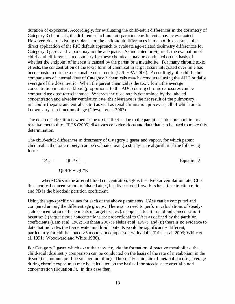
13

duration of exposures. Accordingly, for evaluating the child-adult differences in the dosimetry of Category 3 chemicals, the differences in blood:air partition coefficients may be evaluated. However, due to existing evidence on the child-adult differences in metabolic clearance, the direct application of the RfC default approach to evaluate age-related dosimetry differences for Category 3 gases and vapors may not be adequate. As indicated in Figure 1, the evaluation of child-adult differences in dosimetry for these chemicals may be conducted on the basis of whether the endpoint of interest is caused by the parent or a metabolite. For many chronic toxic effects, the concentration of the toxic form of chemical in target tissue integrated over time has been considered to be a reasonable dose metric (U.S. EPA 2006). Accordingly, the child-adult comparisons of internal dose of Category 3 chemicals may be conducted using the AUC or daily average of the dose metric. When the parent chemical is the toxic form, the average concentration in arterial blood (proportional to the AUC) during chronic exposures can be computed as: dose rate/clearance. Whereas the dose rate is determined by the inhaled concentration and alveolar ventilation rate, the clearance is the net result of the pulmonary, metabolic (hepatic and extrahepatic) as well as renal elimination processes, all of which are to known vary as a function of age (Clewell et al. 2002).

The next consideration is whether the toxic effect is due to the parent, a stable metabolite, or a reactive metabolite. IPCS (2005) discusses considerations and data that can be used to make this determination.

The child-adult differences in dosimetry of Category 3 gases and vapors, for which parent chemical is the toxic moiety, can be evaluated using a steady-state algorithm of the following form:

CAss = QP * CI

QP/PB + QL*E

Equation 2

where CAss is the arterial blood concentration; QP is the alveolar ventilation rate, CI is the chemical concentration in inhaled air, QL is liver blood flow, E is hepatic extraction ratio; and PB is the blood:air partition coefficient.

Using the age-specific values for each of the above parameters, CAss can be computed and compared among the different age groups. There is no need to perform calculations of steady-state concentrations of chemicals in target tissues (as opposed to arterial blood concentration) because: (i) target tissue concentrations are proportional to CAss as defined by the partition coefficients (Lam et al. 1982; Krishnan 2007; Pelekis et al. 1997), and (ii) there is no evidence to date that indicates the tissue water and lipid contents would be significantly different, particularly for children aged >3 months in comparison with adults (Price et al. 2003; White et al. 1991; Woodward and White 1986).

For Category 3 gases which exert their toxicity via the formation of reactive metabolites, the child-adult dosimetry comparison can be conducted on the basis of the rate of metabolism in the tissue (i.e., amount per L tissue per unit time). The steady-state rate of metabolism (i.e., average during chronic exposures) may be calculated on the basis of the steady-state arterial blood concentration (Equation 3). In this case then,

14

AMT = (CAss x QL x E)/VL Equation 3

where AMT = amount of metabolite formed per unit time per unit volume of tissue, CAss = arterial blood concentration of the parent chemical, QL = hepatic blood flow rate, E = hepatic extraction ratio and VL = liver volume.

For Category 3 chemicals producing stable or circulating metabolites, the rate of clearance of the metabolite in both adults and children should be additionally taken into account for calculating the dosimetry differences (Figure 1). In the case of metabolites, the clearance via kidney is likely to become more important (compared to parent form of Category 3 gases) such that child-adult differences in glomerular filtration rate (Clewell et al. 2002) might play an important role in determining the magnitude of the dose differences between various age groups. The steady-state equation in such cases would be of the following form:

Cmet = CAss x QL x E

CLmetabolite

Equation 4

Steady-state is achieved rapidly for gases and vapors that have a low volume of distribution and those that are cleared effectively by the biochemical processes. Category 3 gases generally have low blood:air partition coefficients but variable fat:blood partition coefficients (Table 1). U.S. EPA (1994), based on PBPK modeling in rats, indicated that steady-state is attained during subchronic or chronic inhalation exposures to gases with a blood:air partition coefficient < 100 and fat:blood partition coefficient < 100. In effect, almost all of the known Category 3 gases and vapors are expected to attain steady-state during continuous inhalation exposures in humans, even though only the proof of concept is available (Pelekis et al. 1997). In such cases, the use of a steady-state algorithm is likely to be sufficient for evaluating child-adult differences in dosimetry. The same approach is applicable to “acute” scenario, if the parent compound is the toxic agent and steady state is reached. However if the steady state is not reached in the “acute” scenario, regardless of whether toxic moiety is the parent chemical or metabolite (reactive or stable), the child-adult difference in systemic uptake and internal dose may be computed using full-blown physiologically-based pharmacokinetic (PBPK) models.

It is recognized that for several chemicals, based on the current state of knowledge of the mode of action, greater or less information may be available. For example, information on the extent of receptor occupancy, DNA adducts in target site, depletion of glutathione in target tissues, etc. can be used for estimating the child-adult differences in internal dose; however, such data are often not available. In fact, for many chemicals, the appropriate dose metric is not known. In such cases, it is reasonable to use the AUC of the parent chemical as the dose surrogate (U.S. EPA 2000, 2006; Clewell et al. 2002) and evaluate the child-adult differences in dosimetry. This is consistent with the approach for calculating Human Equivalent Concentrations (HECs) under the U.S. EPA’s RfC guidance (U.S. EPA 1994). However, in such cases, the assessor should note the uncertainty introduced by this assumption, and include appropriate caveats.

For some chemicals, limited information may be available for the estimation of chemical-specific kinetic parameters needed for the application of the proposed framework. In those

15

cases, information from a surrogate compound with similar chemical properties or structure activity relationships may be useful in evaluating potential child-adult differences. For example, Beliveau et al. (2003, 2005) used quantitative structure-property relationships to estimate partition coefficients and hepatic clearance for a number of volatile organic compounds. Again, the risk assessors would need to consider any uncertainty introduced by the reliance upon information for a surrogate.

3.0 ANALYSES: APPLICATION OF THE CHILD-ADULT FRAMEWORK TO CHEMICALS WITH SYSTEMIC EFFECTS (CATEGORY 2 AND CATEGORY 3 GASES)

3.1 Introduction

The magnitude of child-adult differences in internal dose of Category 3 gases and vapors has been evaluated using age-specific physiological data as well as chemical-specific partitioning and clearance data in PBPK models or steady-state algorithms (Price et al. 2003; Pelekis et al. 2003; Clewell et al. 2004; Ginsberg et al. 2002; Hattis et al. 2003; Sarangapani et al. 2003). As outlined in Section 2, steady-state algorithms are adequate for estimating the magnitude of child-adult difference in the dosimetry of Category 3 gases when the toxic moiety is the parent chemical or a metabolite. The steady-state approach requires the knowledge of certain parameters that are known to vary as a function of age: alveolar ventilation rate, hepatic blood flow, liver volume and clearance (renal, hepatic and/or pulmonary). Most of the previous analyses estimated the child-adult magnitude in internal dose of Category 3 gases and vapors, using physiological parameters for children (particularly neonates) derived from adult values on the basis of an allometric or regression relationships (Clewell et al. 2004; Ginsberg et al. 2002; Sarangapani et al. 2003). In order to facilitate a broader understanding of the extent of child-adult differences in dosimetry for Category 3 gases as well as to identify situations and parameters leading to maximal magnitude of child-adult differences in the dosimetry for these gases, the present study conducted a number of bounding analyses and case studies in various age groups: (neonates (3 months), toddlers (1 year), preschooler (5 years), middle schooler (10 years)). Accordingly, calculations of internal dose (i.e., steady-state concentration of parent chemical in blood, steady-state concentration of reactive metabolite in liver, and steady-state concentration of circulating metabolite in the body) in adults and children of various age groups were performed by setting hepatic clearance in children equal to (1) zero, (2) blood flow rate to the organ, or (3) a fraction of metabolic capacity of adults based on information on delayed enzyme ontogeny.

16

3.2 Approach

3.2.1 Child-adult differences in dosimetry for Category 3 gases for which parent chemical is the toxic moiety

The steady-state blood concentration of Category 3 gases that are metabolized primarily in liver and eliminated by clearance processes in both liver and lung can be calculated with the knowledge of age-specific blood:air partition coefficient (Pb), alveolar ventilation rate (QP), hepatic blood flow rate (QL) and intrinsic clearance (CLint) (Andersen 1981; Pelekis et al. 1997; Csanady and Filser 2001; Clewell et al. 2004). Available information suggest that neither the blood:air partition coefficient nor the composition of blood (lipid and water content) vary markedly as a function of age (Table 2) (Berenson et al. 1982; Lerman et al. 1984; White et al. 1991; Family Practice Notebook 2005). Therefore, the evaluation of child-adult differences in parent chemical concentrations can be performed with the knowledge of QP, QL and CLint for the various age groups, as well as using the Pb value for one of the age groups (usually adults).

The computation of steady-state blood concentration of Category 3 gases was performed on the basis of Eqn. 2 of the framework:

CAss =

CLp + CLh

QP * CI

where CAss = steady-state arterial blood concentration (µg/L), QP = alveolar ventilation rate (L/h), CI = inhaled concentraton (µg/L), CLp = pulmonary clearance (= QP divided by blood:air partition coefficient (PB)) and CLh = hepatic clearance (= CLint x QL/ (CLint + QL) where CLint = intrinsic clearance (= maximal velocity divided by Michaelis constant) and QL = hepatic blood flow rate (L/h).

The upper-bound of the magnitude of child-adult difference in CAss was calculated, initially, by assuming minimal metabolism in children (i.e., CLh = 0) and maximal metabolism in adults (i.e., CLh = hepatic blood flow rate) such that the hepatic extraction ratio equals 1. The calculations conducted under this scenario focused on identifying the maximal child-adult factor that is likely to be associated with Category 3 gases and vapors for which the parent form represents the toxic moiety. A second bounding analysis was conducted using Eqn. 2 for highly metabolized chemicals, for which hepatic clearance is blood-flow limited in both adults and children. The resulting child-adult ratios of CAss from this scenario would essentially reflect the lower-bound of the child-adult differences in internal dose. A third scenario involved the use of age-specific data on metabolizing enzyme capacity in Eqn. 2. Enzyme ontogeny data were used to estimate CLint in children on the basis of adult values as follows (Clewell et al. 2004; Nong et al. 2006):

CLintChild = CLintAdult*F*VLChild/VLAdult,

where VL is the volume of liver and F is the enzyme activity as a fraction of the adult value. This particular approach was applied to hepatic CYP2E1 and alcohol dehydrogenase (ADH) using data summarized by Clewell et al. (2004).

17

3.2.2 Child-adult differences in dosimetry for Category 3 gases for which reactive metabolite is the toxic moiety

For Category 3 gases exerting toxicity via reactive metabolites, the child-adult dosimetry comparisons of internal dose (i.e., amount per L tissue per unit time) was computed on the basis of Eqn. 3 of the framework:

AMTReactive metabolite = (CAss x CLh)/VL

The magnitude of child-adult differences in internal dose was calculated for the three scenarios described in section 3.1. Accordingly, the CLh value was first set to 0 in children and to QL in adults, as a bounding case. Then, the CLh was set equal to hepatic blood flow in both children and adults, to compute an upper bound of the child-adult difference in internal dose of reactive metabolites. Finally, the age-specific CLh was computed according to the information on the relative content of metabolizing enzyme (CYP2E1, ADH) in children relative to adults.

3.2.3 Child-adult differences in dosimetry for Category 3 gases for which circulating metabolite is the toxic moiety

As noted above, for calculating the internal dose of stable or circulating metabolites, the clearance of metabolites subsequent to their formation should be taken into account (Krishnan and Andersen 1991; Sarangapani et al. 2003; Gentry et al. 2002). Because kidney clearance is likely to play an important role for such metabolites, child-adult differences in glomerular filtration rate need to be taken into account in determining the magnitude of the dose differences between various age groups. The steady-state equation for computing the internal concentration3

CStable metabolite =

of circulating metabolites (as shown in section 2.3) is:

CLmetabolite

CAss x QL x E

The magnitude of child-adult differences in internal dose was initially calculated for the three scenarios described in section 3.2.1. (i.e., bounding case, flow-limited clearance, delayed ontogeny of metabolizing enzymes). For all three scenarios, CLmetabolite was assumed to be adequately represented by renal clearance which was set equal to the age-specific value of glomerular filtration rate (GFR). Additionally, calculation of CStable metabolite was done for a situation in which CLmetabolite is determined by both renal and metabolic clearance processes, subsequent to flow-limited metabolism of parent chemical in adults and children. This particular scenario facilitates the evaluation of an extreme case of child-adult difference in internal dose, in which the capacity-limited difference in clearance of metabolite and flow-limited clearance of parent chemicals might both apply and result in higher child-adult dose ratio (Clewell et al. 2004; Sarangapani et al. 2003; Ginsberg et al. 2005).

3 Because the dose metric of interest is the concentration of the chemical, comparison of concentrations can be considered a comparison of internal dose.

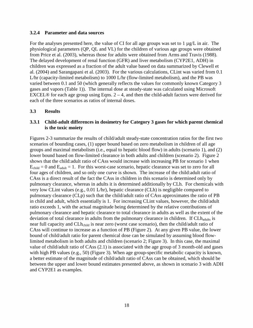
18

3.2.4 Parameter and data sources

For the analyses presented here, the value of CI for all age groups was set to 1 µg/L in air. The physiological parameters (QP, QL and VL) for the children of various age groups were obtained from Price et al. (2003), whereas those for adults were obtained from Arms and Travis (1988). The delayed development of renal function (GFR) and liver metabolism (CYP2E1, ADH) in children was expressed as a fraction of the adult value based on data summarized by Clewell et al. (2004) and Sarangapani et al. (2003). For the various calculations, CLint was varied from 0.1 L/hr (capacity-limited metabolism) to 1000 L/hr (flow-limited metabolism), and the PB was varied between 0.1 and 50 (which generally reflects the values for commonly known Category 3 gases and vapors (Table 1)). The internal dose at steady-state was calculated using Microsoft EXCEL® for each age group using Eqns. 2 – 4, and then the child-adult factors were derived for each of the three scenarios as ratios of internal doses.

3.3 Results

3.3.1 Child-adult differences in dosimetry for Category 3 gases for which parent chemical is the toxic moiety

Figures 2-3 summarize the results of child/adult steady-state concentration ratios for the first two scenarios of bounding cases, (1) upper bound based on zero metabolism in children of all age groups and maximal metabolism (i.e., equal to hepatic blood flow) in adults (scenario 1), and (2) lower bound based on flow-limited clearance in both adults and children (scenario 2). Figure 2 shows that the child:adult ratio of CAss would increase with increasing PB for scenario 1 when Echild = 0 and Eadult = 1. For this worst-case scenario, hepatic clearance was set to zero for all four ages of children, and so only one curve is shown. The increase of the child:adult ratio of CAss is a direct result of the fact the CAss in children in this scenario is determined only by pulmonary clearance, whereas in adults it is determined additionally by CLh. For chemicals with very low CLint values (e.g., 0.01 L/hr), hepatic clearance (CLh) is negligible compared to pulmonary clearance (CLp) such that the child/adult ratio of CAss approximates the ratio of PB in child and adult, which essentially is 1. For increasing CLint values, however, the child/adult ratio exceeds 1, with the actual magnitude being determined by the relative contributions of pulmonary clearance and hepatic clearance to total clearance in adults as well as the extent of the deviation of total clearance in adults from the pulmonary clearance in children. If CLhadults is near full capacity and CLhchild is near zero (worst case scenario), then the child/adult ratio of CAss will continue to increase as a function of PB (Figure 2). At any given PB value, the lower bound of child/adult ratio for parent chemical dose can be simulated by assuming blood flow-limited metabolism in both adults and children (scenario 2; Figure 3). In this case, the maximal value of child/adult ratio of CAss (2.1) is associated with the age group of 3 month-old and gases with high PB values (e.g., 50) (Figure 3). When age group-specific metabolic capacity is known, a better estimate of the magnitude of child/adult ratio of CAss can be obtained, which should be between the upper and lower bound estimates presented above, as shown in scenario 3 with ADH and CYP2E1 as examples.

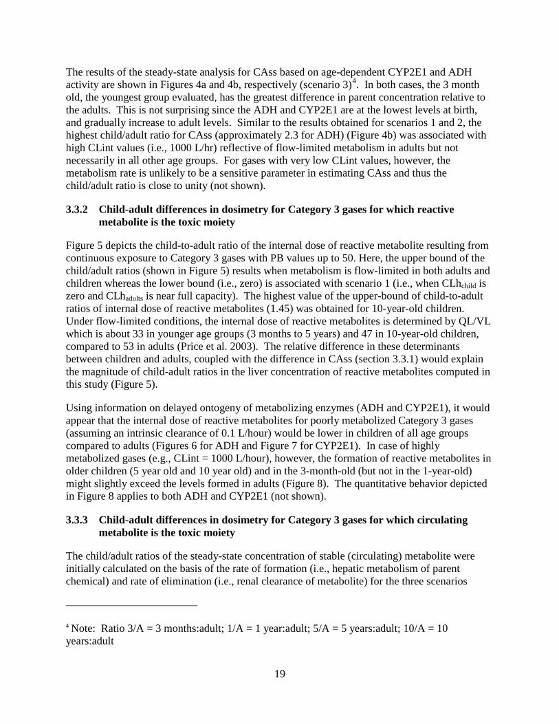
19

The results of the steady-state analysis for CAss based on age-dependent CYP2E1 and ADH activity are shown in Figures 4a and 4b, respectively (scenario 3)4

3.3.2 Child-adult differences in dosimetry for Category 3 gases for which reactive metabolite is the toxic moiety

. In both cases, the 3 month old, the youngest group evaluated, has the greatest difference in parent concentration relative to the adults. This is not surprising since the ADH and CYP2E1 are at the lowest levels at birth, and gradually increase to adult levels. Similar to the results obtained for scenarios 1 and 2, the highest child/adult ratio for CAss (approximately 2.3 for ADH) (Figure 4b) was associated with high CLint values (i.e., 1000 L/hr) reflective of flow-limited metabolism in adults but not necessarily in all other age groups. For gases with very low CLint values, however, the metabolism rate is unlikely to be a sensitive parameter in estimating CAss and thus the child/adult ratio is close to unity (not shown).

Figure 5 depicts the child-to-adult ratio of the internal dose of reactive metabolite resulting from continuous exposure to Category 3 gases with PB values up to 50. Here, the upper bound of the child/adult ratios (shown in Figure 5) results when metabolism is flow-limited in both adults and children whereas the lower bound (i.e., zero) is associated with scenario 1 (i.e., when CLhchild is zero and CLhadults is near full capacity). The highest value of the upper-bound of child-to-adult ratios of internal dose of reactive metabolites (1.45) was obtained for 10-year-old children. Under flow-limited conditions, the internal dose of reactive metabolites is determined by QL/VL which is about 33 in younger age groups (3 months to 5 years) and 47 in 10-year-old children, compared to 53 in adults (Price et al. 2003). The relative difference in these determinants between children and adults, coupled with the difference in CAss (section 3.3.1) would explain the magnitude of child-adult ratios in the liver concentration of reactive metabolites computed in this study (Figure 5).

Using information on delayed ontogeny of metabolizing enzymes (ADH and CYP2E1), it would appear that the internal dose of reactive metabolites for poorly metabolized Category 3 gases (assuming an intrinsic clearance of 0.1 L/hour) would be lower in children of all age groups compared to adults (Figures 6 for ADH and Figure 7 for CYP2E1). In case of highly metabolized gases (e.g., CLint = 1000 L/hour), however, the formation of reactive metabolites in older children (5 year old and 10 year old) and in the 3-month-old (but not in the 1-year-old) might slightly exceed the levels formed in adults (Figure 8). The quantitative behavior depicted in Figure 8 applies to both ADH and CYP2E1 (not shown).

3.3.3 Child-adult differences in dosimetry for Category 3 gases for which circulating metabolite is the toxic moiety

The child/adult ratios of the steady-state concentration of stable (circulating) metabolite were initially calculated on the basis of the rate of formation (i.e., hepatic metabolism of parent chemical) and rate of elimination (i.e., renal clearance of metabolite) for the three scenarios

4 Note: Ratio 3/A = 3 months:adult; 1/A = 1 year:adult; 5/A = 5 years:adult; 10/A = 10 years:adult

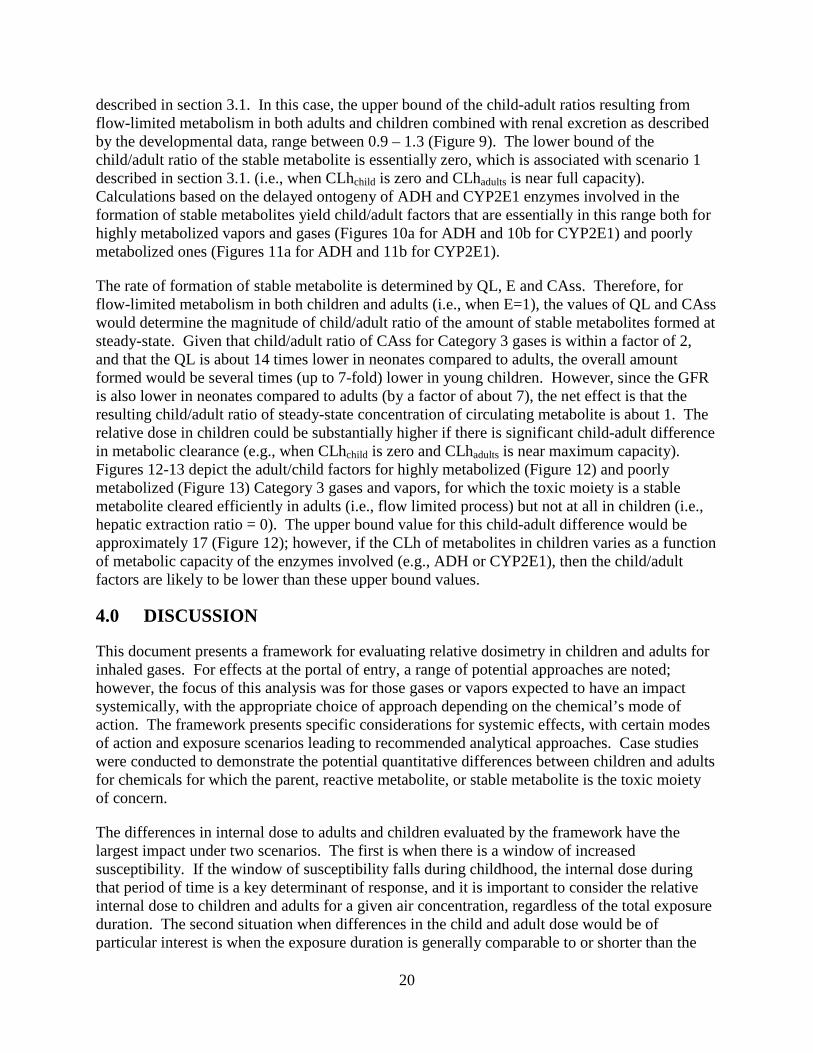
20

described in section 3.1. In this case, the upper bound of the child-adult ratios resulting from flow-limited metabolism in both adults and children combined with renal excretion as described by the developmental data, range between 0.9 – 1.3 (Figure 9). The lower bound of the child/adult ratio of the stable metabolite is essentially zero, which is associated with scenario 1 described in section 3.1. (i.e., when CLhchild is zero and CLhadults is near full capacity). Calculations based on the delayed ontogeny of ADH and CYP2E1 enzymes involved in the formation of stable metabolites yield child/adult factors that are essentially in this range both for highly metabolized vapors and gases (Figures 10a for ADH and 10b for CYP2E1) and poorly metabolized ones (Figures 11a for ADH and 11b for CYP2E1).

The rate of formation of stable metabolite is determined by QL, E and CAss. Therefore, for flow-limited metabolism in both children and adults (i.e., when E=1), the values of QL and CAss would determine the magnitude of child/adult ratio of the amount of stable metabolites formed at steady-state. Given that child/adult ratio of CAss for Category 3 gases is within a factor of 2, and that the QL is about 14 times lower in neonates compared to adults, the overall amount formed would be several times (up to 7-fold) lower in young children. However, since the GFR is also lower in neonates compared to adults (by a factor of about 7), the net effect is that the resulting child/adult ratio of steady-state concentration of circulating metabolite is about 1. The relative dose in children could be substantially higher if there is significant child-adult difference in metabolic clearance (e.g., when CLhchild is zero and CLhadults is near maximum capacity). Figures 12-13 depict the adult/child factors for highly metabolized (Figure 12) and poorly metabolized (Figure 13) Category 3 gases and vapors, for which the toxic moiety is a stable metabolite cleared efficiently in adults (i.e., flow limited process) but not at all in children (i.e., hepatic extraction ratio = 0). The upper bound value for this child-adult difference would be approximately 17 (Figure 12); however, if the CLh of metabolites in children varies as a function of metabolic capacity of the enzymes involved (e.g., ADH or CYP2E1), then the child/adult factors are likely to be lower than these upper bound values.

4.0 DISCUSSION

This document presents a framework for evaluating relative dosimetry in children and adults for inhaled gases. For effects at the portal of entry, a range of potential approaches are noted; however, the focus of this analysis was for those gases or vapors expected to have an impact systemically, with the appropriate choice of approach depending on the chemical’s mode of action. The framework presents specific considerations for systemic effects, with certain modes of action and exposure scenarios leading to recommended analytical approaches. Case studies were conducted to demonstrate the potential quantitative differences between children and adults for chemicals for which the parent, reactive metabolite, or stable metabolite is the toxic moiety of concern.

The differences in internal dose to adults and children evaluated by the framework have the largest impact under two scenarios. The first is when there is a window of increased susceptibility. If the window of susceptibility falls during childhood, the internal dose during that period of time is a key determinant of response, and it is important to consider the relative internal dose to children and adults for a given air concentration, regardless of the total exposure duration. The second situation when differences in the child and adult dose would be of particular interest is when the exposure duration is generally comparable to or shorter than the

21

duration of the age range of interest. Although the approach used in the framework can be used to evaluate the relative dose to children and adults in scenarios involving longer durations of exposure, the impact on response would be much smaller when the response is related to lifetime exposure (e.g., when the appropriate metric is Lifetime Average Daily Dose, or LADD). This is because estimates of cumulative dose over a lifetime resulting from exposure to low concentrations of environmental chemicals are fairly insensitive to age-related kinetic differences, because the greatest differences persist for only a short time (Pelekis et al. 1997; Clewell et al. 2004). Thus, if toxicity for the relevant endpoint is related to cumulative dose, these increases in internal dose would not have a significant effect on risk, unless a window of susceptibility coincided with the period of increased dose.

It should also be noted that analyses presented here are a simplified approach and are not intended to be used quantitatively in risk assessment, in the absence of chemical-specific data. Instead, the intent is to identify situations in which dose metrics in the child may be substantially different from those in the adult. The proposed framework would provide a potential screen to determine if the default toxicokinetic component is adequate when considering exposure to children, noting the additional need to consider variability.

4.1 Comparison with results in the literature

The analyses presented along with the framework were conducted to provide some initial direction regarding conditions under which there are significant dosimetric differences between adults and children. The results of these analyses are consistent with individual chemical-specific analyses in the literature. They suggest that the child/adult difference in steady state arterial concentration (CAss) of the parent chemical is likely to be within a factor of 2.1 for highly metabolized Category 3 gases and vapors. This observation is consistent with the conclusions of the detailed inhalation PBPK modeling studies conducted with selected Category 3 chemicals (furan: 1.5 (Price et al. 2003); styrene 1.8 and vinyl chloride 1.13 (Sarangapani et al. 2003). This is also consistent with the results of Ginsberg et al. (2005), who reported that the maximal child/adult factor for steady-state arterial blood concentration of parent chemicals belonging to Category 3 was 1.75, particularly for flow-limited metabolism in both adults and neonates. In the case of poorly metabolized gases and vapors, the child/adult ratio is likely to be about 1, since child-adult differences in metabolic clearance barely have an influence on the kinetics and internal dose, as shown in this study. This observation is consistent with that of Sarangapani et al. (2003) for perchlorethylene (child/adult ratio = 1.02), a poorly metabolized Category 3 vapor. Larger child/adult ratios would result in the hypothetical case where there is no hepatic clearance in the child and high hepatic clearance in the adult, but such extreme cases were not located in the chemical literature.

Regarding Category 3 gases forming reactive metabolites, the analyses conducted here indicate that the child-adult difference would be maximal when metabolism is flow-limited in adults and children. The maximal value of child-to-adult ratios of internal dose of reactive metabolites found in the present study (1.45) is comparable to those reported for vinyl chloride (1.34) and styrene (1.83) by Sarangapani et al. (2003). The small difference between the present study and the previous studies might be due to the derivation of liver blood flow values by the previous studies on the basis of difference in liver volume between children and adults. The present study, however, used liver blood flow values determined in children following radioactive gold

22

administration (Szantay et al. 1974). The child/adult ratio of the internal dose of reactive metabolite approaches zero as the intrinsic clearance (Clint) becomes smaller (Figures 6 and 7). This is also in agreement with the results of the PBPK modeling study by Sarangapani et al. (2003) in which the child/adult ratio for a poorly metabolized Category 3 chemical (perchloroethylene) was reported to be 0.27.

For Category 3 gases forming stable metabolites, the analyses were based on the assumption that renal clearance would be the sole mechanism of elimination, or it considered both the renal and hepatic routes of clearance to be relevant. In the first case, the calculated ratios ranged from 0.9 to 1.3. However, the child/adult ratio increased if there was a significant child-adult difference in metabolic clearance of the metabolite. In the case of Category 3 gases and vapors for which the stable metabolite (toxic moiety) is cleared efficiently in adults (i.e., flow limited process) but not at all in children (i.e., hepatic extraction ratio = 0), the child/adult ratio can be as high as 18. This is in accord with the observations of a PBPK modeling study of the formation and clearance of a stable metabolite (acetone from isopropanol), which reported a neonate/adult factor ranging from approximately 7 to 9 (Saragapani et al. 2003). Note also that isopropanol is a Category 2 gas, illustrating that the simplified steady state approaches described here give reasonable estimates of the relative systemic dose for children and adults, even for a moderately water soluble chemical. Further studies are required to systematically evaluate the relative contribution of renal, hepatic and pulmonary clearance processes to the total clearance of circulating metabolites formed from similar gases, as well as their overall contribution to the relative dose in children and adults, so as to be able to pinpoint characteristics of gases and vapors that might lead to situations where the dose to children is much higher than that to adults.

Quantitative differences between the examples presented here and previous published analyses were generally due to differences in the age-specific parameters. For example, in addition to the differences noted above regarding age-specific liver blood flow, there were differences in the alveolar ventilation rate (QP). Sarangapani et al. (2003) and Clewell et al. (2004) estimated the age-dependent alveolar ventilation as 66% of the pulmonary ventilation data compiled by U.S. EPA (1997). Because the alveolar dead space may vary with age, the current analysis focused on actual measured values when possible, using the approach of Price et al. (2003). Specifically, the QP for the 3-month old used measured data from Lees et al. (1967), and Price et al. (2003) developed a regression equation to calculate the QP values for ages 1, 5 and 10 years. Inputs to the development of the regression equation were age-specific data on respiratory frequency and tidal volume, and an equation relating physiological dead space to body weight.

The results presented here are also consistent with those of Ginsberg et al. (2005), who identified several conditions under which greater metabolite levels may occur in the infant liver than the adult liver. These conditions include: (1) highly metabolized gases; (2) Category 3 gases at 1 year of age for metabolism pathways that have reached full maturity by this age; and (3) cases where the metabolite formation rate is considerably greater than the metabolite removal rate and the metabolite removal rate involves a cytochrome P450 (CYP) or other pathway that is immature early in life. Except for the third group, these conditions do not consider removal of the metabolite. As another example of identification of the rate-limiting step, if a chemical is cleared primarily by glucuronidation, the low activity at early ages suggests that particular attention should be paid to urinary metabolites to determine whether adequate clearance occurs via alternative conjugation pathway (e.g., sulfation).

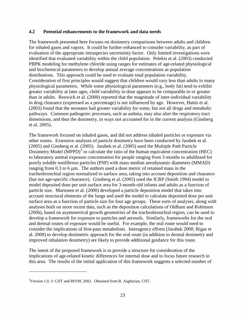
23

4.2 Potential enhancements to the framework and data needs

The framework presented here focuses on dosimetry comparisons between adults and children for inhaled gases and vapors. It could be further enhanced to consider variability, as part of evaluation of the appropriate intraspecies uncertainty factor. Only limited investigations were identified that evaluated variability within the child population. Pelekis et al. (2003) conducted PBPK modeling for methylene chloride using ranges for estimates of age-related physiological and biochemical parameters to develop annual average concentrations as population distributions. This approach could be used to evaluate total population variability. Consideration of first principles would suggest that children would vary less than adults in many physiological parameters. While some physiological parameters (e.g., body fat) tend to exhibit greater variability at later ages, child variability in dose appears to be comparable to or greater than in adults. Renwick et al. (2000) reported that the magnitude of inter-individual variability in drug clearance (expressed as a percentage) is not influenced by age. However, Hattis et al. (2003) found that the neonates had greater variability for some, but not all drugs and metabolic pathways. Common pathogenic processes, such as asthma, may also alter the respiratory tract dimensions, and thus the dosimetry, in ways not accounted for in the current analysis (Ginsberg et al. 2005).

The framework focused on inhaled gases, and did not address inhaled particles or exposure via other routes. Extensive analyses of particle dosimetry have been conducted by Jarabek et al. (2005) and Ginsberg et al. (2005). Jarabek et al. (2005) used the Multiple Path Particle Dosimetry Model (MPPD)5

The intent of the proposed framework is to provide a structure for consideration of the implications of age-related kinetic differences for internal dose and to focus future research in this area. The results of the initial application of this framework suggests a selected number of

to calculate the ratio of the human equivalent concentration (HEC) to laboratory animal exposure concentration for people ranging from 3 months to adulthood for poorly soluble nonfibrous particles (PSP) with mass median aerodynamic diameters (MMAD) ranging from 0.3 to 6 µm. The authors used a dose metric of retained mass in the tracheobronchial region normalized to surface area, taking into account deposition and clearance (but not age-specific clearance). Ginsberg et al. (2005) used the ICRP (Smith 1994) model to model deposited dose per unit surface area for 3-month-old infants and adults as a function of particle size. Martonen et al. (2000) developed a particle deposition model that takes into account structural elements of the lungs and used the model to calculate deposited dose per unit surface area as a function of particle size for four age groups. These sorts of analyses, along with analyses built on more recent data, such as the deposition calculations of Oldham and Robinson (2006), based on asymmetrical growth geometries of the tracheobronchial region, can be used to develop a framework for exposure to particles and aerosols. Similarly, frameworks for the oral and dermal routes of exposure would be useful. For example, the oral route would need to consider the implications of first-pass metabolism. Interagency efforts (Jarabek 2000; Rigas et al. 2000) to develop dosimetric approach for the oral route (in addition to dermal dosimetry and improved inhalation dosimetry) are likely to provide additional guidance for this route.

5Version 1.0, © CIIT and RIVM, 2002. Obtained from B. Asgharian, CIIT.

24

data gaps, where additional research may help to refine analyses of age-related differences in dosimetry. These areas include: (1) age-dependence of blood:air partition coefficients; (2) liver blood flow for children less than 4 years of age; (3) enhanced understanding of age-dependent changes in enzyme activities; and (4) characterization of extrahepatic metabolism.

25

Table 1. Compilation of Partition Coefficients for Some Category 3 Gases

Chemical Blood:Air Partition

Coefficient1

Fat:Blood Partition

Coefficient2

Methyl chloride 2.5 5.4

Dichloromethane 8.9 13

Chloroform 6.9 29

Carbon tetrachloride 2.7 133

Chlorodibromomethane 53 36

Chloroethane 2.7 14

Vinyl Chloride 1.2 17

1,1-Dichloroethane 4.9 33

1,1,2-Trichloroethane 36 40

Benzene 8.2 24

Chlorobenzene 30 43

o-Xylene 35 43

m-Xylene 33 56

p-Xylene 45 39

Styrene 483 724

1Gargas et al. (1989) 2Estimated based on rat Fat:Air partition coefficients and human Blood:Air partition coefficients reported by Gargas et al. (1989). 3Csanady et al. (1994) 4Estimated based on rat Fat:Air partition coefficient reported by Gargas et al. (1989) and human Blood:Air partition coefficient reported by Csanady et al. (1994).

26

Table 2. Age-dependent Lipid and Water Content of Whole Blood

Age (yr) % Lipid1 % Water2

0 0.11 841/2 to 2 0.22 872 to 6 0.21 876 to 12 0.22 86

12 to 18 0.21 86Over 18 0.22 85

1(Berenson et al. 1982) 2(Family Practice Notebook, 2005)

27

Figure 1. Revised framework for evaluating the relative tissue dosimetry in adults and children for inhaled gases.

Reactive

Exposure DurationMode of ActionNature of Effect

Steady StateApproach

(Eq. 2)

Parent

Steady StateApproach +Clearance

(Eq. 4)

Metabolite

Parent orMetabolite

PBPK Model

Parent

Steady StateApproach

(Eq. 2)

Metabolite

Parent orMetabolite

Acute,Window of

vulnerabilityChronic

Stable orReactive

Stable

SystemicPortal of

Entry Systemic

Reach SS

N Y

PBPK Model

Steady StateApproach

(Eq. 3)

Regional TissueConcentration

28

Figure 2. Child/adult ratio of the steady-state concentration of inhaled parent chemical: A bounding case study. The hepatic clearance in children of all ages is set to zero, whereas that in adults is assumed to equal the maximal level (i.e., hepatic blood flow rate).

0

5

10

15

20

0 10 20 30 40 50 60

Blood:Air Partition Coefficient

3 mos1 yr5 yr10 yr

Chi

ld/A

dult

Rat

io

29

Figure 3. Child/adult ratio of the parent chemical concentration at steady-state when metabolism is flow-limited in both adults and children.

0

1

2

3

0 10 20 30 40 50 60Blood:Air Partition Coefficient

Chi

ld/A

dult

Rat

io

1 yr

10 yr

3 mos5 yr

30

Figure 4a. Child/adult ratio of the steady-state concentration of parent chemical for which the metabolism rate is proportional to the CYP2E1 content (intrinsic clearance is 1000 L/hr).

1.0

1.5

2.0

2.5

0 10 20 30 40 50

Blood:Air Partition Coefficient

Chi

ld/A

dult

Rat

io

Ratio 3/A

Ratio 5/A

Ratio 10/A

Ratio 1/A

Figure 4b. Child/adult ratio of the steady-state concentration of parent chemical for which the metabolism rate is proportional to the ADH content (CLint is 1000 L/hr).

0.0

0.5

1.0

1.5

2.0

2.5

0 10 20 30 40 50

Blood:Air Partition Coefficient

Chi

ld/A

dult

Rat

io

Ratio 3/ARatio 5/A

Ratio 10/A

Ratio 1/A

* Ratio 3/A = 3 month:adult; Ratio 1/A = 1 year:adult; Ratio 5/A = 5 years:adult; Ratio 10/A = 10 years:adult

31

Figure 5. Child/adult ratio of the concentration of reactive metabolite at steady-state when metabolism is flow-limited in both adults and children.

0

0.5

1

1.5

2

0 10 20 30 40 50 60

Blood:Air Partition Coefficient

1 yr

10 yr3 mos5 yr

Chi

ld/A

dult

Rat

io

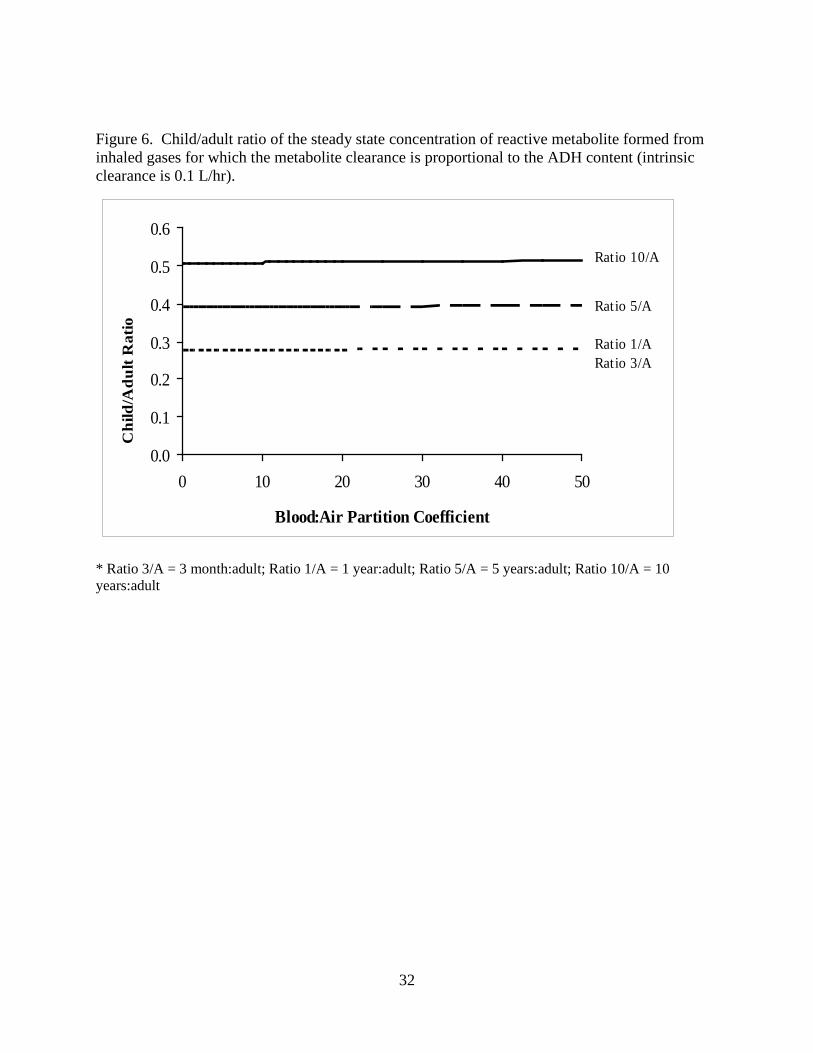
32

Figure 6. Child/adult ratio of the steady state concentration of reactive metabolite formed from inhaled gases for which the metabolite clearance is proportional to the ADH content (intrinsic clearance is 0.1 L/hr).

0.0

0.1

0.2

0.3

0.4

0.5

0.6

0 10 20 30 40 50

Blood:Air Partition Coefficient

Chi

ld/A

dult

Rat

io

Ratio 3/A

Ratio 10/A

Ratio 1/A

Ratio 5/A

* Ratio 3/A = 3 month:adult; Ratio 1/A = 1 year:adult; Ratio 5/A = 5 years:adult; Ratio 10/A = 10 years:adult

33

Figure 7. Child/adult ratio of the steady state concentration of reactive metabolite formed from inhaled gases for which the metabolite clearance is proportional to the CYP2E1 content (intrinsic clearance is 0.1 L/hr).

0.00.10.20.30.40.50.60.70.80.9

0 10 20 30 40 50

Blood:Air Partition Coefficient

Chi

ld/A

dult

Rat

io

Ratio 3/A

Ratio 5/A

Ratio 10/A

Ratio 1/A

* Ratio 3/A = 3 month:adult; Ratio 1/A = 1 year:adult; Ratio 5/A = 5 years:adult; Ratio 10/A = 10 years:adult

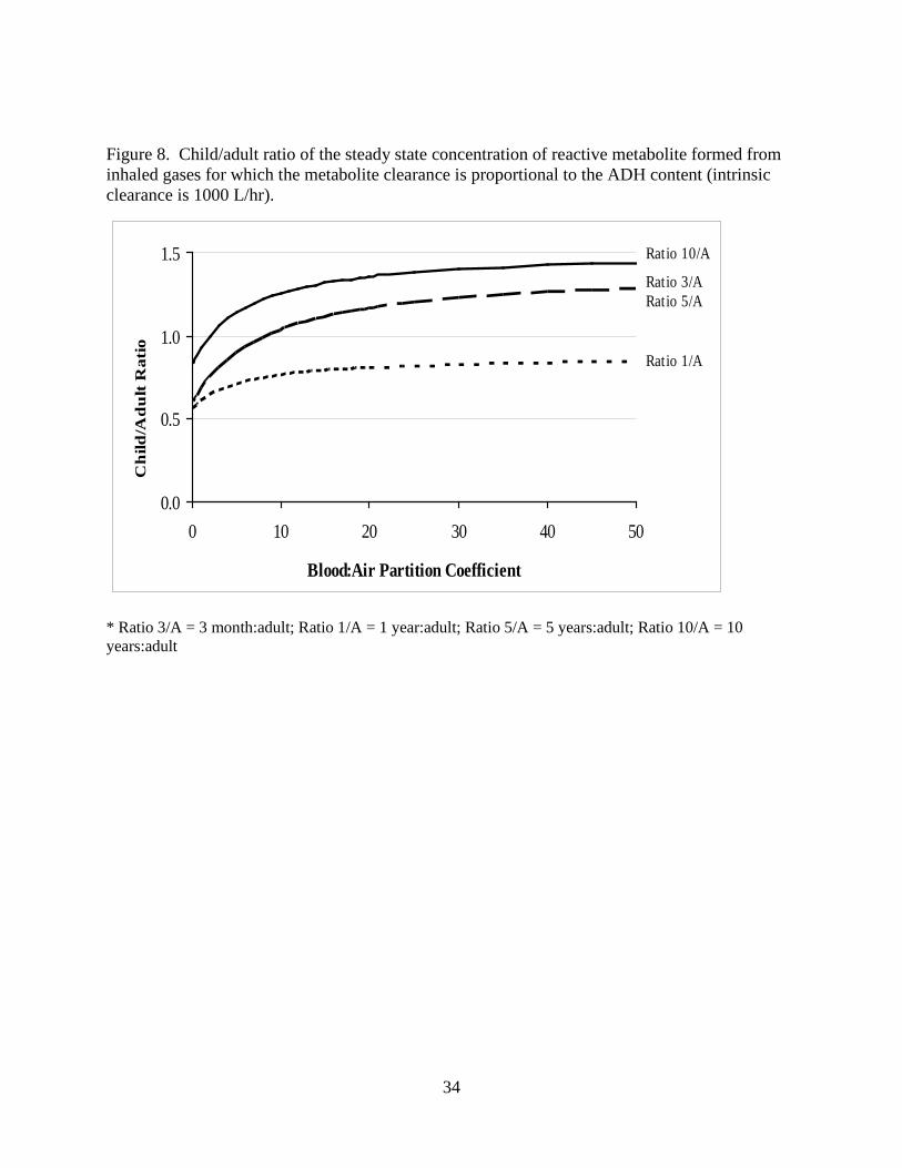
34

Figure 8. Child/adult ratio of the steady state concentration of reactive metabolite formed from inhaled gases for which the metabolite clearance is proportional to the ADH content (intrinsic clearance is 1000 L/hr).

0.0

0.5

1.0

1.5

0 10 20 30 40 50

Blood:Air Partition Coefficient

Ratio 3/ARatio 5/A

Ratio 10/A

Ratio 1/A

Ch

ild/A

du

lt R

atio

* Ratio 3/A = 3 month:adult; Ratio 1/A = 1 year:adult; Ratio 5/A = 5 years:adult; Ratio 10/A = 10 years:adult

35

Figure 9. Child/adult ratio of stable metabolite formed by flow-limited metabolism and cleared by renal excretion.

0

0.5

1

1.5

2

0 10 20 30 40 50 60

Blood:Air Partition Coefficient

Chi

ld/A

dult

Rat

io

1 yr

10 yr3 mos

5 yr

* Ratio 3/A = 3 month:adult; Ratio 1/A = 1 year:adult; Ratio 5/A = 5 years:adult; Ratio 10/A = 10 years:adult

36

Figure 10a. Child/adult ratio of stable metabolite for which the formation rate is proportional to the ADH content and renal clearance is dependent upon the GFR (intrinsic clearance is 1000 L/hr).

0.0

0.5

1.0

1.5

0 10 20 30 40 50

Blood:Air Partition Coefficient

Chi

ld/A

dult

Rat

io

Ratio 3/A

Ratio 5/ARatio 10/A

Ratio 1/A

Figure 10b. Child/adult ratio of stable metabolite for which the formation rate is proportional to the CYP2E1 content and renal clearance is dependent upon the GFR (intrinsic clearance is 1000 L/hr).

0.0

0.5

1.0

1.5

0 10 20 30 40 50

Blood:Air Partition Coefficient

Chi

ld/A

dult

Rat

io Ratio 3/A

Ratio 5/ARatio 10/A

Ratio 1/A

* Ratio 3/A = 3 month:adult; Ratio 1/A = 1 year:adult; Ratio 5/A = 5 years:adult; Ratio 10/A = 10 years:adult

37

Figure 11a. Child/adult ratio of stable metabolite for which the formation rate is proportional to the ADH content and renal clearance is dependent upon the GFR (intrinsic clearance is 0.1 L/hr).

0.0

0.1

0.2

0.3

0.4

0.5

0.6

0 10 20 30 40 50

Blood:Air Partition Coefficient

Chi

ld/A

dult

Rat

io

Ratio 3/A

Ratio 5/ARatio 10/A

Ratio 1/A

Figure 11b. Child/adult ratio of stable metabolite for which the formation rate is proportional to the CYP2E1 content and renal clearance is dependent upon the GFR (intrinsic clearance is 0.1 L/hr).

0.00.10.20.30.40.50.60.70.8

0 10 20 30 40 50

Blood:Air Partition Coefficient

Chi

ld/A

dult

Rat

io

Ratio 3/A

Ratio 5/ARatio 10/A

Ratio 1/A

* Ratio 3/A = 3 month:adult; Ratio 1/A = 1 year:adult; Ratio 5/A = 5 years:adult; Ratio 10/A = 10 years:adult

38

Figure 12. Child/adult ratio of steady state concentration of a stable metabolite with efficient metabolic clearance in adults (i.e., flow limited process) but only renal clearance in children (i.e., hepatic extraction ratio = 0) (intrinsic clearance of parent is 1000 L/hr).

0

5

10

15

20

0 10 20 30 40 50

Blood:Air Partition Coefficient

Chi

ld/A

dult

Rat

io Ratio 3/A

Ratio 5/ARatio 10/A

Ratio 1/A

* Ratio 3/A = 3 month:adult; Ratio 1/A = 1 year:adult; Ratio 5/A = 5 years:adult; Ratio 10/A = 10 years:adult

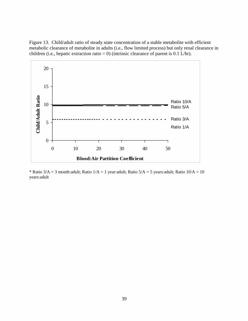
39

Figure 13. Child/adult ratio of steady state concentration of a stable metabolite with efficient metabolic clearance of metabolite in adults (i.e., flow limited process) but only renal clearance in children (i.e., hepatic extraction ratio = 0) (intrinsic clearance of parent is 0.1 L/hr).

0

5

10

15

20

0 10 20 30 40 50

Blood:Air Partition Coefficient

Chi

ld/A

dult

Rat

io

Ratio 3/A

Ratio 10/ARatio 5/A

Ratio 1/A

* Ratio 3/A = 3 month:adult; Ratio 1/A = 1 year:adult; Ratio 5/A = 5 years:adult; Ratio 10/A = 10 years:adult

40

5.0 References

Andersen ME. (1981). A physiologically based toxicokinetic description of the metabolism of inhaled gases and vapors: analysis at steady state. Toxicol Appl Pharmacol 60, 509-526.

Arms AD; Travis CC. (1988). Reference Physiological Parameters in Pharmacokinetic Modeling. Washington, DC: Office of Health and Environmental Assessment.

Asgharian B; Wood R; Schlesinger RB. (1995). Empirical modeling of particle deposition in the alveolar region of the lungs: a basis for interspecies extrapolation. Fundam Appl Toxicol 27, 232-238.

Beliveau M; Lipscomb J; Tardif R; Krishnan K. (2005). Quantitative structure-property relationships for interspecies extrapolation of the inhalation pharmacokinetics of organic chemicals. Chem Res Toxicol 18, 475-485.

Beliveau M; Tardif R; Krishnan K. (2003). Quantitative structure-property relationships for physiologically based pharmacokinetic modeling of volatile organic chemicals in rats. Toxicol Appl Pharmacol 189, 221-232.

Berenson G; Frank G; Hunter S. (1982). Cardiovascular risk factors in children -- should they concern the pediatrician? Amer. J. Dis. Child. 136, 855-862.

Bogdanffy M; Plowchalk D; Sarangapani R; Starr T; Andersen M. (2001). Mode-of-action-based dosimeters for interspecies extrapolation of vinyl acetate inhalation risk. Inhal Toxicol 13, 377-396.

Bogdanffy MS; Sarangapani R. (2003). Physiologically-based kinetic modeling of vapours toxic to the respiratory tract. Toxicol Lett 138, 103-117.

Clewell HJ; Gentry PR; Covington TR; Sarangapani R; Teeguarden JG. (2004). Evaluation of the potential impact of age- and gender-specific pharmacokinetic differences on tissue dosimetry. Toxicol Sci 79, 381-393.

Clewell HJ; Teeguarden J; McDonald T; Sarangapani R; Lawrence G; Covington T; Gentry R; Shipp A. (2002). Review and Evaluation of the Potential Impact of Age and Gender-Specific Pharmacokinetic Differences on Tissue Dosimetry. Crit Rev Toxicol 32, 329-389.

Csanady GA; Filser JG. (2001). The relevance of physical activity for the kinetics of inhaled gaseous substances. Arch Toxicol 74, 663-672.

Csanady GA; Mendrala AL; Nolan RJ; Filser JG. (1994). A physiologic pharmacokinetic model for styrene and styrene-7,8-oxide in mouse, rat and man. Arch Toxicol 68, 143-157.

Daston G; Faustman E; Ginsberg G; Fenner-Crisp P; Olin S; Sonawane B; Bruckner J; Breslin W; McLaughlin TJ. (2004). A framework for assessing risks to children from exposure to environmental agents. Environ Health Perspect 112, 238-256.

41

de Zwart LL; Haenen HE; Versantvoort CH; Sips AJ. (2002). Pharmacokinetics of ingested xenobiotics in children: A comparison with adults. RIVM for Ministry of Health, Welfare and Sports.

de Zwart LL; Haenen HE; Versantvoort CH; Wolterink G; van Engelen JG; Sips AJ. (2004). Role of biokinetics in risk assessment of drugs and chemicals in children. Regul Toxicol Pharmacol 39, 282-309.

EEA (European Environmental Agency); WHO (World Health Organization). (2002). Children's Health and Environment: A Review of Evidence. Copenhagen: Environmental Issue Report. No. 29.

Family Practice Notebook. (2005). A Family Medicine Resource. Hematocrit: Hematocrit Cutoffs for Anemia. vol. 2005.

Gargas M; Burgess R; al. e. (1989). Partition coefficients of Low-Molecular-Weight Volatile chemicals in various liquids and tissues. Toxicol Appl Pharmacol 98, 87-99.

Gargas M; Burgess R; Voisard D; Cason G; Andersen M. (1989). Partition coefficients of Low-Molecular-Weight Volatile chemicals in various liquids and tissues. Toxicol Appl Pharmacol 98, 87-99.

Gentry PR; Covington TR; Andersen ME; Clewell HJ, 3rd. (2002). Application of a physiologically based pharmacokinetic model for isopropanol in the derivation of a reference dose and reference concentration. Regul Toxicol Pharmacol 36, 51-68.

Ginsberg G; Foos B; Firestone M. (2005). Review and analysis of inhalation dosimetry methods for application to children's risk assessment. In press.

Ginsberg G; Hattis D; Miller R; Sonawane B. (2004). Pediatric pharmacokinetic data: Implications for environmental risk assessment for children. Pediatrics 113, 973-983.

Ginsberg G; Hattis D; Russ A; Sonawane B. (2004). Physiologically based pharmacokinetic (PBPK) modeling of caffeine and theophylline in neonates and adults: Implications for assessing children's risks from environmental agents. J Toxicol Environ Health A 67, 297-329.

Ginsberg G; Hattis D; Sonawane B. (2004). Incorporating pharmacokinetic differences between children and adults in assessing children's risks to environmental toxicants. Toxicol Appl Pharmacol 198, 164-183.

Ginsberg G; Hattis D; Sonawane B; Russ A; Banati P; Kozlak M; Smolenski S; Goble R. (2002). Evaluation of child/adult pharmacokinetic differences from a database derived from the therapeutic drug literature. Toxicol Sci 66, 185-200.

Ginsberg G; Slikker W, Jr.; Bruckner J; Sonawane B. (2004). Incorporating children's toxicokinetics into a risk framework. Environ Health Perspect 112, 272-283.

Haddad S; Restieri C; Krishnan K. (1999). Physiological modeling to characterize adult-children

42

differences in pharmacokinetics. Toxicologist 48, 657.

Hanna LM; Lou SR; Su S; Jarabek AM. (2001). Mass transport analysis: Inhalation RfC methods framework for interspecies dosimetric adjustment. Inhal Toxicol 13, 437-463.

Hattis D; Ginsberg G; Sonawane B; Smolenski S; Russ A; Kozlak M; Goble R. (2003). Differences in pharmacokinetics between children and adults--II. Children's variability in drug elimination half-lives and in some parameters needed for physiologically-based pharmacokinetic modeling. Risk Anal 23, 117-142.

Health Canada. (2002). Children's Health Priorities within the Pest Management Regulatory Agency. Ottawa, Ontario, Canada: Pesticide Management Regulatory Agency.

Hofmann W. (1982). Mathematical model for the postnatal growth of the human lung. Respir Physiol 49, 115-129.

IPCS. (2006). Environmental Health Criteria 237: Principles for evaluating health risks in children associated with exposure to chemicals. Geneva: World Health Organization.

IPCS (International Programme for Chemical Safety). (2005). Harmonization Project Document No. 2. Chemical-Specific Adjustment Factors For Interspecies Differences And Human Variability: Guidance Document For Use Of Data In Dose/Concentration–Response Assessment. Geneva, Switzerland: World Health Organization.

Jarabek A. (2000). U.S. EPA mode of action: Framework for dosimetry model development. SRA.

Jarabek AM; Asgharian B; Miller FJ. (2005). Dosimetric Adjustments for Interspecies Extrapolation of Inhaled Poorly Soluble Particles (PSP). Inhal Toxicol.

Kimbell JS; Gross EA; Joyner DR; Godo MN; Morgan KT. (1993). Application of computational fluid dynamics to regional dosimetry of inhaled chemicals in the upper respiratory tract of the rat. Toxicol. Appl. Pharmacol. 121, 253-263.

Krishnan K. (2007). Chapter in Principles and Methods of Toxicology. In Hayes W. Boston, MA: CRC, pp. (Release date, September 12, 2007).

Krishnan K; Andersen M. (1991). Physiological Modeling and Cancer Risk Assessment. In Rescignio A; Thakur A, New Trends in Pharmacokinetics. NY: Plenum Press, pp. 335-354.

Lam G; Chen M; al. e. (1982). Determination of tissue to blood partition coefficients in physiologically-based pharmacokinetic studies. J Pharm Sci 71, 454-456.

Lees M; Way R; Ross B. (1967). Ventilation and respiration gas transfer of infants with increased pulmonary blood flow. Pediatrics 40, 262. (as cited by Price et al. 2003).

Lerman J; Gregory GA; Willis MM; Eger EI, 2nd. (1984). Age and solubility of volatile anesthetics in blood. Anesthesiology 61, 139-143.

43

Martonen TB; Graham RC; Hofmann W. (1989). Human subject age and activity level: factors addressed in a biomathematical deposition program for extrapolation modeling. Health Phys 57 Suppl 1, 49-59.

Martonen TB; Schroeter JD; Hwang D; Fleming JS; Conway JH. (2000). Human lung morphology models for particle deposition studies. Inhal Toxicol 12 Suppl 4, 109-121.

Nong A; McCarver DG; Hines RN; Krishnan K. (2006). Modeling interchild differences in pharmacokinetics on the basis of subject-specific data on physiology and hepatic CYP2E1 levels: a case study with toluene. Toxicol Appl Pharmacol 214, 78-87.

Oldham MJ; Robinson RJ. (2006). Calculated deposition in growing tracheobronchial airways: effect of growth-rate assumptions. Inhal Toxicol 18, 803-808.

Overton JH; Graham RC. (1989). Predictions of ozone absorption in human lungs from newborn to adult. Health Phys 57 Suppl 1, 29-36.

Pelekis M; Gephart LA; Lerman SE. (2001). Physiological-model-based derivation of the adult and child pharmacokinetic intraspecies uncertainty factors for volatile organic compounds. Regul Toxicol Pharmacol 33, 12-20.

Pelekis M; Krewski D; Krishnan K. (1997). Physiologically based algebraic expressions for predicting steady-state toxicokinetics of inhaled vapors. Toxicol Methodol 7, 205-225.

Pelekis M; Nicolich MJ; Gauthier JS. (2003). Probabilistic framework for the estimation of the adult and child toxicokinetic intraspecies uncertainty factors. Risk Anal 23, 1239-1255.

Plunkett LM; Turnbull D; Rodricks JV. (1992). Differences Between Adults and Children Affecting Exposure Assessment. In Guzelian P;Henry C; Olin S, Similarities and Differences Between Children and Adults: Implications for Risk Assessment. Washington, DC: ILSI Press, pp. 79-94.

Price K; Haddad S; Krishnan K. (2003). Physiological modeling of age-specific changes in the pharmacokinetics of organic chemicals in children. J Toxicol Environ Health A 66, 417-433.

Renwick AG. (1998). Toxicokinetics in infants and children in relation to the ADI and TDI. Food Addit Contam 15 Suppl, 17-35.

Renwick AG; Dorne JL; Walton K. (2000). An analysis of the need for an additional uncertainty factor for infants and children. Regul Toxicol Pharmacol 31, 286-296.

Rigas ML; Catlin SN; Ben-Jebria A; Ultman JS. (2000). Ozone uptake in the intact human respiratory tract: relationship between inhaled dose and actual dose. J Appl Physiol 88, 2015-2022.

Sarangapani R; Gentry PR; Covington TR; Teeguarden JG; Clewell HJ, 3rd. (2003). Evaluation of the potential impact of age- and gender-specific lung morphology and ventilation rate on the dosimetry of vapors. Inhal Toxicol 15, 987-1016.

44

Scheuplein R; Charnley G; Dourson M. (2002). Differential sensitivity of children and adults to chemical toxicity. I. Biological basis. Regul Toxicol Pharmacol 35, 429-447.

Smith H ed. (1994). Human respiratory tract model for radiological protection: A report of a Task Group of the International Commission on Radiological Protection. In: Annals of the ICRP: Published for the International Commission on Radiological Protection by Pergamon Press.

Snodgrass W. (1992). Physiological and Biochemical Differences Between Children and Adults as Determinants of Toxic Response to Environmental Pollutants. In Guzelian P;Henry C; Olin S, Similarities and Differences Between Children and Adults: Implications for Risk Assessment. Washington, DC: ILSI Press, pp. 35-42.

Szantay V; Tamas S; Marian L; Bochis G. (1974). [Changes of hepatic blood flow in children as a function of age]. Rev Roum Med Intern 11, 91-93 (as cited in Price et al. 2003).

US EPA (U.S. Environmental Protection Agency). (1994). Methods for Derivation of Inhalation Reference Concentrations and Application of Inhalation Dosimetry. Washington DC: National Center for Environmental Assessment, Office of Research and Development.

US EPA (U.S. Environmental Protection Agency). (1997). Exposure Factors Handbook: Volume I. General Factors. Washington, DC: Office of Research and Development.

US EPA (U.S. Environmental Protection Agency). (2000). Benchmark Dose Technical Guidance Document (external review Draft). Washington, DC: Risk Assessment Forum.

US EPA (U.S. Environmental Protection Agency). (2006). Approaches for the Application of Physiologically Based Pharmacokinetic (PBPK) Models and Supporting Data in Risk Assessment (Final Report). Washington, DC: National Center for Environmental Assessment, Office of Research and Development.

White D; Widdowson E; Woodard H; Dickerson J. (1991). The composition of body tissues (II): Fetus to young adult. Br J Radiol 64, 149-159 (as cited in Price et al 2003).

Wolterink G; Piersma AH; van Engelen JG. (2002). Risk Assessment of Chemicals: What About Children? : RIVM for Ministry of Health, Welfare and Sports.

Woodard HQ; White DR. (1986). The composition of body tissues. Br. J. Radiol 59, 1209-1219 (as cited in Price et al. 2003).