
PDF - Conferences
435
-
Upload
khangminh22 -
Category
Documents
-
view
0 -
download
0
Transcript of PDF - Conferences


4th International Engineering Conference on
Developments in Civil & Computer
Engineering Applications
Feb 26-27, 2018
ISSN 2409 - 6997

This Page Intentionally Left Blank

i
Preface The 4th International Engineering Conference on Developments in Civil and
Computer Engineering Applications (IEC 2018, Erbil) is held for the period from 26
to 27 February 2018. The conference is jointly organized by Ishik University and Erbil
Polytechnic University.
The International Engineering Conference on Developments in Civil and Computer
Engineering Applications (IEC2018) is the interdisciplinary forum for the
presentation of new advances and research results in the fields of Civil and Computer
Engineering applications. The conference tracks included the following research
topics: Geo-Technical Engineering, Environmental Engineering, Fluid and Hydraulic
Engineering, Green Buildings, Smart Buildings, Transportation Engineering,
Restoration and Rehabilitation of Historical Buildings, Construction Management,
Mechanical Energy, Sustainability of Concrete and Steel Structures, Petroleum and
Mining Engineering, Artificial and Computational Intelligence, Control and Robotics,
Communications, Networking and Protocols, Parallel and Distributed Processing,
Signal and Multimedia Processing, Biomedical and Health Informatics, Mobile and
Smartphone Applications, Software Engineering and Applications, Green Computing
for Sustainable Energy, Cloud Computing, Computer Security, Smart Houses,
Mechatronics and Surveying and Geomatics Engineering.
The program committee (the reviewers) is comprised of 56 members, all of which are
Ph.D holders in certain fields of engineering, relevant to one or more conference
tracks mentioned above. The same international conference standards that were
adopted in the previous IEC2017, Erbil were adopted in IEC2018, as well. All paper
submissions are blind peer-reviewed by at least three program committee members to
ensure that submissions conform to certain quality measures. The quality measures
included several criteria such as writing skill, quality of the content, fitness of the title,
significance for theory or practice, originality and innovation level.
This year, the total number of submitted manuscripts stood at 45 from several
countries including Iraq, Nigeria, Peru, Turkey, Australia, Portugal, Iran and
Hungary. By category, 32 papers were related to Civil Engineering topics while 13
articles were written in the Computer Engineering related fields. The names of the
institutions and the number of submissions received from those institutions are as
follows: Cihan University (2), Duhok Polytechnic University (2), Eastern
Mediterranean University (1), Erbil Polytechnic University (8), Halabja University
(1), Ishik University (7), Koya Technical Institute, EPU (2), Soran University (1),
Middle Technical University (1), Ministry of Electricity (1), Mosul University (1),
University of Ninevah (2), Salahaddin University-Erbil (3), Universidad Nacional del
Callao (1), University of Duhok (3), University of Sulaimani (4), Western Sydney
University (1), University of Anbar (1), University of Miskolc (1), American
University of Kurdistan (1), Koya University (1).

ii
In IEC2018, a 69% article acceptance rate has been reached after a thorough
reviewing process. The authors of manuscripts exceeding certain plagiarism
percentage were notified to adjust their manuscripts or otherwise these submissions
were rejected with a plagiarism note to the authors. Each submitted manuscript was
double-checked for plagiarism and template format while reviewed by at least three
members. Some reviewed submissions were marked as “revise” and authors of those
submissions were given the chance to revise their manuscripts considering the
reviewers’ professional feedback. These revised manuscripts were resubmitted for
one final review process either to get accepted or declined. Some other manuscripts
were not accepted or withdrawn because they were not within the conference scope.
Regarding the conference, two panels were organized, one in the field of Computer
Engineering and the other one in Civil Engineering. The first panel was titled as “New
Trends in IoT” and chaired by Dr. Saman Mirza Abdullah (Faculty of Engineering,
Software Engineering, Koya University). The other members for this panel were
Assist. Prof. Dr. Tara Ibrahim Ali Yahiya (School of Science and Engineering,
University of Kurdistan-Hewler) and Mr. Dler Mawlod (Director of CISCO
ASC/ITC).
The topics of the second panel were “Plate Tectonics and Earthquakes” and
“Unmanned Aerial Vehicle (UAV) in Disaster Management”, respectively. The chair
of this panel was Prof. Dr. Bayan Salim Al-Numan from the Civil Engineering
Department of Ishik University. The other panelists were Assist. Prof. Dr. Qubad
Zeki,Head of Surveying and Geomatics Engineering (Ishik University) and Assist.
Prof. Dr. Srood Farooq Omar, Head of Petroleum and Mining Engineering (Ishik
University).
Dr. Günter Şenyurt
Editor-in-Chief

iii
IEC2018
Organizing Committee
Dr. Idris Hadi
Honarable Chair
President of Ishik University,
Erbil, Iraq
Assist. Prof. Dr. Kawa
Sherwani
Honarable Chair
President of Erbil Polytechnic
University, Erbil, Iraq
Dr. Selcuk Cankurt
Chair
Faculty of Engineering,
Computer Engineering Department,
Ishik University
Dr. Ranj Sirwan Abdullah
Co-Chair
Vice Dean of Engineering
Technical College,
Erbil Polytechnic University
Dr. Günter Şenyurt
Editor-in-Chief
Faculty of Engineering,
Computer Engineering
Department, Ishik University

iv
IEC2018
Higher Committee
Assist. Prof. Basil Younis
Head of Civil Engineering
Department, Erbil Polytechnic
University
Dr. Ranj Sirwan Abdullah
Vice Dean of Engineering
Technical College,
Erbil Polytechnic University
Dr. Mehmet Özdemir
Vice President for Scientific
Affairs
Ishik University, Erbil, Iraq
Dr. Nageb Toma Bato
Vice President for Scientific
Affairs
Erbil Polytechnic University,
Erbil, Iraq
Dr. Halit Vural
Dean of Engineering Faculty,
Ishik University, Erbil, Iraq
Dr. Bzar Khidir Hussan
Head of Information System
Engineering Department, Erbil
Polytechnic University

v
IEC2018
Organizing Committee
Prof. Dr. Bayan Salim
ALNu’man
Civil Engineering Department,
Ishik University
Assoc. Prof. Dr. Thamir
Mohammed Ahmed
Civil Engineering Department,
Ishik University
Assist. Prof. Dr. Srood
Farooq
Head of Petroleum and Mining
Engineering Department, Ishik
University
Assist. Prof. Dr. Azad
Mohammed Ali
Head of Mechatronics
Department, Ishik University
Assist. Prof. Qubad Zeki
Henari
Head of Surveying and
Geomatics Engineering
Department, Ishik University
Dr. Ganjeena Jalal Madhat
Erbil Technology Institute
Erbil Polytechnic Univeristy,
Erbil, Iraq
Dr. Adnan Shihab
Director of International
Relations, Erbil Polytechnic
University
Dr. Gunter Senyurt
Computer Engineering
Department, Ishik University
Dr. Selcuk Cankurt
Computer Engineering
Department, Ishik University
Dr. Ranj Sirwan Abdullah,
Deputy Dean of Erbil Technical
Engineering College, Erbil
Polytechnic University

vi
IEC2018
Organizing Committee
Dr. Bzar Khidir Hussan
Erbil Technical Engineering
College, Information System
Engineering Department, Erbil
Polytechnic University
Dr. Khaleel Hassan Younis
Erbil Technology Institute,
Road Construction, Erbil
Polytechnic University
Dr. Bahman Omar Taha
Erbil Technical College, Civil
Engineering Department, Erbil
Polytechnic University
Mr. Safwan Mawlud
Head of Computer Engineering
Department, Ishik University
Mr. Ömer Akar
Director of Media and Design
Office, Ishik University
Mr. Ali Abdulla Salih
Director of General Relations
Erbil Polytechnic University,
Erbil, Iraq
Dr. Brzo Hamza Dzayee
Faculty of Engineering
Erbil Polytechnic University
Dr. Saman Mirza Abdullah
Software Engineering
Department, Koya University
Mr. Musa Masood Ameen
Secretary
Computer Engineering
Department
Ishik University, Erbil, Iraq
Mr. Barham Haidar
Head of Civil Department
Ishik University

vii
IEC2018
Program Committee
Prof. Dr. Bayan Salim AL-
Nu'man
Civil Engineering Department
Ishik University, Erbil, Iraq
Prof. Dr. Omar Qarani Aziz
College of Engineering, Civil
Engineering Department,
Salahaddin University,
Erbil,Iraq
Prof. Dr. Moayad Y. Potrus
College of Engineering,
Software Engineering
Department, Salahaddin
University-Erbil
Assoc. Prof. Dr. Thamir
Mohammed Ahmed
Faculty of Engineering, Civil
Engineering Department,
Ishik University
Assist. Prof. Dr Basil Younus
Mustafa
Head of Civil Engineering
Department
Erbil Polytechnic University,
Erbil, Iraq
Assist. Prof. Dr. Shuokr
Qarani Aziz
College of Engineering, Civil
Engineering Department,
Salahaddin University-Erbil
Assoc. Prof. Dr.Shirzad
B.Nazhat
Petroleum Engineering
Department
Soran University, Soran, Erbil,
Iraq
Assist. Prof. Dr. Husein Ali
Husein
Architectural Engineering
Department
Koya University, Koya, Iraq
Assist. Prof. Dr. Tara
Ibrahim Ali Yahiya
School of Science and
Engineering, Computer Science
and Engineering Department,
University of Kurdistan-Hewler
Assist. Prof. Dr. Jafar A. Ali
Petroleum Engineering
Department
Koya University, Koya, Iraq

viii
IEC2018
Program Committee
Assist. Prof. Dr. Younis
Mahmood M.Saleem
College of Engineering,
Architectural Engineering
Department, University of
Technology
Assist. Prof. Dr. Faris Ali
Mustafa
College of Engineering,
Architectural Engineering
Department, Salahaddin
University-Erbil
Assist. Prof. Dr. Noori Sadeq
Ali
College of Engineering, Civil
Engineering Department, Cihan
University-Erbil
Assist. Prof. Dr. Wrya
Muhammad Ali Monnet
School of Science and
Engineering, Computer Science
and Engineering Department,
University of Kurdistan-Hewler
Assist. Prof. Dr. Hassan
Majeed Hassoon
Faculty of Engineering, Interior
Design Department, Ishik
University
Assist. Prof. Dr. Mazin S Al-
Hakeem
College of Engineering,
Computer Techniques
Engineering, Al-Mustafa
University College
Assist. Prof. Dr. Ayad Zeki
Saber Agha
Erbil Technical Engineering
College, Civil Engineering
Department, Erbil Polytechnic
University
Assist. Prof. Dr. Lokman H.
Hassan
College of Engineering,
Electrical and Computer
Engineering Department,
University of Duhok

ix
IEC2018
Program Committee
Assist. Prof. Dr. Bengin
Awdel Herki
College of Engineering, Civil
Engineering Department, Soran
University
Assist. Prof. Dr. Srood
Farooq
Head of Petroleum and Mining
Engineering Department
Ishik University
Assist. Prof. Dr. Tarik A.
Rashid
School of Science and
Engineering, University of
Kurdistan-Hewler
Assist. Prof. Dr. Nejdet
Dogru
Information Technologies
Department, International
Burch University
Assist. Prof. Dr. Faiq M.
Sarhan Alzawiny
Al-Nahrain University
Faculty of Engineering
Assist. Prof. Dr. Abdullah
Salman
University of Technology
Faculty of Engineering
Assist. Prof. Dr. Abbas
Hamza
University of Technology
Faculty of Engineering
Assist. Prof. Dr. Falah Al-
Jabery
University of Technology
Faculty of Engineering
Assist. Prof. Qubad Zeki
Henari
Head of Surveying and
Geomatics Engineering
Department, Ishik University
Dr. Saman Mirza Abdullah
Faculty of Engineering,
Software Engineering
Department, Koya University

x
IEC2018
Program Committee
Dr. Saad Essa
Erbil Technical Engineering
College, Civil Engineering
Department, Erbil Polytechnic
University
Dr. Omer Muhie Eldeen
Taha
College of Engineering, Civil
Engineering Department,
Kirkuk University
Dr. Mohammed F Eessa
Abomaali
Computer Techniques
Engineering, Computer
Techniques Engineering,
Alsafwa University College
Dr. Sarkawt Asaad Hasan
Erbil Engineering Technical
College, Civil Engineering
Department, Erbil Polytechnic
University
Dr. Günter Şenyurt
Computer Engineering
Department
Ishik University, Erbil, Iraq
Dr. Abdulfattah Ahmad
Amin
Erbil Technology Institute
Surveying, Erbil Polytechnic
University
Dr. Ganjeena Jalal Madhat
Khoshnaw
Road Construction Department,
Erbil Politechnic University
Dr. Hafedh Abd Yahya
Architecture Department
Ishik University, Erbil, Iraq
Dr. Iyd Eqqab Maree
Erbil Technical Engineering
College, Erbil Polytechnic
University
Dr. Sirwan Khuthur Mala
College of Engineering,
Structural Engineering
Department, Salahaddin
University

xi
IEC2018
Program Committee
Dr. Siyamand T. Peerdawood
Faculty of Engineering, Civil
Engineering Department, Ishik
University
Dr. Yaseen Ahmed
Hamaamin
College of Engineering, Civil
Engineering Department,
University of Sulaimani
Dr. Botan Majeed AL-Hadad
Erbil Technology Institute,
Road Construction Department,
Erbil Polytechnic University
Dr. Mohammed Ali Ihsan
Saber
College of Engineering, Civil
Engineering Department,
Salahaddin University-Erbil
Dr. Abdulbasit Al-Talabani
Faculty of Engineering,
Software Engineering
Department, Koya University
Dr. Reben Kurda
Faculty of Engineering,
Software Engineering
Department, Koya University
Dr. Rahel Khalid Ibrahim
Faculty of Engineering, Civil
Engineering Department, Koya
University
Dr. Alaa Muheddin
Abdulrahman
College of Engineering,
Electrical Engineering
Department, University of
Sulaimani
Dr. Kamaran Ismail
Faculty of Engineering
Soran University
Dr. Roojwan Hawezi
Faculty of Engineering
Erbil Polytechnic University,
Erbil, Iraq

xii
IEC2018
Program Committee
Dr. Khaleel Hassan Younis
Erbil Technology Institute,
Road Construction,
Erbil Polytechnic University
Dr. Halit Vural
Faculty of Engineering,
Computer Engineering
Department,
Ishik University
Dr. Selcuk Cankurt
Faculty of Engineering,
Computer Engineering
Department, Ishik University
Dr. Bahman Omar Taha
Erbil Technical College, Civil
Engineering Department, Erbil
Polytechnic University
Bzar khidir Hussan
Faculty of engineering
Erbil Polytechnic University
Ranj Sirwan Abdullah
Faculty of engineering
Erbil Polytechnic University
Dr. Ari Arif Abdulrahman
Faculty of Engineering,
Koya University
Dr. Ali Ahmed
Faculty of Engineering
University of Basrah

xiii
IEC2018
Editorial Board
Mr. Behcet Çelik
Editor
Information Technologies
Department
Ishik University, Erbil, Iraq
Ms. Bahren Ali Hassan
Editor
Information Technologies
Department
Ishik University, Erbil, Iraq
Ms. Marwa Awni
Editor
Computer Engineering Department
Ishik University, Erbil, Iraq

xiv
IEC2018
Organizing Committee
Technical Support Team
Mr. Abulkareem Habbab, Mechatronics Department, Ishik University
Mr. Arkan Yousif, Publication and Media Office, Ishik University
Mr. Ahmed Azmi, Publication and Media Office, Ishik University
Mr. Ahmed Nariman, Architecture Engineering Department, Ishik University
Ms. Avan Azad, Information Technology Department, Ishik University
Mr. Baban Jamal, Rectorate, Ishik University
Ms. Farah Maysan, Interior Design Department, Ishik University
Mr. Halmat Muslih, Civil Engineering Department, Ishik University
Mr. Hawraz Hamid, Rectorate, Ishik University
Ms. Hazheen Nasih, Interior Design Department, Ishik University
Mr. Hevar J. Abdulrahman, Civil Engineering Department, Ishik University
Mr. Hunar Mahdi Salih, Petroleum Engineering Department, Ishik University
Ms. Israa Nazhat, Computer Engineering Department, Ishik University
Mr. Karzan Abdulmajid, IT Service, Ishik University
Mr. Kewan Hama Amen,IT Service , Ishik University
Mr. Mohammed Kamal, Information Technology Department, Ishik University
Mr. Mohammed Qadir, Surveying Engineering Department, Ishik University
Mr. Mohammed Salam, Computer Engineering Department, Ishik University
Mr. Mohammed Sherwan, Publication and Media Office, Ishik University
Mr. Muhammed Abdulsattar, Accounting Office, Ishik University
Ms. Naz Noori, Civil Engineering Department, Ishik University
Ms. Naza Ghani, Engineering Faculty, Ishik University
Mr. Nurullah Darici, Rectorate, Ishik University
Mr. Rebin Mohammed, Information Technology Department, Ishik University
Ms. Samiha Habbal, Information Technology Department, Ishik University
Ms. Shaida Mustafa, Petroleum Engineering Department, Ishik University
Mr. Shallaw Hamza, Interior Design Department, Ishik University
Mr. Shamal Mohammed, Surveying Engineering Department, Ishik University
Mr. Shkar Latif, Civil Engineering Department, Ishik University
Mr. Usman Eschanov, IT Service, Ishik University
Mr. Yasar Yilmaz, IT Service, Ishik University
Mr. Wafaa Wasfi, Architecture Engineering Department, Ishik University
Ms. Zainab Akram, Engineering Faculty, Ishik University
Mr. Ranjdar Kamal, Erbil Polytechnic University
Mr. Safeen Majeed, Erbil Polytechnic University
Mr. Himdad Tahir, Erbil Polytechnic University
Mr. Farhad Thahir, Erbil Polytechnic University
Mr. Abdulsattar, Erbil Polytechnic University
Mr. Shahab Rafaat, Erbil Polytechnic University
Mr. Hawre Mahmood Abbas, Erbil Polytechnic University

xv
This Page Intentionally Left Blank

xvi
IEC2018
Keynote Speaker
Prof. Dr. Riadh Al-Mahaidi
Professor of Structural Engineering,
Vice President (International Engagement)
Director, Smart Structures Laboratory
Dr Riadh Al-Mahaidi is a Professor of Structural Engineering and
Director of the Smart Structures Laboratory at Swinburne University
of Technology. He also holds the position Vice President
(International Engagement) at Swinburne. Prior to joining
Swinburne in January 2010, he was the Head of the Structures Group
at Monash University. Over the past 20 years, he focused his
research and practice on life time integrity of bridges, particularly in
the area of structural strength assessment and retrofitting using
advanced composite materials.He currently leads a number of
research projects on strengthening of bridges using fibre reinforced
polymers combined cement-based bonding agents, fatigue life
improvement of metallic structures using advanced composite
systems and shape memory alloys. He recently started some projects
on hybrid testing of structures. He received a BSc (Hon 1) degree in
civil engineering from the University of Baghdad and MSc and PhD
degrees in structural engineering from Cornell University in the
United States. To date, Riadh published over 185 journal and 235
conference papers and authored/edited 10 books and conference
proceedings. He was awarded the 2012 Vice Chancellor’s
Internationalization Award, the RW Chapman Medals in 2005 and
2010 for best journal publication in Engineers Australia Structural
Journal, best paper awards at ACUN-4 (2002) and ACUN-6 (2012)
Composites conferences. Prof Al-Mahaidi and his research group
won the 2016 Engineers Australia Excellence Award for Innovation,
Research and Development (High Commendation) for the Multi-
Axis Substructure Testing (MAST) System they built at Swinburne.
He was recently awarded the 2017 WH Warren Medal by Board of
the College of Civil Engineers of Engineers Australia.

xvii
This Page Intentionally Left Blank

xviii
IEC2018 Keynote Speaker
Prof. Dr. Sabah A. Jassim
Professor of Mathematics and
Computation, Applied Computing
Department University of Buckingham,
Buckingham, UK
Prof. Dr. Sabah A. Jassim is a pure mathematician by training but
have a strong interest in computing research that are intensively
reliant on mathematical techniques and structures. My original
interest was in Group theory and Riemann surfaces influenced to
varying degrees my different computational research activities. My
research profile covers a wide range of mathematics and
computation areas of Computational Geometry; Graph and group
algorithms; classification of Riemann surfaces and Riemannian
manifolds; Biometrics authentications and crypto-systems; Security
of multimedia objects; Dimension reduction and Compressive
sensing; Dynamic cryptography; Bioinformatics; Visual speech and
word recognition. My recent research investigations are focused on
developing smart machine learning algorithms that exploit
topological features (persistent homology). These algorithms are
currently applied for biomedical image analysis and intelligent
diagnostics, as well as for digital Forensics. I published over 120
papers, in refereed journals and conferences, on the work done above
research areas. I also contributed 5 book chapters, and edited the
proceedings of an annual international SPIE conference held in the
USA since 2007. I have successfully supervised 21 PhD and 8 MSc
theses in areas of Mathematics and Computation. Currently I am
supervising 10 PhD students at different stages of their program.
I act as External examiner of PhD thesis at various UK and EU
universities, and review publications for international journal and
conferences. I participated in EU funded FP6 projects, e.g. the
SecurePhone and the BROADWAN projects. I am contributing to
supervision of Innovate-UK funded Knowledge Transfer Projects
(KTP) with industry.

xix
This Page Intentionally Left Blank

xx
Table of Contents
A Review of Person Recognition Based on Face Model……………………
Shakir F. Kak, Firas Mahmood Mustafa and Pedro Valente
1
Classical Cryptography for Kurdish Language..............................................
Najdavan A. Kako
20
A Comparative Study of The Seismic Provisions Between Iraqi Seismic
Codes 2014 And 1997 for Kurdistan Region/Iraq …………………….........
Bahman Omar Taha, Sarkawt Asaad Hasan 29
Investigation of Seismic Performance and Reliability Analysis of
Prestressed Reinforced Concrete Bridges……..…………………………….
M.Hosseinpour, M.Celikag, H. AkbarzadehBengar
45
Investigating Flexural Strength of Beams Made with Engineered
Cementitious Composite (Ecc) Under Static and Repeated
Loading………………………………………………………………………
Kawa O. Ameen, Bayar J.Al-Sulayvani, Diyar N. Al-Talabani
56
An Evolutionary Model for Optimizing Rail Transit Station
Locations…….................................................................................................
Chro H. Ahmed, Hardy K. Karim,Hirsh M. Majid
74
Thermal and Financial Evaluations of Municipal Solid Waste from Erbil
City-Iraq……………………………………………………………………..
Shuokr Qarani Aziz and Jwan Sabah Mustafa
86
Heavy Metal Pollutant Load from a Major Highway Runoff - Sulaimani
City…………………………………………………………………………
Yaseen Ahmed Hamaamin
98
A Case Study: Effect of Soil-Flexibility on The Seismic Response of
Reinforced Concrete Intermediate-Rise Regular Buildings in Halabja
City…………………………………………………………………………..
.Rabar Hama Ameen Faraj
111
Application of Nano Materials to Enhance Mechanical Performance and
Microstructure of Recycled Aggregate Concrete…………………………...
Khaleel H. Younis, Shelan Muhammed Mustafa
122
Employing Smartphone and Compact Camera in Building
Measurements……………………………………………………………….
Haval A. Sadeq
134

xxi
Table of Contents
An Approach for Description of Elastic Parameters of Cross-Anisotropic
Saturated
Soils………………………………………………………………………….
Ahmed Mohammed Hasan
150
Hydrological Study and Analysis of Two Farm Dams in Erbil
Governorate………………………………………………………………….
Basil Younus Mustafa
162
Influence of Upstream Blanket on Earth Dam
Seepage………………………………………………………………………
Krikar M-Gharrib Noori, Hawkar Hashim Ibrahim, Dr.Ahmed Mohammed
Hasan
178
Self-Compacting Concrete Reinforced with Steel Fibers f rom
Scrap Tires: Rheological and Mechanical Properties………………
Khaleel H. Younis, Fatima Sh. Ahmed, Khalid B. Najim
189
Mechanical Properties of Concrete Using Iron Waste as a Partial
Replacement of Sand ………………………………………………………..
Krikar M-Gharrib Noori, Hawkar Hashim Ibrahim 204
Efficient Techniques to Miniaturize the Size of Planar Circular Monopole
Antenna……………………………………………………………………..
Y. A. Fadhel and R. M. Abdulhakim 216
Analysis of Elastic Beams on Linear and Nonlinear Foundations Using
Finite Difference
Method……………………………………………........................................
Saad Essa
236
Experimental Study on Hardened Properties of High Strength Concretes
Containing Metakaolin and Steel Fiber……………………………………...
Barham Haidar Ali, Arass O. Mawlod, Ganjeena Jalal Khoshnaw, Junaid
Kameran
251
Prediction of CBR and Mr of Fine Grained Soil using DCPI…………….....
Alle A. Hussein,Younis M. Alshkane
268
Evaluation of Wastewater Characteristics in the Urban Area of
Sulaimanyah Governorate in Kurdistan-Iraq………………………………...
Abdulfattah Ahmad Amin
283

xxii
Table of Contents
Effect of Steel Reinforcement on the Minimum Depth-Span
Ratio…………………………………………………………………………
Mereen Hassan Fahmi Rasheed, and Saad Essa
291
Compressive Strength and Water Sorptivity of Steam Cured Lightweight
Aggregate Concrete………………………………………………………….
Junaid K. Ahmed, Arass O. Mawlod, Omer M.E. Taha, Barham H. Ali
303
Proposed Sustainability Checklist for Construction Projects……………….
Bayan S. Al-Nu’man and Thamir M. Ahmed
320
Application of a Proposed Sustainability Checklist for Construction
Projects………………………………………………………………………
Thamir M. Ahmed and Bayan S. Al-Nu’man
331
Modelling Energy Demand Forecasting Using Neural Networks with
Univariate Time Series………………………………………………………
S. Cankurt and M. Yasin
341
Experimental Study and Prediction Maximum Scour Depth Equation of
Local Scour Around Bridge Pier…………………………………………….
Mohammed Tareq Shukri, M. Günal, Junaid Kameran Ahmed
350
Use of Different Graded Brass Debris in Epoxy-Resin Composites for
Improving Mechanical Properties…………………………………………...
Younis Khalid Khdir, Gailan Ismail Hassan
360
A New Taxonomy of Mobile Banking Threats, Attacks and User
Vulnerabilities……………………………………………………………….
Saman Mirza Abdullah, Bilal Ahmed, Musa M.Ameen
372
Case Study: Investigating the 2013 Asiacell Warehouse Steel Portal Frame
Failure………………………………………………………………………
Razaq Ferhadi
385

4th International Engineering Conference on Developments in Civil & Computer Engineering Applications
2018 ( ISSN 2409-6997)
1
A Review of Person Recognition Based on Face Model
Shakir F. Kak1, Firas Mahmood Mustafa2, Pedro Valente3
1Duhok Polytechnic University (DPU), Akre Technical Institute, 2Duhok Polytechnic University
3 Univ Portucalense (UPT), Research on Economics, Management and Information [email protected], [email protected], [email protected]
doi:10.23918/iec2018.01
ABSTRACT
Face recognition has become an attractive field in computer based application development
in the last few decades. That is because of the wide range of areas they used in. And because
of the wide variations of faces, face recognition from the database images, real data, capture
images and sensor images is challenging problem and limitation. Image processing, pattern
recognition and computer vision are relevant subjects to face recognition field. The
innovation of new approaches of face authentication technologies is continuous subject to
build much strong face recognition algorithms. In this work, to identify a face, there are
three major strategies for feature extractions are discussed. Appearance-based and Model-
based methods and hybrid techniques as feature extractions are discussed. Also, review of
major person recognition research the characteristics of good face authentication
applications, Classification, Distance measurements and face databases are discussed while
the final suggested methods are presented. This research has six sections organized as
follow: Section one is the introduction. Section two is dedicated to applications related to
face recognition. In Section three, face recognition techniques are presented by details. Then,
classification types are illustrated in Section four. In section five, standard face databases are
presented. Finally, in Section six, the conclusion is presented followed by the list of
references.
Keywords: Appearance -based model. Model based, Hybrid based, Classification, Distance
Measurements, Face Databases, Face Recognition.

4th International Engineering Conference on Developments in Civil & Computer Engineering Applications
2018 ( ISSN 2409-6997)
2
1. INTRODUCTION
Over the most recent couple of decades, face recognizing is considered as standout among
the most imperative applications compared to other biometric based systems. The face
recognition issues can be stated as follows: Given a database consists of many face pictures
of known people and a one input face picture, the process aims to verify or determine the
identity of the person in the input image [1]. Biometric-based strategies have developed as
the most capable alternative for perceiving people as of late since, rather than confirming
individuals and conceding them access to physical and virtual spaces based on passwords,
PINs, keen cards, plastic cards, tokens, keys etc., these strategies analyze a person's
physiological as well as behavioral attributes with a specific end goal to decide and/or
ascertain his/her identity. Passwords and PINs are difficult to recollect and can be stolen or
speculated; cards, tokens, keys and so forth can be lost, overlooked, purloined or copied;
attractive cards can wind up noticeably tainted and garbled. However, natural biological of
people cannot be lost, overlooked, stolen or manufactured. For example, physiological
characteristics of person, such as facial images, fingerprints, finger geometry, hand
geometry, hand veins, palm, iris, retina, ear and voice and behavioral traits, such as gait,
signature and keystroke dynamics, which are used in biometric strategies for person
verification or identification especially for security systems. Security application witnessed
a huge development during the last few decades which is a natural result of the technology
revolution in all fields, especially in smart environment sectors. Face features in face
recognition for individual identification are considered a major method of the biometric area.
Nowadays, the person appears in the video or digital image can automatically be identifying
that person by Facial Recognition System (FRS) which is a significant technique to enhance
security problems [2]. Recently, many researchers focused on the face recognition
techniques. The human face in a person recognition application is a unique and valuable
trait. It seems to offer a few points of interest over other biometrics, many methods are
illustrated here, almost all other innovations require some deliberate activity by the client,
i.e., the client needs to put his/her hand on a hand-rest for fingerprinting or hand geometry
location and needs to remain in a settled position before a camera for iris or retina
recognizable proof. Be that as it may, it should be possible using face recognition inactively
with no express activity or cooperation with respect to the member since face pictures can
be gained

4th International Engineering Conference on Developments in Civil & Computer Engineering Applications
2018 ( ISSN 2409-6997)
3
TABLE 1.
Illustrate the most method that face recognition are covers [4]-[6]
from a distance by a camera. In contrast, low resolution, light, person poses, and illumination
variation are some of the drawbacks of faced person recognition. Sometimes person face
might be invisible. Therefore, face recognition system provides the researchers the
opportunity to invent a new method to solve these drawbacks, which will enhance security
and help in discovering new optimization techniques for face recognition [1]-[3]. The idea
behind the face recognition system is to determine the known and unknown faces, so a face
recognition system is basically, use pattern recognition. Because of the person recognition
challenges, such as; faces are highly dynamic and pose, scantiest in this area of pattern
recognition, artificial intelligence and computer vision had suggested many solutions to
enhance the accuracy and robustness of recognition [4].
APPLICATION OF FACE RECOGNITION
Nowadays, the biometric base security application has dramatically increased,
especially on face recognition area. Thus, because face recognition application is a
powerful way to accurate and robust personal security such as smart home, smart card, law
enforcement, surveillance, entrainment [4]-[6]. Table 1. Illustrate the most methods that
face recognition are covers.
Fields Scenarios of applications (Examples)
Security Terrorist alert, secure flight boarding systems, stadium audience scanning, computer security.
Face ID Driver licenses, entitlement programs, immigration, national ID.
Face Indexing Labeling faces in video.
Access Control Border-crossing control, facility access, vehicle access, smart kiosk and ATM, computer
access and computer program access.
Multimedia Environment Face-based search, face-based video segmentation summarization and event detection.
Smart Cards Application Stored value security and user authentication.
Human Computer
Interaction (HCI)
Interactive gaming and proactive computing.
Face Databases Face indexing and retrieval, automatic face labeling and face classification.
Surveillance Advanced video surveillance, nuclear plant surveillance, park surveillance and neighborhood watch, power grid surveillance as well as CCTV Control and portal control.

4th International Engineering Conference on Developments in Civil & Computer Engineering Applications
2018 ( ISSN 2409-6997)
4
2.1 SMART HOME
Recently, the design of smart homes or cities has become one of the things that many
researchers have focused. For example, design a smart house for people with special needs,
patients or the general public to help them meet their needs in the easiest and fastest way.
With the development of the devices and the possibility of connecting with the outside world
and the use of home appliances remotely using modern technology, for example, facial
recognition techniques or speech or gate behavior without the needs to physical connection
from the person, such as fingerprint reaction depends on the recognized person prompted
researchers to design the smart home depending on the person needs. Hence the importance
of using facial recognition techniques to design smart homes.
PRINCIPLES OF FACE RECOGNITION SYSTEM
Face recognition is an action that humans perform routinely and effortlessly in our daily
lives. The person identification for the face appears in the input data is the face recognition
process. The face recognition process shown in Figure 1.
FIGURE 1. Face recognition process
There are several methods used for person face feature extraction which illustrated in Figure 2 [5]-[6].
Input: test image or video
Person face detection Process
Person face recognition
Process
Output: person identification/
verification

4th International Engineering Conference on Developments in Civil & Computer Engineering Applications
2018 ( ISSN 2409-6997)
5
FIGURE 2. Face recognition approaches
Face recognition techniques
Holistic (Appearance) Techniques
Statistical
Non- Linear
Kernel PCA (KPCA)
Kernel LDA (KLDA)
Principle Curves and Non-Liner
(PCA)
Liner
Principle Component
Analysis (PCA)
Linear discriminant
Analysis (LDA)
Discriminative Component
Vector (DCV
Independent Component
Analysis (ICA)
Neural
Probabilistic Decision
Multi-Layer perceptron (MLP)
Dynamic Link Architecture
(DLA)
Self-Organizing Map(SOM) PCA
& LDA
Hybrid Techniques
LBP & PCA
PCA & LDA
Model-Based Techniques
Two Dimensions
Local Features Analysis (LFA)
Elastic Bunch Graph Matching
(EBGM)
Three Dimensions
Three Dimensional Morphable

4th International Engineering Conference on Developments in Civil & Computer Engineering Applications
2018 ( ISSN 2409-6997)
6
3.1 MODEL BASED TECHNIQUES
Face recognition techniques uses model-based strategies to develop a model of the person
facial that extract facial features [7]. These strategies can be made invariant to lighting, a
size and alignment. In addition, other advantages of these techniques such as rapid matching
and compactness of the representation of face images [8]. In contrast, the main disadvantage
of this model is the complexity of face detection [9].
3.1.1 3D MORPHABLE MODEL
The 3D strategies for face recognition use the 3D sensor to capture data from face. This
model can be classified into two major types: 3D poses estimation and the 3D face
reconstruction [10]. In the research [11] (Hu et al., 2014) presented “A novel Albedo Based
3D Morphable Model (AB3DMM)” is presented. They used in the proposed method the
illumination normalization in a pre-processing stage to remove the illumination component
from the images. The results of this research reached 86.76% of recognition on Multi- PIE
database which used to evaluate SSR+LPQ. Also, in [12] (Changxing Ding et al. 2016)
mentioned that 3D facial landmarks are projected in a grid shape in the 2D image, and then
by aligning five facial landmarks semantically of the corresponding face images with a
generic 3D face model.
3.1.2 ELASTIC BUNCH GRAPH MATCHING (EBGM):
This algorithm identifies a human in a new appearance picture by comparing his/her new
face image with other faces in the database. The process of this algorithm started by
extracting feature component vectors using Gabor Jets from a highlighted point on the face.
Next, the extracted features are matched to corresponding features from the other faces in
the database [13]-[14].

4th International Engineering Conference on Developments in Civil & Computer Engineering Applications
2018 ( ISSN 2409-6997)
7
3.2 HOLISTIC (APPEARANCE) BASED METHODS
These methods are based on global representations of faces instead of local representation
on the entire image for identifying faces. This model takes into consideration global features
from the given set of faces in face recognition process. This model can be categorized into
three main subspaces: Statistical (Linear (e.g. PCA, LDA, and ICA) and Non- Linear (e.g.
KPCA)), Neural (e.g. DLA, MLP) and Hybrid (e.g. PCA with DLP) [9], [14]-[15].
3.2.1 PRINCIPLE COMPONENT ANALYSIS:
This method is used for dimension reduction and feature extractions. Turk and Pentland
were first used PCA for human face recognition [16], and the person faces reconstruction
was done by Kirby and Sirovich [17]. This strategy helped to reduce
the dimensionality of the original data by extracting the main components of
multidimensional data [18]-[19]. The face recognition process is based on the new obtained
data. The illumination normalization is very much necessary for Eigenfaces. Instead of
Eigenfaces, Eigenfeatures like eye, nose, mouth, cheeks, and so forth is used. Calculating
the subspace of the low dimensional representation is used for data compression [16], [20]-
[23]. The work [24] done by (Abdullah et al., 2012) presented three experiments to enhance
PCA efficiency by reducing the computational time while keeping the performance same.
The results showed that the accuracy is same with the second experiment with less
computational time. According to this approach, the computation time reduced by 35%
compared with the original PCA method especially with a large database. While, (Mohit P.
Gawande et al., 2014) [25] has proposed a new face recognition system for personal
identification and verification using different distance classifiers with PCA. This technique
is applied on ORL database. The experiment results show that PCA provided improved
results using Euclidian distance classifier and the squared Euclidian distance classifier than
the City Block distance classifier, which gives better results than the squared Chebyshev
distance classifier. While, using the Euclidian and the Squared Euclidian distance classifier,
the recognition rate is the same. In addition, (Poon et al., 2016) [26] presented several
techniques for illumination invariant were examined and determine powerful one for face
recognition that works better with PCA. The selected technique is named Gradient faces and
at the pre-processing stage the experimental results showed that improves the recognition
rate. Whereas, (Barnouti, N.H., 2016) [27] Illustrate a system using PCA-BPNN with DCT.
In this method, PCA is combined with BPNN, and from face recognition view, the technique

4th International Engineering Conference on Developments in Civil & Computer Engineering Applications
2018 ( ISSN 2409-6997)
8
will distinguish human faces easily. Also, the face databases are compressed using DCT.
The recognition rate of this method is more than 90% that carried out on Face94 and Grimace
face databases. In contrast, (Fares Jalled 2017) [28] Proposed “Normalized Principal
Component Analysis (NPCA) for face recognition”. The experiment result of face
recognition performance rate is carried out on the ORL and Indian Face Database.
3.2.2 INDEPENDENT COMPONENT ANALYSIS (ICA)
This algorithm is a linear combination of statistically independent data points. The main
goal of this technique in contrast of PCA which supply an independent image representation
instated of uncorrelated one of PCA [29]. ICA minimizes the input of both second-order and
higher-order dependencies. It follows the Blind Source Separation (BSS) problem; it aims
to decompose an observed signal into a linear combination of unknown independent signals
[30]-[31]. The research [32] (Sharma and Dubey, 2014) provided face recognition system
using PCA–ICA, and training using neural networks as a Hybrid feature extraction. This
technique extracts the invariant facial features by implementing PCA/ICA-based facial
recognition system to build a refined and reliable face recognition system. Also, in [33]
(Kailash J. et al., 2016) it has been illustrated that the cost function is reduced to maximizing
the independence of extracted features as well as the sum of the mutual information between
extracted features and a target variable. The global feature extraction based on edge
information, and the local features based on modular ICA which is used in this research. As
a summary, the new technique of feature extraction work will give future direction for the
research in biometrics field.
3.2.3 HIDDEN MARKOV MODEL (HMM)
This approach is used within speech application. Using this method in face recognition
will automatically split the faces into different areas, such as the eyes, nose, and mouth,
which can be related with the situations of an HMM [30]-[34]. (P. Phaneemdra et al.,2015)
[35] presented that, the insignificants pixels of the face have been taken as blocks and apply
the Discrete Cosine Transform (DCT) on face image's blocks. Also, reducing the
dimensionality for the result of applying the DCT using PCA method directly which makes
the technique very fast. The experiments show the recognition rate obtained using this
method is 95.211% when using half of the images for training from ORL database.

4th International Engineering Conference on Developments in Civil & Computer Engineering Applications
2018 ( ISSN 2409-6997)
9
3.2.4 KERNEL PRINCIPAL COMPONENT ANALYSIS (KPCA)
The main idea of KPCA is to first map the input space into a feature space using nonlinear
mapping and then to calculate the principal components in that feature space. Also, KPCA
requires the solution of an eigenvalue problem, which does not requires additional
optimization. Furthermore, the number of principal components need not be specified
previously to modeling [8].
(Wang and Zhang, 2010) [36] Proposed a new method for extracting suitable features
and handling face expressions. In this study, the polynomial kernel is successfully employed.
Also, for classification, they used the Euclidean distance and k-nearest neighbor. The
experiment results are similar of these obtained by traditional PCA-based methods. While,
(Vinay et al., 2015) [37] presented a study, a comparison between Gabor-PCA and Gabor-
KPCA variants has performed to show the dissimilarity in performance between them. The
comparison used the ORL database to test the system performance. The results illustrated
that the GABOR-PCA was more successful than Gabor-KPCA by 6.67%, 0.83%, 12.00%
and 4.17% using Euclidean, Cosine, City Block and MAHCOS distances respectively.
3.2.5 LINEAR DISCRIMINANT ANALYSIS (LDA)
This algorithm also is called Fisherface which uses a supervising learning method by it
using more than one training image for individual class. Also, this method searches linear
mixtures of features while conserving class separately. In addition, it is tries to model the
differences among different classes (unlike PCA algorithm) and it distinguishes between the
differences inside a person and the others persons. Whereas, PCA emphases on discovering
the all-out variation within a pool of pictures. LDA is less sensitive to light, pose, and
expressions [38],[46]. (Changhui Hu et al. 2015)[39] presented decomposition of an image
sample and its transpose is performed by the reverse thinking method which is applied by
using experimental analysis, using the Lower-Upper (LU) decomposition algorithm. After
that, a projection space evaluation is done using the Fisher Linear Discriminant Analysis
(FLDA). Finally, the Euclidean distance is adapted as classifier. This technique is applied
on face FERET, AR, ORL and Yale B databases and the results gives a better efficiency.
While, Arabia SOULA et al, 2016[40] offered a method of classification using the
distinctiveness of Gabor features and the robustness of ordinal measures based on Kernel
Fisher Discriminant Analysis. The face image blocks are concatenated and the PCA is used

4th International Engineering Conference on Developments in Civil & Computer Engineering Applications
2018 ( ISSN 2409-6997)
10
in dimension reduction of a feature vector. Each feature vector is considered as a feature
input for the proposed Multi-Class KFD classifier based on RBF Kernel is represented by
the feature vector. The results obtained on ORL and Yale face showed that the performance
improved as (88.8%) over the LDA (33.3%).
3.2.6 KERNEL LINEAR DISCRIMINANT ANALYSIS (KLDA)
Kernel algorithm exploits the higher order statistics. This technique can calculate the dot
products of two feature vectors. The kernel strategy constructs of nonlinear forms for any
method that can be communicated exclusively in term of dot products results. And increase
in dimensionality is given, the mapping is done by using kernel functions that satisfy
Mercer’s theorem which is more economical and efficient [9],[41]. In [42] (Naveen Kumar
H N et al.) , Histogram of Oriented Gradient (HOG) elements, and Support Vector Machine
(SVM) is utilized for characterization. The proposed work is applied on Cohn-kanade data
index for six essential expressions. The result showed that, it has a superior rate when shape
and appearance elements are utilized as opposed to surface or geometric elements. But, in
(Farag G. Zbeda et al. 2016) [43] they used HOG and PCA techniques, the proposed
technique firstly, extracted features at different scales using HOG method, next, PCA used
on these feature vectors. The experiment results show gives an equivalent recognition rate
at very small size with a low resolution where the face details are hard to be distinguished.
4. DISTANCE MEASUREMENTS AND CLASSIFICATION
There are several distance measurements methods for face recognition are used as
illustrated below:
4.1 EUCLIDEAN DISTANCE
It is a common method and it is defined as the straight-line distance between two points,
which examines the root of square differences between the coordinates of a pair of images.
Euclidean distance computed using the Equation (1)
𝐷(𝑥. 𝑦) = √∑ (𝑥𝑖 − 𝑦𝑖)2𝑛𝑖=0 (1)
Suppose x is a test image and y is a training image, where n is the number of images. A
minimum Euclidean Distance classifier is used as a condition to find the best- matched test
image in the training samples [45].

4th International Engineering Conference on Developments in Civil & Computer Engineering Applications
2018 ( ISSN 2409-6997)
11
4.2 SQUARE EUCLIDEAN DISTANCE (SED)
This method is obtained without the square roots. The equation becomes as shown in
Equation (2): [25],[46]:
Squerd ED(𝑥. 𝑦) = ∑ (𝑥𝑖 + 𝑦𝑖)2𝑁𝑜. 𝑜𝑓 𝑖𝑚𝑎𝑔𝑒𝑠
𝑖=1 (2)
4.3 CHEBYSHEV DISTANCE
Chebyshev distance also is known maximum metric. The maximum metric (distance)
between two vectors x and y, with standard coordinates 𝑥𝑖 and 𝑦𝑖, respectively, is obtained
by the Equation (3): [25],[ 9]
lim𝑛→∞
(∑ |𝑥𝑖−𝑛𝑖=1 𝑦𝑖|𝑛)
1
𝑛 (3)
4.4 CITY BLOCK DISTANCE:
This method also is known Manhattan Distance Classifier. The sum of absolute
differences between two vectors is called the L1 distance, or city-block distance. This
classifier used the Equation (4): [25],[46]:
𝐶𝑖𝑡𝑦 𝐵𝑙𝑜𝑐𝑘(𝑥. 𝑦) = |𝑥 − 𝑦| = ∑ |𝑥𝑖 − 𝑦𝑖 |𝑁𝑜.𝑜𝑓 𝐼𝑚𝑎𝑔𝑒𝑠𝑖=0 (4)
4.5 K-NEAREST NEIGHBOR
The K-NN classifier is a popular classifier for face recognition in terms of time
consuming. Also, this classifier is the simplest one among other classifier algorithms. While
other methods for example SVM is better in term of accuracy. The K-NN is based on the
closest training samples on the feature space. The input image test recognized due to the
nearest point with the training images data set [47].

4th International Engineering Conference on Developments in Civil & Computer Engineering Applications
2018 ( ISSN 2409-6997)
12
4.7 SUPPORT VECTOR MACHINE (SVM) AND MULTI-CLASS SVM (MCSVM)
Support Vector Machine (SVM) is one of the most popular techniques in classification
problems. A classification algorithm that has successfully been used in this framework is the
all-known (SVM). In contrast, this method cannot be applied only when the feature vectors
defining samples have missing entries. The SVM classifier has the advantage over the
traditional neural network which it can achieve better generalization performance and Multi-
Class SVM has better performance and accuracy with other classification types [48]-[49].
4.8 ARTIFICIAL NEURAL NETWORK (ANN)
It is a well-known and robust classification technique which is used for face recognition
systems. In the face recognition process, several structures of ANN are utilized for
classification, such as Retinal Connected Neural Network, Polynomial Neural Network,
Convolutional Neural Network, Evolutionary Optimization of Neural Networks and Back
Propagation Neural Networks. The importance of this classifier because of its reacts as
human brain [50].
5. STANDARD FACE DATABASES IN BIOMETRIC
Biometric systems for recognition based human faces are based on several databases. The
database shows “usual” variability in facial expression, resolution, pose, gender, age,
lighting, focus, background make-up, photographic, quality, accessories, occlusions, and
race. [27],[51]. Below some of these databases:
5.1 FACE94 DATABASE
The Face 94 database holds 153 images, each with a resolution of 180x200 pixels, and
the directories include images of female and male persons in separate directories. Some of
the images are taken with glasses, and a mixture of tungsten and fluorescent overheads and
the lighting is artificial [51]-[52].

4th International Engineering Conference on Developments in Civil & Computer Engineering Applications
2018 ( ISSN 2409-6997)
13
5.2 FERET DATABASE
The images included in this database are parted into two sets: gallery and probe images.
The images in Gallery parts are with known labels, while the images in probe part are
matched with gallery images for identification [53].
5.3 AT&T (ORL) DATABASE
The ORL database contains 40 different persons (subjects) with 10 images for the
individual person, with the total of 400 images. The resolution of each image is 92x112
pixels, for a total of 10,304 pixels, and the file's extension is stored in PGM format [44],[54].
5.5 YALE FACE DATABASE B
The database images consist of 10 persons and recorded in 9 poses (5 poses at 12°, 3
poses at 24°, and 1 frontal view from the camera axis) under 64 different lighting conditions
[44],[54].
5.7 INDIAN DATABASE
The Indian contains person face images in JPEG, 24-bit RGB format, and the resolution
of these images is 180x200 pixel portrait formats with the plain background. There are 20
persons each having 20 images. All the images have a bright homogeneous background, with
variant positions [41],[51].

4th International Engineering Conference on Developments in Civil & Computer Engineering Applications
2018 ( ISSN 2409-6997)
14
6. CONCLUSIONS
This paper has attempted to review a significant number of papers to cover the recent
development in the field of face recognition. This paper has attempted to illustrate the
importance of face recognition and its various applications field, techniques, classification,
distance measurements, face databases are deliberated. Also, review a significant number of
papers to cover the recent development in the field of face recognition. Face recognition is
done by several types of algorithms – appearance-based and model-based or combination of
this tow types named hybrid approaches. Present research reveals that for enhanced face
recognition new algorithm must evolve using hybrid methods. Face expression, occlusion,
pose variation and illumination problems are still challenging. Distance Measurement
methods such as Euclidean Distance, City Block ... etc. are necessary for recognition process
are discussed. In addition, some of the standard face recognition databases and its properties
such as ORL, and Indian etc., are discussed which are used to test any new proposed system
performance. Finally, for more detailed understanding of reviewed approaches, the list of
references is enlisted.

4th International Engineering Conference on Developments in Civil & Computer Engineering Applications
2018 ( ISSN 2409-6997)
15
REFERENCES
[1] Rabia Jafrial, "A Survey of Face Recognition Techniques", Journal of Information
Processing Systems, Vol.5, No.2, June 2009.
[2] Ghazi Mohammed Zafaruddin et al., "Face Recognition: A Holistic Approach Review",
IEEE, 2014.
[3] Ardinintya Diva Setyadi et al., "Human Character Recognition Application Based on
Facial Feature Using Face Detection", IEEE, International Electronics Symposium (IES),
2015.
[4] Stan Z. Li and Anil K. Jain, "Handbook of Face Recognition", Springer, ISBN 978-0-
85729-931-4, e-ISBN 978-0-85729-932-1, Second Edition, 2011.
[5] Divyarajsinh N. Parmar et al., "Face Recognition Methods & Applications ", IJCTA,
Int.J.Computer Technology & Applications, Vol. 4 (1), 84-86, ISSN: 2229-6093, 2013.
[6] Pallabi Parveenet al.," Face Recognition using Multiple Classifiers", Proceedings of the
18th IEEE International Conference on Tools with Artificial Intelligence (ICTAI'06)
2006.
[7] Laurenz Wiskott et al., " Face Recognition by Elastic Bunch Graph Matching", In
Intelligent Biometric Techniques in Fingerprint and Face Recognition, eds. L.C. Jain,
publ. CRC Press, ISBN 0-8493-2055-0, Chapter 11, pp. 355-396, (1999).
[8] Uma Shankar Kurmi et al. "Study of Different Face Recognition Algorithms and
Challenges", International Journal of Engineering Research (ISSN:2319-
6890)(online),2347-5013(print),Volume No.3, Issue No.2, pp:112-115 01 Feb. 2014.
[9] Nawaf Hazim Barnouti et. al., "Face Recognition: A Literature Review", International
Journal of Applied Information Systems (IJAIS) – ISSN: 2249-0868 Foundation of
Computer Science FCS, New York, USA Volume 11 – No. 4, September 2016 –
www.ijais.org, 2016.
[10] Ankur Patel et al., "3D Morphable Face Models Revisited", 978-1-4244-3991-1/09,
IEEE, 2009.
[11] Guosheng Hu et al., "Robust face recognition by an albedo based 3D morphable", 2014.
[12] Changxing Ding et al. “Pose-invariant face recognition with homography-
basednormalization",Elsevier,http://dx.doi.org/10.1016/j.patcog.2016.11.024; Accepted
28 November 2016.
[13] Deepali H. Shah et al.," The Exploration of Face Recognition Techniques ", International
Journal of Application or Innovation in Engineering & Management (IJAIEM) Volume
3, Issue 2, February 2014 ISSN 2319 – 4847, 2014.
[14] Michelle Strout et al, "FacePerf: Benchmarks for Face Recognition
Algorithms",Conference Paper October 2007 DOI: 10.1109/IISWC.2007.4362187 ·
Source: IEEE Xplore, 2007.
[15] Ghazi Mohammed Zafaruddin et al., "Face Recognition: A Holistic Approach Review",
IEEE, 2014.

4th International Engineering Conference on Developments in Civil & Computer Engineering Applications
2018 ( ISSN 2409-6997)
16
[16] Sujata G. Bheleet al., "A Review Paper on Face Recognition Techniques", International
Journal of Advanced Research in Computer Engineering & Technology (IJARCET),
Volume 1, Issue 8, October 2012.
[17] Yong Xu et al., "Using Discriminant Eigenfeatures for Image Retrieval", IEEE,
Transaction on pattern analysis and machine intelligence, VOL. 18, NO. 8, AUGUST
1996 .
[18] Marijeta Slavković et al., "Face Recognition Using Eigenface Approach", Serbian journal
of electrical engineering,Vol. 9, No. 1, February 2012, 121-130.
[19] Nawaf Hazim Barnouti et al.,"Improve Face Recognition Rate Using Different Image
Pre-Processing Techniques", International Journal of Computer Applications (0975 –
8887) Volume 142 – No.6, May 2016.
[20] Nilind Sharma et al.,” Face Recognition Analysis Using PCA, ICA and Neural Network",
International Journal of Digital Application & Contemporary research Website:
www.ijdacr.com (Volume 2, Issue 9, April 2014).
[21] Krishna Dharavath et al., "Improving Face Recognition Rate with Image Preprocessing",
Indian Journal of Science and Technology, Vol 7(8), 1170–1175, August 2014.
[22] Parvinder S. Sandhu et al., "Face Recognition Using Eigen face oefficients and Principal
Component Analysis”, International Journal of Computer, Electrical, Automation,
Control and Information Engineering Vol: 3, No: 4, 2009.
[23] Ratnawati Ibrahim et al., "Study of Automated Face Recognition System for Office Door
Access Control Application", IEEE, 2011.
[24] Manal Abdullah et al., "OPTIMIZING FACE RECOGNITION USING PCA",
International Journal of Artificial Intelligence & Applications (IJAIA), Vol.3, No.2,
March 2012.
[25] Mohit P. Gawande et al., "Face recognition using PCA and different distance classifiers"
IOSR Journal of Electronics and Communication Engineering (IOSR-JECE) e-ISSN:
2278-2834, Volume 9, Issue 1, Ver. VI (Feb. 2014), PP 01-05.
[26] Bruce Poon et. al., "PCA Based Human Face Recognition with Improved Methods for
Distorted Images due to Illumination and Color Background", IAENG International
Journal of Computer Science, 43:3, IJCS_43_3_02, 2016.
[27] Nawaf Hazim Barnouti, "Face Recognition using PCA-BPNN with DCT Implemented
on Face94 and Grimace Databases International Journal of Computer Applications (0975
– 8887) Volume 142 – No.6, May 2016.
[28] Fares Jalled, "Face Recognition Machine Vision System Using Eigenfaces", arXiv:
1705.02782v1 [cs.CV] 8 May 2017.
[29] Aapo Hyv¨arinen et al., "Independent Component Analysis", A WileyInter science
Publication, JOHN WILEY & SONS, INC,2001.

4th International Engineering Conference on Developments in Civil & Computer Engineering Applications
2018 ( ISSN 2409-6997)
17
[30] Deepali H. Shah et al., "The Exploration of Face Recognition Techniques", International
Journal of Application or Innovation in Engineering & Management (IJAIEM), Volume
3, Issue 2, February 2014.
[31] Önsen et al., "FACE RECOGNITION USING PCA, LDA AND ICA APPROACHES
ON COLORED IMAGES", ISTANBUL UNIVERSITY – JOURNAL OF
ELECTRICAL & ELECTRONICS ENGINEERING, 2003.
[32] Nilind Sharma et al., "Face Recognition Analysis Using PCA, ICA And Neural Network
International Journal of Digital Application & Contemporary research Website:
www.ijdacr.com (Volume 2, Issue 9, April 2014).
[33] Kailash J. Karande et al., “Facial Feature Extraction using Independent Component
Analysis", Annual Int'l Conference on Intelligent Computing, Computer Science &
Information Systems (ICCSIS-16) April 28-29, 2016 Pattaya (Thailand).
[34] Yi Sun, Xiaochen Chen et al., "Tracking Vertex Flow and Model Adaptation for Three-
Dimensional Spatiotemporal Face Analysis", IEEE: System and humans, VOL. 40, NO.
3, MAY 2010.
[35] P. PHANEEMDRA et al., "Human Face Detection and Recognition using PCA and DCT
in HMM", International journal of scientific engineering and technology research, ISSN
2319-8885 Vol.04, Issue.35, pp.: 7080-7085, 2015.
[36] Yanmei Wang et al., "Facial Recognition Based on Kernel PCA", Third International
Conference on Intelligent Networks and Intelligent Systems, 2010.
[37] Vinay.A et al., "Face Recognition using Gabor Wavelet Features with PCA and KPCA -
A Comparative Study", 3rd International Conference on Recent Trends in Computing
(ICRTC-2015).
[38] Marryam Murtaza et al., "Face Recognition Using Adaptive Margin Fisher’s Criterion
and Linear Discriminant Analysis (AMFC-LDA)" , The International Arab Journal of
Information Technology, Vol. 11, No. 2, March 2014.
[39] Changhui Hu et al., "A new face recognition method based on image decomposition for
single sample per person problem", Neurocomputing,
http://dx.doi.org/10.1016/j.neucom. 2015.
[40] Arbia SOULA et al., "A Novel Kemelized Face Recognition System" , Proceedings of
2016 4th International Conference on Control Engineering & Information Technology,
Tunisia, Hammamet- December, 16-18, 2016.

4th International Engineering Conference on Developments in Civil & Computer Engineering Applications
2018 ( ISSN 2409-6997)
18
[41] Umesh Ashok Kamerikar et al., "Experimental Assessment of LDA and KLDA for
Face Recognition", International Journal of Advance Research in Computer Science and
Management Studies, ISSN: 2321-7782 (Online), Volume 2, Issue 2, February 2014.
[42] Naveen Kumar H N et al., "Human Facial Expression Recognition from Static
Images using Shape and Appearance Feature", IEEE, 2016.
[43] Farag G. Zbeda et al., "PCA-HOG Descriptors for Face Recognition in very Small
Images", International Journal of Advanced Research in Computer Science and
Software Engineering, Volume 6, Issue 9, September 2016.
[44] Nawaf Hazim Barnouti et al., "Improve Face Recognition Rate Using Different
Image Pre-Processing Techniques", American Journal of Engineering Research
(AJER) e-ISSN: 2320-0847 p-ISSN: 2320-0936 Volume-5, Issue-4, pp-46-53, 2016.
[45] Jiali Yu et al., "Face Recognition Based on Euclidean Distance and Texture
Features", IEEE, International Conference on Computational and Information
Sciences, 2013.
[46] Kuldeep Singh Sodhi et al., "FACE RECOGNITION USING PCA, LDA AND
VARIOUS DISTANCE CLASSIFIERS", Journal of Global Research in Computer
Science, Volume 4, No. 3, March 2013.
[47] Dhriti et al., " K-Nearest Neighbor Classification Approach for Face and Fingerprint
at Feature Level Fusion International Journal of Computer Applications (0975 – 8887)
Volume 60– No.14, December 2012.
[48] Navpreet Kaur, "Review of Face Recognition System Using MATLAB",
International Journal of Computer Science Trends and Technology (IJCST) – Volume
4 Issue 3, May - Jun 2016.
[49] Supriya D. Kakade, "A Review Paper on Face Recognition Techniques",
International Journal for Research in Engineering Application & Management
(IJREAM), ISSN: 2494-9150 Vol-02, Issue 02, MAY 2016.
[50] Omaima N. A. AL-Allaf, " REVIEW OF FACE DETECTION SYSTEMS
BASED ARTIFICIAL NEURAL NETWORKS ALGORITHMS", The
International Journal of Multimedia & Its Applications (IJMA) Vol.6, No.1,
February 2014.
[51] Nawaf Hazim Barnouti et al., "Face Detection and Recognition Using Viola-Jones
with PCA-LDA and Square Euclidean Distance", International Journal of Advanced
Computer Science and Applications, Vol. 7, No. 5, 2016.

4th International Engineering Conference on Developments in Civil & Computer Engineering Applications
2018 ( ISSN 2409-6997)
19
[52] Kiran D. Kadamet al., "Face Recognition using Principal Component Analysis with
DCT" , International Journal of Engineering Research and General Science Volume
2, Issue 4, ISSN 2091-2730, June-July, 2014.
[53] A. Gumedeal. , "Hybrid Component-based Face Recognition", IEEE, 2017.
[54] Kuldeep Singh Sodhi, "Comparative Analysis of PCA-based Face Recognition
System using different Distance Classifiers", International Journal of Application or
Innovation in Engineering & Management (IJAIEM), ISSN 2319 - 4847 ,Volume 2,
Issue 7, July 2013.

4th International Engineering Conference on Developments in Civil & Computer Engineering
Applications 2018 ( ISSN 2409-6997)
20
CLASSICAL CRYPTOGRAPHY FOR KURDISH LANGUAGE
Najdavan A. Kako
Duhok Polytechnic University
doi:10.23918/iec2018.02
ABSTRACT
The most important concern in different data communication and transmission is to
secure this data for every county individually. To transmit data through unsecure
channel we need to use cryptographic algorithms, Kurdish language spoken by more
than five million people. Unfortunately, there is no use of this language alphabet in
data encryption and decryption. The purpose of this paper is to introduce the Kurdish
alphabet usage in cryptography with a new symmetric algorithm which consist of 34
letters with using its ASCII Unicode and distributing the keys over the secure channel
to decipher the text. This is the first attempt to apply an algorithm on the Kurdish
characters.
Keywords: Symmetric, Asymmetric, Kurdish language, Modular.

4th International Engineering Conference on Developments in Civil & Computer Engineering
Applications 2018 ( ISSN 2409-6997)
21
1. INTRODUCTION
Data security known is a set of techniques to write a message in an encrypted
form and sent it between the sender and the recipient, the first use of cryptography
goes back to 1900 BC when the Egyptians used hieroglyphs to serve the Pharaohs
[1]. According to some experts' statements, the cryptography appeared
spontaneously after the invention of the writing arts with applications between
diplomatic letters to the battle plans in the war [2, 3]. After the widespread of
computers and developing it in communications and networking fields the new
format of cryptography is appeared. When transferring and communicating data, the
encryption is very important, especially in non-trusted environment, which includes
networks in general and the internet in special. The clear text or plaintext is the data
that can be easily read and understood without any particular alteration. The way to
hide and disguise this data is called encryption. The ciphertext or the mysterious text
is a non-readable and not understandable text, which was conducted by the
cryptographic operations. Restoring the ciphertext to the original text is called
decryption. The goals that must be achieved to achieve data security are:
• Authentication: The emphasis that the communicating object is the one that
it affirms to be.
• Access Control: The averting of unauthorized employ of a recourse
• Data Confidentiality: The averting of data from unauthorized detection.
• Data Integrity: to ensure that data receipted are exactly as sent by an
authorized object.
• Nonrepudiation: Provides security against negation by one of the entities
included in a connection of having shared in all or part of the connection.
• Availability Service: Proof that the message was sent from a specific
destination [4, 5].
The secret key is also embedded to the encryption algorithm, donor and recipient
must have gained copies of the secret key in a secure pattern and must keep the key
secure. The secret key is classified in cryptography in general either is stream cipher
or a block cipher. Stream cipher works on one bit at time with implementation some
form of feedback, so the key is constantly changing. Therefore, the cryptography

4th International Engineering Conference on Developments in Civil & Computer Engineering
Applications 2018 ( ISSN 2409-6997)
22
does not only protect data from theft or changing, but, can be used to authenticate
users. In general, there are three schemes of cryptographic that typically used to
realize these goals: symmetric cryptography (or secret key), asymmetric
cryptography (or public-key) and hash functions. Anyways, preliminary unencrypted
data have referred to as plaintext. It is enciphered into cipher text, which will in turn
usually be deciphered into usable plaintext [6, 7].
2. LITERATURE REVIEW
Symmetric key algorithm using ASCII characters proposed by Ayushi (2010).
Anyone can be understood the message in clear text knowing the language if there is
no codified method applied to the message in any way. Thus, we have to hide
information from anyone for whom it is purposed, even they are on observation for
encrypted data to ensure that we must use coding scheme [8].
An encryption algorithm based on ASCII value of data proposed by Satyajeet R.
Shinge, Rahul Patil proposed (2014). They used a symmetric cryptographic
algorithm based on the ASCII values of characters in the plaintext to encrypt and
decrypt data. The timely execution of suggested algorithm was better and less. To
encrypt the message the technique generates key spontaneously and it is transformed
to another string for both encryption and decryption [9].
The effective symmetric key algorithm on Arabic characters introduce by Prakash
Kuppuswamy, Yahya Alqahtani (2014). They proposed an integer value numerate
from 0-9 called synthetic value assigning to a modular 37 and Arabic letters. Select
an integer value and calculate its inverse with modular 37. To decrypt messaging the
symmetric key allocation should be executed over the secured channel [10].
A. Vijayan, T. Gobinath and M. Saravanakarthikeyan (2016) in this research, they
introduce an algorithm called AVB algorithm “ASCII value based encryption
system” which is used to improve the data safety. The algorithm use ASCII value of
data. ASCII value of the character is coded using normal mathematical calculation
for number of time on a specific character and transformed to numerical value.
Then, the cipher text is decoded to obtain the plain text [11].
In 2016 Pramod Gorakh Patil, Vijay Kumar Verma proposed “a reliable secret key
algorithm for encryption and decryption of text data”. An effective, reliable

4th International Engineering Conference on Developments in Civil & Computer Engineering
Applications 2018 ( ISSN 2409-6997)
23
symmetric key based algorithm was proposed by them to encrypt and decrypt the
data text. They use ASCII (8 bit) value of characters and implement some simple
logical NOT and binary division to calculate and produce. The implementing of the
proposed technique is very simple to understand [12].
3. PROPOSED WORK
Since it is a first attempt to use Kurdish letters in cryptography to ensure data
transmission their environment. Kurdish language is read and write in two ways
either as a Latin alphabet or Arabic (Persian) alphabet, which is the official language
in the country and starting from right to left, but we have proposed in our
experiences the text that begins from left to right as it is in the English alphabet. One
of the defying parts of modern computer science is to encipher and decipher the data
in an effective way. In this research, we propose an algorithm that uses the ASCII
values of the plaintext to encrypt it. This method randomly generates a key to uses it
with encryption and decryption. Because of using the same key in the encryption
and decryption procedure, it can be said that this is symmetric cryptographic
algorithm. Whoever, the user Identification involve of Kurdish alphabets consist 34
letters. We are making a synthetic table using Kurd letters and their ASCII given in
the Table 1.
TABLE 1.
ASCII for Kurdish Letters
New Symmetric Key Algorithm
Key generation
Step 1: Choose randomly any number to be a key1
Step 2: Choose again any number making key2 then repeat step 2.
Step 3: Using modulo 1720 to find the inverse of key2.
ئ ا ب پ ت ج چ ح خ د ر ڕ
12 11 10 9 8 7 6 5 4 3 2 1
1685 1585 1583 1582 1581 1670 1580 1578 1662 1576 1575 1574
ز ژ س ش ع غ ف ڤ ق ک گ ل
24 23 22 21 20 19 18 17 16 15 14 12
1604 1711 1705 1602 1700 1601 1594 1593 1588 1587 1688 1586
ڵ م ن و ۆ وو ھ ە ی ێ
34 33 32 31 30 29 28 27 26 25
1742 1740 1749 1607 1735 1734 1608 1606 1605 1717

4th International Engineering Conference on Developments in Civil & Computer Engineering
Applications 2018 ( ISSN 2409-6997)
24
Encryption algorithm
Step 1: Generate the decimal value of the character using text-to-decimal
converter
Step 2: Add character value with random selected key1.
Step 3: Multiply the step 2 output with random selected key2
Step 4: Calculate with modulo 1720.
Step 5: Convert Decimal to Text
Decryption algorithm
Step 1: Convert text to decimal
Step 2: Multiply received letter with inverted key2
Step 3: Subtract the result of step 2 with key1
Step 4: Calculate with modulo 1720.
Step 5: Convert decimal to text.
FIGURE 1. Encryption/Decryption Algorithm

4th International Engineering Conference on Developments in Civil & Computer Engineering
Applications 2018 ( ISSN 2409-6997)
25
4. IMPLEMENTATION
The effect of security is to encrypt text professionally that can abate the value of
protest and capability of edition and falsehood. The confidentiality of data needs the
encryption clearly to address. Furthermore, it can be used to achieve the privacy of
data that can be read only for authorized one and difficult to modify in significant
behavior. It is a keystone of network protocols security to be provided to accomplish
network tasks. The results are described through an agreed-on sequence of protocol
action. A good example when some users required the availability of resources for
some operating system at different tasks. Hence, encryption is support availability.
So, the heart of computer security is encryption.
کیە بنەن نیھو رەگەئTABLE 2.
Kurdish Decimal Values.
ی و ھ ر ە گ ە ئ
1574 1749 1711 1749 1585 1607 1608 1740
ک ە ی ن ب ە ن ن
1606 1606 1749 1576 1606 1740 1749 1705
Processing of key
1) Choosing a two random integer number to be key1 =17 and key2= 41.
2) Finding modular multiplicative inverse for key2 = 881 to use in decrypting.

4th International Engineering Conference on Developments in Civil & Computer Engineering
Applications 2018 ( ISSN 2409-6997)
26
Encrypti
TABLE 3.
Encryption Method.
PT Text to
Decimal add key1 = 17
Multiply by
key2 =41 mod 1720
Decimal to
Text
ط 1591 65231 1591 1574 ێ
¦ 166 72406 1766 1749 ە
ň 328 70848 1728 1711 گ
¦ 166 72406 1766 1749 ە
ł 322 65682 1602 1585 ر
ӈ 1224 66584 1624 1607 ه
ӱ 1265 66625 1625 1608 و
1517 72037 1757 1740 ی
ҟ 1183 66543 1623 1606 ن
ҟ 1183 66543 1623 1606 ن
¦ 166 72406 1766 1749 ە
ډ 1673 65313 1593 1576 ب
ҟ 1183 66543 1623 1606 ن
1517 72037 1757 1740 ی
¦ 166 72406 1766 1749 ە
R 82 70602 1722 1705 ک
Decryption TABLE 4.
Decryption Method.
CT Text to
Decimal
Multiply by inv.
key2 = 881
Subtract with
key1 =17 mod 1720
Decimal to
Text
ێ 1574 1401654 1401671 1591 ط
ە 29+1720 146229 146246 166 ¦
ň 328 288968 288951 1711 گ
ە 29+1720 146229 146246 166 ¦
ł 322 283682 283665 1585 ر
ӈ 1224 1078344 1078327 1607 ھ
ӱ 1265 1114465 1114448 1608 و
ی 20+1720 1336460 1336477 1517
ҟ 1183 1042223 1042206 1606 ن
ҟ 1183 1042223 1042206 1606 ن
ە 29+1720 146229 146246 166 ¦
ب 1576 1473896 1473913 1673 ډ
ҟ 1183 1042223 1042206 1606 ن
ی 20+1720 1336460 1336477 1517
ە 29+1720 146229 146246 166 ¦
R 82 72242 72225 1705 ک

4th International Engineering Conference on Developments in Civil & Computer Engineering
Applications 2018 ( ISSN 2409-6997)
27
5. CONCLUSION
In this work we attempted an algorithm to encipher and decipher Kurdish letters
employing decimal value of its letters to secure Kurdish communications. A two
keys are used for encryption/decryption. The algorithm was tested for different sizes
of messages and the method of trying Kurdish letters it has been used on other
cryptography algorithm. The results exhibits that the proposed method is progressed
the performance interaction, however the good quality of security services are
provided for Kurds communication in different fields.
6. FUTURE WORKS
Each letter of international languages have a certain frequency depending on its
repetition in writing and this method is used as an aid to breaking algorithms. In
future we will conduct the frequency analysis of Kurdish letters in both dialects
(Kurmanji and Surani) over many sources to get stable distribution of letter
frequency analysis.
REFERENCES
[1] A. D’Agapeyeff, “Codes and Ciphers,” A History of Cryptography,
Blackfriars Press, 1949.
[2] W. F. Friedman, “History of the Use of Codes,” Aegean Park Press, Laguna
Hills, CA, 1977.
[3] R. Nichols, Lanaki’s. “Classical Cryptography Course,” Lecture 6, Part II:
“Arabian Contributions to Cryptology”, American Cryptogram Association,
Jan. 1996. Accessed from the web February 9, 2013.
[4] S. William, “Cryptography and Network Security” Principles and Practice, 7th
edition, Pearson, Inc., 2017 pp 21-45.

4th International Engineering Conference on Developments in Civil & Computer Engineering
Applications 2018 ( ISSN 2409-6997)
28
[5] S. Singh, “The Code Book,” The Science of Secrecy from Ancient Egypt to
Quantum Cryptography, Anchor Books (a division of Random House), New
York, 1999.
[6] M. Cozzens and S. J. Miller, "The Mathematics of Encryption," An
Elementary Introduction, Vol. 09, Mathematical World, Providence, Rhode
Island: The American Mathematical Society, 2013, pp. 133-180.
[7] S. Singh, “Arab Code Breakers,” SimonSingh.net, 2012, accessed February
14, 2013.
[8] Ayushi, “A Symmetric Key Cryptographic Algorithm”, International Journal
of Computer Applications, Vol. 1, No. 3, pp. 1-4, Feb 2010, ISSN: 0975 -
8887.
[9] S. R. Shinge, R. Patil, “An Encryption Algorithm Based on ASCII Value of
Data”, International Journal of Computer Science and Information
Technologies, Vol. 5, Issue 6, pp. 7232-7234, November 2014, ISSN 0975-
9646.
[10] P. Kuppuswamy, S. Al-Khalidi, “New Innovation of Arabic Language
Encryption Technique Using New Symmetric Key Algorithm”, International
Journal of Advances in Engineering & Technology, Vol. 7, Issue 1, pp. 30-37,
March 2014, ISSN: 2231-1963.
[11] A. Vijayan, T. Gobinath and M.Saravanakarthikeyan, “ASCII Value Based
Encryption System (AVB)”, International Journal of Engineering Research
and Applications, Vol. 6, Issue 6, pp. 08-11, April 2016, ISSN: 2248-9622.
[12] P. G. Patil1, V. K. Verma, “A Reliable Secret Key Algorithm for Encryption
and Decryption of Text Data”, International Journal of Recent Trends in
Engineering & Research, Vol. 2, Issue 2, pp. 114-118, February 2016, ISSN:
2455-1457.

4th International Engineering Conference on Developments in Civil & Computer Engineering
Applications 2018 ( ISSN 2409-6997)
29
A COMPARATIVE STUDY OF THE SEISMIC PROVISIONS
BETWEEN IRAQI SEISMIC CODES 2014 AND 1997 FOR
KURDISTAN REGION/IRAQ
Bahman Omar Taha1,Sarkawt Asaad Hasan2
1&2 Erbil Polytechnic University [email protected],[email protected]
doi:10.23918/iec2018.03
ABSTRACT
This paper addresses the effect of the seismic design response spectral acceleration
parameters recommended by the Iraq Seismic code 2014 (ISC 2014) compared to
that recommended by the previous Iraq Seismic code 1997 (ISC 1997) for the cities
of Kurdistan Region of Iraq (Erbil, Duhok, Sulaymaniyah and Halabja). The seismic
design response spectral recommended by the ISC 2014 for these cities have been
prepared for hard rock, rock, very stiff soil, stiff soil, and soft soil. Then, based on
the equivalent lateral force procedure, the base shear calculated using both codes
have been compared for two case studies of reinforced concrete building consists of
5 and 15 floors. the results showed that ISC 2014 provisions results in a dramatic
increase in the base shear forces especially for the cities of Halabja and
Sulaymaniyah, followed by Erbil city, while the effect on Duhok city was relatively
low. As a supplementary work, modal response spectrum analysis has been
performed using ISC 2014 on a 5 and 15 story regular reinforced concrete framed
building constructed on soil type D-stiff soil and located in Erbil to evaluate the
results of the equivalent lateral force procedure.based on ISC 2014 provisions, all
the buildings in KRI should be assigned to the seismic risk class D, meaning that the
building construction system should be either special reinforced concrete frame,
special reinforced shear wall, special reinforced masonry wall, special steel frame,
or ordinary/intermediate steel frame for specific frame configurations.
Keywords: Iraqi Seismic Code, Response Spectrum, Equivalent Lateral Force,
Modal Analysis
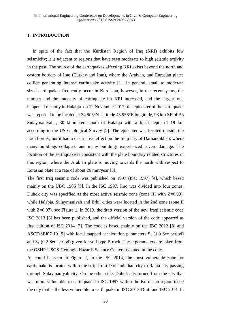
4th International Engineering Conference on Developments in Civil & Computer Engineering
Applications 2018 ( ISSN 2409-6997)
30
1. INTRODUCTION
In spite of the fact that the Kurdistan Region of Iraq (KRI) exhibits low
seismicity; it is adjacent to regions that have seen moderate to high seismic activity
in the past. The source of the earthquakes affecting KRI exists beyond the north and
eastern borders of Iraq (Turkey and Iran), where the Arabian, and Eurasian plates
collide generating Intense earthquake activity [1]. In general, small to moderate
sized earthquakes frequently occur in Kurdistan, however, in the recent years, the
number and the intensity of earthquake hit KRI increased, and the largest one
happened recently in Halabja on 12 November 2017; the epicenter of the earthquake
was reported to be located at 34.905°N latitude 45.956°E longitude, 93 km SE of As
Sulaymaniyah , 30 kilometers south of Halabja with a focal depth of 19 km
according to the US Geological Survey [2]. The epicenter was located outside the
Iraqi border, but it had a destructive effect on the Iraqi city of Darbandikhan, where
many buildings collapsed and many buildings experienced severe damage. The
location of the earthquake is consistent with the plate boundary related structures in
this region, where the Arabian plate is moving towards the north with respect to
Eurasian plate at a rate of about 26 mm/year [3].
The first Iraq seismic code was published on 1997 (ISC 1997) [4], which based
mainly on the UBC 1985 [5]. In the ISC 1997, Iraq was divided into four zones,
Duhok city was specified as the most active seismic zone (zone III with Z=0.09),
while Halabja, Sulaymaniyah and Erbil cities were located in the 2nd zone (zone II
with Z=0.07), see Figure 1. In 2013, the draft version of the new Iraqi seismic code
ISC 2013 [6] has been published, and the official version of the code appeared as
first edition of ISC 2014 [7]. The code is based mainly on the IBC 2012 [8] and
ASCE/SEI07-10 [9] with local mapped acceleration parameters S1 (1.0 Sec period)
and SS (0.2 Sec period) given for soil type B rock. These parameters are taken from
the GSHP-USGS-Geologic Hazards Science Center, as stated in the code.
As could be seen in Figure 2, in the ISC 2014, the most vulnerable zone for
earthquake is located within the strip from Darbandikhan city to Rania city passing
through Sulaymaniyah city. On the other side, Duhok city turned from the city that
was more vulnerable to earthquake in ISC 1997 within the Kurdistan region to be
the city that is the less vulnerable to earthquake in ISC 2013-Draft and ISC 2014. In

4th International Engineering Conference on Developments in Civil & Computer Engineering
Applications 2018 ( ISSN 2409-6997)
31
the next sections, ISC 2013-Draft will not be mentioned, as it similar to ISC 2014
for the parameters reported in the current study.
FIGURE 1. Seismic zonic map for Iraq (ISC 1997)
a) 0.2 Sec b) 1.0 Sec
FIGURE 2. Spectral response acceleration (5% of critical damping), site class B rock (ISC 2013-
draft and ISC 2014)
In this paper, the ISC 2014 provisions is evaluated through the effects on the base
shear force in comparison with that found using ISC 1997 provisions, calculated
using equivalent lateral force analysis. For this purpose, two case studies of
reinforced concrete framed buildings (5 story and 15 Story) located in the main
cities of the KRI (Erbil, Duhok, Sulaymaniyah and Halabja) were taken. The base
shear force is the key indicator on the level that the building needs to be
proportionated, designed and detailed to resist earthquake forces.

4th International Engineering Conference on Developments in Civil & Computer Engineering
Applications 2018 ( ISSN 2409-6997)
32
2. ISC 2014 RESPONSE SPECTRUM
The response spectrum components defined in the ISC 2014 is similar to that
defined in the IBC 2012 [8] and ASCE/SEI7-10 [9], except for having no long-
period transition at large period range, where for all buildings with periods greater
than Ts, the spectral response acceleration (Sa) is found by SD1/T, see Figure 3.
Based on ISC 2014 [7], the response spectrum has been prepared for all four main
cities in KRI for all soil types as classified by ISC 2014 (A: hard rock, B: rock, C:
very stiff soil, D: stiff soil, E: soft soil), see Figure 4. As could be seen, the most
vulnerable cities to the effect of the earthquake are Halabja and Sulaymaniyah, while
Duhok city is the least vulnerable city within the KRI.
Ss=0.2-second spectral
response acceleration,
from maps.
S1=1-second spectral
response acceleration,
from maps.
SMS = Fa SS
SM1 = Fv S1
Fa, Fv = Site
coefficient, taken
from tables based on
the soil type and the
spectral response
acceleration
SDS= 2/3 SMS
SD1= 2/3 SM1
T = the fundamental
period of the
structure, sec
T0 = 0.2 ( SD1 / SDS)
Ts = ( SD1 / SDS)
From ISC 2014
SS= 1.08, S1= 0.43
(Duhok)
SS= 1.38, S1= 0.55
(Erbil)
SS= 2.10, S1= 0.84 (Sul.
)
SS= 2.16, S1= 0.86
(Halabja)
FIGURE 3. Seismic design response spectrum, as defined in ASCE/SEI7-10 [9] and IBC 2012 [8]
This part does not
exist in ISC 2014
4th International Engineering Conference on Developments in Civil & Computer Engineering
Applications 2018 ( ISSN 2409-6997)
33
a) Duhok City b) Erbil City
c) Sulaymaniyah City d) Halabja City
FIGURE 4. Seismic design response spectrum for the Kurdistan region of Iraq, based on the ISC
2014 [7]
Abdulhameed A. Y et. al. [10] suggested three response spectrums for building
design in KRI, see Figure 5, dividing the region into two zones: zone A (the strip at
the border with Iran and Turkey) and B (the remaining parts of KRI). These spectra
were based on using PGA (Peak Ground Acceleration) equal to 0.5g for zone A, and
0.4g for zone B. In Figure 6, the response spectra for Halabja, Erbil and Duhok
cities for the soil types B (rock) and D (stiff soil) as suggested by the ISC 2014 are
presented to be compared with Figure 5.
The comparison shows good agreement for Halabja (rock), Erbil (rock) and Erbil
(Soil). However, for Duhok city, it is not clear from Figure 5 whether it is included
within zone A or B, and no information was found in the paper in the respect. The
spectra for Sulaymaniyah is not reported in Figure 6, as they are very close to those
reported for Halabja city, see Figure 4.
0
0.2
0.4
0.6
0.8
1
1.2
1.4
0 1 2 3 4 5 6 7 8 9 10
Sa
(g
)
Period (s)
Soil Type E - Soft Soil
Soil Type D - Stiff Soil
Soil Type C - Very Stiff Soil
Soil Type B - Rock
Soil Type A - Solid Rock
0
0.2
0.4
0.6
0.8
1
1.2
1.4
0 1 2 3 4 5 6 7 8 9 10
Sa
(g
)
Period (s)
Soil Type E - Soft Soil
Soil Type D - Stiff Soil
Soil Type C - Very Stiff Soil
Soil Type B - Rock
Soil Type A - Solid Rock
0
0.2
0.4
0.6
0.8
1
1.2
1.4
0 1 2 3 4 5 6 7 8 9 10
Sa
(g
)
Period (s)
Soil Type E - Soft Soil
Soil Type D - Stiff Soil
Soil Type C - Very Stiff Soil
Soil Type B - Rock
Soil Type A - Solid Rock
0
0.2
0.4
0.6
0.8
1
1.2
1.4
0 1 2 3 4 5 6 7 8 9 10
Sa
(g
)
Period (s)
Soil Type E - Soft Soil
Soil Type D - Stiff Soil
Soil Type C - Very Stiff Soil
Soil Type B - Rock
Soil Type A - Solid Rock

4th International Engineering Conference on Developments in Civil & Computer Engineering
Applications 2018 ( ISSN 2409-6997)
34
FIGURE 5. Response spectrums for KRI as
recommended by Yaseen A. A. et. Al. [10]
FIGURE 6. Response spectrums for KRS as
recommended by ISC 2014 [7]
1. SEISMIC RESPONSE COEFFICIENT (ISC 2014 - ISC 1997)
The reported response spectrums given in Figure 4 could be used in any of the
two seismic analysis methods specified by the ISC 2014 [7]: i) Equivalent Lateral
Force Analysis (ELFA); ii) Modal Response Spectrum Analysis (MRSA). On the
other side, ISC 1997 [4] does not include MRSA as an analysis tool; instead, it
specifies the Dynamic Time History Analysis (DTHA) as the 2nd analysis tool.
Therefore, for a rational comparison between these two codes, only the ELFA
results will be compared in the current paper. for both ISC 1997 and ISC 2014, the
seismic response coefficient (Cs), required for the ELFA method, has been
constructed for a study case (special reinforced concrete frame building) with high
occupancy rate (more than 300 persons) with no special or high importance to the
public for all four cities. This case has been chosen because it has the same live load
ratio included within the effective seismic weight (W = total dead load + 25 % of the
floor live load) in both codes; further, it represents the large percentage of the frame
buildings constructed in the KRI region. the Seismic Response Coefficient (CS)
represents the amount of the base shear at the bottom floor taken as a ratio of the
total gravity vertical seismic load (W). The procedure for the calculation of the Cs in
both codes are summarized in Table 1. The calculated CS coefficient is shown in
Figure 7 for soil of types A, B, C, D and E as classified in the ISC 2014 [7]; by
comparing this coefficient between the ISC 2014 and ISC 1997, the change in the
base shear will be clear; for comparison purposes, soils of Types I, II and III as
specified in the ISC 1997 [4] are equivalent to soil types A-B, C-D, E-F in the ISC
2014 [7], respectively.
0
0.2
0.4
0.6
0.8
1
1.2
1.4
1.6
0 1 2 3 4 5 6 7 8 9 10
Sa (g
)
Period (s)
Halabja-Soil Type B- Rock -
Halabja-Soil Type D- Stiff Soil -
Erbil-Soil Type B-Rock-
Erbil-Soil Type D-Stiff Soil-
Dohuk-Soil Type B- Rock -
Dohuk-Soil Type D- Stiff Soil -A
B
`
`
`
Halabja – Rock (ISC 2014) = Erbil– Stiff Soil (ISC 2014) = Erbil– Rock (ISC 2014) =

4th International Engineering Conference on Developments in Civil & Computer Engineering
Applications 2018 ( ISSN 2409-6997)
35
TABLE 1.
Details of the equivalent lateral force analysis procedure
ISC 1997 [4] ISC 2014 [7]
I I = 1.0 Class III I I = 1.25 Class III
T 0.1 N ; N: Number of floors T T = 0.1 N (for 5 story); N: Number of floors
T = 0.044 h0.9 ( for 15 story); h: floor height
K K = 0.85 (High ductility moment resisting
frame) R R = 6.5 (Special RC frame)
Z Z= 0.09 Duhok
Z= 0.07 (Halabja, Sulaymaniyah , Erbil)
(SS)
(S1)
SS= 1.08, S1= 0.43 (Duhok)
SS= 1.38, S1= 0.55 (Erbil)
SS= 2.10, S1= 0.84 (Sulaymaniyah )
SS= 2.16, S1= 0.86 (Halabja)
S
S=0.5/T (rock)
S=0.75/T (stiff, medium Stiff Soil)
S= 1.0/T (soft Soil); S≤ 1.0 (all soils)
SMS
SM1
SMS = Fa SS
SM1 = Fv S1
Fa, Fv = Site coefficient
SDS
SD1
SDS= 2/3 SMS
SD1= 2/3 SM1
Cs Cs=Z K I S Cs
Cs = SDS / ( R / I )
Cs ≤ SD1/ ( R . T / I )
Cs ≥ 0.044 SD1 I ; Cs ≥ 0.01
Vs Vs = Cs W Vs Vs = Cs W
I, Importance Factor
T, Building Fundamental period
K, Structural System Coefficient
Z, Seismic Hazard Coefficient
S, Dynamic Coefficient
Cs, Seismic Response Coefficient
Vs, Base Shear
I, Importance Factor
T, Building Fundamental period
R, Response modification coefficient
SS, Mapped spectral accelerations for short period
S1, Mapped spectral accelerations for 1-Sec period
SMS SM1, Maximum Considered Earthquake (MCE)
spectral response acceleration
SDS SD1, 5% damped Design spectral response
acceleration
Cs, Seismic Response Coefficient
Vs, Base Shear

4th International Engineering Conference on Developments in Civil & Computer Engineering
Applications 2018 ( ISSN 2409-6997)
36
As two case studies, two values of building periods are taken, T=0.5 Sec (low-rise
concrete frame building of 5 stories), T=1.5 Sec (intermediate-rise concrete frame
building of 15 stories). For these two-time periods, CS have been extracted from
Figure 7 for both ISC 2014 and ISC 1997 codes; further, the ratios between CS
coefficients, which are equal to the base shear ratio, are reported in Table 2 and
shown graphically in Figure 8 for different soil types and for all four main cities.
As could be seen, there is a significant increase in the base shear forces for the two
building cases in Halabja and Sulaymaniyah, followed by Erbil then Duhok. This
shows the massive impact that the introduction of the ISC 2014 has on the value of
design seismic forces, and consequently the design implications.
a) Duhok City b) Erbil City
c) Sulaymaniyah City d) Halabja City
FIGURE 7. Seismic response coefficient (Cs) using ISC 1997 [4] and ISC 2014 [7]
0
0.05
0.1
0.15
0.2
0 0.5 1 1.5 2 2.5 3 3.5 4 4.5 5
Seis
mic
Re
spo
nse
Co
eff
icie
nt (
Cs)
Period (s)
ISC2014 - Soil E - Soft Soil
ISC2014 - Soil D- Stiff Soil
ISC2014 - Soil C - Very Stiff Soil
ISC2014 - Soil B-Rock
ISC2014 - Soil A- Hard Rock
ISC1997-Soil III
ISC1997-Soil II
ISC1997-Soil I
0
0.05
0.1
0.15
0.2
0 0.5 1 1.5 2 2.5 3 3.5 4 4.5 5
Seis
mic
Re
spo
nse
Co
eff
icie
nt (
Cs)
Period (s)
ISC2014 - Soil E - Soft Soil
ISC2014 - Soil D- Stiff Soil
ISC2014 - Soil C - Very Stiff Soil
ISC2014 - Soil B-Rock
ISC2014 - Soil A- Hard Rock
ISC1997-Soil III
ISC1997-Soil II
ISC1997-Soil I
0
0.05
0.1
0.15
0.2
0.25
0.3
0 0.5 1 1.5 2 2.5 3 3.5 4 4.5 5
Seis
mic
Re
spo
nse
Co
eff
icie
nt (
Cs)
Period (s)
ISC2014 - Soil E - Soft Soil
ISC2014 - Soil D- Stiff Soil
ISC2014 - Soil C - Very Stiff Soil
ISC2014 - Soil B-Rock
ISC2014 - Soil A- Hard Rock
ISC1997-Soil III
ISC1997-Soil II
ISC1997-Soil I

4th International Engineering Conference on Developments in Civil & Computer Engineering
Applications 2018 ( ISSN 2409-6997)
37
TABLE 2.
Base shear ratio (ISC 2014/ISC 1997)
Base shear ratio (ISC 2014/ISC 1997), %
5 story building, T=0.5 Sec 15 story building, T=1.5 Sec
Soil type
aver
age
Soil type
aver
age
h
ard
rock
rock
ver
y
stif
f
stif
f
soft
har
d
rock
rock
ver
y
stif
f
stif
f
soft
A B C D E A B C D E
Duhok 115 144 181 192 163 159 124 155 132 151 173 147
Erbil 190 237 297 297 268 258 204 255 205 237 284 237
Sulaymaniyah 290 362 452 452 407 393 311 388 314 362 434 362
Halabja 296 371 465 465 419 403 319 399 321 371 434 369
a) 5-Storey Building b) 15-Storey Building
FIGURE 8. Base shear ratio (ISC 2014/ISC 1997)
2. MODAL RESPONSE SPECTRUM ANALYSIS
Apart from the ELFA, there is no common seismic analysis procedure between
ISC 2014 and ISC 1997; this was the reason for choosing ELFA for comparison. To
confirm that the ELFA is the driving seismic analysis tool for regular low-rise to
intermediate-rise building, modal response spectrum analysis has been conducted
according to ISC 2014 for 5-storey and 15-storey special reinforced concrete frame
building (Importance Class III) located in Erbil city, constructed on a site class D
stiff soil using ETABS 16.2.0, see Figure 9.
The seismic base shear determined by both methods (equivalent lateral force (Vs)
and maximum response spectrum analysis (Vd)) are reported in Table 3. According
the ISC 2014, as Vd is less than 0.85Vs, then the Vd must be raised to be equal to
85% of Vs. Based on that, the ELFA is superior to MRSA for regular RC buildings
0
100
200
300
400
500
Dohuk Erbil Sulimania Halabja
Bas
e Sh
ear
rati
o (I
SC2
01
4/I
SC1
997)
, %
City
Hard Rock
Rock
Very Stiff Soil
Stiff Soil
Soft Soil
0
100
200
300
400
500
Dohuk Erbil Sulimania Halabja
Bas
e Sh
ear
rati
o (I
SC2
01
4/I
SC1
997)
, %
City
Hard Rock
Rock
Very Stiff Soil
Stiff Soil
Soft Soil

4th International Engineering Conference on Developments in Civil & Computer Engineering
Applications 2018 ( ISSN 2409-6997)
38
in the range of number of floors tested; this justify the use of the ELFA as the base
for comparison between the ISC 2014 and ISC 1997 in the current paper
FIGURE 9. ETABS model geometry of the buildings.
TABLE 3.
Static and dynamic calculated base shear
Building Direction Vs (Static) kN Vd (Dynamic) kN 0.85Vs/Vd
5 Story X 7304.76 2591.62 2.396
Y 7304.76 2524.03 2.460
15 Story X 8979.99 3393.49 2.249
Y 8979.99 3255.56 2.345
3. STRUCTURAL DESIGN CONSIDERATION FOR KRI
Based on the ISC 2014, there are four classes (A, B, C, D) for seismic design
classification. This does not match ASCE/SEI7-10 [9], where six seismic design
classes are defined (A, B, C, D, E, F). In the ISC 2014, the class for each site
depends on the values of SDS and SD1; if SDS ≥ 0.5 g or SD1 ≥ 0.2 g, the category of
the site is assigned to be class D. Referring to Figures 3 and 4, both conditions are
valid, therefore, all buildings constructed in the KRI region is considered to be of
class D for all soil types no matter what it is the function or the construction system
of the building. Based on ISC 2014 [7] and ASCE/SEI7-10 [9], for class D, all
concrete frame building should be special type, as no ordinary or intermediate
concrete frame is allowed to be built. ISC 2014 refers to ACI318 code [11] as the

4th International Engineering Conference on Developments in Civil & Computer Engineering
Applications 2018 ( ISSN 2409-6997)
39
designing and construction tool of reinforced concrete buildings for ordinary and
seismic loading; therefore, these special concrete frame buildings built in KRI
should confirms to ACI requirements, which requires special member size and
strength limitations and reinforcement details for the columns, beams and
foundation that are not applied currently in the construction in KRI region. The
effects of the building systems in KRI to be in seismic design class D will be
increasing the requirements for detailing and proportioning, with expectations of
increased deformation capacity, meaning that further design criteria need to be
applied as listed in Tables 4 and 5.Regarding the Seismic Analysis Procedure
Selection, Table 6 lists the selection criteria used in ISC 1997 [4] and ISC 2014 [7].
As seen, ISC 1997 considers only the importance class of the building, while ISC
2014 bases the selection on the building height (T value) and the irregularity in the
building, which is more rational, as the dynamic behavior of the building is related
to these two factors.
TABLE 4.
Seismic design criterial needs for masonry and steel construction constructed in KRI (seismic class
D), based on ISC 2014 [7]
Building system Structural system allowed Limits (ISC 2014, Table 3-2-1)
Masonry wall system * Special* masonry reinforced shear
wall is allowed. Height ≤ 50 m
Moment resisting steel frame#
Special No limit
Intermediate & ordinary Specific limitations listed
*: Building Code Requirements for Masonry Structures (ACI 530-02/ASCE 5-02/TMS 402-02) [12] is the code
permitted by the ISC 2014 for designing Masonry Wall system.
#: Seismic Provisions for Structural Steel Buildings (ANSI/AISC 341-16) [13] is the code permitted by the ISC
2014 for designing Masonry Steel frame.

4th International Engineering Conference on Developments in Civil & Computer Engineering
Applications 2018 ( ISSN 2409-6997)
40
TABLE 5.
Design criterial needs for reinforced concrete frame Buildings constructed in KRI (seismic class D),
based on ISC 2014 [7] and ACI 318-14 [11]
Building system
Structural
system
allowed
Limits
(ISC 2014,
Table 3-2-1)
Ordinary
ACI
chapters to
satisfy
Additional ACI sections
to satisfy
Cast-in-place
RC concrete shear wall Special*
Height
≤ 50 m
CH 1 to 17
CH 19 to 26
Sections 18.2.2 - 18.2.8
Sections 18.10
Reinforced concrete shear walls in
dual systems with special
reinforced concrete frame
Special* No Limit Same Sections 18.2.2 - 18.2.8
Sections 18.10
Reinforced concrete shear walls in
dual systems with intermediate
reinforced concrete frame
Special* Height
≤ 50 m Same
Sections 18.2.2 - 18.2.8
Sections 18.10
Cast-in-place moment resisting RC
concrete frame Special* No limit Same
Sections 18.2.2 - 18.2.8
Sections 18.6 - 18.8
Foundation Same Sections 18.13
* the term “special” (Compared with “ordinary”, “intermediate”, and) refer to increasing requirements for
detailing and proportioning, with expectations of increased deformation capacity, as defined in ACI 318.
TABLE 6.
Seismic analysis selection procedure
Analysis Procedure ISC 1997 [4] ISC 2014 [7]
Equivalent lateral force analysis All cases apart from
buildings of I=1.5
Regular buildings with T < 3.5 Ts
Irregular buildings with T < 3.5 Ts,
but with specific type of irregularity
Modal response spectrum analysis Not included in the code All other cases
Dynamic time history analysis Buildings of Importance
class I=1.5 Not included in the code
4. PEAK GROUND CANCELATION (PGA)
The comparison presented in this study showed that there is a significant increase
in the base shear for buildings constructed in KRI according to ISC 2014 compared
to ISC 1997. This increase is mainly due to S1 and SS parameters assigned to this
region by ISC 2014, which are affecting the values of the parameters SD1 and SDS.
To assess these values, they need to be returned back to their original status, which
is Peak Ground Acceleration (PGA), the maximum amplitude of recorded
acceleration, termed also as zero period acceleration [14, pp. 1-11].Therefore, at
T=0:
PGA = Sa (1)
From Figure 1, the first inclined part in the response spectrum is defined as:
Sa = SDS ( 0 .4 + 0.6 (T/T0) ) (2)

4th International Engineering Conference on Developments in Civil & Computer Engineering
Applications 2018 ( ISSN 2409-6997)
41
Then, at T=0:
Sa = 0.4 SDS (3)
The SDS value is related to an earthquake with a 10% probability of occurrence in 50
years (Corresponding to 475-year recurrence interval) [15, p. 385]. On the other
hand, the PGA map for Iraq (given in Figure 10) is for the same probability of
occurrence, therefore by substituting Equation (1) in Equation (3)
PGA = 0.4 SDS (4)
PGA = 0.4 x (2/3) x Fa x SS (5)
As Fa = 1 for Site Class B rock in ISC 2014 [7] , then
PGA = SS / 3.75 (6)
Based on Equation (6) and Figure 3, the PGA values for Site Class B rock taken by
ISC 2014 seems to be as follows: 0.282g for Duhok, 0.368g for Erbil, 0.56g for
Sulaymaniyah and 0.576g for Halabja. On the other hand, the 475-year return period
PGA map in Figure 10, provided by the Global Seismic Hazard Assessment
Program [2], shows the PGA values to be around 0.21g for Duhok, 0.24g for Erbil,
0.42g for Sulaymaniyah and 0.42g for Halabja. The comparison suggests that the
values of SS and S1 recommended by ISC 2014 are overestimated,
FIGURE 10. Peak ground acceleration (PGA) map for rock with a 10% probability of exceedance in
50 years (475-year return period) as reported by Global Seismic Hazard Assessment Program [16]
Duh
ok Erbil
Halb
Sul

4th International Engineering Conference on Developments in Civil & Computer Engineering
Applications 2018 ( ISSN 2409-6997)
42
5. CONCLUSIONS
The conclusions drawn from the current study could be summarized as below:
1- The equivalent lateral force analysis for the two case studies of Reinforced
Concrete Frame buildings (5 and 15 Stories) showed an increase in the Base shear
using ISC 2014 compared with that obtained using ISC 1997 in the percentages
shown below
- 115 % to 192 % for Duhok city; 190 % to 297 % for Erbil city.
- 290 % to 452 % for Sulaymaniyah city; 296 % to 465 % for Halabja city.
2- The applications of the current ISC 2014 imply considerable change in the
building systems built in KRI, including the requirement of having:
- Special system (according to ACI318-14) for reinforced concrete frames,
reinforced shear wall systems.
- Special system for steel frames in general (according to ANSI/AISC 341-16),
with some exception to use ordinary or intermediate systems for some specific
cases of low rise buildings.
- Special system for Masonry Bearing Wall system (according to ACI 530-
02/ASCE 5-02/TMS 402-02).
These require a dramatic change in the structural analysis and the design
procedures applied currently on the buildings constructed in KRI region.
3- The Equivalent lateral force analysis is proved to be superior to the modal
response spectrum analysis as a seismic analysis tool for regular reinforced
concrete buildings up to 15 floors in the ISC 2014.
4-The recommended SS and S1 values in the ISC 2014 seems to be overestimated
compared with the local values for the peak ground acceleration given by
GSHAP.

4th International Engineering Conference on Developments in Civil & Computer Engineering
Applications 2018 ( ISSN 2409-6997)
43
REFERENCES
[1] Ghassan I. Aleqabi and Hafidh A. A. Ghalib , "Seismic Hazard Assessment of
Northern Iraq," Journal of Zankoy Sulaimani-Part-A- (Pure and Applied
Sciences), no. Special Issue, GeoKurdistan II, pp. 319-330, 2016.
[2] " National Earthquake Information Center website," United States Geological
Survey, Earthquake Hazards Program, [Online]. Available:
https://earthquake.usgs.gov/. [Accessed 02 December, 2017].
[3] "Swiss Seismological Service (SED)," , [Online]. Available:
http://www.seismo.ethz.ch. [Accessed 02 December 2017].
[4] Ministry of Industrial and Mineral-Centeral Organaziation for Standarazation
and Quality Control, "Iraqi Seismic Code Requirements for Buildings,"
Building Research Centre, Baghdad, 1997.
[5] UBC 1985, "Uniform Building Code," International Conference of Building
Officials, California, USA, 1985.
[6] Ministry of Construction and Housing-Centeral Organaziation for
Standarazation and Quality Control, "Seismic Code 2013 - Draft Version,"
Baghdad, 2013.
[7] Ministry of Construction and Housing-Centeral Organaziation for
Standarazation and Quality Control, "Seismic Code - Iraqi Building Code 303,"
Ministry of Construction and Housing-Federal Government, Baghdad, 2014.
[8] IBC 2012, "International Building Code," International Code Council, USA,
2011.
[9] ASCE/SEI 7-10, "Minimum Design Loads for Buildings and Other Structures,"
American Society of Civil Engineers, Virginia, 2010.
[10] Abdulhameed A. Y., David B., Nikos N., "Time History Analysis of Existing
Buildings in the Kurdistan Region of Iraq," in First International Engineering

4th International Engineering Conference on Developments in Civil & Computer Engineering
Applications 2018 ( ISSN 2409-6997)
44
Conference (IEC2014), Erbil, Iraq, 2014.
[11] ACI 318-14, "Building Code Requirments for Reinforced Concrete (ACI 318-
14) and Comentray," American Concrete Institute, Farmington Hills, Detroit,
2014.
[12] ACI 530-02/ASCE 5-02/TMS 402-02, "Building Code Requirements for
Masonry Structures," Masonry Standards Joint Committee (MSJC), USA, 2002.
[13] ANSI/AISC 341-16, "Seismic Provisions for Structural Steel Buildings,"
AISC, Chicago,, 2016.
[14] Chen W.F., Lui E.M., Earthquake Engineering for Structural Design, NW,
USA: CRC Press, 2006.
[15] B. S. Taranath, Reinforced Concrete Design of Tall Buildings, NW: CRC
Press, 2010.
[16] " Global Seismic Hazard Assesment Program," [Online]. Available:
http://www.seismo.ethz.ch/static/GSHAP/. [Accessed 07 12 2017].

4th International Engineering Conference on Developments in Civil & Computer Engineering Applications
2018 ( ISSN 2409-6997)
45
INVESTIGATION OF SEISMIC PERFORMANCE AND RELIABILITY
ANALYSIS OF PRESTRESSED REINFORCED CONCRETE BRIDGES
M. Hosseinpour1, M.Celikag2, H. AkbarzadehBengar3
1&2EMU, Gazimagusa 3University of Mazandaran,
[email protected] ,[email protected],[email protected]
doi:10.23918/iec2018.04
ABSTRACT
Given the vital importance of bridges in life arteries, safety of these structures against
destructive agents such as earthquake is of utmost importance. Using pre-stressed columns in
bridges will improve their seismic response, because these columns have high displacement
capacity during earthquake and a small permanent displacement after earthquake. Therefore,
the need for further study on these structures is felt more than ever. In this paper, firstly, pre-
stressed columns were analyzed under reciprocating static load using OpenSees software and
results show that pre-stressing bridge columns will improve the quasi-static response of
columns and column section bearing. Below, we examine the reliability analysis of pre-stressed
bridge samples against force of the earthquake and the effect of different random variables on
reliability of bridge. The results show that structural damping and earthquake magnitude have
a significant effect on reliability of bridges. Changes in characteristic strength of concrete at
ultimate limit and mean resistance of section, effect significantly on reliability of bridge
structure.
Keywords: Concrete Bridge, Pre-stressed concrete structures, seismic performance, finite
element analysis, Structural reliability.
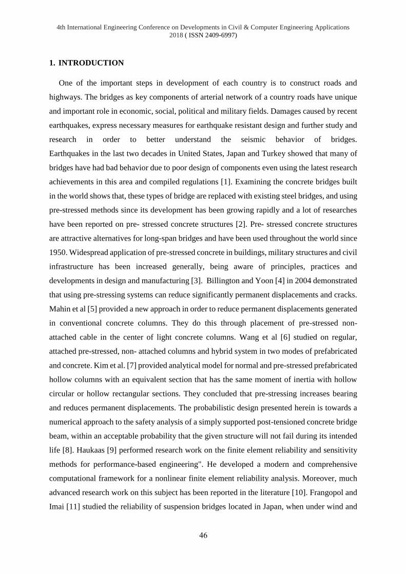
4th International Engineering Conference on Developments in Civil & Computer Engineering Applications
2018 ( ISSN 2409-6997)
46
1. INTRODUCTION
One of the important steps in development of each country is to construct roads and
highways. The bridges as key components of arterial network of a country roads have unique
and important role in economic, social, political and military fields. Damages caused by recent
earthquakes, express necessary measures for earthquake resistant design and further study and
research in order to better understand the seismic behavior of bridges.
Earthquakes in the last two decades in United States, Japan and Turkey showed that many of
bridges have had bad behavior due to poor design of components even using the latest research
achievements in this area and compiled regulations [1]. Examining the concrete bridges built
in the world shows that, these types of bridge are replaced with existing steel bridges, and using
pre-stressed methods since its development has been growing rapidly and a lot of researches
have been reported on pre- stressed concrete structures [2]. Pre- stressed concrete structures
are attractive alternatives for long-span bridges and have been used throughout the world since
1950. Widespread application of pre-stressed concrete in buildings, military structures and civil
infrastructure has been increased generally, being aware of principles, practices and
developments in design and manufacturing [3]. Billington and Yoon [4] in 2004 demonstrated
that using pre-stressing systems can reduce significantly permanent displacements and cracks.
Mahin et al [5] provided a new approach in order to reduce permanent displacements generated
in conventional concrete columns. They do this through placement of pre-stressed non-
attached cable in the center of light concrete columns. Wang et al [6] studied on regular,
attached pre-stressed, non- attached columns and hybrid system in two modes of prefabricated
and concrete. Kim et al. [7] provided analytical model for normal and pre-stressed prefabricated
hollow columns with an equivalent section that has the same moment of inertia with hollow
circular or hollow rectangular sections. They concluded that pre-stressing increases bearing
and reduces permanent displacements. The probabilistic design presented herein is towards a
numerical approach to the safety analysis of a simply supported post-tensioned concrete bridge
beam, within an acceptable probability that the given structure will not fail during its intended
life [8]. Haukaas [9] performed research work on the finite element reliability and sensitivity
methods for performance-based engineering". He developed a modern and comprehensive
computational framework for a nonlinear finite element reliability analysis. Moreover, much
advanced research work on this subject has been reported in the literature [10]. Frangopol and
Imai [11] studied the reliability of suspension bridges located in Japan, when under wind and

4th International Engineering Conference on Developments in Civil & Computer Engineering Applications
2018 ( ISSN 2409-6997)
47
earthquake loads. They applied spectral analysis and evaluated the reliability of the structure.
The mechanical and geometrical properties of the sections were taken as the random variables.
In this paper, the behavior of pre-stressed and attached columns under seismic loading as well
as seismic reliability of arch concrete bridge using the finite element method are studied.
2. THEORY OF THE PROBLEM
The equation of system motion affected by earthquake forces can be expressed as follows:
[𝑀]u + [C]u + [K]u = Peff(t) (1)
In this equation [M] is concentrated mass matrix, [C] is damping matrix, [K] is stiffness matrix,
Peff(t) is earthquake effective force vector, u is displacement vector, u is velocity vector
and u is acceleration vector. Calculating the response of bridge structure of equation (1) is
resolved using standard modal conversion technique.
𝑞n(t) + 2ξnωnqn(t) + ωn2qn(t) = −Γnug(t) (2)
In this equation, qn(t) is normal coordinates, ξn is structural damping percent of nth mode,
ωnis natural frequency of nth mode, Γn is modal distribution coefficient and ug(t) is the vertical
acceleration caused by earthquake. Equation (2) can be expressed as follows:
𝑞n(t)
Γn+ 2ξnωn
qn(t)
Γn+ ωn
2qn(t)
Γn= −ug(t) (3)
Assuming𝑞n(t)
Γn= 𝐷𝑛(𝑡), the equation (2) is expressed as follows:
𝐷𝑛(𝑡) + 2ξnωn𝐷𝑛(𝑡) + ωn
2𝐷𝑛(𝑡) = −ug(t) (4)
Equation (3), is system motion equation with a single degree of freedom and it can be easily
solved using numerical methods. Solving equation (3) we can obtain structural displacements
in different modes. Since the response of total structure and applied would be calculated as
follows.
𝑢(𝑡) = ∑𝑢𝑛(𝑡)
𝑁
𝑛=1
= ∑ Γn
N
𝑛=1
ϕn𝐷𝑛(𝑡) (4) and 𝑓𝑠(t) = [K]𝑢(𝑡) (5)
Failure due to bending compared to other modes of failure is the most common type of failure
mode in reinforced concrete structures. Thus, in the present study, reliability of structure is
calculated for flexural failure. Bridge structure is modeled using finite element software as

4th International Engineering Conference on Developments in Civil & Computer Engineering Applications
2018 ( ISSN 2409-6997)
48
continuous beam with Beam two-dimensional element. Dead load is distributed evenly as linear
load along elements. Vertical seismic accelerations are considered as earthquake load on
structures. Bridge structural reliability analysis was conducted using FOSM Method. For
calculating the reliability of bridge structure, a certain percentage of ultimate bending strength
is considered as a resistance force and bending moment caused by earthquake is considered as
force due to loading. Bridge structure is analyzed for a number of earthquakes as 50
accelerogram and finally, mean and standard deviation values of bridge structure reactions are
calculated according to results of analysis. In general, if equations related to probability
distribution functions of random variables are available, the reliability of structures will be
calculated using integral equations listed in Equations 6 and 7.
Pf = 1 − R0 = 1 − ∫ fs+∞
−∞(s)[1 − FR(s)]𝑑𝑠 = ∫ 𝑓𝑠
+∞
−∞(𝑠)𝐹𝑅(𝑠)𝑑𝑠 (6)
Pf = 1 − ∫ fR
+∞
−∞
(r)Fs(r)𝑑𝑟 (7)
Where Pf is structural failure probability, R0is reliability of structures, fx(x) is probability
density function and Fx(x) is cumulative distribution function. The failure probability function
can be expressed as the following equation:
𝑃𝑓 = ∅ (𝜇𝑆 − 𝜇𝑅
√𝜎𝑅2 + 𝜎𝑆
2) (8)
In equation 8, ∅ is standard normal distribution function, 𝜇𝑆 is mean force applied on structure,
𝜇𝑅 is mean structure strength, σ𝑅 is structure standard deviation and σS is standard deviation
value of loading. If structural reliability index is β =μg
σg , therefore, structural failure probability
can be expressed as: 𝑃𝑓 = ∅(−𝛽) (9)
Finally, the reliability index of structures is expressed by Equation 10. 𝛽 = −∅−1(𝑃𝑓) (10)
Ultimate strength limit state and allowable stresses limit state are considered as limit
conditions. For these two cases, the limit conditions are defined as follows: 𝜀cu ≤ 0.0035
In this equation εcu is compression stress of concrete tension area. For limit requirement,
security margin equation is considered as: 𝑔u = αM𝑢 − Ms (11)
Where, Mu is sectional ultimate resistance moment, Ms is loading moment and α is a coefficient
smaller than 1 that each stage represents the percentage of ultimate moments dedicated to

4th International Engineering Conference on Developments in Civil & Computer Engineering Applications
2018 ( ISSN 2409-6997)
49
counter loading moment due. For allowable limit stress, the below equation is established:
fct ≤ fct (12)
Where, fct is tension stress of concrete tension area and fct is allowable tension stress of
concrete. Security margin equation for this state is considered as: ge = αMe − Ms (13)
3. STUDYING PRE-STRESSED COLUMNS UNDER RECIPROCAL QUASI-STATIC
LOAD
Loading is done according to Figure 1. Loading pattern by controlling displacement for
applying load of reciprocating wheels. Loading continues until the load of reaches to maximum
value of 0.85.
FIGURE 1. The procedure of loading pattern and experiment
Cross-section of columns is 50 × 36 cm for typical and pre-stressed columns. 26 armatures
of 12 mm diameter were used in conventional concrete columns round cross-section and six
wires of 5 mm diameter were used around a wire with the same diameter for pre- stressed
section. Lateral load applied point is 1550 mm above the column fixed base and studying is
based on flexural failure. Concrete design strength is 32.5 MPa and conventional bars yield
strength is 335 MPa and ultimate stress of pre-stressed tendons is 1860 MPa. Constant
compressive force of 576 KN is applied to simulate the gravity loads applied at the time of
service at the top of column. Modeling is carried out using OpenSees software where the
structural analysis is done using finite element method. Nodes are defined in OpenSees
software for pre-stressed system and a graphical form of nodes were drawn using OPS software
in order to ensure the accuracy. All parts of fiber section move fully coherent, total cross section

4th International Engineering Conference on Developments in Civil & Computer Engineering Applications
2018 ( ISSN 2409-6997)
50
is defined using fiber section that is able to define simultaneously bars, tendons and concrete
with different stress-strain diagram in different locations of a cross-section. According to the
fact that in pre-stressed systems tendons are involved with concrete, therefore, it shows the
necessity of using a single fiber. However, the materials used in fiber cross section must be
defined previously. Material Initial Stress is used in order to apply pre-stressed force.
Also, effects of growth and Pinching of Hysteresis curve and considering Boushinger principle
and the ability to change are features of this type of material. Figures 2 and 3, show the results
of conventional and pre-stressed concrete column analysis. These figures are related to
proposed model using the materials. As can be seen in Figure 2, it is found that permanent
displacement is reduced greatly and bearing capacity is increased. Also, according to Figure 3,
which corresponds to pre-stressed post- tension concrete column, permanent displacement is
reduced and bearing capacity is more than post- tension state.
FIGURE 2. Non- attached pre-stressed hysteresis curve diagram
FIGURE 3. Attached pre-stressed hysteresis curve diagram

4th International Engineering Conference on Developments in Civil & Computer Engineering Applications
2018 ( ISSN 2409-6997)
51
4. THE RELIABILITY OF BRIDGES AGAINST EARTHQUAKE-INDUCED
FORCES
According to partial surveys conducted on reliability analysis of bridge structures against
earthquake forces, in this section, the reliability of an arch pre-stressed concrete bridge against
earthquake forces are examined. In this section, the mechanical properties of materials,
geometric characteristics of sections, structural damping rate, magnitude and maximum
acceleration of earthquake are considered as random variables. The bridge is modeled as a
continuous beam and linear system behavior is assumed. Vertical accelerations of earthquake
are considered as loads applied on bridges for time history analysis of bridge structure during
an earthquake and probability density distribution function of random variables are extracted
from existing sources and normal probability distribution function is assumed for those
variables that had no sources. The examined pre-stressed arched bridge sample includes a
three-span bridge with central span of 125 m length and first and second lateral span with length
of 55.35 and 45 meters, respectively.
Figure 4 shows the changes of reliability index of bridge structure based on standard deviation
of concrete characteristic strength for final resistance limit state. Each curve corresponds to a
certain percentage of section ultimate strength. As can be seen, a bridge reliability index change
is not considerable per high percentage of cross-resistance but structural changes reliability
index is increased as cross-resistance decreased. The reason is that effects of fluctuations
arising from changes of concrete characteristic strength on reliability index against section
ultimate resistance are trivial. Increasing the percentage of concrete ultimate strength that is
used to deal with the external load, the characteristic resistance of concrete changes effects on
reliability index is decreased. Figure 5 shows the changes of bridge structure reliability for
allowable stress limit state. In limit state, due to the low level of resistance, total resistance of
section is considered to cope with the effects of external loading. As can be seen from diagram,
changes in specific strength of concrete does not effect on bridge structure reliability index.
The interesting point is percentage of structural damping effect because 3 percent increase of
structural damping results in double increase of structural reliability index.

4th International Engineering Conference on Developments in Civil & Computer Engineering Applications
2018 ( ISSN 2409-6997)
52
FIGURE 4. The effect of characteristic resistance changes on reliability index for damping percentage (5%
ultimate strength limit state)
FIGURE 5. The effect of characteristic resistance changes on reliability index (allowable stress limit state)
Figure 6 shows the effect of structural damping changes on reliability index of bridge structure
for ultimate strength limit state per different percentages of section resistance.
As can be seen from the figure, changes of structural damping effect are evident on reliability
changes of bridge structure. The changes of lower amounts of section resistance are more than
high levels of section resistance, so that increasing resistance results in curve section tendency
to flat and horizontal state.
Figure 7 shows the percentage of structural damping effect changes on reliability index of
bridge structure in allowable stress limit state. As can be seen, the effect of random variable
changes on reliability index changes in limit state is somewhat obvious. In a general conclusion

4th International Engineering Conference on Developments in Civil & Computer Engineering Applications
2018 ( ISSN 2409-6997)
53
we can say that the important random variable of this issue is bridge structural damping
percentage.
FIGURE 6. Changes of bridge structure reliability index per changes of structural damping percentage, ultimate
strength limit state
FIGURE 7. Changes of bridge structure reliability index per changes of structural damping percentage, ultimate
allowable tension limit state

4th International Engineering Conference on Developments in Civil & Computer Engineering Applications
2018 ( ISSN 2409-6997)
54
5. CONCLUSION
The study examines behavior of attached and non- attached pre-stressed column under
reciprocating quasi-static load by controlling the displacement using the finite element
model and effects of concrete characteristic strength parameters and the percentage of
structural damping on bridge structure reliability. the results show that using new materials and
direct apply of pre-stressing force will increase the accuracy of analytical models. It was found
that pre-stressing improves the quasi-static response of concrete columns and meets concrete
weakness largely in tension. In the case of non- attached pre-stressing, it can also be expressed
that pre- stressing increases section bearing significantly and on the other hand, it reduces
permanent displacement. the structural damping percentage is one of the key parameters in
seismic design of bridge structures and results show that controlling this parameter is necessary
for safe design. In most cases, except in the case of structural damping percentage for other
random variables, fluctuations of bridge structure reliability index per changes in random
variables for low percentages of section resistance and high percentages of section resistance
is trivial and nearly tends to be uniform. changes of concrete characteristic strength in allowable
tension limit state does not effect on reliability of bridge. But in ultimate limit state and mean
resistance level, it effects significantly on structural reliability and fluctuations of bridge
reliability caused by changes of concrete specific strength are less compared to fluctuations
arising from changes of structural damping.

4th International Engineering Conference on Developments in Civil & Computer Engineering Applications
2018 ( ISSN 2409-6997)
55
REFERENCES
[1] R. M Pablo, “Risk Assessment of Highway Bridges”, A Reliability-based Approach,
Paper 158, ENT 209 Indiana University-Purdue University Fort Wayne, 2008.
[2] H. Weiher, and K. Zilch, “Condition of Post-tensioned Concrete Bridges - Assessment
of the German Stock by a Spot Survey of Damages”. In: Proc. of First International Conference
on Advances in Bridge Engineering, Brunel University, London, 2006.
[3] P.J Barr, J.F Stanton, and M.O Eberhard, “Effects of Temperature Variations on Precast,
Prestressed Concrete Bridge Girders”. Journal of Bridge Engineering, ASCE, March / April
2005.
[4] Billington, S.L. and J. Yoon, “Cyclic response of unbonded posttensioned precast columns
with ductile fiber-reinforced concrete”. Journal of Bridge Engineering, 2004. 9(4): p. 353-363.
[5] Mahin, S., J. Sakai, and H. Jeong. “Use of partially prestressed reinforced concrete
columns to reduce post-earthquake residual displacements of bridges”. In Fifth National
Seismic Conference on Bridges & Highways, San Francisco, California. 2006.
[6] Wang, Z., et al., “Numerical Analytical Model for Seismic Behavior of Prestressing
Concrete Bridge Column Systems”. Procedia Engineering, 2011. 14: p. 2333-2340.
[7] Kim, T.H., D.J. Seong, and H.M. Shin, “Seismic Performance Assessment of Hollow
Reinforced Concrete and Prestressed Concrete Bridge Columns”. International Journal of
Concrete Structures and Materials, 2012: p. 1-12.
[8] Biondini, F., Frangopol, D.M., Bontempi, F., Malerba, P.G., “Reliability of material and
geometrically non-linear reinforced and prestressed concrete structures”, Journal of Computers
and Structures, 2004.
[9] Haukaas, T. “Finite element reliability and sensitivity methods for performance-based
engineering”, Ph.D. Thesis, Dept. of Civil and environmental Engineering, University of
California, Berkeley, 2003.
[10] Kiureghian, A.D., Haukaas, T. and Fujimura, K. “Structural reliability software at the
University of California, Berkeley”, Structural Safety, 28, pp. 44-67, 2006.
[11] Frangopol, D.M. and Imai, K. “Reliability of long span bridges based on design
experience with the Honshu-Shikoku bridges”, Journal of Constructional Steel Research,
60(3), pp. 373-392, 2004.

4th International Engineering Conference on Developments in Civil & Computer Engineering
Applications 2018 ( ISSN 2409-6997)
56
INVESTIGATING FLEXURAL STRENGTH OF BEAMS MADE
WITH ENGINEERED CEMENTITIOUS COMPOSITE (ECC)
UNDER STATIC AND REPEATED LOADING
Kawa O. Ameen1, Bayar J.Al-Sulayvani2, Diyar N. Al-Talabani3
1&2 Mosul University 3Cihan University-Erbil
[email protected], [email protected], [email protected]
doi:10.23918/iec2018.05
ABSTRACT
The main purpose of this research is to investigate the flexural strength of reinforced
ECC beams under static and repeated loading. Eighteen reinforced ECC beams with
deferent fiber content and deferent steel ratio were constructed and tested by
applying static and repeated loading. The experimental variables considered in this
study include fiber content, steel ratio, and loading type (static or repeated). All
beams were geometrically similar with the dimension of (120mm in width, 200mm
in depth, and 1000mm in length) and the applied loads were subjected to the beams
with two point loads and simply supported span. The experimental outputs divided
into four parts: the first part concerned with the effect of fiber content on the load-
deflection curves. The second part focused on the effect of steel ratio on the load-
deflection curves. Furthermore, the third part studied the comparison between static
and repeated loading. Eventually, the last part investigated the effect of fiber content
and steel ratio on flexural toughness. In reinforced ECC, with increasing fiber content
(for the same flexural reinforcement) the sample will increase its flexural strength.
In general, to increase the ultimate flexural strength, the addition of steel ratio has
much higher effect than increasing fiber content. Finally, for identical reinforced
ECC beams, the flexural strength will be lower when applying repeated load other
than static one.
Keywords: Engineered Cementitious Composite (ECC); Repeated Load; Flexural Strength; Flexural Toughness.

4th International Engineering Conference on Developments in Civil & Computer Engineering
Applications 2018 ( ISSN 2409-6997)
57
1. INTRODUCTION
In the past several decades, concrete with increasingly high compressive strength
have been used for many structural applications. However, most of these materials
remained brittle. In some cases, the brittleness as measured by brittleness number
actually increases as the compressive strength goes up [1]. This poses potential danger
and limitation of high strength concrete in structural fields. in the last several years,
the University of Michigan has been investigating a composite material named
Engineered Cementitious Composites (ECC). In many respects, this material has
properties similar to medium to high strength concrete. Furthermore, the tensile strain
capacity generally exceeds 1%. a number of investigations have been achieved on the
applications of ECC in structural applications at the University of Michigan in the US,
Kajima Corporation, University of Tokyo, and Building Research Institute, Tsukuba
City in Japan. These studies involve the usage of ECC in shear elements subjected to
cyclic loading, in beam-column connections, in shear wall retrofitting of reinforced
concrete (R/C) buildings, in R/C beams as durable cover for re-bar corrosion control,
and in general concrete structural repair [2].
The principal aims of this study are summarized as follows:
1. Investigating experimentally the effect of fiber volume fraction on the mechanical
properties of the flexural beams.
2. Investigating practically the effect the steel ratio on the response of beam deflection.
3. Investigating experimentally the effectiveness of loading types on the flexural
strength of reinforced ECC beams.
2. EXPERIMENTAL PROGRAM
The eighteen reinforced ECC beams were casted in the steel molds with 1000mm
length, 120mm width, and 200mm height. Although ECC has excellent shear strength,
extra shear reinforcement was added to make sure that the beams will fail by flexural
first. All of the specimens were reinforced with compression reinforcement 2Ø8mm
and the tensile reinforcements were 2Ø8mm, 3Ø8mm, and 4Ø8mm. The shear regions
were reinforced with stirrups Ø6mm at 110mm, but the middle third part was
unreinforced with stirrups. Figure (1) explained the internal details for one of the
specimens. The reinforced beams were tested under two point load test.

4th International Engineering Conference on Developments in Civil & Computer Engineering
Applications 2018 ( ISSN 2409-6997)
58
FIGURE 1. Reinforcement details of LS beams
The experimental works were divided into three parts: the first part studied the effect
of flexural steel ratio, the second part studied the effect of fiber content, and, the last
part studied the effect of load types.
Part I: the effect of flexural steel ratio
For this part, three flexural reinforcement ratio, ρ (ρ=As/bd), were used; namely, LS,
MS, and HS. Each of specimen has ρ as 0.004911, 0.007367, and 0.009822,
respectively. To represent this effect, eighteen samples were tested, each six sample
with the same steel ratio.
Part II: the effect of fiber volume fraction
For this part, three fiber volume fraction were used; namely LF, MF, and HF, each of
them were 0.75%, 1.5%, and 3% respectively. To study the effect of fiber volume
fraction on the response of ECC beams, eighteen beams were tested each six had the
same fiber content (first six samples had 6.76 kg/m3 of fiber, second six samples had
13.52 kg/m3 of fiber, and third six samples had 27.04 kg/m3 of fiber).
Part III: the effect of load type
The overall tested specimens were divided into two groups, the first nine samples were
tested by applying static load until the failure, and another remained nine specimen
tested using repeated loads.

4th International Engineering Conference on Developments in Civil & Computer Engineering
Applications 2018 ( ISSN 2409-6997)
59
3. CONSTITUENT MATERIAL PROPERTIES
3.1 . CEMENT
Ordinary Portland cement (Type I) of Kirkuk mark was used in casting all the beams
and cylinders. Before using cement, it was kept in a dried place to avoid it from the
atmospheric severe. The physical properties of the used cement is given in Table (1).
The results are conformed to the Iraqi Standard Specification (IS-No.5, 1984) [3].
TABLE 1.
Physical properties of cement
Property Result Iraqi Specification
Limits I.Q.S 5/1984 Fineness (residual on
sieve
No.170),%
4 Not more than 10
Fineness (Blain), cm2/gr 3277
Initial setting time, min. 12
7
Not less than 45
Final setting time, min 18
8
Not more than 600
Compressive
strength (MPa)
3-day
age
3.39 Not less than 16
7-day
age
2.36 Not less than 24
3.2 .SILICA FUME
In the present study, MasterRoc MS 610 was used which was the trade name of the
high quality silica fume powder for high performance concrete. The use of this type
of silica fume was changed the porous structure of the concrete making it denser and
more resistant to any type of external influence. The technical data was explained in
Table (2).
TABLE 2.
Technical data of MasterRoc MS 610
Density 0.55-0.7 kg/l
Recommended
Dosage
5-15% of the cement
weight Chloride Contend <0.1
% Colour Gre
y Form Powd
er

4th International Engineering Conference on Developments in Civil & Computer Engineering
Applications 2018 ( ISSN 2409-6997)
60
3.3. FIBER
To obtain multiple and nearly spaced crack, the use of fiber was essential which
was made the brittle property of the matrix to the ductile one. Polypropylene fibers
of C080 FiberCem mark was used in preparing all samples. The physical and the
mechanical properties were showed in Table (3).
TABLE 3.
Physical and mechanical properties of C080 FberCem
Length 12 mm
Density 3
Yield Point 35.52 MPa
Elongation at Yield 11%
Tensile Break 35.52 MPa
Elongation at Yield 400 %
Tensile Modulus 1.312 GPa
Physical state at 20oC solid
Melting point 160-165 oC
colour white opaque
3.4. SUPERPLASTICIZERS
The Flocrete SP90S was used as plasticizers which complies with ASTM C494
[4], Type B, D, and G, depending on the dose. The Flocrete SP90S can be used with
all types of Portland cement and cement replacement materials and should be added
to the concrete with the mixing water to attain optimum performance. Table (4)
shows the technical data of Flocrete SP90S.
TABLE 4.
Technical properties of Florcrete SP90S at 25 ºC
Density 1.17∓ 0.01 kg/l
Recommended Dosage 0.80-2.10 liters/100 kg
of cementitious
materials
Chloride Contend Nil
Freezing point ≈ -2ºC
Color Brown liquid

4th International Engineering Conference on Developments in Civil & Computer Engineering
Applications 2018 ( ISSN 2409-6997)
61
3.5. WATER
Ordinary clean tap water was used for casting and curing all beams and cylinders.
The constituent materials (cement, silica fume, fibers, plasticizers, and water) used in
this study was shown in Figure (2).
FIGURE 2. Constituent materials
3.6. STEEL REINFORCEMENT
Two types of steel reinforcement were used to reinforce the beam specimen one of
them as flexural reinforcement and another as shear reinforcement. The flexural and
shear reinforcement were deformed steel bars of size (8 mm in diameter) and (5.59
mm in diameter), respectively. Three specimens of each type were tested under tension
according to ASTM A370-05 [5]. The yield stress and the ultimate strength and other
experimental results will summarize in Table (5).
TABLE 5.
Reinforcement properties
Sample Flexural
Reinforcement
Shear
Reinforcement Diameter (mm) 8 5.59
Area (mm2) 50.26 24.54
Ultimate load
(kN)
803 767 739 689 575 559
Yield Stress
(MPa) 712 671 639 675 557 527
674 (average) 586 (average)
Elongation (%) 10.11 10.17 9.07 4.10 4.36 4.10

4th International Engineering Conference on Developments in Civil & Computer Engineering
Applications 2018 ( ISSN 2409-6997)
62
4. SAMPLE PREPARATION
4.1. MIX PROPORTIONS
The mixture details for one cubic meter and mix proportion were shown in Table (6).
This mixture had showed the unique properties of ECC [6].
TABLE 6.
Mix proportions
Parameters Amount (kg/m3) Fraction (%)
Cement 1339.75 1.00 by weight
Silica Fume 133.97 0.10 by weight
Plasticizers 26.79 0.02 by weight
Water 468.56 0.35 by weight
LF 6.76 0.75 by volume
MF 13.52 1.50 by volume
HF 27.04 3.00 by volume
4.2 .MIXING PROCESS
FIGURE 3. Mixing procedures

4th International Engineering Conference on Developments in Civil & Computer Engineering
Applications 2018 ( ISSN 2409-6997)
63
The eighteen reinforced ECC beams were prepared using the following steps:
1. All quantities were weighed and packed in a dry container.
2. After measuring the weight of all mix constituents, silica fume was slowly
added to the cement and mixed together.
3. Plasticizers were added to water and then they added to the mixture of cement
and silica fume.
4. Mix became uniform by used rotated drill with three steel blade head.
5. After the mixed materials became uniform, the dispersed fibers were slowly
added by hand to the matrix.
The mixing steps were clarified in Figure (3). The total mixing time ranged between
15 and 30 min, depending on the batch size and the amount of fiber used (fiber
volume fraction). Note that the workability of the 3% fiber composites was not as
good as that for the lower fiber volume fraction composites.

4th International Engineering Conference on Developments in Civil & Computer Engineering
Applications 2018 ( ISSN 2409-6997)
64
4.3. CASTING AND CURING
FIGURE 4. Casting and curing steps
When the mix was ready, the casting and curing stages were begun by following
the steps below:
1. Steel mold were treated with oil prior to putting the reinforcement cage to
prevent adhesion with concrete after hardening of ECC. (Figure (4a)).
2. Placing the required steel reinforcement in the steel mold (Figure (4b)). The
clear concrete cover of 20mm was maintained by using crushed tile to prevent
the effective depth, d, from changing its quantity.
3. Concrete was poured in the steel molds, and it was compacted using electrical
handle vibrator. The cylindrical and beams were filled with ECC into three
equal layers. Each layer was vibrated for 30 seconds (Figure (4c) and (4d)).
4. The upper surface of concrete was smoothly treated after casting was completed
using hand trowel.

4th International Engineering Conference on Developments in Civil & Computer Engineering
Applications 2018 ( ISSN 2409-6997)
65
5. After casting, all reinforced ECC beam specimens and cylinders were covered
with nylon for one day prior to demolding.
6. After 24 hours, the samples were demolded, symbolized, and placed in a water
curing tank for 4 weeks (Figure (4e) and (4f)).
7. When curing time was completed, they were removed from water and prepared
for testing. The specimens were painted by white emulsion before testing to
better monitor the development of cracks.
5. DESCRIPTION OF TESTING MACHINE
During the experimental work many devices were used some of them used for
applying loads another used for measuring purpose. A brief description for their
capacities were mentioned below:
1. Three point testing machine: it has the capacity of
3000 kN and used for testing ECC beams. By attaching sensor to the middle of
reinforced ECC beams, deflections could be computed electrically.
2. Data collector: it has four channels each one connected to sensor with
capacity of computing deflections and/or strains. With the manufacturer
software, the load deflection curves data were obtained.
3. Hydraulic universal testing machine (UTM 4000): with capacity of 600 kN, it
was used for reinforcement testing.

4th International Engineering Conference on Developments in Civil & Computer Engineering
Applications 2018 ( ISSN 2409-6997)
66
FIGURE 5. Testing machines
6. DESCRIPTION OF REPEATED LOADS
Concrete behavior subjected to repeated loads is different from the one subjected
to static loads. Repeated loads caused crushing in some part of concrete because of
loading and unloading process and also it were applied at low number of cycles and
high intensity loading. the mechanism of applied repeated load is differ from static
one. The ultimate static load (Pult) must be recorded first by testing one of the
specimen. The first cycle should begin with 0.4Pult and increased 0.1Pult for every
cycle until the failure of specimen. The use of 40 as the first applied load depend
on the principle that the loads bellow that limit will not effect on the elastic behavior
of the sample. Figure (6) shows the history of applied repeated loads.
FIGURE 6. Mechanism of applying repeated load

4th International Engineering Conference on Developments in Civil & Computer Engineering
Applications 2018 ( ISSN 2409-6997)
67
7. LOAD-DEFLECTION CURVES (P- Δ)
Generally, the load-deflection curve defines behavior of tested sample during its
loading stages. Many important parameters are depending on the shape of load-
deflection curve such as toughness, stiffness, ductility, first cracking load and
deflection, and so on. in this study, two types of load-deflection curves were plotted
for applied static and repeated loading. Figure (7) to (9) or (13) to (15) showed the
load-deflection curves for nine samples tested by applying static load .And, Figure
(10) to (12) or (16) to (18) explained the applied load versus central deflection for
remained nine samples which were tested by applying repeated load.
FIGURE 7. Load-deflection curves for HF-HS,
MF-HS, and LF-HS with static load
FIGURE 8. Load-deflection curves for HF-MS,
MF-MS, and LF-MS with static load
FIGURE 9. Load-deflection curves for HF-LS,
MF-LS, and LF-LS with static load
FIGURE 10. Load-deflection curves for HF-HS,
MF-HS, and LF-HS with repeated load

4th International Engineering Conference on Developments in Civil & Computer Engineering
Applications 2018 ( ISSN 2409-6997)
68
FIGURE 15. Load-deflection curves for LF-HS, LF-
MS, and LF-LS with static load
FIGURE 16. Load-deflection curves for HF-HS,
HF-MS, and HF-LS with repeated load
FIGURE 11. Load-deflection curves for HF-MS, MF-
MS, and LF-MS with repeated load
FIGURE 12. Load-deflection curves for HF-LS, MF-
LS, and LF-LS with repeated load
FIGURE 13. Load-deflection curves for HF-HS, HF-
MS, and HF-LS with static load
FIGURE 14. Load-deflection curves for MF-HS,
MF-MS, and MF-LS with static load

4th International Engineering Conference on Developments in Civil & Computer Engineering
Applications 2018 ( ISSN 2409-6997)
69
7.1. EFFECT OF FIBER VOLUME FRACTION ON P-Δ
Figure (7) to (9) showed the effect of fiber content on load-deflection curve for
each steel ratio by applying static load and Figure (10) to (12) explained the same
effect but with applying repeated loading. Figure (7) showed the effect of fiber content
for HS beams. It was showed that with increasing fiber content from 0.75% to 1.5%
and 3%, the ultimate strength was increased by 3.16% and 14.05%, respectively.
Also, Figure (8) explained the effect of fiber content for MS beams. It was stated that
with increasing fiber content from 0.75% to 1.5% and 3%, the ultimate strength was
increased by 4.09% and 13.87%, respectively. Finally, Figure (9) clarify the effect of
fiber content for LS beams. It was explained that with increasing fiber content from
0.75% to 1.5% and 3%, the ultimate strength was increased by 9.68% and 20.34%,
respectively.
7.2. EFFECT OF STEEL RATIO ON P-Δ
The effect of steel ratio on load-deflection curves was indicated in Figure (13),
(14), and (15) for applied static loading and Figure (16), (17), and (18) for applied
repeated load. Figure (13) was used to show the effect of steel ratio on load-deflection
curves for HF beams. It was clear that with increasing steel ratio from 0.004911 to
0.007367 and 0.009823, the ultimate strength was increased to 22.51% and 38.89%,
respectively. and, Figure (14) was used to explain the effect of steel ratio on load-
FIGURE 17. Load-deflection curves for MF-HS,
MF-MS, and MF-LS with repeated load
FIGURE 18. Load-deflection curves for LF-HS,
LF-MS, and LF-LS with repeated load

4th International Engineering Conference on Developments in Civil & Computer Engineering
Applications 2018 ( ISSN 2409-6997)
70
deflection curves for HF beams. It was showed that with increasing steel ratio from
0.004911 to 0.007367 and 0.009823, the ultimate strength was increased by 23.89%
and 39.27%, respectively. also, Figure (15) was used to state the effect of steel ratio
on load-deflection curves for HF beams.it was clear that with increasing steel ratio
from 0.004911 to 0.007367 and 0.009823, the ultimate strength was increased to
28.33% and 43.36%, respectively.
7.3. COMPARISON BETWEEN STATIC AND REPEATED LOADING
Usually the load types affect the final results of tested sample. For identical beams,
the strength will be lower when applying repeated load other than static one due to the
effect of fatigue during loading and unloading processes.
Figure (19) showed the load deflection curves for two beams having the same
properties, LF-LS, one of them tested under static load and the other with repeated
load.
FIGURE 19. Effect of load type on load-deflection curve for LF-LS beam
Table (8) illustrated the results of all eighteen samples from which it can be concluded
that the percent of decreasing strength had significant effect with steel ratio compared
to fiber effect. The results showed that HF-HS beams had maximum percent of
difference between ultimate static load and ultimate repeated load (12.4%), however,
LF-MS showed the minimum value (1.1%).
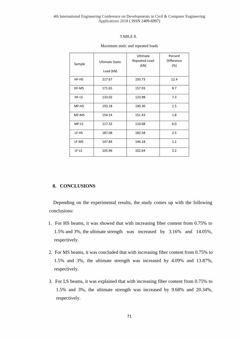
4th International Engineering Conference on Developments in Civil & Computer Engineering
Applications 2018 ( ISSN 2409-6997)
71
TABLE 8.
Maximum static and repeated loads
Sample
Ultimate Static
Load (kN)
Ultimate
Repeated Load
(kN)
Percent
Difference
(%)
HF-HS 217.67 193.73 12.4
HF-MS 171.65 157.93 8.7
HF-LS 133.02 123.98 7.3
MF-HS 193.18 190.30 1.5
MF-MS 154.14 151.43 1.8
MF-LS 117.32 110.68 6.0
LF-HS 187.08 182.58 2.5
LF-MS 147.84 146.18 1.1
LF-LS 105.96 102.64 3.2
8. CONCLUSIONS
Depending on the experimental results, the study comes up with the following
conclusions:
1. For HS beams, it was showed that with increasing fiber content from 0.75% to
1.5% and 3%, the ultimate strength was increased by 3.16% and 14.05%,
respectively.
2. For MS beams, it was concluded that with increasing fiber content from 0.75% to
1.5% and 3%, the ultimate strength was increased by 4.09% and 13.87%,
respectively.
3. For LS beams, it was explained that with increasing fiber content from 0.75% to
1.5% and 3%, the ultimate strength was increased by 9.68% and 20.34%,
respectively.

4th International Engineering Conference on Developments in Civil & Computer Engineering
Applications 2018 ( ISSN 2409-6997)
72
4. To increase the ultimate strength, the addition of steel ratio has much higher effect
than increasing fiber content.
5. For identical beams, the strength will be lower when applying repeated load other
than static one due to the effect of fatigue in the times of loading and unloading
processes. The results showed that HF-HS beams had maximum percent of
variation between ultimate static load and ultimate repeated load (12.4%),
however, LF-MS showed the minimum value (1.1%).
6. With specific fiber content the specimens with high steel ratio had the highest
toughness, the specimens with medium steel ratio showed intermediate
toughness, and the specimens with the minimum steel ratio showed the lowest
toughness.
ACKNOWLEDGEMENTS
Many thanks to Bakhtiar A. Muheiddin for his supporting in my study and research
and I ask Allah to put his pure soul in paradise.

4th International Engineering Conference on Developments in Civil & Computer Engineering
Applications 2018 ( ISSN 2409-6997)
73
REFERENCES
[1] Hillerborg, A., "Analysis of one single crack in fracture mechanics of
concrete", edited by F.H. Wittmann, Elsevier Science Publishers B.V.,
Amsterdam, 1983, pp. 223-249.
[2] Victor C. Li, "Engineered cementitious composite for structural applications",
ASCE J, Materials in Civil Engineering, Vol. 10, No. 2, 1998, pp. 66-69.
[3] Iraqi Specification No.05, "Portland cement", Baghdad, Iraq, 1984, (In Arabic).
[4] ASTM C494/C 494M-99a, "Standard Specification for Chemical Admixtures
for Concrete", Annual Book of ASTM Standards, pp. 9.
[5] ASTM A 370-03a, "Standard test methods and definitions for mechanical
testing of steel products", Annual Book of ASTM Standards, pp. 49.
[6] Salahuddin Qudah, Mohamed Maalej, "Application of engineered cementitious
composites (ECC) in interior beam–column connections for enhanced seismic
resistance", Engineering Structures, Vol. 69, 2014, pp. 234-245.
[7] ASTM C1018-97, "Standard test method for flexural toughness and first-crack
strength of fiber-reinforced concrete (using beam with third-point loading)",
Annual Book of ASTM Standards, pp. 8.
[8] JSCE-SF4, "Method of tests for flexural strength and flexural toughness of
steel-fiber-reinforced concrete", Concr Libr JSCE, Japan Soc of Civ Eng,
Tokyo, Vol. 3, 1984, pp. 58-61.

4th International Engineering Conference on Developments in Civil & Computer Engineering
Applications 2018 ( ISSN 2409-6997)
74
AN EVOLUTIONARY MODEL FOR OPTIMIZING RAIL
TRANSIT STATION LOCATIONS
Chro H. Ahmed1, Hardy K. Karim2,Hirsh M. Majid3
1,2&3University of Sulaimani, Iraq. [email protected],2 [email protected] ,[email protected]
doi:10.23918/iec2018.06
ABSTRACT
Optimizing rail transit station locations is a very complex engineering problem. The
requirements and constraints that should be considered in locating rail transit stations
are complex and interrelated. Although several optimization models have been
developed to solve the rail transit station location problem, most of them focus on a
single objective and only yield a suboptimal solution to the problem. Multiple-
objective models for optimizing rail transit station locations are rare in the literature
and their capabilities are very limited. This paper, addresses the limitations in the
existing models by developing an evolutionary model, taking into account various
local conditions and the multiple planning requirements that arise from passenger,
operator and the community to optimize station locations. The model uses an
evolutionary solution algorithm (a search algorithm that imitates the natural evolution
process) based on genetic algorithm (GA) integrated with geographic information
system (GIS) tools to perform the optimal search. The model was applied to an
artificial case study and the results demonstrate that the model can optimally locate
stations that satisfied the identified planning requirements and constraints.
Keywords: Rail Transit Station, Optimization, Genetic algorithm, GIS.

4th International Engineering Conference on Developments in Civil & Computer Engineering
Applications 2018 ( ISSN 2409-6997)
75
1. INTRODUCTION
Continuous growth of urban areas and associated needs for mobility have given
rise to the need for building new rail transit systems or expanding existing ones. A rail
transit system can play a crucial role in reliving transport problems, such as
congestion, increased travel time and air pollution. At the same time, it can also
provide safe, reliable and convenient service for population within major corridors
and to important activity areas. However, the establishment of a rail transit system
requires massive investments and exerts permanent impacts on the travel pattern, land
use development and even environmental characteristics across potential service
areas. Therefore, its actual implementation requires rigorous planning and evaluation
processes. The planning of a rail transit system involves determination of station
locations and network of lines linking the stations. It is, however, a truism that rail
transit stations represent a point at which people can have access to a rail transit
system and that it is an important factor for a rail transit system to be selected as an
alternative transport mode. Therefore, rail transit stations represent a crucial part of
the planning process. The determination of station locations requires consideration of
various local factors including travel demand patterns, land use patterns, existing
transport network, and topography while satisfying a number of complex and
interrelated requirements of the various rail transit system stakeholders (passenger,
operator and the community). This necessitates the application of optimization models
to achieve an optimal (reliable and cost effective) solution. Subsequently, this paper
formulates the rail transit planning process as an optimization problem to seek the
optimal locations of stations. It is, however, difficult to model the rail transit station
requirements with simple mathematical functions due to their complexities which
involve non differentiable, nonlinear, discontinuous structure. Therefore, an
evolutionary optimization algorithm based on a GA is designed to efficiently solve
the problem. A GA is an evolutionary optimization technique widely utilized for
solving various complex problems. Following the concept of biological evolution, a
GA evolves a population of different alternative solutions towards the optimal
solution. The evolution begins with a population of random alternative solutions and
progresses over a number of generation/iterations. In each generation/iteration, the
fitness of the population is evaluated with respect to the desired objectives of the
problem. Thereafter, a number of individuals are selected stochastically from the

4th International Engineering Conference on Developments in Civil & Computer Engineering
Applications 2018 ( ISSN 2409-6997)
76
current population based on their fitness values and modified with genetic operators
(crossover and mutation) to produce a new population for the next
generation/iteration. This process is continued until a specified number of
generations, which is fixed a priori, either have elapsed or other predetermined
convergence criteria are met [1, 2].
1. LITERATURE REVIEW
Many researchers and planners have made many attempts to develop various
optimization models for solving rail transit station location problem. Vuchic and
Newell [3] developed an analytical model to determine spacing between stations along
a predetermined rail line. With respect to the objective of minimum passenger travel
time, the model calculated interstation spacing by solving a set of partial differential
equations specifying the optimality condition. Vuchic [4], Kikuchi and Vuchic [5],
and Wirasinghe [6], considered various improvements to the Vuchic and Newell’s
approach for determining the optimal station spacing. However, these models have
only limited practical applications due to oversimplification of the problem by
assuming uniform distribution of population along rail transit lines and that the
population of an area served by the rail line commutes to one central points. Recent
studies therefore, attempted to further improve these models through removing
unrealistic assumptions and incorporating various planning and real world constraint
requirements. Laporte et al., [7] developed a model for locating a prefixed number of
stations on a predetermined rail transit alignment with the objective to maximize
population coverage while satisfying interstation spacing constraint. The study
estimated the demand for each potential station by triangulation of census tracts,
assuming that the percentage of the captured travellers decreases with their access
distance from the station. Schöbel et al. [8] presented a model to locate additional
stations along existing rail line networks, considering the trade-off between positive
and negative effects of additional stations. The objective of the model was to minimize
the number (cost) of additional stations while ensuring coverage of all demand
centers. The demand center, which may represent a settlement area, shopping center,
school, etc., was assumed to be covered if the next station was within a specified
radius from it. In an extended effort, Hamacher et al. [8] built up on Schöbel et al. [9]

4th International Engineering Conference on Developments in Civil & Computer Engineering
Applications 2018 ( ISSN 2409-6997)
77
study by seeking to satisfy two different objective functions of demand covering and
accessibility to stations. Following the same approach, Carrizosa et al. [10] proposed
a model seeking a set of additional stations covering all demand centers but, instead
of minimizing the number of additional stations, the additional passenger travel time
due to the additional stations were minimized. In another study, Jha and Oluokun [11]
addressed the determination of the optimal station locations along a predetermined
rail transit alignment using artificial intelligence based optimization techniques and
GIS. Similarly, using GIS tools Samanta and Jha [12] used GA to seek the best set of
station locations along a rail transit line to minimize total system cost while ensuring
that the interstation distances remain constraints. The model defined the total system
as a function of passenger total travel time, system operation and construction costs.
Despite the capabilities of the aforementioned optimization models in addressing
many aspects of rail transit station locations, most of them have a number of
limitations that necessitate further improvements in order to achieve optimal (reliable
and cost effective) solution to the problem. These limitations include: (a) primarily,
many of these models neglect initial feasibility study to identify potential station
locations, assuming that rail transit stations can be located anywhere in the study area
or along the rail transit line without considering the various environmental,
topological and budget constraints; (b) most of these models disregard the effects of
various local factors of the study area , such as land use pattern, land values, existing
roadway network and topography on the overall system performance and cost and; (c)
many of these models address partial aspects of the problem by focusing mainly on
the coverage of traffic demand or population with other critical passenger, operator
and community related aspects being ignored. This paper addresses these limitations
by developing a new evolutionary based model integrated with GIS tools to determine
the optimal set of station locations for a rail transit line. The proposed model takes
into account initial feasibility of station sites, various local factors and multiple
planning requirements that arise from passenger, operator and the community.

4th International Engineering Conference on Developments in Civil & Computer Engineering
Applications 2018 ( ISSN 2409-6997)
78
3. THE MODEL FRAMEWORK
The model framework comprises two stages, as shown in Figure 1. In the first
stage, the model measures the feasibility of station sites to identify a pool of feasible
station locations using a GIS-based algorithm. In the second stage, the model selects
the best set of stations from the feasible station pool identified in the first stage using
an optimization procedure based on a GA while interacting with GIS supporting
system. Once the optimal station locations are determined, they are connected to
obtain the rail line alignment. However, since the focus of this paper is to find optimal
station locations along a rail transit line, it is assumed that the final alignment of the
rail line is obtained through the linear connections of the stations. The mathematical
formulations of these two stages are discussed and detailed in the next section.
FIGURE 1. The Model Framework
4. MATHEMATICAL FORMULATION
As mentioned in section 3, prior to the optimization process the model evaluates
the feasibility of station locations to identify a candidate pool of stations using a GIS-
based algorithm. Performing such a feasibility analysis can effectively speed up the
planning process and improve decision-making in selecting reliable and cost effective
solutions. This is by: (1) excluding environmental protected areas that may result in
significant unnecessary increases in the station construction cost from the
optimization search space. In addition, the exclusion of these areas results in
significant decreases of computation time in exploring unnecessary areas of the search
space (2) identifying areas that have high intensity of residential and commercial land
use areas . The coordination of rail transit stations with these land use areas can
significantly increase the number of potential passengers utilizing the system, which
Stage 1:
• Identify a candidate pool offeasible station locations using aGIS based algorithm.
Stage 2:
• Identify an optimum subset ofthe feasible stations within acontext of an optimizationprocess using GA integrated withGIS tools.

4th International Engineering Conference on Developments in Civil & Computer Engineering
Applications 2018 ( ISSN 2409-6997)
79
in turn results in reduced overall vehicle travel, and thereby reduced traffic congestion
and improved mobility. The proposed GIS-algorithm applies the following three main
steps to screen the potential served area and perform evaluation analysis for generating
a pool of feasible station locations.
Step 1: dividing the study area into grids (Gi) and creating a GIS layer for stations
(Ω𝑠𝑡). It is assumed that each of the generated grids represents a potential location for
a rail station. The size of each grid, therefore, should represent the typical size of a
rail station.
Step 2: finding all station grids that intersect with environmentally protected areas and
excluding them from the search space of feasible station locations. This is done by
laying the generated station grid layer (Ωst) over the environmentally sensitive areas
layers (Ωenv) to generate the feasible grid layer for station(Ωfs). The environmentally
protected areas include historic buildings, green parks, woodlands, rivers and sites of
scientific interest.
Ω𝑓𝑠 = Ω𝑠𝑡 ∩ Ω𝑒𝑛𝑣 (1)
Step 3: identifying all the grids within the feasible station layer (Ωfs) with the average
commercial land use areas within the defined walking distance of stations greater than
the pre-specified threshold value of commercial land use areas and assigning them
with an integer value. In this paper, the commercial land uses areas include
recreational centers, shopping malls, office complexes, industrial complexes and
university campuses.
∀𝐺𝑖 ∈ Ωfs →= 1 𝑖𝑓 (∑ 𝐶𝐴 |Dw) ≥ VCA (2)
Where: 𝐶𝐴 is the average commercial land use areas within walking distance of
station; Dw is the defined walking distance to stations and; VCA is the pre-specified
threshold value of average commercial land use areas within Dw.
Step 4: identifying all the grids within the feasible station layer (Ωfs) with the average
population density within the defined walking distance of stations greater than the pre-
specified threshold value of population density and assigning them with an integer
value.

4th International Engineering Conference on Developments in Civil & Computer Engineering
Applications 2018 ( ISSN 2409-6997)
80
∀𝐺𝑖 ∈ Ωfs →= 1 𝑖𝑓 (∑ 𝑃𝐷 |Dw) ≥ VPD (3)
Where: 𝑃𝐷 is the average population density within Dw and; VPD is the pre-specified
threshold value of average population density within Dw.
Once the pool of feasible station locations is generated, the model selects the best set
of stations from the generated pool within the context of an optimization procedure
using an evolutionary search algorithm based on a GA supported by a background
GIS database. The optimization framework is designed to accommodate various local
factors, incorporate multiple objectives and constraints that arise from passenger,
operator and community requirements and compute the optimal solution. The
objective of the optimization process is to minimize passenger, operator and
community costs. The following are key steps of the developed GA based
optimization algorithm:
Step 1: generating the alternative solutions (i.e., population) by randomly selecting a
set of stations (Si) from the station pool generated in the first stage and connecting
them linearly while ensuring that: (a) the number of the selected stations falls within
predefined minimum (Nsmin) and maximum (Nsmax) limits set by rail transit system
planners and; (b) the distance between selected stations fall within predefined
minimum (∆smin) and maximum (∆smax) station spacing. It is assumed that,
depending on the major traffic flow patterns of the area to be served, rail transit system
planners are able to locate the terminal stations prior to the optimization process. That
is, the model seeks the best locations of intermediate stations.
Step 2: evaluating the fitness value of each alternative solution which is a function of
three main components; passenger, operator and community costs.
𝑇𝐶 = 𝑃𝐶 + 𝑂𝐶 + 𝐶𝐶 (4)
Where: 𝑇𝐶 is the total system cost ($), 𝑃𝐶 ,𝑂𝐶, 𝐶𝐶 are the passenger, operator and
community costs ($) respectively.
PC = Ta × A0 + Tw × W0 + Tt × T0 (5)

4th International Engineering Conference on Developments in Civil & Computer Engineering
Applications 2018 ( ISSN 2409-6997)
81
Where: Ta is the passenger’s access time to/from station (min); A0 is the costs of
access time ($/min); Tw is waiting time at station (min); W0 is the cost of waiting time
($/min); Tt is on train travel time (min) and; T0 is the unit cost of on train travel time
($/min). The passenger access time to/from rail stations is a function of the passenger
walking distance and speed to/from stations. It is computed through artificial links
that created between traffic analysis zones (TAZs) and feasible station locations.
These links measure the distance between the centroids of the each TAZ and feasible
station location (Da), thus the access time is calculated by dividing this distance (Da)
to passenger walking speed (Va). The waiting time is assumed to be equal to half of
the train headway (𝐻𝑤) which is a function of train frequency. The on-train travel
time is calculated by dividing the distance between boarding and alighting station (𝐷𝑠)
by the train speed (𝑉𝑡).
𝑂𝑐 = 𝐿𝑡 × 𝑀0 (6)
Where: 𝐿𝑡 is the total train km travelled distance and ; 𝑀0is the unit operation and
maintenance cost for train ($/km).
𝐶𝐶 = 𝐿𝑆 + 𝐵𝑠 (7)
Where: 𝐿𝑆 is the land acquisition cost for stations ($); 𝐵𝑠 is the cost of building
stations ($). The land acquisition costs are fed into the evaluation process via
interaction with GIS while the cost of building stations is assumed to be fixed.
Step 3: evolving the initial solutions generated in step 1 over a series of
generations/iterations based on their fitness values calculated in step 2 to converge
towards the optimal solution. This is by applying three genetic operators, selection,
crossover and mutation, adopting the approach developed by [13].
Step 4: terminating the evolution process when searching through the predefined
number of generations is reached or improvement in the objective function value is
negligible (less than 1%).

4th International Engineering Conference on Developments in Civil & Computer Engineering
Applications 2018 ( ISSN 2409-6997)
82
5. CASE STUDY
The effectiveness of the proposed model was examined by applying it to an
artificial case study. The size of the case study was 36 km2 (8.0 km x 4.5 km). Each
of the land use pattern, population density and land value datasets were created
artificially for the study area and digitized for the analysis purpose. The land use
pattern dataset contained commercial land use areas and environmentally protected
areas. As discussed in section 4, the commercial land use areas include recreational
centers, shopping malls, office complexes, industrial complexes and university
campuses while the environmentally protected areas include historic buildings, green
parks, woodlands, rivers and sites of scientific interest. After the preparation of the
required datasets and defining the model input parameters, the model was
implemented. Figure 2 presents the candidate pool of feasible station locations
generated in stage 1 of the model evaluation process. It is very interesting to note that
the candidate feasible stations mainly cover the most densely populated and
commercial areas of the study area. This is in addition to excluding the
environmentally protected areas from the search space. These results indicate that
screening the study area for feasible station locations prior to the optimization process
plays an important role in directing the search towards the promising region of the
search space.
FIGURE 2. Generated Feasible Station Locations

4th International Engineering Conference on Developments in Civil & Computer Engineering
Applications 2018 ( ISSN 2409-6997)
83
Figure 3 shows the best locations of stations, obtained in stage 2 of the model
evaluation process, which were selected from the generated feasible station pool. The
optimal solution consists of 7 stations, covering more than 138,700 people within 800
meters walking distance of stations, which comprises almost 27 percent of the case
study’s total population. Furthermore, the obtained solution covers more than 45
percent of the case study’s commercial areas, which include recreational areas,
shopping malls, office complexes and industrial complexes within 800 meters walking
distance of the stations. These results, therefore, indicate that the model can
effectively find a robust and reliable solution.
FIGURE 3. Optimized Station Locations
6. CONCLUSION
This paper presented an evolutionary optimization model for locating rail transit
stations. The model first evaluated the feasibility of the potential served area to
generate a pool of feasible stations considering various local and environmental
factors. The best set of these feasible stations were then selected within the context
of an optimization process using GA while interacting with GIS supporting system.
The optimization framework accommodated complex correlation and interaction of
the multiple requirements and constraints arising from different rail transit system
stakeholders; passenger, operator and the community, and made trade-off between
them in order to achieve a reliable and cost effective solution. To demonstrate its

4th International Engineering Conference on Developments in Civil & Computer Engineering
Applications 2018 ( ISSN 2409-6997)
84
effectiveness in finding good solutions, the model was applied to an artificial case
study. The results revealed that the model can effectively resolve the essential trade-
off between minimum passenger travel time and operation and maintenance cost on
the one hand, and the minimum construction cost of the stations on the other hand,
while also satisfying various constraints. Furthermore, the results revealed that
performing a feasibility analysis for potential station locations prior to the
optimization process can effectively improve the performance of the model to realize
an optimal (reliable and cost effective) solution, by directing the search to explore the
most promising regions in the search space.
REFERENCES
[1] Goldberg, D. E., Genetic Algorithms in Search, Optimization, and Machine
Learning, Massachusetts: AddisonWesley, 1989.
[2] Goldberg , D. E. and Deb, K. , "A comparison analysis of selection schemes used
in genetic algorithms", in Foundations of Genetic Algorithms, G.J. E. Rawlins,
Ed. California: Morgan Kaufmann, 1991.
[3] Vuchic, V. R. and Newell, G. F., "Rapid transit interstation spacings for minimum
travel time," Transportation Science, Vol.2, (4) pp. 303-309,1968.
[4] Vuchic, V. R., "Rapid transit interstation spacings for maximum number of
passengers,"
Transportation Science, Vol.3, (3) pp. 214-232, 1969.
[5] Kikuchi, S. and Vuchic, V. R., "Transit vehicle stopping regimes and spacings,"
Transportation Science, Vol.16, (3) pp. 311-331, 1982.
[6] Wirasinghe, S. C. and Vandebona., U., "Some aspects of the location of subway
stations and routes, " in Fourth International Symposium on Locational Decisions
(ISOLDE), Belgium, 1987.
[7] Laporte, G., Mesa, J. A. and Ortega, F. A., "Locating stations on rapid transit
lines," Computers& Operations Research, Vol.29, (6) pp. 741-759, 2002.

4th International Engineering Conference on Developments in Civil & Computer Engineering
Applications 2018 ( ISSN 2409-6997)
85
[8] Schöbel, A., Hamacher, H., Liebers, A. and Wagner, D., "The continuous stop
location problem in public transportation networks," Technical Report 81,
Wirtschaftsmathematik, University of Kaiserslautern, Germany, 2002.
[9] Hamacher, H. W., Horn, S. and Schöbel, A., "Stop location design in public
transportation
networks: Covering and accessibility objectives," TOP, Vol.17, (2) pp. 335-346,
2009.
[10] Carrizosa, E., Harbering, J. and Schöbel, A., "Minimizing the passengers’
traveling time in the stop location problem," Journal of the Operational Research
Society, Vol 67,(10) pp. 1325-1337, 2016.
[11] Jha, M. K. and Oluokun, C., "Optimizing station locations along transit rail
lines with geographic information systems and artificial intelligence", in
Computers in Railways IX, Allan, J., Brebbia, C.A., Hill, R.J., Sciutto, G., Sone,
S. , Eds. Southampton: WIT Press, 2004.
[12] Samanta, S. and Jha, M., "Identifying feasible locations for rail transit stations:
Two-stage analytical model," Transportation Research Record, (2063) pp. 81-88,
2008.
[13] Chro, A. , "GIS and genetic algorithm based integrated optimization for rail
transit system planning, " Ph.D. dissertation, Imperial College London, London,
UK, 2016.

4th International Engineering Conference on Developments in Civil & Computer Engineering
Applications 2018 ( ISSN 2409-6997)
86
THERMAL AND FINANCIAL EVALUATIONS OF MUNICIPAL
SOLID WASTE FROM ERBIL CITY-IRAQ
Shuokr Qarani Aziz1,Jwan Sabah Mustafa2
1Salahaddin University-Erbil, Iraq
2General Directorate of Dams and Reservoirs, Erbil [email protected], [email protected],[email protected], [email protected]
doi:10.23918/iec2018.07
ABSTRACT
This work was aimed to study municipal solid waste (MSW) disposal problems and
energy income from it. Open dumpsite and only buried of MSW causes risks to the
people and the environment. Burring mixed MSW (without separation, leachate and gas
collection) at Erbil Landfill Site (ELS) leads to leftover income and energy. Recyclable
materials such as plastic, metals, glass, paper and cartons at ELS are income sources.
Results revealed that average amount of daily disposed plastic, food waste, corrugated
paper, other organics, wood, diapers, other inorganics, ferrous, and glass at ELS were
34%, 27%, 14%, 7%, 6%, 5%, 2%, 2%, 2%, and 1%, respectively. Additionally, thermal
solution is required to convert the MSW and natural emitted gas from ELS to be a great
source for the energy. Currently, produced methane gas and electricity from ELS are
estimated to be 3,839,669.265 m3 and 18,000.762 Kw for 1,223,834 populations,
respectively. Expected annual income from recyclable materials is 97.528 *106 $.
Finally, proper solution for disposed of MSW in Erbil City results in decreasing risks
and environmental pollution, attainment of income by recyclable materials and release
energy from gas and electricity.
Keywords: Solid waste, Methane gas, Energy, Income, Erbil City, Landfill.

4th International Engineering Conference on Developments in Civil & Computer Engineering
Applications 2018 ( ISSN 2409-6997)
87
1. INTRODUCTION
Communal systems for disposal and treatment of municipal solid waste (MSW) are
open dumping, sanitary landfill, thermal treatment (anaerobic, pyrolysis, incineration,
gasification, and plasma arc gasification) and composting. Technical landfills has been
discovered to be the utmost economic MSW disposal method when equated with other
systems of disposal, such as thermal and composting [1-3]. But the produced landfill
leachate and gas emissions are common shortcomings of the MSW [4-5]. Without
scientific solution, disposed landfill leachate and emitted gas from Erbil Landfill Site
(ELS) cause pollution of the environment.
ELS regards as anaerobic landfill with daily cover-Level II [6]. In type II landfills,
proper gas and leachate managements are not available [7]. Organization of emitted gas
leads to decreasing environmental pollution and achieving income from the produced
energy.
Increments of population numbers, growth of investment and economy, tourist, and
industrialization are between the key parameters that promote the generation rate of
MSW. Disposal of around 2000 tons/day of mixed MSW at ELS requires sufficient
landfilling area, proper design, and management [8]. Issues on the engineering designs
of landfill sites can often be detected in the developing countries, such as Iraq. Presently,
more than 40 open dumpsites and landfills are available in Erbil City- Iraq. Most of the
landfills consist only of dumping sites of mixed MSW without any managements to
protect environment [6]. In addition, mixed disposed MSW leads to rapid finishing of
landfill areas and lost huge income from daily covering the recyclable materials by soil.
A study on domestic solid waste components published by [2]. The percentage of the
recyclable materials plastic, metals, glass, and papers were 6.28%, 3.6%, 3.42%, 5.9%,
respectively. The average amount of recyclable materials is more than 30 % in southern
Asia Nations [7]. Based on the study conducted by Erbil Municipality in 2016, the
percentage amount for plastic, food waste, paper, other organics, wood, diapers, other
in-organics, ferrous, glass, and aluminum are 34%, 27%, 14%, 7%, 6%, 5%, 2%, 2%,
2%, and 1%, respectively [8].The disposed MSW at ELS is a massive amount which
results environmental pollution and losing of affordable amount of money.

4th International Engineering Conference on Developments in Civil & Computer Engineering
Applications 2018 ( ISSN 2409-6997)
88
The objectives of the present work were: 1) to study the achievable income from
recyclable MSW materials and 2) feasible produced energy (methane gas and
electricity) from disposed MSW in Erbil City.
2. MATERIALS AND METHODS
The current work presented the ELS problems, especially mixed MSW without
separation and emitted gas, and attainment of income and energy from MSW at ELS.
The data were obtained from literature and Presidency of Erbil Municipality [2-6, 8-9].
To see the risks directly and to get extra information, site visit were carried out to ELS
in June and November 2017. The quantity of produced methane gas and energy was
based on equations and information from references [9-12]. Information and data given
in the present research were obtained from published works, presidency of Erbil
Municipality and administration staff for ELS and it became a scientific document for
the upcoming works. The details for ELS, recyclable materials, and energy production
are shown below.
2.1 ELS (ERBIL LANDFILL SITE)
ELS is located on the left side of Erbil-Mosul main road near Kani-Qrzhala Sub-
district in Erbil City, Iraq. The geographical coordinates are 36°10'23'' N and 43°35'32''
E. It is opened in 2001 and it is approximately 15 km from Erbil City center. The total
site area of ELS is 37 ha. Most part of the area has been used. In 2017, the site receives
about 2000 tons of mixed MSW daily (Based on Administration Staff of ELS, 5
November 2017), Figure 1:
FIGURE 1. Satellite image of Erbil Landfill (Kani-Qrzhala) site.

4th International Engineering Conference on Developments in Civil & Computer Engineering
Applications 2018 ( ISSN 2409-6997)
89
The buried MSW is mixed without proper separation of the components. A small portion
of recyclable materials, such as plastic, glass, and metals, are being separated by
scavengers persons. Due to lack of scientific sanitary landfill design in this site, the
formed gas is emitted to the atmosphere without any gas collection system which can be
used as renewable source of energy, Figures 2 and 3.
FIGURE 2. Gas emission at ELS (13 June 2017)
FIGURE 3. Separation and collection of recyclable MSW at ELS (13 June 2017)

4th International Engineering Conference on Developments in Civil & Computer Engineering
Applications 2018 ( ISSN 2409-6997)
90
2.2 RECYCLABLE MATERIALS
In this research, recyclable materials for MSW at ELS represent plastic, metals, glass,
and papers [9].
2.3 ENERGY PRODUCTION
2.3.1 METHANE GAS PRODUCTION
Usually, proper landfill management required to enhance both yield and quality of
gas. In order to estimate gas production, four parameters should be known which are: (a)
gas yield per unit weight of waste, (b) the lag time prior to gas production, (c) the shape
of the lifetime gas production curve, (d) and the duration of gas production [10].
An equation is used to determine gas production, which published by Environmental
Protection Agency (EPA) and the model called Landfill Gas Emission Model (Land
GEM), and the equation ranging from single value to linear increase/ linear decline, to
exponential decline as follow [10]:
𝑸𝑻 = ∑ 𝟐𝒌𝑳°
𝒏
𝒊=𝟏
𝑴𝒊𝒆𝒆−𝒌𝒕𝒊 (𝟏)
Where:
QT = total gas emission rate from a landfill, volume/time.
n = total time periods of waste placement.
k = landfill gas emission constant, time -1.
Lₒ= methane generation potential, volume/mass of waste.
ti = age of the ith section of waste, time.
Mi = mass of wet waste, placed at time i.
Erbil landfill opened in 2001 year, and it receiving 2000 tons/day, which means 730,000
tons/year. Assume landfill emission gas constant is (0.0307 year-1), and the methane
generation potential is (140 m3/tons), to estimate peak gas production:
For the first year of opening in (2001):
QT= 2(0.0307)*(140)*(730,000)*(e -0.0307(1) )
QT=6,085,362.114 m3

4th International Engineering Conference on Developments in Civil & Computer Engineering
Applications 2018 ( ISSN 2409-6997)
91
For age at ti =15 (in 2016)
QT= 2(0.0307)*(140)*(730,000)*(e -0.0307(15) )
QT=3,959,375.196m3
For age ti =16 (in 2017)
QT= 2(0.0307)*(140)*(730,000)*(e -0.0307(16) )
QT=3,839,669.265 m3
2.3.2 POWER GENERATION
The generation rate (GR) of disposed garbage, plastic, paper and fabric = 608.02
g/cap/d (excluding glass and metals) [2, 9].
608.02 g/cap/d = 1.34 Ib/cap/d
Energy available in each 105 population [9, 11-12].
= 1.34 * 105*4500/24
= 2.51 * 107 BTU/h
Where BTU is British thermal unit
But, the efficiency is 20% and the theoretical value of the mechanical equivalent of heat
is 3413 BTU/h. Therefore the heat rate is:
3413 / 0.2 = 17065 BTU / KWh
Energy generated (KW) = rateheat
fuelin availableHeat
= 2.51 * 107 / 17065
= 1470.85 KW for each 105 population
For population of 1,223, 834 [8]:
Energy generated (KW) = 18000. 762 for 1,223, 834 populations
For MSW at ELS, GR= 1270 g /cap/d =2.803 Ib/cap/d [8].
Energy available in each 105 population
= 2.803 * 105*4500/24
= 5.256 * 107 BTU/h
Disposed MSW at ELS produces from 1,223, 834 [8]:
Energy available for 1,223, 834 populations = 6.432 * 108 BTU/h

4th International Engineering Conference on Developments in Civil & Computer Engineering
Applications 2018 ( ISSN 2409-6997)
92
3. RESULTS AND DISCUSSIONS
3.1 CURRENT SITUATION OF ELS
ELS considered as Level 2, which is sanitary landfill with daily cover, and anaerobic
landfill, it also in the methane formation phase [6]. Based on the landfill structures shown
in literature, upgrading the site from Level 2 to Level 3 Level 4 is essential [2]. Disposal
of mixed MSW at ELS leads to terminate the provided areas for Landfilling. A part of
recyclable materials is separated by scavengers only, Figures 3-4. Providing suitable
system for separation of recyclable materials is recommended. In addition, a mixed-
waste materials recovery facility (MRF) technology is recommended [9]. On the other
hand, formed landfill leachate still discharges to the natural environment without
treatment [3-4, 13].
FIGURE 4. Collected recyclable materials by scavengers at ELS (5 November 2017)
3.2 INCOME FROM RECYCLABLE MATERIALS
Recycling is an important subject in life, especially when it used final disposal
products and again reused [14]. The recycling targets of the global waste management
system, therefore focusing on the complete waste collection in future, and the
achievement of waste management in study area. Therefore the necessary recycling
facility required, but the waste still not separately collected. The aim of MSW recycling
programs should not be to increase MSW recycling [15]. The objective should be to
upgrade environmental quality and the sustainability of the economy, and from
construction and demolition materials.
Recycling of MSW materials lead to achieving income, decreasing amount of MSW in
landfills, minimizing environmental pollution, decreasing number of MSW collector
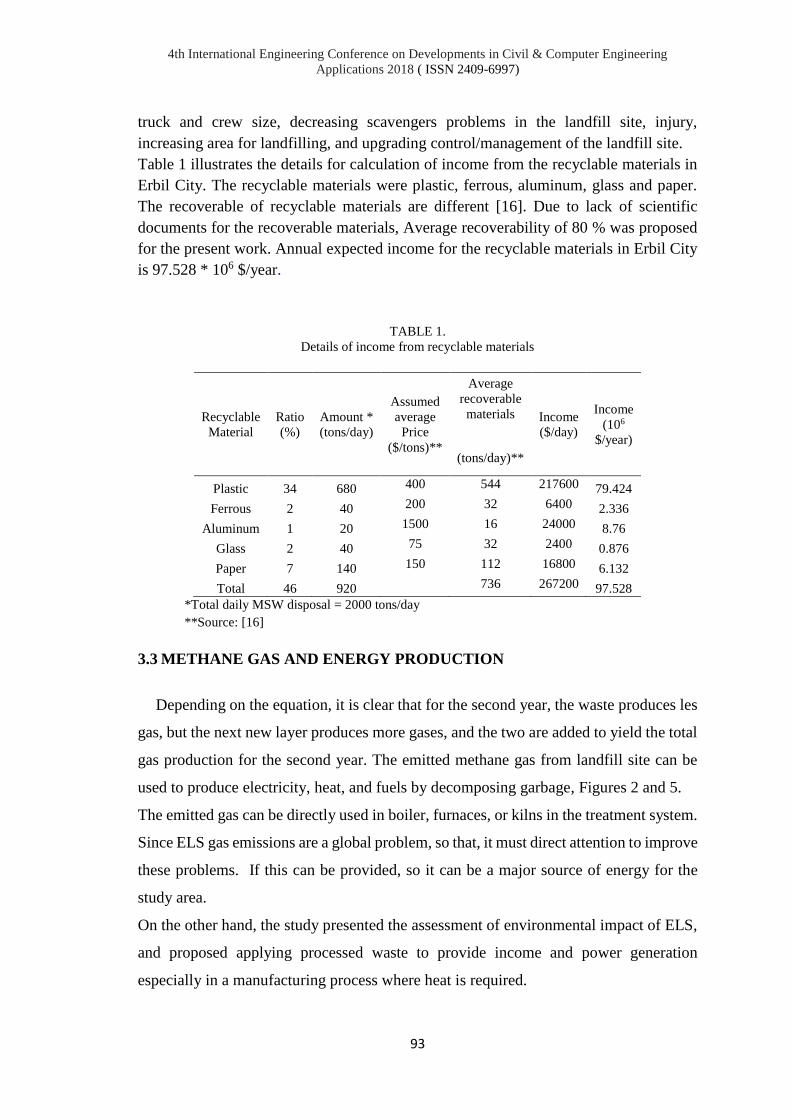
4th International Engineering Conference on Developments in Civil & Computer Engineering
Applications 2018 ( ISSN 2409-6997)
93
truck and crew size, decreasing scavengers problems in the landfill site, injury,
increasing area for landfilling, and upgrading control/management of the landfill site.
Table 1 illustrates the details for calculation of income from the recyclable materials in
Erbil City. The recyclable materials were plastic, ferrous, aluminum, glass and paper.
The recoverable of recyclable materials are different [16]. Due to lack of scientific
documents for the recoverable materials, Average recoverability of 80 % was proposed
for the present work. Annual expected income for the recyclable materials in Erbil City
is 97.528 * 106 $/year.
TABLE 1.
Details of income from recyclable materials
Recyclable
Material
Ratio
(%)
Amount *
(tons/day)
Assumed
average
Price
($/tons)**
Average
recoverable
materials Income
($/day)
Income
(106
$/year)
(tons/day)**
Plastic 34 680 400 544 217600 79.424
Ferrous 2 40 200 32 6400 2.336
Aluminum 1 20 1500 16 24000 8.76
Glass 2 40 75 32 2400 0.876
Paper 7 140 150 112 16800 6.132
Total 46 920 736 267200 97.528
*Total daily MSW disposal = 2000 tons/day
**Source: [16]
3.3 METHANE GAS AND ENERGY PRODUCTION
Depending on the equation, it is clear that for the second year, the waste produces les
gas, but the next new layer produces more gases, and the two are added to yield the total
gas production for the second year. The emitted methane gas from landfill site can be
used to produce electricity, heat, and fuels by decomposing garbage, Figures 2 and 5.
The emitted gas can be directly used in boiler, furnaces, or kilns in the treatment system.
Since ELS gas emissions are a global problem, so that, it must direct attention to improve
these problems. If this can be provided, so it can be a major source of energy for the
study area.
On the other hand, the study presented the assessment of environmental impact of ELS,
and proposed applying processed waste to provide income and power generation
especially in a manufacturing process where heat is required.

4th International Engineering Conference on Developments in Civil & Computer Engineering
Applications 2018 ( ISSN 2409-6997)
94
By using refused derived fuel (RDF) for the purpose of achieving high calorific fractions
from processed (MSW) and industrial wastes or any other wastes are alternative to
convert (waste to energy) plants.
RDF production appear most common way to achieve relatively high levels of recycling
and composting ELS as high rates of source separation leave non-recyclable residues,
which are suitable for RDF production.
Even in cities where the source of separation is not so well-developed, and where the
source of separation with or without residual waste processed, it might be sufficient to
get the landfill directive target, especially in waste management system will be very
important.
In the present work, the expected total gas emission rate (QT) form ELS in 2017 is
3,839,669.265 m3 which is huge amount and need proper management. Estimated
electric energy generation is 18,000.762 KW for 1,223, 834 populations. Authority has
problem for supplying 24 hours electricity for Erbil population due to loses and bad using
of electricity, increasing population number etc. Finding another source for supplying
electric with 18,000.762 KW from disposed MSW to Erbil City is very important and
leads to environmental pollution. Furthermore, predictable energy available for 1,223,
834 populations in Erbil City is 6.432 * 108 BTU/h. Nowadays, achieving this quantity
of energy to Erbil City from discarded MSW is so valuable and results in decreasing
pollution in the city.

4th International Engineering Conference on Developments in Civil & Computer Engineering
Applications 2018 ( ISSN 2409-6997)
95
FIGURE 5. Gas emission from ELS (5 November 2017)
4. CONCLUSIONS
In this study, it was observed that there is a lack from MSW management as ELS. Gas
emission, leachate production, burring and inadequate of recyclable materials, and non-
acceptable view are main characteristics of ELS. A number of buildings and facilities
such as offices for administration, laboratory, guard house, weighing station, storerooms,
fence, gas collection, leachate collection and treatment unit, and wells for groundwater
monitoring are essential for ELS. Upgrading ELS from Level 2 to level 4 by proper
management for emitted gas and produced landfill leachate is recommended. Providing
suitable system for separation of recyclable materials is suggested as well. Expected
annual income from recyclable materials is 97.528 *106 $. Foreseeable quantity of
methane gas at ELS in 2017 is 3,839,669.265 m3. Predictable amount of energy and
electric from MSW at ELS are 6.432 * 108 BTU/ h and 18,000.762 KW, respectively.
Form ELS the measured methane gas from obtained data have the wide variability over
space, in some cases, the land fill has been shown to act as net sinks for atmospheric
methane, it should be incorporate to measure the influence of the produced gas and
controlling it by the presence of gas recovery wells. At different locations at ELS huge
amount of gas emitted to the environment, Figure 2. In July and August 2017, 18 gas
collection pipes were penetrated to the landfill site ground. Distances between pipes are
around 80 m and surrounded by filter materials.
For the entire ELS, a dis-acceptable view is seen. Administration building, laboratory,
drivers and labors building, guard house, garage, fence, green area, sanitary system,
weighing station etc. are essential for ELS.
The classification of solid waste form ELS revealed that most of the wastes are consists
of plastic, food waste, corrugated paper, by percentages of 34%, 27%, 14%, respectively.

4th International Engineering Conference on Developments in Civil & Computer Engineering
Applications 2018 ( ISSN 2409-6997)
96
The ratios refer to that if the waste managed properly, it can provide a very large income
and energy as well. The amount of recyclable materials from domestic wastes is 20.66%.
Due to life style and economic factors in Erbil most parts of the domestic waste is food
and organic wastes which was 79.34%.
REFERENCES
[1] Davis, M.L., Cornwell, D.A., Introduction to Environmental Engineering .4th
edition. (International Edition). McGraw Hill, New York, 2008.
[2] Aziz, S.Q., Aziz, H.A., Bashir M.J.K., and Yusoff, M.S. “Appraisal of domestic
solid waste generation, components, and the feasibility of recycling in Erbil,
Iraq”. Waste Management & Research, Vol. 29, No. 8, pp. 880-887, 2011
[3] Aziz, S.Q. and Maulood, Y.I. “Contamination Valuation of Soil and
Groundwater Source at Anaerobic Municipal Solid Waste Landfill Site”,
Environmental Monitoring and Assessment. Vol. 187, No. 12, DOI:
10.1007/s10661-015-4971-y., 2015.
[4] Aziz, S.Q., Aziz, H.A., Bashir, M.J.K., and Abu Amr, S. “Expected
environmental risks of the produced leachate from Erbil landfill site on the
surrounded water sources”. 4th International Engineering Conference (IEC4),
Gaza, Palestine. , 2012.
[5] Aziz, S.Q. “Produced Leachate from Erbil Landfill Site, Iraq: Characteristics,
Anticipated Environmental Threats and Treatment”. In 16th International
Conference on Petroleum, Mineral Resources and Development, Cairo, Egypt,
2013, Feb.10-12.
[6] Maulood, Y.I. and Aziz, S.Q. (2016) Soil and Municipal Solid Waste Leachate
Characterization at Erbil Anaerobic Landfill Site, The Official Scientific Journal
of Salahaddin University-Erbil, ZJPAS Vol. 28, No.3, 104-113.
[7] Aziz, S.Q. “Landfill Leachate Treatment Using Powdered Activated Carbon
Augmented Sequencing Batch Reactor (SBR) Process”, Ph.D. dissertation, Un
Published, School of Civil Engineering, Universiti Sains Malaysia (USM),
Malaysia, 2011.

4th International Engineering Conference on Developments in Civil & Computer Engineering
Applications 2018 ( ISSN 2409-6997)
97
[8] Presidency of Erbil Municipality (2017) A study on Erbil municipal solid waste
components, June 2016.
[9] Aziz, S.Q. “A Quantitative Study on Domestic Solid Waste Components in
Arbil City”. Zanco-Journal of Pure and Applied Sciences, Salahaddin University-
Erbil, Vol.21, No.4, (59–71), 2009.
[10] Worrell, W.A. and Vesilind, P.A. Solid Waste Engineering. Second edition,
Publisher, Global Engineering: Christopher M. Shortt, 2012
[11] Tchobanoglous, G., Theisen, H., ans Eliassen, R., Solid Waste- Engineering
principles and management issues. Second edition. McGraw-Hill International
,1993.
[12] Sabir, S. “Domestic solid waste management in Erbil City & their effects on
surface and sub-surface water”. Journal of Zanco, Vol. 14, No. 2., 2002.
[13] Aziz, S.Q., Aziz, H.A., Yusoff, M.S., Bashir M.J.K., and Umar, M. “Leachate
characterization in semi-aerobic and anaerobic sanitary landfills: A comparative
study”. Journal of Environmental Management, Vol. 91,2010, pp 2608-2614.
[14] Environmental Protection Agency (EPA) “Municipal Solid Waste Generation,
Recycling, and Disposal in the United States: Facts and Figures for 2012”, United
States, 2012.
[15] Lave, B. L., Hendrickson, C.T., Conway-Schempf, N.M., and McMichael, F. C.
“Municipal Solid Waste Recycling Issues”. Journal Of Environmental Engineering,
October 1999.
[16] COVEC, Expert Analysis plus Practical Advice “Recycling: Cost Benefit
Analysis”. Final report prepared for Ministry for the Environment, COVEC
Limited Level 11 Gen-i tower 66 Wyndham Street, PO Box 3224 Shortland Street
Auckland New Zealand, April 2007.

4th International Engineering Conference on Developments in Civil & Computer Engineering
Applications 2018 ( ISSN 2409-6997)
98
HEAVY METAL POLLUTANT LOAD FROM A MAJOR
HIGHWAY RUNOFF - SULAIMANI CITY
Yaseen Ahmed Hamaamin
University of Sulaimani, KRG, Iraq
doi:10.23918/iec2018.08
ABSTRACT
First flush is the first rainfall after a dry season, which washes out several months of
contaminant buildup. Surface runoff from highways can be considered as a critical
nonpoint source of water resources heavy metals pollution. In this study, samples of
rainfall runoff were collected after the first and second rainfall from a major highway in
Sulaimani City and tested for expected Zinc(Zn), Copper (Cu) and Lead (Pb) heavy
metals pollutants. Results revealed levels of heavy metals pollution in the highway runoff
from the first and second rainfalls which can be considered as heavy metal pollution
source for receiving water bodies. After first flush, average test results of heavy metals
pollutants were 0.062 part per million (ppm), 0.075 ppm and 0.051 ppm for Zn, Cu and
Pb respectively. Low Impact Development (LID) practices found to be a new sustainable
stormwater management. Though, the removal of heavy metals from water is costly,
consequently, a set of LID techniques are recommended for stormwater treatment as cost
effective stormwater treatment for streets and highway runoff treatment. Furthermore, as
Sulaimani city uses combined (sanitary and stormwater) sewer system, LID systems can
reduce flooding, which makes the treatment of combined wastewater more feasible,
improving the quality of receiving water bodies.
Keywords: Sulaimani, Runoff, LID Systems, Heavy Metals, Bioretention Basins.

4th International Engineering Conference on Developments in Civil & Computer Engineering
Applications 2018 ( ISSN 2409-6997)
99
1. INTRODUCTION
Roadways and streets as the non-point source of pollution are considered as one
of the largest sources of environmental heavy metals pollution. Zinc (Zn), Copper (Cu),
and Lead (Pb) are most common heavy metals released from on road automobiles parts
wearing and tearing [1]. However, Lead concentrations have been reduced due to
prohibiting leaded gasoline worldwide, but it is still might be used as an octane booster
additive to gasoline in some developing countries [2].
While rainfall runoff moves on ground, it carries away natural and manmade pollutants,
in conclusion depositing them into downstream water bodies such as lakes, rivers and
ground water [3]. Cu, Pb and Zn were found in almost all urban street and highway
stormwater runoff in concentrations that would violate the U.S. Environmental Protection
Agency (EPA) for water quality criteria, seldom cadmium and mercury were also present
above those standards [4]. Car brake pads release Cu, while tire wear releases Zn, also
motor oil and fuel burn or leakage can become another pollution sources to the
environment [1,5]. Chronic exposure to heavy metals can result in many human disorders
and increases cancer risks [6, 7, 8].
Since the 1970s, the non-point sources of pollutions are controlled using Best
Management Practices (BMPs) that are designed to limit the quantity of pollutants
released into a waterbody. BMPs, are structures, tools, or processes for removing or
reducing stormwater runoff pollutants from reaching downstream receiving water bodies
[5]. From the 1990s, EPA agencies have started to assess and adopt the local stormwater
management plans through the adoption of local BMPs replicating the natural filtering
and pollutants removals from storm runoffs which are known as Low Impact
Development (LID) [5,9]. LID is an on-site interrupting and delaying of the runoff flow
on pervious areas, LID utilizes the possible biological, chemical and physical processes
that are found in the natural environment to maintain or restore the watershed's hydrologic
and ecological functions [2,10].
The first half inch rainfall after the dry season (first flush) is considered the more
hazardous and contaminated runoff, which washes away about 80% of the total mass of

4th International Engineering Conference on Developments in Civil & Computer Engineering
Applications 2018 ( ISSN 2409-6997)
100
pollutants built-up on roads and streets [11]. Sediment particles are more critical for
pollutants adsorption and transporting with storm runoff [2,12]. Furthermore, sediments
deposited in lakes and rivers impair the water quality and degrade the ecosystem of the
water bodies, stormwater runoff contributes about 70 % of the pollution in rivers and
lakes [10].
Urbanization and elevated number of automobiles in the Kurdistan Region of Iraq are
contributed to the deterioration of the environment and water resources quality [13]. The
objective of this study is to measure and estimate the heavy metal pollution involvement
of streets to water resources in Sulaimani City which impair the quality of water in the
area. Finally, from literature, the author suggested some effective methods to reduce and
eliminate the impacts of highways and roads pollutants on water resources downstream
of Sulaimani City by selecting sustainable LID practices for the stormwater runoff
management.
2. LOW IMPACT DEVELOPMENT (LID)
LID is the on-site interrupting and delaying the runoff flow on pervious areas such
as grassed or graveled swales and bioretention basins. LID gives the water a chance to
infiltrate and also the removal of pollutants (settled, filtered and up-taken by plants),
consequently reduce amount of runoff at the outlet and improve water quality as well
[3,9]. LID is the stormwater management at the site or at the pollution source, using
treatment and volume control practices for storm events at lower costs of construction
[14]. The LID practices execution recharges groundwater, and decreases soil erosion
which consequently reduces pollutant transport due to their attachments to the sediment
particles. There are different types of LID systems such as bioretention (rain garden),
lawn swales (vegetated channel), vegetated rooftops, rain harvesting (rain barrels),
cisterns, vegetated filter strips and permeable pavements. Perhaps, the most practical and
popular types are the following:

4th International Engineering Conference on Developments in Civil & Computer Engineering
Applications 2018 ( ISSN 2409-6997)
101
2.1. SWALES
Swales or Bioswales are small trenches usually constructed in the road medians
or beside streets which convey and infiltrate the collected rainwater from roads and
sidewalks (Figure 1). There are two types of swales rock surface infiltration swales and
grass surface swales, which the bed and sides of bioswales channel covered with native
grasses. Swales have underneath perforated pipe to convey the filtered water to the
stormwater sewer pipe network. Also they usually have inlet risers to drain the excess
stormwater overflow beyond the infiltration capacity of the swales. Continuous street
curbstone should be interrupted, to let flowing runoff entrance from street to the swale
management structure. Continuity of swales interrupted by building entrances and road
branches can be achieved by underground pipes connecting between discontinuous
swales [9,14].
2.2. BIORETENTION BASINS
Bioretention basins are depressed area designed to capture and retain the
stormwater for a specific time before entering the stormwater management facilities
(Figure 2). This depressed small pond usually contains plants such as native grasses and
trees which help retard the flow rate and up-taking of the pollutants. Bioretention can be
used to improve the treatment as secondary treatment units for streets runoff overflow
from bioswales. Bioretention basins fundamental element is the filter media which consist
of 60- 120 cm material composed from 65% sand, 20% sandy loam and 15% vegetation
based feedstock. A shallow depth of water (about 30 cm) is hold inside the bioretention
basin. Overflow inlets are provided to safeguard surface flooding from retention area to
the surrounding lands during storm events [9,14].
2.3. PERMEABLE PAVEMENT
Local roads, parking lots and sidewalk surface can be constructed from
permeable and perforated materials such as permeable pavements and porous tiles to
allow water to infiltrate down to the ground. Also, parking lots and impervious pavements

4th International Engineering Conference on Developments in Civil & Computer Engineering
Applications 2018 ( ISSN 2409-6997)
102
can be interrupted by pervious soil strips as much as possible in areas which are not
obstacle the movement of cars and parking activity. The technique of reducing impervious
area and increasing pervious areas is known as green parking method. Implementing
green parking practice reduces pollutants washout volume from parking areas, decreases
the urban heat island effect, recharges groundwater and improves aesthetics of the site
[15].
3. METHODOLOGY
3.1 STUDY AREA
For this study, Tasluja major highway was selected as the research area. The
highway connects Sulaimani City with Kirkuk City and considered as one of the city’s
roadways with high volume of traffic load, Figure 3. The City of Sulaimani as one of
largest cities of Kurdistan Regional Government in Iraq, is located at north east of Iraq
on the Iran border with geographic coordinates of Latitude = 35°33′40″ N and Longitude
=45°26′14″. The weather of the city is dry and warm in summer with average temperature
of 31.5°C, while the city is cold and wet during winter season with average.
Native grass
Side shoulder
Filter fabric
>15cm gravel layer
80cm sand
2H:1V slope
or flatter
1-2m with of channel
Overflow inlet
>10cm perforated pipe to drain excess water
Side shoulder
Optional trees on one side, or both sides

4th International Engineering Conference on Developments in Civil & Computer Engineering
Applications 2018 ( ISSN 2409-6997)
103
FIGURE 1. Bioswales for streets, [14]
FIGURE 2. Typical bioretention basin, [14]
Temperature of 7.6oC. The evaporation during summer and winter are 329.5 (mm) and
53 (mm) respectively. Precipitation starts with light rainfall in October and strengthens
during November and mostly continues to May. The average annual precipitation varies
between 328mm for dry years and 848mm for wet years [13,16]. Sulaimani as a
developing city is observing a rapid growth and development, current population more
than 735000 with massive traffic volume with high number of cars. Sulaimani city has a
combined sewer system which collects the stormwater and sanitary sewage together in a
single pipe system that drains the sewage downstream of the city without any treatment
plants [17].
Width >15 cm
Natural soil
Inlet pipe from
bioswales
Vegetation
Vegetation
Ground water recharge
Min. 20cm
pipe drain to
sewer system
Overflow
outlet
structure
Retained water with
30cm max depth
Chipped wood layer 7 cm
60- 120 cm thickness
Filter media (65%
sand, 20% sandy loam
and 15% vegetation
based feedstock)
Pretreatment
gravel trench
20-30 cm depth

4th International Engineering Conference on Developments in Civil & Computer Engineering
Applications 2018 ( ISSN 2409-6997)
104
FIGURE 3. Study area: Tasluja Highway
3.2 RUNOFF SAMPLING
Rainfall runoff were collected from Tasluja highway. Four sampling points were
assigned on the highway, two points at each side, to collect samples of runoff depending
on the highest amount of drainage area from the highway surface. Two sets of samples
were collected after the first and the second rainfall events. The first rainfall (first flush)
occurred on November 2, 2016, and the second rainfall was happened on November 29,
2016. Four samples of runoff from the street were collected after each rainfall at the same
specified sites along Tasluja highway. Water samples were collected, transferred in sealed
plastic bottles and tested during the next 24 hours for heavy metals contents (Zn, Cu and
Pb) using Perkin Elmer ICP-OES Optema 2100 Optical Emission Spectrometer.

4th International Engineering Conference on Developments in Civil & Computer Engineering
Applications 2018 ( ISSN 2409-6997)
105
4. RESULTS AND DISCUSSIONS
Tearing and wearing of operative vehicle parts on roads is the major source of
heavy metal pollution in runoff from highways and roads. Results of the heavy metal tests
for both first and second flush runoff samples are shown in Tables 1 and 2 respectively.
Test results show that the samples of runoff from roads of the city are polluted with heavy
Zn, Cu and Pb heavy metals which can deteriorate the quality of water in the downstream
area. As the first flush washes out long dry season collected pollutants, for this reason, in
general higher heavy metal concentration can be observed from the first flush sample
results compared to the second rainfall results. However, Pb heavy metal could not be
detected for all sample points for the second rainfall sample results. According to USEPA
[18], maximum allowable concentration of Zn, Cu and Pb heavy metals in water are 5
mg/L (ppm), 1.3 mg/L and 0.015 mg/L. Tables 1 and 2 show that the average Zn
concentration for first and second rainfalls of 0.062 mg/L and 0.022 mg/L respectively
are below the maximum allowable limit in surface water. Also Cu average concentration
of 0.075 mg/L for both rainfalls are below the maximum allowable limit of USEPA.
Comparing to the standards, Pb contents of 0.051 mg/L is higher than the allowable limit
of 0.015 mg/L. However, Lead was not detected in the second rainfall, this may be
because of inexistence of the pollutant spill during the period between the two rainfalls.
Nevertheless, the shown accumulated amount of pollution is out of only two rainfall
events, therefore continuous receiving of heavy metals at the downstream water bodies
results in the buildup of heavy metal which exceeds the maximum allowable limits
resulting in pollution in the downstream environment.

4th International Engineering Conference on Developments in Civil & Computer Engineering
Applications 2018 ( ISSN 2409-6997)
106
TABLE 1.
First rainfall runoff water samples result of heavy metals tests
Sample Number Zn (mg/L) Cu (mg/L) Pb (mg/L)
1 0.118 0.085 0.01
2 0.030 0.084 0.099
3 0.024 0.064 0.009
4 0.076 0.067 0.085
Average 0.062 0.075 0.051
TABLE 2.
Second rainfall runoff water samples result of heavy metals tests
Sample Number Zn (mg/L) Cu (mg/L) Pb (mg/L)
1 0.01 0.078 Not detected
2 0.001 0.077 Not detected
3 0.002 0.076 Not detected
4 0.076 0.067 Not detected
Average 0.022 0.075 Not detected
Figure 4 shows Zn, Cu and Pb heavy metals concentration for first and second
rainfalls at each of the sample locations of 1,2,3 and 4. Zn concentrations are reduced in
the second rainfall compared to the first rainfall, this may due to spilling less amounts of
Zn during the one-month period between the two rainfalls. Cu concentration stayed
almost same for the two rainfalls, means existence of same amount of Cu during the
period between the two rainfalls. As a final point, concentration of Pb was not detected
in the second rainfall, which may be due to not existence of reasonable amount of Pb spill
in the period between the two rainfall events. While LID practices can reduce the
environmental impacts of roads and highways on receiving water, the city can use a set
of LID systems to enhance quality of water.

4th International Engineering Conference on Developments in Civil & Computer Engineering
Applications 2018 ( ISSN 2409-6997)
107
FIGURE 4. Comparison of Zn, Cu and Pb concentrations for 1st and 2nd rainfalls
0
0.02
0.04
0.06
0.08
0.1
0.12
0.14
1 2 3 4
Zn(m
g/L)
Sample number
Rainfall-1
Rainfall-2
0
0.02
0.04
0.06
0.08
0.1
0.12
0.14
1 2 3 4
Cu
(mg/
L)
Sample number
Rainfall-1Rainfall-2
0
0.02
0.04
0.06
0.08
0.1
0.12
0.14
1 2 3 4
Pb
(mg/
L)
Sample number
Rainfall-1
Rainfall-2

4th International Engineering Conference on Developments in Civil & Computer Engineering
Applications 2018 ( ISSN 2409-6997)
108
5. CONCLUSIONS
Pollutants from tearing and wearing of cars parts and tires considered as a hazardous
nonpoint source of heavy metal contaminations. Heavy metals namely Zn, Cu and Lead
were detected in samples of stormwater from Sulaimani City main roads. First flush (1st
rainfall) runoff has more contamination load compared to 2nd rainfall. After first flush,
average test results of heavy metals pollutants were 0.062 ppm, 0.075 ppm and 0.051 ppm
for Zn, Cu and Pb respectively. After second rainfall average test results were 0.022 ppm,
0.075 ppm for Zn, Cu respectively, while Pb heavy metal was not detected. Results of
this study showed that the Pb concentration in highway runoffs are higher than the
allowable Pb concentration in surface water, while the Zn and Cu concentrations are lower
than the maximum allowable concentration. However, the concentration of heavy metals
pollutants is relatively low, but continues receiving even small doses will be buildup and
collected in water bodies to cause severe heavy metal pollution hereafter. Using LID
systems to treat runoff from highways and impervious areas can reduce heavy metal
pollutant and protect Sulaimani City environment.
6. RECOMMENDATION
This study suggests the following LID systems to manage the stormwater for
streets and roads of Sulaimani City:
Grass swales (with vegetation) and rock swales (without vegetation) in the medians and
shoulder of the streets to treat rainfall flow from both sides of the street.
Bioretention basins are recommended in the appropriate areas to improve the treatment
as secondary treatment units for streets runoff overflow from bioswales.
Parking lots and impervious pavements can be interrupted by pervious soil strips as
much as possible (green parking), or using pervious pavements may be used.

4th International Engineering Conference on Developments in Civil & Computer Engineering
Applications 2018 ( ISSN 2409-6997)
109
Implementing green parking practice reduces pollutants washout volume from parking
areas, decreases the urban heat island effect, recharges groundwater and improves
aesthetics of the site.
Whereas the city has combined sewer network which collect sanitary wastewater and
stormwater in one sewer pipe network, application of LID systems can reduce the
amount of accumulated water during storms which make treatment of the combined
sewer systems for the city feasible during storm events.
ACKNOWLEDGEMENTS
The author would like to express his deep gratitude to Kurdistan Region Strategic
Research Center for their contribution to conduct this study.
REFERENCES
[1] National Cooperative Highway Research Program, (NVSWCD), 2006. Evaluation
of Best Management Practices for Highway Runoff Control. No. 565.
Transportation Research Board.
http://www.fairfaxcounty.gov/nvswcd/newsletter/heavymetal.htm Accessed 10
July 2015.
[2] Zhang, J.J. and Day, D., 2015. Urban Air Pollution and Health in Developing
Countries. In Air Pollution and Health Effects (pp. 355-380). Springer London.
[3] U.S.E.P.A., 2007. Reducing Stormwater Costs through Low Impact Development
(LID) Strategies and Practices. EPA Publication No. EPA 841-F-07-006.
Washington. D.C. www.epa.gov/nps/lid.
[4] Fred Lee, G. and Jones-Lee, A. 2005. Urban Stormwater Runoff Water Quality
Issues. Water Encyclopedia. 3:432–437.
[5] Field, R., Struck, S.D., Tafuri, A.N., Ports, M.A., Clar, M., Clark, S. and Rushton,
B., 2006. BMP Technology in Urban Watersheds. Current and future directions.
Virginia: American Society of Civil Engineers (ASCE) ISBN: 0-7844-0872-6.
[6] World Health Organization (WHO), 1996. Health criteria and other supporting
information.

4th International Engineering Conference on Developments in Civil & Computer Engineering
Applications 2018 ( ISSN 2409-6997)
110
[7] Councell, T.B., Duckenfield, K.U., Landa, E.R. and Callender, E., 2004. Tire-wear
particles as a source of zinc to the environment. Environmental Science and
Technology, Washington-DC, 38, pp.4206-4214.
[8] Geiger, A. and Cooper, J., 2010. Overview of Airborne Metals Regulations,
Exposure Limits, Health Effects, and Contemporary Research. US Environmental
Protection Agency. Accessed Accessed on August, 25, p.2015.
[9] Theis, T.; Tomkin, J., 2012. Sustainability: A Comprehensive Foundation;
University of Illinois: Urbana-Champagne, Il, USA.
[10] Flint, K.R., 2004. Water quality characterization of highway stormwater runoff
from an ultra-urban area (Doctoral dissertation, University of Maryland, College
Park).
[11] Jones, D.E., 2012. Development and evaluation of best management practices
(BMPs) for highway runoff pollution control.
[12] Gunawardana, C., Goonetilleke, A., Egodawatta, P., Dawes, L. and Kokot, S.,
2011. Role of solids in heavy metals buildup on urban road surfaces. Journal of
Environmental Engineering, 138(4), pp.490-498.
[13] Zakaria, S., Mustafa, Y.T., Mohammed, D.A., Ali, S.S., Al-Ansari, N. and
Knutsson, S., 2013. Estimation of annual harvested runoff at Sulaymaniyah
Governorate, Kurdistan region of Iraq. Natural Science, 2013.
[14] County of San Diego, 2014. Low Impact Development Handbook, Stormwater
Management Strategies. Department of Public Works, 5510, San Diego, California
92123.
[15] Cahill, T.H., 2012. Low impact development and sustainable stormwater
management. John Wiley & Sons.
[16] Al-Ansari, N., Abdellatif, M., Zakaria, S., Mustafa, Y.T. and Knutsson, S., 2014.
Future Prospects for Macro Rainwater Harvesting (RWH) Technique in North East
Iraq. Journal of Water Resource and Protection, 2014.
[17] Barzinji, Dana A. Mohammed, and Dilshad GA Ganjo. 2014." Water Pollution,
Limnological Investigations in Kurdistan Region and Other Part of Iraq.”
[18] U.S. E.P.A., 1994a. “Summary of EPA finalized National primary drinking water
regulations: U.S. E.P.A. Region VIII, 7 p.

4th International Engineering Conference on Developments in Civil & Computer Engineering Applications
2018 ( ISSN 2409-6997)
111
A CASE STUDY: EFFECT OF SOIL-FLEXIBILITY ON THE
SEISMIC RESPONSE OF REINFORCED CONCRETE
INTERMEDIATE-RISE REGULAR BUILDINGS IN HALABJA CITY
Rabar Hama Ameen Faraj
Halabja University, Kurdistan Region, Iraq
doi:10.23918/iec2018.09
ABSTRACT
On November 2017 an earthquake hit the city of Halabja which is located at Iraq-Iran border
with the magnitude of 7.3 according to Richter scale. However, the damages still can be
considered not that huge comparing to the intensity of the earthquake shake. Therefore, this
paper has been carried out to investigate the effects of different soil profiles on the amount
of damages and the behavior of buildings during earthquakes. In this paper the flexibility of
soil or soil structure interaction (SSI) has not been considered and the conventional method
(equivalent static lateral force procedure) which assumed that the structure is fixed at the
base has been used for analysis. Three dimensional (3D) Model of eight storey residential
building with plan dimensions of 20mX12m, each storey having a height of 3.2 m have been
developed to analyze and compare the effect of seismic forces on multistory building by
commercially available computer program, ETABS 2016. Various seismic parameters have
been taken from ASCE7-10 and Iraqi Seismic code 2013 for Halabja city and five soil
profile types (SA, SB, SC, SD and SE) have been considered during analysis according to
both codes. The base shears, storey moments, max story displacements, and inelastic storey
drift responses with respect to change in storey level and soil conditions of the structure
have been calculated. Based on the current paper, It has been observed that the soil profile
type have significant influences on the behavior of the building during earthquakes.
Additionally, the seismic forces are significantly reduced for harder soil profiles which
could be one of the most important factors behind having small damages during Halabja
earthquake.
Keywords: Soil profile types, RC buildings, Standard Codes, Seismic behaviour, Halabja
city.

4th International Engineering Conference on Developments in Civil & Computer Engineering Applications
2018 ( ISSN 2409-6997)
112
1. INTRODUCTION
The Earthquake causes different shaking intensities at different site locations. Nowadays, it
is significant to avoid damaging the structure while having earthquake at high level of
intensity. This is because earthquake might destruct the buildings due to causing different
shaking intensities. On November 2017 an earthquake hit the city of Halabja which is
located at Iraq-Iran border with the magnitude of 7.3 by Richter scale according to the
United States Geological Survey (USGS) [1]. However, the damages still can be considered
not that huge comparing to the intensity of the earthquake shake. There are many aspects
that have a clear impact on the intensity of shaking of the building, such as the strong shaking
and its duration, the profile of the soil type in the area, frequency content of the motion, and
distance from fault or epicenter [2]. The research and investigations conducted in the last
decades, demonstrate a dynamic relation between the firmness of the structure and the type
of soil on which it is built on. This dynamic soil-structure interaction (SSI) can sometimes
have a remarkable role in determining the amount of displacements and forces faced to the
built structure. The process of analyzing high rise RC of buildings is facilitated in the way
that a fixed base is assumed and the influence of SSI is neglected. However, various types
of soil can influence the dynamic and static characteristics of the building structures and
consequently control the structures’ dynamic and static behavior. In order to analyze the
building structures with regard to their dynamic and static loadings, certain parameters such
as storey bending moments, the basic natural periods, storey displacements or drifts, and
base shear forces should be taken into consideration and assessed appropriately [3].
Anand N, et la 2010 [4] carried out an investigation in which they analyzed one to fifteen
storey three dimension frames, once with shear wall and once without, along with three
various kinds of soil and then analyzed them according to the codal provision and compared
the results in different regards. It was shown that the base shear values in the three kinds of
soil for frames up to three storeys were similar. However, the base shear values for frames
above three storeys grew with change of soil type from hard to medium and medium to soft.
The base shear reduction percentage for all the frames investigated varied from 0 to 18.5%
when the soil changed from soft to medium whereas the amount reduced to 0 to 26.5% when
the soil changed from medium to hard. Similarly, the lateral displacement increased with

4th International Engineering Conference on Developments in Civil & Computer Engineering Applications
2018 ( ISSN 2409-6997)
113
reduction in the hardness of the soil on which the building frames were erected upon. The
lateral displacement percentage for all the building frames witnessed a decrease of 0-26.5%
when the soil changed from medium to hard and 0-18.7% when the type of soil changed
from soft to medium. The Moment in the columns and the Axial force increases when the
type of soil changes from hard to medium and medium to soft.
A. Massumi and H.R. Tabatabaiefar [5] considered SSI influences in seismic design of
ductile RC- Moment Resisting Frame Systems (MRFS) according to Iranian code. Dynamic
SSI is necessary for assessing structural safety during earthquakes. For this reason four types
of buildings consisting 3, 5, 7 &10 stories resting on three different types of soils according
to Iranian codes were analyzed. Soil was modeled by Finite Element method. The results
led to a conclusion that SSI is necessary for buildings higher than three stories on soil type
whose Vs<175 m/s and for buildings greater than seven stories on soil type 175<
Vs<375m/s. However, due to reducing the computational effort, and the lack of information
about local soil data to determine the soil profile types for Halabja city, this paper followed
the foundation modeling of ASCE7-10 [6] and UBC 1997 [7] which permitted to consider
the structure to be fixed at the base for the purposes of determining seismic forces.
2. ANALYSIS APPROACH
The Case study involves assessing the seismic performance of eight story residential
regular building while varying site conditions. Nevertheless, the local soil profile data for
Halabja city was not available due to not having previous site soil investigations in this
regard in the city. Therefore, the building site soil classes were assumed in this analysis are:
soil class A corresponding to ‘Hard rock’, soil class B corresponding to ‘Rock’, soil class C
corresponding to ‘Very dense soil and soft rock’, soil class D corresponding to ‘Stiff soil’
and soil class E corresponding to ‘Soft clay soil’, in regard with ASCE 7-10 [6]. The
flexibility of soil or SSI has not been considered and the building was assumed to be fixed
at the base. Commercially available computer program, ETABS 2016 (CSI 2007) [8] has
been used to compare the seismic forces, displacements and drifts in a (3D) model of
multistory building.

4th International Engineering Conference on Developments in Civil & Computer Engineering Applications
2018 ( ISSN 2409-6997)
114
2.1. THE BUILDING MODEL
The structure analyzed in this study is residential reinforced frame building, which consists
of 5 grids in X-direction and 4 grids in Y-direction. To withstand lateral forces, a system
consisting of special moment resisting frames (SMRF) was used assuming fixed base joints
at the ground surface. A floor height of 3.2 m was assumed for all stories except ground
level with 4 m. The details of the building are shown in Figure 1 and Figure 2.
FIGURE 1. Typical Building Floor Plan

4th International Engineering Conference on Developments in Civil & Computer Engineering Applications
2018 ( ISSN 2409-6997)
115
FIGURE 2. Typical 3D model
The materials were selected for the building based on their availability in the Kurdistan
region market. It was assumed that the ultimate compressive strength of concrete f’c =
25MPa; the reinforcement yield strength fy = 420MPa, and a modulus of elasticity of
200GPa.
The gravity dead loads assigned to the building are the self-weights of the structural
elements including the reinforced concrete columns, slabs and beams. The weights of
the nonstructural elements (e.g. tiling, partitions, finishing, etc.) were modeled as a
superimposed uniform dead load equal to 4kN/m2. A uniform live load of 2kN/m2 was
used for all residential areas based on the ASCE 7-10 [6] load requirement criteria.
The Column dimensions are 0.5x0.5 m up to storey four and 0.4x0.4 m for upper
stories. The beams were 0.5m in depth and 0.4m in width with the floor slab depth of
0.15m.

4th International Engineering Conference on Developments in Civil & Computer Engineering Applications
2018 ( ISSN 2409-6997)
116
2.2. SEISMIC ANALYSIS
As an internationally acceptable method for this type of regular buildings (Equivalent
Lateral Force Analysis) has been used to calculate all seismic forces and displacements
according to ASCE7-10 Code [6] and the Iraqi seismic code 2013 [9] which is mainly
adopted from ASCE7-10 [6]. The seismic coefficients and parameters have been taken
from both previous codes as shown in table 1.
TABLE 1.
Seismic Load Parameters
Parameter value
S s: mapped MCE, 5 percent damped, spectral response acceleration
parameter at short periods. (for halabja city) 2.16 (g)
S1: mapped MCE, 5 percent damped, spectral response acceleration
parameter at a period of 1 s. (for halabja city) 0.86 (g)
R = response modification coefficient (SMRF) 8
W = effective seismic weight of the building Dead Loads+
%25 live load
Cd = deflection amplification factor 5.5
Ie = the importance factor (residential Building) 1
Ta = approximate fundamental period of the
Building 0.886 sec.
Risk Category II
3. RESULTS AND DISCUSSIONS
3.1 STOREY DISPLACEMENTS
Figure 3 and Figure 4 shows the maximum story displacements in both directions of the
building. The results showed that, the max. Storey displacements for both directions
significantly reduced through changing the soil profiles. For instance, the max. Story
displacement at storey 8 in X direction is only 34.11 mm for soil profile type SA. However,
this value dramatically increased to 92 mm for soil profile type SE. On the other hand, the
Y direction follows the same trend with 36 mm and 99 mm max. storey displacements at
storey 8 for soil profile types SA and SE respectively. However, Y direction displacements
are relatively larger than the other direction due to smaller width compared to the length of
the building. Similar results were found in other studies [4].

4th International Engineering Conference on Developments in Civil & Computer Engineering Applications
2018 ( ISSN 2409-6997)
117
FIGURE 3. Max Storey Displacements in X direction
FIGURE 4. Max Storey Displacements in Y direction
3.2 INELASTIC STOREY DRIFTS
The inelastic storey drift results are presented in Figure 5 and Figure 6 for both X and
Y directions. The figures illustrate that the inelastic storey drift will not necessarily occur
at the top level and for the analyzed building it occurs at level 5. The highest inelastic
storey drift values occurred in Y direction with approximately 88 mm for soil profile
type SE at level 5. However, the lowest values were calculated for soil profile type SA
in X direction with approximately 10.6 mm at level 8. Therefore, it can be said that with
increasing the soil flexibility the inelastic storey drifts significantly increased especially
for soil profile type SE.
0
10
20
30
40
50
60
70
80
90
100
Base Story1 Story2 Story3 Story4 Story5 Story6 Story7 Story8
Sto
ry D
isp
acem
en
ts-m
m
SE
SD
SC
SB
SA
0
10
20
30
40
50
60
70
80
90
100
110
Base Story1 Story2 Story3 Story4 Story5 Story6 Story7 Story8
Sto
ry D
isp
lace
me
nts
-mm
SE
SD
SC
SB
SA

4th International Engineering Conference on Developments in Civil & Computer Engineering Applications
2018 ( ISSN 2409-6997)
118
FIGURE 5. Inelastic Storey Drifts in X direction
FIGURE 6. Inelastic Storey Drifts in Y direction
3.3 STOREY SHEARS
The results shown in Figures 7 demonstrate that the soil profile type has a significant
contribution in increasing the storey shear of the building. This influence is more marked
in buildings built on softer soils. The maximum storey shear was found at the base of
the structure for soil profile type SE with 3384KN. There was about %270 increase in
storey shear at the base of the building when the soil profile type changed from SA to
SE. Similar results were observed in previous studies [10]
0
10
20
30
40
50
60
70
80
90
Story1 Story2 Story3 Story4 Story5 Story6 Story7 Story8
Inel
asti
c St
ory
Dri
fts-
mm
SE
SD
SC
SB
SA
0
10
20
30
40
50
60
70
80
90
100
Story1 Story2 Story3 Story4 Story5 Story6 Story7 Story8
Ine
last
ic S
tory
Dri
fts-
mm
SE
SD
SC
SB
SA

4th International Engineering Conference on Developments in Civil & Computer Engineering Applications
2018 ( ISSN 2409-6997)
119
FIGURE 7. Story Shear
3.4 STORY MOMENTS
Figure 8 demonstrates the storey moments for different soil profile types and varying
storey levels. The results show that there was a systematical increase in story moments
through changing the soil profile type from SA to SE. There is also about %275 increase
in storey moment at the base of the building when the soil profile type changed from SA
to SE. However, the results indicated that the soil profile types SA and SB have
approximately the same effect on the storey moments.
FIGURE 8. Story Moment
0
500
1000
1500
2000
2500
3000
3500
4000
Story1 Story2 Story3 Story4 Story5 Story6 Story7 Story8
Sto
ry S
hea
r [K
n]
SE
SD
SC
SB
SA
0
10000
20000
30000
40000
50000
60000
70000
80000
Base Story1 Story2 Story3 Story4 Story5 Story6 Story7 Story8
Sto
ry M
om
en
t [K
n-m
]
SE
SD
SC
SB
SA

4th International Engineering Conference on Developments in Civil & Computer Engineering Applications
2018 ( ISSN 2409-6997)
120
4. CONCLUSION
In the present study, a reinforced concrete 8 storey regular residential building was
analyzed under different soil profile types to determine the effect of soil flexibility on
the seismic forces and behavior of the building. Based on the previous results, it was
found that seismic forces and response of structures is influenced greatly by soil profile
types. Ignoring the soil site investigation to determine the soil profile type for a specific
site can significantly affect the performance of the structures during earthquake and lead
to devastating effects. Additionally, the seismic forces and displacements are
significantly reduced for harder soil profiles which could be one of the most important
factors behind having small damages during Halabja earthquake.
5. RECOMMENDATIONS
There is no local soil data available for halabja city to specify the soil profile types.
Therefore, it seems that it is crucial to hold soil site investigations in the city to determine
shear wave velocity and other related factors which are important to specify the soil
types of the city. Then, a profound case study for buildings in the city could be conducted
by considering soil structure interaction during analysis.

4th International Engineering Conference on Developments in Civil & Computer Engineering Applications
2018 ( ISSN 2409-6997)
121
REFERENCES
[1] https://earthquake.usgs.gov/earthquakes/map/
[2] Hassoun MN, Al-Manaseer A. Structural concrete: theory and design. John wiley
& sons; 2012 Jun 14.
[3] Khobragade, N. D., and A. Nikhade. "Effects of Seismic Forces on Multi-Storey
Building for Different Zones & Soil Condition." International Journal for
Technological Research in Engineering 3 (2016): 2368-2371.
[4] Anand N, Mightraj C, Prince Arulraj G. Seismic behaviour of RCC shear wall
under different soil conditions. In Indian geotechnical conference 2010 Dec 16
(pp. 119-120).
[5] Tabatabaiefar, Hamid Reza, and Ali Massumi. "A simplified method to
determine seismic responses of reinforced concrete moment resisting building
frames under influence of soil–structure interaction." Soil Dynamics and
Earthquake Engineering 30, no. 11 (2010): 1259-1267.
[6] American Society of Civil Engineers. Minimum design loads for buildings and
other structures. Vol. 7. Amer Society of Civil Engineers, 2011.
[7] Code UB. Uniform building code. InInternational Conference of Building
Officials, Whittier, CA 1997
[8] Computers and Structures Inc. Analysis Reference Manual for SAP2000,
ETABS, and SAFE, (2007).
[9] Iraqi seismic code ( 303م.ب.ع. .2013 ,وزارة االعمارواالسكان والبلديات واالشغال العامة (
[10] Jayalekshmi BR, Chinmayi HK. Effect of Soil Flexibility on Seismic Force
Evaluation of RC Framed Buildings with Shear Wall: A Comparative Study of IS
1893 and EUROCODE8. Journal of Structures. 2014 Mar 30;2014.

4th International Engineering Conference on Developments in Civil & Computer Engineering
Applications 2018 ( ISSN 2409-6997)
122
APPLICATION OF NANO MATERIALS TO ENHANCE
MECHANICAL PERFORMANCE AND MICROSTRUCTURE
OF RECYCLED AGGREGATE CONCRETE
Khaleel H. Younis1, Shelan Muhammed Mustafa2
1&2Erbil Technology Institute, Erbil Polytechnic University (EPU), Erbil, Kurdistan-Iraq 1Ishik University
1Knowledge University, Erbil [email protected], [email protected]
doi:10.23918/iec2018.10
ABSTRACT
The use of recycled aggregate in the production of concrete could enhance
sustainability of concrete. This study aims at investigating the influence of using
nanoparticles of SiO2 to improve the behavior of recycled aggregate concrete (RAC)
containing recycled aggregate (RA) derived from processing construction and
demolition waste of concrete buildings. The examined properties included
compressive strength and the microstructure of RA and RAC with and without
nanoparticles of SiO2. Nine mixes: one control mix with natural aggregate without
nanoparticles, two mixes with RA at 50% and 100% contents (without
nanoparticles) and three mixes for each content of RA with nanoparticles content of
0.4, 0.8 and 1.2% (by mass of cement) were investigated. The results showed that
nanoparticles of silica can improve the compressive strength and modify the
microstructure of RAC.
Keywords: Nanoparticles SiO2, Compressive strength, Recycled aggregate, SEM.

4th International Engineering Conference on Developments in Civil & Computer Engineering
Applications 2018 ( ISSN 2409-6997)
123
1. INTRODUCTION
The world is currently facing a global sustainability and environmental issue due
to the increasing generation of massive quantities of waste by construction and
demolition activities. More than 500 million of tons of construction and demolition
waste (CDW) are generated worldwide annually [1]. Such huge quantity of CDW
requires substantial areas of landfill to dispose, causing serious environmental
issues. Also, depletion of natural resources of natural aggregates used in the
production of concrete contributes to other environmental and sustainability
concerns. These environmental issues and concerns have led the researchers
worldwide to examine methods to mitigate the impact of these issues on the
environment. One way is recycling the CDW and reusing them as aggregate and as
an alternative to the natural aggregate in concrete. The utilization of recycled
aggregate (RA) in concrete can save the environment through conserving the scarce
landfill areas and reduce the consumption rate of the natural resources of aggregates
[1,2] . the use of the RA generated from processing CDW of concrete elements in
new concrete has been investigated for decades. Nonetheless, the properties of the
recycled aggregate concrete (RAC), as reported by the researchers, are inferior to
that of the natural aggregate concrete (NAC). RAC exhibits low compressive, tensile
and flexural strength as well as high water absorption, porosity and shrinkage [1,3].
Many researchers have attributed this performance of RAC to the heterogeneous
nature of the RA caused by the attached mortar. The attached mortar is characterized
by high porosity, microcracks and flaws which make the RA particle weak and
having loose microstructure. Weak interfacial transition zone (ITZ) between the
recycled concrete aggregate (RCA) and the cement matrix has also been identified
[1,3,4]. Therefore, researchers have tried various approaches to improve the
properties of RAC [4] . Some have examined the utilization of reactive, fine and
ultrafine cementitious materials such as fly ash, ground granulated blast furnace slag
and silica fume [4,5]. It is reported that these materials help to improve the
performance of RAC due to the pozzolanic reaction and the filling ability resulting
in a dense microstructure and strong ITZ [3]. However, the use of these materials in
RAC does not always leads to a performance comparable to that of NAC. Hence, the
need for investigating other materials is vital. nanomaterial, especially Nano SiO2
(Nano silica) is a promising material in this regard. Owing to its very small size (in

4th International Engineering Conference on Developments in Civil & Computer Engineering
Applications 2018 ( ISSN 2409-6997)
124
the range of nanometers) and the pozzolanic reaction, Nano silica particles are very
effective in enhancing the performance of concrete [6]. Nanomaterial, particularly
nano SiO2, has the ability to improve the strength and the durability of concrete
through accelerating the hydration reaction and filling the micropores in the cement
paste structure. Studies [6-8] have shown that the addition of nano-silica results in
increased compressive , tensile and flexural strength of normal concrete. Studies on
the use of nano-silica to upgrade the performance of RAC are rare. Thus, this study
aims at investigating the effect of using nano SiO2 to improve the mechanical
properties and modify the microstructure of RAC.
2. MATERIALS AND EXPERIMENTAL PROGRAMME
2.1 MATERIALS
Cement
Portland Cement (CEM I type) was used in this study meeting the requirements
of Iraqi specifications [9]. The cement is manufactured by Mas company located in
Sulymania –Iraq.
Aggregates
Two types of coarse aggregates were used, natural and recycled. The natural gravel
was rounded river aggregate with a maximum size of 20 mm, water absorption of
0.8% and specific gravity of 2.6. The coarse RA was recycled concrete aggregate
produced by crushing old concrete portions generated by demolishing old concrete
buildings. The water absorption and the specific gravity of the RA were 3.3% and
2.45, respectively. The fine aggregate used in this study was sand with a maximum
size of 5 mm.
Nano Materials
The materials phase used in this study was nano-silica supplied by HWNANO
company in China. The nano SiO2 was in the form of powder with purity of 99%
SiO2 (see Figure.1). The average particle size of the nan-silica was between 20- 30
nm with surface area of 125 m2/g. The X-ray diffraction (XRD) analysis of a powder
sample of the SiO2 nanoparticles is shown in Figure 1.
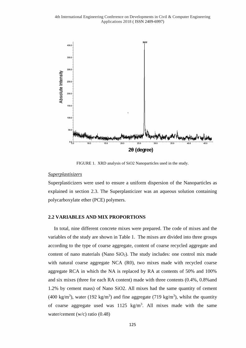
4th International Engineering Conference on Developments in Civil & Computer Engineering
Applications 2018 ( ISSN 2409-6997)
125
FIGURE 1. XRD analysis of SiO2 Nanoparticles used in the study.
Superplastisizers
Superplasticizers were used to ensure a uniform dispersion of the Nanoparticles as
explained in section 2.3. The Superplasticizer was an aqueous solution containing
polycarboxylate ether (PCE) polymers.
2.2 VARIABLES AND MIX PROPORTIONS
In total, nine different concrete mixes were prepared. The code of mixes and the
variables of the study are shown in Table 1. The mixes are divided into three groups
according to the type of coarse aggregate, content of coarse recycled aggregate and
content of nano materials (Nano SiO2). The study includes: one control mix made
with natural coarse aggregate NCA (R0), two mixes made with recycled coarse
aggregate RCA in which the NA is replaced by RA at contents of 50% and 100%
and six mixes (three for each RA content) made with three contents (0.4%, 0.8%and
1.2% by cement mass) of Nano SiO2. All mixes had the same quantity of cement
(400 kg/m3), water (192 kg/m3) and fine aggregate (719 kg/m3), whilst the quantity
of coarse aggregate used was 1125 kg/m3. All mixes made with the same
water/cement (w/c) ratio (0.48)
2θ (degree)

4th International Engineering Conference on Developments in Civil & Computer Engineering
Applications 2018 ( ISSN 2409-6997)
126
TABLE 1.
Code of mixes and variables of study
Mix no. Mix code Type of coarse
aggregate
Nano SiO2 content
%a
Coarse recycled aggregate
content (%)
1 R0 Natural 0 0
2 R50 Natural+Recycled
Industrial
0 50
3 R100 Recycled 0 100
4 R50N0.4 Natural+Recycled 0.4 50
5 R50N0.8 Natural+Recycled 0.8 50
6 R50N1.2 Natural+Recycled 1.2 50
7 R100N0.4 Recycled 0.4 100
8 R100N0.8 Recycled 0.8 100
9 R100N1.2 Recycled 1.2 100 a By cement mass.
2.3 MIXING, SPECIMENS PREPARATION AND CURING
A pan mixer with capacity of 0.1 m3 was used to mix the ingredients and prepare
all concrete mixtures. For the mixes containing Nano SiO2, the nano silica powder
was added to a one liter of water and an amount of super plasticizer (0.5% by mass
of cement) to form an aqueous solution. The solution was mixed using a high speed
blender to ensure a uniform distribution of the Nano particles and avoiding the
agglomeration of these particles. the procedure of mixing the ingredients of the
concrete was as follows: Firstly, the coarse aggregate was added and mixed with the
aqueous solution of Nano SiO2 and part of the mixing water for 1 minute. Then, the
ingredients were left in the mixer pan for 10 minutes to allow the recycled coarse
aggregate to absorb the Nano particles and form a coat layer on their surfaces.
Secondly, the fine aggregate, cement and the rest of the mixing water were added
and mixed for 3 minutes. after the completion of mixing the ingredients, for each
mix: three (100 mm) cubes were cast. The concrete was mixed using a pan mixer
and compacted using a vibrating table. After casting, the specimens were then
covered by plastic sheets and allowed to cure for 24 hours before being demoulded.
Then, the specimens were kept in water tanks for 27 days for further curing.

4th International Engineering Conference on Developments in Civil & Computer Engineering
Applications 2018 ( ISSN 2409-6997)
127
2.4 TESTS
Compressive Strength Test.
The compressive strength was obtained at age of 28 days using the 100 mm cubes
according to BS EN 12390-3 [10].
Microstructure Observations
Individual particles of recycled coarse aggregate were investigated using a digital
microscope. Scanning electron microscopy (SEM) was also used to assess the
microstructure of the RA particles and concrete samples with and without
Nanoparticles of SiO2.
3. RESULTS AND DISCUSSION
3.1 COMPRESSIVE STRENGTH
The results of the compressive strength at the age of 28 days for all mixes are
presented in Table 2. The result of each mix is the average of three specimens. The
table also shows the normalized strength (to that of the plain concrete, mix R0).
TABLE 2.
Results of compressive strength test
Mix
Compressive strength
Strength in
(MPa)
Normalized
Strength
R0 40.6 1.00
R50 34.1 0.84
R100 30.2 0.74
R50 N0.4 37.5 0.92
R50 N0.8 40.3 0.99
R50N1.2 41.0 1.00
R100N0.4 32.0 0.79
R100N0.8
34.2 0.84
R100N1.2 35.1 0.86

4th International Engineering Conference on Developments in Civil & Computer Engineering
Applications 2018 ( ISSN 2409-6997)
128
FIGURE 2. Compressive strength of all mixes
As expected, the compressive strength of the RAC mixes (R50, R100) is lower than
that of the control mix (R0), as can be seen in Table 2 and Figure 2. This is mainly
due to the heterogeneous nature of the recycled aggregate which is characterized by
a weak and cracked surfaces resulted from the crushing process of demolished
concrete [3-4]. The compressive strength of RAC decreased by 16% and 26% when
the natural aggregate was replaced by 50% and 100%, respectively.
FIGURE 3. Effect of Nano silica particles content on the increase of compressive strength.
Figure 3. also shows that the addition of Nano SiO2 enhanced the compressive
strength of the mixes containing recycled aggregate. It is clear that the content of
Nano particles affects the degree of strength enhancement. It can be seen that the
compressive strength increases with the increase of content of Nano silica regardless
25
30
35
40
45
0 0.4 0.8 1.2 1.6
Com
pre
ssiv
e s
trengt
h,
MPa
Nano Silica content (% of cement mass)
50%
100%
0%
RAcontent
R0

4th International Engineering Conference on Developments in Civil & Computer Engineering
Applications 2018 ( ISSN 2409-6997)
129
of the recycled aggregate content. For example, when the Nano silica is added at
contents of 0.4%, 0.8% and 1.2%, the compressive strength increases by 10%, 18%
and 20% for mixes containing 50% RA and by 6%, 13%and 16% for mixes made
with 100% RA. The results also show that the increase in strength for mixes
containing 50% RA is higher than those with 100% RA at all Nano silica contents. It
seems that the addition of Nano silica at contents up to 0.8% (by mass of cement) to
the RAC mixes is very beneficial and can result in comparable strength to that of the
control mix R0 (mix with natural coarse aggregate). The mechanisms leading to this
improvement is explained in the next section where the effect of adding the
nanoparticles on the microstructure of the RAC is discussed.
3.2 MICROSCOPIC AND SCANNING ELECTRON MICROSCOPY (SEM)
OBSERVATIONS
-Recycled aggregate specimens (particles)
The surface of some individual particles of the recycled aggregate with and
without Nano silica was observed by a microscope to support and justify the gained
enhancement in the compressive strength for the mixes made with recycled coarse
aggregate. Also, SEM images for recycled aggregate concrete specimens were taken
and used for the same purpose.
Figure 4a shows an image taken by a microscope with a magnification of 20x for
the surface of a recycled aggregate particle. Microcracks and voids can be identified
on the surface of the RA particle as can be seen in Figure 4b. These microcracks and
voids are the main cause of the weakness of the RA which in turn results in low
strength concrete [3,4]. A weak and cracked zone between the natural aggregate
(NA) and the attached mortar (ITZ) can be observed. These microcracks and weak
ITZ are usually caused by the process of the crushing of the demolished concrete
[3]. Similarly, microcracks and weak ITZ can be identified in Figure 4c which
shows an SEM image for the surface of a particle of RA.

4th International Engineering Conference on Developments in Civil & Computer Engineering
Applications 2018 ( ISSN 2409-6997)
130
(a) (b)
(c)
FIGURE 4. a- RA particle at 20x magnification b- RA surface at 200x magnification
c- SEM image of the surface of a recycle aggregate particle.
To assess the effect of adding the Nano silica as a coat layer around the RA particles
on their surfaces, microscopic images were taken for individual particles as can be
seen in Figure 5. The effect of the nano silica on the surface of the RA particles is
clear. The Nano silica modifies the surface by sealing all the microcracks and filling
all the voids. This modification can partly explain the enhancement in the strength
gained by adding the Nano silica to the mixes with RA.
FIGURE 5. Effect of Nano silica content on the coating layer of RA particles
-Concrete specimens
The effect of using SiO2 nanoparticles on the microstructure of RAC was also
evaluated through observing concrete specimens with and without Nano SiO2. The
SEM images for the concrete specimens were taken and presented in Figure 6 and
Figure7. Figure 6 shows SEM image for the RAC without SiO2 nanoparticles. The
image clearly shows the fact that there are different ITZs in RAC: ITZ1 which exist
NAITZ
Attached mortar
Microcracks
0.4 % NanoSiO2
0.8 % NanoSiO2
1.2 % NanoSiO2
NA
Attached mortar
NA
Microcracks
Voids

4th International Engineering Conference on Developments in Civil & Computer Engineering
Applications 2018 ( ISSN 2409-6997)
131
between the NA particle and the old attached mortar ; ITZ2 which lays between the
NA particles and the new cement matrix (mortar) and ITZ3 which develops between
the new and the old cement mortars. The existence of these ITZs with different
microstructures increases the heterogeneous nature of RAC and hence results in a
weak concrete in terms of both strength and durability aspects. Also, the image
shows that ITZ3 is like the other two ITZs is porous and can be clearly identified by
the very fine black line. The high porosity of this ITZ is due to the high
concentration of Ca(OH)2 resulted from the hydration of cement which is known for
its high porosity.
FIGURE 6. SEM image explains the ITZ s of in RAC sample without Nano silica
On the other hand, the ITZ3 in the RAC specimen (shown in Figure 7) included
coated (with SiO2 nanoparticles) RA particles cannot be clearly identified with a
black line. Although, the old attached mortar and the new mortar can be recognized
by their different porosity and microstructure, the two parts seems to be connected
very well and the zone between them (which is the ITZ3) are very dense and refined
(see Figure 6b). The densification of the microstructure of the ITZ3 can be attributed
to the effect of adding the SiO2 nanoparticles. These nanoparticles can result in a
dense ITZ though two mechanisms: one is physical and the other is chemical. The
latter is attributed to the chemical ability of the SiO2 nanoparticles to react with the
Ca(OH)2 (one of the cement hydration products) and leading to the formation of
more gel product, calcium silicate hydroxide (C-S-H) which is the product
responsible of the strength of the concrete and dense microstructure of the ITZ in
concrete [6,7]. The former, can be due to large surface area and the super-ultra-fine
size of the nanoparticles. This small size of these particles help in filling up all the
NA
ITZ2
ITZ3
ITZ1
Old
mortar
New
mortar

4th International Engineering Conference on Developments in Civil & Computer Engineering
Applications 2018 ( ISSN 2409-6997)
132
micro/nano pores and voids exit in the attached mortar and the ITZ resulting in a
more densefied microstructure of the cement matrix [7,8]. Hence, these two
mechanisms seem to be the main reason behind the improvement in the strength of
the RAC containing SiO2 Nanoparticles.
(a) (b)
FIGURE 7. a-SEM image of a concrete sample with Nano silica, b- image of the ITZ s of a
concrete sample with Nano silica
4. CONCLUSIONS
. The following conclusions can be drawn based on the results and discussion:
- The addition of Nanoparticles of SiO2 can improve the compressive strength of
recycled aggregate concrete regardless of the content of RA.
- The increase in compressive strength depends on the content of the Nano SiO2
content.
- The addition of nanoparticles of silica at contents of 0.4%, 0.8% and 1.2% ,
results in an increase in the compressive strength of 10%, 18% and 20% for
mixes containing 50% RA and of 6%, 13%and 16% for mixes made with 100%
RA, respectively.
- Microscopic and SEM observations revealed the heterogeneous nature of the RA
particles which is characterized by weak and cracked attached mortar and porous
ITZ.
- RAC microstructure can be positively modified though the addition of SiO2
nanoparticles which can help densefy the microstructure RAC by phyiso-
chemical mechanisms.
- RAC with Nanoparticles of SiO2 can demonstrate comparable strength to that of
NAC; hence, great enhancement in terms of sustainability and environmental
effects of RA can be achieved.
0.5
NA
NA
Old cement
mortar New cement
mortar
NA
NA
ITZ1
ITZ2
ITZ3
0.5

4th International Engineering Conference on Developments in Civil & Computer Engineering
Applications 2018 ( ISSN 2409-6997)
133
REFERENCES
[1] Younis, K. H. and K. Pilakoutas, Strength prediction model and methods for
improving recycled aggregate concrete. Construction and Building Materials,
Vol. 49, No. 0, pp. 688-701, 2013.
[2] Tam, V.W., 2008. On the effectiveness in implementing a waste-management-
plan method in construction. Waste management, 28(6), pp.1072-1080.
[3] Tam, V.W., Gao, X.F. and Tam, C.M., 2005. Microstructural analysis of
recycled aggregate concrete produced from two-stage mixing approach.
Cement and Concrete Research, 35(6), pp.1195-1203.
[4] Katz, A. (2004). "Treatments for the improvement of recycled aggregate."
Journal of Materials in Civil Engineering 16(6): 597-603.
[5] Berndt, M. L. (2009). "Properties of sustainable concrete containing fly ash,
slag and recycled concrete aggregate." Construction and Building Materials
23(7): 2606-2613.
[6] Sanchez, F. and Sobolev, K., 2010. Nanotechnology in concrete–a review.
Construction and building materials, 24(11), pp.2060-2071.
[7] Said, A.M., Zeidan, M.S., Bassuoni, M.T. and Tian, Y., 2012. Properties of
concrete incorporating nano-silica. Construction and Building Materials, 36,
pp.838-844.
[8] Shaikh, F.U.A., Odoh, H. and Than, A.B., 2014. Effect of nano silica on
properties of concretes containing recycled coarse aggregates. Proceedings of
the Institution of Civil Engineers-Construction Materials, 168(2), pp.68-76.
[9] IQS No. 45/1984 ‘’Iraqi Specification for Cement’’ (1984)
[10] BS EN 12390-3, Testing hardened concrete Part 3: Compressive strength of
test specimens. British Standard Institution, London, UK, 2009.

4th International Engineering Conference on Developments in Civil & Computer Engineering
Applications 2018 ( ISSN 2409-6997)
134
EMPLOYING SMARTPHONE AND COMPACT CAMERA IN
BUILDING MEASUREMENTS
Haval A. Sadeq
Salahaddin University-Erbil
doi:10.23918/iec2018.11
ABSTRACT
This paper investigates the possibility of implementing images from smartphones
and compact cameras for building measurement, such as archaeological buildings,
for documentation purposes based on point cloud produced via photogrammetric
technique. Images of the object are first captured from different positions. Then, the
images are processed for the interior and exterior orientations to produce point
cloud. For object registration, one distance is measured at the site, which is assigned
to the model and used for scaling. The generated point cloud is subsequently
exported into various software, such as AutoCAD, to take measurements or for any
architectural studies. Two types of smartphone with different camera resolutions and
two types of compact camera are used in the test. Results are validated by comparing
several real measurements from the site. The quality of the data is proven to be
accurate up to centimetre accuracy.
Keywords: smartphone camera, compact camera, point cloud, photogrammetry,
archaeological, accuracy.

4th International Engineering Conference on Developments in Civil & Computer Engineering
Applications 2018 ( ISSN 2409-6997)
135
1. INTRODUCTION
Traditional building measurement using tapes is considered to be time
consuming, especially at high-altitude areas or areas that have restricted access due
to risks, such as ruined archaeological sites. By contrast, using equipment, such as
laser scanning, total stations and theodolites, are considered to be expensive because
they are time consuming and are designed on specialized people. The task has
become difficult because it requires to measure architectural buildings that have
complex architectural objects.The evolution of compact digital cameras and
smartphone technology, which is accompanied by high-resolution and small size
charge-coupled device (CCD) and complementary metal-oxide semiconductor
(CMOS), has increased the demand for such equipment. In addition, the decrease in
their size and the ease of image capturing have enabled users to carry them in the
pocket. This paper focuses on using photogrammetry to generate the model for the
building based on point cloud using compact and mobile phone camera. Considering
the popularity of photogrammetric software, people can easily process the images
for model generation and use it for measurement purposes.Close range
photogrammetry is widely used to produce orthomaps for the front view of buildings
using metric camera. Subsequently, metric cameras are used to capture image for the
purpose of façade reconstruction with the introduction of digital photogrammetry.
The development of off-the-shelf and built-in mobile cameras has resulted in the
popularity of this system, which is only used for photography. Different studies have
been conducted for the purpose of 3D reconstruction, and a method is suggested for
interactive 3D model reconstruction based on mobile phones using photogrammetric
techniques [1]. Smartphones are used in 3D model generation for the purpose of
updating 3D urban maps and detailed enhancements [1]. The accuracy of mobile
phone sensors is compared with off-the-shelf cameras, which showed positive
results for photogrammetric product implementation [2]. An algorithm least square
model image fitting is also [3] implemented by using built-in GPS and image
orientation from smartphones as initial values to enhance the exterior image
orientation for photogrammetric products that can be used in building construction.
[4] assessed the possibility of using mobile phone cameras in UAV for DEM and
orthophoto generation. In this study, the images of three buildings are captured using
smartphone and compact camera, and point cloud is automatically generated using

4th International Engineering Conference on Developments in Civil & Computer Engineering
Applications 2018 ( ISSN 2409-6997)
136
CapturingReality software https://www.capturingreality.com/, which is considered
for its simplicity. The process is started by loading the captured images in the
software, and the photogrammetric process is automatically started to produce point
cloud.This paper is structured as follows. Section 1 presents the introduction.
Section 2 describes the study area, and Section 3 depicts the implemented camera.
Section 4 shows the geometric processing and the result analysis is in Section 5.
Finally, Section 6 provides the conclusion.
1. STUDY AREA
In this study, three study areas are selected that are located in Erbil-Iraq. The first
study area shown in FIGURE 1(a) is referred as study area-1, which is located in
Erbil Citadel and represents the rear side of the grand gate at Erbil citadel. This
object is considered difficult for surveyors to take measurements at the upper side of
the building because it is considered to have high altitude and is difficult to access
the top of the building. Study area-2 shown in FIGURE 1(b) is also located in Erbil
citadel, which is considered to be an old archaeological building although it has been
renovated. The area is displayed for tourists but with limited accessibility, as shown
in the figure. A warning tape surrounds this area, and people can only view it
because it is considered to be a ruined area. Thus, images are captured at a distance
without the users entering the site. These sites are under the supervision of the High
Commission for Erbil Citadel Revitalization (HCECR), which is authorized with the
control and renovation of the historical building in Citadel. Study area-3 shown in
FIGURE 1(c), is considered to be a modern building with different architectural
objects and textures. This study area is considered to have smooth surfaces that
enable the easy identification of points.

4th International Engineering Conference on Developments in Civil & Computer Engineering
Applications 2018 ( ISSN 2409-6997)
137
(a)
(b)
(c)
FIGURE 1. Selected study areas (a) study area-1, citadel gate is considered to be high altitude (b)
study area-2 represents the renovated area that has been restricted for users to access (c) study area-3,
modern house with different architectural materials and styles.
2. IMPLEMENTED SMARTPHONE CAMERA
In this research, four different types of cameras are used for image capture, as
shown in FIGURE 2. Two different types of smartphone cameras are used, namely,
Samsung smartphone model GT-I9060I with 5 MP and Samsung smartphone J730F
Galaxy with 13 MP. In addition, two different compact cameras are used, namely,
Canon camera IXUS160 with 20 MP and Sony camera model HX60V with 20.3 MP
resolution. These cameras are known as off-the-shelf cameras because they are not
specified for photogrammetric purposes and are designed for amateur users.
(a)
(b)
(c)
(d)
FIGURE 2. used mobile phones (a) Samsung smartphone model GT-I9060I resolution 5 MP (b)
Samsung smartphone J730F Galaxy 13 MP (c) Canon compact camera IXUS160 resolution 20 MP
(d) Sony Compact Camera HX60V resolution 20.4 MP.
As shown in Table 1, two different types of sensors, namely, CCD and CMOS,
are adopted in the camera. The two sensors are functioning with similar principle,
which is to convert light into electrons, and they are invented at the same period of
time. These mobile phones are considered to have small sensor size, which is known
Warning tape

4th International Engineering Conference on Developments in Civil & Computer Engineering
Applications 2018 ( ISSN 2409-6997)
138
as CMOS. CCD images are considered to have low-noise ratio and less susceptible
to noise than CMOS. CMOS sensors are also considered to be less sensitive to light
than CCD sensors because they have several transistors located next to them and are
considered to consume low battery life, which made them dominant over CCD
sensors in mobile phones. Thus, the future of CMOS sensors is the focus of the
company [5].
TABLE 1.
Specification of smartphone and compact cameras
Item
Samsung
smartphone model
GT-I9060I
Samsung
smartphone
J730F Galaxy
Canon camera
IXUS160 Compact
Camera
Sony camera
HX60V Compact
Camera
Sensor resolution 5 MP 13 MP 20 MP 20.4 MP
Sensor type CMOS CMOS CCD CMOS
Image format (pixels) 2560 x 1920 4160 x 3120 5152 x 3864 5184 x 3888
Focal length (mm) 2.6 3.71 5 4.3–129
Pixel size(µm) * 1.133 1.196 1.188
Sensor size(mm) * 4.73 x 3.49 6.16 x 4.62 6.16 x 4.62
Crop factor * 7.37 5.62 5.62
*Indicates that the information is unavailable.
The number of captured images is varied and is based on the complexity and
arrangement of the structure. For instance, the number of captured images in study
area-1 is 40 images because the object is façade of building. For study area-2, 96
images are used because the area has different objects, which are considered to be
larger than other objects. The captured objects behind the warning tape are shown in
FIGURE 1 (b). For study area-3, 60 images are captured because the area is
identified to be the façade of the building and has less details than study area-2.
3. GEOMETRIC PROCESSING
This stage represents the photogrammetric process, which is achieved in
CapturingReality software. At this stage, the images are processed to determine the
camera parameters, real position and attitude of images and point cloud generation.
3.1. INTERIOR ORIENTATION
Interior orientation is the process that determines the internal geometry of the
camera as it used during image capturing, which is designed for calibrated focal
length, principal point location, lens the distortion, and sensor size. These
parameters are necessary to calculate the actual location of the image space and

4th International Engineering Conference on Developments in Civil & Computer Engineering
Applications 2018 ( ISSN 2409-6997)
139
remove all the distortions from the image. The parameters of metric camera are
obtained at the lab through specific test. For the off-the-shelf camera (used in this
paper), two main methods are used for determining the camera parameters, which
are known as field test or pre-calibration or through self-calibration [6]. According
to the literature, the result of self-calibration can provide more accurate result than
pre-calibration [7-10] because it is included in the bundle adjustment process during
aerial triangulation. The camera parameter used in this research is based on self-
calibration. For the calculation, the initial values are used, such as focal length,
image format, ISO speed, and aperture. The initial values of the camera are saved in
image metadata known as exchangeable image file format. The cameras used in this
study, which are either smartphone or compact camera, are considered to have these
parameters. In FIGURE 3, the interior orientation of Samsung SM-J730F is
determined, and the lens distortion is plotted on the image, as shown in FIGURE
3(a). The tie point, which is used in parameters determination via self-calibration, is
marked. This condition shows that the point is marked on the objects, as shown in
FIGURE 3 (b). The parameters of the camera Samsung SM-J730F are shown in
FIGURE 3 (c), which are related to focal length, principal point location and lens
distortion. The focal length of Samsung SM-J730F is 3.71 mm. However, the value
of 27.736067 mm in the determined calibration is based on 35 mm focal length and
is equivalent to (35 mm). These equivalent values are selected to compare the
viewing angles between different cameras. Camera industries have introduced the
term ‘35 mm focal length camera’ [11]. This value can be determined by multiplying
the focal length of the camera by focal length multiplier, crop factor or format factor,
which is provided by manufacturers (7.37 from TABLE 1). Thus, the calibrated
focal length is 3.76 mm.

4th International Engineering Conference on Developments in Civil & Computer Engineering
Applications 2018 ( ISSN 2409-6997)
140
The model used in this study for the determination of image distortion model is
represented in Equation (1), and is used in image correction ascribed by Brown [12].
The model is known as an eight-parameter physical model that is originally
developed for film cameras. However, this model is valuable for digital cameras.
where ∆𝑥 and ∆𝑦 represent the corrections in x and y directions, respectively;
𝑎𝑛𝑑 are distances from a point to the principal point with respect to x and y
directions; 𝑟 is the radial distance from a point to the principal point;
𝐾1, 𝐾2 𝑎𝑛𝑑 𝐾3 are radial distortion coefficients; 𝑃1 𝑎𝑛𝑑 𝑃2 are coefficients for
decentring distortion; and 𝑏1 𝑎𝑛𝑑 𝑏2 represent the affinity of non-orthogonal
parameters.
3.2. EXTERIOR ORIENTATION
At this stage, the position of images (X, Y and Z) and attitudes (𝜔, 𝜑, 𝑘) are
determined. In general, the solution of airborne images for exterior orientation has
reached a high precision level, especially with the attached GNSS/IMU information,
which subsequently minimized the required GCPs [10, 13, 14]. However, the close-
range images are considered challenging, because they rarely have GNSS/IMU
instruments attached to the camera due to cost and load issues. Although this
condition exists in mobile phones or several cameras, they are considered to have
low accuracy, and they can be used as initial values. Thus, different approaches
(a)
(b)
(c)
FIGURE 3. Interior orientation process using camera Samsung SM-J730F for study area-1 (a) shows
the amount of distortion that has been affected on the image (b) detected tie point used in calibration
(c) screenshot showing the determined parameters of interior orientations.
∆𝑥 = −𝑥0 −
𝑐∆𝑐 + 𝑟2𝐾1 + 𝑟4𝐾2 + 𝑟6𝐾3 + (22 + 𝑟2)𝑃1 + 2𝑃2𝑥𝑦 + 𝑏1 + 𝑏2;
∆𝑦 = −𝑦0 −
𝑐∆𝑐 + 𝑟2𝐾1 + 𝑟4𝐾2 + 𝑟6𝐾3 + 2𝑃1𝑥𝑦 + (22 + 𝑟2)𝑃2;
(1)

4th International Engineering Conference on Developments in Civil & Computer Engineering
Applications 2018 ( ISSN 2409-6997)
141
should be integrated because of the instability of camera calibration process [15, 16].
Although providing data for exterior orientation in close-range photogrammetry is
challenging, the images can be processed without providing any information about
the image position or orientation. In addition, these approaches can be used to deal
with images that are considered to be randomly captured and without sequences.
These approaches can process images that have different illuminations and different
perceptive views, which are captured from different non-calibrated or non-metric
cameras [17-19]. Self-calibration technique is applied to the current
photogrammetric tasks, in which the interior orientation is achieved during project
implementation or exterior orientation. In this technique, the object points combined
with the unknown feature point of interest that appeared in different photos are used
in the process [20]. Self-calibration is introduced in Bundle Block adjustment. Thus,
camera parameters, such as lens distortion and others, are collectively determined
via determination of the object coordinates, which provide more accurate results
than test-field calibration [21]. In the photogrammetric process of model registration
or absolute orientation (i.e. scaling and georeferencing), seven parameters, namely,
three translations, three rotations and one scale parameter [20], are required. This
research focuses on distance measurement and does not require the coordinates of
the points. Therefore, the model is only adjusted. The distance is measured in the
model using tape instrument and is assigned in the model, as shown in FIGURE 4.
The same procedure is applied to other study areas.

4th International Engineering Conference on Developments in Civil & Computer Engineering
Applications 2018 ( ISSN 2409-6997)
142
FIGURE 4. Defined distance is shown for the purpose of scaling the models.
3.3. POINT CLOUD GENERATION
Apart from image triangulation, images are available for point cloud construction.
Point cloud is the result of image matching, which is obtained via collinearity
equations. Image matching is considered as the main critical stage in
photogrammetry. Different image matching techniques have been developed [22-
27]. The technique used in this study is based on the technique that is available in
the reality capture software, which is robust for the production of a point cloud, as
shown in
FIGURE 5. The technique is not revealed for confidentiality purposes. The
common technique that is considered to provide acceptable result is the least square
matching, which is based on signal matching that depends on grey values [10].
However, a robust technique, which is called semi-global matching, has been
developed. This technique can produce accurate results for 3D object reconstruction.
This method requires large overlapping areas [28].
FIGURE 5. Produced point cloud (left image) and rendered object using images from Samsung J7 in
study area-1(right image) with camera pose location.

4th International Engineering Conference on Developments in Civil & Computer Engineering
Applications 2018 ( ISSN 2409-6997)
143
For good visibility, point cloud is rendered for better visualization. The rendering
issue is not related to the accuracy of quantity measurement. However, this issue is
considered an important requirement for architects to produce realistic views of the
object and for good analysis. FIGURE 6 shows the result on study area-2 that has
rendered the models from four cameras samples, which shows that all objects are
represented. In the rendering model, the roofs of buildings are not generated due to
missing photos from the top of the buildings.
Samsung GT
Samsung J7
Canon Camera
Sony camera
FIGURE 6. Rendered study-area-2, four different rendered models produced from smartphone and
compact cameras with the camera pose location.
The produce point cloud model can be used for measurement and documentation
purposes to produce a plan view. As shown in FIGURE 7, the top view of study
area-2 with all details should produce a map for the site or building layout. The
camera did not reach all the areas and has captured images only from one side.
However, all the distant walls have been clearly produced.

4th International Engineering Conference on Developments in Civil & Computer Engineering
Applications 2018 ( ISSN 2409-6997)
144
FIGURE 7. Top view of study area-2 obtained from point cloud, which shows the
captured image area and the logo of the ‘reality capturing software’.

4th International Engineering Conference on Developments in Civil & Computer Engineering
Applications 2018 ( ISSN 2409-6997)
145
4. RESULT ANALYSIS
For the model analysis, a set of measurements is selected at three locations. For
the assessment, overall 55 different planemetric measurements are used to assess the
accuracy of the obtained point cloud. At the site, the distances are obtained from
different directions (i.e. in the X, Y and Z directions). Then it is compared with the
measurements that are obtained from point cloud using ReCap, as shown in
FIGURE 8. ReCap is built in AutoCAD software, which is designed for laser
scanning point cloud measurement. For good point selection of dimensions, the
available colour feature in point cloud is clearly represented, which is similar to the
point cloud available in laser scanning.
FIGURE 8. Generated point cloud in study area-3 with Sony camera with several measured distances
on Autodesk ReCap-2014.

4th International Engineering Conference on Developments in Civil & Computer Engineering
Applications 2018 ( ISSN 2409-6997)
146
For qualitative analysis, a statistical analysis is applied to the residual. The
achieved analysis tests are mentioned in Equations (2), (3) and (4) to obtain the
accuracy of the obtained point cloud from each of the mentioned devices in three
Study areas, as follows:
where ∆ℎ𝑖 represents the residual or error between the measured distance on point
cloud and actual distance, and 𝒏 represents the number of measurements.
The statistical analysis is listed in TABLE 2, which shows that the accuracy of point
cloud increases with the increase in the resolution of the image. The accuracy in the
worst case is less than 0.08 m using smartphone camera. The accuracy is increased
to 0.051 in the worst case and 0.35 in the best case with the increase in resolution by
using J7. Compact cameras showed better performance than smartphone cameras in
terms of study areas 1 and 2, and they are not much different, which is in the worst
case less than 0.045 m. For the standard deviations and biases, all the samples for the
worst case is 0.61 m and −0.022m, respectively. With the increase in the resolution
of sensors, such as Samsung J7 and compact camera, the standard deviation and bias
is improved to 0.51 and 0.22 m.
𝜇 =1
𝑛 ∑ ∆ℎ𝑖
𝑛i=1 ;
(2)
𝜎 = √1
(𝑛−1)∑ (∆ℎ𝑖 −𝑛
i=1 𝜇)2;
(3)
𝑅𝑀𝑆𝐸 = √1
𝑛∑ ∆ℎ𝑖
2𝑛i=1 ; (4)

4th International Engineering Conference on Developments in Civil & Computer Engineering
Applications 2018 ( ISSN 2409-6997)
147
TABLE 2.
Obtained statistical data in analysing the accuracy of point cloud, the accuracy is in in the three
directions X,Y, Z.
Statistical
test
Samsung smartphone
model GT-I9060I
Samsung smartphone
J730F Galaxy
Canon camera
IXUS160
Sony camera
HX60V Compact
Camera
Stu
dy
are
a-1
RMSE (m) 0.079 0.044 0.033 0.033
STD (m) 0.055 0.027 0.032 0.028
Bias (m) 0.001 −0.017 −0.002 −0.022
Stu
dy
area
-2 RMSE (m) 0.068 0.051 0.044 0.038
STD (m) 0.061 0.051 0.026 0.033
Bias (m) 0.008 0.007 0.015 −0.002
Stu
dy
are
a-3
RMSE (m) 0.046 0.035 0.044 0.034
STD (m) 0.044 0.036 0.049 0.038
Bias (m) 0.013 −0.010 0.005 −0.014
5. CONCLUSIONS
An efficient technique to obtain the measurements of buildings with reasonable
accuracy by using sensors is proposed. This technique is inexpensive and easy-to-
use rather than using expensive devices, such as specific photogrammetric cameras.
Any type of camera can be used although Samsung mobile phone and Canon Power
Shot camera are used in the test. As shown in the result, as the quality of the camera
increases the accuracy of the model is increased. The analysis showed that CMOS
technology provided better accuracy than CCD under the same resolution. Modern
technology has focused on the predominance of CMOS on imaging devices and has
obtained more support for improvement from mobile companies.
The technique used in this study can minimize the work needed in documentation.
The technique can help obtain quick measurements in the area. In addition, a real 3D
model of the object can be obtained and can be used to produce the site layout. The
attached colour to the point cloud will help the user identify the points accurately.
ACKNOWLEDGEMENTS
The author would like to appreciate the CapturingReality company for their
cooperation in providing a redeem license to export the data. The author would like
to acknowledge HCECR for permitting the access to measure the dimensions of the
implemented study area.

4th International Engineering Conference on Developments in Civil & Computer Engineering
Applications 2018 ( ISSN 2409-6997)
148
REFERENCES
[1] B. Sirmacek and R. Lindenbergh, "Accuracy assessment of building point
clouds automatically generated from iphone images," ISPRS - International
Archives of the Photogrammetry, Remote Sensing and Spatial Information
Sciences, vol. XL-5, pp. 547-552, 2014.
[2] A. Gruen and M. D. Akca, "Mobile photogrammetry," Vorträge
Dreiländertagung SGPBF, DGPF und OVG, vol. 16, pp. 441-451, 2007.
[3] S. Wang, "Toward Automated FAÇADE Texture Generation for 3d
Photorealistic City Modelling with Smartphones or Tablet Pcs," ISPRS-
International Archives of the Photogrammetry, Remote Sensing and Spatial
Information Sciences, pp. 351-354, 2012.
[4] J. Kim, S. Lee, H. Ahn, D. Seo, S. Park, and C. Choi, "Feasibility of
employing a smartphone as the payload in a photogrammetric UAV system,"
ISPRS Journal of Photogrammetry and Remote Sensing, vol. 79, pp. 1-18,
2013.
[5] D. Durini, High performance silicon imaging: fundamentals and applications
of cmos and ccd sensors: Elsevier, 2014.
[6] E. Edwards, E. Fey, P. A. Jones, R. K. Jungquist, A. G.LAreau, J. Lebarron, et
al., "Cameras and sensing systems," in Manual of Photogrammetry, J. C.
McGlone, Ed., ed: American Society for Photogrammetry and Remote
Sensing, 2013.
[7] J. S. Aber, I. Marzolff, and J. Ries, Small-format aerial photography:
Principles, techniques and geoscience applications: Elsevier, 2010.
[8] S. Harwin, A. Lucieer, and J. Osborn, "The Impact of the Calibration Method
on the Accuracy of Point Clouds Derived Using Unmanned Aerial Vehicle
Multi-View Stereopsis," Remote Sensing, vol. 7, pp. 11933-11953, 2015.
[9] D. Herrera, C. J. Kannala, and J. Heikkila, "Forget the checkerboard: Practical
self-calibration using a planar scene," pp. 1-9, 2016.
[10] T. Rosnell and E. Honkavaara, "Point cloud generation from aerial image data
acquired by a quadrocopter type micro unmanned aerial vehicle and a digital
still camera," Sensors (Basel), vol. 12, pp. 453-80, 2012.
[11] R. Sheppard, Digital photography: top 100 simplified tips & tricks vol. 25:
John Wiley & Sons, 2010.
[12] W. Forstner, B. Wrobel, F. Paderes, C. S. Fraser, J. Dolloff, E. M. Mikhail, et
al., "Analytical Photogrammetric Operations," in Manual of Photogrammetry,
J. D. McGlone, Ed., Sixth Edition ed Bethesda: American Society of
Photogrammetry and Remote Sensing (ASPRS), 2013.
[13] G. Buyuksalih and Z. Li, "Practical experiences with automatic aerial
triangulation using different software packages," The Photogrammetric
Record, vol. 18, pp. 131-155, 2003.
[14] J. Kremer and E. Kruck, "Integrated Sensor Orientation–Two Examples to
show the Potential of simultaneous GPS/IMU and Image Data Processing,"
Theory, Technology and Realities of Inertial/GPS Sensor Orientation, 2003.
[15] K. Gutjahr, P. Hafner, M. Ofner, K. Längauer, M. Wieser, and N. Kühtreiber,
"Performance of GNSS/IMS integration methods in context of a near real-time
airborne mapping platform," EuroCOW10, Commission III, WG, vol. 3, 2010.

4th International Engineering Conference on Developments in Civil & Computer Engineering
Applications 2018 ( ISSN 2409-6997)
149
[16] K.-W. Chiang, H.-W. Chang, C.-Y. Li, and Y.-W. Huang, "An artificial neural
network embedded position and orientation determination algorithm for low
cost MEMS INS/GPS integrated sensors," Sensors, vol. 9, pp. 2586-2610,
2009.
[17] S. Agarwal, Y. Furukawa, N. Snavely, I. Simon, B. Curless, S. M. Seitz, et al.,
"Building rome in a day," Communications of the ACM, vol. 54, pp. 105-112,
2011.
[18] M. Brown and D. G. Lowe, "Automatic Panoramic Image Stitching using
Invariant Features," International Journal of Computer Vision, vol. 74, pp. 59-
73, 2006.
[19] I. Stamos and P. E. Allen, "3-D model construction using range and image
data," vol. 1, pp. 531-536, 2000.
[20] K. Kraus, Photogrammetry: geometry from images and laser scans, 2nd ed.:
Walter de Gruyter, 2007.
[21] T. A. Clarke and J. G. Fryer, "The development of camera calibration methods
and models," The Photogrammetric Record, vol. 16, pp. 51-66, 1998.
[22] N. Haala, "Comeback of digital image matching," in Photogrammetric Week,
2009, pp. 289-301.
[23] W. Tao, Y. Lei, and P. Mooney, "Dense point cloud extraction from UAV
captured images in forest area," pp. 389-392, 2011.
[24] F. Leberl, A. Irschara, T. Pock, P. Meixner, M. Gruber, S. Scholz, et al., "Point
Clouds," Photogrammetric Engineering & Remote Sensing, vol. 76, pp. 1123-
1134, 2010.
[25] A. Gruen, "Development and Status of Image Matching in Photogrammetry,"
The Photogrammetric Record, vol. 27, pp. 36-57, 2012.
[26] E. Gülch, "Advanced matching techniques for high precision surface and
terrain models," in Photogrammetric Week, 2009, pp. 303-315.
[27] M. Pohanka, K. Musilek, and K. Kuca, "Evaluation of aflatoxin B1--
acetylcholinesterase dissociation kinetic using the amperometric biosensor
technology: prospect for toxicity mechanism," Protein Pept Lett, vol. 17, pp.
340-2, Mar 2010.
[28] H. Hirschmuller, "Stereo processing by semiglobal matching and mutual
information," IEEE Trans Pattern Anal Mach Intell, vol. 30, pp. 328-41, Feb
2008.

4th International Engineering Conference on Developments in Civil & Computer Engineering
Applications 2018 ( ISSN 2409-6997)
150
AN APPROACH FOR DESCRIPTION OF ELASTIC
PARAMETERS OF CROSS-ANISOTROPIC SATURATED
SOILS
Ahmed Mohammed Hasan
Salahaddin University-Erbil
[email protected] or [email protected]
doi:10.23918/iec2018.12
ABSTRACT
The processes of deposition and consolidation in natural soils or compaction in fill
materials will typically produce soils that are initially cross-anisotropic (also known
as transversely isotropic or orthotropic) in terms of both small strain elastic
behaviour and large strain plastic behaviour. For small strain elastic behaviour, five
elastic parameters are required to fully describe cross-anisotropic soils such as two
Young’s moduli (Ev in vertical direction and Eh in horizontal direction), two
Poisson’s ratios (vvh horizontal strain due to vertical strain and vhh horizontal strain
due to horizontal strain) and an independent shear modulus such as Ghv (a shear
wave horizontally transmitted with vertically polarised). These five elastic
parameters have been expressed in different fashions in the literature. In this paper
results from derivations showed that it is possible to express the elastic parameters
for cross-anisotropic soils in a different way than that expressed in the literature
using as a function of independent measurements of two shear moduli and two
constrained moduli from three pairs of bender/extender elements BEEs fitted on a
cross-anisotropic soil sample in a triaxial apparatus and measuring or assuming the
value of vhh using combination of triaxial testing system and bender/extender
element testing system,
Keywords: elastic parameters, cross-anisotropic soils, bender/extender elements,
shear and constrained moduli.

4th International Engineering Conference on Developments in Civil & Computer Engineering
Applications 2018 ( ISSN 2409-6997)
151
1. INTRODUCTION
For a shear wave, the direction of motion of the soil particles (the wave
polarisation) is perpendicular to the direction of wave transmission, as shown in
Figure 1 [1]. Hence, different shear wave velocities can be measured, depending
upon the direction of the wave transmission and the direction of the wave
polarisation, e.g. Vsvh , Vshv and Vshh (see Figure 2 [2,3]), where the second subscript
gives the wave transmission direction, the third subscript gives the wave polarisation
direction and v and h represent vertical and horizontal respectively. For compression
waves, the direction of particle motion (wave polarisation) is the same as the
direction of wave transmission (see, Figure 1). By transmitting compression waves
in vertical and horizontal directions, compression waves velocities Vpv and Vph can
be measured (see Figure 2).
The importance of anisotropy of very small strain behaviour has been investigated
by many authors [4-7]. They showed, using numerical analysis, that including
anisotropy of G during the prediction of deformations of tunnelling in stiff clays
(such as London clay) appeared to play a vital role.
FIGURE 1. Compression and shear wave travel: (a) Compression wave with horizontal transmission,
Vph (b) Shear wave with horizontal transmission and vertical polarisation, Vshv (c) Shear wave with
horizontal transmission and horizontal polarisation, Vshh [1]

4th International Engineering Conference on Developments in Civil & Computer Engineering
Applications 2018 ( ISSN 2409-6997)
152
FIGURE 2. Multi-directional pairs of BEEs fitted on a triaxial soil sample [2,3]
This anisotropy of soil fabric can evolve during plastic straining, leading to changes
in the anisotropy of mechanical behaviour. These changes of anisotropy caused by
changes of soil fabric are therefore termed strain induced anisotropy [8]. The 5
independent elastic constants of cross-anisotropic soils have been expressed using
different techniques in the literature. For example, two of them are presented here.
Stokoe et al. [9] and Fioravante & Cappoferri [10] showed that the 5 independent
elastic constants of cross-anisotropic soils could be measured with bender/extender
elements if an additional extender element was used to determine a constrained
modulus M in an oblique direction. Alternatively, Pennington [11] showed how all 5
independent constants could be determined by combining bender element testing (to
measure Ghv and Ghh) with local strain measurement on triaxial samples (to measure
Ev, Eh and vvh). This does, however, have the drawback of combining two different
types of measurement (at two different strain amplitudes). The main objective of this
paper is to express the elastic parameters for cross-anisotropic saturated soils in a
different fashion than those have been presented in the literature. The current
expressions use a combination of triaxial testing system and bender/extender
element testing system whereas other expressions employ, for example, either a
triaxial testing system with local strain measurement on triaxial samples [11] or a
cubical calibration chamber with geophone systems [9]. It means that additional
equipment (i. e. bender/extender element testing system) in the geotechnical

4th International Engineering Conference on Developments in Civil & Computer Engineering
Applications 2018 ( ISSN 2409-6997)
153
laboratory can be used to measure independent elastic constants and then express
them.
1. BENDER/EXTENDER ELEMENT TESTING
Bender/extender elements are piezoelectric transducers that can transmit and
receive shear waves and compression waves in order to determine shear wave
velocity Vs and compression wave velocity Vp . These wave velocities can then be
used to determine very small strain elastic values of shear modulus G and
constrained modulus M as follows Biot [12].:
2
sVG (1)
2pVM (2)
where ρ is the bulk density of the soil. In all cases, the wave velocity V (i.e. Vs or Vp)
is determined from a measurement of travel time t and the known tip-to-tip distance
Ltt between transmitter and receiver elements [13]:
t
LV tt (3)
2. ELASTICITY THEORY
3.1 ELASTIC MODULI OF ISOTROPIC SATURATED SOILS
At very small strains, the behaviour of saturated soils can be treated as elastic. If
the soil is isotropic, the elastic behaviour can be represented by two independent
elastic properties, which are normally selected either as Young’s modulus E and
Poisson’s ratio ν or as shear modulus G and bulk modulus K [14], where:
)1(2 v
EG
(4)
)21(3 v
EK
(5)

4th International Engineering Conference on Developments in Civil & Computer Engineering
Applications 2018 ( ISSN 2409-6997)
154
For saturated soil, it can be helpful to choose to express the elastic properties in
terms of G and K (rather than E and ν ), because shear modulus G should be the
same for both drained and undrained behaviour, and K is often considered as infinite
for undrained behaviour. For linear elastic behaviour, G and K are constants, but
soils often show non-linear elastic behaviour, with G and K varying with stress,
strain or soil state.
Constrained modulus M is the elastic modulus (applied normal stress increment
divided by normal strain increment in the same direction) for a condition where
strain is prevented in both perpendicular directions. For an isotropic elastic soil, M
can be expressed in terms of E and ν , or in terms of G and K [14]:
)1)(21(
)1(
vv
vEM
(6)
GKM3
4 (7)
Equations (1) and (2) show that the shear wave velocity Vs and compression wave
velocity Vp measured in bender/extender elements BEE tests depend upon G
(Equation 4) and M (Equation 6 or 7), respectively.
3.2 ELASTIC MODULI OF ANISOTROPIC SATURATED SOILS
Love [15] showed that thermodynamic considerations mean that the stiffness
matrix (and compliance matrix) of an elastic material must be symmetric. This
means that the most general form of linear anisotropic elastic behaviour involves 21
(rather than 36) independent elastic constants, for example see Graham and
Houlsby[16]. For a cross-anisotropic elastic material, with the same properties in all
horizontal directions but different properties in vertical directions, symmetry of the
stiffness and compliance matrices implies that [15]:
v
vh
h
hv
E
v
E
v (8)

4th International Engineering Conference on Developments in Civil & Computer Engineering
Applications 2018 ( ISSN 2409-6997)
155
where Eh and Ev are the Young’s moduli in horizontal and vertical directions
respectively, νhv is the Poisson’s ratio giving the ratio of vertical to horizontal strain
increment caused by a uniaxial stress increment in the horizontal direction, and νvh is
the Poisson’s ratio giving the ratio of horizontal to vertical strain increment caused
by a uniaxial stress increment in the vertical direction. Thermodynamic
considerations also imply that for this cross-anisotropic material, the shear moduli
Gvh , Ghv and Ghh are given by [15]:
vhhv GG (9)
)1(2 hh
hhh
v
EG
(10)
This means that, as shown by Graham & Houlsby [14], the behaviour of a cross-
anisotropic elastic material involves only 5 independent elastic constants, which can
be taken as Ev , Eh , νvh , νhh and Gvh. The stress-strain relations of this cross-
anisotropic elastic material can then be expressed as [15]:
zx
yz
xy
h
hh
hv
hv
v
vh
v
vh
v
vh
hh
hh
v
vh
h
hh
h
zx
yz
xy
zz
yy
xx
E
vG
G
EvE
v
E
vE
v
EE
vE
v
E
v
E
'zz
'yy
'xx
)1(2
1
1
1
1
1
(11)
For the conditions of the triaxial test, Equation (11) gives:
'h
'v
21
v
vh
v
vE
v
E (12)

4th International Engineering Conference on Developments in Civil & Computer Engineering
Applications 2018 ( ISSN 2409-6997)
156
'v
'h
1
v
vh
h
vh
h
hE
v
E
v
E (13)
where x and y are horizontal directions, z is the vertical direction, ∆𝜎𝑥𝑥′ , ∆𝜎𝑦𝑦
′ and
∆𝜎𝑧𝑧′ are normal stress increments, ∆𝜀𝑥𝑥 , ∆𝜀𝑦𝑦 and ∆𝜀𝑧𝑧 are corresponding normal
strain increments, ∆𝜏𝑦𝑧 , ∆𝜏𝑧𝑥 and ∆𝜏𝑥𝑦 are shear stress increments and ∆𝛾𝑥𝑦 , ∆𝛾𝑦𝑧
and ∆𝛾𝑧𝑥 are corresponding shear strain increments.
3. DERIVATION OF EXPRESSIONS FOR EH , EV AND VVH
4.1 EXPRESSIONS FOR Mv
If a stress increment ∆σv' is applied in a vertical direction, to produce a
corresponding strain increment ∆εv in that direction, while strains are prevented in
the horizontal direction (i.e. Δεh=0). Equation 13 can be re-arranged to give:
'v
'
)1(
vh
vh
v
hh
v
v
E
E (14)
By inserting Equation 14 into Equation 12:
'v
)1(
21
hh
vh
v
h
v
vh
v
vv
v
E
E
E
v
E (15)
For this situation of no horizontal strain, the vertical constrained modulus Mv is
defined by [17]:
v
vM
'v
m(16)
Comparing Equation 15 and 16:
)1(21
hh
vh
v
hvh
vv
v
v
E
Ev
EM
(17)
This simplifies to the standard result for the constrained modulus of an isotropic
elastic material (see Equation 6) if Ev = Eh =E and νvh = νhh = ν .

4th International Engineering Conference on Developments in Civil & Computer Engineering
Applications 2018 ( ISSN 2409-6997)
157
4.2 EXPRESSIONS FOR Mh
Consider a situation where a stress increment Δσ′xx is applied in one horizontal
direction (x), to produce a corresponding strain increment (Δεxx) in that direction,
while strains are prevented in the other horizontal direction (Δεyy=0) and in the
vertical direction (Δεzz=0). Equation 11 now gives:
'z
'y
'x
1
v
vh
h
vh
h
xE
v
E
v
E (18)
01 '
z'y
'x
v
vh
hh
hhy
E
v
EE
v (19)
01 '
z'y
'x
vv
vh
v
vhz
EE
v
E
v (20)
Solving the two simultaneous equations of Equations 19 and 20 for Δσ′y and Δσ′z
gives:
'x2
2'y
hvhv
hvhvhh
EvE
EvEv (21)
'x2
'z
)1(
hvhv
vvhhh
EvE
Evv (22)
Inserting for Δσ′y and Δσ′z from Equations 21 and 22 in Equation 18 and re-
arranging:
'x2
22
)(
)1(2)1(
hvhvh
hhhvhvhhx
EvEE
EvvEv (23)
For this situation of zero strain in the y (horizontal) and z (vertical) directions, the
horizontal constrained modulus Mh is defined by:

4th International Engineering Conference on Developments in Civil & Computer Engineering
Applications 2018 ( ISSN 2409-6997)
158
h
xM
'x
(24)
Comparing Equations 23 and 24:
hhhvhvhh
hvhvhh
EvvEv
EvEEM
)1(2)1(
)2(22
2
(25)
This simplifies to the standard result for the constrained modulus of an isotropic
elastic material (Equation 6) if Ev = Eh =E and νvh = νhh = ν.
4.3 EXPRESSIONS FOR Eh , Ev AND vvh
One of the five independent elastic moduli of a cross-anisotropic soil (Ghv = Ghv)
can be measured directly from one of the measurements provided by the standard
arrangement of three BEE pairs. None of the other 4 independent elastic moduli of a
cross-anisotropic soil (Eh , Ev , νvh and νhh ) can be determined from this standard
arrangement of three BEE pairs, however if the value of one of them (say νhh ) is
known or assumed, then it is possible to determine the values of the other three (say
Eh , Ev and νvh) from the other three parameters measured by the standard
arrangement of three BEE pairs (Ghh , Mv and Mh).
Re-arranging Equation 10 gives:
hhhhh GvE )1(2 (26)
Inserting Equation 26 into Equation 17 and re-arranging:
hhhhhvhvvhhh GMvvEEMv )1(4))(1( 2 (27)
Similarly, inserting Equation 26 into Equation 25:
hhhhhhhvhvhhhhh GGMvvEGMv ))(1(4]2)1[( 2 (28)

4th International Engineering Conference on Developments in Civil & Computer Engineering
Applications 2018 ( ISSN 2409-6997)
159
If Ghh , Mv and Mh are known, and νhh is either known or assumed, Equations 28 and
29 form two simultaneous equations in 2 unknowns ( Ev and νvh ). Solving:
))(1(
)1(
hhhhh
hhvhhv
GMv
GMvE
(29)
2/1
)1(
2)1(
)(2
1
hh
hhhhhv
hhh
vhv
GMvM
GMv (30)
Equations 26, 29 and 30 provide expressions for the independent elastic moduli Eh ,
Ev and νvh in terms of three of the moduli measured by the standard arrangement of
three BEE pairs (Ghh , Mv and Mh) and the final independent elastic modulus νhh , the
value of which must be either known independently or assumed.
It is clear that BEE tests using the conventional arrangement of three pairs of BEEs
(one transmitting vertically and two transmitting horizontally) provide only 4
independent measurements and hence cannot be used to determine all 5 independent
elastic constants for a cross-anisotropic soil.
4. CONCLUSION
Based on the preceding derivations, it can be concluded that it is possible to use a
combination of triaxial testing system and three pairs of bender/extender elements
BEEs fitted on a cross-anisotropic soil sample, to express elastic parameters for
cross-anisotropic soils in a different fashion than those have been expressed in the
literature. Expressions for the independent elastic moduli Eh , Ev and νvh are derived
in terms of three of the moduli measured by the standard arrangement of three BEE
pairs (Ghh , Mv and Mh) and the final independent elastic modulus νhh , the value of
which must be either known independently or assumed.

4th International Engineering Conference on Developments in Civil & Computer Engineering
Applications 2018 ( ISSN 2409-6997)
160
REFERENCES
[1] C., Clayton, “Stiffness at small strain: research and practice”, Géotechnique,
61 (1), 5-37, 2011.
[2] A. M. , Hasan, “Small strain elastic behaviour of unsaturated soil investigated
by bender/extender element testing”, PhD dissertation, University of
Glsgow, UK, 2016.
[3] A. M. Hasan, and S. J. Wheeler, “Influence of compaction procedure on elastic
anisotropy” Proc. 5th International Conference on Unsaturated Soils,
Sydney, Australia, 2014, Vol. 1, pp. 285-289.
[4] K. M., Lee, and R., Rowe, “Deformation caused by surface loading and
tunnelling: the role of elastic anisotropy”, Géotechnique, 39 (1), 125-14,
1989.
[5] B. Simpson, J. H. Atkinson, and V. Jovicic, “The influence of anisotropy on
calculations of ground settlements above tunnels”, Proceedings of the
international symposium on geotechnical aspects of underground
construction in soft ground, Rotterdam: Balkema, 1996, 591-594.
[6] J. Wongsaroj, K. Soga, S. Yimsiri, and. M. R. J., “Stiffness anisotropy of
London clay and its modelling: laboratory and field”, Advances in
geotechnical engineering: the ICE, Proceedings of the Skempton
conference, 1, London, UK, 2004.
[7] A. Grammatikopoulou, F. C. Schroeder, A. Gasparre, N. Kovacevic, and V.
Germano, “The influence of stiffness anisotropy on the behaviour of stiff
natural clay”, Geotechnical and Geological Engineering, 32, 1377-
1387, 2014.
[8] V. Jovicic, and M. Coop, “The measurement of stiffness anisotropy in clays
with bender element tests in triaxial apparatus”, Geotechnical Testing
Journal, 21 (1), 3-10, 1998.
[9] K. H. Stokoe, S. K. Hwang, N. K. J. Lee, & R. D. Andrus, “Effect of various
parameters on the stiffness and damping of soils at small to medium

4th International Engineering Conference on Developments in Civil & Computer Engineering
Applications 2018 ( ISSN 2409-6997)
161
strains”, Keynote Lecture. Proc. 1st Int. Symp. on Pre-Failure
Deformation of Geomaterials, Hokkaido, 1995, 2, 785-816.
[10] V. Fioravante, and R. Capoferri, ”On the use of multi-directional piezoelectric
transducers in triaxial testing”, Geotechnical Testing Journal, 24 (3),
243-255, 2001.
[11] D., Pennington, “The anisotropic small strain stiffness of Cambridge Gault
clay”, PhD dissertation, University of Bristol, UK, 1999.
[12] M. A., Biot, “Theory of propagation of elastic waves in a fluid saturated
porous solid”, Journal of Acoustical Sociaty of America . 28, No. 2,168-
178, 1956.
[13] J. Viggiani, and J. H. Atkinson, “Interpretation of Bender Element Tests”
Géotechnique, 45 (1), 149-154, 1995.
[14] L.D. Landau, and E.M. Lifshitz, “Theory of Elasticity”, Course of Theoretical
Physics. (2nd Ed), Pergamon: Oxford, 7, 13, 1970.
[15] A. Love, A treatise on the Mathematical theory of elasticity, University Press,
Cambridge, 1927.
[16] J. Graham, and G. T. Houlsby, “Anisotropic elasticity of a natural clay”
Géotechnique, 33 (3), 354-354, 1983.
[17] W. Powrie, Soil Mechanics concepts and applications, 3rd. ed.
Abingdon, UK: Taylor and Francis group, 2014.

4th International Engineering Conference on Developments in Civil & Computer Engineering
Applications 2018 ( ISSN 2409-6997)
162
HYDROLOGICAL STUDY AND ANALYSIS OF TWO FARM
DAMS IN ERBIL GOVERNORATE
Basil Younus Mustafa1
1Erbil Polytechnic University, Erbil Technical Engineering College 1Ishik University
doi:10.23918/iec2018.13
ABSTRACT
This research presents hydrological study and analysis for two proposed farm dams
(Chaluk and Zurgazraw) located in Erbil Governorate - Iraqi Kurdistan Region. Many
site visits were made to the Chaluk and Zurgazraw areas to select the most suitable
site for the farm dams. The area and properties of the catchment area for both farm
dams were measured by arc GIS software and were equal to 1.99, and 3.97 km2 for
Chaluk and Zurgazraw farm dams, respectively. The topographic study and surveying
of the selected sites aimed to construct the contour maps of the sites, determine the
capacity of the reservoir for different heights of the farm dam embankment, and locate
the centerline of the dam and spillway. In the hydrological analysis, as the proposed
farm dam’s streams are ungauged streams with no runoff data records, the U.S. Soil
Conservation Service (SCS) method was used to find the annual runoff yield. This
method depends on physical parameters of the catchment area and daily rainfall depth
data taken from Erbil Meteorological station; the calculated minimum, maximum, and
average runoff yield were equal to 16556, 233407, and 103957 m3 for Chaluk, and
33030, 456641, and, 207393 m3, Zurgazraw farm dam. The Australian (ARR)
organization method was used to determine the 50 year return period peak discharge
for the farm dams catchment area, which were equal to 14.71, and 24.07 m3/sec for
Chaluk, and Zurgazraw farm dams, respectively. Based on the calculated average
annual inflow and calculated annual sediment inflow into farm dams by Universal
Soil Loss Equation, the dead, and live storages elevations, and volumes were fixed to
be equal to 411, and 418 m.a.s.l. (meters above sea level) and 7741, and 103425 m3
for Chaluk, and 404, and 412 m.a.s.l 20863, and 293822m3 for Zurgazraw farm dam.
Keywords: Farm dam, Runoff, Catchment area, Peak discharge, Curve number,
Sediment inflow

4th International Engineering Conference on Developments in Civil & Computer Engineering
Applications 2018 ( ISSN 2409-6997)
163
1. INTRODUCTION
Kurdistan region of Iraq is frequently subjected to a severe drought, which causes
shortages, as the available water resources do not satisfy water demands for domestic,
livestock consumption, agriculture, tourism and environment requirements.
Therefore, the water resources management becomes one of the most important
facility to solve the drought issues. Water harvesting is a useful practice to capture
runoff and utilize it in situ for various uses especially supplemental irrigation during
drought spells [1].
Investigations and studies started for water harvesting through the construction of
small reservoirs (farm dams) everywhere feasible, that aims at collection of excess
rainfall water and conservation of the eroded soil, in addition to groundwater recharge.
Two locations near Chaluk and Zurgazraw villages in Erbil Governorate were
proposed for conducting the feasibility studies and design of small reservoirs (farm
dams) in order to reclaim water resources in the region. The present study is a part of
feasibility study and design of Chaluk and Zurgazraw farm dams, and was conducted
at the request of International Center for Agriculture Research in the Dry Areas
(ICARDA).
2. GENERAL DATA
2.1 SITE SELECTION
Many site visits were made to the Chaluk and Zurgazraw areas to select the most
suitable site for the farm dams; three potential locations were selected for each area to
construct the farm dam in it. For each area, the selection of the suitable one, among
the three locations, has been done based on the followings [2]:
a. Topography and storage capacity: For economic feasibility of storage project, it
is necessary that the length of the farm dam embankment body should be as small
as possible and for a given height it should store a maximum volume of water, this
factor was taken into consideration in the selection of both farm dams site.
b. Catchment Area and Hydrology: The catchment area upstream the farm dam
location is sufficient catchment and it is expected that it will bring enough amount
of water to fill the reservoir. To be sure about this factor, the hydrological study
of the catchment area has been being prepared.

4th International Engineering Conference on Developments in Civil & Computer Engineering
Applications 2018 ( ISSN 2409-6997)
164
c. Foundation: A good foundation for the farm dam embankment body will be
provided after a geotechnical investigation of the selected site, it is very important
to find the soil permeability, the location of bedrock and to know whether the
foundation is pervious or impervious.
d. The availability of the materials for construction: It is very important for the
economic feasibility of the project to have a suitable material for construction near
the selected site to minimize the cost of the project, which has been ensured for
both areas of studies.
e. Spillway Location: The selected site of the farm dam has a suitable location for
the spillway structure to release surplus water during the floods.
f. Irrigation Command: The selected site is suitable for irrigation purposes; the site
is upstream of the cultivated areas, hence these areas can be easily irrigated during
the drought days, so the supplementary irrigation technique can be easily provided
to the area.
The Topographic study and surveying of the selected sites aimed to construct
contour maps of the sites, determine the capacity of the reservoir for different heights
of the farm dams’ embankment and locate the axes of the lake and spillway. Two
reference points were taken GPS; then, data were collected using total station (Topcon
GTS235) every 10 to 15m for the construction of topographic maps and surface
details. Chaluk and Zurgazraw villages (farm dams’ locations) are situated to the
South and South East of Erbil city, Iraqi Kurdistan region. Additional details for the
farm dams’ locations are listed in the Table (1), and shown in the prepared counter
maps in Figure (1).
TABLE 1.
Coordinates for the Proposed Farm Dams
No. Farm Dam and
Village Name
Sub- District to
which they belong UTM Coordinates
1 Chaluk Khabat X Y Z BM1 383599.55 4010641.7 415.97 BM2 383485.42 4010675.3 419.62 BM3 383604.82 4010537 417.8
2 Zurgazraw Shamamik BM1 397310.08 3974029 416.85 BM2 397454.12 3973812 415.12 BM3 397253.14 3973890.2 412.08

4th International Engineering Conference on Developments in Civil & Computer Engineering
Applications 2018 ( ISSN 2409-6997)
165
FIGURE 1. Contour Maps of Proposed Farm Dams
2.2 CLIMATE
The Chaluk farm dam site is situated 25 km west of Erbil city and 3.5 km east of
Khabat District, and the Zurgazraw farm dam site is situated 30 km South of Erbil
city. The farm dams are located in a semi-arid zone, with hot summer and cold winter,
and the rainfall occurs from October to May. Full and complete meteorological data
records for the areas are available at Erbil meteorological station; this is because there
is no closer meteorological station near the farm dams’ sites. Erbil Metrological
station has records for the daily rainfall data for the period from 1992-1993 to 2010-
2011, and the maximum 24hr rainfall depths the period from 1975-1976 to 2010-2011.
The recorded minimum and maximum monthly temperature in Erbil metrological
station for the period 1993-2010 is 4.1 Co in January, and 41.8 Co in July. The recorded
average annual evaporation for the period 2001–2010 was 2485.3 mm, and the
minimum and maximum average monthly humidity for the period 2000-2010 are
26.5%, in July and 68.8% in January, respectively. The average annual rainfall depth
for the period from 1941-1942 to 2010-2011 is 403 mm, and the max 24hr rainfall
depth for the period from 1975-1976 to 2010-2011 is 75.7 mm, which occurred in
February,1995 [3].
Chaluk Farm Dam Zurgazraw Farm Dam

4th International Engineering Conference on Developments in Civil & Computer Engineering
Applications 2018 ( ISSN 2409-6997)
166
2.3 TARGET BENEFICIARIES
Villages downstream of the farm dams will benefit from the stored water of the
farm dam for supplemental irrigation, and livestock watering. Table (2) shows general
Socio-Economic data of the proposed farm dams.
TABLE 2.
General Socio-Economic Data for Proposed Farm Dams
No. Hill Lake
Name
Beneficiary
Village
No. of
Families Population
No. of Animals Agriculture
(ha) Small Large
1 Chaluk Chaluk 80 400 900 105 50
2 Zurgazraw Zurgazraw 45 225 500 255 125
3. HYDROLOGICAL ANALYSIS
3.1 CATCHMENT AREA
The catchment area shape and properties of the proposed farm dams, measured by
arc GIS software, are shown in figure (2) and table (3). In general, the catchment areas
shape has rather a hilly topography, very little flat land with steep slopes at some parts
of the basin. The rainfall-runoff take places in the valleys in winter, but no historical
flow measurements are available for the streams of the catchment area.
FIGURE 2. Proposed Farm Dams Catchment Area
TABLE 3.
Farm Dams Catchment Properties
Farm Dam Name Chaluk Zurgazraw
Basin Area 1.99 km^2 3.97 km^2
Basin Length 2722.76 m 11750.88 m
Basin Slope 0.0923 m/m 0.0819 m/m
Basin Perimeter 9256.43 m 5733.16 m
Basin Shape Factor 3.73 mi^2/mi^2 1.28 mi^2/mi^2
Mean Basin Elevation 431.39 m 411.99 m
Maximum Stream Length 3315 m 4550m
Maximum Stream Slope 0.03016 m/m 0.034 m/m
Chaluk Farm
Dam Zurgazraw Farm
Dam

4th International Engineering Conference on Developments in Civil & Computer Engineering
Applications 2018 ( ISSN 2409-6997)
167
3.2 ESTIMATING THE CATCHMENT ANNUAL YIELD FROM SURFACE
RUNOFF
The most readily available source of water is the surface water in rivers and lakes.
This water is usually stored in dams. In certain parts, fortunate farmers have ‘run of
the river’ schemes, that is, they do not need storages because the flows in the rivers
are so reliable that they can meet all requirements. This is the situation in areas of
consistently high rainfall.
The proposed farm dams’ streams are ungauged streams with no runoff data records.
There are many methods to calculate the runoff yield for ungauged streams; they
depend on the stream catchment area characteristics and measured annual rainfall
depth. The variability of rainfall limits the accuracy of forecasting, and hence, the
reliability of these methods. It therefore follows that, despite the most careful
calculations, it is difficult to guarantee that a farm dam will always meet requirements.
However, a method of estimating the potential catchment yield must be adopted so
that a farm water supply scheme can be planned on a reasonably sound basis. Usually,
the most accurate method for estimating the yield of the ungauged streams is SCS
(Soil Conservation Services); this method is used for the calculation of the daily runoff
by using daily recorded rainfall data for the farm dam site and catchment area
characteristics. In 1954 [4], SCS derived the following equation for calculating
surface runoff depth in (mm):
SRO = (P−0.2S)2
(P+0.8S) ……… (1)
Where:
P is daily rainfall depth in (mm), and
S is a potential maximum retention in (mm), that can be calculated from the following
equation:
S = 25400
RCN− 254 …….. (2)
RCN: is runoff coefficient called runoff curve number, which depends on the soil type,
land use and infiltration rate.
The Runoff Curve Number (RCN) technique has been proven to be a very useful
tool for evaluating effects of changes in land use and treatment on surface runoff. It is

4th International Engineering Conference on Developments in Civil & Computer Engineering
Applications 2018 ( ISSN 2409-6997)
168
the procedure most frequently used within the SCS and by hydrologists worldwide to
estimate surface runoff from ungauged watersheds. The infiltration rate is the rate at
which water enters the soil at the surface and which is controlled by surface
conditions. The hydrologic soil groups, as defined by SCS soil scientists according to
infiltration rate, are: A type Soils having high infiltration rates (greater than 0.76
cm/hr), B type Soils having moderate infiltration rates (between 0.38 – 0.76 cm/hr),
C type Soils having slow infiltration rates (between 0.13 – 0.38 cm/hr), and D type
soils having very slow infiltration rates (less than 0.13 cm/hr). SCS gives RCN
corresponding to above soil groups in tables [5].
In the SCS method of runoff estimation, the effects of the surface conditions of a
watershed are evaluated by means of land use and treatment classes. Land use is the
watershed cover and it includes every type of vegetation suggested by SCS [4].
SCS prepared a table gives RCN corresponding to the land uses. The tabulated RCN
values are for normal soil moisture conditions which are referred to as Antecedent
Moisture Condition II (AMC-II). AMC-I has the lowest runoff potential and the
watershed soils are dry. AMC-III has the highest runoff potential as the watershed is
practically saturated from antecedent rainfall. The following equations shall compute
RCN for AMC-I or AMC-III [6]:
RCN(I) =4.2 RCN(II)
10 − 0.058 RCN(II) …….. (3)
RCN(III) =23 RCN(II)
10 + 0.13 RCN(II) …….. (4)
For each Farm dam catchment area, the runoff curve number (RCN) was
calculated from SCS tables based on the hydrologic soil groups and the nature of the
antecedent moisture condition for AMC-II group (weighted mean) without dividing
the area into sub-areas; as the areas are not large. In the calculation, the following
were assumed:
a- Soil cover of the Farm dam catchment areas are Loam soil, type C, Soils having
slow infiltration rates.
b- The land use of the Farm dam catchment areas is Small grain, Straight row.
c- Months October and November are regarded as AMC-I condition because the
land is at its lowest moisture content, a period of starting rainfall, the duration between
two rainfalls are almost long then the probability of runoff is low. Months December,

4th International Engineering Conference on Developments in Civil & Computer Engineering
Applications 2018 ( ISSN 2409-6997)
169
January, and February are considered to be AMC-II condition; this is because the soil
moisture increases, the duration between two successive rainfalls is short and the
probability of runoff increases. Months March, April and May are considered as
AMC-III due to the fact that the soil is almost saturated and the possibility of runoff
is at the maximum level.
Based on the above steps and conditions, the runoff curve numbers for the farm
dam catchment areas were found to be equal to 84, 68.8 and 92.4 for groups AMC-II,
AMC-I and AMC-III, respectively.
Based on the daily rainfall data for the interval from (1992-1993) to (2010-2011)
and using Equations (1) and (2), the daily, monthly, and annual runoff depth were
calculated as summarized in Table (4). Based on this table, the average annual runoff
depth is found to be 52.24 mm, and by multiplying the runoff depth by the catchment
area of each farm dam, the annual inflow volume in (m3) is calculated, as shown in
the Table (5).
TABLE 4.
Summery of average, minimum, and maximum annual surface runoff calculation
Month Oct. Nov. Dec. Jan. Feb. march April May Total
Year Runoff
(mm)
Runoff
(mm)
Runoff
(mm)
Runoff
(mm)
Runoff
(mm)
Runoff
(mm)
Runoff
(mm)
Runoff
(mm)
Runoff
(mm)
1992-1993 0.0 12.9 11.4 6.5 3.4 11.9 57.1 14.1 117.3
1993-1994 0.0 0.0 2.5 10.0 11.6 52.8 16.0 0.4 93.2
1994-1995 0.9 1.6 6.9 9.8 46.3 22.9 13.3 0.0 101.8
1995-1996 0.0 1.6 0.0 7.0 0.1 20.4 6.1 0.0 35.1
1996-1997 0.0 0.0 7.2 10.9 2.5 15.5 11.9 0.0 48.1
1997-1998 0.0 0.0 9.4 11.3 0.0 16.2 4.6 0.0 41.5
1998-1999 0.0 0.0 0.7 1.8 4.0 1.3 0.4 0.0 8.3
1999-2000 0.0 0.0 6.3 2.4 0.2 2.2 1.6 0.2 13.0
2000-2001 0.0 0.0 2.4 1.7 3.1 44.2 11.1 0.0 62.5
2001-2002 0.0 0.0 1.1 8.7 0.2 32.9 9.4 0.0 52.3
2006-2007 0.4 0.0 0.6 4.5 14.6 7.0 3.2 0.4 30.8
2007-2008 0.0 0.0 0.0 0.1 1.4 31.5 0.0 0.0 33.1
2008-2009 2.2 0.0 0.1 0.0 0.2 22.3 1.8 0.1 26.7
2009-2010 0.0 0.0 6.9 0.3 9.2 26.0 2.3 2.8 47.4
2010-2011 0.0 0.0 0.9 11.2 2.0 5.9 52.2 0.4 72.5
Total 3.5 16.1 56.2 86.1 98.9 313.2 191.2 18.4 783.6
Average 0.2 1.1 3.7 5.7 6.6 20.9 12.7 1.2 52.2
max 2.2 12.9 11.4 11.3 46.3 52.8 57.1 14.1 117.3
Min 0.0 0.0 0.0 0.0 0.0 1.3 0.0 0.0 8.3
TABLE 5.
Catchment yield from surface runoff for the both proposed farm dams
No. Farm dam
name
Annual Runoff Depth (SRO) in
(mm)
Catchment
area (A) in
(Km2)
Runoff yield volume (V) in (m3)
Max. Min. Avg. Max. Min. Avg.
1 Chaluk 8.32 117.29 52.24 1.99 16,556 233,407 103,957
2 Zurgazraw 8.32 117.29 52.24 3.97 33,030 465,641 207,393

4th International Engineering Conference on Developments in Civil & Computer Engineering
Applications 2018 ( ISSN 2409-6997)
170
3.3 PEAK (FLOOD) DISCHARGE CALCULATION
The peak flood is the maximum flood to be expected from a catchment following
a rainfall of estimated intensity and duration for a selected return period. In many parts
of the Iraqi Kurdistan region, information is not available or smaller streams are not
gauged to allow estimation of such floods for spillway design purposes. A very
approximate peak flood estimate can be made by taking the highest daily rainfall
figure for the catchment and making the assumptions that all farm dams in the same
catchment is 100 percent full, the ground is saturated, and 100 percent run-off will
occur. An important element in designing spillways of a farm dam is to establish run-
off within a specified return period (recurrence interval). Selection of a return period
depends on the economic balance between cost of periodic repair or replacement and
the cost of providing additional capacity to reduce the cost of repair or replacement.
Most spillways on farm dams are cut into the earth because concrete is too expensive
but concrete lined spillways are more resistant to flood current erosion and more stable
than earth type spillway. The generally accepted flood frequency return periods used
for Minor dams and farm dams are (depending on consequences of overtopping) 10-
50 years [2].
As the farm dams’ catchment area streams are ungauged streams (no data record
for flood discharges), the Peak (flood) discharges were calculated using empirical
methods, which depends on the maximum rainfall depth and catchment area
characteristics. The main methods are:
1- SCS Unit Hydrograph method [7]
This method involves determining the peak rate of runoff (Qp) expressed in
(m3/sec) per cm of runoff from a given drainage area. This (Qp) is primarily a function
of the time it takes for runoff to travel through the basin to the design point. Once this
rate of runoff is determined, it can be multiplied by the amount of runoff to produce a
discharge. The SCS model can be considered the most suitable for medium and large
catchment areas.

4th International Engineering Conference on Developments in Civil & Computer Engineering
Applications 2018 ( ISSN 2409-6997)
171
2- Run-off (ARR)-A Guide to Flood Estimation [2]
This method is used for small to medium-sized ungauged rural catchments for an
Average Recurrence Interval (Return period) of 50 years especially for farm dam
spillway discharge design. This method is developed in Australian (ARR)
organization takes into consideration rainfall intensity, catchment characteristics and
size, the average slope of the waterway and its length from source to the Farm dam
site. The formula is:
QY = 0.278 ∗ CY ∗ ITC ∗ A …… (5)
Where QY is the flood discharge for 50 years return period (m3/sec), CY is run-off
coefficient (dimensionless) depends on return period (Y) for 50 years return period is
equal to 0.25 [1], ITc is average rainfall intensity (mm/hr) for design duration of (Tc),
and A is area of catchment (km2).
ITC = PT
TC …… (6)
Where Tc is the design duration or concentration time in (hr), for ungauged
watersheds. it can be worked out by the California formula, which is:
TC = ( 0.871L3
∆H)0.385 … ... (7)
Where Tc in (hr), L is the length in (km) of the particular flow path and ΔH is the
maximum elevation difference in the catchment area. Table (6) shows the calculation
of Tc for all proposed farm dams catchment areas.
TABLE 6.
Calculation of time of concentration (Tc)
No. Farm Dam Name Length (m) ΔH (m) Tc (hr)
1 Chaluk 3315 100 0.643
2 Zurgazaw 4550 155 0.784
PT is maximum 24hr design rainfall depth. As the Normal practice in this method
is to use 24 hours as the design rainfall duration, the current study is based on the
available recorded 24 hr max rainfall depth in the Erbil meteorological station for 36
years’ period from (1975-1976) to (2010-2011).
Using the frequency analysis by Gumble distribution Equations (8), (9), (10), (11),
and (12) below [8], the max. 24 hr rainfall amount for return periods (2, 3, 4,5,10, 25,
and 50) years were obtained for the farm dams catchment area under study as shown
in the Table (7).

4th International Engineering Conference on Developments in Civil & Computer Engineering
Applications 2018 ( ISSN 2409-6997)
172
PT = P` + KT ………… (8)
Where PT is 24hr max. rainfall depth for any return period (T) (mm), P` is Average
values of 24hr max. Rainfall depth data is Standard Deviation of 24hr max, which
is calculated using Equation (9):
= √∑(Pi−P`)2
(n−1) …… (9)
P` =∑ Pi
n ……. (10)
Where n is No. of recorded rainfall data,
KT = −(0.779) ∗ (0.577 + y) ……… (11)
y = lnln(T
T−1 ) ……… (12)
TABLE 7.
24hr max. Rainfall calculation by Gumble distribution
T (year) 2 3 5 10 25 50
y = -ln-ln(1-1/T) 0.367 0.903 1.500 2.250 3.199 3.902
KT -0.164 0.254 0.720 1.305 2.044 2.592
PT in (mm) 35.0 40.1 45.7 52.8 61.7 68.4
Using the values of Tc and PT obtained in Tables (6) and (7), the rainfall intensity
in (mm/hr) from Equation (6), and the flood discharge (QY) in (m3/sec) from Equation
(5) for (50) years return period were calculated for both farm dams’ catchment area,
as shown in Table (8).
TABLE 8.
Flood discharge by (ARR) Method for both proposed farm dams
Farm Dam Name PT
(mm)
Tc
(hr)
I
(mm/hr) CY
A
(Km2)
(Q)T (m3/ sec) for
T= 50 years
Chaluk 68.40 0.643 106.38 0.25 1.99 14.71
Zurgazraw 68.40 0.784 87.24 0.25 3.97 23.07
4. FARM DAMS CHARACTERISTICS
4.1 FARM DAMS SEDIMENTATION
The loss of soil by erosion in the farm dams’ catchment area was calculated using
Universal Soil Loss Equation [9]:
A = R ∗ LS ∗ K ∗ C ∗ P ……… (13)
Where: A is mean annual soil loss (ton/ hectare/ year), R is rainfall erosivity index,
R value for the farm dams site is found from the iso-rodent map for northern Iraq

4th International Engineering Conference on Developments in Civil & Computer Engineering
Applications 2018 ( ISSN 2409-6997)
173
prepared by Nikolav, 1983 using the Wischmeir equation, 1962 [10], which is equal
to 50. K is soil erodibility in the metric unit (Ton/hectare/unit of rainfall erosivity),
K=o.5, is calculated from the map for northern Iraq prepared by Nikolav,1983 [10].
P is the soil conservation practice factor, which is defined as the ratio of soil loss
from the field with supporting practices as contouring, strip cropping, minimum
tillage or terracing to that with straight row farming up and downslope, depending on
the land slope P value can be found from a table prepared by Nikolav, 1983 [10]. For
the farm dams site, the average land slope is equal to 4%, and from Nikolav table, P
would be equal to 0.5.
C is the cropping management factor, which is the ratio of soil loss from land
cropped under the specified condition to the corresponding soil loss from tilled
continuous fallow. C is equal to 0.16 for Biennial rotation (a common practice in Iraq)
[10].
LS is the topographic factor for the site calculated as a function of the slope length
(L) and slope steepness (S) from Equation (14) below, in which L is in meter and S is
in percentage. The slope steepness (s) for the catchment area was taken as 4 % for
average slope length (L=50 m), yielding LC to be equal to 0.52 from Equation (14)
and A to be equal to 1.4 Ton/hectare/year from Equation (13).
LS = l0.5(0.0138 + 0.00965 ∗ S + 0.00138 ∗ S2 ………. (14)
Table (9) presents the procedure to calculate the volume of the accumulated
sediment for 50 years return period, which is the product of the multiplication of the
catchment area, mean annual loss (A) and 50 years return period divided by the
sediment density (1.6).
TABLE 9.
Mean annual soil loss for the farm dams
Farm Dam
Name
Catchment
Area
(hectares)
A (mean
annual soil
loss)
(ton/ha/year)
A (mean
annual soil
loss)
(ton/year)
Sediment
Density
A (mean
annual
soil loss)
(m3/year)
Volume of
sediment for
T=50 years
(m3)
Chaluk 199 1.04 206/96 1.6 114.97 6467.5
Zurgazraw 397 1.04 412.88 1.6 229.37 12900

4th International Engineering Conference on Developments in Civil & Computer Engineering
Applications 2018 ( ISSN 2409-6997)
174
4.2 FARM DAMS AREA - VOLUME CAPACITY TABLES
Based on contour maps of 1m contour interval (H) prepared for both surveyed
farm dams, the volume between two successive contours has been calculated using
the cone formula (Equation 17) based on the area of top counter (A1) and the area of
the bottom counter (A2). Repeating these calculations for all counter intervals, the
storage capacity table for each farm dams has been prepared as shown in Table (9).
V = (H
3) ∗ (A1 + A2 + √A1 + A2 + A1A2 ) ……… (17)
Based on the sediment volume calculations, Table (10) has been prepared to
determine the elevations and the storage capacity for the proposed farm dams. The
elevation and volume of the dead storage were fixed as 411 m.a.s.l., and 7741 m3 for
Chaluk, and 404 m.a.s.l., and 20863 m3 for Zurgazraw farm dams, respectively. The
normal water storage (spillway crest) and Embankment crest elevations were fixed at
418, and 420 m.a.s.l. for Chaluk, and 412, and 414 m.a.s.l. for Zurgazraw farm dams
respectively. The live storage volume was calculated to be equal to 103425 m3 for
Chaluk, and 293822 m3 for Zurgazraw farm dams respectively.
TABLE 10.
Farm Dams Elevation, Storage Capacity Calculation
Contour
(m)
Area
(m2)
Volume
(m3)
Accumulative
Volume (m3)
Contour
(m)
Area
(m2)
Volume
(m3)
Accumulative
Volume (m3)
407 123 41 41 401 1660 553 553
408 612 337 378 402 5224 3276 3829
409 1616 1074 1452 403 8498 6795 10625
410 3122 2328 3780 404 12084 10239 20863
411 4864 3961 7741 405 16449 14211 35074
412 6986 5893 13634 406 21227 18787 53862
413 9483 8203 21836 407 27363 24230 78092
414 12074 10753 32589 408 35149 31175 109267
415 15258 13635 46224 409 43363 39184 148451
416 19251 17216 63440 410 51450 47349 195800
417 23930 21548 84988 411 59287 55322 251123
418 28493 26178 111166 412 67936 63563 314685
419 413 67936 67936 382621
420 414
Chaluk Farm Dam Elevation, Storage Capacity
Table
Zurgazraw Farm Dam Elevation, Storage
Capacity Table
Based on the sediment volume calculations, Table (11) has been prepared to
determine the elevations and the storage capacity for the proposed farm dams.

4th International Engineering Conference on Developments in Civil & Computer Engineering
Applications 2018 ( ISSN 2409-6997)
175
The elevation and volume of the dead storage were fixed as 411 m.a.s.l., and 7741
m3 for Chaluk, and 404 m.a.s.l., and 20863 m3 for Zurgazraw farm dams, respectively.
The normal water storage (spillway crest) and Embankment crest elevations were
fixed at 418, and 420 m.a.s.l. for Chaluk, and 412, and 414 m.a.s.l. for Zurgazraw
farm dams respectively. The live storage volume was calculated to be equal to 103425
m3 for Chaluk, and 293822 m3 for Zurgazraw farm dams respectively.
TABLE 11.
Storages and Levels of Proposed Farm Dams
Item
Chaluk Farm Dam Zurgazraw Farm Dam
Dead Storage Level (m.a.s.l) 411 404
Dead Storage Volume (m3) 7,741 20,863
Dead Storage Flooded area (m2) 4,864 12,084
Live Storage (Spillway Crest) Level (m.a.s.l) 418 412
Live Storage Volume (m3) 103,425 293,822
Live Storage Flooded area (m2) 28,493 67,936
Total Volume (m3) 111,166 314,685
Embankment Bed level at the center line (m.a.s.l) 407 401
Embankment crest level (m.a.s.l) 420 414
Embankment height (m) 13 13

4th International Engineering Conference on Developments in Civil & Computer Engineering
Applications 2018 ( ISSN 2409-6997)
176
5. CONCLUSIONS
The purpose of Construction of the Chaluk and Zurgazraw proposed farm dams will
be for supplemental irrigation, and livestock watering. The catchment area of the
proposed Chaluk and Zurgazraw farm dams have been calculated by arc GIS software
are, equal to 1.99, and 3.97 km2, respectively. Based on the topographic study of the
sites, the capacity of the reservoir for different heights of the farm dams’ embankment
determined.
The daily, monthly and annual runoff depth and volume have been calculated based
on SCS equation for the farm dams’ catchment areas using recorded daily rainfall
depth in Erbil metrological station for the period from 1992-2011. The minimum,
maximum, and average annual runoff volume have been found to be equal to 16556,
233407, and 103957 m3 for Chaluk farm dam, and 33030, 465641, and 207393 m3 for
Zurgazraw farm dam, respectively.
The Peak (flood) discharges for the farm dams’ catchment areas have been determined
(using ARR method) based on the recorded maximum (24hr) rainfall depth in Erbil
metrological station for the period from 1975-2011, which were found to be equal to
14.71, and 24.07 m3/sec for the Chaluk and Zurgazraw farm dams, respectively.
The elevations of embankment crest were fixed at 420, and 414 m.a.s.l., and the
normal water level at 418, and 412 m.a.s.l. for Chaluk and Zurgazraw farm dams,
respectively. Based on the calculated sediment accumulation volume in the farm dams
for 50 years return period, the dead storage elevation was fixed at 411, and 404
m.a.s.l., these elevations resulting a dead storage volume of 7741, and 12084 m3, and
live storage capacity equal to 103425, and 293822 m3 for Chaluk and Zurgazraw farm
dams, respectively.

4th International Engineering Conference on Developments in Civil & Computer Engineering
Applications 2018 ( ISSN 2409-6997)
177
REFERENCES
[1] Mark J. Hammer and Kenneth A., “Hydrology and quality of water resources",
published by John Willey and Sons, 1981.
[2] Barry Lewis, “Farm dams Planning Construction and Maintenance “, National
Library Cataloguing Publication, 2002.
[3] General Directorate of Water Recourses, Iraqi Kurdistan Region "Erbil Station
Metrological Data for Period 1941-2011".
[4] Soil Conservation Service, “Urban Hydrology for Small Watersheds", Technical
Release No. 55, U.S. Dept. of Agriculture, Washington, D.C., January 1975.
[5] U.S. Department of Agriculture, Soil Conservation Service, "Technical Release
No. 55: Urban Hydrology for Small Watersheds", Washington, D.C., June 1986.
[6] Richard H. McCuen, "A Guide to Hydrologic Analysis Using SCS Methods",
Prentice-Hall, Englewood Cliffs, N.J., 1982.
[7] B. Y. Mustafa, “Flood discharge calculation for ungauged watersheds in Erbil
Governorate", Journal of Zanko, Salahaddin university/Erbil, Vol.19, No.2, 2007.
[8] Vector Miguel Ponce, "Engineering Hydrology Principles and Practice" Pub. by
McGraw-Hill, 1998.
[9] White W.R.-Milli, "Sediment Transport Theories A review", Proc. Inst. Civ.
Eng., part2,1975.
[10] Sando P. Nikolov, "Rainfall Erosion in Northern Iraq an Aid to Soil
Conservation", Baghdad, 1983.
[11] Sherman, L.K., "Stream flow from rainfall by the unit-graph method", Eng.
News Rec., Vol. 108, pp. 501-505, April, 1932.
[12] Richard C. Sorrel, P.E., "Computing Flood Discharges for Small Ungauged
Watersheds" Geological and Land Management Division, Jul.2003.
[13] Soil Conservation Service, “Hydrology, Sec. 4 of National Engineering
Handbook", U.S. Dept. of Agriculture, Washington, D.C., 1972.

4th International Engineering Conference on Developments in Civil & Computer Engineering
Applications 2018 ( ISSN 2409-6997)
178
INFLUENCE OF UPSTREAM BLANKET ON EARTH DAM
SEEPAGE
Krikar M-Gharrib Noori1, Hawkar Hashim Ibrahim2, Dr.Ahmed Mohammed Hasan3
1Koya Technical Institute, EPU, Koya, KRG-Iraq
2&3 College of Engineering, Salahaddin University-Erbil [email protected], [email protected], [email protected]
doi:10.23918/iec2018.14
ABSTRACT
Seepage is one of the main causes of earth dam failure. Concerning the failure, the
control of seepage is required. In this study, the analyses of seepage problem were
performed on Shiwashok earth dam body and its foundation. This study has
concentrated on the efficiency of using upstream blanket to reduce seepage discharge
and the uplift pressure of Shiwashok earth dam in Kurdistan region of Iraq. To meet
the aims of this study, different clay blanket lengths and thicknesses were
investigated. Two dimensional simulations of 23m high Shiwashok earth dam were
carried out using the numerical analysis SEEP/W software using existing data of the
geometrical and mechanical properties of the earth dam and its foundation. The
outcomes showed that lengthening the clay blanket and increasing blanket thickness
reduced the percentage of seepage amount and uplift pressure at the downstream side
of the dam. It can be concluded from the results of the simulations that the optimum
blanket length (BL) and the blanket thickness (t) were 80m, and 1m to 1.5m,
respectively.
Keywords: Seepage Control, Clay Blanket, Shiwashok Earth Dam, SEEP/W.

4th International Engineering Conference on Developments in Civil & Computer Engineering
Applications 2018 ( ISSN 2409-6997)
179
1. INTRODUCTION
Embankment dams are primarily built from compacted soil or rock. They are the
principal means of storing water[1]. When the embankment dams are impounded with
water, they are subject to seepage through their embankments and foundations.
Seepage is considered one of the common reasons that cause failure in earth dam [2].
There are many different methods to decrease and control the seepage discharge at the
foundation of embankment dams such as grout curtain, concrete wall, slurry trench,
cutoff wall, upstream blanket, filters, sand drains, and relief wells [3], [4]. The
selection of the seepage control approaches is based on some aspects including
material availability, cost, soil type, construction access, machinery availability, and
construction access [5]. Each of these approaches has its own, technical, economical
and practical limitations. For example, in a case that the reservoir head exceeds 200
ft (60.96m) upstream blankets should not be used because the hydraulic gradient
acting across the blanket may result in piping and serious leakage [6]. Therefore, using
any of the seepage control approaches or a combination of them can be provided with
the foundation condition and the practical limitation considerations.
Rezk and Senoon [7] calculated the seepage problem of earth dam with upstream
blanket analytically to evaluate the effect of the blanket length on each of seepage and
head loss. It was recommended to apply mathematical solution to find seepage
discharge and head loss for earth dam with upstream blanket. It was recommended to
apply a mathematical solution to find seepage discharge and head loss for earth dam
with the upstream blanket. It was found that the mathematical solution could be
validly applied for the relative depth of the upstream impervious layer (d/L) ratio
ranging from 0.014 to 0.164. In Goharnejad, et al. [8] study the effects of upstream
clay blankets in terms of geometry, and dimensions were examined to reduce the
seepage in the foundation of Farim Sahra Dam in Iran. According to the results,
upstream blanket considerably decreases seepage discharge and the upstream clay
blanket with 0.75 m thickness and 150 m length suggested. In this case, the seepage
amount is about 73% less than the amount when there is no clay blanket, and the
possible applied thickness is at least 0.75m, which might be changed according to the
topographical situation.
This study concerns about investigating of Shiwashok earth dam, which has already
designed without clay blanket, which is not constructed yet. To avoid failure of the

4th International Engineering Conference on Developments in Civil & Computer Engineering
Applications 2018 ( ISSN 2409-6997)
180
dam, before construction, checking stability and re-designing of the dam is crucial.
For that reason, in this paper, the effects of various upstream blanket lengths and
thicknesses on seepage discharge and uplift pressure were studied. Numerical
simulation carried out using SEEP/W software used to study seepage in Shiwashok
earth dam.
2. MATERIAL AND METHODS
2.1 SEEPAGE THEORY
SEEP/W is formulated on the basis that the flow of water through both saturated
and unsaturated soil follows Darcy's Law [9]:
𝑞 = 𝑘𝑖𝐴 (1)
where q is the specific discharge, k is the hydraulic conductivity, i is the gradient of
total hydraulic head and A is cross-sectional area of flow. The rate of underseepage
may be estimated for pervious foundation, which is cut off by a clay blanket by [10]:
𝑄𝑜
𝐾𝑜 𝐻=
1
0.88 + [𝐵 + 𝐵𝐿
𝐷𝑓]
(2)
where 𝑄𝑜 is rate of underseepage in m/sec per running meter of dam, 𝐾𝑜 is
permeability of the foundation in m/sec., 𝐻 is head of water in the reservoir in m, B
is width of the base of the core in m, 𝐷𝑓 is depth of the foundation in m, and BL is
Blanket length.
2.2 NUMERICAL SIMULATION
In this study, for the purpose of seepage analysis through a heterogeneous earth
dam, Shiwashok zoned earth dam was taken to model as a case study. It is 23 m height,
its crest crown is 7 m wide and the base width of the dam is 136 m. The reservoir
water level is 20 m high faces the upstream side. The upstream face of the dam has a
slope of 1:2.75 while the downstream slope of the dam designed to have a 1:2.5 slope
with 2 m berm and its height is 12 m from the base level. The downstream slope is
flattened to 1:2.75 in the downward direction below the berm elevation. A cofferdam
with 11 m high and 4 m width crest will be a part of the main dam body while its crest
will be a berm for the upstream slope. The upstream face of the cofferdam has a slope

4th International Engineering Conference on Developments in Civil & Computer Engineering
Applications 2018 ( ISSN 2409-6997)
181
of 1:2.75, while the downstream slope of the cofferdam designed to have a 1:2.25
slope. The crest of the core is at 22 m high and its width is 4 m. It will expand with a
slope 1:3.75 to the foundation to reach about 15 m at a lowest level of the dam. The
filter material was used on the downstream side and extends along the downstream
side foundation. The hydraulic conductivity of the dam components is described in
Table 1.
TABLE 1.
The permeability of the materials used in the components of the dam
Types of materials Permeability (k)
Shell 1 * 10-6 m/sec
Core 3 * 10-9 m/sec
Filter 5 * 10-4 m/sec
Foundation 1 * 10-6 m/sec
Using the numerical analyses of SEEP/W software and having the mechanical and
geometrical properties of the dam and its foundation, two-dimensional simulation of
Shiwashok earth dam with 25 m assumed alluvial foundation was carried out. The
study was performed to investigate the effects of the upstream blanket with the same
permeability of the core (k = 3*10-9 m/sec), on the seepage amount and uplift
pressure. The parameters used in analyses are the thickness of the blanket (t), and the
length of the blanket (BL). Figure 1 shows Shiwashok earth dam cross section with
and without clay blanket.
FIGURE 1. Cross section of Shiwashok earth dam used in this study
(a) without clay blanket (b) With clay blanket
(a)
(b)

4th International Engineering Conference on Developments in Civil & Computer Engineering
Applications 2018 ( ISSN 2409-6997)
182
3. RESULTS AND DISCUSSION
Seepage analysis performed, considering geometrical parameters and material
properties of Shiwashok earth dam, using the SEEP/W software (GeoStudio 2007).
To mesh the models, rectangular elements with 4-nodes as well as 3-node triangular
elements were considered. Results from different models, compared and discussed
extensively to select the best model. The results included the seepage reduction, the
quantity of seepage through the dam, the pore water pressure distribution, and the
effects upstream blanket. Since cutoff trenches are not essential or are quite costly, an
upstream blanket tied into the core of the dam and was used to reduce underseepage.
In order to investigate the effects of the clay blanket on the seepage reduction, and
pore water pressure, various clay blanket lengths with different thickness were used.
The blanket lengths that used in this study were (55m, 80m, 105m, and 130 m).
The study demonstrates that for a constant blanket thickness, the percentage of
seepage amount reduced due to the increase in the length of the clay blanket.
Lengthening the clay blanket caused an increase in the length of the water flow path
and thus induced a decrease in the hydraulic gradient and uplift pressure at the
downstream side of the dam. This, in turn, caused a reduction in the velocity and
therefore a decrease in the discharge at the dam foundation.
Figure 2 shows the reduction of seepage as a result of an increase in the length of the
blanket for different blanket thickness and compared with the curve plotted by the
USBR [10]. It is clear that obtained curve from the SEEP/W for the blanket thickness
of 2.5 m has slightly difference with the USBR (2014) designed curve but a great
difference can be noticed for a dam with the thickness of 0.5 m . It is important to note
that the blanket lengths with less than four times the reservoir water depth (BL/H < 4)
reduce seepage considerably; however, it is also noticeable that the longer blanket
length does not have a significant effect on the percentage of seepage quantities and
seepage reduction. Hence, the determined length for upstream the blanket can be
suggested as four times the water level height.

4th International Engineering Conference on Developments in Civil & Computer Engineering
Applications 2018 ( ISSN 2409-6997)
183
FIGURE 2. Shows the relationship between the percentage of (a) seepage quantity and (b) seepage
reduction with the ratio of blanket length to the water head (BL/H) for different blanket thicknesses
compared to the curve plotted by [USBR [10]].
As far as the blanket thickness is concerned, five cases have been considered for
the study. The outcomes indicated that increasing the blanket thickness could play a
significant role to reduce the seepage discharge. Figure 3 explains the effect of the
blanket thickness with different lengths in the reduction of seepage in the dam
foundation. Subsequently, increasing in blanket thickness causes decrease the seepage
discharge. It can be seen that the blanket thicknesses of more than 1.5 m do not have
a considerable effect in seepage reduction. Therefore, it is important to note that the
blanket thicknesses between 1m to 1.5m are a good choice for reducing seepage
quantities.
0
20
40
60
80
100
0 1 2 3 4 5 6 7
See
pa
ge
Qu
an
tity
[%
]
BL/H [m/m]
Seep/W [ t= 0.5 m]Seep/W [ t=1 m]Seep/W [ t=1.5 m]Seep/W [ t= 2 m]Seep/W [ t=2.5 m]USBR (2014)
(a)
0
20
40
60
80
100
0 1 2 3 4 5 6 7
Red
uct
ion
in
See
pa
ge[
%]
BL/H [m/m]
Seep/W [ t= 0.5m ]Seep/W [ t= 1 m ]Seep/W [ t= 1.5m ]Seep/W [ t= 2 m ]Seep/W [ t= 2.5m ]USBR (2014)
(b)

4th International Engineering Conference on Developments in Civil & Computer Engineering
Applications 2018 ( ISSN 2409-6997)
184
FIGURE 3. Illustrates the relationship between the percentage of (a) seepage quantity and (b)
seepage reduction with various blanket thickness (t=0.5m. 1m, 1.5m, 2m, 2.5m) for three different
blanket length.
Figure 4 compares the effect of pore water pressure for the dam without and with
upstream blankets with different lengths and thicknesses at the level directly under
the embankment at the downstream side of the dam. It is obvious that the upstream
blankets have the influence in decreasing the amount of pore water pressure. The
amount of reducing of pore water pressure for the same thickness with different
lengths are almost similar. This is because of existing of the filter at the downstream
side of the dam. Whereas, when the lengths of the upstream blanket are increased the
amount of pore water pressure slightly decrease.
0
20
40
60
80
100
0 1 2 3
Rel
ati
ve
seep
ag
e am
ou
nt
[%]
Blanket thickness [m]
BL= 55 m
BL= 80 m
BL= 105 m
BL= 130 m
(a)
0
20
40
60
80
100
0 1 2 3
Red
uct
ion
of
seep
ag
e [
%]
Blanket thickness [m]
BL= 55 mBL= 80 mBL= 105 mBL= 130 m
(b)

4th International Engineering Conference on Developments in Civil & Computer Engineering
Applications 2018 ( ISSN 2409-6997)
185
FIGURE 4. Shows the distribution of pore water pressure at the downstream side directly under the
embankment due to the effects of the variation of blanket thickness and blanket length (a) BL= 55m,
(b) BL= 80m, (c) BL= 105m, and (d) BL= 130 m.
Figure 5 compares the influence of pore water pressure for the dam without and
with upstream blankets with different lengths and thicknesses at 4 m below under the
embankment at the downstream side of the dam. It is important to note that the
upstream blankets have considerable effect in decreasing the amount of pore water
pressure. It is also noticeable that the differences are declined significantly from the
centroid of the dam toward toe of the dam, particularly at the last 20 m. This is because
there is a filter at the downstream side of the dam.
(b)
0
2
4
6
8
10
75 95 115 135
Po
re W
ate
r P
ress
ure
[K
pa
]
X [m] down stream side
BL= 55m
Without blanket
t= 0.5m
t= 1m
t= 1.5m
t= 2m
t= 2.5m
0
2
4
6
8
10
75 95 115 135
Po
re W
ate
r P
ress
ure
[k
Pa
]
X [m] down stream side
BL= 80 m
Without blankett= 0.5mt= 1mt= 1.5mt= 2mt= 2.5m
(a)
(d) (c)
0
2
4
6
8
10
75 95 115 135
Po
re W
ate
r P
ress
ure
[k
Pa
]
X [m] down stream side
BL=130 m
Without blanket
t= 0.5m
t= 1m
t= 1.5m
t= 2m
t= 2.5m
0
2
4
6
8
10
75 95 115 135
Po
re W
ate
r P
ress
ure
[k
Pa
]
X [m] down stream side
BL= 105 m
Without blankett= 0.5mt= 1mt= 1.5mt= 2mt= 2.5m

4th International Engineering Conference on Developments in Civil & Computer Engineering
Applications 2018 ( ISSN 2409-6997)
186
FIGURE 5. Shows the distribution of pore water pressure at the downstream side four meters under
the embankment due to the effects of the variation of blanket thickness and blanket length (a) BL=
55m, (b) BL= 80m, (c) BL= 105m, and (d) BL= 130 m.
30
50
70
90
110
75 95 115 135
Po
re W
ate
r P
ress
ure
[K
pa
]
X [m] down stream side
BL= 55m
Without blanket
t= 0.5m
t= 1m
t= 1.5m
t= 2m
t= 2.5m
30
50
70
90
110
75 95 115 135P
ore
Wa
ter P
ress
ure
[k
Pa
]X [m] down stream side
BL= 80 m
Without blanket
t= 0.5m
t= 1m
t= 1.5m
t= 2m
t= 2.5m
(a) (b)
30
50
70
90
110
75 95 115 135
Po
re W
ate
r P
ress
ure
[k
Pa
]
X [m] down stream side
BL= 105 m
Without blanket
t= 0.5m
t= 1m
t= 1.5m
t= 2m
t= 2.5m
30
50
70
90
110
75 95 115 135
Po
re W
ate
r P
ress
ure
[k
Pa
]
X [m] down stream side
BL=130 m
Without blanket
t= 0.5m
t= 1m
t= 1.5m
t= 2m
t= 2.5m
(c) (d)

4th International Engineering Conference on Developments in Civil & Computer Engineering
Applications 2018 ( ISSN 2409-6997)
187
Comparing values of pore water pressure from Figure 4, with their corresponding
values at the same distance in Figure 5 (i.e. at the same distance of X[m] downstream
side), it is clear that the trend of reduction of the pore water pressure is substantially
different. This is probably attributable to the existing of the filter at the level of 0 m
(see Figure 1) and not at the level of -4 m which helps the pore water pressure to
quickly reach to zero.
4. CONCLUSION
In this paper, to reduce the underseepage and pore water pressure, the effects of the
upstream blanket with different lengths and thicknesses tied to the core were
investigated. Based on the analyses performed of the results using SEEP/W software
using the existing data, it can be concluded that the blanket length of 80 m and
thickness of 1 m to 1.5 m can be recommended to be preferably utilized in a real
construction. This means that the blanket length is four times greater than water head.
The blanket thickness more than 1.5 m is not quite effective in the reduction of
seepage and pore water pressure. The Shiwashok earth dam has not been constructed
yet by the Kurdistan Regional Government (KRG) due to economic crisis. The final
proposed design of the Shiwashok dam did not include a clay blanket (see Figure 1a),
therefore this study recommends to add a clay blanket with the details presented in
this paper, in order to increase safety and avoid possible failure to the dam.

4th International Engineering Conference on Developments in Civil & Computer Engineering
Applications 2018 ( ISSN 2409-6997)
188
REFERENCES
[1] D. P. Coduto, M.-C. R. Yeung, and W. A. Kitch, Geotechnical engineering :
principles and practices. Upper Saddle River: Pearson, 2011.
[2] S. United, Army, and E. Corps of, Engineering and design. general design and
construction considerations. [Washington, D.C.]: U.S. Army Corps of
Engineers, 1994.
[3] P. Peter, "Canal and river levees. Developments of civil engineering. Vol. 29,"
ed: Elsevier/North-Holland, Inc., New York, 1982.
[4] James L. Sherard, Richard J. Woodward, and Stanley F. Gizienski, Earth and
earth-rock dams : engineering problems of design and construction. Ann Arbor
(Mich.): UMI, 1992.
[5] B. Tatone, C. Donnelly, D. Protulipac, and C. Clark, "Evaluation of the
hydraulic efficiency of a newly constructed plastic concrete cut-off wall," in
Proc., 2009 Canadian Dam Association Annual Conf, 2009.
[6] E. Williams, "Seepage Analysis and Control for Dams," Department of the
Army US Army Corps of Engineers, Washington, 1986.
[7] M. A. E.-R. M. Rezk and A.-A. A. A. Senoon, "Analytical solution of earth
dam with upstream blanket," Alexandria Engineering Journal, vol. 51, pp. 45-
51, 2012/03/01/ 2012.
[8] H. Goharnejad, M. Noury, A. Noorzad, A. Shamsaie, and A. Goharnejad, "The
effect of clay blanket thickness to prevent seepage in dam reservoir," Res. J.
Environ. Sci. Research Journal of Environmental Sciences, vol. 4, pp. 558-
565, 2010.
[9] GEO-SLOPE, Seepage Modeling with SEEP/W 2007. Calgary, Alberta,
Canada: GEO-SLOPE International Ltd, 2008.
[10] USBR, Embankment Dams, Chapter 8: Seepage Washington, D.C.: U.S.
Department of the Interior, Bureau of Reclamation, 2014.

4th International Engineering Conference on Developments in Civil & Computer Engineering
Applications 2018 ( ISSN 2409-6997)
189
SELF-COMPACTING CONCRETE REINFORCED WITH
STEEL FIBERS FROM SCRAP TIRES: RHEOLOGICAL AND
MECHANICAL PROPERTIES
Khaleel H. Younis1, Fatima Sh. Ahmed2 , Khalid B. Najim3
1Erbil Polytechnic University (EPU), Erbil, Kurdistan-Iraq 2&3University of Anbar - Anbar, Iraq.
1Ishik University, Erbil, Kurdistan-Iraq 1Knowledge University, Erbil, Kurdistan-Iraq
[email protected], [email protected],[email protected]
doi:10.23918/iec2018.15
ABSTRACT
The aim of this study is to evaluate the rheological behavior and the mechanical
performance of SCC with different contents and lengths of recycled steel fiber (RSF)
recovered from scrap tires. The rheological properties investigated in this study include:
slump flow, J-ring, L-box, and V-funnel tests. The mechanical properties include:
compressive and flexural strength. The parameters of the study are fiber content and
length. In total, thirteen self-compacting concrete (SCC) mixtures were prepared. Three
fibers contents 30, 60 and 90 kg/m3 were investigated and for each fiber contents Wf,
four mixes were prepared with four different fiber lengths (Lf) (10, 15, 25, 35 mm). A
control mix (plain SCC) was also prepared for comparison reasons. The results showed
that the addition of RSF decreased the slump flow, slowed down the flow rate and
increased the V-funnel time but maintained the requirement of SCC up to 60 kg/m3 fiber
content. Shorter fibers had less effect on the rheological behavior of SCC than long
fibers. Both RSF content and length affected the compressive strength and the flexural
strength of SCC. Long RSF reduced compressive strength but increased the flexural
strength.
Keywords: Recycled steel fiber; SCC, Rheological properties; compressive strength;
flexural strength.

4th International Engineering Conference on Developments in Civil & Computer Engineering
Applications 2018 ( ISSN 2409-6997)
190
1. INTRODUCTION
Both developed and developing countries are suffering from the enormous number
of tires accumulated every year. Billions of tires are discarded every year worldwide [1].
The disposal of such huge number of waste tires has a large impact on the environment.
Also, waste tires can cause serious issues to the human health and increase fire hazards
in the case of burning or illegal dumping [2, 3]. The utilization of such huge waste of
tires in the production of self-compacting concrete (SCC) is a decent and sustainable
solution to mitigate serious environmental issues [2]. Self-compacting concrete (SCC) is
a type of concrete, which has unique properties that enable it to be placed and
compacted during casting without any external aid saving time needed for construction
[4]. The use of recycled steel fiber (RSF) recovered from scrap tires as reinforcement in
SCC can be a valuable solution for the aforementioned issues associated with the
disposal of waste tires. This will also enhance the sustainability of SCC and make this
type of concrete eco-friendly. The characteristics of SCC in the fresh state are vital since
SCC should have the ability to consolidate, pass the reinforcing rebars and fill all form’s
parts and corners with no segregation [4]. The addition of manufactured steel fibers to
SCC mixtures affects its properties in fresh and hardened states [5,6]. Previous studies
[5-7], have reported that the use of manufactured steel fibers in SCC may have an
adverse effect on the rheological properties of SCC. Manufactured steel fibers can
reduce the flowability, increase the viscosity (decrease the passing ability), increase the
risk of segregation and decrease the density of the fresh SCC. However, studies on the
effect of use of RSF in SCC mixtures on the fresh properties are rare. The use of
discontinuous manufactured steel fibers in different length and content by randomly
distributing them in a concrete member may be useful to improve the tensile, flexural,
shear, impact strength and reducing shrinkage. Due to the ability of these steel fibers to
arrest and slow down the crack growth, these fibers can limit the cracks at early stage of
loading history (microcracks) [5,6]. The effect using RSF on the mechanical properties
of normal concrete has been reported by several studies [2, 8-11]. It has been reported
that RSF can show performance similar to that of manufactures steel fibers [2,9,10].

4th International Engineering Conference on Developments in Civil & Computer Engineering
Applications 2018 ( ISSN 2409-6997)
191
Therefore, it can be used as alternative to the expensive manufactured steel fibres.
Nonetheless, studies that tackle the influence of RSF on the mechanical performance of
SCC are rare. Hence, this article is part of a research aims at assessing the properties of
SCC with different content and length of RSF in both fresh and hardened conditions.
This article describes the experimental program, presents the experimental results and
analyses the effect of different content and length of RSF on the rheological and
mechanical properties of SCC.
2. EXPERIMENTAL WORK
2.1 MATERIALS
Portland Cement (type I) produced by AL-MAS cement factory (42.5 R – B.S)
12/96 in Kurdistan-Iraq was used in this study. The specific gravity and specific surface
area of cement were 3.12 and 314 m2/kg, respectively. The adopted cement conforms to
the Iraqi specification No.5/1984 [12] The silica fume used in this study was in the form
of a gray powder having a specific gravity of 2.2. Its commercial name is Sika Fume-
HR. It was used in all mixes as a partial replacement of cement with 10% by weight.
Natural rounded river aggregate was used as coarse aggregate with a maximum size of
14 mm. and specific gravity of 2.65.Natural river sand was used as fine aggregate with
a maximum size of 4.75 mm. The specific gravity and fineness modulus are 2.67 and
2.8, respectively. High water reduction admixture (HWRA) as super plasticizer (SP)
was used to provide high workability that essentially required for SCC. Sika viscocrete
super E4-S was used in this study in this study, the RSF was collected from a factory of
recycling scrap tires located near Erbil city. The factory is recovering rubber from the
scrap tires while the steel wires were discarded as waste as shown in Figure 1. In this
study, those wires were collected and prepared to be reused as concrete reinforcement.
These steel wires were cleaned from remaining rubber and burned carbon existing on
the surface of these wires to provide a good adhesion with concrete, as seen in Figure 2.
After cleaning, the steel wires were cut into four different lengths (10, 15, 25 and 35
mm) using plate cutting machine. The scrap steel wires were separated manually into
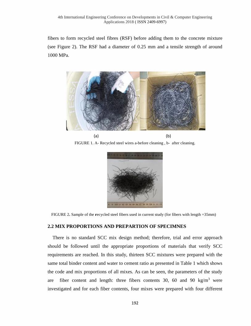
4th International Engineering Conference on Developments in Civil & Computer Engineering
Applications 2018 ( ISSN 2409-6997)
192
fibers to form recycled steel fibres (RSF) before adding them to the concrete mixture
(see Figure 2). The RSF had a diameter of 0.25 mm and a tensile strength of around
1000 MPa.
FIGURE 1. A- Recycled steel wires a-before cleaning , b- after cleaning.
FIGURE 2. Sample of the recycled steel fibers used in current study (for fibers with length =35mm)
2.2 MIX PROPORTIONS AND PREPARTION OF SPECIMNES
There is no standard SCC mix design method; therefore, trial and error approach
should be followed until the appropriate proportions of materials that verify SCC
requirements are reached. In this study, thirteen SCC mixtures were prepared with the
same total binder content and water to cement ratio as presented in Table 1 which shows
the code and mix proportions of all mixes. As can be seen, the parameters of the study
are fiber content and length: three fibers contents 30, 60 and 90 kg/m3 were
investigated and for each fiber contents, four mixes were prepared with four different
(a) (b)

4th International Engineering Conference on Developments in Civil & Computer Engineering
Applications 2018 ( ISSN 2409-6997)
193
fiber lengths (Lf) (10, 15, 25, 35 mm). A control mix (plain SCC) was also prepared for
comparison reasons. In the study, all mixes have been prepared by following European
guidelines of SCC EFNARC [4]. A 0.04 m3 mechanical rotary mixer was employed in
the production of concrete mixtures. Three (100 mm) cubes and three prisms
100×100×500 mm, were cast for each mix. After casting, the specimens were then
covered by plastic sheets and allowed to cure for 24 hours before being demoulded.
Then, the specimens were kept in water tanks for 27 days for further curing.
TABLE 1.
Code of mixes and mix proportions in kg/m3.
2.3 TEST METHODS
Rheological properties
Slump flow, T50 flow time, J-ring, L-box, BJ, TJ, and V-funnel were conducted to
assess the fresh properties of the SCC mixes. These tests were undertaken following the
specifications and guidelines of European Federation of National Associations
Representing producers and applicators of specialist building products for Concrete
(EFNARC) for SCC [4]. The sequence of performing the fresh concrete tests was the
same with all mixes. The fresh properties were conducted immediately after the
completion of concrete mixing.

4th International Engineering Conference on Developments in Civil & Computer Engineering
Applications 2018 ( ISSN 2409-6997)
194
Mechanical properties
The compressive strength was obtained at age of 28 days using the (100 mm cubes)
and BS EN 12390-3 [13]. The flexural strength was obtained at 28 days using (100×100
×500) mm prisms. All prisms were tested in two-point loading over a span of 300 mm
following the recommendations of the BS EN 12390-5 [14].
3. RESULTS AND DISCUSSIONS
3.1 RHEOLOGICAL PROPERTIES
To evaluate the effect of the use of RSF on the performance of SCC mixtures, the
rheological behavior of all mixes was quantified by assessing: 1- flow, viscosity and
filling ability of concrete by slump flow and V-funnel tests; 2- the passing ability of
concrete by j-ring and L-box tests (see Figure 3). The results of all fresh concrete
properties and the limits of EFNARC are presented in Table 2. In general, it can be seen
that the rheological properties of SCC showed a gradual degradation with the addition
of RSF. It was shown that both RSF content (Wf) and length (Lf) affected the
rheological of SCC.
FIGURE 3. Rheological properties tests: a- slump flow, b- j-ring , c-V-funnel, d- L-box,
C D
A B

4th International Engineering Conference on Developments in Civil & Computer Engineering
Applications 2018 ( ISSN 2409-6997)
195
TABLE 2.
Result of rheological properties of all mixes.
-Slump flow and J-ring tests
For the slump flow test results, as can be seen in Table 2 and Figure 4, the flow
characteristics decreased proportionally with increasing RSF content. The reduction in
flow properties was clearly observed when long fibers is used rather than short ones.
The control mix M0 which is plain SCC (without RSF) showed a 788 mm slump flow
and 2.25sec. flow time (T500). For mixes having 30 kg/m3 fibers content, a marginal
effect on slump flow and fluidity was observed compared to the control mix M0.
Where, the slump flow of M1, M2, M3 and M4 reduced by only 4.2 %, 5.5 %, 8.0% and
8.6%, for fiber lengths of 10, 15, 25 and 35 mm, respectively. The reduction in slump
flow clearly increased when fiber content increased to 60 kg/m3. Table 2 shows that the
reduction in slump flow of M5, M6, M7 and M8 compared to M0 was 8.6%, 11.1%,
15.6 %, and 18.1%, respectively. Additionally, at higher fibers content 90 kg/m3, the
reduction in slump flow significantly increased, particularly with long fibers. In

4th International Engineering Conference on Developments in Civil & Computer Engineering
Applications 2018 ( ISSN 2409-6997)
196
comparison to M0, the slump flow of mixes M9, M10, M11 and M12 declined by
15.0%, 16.2%, 27% and 28.9%, respectively.
All mixes of the fiber contents of 30 and 60 kg/m3 fulfill the EFNARC requirements [4]
of slump flow as can be seen in Figure 4. This means that these mixes still maintain the
characteristics of SCC. However, for mixes with 90 kg/m3 content, the slump flow of
the mixes with long fibers (25mm and 35mm) does not meet the requirements of
EFNARC,
FIGURE 4. Effect of RSF content on slump flow.
This reduction in slump flow due to the addition of RSF could be attributed to the
resistance to flow that develops because of the presence of RSF ; hence increasing the
internal friction between aggregate particles and fibers [5,6]. The increasing in the
internal friction proportionally increased with fiber content (Wf). The high stiffness
(modulus of elastic) of steel fibers could be one of the sources for a likely increase in
inter-particle friction under the free flow [5,15] with a possible absorbing of the moving
energy [11]. In terms of RSF length, regardless of the fiber content, the tangle of long
fibers caused reduction in slump flow more than short fibers.
As far as the results of flow time, j-ring (flow and Bj) are concerned, similar behavior to
that of the slump flow was observed for the mixes containing RSF. The increase in the
fiber content and length adversely affected the results of flow time and j-ring tests. The
reduction in flow time and j-ring flow is an indication of the high viscosity of the mixes
with RSF. Despite the negative effect of the RSF on the results of flow time and j-ring
EFNARC LIMITS

4th International Engineering Conference on Developments in Civil & Computer Engineering
Applications 2018 ( ISSN 2409-6997)
197
tests, all mixes with RSF (apart from M11 and M12) conform with the limits of
EFNARC [4]as can be seen in Table 2.
V-funnel and L-box tests
The results of V-funnel test, as can be seen in Table 2, show that the mixes
incorporating of RSF exhibited an increase in V-funnel time compared to the plain SCC.
The V-funnel time gradually increased with RSF content and length. The addition of
RSF with 30 kg/m3 showed little effect on passing ability of concrete through the V-
funnel. At this RSF content, time recorded in V-funnel test in comparison to M0
decreased by 3.75%, 4.4%, 5.75% and 8.5% for M1, M2, M3 and M4, respectively. The
time needed by RSF mixes to pass through the V-funnel increased with RSF content at
60 kg/m3 by 17.5%, 31.25%, 43.12% and 45% for M5, M6, M7 and M8 compared to
the control mix M0; Figure 5. As the fibers content increased to 90 kg/m3, V-funnel test
results exceeded the upper limit of EFNARC guidelines [4]. Much higher increase 50%,
68.7%, 95% and 112.5% in the V-funnel time was recorded for mixes M9, M10, M11
and M12, respectively, compared to the control mix. This could be due to the same
reasons mentioned previously related to the increased internal friction between
aggregate particles and RSF leading to high viscosity and increased flow time through
V-funnel [15]. Additionally, the long fibers prevent the aggregate particle from the free
movement causing delay in flow [15]
FIGURE 5. Effect of RSF content on V-funnel time (sec).
EFNARC LIMITS

4th International Engineering Conference on Developments in Civil & Computer Engineering
Applications 2018 ( ISSN 2409-6997)
198
L-box test was performed to assess passing ability of all SCC mixes, and the results of
which are shown in Table 2. The results showed that the incorporation of RSF
negatively affected the passing ability of mixes with RSF. It is clear that this reduction
in blocking ratio depends on both the fiber content Wf and fiber length Lf. The higher
the RSF content the higher the reduction in the passing ability of the mixes. Also, the
passing ability decreased when the length of the fibers increased. However, all mixes
with RSF (apart from M11 and M12) meet the requirements of EFNARC [4]as can be
seen in Figure 6. The reduction in passing ability can be attributed to the presence of
fibers which work as obstacles and de-accelerate the movement. The influence of
adding RSF is significantly appearing with high contents (90 kg/m3) and with long
fibers. Long fibers could lead to a reduction in the internal energy needed for the mix to
move freely.
FIGURE 6. Effect of RSF content on blocking ratio (L-box test)
From the results of the rheological properties, it seems that the RSF can be used up to
60 kg/m3 content with no effect on the properties of being SCC as all requirements of
EFNARC can be satisfied. Higher contents such as 90 kg/m3 can be used but the length
of the RSF should not exceed 15 mm.
EFNARC
LIMITS

4th International Engineering Conference on Developments in Civil & Computer Engineering
Applications 2018 ( ISSN 2409-6997)
199
3.4 MECHANICAL PROPERTIES
The results of the mechanical properties including compressive strength and flexural
strength for all mixes are presented in Table 3. The results are the average of three
specimens.
TABLE 3.
Result of compressive and flexural strength of all mixes
-Compressive strength
The inclusion of RSF doesn’t show significant effect on compressive strength of SCC
mixtures. From test results presented in Table 3, mixes show either a slight increase or
decrease in compressive strength comparing to the control mix (plain SCC).
The results show that the two parameters (fiber content and length) examined in this
study affected the compressive strength of SCC mixes containing RSF. The effect of
these parameters is shown in Figure 7. It can be seen that for low fiber content (30
kg/m3) the compressive strength increases (for all RSF lengths) up to 12.7% compared
to the control mix; whereas for high fiber content (90 kg/m3), the strength decreases (for
all RSF lengths) by up to 12.7% compared to the control mix. However, for moderate
fiber content (60 kg/m3) the compressive strength slightly increased for short fibers (10
and 15mm) and slightly declined for long fibers (25 and 35mm).Same results were
concluded by researchers [7,15] but for manufactured steel fibers. For all fiber contents,

4th International Engineering Conference on Developments in Civil & Computer Engineering
Applications 2018 ( ISSN 2409-6997)
200
the compresive strength increased with the decrease of the length of the fibers which
means shorter fibers exhibited better performance in terms of comreessive strength.
FIGURE 7. Effect of RSF length and content on the compressive strength of SCC.
The increase in compressive strength for low content and short fibers could be due to
the ability of short fibers in delaying the propagation of microcracks and slowing down
the development of microcracks to macrocrcks and; thus delaying the failure of concrete
[2,8]. Also, the incorporation of RSF could transfer the compression failure from
collapse/ brittle to ductile failure [8] which also lead to higher strength before failure.
This result were in a compatibility with previous results [15],
The reduction in compressive strength for high contents and long fiber might be due to a
reduction in rheological of RSFSCC mixes as mentioned in the presvius section.
Furthermore, adding RSF could increase the pososity of concrete due to the increase in
the entrapped air voids which considered as concrete defect [2]. During mixing and
casting, fibres may entrap large air voids especially with high content of fibres [2].
Moreover, the reduction in strength can be attributed to the existence of long fibers
ineffective in arresting microcracks [11]. Additionally, the existence of long RSF could
increase the entrapp air voids due to balling and tangle of fibers. This would result in
accelerating the propagation of cracks and failure.

4th International Engineering Conference on Developments in Civil & Computer Engineering
Applications 2018 ( ISSN 2409-6997)
201
-Flexural strength
Table 3 also shows the results of the flexural of all SCC mixes. The performance of
SCC mixes with RSF under compression loading is not the same as under bending
loading. Regardless of the fiber content, all SCC mixes with RSF show higher flexural
strength than that of the plain SCC. Additionally, for the same fiber content, the higher
the fiber length the higher the flexural strength as can be seen in Figure 8. For example,
the flexural strength increased by 11.0%, 16.8%, 26.8% and 27.4% for mixes M1, M2,
M3 and M4 compared to M0, respectively. It was expected that mixes with 90 kg/m3
RSF content would show the best flexural performance; however, these mixes exhibited
less flexural strength enhancement compared with the 30 kg/m3 fiber content. This
could be due to the same effect related to the development of air voids at high contents
of RSF which is mentioned earlier. The best flexural performance is shown by mixes
with 60 kg/m3 fiber content. At this fiber content, enhancements in the flexural strength
of up to 34% were observed.
FIGURE 8. Effect of RSF length and content on the flexural strength of SCC.
The enhancement in flexural strength due to RSF incorporation can be mainly attributed
to the role of fibers in bridging the microcracks and arresting the sides of the
macrocracks in concrete body and hence delaying the occurrence of concrete failure [2,
15,11]. Also, this behavior could be partly due to the pull-out resistance of fibers
[11]which increases with the increase of fiber length. This can result in a significant
increase in fracture resistance and thus increasing the ductility of SCC mixes [11].
RSF content kg/ m3
Plain SCC

4th International Engineering Conference on Developments in Civil & Computer Engineering
Applications 2018 ( ISSN 2409-6997)
202
4. CONCLUSIONS
The discussion of the results can lead to the following conclusions:
- The use of RSF reduced the slump flow and J-ring flow and decelerated the flow
rate (T500) of SCC mainly due to the increase in inter-particle friction under the
free flow. However, all mixes with RSF (apart from mixes with high content 90
kg/m3 and long fibers 25 and 35 mm) maintain the EFNARC requirement of
slump flow and flow rate.
- Mixes with RSF exhibited higher viscosity and lower passing ability than that of
plain SCC as the V-funnel time increased and the blocking ratio decreased with
the increase of RSF content and length. Nonetheless, all mixes with RSF (apart
from mixes with high content and long fibers) comply with EFNARC
requirements.
- For low fiber content (30 kg/m3) the compressive strength increased (for all
RSF lengths) up to 12.7% compared to the control mix; whereas for high fiber
content (90 kg/m3), the strength decreased (for all RSF lengths) by up to 12.7%
compared to the control mix. However, for moderate fiber content (60 kg/m3)
the compressive strength slightly increased for short fibers (10 and 15mm) and
slightly declined for long fibers (25 and 35mm).
- All SCC mixes with RSF showed higher flexural strength than that of the plain
SCC by up to 34%. For the same fiber content, the higher the fiber length the
higher the flexural strength.
- The utilization of RSF in SCC can lead to an innovative, sustainable and cost-
effective self-compacting fibre reinforced concrete.

4th International Engineering Conference on Developments in Civil & Computer Engineering
Applications 2018 ( ISSN 2409-6997)
203
REFERENCES
[1] Thomas, B.S. and R.C. Gupta, Properties of high strength concrete containing
scrap tire rubber. Journal of Cleaner Production, 2016. 113: p. 86-92.
[2] Younis, K. H., (2016) “Mechanical perfromance of concrete reinforced with
recycled steel fibres extracted from post-consumer tyres)” Proceedings of the
2nd International Engineering Conference on Developments in Civil
Engineering and Computer Applications (2nd IEC2016) 20 – 22 February, Erbil-
Kurdistan-Iraq.
[3] Thomas, B.S., and R. C. Gupta. "A comprehensive review on the applications of
waste tire rubber in cement concrete." Renewable and Sustainable Energy
Reviews 54 (2016): 1323-1333.
[4] EFNARC (2005) “The European Guidelines for self-compacting concrete:
specification, production, and use” http://www.efnarc.org/(Accessed on August
2016)
[5] A. S. El-Dieb and M.M.R. Taha, flow characteristics and acceptance criteria of fiber-
reinforced self-compacting concrete (FR-SCC). Construction and Building Materials,
2012. 27: p. 11. [6] Gencel, O., et al., Workability and mechanical performance of steel fiber-
reinforced self-compacting concrete with fly ash. Composite interfaces, 2011.
18(2): p. 169-184.
[7] Madandoust, R., et al., Assessment of factors influencing mechanical properties
of steel fiber reinforced self-compacting concrete. Materials & Design, 2015. 83:
p. 284-294.
[8] Younis, K. H. and K. Pilakoutas, Strength prediction model and methods for
improving recycled aggregate concrete. Construction and Building Materials,
Vol. 49, No. 0, pp. 688-701, 2013.
[9] Tlemat, H., Steel fibres from waste tyres to concrete: testing, modelling and
design. PhD.thesis, The University of Sheffield, UK, 2004.
[10] Pilakoutas, K., K., Neocleous, Tlemat, H., Reuse of steel fibres as
concrete reinforcement. Engineering Sustainability, Vol. 157, No. ES3, pp. 131-
138, (2004)
[11] Centonze, G., M. Leone, and M. Aiello, Steel fibers from waste tires as
reinforcement in concrete: A mechanical characterization. Construction and
Building Materials, 2012. 36: p. 46-57.
[12] IQS No. 45/1984 ‘’Iraqi specification for aggregate’’ (1984).
[13] BS EN 12390-3, Testing hardened concrete Part 3: Compressive
strength of test specimens. British Standard Institution, London, UK, 2009.
[14] BS EN 12390-5:2009, Testing hardened concrete Part 5: Flexural
strength of test specimens.British Standard Institution, London, UK, 2009.
[15] Khayat, K. and Y. Roussel, Testing and performance of fiber-reinforced,
self-consolidating concrete. Materials and Structures, 2000. 33(6): p. 391-397.

4th International Engineering Conference on Developments in Civil & Computer Engineering
Applications 2018 ( ISSN 2409-6997)
204
MECHANICAL PROPERTIES OF CONCRETE USING IRON
WASTE AS A PARTIAL REPLACEMENT OF SAND
Krikar M-Gharrib Noori1 , Hawkar Hashim Ibrahim2
1 Koya Technical Institute, EPU
2Salahaddin University-Erbil 1 [email protected], 2 [email protected]
doi:10.23918/iec2018.16
ABSTRACT
The utilising of iron waste in concrete as a partial replacement of sand is attaining
enormous significance nowadays, mostly because of the improvement in the
strength of concrete and environmental benefits. The aim of this study is to assess
the possibility of applying iron waste in different percentages (6%, 12%, 18%, 24%,
and 30%) as fine aggregate replacement of sand to increase the strength of concrete.
For this purpose, the mix proportion was designed as (1:2.12:2.37) for giving 33
MPa of compressive strength of concrete at 28 days of curing. In order to achieve
the goal of the study, laboratory experiments, compressive strength, and flexural
tensile strength were conducted to determine the influence of iron waste on the
strength of concrete. Thus, based on this study, the progress of strength with the
percentages of iron waste in different time was plotted. According to the results, it
can be found that 12% of iron waste is more efficient than the other percentages in
both compressive and flexural strength because it obtains the maximum strength in
the shortest time, and it seems that increasing iron waste more than 12% leading to
decrease the strength of the concrete.
Keywords: Concrete, Sand Replacement, Iron Waste, Compressive Strength,
Flexural Tensile Strength.

4th International Engineering Conference on Developments in Civil & Computer Engineering
Applications 2018 ( ISSN 2409-6997)
205
1. INTRODUCTION
Nowadays, one of the most commonly expended construction material in the
world is concrete. It consists of cement, sand, gravel, and water. Additional
materials could be supplied to the mixture. The concrete comprises amount of
entrapped air and may have knowingly entrained air attained using an admixture or
air-entraining cement [1]. Sand as fine aggregate is more extensively consumed in
concrete construction. Hence, numerous developing countries have nowadays faced
a struggle in providing the quantity of natural sand so that encounter the enhancing
desires of infrastructural development in recent years [2]. In this regard, sand could
be replaced by different waste materials, which might be able to improve plasticity,
workability, and increase concrete strength to enhance durability [3]. In terms of
waste materials environment impact, advancements in technology enhance not only
human comforts but also damages the environment [4]. Although industrialization is
one of the key factors for growing economy, also it has led to serious troubles that
leading to environmental pollution. Waste materials, discharged in large quantities
by industries, create serious environmental problems. To lowest possible
environmental impact, the reusing of these waste materials will become an essential
standard to protect the environment [5]. Regarding this, reusing unwanted remaining
materials will be a popular substitute for disposaling the waste, in this waste
utilization, possible pollution problems and cost are reduced or even the pollution is
removed along with the achievement of environment protection. However, to use
available materials most efficiently, the consideration of utilization strategy should
be combined with the considerations of energy and environment [6]. Iron waste is
one of the materials discharged in great amounts by-product of the steel industry in
Kurdistan Region of Iraq. Disposing this waste impact negatively on the
environment. Iron waste, due to its high strength and durability, might be able to
increase a concrete strength in terms of compressive strength and flexural tensile [3].
The presented work studies the effective of iron waste on compressive strength and
flexural tensile strength of concrete based on laboratory tests. According to the past
literature, during the history of the industries of iron and steel, different methods
have been attempted to create operational use of the waste materials of iron and
steel. Various studies have been done to use the waste material in the concrete
mixture for improving concrete properties and preventing the environment from

4th International Engineering Conference on Developments in Civil & Computer Engineering
Applications 2018 ( ISSN 2409-6997)
206
these unwanted materials. In this study, some of them will be reviewed. Dubey, et
al. [7] considered using the blast furnace slag powder to determine its effect on
compressive strength of concrete. In this study, blast furnace slag was partially used
as a replacement of cement in different percentage 5 to 30%. It has been discovered,
from the experimental investigations, that the optimum substitution of Ground
Granulated Blast Furnace Slag Powder to cement is 15% without changing much the
compressive strength. Ugama, et al. [8] examined determining the appropriateness of
using iron ore tailing (IOT) to partly replace fine aggregate for concrete which it is
utilized for rigid pavement. The control mix composites a normal mixture of
concrete which only sand functioned as fine aggregate, while the replaced sand in
the other mixes was by 20%, 40%, 60%, 80% and 100% iron ore tailing (IOT).
Strength and consistency tests were studied on all samples of concrete. It was
noticed that increasing the ratio of iron ore tailing in the mixture, leads to decrease
in the concrete workability. The results for tests of compressive and indirect tensile
strength at twenty eight days were 43.67 N/mm2 and 2.69 N/mm2, respectively.
They were attained for concrete when 20% iron ore tailing (IOT) was used, then the
results equated to compressive strength and indirect tensile strength outcomes of
45.02 N/mm2 and 2.64 N/mm2 respectively, gained at 28 days as only sand as a fine
aggregate was used. Alzaed [9] studied the effect of iron filings on concrete strenth
as one of the portions of the concrete mixture. In the paper, the iron filing was
supplied to the concrete mix in four different percentage, to detrmine the difference,
which might be gained in compression and tensile concrete strengths at twenty eight
days. In the study, numerous standard cubes and cylinders were fabricated and tested
using 0% (control), 10%, 20% and 30% of iron filing in the concrete mix. It was
determined that when iron filing supplemented to the concrete mix, the compressive
strength of concrete increased steadily while the tensile strength showed a minor
effect as the ratio of iron filing applied more than 10%. As a result, two formulas
were suggested, which might be utilized to expect the quantity of increasing
corresponding to each percentage of iron filing contributed to the concrete mix.
Ghannam, et al. [3] carried out an experimental investigation to explore the
possibility of using the iron powder (IP) and granite powder (GP) to partially replace
to fine aggregate in concrete mixture. The percentages 5%, 10%, 15%, and 20% of
GP and IP were added to replace sand by weight. It was found that the most

4th International Engineering Conference on Developments in Civil & Computer Engineering
Applications 2018 ( ISSN 2409-6997)
207
effective replacement percentage of sand with granite powder in concrete was 10%
by weight in increasing the compressive and flexural strength compared to other
ratios. The test results showed that the compressive strength increased nearly 30%,
as sand partly replaced to 10% of GP in concrete, compared with normal concrete.
Similar results were also found for the flexure. It was moreover remarked that
substituting of sand with up to 20% of iron powder by weight in concrete resulted in
increasing in compressive and flexural strength of the concrete.
2. STUDY IMPLICATION
Iron waste is an industrial by-product that is produced as a result of producing
steel from the steel factory. This waste material can be applied as partial
replacement of sand in concrete. The aim of this study is to evaluate the suitability
of using iron waste as a partial replacement of fine aggregate and to observe that
iron waste leads to increase the compressive strength, and flexural strength of
concrete, as used in certain proportions. The experimental research considered in
this study displayed the mechanical properties of concrete have enhanced as sand
was replaced partially by iron waste in certain proportions. Furthermore, recycling
of this by-product and employing it in concrete will decrease its effect on the
environment and its health hazards. The usage of iron waste instead of sand will
reduce using of sand in the construction industry hence maintaining more of this
natural resource.
3. EXPERIMENTAL INVESTIGATION
The experimental program included preparing concrete cubes and beams with
and without iron waste replacement. The concrete mixture consists of Portland
cement, sand, coarse aggregates, iron waste, and water. The cubes were prepared to
evaluate the concrete compressive strength and the beams were equipped to assess
the flexural strength.

4th International Engineering Conference on Developments in Civil & Computer Engineering
Applications 2018 ( ISSN 2409-6997)
208
4. MATERIALS AND METHODOLOGY
4.1 MATERIALS
Materials that used for this study comprised of cement, fine aggregates (sand),
coarse aggregates (gravel), iron waste, and water. According to ASTM codes,
necessary tests were carried out for the materials.
4.1.1 CEMENT
Cement is a binder substance that can bind other materials together. Physical
properties of Ordinary Portland cement was found and compared with the code
specification (ASTM C 150) which is shown in Table 1. The results are compatible
with the code specification.
TABLE 1.
Properties of cement with the code specification
No Parameters Values Code Specification
ASTM C150
1 Fineness 0.04 0.01 – 0.06
2 Specific gravity 3.1 around 3.15
3 Consistency 28 % 26% – 30 %
4 Initial Setting time (minutes) 70 ≥ 45
5 Final Setting time (minutes) 290 ≤ 375
4.1.2 FINE AGGREGATE (SAND)
Sand is a naturally occurring granular material composed of finely material
particles. The fine aggregate passed through sieve #4 (4.75 mm) and predominately
retained on sieve # 200 (75 𝜇m) was used. The sand has a specific gravity of 2.67,
bulk density 1647 kg/m3 and the fineness modulus equal to 2.6.
4.1.3 COARSE AGGREGATE (GRAVEL)
Coarse aggregate is one of the main components of concrete composite materials.
The maximum size of coarse aggregate was 12.5 mm used. The gravel has a specific
gravity of 2.74, bulk density 1600 kg/m3 and the fineness modulus equal to 6.2.

4th International Engineering Conference on Developments in Civil & Computer Engineering
Applications 2018 ( ISSN 2409-6997)
209
4.1.4 IRON WASTE
Iron waste is a by-product material. When the waste material is disposed of, it
will affect the environment. Over the past few years, the amount of this material
have been increased by steel factories in the Kurdistan region of Iraq. In order to
reduce the impact of waste materials on the environment, iron waste could be used
instead of sand concrete mixture. The iron waste has a specific gravity, bulk density
and the fineness modulus with 3.56, 2168 kg/m3, and 2.3, respectively. It should be
noted that there is a difference between the density of the sand and the iron waste
that will be expected to affects the density of the concrete. Furthermore, the waste
material was accumulated in a steel factory in Bazyan related (Sulaymani
Province).The quantities of this waste material will be increase and it will effect on
our environment. Therefore, it is crucial to use this material to improve concrete
properties.
4.1.5 WATER
A clean water is used for mixing process and curing. The used water should be
applied according to the mix proportion design.
4.2 METHODOLOGY
4.2.1 WORK PLAN
As it is described previously that using iron waste in concrete as replacement of
sand might increases its strength. To find out that experimental method was used,
both flexural tensile strength and compressive strength of concrete were considered
to be tested. Regarding this, the research is planned as firstly ordinary concrete with
only cement, sand, aggregate, and water as control was prepared. Then fine
aggregate sand is partially replaced by iron waste in different percentage. The
percentages were as follows: (6%, 12%, 18%, 24%, and 30%) for compressive
strength and for flexural tensile strength. For each percentage, nine cubes and nine
beams were made up. Overall, total samples were 54 cubes and 54 flexural beams.
The cubes with dimensions of (100*100*100) mm samples were used for the
compressive strength test, and utilizing beam specimens with dimensions of (100 ×

4th International Engineering Conference on Developments in Civil & Computer Engineering
Applications 2018 ( ISSN 2409-6997)
210
100 × 500mm) for the flexural tensile strength test. The samples were tested after
three different times of curing (7, 14, 28) days.
4.2.2 CONCRETE MIX DESIGN
The mix proportions are important to a strong and durable concrete. The mix
design should achieve the desired workability of concrete to prevent segregation and
allow for ease of placement. In this regard, using the standard mix design according
to Dixon, et al. [1], the mixture was designed for giving compressive strength of
concrete of 33 MPa after 28 days of curing. The mix proportion was prepared as
(1:2.12:2.37). Table 2 shows the weight of mixture components. The percentages of
iron waste (0, 6, 12, 18, 24, and 30 %) were used instead of sand.
TABLE 2.
Quantities of materials used in kg/m3
Iron Waste
Percentage %
Cement
kg/m3
Iron Waste
kg/m3
Sand
kg/m3
Aggregate
kg/m3
Water
kg/m3
Water/
cement
0% 385 0 818 912 200 0.52
6% 385 49.08 768.92 912 200 0.52
12% 385 98.16 719.84 912 200 0.52
18% 385 147.24 670.76 912 200 0.52
24% 385 196.32 621.68 912 200 0.52
30% 385 245.4 572.6 912 200 0.52

4th International Engineering Conference on Developments in Civil & Computer Engineering
Applications 2018 ( ISSN 2409-6997)
211
4.2.3 LABORATORY TESTS
The concrete slump test is a practical test to measure the consistency of the
concrete to check the workability of fresh concrete. In this regard, slump tests
according to ASTM C143 were carried out for all mix ratios. Figure 1 (a) shows the
slump test. Compression tests and flexural tests were implemented on concrete
cubes, and concrete beams respectively. Compressive strength is the capacity of a
material or structure to withstand loads tending to reduce size. The compressive
strength samples were prepared according to ASTM C39 [10], concerning this, nine
standard compressive concrete cube specimens (100 × 100 × 100mm) were
fabricated to be tested for zero percent and each proportion of iron waste.
Meanwhile, the flexural strength (modulus of rupture) samples were prepared
according to ASTM C293 [11]. A plain concrete beam (100 x 100 x 500 mm) was
loaded in flexure at the third points of 300-mm span until it fails due to cracking on
the tension face. Modulus of rupture is computed as [12]:
𝑅 =3𝑃𝐿
2𝑏𝑑3 (1)
where; R is the modulus of rupture [MPa], P is a maximum applied load indicated
by testing machine [N], L is the span length [m], b is the average width of specimen
[mm] and d is the average depth of specimen [mm]. the samples were cured for 7
days, 14 days, and 28 days under standard conditions. Then the tests of the
specimens were implemented. The test of the samples for a compressive strength by
MPa and flexural strength by KN at 7 days, 14 days, and 28 days were carried out.
Figure 1 (b) & (c) show the compression test and flexural test respectively.
Regarding preparing the samples, fifty-four cubes were prepared for compressive
strength, every eighteen samples were tested at 7 days, 14 days and 28 days for
control and other proportions. Meanwhile, fifty-four beams were tested for the
flexural strength test. Similarly, for the flexure, every eighteen samples were tested
at 7 days, 14 days and 28 days for control and other proportions. Moreover, the test
results of the cubes, and beams, of concrete made with IP were equated to the test
results of the normal concrete (control) specimens.

4th International Engineering Conference on Developments in Civil & Computer Engineering
Applications 2018 ( ISSN 2409-6997)
212
50
55
60
65
70
0% 6% 12% 18% 24% 30%
Hig
ht
[mm
]
Iron Waste percentages [%]
Slump Tests
5. RESULTS AND DISCUSSION
5.1. SLUMP TEST
The outcomes show that the slump decreased slightly and gradually as iron waste
increased. This means that the workability of the concrete is in an acceptable range
with a good durability of concrete. Figure 2 displays the slump test for all mixing
ratio.
FIGURE 2. Presents the slump test for all mixing ratio
5.2. COMPRESSIVE STRENGTH TEST
Compressive strength test was carried out to evaluate the strength progress of
concrete, comprising different percentages of iron waste at the age of 7, 14, 28 days,
respectively. It is shown in Figure 3 that increasing the iron waste leading to
FIGURE 1. (a) Slump Test, (b) & (c) display compressive and flexure strength specimen test
(a) (b) (c)

4th International Engineering Conference on Developments in Civil & Computer Engineering
Applications 2018 ( ISSN 2409-6997)
213
gradually gains in the compressive strength. It is observed that increasing the iron
waste to 12% gives the highest strength among the results, which from this point
onwards increasing the amount of iron waste decreases the strength of concrete. It
can be realized that using 12% iron waste in concrete will give 15% more
compressive strength in 28 days than normal concrete (control).
5.3. FLEXURAL TENSILE STRENGTH TEST
Regarding the flexural tensile strength, flexural samples were tested to evaluate
the strength of concrete, containing various ration of iron waste. Based on the results
shown in Figure 4, the flexural tensile strength gradually increases as the iron waste
percentage reaches 12%. It is clear from the figure that increasing iron waste more
than 12% leads to falling down the flexural tensile strength. Therefore, it can be said
that iron waste can be limitedly used to be effective as a replacement of sand to
increase the strength of concrete. As a result, it can be concluded that using waste
materials are the benefit in terms of not only preserving the environment, but also
improving the structural properties of concrete.
FIGURE 3. Compressive strength of different iron waste percentages for
different time of curing
0
10
20
30
40
50
0% 6% 12% 18% 24% 30%
Co
mp
ress
ive
Str
ength
[M
Pa]
Iron Waste Percentage [ %]
7 days
14 days
28 days

4th International Engineering Conference on Developments in Civil & Computer Engineering
Applications 2018 ( ISSN 2409-6997)
214
FIGURE 4. Shows the flexural tensile strength of different iron waste
percentages for different time of curing
0
0.4
0.8
1.2
1.6
2
0% 6% 12% 18% 24% 30%
Fle
xure
Ten
sile
Str
ength
[Mp
a]
Iron Waste Percentage [%]
7 days14 days28 days
6. CONCLUSIONS
In conclusion, the workability of the concrete is slightly and gradually decreased
by increasing iron waste. The strength of concrete increased while curing was
prolonged. The compressive and flexural tensile strength slightly increased by
increasing iron waste ratio until 12%. It can be noted that using 12% iron waste in
concrete gave 15% more compressive strength in 28 days than normal concrete. It
should be significantly concentrated on that the mix ratio was basically designed to
gives 33 MPa at 28 days but more than this can be obtained at 7 days by adding 12%
of iron waste which was about 35 MPa. So in case, the concrete needs to reach the
maximum compressive strength in the shortest time, 12% iron waste can be
recommended to use in the concrete.
7. ACKNOWLEDGMENT
The authors would like to thank Koya University for its help in providing the
necessary facilities needed to perform this research.

4th International Engineering Conference on Developments in Civil & Computer Engineering
Applications 2018 ( ISSN 2409-6997)
215
REFERENCES
[1] D. E. Dixon, J. R. Prestrera, G. R. Burg, E. A. Abdun-Nur, S. G. Barton, L.
W. Bell, et al., "Standard Practice for Selecting Proportions for Normal,
Heavyweight, and Mass Concrete (ACI 211.1-91)," 1991.
[2] S. Raman, M. Safiuddin, and M. Zain, "Non-destructive evaluation of
flowing concretes incorporating quarry waste," Asian journal of civil
engineering (Building and Housing), vol. 8, pp. 597-614, 2007.
[3] S. Ghannam, H. Najm, and R. Vasconez, "Experimental study of concrete
made with granite and iron powders as partial replacement of sand,"
Sustainable Materials and Technologies, vol. 9, pp. 1-9, 2016.
[4] R. Joshi, "Effect of using selected industrial waste on compressive and
flexural strength of concrete," International Journal of Civil and Structural
Engineering, vol. 4, p. 116, 2013.
[5] A. Jayaraman, N. Karthiga Shenbagamn, and V. Senthilkumar, "Eco
Friendly Building Materials Used for High strength and high performance
Concrete," International Journal of ChemTech Research, vol. 10, pp. 23-28,
2017.
[6] B. Bahoria, D. Parbat, P. Naganaik, and U. Waghe, "Comprehensive
literature review on use of waste product in concrete," International journal
of Application or Innovation in Engineering & Management, vol. 2, pp. 387-
394, 2013.
[7] A. Dubey, R. Chandak, and R. Yadav, "Effect of blast furnace slag powder
on compressive strength of concrete," International Journal of Scientific &
Engineering Research, vol. 3, pp. I094-I098, 2012.
[8] T. Ugama, S. Ejeh, and D. Amartey, "Effect of iron ore tailing on the
properties of concrete," Civil and Environmental Research, vol. 6, p. 7, 2014.
[9] A. Alzaed, "Effect of iron filings in concrete compression and tensile
strength," International Journal of Recent Development in Engineering and
Technology, vol. 3, pp. 121-125, 2014.
[10] A. Standard, "ASTM C39 Standard Test Method for Compressive Strength
of Cylindrical Concrete Specimens," ASTM International, 2015.
[11] M. American Society for Testing, C. o. C. Committee, A. Concrete, and A.
S. C. o. T. f. Strength, Standard test method for flexural strength of concrete
(using simple beam with center-point loading). Philadelphia, Pa.: ASTM
International, 2010.
[12] D. A. Fanella, Reinforced concrete structures : analysis and design, 2016.

4th International Engineering Conference on Developments in Civil & Computer
Engineering Applications 2018 ( ISSN 2409-6997)
216
EFFICIENT TECHNIQUES TO MINIATURIZE THE SIZE
OF PLANAR CIRCULAR MONOPOLE ANTENNA
Y. A. Fadhel1,R. M. Abdulhakim2
1University of Duhok
2Nawroz University
[email protected], [email protected]
doi:10.23918/iec2018.17
ABSTRACT
Recently different techniques have been adopted by many researcher to
minimize the size of antennas being employed in compact devices. In this
paper miniaturization of a planar circular monopole antenna (PCMA) has
been introduced while maintaining its working range of frequencies covering
the UWB range (3.1~10.6 GHz). Two different techniques are suggested;
firstly, the PCMA radiator has been modified by eliminating areas with least
concentrated current distribution, which led to generation of a crescent-shape
radiator and the overall size reduction reached 11.76% of the original size.
Secondly, the edge of the circular radiator has been corrugated according to
some suggested formulas, which increased the size reduction to about 42.6%.
Another advantage has been achieved for the corrugated PCMA by extending
the upper limit of its impedance bandwidth to 13.85 GHz. All designed
antennas have been fabricated and verified via practical experimental
measurements. Simulated and measured results have shown that both
techniques were succeeded in miniaturizing the overall size of PCMA antenna,
but precisely, corrugation technique was more efficient.
Keywords: Miniaturized Antennas, PCMA, Crescent-Shaped, Corrugation,
UWB.

4th International Engineering Conference on Developments in Civil & Computer
Engineering Applications 2018 ( ISSN 2409-6997)
217
1. INTRODUCTION
Since adopting the UWB standard by Federal Communication
Commission (FCC ) in 2002 [1] for short-range peer-to-peer ultra-fast
communication, researchers competed in designing different types of
antennas that obey the wideband range of frequencies (3.1 GHz ~ 10.6 GHz)
which is required by this technology. Some of these antennas were planar and
others were non-planar. Concerning to the planar microstrip antennas the
main challenge was represented in its narrow band feature, which has been
overcame via designing of a certain shapes of antennas having different aspect
lengths in the way of the exciting current to be resonating with different
wavelengths which in turn widening the range of frequencies to cover the
UWB range. Among these shapes were; the triangular, elliptical, circular, ring,
etc. [2, 3]. It has been concluded in [4] as a common silent characteristic for
all designed antenna shapes that; the impedance bandwidths of these antennas
will be wider as much as the edges of their radiating elements are having a
round or smoothly curved shapes. In turn, this will be more convenient for
their features with UWB requirements.
In spite of the complexity in designing of these UWB antennas but the
challenges were raised up when different techniques suggested for
miniaturizing them. For instance, symmetrical exponential corrugations have
been introduced in the radiator of tapered slot antenna (TSA) by [5] which
enables the antenna to resonate at lower frequencies with comparably smaller
size structure. The depth of these corrugation slots has been selected to be less
than quarter of the effective wavelength at the lowest operation frequency,
and this presents an inductive reactance against the passing wave which in
turn increases the effective electrical length of the structure. Although the
TSA antenna in general, is characterized by its directional radiation pattern,
but omnidirectional TSA has also been introduced as that in [6], where some
corrugations have been made to miniaturize its size. In addition to these

4th International Engineering Conference on Developments in Civil & Computer
Engineering Applications 2018 ( ISSN 2409-6997)
218
aforementioned benefits of corrugations in miniaturization of planar antennas,
it has been shown in [7] that adding the corrugation slots could improve the
antenna gain very efficiently, where several corrugation shapes like;
rectangular, saw tooth and cosine shapes have been used. Therefore,
corrugation technique has been suggested in this paper to modify the circular
radiator of PCMA which gives 42.6% of reduction compared to the original
antenna size. This miniaturization will be achieved via some suggested
formulas Another technique of miniaturization is depending on the current
distribution analysis to suggest elimination for some metallization areas of
that antenna, like that performed in [8], in which a crescent-shape has been
introduced as a miniaturized shape of original elliptical shape radiator.
Another work by [9] evolved the crescent-shape antenna from elliptical shape
by carving a circular hole inside the radiator symmetrically, which succeeded
to remove 40% of the metallization and 60% of the ellipse area. But these
aforementioned works have failed to make reduction in the overall size.
Unlike other design in [10] which modified a slot antenna that enabled up to
63% of overall size miniaturization after removing some areas but the
modification here was associated with major changes in the shape of the
antenna by changing the U-shape radiator to cactus shape, and also the
modified antenna has not stay slot antenna anymore .The elimination of
undesired areas is also introduced in this paper due to the aforementioned
reasons but with minor changes in the shape of the original antenna, in a trial
to enhance the design procedure that might be extended to other shapes of
planar antennas. The miniaturization process suggested here is considered as
a complementary process for the main design procedure. The original antenna
to be designed will be a PCMA as one of the common UWB antennas, and its
current distribution will be simulated, to figure out the undesired or least
current distributed areas. Then these areas will be eliminated to generate the
planar crescent-shape monopole antenna (PCSMA) which will achieve a

4th International Engineering Conference on Developments in Civil & Computer
Engineering Applications 2018 ( ISSN 2409-6997)
219
reduction in the overall size by not less than 11.76% while almost maintaining
the same characteristics as that of the original antenna.
2. ANTENNA DESIGN
A PCMA antenna has been selected to be designed as one of the common
and simple planar monopole antennas that covers the entire UWB frequency
range. Figure 1 shows the PCMA antenna designed here, and the dimensions
have been designed according to the relations suggested by [11] as follows:
𝑓𝐿 =𝑐
𝜆=
7.2
(𝐿 + 𝑟 + 𝑃) ∗ 𝑘 𝐺𝐻𝑧 (1)
Where fL is the lower band-edge frequency, r and L are deciding the size of a
virtual cylindrical monopole antenna which corresponding to the values of its
radius and effective height, respectively. The area of this virtual antenna is
considered to be equal to the radiator area of PCMA antenna. And accordingly,
they could be calculated as follow [11]:
𝐿 = 2 𝑅 (2)
𝑟 = 𝑅/4 (3)
where R is the radius of the circular radiator, also one can say that P is the
neck length in cm for the 50 Ω microstrip feed line between the radiator
element and the ground plane, the width of the microstrip feed line is WT, the
value of 𝑘 = √𝜀𝑒𝑓𝑓 and P will be omitted or included in the LC dimension
as shown in figure 1. The approximated value of εeff has been calculated as
[12]:
𝜀𝑒𝑓𝑓 ≈𝜀𝑟 + 1
2 (4)
The whole planar antennas designed here were using FR4 substrate with
thickness of 1.6 mm, and εr = 4.3 which gives εeff = 2.65, accordingly k is

4th International Engineering Conference on Developments in Civil & Computer
Engineering Applications 2018 ( ISSN 2409-6997)
220
1.627. This value is suggested by [13] to be taken 1.15 as an empirical value.
Therefore if the lower frequency is chosen to be 2 GHz, then R will be equal
to 11.7 mm, but it has been taken as R = 12.5 mm to ensure earlier starting for
the working band of frequencies.
Other
parameters were LG = 22.7 mm, LC = 13 mm and WT = 2.8 mm. The all
aforementioned design parameters are shown in the Table 1.
FIGURE 1. Geometry of the simulated PCMA antenna.
TABLE 1.
Design parameters of PCMA antenna.
Parameter Dimension (mm)
P 0.5
R 12.5
WS 40
WT 2.8
LS 51
LG 22.7
LC 13

4th International Engineering Conference on Developments in Civil & Computer
Engineering Applications 2018 ( ISSN 2409-6997)
221
3. MINIATURIZATION
After designing the PCMA antenna, it is necessary to miniaturize it while
preserving its features almost unchanged. The miniaturization process has
been performed by two different methods. The first technique was achieved
through eliminating the areas with least distributed surface current which
generates a crescent-shaped radiator to decrease the overall height of the
radiator while preserving those areas with most distributed surface current.
Therefore the overall height has been reduced physically while the most
important areas have been preserved in a trail to keep same antenna features
as those of the original antenna. Figure 2 shows the PCSMA antenna and all
of its parameters are listed in Table 2. The dimensions of this antenna have
been optimized to get closer features to the parent antenna, and the overall
size is reduced to 88.2% (40*45/40*51=0.882) of the original antenna.
TABLE 2.
Design parameters of PCSMA antenna.
Parameter Dimension (mm)
LC1 13
LC2 19
LS 45
LG 22.75
WS 40
WT 2.8
P 0.5
R1 12.5
R2 11
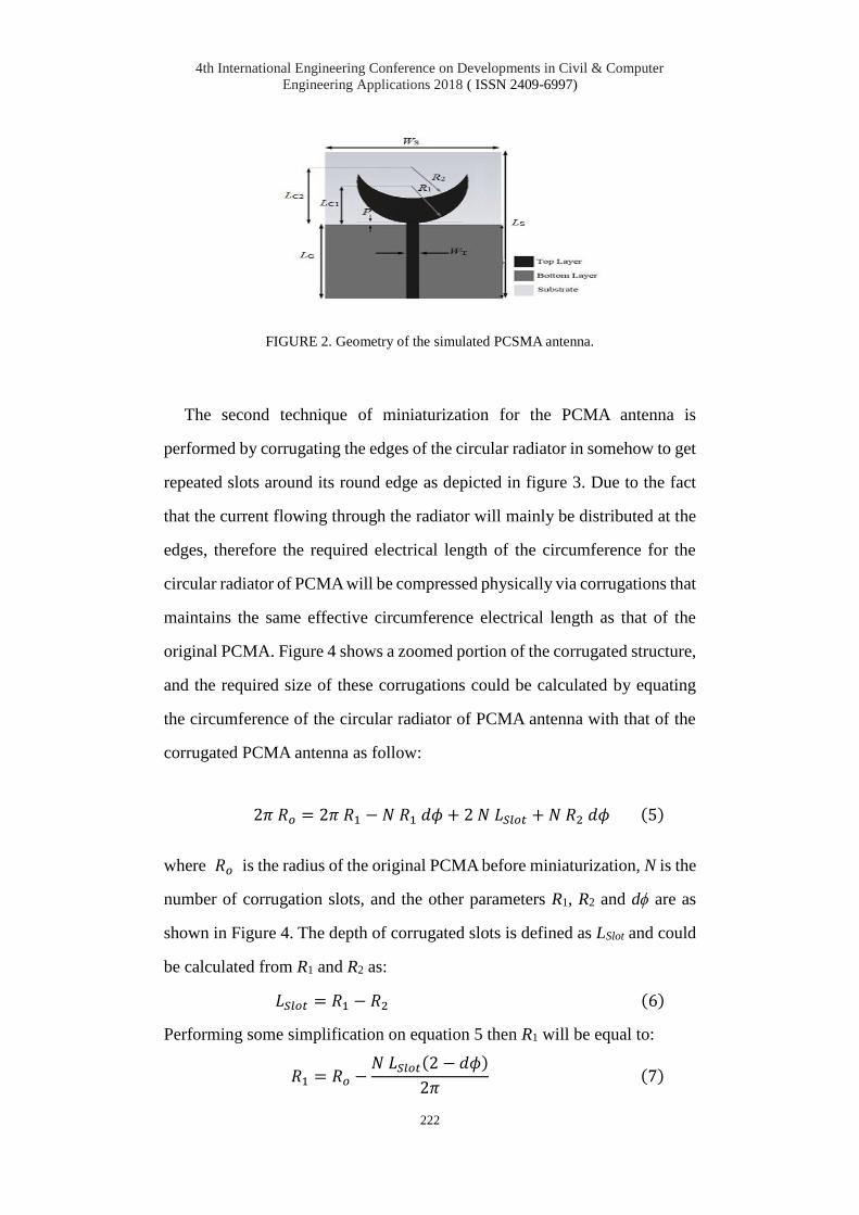
4th International Engineering Conference on Developments in Civil & Computer
Engineering Applications 2018 ( ISSN 2409-6997)
222
FIGURE 2. Geometry of the simulated PCSMA antenna.
The second technique of miniaturization for the PCMA antenna is
performed by corrugating the edges of the circular radiator in somehow to get
repeated slots around its round edge as depicted in figure 3. Due to the fact
that the current flowing through the radiator will mainly be distributed at the
edges, therefore the required electrical length of the circumference for the
circular radiator of PCMA will be compressed physically via corrugations that
maintains the same effective circumference electrical length as that of the
original PCMA. Figure 4 shows a zoomed portion of the corrugated structure,
and the required size of these corrugations could be calculated by equating
the circumference of the circular radiator of PCMA antenna with that of the
corrugated PCMA antenna as follow:
2𝜋 𝑅𝑜 = 2𝜋 𝑅1 − 𝑁 𝑅1 𝑑𝜙 + 2 𝑁 𝐿𝑆𝑙𝑜𝑡 + 𝑁 𝑅2 𝑑𝜙 (5)
where 𝑅𝑜 is the radius of the original PCMA before miniaturization, N is the
number of corrugation slots, and the other parameters R1, R2 and dϕ are as
shown in Figure 4. The depth of corrugated slots is defined as LSlot and could
be calculated from R1 and R2 as:
𝐿𝑆𝑙𝑜𝑡 = 𝑅1 − 𝑅2 (6)
Performing some simplification on equation 5 then R1 will be equal to:
𝑅1 = 𝑅𝑜 −𝑁 𝐿𝑆𝑙𝑜𝑡(2 − 𝑑𝜙)
2𝜋 (7)

4th International Engineering Conference on Developments in Civil & Computer
Engineering Applications 2018 ( ISSN 2409-6997)
223
where dϕ is in radians while other parameters are all in (mm). The number of
corrugated slots N will not be related directly with dϕ because in the case of
this design two additional slots will be hidden within the microstrip feedline
side therefore:
(𝑁 + 2) =2𝜋
𝑑𝜙 (8)
Now if N is taken as 28, 𝑅𝑜= 12.5 mm, LSlot = 0.65 mm, then equation 8 gives
dϕ = π/30 (rad) which is equal to (6°) and equation 7 gives R1 = 7.01 mm,
which has been taken 7 mm in this design. The all design parameters are listed
in Table 3. It is worthy to mention that for different number of corrugated
slots more or less than 28 that used here then the number of hidden slots will
be changed and equation 8 will be changed accordingly.
If it is desired to make the depth of the corrugated slots equal to their width
which is the arc length then LSlot will be given as:
𝐿𝑆𝑙𝑜𝑡 = 𝑅1 𝑑𝜙 (9)
Accordingly, if equations 8 & 9 are substituted into equation 7, then R1 will
be:
𝑅1 =2𝜋 𝑅𝑜
6𝜋 − 2𝜋 𝑑𝜙 − 4 𝑑𝜙 + 2 𝑑𝜙2 (10)
This technique has reduced the original size of the radiator while kept the
required electrical length of the circumference unaffected via the compressing
taken place in the corrugated circumference. Accordingly, the important
characteristics of the antenna have been preserved while the overall size is
reduced to 57.4% ((30*39/40*51)*100%=57.35%) of the original antenna
size.

4th International Engineering Conference on Developments in Civil & Computer
Engineering Applications 2018 ( ISSN 2409-6997)
224
FIGURE 3. Geometry of the simulated corrugated PCMA.
FIGURE 4. Details of the corrugated structure.
TABLE 3.
Design parameters of corrugated PCMA antenna.
Parameter Dimension (mm)
LC 7.65
LSlot 0.65
LS 39
LG 22.75
WS 30
WSlot 1
WT 2.8
P 0.5
R1 7
R2 6.35

4th International Engineering Conference on Developments in Civil & Computer
Engineering Applications 2018 ( ISSN 2409-6997)
225
4.RESULTS AND DISCUSION
PCMA has been designed as one of the common UWB antennas with
dimensions and geometry as mentioned in previous section, then two different
techniques have been used; firstly, by eliminating the undesired or least
current distributed areas to generate a planar crescent-shaped monopole
antenna (PCSMA), secondly by corrugating the round edge of the circular
radiator to miniaturize its circumference. All the designed UWB antennas
have been simulated using CST Microwave StudioTM software package.
Figure 5 shows the simulation results of the return loss curves versus
frequency for the PCMA, PCSMA, and Corrugated PCMA. It shows that all
of these designed antennas are maintaining their working which covered the
entire UWB. Investigating the surface current distributions for the three
designed antennas are shown in figures 6 to 8 and they were plotted for 5 and
9 GHz of frequencies. The PCSMA will offer the required area of
metallization in least size compared to the PCMA. Therefore, it has been
concluded that the current will be concentrated at this miniaturized area which
is almost distributed at the lower side edges of the radiator. While in
corrugated PCMA the current will follow a corrugated path offered by the
radiator edge and it will cross the required path with least height compared to
PCMA, which validates the technique of eliminating the undesired areas.
After completing the design and simulation of the aforementioned antennas,
the all three antennas have been fabricated as shown in figures 9 to 11, and
tested via Rohde & Schwarz® ZVL13 VNA. The return loss data has been
measured for the all three antennas and plotted in comparison with their
simulation one as shown in figures 12 to 14. The measurement results are
almost agreed with the simulation results except some shifting due to
imperfection in the fabrication. However, the practical experimental
measurements validate the design and its modification which performed to
miniaturize the size of the PCMA. Therefore the miniaturized antennas will

4th International Engineering Conference on Developments in Civil & Computer
Engineering Applications 2018 ( ISSN 2409-6997)
226
be working with almost the same features with least size which satisfy the
goal of this research.
The simulated and measured radiation patterns in E and H planes for the three
antennas are shown in figures 15 to 17 for 5 and 9 GHz of frequencies.
Measured radiation patterns are almost meet the simulated patterns. And also
the miniaturization techniques have nearly not affected the radiation pattern
that performed by PCSMA nor corrugated PCMA. Finally, the simulated
realized gain curves for PCMA, PCSMA and corrugated PCMA have been
plotted as shown in figure 18. For PCMA it is noticed that almost the gain is
increased with increments in the frequency, which is common in UWB
antennas, while for corrugated PCMA and in spite of the great miniaturization
occurred in its size but its gain (not less than 2 dB) was still having a
reasonable value comparing to the gain of half wave dipole antenna (i.e. 2.15
dB), and getting up to (4.8 dB at 9.5 GHz). Although the miniaturization ratio
in corrugated PCMA is greater than that of PCSMA but its gain still better
than the gain of PCSMA, and this may back to the circumference length in
the corrugated PCMA that has been maintained via corrugated edge, while it
is truncated in PCSMA.
FIGURE 5. Comparison of simulated return loss curves for the PCMA, PCSMA and
corrugated PCMA

4th International Engineering Conference on Developments in Civil & Computer
Engineering Applications 2018 ( ISSN 2409-6997)
227
(a) (b)
FIGURE 6. Surface current distribution for the PCMA at (a) 5 GHz, and (b) 9 GHz.
(a) (b)
FIGURE 7. Surface current distribution for the PCSMA at (a) 5 GHz, and (b) 9 GHz.
(a) (b)
FIGURE 8. Surface current distribution for the Corrugated PCMA at (a) 5 GHz, and (b) 9
GHz.

4th International Engineering Conference on Developments in Civil & Computer
Engineering Applications 2018 ( ISSN 2409-6997)
228
FIGURE 9. Fabricated PCMA.
FIGURE 10. Fabricated PCSMA.
FIGURE 11. Fabricated corrugated PCMA.

4th International Engineering Conference on Developments in Civil & Computer
Engineering Applications 2018 ( ISSN 2409-6997)
229
FIGURE 12. Return loss curves (measured and simulated) for the PCMA.
FIGURE 13. Return loss curves (measured and simulated) for the PCSMA.
FIGURE 14. Return loss curves (measured and simulated) for the Corrugated PCMA.

4th International Engineering Conference on Developments in Civil & Computer
Engineering Applications 2018 ( ISSN 2409-6997)
230
FIGURE 15. Radiation patterns simulated (ــ ــ ــ) and measured (ـــــ) of the PCMA in H and
E planes, for frequencies of 5 and 9 GHz.

4th International Engineering Conference on Developments in Civil & Computer
Engineering Applications 2018 ( ISSN 2409-6997)
231
FIGURE 16. Radiation patterns simulated (ــ ــ ــ) and measured (ـــــ) of the PCSMA in H
and E planes, for frequencies of 5 and 9 GHz.

4th International Engineering Conference on Developments in Civil & Computer
Engineering Applications 2018 ( ISSN 2409-6997)
232
FIGURE 17. Radiation patterns simulated (ــ ــ ــ) and measured (ـــــ) of the Corrugated
PCMA in H and E planes, for frequencies of 5 and 9 GHz.
FIGURE 18. Comparison of simulated realized gain curves for the PCMA, PCSMA and
corrugated PCMA.

4th International Engineering Conference on Developments in Civil & Computer
Engineering Applications 2018 ( ISSN 2409-6997)
233
5. CONCLUSIONS
Two techniques have been suggested here to miniaturize the overall size
of PCMA; the first technique has been performed by eliminating the least
current distributed areas, which resulted in a crescent-shaped radiator. While
the second technique introduces corrugated slots around the round edge of the
PCMA radiator, in which a 57.4% of overall size reduction has been achieved
while its gain was still maintaining more than (2 dB), which is comparable
with that of half wave dipole antenna. Results shown that corrugation
technique was more efficient due to the reduction in size was 42.6% which is
more than 11.76% for the other techniques, also the upper limit of the
impedance bandwidth for the corrugated PCMA has been extended to 13.85
GHz. Another advantage of the corrugation technique has been shown that
the gain characteristics was better than that of area eliminating technique, and
the reason may back to maintaining the perimeter electrical length in
corrugated PCMA as much as that of the original PCMA antenna, while in
PCSMA a certain portion of the perimeter's upper side has been truncated.
However, both miniaturized antennas are still having the required
characteristics just like the original parent PCMA antenna that obey the UWB
requirements.

4th International Engineering Conference on Developments in Civil & Computer
Engineering Applications 2018 ( ISSN 2409-6997)
234
REFERENCES
[1] First Report and Order (FCC 02-48), “New Public Safety Applications
and Broadband Internet Access Among Uses Envisioned by FCC
Authorization of Ultra-Wideband Technology,” Action by the
Commission Feb. 14, 2002.
[2] Sayidmarie, K. H., & Fadhel, Y. A., “Self-Complementary Circular Disk
Antenna for UWB Applications,” Progress In Electromagnetics Research
C, Vol. 24, 111-122, 2011.
[3] Sayidmarie, K. H, and Fadhel, Y. A., “Design Aspects of UWB Printed
Elliptical Monopole Antenna with Impedance Matching”, Loughborough
Antennas & Propagation Conference LAPC2012, UK, Nov. 2012.
[4] Fadhel, Y. A., “Design and Implementation of Ultra Wide Band Antennas
for Imaging Applications,” PhD Thesis, University of Mosul, July, 2013.
[5] Beada'a, J. M., Abbosh, A. M., Mustafa, S., and Ireland, D., “Microwave
System for Head Imaging,” IEEE Transactions on Instrumentation and
Measurement, Vol. 63, No. 1, 117-123, 2014.
[6] Bialkowski, M. E., Abbosh, A. M., Wang, Y., Ireland, D., Bakar, A. A.,
and Mohammed, B. J., “Microwave Imaging Systems Employing
Cylindrical, Hemispherical and Planar Arrays of Ultrawideband
Antennas,” Proceedings of the Asia-Pacific Microwave Conference
APMC2011, pp. 191-194, Dec., 2011.
[7] Chareonsiri, Y., Thaiwirot, W., and Akkaraekthalin, P., “Design of Ultra-
Wideband Tapered Slot Antenna by Using Binomial Transformer with
Corrugation,” De Gruyter, Frequenz 2017, Journal of RF-Engineering
and Telecommunications, 2017.
[8] Chen, M. S., Weng, W. C., & Wang, S. T. (2013, February), “Design of
the Crescent-Shape Planar Ultra-wideband Antenna with a Band-notch

4th International Engineering Conference on Developments in Civil & Computer
Engineering Applications 2018 ( ISSN 2409-6997)
235
Structure,” IEEE 2nd International Symposium on Next-Generation
Electronics (ISNE), pp. 271-274, Kaohsiung , Taiwan, Feb., 2013.
[9] Azenui, N. C., and Yang, H. Y. D., “A Printed Crescent Patch Antenna for
Ultrawideband Applications,” IEEE Antennas and Wireless Propagation
Letters, Vol. 6, 113-116, 2007.
[10] Nikolaou, S., and Abbasi, M. A. B., “Miniaturization of UWB Antennas
on Organic Material,” International Journal of Antennas and
Propagation, Vol. 2016, 12 pages, Article ID 5949254, 2016.
[11] Ray, K. P., “Design Aspects of Printed Monopole Antennas for Ultra-
wide Band Applications,” International Journal of Antennas and
Propagation, Vol. 2008, 8 pages, Article ID 713858, 2008.
[12] Balanis C. A., “Antenna Theory Analysis and Design,” John Wiley &
Sons Inc, 3rd ed., 2005.
[13] Matin, M. A., “Ultra Wideband Communications: Novel Trends–
Antennas and Propagation”, Published by InTech, Croatia, pp. 177-183,
July, 2011.

4th International Engineering Conference on Developments in Civil & Computer Engineering
Applications 2018 ( ISSN 2409-6997)
236
ANALYSIS OF ELASTIC BEAMS ON LINEAR AND
NONLINEAR FOUNDATIONS USING FINITE DIFFERENCE
METHOD
Saad Essa
Erbil Polytechnic University ,Ishik University,
[email protected], [email protected]
doi:10.23918/iec2018.18
ABSTRACT
An approximate method is developed to analyze the deflection in beams and beam-
column by solving the differential equation for the elastic deformation of beam and
beam-column. The analysis is performed using the central difference of finite
difference method for the Euler-Bernoulli beam and beam-column supported on an
elastic, nonlinear foundation with rigid or elastic discrete supports. To make a
verification of the results, Laplace Transformation method is used to solve the
elastic differential equation of beam and beam-column based on linear elastic
supports and the results are compared with the finite difference method. Two types
of beams are selected, simply supported and fixed-fixed with five elastic supports of
an idealized soil. In the nonlinear idealization, the division of force into many levels
are assumed and based on these forces, the equivalent displacements are obtained
from an assumed power law equation by using the finite difference method. Central
finite difference scheme has a second order is used throughout the numerical
analysis with five nonlinear behavior of springs separated by an equal distance
between them.
Keywords: Finite difference method, Euler-Bernoulli beam, Laplace transformation.

4th International Engineering Conference on Developments in Civil & Computer Engineering
Applications 2018 ( ISSN 2409-6997)
237
1. INTRODUCTION
Beams on an elastic foundation has been solved by many researchers and
analytical solutions of the differential equation have been proposed [1-2]. The
geometric stiffness matrix was formulated and derived for beams on elastic
foundation by Eisenber et al. [3]. Many authors used a finite element technique to
find an approximate solution. Two-parameter elastic foundations were formulated to
analyze beams based on exact displacement function [4]. Analysis of finite element
beam column on elastic Winkler foundation was carried out using exact stiffness
matrix terms [5]. Lower order of finite strip method developed for the analysis of
soil-iteration models. At the early stage, the model was used for soil layered under
vertical load with uniform soil properties. The change of soil properties in the
longitudinal direction was included in the research by Cheung et al. [6] and
Oskoorouchi et al. [7]. Mixing between finite strip method and soil spring system
has been developed and applied to study the plate vibration responses on elastic
foundation with different boundary conditions [8-9]. Vallabhan and Das [10]
estimated a non-dimensional third parameter using iterative procedure to represent
the distribution displacement of beams rested on elastic foundation. Omurtag et al.
[11] used a mixed-type formulation based on Gateaux differential for the derivation
of Kirchhoff plate-elastic foundation interaction. Binesh [12] used a mesh-free
method for the analysis of a beam on two parameter elastic foundation. Sato et al.
[13] obtained an exact solution for beam on elastic foundation in static and free
vibration problems based on equidistant elastic supports. Jumel et al. [14] proposed
a first order correction to take into account of interface elasticity and transverse
anticlastic curvature of flexible substrate. Borak and Marcian [15] used modified
Bettis theorem to develop an alternative analytical solution of beams on an elastic
foundation. The calculation was based on the determine of beam’s deflection on an
elastic foundation from the deflection of a reference beam which is topologically
equivalent. In this paper, the nonlinear assumption of soil behavior is used to
analyze Euler-Bernoulli elastic beam and beam-column under compression load
rested on it. Numerical method based on the finite difference method is used for the
analysis of fourth-order linear ordinary differential equation of beam and beam-
column. The constants in this equation are determined by using the boundary
conditions of simply supported and fixed-fixed ends. In addition, closed form

4th International Engineering Conference on Developments in Civil & Computer Engineering
Applications 2018 ( ISSN 2409-6997)
238
solution based on the Laplace transformation method is used to get the results under
the same conditions. Numerical examples are illustrated for both elastic beam and
beam-column on the nonlinear soil behavior and the results are showed in figures
and tables.
2. MODELLING OF SOIL MECHANICAL PROPERTIES AND
ALGORITHM
Throughout analysis of any foundation, soil is not a linear material and for
modeling it as a linear material could cause a considerable error. Soil actually
behaves as a hyperbolic curve in relationship of stress-strain [3]. Load deflection
relationship curve might be assumed to exist, as shown in Figs. 1-5 when modelling
the reaction of a soil foundation. In every iteration of the force level, the tangent of
the curve is obtained which means the slope of the force-displacement curve of soil.
In this study, this curve is obeyed according to the nonlinear behavior of soil that
defined in Eq. (1)
0.5 nuP P (1)
where uP is the ultimate soil bearing capacity of the soil in 2/kN m and is the
strain of soil underneath the footing. n is the power law variation that changes with
the applied force and displacement. Here, the strain equals to the actual
displacement because the length is assumed for one meter. Five nodes are idealized
for the nonlinear soil reaction using the finite difference method to find the
displacements. The load per unit area of foundation is plotted with displacement for
each spring as shown in Figs 1-5. For each figure, the corresponding deflection are
selected based on five loads chosen as 0.1, 0.25, 0.5, 0.75, and 1.0. These curves
behavior which are represented the soil mechanical activities are working based on
Eq. (1). The value of power n in Eq. (1) goes to decline with increasing of load step
from 0.1 to 1.0. The differential equation that describing the elastic deflection curve
of Euler-Bernoulli beam-column on a nonlinear elastic foundation under the action
of a distributed load is governed by Eq. (2)
2 2 2
2 2 2( ) ( )
d d y d yEI P k x y w x
dx dx dx
(2)

4th International Engineering Conference on Developments in Civil & Computer Engineering
Applications 2018 ( ISSN 2409-6997)
239
where ( )y x is the deflection of the beam, E is the modulus of elasticity of the
material made for the beam, I is the moment of inertia of the cross-section, P is
the axial load applied at the ends to the beam, ( )w x is the applied distributed load
and ( )k x is the foundation modulus. In the linear analysis of foundation, ( )k x is
taken as a constant number while in the nonlinear foundation analysis varies in its
values with respect to its position.
0.00
0.02
0.04
0.06
0.08
0.10
0.0000 0.0025 0.0050 0.0075 0.0100
soil
rea
ctio
n P
,
soil displacement, m
0.849485n
2/
kNm
0.00
0.05
0.10
0.15
0.20
0.25
0.0000 0.0025 0.0050 0.0075 0.0100
soil
rea
ctio
n P
,
soil displacement, m
0.650515n
2/
kNm
FIGURE 1. Load-displacement curve of soil
at 20.10 /P kN m FIGURE 2. Load-displacement curve of soil
at 20.25 /P kN m
0.00
0.10
0.20
0.30
0.40
0.50
0.0000 0.0025 0.0050 0.0075 0.0100
soil
rea
ctio
n P
,
soil displacement, m
0.5n
/kN
m
0.000
0.125
0.250
0.375
0.500
0.625
0.750
0.0000 0.0025 0.0050 0.0075 0.0100
soil
rea
ctio
n P
,
soil displacement, m
/kN
m
0.411954n
FIGURE 3. Load-displacement curve of soil
at 20.50 /P kN m FIGURE 4. Load-displacement curve of
soil at 20.75 /P kN m

4th International Engineering Conference on Developments in Civil & Computer Engineering
Applications 2018 ( ISSN 2409-6997)
240
0.0
0.2
0.4
0.6
0.8
1.0
0.0000 0.0025 0.0050 0.0075 0.0100
soil
rea
ctio
n P
,
soil displacement, m
0.349485n
/kN
m
FIGURE 5. Load-displacement curve of soil
at 21.0 /P kN m
With applying finite difference scheme, Eq. (2) can be written for the elastic beam-
column on nonlinear foundation as
4 4
22 1 1 2 1 14 6 4 ( 2 ) i i i
i i i i i i i i
P w h k y hy y y y y y y y h
EI EI EI
(3)
In the case of elastic beam on nonlinear foundation can be calculated in the same
Eq. (3) with 0P . The second and fourth order derivatives in Eq. (2) are
substituted by second order central difference approximation in the finite difference
equation (Eq. (3)). The finite difference grid is used for the analysis of beam and
beam-column rested on elastic nonlinear foundation with taking a limit number of
idealized springs. The distances between the springs are taken an equal and the axial
load as a compression load at the ends. In the conventional finite difference analysis,
the geometric and boundary conditions of the equilibrium differential equation are
considered. The condition that y and y are zero at station i is approximated using
Eq. (4) and Eq. (5) respectively, as
1 1 0i iy y (4)
1 12 0i i iy y y (5)
Figure 6 shows the simply supported beam-column on five nonlinear idealized
springs with equal distances between them.

4th International Engineering Conference on Developments in Civil & Computer Engineering
Applications 2018 ( ISSN 2409-6997)
241
FIGURE 6. Simply supported beam-column rested on five springs.
The algorithm processes in this study are followed as the following steps: In the first
load step ( 0.1P ) with the constant last strain ( 0.01 ), the power n is
determined to equal 0.849485 according to the Eq. (1) with taking 10.0uP . After
then, the stiffness ( k ) is equal to the slope of the load-deflection curve by assuming
the deflection equals to the strain for idealized springs. Then the k values for the
five springs are approximately linear for this step and equal to 10.0 because the
exact values in this step can't be determined without present the springs deflection.
By applying the finite difference technique (Eq. (3)), values of the springs deflection
can be determined based on the constant value of stiffness ( 10.0k ) for all
assumed nodes. For the second step ( 0.25P ), the value of power n can be
determined with constant final strain ( 0.01 ). In this step, with determining the
values of deflections from the first step, the new stiffness ( k ) for all five nodes can
be calculated by substituting the deflection values in the derivative of Eq. (1)
( 0.1505154.24743/ ) which considers the slope of the load-deflection curve then the
corrected deflections can be evaluated by applying the same equation of finite
difference method. For the third step ( 0.5P ), the same procedures are applied
from calculating the power n and evaluating the stiffness based on the second step
deflections to reach the new corrected deflections. The processes are repeated for the
fourth step ( 0.75P ) and fifth step ( 1.0P ). The observation of this algorithm is
the load-deflection curve goes from linear at the first step to nonlinear behavior
ending with the power 0.349485n . The soil beneath the beam or beam-column
behaves actually according to the mentioned five steps. The reason to stop of these
processes at the last step is the small difference between the values of numerical
method (finite difference method) and the exact solution (Laplace Transformation).

4th International Engineering Conference on Developments in Civil & Computer Engineering
Applications 2018 ( ISSN 2409-6997)
242
2.1 LAPLACE TRANSFORMATION METHOD
In this section, the Laplace transformation method is used to find the deflections
of beam rested on linear elastic foundation. To apply this method, the basic principle
is defined as ( )F s be a given function. The Laplace transform ( )F s of function
( )f t is defined by
0
( ) ( ) , 0sxf x e f x dx s
L (6)
By rearranging the fourth order differential equation in Eq. (2), the equation can be
written as
(4) 4 2 ( )( ) 4 ( ) ( )
w xy x y x y x
EI (7)
where, 44 /k EI ( k is the foundation modulus) and 2 /P EI ( P is the axial
applied load at the beam ends). By taking the Laplace transformation for the fourth
order differential equation in Eq. (7) under constant value of the distributed load
( )w x , the equation becomes
2 2
4 4 2 2
(0) (0) (0) (0)( )
( ) 4
EIs s sy y sy y wf s
EIs s s
(8)
For simply supported beam rested on elastic foundation under axial load at the ends
of the beam, the boundary conditions at the ends which satisfying the Eq. (8) are
deflection and moment equal to zero ( (0) ( ) (0) ( ) 0y y l y y l ) and Eq. (8)
can be written as
2 22 1
4 2 2 4( )
4
w EIs c c sf s
EIs s s
(9)

4th International Engineering Conference on Developments in Civil & Computer Engineering
Applications 2018 ( ISSN 2409-6997)
243
where 1 (0)c y and 2 (0)c y . In addition, by applying the boundary conditions
for the fixed-fixed beam with axial load at the ends with taking the deflection and
slope at the ends equal to zero ( (0) ( ) (0) ( ) 0y y l y y l ), Eq. (8) can be
written as
2 1
4 2 2 4( )
4
w EIs c c sf s
EIs s s
(10)
where 1 (0)c y and 2 (0)c y .
3. NUMERICAL EXAMPLES
The aim of this section is to validate the solution procedure for the
determination of the beam deflection rested on elastic foundation. To do so,
several examples of the analysis of beam columns are illustrated based on the
analytical and numerical solutions. The first example explains beam ( 0.0 )
and beam-column ( 1.0 ) with simply supported on elastic foundations while
the second one is treating with beam and beam-column with fixed ends. For the
both examples, the parameters are selected as a following data: 1.0k , 2.0k
, 1.0EI , 10.0uP and 1.0L . The constants for simply supported and
fixed-fixed respectively are 1 0.0412493c , 2 0.0412493c and
1 0.0831848c , 2 0.499307c . These constants are used for Laplace
transformation method in Eqs. (9) and (10). The results in the Figs. 7-14 show
deflection by using analytical method for both beam and beam-column in the
case of simply supported and fixed-fixed conditions. Tables (1) and (2) show the
numerical deflection of beam and beam-column on elastic foundation for both
simply supported and fixed-fixed, respectively based on central difference of
finite difference method. Tables (3) and (4) represent stiffness values and
corresponding deflection which should be used in the tangent equation at each
level for simply supported beam. In addition, tables (5) and (6) show the
stiffness values and corresponding deflection for fixed-fixed beam rested on
nonlinear foundation, respectively.

4th International Engineering Conference on Developments in Civil & Computer Engineering
Applications 2018 ( ISSN 2409-6997)
244
TABLE 1.
Numerical deflection of simply supported beam and beam-column on elastic foundation ( m ).
Divided length, m Deflection
1, 0k
Deflection
2, 0k
Deflection
1, 1k
Deflection
2, 1k
0.0 0.000000 0.000000 0.000000 0.000000
1/6 0.006680 0.006611 0.007437 0.007351
2/6 0.011451 0.011330 0.012760 0.012611
3/6 0.013168 0.013029 0.014679 0.014506
4/6 0.011451 0.011330 0.012760 0.012611
5/6 0.006680 0.006611 0.007437 0.007351
6/6 0.000000 0.000000 0.000000 0.000000
TABLE 2.
Numerical deflection of fixed-fixed beam and beam-column on elastic foundation ( m ).
Divided length,
m
Deflection
1, 0k
Deflection
2, 0k
Deflection
1, 1k
Deflection
2, 1k
0.0 0.000000 0.000000 0.000000 0.000000
1/6 0.001123 0.001120 0.001148 0.001145
2/6 0.002566 0.002559 0.002634 0.002627
3/6 0.003175 0.003167 0.003263 0.003255
4/6 0.002566 0.002559 0.002634 0.002627
5/6 0.001123 0.001120 0.001148 0.001145
6/6 0.000000 0.000000 0.000000 0.000000

4th International Engineering Conference on Developments in Civil & Computer Engineering
Applications 2018 ( ISSN 2409-6997)
245
0.000
0.004
0.008
0.012
0.016
0.0 0.2 0.4 0.6 0.8 1.0
Defl
ecti
on, m
Beam length, m
(0.5) 0.012888y
0.000
0.004
0.008
0.012
0.016
0.00 0.20 0.40 0.60 0.80 1.00
Defl
ecti
on, m
Beam length, m
(0.5) 0.012758y
FIGURE 7. Analytical deflection of simply
supported beam on linear elastic foundation with
1k and 0 .
FIGURE 8. Analytical deflection of simply
supported beam on linear elastic foundation with
2k and 0 .
0.000
0.004
0.008
0.012
0.016
0.0 0.2 0.4 0.6 0.8 1.0
Def
lect
ion,
m
Beam length, m
0.( 00. 1 35) 43 0y
0.000
0.004
0.008
0.012
0.016
0.0 0.2 0.4 0.6 0.8 1.0
Def
lect
ion,
m
Beam length, m
0.( 00. 1 65) 41 9y
FIGURE 9. Analytical deflection of simply
supported beam-column on linear elastic
foundation with 1k and 1 .
FIGURE 10. Analytical deflection of simply
supported beam-column on linear elastic
foundation with 2k and 1 .
0.000000
0.001000
0.002000
0.003000
0.0 0.2 0.4 0.6 0.8 1.0
Def
lect
ion, m
Beam length, m
(0.5) 0.002599y
0.000000
0.001000
0.002000
0.003000
0.0 0.2 0.4 0.6 0.8 1.0
Def
lect
ion,
m
Beam length, m
0.( 00. 0 95) 25 4y
FIGURE 11. Analytical deflection of fixed-fixed beam
on linear elastic foundation with 1k and 0 .
FIGURE 12. Analytical deflection of fixed-fixed beam
on linear elastic foundation with 2k and 0 .

4th International Engineering Conference on Developments in Civil & Computer Engineering
Applications 2018 ( ISSN 2409-6997)
246
0.000000
0.001000
0.002000
0.003000
0.0 0.2 0.4 0.6 0.8 1.0
Def
lect
ion,
m
Beam length, m
0.( 00. 0 65) 26 5y
0.000000
0.001000
0.002000
0.003000
0.0 0.2 0.4 0.6 0.8 1.0
Def
lect
ion,
m
Beam length, m
0.( 00. 0 65) 26 0y
FIGURE 13. Analytical deflection of fixed-fixed beam
on linear elastic foundation with 1k and 1 .
FIGURE 14. Analytical deflection of fixed-fixed beam
on linear elastic foundation with 2k and 1 .
TABLE 3.
Stiffness of load per unit area and deflection curve for simply supported beam ( 2/kN m ).
Beam length, m 1k 2k 3k 4k 5k
0.10 10.0000 43.2154 71.7068 60.8176 70.5617
0.25 10.0000 35.8092 54.8407 44.3825 49.7651
0.5 10.0000 34.1072 51.1660 40.9110 45.4655
0.75 10.0000 35.8092 54.8407 44.3825 49.7651
1.00 10.0000 43.2154 71.7068 60.8176 70.5617
TABLE 4.
Deflection of simply-supported beam rested on nonlinear foundation for five iterations ( m ).
Beam length, m 1u 2u
3u 4u
5u
0.10 0.000610 0.001216 0.003161 0.003396 0.004345
0.25 0.001045 0.002078 0.005401 0.005808 0.007432
0.5 0.001201 0.002387 0.006204 0.006674 0.008540
0.75 0.001045 0.002078 0.005401 0.005808 0.007432
1.00 0.000610 0.001216 0.003161 0.003396 0.004345

4th International Engineering Conference on Developments in Civil & Computer Engineering
Applications 2018 ( ISSN 2409-6997)
247
TABLE 5.
Stiffness of load per unit area and deflection curve for fixed-fixed beam ( 2/kN m ).
Beam length, m 1k 2k
3k 4k
5k
0.10 10.0000 16.7481 57.3219 110.6000 145.3530
0.25 10.0000 14.7920 42.9680 73.3240 89.7250
0.5 10.0000 14.3261 39.8927 65.9587 79.2439
0.75 10.0000 14.7920 42.9680 73.3240 89.7250
1.00 10.0000 16.7481 57.3219 110.6000 145.3530
TABLE 6.
Deflection of fixed-fixed beam rested on nonlinear foundation for five iterations ( m ).
Beam length, m 1u 2u
3u 4u
5u
0.10 0.000110 0.000272 0.000511 0.000718 0.000925
0.25 0.000251 0.000620 0.001162 0.001632 0.002102
0.5 0.000310 0.000767 0.001437 0.002016 0.002596
0.75 0.000251 0.000620 0.001162 0.001632 0.002102
1.00 0.000110 0.000272 0.000511 0.000718 0.000925
4. CONCLUSIONS
In this study, a finite difference method for the analysis of beam and beam-column
resting on nonlinear elastic foundation is formulated based on the iterative
procedure. In addition, to control the accuracy of the numerical method, exact
solution for beam and beam-column of Euler-Bernoulli on a nonlinear elastic
foundation is investigated based on the proposed formula in Eq. (1). The nonlinear
load-displacement curve of the soil is plotted at each of the load step with
determining the power n at each of load level. With applying the finite difference
procedures at each load level, the displacements corresponding to it are determined
then used in Eq. (3) to find the next level displacements under the equal of point

4th International Engineering Conference on Developments in Civil & Computer Engineering
Applications 2018 ( ISSN 2409-6997)
248
load at each of the five interior nodes. The iterative procedure converges rapidly to
the solution after the fifth trail because the value of the power n decreases with the
advance steps and the curve approaches to the ideal curve path of soil. The final
strain of the soil behavior at all levels is selected as a constant value ( 0.01 ) and
the value of the power ( n ) is determined at each load level. Accuracy is controlled
by using the Laplace Transformation method with the inverse Eq. (10) which refer
to the closed form solution. Two examples are solved for both beam and beam-
column based on Euler-Bernoulli theory which show the characteristic features for
applying the both methods. The analytical method using Laplace transformation is
idealized in the figures with evaluating maximum displacement for all cases. It is
shown that, for a twice stiffness value of beam and beam-column, the foundation
deflections are reduced for simply supported and fixed-fixed ends. On the other
hand, the deflections increase in the case of beam-column which refers to presence
of axial load ( 1 ) than in the case of beam only ( 0 ). Moreover, the deflection
of foundation rested on nonlinear soil behavior and the effect of compression axial
with simply supported ends is greater than that for the fixed-fixed ends.
ACKNOWLEDGEMENTS
The author wishes to thank Associate Prof. Dr. Hakan Argeso from the Department
of Manufacturing Engineering at Atilim University, Ankara-Turkey, for his valuable
help and support.

4th International Engineering Conference on Developments in Civil & Computer Engineering
Applications 2018 ( ISSN 2409-6997)
249
REFERENCES
[1] R. D. Cook, Concepts and applications of finite element analysis, John Wiley &
Sons, 2007.
[2] Miyahara, F., & Ergatoudis, J. G., "Matrix analysis of structure-foundation
interaction," Journal of the Structural Division, vol. 102, no. 1, pp. 251-265,
1976.
[3] Eisenberger, M., Yankelevsky, D. Z., & Clastornik, J., "Stability of beams on
elastic foundation," Computers & structures, vol. 24, no. 1, pp. 135-139, 1986.
[4] Zhaohua, F., & Cook, R. D., "Beam elements on two-parameter elastic
foundations," Journal of Engineering Mechanics, vol. 109, no. 6, pp. 1390-
1402, 1983.
[5] Yankelevsky, D. Z., & Eisenberger, M., "Analysis of a beam column on elastic
foundation," Computers & structures, vol. 23, no. 3, pp. 351-356, 1986.
[6] Cheung, Y. K., Tham, L. G., & Guo, D. J., "Applications of finite strip and
layer methods in micro-computers," in International Conference on Numerical
Methods in Geomechanics (ICONMIG), 1985.
[7] Oskoorouchi, A. M., Novrouzian, B., De Roeck, G., & Van Den Broeck, J.,
"Zoned finite strip method and its applications in geomechanics," Computers
and Geotechnics, vol. 11, no. 4, pp. 265-294, 1991.
[8] Huang, M. H., & Thambiratnam, D. P., "Analysis of plate resting on elastic
supports and elastic foundation by finite strip method," Computers &
Structures, vol. 79, no. 29, pp. 2547-2557, 2001.
[9] Chow, Y. K., Swaddiwudhipong, S., & Phoon, K. F., "Finite strip analysis of
strip footings: Horizontal loading," Computers and Geotechnics, vol. 8, no. 1,

4th International Engineering Conference on Developments in Civil & Computer Engineering
Applications 2018 ( ISSN 2409-6997)
250
pp. 65-86, 1989.
[10] Vallabhan, C. G., & Das, Y. C., "Parametric study of beams on elastic
foundations," Journal of engineering mechanics, vol. 114, no. 12, pp. 2072-
2082, 1988.
[11] Omurtag, M. H., Özütok, A., Aköz, A. Y., & OeZCELİKOeRS, Y. U. N. U. S.,
"Free vibration analysis of Kirchhoff plates resting on elastic foundation by
mixed finite element formulation based on Gateaux differential," International
Journal for Numerical Methods in Engineering, vol. 40, no. 2, pp. 295-317,
1997.
[12] Binesh, S. M., "Analysis of beam on elastic foundation using the radial point
interpolation method," Scientia Iranica, vol. 19, no. 3, pp. 403-409, 2012.
[13] Sato, M., Kanie, S., & Mikami, T., "Mathematical analogy of a beam on elastic
supports as a beam on elastic foundation," Applied Mathematical Modelling,
vol. 32, no. 5, pp. 688-699, 2008.
[14] Jumel, J., Budzik, M. K., & Shanahan, M. E., "Beam on elastic foundation with
anticlastic curvature: Application to analysis of mode I fracture tests,"
Engineering Fracture Mechanics, vol. 78, no. 18, pp. 3253-3269, 2011.
[15] Borák, L., & Marcián, P., "Beams on elastic foundation using modified Betti׳ s
theorem," International Journal of Mechanical Sciences, vol. 88, pp. 17-24,
2014.

4th International Engineering Conference on Developments in Civil & Computer Engineering
Applications 2018 ( ISSN 2409-6997)
251
EXPERIMENTAL STUDY ON HARDENED PROPERTIES OF
HIGH STRENGTH CONCRETES CONTAINING
METAKAOLIN AND STEEL FIBER
Barham Haidar Ali1, Arass O. Mawlod2, Ganjeena Jalal Khoshnaw3, Junaid Kameran4
1,3&4 Ishik University, Erbil, KRG, Iraq 2University of Raparin, KRG
3ErbilPolytechnic University
[email protected], [email protected], [email protected]
doi:10.23918/iec2018.19
ABSTRACT
In this paper the outcomes of an experimental research on mechanical properties of
conventional concrete and a concrete incorporated metakaolin (MK) with and without
steelfiber. One of the ingredients of the concrete mixture was metakaolin; Portland
cement was partially substituted with metakaolin (MK) as 10% by weight of the total
binder content. Steel fibers with length/aspect ratios of 60/80 and hook ended was
embedded into the concrete to make fiber reinforced concretes. Value of water/binder
ratios (w/b) was 0.35. To know the impacts of MK and steelfiber, the mechanical
behaviors of the concrete were investigated such as: compressive, flexure, and
bonding strength of the concretes. At the age of 28 days in room temperature, tests
were held. The level of the significance of the variance on the hardened properties of
concrete was achieved through the calculation of the experimental results.
Keywords: Bonding strength; Compressive strength concrete; Metakaolin; Steel
fiber; Flexure strength.

4th International Engineering Conference on Developments in Civil & Computer Engineering
Applications 2018 ( ISSN 2409-6997)
252
1. INTRODUCTION
Concrete is the most commonly used building material all over the world because
of its versatility and availability. Especially reinforced concrete structural elements
have been indispensable parts of construction works due to the ease in erection and
relatively lower cost than the other structural materials. The proper adherence between
reinforcingbars and concrete is the most desired feature because of the fact that
structural capacity of reinforcedconcrete members depends on the monolithic
behavior. The prominent component controlling the competence of the bond is mostly
the quality of concrete. Because the reinforcing steel bars are obtained from a fixed
manufacturing process and the properties do not significantly fluctuate compared to
concrete. However, structural concretes have many different characteristics
depending mainly on the amount and type of the ingredients [1]. It is reported that
concrete with improved mechanical property has superior adherence with reinforcing
steel bars [2]. apart from its excellent properties, concrete shows a rather low
performance when subjected to tensilestress. For this reason, the utilization of fibers
to provide enhancement in tensile strength behavior of concrete has attracted the
interest of the researchers [3-9]. Mechanicalproperties of concrete can be improved
by exploitation of reinforcement with randomlyoriented short separated fibers, which
obstruct and/or control initiation and propagation of cracks. Fiber reinforced concrete
(FRC) can keep on resisting much amount of loads even at deflections. The
characteristics and performance of FRC varies depending on matrix properties as well
as the fibermaterial, fiber concentration, fiber geometry, fiberorientation, and
distribution of fiber [8]. in order to enhance the mechanical properties, particularly
compressive strength, use of some pozzolanic materials has been studied by
researchers for many years [10-16]. Pozzolans, like silica fume and fly ash, are the
most usual known mineral admixtures utilized in manufacturing of high-strength
concrete. These materials grant extra performance to the concrete by reacting with
Portland cement hydration products to form secondary C-S-H gel, the main function
part of the paste are providing strength for concrete [17].In previous two decades,
there has been a growing attraction in the beneficiation of metakaolin (MK) as a
supplementary cementing material in concrete to enhance its features. MK is an
ultrafine pozzolana, manufactured by calcination of purified kaolin clay at a
temperature ranging from 650 to 900 oC to separate the chemically bound water and

4th International Engineering Conference on Developments in Civil & Computer Engineering
Applications 2018 ( ISSN 2409-6997)
253
ruin the crystalline structure [18-19]. Unlike other industrial by-product materials,
MK needs a thorough process of manufacturing. It has to be carefully refined to
remove inert impurity and ground to particles of micron size. Research has shown that
concrete mixtures containing high-reactivity MK present comparable performance to
the ones with other mineral admixtures in terms of mechanical properties as well as
permeability and durability properties [20-28]. Moreover, the use of this material is
also environmentally friendly due to the reduction of CO2 emission to the atmosphere
by decreasing Portland cement consumption.
In this study, the integrated impact of MK and steel fiber on mechanical properties of
concretes was examined through an experimental program. One water/binder (w/b)
ratio has been applied to manufacture the concretes. For steel fiber reinforced
concretes, steel fiber with length/aspect ratios of 60/80 was used. The steel fibers were
supplemented to concrete with 0.25% and 0.75% of the volume of the concrete. The
mechanical properties of the concretes were measured through compressive and
flexural tensile strength testing at the end of 28 days of curing. Moreover, adherence
between reinforcing steel bar and concrete were evaluated by means of bonding
strength examine at the same age.
2. METHODOLOGY
2.1. MATERIALS
2.1.1 CEMENT
CEM I type Portland cement having specific gravity of 3.14 and Blaine
fineness of 328 m2/kg was used for making ready the concrete examine
samples utilized indetermination of mechanical properties. The chemical
composition of the cement as it is seen in Table 1.
2.1.2 Metakaolin
The metakaolin utilized in this research is a white powder with a Dr. Lange
whiteness value of 87. It has a specific gravity of about 2.60, and specific surface
area (Nitrogen BET Surface Area) of 18000 m2/kg. Physical and chemical
properties of MK used in this research are also shown in Table 1. The source for
obtaining the MK is from Czech Republic.

4th International Engineering Conference on Developments in Civil & Computer Engineering
Applications 2018 ( ISSN 2409-6997)
254
TABLE 1.
Features of Portlandcement and metakaolin.
Item Portland Cement Metakaolin
Ch
emic
al p
rop
erti
es
CaO (%) 62.58 0.5
SiO2 (%) 20.25 53
Al2O3 (%) 5.31 43
Fe2O3 (%) 4.04 1.2
MgO (%) 2.82 0.4
SO3(%) 2.73 -
K2O 0.92 -
Na2O 0.22 -
LOI (%) 1.02 0.4
Ph
ysi
cal
pro
per
ties
Specific gravity 3.14 2.60
Fineness (m2/kg) 327* 18000**
* Blaine specific surface area
** BET specific surface area
2.1.3 AGGREGATE
Fine aggregate was a mix of river sand and crushed sand whereas
the coarse aggregate was river gravel with a maximum particle size of
22 mm. Aggregates were gained from local sources. Properties of the
aggregates are given in Table 2. Grading of the aggregate mixture was
kept constant for all concretes. Figure 1. shows the gradation of
aggregate.
FIGURE 1. Grading of aggregate.

4th International Engineering Conference on Developments in Civil & Computer Engineering
Applications 2018 ( ISSN 2409-6997)
255
TABLE 2.
Sieveanalysis and physicalproperties of aggregates.
Sie
ve
An
aly
sis
Sievesize, (mm)
Passing (%)
FineAggregate CoarseAggregate
River
Sand
Crushed
Sand
No I
(4-16 mm)
No II
(16-22 mm)
31.5 100 100 100 100
16.0 100 100 100 27.7
8.0 99.7 100 31.5 0.6
4.0 94.5 99.2 1.0 0.1
2.0 58.7 63.3 0.5 0.0
1.0 38.2 43.7 0.5 0.0
0.50 24.9 28.4 0.5 0.0
0.25 5.4 16.4 0.4 0.0
Fineness modulus 2.87 2.57 5.66 6.72
Ph
ysi
cal
Pro
per
ties
Specific gravity 2.79 2.42 2.72 2.73
Absorption, % 0.55 0.92 0.45 0.42
2.1.4 SUPERPLASTICIZER
Sulphonated naphthalene formaldehyde based high range water-
reducing admixture with specific gravity of 1.19 was employed to
achieve slump value of 14±2 cm for the ease of handling, placing, and
consolidation in all concrete mixtures. The superplasticizer was
adjusted at the time of mixing to obtain the specified slump.
2.1.5 STEEL FIBER
One sorts of commercially available hooked end steel fibers (Dramix
60/80) was used for manufacturing of steel fiber reinforced concretes.
The geometrical properties and aspect ratios of the steel fiber is given
in Table 3.
TABLE 3.
Features of steel Fiber
Designation of the
steel fibre
Diameter D (mm) Length L (mm) Aspect ratio
(L/D)
SF 0.75 60 80

4th International Engineering Conference on Developments in Civil & Computer Engineering
Applications 2018 ( ISSN 2409-6997)
256
2.1.6 STEEL BAR
16 mm diameter of reinforcing ribbed steel bars used. The yield
strength of 420 MPa were used for preparing the reinforced concrete
samples to be utilized for examining the bonding strength.
2.2 . MIX PROPORTION
A series of concrete mixture with water-to-binder ratios of 0.35 was designed to
manufacture plain and MK containing concretes. MK modified concretes were
manufactured by 10% substitute of the cement with MK by the weight. For
manufacturing of steel fiber (SF) reinforced concretes, a type of (SF) was
supplemented to the concrete by 0.25% and 0.75% of the total concrete volume.
Therefore, 6 various sorts of concrete mixtures were made for testing the
mechanical properties of the concretes. The specification of the concrete mixtures
are shown in Table 4. the designations of each mix were produced based on
containing of MK , sort of steel fiber, and volume fraction of steelfiber. For
instance, 10M 0.75SF name stands for the concrete containing 10% MK and
0.75% steel fiber (SF). Freshly poured concrete samples were enclosed with
plastic sheet and stocked in laboratory at 21±2 oC for 24 hours. Then, the samples
were removed from the mold and transferred to a water tank for curing up to 28th
day.

4th International Engineering Conference on Developments in Civil & Computer Engineering
Applications 2018 ( ISSN 2409-6997)
257
2.3 . EXAMINING THE SAMPLES
The concrete samples having different dimensions were used for examining.
Cubic samples having 150x150x150 mm were used for compressive strength. For
three point flexural tensile strength testing, prismatic samples with 100x100x500
mm dimensions were used to ensure 450 mm span length for examining. Bonding
strength between concrete and reinforcement was examined on cubic reinforced
concrete sample. To ensure uniform load distribution, a smooth surface is
required. So, the top surface of the pullout samples were capped with gypsum
coating. The details and dimensions of the pullout examining samples are shown
in Figure 2. For each examine, three samples were used. Each experimental
variance was defined by averaging the results gained from those samples. All of
examines were held at the end of 28 day curing period.
FIGURE 2. Details of the bondingstrength examined samples.

4th International Engineering Conference on Developments in Civil & Computer Engineering
Applications 2018 ( ISSN 2409-6997)
258
TABLE 4.
Plain and steel fiber reinforced concretes containing metakaolin (kg/m3)
Mix ID w/b
ratio Water Cement Metakaolin
FineAggregate CoarseAggregate SteelFiber
SP*
Natural
sand
Crushed
sand
No I
(4-16 mm)
No II
(16-22
mm)
SF
Control
I
0.35
157.5 450 0 663.1 284.2 568.4 378.9
0
19.62
58.85
0
19.62
58.85
11.25
M0-
25SF 157.5 450 0 663.1 284.2 568.4 378.9 12.5
M0-
75SF 157.5 450 0 663.1 284.2 568.4 378.9 13.75
Control
II 157.5 405 45 660.0 282.9 565.7 377.2 10
M10-
25SF 157.5 405 45 660.0 282.9 565.7 377.2 11.25
M10-
75SF 157.5 405 45 660.0 282.9 565.7 377.2 13
*SP:Superplastizer

4th International Engineering Conference on Developments in Civil & Computer Engineering
Applications 2018 ( ISSN 2409-6997)
259
2.4 . TEST METHODS
The compression test fitting to ASTM C39 [29] was held on the samples by a 3000
KN capacity testing machine. Three-point flexural tensile strength complying with
ASTMC293 [30] was implemented to the prismatic samples through 100 kN
capacity bending frame. Bonding strength of the concretes was found according
to RILEM RC6 [31]. According to the standard the bonding strength, τ, is
measured by dividing the tensile force by the surface area of the steelbar
embedded in concrete (Equation 1). For this examine, a special modified test
apparatus was established to 600 kN capacity universaltesting machine.
Ld
F
(Equation 1)
Where F is the tensile load at failure (N), d and L are the diameter (mm) and
embedment length (mm) of the reinforcing steel bar, respectively. In this research
d and L are 16 mm and 150 mm, respectively.
3. RESULT AND DISCUSSION
In this paper, the mechanical properties of concrete are investigated the
results are shown in the Table 5. each compressive strength, bond strength,
and flexural strength are discussed in the following paragraphs.
TABLE 5.
Test results of the compressive, bond, flexural, and tensile strength.
w/b Mixes Com. Str.
(MPa)
Bond Str.
(MPa)
Flex. Str.
(MPa)
0.35
0MK0SF 62.7 11.7 5.8
0MK0.25SF 66 13.1 7.1
0MK0.75SF 72 16 7.4
10MK0SF 62.3 12.6 7.1
10MK0.25SF 72.4 14 7.6
10MK0.75SF 75.7 16.9 7.9
3.1. COMPRESSIVE STRENGTH
Figure 3.Shows the changes in compressive strength of the plain and MK contained
concretes with the increase in the quantity of fiber reinforcement. Table 5, shows that
the plain concretes compressive strength values were between 62.7 MPa and 72 MPa

4th International Engineering Conference on Developments in Civil & Computer Engineering
Applications 2018 ( ISSN 2409-6997)
260
for specified w/b ratios of 0.35, while MK contained ones had compressive strength
values between 62.3 MPa for the previous and 75 MPa for the latter. The compressive
strength results revealed that containing of MK had a slight impact on the compressive
strength of the concretes. Same outcomes have been reported by previous authors [9,
22-27]. For instance, in the research of Güneyisi et al. [24] concretes containing 5%
and 15% substitute level of MK yielded relatively recorded a higher value of strength
than that of plain concretes. As it shown from the Figure 3, Rising the amount of SF
concluded in ascending of the compressive strength of the concretes without
depending on the addition of MK. Nili and Afroughsabet [8] stated that 28 day
compressive strengths of plain concrete produced with w/b ratio of 0.46 were 41.30
MPa, 46.35 MPa, and 47.25 MPa for steel fiber volume fractions of 0%, 0.5%, and
1.0%, respectively. Moreover, the impact of steel fiber is also obviously illustrated in
Figure 3. The higher the percentage of steel fiber, the higher the ascending in
compressive strength was monitored, especially for MK contained ones. Forinstance,
the plain concretes made with steel fiber volume fraction of 0.25% and 0.75% had 66
MPa and 72 MPa, respectively. However MK contained concretes with the same
parameters and percentage of steel fiber had 72.4 MPa and 75.7 MPa, respectively.
FIGURE 3. Effect of steel fiber and MK incorporated concretes on the compressive strength.

4th International Engineering Conference on Developments in Civil & Computer Engineering
Applications 2018 ( ISSN 2409-6997)
261
3.2 . TENSILE STRENGTH
The tensile strength of plain and MK included concretes were monitored with respect
to flexure tensile strength. The test outcomes of flexural tensile strength examines are
presented in Table 5, and figure 4 , respectively, to demonstrate the effectiveness of
steel fiber reinforcement. It was stated that the main and importance contribution of
the steel fibers was caused in increasing of flexural tensile strength capacity of the
concrete [32]. Another distinguishable result from the tensile strength examining is
that unlike previous results, the contribution MK with increasing SF was observed to
be better. This condition may be attributed to the distribution of the steel
reinforcement within the cement matrix. Namely, the short steel fiber, the more
homogenous distribution may be achieved. Sanal and Özyurt [33] investigated the
effect of orientation of steel fibers on the mechanical performance of the concretes.
They reported that, short-cut steel fibers have a tendency to align in the flow direction
and greater orientation density in the pouring direction resulted in a greater flexural
toughness.
FIGURE 4. Effect of steel fiber and MK incorporated concretes on the three-point flexural strength.

4th International Engineering Conference on Developments in Civil & Computer Engineering
Applications 2018 ( ISSN 2409-6997)
262
3.3. BONDIN GSTRENGTH
Bonding strength of the concretes versus the amount of the steel fiber reinforcement
is showed in Table (5) and plotted Figure 5. The figure depicted that the ascending in
the volume fraction of SF concluded in great change in the bonding strength. The
observation seems to be applicable to 0% and 0.75% use of steel fiber. Nevertheless,
inclusion of MK to the concretes imparted additional performance in terms of bonding
strength. For instance, the highest bonding strength for MK modified concretes was
monitored as 16.9 MPa, while the minimum value for plain concrete was monitored
as 12.5 MPa. Therefore, 35% improvement in bonding strength capacity was achieved
by combined inclusion of MK and steel fibers. Baran et al. [34] stated that steelfibers
improve the pull-out resistance of strands by controlling the crack growth inside
concrete blocks. They reported that, by this method, the grade of confinement at the
strand-concrete interface was ascended, which concluded in enhancement in both
friction and mechanical bond components of the resistance. Their outcomes also
displayed that more than 30% ascending was acquired in pull-out strength due to fiber
reinforcement. Being one of the most known mineral admixtures MK is known to
have comparable contribution to the mechanical and durability performance of
concretes as silica fume does [22, 24, 25]. However, the studies regarding the effect
of inclusion of MK on the bonding strength between concrete and steel bars has not
yet attracted the adequate attention. The former outcomes introduced for silica fume
included steel fiber reinforced concretes may underlined the impact of usage of MK
for this purpose. In the research of Chan and Chu [35], the impact of silica fume on
the bond properties of steel fiber in matrix of reactive powder concrete (RPC) were
investigated. They carried out pullout tests in their experimental program, with the
silica fume inclusion as the parent variable. They pointed out that the inclusion of
silica fume in RCP matrix greatly improve the fiber–matrix bond. Abu-Lebdeh et al
[36] also brought to light that the quality of matrix has pronounced significance on
the bonding and tensile strain capacity of steel fibers in high strength concrete.
Consequently, owing to its superior increment in cemen tmatrix as an outcome of pore
size refinement [28], MK assured enhancement in the pullout capacity of the
reinforced concretes.
Photographic views of the pullout samples examined in this research are presented in
Figure 6. As it is shown, after failure, the reinforcing steel bars were separated from

4th International Engineering Conference on Developments in Civil & Computer Engineering
Applications 2018 ( ISSN 2409-6997)
263
the concretes without steel fiber, whereas steel fiber reinforced concretes did not
extricate the steel bars.
FIGURE 5. Effect of steelfiber and MK incorporated concretes on the bondstrength.
(a) (b) FIGURE 6. Typical failurepatterns of concretes a) without fiberreinforcement and b) withfiber
reinforcement.

4th International Engineering Conference on Developments in Civil & Computer Engineering
Applications 2018 ( ISSN 2409-6997)
264
3. CONCLUSION
The following outcomes are achieved according to the experimental outcomes
presented above.
The use of MK as a substitute material resulted in enhanced mechanical
properties of concretes compared to plain ones for the given w/b ratios. The
outcomes show that the incorporating of MK mainly impacts on increasing of
bonding strength. A slight impact of MK incorporation is recorded for
compressive and flexural tensile strength. The content of steel fibers also
contributed to the compressive strength. The steel fibers (SF) provided higher
compressive strength improvement with ascend in volume fraction. The grade
of enhancement was more prominent for MK concretes than plain ones.
By incorporation of steel fibers significant enhancement in bonding and tensile
strength capacities of the concretes were observed. The steel fibers with higher
volume fraction of steel fibers (SF) demonstrated higher development in
bonding strength. These impacts of steel fiber reinforced concretes may be
attributed to the dispersion and orientation of the steel fibers within the
concrete.

4th International Engineering Conference on Developments in Civil & Computer Engineering
Applications 2018 ( ISSN 2409-6997)
265
REFERENCES
[1] Mehta PK, Monteiro PJM. (2006).Concrete: Microstructure, Properties, and
Materials. 3rd Edn, McGraw-Hill, USA.
[2] Ersoy U, Özcebe G, Tankut T. (2003). Reinforced concrete. METU Press.
Ankara, Turkey.
[3] Bentur A, Mindess S, Diamond S. (1985). Pull out processes in steel fiber
reinforced cement, International Journal of Cement Composites & Lightweight
Concrete . 7(1), 29-38.
[4] Barros JAO, Cruz JS. (2001). Fracture energy of steel fiber-reinforced concrete.
Mechanics of Composite Materials and Structures. 8 (1), 29–45.
[5] Banthia N, Trottier JF. (1995). Concrete reinforced with deformed steel fibres.
Part II: Toughness characterization. ACI Materials Journal. 92 (2), 146-154.
[6] Khayat KH, Roussel Y. (2000). Testing and performance of fiber reinforced,
self-consolidating concrete. Materials and Structures. 33, 391 – 397.
[7] Quian CX, Stroeven P. (2000). Development of hybrid polypropylene-steel fibre
reinforced concrete. Cement and Concrete Research. 30, 63-69.
[8] Yurtseven AE. (2004). Determination of mechanical properties of hybrid fiber
reinforced concrete. MSc thesis, METU, Ankara, Turkey.
[9] Nili M, Afroughsabet V. (2012). Property assessment of steel–fibre reinforced
concrete made with silica fume. Construction and Building Materials. 28, 664–
669.
[10] Güneyisi E, Gesoğlu M, Mermerdaş K. (2008). Improving strength, drying
shrinkage, and pore structure of concrete using metakaolin. Materials and
Structures. 41, 937-949.
[11] Al-Khaja WA. (1994). Strength and time-depended deformations of silica fume
concrete for use in Bahrain. Construction and Building Materials. 8, 169-172.
[12] Brooks JJ, MegatJohari MA, Mazloom M. (2000). Effect of admixtures on the
setting times of high-strength concrete. Cement Concrete Composites. 22 ,293-
301.
[13] Hooton RD. (1993). Influence of silica fume replacement of cement on physical
properties and resistance to sulfate attack, freezing and thawing, and alkali silica
reactivity. ACI Material Journal. 90, 143–151.

4th International Engineering Conference on Developments in Civil & Computer Engineering
Applications 2018 ( ISSN 2409-6997)
266
[14] Chindaprasirt P, Homwuttiwong S, Sirivivatnanon V. (2004). Influence of fly
ash fineness on strength, drying shrinkage and sulfate resistance of blended
cement mortar. Cement and Concrete Research. 34, 1087-1092.
[15] Khatri RP, Sirivivatnanon V, Yu LK. (1997). Effect of curing on water
permeability of concretes prepared with normal Portland cement and with slag
and silica fume. Magazine of Concrete Research. 49, 162-172.
[16] Ramezanianpour AA, Malhotra VM. (1995). Effect of curing on the compressive
strength, resistance to chloride ion penetration and porosity of concretes
incorporating slag, fly ash, or silica fume. Cement Concrete Composites. 17,
125–33.
[17] Neville AM.(1996). Properties of Concrete, 4th and final ed., Addison Wesley
Logman, England.
[18] Kakali G, Perraki T, Tsivilis S, Badogiannis E. (2001). Thermal treatment of
kaolin: the effect of mineralogy on the pozzolanic activity. Applied Clay
Science. 20, 73-80.
[19] Al-Akhras NM. (2006). Durability of metakaolin concrete to sulfate attack.
Cement Concrete Research. 36, 1727–1734.
[20] Coleman NJ, Page CI. (1997). Aspect of the pore solution chemistry of hydrated
cement pastes containing metakaolin. Cement Concrete Research. 27, 147-154.
[21] Brooks JJ, Johari MAM. (2001). Effect of metakaolin on creep and shrinkage
of concrete. Cement Concrete Composites. 23, 495-502.
[22] Boddy A, Hooton RA, Gruber KA. (2001). Long-term testing of the chloride-
penetration resistance of concrete containing high-reactivity metakaolin.
Cement Concrete Research. 31, 759-765.
[23] Ding JT, Li Z. (2002). Effects of metakaolin and silica fume on properties of
concretes. ACI Materials Journal. 99, 393-398.
[24] Güneyisi E, Mermerdaş K. (2007). Comparative study on strength, sorptivity,
and chloride ingress characteristics of air-cured and water-cured concretes
modified with metakaolin. Materials and Structures. 40, 1161-1171.
[25] Güneyisi E, Gesoğlu M, Karaoğlu S, Mermerdaş K. (2012). Strength,
permeability and shrinkage cracking of silica fume and metakaolin concretes.
Construction and Building Materials. 34, 120-130.

4th International Engineering Conference on Developments in Civil & Computer Engineering
Applications 2018 ( ISSN 2409-6997)
267
[26] Poon CS; Kou SC, Lam L. (2006). Compressive strength, chloride diffusivity
and pore structure of high performance metakaolin and silica fume concrete,
Construction and Building Materials. 20 (10), 858-865.
[27] Kim HS, Lee SH, Moon HY. (2007). Strength properties and durability aspects
of high strength concrete using Korean metakaolin. Construction and Building
Materials. 21, 1229-1237.
[28] D.S. Klimesch, A. Ray, (1998). Autoclaved cement– quartz pastes with
metakaolin additions. Advanced Cement Based Mater. 7, 109–118.
[29] ASTM C39/C39M-12. (2012). Standard test method for compressive strength of
cylindrical concrete specimens annual book of ASTM Standard, Vol. 04-02, 7
pages. Philadelphia, USA.
[30] ASTM C293/C293M-10 (2012). Standard test method for flexural strength of
concrete (Using simple beam with center-point loading) Annual Book of ASTM
Standard, Vol. 04-02, 3 pages. Philadelphia, USA.
[31] RILEM RC 6, (1996). Recommendations for the testing and use of constructions
materials bond test for reinforcement steel. 2. Pull-out test, 3 pages
[32] KayaliO, Haque MN, Zhu B. (2003). Some characteristics of high strength fiber
reinforced lightweight aggregate concrete. Cement and concrete composites .25,
207–213.
[33] Sanal İ, Özyurt N. (2010). Effects of formwork dimensions on the mechanical
performance of fiber-reinforced cement based materials,9th International
Congress on advances in civil engineering, 27-30 Karadeniz Technical
University, Trabzon, Turkey.
[34] Baran E, Akis T, Yesilmen S. (2012). Pull-out behavior of prestressing strands
in steel fiber reinforced concrete. Construction and building materials. 28, 362–
371.
[35] Chan Y, Chu S. (2004). Effect of silica fume on steel fiber bond characteristics
in reactive powder concrete. Cement Concrete Research. 34.1167–1172.
[36] Abu-Lebdeh T, Hamoush S, Heard W, Zornig B. (2011). Effect of matrix
strength on pullout behavior of steel fiber reinforced very-high strength concrete
composites. Construction and Building Materials. 25, 39–46.

4th International Engineering Conference on Developments in Civil & Computer Engineering
Applications 2018 ( ISSN 2409-6997)
268
PREDICTION OF CBR AND MR OF FINE GRAINED SOIL
USING DCPI
Alle A. Hussein1,Younis M. Alshkane2
1&2University of Sulaimani, Kurdistan Region, Iraq [email protected]
doi:10.23918/iec2018.20
ABSTRACT
Determining the in-situ engineering properties such as Modulus of Resilient (Mr),
California Bearing Ratio (CBR) and for some subgrade materials in road
construction has always been an economic challenge for geotechnical engineers.
Therefore, a number of in-situ tests have been developed to overcome this challenge.
One of the most adaptable techniques that can be used to predict geotechnical
properties of soils economically is Dynamic Cone Penetration Index test (DCPI). It is
accomplished by dropping 8-kg hammer over a height of 575mm and assessing the
penetration depth of a 60° cone tip with 20 mm base diameter into the ground per
blow for each tested depth. In this paper, the empirical equations to predict CBR and
Mr of fine-grained soil using DCPI were reviewed and revised based on data
obtained from the literature review. Based on the statistical analysis, two empirical
equations were proposed to predict CBR and Mr. The obtained results verify the
reliability of the modified equations. Also, the correlation between DCPI and dry
density of fine-grained soils was studied.
Keywords: DCPI, CBR, Resilient Modulus, Dry Unit Weight, Water Content,
Cohesive Soil.

4th International Engineering Conference on Developments in Civil & Computer Engineering
Applications 2018 ( ISSN 2409-6997)
269
1. INTRODUCTION
CBR and Mr of subgrade materials are crucially required to design subbase and
base of road constructions. Usually, the values of these parameters are determined
from the laboratory tests. However, laboratory tests demand a significant effort as
well as time consuming. The simple alternative method is to use the Dynamic Cone
Penetration Index (DCPI). A comprehensive undisturbed sample can be defined as a
soil with an in-place structure that is absolutely unchanged. Such samples are vital
for the laboratory tests that examine the structures of the soil. Yet, several issues
make it practically incredible to obtain a justly undisturbed sample. In concern to
those issues, various techniques have been developed to conduct in-situ tests such as
dynamic cone penetrometer device (DCP), which is initially developed by Scala [1].
DCPI has been used to characterize sites of pavement layers and subgrades. The
degree of compaction, water content, California bearing ratio and resilient modulus
(Mr) are the major technical keys that significantly affect the for subgrade’s
resistance to deformation[2,3,4]. DCP device is well-known for its easiness to
operate with low costs, superiority to provide consistent results, and rapid assessment
of soil properties. It is significantly cheaper and faster than digging bore holes,
mainly when the depth of examination is low and the soils being explored are not
gravel materials [5, 6]. Nevertheless, sometimes false values are obtained in the field
when piston tip rests on a small stone unit or pebble. Furthermore, it should always
be kept in mind that DCP measured parameters are gained at natural water content.
when relating these values back to those determined in the laboratory, the mentioned
circumstances must be taken into consideration.
2. CBR PREDICTION FROM DCP
CBR is measured by converting pavement unbound material strength values
which result from cone penetration resistance [7]. In 1969, the results of DCPI were
correlated with CBR values by Van Vuuren [7]. The United States Army Corps of
Engineers (USACE) [8] found a relationship between CBR) and DCPI* that was
generally used by geotechnical engineers.

4th International Engineering Conference on Developments in Civil & Computer Engineering
Applications 2018 ( ISSN 2409-6997)
270
CBR = 292/(DCPI)1.12 (1)
Webster et al. [8] as reported by Mejías-Santiago et al. [7] developed the following
Equations (2 and 3) to take into account the plasticity of soils as high plasticity (CH)
clays and low plasticity clays (CL) of CBR values smaller than 10%:
CBR = 1/ (0.017019 x DCPI)2 for CL soils CBR<10 (2)
CBR = 1/ (0.002871 x DCPI) for CH soils (3)
These empirical equations are accepted by many agencies and experts. These
equations are used in ASTM D6951 for predicting CBR using DCPI. Similar
relationships are found in literature based on both laboratory and field measurements
of CBR. Table 1 presents the empirical equations to estimate CBR from DCPI value.
TABLE 1.
DCP and CBR relationships obtained from literature [7]
*Some references use the abbreviation (PR) instead of (DCPI).
3. PREDICTION OF Mr FROM DCPI
Determining resilient modulus from laboratory tests is time consuming,
expensive and involves high-quality undisturbed samples. As an alternative, the
DCPI is a suitable method to estimate the modulus value in the field because of its
simplicity and portability. Literature found many empirical correlations that connect
the value of CBR to value of DCPI. Heukelom and Klomp [15] proposed the linear
equation as given by Equation 4 for cohesive soils having a CBR value of less than
or equal to 10. Powell et al. [16] suggested Equation 5 as an alternative one between
CBR and resilient modulus which is suitable for CBR values of 2 to 12. Various
relationships were found by researchers are presented in Table 2.
References Correlation (DCPI in mm/blow) Type of study
Livneh [9] log CBR = 2.20 – 0.71 (log DCPI) 1.5 Lab
Harison [10] log CBR = 2.81 – 1.32 log DCPI Lab
Gabr et al. [11] log CBR = 1.4 - 0.55 log DCPI Both
Abu-Farsakh et al [12] CBR = 1,161.1/(DCPI)1.52 Both
George et al. [13] log CBR = 1.68 – 0.78 log DCPI Field
Patel and Patel [14] CBR = 24.903/(DCPI)1.331 Lab

4th International Engineering Conference on Developments in Civil & Computer Engineering
Applications 2018 ( ISSN 2409-6997)
271
Mr (MPa) = 10.34 CBR (4)
Mr (MPa) = 17.58 CBR0.64 (5)
TABLE 2.
DCP and Mr relationships obtained from literature [7]
4. METHODOLOGY
Data collected from the literature review was subjected to a statistical analysis
so as to develop new empirical equations to estimate values of CBR and Mr of
subgrade and base materials using DCPI. The study focused on CBR and Mr data. In
addition, moisture content and dry unit weight corresponding to DCPI was studied.
This process was made possible by using data from earlier studies and then graphing
them to understand how each parameter impacted on the results obtained by other
authors. Data from different references through (2005 and 2017) is presented in
Table 3.
5. DYNAMIC CONE PENETRATION TEST (DCPI)
5.1 DCP INSTRUMENT
Figure 1 shows the DCP equipment that was adopted by ASTM under the fixed
term D6951/D6951M. It comprises of two 16-mm (5/8-inch) diameter shafts coupled
at a near midpoint, and a handle which is located at the upper part of the device. The
mass of the hammer is 8-Kg that can be dropped freely from a height of 575 mm to
transfer energy through the lower shaft to the tip of cone. The lower shaft contains an
anvil and a pointed tip sloped at 60 degrees. The tip is driven into the soil by
Reference Correlation
DCPI in mm/blow and Mr in MPa Type of study
Chen et al. [17] Mr = 338/DCPI0.39 Field
Chen et al. [18] Mr = 537.76/DCPI0.66 Field
Abu-Farsakh et al. [12] ln(Mr) = 2.35+(5.21/ln(DCPI)) Field
Herath et al. [19] Mr = 16.28+(928.24/DCPI) Both
Nazzal et al. [20] Mr =5,301.54/(DCPI1.44+8.31) Field
Mohammad et al. [21] Mr =151.80/DCPI1.10 Both
George et al . [13] Mr =600.61/DCPI1.31 Field

4th International Engineering Conference on Developments in Civil & Computer Engineering
Applications 2018 ( ISSN 2409-6997)
272
dropping the hammer into the anvil which serves as the lower stopping mechanism
for the hammer. By measuring the penetration of lower shaft into the soil after each
hammer drop the underlying soil strength is determined. This value is recorded in
millimeters per blow and is known as dynamic cone penetration index (DCPI)
(ASTM). By plotting the DCPI versus depth, thickness and strength of different soil
layers can be obtained.
FIGURE 1. The dynamic cone penetrometer device [22]

4th International Engineering Conference on Developments in Civil & Computer Engineering
Applications 2018 ( ISSN 2409-6997)
273
5.2 SUMMERY OF DCP TEST
The DCP tip can be pushed into soil under consideration by bracing the sliding
hammer to the handle then releasing it.Figure 2 shows the test setup. The net
penetration for a given number of blows can be measured in mm/blow and named as
DCPI. This value can be correlated with geotechnical properties such in situ CBR,
shear strength, dry unit weight and Mr [23].
FIGURE 2. DCP test operation [24]

4th International Engineering Conference on Developments in Civil & Computer Engineering Applications
2018 ( ISSN 2409-6997)
274
TABLE 3.
Literature review on DCP data corresponding to different parameters
Referenc
e Soil type
DCPI
(mm/
blow)
CBR % Mr MPa W% γdry
(KN/m3) Remarks
Abu-
Farsakh
et al., [12]
CM and
MC
6.52 -
11.83
24.22 -
62.5 -- -- --
The results showed a good
correlation between the DCP-
PR and the CBR value with R2
of 0.84
Mohamm
ad et al.,
[26]
Clay and
Clayey
Silt
9 -
65.2 --- 7.5 - 91.7 12 - 36.7
A good agreement was
obtained between the Mr
predicted using DCPI
George et
al.,[13]
SM and
SC
1 -
18.3 3.9 - 50 --- 5.8 - 19 8.23 - 22.68
The best fit curve obtained
followed a logarithmic
model
Sahoo
and
Reddy,
[25]
ML and
CL
6.82 -
105 1 - 46.18 --- 7.2 - 11.4 19.2 - 20.8
logarithmic relationships have
been developed correlating
the Laboratory DCP values
with the corresponding CBR
values
Patel et
al.,[14]
Sandy
Soils,
Sandy-
Clay
soils and
Clayey
soils
16.6 -
29.4 9.5 - 3.5 --- 8 - 10.2 19 - 20.5
Good relationship observed
between DCPI and CBR with
R2 greater than 0.8

4th International Engineering Conference on Developments in Civil & Computer Engineering Applications
2018 ( ISSN 2409-6997)
275
TABLE 3.
(continued)
Reference Soil type DCPI
(mm/blow) CBR % Mr MPa W%
γdry
(KN/m3
)
Remarks
Herath et
al.,[19]
CL, CL-ML
and CH *6.54 - 63.7
38.8 -
106
-- 8.5 - 32.8 13.1 -
18.9
A good correlation was
obtained between the
predicted and measured
Mr using DCPI.
Mohammad et
al.,[21] Silt and Clay 9 - 65.2 --
7.6 -
87.4 5 - 60 --
A Good relationship was
found to predict Mr using
DCPI
Singh et al.,
[27]
CL, ML-CL
and SM 12 - 21.33 3 - 9.07 --- 4.9 - 14.6 ---
Increase in PI of soil
adversely affect the
performance of the
subgrade
Sisodia and
Amin, [28]
Clayey, Silt
and Sandy
Soils
9.8 - 32.52 3.4 - 8.2 --- 9.8 - 13.6 18 - 20.3
Logarithmic relationship
was observed among
DCPI and CBR with an R2
of 0.88
Current study Fine grained
soil 1 - 105 1 - 48.14
7.5 –
91.4 4.9 – 14.6
17.9 –
20.9
Power relation was
observed between DCPI
and both CBR and Mr,
Remarks
Different
types of fine
grained soils
were
investigated
DCPI data
varies from
1 to 105
mm/blow
CBR
varies
from 1
to 106
percent
Mr
varies
from 7.5
to 91.7
MPa
W%
ranged
from 4.9
to 60
percent
Dry unit
weight
varies
from
8.23 to
22.68
CBR, Mr, W% and dry unit
weight have been studied

4th International Engineering Conference on Developments in Civil & Computer Engineering Applications
2018 ( ISSN 2409-6997)
276
6. RESULTS AND DISCUSSION
Geotechnical properties (CBR and Mr) of fine grained soil were the main aim in
this research. A data of 132 data was collected from literature where DCPI and in situ
CBR values were conducted. A data of 146 was collected from literature in which DCPI
and lab data were analyzed. Furthermore, collected data points for DCPI corresponding
to moisture content and dry unit weight were (55 and 44) points, respectively, are
presented in Table 4. In the statistical analysis, the simple regression analysis was
utilized and the coefficient of correlation (R) is used to determine the suitability of the
fit. It describes the relative correlation between the predicted and actual results. The
guide proposed by Smith (1993) was adopted as follows: (a) a robust correlation exists
between two sets of variables if R=>0:8; (b) correlation exists between two sets of
variables if 0:2 < R=< 0:8; (c) a weak correlation occurs between two sets of variables.
If R=< 0:2.
TABLE 4.
Data collected in this research
After analyzing the collected data, the relationships between each of CBR, Mr, W%, and
dry unit weight with DCPI were obtained. On one hand, a power relationship was found
between DCPI and each of CBR, Mr, and dry unit weight. However, the value of the R2
varied in the developed relationships. The values of R2 were 0.64, 0.77 and 0.58 for
CBR, Mr, and dry unit weight, respectively, as shown in Figures (3, 4, and 5). On the
other hand, the DCPI has a logarithmic relationship with W% with an R2 of 0.36 (see,
Figure.6).
Parameter
No. of
collected
data
References
CBR 132 Wu and Sargand, [7] ; George et al., [13] ; Patel et al., [14]; Singh et
al., [27]; Sisodia and Amin, [28]
Mr 146 Mohammad et al., [21] ; Mohammad et al., [26]; Herath et al., [19]
W% 55 Patel et al., [14]; Singh et al., [27]; Sisodia et al., [28]
Dry unit
weight 44 Patel et al., [14]; Sisodia et al., [28]

4th International Engineering Conference on Developments in Civil & Computer Engineering Applications
2018 ( ISSN 2409-6997)
277
FIGURE 3. Relationship between DCPI and CBR
FIGURE 4. Relationship between DCPI and Mr
CBR= 64.727(DCPI)-0.724
R² = 0.64
0
10
20
30
40
50
60
70
0 20 40 60 80 100 120
CB
R%
DCPI mm/blow
Mr = 1002(DCPI)-1.052
R² = 0.77
0
20
40
60
80
100
120
140
160
0 10 20 30 40 50 60 70
Mr
MP
a
DCPI (mm/blow)

4th International Engineering Conference on Developments in Civil & Computer Engineering Applications
2018 ( ISSN 2409-6997)
278
FIGURE 5. Relationship between DCPI and dry unit weight
FIGURE 6. Relation between DCPI and W %.
From the analysis, the following empirical equations are proposed to estimate CBR, Mr,
γdry, w% from DCPI value:
ɣd = 24.254(DCPI)-0.068
R² = 0.56
17.5
18
18.5
19
19.5
20
20.5
21
21.5
0 20 40 60 80 100 120
Dry
unit
wei
ght
(K
N/m
3 )
DCPI (mm/blow)
W% = 2.971ln(DCPI) + 1.2336
R² = 0.36
0
2
4
6
8
10
12
14
16
0 20 40 60 80 100 120
W%
DCPI (mm/blow)

4th International Engineering Conference on Developments in Civil & Computer Engineering Applications
2018 ( ISSN 2409-6997)
279
CBR = 64.727*(DCPI)-0.724 (R2 =0.64) (6)
Mr = 1002*(DCPI)-1.052 (R2 =0.77) (7)
γdry = 24.254(DCPI)-0.068 (R2 =0.56) (8)
W% = 2.971*ln (DCPI) +1.2336 (R2 =0.36) (9)
It would be interesting to study the reliability of the empirical equation developed in the
literature and in this study using extensive statistical analysis.
8. CONCLUSIONS
In this study the empirical equations to predict CBR and Mr values using DCPI were
modified using data obtained from literature, the study focused on fine grained soil.
According the statistical analysis of the collected data, the following conclusions are
made:
1. A power relationship was found between Mr and DCPI with coefficient of
determination( 𝑅2) of 0.77
2. A power relationship was found between CBR and DCPI with coefficient of
determination (𝑅2) of 0.64.
3. A poor correlation was found between dry unit weight and DCPI with 𝑅2 of 0.56
whereas a very poor correlation was found between water content and DCPI
value (𝑅2 = 0.36).
4. Resilient modulus and CBR values are influenced by the moisture content and dry
unit weight, Theses values decreased with an increase of moisture content and
increased with an increase of dry unit weight.
5. Dynamic cone penetrometer test (DCP) can be recommended devise to predict the
geotechnical properties of soils.

4th International Engineering Conference on Developments in Civil & Computer Engineering Applications
2018 ( ISSN 2409-6997)
280
REFERENCES
[1] A. J. Scala, “Simple methods of flexible pavement design using cone
penetrometers,” New Zealand Engineering, vol. 11, (2), 34, 1956.
[2] C. E. Cary, and C. E. Zapata, “Resilient modulus for unsaturated unbound
materials,” Road Materials and Pavement Design, vol. 12, (3), pp. 615-638, 2011.
[3] C. W. Ng, C. Zhou, Q. Yuan, and J. Xu, “Resilient modulus of unsaturated
subgrade soil: experimental and theoretical investigations,” Canadian Geotechnical
Journal, vol. 50, (2), pp. 223-232, 2013.
[4] B. Yang, R. Zhang, X. Zha, C. Liu, and Q. Pan, “Improved testing method of
dynamic cone penetrometer in laboratory for evaluating compaction properties of soil
subgrade,” Road Materials and Pavement Design, vol.17, (2), pp. 487-498, 2015.
[5] A. Sawangsuriya, and T. B. Edil, “Evaluating stiffness and strength of pavement
materials,” Proceedings of the Institution of Civil Engineers-Geotechnical
Engineering, vol. 158, (4), pp. 217-230, 2005.
[6] S. D. Mohammadi, M. R. Nikoudel, H. Rahimi, and M. Khamehchiyan,
“Application of the dynamic cone penetrometer (DCP) for determination of the
engineering parameters of sandy soils,” Engineering Geology, vol. 101, (3), pp. 195-
203, 2008.
[7] Mejías-Santiago, M., García, L., & Edwards, L. “Assessment of Material Strength
Using Dynamic Cone Penetrometer Test for Pavement Applications’’ In Airfield and
Highway Pavements ASCE, 2015, pp. 837-848.
[8] S. L. Webster, R. H. Grau, and T. P. Williams, “Description and application of
dual mass dynamic cone penetrometer,” Instruction report, U.S. Army Engineer
Research and Development Center, Vicksburg, Mississippy, U.S.A, 1992.
[9] M. Livneh, “The correlation between dynamic cone penetrometer (DCP) and CBR
values,” Transportation Research Institute, Technion, Israel Institute of Technology,
1987.
[10] J. A. Harison, M. Grant, A. Nataatmadja, and G. Woodman, “Correlation
between California bearing ratio and dynamic cone penetrometer strength
measurement of soils,” Proceedings of the Institution of Civil Engineers, vol. 87, (1),
pp. 119-125,1989.

4th International Engineering Conference on Developments in Civil & Computer Engineering Applications
2018 ( ISSN 2409-6997)
281
[11] M. A. Gabr, K. Hopkins, J. Coonse, and T. Hearne, “DCP criteria for
performance evaluation of pavement layers,” Journal of performance of constructed
facilities, vol. 14, (4), pp. 141-148, 2000.
[12] M. Abu-Farsakh, M. Nazzal, K. Alshibli, and E. Seyman, “Soil parameters for
pavement design and subgrade resilient modulus: Application of dynamic cone
penetrometer in pavement construction control,” Transportation Research Record:
Journal of the Transportation Research Board, pp. 52-61, 2005.
[13] V. George, N. C. Rao, and R. Shivashankar, “PFWD, DCP and CBR correlations
for evaluation of lateritic subgrades,” International Journal of Pavement Engineering,
vol. 10, (3), pp. 189-199, 2009.
[14] M. A. Patel, H. S. Patel, and G. Dadhich, “ Prediction of subgrade strength
parameters from dynamic cone penetrometer index, modified liquid limit and moisture
content,” in Procedia-Social and Behavioral Sciences, pp. 245-254, 2013.
[15] W. Heukelom, and A. Klomp, “Dynamic testing as a means of controlling
pavements during and after construction,” In International Conference on The
Structural Design of Asphalt Pavements, Vol. 203, (1), 1962.
[16] W. D. Powell, J. F. Potter, H. C. Mayhew, and M. E. Nunn, “The structural
design of bituminous roads,” Report, Transport Research Laboratory, Crowthorne,
Berkshire, U.K, 1984.
[17] J. Chen, M. Hossain, and T. Latorella, “Use of falling weight deflectometer and
dynamic cone penetrometer in pavement evaluation,” Transportation Research
Record: Journal of the Transportation Research Board, pp. 145-151, 1999.
[18] D. H. Chen, D. F. Lin, P. H. Liau, and J. Bilyeu, “A correlation between
dynamic cone penetrometer values and pavement layer moduli,” Geotechnical Testing
Journal, vol. 28, (1), pp. 42-49, 2005.
[19] A. Herath, L. N. Mohammad, K. Gaspard, R. Gudishala, and M. Y. Abu-Farsakh,
“The use of dynamic cone penetrometer to predict resilient modulus of subgrade
soils,” Geo-Frontiers 2005, Geotechnical Special Publication ASCE, Reston, 2005.
[20] M. Nazzal, M. Abu-Farsakh, K. Alshibli, and L. Mohammad, “Evaluating the
light falling weight deflectometer device for in situ measurement of elastic modulus of
pavement layers,” Transportation Research Record: Journal of the Transportation
Research Board, pp. 13-22, 2007.
[21] L. N. Mohammad, A. Herath,, M. Y. Abu-Farsakh, K. Gaspard, and R.
Gudishala, “Prediction of resilient modulus of cohesive subgrade soils from dynamic

4th International Engineering Conference on Developments in Civil & Computer Engineering Applications
2018 ( ISSN 2409-6997)
282
cone penetrometer test parameters,” Journal of Materials in Civil Engineering, pp.
986-992, 2007.
[22] W. Hong, and J. Lee, “Application of a nondestructive method to evaluate the
active layer in a cold region,” (Sciences in Cold and Arid Region), [online] 2018,
http://www.scar.ac.cn/fulltext/2017/3/20170305.htm (Accessed: 4 February 2018).
[23] American Association of State Highway, & Transportation Officials. AASHTO
Guide for Design of Pavement Structures, Vol. 1, 1993.
[24] Sitetestingservices, I2Analytical,[online],
http://www.i2analytical.com/services/geotechnical-testing/site-testing-services/
(Accessed: 4 February 2018).
[25] P. K. Sahoo, and K. S. Reddy, “Evaluation of subgrade soils using dynamic cone
penetrometer,” International Journal of Earth Sciences and Engineering, vol. 2, (4),
pp. 986-992, 2009.
[26] L. N. Mohammed, K. Gaspard, A. Herath, and M. D. Nazzal, “Comparative
evaluation of subgrade resilient modulus from non-destructive, in-situ, and laboratory
methods,”Instruction report, Louisiana Department of Transportation and
Development, Louisiana, U.S.A, 2007.
[27] D. Singh, J. N. Jha, and K. S. Gill, “Evaluation of existing alluvial soil subgrade
using dynamic cone penetrometer and index properties,” International Journal of
Current Advanced Research, vol. 6, (7), pp. 4669-4675, 2017.
[28] M. Sisodia, and A. Amin, “Sub-grade soil assessment using correlation between
dynamic cone penetration indexes (DCPI) unconfined compressive strength (UCS),”
International Journal for Research in Applied Science and Engineering Technology,
vol. 5, (8), 2017.
[29] Smith, M. , “Neural Networks for Statistical Modeling’’, John Wiley &;Sons,
Inc, 1993.

4th International Engineering Conference on Developments in Civil & Computer Engineering
Applications 2018 ( ISSN 2409-6997)
283
EVALUATION OF WASTEWATER CHARACTERISTICS IN
THE URBAN AREA OF SULAIMANYAH GOVERNORATE IN
KURDISTAN-IRAQ
Abdulfattah Ahmad Amin
Erbil Polytechnic University / Erbil Technology Institute
Ishik University - Erbil
doi:10.23918/iec2018.21
ABSTRACT
The population of Iraqi Kurdistan region is increasing rapidly. This has increased
pressure on water supply and waste water management in the region. The
Sulaimanyah city and other cities of Iraqi Kurdistan region are facing serious
challenges in this regard. the present paper is aimed to study the characteristics of
waste water in Sulaimanyah city, its harmful effects on environment and how to deal
with these problems in order to safeguard the city from environmental pollution. All
important parameters such as biological oxygen demand, chemical oxygen demand,
total suspended solid, turbidity and phosphorus of waste water study were found
higher than standard value. Only pH value was found in a standard range. Two types
of samples of waste water were collected (stagnant and running) from three different
places in Sulaimanyah. The values of different parameters for these samples are: pH
range was 7.57-7.06, conductivity range is 190- 813 µЅ/cm, turbidity range was 37-
250 mg/L, dissolved oxygen (DO) range is 3.25-6.5 mg/L, biological oxygen demand
(BOD5) range was 18-58 mg/L, chemical oxygen demand (COD) range was 10-110
ppm, phosphorous range was 3.48 -6.26 ppm and total suspended solid (TSS) 84-284
mg/L. Such type of water is not suitable for vegetation and other agricultural purposes.
Keywords: wastewater, BOD5, COD, conductivity, TSS, pH.

4th International Engineering Conference on Developments in Civil & Computer Engineering
Applications 2018 ( ISSN 2409-6997)
284
1. INTRODUCTION
Today is an important time for criticizing waste water effluent and thinking about
water shortages, both occur with the ramifications of continuous population growth.
In urban areas, the poor management of water use, and waste water management
strategies might cause shortage of water [1]. Environmental pollution will be
unquestionably one of the major significant problems due to human activities, and
waste water will be an important part of major threat for pollution in the affected area.
The globally billions of citizens lack access to safe drinking water and face waste
water sanitation problems [2]. The Iraqi Kurdistan region might sewerage system
problem. However, poor practices of using water raises serious question on how water
is supplied to different cities including Sulaimanyah that has a sewerage network
system. waste water is produced from human activities. Volume of waste water has
been increased by domestic, industrial and commercial activities. Improved living
conditions, and urbanization also play vital role in this regard. Scientific study reveals
that waste water consists of 99.9% of clean water, but only 0.1% of solids or
undesirable species [3]. In this paper, physiochemical characteristics of waste water
from Sulaimanyah city are studied in order to determine their organic load and impact
on environment. one of the difficulties to implement an appropriate waste water
treatment and management system is the current economic situation in the region.
Lack of interest by relevant authorities in understanding the problems associated with
waste water, its treatment and management might be another reason for what has been
observed as a result of this study.
2. STUDY AREA
Sulaimanyah city is the second biggest city in Iraqi Kurdistan region.
Geographically it is located between latitude 45° 20ꞌ east and longitude north 35° 30ꞌ.
Waste water enters into the Tanjero River from the southeast of Sulaimanyah city.
This river runs for more than 20 km and passes through several villages and country
sides before it sinks into Darbandikhan. The waste water samples were collected from
Tanjero, Qaragull, and Tapilkarm sites of Sulaimanyah city. These samples were
collected from stagnant and running waste water.

4th International Engineering Conference on Developments in Civil & Computer Engineering
Applications 2018 ( ISSN 2409-6997)
285
3. SAMPLING AND METHODOLOGY
18 samples were collected in total from three different (Tanjero, Qaragull, and
Tapilkarm) sites during July-September 2017. Among these, nine samples were
collected from stagnant waste water and nine from the running waste water. The pH,
electrical conductivity, turbidity, dissolved oxygen, BOD5 were measured with the
help of pH, turbidity and DO, and BOD5 meter in the Ministry Lab of Natural
Resources.
4. RESULTS AND DISCUSSIONS
In this paper, eight parameters of physicochemical characteristics were checked.
Three destinations of Sulaimanyah were selected which include Tanjero, Qaragull,
and Tapilkarm. Also, from each station, two types (stagnant and running) of waste
water samples were collected.
TABLE 1.
Physicochemical characteristics of stagnant waste water samples collected from different sites of
Sulaimanyah city.
S. No. Parameters Tanjero Qragull Tapikarm
1 pH 7.06 7.57 7.13
2 Conductivity (µs/cm) 361 813 195
3 Turbidity (NTU) 37 155 180
4 TSS (ppm) 44 187 168
5 COD (mg/L)+ 61 110 45
6 Phosphorus(ppm) 5.76 5.93 6.26
7 BOD5 (mg/L) 58 40 42
8 DO (mg/L) 4.1 2.1 3.2

4th International Engineering Conference on Developments in Civil & Computer Engineering
Applications 2018 ( ISSN 2409-6997)
286
TABLE 2.
Physicochemical characteristics of running waste water samples collected from different sites of
Sulaimanyah city.
S. No. Parameters Tanjero Qragull Tapikarm
1 pH 7.12 7.03 7.26
2 Conductivity (µs/cm) 290 290 390
3 Turbidity (NTU) 104 250 67
4 TSS (ppm) 89 284 84
5 COD (mg/L) 10 53 35
6 Phosphorus(ppm) 3.66 4.38 3.48
7 BOD5 (mg/L) 29 30 19
8 DO (mg/L) 5.66 4.45 7.26
The pH value also tells about the main sources of the growth of microorganisms in
waste water. Generally, it requires a pH between 6.5 and 7.5 for optimal growth. The
pH value higher than 8.5 and lower than 5 directly influences the growth of
microorganisms [4, 5]. The pH value in waste water samples from Sulaimanyah city
were found to fall in the range of 7 to 7.5.
BOD5, “Higher BOD, means higher organic matter “Microorganisms use water,
which is dissolved by the atmospheric oxygen for biochemical oxidation of organic
matter [6]. In stagnant waste water samples from Tanjarow (Sulaimanyah city), BOD5
is found in high amount, which is 58 mg/l. While in running waste water sample from
the same destination BOD5 is 28 mg/l. High BOD5 is due to central sewerage system
which contains black and gray water. Also, the lower range of BOD5 in samples of
running water at the third destination (TapiKarm) 18 mg/l was noticed. This clearly
shows that waste water in Sulaimanyah does not undergo any treatment.
Phosphate is the main form of total phosphorus in water and waste water body. It is
found two forms in waste water bodies. The first one is organic and the second one is
inorganic form. High concentration of phosphate form of phosphorus compound may
produce an issue of water bodies (algae). Phosphate concentration in waste water
samples collected from for the direct discharge into the environment was found

4th International Engineering Conference on Developments in Civil & Computer Engineering
Applications 2018 ( ISSN 2409-6997)
287
higher. According to standard value of phosphate is (3 ppm) [7].The value in table
indicates that in Sulaimanyah city, there is higher range because direct discharge of
waste water. High concentration of phosphate recorded in the stagnant waste water
samples as compared to the running waste water samples flow of wastewater at all
three destinations.
Turbidity is the amount of suspended matter such as the clay, silt, inorganic matter
and organic matter in water and waste water. The presences of these matters in water
change the color and form of water. The turbidity measures the sprinkling of the light
on the suspended particle in water and its value equivalent to 5 NTU is suitable for
drinking [5]. Furthermore, the turbidity was found more in running waste water
samples than in stagnant waste water samples.
Dissolved Oxygen is the most significant element in water quality control. The
concentration of dissolved oxygen content of water is affected by the temperature.
Reduction of the dissolved oxygen in water can encourage the microbial depletion of
nitrate to nitrite. At 40ºC, the concentration is 10.05 mg/l, while at 8ºC dissolved
oxygen in wastewater is (20.4 mg/l) [5].The samples collected from Sulaimanyah was
found to contain dissolved oxygen between 3.25 to 6.71 mg/l.
COD is the amount of oxygen equal to organic matter. Also, it is the amount of oxygen
required to oxidize the organic compound completely to CO2 and H2O [8]. It is the
most important and rapidly measured variable for categorizing water bodies. The
value of COD is higher than the value of BOD5. Generally, this indicates that less
number of compounds can be biologically oxidized than the number which can be
chemically oxidized [9]. The COD is negatively correlated with CO2, pH and nitrate
and positively correlated with conductivity and turbidity. Water contamination can be
categorized by the chemical oxygen demand value according to (EPA globally, 2000).
It is assumed that, the range of COD between (4-8) ppm is low level and (12 -16) ppm
is high level. COD in the waste water samples of Sulaimanyah indicates high level
contaminations. Especially the Qaragull area waste water samples were found highly
contaminated because of the waste water discharge from industry without any
treatment.
TSS (Total suspended Solids) is the amount of composed algae, clay, and fine mineral.
The human activities results in high concentration of TSS [10]. In samples from

4th International Engineering Conference on Developments in Civil & Computer Engineering
Applications 2018 ( ISSN 2409-6997)
288
Sulaimanyah higher concentration of TSS were noticed. In general 30ppm of TSS
concentrations is considered suitable or acceptable in natural waters [11].The main
reason of high TSS values is the centralized sewerage system is the in Sulaimanyah.
FIGURE 1. Above figure shows comparison of samples of stagnant waste water and samples of running
waste water in Tanjero, Qargull and Tapikarm Sulaimanyah.
Note: S stands for stagnant waste water sample and R stands for running waste water
sample.
The pH value observed is an optimum value and falls in the standard range. The
observed value of pH is acceptable to be discharged into the environment without
treatment. The value of TSS was observed much higher than the standard values. The
use of waste water in industry, agriculture and recharging the ground water are the
main purposes for treating wastewater. The high value of BOD5 changes the color of
waste water samples into gray and Black water. In order to reduce the pressure on
fresh water resources and to reduce health risks, safe use of waste water needs to be
ensured in the best possible way.

4th International Engineering Conference on Developments in Civil & Computer Engineering
Applications 2018 ( ISSN 2409-6997)
289
5. CONCLUSION
The waste water in Sulaimanyah city of Iraqi Kurdistan region is found unsuitable to
be discharged into environment without treatment. These issues associated with waste
water might cause serious problems to environment and public health. The pH or
alkalinity value in waste water samples is in standard ranges but turbidity is exceeding
permissible and standard value. The majority of the channel waste water is polluted
by industry. BOD5 for the stagnant waste water samples is higher than the waste water
samples of running water. The higher values of BOD5 in waste water samples indicate
higher contaminations and effect the environment in a bad way. COD and electrical
conductivity wastewater value were found in line with standard values. Such type of
waste water can be used for irrigation purposes for growing crops but it is not suitable
for vegetables.
RECOMMENDATION(S)
It is proposed to develop an overall system for waste water management with proper
planning. Waste water is rich source of renewable energy if managed properly. In
doing so, environment can be protected from pollution, more water will be available
for irrigation, risks to public health could be minimized and agricultural land can be
fertilized free of cost. It’s the time to prepare and adapt a new strategic approach to
find a suitable solution for waste water management in Sulaimanyah. More active and
improved monitoring of waste water is required and a comprehensive check needs to
be put in place on discharging waste water into environment.

4th International Engineering Conference on Developments in Civil & Computer Engineering
Applications 2018 ( ISSN 2409-6997)
290
REFERENCES
[1] H. M. Jasim, Yousaf. Y.A.A. Kurdi, F.H.I Al nidai,” Environmental Issues in
Erbil City,” International Journal of Engineering Trends and Technology, 4(8),
p. 7.2013.
[2] World Health Organization (WHO) Geneva, Addendum Microbiological agents
in drinking water, 2nd edition, 2002.
[3] N.S.Topare, S.JAttar, M.M Manef ,” Sewage/Waste Water Treatment
Technologies: A Review, Scientific Review and Chemical
Communication,1(1),18-24,2011.
[4] D. Bouknanaa, B. Hammoutia , R. Salghid , S. Jodehe , A. Zarrouka , I. Warade
A. Aounitia , M. Sbaab ,” Physicochemical Characterization of Olive Oil Mill
Wastewaters in the eastern region of Morocco,” J. Mater. Environ. Sci. 5 (4),
1039-1058, 2014.
[5] World Health Organization (WHO),Guideline for Drinking Water Quality. 3rd
edition, Vol. 1, Recommendations, Geneva P. 512-520,2006.
[6] B. Y. Ammary, “Nutrients requirements in biological industrial wastewater
treatment,” African Journal of Biotechnology, vol. 3 (4), pp. 236-238, April
2004.
[7] J.Cleary, C. Slater, and D.Diamond,” Analysis of Phosphate in Wastewater
Using an Autonomous Microfluidics-Based Analyser,” World Academy of
Science, Engineering and Technology, vol 52, 196-199, 2009.
[8] G.Bitton,” Waste water microbiology,” Journal of Environmental
Protection,” Vol.7, No.5, March 31, 2016.
[9] J. Kwak, B.Khang, E. Kim,and H .Kim, “Estimation of Biochemical Oxygen
Demand Based on Dissolved Organic Carbon, UV Absorption, and
Fluorescence Measurement,” Journal of Chemistry, vol 2013, Article ID
243769, 9 pages,2013.
[10] D.Safari , G.Mulongo , D.Byarugaba and W.Tumwesigye ,” Impact of Human
Activities on the Quality of Water in Nyaruzinga Wetland of Bushenyi District
– Uganda,” Int. Res. J. Environment Sci, Vol. 1(4), 1-6, November 2012.
[11] ISO, Environmetal Management – life cycle assessment- principls and
Framwork: International Standard 14040. International Standards Organisation,
Geneva,2006.

4th International Engineering Conference on Developments in Civil & Computer Engineering
Applications 2018 ( ISSN 2409-6997)
291
EFFECT OF STEEL REINFORCEMENT ON THE MINIMUM
DEPTH-SPAN RATIO
Mereen Hassan Fahmi Rasheed1,Saad Essa2
1 Erbil Polytechnic University 2Ishik University
[email protected],[email protected]
doi:10.23918/iec2018.22
ABSTRACT
Building codes and standards include methods and provisions for deflection control
and determining minimum thickness of slabs and beams, also determining the
immediate and long or time-dependent deflection. The ACI code depth-span
limitations tabulated for normal weight concrete and specified yield strength of steel,
for other values of steel yield strength and lightweight concrete, correction factors
are provided. In this study, correction factors are suggested to include the effect of
tensile reinforcement on the depth-span ratio in addition to the ACI code correction
factors.
Keywords: Deflection, Depth-span ratio, Deflection control.

4th International Engineering Conference on Developments in Civil & Computer Engineering
Applications 2018 ( ISSN 2409-6997)
292
1. INTRODUCTION
Deflection control of building codes and standards include methods and provisions
for calculating deflection as minimum thickness of slabs and beams. There are two
approaches to deflection control.
i. Indirect method, by assuming suitable upper limits on the depth-span ratio
which is satisfactory for many cases of spans, loads, load distribution,
member size and properties.
ii. Direct method by calculating the deflection for the actual case and compare
the results with the specific limitations that permitted by the codes and
standards.
Generally, the deflection is occurring during the normal service life of the member
due to full dead load and some fraction of live load. The ACI code (ACI Committee,
American Concrete Institute, & International Organization for Standardization,
2014) and other design codes and specifications calculate the deflection under loads
up to the full-service load to ensure that stresses in the stream fiber in both steel and
concrete remain within the elastic ranges, i.e. the un-cracked section properties are
used in the calculations of the immediate deflection. Then the long term or time
dependent deflection are calculated due to concrete creep and shrinkage along the
life of the structure.
ACI code (ACI Committee, American Concrete Institute, & International
Organization for Standardization, 2014), provides the minimum depth for one-way
slabs and beams shown in table (1), for non-prestressed condition, normal weight
concrete with density ( 145 pcfcw or 32320 /kg m ) and steel reinforcement yield
strength ( 60000 psiyf or 414 MPa ). Correction factors are used for light weight
concrete with density in the range pcf90 115 or 3kg/m1440 – 1840 and yield
strength other than ( 60000 psi ):
1.65 0.005 1.09w cw (1)
0.4100000
y
y
f (2)

4th International Engineering Conference on Developments in Civil & Computer Engineering
Applications 2018 ( ISSN 2409-6997)
293
TABLE 1.
Minimum thickness ( h ) ACI code limitation [1-10]
Support type One-way slab Beam
Simply supported / 20L /16L
One end continuous (Propped) / 24L /18.5L
Two ends continuous (Fixed ended) / 28L / 21L
Cantilever /10L / 8L
The minimum thickness calculated by the code provisions to ensure that the beam or
slab will be stiff enough and the deflection within the permissible range. Generally,
deflections are influenced by load, span, beam cross section properties, material
properties and support conditions (simply supported, fixed or free).
Elastic deflection can be expressed in the following general form (Nilson, A. H.,
Darwin, D., & Dolan, C. W., 2010; Wight, J. K., 2016; McCormac, J. C., & Brown,
R. H., 2015):
load, span, support conditionsf
EI (3)
Where:
EI the flexural rigidity of the member ( 2.N mm ).
E modulus of elasticity of the material ( MPa ).
I moment of inertia of the cross section ( 4mm ).
load, span, support conditionsf is a function of the load, span and support
conditions, which is determined by elastic analysis, table (2) shows the maximum
deflection of different type beams and loadings (Hibbeler, R. C., & Kiang, T., 2015;
Spiegel, L., & Limbrunner, G. F., 2003; Ghali, A., Neville, A., & Brown, T. G.,
2003). Factors affecting of reinforced concrete beams and slabs are loadings,
material property E, section property I, boundary conditions or support conditions
and time dependent factors due to creep and shrinkage on concrete, also the
deflection can be controlled by addition of the steel reinforcement bars in tension
and compression zones or using pre-stressing concrete. Lee et al (Lee, Y. H., Kim,
M. S., Lee, J., & Scanlon, 2013) compared provisions of different codes and

4th International Engineering Conference on Developments in Civil & Computer Engineering
Applications 2018 ( ISSN 2409-6997)
294
standards about minimum thickness, they concluded that the CSA and ACI
provisions have limited application and the proposed equation is recommended for
calculation the minimum thickness. Beal (Beal, A. N., 1983) presented an
approximated depth-span ratio for the preliminary design specifications in term of
( 2/M bd ) rather than ( /sA bd ) to include the effect of steel design stress. Shehata et
al (Shehata, I. A., Shehata, L. C., & Garcia, S. L., 2003) presented a theoretical
study for the minimum steel ratio that are required for bending, shear and torsion for
beams with different concrete strengths. Ho et al (Ho, J. C. M., Kwan, A. K. H., &
Pam, H. J., 2004) developed a simplified method for providing minimum flexural
ductility and evaluation of maximum values of tension steel ratio and neutral axis
depth corresponding to the proposed minimum curvature ductility factor for various
concrete grades and steel yield strengths. Akmaluddin (Akmaluddin, A., 2011)
presented an improvement model of the effective moment of inertial to predict the
short-term deflection of reinforced light weight concrete beam. The proposed model
is verified and compared with experimental results of nine beams, good agreement is
obtained with the experimental results and in some cases, have similar trend to the
ACI and SNI provisions.
TABLE 2.
Maximum deflection of different types of loads and beams 4 /k wL EI
Beam type Loading k
Simply supported Uniform distributed load 5/384
One end continuous (Propped) Uniform distributed load 1/185
Two ends continuous (Fixed ended) Uniform distributed load 1/384
Cantilever Uniform distributed load 1/8
Simply supported Concentrated load at mid-span
1/48
One end continuous (Propped) Concentrated load at mid-span
1/192
Two ends continuous (Fixed ended) Concentrated load at mid-span
1/48√5
Cantilever Concentrated load at tip 1/3
Un-cracked section property ( utI ) is used in the calculation of deflection up to
cracking moment when the tensile stress at the extreme fiber reached to the tensile

4th International Engineering Conference on Developments in Civil & Computer Engineering
Applications 2018 ( ISSN 2409-6997)
295
strength of the concrete ( rf ), but beyond this limit, effective moment of inertia ( eI )
is used which is lied between cracking and un-cracked moment of inertia, as given
in the following equation:
3 3
1e cr a ut crcr aI M M I IM M (4)
where: crI cracked transformed section moment of inertia ( 4mm ).
utI un-cracked transformed section moment of inertia ( 4mm ).
eI effective moment of inertia ( 4mm ).
aM maximum bending moment due to the service load ( .kN mm ).
crM cracking bending moment due to the service load ( .kN mm ) and equal to:
r utcr
t
f IM
y (5)
rf modulus of rupture of the concrete ( MPa ).
ty distance from the neutral axis of the section to the extreme fiber at the tension
face ( mm ).
2. METHODOLOGY
In this study a modification factor is suggested on the depth-span ratio which is
recommended in ACI code including the effect of the tension reinforcement on the
determination of the moment of inertia taking f and E in equation (3) are constant.
For rectangular section without reinforcement: 3 12utI bh while for beams with
tension reinforcement:
12
1
s
s
hbh A dn
ybh An
2 23 12 ( 1)/ 2ut sI bh bh n Ay h d y
where: b width of the beam ( mm ).
h total depth of the beam ( mm ).
d effective depth of the beam ( mm ).

4th International Engineering Conference on Developments in Civil & Computer Engineering
Applications 2018 ( ISSN 2409-6997)
296
sA area of the tension reinforcement ( 2mm ).
y distance from the extreme fiber compression to the neutral axis of a concrete
beam.
s cn E E
sE Modulus of elasticity of steel 200000 MPa .
cE Modulus of elasticity of concrete ( MPa ) 4730 cf
cf cylinder compressive strength of the concrete ( MPa ).
By equating the moment of inertia of the beam with tension reinforcement with the
equivalent section without reinforcement which giving the same deflection, the new
equivalent depth ( 1h ) is determined form the following equation:
2
11 113
1 11
1 1
2
11 11 3
11
1 1
112 2 2
1
11221
1
hbh dbdn
bh bhh
bh bdn
hbh dbdn
bhbdn dbh bdn
(6)
where: 1 1 central coverd h
reinforcement index ratio sA bd
Assuming ( 1 10.85d h ), equation (6) leads to polynomial equation of 5th degree
which is solved using Newton – Raphson method to find the value of the equivalent
depth ( 1h ).
3. NUMERICAL EXAMPLE
Take a beam with the following dimensions:
10in 250 mmb , 20in 500 mmh , 4000 psi 28MPacf and
60000 psi (414 Pa)yf . Taking reinforcement b (balance reinforcement
index).

4th International Engineering Conference on Developments in Civil & Computer Engineering
Applications 2018 ( ISSN 2409-6997)
297
10.85 ucb
u yy
f
f
(7)
Substituting eq. (7) in eq. (6), the following equation is obtained:
5 4 3 2
1 1 1 1 111.77 28.42 8000 54264 92108.4 0h h h h h (8)
this equation is solved to determine 1 18.69in 474.7 mmh .
By applying the same procedures, the equivalent depth ( 1h ) is determined for
different value of reinforcement ratio indices ( ) as shown in table (3).
TABLE 3.
Results of Calculations of the numerical example.
b h 1h
1 /h h %
Reduction
0 0.00 20 in 500 mm 20 in 500 mm 1.000 0.00
0.5 b 0.50 20 in 500 mm 19.32 (490.73) 0.966 3.40
t 0.63 20 in 500 mm 19.2 (487.68) 0.960 4.00
max 0.72 20 in 500 mm 19.09 (484.89) 0.955 4.55
b 1.00 20 in 500 mm 18.69 (474.73) 0.935 6.55
1max
0.85
0.004
uc
uy
f
f
(9)
10.85
0.005
uct
uy
f
f
(10)
Figure (1) shows the relation between the ratio ( 1h h ) and the reinforcement indices
ratio ( b ), as shown the ratio ( 1h h ) decreased as the reinforcement ratio ( b )
is increased, this mean that smaller depth is required as the tension reinforcement
area is increased. The best fit equation obtained from figure (1) is:

4th International Engineering Conference on Developments in Civil & Computer Engineering
Applications 2018 ( ISSN 2409-6997)
298
1 1 0.065 bh h (11)
FIGURE 1. Effect of reinforced indices ratio on the correction factor ( )
Equation (11) represent the correction factor for the depth ( h ) which is determined
form ACI code limitation table (1).
The above equation (11) can be written in another way:
1 ACIh h (12)
where ( ) is the correction factor for the steel reinforcement effect as shown in
table (4).
1 0.065 b (13)
or
1 ACI1 0.065 bh h (14)
The statistics properties from table (4) can be arranged like:
0.99996avgR , Correlation ( 0.9 1) 989r , Standard Devia 0.0tio 3n 238 ,
Variance 0.00057 . The corrected total depth can be expressed in another form:
1
Lh
N
(15)
where: N is a constant depends on the support condition as shown in table (1) and
L is the span of the beam.
Values of ( ) are shown in table (5) for different values of ( b ). Figure (2)
shows effect of the reinforcement indices ratio ( b ) of the correction factor ( ),

4th International Engineering Conference on Developments in Civil & Computer Engineering
Applications 2018 ( ISSN 2409-6997)
299
as shown value of ( ) increased as the ratio ( b ) is increased. This means that
smaller total depth is required with increasing the steel reinforcement area as
expected. The best fit equation obtained from figure (2) to predict ( ) in term of
reinforcement indices ratio ( b ) is shown below:
1 0.069 b (16)
or
1
1 0.069 b
Lh
N
(17)
The results of equations (13) and (16) are used to find the modified depth-span ratios
including the effect of the tension reinforcement area for beams and slabs, as shown
in tables (6a) and (6b).
TABLE 4.
Correction factor ( ).
/ b 1 /h h
cal cal /R
0 0.00 1.0000 1.0000 1.0000
0.5 b 0.50 0.9660 0.9675 1.0016
t 0.63 0.9600 0.9591 0.9991
max 0.72 0.9545 0.9532 0.9986
b 1.00 0.9345 0.9350 1.0005
TABLE 5.
Correction factor ( ).
/ b cal
cal /R
0 0.00 1.0000 1.0000 1.0000
0.5 b 0.50 1.0352 1.0345 0.9993
t 0.63 1.0417 1.0435 1.0017
max 0.72 1.0477 1.0497 1.0019
b 1.00 1.0701 1.0690 0.9990
The statistics properties from table (5) can be arranged as the following:
1.00039avgR , Correlation ( 0.9 2) 984r , Standard Devia 0.0tio 2n 254 ,
Variance 0.00065 .

4th International Engineering Conference on Developments in Civil & Computer Engineering
Applications 2018 ( ISSN 2409-6997)
300
TABLE 6A.
Modified minimum thickness ( /L N ) and N for beams.
/ b Simply
supported
One end
continuous
(Propped)
Two ends
continuous
(Fixed ended)
Cantilever
0 0.00 16 18.5 21 8
0.5 b 0.50 16.563 19.151 21.739 8.282
t 0.63 16.667 19.271 21.875 8.333
max 0.72 16.763 19.382 22.001 8.381
b 1.00 17.121 19.797 22.472 8.560
TABLE 6B.
Modified minimum thickness ( /L N ) and N for slabs.
/ b Simply
supported
One end
continuous
(Propped)
Two ends
continuous
(Fixed ended)
Cantilever
0 0.00 20 24 28 10
0.5 b 0.50 20.704 24.845 28.986 10.352
t 0.63 20.833 25.000 29.167 10.417
max 0.72 20.953 25.144 29.335 10.477
b 1.00 21.402 25.682 29.963 10.701
FIGURE 2. Effect of reinforced indices ratio on the correction factor

4th International Engineering Conference on Developments in Civil & Computer Engineering
Applications 2018 ( ISSN 2409-6997)
301
4. CONCLUSIONS
1. A modification of the ACI code span-depth ratio is suggested in this study to
include the effect of tension reinforcement area in addition to the correction
for concrete type and yielding strength of steel bars.
2. The correction factors ( and ) are determined in term the reinforcement
indices ratio ( b ).
3. The correction factor ( ) decreased with increasing the value of the
reinforcement indices ratio ( b ).
4. The correction factor ( ) increased with increasing the value of the
reinforcement indices ratio ( b ).
5. Suitable equations are proposed to predict value of ( ) and ( ).

4th International Engineering Conference on Developments in Civil & Computer Engineering
Applications 2018 ( ISSN 2409-6997)
302
REFERENCES
[1] ACI Committee, American Concrete Institute, & International Organization
for Standardization. (2014). Building code requirements for structural
concrete (ACI 318-14) and commentary. American Concrete Institute.
[2] Akmaluddin, A. (2011). Effect of Tensile Reinforcement Ratio on the
Effective Moment of Inertia of Reinforced Lightweight Concrete Beams
for Short Term Deflection Calculation. Journal of Engineering and
Technological Sciences, 43(3), 209-226.
[3] Beal, A. N. (1983). Span Depth Ratios For Concrete Beams And Slabs.
Structural Engineer-Part A, 61(4), 121-123.
[4] Ghali, A., Neville, A., & Brown, T. G. (2003). Structural analysis: a unified
classical and matrix approach. Crc Press.
[5] Hibbeler, R. C., & Kiang, T. (2015). Structural analysis. Pearson Prentice
Hall.
[6] Ho, J. C. M., Kwan, A. K. H., & Pam, H. J. (2004). Minimum flexural
ductility design of high-strength concrete beams. Magazine of concrete
research.
[7] Lee, Y. H., Kim, M. S., Lee, J., & Scanlon. (2013). Comparison of
minimum thickness provisions for concrete beams in building codes and
standards. Canadian Journal of Civil Engineering, 40(7), 595-602.
[8] McCormac, J. C., & Brown, R. H. (2015). Design of reinforced concrete.
John Wiley & Sons.
[9] Nilson, A. H., Darwin, D., & Dolan, C. W. (2010). Design of concrete
structures. New York, USA: McGraw-Hill Companies.
[10] Shehata, I. A., Shehata, L. C., & Garcia, S. L. (2003). Minimum steel ratios
in reinforced concrete beams made of concrete with different strengths-
Theoretical approach. Materials and Structures, 3.
[11] Spiegel, L., & Limbrunner, G. F. (2003). Reinforced concrete design.
Prentice Hall.
[12] Wight, J. K. (2016). Reinforced concrete: mechanics and design. Pearson
Education.

4th International Engineering Conference on Developments in Civil & Computer Engineering
Applications 2018 ( ISSN 2409-6997)
303
COMPRESSIVE STRENGTH AND WATER SORPTIVITY
OF STEAM CURED LIGHTWEIGHT AGGREGATE
CONCRETE
Junaid K. Ahmed1, Arass O. Mawlod2, Omer M.E. Taha3, Barham H. Ali4
1&4 Ishik university. Erbil. Kurdistan. Iraq. 2University of Raparin. Ranyah. Kurdistan. Iraq.
3Kirkuk university. Kirkuk. Iraq [email protected] ,[email protected],[email protected]
doi:10.23918/iec2018.23
ABSTRACT
In this paper, compressive strength of concrete and water sorptivity of concrete partially
replace aggregate by light weight fly ash aggregate in different ratio were studied.
Different percentage of lightweight fine aggregate (LWFA) and a constant amount of
lightweight coarse aggregate (LWCA) and were used to yield the concrete. Various
amounts of LWFA were achieved by volumetric substitution of fine aggregate, six
different replacement levels as, 0%, 25%, 50%, 75%, and 100% were utilized. Hence, in
this experimental study six various concrete mixtures were produced. Steam curing
method was applied to the concrete production. At first steam curing (SC) is exposed to
concrete productions, and then the samples were moved to water until testing date.
Enhancement of water sorptivity test was conducted at 28 days and 56 days. And
enhancement of compressive strength test was applied over 56 days.
Keywords: Fly ash, Lightweight Aaggregate, Sstrength development, Water Sorptivity.

4th International Engineering Conference on Developments in Civil & Computer Engineering
Applications 2018 ( ISSN 2409-6997)
304
1. INTRODUCTION
Fly ash is fabricated is massive volumes from coal-fired thermal power plants, but
unfortunately, only a small quantity is utilized a cement replacement in concrete. The
current disposal practice is to dump large amounts of fly ash in landfills and storage
ponds. Fly ash has become one of the main causes of air and water pollution, which
drives to problems of discarding as well as environmental damage. It is worth
mentioning that in the recent past, fly ash and sintering aid powders were used in the
advancement of new lightweight building materials. Physical features and strength of
artificial lightweight sintered aggregates generated from different industrial by products
were previously researched by Cheeseman and Virdi (2005), Cheeseman et al. (2005),
Mangialardi (2001) and Wang et al. (2002). The conformity of fly ash for the
pelletization and sintering process, on the other hand, is hard to guess because many
physico-chemical factors are enclosed. The features of aggregates influenced by the
types and amount of binder that did not change chemical composition but the
microstructure of the aggregate, which is concluded by Ramamurthy and Harikrishnan
(2006). Wasserman and Bentur (1997) reported that heat and polymer treatment change
the structure and features of sintered fly ash lightweight aggregate (Lytag) to gain
aggregates different in their strength, absorption and pozzolanic activity. Verma et al.
(1998) investigated that producing of lightweight aggregate becomes a kind of trade in
some countries such as USA, Russia, UK, Germany and Poland. The strength; stiffness
and durability of concrete made with artificial lightweight aggregate studied by Al-
Khaiat and Haque (1998), Al-Khaiat and Haque (1999), Kayali et al. (1999), Kayali et
al. (2003),Yun et al. (2004) and ,Chiaia et al. (2010). Kockal and Ozturan (2010)
revealed that durability transports very significant for concrete structures, with respect to
the strength/weight ratio. Long-term durability is defined by the permeability of
concrete. Permeable concrete is defenseless and can be effected by water and harmful
substances, which in turn cause disintegrate of the concrete and reinforcement. The
interferential transition zone between aggregate and the cement matrix effects on the
strength, stiffness and durability of concrete.

4th International Engineering Conference on Developments in Civil & Computer Engineering
Applications 2018 ( ISSN 2409-6997)
305
Hanson (1963), Neville (1997), and Turkel and Alabas (2005) studied that when the
steam is fabricated at atmospheric pressure, the temperature should be kept under 100oC.
Rajdy and Richards (1973), Taylor (1997) concluded that the pozzolanic reaction,
thermo-activated by a high curing temperature, provided the development of C–S–H and
conformed the phases to the damage of calcium hydroxide. The negative influence of
steam curing may be due to the coarser pore structure, improved micro-cracking and
delayed ettringite formation. The impact of curing temperature on the features of cement
mortars and concretes has been the topic of several researches. It is commonly clarified
that a high curing temperature directly after casting supports the development of
mechanical features at early ages but adversely influences the strength at later ages. The
findings of the study Mouret et al. (2003) showed that concrete cured at 35oC had 10%
less 28-day compressive strength when compared with the similar concrete cured at
20oC. Verbeck and Helmuth (1968) pointed out that by increasing the curing
temperature form 20oC and 50oC causes a 28% reduction in strength. Verbeck and
Helmuth (1968) reported that the reduction at later age strength was referred to the rapid
initial rate of hydration at higher temperature which retarded the subsequent hydration
and produced a non uniform distribution of the hydration products. According to the
study of Topcu and Toprak (2005), the increase in the curing temperatures of 20oC,
40oC, and 60oC improved the strength at the early ages, but affected negatively the 28-
day compressive strength of concrete made with river sand or crush stone sand. Baoju et
al. (2005) exhibited the compressive strength of concrete containing ultrafine fly ash
with or without slag effected by steam curing. They deduced that the concrete containing
ultrafine fly ash (UFA) had much lower early strength after 13 h steam curing and the
difference between the 28-day compressive strength of the 13 h cured steam concrete
and that of the moist-cured concrete was significant. This finding indicated that the
steam curing adaptability of UFA seemed to be rather poor. In another study Baoju et al.
(2001), however, ultrafine fly ash composite was developed by adding some mineral
powders into UFA. It was observed that concrete containing ultrafine fly ash composite
and ground blast furnace slag gave the desired early compressive strength. Yazıcı et al.
(2005) showed the usability of the fly ash in mixtures for the precast concrete industry.
They revealed that steam curing enhanced the 1-day strength values of high volume fly

4th International Engineering Conference on Developments in Civil & Computer Engineering
Applications 2018 ( ISSN 2409-6997)
306
ash concretes from about 10 to 20 MPa. However, the ultimate compressive strength of
steam-cured fly ash concrete was much lower than that of the standard-cured concrete.
They concluded that the amount of bigger pores increased with increasing curing
temperature associated with a rise in the mean pore radius, which was the reason for the
difference in compressive strength at elevated temperatures compared to storage at 20oC.
Aside from the strength, the durability related features of the concretes were also
negatively affected by curing at high temperatures. However, there is limited research on
the durability performance of steam-cured concrete. According to Ho and Lewis (1992)
and Ho (1998), steam-cured ordinary Portland cement concrete cover was poor in
quality and equivalent to that achieved with only 2–3 days standard curing as showed by
the water sorptivity tests. Ho et al.(1992) discovered the potential benefits of steam-
curing on concrete mixes incorporating various combinations of fly ash, slag, and silica
fume. It was explored that the steam-cured concretes were more porous as showed by
their higher sorptivity compared with the standard cured specimens. Mixes with silica
fume appeared to have the best performance with high early strength and low
sorptivity.Ho and Cao (1994) studied that the quality of steam-cured concrete containing
20% fly ash was better than that with 28-days standard curing. Similar results were
attained for blended cements containing 35% blast furnace slag by Ho et al. (1997) , Ho
et al. (2003). According to the intensive research trials spent to increase the durability of
steam-cured concrete. In recent years, the interest for using fly ash in the generation of
lightweight aggregate has been a growing. The performance features of the lightweight
concretes and the normal weight concrete were studied through compressive strength,
representing the mechanical behavior, and through water sorptivity, representing the
transport features of concrete. In the light of the findings revealed in the literature, the
main aim of this paper is to examine the influences of lightweight fly ash aggregate
(including fine and coarse) on the compressive strength, water sorptivity of the steam
cured lightweight concrete which was kept for 17 h under high temperature about 70oC.

4th International Engineering Conference on Developments in Civil & Computer Engineering
Applications 2018 ( ISSN 2409-6997)
307
2. EXPERIMENTALMETHODOLOGY
2.1Materials:
Portland cement, fine and coarse aggregates of crushed lime stone for control mixes, and
artificial light weight aggregate made with fly ash including fine and coarse were used
as materials in this study. To attain the required slump superplasticizer was used. CEM
I-42.5R Portland cement (PC) complying with European Standards EN 197 (similar to
ASTM C150 Type-1 cement) was used. Table 1 shows the physical properties and
chemical composition of the PC. The maximum particle size of coarse aggregate was
considered as 12 mm, and local aggregates were used. Pelletization disc in laboratory
was used to produce the LWA including coarse and fine from fly ash. LWFA was
substituted by fine normal weight crushed lime stone. A commercially available
sulphonated naphthalene formaldehyde-based superplasticizer with a specific gravity of
1.22 was used to provide a consistent workability.

4th International Engineering Conference on Developments in Civil & Computer Engineering
Applications 2018 ( ISSN 2409-6997)
308
TABLE 1.
Properties of plain Portland cement (CEM I 42.5R)
Composition Percentage
SiO2(%) 19.79
Al2O3(%) 3.85
Fe2O3(%) 4.15
CaO (%) 63.84
MgO (%) 3.22
SO3(%) 2.75
Na2O(%) -
K2O(%) -
Cl-(%) 0.0063
Insoluble residue(%) 0.34
Loss on ignition(%) 0.87
Free lime(%) 1.28
Vicat time strat
Start
2:42
(h:min) stop
Stop
3:44
Le chatelier (mm) 1
Fineness
45 µm
15.3
(%) 90 µm 1.47
Specific surface (cm2/gr) 3349
Specific gravity (gr/cm3) 3.12
2.2 PRODUCTION OF LWFA AND LWCA
In the first stage of the experimental program lightweight fly ash aggregates (LWA)
were produced through the cold bonding agglomeration process of fly ash and Portland
cement in a tilted pan at ambient temperature. For this, 10% PC and 90% FA were
mixed in powder form in the pelletizer shown in Fig. 1. After the dry powder mixture of
about 10–13 kg was fed into the pan, the disc was rotated

4th International Engineering Conference on Developments in Civil & Computer Engineering
Applications 2018 ( ISSN 2409-6997)
309
at a constant speed to assure the homogeneity of the mixture. The amount of sprayed
water used during pelletization process has been determined as the coagulant to form
spherical pellets with the motion of rolling disc. The optimum water content required for
each type of powder was determined according to ASTM D2216-10 [35]. Then, the
water was sprayed on the mixture with a quantity of 22% by weight. The formation of
pellets occurred between 10–12 min in trial productions. The total pelletization time was
determined as 20 min for the compaction of fresh pellets. Finally, they were kept in
sealed plastic bags for 28 days in a curing room in which the temperature and relative
humidity were 21 _C and 70%, respectively. The curing method adopted in this study is
a practical and simple method to fit the laboratory conditions. At the end of the curing
period, hardened aggregates were sieved into fractions from 4 to 16 mm sizes to be used
as coarse aggregate in concrete production [36].
FIGURE 1. The general view of the pelletization disc.
2.3 CONCRETE MIXTURE DETAILS AND SPECIMENS
One set of controlmixtures with the same w/cm ratios of 0.35 with 450 kg/m³ were
designed. Steam curing was applied. In order to examine the impact of light weight fine
aggregate fly ash was used as a parameter which replaced with (0%, 25%, 50%, 75%,
and 100%) fine normal weight crushed stone aggregate (by weight). Six different
mixtures were set in this experiment, and the details shown in Table 2. A constant of

4th International Engineering Conference on Developments in Civil & Computer Engineering
Applications 2018 ( ISSN 2409-6997)
310
aggregate grading mixture was used for all concretes. The mixtures shown in Table 2
were designed to have slump values of 150 ± 20 mm for w/cm ratios of 0.35 for the ease
of handling, placing, and consolidation. To attain the required slump the superplasticizer
was added at the time of mixing.
All concretes were mixed in accordance with ASTM C192 standard in a power-driven
revolving pan mixer. For each mixture, eight 150 mm x 150mm x 150mm cubes for
compressive strength testing, three Φ100x200-mm cylinders for determining water
sorptivity testing and compacted by a vibrating table.
The samples after finishing and casting process, were put in a closed chamber for
applying steam curing process and keeping for 17 h, after passing one, day all samples
were demoulded and then were put in a water tank at 20 ±2 0C until the date of the tests
age.
TABLE 2.
Mixture proportioning of the concrete Steam curing.
Description
ID w/c
Cement
(kg/m3)
Coarse aggregate% Fine aggregate % SP***
(Gr/m3) NWA* LWA** NWA LWA
S0
(control)
0.35
450
100
0
100
0
12000
S-0 0.35 450 0 100 100 0 4086.96
S-25 0.35 450 0 100 75 25 3173.91
S-50 0.35 450 0 100 50 50 2000
S-75 0.35 450 0 100 25 75 900
S-100 0.35 450 0 100 0 100 500
* Normal weight aggregate
**Lightweight aggregate
*** Super plasticizer
2.4 CURING CONDITION
In steam-curing condition, fresh specimens within the moulds were placed in the steam
chamber and subjected to the heat treatment cycle, as shown in Fig. 2. In this study, the

4th International Engineering Conference on Developments in Civil & Computer Engineering
Applications 2018 ( ISSN 2409-6997)
311
steam curing cycle had a total duration of 23 h inclusive of 2 h of preheating, 3 h of
heating until the desired temperature of 70oC was reached, which remained constant for
17 h, before the final cooling of the chamber which lasted 1 h. The steam curing
chamber’s humidity was above 90%. The samples were stripped and placed in water at
20 ± 2ºC in compliance with ASTM C192 until the date of testing.
0
20
40
60
80
0 2 4 6 8 10 12 14 16 18 20 22 24
Tem
pera
ture
[ C
]
Time (Hour)
FIGURE 2. Schematic representation of steam curing procedure
2.4 TEST METHODS
2.4.1 COMRESSIVE STRENGTH:
The concrete cubes (150X150X150 mm) were tested under compression at one, three,
28, and 56 days after casting. The tests were performed by a 2000 kN capacitytesting
machine in coincidence withASTM C39. For each mixture two specimens were tested in
all testing age and results observation wastaken for the various amounts of LWFA
replacements.
2.4.2 WATER SORPTIVITY:
The term of water sorptivity is used to characterize water entry into pores of
unsaturatedconcrete due to capillarysuction. The rate of water absorption was measured
according to ASTM C1585-04. For the test, twospecimens with dimensionsof (Ø100 x
85)mm cut from(Ø100 x 200) cylinders were utilized. At ages of 28days and 56days, the
samples were dried first in an oven atabout 1050C for one day till steady massand then
allowedto cool to ambienttemperature in a closedcontainer. Then, the sides ofthe
samples were painted with paraffin andthe sorptivitytest was performed byplacing the
samples onglass rods in atray containingwater suchthat their bottomsurface was 5mm
deep in water, thus allowing the water movement to be free through the bottomsurface.

4th International Engineering Conference on Developments in Civil & Computer Engineering
Applications 2018 ( ISSN 2409-6997)
312
The sampleds were weighed after they removed from the tray at different interval of
times up to 1 h to evaluatethe massgain. The absorbed waters volume were determine
by dividing the gained mass by the nominalsurface area of the sample andby the
waterdensity. These values were plottedagainst the squareroot of time. The sorptivity
coefficient of the concrete was defined as the slope of the best fit line. For each feature
of the concrete, two specimens were tested and the average of them was reported as the
sorptivity coefficient.
3. RESULTS&DISCUSSION
3.1 COMPRESSIVESTRENGTH:
Fig. 3shows values of compressivestrength ofthe LWCs subjected to steam curing,
respectively. As clarified in Fig. 3, the decrease in compressivestrength considerably
occurs by increasing the amount of replacement of LWFA. Since the changing in coarse
aggregate was occurred from normal weight coarse aggregate of crushed lime stone into
lightweight coarse aggregate fly ash, decrease in compressive strength can also be
observed and this reduction continues with increasing amount of LWFA. A detailed
comparison of the various LWFA replacements is shown in Table 3. By replacing the
amount of light weight coarse aggregate fly ash fully instead of coarse aggregate crushed
lime stone the decrease of strength was observed more clearly. But when the fine
aggregate became variable and the coarse light weight fly ash aggregate kept constant
for the remaining four mixes, strength of each mixes decreases by a small value by
increasing the amount of LWFA replacement, as shown inFig. 4. Theexperimental
results indicatedthat by increasing percentage of LWFA, the compressivestrength of the
concretes is reduced.

4th International Engineering Conference on Developments in Civil & Computer Engineering
Applications 2018 ( ISSN 2409-6997)
313
TABLE 3.
Values of compressive strength.
Amount of
LWFA*
(%)
Compressive-strength (steam-curing)(MPa)
1day 3days 28days 56days
Control 47.245 51.324 54.471 57.52
0 31.90 32.60 38.15 38.27
25 28.88 30.92 35.76 35.95
50 23.86 25.47 31.79 32.95
75 23.45 24.66 30.06 31.20
100 21.31 23.35 28.46 28.66
*Lightweight Fly Ash Fine Aggregate
10
20
30
40
50
0 25 50 75 100
Com
pre
ssiv
e s
treng
th (
Mpa)
LWFA replacement level (%)
56 days
28 days
3 days
1 day
FIGURE 3. Compressive strength subjected to steam curing at different ages
3.2 WATER SORPTIVTY:
The differences in the sorptivity values, based on the amount of LWFA, are given in Fig.
4. The influence of LWFA, which causes the increased sorptivity of concretes, can
clearly be seen. The sorptivity coefficients of the control concretes are small in value, as
revealed in a comparison of the various LWFA replacements, due to replacing normal
weight coarse aggregate into lightweight coarse aggregate fly ash and this rising of
sorptivity value were continued with increased amount replacement of LWFA as shows
in detail in Table 4. The replacemennt of LWFA at 0%, 25%, 50%, 75%, and 100%

4th International Engineering Conference on Developments in Civil & Computer Engineering
Applications 2018 ( ISSN 2409-6997)
314
resulted in the increasing value of the sorptivity coefficients by almost 8.5%, 20.28%,
30.93%, and 31%, respectively, for 28-days, and by 11.63%, 12.13%, 26.74%, and
25.14%, respectively, for 56-days for steam curing conditions. Moreover, increasing the
amount of replacement of LWFA content increased the sorptivity associated with the
strength reduction of the concrete for both steam curing conditions as aresult of
thecoarser pore-structure, the result also achieved by Gu¨neyisi and Mermerdas (2007),
Bai et al. (2002), and Erdogdu and Kurbetci (1998). The increase in the sorptivity of
steam cured concretes may be attributed to the adverse effectof steam curingon the pore
sizedistribution. According to Erdogdu, and Kurbetci (1998), heat treatment effect the
porestructure of cementpaste by rising the amount of large pores in thecement
paste.Similarly, Reinhardt ,and Stegmaier (2006) stated that increasing
curingtemperature, the amountof biggerpores increased associated withthe rise in the
meanpore radius.
TABLE 4.
Values of water sorptivity (mm/min1/2).
Amount of
LWFA (%)
28 days 56 days
Steam Curing Steam Curing
Control 0.0765 0.0795
0 0.168 0.159
25 0.1815 0.1775
50 0.2175 0.215
75 0.284 0.2725
100 0.3685 0.341

4th International Engineering Conference on Developments in Civil & Computer Engineering
Applications 2018 ( ISSN 2409-6997)
315
FIGURE 4. Water sorptivity coefficient of LWCs subjected steam curing at different ages
4. CONCLUSION
According to some evidences that were achieved in the current study, the following
outcomes can be obtained:
1-The compressive strength at early age, for example at 1-day, is much more enough in
gaining of strength as compared to the sample at the same age of moist cured. In the
mass production of precast units such as blocks, pipe, pre-stressed units, etc., it is often
desirable to hasten the process of hydration and hardening, so that the units may be
installed within a few days after manufacture, and thus, avoiding storage problems.
2-Based on the test results achieved in this research (see Table 3), steam curing is
preferable for lightweight concrete made with fly-ashaggregate since thedifference
between compressive-strength at 1-day and at 56-days was insignificant.
3-The results also clearly show that increasing the amount LWFA replacement decreases
compressive strength and increases in water sorptivity.

4th International Engineering Conference on Developments in Civil & Computer Engineering
Applications 2018 ( ISSN 2409-6997)
316
REFERENCES
[1] Al-Khaiat, H. & Haque, M.N., (1998) Effect of Initial Curing On Early Strength
and Physical Properties Of A Lightweight Concrete. Cement Concrete Research, 28:
859–866.
[2] Al-Khaiat, H., and Haque, N., (1999). Strength and Durability of Lightweight and
Normal Weight Concrete. Journal of Material Civil Engineering, 11: 231–235.
[3] Bai, J., Wild, S., and Sabir, B.B., (2002) Sorptivity and Strength of Air-Cured and
Water-Cured PC-PFA-MK Concrete and the Influence of Binder Composition On
Carbonation Depth. Cement Concrete Research, 32:1813–1821.
[4] Baoju, L., Youjun, X., and Jian, L., (2005) Influence Of Steam Curing On The
Compressive Strength Of Concrete Containing Supplementary Cementing Materials.
Cement Concrete Research, 35: 994–998.
[5] Baoju, L., Youjun, X., Shiqiong, Z. & Jian, L., (2001) Some Factors Affecting
Early Compressive Strength Of Steam-Curing Concrete With Ultrafine Fly Ash.
Cement Concrete Research, 31: 1455– 1458.
[6] Cheeseman, C.R., and Virdi, G.S. (2005) Properties And Microstructure Of
Lightweight Aggregate Produced From Sintered Sewage Sludge Ash. Resource
Conserv Recycle, 45 (1), 18–30.
[7] Cheeseman, C.R., Makinde, A. & Bethanis, S. (2005). Properties of lightweight
aggregate produced by rapid sintering of incinerator bottom ash. Resource conserv
recycle, 43 (2), 147–162.
[8] Chiaia, B., Van Mier, J.G.M & Vervuurt, A., (2010) Crack Growth Mechanisms in
Four Different Concretes: Microscopic Observations and Fractal Analysis. Cement
Concrete Research, 28: 103–114.

4th International Engineering Conference on Developments in Civil & Computer Engineering
Applications 2018 ( ISSN 2409-6997)
317
[9] Erdogdu, S., and Kurbetci, S., (1998). Optimum Heat Treatment Cycle for
Cements of Different Type and Composition. Cement Concrete Researc, 28:1595–
1604.
[10] Gu¨neyisi, E., and Mermerdas, K., (2007) Comparative Study On Strength,
Sorptivity, And Chloride Ingress Characteristics Of Air-Cured And Water-Cured
Concretes Modified With Metakaolin. J.Material Structure. 40:1161–1171.
[11] Hanson, J.A., (1963) Optimum Steam Curing Procedure in Precasting Plants. ACI
J Proc, 60: 75–100.
[12] Ho, D.W.S., Chirgwin, G.J., & Mak, S.L. (1997). Water Sorptivity of Heat-Cured
Concrete for Bridge Structures. In: Proceedings of Third CANMET/ACI International
Conference on Advances in Concrete Technology Auckland, pp 97–108.
[13] Ho, D.W.S., Chua, C.W., & Tam, C.T., (2003) Steam-Cured Concrete
Incorporating Mineral Admixtures. Cement Concrete Research, 33: 595–601.
[14] D.W.S., (1998) How Well Concrete Be Cured. In: Proceeding Of Fourth
CANMET/ACI International Conference on Advances in Concrete Technology.
Tokushima,Japan. pp 141– 151.
[15] Ho, D.W.S., & Cao, T. (1994) Water Sorptivity Of Steam Cured Concrete. CIA
(NSW) Seminar on the Structural Use of Precast Concrete. Concrete Institute of
Australia, 10 pp.
[16] Ho, D.W.S., and Lewis, R.K., (1992) Curing Techniques and Their Effectiveness.
Concr Austria, 18: 3–7.
[17] Kayali, O., Haque, M.N., & Zhu, B., (1999) Drying Shrinkage of Fibre-
Reinforced Lightweight Aggregate Concrete Containing Fly Ash. Cement Concrete
Research, 29: 1835–1840.

4th International Engineering Conference on Developments in Civil & Computer Engineering
Applications 2018 ( ISSN 2409-6997)
318
[18] Kayali, O., Haque, M.N., and Zhu, B,(2003) Some Characteristics Of High
Strength Fiber Reinforced Lightweight aggregate concrete. Cement Concrete
Composite, 25: 207–213.
[19] Kockal, N.U, & Ozturan, T., (2010) Effects of lightweight fly ash aggregate
properties on the behavior of lightweight concretes. J. Hazard Material, 179(1–3),
954–965.
[20] Mangialardi, T., (2001) Sintering Of Msw Fly Ash For Reuse As A Concrete
Aggregate. J. Hazard Material, 87(B), 225–239.
[21] Mouret, M., Bascoul, A., & Escadeillas, G., (2003) Strength Impairment Of
Concrete Mixed In Hot Weather Relation To Porosity Of Bulk Fresh Concrete Paste
And Maturity. Mag Concrete Research, 55, 215–223.
[22] Neville, A.M., (1997). Properties of Concrete. London, UK. Pitman Publishing.
[23] Rajdy, F., & Richards, C., (1973) Effect of Curing and Heat Treatment History on
the Dynamic Mechanical Response and The Pore Structure Of Hardened Cement
Paste. Cement Concrete Research, 3: 7–21.
[24] Ramamurthy, K., and Harikrishnan, K.I., (2006) Influence of Binders on Properties
of Sintered Fly Ash Aggregate. Cement Concrete Research, 8 (1), 33–38.
[25] Reinhardt. H.W and Stegmaier, M. (2006) Influence Of Heat Curing On The Pore
Structure And Compressive Strength Of Self-Compacting Concrete (SCC). Cement
Concrete Research, 36: 879– 885.
[26] Taylor, H.F.W. (1997) “Cement chemistry.” London, Thomas Telford.
[27] Topcu, I.B., and Toprak, .M.U., (2005) Fine Aggregate and Curing Temperature
Effect on Concrete Maturity. Cement Concrete Research, 35: 758–762.
[28] Turkel, S., Alabas, V., (2005) The Effect Of Excessive Steam Curing On Portland
Composite Cement Concrete. Cement Concrete Research, 35: 405–411.

4th International Engineering Conference on Developments in Civil & Computer Engineering
Applications 2018 ( ISSN 2409-6997)
319
[29] Verbeck, G.J., & Helmuth, R.H., (1968) Structures and Physical Properties of
Cement Pastes. In: The Cement Association of Japan (Ed) Proceedings of the 5th
International Symposium on the Chemistry of Cement. Tokyo,Japan. pp 1–32.
[30] Verma, C.L., Handa, S.K, Jain, S.K., & Yadav, R.K. (1998) Techno-Commercial
Perspective Study For Sintered Fly Ash Light-Weight Aggregates In India.
Construction Build Material. 12(6–7). 341–346.
[31] Wang, K.S., Sun, C.J., & Yeh, C.C., (2002). The Thermo Treatment of Msw
Incinerator Fly Ash for Use as an Aggregate: A Study of the Characteristics of Size
Fractioning. Resource Conserv Recycle, 35:177–190.
[32] Wasserman, R., & Bentur, A., (1997) Effect Of Lightweight Fly Ash Aggregate
Microstructure On The Strength Of Concretes. Cement Concrete Research, 27(4),
525–537.
[33] Yazıcı, H., Aydın, S., Yig˘iter, H., & Baradan, B., (2005) Effect Of Steam Curing
On Class C High-Volume Fly Ash Concrete Mixtures. Cement Concrete Research,
35:1122–1127.
[34] Yun, B., Ratiyah, I., & Basheer, P.A.M., (2004) Properties Of Lightweight
Concrete Manufactured With Fly Ash, Furnace Bottom Ash And Lytag. In:
International workshop on sustainable development and concrete technology.
Beijing,Chine. 77–88.
[35] ASTM D2216-10, Standard Test Methods for Laboratory Determination of Water
(Moisture) Content of Soil and Rock by Mass; 2010.
[36] Mehmet Gesog˘lu ,Erhan Guneyisi , Barham Ali and Kasım Mermerdas, (2013)
Strength and transport properties of steam cured and water cured lightweight
aggregate concretes. ELSEVIER Construction and Building Materials, Volume 49,
December 2013, Pages 417-424

4th International Engineering Conference on Developments in Civil & Computer Engineering Applications
2018 ( ISSN 2409-6997)
320
PROPOSED SUSTAINABILITY CHECKLIST FOR
CONSTRUCTION PROJECTS
Bayan S. Al-Nu’man1 , Thamir M. Ahmed2
1&2Ishik University [email protected],[email protected]
doi:10.23918/iec2018.24
ABSTRACT
Sustainability is a vital and effective contribution to control the use of natural resources in
a scientific and accurate manner without wasting work and preserving these resources to
meet the current and future needs of societies. The goal of achieving sustainability in
construction projects requires procedures that start from design through the use of
recyclable materials or reuse. To ensure this, the standards must be defined and
implemented in a precise and practical manner. Sustainability criteria for construction
projects are organized in sets of questions to be answered by the construction projects
officials. These questions take focus on the main building construction steps .The
checklist considers weighting the questions according to their level of effect on the
sustainability measures. in the current work, 22 construction projects were evaluated in the
province of Erbil / Kurdistan region of Iraq through the inclusion of a set of sustainability
criteria in the form of questions addressed to the engineers and project managers. The
results were analyzed to determine the implementation approaches of the sustainability
criteria. Economic, social and environmental factors were included and construction steps
were weighed in the questions of the checklist according to these factors. The results
confirms the effectiveness of the proposed checklist for estimating a sustainability score
for construction projects.the results show high variations in applying sustainability
measures in the various construction steps in all of the construction projects. The reasons
are due to the absence or weakness of binding laws and the lack of adoption of
comprehensive designs based on the pillars of sustainability.
Keywords: Engineering Sustainability, Checklist, Construction Projects

4th International Engineering Conference on Developments in Civil & Computer Engineering Applications
2018 ( ISSN 2409-6997)
321
1. INTRODUCTION
In the modern engineering and architectural culture, sustainable design and energy
efficiency have become paramount in design and application for architects, engineers and
users as civic requirements and financial limitations mount. In all areas of civil
engineering, engineers are encouraged to ensure that projects have the maximum lifespan
for their intended use and employ the least amount of natural resources (e.g., raw materials
and energy required for their production) while still meeting client, economic, social
demands and code requirements. ASCE adopted a Code of Ethics, which is the “model for
professional conduct” for ASCE members (ASCE, 2006). Within this Code, ASCE has
four fundamental principles and seven fundamental canons. Sustainability is mentioned in
the first principle: “using [engineer’s] knowledge and skill for the enhancement of human
welfare and the environment.” This principle directly addresses two of the three pillars of
sustainability, social and environmental. This act by ASCE of including sustainable
principles into their Code of Ethics enforces the commitment of the civil engineering
community in understanding and incorporating sustainable practices into the field ,
(Charles J. Kibert, 2016), (Andrew Braham, 2017) .(Al-Nu’man and Ahmed) 2016, put a
detailed checklist useful for construction officials to measure the sustainability condition
of construction projects .The same authors (Al-Nu’man and Ahmed) 2016 , applied the
developed guidelines on 16 large projects in Kurdistan. Approximately 50% was the score
for the application of sustainability measures.
2. ASSUMPTION
The current study is based on the following hypotheses:
1. A questionnaire has been adopted and has included more than 95 questions related to
most sustainability measures criteria.
2. The results of the study were based on the answers of the engineer or the project manager
and no physical or field investigation have been made.
3. The questions were given different weight of importance. For questions thought to cover
the three pillars of sustainability namely, the economic, the social and the environment
dimensions, they were given the higher weight (Class A of 3 points). For questions thought
to cover the two pillars of sustainability namely, the economic, and the social dimensions,

4th International Engineering Conference on Developments in Civil & Computer Engineering Applications
2018 ( ISSN 2409-6997)
322
they were given the medium weight (Class B of 2 points). For questions thought to cover
one pillar of sustainability namely, the environment dimensions, they were given the lower
weight (Class C of 1 points).
3. QUESTIONNAIRE AND PROJECTS CONSIDERED
The questionnaires were submitted to the managers of these projects or the engineers.
The response and interaction of the concerned parties in these projects was good and within
the acceptable and useful limits. The accuracy of the responses is relative but sufficient to
determine performance and performance indicators. the following is a detailed description
of the format of the questions that have been approved and are classified according to the
stages of construction workers and have covered most of the basic elements that reflect the
implementation of the sustainability criteria.
The following are Questions presented to the projects officials.
“The answers required are only by (Yes/No).
The (Yes) means that sustainability measures are considered in a satisfactory way, the (No)
means that sustainability measures are not considered. Reminding hereby that classes A,
B and C were given to questions according to their greater impact on principle of
sustainability, as mentioned in the assumptions.
1-Site and materials of Construction.
A1 - Avoid construction on main agricultural land
A2-Avoid building on undeveloped land that is environmentally sensitive.
A3-Avoid building on public gardens or adjacent lands to water bodies.
A4 - Choose a building that is well connected to existing public transport networks
A5 - Minimize the impact of the building and protect and promote natural vegetation.
A6 - Proper landscaping, use of contaminated rainwater, and recycled wastewater.
A7 - Minimize the surface of an impervious surface (eg parking) and provide surface
drainage system that conducts water to areas on site.
A8-Grading the site to appropriate slopes and planting vegetation that holds the soil in
place to prevent erosion.

4th International Engineering Conference on Developments in Civil & Computer Engineering Applications
2018 ( ISSN 2409-6997)
323
A9 - Distinct location characteristics such as rock formations, forests, pastures,
streams, swamps, trails and recreational facilities never be replaced .
A10 - Shadow provision, surface or reflective surface surfaces, reflective paving
materials. Identifying a building for the best exposure to sunlight and wind increases
solar heat gain in winter and reduces it in summer to provide heating fuel and air
conditioning.
A11- Protection of trees and areas sensitive to the site from damage during
construction.
Soil A12 - Soil should be carefully stored during construction and reused on site.
A13 - Construction waste is recycled.
A14 - When the steel frame is demolished, its materials are recycled.
B1 - Guard against soil erosion by water and wind during construction.
B2 - Construction machinery should be selected and maintained so that air pollution is
minimized.
B3-Clay and shale, raw materials for bricks, plentiful.
B4 These wastes usually go to landfills or buried at the site.
B5 -When a brick building is demolished, the proper brick can be cleaned from the
mortar and reused.
B6- Waste bricks can be crushed and used in landscaping. Brick and mortar debris can
also be used as fill in situ.
B7-Steel is galvanized, or given long-lasting polymer coating, or made of more
expensive stainless steel.
C1-Surplus extracted soil should be reused either on site or in another nearby location.
C2 - Clay brick can include recycled brick dust, Post-industrial waste such as fly ash.
C3- Sellers apply to brick construction
C4 - Are some spraying materials used on fire-resistant materials?
C5-Steel exposed to weather needs to be repainted periodically

4th International Engineering Conference on Developments in Civil & Computer Engineering Applications
2018 ( ISSN 2409-6997)
324
C6- Steel framing members should be built in walls and the walls are thermally
broken or insulated in such a way that they do not run heat between the inside and
outside.
C7-Surface oil and protective coating, sometimes outgas and cause inhabitant
discomfort, are not used.
2-Waste, recycling and green uses.
A1-Use of waste materials from other industries such as fly ash from power plants and
slag from iron kilns, copper slag, masonry sand, mill scale, sand gravel and other
components of cement and concrete.
A2- Reduce energy consumption, waste, pollutants emissions from each step of the
concrete construction process, from the quarries of raw materials through the eventual
demolition of concrete construction.
A3- Templates can be reused many times.
A4 - When a concrete building is demolished, the reinforcing steel is recycled.
B1 - Use of concrete made from locally extracted materials and local processing plants
to reduce the transport of building materials over long distances.
B2- Minimize the use of materials for molds and fixation.
B3 concrete forms are reused.
B4 - Fragments of crushed concrete can be crushed, sorted and used as new concrete
complexes.
B5-parking garages replacement shop surface parking.
B6-Concrete thermal blocks are used to reduce heating and cooling costs.
B7-photo-catalysts are added to the concrete used for road construction and
construction.
C1 - Waste materials such as powdered glass, recycled, used foundry sand, recycled
concrete replace part of conventional aggregates in concrete.
C2 - Concrete that uses less water using super plastic materials, air entrainment, fly
ash.

4th International Engineering Conference on Developments in Civil & Computer Engineering Applications
2018 ( ISSN 2409-6997)
325
C3 - Excess concrete is often thrown on the site, where it is cut and removed later and
transferred to the landfill for disposal.
C4 - The empty jumper mixing truck must be washed after each batch transfer, these
wastes can be recovered and recycled as aggregates and mixing water
C5- Release compounds and processing compounds are used.
C6 - Destroyed concrete is buried on site, used to fill other sites, or dumped in a
landfill.
C7-Previous concrete, made of coarse aggregate only, is used
C8- In the field of brown field development, concrete packing materials can be used
to stabilize the soil.
C9-Concrete paving is used in black instead of asphalt pavers.
C10 - Internal concrete slabs made of white concrete are used.
3-Roofs
A1-A Roof Rainwater can be made into a tank, or pond for use as domestic water,
industrial water, or irrigation.
A2-A surface can support solar heat collectors to save electricity
B1-A roof is used properly to shade the windows from the high summer sun but
recognizing the light warming from the sun in the winter is low.
B2- The light-colored ceiling cover is used.
B3-Reflective surfaces are used.
B4-bitumen is used to rely heavily on asphalt compounds derived from coal and
petroleum
B5 - Materials resulting from the demolition of built roof membranes are usually
burned or transported to waste dumps.
C1. In hot climates, the shading layer is used above the ceiling, with a free ventilation
space in between.
C2-cellulose insulation material is used in surfaces.
C3 - Glass wool and mineral wool thermal insulation materials are used in surfaces.

4th International Engineering Conference on Developments in Civil & Computer Engineering Applications
2018 ( ISSN 2409-6997)
326
C4-Polystyrene foam thermal insulation material is used in surfaces.
C5- Roofing panels made of cellulose or glass fiber surfaces.
C6-adhesive bonding, solvent welding, and thermal welding of the layers may give off
volatile organic compounds (FOC), are not used.
C7-thermal membranes are used as single chips.
4-Exterior wall system
A1 - The outer wall system is used in the entire glass.
B1- glass is used where it can provide daylight lighting and provide views
The south facing surfaces are used from the outer wall to generate electricity.
C1-Windows is opened and closed by occupants.
C2-Thermal bridges are removed from the outer wall.
C3-Fresh air must be provided by the ventilation system in the building, not by air leaking
through the outer wall.
C4 glass is used to provide the solar heat of the building in the winter, but be careful to
avoid glare, high local temperature, ultra violet degradation of internal surfaces and
furnishings exposed to sunlight.

4th International Engineering Conference on Developments in Civil & Computer Engineering Applications
2018 ( ISSN 2409-6997)
327
5-Interior wall system
A1-Gypsum Waste generated during construction is minimized by scaling walls and
ceilings to make effective use of entire boards or by ordering custom size plates for
non-standard sized surfaces.
B1-gypsum board scrap can be permanently stored in hollow cavities of finished walls,
eliminate disposal of transportation costs and reduce the amount of material destined
for landfill waste.
C1 - additives used in the manufacture of gypsum boards that are moisture resistant
and fire resistant are not potential sources of volatile organic emissions (FOCs)?
C2-paints, adhesives that cover the wall used to finish gypsum surfaces can be
significant emitters of VOCs, are not used.
6-Finishing materials
A1- The finished material has high recycled content.
A2-Floor plans that are flexible and easily adaptable are used with new uses and
partitioning systems that are easy to modify and encourage building reconstruction.
B1-Finished materials eventually finish in landfills.
B2- Finished materials are processed, and manufactured locally.
B3-Indoor Finishing materials and coatings including emitters do not use? For example
glue and folders used in wood panels and other manufactured wood products, the
leveling compounds applied to supporting, fabrics, carpets, dressings, carpet cushions,
carpet adhesives, antimicrobial treatments, carpet mothproofing, wall adhesives
covering flexible flooring adhesives and vinyl in all its forms, gypsum board Common
vehicles, curtains and upholstery fabrics, paints, varnishes, stains, and more.
B4-formaldehyde gas is not used? It is irritating to build passengers, causing nausea
and headaches, and can aggravate asthma.
B5-Organic compounds folate are not used? They're air pollutants.
B6-Use of high ceilings, low partitions, transparency, reflective surfaces, and light
colors can maximize day lighting potential and views to the exterior.
B7- Areas designed with exposed structure and without suspended ceilings.

4th International Engineering Conference on Developments in Civil & Computer Engineering Applications
2018 ( ISSN 2409-6997)
328
B8- concrete, stone, construction, ceramic tile, cement mortar and plaster used. It is
chemically inert and emission-free.
C1 - Internal finishes derived from rapidly renewable sources, such as bamboo flooring
or certified timber, reduce the depletion of limited raw materials and the protection of
forest ecosystems.
C2-chemical 4-phenyl cyclohexane is not used. Emitted rubber folders are used in
some carpets and pads. A carcinogen.
C3-acoustic ceiling tile are not used? It can be a source of volatile organic emissions
(FOC) as well as a repository of emissions from other sources.
C4-light-emitting acoustic tiles used.
C5 - Organic adhesives used in tiles and resins are not used? Could it be sources of
emissions.
C6 - Sealants applied to hardwood flooring materials to provide water repellent and
protection against staining potential sources of emissions, are not used?
C7-self-leveling used in the preparation of Subfloors for flexible floor coatings are
potential sources of emissions, are not used?
C8-vinyl (polyvinyl chloride) is a component of many flexible floor coverings and
other interior finishing products, is used.
C9- Carpets and pillows are made with at least some recycled material.
C10- The applied adhesives in the factory are used. They tend to have lower VOC
emissions than adhesives applied to the construction site.
C11- Carpet tiles not full carpets are used. Tile allows easy spot replacement, reduces
the need to replace the full carpet when the area becomes small worn or damaged, thus
prolonging the life of carpet installation and reduce waste.

4th International Engineering Conference on Developments in Civil & Computer Engineering Applications
2018 ( ISSN 2409-6997)
329
4. CONCLUSIONS AND RECOMMENDATIONS
This work calls for the raise of awareness of the relevant issues through the media and
the holding of seminars, as well as the enactment of laws binding the implementation of
sustainability standards in all phases of projects initiated in the region. However, this study
represented an attempt to indicate the strengths and weaknesses in the extent to which
sustainability criteria were applied in selected projects. They may not live up to high levels
of accuracy, but they remain important in determining the indicators that are useful in
determining the path of treatments towards this strategic objective.
The current study is an attempt to create a vision of the overall engineering performance
of the construction projects and the extent of convergence of the criteria of sustainability
and the need to conduct research and studies to cover all aspects of this important subject
The questionnaire form should cover more work items and it is better if it is extent to the
design. Also the assessments will be more strength if it is support by field observation.
State institutions and ministries must take responsibility for formulating policies and
setting standards and controls for all companies and sectors to adopt sustainability
standards starting from design, implementation and operation.

4th International Engineering Conference on Developments in Civil & Computer Engineering Applications
2018 ( ISSN 2409-6997)
330
REFERENCES
[1] American Society of Civil Engineers, (2006), Code of Ethics.
[2] Andrew Abraham, (2017), Fundamentals of Sustainability in Civil
Engineering.
[3] Charles J. Kibert, 2016, Sustainable Construction: Green Building Design
and Delivery
[4] Al-Nu’man, Bayan S., Ahmed, Thamir M., Tahir, D. and Agar,
B.,”Assessment of sus performant of construction projects in Kurdistan”
proc. of the first international conference on development in civil and
computer engineering applications, IEC 2014, Ishik University, Erbil, Iraq,
Nov. 2014, pp.19-27.
[5] Al-Nu’man, Bayan S., and Ahmed, Thamir M.,”Sustainabiliy in
construction projects: part 1 elements” proc. of the second international
conference on development in civil and computer engineering applications,
IEC 2016, Ishik University, Erbil, Iraq, Feb. 2016, pp.61-68.
[6] Al-Nu’man, Bayan S., and Ahmed, Thamir M.,”Sustainabiliy in
construction projects: part 2 case studies” proc. of the second international
conference on development in civil and computer engineering applications,
IEC 2016, Ishik University, Erbil, Iraq, Feb. 2016, pp.69-77.

4th International Engineering Conference on Developments in Civil & Computer Engineering Applications
2018 ( ISSN 2409-6997)
331
APPLICATION OF A PROPOSED SUSTAINABILITY CHECKLIST FOR
CONSTRUCTION PROJECTS
Thamir M. Ahmed1 ,Bayan S. Al-Nu’man2
1&2Ishik University [email protected],[email protected]
doi:10.23918/iec2018.25
ABSTRACT
In the current work, 22 construction projects were evaluated in the province of Erbil /
Kurdistan region of Iraq through the inclusion of a set of sustainability criteria in the form
of questions addressed to the engineers and project managers. The results were analyzed
to determine the implementation approaches of the sustainability criteria. Economic, social
and environmental factors were included and construction steps were weighed in the
questions of the checklist, developed in a companion paper, according to these factors. The
results confirms the effectiveness of the proposed checklist for estimating a sustainability
score for construction projects. In average, the score of approximately 54% of applying
the sustainability measures was obtained. The results show high variations in applying
sustainability measures in the various construction steps in all of the construction projects.
The reasons are due to the absence or weakness of binding laws, absence of sustainability
requirements as a topic in civil engineering curricula, and the lack of adoption of
comprehensive designs based on the pillars of sustainability.
Keywords: Engineering Sustainability, Checklist, Construction Projects.

4th International Engineering Conference on Developments in Civil & Computer Engineering Applications
2018 ( ISSN 2409-6997)
332
1. INTRODUCTION
In all areas of civil engineering, engineers are encouraged to ensure that projects have
the maximum lifespan for their intended use and employ the least amount of natural
resources (e.g., raw materials and energy required for their production) while still meeting
client, economic, social demands and code requirements. this subject is of vital importance
in Erbil province; with the existence of many construction projects all over the city and
the lack of proper knowledge on evaluation and measurement of sustainability of
construction projects. The authors tried in previous works to develop a framework of
sustainability performance checklist for construction projects. (Al-Nu’man et al,) in 2014,
investigated 11 of the largest construction projects in Kurdistan of Iraq to find out to what
degree the sustainability measures were implemented. They obtained 40.48% in average
as a score of sustainability in construction projects. They found that “building and material
reuse”, “recycling” and “waste prevention” requires great attention. (Al-Nu’man and
Ahmed) 2016, put a detailed checklist useful for construction officials to measure the
sustainability condition of construction projects. The same authors (Al-Nu’man and
Ahmed) 2016, applied the developed guidelines on 16 large projects in Kurdistan.
Approximately 50% was the score for the application of sustainability measures.
2. OBJECTIVES AND METHODOLOGY
The objectives are to examine sustainability assessment for different construction
stages, and to evaluate the sustainability of the collected responses on construction process
of projects in Erbil province, more thoroughly, through interviews with project engineers.
A project sustainability performance checklist was developed in a companion paper (Al-
Nu’man and Ahmed 2018), that can be used by all construction project participants to
understand, assess and improve sustainability performance of construction projects. The
data used for analysis are mainly from a comprehensive literature review. Interviews were
invited and arranged with different project parties, including engineers and managers.
These interview discussions provide valuable comments on the sustainability measures
that were taken into consideration through the construction process.

4th International Engineering Conference on Developments in Civil & Computer Engineering Applications
2018 ( ISSN 2409-6997)
333
3. RESULTS OF AWIDE SURVEY AND DISCUSSION
The checklist described in (Al-Nu’man and Ahmed) 2018 is used in a wide survey on
22 large projects in Kurdistan. Table 1 shows the list of these projects, the corresponding
sustainability average scores and weighted average scores. The average score considers all
the questions are of the same weight. The weighted average score considers a weighted
average based on 3 points for class A questions, 2 points for class B questions and 1 point
for class C questions. Figures 1 to 6 show the results of answers on the checklist on the
specific main construction steps namely; site, wastes and recycling, roofs, exterior wall
systems, interior wall systems, and finishing materials.Figure 7 summarizes the results
according to construction category and questions class.
FIGURE 1. Answers for site and materials of constructions
0
10
20
30
40
50
60
70
1.A
11
.A2
1.A
31
.A4
1.A
51
.A6
1.A
71
.A8
1.A
91
.A1
01
.A1
11
.A1
21
.A1
31
.A1
4
1.B
11
.B2
1.B
31
.B4
1.B
51
.B6
1.B
7
1.C
11
.C2
1.C
31
.C4
1.C
51
.C6
1.C
7
(Yes
/No
)
Questions
Site and materrials of constructions
Yes No

4th International Engineering Conference on Developments in Civil & Computer Engineering Applications
2018 ( ISSN 2409-6997)
334
FIGURE 2. Answers for waste, recycling and green uses
FIGURE 3. Answers for roofs
0
10
20
30
40
50
60(Y
es/N
o)
Questions
Waste, Recycling and green uses
Yes No
0
5
10
15
20
25
30
35
40
45
3.A1 3.A2 3.B1 3.B2 3.B3 3.B4 3.B5 3.C1 3.C2 3.C3 3.C4 3.C5 3.C6 3.C7
(Yes
/No
)
Questionse
Roofs
Yes No

4th International Engineering Conference on Developments in Civil & Computer Engineering Applications
2018 ( ISSN 2409-6997)
335
FIGURE 4. Answers exterior wall systems
FIGURE 5.Answers interior wall systems
0
10
20
30
40
50
60
4.A1 4.B1 4.B2 4.C1 4.C2 4.C3 4.C4
(Yes
/No
)
Questions
Exterior wall system
Yes No
0
5
10
15
20
25
30
35
40
5.A1 5.B1 5.C1 5.C2
(Yes
/No
)
Questions
Interior wall system
Yes No

4th International Engineering Conference on Developments in Civil & Computer Engineering Applications
2018 ( ISSN 2409-6997)
336
FIGURE 6. Answers for finishing
FIGURE 7. Answers for scores of considered projects
From the results it can be concluded as follows:
Most of the projects took into consideration the site selection for various reasons; main
reason being the transportation system and how far the project is from main streets.
However most of the projects were not making use of recycled materials. from the results
it was found that most of the firms or companies did not have specific policies for
minimizing wastes and recycling them. The survey results indicated that the five most
significant sources of construction waste were design changes, leftover mater ial
0
10
20
30
40
50
60(Y
es/N
o)
Questionse
Finishing
Yes No
01020304050607080
Gam
e C
ente
r
Par
k V
iew
UB
Ho
spit
al
Wes
t E
rbil
…
An
kaw
a…
Ro
ya
Tow
ers
Gu
nd
i Z
hia
ni…
Just
ice
Tow
er
Em
pir
e
Laz
ha
for
Pou
ltry
New
Sh
aqla
wa…
Zan
ko
Pri
vat
e…
VIA
Baz
ar
Pel
city
ICC
B-M
ult
i-…
ICC
B-…
Bia
ban
- H
ouse
…
Atl
anti
c C
ity
Hab
itat
bu
ild
ing
Un
der
pas
s -
60
…
Tun
nel
of
Koy
a…
Res
iden
tial
…
(yes
)
(Projects)
Chart Title
A B C

4th International Engineering Conference on Developments in Civil & Computer Engineering Applications
2018 ( ISSN 2409-6997)
337
scraps, wastes from packaging, design/detailing errors, and poor weather.
The result indicated that most of the projects used the traditional design and materials for
the roof systems. However, some projects employed insulation layers for minimizing daily
heat flow and therefore minimizing daily energy demand. As for water management, it is
confirmed that green roofs significantly mitigate storm water runoff generation, most of
the projects below did not include this aspect into their roof construction phase. Some
aspects of sustainability were not witnessed in designing the exterior walls of most of the
buildings. Companies stated that the cost of applying sustainable measures like green
walls, for example, outweigh or compensate the benefits of such techniques. It is important
to state that most of the projects did not consider the problems associated with using
volatile organic compounds while furnishing the interior or during painting. Some stated
that sustainability measures were not even discussed during the project feasibility studies.
Most of the projects were not compatible with the sustainability requirements for finishing
materials. Materials with VOCs has been used in furnishing also no materials of recycled
content has been used or what is specified as green materials. The cost of sustainable
material use is a factor, as stated before the sustainability standards were not included
during the feasibility study nor implemented during the construction stage. Lack of policy
within the companies also acts as a major factor.
4. SUMMARY OF QUESTIONAIRE OUTPUT
Overall, the case studies show that the sustainability assessment checklist succeeds in
assessing sustainability in civil engineering projects if the data is available and reliable.
Sustainability data is therefore the key requirement to successfully apply the sustainability
assessment checklist. Without specific indicator data, the framework can still be applied,
but it is expected that the indicator is given insignificant points since the assessor cannot
substantiate a certain indicator score. Table 1 shows the sustainability scores of the
projects.

4th International Engineering Conference on Developments in Civil & Computer Engineering Applications
2018 ( ISSN 2409-6997)
338
TABLE 1.
Sustainability Scores of the projects
Project's name A score % B score % C score % Av.Score Av.Wt.Score
Game Center 162.50 93.33 51.22 50.68 51.18
Park View 237.50 193.33 58.54 78.12 81.56
UB Hospital 162.50 100.00 53.66 52.61 52.69
West Erbil Emerg. Hosptial 200.00 126.67 53.66 61.22 63.39
Ankawa Private hopital 162.50 80.00 39.02 44.40 46.92
Roya Towers 175.00 126.67 65.85 62.51 61.25
Gundi Zhiani Hawcharekh 150.00 80.00 29.27 39.76 43.21
Justice Tower 187.50 100.00 56.10 56.20 57.27
Empire 225.00 106.67 39.02 55.79 61.78
Lazha for Poultry 100.00 86.67 31.71 36.12 36.40
New Shaqlawa City 187.50 100.00 36.59 49.70 54.01
Zanko Private Hospital 125.00 106.67 36.59 43.86 44.71
VIA Bazar 225.00 113.33 68.29 66.65 67.77
Pelcity 212.50 100.00 43.90 54.91 59.40
ICCB-Multi-Story -building 200.00 106.67 34.15 51.38 56.80
ICCB-Company- Worehouse 187.50 86.67 29.27 45.03 50.57
Biaban - House buildings 200.00 86.67 34.15 48.05 53.47
Atlantic City 212.50 153.33 56.10 67.87 70.32
Habitat building 287.50 193.33 80.49 91.00 93.55
Under pass - 60 m, Erbil 175.00 20.00 9.76 26.03 34.13
Tunnel of Koya Road 125.00 20.00 12.20 21.29 26.20
Residential building , Basra 300.00 200.00 80.49 93.50 96.75
Average % 190.91 108.18 45.45 57.42 54.39
The average of sustainability score was (57.42 % ) and the weighted average score was
(54.39 % ). The classification into ‘strong’, ‘normal and ‘weak’ sustainability questions
in the checklist do influence the results and therefore it may be recommended to follow.

4th International Engineering Conference on Developments in Civil & Computer Engineering Applications
2018 ( ISSN 2409-6997)
339
8 .CONCLUSIONS AND RECOMMENDATIONS
In this regard, the present study concluded some of the results as follows:
1. Most of the projects took into consideration the site selection for various reasons;
main reason being the transportation system and how far the project is from main
streets.
2. Most of the projects were not making use of recycled materials.
3. Most of the firms or companies did not have specific policies for minimizing
wastes and recycling them.
4. Most of the projects used the traditional design and materials for the roof systems.
5. Materials with VOCs, which are not sustainable materials, have been used in
furnishing.
6. The average sustainability score (57.42%) and the weighted one (54.39) are
approximately similar to what was scored in previous works (4,5,6) which
confirms that this checklist questionnaire is effective in estimating .

4th International Engineering Conference on Developments in Civil & Computer Engineering Applications
2018 ( ISSN 2409-6997)
340
REFERENCES
[1] American Society of Civil Engineers, (2006), Code of Ethics.
[2] Andrew Abraham, (2017), Fundamentals of Sustainability in Civil Engineering.
[3] Charles J. Kibert, 2016, Sustainable Construction: Green Building Design and
Delivery
[4] Al-Nu’man, Bayan S., Ahmed, Thamir M., Tahir, D. and Agar, B., “Assessment
of sustainability performance of construction projects in Kurdistan” proc. of the
first international conference on development in civil and computer engineering
applications, IEC 2014, Ishik University, Erbil, Iraq, Nov. 2014, pp.19-27.
[5] Al-Nu’man, Bayan S., and Ahmed, Thamir M., “Sustainabiliy in construction
projects: part 1 elements” proc. of the second international conference on
development in civil and computer engineering applications, IEC 2016, Ishik
University, Erbil, Iraq, Feb. 2016, pp.61-68.
[6] Al-Nu’man, Bayan S., and Ahmed, Thamir M., “Sustainability in construction
projects: part 2 case studies” proc. of the second international conference on
development in civil and computer engineering applications, IEC 2016, Ishik
University, Erbil, Iraq, Feb. 2016, pp.69-77.
[7] Al-Nu’man, Bayan S., and Ahmed, Thamir M., “Proposed sustainability
checklist for construction projects” to be published in the proc. of the fourth
international conference on development in civil and computer engineering
applications, IEC, Feb. 2018, Ishik University, Erbil, Iraq.

4th International Engineering Conference on Developments in Civil & Computer Engineering
Applications 2018 ( ISSN 2409-6997)
341
MODELLING ENERGY DEMAND FORECASTING USING
NEURAL NETWORKS WITH UNIVARIATE TIME SERIES
S. Cankurt1, M. Yasin2
1&2Ishik University Erbil, Iraq
[email protected] ,[email protected]
doi:10.23918/iec2018.26
ABSTRACT
The new era of consumption and change in the behavior of people in developing
countries that we facing in recent decades has made not only the energy sector but
also all resource suppliers in different sectors not to fulfill the demand in the field.
The electricity, which is one of the main power resources, has become one of the
major issues to be overcome for the governments. Predicting the future energy
demand is always the most valuable information to achieve any success in many
sectors. In this paper, a daily forecasting of the maximum energy demand in Kurdistan
region of Iraq is investigated based on an artificial natural network and sliding window
techniques. The standard mean absolute percentage error method is used to evaluate
the accuracy of forecasting models.
Keywords: Neural networks, Sliding window technique, Energy demand forecasting.

4th International Engineering Conference on Developments in Civil & Computer Engineering
Applications 2018 ( ISSN 2409-6997)
1. INTRODUCTION
One of the most important factors to improve the quality of life is energy, it also
ensures the economic and social development. However, rising energy prices, climate
change, and global warming has led to an increase in energy demand throughout the
world. On the other side the rapid consumption of fossil fuel and being dependent on
it, as well as the insufficiency investment for developing new technologies, to meet
the growing demand for commercial energy, makes countries worry about the security
of energy supply. the Electricity Control Center located in Erbil is the highest
authority for distributing the generated electricity to the cities of the region. The city
distribution center directorate manages for the equivalent distribution of the supplied
energy according to the hourly schedule for each district in the city. The main energy
generation in the region comes from dams and fossil fuel. However, since the late of
2014 due to the economic crises, the gas power plants is not used as one of the main
energy sources.
1.1. LITERATURE REVIEW
Using ANN for load forecasting is one of the most popular approaches for
predicting the energy demand. In 2006, seasonal autoregressive integrated moving
average (SARIMA) has been used for monthly peak-load demand forecasting in
Sulaimany in KRG governorate [1]. A similar approach in Bagdad has been handled
for short-term load prediction based on hourly consumption adding to weather data
combining with electricity consumption in 2010 [2]. since 2008 for predicting the
electricity price in a liberal electricity market in Turkey, load forecasting has gain
importance for the supporting financial market, many researchers focused on using
the different approaches for more accurate results. In 2015, a multivariable approach
has been used by supporting the time series data combining with weather historical
data for just big cities to predict more accurate electricity consumption in Turkey [3].
In the literature, integration of the neural network approach and sliding window time
series technique is employed for the forecasting in several different applications. For
example, it has been used by Vornberger and Thiesing for sales forecasting [4], and

4th International Engineering Conference on Developments in Civil & Computer Engineering
Applications 2018 ( ISSN 2409-6997)
343
by Vafaeipour et al. for prediction of wind velocity [5]. In this study, we have used
the neural network approach with sliding window time series technique to forecast the
maximum energy demand in the Kurdistan region of Iraq.
2. DEVELOPMENT OF THE ENERGY DEMAND MODELS
2.1. DATASET PREPARATION
In this paper, the data used in the development of the forecasting models is the
single time series (univariate) of historical electricity demand data obtained from the
Electricity Control Center (ECC) of Kurdistan region in Iraq. The data is accumulated
daily and involves the maximum electrical demand load in Mega Watt (MW) from
1st January 2014 to 31st October 2017. by using sliding window technique with the
lag size of 14, step size of 1 and horizon size of 1, 3, 7 and 14 we have generated 4
datasets in a tabular format from single time series data. normalization of the dataset
could help improve the performance of the network by reducing effects of noisy data
and flatting the distribution of the attributes [6]. We have used a transformation
technique, which scales the data between the upper and lower limits of -1 and 1. This
transformation can be archived by using the following expression:
𝑥𝑛𝑜𝑟𝑚𝑖𝑙𝑖𝑧𝑒𝑑 =2 × 𝑥 − (𝑥𝑚𝑎𝑥 + 𝑥𝑚𝑖𝑛)
𝑥𝑚𝑎𝑥 − 𝑥𝑚𝑖𝑛
being 𝑥 is original value, 𝑥𝑛𝑜𝑟𝑚𝑖𝑙𝑖𝑧𝑒𝑑 is scaled value between -1 and 1, and 𝑥𝑚𝑎𝑥 is
the maximum value, 𝑥𝑚𝑖𝑛 is the minimum value in the data.
2.2 ARTIFICIAL NEURAL NETWORKS
In this paper, we have used the multilayer ANN models to forecast the maximum
energy demand. The multilayer perceptron is one of the widely used Multilayer ANN
models, which is an advancement of single layer perceptron. A single perceptron [7]
and a typical multilayer perceptron network are depicted in Figure 1 and 2
respectively. Multilayer network design of perceptron makes able the ANN models to
solve the non-convex classification and non-linear regression problems. MLP models
are boosted after the introduction of the backpropagation (BP) algorithm, which is one

4th International Engineering Conference on Developments in Civil & Computer Engineering
Applications 2018 ( ISSN 2409-6997)
of the widely employed training algorithms in ANN models and initially formulated
in 1986 by Rumelhart, Hinton, and Williams and it is developed more later [7].
FIGURE 1. A single neuron
Backpropagation method overcomes the adjustment shortcoming of the intermediate
weights to justify the strength of the connections in the hidden layers that is the
training process of the neural network. BP uses the gradient descent training
algorithm, which aims to minimize the total squared error (E), defined as follows [7]:
𝐸 =1
2∑ 𝐸𝑠 =
1
2
𝑆
𝑠
∑ ∑(𝑡𝑠𝑖 − 𝑝𝑠𝑖)2
𝑁
𝑖
𝑆
𝑠
where 𝐸𝑠 is the error presented after input s, t is the real output and p is the predicted
output. This calculation iterated thorough the nested loop for each input set indexed
as s and each processing unit indexed as i [7].
2.3 DEVELOPMENT OF THE ANN FORECASTING MODEL
In this study, we have used the Time Series Analysis and Forecasting package [8]
and WEKA workbench [9] to develop time series models based on the multilayer
ANN models to forecast the maximum electrical energy demand. Various network
models based on multi-layer feedforward architecture are tested with different designs
and different configurations of hyper-parameters. After several trials, the near-optimal
values for the parameters of the multilayer neural network are observed as the learning
rate of 0.05, momentum value of 0.1, and one hidden layer with neurons of 14. The
architecture of the network is illustrated in Figure 2. It has 14 sigmoid type of neurons
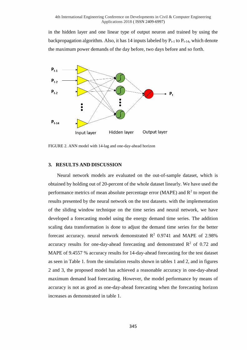
4th International Engineering Conference on Developments in Civil & Computer Engineering
Applications 2018 ( ISSN 2409-6997)
345
in the hidden layer and one linear type of output neuron and trained by using the
backpropagation algorithm. Also, it has 14 inputs labeled by Pt-1 to Pt-14, which denote
the maximum power demands of the day before, two days before and so forth.
FIGURE 2. ANN model with 14-lag and one-day-ahead horizon
3. RESULTS AND DISCUSSION
Neural network models are evaluated on the out-of-sample dataset, which is
obtained by holding out of 20-percent of the whole dataset linearly. We have used the
performance metrics of mean absolute percentage error (MAPE) and R2 to report the
results presented by the neural network on the test datasets. with the implementation
of the sliding window technique on the time series and neural network, we have
developed a forecasting model using the energy demand time series. The addition
scaling data transformation is done to adjust the demand time series for the better
forecast accuracy. neural network demonstrated R2 0.9741 and MAPE of 2.98%
accuracy results for one-day-ahead forecasting and demonstrated R2 of 0.72 and
MAPE of 9.4557 % accuracy results for 14-day-ahead forecasting for the test dataset
as seen in Table 1. from the simulation results shown in tables 1 and 2, and in figures
2 and 3, the proposed model has achieved a reasonable accuracy in one-day-ahead
maximum demand load forecasting. However, the model performance by means of
accuracy is not as good as one-day-ahead forecasting when the forecasting horizon
increases as demonstrated in table 1.

4th International Engineering Conference on Developments in Civil & Computer Engineering Applications 2018 (
ISSN 2409-6997)
FIGURE 3. Forecasted versus actual maximum demand load for the test dataset and 14 days ahead forecasting
TABLE 1.
Forecasting errors 1 to 14 days ahead for the test dataset
25
30
35
40
45
50
55
60
65
25/1/17 25/2/17 25/3/17 25/4/17 25/5/17 25/6/17 25/7/17 25/8/17 25/9/17 25/10/17
Max
imu
m D
em
and
Hu
nd
red
s
Time (days)
actual predicted
Target
1 day
ahead
3 days
ahead
7 days
ahead
9 days
ahead
14
days
ahead
Mean
absolute
percentage
error (%) 2.9797 4.7363 6.2725 7.5372 9.4557
R² 0.9741 0.9326 0.8695 0.8263 0.719

4th International Engineering Conference on Developments in Civil & Computer Engineering
Applications 2018 ( ISSN 2409-6997)
347
FIGURE 4. Correlation of actual and predicted maximum demand load in MW (1-step ahead)
TABLE 2.
Forecasted versus actual maximum demand
load for the last 10 data points in the test dataset
using 1-step ahead forecasting model
R² = 0.9741
20
25
30
35
40
45
50
55
60
65
25 30 35 40 45 50 55 60 65
Pre
dic
ted
de
man
dH
un
dre
ds
Actual demand Hundreds
instance # actual (MW) predicted (MW)
1391 2772 2771.29
1392 2804 2783.36
1393 2803 2887.68
1394 3023 2700.35
1395 2954 3041.65
1396 2811 2956.41
1397 2947 2818.57
1398 3014 2922.05
1399 3029 3029.05
1400 2978 2999.72

4th International Engineering Conference on Developments in Civil & Computer Engineering
Applications 2018 ( ISSN 2409-6997)
4. CONCLUSION
In this paper, we have developed a neural network model based on a multilayer
feedforward neural network to forecast the maximum electrical energy demand by
employing the single time series data (univariate) for the case of Kurdistan region in
Iraq. This study treats the single time series data as multivariable by employing the
moving window data pre-processing method which is a way to apply the machine
learning and data mining forecasting techniques in the case of having the single time
series. Like many other previous successful attempts for the demand forecasting and
function approximation in the literature, in this case, multilayer neural network is also
demonstrated satisfactory estimation with an accuracy of MAPE 2.98%. Neural
networks are able to successfully approximate the continuous functions including the
non-linear functions and can also efficiently deals with noisy data. These properties
make the neural network a strong forecasting tool [6]. Yet another side, it requires a
systematic development methodology starting from data pre-processing, designing of
the network architecture, configuration of the parameters to the evaluation of the
network. Especially implementation and configuration stages of the neural networks
are more of an art than science, which requires many trials and fails.

4th International Engineering Conference on Developments in Civil & Computer Engineering
Applications 2018 ( ISSN 2409-6997)
349
REFERENCES
[1] Y. H. Kareem and A. R. Majeed, "Monthly Peak-load Demand Forecasting for
Sulaimany Governorate Using SARIMA.," 2007.
[2] M. R. G. Al-Shakarchi and M. M. Ghulaim, "Short-Term Load Forecasting for
Baghdad Electricity Region," Electric Machines & Power Systems, p. 16, 2010.
[3] M. Yasin, T. Göze, İ. Özcan, V. Ç. Güngör and Z. Aydın, "Short term electricity
load forecasting: A case study of electric utility market in Turkey," in Smart
Grid Congress and Fair (ICSG), 2015 3rd International Istanbul, Istanbul, 2015.
[4] O. Vornberger and F. M. Thiesing, "Sales Forecasting Using Neural Networks,"
in ICNN97, Texas, 1997.
[5] M. Vafaeipour, O. Rahbari, M. A. Rosen, F. Fazelpour and P. Ansarirad,
"Application of sliding window technique for prediction of wind velocity time
series," International Journal of Energy and Environmental Engineering, 2014.
[6] I. Kaastra and M. Boyd, "Designing a neural network for forecasting financial
and economic time series," Neurocomputing, pp. 215-236, 1996.
[7] D. Graupe, Principles of Artificial Neural Networks, 3rd ed., 2013.
[8] M. Hall, "Time Series Analysis and Forecasting with WEKA," 2014.
[9] I. Witten, E. Frank, M. A. Hall and C. J. Pal, "Data Mining: Practical Machine
Learning Tools and Techniques," 2016.

4th International Engineering Conference on Developments in Civil & Computer Engineering
Applications 2018 ( ISSN 2409-6997)
350
EXPERIMENTAL STUDY AND PREDICTION MAXIMUM
SCOUR DEPTH EQUATION OF LOCAL SCOUR AROUND
BRIDGE PIER
Mohammed Tareq Shukri1, M. Günal2, Junaid Kameran Ahmed3
1&3Ishik University, Erbil, Iraq,
2Gaziantep University, Gaziantep, Turkey [email protected],[email protected],[email protected]
doi:10.23918/iec2018.27
ABSTRACT
Scour is a problem which happen in the flowing stream, rivers and it’s a natural
phenomenon made due to the erosive action of which removes the sediment particles
around the structures placed in water. It means the lowering of the riverbed level by
water erosions such that there is a direction to reveal structural foundations. The
flowing water cause erosive action, excavating and relocate material from the bed
and banks of streams and from around the piers of bridges. In this paper an attempt
is made to evaluation the temporal variation of scour depth at non-uniform
cylindrical bridge pier, in this paper 3 samples of circular bridge piers tested with
different size which conducted in a 8.3 m length and 0.8 m width cannel by
analyzing the data from experimental work analyzing the data to estimate equation
which predict maximum scour depth.
Keywords: scour, local scour, bridge piers.

4th International Engineering Conference on Developments in Civil & Computer Engineering
Applications 2018 ( ISSN 2409-6997)
351
1. INTRODUCTION
Scour is defined as the erosion of streambed sediment around an obstruction in a
flow field (Chang 1988) [1]. It is movement and removal of the sediment around
bridge pier. Bridge scour isusually divided into general scour, contraction scour and
local scour. The local scour may happen in any time especially in flood time caused
collapse for bridges and loss many lives. Figure 1, shows the complex vortex system
occure when down flow waves rolls up as it continues to create a hole through
interaction with the oncoming flow. The vortex then extends downstream along the
sides of the pier. This vortex is often referred to as horseshoe vortex because of its
great similarity to a horseshoe. Even though a lot of work, the predicted of
equilibrium depth of maximum scour analyzed depending on both the numerical and
experimental studies, many researchers still are interested in the basic understanding
of the scour mechanism. Local scour was classified into live-bed scour and clear-
water scour depend on the variance of the approach flow sediment transportation
pattern, (Chabert and Engeldinger, 1956) [2].
.Therefore, the scour study has become a topic of continued interest to the
investigators. Review of the important experiments and field studies was given by
Breusers et al. (1977) [3]; Dargahi (1982) [4]; Dey (1997) [5]; Hoffmans and
Verheij (1997) [6]; Melville and Coleman (2000) [7]; and Richardson and Davis
(2001) [8].
FIGURE 1. Vortex motion around a pier Melville & Coleman (2000) [7]

4th International Engineering Conference on Developments in Civil & Computer Engineering
Applications 2018 ( ISSN 2409-6997)
352
1.1 . SCOUR PROCESS
The sediment particles close to the pier started to move when flow reaches a
certain velocity in the channel; scour is initiated. The eroded particles will
carried from the front of the pier to the direction of downstream by following the
stream pattern. By flow velocity increase, more particles will get displaced, then
creating a scour hole increasing in size and depth. Eventually a maximum scour
depth, (ds) max, is reached which corresponds to a flow velocity being near to the
critical velocity U=Ucr. For nonuniform particles, the large size of the particles
will be sediment in the scour hole, and an armoring layer forms itself in the
scour hole. Then by increasing flow velocity, U<Ucr, is caused for a transport of
sediments in and out of the scour hole, but the scour depth remains essentially
constant. Thus an average equilibrium scour depth, ds, establishes itself, being
slightly smaller than the maximum scour depth, (ds)max (Figure 2) .
FIGURE 2. Time-dependent development of scour depth (Raudlivi and Ettema 1983) [9].
2. EXPERIMENTAL SETUP
A circulating flume used in this study for the experiment work as shown in
figure 3 and figure 4. The size of the flume are (8.3 0.8, 0.9) m. The study section
was setup about 2.8 m from inlet of the flume which is filled with sand according to
the literature study the medium size of the particles d50= 4mm and gradation
coefficient σg=1.15 the depth of the section is 20 cm and with a length of 1.5m. The

4th International Engineering Conference on Developments in Civil & Computer Engineering
Applications 2018 ( ISSN 2409-6997)
353
shape of the models is circular with a diameter of 5cm and 7.5 cm 11.1cm
respectively. The pump ability 25 l/sec located at the left of the channel served the
system and by a valve the flow in the channel controlled. A rectangular weir located
at the end of the channel to measure the discharge and there is a point gage to
measure the depth of the scour hole. To keep the flow uniform before and after the
bridge pier, a ramp was constructed and fastened to the upstream and downstream of
the test section of the channel. The detail of experimental data given in Table 1. The
variation of local scour depth with time is measured at various time by stopping the
experiments and run it again.
FIGURE 3. Schematic illustration of the experimental flume system
FIGURE 4. View of experimental work

4th International Engineering Conference on Developments in Civil & Computer Engineering
Applications 2018 ( ISSN 2409-6997)
354
TABLE 1.
Experimental conditions
Run diameter (cm) h (cm) time (min) discharge (m3/s) observed ds (cm) computed ds (cm)
A1 5 2.5 15 0.00629 6 5.482703675
A2 5 4.4 30 0.016 7.7 6.496038265
A3 5 5.4 30 0.02326 8.2 6.907659147
A4 5 5.7 30 0.02519 8.5 7.057342092
B1 7.5 2.5 50 0.00629 6.1 7.28213382
B2 7.5 4.4 30 0.016 9.1 8.628046079
B3 7.5 5.4 30 0.02326 9.7 9.174761444
B4 7.5 5.8 50 0.02519 10.5 9.373570517
C1 11.1 2.5 30 0.00629 6.4 9.805482815
C2 11.1 4.4 40 0.016 11.2 11.35260838
C3 11.1 5.4 35 0.02326 11.7 12.07196539
C4 11.1 5.8 30 0.02519 11.9 12.33355434
*A: code for 5 cm circular pier *B: code for 11 cm circular pier *C: code for 7.5 cm circular pier
3. PREDICTED MAXIMUM SCOUR DEPTH
In this study there are parameters effects on maximum scour depth; results of
Group 3 tests show us the relation between these parameters and maximum scour
depth. Computer software Step-wise Regression© which it was one of the
regression analysis methods and fitted data, Step-wise Regression used in this study
to analyses the results of the maximum scour depth to get formula which give us
maximum scour depth (ds). The parameters like (d) pier width, (t) time of
equilibrium, (Q) discharge, (h) flow depth, used to analyses a formula for maximum
scour depth. In the program, there are many types of regression method as shown
in Figure 4, it will necessary to try all methods to know the best one. In this study,
linear method, linear+ interaction method, and full quadratic method are used to
predict maximum scour depth, it is seen that the last method is the best method in
this study to predict maximum scour depth.

4th International Engineering Conference on Developments in Civil & Computer Engineering
Applications 2018 ( ISSN 2409-6997)
355
FIGURE 5. Step-wise regression input window
3.1. QUADRATIC REGRESSION METHOD
The formule rusults acoording to this method depending on, (h) depth flow, (d)
pier diameter, (Q) discharge, with R- square value R2= 0.988 and Standard Error of
0.00260. According to this results the quadratic method was an best suited method
to predict eqilibrium scour depth by Equation (1) for this study. Figure 5, shows the
comparison between determined and observed maximum scour depths using
quadratic equation.
(1)
Where dse: Equilibrium scour depth (m), d: Pier diameter (m), Q: Flow discharge
(m3/s)
FIGURE 6. Comparing between determined and observed scour depth for quadratic equation

4th International Engineering Conference on Developments in Civil & Computer Engineering
Applications 2018 ( ISSN 2409-6997)
356
3.2. COMPARISON BETWEEN PREDICTED EQUATION AND
EQUATIONS FROM LITERATURE
In this study, the experiments were carried with (5, 7.5 and 11) cm circular piers
with four discharges. Shen II [10] developed an equation to predicted maximum
scour depth by depending on Froude number (Fr), Flow depth and pier size
(2)
Laursen and Toch (1956) [11] developed equations by depend on experimental work
in Iowa institute of hydraulic research, laursen and Toch equations assumes that
flow depth is the most important factor in determining scour depth
(3)
(Figure 6a,6b,6c) shows the comparison between Shen II [10], Laursen and Toch
(1956) [11], with experimental data and the predicted maximum scour depth, it’s
clear from the figure that maximum scour depth in experimental work close to the
results of predicted equations from this study and the results of Laursen and Toch
(1956) [11] for the three sections, the results of Shen II equations shows some
variance with other results and this due to “Laursen and Toch (1956) [11] equation
assumes that the flow depth is most important factor in determining the scour depth,
whereas the Shen II [10] equation assumes that velocity is important by including
the Freud number” (Les Hamill, 1999) [12].

4th International Engineering Conference on Developments in Civil & Computer Engineering
Applications 2018 ( ISSN 2409-6997)
357
0
2
4
6
8
10
12
14
16
0 5 10 15 20 25 30
ds
ma
x
di scharge lit/s
SA
Experiment data SHEN II Laursen and Toch predected equation
FIGURE 7. (a) Comparison between m.s.d results for sample A
0
2
4
6
8
10
12
14
16
18
20
0 5 10 15 20 25 30
ds
max
discharge lit/s
SBExperiment data Laursen and Toch SHEN II predected equation
FIGURE 7. (b) Comparison between m.s.d results for sample B

4th International Engineering Conference on Developments in Civil & Computer Engineering
Applications 2018 ( ISSN 2409-6997)
358
0
4
8
12
16
20
24
28
0 5 10 15 20 25 30
ds
max
dischrge lit/s
SCExperiment data Laursen and Toch predected SHEN II
FIGURE 7. (c) Comparison between m.s.d results for sample C
4. CONCLUSIONS
1. The present experimental results showed that for the same sediments size and
discharge the depth of scour is directly proportional with pier diameter
2. The results of the predicted equation of this work regarding the flow depth factor
indicated a good agreement with Laursen and Toch (1956) [11].

4th International Engineering Conference on Developments in Civil & Computer Engineering
Applications 2018 ( ISSN 2409-6997)
359
REFERENCES
[1] Chang, H.H. 1988. Fluvial processes in river engineering. John Wiley & Sons, 432 p.
[2] Chabert, J. and Engeldinger, P. (1956). “Etude des affouillements autor des piles
depoints (Study of scour at bridge piers).” Bureau central d’Etudes les
Equipment d’ OutreMer, Laboratory National d’ Hydraulique, France.
[3] Breusers, H.N.C., Nicollet, G. and Shen, H.W.”Local scour Around cylindrical
piers”.(1977) Journal of Hydraulic Research, 15(3): 211-252
[4] Dargahi, B. (1982): Local scour at bridge piers- A review of theory & practice.
TRITA-AMI 114, RIT, Hyr. Eng. Stockholm.
[5] Dey, S, 1997, Local scour at piers, A review of development of research Int. J.
Sediment .Res IJSH, 12 .23-46.Fluvial hydraulics, Walter H. Graf, 2003, “local
scour” CH 9, 611-662.
[6] Hoffmans, G.J.C.M. and Verheij, H.J. 1997. Scour manual. A.A. Balkema,
Rotterdam, Netherlands, 205 p.
[7] Melville, B.W. and Coleman, S.E. 2000. Bridge scour. Water Resources
Publications, LLC, Colorado, U.S.A., 550 p.
[8] Richardson, E.V., and Davis (2001). Evaluating Scour at Bridged, Hydraulic
Engineering Circular No. 18 Fourth Edition. US Federal Highway
Administration, Publication FHWA NHI 01-001.
[9] Raudkivi, A. J. and Ettema, R. (1983). “Clear-water scour at cylindrical piers.”
J. Hydraul. Engrg., 109(3), 339 350.
[10] Shen, H.W., Schneider, V.R. and Karaki, S.S., (1966), "Mechanics of Local
Scour", Colorado State University, Civil Engineering Dept., Fort Collins,
Colorado, Pub. No. CER66-HWS22.
[11] Laursen, E.M. and Toch, A. 1956. Scour around bridge piers and abutments.
Iowa Highway Research Board, Bulletin # 4, Bureau of Public Roads, Iowa.
[12] Less Hamil, Bridge Hydraulics, 1st, London: E &FN spon, 1999

4th International Engineering Conference on Developments in Civil & Computer Engineering
Applications 2018 ( ISSN 2409-6997)
360
USE OF DIFFERENT GRADED BRASS DEBRIS IN EPOXY-RESIN
COMPOSITES FOR IMPROVING MECHANICAL PROPERTIES
Younis Khalid Khdir1, Gailan Ismail Hassan2
1&2Erbil Polytechnic University (EPU), Erbil, Technical Engineering College, Erbil 1&2Ishk university, Erbil, Iraq
[email protected], [email protected]
doi:10.23918/iec2018.28
ABSTRACT
This study deals with the brass debris which is obtained through matte smelting and
refining of brass or different machining process like grinding operation, to use as filler
in epoxy-resin composites. The common uses options for brass debris are recycling, and
production of value-added waste products. In this study random mixing processes to
prepare (Epoxy / brass) composites done by using brass debris of three different grades
with different grain size (600, 800 and 1180) µm as reinforcement in epoxy resin with
different weight percentages (2%, 4%, 6% and 8%) respectively. Using tensile and
impact test to evaluate the mechanical properties of the prepared composites. Results
show that with coarse grain size of brass debris added to epoxy resin, it is very
important to decrease the amount of weight percentage added to it, so as to improve the
tensile or impact properties of (Epoxy / Brass debris) composites. On the other hand a
very low weight percentage (2%, 4%, 6%, 8%) of metal brass debris which there is no
significant improvement in toughness, noticed that can significantly reduce the impact
absorbed energy (impact toughness) of the composite samples. The best value of the
toughness can be obtained with the epoxy-BD600 and weight percent of 8%. This
research includes processing procedure, and study of the mechanical behavior of grades
of such brass debris filled epoxy-resin composites. This paper concluded that the
possibility of utilize of brass debris as secondary filler element for the preparation of
composite materials and producing the bras debris such as added-value products.
Keywords: Waste Utilization, Debris, Composites, Epoxy Resin, Reinforcement.

4th International Engineering Conference on Developments in Civil & Computer Engineering
Applications 2018 ( ISSN 2409-6997)
361
1. INTRODUCTION
Using debris of waste materials obtained during matte smelting and refining of
different machining process like grinding operation, to use as filler in epoxy-resin
composites. In our study we focused on brass debris, because of there is limited studies
using this type of filling. The best options for brass debris are recovery of waste metal,
recycling, and production of composite products. The advantage of these type of
composites is that they are strong and light. By choosing a suitable combination of
matrix and filler material, a new composite can be made that exactly has a property
which is suitable for the requirements of a particular application.
Yun Liu et al., (2016) used Cu-doped graphene (graphenit-Cu) as a filler to prepare
epoxy composite, in his research to study the effect of Cu-doped graphene on the
thermal properties of epoxy composites, they concluded that adding graphenit-Cu had
slight effect on the thermo-mechanical properties of epoxy composite materials [1].
Keong et al., (2017) used municipal solid waste (MSW) is incineration ash, which is
rich in a mixture of oxide and carbonate ceramics, as fillers for composite materials. [2].
Li and Cui (2016) focused on improving the mechanical properties of epoxy base
material by adding of an amino-terminated hyper branched polymer (ATHBP) grown
on glass fiber [3]. Chang et al., (2015) investigated the characterization of tungsten-
epoxy composites for ɤ-rays radiation shielding by blending epoxy resin through adding
different weight percent of tungsten powder [4]. Lee et al., (2016) studied using of
polyethersulfone as filler material to increase the thermal and mechanical properties of
triglycidyl-p-aminophenol epoxy resin [5]. Yang et al., (2016) used simple hot-press
with vacuum treatment to prepare silk fabric reinforced epoxy composites so as to
achieve a maximum volume fraction of reinforcement, 70% silk. They investigated
mechanical properties so that the flexural strength increased linearly by increasing silk
volume fraction from 30 to 60 volume % but diminished slightly at volume 70%. [6].
He et al., (2011) showed impact strength of ceria-epoxy resin composites adding the
ceria nanoparticles with different shapes and sizes added to epoxy resin. [7]. Goud and
RAO (2011) investigated the fibre content effect on the mechanical properties of

4th International Engineering Conference on Developments in Civil & Computer Engineering
Applications 2018 ( ISSN 2409-6997)
362
unidirectional Roystonea regia natural-fibre-reinforced epoxy composites. [8]. Couillard
and Peter (1997) studied the behavior of bending fatigue on one-dimensional,
continuous-carbon-fiber/epoxy composite strands by producing a maximum strain.
They determined that this type of composite did undergo fatigue and at high strains,
damage occurred through matrix cracking, fiber breakage, and interfacial shear
failure [9].
Papargyris et al., (2008) studied composite manufacturing techniques using
conventional and microwave heating methods to prepare carbon fibre/epoxy composites
to compare their mechanical and physical properties. Based on the mechanical testing
similar values of the flexural strength for the two types of carbon fibre/epoxy
composites were obtained [10]. Biswas and Satapathy (2010a, 2010b) fabricate hybrid
composites from bamboo fiber epoxy matrix composites with various weight
proportions of red mud to study erosion characteristics in comparing with glass-epoxy
composites under same test conditions. They concluded that even the bamboo based
composites behave relatively inferior mechanical properties, their performance of
erosion wear is better than the glass fiber reinforced composites. [11, 12]. Kim et al.,
(2013) prepared fiber reinforced epoxy/hybrid silica composite to study their
mechanical properties by adding super fibers such as aramid fiber. They confirmed that
the effect of the epoxy/hybrid silica on the mechanical properties affecting in a demand
for a resin system with very good mechanical properties [13]. In this work, brass debris
was combined with epoxy resin by handily cold process technic to prepare different
composites with various weight percent of brass debris and different size of
reinforcement. The aim of this research is development of a composite with higher
tensile strength as compared with pure epoxy and in the other hand we can use the
wasted materials such as brass debris. The reinforcement particles distributed over the
epoxy resin randomly and homogenous, to prepare these specimen for tensile and
impact tests. In the experimental procedure we explained the fabricating all of these
composites. And in results explained well in next section, and the conclusions of this
job were written in the last paragraph.

4th International Engineering Conference on Developments in Civil & Computer Engineering
Applications 2018 ( ISSN 2409-6997)
363
2. EXPERIMENTAL DESIGN
2.1. MATERIALS
Transparent epoxy (Sikadur -52) is used as matrix which is a liquid of low viscosity
as compared with other thermosets and its converted to solid state by adding hardener
(Sikadur -52 hardener) at ratio of 2:1 the technical properties of Sikadur -52 according
to the data sheet of Sika company are listed in Table 1.
TABLE 1.
Technical properties of Sikadur -52, according to data sheet of the company.
Compressive
Strength
Flexural
Strength
Tensile
Strength
Pot life Density Viscosity
53 MPa for 10
days at 20˚C
50 MPa at
20˚C
25 MPa ~ 120 min at 5˚C
~ 10 min at 30˚C
1.1 kg/l at
20˚C
~ 1200 MPa at 10˚C
~ 430 MPa at 20˚C
While the reinforcement are brass debris with different grain size (600, 800 and 1180
µm) with different weight percentages (2%, 4%, 6% and 8%) respectively. These
different grain size prepared by using sieve analysis (or gradation test) is a practice or
procedure used to assess the particular size distribution of a granular material. It is a
simple technique of particle sizing.
2.2. PREPARATION OF BRASS DEBRIS-EPOXY COMPOSITES
A series of brass debris reinforced epoxy composites has been manufactured using
simple cold techniques. The composite was made using a steel mold according to
standard specifications ASTM D638, the specimen size is shown in figure 1a for tensile
test. The Universal Tensile Machine LY-1066A was used to test the specimen for
tensile tests. And for impact test according to standard specification ISO 179, the
specimen dimension explained in the figure 1b. The LY-XBD-5 Electric Charpy Impact
test machine was used for impact tests, at room temperature

4th International Engineering Conference on Developments in Civil & Computer Engineering
Applications 2018 ( ISSN 2409-6997)
364
(a) (b)
FIGURE 1. Specimen of (a) tensile test, (b) of Charpy Impact test, all dim. in mm.
Tensile and Impact composite samples were prepared by pure epoxy matrix (rate of 2:1
base to hardness) into both impact and tensile molds then distribute the different grades
of brass debris (600 µm, 800 µm and 1180 µm) with weight percentages (2, 4, 6, and
8%) manually into both kinds of mold. The prepared tensile and impact samples
(Epoxy-BD600), (Epoxy-BD800) and (Epoxy-BD1180) properties shown in Table 2.
TABLE 2.
Specifications of the prepared specimen for tensile and impact tests
No. Symbol Refinement Weight fraction of Refinement WtR %
1 Epoxy - -
2 BD 600 brass debris of grain size 600 µm 2%, 4%, 6%, 8%
3 BD 800 brass debris of grain size 800 µm 2%, 4%, 6%, 8%
4 BD 1180 brass debris of grain size 1180 µm 2%, 4%, 6%, 8%
Both tensile and impact samples were left for one week at room temperature to be cared
as shown in figure 2.
(a) (b)
FIGURE 2. Samples of prepared specimen of (a) tensile and (b) impact tests for 600 µm

4th International Engineering Conference on Developments in Civil & Computer Engineering
Applications 2018 ( ISSN 2409-6997)
365
3. RESULTS AND DISCUSSION
3.1. TENSILE TEST
We noticed that the fracture occurred in different areas, this phenomenon can be
interpreted physically, because of the random distribution of brass debris particles and
the agglomeration of some particles in some location while the density of these particles
change from a location to another microscopically. The results as in figure 3a, 3b, 3c
and 3d indicated that the tensile strength of the brass debris-epoxy composite increased
as compared with the pure epoxy, and the elongation also increased for different sizes of
reinforcement (600, 800 and 1180 µm) and different weight percent (2, 4, 6 and 8%)
because of the increasing bonding area between the brass particle and epoxy resin. The
existence of brass particles leads to more elongation and more strength also. Noticed
that the enhance of tensile properties reaches the maximum value at Epoxy-BD600 with
8% of brass debris weight percent and the tensile strength become 48.9 MPa, as
compared for pure epoxy which is 33,65 MPa. Where for the composite Epoxy-BD800
with 6% of brass debris weight percent the tensile strength reaches the maximum value
of 49.16 MPa which is little greater than the tensile strength of Epoxy-BD600. Also we
found that the maximum tensile strength can be obtained by the Epoxy-BD1180 with
brass debris weight percent of 2% and become 45.95 MPa. And for other composite
such as Epoxy-BD800 with brass debris weight percent of 6% can reach the maximum
tensile strength.

4th International Engineering Conference on Developments in Civil & Computer Engineering
Applications 2018 ( ISSN 2409-6997)
366
0
10
20
30
40
50
0 1 2 3 4 5 6 7 8 9 10 11 12
Str
es
s (M
Pa)
Strain
Epoxy
BC600μm 2%
BC800μm 2%
BC1180μm 2%
0
5
10
15
20
25
30
35
40
45
50
0 1 2 3 4 5 6 7 8 9 10 11 12
Str
es
s (M
Pa)
Strain
Epoxy
BC600μm 4%
BC800μm 4%
BC1180μm 4%
(a) (b)
0
10
20
30
40
50
60
0 1 2 3 4 5 6 7 8 9 10 11 12 13
Str
es
s (M
PA
)
Strain
Epoxy
BC600μm 6%
BC800μm 6%
BC1180μm 6%0
10
20
30
40
50
60
0 1 2 3 4 5 6 7 8 9 10 11
Str
es
s (M
Pa)
Strain
Epoxy
BC600μm 8%
BC800μm 8%
BC1180μm 8%
(c) (d)
FIGURE 3. Stress-Strain curves of Epoxy and BD (600,800 and 1180 µm) for weight percentage (a) 2%,
(b) 4%, (c) 6%, and (d) 8%
Comparing all the combined results explained in figure 4. According to the practical
data obtained, we found that the overall maximum tensile strength can be reached by
the composite Epoxy-BD800 with 6% of brass debris weight percent, as noted in the
figure and reaches 49.16 MPa which is very important to be selected to produce a
composite with higher tensile strength properties. Understanding of the mechanical
properties of composite materials is very important for scientific professions and
technical. This knowledge leads to select the suitable composite material. The materials
test provides the essential data in a quantified manner. We can conclude that with
increasing the grain size of the brass debris added to pure epoxy matrix, it is suitable to
decrease the amount of weight percentage added. And the best of all specimen is 6 wt%
(Epoxy-BD800) because it’s has the highest value of maximum stress (49.16 MPa) with
the highest value of strain (12.17 mm/mm). According to the result of this research, it is

4th International Engineering Conference on Developments in Civil & Computer Engineering
Applications 2018 ( ISSN 2409-6997)
367
able to use the waste materials such as brass debris to fabricate new developed
composite with higher tensile strength which can be used for different purpose.
33,65
41
44,21
44,21
48,948,81
25,82
49,16 40,6745,98
34,73
41,73 44,56
0
5
10
15
20
25
30
35
40
45
50
1 2 3 4
σ(M
Pa)T
itle
Brass debris weight percent %
Epoxy
BC600μm
BC800μm
BC1180μm
Ep
ox
2% 4% 6% 8%
FIGURE 4. Maximum stress value of [(Epoxy-BD600), (Epoxy-BD800) and (Epoxy-BD1180)] for all
weight percentage (2, 4, 6 and 8%)
3.2. IMPACT TEST
The second group of the tests is impact test. We noted that the entire specimen is
broken in the notch location, for different size of reinforcement composites and
different weight percent of brass debris. The results as indicated in figures 5a, 5b, 5c
and 5d showed that the toughness of the composites increase with increasing the size of
the reinforcement, till 800 µm, and after that any increasing in the reinforcement size
leads to slight decrease in the toughness values because of the randomly distributed of
the brass debris particles in the epoxy resin.

4th International Engineering Conference on Developments in Civil & Computer Engineering
Applications 2018 ( ISSN 2409-6997)
368
55,31
72,2966,35
0
10
20
30
40
50
60
70
80
1 2 3
To
ug
hn
es
s (
J/m
)Title
55,25
72,4364,92
0
10
20
30
40
50
60
70
80
1 2 3
Toughness (J/
m)T
itle
(a) (b)
58,62
70,27
64,48
50
55
60
65
70
75
1 2 3
Toughness (J/m
)Title
74,82 68,0962,22
0
20
40
60
80
1 2 3
Toughness (J/m
)Title
(c) (d)
FIGURE 5. Impact Toughness of (a) 2%, (b) 4%, (c) 6% and (d) 8% for [(Epoxy-BD600), (Epoxy-
BD800) and (Epoxy-BD1180)]
With increasing the weight percentage of the reinforcement particles to 8%, there is a
slight decrease with increasing the particle size from 600 µm to 1180 µm as showed in
figure 5d. Then if we compare all the results of toughness together with the toughness
of pure epoxy see figure 6, we found that with different grades of brass debris (600 µm,
800 µm and 1180 µm) with weight percentages (2, 4, 6, and 8%), the best value of the
toughness can be obtain with the epoxy-BD600 and weight percent of 8%. It is
important to note that although change weight percentage addition of brass debris with
different grain size, there are no significant improvement in toughness. Overall, Epoxy
sample without any reinforcement has a higher toughness than the other samples. In
general, there is no a significant effect for the toughness purpose for this type of
composite.

4th International Engineering Conference on Developments in Civil & Computer Engineering
Applications 2018 ( ISSN 2409-6997)
369
73,29
55,31 55,2558,62
74,8272,29 72,43 70,27
68,0966,35 64,92 64,48
62,22
0
10
20
30
40
50
60
70
80
1 2 3 4
To
ug
hn
ess (J/m
)Title
Brass debris weight percent %
Epoxy
BC600μm
BC800μm
BC1180μm
FIGURE 6. Impact Toughness of Epoxy reinforced by (Epoxy-BD 600, Epoxy-BD 800 and Epoxy-BD
1180 µm) for weight percentage (2%, 4%, 6% and 8%)
4. CONCLUSION
1. It is possible to fabricate a new epoxy composite using waste materials such as
brass debris, with higher tensile strength.
2. With increasing grain size of added reinforcement to the epoxy resin, it is very
important to decrease the amount of weight percentage added to it so as to
improve the tensile properties of (Epoxy-Brass debris) composites.
3. It is important to note that there is no significant improvement in toughness,
pure epoxy has a slight difference toughness than the other epoxy brass
composites.
4. The best value of the toughness can be obtain only with the epoxy-BD600 and
weight percent of 8%.
ACKNOWLEDGMENTS
Thanks to engineer Mustafa Sabah, Goran Ghafur and Rawand Younis for their
efforts helping us in the practical part.
Epo
xy
2%
4%
6%
8%

4th International Engineering Conference on Developments in Civil & Computer Engineering
Applications 2018 ( ISSN 2409-6997)
370
REFERENCES
[1] Y. Liu, H. V., Babu, J., Zhao, A., Goñi-Urtiaga, R., Sainz, R., Ferritto, M., Pita,
De-Yi. Wang, "Effect of Cu-doped graphene on the flammability and thermal
properties of epoxy composites", Composites Part B: Engineering, vol. 89, pp.
108-116. 2016.
[2] G. C. Keong, M. H. B. M. Walad, O. W. Xiong, M. N. Haikel, C. H. Ling, R.
K.S/O Ravichadran, L. T. Kiang, T. L. Hing, "A Study on Mechanical Properties
and Leaching Behaviour of Municipal Solid Waste (MSW) Incineration
Ash/Epoxy Composites", Energy Procedia, vol. 143, pp. 448-453. 2017.
[3] S. Li and C. Cui, "Enhancing the mechanical properties of epoxy resin by addition
of an amino-terminated hyperbranched polymer grown on glass fiber", Journal of
materials science, vol. 51, (4), pp. 1829-1837. 2016.
[4] L. Chang, Y. Zhang, Y. Liu, J. Fang, W. Luan, X. Yang, W. Zhang, "Preparation
and characterization of tungsten/epoxy composites for γ-rays radiation shielding",
Nuclear Instruments and Methods in Physics Research Section B: Beam
Interactions with Materials and Atoms, vol. 356, pp. 88-93. 2015.
[5] S.-E. Lee, E. Jeong, M. Y. Lee, M.-K. Lee, Y.-S. Lee, "Improvement of the
mechanical and thermal properties of polyethersulfone-modified epoxy
composites", Journal of Industrial and Engineering Chemistry, vol. 33, pp. 73-79.
2016.
[6] K. Yang, R. O. Ritchie, Y. Gu, S. J. Wu, J. Guan, "High volume-fraction silk
fabric reinforcements can improve the key mechanical properties of epoxy resin
composites", Materials & Design, vol. 108, pp. 470-478. 2016.
[7] X. He, D. Zhang, H. Li, J. Fang, L. Shi, "Shape and size effects of ceria
nanoparticles on the impact strength of ceria/epoxy resin composites",
Particuology, vol. 9, (1), pp. 80-85. 2011.
[8] G. Goud, and R. Rao, "Effect of fibre content and alkali treatment on mechanical
properties of Roystonea regia-reinforced epoxy partially biodegradable
composites", Bulletin of Materials Science, vol. 34, (7), pp. 1575-1581. 2011.

4th International Engineering Conference on Developments in Civil & Computer Engineering
Applications 2018 ( ISSN 2409-6997)
371
[9] R.A.A. Couillard, and P. Schwartz, "Bending fatigue of carbon-fiber-reinforced
epoxy composite strands", Composites science and technology, vol. 57, (2), pp.
229-235. 1997.
[10] D. Papargyris, R. Day, A. Nesbitt, D. Bakavos, "Comparison of the mechanical
and physical properties of a carbon fibre epoxy composite manufactured by resin
transfer moulding using conventional and microwave heating", Composites
science and technology, vol. 68, (7), pp. 1854-1861. 2008.
[11] S. Biswas, and A. Satapathy, "A comparative study on erosion characteristics of
red mud filled bamboo–epoxy and glass–epoxy composites", Materials & Design,
vol. 31, (4), pp. 1752-1767. 2010.
[12] S. Biswas, and A. Satapathy, "Use of copper slag in glass-epoxy composites for
improved wear resistance", Waste Management & Research, vol. 28, (7), pp. 615-
625. 2010.
[13] D. Kim, I. Chung, and G. Kim, "Study on mechanical and thermal properties of
fiber-reinforced Epoxy/Hybrid-silica composite", Fibers and Polymers, vol. 14,
(12), pp. 2141-2147. 2013.

4th International Engineering Conference on Developments in Civil & Computer Engineering
Applications 2018 ( ISSN 2409-6997)
372
A NEW TAXONOMY OF MOBILE BANKING THREATS,
ATTACKS AND USER VULNERABILITIES
Saman Mirza Abdullah1, Bilal Ahmed2, Musa M.Ameen3
1Koya University, Koya, Iraq 1,2&3Ishik University,Erbil, Iraq
[email protected], [email protected] [email protected] ,[email protected]
doi:10.23918/iec2018.29
ABSTRACT
Mobile banking becomes an interested technique within the modern bank
establishments. It facilitates the transactions and day lifestyle of customers. It
minimizes the impact of location and time for doing bank activities and communicate
with bank servers. However, the process is not less risks from attackers and hackers,
especially, user behaviors that opens and creates many vulnerabilities in this system.
This work presents a new taxonomy for mobile banking attackers and threats. Through
this taxonomy, this work will identify the important user vulnerabilities that attackers
may misuse them for penetrating systems and steal privacy and sensitive date. The
main contribution of this work is providing important suggestions for mobile banking
users so that they can take them as precaution for protecting their privacy and financial
aspects. The work concluded that there are many user behaviors of mobile banking
leading to bring threats inside to systems. The work presents many suggestions for
users so that their systems be protected from malicious activities and malwares. Many
future aspects have been presented.
Keywords: Mobile Banking, Threats and Attacks, User Vulnerabilities.

4th International Engineering Conference on Developments in Civil & Computer Engineering
Applications 2018 ( ISSN 2409-6997)
373
1. INTRODUCTION
Mobile malwares (MM) are considered as a new and unlike threats for the mobile
users. It is a growing security concern and expected to be continue as users perform
sensitive actions on their smartphones. Most mobile users have no idea about different
ways that thoroughly MMs (attackers and intruders) are penetrating their mobile
systems without their privileges and prior knowledge. The worst case is the users
consider themselves immune from such threats and they don’t have enough
knowledge about the rapid growth in the number and the type of mobile malwares[1]
. According to a report from the McAfee Labs, 1.5 million of new incidents have been
detected in the first quarter of the year 2017. With such increase, the landscape of the
mobile threats and attacks are evolving in such a way that makes financial institutions
(such as banks) and their customers always worry about the risks that expected from
the process of online and mobile banking [2]. Therefore, it is necessary to study the
feature(s) of every new mobile malware soon they have been propagated and defected
systems. It is also necessary to conduct researches to find precautions for future
possible threats and increase users’ awareness towards such MMs.
New malwares, which are also known as the zero-day threats and attacks, are coming
with different features and they follow varieties of policies and techniques. Malware
analyzers need to perform reverse engineering processes on each new malware as they
appear, so that they can reveal their secrets, such as the group that they belonged to.
However, each malware has different policy in the design. The common point between
malwares is that they misuse wide range of vulnerabilities to penetrate targeted
systems. To simplify the revealing process, researchers are always grouping malwares
based on the similarity among some defined features [3]. The most common grouping,
is classifying malwares based on the technique(s) they are using while they penetrate
mobile systems. In the other hand, researchers are grouping malwares based on the
device type and the software platform. Other groupings are done based on the goals
and purposes that MMs has been designed for. As an example, some malwares aimed
to disclose privacy on the victim mobile, by steeling sensitive information or money,
and in some cases attackers are penetrating mobile systems just for fun. At the end,
breaking the defense systems of the mobile devices or the banks by bypassing the

4th International Engineering Conference on Developments in Civil & Computer Engineering
Applications 2018 ( ISSN 2409-6997)
374
security solutions is the main target for all MMs in each group. Understanding the
MM features through grouping them under different categories may help the task of
mobile defense systems much easier, better analyze and evaluate malwares, and
mobile users can understand their behaviors more, which will consequently, minimize
the impact of malicious codes on the mobile systems[4]. this work describes the
environment of the MMs in a form of some interrelated assets. Each asset covers
some parts or elements that are essential in performing the mobile banking or
transaction communication. This paper consist of six sections. The first section is
introduction to the field of the mobile banking in the view of security. Section two is
describing the fundamental framework of mobile banking and briefly states some
differences between online banking and mobile banking. Section (3) is proposing a
new taxonomy for the mobile vulnerabilities that misused by the MMs. Section (4)
gives some examples of threats and attacks that are related to user vulnerability asset
with a brief description on the policies of each MM family. Finally, some
recommendations, suggestions, and advices have been explained on how to be on the
safe side while enjoying using mobile banking facilities.
2. LITERATURE REVIEW
Based on the best knowledge of the author, the activities of the mobile banking
have been started with SMS services, and the history of initiating such services is
going back to 1999 [5]. Many countries at that time tried to employ the mobile devices
in the financial and banking issues and they suggested better processor and
communication facilities to cover more services. Soon developed countries
encouraged the banks to provide customers with mobile services [6]. Even more,
developed countries tried to include some multimedia services of the mobile in the
banking issues [7]. Services, such as paying bills, payment transferring, online
shopping and checking accounts were the expected and required services for the future
of the mobile banking [8]. However, the security concerns became an important
problem within the infrastructure of the mobile banking. Therefore, many works
developed some security frameworks and others argued some security assessment
processes [9, 10]. Within these frameworks and assessments, the mobile users and
their behaviors were the most important security questions. User vulnerabilities still
important in many recent works as they become the main vulnerabilities for the mobile
attackers’ penetration, beside system vulnerabilities. one of the recent works

4th International Engineering Conference on Developments in Civil & Computer Engineering
Applications 2018 ( ISSN 2409-6997)
375
addressed an assessment of the mobile vulnerabilities within Android and iPhone
OS[11]. The work argued some vulnerabilities of the mobile banking applications that
released and certified by the banks. The work showed that some banks are using
simple HTTP protocol without concerning to the security issues that related to the
man in the middle attack. The work just focused on the vulnerabilities of those
applications and forgot to analyze user vulnerabilities that also misused by attackers
work in the middle way. Many works focused on securing the communication
channels between customers and bank servers. In those works, stronger encryption
methods are proposed [12]. However, the weak point of the mobile banking systems
are the users themselves. Within any downloading of games or unknown applications,
a Trojan malware could insert itself to the system and make itself active for opening
a back door for attackers. The possibility of downloading Trojan is in increase as the
work [13] reported that number of Trojan infected apps in the mobile application
sources, such as Google Play Store and iOS app store, are increased unpredictably.
Another part that more concerned the security of the mobile banking systems are the
security of the physical storage of data in bank sides. One of the most important
attacks that related to the server security is SQL injection. Such attacks inject a
malicious code inside the database of the bank and do activities they need. Many
authors worked on that problem and they designed SQL Injection detection systems
[14]. Although mobile users may not have impact on those database security,
employers in the bank whom working on such dataset may be misused by attackers.
It seemed that all framework of the mobile banking needed to be securable. Moreover,
a great part of the security breaching is the responsibility of the user vulnerability.
Therefore, this work presents a new taxonomy of the mobile banking threats and
attacks and discusses the impact of user vulnerabilities on each part.
3. SECURTIY PERSPECTIVES OF MOBILE BANKING
Today, banks in most developed countries offer mobile banking services for their
customers. It is putting essential banking services as a mobile applications and let
users (bank customers) to use them remotely either from their smartphones or tablets.
The most common services that provided through mobile banking applications are bill
payments, fund transferring, checking transactions and balance, and sending some
security alerts or reminders [15]. The most important part of the mobile bank services

4th International Engineering Conference on Developments in Civil & Computer Engineering
Applications 2018 ( ISSN 2409-6997)
376
is to ensure users that their communication with the bank is been transferred via a
secure and protected channel. This will increase the trust of mobile bank users and
their acceptance to the system, which is not really an easy matter as shown in some
statistical figures. Researches been conducted for specific countries and bank. A
paper found that 69% of German banks are providing m-banking services, and it
showed that 79% of the people are using m-banking. Among all users and nonusers
of mobile banking, only 77% of them are still worrying about the security of m-
banking [16]. Therefore, securing the systems of the m-banking is becoming a very
essential issue, however, it is not easy. the typical infrastructure of any m-banking is
shown in Figure-1 [17] . The core idea is establishing a communication channel with
the core bank systems using mobile communication system, Internet networks, and
mobile banking servers. In the figure, the part of the mobile communication systems,
implicitly, comes within the Internet network. Another implicit part of the m-banking
systems is the users, or the bank customers that are performing banking transactions
through their mobile devices.
FIGURE 1. Typical Mobile Banking Systems
At each stage or part of the m-banking infrastructure, a special level of security
defense systems are required and many security challenges will be there. According
to this scenario, this work has divided the different parts of the m-banking systems,
specifically from a security perspective, into four groups or assets; mobile user
behaviors, mobile applications, hardware, and the mobile or the Internet network
systems. Classifying the whole m-banking systems into four assets from a security
perspective have been done according to the type and the policy of the attacks
penetrating the m-banking systems. At each part (asset), special types of threats are
misusing the vulnerabilities that could be found only in the corresponding part. To

4th International Engineering Conference on Developments in Civil & Computer Engineering
Applications 2018 ( ISSN 2409-6997)
377
provide a full immune m-banking service, special defense systems should be
designed. The proposed defense systems firstly need to know and analyze all threats
and attacks at each part. Secondly, the defense system should be aware about the
policies and vulnerabilities that might be misused by attackers and various threats to
penetrate the corresponding part. Then, designing a fully protective system for
securing m-banking system can be achieved [4]. next section explains in detail about
the taxonomy of the MMs in the viewpoint of the above mentioned assets.
4. NEW TAXONOMY OF MM
The new MM taxonomy proposed in this work is considering each part of the
mobile banking system as an asset, as shown in Figure 2.
FIGURE 2. The main assets of the mobile banking systems
As shown in Figure 2, no part of mobile banking system is free from threats and
attacks. Every single piece of the mobile banking system, from the device to the
server, either physical or software are all entitled to different attacks through the
vulnerabilities and flaws found in each asset. Table 1 lists the names of most known
attack types under four different categories or assets. The mentioned attacks at each
level can be considered as serious threats on mobile bank systems and customers.

4th International Engineering Conference on Developments in Civil & Computer Engineering
Applications 2018 ( ISSN 2409-6997)
378
TABLE 1.
The New Taxonomy of Mobile Banking Threats and Attacks [1, 16, 18]
Assets-1
Devices
Assests-2
Network
Assets-3
Physical Storage
Assets-4
User Vulnerabilities
Phishing Wi-Fi (No Encryption or
Weak Encryption) Platform Vulnerabilities
No Passcode/Weak
Passcode
Framing Rogue Access Point Server Misconfiguration iOS Jailbreak
Click Jacking Packet Sniffing Cross-Site Scripting
(XSS) Android Rooting
Man-in-the-Middle
(MITM)
Man-in-the-Middle
(MITM)
Cross-Site Request
Forgery (CSRF)
Password and Data
Accessibility
Buffer Overflow Session Hacking Weak Input Validation User-Initiated Code
Data Caching DNS (Domain Name
Systems) poisoning
Brute Force Attacks
SQL Injection Sensitive Data Storage
No Encryption/Weak
Encryption
SSL (Secure Sockets
Layers) Privilege Escalation
User skills and
experience about
security
Baseband Attack Fake SSL certificate Data Dumping Phishing
SMIshing OS Command Execution
Improper SSL
Validation
Dynamic Runtime
Injection
Escalated privileges
One of the best ideas of classifying mobile banking threats and vulnerabilities is to
provide solutions that come fit with each asset. Therefore, this work will provide
security solution(s) for each threats and attacks that more related to the user
vulnerabilities.
5. USER RELATED ATTACKS IN MOBILE BANKING
Categorizing mobile banking threats makes the process of finding security
solutions easier for security specialists and researchers. It divides the task of a fully
immune mobile banking system on individual defense and protective systems. As shown
in Table-1, assets of mobile banking are divided into four parts. Each part covers a
group of attacks and threats, and of course, each individual attack has its own policy
and technique to penetrate systems. In Table-2, most attacks that related to the user
vulnerabilities have been described shortly. Next section, important suggestions for
mobile banking users will be given.

4th International Engineering Conference on Developments in Civil & Computer Engineering
Applications 2018 ( ISSN 2409-6997)
379
TABLE 2.
Attacks, their policies and some solutions [1-4, 19]
Attacks and Threats Definition and Policies
Phishing It uses legitimate personation for stealing privacy or login credential information. It dose
that through urgent emails to target victims.
Framing It inserts some fake frames in a legitimate website for a bank or company for collecting
privacy or login credential information.
Click Jacking
It is exactly like framing, but the attacker will put an invisible button on some interested
button. The malicious activities will be done when a user clicked the interested bottom
and it doesn’t has idea that there is a hidden bottom
Man-in-the-Middle
(MITM)
This type of hacking is done through a lot of malicious ways. The most popular ways are
the email hijacking and WiFi eavesdropping
Buffer Overflow Attackers try to write into some temporary memory locations more than they can hold.
Data Caching
This attack has some similarity with buffer overflow. They try to over follow the cache
memory, breaking AES keys based on some timing or power consumptions, or sometime
through provoking the eviction of recently accessed data
Baseband Attack
This attack can penetrate both Android and iOS based devices. It is usually attacking a
device over the air. It starts through operating an adversary on a rough based station that
somehow close enough to communicate with target device. It has ability to locate the
position of the user and can break the privacy that stored on the device.
SMiShing SMiShing is shorten of SMS Phishing. It sends an interested SMS thoroughly a user will be
motivated to download Trojan Horse, virus, or other type of malwares.
Improper SSL
Validation
It is very important to secure the communication between the bank and the client. This
process done using a valid Secure Sockets Layer (SSL), which is standard security
technology, and it depends on encryption. Using improper SSL makes the job of attacker
easy to listen to these communications and steal privacies.
Dynamic Runtime
Injection
It is the process of calling and controlling a library that permit a malicious code to be
injected or replaced in a mobile device. It starts with clicking an unknown email then it
controls the SSL communication process at run time.
Unintended
permission
Many permission requests will be accepted set by applications and mobile users are
accepting them. These permissions, after they allowed, they change the status of many
private objects to public among applications.
Improper Certificate
Validation
It comes with using or installing invalid, cracked, illegal software and applications. The
attacker will try to overcome the SSL protocol and conduct an illegal communication with
client.
Escalated Privileges Is gaining the access to many parts of the mobile through different way, which one of
them is rooting the devices
No Passcode/Weak
Passcode Passcode used to lock mobile devices and protect it from an authorized person.
OS Jailbreak and
Rooting These to apps used by mobile users (iPhone and Android) to get apps free.
Password and Data
Accessibility
The most common way for protecting data is avoiding accessibility through using
passwords.
User’s Initiated Code Quick Response (QR) Code becomes very come among mobile users.
Sensitive Data Storage Sensitive data should be kept in a very secure storage (Strong password and Encryption
algorithm). Attackers typically don’t break crypto directly.
User skills and
experience about
security
Most attackers are penetrating systems because of unawareness of the users to the mobile
devices and apps.

4th International Engineering Conference on Developments in Civil & Computer Engineering
Applications 2018 ( ISSN 2409-6997)
380
6. SUGGESTIONS FOR MOBILE BANKING USERS
The pillars’ responsibility of security framework for any mobile banking system
should be includes Bank Strategic IT Policy, IT technician beside the behaviors of the
bank customers themselves. All involved parties in the system need to cooperate to
have a safeguard zone and to minimize the risk of threats and attacks penetrations. In
this section, this work provides the role of users in keeping the vulnerabilities as close
as possible and increase their awareness about the possible open gates that thoroughly
attackers may penetrating their systems. Although this work classified the attacks in
the process of mobile banking into four assets (Figure 1), attacks due to user behaviors
and vulnerabilities are more focused. In general, user vulnerabilities come in the first
and fourth assets. While asset number two and three are more about the mobile
communication and bank establishments. To avoid vulnerabilities in any mobile
banking system, users should strongly consider the following recommendations and
suggestions:
1. Users should not open any urgent notes or emails that originated by their
banks, especially, if the email or note asks private information. Banks never
send or ask privacies through mobiles or in urgent ways. Such messages or
emails have high probability of containing phishing.
2. Many emails or note senders will ask customers some privacy information
through filling sort of forms sent through a link. Once the link opened
customers will see some frames added to the opened website. Or, the link will
direct customers to a fake page where looks almost like the correspondence
bank website. Any information given to such frames and websites will put
users in the risk of stealing their privacy and financial information through a
type of attack known as the man in the middle. Through such links the attacker
can control the communication of customers and the corresponding banks.
3. Many mobile users are interested in downloading free apps and software
through the process of rooting or jailbreaking their device. Such rooting
processes will bypass the security and the permission controls that protecting
the Kernel root of the mobile devices, thus the device becomes open for
attackers to access any private and sensitive data that kept inside the mobile.
Of course, stealing the credit card numbers and QR codes will be one of the

4th International Engineering Conference on Developments in Civil & Computer Engineering
Applications 2018 ( ISSN 2409-6997)
381
revealed data. Moreover, buffer over follow and data catching attacks will get
advantages from jailbreaking mobiles for making devices working slowly and
have bad respond.
4. Many attackers are working within the asset three, which is related to network
part. However, users of mobile banking are also involving in this process of
penetration. It is the role of the mobile users to give permissions to an app to
escalate their privileges. Dynamic runtime injection attack is the most
effective attacks that gets the advantages form the user permission. Users
should be aware about the type of the access that an app is asking for
controlling Kernel or other applications. For example, a game asking you to
access your contact number list or read your SMS lists. Users should ask
themselves about the relation between this app and contact list. If users
couldn’t find any relation the requested access should be blocked.
5. SMS is the main gate of attackers toward the mobile devices in mobile banking
apps.
a. A type of phishing called SMIshing is the most popular attack that
thoroughly many Trojans and worms are penetrating systems. Users
should not open SMS messages from unknown or suspicious senders
or should not click on any link that comes through an SMS from
strangers.
b. Another type of attack is called DDoS attack. This attack may come
inside the mobile devices through opening and clicking a link inside
an SMS came from stranger destination. The attack will control the
communication or the SSL validation between the mobile and the bank
server.
6. The fist access control type of any mobile devises is the passcode. All type of
passcode should be strong and undetectable. When a mobile become
physically with an attacker the first trial that the attacker will do is hacking the
passcode. Mobiles that supporting bioinformatics access are much safer than
others. There are many attackers use the track of keystrokes as type of breaking
the access defense process. If the user depend on QR access, it should be aware
that his/her QR could be extracted somewhere
7. Storage places of sensitive data should be strongly protected through a very
powerful password. There are many recommendations about the formulation

4th International Engineering Conference on Developments in Civil & Computer Engineering
Applications 2018 ( ISSN 2409-6997)
382
of the passwords. Users should have knowledge about distinguishing weak
passwords from strong one.
7. CONCLUSION
This work concluded that responsibility for building a strong security framework of
any mobile banking is not on the bank or just on the customer, it a pair responsibility.
It is very important for users to understand their vulnerabilities and avoid them. To be
more understandable, this work classified the attacks in the process of mobile banking
into four categories. The work focuses more on the user vulnerabilities, as it is relevant
to all categories. This work found that user behavior couldn’t be separated from the
main framework of mobile banking security. Moreover, the only way for educating
mobile users is through publishing some suggestions, which are not easy to be well
understood as they required security skills and experiences. For the future work, this
work preferred and designing a security framework for mobile banking that put all
assets together in one frame. It will be great if some intelligent techniques as detection
systems for each asset will be designed, and it will be better if an intelligent mobile
banking systems could be presented in the viewpoint of smart cities, such as using the
concept of Internet of Thing (IoT).

4th International Engineering Conference on Developments in Civil & Computer Engineering
Applications 2018 ( ISSN 2409-6997)
383
REFERENCES
[1] P. Y an and Z. Yan, "A survey on dynamic mobile malware detection,"
Software Quality Journal, pp. 1-29, 2017.
[2] MaCafee, "McAfeeLabsThreatsReport,
"https://www.mcafee.com/us/resources/reports/rp-quarterly-threats-jun-2017.
pdf2017 2017.
[3] F. Martinelli, F. Marulli, and F. Mercaldo, "Evaluating Convolutional
NeuralNetwork for Effective Mobile Malware Detection," Procedia Computer
Science, vol. 112, pp. 2372-2381, 2017.
[4] R. Unuchek and V. Chebyshev, "Mobile malware evolution: 2013," AO
Kapersky Lab, 2014.
[5] D. irch, "Banking on the Move The internet isn’t the only new digital
channel," 1999.
[6] B. Must and K. Ludewig, "Mobile money: cell phone banking in
developing countries," Policy Matters Journal, vol. 7, pp. 27-33, 2010.
[7] M. H. Hasan and A. Khalid, "Development of Multimedia Messaging
Service (MMS)-based receipt system for mobile banking," in Information
Technology (ITSim), 2010 International Symposium in, 2010, pp. 1-6.
[8] N. Mallat, M. Rossi, and V. K. Tuunainen, "Mobile banking services,"
Communications of the ACM, vol. 47, pp. 42-46, 2004.
[9] D. Weerasinghe, V. Rakocevic, and M. Rajarajan, "Security framework for
mobile banking," in Trustworthy Ubiquitous Computing, ed: Springer, 2012,
pp. 207-225.
[10] L. Nosrati and A. M. Bidgoli, "Security assessment of mobile-banking,"
in Computing and Communication (IEMCON), 2015 International
Conference and Workshop on, 2015, pp. 1-5.
[11] S. Bojjagani and V. Sastry, "VAPTAi: A Threat Model for Vulnerability
Assessment and Penetration Testing of Android and iOS Mobile Banking
Apps," in Collaboration and Internet Computing (CIC), 2017 IEEE 3rd
International Conference on, 2017, pp. 77-86.
[12] H. N. Huxham, "Mobile banking system with cryptographic expansion
device," ed: Google Patents, 2017.

4th International Engineering Conference on Developments in Civil & Computer Engineering
Applications 2018 ( ISSN 2409-6997)
384
[13] S. K. Shukla, "Trust and Security Must Become a Primary Design
Concern in Embedded Computing," ACM Transactions on Embedded
Computing Systems (TECS), vol. 17, p. 1, 2018.
[14] N. Shah, "Securing Database Users from the Threat of SQL Injection
Attacks," 2017.
[15] K. Kavitha, "Mobile Banking Supervising System-Issues, Challenges and
Suggestions to improve Mobile Banking Services," Advances in Computer
Science: an International Journal, vol. 4, pp. 65-67, 2015.
[16] C.-. Insights, "Mobile Banking Security: Challenges, Solutions," USA,
Report2015.
[17] mpss. (2018). Myanmar Paymnet Solution Services.
[18] A. Feizollah, N. B. Anuar, R. Salleh, and A. W. A. Wahab, "A review on
feature selection in mobile malware detection," Digital Investigation, vol. 13,
pp. 22-37, 2015.
[19] S. M. A. Ghani, M. F. Abdollah, R. Yusof, and M. Z. Mas’ud,
"Recognizing API Features for Malware Detection Using Static Analysis,"
Journal of Wireless Networking and Communications, vol. 5, pp. 6-12, 2015.

4th International Engineering Conference on Developments in Civil & Computer Engineering Applications 2018
( ISSN 2409-6997)
385
CASE STUDY: INVESTIGATING THE 2013 ASIACELL WAREHOUSE
STEEL PORTAL FRAME FAILURE
Razaq Ferhadi
American University of Kurdistan, Duhok, Kurdistan Region-Iraq
doi:10.23918/iec2018.30
ABSTRACT
In a windy morning of March 17, 2013, a warehouse belonged to Asiacell Telecom collapsed
during construction. The structure was a relatively large 108m by 48m double-span steel portal
frame designed by an Iranian engineering firm and constructed by a local construction company.
This catastrophic structure collapse that killed three workers and injured few, was a sudden
failure that triggered an intense investigation to determine the cause to avoid the occurrence of
the same mistake in the future.
This research paper is the product and outcome of the forensic structural analysis performed by
the author for Asiacell that indicates the exact reasons behind the catastrophic failure. It
provides the evidence to be a lesson-learned document for the future steel structure construction
in Iraqi Kurdistan.
Keywords: Case Study, Steel Portal Frame, Structural Failure.

4th International Engineering Conference on Developments in Civil & Computer Engineering Applications 2018
( ISSN 2409-6997)
386
1. INTRODUCTION AND PROBLEM STATEMENT
This paper is a further investigation of the original analysis prepared to fulfill the request of
Asiacell, who owns the warehouse complex. The case was originally investigated and reported
to Asiacell in 2013 [1]. As such, an evaluation of the design and construction process started
few days after the incident to determine the cause. The evaluation includes construction as well
as the structural design. The structure (Figure 1) was located in Sulaimany in Kurdistan Region
and was a part of a warehouse complex that consisted of a total of four portal frame structures
besides few other buildings for the office. This frame, which was the largest one of the group,
catastrophically collapsed during the construction process and triggered an investigation by
Asiacell to enhance the construction safety and insure that this kind of tragedies will not happen
again.This paper depicts the structural analysis and design, and evaluates the construction
management in order to highlight the cause of the catastrophic failure of the structure. As this
type of failure is dangerous being a source of safety concerns and cause of losing money besides
time consumption, Asiacell demanded that work to be halted immediately and strong measures
to be taken seriously through a thorough forensic analysis to prevent this type of failures in the
future. The author of this paper was a part of the team of investigators hired by Asiacell for this
purpose and this paper is the result of the calculation and evaluation of the frame.
As in any construction failure in the world, fingers were pointed to the design and construction
process. As such, it was necessary to review the design documents first and determine whether
there are any flaws in it that might caused the failure.
FIGURE 1. Asiacell Warehouse Portal Frame Model

4th International Engineering Conference on Developments in Civil & Computer Engineering Applications 2018
( ISSN 2409-6997)
387
2. WHAT WENT WRONG?
The 108m x 84m steel portal frame collapsed during construction as a result of a dynamic
lateral load caused by the collapse of the 50 ton rough terrain crane and hitting one of the
rafters. The rafter that was connected to the outer columns and fixed on the concrete via four
anchor rods, collapsed under the impact as one piece frame and hit the adjacent frame section
and caused a catastrophic abrupt-action collapse of the whole structure as a domino effect
(Figure 2).
The collapse was catastrophic as it killed three steel workers and injured few others. The crane
failed under the strong wind while its telescopic boom was extended all the way. Despite that
the load that the crane carried during the failure was well within its capacity, a question was
raised as to why the construction was not halted during the high wind weather that was above
50 km per hour? Obviously, this was a flaw in the construction management of the project but
then another question popped up: why the frame collapsed under the relatively-low impact
load? This question is answered in the following paragraphs.
3. INVESTIGATION METHODOLOGY
The frame design was evaluated using Autodesk Robot Structural Analysis Professional
2013 software. The pitched roof steel portal frame was modeled to have the same member
sections as the original design and was analyzed using the conventional LRFD method for steel
structure. As the structure is a moment resisting and braced frame, special care has been taken
to have members of tapered sections whereby the bigger sections are located at the location of
bigger bending moment.Stiffeners have been provided to tackle torsion and lateral torsional
buckling. The analysis is in accordance with ANSI/AISC 360-2013 [2].
The base plates were analyzed in accordance with AISC Steel Construction Manual, 9th Edition
using Allowable Stress Design (ASD) [3] and following the procedures specified in the book
Design of Welded Structures [4] and AISC Steel Design Guide 1 [5]. The anchor rods were
analyzed in accordance with Appendix D of ACI 318-08 using LRFD Method [6].
The construction aspect was evaluated using a site visit investigation by checking the
damages caused in the frame members, connections, and foundation. The observations were

4th International Engineering Conference on Developments in Civil & Computer Engineering Applications 2018
( ISSN 2409-6997)
388
photographed and illustrated in this paper. First, the design details are clarified and
analyzed. Then, the construction process is investigated and the causes of the failure are
concluded.
4. FRAME DESIGN DETAIL
The steel portal frame, which had a span of 84.0m and a length of 108m, was designed to
have two spans and 18 bays (Figure 3). It was designed to be supported by side and
intermediate columns on the direction of 84.0m span, which makes it to have two successive
spans of 42.0m long (Figure 4). The frame possessed bays of 6.0m span on the traverse
direction with column height of 10m on the sides and 15m in the middle. The structural steel
was of Grade S275 according to Eurocode 3.
FIGURE 3. Asiacell Warehouse Frame Plan
FIGURE 1. Collapsed Frame as Domino Action

4th International Engineering Conference on Developments in Civil & Computer Engineering Applications 2018
( ISSN 2409-6997)
389
FIGURE 4. Typical Portal Frame Elevation
The frame consisted of the following main elements that were analyzed in detail:
1. Main Frame Columns: The main frame columns were designed to have tapered
section on one side that were 600mm at the base and 1200mm at the top. The flanges
had a width of 300mm and thickness of 16mm while the web had 10mm thickness.
2. Main Frame Rafters: The main frame rafter beams were designed to have four
sections that were 1200mm at the column connections and at the pitch point and
tapered for 12m to a constant section of 800mm. The flanges had a width of 300mm
and thickness of 16mm while the web was 10mm thick.
FIGURE 5. Portal Frame Side Wall Detail
3. Main Frame Intermediate Columns: The main frame intermediate columns were
tapered sections on both sides that were 600mm at the base and 1200mm at the top
and had the same plate thicknesses as the main frame columns.

4th International Engineering Conference on Developments in Civil & Computer Engineering Applications 2018
( ISSN 2409-6997)
390
4. End Wall Columns: The end wall columns were the standard sections of IPE 240.
5. End Wall Beams: The end wall beams were the standard sections of UAP 100.
6. Wall Bracings: The walls were braced in four bays with CAE 70x6 sections as shown
in
7. Wall Beams: The wall beams were 100x100x2 box section beams.
8. Roof Beams: The main frames were tight together through 12 roof beams of steel
tubes of 100x100x2 equally spaced.
9. Roof Purlins: The roof purlins were designed to be 175mm Z sections.
10. Wall and Roof Covers: The walls were designed to be covered with 50mm thick
sandwich panels while the roofs to be covered with 80mm thick sandwich panels
(Figure 6)
11. Roof Bracing: The roof was designed to have the bracing plan showing in Figure 7
with ϕ16 smooth steel bars.
12. Foundations: The columns were supported on isolated footings connected together
with tie beams through the footing pedestals as shown in Figure 8.
13. Foundation Connections: The main columns were designed to be connected to the
foundation through four ϕ29, 600mm long anchor rods that were embedded 470mm
in concrete. The base plates were 620mm x 320mm x 20mm (Figure 9).
FIGURE 6. Front, Rear, and Side Elevations

4th International Engineering Conference on Developments in Civil & Computer Engineering Applications 2018
( ISSN 2409-6997)
391
FIGURE 7. Portal Frame Structural Roof Plan
FIGURE 8. Footing Details

4th International Engineering Conference on Developments in Civil & Computer Engineering Applications 2018
( ISSN 2409-6997)
392
5. DESIGN LOAD
The frame has been designed for the following loads (Table 1):
a) Self-Weight : Steel frame own weight
b) Cladding and Purlin Load : 25 Kg/m²
c) Service Load : 10 Kg/m²
d) Snow Load : 30 Kg/m²
e) Wind Loading of 120km/h as per ASCE7-10.
Seismic load is ignored since it seldom controls with this type of structure and in that
region. A total of 34 Load combinations are created using LRFD method in accordance
with ASCE7-10 (Table 2 ).
FIGURE 9. Anchor Rod and Base Plate Details

4th International Engineering Conference on Developments in Civil & Computer Engineering Applications 2018
( ISSN 2409-6997)
393
TABLE 1.
Design Loads
Label Case name Nature Analysis type
1 Self-weight Self-weight dead Static - Linear
2 W_lr(+) Wind L/R pres.(+) wind Static - Linear
3 W_lr(+)_C(+)_ Wind L/R pres.(+) Cp 1 wind Static - Linear
4 W_lr(-) Wind L/R pres.(-) wind Static - Linear
5 W_lr(-)_C(+)_ Wind L/R pres.(-) Cp 1 wind Static - Linear
6 W_rl(+) Wind R/L pres.(+) wind Static - Linear
7 W_rl(+)_C(+)_ Wind R/L pres.(+) Cp 1 wind Static - Linear
8 W_rl(-) Wind R/L pres.(-) wind Static - Linear
Label Case name Nature Analysis type
9 W_rl(-)_C(+)_ Wind R/L pres.(-) Cp 1 wind Static - Linear
10 W_fr(+) Wind Fr./Rear pres.(+) wind Static - Linear
11 W_fr(+)_C(+)_ Wind Fr./Rear pres.(+) Cp 1
wind Static - Linear
12 W_fr(-) Wind Fr./Rear pres.(-) wind Static - Linear
13 W_fr(-)_C(+)_ Wind Fr./Rear pres.(-) Cp 1
wind Static - Linear
14 Wrf(+) Wind Rear/Fr. pres.(+) wind Static - Linear
15 Wrf(+)_C(+)_ Wind Rear/Fr. pres.(+) Cp 1
wind Static - Linear
16 Wrf(-) Wind Rear/Fr. pres.(-) wind Static - Linear
17 Wrf(-)_C(+)_ Wind Rear/Fr. pres.(-) Cp 1
wind Static - Linear
306 SNOW1 Snow case I snow Static - Linear
307 SNOW1 Snow case I edge snow Static - Linear
308 SNOW2_lr Snow case II l/r snow Static - Linear
309 SNOW2_lr Snow case II l/r edge snow Static - Linear
310 SNOW2_rl Snow case II r/l snow Static - Linear
311 SNOW2_rl Snow case II r/l edge snow Static - Linear

4th International Engineering Conference on Developments in Civil & Computer Engineering Applications 2018
( ISSN 2409-6997)
394
TABLE 2.
Design Load Combinations
Combs Definition Combs Definition Combs Definition Combs Definition
ULS/ 1 1(1.4) ULS/ 10 1(1.2) + 10(1.6)
ULS/ 19 1(0.9) + 2(1.6)
ULS/ 28 1(0.9) + 11(1.6)
ULS/ 2 1(1.2) + 2(1.6) ULS/ 11 1(1.2) + 11(1.6)
ULS/ 20 1(0.9) + 3(1.6)
ULS/ 29 1(0.9) + 12(1.6)
ULS/ 3 1(1.2) + 3(1.6) ULS/ 12 1(1.2) + 12(1.6)
ULS/ 21 1(0.9) + 4(1.6)
ULS/ 30 1(0.9) + 13(1.6)
ULS/ 4 1(1.2) + 4(1.6) ULS/ 13 1(1.2) + 13(1.6)
ULS/ 22 1(0.9) + 5(1.6)
ULS/ 31 1(0.9) + 14(1.6)
ULS/ 5 1(1.2) + 5(1.6) ULS/ 14 1(1.2) + 14(1.6)
ULS/ 23 1(0.9) + 6(1.6)
ULS/ 32 1(0.9) + 15(1.6)
ULS/ 6 1(1.2) + 6(1.6) ULS/ 15 1(1.2) + 15(1.6)
ULS/ 24 1(0.9) + 7(1.6)
ULS/ 33 1(0.9) + 16(1.6)
ULS/ 7 1(1.2) + 7(1.6) ULS/ 16 1(1.2) + 16(1.6)
ULS/ 25 1(0.9) + 8(1.6)
ULS/ 34 1(0.9) + 17(1.6)
ULS/ 8 1(1.2) + 8(1.6) ULS/ 17 1(1.2) + 17(1.6)
ULS/ 26 1(0.9) + 9(1.6)
ULS/ 9 1(1.2) + 9(1.6) ULS/ 18 1(0.9) ULS/ 27 1(0.9) + 10(1.6)

4th International Engineering Conference on Developments in Civil & Computer Engineering Applications 2018 (
ISSN 2409-6997)
395
The other side of this investigation includes the construction management to determine
whether all the members of the structure are assembled per the design drawings and the
specifications, if any, are followed. A field trip investigation was performed on March 18th
2013 for this purpose.
6. THE STRUCTURAL ANALYSIS RESULTS
As mentioned above, the 108m x 84m steel structure was modeled and analyzed in Autodesk
Robot Structural Analysis Professional. The loads are applied as shown in the previous section. The
structural analysis resulted in the following:
Outer Columns: The outer columns are tapered I sections. They all maintain their structural
integrity for the loads with an interaction ratio of 0.26.
Center Columns: Center columns fail to resist the loads. Despite that it has an interaction ratio of
0.26, it fails the stability requirement with kL/r to exceed the maximum required of 200 by16.64.
These columns must be tied and braced to each other to reduce the unbraced length. The controlling
column fails under the load combination number 16, which is dead load plus wind load.
Rafters: Rafters fail to resist the loads. The controlling member has an interaction ratio of 3.24. The
controlling load combination is combination number 8.
Purlins: The purlins fail under the wind and snow load combinations. The controlling member got
an interaction ratio of 3.24. This member also fails the stability requirement as mentioned above by
a large amount. Side Wall Bracing: The controlling member, which did not have a sufficient section
modulus, failed the stability requirement by approximately 200. The enveloping load combination is
number 4. Roof Bracing: These members failed in both of the strength requirements. The
controlling member has an interaction ratio of 57.26.
Base Plate Analysis: Base plates are analyzed using AISC ASD9 methodology. For that, the load
combinations in the Autodesk Robot Structural Analysis Professional are changed to ASD. The results
of the reaction forces are calculated and the envelop values are taken as conservative approach to
evaluate the base plates. These envelop values are shown in Table 3 and Figure 10.

4th International Engineering Conference on Developments in Civil & Computer Engineering Applications 2018 (
ISSN 2409-6997)
396
TABLE 3.
Envelop Reactions Per ASD Combinations
FIGURE 10. Base Plate Analysis
FX (kN) FY (kN) FZ (kN) MX (kNm) MY (kNm) MZ (kNm)
MAX 31.24 0.99 102.45 0.32 81.61 0.01
Node 96 3 1254 96 96 101
Case 6 1 1 1 6 14
MIN -31.18 -0.88 -110.88 -0.28 -81.61 -0.01
Node 94 101 1255 1176 94 99
Case 2 1 10 1 2 14

4th International Engineering Conference on Developments in Civil & Computer Engineering Applications 2018 (
ISSN 2409-6997)
397
These values are inserted in an Excel sheet created specifically to analyze the base plates.
The results show that the base plates are capable to resist the loads and maintain their structural
integrity as follows. Note that the bearing pressure is exceeded the allowable by approximately
2%, which is acceptable in this case.
Front and Back Wall Bracing: The 4mm thick plate that was designed and used as bracing
member, is not sufficient to handle the loads. The interaction ratio is huge.
Anchor Rod Analysis: The controlling footing was chosen for the analysis of the anchor rods
since these bolts pulled out from the concrete. The base plate dimensions are 620mm x 320mm
x 20mm and the anchor rods are φ29mm M8.8 bolts of 600mm long. The base plates were
supported by a concrete pedestal of 700mm x 400mm. As such, the base plate is flush oriented
with the pedestal on the outer edge as shown in Section C-C of sheet number 32 of the design
drawings. The anchor rods are embedded in concrete for a distance of approximately 470mm.
The representative core tests taken from the foundation on April 7, 2013 shows that the concrete
passed the required compressive strength of 32 MPa. The results of the anchor rod analysis
indicate that if they were installed as per the design drawings they were maintaining their
structural integrity (Table 4). However, it is quite clear that the anchor rods failed to fulfill the
requirements of the ASTM A307-97 since the elongation did not reach the lower limit [7].
According to ASTM A307-97, the minimum elongation percent in 50mm bar shall be 23% but
the bars tested have elongations of 2.6%, 1.7%, and 1.4% as shown in Table 5. These values are
too low. Based on the test results, although the tensile strength of the anchor rods has reached
the required value, its elongation ratio did not meet the requirements. This has caused an abrupt
pull out and/or premature ductile failure of the anchor rods which led the structure to collapse
(Figure 11).

4th International Engineering Conference on Developments in Civil & Computer Engineering Applications 2018 (
ISSN 2409-6997)
398
TABLE 4.
Summary Anchor Rod Analysis
A trial and error was conducted to determine the lowest compressive strength of concrete that
provides the sufficient capacity. The minimum 𝑓𝑐′ that maintains the structural integrity and
ensures that the anchor rods will not pull out from the concrete and the concrete will not crush
under the interaction of shear and tension is 17.0MPa. The core tests show that the actual
compressive strength exceeds the required value of 32MPa, which is almost twice as this value
that ensures that concrete will not crush during stress. The high value of concrete compressive
strength would have been an advantage if the anchor rods acted as ductile material but that
never happened.
Therefore, the concrete crush is not from any glitches or quality from the foundation concrete
but rather from the large impact pulling load that transferred almost wholly to concrete
because the anchor rods failed to elongate as a ductile material.
Failure Type Utilization Ratio
Steel Failure (T) 0.063
Concrete Breakout (T) 0.49
Pullout (T) 0.111
Side-face Blowout (T) 0.416
Steel Failure (V) 0.028
Concrete Breakout (V) 0.351
Concrete Pryout (V) 0.102
Stress Ratio 0.841

4th International Engineering Conference on Developments in Civil & Computer Engineering Applications 2018 (
ISSN 2409-6997)
399
TABLE 5.
Anchor Rod Lab Test Result
FIGURE 11. Anchor Rod Pull-Out Fail

4th International Engineering Conference on Developments in Civil & Computer Engineering Applications 2018 (
ISSN 2409-6997)
400
7.ANALYSIS OF THE CONSTRUCTION ASPECT
It was noticed during the field trip that the rafter-column connection bolts were not snug
tight and lacked the appropriate torque. This was noticed in several connections (Figure 12).
This loose connection caused bolt thread failure in shear in some of these connection and bolt
threads totally or partially sheared away as the result of the large dynamic impact from the
collapsed members (Figure 13).
FIGURE 12. Snug Tight Connection During Construction
FIGURE 13. Shear Failure of Bolt Threa

4th International Engineering Conference on Developments in Civil & Computer Engineering Applications 2018 (
ISSN 2409-6997)
401
As mentioned above in The Structural Analysis section, few anchor rods at the frame sections close
to the assembly crane failed and caused the collapse of the frame sections. Few of these anchor rod
failures were ductile as shown in Figure 14 (left) while several others pulled out from the concrete
as shown in Figure 14 (right). This can be caused by a glitch in the design of the anchor rods that
caused the concrete to crush under the pull-out force (Figure 14 and Figure 15) or by construction
negligence. However, as discussed in the design section, the laboratory tests showed that the bolt
materials lacked elongation; as such, did not act as a ductile material and caused this pullout failure.
Few base plates failed besides the anchor rods. Some of them bent, while some others went one step
further by failing under tear through by the anchor rods (Figure 16).
The base plate design evaluation shows that they have been designed to maintain their structural
integrity for the applied loads. This indicates that the anchor rods were not tightened as required that
permitted a dynamic impact on the anchor rod holes (Figure 16). On the other hand, the construction
process of casing the pedestals that contained the anchor rods lacked quality work and common
practice.
FIGURE 14. Anchor Rod Failure, Ductile Failure (left) and Non-Ductile Failure (right)
The pedestals that contained the anchor bolts were fairly short and was much better to cast them
monolithically with the tie beams. The ideal method to cast the pedestals monolithically with the other
parts of the foundation and install the anchor rods is by leaving a hole through
the top leveling plate to allow the pedestals to be casted concrete monolithically with the other parts of the
foundation (Figure 17).

4th International Engineering Conference on Developments in Civil & Computer Engineering Applications 2018 (
ISSN 2409-6997)
402
Anchor bolts must be designed to be ductile. To do this, the designing pullout strength of the concrete
failure cone (𝑈𝑝) must be equal to the minimum specified tensile strength (𝐹𝑢𝐴𝑡) (Shipp & Haninger,
1963). Unfortunately, this was not the case in this structure.
FIGURE 15. Anchoor Rod Pull-Out and Concrete Crush Failure
FIGURE 16. Base Plate Tear Through Failure
Despite having small height, it was noticed that the foundation pedestals were not casted
monolithically with the rest of the foundation but rather after casting the footing. This can be
noticed from Figure 18 that a gap was left underneath the top plate that was filled with concrete
after casting a portion of the pedestal. This created a construction joint not so far from the top plate
and the contractor was not able to vibrate that portion of concrete and made it prone to having
voids in the pedestals.

4th International Engineering Conference on Developments in Civil & Computer Engineering Applications 2018 (
ISSN 2409-6997)
403
FIGURE 17. Typical Common Practice Pedestal Construction
FIGURE 18. Actual Pedestal Casting
In few column bases, it was noticed as shown in Figure 19 that the gap underneath the column
base plate was filled when the floor slab was cast and therefore, created a weak joint between
the old concrete of the pedestal that connects to the tie beams and that portion of it that is above
it. This is also an indication that normal common practice was not followed and the construction
process lacked quality. In addition, the construction management was poor. The bolts should
have been tested in a certified laboratory and the designers’ approval should have been taken
prior to using them. Also, the manufacturer’s certification is missing for the rest of materials
used such as the nuts, washers, etc. As such, this flaw is a glitch in the construction management
of the project that should become lesson-learned for future similar projects.

4th International Engineering Conference on Developments in Civil & Computer Engineering Applications 2018 (
ISSN 2409-6997)
404
FIGURE 19. Gap Under Base Plates Casted with Floor
7. CONCLUSION
a. CONSTRUCTION MANAGEMENT AND MATERIALS
The following results are concluded based on the investigation:
I. The 108m x 84m portal frame structure was not erected in a safe way. Safety rules are not
followed and wise engineering judgment was altered. The rigging process was not conducted in an
appropriate way by continuing construction during an extreme wind that caused the crane to
collapse.
II. Connection bolts were not snug tightened to ease the construction process. This method is
very risky and is normally used when the connection holes are not in accurate spots so the installer
does not tight the bolts until all the frame parts are installed. This is was a part of the collapse
cause. The dynamic force associated with the collapse of the crane and the wind transferred the
impact into the bolts. Since the bolts were not tightened enough, it caused a severe damage to the
connection bolts that the threads of some of them sheared away by the impact. Also, few base
plates failed under the impact load since the anchor rods were not snug tightened that caused a
punch through the bolt holes in addition to severe buckling.
III. The catastrophic collapse of the structure occurred because of failure in the anchor rods and
the base plates in addition to concrete failure that caused the anchor pull-out in few places.
IV. The abrupt-action collapse occurred as a result of bad anchoring the structure and bad
connecting the rafters to the columns. Construction sequence of the member installation was
managed poorly.

4th International Engineering Conference on Developments in Civil & Computer Engineering Applications 2018 (
ISSN 2409-6997)
405
V. The concrete of the footing pedestals where the columns are anchored to the footing crushed during
the collapse. This must not happen under any circumstances because the anchor rods are designed
correctly. The analysis of these anchor rods shows that they are designed to be ductile. This means
if any failure has to happen, the anchor rods to fail prior to failure in concrete and prevent crushing
concrete to avoid an abrupt collapse. As the concrete of the pedestals crushed in few places and the
anchor rods pulled out from concrete, and the core tests show that the compressive strength of
concrete meets the requirement of 32MPa, fingers are pointed to the material of the anchor rods. The
anchor rods failed the elongation requirement test per ASTM A307-97 as per Seko Engineering
House’s report number 2468 on March 27, 2013. This means that the anchor rods did not act as
ductile material and allowed concrete to crush.
VI. The gap underneath the column base plate was filled when the floor slab was cast and therefore,
created a weak joint between the old concrete of the pedestal that connects to the tie beams and that
portion of it that is above it. As such, the weak spot in the anchor embedment was participated in the
concrete breakout mechanism as per part iii of Figure RD.4.1 of ACI Code 318 [6].
b. DESIGN
As mentioned above in this paper, the warehouse structure was evaluated for structural
integrity. The following are the conclusion of this analysis:
I. The outer columns maintain their structural integrity per the design.
II. The interior columns fail to maintain their structural integrity and lack lateral bracing.
III. The rafters fail to maintain their structural integrity and are not qualified for the load.
IV. None of the lateral bracings of the wall and the roof are capable to maintain their structural
integrity for the load.
V. The base plates are capable to maintain their structural integrity and are qualified for the
load per the design.
VI. The design anchor rods are capable to maintain their structural integrity and are qualified for
the load per the design.

4th International Engineering Conference on Developments in Civil & Computer Engineering Applications 2018 (
ISSN 2409-6997)
406
c. V3. CAUSE OF THE CATASTROPHIC COLLAPSE
Based on the evaluation shown above and calculations, fingers are pointed to both of the design and
construction management. Since the design lacks integrity, constructing it is not safe either. However, it is
believed that the catastrophic collapse is caused by construction mistakes, safety negligence, and not following
the standards by not tightening the bolts and poorly managing the sequence of the construction process.
Despite that the design lacks integrity; if it was constructed the right way then it would not be going to collapse
under the circumstances of the time of failure because the wind that blew at that time did not have the sufficient
pressure on the structure to push it down. This is because the structure was open in all directions and the siding
was not installed yet. In this case, the structure can withstand its own weight plus a minor pressure from the
wind. As such, the cause of the collapse is from the negligence in construction management and materials not
meeting the design requirements. Details of the mistakes are outlined in Construction Management and
Materials section clarified above.

4th International Engineering Conference on Developments in Civil & Computer Engineering Applications 2018 (
ISSN 2409-6997)
407
REFERENCES
[1] R. Ferhadi and H. Khoshavi, "Evaluation of the Structural Design of the Steel Portal Frames,
Part A: 108m X 84m Storage Warehouse," Seko Engineering House, Sulaymani, 2013.
[2] American Institute of Steel Construction, Inc., Steel Construction Manual, ANSI/AISC 360, 13
ed., AISC, 2013.
[3] American Institute of Steel Construction, Inc., Steel Construction Manual, ANSI/AISC 360,
Allowable Stress Design, 9 ed., AISC, 1989.
[4] W. Blodgett, Design of Welded Structures, James F. Lincoln Arc Welding Foundation, 1966.
[5] J. M. Fisher and L. A. Kloiber, Steel Design Guide 1, Base Plate and Anchor Rod Design, 2nd,
Ed., AISC, 2006.
[6] American Concrete Institute, Building Code R quirements for Structural Concrete (ACI 318-
08) and Commentary, ACI, 2008.
[7] American Society for Testing and Materials (ASTM International), ASTM A307-97, Standard
Specification for Carbon Steel Bolts and Studs, 60 000 PSI Tensile Strangth, vol. A307, ASTM
International, 1997.
[8] G. J. Shipp and R. E. Haninger, "Design of Headed Anchor Bolts," Engineering Journal, vol. 20,
pp. 5-69, 1963.

This Page Intentionally Left Blank

Sponsors of IEC2018

This Page Intentionally Left Blank